Sebuah Kajian Pustaka: - Semantic Scholar

Indonesian Journal of Electrical Engineering and Computer Science

Vol. 15, No. 3, September 2019, pp. 1144~1153

ISSN: 2502-4752, DOI: 10.11591/ijeecs.v15.i3.pp1144-1153 1144

Journal homepage: http://iaescore.com/journals/index.php/ijeecs

Improved load flow formulation for radial distribution

networks

Norainon Mohamed1, Dahaman Ishak2 1Faculty of Electrical and Electronics Engineering, Universiti Malaysia Pahang, Malaysia

2School of Electrical and Electronic Engineering, Universiti Sains Malaysia, Malaysia

Article Info ABSTRACT

Article history:

Received Oct 1, 2018

Revised Dec 10, 2018

Accepted Jan 25, 2019

This paper aims to provide an improved load flow formulation for solving load flow problem in radial distribution networks. The improved algorithm is

formulated from the basic Kirchoff’s voltage law. The proposed method does not need any matrix multiplication, and the voltage equation is derived to compute the voltage at each node. The proposed method is then tested on 28-bus, IEEE-33 and IEEE-69 systems of radial distribution networks with different resistance to reactance ratio and different condition of loads. The simulation results from the suggested algorithm show that the proposed method has fast convergence capability compared with other existing methods. A very good agreement is achieved.

Keywords:

Load flow

Power loss

Radial distribution network

Real power loss Voltage profile Copyright © 2019 Institute of Advanced Engineering and Science.

All rights reserved.

Corresponding Author:

Dahaman Ishak,

School of Electrical and Electronic Engineering,

Universiti Sains Malaysia, 14300 Nibong Tebal, Penang, Malaysia.

Email: [email protected]

1. INTRODUCTION

Load flow study can be considered as an important aspect of power system planning, analysis,

operation and control. It is normally used to check whether the voltage profiles are within the limits

throughout the network at the design stage [1]. Additionally, the load flow study can also predict the network

stability, reliability and the required protection scheme. However, the conventional Newton-Rhapson and fast

decoupled load flow methods for the transmission systems often encounter convergence problem and cannot

be applied for the distribution networks due to high R/X ratio [2]. For the load flow analysis to be acceptable,

it should meet the conditions for low storage requirement, high speed, high reliability, accepted versatility

and simplicity [3]. Therefore, many researchers have attempted to propose modified versions of conventional

power flow related to the distribution networks. For instance, researchers in [4, 5] proposed load flow solution to calculate the voltage magnitudes

but did not mention any procedures to estimate the voltage phase angles. In [6], the authors implemented the

load flow solution for radial and meshed distribution networks by using matrix multiplication. Another load

flow method using dynamic data matrix for radial distribution systems was provided in [7]. However,

the proposed method depends on the system’s topology and converged after more than twenty iterations.

A novel matrix transformation technique was developed in [8], which directly solves the determinants of

branch flows in the radial distribution networks, consequently it makes forward and backward sweeps based

on load flow method. Another load flow analysis hybridized with PV nodes and backward/forward sweep

was presented in [9]. A novel of load flow algotirhm was proposed by the authors in [10] for calculating the

distribution grid systems. Researchers in [11] implemented the traditional load flow method in distribution

networks, but the method was not useful for active distribution system networks and the load was modelled

Indonesian J Elec Eng & Comp Sci ISSN: 2502-4752

Improved load flow formulation for radial distribution networks (Norainon Mohamed)

1145

using heuristic method. Another method called multi-agent communication system was proposed by the

authors in [12] in order to solve for unbalanced radial distribution networks. In [13], a load flow approach for

radial distribution system was developed using different static of loads. Cholesky factorization method was

used for the load flow analysis by modelling the loads and wind power as probability functions in [14].

A technique called breadth first search (BFS) method was developed to integrate with backward/forward

sweep technique for solving the distribution networks in [15].

However, this paper aims to improve the existing load flow studies aforementioned, to fill the

research gaps of longer execution time, high computational burden, complicated coding scheme to identify

the branches and nodes by providing a simplified method to evaluate the voltage magnitude and its phase

angle, the real and reactive power losses under influence of diferent R/X ratios and different load conditions. The improved load flow formulation is then tested on standard distribution systems, and the simulation

results are compared with other existing methods.

2. ASSUMPTIONS

In order to implement the improved load flow formulation, it is assumed that the three-phase

systems are balanced and the charging capacitance is neglected

3. PROBLEM FORMULATIONS

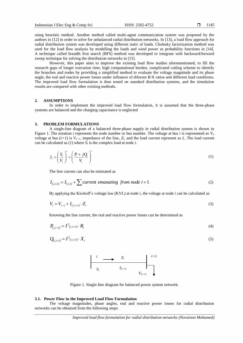
A single-line diagram of a balanced three-phase supply in radial distribution system is shown in Figure 1. The notation i represents the node number or bus number. The voltage at bus i is represented as Vi,

voltage at bus (i+1) is Vi+1, impedance of the line, Zi, and the load current represent as Ii. The load current

can be calculated as (1) where Si is the complex load at node i.

**

i

ii

i

ii

V

jQP

V

SI (1)

The line current can also be estimated as

111, inodefromemanatingcurrentII iii (2)

By applying the Kirchoff’s voltage law (KVL) at node i, the voltage at node i can be calculated as

iiiii ZIVV 1,1 (3)

Knowing the line current, the real and reactive power losses can be determined as

iiiii RIP 1,2

1, (4)

iiiii XIQ 1,2

1, (5)

Figure 1. Single-line diagram for balanced power system network.

3.1. Power Flow in the Improved Load Flow Formulation

The voltage magnitudes, phase angles, real and reactive power losses for radial distribution

networks can be obtained from the following steps:

i

Vi I(i+1)

Zi

V(i+1)

i+1

ISSN: 2502-4752

Indonesian J Elec Eng & Comp Sci, Vol. 15, No. 3, September 2019 : 1144 - 1153

1146

Step 1: Read the line and the load data.

Step 2: Initialize the base values for MVA and kV.

Step 3: Calculate the base impedance and convert the line and load parameters into per unit (p.u) value.

Step 4: Construct the incidence matrix [16] to identify the branches and nodes.The positive value of 1

indicate the sending end of the branch i, negative value of 1 will be the receiving end of the branch i, and 0 if

there is no connection between the nodes. The incidence matrix for the branch to node is

Step 5: Construct the node to branch which is the inverse incidence matrix [16].

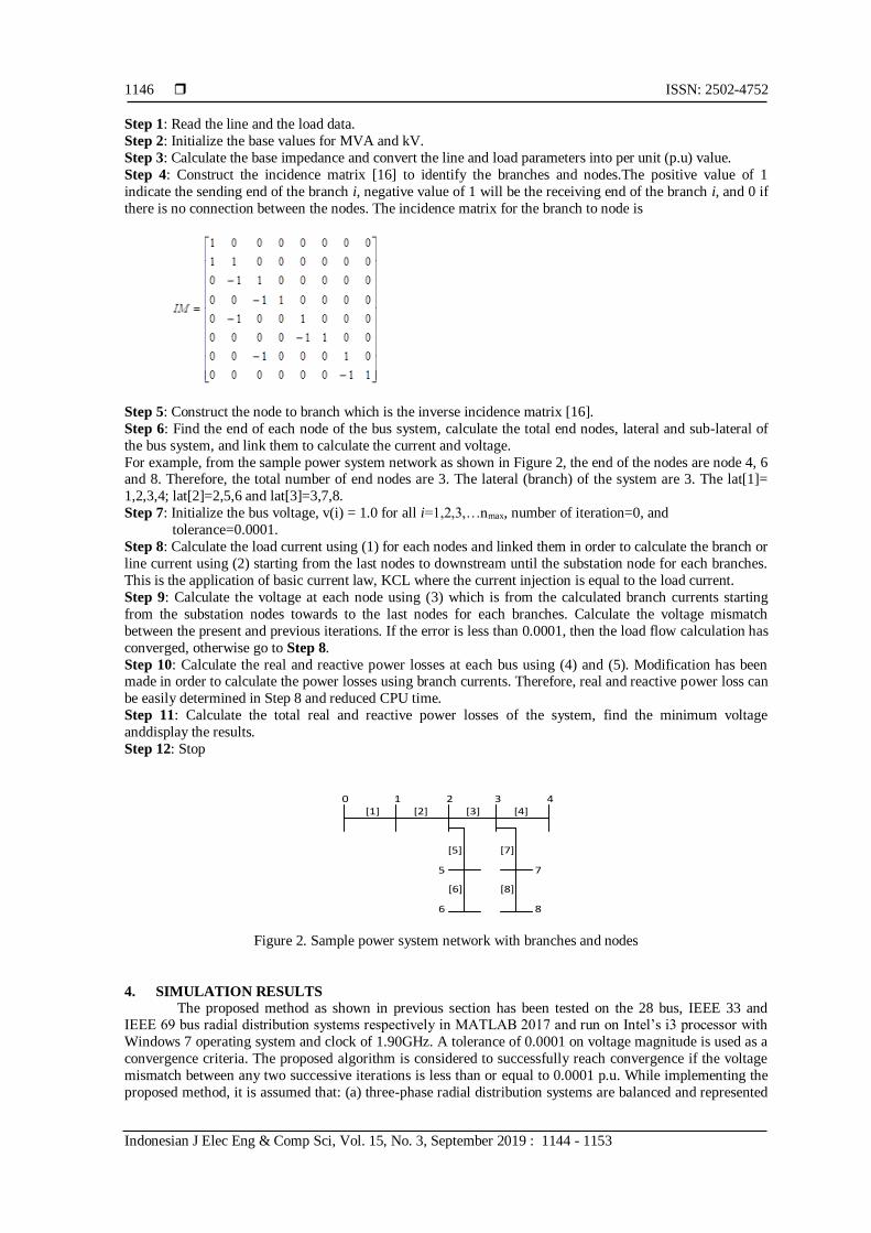
Step 6: Find the end of each node of the bus system, calculate the total end nodes, lateral and sub-lateral of

the bus system, and link them to calculate the current and voltage.

For example, from the sample power system network as shown in Figure 2, the end of the nodes are node 4, 6 and 8. Therefore, the total number of end nodes are 3. The lateral (branch) of the system are 3. The lat[1]=

1,2,3,4; lat[2]=2,5,6 and lat[3]=3,7,8.

Step 7: Initialize the bus voltage, v(i) = 1.0 for all i=1,2,3,…nmax, number of iteration=0, and

tolerance=0.0001.

Step 8: Calculate the load current using (1) for each nodes and linked them in order to calculate the branch or

line current using (2) starting from the last nodes to downstream until the substation node for each branches.

This is the application of basic current law, KCL where the current injection is equal to the load current.

Step 9: Calculate the voltage at each node using (3) which is from the calculated branch currents starting

from the substation nodes towards to the last nodes for each branches. Calculate the voltage mismatch

between the present and previous iterations. If the error is less than 0.0001, then the load flow calculation has

converged, otherwise go to Step 8.

Step 10: Calculate the real and reactive power losses at each bus using (4) and (5). Modification has been made in order to calculate the power losses using branch currents. Therefore, real and reactive power loss can

be easily determined in Step 8 and reduced CPU time.

Step 11: Calculate the total real and reactive power losses of the system, find the minimum voltage

anddisplay the results.

Step 12: Stop

Figure 2. Sample power system network with branches and nodes

4. SIMULATION RESULTS

The proposed method as shown in previous section has been tested on the 28 bus, IEEE 33 and IEEE 69 bus radial distribution systems respectively in MATLAB 2017 and run on Intel’s i3 processor with

Windows 7 operating system and clock of 1.90GHz. A tolerance of 0.0001 on voltage magnitude is used as a

convergence criteria. The proposed algorithm is considered to successfully reach convergence if the voltage

mismatch between any two successive iterations is less than or equal to 0.0001 p.u. While implementing the

proposed method, it is assumed that: (a) three-phase radial distribution systems are balanced and represented

0 1 2

5

6

3 4

7

8

[1] [2] [3] [4]

[5]

[6] [8]

[7]



1147

by their single-line diagrams; (b) charging capacitance is neglected in the distribution voltage level.; (c) the

load flow has been compared for constant power load modeling.

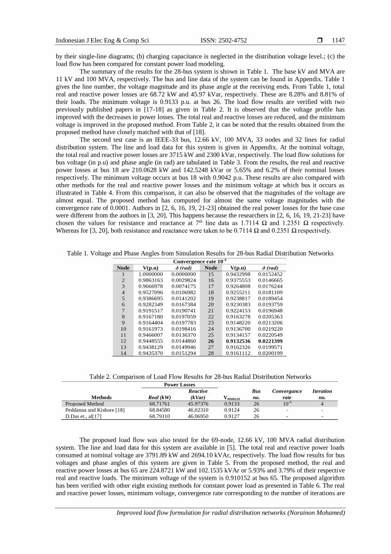
The summary of the results for the 28-bus system is shown in Table 1. The base kV and MVA are

11 kV and 100 MVA, respectively. The bus and line data of the system can be found in Appendix. Table 1

gives the line number, the voltage magnitude and its phase angle at the receiving ends. From Table 1, total

real and reactive power losses are 68.72 kW and 45.97 kVar, respectively. These are 8.28% and 8.81% of

their loads. The minimum voltage is 0.9133 p.u. at bus 26. The load flow results are verified with two

previously published papers in [17-18] as given in Table 2. It is observed that the voltage profile has

improved with the decreases in power losses. The total real and reactive losses are reduced, and the minimum

voltage is improved in the proposed method. From Table 2, it can be noted that the results obtained from the proposed method have closely matched with that of [18].

The second test case is an IEEE-33 bus, 12.66 kV, 100 MVA, 33 nodes and 32 lines for radial

distribution system. The line and load data for this system is given in Appendix. At the nominal voltage,

the total real and reactive power losses are 3715 kW and 2300 kVar, respectively. The load flow solutions for

bus voltage (in p.u) and phase angle (in rad) are tabulated in Table 3. From the results, the real and reactive

power losses at bus 18 are 210.0628 kW and 142.5248 kVar or 5.65% and 6.2% of their nominal losses

respectively. The minimum voltage occurs at bus 18 with 0.9042 p.u. These results are also compared with

other methods for the real and reactive power losses and the minimum voltage at which bus it occurs as

illustrated in Table 4. From this comparison, it can also be observed that the magnitudes of the voltage are

almost equal. The proposed method has computed for almost the same voltage magnitudes with the

convergence rate of 0.0001. Authors in [2, 6, 16, 19, 21-23] obtained the real power losses for the base case were different from the authors in [3, 20]. This happens because the researchers in [2, 6, 16, 19, 21-23] have

chosen the values for resistance and reactance at 7th line data as 1.7114 Ω and 1.2351 Ω respectively.

Whereas for [3, 20], both resistance and reactance were taken to be 0.7114 Ω and 0.2351 Ω respectively.

Table 1. Voltage and Phase Angles from Simulation Results for 28-bus Radial Distribution Networks

Table 2. Comparison of Load Flow Results for 28-bus Radial Distribution Networks

The proposed load flow was also tested for the 69-node, 12.66 kV, 100 MVA radial distribution

system. The line and load data for this system are available in [5]. The total real and reactive power loads

consumed at nominal voltage are 3791.89 kW and 2694.10 kVAr, respectively. The load flow results for bus

voltages and phase angles of this system are given in Table 5. From the proposed method, the real and

reactive power losses at bus 65 are 224.8721 kW and 102.1535 kVAr or 5.93% and 3.79% of their respective

real and reactive loads. The minimum voltage of the system is 0.910152 at bus 65. The proposed algorithm

has been verified with other eight existing methods for constant power load as presented in Table 6. The real

and reactive power losses, minimum voltage, convergence rate corresponding to the number of iterations are

Convergence rate 10-4

Node V(p.u) δ (rad) Node V(p.u) δ (rad)

1 1.0000000 0.0000000 15 0.9432998 0.0152452

2 0.9863163 0.0029824 16 0.9375553 0.0146665

3 0.9666978 0.0074175 17 0.9264808 0.0176244

4 0.9527096 0.0106982 18 0.9255211 0.0181109

5 0.9386695 0.0141202 19 0.9238817 0.0189454

6 0.9282349 0.0167384 20 0.9230383 0.0193759

7 0.9191517 0.0190741 21 0.9224153 0.0196948

8 0.9167180 0.0197059 22 0.9163278 0.0205363

9 0.9164404 0.0197783 23 0.9148220 0.0213206

10 0.9161973 0.0198416 24 0.9136700 0.0219220

11 0.9466007 0.0136370 25 0.9134157 0.0220549

12 0.9448555 0.0144860 26 0.9132536 0.0221399

13 0.9438129 0.0149946 27 0.9162326 0.0199571

14 0.9435370 0.0151294 28 0.9161112 0.0200199

Methods

Power Losses

Vmin(p.u)

Bus

no.

Convergance

rate

Iteration

no. Real (kW)

Reactive

(kVar)

Proposed Method 68.71761 45.97376 0.9133 26 10-4 4

Peddanna and Kishore [18] 68.84580 46.02310 0.9124 26 - -

D.Das et., al[17] 68.79110 46.06950 0.9127 26 - -

ISSN: 2502-4752


1148

shown in Table 6. From this table, the results from the proposed load flow technique have agreed very well

with those presented in [18].

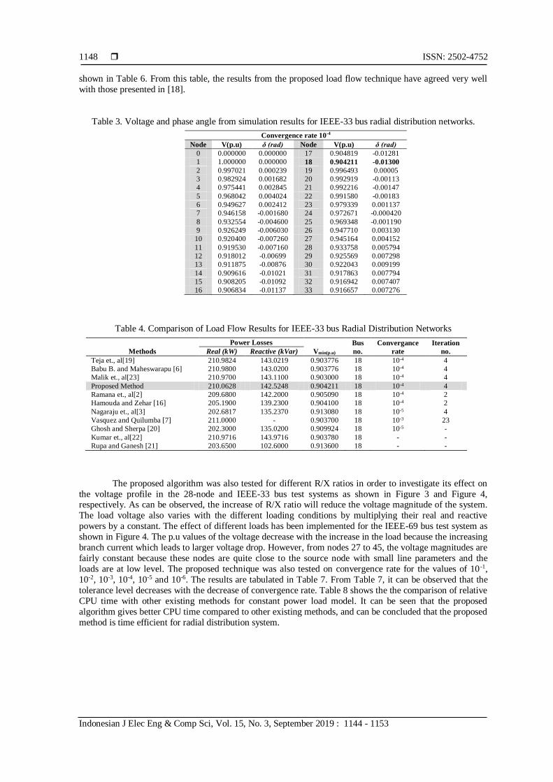
Table 3. Voltage and phase angle from simulation results for IEEE-33 bus radial distribution networks.

Table 4. Comparison of Load Flow Results for IEEE-33 bus Radial Distribution Networks

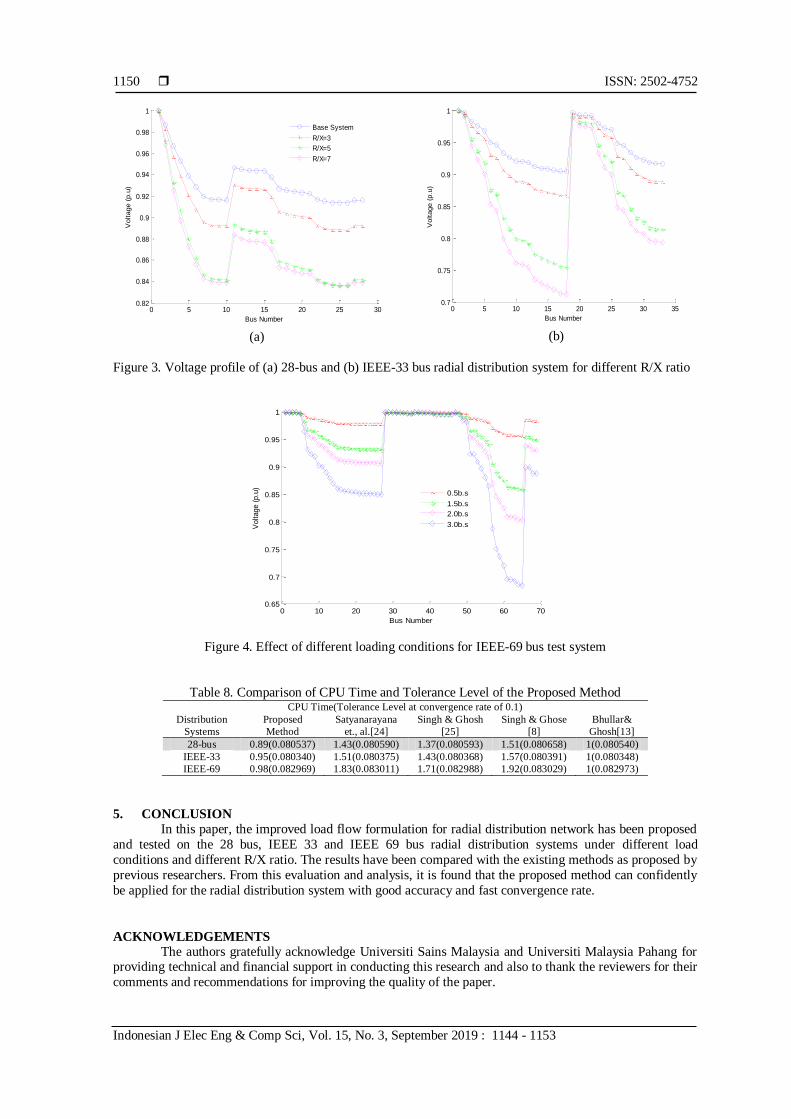
The proposed algorithm was also tested for different R/X ratios in order to investigate its effect on

the voltage profile in the 28-node and IEEE-33 bus test systems as shown in Figure 3 and Figure 4, respectively. As can be observed, the increase of R/X ratio will reduce the voltage magnitude of the system.

The load voltage also varies with the different loading conditions by multiplying their real and reactive

powers by a constant. The effect of different loads has been implemented for the IEEE-69 bus test system as

shown in Figure 4. The p.u values of the voltage decrease with the increase in the load because the increasing

branch current which leads to larger voltage drop. However, from nodes 27 to 45, the voltage magnitudes are

fairly constant because these nodes are quite close to the source node with small line parameters and the

loads are at low level. The proposed technique was also tested on convergence rate for the values of 10 -1,

10-2, 10-3, 10-4, 10-5 and 10-6. The results are tabulated in Table 7. From Table 7, it can be observed that the

tolerance level decreases with the decrease of convergence rate. Table 8 shows the the comparison of relative

CPU time with other existing methods for constant power load model. It can be seen that the proposed

algorithm gives better CPU time compared to other existing methods, and can be concluded that the proposed

method is time efficient for radial distribution system.

Convergence rate 10-4


0 0.000000 0.000000 17 0.904819 -0.01281

1 1.000000 0.000000 18 0.904211 -0.01300

2 0.997021 0.000239 19 0.996493 0.00005

3 0.982924 0.001682 20 0.992919 -0.00113

4 0.975441 0.002845 21 0.992216 -0.00147

5 0.968042 0.004024 22 0.991580 -0.00183

6 0.949627 0.002412 23 0.979339 0.001137

7 0.946158 -0.001680 24 0.972671 -0.000420

8 0.932554 -0.004600 25 0.969348 -0.001190

9 0.926249 -0.006030 26 0.947710 0.003130

10 0.920400 -0.007260 27 0.945164 0.004152

11 0.919530 -0.007160 28 0.933758 0.005794

12 0.918012 -0.00699 29 0.925569 0.007298

13 0.911875 -0.00876 30 0.922043 0.009199

14 0.909616 -0.01021 31 0.917863 0.007794

15 0.908205 -0.01092 32 0.916942 0.007407

16 0.906834 -0.01137 33 0.916657 0.007276

Methods

Power Losses

Vmin(p.u)

Bus

no.

Convergance

rate

Iteration

no. Real (kW) Reactive (kVar)

Teja et., al[19] 210.9824 143.0219 0.903776 18 10-4 4

Babu B. and Maheswarapu [6] 210.9800 143.0200 0.903776 18 10-4 4

Malik et., al[23] 210.9700 143.1100 0.903000 18 10-4 4

Proposed Method 210.0628 142.5248 0.904211 18 10-4 4

Ramana et., al[2] 209.6800 142.2000 0.905090 18 10-4 2

Hamouda and Zehar [16] 205.1900 139.2300 0.904100 18 10-4 2

Nagaraju et., al[3] 202.6817 135.2370 0.913080 18 10-5 4

Vasquez and Quilumba [7] 211.0000 - 0.903700 18 10-3 23

Ghosh and Sherpa [20] 202.3000 135.0200 0.909924 18 10-5 -

Kumar et., al[22] 210.9716 143.9716 0.903780 18 - -

Rupa and Ganesh [21] 203.6500 102.6000 0.913600 18 - -



1149

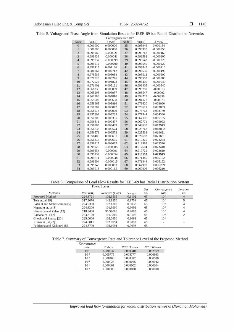
Table 5. Voltage and Phase Angle from Simulation Results for IEEE-69 bus Radial Distribution Networks Convergence rate 10-4


0 0.000000 0.000000 35 0.998946 0.000184

1 1.000000 0.000000 36 0.999918 -0.000050

2 0.999966 -0.000021 37 0.999747 -0.000160

3 0.999932 -0.000041 38 0.999588 -0.000200

4 0.999837 -0.000099 39 0.999542 -0.000220

5 0.999012 -0.000290 40 0.999540 -0.000220

6 0.990115 0.001166 41 0.998843 -0.000410

7 0.980862 0.002712 42 0.998550 -0.000490

8 0.978656 0.003084 43 0.998512 -0.000500

9 0.977528 0.003276 44 0.998503 -0.000500

10 0.972527 0.004823 45 0.998405 -0.000540

11 0.971401 0.005131 46 0.998405 -0.000540

12 0.968236 0.006099 47 0.999787 -0.00013

13 0.965298 0.006957 48 0.998547 -0.00092

14 0.962386 0.007810 49 0.994719 -0.00338

15 0.959503 0.008658 50 0.994177 -0.00373

16 0.958968 0.008816 51 0.978620 0.003090

17 0.958082 0.009077 52 0.978611 0.003093

18 0.958073 0.009079 53 0.974762 0.003779

19 0.957602 0.009235 54 0.971544 0.004366

20 0.957300 0.009335 55 0.967105 0.005185

21 0.956811 0.009497 56 0.962771 0.005992

22 0.956805 0.009499 57 0.940635 0.013943

23 0.956733 0.009524 58 0.929747 0.018002

24 0.956578 0.009578 59 0.925538 0.019621

25 0.956406 0.009631 60 0.920602 0.021691

26 0.956337 0.009655 61 0.913275 0.023264

27 0.956317 0.009662 62 0.912988 0.023326

28 0.999925 -0.000005 63 0.912604 0.023410

29 0.999854 -0.000091 64 0.910721 0.023819

30 0.999732 -0.000054 65 0.910152 0.023943

31 0.999711 -0.000048 66 0.971345 0.005152

32 0.999604 -0.000015 67 0.971344 0.005152

33 0.999348 0.000063 68 0.967907 0.006209

34 0.999013 0.000165 69 0.967906 0.006210

Table 6. Comparison of Load Flow Results for IEEE-69 bus Radial Distribution System

Methods

Power Losses

Vmin(p.u)

Bus

no.

Convergance

rate

Iteration

no. Real (kW) Reactive (kVar)

Proposed Method 224.8721 102.1535 0.9102 65 10-4 4

Teja et., al[19] 317.9070 143.8350 0.8754 65 10-4 5

Babu B and Maheswarapu [6] 224.9300 102.1300 0.9038 65 10-4 4

Nagaraju et., al[3] 224.6300 101.9900 0.9092 65 10-5 4

Hamouda and Zehar [12] 218.8400 95.59000 0.9095 65 10-4 4

Ramana et., al[2] 223.3100 101.3800 0.9106 65 10-4 2

Ghosh and Sherpa [20] 225.0000 102.0950 0.9068 65 10-5 -

Kumar et., al[22] 224.8011 102.0954 0.9092 65 - -

Peddanna and Kishore [18] 224.8799 102.1091 0.9093 65 - -

Table 7. Summary of Convergence Rate and Tolerance Level of the Proposed Method Convergence

rate 28-bus IEEE 33-bus IEEE 69-bus

10-1 0.080537 0.080340 0.082969

10-2 0.005775 0.005777 0.006993

10-3 0.000408 0.000392 0.000580

10-4 0.000026 0.000015 0.000042

10-5 0.000001 0.000002 0.000004

10-6 0.000000 0.000000 0.000000

ISSN: 2502-4752


1150

(a)

(b)

Figure 3. Voltage profile of (a) 28-bus and (b) IEEE-33 bus radial distribution system for different R/X ratio

Figure 4. Effect of different loading conditions for IEEE-69 bus test system

Table 8. Comparison of CPU Time and Tolerance Level of the Proposed Method CPU Time(Tolerance Level at convergence rate of 0.1)

Distribution

Systems

Proposed

Method

Satyanarayana

et., al.[24]

Singh & Ghosh

[25]

Singh & Ghose

[8]

Bhullar&

Ghosh[13]

28-bus 0.89(0.080537) 1.43(0.080590) 1.37(0.080593) 1.51(0.080658) 1(0.080540)

IEEE-33 0.95(0.080340) 1.51(0.080375) 1.43(0.080368) 1.57(0.080391) 1(0.080348)

IEEE-69 0.98(0.082969) 1.83(0.083011) 1.71(0.082988) 1.92(0.083029) 1(0.082973)

5. CONCLUSION

In this paper, the improved load flow formulation for radial distribution network has been proposed

and tested on the 28 bus, IEEE 33 and IEEE 69 bus radial distribution systems under different load

conditions and different R/X ratio. The results have been compared with the existing methods as proposed by

previous researchers. From this evaluation and analysis, it is found that the proposed method can confidently

be applied for the radial distribution system with good accuracy and fast convergence rate.

ACKNOWLEDGEMENTS

The authors gratefully acknowledge Universiti Sains Malaysia and Universiti Malaysia Pahang for providing technical and financial support in conducting this research and also to thank the reviewers for their

comments and recommendations for improving the quality of the paper.

0 5 10 15 20 25 300.82

0.84

0.86

0.88

0.9

0.92

0.94

0.96

0.98

1

Bus Number

Voltage (

p.u

)

Base System

R/X=3

R/X=5

R/X=7

0 5 10 15 20 25 30 350.7

0.75

0.8

0.85

0.9

0.95

1

Bus Number

Voltage (

p.u

)

0 10 20 30 40 50 60 700.65

0.7

0.75

0.8

0.85

0.9

0.95

1

Bus Number

Voltage (

p.u

)

0.5b.s

1.5b.s

2.0b.s

3.0b.s



1151

REFERENCES [1] A. D. Rana, J. B. Darji, Mosam Pandya, "Backward/Forward Sweep Load Flow Algorithm for Radial Distribution

System", International Journal of Scientific Research and Development, vol. 2(01), pp. 398-400, 2014. [2] T. Ramana, V. Ganesh, S. Sivanagaraju, "Simple and Fast Load Flow Solution for Electrical Power Distribution

Systems", International Journal of Electrical Engineering and Informatics, vol. 5, pp. 245-255, Sept 2013. [3] K. Nagaraju, S. Sivanagaraju, T. Ramana, P. V. Prasad, "A Novel Load Flow Method for Radial Distribution

Systems for Realistic Loads", Electric Power Components and Systems, vol. 39, pp. 128-141, 2011. [4] D. Das, D. P. Kothari, and A. Kalam, "Simple and Efficient Method for Load Flow Solution of Radial Distribution

Networks", Elect. Power Energy Syst, vol. 17(5), pp. 335-346, 1995. [5] R. Ranjan and D. Das, "Simple and Efficient Computer Algorithm to Solve Radial Distribution Networks",

Electric Power Components and Systems, vol. 31(1), pp. 95-107, 2003. [6] Kiran Babu B. and Sydulu Maheswarapu, "An Efficient Power Flow Method for Radial Distribution System

Studies under Various Load Models", Electric Power Components and Systems, vol. 16, pp. 1-6, 2016. [7] Wilson A. Vasquez and Franklin L. Quilumba, "Load Flow Method for Radial Distribution Systems with

Distributed Generation using a Dynamic Data Matrix", Electric Power Components and Systems, vol. 16, pp. 1-6, 2016.

[8] S. Singh and T. Ghose, "Improved Radial Load Flow Method", Electric Power Components and Systems, vol. 44, pp. 721-727, 2013.

[9] Yuntao, J.u, Wenchun, W.u, Bomim, Zhang Z. & Hongbin, Sun S., “Loop Analysis Based Continous Power Flow Algorithm for Distribution Networks”, IET Generation, Transmission and Distribution, vol.8(7),

pp.1284-1292, 2014. [10] Eltantawy, A.B. & Salama, M.M.A., "A Novel Zooming Algorithm for Distribution Load Flow Analysis for Smart

Grid", IEEE Transaction of Smart Grids, vol. 5(4), pp. 1701-1711, 2014. [11] Nikmehr, N., and Najafi Ravadanegh, "Heuristic Probabilistic Power Flow Algorithm for Microgrids Operation and

Planning", IET Generation, Transmission and Distribution, vol.8(11), pp.985-995, 2015. [12] Nguyen, C.P. & Flueck, A.J., "A Novel Agent Based Distributed Power Flow Solver for Smart Grids",

IEEE Transaction of Smart Grids, vol. 6(3), pp. 1261-1270, 2015. [13] Suman Bhullar & Smarajit Ghosh, "A Novel Search Technique to Solve Load Flow of Distribution Networks",

Journal of Engineering Research, vol. 5(4), pp. 60-75, 2017. [14] Narayan, K.S & Kumar, A., "Impact of Wind Correlation and Load Correlation on Probabilistic Load Flow for

Radial Distribution Systems", IEEE International Conference on Signal Processing, Informatics, Communication and Energy Systems, Kozhikode(Kerala), pp. 1-5, 2015.

[15] S. Sunisith, K. Meena, "Backward/Forward Sweep Based Distribution Load Flow Method", International Electrical Engineering Journal, vol. 5(9), pp. 1539-1544, 2014.

[16] Abdellatif Hamouda and Khaled Zehar, "Improved Algorithm for Radial Distribution Networks Load Flow Solution", Electric Power and Energy Systems, vol. 33, pp. 508-514, 2011.

[17] D. Das, D. P. Kothari, and H. S. Nagi, "Novel Method for Solving Radial Distribution Networks", IEEE Proc

Gener. Transm. Distrib., vol. 141(4), pp. 291-298, 1994. [18] Gundugallu Peddana and Y. Siva Rama Kishore, "Power Loss Allocation of Balanced Radial Distribution

Systems", International Journal of Science and Research, vol. 4(9), pp. 360-366, September 2015. [19] B. Ravi Teja, V. V. S. N. Murty, Ashwani Kumar, "An Efficient and Simple Load Flow Approach for Radial and

Meshed Distribution Networks", International Journal of Grid Distributed Computing, vol. 9(2), pp. 85-201, 2016. [20] Smarjit Ghosh and Karma Sonam Sherpa, "An Efficient Method for Load-Flow Solution of Radial Distribution

Networks", World Academy of Scince, Engineering and Technology, vol. 21, pp. 700-708, 2008. [21] J. A. Michline Rupa and S. Ganesh, "Power Flow Analysis for Radial Distribution System using

Backward/Forward Sweep Method", International Journal of Electrical and Computing Engineering (IJECE), vol. 8(10), pp. 1621-1625, 2014.

[22] V.Kumar, Shubham Swapnil, R. Ranjan and V. R. Singh, "Improved Algorithm for Load Flow Analysis of Radial Distribution System", Indian Journal of Science and Technology, vol. 10(18), pp. 1-7, May 2017.

[23] Nitin Malik, Shubham Swapnil, Jaimin D.Shah, Vaibhav A. Maheshwari, "Simple Robust Power Flow Method for Radial Distribution Systems", Journal of Information, Knowledge and Research in Electrical Engineering, vol. 3(01), pp. 412-417, 2014.

[24] Satyanarayana, S.Ramana, T.,Sivanagaraju, S., & Rao, G.K., "An Efficient Load Flow Solution for Radial

Distribution Network Including Voltage Dependent Load Models", Electric Power Components and Systems, vol. 35(5), pp. 539-551, 2007.

[25] Singh, Kultar Deep & Ghosh, T., “A New Efficient Method for Load Flow Solution for Radial Distribution Networks”, Electrical Review: Engineering and Technology, pp. 66-73, 2011Eltantawy, A.B. & Salama, M.M.A., "A Novel Zooming Algorithm for Distribution Load Flow Analysis for Smart Grid", IEEE Transaction of Smart Grids, vol. 5(4), pp. 1701-1711, 2014.

ISSN: 2502-4752


1152

BIOGRAPHIES OF AUTHORS

Norainon Mohamed received the B.Eng degree in Industrial Electronics from Universiti Malaysia Perlis, Malaysia in 2008 and Master Degree in Electrical Engineering from Universiti Malaysia Pahang in 2010. She is currently pursuing the PhD degree with the School of Electrical and Electronic Engineering, Universiti Sains Malaysia, Penang, Malaysia. Her current research area includes power system analysis, distribution and transmission systems and renewable

energy resources.

Dahaman Ishak received the BSc degree in electrical engineering from Syracuse University,

Syracuse, NY, USA, the MSc degree in electrical power from the University of Newcastle Upon Tyne, Newcastle upon Tyne, UK, and the PhD degree in electrical engineering from the University of Sheffield, Sheffield, UK, in 1990, 2001 and 2005 respectively. He is currently an Associate Professor with the School of Electrical and Electronic Engineering, Universiti Sains Malaysia, Penang, Malaysia. His current research interests include permanent magnet brushless machines, electrical drives, power electronic converters and renewable energy.s

APPENDIX A

Table A1: 28-bus radial distribution systems Branch

no.

Sending

Bus

Receiving

Bus

R

(ohms)

X

(ohms)

1 1 2 1.197 0.820

2 2 3 1.796 1.231

3 3 4 1.306 0.896

4 4 5 1.851 1.268

5 5 6 1.524 1.044

6 6 7 1.905 1.305

7 7 8 1.197 0.820

8 8 9 0.653 0.447

9 9 10 1.143 0.783

10 4 11 2.823 1.172

11 11 12 1.184 0.491

12 12 13 1.002 0.416

13 13 14 0.455 0.189

14 14 15 0.546 0.227

15 5 16 2.550 1.058

16 6 17 1.366 0.567

17 17 18 0.819 0.340

18 18 19 1.548 0.642

19 19 20 1.366 0.567

20 20 21 3.552 1.474

21 7 22 1.548 0.642

22 22 23 1.092 0.453

23 23 24 0.910 0.378

24 24 25 0.455 0.189

25 25 26 0.364 0.151

26 8 27 0.546 0.226

27 27 28 0.273 0.113

Node

No. PL(kW)

Node

No. PL(kW)

1 0.000 15 35.28

2 35.28 16 35.28

3 14.00 17 8.960

4 35.28 18 8.960

5 14.00 19 35.28

6 35.28 20 35.28

7 35.28 21 14.00

8 35.28 22 35.28

9 14.00 23 8.960

10 14.00 24 56.00

11 56.00 25 8.960

12 35.28 26 35.28

13 35.28 27 35.28

14 14.00 28 35.28

Power factor of the load is taken as cos ϕ=0.70

Reactive power load = PL tan ϕ

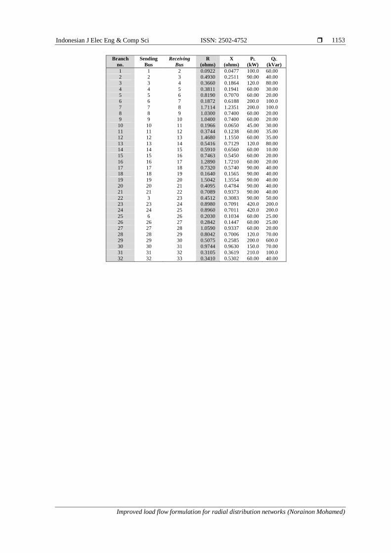
Table A2: IEEE-33 bus radial distribution systems



1153

Branch

no.

Sending

Bus

Receiving

Bus

R

(ohms)

X

(ohms)

PL

(kW)

QL

(kVar)

1 1 2 0.0922 0.0477 100.0 60.00

2 2 3 0.4930 0.2511 90.00 40.00

3 3 4 0.3660 0.1864 120.0 80.00

4 4 5 0.3811 0.1941 60.00 30.00

5 5 6 0.8190 0.7070 60.00 20.00

6 6 7 0.1872 0.6188 200.0 100.0

7 7 8 1.7114 1.2351 200.0 100.0

8 8 9 1.0300 0.7400 60.00 20.00

9 9 10 1.0400 0.7400 60.00 20.00

10 10 11 0.1966 0.0650 45.00 30.00

11 11 12 0.3744 0.1238 60.00 35.00

12 12 13 1.4680 1.1550 60.00 35.00

13 13 14 0.5416 0.7129 120.0 80.00

14 14 15 0.5910 0.6560 60.00 10.00

15 15 16 0.7463 0.5450 60.00 20.00

16 16 17 1.2890 1.7210 60.00 20.00

17 17 18 0.7320 0.5740 90.00 40.00

18 18 19 0.1640 0.1565 90.00 40.00

19 19 20 1.5042 1.3554 90.00 40.00

20 20 21 0.4095 0.4784 90.00 40.00

21 21 22 0.7089 0.9373 90.00 40.00

22 3 23 0.4512 0.3083 90.00 50.00

23 23 24 0.8980 0.7091 420.0 200.0

24 24 25 0.8960 0.7011 420.0 200.0

25 6 26 0.2030 0.1034 60.00 25.00

26 26 27 0.2842 0.1447 60.00 25.00

27 27 28 1.0590 0.9337 60.00 20.00

28 28 29 0.8042 0.7006 120.0 70.00

29 29 30 0.5075 0.2585 200.0 600.0

30 30 31 0.9744 0.9630 150.0 70.00

31 31 32 0.3105 0.3619 210.0 100.0

32 32 33 0.3410 0.5302 60.00 40.00

Sebuah Kajian Pustaka: - Semantic Scholar

Documents

Transcript of Sebuah Kajian Pustaka: - Semantic Scholar