Seasonal and interannual variability of satellite-derived chlorophyll

pigment, surface height, and temperature off Baja California

T. Leticia Espinosa-Carreon,1

Centro de Investigacion Cientıfica y de Educacion Superior de Ensenada, Baja California, Mexico

P. T. StrubCollege of Oceanic and Atmospheric Sciences, Oregon State University, Corvallis, Oregon, USA

Emilio Beier,1 Francisco Ocampo-Torres, and Gilberto Gaxiola-CastroCentro de Investigacion Cientıfica y de Educacion Superior de Ensenada, Baja California, Mexico

Received 22 August 2003; revised 19 December 2003; accepted 23 January 2004; published 24 March 2004.

[1] Mean fields, seasonal cycles, and interannual variability are examined for fields ofsatellite-derived chlorophyll pigment concentrations (CHL), sea surface height (SSH), andsea surface temperature (SST) during 1997–2002. The analyses help to identify threedynamic regions: an upwelling zone next to the coast, the Ensenada Front in the north,and regions of repeated meanders and/or eddy variability west and southwest of PointEugenia. High values of CHL are found in the upwelling zone, diminishing offshore. Theexception is the area north of 31�N (the Ensenada Front), where higher CHL are foundabout 150 km offshore. South of 31�N, the long-term mean dynamic topography decreasesnext to the coast, creating isopleths of height parallel to the coastline, consistent withsouthward geostrophic flow. North of 31�N the mean flow is toward the east, consistentwith the presence of the Ensenada Front. The mean SST reveals a more north-southgradient, reflecting latitudinal differences in surface heating due to solar radiation.Harmonic analyses and EOFs reveal the seasonal and interannual patterns, including theregion of repeated eddy activity to the west and southwest of Point Eugenia. A maximumCHL occurs in spring in most of the inshore regions, reflecting the growth ofphytoplankton in response to the seasonal maximum in upwelling-favorable winds. SSTand SSH anomalies are negative in the coastal upwelling zone in spring, also consistentwith a response to the seasonal maximum in upwelling. When the seasonal cycle isremoved, the strongest signal in the EOF time series is the response to the strong 1997–1998 El Nino, with a weaker signal representing La Nina (1998–1999) conditions.El Nino conditions consist of low chlorophyll, high SSH, and high SST, with oppositeconditions during La Nina. INDEX TERMS: 4223 Oceanography: General: Descriptive and regional

oceanography; 4227 Oceanography: General: Diurnal, seasonal, and annual cycles; 4275 Oceanography:

General: Remote sensing and electromagnetic processes (0689); KEYWORDS: chlorophyll, El Nino, La Nina,

Baja California, California Current

Citation: Espinosa-Carreon, T. L., P. T. Strub, E. Beier, F. Ocampo-Torres, and G. Gaxiola-Castro (2004), Seasonal and

interannual variability of satellite-derived chlorophyll pigment, surface height, and temperature off Baja California, J. Geophys. Res.,

109, C03039, doi:10.1029/2003JC002105.

1. Introduction

[2] In this paper, we examine the links between physicalforcing and the lower trophic levels off Baja California, in thesouthern part of the California Current System (CCS).The mean flow in the CCS is equatorward next to the coastin the Northeast Pacific Ocean [Hickey, 1979, 1998]. It is

delimited at its northern boundary by the eastward NorthPacific Current, which divides the Subtropical Gyre from theSubarctic Alaska Gyre. At its southern extreme, the CCSflows into the westward North Equatorial Current [Pares-Sierra et al., 1997]. At the most basic level, the flow of theCalifornia Current is controlled by the equatorward currentneeded to complete the Subtropical Gyre and by the predom-inantly equatorward winds. This area is considered to be anoceanographic transitional zone between midlatitude andtropical ocean conditions [Durazo and Baumgartner, 2002].[3] The CCS is often depicted as a prototype eastern

boundary current (EBC), with a 2-D upwelling structure

JOURNAL OF GEOPHYSICAL RESEARCH, VOL. 109, C03039, doi:10.1029/2003JC002105, 2004

1Also at College of Oceanic and Atmospheric Sciences, Oregon StateUniversity, Corvallis, Oregon, USA.

Copyright 2004 by the American Geophysical Union.0148-0227/04/2003JC002105$09.00

C03039 1 of 20

consisting of offshore Ekman transport at the surface andsubsurface onshore return flow. An equatorward jet formsat the offshore edge of the upwelled water, which is cold,salty, and rich in nutrients. These nutrients lead to anincrease in primary production, which provides the basisfor a productive ecosystem.[4] Unlike the simple 2-D patterns depicted in most

textbooks, however, synoptic circulation patterns observedin the CCS and other EBCs are characterized by complexmesoscale eddies, fronts, and meanders, with horizontalscales from tens to hundreds of kilometers [Pelaez andMcGowan, 1986]. This structure develops seasonallyand varies on interannual and longer scales [Pelaezand McGowan, 1986; Strub et al., 1991]. In this paper,we use satellite observations of chlorophyll pigmentconcentration, sea surface height, and temperature toillustrate the space and time relationships between bio-logical and physical processes off Baja California. Thisregion has been previously described by Gomez-Valdesand Velez-Munoz [1982], Pares-Sierra et al. [1997] andDurazo and Baumgartner [2002]. The analysis in thispaper also builds on previous work using in situ andsatellite chlorophyll estimations from Bernal [1981],Pelaez and Guan [1982], Pelaez and McGowan [1986],Strub et al. [1990], Thomas and Strub [1990], Fargion etal. [1993], Thomas et al. [1994], Hayward et al. [1999],Kahru and Mitchell [2000, 2001, 2002], Bograd et al.[2000], and Durazo et al. [2001].

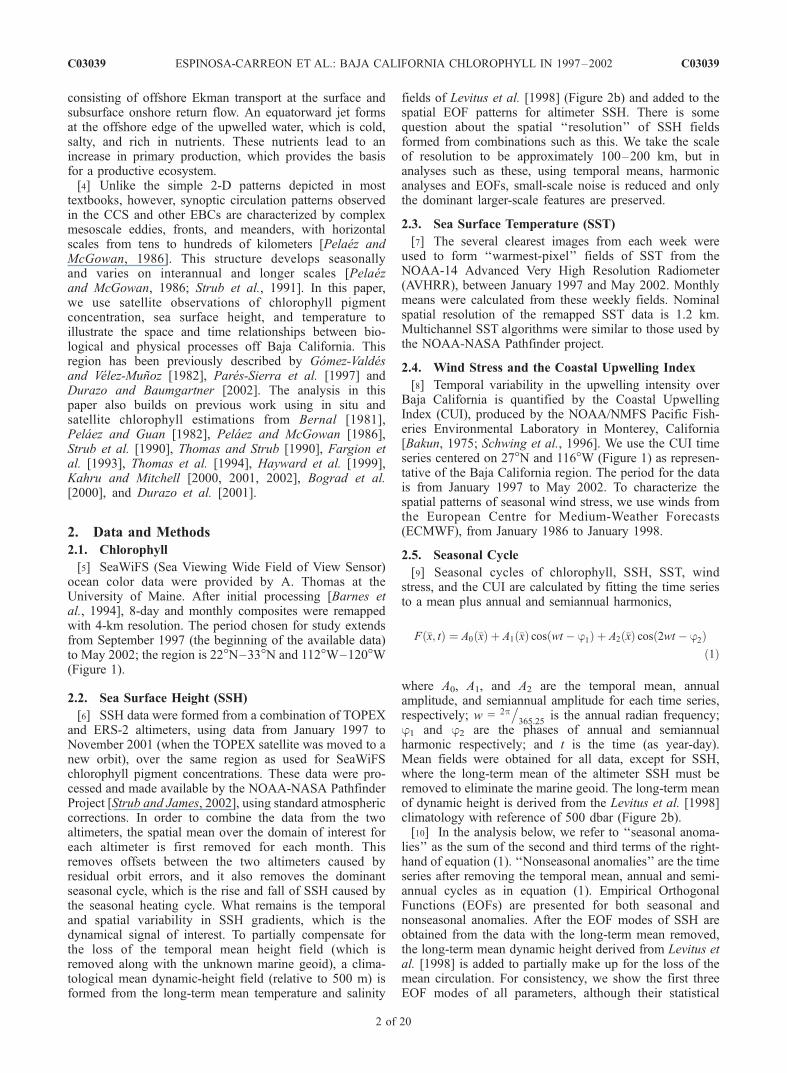
2. Data and Methods

2.1. Chlorophyll

[5] SeaWiFS (Sea Viewing Wide Field of View Sensor)ocean color data were provided by A. Thomas at theUniversity of Maine. After initial processing [Barnes etal., 1994], 8-day and monthly composites were remappedwith 4-km resolution. The period chosen for study extendsfrom September 1997 (the beginning of the available data)to May 2002; the region is 22�N–33�N and 112�W–120�W(Figure 1).

2.2. Sea Surface Height (SSH)

[6] SSH data were formed from a combination of TOPEXand ERS-2 altimeters, using data from January 1997 toNovember 2001 (when the TOPEX satellite was moved to anew orbit), over the same region as used for SeaWiFSchlorophyll pigment concentrations. These data were pro-cessed and made available by the NOAA-NASA PathfinderProject [Strub and James, 2002], using standard atmosphericcorrections. In order to combine the data from the twoaltimeters, the spatial mean over the domain of interest foreach altimeter is first removed for each month. Thisremoves offsets between the two altimeters caused byresidual orbit errors, and it also removes the dominantseasonal cycle, which is the rise and fall of SSH caused bythe seasonal heating cycle. What remains is the temporaland spatial variability in SSH gradients, which is thedynamical signal of interest. To partially compensate forthe loss of the temporal mean height field (which isremoved along with the unknown marine geoid), a clima-tological mean dynamic-height field (relative to 500 m) isformed from the long-term mean temperature and salinity

fields of Levitus et al. [1998] (Figure 2b) and added to thespatial EOF patterns for altimeter SSH. There is somequestion about the spatial ‘‘resolution’’ of SSH fieldsformed from combinations such as this. We take the scaleof resolution to be approximately 100–200 km, but inanalyses such as these, using temporal means, harmonicanalyses and EOFs, small-scale noise is reduced and onlythe dominant larger-scale features are preserved.

2.3. Sea Surface Temperature (SST)

[7] The several clearest images from each week wereused to form ‘‘warmest-pixel’’ fields of SST from theNOAA-14 Advanced Very High Resolution Radiometer(AVHRR), between January 1997 and May 2002. Monthlymeans were calculated from these weekly fields. Nominalspatial resolution of the remapped SST data is 1.2 km.Multichannel SST algorithms were similar to those used bythe NOAA-NASA Pathfinder project.

2.4. Wind Stress and the Coastal Upwelling Index

[8] Temporal variability in the upwelling intensity overBaja California is quantified by the Coastal UpwellingIndex (CUI), produced by the NOAA/NMFS Pacific Fish-eries Environmental Laboratory in Monterey, California[Bakun, 1975; Schwing et al., 1996]. We use the CUI timeseries centered on 27�N and 116�W (Figure 1) as represen-tative of the Baja California region. The period for the datais from January 1997 to May 2002. To characterize thespatial patterns of seasonal wind stress, we use winds fromthe European Centre for Medium-Weather Forecasts(ECMWF), from January 1986 to January 1998.

2.5. Seasonal Cycle

[9] Seasonal cycles of chlorophyll, SSH, SST, windstress, and the CUI are calculated by fitting the time seriesto a mean plus annual and semiannual harmonics,

F �x; tð Þ ¼ A0 �xð Þ þ A1 �xð Þ cos wt � j1ð Þ þ A2 �xð Þ cos 2wt � j2ð Þð1Þ

where A0, A1, and A2 are the temporal mean, annualamplitude, and semiannual amplitude for each time series,respectively; w = 2p

�365:25

is the annual radian frequency;j1 and j2 are the phases of annual and semiannualharmonic respectively; and t is the time (as year-day).Mean fields were obtained for all data, except for SSH,where the long-term mean of the altimeter SSH must beremoved to eliminate the marine geoid. The long-term meanof dynamic height is derived from the Levitus et al. [1998]climatology with reference of 500 dbar (Figure 2b).[10] In the analysis below, we refer to ‘‘seasonal anoma-

lies’’ as the sum of the second and third terms of the right-hand of equation (1). ‘‘Nonseasonal anomalies’’ are the timeseries after removing the temporal mean, annual and semi-annual cycles as in equation (1). Empirical OrthogonalFunctions (EOFs) are presented for both seasonal andnonseasonal anomalies. After the EOF modes of SSH areobtained from the data with the long-term mean removed,the long-term mean dynamic height derived from Levitus etal. [1998] is added to partially make up for the loss of themean circulation. For consistency, we show the first threeEOF modes of all parameters, although their statistical

C03039 ESPINOSA-CARREON ET AL.: BAJA CALIFORNIA CHLOROPHYLL IN 1997–2002

2 of 20

C03039

significance varies between CHL, SST, and SSH. Regard-less of formal statistical certainty, the patterns are generallyinterpretable in terms of expected mesoscale dynamics.

3. Results and Discussion

3.1. Mean Fields

[11] The mean chlorophyll pigment concentrations aregreatest in an alongshore band next to the coast, approxi-mately 50–100 km wide (Figure 2a), except north of 31�N,where the pigment concentrations are higher offshore. Theeutrophic nearshore region (chlorophyll >1 mg m�3) hasbeen previously described by Kahru and Mitchell [2000],along with the oligotrophic offshore ocean (chlorophyll<0.2 mg m�3) and the mesotrophic intermediate zone(chlorophyll �0.2–1.0 mg m�3). The mean SSH field

(Figure 2b) calculated from climatological temperaturesand salinities [Levitus et al., 1998] slopes downward towardthe coast as expected for equatorward flow [Simpson et al.,1986]. South of 31�N, both pigment and SSH are consistentwith the equatorward mean wind stress (Figure 3a), which isupwelling-favorable. The mean field of SST shows strongnorth-south gradients, with isopleths approximately perpen-dicular to the coast in the southern region (Figure 2c). SSTdiminishes from about 21�C in the southeast to �17�C offnorthwest Baja California, as also reported by Lynn et al.[1982]. Temperatures are 3�–5�C higher than reportedby Gallaudet and Simpson [1994], however, due to thepresence of the 1997–1998 El Nino in our data set andthe larger domain considered. The northern part of thepigment and SST, and SSH fields in Figure 2 show a strongnorth-south gradient associated with the ‘‘Ensenada Front’’

Figure 1. Study area, with isobaths of 200 m. The location of the Coastal Upwelling Index (CUI) isindicated by the asterisk located at 27�N, 116�W, selected as a representative of the Baja Californiaregion.

C03039 ESPINOSA-CARREON ET AL.: BAJA CALIFORNIA CHLOROPHYLL IN 1997–2002

3 of 20

C03039

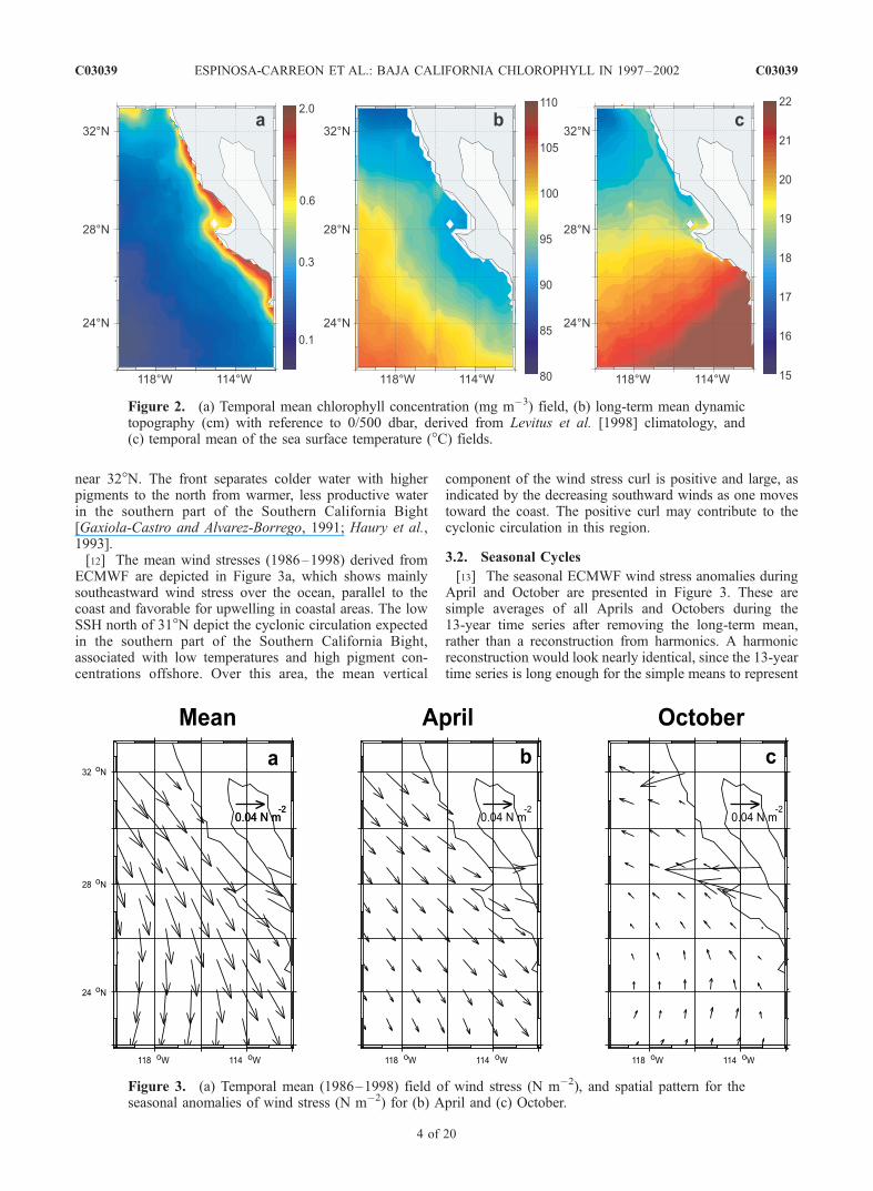
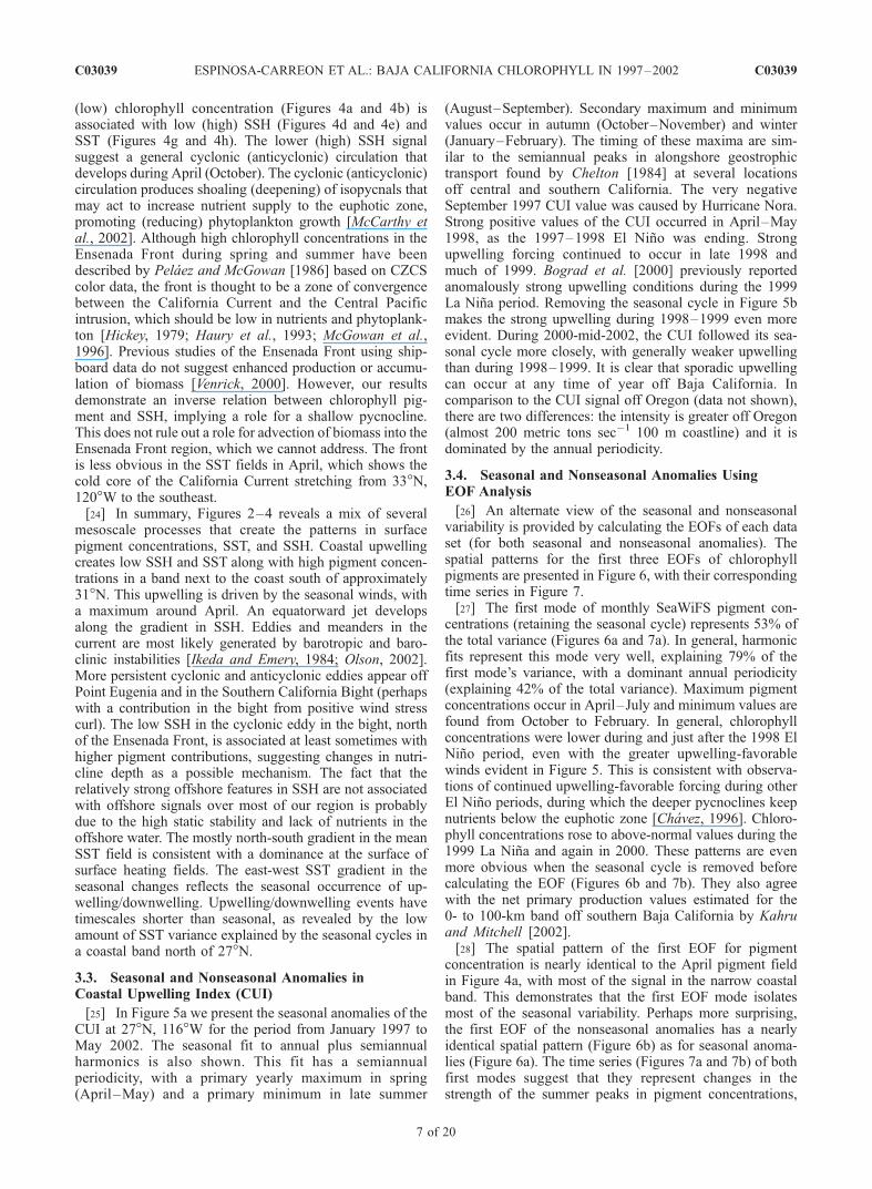
near 32�N. The front separates colder water with higherpigments to the north from warmer, less productive waterin the southern part of the Southern California Bight[Gaxiola-Castro and Alvarez-Borrego, 1991; Haury et al.,1993].[12] The mean wind stresses (1986–1998) derived from

ECMWF are depicted in Figure 3a, which shows mainlysoutheastward wind stress over the ocean, parallel to thecoast and favorable for upwelling in coastal areas. The lowSSH north of 31�N depict the cyclonic circulation expectedin the southern part of the Southern California Bight,associated with low temperatures and high pigment con-centrations offshore. Over this area, the mean vertical

component of the wind stress curl is positive and large, asindicated by the decreasing southward winds as one movestoward the coast. The positive curl may contribute to thecyclonic circulation in this region.

3.2. Seasonal Cycles

[13] The seasonal ECMWF wind stress anomalies duringApril and October are presented in Figure 3. These aresimple averages of all Aprils and Octobers during the13-year time series after removing the long-term mean,rather than a reconstruction from harmonics. A harmonicreconstruction would look nearly identical, since the 13-yeartime series is long enough for the simple means to represent

Figure 2. (a) Temporal mean chlorophyll concentration (mg m�3) field, (b) long-term mean dynamictopography (cm) with reference to 0/500 dbar, derived from Levitus et al. [1998] climatology, and(c) temporal mean of the sea surface temperature (�C) fields.

Figure 3. (a) Temporal mean (1986–1998) field of wind stress (N m�2), and spatial pattern for theseasonal anomalies of wind stress (N m�2) for (b) April and (c) October.

C03039 ESPINOSA-CARREON ET AL.: BAJA CALIFORNIA CHLOROPHYLL IN 1997–2002

4 of 20

C03039

the seasonal cycle. The April wind stress anomalies aretoward the southeast, similar to and reinforcing the temporalmean (the maximum in upwelling-favorable winds isapproximately at this time). In contrast, the October windstress anomalies are toward the northwest, representing adecrease in the upwelling-favorable winds, but not a reversalover the ocean.[14] Similar seasonal anomalies of chlorophyll, SSH, and

SST are reconstructed from the harmonic fits in Figure 4. Asfor winds, the April and October fields are presentedwithout the temporal mean (Figure 2), to emphasize theseasonal changes. The percentages of the total varianceexplained by the harmonic fits at each location are shownFigures 4c, 4f, and 4i.[15] Maximum amplitudes of the pigment seasonal cycles

for most locations are approximately 0.5 mg m�3, largestnext to the coast and near zero in offshore regions. Thenegative seasonal anomalies in October combine with thenearshore mean field (values of 0.6 mg m�3 or more) toreduce pigment concentrations to near zero. The varianceexplained by the pigment seasonal cycles next to the coast inthe primary upwelling regions reaches values between 45%to 65% (Figure 4c), largest south of Points Eugenia and Baja.[16] The magnitudes of the SSH seasonal cycles reach

values of 6 cm, and these are not restricted to the coastalupwelling regions. Rather, the pattern south of 28�N inApril shows high offshore SSH when the coastal ocean haslow SSH. The opposite pattern occurs south of 30�N inOctober. Combined with the mean SSH field in Figure 2b,these fields describe strong equatorward flow in spring andweak or reversed flow in fall. This timing is consistent witha maximum in upwelling-favorable wind stress (Figure 3b)that occurs earlier off Baja California than in the rest of theCalifornia Current farther north [Huyer, 1983; Lynn andSimpson, 1987].[17] The high seasonal variability in the offshore SSH

fields is not the usual seasonal variability in steric heightsthat is typical of altimeter fields. This seasonal steric signalis mostly removed when we subtract the spatial mean fromeach altimeter data set (TOPEX/Poseidon or ERS-2) beforecombining them to form monthly SSH fields. Rather, thesepatterns are associated with persistent meanders and eddiesin the flow field that reoccur on a seasonal timescale atpreferred locations. Previous studies of the California Cur-rent farther north have documented similar meanders andeddies and have related them to three processes: wind-forcing, instabilities of the coastal flow (barotropic andbaroclinic), and coastal geometry [Ikeda and Emery, 1984;Narimousa and Maxworthy, 1989; Simpson and Lynn,1990; Strub et al., 1991; Abbott and Barksdale, 1991;Haidvogel et al., 1991; Pares-Sierra et al., 1993; Barth etal., 2000].[18] Off Baja California, we expect similar processes to

create eddies and meanders, and Soto-Mardones et al.[2004] suggest that the geometry of the coastline is oneof the primary mechanisms of eddy generation off BajaCalifornia (the other is the interaction of the cool, equator-ward California Current at the surface and the polewardCalifornia Undercurrent). A particularly strong pair offeatures in SSH is found west of Point Eugenia, where inApril, there is a region of low SSH north of high SSH(opposite in October). This indicates a tendency for cyclonic

meanders north of Point Eugenia in April (when currents arestrongest), with anticyclonic meanders west/southwest of thepoint. While the seasonal harmonics explain only 10–15% of the variance over much of the region, they explain25–40% of the variance in the SSH feature west-southwestof Point Eugenia (high SSH in April and low SSH inOctober). Thus this is a regularly reoccurring meander andappears related to the location of Point Eugenia. The otherlocations where the harmonic fits explain 25–40% ofthe variance include southern coastal regions and the coreof the CCS north of the Ensenada Front (Figure 4f).[19] Why are there no increased pigment concentrations

associated with the shoaling of the thermocline in offshorecyclonic eddies, as described by McCarthy et al. [2002]?The most likely explanation is that offshore surfacenutrients are depleted, offshore stratification is strong, andthe nutricline is too deep for the geostrophically raisedpycnocline in cyclonic eddies to bring nutrients to withinthe euphotic zone.[20] The amplitudes of the harmonic fits to the SST fields

produce maximum values of ±3�C, concentrated next to thecoast south of Point Eugenia (Figures 4g and 4h). This iseasier to see in the October SST field. Thus the harmoniccycles create the onshore-offshore gradients (south of30�N), which are expected for upwelling systems, but aremostly missing in the mean field. This indicates that themean fields are primarily created by surface heating pro-cesses, with strong latitudinal gradients, while the seasonalvariability is controlled by internal processes such asvertical advection (coastal upwelling) and horizontal advec-tion [Pares-Sierra et al., 1997]. Off northern Baja Califor-nia, the seasonal SST range is reduced to 1�C.[21] The variance explained by the harmonic seasonal

cycle of SST (Figure 4i) is lowest in a narrow band next tothe coast (45–50%) from Point Eugenia to the north.Offshore of this narrow band, the variance explained isgenerally more than 65–70%, except in a band extending tothe southwest off Point Eugenia, where eddies may exertmore influence. These coastal and offshore bands where theharmonic fits explain less variance imply greater nonsea-sonal ‘‘noise’’ in the monthly SST fields. This could becaused by the combination of short timescales for theupwelling and eddy SST signals, coupled with irregularcloud cover, which causes the monthly ‘‘averages’’ to beunduly influenced by sporadic sampling. These short time-scales are in contrast to the long timescales of strongseasonal warming and cooling, which dominate the monthlymeans over most of the domain (where upwelling andeddies are not present).[22] Focusing on the inshore region, an inverse relation-

ship is found between SSH and chlorophyll (Figures 4a, 4b,4d, and 4f ). The low SSH and high pigments are consistentwith coastal upwelling and equatorward flow in earlyspring. These processes together produce cold (low stericheight) and nutrient-rich inshore waters, increasing phyto-plankton growth. The opposite conditions are found duringfall, when the poleward flow is present and warm andnutrient-poor water dominates the inshore conditions. Bothscenarios are consistent with the wind stress seasonalanomalies during April and October (Figures 3b and 3c).[23] A second region of interest is the offshore Ensenada

Front (32�N–33�N, 118�W–120�W), where an area of high

C03039 ESPINOSA-CARREON ET AL.: BAJA CALIFORNIA CHLOROPHYLL IN 1997–2002

5 of 20

C03039

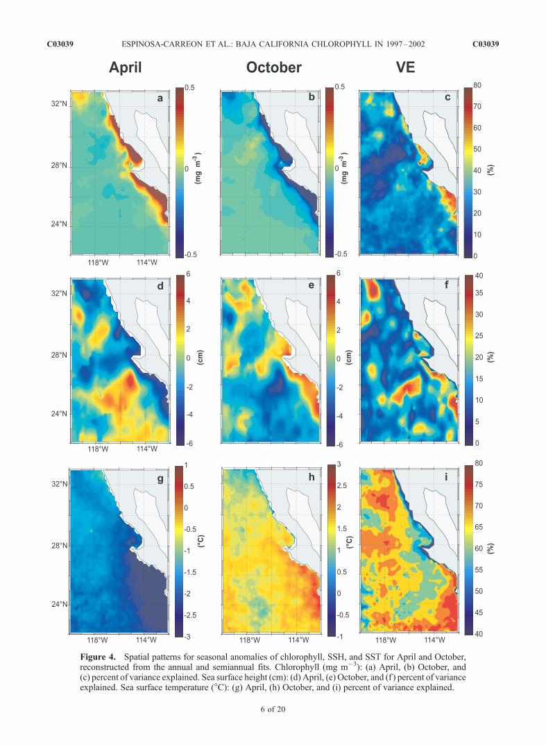
Figure 4. Spatial patterns for seasonal anomalies of chlorophyll, SSH, and SST for April and October,reconstructed from the annual and semiannual fits. Chlorophyll (mg m�3): (a) April, (b) October, and(c) percent of variance explained. Sea surface height (cm): (d) April, (e) October, and (f ) percent of varianceexplained. Sea surface temperature (�C): (g) April, (h) October, and (i) percent of variance explained.

C03039 ESPINOSA-CARREON ET AL.: BAJA CALIFORNIA CHLOROPHYLL IN 1997–2002

6 of 20

C03039

(low) chlorophyll concentration (Figures 4a and 4b) isassociated with low (high) SSH (Figures 4d and 4e) andSST (Figures 4g and 4h). The lower (high) SSH signalsuggest a general cyclonic (anticyclonic) circulation thatdevelops during April (October). The cyclonic (anticyclonic)circulation produces shoaling (deepening) of isopycnals thatmay act to increase nutrient supply to the euphotic zone,promoting (reducing) phytoplankton growth [McCarthy etal., 2002]. Although high chlorophyll concentrations in theEnsenada Front during spring and summer have beendescribed by Pelaez and McGowan [1986] based on CZCScolor data, the front is thought to be a zone of convergencebetween the California Current and the Central Pacificintrusion, which should be low in nutrients and phytoplank-ton [Hickey, 1979; Haury et al., 1993; McGowan et al.,1996]. Previous studies of the Ensenada Front using ship-board data do not suggest enhanced production or accumu-lation of biomass [Venrick, 2000]. However, our resultsdemonstrate an inverse relation between chlorophyll pig-ment and SSH, implying a role for a shallow pycnocline.This does not rule out a role for advection of biomass into theEnsenada Front region, which we cannot address. The frontis less obvious in the SST fields in April, which shows thecold core of the California Current stretching from 33�N,120�W to the southeast.[24] In summary, Figures 2–4 reveals a mix of several

mesoscale processes that create the patterns in surfacepigment concentrations, SST, and SSH. Coastal upwellingcreates low SSH and SST along with high pigment concen-trations in a band next to the coast south of approximately31�N. This upwelling is driven by the seasonal winds, witha maximum around April. An equatorward jet developsalong the gradient in SSH. Eddies and meanders in thecurrent are most likely generated by barotropic and baro-clinic instabilities [Ikeda and Emery, 1984; Olson, 2002].More persistent cyclonic and anticyclonic eddies appear offPoint Eugenia and in the Southern California Bight (perhapswith a contribution in the bight from positive wind stresscurl). The low SSH in the cyclonic eddy in the bight, northof the Ensenada Front, is associated at least sometimes withhigher pigment contributions, suggesting changes in nutri-cline depth as a possible mechanism. The fact that therelatively strong offshore features in SSH are not associatedwith offshore signals over most of our region is probablydue to the high static stability and lack of nutrients in theoffshore water. The mostly north-south gradient in the meanSST field is consistent with a dominance at the surface ofsurface heating fields. The east-west SST gradient in theseasonal changes reflects the seasonal occurrence of up-welling/downwelling. Upwelling/downwelling events havetimescales shorter than seasonal, as revealed by the lowamount of SST variance explained by the seasonal cycles ina coastal band north of 27�N.

3.3. Seasonal and Nonseasonal Anomalies inCoastal Upwelling Index (CUI)

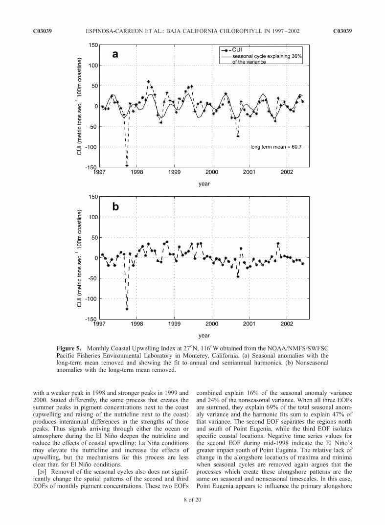
[25] In Figure 5a we present the seasonal anomalies of theCUI at 27�N, 116�W for the period from January 1997 toMay 2002. The seasonal fit to annual plus semiannualharmonics is also shown. This fit has a semiannualperiodicity, with a primary yearly maximum in spring(April–May) and a primary minimum in late summer

(August–September). Secondary maximum and minimumvalues occur in autumn (October–November) and winter(January–February). The timing of these maxima are sim-ilar to the semiannual peaks in alongshore geostrophictransport found by Chelton [1984] at several locationsoff central and southern California. The very negativeSeptember 1997 CUI value was caused by Hurricane Nora.Strong positive values of the CUI occurred in April–May1998, as the 1997–1998 El Nino was ending. Strongupwelling forcing continued to occur in late 1998 andmuch of 1999. Bograd et al. [2000] previously reportedanomalously strong upwelling conditions during the 1999La Nina period. Removing the seasonal cycle in Figure 5bmakes the strong upwelling during 1998–1999 even moreevident. During 2000-mid-2002, the CUI followed its sea-sonal cycle more closely, with generally weaker upwellingthan during 1998–1999. It is clear that sporadic upwellingcan occur at any time of year off Baja California. Incomparison to the CUI signal off Oregon (data not shown),there are two differences: the intensity is greater off Oregon(almost 200 metric tons sec�1 100 m coastline) and it isdominated by the annual periodicity.

3.4. Seasonal and Nonseasonal Anomalies UsingEOF Analysis

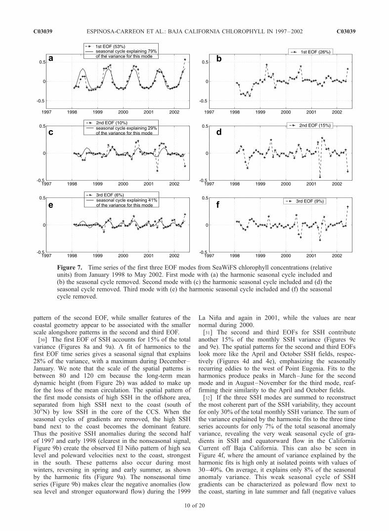
[26] An alternate view of the seasonal and nonseasonalvariability is provided by calculating the EOFs of each dataset (for both seasonal and nonseasonal anomalies). Thespatial patterns for the first three EOFs of chlorophyllpigments are presented in Figure 6, with their correspondingtime series in Figure 7.[27] The first mode of monthly SeaWiFS pigment con-

centrations (retaining the seasonal cycle) represents 53% ofthe total variance (Figures 6a and 7a). In general, harmonicfits represent this mode very well, explaining 79% of thefirst mode’s variance, with a dominant annual periodicity(explaining 42% of the total variance). Maximum pigmentconcentrations occur in April–July and minimum values arefound from October to February. In general, chlorophyllconcentrations were lower during and just after the 1998 ElNino period, even with the greater upwelling-favorablewinds evident in Figure 5. This is consistent with observa-tions of continued upwelling-favorable forcing during otherEl Nino periods, during which the deeper pycnoclines keepnutrients below the euphotic zone [Chavez, 1996]. Chloro-phyll concentrations rose to above-normal values during the1999 La Nina and again in 2000. These patterns are evenmore obvious when the seasonal cycle is removed beforecalculating the EOF (Figures 6b and 7b). They also agreewith the net primary production values estimated for the0- to 100-km band off southern Baja California by Kahruand Mitchell [2002].[28] The spatial pattern of the first EOF for pigment

concentration is nearly identical to the April pigment fieldin Figure 4a, with most of the signal in the narrow coastalband. This demonstrates that the first EOF mode isolatesmost of the seasonal variability. Perhaps more surprising,the first EOF of the nonseasonal anomalies has a nearlyidentical spatial pattern (Figure 6b) as for seasonal anoma-lies (Figure 6a). The time series (Figures 7a and 7b) of bothfirst modes suggest that they represent changes in thestrength of the summer peaks in pigment concentrations,

C03039 ESPINOSA-CARREON ET AL.: BAJA CALIFORNIA CHLOROPHYLL IN 1997–2002

7 of 20

C03039

with a weaker peak in 1998 and stronger peaks in 1999 and2000. Stated differently, the same process that creates thesummer peaks in pigment concentrations next to the coast(upwelling and raising of the nutricline next to the coast)produces interannual differences in the strengths of thosepeaks. Thus signals arriving through either the ocean oratmosphere during the El Nino deepen the nutricline andreduce the effects of coastal upwelling; La Nina conditionsmay elevate the nutricline and increase the effects ofupwelling, but the mechanisms for this process are lessclear than for El Nino conditions.[29] Removal of the seasonal cycles also does not signif-

icantly change the spatial patterns of the second and thirdEOFs of monthly pigment concentrations. These two EOFs

combined explain 16% of the seasonal anomaly varianceand 24% of the nonseasonal variance. When all three EOFsare summed, they explain 69% of the total seasonal anom-aly variance and the harmonic fits sum to explain 47% ofthat variance. The second EOF separates the regions northand south of Point Eugenia, while the third EOF isolatesspecific coastal locations. Negative time series values forthe second EOF during mid-1998 indicate the El Nino’sgreater impact south of Point Eugenia. The relative lack ofchange in the alongshore locations of maxima and minimawhen seasonal cycles are removed again argues that theprocesses which create these alongshore patterns are thesame on seasonal and nonseasonal timescales. In this case,Point Eugenia appears to influence the primary alongshore

Figure 5. Monthly Coastal Upwelling Index at 27�N, 116�Wobtained from the NOAA/NMFS/SWFSCPacific Fisheries Environmental Laboratory in Monterey, California. (a) Seasonal anomalies with thelong-term mean removed and showing the fit to annual and semiannual harmonics. (b) Nonseasonalanomalies with the long-term mean removed.

C03039 ESPINOSA-CARREON ET AL.: BAJA CALIFORNIA CHLOROPHYLL IN 1997–2002

8 of 20

C03039

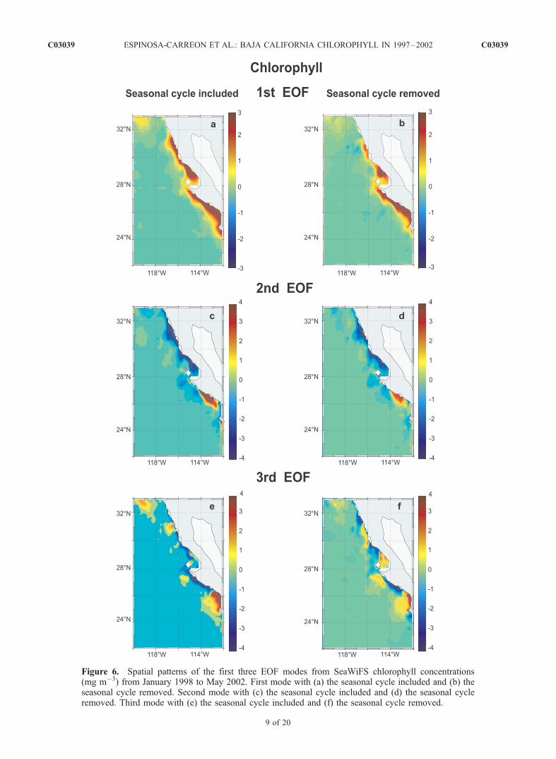
Figure 6. Spatial patterns of the first three EOF modes from SeaWiFS chlorophyll concentrations(mg m�3) from January 1998 to May 2002. First mode with (a) the seasonal cycle included and (b) theseasonal cycle removed. Second mode with (c) the seasonal cycle included and (d) the seasonal cycleremoved. Third mode with (e) the seasonal cycle included and (f) the seasonal cycle removed.

C03039 ESPINOSA-CARREON ET AL.: BAJA CALIFORNIA CHLOROPHYLL IN 1997–2002

9 of 20

C03039

pattern of the second EOF, while smaller features of thecoastal geometry appear to be associated with the smallerscale alongshore patterns in the second and third EOF.[30] The first EOF of SSH accounts for 15% of the total

variance (Figures 8a and 9a). A fit of harmonics to thefirst EOF time series gives a seasonal signal that explains28% of the variance, with a maximum during December–January. We note that the scale of the spatial patterns isbetween 80 and 120 cm because the long-term meandynamic height (from Figure 2b) was added to make upfor the loss of the mean circulation. The spatial pattern ofthe first mode consists of high SSH in the offshore area,separated from high SSH next to the coast (south of30�N) by low SSH in the core of the CCS. When theseasonal cycles of gradients are removed, the high SSHband next to the coast becomes the dominant feature.Thus the positive SSH anomalies during the second halfof 1997 and early 1998 (clearest in the nonseasonal signal,Figure 9b) create the observed El Nino pattern of high sealevel and poleward velocities next to the coast, strongestin the south. These patterns also occur during mostwinters, reversing in spring and early summer, as shownby the harmonic fits (Figure 9a). The nonseasonal timeseries (Figure 9b) makes clear the negative anomalies (lowsea level and stronger equatorward flow) during the 1999

La Nina and again in 2001, while the values are nearnormal during 2000.[31] The second and third EOFs for SSH contribute

another 15% of the monthly SSH variance (Figures 9cand 9e). The spatial patterns for the second and third EOFslook more like the April and October SSH fields, respec-tively (Figures 4d and 4e), emphasizing the seasonallyrecurring eddies to the west of Point Eugenia. Fits to theharmonics produce peaks in March–June for the secondmode and in August–November for the third mode, reaf-firming their similarity to the April and October fields.[32] If the three SSH modes are summed to reconstruct

the most coherent part of the SSH variability, they accountfor only 30% of the total monthly SSH variance. The sum ofthe variance explained by the harmonic fits to the three timeseries accounts for only 7% of the total seasonal anomalyvariance, revealing the very weak seasonal cycle of gra-dients in SSH and equatorward flow in the CaliforniaCurrent off Baja California. This can also be seen inFigure 4f, where the amount of variance explained by theharmonic fits is high only at isolated points with values of30–40%. On average, it explains only 8% of the seasonalanomaly variance. This weak seasonal cycle of SSHgradients can be characterized as poleward flow next tothe coast, starting in late summer and fall (negative values

Figure 7. Time series of the first three EOF modes from SeaWiFS chlorophyll concentrations (relativeunits) from January 1998 to May 2002. First mode with (a) the harmonic seasonal cycle included and(b) the seasonal cycle removed. Second mode with (c) the harmonic seasonal cycle included and (d) theseasonal cycle removed. Third mode with (e) the harmonic seasonal cycle included and (f) the seasonalcycle removed.

C03039 ESPINOSA-CARREON ET AL.: BAJA CALIFORNIA CHLOROPHYLL IN 1997–2002

10 of 20

C03039

Figure 8.

C03039 ESPINOSA-CARREON ET AL.: BAJA CALIFORNIA CHLOROPHYLL IN 1997–2002

11 of 20

C03039

for the second EOF) and reaching its maximum value southof 30�N in early winter (positive values of the first EOF),switching to equatorward flow in spring and summer(negative first EOF, positive second and third EOFs). Ofthe nonseasonal anomaly SSH fields, the first EOF showsthe ENSO effects, with positive SSH anomalies (polewardflow) during the second half of 1997, switching by mid-1998 to negative anomalies (equatorward flow) for much ofmid-1998 through 1999.[33] Considering SST (Figures 10 and 11), the first mode

alone accounts for 88% of the seasonal anomaly variance.However, although the second and third modes account foronly 2% and 1% of the variance, their time series arereasonably well represented by harmonic seasonal cycles,their spatial patterns are coherent and they act to modulatethe seasonal cycle seen in the first EOF in a meaningfulmanner. When the seasonal cycle is not removed, theharmonic fits represent 75% of the variability in the firstEOF (66% of the total variance; adding the second and thirdharmonic fits explains only 1% more). The seasonal vari-

ability is dominated by an annual component, representingseasonal heating. It reaches a strong maximum at the end ofthe heating cycle in August–September, and a minimumat the end of the cooling cycle in early spring (March–April). The spatial pattern of this SST mode is positiveeverywhere (no zero crossing), with maximum values(>5�C) next to the coast south of Point Eugenia, lowervalues (>3.5�C) next to the coast north of Point Eugenia,and minimum values (>2�C) offshore. Thus, when the timeseries is negative during February–June (the peak upwell-ing season), the region south of Point Eugenia is generallycoldest, the region next to the coast north of Punta Eugeniais cool, and the offshore region is least cool (but all haveseasonally cooled). When the time series is positive inJuly–November (the weaker upwelling season), this patternis reversed, resulting in changes of up to 10�C south ofPoint Eugenia. This structure is in agreement with Gallaudetand Simpson [1994], representing the strong seasonal/inter-annual SST cycle observed in the California Current System[Lynn et al., 1982; Lynn and Simpson, 1987].

Figure 8. Spatial patterns of the first three EOF modes of sea surface height (SSH in cm), from January 1997 toNovember 2001. A long-term mean dynamic height relative to 0/500 m (Figure 2b) has been added from Levitus et al.[1998] climatology. First mode with (a) the seasonal cycle included and (b) the seasonal cycle removed. Second mode with(c) the seasonal cycle included and (d) the seasonal cycle removed. Third mode with (e) the seasonal cycle included and(f ) the seasonal cycle removed.

Figure 9. Time series of the first three EOF modes of sea surface height (SSH in relative units) duringJanuary 1997 to November 2001. First mode with (a) the harmonic seasonal cycle included and (b) theseasonal cycle removed. Second mode with (c) the harmonic seasonal cycle included and (d) the seasonalcycle removed. Third mode with (e) the harmonic seasonal cycle included and (f) the seasonal cycleremoved.

C03039 ESPINOSA-CARREON ET AL.: BAJA CALIFORNIA CHLOROPHYLL IN 1997–2002

12 of 20

C03039

Figure 10. Spatial pattern of the first-three EOFs modes of sea surface temperature (SST in �C) fromJanuary 1997 to May 2002. First mode with (a) the seasonal cycle included and (b) the seasonal cycleremoved. Second mode with (c) the seasonal cycle included and (d) the seasonal cycle removed. Thirdmode with (e) the seasonal cycle included and (f) the seasonal cycle removed.

C03039 ESPINOSA-CARREON ET AL.: BAJA CALIFORNIA CHLOROPHYLL IN 1997–2002

13 of 20

C03039

[34] As with SSH, the time series for the first SST modeis most positive during the El Nino, which is more evidentin the time series when the seasonal signal is removed(Figures 10b and 11b). The El Nino warming off BajaCalifornia is strongest from August 1997 to March 1998,with the strongest SST anomalies of about 4�C concentratedalong the coast south of Point Eugenia between 25�N and28�N. The La Nina influence off Baja California is alsocaptured by the first nonseasonal EOF, with SST anomaliesaround �2�C (Figures 10b and 11b). During the last 3 yearsof our data, especially during 2000, SST as represented bythe first EOF remained slightly negative but close to theseasonal cycle.[35] The second EOF of SST seasonal anomalies describes

cool water around and south of Point Eugenia with semian-nual peaks in May–July and November–December. Itseffect is to maintain cool water around Point Eugenia asthe overall area experiences seasonal warming and upwellingdecreases in June–July (Figures 10c and 11c). The secondnonseasonal EOF explains 5% of the nonseasonal varianceand again represents cool water around and south of PointEugenia (warmer when the time series is negative during theEl Nino and in mid-1999). This pattern contributes severalperiods of cooler water during 2000. The zero line extendsalong the core of the California Current, allowing thetemperature difference between the coast and offshore to

increase and decrease. The third seasonal mode of temper-ature (Figures 10e and 11e) explains only 1% of variance,but represents the spatial pattern of cool water advectionfrom the north in the core of the CCS. It is positive duringfall and winter (following the strong cool advection insummer), becoming negative in April–May (after theminimum of cool advection or the occurrence of warmadvection from the south in winter).

3.5. Qualitative Correlation Analyses

[36] A standard method used to quantify the degree oflocal upwelling forcing and response is to calculate corre-lations between the CUI time series and the first EOF timeseries of the other variables. When the seasonal cycles arenot removed, the correlation coefficients between the sea-sonal anomalies of the CUI on one hand and seasonalanomalies of SST, pigment concentrations, and SSH are�0.47, 0.37, and �0.31, respectively. These correlations arequalitatively as expected for seasonal upwelling coastalocean systems. For each EOF, positive time series corre-sponds to positive values next to the coast, so theserelationships show that stronger upwelling-favorable windsin spring are coincident with lower temperatures, higherpigments, and lower SSH next to the coast. No causalrelationship can be inferred from the correlations, sincethe presence of the seasonal cycles artificially increases

Figure 11. Time series of the first three EOF mode of sea surface temperature (SST in relative units)from January 1997 to May 2002. First mode with (a) the harmonic seasonal cycle included and (b) theseasonal cycle removed. Second mode with (c) the harmonic seasonal cycle included and (d) the seasonalcycle removed. Third mode with (e) the harmonic seasonal cycle included and (f) the seasonal cycleremoved.

C03039 ESPINOSA-CARREON ET AL.: BAJA CALIFORNIA CHLOROPHYLL IN 1997–2002

14 of 20

C03039

the correlations and makes the determination of statisticalsignificance problematic [Chelton, 1982]. Removing theseasonal cycles results in reduced values of the correlationsand marginally significant correlations between increasedupwelling forcing and lower SST and SSH (with correlationcoefficients of �0.29 and �0.23, respectively). There is norelation between nonseasonal time series of the CUI andfirst EOF pigment concentrations.[37] When pigment concentrations are directly correlated

with SST and SSH, the relationships between seasonalanomaly time series are again as expected. Correlationcoefficients between CHL and SST or SSH are �0.49 or�0.33, respectively, showing the presence of high pigmentconcentrations for conditions when SST and SSH are low.These relationships again weaken to the point of insignif-icance for the time series of nonseasonal anomalies.[38] Relating nonseasonal monthly chlorophyll pigment

fields to local forcing is always a perplexing problem [Strubet al., 1990], and a number of problems with thesecomparisons could be named. In this case, however, thesimplest reason for the low nonseasonal correlations is thepresence of El Nino signals in the relatively short timeseries (Figures 7b, 9b, and 11b). These signals increaseSSH and deepen the pycnocline and nutricline, indirectlydecreasing nutrients and pigment concentrations, althoughwind stress anomalies remain upwelling-favorable duringthe El Nino (Figure 5b). Following the El Nino, the timeseries show that SSH and SST anomalies were low andpigment concentrations were high during 1999, when theCUI anomaly was positive (La Nina?); however, pigmentconcentration anomalies were also high in 2000 and part of2001, when the CUI anomaly was mostly negative. Thus,during this 4- to 5-year period off Baja California, the‘‘local’’ monthly wind stress anomalies are simply not thedominant factor controlling monthly pigment concentrationanomalies.

3.6. Chlorophyll Concentrations off Baja CaliforniaDuring the El Nino

[39] Previous descriptions of the region off Baja Califor-nia during the El Nino have characterized its reducedmesoscale activity and increased poleward surface flow[Durazo and Baumgartner, 2002]. This results in an inflowof warm Subtropical Surface Water (StSW) from the southand offshore, high SSH, and poor nutrients due a deepenednutricline [Chavez et al., 2002; Collins et al., 2002; Lynn andBograd, 2002; Strub and James, 2002]. The timing of the ElNino effects at the eastern equatorial Pacific is well estab-lished, with two periods of high SSH, depressed isotherms,and increased SST: May–July and October–December 1997[Chavez et al., 1998; McPhaden, 1999]. The timing of thearrival of the signal in the CCS depends on the variableexamined.[40] The EOF time series of chlorophyll in Figures 7a and

7b from SeaWiFS suggests that the El Nino event off BajaCalifornia was in place by January 1998 and extended toJuly 1998, with a transition to La Nina conditions duringAugust 1998 to January 1999. Kahru and Mitchell [2000]report a similar temporal progression. Unfortunately, theSeaWiFS data are not available before September 1997 todocument the transition into El Nino conditions. In the SSHEOF time series (Figures 9a and 9b), the El Nino event

starts in August 1997 and ends in February 1998, with atransition period to La Nina from February to September1998. The SST EOF time series (Figures 11a and 11b)shows a smoother increase and warm SST anomaliesbetween mid-1997 to mid-1998. Lynn et al. [1998] andDurazo and Baumgartner [2002] proposed that the El Ninoeffects in our study area were present by October 1997,using hydrographic temperature and salinity data. In a largerscale study, Strub and James [2002] show a rapid move-ment of high altimeter SSH anomalies from the equator tothe Gulf of California in May–June 1997, followed by amore gradual progression up the coast of Baja California inJuly–August. The end of the El Nino was even moredramatic than the beginning. Kahru and Mitchell [2001]used satellite SST fields to demonstrate an abrupt change in1998 from one of the warmest months (since 1981) to oneof the coldest months in their 20-year SST time series. Theinfluence of La Nina event was evident during all of 1999 inall the time series (Figures 7a, 7b, 9a, 9b, 11a, and 11b),diminishing its influence after that.[41] Since our primary interest is in the phytoplankton

signal, we provide a more complete view of the progressionduring the El Nino by using monthly nonseasonal anomaliesof surface chlorophyll concentrations from September 1997through August 1998 (Figure 12). These anomalies areformed by removing the seasonal cycle, (as in equation (1))from the time series. During September 1997, there arepositive anomalies (>0.3 mg m�3) at inshore locations northof Point Eugenia (28�N–30�N) (Figure 12a). In October,anomalies increased in area and magnitude to >0.6 mg m�3

and moved slightly to the north and offshore of San Quintin(Figure 12b). Although this movement may represent dis-placement of positive anomalies by an inflow from the south,it looks like a local process without connection to highvalues of pigment farther south. High chlorophyll valuesoff San Quintin have been reported during October for otheryears [Pelaez and McGowan, 1986; Aguirre-Hernandez etal., 2004]. Phytoplankton species composition duringOctober 1997 in this region of high pigment concentrationswere dominated mainly by dinoflagelates and diatoms(�105 cells L�1) (C. Bazan-Guzman et al., Distribucion delos principales grupos fitoplanctonicos y protozoarios enaguas adyacentes a la penınsula de Baja California (inSpanish), CICESE technical report, in preparation, 2004).This suggests an advanced stage of ecosystem succession,which should be followed by lower nutrient concentrations.However, it is also possible that the increase in phytoplank-ton biomass during October and subsequent months isrelated to strong ‘‘Santana’’ winds, carrying dust and micro-nutrients to the ocean from the Baja California desert. Thesewinds are common in the region from September toNovember, and their effects during February 2002 are welldescribed by Castro et al. [2003].[42] During November 1997 to March 1998 (Figures 12c

to 12g), positive pigment anomalies of �0.2 mg m�3 occurin the offshore region, while negative anomalies developnext to the coast and reach values of <�0.8 mg m�3 duringMarch to July 1998 (Figures 12g to 12k). By August 1998(Figure 12l), the nearshore negative pigment anomaliesbegan to decrease in magnitude. Kahru and Mitchell[2000, 2002] examined these anomalously high offshorepigment concentrations and hypothesized that phytoplankton

C03039 ESPINOSA-CARREON ET AL.: BAJA CALIFORNIA CHLOROPHYLL IN 1997–2002

15 of 20

C03039

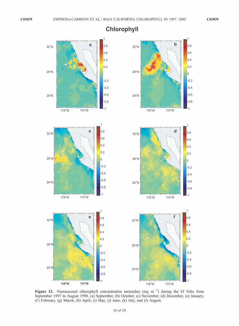
Figure 12. Nonseasonal chlorophyll concentration anomalies (mg m�3) during the El Nino fromSeptember 1997 to August 1998. (a) September, (b) October, (c) November, (d) December, (e) January,(f ) February, (g) March, (h) April, (i) May, (j) June, (k) July, and (l) August.

C03039 ESPINOSA-CARREON ET AL.: BAJA CALIFORNIA CHLOROPHYLL IN 1997–2002

16 of 20

C03039

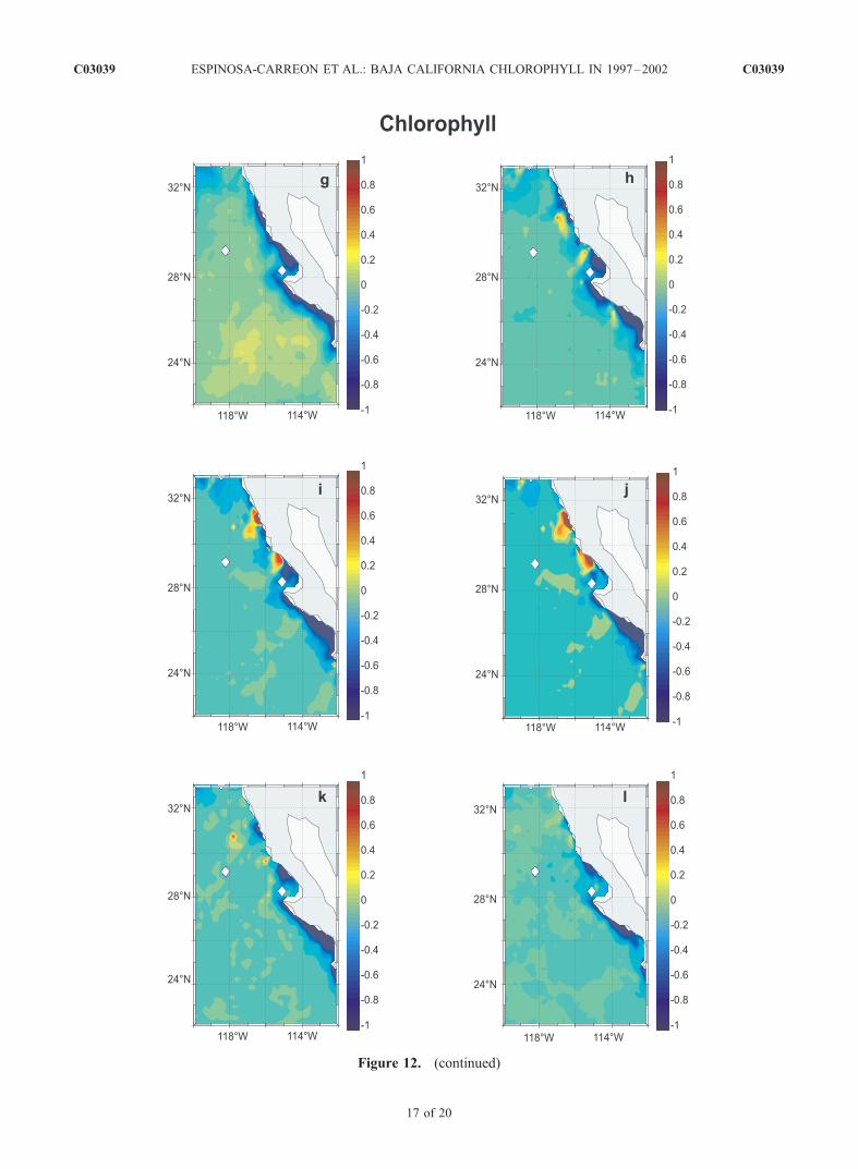
Figure 12. (continued)

C03039 ESPINOSA-CARREON ET AL.: BAJA CALIFORNIA CHLOROPHYLL IN 1997–2002

17 of 20

C03039

assemblages in the warm and stratified offshore waters werecaused by nitrogen-fixing cyanobacteria. However, bloomsof Trichodesmium do not usually produce strong anomaliesin satellite-derived pigment concentrations. Subramaniam etal. [2002] show that standard ocean color chlorophyllalgorithms would underestimate Trichodesmium-specificchlorophyll by a factor of at least 4, due to self-shading bythe colonies. This suggests that other phytoplanktoncommunities may have been present, interacting with thecyanobacteria to enhance the positive anomalies in theoffshore region. Hypotheses for the source of the elevatedpigment anomalies (whatever the species) include advectionof phytoplankton or nutrients from the north or from off-shore. Advection from farther north might imply that theequatorward California Current was displaced offshore bywater intruding next to the coast from the south. Advectionfrom offshore might include nutrients that were raised intothe euphotic zone by the increased Ekman suction caused bystorms associated with atmospheric El Nino conditions. Thesource of the offshore pigment anomalies remains to bedefinitively determined.

4. Conclusions

[43] 1. The seasonal variability in satellite-derived chlo-rophyll pigment concentrations, sea surface height, and seasurface temperature is estimated off Baja California between22�N and 34�N using harmonic fits and EOFs for timeseries spanning 4–5 years (1997 to late 2001 for SSH, 1997to mid-2002 for SST, and 1998 to mid-2002 for pigment).These help to identify three dynamic regions off BajaCalifornia: an upwelling zone next to the coast, the Ense-nada Front in the north (in the Southern California Bight),and regions of repeated meanders and/or eddy variabilitywest and southwest of Punta Eugenia (Figures 4 and 6–11).[44] 2. The seasonal cycles explain the most variance for

SST over a broad offshore area and explain the leastvariance for SSH. The seasonal cycle for pigment concen-trations is more confined to a narrow (<50 km) coastalregion than for SST and SSH (Figures 4 and 6–7). Thetiming of the seasonal changes strongly implicates upwell-ing-favorable winds as the driving force over seasonaltimescales. On nonseasonal timescales, however, changesin the monthly wind anomalies do not appear to be theprimary source of variability in the oceanic parameters,especially not in monthly anomalies of surface chlorophyllpigment concentrations.[45] 3. Features in coastal geometry (capes and bays,

especially the presence of Point Eugenia), appear to playan important role in the alongshore spatial patterns ofthe first three EOF modes of seasonal and nonseasonalof chlorophyll pigment concentration (Figure 6). PointEugenia also appears to affect the seasonal and nonseasonalEOF patterns in SST (Figures 4 and 10). A dominant eddypair develops seasonally west of Point Eugenia, one of thefew places where the harmonic seasonal cycle accounts foras much of 40% of the SSH variance (Figures 4 and 8).[46] 4. In the study area, the strongest effects are seen in

the coastal region during the El Nino, with weaker effectsduring La Nina (Figures 6b, 7b, 8b, 9b, 10b, and 11b).These effects are one of the sources of the low correlationsbetween nonseasonal anomalies of wind-forcing (monthly

CUI anomalies) and the nonseasonal EOFs of pigmentconcentration anomalies.[47] 5. Chlorophyll pigment concentrations in the offshore

region can be positive during El Nino conditions, as theywere in 1998 (Figure 12), for reasons not presently known.[48] The coastal upwelling zone identified in the first

conclusion above is the most inshore of three regionsdefined by the temporal mean of the satellite chlorophyllpigment concentrations off Baja California during 1998–2002 (Figure 2a): an inshore eutrophic area, an oligotrophicoffshore region, and an intermediate mesotrophic zone.High pigment concentrations are also found in the regionnorth of the Ensenada Front.[49] The long-term mean dynamic height (Figure 2b)

has lower values (�90 cm) next to the coast, consistentwith upwelling of dense water, and highest values offshore(�105 cm). SSH isopleths of constant height are roughlyparallel to the coast, indicating a current toward the southeast(the California Current). North of 31�N, there is a region oflow SSH, a signature of anticyclonic recirculation in theSouthern California Bight north of the Ensenada Front.[50] The mean field of SST (Figure 2c) shows a north-

south gradient, approximately perpendicular to the coast.Unlike the other mean fields, the north-south gradient in themean SST field indicates control by surface processes, inthis case surface heating with a strong latitudinal gradient.[51] Seasonal anomalies of chlorophyll concentrations

(Figures 4 and 6) show a spatial distribution similar to themean distribution, again identifying the coastal upwellingband with maximum values (up to 0.5 mg m�3) duringApril and near-zero values in the offshore region (secondconclusion). Seasonal anomalies of SST (Figure 4 and 10)are negative in a coastal region in April, but not restricted toas narrow a coastal band as chlorophyll concentrations. Theseasonal anomalies in SST are especially strong near and tothe south of Point Eugenia. SSH anomalies (Figures 4 and 8)also show a spatial distribution with high amplitudes againstthe coast, but less concentrated than chlorophyll concen-trations. The coastal SSH anomalies are low next to the coastin April and highest around October.[52] These seasonal patterns are consistent with the mean

pattern of seasonal forcing by ECMWF winds during1986–98. Over the ocean, the mean wind field is favorablefor upwelling next to the coast over the entire study region(Figure 3). These winds have a seasonal upwelling-favor-able maximum in early spring and a minimum in fall, but donot reverse over the ocean. The coincident timing ofextremes of forcing and responses in April, typical ofupwelling systems, leads us to identify the prime sourceof seasonal changes in pigment concentrations, SST andSSH as the equatorward winds (second conclusion). Theseasonal cycles of chlorophyll concentrations and SST arestrong (explaining 42% and 66% of the total variance),while the seasonal cycle of SSH is weak (explaining only4% of the total variance).[53] The spatial patterns for seasonal changes in SSH

include cyclonic and anticyclonic meanders or eddies to thewest and southwest of Point Eugenia (Figures 4 and 8), thethird region identified in the first conclusion. Furtherevidence for repeated eddies in this region is provided bythe seasonal cycle for SST, which explains least variance ina narrow coastal region and along the hypothesized path of

C03039 ESPINOSA-CARREON ET AL.: BAJA CALIFORNIA CHLOROPHYLL IN 1997–2002

18 of 20

C03039

eddies to the west and southwest of Point Eugenia(Figure 4i). We hypothesize that this is due to the shorttimescales for these events in the SST signal and theirirregular sampling due to clouds. Next to the coast, thespatial patterns of EOFs for SST and pigment concentrationanomalies suggests control by the time-invariant coastalgeometry, as does the similarity between patterns in theseasonal and nonseasonal EOFs. This and the region ofeddy activity off Point Eugenia support the third conclusion.[54] When the seasonal cycles are removed, the largest

signals are those of the ENSO variability, with El Nino(La Nina) effects characterized by high (low) sea surfaceheight, warm (cold) SST, and low (high) chlorophyll con-centrations next to the coast. Mechanisms that causeLa Nina conditions are not as well understood as El Nino.Nonseasonal anomalies were dominated by cold conditionsfollowing the El Nino in 1999–2001, especially during1999. Nonseasonal wind anomalies during El Nino canremain upwelling-favorable, and during La Nina they canbe either upwelling- or downwelling-favorable. This is amajor cause for low correlations between nonseasonal timeseries of winds and chlorophyll pigment concentrations(second and fourth conclusions).[55] The nonseasonal fields of pigment concentrations

suggest an offshore movement of high pigment concentra-tions in September–October 1997, followed by positivechlorophyll anomalies in the offshore region betweenNovember 1997 and March 1998. Even stronger negativepigment concentrations anomalies occur next to the coastduring January–August 1998. The negative anomaliespersist longest south of Point Eugenia. Several possiblehypotheses have been suggested for the positive offshorepigment anomalies during the El Nino, but none have beenconfirmed or eliminated at this time (fifth conclusion).

[56] Acknowledgments. The first author had a fellowship fromCONACyT, Mexico, and support through projects Fase I, Oceanografıapor Satelite (225080-5-4302PT; DAJ J002/750/00), G-35326, CICESE(Ecology Department), IAI-CRN 062, IOCCG, and COAS-OSU (NAS5-31360, OCE-9907854). SeaWiFS chlorophyll pigment data were processedand made available by Andrew Thomas, at the University of Maine.Altimeter data came from the NOAA-NASA Pathfinder project. SST datawas collected by Ocean Imaging, Inc., and archived at Oregon StateUniversity, as part of the U.S. GLOBEC NEP project, with support fromNSF grant OCE-0000900. This is contribution number 422 of the U.S.GLOBEC program, jointly funded by the National Science Foundation andthe National Oceanic and Atmospheric Administration. This is also acontribution of the IMECOCAL-CICESE research program to the scientificagenda of the Eastern Pacific Consortium of the InterAmerican Institute forGlobal Change Research (IAI-EPCOR). J.M. Dominguez drafted the finalfigures.

ReferencesAbbott, M. R., and B. Barksdale (1991), Phytoplankton pigment patternsand wind forcing off central California, J. Geophys. Res., 96, 14,649–14,667.

Aguirre-Hernandez, E., G. Gaxiola-Castro, S. Najera-Martınez,T. Baumgartner, M. Kahru, and B. G. Mitchell (2004), Phytoplanktonabsorption, photosynthetic parameters, and primary production off BajaCalifornia, summer and autumn 1998, Deep Sea Res., Part II, in press.

Bakun, A. (1975), Daily and weekly indices, west coast of North America,1967–1973, NOAA Tech. Rep., NMFS SSRF-693.

Barnes, R. A., A. W. Holmes, W. L. Barnes, W. E. Esaias, C. R. McClain,and T. Svitek (1994), SeaWiFS Prelaunch Radiometric Calibration andSpectral Characterization, NASA Tech. Memo., 104566, 55 pp.

Barth, J. A., S. D. Piece, and R. L. Smith (2000), A separating upwellingcoastal jet at Cape Blanco, Oregon and its connection to the CaliforniaCurrent System, Deep Sea Res., Part II, 47, 783–810.

Bernal, P. A. (1981), A review of the low-frequency response of the pelagicecosystem in the California Current, Calif. Coop. Ocean. Fish. Invest.Rep., 22, 49–62.

Bograd, S. J., et al. (2000), The state of the California Current, 1999–2000:Forward to a new regimen?, Calif. Coop. Ocean. Fish. Invest. Rep., 41,26–52.

Castro, R., A. Pares-Sierra, and S. G. Marinone (2003), Evolution andextension of the Santa Ana winds of February 2002 over the ocean, offCalifornia and the Baja California Peninsula, Cienc. Mar., 29, 275–281.

Chavez, F. P. (1996), Forcing and biological impact of onset of the 1992 ElNino in central California, Geophys. Res. Lett., 23, 265–268.

Chavez, F. P., P. G. Strutton, and M. J. McPhaden (1998), Biological-physical coupling in the central equatorial Pacific during the onset ofthe 1997–1998 El Nino, Geophys. Res. Lett., 25, 3543–3546.

Chavez, F. P., J. T. Pennington, C. G. Castro, J. P. Ryan, R. P. Michisaki,B. Schlining, P. Walz, K. R. Buck, A. McFadyen, and C. A. Collins(2002), Biological and chemical consequences of the 1997–1998 ElNino in central California waters, Prog. Oceanogr., 54, 205–232.

Chelton, D. B. (1982), Statistical reliability and the seasonal cycle: Com-ments on ‘‘Bottom pressure measurements across the Antarctic Circumpo-lar Current and their relation to the wind,’’Deep Sea Res., 29, 1381–1388.

Chelton, D. B. (1984), Seasonal variability of alongshore geostrophicvelocity off central California, J. Geophys. Res., 89, 3473–3486.

Collins, C. A., C. G. Castro, H. Asanuma, T. A. Rago, S.-K. Han,R. Durazo, and F. P. Chavez (2002), Changes in the hydrography ofCentral California waters associated with the 1997–98 El Nino, Prog.Oceanogr., 54, 129–147.

Durazo, R., and T. R. Baumgartner (2002), Evolution of oceanographicconditions off Baja California, 1997–1999, Prog. Oceanogr., 54, 7–31.

Durazo, R., et al. (2001), The state of the California Current, 2000–2001:A third straight La Nina year, Calif. Coop. Ocean. Fish. Invest. Rep., 42,29–60.

Fargion, G. S., J. A. McGowan, and R. H. Stewart (1993), Seasonality ofchlorophyll concentrations in the California Current: A comparison oftwo methods, Calif. Coop. Ocean. Fish. Invest. Rep., 34, 35–50.

Gallaudet, T. C., and J. J. Simpson (1994), An empirical orthogonal func-tion analysis of remotely sensed sea surface temperature variability andits relation to interior oceanic processes of Baja California, Remote Sens.Environ., 47, 375–389.

Gaxiola-Castro, G., and S. Alvarez-Borrego (1991), Relative assimilationnumbers of phytoplankton across a seasonally recurring front in theCalifornia Current off Ensenada, Calif. Coop. Ocean. Fish. Invest.Rep., 32, 91–96.

Gomez-Valdes, J., and H. Velez-Munoz (1982), Variacion estacional detemperatura y salinidad en regiones costeras de la Corriente de California,Cienc. Mar., 8, 167–176.

Haidvogel, D. B., A. Beckmann, and K. S. Hedstrom (1991), Dynamicalsimulations of filament formation and evolution in the coastal transitionzone, J. Geophys. Res., 96, 15,017–15,040.

Haury, I. R., E. Venrick, C. L. Fey, J. A. McGowan, and P. P. Niiler (1993),The Ensenada Front: July 1985, Calif. Coop. Ocean. Fish. Invest. Rep.,34, 69–88.

Hayward, T. L., et al. (1999), The state of the California Current, 1998–1999: Transition to cool-water conditions, Calif. Coop. Ocean. Fish.Invest. Rep., 40, 29–62.

Hickey, B. M. (1979), The California Current System–Hypotheses andfacts, Prog. Oceanogr., 8, 191–279.

Hickey, B. M. (1998), Coastal oceanography of western North Americafrom the tip of Baja California to Vancouver Island, Sea, 11, 345–393.

Huyer, A. (1983), Coastal upwelling in the California Current System,Prog. Oceanogr., 12, 259–284.

Ikeda, M., and W. J. Emery (1984), Satellite observations and modeling ofmeanders in the California Current System off Oregon and northernCalifornia, J. Phys. Oceanogr., 14, 1434–1450.

Kahru, M., and G. Mitchell (2000), Influence of 1997–1998 El Nino on thesurface chlorophyll in the California Current, Geophys. Res. Lett., 27,2937–2940.

Kahru, M., and G. Mitchell (2001), Seasonal and nonseasonal variability ofsatellite-derived chlorophyll and colored dissolved organic matter con-centration in the California Current, J. Geophys. Res., 106, 2517–2529.

Kahru, M., and B. G. Mitchell (2002), Influence of the El Nino–La Ninacycle on satellite-derived primary production in the California Current,Geophys. Res., 29(17), 1846, doi:10.1029/2002GL014963.

Levitus, S., T. P. Boyer, M. E. Conkright, T. O’Brien, J. Antonov,C. Stephens, L. Stathopolos, D. Johnson, and R. Gelfeld (1998), WorldOcean Database 998, vol. 1, Introduction, NOAA Atlas NESDIS 18, Natl.Oceanic and Atmos. Admin., Silver Spring, Md.

Lynn, R. J., and S. J. Bograd (2002), Dynamic evolution of the 1997–1999El Nino-La Nina cycle in the southern California Current System, Prog.Oceanogr., 54, 59–75.

C03039 ESPINOSA-CARREON ET AL.: BAJA CALIFORNIA CHLOROPHYLL IN 1997–2002

19 of 20

C03039

Lynn, R. J., and J. J. Simpson (1987), The California Current System: Theseasonal variability of physical characteristics, J. Geophys. Res., 92,12,947–12,966.

Lynn, R. J., K. A. Bliss, and L. E. Eber (1982), Vertical and horizontaldistributions of seasonal mean temperature, salinity, sigma-t, stability,dynamic height, oxygen and oxygen saturation in the California Current,1950–1978, Calif. Coop. Ocean. Fish. Invest. Atlas, 30, 513 pp.

Lynn, R. J., et al. (1998), The State of California Current, 1997–1998:Transition to El Nino conditions, Calif. Coop. Ocean. Fish. Invest.Rep., 39, 25–49.

McCarthy, J. J., A. R. Robinson, and B. J. Rothschild (2002), Introduction-biological-physical interactions in the sea: Emergent findings and newdirections, in The Sea, vol. 12, edited by A. R. Robinson, J. J. McCarthy,and B. J. Rothschild, pp. 1–16, John Wiley, New York.

McGowan, J. A., D. B. Chelton, and A. Conversi (1996), Plankton pattern,climate and change in the California Current, Calif. Coop. Ocean. Fish.Invest. Rep., 37, 45–68.

McPhaden, M. J. (1999), Genesis and evolution of the 1997–1998 El Nino,Science, 283, 950–954.

Narimousa, S., and T. Maxworthy (1989), Applications of a laboratorymodel to the interpretation of satellite and field observations of coastalupwelling, Dyn. Atmos. Oceans, 13, 1–46.

Olson, D. B. (2002), Biophysical dynamics of ocean fronts, in The Sea,vol. 12, edited by A. R. Robinson, J. J. McCarthy, and B. J. Rothschild,pp. 188–218, John Wiley, Hoboken, N.J.

Pares-Sierra, A., W. B. White, and C. K. Tai (1993), Wind-driven coastalgeneration of annual mesoscale eddy activity in the California CurrentSystem: A numerical model, J. Phys. Oceanogr., 23, 1110–1121.

Pares-Sierra, A., M. Lopez, and E. Pavıa (1997), Oceanografıa Fısica delOceano Pacıfico Nororiental, in Contribuciones a la Oceanografıa Fısicaen Mexico, Monogr. Ser., vol. 3, pp. 1–24, Union Geofıs. Mex., PuertoVallarta, Mex.

Pelaez, J., and F. Guan (1982), California Current chlorophyll measure-ments from satellite data, Calif. Coop. Ocean. Fish. Invest. Atlas, 23,212–225.

Pelaez, J., and J. A. McGowan (1986), Phytoplankton pigment patterns inthe California Current as determined by satellite, Limnol. Oceanogr., 31,927–950.

Schwing, F. B., M. O’Farrel, J. Steger, and K. Blaltz (1996), Coastalupwelling indices, west coast of North America 1946–1995, NOAA Tech.Rep., NMFS SWFSC-231.

Simpson, J. J., and R. J. Lynn (1990), A Mesoscale eddy dipole in theoffshore California Current, J. Geophys. Res., 95, 13,009–13,022.

Simpson, J. J., C. J. Koblinsky, J. Pelaez, L. R. Haury, and D. Wiesenhahn(1986), Temperature–plant pigment–optical relations in a recurrent off-shore mesoscale eddy near Point Conception, California, J. Geophys.Res., 91, 12,919–12,936.

Soto-Mardones, L., A. Pares-Sierra, J. Garcıa, R. Durazo, and S. Hormazabal(2004), Analysis of the mesoscale structure in the IMECOCAL region(off Baja California) from Hydrographic, ADCP and Altimetry Data,Deep Sea Res., Part II, in press.

Strub, P. T., and C. James (2002), The 1997–1998 Oceanic El Nino signalalong the southeast and northeast Pacific boundaries–An altimetric view,Prog. Oceanogr., 54, 439–458.

Strub, P. T., C. James, A. Thomas, and M. Abbot (1990), Seasonal andnonseasonal variability of satellite-derived surface pigments concentra-tion in the California Current, J. Geophys. Res., 95, 11,501–11,530.

Strub, P. T., P. M. Kosro, and A. Huyer (1991), The nature of cold filamentsin the California Current System, J. Geophys. Res., 96, 14,743–14,768.

Subramaniam, A., C. W. Brown, R. R. Hood, E. J. Carpenter, and D. G.Capone (2002), Detecting Trichodesmium blooms in SeaWiFS imagery,Deep Sea Res., Part II, 49, 107–121.

Thomas, A. C., and P. T. Strub (1990), Seasonal and interannual variabilityof pigment concentrations across a California Current frontal zone,J. Geophys. Res., 95, 13,023–13,042.

Thomas, A. C., F. Huang, P. T. Strub, and C. James (1994), Comparisonof the seasonal and interannual variability of phytoplankton pigmentconcentrations in the Peru and California Current systems, J. Geophys.Res., 99, 7355–7370.

Venrick, E. L. (2000), Summer in the Ensenada Front: The distribution ofphytoplankton species, July 1985 and September 1988, J. Plankton Res.,22, 813–841.

�����������������������E. Beier, T. L. Espinosa-Carreon, G. Gaxiola-Castro, and F. Ocampo-

Torres, Centro de Investigacion Cientıfica y de Educacion Superior deEnsenada, Km 107 Carr, Tijuana-Ensenada, Ensenada, Baja California,Mexico. (ebeier@cicese.mx; lespinos@cicese.mx; ggaxiola@cicese;ocampo@cicese.mx)P. T. Strub, College of Oceanic and Atmospheric Sciences, Oregon State

University, 104 Ocean Administration Building, Corvallis, OR 97331-5503,USA. (tstrub@coas.oregonstate.edu)

C03039 ESPINOSA-CARREON ET AL.: BAJA CALIFORNIA CHLOROPHYLL IN 1997–2002

20 of 20

C03039