Searches for Axion-Like Particles

with X-ray Astronomy

Nicholas JenningsSomerville College

University of Oxford

A thesis submitted for the degree of

Doctor of Philosophy

Trinity 2018

Acknowledgements

Firstly I would like to thank my supervisor Joseph Conlon for his teachingand guidance over the course of my time at Oxford. I would like tothank all my collaborators from whom I have learned so much: MarcusBerg, Francesca Day, Sven Krippendorf, Andrew Powell, Francesco Muiaand Markus Rummel. I would also like to thank the wider TheoreticalPhysics community at Oxford for many stimulating seminars, lectures andconversations. I have been funded by the Science and Technology FacilitiesCouncil and my supervisor’s European Research Council grant.

I would like to thank Anna, Jeannette, Ian and Laura for the time andeffort they took to help with proof-reading this thesis, and their generalsupport and inspiration.

Statement of Originality

This thesis is entirely written by myself, except as indicated in the text.It contains work that I have conducted individually and in collaborationwith my supervisor and his group. Here I detail my contributions to workdone in collaboration. Chapter 1 contains an introductory review thatis entirely my own work. Chapter 2 sets out the Aims and Objectivesof the thesis, and is entirely my own work. Chapters 3, 4 and 5 arebased collectively on the papers [1], [2] and [3]. The work in these paperswas done collaboratively with Joseph Conlon, Francesca Day and SvenKrippendorf as well as: with Marcus Berg, Andrew Powell and MarkusRummel [1]; with Markus Rummel [2]; and with Francesco Muia [3].

My main contributions to these papers were: processing and analysing theChandra satellite images of NGC 1275; and modelling the contaminationin the Chandra NGC 1275 images using the jdpileup analysis tool, andwriting up the relevant sections in [1]; processing and analysing Chandrasatellite images of other point sources in [2]; running the SIXTE softwareto simulate the Athena satellite; deriving estimated ALP bounds fromAthena; and writing up the paper [3]. In Chapter 5 I briefly cover workdone in [4], which was done collaboratively with Joseph Conlon, FrancescaDay, Sven Krippendorf and Markus Rummel. Chapter 6 is my conclusionwhich is entirely my own work. No part of this thesis has been submittedfor any other qualification.

Abstract

Axion-Like Particles (ALPs) are a very well-motivated class of Beyond theStandard Model particles. They can be implemented as a minimal exten-sion of the Standard Model that could solve many mysteries (the StrongCP Problem, Dark Matter, origin of Inflation), and also commonly arisein String Theory compactifications. This motivates the commissioning ofdedicated experiments looking for these particles, as well as the utilisa-tion of telescope data to search for their astrophysical effects. Throughtheir coupling to electromagnetism, they will interconvert with photonsin the presence of a magnetic field. A promising environment to look forthis effect is the intracluster medium of Galaxy Clusters, which can haveweak but very extensive magnetic fields. At X-ray energies, the conversionprobability of photons to ALPs is periodic in energy, imprinting a quasi-sinusoidal oscillation on the energy spectrum of an object shining throughthe cluster. This thesis describes an analysis of data taken by the Chandraand XMM-Newton satellites of point sources (such as active galactic nu-clei) shining through galaxy clusters. The absences of modulations in thespectra of these objects lead to constraints on the ALP-photon coupling.With this analysis, a previously unexplored region of parameter space isruled out. This thesis also details simulations that were performed of thecapabilities of the Athena X-ray Observatory, due to launch in 2028, andpredicts its ability to place further constraints on ALPs.

Contents

1 Introduction to Axions 11.1 The Strong CP Problem and the QCD axion . . . . . . . . . . . . . . 1

1.1.1 Quantum Chromodynamics and the Strong CP Problem . . . 11.1.2 Solutions to the Strong CP Problem . . . . . . . . . . . . . . 31.1.3 Axions as a solution to the Strong CP Problem . . . . . . . . 41.1.4 “Invisible” Axions . . . . . . . . . . . . . . . . . . . . . . . . . 5

1.2 Axion-Like Particles in String Theory . . . . . . . . . . . . . . . . . . 71.3 Dark Matter . . . . . . . . . . . . . . . . . . . . . . . . . . . . . . . . 101.4 Axion-photon conversion in magnetic fields . . . . . . . . . . . . . . . 12

1.4.1 Dispersion relations for photons in a magnetic field . . . . . . 121.4.2 Interconversion with ALPs . . . . . . . . . . . . . . . . . . . . 14

1.5 Review of constraints . . . . . . . . . . . . . . . . . . . . . . . . . . . 161.5.1 Light Shining through Walls . . . . . . . . . . . . . . . . . . . 171.5.2 Stellar energy-loss . . . . . . . . . . . . . . . . . . . . . . . . . 171.5.3 Helioscopes . . . . . . . . . . . . . . . . . . . . . . . . . . . . 181.5.4 Resonant Cavities . . . . . . . . . . . . . . . . . . . . . . . . . 181.5.5 Black Hole superradiance . . . . . . . . . . . . . . . . . . . . . 181.5.6 Searches for ALPs with satellites . . . . . . . . . . . . . . . . 191.5.7 Summary . . . . . . . . . . . . . . . . . . . . . . . . . . . . . 19

2 Aims and Objectives 21

3 Analysis of Galaxy Clusters 243.1 Magnetic Fields in the Intracluster Medium . . . . . . . . . . . . . . 24

3.1.1 Faraday Rotation Measures . . . . . . . . . . . . . . . . . . . 253.1.2 Synchrotron Radiation and Equipartition . . . . . . . . . . . . 263.1.3 Inverse Compton Scattering . . . . . . . . . . . . . . . . . . . 263.1.4 Summary of galaxy cluster magnetic field measurements . . . 27

i

3.2 Modelling properties of the intracluster medium . . . . . . . . . . . . 283.3 Calculating ALP-photon conversion probability in clusters . . . . . . 303.4 Candidate target sources . . . . . . . . . . . . . . . . . . . . . . . . . 323.5 Data processing of X-ray satellites . . . . . . . . . . . . . . . . . . . . 33

3.5.1 Chandra . . . . . . . . . . . . . . . . . . . . . . . . . . . . . . 343.5.2 XMM-Newton . . . . . . . . . . . . . . . . . . . . . . . . . . . 403.5.3 The future satellite Athena . . . . . . . . . . . . . . . . . . . . 41

3.6 Procedure to constrain the ALP-photon coupling . . . . . . . . . . . 443.7 Simulating bounds for future satellites . . . . . . . . . . . . . . . . . 45

4 Results 474.1 Point sources in/behind Galaxy Clusters . . . . . . . . . . . . . . . . 47

4.1.1 Summary of Point Sources Selected . . . . . . . . . . . . . . . 474.2 NGC 1275 . . . . . . . . . . . . . . . . . . . . . . . . . . . . . . . . . 49

4.2.1 Chandra observations . . . . . . . . . . . . . . . . . . . . . . . 494.2.2 Chandra Analysis . . . . . . . . . . . . . . . . . . . . . . . . . 514.2.3 Pileup . . . . . . . . . . . . . . . . . . . . . . . . . . . . . . . 544.2.4 Analysis of residuals in Chandra NGC 1275 data . . . . . . . . 634.2.5 The Presence of the 6.4 keV Iron line . . . . . . . . . . . . . . 684.2.6 Bounds from Chandra data . . . . . . . . . . . . . . . . . . . 694.2.7 Validation with MARX simulation . . . . . . . . . . . . . . . 724.2.8 XMM-Newton observations . . . . . . . . . . . . . . . . . . . . 764.2.9 XMM-Newton Analysis . . . . . . . . . . . . . . . . . . . . . . 77

4.3 Bounds from other point sources . . . . . . . . . . . . . . . . . . . . . 794.3.1 Quasar B1256+281 behind Coma . . . . . . . . . . . . . . . . 794.3.2 Quasar SDSS J130001.47+275120.6 behind Coma . . . . . . . 814.3.3 NGC3862 within A1367 . . . . . . . . . . . . . . . . . . . . . 824.3.4 Central AGN IC4374 of A3581 . . . . . . . . . . . . . . . . . . 844.3.5 Central AGN of Hydra A . . . . . . . . . . . . . . . . . . . . . 844.3.6 Seyfert galaxy 2E3140 in A1795 . . . . . . . . . . . . . . . . . 854.3.7 Quasar CXOUJ134905.8+263752 behind A1795 . . . . . . . . 854.3.8 UGC9799 in A2052 . . . . . . . . . . . . . . . . . . . . . . . . 87

4.4 Simulated bounds from Athena Observations . . . . . . . . . . . . . . 89

ii

5 Discussion 945.1 Comments on NGC 1275 . . . . . . . . . . . . . . . . . . . . . . . . . 94

5.1.1 Thermal component . . . . . . . . . . . . . . . . . . . . . . . 955.1.2 Pileup and Bounds . . . . . . . . . . . . . . . . . . . . . . . . 955.1.3 Analysis of residuals in Chandra NGC 1275 data . . . . . . . . 96

5.2 Limitations of the study . . . . . . . . . . . . . . . . . . . . . . . . . 1005.3 Comparison with other studies . . . . . . . . . . . . . . . . . . . . . . 102

5.3.1 Chandra and XMM-Newton . . . . . . . . . . . . . . . . . . . 1025.3.2 Athena . . . . . . . . . . . . . . . . . . . . . . . . . . . . . . . 103

5.4 Constraints on ALPs as Dark Matter . . . . . . . . . . . . . . . . . . 1035.5 Potential for improvement . . . . . . . . . . . . . . . . . . . . . . . . 103

6 Conclusions and Outlook 105

Bibliography 106

iii

List of Figures

1.1 Overview of exclusion limits on the ALP-photon coupling, plottedagainst mass. . . . . . . . . . . . . . . . . . . . . . . . . . . . . . . . 20

3.1 Photon conversion probability through a single-domain magnetic fielddue to ALP interconversion. . . . . . . . . . . . . . . . . . . . . . . . 31

3.2 Photon survival probability through a cluster magnetic field due toALP interconversion. . . . . . . . . . . . . . . . . . . . . . . . . . . . 32

3.3 Photon survival probability through a magnetic field, convolved with100 eV detector resolution. . . . . . . . . . . . . . . . . . . . . . . . . 36

3.4 Photon survival probability through a cluster magnetic field, convolvedwith a 2.5 eV detector resolution. . . . . . . . . . . . . . . . . . . . . 43

4.1 The NGC 1275 Chandra images. . . . . . . . . . . . . . . . . . . . . . 514.2 The stacked spectrum of the ACIS-I edge observations from the full

extraction region. . . . . . . . . . . . . . . . . . . . . . . . . . . . . . 534.3 The stacked spectrum of the ACIS-I midway observations from the full

extraction region. . . . . . . . . . . . . . . . . . . . . . . . . . . . . . 544.4 The stacked spectrum of the ACIS-S observations from the full extrac-

tion region. . . . . . . . . . . . . . . . . . . . . . . . . . . . . . . . . 554.5 The stacked spectrum of the ACIS-I edge observations with central

pixels removed. . . . . . . . . . . . . . . . . . . . . . . . . . . . . . . 574.6 The stacked spectrum of the ACIS-I midway observations with central

pixels removed. . . . . . . . . . . . . . . . . . . . . . . . . . . . . . . 574.7 The stacked spectrum of the ACIS-S edge observations with central

pixels removed. . . . . . . . . . . . . . . . . . . . . . . . . . . . . . . 594.8 The stacked spectrum of the ACIS-S observations with pileup model. 614.9 The stacked spectrum of the ACIS-I midway observations with pileup

model. . . . . . . . . . . . . . . . . . . . . . . . . . . . . . . . . . . . 624.10 The stacked spectrum of the ACIS-I edge observations with pileup model. 63

iv

4.11 The improvement in χ2 attainable by adding a negative Gaussian atthe specific energy for ACIS-I Edge observations. . . . . . . . . . . . 65

4.12 The improvement in χ2 attainable by adding a negative Gaussian atthe specific energy for ACIS-I Midway observations. . . . . . . . . . . 65

4.13 The improvement in χ2 attainable by adding a negative Gaussian atthe specific energy for ACIS-S observations. . . . . . . . . . . . . . . 65

4.14 The overall significance and location for the 3.5 keV deficit. . . . . . . 664.15 A fit to the clean ACIS-I edge observations with ALP-photon conver-

sion modelled. . . . . . . . . . . . . . . . . . . . . . . . . . . . . . . . 674.16 The photon survival probability for the fit shown in Figure 4.15. . . 674.17 The Fe Kα line in the cleaned ACIS-S data. . . . . . . . . . . . . . . 684.18 The 95% upper bounds on the ALP-photon coupling in comparison to

previously obtained bounds on ALPs. . . . . . . . . . . . . . . . . . . 724.19 An example of simulated data using ChaRT and MARX. . . . . . . . 764.20 MOS 2001 spectral fit. . . . . . . . . . . . . . . . . . . . . . . . . . . 794.21 MOS 2006 spectral fit. . . . . . . . . . . . . . . . . . . . . . . . . . . 814.22 The stacked spectrum of the quasar B1256+281 behind Coma. . . . . 824.23 The stacked spectrum of the quasar SDSS J130001.48+275120.6 behind

Coma. . . . . . . . . . . . . . . . . . . . . . . . . . . . . . . . . . . . 834.24 The stacked spectrum of the AGN NGC3862 in A1367. . . . . . . . . 834.25 The stacked spectrum of the central cluster galaxy IC4374 located in

A3581. . . . . . . . . . . . . . . . . . . . . . . . . . . . . . . . . . . . 844.26 The stacked spectrum of the bright Seyfert 1 galaxy 2E3140 located in

A1795. . . . . . . . . . . . . . . . . . . . . . . . . . . . . . . . . . . . 864.27 The stacked spectrum of the quasar CXOU J134905.8+263752 behind

A1795. . . . . . . . . . . . . . . . . . . . . . . . . . . . . . . . . . . . 874.28 The stacked spectrum of the central cluster galaxy UGC9799 located

in A2052. . . . . . . . . . . . . . . . . . . . . . . . . . . . . . . . . . 884.29 A simulated 200 ks dataset for NGC 1275 including ALP interconversion. 914.30 Comparison of Chandra and Athena limits with previous bounds. . . 93

v

Chapter 1

Introduction to Axions

1.1 The Strong CP Problem and the QCD axion

1.1.1 Quantum Chromodynamics and the Strong CP Problem

The Standard Model (SM) remains our best description of particle physics to date,and has an excellent track record of explaining data from experiments ranging fromhigh-energy supercolliders to precision tests of its fundamental parameters. The SMorganises the particles of nature into the gauge symmetry group SU(3)×SU(2)×U(1),where SU(N) is the special unitary group of dimension N. SU(2)×U(1) incorporatesthe electromagnetic and weak nuclear forces of nature, with photons and the W,Zbosons being the mediators. SU(3)C relates to the strong nuclear force, with the Creferring to the color charge of particles that determines how they interact via thestrong force. The theory underpinning our understanding of the strong force is knownas Quantum Chromodynamics (QCD), with the following Lagrangian density:

L = − 1

g2GaµνG

aµν +∑f

ψf (iDµγµ −mf )ψf (1.1)

As the masses for the up and down quarks are much smaller than ΛQCD (thescale below which quarks are confined into hadrons), we can consider the limit wherethese masses are zero. In this case, there is a SU(2) ⊗ SU(2) chiral symmetry ofthe QCD Lagrangian. The diagonal subgroup is isospin, while the remainder is aNambu-Goldstone symmetry with the pions as the massless Nambu-Goldstone bosons.This symmetry is dynamically broken by quark condensates 〈uu〉, 〈dd〉, leading tosmall masses for the pions. However, there is an additional U(1) symmetry of theLagrangian when the up and down quark masses are zero:

ψf → e−iαγ5ψf , f = 1, 2. (1.2)

1

where ψ1 and ψ2 are the up and down quarks. This symmetry is broken by the samequark condensates as break the chiral SU(2)⊗SU(2) symmetry, which indicates thereshould be a fourth light meson. However, no such particle exists.

This was dubbed “The U(1)A problem” by S. Weinberg [5] because there appearedto be no Lagrangian term that could break this U(1)A symmetry. The chiral anomaly[6, 7, 8] does provide a contribution to the action:

δW = αg2sN

32π2

∫d4xGa

µνGaµν , (1.3)

however the term inside the integral is a total divergence:

GaµνG

aµν = ∂µKµ = ∂µε

µαβγAaα

(Gaβγ −

gs3fabcAbβAcγ

). (1.4)

This means that the contribution to the action is a surface integral. If one assumesthe boundary condition Aµa = 0 at spatial infinity, the contribution disappears andthere is no U(1)A-breaking term. However, it was shown in [9, 10] that the boundarycondition is Aµa = 0 or a gauge transformation thereof. These gauge transformationsΩn are characterised by their behaviour at spatial infinity:

Ωn → e2πin, (1.5)

where n is an integer characterising the topological winding number. Field configura-tions of different winding numbers cannot be continuously deformed into each other.Taking the superposition of these n-vacua gives the true vacuum:

|θ〉 =∑n

einθ|n〉. (1.6)

The existence of this complicated vacuum structure in QCD leads to an additionalterm in the effective action:

Seff [A] = SQCD[A] + θg2s

32π2

∫d4xGa

µνGaµν (1.7)

We now wish to calculate the experimental effects of this extra Lagrangian term.To do so, we must incorporate our above discussion of SU(3) gauge theory into atheory with quarks and weak interactions. The quark masses are described by theCabibbo–Kobayashi–Maskawa (CKM) matrix, which is measured to be complex. Di-agonalising to a physical basis requires a chiral transformation, which changes the

2

theta vacuum [11]. Thus θ receives a correction:

θ = θ + arg det M (1.8)

for a mass matrix Mij.The extra term in Equation 1.7 breaks parity and time reversal invariance, but

conserves charge conjugation invariance in the strong force. Thus the term breaksCP invariance. The main effect that can be experimentally detected is an inducedneutron electric dipole moment (EDM) that takes the following form:

dn 'e θ mq

m2N

. (1.9)

The most sensitive constraint on the neutron EDM is −3.8 < dn < 3.4 × 10−26 e cm

at 95% confidence limit (CL) [12]. This implies that θ . 10−10. The smallness ofthis number presents a puzzle, known as the “Strong CP Problem”. Both componentsof θ are dimensionless quantities that are typically large. Given that they resultfrom different interactions, there is nothing in the SM to indicate that they ought tocancel so exactly. If one makes an argument that θ = 0, one must also explain whyarg det M is so small. This places a severe constraint on models that can successfullysolve the Strong CP Problem. I provide an incomplete review of proposed solutionsin the literature below.

1.1.2 Solutions to the Strong CP Problem

Spontaneous breaking of CP

We can set θ = 0 if CP is a symmetry of the Standard Model. Upon spontaneousbreaking of this symmetry, radiative corrections from loop diagrams will generate acorrection to θ. We require the corrections to be smaller than 10−10, which in generalconstrains the models to require the contributions of 1-loop diagrams to cancel as well.The following papers contain models that achieve small θ [13, 14, 15, 16], althoughsome of them are not compatible with the latest experimental constraints. Some ofthese rely on the high energy, CP -conserving theory being broken to the SM withadditional particles that have hitherto escaped detection. It has also been challengingto include them in a Grand Unified Theory (GUT). An elegant class of GUTs that arebroken to the SM and feature small θ were discovered in [17, 18, 19]. These solutionsto the Strong CP Problem are known collectively as the Nelson-Barr Mechanism.

3

An overview of the challenges facing this model, including hierarchy and fine-tuningproblems, can be found in [20].

Massless up quark

An additional chiral symmetry would solve the Strong CP Problem. This could beachieved if arg det M = 0, which could occur if the lightest quark (the up quark)was massless [21]. However, lattice calculations indicate that the up quark massmu ∼ 1 MeV, which strongly disfavours this explanation [22].

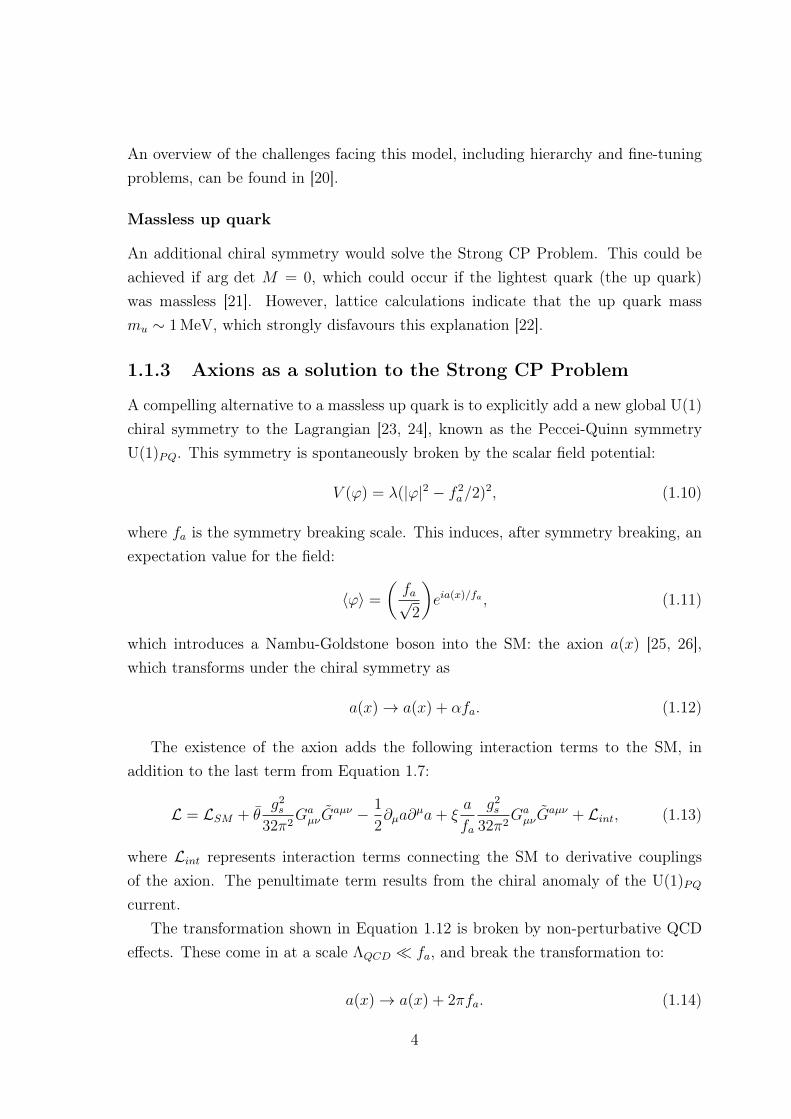
1.1.3 Axions as a solution to the Strong CP Problem

A compelling alternative to a massless up quark is to explicitly add a new global U(1)chiral symmetry to the Lagrangian [23, 24], known as the Peccei-Quinn symmetryU(1)PQ. This symmetry is spontaneously broken by the scalar field potential:

V (ϕ) = λ(|ϕ|2 − f 2a/2)2, (1.10)

where fa is the symmetry breaking scale. This induces, after symmetry breaking, anexpectation value for the field:

〈ϕ〉 =

(fa√

2

)eia(x)/fa , (1.11)

which introduces a Nambu-Goldstone boson into the SM: the axion a(x) [25, 26],which transforms under the chiral symmetry as

a(x)→ a(x) + αfa. (1.12)

The existence of the axion adds the following interaction terms to the SM, inaddition to the last term from Equation 1.7:

L = LSM + θg2s

32π2GaµνG

aµν − 1

2∂µa∂

µa+ ξa

fa

g2s

32π2GaµνG

aµν + Lint, (1.13)

where Lint represents interaction terms connecting the SM to derivative couplingsof the axion. The penultimate term results from the chiral anomaly of the U(1)PQ

current.The transformation shown in Equation 1.12 is broken by non-perturbative QCD

effects. These come in at a scale ΛQCD fa, and break the transformation to:

a(x)→ a(x) + 2πfa. (1.14)

4

This generates an effective potential for the axion which has its minimum at〈a〉 = −θfa/ξ, as described by the Vafa-Witten Theorem [27]. Therefore, the axiondynamically relaxes to a minimum where the θ term is cancelled out, and the StrongCP Problem is solved. This creates a periodic effective potential for the axion, of theform (redefining a→ aphys = a− 〈a〉 so that V (0) = 0):

V (a) = Λ4a

(1− cos

(aphysfa

)). (1.15)

(For brevity I will refer to aphys as a from now on). This generates an effective massfor the axion with its second derivative of the form:

m2a =

⟨∂2V

∂a2

⟩ ∣∣∣∣〈a〉=0

=Λ4a

f 2a

. (1.16)

Thus the axion is a pseudo-Nambu Goldstone boson.The values of Λa and fa are model dependent. They can be calculated using

current algebra techniques or effective Lagrangian descriptions. For the QCD axionthe mass takes the form:

ma = Amπfπfa

√mumd

mu +md

, (1.17)

where A is a constant that represents the specific couplings of the axion to other SMparticles for a particular theory (I will go into more detail below).

1.1.4 “Invisible” Axions

In the original PQWW (Peccei-Quinn-Weinberg-Wilczek) model [25, 26, 23], theU(1)PQ symmetry is achieved through two Higgs doublets: one giving mass to up-typequarks, and the other giving mass to down-type quarks and leptons. The Yukawainteractions are:

L = ΓuijQLiΦ1uRj + ΓdijQLiΦ2dRj + Γ`ijLLiΦ2`Rj + h.c., (1.18)

with the axion being the common phase field of Φ1 and Φ2:

Φ1 =v1√

2eiax/vF

(10

), Φ2 =

v2√2

eia/xvF(

01

), (1.19)

5

where x = v2/v1 and vF =√v2

1 + v22. The ALP-photon-photon interaction comes

from the Lagrangian term:

Laγγ =α

4πKaγγ

a

faFaµνF

µνa , (1.20)

where the coupling Kaγγ receives contributions from the axion mixing with the π0

and η mesons:

Kaγγ =N

2

(x+

1

x

)mu

mu +md

, (1.21)

where N is the number of quark flavours. The mass of the axion is given by Equa-tion 1.17 with:

A =N

2

(x+

1

x

). (1.22)

In this model fa is at the scale of electroweak symmetry breaking vF ' 250 GeV.This has long since been ruled out by beam dump experiments [28] and colliders [29].However, models that put fa at a much higher scale, known as ‘invisible axion’ models[30], have not been ruled out across all parameter space.

KSVZ axion

The Kim-Shifman-Vainshtein-Zakharov (KSVZ) axion [31, 32] features a scalar fieldσ and a heavy quark Q that both carry PQ charge. They interact via the Yukawaterm:

LY = −λQσQLQR + h.c. (1.23)

The KSVZ axion interacts with light quarks via the color and EM anomalies:

LKSV Z ⊃ a

fa

(g2s

32π2GaµνG

µνa + 3e2

Q

α

4πFaµνF

µνa

), (1.24)

where eQ is the electromagnetic charge of the heavy quark. Note that there are

6

no tree-level couplings to leptons for the KSVZ axion. The resulting axion-photoncoupling is:

Kaγγ = 3e2Q −

4md +mu

3(md +mu). (1.25)

Canonically one takes the Q field to be neutral, so eQ = 0. For the KSVZ axionA = 1 as defined in Equation 1.17, giving a mass:

ma = 6.3 eV

(106 GeV

fa

). (1.26)

DFSZ axion

The Dine-Fischler-Srednicki-Zhitnisky (DFSZ) axion [33, 34] requires two Higgs dou-blets Hu and Hd like the PQWW axion, plus an additional scalar field φ. The Higgsdoublets and the scalar interact via the potential:

V = λHφ2HuHd. (1.27)

This has a mass corresponding to Equation 1.17 where A = C = 6 is the coloranomaly (also known as the Domain Wall Number i.e. the number of vacua in therange a ∈ [0, 2πfa]). The axion-photon coupling is:

Kaγγ =4

3− 4md +mu

3(md +mu). (1.28)

1.2 Axion-Like Particles in String Theory

We have seen how the axion solves the Strong CP Problem, and how it can be includedin a minimal extension of the Standard Model. We can search for the axion eitherthrough its coupling to the strong force (GG) or electromagnetism (FF ). One couldalso consider searching for particles that have couplings in these forms, independentlyof whether they solve the Strong CP Problem. This removes the dependence of theaxion mass on the order parameter as given by Equation 1.17, meaning that one could

7

consider searching for such particles anywhere in the ma–fa plane. I refer to particlesthat do not exist on the line defined in Equation 1.17 as Axion-Like Particles (ALPs),to distinguish them from axions that solve the Strong CP Problem1.

The question is, whether there are any compelling motivations for such particlesto exist. The answer is emphatically yes, when one looks at String Theory modelsthat compactify a 10-dimensional superstring theory (or 11-dimensional M-Theory)down to the 4 dimensions we are familiar with.

I present a very brief outline of the appearance of axions in heterotic string theory.For reviews, see [35, 36]. All superstring theories contain an antisymmetric field tensorBMN , where M,N = 0, ..., 9 which ensures anomaly cancellation. Its gauge invariantfield strength tensor is:

H = dB − ω3Y + ω3L, (1.29)

ω3Y = tr(AF − 1

3A3), ω3L = tr(ωR− 1

3ω3), (1.30)

where A is the gauge field, F is the Yang-Mills field strength, ω the spin connectionand R the Riemann tensor. The Bianchi identity for H is:

dH =1

16π2(trR ∧R− trF ∧ F ), (1.31)

where the wedge products are equivalent to FF terms written in differential form no-tation. The relevant terms in the low-energy 10-dimensional supergravity Lagrangianare:

L ⊃ 1

2κ210

√−gR− 1

4κ210

H ∧ ?H − α′

8κ210

trF ∧ ?F, (1.32)

where R is the Ricci scalar and F is the curvature of SO(32), and κ210/g

210 = α′/4.

Compactifying on a six-dimensional manifold Z with volume VZ gives a 4-dimensionaleffective action with a term:

S ⊃ −2πVZg2s l

4s

∫ (1

2H ∧ ?H

). (1.33)

Focussing on modes of the B-field tangent to the 4D manifold, and constant onZ, we introduce a Lagrange multiplier for the Bianchi identity of Equation 1.31:

S(a) =g2s l

4s

2πVZ

∫d4x

(−1

2∂µa∂

µa

)+

∫a

1

16π2(trF ∧ F − trR ∧R). (1.34)

Thus we have an axion with decay constant [37]:1This is standard nomenclature in the literature. An alternative convention refers to these parti-

cles generally as axions, and specifies the QCD axion as the one that solves the Strong CP Problem.

8

fa =g2s l

2s√

2πVZ. (1.35)

This is the so-called model-independent axion, as its properties are somewhatindependent of the manifold Z. Such an axion would typically have a decay constantO(1016 GeV). In addition, there are model-dependent heterotic string axions thatcorrespond to zero-modes of the B-field on Z. After compactification we have a 4-dimensional effective action for the modes bi, which only features derivative couplings.Axionic couplings arise due to the Green-Schwarz anomaly cancellation mechanism,which introduces one-loop couplings. The decay constant for a linear combination ofbi (for a near-isotropic Z) is:

fa ∼V

1/3Z

2πg2s l

4s

, (1.36)

giving typical values fb ∼ 1017 GeV.As before, non-perturbative effects generate an effective potential for the axion,

which generates a mass. The contribution to the superpotential from these effects is:

W = M3e−Sinst+ia, (1.37)

where M is the scale of the instanton effects. Plugging this into the effective scalarpotential:

V = eK/M2P (KijDiWDjW − 3|W |2/M2

P ), (1.38)

where K is the Kähler potential, we find an axion potential of the form shown inEquation 1.15, with:

Λ4a = m2

SM2ple−Sinst , (1.39)

where mS is the scale of SUSY breaking. In the case of model-dependent axionsSinst ∝ VC , where VC is the volume of the cycle. This produces axions with mass:

m2a =

(m2SM

2P

f 2a

)e−AVC , (1.40)

for a model-dependent constant A. It is therefore possible to have a large (O(100))number of axions with a similar number per decade of mass. This motivates experi-mental searches for ALPs at many different masses.

Axion-Like Particles can also appear in E8 × E8 heterotic String Theory [38],and Type I, IIA and IIB String Theories [39], as well as M-Theory [40]. The higherdimensional gauge invariance of the field guarantees that the axions generated will bemassless in all orders of perturbation theory. Therefore, with the only source of mass

9

coming from instanton effects, there could be many light Axion-Like Particles [41].This plenitude of ALPs is referred to as the string axiverse [42]. For more details onALPs in String Theory see [43, 44, 45, 46, 47].

1.3 Dark Matter

At least 80% of the matter in the Universe is Dark Matter (DM) that interactsvery weakly with the Standard Model. This conclusion comes from galaxy rotationcurves and the CMB power spectrum, among other observations. This indicates thepresence of at least one new BSM particle. The DM must be cold, stable and weaklyinteracting.

Axions are certainly weakly-interacting, and for low masses are very stable. Axionsproduced thermally in the early Universe that then freeze out once the interactionrate is smaller than the Hubble rate would be a hot component of Dark Matter.There are severe experimental restrictions on the proportion of Dark Matter that canbe hot. Cold axions could be produced in the early Universe through another process:the ‘misalignment mechanism’. The axion field, after U(1) symmetry breaking andinstanton effects, evolves in a FLRW universe in the following way:

a+ 3Ha+ma(T )2a = 0, (1.41)

where H = R/R is the Hubble parameter for scale parameter R and the axion massma(T ) depends on the temperature of the Universe T , being practically zero for Tgreater than the scale of non-perturbative physics Λa. The density of the backgroundaxion field is:

ρ =1

2a2 +ma(T )2a2. (1.42)

At early times H > ma, the axion field is overdamped and frozen at its initialvalue θa. Later when H < ma the axion begins to oscillate around its minimum.Here the density scales as ρa ∝ R(t)−3, meaning that it behaves as matter (unlikefor example neutrinos which behave as radiation). The cosmic mass fraction of coldaxions is set by the initial misalignment angle θa and fa:

Ωah2 ≈ 0.71

(fa

1012 GeV

)7/6(θaπ

)2

, (1.43)

provided that the reheating temperature is below fa and that there is negligible decayto BSM particles. The cosmic mass fraction is inferred to be [48]:

10

ΩDMh2 = 0.1186± 0.0020, (1.44)

meaning that cold axions could comprise a fraction of cold DM up to 100%. Toprevent overclosure of the universe, a bound of fa . 3 × 1011 GeV is inferred for anaverage misalignment angle of θ2

a = π2/3. This bound could be extended upwards ifθa happened to be small.

A potential ‘drawback’ of the theory of axion Dark Matter is that there is noprediction for the initial misalignment in our Universe, and thus the abundance ofDM in the Universe. It seems somewhat arbitrary that the DM abundance is suchthat the Universe is long-lived and supports complex structure, unless one invokesanthropic arguments. In addition, there is no guarantee that axions comprise 100% ofthe Dark Matter, meaning that any experiments attempting to detect it are sensitivenot only to the coupling to the SM but also to the fraction of ALP DM to total DM.This makes such experiments highly model-dependent.

Axion-Like Particles can also be viable Dark Matter candidates. In fact, Cold DarkMatter has a number of small-scale ‘problems’ where predictions of the model are intension with astrophysical observations [49]. These include the ‘missing satellite’problem [50, 51] (too few low-mass satellites observed in the Milky Way), the too-big-to-fail problem [52] (massive satellites in the Milky Way are too dark), and thecore-cusp problem (observations of many low-mass systems show a flat central densityprofile rather than a cusp expected from collisionless CDM). These ‘problems’ maybe a result of incorrectly simulating the effects of baryonic feedback on structureformation [53], or could point to DM having a component that is not composed ofcold, collisionless particles [54, 55].

There is a possibility that these problems could be solved if the Dark Matterconsists of ultralight ALPs (ma . 10−22 eV). The density of ALPs produced bythe misalignment mechanism depends on when the ALP oscillations begin in cosmichistory. A good approximation, for the case that it happens during the radiation-dominated epoch, is [56]:

Ωa ≈1

6(9Ωr)

3/4(ma

H0

)1/2( faMpl

)2

θ2a (1.45)

where Ωr is the energy density of radiation. When simulating the cosmic evolutionof the DM density, wavelike effects must be taken into account on scales of order thede Broglie wavelength of the ALP (for ma = 10−22 eV this scale is around 1 kpc).N-body simulations of ultralight ALP DM indicate that smoother cores would result

11

compared to CDM [57]. Other wavelike effects such as interference bands might alsooccur. In short, ultralight ALP DM could help explain current tensions with CDMmodels, while also providing unique phenomenology to search for [58, 59]. Otherconsequences of ALP DM could include axion miniclusters [60, 61, 62, 63] and causticrings [64, 65].

1.4 Axion-photon conversion in magnetic fields

In summary, Axion-Like Particles are extremely versatile when it comes to solvingextant problems in cosmology. Such models require relatively little fine-tuning asthere are few parameters in ALP models to play with, and often a large range ofmasses and couplings are allowed, based on current experimental constraints. Thismotivates attempts to observe the existence of ALPs directly via their couplings tothe SM. In particular, their coupling to Electromagnetism gaγγ could allow detectionof ALPs with telescopes or laser experiments. An ALP will decay to two photonswith the rate:

Γa→γγ =g2aγγm

3a

64π. (1.46)

Therefore using telescopes to search for Extragalactic Background Light (EBL) allowsone to constrain high mass, high coupling ALPs [66]. In addition these photons wouldcause distortion of the Cosmic Microwave Background Radiation blackbody spectrum,and influence the abundance of deuterium depending on the epoch of axion decay [67].This constrains the QCD axion to have a mass ma . 10 eV.

If one wishes to look at lower masses and couplings, the conversion rate to photonsneeds to be enhanced. It was shown in [68] that this can be achieved with macroscopicmagnetic fields. In this section, I review the derivation of the conversion probabilitiesfor ALPs to photons.

1.4.1 Dispersion relations for photons in a magnetic field

The propagation of a photon through a time- and space-independent external mag-netic field, for sufficiently small photon energy ω and magnetic field strength B (Iwill define ‘small’ shortly), is well described by the fourth-order expansion of theEuler-Heisenberg effective Lagrangian [69]2:

2For all equations in this thesis I use natural units ~ = c = 1.

12

Lγγ = −1

4FµνF

µν +α2

360m4e

[4(FµνFµν)2 + 7(FµνF

µν)2]

=1

2(E2 −B2) +

2α2

45m4e

[(E2 −B2)2 + 7(E ·B)2], (1.47)

where E = Ewave is the electric field of the photon, B = Bwave + B is the sum of thephoton magnetic field and the external magnetic field, α = e2/4π, and me and e arethe electron mass and charge respectively. This Lagrangian is a good approximationprovided B Bcrit = m2

e/e ≈ 4.41× 1013 Gauss (G) and ω 2me, i.e. the thresholdfor photopair production. The second term in each line of Equation 1.47 causes apolarisation of the vacuum, with a different index of refraction perpendicular to themagnetic field (n⊥) to that parallel to the magnetic field (n‖). We show this bycalculating the electric displacement Dwave ≡ ∂L/∂Ewave and magnetic intensityHwave ≡ −∂L/∂Bwave, keeping only terms linear in E or B:

Dwavei = εijE

wavej =

[δij(1−

2α2B2

45πm4e

) +7α2B2

45πm4e

bibj

]Ewavej (1.48)

Hwavei = µ−1

ij Bwavej =

[δij(1−

2α2B2

45πm4e

)− 4α2B2

45πm4e

bibj

]Bwavej . (1.49)

where B and bi are the external magnetic field magnitude and direction respectively.We then plug these quantities into the source-free Maxwell equations:

∇ ·Dwave = 0 ∇ ·Bwave = 0

∇× Ewave = −∂Bwave/∂t ∇×Hwave = ∂Dwave/∂t. (1.50)

The result of this calculation is that there are two propagation eigenmodes where theelectric field of the photon is parallel/perpendicular to the external magnetic field.In these two cases, the indices of refraction are:

n⊥ = 1 +4

2ξ sin2 Θ, n‖ = 1 +

7

2ξ sin2 Θ, (1.51)

where ξ = (α/45π)(B/Bcrit)2 and cos Θ = b · k. We note that the indices of re-

fraction are small perturbations from unity. We can write out the stationary wave

13

equation, for a photon travelling along the z-direction, with the plane wave ansatzA(t, z) = A exp i(ωt− kzz) in the following way:(

ω2 + ∂2z +

(Q⊥ QF

QF Q‖

))(|A⊥〉|A‖〉

)= 0, (1.52)

where Q⊥/‖ = 2ω2(n⊥/‖ − 1), and QF is a term responsible for the Faraday Rota-tion effect. While the Faraday Rotation effect is negligible at the photon energieswe will be interested in for this thesis, it is a useful diagnostic for the strength of anextragalactic magnetic field, and we will explore it in more detail in Chapter 3. Ifthe magnetic field is unvarying on scales of the photon wavelength, we can expandω2 + ∂2

z = (ω + i∂z)(ω − i∂z) = (ω + k)(ω − i∂z) ≈ 2ω(ω − i∂z) as k = n⊥/‖ω ≈ ω.We therefore write the linearised wave equation:(

ω − i∂z +

(∆⊥ ∆F

∆F ∆‖

))(|A⊥〉|A‖〉

)= 0, (1.53)

where ∆⊥/‖/F = Q⊥/‖/F/2ω. The above equation accounts for the vacuum effects onthe propagation of a photon in a magnetic field. Additional effects can come fromthe medium through which the propagation occurs. In a plasma featuring electronsand heavy ions, the diagonal terms will be corrected by a term proportional to theplasma frequency:

ωpl =√

4παne/me =

(ne

10−3cm−3

)0.5

1.2× 10−12 eV, (1.54)

where ne is the number density of electrons. The wave equation is then:(ω − i∂z +

(∆pl + ∆⊥ ∆F

∆F ∆pl + ∆‖

))(|A⊥〉|A‖〉

)= 0, (1.55)

where ∆pl = −ω2pl/2ω.

1.4.2 Interconversion with ALPs

In this section, I follow the working of [68, 70, 71]. With the inclusion of ALPs, theLagrangian shown in Equation 1.47 is supplemented by the terms:

Laγγ =1

2(∂µa∂

µa−m2aa

2) +1

4MaFµνF

µν , (1.56)

14

where M = 1/gaγγ is the scale of the PQ symmetry breaking. The Euler-Lagrangeequation of motion for an ALP travelling in the z-direction (again using the planewave ansatz) is:

(ω2 + ∂2z −m2

a)|a〉+ωBT

M|A‖〉 = 0, (1.57)

where BT is the component of the magnetic field perpendicular to the z-axis. Onecan see that mixing occurs between the ALP state and a photon state in a manneranalogous to neutrino mixing. An initial quantum state of an ALP will evolve in thefollowing way:

|ψinit〉 = |a(ω)〉 −→ |ψfinal〉 = α|γ(ω)〉+ β|a(ω)〉 ,

where |α|2 + |β|2 = 1, and γ(ω) [a(ω)] denotes a photon [ALP] with energy ω. ThusALPs interconvert with photons as they propagate through the magnetic field. Onecan also see that only the parallel eigenmode of the photon interacts with the ALP.This is because the perpendicular eigenmode is even under CP , while the paralleleigenmode and the ALP are odd, and so it decouples from the ALP modes.

The equation of motion for the parallel eigenmode of the photon receives an identi-cal correction from the presence of ALPs, allowing us to write the linearised equationsof motion:ω +

∆pl + ∆⊥ ∆F 0∆F ∆pl + ∆‖ ∆γa

0 ∆γa ∆a

− i∂z |A⊥〉|A‖〉

|a〉

= 0, (1.58)

where ∆γa = B⊥/2M and ∆a = −m2a/2ω.

In the event that the term ∆F corresponding to Faraday rotation is negligiblecompared to the other terms (which is the case for high energies), the perpendiculareigenmode decouples completely from the others. We can linearise the remaining 2×2

matrix by rotating to a new basis:(|A′‖〉|a′〉

)=

(cos θ sin θ− sin θ cos θ

)(|A‖〉|a〉

), (1.59)

where the rotation angle is:

15

θ =1

2arctan

(2∆γa

∆pl + ∆‖ −∆a

). (1.60)

For the extragalactic magnetic fields that I will be analysing in this thesis, it isgenerally the case that ∆pl ∆‖, so we can neglect the latter term. Finally we are ina position to calculate the probability that an initial state photon, after propagatingthrough a constant magnetic field for a distance L, has converted to an ALP:

|〈γ(0)|a(z)〉|2 = Pa→γ = sin2 (2θ) sin2

(∆

cos(2θ)

), (1.61)

where

∆ =m2effL

4ω, m2

eff = |m2a − ω2

pl| . (1.62)

Henceforth we assume ma ωpl and set it to zero. After plugging in constants,tan(2θ) and ∆ evaluate to:

tan(2θ) = 4.9× 10−2

(10−4 cm−3

ne

)(B⊥

1µG

)(ω

3.5 keV

)(1013 GeV

M

), (1.63)

∆ = 1.5× 10−2

(ne

10−4 cm−3

)(3.5 keV

ω

)(L

10 kpc

). (1.64)

For ∆ 1 and θ 1 the conversion probability simplifies to:

P (a→ γ) = 2.3× 10−8

(B⊥

1µG

L

1 kpc

1013 GeV

M

)2

. (1.65)

The study of photon-ALP interconversion in astrophysical magnetic fields is well-developed; I provide an incomplete list of articles on the subject here [72, 73, 74, 75,76, 77, 78, 79, 80, 81, 82, 83, 84, 85, 86, 87, 88, 89, 90, 91, 92].

1.5 Review of constraints

We have seen that there is strong motivation to search for ALPs across almost all ofthe ga−ma plane, where ga refers generally to the couplings to SM particles (gaγγ, gaeeetc.). In this Section I briefly mention the strongest experimental constraints on ALPcouplings to SM particles, as well as those from astrophysical observations. Broadlyspeaking, the experiments can be divided into two kinds. The first kind assumes

16

that ALPs constitute a significant proportion of Dark Matter. As such, these boundsshould be expressed in terms of the fraction Z = ρADM/ρDM : the ratio of ALPDM density to the total DM density. The second kind is more model-independent,depending only on ALP couplings and mass (plus models of astrophysical systemssuch as stars, galaxy clusters where appropriate). For a review of experiments, see[93].

1.5.1 Light Shining through Walls

In this experimental set-up, a laser generates photons that pass through two super-conducting dipole magnets separated by an optical barrier. Photons that convert toALPs can pass through the “wall”, and can be reconverted to photons on the otherside. The advantage of this method is that one has an excellent understanding ofthe ALP beam for a given gaγγ coupling. The disadvantage is that the probabil-ity Pγ→a→γ = |Pγ→a|2 ∝ g4

aγγ is highly dependent on the ALP coupling. The bestlimit is from the OSQAR experiment [94], which used two 9T LHC magnets and an18.5W laser. They found a bound of gaγγ < 3.5× 10−8 GeV−1 at 95% confidence forma . 0.3 meV [95].

1.5.2 Stellar energy-loss

Low-mass ALPs produced in the centre of stars would efficiently transport energy outof stars due to their weak interactions with SM particles. Stars would therefore beshorter-lived, allowing us to constrain the coupling by looking at populations of stars.An analysis comparing the number of stars on the horizontal branch (HB) to those onthe Red-giant branch (RGB) in 39 globular clusters (GCs) found an upper bound at95% confidence of gaγγ < 6.6×10−11 GeV−1 for ma . 10 keV [96]. While such studiesdepend on what stellar models are used, the bound is three orders of magnitudebetter than LSW experiments, and represents the best bound across a large massrange. Weaker constraints can be derived from the neutrino flux from the Sun andhelioseismology. In addition, the coupling to electrons gaee can be constrained fromanalyses of RGB stars [97] and White Dwarf cooling [98].

Another stringent bound on the ALP-photon coupling can be derived using similararguments of constraining energy transport in supernovae. In particular, the non-observation of a gamma-ray flux coincident with SN 1987A by the SMM satelliteprovides a constraint of gaγγ . 5.3× 10−12 GeV−1 for ma . 4.4× 10−10 eV [99]. This

17

provides the best broadband ALP-photon coupling constraint, albeit in a lower rangethan the constraint from GCs.

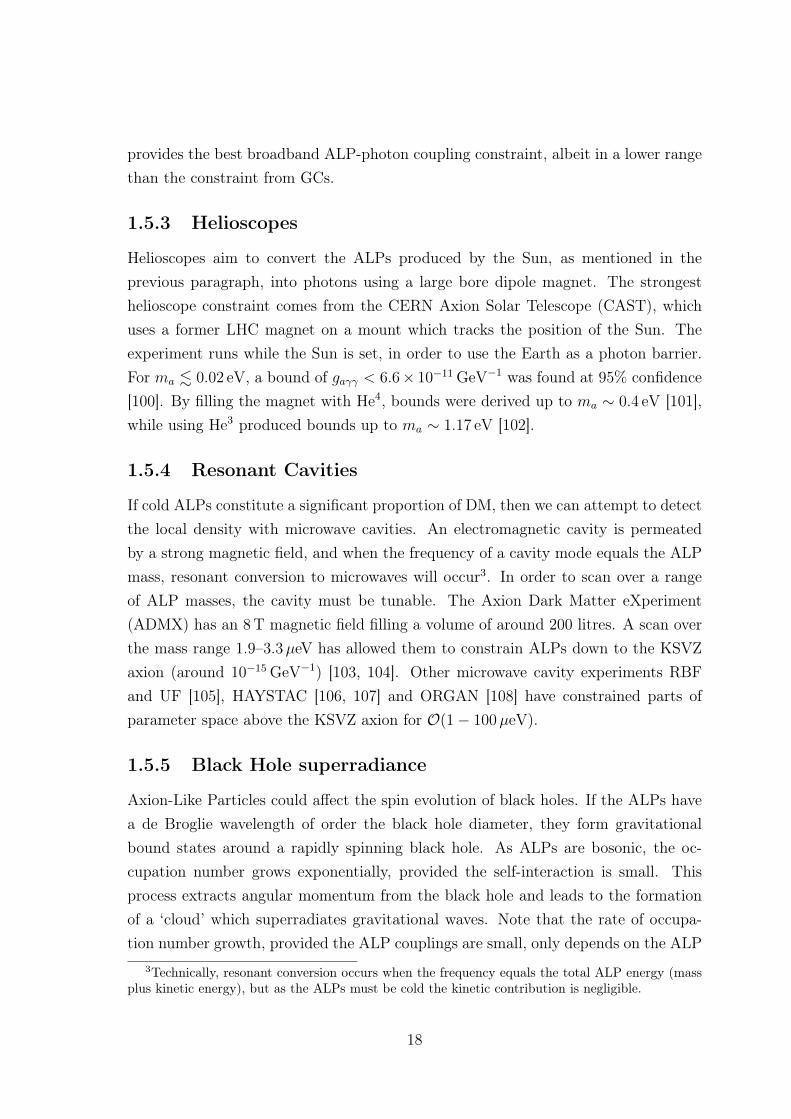
1.5.3 Helioscopes

Helioscopes aim to convert the ALPs produced by the Sun, as mentioned in theprevious paragraph, into photons using a large bore dipole magnet. The strongesthelioscope constraint comes from the CERN Axion Solar Telescope (CAST), whichuses a former LHC magnet on a mount which tracks the position of the Sun. Theexperiment runs while the Sun is set, in order to use the Earth as a photon barrier.For ma . 0.02 eV, a bound of gaγγ < 6.6× 10−11 GeV−1 was found at 95% confidence[100]. By filling the magnet with He4, bounds were derived up to ma ∼ 0.4 eV [101],while using He3 produced bounds up to ma ∼ 1.17 eV [102].

1.5.4 Resonant Cavities

If cold ALPs constitute a significant proportion of DM, then we can attempt to detectthe local density with microwave cavities. An electromagnetic cavity is permeatedby a strong magnetic field, and when the frequency of a cavity mode equals the ALPmass, resonant conversion to microwaves will occur3. In order to scan over a rangeof ALP masses, the cavity must be tunable. The Axion Dark Matter eXperiment(ADMX) has an 8T magnetic field filling a volume of around 200 litres. A scan overthe mass range 1.9–3.3µeV has allowed them to constrain ALPs down to the KSVZaxion (around 10−15 GeV−1) [103, 104]. Other microwave cavity experiments RBFand UF [105], HAYSTAC [106, 107] and ORGAN [108] have constrained parts ofparameter space above the KSVZ axion for O(1− 100µeV).

1.5.5 Black Hole superradiance

Axion-Like Particles could affect the spin evolution of black holes. If the ALPs havea de Broglie wavelength of order the black hole diameter, they form gravitationalbound states around a rapidly spinning black hole. As ALPs are bosonic, the oc-cupation number grows exponentially, provided the self-interaction is small. Thisprocess extracts angular momentum from the black hole and leads to the formationof a ‘cloud’ which superradiates gravitational waves. Note that the rate of occupa-tion number growth, provided the ALP couplings are small, only depends on the ALP

3Technically, resonant conversion occurs when the frequency equals the total ALP energy (massplus kinetic energy), but as the ALPs must be cold the kinetic contribution is negligible.

18

mass. Thus constraints derived from black hole superradiance extend to arbitrarilysmall couplings in a given mass range.

This phenomenon would lead to gaps in the mass-spin plot of black hole pop-ulations [109]. Precision studies of stellar mass black holes exclude ALPs at 95%confidence in a mass range 6×10−13 eV < ma < 2×10−11 eV [110]. The gravitationalwaves emitted by ALPs around a black hole could be detected by Advanced LIGO[110]. Advanced LIGO could also be used to look at gravitational wave signals fromblack hole binary mergers, which would be affected by the presence of ALPs [111].

1.5.6 Searches for ALPs with satellites

As searching for ALPs-photon conversion in astrophysical magnetic fields is the topicof this thesis, I do not go into detail here. However, I will briefly mention the mainprevious results. X-ray observations of the Hydra A cluster produce a bound ofgaγγ . 8.3×10−12 GeV−1 for massesma . 7×10−12 eV [112]. Gamma-ray observationsof NGC1275 with Fermi-Lat produce bounds of gaγγ . 5 × 10−12 GeV−1 for 0.5 .

ma . 5 neV [113]. The H.E.S.S. collaboration observed the AGN PKS 2155-304, andproduced bounds of gaγγ . 2.1×10−11 GeV−1 for 1.5×10−8 eV . ma . 6.0×10−8 eV

[114].

1.5.7 Summary

I summarise the current bounds on the ALP-photon coupling in Figure 1.1 (takenfrom the Particle Data Group review 2016 [48]). We see that, while a large part ofparameter space has already been excluded, a significant unprobed region remains.Finding new ways to probe this parameter space is an important endeavour.

19

Figure 1.1: Overview of exclusion limits on the ALP-photon coupling, plotted againstmass. Included in the graph are the mass-coupling relations for the KSVZ and DFSZaxions (within the yellow band). Full references can be found in the Particle DataGroup review on Axions and other similar particles [48].

20

Chapter 2

Aims and Objectives

We have seen that Axion-Like Particles are very well-motivated particles that extendthe Standard Model. The QCD axion solves the Strong CP Problem, and could bea solid candidate for being Dark Matter. The coupling of the axions to photons hasbeen constrained through a number of experiments and astrophysical observations. Atlower masses, the coupling of the QCD axion to electromagnetism becomes very weak,meaning that, for the time being at least, this region of parameter space is beyondour experimental reach. One might therefore conclude that experiments that do notreach the QCD axion ‘line’ are of no benefit other than as an incremental advance oftechnology that might eventually reach down to these exceptionally weak couplings.However, there is a strong motivation to analyse this data carefully to look for Axion-Like Particles that could exist in this parameter space. String theory provides manyconstructions that contain multiple ALPs that can exist in these areas of parameterspace. In addition, simple model-building involving multiple ALPs can push theQCD axion to regions of parameter space where the coupling to electromagnetism isenhanced. We therefore have compelling reasons to find new ways to reach this areaof parameter space experimentally.

We have seen that ALPs convert with photons in the presence of a magneticfield, acting as the third polarisation state of the effectively massive photon. Thedependence of the conversion probability on certain key parameters can point theway for us to begin our search. The probability increases with the product of themagnetic field strength and the length of the domain squared. One can therefore lookto high strength magnetic fields (with the corresponding budgetary limitation of onlybeing able to produce one across a short distance) or look to weak magnetic fieldsthat compensate by extending across great distances. Clearly we cannot generatesuch fields on Earth; however, we know that such fields exist in some of the largeststructures in the universe: galaxy clusters and the giant lobes of radio galaxies.

21

These appear therefore to be good targets to examine the ALP-photon conversionprobability in greater detail.

We will see in Chapter 3 that the conversion probability in galaxy cluster magneticfields increases with the square of the energy, up to a point of saturation, implyingthat we should observe galaxy clusters at high energies to benefit from this. The mostinteresting energy region, between minimal conversion at low energies and saturationat high energies, has a probability that oscillates, which would modulate the spectraof astrophysical objects.

Galaxy clusters at X-ray energies sit at a sweet spot for photon-ALP physics. Thisis due to two key results. First, galaxy clusters are particularly efficient environmentsfor photon-ALP interconversion. The electron densities are relatively low. Clustershave magnetic fields that are not significantly smaller than in galaxies, but in whichthe B-field extends over megaparsec scales, far greater than the tens of kiloparsecsapplicable for galactic magnetic fields. The magnetic field coherence lengths in clus-ters are also larger than in galaxies, comfortably reaching tens of kiloparsecs. Formassless ALPs, this feature singles out galaxy clusters as providing the most suitableenvironment in the universe for ALP-photon interconversion.1

The second key result is that, for the electron densities and magnetic field struc-tures present within galaxy clusters, the photon-ALP conversion probability is energy-dependent, with a quasi-sinusoidal oscillatory structure at X-ray energies. This pro-vides distinctive spectral features to search for.

The overall goal of this thesis is therefore to evaluate how X-ray observations ofstructures containing large magnetic fields can constrain the axion-photon coupling.With this in mind we have the following objectives:

1. Identify structures (galaxy clusters and radio galaxies) that have measurementsof an extensive magnetic field that could produce significant conversion.

2. Model these magnetic fields using the best-fit parameters that have been mea-sured so far, and thereby calculate the conversion probability of photons toALPs in the X-ray regime for a given coupling.

3. Identify data sets from the publicly available archives for the latest generationof X-ray satellites.

1Although they appear appealing, magnetars and related objects do not provide efficient envi-ronments for ALP-photon conversion [71].

22

4. Reprocess and fit the data to models for the sources without ALPs. Use thegoodness-of-fit to constrain the ALP-photon coupling.

5. Analyse any deviations from the best fit and discuss their possible systematic,astrophysical and new physics explanations.

6. Assess the experimental reach of future X-ray satellites to constrain this cou-pling further.

23

Chapter 3

Analysis of Galaxy Clusters

Galaxy clusters are the largest gravitationally bound structures in the Universe. Onlyabout 1% of the total mass is contained in the component galaxies. A further 9% isaccounted for by the intracluster medium (ICM), a magnetised plasma trapped withinits gravitational well. The remaining 90% is dark matter. Galaxy clusters typically arehundreds of kiloparsecs in size. The ICM in a galaxy cluster can contain a magneticfield that also extends across similar distances. Typical temperatures are O(1 −10 keV), with X-ray emission occurring via thermal bremsstrahlung. Observations ofatomic lines in this X-ray emission show that the ICMs have subsolar abundances ofheavy ions. A subset of galaxy clusters contain a core O(20 kpc) of dense gas with acooling time less than the age of the universe. For a review of the properties of theICM, see [115].

In this section, we outline the procedure we use to derive a bound on the ALP-photon coupling from X-ray data of point sources in galaxy clusters. This method isbroadly similar to that described and used in [84].

3.1 Magnetic Fields in the Intracluster Medium

Below we discuss methods that constrain the properties of intracluster magnetic fields.The Zeeman effect can be used to measure directly the strength and orientation ofmagnetic fields:

∆ν0 =eB

4πmec= 2.8

B

µGHz, (3.1)

meaning that an O(1µG) magnetic field causes only an O(1 Hz) splitting in thefrequency, far below the resolution of detectors.

24

Individual methods have degeneracies (for example between the relativistic elec-tron density and the magnetic field strength), so often a combination of methods isrequired to evaluate the parameters.

3.1.1 Faraday Rotation Measures

We have already touched on the dispersion of a photon through a magnetic field inSubsection 1.4.1. The difference between the refractive indices perpendicular andparallel to the magnetic field induces rotation in the electromagnetic wave, which canbe measured by polarimeters. Once the effects of the plasma are taken into account,the refractive indices are:

nL,R ≈ 1− 1

2

ω2p

ω(ω ± eB‖/me), (3.2)

for ωp, eB‖/me ω [116]. For two opposite-handed waves travelling a path lengthdl, this creates a phase difference:

dφ = ωdt = ω∆n dl ≈ 4πe3

ω2m2e

neB‖ dl, (3.3)

where B‖ is the magnetic field along the line of sight, and we have used ω2pl =

4παne/me. The intrinsic polarisation angle χ of the light after travelling a pathlength dl will change by an angle dχ = dφ/2. Writing in terms of the FaradayRotation Measure:

RM =e3

2πm2e

∫ L

0

ne(l)B‖(l) dl rad m−2, (3.4)

the intrinsic polarisation of a source shining through a cluster of length L is:

χ = χ0 +RM λ2, (3.5)

where λ is the wavelength. This allows one to probe the strength of the magneticfield parallel to the line of sight. The dependence on λ means that radio telescopesare best placed to look for the effects of Faraday rotation.

25

3.1.2 Synchrotron Radiation and Equipartition

Relativistic electrons propagating through a magnetic field will emit synchrotron ra-diation into a cone of half power width ∝ 1/γ. The spectrum of synchrotron radiationfrom a single electron is sharply peaked around the critical frequency:

νe =3

4π

eB sin θ

mecγ2β2, (3.6)

where θ is the angle between the electron’s direction of motion and the magnetic field,and β = v/c for electron velocity v. The emitted synchrotron power is:

Psyn =2e4

3m2ec

3(B sin θ)2γ2β2, (3.7)

One can see that extracting the magnetic field strength B from an observed syn-chrotron emission energy spectrum requires knowledge of the energy spectrum ofrelativistic electrons in the intracluster medium. Often this is not well constrainedtheoretically or experimentally. The challenge is to separate the synchrotron emis-sion from thermal emission. It also involves detecting hard X-rays, which will meansmaller data sets than radio waves.

We can estimate the strength of the magnetic field by assuming that the com-bined energy of relativistic particles (electrons and protons) and the magnetic field isminimised:

Utot = UB + Uel + Upr, (3.8)

where UB = B2V/8π for a magnetic field filling a volume V and

Uel = V

∫ ε2

ε1

N(ε) ε dε (3.9)

is the energy density in relativistic electrons of energies between ε1 and ε2.Assuming Upr = kUel for some constant k, we can estimate the equipartition

magnetic field strength. The parameter k depends on assumptions made about thecreation of the relativistic protons and electrons, and in the standard analysis is takento be 1.

3.1.3 Inverse Compton Scattering

An independent way to constrain B using synchrotron radiation is to compare itto Inverse Compton scattering. Highly energetic electrons can lose their energy by

26

transferring it to photons through Inverse Compton Scattering, emitting photons withthe frequency:

νout =4

3γ2νin. (3.10)

For electrons in the intracluster medium scattering off the Cosmic MicrowaveBackground, which has a temperature of 3.1 K, will lead to hard X-rays being pro-duced. Calculating the flux density SIC(νx) and comparing it to the flux density ofsynchrotron radiation Ssyn(νr) allows us to derive the magnetic field strength [117]:

B ∝(Ssyn(νr)

SIC(νx)

) 2g+1(νrνx

) g−1g+1

, (3.11)

where g is the power law index of the relativistic electron spectrum. The limitationof this method is separating the non-thermal IC emission from thermal emission inthe hard X-ray regime.

3.1.4 Summary of galaxy cluster magnetic field measurements

For some of the clusters we will examine, information about the electron densitiesand coherence lengths will be experimentally inferred, while others will have to beinferred from similar clusters. In all cases, we will require there to be a confirmedmeasurement of an intrinsic magnetic field strength.

Coma Cluster

The Coma cluster has a well-measured set of magnetic field parameters. From Fara-day rotation measures a central magnetic field value of B0 = 4.7+0.8

−0.7 µG is inferred[118]. Its radial profile is B(r) ∝ ne(r)

η with η = 0.5+0.2−0.1. The magnetic field power

spectrum is well described by a Kolmogorov (η = 5/3) power spectrum with mini-mum/maximum scale 2 kpc/34 kpc. Its properties will be used to estimate those ofother galaxies for which no observations appropriate to determine them have beenperformed. However this does not mean that the Coma cluster is the best target forALP-photon conversion. Other clusters benefit from a higher inferred central mag-netic field value, or a brighter point source shining through the cluster towards us.In all cases where the Coma cluster is used to infer the properties of other clusters,the value used will be that is most conservative for ALP-photon conversion while stillremaining within the quoted error range.

27

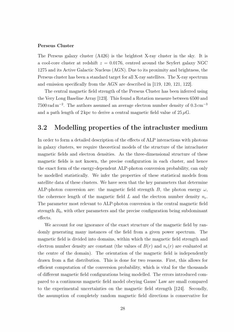
Perseus Cluster

The Perseus galaxy cluster (A426) is the brightest X-ray cluster in the sky. It isa cool-core cluster at redshift z = 0.0176, centred around the Seyfert galaxy NGC1275 and its Active Galactic Nucleus (AGN). Due to its proximity and brightness, thePerseus cluster has been a standard target for all X-ray satellites. The X-ray spectrumand emission specifically from the AGN are described in [119, 120, 121, 122].

The central magnetic field strength of the Perseus Cluster has been inferred usingthe Very Long Baseline Array [123]. This found a Rotation measure between 6500 and7500 radm−2. The authors assumed an average electron number density of 0.3 cm−3

and a path length of 2 kpc to derive a central magnetic field value of 25µG.

3.2 Modelling properties of the intracluster medium

In order to form a detailed description of the effects of ALP interactions with photonsin galaxy clusters, we require theoretical models of the structure of the intraclustermagnetic fields and electron densities. As the three-dimensional structure of thesemagnetic fields is not known, the precise configuration in each cluster, and hencethe exact form of the energy-dependent ALP-photon conversion probability, can onlybe modelled statistically. We infer the properties of these statistical models fromsatellite data of these clusters. We have seen that the key parameters that determineALP-photon conversion are: the magnetic field strength B, the photon energy ω,the coherence length of the magnetic field L and the electron number density ne.The parameter most relevant to ALP-photon conversion is the central magnetic fieldstrength B0, with other parameters and the precise configuration being subdominanteffects.

We account for our ignorance of the exact structure of the magnetic field by ran-domly generating many instances of the field from a given power spectrum. Themagnetic field is divided into domains, within which the magnetic field strength andelectron number density are constant (the values of B(r) and ne(r) are evaluated atthe centre of the domain). The orientation of the magnetic field is independentlydrawn from a flat distribution. This is done for two reasons. First, this allows forefficient computation of the conversion probability, which is vital for the thousandsof different magnetic field configurations being modelled. The errors introduced com-pared to a continuous magnetic field model obeying Gauss’ Law are small comparedto the experimental uncertainties on the magnetic field strength [124]. Secondly,the assumption of completely random magnetic field directions is conservative for

28

producing ALP-induced oscillations, as they will destructively interfere between do-mains. As we are seeking to constrain the ALP-photon coupling, we must ensure ourassumptions are conservative to produce robust bounds.

Where there are direct estimates of the parameters for the galaxy cluster beingstudied, we use the best fit values. For the Perseus cluster, we separately calculate thebound for smaller magnetic field strength and coherence length, as an illustration ofthe effect of these parameters on the bounds. For galaxy clusters that do not have adirect estimate of a particular parameter, that value is inferred from a similar galaxycluster, with the most conservative value taken from the quoted error range.

We assume the electron number density is spherically symmetric, depending onlyon the distance to the centre of the cluster r. In addition we assume that the magneticfield strength is proportional to the electron number density to some exponent B(r) ∝ne(r)

η. We now illustrate our approach for the Perseus Cluster. The details for eachgalaxy cluster are shown in Chapter 4.

Direct measurements of magnetic fields of galaxy clusters are not always possible,as the necessary radio sources may not exist. The recent paper on the A194 magneticfield [125] summarises extant measurements of cluster magnetic fields (see its Table8).

This thesis involves both sources that are at the centre of a cluster, and also sourcesthat are significantly offset from the centre. ALP-photon constraints depend on themagnetic field along the line of sight from the source. For sources whose projectedposition is at a significant offset from the centre of the cluster, the field along the lineof sight depends on both the overall central magnetic field of the cluster, denoted B0,and the rate at which the field decreases away from the centre.

This is parametrised by assuming the cluster magnetic field to be radially sym-metric,

B(r) ∼ B0

(ne(r)

n0

)η.

η is expected to lie somewhere between 0.5 and 1. The former represents an equipar-tition between magnetic field energy and themal energy (〈B2〉 ∼ nekBT ), while avalue η = 2/3 corresponds to a magnetic field that is frozen into the gas. A value ofη = 1 has been found for the cool-core cluster Hydra A [126] (with a best-fit centralmagnetic field B0 = 36 µG). For the same value of B0, a higher value of η will meana more rapid drop-off of magnetic field strength with radius. We use an intermediatevalue of η = 0.7. A β-model for the electron density takes the form

ne(r) = n0

(1 +

r2

r2c

)−3β/2

,

29

where rc is the core radius. Although not perfect, the β model captures the grossbehaviour of the electron density in a cluster.

Perseus Cluster magnetic field

Based on results for the Coma cluster, we assume that B decreases with radius asB ∝ n0.7

e [127]. The electron density ne has the radial distribution found in [119],

ne(r) =3.9× 10−2

[1 + ( r80 kpc

)2]1.8+

4.05× 10−3

[1 + ( r280 kpc

)2]0.87cm−3 .

We simulate each field realisation with 600 domains. The length l of each domain isbetween 3.5 and 10 kpc, randomly drawn from a power law distribution with minimumlength 3.5 kpc and power 0.8. We therefore have:

P (l = x) = N

0 for x > 10 kpc ,

x−1.2 for 3.5 kpc < x < 10 kpc ,

0 forx < 3.5 kpc ,

(3.12)

with normalisation constant N .The coherence length and power spectrum of the magnetic field in the centre of

Perseus is not observationally determined. Instead, these parameters are motivatedby those found for the cool core cluster A2199 [128], taking a conservative value forthe magnetic field radial scaling.

3.3 Calculating ALP-photon conversion probabilityin clusters

We compute the energy-dependent conversion probability through our magnetic fieldmodel as described above. We choose an energy range that encompasses that ofthe detector (Chandra’s ACIS, XMM-Newton’s EPIC and Athena’s X-IFU). For themajority of images, this is 0.1–10 keV. In cases where the data is contaminated bypile-up and we need to discard data at higher energies, we reduce the energy rangeof the simulation. From this energy range we select enough energies to ensure thatthe sampling is better than the energy resolution of the detector.

For the electron densities and magnetic field structures present within galaxyclusters, the photon-ALP conversion probability is energy-dependent, with a quasi-sinusoidal oscillatory structure at X-ray energies. We can see this by plugging in therelevant numbers into Equation 1.61. The amplitude of the oscillations, and their

30

period, grow as the square of the energy, as is shown in Figure 3.1. The inefficiencyof conversion at energies E . 0.2keV implies that effects of photon-ALP conversionare not visible in the optical (and below) range.

Figure 3.1: The photon survival conversion through a single-domain of a mag-netic field due to ALP interconversion. The magnetic field strength is 1µG, withan average electron number density of 10−3 cm−3. The ALP-photon coupling isgaγγ = 5× 10−12 GeV−1, equal to the upper limit from SN1987A. One can see the os-cillations growing with energy, being particularly pronounced in the 1−10 keV range,before the conversion probability saturates at higher energies. The domain length of350 kpc is deliberately exaggerated over a typical domain length in a cluster magneticfield, in order to clearly show the oscillatory peaks. A more realistic magnetic fieldconfiguration is shown in Figure 3.2.

To calculate the conversion probability across the galaxy cluster magnetic fieldwe use multiple domains, each of which has a conversion probability amplitude calcu-lated. These amplitudes are then multiplied across all domains, and finally squaredto produce a total conversion probability. We provide an example of the distinctivepattern of the features in Figure 3.2, where we plot a photon survival along a singleline of sight modelled on that through the centre of the Perseus Cluster. However

31

the location of the oscillations in the spectrum depends on the actual magnetic fieldstructure along the line of sight. There is also an overall reduction in luminosity, butthis can be absorbed into the overall normalisation of the spectrum. For unpolarisedlight the γ → a conversion probability cannot exceed fifty per cent, and in the limit ofstrong coupling saturates at an average value of 〈P (γ → a)〉 = 1/3 (for example, see[129]). It therefore follows that, expressed as a ratio of data to model, the maximalallowed range of ALP-induced modulations is approximately ±30%.1

/

Figure 3.2: The photon survival probability through a randomly generated mag-netic field due to ALP interconversion. A central magnetic field of B0 = 25µGwas assumed, with a radial scaling of 〈B(r)〉 ∼ ne(r)

0.7. There were 200 do-mains, with lengths randomly sampled from a Pareto distribution with range 3.5– 10 kpc. The total propagation length was 1200 kpc. The ALP-photon couplingis gaγγ = 1.5 × 10−12 GeV−1 (roughly a factor of three beyond the current upperlimit gaγγ < 5 × 10−12 GeV−1 from SN1987A). This quasi-sinusoidal structure arisesgenerically in random field configurations.

3.4 Candidate target sources

Bright point-like sources either behind or embedded in a galaxy cluster are particu-larly attractive for searching for ALP-induced modulations. The galaxy cluster pro-

1We re-emphasise here that photon-ALP conversion involves quantum oscillations between statesrather than absorption. Therefore for passage from A→ C the survival probability P (A→ C) doesnot equal P (A→ B)× P (B → C).

32

vides a good environment for ALP-photon conversion; the bright point source ensuresthere are many photons, all passing along the same line of sight.

These factors make quasar or active galactic nucleus (AGN) spectra attractive forsearching for ALPs. Emission from an AGN arises from matter accreting onto thecentral black hole. As evidenced by the rapid time variability of AGN luminosities, thephysical region sourcing the X-ray AGN emission is tiny – of order a few Schwarschildradii of the central black hole. As cluster magnetic fields are ordered on kiloparsecscales, this implies that for all practical purposes every photon arising from the AGNhas experienced an identical magnetic field structure during its passage to us.

To first approximation, at X-ray energies an AGN spectrum can be described asan absorbed power law. The effect of ALPs is then to imprint a quasi-sinusoidalmodulation on this power law, of relative amplitude at most O(30%) and with amodulation period of order a few hundred eV. As the fractional Poisson error on Ncounts is 1√

N, and CCD detectors such as those on Chandra and XMM-Newton have

intrinsic energy resolutions of aroundO(100 eV), it therefore requires large numbers ofcounts to be able to distinguish any ALP-induced modulations from normal statisticalfluctuations.

NGC 1275 (Perseus Cluster)

All the above facts make the AGN of the Seyfert galaxy NGC 1275 an excellentcandidate for searching for ALP-photon interconversion. NGC 1275 is the centralgalaxy of the Perseus cluster, which as a cool core cluster should have a high centralmagnetic field (estimated as 25 µG in [123]) – implying the sightline from NGC 1275to us should be efficient at ALP-photon conversion.

The nucleus is intrinsically bright and unobscured, with a spectrum that is wellcharacterised by a power law and narrow Fe Kα line, absorbed by the galactic nHcolumn density [119]. Furthermore, there is enormous Chandra observation time onNGC 1275, encompassing 1.5 Ms in total. This results in over half a million photoncounts originating from the central AGN, although for the on-axis observations quitea number are contaminated by pile-up. This is a level two orders of magnitude largerthan the study in [84] involving Hydra A.

3.5 Data processing of X-ray satellites

X-ray satellites have a good chance to detect modulations in energy spectra resultingfrom ALP-photon conversion. Figure 3.3 shows that for galaxy cluster magnetic fields

33

significant ALP-induced modulation occurs between 1–10 keV, an energy range thatinstruments on Chandra, XMM-Newton and Athena cover. Three features of thesesatellites are crucial to detecting these modulations:

1. Energy resolution The finite energy resolution of the detector will mean thatrapid oscillations, as found at low energies, will be lost. This is shown in Fig-ure 3.3, where the survival probability is convolved with a Gaussian distributionof 150 eV.

2. Angular resolution This must be good enough to resolve a single line of sight.If photons arriving on the same pixel have passed through different magneticfield configurations to each other, the oscillations will undergo destructive in-terference. In addition, for galaxy clusters that have significant X-ray emissionfrom the intracluster medium, it is useful to be able to distinguish the AGNspectrum from the background.

3. Effective Area In order to distinguish the oscillations from Poisson fluctua-tions, we require sufficient photon statistics in the data set. A large effectivearea of the telescope will provide more photon counts for the same exposuretime.

In this section we discuss the X-ray satellites currently in operation that are bestsuited to ALP searches. We review their limitations and describe the plans for futuresatellites that will have increased sensitivity to ALP induced oscillations.

3.5.1 Chandra

The Chandra X-ray Observatory was launched by NASA in 1999. It combines theHigh Resolution Mirror Array (HMRA), capable of excellent angular resolution, withthe Advanced CCD Imaging Spectrometer (ACIS). The former consists of a nestedset of four paraboloid-hyperboloid (Wolter-1) grazing-incidence X-ray mirror pairs,with the largest having a diameter of 1.2m (taken from the Chandra Proposer’sGuide2). The effective area is 600 cm2 at 1.5 keV. The point-spread function (PSF)and the encircled energy fraction for a given radius depend upon off-axis angle andenergy. The HRMA PSF has been simulated with numerical raytrace calculations:the increase in image size with off-axis angle is greatest for the inner shell, and henceis larger for higher X-ray energies.

2http://cxc.harvard.edu/proposer/POG/html/chap6.html

34

ACIS consists of two charged coupled device (CCD) arrays: a 2 × 2 chip array,ACIS-I; and a 1× 6 chip array, ACIS-S. One ACIS-S chip provides an 8 arcminute by8 arcminute field of view, while ACIS-I provides a 16 arcminute by 16 arcminute fieldof view. The CCD is a device composed primarily of silicon, with pixels separated bygates. Upon absorption of an X-ray photon a proportional number of electrons areliberated, which are then confined by electric fields. The array is exposed for a timethat depends on the mode being used (in full frame this is ∼ 3.2 s). The charge is thenpassed to a serial read-out at the end of a row. The energy resolution of the detectordepends on the fraction of the charge collected, the charge transfer inefficiency frompixel to pixel in the read-out phase, the resolution of the read-out amplifiers, readnoise and the off-chip analog processing electronics. Note that a single photon maycreate electron-hole pairs in multiple pixels. Pixels with a charge deposit above thethreshold, plus the surrounding pixels, are “graded” based on the likelihood that theevent was a photon absorption (instead of, say, a cosmic ray).

Figure 3.3 compares the photon survival probability shown in Figure 3.2 withthe same probability convolved with a Gaussian with full width at half maximum(FWHM) of 150 eV, representing the approximate energy resolution of the CCD de-tectors present on Chandra and XMM-Newton satellites (the precise figure of 150eV

is taken from the in-orbit performance of the ACIS-I detectors on Chandra, see ta-ble 6.4 of the Chandra proposer’s guide3). While at lowest energies the oscillationsare too rapid to be resolved by CCD detectors, and would require micro-calorimeterssuch as those that were present on Hitomi4, in general it is fortuitous that the scalesof the oscillations match those of the X-ray telescopes extensively used to observegalaxy clusters.

We use CIAO 4.7 [130], Sherpa [131] and HEASOFT 6.17 for the Chandra dataanalysis.5 After the data is reprocessed using CALDB 4.6.9, it is cleaned from timeperiods that are polluted by flares using the program chips. We analyse the imagesand count rates of each observation using the image software ds9.

The boundaries of the ellipse are set by the location where the image of the pointsource ceases to dominate the background cluster emission. The background is takenfrom an elliptical annulus around the point source, with the inner ellipse slightlylarger than for the source extraction region. Spectra and responses are created usingspecextract for each observation, and then stacked using combine_spectra. In

3http://cxc.harvard.edu/proposer/POG/html/chap6.html4The energy resolution from Hitomi was around ∼ 5 eV.5The update to CIAO 4.8 affects data taken in Continuous Clocking mode, which does not apply

to these observations.

35

/

/

Figure 3.3: Left—The photon survival probability after passing through a randomlygenerated magnetic field. A central magnetic field of B0 = 25µG was assumed, witha radial scaling of 〈B(r)〉 ∼ ne(r)

0.7. There were 200 domains, with lengths randomlysampled from a Pareto distribution with range 3.5 – 10 kpc. The total propaga-tion length was 1200 kpc. The ALP-photon coupling is gaγγ = 1.5 × 10−12 GeV−1

(roughly a factor of three beyond the current upper limit gaγγ < 5 × 10−12 GeV−1

from SN1987A). This quasi-sinusoidal structure arises generically in random fieldconfigurations. Right—The photon survival probability for the same magnetic fieldconvolved with a Gaussian with FWHM of 150 eV.

general we bin so that there are approximately one hundred bins in total. If there aretoo few counts per bin, then the fit is insensitive to localised modulations as can beproduced by ALPs, as the goodness-of-fit is insensitive to the sign of the residuals.We use Sherpa’s Levenberg-Marquardt fitting method with Poisson errors derivedfrom the value of the data in each bin.

Pile-Up

Bright sources whose light shines on very few pixels of a CCD detector will havetheir inferred spectra significantly contaminated by pile-up. The energy recorded onthe individual ACIS pixels (each approximately 0.5 arcseconds square) is read outapproximately every three seconds (one frame time) when Chandra is operating in“full frame mode”. Based on groupings of 3×3 pixels, events are graded. “Bad grades”are assigned to signals that are not likely to be the result of a photon interaction (anexample of a non-photon interaction would be a cosmic ray), while “good grades”indicate the signal is likely to be a photon.

Pile-up refers to the arrival of more than one photon in this grouping withinthe same readout frame. This can lead to the energy of the two (or more) incidentphotons being summed, and either treated incorrectly as a single photon event ofhigher energy, or assigned a bad grade (grade migration). For an on-axis bright

36

source (as in the ACIS-S observations of NGC 1275), the level of pile-up can be high,and the resulting spectrum contains events with two, three (and more) photons. Aspile-up is a statistical feature of the number of arriving photons, some level of pile-upis inevitable in any observation. The question is always whether the magnitude ofpile-up is sufficient to corrupt the science analysis being undertaken.

In terms of the measured photon distribution, the general effect of pile-up is tocause a hardening of the spectrum: two or more lower-energy photons are misidentifiedas a single higher-energy photon. This implies that for a fit of a single power law toa photon distribution, as pile-up increases the best-fit power law index will decrease.In a spectrum contaminated by pile-up, this makes it harder to determine the correctoriginal power law index.

There are two basic methods we can employ to reduce the effects of pile-up on theanalysis. The first is to reduce the amount of pile-up by using an annular extractionregion and extracting the spectrum only from the wings of the point spread function.The point spread function of the telescope causes the arriving photons to be spreadout on the detector, with the degree of spread increasing as one moves progressivelyoff-axis. Furthermore, the point spread function is mildly energy-dependent: photonswith higher energy are spread out further than photons with smaller energy. Whilefewer photons arrive in the wings of the point spread function, those that do sufferless from pile-up than those arriving on the central pixels. The second is to modelthe pile-up, and the distortion it induces on the spectrum, explicitly. We shall utiliseboth approaches below.

We set the ds9 binning such that the ds9 pixels are essentially the same size asthe physical Chandra pixels (half an arc-second across). We then create an extractionregion manually excluding all ds9 pixels which are neighbours (either side-by-side ordiagonally) to any pixel with total counts greater than 1% of the overall exposuretime. Using the pileup_map tool we can estimate the pile-up fraction of each pixel.

The jdpileup model is described in [132]. This model is specific to modelling asource that is on-axis. The model assumes Poisson statistics to calculate the prob-ability of different numbers of photons hitting an event-detection cell (a 3×3 pixelregion in Chandra) within the read-out time adjusted to these respective observa-tions. The model then convolves this probability with the probability of such eventsbeing assigned a ‘good’ grade, and the conversion from photon energy to pulse heightby the detector. Obviously this is a non-linear process: the pile-up in any particularbin depends on the energy spectrum for all energies below the bin. The parametersof the model therefore need to be determined together with those for the spectrum

37

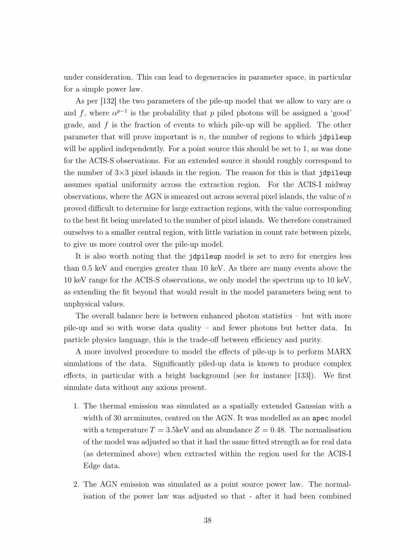
under consideration. This can lead to degeneracies in parameter space, in particularfor a simple power law.

As per [132] the two parameters of the pile-up model that we allow to vary are αand f , where αp−1 is the probability that p piled photons will be assigned a ‘good’grade, and f is the fraction of events to which pile-up will be applied. The otherparameter that will prove important is n, the number of regions to which jdpileup

will be applied independently. For a point source this should be set to 1, as was donefor the ACIS-S observations. For an extended source it should roughly correspond tothe number of 3×3 pixel islands in the region. The reason for this is that jdpileupassumes spatial uniformity across the extraction region. For the ACIS-I midwayobservations, where the AGN is smeared out across several pixel islands, the value of nproved difficult to determine for large extraction regions, with the value correspondingto the best fit being unrelated to the number of pixel islands. We therefore constrainedourselves to a smaller central region, with little variation in count rate between pixels,to give us more control over the pile-up model.

It is also worth noting that the jdpileup model is set to zero for energies lessthan 0.5 keV and energies greater than 10 keV. As there are many events above the10 keV range for the ACIS-S observations, we only model the spectrum up to 10 keV,as extending the fit beyond that would result in the model parameters being sent tounphysical values.

The overall balance here is between enhanced photon statistics – but with morepile-up and so with worse data quality – and fewer photons but better data. Inparticle physics language, this is the trade-off between efficiency and purity.

A more involved procedure to model the effects of pile-up is to perform MARXsimulations of the data. Significantly piled-up data is known to produce complexeffects, in particular with a bright background (see for instance [133]). We firstsimulate data without any axions present.

1. The thermal emission was simulated as a spatially extended Gaussian with awidth of 30 arcminutes, centred on the AGN. It was modelled as an apec modelwith a temperature T = 3.5keV and an abundance Z = 0.48. The normalisationof the model was adjusted so that it had the same fitted strength as for real data(as determined above) when extracted within the region used for the ACIS-IEdge data.

2. The AGN emission was simulated as a point source power law. The normal-isation of the power law was adjusted so that - after it had been combined

38

with the thermal emission and the pileup processing applied - it had the samenormalisation as the real data when extracted over the same extraction region.

3. The two individual simulations were then combined using marxcat and theMARX pileup processing applied to the combined simulation.

4. Counts were grouped to 500 and the combined spectrum was fitted with the sumof a power law plus thermal emission. The previous two steps were iterated untilthe fitted strength and index of the power law matched that of the real data.

We now repeat the MARX simulations including the effects of axions in the data.We multiply the AGN power law with a P (γ → γ) survival probability coming fromphoton-ALP conversion. As this leads to a net reduction in the number of photonspresent, we adjust the intrinsic normalisation upwards so that the fitted normalisationmatches the actual data.

For a fixed ALP coupling, we generate 50 fake data samples. To compare theseresults to those described above using Sherpa’s fake_pha command, we simulate threeseparate ALP couplings: gaγγ = 1, 1.5, 2 × 10−12GeV−1. In all cases we assume the‘optimistic’ magnetic field model.

The above analysis uses MARX’s simulation of Chandra’s optics. The most ad-vanced simulation of Chandra’s optics is through the ChaRT simulator ([134]), ratherthan MARX. As ChaRT requires the original source spectrum to be manually up-loaded to a website, it is not possible to automate this process to produce axion bounds(as every different ALP conversion template represents a different source spectrum).

Errors in the Fitted Parameters

For fits of spectra to models, the paper includes the fitted statistical errors. However,significant caution should be applied when interpreting such a quantity (for example,a power law index) as an error on the intrinsic spectrum of the source. Systematicerror on overall power law indices are likely to be much larger. While hard to quantify,there are several clear sources of such systematic effects:

1. Although the cleaned spectra have significantly reduced levels of pile-up, nospectrum can be entirely free of pile-up. Pile-up automatically leads to a hard-ening of spectral indices, as it moves photons from low to high energies.

2. The point spread function of Chandra is a function of energy, and more energeticphotons tend to be spread out more. For spectra such as those used here, where

39

a central and highly piled-up core is excluded, this will bias the analysed photonsto higher energy. While the Chandra analysis software aims to take this intoaccount, this correction will not be perfect, particularly for off-axis sourceswhere the form of the optical image is more complex (as for the ACIS-I Midwaydata, where the AGN image takes on a ‘Maltese cross’ form).

3. Generally, there are systematic errors on the overall power law index that willarise because the optical conditions are significantly different on-axis and off-axis. These are hard to quantify, but are certainly much larger than the purelystatistical errors on fitted parameters.

4. The AGN luminosity is time-variable and the power law index will be time-variable as well. For observations taken at different times, the intrinsic powerlaw of the source may be different.

3.5.2 XMM-Newton

The X-ray Multi-Mirror Mission (XMM-Newton) was launched by ESA in 1999. Theoptics are three X-ray telescopes, each consisting of 58 Wolter I grazing-incidencegold-coated mirrors. They have an effective area of 1500 cm2 at 2 keV. There is alsoan effective area edge just above 2 keV due to the gold coating.

On board XMM Newton is the European Photon Imaging Camera (EPIC) con-sisting of three CCD cameras. Two of these are part of the MOS camera, comprisingMetallic Oxide Semiconductor cameras. The third uses pn CCDs, and so is referredto as the pn camera. MOS receives photons passing through reflection gratings, whilepn has an unobstructed view. The detector can be set up in full frame mode, with aframe time of 2.6 s for MOS and 73.4ms for pn. In addition pn can be run in extendedframe mode with a frame time of 199.1ms.

The pixel size of pn is 4.1 arcseconds and 1.1 arcseconds for MOS. This meansthat pn in extended full frame mode is more susceptible to pile-up than MOS. Ingeneral, pile-up is an issue for all XMM-Newton observations of NGC 1275 as we willdiscuss in the XMM-Newton analysis.

A significant difference between XMM-Newton and Chandra is the angular reso-lution. For both MOS and pn, the radius of the disk containing 50 % of the photonscollected in the focal plane (Half Energy Width) is around 8.5 arcseconds at 1.5 keV,while for Chandra it is much smaller at ∼ 0.5 arcseconds (FWHM). The FWHM forMOS-1 in orbit is 4.3 arcseconds, for MOS-2 is 4.4 arcseconds, and for pn is 12.5arcseconds due to the large pixel size. As the central region of the Perseus cluster is

40

also intrinsically bright, this makes it harder to separate AGN and cluster emissionfor the XMM-Newton observations.

The effective area at 1 keV is 922 cm2 for MOS and 1227 cm2 for pn compared to340 cm2 for Chandra. This allows MOS and pn combined to collect roughly 7 timesmore photons in a given observation time than Chandra (although this also increasesthe amount of pile-up).

Analysis

We use SAS version 15.0.0. As data has been taken in the past, we reprocess it withup to date calibrations via cifbuild. To remove flares, we apply the standard filtersof counts/s < 0.35 for MOS and counts/s < 0.4 for pn. After selecting the extractionregion for the point source we check if pile-up is an issue using the SAS tool epatplot.

After applying eveselect to generate the spectra, we use rmfgen and arfgen togenerate the response files. We use epicspeccombine to combine different observa-tions. We compare this to using the ftools routines mathpha, addrmf and addarf (asepicspeccombine does not produce an arf file). We complete our analysis by fittingthe spectra using the programs Xspec [135] and Sherpa [131].

3.5.3 The future satellite Athena

Searches for these oscillations can be used to constrain ALP parameter space. Currentconstraints on ALPs derived in this fashion [84, 1, 136, 2] are based on data taken withCCD detectors, which have an energy resolution of O(100 eV). A large improvementwith sensitivity will be achieved once data becomes available from microcalorimeterswith O(a few eV) energy resolution. Such microcalorimeters will be on board theAdvanced Telescope for High ENergy Astrophysics (ATHENA), currently scheduledto launch in 2028. Its X-IFU instrument will have a large effective area, good imagingand an energy resolution of ∼ 2.5eV, greatly enhancing the discovery potential forALPs.

We estimate the experimental sensitivity of Athena to ALPs. We do so usingsimulated data for a mock observation of NGC 1275, hosting the radio source 3C 84,which contains the central AGN of the Perseus cluster. This allows us to comparedirectly the capabilities of Athena to the present-day satellites discussed above.

One major limiting constraint on existing data is the energy resolution of thedetectors. If they exist, ALPs provide oscillatory structure all the way down tothe lowest energies. However, as illustrated in Figure 3.4, detectors with energy

41

Athena (X-IFU) Chandra (ACIS-I)Energy range 0.2–12 keV 0.3–10 keV

Energy resolution 2.5 eV 150 eVat 6 keV

Spatial resolution 5 arcsec 0.5 arcsecTime resolution 10 µs 0.2 s

(2.8 ms single row)Effective area 2 m2 @ 1 keV 600 cm2 @ 1.5 keV

Table 3.1: Parameters taken from the Athena Mission Proposal and the ChandraProposer’s Guide.

resolutions of O(100 eV) cannot resolve this structure at lower energies – but thisdoes become accessible once a resolution of O(2.5 eV) is achieved. We now discussthe future Athena X-ray observatory, whose greatly enhanced technical capabilitiesoffer improved sensitivity to ALP-photon interconversion.

Athena is an ESA mission to explore the Hot and Energetic Universe, due tolaunch in 2028 [137]. The mirror will have a 2 m2 effective area and a 5 arcsecangular resolution. There are two instruments: the X-ray Integral Field Unit (X-IFU) and the Wide Field Imager (WFI). Here we focus on the former, which willconsist of an array of TiAu Transition Edge Sensor (TES) thermistors. An efficientphoton absorber is attached to a film of TiAu superconductor. The array is cooledto a temperature of 50 mK, keeping the TiAu in equilibrium between the normaland superconducting state. The transition between the states is very sharp, meaningthat a small deposit of energy can effect an excitation. The increase in resistancecaused by an increase in heat is then measured. The energy resolution of a singlemicro-calorimeter pixel is predicted to be 2 eV.

Once noise from read-out, fluctuations in the environment and gain miscalibrationis taken into account, X-IFU is planned to achieve an energy resolution of 2.5 eV below7 keV [138], meaning it will be able to resolve narrow spectral oscillations. X-IFUwill be sensitive to the energy range 0.2–12 keV [139]. A readout time of ∼ 10 µs

will ensure pileup contamination is minimised. Table 3.1 contains a summary of itsproperties, taken from the Athena Mission Proposal6, compared to properties of theChandra ACIS-I detector, taken from the Chandra Proposer’s Guide7.

The combination of larger effective area, greatly improved energy resolution and6http://www.the-athena-x-ray-observatory.eu/images/AthenaPapers/

The_Athena_Mission_Proposal.pdf7http://cxc.harvard.edu/proposer/POG/html/chap6.html

42

[]

[]

Figure 3.4: Above—A randomly generated photon survival probability along the lineof sight from NGC 1275 to us: unconvolved (blue), convolved with a Gaussian withFWHM 150 eV (a typical energy resolution of Chandra’s ACIS-I detector (red)) and2.5 eV for Athena’s X-IFU detector (orange). A central magnetic field of B0 = 25µGwas used, with a radial scaling of B ∼ n0.7

e , further details in Section 3.2. TheALP-photon coupling is gaγγ = 5× 10−13 GeV−1. Small, rapid oscillations at lowenergies, and larger oscillations at high energies, are generic features of these survivalprobabilities. At energies < 2 keV Chandra is unable to resolve oscillations whileAthena performs much better. Left—The same photon survival probabilities, showingthe sensitivity of X-IFU to oscillations at low energies.

43

reduced pileup contamination means Athena has far more potential to detect ALP-induced oscillations than the best current satellites. The aim of this paper is to makethe first quantitative estimate of the extent to which Athena will be able to improveconstraints on gaγγ.

3.6 Procedure to constrain the ALP-photon coupling

For convenience we will restrict our analysis to massless ALPs. As the efficiency ofALP-photon conversion is proportional to 1/|m2

a − ω2pl|−2, the results will hold for

all m2a ω2

pl. This is the case for all galaxy clusters we study when the ALP massma . 10−12eV.

To obtain approximate bounds on gaγγ, we compare two models for the flux F (E)

observed from NGC 1275:

• Model 0: An absorbed power law F0(E) = AE−γ × e−nHσ(E), as described inEquation (4.1).

• Model 1: An absorbed power law multiplied by the photon survival probabilityassuming the existence of ALPs with coupling gaγγ. In this case the predictedflux also depends upon the magnetic field B along the line of sight. We haveF1(E,B) = AE−γ × e−nHσ(E) × Pγ→γ(E(1 + z),B, gaγγ).

We compute 95% confidence limits on gaγγ by generating fake data from Model1 and assessing how well it is fit by Model 0 i.e. how well the oscillations due toALP-photon conversion can hide in the Poisson noise. As it has minimal pile-up, weuse the clean ACIS-I edge observations for this analysis. We fit the spectrum between1 and 4 keV (a region unaffected by pile-up) and bin such that there are 1000 countsin each energy bin. Our procedure to determine whether ALPs with coupling gaγγare excluded at the 95% confidence level is as follows:

1. Fit Model 0 to the real data and find the corresponding reduced χ2, χ2data.

2. Randomly generate 50 different magnetic field realisations Bi for the line ofsight to the point source.

3. For each Bi, compute Pγ→γ(E,Bi, gaγγ) by numerically propagating photons atdifferent energies through Bi, as described for example in [87]. We take 300photon energies equally spaced between 1 and 4 keV.

44

4. For each Bi, generate 10 fake data sets from Model 1, using Sherpa’s fake_phamethod.

5. Fit Model 0 to each of the 500 fake data sets and find the corresponding reducedχ2, χ2

i for each.

6. If fewer than 5% of the χ2i are lower than χ2

data, gaγγ is excluded at the 95%

confidence level.

We scan over gaγγ in steps of 10−13 GeV−1. For the gaγγ value excluded, we alsocheck that the three values above it in our grid are also excluded. For the magneticfield parameters described above, we find gaγγ . 1.4 × 10−12 GeV−1 which is shownin Figure 4.18.

If we consider a more pessimistic scenario with B0 = 15µG and a minimumcoherence length of 0.7 kpc, we instead find gaγγ . 2.7 × 10−12 GeV−1. If we takean even more pessimistic scenario in which the central field is B0 = 10µG and theminimum coherence length is 0.7 kpc, the bound increases further to gaγγ . 4.0 ×10−12 GeV−1.

3.7 Simulating bounds for future satellites

We use the following procedure to determine whether a particular value of gaγγ isexcluded: we varied the ALP-photon coupling gaγγ from gaγγ = 5 × 10−13 GeV−1 togaγγ = 1× 10−13 GeV−1, with stepsize 0.5× 10−13 GeV−1. As the bound is dependenton uncertainties in the magnetic field strength of a factor of 2, and we are only usingsimulated data, we do not consider step sizes smaller than this. For each gaγγ:

1. Generate 50 configurations of the magnetic field Bi.

2. Use the Bi to calculate the survival probability Pγ→γ along the line of sight fordifferent photon energies (as done in [87]). We calculate for 8000 equally spacedphoton energies in the range 0.01–10 keV.

3. Combine each Pγ→γ with the AGN spectrum.

4. Generate 10 fake PHAs for each spectrum, providing 500 fake data samples intotal.

5. Fit the fake data to Model 0, and calculate the reduced chi-squareds χ21.

45

6. Generate 100 fake PHAs based on Model 0, and compute the average of theirreduced chi-squareds χ2

0. Assuming the absence of ALPs, this represents theexpected quality of the fit to the single real data set. If the actual data is apoor fit for some reason, then this will weaken the level of the resulting boundsthat we can produce.

7. Determine the percentage of fake data sets that have a reduced chi-squaredχ2

1 < max(〈χ20〉, 1). If this is true for fewer than 5 per cent of the data sets, the

value of gaγγ is excluded at 95 per cent confidence.

46

Chapter 4

Results

4.1 Point sources in/behind Galaxy Clusters

We searched for appropriate sources by examining the Chandra archive, using a com-bination of manual inspection of images and SIMBAD [140] to locate bright pointsources shining through galaxy clusters. We used the Chandra archive as its superiorangular resolution makes it the best telescope to distinguish point sources from clus-ter emission. When candidate sources were found in the Chandra archive, we checkedwhether the XMM-Newton archive contained observations of the same source.

We focused on nearby clusters as they are more likely to have a distant sourcebehind them. This also allows, for the cases of sources embedded in the cluster, agreater discrimination of the point source from the contiguous diffuse emission.

4.1.1 Summary of Point Sources Selected

We list the point sources included within this paper. We exclude previously stud-ied sources (Hydra A, NGC 1275 and M87). We assume a cosmology with H0 =

73 km s−1, and source redshifts have been identified using either SIMBAD [140] orNED1. The point sources are:

1. The Sy1.5 galaxy NGC 1275 at the centre of the Perseus Cluster has beenobserved for 1Ms by Chandra ACIS-S, with observations taken in 2002 and2004, and also for a further 0.5Ms by Chandra ACIS-I in 2009. There are also180 ks of observation time with XMM-Newton taken in 2001 and 2006.

2. The bright Sy1 galaxy 2E3140 at z=0.05893 within A1795 located at (RA,DEC)= (13:48:35, +26:31:09) and offset from the centre of the cluster by 417

′′ (a1http://ned.ipac.caltech.edu/

47

projected distance of 456 kpc). In total, this is the subject of 660 ks of Chandratime.

3. The quasar CXOU J134905.8+263752 at z = 1.30 behind A1795, at (RA, DEC)= (13:49:06, 26:37:48) and offset from the cluster centre by 177

′′ at a projecteddistance of 194 kpc, and the subject of 985 ks of Chandra time.

4. The central AGN UGC9799 of the cluster A2052 (redshift z=0.0348) at (RA,DEC) = (15:16:45, +07:01:18), with 654 ks of Chandra time.

5. The quasar B1256+281 at redshift z=0.38 at (RA,DEC) = (12:59:17,+27:53:46)shining through the Coma cluster (z=0.023). This is offset by 521

′′ from thecluster centre, at a projected distance of 232 kpc, and there is 493 ks of Chandratime containing it.

6. The quasar SDSS J130001.48+275120.6 at redshift z = 0.975 at (RA,DEC) =(13:00:01, +27:51:20) shining through the Coma cluster (z=0.023), offset by484

′′ from the cluster centre at a projected distance of 215 kpc, and with 574 ksof Chandra time on it.

7. The bright AGN, NGC3862, within the cluster A1367 (z=0.0216) and at anoffset of 443

′′ from the cluster centre (a projected distance of 186 kpc), at(RA,DEC) = (11:45:05, +19:36:23), and the subject of 75 ks of public Chandratime.

8. The central AGN of the Hydra A galaxy cluster (z=0.052) at (RA, DEC) =(09:18:05, -12:05:44). This has been analysed in [112] and we include it here forcompleteness. It has 240 ks of Chandra observation time.

9. The central AGN IC4374 of the cluster A3581 (z=0.023), at (RA, DEC) =(14:07:29, -27:01:04), with 85 ks of Chandra time.

10. The central LINER-type AGN of the Virgo cluster, at the heart of the galaxyM87, with redshift=0.004 and coordinates (RA, DEC) = (12:30:49, +12:23:28).This shines through the Virgo cluster towards us.

A summary of the sources used can be found in Table 4.1.

48

Source (RA,DEC) Cluster Source Offset Chandra(redshift) redshift arcsec|kpc exposure

(ks)NGC 1275 (03:19:48.1, Perseus 0.0176 0 0 1500

+41:30:42) 0.0176B1256+281 (12:59:17, Coma 0.38 521 232 493

+27:53:46) 0.023SDSS (13:00:01, Coma 0.975 484 215 574

J130001.48+275120.6 +27:51:20) 0.023NGC 3862 (11:45:05, A1367 0.0216 443 186 75

+19:36:23) 0.0216IC 4374 (14:07:29, A3581 0.022 0 0 85

-27:01:04) 0.0232E3140 (13:48:35, A1795 0.059 417 456 660

+26:31:09) 0.062CXOU (13:49:06, A1795 1.30 177 194 985

J134905.8+263752 26:37:48) 0.062UGC9799 (15:16:45, A2052 0.0345 0 0 654

+07:01:18) 0.0348

Table 4.1: An enumeration of the sources used.

4.2 NGC 1275

4.2.1 Chandra observations

The deep Chandra observations involving NGC 1275 can be divided into three maingroups. The first involves 200 ks of ACIS-S observations taken in 2002 together with800 ks of ACIS-S observations taken in 2004. In these observations, NGC 1275 is closeto the aimpoint. The second group involves 300ks of ACIS-I observations carried outin 2009, where NGC 1275 is approximately midway between the edge of the chips andthe aimpoint. The third group involves 200 ks of ACIS-I observations also taken in2009, in which NGC 1275 is close to the edge of one of the chips, around 8 arcminutesfrom the aimpoint. Finally, there are also some brief pre-2002 observations that wedo not include.

This separation of the observations is necessitated by the growth of the pointspread function away from on-axis. In the first group, the photons from the AGNsuffer little dispersion and are highly concentrated on a few pixels. In the thirdgroup, the arriving photons are scattered over many pixels, whereas the second groupis intermediate. This is illustrated in Figure 4.1, which shows images of NGC 1275

49

Obs ID Exposure [ks] Year Instrument Location of NGC 1275

3209 95.77 2002 ACIS-S Central3404 5.31 2002 ACIS-S Central4289 95.41 2002 ACIS-S Central4946 23.66 2004 ACIS-S Central4947 29.79 2004 ACIS-S Central6139 56.43 2004 ACIS-S Central6145 85 2004 ACIS-S Central4948 118.61 2004 ACIS-S Central4949 29.38 2004 ACIS-S Central6146 47.13 2004 ACIS-S Central4950 96.92 2004 ACIS-S Central4951 96.12 2004 ACIS-S Central4952 164.24 2004 ACIS-S Central4953 30.08 2004 ACIS-S Central11715 73.36 2009 ACIS-I Midway11716 39.64 2009 ACIS-I Midway12037 84.63 2009 ACIS-I Midway11714 91.99 2009 ACIS-I Midway11713 112.24 2009 ACIS-I Edge12025 17.93 2009 ACIS-I Edge12033 18.89 2009 ACIS-I Edge12036 47.92 2009 ACIS-I Edge

Table 4.2: The Chandra observations used. The last column shows the location ofNGC 1275 in the respective observation relative to the focal point.

50

3” 3” 3”

Figure 4.1: NGC 1275 in three types of observation, from left to right: centre of thechip in 2004 (Chandra ObsID 4952), midway between the edge and centre of the chipin 2009 (ObsID 11714), and the edge of the chip in 2009 (ObsID 11713). The colourcoding is adjusted to account for the different observation times such that each colourcorresponds to the same count-rate across images.

for each of the different observation types.The observations were taken in “full frame” mode, with a readout time of 3.1 s.We see from these observations that the brightness of the AGN varies substantially

with time. As described in [122], the NGC 1275 AGN was brightest from 1970 to1990, before rapidly declining by an order of magnitude until around 2000. Sincethen, it appears to have brightened significantly over the decade from 2003 onwards,although it has not yet returned to the luminosities it had pre-1990.

4.2.2 Chandra Analysis

After the data is reprocessed, it is cleaned from time periods that are polluted byflares using the program chips. We find that only Obs ID 4950 is affected by flaresand the cleaning reduces the observation time slightly from 96.12 ks to 89.23 ks forthis observation.

Spectral Analysis

We first extract the spectrum for NGC 1275 for the ACIS-I edge observations (11713,12025, 12033, 12036), where the AGN is around seven arcminutes off the optical axis,using the full extraction region without any exclusion of the central core. This is onlyvalid for the edge observations where pile-up is relatively low throughout the wholeimage. Spectra and responses were created using specextract for each observation,and then stacked using combine_spectra. An ellipse around NGC 1275 of radii11.6 and 7.2 arcseconds was used for the extraction region. The boundaries of the

51

ellipse were set by the location where the image of the AGN ceased to dominate thebackground cluster emission. The background was taken from an elliptical annulusaround NGC 1275, with the outer radii being 19 and 13 arcseconds and the innerradii 13.3 and 9.3 arcseconds (for the two short observations 12025 and 12033 thisregion goes beyond the edge of the chip, and a rectangular box was used instead forthe background).

The resulting stacked spectrum contains around 266000 counts, reducing to 230000after background subtraction, giving a ratio of 6.5:1 for the AGN against the clusteremission. The resulting spectrum was binned to ensure a minimum of 2000 counts abin, and fitted between 0.8 and 5 keV with an absorbed power law xswabs× powlaw1d,

AE−γ × e−nHσ(E) . (4.1)

Here A denotes the normalisation of the power law, γ the power law index, and nHthe effective Hydrogen column density.

The resulting fit is shown in Figure 4.2, together with the fractional ratio of datato model. The best-fit value of nH is 2.3 × 1021 cm−2 and the power law index isγ = 1.83 ± 0.01. While the absorbed power law is a reasonable characterisation ofthe data, there are two large localised residuals: one positive between 2–2.2 keV andone negative around 3.4–3.6 keV. There is an upward trend at 5 keV. As the effectivearea of Chandra begins to fall off rapidly here, and there are also intrinsically fewerphotons expected, pile-up plays a proportionately more important role. This risingtrend continues beyond 5 keV and we attribute this to the effects of pile-up.

For the 300 ks of ACIS-I Midway observations with the AGN around 3 arcminutesfrom the aimpoint, a comparable full extraction results in a spectrum that is stillhighly piled up (the best-fit index is an unphysically hard γ = 1.30). This is evenmore the case for the ACIS-S observations, where a similar full extraction producesan index of γ = 0.66. For these cases, it is necessary to account for pile-up to extractphysical results.

We next plot the complete spectra for the ACIS-I observations in which NGC1275 is midway on the chip (11714, 11715, 11716, 12037). As for each observationNGC 1275 is in different locations relative to the aimpoint, the optical distortionsdiffer for each case and customised extraction regions were used. For 11714, this wasa circle of radius 3.5 arcseconds. For 11715, this was an ellipse of radii 4.6 and 6.4arcseconds. For 11716, an ellipse of radii 4.4 and 5.7 arcseconds was used, while for12037 an ellipse of radii 4.1 and 6.4 arcseconds was used. In all cases the backgroundwas taken from a circular annulus around NGC 1275 of radii 8.5 and 20 arcseconds.

52

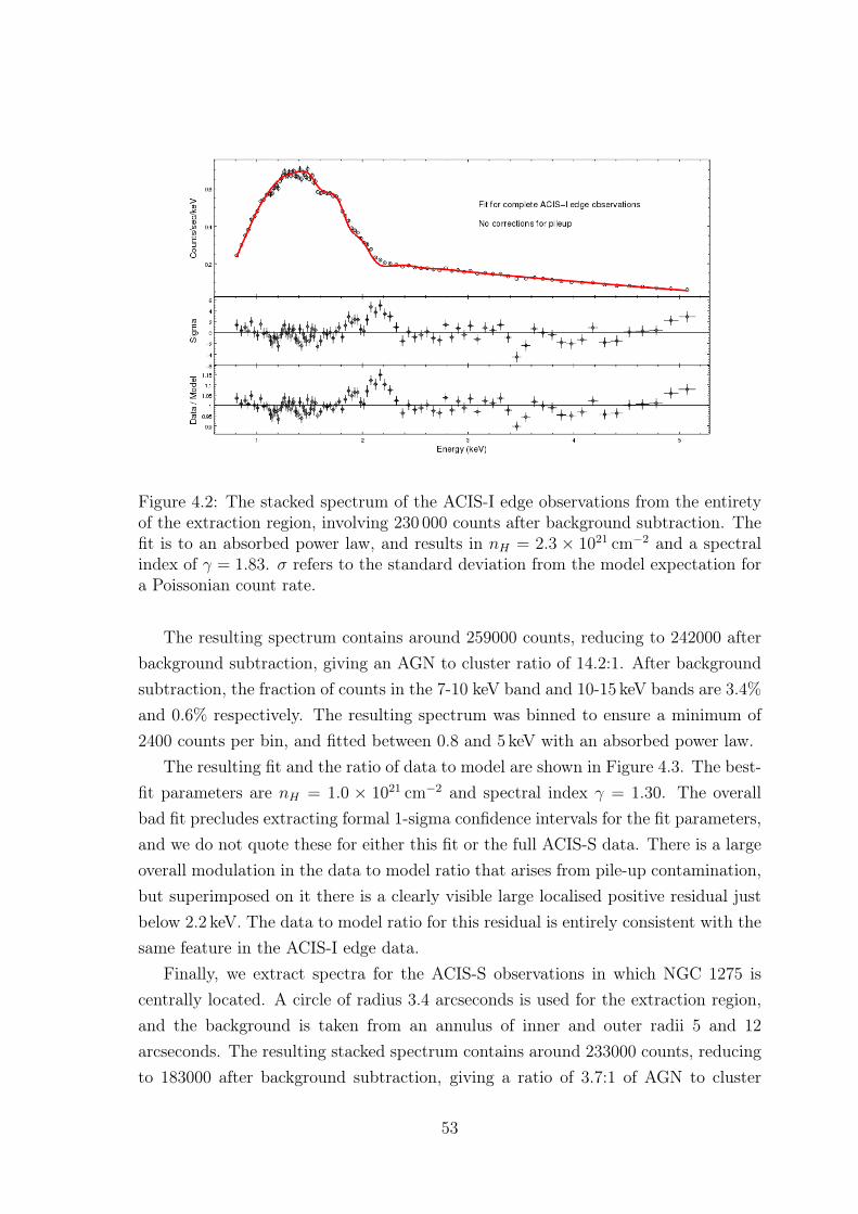
Figure 4.2: The stacked spectrum of the ACIS-I edge observations from the entiretyof the extraction region, involving 230 000 counts after background subtraction. Thefit is to an absorbed power law, and results in nH = 2.3 × 1021 cm−2 and a spectralindex of γ = 1.83. σ refers to the standard deviation from the model expectation fora Poissonian count rate.

The resulting spectrum contains around 259000 counts, reducing to 242000 afterbackground subtraction, giving an AGN to cluster ratio of 14.2:1. After backgroundsubtraction, the fraction of counts in the 7-10 keV band and 10-15 keV bands are 3.4%and 0.6% respectively. The resulting spectrum was binned to ensure a minimum of2400 counts per bin, and fitted between 0.8 and 5 keV with an absorbed power law.

The resulting fit and the ratio of data to model are shown in Figure 4.3. The best-fit parameters are nH = 1.0 × 1021 cm−2 and spectral index γ = 1.30. The overallbad fit precludes extracting formal 1-sigma confidence intervals for the fit parameters,and we do not quote these for either this fit or the full ACIS-S data. There is a largeoverall modulation in the data to model ratio that arises from pile-up contamination,but superimposed on it there is a clearly visible large localised positive residual justbelow 2.2 keV. The data to model ratio for this residual is entirely consistent with thesame feature in the ACIS-I edge data.

Finally, we extract spectra for the ACIS-S observations in which NGC 1275 iscentrally located. A circle of radius 3.4 arcseconds is used for the extraction region,and the background is taken from an annulus of inner and outer radii 5 and 12arcseconds. The resulting stacked spectrum contains around 233000 counts, reducingto 183000 after background subtraction, giving a ratio of 3.7:1 of AGN to cluster

53

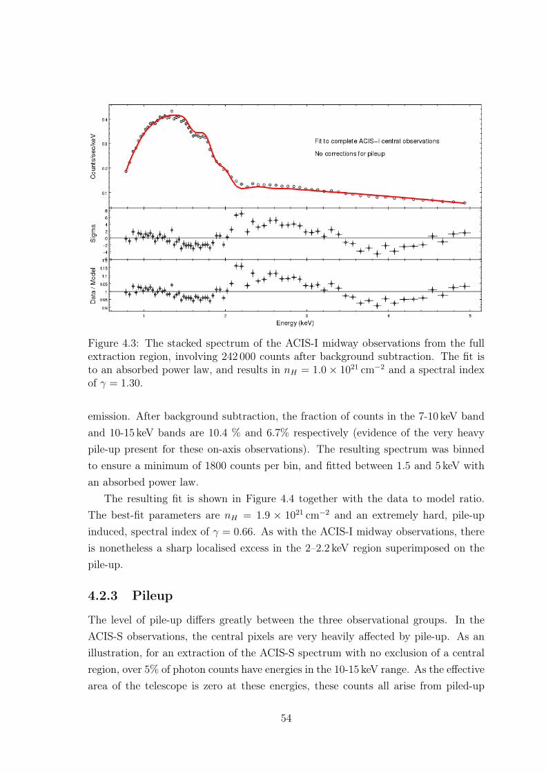
Figure 4.3: The stacked spectrum of the ACIS-I midway observations from the fullextraction region, involving 242 000 counts after background subtraction. The fit isto an absorbed power law, and results in nH = 1.0× 1021 cm−2 and a spectral indexof γ = 1.30.

emission. After background subtraction, the fraction of counts in the 7-10 keV bandand 10-15 keV bands are 10.4 % and 6.7% respectively (evidence of the very heavypile-up present for these on-axis observations). The resulting spectrum was binnedto ensure a minimum of 1800 counts per bin, and fitted between 1.5 and 5 keV withan absorbed power law.

The resulting fit is shown in Figure 4.4 together with the data to model ratio.The best-fit parameters are nH = 1.9 × 1021 cm−2 and an extremely hard, pile-upinduced, spectral index of γ = 0.66. As with the ACIS-I midway observations, thereis nonetheless a sharp localised excess in the 2–2.2 keV region superimposed on thepile-up.

4.2.3 Pileup

The level of pile-up differs greatly between the three observational groups. In theACIS-S observations, the central pixels are very heavily affected by pile-up. As anillustration, for an extraction of the ACIS-S spectrum with no exclusion of a centralregion, over 5% of photon counts have energies in the 10-15 keV range. As the effectivearea of the telescope is zero at these energies, these counts all arise from piled-up

54

Figure 4.4: The complete stacked spectrum of the ACIS-S observations, involving183 000 counts after background subtraction. The fit is to an absorbed power law,and results in nH = 1.9× 1021 cm−2 and a spectral index of γ = 0.66.

events in which several photons have arrived in the same readout frame. In contrast,pile-up is far more moderate for the ACIS-I edge observations (for which a similarextraction across the entirety of the image results in only 0.1% of counts lying in the10-15 keV range).

Given the data, there are two basic methods we can employ to reduce the effectsof pile-up on the analysis. The first is to reduce the amount of pile-up by using anannular extraction region and extracting the spectrum only from the wings of thepoint spread function. The point spread function of the telescope causes the arrivingphotons to be spread out on the detector, with the degree of spread increasing asone moves progressively off-axis. We note that the point spread function is mildlyenergy dependent: photons with higher energy are spread out further than photonswith smaller energy. While fewer photons arrive in the wings of the point spreadfunction, those that do suffer less from pile-up than those arriving on the centralpixels. The second is to model the pile-up, and the distortion it induces on thespectrum, explicitly. We shall utilise both approaches below.

55

Removing central pixels

We analyse the images and count rates of each observation using the image softwareds9. We set the ds9 binning such that the ds9 pixels are the same size as thephysical Chandra pixels (half an arc-second across). We then create an extractionregion manually excluding all ds9 pixels which are neighbours (either side-by-side ordiagonally) to any pixel with total counts greater than 1% of the overall exposuretime. Using the pileup_map tool, this results in almost all retained pixels having apile-up fraction lower than 5%.2 Using arfcorr, the responses reflect the presence ofa central exclusion in the extraction region.

We first show in Figure 4.5 the ACIS-I edge observations with a central exclusionaccording to the above method. As these observations are relatively clean to beginwith, the fractional change in the number of counts is relatively small. There are now187000 counts before background subtraction and 153000 counts afterwards. Thefraction of counts in the 7–10 keV and 10–15 keV regions are 1.2% and 0.04%. Thebest-fit spectral index is γ = 1.85±0.015 (the errors quoted here and in the remainderof this paper are statistical 1-σ errors, see Appendix 3.5.1 for more details) withnH = 2.2 × 1021 cm−2. While the statistical significance of the features at 2–2.2 keVand 3.4–3.5 keV reduces (consistent with the reduced photon counts), the magnitudesof the data to model fluctuations remain the same.

We now perform a similar cleaning of the ACIS-I observations with the sourcemidway on the chip. As the central pixels are heavily piled-up, in this case thecleaning procedures significantly increases the quality of the fit. This is at the cost ofa significant reduction in photon statistics: there are now only 88000 counts beforebackground subtraction, and 74000 after background subtraction. We group countsso that there are 700 counts per bin, leading to a spectral index of γ = 1.64 ± 0.02

with nH = 1.3 × 1021 cm−2. With a Q-value of 0.18 and a reduced χ2 of 1.14 for 86degrees of freedoms, this is now an overall good fit to the data (see Figure 4.6).3

2For these observations, the telemetry limit was 15 keV and any (piled-up) photons recorded withenergy larger than this were not telemetered to the ground. For there to be a significant number ofsuch events, there would also exist a tail of photons with energies close to, but below, the telemetrylimit. From the < 0.2% fraction of photons measured in the 10-15 keV band for the cleaned spectra,we can infer that these contained very few un-telemetered events. The same analysis shows thatthere are very few un-telemetered events for the ACIS-I edge observations even without excising thecentral part of the image, but the central high pile-up regions of the ACIS-I Midway and ACIS-Sobservations did have significant numbers of un-telemetered events.

3Fitting the different observations individually produces results for γ that are consistent with thestacked result, both for the Midway and Edge observations.

56

Figure 4.5: The stacked spectrum of the ACIS-I edge observations, with centralpixels excluded according to the prescription in the text. There are 153 000 countsafter background subtraction. The fit is to an absorbed power law, and results innH = 2.2× 1021 cm−2 and a spectral index of γ = 1.85± 0.015.

Figure 4.6: The stacked spectrum of the ACIS-I midway observations, with centralpixels excluded according to the prescription in the text. There are 74 000 countsafter background subtraction. The fit is to an absorbed power law, and results innH = 1.3× 1021 cm−2 and a spectral index of γ = 1.64± 0.02.

57

We note that the spectral index γ is clearly different from that found with theACIS-I edge data. However, this spectrum was obtained by excluding the central partof the image and extracting only from the wings of the point spread function. Bycomparison with the brightness of the AGN measured in the contemporaneous ACIS-Iedge observations, we can infer that this spectrum retains only around one quarterof the total number of photons from the AGN. As the ACIS point spread functionincreases with energy, this biases the analysed photons towards a harder spectrum(and a lower γ). In principle, this is taken into account in the analysis procedure, asthe aperture correction of arfcorr modifies the response to reflect the exclusion of thecentral part of the image. However, it is also the case that the image has a complexform with neither a spherical nor an elliptical shape. Instead, the image of the AGN– traced by the excluded central region – resembles a ‘Maltese cross’ shape, as can beseen in Figure 4.1.

The objective of this work is to constrain large, localised modulations in the spec-trum of the AGN that could arise from ALP-photon conversion. For this purposewe therefore do not regard these different values of γ as problematic, particularlygiven the large difference in observational conditions between the two sets of obser-vations and the large fraction of photons that are excluded in the ACIS-I Midwayobservations.

We perform a similar procedure for the ACIS-S observations. In this case wereduce pile-up by removing a central square of 16 pixels (2 arcseconds square) from anextraction region of a circle of radius 3.4 arcseconds. The resulting cleaned spectrumhas 117000 counts before background subtraction and 74000 counts after backgroundsubtraction. After background subtraction there are now 0.1% counts in the 10–15 keV band and 1.1% of counts in the 7–10 keV band, indicating that this spectrumis now substantially cleaner. We group counts so that there are at least 700 countsper bin. In this case, an absorbed power law is not sufficient for a good fit andwe supplement this by a soft thermal component using xsapec (the presence of athermal component for NGC 1275 was also reported in [120]). The presence of a softthermal component substantially improves the fit, resulting in an acceptable Q valueof 10−2. The resulting fit (see Figure 4.7) has nH = 1.6× 1021 cm−2 and a power lawindex of γ = 1.84 ± 0.03. The thermal component has a temperature T = 0.92 keV.At this temperature, the amplitude and abundance of the thermal component arelargely degenerate in the fit. Fixing the abundance at solar abundance, the relativeamplitude of thermal component to the power law is 0.15.

58

Figure 4.7: The stacked spectrum of the ACIS-S observations, with a central 16-pixelsquare excluded. The fit is to an absorbed power law and soft thermal component.

Modelling pileup

Here we aim to model the pile-up directly. While this modelling does not provide acomplete picture of pile-up, it ameliorates its effect. A full treatment would requirecustomised tools going beyond the scope of this paper (the pile-up tool jdpileup [132]provided with Sherpa is optimised for on-axis sources, while NGC 1275 is off-axis inall ACIS-I observations).

We first describe our pile-up modelling for the ACIS-S observations, where theimage of NGC 1275 is on-axis. This results in a high degree of pile-up – the centralpixels have large numbers of counts above 10 keV, all of which arise from multi-photonpile-up events.

We use the jdpileup model as described in [132]. As this model assumes thesource is on-axis, it is directly appropriate here. The model assumes Poisson statis-tics to calculate the probability of different numbers of photons hitting an event-detection cell (a 3×3 pixel region in Chandra) within the read-out time adjusted tothese respective observations. For the ACIS-S and ACIS-I midway observations, theread-out time was 3.1 seconds, and for the ACIS-I edge observations it was 3.2 sec-onds. The model then convolves this probability with the probability of such eventsbeing assigned a ‘good’ grade, and the conversion from photon energy to pulse heightby the detector. We note that the non-linearity of pile-up (the dependence on theenergy spectrum for all energies below the bin) will cause degeneracies in the inferredparameters of the jdpileup model (α and f) with those of the energy spectrum [132].

59

The parameter n, the number of regions to which jdpileup will be applied inde-pendently, was set to 1 for the ACIS-S observations (as the target was a point source).For an extended source it should roughly correspond to the number of 3×3 pixel is-lands in the region, as jdpileup assumes spatial uniformity across the extractionregion. For the ACIS-I midway observations, where the AGN is smeared out acrossseveral pixel islands, the value of n proved difficult to determine for large extractionregions, with the value corresponding to the best fit being unrelated to the numberof pixel islands. We therefore constrained ourselves to a smaller central region, withlittle variation in count rate between pixels, to give us more control over the pile-upmodel.

It is also worth noting that the jdpileup model is set to zero for energies lessthan 0.5 keV and energies greater than 10 keV. As there are many events above the10 keV range for the ACIS-S observations, we only model the spectrum up to 10 keV,as extending the fit beyond that would result in the model parameters being sent tounphysical values.

For the ACIS-S pile-up analysis, we used a circular region around NGC 1275 ofradius 3.5 arcseconds, with the background taken from an annular region of innerradius 4 arcseconds and outer radius 7 arcseconds. Counts were grouped to 1500 perbin. The spectrum was modelled using an absorbed power law and thermal emissionwith temperature T = 0.85 keV, and fitted with the jdpileup model for energy valuesbetween 1 and 10 keV. The data was fit using the moncar Monte-Carlo method, andrun several times to ensure the global minimum had been found.

The resulting fit and the ratio of data to model are shown in Figure 4.8. Thebest-fit parameters involve nH = 2.6×1021 cm−2 and a spectral index γ = 1.81.4 Thebest-fit α and f parameters of jdpileup were α = 0.660 and f = 0.943 respectively.We can clearly see that this model provides a reasonable description of the data allthe way up to 10 keV, and produces physically sensible values for nH and γ, despitethe model estimating a pile-up fraction of 82%. The reduced statistic of the fit is1.75, with a Q-value of 10−5. While we re-emphasise that this will not represent aperfect account of pile-up, it does capture the relevant physics, producing a sensiblefit with physical parameters.

For the ACIS-I midway observations we considered a central 6×6 pixel extractionregion (this is almost exactly the complement of the clean ACIS-I midway spectrumused in the previous subsection). The resulting spectrum contains around 136000

4As the uncertainties on the pile-up modelling are hard to quantify, we only quote best-fit pa-rameters and do not include errors.

60

Figure 4.8: The ACIS-S observations, involving 177 000 counts after backgroundsubtraction. The fit is to an absorbed power law with a thermal component ofT = 0.85 keV, and pile-up is modelled with jdpileup. The ratio of data to model isshown at the bottom of this figure.

counts, reducing to 134000 after background subtraction, giving a very high AGN tocluster contrast of 67:1. After background subtraction, the fraction of counts in the7-10 keV band and 10-15 keV bands are 5.3% and 1.2% respectively. Counts weregrouped to 1000 per bin. The spectrum was modelled using an absorbed power lawand fitted with the jdpileup model, this time for energy values between 1 and 9 keV,to ensure no counts with energy greater than 10 keV were included in the final bin.The jdpileup parameter n was set to 4, the number of 3×3 pixel islands in theextraction region.

The resulting fit and ratio of data to model are show in Figure 4.9. The best-fitparameters involve nH = 2.5× 1021 cm−2 and a spectral index γ = 1.93. The best-fitα and f parameters of jdpileup were α = 0.324 and f = 0.975 respectively, andthe estimated pile-up fraction was 35%. While the fit is not perfect, it does give areasonable characterisation of the data.

We finally consider the case of the ACIS-I edge observations, where pile-up isrelatively weak. Although a reasonable fit can be made with no pile-up modelling,we now aim at modelling the pile-up also in these observations for completeness.There is a rule of thumb5 that 0.007 counts/second per 3×3 pixel island is about 1%

5cxc.harvard.edu/csc/memos/files/Davis_pileup.pdf

61

Figure 4.9: The ACIS-I midway observations from a central 6×6 pixel region, involv-ing 134 000 counts after background subtraction. The fit is to an absorbed power lawand pile-up is modelled with jdpileup.

pile-up, and 0.07 counts/second is about 10%. We will assume that the ACIS-I edgeobservations with mild cleaning have pile-up fractions of 10% or lower.

For the ACIS-I edge observations, we used as source an elliptical annulus of radii 3and 5 arcseconds, with the 12 brightest pixels removed by a contour. The backgroundwas extracted from an elliptical annulus of outer radii 18 and 23 arcseconds, with innerradii 8 and 12 arcseconds. The resulting spectrum contains around 128000 counts,reducing to 111000 after background subtraction, giving an AGN to cluster ratio of6:1. After background subtraction, the fraction of counts in the 7–10 keV band and10–15 keV bands are 1.1% and 0.1% respectively. We grouped counts to 1000 per bin.Here there are fewer counts out at higher energies than in the previous two sets ofobservations, so we fit only out to 5 keV. The jdpileup parameter n was set to 16,the number of 3×3 pixel islands in the extraction region. This should only be thoughtof as a rough estimate, as the jdpileup model is stated to be accurate for on-axispoint sources, and the edge observations are also not spatially uniform in terms ofcounts. The fit is to an absorbed power law, and results in nH = 2.7 × 1021 cm−2

and a spectral index of γ = 1.89. The best-fit α and f parameters of jdpileup wereα = 0.52 and f = 0.87 respectively. The pile-up fraction was 3%, consistent withestimates and very mild as expected.

Given the high flux levels of the source, a cleaner spectrum requires reducing theeffects of pile-up in the spectrum. The first method involves excluding a central region

62

Figure 4.10: The ACIS-I edge observations, involving 110000 counts after back-ground subtraction. The fit is to an absorbed power law and pile-up is modelledwith jdpileup.

of highest pile-up from the analysis. While this reduces the photon counts – and so thestatistical significance of any features in the spectrum – it also allows produces purerspectra of higher quality. The second method is to keep the full spectrum, but modelthe pile-up explicitly. For the purpose of placing bounds on ALPs and constrainingthe existence of ALP-induced spectral modulations, the most useful spectra are thosewhere photon events occur at their true energies.

Finally, we also considered Chandra’s grating observations of NGC 1275 (ObsIDs333 and 428 with HETG) as a means to reduce pile-up, but this reduced counts tothe point where it did not seem worthwhile.

4.2.4 Analysis of residuals in Chandra NGC 1275 data

No residuals in the spectra exceed 10%. At the 10% level, the Chandra spectra pre-sented in the main body of the paper show two main features departing from a powerlaw: an excess at 2–2.2 keV, present in all Chandra observations with overwhelm-ing statistical significance, and a deficit 3.4–3.5 keV that is not as strong but is stillpresent at almost five (local) sigma in the ACIS-I edge data. These features ensurethat an absorbed power law (plus thermal component) is not a good fit to the data.

We perform a statistical analysis of these features at E ∼ 2 keV and E ∼ 3.5 keV.

We first consider the E ∼ 2 keV feature. Considering the clean ACIS-I Edge data,

63

we include a positive Gaussian (xswabs ∗ (xspowerlw+xsgaussian)) and analyse itseffect on the fit. For a zero-width Gaussian, this leads to an improvement in the fitby ∆χ2 = 33.7 with a best-fit energy of 2.13 keV. For a finite-width Gaussian, theimprovement is ∆χ2 = 48.0, with a best-fit energy of 2.02 keV and a best-fit width of0.2 keV.

For the ACIS-I midway data, a similar additional Gaussian improves the fit by∆χ2 = 18.6 with a best-fit energy of 2.17 keV (the fitted width is much smallerthan the detector resolution and so results are identical for zero-width and finite-width Gaussians). For the ACIS-S data, the additional Gaussian improves the fit by∆χ2 = 20.3 with a best-fit energy of 2.06 keV (again, fitting the width gives a resultsmaller than the detector resolution and so does not affect the result).

For the 3.5 keV feature, we consider the cleaned datasets for the three sets ofobservations and include a negative Gaussian (xswabs ∗ (xspowerlw− xsgaussian)).We formally treat the Gaussian as zero-width, but any finite width much narrowerthan the ACIS energy resolution gives an identical result. For the three data sets(ACIS-I Edge, ACIS-I Midway, and ACIS-S) we plot below (Figures 4.11-4.13) theimprovement in the χ2 that can come from adding an additional negative Gaussian∆χ2

NG. The ACIS-I Edge data show a strong preference for an additional negativeGaussian (∆χ2 ∼ 17) at 3.5 keV. For both the ACIS-I Midway and ACIS-S data, anegative Gaussian at 3.5 keV mildly improves the fit (∆χ2 ∼ 1.5 and ∆χ2 ∼ 0.4) butis not required (as the ACIS-I Edge dataset is both larger and cleaner than the othertwo datasets, these results are consistent – in particular, the inferred strength of thedip is consistent within 2 σ).

Across all three plots, the largest feature is clearly seen to be the residual inthe ACIS-I Edge data at 3.5 keV. The next strongest residuals are two features atE ∼ 1.2 keV (ACIS-I Edge) and E ∼ 1.4 keV (ACIS-S) with ∆χ2 ∼ 10. In both cases,there are very strong atomic lines visible in the background spectra at precisely theseenergies (Fe XXI, Fe XXII, Fe XXIII, Fe XXIV, Mg XII). These features can bereliably associated with these atomic lines, coming from a small mis-subtraction ofthe background (deep in the core of the Perseus cluster, the physical conditions ofthe gas in the signal region and background region will not be precisely identical).

In Figure 4.14, we produce a combined plot of the significance of the 3.5 keVdeficit across all Chandra observations. In order to compare observations taken atdifferent times and with different intrinsic AGN luminosities, to measure the strengthof the deficit we have used the induced fractional deficit of photons in the 3.3 –

64

1 2 3 4 5E [keV]

5

10

15

ΔχNG2

Figure 4.11: The improvement in χ2 attainable by adding a negative Gaussian at thespecific energy for ACIS-I Edge observations.

1 2 3 4 5E [keV]

2

4

6

8

10ΔχNG

2

Figure 4.12: The improvement in χ2 attainable by adding a negative Gaussian at thespecific energy for ACIS-I Midway observations.

1 2 3 4 5E [keV]

2

4

6

8

10ΔχNG

2

Figure 4.13: The improvement in χ2 attainable by adding a negative Gaussian at thespecific energy for ACIS-S observations.

65

1σ

2σ

3σ

3.35 3.40 3.45 3.50 3.55 3.60

0.00

0.01

0.02

0.03

0.04

0.05

0.06

Energy of negative Gaussian in observer frame [keV]

Fractionalphotondeficitin3.3-3.7keV

Figure 4.14: The overall significance and location for the 3.5 keV deficit, combinedacross all Chandra observations (cleaned datasets only). We have used the inducedfractional deficit in photons in the 3.3 - 3.7 keV region to facilitate a uniform compar-ison for the strength of the dip, as the AGN luminosity varies between observations.

3.7 keV regime. The feature remains over 3σ significant globally, and is also locatedat precisely the same energy as the diffuse cluster excess observed in [141, 142].

ALP Interpretation of Features

The purpose of this paper was to use the extraordinary dataset of counts from theNGC 1275 AGN to search for spectral irregularities, with the intent of constrainingALP parameters. This search has resulted in two features being present in the dataat high statistical significance, the former of which is consistent with arising frompile-up around the Iridium edge.

It is not possible for us to constrain ALP couplings beyond a level where theywould produce residuals comparable to these features. We can estimate approximatelythat to produce such residuals would require an ALP-photon coupling of magnitudegaγγ ∼ 1− 5× 10−12 GeV−1. For example, Figure 4.15 shows a fit to the clean ACIS-I edge observations with an absorbed power law multiplied by the photon survivalprobability Pγ→γ. In this case, Pγ→γ was calculated assuming the existence of ALPswith gaγγ = 1 × 10−12 GeV−1 and a central magnetic field B0 = 25µG. We see thatthe anomalies at 2.2 keV and 3.5 keV have been alleviated by the presence of ALPs(although, for this magnetic field, at the expense of creating similarly sized anomaliesat higher energies). Figure 4.16 shows the corresponding photon survival probabilityspectrum.

66

Figure 4.15: A fit to the clean ACIS-I edge observations with an absorbed power lawmultiplied by the photon survival probability for a specific example of ALP-photonconversion. We include ALPs with gaγγ = 1×10−12 GeV−1 and assume a central fieldof B0 = 25µG. The reduced χ2 is 1.51, compared to 1.65 for a fit to an absorbedpower law without ALPs.

Figure 4.16: The photon survival probability for the fit shown in Figure 4.15.

67

4.2.5 The Presence of the 6.4 keV Iron line

As the cleaned spectra in the main body of the paper are only extracted up to5 keV, it is a useful consistency check to ensure that the reflected iron Fe Kα line at6.4 keV (6.3 keV after redshifting) is present in our spectra. For this purpose we usethe cleaned spectra for each of the three sets of Chandra observations, and fit thespectrum only between 5.5 and 7 keV. We fit first a power law, and then the sum ofa power law and a Gaussian (we do not fit nH as absorption is irrelevant at theseenergies).

We determine the best-fit central energy of the additional Gaussian and the re-sulting improvement in χ2. These fits are summarised in Table 4.3 below and we alsoshow explicitly the fit for the ACIS-S data in Figure 4.17.

Data set Power law index Eline (keV) ∆χ2 (Degrees of freedom)

ACIS-I Edge 0.84+0.3−0.1 6.32+0.06

−0.05 6.8/2ACIS-I Midway −0.14+0.03

−0.02 6.33+0.05−0.06 2.2/2

ACIS-S Central 0.49+0.07−0.11 6.29+0.02

−0.03 12.2/2

Table 4.3: Fit parameters for a (power law + Gaussian) fit between 5.5 and 7 keV.

Figure 4.17: The Fe Kα line in the cleaned ACIS-S data.

These show that the iron line is clearly present in the ACIS-S and ACIS-I Edgedata, and marginally present in the ACIS-I Midway data. As ACIS-S has betterenergy resolution than ACIS-I, it is unsurprising that the Fe line is found at highestsignificance there.

68

We note that all spectral indices are unphysically hard (and even negative for theACIS-I Midway data). This is a clear consequence of pile-up. For energies above5 keV, the Chandra effective area is falling off rapidly. There are also intrinsicallyfar fewer source photons than are present at lower energies, given the power lawspectrum. The effects of pile-up at these higher energies are therefore far more severethan at lower energies.

While these spectra have been cleaned, this does not mean that there is zero pile-up. For the bulk of the spectra, the effects of pile-up in the cleaned spectra are at thelevel of a few per cent. However, for E > 5 keV the effects of pile-up are substantiallymore important for the above reasons: the combination of the intrinsic decline in thespectrum and the fall-off in the Chandra effective area implies that pile-up plays aproportionally far more severe role at high energies.

4.2.6 Bounds from Chandra data

From the perspective of constraints on ALPs, the overall summary of the data is thatthe spectrum from NGC 1275 is fit by an absorbed power law, with residuals fromthe power law not larger than 10%. We will further discuss residuals at the 10% levelin Appendix 4.2.4 (in particular features around 2 - 2.2 keV and at 3.5 keV). However,the absence of any modulations in the spectrum at a level greater than 10% allowspowerful constraints to be placed on ALP parameter space.

In particular, this allows us to say that on passing from NGC 1275 through thePerseus cluster and towards us, 〈P (γ → a)〉 . 20%. It follows that ALP-photoncouplings large enough to generate the saturated limit of 〈P (γ → a)〉 = 1/3 are ro-bustly excluded, as these would produce larger residuals in the data than are actuallyobserved.

Note that this approach to placing bounds is conservative. The simulated data(with ALPs) is idealised – it has no pileup present and assumes a perfect subtractionof the cluster background. Couplings are excluded when they lead to simulated datathat would still be a worse fit than the actual data, even though the simulated datais observationally ideal while the real data contains effects such as pileup and clusterbackground that lead to increased residuals and make it far noisier than simulateddata.

To obtain approximate bounds on gaγγ, we compare two models for the flux F (E)

observed from NGC 1275:

69

• Model 0: An absorbed power law F0(E) = AE−γ × e−nHσ(E), as described inEquation (4.1).

• Model 1: An absorbed power law multiplied by the photon survival probabilityassuming the existence of ALPs with coupling gaγγ. In this case the predictedflux also depends upon the magnetic field B along the line of sight. We haveF1(E,B) = AE−γ × e−nHσ(E) × Pγ→γ(E(1 + z),B, gaγγ).

Although we have (limited) empirical estimates of the strength of the magneticfield in Perseus, the exact structure is unknown. In practice, we randomly generatemany instances of the field from a given power spectrum. The parameter most relevantto ALP-photon conversion is the central magnetic field strength B0, estimated as25µG in [123]. Based on results for the Coma cluster, we assume that B decreaseswith radius as B ∝ n0.7

e [127]. The electron density ne has the radial distributionfound in [119],

ne(r) =3.9× 10−2

[1 + ( r80 kpc

)2]1.8+

4.05× 10−3

[1 + ( r280 kpc

)2]0.87cm−3 .

We simulate each field realisation with 600 domains. The length l of each domain isbetween 3.5 and 10 kpc, randomly drawn from a power law distribution with minimumlength 3.5 kpc and power 0.8. We therefore have:

P (l = x) = N

0 for x > 10 kpc ,

x−1.2 for 3.5 kpc < x < 10 kpc ,

0 forx < 3.5 kpc ,

(4.2)

with normalisation constant N .The coherence length and power spectrum of the magnetic field in the centre of

Perseus is not observationally determined. Instead, these parameters are motivatedby those found for the cool core cluster A2199 [128], taking a conservative value forthe magnetic field radial scaling. The magnetic field and electron density are constantin each domain, with B(r) and ne(r) evaluated at the centre of the domain and thedirection of B chosen at random.

We compute 95% confidence limits on gaγγ by generating fake data from Model 1and assessing how well it is fit by Model 0 i.e. how well the oscillations due to ALP-photon conversion can hide in the Poisson noise. As it has minimal pile-up, we use theclean ACIS-I edge observations for this analysis. We fit the spectrum between 1 and4 keV (a region unaffected by pile-up) and bin such that there are 1000 counts in each

70

energy bin. We use Sherpa’s Levenberg-Marquardt fitting method with Poisson errorsderived from the value of the data in each bin. Our procedure to determine whetherALPs with coupling gaγγ are excluded at the 95% confidence level is as follows:

1. Fit Model 0 to the real data and find the corresponding reduced χ2, χ2data.

2. Randomly generate 50 different magnetic field realisations Bi for the line ofsight to NGC 1275.

3. For each Bi, compute Pγ→γ(E,Bi, gaγγ) by numerically propagating photons atdifferent energies through Bi, as described for example in [87]. We take 300photon energies equally spaced between 1 and 4 keV.

4. For each Bi, generate 10 fake data sets from Model 1, using Sherpa’s fake phamethod.

5. Fit Model 0 to each of the 500 fake data sets and find the corresponding reducedχ2, χ2

i for each.

6. If fewer than 5% of the χ2i are lower than χ2

data, gaγγ is excluded at the 95%

confidence level.

We scan over gaγγ in steps of 10−13 GeV−1. For the gaγγ value excluded, we alsocheck that the three values above it in our grid are also excluded. For the magneticfield parameters described above, we find gaγγ . 1.4 × 10−12 GeV−1 which is shownin Figure 4.18.

If we consider a more pessimistic scenario with B0 = 15µG and a minimumcoherence length of 0.7 kpc, we instead find gaγγ . 2.7 × 10−12 GeV−1. If we takean even more pessimistic scenario in which the central field is B0 = 10µG and theminimum coherence length is 0.7 kpc, the bound increases further to gaγγ . 4.0 ×10−12 GeV−1.

We finally note that if we excluded the feature at 2.2 keV from the fit, removingthe 1.8 - 2.3 keV region based on this being the location of an effective area edge,the bounds would improve significantly, to gaγγ . 1.1 × 10−12 GeV−1 for the case ofa central magnetic field of B0 = 25µG (see Appendix 4.2.4). This illustrates theconservative nature of the bounds compared to any mis-modelling of the actual data.

71

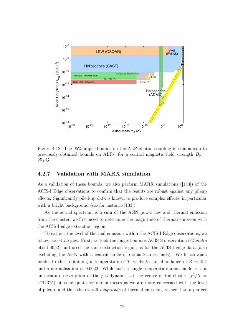
Axio

n C

ouplin

g |G

Aγγ | (

GeV

-1)

Axion Mass mA (eV)

10-18

10-16

10-14

10-12

10-10

10-8

10-6

10-30

10-25

10-20

10-15

10-10

10-5

100

LSW (OSQAR)

Helioscopes (CAST)

Haloscopes(ADMX)

Tele

scopes

Horizontal Branch Stars

KSVZ

DFSZ

VMB(PVLAS)

SN 1987AHESS

NGC1275 - Chandra

Hydra A - Wouters/Brun

Fermi-LAT

Figure 4.18: The 95% upper bounds on the ALP-photon coupling in comparison topreviously obtained bounds on ALPs, for a central magnetic field strength B0 =25µG.

4.2.7 Validation with MARX simulation

As a validation of these bounds, we also perform MARX simulations ([143]) of theACIS-I Edge observations to confirm that the results are robust against any pileupeffects. Significantly piled-up data is known to produce complex effects, in particularwith a bright background (see for instance [133]).

As the actual spectrum is a sum of the AGN power law and thermal emissionfrom the cluster, we first need to determine the magnitude of thermal emission withthe ACIS-I edge extraction region.

To extract the level of thermal emission within the ACIS-I Edge observations, wefollow two strategies. First, we took the longest on-axis ACIS-S observation (Chandraobsid 4952) and used the same extraction region as for the ACIS-I edge data (alsoexcluding the AGN with a central circle of radius 2 arcseconds). We fit an apec

model to this, obtaining a temperature of T ∼ 4keV, an abundance of Z ∼ 0.4

and a normalisation of 0.0022. While such a single-temperature apec model is notan accurate description of the gas dynamics at the centre of the cluster (χ2/N =

474/375), it is adequate for our purposes as we are more concerned with the levelof pileup, and thus the overall magnitude of thermal emission, rather than a perfect

72

spectral shape. Using this model together with the exposure and responses for theACIS-I edge observations, this suggests the presence of around ∼ 30k thermal countspresent in the ACIS-I spectrum.

Secondly, as a check on this, we also used purely the ACIS-I edge data and directlyfit it with a sum of an absorbed power law and absorbed thermal emission. In doingthis, we froze the temperature and abundance of the thermal model to the valuesobtained from the Hitomi spectrum of the central region of the Perseus cluster, T =3.48 keV and Z = 0.54 ([144]). This produced a best-fit normalisation for the apec

norm of 0.0027, comparable to that attained when using the ACIS-S data to determinethe magnitude of thermal emission. This slightly higher value would correspond to atotal of ∼ 36k counts from thermal emission within the ACIS-I Edge spectrum. Asboth results are consistent, they show that of the ∼ 270k counts in the ACIS-I edgespectrum only around 10-15% arise from thermal cluster emission.

We then implement a MARX simulation of the ACIS-I edge observations. Forthis, we used the observational parameters (date, on-axis location and roll angle) forthe longest ACIS-I edge observation of the AGN (Chandra obsid 11713). As all thefour actual ACIS-I Edge observations have similar properties, we set the exposure ofthis MARX simulation to 200ks, the total exposure of the actual data.

The data was first simulated without any axions present.

1. The thermal emission was simulated as a spatially extended Gaussian with awidth of 30 arcminutes, centred on the AGN. It was modelled as an apec modelwith a temperature T = 3.5keV and an abundance Z = 0.48. The normalisationof the model was adjusted so that it had the same fitted strength as for real data(as determined above) when extracted within the region used for the ACIS-IEdge data.

2. The AGN emission was simulated as a point source power law. The normal-isation of the power law was adjusted so that - after it had been combinedwith the thermal emission and the pileup processing applied - it had the samenormalisation as the real data when extracted over the same extraction region.

3. The two individual simulations were then combined using marxcat and theMARX pileup processing applied to the combined simulation.

4. Counts were grouped to 500 and the combined spectrum was fitted with the sumof a power law plus thermal emission. The previous two steps were iterated untilthe fitted strength and index of the power law matched that of the real data.

73

We generated a total of 50 fake data samples in this way. To match the fittedstrength of the AGN (4.7 × 10−3 ph cm−2 s−1 keV−1 at 1 keV) required an intrinsicstrength of 6.4×10−3 ph cm−2 s−1 keV−1 at 1 keV. Comparison of the number of countswithin the extraction region in the marx event files pre- and post-pileup processingsuggests an overall pileup fraction of 15% in the dataset. Nonetheless, the pileup isnot sufficient to make the spectral fit unsatisfactory (the reduced χ2 values clusteraround unity for ∼ 250 degrees of freedom, with the largest reduced χ2 being 1.37).

As a test of an even more piled-up spectrum with a similar number of photoncounts, we also simulated data using a 100ks MARX exposure but with the intrinsicAGN strength doubled. As this normalisation of 12.8 × 10−3 ph cm−2 s−1 keV−1 at1 keV is much larger than that present in the 2016 Hitomi data, and as the AGNhas been increasing in strength from 2001 onwards (see [122]), pileup is much greaterthan in the actual 2009 data. The fit now tends to be worse, but not terrible. Amongthe fifty fake data samples, the average reduced χ2 is ∼ 1.25 for ∼ 250 degrees offreedom, but there are a few cases still with a reduced χ2 < 1.

We now repeat the MARX simulations including the effects of axions in the data.We multiply the AGN power law with a P (γ → γ) survival probability coming fromphoton-ALP conversion. As this leads to a net reduction in the number of photonspresent, we adjust the intrinsic normalisation upwards so that the fitted normalisationmatches the actual data.

For a fixed ALP coupling, we generate 50 fake data samples. To compare theseresults to those described above using Sherpa’s fake_pha command, we simulate threeseparate ALP couplings: gaγγ = 1, 1.5, 2 × 10−12 GeV−1. In all cases we assume the‘optimistic’ magnetic field model. We directly fitted the absorbed sum of a power lawand apec thermal emission to the ACIS-I Edge extraction region for the fake data,and compared to the quality of the fit when doing so using the real data.6 We firstgroup counts to 500 and fit between 1 and 5 keV using the chi2datavar statistic.Applied to the real data, this gives a reduced χ2 of 1.83 (coming from the excessaround 2 keV).

We then apply this fit to data involving axions. Of the fifty fake data sets producedusing gaγγ = 2 × 10−12 GeV−1, the lowest reduced χ2 was 4.07. When gaγγ = 1.5 ×10−12 GeV−1, the average reduced χ2 is still ∼ 2.5, but now with three out of fiftyspectra with better fits than the actual data (χ2/N < 1.83). When gaγγ = 1.0 ×

6This is marginally different from the analysis procedure described in earlier sections, as it aimsat fitting the thermal emission rather than subtracting it. We also did this analysis subtractingbackground emission from the real data set, and fitting only with a power law. The results howeverare very similar, with no significant changes to the excluded coupling.

74

10−12 GeV−1, more than half the fake spectra have better fits than the actual data.Using 95% confidence level exclusions, this shows that gaγγ = 2 × 10−12GeV−1 isstrongly excluded (the best scenario having a reduced χ2 of 4.07), while gaγγ = 1.5×10−12 GeV−1 is on the boundary of exclusion, and gaγγ = 1 × 10−12 GeV−1 is clearlynot excluded.

This extremely sharp behaviour of the reduced χ2 with gaγγ can be understoodqualitatively. As P (γ → a) ∝ g2

aγγ, a linear increase in gaγγ leads to a quadraticincrease in the amplitudes of modulations in the data. For a Poissonian process, theamount of data required to detect a fixed fractional deviation grows quadratically withthe size of the deviation. So, roughly, a decrease in gaγγ by a factor of two requires asixteen-fold increase in the quantity of data for the same statistical sensitivity.

We also repeated this using a 100 ks exposure with an AGN that is twice as bright(to give a data sample that has a similar number of photons, but is substantiallymore piled up than the actual data). It is again the case that gaγγ = 2×10−12 GeV−1

is strongly excluded, gaγγ = 1 × 10−12 GeV−1 is not excluded, and gaγγ = 1.5 ×10−12 GeV−1 is marginal.

We note that there are of course several differences between the MARX simulationand actual data processing. The MARX treatment of pileup is simpler than the realphysics of deposited electron clouds from the interaction of photons with CCD chips.The MARX simulation also does not take into account Charge Transfer Inefficienciespresent on the actual chips, which obstruct the flow of charge to the readout. However,these results imply that, in terms of bounding gaγγ, uncertainties due to pileup appearto be far smaller than uncertainties due to the cluster magnetic field.

The above bounds used MARX’s simulation of Chandra’s optics. The most ad-vanced simulation of Chandra’s optics is through the ChaRT simulator ([134]), ratherthan MARX. As ChaRT requires the original source spectrum to be manually up-loaded to a website, it is not possible to automate this process to produce axionbounds (as every different ALP conversion template represents a different sourcespectrum). However, for each of the couplings gaγγ = 1, 1.5, 2 × 10−12 GeV−1, wesimulated some individual ChaRT spectra. For the spectra simulated, the results aresimilar to those of the MARX simulations. We plot in figure 4.19 a sample spectrumfor gaγγ = 2×10−12 GeV−1. The ALP induced modulations are clearly visible leadingto a large badness-of-fit.

75

Figure 4.19: An example of simulated data using ChaRT and MARX reproducingthe observational conditions for the ACIS-I edge observations, for an axion couplingof gaγγ = 2 × 10−12 GeV−1. In this case the spectrum is directly fit with the sum ofa power law and thermal apec emission (the ingredients to the simulation). Despitethe pileup fraction of ∼ 15%, the axion-induced modulations are clearly visible andcannot be fit by any conventional astrophysical model.

4.2.8 XMM-Newton observations

There are two observations of NGC 1275 with significant exposure time, see Table 4.4.The first one, 0085110101, was taken in 2001 when the AGN had its lowest emissivityin observational history. The second observation, 0305780101, was taken when theemissivity was still relatively low but nevertheless almost twice as bright as in 2001.NGC 1275 is on-axis in both observations.

The 2001 observation was taken in full frame mode, while the 2006 observationwas taken in extended full frame mode. This affects the frame time of the pn camera,which is 73.4ms in full frame mode and 199.1ms in extended full frame mode. ForMOS, the frame time is 2.6 s. The pixel size of pn is 4.1 arcseconds and 1.1 arcsecondsfor MOS. This means that pn in extended full frame mode is more susceptible to pile-up than MOS. In general, pile-up is an issue for all XMM-Newton observations ofNGC 1275 as we will discuss in the XMM-Newton analysis.

A significant difference between XMM-Newton and Chandra is the angular reso-lution. For both MOS and pn the radius of the disk containing 50% of the photonscollected in the focal plane (Half Energy Width) is around 8.5 arcseconds at 1.5 keV,

76

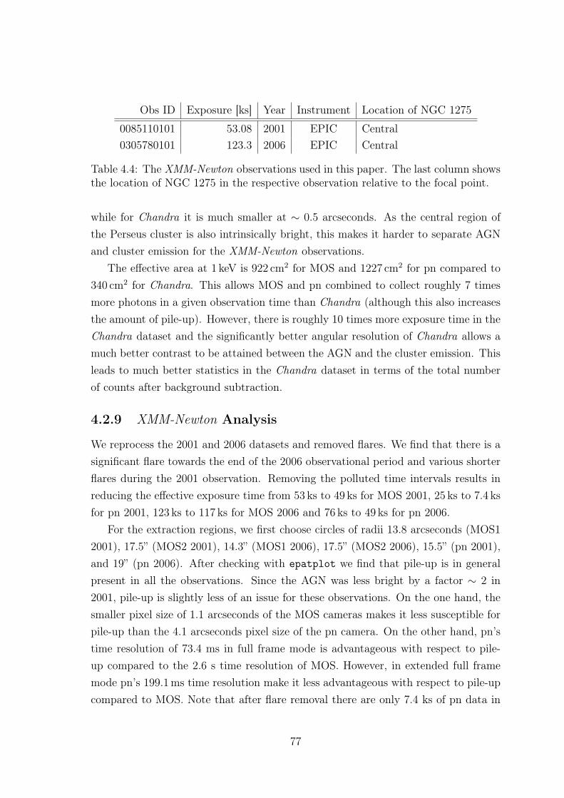
Obs ID Exposure [ks] Year Instrument Location of NGC 1275

0085110101 53.08 2001 EPIC Central0305780101 123.3 2006 EPIC Central

Table 4.4: The XMM-Newton observations used in this paper. The last column showsthe location of NGC 1275 in the respective observation relative to the focal point.

while for Chandra it is much smaller at ∼ 0.5 arcseconds. As the central region ofthe Perseus cluster is also intrinsically bright, this makes it harder to separate AGNand cluster emission for the XMM-Newton observations.

The effective area at 1 keV is 922 cm2 for MOS and 1227 cm2 for pn compared to340 cm2 for Chandra. This allows MOS and pn combined to collect roughly 7 timesmore photons in a given observation time than Chandra (although this also increasesthe amount of pile-up). However, there is roughly 10 times more exposure time in theChandra dataset and the significantly better angular resolution of Chandra allows amuch better contrast to be attained between the AGN and the cluster emission. Thisleads to much better statistics in the Chandra dataset in terms of the total numberof counts after background subtraction.

4.2.9 XMM-Newton Analysis

We reprocess the 2001 and 2006 datasets and removed flares. We find that there is asignificant flare towards the end of the 2006 observational period and various shorterflares during the 2001 observation. Removing the polluted time intervals results inreducing the effective exposure time from 53 ks to 49 ks for MOS 2001, 25 ks to 7.4 ksfor pn 2001, 123 ks to 117 ks for MOS 2006 and 76 ks to 49 ks for pn 2006.

For the extraction regions, we first choose circles of radii 13.8 arcseconds (MOS12001), 17.5” (MOS2 2001), 14.3” (MOS1 2006), 17.5” (MOS2 2006), 15.5” (pn 2001),and 19” (pn 2006). After checking with epatplot we find that pile-up is in generalpresent in all the observations. Since the AGN was less bright by a factor ∼ 2 in2001, pile-up is slightly less of an issue for these observations. On the one hand, thesmaller pixel size of 1.1 arcseconds of the MOS cameras makes it less susceptible forpile-up than the 4.1 arcseconds pixel size of the pn camera. On the other hand, pn’stime resolution of 73.4 ms in full frame mode is advantageous with respect to pile-up compared to the 2.6 s time resolution of MOS. However, in extended full framemode pn’s 199.1ms time resolution make it less advantageous with respect to pile-upcompared to MOS. Note that after flare removal there are only 7.4 ks of pn data in

77

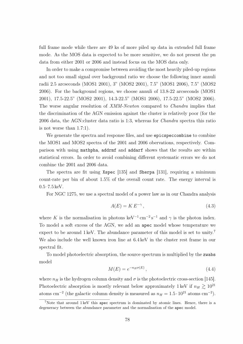
full frame mode while there are 49 ks of more piled up data in extended full framemode. As the MOS data is expected to be more sensitive, we do not present the pndata from either 2001 or 2006 and instead focus on the MOS data only.

In order to make a compromise between avoiding the most heavily piled-up regionsand not too small signal over background ratio we choose the following inner annuliradii 2.5 arcseconds (MOS1 2001), 3” (MOS2 2001), 7.5” (MOS1 2006), 7.5” (MOS22006). For the background regions, we choose annuli of 13.8-22 arcseconds (MOS12001), 17.5-22.5” (MOS2 2001), 14.3-22.5” (MOS1 2006), 17.5-22.5” (MOS2 2006).The worse angular resolution of XMM-Newton compared to Chandra implies thatthe discrimination of the AGN emission against the cluster is relatively poor (for the2006 data, the AGN:cluster data ratio is 1:3, whereas for Chandra spectra this ratiois not worse than 1.7:1).

We generate the spectra and response files, and use epicspeccombine to combinethe MOS1 and MOS2 spectra of the 2001 and 2006 obervations, respectively. Com-parison with using mathpha, addrmf and addarf shows that the results are withinstatistical errors. In order to avoid combining different systematic errors we do notcombine the 2001 and 2006 data.

The spectra are fit using Xspec [135] and Sherpa [131], requiring a minimumcount-rate per bin of about 1.5% of the overall count rate. The energy interval is0.5–7.5 keV.

For NGC 1275, we use a spectral model of a power law as in our Chandra analysis

A(E) = K E−γ , (4.3)

where K is the normalisation in photons keV−1 cm−2 s−1 and γ is the photon index.To model a soft excess of the AGN, we add an apec model whose temperature weexpect to be around 1 keV. The abundance parameter of this model is set to unity.7

We also include the well known iron line at 6.4 keV in the cluster rest frame in ourspectral fit.

To model photoelectric absorption, the source spectrum is multiplied by the zwabsmodel

M(E) = e−nHσ(E) , (4.4)

where nH is the hydrogen column density and σ is the photoelectric cross-section [145].Photoelectric absorption is mostly relevant below approximately 1 keV if nH & 1021

atoms cm−2 (the galactic column density is measured as nH = 1.5 ·1021 atoms cm−2).7Note that around 1 keV this apec spectrum is dominated by atomic lines. Hence, there is a

degeneracy between the abundance parameter and the normalisation of the apec model.

78

The fitted spectra are shown in Figures 4.20 and 4.21. While the fit is good(see Table 4.5), there are both fewer counts and a worse contrast against the clusterbackground than for the Chandra data. From the perspective of ALP constraints, wecan say that modulations of the spectrum are not allowed beyond the 20% level – aweaker constraint than for the Chandra data.

0.1

0.02

0.05

0.2

0.5

norm

alize

d co

unts

s−1

keV

−1

data and folded modelEPIC MOS 2001 NGC1275

1 2 3 4 5 6

0.8

1

1.2

1.4

ratio

Energy (keV)rummel 2−May−2016 19:40

Figure 4.20: MOS 2001 spectral fit. The best-fit parameters are listed in Table 4.5.

4.3 Bounds from other point sources

The magnetic field model parameters we use for each cluster are shown in Table 4.6.

4.3.1 Quasar B1256+281 behind Coma

This quasar is located behind the Coma cluster at a redshift of z = 0.38. Its sight-line passes through the entirety of the Coma intra-cluster medium (ICM). There arearound 5000 counts from the source, of which around 10% can be attributed to theICM (as the source is always off-axis, the Chandra Point Spread Function is degradedcompared to an on-axis observation, increasing the level of contamination from ther-mal cluster emission).

Grouping counts so that there are at least 40 counts per bin, the quasar spectrumfrom 0.5 to 7 keV is well-fit by an unabsorbed power law with photon index 1.75±0.04

79

MOS 2001 MOS 2006

Exposure [ks] 49 118Counts ∼ 47000 ∼ 63000γ 1.65 ± 0.03 1.65 ± 0.03Tsoft 0.84 ± 0.06 0.80 ± 0.06

nH [ 1022 atoms cm−2 ] 0.13 ± 0.03 0.13 ± 0.03χ2/ dof 154 / 131 205 / 178Q-value 0.08 0.08

Table 4.5: Fit results for the XMM-Newton MOS observations from 2001 and 2006.These results are in agreement with the fit parameters found in [119] for the 2001MOS data of NGC 1275.

Source Cluster ne,0 rc β B0 Ltotal(10−3cm−3) (kpc) µG (Mpc)

B1256+281 Coma 3.44 291 0.75 4.7 2SDSS J130001.47+275120.6 Coma 3.44 291 0.75 4.7 2

NGC3862 A1367 1.15 308 0.52 3.25 1IC4374 A3581 20 75 0.6 1.5 12E3140 A1795 50 146 0.631 20 1

CXOUJ134905.8+263752 A1795 50 146 0.631 20 2UGC9799 A2052 35 32 0.42 11 1

Table 4.6: Parameters for the electron density and magnetic field models used for eachof the clusters. All sources use η = 0.7, Lmin = 1 kpc and Lmax = 17 kpc. For Comathe parameters are taken from [146]. For A1367 the β-model parameters come from[147] and the magnetic field from the article by M. Henriksen in [148]. For A1795 thecentral magnetic field is taken from [149], the β-model parameters from [150] and thecentral electron density from [151]. For A2052 the parameters are taken from [152]and [153] (correcting an error in the conversion of the core radius from arcseconds tokiloparsecs). For the poor cluster A3581 the central electron density is taken from[154, 155]. We could not find beta model parameters in the literature and have usedillustrative values of rc = 75 kpc and β = 0.6. For the central magnetic field we usedthe value for the poor cluster A194 [125] of B0 = 1.5µG.

80

0.01

0.1

0.02

0.05

0.2no

rmal

ized

coun

ts s

−1 k

eV−1

data and folded modelEPIC MOS 2006 NGC1275

1 2 3 4 5 6 7

0.8

1

1.2

1.4

ratio

Energy (keV)rummel 2−May−2016 19:41

Figure 4.21: MOS 2006 spectral fit. The best-fit parameters are listed in Table 4.5.

(a reduced χ2 of 0.88 for 96 degrees of freedom). There is no requirement for an Fe Kαline. The spectrum is plotted in Figure 4.22. No significant residuals are observed,and we can say that there are no ALP-induced modulations in the spectrum beyondthe 20% level.

Simulating fake data with an ALP present in the spectrum as described in Chap-ter 3, the 95% confidence level bound is gaγγ < 6× 10−12 GeV−1.

4.3.2 Quasar SDSS J130001.47+275120.6 behind Coma

This is an even more distant quasar, at redshift 0.975. The sightline again passesthrough the entirety of the Coma ICM. There are around 3000 counts after back-ground subtraction (around 3800 prior), and the resulting spectrum is well fit by thesum of an unabsorbed power law with photon index γ = (1.80± 0.05) and an Fe Kαline at 6.4 keV in the rest frame (inclusion of the Fe line gives an improvement of∆χ2 = 5 in the fit, and so is 2.2σ preferred). Fitting from 0.5 to 7 keV, and groupingcounts so that there are at least 30 counts per bin, the reduced χ2 is 0.99 for 95degrees of freedom.

The spectrum is plotted in Figure 4.23. The relatively small number of countsmeans that we can only restrict ALP-induced spectral irregularities to the . 30%

level, as there is not the statistical leverage to constrain beyond that.

81

Figure 4.22: The stacked spectrum of the quasar B1256+281 behind Coma. The fitis an unabsorbed power law of photon index γ = (1.75± 0.03).

The small count allows no value of gaγγ to be ruled out at the 95% confidencelevel. (A value of gaγγ = 10−11 GeV−1 is excluded at 87% confidence level.)

4.3.3 NGC3862 within A1367

The AGN NGC3862 within the cluster A1367 is characterised by a very soft powerlaw (photon index 2.30± 0.03) absorbed by a column density of NH = 5× 1020 cm−2,supplemented by a soft thermal component T ∼ 0.3 keV). Grouping counts so thatthere are at least 50 counts per bin, the reduced χ2 is 0.83 for 144 degrees of freedom,with a total of 21000 counts after background subtraction. The spectrum is plotted inFigure 4.24 and the resulting fit shows no sign of any significant spectral irregularities.

The low electron density within A1367 increases the efficiency of ALP-photonconversion (as it reduces the effective mass differential between the photon and theALP). The large number of counts then allows good bounds to be obtained, gaγγ <2.4×10−12 GeV−1 at 95% confidence and gaγγ < 2.9×10−12 GeV−1 at 99% confidence.

82

Figure 4.23: The stacked spectrum of the quasar SDSS J130001.48+275120.6 behindComa at z=0.975. The fit is an unabsorbed power law of photon index γ = (1.80 ±0.05) plus an Fe Kα line at 6.4 keV in the rest frame.

Figure 4.24: The stacked spectrum of the AGN NGC3862 in A1367. The fit is thesum of a power law of photon index γ = (2.30± 0.05) plus a soft thermal componentwith temperature 0.3 keV, absorbed by a column density of NH = 5× 1020 cm−2.

83

Figure 4.25: The stacked spectrum of the central cluster galaxy IC4374 located inA3581. A reasonably good fit is provided by an absorbed power law with γ = 2.00±0.05 and NH = (9 ± 1.5) × 1020 cm−2. Grouping counts with at least 40 counts perbin, the reduced χ2 is 1.13 for 82 degrees of freedom.

4.3.4 Central AGN IC4374 of A3581

This central AGN has around 4400 counts after background subtraction (4600 priorto background subtraction). A reasonably good fit is provided by an absorbed powerlaw with γ = 2.00± 0.05 and NH = (9± 1.5)× 1020 cm−2. Grouping counts with atleast 40 counts per bin, the reduced χ2 is 1.13 for 82 degrees of freedom. The spectrumis plotted in Figure 4.25. As this is a very poor cluster, the central magnetic fieldis expected to be very weak. This reduces conversion efficiency, with the result thatthis source is unable to provide any constraints - a combination of the small numberof counts and the weak magnetic field.

4.3.5 Central AGN of Hydra A

This system was studied in [112]. It is the central AGN (at redshift z=0.05) of theHydra A galaxy cluster. There is a relatively poor contrast against the surroundingcluster, and we obtain around 2000 counts after background subtraction. There is athick local absorbing column density, with a fit from 1.5 to 6 keV giving a best-fitvalue of nH = (2.64 ± 0.47) × 1022 cm−2 and a power law index γ = 1.63 ± 0.20

84

(consistent with the results of [112]). However, the low number of counts and weakcontrast against the cluster means that ALP-photon interconversion is constrainedonly at the 30% level.

4.3.6 Seyfert galaxy 2E3140 in A1795

This is a bright unobscured AGN. Its redshift is 0.059, compared to a cluster redshiftof 0.062. The radial velocity difference is 1000 kms−1, which is within the range ofthe A1795 velocity dispersion, and is consistent with 2E3140 being a bound memberof the cluster A1795, with a sightline that passes through the intracluster medium.

However, we do not know the precise 3D location within the intracluster medium,and therefore the extent of the line of sight within the ICM. We assume a midwayposition.8 The extracted spectrum contains around 78000 counts (of which around1000 are ICM background). The spectrum from 0.5 to 6 keV is very well fit by thesum of a power law with photon index γ = 2.11 ± 0.01, a soft thermal componentwith T ∼ 0.1keV and a weak Fe Kα line at 6.4 keV in the rest frame (the Sherpamodel powlaw1d + xsapec + xszgauss). No absorption is required in the fit (this isconsistent with the small value of the galactic NH value towards A1795). Groupingcounts so that there are at least 500 in each bin, the overall fit is excellent with areduced χ2 of 0.98 for 103 degrees of freedom. The spectrum is plotted in Figure 4.26.

The large number of counts joined to the excellent fit results in strong bounds.Simulating fake data as in Chapter 3, we obtain gaγγ < 1.5 × 10−12 GeV−1 at 95%confidence level and gaγγ < 1.6× 10−12 GeV−1 at 99% confidence level.

4.3.7 Quasar CXOUJ134905.8+263752 behind A1795

This z = 1.3 quasar is an obscured AGN with a total of around 5000 counts (5300before background subtraction) arising from 985ks of Chandra observation time. Itis fit by an absorbed power law, with a local absorption column density of NH =

(1.0 ± 0.1) × 1022 cm−2, and a power law photon index of γ = 1.61 ± 0.04. Nocontribution from Milky Way absorption is required in the fit. Bins are groupedso that each bin has at least 40 counts. The overall fit between 0.5 and 7 keV isgood, with a reduced χ2 of 1.12 for 96 degrees of freedom. The spectrum is shown inFigure 4.27.

8This is perhaps supported by the large velocity relative to the cluster centre, as an objectundergoing harmonic motion about a central source has maximal relative velocity at the midpointof its oscillation.

85

Figure 4.26: The stacked spectrum of the bright Seyfert 1 galaxy 2E3140 locatedin A1795. The fit is the sum of a power law with γ = 2.11 ± 0.01, a soft thermalcomponent with T ∼ 0.1 keV and a weak Fe Kα line at 6.4 keV in the rest frame(powlaw1d + xsapec + xszgauss). Grouping counts so that there are at leat 500 ineach bin, the overall fit is excellent with a reduced χ2 of 0.98 for 103 degrees offreedom.

86

Figure 4.27: The stacked spectrum of the z = 1.3 quasar CXOU J134905.8+263752behind A1795. The fit is to an absorbed power law, with a local absorption columndensity of NH = (1.0 ± 0.1) × 1022 cm−2, and a power law photon index of γ =1.61± 0.04. Bins are grouped so that each bin has at least 40 counts. The overall fitbetween 0.5 and 7 keV is good, with a reduced χ2 of 1.12 for 96 degrees of freedom.

The relatively small number of counts means that no strong bounds can be ex-tracted for this source (gaγγ < 10−11 GeV−1 only at 75% confidence level).

4.3.8 UGC9799 in A2052

This central AGN of the cluster A2052 is well characterised by an unabsorbed powerlaw with photon index γ = 1.85 ± 0.04 supplemented by a soft thermal componentwith T ∼ 0.9± 0.2 keV. There are 4300 counts after background subtraction. Fittingbetween 0.5 and 7 keV, and grouping counts so that there are at least 30 counts perbin, the reduced χ2 is 1.12 for 94 degrees of freedom. The soft spectrum, combinedwith the relatively low number of counts, implies that ALP-induced modulations areonly excluded above the 20% level. The spectrum is plotted in Figure 4.28.

As with A3581, the relatively small number of counts means that this source isunable to provide useful constraints, and gaγγ = 10−11 GeV−1 is not excluded by thissource.

87

Figure 4.28: The stacked spectrum of the central cluster galaxy UGC9799 located inA2052. The fit is to an unabsorbed power law with photon index γ = 1.85 ± 0.04supplemented by a soft thermal component with T ∼ 0.9 ± 0.2 keV. There are 4300counts after background subtraction. Fitting between 0.5 and 7 keV, and groupingcounts so that there are at least 30 counts per bin, the reduced χ2 is 1.12 for 94degrees of freedom.

88

4.4 Simulated bounds from Athena Observations

In terms of estimating bounds on gaγγ we use the same method as previously appliedwith Chandra data [1]. This allows for a direct comparison between the capabilitiesof Chandra and Athena in terms of placing bounds.

We simulate Athena observations of NGC 1275, using two models for the photonspectra of the AGN. The first is a standard spectrum without ALPs, and the secondis a model with the same spectrum multiplied by the photon survival probabilitydistribution as introduced in Chapter 3. Using simulations of the X-IFU detectorresponse, we fit spectra generated with ALP-photon conversion to the model withoutALPs (Model 0), and then we compare this fit to a fit of the spectrum generatedwithout ALPs to the same model. To allow for the uncertainty in the magnetic fieldconfiguration along the line of sight, we repeat this analysis using many differentrandomly generated magnetic fields.

The two photon spectra that we model are:

1. Model 0: An absorbed power law plus thermal background:

F0(E) = (AE−γ + BAPEC)× e−nHσ(E,z), (4.5)

where A and γ are the amplitude and index of the power law, E is the energy,nH is the equivalent hydrogen column, σ(E, z) is the photo-electric cross-sectionat redshift z, and BAPEC is the standard plasma thermal emission model.

2. Model 1: An absorbed power law plus thermal background, multiplied by atable of survival probabilities for photons of different energies:

F1(E,B) = (AE−γ + BAPEC)× e−nHσ(E,z) × Pγ→γ(E(1 + z),B, gaγγ) . (4.6)

The index of the power law was set based on the best-fit value from the cleanestChandra observations of NGC 1275, and its normalisation was determined based onthe Hitomi 230 ks observation of Perseus in 2016 [156]. As the AGN in 2016 wasroughly twice as bright as in 2009 and it has previously exhibited large historicalvariation [122], it may be again much brighter (or dimmer) in 2028, which wouldaffect both the contrast against the cluster background and also the observation timerequired to achieve a certain constraint on gaγγ.

The 2016 Hitomi observation also constrained the temperature, abundances andvelocity dispersion of the cluster thermal emission to a high degree of accuracy [156].For the spectral shape of the cluster background, we used the single-temperature

89

Model parameter symbol valuezwabs nH column density nH 0.24× 1022cm−2

redshift z 0.0176powerlaw index γ 1.8

normalisation A 9× 10−3

bapec temperature kT 3.48 keVabundances 0.54 solarvelocity dispersion v 178 m s−1

normalisation N 9× 10−4

Table 4.7: Parameters of the absorbed power law describing the spectrum ofNGC 1275, and the thermal model of the cluster background.

bapec model that was a good fit to the Hitomi spectrum across its field of view.While this single-temperature model is unlikely to be a good fit for the backgroundcontiguous to the AGN, it represents a useful proxy for the actual background thatcan only be determined at the time. The normalisation of the background was set byextracting a circular region of the cluster emission close to the AGN from the Chandraobservations, of radius equal to the angular resolution of Athena, and determining thebest fit. All model parameters are shown in Table 4.7.

As for the study with Chandra, we take the central magnetic field value as B0 ∼25µG, following [123]. We also assume that B decreases with radius as B(r) ∝ne(r)

0.7. As there is not a direct measurement of the power spectrum and coherencelength for the Perseus magnetic field, we base the model on those inferred for the coolcore cluster A2199 [128].

The electron density ne has the radial distribution found in [119]:

ne(r) =3.9× 10−2

[1 + ( r80 kpc

)2]1.8+

4.05× 10−3

[1 + ( r280 kpc

)2]0.87cm−3. (4.7)

The magnetic field is generated over 300 domains, whose lengths are drawn froma Pareto distribution between 3.5 kpc and 10 kpc with power 2.8. In each domain themagnetic field and electron density are constant, with a random direction of B. Wethen calculate the survival probability of a photon passing through this region, asdescribed in [87].

The simulations were performed using the Simulation of X-ray Telescopes (SIXTE)code, a multi-instrument simulation package. It aims to offer an end-to-end simula-tion, i.e. the full detector chain from the source to the final data. It models thetelescope’s vignetting, ARF and PSF, and X-IFU’s response, event reconstructionand pileup [157].

90

norm

alis

ed c

ount

s s-1

keV

-1(d

ata-

mod

el)/e

rror

Energy (keV)

Figure 4.29: A simulated 200 ks dataset for NGC 1275 with gaγγ = 3× 10−13 GeV−1,and its fit to Model 0. The characteristic ALP-induced modulations are apparent.

The spectrum of NGC 1275, and the cluster background, were modelled in XSPEC9

as an absorbed power law plus a thermal component, zwabs ∗ (powerlaw + bapec).This spectrum, either multiplied by the photon survival probabilities or not, wasconverted to the SIMPUT10 file format using the command simputfile. The mir-ror and detector response were modelled with xifupipeline, using the ARF fileathena_xifu_1469_onaxis_pitch249um_v20160401.arf. We use the RMF fileathena_xifu_rmf_v20160401.rmf. This generated an event FITS file, which wasthen converted into a PHA file using makespec. We produced a fit to this spectrumin XSPEC, using the Levenberg-Marquardt fitting method to calculate the reducedχ2. Figure 4.29 shows one simulation for gaγγ = 3× 10−13 GeV−1 and its fit to anabsorbed power law.

We use the following procedure to determine whether a particular value of gaγγ isexcluded: we varied the ALP-photon coupling gaγγ from gaγγ = 5 × 10−13 GeV−1 to

9https://heasarc.gsfc.nasa.gov/xanadu/xspec/manual/manual.html10http://hea-www.harvard.edu/heasarc/formats/simput-1.0.0.pdf

91

gaγγ = 1× 10−13 GeV−1, with stepsize 0.5× 10−13 GeV−1. As the bound is dependenton uncertainties in the magnetic field strength of a factor of 2, and we are only usingsimulated data, we do not consider step sizes smaller than this. For each gaγγ:

1. Generate 50 configurations of the magnetic field Bi.

2. Use the Bi to calculate the survival probability Pγ→γ along the line of sight fordifferent photon energies (as done in [87]). We calculate for 8000 equally spacedphoton energies in the range 0.01–10 keV.

3. Combine each Pγ→γ with the AGN spectrum.

4. Generate 10 fake PHAs for each spectrum, providing 500 fake data samples intotal.

5. Fit the fake data to Model 0, and calculate the reduced chi-squareds χ21.

6. Generate 100 fake PHAs based on Model 0, and compute the average of theirreduced chi-squareds χ2

0. Assuming the absence of ALPs, this represents theexpected quality of the fit to the single real data set. If the actual data is apoor fit for some reason, then this will weaken the level of the resulting boundsthat we can produce.

7. Determine the percentage of fake data sets that have a reduced chi-squaredχ2

1 < max(〈χ20〉, 1). If this is true for fewer than 5% of the data sets, the value

of gaγγ is excluded at 95% confidence.

For a simulation of 200 ks of data with the nominal mirror configuration, wederive a projected bound of gaγγ . 1.5× 10−13 GeV−1 at 95% confidence. At 99%confidence the bound is gaγγ . 2.5× 10−13 GeV−1. We plot these results in Fig. 4.30alongside published data limits. This represents an order of magnitude improvementover the bound derived from the 200 ks of Chandra ACIS-I observations in [1]. Wealso find that even a short 10 ks observation will lead to an improved bound ofgaγγ . 4.5× 10−13 GeV−1.

92

Axi

on

Co

up

ling

|G

Aγγ | (

Ge

V-1

)

Axion Mass mA (eV)

10-18

10-16

10-14

10-12

10-10

10-8

10-6

10-30 10-25 10-20 10-15 10-10 10-5 100

LSW (OSQAR)

Helioscopes (CAST)

Haloscopes(ADMX)

Tele

scopes

Horizontal Branch Stars

KSVZ

DFSZ

VMB(PVLAS)

SN 1987A HESS

NGC1275 - Chandra

NGC1275 - Athena

Fermi-LAT

NGC1275 - Athena99%

95%

Figure 4.30: Overview of exclusion limits on axion couplings vs mass. For axionmasses ma ∼ 10−12 eV then ALP-photon conversion can enter a resonant regime,with the potential of stronger bounds around this critical mass. We do not performa detailed study of the resonant regime in this work and focus only on the low-massregion. Full references can be found in the Particle Data Group review on Axionsand other similar particles [48].

93

Chapter 5

Discussion

We were able to derive bounds on gaγγ in the mass rangema . 10−12 eV from a numberof X-ray observations of point sources in galaxy clusters. The Chandra observations ofNGC 1275 in the Perseus Cluster produced a bound of gaγγ . 1.4×10−12 GeV−1 witha central magnetic field strength of 25µG in the model. This utilised the combined200 ks of observations (ObsID 11713, 12025, 12033, 12036) where the image of theAGN was on the edge of the CCD detector chip. The Chandra observations of 2E3140in the cluster A1795 produces a similar bound of gaγγ . 1.5 × 10−12 GeV−1. TheChandra observations of the AGN NGC3862 behind the Coma Cluster produce abound of gaγγ . 2.4× 10−12 GeV−1.

Simulations of the future Athena mission show that an observation of NGC 1275of 200 ks would produce a bound of gaγγ . 1.5× 10−13 GeV−1, an order of magnitudebetter than the Chandra observations used.

5.1 Comments on NGC 1275

The ACIS-I and ACIS-S observations with Chandra generate over half a million X-ray counts from the central AGN – a dataset of extraordinary quality for searchingfor spectral irregularities. The 180 ks of observation time with XMM-Newton allowsus to cross-check our results, but does not provide the same stringent bounds. Thisis despite a number of technical issues in the Chandra data of NGC 1275, includingthermal components in the modelling, pileup, and residuals appearing in the data.We discuss these factors below.

94

5.1.1 Thermal component

Why is a soft thermal component necessary for a good fit in the ACIS-S observationsbut not in the ACIS-I observations? There are two main reasons. First, the effectivearea of ACIS-S has more support at low energies than for ACIS-I. The net result isthat for ACIS-S the peak of the observed photon spectrum is around 1 keV, whereasfor the ACIS-I observations the peak is around 1.6 keV. This implies that the ACIS-Sobservations have a proportionally higher fraction of low-energy photons, and so aremore sensitive to the presence of a soft thermal component.

Secondly, the ACIS-S and ACIS-I observations were taken at different times -the former in 2002 and 2004 and the latter in 2009. Over this period the intrinsicbrightness of the AGN, as measured by the power law component, has increasedsignificantly. Assuming that the soft thermal component arises differently from thehard power law, and that the absolute strength of the soft thermal component hasremained the same over this period, its relative significance would be much greaterin the ACIS-S observations.

We have checked that one can add a soft thermal component to the ACIS-I spectra,of the same absolute magnitude as for the ACIS-S spectra, without affecting thequality of the fit. As for the ACIS-I observations, the thermal component neithersignificantly improves or worsens the fit, and does not affect the above results, wehave not included it explicitly for the ACIS-I data.

5.1.2 Pileup and Bounds

Before we describe the data in detail, we comment on the relationship between theaccuracy of the fit and the bounds on ALP parameters that we are able to produce.This is relevant as the data involves a bright point source at the middle of a brightand complex continuum background (the centre of the Perseus cluster).

Constraints on ALPs arise because they induce modulations that would make theconventional fit (an absorbed power law) a bad one. The constraints on ALPs comefrom requiring that the badness-of-fit that ALPs would induce is no worse than thatpresent in the actual data – a coupling gaγγ is excluded when it would lead to a fitthat is worse than actually occurs. To place bounds on ALPs in this way, it is notnecessary that the actual data be a perfect fit. It is true that the better the fit ofthe actual data to an absorbed power law, the stronger are the bounds that can beplaced on ALPs. However, even if the actual data is only – for example – within 10%

95

of the standard fit, then this still implies the exclusion of ALP couplings large enoughto give 30% modulations in the data.

This method of producing bounds is conservative. The simulated data we use whenconsidering the effects of ALPs is more idealised than for real data. In particular,the simulated data does not account for any possible observational or instrumentalinaccuracies arising from the complexity for the source, such as pileup from a highphoton flux or possible mis-subtraction of the cluster background when obtaining theAGN spectrum.

On the other hand, in the actual data there are various observational, instrumen-tal or astrophysical effects that could cause the standard fit to fail to be a perfectdescription of the measured data, even without any exotic physics. These include

1. As mentioned above, pile-up can lead to photons being registered at the wrongenergy. This can lead to fake excesses at the location of effective area dips.

2. The X-ray emission at the centre of the Perseus cluster has an intensity thatvaries spatially away from the nucleus. As the background regions differ from thesource region used, the process of background subtraction may lead to residualcluster emission being present in addition to the AGN spectrum.

3. The response files may not deal fully accurately with cases where the centre ofthe image has significant pile-up.

We will exclude ALP couplings for which idealised simulated data is still a worse fitcompared to the noisier actual data. ‘Noise’ in the actual data reduces the bounds thatcan be placed on ALPs (as small genuine ALP-induced modulations could hide underthe noise), but still robustly allows the exclusion of large ALP-induced modulations.The bounds that we place here are therefore conservative, but with the potential offurther improvement from better modelling of the actual data or through observingNGC 1275 with cleaner settings (such as a shorter read-out time).

5.1.3 Analysis of residuals in Chandra NGC 1275 data

No residuals in the spectra exceed 10%. At the 10% level, the Chandra spectra pre-sented in the main body of the paper show two main features departing from a powerlaw: an excess at 2–2.2 keV, present in all Chandra observations with overwhelm-ing statistical significance, and a deficit 3.4–3.5 keV that is not as strong but is stillpresent at almost five (local) sigma in the ACIS-I edge data. These features ensurethat an absorbed power law (plus thermal component) is not a good fit to the data.

96

Here we discuss potential instrumental, astrophysical or new physics explanations.

The 2.2 keV residual

Despite the overwhelming statistical significance of the feature at 2-2.2keV, it is at thesame location of a sharp effective area edge from the Iridium coating of the mirrors.As pile-up arising from high flux levels can generate fake excesses at the location ofsuch edges, we associate the feature with this edge and do not discuss it further.

The sharp drop in the effective area at this energy means that there is a dan-ger of contamination from the many photons at neighbouring energies. We thereforecarefully consider instrumental effects that could account for this excess. For com-pleteness, we also briefly comment on possible astrophysical explanations.

Instrumental effects

The most obvious source of contamination in the spectra as a whole is pile-up. Asnoted in Section 3.5.1, pile-up contamination at energy E is dependent on the effectivearea at energies Ei, where Ei denotes the individual photon energies leading to a piled-up event at energy E. We therefore expect a higher pile-up fraction in an effectivearea dip.

We reiterate that accounting for pile-up contamination in data is highly non-trivial, as two completely different effects must be modelled (grade migration andenergy migration). As we do not have knowledge of the “true” spectrum, we cannotdo this analytically. We attempted to mitigate the effect of pile-up by cutting outthe central region of the AGN image. This did not remove the excess, as it remainedat the 10% level. However, as pile-up will alter the PSF of the detector, this doesnot disprove the pile-up explanation. Nor does the failure of the model jdpileup toaccount for the excess: fitting data to a power law plus a pile-up model is highlydegenerate between a hard spectrum with little pile-up, or a soft spectrum with a lotof pile-up. We therefore retain pile-up as a possible explanation.

Another possible instrumental explanation is a miscalibration of the effective areaat high fluxes. A miscalibration at the level of 10% would account for all of theresidual. However, it is unclear why the miscalibration should be the same in ACIS-Sand ACIS-I, and at different locations on the ACIS-I chip. Despite this, the possibilitythat effective area miscalibration is a contributory factor cannot be ruled out.

One final possibility that we consider is gain miscalibration. As there are manymore photons at 1.8-2.0 keV than at 2-2.2 keV, it only requires a few photons at 1.8-2.0

97

keV to be misidentified as 2.0-2.2 keV to create a significant excess. However, thermalemission lines in the cluster background provide no evidence of gain miscalibration,and modelling gain directly in xspec produces no improvement in the fit. We thereforedo not consider this to be a likely explanation.

Astrophysical explanations

One possibility is that the feature we observe is not a feature of the AGN, but insteadarises from a mis-subtraction of the background. However, the brightness of the AGN,combined with the superb angular resolution of Chandra, means that we are able toobtain high ratios of AGN vs. cluster emission. In particular, in both ACIS-I edge andcentral observations we are able to achieve an AGN to cluster contrast reaching up to15:1 (and even reaching 60:1 when we model pile-up directly) – making it impossiblethat a 10% localised excess could arise from the cluster emission.1

Another possibility is fluorescent emission from a neutral Kα line from Sulphur at2.27 keV, arising from the accretion disc when illuminated by hard X-rays. Howeverthe energy of excess is too low, and its strength too large, to make this a reasonableexplanation in comparison with the Fe Kα at ∼ 6.3 keV.

The 3.5 keV deficit

We now consider possible explanations for the feature at 3.4–3.5 keV, present as adeficit of data compared to model. This is present at very high significance in theACIS-I edge observations. Given the smaller data samples present there, the ACIS-Imidway and ACIS-S observations are compatible but are not significant in themselves.

While this feature lacks the statistical significance of the one at 2–2.2 keV, it isharder to come up with instrumental or astrophysical explanations for such a deficit.Compared to the 2–2.2 keV region, at 3.4–3.5 keV the Chandra effective areas aresmooth functions of energy, and in general this is a clean part of the spectrum, so theprevious arguments for pile-up contamination or effective area miscalibration do notapply here.

The simplest explanation is as a statistical fluctuation – although as this deficit ispresent as a local ∼ 4.5σ deficit in the ACIS-I edge observation, such an explanationis problematic. It is also notable that this occurs at precisely the same energy as forthe diffuse excess found in [141, 142].

1Although the spectra presented for the ACIS-I edge observations involve an AGN to clusterratio of 6.4:1, by reducing the extraction region we are able to increase this ratio at the cost of onlya small reduction in the overall photon count.

98

In terms of conventional astrophysical explanations, the most obvious candidatefor this deficit would be an atomic absorption line. However it is difficult to see howthis could work, as there are no strong lines around this energy. Even more seriously,absorption along the sightline to NGC 1275 dominantly arises from the Milky Way –this is evidenced by the fitted values of nH , which are all consistent with the galacticvalue towards Perseus of nH ' 1.5 × 1021cm−2. This implies that, if the feature at3.4–3.5 keV did arise from atomic absorption, a similar feature should also arise forthe continuum cluster spectrum of Perseus, as the galactic nH values have degree-scalegradients and so nH is approximately the same for all sightlines to Perseus. However,no such absorption feature at 3.5 keV is detected in the cluster spectra of Perseus— indeed, precisely the opposite is found and instead a significant excess is found at3.5 keV [141, 142] (for a review see [158]).

The most plausible conventional explanation of the 3.4–3.5 keV deficit is then asa localised detector effect or statistical fluctuation for the ACIS-I edge observations,combined with mild downwards statistical fluctuations for the ACIS-S and ACIS-Icentral observations. However, we also note that inspection of the background regionfor the ACIS-I edge observations does not show any deficit around 3.4–3.5 keV.

New physics explanations

Given the observations of [141, 142] of an unidentified line at 3.5 keV in diffuseemission from the Perseus cluster, it is an interesting fact that we observe a deficitat ∼ 3.5 keV in our observations of the NGC 1275 AGN at the centre of the cluster.This of course may be just a coincidence, but in the context of new physics modelswe mention two ways that these facts could be more than simply a coincidence.

The first involves models of excited dark matter invoked for the 3.5 keV line,where dark matter has a resonance at an energy ∼ 3.5 keV above its ground state (forexample as in [159, 160, 161, 162, 163, 164]). In this case there is then an absorptioncross-section of E ∼ 3.5keV photons on dark matter. While for an isotropic initialdistribution of photons such absorption and re-emission would not affect the photonspectrum, for a directional beam dark matter absorption will result in an absorptionhole in the spectrum (the presence of an absorbing torus around an AGN ensures itsoutward radiation is indeed directional).

Would such an effect have been observed already elsewhere? We do not see why.In this scenario, the relevant quantity determining the fractional absorption rate isthe dark matter column density along the line of sight. It is entirely plausible thatthe dark matter column density towards the NGC 1275 AGN is larger than for almost

99

any other direction in the universe. This is because the emission all originates veryclose to the central AGN, and so the column density is sensitive to not just thePerseus cluster, but also the central cluster galaxy NGC 1275 right down to any sub-pc level dark matter spikes close to the central supermassive black hole. The effect weobserve is not large – a 10% reduction over around 100 eV in width – and requires aspectrum with O(105) counts for a statistically significant detection. With a smallerdark matter column density, the effect would reduce to an unobservable O(1%) effect.

There is a second possible connection to the 3.5 keV line. An attractive scenariofor the 3.5 keV line involves decay of dark matter to 3.5 keV ALPs, which then convertto photons through axion-photon conversion in the cluster magnetic field [165, 166,167, 168]. In this scenario the strength of the 3.5 keV line depends on the efficiencyof ALP-photon interconversion – and so broadly is expected to be larger in regionswith large magnetic fields extended over wide areas: for example, in galaxy clustersas opposed to galaxies. The 3.5 keV line is observed to be stronger towards thecentre of Perseus than for other clusters; one way this could arise is if it fortuitouslyhappens that ALP-photon interconversion is particularly efficient around 3.5 keV forsightlines towards the centre of Perseus. In this case, the presence of a deficit ofE ∼ 3.5 keV photons from NGC 1275 and an excess of E ∼ 3.5 keV photons from thecluster as a whole could come from the same underlying physics – efficient photon-ALP interconversion at energies E ∼ 3.5 keV along sightlines towards the centre ofPerseus.

ALP Interpretation of Features

It is possible that these features are the result of the searched-for ALP oscillationsin the data. While the presence of the largest feature at the Iridium edge forbidsus from taking this interpretation too seriously, we estimated the strength of ALP-photon coupling that could induce oscillations like this. This gave a value gaγγ ∼1 × 10−12 GeV−1. We can see therefore that Athena will comfortably rule out (orconfirm) an ALP origin for these features.

5.2 Limitations of the study

A major source of uncertainty for this methodology is the magnetic field modelling.In particular, the experimental error on the central magnetic field strength producesa similar amount of error for gaγγ. Furthermore, a lack of 3D information about themagnetic field restricts our analysis to a statistical one, based on the likelihood that

100

such a coupling would produce a given fit. Future measurements of the propertiesof the magnetic field from the Square Kilometer Array will substantially improve theerror on the bounds. However, the statistical nature of the bound will remain withouta specific 3D model of the magnetic field.

As we rely on archival data, the sources used here are not necessarily intrinsicallyoptimal – for any source we rely on the existence of sufficient observational time toproduce a usable number of photons. As one example, we use in this paper a z = 1.3

quasar that shines through the cluster A1795. This is usable solely because there isa total of 985ks of Chandra time including it in the field of view. A much shorterexposure would have contained insufficient photons to be useful.

The consequence of the increasing point spread function towards the edge of thechip for the Chandra satellite is that, despite having the shortest observation time, itis the third group (the 200 ks in which NGC 1275 is at the edge of the detector) thatprovides the cleanest data set. In the first case, the superb optics of Chandra workagainst it; almost all photons are concentrated onto a few pixels, and these centralpixels are highly contaminated by pile-up. In this case a clean spectrum can only beobtained by extracting from the wings of the point spread function – which howeverreduces the photon count. In the last case however, being highly off-axis causessufficient degradation of the optics that the arriving photons are scattered over manypixels, resulting in greatly reduced pile-up. The second grouping is intermediary inquality between these two.

The combination of pile-up and the intrinsic brightening of the AGN implies that,despite the shorter observation times, each of the stacked 200 ks and 300 ks ACIS-Iedge and midway observations from 2009 has more counts than the 1Ms of ACIS-Sobservations taken in 2002 and 2004. Furthermore, when we consider cleaned spectrathat exclude regions of high pile-up, the total counts in the ACIS-I edge spectra aremore than in the ACIS-I midway and ACIS-S observations put together. These factorsmake the ACIS-I edge observations the optimal for analysis purposes, even thoughthey involve the shortest observational time. Overall, the bounds derived from theChandra observations of NGC 1275 are weaker than they would be if no artifacts inthe data were restricting goodness of fit. This makes the bounds more conservativethan they would be with a clean data set.

In terms of the satellites’ capabilities and their effect on the constraints derivedon gaγγ, the most important features are the angular resolution, effective area andenergy resolution. The angular resolution must be good enough to resolve pointsources sufficiently well against the cluster background, while a large effective area

101

allows enough data to be collected to distinguish ALP oscillations from noise. Lastly,a good energy resolution is vital to ensure oscillations are not smeared out and lost,especially at lower energies.

5.3 Comparison with other studies

5.3.1 Chandra and XMM-Newton

The bounds from NGC 1275 are about a factor of 5 improvement over those derivedfrom Hydra A in [112] of gaγγ . 8.3 × 10−12 GeV−1. The improvement is consistentwith the fact that the NGC 1275 data set contains far more counts than the Hydra Aone. The ACIS-I and ACIS-S observations with Chandra generate over half a millionX-ray counts from the central AGN. In contrast, the AGN in the centre of Hydra A isnowhere near as bright, and has relatively poor contrast with the intracluster emission.Despite the 238 ks of exposure time available, only about 2000 counts remain afterbackground subtraction, compared to the 153 000 counts for the ‘cleaned’ ACIS-I edgeobservations. Therefore NGC 1275 represents a much improved source to search forALP-photon conversion.

Our results from NGC 1275 are a factor of 3 improvement over the previousbest limits, derived from gamma-ray observations from SN 1987A, in the mass rangema . 10−12 eV. For ALP masses greater than this, the SN 1987A bounds will re-main superior, as our bound increases rapidly with increasing mass (I discuss theeffect of increasing mass in more detail below). Once again the improvement canbe explained by the large size of the data set at our disposal, in addition to thegreater extent of the magnetic field in the Perseus Cluster than the Milky Way al-lowing stronger interconversion with ALPs. We have demonstrated that, even for ourmost conservative assumptions about the central magnetic field strength (10µG) andminimum coherence length (0.7 kpc) of the magnetic field in Perseus, our bound ofgaγγ . 4.0 × 10−12 GeV−1 is still an improvement over SN 1987A. No new data canbe taken of SN 1987A, whereas (as we shall discuss below) new observations of NGC1275 could improve our bound.

The fitted spectra from XMM-Newton show a good fit. However, there are bothfewer counts and a worse contrast against the cluster background than for the Chandradata. From the perspective of ALP constraints, we can say that modulations of thespectrum are not allowed beyond the 20% level – a weaker constraint than for theChandra data. This is unsurprising due to the poorer angular resolution of XMM-Newton leading to larger issues with pileup.

102

5.3.2 Athena

The estimated order of magnitude improvement in the bound from Athena is due to acombination of larger effective area, greatly improved energy resolution and reducedpileup contamination. These combined effects mean Athena has far more potential todetect ALP-induced oscillations than the best current satellites. It should be notedthat this estimate is based on the calibration of the satellite being the same as ispredicted from the SIXTE software, as well as there being no unexpected physicsrevealed in the data set.

These bounds are substantially better than any current experimental or astrophys-ical bound, and also go beyond the capabilities of the IAXO helioscope for ultralightALP masses [169]. The proposed DM haloscope ABRACADABRA has the potentialto explore gaγγ down to 10−17 GeV−1 for ma ∈ [10−14, 10−6] eV [170], if ALPs consti-tute the Dark Matter. The existence of ALP-induced oscillations in galaxy clustersis independent of this. Proposed CMB experiments such as PIXIE [171] and PRISM[172] could produce a constraint gaγγB < 10−16 GeV−1 nG which might be competi-tive with bounds from galaxy clusters if the cosmic magnetic field is close enough tosaturation ∼ nG [173]. Black hole superradiance also offers tentative constraints onALPs in the mass range ma ∈ [10−14, 10−10] eV, depending on measurements of blackhole spin [111].

5.4 Constraints on ALPs as Dark Matter

An important question to ask is whether the parameter space excluded by our studiescontains any viable ALP DM candidates. The short answer is no. Plugging the valuesfor fa that have been excluded (∼ 1012 GeV for the NGC1275 Chandra study, and∼ 1013 GeV for the NGC1275 Athena study) and the small mass limit ma . 10−12 eV

into Equation 1.45, we find that the ALP density would be many orders of magnitudebelow the measured energy density for Dark Matter. We therefore conclude that suchparticles could at most contribute a tiny fraction to the DM density of the Universe.

5.5 Potential for improvement

There are a number of ways the analysis shown in this thesis can be extended andoptimised. Firstly, calculating the ALP-photon conversion probability for non-zeromasses allows us to extend the bounds above ma . 10−12 eV. This work was con-ducted in [174], which extend the bounds in this thesis up to ma . 6× 10−12 eV.

103

We have discussed how the data used in our analysis was not optimised for obser-vations of AGN spectra. Satellite missions utilising shorter frame times, or gratings,could reduce pileup contamination and increase energy resolution, improving our de-termination of the AGN spectrum. This could potentially improve the constraintson gaγγ. In addition, given the statistical nature of these results, it is important tocorroborate these findings with as many different galaxy clusters with magnetic fieldsas possible. Since the work shown in this thesis was published, a study of M87 wasdone in [136], finding a similar bound to our studies.

There could be potential to improve our constraints on gaγγ using different sta-tistical techniques. As the 3D structure of the magnetic field in a galaxy cluster isnot known, neither are the precise energy and amplitude of ALP-induced oscillationsin that cluster. Our bounds represent the point at which these oscillations on aver-age become small compared to Poisson fluctuations. However, the discrete Fourierspectrum of ALP-oscillations is very different to noise, having greater amplitude andperiod at higher energies. Devising a statistical test that could discriminate theseoscillations from noise could be exploited to push the bound down further.

Planned future polarimetry missions such as XIPE, IXPE and PolStar could alsobe used to constrain gaγγ. As the ALP-photon conversion only occurs for polarisa-tions perpendicular to the magnetic field, previously unpolarised light would becomepolarised after passing through a large magnetic field. In addition, the degree ofpolarisation would be energy-dependent in the X-ray regime, similarly to the ALP-oscillations shown in this thesis, making it possible to differentiate signal from back-ground. It is unclear whether this could produce a better constraint on gaγγ, but itmerits detailed study.

104

Chapter 6

Conclusions and Outlook

In this thesis I have conducted a search for Axion-Like Particles, well-motivated ex-tensions of the Standard Model, using X-ray astronomy. I have constrained theircoupling to photons gaγγ by looking for conversion in the large magnetic fields ofgalaxy clusters. By analysing bright point sources within or behind these clusters,we were able to constrain gaγγ from the absence of quasi-sinusoidal modulations intheir spectra induced by the energy-dependent ALP-photon conversion. The boundsderived from analysing the AGN in NGC1275 at the centre of the Perseus Cluster areabout a factor of 5 improvement over those derived from a previous study of pointsources in the Hydra A cluster. These bounds are a factor of 3 improvement overthe previous best limits, derived from gamma-ray observations from SN 1987A, inthe mass range ma . 10−12 eV. We have also demonstrated that the future satelliteAthena could potentially improve this bound by a further order of magnitude, rep-resenting an improvement unmatched by any currently planned experiments for thismass range.

105

Bibliography

[1] Marcus Berg, Joseph P. Conlon, Francesca Day, Nicholas Jennings, Sven Krip-pendorf, Andrew J. Powell, and Markus Rummel. Constraints on Axion-LikeParticles from X-ray Observations of NGC1275. Astrophys. J., 847(2):101, 2017.doi: 10.3847/1538-4357/aa8b16.

[2] Joseph P. Conlon, Francesca Day, Nicholas Jennings, Sven Krippendorf, andMarkus Rummel. Constraints on Axion-Like Particles from Non-Observationof Spectral Modulations for X-ray Point Sources. JCAP, 1707(07):005, 2017.doi: 10.1088/1475-7516/2017/07/005.

[3] Joseph P. Conlon, Francesca Day, Nicholas Jennings, Sven Krippendorf, andFrancesco Muia. Projected bounds on ALPs from Athena. Mon. Not. Roy.Astron. Soc., 473(4):4932–4936, 2018. doi: 10.1093/mnras/stx2652.

[4] Joseph P. Conlon, Francesca Day, Nicholas Jennings, Sven Krippendorf, andMarkus Rummel. Consistency of Hitomi, XMM-Newton, and Chandra 3.5 keVdata from Perseus. Phys. Rev., D96(12):123009, 2017. doi: 10.1103/PhysRevD.96.123009.

[5] Steven Weinberg. The U(1) Problem. Phys. Rev., D11:3583–3593, 1975. doi:10.1103/PhysRevD.11.3583.

[6] Stephen L. Adler. Axial vector vertex in spinor electrodynamics. Phys. Rev.,177:2426–2438, 1969. doi: 10.1103/PhysRev.177.2426. [,241(1969)].

[7] J. S. Bell and R. Jackiw. A PCAC puzzle: π0 → γγ in the σ model. NuovoCim., A60:47–61, 1969. doi: 10.1007/BF02823296.

[8] Kazuo Fujikawa. Path Integral for Gauge Theories with Fermions. Phys. Rev.,D21:2848, 1980. doi: 10.1103/PhysRevD.21.2848,10.1103/PhysRevD.22.1499.[Erratum: Phys. Rev.D22,1499(1980)].

106

[9] Gerard ’t Hooft. Symmetry Breaking Through Bell-Jackiw Anomalies. Phys.Rev. Lett., 37:8–11, 1976. doi: 10.1103/PhysRevLett.37.8. [,226(1976)].

[10] Gerard ’t Hooft. Computation of the Quantum Effects Due to a Four-Dimensional Pseudoparticle. Phys. Rev., D14:3432–3450, 1976. doi: 10.1103/PhysRevD.18.2199.3,10.1103/PhysRevD.14.3432. [,70(1976)].

[11] R. Jackiw and C. Rebbi. Vacuum Periodicity in a Yang-Mills Quantum The-ory. Phys. Rev. Lett., 37:172–175, 1976. doi: 10.1103/PhysRevLett.37.172.[,353(1976)].

[12] C. A. Baker et al. An Improved experimental limit on the electric dipole momentof the neutron. Phys. Rev. Lett., 97:131801, 2006. doi: 10.1103/PhysRevLett.97.131801.

[13] M. A. B. Beg and H. S. Tsao. Strong P, T Noninvariances in a SuperweakTheory. Phys. Rev. Lett., 41:278, 1978. doi: 10.1103/PhysRevLett.41.278.

[14] Howard Georgi. A Model of Soft CP Violation. Hadronic J., 1:155, 1978.

[15] Rabindra N. Mohapatra and G. Senjanovic. Natural Suppression of Strongp and t Noninvariance. Phys. Lett., 79B:283–286, 1978. doi: 10.1016/0370-2693(78)90243-5.

[16] Gino Segre and H. Arthur Weldon. Natural Suppression of Strong P and T

Violations and Calculable Mixing Angles in SU(2) X U(1). Phys. Rev. Lett.,42:1191, 1979. doi: 10.1103/PhysRevLett.42.1191.

[17] Stephen M. Barr and Paul Langacker. A Superweak Gauge Theory of CPViolation. Phys. Rev. Lett., 42:1654, 1979. doi: 10.1103/PhysRevLett.42.1654.

[18] Ann E. Nelson. Naturally Weak CP Violation. Phys. Lett., 136B:387–391, 1984.doi: 10.1016/0370-2693(84)92025-2.

[19] Stephen M. Barr. Solving the Strong CP Problem Without the Peccei-QuinnSymmetry. Phys. Rev. Lett., 53:329, 1984. doi: 10.1103/PhysRevLett.53.329.

[20] Michael Dine and Patrick Draper. Challenges for the Nelson-Barr Mechanism.JHEP, 08:132, 2015. doi: 10.1007/JHEP08(2015)132.

[21] David B. Kaplan and Aneesh V. Manohar. Current Mass Ratios of the LightQuarks. Phys. Rev. Lett., 56:2004, 1986. doi: 10.1103/PhysRevLett.56.2004.

107

[22] Sinya Aoki et al. Review of lattice results concerning low-energy particle physics.Eur. Phys. J., C74:2890, 2014. doi: 10.1140/epjc/s10052-014-2890-7.

[23] R. D. Peccei and Helen R. Quinn. CP Conservation in the Presence of Instan-tons. Phys. Rev. Lett., 38:1440–1443, 1977. doi: 10.1103/PhysRevLett.38.1440.[,328(1977)].

[24] R. D. Peccei and Helen R. Quinn. Constraints Imposed by CP Conservationin the Presence of Instantons. Phys. Rev., D16:1791–1797, 1977. doi: 10.1103/PhysRevD.16.1791.

[25] Frank Wilczek. Problem of Strong p and t Invariance in the Presence of Instan-tons. Phys. Rev. Lett., 40:279–282, 1978. doi: 10.1103/PhysRevLett.40.279.

[26] Steven Weinberg. A New Light Boson? Phys. Rev. Lett., 40:223–226, 1978.doi: 10.1103/PhysRevLett.40.223.

[27] Cumrun Vafa and Edward Witten. Parity Conservation in QCD. Phys. Rev.Lett., 53:535, 1984. doi: 10.1103/PhysRevLett.53.535.

[28] Y. Asano, E. Kikutani, S. Kurokawa, T. Miyachi, M. Miyajima, Y. Nagashima,T. Shinkawa, S. Sugimoto, and Y. Yoshimura. Search for a Rare Decay ModeK+ —> pi+ Neutrino anti-neutrino and Axion. Phys. Lett., 107B:159, 1981.doi: 10.1016/0370-2693(81)91172-2. [,411(1981)].

[29] Ken Mimasu and Verónica Sanz. ALPs at Colliders. JHEP, 06:173, 2015. doi:10.1007/JHEP06(2015)173.

[30] Mark B. Wise, Howard Georgi, and Sheldon L. Glashow. SU(5) and the InvisibleAxion. Phys. Rev. Lett., 47:402, 1981. doi: 10.1103/PhysRevLett.47.402.

[31] Jihn E. Kim. Weak Interaction Singlet and Strong CP Invariance. Phys. Rev.Lett., 43:103, 1979. doi: 10.1103/PhysRevLett.43.103.

[32] Mikhail A. Shifman, A. I. Vainshtein, and Valentin I. Zakharov. Can Confine-ment Ensure Natural CP Invariance of Strong Interactions? Nucl. Phys., B166:493–506, 1980. doi: 10.1016/0550-3213(80)90209-6.

[33] Michael Dine, Willy Fischler, and Mark Srednicki. A Simple Solution to theStrong CP Problem with a Harmless Axion. Phys. Lett., 104B:199–202, 1981.doi: 10.1016/0370-2693(81)90590-6.

108

[34] A. R. Zhitnitsky. On Possible Suppression of the Axion Hadron Interactions.(In Russian). Sov. J. Nucl. Phys., 31:260, 1980. [Yad. Fiz.31,497(1980)].

[35] Peter Svrcek and Edward Witten. Axions In String Theory. JHEP, 06:051,2006. doi: 10.1088/1126-6708/2006/06/051.

[36] Andreas Ringwald. Searching for axions and ALPs from string theory. J. Phys.Conf. Ser., 485:012013, 2014. doi: 10.1088/1742-6596/485/1/012013.

[37] Edward Witten. Some Properties of O(32) Superstrings. Phys. Lett., 149B:351–356, 1984. doi: 10.1016/0370-2693(84)90422-2.

[38] Kiwoon Choi and Jihn E. Kim. Compactification and Axions in E(8) x E(8)-prime Superstring Models. Phys. Lett., 165B:71–75, 1985. doi: 10.1016/0370-2693(85)90693-8.

[39] Michele Cicoli, Mark Goodsell, and Andreas Ringwald. The type IIB stringaxiverse and its low-energy phenomenology. JHEP, 10:146, 2012. doi: 10.1007/JHEP10(2012)146.

[40] Bobby Samir Acharya, Konstantin Bobkov, and Piyush Kumar. An M TheorySolution to the Strong CP Problem and Constraints on the Axiverse. JHEP,11:105, 2010. doi: 10.1007/JHEP11(2010)105.

[41] Tom Banks, Michael Dine, Patrick J. Fox, and Elie Gorbatov. On the possibilityof large axion decay constants. JCAP, 0306:001, 2003. doi: 10.1088/1475-7516/2003/06/001.

[42] Asimina Arvanitaki, Savas Dimopoulos, Sergei Dubovsky, Nemanja Kaloper,and John March-Russell. String Axiverse. Phys. Rev., D81:123530, 2010. doi:10.1103/PhysRevD.81.123530.

[43] Kiwoon Choi and Jihn E. Kim. Harmful Axions in Superstring Models. Phys.Lett., 154B:393, 1985. doi: 10.1016/0370-2693(85)90416-2. [Erratum: Phys.Lett.156B,452(1985)].

[44] Stephen M. Barr. Harmless Axions in Superstring Theories. Phys. Lett., 158B:397–400, 1985. doi: 10.1016/0370-2693(85)90440-X.

[45] Tom Banks and Michael Dine. The Cosmology of string theoretic axions. Nucl.Phys., B505:445–460, 1997. doi: 10.1016/S0550-3213(97)00413-6.

109

[46] Joseph P. Conlon. The QCD axion and moduli stabilisation. JHEP, 05:078,2006. doi: 10.1088/1126-6708/2006/05/078.

[47] Michele Cicoli, Joseph P. Conlon, and Fernando Quevedo. Dark radiationin LARGE volume models. Phys. Rev., D87(4):043520, 2013. doi: 10.1103/PhysRevD.87.043520.

[48] C. Patrignani et al. Review of Particle Physics. Chin. Phys., C40(10):100001,2016. doi: 10.1088/1674-1137/40/10/100001.

[49] David H. Weinberg, James S. Bullock, Fabio Governato, Rachel Kuzio de Naray,and Annika H. G. Peter. Cold dark matter: controversies on small scales. Proc.Nat. Acad. Sci., 112:12249–12255, 2015. doi: 10.1073/pnas.1308716112.

[50] B. Moore, S. Ghigna, F. Governato, G. Lake, Thomas R. Quinn, J. Stadel, andP. Tozzi. Dark matter substructure within galactic halos. Astrophys. J., 524:L19–L22, 1999. doi: 10.1086/312287.

[51] Anatoly A. Klypin, Andrey V. Kravtsov, Octavio Valenzuela, and FranciscoPrada. Where are the missing Galactic satellites? Astrophys. J., 522:82–92,1999. doi: 10.1086/307643.

[52] Michael Boylan-Kolchin, James S. Bullock, and Manoj Kaplinghat. Too big tofail? The puzzling darkness of massive Milky Way subhaloes. Mon. Not. Roy.Astron. Soc., 415:L40, 2011. doi: 10.1111/j.1745-3933.2011.01074.x.

[53] Andrew Pontzen and Fabio Governato. Cold dark matter heats up. Nature,506:171–178, 2014. doi: 10.1038/nature12953.

[54] David N. Spergel and Paul J. Steinhardt. Observational evidence for self-interacting cold dark matter. Phys. Rev. Lett., 84:3760–3763, 2000. doi:10.1103/PhysRevLett.84.3760.

[55] Paul Bode, Jeremiah P. Ostriker, and Neil Turok. Halo formation in warm darkmatter models. Astrophys. J., 556:93–107, 2001. doi: 10.1086/321541.

[56] David J. E. Marsh and Pedro G. Ferreira. Ultra-Light Scalar Fields and theGrowth of Structure in the Universe. Phys. Rev., D82:103528, 2010. doi: 10.1103/PhysRevD.82.103528.

110

[57] Hsi-Yu Schive, Tzihong Chiueh, and Tom Broadhurst. Cosmic Structure as theQuantum Interference of a Coherent Dark Wave. Nature Phys., 10:496–499,2014. doi: 10.1038/nphys2996.

[58] Renée Hlozek, David J. E. Marsh, and Daniel Grin. Using the Full Power ofthe Cosmic Microwave Background to Probe Axion Dark Matter. Mon. Not.Roy. Astron. Soc., 476(3):3063–3085, 2018. doi: 10.1093/mnras/sty271.

[59] Eric Armengaud, Nathalie Palanque-Delabrouille, Christophe Yèche, DavidJ. E. Marsh, and Julien Baur. Constraining the mass of light bosonic darkmatter using SDSS Lyman-α forest. Mon. Not. Roy. Astron. Soc., 471(4):4606–4614, 2017. doi: 10.1093/mnras/stx1870.

[60] Edward W. Kolb and Igor I. Tkachev. Axion miniclusters and Bose stars. Phys.Rev. Lett., 71:3051–3054, 1993. doi: 10.1103/PhysRevLett.71.3051.

[61] Kathryn M. Zurek, Craig J. Hogan, and Thomas R. Quinn. AstrophysicalEffects of Scalar Dark Matter Miniclusters. Phys. Rev., D75:043511, 2007. doi:10.1103/PhysRevD.75.043511.

[62] Malcolm Fairbairn, David J. E. Marsh, and Jérémie Quevillon. Searching for theQCD Axion with Gravitational Microlensing. Phys. Rev. Lett., 119(2):021101,2017. doi: 10.1103/PhysRevLett.119.021101.

[63] Malcolm Fairbairn, David J. E. Marsh, Jérémie Quevillon, and Simon Rozier.Structure formation and microlensing with axion miniclusters. Phys. Rev., D97(8):083502, 2018. doi: 10.1103/PhysRevD.97.083502.

[64] Pierre Sikivie. The caustic ring singularity. Phys. Rev., D60:063501, 1999. doi:10.1103/PhysRevD.60.063501.

[65] Aravind Natarajan and Pierre Sikivie. The inner caustics of cold dark matterhalos. Phys. Rev., D73:023510, 2006. doi: 10.1103/PhysRevD.73.023510.

[66] M. Ted Ressell. Limits to the radiative decay of the axion. Phys. Rev., D44:3001–3020, 1991. doi: 10.1103/PhysRevD.44.3001.

[67] Eduard Masso and Ramon Toldra. New constraints on a light spinless particlecoupled to photons. Phys. Rev., D55:7967–7969, 1997. doi: 10.1103/PhysRevD.55.7967.

111

[68] P. Sikivie. Experimental Tests of the Invisible Axion. Phys. Rev. Lett., 51:1415–1417, 1983. doi: 10.1103/PhysRevLett.51.1415,10.1103/PhysRevLett.52.695.2.[,321(1983)].

[69] W. Heisenberg and H. Euler. Folgerungen aus der Diracschen Theorie desPositrons. Z. Phys., 98:714–732, 1936. doi: 10.1007/BF01343663.

[70] P. Sikivie. Detection rates for “invisible”-axion searches. Phys. Rev. D, 32:2988–2991, Dec 1985. doi: 10.1103/PhysRevD.32.2988. URL http://link.

aps.org/doi/10.1103/PhysRevD.32.2988.

[71] Georg Raffelt and Leo Stodolsky. Mixing of the Photon with LowMass Particles.Phys. Rev., D37:1237, 1988. doi: 10.1103/PhysRevD.37.1237.

[72] Jack W. Brockway, Eric D. Carlson, and Georg G. Raffelt. SN1987A gamma-ray limits on the conversion of pseudoscalars. Phys. Lett., B383:439–443, 1996.doi: 10.1016/0370-2693(96)00778-2.

[73] J. A. Grifols, E. Masso, and R. Toldra. Gamma-rays from SN1987A due topseudoscalar conversion. Phys. Rev. Lett., 77:2372–2375, 1996. doi: 10.1103/PhysRevLett.77.2372.

[74] Mattias Christensson and Malcolm Fairbairn. Photon-axion mixing in aninhomogeneous universe. Phys. Lett., B565:10–18, 2003. doi: 10.1016/S0370-2693(03)00641-5.

[75] Malcolm Fairbairn, Timur Rashba, and Sergey V. Troitsky. Transparency ofthe Sun to gamma rays due to axionlike particles. Phys. Rev. Lett., 98:201801,2007. doi: 10.1103/PhysRevLett.98.201801.

[76] Malcolm Fairbairn, Timur Rashba, and Sergey V. Troitsky. Photon-axion mix-ing and ultra-high-energy cosmic rays from BL Lac type objects - Shining lightthrough the Universe. Phys. Rev., D84:125019, 2011. doi: 10.1103/PhysRevD.84.125019.

[77] Clare Burrage, Anne-Christine Davis, and Douglas J. Shaw. Active GalacticNuclei Shed Light on Axion-like-Particles. Phys. Rev. Lett., 102:201101, 2009.doi: 10.1103/PhysRevLett.102.201101.

112

[78] Malcolm Fairbairn, Timur Rashba, and Sergey V. Troitsky. Photon-axion mix-ing and ultra-high-energy cosmic rays from BL Lac type objects - Shining lightthrough the Universe. Phys. Rev., D84:125019, 2011. doi: 10.1103/PhysRevD.84.125019.

[79] Alessandro Mirizzi and Daniele Montanino. Stochastic conversions of TeV pho-tons into axion-like particles in extragalactic magnetic fields. JCAP, 0912:004,2009. doi: 10.1088/1475-7516/2009/12/004.

[80] Fabrizio Tavecchio, Marco Roncadelli, Giorgio Galanti, and Giacomo Bonnoli.Evidence for an axion-like particle from PKS 1222+216? Phys. Rev., D86:085036, 2012. doi: 10.1103/PhysRevD.86.085036.

[81] A. Payez, J. R. Cudell, and D. Hutsemekers. New polarimetric constraints onaxion-like particles. JCAP, 1207:041, 2012. doi: 10.1088/1475-7516/2012/07/041.

[82] Dieter Horns, Luca Maccione, Manuel Meyer, Alessandro Mirizzi, Daniele Mon-tanino, and Marco Roncadelli. Hardening of TeV gamma spectrum of AGNs ingalaxy clusters by conversions of photons into axion-like particles. Phys. Rev.,D86:075024, 2012. doi: 10.1103/PhysRevD.86.075024.

[83] Manuel Meyer, Dieter Horns, and Martin Raue. First lower limits on thephoton-axion-like particle coupling from very high energy gamma-ray obser-vations. Phys. Rev., D87(3):035027, 2013. doi: 10.1103/PhysRevD.87.035027.

[84] Denis Wouters and Pierre Brun. Constraints on Axion-like Particles from X-Ray Observations of the Hydra Galaxy Cluster. Astrophys. J., 772:44, 2013.doi: 10.1088/0004-637X/772/1/44.

[85] Malcolm Fairbairn. Axionic Dark Radiation and the Milky Way’s MagneticField. Phys. Rev., D89(6):064020, 2014. doi: 10.1103/PhysRevD.89.064020.

[86] Joseph P. Conlon and M. C. David Marsh. Excess Astrophysical Photons froma 0.1-1 keV Cosmic Axion Background. Phys. Rev. Lett., 111(15):151301, 2013.doi: 10.1103/PhysRevLett.111.151301.

[87] Stephen Angus, Joseph P. Conlon, M. C. David Marsh, Andrew J. Powell, andLukas T. Witkowski. Soft X-ray Excess in the Coma Cluster from a CosmicAxion Background. JCAP, 1409(09):026, 2014. doi: 10.1088/1475-7516/2014/09/026.

113

[88] Alexandre Payez, Carmelo Evoli, Tobias Fischer, Maurizio Giannotti, Alessan-dro Mirizzi, and Andreas Ringwald. Revisiting the SN1987A gamma-raylimit on ultralight axion-like particles. JCAP, 1502(02):006, 2015. doi:10.1088/1475-7516/2015/02/006.

[89] Andrew J. Powell. A Cosmic ALP Background and the Cluster Soft X-rayExcess in A665, A2199 and A2255. JCAP, 1509(09):017, 2015. doi: 10.1088/1475-7516/2015/09/017.

[90] Alexandra Dobrynina, Alexander Kartavtsev, and Georg Raffelt. Photon-photon dispersion of TeV gamma rays and its role for photon-ALP conversion.Phys. Rev., D91:083003, 2015. doi: 10.1103/PhysRevD.91.083003.

[91] Martin Schlederer and Günter Sigl. Constraining ALP-photon coupling usinggalaxy clusters. JCAP, 1601(01):038, 2016. doi: 10.1088/1475-7516/2016/01/038.

[92] Joseph P. Conlon, M. C. David Marsh, and Andrew J. Powell. Galaxy clusterthermal x-ray spectra constrain axionlike particles. Phys. Rev., D93(12):123526,2016. doi: 10.1103/PhysRevD.93.123526.

[93] Yevgeny V. Stadnik and Victor V. Flambaum. New generation low-energyprobes for ultralight axion and scalar dark matter. Mod. Phys. Lett., A32:1740004, 2017. doi: 10.1142/S0217732317400041.

[94] Pierre Pugnat et al. First results from the OSQAR photon regeneration ex-periment: No light shining through a wall. Phys. Rev., D78:092003, 2008. doi:10.1103/PhysRevD.78.092003.

[95] R. Ballou et al. New exclusion limits on scalar and pseudoscalar axionlikeparticles from light shining through a wall. Phys. Rev., D92(9):092002, 2015.doi: 10.1103/PhysRevD.92.092002.

[96] Adrian Ayala, Inma Domínguez, Maurizio Giannotti, Alessandro Mirizzi, andOscar Straniero. Revisiting the bound on axion-photon coupling from GlobularClusters. Phys. Rev. Lett., 113(19):191302, 2014. doi: 10.1103/PhysRevLett.113.191302.

[97] Nicolás Viaux, Márcio Catelan, Peter B. Stetson, Georg Raffelt, Javier Re-dondo, Aldo A. R. Valcarce, and Achim Weiss. Neutrino and axion bounds

114

from the globular cluster M5 (NGC 5904). Phys. Rev. Lett., 111:231301, 2013.doi: 10.1103/PhysRevLett.111.231301.

[98] Georg G. Raffelt. Axion Constraints From White Dwarf Cooling Times. Phys.Lett., 166B:402–406, 1986. doi: 10.1016/0370-2693(86)91588-1.

[99] Alexandre Payez, Carmelo Evoli, Tobias Fischer, Maurizio Giannotti, Alessan-dro Mirizzi, and Andreas Ringwald. Revisiting the SN1987A gamma-raylimit on ultralight axion-like particles. JCAP, 1502(02):006, 2015. doi:10.1088/1475-7516/2015/02/006.

[100] V. Anastassopoulos et al. New CAST Limit on the Axion-Photon Interaction.Nature Phys., 13:584–590, 2017. doi: 10.1038/nphys4109.

[101] E. Arik et al. Probing eV-scale axions with CAST. JCAP, 0902:008, 2009. doi:10.1088/1475-7516/2009/02/008.

[102] M. Arik et al. Search for Solar Axions by the CERN Axion Solar Telescopewith 3He Buffer Gas: Closing the Hot Dark Matter Gap. Phys. Rev. Lett., 112(9):091302, 2014. doi: 10.1103/PhysRevLett.112.091302.

[103] Stephen J. Asztalos et al. An Improved RF cavity search for halo axions. Phys.Rev., D69:011101, 2004. doi: 10.1103/PhysRevD.69.011101.

[104] S. J. Asztalos et al. A SQUID-based microwave cavity search for dark-matteraxions. Phys. Rev. Lett., 104:041301, 2010. doi: 10.1103/PhysRevLett.104.041301.

[105] C. Hagmann, P. Sikivie, N. S. Sullivan, and D. B. Tanner. Results from a searchfor cosmic axions. Phys. Rev., D42:1297–1300, 1990. doi: 10.1103/PhysRevD.42.1297.

[106] B. M. Brubaker et al. First results from a microwave cavity axion search at24 µeV. Phys. Rev. Lett., 118(6):061302, 2017. doi: 10.1103/PhysRevLett.118.061302.

[107] L. Zhong et al. Results from phase 1 of the HAYSTAC microwave cavity axionexperiment. Phys. Rev., D97(9):092001, 2018. doi: 10.1103/PhysRevD.97.092001.

115

[108] Ben T. McAllister, Graeme Flower, Eugene N. Ivanov, Maxim Goryachev,Jeremy Bourhill, and Michael E. Tobar. The ORGAN Experiment: Anaxion haloscope above 15 GHz. Phys. Dark Univ., 18:67–72, 2017. doi:10.1016/j.dark.2017.09.010.

[109] Asimina Arvanitaki and Sergei Dubovsky. Exploring the String Axiverse withPrecision Black Hole Physics. Phys. Rev., D83:044026, 2011. doi: 10.1103/PhysRevD.83.044026.

[110] Asimina Arvanitaki, Masha Baryakhtar, and Xinlu Huang. Discovering theQCD Axion with Black Holes and Gravitational Waves. Phys. Rev., D91(8):084011, 2015. doi: 10.1103/PhysRevD.91.084011.

[111] Asimina Arvanitaki, Masha Baryakhtar, Savas Dimopoulos, Sergei Dubovsky,and Robert Lasenby. Black Hole Mergers and the QCD Axion at AdvancedLIGO. Phys. Rev., D95(4):043001, 2017. doi: 10.1103/PhysRevD.95.043001.

[112] Denis Wouters and Pierre Brun. Constraints on Axion-like Particles from X-Ray Observations of the Hydra Galaxy Cluster. Astrophys. J., 772:44, 2013.doi: 10.1088/0004-637X/772/1/44.

[113] M. Ajello et al. Search for Spectral Irregularities due to Photon–Axionlike-Particle Oscillations with the Fermi Large Area Telescope. Phys. Rev. Lett.,116(16):161101, 2016. doi: 10.1103/PhysRevLett.116.161101.

[114] A. Abramowski et al. Constraints on axionlike particles with H.E.S.S. from theirregularity of the PKS 2155-304 energy spectrum. Phys. Rev., D88(10):102003,2013. doi: 10.1103/PhysRevD.88.102003.

[115] Alfonso Cavaliere and Andrea Lapi. The Astrophysics of the IntraclusterPlasma. Phys. Rept., 533:69–94, 2013. doi: 10.1016/j.physrep.2013.08.001.

[116] Federica Govoni and Luigina Feretti. Magnetic field in clusters of galaxies. Int.J. Mod. Phys., D13:1549–1594, 2004. doi: 10.1142/S0218271804005080.

[117] G. R. Blumenthal and R. J. Gould. Bremsstrahlung, synchrotron radiation,and compton scattering of high-energy electrons traversing dilute gases. Rev.Mod. Phys., 42:237–270, 1970. doi: 10.1103/RevModPhys.42.237.

116

[118] A. Bonafede, L. Feretti, M. Murgia, F. Govoni, G. Giovannini, D. Dallacasa,K. Dolag, and G. B. Taylor. The Coma cluster magnetic field from Faradayrotation measures. Astron. Astrophys., 513:A30, 2010. doi: 10.1051/0004-6361/200913696.

[119] E. Churazov, W. Forman, C. Jones, and H. Bohringer. XMM-newton observa-tions of the perseus cluster I: the temperature and surface brightness structure.Astrophys. J., 590:225–237, 2003. doi: 10.1086/374923.

[120] S. Yamazaki, Y. Fukazawa, M. Sasada, R. Itoh, S. Nishino, H. Takahashi,K. Takaki, K. S. Kawabata, M. Yoshida, and M. Uemura. X-Ray and OpticalMonitoring of a Gamma-Ray-Emitting Radio Galaxy, NGC 1275. Publicationsof the Astronomical Society of Japan, 65, April 2013. doi: 10.1093/pasj/65.2.30.

[121] Barbara Balmaverde, Alessandro Capetti, and Paola Grandi. The Chandraview of the 3c/fri sample of low luminosity radio-galaxies. Astron. Astrophys.,451:35, 2006. doi: 10.1051/0004-6361:20053799.

[122] A. C. Fabian, S. A. Walker, C. Pinto, H. R. Russell, and A. C. Edge. Effectsof the variability of the nucleus of NGC 1275 on X-ray observations of thesurrounding intracluster medium. Mon. Not. Roy. Astron. Soc., 451(3):3061–3067, 2015. doi: 10.1093/mnras/stv1134.

[123] G. B. Taylor, N. E. Gugliucci, A. C. Fabian, J. S. Sanders, Gianfranco Gentile,and S. W. Allen. Magnetic fields in the center of the perseus cluster. Mon. Not.Roy. Astron. Soc., 368:1500–1506, 2006. doi: 10.1111/j.1365-2966.2006.10244.x.

[124] Stephen Angus, Joseph P. Conlon, M. C. David Marsh, Andrew J. Powell, andLukas T. Witkowski. Soft X-ray Excess in the Coma Cluster from a CosmicAxion Background. JCAP, 1409(09):026, 2014. doi: 10.1088/1475-7516/2014/09/026.

[125] F. Govoni et al. Sardinia Radio Telescope observations of Abell 194 - the intra-cluster magnetic field power spectrum. Astron. Astrophys., 603:A122, 2017. doi:10.1051/0004-6361/201630349.

[126] P. Kuchar and T. A. Enßlin. Magnetic power spectra from Faraday rotationmaps. REALMAF and its use on Hydra A. Astron.Astrophys., 529:A13, May2011. doi: 10.1051/0004-6361/200913918.

117

[127] A. Bonafede, L. Feretti, M. Murgia, F. Govoni, G. Giovannini, D. Dallacasa,K. Dolag, and G. B. Taylor. The Coma cluster magnetic field from Faradayrotation measures. Astron. Astrophys., 513:A30, 2010. doi: 10.1051/0004-6361/200913696.

[128] V. Vacca, M. Murgia, F. Govoni, L. Feretti, G. Giovannini, R. A. Perley, andG. B. Taylor. The intracluster magnetic field power spectrum in A2199. Astron.Astrophys., 540:A38, 2012. doi: 10.1051/0004-6361/201116622.

[129] Denis Wouters and Pierre Brun. Irregularity in gamma ray source spectra asa signature of axionlike particles. Phys. Rev., D86:043005, 2012. doi: 10.1103/PhysRevD.86.043005.

[130] A. Fruscione, J. C. McDowell, G. E. Allen, N. S. Brickhouse, D. J. Burke, J. E.Davis, N. Durham, M. Elvis, E. C. Galle, D. E. Harris, D. P. Huenemoerder,J. C. Houck, B. Ishibashi, M. Karovska, F. Nicastro, M. S. Noble, M. A. Nowak,F. A. Primini, A. Siemiginowska, R. K. Smith, and M. Wise. CIAO: Chandra’sdata analysis system. In Society of Photo-Optical Instrumentation Engineers(SPIE) Conference Series, volume 6270 of Proceedings of the International So-ciety for Optical Engineering, page 62701V, June 2006. doi: 10.1117/12.671760.

[131] P. Freeman, S. Doe, and A. Siemiginowska. Sherpa: a mission-independent dataanalysis application. In J.-L. Starck and F. D. Murtagh, editors, Astronomi-cal Data Analysis, volume 4477 of Proceedings of the International Society forOptical Engineering, pages 76–87, November 2001. doi: 10.1117/12.447161.

[132] J. E. Davis. Event Pileup in Charge-coupled Devices. Astrophys. J, 562:575–582, November 2001. doi: 10.1086/323488.

[133] D. E. Harris, C. C. Cheung, J. A. Biretta, W. B. Sparks, W. Junor, E. S. Perl-man, and A. S. Wilson. The outburst of hst-1 in the m87 jet. The AstrophysicalJournal, 640(1):211, 2006. URL http://stacks.iop.org/0004-637X/640/i=

1/a=211.

[134] C. Carter, M. Karovska, D. Jerius, K. Glotfelty, and S. Beikman. ChaRT: TheChandra Ray Tracer. In H. E. Payne, R. I. Jedrzejewski, and R. N. Hook,editors, Astronomical Data Analysis Software and Systems XII, volume 295 ofAstronomical Society of the Pacific Conference Series, page 477, 2003.

118

[135] K. A. Arnaud. XSPEC: The First Ten Years. In G. H. Jacoby and J. Barnes,editors, Astronomical Data Analysis Software and Systems V, volume 101 ofAstronomical Society of the Pacific Conference Series, page 17, 1996.

[136] M. C. David Marsh, Helen R. Russell, Andrew C. Fabian, Brian P. McNa-mara, Paul Nulsen, and Christopher S. Reynolds. A New Bound on Axion-LikeParticles. JCAP, 1712(12):036, 2017. doi: 10.1088/1475-7516/2017/12/036.

[137] Kirpal Nandra et al. The Hot and Energetic Universe: A White Paper present-ing the science theme motivating the Athena+ mission. 2013.

[138] Luciano Gottardi et al. Development of TES-based detectors array for the X-rayIntegral Field Unit (X-IFU) on the future x-ray observatory ATHENA. Proc.SPIE Int. Soc. Opt. Eng., 9144:91442M, 2014. doi: 10.1117/12.2056920.

[139] Didier Barret et al. The Athena X-ray Integral Field Unit (X-IFU). Proc. SPIEInt. Soc. Opt. Eng., 9905:99052F, 2016. doi: 10.1117/12.2232432.

[140] Marc Wenger et al. The simbad astronomical database. Astron. Astrophys.Suppl. Ser., 143:9, 2000. doi: 10.1051/aas:2000332.

[141] Esra Bulbul, Maxim Markevitch, Adam Foster, Randall K. Smith, MichaelLoewenstein, and Scott W. Randall. Detection of An Unidentified EmissionLine in the Stacked X-ray spectrum of Galaxy Clusters. Astrophys. J., 789:13,2014. doi: 10.1088/0004-637X/789/1/13.

[142] Alexey Boyarsky, Oleg Ruchayskiy, Dmytro Iakubovskyi, and Jeroen Franse.Unidentified Line in X-Ray Spectra of the Andromeda Galaxy and PerseusGalaxy Cluster. Phys. Rev. Lett., 113:251301, 2014. doi: 10.1103/PhysRevLett.113.251301.

[143] J. E. Davis, M. W. Bautz, D. Dewey, R. K. Heilmann, J. C. Houck, D. P.Huenemoerder, H. L. Marshall, M. A. Nowak, M. L. Schattenburg, N. S. Schulz,and R. K. Smith. Raytracing with MARX: x-ray observatory design, calibration,and support. In Space Telescopes and Instrumentation 2012: Ultraviolet toGamma Ray, volume 8443 of Proc. SPIE, page 84431A, September 2012. doi:10.1117/12.926937.

[144] F. A. Aharonian et al. Hitomi constraints on the 3.5 keV line in the Perseusgalaxy cluster. Astrophys. J., 837(1):L15, 2017. doi: 10.3847/2041-8213/aa61fa.

119

[145] R. Morrison and D. McCammon. Interstellar photoelectric absorption cross-sections, 0.03-10 keV. Astrophys. J., 270:119, 1983. doi: 10.1086/161102.

[146] A. Bonafede, L. Feretti, M. Murgia, F. Govoni, G. Giovannini, D. Dallacasa,K. Dolag, and G. B. Taylor. The Coma cluster magnetic field from Faradayrotation measures. Astron. Astrophys., 513:A30, 2010. doi: 10.1051/0004-6361/200913696.

[147] Torsten A. Ensslin, Peter L. Biermann, Ulrich Klein, and Sven Kohle. Clusterradio relics as a tracer of shock waves of the large - scale structure formation.Astron. Astrophys., 332:395, 1998.

[148] H. V. Klapdor-Kleingrothaus and I. V. Krivosheina, editors. Dark Matter inAstrophysics and Particle Physics - Proceedings of the 7th International Hei-delberg Conference on Dark 2009, 2010. doi: 10.1142/7610.

[149] J. P. Ge and F. N. Owen. Faraday rotation in cooling flow clusters of galaxies.I - Radio and X-ray observations of Abell 1795. ApJ, 105:778–787, March 1993.doi: 10.1086/116471.

[150] S. Ettori. β-model and cooling flows in X-ray clusters of galaxies. MNRAS,318:1041–1046, November 2000. doi: 10.1046/j.1365-8711.2000.03664.x.

[151] T. J. Dennis and B. D. G. Chandran. Turbulent Heating of Galaxy-ClusterPlasmas. ApJ, 622:205–216, March 2005. doi: 10.1086/427424.

[152] E. L. Blanton, C. L. Sarazin, and B. R. McNamara. Chandra Observation ofthe Cooling Flow Cluster Abell 2052. ApJ, 585:227–243, March 2003. doi:10.1086/345984.

[153] R. E. G. Machado and G. B. Lima Neto. Simulations of gas sloshing in galaxycluster Abell 2052. MNRAS, 447:2915–2924, March 2015. doi: 10.1093/mnras/stu2669.

[154] R. M. Johnstone, A. C. Fabian, and G. B. Taylor. X-ray and radio observationsof the poor cluster A3581 which hosts the radio galaxy PKS 1404-267. MNRAS,298:854–860, August 1998. doi: 10.1046/j.1365-8711.1998.01675.x.

[155] R. M. Johnstone, A. C. Fabian, R. G. Morris, and G. B. Taylor. The galaxycluster Abell 3581 as seen by Chandra. MNRAS, 356:237–246, January 2005.doi: 10.1111/j.1365-2966.2004.08445.x.

120

[156] F. A. Aharonian et al. Hitomi constraints on the 3.5 keV line in the Perseusgalaxy cluster. Astrophys. J., 837(1):L15, 2017. doi: 10.3847/2041-8213/aa61fa.

[157] J. Wilms, T. Brand, D. Barret, T. Beuchert, J.-W. den Herder, I. Kreyken-bohm, S. Lotti, N. Meidinger, K. Nandra, P. Peille, L. Piro, A. Rau, C. Schmid,R. K. Smith, C. Tenzer, M. Wille, and R. Willingale. ATHENA end-to-end simulations. In Space Telescopes and Instrumentation 2014: Ultravioletto Gamma Ray, volume 9144 of Proc. SPIE, page 91445X, July 2014. doi:10.1117/12.2056347.

[158] Dmytro Iakubovskyi. Observation of the new line at 3.55 keV in X-ray spectraof galaxies and galaxy clusters. 2015.

[159] Douglas P. Finkbeiner and Neal Weiner. X-ray line from exciting dark matter.Phys. Rev., D94(8):083002, 2016. doi: 10.1103/PhysRevD.94.083002.

[160] James M. Cline and Andrew R. Frey. Nonabelian dark matter models for 3.5keV X-rays. JCAP, 1410:013, 2014. doi: 10.1088/1475-7516/2014/10/013.

[161] James M. Cline and Andrew R. Frey. Consistency of dark matter interpretationsof the 3.5 keV x-ray line. Phys. Rev., D90(12):123537, 2014. doi: 10.1103/PhysRevD.90.123537.

[162] Asher Berlin, Anthony DiFranzo, and Dan Hooper. 3.55 keV line from excitingdark matter without a hidden sector. Phys. Rev., D91(7):075018, 2015. doi:10.1103/PhysRevD.91.075018.

[163] Prateek Agrawal, Zackaria Chacko, Can Kilic, and Christopher B. Verhaaren.A Couplet from Flavored Dark Matter. JHEP, 08:072, 2015. doi: 10.1007/JHEP08(2015)072.

[164] Francesco D’Eramo, Kevin Hambleton, Stefano Profumo, and Tim Stefaniak.Dark matter inelastic up-scattering with the interstellar plasma: A new sourceof x-ray lines, including at 3.5 keV. Phys. Rev., D93(10):103011, 2016. doi:10.1103/PhysRevD.93.103011.

[165] Michele Cicoli, Joseph P. Conlon, M. C. David Marsh, and Markus Rummel.3.55 keV photon line and its morphology from a 3.55 keV axionlike particle line.Phys. Rev., D90:023540, 2014. doi: 10.1103/PhysRevD.90.023540.

121

[166] Joseph P. Conlon and Francesca V. Day. 3.55 keV photon lines from axion tophoton conversion in the Milky Way and M31. JCAP, 1411:033, 2014. doi:10.1088/1475-7516/2014/11/033.

[167] Joseph P. Conlon and Andrew J. Powell. A 3.55 keV line from DM → a → γ:predictions for cool-core and non-cool-core clusters. JCAP, 1501(01):019, 2015.doi: 10.1088/1475-7516/2015/01/019.

[168] Pedro D. Alvarez, Joseph P. Conlon, Francesca V. Day, M. C. David Marsh,and Markus Rummel. Observational consistency and future predictions for a 3.5keV ALP to photon line. JCAP, 1504(04):013, 2015. doi: 10.1088/1475-7516/2015/04/013.

[169] Maurizio Giannotti, Jaime Ruz, and Julia K. Vogel. IAXO, next-generationof helioscopes. In Proceedings, 38th International Conference on High EnergyPhysics (ICHEP 2016): Chicago, IL, USA, August 3-10, 2016, 2016. URLhttp://inspirehep.net/record/1498053/files/arXiv:1611.04652.pdf.

[170] Yonatan Kahn, Benjamin R. Safdi, and Jesse Thaler. Broadband and ResonantApproaches to Axion Dark Matter Detection. Phys. Rev. Lett., 117(14):141801,2016. doi: 10.1103/PhysRevLett.117.141801.

[171] A. Kogut et al. The Primordial Inflation Explorer (PIXIE): A Nulling Po-larimeter for Cosmic Microwave Background Observations. JCAP, 1107:025,2011. doi: 10.1088/1475-7516/2011/07/025.

[172] Philippe André et al. PRISM (Polarized Radiation Imaging and SpectroscopyMission): An Extended White Paper. JCAP, 1402:006, 2014. doi: 10.1088/1475-7516/2014/02/006.

[173] Hiroyuki Tashiro, Joseph Silk, and David J. E. Marsh. Constraints on primor-dial magnetic fields from CMB distortions in the axiverse. Phys. Rev., D88(12):125024, 2013. doi: 10.1103/PhysRevD.88.125024.

[174] Linhan Chen and Joseph P. Conlon. Constraints on Massive Axion-Like Parti-cles from X-ray Observations of NGC1275. 2017. doi: 10.1093/mnras/sty1591.

122