hep-

th/9

4081

24

23 A

ug 1

994

TPJU-18/94BI-TP-94/44NBI-HE-94-38August 1994Search for scaling dimensions for random surfaces with c=1byJ. Ambj�rn 1, P. Bia las 2, Z. Burda 3,4,5, J. Jurkiewicz 1,5 and B. Petersson 3AbstractWe study numerically the fractal structure of the intrinsic geometry of random surfacescoupled to matter �elds with c = 1. Using baby universe surgery it was possible to simu-late randomly triangulated surfaces made of 260.000 triangles. Our results are consistentwith the theoretical prediction dH = 2 +p2 for the intrinsic Hausdor� dimension.

1The Niels Bohr Institute, Blegdamsvej 17, DK-2100 Copenhagen �, Denmark2Institute of Computer Science, Jagellonian University, ul. Nawojki 11, 30-072 Krak�ow, Poland3Fakult�at f�ur Physik, Universit�at Bielefeld, Postfach 10 01 31, Bielefeld 33501, Germany4A fellow of the Alexander von Humboldt Foundation.5Permanent address: Institute of Physics, Jagellonian University, ul. Reymonta 4, PL-30 059,Krak�ow 16, Poland

IntroductionDuring the last years great progress has been made in the understanding of two di-mensional quantum gravity (see [1] for a review, and references therein). Both thecontinuum and discrete approaches resulted in a consistent description of the universalcritical properties of 2d gravity interacting with conformal matter �elds with c � 1. As aconsequence, an e�ective picture of a typical quantum surface of 2d gravity was obtainedin terms of self similar branching structure of baby universes which results directly fromthe scaling of surface entropy, and vice versa [2]. Despite the progress made, there arestill some important issues requiring elaboration. One of them is the description of theintrinsic geometry by its internal scaling dimensions.In the dynamical triangulation approach, the surface is built from equilateral trianglesglued along the edges. Each surface has a dual �3 graph associated with it, with verticescorresponding to the centers of the triangles of the surface. One can de�ne the intrinsicgeometry using the concept of a geodesic distance between any two vertices on a graph.In the dual formulation we de�ne a distance r between two triangles as the length ofthe shortest path connecting the vertices of the dual graph following the links of thegraph. Similarly one can de�ne the distance r� between the vertices of the surface asthe length of the shortest path along the edges of triangles. On a surface built from theequilateral triangles the length of geodesic is just the number of links of the path. Thesetwo de�nitions di�er for any particular surface, but we expect the scaling properties tobe the same in the ensemble of surfaces.Let v(R) be a number of points whose geodesic distance from a certain referencepoint, p on a dual graph is less or equal R. These points form a ball (or disc) with aradius R. One de�nes internal Hausdor� dimension dH by:hv(R)i �! RdH for R!1 (1)The averaging h:::i goes over the points on a graph and over di�erent graphs contributingto the ensemble. Because of the surface branching, a typical disc is not simply{connectedand hence its boundary is disconnected. Denote the number of connected parts of theboundary by n(R) and de�ne the so called branching scaling dimension dB by :hn(R)i �! RdB for R!1 (2)The values of scaling dimensions are known, dH = 2 and dB = 1, for random surfaceswith large positive c which correspond to branched polymers [3], and for surfaces withlarge negative c, which are at, dH = 2 and dB = 0. The dimensions are, however, notknown in general.The de�nition (1) of the scaling dimension is sometimes referred to as a "mathe-matical" de�nition to distinguish from the "physical" de�nition based on the "physical"distance de�ned from the asymptotic fall{o� of a massive propagator on a graph [4]. In[5] it was shown that the massive propagator distance and the mathematical distance,and hence the Hausdor� dimensions, are equivalent.Numericalmeasurements of the scaling dimensions require simulation of large lattices.The range of distances { the discs' radii R, in which the formula (1) is applicable, is on1

one hand limited from below to distances much larger than the cut-o�, but on the otherhand the discs must be much smaller that the system itself. This can be written as1 � R � h �Ri, where h �Ri is the average geodesic separation between points in thesystem, which provides a kind of typical scale for linear extension of the system. Therange limitation for Rmake a direct use of the de�nition of scaling dimension di�cult andusually one cannot avoid strong �nite size e�ects. Therefore we propose for numericalpurposes to consider an alternative de�nition of the Hausdor� dimension. For a givenensemble with the area Nt (number of of triangles) we �nd an average geodesic separationbetween points and then look how it scales with the lattice size. We de�ne, the scalingdimension DH by h �Ri �! N1=DHt (3)and use a capital letter to distinguish it from dH . In the in�nite size limit we expectDH = dH . The advantage of using the de�nition (3) is that �nite size e�ects are expectedto be smaller.The largest lattices used until now in measurements of the scaling dimensions were ofthe size 1:3 � 105 triangles in pure gravity [6] and 5:0 � 106 triangles in the case of gravityinteracting with matter �elds with c = �2 [7]. It was possible to reach these large latticesizes due to the recursive sampling technique speci�c for the two cases. Recently wehave proposed baby universe surgery as a suitable algorithm for simulation of the largesystems in general 2d quantum gravity systems [8]. In the present paper we use thisalgorithm to simulate random surfaces coupled to a single gaussian �eld, i.e. a mattersystem with c = 1. The �eld Xi is concentrated in the center of the triangle i and theaction of the gaussian �eld is S = Pij(Xi �Xj)2, where the sum runs over the links ofthe dual lattice (pairs ij of neighboring triangles). We simulate lattices up to the size of2:6 � 105 triangles.The AlgorithmThe algorithm has been presented in detail in the paper [8]. The main idea is to useunderlying branching structure of a typical surface in the update scheme. The basicconcept is that of a minimal neck, de�ned as a loop of length three which does not forma triangle of the surface. Such a loop cuts the surface in two parts, the smaller of whichis called a minimal loop baby universe, abbreviated minbu. The elementary step of thealgorithm is to �nd a minbu on surface, then cut it and paste in place of a randomlychosen triangle. To assure detailed balance special care should be taken when choosingthe minbus. They can be selected with a uniform distribution as was assumed in [8].Here we use slightly di�erent version of the algorithm. To pick up a minbu, we choserandomly a link on the surface and �nd all minimal necks which contain this link. If thenumber of the necks is zero, we chose another link. In case there are minimal necks, thenumber of them can be larger than 1. Denote by nold this number for a given link lold. Weselect one of the minimal necks with probability 1=nold. The minbu is then pasted intoa triangle lying outside the minbu. There are six ways of pasting a minbu on a trianglecorresponding to six link permutations. In the algorithm we choose randomly one of2

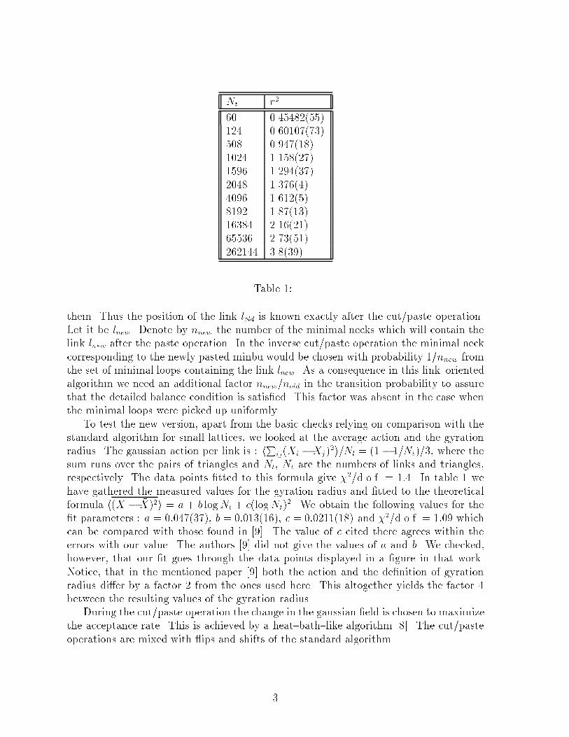
Nt �r260 0.45482(55)124 0.60107(73)508 0.947(18)1024 1.158(27)1596 1.294(37)2048 1.376(4)4096 1.612(5)8192 1.87(13)16384 2.16(21)65536 2.73(51)262144 3.8(39)Table 1:them. Thus the position of the link lold is known exactly after the cut/paste operation.Let it be lnew. Denote by nnew the number of the minimal necks which will contain thelink lnew after the paste operation. In the inverse cut/paste operation the minimal neckcorresponding to the newly pasted minbu would be chosen with probability 1=nnew fromthe set of minimal loops containing the link lnew. As a consequence in this link{orientedalgorithm we need an additional factor nnew=nold in the transition probability to assurethat the detailed balance condition is satis�ed. This factor was absent in the case whenthe minimal loops were picked up uniformly.To test the new version, apart from the basic checks relying on comparison with thestandard algorithm for small lattices, we looked at the average action and the gyrationradius. The gaussian action per link is : hPij(Xi �Xj)2i=Nl = (1 � 1=Nt)=3, where thesum runs over the pairs of triangles and Nl, Nt are the numbers of links and triangles,respectively. The data points �tted to this formula give �2=d.o.f. = 1:4. In table 1 wehave gathered the measured values for the gyration radius and �tted to the theoreticalformula h(X � �X)2i = a + b logNt + c(logNt)2. We obtain the following values for the�t parameters : a = 0:047(37), b = 0:013(16), c = 0:0211(18) and �2=d.o.f. = 1:09 whichcan be compared with those found in [9]. The value of c cited there agrees within theerrors with our value. The authors [9] did not give the values of a and b. We checked,however, that our �t goes through the data points displayed in a �gure in that work.Notice, that in the mentioned paper [9] both the action and the de�nition of gyrationradius di�er by a factor 2 from the ones used here. This altogether yields the factor 4between the resulting values of the gyration radius.During the cut/paste operation the change in the gaussian �eld is chosen to maximizethe acceptance rate. This is achieved by a heat{bath{like algorithm [8]. The cut/pasteoperations are mixed with ips and shifts of the standard algorithm.3

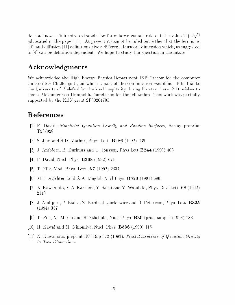
MeasurementsThe measurements of intrinsic geometry were performed mainly on graphs dual to thetriangulations. To �nd the number of points lp(R) lying at a distance R from a givenpoint p on a graph, we follow the standard technique. We �nd a layer of points at adistance one, by visiting all its neighbors. In our case there are always 3 points since itis a �3 graph. Next we visit all the neighbours of the points in the �rst layer, which havenot yet been visited to determine the set of points at a distance 2. Repeating recursivelythe procedure we �ll the histogram lp(R) until the whole graph gets covered. Integratingover distances we obtain the number of points within a distance R, i.e. the disc areavp(R) = PRr=1 lp(r). The easiest way to determine the number of disconnected parts ofthe disc boundary is to �nd in addition the numbers of links and elementary faces on thedisc and make use of Euler's formula np(R) = 2+#links�#point�#faces. Averagingover points p and di�erent surfaces of the ensemble gives us quantities hv(R)i and hn(R)ion the lhs of (1) and (2).The distributions lp(R) can be used to de�ne the average geodesic separation betweenpoints on the surface : �R = *PRR � lp(R)PR lp(R) +p : (4)In a similar way we can de�ne higher moments Rp of the distribution lp(R). The av-eraging h::ip is over all points on a graph. In practice it is approximated by samplingover a certain random subset of them since otherwise the measurement would be to timeconsuming.We performed simulations for lattices with the sizes being a power of 2, ranging from210(1024) to 218 (262144) triangles, skipping 215 and 217. For smaller lattices (up to 214)we collected the data during more than 104 integrated correlation times � of the slowestmode in the update scheme. For small lattices the slowest mode corresponds to thegyration radius, (X � �X)2, while for larger lattices it is the average geodesic distance�R [8]. The measurements were then taken every 10� . The distribution of np(R) andlp(R) were averaged over samples of 104 points p. We discarded the data from the �rst100� of (X � �X)2. For the largest lattice we run the simulation for around 60� takingmeasurements roughly every autocorrelation time. The thermalization took 20� . Thecomputations were done on the HP 715/720 workstations and on the SG Challenge Lworkstation. The presented data require the equivalent of 3 months of CPU time on HP720.ResultsLet us �rst discuss the branching dimension dB (2). In �g.1a we plot in the log log scalethe number of boundaries hn(R)i against the radius R for di�erent lattice sizes. Thedecrease of hn(R)i for R � hRi comes from the �nite size of the lattices. The smallerR is, the weaker the �nite size e�ects a�ect the distribution hn(R)i. For triangulationslarge enough, R can be taken much larger than 1 and much smaller than hRi so that one4

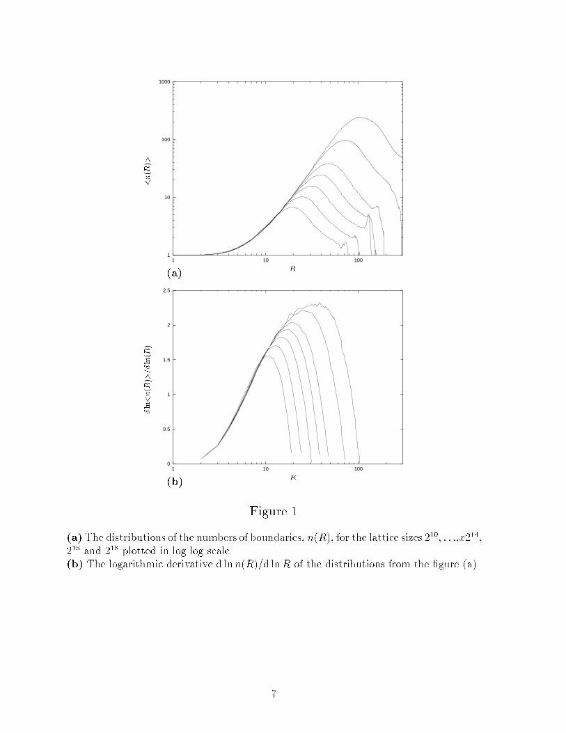
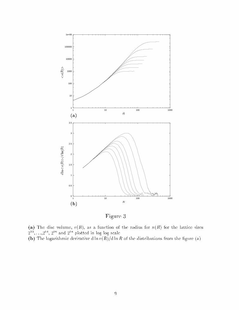
can simultaneously investigate features of the continuous geometry and is not a�ected bythe �nite size of the system. This is the region where we look for the scaling dimension.For di�erent lattice sizes we de�ne numerically the quantity d lnhn(R)i=d lnR and checkwhether it goes to a constant in a certain range 1 � R � h �Ri in the limit of largesizes. The results of di�erentiating is shown in �g.1b. Comparing the curves for twolargest lattices, one can see the �rst indication of the occurrence of an interval in R inwhich the dependence of d lnhn(R)i=d lnR on the lattice size develops a plateau. This ismore transparently seen for the same quantity measured on the original surfaces. Thelatter quantity is presented in �g.2b which is the logarithmic derivative of the number ofboundaries hn�(R�)i measured for discs on the original graphs (triangulations), shown in�g.2a. The derivative d lnn�(R�)=d lnR� seems to saturate above 2:5 at a value whichis larger than the maximal value of d lnn(R)=d lnR found on the dual graphs. This isa result of di�erent �nite size e�ects on the triangulations and the dual graphs. Onebelieves however that in the in�nite volume limit they will approach the same universalvalue re ecting universal, regularization independent continuum geometry. To check thisexplicitly one should go to even larger lattices. In �g.3a,b we plot the disc volume v(R)and its logarithmic derivative d ln v(R)=d lnR versus R. Similarly to the case c = �2[7], the height of the maxima of the derivative d ln v(R)=d lnR saturates much moreslowly with R than was the case for d lnn(R)=d lnR. In �g.4a we plot in diamonds theheights of the maxima of d ln v(R)=d lnR for di�erent lattice sizes. In the same picturewe plot in solid line the values of the e�ective Hausdor� dimension DH obtained fromthe formula (3). More precisely, the curve is obtained by taking a derivative of thecurve going through the data points for the average separation h �Ri versus lattice size Ntpresented in �g.4b. In order to take the derivative we �rst �tted an auxiliary function(a third order polynomial in the log log variable) to the data points in �g.4b, and thenwe took its derivative d lnh �Ri=d lnNt. It's inverse is plotted in �g.4a. The polynomialsu�ces for this purpose in the sense that it gives a smooth function (see dashed line in�g.4b) with high �t goodness : �2=d.o.f. around 1. Needless to say one cannot take this�t as an extrapolation formula for the e�ective Hausdor� dimension DH .The curves representing the e�ective Hausdor� dimension dH and DH show gradual attening. Though it is di�cult to make extrapolations of the curves it is tempting tosay that both curves approach the same asymptotic value compatible with the prediction2 +p2 [10].DiscussionThe results presented in this paper indicate the existence of the internal scaling dimen-sions for random surfaces with c = 1. The value of the branching dimension can beroughly estimated to be around dB = 2:5 which seem to be very close to that for c = �2and is much higher than for branched polymers (corresponding to c =1). It would bevery interesting to investigate how it changes with c just above the c = 1 barrier.From our data we can put a lower bound on the Hausdor� dimension: dH > 3. Thee�ective value seems to tend to the theoretical prediction 2 +p2 [10], but because we5

do not know a �nite size extrapolation formula we cannot rule out the value 2 + 2p2advocated in the paper [11]. At present it cannot be ruled out either that the fermionic[10] and di�usion [11] de�nitions give a di�erent Hausdor� dimension which, as suggestedin [4] can be de�nition dependent. We hope to study this question in the future.AcknowledgmentsWe acknowledge the High Energy Physics Department INP Cracow for the computertime on SG Challenge L, on which a part of the computation was done. P.B. thanksthe University of Bielefeld for the kind hospitality during his stay there. Z.B. wishes tothank Alexander von Humboldt Foundation for the fellowship. This work was partiallysupported by the KBN grant 2P30204705.References[1] F. David, Simplicial Quantum Gravity and Random Surfaces, Saclay preprintT93/028.[2] S. Jain and S.D. Mathur, Phys. Lett. B286 (1992) 239.[3] J. Ambj�rn, B. Durhuus and T. Jonsson, Phys.Lett B244 (1990) 403.[4] F. David, Nucl. Phys. B368 (1992) 671.[5] T. Filk, Mod. Phys. Lett, A7 (1992) 2637.[6] M.E. Agishtein and A.A. Migdal, Nucl.Phys. B350 (1991) 690.[7] N. Kawamoto, V.A. Kazakov, Y. Saeki and Y. Watabiki, Phys. Rev. Lett. 68 (1992)2113.[8] J. Ambj�rn, P. Bialas, Z. Burda, J. Jurkiewicz and B. Petersson, Phys. Lett. B325(1994) 337.[9] T. Filk, M. Marcu and B. Sche�old, Nucl. Phys. B30 (proc. suppl.) (1993) 783.[10] H. Kawai and M. Ninomiya, Nucl. Phys. B336 (1990) 115.[11] N. Kawamoto, preprint INS-Rep 972 (1993), Fractal structure of Quantum Gravityin Two Dimensions6

<n(R)>1

10

100

1000

1 10 100(a) Rdln<n(R)>=dln(R)

0

0.5

1

1.5

2

2.5

1 10 100(b) RFigure 1(a) The distributions of the numbers of boundaries, n(R), for the lattice sizes 210; : : :,x214,216 and 218 plotted in log log scale.(b) The logarithmic derivative d lnn(R)=d lnR of the distributions from the �gure (a).7

<n� (R� )>1

10

100

1000

1 10 100(a) R�dln<n� (R� )>=dln(R� )

0

0.5

1

1.5

2

2.5

3

1 10 100(b) R�Figure 2(a) The distributions of the numbers of boundaries, n�(R�), for the lattice sizes 210; : : :,214,216 and 218 plotted in log log scale.(b) The logarithmic derivative d lnn�(R�)=d lnR� of the distributions from the �gure(a).8

<v(R)>1

10

100

1000

10000

100000

1e+06

1 10 100 1000(a) Rdln<v(R)>=dln(R)

0

0.5

1

1.5

2

2.5

3

3.5

1 10 100 1000(b) RFigure 3(a) The disc volume, v(R), as a function of the radius for n(R) for the lattice sizes210; : : :,214, 216 and 218 plotted in log log scale.(b) The logarithmic derivative d ln v(R)=d lnR of the distributions from the �gure (a).9

D H;maxdln<v(R)>=dln(R)1.6

1.8

2

2.2

2.4

2.6

2.8

3

3.2

100 1000 10000 100000 1e+06(a) Nt<� R>

1

10

100

1000

100 1000 10000 100000 1e+06(b) NtFigure 4(a) The position of the maxima of the logarithmic derivative d ln v(R)=d lnR (�g.3b)for di�erent lattice sizes (3). The e�ective Hausdor� dimension DH obtained from thelogarithmic derivative d lnh �Ri=d lnNt of the �t presented in �g. (b).10