arX

iv:c

ond-

mat

/010

3200

v2 [

cond

-mat

.dis

-nn]

15

Mar

200

1

Phase coexistence and finite-size scaling in random combinatorial problems

Michele Leone†, Federico Ricci-Tersenghi‡ and Riccardo Zecchina§† SISSA, Via Beirut 9, Trieste, Italy

†,‡,§ The Abdus Salam International Center for Theoretical Physics, Condensed Matter GroupStrada Costiera 11, P.O. Box 586, I-34100 Trieste, Italy

(February 1, 2008)

We study an exactly solvable version of the famous random Boolean satisfiability problem, theso called random XOR-SAT problem. Rare events are shown to affect the combinatorial “phasediagram” leading to a coexistence of solvable and unsolvable instances of the combinatorial problemin a certain region of the parameters characterizing the model. Such instances differ by a non-extensive quantity in the ground state energy of the associated diluted spin-glass model. We alsoshow that the critical exponent ν, controlling the size of the critical window where the probabilityof having solutions vanishes, depends on the model parameters, shedding light on the link betweenrandom hyper-graph topology and universality classes. In the case of random satisfiability, a similarbehavior was conjectured to be connected to the onset of computational intractability.

PACS Numbers : 89.80.+h, 75.10.Nr

I. INTRODUCTION

The satisfaction of constrained Boolean formulae, the so called Satisfiability (SAT) problem, is a key problem ofcomplexity theory in computer science that can be recast as an energy minimization problem (ground state search)in diluted spin glass models. Many hard computational problems have been shown to be NP-complete [1] through apolynomial mapping onto the SAT problem, which in turn was the first problem identified as NP-complete by Cookin 1971 [2].

Recently [3], the research activity has become more and more focused on the study of the random version of SATproblem defined as follows. Consider N Boolean variables xi, i = 1, . . . , N . Call clause C the logical OR of Krandomly chosen variables, each of them being negated or left unchanged with equal probabilities. Then repeat thisprocess by drawing independently M random clauses Cσ, σ = 1, . . . , M . The logical AND of all clauses F is said tobe satisfiable if there exists a logical assignment of the {xi} evaluating F to true, unsatisfiable otherwise.

Numerical experiments have concentrated upon the study of the probability PN (γ, K) that a given F includingM = γN clauses be satisfiable. For large sizes, there appears a remarkable behavior : P∞(γ, K) seems to be unityfor γ < γc(K) and vanishes for γ > γc(K) [4,5]. Such an abrupt threshold behavior, separating a so-called SAT phasefrom an UNSAT one, has indeed been rigorously confirmed for 2-SAT, which is in P, with γc(2) = 1 [6]. For K ≥ 3,K-SAT is NP-complete and much less is known. The existence of a sharp transition has not been rigorously provenyet but relatively good estimates of the thresholds have been found: γc(3) ≃ 4.2 ÷ 4.3 [7]. Moreover, some rigorouslower and upper bounds to γc(3), have been established [7].

The interest in random K-SAT arises from the fact that it has been observed numerically that hard random instancesare created when the problems are critically constrained, i.e. close to the SAT/UNSAT phase boundary [3,4]. Thestudy of such hard instances represent a theoretical challenge towards a concrete understanding of complexity andthe analysis of algorithms. Moreover, hard random instances are also test-bed for the optimization of heuristic(incomplete) search procedures which are widely used in practice.

The statistical mechanics study of random K-SAT have provided some geometrical understanding of the onset ofcomplexity at the phase transition through the introduction of a functional order parameter which describes thegeometrical structure of the space of solutions. The nature of the SAT/UNSAT transition for the different valuesof K appears to be a particularly relevant prediction [8]. The SAT/UNSAT transition is accompanied by a smooth(respectively abrupt) change in the structure of the solutions of the 2-SAT (resp. 3-SAT) problem. More specifically,at the phase boundary a finite fraction of the variables become fully constrained while the entropy density remainsfinite. Such a fraction of frozen variables (i.e. those variables which take the same value in all solutions) may undergoa continuous (2-SAT) or discontinuous (3-SAT) growth at the critical point. This discrepancy is responsible for thedifference of typical complexities of both models recently observed in numerical studies. The typical solving time ofsearch algorithms displays an easy-hard pattern as a function of γ with a peak of complexity close to the threshold.The peak in search cost seems to scale polynomially with N for the 2-SAT problem and exponentially with N in the3-SAT case. From an intuitive point of view, the search for solutions ought to be more time-consuming in presence of

1

a finite fraction of fully quenched variables since the exact determination of the latter requires an almost exhaustiveenumeration of their configurations.

To test this conjecture, a mixed 2 + p-model has been proposed, including a fraction p (resp. 1 − p) of clausesof length two (resp. three) and thus interpolating between the 2-SAT (p = 0) and 3-SAT (p = 1) problems. Thestatistical mechanics analysis predicts that the SAT/UNSAT transition becomes abrupt when p > p0 ≃ 0.4 [8–11].Precise numerical simulations support the conjecture that the polynomial/exponential crossover occurs at the samecritical p0. Though the problem is both critical (γc = 1/(1 − p) for p < p0) and NP-complete for any p > 0, it isonly when the phase transition becomes of the same type of the 3-SAT case that hardness shows up. An additionalargument in favor of this conclusion is given by the analysis of the finite-size effects on PN (γ, K) and the emergence ofsome universality for p < p0. A detailed account of these findings may be found in [8–12]. For p < p0 the exponent ν,which describes the shrinking of the critical window where the transition takes place, is observed to remain constantand close to the value expected for 2-SAT. The critical behavior is the same of the percolation transition in randomgraphs (see also ref. [13]). For p > p0 the size of the window shrinks following some p-dependent exponents towardits statistical lower bound [14] but numerical data did not allow for any precise estimate.

In this paper, we study an exactly solvable version of the random 2+p SAT model which displays new features andallows us to settle the issue of universality of the critical exponents. The threshold of the model can be computedexactly as a function of the mixing parameter p in the whole range p ∈ [0, 1]. Rare events are found to be dominantalso in the low γ phase, where a coexistence of satisfiable and unsatisfiable instances is found. A detailed analysis forthe p = 1 case can be found in ref. [15].

The existence of a global – polynomial time – algorithm for determining satisfiability allows us to perform a finitesize scaling analysis around the exactly known critical points over huge samples and to show that indeed the exponentcontrolling the size of the critical window ceases to maintain its constant value ν = 3 and becomes dependent on p assoon as the phase transition becomes discontinuous, i.e. for p > p0 = .25. Above p0 and below p1 ∼ 0.5, the exponentν takes intermediate values between 3 and 2. Finally, above p1 the critical window is determined by the statisticalfluctuations of the quenched disorder [14] and so ν = 2.

II. MODEL DEFINITION AND OUTLINE OF SOME RESULTS

The model we study can be viewed as the mixed 2+p extension of the 3-hyper-SAT (hSAT) model discussed in [15],as much as the 2+p-SAT [8] is an extension of the usual K-SAT model. In computer science literature the hSAT modelis also named XOR-SAT and its critical behavior is considered an open issue [16]. Given a set of N Boolean variables{xi = 0, 1}i=1,...,N we can write an instance of our model as follows. Firstly we define the elementary constraints (amixture of 4 and 2-clauses sets with 50% satisfying assignments):

C(ijk| + 1) = (xi ∨ xj ∨ xk) ∧ (xi ∨ xj ∨ xk) ∧ (xi ∨ xj ∨ xk) ∧ (xi ∨ xj ∨ xk)

C(ijk| − 1) = (xi ∨ xj ∨ xk) ∧ (xi ∨ xj ∨ xk) ∧ (xi ∨ xj ∨ xk) ∧ (xi ∨ xj ∨ xk) , (1)

for the 3-hSAT part, and

C(ij| + 1) = (xi ∨ xj) ∧ (xi ∨ xj)

C(ij| − 1) = (xi ∨ xj) ∧ (xi ∨ xj) , (2)

for the 2-hSAT part. ∧ and ∨ are the logical AND and OR operations respectively and the over-bar is the logicalnegation. A more compact definition can be achieved by the use of the exclusive OR operator ⊕, e.g. C(ijk| + 1) =xi ⊕ xj ⊕ xk. Then, we randomly choose two independent sets E3 and E2 of pM triples {i, j, k} and (1− p)M couples{i, j} among the N possible indices and respectively pM and (1− p)M associated unbiased and independent randomvariables Tijk = ±1 and Jij = ±1, and we construct a Boolean expression in Conjunctive Normal Form (CNF) as

F =∧

{i,j,k}∈E3

C(ijk|Tijk)∧

{i,j}∈E2

C(ij|Jij) . (3)

As in [15], we can build a satisfiable version of the model choosing clauses only of the C(ij|+1) and C(ijk|+1) type.For p < p0 the problem is easily solved by local and global algorithms, whereas interesting behaviors are found forp > p0, where the local algorithms fail.

The above combinatorial definition can be recast in a simpler form as a minimization problem of a cost-energyfunction on a topological structure which is a mixture of a random graph (2-spin links) and hyper-graph (3-spinhyper-links). We end up with a diluted spin model where the Hamiltonian reads

2

HJ [S] = M −∑

{i,j,k}∈E3

Tijk SiSjSk −∑

{i,j}∈E2

Jij SiSj , (4)

where the Si are binary spin variables and the the random couplings can be either ±1 at random. The satisfiableversion is nothing but the ferromagnetic model: Tijk = 1 and Jij = 1 for any link.

As the average connectivity γ of the underlying mixed graph grows beyond a critical value γc(p), the frustratedmodel undergoes a phase transition from a mixed phase in which satisfiable instances and unsatisfiable ones coexist toa phase in which all instances are unsatisfiable. At the same γc(p) the associated spin glass system, undergoes a zerotemperature glass transition where frustration becomes effective and the ground state energy is no longer the lowestone (i.e. that with all the interactions satisfied). At the same critical point the unfrustrated, i.e. ferromagnetic, versionundergoes a para–ferro transition, because the same topological constraints that drive the glass (mixed SAT/UNSATto UNSAT) transition in the frustrated model are shown to be the ones responsible for the appearance of a nonzerovalue of the magnetization in the unfrustrated one [15]. We shall take advantage of such coincidence of critical linesby making the analytical calculation for the simpler ferromagnetic model.

Moreover, the nature of the phase transition changes from second to random first order, when p crosses the criticalvalue p0 = 1/4. For p > p0 the critical point γc(p) is preceded by a dynamical glass transition at γd(p) where ergodicitybreaks down and local algorithms get stuck (local algorithms are procedures which update the system configurationonly by changing a finite number of variable at the same time, e.g. all single or multi spin flip dynamics, togetherwith usual computer scientists heuristic algorithms). The dynamical glass transition exist for both versions of themodel [17] and corresponds to the formation of a locally stable ferromagnetic solution in the unfrustrated model [18](the local stability is intimately related to the ergodicity breaking).

III. STATISTICAL MECHANICS ANALYSIS

Following the approach of ref. [15], we compute the free energy of the model with the replica method, exploiting theidentity log ≪ Zn ≫= 1+n ≪ log Z ≫ +O(n2). The nth moment of the partition function is obtained by replicatingn times the sum over the spin configurations and then averaging over the quenched disorder

≪ Zn ≫=∑

S1,S2,...,Sn

≪ exp

(

−β

n∑

a=1

HJ [Sa]

)

≫ , (5)

Since each of the M clauses is independent, the probability distributions of the ferromagnetic couplings can be writtenas

P ({Tijk}) =∏

i<j<k

[(

1 −6γp

N2

)

δ(Tijk) +6γp

N2δ(Tijk − 1)

]

P ({Jij}) =∏

i<j

[(

1 −2γ(1 − p)

N

)

δ(Jij) +2γ(1 − p)

Nδ(Jij − 1)

]

, (6)

giving the following expression for the ≪ Zn ≫:

≪ Zn ≫=∑

S1i,S2

i,...,Sn

i

exp

−βγNn − γN +pγ

N2

∑

ijk

eβ∑

aSa

i Saj Sa

k +(1 − p)γ

N

∑

ij

eβ∑

aSa

i Saj + O(1)

(7)

Introducing the occupation fractions c(~σ) (fraction of sites with replica vector ~σ), one gets

− βF [c] = −γ(1 + βn) −∑

~σ

c(~σ) log c(~σ) + (1 − p)γ∑

~σ,~ρ

c(~σ)c(~ρ)eβ∑

aσaρa

+ pγ∑

~σ,~ρ,~τ

c(~σ)c(~ρ)c(~τ )eβ∑

aσaρaτa

. (8)

In the thermodynamic limit we can calculate the free energy via the saddle point equation obtaining

c(~σ) = exp

−Λ + 2(1 − p)γ∑

~ρ

c(~ρ) exp(β∑

a

σaρa) + 3pγ∑

~ρ,~τ

c(~ρ)c(~τ ) exp(β∑

a

σaρaτa)

(9)

3

The Lagrange multiplier Λ = −γ(2 + p) ensures the normalization constraint∑

~σ c(~σ) = 1 in the limit n → 0.Finding the minimal (zero in the unfrustrated case) value of the cost function amounts to studying the β → ∞ (zerotemperature) properties of the model. In the Replica Symmetric (RS) Ansatz, the behavior of the spin magnetizationcan be described in terms of effective fields m = tanhβh whose probability distribution is defined through

c(~σ) =

∫ ∞

−∞

dhP (h)eβh∑

aσa

(2 cosh(βh))n. (10)

In the unfrustrated or ferromagnetic case, the P (h) turns out to have the following simple form

P (h) =∑

l≥0

rlδ(h − l) , (11)

where the effective fields only assume integer values. In the satisfiable model the saddle point equations all collapsein one single self-consistency equation for r0:

r0 = e−3pγ(1−r0)2−2(1−p)γ(1−r0) =

∞∑

c1=0

∞∑

c2=0

e−3pγe−2(1−p)γ (3pγ)c1

c1!

(2(1 − p)γ)c2

c2!(1 − (1 − r0)

2)c1(r0)c2 . (12)

The equations for the frequency weights rl with l > 0 follow from the one for r0 and read

rl =[3pγ(1 − r0)

2 + 2(1 − p)γ(1 − r0)]l

l!. (13)

The previous self consistency equations for r0 (or for the magnetization m = 1 − r0) can easily be derived by thesame probabilistic argument used in [15], due to the fact that the clause independence allows to treat the graph andthe hyper-graph part separately. Note that in the simple limit p = 0 we retrieve the equation for the percolationthreshold in a random graph of connectivity γ [19],

1 − r0 = e−2γ∞∑

k=0

(2γ)k

k!(1 − rk

0 ) . (14)

Since the ground state energy of the ferromagnetic model is zero, the free energy coincides with the ground stateentropy, which can be written as a function of p, r0 and γ:

S(γ) = log(2)[r0(1 − log(r0)) − γ(1 − p)(1 − (1 − r0)2) − γp(1 − (1 − r0)

3)] (15)

To find the value of the paramagnetic entropy we put ourself in the phase where all sets of 4- and 2-clauses actindependently, each therefore dividing the number of allowed variables choice by two: the number of ground stateswill be Ngs = 2N−pγN−(1−p)γN = 2N(1−γ). The resulting value of Spara = (1− γ) log(2) coincides with the one foundsetting r0 = 1 in Eq.(15). This may not be the case in more complicated models, where the ground state entropy isa complicated function of γ also for γ < γc, reflecting the fact that the magnetization probability distribution in theparamagnetic phase could be different from a single delta peak in m = 0.

4

0.2 0.4 0.6 0.8 1

0.5

0.6

0.7

0.8

0.9

0.2 0.4 0.6 0.8 1

0.2

0.4

0.6

0.8

p

γ

γc

γd

mc

md

s

FIG. 1. Critical lines (static and dynamic) in the (γ, p) plane. The black dot at (0.667,0.25) separates continuous transitionsfrom discontinuous ones (where γd < γc). Inset: Critical magnetizations at γd(p) and γc(p) versus p.

Solving the saddle point equation for r0, we find that a paramagnetic solution with r0 = 1 always exists, while ata value of γ = γd(p) there appears a ferromagnetic solution in the satisfiable model. For p = 0, the critical valuecoincides as expected with the percolation threshold γd(0) = 1/2. As long as the model remains like 2-SAT, up top < p0 = 0.25, the threshold is the point where the ferromagnetic solution appears and also where its entropy exceedsthe paramagnetic one. The critical magnetization is zero and the transition is continuous. For larger values of thecontrol parameter p the transition becomes discontinuous. There appears a dynamical transition at γ = γd(p) wherelocally stable solutions appear. At γ = γc(p) > γd(p), the non trivial r0 6= 1 solution acquires an entropy larger thanthe paramagnetic one and becomes globally stable. The shape of γ = γd(p) and γ = γc(p) as functions of p are shownin Fig. 1. The inset picture shows the magnetization of the model at the points where the dynamical and the statictransitions take place.

IV. NUMERICAL SIMULATIONS

The model can be efficiently solved by a polynomial algorithm based on a representation modulo two (i.e. in Galoisfield GF[2]). If a formula can be satisfied, then a solution to the following set of M equations in N variables exists

{

SiSjSk = Tijk ∀{i, j, k} ∈ E3

SiSj = Jij ∀{i, j} ∈ E2(16)

Through the mapping Si = (−1)σi , Jij = (−1)ηij and Tijk = (−1)ζijk , with σi, ηijk, ζijk ∈ {0, 1}, Eq.(16) can berewritten as a set of binary linear equations

{

(σi + σj + σk) mod 2 = ζijk ∀{i, j, k} ∈ E3

(σi + σj) mod 2 = ηij ∀{i, j} ∈ E2(17)

For any given set of couplings {ηij , ζijk}, the solutions to these equations can be easily found in polynomial time bye.g. Gaussian substitution. The solution to the M linear equations in N variables can be summarized as follows: anumber Ndep of variables is completely determined by the values of the coupling {ηij , ζijk} and by the values of theNfree = N −Ndep independent variables. The number of solutions is 2Nfree and the entropy S(γ) = log(2)Nfree/N =log(2)(1−Ndep(γ)/N). As long as Ndep = M we have the paramagnetic entropy Spara = log(2)(1−γ). However Ndep

may be less than M when the interactions are such that one can generate linear combinations of equations where no

5

σ’s appear, like 0 = f({ηij , ζijk}). This kind of equations correspond to the presence of loops (resp. hyper-loops [15])in the underlying graph (resp. hyper-graph). A hyper-loops (generalization of a loop on a hyper-graph) is defined asa set S of (hyper-)links such that every spin (i.e. node) is “touched” by an even number of (hyper-)links belonging toS (see Fig. 2).

p = 0

hyper-loop

p > 0

loop

FIG. 2. Typical loop and hyper-loop. Lines are 2-spin links, while triangles are 3-spin links. Note that every vertex has aneven degree.

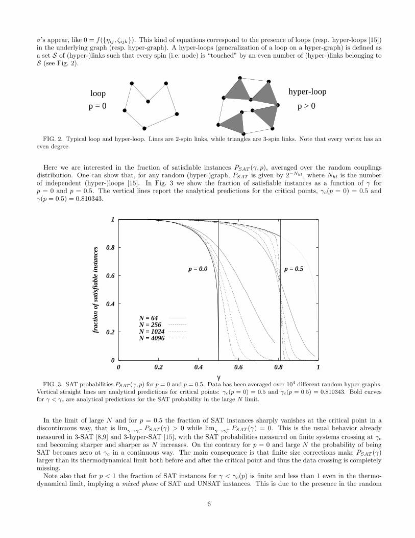
Here we are interested in the fraction of satisfiable instances PSAT (γ, p), averaged over the random couplingsdistribution. One can show that, for any random (hyper-)graph, PSAT is given by 2−Nhl , where Nhl is the numberof independent (hyper-)loops [15]. In Fig. 3 we show the fraction of satisfiable instances as a function of γ forp = 0 and p = 0.5. The vertical lines report the analytical predictions for the critical points, γc(p = 0) = 0.5 andγ(p = 0.5) = 0.810343.

0

0.2

0.4

0.6

0.8

1

0 0.2 0.4 0.6 0.8 1

frac

tion

of s

atis

fiab

le in

stan

ces

γ

p = 0.0 p = 0.5

N = 64 N = 256 N = 1024N = 4096

FIG. 3. SAT probabilities PSAT (γ, p) for p = 0 and p = 0.5. Data has been averaged over 104 different random hyper-graphs.Vertical straight lines are analytical predictions for critical points: γc(p = 0) = 0.5 and γc(p = 0.5) = 0.810343. Bold curvesfor γ < γc are analytical predictions for the SAT probability in the large N limit.

In the limit of large N and for p = 0.5 the fraction of SAT instances sharply vanishes at the critical point in adiscontinuous way, that is limγ→γ−

cPSAT (γ) > 0 while limγ→γ+

cPSAT (γ) = 0. This is the usual behavior already

measured in 3-SAT [8,9] and 3-hyper-SAT [15], with the SAT probabilities measured on finite systems crossing at γc

and becoming sharper and sharper as N increases. On the contrary for p = 0 and large N the probability of beingSAT becomes zero at γc in a continuous way. The main consequence is that finite size corrections make PSAT (γ)larger than its thermodynamical limit both before and after the critical point and thus the data crossing is completelymissing.

Note also that for p < 1 the fraction of SAT instances for γ < γc(p) is finite and less than 1 even in the thermo-dynamical limit, implying a mixed phase of SAT and UNSAT instances. This is due to the presence in the random

6

hyper-graph of loops made only by 2-spin links (indeed the mixed phase is absent for p = 1 when only 3-spin interac-tions are allowed [15]). The expression for the SAT probability in the thermodynamical limit (bold curves in Fig. 3,the lower most for p = 0 and the uppermost for p = 0.5) can be calculated analytically and the final result is

PSAT (γ, p) = e12γ(1−p)[1+γ(1−p)] [1 − 2γ(1 − p)]1/4 for γ ≤ γc(p) . (18)

In order to obtain to above expression we note that the SAT probability is related to the number of (hyper-)loops by

PSAT (γ, p) =

∞∑

m=0

P (m; γ, p)2−m , (19)

where P (m; γ, p) is the probability of having m (hyper-)loops in a random (hyper-)graph with parameters γ and p,and the factor 2−m comes from the probability that for all the m (hyper-)loops the product of the interactions is 1(thus giving no contradiction in the formula). In order to estimate P (m; γ, p) we may restrict ourselves to consideronly simple loops (made of 2-spin links), because hyper-loops which involve at least one 3-spin link are irrelevant inthe thermodynamical limit. This can be easily understood with the help of the following counting argument.

The probability that a given 2-spin link is present in a random (γ, p) hyper-graph is p2 = 2γ(1 − p)/N and for a3-spin hyper-link is p3 = 6γp/N2. Thus the probability of finding in a random (γ, p) hyper-graph a hyper-loop madeof n2 links and n3 hyper-links (n3 must be even) is just the number of different ways one can choose the (hyper-)linkstimes pn2

2 pn3

3 . Because the number of nodes belonging to a hyper-loop of this kind is at most nn = n2 + 3n3/2 andthe number of different hyper-loops of this kind is order Nnn , we have that the probability of having a hyper-loopwith n2 links and n3 hyper-links is order N−n3/2.

Then, for γ < γc the number of hyper-loops is still finite (their number becomes infinite only at γc where a transitionto a completely UNSAT phase takes place) and the SAT probability, in the large N limit, is completely determinedby the number of simple loops (n3 = 0).

The typical number of these loops does not vanish for γ < 12(1−p) , and therefore such “rare” events lead to a

coexistence of SAT and UNSAT instances with equal energy density.The average number of loops of length k can be easily calculated and it is given by xk/(2k), where x = 2γ(1 − p).

The average number of loops of any size

A(x) =

∞∑

k=3

xk

2k= −

1

2ln(1 − x) −

x

2−

x2

4, (20)

indeed diverges for x → 1, that is for γ → 12(1−p) . The probability of having m loops in a random (γ, p) hyper-graph

is then

P (m; γ, p) = e−A(x) A(x)m

m!, (21)

and the fraction of SAT instances turns out to be the one in Eq.(18).We have numerically calculated the SAT probabilities for many p and N values, finding a transition from a mixed

to a completely UNSAT phase at the γc(p) analytically calculated in the previous section. We also find, in agreementwith analytical results, that the transition is continuous as long as p ≤ 1/4 and then it becomes discontinuous in theSAT probability.

Let us now concentrate on the scaling with N of the critical region. We have considered several alternative definitionsfor the critical region. The one we present here seems to be the simplest and also the most robust, in the sense it canbe safely used when the transition is both continuous (p ≤ 0.25) and discontinuous (p > 0.25). We assume that thesize of the critical region is inversely proportional to the derivative of the SAT probability at the critical point

w(N, p)−1 =∂PSAT (γ, p)

∂γ

∣

∣

∣

∣

γ=γc

. (22)

For any value of p the width w(N) goes to zero for large N and the scaling exponent ν(p) is defined through

w(N, p) ∝ N−1/ν(p) . (23)

7

0.01

0.1

1

10 100 1000 10000

w(N

,p)

N

p = 0.0 p = 0.2 p = 0.3 p = 0.4 p = 0.5 p = 0.75p = 1.0

FIG. 4. Scaling of the critical window width. Errors are smaller than symbols. Lines are fits to the data.

1

1.5

2

2.5

3

0 0.25 0.5 0.75 1

ν(p)

pFIG. 5. Critical ν exponents obtained from the fits shown in Fig. 4. For p = 0.75 and p = 1 filled squares show the subleading

term power exponent, the leading term one being fixed to −1/2 (filled circles).

In Fig. 4 we show, in a log-log scale, w(N, p) as a function of N for many p values, togheter with the fits to thedata. The uppermost and lowermost lines have slopes −1/3 and −1/2 respectively. Data for p ≤ 0.5 can be perfectlyfitted by simple power laws (straight lines in Fig. 4) and the resulting ν(p) exponents have been reported in Fig. 5.We note that as long as p ≤ 0.25 the ν exponent turns out to be highly compatible with 3, which is known to be theright value for p = 0. Thus we conclude that for p < 1/4 the exponents are those of the p = 0 fixed point.

For 0.25 < p ≤ 0.5 we find that the ν exponent takes non-trivial values between 2 and 3. Then one of the followingtwo conclusions may hold. Either the transition for p > p0 is driven by the p = 1 fixed point and the ν exponent is not

8

universal, or more probably any different p value defines a new universality class. This result is very surprising andinteresting for the possibility that different universality classes are simply the consequence of the random hyper-graphtopology.

More complicated is the fitting procedure for p > 0.5. In a recent paper [14] Wilson has shown that in SATproblems there are intrinsic statistical fluctuations due to the way one construct the formula. This white noiseinduces fluctuations of order N−1/2 in the SAT probability. If critical fluctuations decay faster than statistical ones(i.e. ν < 2), in the limit of large N the latter will dominate and the resulting exponent saturates to ν = 2. Data forp = 0.75 and p = 1 shown in Fig. 4 have a clear upwards bending, which we interpret as a crossover from critical(with ν < 2) to statistical (ν = 2) fluctuations. Then we have fitted these two data sets with a sum of two powerlaws, w(N) = AN−1/ν + BN−1/2. The goodness of the fits (shown with lines in Fig. 4) confirm the dominance ofstatistical fluctuations for large N . Moreover we have been able to extract also a very rough estimate of the criticalexponent ν from the subleading term. In Fig. 5 we show with filled squares these values, which turn out to be moreor less in agreement with a simple extrapolation from p ≤ 0.5 results.

V. CONCLUSIONS AND PERSPECTIVES

The exact analysis of a solvable model for the generation of random combinatorial problems has allowed us to showthat combinatorial phase diagrams can be affected by rare events leading to a mixed SAT/UNSAT phase. The energydifference between such SAT and UNSAT instances is non extensive and therefore non detectable by the usual β → ∞statistical mechanics studies. However, a simple probabilistic argument is sufficient to recover the correct proportionof instances.

Moreover, through the exact location of phase boundaries together with the use of a polynomial global algorithmfor determining the existence of solutions we have been able to give a precise characterization of the critical exponentsν depending on the mixing parameter p. The p-dependent behavior conjectured in ref. [8] for the random 2 + pSAT case finds here a quantitative confirmation. The mixing parameter dependency also shows that the value of thescaling exponents is not completely determined by the nature of the phase transition and that the universality classthe transtion belongs to is very probably determined by the topology of the random hyper-graph. The model westudy has also a physical interpretation as a diluted spin glass system. It would be interesting to know whether theparameter-dependent behavior of critical exponent plays any role in some physically accessible systems.

A last remark on the generalization of the present model. With the same analytical techniques presented here,one can easily solve a Hamiltonian containing a fraction fk of k-spin interacting terms for any suitable choice ofthe parameters fk [20]. The case presented in this paper (f2 = 1 − p and f3 = p) is the simplest one. There arechoices which show a phase diagram still more complex with, for example, a continuos phase transition preceded bya dynamical one.

† Email: mleone@sissa.it‡ Email: riccife@ictp.trieste.it§ Email: zecchina@ictp.trieste.it

[1] M. Garey, and D.S. Johnson, Computers and Intractability; A guide to the theory of NP–completeness, (Freeman, SanFrancisco, 1979); C. Papadimitriou, Computational Complexity (Addison-Wesley, Reading, MA, 1994).

[2] S.A. Cook, in Proceedings of the Third Annual ACM Symposium on Theory of Computing (ACM, New York, 1971), p. 151.[3] Artif. Intel. 81, issues 1–2 (1996).[4] D. Mitchell, B. Selman, and H. Levesque, in Proceedings of the Tenth National Conference on Artificial Intelligence (AAAI-

92) (AAAI Press, Menlo Park, CA, 1992), p. 459.[5] S. Kirkpatrick and B. Selman, Science 264, 1297 (1994).[6] A. Goerdt, in Proceedings of the 17th International Symposium on Mathematical Foundations of Computer Science, in

Lecture Notes in Computer Science, vol. 629 (Spinger, 1992), p. 264; J. Comput. Syst. Sci. 53, 469 (1996). V. Chvatal andB. Reed, in Proceedings of the 33rd IEEE Symposium on Foundations of Computer Science (IEEE, New York, 1992), p.620.

[7] special issue on NP-hardness and Phase Transitions, O. Dubois, R. Monasson, B. Selman and R. Zecchina, TheoreticalComputer Science in press.

[8] R. Monasson, R. Zecchina, S. Kirkpatrick, B. Selman and L.Troyansky, Nature (London) 400, 133 (1999).

9

[9] R. Monasson, R. Zecchina, S. Kirkpatrick, B. Selman and L.Troyansky, Random Structures and Algorithms 3, 414 (1999).[10] R. Monasson and R. Zecchina, J. Phys. A 31, 9209 (1998).[11] G. Biroli, R. Monasson, M. Weigt, Eur. Phys. J. B 14, 551 (2000).[12] R. Monasson and R. Zecchina, Phys. Rev. Lett. 76, 3881 (1996); Phys. Rev. E 56, 1357 (1997).[13] B. Bollobas, C. Borgs, J.T. Chayes, J.H. Kim and D.B. Wilson, preprint arXiv:math.CO/9909031.[14] D.B. Wilson, preprint arXiv:math/0005136.[15] F. Ricci-Tersenghi, M. Weigt and R. Zecchina, Phys. Rev. E 63, 026702 (2001).[16] N. Creignou and H. Daude, Discr. Appl. Math. 96–97, 41 (1999).[17] S. Franz, M. Mezard, F. Ricci-Tersenghi, M. Weigt and R. Zecchina, preprint cond-mat/0103026.[18] S. Franz, M. Leone, F. Ricci-Tersenghi and R. Zecchina, in preparation.[19] B. Bollobas, Random Graphs (Academic Press, London, 1985).[20] M. Leone, F. Ricci-Tersenghi and R. Zecchina, in preparation.

10