Sea-ice data assimilation at the mid-Holocene - CP

CPD9, 6515–6549, 2013

Sea-ice dataassimilation at the

mid-Holocene

F. Klein et al.

Title Page

Abstract Introduction

Conclusions References

Tables Figures

J I

J I

Back Close

Full Screen / Esc

Printer-friendly Version

Interactive Discussion

Discussion

Paper

|D

iscussionP

aper|

Discussion

Paper

|D

iscussionP

aper|

Clim. Past Discuss., 9, 6515–6549, 2013www.clim-past-discuss.net/9/6515/2013/doi:10.5194/cpd-9-6515-2013© Author(s) 2013. CC Attribution 3.0 License.

Open A

ccess

Climate of the Past

Discussions

This discussion paper is/has been under review for the journal Climate of the Past (CP).Please refer to the corresponding final paper in CP if available.

Model-data comparison and dataassimilation of mid-Holocene Arcticsea-ice concentrationF. Klein1, H. Goosse1, A. Mairesse1, and A. de Vernal2

1Université catholique de Louvain, Earth and Life Institute, Georges Lemaître Centre for Earthand Climate Research, Place Louis Pasteur, 3, 1348 Louvain-la-Neuve, Belgium2GEOTOP, Université du Québec à Montréal, P.O. Box 8888, succursale “centre ville”Montréal, Qc, H3C 3P8 Canada

Received: 15 November 2013 – Accepted: 29 November 2013– Published: 10 December 2013

Correspondence to: F. Klein ([email protected])

Published by Copernicus Publications on behalf of the European Geosciences Union.

6515

http://www.clim-past-discuss.net

http://www.clim-past-discuss.net/9/6515/2013/cpd-9-6515-2013-print.pdf

http://www.clim-past-discuss.net/9/6515/2013/cpd-9-6515-2013-discussion.html

http://creativecommons.org/licenses/by/3.0/

CPD9, 6515–6549, 2013


mid-Holocene

F. Klein et al.

Title Page



Tables Figures

J I

J I

Back Close

Full Screen / Esc



Discussion

Paper

|D

iscussionP

aper|

Discussion

Paper

|D

iscussionP

aper|

Abstract

The consistency between a new quantitative reconstruction of Arctic sea-ice concen-tration based on dinocyst assemblages and the results of climate models has beeninvestigated for the mid-Holocene. The comparison shows that the simulated sea-icechanges are weaker and spatially more homogeneous than the recorded ones. Fur-5

thermore, although the model-data agreement is relatively good in some regions suchas the Labrador Sea, the skill of the models at local scale is low. The response of themodels follows mainly the increase in summer insolation at large scale. This is mod-ulated by changes in atmospheric circulation leading to differences between regionsin the models that are albeit smaller than in the reconstruction. Performing simulations10

with data assimilation using the model LOVECLIM amplifies those regional differences,mainly through a reduction of the southward winds in the Barents Sea and an increasein the westerly winds in the Canadian Basin of the Arctic. This leads to an increase inthe ice concentration in the Barents and Chukchi Seas and a better agreement with thereconstructions. This underlines the potential role of atmospheric circulation to explain15

the reconstructed changes during the Holocene.

1 Introduction

Sea-ice is a key element of the global climate system. First, it enhances climate re-sponse at high latitudes of the Northern Hemisphere as it is involved in various feed-backs, in particular the classical ice albedo feedback (Holland and Bitz, 2003; Serreze20

et al., 2009; Screen and Simmonds, 2010; Stroeve et al., 2011). Second, sea-ice playsa role in deep water formation through brine rejection which is a crucial driver of theglobal thermohaline circulation (Lohmann and Gerdes, 1998; Goosse and Fichefet,1999). Third, it modifies the exchanges of heat and gases between the atmosphereand polar oceans because of its insulation properties (Ebert and Curry, 1993). Conse-25

quently, changes in Arctic sea-ice cover and thickness influence the atmospheric and

6516





CPD9, 6515–6549, 2013


mid-Holocene

F. Klein et al.

Title Page



Tables Figures

J I

J I

Back Close

Full Screen / Esc



Discussion

Paper

|D

iscussionP

aper|

Discussion

Paper

|D

iscussionP

aper|

hydrographic conditions at high latitudes, which may in turn have an impact on the Eu-ropean and the North-American climate (e.g. Serreze et al., 2007; Francis and Vavrus,2012).

The processes involved in the sea-ice behavior are complex, which explains why cli-mate models still have clear biases in simulating sea-ice for present-day conditions5

(Stroeve et al., 2012; Massonnet et al., 2012). It is thus important to improve ourunderstanding of sea-ice and its representation in climate models, especially in thecurrent context of a decreased Arctic sea-ice cover and thickness over the past fewdecades (Serreze et al., 2007; Stroeve et al., 2011), likely related to anthropogenicclimate change (e.g. Notz and Marotzke, 2012).10

The analysis of past sea-ice fluctuations provides an interesting complement to thestudy of the last decades, in particular the ones focusing on the Holocene (the currentinterglacial) as the boundary conditions of the climate system were roughly similar tothe present ones (Wanner et al., 2008). In the absence of direct instrumental measures,this can be achieved by two complementary approaches, proxy-based reconstructions15

(e.g. Funder et al., 2011; Müller et al., 2012) and modelling (e.g. Goosse et al., 2013;Berger et al., 2013). This allows, amongst others, to contextualize the recent climatechanges, to validate climate models results, and to improve the physical understandingof the system (Zhang et al., 2010; Braconnot et al., 2012).

Here we will focus on the mid-Holocene (6 ka, hereafter MH) as it is a classical period20

that is reasonably well documented as much in terms of proxy data (see Sect. 3.1) asin terms of models results since it is a standard target for the Paleoclimate ModelIntercomparison Project (PMIP, e.g. Braconnot et al., 2007). The MH coincides withthe end of a warm period in the Arctic that started about 9 ka (Sundqvist et al., 2010)due to a high orbitally-driven summer insolation. Insolation has its maximum at around25

11 ka (Berger, 1978) but the warmest conditions have been asynchronous across theArctic due to the effect of the lingering Laurentide Ice Sheet (Kaufman et al., 2004;Renssen et al., 2009). At 6 ka, some regions were thus already experiencing a cooling

6517





CPD9, 6515–6549, 2013


mid-Holocene

F. Klein et al.

Title Page



Tables Figures

J I

J I

Back Close

Full Screen / Esc



Discussion

Paper

|D

iscussionP

aper|

Discussion

Paper

|D

iscussionP

aper|

(for instance Alaska) while others were still close to their maximum temperature (likenortheast Canada) (Kaufman et al., 2004).

Although most Arctic proxies support lower sea-ice conditions during the MH as com-pared to the entire Holocene, the recorded changes are not homogeneous betweenthe different regions (see Sect. 3.1). In addition to modifications in the oceanic and5

atmospheric circulations or to the influence of the remnant Laurentide Ice Sheet thatcould have an impact at a large scale, complex local topography can be responsible fora high heterogeneous response on small spatial scales. This is particularly the casein the Canadian Arctic Archipelago (CAA) with its complicated disposition of narrowstraits, where proxy records display contrasted signals for nearby locations (e.g. Vare10

et al., 2009; Atkinson, 2009). Furthermore, the uncertainties related to the interpreta-tion of proxies or to their dating can also explain some of the discrepancies (Polyaket al., 2010; Sundqvist et al., 2010).

In qualitative agreement with data, models simulate less sea-ice extent in summerduring the MH as compared to the pre-industrial (PI) conditions, following the higher15

summer insolation (Berger et al., 2013; Goosse et al., 2013). However, no quantitativeestimate of the agreement exists up to now given the lack of a consistent quantitativesea-ice reconstruction covering the Arctic. In this context, this paper aims at compar-ing the MH sea-ice concentration simulated by the model of intermediate complexityLOVECLIM and by general circulation models (GCMs) with a new quantitative recon-20

struction of Arctic sea-ice concentration based on dinocyst assemblages (de Vernalet al., 2013). This model-data comparison is intended first to estimate if climate modelsare able to reproduce the spatial pattern deduced from proxy records. In a second step,a simulation with data assimilation is performed with the climate model LOVECLIM. Theimpact of this additional constraint improves by construction the consistency between25

the models results and the reconstructions. This allows investigating in more detailsthe processes governing sea-ice conditions at 6 ka and analysing the potential originof the biases seen in the simulations without data assimilation.

6518





CPD9, 6515–6549, 2013


mid-Holocene

F. Klein et al.

Title Page



Tables Figures

J I

J I

Back Close

Full Screen / Esc



Discussion

Paper

|D

iscussionP

aper|

Discussion

Paper

|D

iscussionP

aper|

The models selected, the experimental design and the proxy reconstruction based ondinocyst assemblages are presented in Sect. 2. Section 3 starts with a short descriptionof the observed sea-ice changes. It is followed by an analysis of the results of thesimulations without data assimilation and finally of the simulation with data assimilation.Conclusions are presented in Sect. 4.5

2 Methodology

2.1 Models description

Experiments have been performed with the three-dimensional Earth climate model ofintermediate complexity LOVECLIM version 1.2 (Goosse et al., 2010). It includes a rep-resentation of the atmosphere, ocean, sea-ice and land surface including vegetation.10

The atmospheric component is ECBilt2 (Opsteegh et al., 1998), a quasi-geostrophicspectral model with T21 horizontal resolution (corresponding to 5.6◦ ×5.6◦ latitude-longitude) and 3 vertical levels in addition to the surface. Ocean and sea-ice are sim-ulated by CLIO3 (Goosse and Fichefet, 1999), which is a general circulation modelcoupled to a comprehensive thermodynamic-dynamic sea-ice model. Its horizontal15

resolution is of 3◦ by 3◦ and the ocean is divided into 20 unevenly spaced verticallevels. LOVECLIM also contains the vegetation model VECODE (Brovkin et al., 2002),that takes into account the distibution of 3 different land covers (deserts, grasses andforests) using the same resolution as ECBilt2. Due to its coarse resolution and to sim-plifications introduced in the representation of some atmospheric processes, LOVE-20

CLIM is much faster than the more sophisticated coupled climate models. It allowsto produce the large amount of simulations required for the data assimilation process(see Sect. 2.2). In this study, two different 6 ka LOVECLIM simulations are examined:LOVECLIM without assimilation (referred as LOVECLIM no assim) and LOVECLIM withsea-ice data assimilation (LOVECLIM assim SIC).25

6519





CPD9, 6515–6549, 2013


mid-Holocene

F. Klein et al.

Title Page



Tables Figures

J I

J I

Back Close

Full Screen / Esc



Discussion

Paper

|D

iscussionP

aper|

Discussion

Paper

|D

iscussionP

aper|

In addition to LOVECLIM simulations, MH experiments performed with GCMs follow-ing the framework of the third phase of the Paleoclimate Modelling IntercomparisonProject (PMIP3, Otto-Bliesner et al., 2009), referred as midHolocene, are analyzed.The simulations from which the PI reference values have been obtained cover the pe-riod 1850–2000 and are referred as historical in the fifth phase of the Coupled Model5

Intercomparison Project (CMIP5, Taylor et al., 2012). The GCMs selected here (Table1) are the ones for which the variables of interest for our diagnostics were available atthe time of the analysis.

2.2 Data assimilation method

LOVECLIM results have been constrained to follow a proxy-based sea-ice reconstruc-10

tion through a process of assimilation, using a particle filter with re-sampling (vanLeeuwen, 2009; Dubinkina et al., 2011), in the same way as in several recent stud-ies (e.g. Goosse et al., 2012; Mathiot et al., 2013; Mairesse et al., 2013). First, anensemble of 96 simulations (called particles) is initialized from slightly different seasurface temperature for each particles, allowing different time developments. After 1 yr15

of simulation, the likelihood of each particle is computed from the difference betweenthe proxy-based reconstructed and the simulated sea-ice concentration. The particlestoo distant from the reconstruction are abandoned whereas the ones close enough arekept as a basis for the next year simulation. In order to maintain a constant number ofparticles until the end of the simulated period, a resampling function of the particles20

likelihood is conducted annually. The sea surface temperature of the copies is oncemore perturbed to obtain different time developments for the following year, and thewhole procedure is repeated sequentially every year until the end of the simulation,here 400 yr.

6520





CPD9, 6515–6549, 2013


mid-Holocene

F. Klein et al.

Title Page



Tables Figures

J I

J I

Back Close

Full Screen / Esc



Discussion

Paper

|D

iscussionP

aper|

Discussion

Paper

|D

iscussionP

aper|

2.3 Proxy-based sea-ice reconstruction

The MH proxy-based sea-ice reconstruction used to evaluate models performance andto constrain LOVECLIM simulations is derived from cysts produced by dinoflagellates(dinocyst). The dinocyst distribution in Arctic and sub-Arctic seas is indeed controlledby several environmental parameters including productivity, salinity, temperature and5

most importantly sea-ice (de Vernal and Rochon, 2011). The dataset is based on thedinocyst content of 18 cores collected in the North Atlantic and Arctic Oceans (Table 2and Fig. 1). Sea-ice reconstruction is expressed in terms of annual mean concentration(in %) and is associated with a standard error of ±11 % (de Vernal et al., 2013). Thisvalue is used as the estimate of the reconstruction uncertainty for the evaluation of the10

likelihood in the experiment with data assimilation.The proxy records include variability at (multi-)centennial time scale that could not

be reproduced in the time-slice experiments performed following the PMIP protocol.Therefore, we consider the MH as a period of 1 kyr, i.e. 6±0.5 ka, which limits the con-tribution of internal variability and non-orbital forcings. The choice of such an interval15

length also allows neglecting the potential biases related to dating uncertainties.The model-data comparison and the data assimilation are performed using anoma-

lies considering the PI conditions (1850–1900 yr AD) as reference period. We havepreferred this option rather than using recent observed sea-ice cover, since comparingsea-ice conditions inferred from dinocyst content with satellite data would have lead20

to additional uncertainties. Furthermore, the recent period is far from being adequatefor calculating anomalies since it presents rapid changes characterized by a significantdecrease in sea-ice (e.g. Stroeve et al., 2011). Unfortunately, many of the availablereconstructed time series used here are not continuous up to 1900. We have thus de-cided to reconstruct the reference dataset by computing a linear interpolation of those25

time series up to the period 1850–1900 AD. To avoid extrapolating over too long peri-ods, the proxy records ending before 2 ka have been discarded from our analysis.

6521





CPD9, 6515–6549, 2013


mid-Holocene

F. Klein et al.

Title Page



Tables Figures

J I

J I

Back Close

Full Screen / Esc



Discussion

Paper

|D

iscussionP

aper|

Discussion

Paper

|D

iscussionP

aper|

2.4 Experimental design

All the MH simulations represent equilibrium conditions corresponding to 6 ka. Theyuse the orbital forcing following Berger (1978). The changes in greenhouse gases con-centration are taken from Flückiger et al. (2002) for LOVECLIM simulations, which isslightly different of the ones used in the framework of CMIP5/PMIP3 (http://pmip3.lsce.5

ipsl.fr/). As in Mathiot et al. (2013) and Mairesse et al. (2013), LOVECLIM simulationsalso consider slight changes in ice sheets topography and surface albedo followingthe reconstruction of Peltier (2004), as well as in freshwater fluxes from Antarctic icesheet melting according to Pollard and DeConto (2009) results. This represents a smalldifference as compared to the CMIP5/PMIP3 protocol as the latter prescribes present-10

day ice sheet topography and no change in freshwater fluxes at 6 ka with respect topresent. However, this has virtually no effect on results.

For the reference period corresponding to PI values, we have averaged all the resultsfrom available members for each GCM and from a set of experiments with LOVECLIM(Crespin et al., 2012) over the period 1850–1900 (over the period 1860–1900 in the15

cases of HadGEM2-CC and HadGEM2-ES).

3 Results and discussion

3.1 Sea-ice changes at 6 ka deduced from observations

Despite the general context of high summer temperatures and low sea-ice conditionscharacterizing the high northern latitudes during the early to mid-Holocene (Wanner20

et al., 2008; Polyak et al., 2010; Sundqvist et al., 2010), the quantitative proxy basedsea-ice reconstructions based on dynocists display heterogeneous and weak anoma-lies at 6 ka (Fig. 1). Lower annual mean sea-ice concentration is recorded at the MH inthe Fram Strait, northern Baffin Bay and Labrador Sea as compared to PI period. On

6522





http://pmip3.lsce.ipsl.fr/



CPD9, 6515–6549, 2013


mid-Holocene

F. Klein et al.

Title Page



Tables Figures

J I

J I

Back Close

Full Screen / Esc



Discussion

Paper

|D

iscussionP

aper|

Discussion

Paper

|D

iscussionP

aper|

the contrary, the MH is characterized by higher sea-ice concentration in the ChukchiSea, and to a lesser extent, in the Barents Sea and in the Barrow Strait (in the CAA).

Most of these dinocyst-based sea-ice records appear directly consistent with localtemperature and other sea-ice MH records. In agreement with the reduced ice con-centration in Nares Strait and in Fram Strait (id 5 and 17 on Fig. 1), several sea-ice5

conditions reconstructions based on driftwood deposits and on beach ridges show rareor absent multiyear sea-ice at the MH as far North as the northern coasts of Greenland(Bennike, 2004; Funder and Kjaer, 2007; Funder et al., 2009; Möller et al., 2010; Fun-der et al., 2011) and Ellesmere Iceland (England et al., 2008), while these coastlinesare presently permanently surrounded by pack ice (Polyak et al., 2010). Low sea-ice10

conditions as compared to the entire Holocene are also inferred from the analysis ofIP25 in sediment cores collected at the continental slope of West Spitsbergen (Mülleret al., 2012).

Further south, along the East Greenland Shelf, Müller et al. (2012) highlighted rela-tively high sea-ice cover at the MH as compared to the whole Holocene based on IP2515

and brassicasterol. This contradicts the reconstruction of Jennings et al. (2002) de-rived from records of ice-rafted detritus, while dinocyst-based reconstruction show nochanges at 6 ka as compared to the PI period (id 15). Off northern Iceland, the extentof drift ice seemed to reach a minimum at the MH relative to the past 10 kyr, accordingto a reconstruction based on the presence of quartz (Andrews et al., 2009).20

In the CAA, the MH sea-ice record deduced from various proxies is very hetero-geneous which is consistent with the dinocyst-based records (id 3 to 5). On the onehand, the little amount of bowhead bones found indicates high sea-ice coverage (Dykeet al., 1996; Atkinson, 2009) but on the other hand, the analysis of IP25 in several sed-iment cores suggests low spring sea-ice occurrence at the MH compared to the whole25

Holocene period (Vare et al., 2009; Belt et al., 2010). Further west, the higher sea-iceconcentration recorded over the Chukchi Sea at the MH (id 1 and 2) is in agreementwith the MH temperature lower than present inferred from oxygen isotope ratios in lakesediments in Alaska (Anderson et al., 2001).

6523





CPD9, 6515–6549, 2013


mid-Holocene

F. Klein et al.

Title Page



Tables Figures

J I

J I

Back Close

Full Screen / Esc



Discussion

Paper

|D

iscussionP

aper|

Discussion

Paper

|D

iscussionP

aper|

Finally, the negative sea-ice concentration anomaly displayed in the Barents Sea (id18) appears to stand in contrast to continental proxies that show high temperatures atthe MH relative to the entire Holocene in the North of Scandinavia, although these latterrepresent July means (e.g. Seppä and Birks, 2001, 2002). The conclusions derivedfrom the dinocyst-based reconstruction of de Vernal et al. (2013) are thus generally5

confirmed by other proxy-based reconstructions, even if some discrepancies exist.

3.2 Simulations without data assimilation

We first discuss the simulated sea-ice cover for the model grid points that contain onesea-ice proxy record displayed on Fig. 1. We assume that the spatial representative-ness of each core corresponds to the matching grid cell for each model, while the latter10

have different spatial resolution. We mainly focus on 8 of the 18 available cores (id 1, 2,3, 4, 5, 15, 17 and 18) because the other ones are located south of the simulated sea-ice edge for most of the GCMs and LOVECLIM for both the MH and the PI periods, andthus display no change in sea-ice concentration. Since the proxy records are calibratedto represent annual means, we primarily focus on the annual means of the models, al-15

though seasonal means are also considered in order to get a better understanding ofthe processes that drive the simulated sea-ice cover.

As compared to the reference period 1850–1900, models results show globally lowerannual mean sea-ice concentrations for the MH at the studied locations in the Arctic(Fig. 2). This is consistent with the smaller extent and thinner Arctic sea-ice obtained in20

models for the MH (Berger et al., 2013). The signal is especially clear over the ChukchiSea (id 1 and 2) and the CAA (id 3 to 5) where all models depict weak negative anoma-lies. This annual decrease in sea-ice cover is mainly due to a lower sea-ice concen-tration in summer in response to the relatively strong increase in insolation (in average24.35 Wm−2 for these regions, Fig. 3c). To a lesser extent, fall also contributes to the25

decrease in annual sea-ice cover especially in the Chukchi Sea, despite a dwindlinginsolation at 6 ka (in average −7.27 Wm−2, Fig. 3d). This can be explained by the in-ertia of the system: higher summer insolation leads to a decrease in ice thickness and

6524





CPD9, 6515–6549, 2013


mid-Holocene

F. Klein et al.

Title Page



Tables Figures

J I

J I

Back Close

Full Screen / Esc



Discussion

Paper

|D

iscussionP

aper|

Discussion

Paper

|D

iscussionP

aper|

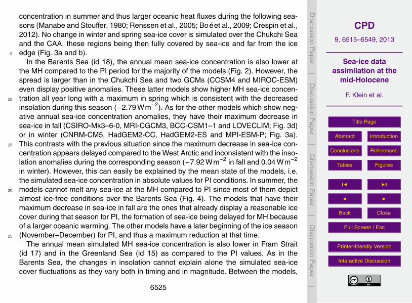
concentration in summer and thus larger oceanic heat fluxes during the following sea-sons (Manabe and Stouffer, 1980; Renssen et al., 2005; Boé et al., 2009; Crespin et al.,2012). No change in winter and spring sea-ice cover is simulated over the Chukchi Seaand the CAA, these regions being then fully covered by sea-ice and far from the iceedge (Fig. 3a and b).5

In the Barents Sea (id 18), the annual mean sea-ice concentration is also lower atthe MH compared to the PI period for the majority of the models (Fig. 2). However, thespread is larger than in the Chukchi Sea and two GCMs (CCSM4 and MIROC-ESM)even display positive anomalies. These latter models show higher MH sea-ice concen-tration all year long with a maximum in spring which is consistent with the decreased10

insolation during this season (−2.79 Wm−2). As for the other models which show neg-ative annual sea-ice concentration anomalies, they have their maximum decrease insea-ice in fall (CSIRO-Mk3–6-0, MRI-CGCM3, BCC-CSM1–1 and LOVECLIM; Fig. 3d)or in winter (CNRM-CM5, HadGEM2-CC, HadGEM2-ES and MPI-ESM-P; Fig. 3a).This contrasts with the previous situation since the maximum decrease in sea-ice con-15

centration appears delayed compared to the West Arctic and inconsistent with the inso-lation anomalies during the corresponding season (−7.92 Wm−2 in fall and 0.04 Wm−2

in winter). However, this can easily be explained by the mean state of the models, i.e.the simulated sea-ice concentration in absolute values for PI conditions. In summer, themodels cannot melt any sea-ice at the MH compared to PI since most of them depict20

almost ice-free conditions over the Barents Sea (Fig. 4). The models that have theirmaximum decrease in sea-ice in fall are the ones that already display a reasonable icecover during that season for PI, the formation of sea-ice being delayed for MH becauseof a larger oceanic warming. The other models have a later beginning of the ice season(November–December) for PI, and thus a maximum reduction at that time.25

The annual mean simulated MH sea-ice concentration is also lower in Fram Strait(id 17) and in the Greenland Sea (id 15) as compared to the PI values. As in theBarents Sea, the changes in insolation cannot explain alone the simulated sea-icecover fluctuations as they vary both in timing and in magnitude. Between the models,

6525





CPD9, 6515–6549, 2013


mid-Holocene

F. Klein et al.

Title Page



Tables Figures

J I

J I

Back Close

Full Screen / Esc



Discussion

Paper

|D

iscussionP

aper|

Discussion

Paper

|D

iscussionP

aper|

the simulated mean state likely plays a role there too but the interpretation seems morecomplex.

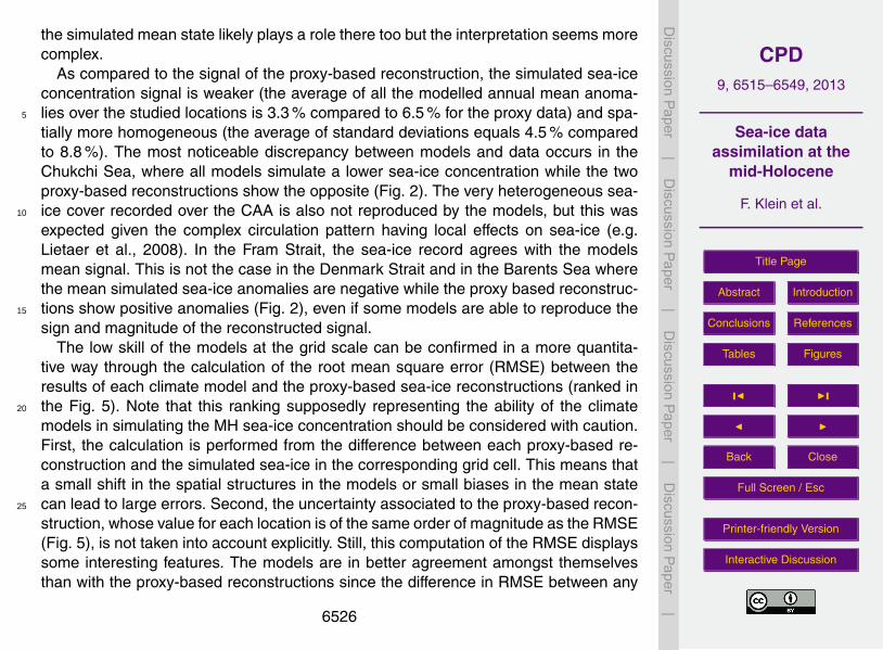
As compared to the signal of the proxy-based reconstruction, the simulated sea-iceconcentration signal is weaker (the average of all the modelled annual mean anoma-lies over the studied locations is 3.3 % compared to 6.5 % for the proxy data) and spa-5

tially more homogeneous (the average of standard deviations equals 4.5 % comparedto 8.8 %). The most noticeable discrepancy between models and data occurs in theChukchi Sea, where all models simulate a lower sea-ice concentration while the twoproxy-based reconstructions show the opposite (Fig. 2). The very heterogeneous sea-ice cover recorded over the CAA is also not reproduced by the models, but this was10

expected given the complex circulation pattern having local effects on sea-ice (e.g.Lietaer et al., 2008). In the Fram Strait, the sea-ice record agrees with the modelsmean signal. This is not the case in the Denmark Strait and in the Barents Sea wherethe mean simulated sea-ice anomalies are negative while the proxy based reconstruc-tions show positive anomalies (Fig. 2), even if some models are able to reproduce the15

sign and magnitude of the reconstructed signal.The low skill of the models at the grid scale can be confirmed in a more quantita-

tive way through the calculation of the root mean square error (RMSE) between theresults of each climate model and the proxy-based sea-ice reconstructions (ranked inthe Fig. 5). Note that this ranking supposedly representing the ability of the climate20

models in simulating the MH sea-ice concentration should be considered with caution.First, the calculation is performed from the difference between each proxy-based re-construction and the simulated sea-ice in the corresponding grid cell. This means thata small shift in the spatial structures in the models or small biases in the mean statecan lead to large errors. Second, the uncertainty associated to the proxy-based recon-25

struction, whose value for each location is of the same order of magnitude as the RMSE(Fig. 5), is not taken into account explicitly. Still, this computation of the RMSE displayssome interesting features. The models are in better agreement amongst themselvesthan with the proxy-based reconstructions since the difference in RMSE between any

6526





CPD9, 6515–6549, 2013


mid-Holocene

F. Klein et al.

Title Page



Tables Figures

J I

J I

Back Close

Full Screen / Esc



Discussion

Paper

|D

iscussionP

aper|

Discussion

Paper

|D

iscussionP

aper|

models is smaller (largest difference is equal 5.6 %) than any RMSE using the re-construction (smallest RMSE is equal to 8.8 %). Furthermore, assuming no change insea-ice concentration between PI and MH provides an even lower RMSE than the oneof any model (this is equivalent to compute the RMSE using a constant field of anoma-lies being equal to zero for the models results, see the purple bar on Fig. 5). This is5

consistent with the absence of skill at the local scale discussed in Hargreaves et al.(2013) and in Mairesse et al. (2013) for temperature data.

At a larger scale, the atmospheric circulation changes may explain the spatial struc-ture of the simulated sea-ice anomalies in various models. Here the atmospheric cir-culation is inferred from the surface pressure for the GCMs because the geopotential10

heights were not available for all of them at the time of the analysis. For the LOVECLIMsimulations, we preferred using the geopotential heights at the pressure level 800 hPabecause it is a direct dynamical variable that gives more reliable results than the sur-face pressure. We have checked for the models for which both the geopotential heightsand the surface pressure were available and these two variables give qualitatively the15

same atmospheric patterns.The simulated atmospheric circulation changes between the MH and the PI are rel-

atively weak, and appear to have a relatively complex spatial structure (Fig. 6 and 7).Overall, the models disagree on many aspects of the changes, although some commonatmospheric patterns can be found in spring (trend similar to a more negative Arctic Os-20

cillation regime), summer and autumn (higher geopotential height over northern Pacificand globally lower over the Eurasian continent) (not shown). Depending on the modelselected, the atmospheric circulation can exacerbate or mitigate the decreased sea-ice cover initially due to the higher summer insolation over the Chukchi Sea. Indeed,some models display atmospheric circulation patterns that tend to induce some sea-ice25

converging towards that region (e.g. CCSM4, MRI-CGCM3, MIROC-ESM) or to push itaway (e.g. LOVECLIM no assim, BCC-CSM1-1). Nevertheless, the link between atmo-spheric circulation and sea-ice concentration is hard to estimate because of the likelydominant role of the thermodynamical response to insolation changes.

6527





CPD9, 6515–6549, 2013


mid-Holocene

F. Klein et al.

Title Page



Tables Figures

J I

J I

Back Close

Full Screen / Esc



Discussion

Paper

|D

iscussionP

aper|

Discussion

Paper

|D

iscussionP

aper|

The role of the atmospheric circulation does not appear to be clearer in the Bar-ents Sea where the positive annual anomalies displayed by CCSM4 and MIROC-ESMcannot be explained by the respectively southerly and easterly winds anomalies sim-ulated there, although the northerly winds simulated by CNRM-CM5 could explain thelarge negative sea-ice anomalies simulated by this model. The different responses of5

the models appear thus to imply too many processes to be analyzed in the presentframework using available diagnostics. The potential role of atmospheric circulationwill be more deeply analyzed in the next section involving data assimilation. In thatcase, model physics is the same and the only differences are the ones induced by thedata constrain which manifests itself in our experiments mainly through atmospheric10

circulation changes.

3.3 Simulations with data assimilation

Without assimilation, the sea-ice concentration simulated by LOVECLIM is far from thereconstructed one (Fig. 5), especially in the Chukchi Sea where it displays the mostnegative anomalies among all models while the proxy-based reconstructions show pos-15

itive ones (Fig. 2). As expected, data assimilation leads to a better agreement with themajority of the proxy-based reconstructions (green triangle to be compared with greensquares on Fig. 2). In particular over the Chukchi Sea (id 1 and 2), LOVECLIM withdata assimilation has an annual mean ice concentration higher than LOVECLIM with-out data assimilation by respectively 9.7 % and 12.1 % where the cores 1 and 2 are20

located. This strong increase is however not sufficient to get positive anomalies. Overthat region, the increase of the simulated sea-ice can only occur in summer and autumnbecause the rest of the year is already fully covered by sea-ice at the MH. However, thesignificant higher insolation in summer and its lingering effect in autumn prevents anymassive increase in sea-ice. Furthermore, the proxy-based reconstruction uncertainty25

is larger than the signal depicted by the first core, which leads to a too weak constraintto get positive anomalies.

6528





CPD9, 6515–6549, 2013


mid-Holocene

F. Klein et al.

Title Page



Tables Figures

J I

J I

Back Close

Full Screen / Esc



Discussion

Paper

|D

iscussionP

aper|

Discussion

Paper

|D

iscussionP

aper|

Over the CAA (id 3 to 5), the signal of the proxy-based reconstructions is too het-erogeneous to be simulated by LOVECLIM. Compared to the simulation without dataassimilation, the simulation with data assimilation provides a slightly increased annualmean sea-ice concentration because of a less reduced summer sea-ice. Yet, the an-nual anomalies are still negative which is consistent with two out of the three cores5

located there (id 3 and 5). At the Denmark Strait (id 15), the consistency betweenLOVECLIM and the proxy-based reconstruction is lower after data assimilation, dueto a decreased winter and spring sea-ice concentration (Fig. 3a and b). However, thesimulated sea-ice stays within the range of the proxy-based reconstruction error.

Further North, in Fram Strait (id 17), LOVECLIM without assimilation is very close to10

the data and the assimilation has virtually no effect on the simulated sea-ice. Eventu-ally, the simulated annual sea-ice concentration at the Barents Sea (id 18) is increasedby 4.8 % in the simulation with data assimilation compared to the simulation without as-similation. LOVECLIM gets this way closer to the data but fails at simulating a positiveanomaly to be really consistent with the data that shows an increased sea-ice con-15

centration by 5.7 %. This last proxy-based reconstruction may appear inconsistent withother reconstructions at the MH (see Sect. 3.1). Its trend over the Holocene is morethan twice as small as the confidence interval and it is not statistically significative ac-cording to the t test (95 % confidence). As it is the only core on the Eurasian coastand is then potentially important, its effect on the whole assimilation process has been20

tested in additional sensitivity experiments. However, changing its sea-ice concentra-tion value (to 0 and −20 % instead of 5.75 %) does not lead to large changes in sea-iceconcentration at the other cores locations or in the RMSE of the model (not shown).This core is thus not critical for the assimilation process at a large scale, LOVECLIMbeing able to fit locally the new core values without altering significantly the sea-ice25

results somewhere else.Overall, the data assimilation leads to a modest decrease of the RMSE (9.6 % com-

pared to 12.8 %, Fig. 5), but the agreement between LOVECLIM with data assimila-tion and the sea-ice reconstruction is still far from being perfect. This is not surprising

6529





CPD9, 6515–6549, 2013


mid-Holocene

F. Klein et al.

Title Page



Tables Figures

J I

J I

Back Close

Full Screen / Esc



Discussion

Paper

|D

iscussionP

aper|

Discussion

Paper

|D

iscussionP

aper|

considering first the uncertainty of the data which is of the same order of the signalat many locations making the constraint relatively weak. Second, the initial differencebetween the simulated sea-ice by LOVECLIM without data assimilation and the recon-structed one is large compared to the magnitude of the anomalies. The data assim-ilation method used here does not consist in changing the physics or parameters of5

the model but instead in selecting the simulations among an ensemble that best fit thedata. Consequently, the potential to modify significantly the way LOVECLIM simulatesthe sea-ice at the MH is limited. Furthermore, the spatial resolution is rather coarsein LOVECLIM and therefore it cannot take into account small spatial scale processespotentially dominant over regional processes for some records.10

The simulation with sea-ice data assimilation is thus not fully consistent with thesea-ice proxy-based reconstruction, but is overall closer to it. The improved consis-tency associated mainly with higher sea-ice concentration in the Chukchi Sea and inthe Barents Sea is achieved through changes in the atmospheric circulation. Indeed,the higher pressure anomaly centered on the Aleutian in the simulation with data as-15

similation compared to the simulation without data assimilation leads to a cooling inthe Chukchi Sea and to a convergence of sea-ice in that region (Fig. 8). On the otherside of the Arctic, the lower pressure anomaly centered on Russia is responsible fora cooling over the Barents and thus leads to the increased simulated sea-ice wherecore 18 is located.20

4 Conclusions

We have compared a new quantitative reconstruction of mean annual sea-ice concen-tration at the MH with models output. Overall, the simulated sea-ice changes at the MHas compared to the PI period are weaker and spatially more homogeneous than thereconstructed ones. As evidenced by the RMSE, the skill of the models at local scale25

is low and the models are in better agreement between themselves than with data.

6530





CPD9, 6515–6549, 2013


mid-Holocene

F. Klein et al.

Title Page



Tables Figures

J I

J I

Back Close

Full Screen / Esc



Discussion

Paper

|D

iscussionP

aper|

Discussion

Paper

|D

iscussionP

aper|

A general agreement between models and proxy-based reconstructions is found inthe Labrador Sea while a large discrepancy occurs in the Chukchi Sea, where mod-els are not able to reproduce the recorded increase in sea-ice concentration at theMH compared to the PI period. Over that region, the increased summer insolation ap-pears to be a dominant driver for the simulated sea-ice changes, while atmospheric5

circulation can mitigate or exacerbate the decrease in sea-ice concentration. BetweenGreenland and the Barents Sea, the simulated sea-ice concentration is more variableamongst models making the agreement between models and data depending on themodel considered. Over the whole Arctic, but particularly in this regions, the meanstate of the models influences the timing of the simulated sea-ice changes with obvi-10

ously a reduction of the MH sea-ice concentration compared to PI values only at thetime when there is already sea-ice in PI.

In addition to the role of insolation and to the link between the mean state and themodels response, the mechanisms that control the simulated sea-ice concentration aredifficult to precisely identify for all models in the present framework.15

When LOVECLIM is constrained to follow the signal recorded in the proxy-basedreconstructions using data assimilation, the resulting simulation show overall a bet-ter agreement with data. This is mainly due to a decrease in the magnitude of thesoutherly winds in the Barents Sea and to stronger westerlies in the Beaufort andthe Chukchi Seas. The agreement between models results and proxy based recon-20

structions is, however, still far from perfect. This can be explained to some extent bythe relatively small magnitude of the reconstructed signal compared to the uncertain-ties. The atmospheric circulation anomalies induced by data assimilation can then beviewed as the main process leading qualitatively to a better model-data agreement.A larger amplitude of this pattern would lead to smaller model-data discrepancies but25

the value obtained in our simulation is setup by the experimental design, in particularthe selected data uncertainties.

Acknowledgements. We acknowledge all those involved in producing the PMIP an CMIP multi-model ensemble and all the climate modelling groups for making available their model output.

6531





CPD9, 6515–6549, 2013


mid-Holocene

F. Klein et al.

Title Page



Tables Figures

J I

J I

Back Close

Full Screen / Esc



Discussion

Paper

|D

iscussionP

aper|

Discussion

Paper

|D

iscussionP

aper|

We acknowledge the World Climate Research Programme’s Working Group on Coupled Mod-elling, which is responsible for CMIP. For CMIP the US Department of Energy’s Program forClimate Model Diagnosis and Intercomparison provides coordinating support and led develop-ment of software infrastructure in partnership with the Global Organization for Earth SystemScience Portals. The research leading to these results has received funding from the Euro-5

pean Union’s Seventh Framework programme (FP7/2007–2013) under grant agreement no.243908, “Past4Future: Climate change – Learning from the past climate”. Computational re-sources have been provided by the supercomputing facilities of the Université catholique deLouvain (CISM/UCL) and the Consortium des Equipements de Calcul Intensif en FédérationWallonie Bruxelles (CECI) funded by FRS-FNRS. Hugues Goosse is senior research associate10

with the FRS/FNRS, Belgium. This is Past4Future contribution XXX.

References

Anderson, L., Abbott, M. B., and Finney, B. P.: Holocene climate inferred from oxygen isotoperatios in lake sediments, Central Brooks Range, Alaska, Quaternary Res., 55, 313–321,doi:10.1006/qres.2001.2219, 2001. 652315

Andrews, J. T., Darby, D., Eberle, D., Jennings, A. E., Moros, M., and Ogilvie, A.: A robust,multisite Holocene history of drift ice off northern Iceland: implications for North Atlanticclimate, The Holocene, 19, 71–77, doi:10.1177/0959683608098953, 2009. 6523

Atkinson, N.: A 10 400-year-old bowhead whale (Balaena mysticetus) skull from Ellef RingnesIsland, Nunavut: implications for sea-ice conditions in high Arctic Canada at the end of the20

Last Glaciation, Arctic, 62, 38–44, 2009. 6518, 6523Belt, S. T., Vare, L. L., Massé, G., Manners, H. R., Price, J. C., MacLachlan, S. E., Andrews, J. T.,

and Schmidt, S.: Striking similarities in temporal changes to spring sea ice occurrence acrossthe central Canadian Arctic Archipelago over the last 7000 years, Quaternary Sci. Rev., 29,3489–3504, doi:10.1016/j.quascirev.2010.06.041, 2010. 652325

Bennike, O.: Holocene sea-ice variations in Greenland: onshore evidence, The Holocene, 14,607–613, doi:10.1191/0959683604hl722rr, 2004. 6523

Berger, A.: Long-term variations of daily insolation and Quaternary climatic changes, J. Atmos.Sci., 35, 2363–2367, 1978. 6517, 6522

6532





http://dx.doi.org/10.1006/qres.2001.2219

http://dx.doi.org/10.1177/0959683608098953

http://dx.doi.org/10.1016/j.quascirev.2010.06.041

http://dx.doi.org/10.1191/0959683604hl722rr

CPD9, 6515–6549, 2013


mid-Holocene

F. Klein et al.

Title Page



Tables Figures

J I

J I

Back Close

Full Screen / Esc



Discussion

Paper

|D

iscussionP

aper|

Discussion

Paper

|D

iscussionP

aper|

Berger, M., Brandefelt, J., and Nilsson, J.: The sensitivity of the Arctic sea ice to orbitally inducedinsolation changes: a study of the mid-Holocene Paleoclimate Modelling IntercomparisonProject 2 and 3 simulations, Clim. Past, 9, 969–982, doi:10.5194/cp-9-969-2013, 2013. 6517,6518, 6524

Boé, J., Hall, A., and Qu, X.: Current GCM – unrealistic negative feedback in the Arctic, J.5

Climate, 22, 4682–4695, doi:10.1175/2009JCLI2885.1, 2009. 6525Braconnot, P., Otto-Bliesner, B., Harrison, S., Joussaume, S., Peterchmitt, J.-Y., Abe-Ouchi, A.,

Crucifix, M., Driesschaert, E., Fichefet, T., Hewitt, C. D., Kageyama, M., Kitoh, A., Laîné, A.,Loutre, M.-F., Marti, O., Merkel, U., Ramstein, G., Valdes, P., Weber, S. L., Yu, Y., andZhao, Y.: Results of PMIP2 coupled simulations of the Mid-Holocene and Last Glacial Maxi-10

mum – Part 1: experiments and large-scale features, Clim. Past, 3, 261–277, doi:10.5194/cp-3-261-2007, 2007. 6517

Braconnot, P., Harrison, S. P., Kageyama, M., Bartlein, P. J., Masson-Delmotte, V., Abe-Ouchi, A., Otto-Bliesner, B., and Zhao, Y.: Evaluation of climate models using palaeoclimaticdata, Nat. Clim. Change, 2, 417–424, doi:10.1038/nclimate1456, 2012. 651715

Brovkin, V., Bendtsen, J., Claussen, M., Ganopolski, A., Kubatzki, C., Petoukhov, V.,and An-dreev, A.: Carbon cycle, vegetation, and climate dynamics in the Holocene:experiments with the CLIMBER-2 model, Global Biogeochem. Cy., 16, 86-1–86-20,doi:10.1029/2001GB001662.1., 2002. 6519

Collins, W. J., Bellouin, N., Doutriaux-Boucher, M., Gedney, N., Halloran, P., Hinton, T.,20

Hughes, J., Jones, C. D., Joshi, M., Liddicoat, S., Martin, G., O’Connor, F., Rae, J., Senior, C.,Sitch, S., Totterdell, I., Wiltshire, A., and Woodward, S.: Development and evaluation of anEarth-System model – HadGEM2, Geosci. Model Dev., 4, 1051–1075, doi:10.5194/gmd-4-1051-2011, 2011. 6540

Crespin, E., Goosse, H., Fichefet, T., Mairesse, a., and Sallaz-Damaz, Y.: Arctic climate over25

the past millennium: annual and seasonal responses to external forcings, The Holocene, 23,321–329, doi:10.1177/0959683612463095, 2012. 6522, 6525

de Vernal, A. and Rochon, A.: Dinocysts as tracers of sea-surface conditions and sea-ice coverin polar and subpolar environments, IOP Conference Series: Earth and Environmental Sci-ence, 14, 012007, doi:10.1088/1755-1315/14/1/012007, 2011. 652130

de Vernal, A., Hillaire-Marcel, C., Rochon, A., Fréchette, B., Henry, M., Solignac, S., and Bon-net, S.: Dinocyst-based reconstructions of sea ice cover concentration during the Holocene

6533





http://dx.doi.org/10.5194/cp-9-969-2013

http://dx.doi.org/10.1175/2009JCLI2885.1

http://dx.doi.org/10.5194/cp-3-261-2007

http://dx.doi.org/10.5194/cp-3-261-2007

http://dx.doi.org/10.5194/cp-3-261-2007

http://dx.doi.org/10.1038/nclimate1456

http://dx.doi.org/10.1029/2001GB001662.1.

http://dx.doi.org/10.5194/gmd-4-1051-2011



http://dx.doi.org/10.1177/0959683612463095

http://dx.doi.org/10.1088/1755-1315/14/1/012007

CPD9, 6515–6549, 2013


mid-Holocene

F. Klein et al.

Title Page



Tables Figures

J I

J I

Back Close

Full Screen / Esc



Discussion

Paper

|D

iscussionP

aper|

Discussion

Paper

|D

iscussionP

aper|

in the Arctic Ocean, the northern North Atlantic Ocean and its adjacent seas, QuaternarySci. Rev., 79, 111–121, doi:10.1016/j.quascirev.2013.07.006, 2013. 6518, 6521, 6524, 6541

Dubinkina, S., Goosse, H., Sallaz-Damaz, Y., Crespin, E., and Crucifix, M.: Testing a particlefilter to reconstruct climate changes over past centuries, Int. J. Bifurcat. Chaos, 1–9, 2011.65205

Dyke, A. S., Hooper, J., and Savelle, J. M.: A History of Sea Ice in the Canadian ArcticArchipelago based on postglacial remains of the bowhead whale (Balaena mysticetus), Arc-tic, 49, 235–255, 1996. 6523

Ebert, E. E. and Curry, J. A.: An intermediate one-dimensional thermodynamic sea icemodel for investigating ice-atmosphere interactions, J. Geophys. Res., 98, 10085–10109,10

doi:10.1029/93JC00656, 1993. 6516England, J. H., Lakeman, T. R., Lemmen, D. S., Bednarski, J. M., Stewart, T. G., and

Evans, D. J. A.: A millennial-scale record of Arctic Ocean sea ice variability andthe demise of the Ellesmere Island ice shelves, Geophys. Res. Lett., 35, L19502,doi:10.1029/2008GL034470, 2008. 652315

Flückiger, J., Monnin, E., Stauffer, B., Schwander, J., and Stocker, T. F.: High-resolutionHolocene N2O ice core record and its relationship with CH4 and CO2, Global Biogeochem.Cy., 16, 10-1–10-8, 2002. 6522

Francis, J. and Vavrus, S. J.: Evidence linking Arctic amplification to extreme weather in mid-latitudes, Geophys. Res. Lett., 39, L06801, doi:10.1029/2012GL051000, 2012. 651720

Funder, S. and Kjaer, K.: Ice free Arctic Ocean, an early Holocene analogue, Eos, Transactionsof the American Geophysical Union, Fall Meeting 2007, abstract #PP11A-0203, 2007. 6523

Funder, S., Kjaer, K., Linderson, H., and Olsen, J.: Arctic driftwood – an indicator of multiyearsea ice and transportation routes in the Holocene, Geophys. Res. Abstracts 11 EGU 2009,Vienna, Austria, 2009. 652325

Funder, S., Goosse, H., Jepsen, H., Kaas, E., Kjæ r, K. H., Korsgaard, N. J., Larsen, N. K.,Linderson, H., Lyså, A., Möller, P., Olsen, J., and Willerslev, E.: A 10 000-yearrecord of Arctic Ocean sea-ice variability-view from the beach., Science, 333, 747–50,doi:10.1126/science.1202760, 2011. 6517, 6523

Gent, P. R., Danabasoglu, G., Donner, L. J., Holland, M. M., Hunke, E. C., Jayne, S. R.,30

Lawrence, D. M., Neale, R. B., Rasch, P. J., Vertenstein, M., Worley, P. H., Yang, Z.-L., andZhang, M.: The Community Climate System Model Version 4, J. Climate, 24, 4973–4991,doi:10.1175/2011JCLI4083.1, 2011. 6540

6534






http://dx.doi.org/10.1029/93JC00656

http://dx.doi.org/10.1029/2008GL034470

http://dx.doi.org/10.1029/2012GL051000

http://dx.doi.org/10.1126/science.1202760

http://dx.doi.org/10.1175/2011JCLI4083.1

CPD9, 6515–6549, 2013


mid-Holocene

F. Klein et al.

Title Page



Tables Figures

J I

J I

Back Close

Full Screen / Esc



Discussion

Paper

|D

iscussionP

aper|

Discussion

Paper

|D

iscussionP

aper|

Goosse, H. and Fichefet, T.: Importance of ice-ocean interactions for the global ocean circula-tion: a model study, J. Geophys. Res.-Oc., 104, 23337–23355, 1999. 6516, 6519

Goosse, H., Brovkin, V., Fichefet, T., Haarsma, R., Huybrechts, P., Jongma, J., Mouchet, A.,Selten, F., Barriat, P.-Y., Campin, J.-M., Deleersnijder, E., Driesschaert, E., Goelzer, H.,Janssens, I., Loutre, M.-F., Morales Maqueda, M. A., Opsteegh, T., Mathieu, P.-P.,5

Munhoven, G., Pettersson, E. J., Renssen, H., Roche, D. M., Schaeffer, M., Tartinville, B.,Timmermann, A., and Weber, S. L.: Description of the Earth system model of intermediatecomplexity LOVECLIM version 1.2, Geosci. Model Dev., 3, 603–633, doi:10.5194/gmd-3-603-2010, 2010. 6519

Goosse, H., Crespin, E., Dubinkina, S., Loutre, M.-F., Mann, M. E., Renssen, H., Sallaz-10

Damaz, Y., and Shindell, D.: The role of forcing and internal dynamics in explaining the “Me-dieval Climate Anomaly”, Clim. Dynam., 382, 2847–2866, doi:10.1007/s00382-012-1297-0,2012. 6520

Goosse, H., Roche, D., Mairesse, A., and Berger, M.: Modelling past sea ice changes, Quater-nary Sci. Rev., 79, 191–206, doi:10.1016/j.quascirev.2013.03.011, 2013. 6517, 651815

Hargreaves, J. C., Annan, J. D., Ohgaito, R., Paul, A., and Abe-Ouchi, A.: Skill and reliabilityof climate model ensembles at the Last Glacial Maximum and mid-Holocene, Clim. Past, 9,811–823, doi:10.5194/cp-9-811-2013, 2013. 6527

Holland, M. M. and Bitz, C. M.: Polar amplification of climate change in coupled models, Clim.Dynam., 21, 221–232, doi:10.1007/s00382-003-0332-6, 2003. 651620

Jennings, A. E., Knudsen, K. L., Hald, M., Hansen, C. V., and Andrews, J. T.: A mid-Holoceneshift in Arctic sea-ice variability on the East Greenland Shelf, The Holocene, 12, 49–58,doi:10.1191/0959683602hl519rp, 2002. 6523

Kaufman, D., Ager, T., Anderson, N., Andersond, P., Andrews, J., Bartlein, P., Brubaker, L.,Coats, L., Cwynar, L., Duvall, M., Dyke, A., Edwards, M., Eisner, W., Gajewski, K., Geirsdot-25

tir, A., Kaplan, M., Kerwin, M., Lozhkin, A., MacDonald, G., Miller, G., Mock, C., Oswald, W.,Otto-Bliesner, B., Porinchu, D., Ruhland, K., Smol, J., Steig, E., and Wolfe, B.: Holocenethermal maximum in the western Arctic (0–180◦ W), Quaternary Sci. Rev., 23, 529–560,doi:10.1016/j.quascirev.2003.09.007, 2004. 6517, 6518

Lietaer, O., Fichefet, T., and Legat, V.: The effects of resolving the Canadian Arc-30

tic Archipelago in a finite element sea ice model, Ocean Model., 24, 140–152,doi:10.1016/j.ocemod.2008.06.002, 2008. 6526

6535









http://dx.doi.org/10.5194/cp-9-811-2013

http://dx.doi.org/10.1007/s00382-003-0332-6

http://dx.doi.org/10.1191/0959683602hl519rp


http://dx.doi.org/10.1016/j.ocemod.2008.06.002

CPD9, 6515–6549, 2013


mid-Holocene

F. Klein et al.

Title Page



Tables Figures

J I

J I

Back Close

Full Screen / Esc



Discussion

Paper

|D

iscussionP

aper|

Discussion

Paper

|D

iscussionP

aper|

Lohmann, G. and Gerdes, R.: Sea ice effects on the sensitivity of the thermohaline circulation, J.Climate, 11, 2789–2803, doi:10.1175/1520-0442(1998)011<2789:SIEOTS>2.0.CO;2, 1998.6516

Mairesse, A., Goosse, H., Mathiot, P., Wanner, H., and Dubinkina, S.: Investigating the con-sistency between proxy-based reconstructions and climate models using data assimilation:5

a mid-Holocene case study, Clim. Past, 9, 2741–2757, doi:10.5194/cp-9-2741-2013, 2013.6520, 6522, 6527

Manabe, S. and Stouffer, R. J.: Sensitivity of a Global Climate Model to an In-crease of CO2 Concentration in the Atmosphere, J. Geophys. Res., 85, 5529–5554,doi:10.1029/JC085iC10p05529, 1980. 652510

Massonnet, F., Fichefet, T., Goosse, H., Bitz, C. M., Philippon-Berthier, G., Holland, M. M., andBarriat, P.-Y.: Constraining projections of summer Arctic sea ice, The Cryosphere, 6, 1383–1394, doi:10.5194/tc-6-1383-2012, 2012. 6517

Mathiot, P., Goosse, H., Crosta, X., Stenni, B., Braida, M., Renssen, H., Van Meerbeeck, C. J.,Masson-Delmotte, V., Mairesse, A., and Dubinkina, S.: Using data assimilation to investigate15

the causes of Southern Hemisphere high latitude cooling from 10 to 8 ka BP, Clim. Past, 9,887–901, doi:10.5194/cp-9-887-2013, 2013. 6520, 6522

Möller, P., Larsen, N. K., Kjaer, K. H., Funder, S., Schomacker, A., Linge, H., and Fabel, D.: Earlyto middle Holocene valley glaciations on northernmost Greenland, Quaternary Sci. Rev., 29,3379–3398, doi:10.1016/j.quascirev.2010.06.044, 2010. 652320

Müller, J., Werner, K., Stein, R., Fahl, K., Moros, M., and Jansen, E.: Holocene cool-ing culminates in sea ice oscillations in Fram Strait, Quaternary Sci. Rev., 47, 1–14,doi:10.1016/j.quascirev.2012.04.024, 2012. 6517, 6523

Notz, D. and Marotzke, J.: Observations reveal external driver for Arctic sea-ice retreat, Geo-phys. Res. Lett., 39, 1–6, doi:10.1029/2012GL051094, 2012. 651725

Opsteegh, B. J. D., Haarsma, R. J., Selten, F. M., Kattenberg, A., and Bilt, D.: ECBILT: a dy-namic alternative to mixed boundary conditions in ocean models, Tellus A, 50, 348–367,1998. 6519

Otto-Bliesner, B. L., Joussaume, S., Braconnot, P., Harrison, S. P., and Abe-Ouchi, A.: Model-ing and Data Syntheses of Past Climates: Paleoclimate Modelling Intercomparison Project30

Phase II Workshop, Eos, Transactions American Geophysical Union, 90, Estes Park, Col-orado, 2009. 6520

6536





http://dx.doi.org/10.1175/1520-0442(1998)011%3C2789:SIEOTS%3E2.0.CO;2

http://dx.doi.org/10.1029/JC085iC10p05529

http://dx.doi.org/10.5194/tc-6-1383-2012

http://dx.doi.org/10.5194/cp-9-887-2013



http://dx.doi.org/10.1029/2012GL051094

CPD9, 6515–6549, 2013


mid-Holocene

F. Klein et al.

Title Page



Tables Figures

J I

J I

Back Close

Full Screen / Esc



Discussion

Paper

|D

iscussionP

aper|

Discussion

Paper

|D

iscussionP

aper|

Peltier, W.: Global glacial isostasy and the surface of the ice-ahe Earth: theICE-5G (VM2) Model and GRACE, Annu. Rev. Earth Pl. Sc., 32, 111–149,doi:10.1146/annurev.earth.32.082503.144359, 2004. 6522

Pollard, D. and DeConto, R. M.: Modelling West Antarctic ice sheet growth and collapse throughthe past five million years, Nature, 458, 329–32, doi:10.1038/nature07809, 2009. 65225

Polyak, L., Alley, R. B., Andrews, J. T., Brigham-Grette, J., Cronin, T. M., Darby, D. A.,Dyke, A. S., Fitzpatrick, J. J., Funder, S., Holland, M., Jennings, A. E., Miller, G. H.,O’Regan, M., Savelle, J., Serreze, M., St. John, K., White, J. W., and Wolff, E.: History of seaice in the Arctic, Quaternary Sci. Rev., 29, 1757–1778, doi:10.1016/j.quascirev.2010.02.010,2010. 6518, 6522, 652310

Renssen, H., Goosse, H., Fichefet, T., Brovkin, V., Driesschaert, E., and Wolk, F.: Simulating theHolocene climate evolution at northern high latitudes using a coupled atmosphere-sea ice-ocean-vegetation model, Clim. Dynam., 24, 23–43, doi:10.1007/s00382-004-0485-y, 2005.6525

Renssen, H., Seppä, H., Heiri, O., Roche, D. M., Goosse, H., and Fichefet, T.: The spatial15

and temporal complexity of the Holocene thermal maximum, Nat. Geosci., 2, 411–414,doi:10.1038/ngeo513, 2009. 6517

Rotstayn, L. D., Collier, M. a., Dix, M. R., Feng, Y., Gordon, H. B., O’Farrell, S. P., Smith, I. N.,and Syktus, J.: Improved simulation of Australian climate and ENSO-related rainfall variabilityin a global climate model with an interactive aerosol treatment, Int. J. Climatol., 30, 1067–20

1088, doi:10.1002/joc.1952, 2009. 6540Screen, J. a., and Simmonds, I.: The central role of diminishing sea ice in recent Arctic temper-

ature amplification., Nature, 464, 1334–7, doi:10.1038/nature09051, 2010. 6516Seppä, H., and Birks, H.: July mean temperature and annual precipitation trends during the

Holocene in the Fennoscandian tree-line area: pollen-based climate reconstructions, The25

Holocene, 11, 527–539, doi:10.1191/095968301680223486, 2001. 6524Seppä, H., and Birks, H.: Holocene climate reconstructions from the Fennoscandian

tree-line area based on pollen data from Toskaljavri, Quaternary Res., 57, 191–199,doi:10.1006/qres.2001.2313, 2002. 6524

Serreze, M. C., Barrett, A. P., Stroeve, J. C., Kindig, D. N., and Holland, M. M.: The emergence30

of surface-based Arctic amplification, The Cryosphere, 3, 11–19, doi:10.5194/tc-3-11-2009,2009. 6516

6537





http://dx.doi.org/10.1146/annurev.earth.32.082503.144359

http://dx.doi.org/10.1038/nature07809


http://dx.doi.org/10.1007/s00382-004-0485-y

http://dx.doi.org/10.1038/ngeo513

http://dx.doi.org/10.1002/joc.1952

http://dx.doi.org/10.1038/nature09051

http://dx.doi.org/10.1191/095968301680223486

http://dx.doi.org/10.1006/qres.2001.2313

http://dx.doi.org/10.5194/tc-3-11-2009

CPD9, 6515–6549, 2013


mid-Holocene

F. Klein et al.

Title Page



Tables Figures

J I

J I

Back Close

Full Screen / Esc



Discussion

Paper

|D

iscussionP

aper|

Discussion

Paper

|D

iscussionP

aper|

Serreze, M. C., Holland, M. M., and Stroeve, J.: Perspectives on the Arctic’s shrinking sea-icecover., Science, 315, 1533–1536, doi:10.1126/science.1139426, 2007. 6517

Stevens, B., Giorgetta, M., Esch, M., Mauritsen, T., Crueger, T., Rast, S., Salzmann, M.,Schmidt, H., Bader, J., Block, K., Brokopf, R., Fast, I., Kinne, S., Kornblueh, L., Lohmann, U.,Pincus, R., Reichler, T., and Roeckner, E.: The atmospheric component of the MPI-M earth5

system model: ECHAM6, J. Adv. Model. Earth Syst., 5, 1–27, doi:10.1002/jame.20015, 2013.6540

Stroeve, J. C., Serreze, M. C., Holland, M. M., Kay, J. E., Malanik, J., and Barrett, A. P.: TheArctic’s rapidly shrinking sea ice cover: a research synthesis, Climatic Change, 110, 1005–1027, doi:10.1007/s10584-011-0101-1, 2011. 6516, 6517, 652110

Stroeve, J. C., Kattsov, V., Barrett, A., Serreze, M., Pavlova, T., Holland, M., and Meier, W. N.:Trends in Arctic sea ice extent from CMIP5, CMIP3 and observations, Geophys. Res. Lett.,39, 1–7, doi:10.1029/2012GL052676, 2012. 6517

Sundqvist, H. S., Zhang, Q., Moberg, A., Holmgren, K., Körnich, H., Nilsson, J., andBrattström, G.: Climate change between the mid and late Holocene in northern high lati-15

tudes – Part 1: Survey of temperature and precipitation proxy data, Clim. Past, 6, 591–608,doi:10.5194/cp-6-591-2010, 2010. 6517, 6518, 6522

Taylor, K. E., Stouffer, R. J., and Meehl, G. A.: An Overview of CMIP5 and the ExperimentDesign, B. Am. Meteorol. Soc., 93, 485–498, doi:10.1175/BAMS-D-11-00094.1, 2012. 6520

van Leeuwen, P. J.: Particle Filtering in Geophysical Systems, Mon. Weather Rev., 137, 4089–20

4114, doi:10.1175/2009MWR2835.1, 2009. 6520Vare, L. L., Massé, G., Gregory, T. R., Smart, C. W., and Belt, S. T.: Sea ice variations in the

central Canadian Arctic Archipelago during the Holocene, Quaternary Sci. Rev., 28, 1354–1366, doi:10.1016/j.quascirev.2009.01.013, 2009. 6518, 6523

Voldoire, A., Sanchez-Gomez, E., Salas y Mélia, D., Decharme, B., Cassou, C., Sénési, S.,25

Valcke, S., Beau, I., Alias, A., Chevallier, M., Déqué, M., Deshayes, J., Douville, H., Fernan-dez, E., Madec, G., Maisonnave, E., Moine, M.-P., Planton, S., Saint-Martin, D., Szopa, S.,Tyteca, S., Alkama, R., Belamari, S., Braun, A., Coquart, L., and Chauvin, F.: The CNRM-CM5.1 global climate model: description and basic evaluation, Clim. Dynam., 40, 2091–2121,doi:10.1007/s00382-011-1259-y, 2012. 654030

Wanner, H., Beer, J., Bütikofer, J., Crowley, T. J., Cubasch, U., Flückiger, J., Goosse, H.,Grosjean, M., Joos, F., Kaplan, J. O., Küttel, M., Müller, S. A., Prentice, I. C.,Solomina, O., Stocker, T. F., Tarasov, P., Wagner, M., and Widmann, M.: Mid- to

6538





http://dx.doi.org/10.1126/science.1139426

http://dx.doi.org/10.1002/jame.20015

http://dx.doi.org/10.1007/s10584-011-0101-1

http://dx.doi.org/10.1029/2012GL052676

http://dx.doi.org/10.5194/cp-6-591-2010

http://dx.doi.org/10.1175/BAMS-D-11-00094.1

http://dx.doi.org/10.1175/2009MWR2835.1


http://dx.doi.org/10.1007/s00382-011-1259-y

CPD9, 6515–6549, 2013


mid-Holocene

F. Klein et al.

Title Page



Tables Figures

J I

J I

Back Close

Full Screen / Esc



Discussion

Paper

|D

iscussionP

aper|

Discussion

Paper

|D

iscussionP

aper|

Late Holocene climate change: an overview, Quaternary Sci. Rev., 27, 1791–1828,doi:10.1016/j.quascirev.2008.06.013, 2008. 6517, 6522

Watanabe, S., Hajima, T., Sudo, K., Nagashima, T., Takemura, T., Okajima, H., Nozawa, T.,Kawase, H., Abe, M., Yokohata, T., Ise, T., Sato, H., Kato, E., Takata, K., Emori, S., andKawamiya, M.: MIROC-ESM 2010: model description and basic results of CMIP5-20c3m5

experiments, Geosci. Model Dev., 4, 845–872, doi:10.5194/gmd-4-845-2011, 2011. 6540Yukimoto, S., Adachi, Y., Hosaka, M., Sakami, T., Yoshimura, H., Hirabara, M., Tanaka, T. Y.,

Shindo, E., Tsujino, H., Deushi, M., Mizuta, R., Yabu, S., Obata, A., Nakano, H., Koshiro, T.,Ose, T., and Kitoh, A.: A new global climate model of the meteorological research institute:MRI-CGCM3 – model description and basic performance, J. Meteorol. Soc. Jpn. A, 90, 23–10

64, doi:10.2151/jmsj.2012-A02, 2012. 6540Zhang, J., Woodgate, R., and Moritz, R.: Sea ice response to atmospheric and oceanic forcing

in the Bering Sea, J. Phys. Oceanogr., 40, 1729–1747, doi:10.1175/2010JPO4323.1, 2010.6517

6539







http://dx.doi.org/10.2151/jmsj.2012-A02

http://dx.doi.org/10.1175/2010JPO4323.1

CPD9, 6515–6549, 2013


mid-Holocene

F. Klein et al.

Title Page



Tables Figures

J I

J I

Back Close

Full Screen / Esc



Discussion

Paper

|D

iscussionP

aper|

Discussion

Paper

|D

iscussionP

aper|

Table 1. CMIP5/PMIP3 GCMs characteristics and references.

Model name Modelling center Reference

BCC-CSM1-1 Beijing Climate Center, China Meteorological Ad-ministration

http://bcc.cma.gov.cn/bcccsm/

CCSM4 National Center for Atmospheric Research Gent et al. (2011)CNRM-CM5 Centre National de Recherches Meteo-

rologiques/Centre Europeen de Recherche etFormation Avancees en Calcul Scientifique

Voldoire et al. (2012)

CSIRO-Mk3.6.0 Commonwealth Scientific and Industrial ResearchOrganization in collaboration with Queensland Cli-mate Change Centre of Excellence

Rotstayn et al. (2009)

HadGEM2-CC Met Office Hadley Centre Collins et al. (2011)HadGEM2-ES Met Office Hadley Centre Collins et al. (2011)MIROC-ESM Japan Agency for Marine-Earth Science and Tech-

nology, Atmosphere and Ocean Research Institute(The University of Tokyo), and National Institute forEnvironmental

Watanabe et al. (2011)

MPI-ESM-P Max Planck Institute for Meteorology Stevens et al. (2013)MRI-CGCM3 Meteorological Research Institute Yukimoto et al. (2012)

6540







CPD9, 6515–6549, 2013


mid-Holocene

F. Klein et al.

Title Page



Tables Figures

J I

J I

Back Close

Full Screen / Esc



Discussion

Paper

|D

iscussionP

aper|

Discussion

Paper

|D

iscussionP

aper|

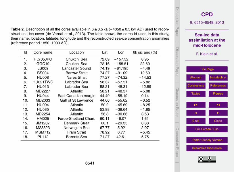
Table 2. Description of all the cores available in 6±0.5 ka (−4050±0.5 kyr AD) used to recon-struct sea-ice cover (de Vernal et al., 2013). The table shows the cores id used in this study,their name, location, latitude, longitude and the reconstructed sea-ice concentration anomalies(reference period 1850–1900 AD).

Id Core name Location Lat Lon 6k sic ano (%)

1. HLY05JPC Chukchi Sea 72.69 −157.52 8.952. GGC19 Chukchi Sea 72.16 −155.51 22.603. LS009 Lancaster Sound 74.19 −81.195 −4.494. BS004 Barrow Strait 74.27 −91.09 12.605. HU008 Nares Strait 77.27 −74.32 −14.536. HU021TWC Labrador Sea 58.37 −57.51 −5.827. HU013 Labrador Sea 58.21 −48.31 −12.598. MD2227 Atlantic 58.21 −48.37 −5.089. HU044 East Canadian margin 44.49 −55.19 0.14

10. MD2033 Gulf of St Lawrence 44.66 −55.62 −0.5211. HU094 Atlantic 50.2 −45.69 −8.2512. HU085 Atlantic 53.98 −38.64 −1.8513. MD2254 Atlantic 56.8 −30.66 3.5314. HM025 Faroe-Shetland Chan. 60.11 −6.07 1.6115. JM1207 Denmark Strait 68.1 −29.35 0.8816. M23323 Norwegian Sea 67.77 5.92 2.0717. MSM712 Fram Strait 78.92 6.77 −5.4518. PL112 Barents Sea 71.27 42.61 5.75

6541





CPD9, 6515–6549, 2013


mid-Holocene

F. Klein et al.

Title Page



Tables Figures

J I

J I

Back Close

Full Screen / Esc



Discussion

Paper

|D

iscussionP

aper|

Discussion

Paper

|D

iscussionP

aper|

150o W

120

o W

90

oW

60 o

W

30 oW

0o

30o E

60

o E

9

0oE

120 o

E

150 oE

180oW

50oN

60oN

70oN

80oN

150o W

120

o W

90

oW

60 o

W

30 oW

0o

30o E

60

o E

9

0oE

120 o

E

150 oE

180oW

50oN

60oN

70oN

80oN

1 2

3 4

5

6 7 8

9 10

11 12 13 14

15

16

17 18

Sea−ice concentration (%)−20 −15 −10 −5 0 5 10 15 20

Fig. 1. Proxy-based annual mean sea-ice concentration anomalies (in %) at the MH (referenceperiod 1850–1900 AD).

6542





CPD9, 6515–6549, 2013


mid-Holocene

F. Klein et al.

Title Page



Tables Figures

J I

J I

Back Close

Full Screen / Esc



Discussion

Paper

|D

iscussionP

aper|

Discussion

Paper

|D

iscussionP

aper|

1 2 3 4 5 6 7 8 9 10 11 12 13 14 15 16 17 18

−30

−20

−10

0

10

20

Core id

Sea

−ice

con

cent

ratio

n (%

)

ReconstructionsCCSM4CNRM_CM5CSIRO_Mk3_6_0HadGEM2_CCHadGEM2_ESMIROC_ESMMPI_ESM_PMRI_CGCM3bcc_csm1_1LOVECLIM_noassimLOVECLIM_assimSIC

1 2 3 4 5 6 7 8 9 10 11 12 13 14 15 16 17 18

30

20

10

0

−10

−20

Inso

latio

n(W

.m−2

)

1 2 3 4 5 6 7 8 9 10 11 12 13 14 15 16 17 18

−30

−20

−10

0

10

20

Core id

Sea

−ice

con

cent

ratio

n (%

)

Chukchi SeaChukchi Sea

sssddddddd

CAA

Chukchi Sea

sssddddddd

Denmark StraitChukchi Sea

sssddddddd

Fram StraitChukchi Sea

sssddddddd

Barents SeaChukchi Sea

sssddddddd

Fig. 2. Mid-Holocene annual mean sea-ice concentration anomalies (in %) for the proxy-basedreconstructions (black diamonds with error bars) and the corresponding climate models re-sults. The thick black line is the models mean. The grey shaded areas is the models mean±2 standard deviations. The dashed red line represents the annual mean insolation at eachstudied location (in Wm−2) and corresponds to the reversed right axis. The reference period is1850–1900 AD.

6543





CPD9, 6515–6549, 2013


mid-Holocene

F. Klein et al.

Title Page



Tables Figures

J I

J I

Back Close

Full Screen / Esc



Discussion

Paper

|D

iscussionP

aper|

Discussion

Paper

|D

iscussionP

aper|

(a) Winter

Sea

−ice

con

cent

ratio

n (%

)

Core id1 2 3 4 5 6 7 8 9 10 11 12 13 14 15 16 17 18

−50

−40

−30

−20

−10

0

10

1 2 3 4 5 6 7 8 9 10 11 12 13 14 15 16 17 18

50

40

30

20

10

0

−10

Inso

latio

n(W

.m−2

)

Sea

−ice

con

cent

ratio

n (%

)

Core id1 2 3 4 5 6 7 8 9 10 11 12 13 14 15 16 17 18

−50

−40

−30

−20

−10

0

10

CNRM_CM5

CSIRO_Mk3_6_0

HadGEM2_CC

HadGEM2_ES

MIROC_ESM

MPI_ESM_P

MRI_CGCM3

bcc_csm1_1

LOVECLIM_noassim

LOVECLIM_assimSIC

CCSM4

(b) Spring

Core id

Sea

−ice

con

cent

ratio

n (%

)

1 2 3 4 5 6 7 8 9 10 11 12 13 14 15 16 17 18

−50

−40

−30

−20

−10

0

10

CCSM4

CNRM_CM5

CSIRO_Mk3_6_0

HadGEM2_CC

HadGEM2_ES

MIROC_ESM

MPI_ESM_P

MRI_CGCM3

bcc_csm1_1

LOVECLIM_noassim

LOVECLIM_assimSIC

1 2 3 4 5 6 7 8 9 10 11 12 13 14 15 16 17 18

50

40

30

20

10

0

−10

Inso

latio

n(W

.m−2

)

Core id

Sea

−ice

con

cent

ratio

n (%

)

1 2 3 4 5 6 7 8 9 10 11 12 13 14 15 16 17 18

−50

−40

−30

−20

−10

0

10

(c) Summer

Sea

−ice

con

cent

ratio

n (%

)

Core id1 2 3 4 5 6 7 8 9 10 11 12 13 14 15 16 17 18

−50

−40

−30

−20

−10

0

10

1 2 3 4 5 6 7 8 9 10 11 12 13 14 15 16 17 18

50

40

30

20

10

0

−10

Inso

latio

n(W

.m−2

)

Sea

−ice

con

cent

ratio

n (%

)

Core id1 2 3 4 5 6 7 8 9 10 11 12 13 14 15 16 17 18

−50

−40

−30

−20

−10

0

10

CNRM_CM5

CSIRO_Mk3_6_0

HadGEM2_CC

HadGEM2_ES

MIROC_ESM

MPI_ESM_P

MRI_CGCM3

bcc_csm1_1

LOVECLIM_noassim

LOVECLIM_assimSIC

CCSM4

(d) Autumn

Sea

−ice

con

cent

ratio

n (%

)

Core id1 2 3 4 5 6 7 8 9 10 11 12 13 14 15 16 17 18

−50

−40

−30

−20

−10

0

10

1 2 3 4 5 6 7 8 9 10 11 12 13 14 15 16 17 18

50

40

30

20

10

0

−10

Inso

latio

n(W

.m−2

)

Sea

−ice

con

cent

ratio

n (%

)

Core id1 2 3 4 5 6 7 8 9 10 11 12 13 14 15 16 17 18

−50

−40

−30

−20

−10

0

10

CCSM4

CNRM_CM5

CSIRO_Mk3_6_0

HadGEM2_CC

HadGEM2_ES

MIROC_ESM

MPI_ESM_P

MRI_CGCM3

bcc_csm1_1

LOVECLIM_noassim

LOVECLIM_assimSIC

Fig. 3. Mid-Holocene seasonal mean sea-ice concentration anomalies (in %) for the climatemodels results corresponding to the cores locations. The thick black line corresponds to themodels mean. The grey shaded areas is the models mean ±2 standard deviations. The dashedred line represents the seasonal mean insolation at each studied location (in Wm−2) and cor-responds to the reversed right axis. The reference period is 1850–1900.

6544





CPD9, 6515–6549, 2013


mid-Holocene

F. Klein et al.

Title Page



Tables Figures

J I

J I

Back Close

Full Screen / Esc



Discussion

Paper

|D

iscussionP

aper|

Discussion

Paper

|D

iscussionP

aper|

(a) Mid-Holocene

J F M A M J J A S O N D0

10

20

30

40

50

60

70

80

90

100

Time of the year

Sea−

ice c

oncentr

ation (

%)

CCSM4

CNRM_CM5

CSIRO_Mk3_6_0

HadGEM2_CC

HadGEM2_ES

MIROC_ESM

MPI_ESM_P

MRI_CGCM3

bcc_csm1_1

LOVECLIM_noassim

LOVECLIM_assimSIC

(b) Pre-industrial

J F M A M J J A S O N D0

10

20

30

40

50

60

70

80

90

100

Se

a−

ice

co

nce

ntr

atio

n (

%)

Time of the year

Fig. 4. Mid-Holocene (6 ka) and pre-industrial (1850–1900 AD) mean seasonal cycles of sea-ice concentration (in %) in the Barents Sea (id 18).

6545





CPD9, 6515–6549, 2013


mid-Holocene

F. Klein et al.

Title Page



Tables Figures

J I

J I

Back Close

Full Screen / Esc



Discussion

Paper

|D

iscussionP

aper|

Discussion

Paper

|D

iscussionP

aper|

5

6

7

8

9

10

11

12

13

14

15

Models

RM

SE

(%

)

CNRM

−CM

5

Had

GEM

2−CC

LC−n

oass

im

Had

GEM

2−ES

bcc−

csm

1−1

MRI−

CGCM

3

MPI−

ESM−P

LC−a

ssim

SIC

CSIR

O−M

k3−6

−0

MIR

OC−E

SM

CCSM

4

Anom

alies=

0

LOVECLIM without data assimilation

LOVECLIM with data assimilation

No change between MH and PI

Fig. 5. Ranked RMSE between the MH sea-ice anomalies (reference period 1850–1900 AD)simulated by each model and the proxy based reconstructions. The error bars correspond tothe range of the RMSE when changing the reference period to 1850–1875 AD and 1875–1900AD. The purple bar is the RMSE computed assuming no change between MH and PI.

6546





CPD9, 6515–6549, 2013


mid-Holocene

F. Klein et al.

Title Page



Tables Figures

J I

J I

Back Close

Full Screen / Esc



Discussion

Paper

|D

iscussionP

aper|

Discussion

Paper

|D

iscussionP

aper|

(a) BCC-CSM1-1

150

o W

120

o W

90

oW

60 o

W

30 oW

0o

30o E

60

o E

9

0oE

120 o

E

150 oE

180oW

30

30

30

30

60

90120

−90

−90

−90

−90

−60

−60

−60

−30

−30

−30

−30

−30

0

0

0

0

(b) CCSM4

150

o W

120

o W

90

oW

60 o

W

30 oW

0o

30o E

60

o E

9

0oE

120 o

E

150 oE

180oW

30

3060

90

−90

−90

−60

−60

−60

−60

−60

−60

−60

−30

−30

−30

−30

−30

−30

−30

0

0

0

00

0 0

0

(c) CNRM-CM5

150

o W

120

o W

90

oW

60 o

W

30 oW

0o

30o E

60

o E

9

0oE

120 o

E

150 oE

180oW

30

30

30

30

30

30

60

−90

−60

−60−60

−60

−60

−60

−30

−30

−30

−30

−30

−30

−30

−30

−30

−30

−30

−30

−30

−30

−30

−30

−30

−30

0

0

0

0

0

0

0

0

(d) CSIRO-Mk3-6-0

150

o W

120

o W

90

oW

60 o

W

30 oW

0o

30o E

60

o E

9

0oE

120 o

E

150 oE

180oW

30

30

30

30

60

−90

−90

−60

−60

−60

−60

−60

−30

−30

−30

−30

−30

−30

−30

−30

−30

−30 −30

0

0

0

0

0

(e) HadGEM2-CC

150

o W

120

o W

90

oW

60 o

W

30 oW

0o

30o E

60

o E

9

0oE

120 o

E

150 oE

180oW

30

30

30

30

60

90

90

−90

−90

−90

−90−90

−60

−60

−60

−60

−60

−60

−30

−30

−30

−30

−30

−30

−30 −30

−30

−30

0

0

0

0

0

0

0

0

0

(f) HadGEM2-ES

150

o W

120

o W

90

oW

60 o

W

30 oW

0o

30o E

60

o E

9

0oE

120 o

E

150 oE

180oW

30

30

30

30

30

30

30

60

60

90

90

120

120

−90

−90

−90

−90

−90

−90

−60

−60

−60

−60

−60

−60

−30

−30

−30

−30

−30

−30

−30

−30

−30

0

0

0

0

0

0

0

0

0

0

0

(g) MIROC-ESM

150

o W

120

o W

90

oW

60 o

W

30 oW

0o

30o E

60

o E

9

0oE

120 o

E

150 oE

180oW

30

−90

−90

−90

−90

−60

−60

−60

−60

−60

−30

−30

−30

−30

−30

−30

0

0

0

0

0

(h) MPI-ESM-P

150

o W

120

o W

90

oW

60 o

W

30 oW

0o

30o E

60

o E

9

0oE

120 o

E

150 oE

180oW

30

30

−90−90

−60

−60

−60

−60

−60

−60

−60

−30

−30

−30

−30

−30

−30

0

0

0

0

0

(i) MRI-CGCM3

150

o W

120

o W

90

oW

60 o

W

30 oW

0o

30o E

60

o E

9

0oE

120 o

E

150 oE

180oW

30

30

30

30

60

60

60

90

90

120

120

−60

−60

−60

−60

−30

−30

−30

−30 −

30

−30

−30

−30

−30

−30

−30

−30

0

0

0

0

0

0

0

0

Fig. 6. Annual mean surface pressure anomalies (in Pa) simulated by the GCMs for the MH(reference period 1850–1900 AD).

6547





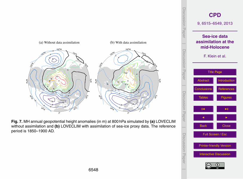
CPD9, 6515–6549, 2013


mid-Holocene

F. Klein et al.

Title Page



Tables Figures

J I

J I

Back Close

Full Screen / Esc



Discussion

Paper

|D

iscussionP

aper|

Discussion

Paper

|D

iscussionP

aper|

(a) Without data assimilation

150

o W

120

o W

90

oW

60 o

W

30 oW

0o

30o E

60

o E

90

oE

120 o

E

150 oE

180oW

−10−8

−8

−8

−6−6

−6

−4

−4

−4

−4

−2

−2

−2

−2

0

0

0

2

2

4

6

8

8

10

0

0

0

(b) With data assimilation

150

o W

120

o W

90

oW

60 o

W

30 oW

0o

30o E

60

o E

90

oE

120 o

E

150 oE

180oW

−8−8

−6−6

−4−4

−4

−4

−2−2

−2

0

0

2

2

4

44

66

8

0

0

0

Fig. 7. MH annual geopotential height anomalies (in m) at 800 hPa simulated by (a) LOVECLIMwithout assimilation and (b) LOVECLIM with assimilation of sea-ice proxy data. The referenceperiod is 1850–1900 AD.

6548





CPD9, 6515–6549, 2013


mid-Holocene

F. Klein et al.

Title Page



Tables Figures

J I

J I

Back Close

Full Screen / Esc



Discussion

Paper

|D

iscussionP

aper|

Discussion

Paper

|D

iscussionP

aper|

150

o W

120

o W

90

oW

60 o

W

30 oW

0o

30o E

60

o E

9

0oE

120 o

E

150 oE

180oW

−5−4−3

−3

−2

−2

−1

−1

−1

0

0

0

0

1

1

1

2

2

2

2

3

3

4

5

0

0

0

0

Fig. 8. Difference between the geopotential height anomalies (in m) at 800 hPa of LOVECLIMwith sea-ice data assimilation and LOVECLIM without data assimilation. The black arrows showthe flow responsible for the change in sea-ice at the Barents Sea and the Chukchi Sea.

6549





Sea-ice data assimilation at the mid-Holocene - CP

Documents

Transcript of Sea-ice data assimilation at the mid-Holocene - CP