xSchwarz Preconditioner for

the Stochastic Finite Element Method

Waad Subber

Joint work with Sebastien Loisel

The NAIS Project

Department of Mathematics

Heriot-Watt University

0/43

Introduction

Motivation

High resolution numerical model

effectively reduces discretization error.does not necessarily enhance confidence in prediction.

The effect of uncertainty need to be considered for realisticcomputer predictions.

Objective

Develop parallel algorithms to quantify uncertainty inlarge-scale computational models.

Methodology

Exploit domain decomposition methods in the spatial directionin conjunction with a functional expansion along the stochasticdimension.

1/43

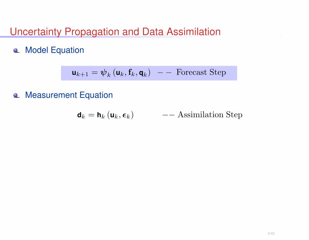
Uncertainty Propagation and Data Assimilation

Model Equation

uk+1 = ψk (uk, fk, qk) −− Forecast Step

Measurement Equation

dk = hk (uk, ǫk) −− Assimilation Step

2/43

Uncertainty Propagation

Traditional Monte Carlo Simulation

Non-intrusive to legacy code

Embarrassingly parallel yet computationally expensive

Polynomial Chaos Expansion

Intrusive or non-intrusive

Computationally efficient

Multiscale representation of uncertainty

3/43

Stochastic Elliptic PDE

Find a random function u(x, θ) : D × Ω → R satisfying the

following equation in an almost surely sense:

∇ · (κ(x, θ)∇u(x, θ)) = f(x), in D × Ω,

u(x, θ) = 0, on ∂D × Ω,

0 < κmin ≤ κ(x, θ) ≤ κmax < +∞, in D × Ω.

4/43

Stochastic Elliptic PDE

Find a random function u(x, θ) : D × Ω → R satisfying the

following equation in an almost surely sense:

∇ · (κ(x, θ)∇u(x, θ)) = f(x), in D × Ω,

u(x, θ) = 0, on ∂D × Ω,

0 < κmin ≤ κ(x, θ) ≤ κmax < +∞, in D × Ω.

Possible realizations of κ(x, θ):

5/43

Uncertainty Representation by Stochastic Processes

Karhunen-Loeve Expansion (KLE)

κ(x, θ) = κ(x) +

M∑

i=1

ξi(θ)√

λiφi(x),

〈ξi(θ)〉 = 0, 〈ξi(θ)ξj(θ)〉 = δij .

Fredholm Integral Equation

∫

Cκκ(x1,x2)φi(x1)dx1 = λiφi(x2).

6/43

Uncertainty Representation by Stochastic Processes

Polynomial Chaos Expansion (PCE)

u(x, θ) =

N∑

i=0

ui(x)Ψi(ξ),

〈Ψi(ξ)〉 = 0, 〈Ψi(ξ)Ψj(ξ)〉 = δij〈Ψ2i (ξ)〉, N + 1 =

(M + p)!

M !p!.

Two-dimensional (M = 2) third order (p = 3) PCE

u(x, θ) = u0(x)+

u1(x)ξ1 + u2(x)ξ2+

u3(x)(ξ2

1 − 1) + u4(x)(ξ1ξ2) + u5(x)(ξ2

2 − 1)+

u6(x)(ξ3

1 − 3ξ1) + u7(x)(ξ2

1ξ2 − ξ2) + u8(x)(ξ1ξ2

2 − ξ1) + u9(x)(ξ3

2 − 3ξ2).7/43

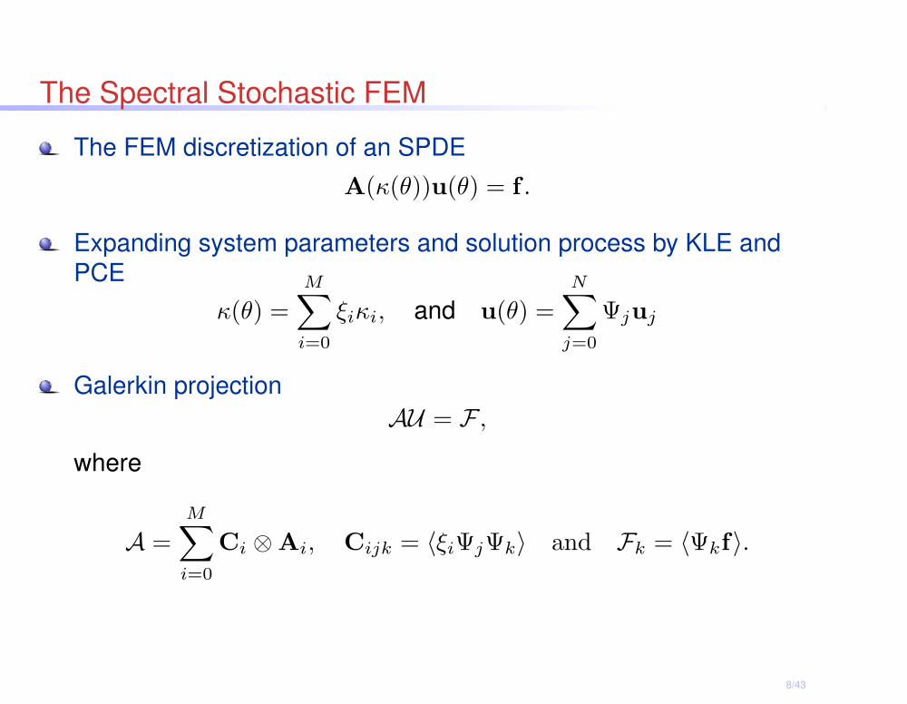
The Spectral Stochastic FEM

The FEM discretization of an SPDE

A(κ(θ))u(θ) = f .

Expanding system parameters and solution process by KLE and

PCE

κ(θ) =M∑

i=0

ξiκi, and u(θ) =N∑

j=0

Ψjuj

Galerkin projection

AU = F ,

where

A =

M∑

i=0

Ci ⊗Ai, Cijk = 〈ξiΨjΨk〉 and Fk = 〈Ψkf〉.

8/43

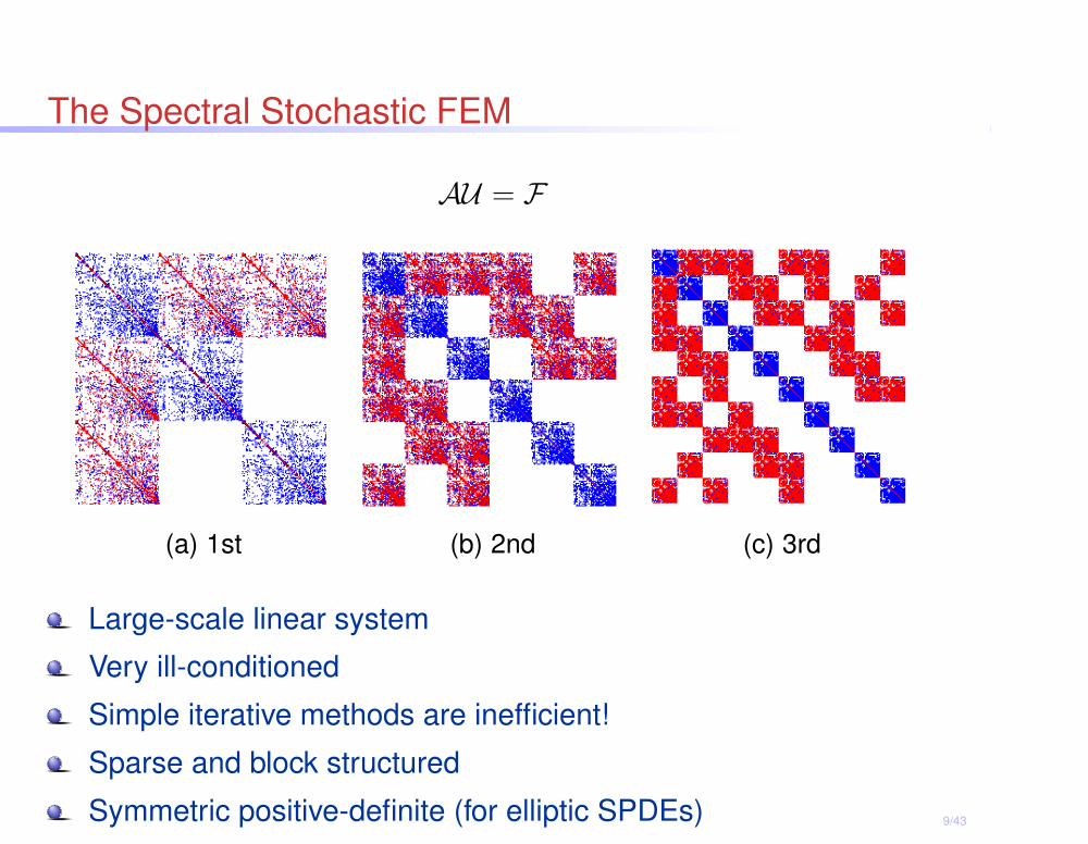
The Spectral Stochastic FEM

AU = F

(a) 1st (b) 2nd (c) 3rd

Large-scale linear system

Very ill-conditioned

Simple iterative methods are inefficient!

Sparse and block structured

Symmetric positive-definite (for elliptic SPDEs) 9/43

Preconditioned Conjugate Gradient Method (PCGM)

A U = F ,

M−1A U = M−1F ,

(M−1) is a good approximation to (A−1)

Condition number of (M−1A) is much smaller than (A)

Eigenvalues of (M−1A) are clustered near one

10/43

Schwarz preconditioner for stochastic PDEs

Partition the spatial domain

Define a restiriction matrix

RTs : Ωs 7→ Ω

For each of KLE coefficient, define the subdomain stiffness matrix

Asi = RsAiR

Ts

Corresponds to

∇ · (κi(x)∇u(x)) = f(x), in Ds,

u(x) = g(x), on ∂Ds.11/43

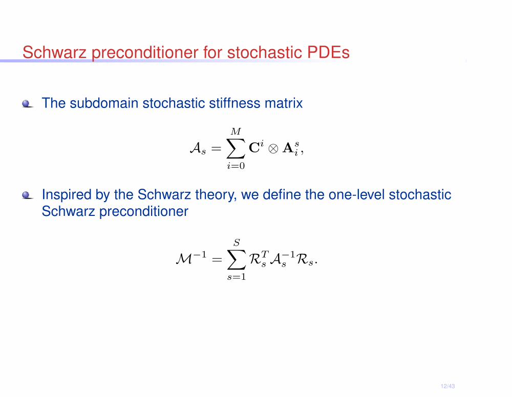
Schwarz preconditioner for stochastic PDEs

The subdomain stochastic stiffness matrix

As =M∑

i=0

Ci ⊗Asi ,

Inspired by the Schwarz theory, we define the one-level stochasticSchwarz preconditioner

M−1 =

S∑

s=1

RTs A

−1s Rs.

12/43

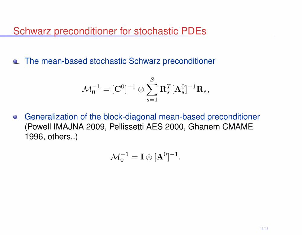
Schwarz preconditioner for stochastic PDEs

The mean-based stochastic Schwarz preconditioner

M−1

0 = [C0]−1 ⊗

S∑

s=1

RTs [A

0s]

−1Rs,

Generalization of the block-diagonal mean-based preconditioner

(Powell IMAJNA 2009, Pellissetti AES 2000, Ghanem CMAME1996, others..)

M−1

0 = I⊗ [A0]−1.

13/43

Coarse Grid Correction

Define a set of bilinear hat basis functions

A coarse grid restiriction operator is defined as

RT0 =

ψ1(x1) ψ2(x1) · · · ψn0(x1)

ψ1(x2) ψ2(x2) · · · ψn0(x2)

...... · · ·

...

ψ1(xni) ψ2(xni

) · · · ψn0(xni

)

14/43

Stochastic additive Schwarz preconditioner

Two-level Schwarz preconditioner for SPDEs

M−1 = RT0 A

−1

0 R0 +

S∑

s=1

RTs A

−1s Rs,

Theorem: The condition number of the stochastic additive Schwarzpreconditioner is bounded by

cond(

M−1A)

≤ Cκmax

κmin

(

1 +H

h

)

.

where C is a constant independent of H, h and δ, M ,and p.

15/43

Numerical Results

Poisson’s equation with random coefficient

∇ · (κ(x, θ)∇u(x, θ)) = f(x), x ∈ Ω,

u(x, θ) = 0, x ∈ ∂Ω.

The permeability coefficient is a Gaussian or Uniformstochastic process with an exponential covariance

Cκκ(x,y) = σ2 exp

(

−|x1 − y1|

b1+

−|x2 − y2|

b2

)

.

16/43

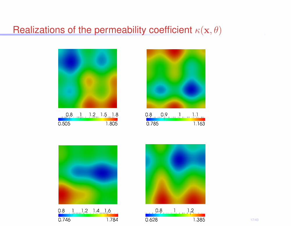
Realizations of the permeability coefficient κ(x, θ)

17/43

Stochastic Features

Mean and Variance of the solution process

(a) µu (b) σ2u

18/43

Stochastic Features

Selected PCE coefficients of the solution process

(a) u7 (b) u8

(a) u13 (b) u14 19/43

Numerical Results

Scalability with respect to dimension and order of the PCE

Gaussian Uniform

M p cond iter cond iter

2 1 9.7092 21 9.7027 21

2 9.7195 21 9.7060 21

3 9.7272 21 9.7077 21

4 9.7335 21 9.7087 21

20/43

Numerical Results

Scalability with respect to dimension and order of the PCE

Gaussian Uniform

M p cond iter cond iter

2 1 9.7092 21 9.7027 21

2 9.7195 21 9.7060 21

3 9.7272 21 9.7077 21

4 9.7335 21 9.7087 21

3 1 9.7097 21 9.7029 21

2 9.7203 21 9.7068 21

3 9.7283 21 9.7090 21

4 9.7347 21 9.7104 21

21/43

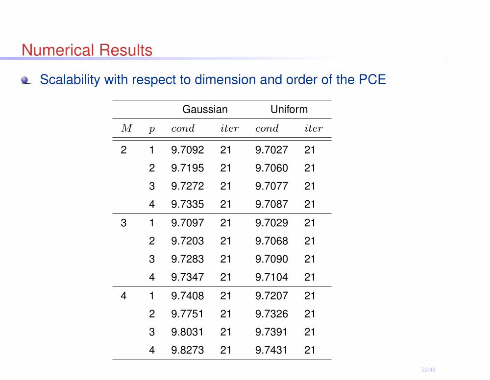
Numerical Results

Scalability with respect to dimension and order of the PCE

Gaussian Uniform

M p cond iter cond iter

2 1 9.7092 21 9.7027 21

2 9.7195 21 9.7060 21

3 9.7272 21 9.7077 21

4 9.7335 21 9.7087 21

3 1 9.7097 21 9.7029 21

2 9.7203 21 9.7068 21

3 9.7283 21 9.7090 21

4 9.7347 21 9.7104 21

4 1 9.7408 21 9.7207 21

2 9.7751 21 9.7326 21

3 9.8031 21 9.7391 21

4 9.8273 21 9.7431 21

22/43

Numerical Results

Scalability with respect to the strength of randomness

Gaussian Uniform

σ

µp cond iter cond iter

0.1 1 9.7408 21 9.7207 21

2 9.7751 21 9.7326 21

3 9.8031 21 9.7391 21

4 9.8273 21 9.7431 21

23/43

Numerical Results

Scalability with respect to the strength of randomness

Gaussian Uniform

σ

µp cond iter cond iter

0.1 1 9.7408 21 9.7207 21

2 9.7751 21 9.7326 21

3 9.8031 21 9.7391 21

4 9.8273 21 9.7431 21

0.2 1 9.7885 21 9.7482 21

2 9.8568 22 9.7704 21

3 9.9134 22 9.7820 21

4 9.9638 22 9.7891 21

24/43

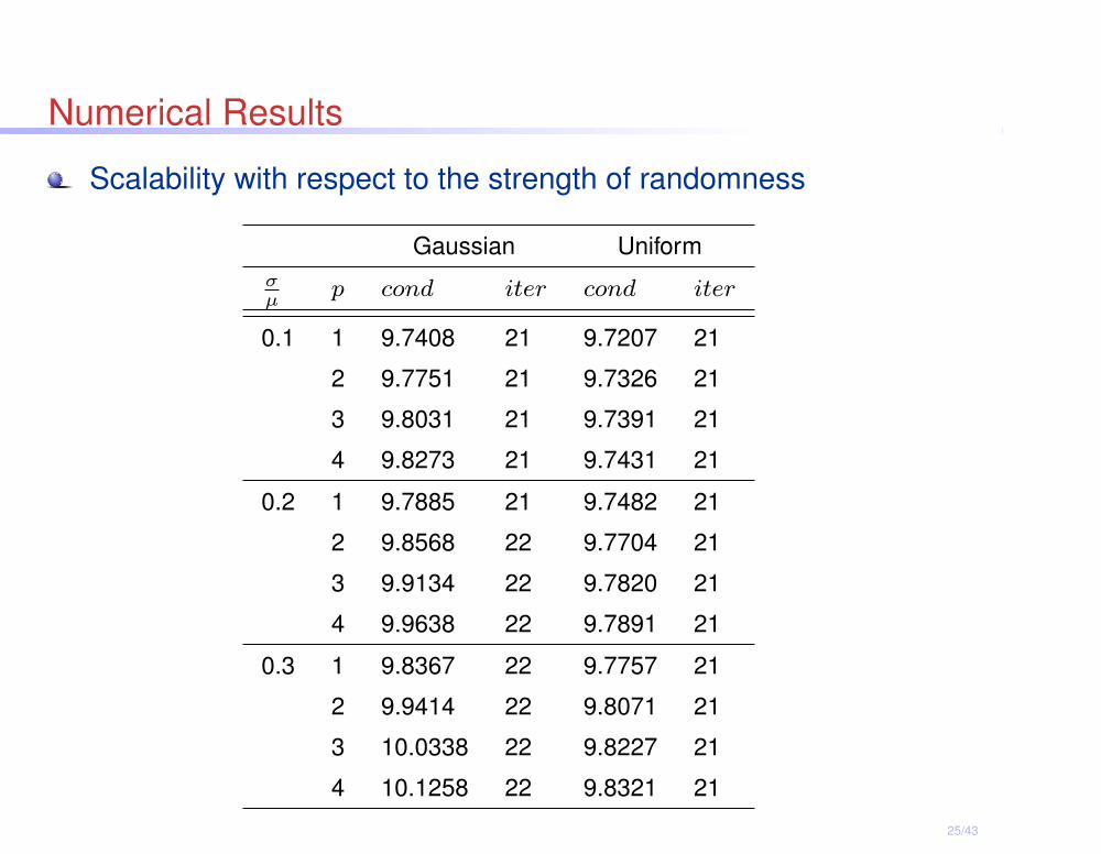
Numerical Results

Scalability with respect to the strength of randomness

Gaussian Uniform

σ

µp cond iter cond iter

0.1 1 9.7408 21 9.7207 21

2 9.7751 21 9.7326 21

3 9.8031 21 9.7391 21

4 9.8273 21 9.7431 21

0.2 1 9.7885 21 9.7482 21

2 9.8568 22 9.7704 21

3 9.9134 22 9.7820 21

4 9.9638 22 9.7891 21

0.3 1 9.8367 22 9.7757 21

2 9.9414 22 9.8071 21

3 10.0338 22 9.8227 21

4 10.1258 22 9.8321 21

25/43

Numerical Results

Scalability with respect to the overlap

Gaussian Uniform

δ p cond iter cond iter

2h 1 7.3252 16 7.3141 16

2 7.3441 16 7.3203 16

3 7.3593 16 7.3236 16

4 7.3724 16 7.3248 16

26/43

Numerical Results

Scalability with respect to the overlap

Gaussian Uniform

δ p cond iter cond iter

2h 1 7.3252 16 7.3141 16

2 7.3441 16 7.3203 16

3 7.3593 16 7.3236 16

4 7.3724 16 7.3248 16

3h 1 5.2401 13 5.2371 13

2 5.2448 14 5.2391 13

3 5.2485 14 5.2401 13

4 5.2517 14 5.2522 13

27/43

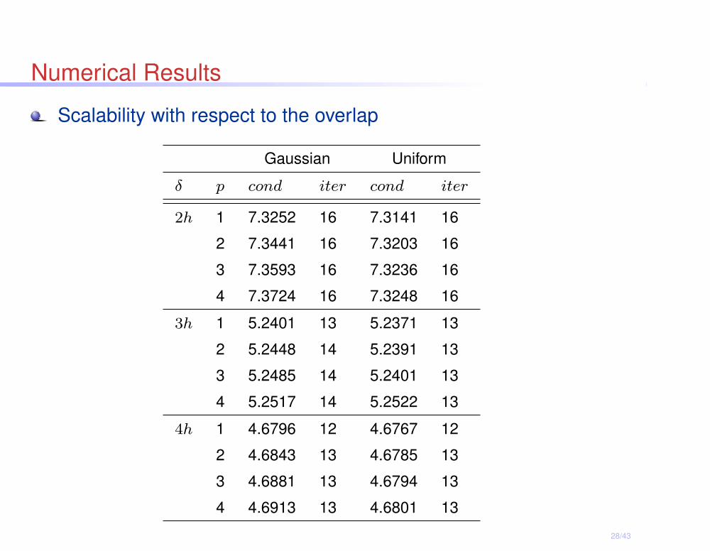
Numerical Results

Scalability with respect to the overlap

Gaussian Uniform

δ p cond iter cond iter

2h 1 7.3252 16 7.3141 16

2 7.3441 16 7.3203 16

3 7.3593 16 7.3236 16

4 7.3724 16 7.3248 16

3h 1 5.2401 13 5.2371 13

2 5.2448 14 5.2391 13

3 5.2485 14 5.2401 13

4 5.2517 14 5.2522 13

4h 1 4.6796 12 4.6767 12

2 4.6843 13 4.6785 13

3 4.6881 13 4.6794 13

4 4.6913 13 4.6801 13

28/43

Numerical Results

Scalability with respect to Hh

: fixed overlap

p = 2

0 2 4 6 8 10 12 14 16 180

2

4

6

8

10

12

14

16

18

H/h

Con

ditio

n nu

mbe

r

IdealM=1M=2M=3M=4

(a) Gaussian

0 2 4 6 8 10 12 14 16 180

2

4

6

8

10

12

14

16

18

H/h

Con

ditio

n nu

mbe

r

IdealM=1M=2M=3M=4

(b) Uniform

M = 2

0 2 4 6 8 10 12 14 16 180

2

4

6

8

10

12

14

16

18

H/h

Con

ditio

n nu

mbe

r

Idealp=1p=2p=3p=4

(c) Gaussian

0 2 4 6 8 10 12 14 16 180

2

4

6

8

10

12

14

16

18

H/h

Con

ditio

n nu

mbe

r

Idealp=1p=2p=3p=4

(d) Uniform29/43

Numerical Results

Scalability with respect to Hh

: proportional overlap δ = 0.1H

p = 2

0 2 4 6 8 10 12 14 16 180

2

4

6

8

10

12

14

16

18

H/h

Con

ditio

n nu

mbe

r

p=1p=2p=3p=4

(a) Gaussian

0 2 4 6 8 10 12 14 16 180

2

4

6

8

10

12

14

16

18

H/h

Con

ditio

n nu

mbe

r

p=1p=2p=3p=4

(b) Uniform

M = 2

0 2 4 6 8 10 12 14 16 180

2

4

6

8

10

12

14

16

18

H/h

Con

ditio

n nu

mbe

r

M=1M=2M=3M=4

(c) Gaussian

0 2 4 6 8 10 12 14 16 180

2

4

6

8

10

12

14

16

18

H/h

Con

ditio

n nu

mbe

r

M=1M=2M=3M=4

(d) Uniform30/43

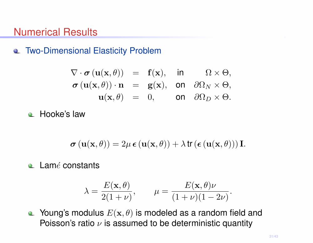
Numerical Results

Two-Dimensional Elasticity Problem

∇ · σ (u(x, θ)) = f(x), in Ω×Θ,

σ (u(x, θ)) · n = g(x), on ∂ΩN ×Θ,

u(x, θ) = 0, on ∂ΩD ×Θ.

Hooke’s law

σ (u(x, θ)) = 2µ ǫ (u(x, θ)) + λ tr (ǫ (u(x, θ))) I.

Lame constants

λ =E(x, θ)

2(1 + ν), µ =

E(x, θ)ν

(1 + ν)(1− 2ν).

Young’s modulus E(x, θ) is modeled as a random field and

Poisson’s ratio ν is assumed to be deterministic quantity

31/43

Stochastic Features

Mean and standard deviation of the displacement field

(a) µu (b) σu

32/43

Stochastic Features

Deformed meshes corresponding to chaos coefficients

(a) u0 (b) u3

(a) u9 (b) u14

33/43

Numerical Results

Scalability with respect to dimension and order of the PCE

Gaussian Uniform

M p cond iter cond iter

2 1 13.6048 23 13.5442 22

2 13.7231 24 13.5699 22

3 13.8751 25 13.5883 22

4 14.0697 25 13.6019 22

34/43

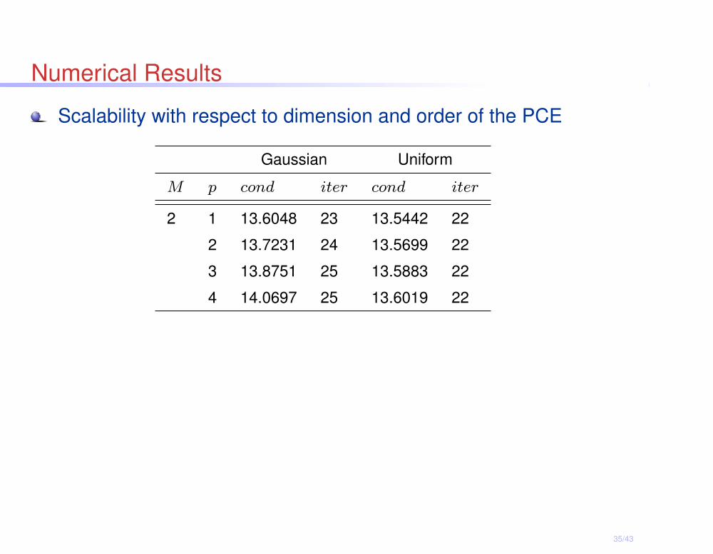
Numerical Results

Scalability with respect to dimension and order of the PCE

Gaussian Uniform

M p cond iter cond iter

2 1 13.6048 23 13.5442 22

2 13.7231 24 13.5699 22

3 13.8751 25 13.5883 22

4 14.0697 25 13.6019 22

35/43

Numerical Results

Scalability with respect to dimension and order of the PCE

Gaussian Uniform

M p cond iter cond iter

2 1 13.6048 23 13.5442 22

2 13.7231 24 13.5699 22

3 13.8751 25 13.5883 22

4 14.0697 25 13.6019 22

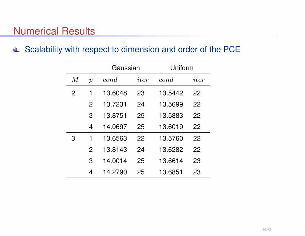
3 1 13.6563 22 13.5760 22

2 13.8143 24 13.6282 22

3 14.0014 25 13.6614 23

4 14.2790 25 13.6851 23

36/43

Numerical Results

Scalability with respect to dimension and order of the PCE

Gaussian Uniform

M p cond iter cond iter

2 1 13.6048 23 13.5442 22

2 13.7231 24 13.5699 22

3 13.8751 25 13.5883 22

4 14.0697 25 13.6019 22

3 1 13.6563 22 13.5760 22

2 13.8143 24 13.6282 22

3 14.0014 25 13.6614 23

4 14.2790 25 13.6851 23

4 1 13.6953 24 13.5981 22

2 13.8824 25 13.6681 23

3 14.0936 25 13.7173 23

4 14.3575 25 13.7525 23

37/43

Numerical Results

Scalability with respect to the strength of randomness

Gaussian Uniform

σ

µp cond iter cond iter

0.1 1 13.5623 22 13.5307 22

2 13.6160 22 13.5546 22

3 13.6626 24 13.5702 22

4 13.7056 24 13.5806 22

38/43

Numerical Results

Scalability with respect to the strength of randomness

Gaussian Uniform

σ

µp cond iter cond iter

0.1 1 13.5623 22 13.5307 22

2 13.6160 22 13.5546 22

3 13.6626 24 13.5702 22

4 13.7056 24 13.5806 22

0.2 1 13.6472 23 13.5745 22

2 13.7786 24 13.6274 22

3 13.9120 24 13.6636 22

4 14.0581 24 13.6888 22

39/43

Numerical Results

Scalability with respect to the strength of randomness

Gaussian Uniform

σ

µp cond iter cond iter

0.1 1 13.5623 22 13.5307 22

2 13.6160 22 13.5546 22

3 13.6626 24 13.5702 22

4 13.7056 24 13.5806 22

0.2 1 13.6472 23 13.5745 22

2 13.7786 24 13.6274 22

3 13.9120 24 13.6636 22

4 14.0581 24 13.6888 22

0.3 1 13.7478 24 13.6230 23

2 14.0075 25 13.7122 23

3 14.3430 25 13.7767 23

4 15.0671 28 13.8243 23

40/43

Numerical Results

Scalability with respect to Hh

p = 2

100

101

100

101

102

H/h

Con

ditio

n nu

mbe

r

IdealM=1M=2M=3M=4

(a) Gaussian

100

101

100

101

102

H/h

Con

ditio

n nu

mbe

r

IdealM=1M=2M=3M=4

(b) Uniform

M = 2

100

101

100

101

102

H/h

Con

ditio

n nu

mbe

r

Idealp=1p=2p=3p=4

(c) Gaussian

100

101

100

101

102

H/h

Con

ditio

n nu

mbe

r

Idealp=1p=2p=3p=4

(d) Uniform41/43

Conclusions

Two-level Schwarz domain decomposition preconditioner isintroduced for the linear system of the spectral stochastic finiteelement method.

The stochastic Schwarz preconditioner achieves aconvergence rate that is independent of the coefficient of

variation, dimension and order of the stochastic expansion.

The condition number of the stochastic Schwarzpreconditioner grows as O

(

Hh

)

.

42/43

Acknowledgment

Financial Support

The Centre for Numerical Algorithms and Intelligent Software

(NAIS Project)

Scottish Funding Council

Engineering and Physical Research Council

43/43