© Rohde & Schwarz; Oscilloscope Fundamentals – Primer

Primer

OSCILLOSCOPE FUNDAMENTALS

2

CONTENTSOverview 3

Where it all began ..........................................................3The digital age beckons .............................................3

Types of digital oscilloscopes .........................................4Digital sampling oscilloscopes ...................................4Real-time sampling oscilloscopes ..............................4Mixed-signal oscilloscopes ........................................4

Basic elements of digital oscilloscopes ..........................5The vertical system ....................................................5The horizontal system ................................................6The trigger system .....................................................6The display system and user interface .......................9

Probes 10Passive probes .........................................................10Active probes ...........................................................11Differential probes ....................................................11Current probes .........................................................11High-voltage probes.................................................11

Benefits of a noninterleaved ADC 12Probe considerations ....................................................13

Circuit loading ..........................................................13Grounding ................................................................13Probe selection process ...........................................13

Oscilloscope benchmark specifications 14Bandwidth ....................................................................14Effective of number of bits (ENOB) ..............................14Channels ......................................................................15Sample rate ..................................................................15Memory depth .............................................................15Types of triggering .......................................................15Rise time ......................................................................15Frequency response .....................................................15Gain (vertical) and timebase (horizontal) accuracy .......16ADC vertical resolution .................................................16Vertical sensitivity .........................................................16Display and user interface ............................................17Communications capabilities .......................................17

Typical oscilloscope measurements 18Voltage measurements ................................................18Phase shift measurements ...........................................18Time measurements .....................................................18Pulse width and rise time measurements ....................18Decoding serial buses ..................................................18Frequency analysis, statistics and math functions .......18

Summary 20

Glossary 21

Rohde & Schwarz Oscilloscope Fundamentals 3

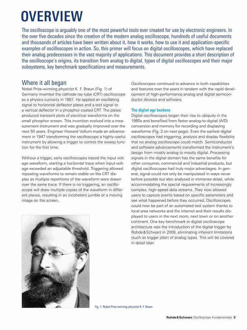
Where it all beganNobel Prize-winning physicist K. F. Braun (Fig. 1) of Germany invented the cathode ray tube (CRT) oscilloscope as a physics curiosity in 1897. He applied an oscillating signal to horizontal deflector plates and a test signal to a vertical deflector in a phosphor-coated CRT. The plates produced transient plots of electrical waveforms on the small phosphor screen. This invention evolved into a mea-surement instrument and was gradually improved over the next 50 years. Engineer Howard Vollum made an advance-ment in 1947 transforming the oscilloscope a highly-useful instrument by allowing a trigger to control the sweep func-tion for the first time.

Without a trigger, early oscilloscopes traced the input volt-age waveform, starting a horizontal trace when input volt-age exceeded an adjustable threshold. Triggering allowed repeating waveforms to remain stable on the CRT dis-play as multiple repetitions of the waveform were drawn over the same trace. If there is no triggering, an oscillo-scope will draw multiple copies of the waveform in differ-ent places, resulting in an incoherent jumble or a moving image on the screen.

Oscilloscopes continued to advance in both capabilities and features over the years in tandem with the rapid devel-opment of high-performance analog and digital semicon-ductor devices and software.

The digital age beckonsDigital oscilloscopes began their rise to ubiquity in the 1980s and benefited from faster analog-to-digital (A/D) conversion and memory for recording and displaying waveforms (Fig. 2 on next page). Even the earliest digital oscilloscopes had triggering, analysis and display flexibility that no analog oscilloscope could match. Semiconductor and software advancements transformed the instrument’s design from mostly analog to mostly digital. Processing signals in the digital domain has the same benefits for other consumer, commercial and industrial products, but digital oscilloscopes had truly major advantages. In gen-eral, signal could not only be manipulated in ways never before possible but also analyzed in immense detail, while accommodating the special requirements of increasingly complex, high-speed data streams. They now allowed users to capture events based on specific parameters and see what happened before they occurred. Oscilloscopes could now be part of an automated test system thanks to local area networks and the internet and their results dis-played to users in the next room, next town or on another continent. One key benchmark in digital oscilloscope architecture was the introduction of the digital trigger by Rohde & Schwarz in 2009, eliminating inherent limitations (such as trigger jitter) of analog types. This will be covered in detail later.

OVERVIEW

Fig. 1: Nobel Prize-winning physicist K. F. Braun

The oscilloscope is arguably one of the most powerful tools ever created for use by electronic engineers. In the over five decades since the creation of the modern analog oscilloscope, hundreds of useful documents and thousands of articles have been written about it, how it works, how to use it and application-specific examples of oscilloscopes in action. So, this primer will focus on digital oscilloscopes, which have replaced their analog predecessors in the vast majority of applications. This document provides a short description of the oscilloscope’s origins, its transition from analog to digital, types of digital oscilloscopes and their major subsystems, key benchmark specifications and measurements.

Analog oscilloscopes Digital storage oscilloscopes Digital oscilloscopes

Analog signals Digital signals Mixed signals

Waveshapes Parallel data Serial data/standards

Signal edges Large scale integration System integration

Documentation Connectivity High frequency effects

Analog storage Usability Faster clock rates

Automatic measurements Sophisticated analysis

Ease of operation

Mea

sure

men

t cha

lleng

es

1950 1980 2010

4

Many oscilloscopes today have specific options, which turn the digital oscilloscope into a hybrid instrument with the analysis capabilities of a logic analyzer. This is valuable to quickly debug digital circuits thanks to its digital trigger-ing capability, high resolution, acquisition capability and analysis tools.

Mixed-signal oscilloscopesMixed-signal oscilloscopes expand digital oscilloscope functions to include logic and protocol analysis, simplify-ing the test bench and allowing synchronous visualiza-tion of analog waveforms, digital signals and protocol details within a single instrument. Hardware developers use mixed-signal oscilloscopes to analyze signal integrity, while software developers use them to analyze signal con-tent. A typical mixed-signal oscilloscope has two or four analog channels and many more digital channels. Analog and digital channels are acquired synchronously so they can be correlated in time and analyzed in one instrument.

Types of digital oscilloscopesThe digital oscilloscope performs two basic functions: acquisition and analysis. During acquisition the sampled signals are saved to memory and during analysis the acquired waveforms are analyzed and output to the dis-play. There are a variety of digital oscilloscopes and those described here are the most common today.

Digital sampling oscilloscopesThe digital sampling oscilloscope samples signals before any signal conditioning such as attenuation or amplifica-tion. The design allows the instrument to have very broad bandwidth, although with somewhat limited dynamic range of 1 V (Vpp). Unlike some other types of digital oscil-loscopes, a digital sampling oscilloscope can capture sig-nals that have frequency components much higher than the instrument’s sample rate. This makes it possible to measure repetitive signals much faster than with any other type of oscilloscope. As a result, digital sampling oscillo-scopes are used in very high bandwidth applications such as fiber optics, where their high cost can be justified.

Real-time sampling oscilloscopesThe benefits of real-time sampling are clear when the fre-quency range of a signal is less than half that of an oscil-loscope’s maximum sample rate. The technique allows the instrument to acquire a very large number of points in a single sweep for a highly precise display. It is currently the only method capable of capturing the fastest single-shot transient signals. The R&S®RTO series oscilloscopes fall into this category.

Board-level embedded systems typically encompass 1 bit signals, clocked and unclocked parallel and serial buses as well as standardized or proprietary transmission formats. All of these paths must be analyzed, typically requiring complex test setups and multiple instruments. It is also often necessary to display both analog and digital signals.

Fig. 2: Oscilloscope measurement challenges

Display

Memory

Attenuator

Amplifier

Vertical system

Amplifier

ADCAcquisitionprocessing

Post-processing

Horizontalsystem

Trigger system


Selecting 8, 10 or some other division is arbitrary. 10 is often chosen for simplicity: It is easier to divide by 10 than 8. Probes also affect display scaling, as they either do not attenuate signals (a 1x probe) or attenuate them 10 times (a 10x probe) and even up to 1000x. Probes will be dis-cussed later.

The input coupling mentioned earlier defines how the sig-nal spans the path between capture by the probe through the cable and into the instrument. DC coupling provides either 1 MΩ or 50 Ω of input coupling. A 50 Ω selection sends the input signal directly to the oscilloscope vertical gain amplifier, so the broadest bandwidth can be achieved. Selection of AC or DC coupling modes (and correspond-ing 1 MΩ termination value) places an amplifier in front of the vertical gain amplifier, usually limiting bandwidth to 500 MHz under all conditions. The benefit of such high impedance is inherent protection from high voltages. By selecting Ground on the front panel, the vertical system is disconnected, so the 0 V point is shown on the display.

Other circuits related to the vertical system include a bandwidth limiter that while decreasing noise in displayed waveforms also attenuates high-frequency signal con-tent. Many oscilloscopes also use a DSP arbitrary equal-ization filter to extend the bandwidth of the instrument beyond the raw response of its frontend by shaping the phase and magnitude response of the oscilloscope chan-nel. However, these circuits require the sampling rate to satisfy Nyquist criteria (sampling rate must exceed twice the maximum fundamental frequency of the signal). To achieve this, the instrument is usually locked into its maxi-mum sampling rate and cannot be lowered to view longer time duration without disabling the filter.

Basic elements of digital oscilloscopesEvery digital oscilloscope has four basic functional blocks: a vertical system, horizontal system, trigger system and display system. To appreciate the overall functionality of a digital oscilloscope, it is important to understand the func-tions and importance of each one.

Much of the front panel of a digital oscilloscope is dedi-cated to vertical, horizontal and trigger functions as they encompass the majority of the required adjustments. The vertical section addresses attenuation or amplification of signals using a control varying volts per division, which changes the attenuation or amplification to adapt the sig-nal to the display. The horizontal controls are for the instru-ment’s timebase and the seconds per division control determines the amount of time per division shown hori-zontally across the display. The triggering system performs the basic function of stabilizing the signal, initiating the oscilloscope to make an acquisition and allowing the user to select and modify the actions of specific types of trig-gers. Finally, the display system includes the display itself and drivers as well as software required for any display functions.

The vertical systemThis oscilloscope subsystem (Fig. 3) allows the user to position and scale the waveform vertically, select a value for input coupling as well as modify signal characteristics to configure them on the display. The user can vertically place the waveform at a precise position on the display and increase or decrease its size. All oscilloscope displays have a grid dividing the visible area into 8 or 10 vertical divisions, each representing a portion of total voltage. An oscilloscope with 10 divisions in the display grid has a total visible signal voltage of 50 V in 5 V divisions.

Fig. 3: The vertical system

Measured signal

Time

Sample timeTime-base

Memory

Triggersystem

ADC

Position of waveform on display

Stop acquisition

Display

Samples

Stored samples

6

The trigger systemThe trigger is one of the fundamental elements of every digital oscilloscope capturing signal events for detailed analysis and provides a stable view of repeating wave-forms. The accuracy of a trigger system as well as its flex-ibility determine how well the measurement signal can be displayed and analyzed. As noted earlier, the digital trigger brings significant advantages for the oscilloscope user in terms of measurement accuracy, acquisition density and functionality.

The analog triggerThe trigger of an oscilloscope (Fig. 4) ensures a stable dis-play of waveforms for continuous monitoring of repetitive signals. As it reacts to specific events it is useful for iso-lating and displaying specific signal characteristics such as runt logic levels that are not reached and signal dis-turbances from crosstalk, slow edges or invalid timing between channels. The number of trigger events and the flexibility of the trigger have been continuously enhanced over the years.

An oscilloscope is digital because the measurement signal is sampled and stored as a continuous series of digital val-ues, until recently the trigger was exclusively an analog cir-cuit to process the original measurement signal. The input amplifier conditions the signal under test to match its amplitude to the operation range of the analog-to- digital converter (ADC) and the display, and the conditioned sig-nal from the amplifier output is distributed in parallel to the ADC and the trigger system.

In one path, the ADC samples the measurement signal and the digitized sample values are written to the acquisi-tion memory. In the other, the trigger system compares the signal to valid trigger events such as passing a trig-ger threshold with the edge trigger. When a valid trigger condition occurs, the ADC samples are finalized and the

The horizontal systemThe horizontal system is more directly related to signal acquisition than the vertical system, and stresses perfor-mance metrics such as sample rate and memory depth as well as others directly related to signal acquisition and conversion. The time between sample points is called the sample interval. It represents the digital values stored in memory that produce the resulting waveform.

The time between waveform points is called the waveform interval. Since one waveform point may be built from sev-eral sample points, the two are related and can sometimes have the same value.

The acquisition mode menu on a typical oscilloscope is very limited because with only one waveform per channel, users can choose only one type of decimation or one type of waveform arithmetic. However, some oscilloscopes can show three waveforms per channel in parallel, and deci-mation type and waveform arithmetic types can be com-bined for each waveform. Typical modes include:

► Sample mode: A waveform point is created with one sample for each waveform interval

► High Res mode: An average of the samples in the waveform interval is displayed for each interval

► Peak detect mode: The minimum and maximum of the sample points within a waveform are displayed for each interval

► RMS: The RMS value of the samples within the waveform interval are displayed; this is proportional to the instantaneous power

Typical waveform arithmetic modes include: ► Envelope mode: Based on the waveforms captured from a minimum of two trigger events, the oscilloscope creates a boundary (envelope) representing the highest and lowest values for a waveform

► Average mode: The average of each waveform interval sample is formed over a number of acquisitions

Fig. 4: Analog trigger

Measured signal

Sample timeTime-base

Memory

Triggersystem

ADC

Position of waveform on display

Stop acquisition

Display

Samples

Samples

Stored samples


The digital triggerIn contrast to an analog trigger, a digital trigger system (Fig. 5) operates directly on the ADC samples and the signal is not split into two paths. The trigger system pro-cesses the signal identical to the one acquired and dis-played. As a result, impairments normal for analog trigger systems are eliminated. To evaluate a trigger point, a digi-tal trigger applies precise DSP algorithms to detect valid trigger events and accurately measure the time stamps. The challenge is implementing real-time signal process-ing for seamless monitoring of measurement signals. For example, the digital trigger in the R&S®RTO series instru-ments employ an 8 bit ADC sampling at 10 Gsample/s and processes data at 80 Gbit/s.

Since the digital trigger uses the same digitized data as the acquisition path, triggering on signal events within the ADC range is possible. For a selected trigger event, the signal is compared with the defined trigger threshold. In a simple example (an edge trigger), an event is detected when the signal crosses the trigger threshold in the requested direction, either a rising or falling slope. In a dig-ital system the signal is represented by samples and the sampling rate must be at least twice as fast as the maxi-mum signal frequency. Only then is the complete recon-struction of the signal possible.

A trigger decision using only ADC samples is insufficient because it can miss trigger threshold crossings, so the timing resolution is increased by upsampling the signal using an interpolator to a rate of 20 Gsample/s. After the interpolator, the comparator compares the sample values to the defined trigger threshold and the output level of the comparator changes if a trigger event is detected.

acquired waveform is processed and displayed. The cross-ing of the trigger level by the measurement signal results in a valid trigger event. To accurately display the signal on the display, trigger point timing must be precise. If not, the displayed waveform will not intersect the trigger point (the cross point of trigger level and trigger position).

This can be caused by several factors. First, in the trigger system the signal is compared to a trigger threshold via a comparator and the timing of the edge at the output of the comparator must be measured precisely with a time-to-digital converter (TDC). If the TDC is inaccurate, displayed waveform will be offset relative the trigger point, causing the offset to change on each trigger event and resulting in trigger jitter.

Another factor is that error sources can be found in the two paths of the measurement signal. The signal is pro-cessed in two different paths (the acquisition path of the ADC and the trigger path) and both contain different lin-ear and nonlinear distortions. This causes systematic mis-matches between the displayed signal and the determined trigger point. In a worst case scenario, the trigger may not react to valid trigger events even though these are visible in the display or may react to trigger events that cannot be captured and displayed by the acquisition path.

The final factor is the presence of noise sources in the two paths as they include amplifiers with different noise levels. This causes delays and amplitude variances that appear as trigger position offsets (jitter) on the display. When imple-mented digitally, the trigger does not include these errors.

Fig. 5: Digital trigger

Only original samples With interpolated samples

Interpolated samples

Blind area

Samples from ADC

8

Pulse width triggering is much like glitch triggering in its mission to seek out specific pulse widths and it allows pulses of any specified width, either negative or positive, to be specified along with horizontal trigger position. The benefit is that the user can see what has occurred before or after the trigger so that if an error is found, viewing what occurred before the trigger was invoked can provide insight into what caused it. If horizontal delay is set to 0, the trigger event will be placed in the middle of the screen and events that occur before the trigger will be seen on the left and those occurring after it on the right.

In addition to these triggers, there are many other types that address specific situations and allow events of interest to be a detected. For example, depending on the instru-ment, the user can trigger on pulses defined by amplitude, time (pulse width, glitch, slew rate, setup & hold, and time out) and by logic state or pattern. Other trigger functions include serial pattern triggering, A + B triggering and par-allel or serial bus triggering.

Digital oscilloscopes can trigger on single events and delayed trigger events, control when to look for events and reset triggering to begin the sequence again after a spe-cific time, state or transition. As a result, events in even the most complex signals can be captured.

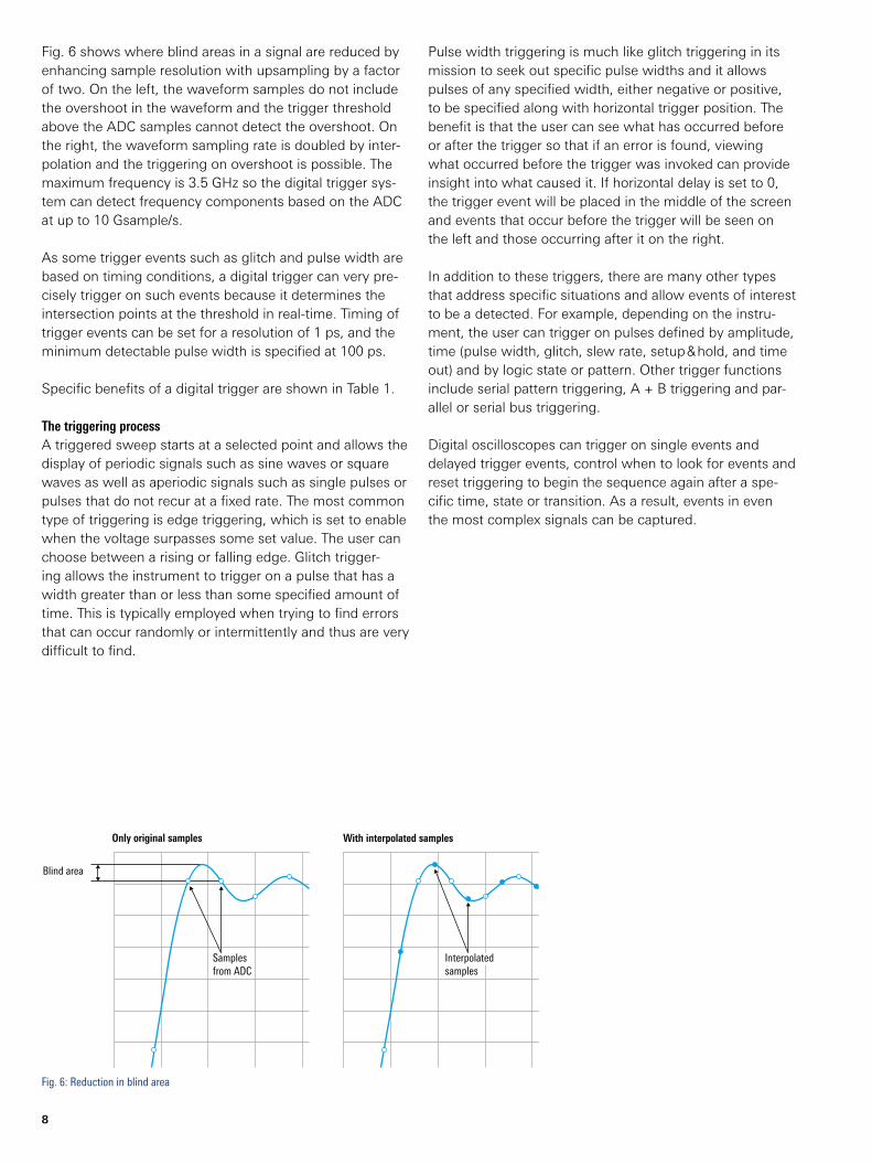
Fig. 6 shows where blind areas in a signal are reduced by enhancing sample resolution with upsampling by a factor of two. On the left, the waveform samples do not include the overshoot in the waveform and the trigger threshold above the ADC samples cannot detect the overshoot. On the right, the waveform sampling rate is doubled by inter-polation and the triggering on overshoot is possible. The maximum frequency is 3.5 GHz so the digital trigger sys-tem can detect frequency components based on the ADC at up to 10 Gsample/s.

As some trigger events such as glitch and pulse width are based on timing conditions, a digital trigger can very pre-cisely trigger on such events because it determines the intersection points at the threshold in real-time. Timing of trigger events can be set for a resolution of 1 ps, and the minimum detectable pulse width is specified at 100 ps.

Specific benefits of a digital trigger are shown in Table 1.

The triggering processA triggered sweep starts at a selected point and allows the display of periodic signals such as sine waves or square waves as well as aperiodic signals such as single pulses or pulses that do not recur at a fixed rate. The most common type of triggering is edge triggering, which is set to enable when the voltage surpasses some set value. The user can choose between a rising or falling edge. Glitch trigger-ing allows the instrument to trigger on a pulse that has a width greater than or less than some specified amount of time. This is typically employed when trying to find errors that can occur randomly or intermittently and thus are very difficult to find.

Fig. 6: Reduction in blind area


sometimes not simple so most instruments help make it easier with trigger hold off, which is an adjustable period of time after a trigger during which the oscilloscope can-not trigger and is useful when triggering on complex waveform shapes to ensure that the oscilloscope triggers only at the desired point.

The display system and user interfaceAs its name implies, the display system controls all aspects of the signal›s presentation to the user. The dis-play’s grid markings together form a grid called a grati-cule or reticle. Digital oscilloscopes and their tasks are complex, so the user interface must be extensive yet easy to understand. For example, the R&S®RTO series touch-screen display uses color-coded control elements, flat menu structures and keys for frequently-used functions. In the R&S®RTM series, a single button starts a quick mea-surement function that shows values for an active signal. Semi-transparent dialog boxes, movable measurement windows, a configurable toolbar and preview icons with live waveforms are available.

Digital oscilloscopes have trigger position control, which sets the horizontal position of the trigger in the waveform record. By varying it the user can capture what the sig-nal looked like before the trigger event. It determines the length of visible signal before and after the trigger point. The oscilloscope slope control adjusts where on the signal the trigger will take place (either the rising or falling edge).

Trigger modesThe trigger mode determines if and when the oscilloscope display´s a waveform. All oscilloscopes have two modes for triggering: a normal mode and an automatic (auto) mode. When set to normal mode, then oscilloscope will trigger only when the signal reaches a specific place on the signal. In auto mode, the instrument sweeps even if no trigger is set.

Trigger coupling and hold offSome oscilloscopes allow coupling (AC or DC) for select-ing the trigger signal and in some coupling for high fre-quency rejection, low-frequency rejection and noise rejection. The more advanced settings are designed to eliminate noise and other spectral components from the trigger signal to prevent false triggering. Ensuring the oscilloscope triggers on the right part of the signal is

Table 1: Digital trigger benefits

Low jitter in real-time

As identical sample values are used for both acquisition and trigger processing, very low trigger jitter (below 1 ps (RMS)) can be achieved. Unlike “software enhanced” trigger systems implemented using post-processing approaches, the digital trigger does not require additional blind time periods after every waveform acquisition. As a result, the R&S®RTO can attain a maxi-mum acquisition and analysis rate of 1 million waveforms/s.

Optimal trigger sensitivity

Analog trigger sensitivity is limited to greater than one vertical division and larger hysteresis can be selected with the instru-ment’s “noise reject” mode for stable triggering on noisy signals. However, a digital trigger allows individual setting of the trigger hysteresis from 0 to 5 divisions to optimize sensitivity for the respective signal characteristic. As a result, precise trig-gering down to 1 mV/div can be achieved with no bandwidth limitation.

No masking of trigger event

An analog trigger requires time after a trigger decision to rearm the trigger circuit before another trigger can occur. During this time, the oscilloscope cannot respond to new trigger events so they are masked. A digital trigger can evaluate individual trigger events within 400 ps intervals with a resolution of 250 fs.

Flexible filtering of trigger signals

An acquisition and trigger ASIC in the R&S®RTO instruments allows flexible programming of the cut-off frequency of a digital lowpass filter in the real-time path and is usable for the trigger signal, measurement signal, or both. Lowpass filtering on the trigger signal suppresses only high-frequency noise while capturing and displaying the unfiltered measurement signal.

Trigger recognition of channel deskew

The timing relationship between oscilloscope input channels is important for measurement and trigger conditions between two or more signals. Analog triggers provide a signal deskew feature to compensate for delays on different inputs, which is processed in the acquisition path after the ADC. As a result, it cannot be seen and inconsistent signals are thus displayed and evaluated by the trigger system. A digital trigger uses identical digitized and processed data so the waveforms seen at the display and the signals processed by the trigger unit are consistent even when channel deskew is applied.

10

An ideal probe is easy to connect, has reliable and safe contacts, does not degrade or distort the transmitted sig-nal, has linear phase behavior and no attenuation, an infi-nite bandwidth, high noise immunity and does not load the signal source. However, in practice all of these attri-butes are impossible and are actually more than most measurement situations require. In practice, the signal to be measured is often not easy to reach, its impedance can widely vary, the overall setup is sensitive to noise and fre-quency dependent, bandwidth is limited and differences in signal propagation create slight timing offsets (skew) between multiple measurement channels.

Fortunately, oscilloscope manufacturers go to great lengths to minimize probe problems and made them easier to connect to the circuit and more reliable once in place. For example, operating an oscilloscope with one hand while holding a probe in the other has always been challenging. The active probes for R&S®RTO oscilloscopes have a probe button allowing users to switch between oscilloscope functions and can be assigned to various functions. The instrument also has an integrated voltmeter called the R&S®ProbeMeter that allows precise DC mea-surements to be made that are more accurate than a tradi-tional oscilloscope channel.

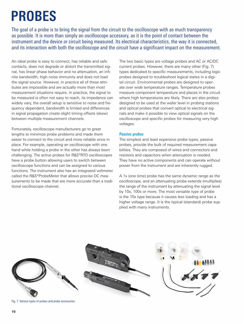
The two basic types are voltage probes and AC or AC/DC current probes. However, there are many other (Fig. 7) types dedicated to specific measurements, including logic probes designed to troubleshoot logical states in a digi-tal circuit. Environmental probes are designed to oper-ate over wide temperature ranges. Temperature probes measure component temperature and places in the circuit where high temperatures are likely. There are also probes designed to be used at the wafer level in probing stations and optical probes that convert optical to electrical sig-nals and make it possible to view optical signals on the oscilloscope and specific probes for measuring very high voltages.

Passive probesThe simplest and least expensive probe types, passive probes, provide the bulk of required measurement capa-bilities. They are composed of wires and connectors and resistors and capacitors when attenuation is needed. They have no active components and can operate without power from the instrument and are inherently rugged.

A 1x (one time) probe has the same dynamic range as the oscilloscope, and an attenuating probe extends (multiplies) the range of the instrument by attenuating the signal level by 10x, 100x or more. The most versatile type of probe is the 10x type because it causes less loading and has a higher voltage range. It is the typical (standard) probe sup-plied with many instruments.

PROBESThe goal of a probe is to bring the signal from the circuit to the oscilloscope with as much transparency as possible. It is more than simply an oscilloscope accessory, as it is the point of contact between the instrument and the device or circuit being measured. Its electrical characteristics, the way it is connected, and its interaction with both the oscilloscope and the circuit have a significant impact on the measurement.

Fig. 7: Various types of probes and probe accessories


Active probesThe advantages of active probes (Fig. 8) include low load-ing on the signal source, adjustable DC offset of the probe tip that allows high resolution on small AC signals that are superimposed on DC levels and automatic recognition by the instrument, eliminating the need for manual adjust-ment. Active probes are available in both single-ended and differential versions. Active probes use active components such as field effect transistors that provide very low input capacitance, which has benefits such as high input imped-ance maintained over a wide frequency range. They also make it possible to measure circuits where impedance is unknown and allow longer ground leads. As active probes have extremely low loading, they are essential when con-nected to high-impedance circuits that passive probes would unacceptably load.

However, the integrated buffer amplifier in active probes works over a limited voltage range and the active probe’s impedance is dependent on signal frequency. Even though they can be made to handle thousands of volts, active probes are still active devices and are not as mechanically rugged as passive probes.

Differential probesAlthough a separate probe for each signal could be used to probe and measure a differential signal, a differential probe is the best method. A differential probe uses a built in differential amplifier to subtract the two signals, there-fore consuming only one channel of the oscilloscope and also providing substantially higher common mode rejec-tion ratio (CMRR) performance over a wider range of fre-quency than single-ended measurements. Differential probes can be used for both single-ended and differential applications.

Current probesCurrent probes work by sensing the strength of an electro-magnetic flux field when current flows through a conduc-tor. This field is then converted to a corresponding voltage for measurement and analysis by an oscilloscope. When used in combination with an oscilloscope’s measurement and math capabilities current probes allow the user to make a variety of power measurements.

High-voltage probesThe maximum voltage for general-purpose passive probes is typically around 400 V. When very high voltages are encountered in a circuit ranging as high as 20 kV, there are probes dedicated to make it possible to safely measure them. Obviously, when making measurements at such high voltages, safety is the primary concern and this type of probe often accommodates it by having a much longer cable length.

A 1x passive, high impedance probe connected to the oscilloscope’s 1 MΩ input has high sensitivity (little attenu-ation). A 10:1 passive, high impedance probe that also connects to the 1 MΩ oscilloscope input, providing wide dynamic range, increased input resistance and low capaci-tance compared to the 1x probe. A 10:1 passive, low impedance probe connects to the 50 Ω oscilloscope input has little impedance variation over frequency but signifi-cantly loads the source because of nominal impedance of 500 Ω.

A 1x probe is desirable when the signal amplitude is low, but when the signal has a mixture of low and moderate amplitude components, a switchable 1x/10x probe is con-venient. The bandwidth of passive probes typically ranges from less than 100 MHz to 500 MHz. In the 50 Ω environ-ments encountered with high speed (high frequency) sig-nals, a 50 Ω probe is required and its bandwidth can be several gigahertz and its rise time 100 ps or even faster.

Passive probes include a low-frequency adjustment con-trol that is used when the probe is connected to the oscil-loscope. Low-frequency compensation matches the probe capacitance to the oscilloscope’s input capacitance. The high frequency adjustment control is used only for oper-ating frequencies above about 50 MHz. Vendor-specific passive probes for higher frequencies are adjusted at the factory so only the low-frequency adjustment must be performed. Active probes do not require these types of adjustments because their properties and compensation are determined at the factory.

Fig. 8: Active probes

5.00

5.50

6.00

6.50

7.00

7.50

0.5 1 2 3 4

Frequency of input signal in GHz

ENOB

in b

it

12

After the probes, the ADC is the first major oscilloscope component the measurement signal passes through, and how it acts on this signal determines how well the downstream processing elements perform. ADCs for oscilloscopes are generally built up from multiple con-verters that are interleaved in parallel and together com-prise the overall device. However, the alternative – using a single ADC has significant benefits and was chosen by Rohde & Schwarz for the R&S®RTO series.

Even when only a few converter cores are interleaved, it is essential that their noise, phase and frequency response characteristics vary as little as possible. In addition, inter-leave timing is critical when measurement intervals are tens of picoseconds and the sampling clock distributed to each converter must also have extraordinarily precise phase characteristics over the device’s entire frequency range, which is not a trivial challenge. Timing of each con-verter within the ADC varies to some degree with respect to the others, so if five converters are interleaved there will be five slightly different sampling clocks, the results of which show up in the frequency domain as components at the fundamental frequency.

These frequency components are typically 40 dB or 50 dB below full-scale (but nevertheless still clearly visible) and appear periodically so they cannot be averaged out like noise. They are caused either by timing, mismatched amplitudes or both. As they exist in both the frequency and time domains they can appear as noise because of the many harmonics at different frequencies that together appear as a random signal over time.

This is why some oscilloscope manufacturers use large numbers of converters, since together they produce results that look like noise and can be identified and miti-gated to some degree. However, the broadband data sig-nal input into an oscilloscope mixes with the spurious con-tent from these converters, producing additional spurious content. In short, the overall oscilloscope noise level (noise plus distortion) limits the number of effective bits that can be derived from an ADC. As interleaving of many convert-ers is a major contributor to noise level, the most obvious way to deal with it is to use one ADC rather than many.

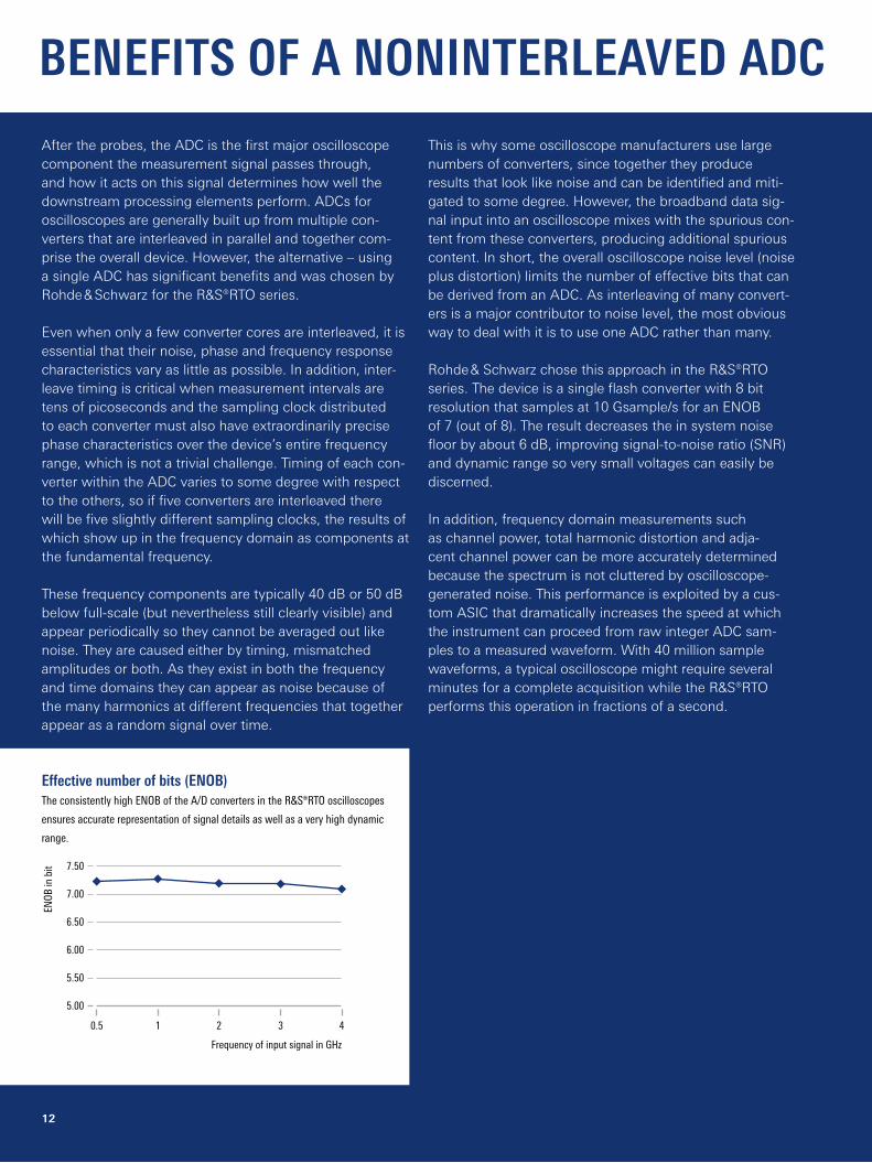
Rohde & Schwarz chose this approach in the R&S®RTO series. The device is a single flash converter with 8 bit resolution that samples at 10 Gsample/s for an ENOB of 7 (out of 8). The result decreases the in system noise floor by about 6 dB, improving signal-to-noise ratio (SNR) and dynamic range so very small voltages can easily be discerned.

In addition, frequency domain measurements such as channel power, total harmonic distortion and adja-cent channel power can be more accurately determined because the spectrum is not cluttered by oscilloscope-generated noise. This performance is exploited by a cus-tom ASIC that dramatically increases the speed at which the instrument can proceed from raw integer ADC sam-ples to a measured waveform. With 40 million sample waveforms, a typical oscilloscope might require several minutes for a complete acquisition while the R&S®RTO performs this operation in fractions of a second.

BENEFITS OF A NONINTERLEAVED ADC

Effective number of bits (ENOB)The consistently high ENOB of the A/D converters in the R&S®RTO oscilloscopes

ensures accurate representation of signal details as well as a very high dynamic

range.


Probe selection processTwo factors are important when choosing the right (volt-age) probe: the bandwidth required to capture the waveform without distortion and the desired minimum impedance to minimize circuit loading. The specified oscil-loscope bandwidth is valid only for a 50 Ω input imped-ance and a limited voltage input range. The instrument bandwidth must be at least five times the highest pulse frequency to be measured in order to preserve the har-monics and thus waveform integrity.

Specified DC impedance has little value for AC measure-ments. Over frequency, the impedance decreases, most dramatically for passive probes. When trying to keep the input impedance at least 10 times as high as the source impedance at the highest signal frequency, the choice between an active or passive probe is simple. This may narrow the choice to only one or two probe models that come closest to meeting the measurement setup require-ments. Active probes are mandatory to fully benefit from oscilloscope bandwidths in the microwave region.

Remember that low frequency impedance is highest in a 10x passive probe, and passive probes generally do not carry DC offsets or introduce noise. Active probes offer constant impedance at frequencies of hundreds of kilo-hertz and highest impedance up to several 100 MHz. Low-impedance probes offer constant impedance up to 1 GHz, and while impedance at one frequency may be desirable a constant but lower impedance prevents harmonic distor-tion of signals.

In short, active probes are recommended for signals with frequency components above 100 MHz and low input capacitance results in a higher resonance frequency. Connections to active probes must be as short as pos-sible for a high usable bandwidth. In addition, if the ground level appears unstable, a differential probe may be required.

With passive probes, it is important to use the model rec-ommended for the particular instrument in use, even if the probe has a higher bandwidth specification than seems necessary. Low input capacitance results in a higher reso-nance frequency. The ground lead should be short to mini-mize ground lead inductance. Be careful when measuring steep edge rise times, as the resonance frequency can be much lower than the system bandwidth. The probe’s impedance should be about ten times the circuit test point impedance as not to load the circuit too heavily.

Probe considerations

Circuit loadingThe most fundamental and important characteristic that the probe adds to the circuit is loading, either resistive, capacitive or inductive. Resistive loading attenuates ampli-tude, shifting DC offset and changing the circuit’s bias. Resistive loading is significant if the probe input resistance is the same as that of the signal being probed, as some of the current flowing in the circuit enters the probe. This reduces the voltage where the circuit meets the probe and cause a malfunctioning circuit to work properly but more often causes it to malfunction. To reduce the effect of resistive loading, use a probe with a resistance greater than 10 times that of the circuit under test.

Capacitive loading decreases the speed of rise time, reduces bandwidth and increases propagation delay. It is caused by the capacitance in the probe tip. It introduces frequency dependent measurement errors and is the greatest problem for delay and rise time measurements. Capacitive loading is caused by the probe’s capacitance acting as a lowpass filter at high frequencies, shunting the high frequency information to ground and significantly reducing probe input impedance at high frequencies. Probes with low capacitance tips are highly desirable.

Inductive loading distorts the measurement signal and is produced by the inductance of the loop between the probe tip to the probe ground lead. The ringing in the signal caused by inductive loading in the ground lead in conjunction with the probe tip capacitance can be miti-gated by effective grounding, This increases the ringing frequency beyond that of the instrument bandwidth. The length of the ground lead should always be as short as possible to reduce the loop size and minimize inductance. Lower inductance minimizes the ringing at the top of the measured waveform.

GroundingProper grounding is essential when making oscilloscope measurements for accuracy and operator safety, especially when working with high voltages. The instrument must be grounded via a power supply cord and must never be operated with the protective earth disconnected. This can result in unwanted low-frequency hum if the signal ground for the DUT is connected to the ground via the mains at a different location, causing a ground loop. Common prac-tice is to have the signal ground insulated from the mains ground and to create a connection to the signal ground close to the signal pin.

14

BandwidthMaximum bandwidth is the most important specification for every digital oscilloscope manufacturer and with good reason: It determines what frequency range the oscillo-scope can accurately measure. If the instrument band-width is inadequate for a specific application, the instru-ment is not an accurate, useful measurement device, since not enough content will be available to display the signal. Oscilloscope bandwidth is defined as the lowest frequency at which the input signal is attenuated by 3 dB, that is, where a sine wave signal would be attenuated to 70.7 % of its true amplitude.

Selecting the proper bandwidth for a given application can be difficult. Obviously, the simplest way to satisfy this requirement is to select an instrument with the high-est bandwidth. However, very high bandwidth oscillo-scopes can be prohibitively expensive. In addition, noise level increases and dynamic range decreases significantly with increased bandwidth. This can increase measure-ment uncertainty by as much as inadequate bandwidth. An oscilloscope with the least possible bandwidth for the applications and signals likely to be encountered is the best choice.

Oscilloscopes primarily measure digital pulses and a square wave is an ideal pulse with infinite bandwidth. The frequency spectrum of this signal consists of a signal at the fundamental frequency and odd harmonics. The ampli-tude of the harmonics follow a sin(x)/x function in fre-quency so the third harmonic is about 13.5 dB below the fundamental and the fifth harmonic is 27 dB below it. The next harmonic, the seventh, is 54 dB and below the noise floor of most oscilloscopes. A rule of thumb for choosing oscilloscope bandwidth is the so-called fifth harmonic rule and is based on the square wave spectrum. This rule often leads to excessive bandwidth choices.

The spectrum described above applies to a perfect square wave but all digital signals have a finite rise time that modifies the ideal square wave spectrum by reducing the amplitude of higher-order harmonics. In many cases, the level of the fifth harmonic is well below the noise floor of the oscilloscope and less bandwidth is adequate. This is typically true for signals with bandwidths of 3 Gbit/s and

higher such as serial data signals whose rise time rela-tive to bit interval is about 30 %. In this case, a bandwidth of less than five times the fundamental is acceptable for accurate measurements.

Achievable bandwidth is also directly affected by the probe, which is not an ideal device and thus has its own bandwidth that must be taken into consideration. The probe bandwidth should always be greater than the oscil-loscope bandwidth by a factor of about 1.5 times. A probe with a bandwidth of 1.5 GHz is required for full oscillo-scope performance. Greater probe bandwidth is important to ensure that the test signals are within the probe’s flat frequency response region. For a typical oscilloscope with a bandwidth of 1 GHz, this region would typically be one third of the maximum probe bandwidth specification or 300 MHz.

More specifically, most test signals are more complex than a simple sine wave and include various spectral compo-nents such as harmonics. To view digital signals, the oscil-loscope should provide about five times greater bandwidth than the clock frequency. For analog signals, the highest frequency of the device to which the oscilloscope is con-nected determines the required oscilloscope bandwidth.

Effective of number of bits (ENOB)Effective number of bits (ENOB) is a specification that can be confusing as it can refer to both the bits of reso-lution achievable by the ADC as well as the total effec-tive number of bits that it can achieve when part of a complete instrument. The first is invariably more than the second and neither specification is ever seen on an oscil-loscope data sheet. However, ENOB is a good acronym to know. ENOB is dictated by many factors, varies with frequency, frontend noise, harmonic distortion and inter-leaving distortion. Oscilloscope vendors tout the nearness of their ENOB to the raw value (such as over 7 out of 8 bits for the R&S®RTO) as it is not a trivial (see Benefits of a noninterleaved ADC on page 12).

OSCILLOSCOPE BENCHMARK SPECIFICATIONSAs with all electronic test equipment, digital oscilloscopes have an array of key specifications. Some are simple but others are either specified in various ways depending on the manufacturer or can be in some other way confusing. Consequently, the definitions below are largely generic.


an ASIC that runs multiple processes in parallel, which dramatically reduces blind time and enables analysis speed to approach 1 million waveforms/s, 20 times faster than other instruments.

Types of triggeringFortunately for oscilloscope buyers, most oscilloscopes come with a variety of traditional triggering capabilities as well as some dedicated to common applications. This is important as many types of triggering can be performed and some applications cannot be adequately addressed without them. Virtually every digital oscilloscope includes edge, glitch and pattern triggering. Mixed-signal oscillo-scopes make it possible to trigger across both logic and oscilloscope channels. Engineers working with common serial interface buses will require triggering protocols for SPI, UART/RS-232, CAN/LIN, USB, I2C, FlexRay™ and oth-ers, so potential triggering requirements are part of the oscilloscope specifications.

Rise timeThe vast majority of applications today require measure-ment of rise time, especially when measuring digital sig-nals that require very fast rise time measurements, making this metric is more important than ever. Oscilloscope rise time determines the actual useful frequency range it can achieve. An oscilloscope with a faster rise time can more accurately represent the details of high-speed transitions. When applied to a probe, its response to a step function indicates the fastest period the probe can transmit to the oscilloscope input. The general rule here is that accurate pulse rise and fall time measurements, the rise time speed of the complete system (oscilloscope and probe) should be three to five times that of the fastest transition.

Frequency responseFrequency response is one of many characteristics that determine digital oscilloscope performance but it is a major one – even though never included on oscilloscope manufacturer data sheets. It remains in the shadows mostly because a Gaussian frequency response shape was always assumed when oscilloscope and signal are analog. A digital oscilloscope can have maximally-flat, Chebyshev, Butterworth, Gaussian or other frequency response curves, and each type differently impacts the overshoot and ringing that cause errors in amplitude and rise time. So, understanding the this mystery specification is important.

All signals are the sum of sine waves at different frequen-cies and phases that appear in the frequency domain as spectral lines, each weighted separately by the oscillo-scope frequency response. Knowing how the frequency response weights each signal components would be bene-ficial, but the user can only guess, as only 3 dB bandwidth and rise time are specified on the data sheet.

ChannelsMost digital oscilloscopes once had 2 or 4 channels but today they can have 20, the result of the need to measure analog and complex digital signals. For the oscilloscope buyer, it is essential that the number of channels likely to be encountered is correctly estimated, as the alterna-tive is building external triggering hardware. When used in embedded debugging applications, mixed-signal oscil-loscopes will interleave 16 logic timing channels with the traditional 2 or 4 channels.

Sample rateThe oscilloscope sample rate is the number of samples acquired within 1 s and should be at least 2.5 times greater than the oscilloscope bandwidth. As the latest digi-tal oscilloscopes have extremely high sample rates and bandwidths in excess of 6 GHz, they are typically designed to accommodate high speed, single shot transient events. They do it by oversampling at rates greater than five times the stated bandwidth. While oscilloscope manufacturers specify a maximum sample rate for their instruments, it only possible when one or two channels are being used. If more channels are used simultaneously, the sample rate is likely to decrease. So the key determinant is how many channels can be used while maintaining the maximum sample rate for the instrument. As with any system where analog signals are converted to digital ones, the greater the sample rate, the greater the resolution and for digital oscilloscopes, the better the displayed results.

Memory depthThis specification is important because as sample rate increases, the amount of memory required to store cap-tured signals increases as well. The greater the instru-ment’s memory the more waveforms it can capture at its full sample rate. Generally speaking, long-term capture periods require significant memory depth but oscillo-scopes can suffer a significant drop in update rate when the deepest memory depth setting is selected.

While performing signal acquisition, conventional oscil-loscopes continuously save, process and display data. While all this is happening, the instrument is essentially blind to the characteristics of the signal being measured. At the highest sampling rates, blind time can actually be greater than 99.5 % of the entire acquisition time so mea-surements are only being made less than 0.5 % of the time, which hides signal faults. Perhaps the most criti-cal need for sufficient signal-capture memory is when an event occurs randomly or very infrequently. With too little memory, the likelihood that the event will not be captured rises dramatically. In addition to high-speed memory, oscil-loscopes such as the R&S®RTO series instruments employ

16

important as the characteristics of the device under test would otherwise be obscured, making accurate amplitude measurements impossible.

Gain (vertical) and timebase (horizontal) accuracyThe oscilloscope’s gain accuracy is the determinant of the precision with which its vertical system can vary the amplitude of the input signal, and horizontal accuracy defines the ability of its horizontal system to visualize sig-nal timing.

ADC vertical resolutionVertical resolution is a metric of the accuracy with which the ADC converts analog voltage to digital bits. For exam-ple, an 8 bit ADC converts a signal to 256 discrete volt-age levels that are distributed across the selected volt per division setting. With 1 mV/div, the least significant bit is 39 µV. This is different from effective number of bits as it does not account for nonideal characteristics within the ADC and the frontend of the oscilloscope.

Vertical sensitivityThe capability of the vertical amplifier to amplify the strength of the signal is called vertical sensitivity and is typically about 1 mV per vertical screen division. All oscil-loscopes do not have sensitivity as great as 1 mV per divi-sion and many rely on software to compensate, which reduces the oscilloscope’s effective number of bits. Bandwidth limiting is also sometimes used to address this shortcoming, especially at settings of lower voltage per division.

Every manufacturer has their own ideal for the frequency response curve. Some believe that a maximally-flat response provides the best results, since it does not devi-ate all the way to the instrument cutoff frequency and then drops off precipitously. The instrument frequency range to can also be extended for very sharp rolloff characteristics.

The maximally-flat frequency response requires signifi-cant tradeoffs. For example, a penalty is paid at the tran-sition frequency since there is no way a response can be perfectly flat and also transition without any bumps in the response at higher frequencies. Butterworth, Chebyshev and other types of responses also produce some irregular-ity in the passband, even with current state-of-the-art of digital filters.

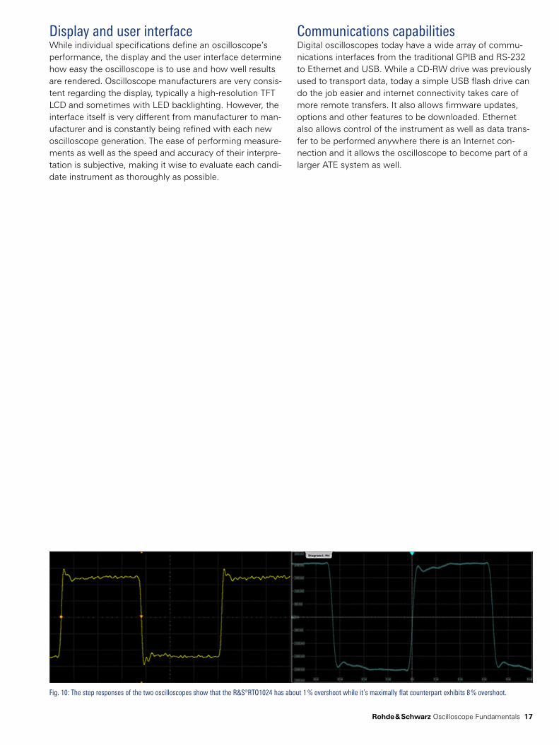
Rohde & Schwarz believes that the traditional Gaussian response represents the best trade-off between conflicting specifications and provides the best overall accuracy and the least ringing and overshoot. Uniquely, it can be real-ized in both the frequency and time domains and does not ring in either one. The frequency response of the R&S®RTO 2 GHz oscilloscope along with a maximally-flat response of a 4 GHz oscilloscope (Fig. 9) shows that the response of the R&S®RTO has nearly a textbook Gaussian form. Fig. 10 compares the step response of both oscilloscopes, the overshoot of the R&S®RTO is 1 % while the maximally-flat oscilloscope has 8 % overshoot. Adopting the Gaussian response requires a trade-off of a narrower 3 dB band-width because the response rolls off gradually. However, it has the highest accuracy (especially at signal edges), elim-inates ringing and has overshoot of less than 1 %, far lower than the industry average of 5 % to 10 % or more. The reduction in overshoot (the maximum amplitude excursion expressed as a percent of the final amplitude) is extremely

Fig. 9: The Gaussian frequency response curve of the R&S®RTO1024 (blue) and that of

maximally-flat oscilloscope (green) superimposed on an ideal Gaussian response (vio-

let) show how close the latter comes to an ideal response.


Display and user interfaceWhile individual specifications define an oscilloscope’s performance, the display and the user interface determine how easy the oscilloscope is to use and how well results are rendered. Oscilloscope manufacturers are very consis-tent regarding the display, typically a high-resolution TFT LCD and sometimes with LED backlighting. However, the interface itself is very different from manufacturer to man-ufacturer and is constantly being refined with each new oscilloscope generation. The ease of performing measure-ments as well as the speed and accuracy of their interpre-tation is subjective, making it wise to evaluate each candi-date instrument as thoroughly as possible.

Fig. 10: The step responses of the two oscilloscopes show that the R&S®RTO1024 has about 1 % overshoot while it’s maximally flat counterpart exhibits 8 % overshoot.

Communications capabilitiesDigital oscilloscopes today have a wide array of commu-nications interfaces from the traditional GPIB and RS-232 to Ethernet and USB. While a CD-RW drive was previously used to transport data, today a simple USB flash drive can do the job easier and internet connectivity takes care of more remote transfers. It also allows firmware updates, options and other features to be downloaded. Ethernet also allows control of the instrument as well as data trans-fer to be performed anywhere there is an Internet con-nection and it allows the oscilloscope to become part of a larger ATE system as well.

18

Voltage measurementsThe basic voltage measurement is actually only the fun-damental step allowing many other calculations to be performed. For example, measurement of peak-to-peak voltage (Vpp) is used to calculate the voltage difference between the low and high points of the waveform and measurements can also use RMS voltage for determining power levels.

Phase shift measurementsAn oscilloscope provides a convenient way to measure phase shift with a function called XY mode. It takes one input signal in the vertical system and another in the hori-zontal system. A Lissajous pattern results showing relative phases and frequencies of alternating voltages. The shape allows phase differences and frequency ratios between the two signals to be determined.

Time measurementsAn oscilloscope can be used to measure time on the hori-zontal scale, which is useful for evaluating pulse character-istics. Frequency is the reciprocal of a period, so once the period is known, frequency is then 1 divided by the period. The clarity of the information display can be improved by making the desired portion of the signal larger.

Pulse width and rise time measurementsEvaluation of the width and rise time of pulses is impor-tant in many applications as their critical characteristics can become corrupted, causing either degradation or complete failure in digital circuits. Pulse width is defined as the time required for the waveform to rise from 50 % of its peak-to-peak voltage to its maximum voltage and then back. Measurement of negative pulse width determines the time required for the waveform to decline from 50 % of its peak-to-peak value to a minimum point. The other parameter related to pulsed signals is rise time, which is defined as the time required for the pulse to go from 10 % to 90 % of full voltage. This industry standard ensures that variations in the pulse transition corners are eliminated.

Decoding serial busesDecoding of serial protocols, such as I2C, SPI, UART/RS-232, CAN, LIN and FlexRay™, is another common set of measurements often performed with an oscilloscope. These measurement capabilities are typically part of one or more oscilloscope software options that can be added as required.

Frequency analysis, statistics and math functionsIn addition to statistic functions such as histogram and mean and average values, the user can apply math func-tions to the measured signals. This makes waveform anal-ysis simpler by allowing the user to meaningfully display the results. By combining and transforming source wave-forms and other data into math waveforms, users can derive the data view that an application requires.

Most oscilloscopes have math functions for adding, sub-tracting, multiplying or dividing signals in the different channels. Other basic math functions include the Fourier transform for viewing the signal frequency composition on the display, and determining the absolute value to show the voltage value of the waveform.

TYPICAL OSCILLOSCOPE MEASUREMENTS Whether analog or digital, the oscilloscope is a versatile test instrument. Even though its basic function measuring and displaying voltages, it can do much more. In addition to the measurements below, many more are available for specific applications with application notes and other documents describing them available widely on the internet. They range from measurement automation described here, signal detection and analysis in commercial and defense systems and a wide array of others.


Mathematical operations, mask tests, histograms, spec-trum display and automatic measurements consume com-puting resources in software, increase blind time and slow instrument responses. Rohde & Schwarz uses its spectrum analysis hardware expertise by performing these func-tions in hardware and combining with low-noise frontends and the high number effective bits in the A/D converter for powerful FFT-based spectrum analysis.

The FFT function is fast and a high acquisition rate con-veys a live spectrum. Rapid signal changes, interference and weak superimposed signals are clearly visible.

In R&S®RTO instruments the mask testing functions were also implemented in hardware to preserve high acquisition rates, while recording a large enough number of wave-forms required to produce statistically relevant data. As stored waveforms are available for analysis, signal faults can be detected and their and their causes identified quickly with a high level of confidence.

20

An oscilloscope is a very versatile instrument used in a wide array of engineering environments. Generally speak-ing, the more effectively implemented the horizontal and vertical systems, the greater the signal fidelity. In addition, trigger flexibility allows the user to set up the oscilloscope with a way to capture signals that appear randomly and infrequently. A good probe or set of probes is essential to get the signal under test into the measurement system.

SUMMARYAs stated earlier, there are many applications for digital oscilloscopes, and their manufacturers invariably pro-vide application notes and other valuable documents that describe them. In addition, there is much more infor-mation that in some cases may be useful for each topic described in this document. As a result, once the oscil-loscope is purchased, one of the next steps should be to acquire as much information as possible about the specific applications the user is likely to encounter.


AAcquisition mode: They way waveform points are created from sample points. Standard modes include sample, peak-detect, high-resolution, average and envelope.

Analog-to-digital converter (ADC): The device and the oscilloscope that converts analog input signals to digital bits, the effectiveness of which determines what performance the oscilloscope can achieve.

Analog signal: A continuous electrical signal that varies in amplitude or frequency in response to changes in voltage.

Averaging: A technique performed by digital signal processing in an oscilloscope that can reduce the noise in the signal and on the display.

BBandwidth: The frequency range of the oscilloscope constrained by the point at which its response is reduced by 3 dB (thus 3 dB bandwidth).

CCircuit loading: The consequence of the probe interacting with the device or circuit under test, the degree of which determines the probe’s transparency to both the instrument and the circuit.

DDigital signal: A signal whose information is a string of bits in contrast with an analog signal that is a continuous range of voltages.

Digital oscilloscope: An oscilloscope that converts an analog input signal to a digital representation of it by using an ADC.

Digital sampling oscilloscope: An oscilloscope that can analyze signals whose frequencies are higher than the instrument’s sampling rate.

Division: The vertical and horizontal lines on the oscilloscope’s display.

EEffective number of bits (ENOB): The actual number of bits in an ADC or digital oscilloscope and a determinant of resolution after converting an analog signal to the digital domain. In ADC, it is typically lower than the device’s stated number of bits.

Envelope: A signal’s highest and lowest points after having been captured over a large number of waveform repetitions.

GLOSSARY

22

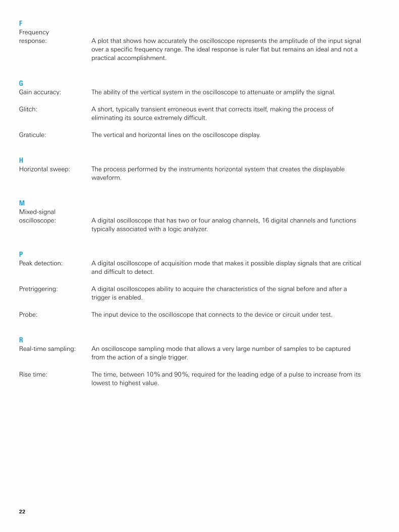
FFrequency response: A plot that shows how accurately the oscilloscope represents the amplitude of the input signal over a specific frequency range. The ideal response is ruler flat but remains an ideal and not a practical accomplishment.

GGain accuracy: The ability of the vertical system in the oscilloscope to attenuate or amplify the signal.

Glitch: A short, typically transient erroneous event that corrects itself, making the process of eliminating its source extremely difficult.

Graticule: The vertical and horizontal lines on the oscilloscope display.

HHorizontal sweep: The process performed by the instruments horizontal system that creates the displayable waveform.

MMixed-signal oscilloscope: A digital oscilloscope that has two or four analog channels, 16 digital channels and functions typically associated with a logic analyzer.

PPeak detection: A digital oscilloscope of acquisition mode that makes it possible display signals that are critical and difficult to detect.

Pretriggering: A digital oscilloscopes ability to acquire the characteristics of the signal before and after a trigger is enabled.

Probe: The input device to the oscilloscope that connects to the device or circuit under test.

RReal-time sampling: An oscilloscope sampling mode that allows a very large number of samples to be captured from the action of a single trigger.

Rise time: The time, between 10 % and 90 %, required for the leading edge of a pulse to increase from its lowest to highest value.


SSampling: The process of acquiring discrete samples of an input signal that are later converted to digital form, and then stored and processed by the oscilloscope.

Sample point: The data acquired by an ADC that is used to calculate waveform points.

Sample rate: The frequency with which a digital oscilloscope samples the signal, measured in sample/s.

Single shot: A transient event acquired by the oscilloscope that occurs only once in the signal stream.

Slope: The ratio of vertical to horizontal distance on the display and is positive when it increases from the left to right parts of the display and negative when it decreases.

TTimebase: Instrument circuitry that controls sweep timing.

Transient: Also known as a single-shot event, a transient is a signal that occurs only once during the signal capture.

Trigger: The oscilloscope subsystem that determines when to display the first instance of a signal.

Trigger hold-off: The user-defined minimum interval between triggers used when it is desirable to trigger on the start of a signal rather than an arbitrary part of the waveform.

Trigger level: The voltage level that the input signal must attain before a trigger is initiated.

VVertical resolution: The precision with which an ADC and an oscilloscope can convert an analog input signal to the digital domain.

Vertical sensitivity: The amount by which the vertical amplifier can amplify a signal.

WWaveform point: The voltage of the signal at a point in time calculated by sample points.

Service that adds value► Worldwide► Local and personalized► Customized and flexible► Uncompromising quality► Long-term dependability

3608

.272

0.62

02.

00 P

DP

/PD

W 1

en

R&S® is a registered trademark of Rohde & Schwarz GmbH & Co. KG Trade names are trademarks of the owners PD 3608.2720.62 | Version 02.00 | September 2021 (sk) Oscilloscope Fundamentals Data without tolerance limits is not binding | Subject to change© 2020 - 2021 Rohde & Schwarz GmbH & Co. KG | 81671 Munich, Germany

Sustainable product design ► Environmental compatibility and eco-footprint ► Energy efficiency and low emissions ► Longevity and optimized total cost of ownership

Certified Quality Management

ISO 9001

Rohde & Schwarz customer supportwww.rohde-schwarz.com/support

Rohde & SchwarzThe Rohde & Schwarz technology group is among the trail-blazers when it comes to paving the way for a safer and connected world with its leading solutions in test & measure-ment, technology systems, and networks & cybersecurity. Founded more than 85 years ago, the group is a reliable partner for industry and government customers around the globe. The independent company is headquartered in Munich, Germany and has an extensive sales and service network with locations in more than 70 countries. www.rohde-schwarz.com

Rohde & Schwarz trainingwww.training.rohde-schwarz.com

Certified Environmental Management

ISO 14001

3608272062

https://www.rohde-schwarz.com/support

https://www.rohde-schwarz.com/support

http://www.training.rohde-schwarz.com

© Rohde & Schwarz; Oscilloscope Fundamentals – Primer

Documents

Transcript of © Rohde & Schwarz; Oscilloscope Fundamentals – Primer