A CALDERÓN MULTIPLICATIVE PRECONDITIONER FOR COUPLED SURFACE-VOLUME ELECTRIC FIELD INTEGRAL EQUATIONS

Hakan Bağcı(1), Francesco P. Andriulli(2), Kristof Cools(3), Femke Olyslager(3), and Eric Michielssen(1)

(1) Radiation Laboratory, Department of Electrical Engineering and Computer Science, University of Michigan, Ann Arbor, MI

(2) Antenna and EMC Lab, Electronics Department, Politecnico di Torino, Torino, Italy

(3) Electromagnetics Group, Department of Information Technology, Ghent University, Ghent, Belgium

Email: bagci@umich.edu

Abstract

A well-conditioned coupled set of surface (S) and volume (V) electric field integral equations (S-

EFIE and V-EFIE) for analyzing wave interactions with densely discretized composite structures

is presented. Whereas the V-EFIE operator is well-posed even when applied to densely

discretized volumes, a classically formulated S-EFIE operator is ill-posed when applied to

densely discretized surfaces. This renders the discretized coupled S-EFIE and V-EFIE system ill-

conditioned, and its iterative solution inefficient or even impossible. The proposed scheme

regularizes the coupled set of S-EFIE and V-EFIE using a Calderόn multiplicative preconditioner

(CMP)-based technique. The resulting scheme enables the efficient analysis of electromagnetic

interactions with composite structures containing fine/subwavelength geometric features.

Numerical examples demonstrate the efficiency of the proposed scheme.

Keywords: surface electric field integral equation, volume electric field integral equations,

multiplicative preconditioning, Calderón preconditioning

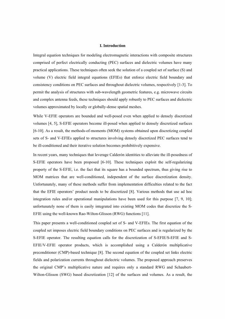
I. Introduction

Integral equation techniques for modeling electromagnetic interactions with composite structures

comprised of perfect electrically conducting (PEC) surfaces and dielectric volumes have many

practical applications. These techniques often seek the solution of a coupled set of surface (S) and

volume (V) electric field integral equations (EFIEs) that enforce electric field boundary and

consistency conditions on PEC surfaces and throughout dielectric volumes, respectively [1-3]. To

permit the analysis of structures with sub-wavelength geometric features, e.g. microwave circuits

and complex antenna feeds, these techniques should apply robustly to PEC surfaces and dielectric

volumes approximated by locally or globally-dense spatial meshes.

While V-EFIE operators are bounded and well-posed even when applied to densely discretized

volumes [4, 5], S-EFIE operators become ill-posed when applied to densely discretized surfaces

[6-10]. As a result, the methods-of-moments (MOM) systems obtained upon discretizing coupled

sets of S- and V-EFIEs applied to structures involving densely discretized PEC surfaces tend to

be ill-conditioned and their iterative solution becomes prohibitively expensive.

In recent years, many techniques that leverage Calderόn identities to alleviate the ill-posedness of

S-EFIE operators have been proposed [6-10]. These techniques exploit the self-regularizing

property of the S-EFIE, i.e. the fact that its square has a bounded spectrum, thus giving rise to

MOM matrices that are well-conditioned, independent of the surface discretization density.

Unfortunately, many of these methods suffer from implementation difficulties related to the fact

that the EFIE operators’ product needs to be discretized [8]. Various methods that use ad hoc

integration rules and/or operational manipulations have been used for this purpose [7, 9, 10];

unfortunately none of them is easily integrated into existing MOM codes that discretize the S-

EFIE using the well-known Rao-Wilton-Glisson (RWG) functions [11].

This paper presents a well-conditioned coupled set of S- and V-EFIEs. The first equation of the

coupled set imposes electric field boundary conditions on PEC surfaces and is regularized by the

S-EFIE operator. The resulting equation calls for the discretization of S-EFIE/S-EFIE and S-

EFIE/V-EFIE operator products, which is accomplished using a Calderόn multiplicative

preconditioner (CMP)-based technique [8]. The second equation of the coupled set links electric

fields and polarization currents throughout dielectric volumes. The proposed approach preserves

the original CMP’s multiplicative nature and requires only a standard RWG and Schaubert-

Wilton-Glisson (SWG) based discretization [12] of the surfaces and volumes. As a result, the

proposed preconditioner is easily implemented into existing MOM codes and the resulting solver

can trivially be accelerated via available fast matrix-vector multiplication methods including the

adaptive integral method (AIM) [13], multilevel fast multipole algorithm (MLFMA) [14, 15], and

their parallelized versions.

This paper is organized as follows. Section II formulates a coupled set of S- and V-EFIEs and

details its CMP-based discretization. Section III verifies the effectiveness of the proposed

regularization technique by applying it to structures with sub-wavelength features, viz., a

dielectric-filled waveguide slot antenna on a shuttle model and dielectric antennas with fine-

featured metallic feeds. Section IV presents conclusions and avenues for future research.

II. Formulation

This section describes the proposed CMP regularization technique for the coupled set of S- and

V-EFIEs. Section II-A formulates the set of S-EFIE and V-EFIE in surface current and electric

flux densities and details its standard MOM-based discretization. Section II-B describes the

proposed CMP regularizer.

A. Coupled Set of S- and V-EFIEs and its MOM Discretization

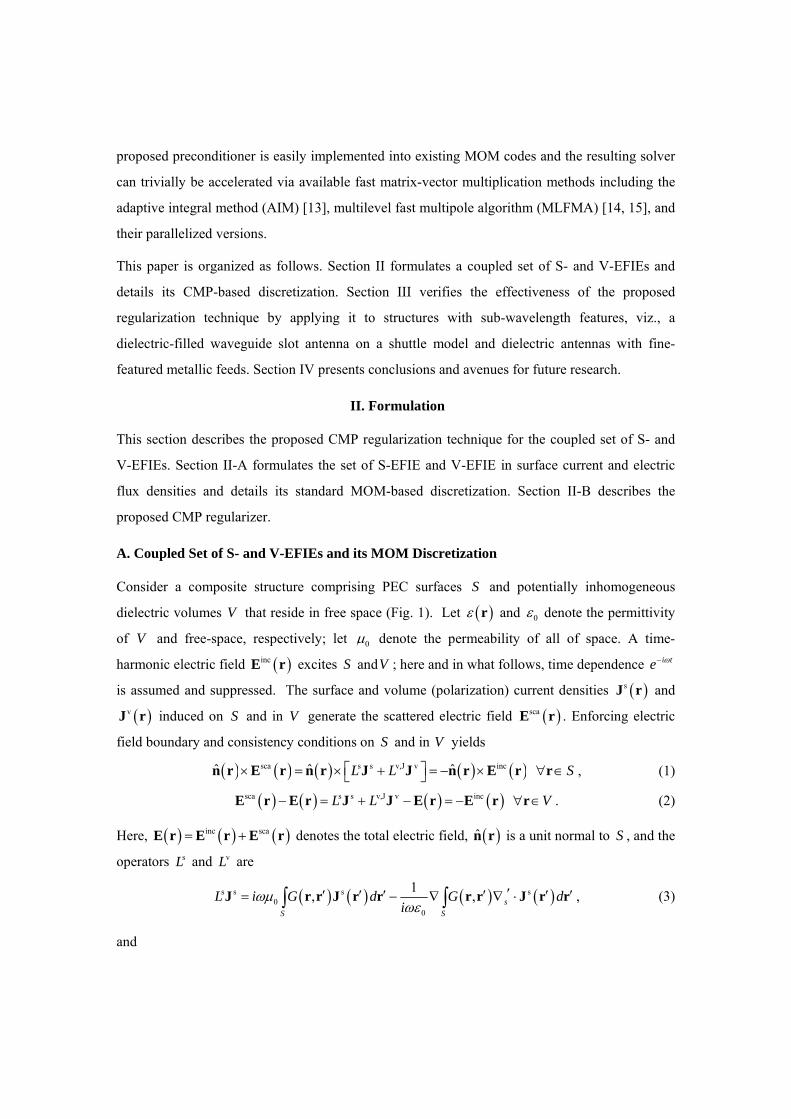
Consider a composite structure comprising PEC surfaces S and potentially inhomogeneous

dielectric volumes V that reside in free space (Fig. 1). Let r and 0 denote the permittivity

of V and free-space, respectively; let 0 denote the permeability of all of space. A time-

harmonic electric field incE r excites S andV ; here and in what follows, time dependence i te

is assumed and suppressed. The surface and volume (polarization) current densities sJ r and

vJ r induced on S and in V generate the scattered electric field scaE r . Enforcing electric

field boundary and consistency conditions on S and in V yields

sca s s v,J v incˆ ˆ ˆ L L S n r E r n r J J n r E r r , (1)

sca s s v,J v inc L L V E r E r J J E r E r r . (2)

Here, inc scaE r E r E r denotes the total electric field, n r is a unit normal to S , and the

operators sL and vL are

s s s s0

0

1, , s

S S

L i G d G di

J r r J r r r r J r r , (3)

and

v,J v v v0

0

1, ,

V V

L i G d G di

J r r J r r r r J r r . (4)

In (3) and (4), | |, 4 | |ikG e r rr r r r is the free-space Green function. In V , vJ r and

E r are related as

v ,i i t J r r D r r r E r V r , (5)

where 01 r r is the contrast parameter [12] and D r r E r is the electric flux

density. Inserting (5) into (1) and (2) yields the coupled set of S- and V-EFIEs in sJ r and

D r :

s s v,D incˆ ˆ L L S n r J D n r E r r , (6)

s s v,I inc L L V J D E r r . (7)

Here the operators v,DL and v,IL , which complement the operator v,JL , are

v,D0

0

1, ,

V V

L i G i d G i di

D r r r D r r r r r D r r , (8)

v,I v,DL L D D D r r . (9)

To numerically solve (6) and (7), S and V are approximated by meshes of planar triangles (with

smallest edge size s ) and tetrahedrons (with smallest edge size v ), and sJ r and D r are

approximated as

RWG

s RWG RWG

1

N

k k

k

I

J r f r , (10)

SWG

SWG SWG

1

N

k k

k

I

D r f r , (11)

where RWGkI , RWG1,...,k N and SWG

kI , SWG1,...,k N are unknown expansion coefficients,

RWGkf r , RWG1,...,k N are zeroth-order div-conforming RWG surface basis functions [Fig.

2(a)] [11] defined on pairs of triangles, and SWGkf r , SWG1,...,k N are zeroth-order div-

conforming SWG volume basis functions [12] defined on tetrahedron facets. To determine the

coefficients RWGkI and SWG

kI , (10) and (11) are inserted into (6) and (7), and the resulting

equations are tested by curl-conforming RWGˆkn r f r , RWG1,...,k N [Fig. 2(b)] and

SWGk r f r , SWG1,...,k N ; this produces the linear system of equations of dimension

RWG SWGN N

ZI V . (12)

Here I and V are vectors of expansion coefficients and tested incident fields, respectively; their

entries are

RWG

RWG RWG

SWG

,

, elsek

k

k N

I k N

I

I , (13)

RWG

RWG inc RWG

s

SWG inc

v

ˆ ˆ, ,

, , else

k

k

k N

k N

n r f r n r E rV

r f r E r, (14)

with s/v

/

,S V

d a r b r a r b r r . The impedance matrix Z in (12) can be decomposed as

RWG/RWG RWG/SWG

SWG/RWG SWG/SWG

Z ZZ

Z Z, (15)

where RWG/RWGZ , SWG/SWGZ , RWG/SWGZ , and SWG/RWGZ account for surface test-surface basis,

volume test-volume basis, surface test-volume basis, and volume test-surface basis interactions,

respectively. Their entries are

RWG/RWG RWG s RWG, s

ˆ ˆ,k k k kL Z n r f r n r f , (16)

SWG/RWG SWG s RWG, v

ˆ,k k k kL Z r f r n r f , (17)

RWG/SWG RWG v,D SWG, s

ˆ ,k k k kL Z n r f r f , (18)

SWG/SWG SWG v,I SWG, v

,k k k kL Z r f r f . (19)

When analyzing electrically large and/or complex structures, i.e., when RWG SWGN N is large,

(12) cannot be solved directly and iterative solves are called for. The computational cost of

solving (12) iteratively scales multiplicatively with the cost of applying the impedance matrix Z

to a trial solution vector and the number of iterations required to reach a specified residual. The

cost of a matrix-vector multiplication always can be reduced by using adaptive integral [13] or

multilevel fast multipole [14, 15] accelerators. The required number of iterations typically scales

with Z ’s condition number with small condition numbers guaranteeing fast convergence of the

iterative solver.

The conditioning of Z depends on the spectral properties of the S- and V-EFIE operators

sˆ Ln r and v,IL . The spectral properties of the S-EFIE operator are well-documented: it is

known that its singular values accumulate at zero and infinity as it contains a singular operator

(the first integral in (3), i.e., the vector potential contribution) and a hypersingular operator (the

second integral in (3), i.e. the scalar potential contribution) [6]; in other words, the S-EFIE

operator is unbounded. As a result, RWG/RWGZ is increasingly ill-conditioned when s 0 .

Unlike the S-EFIE operator, the V-EFIE operator’s spectrum is bounded [4, 5]. The scalar

potential contribution of the V-EFIE operator is Cauchy-singular (but not hypersingular) and its

dominant contribution results from a volume integral. It has been shown in [4, 5] that matrices

resulting from the discretization of V-EFIE operator are well-conditioned regardless of the

discretization density. This means that SWG/SWGZ is well-conditioned even when v 0 .

Unfortunately, RWG/RWGZ alone renders Z ill-conditioned and the iterative solution of (12)

prohibitively expensive or even impossible in the presence of dense discretizations.

B. Calderon Regularization and CMP-based Discretization of Hybrid Set of S- and V-EFIEs

The unbounded nature of the S-EFIE operator can be cured using the well-known Calderón

identity [16]

s s 1 1 1ˆ ˆ

4 2 2L L KK K K

n r n r . (20)

Here s s

s

ˆ ,K G d J n r r r J r r is a compact operator when acting on smooth surfaces

[6]; this makes s sˆ ˆL L n r n r a second kind operator. Therefore, (6) can be regularized

using sˆ Ln r and the set of equations

s s s s v,D s incˆ ˆ ˆ ˆ ˆ ˆ L L L L L S n r n r J n r n r D n r n r E r r , (21)

s s v,I inc L L V J D E r r , (22)

can be solved instead of the standard set (6) and (7).

The discretization of the operator products in (21) is by no means trivial. Various methods that

use ad hoc integration rules and/or operational manipulations for discretizing the operator product

s sˆ ˆL L n r n r have been proposed [7, 9, 10]; however none of these methods is easily

integrated into readily available MOM codes that discretize the standard S-EFIE using the well-

known RWG basis functions [11]. In this work, the CMP approach first proposed in [8] to

discretize Calderón-preconditioned S-EFIEs is used to discretize the operator products in (21).

The reader is referred to [8] for a detailed formal mathematical description of the CMP concept.

Consider the initial discretization of S comprised of planar triangles on which sJ r is expanded

in terms of standard div-conforming RWG functions, RWGkf r , RWG1,...,k N [see (10)]. A

barycentric mesh is obtained by adding the three medians to each triangle of the initial mesh; on

the edges of this barycentric mesh a new set of RWG basis functions BRWGkf r ,

BRWG RWG1,..., 6k N N and Buffa-Christiansen (BC) basis functions [17] BCkf r ,

BC RWG1,...,k N N [Fig. 2(c)] are defined. BC basis functions BCkf r are linear combinations

of BRWGkf r and they are div- and quasicurl-conforming. Note that BCˆ kn r f r are curl- and

quasidiv-conforming [Fig. 2(d)] [17]. These properties render the Gram matrix, which links

spaces discretized by quasicurl-conforming BCkf r and curl-conforming RWGˆ kn r f r , well

conditioned [8]. In the operator product s sˆ ˆL L n r n r , the source and test spaces of the

right S-EFIE operator sˆ Ln r are discretized using RWGkf r and RWGˆ kn r f r , respectively.

The source and test spaces of the left S-EFIE operator sˆ Ln r are discretized using BCkf r and

BCˆ kn r f r , respectively. Similarly, in the operator product s v,Dˆ ˆL L n r n r , the source

and the test spaces of the operator v,Dˆ Ln r are discretized using SWGkf r and RWGˆ kn r f r

, respectively. The left S-EFIE operator sˆ Ln r is discretized as above. These choices of basis

and testing functions render the Gram matrices linking the source space of sˆ Ln r to the test

spaces of sˆ Ln r and v,Dˆ Ln r well-conditioned. The discretized operator products are

expressed as

s s BC/BC 1 RWG/RWG

disˆ ˆL L n r n r Z G Z , (23)

s v,D BC/BC 1 RWG/SWG

disˆ ˆL L n r n r Z G Z . (24)

The entries of the impedance matrices RWG/RWGZ and RWG/SWGZ are given by (16) and (18) while

those of the impedance matrix BC/BCZ and Gram matrix G are

BC/BC BC s BC, s

ˆ ˆ,k k k kL Z n r f r n r f , (25)

and

RWG BC, s

ˆ ,k k k k G n r f r f r . (26)

Note that if one would use div- and curl-conforming RWGs to discretize the source and test

spaces of sˆ Ln r and test space of v,Dˆ Ln r , the Gram matrix

RWG RWG, s

ˆ ,k k k k G n r f r f r would be singular [8]. Let RWGX , BRWGX , and BCX denote

the spaces spanned by RWGkf r , BRWG

kf r , and BCkf r , respectively. Upon constructing

transformation matrices P and R that express basis functions in BCX and RWGX as linear

combinations of those in BRWGX , (23) can be rewritten using only two impedance matrices of the

same type, viz. BRWG/BRWGZ , as

s s BRWG/BRWG 1 T BRWG/BRWG

disˆ ˆ TL L n r n r P Z PG R Z R , (27)

where and the entries of the impedance matrix BRWG/BRWGZ are

BRWG/BRWG BRWG s BRWG, s

ˆ ˆ,k k k kL Z n r f r n r f . (28)

Because only the barycentric mesh (and not the initial one) is supplied to the code, (24) is

replaced with the discretization

s v,D BRWG/BRWG 1 T BRWG/SWG

disˆ ˆ TL L n r n r P Z PG R Z , (29)

where the entries of the impedance matrix BRWG/SWGZ are

BRWG/SWG BRWG v,D SWG, v

ˆ ,k k k kL Z n r f r f . (30)

The discretization of the operator sL in (22) can be achieved classically using RWGkf r and

SWGk r f r . However this is not done directly but using BRWG

kf r and SWGk r f r since

only the barycentric mesh (and not the initial one) is supplied to the code. In other words,

s SWG/RWG SWG/BRWG

disL Z Z R , (31)

where the entries of the impedance matrix SWG/BRWGZ are given by

SWG/BRWG SWG s BRWG, v

,k k k kL Z r f r f . (32)

The discretization of the operator v,IL in (22) is unchanged:

v,I SWG/SWG

disL Z . (33)

The entries of the impedance matrix SWG/SRWGZ are given by (19).

The impedance matrices BRWG/BRWGZ , BRWG/SWGZ , SWG/BRWGZ , and SWG/SRWGZ are trivially

computed using existing MOM codes that use RWG and SWG basis functions. Explicit

expressions of the elements of the matrices P and R can be found in [8].

Inserting (27), (29), (31), and (33) into (21) and (22) discretizing the right hand sides, rearranging

the resulting equations, and applying diagonal preconditioning yields

1BRWG T TB B

SWG

1BRWG T TB B

SWG

P 0 0 0 G 0 R 0D 0 P 0 R 0Z Z I

0 0 0 1 0 1 0 10 D 0 0 0 1

P 0 0 0 G 0D 0 P 0 R 0Z V

0 0 0 1 0 10 D 0 0 0 1

. (34)

Here, the impedance matrix BZ is

BRWG/BRWG BRWG/SWG

B

SWG/BRWG SWG/SWG

Z ZZ

Z Z, (35)

the entries of the matrices BRWGD and SWGD are

SWG

SWG ,,

1 ,

0 elsek k

k k

k k

ZD , (36)

,BRWG,

1 ,

0 elsek k

k k

k k

GD , (37)

the entries of the right hand side vector BV are

BRWG

BRWG inc BRWG

sBk SWG inc

v

ˆ ˆ, ,

, , else

k

k N

k N

n r f r n r E rV

r f r E r, (38)

and I is the vector of unknown coefficients [see (13)]. Note that multiplication with SWGD

properly scales the entries of SWG SWGD Z and multiplication with BRWGD renders BRWG BC/BC 1 RWG/RWGD Z G Z well-conditioned [8] in the presence of multiscale discretizations.

Matrix equation (34) is solved for I iteratively; the number of iterations is independent of the

smallest edge sizes s and v as demonstrated in Section III. The computational cost of solving

(34) is that of performing the matrix-vector multiplications on its left hand side, times the number

of iterations. The cost of multiplying the sparse matrices P , R , and G by a vector scales as only

RWGO N . (Note that inversion of the sparse Gram matrix G is never carried out explicitly;

whenever the matrix-vector product 1G y is needed, it is computed via the iterative solution of

the linear system BRWG BRWGD Gx D y , which only requires a few iterations [8].) The dominant

computational cost at a given iteration is then due to the multiplication of BZ with a vector,

which can be reduced using various acceleration techniques [13-15]. In this work, AIM [13] is

used to for this purpose. Let C and BC represent the costs of multiplying Z and BZ by a

vector; then CMP CMP CMPc c c clog logC C N N N N , where 3

c c1N and

3CMP CMPc c1N are the numbers of nodes on the three dimensional (3-D) auxiliary AIM grid

that encloses the composite structure and is used for accelerating the multiplication of Z and BZ

by a vector, respectively. Here, c and CMPc are the AIM grid sizes (i.e. AIM node spacing);

they are assumed identical along the x , y , and z directions. As a rule of thumb, avec c and

CMP CMP,avec c , where ave

c and CMP,avec are the average edge sizes in the (combined) initial

surface and volume meshes, and the (combined) barycentric surface and volume meshes,

respectively. Ignoring the cost of operations associated with the multiplication of the sparse

matrices, the total cost of solving (12) is TOT iterC N C , while the cost of solving (34) is CMP CMP CMPTOT iter2C N C . Here CMP

iterN and iterN are the numbers of iterations required for the relative

residual error of the solutions of (12) and (34) to reach a certain treshhold. By comparing CMPTOTC

to TOTC , it is concluded that the iterative solution of (34) will be faster than that of (12) as long

as 3CMP CMP,ave ave CMP,ave aveiter iter c c c c0.5 log logN N . The ratio CMP,ave ave

c c is always

smaller than 1 (because of the barycentric division of the surface discretization) but typically

larger than 0.5 (because of the presence of the volumetric mesh).

A more efficient but less trivial implementation is possible. Inserting (23), (24), (31) and (33) into

(21) and (22), discretizing the right hand sides, and applying diagonal preconditioning yields

1 1BRWG BC/BC BRWG BC/BC

SWG SWG

G 0 G 0D 0 Z 0 D 0 Z 0ZI V

0 1 0 10 D 0 1 0 D 0 1. (39)

Solution of (39) using an existing MOM code is far less trivial than that of (34) since now BC/BCZ

needs to be computed explicitly. Additionally, one needs to modify the AIM accelerator to allow

for the fast multiplication of BC/BCZ by a vector. Assuming such an AIM accelerator is

constructed, it can use the same auxiliary grid used for accelerating the matrix-vector

multiplication associated with Z since the support of BC basis functions is (roughly) the same as

that of RWG basis functions defined on the standard mesh (i.e. node spacing needed for auxiliary

AIM grids is the same). This means that the cost of solving (39) is CMP CMPTOT iter iter TOTC N N C ,

where depends on what ratio of the AIM’s grid encloses the PEC surfaces; is at most 2 (This

happens when the structure consists of only PEC surfaces). It is clear from this discussion that the

iterative solution of (39) is faster than that of (12) as long as CMPiter iterN N is satisfied. Numerical

results show that this is satisfied even for moderately dense discretizations.

III. Numerical Results

In this section, the proposed method is applied to the analysis of scattering from spheres and a

shuttle loaded with a dielectric-filled waveguide slot antenna, and radiation from dielectric

antennas inclusive their PEC feeds. The results presented here were obtained using a parallel and

AIM-accelerated MOM code that uses a transpose-free quasi-minimal residual iterative scheme

[18] to solve matrix equations (34) and (12); a diagonal preconditioner is used for (12). All

simulations were carried out on a cluster of dual-core 2.8-GHz AMD Opteron 2220 SE

processors at the Center for Advanced Computing, University of Michigan.

A. Scattering from Spheres

I. PEC and Dielectric Spheres

Consider the two adjacent spheres, one PEC and the other dielectric, shown in Fig. 3(a). The PEC

and dielectric spheres are centered about the origin and 2.5 m,0,0 , respectively; both spheres

have radius 1 m . The dielectric constant of the dielectric sphere is 04.0 r . The spheres are

excited by a y polarized plane wave propagating in the z direction. The frequency of excitation

is 15 MHzf ( 19.986 m ). The simulation is repeated for seven different discretizations

with smallest edge sizes ranging from s v 14.383 cm to s v 1.1264 cm . Table I

presents the number of RWGs ( RWGN ) and SWGs ( SWGN ) for all models analyzed. Fig. 3(b)

presents the number of iterations required (for the relative residual error of the solutions of (34)

and (12) to reach 610 ) versus s v . As expected, the number of iterations required for the

solution of (34) is independent of the discretization density; it is roughly 25 . For the simulation

with the densest discretization density ( s v 1.1264 cm ) measured CPU times indicated that

the iterative solution of (34) was approximately 6.9 times faster than that of (12). Fig. 3(c)

presents the spheres’ radar cross sections (RCSs) computed on the o0 and o90 planes

after solving (34) or (12) using the s v 4.7456 cm mesh. The relative L2 norms of the

difference between the RCS results on the o0 and o90 planes are 0.0221 % and

0.0164 % , respectively.

II. Dielectric Coated PEC Sphere

The proposed method is used to analyze scattering from a dielectric-coated PEC sphere centered

at the origin; the radius of the sphere and the thickness of the dielectric shell are 1 m and 0.2 m ,

respectively [Fig. 4(a)]. The dielectric constant of the shell is 04.0 r . The sphere is excited

by the plane wave used in Section II-A.I. Similarly, the simulation is repeated for seven different

discretizations with smallest edge sizes changing from s v 14.383 cm and s v 1.1264 cm . Table II presents RWGN and SWGN for all discretizations. Fig. 4(b) presents

the number of iterations required (for the relative error of the solutions of (34) and (12) to reach 610 ) versus s v . The number of iterations required for the solution of (34) is constant and

hovers around 24 . For the simulation with the densest discretization density (s v 1.1264 cm ) measured CPU times indicated that the iterative solution of (34) was

approximately 11.2 times faster than that of (12). Fig. 4(c) shows that the solutions of (34) and

(12) for the simulation with 6.9214 cms v are practically the same; the relative norm of

the difference between both solutions is 0.1874 % .

B. Scattering from a Space Shuttle Model

The proposed technique is used to analyze low-frequency scattering from a shuttle model with a

dielectric-filled slot waveguide mounted on its side. The shuttle model is excited by a x polarized

plane wave propagating in the ˆz direction at 26.4 MHzf ( 11.356 m ). The length,

width, and height of the shuttle are 3.6520 , 2.3445 , and 1.3989 , respectively [Fig. 5(a)]. A

slot-waveguide antenna, which is filled with dielectric with 04.0 r , is located on the side of

the shuttle [Fig. 5(b)]. The width and height of the slot and the length of the waveguide are

/150.09 , / 32.792 , and / 50.032 , respectively. The multiscale discretization of the shuttle

and the waveguide surfaces is shown in Fig. 5(c). For this mesh the largest, average, and the

smallest element sizes are 1.1400 m ( /9.96108 ), 0.35120 m ( /32.3339 ), 1.0589 cm (

/1072.45 ), respectively; also RWG 29 409N , and SWG 5022N . The iterative solver required

274 and 7396 iterations for the relative residual error of the solutions of (34) and (12) to reach 610 , respectively [Fig. 5(d)]. Measured CPU times indicated that the iterative solution of (34)

was approximately 2.4 times faster than that of (12). The relative L2 norm of the difference

between the two solutions is 0.2168 % . Fig. 5(d) shows three different views of the magnitude of

the current induced on the shuttle’s surface.

C. Radiation from a Hemispherical Dielectric Resonator

Consider the hemispherical dielectric resonator antenna (with an air gap) shown in Figs. 6 (a)-(c).

The dielectric constant of the hemispherical shell is 08.9 r . The resonator is excited by a

feed probe at 2.0 GHzf ( 0.14989 m ). The multiscale nature of the spatial mesh around

the feed probe is highlighted in Fig. 6 (d). The fine discretization around the feed is called for to

properly model the curvature of the feed probe and the distribution of fields around it. For this

discretization, the largest, average, and the smallest element sizes are 4.46694 mm ( /33.5567 ),

1.11553 mm ( /134.372 ), and 0.124458 mm ( /1204.39 ), respectively; also RWG 43 943N

and SWG 166 953N . The iterative solver required 737 and 11 675 iterations for the relative

residual error of the solutions of (34) and (12) to reach 610 , respectively [Fig. 6 (e)]. Measured

CPU times indicated that the iterative solution of (34) was approximately 3.6 times faster than

that of (12). The relative L2 norm of the difference between the two solutions is 0.8325 % . Fig. 6

(e) shows the normalized radiated field patterns (on the xz and yz planes) obtained from the

solutions of (12) and (34).

D. Radiation from a Dielectric Rod Antenna

Finally, the proposed method is used to analyze radiation from a dielectric rod antenna [Figs. 7

(a)-(d) [19], with 02.1 r . The end of the rod is coated with an antireflective dielectric layer,

with 01.45 r . The antenna is fed by a rectangular PEC waveguide and the waveguide is

excited by a feed probe at 9.0 GHzf ( 3.33102 cm )[19]. Similar to the previous example,

the surface of the feed probe and the waveguide surfaces near to the probe are densely

discretized. For this simulation the largest, average, and smallest element sizes are 2.89224 mm (

/11.5171 ), 1.48322 mm ( / 22.4579 ), and 0.044623 mm ( / 746.480 ), respectively; also RWG 44 692N and SWG 293 737N . The iterative solver required 659 and 14 633 iterations

for the relative residual error of the solutions of (34) and (12) to reach 610 , respectively [Fig. 7

(e)]. Measured CPU times indicated that the iterative solution of (34) was approximately 6.5

times faster than that of (12). The relative norm of the difference between the two solutions is

0.9152 % . Fig. 7 (f) shows that the normalized radiated field pattern (on xz plane) obtained from

the solution of (34) agrees well with that computed using the imaginary-distance beam-

propagation method [19].

IV. Conclusion

This paper presented a CMP-based regularizer for a coupled set of S- and V-EFIEs pertinent to

the analysis of densely discretized hybrid PEC-dielectric structures. The proposed technique

combines a CMP for the S-EFIE and a diagonal preconditioner for the V-EFIE. Just like in the

original CMP, the preconditioner presented herein is multiplicative and easily integrated into

available MOM codes that discretize S- and V-EFIEs using RWG and SWG basis functions,

respectively. The proposed preconditioner is used in conjunction with an existing parallel and

AIM accelerated MOM code. The numerical results obtained using this code confirmed the

effectiveness of the proposed technique and its applicability to the electromagnetic

characterization of composite structures with sub-wavelength features.

Acknowledgments

Authors would like to thank Mr. Felipe Valdés for his help in preparing meshes for the

hemispherical dielectric resonator and the dielectric rod antenna.

This work was supported by the Air Force Office of Scientific Research under Grant MURI

F014432051936 and by the National Science Foundation under Grant DMS 0713771.

Figure Captions

Figure 1: Description of scattering problem involving an abstract composite structure.

Figure 2: Basis functions used in the discretization of S-EFIE. (a) Div-conforming RWG basis

function, RWGkf r , (b) curl-conforming RWG basis function, RWGˆ kn r f r , (c) div- and

quasicurl-conforming BC basis function BCkf r , (d) curl- and quasidiv-conforming BC function,

BCˆ kn r f r .

Figure 3: Analysis of scattering from PEC and dielectric spheres. (a) Geometry and excitation

description. (b) Number of iterations required for the relative residual error of the solutions of

(34) and (12) to reach 610 , versus s v . (c) Comparison of RCS obtained on o0 and o90 planes after solving (34) and (12).

Figure 4: Analysis of scattering from a dielectric-coated PEC sphere. (a) Geometry and excitation

description. (b) Number of iterations required for the relative residual error of the solutions of

(34) and (12) to reach 610 , versus s v . (c) Comparison of solutions of (34) and (12).

Figure 5: Analysis of scattering from a shuttle model with a dielectric-filled slot waveguide

mounted on its fuselage. (a) Geometry and excitation description. (b) The multiscale

discretization of the shuttle and the waveguide surfaces. (c) Relative residual error obtained

during the iterative solution of (34) and (12). (d) Current density induced on surfaces of the

shuttle and the waveguide decibel scale.

Figure 6: Analysis of radiation from a hemispherical dielectric resonator. View of the geometry

from (a) top and (b) bottom. (c) Cross section of the geometry (dimensions are in cm). (d)

Multiscale surface mesh of the geometry (zoomed to the feed probe). (e) Relative residual error

obtained during the iterative solution of (34) and (12). (f) Normalized field patterns computed on

xz and yz planes.

Figure 7: Analysis of radiation from a dielectric rod antenna. (a) Isometric view of the whole

geometry. (b) View of the metallic feed (dimensions are in mm). (c) View of the antireflective

dielectric layer (dimensions are in mm). (d) Cross section of the whole geometry (dimensions are

in mm). (e) Relative residual error obtained during the iterative solution of (34) and (12). (f)

Normalized field patterns computed on xz plane.

Tables

Table I. The numbers of standard RWGs ( RWGN ) and SWGs ( SWGN ) for all seven

discretizations.

s v ( cm ) RWGN SWGN 14.383 1062 4634 11.092 1926 9786 6.9214 3960 24082 4.7456 7632 54232 2.9893 16560 135677 1.7720 67464 652352 1.1264 136923 1393460

Table II. The numbers of standard RWGs ( RWGN ) and SWGs ( SWGN ) for all seven

discretizations.

s v ( cm ) RWGN SWGN 14.383 1062 5962 11.092 1926 11172 6.9214 3960 37014 4.7456 7632 87324 2.9893 16560 261954 1.7720 67464 1419176 1.1264 136923 2747863

Figures

Figure 1

Figure 2(a)

0 0

V

S

sJ r

vJ r

incE r

k

r 0 r r

PEC 0 r

n r

Figure 2(b)

Figure 2(c)

Figure 2(d)

Figure 3(a)

z

yx

PEC Sphere

ˆ ˆk z

incE r

ˆ ˆp y

Dielectric Sphere

Figure 3(b)

Figure 3(c)

o90

o0

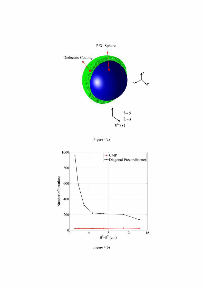
Figure 4(a)

Figure 4(b)

z

yx

ˆ ˆk z

incE r

ˆ ˆp y

Dielectric Coating

PEC Sphere

Figure 4(c)

Figure 5(a)

x

y

z41.472 m

26.624 m

15.886 mˆ ˆ k z

incE r ˆ ˆp x

Figure 5(b)

Figure 5(c)

7.5662 cm

34.631 cm

Figure 5(d)

Figure 5(e)

dB

Figure 6 (a)

Figure 6 (b)

Figure 6 (c)

Figure 6 (d)

x

z

d

2.54

1.52

0.15

1.8157.62

0.362.28

00

0 0

0 08.9 r

Figure 6 (e)

Figure 6 (f)

planeyz

planexz

Figure 7 (a)

Figure 7 (b)

260

xz

y

22.9

10.2

33.6

11.45

xz

y

33.6

33.6

Figure 7 (c)

Figure 7 (d)

0.5

x

z

8.72

5.01

101.2

38.7

38.7

33.6

6 5.01

0 02.1 r

0 0

0 0

0 0 01.45 r

0

260

11

xz

y

11

Figure 7 (e)

Figure 7 (f)

References

[1] C. C. Lu and W. C. Chew, "A coupled surface-volume integral equation approach for the calculation of electromagnetic scattering from composite metallic and material targets," IEEE Trans. Antennas Propagat., vol. 48, no. 12, pp. 1866-1868, Dec. 2000.

[2] A. E. Yilmaz, J.-M. Jin, and E. Michielssen, "A parallel FFT accelerated transient field-circuit simulator," IEEE Trans. Microwave Theory Tech., vol. 53, no. 9, pp. 2851-2865, Sept. 2005.

[3] T. K. Sarkar, S. M. Rao, and A. R. Djordjevic, "Electromagnetic scattering and radiation from finite microstrip structures," IEEE Trans. Microwave Theory Tech., vol. 22, pp. 1568-1575, Nov. 1990.

[4] N. V. Budko and A. B. Samokhin, "Spectrum of the volume integral operator of electromagnetic scattering," SIAM J. Sci. Comput., vol. 28, no. 2, pp. 682-700, 2006.

[5] J. Rahola, "On the eigenvalues of the volume integral operator of electromagnetic scattering," SIAM J. Sci. Comput., vol. 21, no. 5, pp. 1740-1754, 2000.

[6] J.-C. Nedelec, Acoustic and Electromagnetic Equations. New York: Springer-Verlag, 2000.

[7] R. J. Adams, "Physical and analytical properties of a stabilized electric field integral equation," IEEE Trans. Antennas Propagat., vol. 52, no. 2, pp. 362-372, Feb. 2004.

[8] F. P. Andriulli, K. Cools, H. Bagci, F. Olyslager, A. Buffa, S. Christiansen, and E. Michielssen, "A multiplicative Calderon preconditioner for the electric field integral equation," IEEE Trans. Antennas Propagat., vol. 56, no. 8, pp. 2398-2412, Aug. 2008.

[9] S. Borel, D. P. Levadoux, and F. Alouges, "A new well-conditioned integral formulation for Maxwell equations in three dimensions," IEEE Trans. Antennas Propagat., vol. 53, no. 9, pp. 2995-3004, Sep. 2005.

[10] H. Contopanagos, B. Dempart, M. Epton, J. Ottusch, V. Rokhlin, J. Visher, and S. M. Wandzura, "Well-conditioned boundary integral equations for three-dimensional electromagnetic scattering," IEEE Trans. Electromagn. Compat., vol. 50, no. 12, pp. 1824-1930, Dec. 2002.

[11] S. M. Rao, D. R. Wilton, and A. W. Glisson, "Electromagnetic scattering by surfaces of arbitrary shape," IEEE Trans. Antennas Propagat., vol. 30, no. 3, pp. 409-418, May 1982.

[12] D. H. Schaubert, D. R. Wilton, and A. W. Glisson, "A tetrahedral modeling method for electromagnetic scattering by arbitrarily shaped inhomogenous dielectric bodies," IEEE Trans. Antennas Propagat., vol. 32, no. 1, pp. 77-85, Jan. 1984.

[13] E. Bleszynski, M. Bleszynski, and T. Jaroszewic, "AIM:Adaptive integral method for solving large-scale electromagnetic scattering and radiation problems," Radio Sci., vol. 31, no. 5, pp. 1225-151, Sept./Oct. 1996.

[14] W. C. Chew, J. M. Jin, C. C. Lu, E. Michielssen, and J. M. Song, "Fast solution methods in electromagnetics," IEEE Trans. Antennas Propagat., vol. 45, no. 3, pp. 533-543, Mar. 1997.

[15] J. M. Song, C.-C. Lu, and W. C. Chew, "Multilevel fast multipole algorithm for electromagnetic scattering by large complex objects," IEEE Trans. Antennas Propagat., vol. 45, no. 10, pp. 1488-1493, Oct. 1997.

[16] G. C. Hsiao and R. E. Kleinman, "Mathematical foundations for error estimation in numerical solutions of integral equations in electromagnetics," IEEE Trans. Antennas Propagat., vol. 45, no. 3, pp. 316-328, Mar. 1997.

[17] A. Buffa and S. H. Christiansen, "A dual finite element complex on the barycentric refinement," Math. Comput., vol. 76, pp. 1743-1769, 2007.

[18] R. W. Freund, "A transpose-free quasi-minimal residual algorithm for non-hermitian linear systems," SIAM J. Sci. Stat. Comput., vol. 14, pp. 470-482, Mar. 1993.

[19] T. Ando, J. Yamauchi, and H. Nakano, "Numerical analysis of a dielectric rod antenna - Demonstration of the discontinuity-radiation concept," IEEE Trans. Antennas Propagat., vol. 51, no. 8, pp. 2007-2013, Aug. 2003 2003.