51 (2006) APPLICATIONS OF MATHEMATICS No. 5, 495–516

ON A MULTIPLICATIVE TYPE SUM FORM FUNCTIONAL

EQUATION AND ITS ROLE IN INFORMATION THEORY

Prem Nath, Dhiraj Kumar Singh, Delhi

(Received February 2, 2005, in revised version November 1, 2005)

Abstract. In this paper, we obtain all possible general solutions of the sum form functionalequations

k∑

i=1

l∑

j=1

f(piqj ) =k∑

i=1

g(pi)l∑

j=1

h(qj )

and

k∑

i=1

l∑

j=1

F (piqj ) =k∑

i=1

G(pi) +l∑

j=1

H(qj) + λ

k∑

i=1

G(pi)l∑

j=1

H(qj)

valid for all complete probability distributions (p1, . . . , pk), (q1, . . . , ql), k > 3, l > 3 fixedintegers; λ ∈

�, λ 6= 0 and F , G, H, f , g, h are real valued mappings each having the

domain I = [0, 1], the unit closed interval.

Keywords: sum form functional equation, additive function, multiplicative function

MSC 2000 : 39B52, 39B82

1. Introduction

For n = 1, 2, 3, . . . let

Γn =

{

(p1, . . . , pn) : pi > 0, i = 1, . . . , n;

n∑

i=1

pi = 1

}

denote the set of all n-component discrete probability distributions.

495

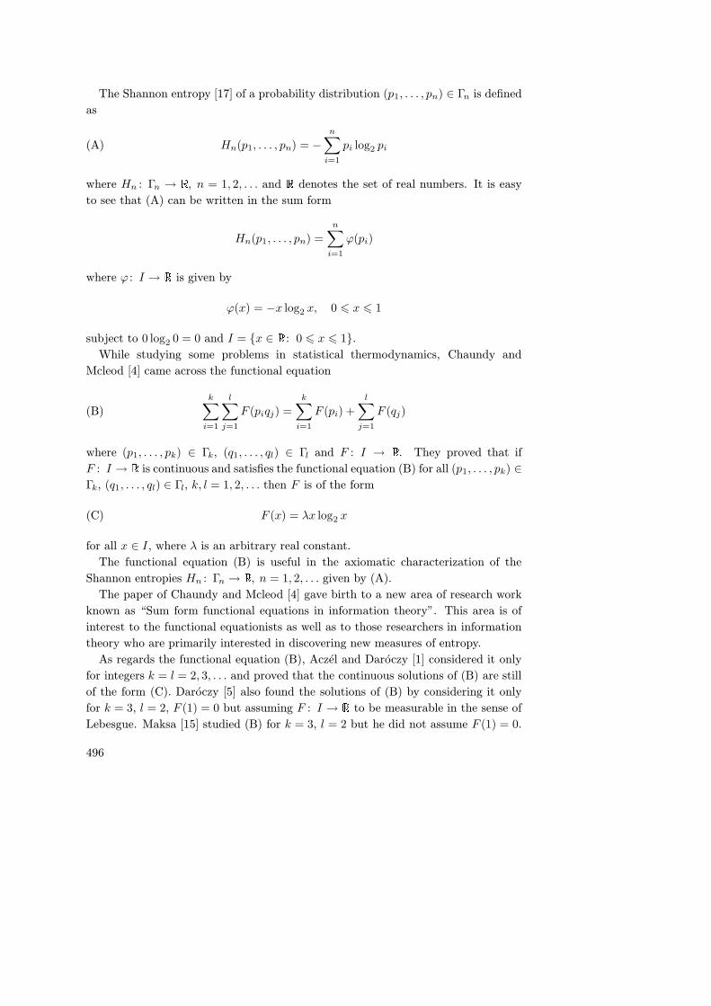
The Shannon entropy [17] of a probability distribution (p1, . . . , pn) ∈ Γn is defined

as

(A) Hn(p1, . . . , pn) = −

n∑

i=1

pi log2 pi

where Hn : Γn → � , n = 1, 2, . . . and � denotes the set of real numbers. It is easyto see that (A) can be written in the sum form

Hn(p1, . . . , pn) =

n∑

i=1

ϕ(pi)

where ϕ : I → � is given by

ϕ(x) = −x log2 x, 0 6 x 6 1

subject to 0 log20 = 0 and I = {x ∈ � : 0 6 x 6 1}.

While studying some problems in statistical thermodynamics, Chaundy and

Mcleod [4] came across the functional equation

(B)k

∑

i=1

l∑

j=1

F (piqj) =k

∑

i=1

F (pi) +l

∑

j=1

F (qj)

where (p1, . . . , pk) ∈ Γk, (q1, . . . , ql) ∈ Γl and F : I → � . They proved that ifF : I → � is continuous and satisfies the functional equation (B) for all (p1, . . . , pk) ∈

Γk, (q1, . . . , ql) ∈ Γl, k, l = 1, 2, . . . then F is of the form

(C) F (x) = λx log2 x

for all x ∈ I , where λ is an arbitrary real constant.

The functional equation (B) is useful in the axiomatic characterization of the

Shannon entropies Hn : Γn → � , n = 1, 2, . . . given by (A).

The paper of Chaundy and Mcleod [4] gave birth to a new area of research work

known as “Sum form functional equations in information theory”. This area is of

interest to the functional equationists as well as to those researchers in information

theory who are primarily interested in discovering new measures of entropy.

As regards the functional equation (B), Aczél and Daróczy [1] considered it only

for integers k = l = 2, 3, . . . and proved that the continuous solutions of (B) are still

of the form (C). Daróczy [5] also found the solutions of (B) by considering it only

for k = 3, l = 2, F (1) = 0 but assuming F : I → � to be measurable in the sense ofLebesgue. Maksa [15] studied (B) for k = 3, l = 2 but he did not assume F (1) = 0.

496

Instead of assuming F : [0, 1] → � to be measurable in the sense of Lebesgue, heassumed F : [0, 1] → � to be bounded on a set of positive measure.Daróczy and Jarai [6] found the solutions of (B) by assuming it for k = 2, l = 2;

and F : I → � to be measurable in the sense of Lebesgue.Finally, without imposing any condition on F : [0, 1] → � , but assuming (B) only

for a fixed pair (k, l), k > 3, l > 3 integers, Losonczi and Maksa [14] found the most

general solutions of (B).

A generalization of the Shannon entropy (A) with which we shall be concerned in

this paper is (with Hαn : Γn → � , n = 1, 2, 3, . . .)

(D) Hαn (p1, . . . , pn) = (1 − 21−α)−1

(

1 −

n∑

i=1

pαi

)

with α > 0, α 6= 1, 0α := 0, α ∈ � . The entropies (D) are known as the nonadditiveentropies of order α, α > 0, α 6= 1 and are due to Havrda and Charvát [9]. It can be

easily seen that

limα→1

Hαn (p1, . . . , pn) = −

n∑

i=1

pi log2 pi = Hn(p1, . . . , pn).

The axiomatic characterization of the entropies (D) leads to the study of the

functional equation

(1.1)k

∑

i=1

l∑

j=1

F (piqj) =k

∑

i=1

F (pi) +l

∑

j=1

F (qj) + λk

∑

i=1

F (pi)l

∑

j=1

F (qj)

where (p1, . . . , pk) ∈ Γk, (q1, . . . , ql) ∈ Γl. Clearly, (1.1) reduces to (B) when λ = 0.

By taking λ = 21−α − 1, α 6= 1, α ∈ � , 0α := 0, the continuous solutions of (1.1)

were found by Behara and Nath [3] for all positive integers k = 2, 3, . . .; l = 2, 3, . . ..

Later on, the continuous solutions of (1.1) for λ 6= 0 and k = 2, 3, . . .; l = 2, 3, . . .

were obtained by Kannappan [11] and Mittal [16]. For fixed integers k > 3, l > 2

and assuming F : I → � to be measurable in the sense of Lebesgue, Losonczi [12]obtained the measurable solutions of (1.1). For fixed integers k > 3, l > 3 and

assuming F : I → � to be measurable in the sense of Lebesgue, Kannappan [10] alsoobtained the Lebesgue measurable solutions of both the functional equations (B)

and (1.1).

As far as we know, Losonczi and Maksa [14] are the first to obtain the general

solutions of (1.1) in the case when λ 6= 0 and fixing integers k and l, k > 3, l > 3.

If we define a mapping f : I → � as

(1.2) f(x) = λF (x) + x

497

for all x ∈ I , λ 6= 0, then the functional equation (1.1) reduces to the multiplicative

type functional equation

(1.3)

k∑

i=1

l∑

j=1

f(piqj) =

k∑

i=1

f(pi)

l∑

j=1

f(qj)

where (p1, . . . , pk) ∈ Γk, (q1, . . . , ql) ∈ Γl. Its general solutions, for fixed integers

k > 3, l > 3, have been obtained by Losonczi and Maksa [14]. Then, by making use

of the equation (1.2), they also obtained the corresponding solutions of (1.1). In this

sense, both (1.1) and (1.3) are useful from the information-theoretic point of view.

In this paper, our object is to find all general solutions of the Pexiderized form

of (1.3), that is,

(1.4)

k∑

i=1

l∑

j=1

f(piqj) =

k∑

i=1

g(pi)

l∑

j=1

h(qj)

for all (p1, . . . , pk) ∈ Γk, (q1, . . . , ql) ∈ Γl; k > 3, l > 3 being fixed integers and

f : I → � , g : I → � , h : I → � . The functional equation (1.4) is also useful fromthe information-theoretic point of view in the sense that it enables us to find the

general solutions of the functional equation

(1.5)k

∑

i=1

l∑

j=1

F (piqj) =k

∑

i=1

G(pi) +l

∑

j=1

H(qj) + λk

∑

i=1

G(pi)l

∑

j=1

H(qj)

where (p1, . . . , pk) ∈ Γk, (q1, . . . , ql) ∈ Γl, λ 6= 0, k > 3, l > 3 being fixed integers

and F : I → � , G : I → � , H : I → � . One can easily see that (1.5) is, indeed, ageneralization of (1.1).

If λ = 1 then (1.5) reduces to

(1.6)

k∑

i=1

l∑

j=1

F (piqj) =

k∑

i=1

G(pi) +

l∑

j=1

H(qj) +

k∑

i=1

G(pi)

l∑

j=1

H(qj).

As far as the authors know, the functional equation (1.6) seems to have been con-

sidered, for the first time, by Gulati [8] who found its Lebesgue measurable solutions

in two cases (i) for k = 1, 2, 3, . . . and l = 1, 2, 3, . . . and (ii) for k = l = 1, 2, 3, . . ..

Surprisingly, the Lebesgue measurable solutions in the two cases are different.

The process of finding the general solutions of (1.4), for fixed integers k > 3, l > 3,

needs determining the general solutions of the functional equation

(1.7)k

∑

i=1

l∑

j=1

T (piqj) =k

∑

i=1

T (pi)l

∑

j=1

T (qj) + (l − k)T (0)l

∑

j=1

T (qj) + l(k − 1)T (0)

where T : I → � and k > 3, l > 3 are fixed integers.

498

Equations (1.4) and (1.5), which are the respective extensions of (1.3) and (1.1),

lead us to the meaningful entropies which cannot be obtained from the simpler equa-

tions (1.1) and (1.3) studied previously by Losonczi and Maksa [14]. This discussion

is carried out in the last Section 5 of this paper; as such a discussion can be carried

out only after obtaining the general solutions of (1.4) and (1.5) which are investigated

in Sections 3 and 4 respectively.

2. The general solutions of functional equation (1.7)

Before investigating the general solutions of (1.7) for fixed integers k and l, k > 3,

l > 3, we need some definitions and results already available in the literature (see

Losonczi and Maksa [14]). Let

∆ = {(x, y) : 0 6 x 6 1, 0 6 y 6 1, 0 6 x+ y 6 1}.

In other words, ∆ denotes the unit closed triangle in

� 2 = � × � = {(x, y) : x ∈ � , y ∈ � }.

A mapping a : � → � is said to be additive if it satisfies the equation

(2.1) a(x+ y) = a(x) + a(y)

for all x ∈ � , y ∈ � .A mapping a : I → � , I = [0, 1] is said to be additive on the triangle ∆ if it

satisfies (2.1) for all (x, y) ∈ ∆.

A mapping m : [0, 1] → � is said to be multiplicative if m(0) = 0, m(1) = 1 and

m(xy) = m(x)m(y) for all x ∈ ]0, 1[, y ∈ ]0, 1[.

Lemma 1. Let ψ : I → � be a mapping which satisfies the functional equation

(2.2)n

∑

i=1

ψ(pi) = c

for all (p1, . . . , pn) ∈ Γn; c a given constant and n > 3 a fixed integer. Then there

exists an additive mapping a : � → � such that

(2.3) ψ(p) = a(p) + ψ(0), 0 6 p 6 1

where

(2.4) a(1) = c− nψ(0).

499

Conversely, if (2.4) holds, then the mapping ψ : I → � defined by (2.3) satisfies thefunctional equation (2.2).

This lemma appears on p. 74 in Losonczi and Maksa [14].

Lemma 2. Every mapping a : I → � , I = [0, 1], additive on the unit triangle ∆,

has a unique additive extension to the whole of � .�������

. This unique additive extension to the whole of � will also be denoted bythe symbol a but now a : � → � .For Lemma 2, see Theorem (0.3.7) on p. 8 in Aczél and Daróczy [2] or Daróczy

and Losonczi [7].

Theorem 1. Let k > 3, l > 3 be fixed integers and T : [0, 1] → � be a mappingwhich satisfies the functional equation (1.7) for all (p1, . . . , pk) ∈ Γk and (q1, . . . , ql) ∈

Γl. Then T is of the form

(2.5) T (p) = a(p) + T (0)

where a : � → � is an additive function with

(2.6)

{

a(1) = −lT (0) 6= −1 + T (1) − T (0) or

a(1) = 1 − lT (0) = T (1) − T (0)

or

(2.7) T (p) = M(p) − b(p) + T (0)

where b : � → � is an additive function with

(2.8) b(1) = lT (0)

and M : [0, 1] → � is a nonconstant nonadditive multiplicative function with

M(0) = 0,(2.9)

M(1) = 1(2.10)

and

M(pq) = M(p)M(q)(2.11)

for all p ∈ ]0, 1[, q ∈ ]0, 1[.

500

��� ���. Let us put q1 = 1, q2 = . . . = ql = 0 in (1.7). We obtain

(2.12) [1 − T (1) − (l − 1)T (0)]

[ k∑

i=1

T (pi) − (k − l)T (0)

]

= 0.

Case 1. 1 − T (1)− (l − 1)T (0) 6= 0. Then (2.12) reduces to

k∑

i=1

T (pi) = (k − l)T (0).

Hence, by Lemma 1, T is of the form (2.5) in which a : � → � is an additive mappingwith a(1) = −lT (0) 6= −1 + T (1) − T (0) as mentioned in (2.6).

Case 2. 1 − T (1)− (l − 1)T (0) = 0.

The functional equation (1.7) may be written in the form

k∑

i=1

[ l∑

j=1

T (piqj) − T (pi)

l∑

j=1

T (qj) − (l − k)T (0)pi

l∑

j=1

T (qj)

]

= l(k − 1)T (0).

Hence, by Lemma 1,

l∑

j=1

T (pqj) − T (p)

l∑

j=1

T (qj) − (l − k)T (0)p

l∑

j=1

T (qj)(2.13)

= A1(p, q1, . . . , ql) −1

kA1(1, q1, . . . , ql) +

l

k(k − 1)T (0)

where A1 : � × Γl → � is additive in the first variable. The substitution p = 0

in (2.13) gives

(2.14) A1(1, q1, . . . , ql) = T (0)

[

k

l∑

j=1

T (qj) − l

]

.

This holds for all (q1, . . . , ql) ∈ Γl.

Let x ∈ [0, 1], (r1, . . . , rl) ∈ Γl. Put successively p = xrt, t = 1, . . . , l in (2.13); add

the resulting l equations and use the additivity of A1. We get

l∑

t=1

l∑

j=1

T (xrtqj) −

l∑

t=1

T (xrt)

l∑

j=1

T (qj) − (l − k)T (0)x

l∑

j=1

T (qj)(2.15)

= A1(x, q1, . . . , ql) −l

kA1(1, q1, . . . , ql) +

l2

k(k − 1)T (0).

501

Now put p = x, q1 = r1, . . . , ql = rl in (2.13). We obtain

l∑

t=1

T (xrt) = T (x)

l∑

t=1

T (rt) + (l − k)T (0)x

l∑

t=1

T (rt)(2.16)

+A1(x, r1, . . . , rl) −1

kA1(1, r1, . . . , rl)

+l

k(k − 1)T (0).

From (2.15) and (2.16), it follows that

l∑

t=1

l∑

j=1

T (xrtqj) − T (x)

l∑

t=1

T (rt)

l∑

j=1

T (qj)(2.17)

− (l − k)T (0)x

l∑

t=1

T (rt)

l∑

j=1

T (qj) −l2

k(k − 1)T (0)

= A1(x, r1, . . . , rl)

l∑

j=1

T (qj) −1

kA1(1, r1, . . . , rl)

l∑

j=1

T (qj)

+l

k(k − 1)T (0)

l∑

j=1

T (qj) + (l − k)T (0)xl

∑

j=1

T (qj)

+A1(x, q1, . . . , ql) −l

kA1(1, q1, . . . , ql).

The left-hand side of (2.17) does not undergo any change if we interchange qj and

rj , j = 1, . . . , l. So, the right-hand side of (2.17) must also remain unchanged after

interchanging qj and rj , j = 1, . . . , l. Consequently, we obtain

A1(x, q1, . . . , ql)

[ l∑

t=1

T (rt) − 1

]

−1

kA1(1, q1, . . . , ql)

[ l∑

t=1

T (rt) − l

]

(2.18)

+l

k(k − 1)T (0)

l∑

t=1

T (rt) + (l − k)T (0)x

l∑

t=1

T (rt)

= A1(x, r1, . . . , rl)

[ l∑

j=1

T (qj) − 1

]

−1

kA1(1, r1, . . . , rl)

[ l∑

j=1

T (qj) − l

]

+l

k(k − 1)T (0)

l∑

j=1

T (qj) + (l − k)T (0)x

l∑

j=1

T (qj).

502

Now we divide our discussion into two cases depending upon whetherl

∑

t=1

T (rt)−1

vanishes identically on Γl or does not vanish identically on Γl.

Case 2.1.l

∑

t=1

T (rt) − 1 vanishes identically on Γl. Then

l∑

t=1

T (rt) = 1

for all (r1, . . . , rl) ∈ Γl. By using Lemma 1, it follows that T is of the form (2.5) in

which a(1) = 1 − lT (0) = T (1) − T (0) as mentioned in (2.6).

Case 2.2.l

∑

t=1

T (rt) − 1 does not vanish identically on Γl.

In this case, there exists a probability distribution (r∗1 , . . . , r∗

l ) ∈ Γl such that

(2.19)l

∑

t=1

T (r∗t ) − 1 6= 0.

Putting r1 = r∗1, . . . , rl = r∗l in (2.18), making use of (2.19) and (2.14) and performing

tedious calculations, it follows that

(2.20) A1(x, q1, . . . , ql) = A2(x)

[ l∑

j=1

T (qj) − 1

]

− (l − k)T (0)x

where A2 : � → � is such that

(2.21) A2(x) =

[ l∑

t=1

T (r∗t ) − 1

]

−1

[A1(x, r∗

1 , . . . , r∗

l ) + (l − k)T (0)x].

From (2.21) it is easy to conclude that A2 : � → � is additive as the mappingx 7→ A1(x, r

∗

1, . . . , r∗l ) is additive. Also, putting x = 1 in (2.21) and making use

of (2.14) by taking qj = r∗j , j = 1, . . . , l it follows that

(2.22) A2(1) = kT (0).

Moreover, from (2.13), (2.14), (2.20) and (2.22) one can derive

l∑

j=1

[T (pqj) +A2(pqj) + (l − k)T (0)pqj − T (0)](2.23)

−[T (p) +A2(p) + (l − k)T (0)p− T (0)]

×

l∑

j=1

[T (qj) +A2(qj) + (l − k)T (0)qj − T (0)] = 0.

503

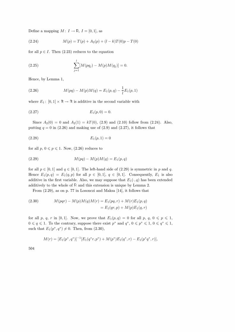
Define a mapping M : I → � , I = [0, 1], as

(2.24) M(p) = T (p) +A2(p) + (l − k)T (0)p− T (0)

for all p ∈ I . Then (2.23) reduces to the equation

(2.25)

l∑

j=1

[M(pqj) −M(p)M(qj)] = 0.

Hence, by Lemma 1,

(2.26) M(pq) −M(p)M(q) = E1(p, q) −1

lE1(p, 1)

where E1 : [0, 1] × � → � is additive in the second variable with

(2.27) E1(p, 0) = 0.

Since A2(0) = 0 and A2(1) = kT (0), (2.9) and (2.10) follow from (2.24). Also,

putting q = 0 in (2.26) and making use of (2.9) and (2.27), it follows that

(2.28) E1(p, 1) = 0

for all p, 0 6 p 6 1. Now, (2.26) reduces to

(2.29) M(pq) −M(p)M(q) = E1(p, q)

for all p ∈ [0, 1] and q ∈ [0, 1]. The left-hand side of (2.29) is symmetric in p and q.

Hence E1(p, q) = E1(q, p) for all p ∈ [0, 1], q ∈ [0, 1]. Consequently, E1 is also

additive in the first variable. Also, we may suppose that E1(·, q) has been extended

additively to the whole of � and this extension is unique by Lemma 2.From (2.29), as on p. 77 in Losonczi and Maksa [14], it follows that

M(pqr) −M(p)M(q)M(r) = E1(pq, r) +M(r)E1(p, q)(2.30)

= E1(qr, p) +M(p)E1(q, r)

for all p, q, r in [0, 1]. Now, we prove that E1(p, q) = 0 for all p, q, 0 6 p 6 1,

0 6 q 6 1. To the contrary, suppose there exist p∗ and q∗, 0 6 p∗ 6 1, 0 6 q∗ 6 1,

such that E1(p∗, q∗) 6= 0. Then, from (2.30),

M(r) = [E1(p∗, q∗)]−1[E1(q

∗r, p∗) +M(p∗)E1(q∗, r) −E1(p

∗q∗, r)],

504

from which it is easy to conclude that M is additive. Now, making use of (2.10),

(2.19), (2.22), (2.24) and the additivity of A2 and M , we have

1 6=

l∑

t=1

T (r∗t ) = M(1) −A2(1) − (l − k)T (0) + lT (0) = 1,

a contradiction. Hence, E1(p, q) = 0 for all p and q, 0 6 p 6 1, 0 6 q 6 1.

Thus, (2.29) reduces to M(pq) = M(p)M(q) for all p and q, 0 6 p 6 1, 0 6

q 6 1. Hence, (2.11) also holds. So, M is a nonconstant nonadditive multiplicative

function. By virtue of (2.24), T is of the form (2.7) in which M is a nonconstant

nonadditive multiplicative function; b : � → � is additive, it is given by b(p) =

A2(p) + (l − k)T (0)p for all p ∈ [0, 1] and (2.8) holds. �

3. The general solutions of functional equation (1.4)

Now we prove

Theorem 2. Let k > 3, l > 3 be fixed integers and let f : I → � , g : I → � ,h : I → � , I = [0, 1], be mappings which satisfy the functional equation (1.4) for all

(p1, . . . , pk) ∈ Γk and (q1, . . . , ql) ∈ Γl. Then any general solution of (1.4) is of the

form

(3.1)

f(p) = b1(p) −1

klb1(1),

g(p) = b2(p) −1

kb2(1),

h any arbitrary function

or

(3.2)

f(p) = b1(p) −1

klb1(1),

g any arbitrary function,

h(p) = b3(p) −1

lb3(1)

or

(3.3)

f(p) = [g(1) + (k − 1)g(0)][h(1) + (l − 1)h(0)]a(p) +A(p) + f(0),

g(p) = [g(1) + (k − 1)g(0)]a(p) + A∗(p) + g(0),

h(p) = [h(1) + (l − 1)h(0)]a(p) + h(0)

505

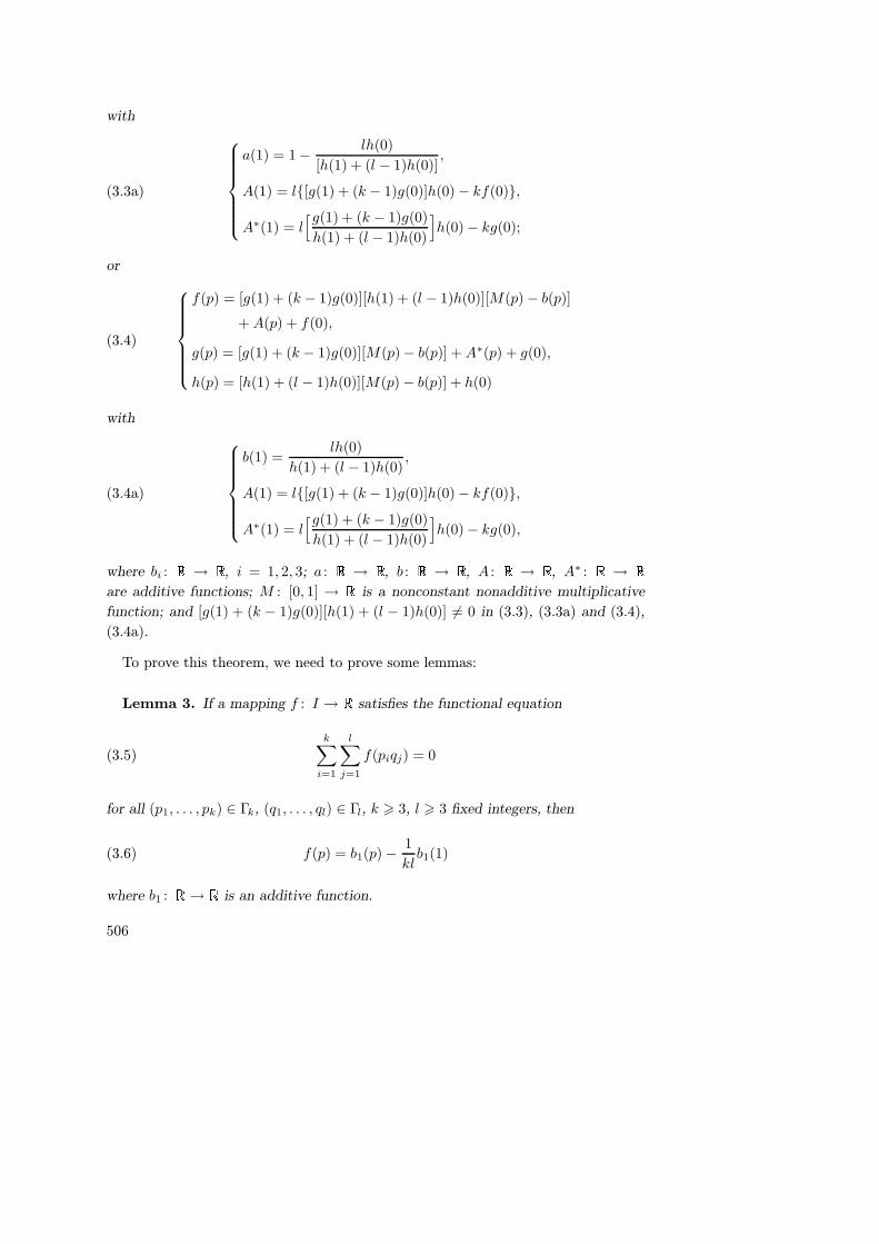
with

(3.3a)

a(1) = 1 −lh(0)

[h(1) + (l − 1)h(0)],

A(1) = l{[g(1) + (k − 1)g(0)]h(0) − kf(0)},

A∗(1) = l[g(1) + (k − 1)g(0)

h(1) + (l − 1)h(0)

]

h(0) − kg(0);

or

(3.4)

f(p) = [g(1) + (k − 1)g(0)][h(1) + (l − 1)h(0)][M(p) − b(p)]

+A(p) + f(0),

g(p) = [g(1) + (k − 1)g(0)][M(p) − b(p)] +A∗(p) + g(0),

h(p) = [h(1) + (l − 1)h(0)][M(p) − b(p)] + h(0)

with

(3.4a)

b(1) =lh(0)

h(1) + (l − 1)h(0),

A(1) = l{[g(1) + (k − 1)g(0)]h(0) − kf(0)},

A∗(1) = l[g(1) + (k − 1)g(0)

h(1) + (l − 1)h(0)

]

h(0) − kg(0),

where bi : � → � , i = 1, 2, 3; a : � → � , b : � → � , A : � → � , A∗ : � → �are additive functions; M : [0, 1] → � is a nonconstant nonadditive multiplicativefunction; and [g(1) + (k − 1)g(0)][h(1) + (l − 1)h(0)] 6= 0 in (3.3), (3.3a) and (3.4),

(3.4a).

To prove this theorem, we need to prove some lemmas:

Lemma 3. If a mapping f : I → � satisfies the functional equation

(3.5)

k∑

i=1

l∑

j=1

f(piqj) = 0

for all (p1, . . . , pk) ∈ Γk, (q1, . . . , ql) ∈ Γl, k > 3, l > 3 fixed integers, then

(3.6) f(p) = b1(p) −1

klb1(1)

where b1 : � → � is an additive function.

506

��� ���. Choose q1 = 1, q2 = . . . = ql = 0. Then equation (3.5) reduces to

k∑

i=1

f(pi) = −k(l− 1)f(0).

Hence, by Lemma 1,

(3.7) f(p) = b1(p) −1

kb1(1) − (l − 1)f(0)

for all p, 0 6 p 6 1, b1 : � → � being any additive function. Putting p = 0 in (3.7),

we obtain f(0) = −b1(1)/kl. Putting this value of f(0) in (3.7), (3.6) readily follows.

�

Lemma 4. Under the assumption stated in the statement of Theorem 2, the

following conclusions hold:

f(p) = [g(1) + (k − 1)g(0)]h(p) +A(p) − [g(1) + (k − 1)g(0)]h(0) + f(0),(3.8)

[g(1) + (k − 1)g(0)]

k∑

i=1

l∑

j=1

h(piqj)(3.9)

=

k∑

i=1

g(pi)

l∑

j=1

h(qj) + l(k − 1)[g(1) + (k − 1)g(0)]h(0),

[h(1) + (l − 1)h(0)]

k∑

i=1

l∑

j=1

g(piqj)(3.10)

=

k∑

i=1

g(pi)

l∑

j=1

h(qj) + k(l − 1)[h(1) + (l − 1)h(0)]g(0),

[h(1) + (l − 1)h(0)]

k∑

i=1

g(pi)(3.11)

= [g(1) + (k − 1)g(0)]k

∑

i=1

h(pi) + (l − k)[g(1) + (k − 1)g(0)]h(0),

[g(1) + (k − 1)g(0)][h(1) + (l − 1)h(0)]

k∑

i=1

l∑

j=1

h(piqj)(3.12)

= [g(1) + (k − 1)g(0)]

k∑

i=1

h(pi)

l∑

j=1

h(qj)

+ (l − k)[g(1) + (k − 1)g(0)]h(0)

l∑

j=1

h(qj)

+ l(k − 1)[g(1) + (k − 1)g(0)][h(1) + (l − 1)h(0)]h(0),

where h(1) + (l − 1)h(0) 6= 0 and A : � → � is an additive function.

507

��� ���. Putting p1 = 1, p2 = . . . = pk = 0 in (1.4), we obtain

l∑

j=1

{f(qj) − [g(1) + (k − 1)g(0)]h(qj)} = −l(k − 1)f(0).

Hence, by Lemma 1 (changing q to p),

(3.13) f(p) = [g(1) + (k − 1)g(0)]h(p) +A(p) −1

lA(1) − (k − 1)f(0)

for all p, 0 6 p 6 1, where A : � → � is an additive function with

(3.14) A(1) = l{[g(1) + (k − 1)g(0)]h(0) − kf(0)}.

From equations (3.13) and (3.14), equation (3.8) follows.

From equations (3.8) and (3.14), it is easy to see that

k∑

i=1

l∑

j=1

f(piqj) = [g(1) + (k − 1)g(0)]

k∑

i=1

l∑

j=1

h(piqj)(3.15)

− l(k − 1)[g(1) + (k − 1)g(0)]h(0).

From (1.4) and (3.15) we get (3.9). The proof of (3.10) is similar and hence omitted.

Now, put q1 = 1, q2 = . . . = ql = 0 in (3.9). We obtain equation (3.11). Multiply-

ing equation (3.9) by h(1) + (l − 1)h(0) 6= 0, we obtain

[g(1) + (k − 1)g(0)][h(1) + (l − 1)h(0)]

k∑

i=1

l∑

j=1

h(piqj)(3.16)

= [h(1) + (l − 1)h(0)]

k∑

i=1

g(pi)

l∑

j=1

h(qj)

+ l(k − 1)[g(1) + (k − 1)g(0)][h(1) + (l − 1)h(0)]h(0).

From (3.11) and (3.16), we obtain equation (3.12). �

��� ���of Theorem 2. We divide our discussion into three cases:

Case 1.k∑

i=1

g(pi) vanishes identically on Γk, that is,

(3.17)

k∑

i=1

g(pi) = 0

508

for all (p1, . . . , pk) ∈ Γk. Then (1.4) reduces to (3.5) and h can be an arbitrary

function. So, f is of the form (3.6) for all p, 0 6 p 6 1. Applying Lemma 1 to (3.17),

we obtain

(3.18) g(p) = b2(p) −1

kb2(1)

for all p, 0 6 p 6 1, b2 : � → � being an additive function. Equations (3.6), (3.18)together with an arbitrary function h constitute the solution (3.1) of (1.4).

Case 2.l

∑

j=1

h(qj) vanishes identically on Γl, that is,

(3.19)

l∑

j=1

h(qj) = 0

for all (q1, . . . , ql) ∈ Γl. Then (1.4) reduces to (3.5) and g can be an arbitrary

function. So, f is of the form (3.6) for all p, 0 6 p 6 1. Applying Lemma 1 to (3.19)

we obtain

(3.20) h(p) = b3(p) −1

lb3(1)

for all p, 0 6 p 6 1, b3 : � → � being an additive function. Equations (3.6), (3.20)together with an arbitrary function g constitute the solution (3.2) of (1.4).

Case 3. Neitherk∑

i=1

g(pi) vanishes identically on Γk norl

∑

j=1

h(qj) vanishes identi-

cally on Γl. Then there exist a (p∗1, . . . , p∗k) ∈ Γk and a (q∗

1, . . . , q∗l ) ∈ Γl such that

k∑

i=1

g(p∗i ) 6= 0 andl

∑

j=1

h(q∗j ) 6= 0, respectively, and consequently

(3.21)

k∑

i=1

g(p∗i )

l∑

j=1

h(q∗j ) 6= 0.

We prove that g(1)+(k−1)g(0) 6= 0. To the contrary, suppose g(1)+(k−1)g(0) =

0. Then (3.9) reduces tok

∑

i=1

g(pi)

l∑

j=1

h(qj) = 0

valid for all (p1, . . . , pk) ∈ Γk and (q1, . . . , ql) ∈ Γl. In particular,k∑

i=1

g(p∗i )l

∑

j=1

h(q∗j ) =

0, which contradicts (3.21). Hence g(1) + (k − 1)g(0) 6= 0.

509

Similarly, making use of (3.10), we can prove that h(1) + (l − 1)h(0) 6= 0. Now

using the fact that h(1) + (l − 1)h(0) 6= 0, equation (3.11) can be written as

k∑

i=1

{

g(pi) −[g(1) + (k − 1)g(0)

h(1) + (l − 1)h(0)

]

h(pi)

}

= (l − k)[g(1) + (k − 1)g(0)

h(1) + (l − 1)h(0)

]

h(0).

Hence, by Lemma 1,

g(p) =[g(1) + (k − 1)g(0)

h(1) + (l − 1)h(0)

]

h(p) +A∗(p) −1

kA∗(1)(3.22)

+(l − k)

k

[g(1) + (k − 1)g(0)

h(1) + (l − 1)h(0)

]

h(0)

for all p, 0 6 p 6 1 where A∗ : � → � is an additive function with

(3.23) A∗(1) = l[g(1) + (k − 1)g(0)

h(1) + (l − 1)h(0)

]

h(0) − kg(0).

From (3.22) and (3.23) we obtain

g(p) =[g(1) + (k − 1)g(0)

h(1) + (l − 1)h(0)

]

h(p) +A∗(p)(3.24)

−[g(1) + (k − 1)g(0)

h(1) + (l − 1)h(0)

]

h(0) + g(0).

Since [g(1) + (k − 1)g(0)][h(1) + (l − 1)h(0)] 6= 0, equation (3.12) gives

k∑

i=1

l∑

j=1

h(piqj)

[h(1) + (l − 1)h(0)](3.25)

=

k∑

i=1

h(pi)

[h(1) + (l − 1)h(0)]

l∑

j=1

h(qj)

[h(1) + (l − 1)h(0)]

+ (l − k)h(0)

[h(1) + (l − 1)h(0)]

l∑

j=1

h(qj)

[h(1) + (l − 1)h(0)]

+ l(k − 1)h(0)

[h(1) + (l − 1)h(0)].

Let us define a mapping T : [0, 1] → � as

(3.26) T (x) = [h(1) + (l − 1)h(0)]−1h(x)

510

for all x ∈ [0, 1]. Then, with the aid of (3.26), (3.25) reduces to the functional

equation (1.7). Also, from (3.26) it is easy to see that T (1) + (l − 1)T (0) = 1.

Consequently, Theorem 1 implies that T is of the form (2.5), along with (2.6) or

(2.7). Equations (2.5), (2.7), (3.8), (3.24) and (3.26) yield the solutions (3.3) along

with (3.3a), and (3.4) along with (3.4a) of the functional equation (1.4). The details

are omitted for the sake of brevity. �

4. The general solutions of functional equation (1.5)

when λ 6= 0

In this section, we prove

Theorem 3. Let k > 3, l > 3 be fixed integers and let F : I → � , G : I → � ,H : I → � , I = [0, 1], be mappings which satisfy the functional equation (1.5) for all

(p1, . . . , pk) ∈ Γk and (q1, . . . , ql) ∈ Γl. Then any general solution of (1.5) is of the

form

(4.1)

F (p) =1

λ

[

b1(p) −1

klb1(1) − p

]

,

G(p) =1

λ

[

b2(p) −1

kb2(1) − p

]

,

H any arbitrary function

or

(4.2)

F (p) =1

λ

[

b1(p) −1

klb1(1) − p

]

,

G any arbitrary function,

H(p) =1

λ

[

b3(p) −1

lb3(1) − p

]

or

(4.3)

F (p) =1

λ{[λ(G(1) + (k − 1)G(0)) + 1][λ(H(1) + (l − 1)H(0)) + 1]a(p)

+A(p) + λF (0) − p},

G(p) =1

λ{[λ(G(1) + (k − 1)G(0)) + 1]a(p) +A∗(p) + λG(0) − p},

H(p) =1

λ{[λ(H(1) + (l − 1)H(0)) + 1]a(p) + λH(0) − p}

511

with

(4.3a)

a(1) = 1 −λlH(0)

[λ(H(1) + (l − 1)H(0)) + 1],

A(1) = λl{[λ(G(1) + (k − 1)G(0)) + 1]H(0) − kF (0)},

A∗(1) = λl[λ(G(1) + (k − 1)G(0)) + 1

λ(H(1) + (l − 1)H(0)) + 1

]

H(0) − λkG(0)

or

F (p) =1

λ{[λ(G(1) + (k − 1)G(0)) + 1][λ(H(1) + (l − 1)H(0)) + 1]

× [M(p) − b(p)] +A(p) + λF (0) − p},

G(p) =1

λ{[λ(G(1) + (k − 1)G(0)) + 1][M(p) − b(p)]

+A∗(p) + λG(0) − p},

H(p) =1

λ{[λ(H(1) + (l − 1)H(0)) + 1][M(p) − b(p)] + λH(0) − p}

(4.4)

with

b(1) =λlH(0)

[λ(H(1) + (l − 1)H(0)) + 1],

A(1) = λl{[λ(G(1) + (k − 1)G(0)) + 1]H(0) − kF (0)},

A∗(1) = λl[λ(G(1) + (k − 1)G(0)) + 1

λ(H(1) + (l − 1)H(0)) + 1

]

H(0) − λkG(0),

(4.4a)

where bi : � → � , i = 1, 2, 3; a : � → � , b : � → � , A : � → � , A∗ : � → �are additive functions; M : [0, 1] → � is a nonconstant nonadditive multiplicativefunction, and

[λ(G(1) + (k − 1)G(0)) + 1][λ(H(1) + (l − 1)H(0)) + 1] 6= 0.

��� ���. Let us write (1.5) in the form

(4.5)

k∑

i=1

l∑

j=1

[λF (piqj) + piqj ] =

k∑

i=1

[λG(pi) + pi]

l∑

j=1

[λH(qj) + qj ].

Define mappings f : I → � , g : I → � , h : I → � as

(4.6)

f(x) = λF (x) + x,

g(x) = λG(x) + x,

h(x) = λH(x) + x

512

for all x ∈ I . Then (4.5) reduces to the functional equation (1.4) whose solutions

are given by (3.1), (3.2), (3.3) along with (3.3a) and (3.4) along with (3.4a), in

which bi : � → � , i = 1, 2, 3; a : � → � , b : � → � , A : � → � , A∗ : � → � areadditive functions and M : [0, 1] → � is a nonconstant nonadditive multiplicativefunction. Now, making use of (4.6) and (3.1), (3.2), (3.3) along with (3.3a), (3.4)

along with (3.4a), the required solutions (4.1), (4.2), (4.3) along with (4.3a) and (4.4)

along with (4.4a) follow. The details are omitted. �

5. Comments

Losonczi [13] considered the functional equation

(5.1)

k∑

i=1

l∑

j=1

Fij(piqj) =

k∑

i=1

Gi(pi) +

l∑

j=1

Hj(qj) + λ

k∑

i=1

Gi(pi)

l∑

j=1

Hj(qj)

with (p1, . . . , pk) ∈ Γk, (q1, . . . , ql) ∈ Γl, λ 6= 0, Fij : I → � , Gi : I → � , Hj : I → �as unknown functions. He found measurable (in the sense of Lebesgue) solutions

of (5.1) by taking k > 3, l > 3 as fixed integers; i = 1, . . . , k, j = 1, . . . , l; in

Theorem 6 on p. 69 in Losonczi [13]. Even if we take k = 3 and l = 3, it is

obvious that the functional equation (5.1) contains fifteen unknown functions, which

is a significantly large number. Hence, it seems improbable that the measurable

solutions of (5.1) will be of direct importance from the information-theoretic point of

view. However, some special cases of (5.1) are certainly useful from the information-

theoretic point of view. For instance, if we take Fij = F , Gi = G, Hj = H , i = 1

to k, j = 1 to l, then (5.1) reduces to (1.5). This is the reason for considering (1.5).

Losonczi and Maksa [14] have shown that if a function F : [0, 1] → � satisfiesequation (1.1) for λ 6= 0, k > 3, l > 3 fixed integers, then it is of the form

F (p) =a(p) + α1 − p

λ, p ∈ [0, 1](5.2)

or

F (p) =M(p) −A(p) − p

λ, p ∈ [0, 1](5.3)

where a, A are additive functions, α1 is an arbitrary constant, A(1) = 0; M is a

multiplicative function and a(1) satisfies

(5.4) a(1) + klα1 = (a(1) + kα1)(a(1) + lα1).

513

From (5.2) it follows that

k∑

i=1

F (pi) =a(1) + kα1 − 1

λ,

which is independent of p1, . . . , pk. So, the solution (5.2) is not of any use from the

information-theoretic point of view. From (5.3) we have

k∑

i=1

F (pi) = Lλk(p1, . . . , pk)

where

(5.5) Lλk(p1, . . . , pk) =

1

λ

( k∑

i=1

M(pi) − 1

)

,

which is certainly useful from the information-theoretic point of view. The nonaddi-

tive measure of entropy, given by Havrda and Charvát [9], is a particular case of (5.5)

when λ = 21−α − 1, α 6= 1 and M : [0, 1] → � is of the form M(p) = pα, 0 6 p 6 1,

α 6= 1, α > 0, 0α := 0, 1α := 1.

The solution (4.1) is not of any relevance in information theory as the mapping H

in it is an arbitrary function. The same is true of (4.2) as the mapping G in it is also

an arbitrary function. As regards (4.3), each of the summandsk∑

i=1

F (pi),k∑

i=1

G(pi),

k∑

i=1

H(pi) is independent of p1, . . . , pk and hence (4.3) is not of much significance

from the point of view of information theory, either.

Solution (4.4) is certainly useful from the information-theoretic point of view. Let

us put

β1 = λ(G(1) + (k − 1)G(0)) + 1,

β2 = λ(H(1) + (l − 1)H(0)) + 1,

β3 = λk(l − 1)F (0)

and

β4 = λ(k − l)H(0).

514

Then from the last line in the statement of Theorem 3, it follows that β1 6= 0, β2 6= 0.

Now, from (4.4) it can be easily seen that

(5.6)

k∑

i=1

F (pi) = β1β2Lλk(p1, . . . , pk) +

1

λ(β1β2 − β3 − 1),

k∑

i=1

G(pi) = β1Lλk(p1, . . . , pk) +

1

λ(β1 − 1),

k∑

i=1

H(pi) = β2Lλk(p1, . . . , pk) +

1

λ(β2 + β4 − 1),

where β1 6= 0, β2 6= 0, β3 and β4 are arbitrary real constants.

Each of the summandsk∑

i=1

F (pi),k∑

i=1

G(pi),k∑

i=1

H(pi) reduces to Lλk(p1, . . . , pk),

given by (5.5) and characterized by Losonczi and Maksa [14] when β1 = 1, β2 = 1,

β3 = 0 (which means F (0) = 0) and β4 = 0 (which means H(0) = 0). So, the

functional equations (1.4) and (1.5) lead certainly to the meaningful entropies given

by (5.6), and the measure Lλk(p1, . . . , pk) given by (5.5) follows as a special case of

them when β1 = 1, β2 = 1, β3 = 0 (that is, F (0) = 0) and β4 = 0 (that is, H(0) = 0).

If we take M(p) = p2, 0 6 p 6 1, then each of the summandsk∑

i=1

F (pi),k∑

i=1

G(pi),

k∑

i=1

H(pi) in (5.6) reduces to an expression of the form

(5.7) µ

{

1

λ

( k∑

i=1

p2

i − 1

)}

+ν

λ(both µ 6= 0 and ν real),

which is the quadratic entropy (upto additive and nonzero multiplicative constants)

due to Vajda [18].

Acknowledgement. The authors are grateful to the referee for his valuable com-

ments which have led to considerable improvement of the paper.

References

[1] J. Aczél, Z. Daróczy: Charakterisierung der Entropien positiver Ordnung und der Shan-nonschen Entropie. Acta Math. Acad. Sci. Hungar. 14 (1963), 95–121. (In German.)

Zbl 0138.14904[2] J. Aczél, Z. Daróczy: On Measures of Information and Their Characterizations. Aca-demic Press, New York-San Francisco-London, 1975. Zbl 0345.94022

[3] M. Behara, P. Nath: Additive and non-additive entropies of finite measurable par-titions. Probab. Inform. Theory II. Lect. Notes Math. Vol. 296. Springer-Verlag,Berlin-Heidelberg-New York, 1973, pp. 102–138. Zbl 0282.94020

[4] T.W. Chaundy, J. B. Mcleod: On a functional equation. Edinburgh Math. Notes 43(1960), 7–8. Zbl 0100.32703

515

[5] Z. Daróczy: On the measurable solutions of a functional equation. Acta Math. Acad.Sci. Hungar. 22 (1971), 11–14. Zbl 0236.39008

[6] Z. Daróczy, A. Jarai: On the measurable solutions of functional equation arising ininformation theory. Acta Math. Acad. Sci. Hungar. 34 (1979), 105–116.

Zbl 0424.39002[7] Z. Daróczy, L. Losonczi: Über die Erweiterung der auf einer Punktmenge additivenFunktionen. Publ. Math. 14 (1967), 239–245. (In German.) Zbl 0175.15305

[8] K.K. Gulati: Some functional equations connected with entropy. Bull. Calcutta Math.Soc. 80 (1988), 96–100. Zbl 0654.39004

[9] J. Havrda, F. Charvát: Quantification method of classification process. Concept of struc-tural α-entropy. Kybernetika 3 (1967), 30–35. Zbl 0178.22401

[10] Pl. Kannappan: On some functional equations from additive and nonadditive measures I.Proc. Edinb. Math. Soc., II. Sér. 23 (1980), 145–150. Zbl 0468.39002

[11] Pl. Kannappan: On a generalization of some measures in information theory. Glas. Mat.,III. Sér. 9 (1974), 81–93. Zbl 0287.39006

[12] L. Losonczi: A characterization of entropies of degree α. Metrika 28 (1981), 237–244.Zbl 0469.94005

[13] L. Losonczi: Functional equations of sum form. Publ. Math. 32 (1985), 57–71.Zbl 0588.39005

[14] L. Losonczi, Gy. Maksa: On some functional equations of the information theory. ActaMath. Acad. Sci. Hungar. 39 (1982), 73–82. Zbl 0492.39006

[15] Gy. Maksa: On the bounded solutions of a functional equation. Acta Math. Acad. Sci.Hungar. 37 (1981), 445–450. Zbl 0472.39003

[16] D.P. Mittal: On continuous solutions of a functional equation. Metrika 23 (1976), 31–40.Zbl 0333.39006

[17] C.E. Shannon: A mathematical theory of communication. Bell Syst. Tech. Jour. 27(1948), 378–423, 623–656.

[18] I. Vajda: Bounds on the minimal error probability on checking a finite or countablenumber of hypotheses. Probl. Inf. Transm. 4 (1968), 9–19.

Authors’ address: P. Nath, D.K. Singh, Department of Mathematics, University ofDelhi, Delhi-110007, India, e-mails: dksingh@maths.du.ac.in, dhiraj426@rediffmail.com.

516