arX

iv:g

r-qc

/931

0008

v3 9

Nov

199

3

CTP#2243

Scalar Field Quantization

on the 2+1 Dimensional Black Hole Background∗

Gilad Lifschytz and Miguel Ortiz

Center for Theoretical Physics

Laboratory for Nuclear Science and

Department of Physics

Massachusetts Institute of Technology

Cambridge, MA 02139, USA

e-mails: gil1 and ortiz @mitlns.mit.edu

(Submitted to Physical Review D)

Abstract

The quantization of a massless conformally coupled scalar field on the 2+1

dimensional Anti de Sitter black hole background is presented. The Green’s

function is calculated, using the fact that the black hole is Anti de Sitter space

with points identified, and taking into account the fact that the black hole

spacetime is not globally hyperbolic. It is shown that the Green’s function

calculated in this way is the Hartle-Hawking Green’s function. The Green’s

function is used to compute 〈T µν 〉, which is regular on the black hole horizon,

and diverges at the singularity. A particle detector response function outside

the horizon is also calculated and shown to be a fermi type distribution. The

back-reaction from 〈Tµν〉 is calculated exactly and is shown to give rise to a

curvature singularity at r = 0 and to shift the horizon outwards. For M = 0

a horizon develops, shielding the singularity. Some speculations about the

endpoint of evaporation are discussed.

03.70.+k, 04.50.+h, 97.60.Lf

Typeset using REVTEX

1

INTRODUCTION

The study of black hole physics is complicated by the many technical and conceptualproblems associated with quantum field theory in curved spacetime. One serious difficultyis that exact calculations are almost impossible in 3+1 dimensions. In this paper we shallinstead study some aspects of quantum field theory on a 2+1 dimensional black hole back-ground. This enables us to obtain an exact expression for the Green’s function of a massless,conformally coupled scalar field in the Hartle-Hawking vacuum [1]. We use this Green’sfunction to study particle creation by the black hole, back-reaction and the endpoint ofevaporation.

We shall work with the 2+1 dimensional black hole solution found by Banados, Teitel-boim and Zanelli (BTZ) [2]. It had long been thought that black holes cannot exist in 2+1dimensions for the simple reason that there is no gravitational attraction, and therefore nomechanism for confining large densities of matter. This difficulty has been circumvented inthe BTZ spacetime1, but not surprisingly, their solution has some features that we do notnormally associate with black holes in other dimensions, such as the absence of a curvaturesingularity. It is interesting to ask whether this spacetime behaves quantum mechanicallyin a way consistent with more familiar back holes.

The spinless BTZ spacetime has a metric [2]

ds2 = −N2dt2 + N−2dr2 + r2dφ2

where

N2 =r2 − r 2

+

ℓ2, r 2

+ = Mℓ2.

Here M is the mass of the black hole. The metric is a solution to Einstein’s equations witha negative cosmological constant, Λ = −ℓ−2, and the curvature of the black hole solutionis constant everywhere. As a result there is no curvature singularity as r → 0. A Penrosediagram of the spacetime is given in Fig. 1.

An important feature of the BTZ solutions is that the solution with M = 0 (which werefer to as the vacuum solution), is not AdS3. Rather, it is a solution that is not globallyAnti de Sitter invariant. It has no horizon, but does have an infinitely long throat for smallr > 0, which is reminiscent of the extreme Reissner-Nordstrom solution in 3+1 dimensions.It is worth noting that there are other similarities between the spinless BTZ black holes,M ≥ 0, and the Reissner-Nordstrom solutions for M ≥ Q. In particular, the temperatureassociated with the Euclidean continuation of the BTZ black holes has been computed in[2], and it was found to increase with the mass, and to decrease to zero as M → 0. Thus,if we carry over the usual notions from four dimensional black holes, the M = 0 solutionappears to be a stable endpoint of evaporation.

A feature of the BTZ solution that we shall make use of, is that the solution arisesfrom identifying points in AdS3, using the orbits of a spacelike Killing vector field. It is

1A charged black hole solution in 2+1 dimensions had previously been found in Ref. [3]. For

further discussions on the BTZ black hole, see Refs. [4].

2

this property that is the starting point of our derivation of a Green’s function on the blackhole spacetime. We construct a Green’s function on AdS3, and this translates to a Green’sfunction on the black hole via the method of images.

A Green’s function constructed in this way is only interesting if we can identify thevacuum with respect to which it is defined. We prove that our construction gives the Hartle-Hawking Green’s function. It is worth noting that for the BTZ black hole, there is a limitedchoice of vacua. Quantisation on AdS3 is hampered by the fact that AdS3 is not globallyhyperbolic, and this necessitates the use of boundary conditions at spatial infinity [5] (seeFig. 2), as discussed in Appendix A. This problem carries over to the black hole solution,and as a result, the value of the field at spatial infinity is governed by either Dirichlet orNeumann type boundary conditions. Thus a Cauchy surface for the region R of the BTZblack hole is either the past or the future horizon only. With this knowledge, the naturaldefinition of the Hartle-Hawking vacuum is with respect to Kruskal modes on either horizon,whereas there does not appear to be a natural definition of an Unruh vacuum (see [6,7] fora discussion of the various eternal black hole vacua). The definition of an Unruh vacuummight be possible given a description of the formation of a BTZ black hole from the vacuumvia some sort of infalling matter, but as far as we are aware, no such construction has beenfound.

Having an explicit expression for the Hartle-Hawking Green’s function, we are able toobtain a number of exact results. As a check, we show that it satisfies the KMS thermalitycondition [8]. We then compute the expectation value of the energy-momentum tensorand the response of a particle detector for both nonzero M and for the vacuum solution.For nonzero M we address the issue of whether the response of the particle detector canbe interpreted as radiation emitted from the black hole, although a clear picture does notemerge.

For the M = 0 solution, we find a non-zero energy-momentum tensor, although thecorresponding Green’s function is at zero temperature, and there is no particle detectorresponse. We interpret this as a sort of Casimir energy. Classically, the vacuum solutionappears to be similar to the extremal Reissner-Nordstrom solution, in the sense that weexpect that if any matter is thrown in, a horizon develops. Quantum mechanically, theM = 0 solution appears to be unstable to the formation of a horizon, when the back-reaction caused by the Casimir energy is taken into account. This suggests that the endpointof evaporation may not look like the classical M = 0 solution.

The paper is organized as follows. In section I we study the 1+1 dimensional solutionwhich arises from a dimensional reduction of the BTZ black hole [9], and show that thevacuum defined by the Anti de Sitter (AdS) modes is the same as that defined by theKruskal modes; with this encouraging result we tackle the 2+1 case. Section II containsa review of the essential features of the geometry of the BTZ black hole. In section IIIwe construct the Wightman Green’s functions on the black hole spacetime from the AdS3

Wightman function, using the method of images. We then show that the Green’s functioncoincides with the Hartle-Hawking Green’s function [1], by showing that it is analytic andbounded in the lower half of the complex V plane on the past horizon (U = 0), whereV , U are the Kruskal null coordinates. We also compute the Wightman function for theM = 0 solution, and compare this to the M → 0 limit of the results for M 6= 0. Section IVcontains a calculation of 〈Tµν〉 for all M ≥ 0. For the black hole solutions, it is regular on

3

the horizon, and for all M it is singular as r → 0. In Section V the response function of astationary particle detector outside the horizon is calculated and shown to be of a fermi typedistribution. A discussion is given of how this response might be interpreted. In SectionVI we calculate the back reaction induced by 〈Tµν〉, and show that the spacetime developsa curvature singularity and a larger horizon for a given M . Throughout this paper we usemetric signature (− + +), and natural units in which 8G = h = c = 1.

I. 2-D BLACK HOLE

Let us begin by looking at quantum field theory on the region of Anti de Sitter spacetimein 1+1 dimensions described by the metric

ds2 = −(

r2 −Mℓ2

ℓ2

)

dt2 +

(

r2 −Mℓ2

ℓ2

)−1

dr2 0 < r <∞ −∞ < t < ∞,

where M is the mass of the solution. This metric was discussed in [9] as the dimensionalreduction of the spinless BTZ black hole, and can be thought of as being a region of AdS2

in Rindler-type co-ordinates. Under the change of co-ordinates

r =√Mℓ2 sec ρ cosλ, tanh

(√Mt

ℓ

)

=sin ρ

sin λ,

where we shall call (λ, ρ) AdS co-ordinates, the metric becomes

ds2 = ℓ2 sec2 ρ(−dλ2 + dρ2)

which for −π2≤ ρ ≤ π

2and −∞ < λ <∞ is just AdS2 [10].

It is possible to define Kruskal-like co-ordinates for this black hole, which do not coincidewith the usual AdS co-ordinates. For r > Mℓ2, they are:

U =

(

r −√Mℓ

r +√Mℓ

)

1

2

cosh

√M

ℓt (1.1)

V =

(

r −√Mℓ

r +√Mℓ

)

1

2

sinh

√M

ℓt. (1.2)

The metric then takes the form

ds2 =−2ℓ2

1 + U VdUdV

where U = V +U , V = V −U , and the transformation between Kruskal and AdS co-ordinatesis

U = tan

(

ρ+ λ

2

)

V = tan

(

ρ− λ

2

)

which is valid over all the Kruskal manifold. The Kruskal co-ordinates cover only the partof AdS2 with

4

−π2≤ ρ ≤ π

2− π

2< λ <

π

2.

We shall now show that the notion of positive frequency in (λ, ρ) (AdS) modes coincideswith that defined in (U, V ) (Kruskal) modes.

The AdS modes for a conformally coupled scalar field are normalized solutions of 2ψ = 0,subject to the boundary conditions

φ(

ρ =π

2

)

= φ(

ρ =−π2

)

= 0.

The positive frequency modes are then

φm =1√mπ

e−imλ sinmρ m even ≥ 0

φm =1√mπ

e−imλ cosmρ m odd ≥ 0

and these define a vacuum state |0〉A in the usual way.The Kruskal modes are solutions of 2ψ = 0 with the boundary condition ψ(U V = −1) =

0. Positive frequency solutions are given by

ψω = Nω

(

e−iωU − eiω/V)

ω > 0

where Nω = (8πω)−1/2, and these define |0〉K . These modes are analytic and bounded in thelower half of the complex U , V plane. In order to show equivalence of the two vacua |0〉Aand |0〉K , it is enough to show that the positive frequency AdS modes can be written as asum of only positive frequency Kruskal modes. Because of the analyticity properties of theKruskal modes, it is enough to show that the AdS modes are analytic and bounded in thelower half of the complex U , V plane [6,11]. Changing co-ordinates, we have

φm =1√πm2i

(

e−2im arctan V − e−2im arctan U)

m even (1.3)

φm =1√πm2i

(

e−2im arctan V + e−2im arctan U)

m odd. (1.4)

Using the definition arctan z = 12i

ln 1+iz1−iz

[15], (1.3) and (1.4) become

φm =1

2√πmi

[(

1 − iV

1 + iV

)m

∓(

1 − iU

1 + iU

)m]

where ± is for m odd or even. These modes can easily be seen to be bounded and analytic inthe lower half of the complex U , V plane for all m. This establishes that the vacuum definedby the AdS modes is the same as that defined by the Kruskal modes. Thus a Green’s functiondefined on this spacetime using AdS co-ordinates (λ, ρ) corresponds to a Hartle-HawkingGreen’s function, in the sense discussed in the Introduction.

5

II. THE GEOMETRY OF THE 2+1 DIMENSIONAL BLACK HOLE

In this paper, we shall be working only with the spinless black hole solution in 2+1dimensions

ds2 = −N2dt2 +N−2dr2 + r2dφ2 (2.1)

where

N2 =r2 − r 2

+

ℓ2, r 2

+ = Mℓ2.

As was shown in [2], this metric has constant curvature, and is a portion of three di-mensional Anti de Sitter space with points identified. The identification is made using aparticular killing vector ξ, by identifying all points xn = e2πniξx. In order to see this mostclearly, it is useful to introduce different sets of co-ordinates on AdS3.

AdS3 can be defined as the surface −v2−u2 +x2 +y2 = −ℓ2 embedded in R4 with metricds2 = −du2 − dv2 + dx2 + dy2. A co-ordinate system (λ, ρ, θ) which covers this space, andwhich we shall refer to as AdS co-ordinates, is defined by [5]

u = ℓ cosλ sec ρ v = ℓ sinλ sec ρ

x = ℓ tan ρ cos θ y = ℓ tan ρ sin θ

where 0 ≤ ρ ≤ π2, 0 < θ ≤ 2π, and 0 < λ < 2π. In these co-ordinates, the AdS3 metric

becomes

ds2 = ℓ2 sec2 ρ(−dλ2 + dρ2 + sin2 ρ dθ2).

AdS3 has topology S1 (time) ×R2 (space) and hence contains closed timelike curves. Theangle λ can be unwrapped to form the covering space of AdS3, with −∞ < λ < ∞, whichdoes not contain any closed timelike curves. Throughout this paper we work with thiscovering space, and this is what we henceforth refer to as AdS3. As mentioned in theIntroduction, even this covering space presents difficulties since it is not globally hyperbolic(see the discussion in Appendix A).

The identification taking AdS3 into the black hole (2.1) is most easily expressed in termsof co-ordinates (t, r, φ), related in an obvious way to those used above, and defined on AdS3

by

u =√

A(r) cosh(

r+

ℓφ)

x =√

A(r) sinh(

r+

ℓφ)

y =√

B(r) cosh(

r+

ℓ2t)

v =√

B(r) cosh(

r+

ℓ2t)

r > r+

u =√

A(r) cosh(

r+

ℓφ)

x =√

A(r) sinh(

r+

ℓφ)

y = −√

−B(r) cosh(

r+

ℓ2t)

v =√

−B(r) cosh(

r+

ℓ2t)

0 > r > r+.

6

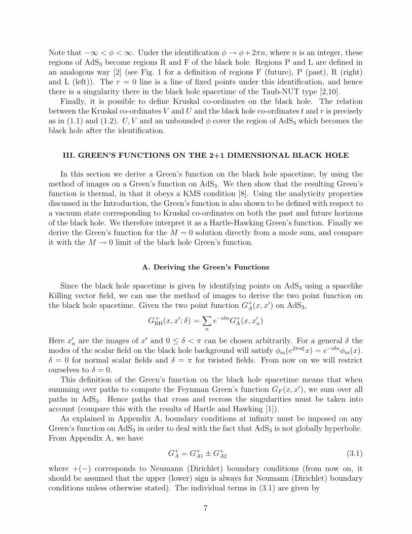
Note that −∞ < φ <∞. Under the identification φ→ φ+2πn, where n is an integer, theseregions of AdS3 become regions R and F of the black hole. Regions P and L are defined inan analogous way [2] (see Fig. 1 for a definition of regions F (future), P (past), R (right)and L (left)). The r = 0 line is a line of fixed points under this identification, and hencethere is a singularity there in the black hole spacetime of the Taub-NUT type [2,10].

Finally, it is possible to define Kruskal co-ordinates on the black hole. The relationbetween the Kruskal co-ordinates V and U and the black hole co-ordinates t and r is preciselyas in (1.1) and (1.2). U, V and an unbounded φ cover the region of AdS3 which becomes theblack hole after the identification.

III. GREEN’S FUNCTIONS ON THE 2+1 DIMENSIONAL BLACK HOLE

In this section we derive a Green’s function on the black hole spacetime, by using themethod of images on a Green’s function on AdS3. We then show that the resulting Green’sfunction is thermal, in that it obeys a KMS condition [8]. Using the analyticity propertiesdiscussed in the Introduction, the Green’s function is also shown to be defined with respect toa vacuum state corresponding to Kruskal co-ordinates on both the past and future horizonsof the black hole. We therefore interpret it as a Hartle-Hawking Green’s function. Finally wederive the Green’s function for the M = 0 solution directly from a mode sum, and compareit with the M → 0 limit of the black hole Green’s function.

A. Deriving the Green’s Functions

Since the black hole spacetime is given by identifying points on AdS3 using a spacelikeKilling vector field, we can use the method of images to derive the two point function onthe black hole spacetime. Given the two point function G+

A(x, x′) on AdS3,

G+BH(x, x′; δ) =

∑

n

e−iδnG+A(x, x′n)

Here x′n are the images of x′ and 0 ≤ δ < π can be chosen arbitrarily. For a general δ themodes of the scalar field on the black hole background will satisfy φm(e2πnξx) = e−iδnφm(x).δ = 0 for normal scalar fields and δ = π for twisted fields. From now on we will restrictourselves to δ = 0.

This definition of the Green’s function on the black hole spacetime means that whensumming over paths to compute the Feynman Green’s function GF (x, x′), we sum over allpaths in AdS3. Hence paths that cross and recross the singularities must be taken intoaccount (compare this with the results of Hartle and Hawking [1]).

As explained in Appendix A, boundary conditions at infinity must be imposed on anyGreen’s function on AdS3 in order to deal with the fact that AdS3 is not globally hyperbolic.From Appendix A, we have

G+A = G+

A1 ±G+A2 (3.1)

where +(−) corresponds to Neumann (Dirichlet) boundary conditions (from now on, itshould be assumed that the upper (lower) sign is always for Neumann (Dirichlet) boundaryconditions unless otherwise stated). The individual terms in (3.1) are given by

7

G+A1(x, x

′) =1

4√

2πℓ(cos(∆λ− iǫ) sec ρ′ sec ρ− 1 − tan ρ tan ρ′ cos ∆θ)

− 1

2

G+A2(x, x

′) =1

4√

2πℓ(cos(∆λ− iǫ) sec ρ′ sec ρ+ 1 − tan ρ tan ρ′ cos ∆θ)

− 1

2 .

∆λ is defined as λ− λ′, and similarly for all other co-ordinates.The sign of the iǫ is proportional to sign(sin ∆λ). It is only important for timelike sepa-

rated points, for which the argument of the square root is negative. In the three dimensionalKruskal co-ordinates on AdS3, the identification is only in the angular direction. For time-like separated points, sign∆λ = sign∆V , where V is the Kruskal time. It follows that forall identified points the sign of iǫ in G(x, x′n) is the same.

We now work in the black hole co-ordinates (t, r, φ), so that the identification takingAdS3 into the black hole spacetime is given by φ→ φ+ 2πn. Under this identification, thetwo point function on the black hole background becomes

G+(x, x′) =1

4√

2πℓ

[

G+1 (x, x′) ±G+

2 (x, x′)]

where for x, x′ ∈ region R

G+1 (x, x′) =

∞∑

n=−∞

rr′

r2+

coshr+(∆φ+ 2πn)

ℓ− 1 − (r2 − r2

+)1

2 (r′2 − r2+)

1

2

r2+

coshr+(∆t− iǫ)

ℓ2

− 1

2

(3.2)

G+2 (x, x′) =

∞∑

n=−∞

rr′

r2+

coshr+(∆φ+ 2πn)

ℓ+ 1 − (r2 − r2

+)1

2 (r′2 − r2+)

1

2

r2+

coshr+(∆t− iǫ)

ℓ2

− 1

2

. (3.3)

For x, x′ ∈ region F,

G+1 (x, x′) =

∞∑

n=−∞

rr′

r2+

coshr+(∆φ+ 2πn)

ℓ− 1 +

(r2+ − r2)

1

2 (r2+ − r′2)

1

2

r2+

coshr+∆t

ℓ2+ iǫ sign ∆V

− 1

2

G+2 (x, x′) =

∞∑

n=−∞

rr′

r2+

coshr+(∆φ+ 2πn)

ℓ+ 1 +

(r2+ − r2)

1

2 (r2+ − r′2)

1

2

r2+

coshr+∆t

ℓ2+ iǫ sign ∆V

− 1

2

.

Of course in this region sign ∆V 6= sign ∆t. For x ∈ region R and x′ ∈ region F, we have

G+1 (x, x′) =

∞∑

n=−∞

rr′

r2+

coshr+(∆φ+ 2πn)

ℓ− 1 − (r2 − r2

+)1

2 (r2+ − r′2)

1

2

r2+

sinhr+∆t

ℓ2+ iǫ sign ∆V

− 1

2

G+2 (x, x′) =

∞∑

n=−∞

rr′

r2+

coshr+(∆φ+ 2πn)

ℓ+ 1 − (r2 − r2

+)1

2 (r2+ − r′2)

1

2

r2+

sinhr+∆t

ℓ2+ iǫ sign ∆V

− 1

2

.

In all of these expressions, G−(x, x′) = 〈0|φ(x′)φ(x)|0〉 is obtained by reversing the sign ofiǫ. All of these expressions are uniformly convergent for x, x′ real, and r, r′ > δ, δ > 0.Notice that as M → 0 (r+ → 0), G(x, x′) will diverge like

∑ 1n

unless we take the Dirichletboundary conditions.

8

From these expressions the Feynman Green’s function can easily be constructed and infact has exactly the same form, but with the sign of iǫ being strictly positive. It should benoted that none of these Green’s functions are invariant under Anti de Sitter transformations,as the Killing vector field defining the identification does not commute with all the generatorsof the AdS group.

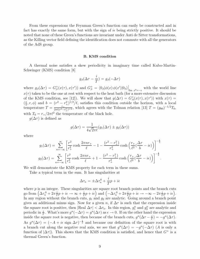
B. KMS condition

A thermal noise satisfies a skew periodicity in imaginary time called Kubo-Martin-Schwinger (KMS) condition [8]

gβ(∆τ − i

T) = gβ(−∆τ)

where gβ(∆τ) = G+β (x(τ), x(τ ′)) and G+

β = 〈0β|φ(x)φ(x′)|0β〉∣

∣

∣

Im x0=−ǫwith the world line

x(τ) taken to be the one at rest with respect to the heat bath (for a more extensive discussionof the KMS condition, see [12]). We will show that g(∆τ) = G+

A(x(τ), x(τ ′)) with x(τ) =( τ

b, r, φ) and b = (r2 − r2

+)1/2/ℓ, satisfies this condition outside the horizon, with a localtemperature T = r+

2πℓ(r2−r2+

)1/2 , which agrees with the Tolman relation [13] T = (g00)−1/2T0,

with T0 = r+/2πℓ2 the temperature of the black hole.

g(∆τ) is defined as

g(∆τ) =1

4√

2πℓ(g1(∆τ) ± g2(∆τ))

where

g1(∆τ) =∞∑

n=−∞

[

r2

r2+

cosh2πnr+ℓ

− 1 − (r2 − r2+)

r2+

cosh(

r+ℓ2

(∆τ

b− iǫ)

)

]− 1

2

g2(∆τ) =∞∑

n=−∞

[

r2

r2+

cosh2πnr+ℓ

+ 1 − (r2 − r2+)

r2+

cosh(

r+ℓ2

(∆τ

b− iǫ)

)

]− 1

2

.

We will demonstrate the KMS property for each term in these sums.Take a typical term in the sum. It has singularities at

∆τn = ±∆τ 0n +

i

Tp + iǫ

where p is an integer. These singularities are square root branch points and the branch cutsgo from

(

∆τ 0n + 2π i

Tp + iǫ→ ∞ + i

Tp+ iǫ

)

and(

−∆τ 0n + 2π i

Tp+ iǫ→ −∞− 2π i

Tp+ iǫ

)

.In any region without the branch cuts, g1 and g2 are analytic. Going around a branch pointgives an additional minus sign. Now for a given n, if ∆τ is such that the expression insidethe square root is positive, then |Real ∆τ | < ∆τn. In this region, gn

1 and gn2 are analytic and

periodic in iT. What’s more gn(−∆τ) = gn(∆τ) as ǫ→ 0. If on the other hand the expression

inside the square root is negative, then because of the branch cuts, gn(∆τ − iT) = −gn(∆τ).

As gn(∆τ) = (−A + iǫ sign ∆τ)−1

2 and because our definition of the square root is witha branch cut along the negative real axis, we see that gn(∆τ) = −gn(−∆τ) (A is only afunction of |∆τ |). This shows that the KMS condition is satisfied, and hence that G+ is athermal Green’s function.

9

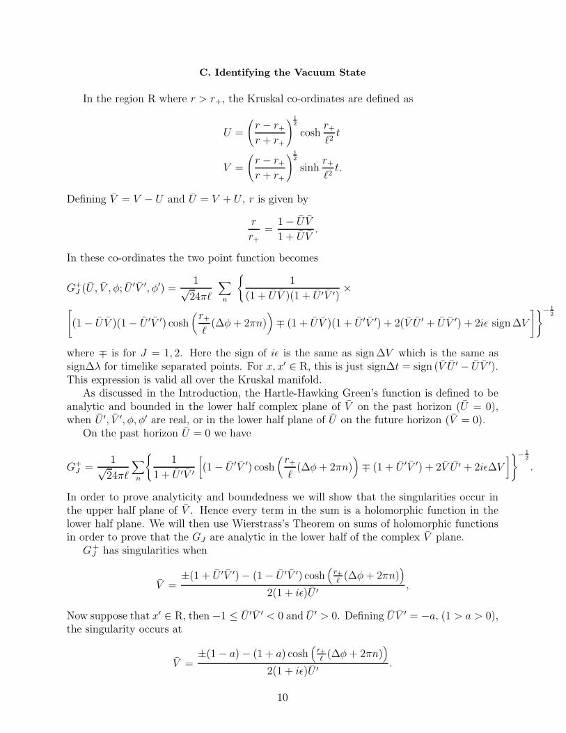
C. Identifying the Vacuum State

In the region R where r > r+, the Kruskal co-ordinates are defined as

U =

(

r − r+r + r+

)1

2

coshr+ℓ2t

V =

(

r − r+r + r+

)1

2

sinhr+ℓ2t.

Defining V = V − U and U = V + U , r is given by

r

r+=

1 − U V

1 + U V.

In these co-ordinates the two point function becomes

G+J (U , V , φ; U ′V ′, φ′) =

1√24πℓ

∑

n

1

(1 + U V )(1 + U ′V ′)×

[

(1 − U V )(1 − U ′V ′) cosh(

r+ℓ

(∆φ+ 2πn))

∓ (1 + U V )(1 + U ′V ′) + 2(V U ′ + U V ′) + 2iǫ sign ∆V

]− 1

2

where ∓ is for J = 1, 2. Here the sign of iǫ is the same as sign ∆V which is the same assign∆λ for timelike separated points. For x, x′ ∈ R, this is just sign∆t = sign (V U ′ − U V ′).This expression is valid all over the Kruskal manifold.

As discussed in the Introduction, the Hartle-Hawking Green’s function is defined to beanalytic and bounded in the lower half complex plane of V on the past horizon (U = 0),when U ′, V ′, φ, φ′ are real, or in the lower half plane of U on the future horizon (V = 0).

On the past horizon U = 0 we have

G+J =

1√24πℓ

∑

n

1

1 + U ′V ′

[

(1 − U ′V ′) cosh(

r+ℓ

(∆φ+ 2πn))

∓ (1 + U ′V ′) + 2V U ′ + 2iǫ∆V]

− 1

2

.

In order to prove analyticity and boundedness we will show that the singularities occur inthe upper half plane of V . Hence every term in the sum is a holomorphic function in thelower half plane. We will then use Wierstrass’s Theorem on sums of holomorphic functionsin order to prove that the GJ are analytic in the lower half of the complex V plane.

G+J has singularities when

V =±(1 + U ′V ′) − (1 − U ′V ′) cosh

(

r+

ℓ(∆φ+ 2πn)

)

2(1 + iǫ)U ′ ,

Now suppose that x′ ∈ R, then −1 ≤ U ′V ′ < 0 and U ′ > 0. Defining U V ′ = −a, (1 > a > 0),the singularity occurs at

V =±(1 − a) − (1 + a) cosh

(

r+

ℓ(∆φ + 2πn)

)

2(1 + iǫ)U ′ .

10

We see that when ǫ→ 0, V is real and negative. Hence V = −A1+iǫ

≃ −A+ iǫ with A > 0, so

that the singularities are in the upper half plane. Similarly, for the future horizon V = 0,there are singularities when

U =±(1 + U ′V ′) − (1 − U ′V ′) cosh(∆φ+ 2πn)

(1 − iǫ)V ′ .

For x′ ∈ R, then −1 < U ′V ′ < 0, and V ′ < 0, so that U = A1−iǫ

= A+ iǫ, with A > 0, so the

singularities are in the upper half plane of U . At this point it should be noted that for G−J

we get singularities in the lower half plane of U on the surface V = 0, and singularities inthe lower half plane of V on the surface U = 0.

For x′ ∈ F, if U = 0 and x and x′ connected by a null geodesic, then ∆V < 0. Thisis the case because for timelike and null separations, sign ∆V = −sign ∆r (r is a timelikeco-ordinate in F) and ∆r is always positive if x is on the horizon. Then it can be checkedthat the singularities are again in the upper half plane of either U or V .

Now that we have established that each term in the infinite sum is holomorphic in thelower half plane of V on the past horizon (and in U on the future horizon) we will useWeierstrass’s Theorem. This states [14] that if a series with analytic terms

f(z) = f1(z) + f2(z) + · · ·

converges uniformly on every compact subset of a region Ω, then the sum f(z) is analytic inΩ, and the series can be differentiated term by term. It is easily seen that unless U ′V ′ = 1,i.e. x′ is at the singularity, the sum converges uniformly on every compact subset of thelower half plane. For U ′V ′ = 1 the sum diverges and the Green’s function becomes singularat r = 0. This is because r = 0 is a fixed point of the identification.

To conclude we have shown that our Green’s function is analytic on the past horizonin the lower half V complex plane, and similarly on the future horizon in the lower half Ucomplex plane. Its singularities occur when x, x′ can be connected by a null geodesics eitherdirectly or after reflection at infinity (see Appendix A and Ref. [7]). We conclude that theGreen’s function we have constructed is the Hartle-Hawking Green’s function as defined inthe Introduction, for both Neumann and Dirichlet boundary conditions.

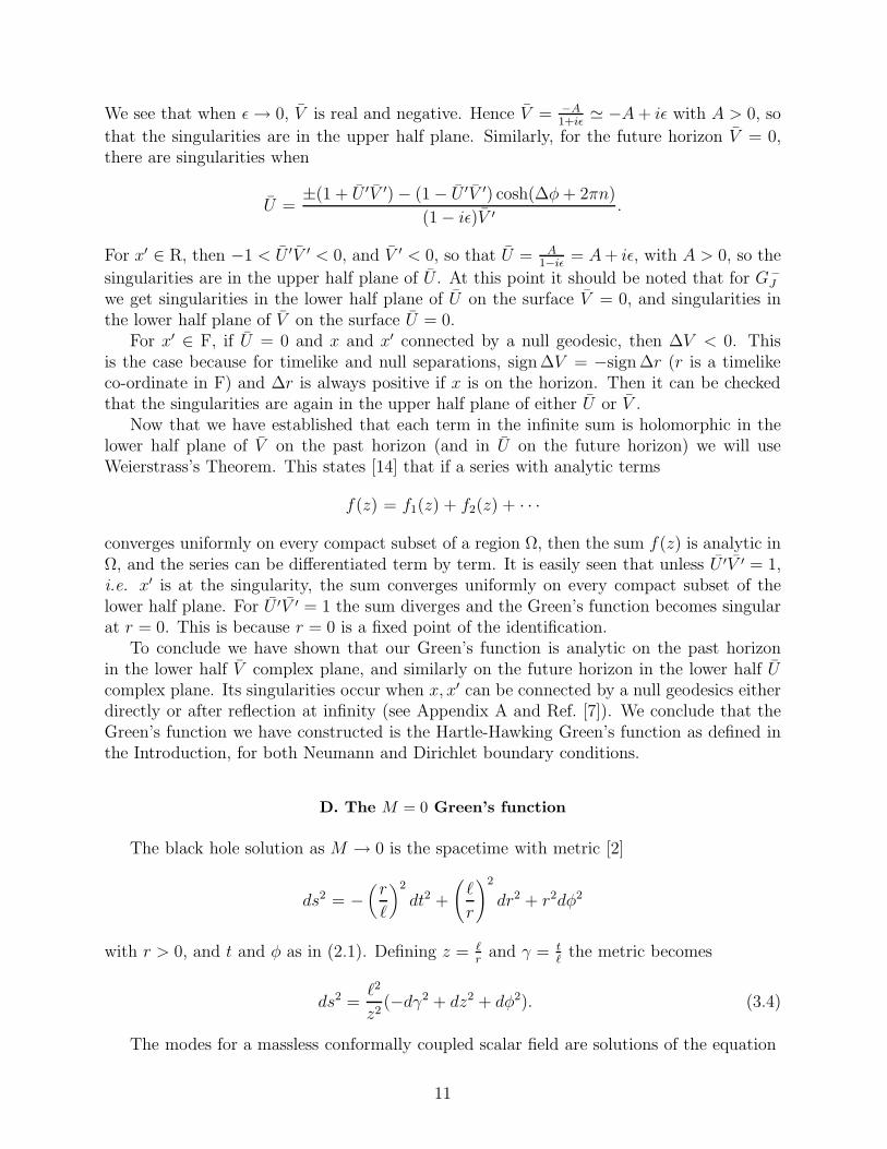
D. The M = 0 Green’s function

The black hole solution as M → 0 is the spacetime with metric [2]

ds2 = −(

r

ℓ

)2

dt2 +

(

ℓ

r

)2

dr2 + r2dφ2

with r > 0, and t and φ as in (2.1). Defining z = ℓr

and γ = tℓ

the metric becomes

ds2 =ℓ2

z2(−dγ2 + dz2 + dφ2). (3.4)

The modes for a massless conformally coupled scalar field are solutions of the equation

11

2φ − 1

8Rφ = 0

where again R = −6ℓ−2, and are given by

φkm = Nω

√

z

le−iωteimφeikz

where ω2 = k2 + m2, m is an integer, and Nω = (8π2ω)1

2 is a normalization constant suchthat (ψmk, ψm′k′) = δmm′δ(k − k′).

As in quantization on AdS3, care must be taken at the boundary z = 0, which is atspatial infinity. The metric (3.4) is conformal to Minkowski spacetime with one spatial co-ordinate periodic and the other restricted to be greater than zero. As in the case of AdS3,we impose the boundary conditions

1√zψ = 0 or

∂

∂z(

1√zψ(z)) = 0

at z = 0, corresponding to Dirichlet or Neumann boundary conditions in the conformalMinkowski metric. Our approach will be to first calculate the Green’s function withoutboundary conditions and them use the method of images to impose them.

Summing modes, we obtain the two point function

G(x, x′) =1

8π2ω

√zz′

ℓ

∑

m

∫

ke−iω∆γ eim∆φ eik∆z dk

=1

2π

√zz′

ℓ

∑

m

eim∆φ G2(y, y′, m)

where G2(y, y′, m) is the massive 1+1 dimensional Green’s function and y = (γ, z).

Now [11],

G2(y, y′, m) =

1

2πK0(|m| d) m 6= 0

= − 1

2πlog d+ lim

n→2

Γ(n2− 1)

nπn2

m = 0

where d = ǫ + i∆ sign ∆t, with ∆ = ((∆γ)2 − (∆z)2)1

2 for timelike separation, and d =

((∆z)2 − (∆γ − iǫ)2)1

2 for spacelike separation. Here K0 is a modified Bessel function. Itfollows that

G(x, x′) =1

4π2

√zz′

ℓ

[

2∑

m>0

cos(m∆β)K0(md) − log d

]

where the infinite constant in the m = 0 expression was dropped to regularize the infrareddivergences of the 1+1 dimensional Green’s function. Using [15]

∞∑

m=1

K0(mx) cos(mxt) =1

2(c+ln

x

4π)+

π

2√

x2 + (xt)2+π

2

∑

l 6=0

[

(

x2 + (2ℓπ − tx)2)− 1

2 − 1

2ℓπ

]

.

12

Here c is the Euler constant. This expression is valid for x > 0 and real t, and gives thefollowing expression for spacelike separated x and x′:

G(x, x′) =1

4π

√zz′

ℓ

∑

n

[

(∆z)2 + (∆φ+ 2πn)2 − (∆γ − iǫ)2]− 1

2 −∑

n 6=0

1

2πn+ c1

=1

4π

√zz′

ℓF (x, x′)

Here c1 = c−ln 4π. Although the above formula was only true for x > 0 and real t, the resultis analytic for every real ∆z, ∆γ and ∆φ. Hence it is also correct for timelike separatedpoints.

This is just what is expected from the conformality to the Minkowski space, other thanthe

∑ 12πℓ

− c1 which regularizes G. Now the boundary condition can be easily put in bywriting

G+(x, x′) =1

4π

√zz′

ℓ(F (x, x′) ± F (x, x′))

where x′ = (γ′,−z′, φ). Notice that for Dirichlet boundary conditions, this agrees with theM → 0 limit of (3.2) and (3.3).

Going to the (t, r, φ) co-ordinates we have

G+M=0 =

1

4π(rr′)−

1

2 (G+1 ± G+

2 )

with

G+1 =

∑

n

ℓ2(

r′ − r

rr′

)2

+ (∆φ+ 2πn)2 −(

∆t− iǫ

ℓ

)2

− 1

2

−∑

n 6=0

1

2πn+ c1

G+2 =

∑

n

ℓ2(

r′ + r

rr′

)2

+ (∆φ+ 2πn)2 −(

∆t− iǫ

ℓ

)2

− 1

2

−∑

n 6=0

1

2πn+ c1

E. Computation of 〈φ2〉

〈φ2〉 is defined as 〈φ2〉 = limx→x′

12GReg(x, x

′) where G = G+ + G− is the symmetricGreen’s function. In order to compute 〈φ2〉, we need to regularize G. Now only the n = 0term in G+

1 is infinite and is just a Green’s function on AdS3. Hence, we can use theHadamard development in AdS3 to regularize G [11]:

GHad =−i

2√

2π

∆1

2

σ1

2

where

13

σ =ℓ2

2[ar cosZ]2 , ∆− 1

2 =sin

(

2σℓ2

)1

2

(

2σℓ2

)1

2

and Z =cos ∆λ− sin ρ sin ρ′ cos ∆θ

cos ρ cos ρ′

(here ∆ is the Van Veleck determinant). Defining

GReg(x, x′) = GBH(x, x′) − GHad(x, x

′)

we get

〈φ2〉 =1

4√

2πℓ

r+r

∑

n 6=0

(

cosh(

r+ℓ

2πn)

− 1)− 1

2 ±∑

n

(

cosh(

r+ℓ

2πn)

− 1 + 2(

r+r

)2)− 1

2

which, for Dirichlet boundary conditions, can be seen to be regular as M → 0 (that isr+ → 0), and to coincide in this limit with the M = 0 result for Dirichlet boundaryconditions.

IV. THE ENERGY-MOMENTUM TENSOR

The energy-momentum tensor for a massless conformally coupled scalar field in AdS3 isgiven by the expression

Tµν(x) =3

4∂µφ(x)∂νφ(x) − 1

4gµνg

ρσ∂ρφ(x)∂σφ(x) − 1

4∇µ∂νφ(x)φ(x) +

1

96gµνRφ

2(x)

where R = −6ℓ−2. In order to compute 〈Tµν〉 one differentiates the symmetric two-pointfunction G = 〈0|φ(x)φ(x′) + φ(x′)φ(x)|0〉 [11], and then takes the coincident point limit.This makes 〈Tµν〉 divergent and regularization is needed. A look at our Green’s functionreveals that only the n = 0 term in G1 diverges as x→ x′, so only the 〈Tµν〉 derived from itshould be regularized.

The n = 0 term is just the Green’s function in AdS3 in accelerating co-ordinates. Thevacuum in which this Green’s function is derived is symmetric under the Anti de Sittergroup and AdS3 is a maximally symmetric space. Hence [16] 〈Tµν〉 = 1

3gµν〈T 〉 where 〈T 〉 =

gµν〈Tµν〉. For a conformally coupled massless scalar field 〈T 〉 = 0 (there is no conformalanomaly in 2+1 dimensions) so 〈TAdS

µν 〉 = 0.Having shown that we may drop the n = 0 term in G1, after a somewhat lengthy

calculation we arrive at the result for M 6= 0,

〈T νµ (x)〉 =

1

16πℓ3r3

∑

n>0

[

r2+f

−1n

2

[

1 ±(

1 + (fnr)−2)− 3

2

]

+ f−3n

]

diag(1, 1,−2)

±3

2

(

1 − r2+

r2

)

f−3n

(

1 + (fnr)−2)− 5

2 diag(1, 0,−1)

(4.1)

where fn = sinh( r+

ℓπn)/r+. diag (a, b, c) is in (t, r, φ) co-ordinates. As expected the n = 0

term from G2 did not contribute.For M = 0 we get from Sec. IIID

14

〈T µν (x)〉 =

1

16πr3

∑

n>0

1

(nπ)3diag (1, 1,−2) ± 3

2(nπ)3

(

1 + (fnr)−2)− 5

2 diag (1, 0,−1)

(4.2)

where now fn = πn/ℓ. Note that the M = 0 result agrees with the M → 0 limit of (4.1).Some properties of 〈T ν

µ 〉 are:

• As we can see from (4.1), far away from the black hole, 〈T µν 〉 obeys the strong energy

condition [10] only for the Dirichlet boundary conditions, while for the Neumannboundary conditions, the energy density is negative in this limit.

• For Dirichlet boundary conditions, as M decreases, although the temperature de-creases, the energy density increases; just the opposite occurs for Neumann boundaryconditions.

• In the limit M → ∞, 〈T µν 〉 → 0 for both sets of boundary conditions, which suggests

the presence of a Casimir effect.

• On the horizon, 〈T µν 〉 is regular, and hence in the semiclassical approximation, the

horizon is stable to quantum fluctuations; on the other hand, at r = 0, 〈T µν 〉 diverges.

• Our Green’s function was thermal in (t, r, φ) co-ordinates, but although 〈T µν 〉 ∼ T 3

loc

for large r, it is not of a thermal type [13].

V. THE RESPONSE OF A PARTICLE DETECTOR

In this section we calculate the response of a particle detector which is stationary in theblack hole co-ordinates (t, r, φ), and outside the black hole. The simplest particle detectorcan be described by an idealized point monopole coupled to the quantum field through aninteraction described by Lint = cm(τ)φ[x(τ)] where τ is the detector’s proper time, andc ≪ 1. The probability per unit time for the detector to undergo a transition from energyE1 to E2 [11] is R(E1/E2) = c2 |〈E2|m(0)|E1〉|2 F (E2 −E1) to lowest order in perturbationtheory, where

F (ω) = lims→0

limτ0→∞

1

2τ0

∫ τ0

−τ0dτ

∫ τ0

−τ0dτ ′ e−iω(τ−τ ′)−S|τ |−S|τ ′| g(τ, τ ′).

g(τ, τ ′) = G+(x(τ), x(τ ′)) and x(τ) is the detector trajectory.F (ω) is called the response function. It represents the bath of particles that the detector

sees during its motion [17]. We take x(τ) = ( τb, r, φ) where b =

(

r2−r2+

ℓ2

)1

2

. Because g(τ, τ ′) =

g(∆τ), then

F (ω) =∫ ∞

−∞e−iω∆τ g(∆τ)d(∆τ) (5.1)

where g(∆τ) = g1(∆τ) ± g2(∆τ). Here

15

gi(∆τ) =r+√24πℓ

(r2 − r2+)−

1

2

∑

n

[

r2+

r2 − r2+

(

r2

r2+

cosh(

r+ℓ

2πn)

∓ 1

)

− coshr+ℓ2

(∆τ

b− iǫ)

]− 1

2

.

(5.2)

In this expression −(+) is for g1(g2).Defining

coshαn =r2+

r2 − r2+

(

r2

r2+

cosh(

r+ℓ

2πn)

− 1

)

and

cosh βn =r2+

r2 − r2+

(

r2

r2+

cosh(

r+ℓ

2πn)

+ 1

)

we have from Appendix B that

F (ω) =1

2

1

eω/T + 1

∑

n

(

P iω2πT

− 1

2

(coshαn) ± P iω2πT

− 1

2

(coshβn))

where T = r+

2πℓ(r2−r2+

)12

is the local temperature. This looks like a fermion distribution with

zero chemical potential and a density of states

D(ω) =ω

2π

∑

n

(

P iω2πT

− 1

2

(coshαn) ± P iω2πT

− 1

2

(coshβn))

.

Notice that F (ω) is finite on the horizon in contrast with black holes in two and fourdimensions (see [18]). This seems to be a consequence of the Fermi type distribution.Statistical inversion in odd-dimensional flat spacetime was first noted in Ref. [12].

If the mass of the black hole satisfies e2π√

M ≫ 1 and 2ℓ−1 > ω ≫ T , then far from thehorizon, r ≫ r+, we can sum the series, and for Dirichlet boundary conditions we obtain

F (ω) ≃ 2π2ℓ2T 2 1

eω/T + 1

(

ω

2πT

)2

+1

4+

8e−3π√

M

π

(

ω

T

)1

2

(

sinw√M

T− cos

w√M

T

)

.

A similar result holds for Neumann boundary conditions at large r,

F (ω) ≃ 1

eω/T + 1

[

1 + 4(

ω

T

)− 1

2

e−π√

M

(

sinω√M

T+ cos

ω√M

T

)]

where the approximation improves for large M as before.It seems clear that the particle detector response will consist of a Rindler-type effect [11],

and, if present, a response due to Hawking radiation (real particles). The former is due tothe fact that a stationary particle detector is actually accelerating, even when r → ∞ (thereis no asymptotically flat region). This is reflected for instance in the fact that for somerange of ω, the behaviour of F (ω) for r ≫ r+ and M ≫ 1 is governed by the n = 0 termin G+, which is AdS invariant. Hence all observers connected by an AdS transformation(a subgroup of the asymptotic symmetry group) register the same response, even though

16

they might be in relative motion; this means that F (ω) as a whole cannot be interpretedas real particles (see [19,20] for a discussion of this point). Unfortunately, one cannot filterout these effects in a simple way, and further work is needed in order to find the spectrumof the Hawking radiation.

Finally, for M = 0, we may again define

Fi(ω) =∫ ∞

−∞e−iω∆τgi(∆τ)d∆τ.

Now, however, g1 and g2 are analytic in the lower half complex plane of ∆τ . Hence for ω > 0we can close the integral in an infinite semicircle in the lower half plane and by Cauchy’stheorem Fi(ω) = 0 for ω > 0 so that no particles are detected by a stationary particledetector.

VI. BACK-REACTION

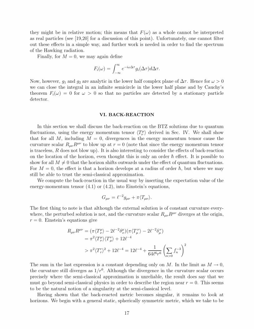
In this section we shall discuss the back-reaction on the BTZ solutions due to quantumfluctuations, using the energy momentum tensor 〈T µ

ν 〉 derived in Sec. IV. We shall showthat for all M , including M = 0, divergences in the energy momentum tensor cause thecurvature scalar RµνR

µν to blow up at r = 0 (note that since the energy momentum tensoris traceless, R does not blow up). It is also interesting to consider the effects of back-reactionon the location of the horizon, even thought this is only an order h effect. It is possible toshow for allM 6= 0 that the horizon shifts outwards under the effect of quantum fluctuations.For M = 0, the effect is that a horizon develops at a radius of order h, but where we maystill be able to trust the semi-classical approximation.

We compute the back-reaction in the usual way by inserting the expectation value of theenergy-momentum tensor (4.1) or (4.2), into Einstein’s equations,

Gµν = ℓ−2gµν + π〈Tµν〉.

The first thing to note is that although the external solution is of constant curvature every-where, the perturbed solution is not, and the curvature scalar RµνR

µν diverges at the origin,r = 0. Einstein’s equations give

RµνRµν = (π〈T µ

ν 〉 − 2ℓ−2δµν)(π〈T ν

µ 〉 − 2ℓ−2δ νµ )

= π2〈T µν 〉〈T ν

µ〉 + 12ℓ−4

> π2〈T rr〉2 + 12ℓ−4 = 12ℓ−4 +

1

64ℓ6r6

(

∑

n>0

f−3n

)2

The sum in the last expression is a constant depending only on M . In the limit as M → 0,the curvature still diverges as 1/r6. Although the divergence in the curvature scalar occursprecisely where the semi-classical approximation is unreliable, the result does say that wemust go beyond semi-classical physics in order to describe the region near r = 0. This seemsto be the natural notion of a singularity at the semi-classical level.

Having shown that the back-reacted metric becomes singular, it remains to look athorizons. We begin with a general static, spherically symmetric metric, which we take to be

17

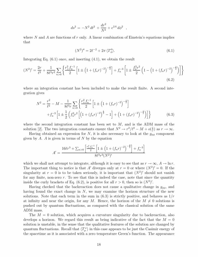
ds2 = −N2 dt2 +dr2

N2+ e2A dφ2 ,

where N and A are functions of r only. A linear combination of Einstein’s equations impliesthat

(N2)′′ = 2ℓ−2 + 2π 〈T φφ〉. (6.1)

Integrating Eq. (6.1) once, and inserting (4.1), we obtain the result

(N2)′ =2r

ℓ2+

1

8ℓ3r2

∑

n>0

r2+f

−1n

2

[

1 ±(

1 + (fnr)−2)− 3

2

]

+ f−3n

[

1 ± f 2nr

2

2

(

1 −(

1 + (fnr)−2)− 3

2

)

]

(6.2)

where an integration constant has been included to make the result finite. A second inte-gration gives

N2 =r2

ℓ2−M − 1

8ℓ3r

∑

n>0

r2+f

−1n

2

[

1 ±(

1 + (fnr)−2)− 1

2

]

+f−3n

[

1 ± 1

2

(

f 2nr

2[

(

1 + (fnr)−2)

1

2 − 1]

+(

1 + (fnr)−2)− 1

2

)]

(6.3)

where the second integration constant has been set to M , and is the ADM mass of thesolution [2]. The two integration constants ensure that N2 → r2/ℓ2 −M + o(1

r) as r → ∞.

Having obtained an expression for N , it is also necessary to look at the gφφ componentgiven by A. A is given in terms of N by the equation

A′ =16ℓr3 +

∑

n>0

[

r2+

f−1n

2

[

1 ±(

1 + (fnr)−2)− 3

2

]

+ f−3n

]

8ℓ3r3(N2)′

which we shall not attempt to integrate, although it is easy to see that as r → ∞, A→ ln r.The important thing to notice is that A′ diverges only at r = 0 or where (N2)′ = 0. If thesingularity at r = 0 is to be taken seriously, it is important that (N2)′ should not vanishfor any finite, non-zero r. To see that this is indeed the case, note that since the quantityinside the curly brackets of Eq. (6.2), is positive for all r > 0, then so is (N2)′.

Having checked that the backreaction does not cause a qualitative change in gφφ, andhaving found the exact change in N , we may examine the horizon structure of the newsolutions. Note that each term in the sum in (6.3) is strictly positive, and behaves as 1/rat infinity and near the origin, for any M . Hence, the horizon of the M 6= 0 solutions ispushed out by quantum fluctuations, as compared with the classical solution of the sameADM mass.

The M = 0 solution, which acquires a curvature singularity due to backreaction, alsodevelops a horizon. We regard this result as being indicative of the fact that the M = 0solution is unstable, in the sense that the qualitative features of the solution are changed byquantum fluctuations. Recall that 〈T ν

µ 〉 in this case appears to be just the Casimir energy ofthe spacetime as it is associated with a zero temperature Green’s function. The appearance

18

of a horizon may be contrasted in an obvious way with 4-dimensional Minkowski spacetime,regarded as the M = 0 limit of the Schwarzschild solution. Minkowski spacetime has noCasimir energy associated with it, and is stable in the above sense.

Note that as M → 0, the horizon is located in a region sufficiently close to r = 0 thatthe semi-classical approximation may break down, i.e. fluctuations in 〈T µ

ν 〉 will be of theorder of 〈T µ

ν 〉. However, if there are n independent scalar fields present, then the ratio of thefluctuations to 〈T µ

ν 〉 becomes negligible in the vicinity of the horizon, as n becomes large.The size of the perturbation on the metric near where the horizon develops may also beestimated. It is approximately an order of magnitude smaller than the curvature of theoriginal solution, a result which is independent of n.

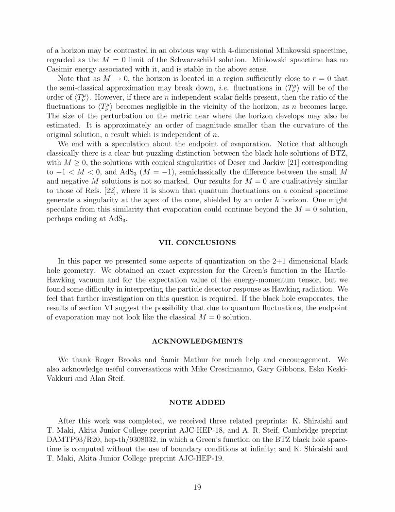
We end with a speculation about the endpoint of evaporation. Notice that althoughclassically there is a clear but puzzling distinction between the black hole solutions of BTZ,with M ≥ 0, the solutions with conical singularities of Deser and Jackiw [21] correspondingto −1 < M < 0, and AdS3 (M = −1), semiclassically the difference between the small Mand negative M solutions is not so marked. Our results for M = 0 are qualitatively similarto those of Refs. [22], where it is shown that quantum fluctuations on a conical spacetimegenerate a singularity at the apex of the cone, shielded by an order h horizon. One mightspeculate from this similarity that evaporation could continue beyond the M = 0 solution,perhaps ending at AdS3.

VII. CONCLUSIONS

In this paper we presented some aspects of quantization on the 2+1 dimensional blackhole geometry. We obtained an exact expression for the Green’s function in the Hartle-Hawking vacuum and for the expectation value of the energy-momentum tensor, but wefound some difficulty in interpreting the particle detector response as Hawking radiation. Wefeel that further investigation on this question is required. If the black hole evaporates, theresults of section VI suggest the possibility that due to quantum fluctuations, the endpointof evaporation may not look like the classical M = 0 solution.

ACKNOWLEDGMENTS

We thank Roger Brooks and Samir Mathur for much help and encouragement. Wealso acknowledge useful conversations with Mike Crescimanno, Gary Gibbons, Esko Keski-Vakkuri and Alan Steif.

NOTE ADDED

After this work was completed, we received three related preprints: K. Shiraishi andT. Maki, Akita Junior College preprint AJC-HEP-18, and A. R. Steif, Cambridge preprintDAMTP93/R20, hep-th/9308032, in which a Green’s function on the BTZ black hole space-time is computed without the use of boundary conditions at infinity; and K. Shiraishi andT. Maki, Akita Junior College preprint AJC-HEP-19.

19

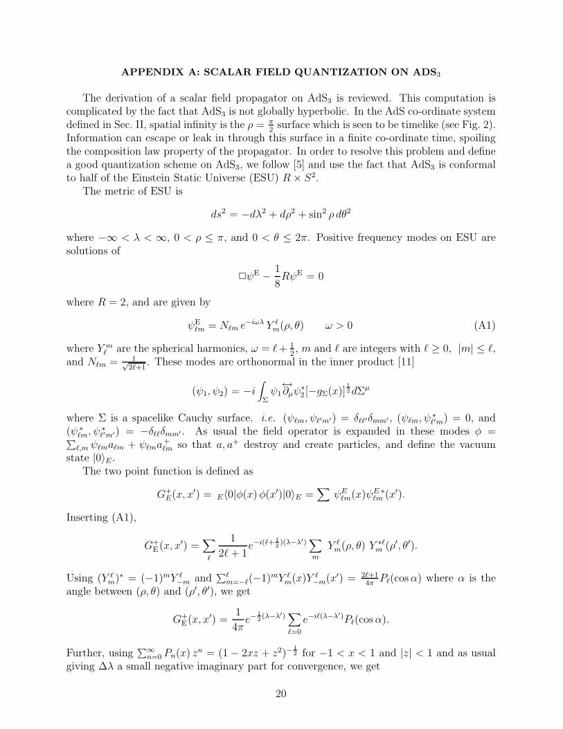
APPENDIX A: SCALAR FIELD QUANTIZATION ON ADS3

The derivation of a scalar field propagator on AdS3 is reviewed. This computation iscomplicated by the fact that AdS3 is not globally hyperbolic. In the AdS co-ordinate systemdefined in Sec. II, spatial infinity is the ρ = π

2surface which is seen to be timelike (see Fig. 2).

Information can escape or leak in through this surface in a finite co-ordinate time, spoilingthe composition law property of the propagator. In order to resolve this problem and definea good quantization scheme on AdS3, we follow [5] and use the fact that AdS3 is conformalto half of the Einstein Static Universe (ESU) R× S2.

The metric of ESU is

ds2 = −dλ2 + dρ2 + sin2 ρ dθ2

where −∞ < λ < ∞, 0 < ρ ≤ π, and 0 < θ ≤ 2π. Positive frequency modes on ESU aresolutions of

2ψE − 1

8RψE = 0

where R = 2, and are given by

ψEℓm = Nℓm e

−iωλ Y ℓm(ρ, θ) ω > 0 (A1)

where Y mℓ are the spherical harmonics, ω = ℓ+ 1

2, m and ℓ are integers with ℓ ≥ 0, |m| ≤ ℓ,

and Nℓm = 1√2ℓ+1

. These modes are orthonormal in the inner product [11]

(ψ1, ψ2) = −i∫

Σψ1

↔∂µψ

∗2 [−gΣ(x)]

1

2dΣµ

where Σ is a spacelike Cauchy surface. i.e. (ψℓm, ψℓ′m′) = δℓℓ′δmm′ , (ψℓm, ψ∗ℓ′m) = 0, and

(ψ ∗ℓm, ψ

∗ℓ′m′) = −δℓℓδmm′ . As usual the field operator is expanded in these modes φ =

∑

ℓ,m ψℓmaℓm + ψℓma+ℓm so that a, a+ destroy and create particles, and define the vacuum

state |0〉E.The two point function is defined as

G+E(x, x′) = E〈0|φ(x)φ(x′)|0〉E =

∑

ψEℓm(x)ψE ∗

ℓm (x′).

Inserting (A1),

G+E(x, x′) =

∑

ℓ

1

2ℓ+ 1e−i(ℓ+ 1

2)(λ−λ′)

∑

m

Y ℓm(ρ, θ) Y ∗ℓ

m (ρ′, θ′).

Using (Y ℓm)∗ = (−1)mY ℓ

−m and∑ℓ

m=−ℓ(−1)mY ℓm(x)Y ℓ

−m(x′) = 2ℓ+14π

Pℓ(cosα) where α is theangle between (ρ, θ) and (ρ′, θ′), we get

G+E(x, x′) =

1

4πe−

1

2(λ−λ′)

∑

ℓ=0

e−iℓ(λ−λ′)Pℓ(cosα).

Further, using∑∞

n=0 Pn(x) zn = (1 − 2xz + z2)−1

2 for −1 < x < 1 and |z| < 1 and as usualgiving ∆λ a small negative imaginary part for convergence, we get

20

G+E =

1

4√

2π(cos(∆λ− iǫ) − cos ρ cos ρ′ − sin ρ sin ρ′ cos ∆θ)

− 1

2

where the square root is defined with a branch cut along the negative real axis and theargument function is between (−π, π) [23]. From now we shall call this two point functionG+

1,E and define G+2,E(x, x′) = G+

1,E(x, x′) where x = (λ, π − ρ, θ). Then,

G+2,E =

1

4√

2π(cos(∆λ− iǫ) + cos ρ cos ρ′ − sin ρ sin ρ′ cos ∆θ)

− 1

2

and G+2,E satisfies also the homogeneous equation (2 − 1

8R)G = 0. Conformally mapping

these solutions to AdS3, where G+A =

√cos ρ cos ρ′G+

E we get

G+1,A(x, x′) =

1

4√

2πℓ(cos(∆λ− iǫ) sec ρ sec ρ′ − 1 − tan ρ tan ρ′ cos ∆θ)

− 1

2

and

G+2,A(x, x′) =

1

4√

2πℓ(cos(∆λ− iǫ) sec ρ sec ρ′ + 1 − tan ρ tan ρ′ cos ∆θ)

− 1

2 .

It can be seen that G+1,A and G+

2,A are functions of σ(x, x′) = 12[(u − u′)2 + (v − v′)2 + (x−

x′)2+(y−y′)2], which is the distance between the spacetime points x, x′ in the 4-dimensionalembedding space.

In order to deal with the problem of global hyperbolicity, it was shown in [5] that imposingboundary conditions on the ESU modes gives a good quantization scheme on the half of ESUwith ρ ≤ π

2, thus inducing a good quantization scheme on AdS4. It may be checked that

this method also works in 2+1 dimensions. The boundary conditions on the ESU modes areeither Dirichlet

ψEℓ,m

(

ρ =π

2

)

= 0 obeyed by ψℓ,m with ℓ +m = odd

or Neumann

∂

∂ρψE

ℓ,m

(

ρ =π

2

)

= 0 obeyed by ψℓ,m with ℓ+m = even.

It is easily verified that the combination G+E = G+

1,E ± G+2,E has the right boundary

condition where the +(−) signs are for Neumann (Dirichlet) boundary conditions.Some remarks are in order: if x, x′ are restricted such that −π < λ(x) − λ(x′) < π then

(1) G+1 E is real for spacelike points, imaginary for timelike points and singular for x, x′

which can be connected by a null geodesic.

(2) G+2 E has the same property when x → x, and if 0 ≤ ρ(x′), ρ(x) < π

2then G2 has sin-

gularities when x, x′ can be connected by a null geodesic bouncing off ρ = π2

boundary.

21

From this we see that if we take the modes in AdS3 as

ψAℓ,m = (cos ρ)

1

2 e−i(ℓ+ 1

2)λ Y m

ℓ (ρ, θ) ℓ +m = odd or ℓ +m = even

then these modes give rise to a well-behaved propagator [5]. The two point function is then

G+A =

√

cos ρ cos ρ′(G+1,A ± G+

2,A)

where +(−) are for Neumann (Dirichlet). The two point function has singularities wheneverx, x′ can be connected by a null geodesic directly or by a null geodesic bouncing off infinity(null geodesics remain null geodesics by a conformal transformation). All other propertieslisted before also stay the same.

Note that it is possible to define a quantization scheme on AdS3 without using boundaryconditions (i.e. just using G+

1,A), which is referred to as transparent boundary conditionsin Ref. [5]. However this requires the use of a two-time Cauchy surface, and its physicalinterpretation is unclear.

APPENDIX B: CALCULATING THE RESPONSE FUNCTION

We are interested in an integral of the type

J(ω) =ℓ2b

r+

∫ ∞

−∞e−

iω2πT

t (coshαn − cosh(t − iǫ))−1

2dt

where T = r+

2πℓ(r2−r2+

)12

is the local temperature. J(ω) = I1(ω) + I2(ω) + I3(ω) where I1 is

the integral from −∞ to −αn, I2 is from −αn to αn, and I3 is from αn to ∞. Recall thatthe square root is defined with the cut along the negative real axis. Then

I1 =ℓ2b

−ir+

∫ −αn

−∞e−

iωt2πT (cosh t− coshαn)−

1

2

I3 =ℓ2b

ir+

∫ ∞

αn

e−iωt2πT (cosh t− coshαn)−

1

2

I2 =2ℓ2b

r+

∫ αn

0cos

ωt

2πT(coshαn − cosh t)−

1

2dt.

Using [15]

∫ ∞

α

e−(ν+ 1

2)t

(cosht− coshα)−1

2

=√

2Qν(coshα) Re ν > −1 α > 0

∫ α

0

cosh(ν + 12)t

(coshα− cosht)1

2

=π√2Pν(coshα) α > 0

where Pν and Qν are associated Legendre functions of the first and second kind respectively,we get

22

I3 = −i√

2ℓ2b

r+Q iω

2πT− 1

2

(coshαn)

I2 =

√2πℓ2b

r+P iω

2πT− 1

2

(coshαn)

I1 =i√

2ℓ2b

r+Q−iω

2πT− 1

2

(coshαn).

Now using Qν(z) −Q−ν−1(z) = π cot(νπ)Pν(z) [15]

J(ω) =2√

2πℓ2b

r+P iω

2πT− 1

2

(coshαn)1

eω/T + 1,

and F1,2(ω), defined by (5.1) and (5.2) in an obvious way, are given by

F1(ω) =1

2

1

eω/T + 1

∑

n 6=0

P iω2πT

− 1

2

(coshαn)

F2(ω) =1

2

1

eω/T + 1

∑

n

P iω2πT

− 1

2

(coshβn).

Notice that although the formulae that we used were not correct when α = 0, neverthelessthe α0 term came out correctly, since

∫ ∞

−∞e−iωt(1 − cosh(2πT t− iǫ))−

1

2

= i∫ 0

−∞e−iωt

∣

∣

∣

√2 sinh(πT t− iǫ)

∣

∣

∣

−1 − i∫ ∞

0e−iωt

∣

∣

∣

√2 sinh(πT t− iǫ)

∣

∣

∣

−1

=∫ ∞

−∞e−iωt

(√2i sinh(πT t) + ǫ

)−1.

This gives [12]

F 01 (ω) =

T

2

∫ ∞

−∞e−iωt (2i sinh(πT t) + ǫ)−1 =

1

2

1

eω/T + 1

which is exactly what we got before as Pν(1) = 1.Combining the results for F1 and F2, we have

F (ω) =1

2

1

eω/T + 1

∑

n

(

P iω2πT

− 1

2

(coshαn) ± P iω2πT

− 1

2

(cosh βn))

.

23

REFERENCES

∗ This work is supported in part by funds provided by the U. S. Department of Energy(D.O.E.) under contract #DE-AC02-76ER03069.

[1] J. B. Hartle and S. W. Hawking, Phys. Rev. D13 2188 (1976).[2] M. Banados, C. Teitelboim and J. Zanelli, Phys. Rev. Lett. 69 1849 (1992); M. Banados,

M. Henneaux, C. Teitelboim and J. Zanelli, Phys. Rev. D48 1506 (1993).[3] B. Reznik, Phys. Rev. D45 2151 (1992).[4] D. Cangemi, M. Leblanc and R. B. Mann, MIT preprint CTP#2162, gr-qc/9211013; R.

B. Mann and S. F. Ross, Phys. Rev. D47 3319 (1993); G. Clement, Class. Qu. Grav.10 L49 (1993); G. Horowitz and D. Welch, Phys. Rev. Lett. 71 328 (1993); N. Kaloper,Phys. Rev. D48 2598 (1993).

[5] S. J. Avis, C. J. Isham and D. Storey, Phys. Rev. D18 3565 (1978).[6] S. A Fulling, J. Phys. A10 917 (1977).[7] G. W. Gibbons and M. Perry, Proc. R. Soc. London A358 467 (1978).[8] R. Kubo, J. Phys. Soc. Jpn. 12 570 (1957); P. C. Martin and J. Schwinger, Phys. Rev.

115 1342 (1959).[9] A. Achucarro and M. E. Ortiz, to appear in Phys. Rev. D; hep-th/9304068.

[10] S. W. Hawking and G. F. R. Ellis The Large Scale Structure of Space Time, CambridgeUniversity Press, Cambridge, UK (1973).

[11] N. D. Birrell and P. C. W. Davies, Quantum Fields in Curved Space, Cambridge Uni-versity Press, Cambridge, UK (1982).

[12] S. Takagi, Prog. Theo. Phys. Supp. 88 (1986).[13] R. C. Tolman, Relativity, Thermodynamics and Cosmology, Oxford, UK (1931).[14] L. V. Ahlfors, Complex Analysis, McGraw-Hill, New York (1966).[15] I. S. Gradshteyn and I. M. Ryzhik, Tables of integrals, series and products, Academic

Press, San Diego (1965).[16] S. Weinberg, Gravitation and Cosmology, Wiley, New York (1971), chapter 13.4.[17] W. G. Unruh, Phys. Rev. D14 870 (1976).[18] P. Candelas, Phys. Rev. D21 2185 (1980).[19] G. W. Gibbons and S. W. Hawking, Phys. Rev. D15 2738 (1977).[20] P. Hajicek, Phys. Rev. D15 2757 (1977).[21] S. Deser and R. Jackiw, Ann. Phys. 153 405 (1984).[22] T. Souradeep and V. Sahni, Phys. Rev. D46 1616 (1993); H. H. Soleng, to appear in

Phys. Scripta, hep-th/9310007.[23] E. W. Hobson, The theory of spherical and ellipsoidal harmonics, Chelsy, New York

(1955).

24

FIGURES

FIG. 1. A Penrose diagram of (a) the M 6= 0 black hole, and (b) the M = 0 solution. Informa-

tion can leak through spatial infinity, unless we impose boundary conditions at r = ∞.

FIG. 2. A Penrose diagram of AdS3. Information can leak in or out through spatial infinity,

and thus Σ is not a Cauchy surface unless we impose boundary conditions at r = ∞.

25

This figure "fig1-1.png" is available in "png" format from:

http://arXiv.org/ps/gr-qc/9310008v3

This figure "fig1-2.png" is available in "png" format from:

http://arXiv.org/ps/gr-qc/9310008v3