Sampling-Based Path Planning for a

Visual Reconnaissance UAV∗

Karl J. Obermeyer†

University of California at Santa Barbara, Santa Barbara, CA 93106

Paul Oberlin‡and Swaroop Darbha§

Texas A&M University, College Station, TX 77843

This article considers a path planning problem for a single fixed-wing aircraft performinga reconnaissance mission using EO (Electro-Optical) camera(s). A mathematical formu-lation of the general aircraft visual reconnaissance problem for static ground targets interrain is given and it is shown, under simplifying assumptions, that it can be reducedto a PVDTSP (Polygon-Visiting Dubins Traveling Salesman Problem), a variation of thefamous TSP (Traveling Salesman Problem). Two algorithms for solving the PVDTSP aredeveloped. They fall into the class of algorithms known as sampling-based roadmap meth-ods because they operate by sampling a finite set of points from a continuous state spacein order to reduce a continuous motion planning problem to planning on a finite discretegraph called a roadmap. Under certain technical assumptions, the algorithms are resolutioncomplete, which means the solution returned provably converges to a global optimum asthe number of samples grows, i.e., as the the resolution of the roadmap becomes finer. Thefirst algorithm is resolution complete under slightly milder assumptions, but the secondalgorithm achieves faster computation times by a novel roadmap construction. Numericalexperiments indicate that, for up to about 20 targets both algorithms deliver very goodsolutions suitably quickly for online purposes. Additionally, the algorithms allow trade-offof computation time for solution quality and are shown extensible to handle wind, airspaceconstraints, any vehicle dynamics, and open-path (vs. closed-tour) problems.

I. Introduction

UAVs (Unmanned Air Vehicles) are increasingly being used for both civilian and military applicationssuch as environmental monitoring, geological survey, surveillance, reconnaissance, and search and rescue.1,2

Good control and planning algorithms are a key component of UAV technology because they can increaseoperational capabilities while reducing risk, costs, and operator workloads. In this article we present anovel path planning algorithm for a single fixed-wing aircraft performing a reconnaissance mission using EO(Electro-Optical) camera(s). Given a set of stationary ground targets in a terrain (natural, urban, or mixed),the objective is to compute a path for the reconnaissance aircraft so that it can photograph all targets inminimum time. That the targets are situated in terrain plays a significant role because terrain features canocclude visibility. As a result, in order for a target to be photographed, the aircraft must be located whereboth (1) the target is in close enough range to satisfy the photograph’s resolution requirements, and (2) theline-of-sight between the aircraft and the target is not blocked by terrain. For a given target, we call the setof all such aircraft positions the target’s visibility region. An example visibility region is illustrated in Fig. 1.In full generality, the aircraft path planning can be complicated by wind, airspace constraints (e.g. due toenemy threats or collision avoidance), aircraft dynamic constraints, and the aircraft body itself occludingvisibility. However, under simplifying assumptions, if we model the aircraft as a Dubins vehiclea, approximatethe targets’ visibility regions by polygons, and let the path be a closed tour, then the reconnaissance pathplanning problem can be reduced to the following.

For a Dubins vehicle, find a shortest planar closed tour which visits at least one point in each ofa set of polygons.

∗This version: June 26, 2011†PhD student, Center for Control, Dynamical Systems, and Computation; karl@engr.ucsb.edu. Student Member AIAA.‡PhD student, Department of Mechanical Engineering; paul.v.oberlin@gmail.com§Professor, Department of Mechanical Engineering; dswaroop@tamu.eduaA Dubins vehicle is one which moves only forward and has a minimum turning radius.3,4

1 of 25

American Institute of Aeronautics and Astronautics

Figure 1. Top shows an example target, a ground vehicle parked next to a building in urban terrain. The set of allpoints which are close enough to the target to satisfy photograph resolution requirements is a solid sphere (bottomleft). The green two-dimensional region in the sky (bottom right) shows the subset of the sphere, at a reconnaissanceaircraft’s altitude h, where target visibility is not occluded by terrain. Assuming the aircraft body itself doesn’t occludevisibility, then flying the aircraft through the green region is sufficient for the target to be photographed, hence we callit the target’s visibility region for fixed aircraft altitude h.

We refer to this henceforth as the PVDTSP (Polygon-Visiting Dubins Traveling Salesman Problem) since itis a variation of the famous TSP (Traveling Salesman Problem).b A graphical illustration of the PVDTSPis shown in Fig. 2.

I.A. Related Work

To our knowledge the PVDTSP has not previously been studied aside from Ref. 6 where we designed a geneticalgorithm. Although the genetic algorithm performs on average fairly well in Monte-Carlo numerical studies,there unfortunately is significant variance in solution quality and no proven performance guarantees. Becausethe PVDTSP has embedded in it the combinatorial problem of choosing the order to visit the polygons, thesolution space is very large and discontinuous. This precludes direct application of numerical optimal controltechniques traditionally used in trajectory optimization, surveyed, e.g., in Ref. 7. However, several relatedvariations of the TSP are of interest (summarized in Table 1). The ETSP (Euclidean TSP) is a TSP wherethe vertices of the graph are points in the Euclidean plane R

2 and the edges are weighted with Euclideandistances. In the ETSPN (Euclidean TSP with Neighborhoods) one seeks a shortest closed Euclidean pathpassing through n subsets of the plane. The ETSP is NP-hard8 and so is the ETSPN by virtue of beinga generalization of the ETSP. The DTSP (Dubins TSP), where a Dubins vehicle must follow a shortesttour through n single point targets in the plane, is known to be NP-hard.12 Various heuristics for bothsingle and multi-vehicle versions of the DTSP can be found, e.g., in Ref. 13, 14, and 15. The PVDTSP

bThe TSP, one of the most famous NP-hard problems of combinatorial optimization, is to find a minimum-cost tour (cyclicpath) through a weighted graph such that every vertex is visited exactly once. If the graph is directed, it is called the ATSP(Asymmetric TSP). See, e.g., Ref.5

2 of 25

American Institute of Aeronautics and Astronautics

Table 1. Relevant Variations of the TSP (Traveling Salesman Problem), all NP-Hard

Name Brief Description References

ATSP (Asymmetric TSP) Find a minimum-cost tour (cyclic path)through a weighted directed graph suchthat every vertex is visited exactly once

5

STSP (Symmetric TSP) Find a minimum-cost tour through aweighted undirected graph such thatevery vertex is visited exactly once

5

ETSP (Euclidean TSP) Special case of STSP where the verticesof the graph are points in the plane R

2

and the edges are weighted with Eu-clidean distances

8

ETSPN (ETSP with Neighborhoods) Find a minimum-cost Euclidean tourpassing through n subsets of the plane

9–11

DTSP (Dubins TSP) Find a minimum-cost tour for a Dubinsvehicle through n single point targets inthe plane

12–20

PVDTSP (Polygon-Visiting DTSP) Find a minimum-cost tour for a Dubinsvehicle through n polygons in the plane

6

FOTSP (Finite One-in-set TSP) Find a minimum-cost tour which passesthrough at least one vertex in each ofa finite collection of clusters, the clus-ters being mutually exclusive finite ver-tex sets

5,21,22

3 of 25

American Institute of Aeronautics and Astronautics

Figure 2. Example problem instance and candidate solution path for the PVDTSP (Polygon-Visiting Dubins Traveling

Salesman Problem). In order to photograph all targets, the aircraft must fly through at least one point in each target’svisibility region (green), cf. Fig. 1.

reduces to the ETSPN in the limit as the vehicle’s minimum turning radius becomes small compared tothe distances between polygons. Similarly, as the area of the polygons goes to zero, the PVDTSP reducesto the DTSP, hence the PVDTSP is NP-hard. There exist a number of algorithms with approximationguarantees for both the DTSP16–18 and ETSPN,9–11 but it appears that extending any of these algorithmsto the PVDTSP would put undesirable restrictions on the problem instances which could be handled, e.g.,the polygons would not be allowed to overlap. The FOTSP (Finite One-in-set TSP)c is the problem offinding a minimum-cost closed path which passes through at least one vertex in each of a finite collection ofclusters, the clusters being mutually exclusive finite vertex sets. The FOTSP is NP-hard because it has asa special case the ATSP (Asymmetric TSP).5 An FOTSP instance can be solved exactly by transforming itinto an ATSP instance using the Noon-Bean transformation from Ref. 21, then invoking an ATSP solver.In the robotics literature,23,24 a sampling-based roadmap methodd refers to any algorithm which operates bysampling a finite set of points from a continuous state space in order to reduce a continuous motion planningproblem to planning on a finite discrete graph called a roadmap. Sampling-based roadmap methods havetraditionally only been used for collision-free point-to-point path planning amongst obstacles, however, inRef. 19 approximate solutions to the DTSP are found by sampling discrete sets of orientations that the Dubinsvehicle can have over each target, essentially approximating a DTSP instance by an FOTSP instance. TheNoon-Bean transformation is then used to convert the FOTSP instance into an ATSP instance so that astandard ATSP solver can be applied. In a reconnaissance context, Ref. 25 solves an FOTSP to decide whichof a pair of cameras a UAV should choose to photograph each of a set of targets in sequence. Discretizationof the vehicle state space in order to approximate the original problem by an FOTSP is a key idea which webuild upon in designing sampling-based roadmap methods for the PVDTSP in the present work.

I.B. Statement of Contribution

There are two main contributions in this article. First, we precisely formulate the general aircraft visualreconnaissance problem for static ground targets in terrain. Under simplifying assumptions, we reduce ourgeneral formulation to the PVDTSP. Although the PVDTSP reduces to the well-studied DTSP and ETSP inthe sparse limit as targets are very far apart and minimum turning radius is small, we provide a worst-case

cWhat we have chosen to call the FOTSP is known variously in the literature as “Group-TSP”, “Generalized-TSP”, “One-of-a-Set TSP”, “Errand Scheduling Problem”, “Multiple Choice TSP”, “Covering Salesman Problem”, or “International TSP”.

dIn this usage, “method” means a high level algorithm having multiple components, each of which may be considered analgorithm in its own right.

4 of 25

American Institute of Aeronautics and Astronautics

analysis demonstrating the importance of developing specialized algorithms for the PVDTSP in scenarioswhere targets are close together and polygons may overlap significantly. An early version of the PVDTSPformulation appeared in our previous work Ref. 6, but that did not include the worst-case analysis.

Our second main contribution is the design, analysis, and numerical study of two algorithms for thePVDTSP. These sampling-based roadmap methods operate by sampling finite discrete sets of poses (positionswith orientations) in the target visibility regions in order to approximate a PVDTSP instance by an FOTSPinstance called the roadmap. Once a roadmap has been constructed, the algorithms apply the Noon-Beantransformation from Ref. 21 to solve the FOTSP. Under certain technical assumptions, the algorithms areresolution complete, which means the solution returned converges to a global optimum as the number ofsamples grows, i.e., as the resolution of the roadmap becomes finer.e The two algorithms differ only in howthey sample poses to construct the roadmap. In the first algorithm, poses are sampled in the interior ofthe visibility regions. This is a fairly straightforward extension of the angle sampling used for the DTSPin Ref. 19. The second algorithm, however, samples so-called entry poses. Entry poses are poses whichare located on the boundary of a visibility region and are oriented towards the interior of that region. Bysampling entry poses, the second algorithm requires slightly stricter assumptions for resolution completeness,but it greatly reduces computation times. While we have borrowed the idea of approximation by an FOTSPfrom Ref. 19, the present work goes beyond a simple extension in that we (1) provide proofs of resolutioncompleteness and (2) use the novel entry-pose sampling technique to reduce computational time complexity.Numerical experiments indicate that our algorithms deliver very good solutions suitably quickly for onlinepurposes when applied to PVDTSP instances having up to about 20 targets. They significantly outperformedthe alternative approaches of the genetic algorithm in Ref. 6 and DTSP over target locations in Ref. 19.Additionally, our algorithms allow a means for a user to trade off computation time for solution quality andtheir modular nature allows them to easily be extended to handle wind, airspace constraints, any vehicledynamics, and open-path (vs. closed-tour) problems.

I.C. Organization

This article is organized as follows. In Sec. II we introduce notation, mathematically formulate the minimum-time reconnaissance aircraft path planning problem, show how to reduce the problem to a PVDTSP, andprovide the worst-case analysis motivating the development of specialized PVDTSP algorithms. We presentour algorithms in Sec. III and convergence analysis in Sec. IV. We numerically validate the algorithm inSec. V, describe extensions in Sec. VI, and conclude in Sec. VII.

II. Mathematical Formulation

We begin with some preliminary notation. The s-dimensional Euclidean space is Rs and S is the circle

parameterized by angle radians ranging from 0 to 2π, 0 and 2π identified. Let T = T1, T2, . . . , Tn be theset of n targets which must be photographed by our aircraft. Given a set A, we denote its cardinality by |A|,its interior by A, its closure by A, and its power set, i.e., the set of all subsets of A, by 2A. Given two setsA and B, A×B is the Cartesian product of these sets. The state of our reconnaissance aircraft is encodedin a vector x, which takes a value in the aircraft’s state space X.

We now define a map V : T → 2X from the set of targets to subsets of the aircraft state space. Underthis map, V(Ti) ⊂ X, called the ith target’s visibility region, is precisely the set of all aircraft states suchthat Ti can be photographed whenever the aircraft is in that state. Let us assume a BVP (Boundary ValueProblem) solver is available which calculates the minimum-time aircraft trajectory between any two states x

and x′, provided a trajectory exists. We treat this minimum time between states as a “black box” distancefunction denoted by d(x,x′). Now our minimum-time reconnaissance path planning problem can bestated as

Minimize : C(x1, . . . ,xn) =∑n−1i=1 d(xi,xi+1) + d(xn,x1)

Subject To : for each i ∈ 1, . . . , n there exists j ∈ 1, . . . , n

such that xj ∈ V(Ti),

(1)

where the decision variables are the states xi (i = 1, . . . , n). Once an optimal sequence of states (x1, . . . ,xn)has been chosen, then the minimum-time state-to-state trajectory planner can be used to connect each

eResolution completeness is a notion of convergence commonly used in the motion planning literature; see, e.g., Ref. 23,24,26and references therein.

5 of 25

American Institute of Aeronautics and Astronautics

pair of consecutive states, thus we obtain a minimum-time closed reconnaissance tour. Since the completestate space of an aircraft can be very complicated, we simplify the discussion by making the followingmain assumptions.

(i) The aircraft is modeled as a Dubins vehicle with minimum turning radius rmin, fixed altitude h, andconstant airspeed Va.Comments: This is common for small low-power UAVs.

(ii) Regardless of state, the aircraft body never occludes visibility between the camera and a target.Comments: This holds when either there are multiple cameras covering all angles from the aircraft, orthere is a sufficiently flexible gimbaled camera with dynamics faster than the aircraft body dynamics.f

(iii) There are no airspace constraints nor wind.Comments: As we will discuss in Sec. VI, our results can easily be extended to handle wind and no-flyzones.

In accordance with assumption (i), the aircraft dynamics take the form

x

y

ψ

=

Va sin(ψ)

Va cos(ψ)

u

, (2)

where (x, y) ∈ R2 are earth-fixed Cartesian coordinates, ψ ∈ S is the azimuth angle, and u is the input to

an autopilot system. Assumption (ii) tells us that a target can be photographed independent of aircraftazimuth ψ, therefore we can abstract out the aircraft’s internal state so that its state space is reduced to

x = (x, y, ψ) ∈ X = R2 × S = SE(2), (3)

and the Visibility regions V(T1), . . . ,V(Tn) can be represented by their 2-dimensional projections onto R2 as

shown in Fig. 1 and 2 (though they are subsets of SE(2)). While the visibility regions may contain circulararcs due to the camera range constraint, they can be well approximated by polygons. Hereinafter we referto the state of a Dubins vehicle interchangeably as “state” or “pose”. The minimum-time path between twoDubins states x and x′ can be computed very quickly in constant time. Let L denote a left turn motionprimitive with radius rmin, R a right turn with radius rmin, and S a straight line segment. The main resultof Refs. 3 and 27 is that every optimal Dubins path can be expressed as a sequence which takes one of sixpossible forms: LRL, RLR, LSL, LSR, RSL, or RSR. One can thus find the optimal path by computingthe length of the six possible path forms and selecting the shortest. This provides us with our “black box”distance function d(x,x′) as it appears in the optimization problem Eq. 1. We write drmin

(x,x′) hereinafterwhenever we wish to emphasize the dependence of the distance function on the vehicle minimum turn radius.We have now reduced our minimum-time reconnaissance path planning problem to a PVDTSP.

In some UAV systems in the field today, target visibility regions are neglected and reconnaissance pathsare planned by simply solving the DTSP over the target positions, i.e., the UAV is restricted to passdirectly over each target in order to photograph it. The worst-case analysis in the following Theorem II.1demonstrates, however, that an arbitrarily large relative cost increase can be incurred by solving the DTSPinstead of the PVDTSP. This cost increase is most pronounced in the dense limit (left in Fig. 3) as targetsbecome very close together, which motivates our development of specialized PVDTSP algorithms for tighturban scenarios especially. In contrast, in the sparse limit (right in Fig. 3) when the minimum turning radiusand visibility region diameters are much smaller than the distances between targets, there is no significantadvantage to solving the PVDTSP over the DTSP nor over the ETSP.

Theorem II.1 (DTSP vs. PVDTSP Worst-Case Analysis). In a fixed compact subset of the plane R2,

solving the DTSP over point targets instead of the PVDTSP over those same targets’ visibility regions mayincur a cost penalty of order Ω(n) in the worst case.g

Proof. The set of all DTSP tours through n point targets is a subset of all PVDTSP tours through those sametargets’ visibility regions, therefore the length of a tour that results from solving the PVDTSP to optimality

fAn omnidirectional camera is another possibility, but they typically have poor resolution.gA function f(n) is said to be Ω(n) if there exist positive constants c and n0 such that f(n) ≥ cn for all n ≥ n0.

6 of 25

American Institute of Aeronautics and Astronautics

can be no greater than that of solving the DTSP. Now it suffices to prove the theorem by demonstrating aclass of visual reconnaissance problem instances, parameterized by the number of targets n, for which thetour cost when solved as a DTSP is order Ω(n) (lower bounded) yet only order O(1) (upper bounded) whensolved as a PVDTSP. One such class of instances is illustrated left in Fig. 3.h Given any n noncolinear pointtargets in the plane, we can linearly scale them until the radius of the circle constructed from any three ofthem has radius smaller than the Dubins vehicle minimum turn radius rmin. This scaling ensures that, inorder to fly a feasible DTSP tour, the aircraft must travel a distance at least πrmin for every two targets.Solving the DTSP over these points would thus cost Ω(n), yet letting the intersection of the targets visibilityregions’ contain all the targets, the PVDTSP could be solved with a single minimum turn radius loop andthus cost only O(1).

Figure 3. In the dense limit (left) as the distances between targets are much smaller than the minimum turning radius,there can be a large penalty incurred (Ω(n), see Theorem II.1 and proof) by solving the DTSP instead of the PVDTSP.In particular, if the densely packed targets are sufficiently noncolinear, an aircraft solving the PVDTSP can photographall targets in a single pass (shown as blue circle), but an aircraft solving the DTSP would only be able to photograph twotargets per pass, where each pass would be at least πrmin long. In the sparse limit (right) when the minimum turningradius and visibility region diameters are much smaller than the distances between targets, there is no significantadvantage to solving the PVDTSP over the DTSP nor over the ETSP.

III. Algorithms

We solve PVDTSPs in two main steps which together constitute our sampling-based roadmap methods.In the fist step, a finite discrete set of poses is sampled in each polygon in order to approximate a PVDTSPinstance by an FOTSP instance. In the second step, the FOTSP is solved by transformation to an ATSP. Theapproximating FOTSP instance is called the PVDTSP roadmap and its structure is made precise throughthe following definitions.

Definition III.1 (ATSP). Given a weighted directed graph G = (V,E) where V is a finite set of vertices

v1, v2, v3, . . . , vnV

and E a set of directed edges with weights

wi,j |i, j ∈ 1, 2, 3, . . . , nV and i 6= j,

the Asymmetric TSP (ATSP) is to find a directed cycle of minimum cost which visits every vertex in V

exactly once.

Definition III.2 (FOTSP). Suppose we have a weighted directed graph G = (V,E) as in the ATSP Def. III.1,but now the vertices are partitioned into finitely many nonempty mutually exclusive vertex sets called clusters

hSuch a class of instances has been used previously in Ref. 17 to show DTSP tours have worst-case length Ω(n).

7 of 25

American Institute of Aeronautics and Astronautics

S = S1, S2, S3, . . . , SnS. The vertices can thus be written as

V =

v(1,1), v(1,2), v(1,3), . . . , v(1,nS1), v(2,1), v(2,2), v(2,3), . . . , v(2,nS2

), . . .

. . . , v(nS ,1), v(nS ,2), v(nS ,3), . . . , v(nS ,nSnS)

,(4)

where v(i,j) is the jth vertex of the cluster Si. Then the Finite One-in-a-set TSP (FOTSP) is to find adirected cycle of minimum cost which visits at least one vertex from each cluster.

Definition III.3 (PVDTSP Roadmap). A roadmap for a PVDTSP instance is an FOTSP instance, as perDef. III.2, where there is one cluster for each polygon. The vertices V are obtained by sampling a finite setof poses in each polygon and assigning them to their respective clusters. The edges E are obtained by makingall possible inter-cluster connections using Dubins minimum-time state-to-state distances as weights.

There are many different possible ways to sample poses for a roadmap. In Sec. III.A we describe onetechnique based on straightforward extension of the angle sampling for the DTSP in Ref. 19. In Sec. III.Bwe describe a novel alternative technique which, as we will see in Sec. V, performs significantly better inpractice. Once a roadmap has been constructed, we find the best tour in it by the procedure described inSec. III.C.

III.A. Constructing a Roadmap from Interior Poses

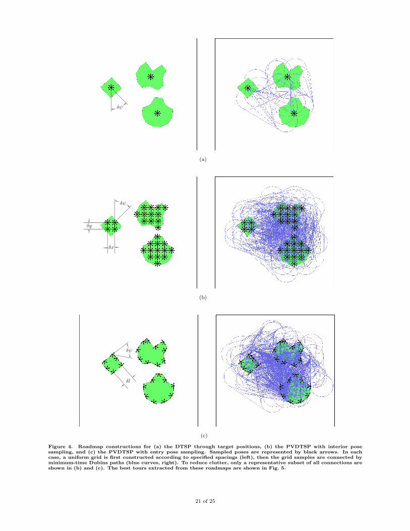
In Ref. 19, a roadmap for the DTSP was constructed by sampling a uniform grid of angles on S at each target.Each cluster in their roadmap thus consisted of a set of vertices (poses) with the same (x, y) coordinatesbut different ψ values evenly spaced at intervals of δψ around [0, 2π) (see Fig. 4a). A generalization of thistechnique for the PVDTSP is to simply construct a roadmap by sampling a uniform grid of poses in theinterior of each visibility region (Fig. 4b). We refer to a roadmap constructed in this manner as an interiorpose roadmap.

Table 2 shows a pseudocode for interior pose roadmap construction. The visibility region parametersV(T1), . . . ,V(Tn) provide the polygons of the PVDTSP instance; rmin is the Dubins vehicle minimum turningradius; nsamples is an estimate of the number of samples the roadmap should contain; and α is a weightingparameter which determines how many angle samples there will be per (x, y) position in the grid. The largerα is, the more angle samples there will be per (x, y) position. We use an estimate nsamples instead of theactual number of samples nsamples because

(i) unless the polygons of the problem instance happen to be squares, it is impossible to know a priorihow many (x, y) samples on a uniform grid will actually fall into each polygon,

(ii) in a uniform grid there is a fixed number of ψ samples per (x, y) sample, so not all sample counts arerealizable, and

(iii) it is convenient for a user to only have to keep track of the single input parameter nsamples rather thanthree separate grid spacing parameters.

Let δx be the uniform grid spacing in the x direction, δy the spacing in the y direction, and δψ the angularspacing. If the polygons were perfect squares with total area A, δxδy divided A evenly, and δψ divided 2πevenly, then we would expect that

nsamples =A

δxδy

2π

δψ. (5)

For general nonsquare polygons, the area A on line 2 can be computed, e.g., by triangulating the polygonsand summing the areas of the triangles.28 Assuming δx = δy = αδψ and solving Eq.5 for the spacings givesthe formulas on line 3 of Table 2. Using these formulas even when the polygons are not squares, nsamples

is in practice very close to the user specified nsamples. Regardless of how close nsamples is to nsamples, a keyfeature for the convergence proof in Sec. IV is that the grid spacings monotonically go to zero as nsamples

increases.Once grid spacings have been set, roadmap samples are generated for the polygons separately, one at

a time (lines 4-9). For a given polygon represented as a list of vertices, an axis-aligned bounding box B

is found simply by selecting the minimum and maximum x and y coordinates over all polygon vertices. A

8 of 25

American Institute of Aeronautics and Astronautics

uniform grid G of poses is then formed on the bounding box according to the spacings δx, δy, and δψ. Theloop on lines 7-9 is a rejection sampling procedure which ensures that only those grid samples are added tothe roadmap which actually lie in the polygon (Fig. 4b, left). Note that even when polygons overlap, theirgrids are sampled separately. This means that identical pose samples may exist in distinct clusters of theroadmap. If the best PVDTSP tour passes through the intersection of polygons, then the roadmap searchprocedure to be described in Sec. III.C automatically selects poses in the intersection.

The roadmap construction is completed on lines 10-16 by adding an edge between all pairs of verticeswhich belong to distinct clusters (Fig. 4b, right). Each edge is weighted by the length drmin

(x,x′) of theminimum-time Dubins path connecting the respective poses.

Table 2. Interior Pose Roadmap Construction

INTERIOR POSE ROADMAP( V(T1), . . . ,V(Tn), rmin, nsamples, α )

Initialize Empty Roadmap and Set Grid Spacings1: (V,E)← (∅, ∅);2: A← total of areas of polygons V(T1), . . . ,V(Tn);

3: δx← 3

q

Aα2πnsamples

; δy ← δx; δψ ← 1αδx;

Sample Clusters4: for i = 1 to n do5: B ← axis-aligned bounding box around V(Ti);6: G← uniform grid on B with translational spacings δx and δy, and anglular spacing δψ;7: for all poses v in G do8: if v ∈ V(Ti) then9: V ← V ∪ v;

Connect Clusters10: for i = 1 to n do11: for j = 1 to n such that j 6= i do12: for all vertices v in cluster i do13: for all vertices v′ in cluster j do14: e← edge from v to v′ with weight drmin

(v, v′);15: E ← E ∪ e;

16: return (V,E);

III.B. Constructing a Roadmap from Entry Poses

With very little loss of generality, we can construct a roadmap by sampling poses on the boundaries of thepolygons rather than the interiors. Let τ∗ = (x∗

1, . . . ,x∗n) be a sequence of poses representing a globally

optimal tour for a particular PVDTSP instance. Assume we know a priori, even before computing τ∗, thatτ∗ passes through the boundary of every polygon. Then each pose x∗

1, . . . ,x∗n can be taken to be (1) located

on the boundary of a polygon and (2) oriented towards the interior of that polygon. We refer to such posesas entry poses. To assume τ∗ can be represented by a sequence of entry poses is not very restrictive in ourexperience. If, for example, at least one of the n visibility regions (perhaps belonging to a remote user) isdisjoint from the other n− 1 visibility regions, then τ∗ is guaranteed to pass through the boundary of everyvisibility region. The space of interior poses we sampled on in Sec. III.A was 3-dimensional, but the space ofentry poses, by being restricted to the polygon boundaries, is only 2-dimensional. Intuitively, this differencein dimensionality may allow us to find better tours with fewer samples by building an entry pose roadmap(Fig. 4c). Indeed, we will see in the numerical experiments in Sec. V that much faster computation timescan be achieved by using entry poses instead of interior poses.

Table 3 shows a pseudocode for entry pose roadmap construction. As for the interior roadmap construc-tion, the parameters are the visibility regions V(T1), . . . ,V(Tn), vehicle minimum turn radius rmin, samplecount estimate nsamples, and angle density weighting α. For reasons similar to those given in Sec. III.A, weuse an estimate nsamples instead of the actual number of samples nsamples. On line 2, the total L of all theperimeter lengths of all the polygons is computed. Let δl be the translational grid spacing along a polygon’sboundary and δψ the angular spacing. If δl divided L evenly and δψ divided π evenly, then we would expect

9 of 25

American Institute of Aeronautics and Astronautics

in a uniform grid that

nsamples =L

δl

π

δψ. (6)

Assuming that δl = αδψ and solving Eq.6 for the spacings gives the formulas on line 3 of Table 3. Using theseformulas, nsamples in practice is very close to the user specified nsamples. Regardless of how close nsamples isto nsamples, a key feature for the convergence proof in Sec. IV is that the grid spacings monotonically go tozero as nsamples increases.

Once grid spacings have been set, roadmap samples are generated for the polygons separately, one at atime (lines 4-7). For a given polygon represented as a list of vertices, the uniform grid G of entry poses isformed simply by stepping along the boundary ∂V(Ti) at increments of δl and adding ⌊απ

δψ⌋ samples per step

(Fig. 4c, left). The loop on lines 6-7 adds all grid samples to the roadmap. As with the interior pose roadmapconstruction, even when polygons overlap, their grids are sampled separately. Identical pose samples maythus exist in distinct clusters of the roadmap. If the best PVDTSP tour passes through the intersection ofpolygons, then the roadmap search procedure to be described in Sec. III.C automatically selects poses in theintersection as necessary.

The roadmap construction is completed on lines 8-13 by adding an edge between all pairs of verticeswhich belong to distinct clusters (Fig. 4c, right). Each edge is weighted by the length drmin

(x,x′) of theminimum-time Dubins path connecting the respective poses.

Table 3. Entry-Pose Roadmap Construction

ENTRY POSE ROADMAP( V(T1), . . . ,V(Tn), rmin, nsamples, α )

Initialize Empty Roadmap and Set Grid Spacings1: (V,E)← (∅, ∅);2: L← total of perimeter lengths of polygons V(T1), . . . ,V(Tn);

3: δl←q

Lαπnsamples

; δψ ← 1αδl;

Sample Clusters4: for i = 1 to n do5: G← uniform grid of entry poses on ∂V(Ti) with translational spacing δl and angular spacing δψ;6: for all poses v in G do7: V ← V ∪ v;

Connect Clusters8: for i = 1 to n do9: for j = 1 to n such that j 6= i do

10: for all vertices v in cluster i do11: for all vertices v′ in cluster j do12: e← edge from v to v′ with weight drmin

(v, v′);13: E ← E ∪ e;

14: return (V,E);

III.C. Finding the Best Tour in a PVDTSP Roadmap

A pseudocode for our roadmap search method is shown in Table 4. This pseudocode represents two differentalgorithms depending on whether INTERIOR POSE ROADMAP or ENTRY POSE ROADMAP is substi-tuted for the ROADMAP function on line 1. The inputs are the target visibility regions V(T1), . . . ,V(Tn),vehicle minimum turn radius rmin, sample count estimate nsamples, and angle density weighting α. Afterthe roadmap is constructed, the function NOON BEAN on line 2 transforms the roadmap FOTSP instance(V,E) into an ATSP instance (V ′, E′) by the Noon-Bean transformation. The Noon-Bean transformation isdefined precisely as follows.

Definition III.4 (Noon-Bean Transformation21). Suppose we are given an FOTSP instance specified, asin Def. III.2, by a weighted directed graph G = (V,E) together with a partitioning into clusters S =S1, S2, S3, . . . , SnS

. Then the Noon-Bean Transformation of this FOTSP instance is an ATSP instance

10 of 25

American Institute of Aeronautics and Astronautics

G′ = (V ′, E′) constructed as follows. Begin with G′ = G, i.e., let V ′ = V and E′ = E, then make these threemodifications to E′:

(i) For each cluster, add zero-weight directed edges to E′ to create a zero-cost cycle which traverses all thevertices of the cluster (so there are a total of nS zero-cost cycles),

(ii) cyclically shift intercluster edges of E′ so that they emanate from the preceding vertex in their respectivezero-cost cycles, and

(iii) add a large penalty M =∑

i,j wi,j, i.e., the total of all weights in G, to the weight of all interclusteredges in E′.

On line 3, an ATSP solver ATSP SOLVE is called on the instance (V ′, E′). Let us assume that we havean ATSP solver at our disposal and the instance (V ′, E′) has been solved. The solution (vk1 , . . . , vknk

) isa list of vertices of the ATSP instance where the sequence ki

nk

i=1 encodes the identifiers of the verticesin the original FOTSP instance. Using these identifiers, the procedure on lines 4-8 extracts the solution(x1, . . . ,xn) to the FOTSP instance. Finally, to produce a sequence of waypoints followable by an aircraft,Dubins minimum-time state-to-state trajectories can be used to interpolate between each pair of states inthe solution encoding (x1, . . . ,xn).

As part of our algorithms, we assume access to an ATSP solver. If we want to compute reconnaissancetours suitably quickly for online purposes, then the ATSP solver must be fast. As can be expected for anNP-hard problem, exact ATSP solvers based on branch and bound can take hours to find solutions that aninexact heuristic solver finds in only seconds. Also, state-of-the-art heuristic TSP solvers, e.g., LKH29 orLinkern,30 perform so well in practice that they are widely accepted as effectively exact for ATSP instanceshaving up to thousands of vertices. In the implementation of our roadmap method we have therefore chosento use the powerful LKH software for solving ATSPs. LKH is based on the Lin-Kernighan Heuristic.31 Tosolve an ATSP, it begins with a randomly generated tour. It then attempts to incrementally improve thetour by repeatedly swapping edges, according to so-called sequential positive-gain lambda-opt moves, untilno further improvement is possible. The inner workings of LKH are very sophisticated, so we refer theinterested reader to Ref. 29 for more details.

Table 4. Sampling-Based Roadmap Method for the PVDTSP

PVDTSP SOLVE( V(T1), . . . ,V(Tn), rmin, nsamples, α )

Construct Roadmap and Corresponding ATSP Instance 1: (V,E)← ROADMAP(V(T1), . . . ,V(Tn), rmin, nsamples, α);2: (V ′, E′)← NOON BEAN(V,E);

Solve ATSP Instance and Extract Best Tour 3: (vk1

, . . . , vknk)← ATSP SOLVE(V ′, E′);

4: cyclically shift (vk1, . . . , vknk

) as necessary to ensure vk1and vknk

come from distinct clusters;5: j ← 1;6: for i = 1 to nk do7: if vki

is the first vertex encountered from a particular cluster then8: xj ← vki

; j ← j + 1;

9: return (x1, . . . ,xn);

IV. Convergence Analysis

Let τ∗ be a globally optimal tour for a PVDTSP instance. Suppose for a moment that the cost functionC : (SE(2))n → R in Eq. 1 were continuous. Then provided any roadmap we use contains a tour sufficientlyclose to τ∗, we would expect PVDTSP SOLVE could find a tour within any given tolerance of C(τ∗). Inother words, continuity of C would imply resolution completeness of our algorithms. Unfortunately, C isnot fully continuous because it is a sum of n discontinuous Dubins distances d(x,x′). However, as we showin the remainder of this section, C does have useful continuity properties which allow us to prove resolutioncompleteness of our algorithms under certain technical assumptions.

11 of 25

American Institute of Aeronautics and Astronautics

IV.A. Continuity Properties and General Position Assumption

Continuity properties of the Dubins distance have been shown in Ref. 32.

Lemma IV.1 (Piecewise Continuity of Dubins Distance32). For fixed initial pose, the Dubins distancefunction d : SE(2) → R is continuous everywhere except on a set Sd of two 2-dimensional smooth surfacesi

embedded in the 3-dimensional domain SE(2). Furthermore, in the limit from one side of each of thesediscontinuity surfaces, d is continuous up to and including on the surface.j

From this we obtain the continuity properties of the PVDTSP cost function.

Lemma IV.2 (Piecewise Continuity of PVDTSP Cost Function). The PVDTSP cost function C : (SE(2))n →R is guaranteed to be continuous everywhere except on a finite set SC of (3n− 1)-dimensional smooth sur-faces embedded in its 3n-dimensional domain (SE(2))n. Furthermore, in the limit from one side of eachdiscontinuity surface, C is continuous up to and including on the surface.

Proof. As a sum of n Dubins distances, C can only be discontinuous at a particular tour τ = (x1, . . . ,xn) ifsome pose in the sequence, say xi, lies on one of the 2-dimensional discontinuity surfaces Sd of the Dubinsdistance d (applying Lemma IV.2 with respect to initial pose xi−1). Let us call the 2-dimensional surfacewhere this occurs s. Then (SE(2))i−1 × s × (SE(2))n−i is one of the (3n − 1)-dimensional surfaces in SC .Taking the union of all surfaces constructed in this manner for i = 1, . . . , n, we obtain all of SC . There thusare only 2n surfaces in SC and each inherits the smoothness and one-sided continuity from Sd.

These continuity properties motivate a general position assumption that will allow us to prove resolutioncompleteness of our algorithms. General position assumptions, also known as generic input assumptions, arecommonly used in the field of computational geometry for proving correctness of algorithms in the absenceof certain input degeneracies which almost never occur.33 We define a PVDTSP instance as being in generalposition if it is not degenerate according to either of the following definitions.

Definition IV.3 (Interior Pose Degeneracy). A PVDTSP instance is interior pose degenerate if there existsa tour τ∗ = (x∗

1, . . . ,x∗n) ∈ V(T1)×· · ·×V(Tn) and δ > 0 such that for every open set A ⊂ V(T1)×· · ·×V(Tn)

it holds that supτ∈A C(τ) ≥ C(τ∗) + δ.

Definition IV.4 (Entry Pose Degeneracy). Let V(Ti) be the set of entry poses of V(Ti) for i = 1, . . . , n. APVDTSP instance is entry pose degenerate if there exists a tour τ∗ = (x∗

1, . . . ,x∗n) ∈ ∂V(T1)× · · · × ∂V(Tn)

and δ > 0 such that for every openk set A ⊂ V(T1) × · · · × V(Tn) it holds that supτ∈A C(τ) ≥ C(τ∗) + δ.

In words, a PVDTSP instance is degenerate if there exists a tour τ∗ such that no matter how finely we maysample interior (resp. entry) poses, we cannot hope that any tour constructed from the sampling comeswithin a prescribed tolerance δ of the cost C(τ∗). An example of a PVDTSP instance which is both interiorpose and entry pose degenerate is shown in Fig. 6. The globally optimal tour τ∗ is a minimum turn radiuscircle which just grazes the outside corners of the triangular visibility regions. Any tour τ 6= τ∗ would haveto veer away from the visibility regions and then come back in order to visit them all. The cost C(τ) is thusbounded away from C(τ∗).

As long as the input data of a PVDTSP instance is subject to some noise, then degeneracies should almostnever occur, i.e., a degenerate problem instance will occur with probability 0. A completely rigorous proofof this would require a highly technical digression into intersection theory.34 We therefore content ourselveswith the general position assumption based on geometric intuition from the following lower-dimensionaloptimization problem. Suppose we want to minimize a function f(x, y) over a unit square in R

2, where

f(x, y) =

0 for√

x2 + y2 ≤ 1

1 else(7)

iThese discontinuity surfaces of the Dubins distance function are traced out by two circular arcs in the (x, y) plane whichvary continuously along the ψ axis. Illustrations are provided in Ref. 32.

jNote that, for our purposes, it is not important which side of the discontinuity surface is continuous up to and includingon the surface.

kBy an “open set in A ∈ V(T1)×· · ·×V(Tn)”, we intend “open” in the relative topology of V(T1)×· · ·×V(Tn) as a subspaceof (SE(2))n.

12 of 25

American Institute of Aeronautics and Astronautics

The optimal solution clearly depends on how the square is situated relative to the unit disk (see Fig. 7). Onecould easily solve this problem in closed form by checking the disk and square for intersection. However,in order to make an analogy with our PVDTSP algorithms, suppose our strategy for minimizing f is tosample a uniform grid of points in the interior of the square and then select the sample with minimum f

value. Notice that f , similar to C, is piecewise continuous and, in the limit from one side of the (unit circle)discontinuity surface, it is continuous up to and including on the surface. These continuity properties implythat in the limit as the grid becomes finer in the square, the value returned by the sampling strategy shouldalways approach the optimum as long as the disk and square share an open set whenever they intersect. Ifthe disk and square do intersect but there is no such open set, we say the problem instance is degenerate.Degeneracy occurs precisely when the disk only intersects the square at a single point, i.e., when the diskis tangent to the square or it touches only at a corner. Given any degenerate problem instance, perturbingthat instance by a normal random variable in R

2 would result in a new problem instance which is degeneratewith probability zero. In this sense, degenerate problem instances almost never occur. Completing ouranalogy with the PVDTSP: C is to f as SC is to the unit circle as visibility regions are to the square. Wethus expect, as long as the interaction between the discontinuity surfaces SC and the visibility regions iswell-behaved, that a PVDTSP instance will be in general position and our algorithms will converge.

IV.B. Resolution Completeness

We are now ready to state the main convergence results.

Theorem IV.5 (Interior Pose Roadmap Convergence). Let V(T1), . . . ,V(Tn) be visibility regions constitutinga PVDTSP instance in general position. Let Ri

∞i=1 be a sequence of roadmaps constructed according to

Def. III.3 such that the vertices of Ri are dense in the visibility regions V(T1), . . . ,V(Tn) in the limit as igoes to infinity. Let τi

∞i=1 be the sequence of best tours contained in the sequence of roadmaps Ri

∞i=1,

respectively. Then the best tour cost C(τi) approaches a global optimum, i.e.,

limi→∞

C(τi) = infτ∈V(T1)×···×V(Tn)

C(τ). (8)

Proof. To prove Eq. 8 it suffices to show that for all ǫ > 0 there exists N such that i > N implies

C(τi) ≤ infτ∈V(T1)×···×V(Tn)

C(τ) + ǫ. (9)

By definition of infimum, there exists a sequence of tours τ ′j∞j=1 in V(T1) × · · · × V(Tn) such that

limj→∞

C(τ ′j) = infτ∈V(T1)×···×V(Tn)

C(τ),

i.e., for all ǫ > 0 there exists N1 such that j > N1 implies

C(τ ′j) ≤ infτ∈V(T1)×···×V(Tn)

C(τ) +ǫ

2. (10)

The general position assumption (specifically the absence of degeneracy per Def. IV.3) implies that for eachτ ′j and ǫ > 0 there exists an open set Aj ⊂ V(T1)×· · ·×V(Tn) such that supτ ′∈Aj

C(τ ′) ≤ C(τ ′j)+ǫ2 . Because

the roadmap poses are sampled densely in the limit, we can always find an N2 large enough that each Ri

contains a tour τi in the open set Aj for all i > N2, hence

C(τi) ≤ C(τ ′j) +ǫ

2(11)

whenever i > N2. Combining Eq. 10 and 11, we obtain the desired result that for all ǫ > 0 there existsN = maxN1, N2 such that i > N implies

C(τi) ≤ C(τ ′j) + ǫ2

≤ infτ∈V(T1)×···×V(Tn) C(τ) + ǫ2 + ǫ

2

= infτ∈V(T1)×···×V(Tn) C(τ) + ǫ.

13 of 25

American Institute of Aeronautics and Astronautics

Theorem IV.6 (Entry Pose Roadmap Convergence). Let V(T1), . . . ,V(Tn) be visibility regions constitutinga PVDTSP instance in general position. Let Ri

∞i=1 be a sequence of roadmaps constructed according to

Def. III.3 such that the vertices of Ri are dense in the entry pose sets V(T1), . . . , V(Tn) in the limit as igoes to infinity. Let τi

∞i=1 be the sequence of best tours contained in the sequence of roadmaps Ri

∞i=1,

respectively. Then the best tour cost C(τi) approaches a global optimum among all tours which pass throughthe boundary of every visibility region, i.e.,

limi→∞

C(τi) = infτ∈∂V(T1)×···×∂V(Tn)

C(τ). (12)

Proof. To prove Eq. 12 it suffices to show that for all ǫ > 0 there exists N such that i > N implies

C(τi) ≤ infτ∈∂V(T1)×···×∂V(Tn)

C(τ) + ǫ. (13)

By definition of infimum, there exists a sequence of tours τ ′j∞j=1 in ∂V(T1) × · · · × ∂V(Tn) such that

limj→∞

C(τ ′j) = infτ∈∂V(T1)×···×∂V(Tn)

C(τ),

i.e., for all ǫ > 0 there exists N1 such that j > N1 implies

C(τ ′j) ≤ infτ∈∂V(T1)×···×∂V(Tn)

C(τ) +ǫ

2. (14)

The general position assumption (specifically the absence of degeneracy per Def. IV.4) implies that for eachτ ′j and ǫ > 0 there exists an open set Aj ⊂ V(T1)×· · ·×V(Tn) such that supτ ′∈Aj

C(τ ′) ≤ C(τ ′j)+ǫ2 . Because

the roadmap poses are sampled densely in the limit, we can always find an N2 large enough that each Ri

contains a tour τi in the open set Aj for all i > N2, hence

C(τi) ≤ C(τ ′j) +ǫ

2(15)

whenever i > N2. Combining Eq. 14 and 15, we obtain the desired result that for all ǫ > 0 there existsN = maxN1, N2 such that i > N implies

C(τi) ≤ C(τ ′j) + ǫ2

≤ infτ∈∂V(T1)×···×∂V(Tn) C(τ) + ǫ2 + ǫ

2

= infτ∈∂V(T1)×···×∂V(Tn) C(τ) + ǫ.

The resolution completeness of our algorithms now follows directly from the roadmap convergence theo-rems.

Corollary IV.7 (Resolution Completeness with Interior Pose Sampling). For a PVDTSP instance in generalposition, suppose the algorithm PVDTSP SOLVE in Table 4 is executed for nsamples = 1, 2, 3, . . ., each timereturning a tour τnsamples

. Suppose further that

(i) for the ROADMAP function on line 1, a roadmap construction as per Def. III.3 is used which samplesposes densely in the visibility regions V(T1), . . . ,V(Tn) in the limit as nsamples goes to infinity, e.g., theINTERIOR POSE ROADMAP function in Table 2, and

(ii) the function ATSP SOLVE on line 3 always returns an exact solution.

Then the best tour cost C(τnsamples) approaches a global optimum, i.e.,

limnsamples→∞

C(τnsamples) = inf

τ∈V(T1)×···×V(Tn)C(τ). (16)

Proof. It is proven in Ref. 21 that the Noon-Bean transformation is exact in the sense that if the exactsolution of the ATSP instance is found, then the extracted solution to the FOTSP instance will also beexact. This means the method will always find the best tour in a given roadmap. The corollary thus followsdirectly from the roadmap convergence Theorem IV.5.

14 of 25

American Institute of Aeronautics and Astronautics

Corollary IV.8 (Resolution Completeness with Entry Pose Sampling). For a PVDTSP instance in generalposition, suppose the algorithm PVDTSP SOLVE in Table 4 is executed for nsamples = 1, 2, 3, . . ., each timereturning a tour τnsamples

. Suppose further that

(i) for the ROADMAP function on line 1, a roadmap construction as per Def. III.3 is used which samplesposes densely in the entry pose sets V(T1), . . . , V(Tn) in the limit as nsamples goes to infinity, e.g., theENTRY POSE ROADMAP function in Table 2, and

(ii) the function ATSP SOLVE on line 3 always returns an exact solution.

Then the best tour cost C(τnsamples) approaches a global optimum among all tours which pass through the

boundary of every visibility region, i.e.,

limnsamples→∞

C(τnsamples) = inf

τ∈∂V(T1)×···×∂V(Tn)C(τ). (17)

Proof. Follows directly from the roadmap convergence Theorem IV.6 as Corollary IV.7 followed from Theo-rem IV.5.

Corollaries IV.7 and IV.8 are valid for any roadmap constructions which sample densely on the visi-bility sets, resp. entry pose sets. Instead of uniform grids, one could sample, e.g., randomly or quasiran-domly.23,24,35

IV.C. Time Complexity

The convergence results in Sec. IV.B show that the tour returned by our algorithm PVDTSP SOLVE con-verges to a global optimum, but they tell us nothing about the rate of convergence. In particular, we haveno way of knowing how many samples are necessary in order to guarantee the tour returned comes within aprescribed tolerance of the global optimum. In this respect, the utility of the convergence theorems is moreconceptual than practical and it remains an important open problem to prove the rate of convergence. In fact,convergence rates are not known for a number of state-of-the-art sampling-based roadmap methods in theliterature, yet these methods perform compellingly well in practice.24,36 That the PVDTSP is NP-hard alsoindicates that there can be no polynomial time complexity guarantees. Despite all this, we are able to providean estimate of time complexity as a function of the input parameter nsamples, and numerical experiments inSec. V show the algorithms perform very well in practice. We derive the estimate by assuming an ATSPinstance with nV vertices can be solved in time O(n2.2

V ). This is the empirically determined average-casetime complexity of state-of-the-art heuristic ATSP solvers based on the Lin-Kernighan heuristic.29,31,37

Proposition IV.9 (Time Complexity). Suppose whenever we execute the algorithmPVDTSP SOLVE in Table 4 it holds that

(i) n≪ nsamples,

(ii) nsamples ≈ nsamples,

(iii) the number of vertices representing each polygon is upper boundedl,

(iv) the roadmap is constructed using INTERIOR POSE ROADMAP in Table 2 orENTRY POSE ROADMAP in Table 3, and

(v) an ATSP solver based on the Lin-Kernighan heuristic, e.g., LKH 29 or Linkern.30 is able to solveATSP instances with nV vertices in time O(n2.2

V ).

Then the time complexity of PVDTSP SOLVE is

O(n2.2samples). (18)

lIn the examples we considered, the number of vertices representing any polygon never exceeded 20.

15 of 25

American Institute of Aeronautics and Astronautics

Proof. We first examine the INTERIOR POSE ROADMAP pseudocode Table 2. Computing the area andbounding box of a single polygon takes time linear in its number of vertices,28 which we assumed con-stant. These computations are performed for n polygons, so lines 1-6 take time O(n). Lines 7-9 makesroughly O(nsamples) constant-time insertions into G and therefore takes O(nsamples) time. We know theseinsertions take roughly constant time for us because (1) checking inclusion in a polygon28 is linear in itsnumber of its vertices, and (2) the fraction of rejected samples is proportional to the ratio of polygon areato bounding box area, which is fixed. On lines 10-15, the O(n2

samples) edges of a nearly complete graphare inserted, each in constant time. This last term dominates, hence we expect the time complexity ofINTERIOR POSE ROADMAP to be O(n2

samples).We turn our attention to the ENTRY POSE ROADMAP pseudocode Table 3. Computing the perimeter

length of n polygons takes O(n) time (line 2). The cluster sampling on lines 4-7 makes no rejections, soO(nsamples) constant-time insertions take O(nsamples) time. On lines 8-13, the O(n2

samples) edges of a nearlycomplete graph are inserted, each in constant time. This last term dominates, hence we expect the timecomplexity of ENTRY POSE ROADMAP to be O(n2

samples).Finally, we examine the PVDTSP SOLVE pseudocode Table 4 itself. As we have just seen, building the

roadmap (line 1) takes time O(n2samples). The Noon-Bean transformation (line 2) also takes time O(n2

samples)

because it adds only nsamples zero-weight edges, but modifies one at a time the other O(n2samples) edges.

Under assumption (v), the ATSP on line 3 can be solved in time O(n2.2samples). Extracting the PVDTSP

solution (lines 4-8) from the ATSP solution takes only O(nsamples) time.Of all the operations in PVDTSP SOLVE, solving the ATSP dominates, hence the time complexity is

O(n2.2samples), or O(n2.2

samples) assuming nsamples ≈ nsamples.

V. Numerical Study

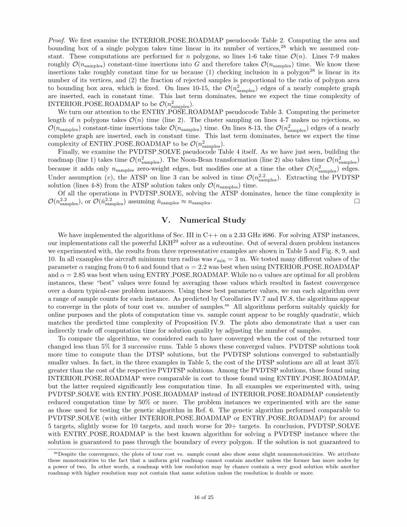
We have implemented the algorithms of Sec. III in C++ on a 2.33 GHz i686. For solving ATSP instances,our implementations call the powerful LKH29 solver as a subroutine. Out of several dozen problem instanceswe experimented with, the results from three representative examples are shown in Table 5 and Fig. 8, 9, and10. In all examples the aircraft minimum turn radius was rmin = 3 m. We tested many different values of theparameter α ranging from 0 to 6 and found that α = 2.2 was best when using INTERIOR POSE ROADMAPand α = 2.85 was best when using ENTRY POSE ROADMAP. While no α values are optimal for all probleminstances, these “best” values were found by averaging those values which resulted in fastest convergenceover a dozen typical-case problem instances. Using these best parameter values, we ran each algorithm overa range of sample counts for each instance. As predicted by Corollaries IV.7 and IV.8, the algorithms appearto converge in the plots of tour cost vs. number of samples.m All algorithms perform suitably quickly foronline purposes and the plots of computation time vs. sample count appear to be roughly quadratic, whichmatches the predicted time complexity of Proposition IV.9. The plots also demonstrate that a user canindirectly trade off computation time for solution quality by adjusting the number of samples.

To compare the algorithms, we considered each to have converged when the cost of the returned tourchanged less than 5% for 3 successive runs. Table 5 shows these converged values. PVDTSP solutions tookmore time to compute than the DTSP solutions, but the PVDTSP solutions converged to substantiallysmaller values. In fact, in the three examples in Table 5, the cost of the DTSP solutions are all at least 35%greater than the cost of the respective PVDTSP solutions. Among the PVDTSP solutions, those found usingINTERIOR POSE ROADMAP were comparable in cost to those found using ENTRY POSE ROADMAP,but the latter required significantly less computation time. In all examples we experimented with, usingPVDTSP SOLVE with ENTRY POSE ROADMAP instead of INTERIOR POSE ROADMAP consistentlyreduced computation time by 50% or more. The problem instances we experimented with are the sameas those used for testing the genetic algorithm in Ref. 6. The genetic algorithm performed comparable toPVDTSP SOLVE (with either INTERIOR POSE ROADMAP or ENTRY POSE ROADMAP) for around5 targets, slightly worse for 10 targets, and much worse for 20+ targets. In conclusion, PVDTSP SOLVEwith ENTRY POSE ROADMAP is the best known algorithm for solving a PVDTSP instance where thesolution is guaranteed to pass through the boundary of every polygon. If the solution is not guaranteed to

mDespite the convergence, the plots of tour cost vs. sample count also show some slight nonmonotonicities. We attributethese monotonicities to the fact that a uniform grid roadmap cannot contain another unless the former has more nodes bya power of two. In other words, a roadmap with low resolution may by chance contain a very good solution while anotherroadmap with higher resolution may not contain that same solution unless the resolution is double or more.

16 of 25

American Institute of Aeronautics and Astronautics

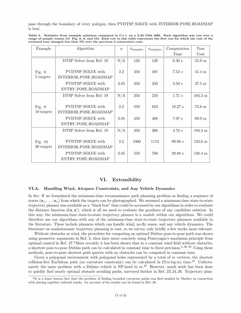
pass through the boundary of every polygon, then PVDTSP SOLVE with INTERIOR POSE ROADMAPis best.

Table 5. Statistics from example solutions computed in C++ on a 2.33 GHz i686. Each algorithm was run over arange of sample counts (cf. Fig. 8, 9, and 10). Each row in this table represents the first run for which the cost of thereturned tour changed less then 5% over the previous 3 consecutive runs.

Example Algorithm α nsamples nsamples Computation Tour

Time Cost

Fig.085 targets

DTSP Solver from Ref. 19 N/A 120 120 0.30 s 55.9 m

PVDTSP SOLVE with 2.2 450 491 7.53 s 41.4 m

INTERIOR POSE ROADMAP

PVDTSP SOLVE with 2.85 350 350 3.50 s 37.5 m

ENTRY POSE ROADMAP

Fig.0910 targets

DTSP Solver from Ref. 19 N/A 250 250 1.71 s 104.3 m

PVDTSP SOLVE with 2.2 550 623 16.27 s 73.8 m

INTERIOR POSE ROADMAP

PVDTSP SOLVE with 2.85 450 468 7.97 s 69.9 m

ENTRY POSE ROADMAP

Fig.01020 targets

DTSP Solver from Ref. 19 N/A 350 360 4.72 s 194.3 m

PVDTSP SOLVE with 2.2 1000 1113 99.98 s 124.6 m

INTERIOR POSE ROADMAP

PVDTSP SOLVE with 2.85 550 708 29.80 s 128.4 m

ENTRY POSE ROADMAP

VI. Extensibility

VI.A. Handling Wind, Airspace Constraints, and Any Vehicle Dynamics

In Sec. II we formulated the minimum-time reconnaissance path planning problem as finding a sequence ofstates (x1, . . . ,xn) from which the targets can be photographed. We assumed a minimum-time state-to-statetrajectory planner was available as a “black box” that could be accessed by our algorithms in order to evaluatethe distance function d(x,x′), which is all we need to evaluate the goodness of any candidate solution. Inthis way, the minimum-time state-to-state trajectory planner is a module within our algorithms. We couldtherefore use our algorithms with any of the minimum-time state-to-state trajectory planners available inthe literature. These include planners which can handle wind, no-fly zones, and any vehicle dynamics. Theliterature on nonholonomic trajectory planning is vast, so we survey only briefly a few works most relevant.

Without obstacles or wind, the procedure for computing an optimal Dubins pose-to-pose path was shownusing geometric arguments in Ref. 3, then later more concisely using Pontryagin’s maximum principle fromoptimal control in Ref. 27.nMore recently it has been shown that in a constant wind field without obstacles,a shortest pose-to-pose Dubins path can be calculated in constant time to fixed precision.4,39,40 Using thesemethods, pose-to-pose shortest path queries with no obstacles can be computed in constant time.

Given a polygonal environment with polygonal holes represented by a total of m vertices, the shortestcollision-free Euclidean path (no curvature constraint) can be calculated in O(m logm) time.41 Unfortu-nately the same problem with a Dubins vehicle is NP-hard in m.42 However, much work has been doneto quickly find nearly optimal obstacle avoiding paths, surveyed further in Ref. 23, 24, 26. Trajectory plan-

nIt is a lesser known fact that the problem of finding bounded curvature paths was first studied by Markov in connectionwith piecing together railroad tracks. An account of his results can be found in Ref. 38.

17 of 25

American Institute of Aeronautics and Astronautics

ners specifically intended for fixed-wing UAVs, which use a branch and bound technique, are described inRef. 43, 44. Another approach to nonholonomic motion planning with obstacles is to use a MILP (MixedInteger Linear Program).45,46

VI.B. Open-Path vs. Closed-Tour Problems

In presenting our algorithms, we considered only closed-tour solutions to the reconnaissance UAV pathplanning problem. One may alternatively wish to find an open reconnaissance path from a fixed initial posexinitial to a different fixed final pose xfinal. In this case, instead of the closed-tour cost function in Eq. 1, weuse the open path cost function

C(x1, . . . ,xn) = d(xinitial,x1) +

n−1∑

i=1

d(xi,xi+1) + d(xn,xfinal).

The algorithms can be applied to open-path problems with only slight modification in how the roadmapis constructed. The open-path roadmap has all the vertices and edges that the closed-tour roadmap ofDef. III.3 does, but in addition has two single-vertex clusters, one for the initial pose and one for the finalpose. The initial single-vertex cluster is connected by distance d-weighted edges outgoing to all vertices innondegenerate clusters. The final single-vertex cluster is connected (1) by a zero-weight edge outgoing to theinitial cluster vertex, and (2) by distance d-weighted edges incoming from all vertices in the nondegenerateclusters.

VII. Conclusion

We have formulated the general aircraft visual reconnaissance problem for static ground targets in terrainand shown that it can be reduced to a new variant of the Traveling Salesman Problem called the PVDTSP.A worst-case analysis demonstrated the importance of developing specialized algorithms for the PVDTSPin scenarios where targets are close together and polygons may overlap significantly. We designed twoalgorithms for the PVDTSP. These sampling-based roadmap methods operate by sampling finite discretesets of poses in the target visibility regions in order to approximate a PVDTSP instance by an FOTSPinstance called the roadmap. Once a roadmap has been constructed, the algorithms apply the Noon-Beantransformation to solve the FOTSP. Under certain technical assumptions, the algorithms are resolutioncomplete. The two algorithms differ only in how they sample poses to construct the roadmap. In the firstalgorithm, poses are simply sampled in the interior of the visibility regions. The second algorithm, however,samples entry poses. Sampling entry poses requires slightly stricter assumptions for resolution completeness,but greatly reduces computation time. Numerical experiments indicate that our algorithms deliver very goodsolutions suitably quickly for online purposes when applied to PVDTSP instances having up to about 20targets. They significantly outperformed the alternative approaches of the genetic algorithm in Ref. 6 andDTSP over target locations in Ref. 19. Additionally, our algorithms allow a means for a user to trade offcomputation time for solution quality and their modular nature allows them to easily be extended to handlewind, airspace constraints, any vehicle dynamics, and open-path (vs. closed-tour) problems.

While the algorithms we have presented are essentially ready to be fielded, there is much room forfuture work. We are currently investigating extensions to multiple vehicles, constant factor approximationguarantees, and a way to calculate how many samples a roadmap needs to guarantee a prescribed accuracy.Aside from improvements to the existing algorithms, it would be interesting to numerically evaluate hybridapproaches.

Acknowledgments

This work was supported by a US Department of Defense SMART Graduate Fellowship( http://www.asee.org/fellowships/smart/ ). Thanks to the following people for helpful comments:F. Bullo (UCSB), R. Holsapple (WPAFB), D. Kingston (WPAFB), M. Mears (WPAFB), F. Obermeyer (ToyonResearch Corp.), S. Rasmussen (Miami Valley Aerospace LLC), C. Schumacher (WPAFB), V. Shafer-man (Technion), R. Spjut (UCSB).

18 of 25

American Institute of Aeronautics and Astronautics

References

1Chandler, P., Pachter, M., and Rasmussen, S., “UAV Cooperative Control,” American Control Conference, Arlington,VA, June 2001, pp. 50–55.

2Ryan, A., Zennaro, M., Howell, A., Sengupta, R., and Hedrick, J. K., “An overview of emerging results in cooperativeUAV control,” IEEE Conf. on Decision and Control , 2004.

3Dubins, L. E., “On curves of minimal length with a constraint on average curvature and with prescribed initial andterminal positions and tangents,” American Journal of Mathematics, Vol. 79, 1957, pp. 497–516.

4McGee, T. G., Spry, S., and Hedrick, J. K., “Optimal path planning in a constant wind with a bounded turning rate,”AIAA Conf. on Guidance, Navigation and Control , San Francisco, CA, Aug. 2005, Electronic Proceedings.

5Gutin, G. and Punnen, A. P., The Traveling Salesman Problem and Its Variations, Kluwer Academic Publishers, Dor-drecht, The Netherlands, 1st ed., 2002.

6Obermeyer, K. J., “Path Planning for a UAV Performing Reconnaissance of Static Ground Targets in Terrain,” AIAA

Conf. on Guidance, Navigation and Control , Chicago, IL, Aug. 2009, To appear.7Betts, J. T., “Survey of Numerical Methods for Trajectory Optimization,” AIAA Journal of Guidance, Control, and

Dynamics, Vol. 21, No. 2, 1998, pp. 193–207.8Papadimitriou, C. H., “The Euclidean Traveling Salesman Problem is NP-Complete,” Theoretical Computer Science,

Vol. 4, 1977, pp. 237–244.9de Berg, M., Gudmundsson, J., Katz, M. J., Levcopoulos, C., Overmars, M. H., and van der Stappen, A. F., “TSP with

Neighborhoods of Varying Size,” 2002, pp. 21–35.10Dumitresco, A. and Mitchell, J. S. B., “Approximation Algorithms for TSP with Neighborhoods in the Plane,” Journal

of Algorithms, Vol. 48, No. 1, 2003, pp. 135–159.11Mata, C. S. and Mitchell, J. S. B., “Approximation Algorithms for Geometric Tour and Network Design Problems,”

Symposium on Computational Geometry, 1995, pp. 360–369.12Le Ny, J., Frazzoli, E., and Feron, E., “The curvature-constrained traveling salesman problem for high point densities,”

IEEE Conf. on Decision and Control , 2007, pp. 5985–5990.13Nygard, K. E., Chandler, P. R., and Pachter, M., “Dynamic network flow optimization models for air vehicle resource

allocation,” 2001.14Schumacher, C., Chandler, P. R., and Rasmussen, S. R., “Task allocation for wide area search munitions,” American

Control Conference, 2002.15Tang, Z. and Ozguner, U., “Motion Planning for Multi-Target Surveillance with Mobile Sensor Agents,” IEEE Transac-

tions on Robotics, Vol. 21, No. 5, 2005, pp. 898–908.16Rathinam, S., Sengupta, R., and Darbha, S., “A Resource Allocation Algorithm for Multi-Vehicle Systems with Non

holonomic Constraints,” IEEE Transactions on Automation Sciences and Engineering, Vol. 4, No. 1, 2007, pp. 98–104.17Savla, K., Frazzoli, E., and Bullo, F., “Traveling Salesperson Problems for the Dubins vehicle,” IEEE Transactions on

Automatic Control , Vol. 53, No. 6, 2008, pp. 1378–1391.18Le Ny, J. and Feron, E., “An Approximation Algorithm for the Curvature-Constrained Traveling Salesman Problem,”

Allerton Conf. on Communications, Control and Computing, Monticello, IL, USA, Sept. 2005.19Oberlin, P., Rathinam, S., and Darbha, S., “A Transformation for a Heterogeneous, Multiple Depot, Multiple Traveling

Salesmen Problem,” American Control Conference, 2009, pp. 1292–1297.20Yadlapalli, S., Malik, W. A., Darbha, S., and Pachter, M., “A Lagrangian-based algorithm for a Multiple Depot, Multiple

Traveling Salesmen Problem,” Nonlinear Analysis: Real World Applications, Vol. 10, No. 4, August 2009, pp. 1990–1999.21Noon, C. E. and Bean, J. C., “An Efficient Transformation of the Generalized Traveling Salesman Problem,” Tech. Rep.

91-26, Department of Industrial and Operations Engineering, University of Michigan, Ann Arbor, 1991.22Fischetti, M., Salazar-Gonzalez, J. J., and Toth, P., The Traveling Salesman Problem and its Variations, chap. 13,

Kluwer, 2002.23Choset, H., Lynch, K. M., Hutchinson, S., Kantor, G., Burgard, W., Kavraki, L. E., and Thrun, S., Principles of Robot

Motion: Theory, Algorithms, and Implementations, MIT Press, 2005.24LaValle, S. M., Planning Algorithms, Cambridge University Press, 2006, Available at http://planning.cs.uiuc.edu.25Ceccarelli, N., Enright, J. J., Frazzoli, E., Rasmussen, S. J., and Schumacher, C. J., “Micro UAV Path Planning for

Reconnaissance in Wind,” American Control Conference, New York, NY, USA, July 2007, pp. 5310–5315.26Latombe, J.-C., Robot Motion Planning, Kluwer Academic Publishers, 1991.27Boissonnat, J.-D., Cerezo, A., and Leblond, J., “Shortest paths of bounded curvature in the plane,” Journal of Intelligent

and Robotic Systems, Vol. 11, 1994, pp. 5–20.28O’Rourke, J., Computational Geometry in C , Cambridge University Press, 2000.29Helsgaun, K., “An effective implementation of the LinKernighan traveling salesman heuristic,” European Journal of

Operational Research, Vol. 126, No. 1, October 2000, pp. 106–130.30Applegate, D. L., Bixby, R. E., and Chvatal, V., The Traveling Salesman Problem: A Computational Study, Applied

Mathematics Series, Princeton University Press, 2006.31Lin, S. and Kernighan, B. W., “An effective heuristic algorithm for the traveling-salesman problem,” Operations Research,

Vol. 21, 1973, pp. 498–516.32Bui, X. N., Boissonnat, J. D., Soueres, P., and Laumond, J. P., “Shortest Path Synthesis for Dubins Non-Holonomic

Robot,” IEEE Transactions on Robotics and Automation, 1994.33Goodman, J. E. and O’Rourke, J., editors, Handbook of Discrete and Computational Geometry, CRC Press, 2nd ed.,

2004.

19 of 25

American Institute of Aeronautics and Astronautics

34Fulton, W., Intersection Theory, Ergebnisse der Mathematik und ihrer Grenzgebiete, Springer Verlag, Berlin, Heidelberg,New York, 1984.

35Niederreiter, H., Random Number Generation and Quasi-Monte Carlo Methods, No. 63 in CBMS-NSF Regional Confer-ence Series in Applied Mathematics, Society for Industrial & Applied Mathematics, 1992.

36Karaman, S. and Frazzoli, E., “Incremental Sampling-based Algorithms for Optimal Motion Planning,” Proceedings of

Robotics: Science and Systems, Zaragoza, Spain, jun 2010.37Applegate, D., Bixby, R., Chvatal, V., and Cook, W., “On the solution of traveling salesman problems,” Documenta

Mathematica, Journal der Deutschen Mathematiker-Vereinigung, Berlin, Germany, Aug. 1998, pp. 645–656, Proceedings of theInternational Congress of Mathematicians, Extra Volume ICM III.

38Kreın, M. G. and Nudelman, A. A., The Markov moment problem and extremal problems: ideas and problems of P. L.

Cebysev and A. A. Markov and their further development, American Mathematical Society, 1977.39McNeely, R., Iyer, R. V., and Chandler, P., “Tour Planning for an Unmanned Air Vehicle under Wind Conditions,”

AIAA Journal of Guidance, Control, and Dynamics, Vol. 30, No. 5, 2007, pp. 1299–1306.40Techy, L. and Woolsey, C. A., “Minimum-Time Path Planning for Unmanned Aerial Vehicles in Steady Uniform Winds,”

AIAA Journal of Guidance, Control, and Dynamics, Vol. 32, No. 6, 2009, pp. 1736–1746.41Hershberger, J. and Suri, S., “An Optimal Algorithm for Euclidean Shortest Paths in the Plane,” SIAM Journal on

Computing, Vol. 28, 1999, pp. 2215–2256.42Reif, J. and Wang, H., “The Complexity of the Two Dimensional Curvature-Constrained Shortest-Path Problem,” In

Proc. Third International Workshop on the Algorithmic Foundations of Robotics, 1998, pp. 49–57.43Eele, A. and Richards, A., “Path-Planning with Avoidance using Nonlinear Branch-and-Bound Optimisation,” AIAA

Conf. on Guidance, Navigation and Control , Hilton Head, South Carolina, 2007, Electronic Proceedings.44Eele, A. and Richards, A., “Comparison of Branching Strategies for Path-Planning with Avoidance using Nonlinear

Branch-and-Bound,” AIAA Conf. on Guidance, Navigation and Control , Honolulu, Hawaii, 2008, Electronic Proceedings.45Borrelli, F., Subramanian, D., Raghunathan, A. U., and Biegler, L. T., “MILP and NLP Techniques for centralized

trajectory planning of multiple unmanned air vehicles,” American Control Conference, 2006.46Richards, A. and How, J. P., “Aircraft trajectory planning with collision avoidance using mixed integer linear program-

ming,” American Control Conference, 2002, pp. 1936–1941.

20 of 25

American Institute of Aeronautics and Astronautics

δψ

(a)

δψ

δy

δx

(b)

δl

δψ

(c)

Figure 4. Roadmap constructions for (a) the DTSP through target positions, (b) the PVDTSP with interior posesampling, and (c) the PVDTSP with entry pose sampling. Sampled poses are represented by black arrows. In eachcase, a uniform grid is first constructed according to specified spacings (left), then the grid samples are connected byminimum-time Dubins paths (blue curves, right). To reduce clutter, only a representative subset of all connections areshown in (b) and (c). The best tours extracted from these roadmaps are shown in Fig. 5.

21 of 25

American Institute of Aeronautics and Astronautics

(a) (b) (c)

Figure 5. The best tours extracted from the roadmaps shown in Fig. 4a, b, and c, respectively. In (a) the DTSP touris restricted to pass directly over the target locations (black disks), but the PVDTSP tours in (b) and (c) exploit thefreedom of the visibility sets.

Figure 6. An example of a PVDTSP instance which is both interior pose and entry pose degenerate. The globallyoptimal solution τ∗ is a minimum turn radius circle (blue) which just grazes the outside corners of the triangularvisibility regions. Any tour τ 6= τ∗ would have to veer away from the visibility regions and then come back in order tovisit them all. The cost C(τ) is thus bounded away from C(τ∗).

(a) (b) (c) (d)

Figure 7. A grid sampling strategy is used to minimize the function f in Eq. 7 over a square. The performance of thestrategy depends on the relative configurations of the unit disk and square. If (a) the disk and square don’t intersect or(b) their intersection contains an open set, then the value returned by the sampling strategy is guaranteed to approachthe optimum as the grid becomes finer. If, however, the problem is degenerate due to (c) tangency or (d) corner pointintersection, then the sampling strategy will not find the optimum no matter how fine the grid is.

22 of 25

American Institute of Aeronautics and Astronautics

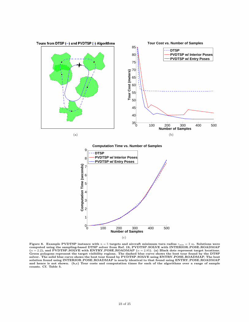
(a)

0 100 200 300 400 50035

40

45

50

55

60

65

70

75

80

85Tour Cost vs. Number of Samples

Number of SamplesT

ou

r C

ost

(m

eter

s)

DTSPPVDTSP w/ Interior PosesPVDTSP w/ Entry Poses

(b)

0 100 200 300 400 5000

1

2

3

4

5

6

7

8

9Computation Time vs. Number of Samples

Number of Samples

Co

mp

uta

tio

n T

ime

(sec

on

ds)

DTSPPVDTSP w/ Interior PosesPVDTSP w/ Entry Poses

(c)

Figure 8. Example PVDTSP instance with n = 5 targets and aircraft minimum turn radius rmin = 3 m. Solutions werecomputed using the sampling-based DTSP solver from Ref. 19, PVDTSP SOLVE with INTERIOR POSE ROADMAP(α = 2.2), and PVDTSP SOLVE with ENTRY POSE ROADMAP (α = 2.85). (a) Black dots represent target locations.Green polygons represent the target visibility regions. The dashed blue curve shows the best tour found by the DTSPsolver. The solid blue curve shows the best tour found by PVDTSP SOLVE using ENTRY POSE ROADMAP. The bestsolution found using INTERIOR POSE ROADMAP is nearly identical to that found using ENTRY POSE ROADMAPand hence is not shown. (b,c) Tour costs and computation times for each of the algorithms over a range of samplecounts. Cf. Table 5.

23 of 25

American Institute of Aeronautics and Astronautics

(a)

0 200 400 600 800 1000 120060

70

80

90

100

110

120

130

140

150

160

170Tour Cost vs. Number of Samples

Number of SamplesT

ou

r C

ost

(m

eter

s)

DTSPPVDTSP w/ Interior PosesPVDTSP w/ Entry Poses

(b)

0 200 400 600 800 1000 12000

20

40

60

80

100

120

140

160

Computation Time vs. Number of Samples

Number of Samples

Co

mp

uta

tio

n T

ime

(sec

on

ds)

DTSPPVDTSP w/ Interior PosesPVDTSP w/ Entry Poses

(c)

Figure 9. Example PVDTSP instance with n = 10 targets and aircraft minimum turn radius rmin = 3 m. Solutionswere computed using the DTSP solver from Ref. 19, PVDTSP SOLVE with INTERIOR POSE ROADMAP (α = 2.2),and PVDTSP SOLVE with ENTRY POSE ROADMAP (α = 2.85). (a) Black dots represent target locations. Greenpolygons represent the target visibility regions. The dashed blue curve shows the best tour found by the DTSP solver.The solid blue curve shows the best tour found by PVDTSP SOLVE using ENTRY POSE ROADMAP. The bestsolution found using INTERIOR POSE ROADMAP is nearly identical to that found using ENTRY POSE ROADMAPand hence is not shown. (b,c) Tour costs and computation times for each of the algorithms over a range of samplecounts. Cf. Table 5.

24 of 25

American Institute of Aeronautics and Astronautics

(a)

0 500 1000100

120

140

160

180

200

220

240

260

280

300

Tour Cost vs. Number of Samples

Number of SamplesT

ou

r C

ost

(m

eter

s)

DTSPPVDTSP w/ Interior PosesPVDTSP w/ Entry Poses

(b)

0 500 10000

50

100

150

200

250

300

350Computation Time vs. Number of Samples

Number of Samples

Co

mp

uta

tio

n T

ime

(sec

on

ds)

DTSPPVDTSP w/ Interior PosesPVDTSP w/ Entry Poses

(c)

Figure 10. Example PVDTSP instance with n = 20 targets and aircraft minimum turn radius rmin = 3 m. Solutionswere computed using the DTSP solver from Ref. 19, PVDTSP SOLVE with INTERIOR POSE ROADMAP (α = 2.2),and PVDTSP SOLVE with ENTRY POSE ROADMAP (α = 2.85). (a) Black dots represent target locations. Greenpolygons represent the target visibility regions. The dashed blue curve shows the best tour found by the DTSP solver.The solid blue curve shows the best tour found by PVDTSP SOLVE using ENTRY POSE ROADMAP. The bestsolution found using INTERIOR POSE ROADMAP is nearly identical to that found using ENTRY POSE ROADMAPand hence is not shown. (b,c) Tour costs and computation times for each of the algorithms over a range of samplecounts. Cf. Table 5.

25 of 25

American Institute of Aeronautics and Astronautics