
Samenstelling promotiecommissie: Rector Magnificus
158
Transcript of Samenstelling promotiecommissie: Rector Magnificus

Het omslag is niet voorzien van lamineerfolie!The cover is not laminated!
Deze afdruk wordt gebruikt voor productie.This printout will be used for production

Influence of wind conditionson wind turbine loads and
measurement of turbulenceusing lidars
1

2

Influence of wind conditionson wind turbine loads and
measurement of turbulenceusing lidars
PROEFSCHRIFT
ter verkrijging van de graad van doctoraan de Technische Universiteit Delft,
op gezag van de Rector Magnificus prof. ir. K.C.A.M. Luyben,voorzitter van het College voor Promoties,
in het openbaar te verdedigenop vrijdag 2 maart 2012 om 12.30 uur
door
Ameya Rajiv SATHE
Master of Technology in Hydrology, Indian Institute of TechnologyRoorkee, India
geboren te Mumbai, India
3

Dit proefschrift is goedgekeurd door de promotoren:
Prof. dr. G.J.W. van BusselProf. dr. J. Mann
Copromotor Dr. ir. W.A.A.M. Bierbooms
Samenstelling promotiecommissie:
Rector Magnificus voorzitterProf. dr. G.J.W van Bussel Technische Universiteit Delft, promotorProf. dr. J. Mann Technical University of Denmark, promotorDr. ir. W.A.A.M. Bierbooms Technische Universiteit Delft, copromotorProf. dr. H. Russchenberg Technische Universiteit DelftProf. dr. A.A.M. Holtslag Wageningen UniversiteitDr. D. Lenschow National Center for Atmospheric Research, USADr. J. Højstrup Romowind DenmarkProf. dr. D.G. Simons Technische Universiteit Delft, reservelid
The research described in this thesis forms part of the project PhD@SEA which issubstantially funded under the BSIK-programme (BSIK03041) of the DutchGovernment and supported by the consortium WE@SEA
Published and distributed by:DUWIND Delft University Wind Energy Research InstituteISBN 978-90-76468-00-6Printed by Wohrmann Print Service, Zutphen, The NetherlandsCopyright c© 2012 by A. Sathe
All rights reserved. Any use or application of data, methods and/or results etc.occurring in this thesis will be at user’s own risk. The author accepts no liability fordamage suffered from use or application.No part of the material protected by this copyright notice may be reproduced orutilized in any form or by any means, electronic or mechanical, includingphotocopying, recording or by any information storage and retrieval system, withoutthe prior permission of the author.
Typeset by the author with the LATEX Documentation System.Author email: [email protected]
4

Dedicated to my mother, my wife, my brother and late maternal grandfather
5

6

Acknowledgements
So many people have contributed directly or indirectly to the completion of this PhDthesis that if I write in detail the contribution of everyone then this in itself would bean autobiography. Nevertheless I would like to mention as many as possible.
First and foremost I thank my supervisor from Risø DTU, Jakob Mann, for hissustained high quality guidance. I don’t know why but I have always believed that astudent is only as good as his teacher. It could perhaps be because of one wonderfullearning experience that I have had with a teacher during my Bachelor studies. Afterhaving a great learning experience with Jakob, my belief has just grown stronger.Without his sustained guidance and support I could not have finished my PhD. Itis evident from the fact that I wrote three journal articles and one conference paperwith him. I also thank him for introducing me to the fascinating world of turbulence.
Delft University is where it all began for me. Hadn’t it been for the opportunitiesprovided by my supervisors Wim Bierbooms and Gerard van Bussel from Delft, Icould not have established strong ties with Risø DTU. I thank Wim and Gerard forthe sustained moral support that they have provided me throughout my PhD. I alsothank Wim for his efforts in supervising me during the initial phase of my PhD. Inthe midst of my PhD I got interested in lidar turbulence research, and it meant thatthe original goals of my PhD had to be modified considerably. Therefore I expressmy gratitude towards Wim and Gerard for giving me immense freedom and lettingme pursue my field of interest.
In Indian culture we are not accustomed to saying ‘Thank you’ to family members,since it makes us feel that we are not close to each other. Hence, I will not use thisword in acknowledging my family. My mother has been a tremendous source ofinspiration whenever I felt that I was wavering in my goals. The values that she hasinstilled in me since my childhood has certainly helped me to finish my PhD. Thestruggles that she has experienced in her life, but the ease with which she has raisedus, has always made me feel that the problems in my PhD were minuscule, and gaveme a lot of strength. My wife has been a tremendous source of support for me inthe last two years. The care and love with which she has emotionally supported mehas helped me immensely to finish my PhD. My late maternal grandfather has beenan embodiment of discipline. On many occasions when the task demanded disciplineI drew inspiration from him. He still inspires me in my life. I value my brother’scontribution because he took care of my mother and maternal grandfather during theentire duration of my PhD. On many occasions when help was needed in the familyhe was always there. At times he has sacrificed his own ambitions for the sake of the
i
7

family, and that has directly helped me to focus on my PhD.
Out of the five years I worked on my PhD, I spent about 1.5 years at Risø DTU. Ihad never imagined that my experience at Risø would be so rewarding. At first I wouldlike to thank Sven-Erik Gryning and Alfredo Pena for guiding me in atmosphericstability and wind profile analysis. Working with them was the beginning of mywonderful learning experiences at Risø. I am grateful to Alfredo for virtually givingme a private scientific writing course. I could myself notice a step change in thequality of my scientific writing skills after having written the first article with himand Sven-Erik. I thank Mike Courtney for giving me opportunity to work in twointeresting and challenging projects, ‘Upwind’ and ‘Safewind’. The constant supportand encouragement that Mike gave me in the last year is highly appreciated. Sharingthe office space with him and Rozenn Wagner at Risø was a fun-filled experience. Ialso thank Abhijit Chougule, who incidentally is a PhD student of Jakob at Risø, forhaving interesting discussions on the fascinating topic of turbulence. We exchangedseveral ideas and continue learning from each other. I thank Torben Larsen for helpingme get acquainted with the turbulence input in HAWC2. I thank Gunner Larsen forhaving interesting discussions on the load calculations. For my stay at Roskilde, Ithank Claus and Lis Jensen, Marete and Finn Hansen, Kjeld Christiansen and LizzieKummel, and Eva and Peter Jensen. I highly appreciate the warmth and affectionthat they have given me and my wife. Because of them we hardly felt that we werethousands of kilometers away from our home in India. Particularly the support thatClaus and Lis has given us is simply unforgettable.
In my times at Delft, I have had many wonderful moments. At first I would like tothank Thanasis Barlas, Busra Akay and Jaume Betran for making my time in Delftmemorable. The wonderful dinners and the philosophical discussions that we hadtogether are now etched in my memories. I thank Thanasis also for helping me withunderstanding the structure of the aero-elastic simulation tool HAWC2. I thank EekeMast for the nice time I had while sharing the office with her, where I have also hadmany interesting discussions about life in general. I thank Thanasis, Eeke and Frans,Claudia and Bertin, and Jaume and Joanna for coming all the way to India to attendmy wedding. The wonderful memories during my wedding will always stay with me.For Matlab doubts in the initial period of my PhD I express my thanks to CarlosFerreira, who suggested me some simple and elegant techniques of data processing.Dick Veldkamp helped me in the load calculations, particularly in getting familiarizedwith the aero-elastic simulation tool Flex5. Rarely I have come across people who areso honest and sincere in helping others, and Dick is one amongst them. EventuallyI did not use Flex5 in my thesis, but I would like to extend my heartfelt gratitudeto Dick for all the help that he provided me. I thank my ex-Master student AndreaVenora for performing a nice job in his thesis. His thirst for knowledge and aptitudefor fine details always kept me on my toes in my work, when I was supervising histhesis. With Gijs van Kuik I had some nice philosophical discussions, and I thankhim for that. I feel calm and happy simply by talking to him. Amongst others in thewind energy section I also thank Turaj Ashuri, Teodor Chiciudean, Ben Geurts andErika Echavarria for the fun times in Delft. Last but certainly not the least I thankSunil and Shweta Kulkarni for the wonderful and memorable times in Amsterdam.They are one of the friends who I can count on during tough times.
8

The PhD project has been carried out under the We@Sea program, BISK-03041,and sponsored by the Dutch Ministry of Economic affairs. The data from the OffshoreWind farm Egmond aan Zee (OWEZ) were kindly made available by NoordZeewindunder the Research Program WE@Sea. The data from Horns Rev were kindlyprovided by Vattenfall A/S and DONG energy A/S as part of the ‘Tall Wind’ pro-ject, which is funded by the Danish Research Agency, the Strategic Research Council,Program for Energy and Environment (Sagsnr. 2104-08-0025). Funding from the EUproject, contract TREN-FP7EN-219048 ‘NORSEWinD’ is acknowledged. The re-sources provided by the EU FP6 UpWind project (Project reference 019945 SES6)and by the Center for computational wind turbine aerodynamics and atmosphericturbulence funded by the Danish Council for Strategic Research grant no. 09-067216is highly appreciated.
9

10
Summary
Variations in wind conditions influence the loads on wind turbines significantly. Inorder to determine these loads it is important that the external conditions are well un-derstood. Wind lidars are well developed nowadays to measure wind profiles upwardsfrom the surface. But how turbulence can be measured using lidars has not yet beeninvestigated. This PhD thesis deals with the influence of variations in wind conditionson the wind turbine loads as well as with the determination of wind conditions usingwind lidars.
Part I of the thesis focuses on analysis of diabatic wind profiles, turbulence, andtheir influence on wind turbine loads. The diabatic wind profiles are analyzed usingthe measurements from two offshore sites, one in the Dutch North Sea, and theother in the Danish North Sea. Two wind profile models are compared, one that isstrictly valid in the atmospheric surface layer, and the other that is valid for the entireboundary layer. The second model is much more complicated in comparison to thefirst. It is demonstrated that at heights more than 50 m above the surface, wheremodern wind turbines usually operate, it is advisable to use a wind profile model thatis valid in the entire boundary layer. The influence of diabatic wind profiles understeady winds on the fatigue damage at the blade root is also demonstrated using theaero-elastic simulation tool Bladed. Furthermore, detailed analysis of the combinedinfluence of diabatic wind profile and turbulence on the blade root flap-wise and edge-wise moments, tower base fore-aft moment, and the rotor bending moments at thehub is carried out using the aero-elastic simulation tool HAWC2. It is found that thetower base fore-aft moment is influenced by diabatic turbulence and a rotor bendingmoment at the hub is influenced by diabatic wind profiles. The blade root loadsare influenced by diabatic wind profiles and turbulence, which results in averagingof the loads, i.e. the calculated blade loads using diabatic wind conditions and thosecalculated using neutral wind conditions are approximately the same. The importanceof obtaining a site-specific wind speed and stability distribution is also emphasizedsince it has a direct influence on wind turbine loads. In comparison with the IECstandards, which generalize the wind conditions according to certain classes of windspeeds, the site-specific wind conditions are demonstrated to give significantly lowerfatigue loads. There is thus a potential in reducing wind turbine costs if site-specificwind conditions are obtained. In this regard we then are faced with measurementchallenges.
The current industry standard for the measurement of wind speed is either thecup or the sonic anemometer. Both instruments require a meteorological mast to be
v
11

mounted at the measurement site. For measuring the wind profile the instrumentsneed to be mounted at several heights on the mast. To install a mast and set up theseinstruments is quite expensive, especially at offshore sites, where the cost of foundationincreases significantly. Besides, there are problems with the flow distortion that haveto be taken care of. In order to overcome these problems it would be ideal to havea remote sensing instrument that measures wind speed. Wind lidars are capable ofdoing that albeit with a price.
Part II of the thesis deals with detailed investigations of the ability of wind lidarsto perform turulence measurements. Modelling of the systematic errors in turbulencemeasurements is carried out using basic principles. Two mechanisms are identifiedthat cause these systematic errors. One is the averaging effect due to the large samplevolume in which lidars measure wind speeds, and the other is the contribution of allcomponents of the Reynolds stress tensor. Modelling of turbulence spectra as meas-ured by a scanning pulsed wind lidar is also carried out. We now understand indetail the distribution of turbulent energy at various wavenumbers, when a pulsedwind lidar measures turbulence. The lidar turbulence models have been verified withthe measurements at different heights and under different atmospheric stabilities. Fi-nally, a new method is investigated that in principle makes turbulence measurementsby lidars possible. The so-called six beam method uses six lidar beams to avoid thecontamination by all components of the Reynolds stress tensor. The theoretical cal-culations carried out demonstrates the potential of this method. In order to avoidaveraging due to volume sampling, a different analysis method is required, which hasnot been investigated in this thesis.
To summarize the entire thesis, it can be said that more work is required to as-certain the influence of atmospheric stability on wind turbine loads. In particular,comparing with the load measurements will go a long way in consolidating the un-derstanding gained from the analysis in this thesis. If lidars are able to measureturbulence, there is a tremendous potential for performing site-specific wind turbinedesign and making the class based design of the IEC standards obsolete.
12

Samenvatting
Variaties in windcondities hebben een belangrijke invloed op de belastingen vanwindturbines. Om deze belastingen nauwkeurig te kunnen bepalen is het van be-lang dat de externe wind condities goed bekend zijn. Wind lidars zijn zeer geschiktom vanaf het oppervlak wind profielen te meten. Maar hoe turbulentie gemeten kanworden met behulp van wind lidars was nog niet onderzocht. Dit proefschrift behan-delt zowel de invloed van variaties in windcondities op de belastingen van windturbinesalsmede het meten van windcondities met behulp van wind lidars.
Deel I van dit proefschrift concentreert zich op de structuur en de turbulentie vandiabatische windprofielen en hun invloed op windturbine belastingen. De diabatischewindprofielen zijn bepaald aan de hand van metingen op twee locaties buitengaats,een in de Nederlandse Noordzee en de andere in de Deense Noordzee. Twee analyt-ische modellen voor het windprofiel zijn met elkaar vergeleken, waarvan de een alleengeldig is in de oppervlaktelaag en de ander de gehele grenslaag beschrijft. Dit tweedemodel is daardoor complexer dan het eerste. Voor hoogtes van meer dan 50 m bovenhet oppervlak, relevant voor moderne windturbines, is het windprofiel dat geldig isvoor de gehele grenslaag het meest gepast. Allereerst is de invloed van het diabat-ische windprofiel op de vermoeiingsschade bij de bladwortel bepaald voor constantewindsnelheden met behulp van het windturbine ontwerppakket Bladed. Verder is eenuitvoerige analyse uitgevoerd, met het windturbine simulatiepakket HAWC2, van degecombineerde invloed van het diabatische windprofiel en turbulentie op de windtur-bine belastingen. Uit deze analyse blijkt dat het moment bij de torenvoet benvloedwordt door de diabatische turbulentie en de buigmomenten bij de rotornaaf wordenbenvloed door het diabatische windprofiel. De belastingen bij de bladwortel wordenzowel door het diabatische windprofiel als door de diabatische turbulentie benvloed.Dit resulteert in een uitmiddeling van de belastingen bij de bladwortel zodat de berek-ende belastingen volgens diabatische windcondities ongeveer gelijk zijn aan die volgensneutrale windcondities. Ook blijkt dat het van groot belang is om de windsnelheids-enstabiliteits-verdeling van de specifieke locatie te gebruiken, omdat dit een directe in-vloed heeft op de windturbine belastingen. De locatie specifieke windcondities gevennamelijk een significant lagere vermoeiingsbelastingen dan de IEC norm. Deze normgeneraliseert windcondities tot bepaalde windsnelheidsklassen. Als de locatie spe-cifieke wind gegevens beschikbaar zijn biedt dat een mogelijkheid om de kostprijs vanwindturbines te verlagen. De uitdaging zit dan in het uitvoeren van gedetailleerdemetingen om deze wind condities te bepalen.
Momenteel wordt voor windmetingen standaard een cup- of een sonische anem-
vii
13
ometer gebruikt. Voor beide instrumenten is een meetmast ter plaatse nodig. Deanemometers dienen op verschillende hoogten geplaatst te worden om een windprofielte kunnen meten. Het plaatsen van een meetmast inclusief instrumentatie is ergkostbaar. Met name geldt dit buitengaats omdat de kosten voor de fundering danaanzienlijk toenemen. Verder dient rekening gehouden te worden met verstoring vande stroming door de meetmast. Een remote sensing instrument zou ideaal zijn omdeze problemen het hoofd te bieden. Wind lidars zijn daartoe gedeeltelijk in staat.
Deel II van deze dissertatie onderzoekt of het mogelijk is om turbulentie te metenmet behulp van wind lidars. Uitgaande van de basisprincipes van het meten metwind lidars zijn de systematische fouten in de turbulentie metingen bepaald. Erzijn twee belangrijke redenen gevonden voor het optreden van systematische foutenbij dergelijke metingen. Systematische fouten worden veroorzaakt doordat een windlidar de snelheden over een groot gebied meet en middelt. De tweede oorzaak vansystematische fouten is de bijdrage van de componenten van de Reynolds spanning-stensor aan de gemeten turbulentie. Met behulp van een scanning-pulsed wind lidarzijn tevens de turbulentie spectra gemeten. Resultaat van dit onderzoek is ondermeerdat nu in detail begrepen wordt hoe de energie van de turbulentie over de verschil-lende golfgetallen is verdeeld als turbulentie wordt gemeten met een pulserende windlidar. Deze lidar turbulentie modellen zijn geverifieerd met metingen op diverse hoo-gtes en voor verschillende atmosferische stabiliteitscondities. Ten slotte is een nieuwemethode onderzocht waarmee het in principe mogelijk wordt om met lidars turbu-lentie te meten. Deze zogenaamde ”six beam” methode gebruikt zes lidar bundelsom de fouten te vermijden ten gevolge van alle componenten van de Reynolds span-ningstensor bij de bepaling van de turbulentie. De uitgevoerde berekeningen tonen demogelijkheden van deze methode. Om gebiedsmiddeling te voorkomen is een andereanalyse methode nodig; dit is in dit proefschrift niet onderzocht.
Samenvattend kan gesteld worden dat meer onderzoek vereist is om de preciezeinvloed van de atmosferische stabiliteit op windturbine belastingen te bepalen. Het zalgeruime tijd vergen, zeker voor wat betreft het uitvoeren van gedetailleerde metingenen het vergelijking met gemeten belastingen, om de verkregen kennis in dit proefschriftte consolideren een aan te vullen. Zodra lidars in staat zijn om turbulentie goed temeten is er een uitstekende mogelijkheid om optimale locatiespecifieke windturbineste ontwerpen, veel gunstiger dan de huidige op de IEC norm gebaseerde standaardwindturbine ontwerpen.
14

Contents
Acknowledgements i
Summary v
Samenvatting vii
1 Introduction 1
1.1 Thesis objectives . . . . . . . . . . . . . . . . . . . . . . . . . . . . . . 3
1.2 Structure of the thesis . . . . . . . . . . . . . . . . . . . . . . . . . . . 31.2.1 Part I . . . . . . . . . . . . . . . . . . . . . . . . . . . . . . . . 41.2.2 Part II . . . . . . . . . . . . . . . . . . . . . . . . . . . . . . . . 41.2.3 Conclusions . . . . . . . . . . . . . . . . . . . . . . . . . . . . . 5
I Diabatic wind profiles, turbulence and their influenceon wind turbine loads 7
2 Offshore wind profiles 9
3 Influence of diabatic wind profiles on wind turbine loads 25
4 Influence of atmospheric stability on wind turbine loads 33
II Turbulence measurements by wind lidars 57
5 Measurement of second-order turbulence statistics using wind lidars 59
6 Measurement of turbulence spectra using a scanning pulsed windlidar 77
7 How can wind lidars measure turbulence? A preliminary invest-igation 111
8 Conclusions and future work 125
8.1 Conclusions . . . . . . . . . . . . . . . . . . . . . . . . . . . . . . . . . 1258.1.1 Overall conclusions . . . . . . . . . . . . . . . . . . . . . . . . . 125
ix
15

8.1.2 Specific conclusions . . . . . . . . . . . . . . . . . . . . . . . . . 126
8.2 Recommendations for future work . . . . . . . . . . . . . . . . . . . . 128
A Appendices 131
A.1 Uncertainty analysis of Obukhov length . . . . . . . . . . . . . . . . . 131
A.2 Derivation of the radial velocity coefficients in a CW lidar . . . . . . . 133
Bibliography 135
Curriculum-vitae 139
16

Chapter 1
Introduction
Energy is vital for the existence of humanity. With tremendous progress in science andtechnology in the last centuries, and the ever-growing world population, energy needskeep increasing. Fortunately, humans have developed ingenious ways of extractingenergy from natural resources. Unfortunately some of that ingenuity has createdproblems that were not existing before, and we are forced to find solutions to thoseman-made problems. Coal fired power plants, for example, satisfy much of the energydemands of the society, but they produce unwanted carbon dioxide (CO2) that haslead to global warming. The same can also be said for the energy extracted from oiland gas. One alternative to such sources of energy is the wind in the atmosphere. Amajor drawback of wind energy is that it can only be harnessed when the wind blows,and that for economic reasons, only within a certain range of wind speeds. This couldperhaps be one of the reasons as to why wind energy has not blossomed into a majorsource of energy, despite dating back centuries to the time of old Persian wind mills.
The maximum theoretical efficiency of the wind energy extraction was calculatedby the German Physicist, Albert Betz in 1919, and was found to be 59.3% [Burtonet al., 2001]. Considering the mechanical and electrical efficiency of different compon-ents of the wind turbine, the overall efficiency is much less. Research in wind energydid not receive much attention until the oil crisis in the 1970s. In the early 1980sthere was a tremendous growth in the development of wind energy, mainly in NorthAmerica. Hundreds of wind turbines were installed in a short period of time. Sub-sequent major problems with many wind turbines led to a dramatic fall in installedwind energy capacity. However, the research continued unabated in Northern Europe,especially Denmark. As the world began clamouring over the cause of the climatechange, interest in renewable energy surged and in the last decade there has been un-precedented growth in the number of wind turbines, both, onshore and offshore. Asa consequence the scientific challenges of optimizing wind energy are ever-increasing.The latest international standards for the design of wind turbines, both, onshore andoffshore have been drafted by the IEC [IEC, 2005a,b]. All over the world developmentof wind farms takes place using the IEC compliant wind turbines.
The IEC [2005a,b] standards prescribe a set of input wind conditions, which thewind turbines have to withstand during their lifetime of approximately 20 years.Wind turbines are designed to withstand fatigue and extreme loads. The focus of this
1
17

thesis is fatigue loads only. Wind profiles and turbulence are very important for windturbines since they influence the power production and fatigue loads. Wind profilesare described in the standards using the power law with a fixed value of the shearexponent (0.2 for onshore sites and 0.11 for offshore sites). Turbulence is describedby either the Mann [1994] or the Kaimal et al. [1972] model. All wind inputs areprescribed for neutral conditions only.
The power law wind profile is an empirical model with no physical basis, but theconvenience of being defined by one parameter only. A more physical representationof the wind profile is based on Prandtl’s mixing length theory [Prandtl, 1932], whichleads to a logarithmic wind profile. Research on diabatic wind profiles has beencarried out since 1950s with the advent of Monin-Obukhov similarity theory [Moninand Obukhov, 1954]. Surprisingly, despite years of research on diabatic wind profiles(particularly for meteorological studies) the IEC [2005a] standard still prescribes theempirical power law wind profile model. In this thesis, diabatic wind profiles arestudied at two offshore sites.
The Mann [1994] model of turbulence was a major contribution in the field ofmicrometeorology in describing the anisotropic turbulence spectral tensor. Up untilthen for wind turbine applications the two-point turbulence statistics were describedusing the empirical Kaimal et al. [1972] spectra in combination with some coherencemodel, e.g. [Davenport, 1961], or the von Karman [1948] isotropic spectral tensormodel. The elegance of using the Mann [1994] model is that the description of thethree-dimensional turbulent structure is captured by only three model parameters,αε2/3, which is a product of the spectral Kolmogorov constant α and the rate ofviscous dissipation of specific turbulent kinetic energy to the two-thirds power ε2/3, alength scale (wavelength of the eddy corresponding to the maximum spectral energy)LM and an anisotropy parameter Γ. The IEC [2005a] standard define these modelparameters for neutral conditions only. In this thesis the Mann [1994] model is alsofitted to measurements under diabatic conditions and used to describe the associatedturbulence.
In recent years interest in estimating wind turbine loads under diabatic condi-tions has been growing. In this thesis the diabatic wind profiles and turbulence areused as input wind conditions and fatigue load calculations are carried out usingthe aero-elastic simulation tool HAWC2. The influence of wind speed and stabilitydistributions at different sites is also investigated.
The wind conditions that are prescribed in the IEC [2005a] standard are dividedaccording to three classes. These classes are defined based on certain generic char-acteristics of the terrain and wind conditions. Thus the load calculations for a givenwind turbine and a site are carried out according to the chosen class based on sitecharacteristics. In reality description of a site based on three classes is very crude,and it would be ideal if site-specific wind conditions are obtained. Moreover, theIEC [2005b] standard for offshore wind turbines recommend using site-specific windconditions, if measurements are available. Amongst other parameters we then needto measure wind profiles and turbulence. Ground-based remote sensing devices likelidars and sodars provide a huge opportunity in this regard. In meteorology, the useof lidars for wind speed measurements has been a subject of research since the 1960s.For wind energy applications, its use has picked up only in the second half of the last
18

decade [Courtney et al., 2008]. As of today lidars are capable of measuring mean windspeeds quite reliably as compared to the cup anemometers [Courtney et al., 2008, Penaet al., 2009, Smith et al., 2006], and IEC standards are being revised to incorporatethem as a standard instrument for the measurement of wind profiles. However, usingthe current measurement configuration their use in the measurement of turbulence isstill questionable [Mann et al., 2009, Sjoholm et al., 2009]. This motivated detailedinvestigations of the ability of lidars to measure turbulence.
1.1 Thesis objectives
At the start of this PhD project the global research objective was to characterize theinflow wind conditions and analyze their influence on wind turbine loads at an offshoresite. There have been only a few measurement campaigns offshore that could meas-ure wind profiles at greater heights. At the first Dutch offshore wind farm, Egmondaan Zee, a meteorological mast was erected in 2005 with a height of about 116.5 mabove the mean sea level. The mast is instrumented at three levels, 21, 70 and 116m in three directions, with several instruments like the cup and sonic anemometers[Kouwenhoven, 2007]. Knowledge of the offshore wind profiles at greater heights waslacking and this provided a wonderful opportunity to measure wind profiles and testmodels. With time the research objective grew in its scope and was revised to alsoincorporate research on turbulence measurements using wind lidars. The measure-ment campaigns carried out using state-of-the-art lidars at the Danish National WindTurbine Test Center, Høvsøre, provided a great opportunity to understand how lidarsmeasure turbulence. With the heavily instrumented meteorological mast at Høvsøreat different heights, a wonderful opportunity was provided to use the measured windprofiles and turbulence under diabatic conditions and calculate wind turbine loadsusing the aero-elastic simulation tool HAWC2. This knowledge has been particularlylacking at the start of the PhD project.
In order to carry out the research in a structured manner the following researchquestions are devised. The answers to these research questions are then combined toform this PhD thesis.
1. How are diabatic wind profiles characterized?
2. Are wind turbine loads influenced by atmospheric stability?
3. Can wind lidars measure turbulence?
4. How do pulsed wind lidars measure turbulence spectra?
5. How would it be possible for wind lidars to measure turbulence?
1.2 Structure of the thesis
This PhD thesis is written as a compilation of four journal and two conference articles.Two journal and two conference articles are already published, whereas the remainingtwo journal articles have been submitted for publication. The structure of this thesisis such that it is divided into two parts. Part one consists of analysis of diabatic wind
19

profiles, turbulence and their influence on wind turbine loads. Part two consists ofinvestigation of turbulence measurements using wind lidars.
1.2.1 Part I
This part is composed of chapters 2 – 4.
Chapter 2 – Offshore wind profiles In this chapter the first research questionposed in section 1.1 is answered. The measurements from two offshore sites in theNorth Sea are used in combination with two wind profile models, one that is validin the atmospheric surface layer, and the other that is valid for the entire boundarylayer. Atmospheric stability is also characterized at these sites, and various stabilitydistributions are obtained. It is demonstrated that for characterizing the wind profilesat greater heights it is important to use those models, which in principle are valid forthe entire boundary layer. This chapter is composed of a journal article published bySathe et al. [2011a].
Chapter 3 – Influence of diabatic wind profiles on wind turbine loads Inthis chapter part of the second research question posed in section 1.1 is answered. Ahypothetical wind turbine is used for load calculations using the aero-elastic simula-tion tool Bladed. The wind conditions are considered to be steady and diabatic windprofiles are used as input wind conditions. It is demonstrated that with the use ofdiabatic wind profiles the fatigue damage is different from that obtained consideringonly the neutral wind profile. The influence of site specific stability distribution is alsoconsidered. From the results of this analysis an impetus is thus provided to performfull scale load calculations considering turbulent winds. This chapter is composed ofa conference article published by Sathe and Bierbooms [2007].
Chapter 4 – Influence of atmospheric stability on wind turbine loads Thisis also related to the second research question posed in section 1.1. The NREL 5MW reference wind turbine is used for load calculations. Diabatic wind profiles andturbulence are used as input wind conditions. It is demonstrated that atmosphericstability has limited influence on wind turbine loads and the definitions of the inputwind conditions are very conservative. This provides an impetus to obtain site-specificinput wind conditions. The influence of site specific wind speed and stability distri-butions is also demonstrated. This chapter is composed of a journal article submittedby Sathe et al. [2011b] to ‘Wind Energy’.
1.2.2 Part II
This part is composed of chapters 5 – 7.
Chapter 5 – Measurement of second-order turbulence statistics using windlidars In this chapter the third research question posed in section 1.1 is answered.Modelling of the systematic errors in turbulence measurements by wind lidars is car-ried out. Two sources of errors are identified in the turbulence measurements by
20

lidars. Comparison of the model and the measurements is carried out under all atmo-spheric stabilities. It is demonstrated that the model agrees with the measurementsquite well under all stabilities. This chapter is composed of a journal article publishedby Sathe et al. [2011c].
Chapter 6 – Measurement of turbulence spectra using a scanning pulsedwind lidar In this chapter the fourth research question posed in section 1.1 isanswered. Modelling of the turbulence spectra as measured by a scanning pulsedwind lidar is carried out. Comparison of the model with the measurements hasdemonstrated that we now theoretically understand the distribution of turbulent en-ergy with respect to the wavenumbers as measured by a scanning pulsed wind lidar.It also provides an impetus to perform modelling of gusts as measured by lidars. Thischapter is composed of a journal article by Sathe and Mann [2011] that is acceptedfor publication in the ‘Journal of Geophysical Research’.
Chapter 7 – How can wind lidars measure turbulence? A preliminaryinvestigation In this chapter part of the fifth research question posed in section 1.1is answered. In order to avoid the systematic errors in turbulence measurements asdescribed in chapters 5 and 6 a new method based on using six lidar beams is in-vestigated. Theoretical calculations are carried out, which demonstrate that the newmethod has the potential that makes turbulence measurements using lidars possible.The optimization of the six beam configuration is carried out based on minimizing therandom errors in the turbulence measurements. This chapter is a conference articlepublished by Sathe et al. [2011d].
1.2.3 Conclusions
Chapter 8 – Conclusions and future work In this chapter individual conclusionsfrom chapters 2 – 7 are stated and combined to form overall conclusions. Severalrecommendations for future work are proposed that can be treated as individualresearch topics.
21

22

Part I
Diabatic wind profiles,turbulence and their influence
on wind turbine loads
7
23

24

Chapter 2
Offshore wind profiles
In this chapter atmospheric stability and wind profile models are analyzed at twooffshore sites in the North Sea. The first site is Egmond aan Zee in the Dutch NorthSea and the second site is Horns Rev in the Danish North Sea. The IEC [2005a]standard prescribes the power law wind profile defined by a shear exponent. There aretwo issues with this model. The first is that it is an empirical model with no physicalbasis, and the second is that no consideration to atmospheric stability is given. Amore physical model of the wind profile is the logarithmic law that is a function offriction velocity u∗ and aerodynamic roughness length z0. It is derived from the localwind shear equation ∂u/∂z = u∗/κz, where u is the mean wind speed, κ is the vonKarman constant and z is the height. Atmospheric stability is characterized in theform of Monin-Obukhov length L. Under diabatic conditions the local wind shear isalso a function of the stability parameter z/L. The φm(z/L) function, which is usedto correct the wind profile model for stability effects, is very different under unstableconditions as compared to stable conditions. We thus obtain different expressionsfor the logarithmic wind profile under diabatic conditions. Strictly speaking thismodel is only applicable to the atmospheric surface-layer, which is approximately thelowermost 10% of the atmospheric boundary layer.
Modern wind turbines operate in the surface layer and well beyond it. There isthus a need to model the wind profile that is valid for the entire boundary layer. In thearticle that follows this introduction we analyze two different wind profile models andcompare it with the measurements. One is the standard surface-layer model and thesecond is the Gryning et al. [2007] model that is valid for the entire boundary layer.The merits and demerits of each of them are described in detail. Atmospheric stabilityis also analyzed at the two offshore sites with a view to describing the climatology atthese sites.
9
25
WIND ENERGY
Wind Energ. 2011; 14:767–780
Published online 10 February 2011 in Wiley Online Library (wileyonlinelibrary.com). DOI: 10.1002/we.456
RESEARCH ARTICLE
Comparison of the atmospheric stability and windprofiles at two wind farm sites over a long marinefetch in the North SeaAmeya Sathe1,2, Sven-Erik Gryning2 and Alfredo Peña2
1 TU Delft, 2629 HS, Delft, The Netherlands2 Wind Energy Division, Risø DTU, 4000, Roskilde, Denmark
ABSTRACT
A comparison of the atmospheric stability and wind profiles using data from meteorological masts located near two windfarm sites in the North Sea, Egmond aan Zee (up to 116 m) in the Dutch North Sea and Horns Rev (HR; up to 45 m) in theDanish North Sea, is presented. Only the measurements that represent long marine fetch are considered. It was observedthat within a long marine fetch, the conditions in the North Sea are dominated by unstable [41% at Egmond aan ZeeOffshore Wind Farm (OWEZ) and 33% at HR] and near-neutral conditions (49% at OWEZ and 47% at HR), and stableconditions (10% at OWEZ and 20% at HR) occur for a limited period. The logarithmic wind profiles with the surface-layerstability correction terms and Charnock’s roughness model agree with the measurements at both sites in all unstable andnear-neutral conditions. An extended wind profile valid for the entire boundary layer is compared with the measurements.For the tall mast at Egmond aan Zee, it was found that for stable conditions, the scaling of the wind profiles with respectto boundary-layer height is necessary, and the addition of another length scale parameter is preferred. At the lower mast atHR, the effect was not noticeable. Copyright © 2011 John Wiley & Sons, Ltd.
KEYWORDS
atmospheric stability; Obukhov length; wind profiles; boundary-layer height
Correspondence
Ameya Sathe, Section Wind Energy, TU Delft, Kluyverweg 1, 2629 HS Delft, The Netherlands.E-mail: [email protected]
Received 5 May 2010; Revised 1 January 2011; Accepted 3 January 2011
1. INTRODUCTION
This study is important for wind energy applications since wind profiles have a significant influence on power productionand loads on turbines. The International Electrotechnical Commission standard1 suggests the use of either a logarithmicprofile without the diabatic correction term or an empirical power law with the power exponent depending on wind speedonly, although it also depends on roughness, height and atmospheric stability.2 Lange et al.3 demonstrated the importanceof using diabatic wind profiles for power production calculations, and Sathe and Bierbooms4 demonstrated the same forsimple load calculations considering only steady winds.
The study of the diabatic wind profile started from a pioneering work on a similarity theory5 [Monin–Obukhov simi-larity theory (MOST)] where the dimensionless wind shear depends on a dimensionless stability parameter. The advent ofMOST led to the experimental research on the empirical similarity relations between the dimensionless wind shear and theatmospheric stability such as those derived from the Kansas experiment.6 The conditions for which the similarity relationsfrom Businger et al.6 are derived depict flat and homogeneous terrain satisfying the assumptions of MOST to the bestpossible extent.
The applicability of MOST to marine conditions is not obvious since the sea roughness length depends on wind speed,which traditionally is represented by the Charnock’s relation.7 Studies have further shown its dependence on fetch8 andwave age9 among others. Numerous studies of wind profiles have been conducted in the past over the land and the sea,resulting in various suggestions on the empirical relation between the non-dimensional wind shear and stability.10–12
Experimental verification over the sea is still a challenge. Walmsley13 studied the wind profile over the sea using data
Copyright © 2011 John Wiley & Sons, Ltd. 767
26

Atmospheric stability and wind profiles over the North Sea A. Sathe, S.-E. Gryning and A. Peña
from Sable Island and concluded that the thermal stratification effect is quite significant. van Wijk et al.14 studied the windprofile over the North Sea and found better agreement with measurements when the diabatic correction was applied thanwith the logarithmic profile. Coelingh et al.15 studied the wind profiles in the Dutch North Sea using measurements (up to75 m) from various platforms and found that the conditions are mainly unstable and that surface-layer theory agreed wellwith the measurements. Recently, Lange et al.16 studied the advection effects (warm air from the land toward sea) on windprofiles and suggested a correction term for the traditional diabatic wind profile. Motta and Barthelmie17 compared mea-surements at different offshore sites in the Baltic Sea and verified the validity of the diabatic wind profile. Gryning et al.18
proposed a new model of wind profile for the entire boundary layer based on the assumption that the friction velocity varieslinearly with height. The wind profiles were also studied using lidars,19 and a new method was proposed to depict marinewind profiles in a non-dimensional form.20 Using the lidar observations, a modified wind profile based on the theory fromGryning et al.18 is suggested for the marine boundary layer in Peña et al.21
The goal of this work is twofold. First is to compare the climatology at two sites in the North Sea in terms of daily, sea-sonal and overall stability distribution. Second is to investigate the wind profile, based on two mixing-length models. Thefirst is the surface-layer wind profile, and the second is the extended model of Gryning et al.18 that characterizes the windprofile in the entire boundary layer. Section 2 describes the theoretical background on wind profiles. Section 3 describesthe data used for the validation of wind profile models. Section 4 describes the results of the atmospheric stability and windprofile analysis. Finally, Section 5 provides a discussion.
2. THEORETICAL BACKGROUND
In the surface layer, the diabatic wind profile is given as
uD u�0
�
hln
� zz0
�� m.z=L/
i(1)
where u�0 is the friction velocity near the ground, � D 0:4 is the von Kármán constant, z is the height, z0 is the aerody-namic roughness length, L is the Obukhov length and m.z=L/ is the empirical stability function. We use the m relationfrom Businger et al.6 for stable conditions and that from Grachev et al.12 for unstable conditions, where L is given as
LD � u�03T
�gw0� 0v
(2)
Here, T is the absolute temperature, �v is the virtual potential temperature and w0� 0v is the virtual kinematic heat flux. Over
the sea, z0 can be approximated by Charnock’s relation:
z0 D ˛u2�0
g(3)
where ˛ is the Charnock parameter (˛ D 0:0144 is used in this analysis based on Gryning et al.2) and g is the accelerationdue to gravity.
Gryning et al.18 extended the wind profile for the entire boundary layer, based on the assumption that the length scale isan inverse summation of three length scales
1
lD 1
LSLC 1
LMBLC 1
LUBL(4)
where LSL, LMBL and LUBL are the length scales of the surface, middle boundary and upper boundary layers, respectively.The justification of using the inverse summation is not given in Gryning et al.,18 but it could be explained if we assumethat the wind profile in the entire boundary layer is a linear sum of wind profiles in the surface, middle boundary and upperboundary layers. The derivation of the extended wind profiles is given in Gryning et al.,18 and only the final forms areshown here. These are
U D u�0
�
�ln
�z
z0
�C z
LMBL� z
zi
�z
2LMBL
��(5)
for neutral conditions,
U D u�0
�
�ln
�z
z0
�� m.z=L/C z
LMBL� z
zi
�z
2LMBL
��(6)
768Wind Energ. 2011; 14:767–780 © 2011 John Wiley & Sons, Ltd.
DOI: 10.1002/we
27

A. Sathe, S.-E. Gryning and A. Peña Atmospheric stability and wind profiles over the North Sea
for unstable conditions and
U D u�0
�
�ln
�z
z0
�� m.z=L/
�1� z
2zi
�C z
LMBL� z
zi
�z
2LMBL
��(7)
for stable conditions, where zi is the height of the planetary boundary layer. zi is assumed to be climatologicallyproportional to u�0 under neutral conditions as
zi D cu�0
jfcj (8)
where fc is the Coriolis parameter and c is a proportionality constant. For a neutral homogeneous terrain, Peña et al.23
estimated c D 0:15 from the re-analysis of the Leipzig wind profile. Considering that the conditions over the sea are nearlyhomogeneous, the same value of c is used in this work. However, under diabatic conditions, there is no agreement ondiagnostic expressions for zi .24 In the absence of measurements, it is expected that the climatological zi decreases as theconditions become more stable. Hence, c D 0:14 is used for stable conditions and c D 0:13 for very stable conditions as inPeña et al.21 The mean value of zi obtained during neutral conditions is also applied for unstable conditions in accordancewith Peña et al.25 The zi estimated using the sound detection and ranging and the radio acoustic sounding system26 hasbeen found to be close to that of the aerosol analysis.
A new scaling parameter in equations (5)–(7) is LMBL. Gryning et al.18 used Rossby number similarity to equate thegeostrophic wind with equations (5)–(7) at z D zi . However, this results in the dependence of LMBL on the uncertainresistance law constants A and B . LMBL can also be fitted to equations (5)–(7) using the measurements, and an empiricalformulation can be devised.18
The traditional way of depicting a wind profile is by plotting the non-dimensional wind speed (u=u�0) against the non-dimensional height (z=z0). Over sea, z0 is not a constant, and the traditional representation is inadequate in a statisticalevaluation, since the individual non-dimensional wind profiles vary with z0 and L. Following Peña et al.,20 the neutralwind profiles are depicted in a non-dimensional form as
u
u�0C 1
�ln
"1C 2
�u�0
u�0C
��u�0
u�0
�2#
D 1
�ln
�z
z0
�(9)
where for each stability class, u�0 is the mean friction velocity, �u�0 is the fluctuation of the friction velocity, andz0 D ˛u�0
2=g is the mean roughness length. Thus, under neutral conditions, the theoretical non-dimensional profilesmatch with the non-dimensional height scaled with z0. Under diabatic conditions, the appropriate m function is sub-tracted from the non-dimensional height in equation (9). A major advantage of this approach is that the wind profiles fora given non-dimensional stability, z0=L, collapse onto a single profile. This approach can be used with the extended windprofiles, equations (5)–(7), by adding appropriate terms to the non-dimensional height. Thus, the variability of marine windprofiles can be observed with respect to stability.
3. DATASETS
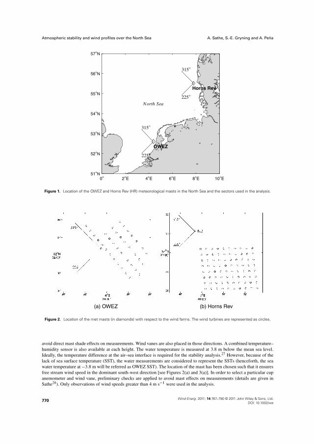
Figure 1 shows the locations of the two offshore sites in the North Sea separated by a distance of about 400 km:
� A 116 m tall meteorological mast located at about 18 km from the coast of Egmond aan Zee, the Netherlands, coor-dinates 52ı36022.900N, 4ı23022.700E [henceforth referred to as the Egmond aan Zee Offshore Wind Farm (OWEZ)],used as the reference for the first Dutch offshore wind farm. The depth of water is approximately 20 m
� A 62 m tall met mast located at about 18 km from the coast of Jutland, Denmark, used as the reference of the largeoffshore wind farm HR I, located at coordinates 55ı3100900N, 7ı4701500E
Figure 2 shows that at OWEZ, the sector that is not influenced by the wakes of the turbines is 135–315ı, and at HR, it is180–360ı and 0–90ı. Figure 3 shows that the dominant wind directions are between 180–300ı at OWEZ and 180–330ıat HR. In order to avoid coastal effects and the internal boundary layer from the land–sea interaction, the sector 225–315ıwas chosen in this analysis for both sites.
3.1. OWEZ
The site comprises 36 Vestas V90 turbines. Meteorological measurements are taken at three levels: 21, 70 and 116 m. Theanalysis was carried out using the 10 min mean measurements between July 2005 and December 2008. Mierij Meteo cupanemometers (KNMI Anemometer model 018, KNMI, De Bilt, The Netherlands) is placed on booms in three directions to
Wind Energ. 2011; 14:767–780 © 2011 John Wiley & Sons, Ltd.DOI: 10.1002/we
769
28
Atmospheric stability and wind profiles over the North Sea A. Sathe, S.-E. Gryning and A. Peña
57°N
56°N
55°N
54°N
53°N
52°N
51°N0° 2°E 4°E 6°E 8°E 10°E
315°
225°
OWEZ
315°
225°
Horns Rev
North Sea
Figure 1. Location of the OWEZ and Horns Rev (HR) meteorological masts in the North Sea and the sectors used in the analysis.
(a) OWEZ (b) Horns Rev
Figure 2. Location of the met masts (in diamonds) with respect to the wind farms. The wind turbines are represented as circles.
avoid direct mast shade effects on measurements. Wind vanes are also placed in those directions. A combined temperature–humidity sensor is also available at each height. The water temperature is measured at 3.8 m below the mean sea level.Ideally, the temperature difference at the air–sea interface is required for the stability analysis.27 However, because of thelack of sea surface temperature (SST), the water measurements are considered to represent the SSTs (henceforth, the seawater temperature at �3:8m will be referred as OWEZ SST). The location of the mast has been chosen such that it ensuresfree stream wind speed in the dominant south-west direction [see Figures 2(a) and 3(a)]. In order to select a particular cupanemometer and wind vane, preliminary checks are applied to avoid mast effects on measurements (details are given inSathe28). Only observations of wind speeds greater than 4 m s�1 were used in the analysis.
770Wind Energ. 2011; 14:767–780 © 2011 John Wiley & Sons, Ltd.
DOI: 10.1002/we
29

A. Sathe, S.-E. Gryning and A. Peña Atmospheric stability and wind profiles over the North Sea
(a) OWEZ (b) Horns Rev
Figure 3. Wind rose from observations at 21 m at OWEZ and 43 m at HR. The numbers inside the circles are the number of10 min observations.
3.2. HR
The measurements at HR are described in Peña et al.21 Here, we use 10 min mean measurements (met mast M2) of windspeed at 15, 30 and 45 m, air temperature at 13 m and water temperature at 4 m below mean sea level. Peña et al.21
compared satellite measurements of SSTs to the water temperatures at HR and found no significant bias. Hence, the watertemperature at �4 m was used directly and will be referred to as HR SST. Relative humidity at 13 m was used to convertthe air temperatures to virtual temperatures. The period available for the analysis is between April 1999 and December2006. Only observations of wind speeds greater than 4 m s�1 were used in the analysis.
4. RESULTS
The study is divided into two parts: statistics of atmospheric stability and validation of wind profile models. MOST is basedon the assumptions of homogeneous, stationary conditions and constant fluxes. It is thus confined to the surface layer. Non-stationarities in the data are checked following Lange et al.16 Usually, the height of the surface layer is about 60–100 mduring unstable and neutral conditions and less than about 30 m during stable conditions.23 Preliminary checks applied atOWEZ revealed that if a filter based on surface-layer height is applied, then only 5% of the available measurements areusable. The study of climatology with such limited data is not of much use. Hence, no filter was applied to the data basedon the surface-layer height. Such checks were not necessary at HR since measurements up to only 45 m were used. Thedata availability at both sites is given in Table I. Seven stabilities were used to classify the observations (see Table II) asgiven in Gryning et al.18 Sathe28 attempted to reason the choice of using a particular stability classification (e.g. that inCoelingh et al.15 and Motta and Barthelmie17 is different from the one in Gryning et al.18). It was concluded that when acontinuous description in terms of L is not feasible, the classification in Table II is appropriate.
Table I. Data availability at OWEZ and HR.
OWEZ (%) HR (%)
Total available dataWind direction, < 225 or > 315ı 63 64Wind direction, > 225 and < 315ı 37 36Data within the selected wind directions (225–315ı)
Filtered data 28 18Available data 72 82
Wind Energ. 2011; 14:767–780 © 2011 John Wiley & Sons, Ltd.DOI: 10.1002/we
771
30

Atmospheric stability and wind profiles over the North Sea A. Sathe, S.-E. Gryning and A. Peña
Table II. Classification of atmospheric stability according toObukhov length intervals.
Very stable 10� L� 50 mStable 50� L� 200 mNear-neutral stable 200� L� 500 mNeutral j L j� 500 mNear-neutral unstable �500� L� �200 mUnstable �200� L� �100 mVery unstable �100� L� �50 m
Estimation of L is not straightforward. High-frequency wind and temperature measurements can be directly used in theeddy covariance method. However, because of the lack of high-frequency temperature measurements, this is not possibleat OWEZ. At HR, no high-frequency measurements are available for the chosen period of analysis. Several methods canbe used to estimate L from the mean observations:3
� Profile methods—Different profile methods are available in the literature.17,29,30 All methods require the use of thewind profile equation (1). Its use is quite debatable, since it is strictly valid in the surface layer only. Moreover, thehigher the measurements, the higher the uncertainty. Thus, its use is justified only if the measurements are availablewithin the first few meters (up to 10 m) for all stability conditions. The lowest measuring height at OWEZ and HRare 21 and 15 m, respectively. Our preliminary study showed that fluxes derived using this method tend to overpredictthe wind profile significantly under stable conditions at OWEZ, and hence, it was not employed in the analysis.
� Gradient Richardson number (Rig) method—Measurements at two different levels in the atmosphere are required toestimate Rig. It can be shown that z=L and therefore m become dependent on the inverse of the square of the windspeed difference between the two levels (1=�u2). High accuracy of wind speed measurements is therefore requiredto measure fluxes. Hence, this method is not used in the analysis.
� Bulk Richardson number (Rib) method—Grachev and Fairall31 provide the dependence of Rib on the stability param-eter z=L. The empirical constants to convert Rib into z=L for unstable and stable conditions were derived usingmeasurements over the ocean. The method has been used in recent studies.3,20,21 Moreover, it requires wind speedmeasurements at one height only to estimate L. Hence, this method was used in the analysis. Observations of windspeed and air temperature at 21 and 15 m at OWEZ and HR, respectively, were used in conjunction with the SST toestimate Rib.
Since the Rib method is sensitive to temperature measurements, the calibrations are checked at both sites. Thetemperature measurements at OWEZ are accurate up to ˙0:1ıC (confidential calibration reports) and at HR up to˙0:354ıC.32 Following Vincent et al.,33 an uncertainty analysis for L is carried out, where it was found that thecombined uncertainty of L increases rapidly as the difference in virtual potential air and sea surface temperatures isreduced. Thus, L is most uncertain in neutral conditions, and as the atmosphere becomes more stable or unstable, theuncertainty in L reduces.
4.1. Statistics of atmospheric stability
The statistics are presented as daily, monthly and overall distributions ofL. The SSTs at OWEZ are corrected by subtracting0:82ıC. Without this correction, the measured non-dimensional wind profiles at OWEZ have a significant offset comparedto the theoretical wind profiles [equation (9)] under all conditions, even at the lowest measurement height. A combinationof satellite and in situ measurements from the European Centre for Medium-Range Weather Forecasts Re-analysis interimdataset was used for comparison with the OWEZ SSTs for a period between July 2005 and October 2008. It is found thatthere is an offset of 0:82ıC at OWEZ. A comparison of SST at HR with the ECMWF, as well as satellite measurements,did not show a significant offset, in agreement with Peña et al.21
Figure 4 shows the daily variation in atmospheric stability for the two sites in the North Sea; no pronounced dailyvariation is found at OWEZ and HR. Only marine sectors are analysed (Figure 1).
Figure 5 shows the seasonal variation of atmospheric stability at both sites. There is a clear seasonal component of atmo-spheric stability at both sites, being more prominent at HR. There is a marked increase of unstable conditions during thesummer months and an increase of stable conditions during the winter months. The peak of unstable conditions is found inlate summer (August/September), whereas the peak in the stable conditions occurs in winter (February). The statistics forthe month of December at OWEZ are not shown because of the limited number of data. The monthly data availability isshown in Table III.
It is observed that for December, the usable data are as low as 1% of the total number of records. It is also noticed thatthe use of unequal numbers of observations in each month weights the results toward the summer.
772Wind Energ. 2011; 14:767–780 © 2011 John Wiley & Sons, Ltd.
DOI: 10.1002/we
31

A. Sathe, S.-E. Gryning and A. Peña Atmospheric stability and wind profiles over the North Sea
5 10 15 200
10
20
30
40
50
60
70
80
90
100
0
10
20
30
40
50
60
70
80
90
100
Hours5 10 15 20
Hours
Fre
qu
ency
of
occ
urr
ence
of
L (
%)
vs s nns n nnu u vu
(a) OWEZ
Fre
qu
ency
of
occ
urr
ence
of
L (
%)
vs s nns n nnu u vu
(b) Horns Rev
Figure 4. Daily variation of atmospheric stability between 225 and 315ı. vs, very stable; s, stable; nns, near-neutral stable;n, neutral; nnu, near-neutral unstable; u, unstable; vu, very unstable.
0
10
20
30
40
50
60
70
80
90
100
Fre
qu
ency
of
occ
urr
ence
of
L (
%)
0
10
20
30
40
50
60
70
80
90
100
Fre
qu
ency
of
occ
urr
ence
of
L (
%)
1 2 3 4 5 6 7 8 9 10 11
Months1 2 3 4 5 6 7 8 9 10 11 12
Months
vs s nns n nnu u vu vs s nns n nnu u vu
(a) OWEZ (b) Horns Rev
Figure 5. Seasonal variation of atmospheric stability between 225 and 315ı. vs, very stable; s, stable; nns, near-neutral stable;n, neutral; nnu, near-neutral unstable; u, unstable; vu, very unstable.
Figure 6 shows the variation of atmospheric stability with wind speed. At both sites, there is an increase of neutral con-ditions with increasing wind speeds. However, at HR there is a sudden increase of near-neutral stable conditions at certainwind speeds—18, 19 and 20 m s�1. This increase is also observed but to a lesser degree at OWEZ. There are many valuesofLwithin the range of 400–500 m, where the spikes are observed. Lowering of the threshold (from 500 to 400 m, Table II)for the neutral interval results in a substantial increase in the number of neutral conditions for those wind speeds, and nospikes are observed. Stability classification is rather sensitive to those values of L that are in the edges of the interval.
Figure 7 shows the variation of atmospheric stability with wind direction. A systematic increase in the number of unsta-ble conditions and a decrease of stable conditions are observed at both sites as the wind direction changes from south-westto north-west, indicating that the air generally is colder for northerly wind directions. The result is also in agreement withan independent investigation carried out at HR.34
Wind Energ. 2011; 14:767–780 © 2011 John Wiley & Sons, Ltd.DOI: 10.1002/we
773
32

Atmospheric stability and wind profiles over the North Sea A. Sathe, S.-E. Gryning and A. Peña
Table III. Monthly data availability of 10 min observations at OWEZ and HR in the long marine fetch sector (225–315ı).
Month Total available data; percentage Percentage of data removed Percentage of usable dataof the whole period by the filter
OWEZ HR OWEZ HR OWEZ HR
January 6 4 1 1 5 3February 6 7 2 1 4 6March 8 5 3 1 5 4April 7 4 2 1 5 3May 4 11 1 2 3 9June 9 14 3 2 6 12July 14 13 5 2 9 11August 14 13 4 2 10 11September 12 11 3 2 9 9October 11 11 2 2 9 9November 6 4 1 1 5 3December 3 3 2 1 1 2
0
10
20
30
40
50
60
70
80
90
100
Fre
qu
ency
of
occ
urr
ence
of
L (
%)
0
10
20
30
40
50
60
70
80
90
100
Fre
qu
ency
of
occ
urr
ence
of
L (
%)
(a) OWEZ (b) Horns Rev
4 6 8 10 12 14 16
Wind speed (m/s)
vs s nns n nnu u vu
Wind speed (m/s)
vs s nns n nnu u vu
4 6 8 10 12 14 16 18 20 22 24
Figure 6. Variation of atmospheric stability with respect to wind speed between 225 and 315ı. vs, very stable; s, stable;nns, near-neutral stable; n, neutral; nnu, near-neutral unstable; u, unstable; vu, very unstable.
Figure 8 shows the overall distribution of atmospheric stability for the two sites. In general, the conditions are mainlyneutral and unstable. This is also in conformity with the observations of Coelingh et al.15 for the Dutch part and of Floors34
for the Danish part of the North Sea. There are more unstable conditions at OWEZ [Figure 8(a)] than at HR [Figure 8(b)]and in general less stable conditions at OWEZ as compared with that at HR.
4.2. Comparison of the non-dimensional wind profiles
Figure 9 shows the comparison of the non-dimensional wind profiles at both sites. The measurements are divided intoseven stability classes (Table II), and a mean (theoretical and measured) profile is plotted for each stability class. The meanobserved parameters are given in Table IV.
The theoretical profiles are computed using equation (9). The stability correction is added to equation (9) using equa-tion (1) for non-neutral conditions. They agree with the measurements very well at both sites in unstable and neutralconditions, particularly at OWEZ. This result is quite significant since there is an ongoing debate on the use of diabaticwind profile, equation (1), in wind energy. A recent study21 has indicated (using a different dataset) that equation (1) canbe used for the marine unstable and neutral conditions even beyond the surface layer, and the wind profiles at OWEZ andHR conform with these findings (Figure 9).
774Wind Energ. 2011; 14:767–780 © 2011 John Wiley & Sons, Ltd.
DOI: 10.1002/we
33

A. Sathe, S.-E. Gryning and A. Peña Atmospheric stability and wind profiles over the North Sea
(a) OWEZ (b) Horns Rev
225 230 235 240 245 250 255 260 265 270 275 280 285 290 295 300 305 310 3150
10
20
30
40
50
60
70
80
90
100
Wind Direction
Fre
qu
ency
of
occ
urr
ence
of
L (
%)
vs s nns n nnu u vu
225 230 235 240 245 250 255 260 265 270 275 280 285 290 295 300 305 310 3150
10
20
30
40
50
60
70
80
90
100
Wind Direction
Fre
qu
ency
of
occ
urr
ence
of
L (
%)
vs s nns n nnu u vu
Figure 7. Variation of atmospheric stability with wind direction. vs, very stable; s, stable; nns, near-neutral stable; n, neutral;nnu, near-neutral unstable; u, unstable; vu, very unstable.
< 1%9%
11%
23%
15%
23%
18%vssnnsnnnuuvu
(a) OWEZ
2%
18%
10%
18%19%
19%
14% vssnnsnnnuuvu
(b) Horns Rev
Figure 8. Overall distribution of atmospheric stability between 225 and 315ı. vs, very stable; s, stable; nns, near-neutral stable;n, neutral; nnu, near-neutral unstable; u, unstable; vu, very unstable.
At OWEZ, equation (1) significantly overpredicts the stable wind profile with increasing height. Scaling with zi reducesthe wind shear at greater heights.21 At HR, such an overprediction is not observed, since the comparison is made at lowmeasurement heights (up to 45 m) only. In the model of Gryning,18 the wind speed profile also depends on zi and LMBL.Peña et al.21 argued that LMBL over the sea is quite large, and hence, its influence can be neglected. This results in scalingthe wind profile under stable conditions with zi only, whereas the unstable and neutral wind profiles conform with thosefrom surface-layer theory [equation (1)]. In our preliminary study, LMBL was fitted to the OWEZ measurements accordingto equations (5)–(7), and it was found that LMBL is very large for unstable and neutral conditions in accordance with Peñaet al.,21 whereas for stable conditions, LMBL could not be neglected. Gryning et al.18 further showed that LMBL dependson the resistance law constants A and B . In this analysis, the values for A and B from Peña et al.25 were used to estimatethe influence of LMBL on the wind profiles in conjunction with zi . The A, B , zi and LMBL values used to obtain theextended wind profiles for stable conditions [equation (7)] are given in Table V.
Figure 10 shows the extended stable wind profiles using equations (1), (7) and (9) at OWEZ. It is observed that thetheoretical profile has a slightly better agreement with the measured profile when the combined effect of zi and LMBLis considered than assuming only the effect of zi . Both approaches agree better with the observations than with thesurface-layer theory. Table VI shows the root mean square error (RMSE) between the stable wind profile models and
Wind Energ. 2011; 14:767–780 © 2011 John Wiley & Sons, Ltd.DOI: 10.1002/we
775
34
Atmospheric stability and wind profiles over the North Sea A. Sathe, S.-E. Gryning and A. Peña
40
38
36
34
32
30
28
25 30 35 40 45 50 55 60 65
40
38
36
34
32
30
28
25 30 35 40 45 50 55 60 65
(a) OWEZ (b) Horns Rev
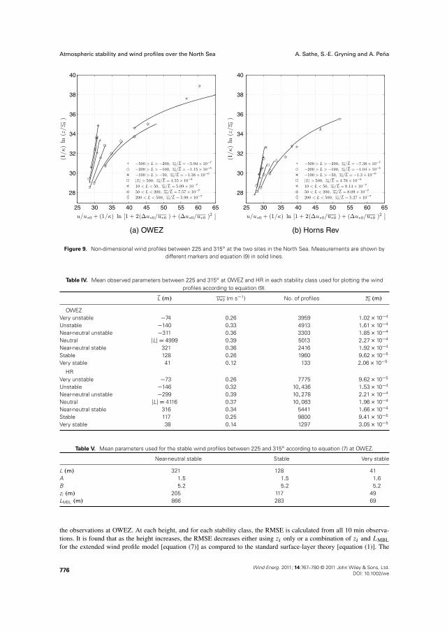
Figure 9. Non-dimensional wind profiles between 225 and 315ı at the two sites in the North Sea. Measurements are shown bydifferent markers and equation (9) in solid lines.
Table IV. Mean observed parameters between 225 and 315ı at OWEZ and HR in each stability class used for plotting the windprofiles according to equation (9).
L .m/ u�0 (m s�1) No. of profiles z0 .m/
OWEZVery unstable �74 0:26 3959 1:02� 10�4
Unstable �140 0:33 4913 1:61� 10�4
Near-neutral unstable �311 0:36 3303 1:85� 10�4
Neutral jLj D 4999 0:39 5013 2:27� 10�4
Near-neutral stable 321 0:36 2416 1:92� 10�4
Stable 128 0:26 1960 9:62� 10�5
Very stable 41 0:12 133 2:06� 10�5
HRVery unstable �73 0:26 7775 9:62� 10�5
Unstable �146 0:32 10;436 1:53� 10�4
Near-neutral unstable �299 0:39 10;278 2:21� 10�4
Neutral jLj D 4116 0:37 10;083 1:96� 10�4
Near-neutral stable 316 0:34 5441 1:66� 10�4
Stable 117 0:25 9800 9:41� 10�5
Very stable 38 0:14 1297 3:05� 10�5
Table V. Mean parameters used for the stable wind profiles between 225 and 315ı according to equation (7) at OWEZ.
Near-neutral stable Stable Very stable
L .m/ 321 128 41A 1:5 1:5 1:6B 5:2 5:2 5:2zi .m/ 205 117 49LMBL .m/ 866 283 69
the observations at OWEZ. At each height, and for each stability class, the RMSE is calculated from all 10 min observa-tions. It is found that as the height increases, the RMSE decreases either using zi only or a combination of zi and LMBLfor the extended wind profile model [equation (7)] as compared to the standard surface-layer theory [equation (1)]. The
776Wind Energ. 2011; 14:767–780 © 2011 John Wiley & Sons, Ltd.
DOI: 10.1002/we
35

A. Sathe, S.-E. Gryning and A. Peña Atmospheric stability and wind profiles over the North Sea
28
30
32
34
36
38
40
25 30 35 40 45 50 55 60 65
Figure 10. Extended wind profiles between 225 and 315ı at OWEZ showing the influence of zi and LMBL under stable conditions.The dashed line shows the influence of zi only, and the solid line shows the combined effect of zi and LMBL. The dash-dot line shows
the traditional surface-layer theory [equation (1)], and the markers are the measurements.
Table VI. Root mean square error in m s�1 between the theoretical profiles and the observations (225–315ı) at OWEZ .
21 m 70 m 116 m
Near-neutral stableEquations (5)–(7) 0:02 1:46 2:62Equations (5)–(7), neglecting LMBL 0:03 1:47 2:62Equation (1) 0 1:47 2:66StableEquations (5)–(7) 0.08 2.5 4.35Equations (5)–7), neglecting LMBL 0:13 2:62 4:39Equation (1) 0 2:36 5:71Very stableEquations (5)–(7) 0:48 5:91 9:22Equations (5)–(7), neglecting LMBL 0:62 6:06 9:24Equation (1) 0 8:48 21:97
approach of using zi only slightly underpredicts the wind profile. Similar comparisons are not required at HR since themeasurements are up to 45 m only, and therefore, the effect on LMBL is small. The stable surface-layer profiles alreadycompared well with the measurements at HR [Figure 9(b)].
4.3. Comparison of the wind speed power spectra
Power spectra of 10 min observations of the horizontal wind speed is derived to illustrate how related are the two sites interms of the wind climate. HR and OWEZ lie in the North Sea separated by approximately 400 km. It is therefore likelythat if the two sites are similar in wind climatology, storm events and weather systems show up at both sites on the spectraon the order of hours. Mesoscale and microscale phenomena associated with coastal effects will show up in the spectra athigh frequencies.
Figure 11 shows the wind spectra comparison based on 10 min measurements. The observations at 21 and 15 m are usedat OWEZ and HR, respectively. All wind directions are used. The period of comparison is between July 2005 and October2006, since continuous measurements are mostly available during this period. For the periods where the data are missing,mean wind speed is used at respective sites. The spectra at OWEZ and HR compare quite well at frequencies of the orderof hours. At high frequencies (of the order of minutes), the spectral energy at OWEZ is greater than that at HR. OWEZis to a large degree surrounded by land as compared with HR (Figure 1), and hence, an increase in mesoscale variability
Wind Energ. 2011; 14:767–780 © 2011 John Wiley & Sons, Ltd.DOI: 10.1002/we
777
36

Atmospheric stability and wind profiles over the North Sea A. Sathe, S.-E. Gryning and A. Peña
Figure 11. Comparison of the pre-multiplied horizontal wind speed power spectra between OWEZ (Egmond) and HR. The graypatch shows the timescales of the order of hours. Data from all wind directions are used.
is expected. Furthermore, at high frequencies, the wakes generated by the turbines contribute to the increase in spectralenergy at OWEZ because of the proximity of the wind turbines as compared with that at HR. The spectral energy at OWEZis higher than at HR likely because the meteorological mast at OWEZ is closer to and has a large wind sector covered bythe wind farm as compared with that at HR (Figure 2). The poor comparison at very low frequencies (order of months)results from the very small number of estimates of the power density.
5. DISCUSSION AND CONCLUSION
Atmospheric stability and wind profile climatology are compared over a long marine fetch at the two sites in the North Seaseparated by about 400 km. It is observed that within a long marine fetch, atmospheric stability in the North Sea is domi-nated by unstable and neutral conditions. Very stable conditions occur rarely (< 1 and 2% at OWEZ and HR, respectively).This result is in agreement with the previous analysis of Coelingh et al. for the Dutch part15 and of Floors34 for the Danishpart of the North Sea. There are differences in the climatology at the two locations within the North Sea. At OWEZ, moreunstable conditions are observed as compared with that at HR and vice versa for stable conditions.
There is no significant daily variation of atmospheric stability conditions at both sites, but the heat capacity of watercauses a seasonal variation. For high wind speeds, near-neutral conditions are more dominant. A systematic increase ofunstable conditions from the south-west to north-west direction at both sites is observed. A different stability classificationhas also been suggested previously,15,17 and its use would increase the number of stable conditions considerably. In thefuture, it would be interesting to arrive at a firm criterion to classify L. Currently, the criterion for selecting the intervals ofL is only based on previous research experience.
Non-dimensional wind profiles have been compared at both sites, and the measurements agree well with the surface-layer theory in unstable and neutral conditions. For stable conditions, surface-layer theory overpredicts the wind speed withincreasing heights at OWEZ. This is not observed at HR likely because of lower measurement heights. In order to assessthe influence of zi on the wind profile, the theory from Gryning et al.18 is used at OWEZ. This introduces a new parameter,LMBL. The comparison of the theoretical profiles with the observations at OWEZ, scaled with zi only and a combination ofzi and LMBL, shows better agreement (see Table VI) than that of traditional surface-layer theory. Under stable conditions,the wind profiles should definitely be scaled by zi , and preferably, LMBL might be applied as another scaling parameter.A comparison of the wind speed spectrum at both sites revealed that the low-frequency events (of the order of hours) arecomparable. This provides a link between the two sites and shows that the two sites are quite similar.
778Wind Energ. 2011; 14:767–780 © 2011 John Wiley & Sons, Ltd.
DOI: 10.1002/we
37

A. Sathe, S.-E. Gryning and A. Peña Atmospheric stability and wind profiles over the North Sea
This analysis will aid the wind farm developers to estimate the power production of wind turbines. The influence on theloads of the wind turbines is still a research question. This study is limited to the long marine fetch sector only (225–315ı).A separate study is required to account for coastal effects and wind turbine wakes.
ACKNOWLEDGEMENTS
The data from the Offshore Wind farm Egmond aan Zee (OWEZ) were kindly made available by NoordZeewind as part ofthe PhD project under the Research Program WE@Sea. The data from Horns Rev were kindly provided by Vattenfall A/Sand DONG energy A/S as part of the ‘Tall Wind’ project, which is funded by the Danish Research Agency, the StrategicResearch Council, Program for Energy and Environment (Sagsnr. 2104-08-0025). Funding from the EU project, contractTREN-FP7EN-219048 ‘NORSEWinD’ is also acknowledged. The authors also want to thank Claire Vincent from RisøDTU for clarifying the uncertainty analysis in the estimation of L.
REFERENCES
1. IEC. Wind turbines—design requirements. IEC 61400-1, International Electrotechnical Commission, 2005.2. Gryning S-E, van Ulden P, Larsen RE. Dispersion from a continuous ground-level source investigated by a K model.
Quarterly Journal of the Royal Meteorological Society 1983; 109: 355–364.3. Lange B, Larsen S, Højstrup J, Barthelmie R. Importance of thermal effects and sea surface roughness for
offshore wind resource assessment. Journal of Wind Engineering and Industrial Aerodynamics 2004; 92: 959–988.DOI: 10.1016/j.jweia.2004.05.005.
4. Sathe A, Bierbooms W. Influence of different wind profiles due to varying atmospheric stability on the fatigue life ofwind turbines. Journal of Physics: Conference Series 2007; 75: 012056. DOI: 10.1088/1742-6596/75/1/012056.
5. Monin AS, Obukhov AM. Basic laws of turbulent mixing in the atmosphere near the ground. Trudy Akademiia NaukSSSR Geofizicheskogo Instituta 1954; 24: 163–187.
6. Businger JA, Wyngaard JC, Izumi Y, Bradley EF. Flux–profile relationships in the atmospheric surface layer. Journalof the Atmospheric Sciences 1971; 28: 181–189.
7. Charnock H. Wind stress over a water surface. Quarterly Journal of Royal Meteorological Society 1955; 81: 639–640.8. Kahma KK, Calkoen CJ. Reconciling discrepancies in the observed growth of wind-generated waves. Journal of
Physical Oceanography 1992; 22: 1389–1405.9. Johnson HK, Højstrup J, Vested HJ, Larsen SE. On the dependence of sea surface roughness on wind waves. Journal
of Physical Oceanography 1998; 28: 1702–1716.10. Dyer AJ. A review of flux–profile relationships. Boundary-Layer Meteorology 1974; 7: 363–372. DOI: 10.1007/
BF00240838.11. Högstrom U. Nondimensional wind and temperature profiles in the atmospheric surface layer. Boundary-Layer
Meteorology 1988; 42: 55–78.12. Grachev AA, Fairall CW, Bradley EF. Convective profile constants revisited. Boundary-Layer Meteorology 2000; 94:
495–515.13. Walmsley JL. On theoretical wind-speed and temperature profiles over the sea with applications to data from Sable
Island, Nova Scotia. Atmosphere-Ocean 1988; 26: 203–233.14. van Wijk AJM, Beljaars ACM, Holtslag AAM, Turkenburg WC. Evaluation of stability corrections in wind speed
profiles over the North Sea. Journal of Wind Engineering and Industrial Aerodynamics 1990; 33: 551–566.15. Coelingh JP, van Wijk AJM, Holtslag AAM. Analysis of the wind speed observations over the North Sea. Journal of
Wind Engineering and Industrial Aerodynamics 1996; 61: 51–69.16. Lange B, Larsen S, Højstrup J, Barthelmie R. The influence of thermal effects on the wind speed profile of the coastal
marine boundary layer. Boundary-Layer Meteorology 2004; 112: 587–617.17. Motta M, Barthelmie RJ. The influence of non-logarithmic wind speed profiles on potential power output at Danish
offshore sites. Wind Energy 2005; 8: 219–236.18. Gryning SE, Batchvarova E, Brümmer B, Jørgensen H, Larsen S. On the extension of the wind profile over
homogeneous terrain beyond the surface layer. Boundary-Layer Meteorology 2007; 124: 251–268. DOI: 10.1007/s10546-007-9166-9.
Wind Energ. 2011; 14:767–780 © 2011 John Wiley & Sons, Ltd.DOI: 10.1002/we
779
38

Atmospheric stability and wind profiles over the North Sea A. Sathe, S.-E. Gryning and A. Peña
19. Peña A, Hasager CB, Gryning SE, Courtney M, Antoniou I, Mikkelsen T. Offshore wind profiling using light detectionand ranging measurements. Wind Energy 2009; 12: 105–124. DOI: 10.1002/we.283.
20. Peña A, Gryning SE. Charnock’s roughness length model and non-dimensional wind profiles over the sea. Boundary-Layer Meteorology 2008; 128: 191–203.
21. Peña A, Gryning SE, Hasager CB. Measurement and modelling of the wind speed profile in the marine atmosphericboundary layer. Boundary-Layer Meteorology 2008; 129: 479–495. DOI: 10.1007/s10546-008-9323-9.
22. Garratt JR. Review of drag coefficients over oceans and continents. Monthly Weather Review 1977; 105: 915–929.23. Peña A, Gryning SE, Mann J, Hasager CB. Length scales of the neutral wind profile over homogeneous terrain. Journal
of Applied Meteorology and Climatology 2010; 49: 792–806. DOI: 10.1175/2009JAMC2148.1.24. Seibert P, Beyrich F, Gryning SE, Joffre S, Rasmussen A, Tercier P. Review and intercomparison of operational
methods for the determination of the mixing height. Atmospheric Environment 2000; 34: 1001–1027.25. Peña A, Gryning SE, Hasager CB. Comparing mixing-length models of the diabatic wind profile over homogeneous
terrain. Theoretical and Applied Climatology 2010; 100: 325–335. DOI: 10.1007/s10546-008-9323-9.26. Emeis S, Münkel C, Vogt S, Müller WJ, Schäfer K. Atmospheric boundary-layer structure from simultaneous
SODAR, RASS, and ceilometer measurements. Atmospheric Environment 2004; 38: 273–286. DOI: 10.1016/j.atmosenv.2003.09.054.
27. Fairall CW, Bradley EF, Godfrey JS, Wick GA, Edson JB. Cool skin and warm layer effects on sea surface temperature.Journal of Geophysical Research 1996; 101: 1295–1308.
28. Sathe A. Project site data—OWEZ data analysis. We@Sea Report, Technical University Delft, 2009.29. Holtslag AAM. Estimates of diabatic wind speed profiles from near-surface observations. Boundary-Layer
Meteorology 1984; 29: 225–250.30. Berkowicz R, Prahm LP. Evaluation of the profile method for the estimation of the surface fluxes of momentum and
heat. Atmospheric Environment 1982; 16: 2809–2819.31. Grachev AA, Fairall CW. Dependence of the Monin–Obukhov stability parameter on the bulk Richardson number
over the ocean. Journal of Applied Meteorology 1996; 36: 406–414.32. Sørensen PB. Wake effect east of the Horns Rev offshore wind farm. Technical Report 209918, Elkraft System. Elsam
Engineering, 2005.33. Vincent CL, Pinson P, Giebel G. Wind fluctuations over the North Sea. International Journal of Climatology 2010.
DOI: 10.1002/joc.2175.34. Floors R. Analysis of diabatic flow modification in the internal boundary layer. Master’s Thesis, Wageningen
University, March 2010.
780Wind Energ. 2011; 14:767–780 © 2011 John Wiley & Sons, Ltd.
DOI: 10.1002/we
39

40
Chapter 3
Influence of diabatic windprofiles on wind turbine loads
In chapter 2 we analyzed wind profiles that are one of the main inputs in load calcula-tions. There is some overlap of the theory described in this paper and that describedin chapter 2. One way to reducing wind turbine costs is to optimize the design. Loadcalculations are an integral part of the design process and are currently performedbased on the IEC [2005a] standard. The description of the input wind field in thisstandard is based on several models or empirical results that are built on many dif-ferent assumptions. The overall result is that the load calculations are performed ina non-optimum environment. This necessitates the use of large safety factors thatresults in excessive use of materials thus increasing the costs significantly. There areopportunities to optimize the load calculations by describing the input wind field ina more realistic manner.
In this chapter load calculations are performed using the aer-elastic simulation toolBladed. The standard surface-layer diabatic wind profile model based on the Monin-Obukhov similarity theory [Monin and Obukhov, 1954] is used in describing the inputwind conditions. The wind field is considered to be steady and the only asymmetryresulting in the input wind field is due to the wind profile. Fatigue damage is obtainedat the blade root as a result of loading due to wind profiles. The influence of usingdifferent stability distributions is also demonstrated. The results obtained providedan impetus to carry out a detail fatigue damage study under diabatic conditions bycombining wind profiles and turbulence.
25
41

Influence of different wind profiles due to varying
atmospheric stability on the fatigue life of wind
turbines
Ameya Sathe, Wim Bierbooms
DUWIND- Delft University Wind Energy Research Institute, Kluyverweg 1, 2629 HS Delft, NL
E-mail: [email protected]
Abstract.Offshore wind energy is being developed on a very large scale in the European seas.
The objective of developing wind energy offshore is to capture greater wind speeds than areencountered onshore and as a result more energy. With this also come more challenges in thedesign of wind turbines due to the hostile offshore environment. Currently the standards foroffshore wind turbines prescribe a site specific design for the support structures and the designfor the rotor nacelle assembly according to onshore standards. Wind turbines are designed towithstand fatigue and ultimate loads. For the fatigue loading several input conditions have beenprescribed, amongst which wind profile is one of them. Wind profile is represented by power lawor logarithmic law as given in the standards. A neutral stability of the atmosphere is consideredwhile obtaining the wind profile using the logarithmic law. In this paper the atmosphericstability is varied in order to estimate different wind profiles and simulations are run in Bladedto check its influence on the fatigue damage at the blade root. The variations in the atmosphericstability has been taken into account by using some typical values of Obukhov length. Fromsteady state simulations it has been found that atmospheric stability is important for fatiguedamage. The analysis showed that variation in the distribution of atmospheric stability causeslarge variations in the fatigue damage for different sites. Thus, it is worthwhile to carry outa full scale study using the turbulent winds and real data for wind turbine and environmentalconditions.
1. Introduction
Offshore wind energy is on a rapid expansion in Europe and many offshore wind farms are beingbuilt. This preludes further development of offshore wind farms all around the world. A windturbine is subjected to various kinds of loads originating from different sources. Aerodynamicloads is one of the sources of loads on wind turbines. These loads occur due to variousinput environmental states that a wind turbine has to encounter. Wind shear is one of theenvironmental state that occurs all the time during the lifetime of a turbine. It is an importantparameter which causes cyclic loading in the rotor and hence fatigue damage. Wind shear isextrapolated from measurements done at lower heights to a height z as given by logarithmiclaw.
uz =u∗kln
(z
z0
)(1)
The Science of Making Torque from Wind IOP PublishingJournal of Physics: Conference Series 75 (2007) 012056 doi:10.1088/1742-6596/75/1/012056
c© 2007 IOP Publishing Ltd 1
42

where u∗ is the friction velocity, k is the von Karman constant and z0 is the roughness length.Wind shear is also given by the power law as:
uzuzr
=
(z
zr
)α(2)
where α is the power exponent, uzr is the reference velocity and zr is the reference height.Equations 1 and 2 assume a neutral stability of the atmosphere while extrapolating to differentheights. Offshore wind farms are being planned for wind turbines with large rotor diameters.This poses a particular question on the viability of using neutral stability to obtain wind shearfrom a reference height. Previous studies [1], [2] and [3] have shown that the energy yieldestimates differ when stability is taken into consideration. In this paper the effects of stabilityclasses have been ascertained on the fatigue damage at the blade root. The resulting damage iscompared with the fatigue damage obtained from logarithmic and exponential wind shear. Theexponential wind shear is obtained using a power law exponent of 0.14 for offshore sites as givenin [4].During the course of the day, cooling and heating of the surface takes place causing differentstability conditions and hence different stratifications. According to Monin-Obukhov similaritytheory the atmospheric stability can be described in terms of stability parameter z/L, where Lis the Obukhov length. Taking stability into account, equation 1 can be written as,
uz =u∗k
[ln
(z
z0
)− ψ
(z
L
)](3)
where ψ(zL
)is the stability parameter. The stability parameter can be calculated using the
Bussinger-Dyer formulation [5]
ψ = 2ln
(1 + φm
2
)+ ln
((1 + φ2
m)
2
)− 2tan−1(x)− π
2for
z
L< 0 (4)
ψ = −β z
Lfor
z
L> 0 (5)
where β and γ are the empirical parameters whose values are taken as 4.8 and 19.3 respectively,[6]. From the wind speed at reference height zr, the wind speed at height z can be obtainedfrom equation 3,
uz = uzrln( z
z0)− ψ( zL)
ln( zrz0 )− ψ( zrL )(6)
In this paper the values of L have been assumed from the classification of stability into fivecategories given in [7].
Table 1. Classification of stability according to Obukhov lengths
very stable 0<L<200 mstable 200<L<1000 m
near-neutral | L | >1000 munstable -1000<L<-200 m
very unstable -200<L<0 m
The sea surface roughness z0 is also not constant and varies with time. Previous studies [1]and [2] have shown that the effect of sea surface roughness is not significant and hence in thispaper, for the analysis, its value is taken as constant. Nevertheless, two extreme values of z0 areassumed and its influence on fatigue damage estimated to verify its influence.
The Science of Making Torque from Wind IOP PublishingJournal of Physics: Conference Series 75 (2007) 012056 doi:10.1088/1742-6596/75/1/012056
2
43

2. Description of the work
The design software used for the fatigue analysis is ‘Bladed’ developed by Garrad Hassan andPartners Ltd. It is a complete design software and an industry standard, which has beenvalidated by Germanischer Llyod. The wind turbine used is a reference turbine which wasprepared for a research project at DUWIND. The characteristics of the turbine are summarizedin table 2.
Table 2. Turbine properties
Class I turbine, Mean wind speed = 10 m/sPower = 5.5MW
Rotor Diameter = 129mHub Height = 95m
Number of Blades = 3Rotational speed = Variable speedcut in wind speed, vcut−in = 4 m/s
cut out wind speed, vcut−out = 25 m/s
As given in table 2, the turbine has a large rotor diameter and is suited for the analysis ofstability influence. The fatigue analysis is carried out for the blade root section. Blade root isselected as the section because it experiences maximum bending moments due to cyclic loadingas compared to any other section on the blade. The blade root is modeled as a thin annularcylinder with an outer diameter of 3.5m and inner diameter of 3.42m. The material for theblade is assumed as Glass Epoxy with an inverse slope on the log-log S-N curve as 9 and anintercept of 70Mpa . The reference height is taken as hub height based on which wind shearacross the rotor plane is determined. A wind turbine’s life has been assumed as 20 years [8] andfatigue damage has been estimated for different stability classes and compared with the fatiguedamage obtained using exponential and logarithmic wind shear assuming a neutral profile. Thesimulations have been run for steady conditions. The choice of the steady wind conditions forthe simulation may not represent the real situation but the analysis would nevertheless givea primary insight into the importance of atmospheric stability. Also, if the steady conditionswould not have a significant effect on the fatigue damage then it may not be worthwhile to go fora full scale study using turbulent winds. Apart from the wind conditions, tower shadow effects,gravity and inertia loads have also been taken into account. This allows for the simulation timeto be reduced from the standard specified 600s [8] to a value representing a minimum of onecomplete cycle of loading. Considering that the turbine is a variable speed turbine the minimumsimulation time should at least be greater than the time required for one revolution of the rotorat minimum wind speed, i. e. 4m/s. The rotor speed at 4m/s was found to be 4rpm and hencethe simulation time should be more than 15s. Nevertheless, the simulation time has been chosenas 90s covering 6 cycles of revolution. Thus it is sufficient to cover even the slowest revolutionof the rotor. A pre-analysis of the effect of varying z0 on the fatigue life was carried out toascertain if its variability would be important. According to DNV offshore standards [9], z0 canvary from 0.0001 for calm sea to 0.003 for coastal waters with the wind blowing from land tosea. With time, z0 would at most vary in the two extreme values. Table 3 shows the influenceof varying z0 on the fatigue damage at blade root.
As seen from table 3 there is some influence of z0 on the fatigue damage. In reality z0 wouldnot attain a fixed value on either side of extremes but would at most hover from one extremeto the other depending on the wind and site conditions. This would reduce the difference in
The Science of Making Torque from Wind IOP PublishingJournal of Physics: Conference Series 75 (2007) 012056 doi:10.1088/1742-6596/75/1/012056
3
44

Table 3. Fatigue Damage for different sea surface roughness
Roughness Fatigue Damage0.003 0.370.0001 0.13
the fatigue damage obtained for two extreme z0 values as shown in table 3. Hence its variationis not accounted for in this paper but could be worthwhile to study using real data. For thispaper z0 is taken as 0.001 assuming that the site would be a coastal site. The combinations forsimulations are made using the wind speed bins of 1m/s from vcut−in to vcut−out for a z0 valueof 0.001 and various values of L as given in table 1. Table 4 summarizes the combination ofsimulations.
Table 4. Simulation parameters
Obukhov Length, L Wind speeds Roughness, z0-300 -100 ∞ 100 300 vcut−in - vcut−out 0.001
The wind shears for a wind speed of 10m/s is given in figure 1 as an example.
Figure 1. Wind shear for different stability conditions at 10m/s
To check the influence of stability, it is important to assume a distribution to be able to assessits effect. Hence, distribution of a particular stability condition sampled by wind speeds is
The Science of Making Torque from Wind IOP PublishingJournal of Physics: Conference Series 75 (2007) 012056 doi:10.1088/1742-6596/75/1/012056
4
45

taken into consideration. [2] gives stability distributions found for various Danish sites. In thispaper the distributions are taken from [2] for Rodsand and Vindeby sites and fatigue damageascertained. Figures 2 and 3 show the distribution of stability conditions sampled by wind speed.
Figure 2. Frequency of occurrence ofstability conditions sampled by wind speed forRodsand site[2]
Figure 3. Frequency of occurrence ofstability conditions sampled by wind speed forVindeby site[2]
These sites are chosen without any special preference as any other offshore site could also havebeen chosen for the analysis. As given in table 4, several simulations were run to calculate thebending moments at the blade root. The time histories of bending moments were converted intostress histories using the following relation:
σ =M.y
I(7)
where σ is the stress at the blade root at a particular time, M is the bending moment, y isthe distance at which the moment acts, which is the radius of the outer diameter and I is themoment of inertia of annular cylinder.
3. Results
Figure 4 shows different stress histories for different stability cases for a wind speed of 10m/s.The figure is just an illustration of various stress histories obtained for various wind speeds andstability classes. The number of cycles to failure and subsequently the fractional damage iscalculated using the following log-log relationship:
log(S) = log(K)− 1
mlog(N) (8)
where S is the stress amplitude in Mpa, log(K) is the intercept, 1m is the inverse slope and N is
the number of cycles to failure. The fatigue damage using different stability classes is calculatedusing following relation:
D =20× 365× 24× 3600
90
25∑U=4
5∑L=1
P (U)L × d(U)L × P (U) (9)
where D is the fatigue damage at the blade root, U is the bin average wind speed,5∑
L=1represents
five stability classes given in table 1, P (U)L is the probability of occurrence of a stability class
The Science of Making Torque from Wind IOP PublishingJournal of Physics: Conference Series 75 (2007) 012056 doi:10.1088/1742-6596/75/1/012056
5
46

Figure 4. Stress histories for different stability conditions at 10m/s
sampled by wind speeds, d(U)L is the fractional damage for the simulation time for respectivestability class at a particular wind speed and P (U) is the probability of occurrence of a particularwind speed. Since the simulations have been performed for 90s the resulting fatigue damagehas been divided by this simulation time. Table 5 summarizes the results obtained from thesimulations.
Table 5. Lifetime fatigue damage using different wind shear models
Method used Fatigue DamageWind shear considering stability classes for Rodsand site 6.12Wind shear considering stability classes for Vindeby site 1.68
Wind shear modeled by logarithmic law and neutral stability 0.25Wind shear modeled by exponential law 1.91
As seen in table 5, the lifetime fatigue is considerably affected by using different models ofwind shear. The distribution of stability shows a significant change in the fatigue damage. ForRodsand site the fatigue damage is considerably higher than for Vindeby site. The wind shearmodeled using logarithmic law gives the lowest fatigue damage.
The Science of Making Torque from Wind IOP PublishingJournal of Physics: Conference Series 75 (2007) 012056 doi:10.1088/1742-6596/75/1/012056
6
47

4. Conclusions
As seen in table 5, considering stability classes while modeling wind shear is an important factorin assessing the fatigue damage more accurately. The importance of distribution of stabilityclasses is clearly emphasized in the results. It can be concluded from the above results thatlogarithmic wind shear with neutral stability underpredicts the fatigue damage depicting a non-conservative approach. It could have been contested that the occurrence of different stabilityconditions would tend to average out the effects over time but the results do not show thisbehavior. Two factors are dependent on it:
• Differences in the wind shears for various stability conditions.
• Frequency of occurrence of a particular stability condition.
Figure 1 shows that the difference in the wind velocities at the lowermost part of the rotor andthe uppermost part for a very stable condition can be up to 5m/s for a hub height velocity of10m/s. This difference increases for a greater hub height velocity and with the increase in rotordiameter. This is a significant difference in the wind speed as compared to that obtained fromthe logarithmic law considering only neutral stability. The importance of a stability is certainlyevident in the difference between the fatigue damage obtained at two sites.Although the results have been obtained for steady state simulations, it provides an impetusto carry out a full scale fatigue damage study by using turbulent winds and real data for windturbines and environmental conditions.
References
[1] Bernhard Lange, Søren Larsen, Jørgen Højstrup, and Rebecca Barthelmie. Importance of thermal effects andsea surface roughness for offshore wind resource assessment. Journal of Wind Engineering and Industrialaerodynamics, pages 959–988, May 2004.
[2] M.Motta and R.J.Barthelmie. The influence of non-logarithmic wind speed profiles on potential power outputat danish offshore sites. Wind Energy, pages 219–236, 2005.
[3] Jonathan Summer and Christian Masson. Influence of atmospheric stability on wind turbine powerperformance curves. Journal of Solar Energy Engineering, 128:531–538, November 2006.
[4] IEC 61400-3. Offshore wind turbines-part 1: Design requirements. 2005.[5] Roland B. Stull. An Introduction to Boundary Layer Meteorology. Kluwer Academic Publishers, 1988.[6] U.Hogstrom. Nondimensional wind and temperature profiles in the atmospheric surface layer. Boundary-
Layer Meteorology, pages 55–78, 1988.[7] Van Wijk AJM, Beljaars ACM, Holtslag AAM, and Turkenburg WC. Evaluation of stability corrections in
wind speed profiles over the north sea. Journal of Wind Engineering and Industrial Aerodynamics, pages551–566, 1990.
[8] IEC 61400-1. Wind turbines-part 1: Design requirements. 2005.[9] DNV Det Norske Veritas. Design of offshore wind turbine structures. June 2004.[10] Bernhard Lange, Søren Larsen, Jørgen Højstrup, and Rebecca Barthelmie. The influence of thermal effects on
the wind speed profile of the coastal marine boundary layer. Boundary-Layer Meteorology, pages 587–617,2004.
The Science of Making Torque from Wind IOP PublishingJournal of Physics: Conference Series 75 (2007) 012056 doi:10.1088/1742-6596/75/1/012056
7
48

Chapter 4
Influence of atmosphericstability on wind turbineloads
Having studied the influence of diabatic wind profiles under steady wind conditionson wind turbine loads in chapter 3 the next obvious step was to perform a full scaleload calculation that included the combined influence of diabatic wind profiles andturbulence. The theory of wind profiles described in this chapter is an overlap ofthat described in chapter 2. The load calculations are carried out for the case ofnormal power production. The aim of this chapter is to answer the following researchquestions:
1. Are wind turbine loads influenced by atmospheric stability?
2. Are wind turbine loads influenced by wind profile models?
3. Are the IEC [2005a] loads different from those calculated using site-specificdiabatic wind profile and turbulence?
Two wind profile models are used. One is the standard surface-layer diabatic windprofile model, and the second is the more advanced Gryning et al. [2007] modelthat is valid for the entire boundary layer. Turbulence is quantified using the Mann[1994] model, where the model parameters under diabatic and neutral conditions areobtained by fitting the model with the measurements at a flat terrain test site inDenmark. In order to compare the influence of wind speed and stability distributionson the loads, four different sites are chosen. The wind profiles and turbulence obtainedat only one site are applied at all other sites. The load calculations are performedusing an aero-elastic simulation tool HAWC2, developed at Risø DTU in Denmark.Fatigue loads are obtained at the blade root, tower base and the hub.
33
49

WIND ENERGY
Wind Energ. 0000; 00:1–23
DOI: 10.1002/we
RESEARCH ARTICLE
Influence of atmospheric stability on wind turbine loadsA. Sathe∗∗+, J. Mann∗∗, T. Barlas∗∗, W.A.A.M. Bierbooms+, G.J.W. van Bussel+
∗∗Wind Energy Division, Risø DTU, Frederiksborgvej 399, 4000 Roskilde, Denmark+ TU Delft, Kluyverweg 1, 2629 HS Delft, The Netherlands
ABSTRACT
Simulations of wind turbine loads for the NREL 5 MW reference wind turbine under diabatic conditions are carried out.
The diabatic conditions are incorporated in the input wind field in the form of wind profile and turbulence. The simulations
are carried out for mean wind speeds between 3 – 16 m/s at the turbine hub height. The loads are quantified as the
cumulative sum of the damage equivalent load for different wind speeds that are weighted according to the wind speed
and stability distribution. Four sites with a different wind speed and stability distribution are used for comparison. The
turbulence and wind profile from only one site is used in the load calculations which are then weighted according to wind
speed and stability distributions at different sites. It is observed that atmospheric stability influences the tower and rotor
loads. The difference in the calculated tower loads using diabatic wind conditions and those obtained assuming neutral
conditions only is up to 17%, whereas the difference for the rotor loads is up to 13%. The blade loads are hardly influenced
by atmospheric stability, where the difference between the calculated loads using diabatic and neutral input wind conditions
is up to 3% only. The wind profiles and turbulence under diabatic conditions have contrasting influences on the loads, e.g.
under stable conditions, loads induced by the wind profile are larger due to increased wind shear, whereas those induced
by turbulence are lower due to less turbulent energy. The tower base loads are mainly influenced by diabatic turbulence,
whereas the rotor loads are influenced by diabatic wind profiles. The blade loads are influenced by both, diabatic wind
profile and turbulence, that leads to averaging of the loads. The importance of using a detailed boundary-layer wind profile
model is also demonstrated. The difference in the calculated blade and rotor loads is up to 6% and 8% respectively, when
only the surface-layer wind profile model is used in comparison to those obtained using a boundary-layer wind profile
model. Finally, comparison of the calculated loads obtained using site-specific and IEC wind conditions is carried out. It
is observed that the IEC loads are up to 95% larger than those obtained using site-specific wind conditions. Copyright c©0000 John Wiley & Sons, Ltd.
KEYWORDS
Atmospheric stability, Wind Profile, Turbulence, Wind turbine loads
Correspondence
∗∗Wind Energy Division, Risø DTU, Frederiksborgvej 399, 4000 Roskilde, Denmark, E-mail: [email protected]
Received . . .
1. INTRODUCTION
Wind turbines are designed to withstand fatigue and extreme loads during their lifetime of approximately 20 years [1].
Amongst different factors that cause fatigue loading, atmospheric turbulence and wind profile have a significant influence.
Copyright c© 0000 John Wiley & Sons, Ltd. 1
Prepared using weauth.cls [Version: 2010/06/17 v1.00]
50

Atmospheric stability and loads Sathe et.al
The IEC standards [1] prescribe a range of wind conditions between the cut-in and cut-out wind speeds under which the
turbine has to operate. Also, a power law wind profile model with a fixed value of the exponent is prescribed. Turbulence
is defined by either the Kaimal model [2], or the more recent Mann model [3]. No consideration to atmospheric stability
is given in the [1] standard neither in the wind profile nor the turbulence model. The [1] standards are known to give a
conservative estimate of the loads. In this study we attempt to answer the following research questions:
1. Are wind turbine loads influenced by wind profile models?
2. Are wind turbine loads influenced by atmospheric stability?
Two diabatic wind profile models are investigated, the first is using the standard surface-layer scaling according to Monin-
Obukhov theory [4], and the second is using the more advanced theory developed by [5] that connects the surface
layer scaling with the geostrophic drag law. Turbulence is simulated using the Mann model under different atmospheric
stabilities. The time-domain aeroelastic code HAWC2 is utilized for the calculation of the loads on various components of
the wind turbine. Fatigue loads are quantified using the concept of Damage Equivalent Loads (DEQ), which for a given
arbitrary number of load cycles would produce the same fatigue damage as that of the sum of the individual load cycles.
Simulations are used to compare the load cases.
The investigation of diabatic wind profile models has been a subject of research since the 1950s. The logarithmic wind
profile with a stability correction term has been used in many research projects. The stability corrections have also been
subject of extensive research [6, 7]. The model is however strictly applicable only in the surface layer, which is roughly
the lower 10% of the atmospheric boundary layer. It is well known that the boundary layer height varies according to
atmospheric stability, where it is typically between 600 – 1000 m under unstable conditions and 150 – 200 m under stable
conditions [8]. Modern wind turbines extend up to 150 m, which means that they operate in and above the surface layer. We
thus need wind profile models that extend up to the the entire boundary layer height. [9, 10] proposed a wind shear model
under neutral conditions that extend up to the entire boundary layer height. [11] extended this model to all atmospheric
stability conditions using the Rossby number similarity theory. Recently, [5] proposed a new diabatic wind profile model
that extends up to the entire boundary layer height, also using the Rossby number similarity theory. The main difference
between these models and the surface-layer model is the inclusion of the boundary layer height parameter that limits
the growth of the wind profile length scale above the surface layer. In this study, we use the model from [5], since the
performance of [9, 10] was similar to [5] when compared with the measurements [11].
For wind turbines we need two-point statistics in order to simulate turbulent wind fields that affects the entire wind
turbine. Thus we either need a three-dimensional spectral tensor model or combine the one-dimensional spectra with
some coherence model. Different spectral tensor models have been proposed in the past [12, 13] but the IEC standards
recommend the Mann model [3] since it incorporates the atmospheric physics to the best possible extent. The starting
point for these models is the isotropic spectral tensor model by [14]. Alternatively the expressions by [2] for the one-
dimensional spectra are recommended to be used with a some coherence model, e.g. [15]. In principle all these models are
valid only under neutral conditions in the surface layer. [16] derived analytical expressions of spectral tensors also under
stable conditions. Due to unavailability of spectral tensor models under unstable conditions and non-stationarity of the
model by [16], we use the Mann model [3] by fitting the model parameters to the data under different stability conditions.
There have been a few studies concerning the influence of the wind conditions on wind turbine loads. [17] studied
the complex terrain effects on turbulence and subsequently on wind turbine loads, and concluded that increased fatigue
loads were caused by increased turbulence. [18] carried out a linear multi-variable regression analysis and concluded
that the vertical component of the wind field and atmospheric stability have a significant influence on blade DEQ. The
wind shear and turbulence effects on rotor fatigue loads were studied by [19]. The wind profile is modelled using the
power law and turbulence using the von-Karman isotropic spectral tensor [14]. They concluded that the increase in wind
shear and turbulence increased rotor fatigue loads considerably. [20] performed a statistical analysis of the influence of
several primary and secondary inflow parameters including atmospheric stability. They used a sequential analysis of each
parameter instead of multi-variable regression analysis and concluded that there is not much influence of atmospheric
stability on fatigue and extreme loads of blades. In contrast [21] studied the influence of coherent turbulent structures
2 Wind Energ. 0000; 00:1–23 c© 0000 John Wiley & Sons, Ltd.
DOI: 10.1002/we
Prepared using weauth.cls
51

Sathe et.al Atmospheric stability and loads
induced by Kelvin-Helmholtz waves under very stable conditions on wind turbine loads and concluded that these large
coherent structures have a significant influence on wind turbine loads. It should however be noted that the site chosen by
[21] for their analysis is such that large coherent structures are observed quite often. [22] performed a parametric study
of several inflow parameters and concluded that they do not influence the fatigue failure as much as the uncertainty in the
material properties. Similar conclusions were made by [23], where a detailed investigation of wind turbine fatigue loads
was carried out using a probabilistic approach. [24] calculated fatigue loads at the blade root using diabatic wind profiles
and steady winds, and concluded that fatigue loads increase using diabatic wind profiles in comparison to those obtained
under neutral conditions. [25] varied turbulence intensity and length scales to investigate their influence on wind turbine
loads and concluded that variation in turbulence parameters have a negligible influence on blade and tower moments but
a significant influence on the yaw moments. Recently, [26] investigated the influence of atmospheric turbulence on wind
turbine rotor torque. The Gaussian and non-Gaussian turbulent time series were simulated using two different models and
comparison with measurements was carried out. They concluded that non-Gaussian turbulence, which is also observed in
the atmosphere significantly increases the loads.
Section 2 of this article gives a description of the sites and the measurements used. Section 3 describes the wind climate
at different sites, giving the wind speed and stability distributions. Section 4 introduces some theory of the wind profile
models and turbulence used in this work. Section 5 briefly explains the aero-elastic simulation tool used in this study. The
load calculations are described in section 6. Finally, we conclude our work with some discussion in section 7.
2. SITE DESCRIPTIONS
Load calculations are performed based on turbulence and mean wind speed data at Høvsøre, which is the Danish National
Test Center for Large Wind Turbines. Based on data availability the range of mean wind speeds chosen is 3 – 16 m/s.
For estimating the cumulative load of all wind speeds the loads need to be weighted according to the joint wind speed
and stability distribution. These distributions are specific to a particular site. Hence, we selected three additional sites with
different distributions of the mean wind speed and atmospheric stability for comparing the cumulative fatigue loads. These
sites are Egmond aan Zee in the Dutch North Sea, Ostergarnsholm in the Baltic sea, and Hurghada in the Gulf of Suez,
Egypt. For all sites we use the turbulence and wind profiles from Høvsøre, in order to isolate the effect of atmospheric
stability.
2.1. Høvsøre
A reference meteorological mast (met-mast), which is 116.5 m tall and intensively equipped with cup and sonic
anemometers, is located at the coordinates 56◦26’26” N, 08◦09’03” E. The site is about 2 km from the West coast of
Denmark. The eastern sector is generally characterized by a flat, homogeneous terrain, and to the South is a lagoon. To
the North, there is a row of five wind turbines. The sonics are placed on the North booms of the met-mast, resulting in
unusable data when the wind is from the South because of the wake of the mast, and from the North because of the wakes
of the wind turbines. In order to bin the wind speeds we use the cup anemometers at 80 and 100 m, since the hub height of
the turbine is 90 m (refer table III). The data is selected between March 2004 – November 2009. To comply with terrain
homogeneity we restrict our analysis to a directional sector of 50◦ – 150◦. Atmospheric stability is characterized using
the standard surface-layer length scale L, commonly known as the Monin-Obukhov length. L is estimated using the eddy
covariance method [27] from the sonic measurements at 20 m. The aerodynamic roughness length z0 = 0.014 cm. More
details of the site and instrumentation can be found in [28].
2.2. Egmond aan Zee – OWEZ
A 116 m tall meteorological mast is located at about 18 km from the coast of Egmond aan Zee (henceforth referred to
as OWEZ, the offshore wind farm Egmond aan Zee), The Netherlands, coordinates 52◦36’22.9” N, 4◦23’22.7” E. The
Wind Energ. 0000; 00:1–23 c© 0000 John Wiley & Sons, Ltd. 3DOI: 10.1002/we
Prepared using weauth.cls
52

Atmospheric stability and loads Sathe et.al
depth of water is approximately 20 m. The stability analysis is carried out using the 10-min mean measurements between
July 2005 – December 2008. In order to avoid turbine wakes and sudden change of roughness from the east, we use a
directional sector of 225◦ – 315◦ such that homogeneous conditions prevail. The wind speed distribution is obtained from
the cup anemometer measurements at 70 m. Atmospheric stability is estimated using the bulk Richardson number method
[29] from the wind speed and temperature measurements at 21 m and the sea-surface temperature. More details of the site
and instrumentation can be found in [30].
2.3. Ostergarnsholm
A 30 m tall mast is located at a small island about 4 km east coast Gotland, in the Baltic Sea, coordinates 57◦27’ N,
18◦59’ E. The stability analysis is carried out using the eddy covariance method [27] from the sonic measurements at
9 m above the surface between June 1995 – July 2002. The island is very flat. For the directional sector 80◦ – 220◦
the data represents undisturbed open sea conditions, for the other sectors the wave field is influenced by limited fetch or
bottom topography [31]. Since one the goals of this study is to assess the influence of atmospheric stability and wind speed
distribution, and not to perform a detailed site specific study, all wind directions are used. The wind speed distribution is
obtained from the cup anemometer measurements at 30 m. More details of the site and instrumentation can be found in
[32, 33].
2.4. Hurghada
A 30 m tall mast is located at a coastal plateau about 650 m to the west of the Gulf of Suez, Egypt, coordinates
27◦18’59” N, 33◦41’56” E. The stability analysis is carried out using the profile temperature difference method [34].
The period of analysis is between March 1991 – November 1996. The measurements are the mean wind speed at 24 m
and temperature difference at 22.5 m. The island is quite flat with a gentle slope to the South west that reaches about 300
m above sea level at a distance of 20 km. To the North West the terrain abruptly rises to about 200 m at a distance of 10
km. In order to avoid the sudden roughness change from the Red Sea, we select a directional sector of 135◦ – 330◦. More
details of the site and instrumentation can be found in [35].
3. WIND CLIMATE AND ATMOSPHERIC STABILITY
Table I. Weibull scale and shape parameters for different sites
Scale (λ) Shape (k)
Høvsøre 9.13 3.82
OWEZ 11.12 3.07
Ostergarnsholm 7.86 2.18
Hurghada 6.56 2.70
Fig. 1 shows the histograms of the mean wind speeds at the four sites. The decrease in the mean wind speed at
Ostergarnsholm and Hurghada is evident by the shift in the distribution to the left in comparison to Høvsøre and OWEZ.
When a Weibull distribution is fitted to the measurements at these sites, we obtain the scale (λ) and shape (k) parameters
as given in table I. At Ostergarnsholm and Hurghada these parameters are significantly smaller than those at Høvsøre and
OWEZ. It would be ideal to obtain these measurements at 90 m at all four sites, however, they are not available. Another
alternative is to extrapolate the wind at different heights to 90 m using some wind profile model. We do not opt for this
because we are interested in having an indication of the influence of variability in site specific distributions on wind turbine
loads and not to perform a detailed site specific analysis.
4 Wind Energ. 0000; 00:1–23 c© 0000 John Wiley & Sons, Ltd.
DOI: 10.1002/we
Prepared using weauth.cls
53

Sathe et.al Atmospheric stability and loads
3 4 5 6 7 8 9 10 11 12 13 14 15 160
500
1000
1500
2000
2500
3000
3500
4000
4500
5000
u (m/s)
P(u)(−
)
(a) Høvsøre
3 4 5 6 7 8 9 10 11 12 13 14 15 160
500
1000
1500
2000
2500
3000
u (m/s)
P(u)(−
)
(b) OWEZ
3 4 5 6 7 8 9 10 11 12 13 14 15 160
200
400
600
800
1000
1200
u (m/s)
P(u)(−
)
(c) Ostergarnsholm
3 4 5 6 7 8 9 10 11 12 13 14 15 160
2000
4000
6000
8000
10000
12000
14000
16000
u (m/s)
P(u)(−
)
(d) Hurghada
Figure 1. Histograms of wind speeds at different sites for the selected wind sectors
Except at Ostergarnsholm, for each site we select a particular directional sector in order to comply with homogeneous
site conditions. As a consequence the number of observations may reduce. In order to verify this we plot the wind rose at
all four sites (Fig. 2). It is seen that except at Høvsøre the data selection is in the prevailing wind direction, but we have a
sufficient number of 10-min observations at all sites. Atmospheric stability is classified into seven stabilities following [5],
and is given in table II.
Table II. Classification of atmospheric stability according to Obukhov length intervals
very stable (vs) 10 ≤ L ≤ 50 m
stable (s) 50 ≤ L ≤ 200 m
near-neutral stable (nns) 200 ≤ L ≤ 500 m
neutral (n) | L |≥ 500 m
near-neutral unstable (nnu) −500 ≤ L ≤ −200 m
unstable (u) −200 ≤ L ≤ −100 m
very unstable (vu) −100 ≤ L ≤ −50 m
Wind Energ. 0000; 00:1–23 c© 0000 John Wiley & Sons, Ltd. 5DOI: 10.1002/we
Prepared using weauth.cls
54

Atmospheric stability and loads Sathe et.al
2000 4000 6000 8000
30
210
60
240
90270
120
300
150
330
180
0
(a) Høvsøre
10000 20000 30000 40000
30
210
60
240
90270
120
300
150
330
180
0
(b) OWEZ
500 1000 1500 2000
30
210
60
240
90270
120
300
150
330
180
0
(c) Ostergarnsholm
10000 20000
30000
30
210
60
240
90270
120
300
150
330
180
0
(d) Hurghada
Figure 2. Wind rose at different sites. The numbers outside the concentric circles are the number of observations at the respectivesites.
Fig. 3 shows the distribution of atmospheric stability with the mean wind speed at the four sites. There is a striking
resemblance in the stability distributions of the two offshore sites, OWEZ (Fig. 3b) and Ostergarnsholm (Fig. 3c), which
are dominated by unstable conditions. At all sites there is an increase in neutral conditions with increasing wind speed,
which indicates that mechanical production is dominant over buoyant production of turbulent kinetic energy. Hurghada
is the most stable site due to cold temperatures prevailing during the long night hours. At both onshore sites the stable
conditions dominate over the unstable conditions. In general this result is in agreement with the European Wind Atlas [36]
where unstable conditions dominate at offshore sites and stable conditions at onshore. The stability distribution at OWEZ
is slightly different from that obtained by [30] because a different data filtering criteria is used in this study.
4. WIND PROFILE AND TURBULENCE
According to similarity theory if we have similar sites, i.e. the friction velocity, surface roughness and buoynacy fluxes
are approximately the same, then the mean wind profile and turbulence should be similar. Thus if we have homogeneous
6 Wind Energ. 0000; 00:1–23 c© 0000 John Wiley & Sons, Ltd.
DOI: 10.1002/we
Prepared using weauth.cls
55

Sathe et.al Atmospheric stability and loads
3 4 5 6 7 8 9 10 11 12 13 14 15 160
10
20
30
40
50
60
70
80
90
100
u (m/s)
P(L|u)
(−)
vs s nns n nnu u vu
(a) Høvsøre
3 4 5 6 7 8 9 10 11 12 13 14 15 160
10
20
30
40
50
60
70
80
90
100
u (m/s)
P(L|u)
(−)
vs s nns n nnu u vu
(b) OWEZ
3 4 5 6 7 8 9 10 11 12 13 14 15 160
10
20
30
40
50
60
70
80
90
100
u (m/s)
P(L|u)
(−)
vs s nns n nnu u vu
(c) Ostergarnsholm
3 4 5 6 7 8 9 10 11 12 13 14 15 160
10
20
30
40
50
60
70
80
90
100
u (m/s)
P(L|u)
(−)
vs s nns n nnu u vu
(d) Hurghada
Figure 3. Distribution of atmospheric stability for each mean wind speed at different sites.
conditions at different sites then we can obtain the wind profile and turbulent structure at only one site and apply those
at other sites. In this study we make use of this assumption by performing a detailed wind profile and turbulence spectra
analysis at Høvsøre only, and applying those at the other three sites. One of the major differences between the offshore
and onshore sites is that the sea-surface roughness varies continuously over the water, whereas it is constant over the
land (unless there has been any changes to the landscape during the period of data analysis). This will obviously have an
influence on the wind profile and turbulence structure. Nevertheless we limit our study to using site specific wind speed
and stability distributions only and use the same wind profile and turbulence at all sites.
4.1. Wind profile
Two wind profile models are studied. The first is the diabatic wind profile in the surface layer given as,
u =u∗κ
[ln( z
z0
)− ψm(z/L)
], (1)
where u is the mean wind speed, u∗ is the friction velocity near the ground, κ = 0.4 is the von Karman constant, z is the
height, and ψm(z/L) is the empirical stability function. We use the ψm relation from [6] for stable, and that from [7] for
Wind Energ. 0000; 00:1–23 c© 0000 John Wiley & Sons, Ltd. 7DOI: 10.1002/we
Prepared using weauth.cls
56

Atmospheric stability and loads Sathe et.al
unstable conditions, where L is given as,
L = − u∗3T
κgw′θ′v. (2)
Here T is the absolute temperature, θv is the virtual potential temperature and w′θ′v is the virtual kinematic heat flux. The
second is the model by [5] that is valid for the entire boundary layer. It is given as follows: for neutral conditions,
(3)u =u∗κ
[ln
(z
z0
)+
z
LMBL− z
zi
(z
2LMBL
)]
for unstable conditions and
(4)u =u∗κ
[ln
(z
z0
)− ψm(z/L) +
z
LMBL− z
zi
(z
2LMBL
)]
for stable conditions,
(5)u =u∗κ
[ln
(z
z0
)− ψm(z/L)
(1− z
2zi
)+
z
LMBL− z
zi
(z
2LMBL
)]
where LMBL is the length scale of the middle boundary layer, and zi is the height of the planetary boundary layer. zi is
assumed to be proportional to u∗ under neutral conditions as,
zi = cu∗|fc| , (6)
where fc is the Coriolis parameter and c is a proportionality constant. For a neutral homogeneous terrain, [37] estimated
c = 0.15 from the reanalysis of the Leipzig wind profile. Under diabatic conditions, there is no agreement on diagnostic
expressions for zi [8]. In the absence of measurements, it is expected that the climatological zi decreases as the conditions
become more stable. Hence, c = 0.14 is used for stable and c = 0.13 for very stable conditions as in [38]. The mean value
of zi obtained during neutral conditions is also applied for unstable conditions in accordance with [11]. LMBL, which is a
function of zi, is estimated following [30].
0 10 20 30 40 50 60 700
20
40
60
80
100
120
140
160
u/u∗ (−)
z(m
)
vuunnunnnssvs
(a) surface-layer theory
0 10 20 30 40 50 60 700
20
40
60
80
100
120
140
160
u/u∗ (−)
z(m
)
vuunnunnnssvs
(b) Boundar-Layer model by [5]
Figure 4. Measured and modelled surface-layer and boundary-layer wind profiles for different stability classes. The markers indicatemeasurements and the lines indicate the models. The unstable, neutral and stable wind profiles from the models are represented by
dashed, solid and dash-dot lines respectively.
The comparison between the measured and modelled wind profile is shown in Fig. 4. The x-axis is normalized by the
friction velocity in order to include the comparison for all mean wind speeds. We observe that there is considerable wind
8 Wind Energ. 0000; 00:1–23 c© 0000 John Wiley & Sons, Ltd.
DOI: 10.1002/we
Prepared using weauth.cls
57

Sathe et.al Atmospheric stability and loads
shear under stable conditions as compared to the unstable and neutral conditions, which is captured in the model by [5]
reasonably well. In surface-layer theory the length scale increases with height without bounds, but in [5] it is limited by the
boundary layer height. The differences between the two models are most pronounced under very stable conditions, where
[5] fits the measurements slightly better (Fig. 4b). For unstable conditions both models agree well with the measurements,
which indicates that limiting the length scale with boundary layer height may not be necessary. [30] gives a more detailed
comparison between the two models.
4.2. Atmospheric turbulence
2 4 6 8 10 12 14 160
0.02
0.04
0.06
0.08
0.1
0.12
0.14
u (m/s)
αε2
/3(m
2/s3)
vuunnunnnssvs
(a) αε2/3
2 4 6 8 10 12 14 160
20
40
60
80
100
120
u (m/s)
LM
(m)
vuunnunnnssvs
(b) LM
2 4 6 8 10 12 14 161.5
2
2.5
3
3.5
4
u (m/s)
Γ(−
)
vuunnunnnssvs
(c) Γ
2 4 6 8 10 12 14 160
0.5
1
1.5
2
2.5
u (m/s)
σu(m
/s)
vuunnunnnssvs
(d) σu
Figure 5. [3] model parameter fits at different mean wind speeds and atmospheric stabilities. The variation of the standard deviationof the u component is also given.
We quantify atmospheric turbulence using the Mann model [3]. This model is described by the three model parameters,
αε2/3, which is a product of the spectral Kolmogorov constant α and the rate of viscous dissipation of specific turbulent
kinetic energy to the two-thirds power ε2/3, a length scale (wavelength of the eddy corresponding roughly to the maximum
spectral energy) LM and an anisotropy parameterΓ. Thus any variation of turbulence with respect to specific site conditions
means variation of αε2/3, LM and Γ. The quite complicated equations of the spectral tensor model may be found in [3].
The αε2/3 parameter results in shifting the spectra in the vertical direction, i.e. increase in the value of αε2/3 results
Wind Energ. 0000; 00:1–23 c© 0000 John Wiley & Sons, Ltd. 9DOI: 10.1002/we
Prepared using weauth.cls
58

Atmospheric stability and loads Sathe et.al
10−2 10−1 100
0
2
4
6
8
10
12
14
16
x 10−3
k1 (m−1)
k1Fij(k
1)(m
2/s2)
uvwuw
Figure 6. Turbulence spectra under very stable conditions for a mean wind speed of 3 m/s
in shifting the spectra up and vice-versa. The LM parameter results in shifting the spectra in the horizontal direction,
i.e. increase in the value of LM results in shifting the spectra to the left and vice-versa. Γ = 0 corresponds to isotropic
turbulence, i.e. σ2u = σ2
v = σ2w, which are the variances for the u, v and w components of the wind field respectively.
Increasing the Γ parameter beyond zero implies that σ2u/σ
2w > 1, σ2
v/σ2w > 1 and σ2
u/σ2v > 1.
The Mann model [3] is a semi empirical model that is strictly valid only for neutral conditions in the surface layer.
Nevertheless, in this study we perform a χ2-fit of the [3] model with the measurements to obtain αε2/3, LM and Γ
(using Eq. 4.1 from [3]) under different atmospheric stabilities at 80 and 100 m for mean wind speeds between 3 – 16
m/s. Ideally, we would like to fit the model with the measurements at 90 m, which is the hub height of the turbine (refer
table III). Unfortunately, at Høvsøre we do not have sonic measurements at 90 m, and hence, αε2/3, LM and Γ are
linearly interpolated between 80 and 100 m to obtain the same at 90 m. We assume that since the difference between the
measurement heights is only 20 m, the model parameters are locally linear (refer Fig. 4 in [39]) and the errors introduced
in the two-point turbulence statistics by linear interpolation of the parameters would be negligible. It should also be noted
that the performance of the Mann model [3] has not been tested in predicting coherences, i.e. two-point statistics under
diabatic conditions, but in this study we assume that the coherences can be predicted under all conditions using this model.
Fig. 5 shows variation of αε2/3, L and Γ with the mean wind speed under diabatic conditions. In Fig. 5a it is observed
that under all stabilities the energy dissipation rate increases with the increase in the mean wind speed. This is mainly
because the turbulent energy production increases with increasing mean wind speeds. For a fixed z, neutral surface-layer
scaling dictates that ε2/3 ∝ u2, which is reflected in Fig. 5a. The neutral conditions have the largest dissipation rates
followed by the unstable conditions. The stable conditions have the smallest rate of dissipation because there is hardly any
turbulent energy production. In Fig. 5b a systematic trend is observed with increasing mean wind speeds such that under
unstable and neutral conditions the length scales increase, whereas under stable conditions they decrease. The increase in
length scales under neutral conditions is in agreement with [39], however the magnitude of increase is much lower than
that observed by [39].
10 Wind Energ. 0000; 00:1–23 c© 0000 John Wiley & Sons, Ltd.
DOI: 10.1002/we
Prepared using weauth.cls
59

Sathe et.al Atmospheric stability and loads
10−2 10−1−0.05
0
0.05
0.1
0.15
k1 (m−1)
k1Fij(k
1)(m
2/s2)
uvwuw
(a) very unstable
10−2 10−1−0.05
0
0.05
0.1
0.15
k1 (m−1)
k1Fij(k
1)(m
2/s2)
uvwuw
(b) unstable
10−2 10−1−0.05
0
0.05
0.1
0.15
k1 (m−1)
k1Fij(k
1)(m
2/s2)
uvwuw
(c) near neutral unstable
10−2 10−1−0.05
0
0.05
0.1
0.15
k1 (m−1)
k1Fij(k
1)(m
2/s2)
uvwuw
(d) neutral
Figure 7. a–d: Turbulence auto-spectra of u, v, w components, and the uw co-spectrum at 80m for the mean wind speed of 9 m/sunder different stabilities. The markers are the measurements and the smooth lines are Mann model [3] fits.
We speculate the decrease in the length scales under stable conditions as follows. From Fig. 6, we observe that there
is a sharp increase in the energy content at low frequencies relative to that observed at high frequencies for low wind
speeds. Under stable conditions there is hardly any turbulent energy as compared to unstable and neutral conditions. This
causes the turbulent energy in the mesoscale range, which is known to be proportional to f−5/3 for f � 2 days−1 [40], to
contribute to the increase in energy at low wavenumbers in the microscale range. This results in increasing the turbulent
length scales at low wind speeds and stable conditions. At high wind speeds the microscale fluctuations becomes more
powerful and the mesoscale contribution at low frequencies cannot be seen. Hence, under stable conditions at low wind
speeds we observe larger length scales as compared to high wind speeds. In general we observe that the length scales are
much larger under unstable conditions than under stable conditions, which is well known [2]. In Fig. 5c we observe that
under neutral conditions the degree of anisotropy is constant with increasing mean wind speeds, whereas except for very
unstable conditions it decreases weakly with increasing mean wind speeds. In general except for very low wind speeds,
anisotropy is largest under neutral conditions whereas it is lowest for unstable conditions. Since the focus of this study is
fatigue loads it is also interesting to observe variation in the degree of turbulence as standard deviation of the u component
of the wind field σu with respect to atmospheric stability and mean wind speed (refer Fig. 5d). It is observed that σu is
Wind Energ. 0000; 00:1–23 c© 0000 John Wiley & Sons, Ltd. 11DOI: 10.1002/we
Prepared using weauth.cls
60
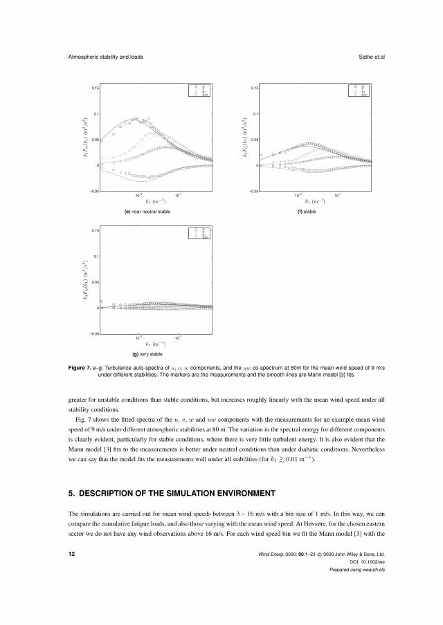
Atmospheric stability and loads Sathe et.al
10−2 10−1−0.05
0
0.05
0.1
0.15
k1 (m−1)
k1Fij(k
1)(m
2/s2)
uvwuw
(e) near neutral stable
10−2 10−1−0.05
0
0.05
0.1
0.15
k1 (m−1)
k1Fij(k
1)(m
2/s2)
uvwuw
(f) stable
10−2 10−1−0.05
0
0.05
0.1
0.15
k1 (m−1)
k1Fij(k
1)(m
2/s2)
uvwuw
(g) very stable
Figure 7. e–g: Turbulence auto-spectra of u, v, w components, and the uw co-spectrum at 80m for the mean wind speed of 9 m/sunder different stabilities. The markers are the measurements and the smooth lines are Mann model [3] fits.
greater for unstable conditions than stable conditions, but increases roughly linearly with the mean wind speed under all
stability conditions.
Fig. 7 shows the fitted spectra of the u, v, w and uw components with the measurements for an example mean wind
speed of 9 m/s under different atmospheric stabilities at 80 m. The variation in the spectral energy for different components
is clearly evident, particularly for stable conditions, where there is very little turbulent energy. It is also evident that the
Mann model [3] fits to the measurements is better under neutral conditions than under diabatic conditions. Nevertheless
we can say that the model fits the measurements well under all stabilities (for k1 � 0.01 m−1).
5. DESCRIPTION OF THE SIMULATION ENVIRONMENT
The simulations are carried out for mean wind speeds between 3 – 16 m/s with a bin size of 1 m/s. In this way, we can
compare the cumulative fatigue loads, and also those varying with the mean wind speed. At Høvsøre, for the chosen eastern
sector we do not have any wind observations above 16 m/s. For each wind speed bin we fit the Mann model [3] with the
12 Wind Energ. 0000; 00:1–23 c© 0000 John Wiley & Sons, Ltd.
DOI: 10.1002/we
Prepared using weauth.cls
61

Sathe et.al Atmospheric stability and loads
turbulence measurements from the sonics and obtain the three model parameters αε2/3, LM and Γ. We obtain the wind
profile over the entire turbine using the wind profile models described in section 4.1. The three-dimensional wind is then
simulated over the entire rotor following [41]. The simulated loads are the blade root flap-wise and edge-wise bending
moments, tower base fore-aft bending moments, and the rotor bending moments at the hub. The blade and rotor loads are
obtained in the rotating coordinate system, whereas the tower loads are obtained in a fixed coordinate system.
Figure 8. Coordinate systems for the blades (subscript B), hub (subscript H) and tower (subscript T)
Fig. 8 shows the coordinate system for the blades, hub, and the tower used in the load calculations. For each blade, the
z-axis is along the blade, y-axis is in the mean wind direction and x-axis is in the lateral direction to the blade tip. The
blade loads are obtained in the rotating blade coordinate system (subscript B) attached to the blade root. The rotor loads at
the hub are obtained in the rotating coordinate system attached to the hub (subscript H). If we consider the initial position
of the rotor such that the blade points upwards then the orientation of the axes are the same as that for the blade coordinate
system, and rotates with this particular blade. The tower loads are obtained in a fixed coordinate system attached to tower
base (subscript T), where the y-axis is along the mean wind direction, x-axis is in the lateral direction and the z-axis is in
the vertical direction.
5.1. Wind turbine
We use the NREL 5 MW reference wind turbine for simulating the turbine loads, which is a fictional representative utility-
scale multi-MW wind turbine, used by research teams throughout the world to standardize baseline offshore wind turbine
specifications, and to quantify the benefits of advanced land- and sea-based wind energy technologies. The details of the
turbine are given by [42]. The main characteristics of the turbine are given in table III.
5.2. Aero-elastic simulation tool – HAWC2
For simulating the aeroelastic response of the wind turbine, and calculating various loads on its components, the aeroelastic
time-domain code HAWC2 is used, developed at Risø-DTU [43, 44]. The structural part of HAWC2 is based on a multi-
body formulation using the floating frame of reference approach, where wind turbine main structures are subdivided into
a number of bodies where each body consists of an assembly of Timoshenko beam elements. Each body has its own
Wind Energ. 0000; 00:1–23 c© 0000 John Wiley & Sons, Ltd. 13DOI: 10.1002/we
Prepared using weauth.cls
62

Atmospheric stability and loads Sathe et.al
Table III. Main properties of the wind turbine
Maximum Power 5 MW
Number of blades 3
Rotor diameter 126 m
Hub height 90 m
Cut-in wind speed 3 m/s
Rated wind speed 11.4 m/s
Cut-out wind speed 25 m/s
Control Variable speed, collective pitch
coordinate system, with calculation of internal inertia loads when this coordinate system is moved in space, so that large
rotation and translation of the body motion is accounted for. The aerodynamic forces are calculated using an unsteady
Blade Element Momentum approach, including additional models for azimuthally dependent induction ∗, dynamic inflow
and tip losses. Static aerodynamic data for all airfoils is provided, which are corrected for rotational effects. The unsteady
aerodynamics of the airfoil sections is taken into account by the Beddoes-Leishman type dynamic stall model of [45]. The
influence of the tower on the inflow is accounted for with a potential flow ’tower shadow’ model. The aerodynamic drag
of the tower and nacelle is also modelled.
6. LOAD CALCULATIONS
In order to quantify the fatigue damage a widely used approach is to divide the random loads experienced by a component
into single amplitude load ranges that are associated with the corresponding number of cycles to failure based on the
experimentally obtained Wohler curve (or the Stress-number of cycles, S-N curve). Following Palmgren-Miner linear
damage rule we then assume that the damage from different load ranges can be linearly added to obtain the total fatigue
damage of a component. Usually it is difficult to obtain the S-N curve of a component material (there is no data for the
S-N curve because the NREL turbine used in this study is a fictitious turbine), and hence, we have to resort to other ways
of quantifying the fatigue damage. Fortunately, we can do that using the concept of Damage Equivalent Load (DEQ). It
is defined as the fatigue load range corresponding to a number of equivalent load cycles NEQ, that produces the same
damage as the real load ranges Di corresponding to the respective load cycles Ni. If we let D denote the total fatigue
damage, DEQ can implicitly be written as,
D =∑
Dmi Ni = Dm
EQNEQ, (7)
where m is the Wohler exponent. In this study m = 12 is used for blades, i.e. corresponding to the glass fiber material,
and m = 3 is used for estimating the hub and tower loads, since they are made up of steel. Rearranging the terms we get,
DEQ =(∑Dm
i Ni
NEQ
)1/m
. (8)
In order to estimate DEQ we thus need some algorithm that separates the random loads into individual load ranges and the
corresponding number of cycles, and assume some value of NEQ. In this study we use the Rainflow counting algorithm
to estimate Di and Ni and assume NEQ = 107 cycles. The cumulative Damage Equivalent Load DEQC including all
mean wind speeds and atmospheric stabilities can be estimated using the wind speed and stability distributions given in
section 3. Thus, if we denote P (L|u) as the distribution of atmospheric stability at given mean wind speed and P (u) as
∗The calculation of thrust and induction is performed in a polar grid using the local wind speed vectors. This improves predictions in case of large wind shear and skew
inflow.
14 Wind Energ. 0000; 00:1–23 c© 0000 John Wiley & Sons, Ltd.
DOI: 10.1002/we
Prepared using weauth.cls
63

Sathe et.al Atmospheric stability and loads
the distribution of the mean wind speeds, then DEQC is estimated as,
DEQC =
16∑u=3
( vs∑L=vu
DEQ × P (L|u))× P (u). (9)
The limits of L indicate the corresponding probability of atmospheric stability at a given mean wind speed, where vu
denotes very unstable conditions, and vs denotes very stable condition. The operating conditions considered are normal
power production for the chosen wind speed range. Variations in the load cases are given in table IV. For each mean wind
speed and atmospheric stability the turbulent field is generated for 10 random seeds to reduce the statistical uncertainty†, and the simulation time is 600 s. Table V gives the normalized DEQC for different cases at different sites. At each
Table IV. Load cases
Cases
I Diabatic boundary-layer wind profile and turbulence
II Neutral boundary-layer wind profile and turbulence
III Diabatic surface-layer wind profile and turbulence
IV IEC load case, power law exponent = 0.2
Table V. Normalized DEQCof bending moments at different sites
Blade root Tower base Rotor loads
Cases flap edge fore-aft Mx My Mz
HøvsøreI 1.000 1.000 1.000 1.000 1.000 1.000
II 0.994 0.996 1.160 0.885 0.996 0.996
III 1.060 1.004 0.987 1.079 1.005 1.016
IV 1.378 1.018 1.749 1.277 1.013 1.089
OWEZI 1.000 1.000 1.000 1.000 1.000 1.000
II 1.029 1.003 1.028 1.032 1.002 0.995
III 0.989 0.998 0.997 0.981 0.998 1.004
IV 1.356 1.029 1.397 1.421 1.024 1.092
OstergarnsholmI 1.000 1.000 1.000 1.000 1.000 1.000
II 1.020 1.001 1.084 0.999 1.001 1.001
III 1.027 1.001 0.990 1.034 1.002 1.011
IV 1.458 1.022 1.776 1.482 1.019 1.110
HurghadaI 1.000 1.000 1.000 1.000 1.000 1.000
II 1.030 0.999 1.170 0.946 0.999 1.009
III 1.040 1.002 0.978 1.053 1.004 1.014
IV 1.491 1.019 1.956 1.420 1.016 1.120
site the loads are normalized with those from the reference case I. The blade flap-wise and edge-wise loads are defined
as the bending moments at the root of the blade along the x and y axis respectively, in the blade coordinate system (Fig.
8). The fore-aft loading of the tower is defined as the bending moment at the base of the tower along the x-axis in the
tower coordinate system (Fig. 8). Mx, My and Mz denote the rotor loads at the hub defined along the x, y and z axis
respectively, in the rotating hub coordinate system (Fig. 8). Cases I and II compare the influence of the diabatic boundary-
layer wind profile and turbulence on the loads with those obtained by assuming neutral conditions only. Cases I and III
†IEC standard [1] recommends simulation for at least 6 random seeds
Wind Energ. 0000; 00:1–23 c© 0000 John Wiley & Sons, Ltd. 15DOI: 10.1002/we
Prepared using weauth.cls
64

Atmospheric stability and loads Sathe et.al
compare the differences in the loads obtained by using boundary-layer and surface-layer wind profile models (section 4.1).
The turbulence used is the same for both cases. Cases I and IV shows the corresponding comparison with the IEC load
case.
6.1. Tower base fore-aft loads
The tower loads will be mainly caused due to the variation in the thrust exerted by the wind field on the rotor. In this study,
the variation in the input wind field is due to the wind profile and turbulence that varies with atmospheric stability. Thus
it is important to understand the variation of the thrust force due to variation in atmospheric stability. We hypothesize that
the force exerted by the wind profile will mainly cause a dynamic moment at the blade root or at the hub, whereas that
exerted by turbulence will cause a dynamic moment at the tower base. If we conceptualize turbulence in the form of eddies
then intuitively it can be said that the larger the size of the eddy, the larger will be the dynamic force, and vice versa. From
Fig. 5b we observe that the turbulence length scales (or characteristic eddy sizes) decrease as the conditions change from
unstable to stable. We then expect that the large eddies under unstable conditions will exert a large dynamic force on the
entire rotor that will cause large dynamic moments in the fore-aft direction. Under stable conditions the rotor will act as
a low-pass filter that causes some averaging of the turbulence. For a three-bladed rotor with blades at 120◦ with respect
to each other, the variation of the force exerted by the wind profile on tower base will average out. We think that this is
because the asymmetry in the loads due to the wind profile will be experienced by all three blades equally, that averages
out as the blades sweep the rotor area.
2 4 6 8 10 12 14 160
100
200
300
400
500
600
u (m/s)
DEQ(kN-m
)
vuunnunnnssvs
Figure 9. Variation of tower base fore-aft loads with respect to mean wind speeds and atmospheric stability.
In order to verify the above reasoning, we plot the variation of tower loads with respect to mean wind speeds and
atmospheric stability in Fig. 9. The loads are largest for unstable and neutral conditions, whereas they are significantly
smaller under stable conditions (of the order of 2). If we compare the turbulent energy in the low wavenumber range (or
large length scales), i.e. between 10−3 < k1 < 10−1 m−1 in Fig. 7, then we observe a relatively small difference between
the unstable and neutral conditions (roughly by a factor of 1.2), but a large difference under stable conditions (roughly
16 Wind Energ. 0000; 00:1–23 c© 0000 John Wiley & Sons, Ltd.
DOI: 10.1002/we
Prepared using weauth.cls
65

Sathe et.al Atmospheric stability and loads
by a factor of 10). At smaller length scales, corresponding roughly to k1 > 10−1 m−1, except for very stable conditions,
the difference in the turbulent energy is relatively small (of the order of 2). Hence, the length scales under unstable and
neutral conditions that contain larger turbulent energy at low wavenumbers cause more fatigue damage than under stable
conditions. Variation of the loads with respect to wind speed is highly non-linear. At about 5 m/s we observe a peak in the
loads because at that wind speed the natural frequency of the tower (≈ 0.33 Hz) correspond to three times the rotational
frequency. At 11 m/s the rated power is produced, and above that wind speed the pitching of the rotor blades causes a
decrease of the loads.
At Høvsøre and Hurghada, we observe a reduction in calculated tower loads of approximately 16% and 17% respectively
under diabatic conditions in comparison to those assuming only neutral conditions, whereas at OWEZ and Ostergarnsholm
the corresponding reduction of approximately 3% and 8% respectively. Høvsøre and Hurghada are dominated by stable
conditions, whereas OWEZ and Ostergarnsholm are dominated by unstable and near-neutral conditions. From Fig. 9, we
observe that under stable conditions the tower loads are much smaller than those under unstable and neutral conditions.
Hence, there is larger reduction in the calculated tower loads using diabatic wind conditions at Høvsøre and Hurghada than
at OWEZ and Ostergarnsholm.
Our intuitive understanding that wind profiles will not influence tower loads is verified by comparing cases I and III,
where under diabatic conditions two different wind profile models are used but with the same turbulence. Even at Høvsøre
and Hurghada, which are stable sites, and where the surface-layer wind profile model predicts a large wind shear (see Fig.
4), there is hardly any difference between the tower loads (up to 2% only). There is a negligible difference (< 1%) in the
calculated tower loads at OWEZ and Ostergarnsholm.
At all sites the calculated IEC tower loads are significantly larger (up to 96%) than those obtained by using diabatic
turbulence and wind shear, which means that the IEC standard [1] is very conservative in the definition of wind shear and
turbulence. The αε2/3 parameter defined according to the IEC standard is about 4.5 to 1.5 times larger for mean wind
speeds from 3 to 16 m/s than that observed at Høvsøre. The LM and Γ parameters are constant according to the IEC
definition and have values of 42 m and 3.9 respectively, whereas from Figs. 5b and 5c we observe that LM and Γ vary
significantly with atmospheric stability and mean wind speed. Wind profile is defined by the power law with an exponent
of 0.2 in the IEC standard for all mean wind speeds, which is also a conservative estimate. The overall result is that we get
a conservative estimate of the tower loads.
6.2. Blade loads
It is interesting to note in Table V that the blade root flap-wise loads are not notably influenced by atmospheric stability,
since the difference in the dynamic loads obtained using diabatic wind conditions and those obtained assuming neutral
conditions is only up to 3%. We hypothesize that the blade flap-wise loads as defined in section 6 will be influenced by
both, the wind profile and turbulence, which will be seen as dynamic moments at the root section. This is in contrast to the
loads observed at the tower base, where only turbulence seems to be influential. The dynamic force exerted by the wind on
the blade due to wind profile under diabatic conditions is in direct contrast with that exerted by turbulence. Under stable
conditions there is a large wind gradient as compared to unstable conditions. Thus wind profile under stable conditions will
exert a larger dynamic force on the blades than under unstable conditions. This has been verified from a previous study
[24], where only steady winds are considered. On the contrary, turbulence is lower under stable conditions as compared to
that under unstable conditions (see Fig. 5d). This means that under stable conditions there will be smaller amplitude load
ranges as compared to unstable conditions. The combined influence on the blades is that the flap-wise loads are averaged
out under diabatic conditions (see cases I and II in table V).
In order to verify the above reasoning, the variation of blade root flap-wise loads with respect to mean wind speeds and
atmospheric stability is plotted in Fig. 10 . We observe that the flap-wise loads are increased only slightly (of the order of
1.2) from unstable to stable conditions. It shows that contrasting influence of wind profiles and turbulence under diabatic
conditions tend to average out the loads. The loads increase with the mean wind speed (Fig. 10) even after the rated wind
speed has reached. This is because wind speed standard deviation increases with the mean wind speed causing greater
Wind Energ. 0000; 00:1–23 c© 0000 John Wiley & Sons, Ltd. 17DOI: 10.1002/we
Prepared using weauth.cls
66

Atmospheric stability and loads Sathe et.al
2 4 6 8 10 12 14 160
500
1000
1500
2000
2500
3000
3500
u (m/s)
DEQ(kN-m
)
vuunnunnnssvs
Figure 10. Variation of blade root flap-wise loads with respect to mean wind speeds and atmospheric stability.
number of large load range cycles to occur at high wind speeds (refer Fig. 5d). At Høvsøre, we observe that the flap-wise
loads are completely averaged out. At Hurghada we observe about 3% difference between cases I and II likely because of
the low Weibull λ and k parameters. At other sites we do not observe much difference in the blade root flap-wise loads
under diabatic and neutral conditions.
We observe a slightly larger influence of using a different wind shear model, where the loads vary by up to 6% (cases I
and III). Using the surface-layer wind profile (case III) we get a large wind gradient under stable conditions thus resulting
in large asymmetrical loading as compared to the model by [5] (case I). At Høvsøre and Hurghada where stable conditions
dominate over unstable conditions this effect is more pronounced. At OWEZ and Ostergarnsholm the conditions are mostly
unstable, and hence, we do not observe much influence of changing the wind shear model. As observed for the tower base
fore-aft loads, the blade root flap-wise loads are significantly larger for the IEC load case (up to 50%) in comparison with
those obtained under diabatic conditions (cases I and IV).
At all sites the blade root edge-wise loads are the least influenced by atmospheric stability, where the difference with
neutral conditions is less than 1%. This is mainly because the gravity forces resulting from the mass of the blades are
more dominant in producing edge-wise loads as compared to the wind loads. For the same reason we also do not see any
influence of using a different wind profile model (cases I and III). Even with the very conservative IEC standard we observe
that the variation in the loads is up to 3% only.
6.3. Rotor loads
The difference between the rotor and blade loads is that the rotor loads are experienced at the hub due to the combined
loading by all three blades, whereas the blade loads are experienced at the respective blade root for each blade. The rotor
yaw and tilt loads can be calculated if the azimuth angle is fixed, but in this study the rotor loads are obtained in a rotating
coordinate system. Thus, the rotor Mx and Mz loads along x and z axis respectively experience alternating yaw and tilting
loads depending on the azimuth position. From table V we see that the rotor loads along the x axis (Mx) obtained under
18 Wind Energ. 0000; 00:1–23 c© 0000 John Wiley & Sons, Ltd.
DOI: 10.1002/we
Prepared using weauth.cls
67

Sathe et.al Atmospheric stability and loads
diabatic conditions are up to 12% larger than those obtained assuming neutral conditions. It is interesting to note that
this result is in contrast to that observed for tower loads, where the loads under neutral conditions were larger than those
obtained under diabatic conditions. From Fig. 8 we see that Mx is calculated by combining the moment of the vertical
blade in one direction with those induced by the other two blades in the opposite direction. As the blades sweep the rotor
area the flapping moments induced by two blades will counteract that induced by the third blade. The larger wind gradient
under stable conditions will induce larger moments at the hub than those under unstable conditions. Hence, at Høvsøre
and Hurghada, which are predominantly stable sites, large Mx loads are experienced at the hub due to large wind shear.
OWEZ and Ostergarnsholm are predominantly unstable sites, and hence we do not observe much difference in the Mx
loads between diabatic and neutral conditions (cases I and II). From the results it seems that the rotor loads are mainly
experienced due to variation in the wind profile, and turbulence has only a minor influence.
2 4 6 8 10 12 14 160
20
40
60
80
100
120
140
160
180
200
u (m/s)
DEQ(kN-m
)
vuunnunnnssvs
Figure 11. Variation of rotor Mx loads with respect to mean wind speeds and atmospheric stability.
The variation of the rotor Mx loads with respect to atmospheric stability and mean wind speeds is plotted in Fig. 11.
We observe that the loads increase significantly with increasing wind speeds when the conditions change from unstable
to stable (by a factor of 2). This provides some basis for the hypothesis that only the wind profile influences rotor Mx
loads. It is interesting to note that the variation of Mx with atmospheric stability is in contrast with that observed for tower
loads (see Figs. 9 and 11). As with the blade loads the rotor Mx loads increase with the mean wind speeds. The hypothesis
that only wind profiles influence rotor Mx loads is further strengthened when we compare cases I and III in table V. The
surface-layer wind profile model with a much larger wind gradient in comparison to the wind profile model by [5] induces
larger rotor Mx loads. At stable sites (Høvsøre and Hurghada) we observe that using the surface layer wind profile model
the rotor Mx loads are up to 8% larger than those obtained using the wind profile model by [5]. At OWEZ, which is
predominantly unstable site, we observe a reduction in the rotor Mx loads. The conservative IEC standards calculate much
larger Mx loads (up to 48%) in comparison to the measured wind conditions.
The rotor loads along the z axis (Mz) are not influenced by atmospheric stability. Taking a closer look at the coordinate
system defined for rotor loads (refer Fig. 8) we observe that the moment along the z-axis will be induced only due to those
Wind Energ. 0000; 00:1–23 c© 0000 John Wiley & Sons, Ltd. 19DOI: 10.1002/we
Prepared using weauth.cls
68

Atmospheric stability and loads Sathe et.al
blades through which the hub coordinate system does not pass. In Fig. 8 it is then due to the two blades at angle of 120◦
and pointing downwards. The resulting moment Mz will then be a summation of a positive moment due to one blade and a
negative moment due to the other blade. If say we had no turbulence and the wind was completely uniform, then Mz would
be zero and in principle we would have no rotor loads along the z-axis. However, in reality wind profile and turbulence
exist, and Mz varies non-linearly with respect to the wind speed. Hence, it will create a differential loading of the two
blades as they sweep the rotor area. The magnitude of this differential loading seems to be small. Hence, we get same Mz
under diabatic and neutral conditions (cases I and II).
The rotor loads along the y axis (My) are not influenced by atmospheric stability. This is because gravity will have a
more dominating influence instead of the wind loads, in a similar manner as compared to the blade root edge-wise loads.
The difference in the loads in comparison with the IEC standard is up to 2% only (cases I and IV).
7. DISCUSSION AND CONCLUSIONS
The main goal of this study is to understand if the wind turbine loads are influenced by atmospheric stability. Load
calculations are performed on the NREL 5 MW reference wind turbine. Atmospheric stability is introduced in the form
of Monin-Obukhov length L in the wind profile models and turbulence. Two wind profile models are used, one that is
the standard surface-layer model and the other that is valid for the entire boundary layer by [5]. Atmospheric turbulence
is modelled using the Mann model [3]. The model is fitted to the turbulence measurements at Høvsøre under diabatic
conditions and the three model parameters αε2/3, LM and Γ are obtained. The loads are simulated using the aero-elastic
simulation tool HAWC2 developed at Risø DTU [44]. Four sites (two offshore and two onshore) with a different wind
speed and stability distribution are chosen. The loads are quantified as the cumulative Damage Equivalent Load (DEQC )
for the blade root flap-wise and edge-wise moments, tower base fore-aft moment and rotor Mx, My and Mz moments at
the hub.
The influence of wind profiles and turbulence have contrasting effect on wind turbine loads under diabatic conditions,
i.e. under stable conditions the wind gradient is large, which induces larger fatigue loads (as observed in [24]), whereas
turbulence is small, which induces smaller fatigue loads. It was observed that under diabatic conditions the tower loads
are influenced mainly by turbulence (Fig. 9), blade loads by a combination of wind profile and turbulence (Fig. 10),
and rotor loads mainly by wind profile (Fig. 11). The calculate tower loads are up to 17% smaller using diabatic wind
conditions in comparison to those obtained under neutral conditions. The corresponding blade loads are up to 3% smaller,
whereas the rotor loads are up to 12% larger than those obtained assuming only neutral conditions. All loads are obviously
dependent on the wind speed and stability distributions. Thus, a wind turbine at a site where stable conditions are dominant
experiences smaller tower loads if diabatic wind conditions are used in load calculations, as compared to loads obtained
assuming neutral conditions only. On the other hand larger rotor Mx loads are experienced using diabatic wind conditions,
as compared to those obtained assuming neutral conditions only. It is to be noted that the rotor loads are specific to the
coordinate system used in load calculations. The behaviour of the tower loads would be opposite for a predominantly
unstable site. This cannot be said for the rotor Mx loads because the difference in the wind gradient between unstable
and neutral conditions is much smaller than that between stable and neutral conditions (see Fig. 4). This means that
approximately same rotor Mx loads are obtained using diabatic wind conditions, as compared to those obtained assuming
only neutral conditions. This is verified for two predominantly unstable offshore sites, OWEZ and Ostergarnsholm. The
blade loads calculated under diabatic conditions average out, and are approximately the same as those obtained assuming
neutral conditions only.
The importance of using a boundary-layer wind profile model is observed for blade and rotor Mx loads, particularly
for stable sites. Thus, if these loads are calculated assuming only the surface-layer wind profile model at stable sites then
the calculated blade and rotor Mx loads will be much larger in comparison to those obtained using a boundar-layer wind
profile model. The main cause of this increase in loading is because in the surface-layer wind profile model under stable
20 Wind Energ. 0000; 00:1–23 c© 0000 John Wiley & Sons, Ltd.
DOI: 10.1002/we
Prepared using weauth.cls
69

Sathe et.al Atmospheric stability and loads
conditions the wind profile length scale increases infinitely, leading to large wind gradients. The boundary-layer wind
profile model by [5] limits the growth of this length scale using the boundary layer height zi, leading to smaller wind shear
(also observed in the measurements in Fig. 4) in comparison to the surface-layer model.
The IEC standards are extremely conservative in its definition of wind shear and turbulence. The calculated loads using
the IEC standard are much larger (up to 95%) in comparison to those obtained using the site specific wind conditions.
This presents a case for performing detailed calculations of the loads for all IEC load cases defined in [1]. The goal is to
eventually reduce wind turbine costs, and such a study can provide valuable comparisons with the current design standard.
As to whether to include atmospheric stability in load calculations depends on the influence of overestimating the loads on
wind turbine costs. A detailed cost analysis is required to make any conclusions about how important atmospheric stability
is for wind turbine loads. Also, a detailed investigation is necessary to verify whether the differences in the calculated loads
under diabatic conditions are larger compared to the uncertainties in the load calculations.
ACKNOWLEDGEMENTS
The data from the Offshore Wind farm Egmond aan Zee (OWEZ) were kindly made available by NoordZeewind as part
of the PhD project under the Research Program WE@Sea. The data at the Høvsøre Test Station was collected under the
auspices of Anders Ramsing Vestergaard and Bjarne Sønderskov. For the data at Ostergarnsholm the authors are grateful to
Xiaoli Larsen from Risø DTU and Anna Rutgersson from Uppsala University for making it available. The authors are also
thankful to Niels Moretensen from Risø DTU for providing the data at Hurghada. The resources provided by the Center
for Computational Wind Turbine Aerodynamics and Atmospheric Turbulence funded by the Danish Council for Strategic
Research grant no. 09-067216 are also acknowledged. The authors are thankful to the help provided by Torben Larsen
from Risø DTU in the aero-elastic simulations. Finally, the authors are also thankful to Gunner Larsen from Risø DTU for
interesting discussions and providing valuable feedback to the article.
REFERENCES
1. IEC. IEC 61400-1. Wind turbines – Part 1: Design Requirements 2005; .
2. Kaimal JC, Wyngaard JC, Izumi Y, Cote OR. Spectral characteristics of surface-layer turbulence. Quarterly Journal
of the Royal Meteorological Society 1972; 98(417):563–589, doi:10.1002/qj.49709841707.
3. Mann J. The spatial structure of neutral atmospheric surface-layer turbulence. Journal of Fluid Mechanics 1994;
273:141–168, doi:10.1017/S0022112094001886.
4. Monin AS, Obukhov AM. Basic laws of turbulent mixing in the atmosphere near the ground. Tr. Akad. Nauk. SSR,
Geofiz. Inst. 1954; 151:163–187.
5. Gryning SE, Batchvarova E, Brummer B, Jørgensen H, Larsen S. On the extension of the wind profile
over homogeneous terrain beyond the surface layer. Boundary-Layer Meteorology 2007; 124(2):251–268, doi:
10.1007/s10546-007-9166-9.
6. Businger JA, Wyngaard JC, Izumi Y, Bradley EF. Flux-profile relationships in the atmospheric surface layer. Journal
of the Atmospheric Sciences 1971; 28:181–189, doi:10.1175/1520-0469(1971)028<0181:FPRITA>2.0.CO;2.
7. Grachev AA, Fairall CW, Bradley EF. Convective profile constants revisited. Boundary-Layer Meteorology 2000;
94(3):495–515.
8. Seibert P, Beyrich F, Gryning SE, Joffre S, Rasmussen A, Tercier P. Review and intercomparison of operational
methods for the determination of the mixing height. Atmospheric Environment 2000; 34(7):1001–1027.
9. Blackadar AK. The vertical distribution of wind and turbulent exchange in a neutral atmosphere. Journal of
Geophysical Research 1962; 67(8):3095–3102, doi:10.1029/JZ067i008p03095.
Wind Energ. 0000; 00:1–23 c© 0000 John Wiley & Sons, Ltd. 21DOI: 10.1002/we
Prepared using weauth.cls
70

Atmospheric stability and loads Sathe et.al
10. Lettau HH. Theoretical wind spirals in the boundary layer of a barotropic atmosphere. Beitr. Phys. Atmos. 1962;
35:195–212.
11. Pena A, Gryning SE, Hasager CB. Comparing mixing-length models of the diabatic wind profile over homogeneous
terrain. Theoretical and Applied Climatology 2010; 100:325–335, doi:10.1007/s10546-008-9323-9.
12. Kristensen L, Lenschow DH, Kirkegaard P, Courtney M. The spectral velocity tensor for homogeneous boundary-
layer turbulence. Boundary-Layer Meteorology 1989; 47(1–4):149–193, doi:10.1007/BF00122327.
13. Maxey MR. Distortion of turbulence in flows with parallel streamlines. Journal of Fluid Mechanics 1982; 124:261–
282, doi:10.1017/S0022112082002493.
14. von Karman T. Progress in the statistical theory of turbulence. Proceedings of National Academy of Sciences, USA,
vol. 34, California Institute of Technology, Pasadena, 1948; 530–539.
15. Kristensen L, Jensen NO. Lateral coherence in isotropic turbulence and in the natural wind. Boundary-Layer
Meteorology 1979; 17(3):353–373, doi:10.1007/BF00117924.
16. Hanazaki H, Hunt JCR. Structure of unsteady stably stratified turbulence with mean shear. Journal of Fluid
Mechanics 2004; 507:1–42, doi:10.1017/S0022112004007888.
17. Fragoulis AN. The complex terrain wind environment and its effects on the power output and loading of wind turbines.
ASME Wind Energy Symposium, American Institute of Aeronautics and Astronautics, Inc., 1997; 33–40. AIAA Paper
97-0934.
18. Sutherland HJ. Analysis of the structural and inflow data from the LIST turbine. Journal of Solar Energy Engineering
- Transactions of ASME 2002; 124(4):432–445, doi:10.1115/1.1507763.
19. Eggers AJ, Digumarthi R, Chaney K. Wind shear and turbulence effects on rotor fatigue and loads control. Journal
of Solar Energy Engineering - Transactions of ASME 2003; 125(4):402–409, doi:10.1115/1.1629752.
20. Nelson LD, Manuel L, Sutherland HJ, Veers PS. Statistical analysis of wind turbine inflow and structural response
data from the LIST program. Journal of Solar Energy Engineering - Transactions of ASME 2003; 125(4):541–550,
doi:10.1115/1.1627831.
21. Kelley ND, Jonkman BJ, Scott GN, Bialasiewicz JT, Redmond LS. The impact of coherent turbulence on wind turbine
aeroelastic response and its simulation. AWEA Windpower, 2005.
22. Downey RP. Uncertainty in wind turbine life equivalent loads due to variation of site conditions. M.sc thesis project,
Technical University of Denmark, Fluid Mechanics Section April 2006.
23. Veldkamp D. Chances in wind energy: A probabilistic approach to wind turbine fatigue design. Phd thesis, Delft
University of Technology 2006.
24. Sathe A, Bierbooms W. The influence of different wind profiles due to varying atmospheric stability on the fatigue life
of wind turbines. The Science of Making Torque from Wind, Journal of Physics: Conference Series, vol. 75, Hansen
MOL, Hansen KS (eds.), 2007; 12 056–12 062, doi:10.1088/1742-6596/75/1/012056.
25. Saranyasoontorn K, Manuel L. On the propogation of uncertainty in inflow turbulence to wind turbine loads. Journal
of Wind Engineering and Industrial Aerodynamics 2008; 96(5):503–523, doi:10.1016/j.jweia.2008.01.005.
26. Mucke T, Kleinhans D, Peinke J. Atmospheric turbulence and its influence on the alternating loads on wind turbines.
Wind Energy 2011; 14(2):301–316, doi:10.1002/we.422.
27. Kaimal JC, Finnigan JJ. Atmospheric Boundary Layer Flows, chap. Acquisition and processing of atmospheric
boundary layer data. 7, Oxford University Press, New York, 1994; 255–257.
28. Sathe A, Mann J, Gottschall J, Courtney MS. Can wind lidars measure turbulence? Journal of Atmospheric and
Oceanic Technology 2011; 28(7):853–868, doi:10.1175/JTECH-D-10-05004.1.
29. Grachev AA, Fairall CW. Dependence of the Monin-Obukhov stability parameter on the bulk Richardson number
over the ocean. Journal of Applied Meteorology 1996; 36:406–414.
30. Sathe A, Gryning SE, Pena A. Comparison of the atmospheric stability and wind profiles at two wind farm sites over
a long marine fetch in the North Sea. Wind Energy 2011; 14(6):767–780, doi:10.1002/we.456.
22 Wind Energ. 0000; 00:1–23 c© 0000 John Wiley & Sons, Ltd.
DOI: 10.1002/we
Prepared using weauth.cls
71

Sathe et.al Atmospheric stability and loads
31. Hogstrom U, Sahle E, Drennan WM, Kahma KK, Smedman AS, Johansson C, Pettersson H, Rutgersson A, Zhang
LTF, Johansson M. Momentum fluxes and wind gradients in the marine boundary layer – a multi-platform study.
Boreal Environment Research 2008; 13:475–502.
32. Larsen X, Smedmann A, Hogstrom U. Air-sea exchange of sensible heat over the Baltic Sea. Quarterly Journal of
the Royal Meteorological Society 2004; 130(597):519–539, doi:10.1256/qj.03.11.
33. Smedmann A, Hogstrom U, Bergstrom H, Rutgersson A. A case study of air-sea interaction during swell conditions.
Journal of Geophysical Research 1999; 104:25 833–25 851, doi:10.1029/1999JC900213.
34. Motta M, Barthelmie RJ. The influence of non-logarithmic wind speed profiles on potential power output at Danish
offshore sites. Wind Energy 2005; :219–236doi:10.1002/we.146.
35. Mortensen NG, Said US, Frank HP, Georgy L, Hasager CB, Akmal M, Hansen JC, Salam AB. Wind atlas for the Gulf
of Suez. Measurements and Modelling 1991 – 2001. New and Renewable Energy Authority, Cairo, and Risø National
Laboratory, Roskilde, 2003. 196 pp.
36. Troen IB, Petersen E. European wind atlas. Technical Report, Risø National Laboratory 1989.
37. Pena A, Gryning SE, Mann J, Hasager CB. Length scales of the neutral wind profile over homogeneous terrain.
Journal of Applied Meteorology and Climatology 2010; 49:792–806, doi:10.1175/2009JAMC2148.1.
38. Pena A, Gryning SE, Hasager CB. Measurement and modelling of the wind speed profile in the marine atmospheric
boundary layer. Boundary-Layer Meteorology 2008; 129(3):479–495, doi:10.1007/s10546-008-9323-9.
39. Pena A, Gryning SE, Mann J. On the length scale of the wind profile. Quarterly Journal of the Royal Meteorological
Society 2010; 136(653):2119–2131, doi:10.1002/qj.714.
40. Larsen XG, Ott S, Badger J, Hahmann AN, Mann J. Recipes for correcting the impact of effective mesoscale
resolution on the estimation of extreme winds. Journal of Applied Meteorology and Climatology 2011; doi:
10.1175/JAMC-D-11-090.1.
41. Mann J. Wind field simulation. Prob. Engng. Mech. 1998; 13(4):269–282.
42. Jonkman J, Butterfield S, Musial W, Scott G. Definition of a 5-MW reference wind turbine for offshore system
development. Technical report, National Renewable Energy Laboratories, Colorado, USA 2008.
43. Larsen TJ, Hansen AM. Influence of Blade Pitch Loads by Large Blade Deflections and Pitch Actuator Dynamics
Using the New Aeroelastic Code HAWC2. Proceedings of the European Wind Energy Conference and Exhibition,
Athens Greece, 2006.
44. Larsen TJ, Hansen AM. How 2 HAWC2, the user’s manual. Risø R report Risø-R-1597(ver. 3-1)(EN), Risø 2007.
45. Hansen MH, Gaunaa M, Madsen HA. A Beddoes-Leishman type dynamic stall model in state-space and indicial
formulations. Risø R report Risø-R-1354(EN), Risø 2004.
Wind Energ. 0000; 00:1–23 c© 0000 John Wiley & Sons, Ltd. 23DOI: 10.1002/we
Prepared using weauth.cls
72

Part II
Turbulence measurements bywind lidars
57
73

74

Chapter 5
Measurement of second-orderturbulence statistics usingwind lidars
The results obtained in chapters 3 and 4 indicate that there is significant difference inwind turbine loads when site-specific wind conditions are used in comparison to thoseobtained using the IEC [2005a] defined wind conditions. This provides a strong in-centive for measuring wind profiles and turbulence at the site where wind turbines willoperate. Cup or sonic anemometers are the state-of-the art in measuring wind speeds.Especially, for turbulence measurements sonic anemometers are widely used. Boththese anemometers require a meteorological mast that adds to the complexity andcost of the measurement campaign. Recently wind lidars have provided a tremendousboost for wind energy purposes, since wind speeds can be measured remotely. Lidarsmeasure the mean wind speeds with very good accuracy as compared to cup anemo-meters [Courtney et al., 2008]. Their ability to perform turbulence measurements isstill a matter of research.
The wind lidars used for wind energy purposes derive wind speeds using the ve-locity azimuth display (VAD) technique. This results in large systematic errors inturbulence measurements. In this chapter we model these errors for a continuous-wave (ZephIR) and a pulsed (WindCube) lidar from the basic principles. We takeinto account the averaging effect of the turbulence measurements that arise due to thelarge sample volume in which lidars measure wind speeds. We also take into accountthe contamination of turbulence components that result from the contribution of allcomponents of the Reynolds stress tensor. The model makes use of the Mann [1994]model to describe the three-dimensional turbulence structure. Comparisons with themeasurements under diabatic conditions are carried out at different heights.
59
75

AMS’s full Copyright Notice
c© Copyright [July 2011] American Meteorological Society (AMS). Permission to usefigures, tables, and brief excerpts from this work in scientific and educational worksis hereby granted provided that the source is acknowledged. Any use of material inthis work that is determined to be “fair use”under Section 107 of the U.S. CopyrightAct or that satisfies the conditions specified in Section 108 of the U.S. Copyright Act(17 USC §108, as revised by P.L. 94-553) does not require the AMS’s permission.Republication, systematic reproduction, posting in electronic form, such as on a website or in a searchable database, or other uses of this material, except as exemptedby the above statement, requires written permission or a license from the AMS. Ad-ditional details are provided in the AMS Copyright Policy, available on the AMSWeb site located at (http://www.ametsoc.org/) or from the AMS at 617-227-2425 [email protected].
76

Can Wind Lidars Measure Turbulence?
A. SATHE
Faculty of Aerospace Engineering, Section Wind Energy, Delft University of Technology, Delft, Netherlands
J. MANN, J. GOTTSCHALL, AND M. S. COURTNEY
Wind Energy Division, Risø DTU, Roskilde, Denmark
(Manuscript received 5 October 2010, in final form 10 January 2011)
ABSTRACT
Modeling of the systematic errors in the second-order moments of wind speeds measured by continuous-
wave (ZephIR) and pulsed (WindCube) lidars is presented. These lidars use the conical scanning technique to
measure the velocity field. The model captures the effect of volume illumination and conical scanning. The
predictions are compared with the measurements from the ZephIR, WindCube, and sonic anemometers at
a flat terrain test site under different atmospheric stability conditions. The sonic measurements are used at
several heights on a meteorological mast in combination with lidars that are placed on the ground. Results
show that the systematic errors are up to 90% for the vertical velocity variance, whereas they are up to 70%
for the horizontal velocity variance. For the ZephIR, the systematic errors increase with height, whereas for
the WindCube, they decrease with height. The systematic errors also vary with atmospheric stability and are
low for unstable conditions. In general, for both lidars, the model agrees well with the measurements at all
heights and under different atmospheric stability conditions. For the ZephIR, the model results are improved
when an additional low-pass filter for the 3-s scan is also modeled. It is concluded that with the current mea-
surement configuration, these lidars cannot be used to measure turbulence precisely.
1. Introduction
A theoretical model is developed to estimate the sys-
tematic errors in the second-order moments of wind
speeds in the atmospheric surface layer measured by li-
dars. The systematic errors are those that arise resulting
from the averaging effect in the sample or pulse volume
and the relatively large circle inwhichDoppler lidars scan
to obtain two-component horizontal wind profiles. Two
types of lidars are considered, the ZephIR, developed
byQinetiQ (Natural Power), as a continuous-wave (CW)
lidar and the WindCube, developed by Leosphere as a
pulsed lidar.1 The verification is carried out by comparing
the variances measured by the ZephIR and WindCube
with that of the sonic anemometers placed at different
heights on a meteorological mast.
Wind energy has expanded rapidly for several decades
and every year thousands of multimegawatt wind turbines
are being installed all over the world. The importance
of wind speed measurements can never be overstated
because the power produced from the wind turbine is
directly proportional to the cube of the wind speed, at
least below turbine-rated wind speeds. Atmospheric tur-
bulence is one of the main inputs in assessing loads on the
wind turbines. Thus, accurate estimation of wind speed
and turbulence at several heights is crucial for the suc-
cessful development of a wind farm. In wind energy,
the current standard is the use of meteorological masts
equipped with cup and/or sonic anemometers. However,
tall meteorological masts are very expensive, and off-
shore the costs increase significantly. The advent of re-
mote sensing devices like lidars gives a further boost to
the development of wind energy. In recent years with
the introduction of the ZephIR and WindCube, there
has been a surge in the verification campaigns of com-
paring the lidar mean wind speed with that of a cup
anemometer for wind energy applications (Smith et al.
Corresponding author address: A. Sathe, L & R, Section Wind
Energy, TU Delft, Kluyverweg 1, 2629 HS Delft, Netherlands.
E-mail: [email protected]
1 These lidars are not the second versions, WindCubeV2 and
ZephIR 300, which were released in 2010, but the first versions of
the instruments.
VOLUME 28 JOURNAL OF ATMOSPHER I C AND OCEAN IC TECHNOLOGY JULY 2011
DOI: 10.1175/JTECH-D-10-05004.1
� 2011 American Meteorological Society 853
77
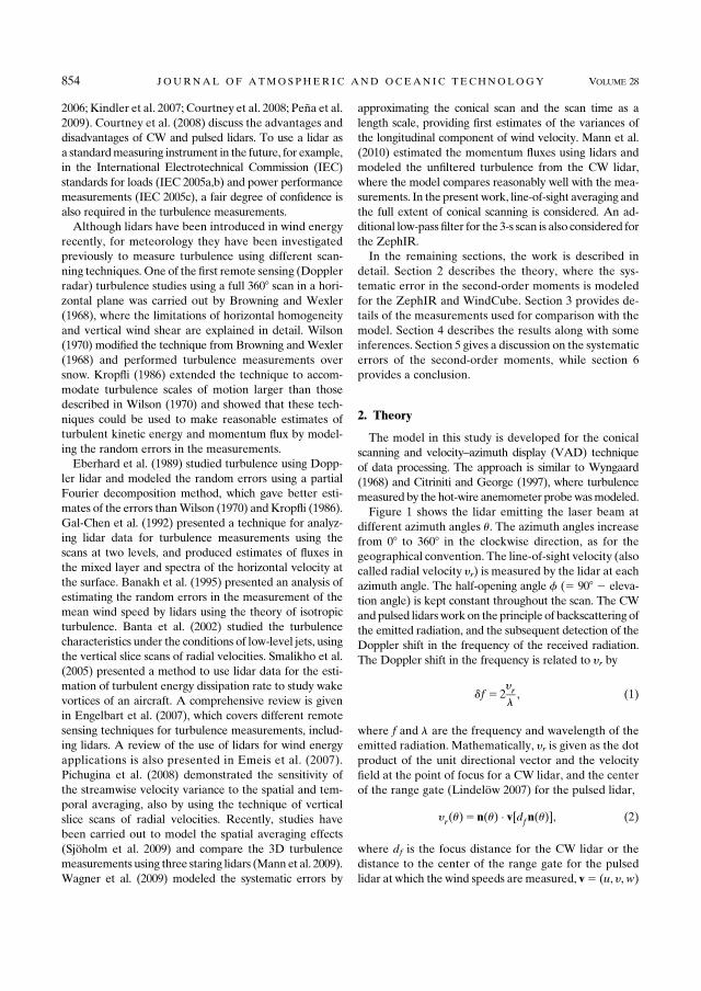
2006; Kindler et al. 2007; Courtney et al. 2008; Pena et al.
2009). Courtney et al. (2008) discuss the advantages and
disadvantages of CW and pulsed lidars. To use a lidar as
a standardmeasuring instrument in the future, for example,
in the International Electrotechnical Commission (IEC)
standards for loads (IEC 2005a,b) and power performance
measurements (IEC 2005c), a fair degree of confidence is
also required in the turbulence measurements.
Although lidars have been introduced in wind energy
recently, for meteorology they have been investigated
previously to measure turbulence using different scan-
ning techniques. One of the first remote sensing (Doppler
radar) turbulence studies using a full 3608 scan in a hori-
zontal plane was carried out by Browning and Wexler
(1968), where the limitations of horizontal homogeneity
and vertical wind shear are explained in detail. Wilson
(1970) modified the technique from Browning andWexler
(1968) and performed turbulence measurements over
snow. Kropfli (1986) extended the technique to accom-
modate turbulence scales of motion larger than those
described in Wilson (1970) and showed that these tech-
niques could be used to make reasonable estimates of
turbulent kinetic energy and momentum flux by model-
ing the random errors in the measurements.
Eberhard et al. (1989) studied turbulence using Dopp-
ler lidar and modeled the random errors using a partial
Fourier decomposition method, which gave better esti-
mates of the errors thanWilson (1970) andKropfli (1986).
Gal-Chen et al. (1992) presented a technique for analyz-
ing lidar data for turbulence measurements using the
scans at two levels, and produced estimates of fluxes in
the mixed layer and spectra of the horizontal velocity at
the surface. Banakh et al. (1995) presented an analysis of
estimating the random errors in the measurement of the
mean wind speed by lidars using the theory of isotropic
turbulence. Banta et al. (2002) studied the turbulence
characteristics under the conditions of low-level jets, using
the vertical slice scans of radial velocities. Smalikho et al.
(2005) presented a method to use lidar data for the esti-
mation of turbulent energy dissipation rate to study wake
vortices of an aircraft. A comprehensive review is given
in Engelbart et al. (2007), which covers different remote
sensing techniques for turbulence measurements, includ-
ing lidars. A review of the use of lidars for wind energy
applications is also presented in Emeis et al. (2007).
Pichugina et al. (2008) demonstrated the sensitivity of
the streamwise velocity variance to the spatial and tem-
poral averaging, also by using the technique of vertical
slice scans of radial velocities. Recently, studies have
been carried out to model the spatial averaging effects
(Sjoholm et al. 2009) and compare the 3D turbulence
measurements using three staring lidars (Mann et al. 2009).
Wagner et al. (2009) modeled the systematic errors by
approximating the conical scan and the scan time as a
length scale, providing first estimates of the variances of
the longitudinal component of wind velocity. Mann et al.
(2010) estimated the momentum fluxes using lidars and
modeled the unfiltered turbulence from the CW lidar,
where the model compares reasonably well with the mea-
surements. In the presentwork, line-of-sight averaging and
the full extent of conical scanning is considered. An ad-
ditional low-pass filter for the 3-s scan is also considered for
the ZephIR.
In the remaining sections, the work is described in
detail. Section 2 describes the theory, where the sys-
tematic error in the second-order moments is modeled
for the ZephIR and WindCube. Section 3 provides de-
tails of the measurements used for comparison with the
model. Section 4 describes the results along with some
inferences. Section 5 gives a discussion on the systematic
errors of the second-order moments, while section 6
provides a conclusion.
2. Theory
The model in this study is developed for the conical
scanning and velocity–azimuth display (VAD) technique
of data processing. The approach is similar to Wyngaard
(1968) and Citriniti and George (1997), where turbulence
measured by the hot-wire anemometer probewasmodeled.
Figure 1 shows the lidar emitting the laser beam at
different azimuth angles u. The azimuth angles increase
from 08 to 3608 in the clockwise direction, as for the
geographical convention. The line-of-sight velocity (also
called radial velocity yr) is measured by the lidar at each
azimuth angle. The half-opening angle f (5 908 2 eleva-
tion angle) is kept constant throughout the scan. The CW
andpulsed lidarswork on the principle of backscattering of
the emitted radiation, and the subsequent detection of the
Doppler shift in the frequency of the received radiation.
The Doppler shift in the frequency is related to yr by
df 5 2yrl, (1)
where f and l are the frequency and wavelength of the
emitted radiation. Mathematically, yr is given as the dot
product of the unit directional vector and the velocity
field at the point of focus for a CW lidar, and the center
of the range gate (Lindelow 2007) for the pulsed lidar,
yr(u)5 n(u) � v[dfn(u)], (2)
where df is the focus distance for the CW lidar or the
distance to the center of the range gate for the pulsed
lidar at which the wind speeds are measured, v5 (u, y,w)
854 JOURNAL OF ATMOSPHER IC AND OCEAN IC TECHNOLOGY VOLUME 28
78

is the instantaneous velocity field evaluated at the focus
point or the center of the range gate dfn(u), and n(u) is
the unit directional vector given as
n(u)5 (cosu sinf, sinu sinf, cosf). (3)
In practice it is impossible to obtain the backscattered
radiation precisely from only the focus point, and there
is always backscattered radiation of different intensities
from different regions in space along the line of sight.
Hence, it is necessary to assign appropriate weights to
the backscattered intensity such that the weight corre-
sponding to the focus point or the center of the range
gate is the highest. Mathematically, the weighted aver-
age radial velocity can be written as
~yr(u)5
ð‘2‘
u(s)n(u) � v[sn(u) 1 dfn(u)] ds, (4)
where u(s) is any weighting function, integrating to one,
and s is the distance along the beam from the focus. For
simplicity we assume that s5 0 corresponds to the focus
distance.
Following are the main assumptions of our model:
(i) The terrain is homogeneous.
(ii) The flow field is frozen during the scan.
(iii) Equation (4) with an appropriately chosen u(s)models the averaging well.
(iv) The spatial structure of the turbulent flow is described
well by the spectral tensor model of Mann (1994).
a. Systematic turbulence errors for the ZephIR lidar
The ZephIR transmits the laser beam through a con-
stantly rotating prism, giving the required half-opening
angle of nominally 308. Each of up to five heights is scan-
ned for 1 or 3 s, corresponding to one or three complete
rotations of the prism. The beam is then refocused to the
next height in the sequence and the scanning procedure is
repeated. Up to five different heights can be selected, with
the sequence (with five heights and 3-s scans) taking up to
18 s to complete. Thus, the lidar spends less than 20% of
the time required tomake a wind profile on any one of the
five heights. A typical scan at each height consists of 50
measurements of yr on the azimuth circle. If we assume the
coordinate system such that u is aligned to the mean wind
direction, y is perpendicular to the mean wind direction,w
is the vertical component, and the mean wind comes from
the north, then ~yr(u) can be expressed as
~yr(u)5A 1 B cosu 1 C sinu, (5)
where the coefficients A 5 wqq cosf, B 5 uqq sinf, and
C 5 yqq sinf, and the sign ambiguity in ~yr(u) is neglected
(see Mann et al. 2010). We use the subscript qq to denote
the velocity components measured by ZephIR, because
they are not the true velocity components u, y, andw. The
assumption that the mean wind comes from the north is
only made for simplicity. For a lidar measuring at many
points on the azimuth circle the choice of the mean wind
direction does not matter since averaging over the entire
circle is carried out. The values of the coefficientsA,B, and
C are found using the least squares method by fitting Eq.
(5) to the measured values of ~yr(u) at all scanned azimuth
angles. The coefficients can be written as Fourier integrals,
A51
2p
ð2p0~yr(u) du, (6)
B51
p
ð2p0~yr(u) cosu du, (7)
C51
p
ð2p0~yr(u) sinu du. (8)
We proceed by deriving expressions for the wqq vari-
ance. The expressions for the (co)variances of the re-
maining components of wind velocity can be derived in
a similar manner.
The variance of A is defined as s2A 5 hA92i, where the
angle brackets denotes ensemble averaging of a vari-
able. From the above definition of A, we can write
s2A5 hw92qqi cos2f. (9)
FIG. 1. Schematic of the velocity–azimuth display scanning.
JULY 2011 SATHE ET AL . 855
79

Using Eq. (6) we can also write,
s2A5
*�1
2p
ð2p0~y9r(u) du
�2+. (10)
Substituting ~yr(u) from Eq. (4) into Eq. (10), con-
verting the square of the integral into a double integral,
and interchanging the order of integration and averaging
we get,
s2A5
1
4p2
ð2p0
ð2p0
ð‘2‘
ð‘2‘
hv9i[s1n(u1) 1 dfn(u1)]v9j[s2n(u2) 1 dfn(u2)]iu(s1)u(s2)ni(u1)nj(u2) ds1 ds2 du1 du2,
51
4p2
ð2p0
ð2p0
ð‘2‘
ð‘2‘
Rij(r)u(s1)u(s2)ni(u1)nj(u2) ds1 ds2 du1 du2, (11)
where hv9i[s1n(u1)1 dfn(u1)]v9j[s2n(u2)1 dfn(u2)]i5Rij(r)
is the covariance tensor separated by a distance r 5[s
1n(u
1)1 d
fn(u
1)]2 [s
2n(u
2)1 d
fn(u
2)] and is related
to the three-dimensional spectral velocity tensorFij(k)
by the inverse Fourier transform,
Rij(r)5
ðFij(k)e
ik�r dk, (12)
whereÐdk[
Ð ‘2‘
Ð ‘2‘
Ð ‘2‘ dk1 dk2 dk3, k 5 (k1, k2, k3) de-
notes the wave vector and the subscripts i, j take the values
from 1 to 3. Inserting Eq. (12) into Eq. (11) we get,
s2A5
ðFij(k)
ð‘2‘
u(s1)
�1
2p
ð2p0ni(u1)e
i(s11d
f)k�n(u
1) du1
�ds1
� ð‘2‘
f(s2)
�1
2p
ð2p0nj(u2)e
i(s21d
f)k�n(u
2) du2
�ds2
�dk.
��(13)
Let ai(k)5Ð ‘2‘u(s)[1/2p
Ð 2p0 ni(u)e
i(s1df)k�n(u1)du]ds, which
physically represents the line-of-sight and conical av-
eraging. Equation (13) can then be written as (using
Eq. 9),
hw92qqi cos2f5
ðFij(k)ai(k)a*j (k) dk, (14)
where the asterisk denotes complex conjugation. Thus
the integral reduces to evaluatingai(k), since the analytical
expressions for Fij(k) are given in Mann (1994). Equation
(16) can then be estimated numerically. For a CW lidar,
u(s) is well approximated by a Lorentzian function
(Sonnenschein and Horrigan 1971),
u(s)51
p
l
l21 s2, (15)
where l is the Rayleigh length (5lbd2f /pr
2b, where lb 5
1.55 mm is the wavelength of the emitted radiation,
and rb 5 19.5 mm is the beam radius). An attempt has
been made to obtain analytical expressions for ai(k).
However, no general analytical solution exists for ai(k)
and at most the integral can be reduced (by integrating
over s) to
ai(k)51
2peidf
k3cosf
ð2p0ni(u 1 u0)e
idfkhsinf cosue2ljk
hcosu sinf1k
3cosfj du, (16)
where kh 5ffiffiffiffiffiffiffiffiffiffiffiffiffiffiffik21 1k22
qis the magnitude of the horizontal
wave vector, cosu0 5 k1/kh, sinu0 5 k2/kh, and ni(u1 u0)
is the component of the unit directional vector obtained
from Eq. (3). Thus numerical integration has to be ap-
plied also for the evaluation of ai(k).
A similar approach is taken for deriving uqq and yqqvariances, where we obtain,
hu92qqi sin2f5
ðFij(k)bi(k)b*j (k) dk, (17)
hy92qqi sin2f5
ðFij(k)gi(k)g*j (k) dk. (18)
The corresponding b and g functions are
bi(k)51
peidf
k3cosf
ð2p0ni(u 1 u0) cos(u 1 u0)e
idfkhsinf cosue2ljk
hcosu sinf1k
3cosfj du, (19)
856 JOURNAL OF ATMOSPHER IC AND OCEAN IC TECHNOLOGY VOLUME 28
80

gi(k)51
peidf
k3cosf
ð2p0ni(u 1 u0) sin(u 1 u0) e
idfkhsinf cosue2ljk
hcosu sinf1k
3cosfj du. (20)
The derivation of the covariances is merely a combina-
tion of the weighting functions ai(k), bi(k), and gi(k),
and their complex conjugates used with Fij(k).
MODELING THE LOW-PASS FILTERING EFFECT
RESULTING FROM THE 3-S SCAN
Because the ZephIR scans three circles in approxi-
mately 3 s, there will be a low-pass filter effect in tur-
bulence measurements. We assume a length scale Lf 5hui 3 3s such that it represents the 3-s averaging. We
assume that the ZephIR scans a circle infinitely fast for
3 s. We model the corresponding filtering effect by a
simple rectangular filter, such that,
f (x)5
1
Lf
for jxj,Lf
2;
0 elsewhere,
8><>: (21)
where x is the center of the scanning circle and f(x) is any
function of x. The corresponding spectral transfer func-
tion is given as
Tf (k1)5 sinc2
k1Lf
2
!, (22)
where sinc(x) 5 sin(x)/x. The variances of uqq, yqq, and
wqq are given as
hu92qqi sin2f5
ðFij(k)bi(k)b*j (k)Tf (k1) dk, (23)
hy92qqi sin2f5
ðFij(k)gi(k)g*j(k)Tf (k1) dk, (24)
hw92qqi cos2f5
ðFij(k)ai(k)a*j(k)Tf (k1) dk. (25)
b. Systematic turbulence errors for theWindCube lidar
The assumption made in section 2a that the mean
wind direction comes from the north cannot be made for
the WindCube, because it measures at four azimuth
FIG. 2. Location of the Høvsøre meteorological mast and details of the site. The wind tur-
bines (circles), light tower (squares), and the meteorological masts (diamonds) are shown. The
meteorological mast from which the measurements are used is indicated (dark diamond) and
the selected wind directions are also shown.
JULY 2011 SATHE ET AL . 857
81

angles only (cf. Fig. 1), for example, north, east, south and
west. In this case the coordinate system is such that u is
aligned in the mean wind direction. Thus,
uwc5 uNS cosQ 1 uEW sinQ, (26)
ywc 5uNS sinQ 2 uEW cosQ, (27)
where uNS and uEW denote wind speeds in the north–
south and east–west directions, respectively, Q denotes
the wind direction, and the subscript wc denotes the ve-
locity components measured by WindCube. From sim-
ple geometrical considerations (cf. Fig. 1),
uNS5~yrN 2 ~yrS2 sinf
, (28)
uEW 5~yrE 2 ~yrW2 sinf
, (29)
where ~yrN, ~y
rS, ~y
rE, and ~y
rWare the weighted average ra-
dial velocities in the north, south, east and west direc-
tions, respectively. For the w component,
wwc5P(~yrN1 ~yrS)1Q(~yrE1 ~yrW)
2 cosf, (30)
where P and Q are the weights associated with the
wind direction such that P 1 Q 5 1. Leosphere uses
FIG. 3. Orientation of the sensors on the meteorological mast and wind rose at 60 m. The
numbers inside the circles are the number of 10-min observations.
FIG. 4. Comparison of the mean wind speed measured by (left) lidars and (right) sonic anemometer.
858 JOURNAL OF ATMOSPHER IC AND OCEAN IC TECHNOLOGY VOLUME 28
82

P5 cos2Q andQ5 sin2Q, and hence, we use the same in
our calculations.
We proceed by deriving expressions for the uwc vari-
ance. The expressions for the (co)variances of the re-
maining components of wind velocity can be derived in
a similar manner. Substituting Eqs. (28) and (29) into
Eq. (26), we get
uwc 51
2 sinf[(~yrN 2 ~yrS) cosQ 1 (~yrE 2 ~yrW) sinQ].
(31)
We define unit vectors in the four directions as
nN 5 n(2Q),
nS 5 n(p 2 Q),
nE 5 np
22 Q
� �,
nW 5 n3p
22 Q
,
(32)
where nN, nS, nE, and nW are the unit directional vectors
in the north, south, east, and west directions, respec-
tively. From Eq. (4), for the north direction,
~yrN 5
ð‘2‘
u(s)nN � v(snN1 dfnN) ds. (33)
To further simplify the notation we define the trans-
lation operator Td acting on any scalar or vector field
j(x),
Tdj(x)5 j(x 1 d). (34)
We also define a convolution operator Cn acting on any
scalar or vector field as
Cnv(x)5
ð‘2‘
u(s)n � v(x 1 ns) ds. (35)
For the north direction, Eq. (33) can be written as
~yrN 5CnNTd
fnNv. (36)
We get similar expressions for the south, east, and west
directions. Equation (31) can then be written as
uwc51
2 sinf[(Cn
NTd
fnN2 Cn
STd
fnS) cosQ
1 (CnETd
fnE2 Cn
WTd
fnW) sinQ]v (37)
We also know that, by definition,
hu92i5ðhu(k)u*(k)idk, (38)
where ^ denotes the Fourier transform and * denotes
complex conjugation. In the Fourier space we have
dTdv(k)5 eik�dv(k), (39)
dCnv(k)5 u(n � k)n � v(k), (40)
where f(k)5 sinc2(klp/2), considering that the weight-
ing function for a pulsed lidar is commonly defined as
u(s)5
lp 2 jsjl2p
for jsj, lp;
0 elsewhere,
8><>: (41)
where lp is the half-length of the ideally rectangular light
pulse leaving the lidar, assuming the matching time
windowing (52lp/c, where c is the speed of light). In
reality, the weighting function may be more rounded,
but this will not affect the conclusions that are drawn.
Thus, in Fourier space Eq. (37) can then be written as
uwc(k)51
2 sinf
[kNeid
fk�n
N sinc2(k � nNlp/2) 2 nSeid
fk�n
S sinc2(k � nSlp/2)] cosQ[nEe
idfk�n
E sinc2(k � nElp/2) 2 nWeidfk�n
W sinc2(k � nWlp/2)] sinQ
)� v(k)[ b(k) � v(k),
((42)
and the variance [from Eq. (38)] as
hu92wci5ðFij(k)bi(k)bj*(k) dk, (43)
where we have implicitly used the relation Fij(k)5hvi(k)vj*(k)i. The (co)variances of other components can
be estimated in a similar manner by first estimating the
TABLE 1. Classification of atmospheric stability according to
Monin–Obukhov length intervals
Very stable (vs) 10 # LMO # 50 m
Stable (s) 50 # LMO # 200 m
Near-neutral stable (nns) 200 # LMO # 500 m
Neutral (n) jLMOj $ 50 m
Near-neutral unstable (nnu) 2500 # LMO # 2200 m
Unstable (u) 2200 # LMO # 2100 m
Very unstable (vu) 2100 # LMO # 250 m
JULY 2011 SATHE ET AL . 859
83
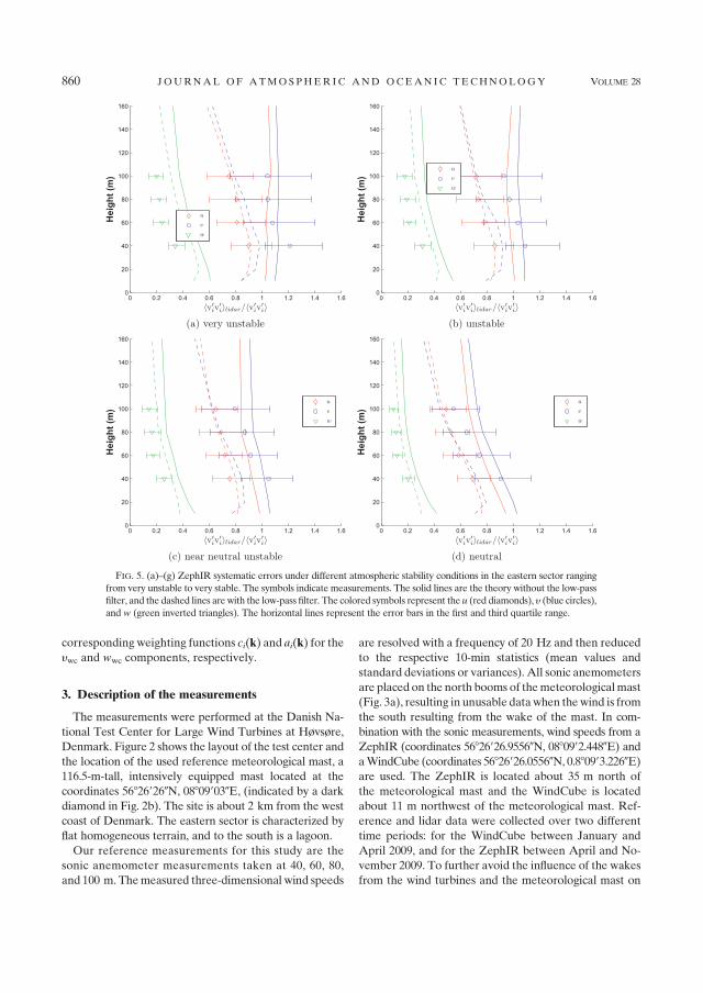
corresponding weighting functions ci(k) and ai(k) for the
ywc and wwc components, respectively.
3. Description of the measurements
The measurements were performed at the Danish Na-
tional Test Center for Large Wind Turbines at Høvsøre,
Denmark. Figure 2 shows the layout of the test center and
the location of the used reference meteorological mast, a
116.5-m-tall, intensively equipped mast located at the
coordinates 568269260N, 088099030E, (indicated by a dark
diamond in Fig. 2b). The site is about 2 km from the west
coast of Denmark. The eastern sector is characterized by
flat homogeneous terrain, and to the south is a lagoon.
Our reference measurements for this study are the
sonic anemometer measurements taken at 40, 60, 80,
and 100 m. Themeasured three-dimensional wind speeds
are resolved with a frequency of 20 Hz and then reduced
to the respective 10-min statistics (mean values and
standard deviations or variances). All sonic anemometers
are placed on the north booms of themeteorologicalmast
(Fig. 3a), resulting in unusable datawhen thewind is from
the south resulting from the wake of the mast. In com-
bination with the sonic measurements, wind speeds from a
ZephIR (coordinates 56826926.95560N, 0880992.4480E) andaWindCube (coordinates 56826926.05560N, 0.880993.2260E)are used. The ZephIR is located about 35 m north of
the meteorological mast and the WindCube is located
about 11 m northwest of the meteorological mast. Ref-
erence and lidar data were collected over two different
time periods: for the WindCube between January and
April 2009, and for the ZephIR between April and No-
vember 2009. To further avoid the influence of the wakes
from the wind turbines and the meteorological mast on
FIG. 5. (a)–(g) ZephIR systematic errors under different atmospheric stability conditions in the eastern sector ranging
from very unstable to very stable. The symbols indicate measurements. The solid lines are the theory without the low-pass
filter, and the dashed lines arewith the low-pass filter. The colored symbols represent the u (red diamonds), y (blue circles),
and w (green inverted triangles). The horizontal lines represent the error bars in the first and third quartile range.
860 JOURNAL OF ATMOSPHER IC AND OCEAN IC TECHNOLOGY VOLUME 28
84

lidar measurements, and inhomogeneities resulting from
the sudden change of roughness (the sea–land transition;
see Fig. 2a), only data periods with easterly winds (508–1508) are analyzed. Figure 3b shows that although the
dominant wind direction is west-northwest, there is also
sufficient data in the chosen directional (eastern) sector.
For the ZephIR 5530 data points were used after using
the entire filter, whereas for the WindCube 4003 data
points were used.
The precision of the sonic anemometer measurements
is estimated to be about61.5%. From comparisons with
cup anemometers, the mean error of the WindCube in
typical flat coastal conditions is within 60.05 m s21,
with a standard deviation in mixed shear conditions of
about 0.15 m s21. The corresponding uncertainty for the
measurements made with a ZephIR is slightly higher
[a detailed list of different error sources is given in
Lindelow-Marsden (2007)].
Figure 4 shows the comparison of the 10-min mean
horizontal wind speed (at 100 m) measured by the
ZephIR and WindCube with the sonic anemometer.
Data are shown for the easterly winds (508–1508) andreference mean wind speeds between 4 and 25 m s21.
To guarantee repeatable conditions the data were fur-
thermore filtered with respect to rain (i.e., only 10-min
periods with no precipitation were considered) and the
availability of the lidar (i.e., 100% of the fast data within
a 10-min period had to be available). The lidar observa-
tions agree reasonably well with those of the sonic ane-
mometer, with coefficients of determination R2 . 0.98,
where the data of the WindCube shows a significantly
better correlation than those of the ZephIR.
4. Comparison of models with the measurements
The estimation ofFij using themodel fromMann (1994)
requires three input parameters: a�2/3, which is a prod-
uct of the spectral Kolmogorov constant a (Monin and
Yaglom1975) and the rate of viscous dissipation of specific
turbulent kinetic energy �2/3; a length scale L, and an
FIG. 5. (Continued)
JULY 2011 SATHE ET AL . 861
85
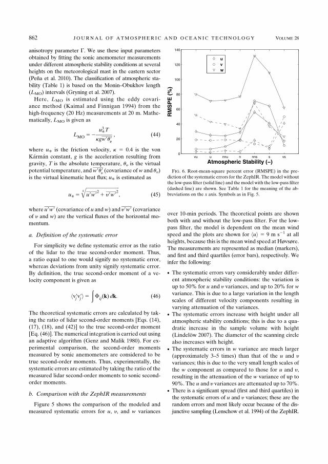
anisotropy parameter G. We use these input parameters
obtained by fitting the sonic anemometer measurements
under different atmospheric stability conditions at several
heights on the meteorological mast in the eastern sector
(Pena et al. 2010). The classification of atmospheric sta-
bility (Table 1) is based on the Monin–Obukhov length
(LMO) intervals (Gryning et al. 2007).
Here, LMO is estimated using the eddy covari-
ance method (Kaimal and Finnigan 1994) from the
high-frequency (20 Hz) measurements at 20 m. Mathe-
matically, LMO is given as
LMO52u3*T
kgw9u9y, (44)
where u* is the friction velocity, k 5 0.4 is the von
Karman constant, g is the acceleration resulting from
gravity, T is the absolute temperature, uy is the virtual
potential temperature, andw9u9y (covariance ofw and uy)
is the virtual kinematic heat flux; u* is estimated as
u*5
ffiffiffiffiffiffiffiffiffiffiffiffiffiffiffiffiffiffiffiffiffiffiffiffiffiffiffiffiffiu9w9
21 y9w9
24
q, (45)
where u9w9 (covariance of u andw) and y9w9 (covarianceof y and w) are the vertical fluxes of the horizontal mo-
mentum.
a. Definition of the systematic error
For simplicity we define systematic error as the ratio
of the lidar to the true second-order moment. Thus,
a ratio equal to one would signify no systematic error,
whereas deviations from unity signify systematic error.
By definition, the true second-order moment of a ve-
locity component is given as
hv9jv9j i5ðFij(k) dk. (46)
The theoretical systematic errors are calculated by tak-
ing the ratio of lidar second-order moments [Eqs. (14),
(17), (18), and (42)] to the true second-order moment
[Eq. (46)]. The numerical integration is carried out using
an adaptive algorithm (Genz and Malik 1980). For ex-
perimental comparison, the second-order moments
measured by sonic anemometers are considered to be
true second-order moments. Thus, experimentally, the
systematic errors are estimated by taking the ratio of the
measured lidar second-order moments to sonic second-
order moments.
b. Comparison with the ZephIR measurements
Figure 5 shows the comparison of the modeled and
measured systematic errors for u, y, and w variances
over 10-min periods. The theoretical points are shown
both with and without the low-pass filter. For the low-
pass filter, the model is dependent on the mean wind
speed and the plots are shown for hui 5 9 m s21 at all
heights, because this is the mean wind speed at Høvsøre.
The measurements are represented as median (markers),
and first and third quartiles (error bars), respectively. We
infer the following:
d The systematic errors vary considerably under differ-
ent atmospheric stability conditions: the variation is
up to 50% for u and y variances, and up to 20% for w
variance. This is due to a large variation in the length
scales of different velocity components resulting in
varying attenuation of the variances.d The systematic errors increase with height under all
atmospheric stability conditions; this is due to a qua-
dratic increase in the sample volume with height
(Lindelow 2007). The diameter of the scanning circle
also increases with height.d The systematic errors in w variance are much larger
(approximately 3–5 times) than that of the u and y
variances; this is due to the very small length scales of
the w component as compared to those for u and y,
resulting in the attenuation of the w variance of up to
90%. The u and y variances are attenuated up to 70%.d There is a significant spread (first and third quartiles) in
the systematic errors of u and y variances; these are the
random errors and most likely occur because of the dis-
junctive sampling (Lenschow et al. 1994) of the ZephIR.
FIG. 6. Root-mean-square percent error (RMSPE) in the pre-
diction of the systematic errors for the ZephIR. Themodel without
the low-pass filter (solid line) and the model with the low-pass filter
(dashed line) are shown. See Table 1 for the meaning of the ab-
breviations on the x axis. Symbols as in Fig. 5.
862 JOURNAL OF ATMOSPHER IC AND OCEAN IC TECHNOLOGY VOLUME 28
86

A thorough scientific investigation is needed to quantify
random errors, but is not the focus of this paper.d The trend of the systematic errors predicted by both
models is in agreement with the observations at all
heights.d With the exception of very stable conditions, the
model with the low-pass filter [Eqs. (23)–(25)] is in
better agreement with the measurements at all heights
than without the low-pass filter.
To quantify the improvement in themodel predictions
using the low-pass filter, we compute the root-mean-
square percent errors (RMSPE) between the measured
and the modeled systematic errors for each stability
condition. RMSPE is given as
RMSPE5
ffiffiffiffiffiffiffiffiffiffiffiffiffiffiffiffiffiffiffiffiffiffiffiffiffiffiffiffiffiffiffiffiffiffiffiffiffiffiffiffiffiffiffiffiffiffiffiffiffiffiffiffiffiffiffiffiffiffiffiffiffiffiffiffiffiffiffiffiffiffiffiffiffiffiffiffiffiffiffiffiffiffiffiffiffiffiffiffiffiffiffiffiffiffiffiffiffiffiffiffiffiffi1
n�
26664hv9i v9i ilidar
hv9i v9i imeasured
2
hv9i v9i ilidarhv9i v9i i
modelledhv9i v9i ilidar
hv9i v9i imeasured
377752
vuuuuuut 3 100, (47)
where median values are used for the measurements.
Figure 6 shows the comparison of the RMSPE in the
prediction of the systematic errors with and without the
low-pass filter for the ZephIR. A significant decrease in
the RMSPE (of the order of 30%) of u and w variances
is observed under all atmospheric stabilities (except for
the very stable condition for u variance) when the low-
pass filtering is used. For the y variance, there is a slight
increase (up to 10%) in the RMSPE under unstable
conditions, whereas for stable conditions a decrease of
up to 40% is observed. Thus, in general, using the low-
pass filter, the model predicts the systematic errors
better than without using the low-pass filter. We also
performed the calculations using the beam radius rb 524 mm, and observed that the RMSPE for all three
variance components changes only slightly (65%).
c. Comparison with the WindCube measurements
Figure 7 shows the comparison of the modeled and
measured systematic errors (section 2a) for u, y, and w
variances over 10-min periods. We infer the following:
d The systematic errors vary considerably under differ-
ent atmospheric stability conditions: the variation is
up to 50% for u and y variances, and up to 20% for the
w variance. The same is also observed for the ZephIR.d The systematic errors decrease with height for the u and
y variances under all atmospheric stability conditions: for
the WindCube, the probe length is constant (Lindelow
2007), and, hence, at lower heights there is a combined
averaging effect resulting from the probe length and
the diameter of the scanning circle. Considering that at
lower heights the length scales are smaller than at higher
heights, it is likely that the variances are attenuated
greater at lower heights than at higher heights. For w
variance, the systematic error is approximately constant,
and is most likely due to the small length scales.
d The systematic error in w variance is much larger
(approximately 3–5 times) than that of the u and y
variances. The same is also observed for the ZephIR.d The spread in the systematic error (first and third
quartiles) of the u and y variances is smaller than that
of the ZephIR; this is most likely because the Wind-
Cube updates the velocity vector approximately every
6.5 s, whereas the ZephIR updates every 18 s.d The systematic error varies significantly with the wind
direction relative to the beam direction forw variance,
and to a lesser degree for u and y variance under all
stability conditions.
Figure 8 shows the comparison of the RMSPE in the
prediction of the systematic errors for the WindCube
and ZephIR (with the low-pass filter). It is observed that
for u and y variances, with the exception of the near-
neutral stable condition, the RMSPE in both lidars is
approximately equal. There is a considerable variation
in the RMSPE for the w variance. This is most likely
because for the WindCube, the w variance is very
sensitive to the wind direction because of its cosine and
sine dependence. In general, for both lidars, except for
the very stable condition, the model predicts the sys-
tematic errors for u variance reasonably well (RMSPE
’ 6%), followed by y variance (RMSPE ’ 12%). It is
difficult to say whether the prediction for the w vari-
ance is less reliable or not (RMSPE of the order of
60%).
We do not model the filtering effect because of the
scanning time (’6.5 s) of WindCube for two reasons:
(i) Since the measurement is carried out at only four
points, with each lasting 0.5 s on the scanning circle,
we cannot assume that the WindCube measures
infinitely fast on the scanning circle (as we did for
the ZephIR). The translations in each direction have
JULY 2011 SATHE ET AL . 863
87
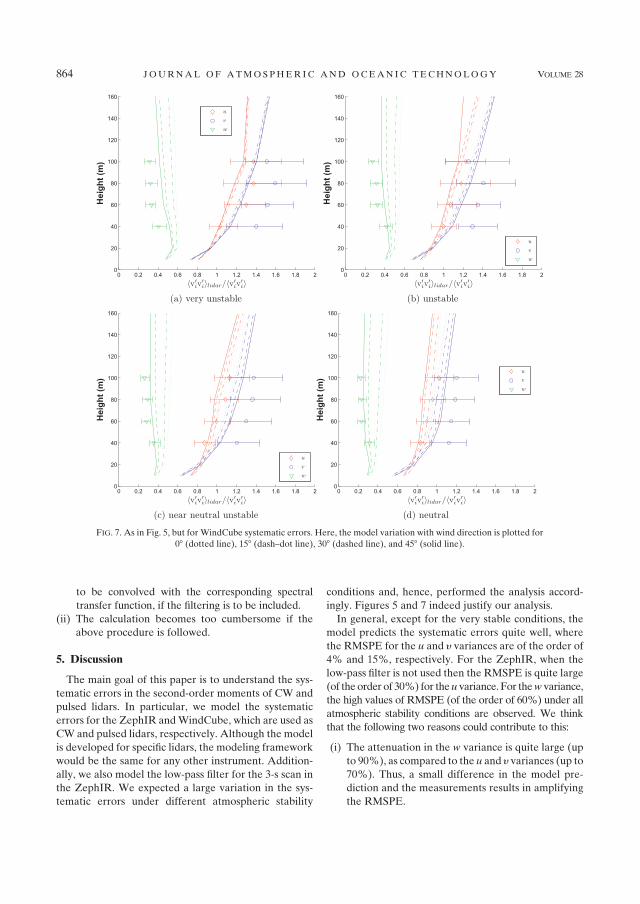
to be convolved with the corresponding spectral
transfer function, if the filtering is to be included.
(ii) The calculation becomes too cumbersome if the
above procedure is followed.
5. Discussion
The main goal of this paper is to understand the sys-
tematic errors in the second-order moments of CW and
pulsed lidars. In particular, we model the systematic
errors for the ZephIR andWindCube, which are used as
CW and pulsed lidars, respectively. Although the model
is developed for specific lidars, the modeling framework
would be the same for any other instrument. Addition-
ally, we also model the low-pass filter for the 3-s scan in
the ZephIR. We expected a large variation in the sys-
tematic errors under different atmospheric stability
conditions and, hence, performed the analysis accord-
ingly. Figures 5 and 7 indeed justify our analysis.
In general, except for the very stable conditions, the
model predicts the systematic errors quite well, where
the RMSPE for the u and y variances are of the order of
4% and 15%, respectively. For the ZephIR, when the
low-pass filter is not used then the RMSPE is quite large
(of the order of 30%) for theu variance. For thew variance,
the high values of RMSPE (of the order of 60%) under all
atmospheric stability conditions are observed. We think
that the following two reasons could contribute to this:
(i) The attenuation in the w variance is quite large (up
to 90%), as compared to the u and y variances (up to
70%). Thus, a small difference in the model pre-
diction and the measurements results in amplifying
the RMSPE.
FIG. 7. As in Fig. 5, but for WindCube systematic errors. Here, the model variation with wind direction is plotted for
08 (dotted line), 158 (dash–dot line), 308 (dashed line), and 458 (solid line).
864 JOURNAL OF ATMOSPHER IC AND OCEAN IC TECHNOLOGY VOLUME 28
88

(ii) For the ZephIR, when the low-pass filter is used in
the model, there is a dependence on the mean wind
speed. The model results (Fig. 5) are shown for hui59 m s21 only. Segregating themodel and observations
for different mean wind speeds will result in reducing
the RMSPE.
For the WindCube, the model predicts a significant var-
iation of thew variance with wind direction [Eq. (30)]. To
estimate the influence of the weights P and Q on the
prediction of systematic errors, we calculate hw9wc2i fromthe equation for w that corresponds to Eq. (38) with two
different ways of calculating w. The first is the formula
used by Leosphere, for example, Eq. (30), withP5 cos2Qand Q 5 sin2Q; the second is P 5 Q 5 ½. The former is
shown as a thin solid line in Fig. 9 and the latter as a thin
dashed line. The spectral tensor parameters used are for
neutral atmospheric stability from Pena et al. (2010) at
100 m. Themeasurements of hw9wc2i/hw92i, shown as broadcurves on Fig. 9, are from the same height, and both
measurements and theory show that hw9wc2i/hw92i using
Leosphere’s choice of P and Q can vary by a factor of 2
solely by changing the wind direction. If P 5 Q 5 ½ is
chosen, then the reduction of the vertical velocity vari-
ance does vary much less with wind direction, but the
overall attenuation is stronger.
Because themodel predicts the trend in the systematic
errors in the w variance reasonably well (Figs. 5 and 7),
qualitatively it could be said that the model also agrees
well with the measurements for the w variance.
While comparing the performance of our model, the
following should also be considered:
d The model is dependent on the three-dimensional
spectral velocity tensor (Mann 1994), which is strictly
valid for neutral conditions only. Thus, one has to be
careful while comparing under different atmospheric
stability conditions. In this study, we have reduced
the uncertainty by using the three input tensor param-
eters that are fitted to the measurements under
FIG. 7. (Continued)
JULY 2011 SATHE ET AL . 865
89

different atmospheric stability conditions (Pena et al.
2010).d While using Eqs. (23)–(25), we have used the same
mean wind speed at all heights. In reality, there is
always wind shear, which also depends significantly on
atmospheric stability (Motta and Barthelmie 2005).
However, the calculations will become too cumber-
some, and hence we made a crude approximation.d The very stable conditions are generally difficult to
analyze. There could be different reasons for the large
deviation in the u and y variances; for example, un-
certainty in the input tensor parameters, and lack of
validity of the spectral tensor model (Mann 1994)
under different atmospheric stability conditionsd Also, contrary to expectation, the measurements under
very stable conditions (Figs. 5 and 8) show a decrease
in the systematic errors for the u and y variances, as
compared to the stable conditions.
There is also some room for reducing redundancy
in the ZephIR measurements, which might reduce the
spread of the systematic errors (quartile range). Instead
of scanning at several points on the circle, only four points
are required. Reducing the measurement points would
increase the dependence of the second-ordermoments on
the wind direction (cf. section 2). However, it would
considerably reduce the time required for completing
a VAD. There is also no need to scan the circle 3 times;
for example, in the present configuration, 50 points are
scanned in approximately 1 s. Thus, four points would
take only 0.08 s. If it measures five heights sequentially,
then the next measurement would be after 0.4 s, giving
a measurement frequency of *2 Hz. Alternatively, at
each of the four points the scans can also be performed
rapidly at different heights sequentially before scanning
the next point.
We are currently looking into alternative ways of ana-
lyzing the lidar data and different beam configurations
that would render turbulence measurements more fea-
sible. One idea is to use two different half opening an-
gles as in Eberhard et al. (1989), who show that all terms
in the Reynolds stress tensor can be obtained by using
the single-beam statistics, without resorting to beam
covariances, which is done in this paper. That would
require significant hardware modifications to the instru-
ments treated here. Another idea is to supplement the
analysis with information on the width of the Doppler
spectra, as done for the momentum flux in Mann et al.
(2010), in order to compensate for the effect of along-
beam averaging.
6. Conclusions
The systematic errors of the second-order moments
measured by lidars using the conical scanning and VAD
technique to process the data are quite large because of
(i) the spatial separation of the data points along the
line-of-sight and
(ii) the spatial separation of the data points in the
conical section.
Also, from Eqs. (14), (17), (18), and (43), the general
lidar equation for the second-order moments using the
VAD data processing technique can be written as
FIG. 8. Comparison of the RMSPE in the prediction of the sys-
tematic errors for theWindCube andZephIR. TheWindCube (solid
line) and ZephIR (dashed line) with the low-pass filter are shown.
See Table 1 for the meaning of the abbreviations on the x axis.
FIG. 9. The ratio of the vertical velocity variance as measured by
the WindCube and the actual variance measured and modeled at
100 m. The theoretical expectations (thin lines) using P 5 cos2QandQ5 sin2Q (solid line) and P5Q5½ (dashed line) in Eq. (30)
are shown. The corresponding measurements are shown (broad
curves), with the first and third quartiles displayed (shades).
866 JOURNAL OF ATMOSPHER IC AND OCEAN IC TECHNOLOGY VOLUME 28
90
hv9mv9nilidar 5ðFij(k)X
mi (k)Xn
j*(k) dk;
Xmi (k)5
bi(k)^bi(k), m5 1
gi(k) ^ ci(k), m5 2
ai(k) ^ ai(k), m5 3
.
8<: (48)
The weighting functions ai(k), bi(k), and gi(k) are used
for theZephIR and ai(k), bi(k), and ci(k) are used for the
WindCube. Thus, the measurement of the second-order
moment by lidar involves interaction of all components
of the spectral velocity tensor Fij(k) weighted by the
corresponding weighting functions Xmi (k). It is to be
noted that Eq. (48) is given in Einstein summation
convention, and, hence, in order to explicitly see the
contribution of all components of Fij(k) on the mea-
surement of the second-order moments by lidar, this
equation must be expanded for all values of the sub-
scripts i and j. In most cases, this results in the attenua-
tion of the second-order moments, whereas in some
cases this also results in amplification of the second-
order moment, for example, as observed for the Wind-
Cube in the unstable conditions (see Fig. 7).
Finally, to answer the question posed in the title ‘‘Can
wind lidarsmeasure turbulence?’’, it is clear that using the
conical scanning and VAD technique to process the data
they cannot be used to measure turbulence precisely.
Acknowledgments. This study is a part of the Ph.D.
project under the We@Sea program, BISK-03041, and
sponsored by the Dutch Ministry of Economic affairs.
The experimental results are all based on data collected
at the Høvsøre Test Station under the watchful eyes of
Anders Ramsing Vestergaard and Bjarne Sønderskov.
We extend our thanks to them for their highly pro-
fessional and good-humored assistance. We are also
obliged to the NORSEWInD project and its leader
Andy Oldroyd, under whose auspices the lidar data
were obtained. Finally, we are grateful for valuable
comments from Torben Mikkelsen, Risø DTU. This
paper has been prepared using resources provided by
the EU FP6 UpWind project (Project reference 019945
SES6) and by the Center for Computational Wind
Turbine Aerodynamics and Atmospheric Turbulence
funded by the Danish Council for Strategic Research
Grant 09-067216.
REFERENCES
Banakh, V. A., I. N. Smalikho, F. Kopp, and C. Werner, 1995:
Representativeness of wind measurements with a CW Doppler
lidar in the atmospheric boundary layer. Appl. Opt., 34, 2055–
2067.
Banta, R. M., R. K. Newsom, J. K. Lundquist, Y. L. Pichugina,
R. L. Coulter, and L. Mahrt, 2002: Nocturnal low-level jet
characteristics over Kansas during CASES-99. Bound.-Layer
Meteor., 105, 221–252.
Browning, K. A., and R. Wexler, 1968: The determination of ki-
nematic properties of a wind field using a Doppler radar.
J. Appl. Meteor., 7, 105–113.Citriniti, J. H., and W. K. George, 1997: The reduction of spatial
aliasing by long hot-wire anemometer probes. Exp. Fluids, 23,
217–224.
Courtney, M., R. Wagner, and P. Lindelow, 2008: Testing and
comparison of lidars for profile and turbulence measurements
in wind energy. Proc. 14th Int. Symp. for the Advancement of
Boundary Layer Remote Sensing, Vol. 1, Risø DTU, Denmark,
IOPConference Series: Earth andEnvironmental Science, 012021.
Eberhard, W. L., R. E. Cupp, and K. R. Healy, 1989: Doppler lidar
measurements of profiles of turbulence and momentum flux.
J. Atmos. Oceanic Technol., 6, 809–819.
Emeis, S., M. Harris, and R. M. Banta, 2007: Boundary-layer ane-
mometry by optical remote sensing for wind energy applica-
tions.Meteor. Z., 16, 337–347, doi:10.1127/0941-2948/2007/0225.
Engelbart, D. A. M., M. Kallistratova, and R. Kouznetsov, 2007:
Determination of the turbulent fluxes of heat and momentum
in the ABL by ground-based remote-sensing techniques (a
review). Meteor. Z., 16, 325–335, doi:10.1127/0941-2948/2007/
0224.
Gal-Chen, T., M. Xu, and W. L. Eberhard, 1992: Estimation of
atmospheric boundary layer fluxes and other turbulence pa-
rameters from Doppler lidar data. J. Geophys. Res., 97 (D17),
18 409–18 423.
Genz, A. C., and A. A. Malik, 1980: An adaptive algorithm for
numerical integration over an n-dimensional rectangular re-
gion. J. Comput. Appl. Math., 6 (4), 295–302.
Gryning, S.-E., E. Batchvarova, B. Brummer, H. Jørgensen, and
S. Larsen, 2007: On the extension of the wind profile over
homogeneous terrain beyond the surface layer. Bound.-Layer
Meteor., 124, 251–268, doi:10.1007/s10546-007-9166-9.IEC, 2005a: Wind turbines—Part I: Design requirements. In-
ternational Electrotechnical Commission IEC 61400-1, 92 pp.
——, 2005b: Offshore wind turbines—Part I: Design requirements.
International Electrotechnical Commission IEC 61400-3,
136 pp.
——, 2005c: Wind turbines—Part 12-1: Power performance mea-
surements of electricity producing wind turbines. Interna-
tional Electrotechnical Commission IEC 61400-12-1, 90 pp.
Kaimal, J. C., and J. J. Finnigan, 1994: Acquisition and processing
of atmospheric boundary layer data. Atmospheric Boundary
Layer Flows, Oxford University Press, 255–257.
Kindler, D., A. Oldroyd, A. Macaskill, and D. Finch, 2007: An
eight month test campaign of the QinetiQ ZephIR system:
Preliminary results. Meteor. Z., 16 (5), 479–489, doi:10.1127/
0941-2948/2007/0226.
Kropfli, R. A., 1986: Single Doppler radar measurement of tur-
bulence profiles in the convective boundary layer. J. Atmos.
Oceanic Technol., 3, 305–314.
Lenschow, D. H., J. Mann, and L. Kristensen, 1994: How long is
long enough when measuring fluxes and other turbulence
statistics? J. Atmos. Oceanic Technol., 11, 661–673.Lindelow, P., 2007: Fibre based coherent lidars for remote wind
sensing. Ph.D. thesis, Technical University Denmark, 164 pp.
Lindelow-Marsden, P., 2007: UpWind D1: Uncertainties in wind as-
sessment with LIDAR. Risø DTU Tech. Rep. Risø-R-1681(EN),
55 pp.
Mann, J., 1994: The spatial structure of neutral atmospheric
surface-layer turbulence. J. Fluid Mech., 273, 141–168.
JULY 2011 SATHE ET AL . 867
91

——, A. Pena, F. Bingol, R. Wagner, and M. S. Courtney, 2010:
Lidar scanning of momentum flux in and above the surface
layer. J. Atmos. Oceanic Technol., 27, 792–806.
——, and Coauthors, 2009: Comparison of 3D turbulence mea-
surements using three staring wind lidars and a sonic ane-
mometer. Meteor. Z., 18 (2), 135–140, doi:10.1127/0941-2948/
2009/0370.
Monin, A. S., and A. M. Yaglom, 1975: Statistical Fluid Mechanics.
Vol. 2. MIT Press, 886 pp.
Motta, M., and R. J. Barthelmie, 2005: The influence of non-
logarithmic wind speed profiles on potential power output at
Danish offshore sites. Wind Energy, 8, 219–236.Pena, A., S.-E. Gryning, and J. Mann, 2010: On the length scale
of the wind profile. Quart. J. Roy. Meteor. Soc., 136 (653),
2119–2131.
——, C. B. Hasager, S.-E. Gryning, M. Courtney, I. Antoniou, and
T. Mikkelsen, 2009: Offshore wind profiling using light de-
tection and ranging measurements.Wind Energy, 12, 105–124,
doi:10.1002/we.283.
Pichugina, Y. L., R. M. Banta, N. D. Kelly, B. J. Jonkman, S. C.
Tucker, R. K. Newsom, and W. A. Brewer, 2008: Horizontal-
velocity and variance measurements in the stable boundary
layer using Doppler lidar: Sensitivity to averaging procedures.
J. Atmos. Oceanic Technol., 25, 1307–1327.
Sjoholm, M., T. Mikkelsen, J. Mann, K. Enevoldsen, and
M. Courtney, 2009: Spatial averaging-effects on turbulence
measured by a continuous-wave coherent lidar.Meteor. Z., 18
(3), 281–287, doi:10.1127/0941-2948/2009/0379.
Smalikho, I., F. Kopp, and S. Rahm, 2005: Measurement of atmo-
spheric turbulence by 2- mm Doppler lidar. J. Atmos. Oceanic
Technol., 22, 1733–1747.
Smith, D.A.,M.Harris, A. S. Coffey, T.Mikkelsen,H. E. Jørgensen,
J. Mann, and R. Danielian, 2006: Wind lidar evaluation at the
Danish wind test site in Høvsøre. Wind Energy, 9, 87–93,
doi:10.1002/we.193.
Sonnenschein, C. M., and F. A. Horrigan, 1971: Signal-to-noise
relationships for coaxial systems that heterodyne backscatter
from atmosphere. Appl. Opt., 10, 1600–1604.
Wagner, R., T. Mikkelsen, and M. Courtney, 2009: Investigation
of turbulence measurements with a continuous wave, coni-
cally scanning lidar. Risø DTU Tech. Rep. Risø-R-1682(EN),
22 pp.
Wilson, D. A., 1970: Doppler radar studies of boundary layer wind
profiles and turbulence in snow conditions. Proc. 14th Conf.
on Radar Meteorology, Tucson, AZ, Amer. Meteor. Soc.,
191–196.
Wyngaard, J. C., 1968: Measurement of small-scale turbulence
structure with hot wires. J. Sci. Instrum., 1, 1105–1108.
868 JOURNAL OF ATMOSPHER IC AND OCEAN IC TECHNOLOGY VOLUME 28
92

Chapter 6
Measurement of turbulencespectra using a scanningpulsed wind lidar
In chapter 5 we modelled the systematic errors that arise in turbulence measurementsby lidars using the VAD scanning technique. Turbulence was quantified in the formof the diagonal components of the Reynolds stress tensor. The systematic error wasquantified in the form of ratio between the lidar and sonic measured turbulence. Abasic question that arises out of that work is, can we use a simple transfer function,where the lidar measured Reynolds stress tensor is divided by the correspondingsystematic error in order to retrieve the true Reynolds stress tensor? To answerthis, we need to understand how turbulent energy is distributed over a range ofwavenumbers. This is because any component of the Reynolds stress tensor is simplythe area under the (Co-) spectral curve.
In this chapter we model the turbulence spectra as measured by a scanning pulsed(WindCube) wind lidar using basic principles. The model is obtained for the casewhere the mean wind direction is aligned with the lidar beams. Nevertheless thesame framework can be used to model for any arbitrary wind directions. Just asin chapter 5 the model makes use of the Mann [1994] model to describe the three-dimensional turbulence structure. Comparison of the model with the measurementsis carried out at two heights. Having understood the distribution of spectral energywith respect to the wavenumbers, the implications of using the scanning pulsed windlidar for wind energy purposes can also be evaluated. Moreover, it could be used tounderstand how a scanning pulsed wind lidar measures gusts, since the gust factor isa function of turbulence spectral moments [Rice, 1944, 1945].
77
93

JOURNAL OF GEOPHYSICAL RESEARCH, VOL. ???, XXXX, DOI:10.1029/,
Measurement of turbulence spectra using scanning1
pulsed wind lidars2
A. Sathe1,2, J. Mann
1
A. Sathe, Wind Energy Division, Risø DTU, Frederiksborgvej 399, 4000 Roskilde, Denmark.
J. Mann, Wind Energy Division, Risø DTU, Frederiksborgvej 399, 4000 Roskilde, Denmark.
1Wind Energy Division, Risø DTU,
Frederiksborgvej 399, 4000 Roskilde,
Denmark.
2Wind Energy Section, Faculty of
Aerospace Engineering, Delft University of
Technology, The Netherlands.
D R A F T September 1, 2011, 9:45pm D R A F T
94

X - 2 SATHE–MANN: TURBULENCE SPECTRA MEASURED BY A PULSED WIND LIDAR
Abstract. Turbulent velocity spectra, as measured by a scanning pulsed3
wind lidar (WindCube), are analyzed. The relationship between ordinary ve-4
locity spectra and lidar derived spectra is mathematically very complex, and5
deployment of the three-dimensional spectral velocity tensor is necessary. The6
resulting scanning lidar spectra depend on beam angles, line-of-sight aver-7
aging, sampling rate, and the full three-dimensional structure of the turbu-8
lence being measured, in a convoluted way. The model captures the atten-9
uation and redistribution of the spectral energy at high and low wavenum-10
bers very well. The model and measured spectra are in good agreement at11
two analyzed heights for the u and w components of the velocity field. An12
interference phenomenon is observed, both in the model and the measure-13
ments, when the diameter of the scanning circle divided by the mean wind14
speed is a multiple of the time between the beam measurements. For the v15
spectrum, the model and the measurements agree well at both heights, ex-16
cept at very low wavenumbers, k1 < 0.005 m−1. In this region, where the17
spectral tensor model has not been verified, the model overestimates the spec-18
tral energy measured by the lidar. The theoretical understanding of the shape19
of turbulent velocity spectra measured by scanning pulsed wind lidar is given20
a firm foundation.21
D R A F T September 1, 2011, 9:45pm D R A F T
95

SATHE–MANN: TURBULENCE SPECTRA MEASURED BY A PULSED WIND LIDAR X - 3
1. Introduction
This study aims to explain how a scanning pulsed wind lidar measures turbulence spec-22
tra in combination with the velocity azimuth display (VAD) technique of data processing.23
In particular, a theoretical model of the turbulence spectra measured by a pulsed wind24
lidar (WindCube) operating in a VAD mode is developed. The model is verified by com-25
paring measurements from a lidar and a sonic anemometer (sonic).26
Turbulence spectra are one of the main inputs in designing any physical structure where27
random variations in the atmosphere produce random vibrations in the structure, such28
as suspension bridges, tall buildings, and wind turbines. Wind turbines, in particular,29
are designed to withstand fatigue and extreme loads during their entire lifetime of ap-30
proximately 20 years. For the turbulence spectra, the IEC standard [IEC , 2005] for wind31
turbine design prescribes either the Kaimal model [Kaimal et al., 1972] or the more recent32
Mann model [Mann, 1994], which models the three-dimensional turbulent structure under33
neutral conditions. Besides normal variations of the wind field in the atmosphere, gusts34
are a major source of extreme loads on many civil engineering structures. Standard gust35
models can be used to characterize the input for these extreme loads, e.g., the gust models36
by Davenport [1964] and Kristensen et al. [1991] are derived from the so-called Rice the-37
ory [Rice, 1944, 1945], where the gust factor is proportional to the moments of turbulence38
spectra. Thus, the model of turbulence spectra in this study is also a prerequisite for39
obtaining a theoretical model of the gust factors measured by lidars.40
In micrometeorology, the structure of turbulence consists of three well-defined regions:41
the energy containing range, inertial sub-range, and dissipative range [Kaimal and Finni-42
D R A F T September 1, 2011, 9:45pm D R A F T
96

X - 4 SATHE–MANN: TURBULENCE SPECTRA MEASURED BY A PULSED WIND LIDAR
gan, 1994]. Sonics are the current industry standard instrument to measure the first two43
turbulence regions that influence wind turbines and other structures. However, a mete-44
orological mast (met-mast) is needed in order to support the boom-mounted sonics at45
several heights. This requirement leads to several disadvantages such as high installation46
costs for taller masts (particularly offshore), flow distortion due to the mast and booms,47
need for several instruments to cover all wind directions, and immobility of the mast. A48
ground-based remote sensing instrument such as a lidar provides an attractive alterna-49
tive. In recent years, with the introduction of commercial wind lidars, there have been50
several verification campaigns for comparing the lidar mean wind speed with that of a51
cup anemometer for wind energy applications [Courtney et al., 2008; Pena et al., 2009].52
Although the performance with respect to mean wind speed is currently relatively well53
understood, in order to use a lidar as a standard measuring instrument in the future, a54
fair degree of confidence is also required in the turbulence measurements.55
Although new to wind energy, for meteorology, lidars have been investigated previously56
to measure turbulence using different scanning techniques. Turbulence statistics from li-57
dars has actually been a topic of research since the 1960s. One of the early measurements58
of turbulence spectra was conducted by Kunkel et al. [1980], where only the longitudinal59
component of the wind field was measured in the convective boundary layer. Good com-60
parisons were obtained with the spectral functions of Kaimal et al. [1976]. Hardesty et al.61
[1982] measured turbulence spectra in the surface layer by conically scanning lidar in the62
vertical plane. Large attenuations were observed in the mid-frequency range that were just63
below the scanning frequency, whereas additional spectral energy was observed at high64
frequencies because of the re-distribution of energy by sampling points rapidly in a circle.65
D R A F T September 1, 2011, 9:45pm D R A F T
97

SATHE–MANN: TURBULENCE SPECTRA MEASURED BY A PULSED WIND LIDAR X - 5
A preliminary model was also constructed that explains the differences between the point66
and lidar spectra. Mayor et al. [1997] performed measurements of velocity spectra in the67
convective boundary layer using a staring lidar. Spatial averaging along the line-of-sight68
was modeled using a spectral transfer function, and an attempt was made to recover the69
true atmospheric spectra by observing inertial sub-range isotropy. Frehlich et al. [1998]70
investigated wind field statistics and turbulence spectra using lidars at different azimuth71
and half opening angles. Drobinski et al. [2000] measured turbulence spectra using a72
horizontally staring lidar beam, where spatial averaging in the line-of-sight velocity was73
modeled using the Kolmogorov spectrum. Good agreements between the modeled and74
measured spectra were obtained. The staring lidar configuration was also investigated75
by Sjoholm et al. [2009] and Mann et al. [2009] for measuring the turbulence spectra of76
line-of-sight velocities and modeling the corresponding transfer function, where the model77
agreed well with the measurements. Lothon et al. [2009] conducted a comprehensive study78
of vertical velocity spectra in the convective boundary layer, also using a vertically star-79
ing lidar. Different cases were found to sporadically agree with the Kristensen et al.80
[1989] spectral tensor model. However, because of large variability within different cases,81
a universal model of the vertical velocity spectra in the convective boundary layer could82
not be developed. Canadillas et al. [2010] compared turbulence spectra measured by a83
WindCube operating in a VAD mode with those measured by a sonic, and observed an84
unexplained increase in the energy between the energy containing range and the inertial85
sub-range. A sudden drop in energy was also observed in the inertial sub-range. Dors86
et al. [2011] performed turbulence spectra measurements in the Kelvin-Helmholtz layer87
by using a fixed lidar beam configuration and a thermosonde. The lidar measurements of88
D R A F T September 1, 2011, 9:45pm D R A F T
98
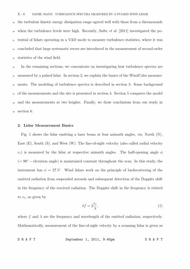
X - 6 SATHE–MANN: TURBULENCE SPECTRA MEASURED BY A PULSED WIND LIDAR
the turbulent kinetic energy dissipation range agreed well with those from a thermosonde89
when the turbulence levels were high. Recently, Sathe et al. [2011] investigated the po-90
tential of lidars operating in a VAD mode to measure turbulence statistics, where it was91
concluded that large systematic errors are introduced in the measurement of second-order92
statistics of the wind field.93
In the remaining sections, we concentrate on investigating how turbulence spectra are94
measured by a pulsed lidar. In section 2, we explain the basics of the WindCube measure-95
ments. The modeling of turbulence spectra is described in section 3. Some background96
of the measurements and the site is presented in section 4. Section 5 compares the model97
and the measurements at two heights. Finally, we draw conclusions from our study in98
section 6.99
2. Lidar Measurement Basics
Fig. 1 shows the lidar emitting a laser beam at four azimuth angles, viz. North (N),
East (E), South (S), and West (W). The line-of-sight velocity (also called radial velocity
vr) is measured by the lidar at respective azimuth angles. The half-opening angle φ
(= 90◦ − elevation angle) is maintained constant throughout the scan. In this study, the
instrument has φ = 27.5◦. Wind lidars work on the principle of backscattering of the
emitted radiation from suspended aerosols and subsequent detection of the Doppler shift
in the frequency of the received radiation. The Doppler shift in the frequency is related
to vr, as given by
δf = 2vrλ, (1)
where f and λ are the frequency and wavelength of the emitted radiation, respectively.
Mathematically, measurement of the line-of-sight velocity by a scanning lidar is given as
D R A F T September 1, 2011, 9:45pm D R A F T
99

SATHE–MANN: TURBULENCE SPECTRA MEASURED BY A PULSED WIND LIDAR X - 7
the dot product of the unit vector in the direction of the measurement and the velocity
field at the center of the measuring volume,
vr(θ) = n(θ) · v(dfn(θ)), (2)
where θ is the azimuth angle, df is the center of the range gate at which the wind speeds
are measured, n(θ) = (cos θ sinφ, sin θ sinφ, cosφ) is the unit directional vector, and v =
(u, v, w) is the instantaneous velocity field evaluated at the range gate dfn(θ). In practice,
for a lidar it is impossible to obtain the backscattered radiation precisely from a single
point, and there is always backscattered radiation of different intensities from different
regions in space along the line-of-sight. Hence, it is necessary to assign appropriate weights
to the backscattered intensity such that the weight corresponding to the center of the range
gate is the highest. For a pulsed lidar, a triangular weighting function ϕ(s) is commonly
assumed [Lindelow , 2007], which is given as
ϕ(s) =
{lp−|s|l2p
for |s| < lp;
0 elsewhere,(3)
where lp is the half length of the ideally rectangular light pulse leaving the lidar, assuming
matching time windowing (= 2lp/c, where c is the speed of light). The weighted average
radial velocity can thus be written as
vr(θ) =
∫ ∞
−∞ϕ(s) n(θ) · v(n(θ)(s+ df )) ds, (4)
where s is the distance along the beam from the center of the range gate.100
In this study, we derive expressions of turbulence spectra assuming that the wind comes
from the North. The equations become too cumbersome if an arbitrary wind direction is
considered. Nevertheless, the same framework can be used in modeling turbulence spectra
D R A F T September 1, 2011, 9:45pm D R A F T
100

X - 8 SATHE–MANN: TURBULENCE SPECTRA MEASURED BY A PULSED WIND LIDAR
for any wind direction. Let us denote the unit vectors in the four directions as
nN = n(−Θ), nS = n(π −Θ), nE = n(π
2−Θ), nW = n(3
π
2−Θ), (5)
where the subscripts of the unit vectors indicate respective directions and Θ is the wind
direction. In this study, we use Θ = 0. If we consider the coordinate system such that
the u component is aligned in the mean wind direction, then from simple geometrical
considerations for Θ = 0, we get
uwc =vrS − vrN2 sinφ
,
vwc =vrE − vrW2 sinφ
,
(6)
where the subscript wc denotes the measurement by the WindCube, and vrN , vrS, vrE,
and vrW are the weighted average radial velocities in the North, South, East, and West
directions, respectively. For the w component, we use the formula by the company that
produces the WindCube, Leosphere,
wwc =P (vrN + vrS) +Q(vrE + vrW )
2 cosφ, (7)
where P and Q are the weights associated with the wind direction such that P +Q = 1.
Leosphere uses P = cos2 Θ and Q = sin2 Θ, and hence, we use the same in our calculations.
Thus, for Θ = 0 we get
wwc =vrN + vrS2 cosφ
. (8)
Further details of the working principles of the WindCube are given in Lindelow [2007].101
3. Modeling the turbulence spectra measured by a pulsed wind lidar
D R A F T September 1, 2011, 9:45pm D R A F T
101

SATHE–MANN: TURBULENCE SPECTRA MEASURED BY A PULSED WIND LIDAR X - 9
By definition, the one-dimensional spectrum of any component of the wind field is given102
as [Wyngaard , 2010]103
Fij(k1) =1
2π
∫ ∞
−∞Rij(x) exp(−ik1x) dx,
=1
2πlim
X→∞
∫ X
−X
Rij(x) exp(−ik1x)(1− |x|X
)dx, (9)
where k1 is the wavenumber, Fij(k1) is the one-dimensional spectrum, Rij(x) is the auto-
covariance function, x is the separation distance, and X is the length of the record. Since
the WindCube cannot make continuous measurements, let us take only discrete values
such that X = NΔx and x = nΔx, where n is an integer multiple, N is the total number
of samples, and Δx is the distance traveled by the wind when the lidar beam shifts from
one azimuth angle to the other. Since it takes about 4 s for the WindCube beam to move
from the North to the South, or from the East to the West, assuming Taylor’s hypothesis
to be valid, we get Δx = u × 4 m, where u is the mean wind speed. If we evaluate the
spectra measured by the WindCube at only discrete wave numbers k1q = 2πq/X, then we
can write
Fijwc(q) =1
2π
N∑n=−N
Rijwc(n) exp
(−i2πnqN
)(1− |n|
N
)Δx. (10)
The challenge now is to find an expression for Rijwc(n). As in Sathe et al. [2011], we make104
the following assumptions:105
1. The flow is horizontally homogeneous and Taylor’s hypothesis is valid.106
2. The spatial structure of the turbulent flow is described well by the spectral tensor107
model of Mann [1994].108
We first demonstrate the model of Rijwc(n) for the u component and use the same109
framework to derive the v and w components.110
D R A F T September 1, 2011, 9:45pm D R A F T
102

X - 10 SATHE–MANN: TURBULENCE SPECTRA MEASURED BY A PULSED WIND LIDAR
We begin by considering the mathematical form of Taylor’s hypothesis such that
v(x, t) = v(x−Δx, 0), (11)
where t is the time. For simplicity, let us first neglect the averaging along the line-of-111
sight. We will introduce this averaging later in the equations. For the turbulence spectra112
measured by the WindCube, it is necessary to consider the exact spatial and temporal113
position of the measurements. The wind vector is constructed using the North and South114
beams such that at any given instant, one current and one previous measurement is used.115
If we assume that at t = 0, we use the current measurement from the North beam and116
the previous measurement from the South beam, then combining Eqs. (6) and (11) we117
can write118
uwc(mΔx) =vrS(nSdf − e1(m− 1)Δx)− vrN(nNdf − e1mΔx)
2 sinφ, for even m, (12)
uwc(mΔx) =vrS(nSdf − e1mΔx)− vrN(nNdf − e1(m− 1)Δx)
2 sinφ, for odd m, (13)
where e1 = (1, 0, 0) is the unit vector in the mean wind direction. Combining even and
odd m from Eqs. (12) and (13), we can write
uwc(mΔx) =[vrS
(nSdf − e1
(m− (1 + (−1)m)
2
)Δx)
− vrN
(nNdf − e1
(m− (1− (−1)m)
2
)Δx)]/(
2 sinφ).
(14)
We know that by definition, Rij(n) = 〈ui(mΔx)uj
((m+n)Δx
)〉, where 〈〉 denotes ensem-
ble averaging. By applying this definition to Eq. (14), we get auto and cross covariances
for the North and South beams. Introducing the averaging along the beam (using Eq. 4)
D R A F T September 1, 2011, 9:45pm D R A F T
103

SATHE–MANN: TURBULENCE SPECTRA MEASURED BY A PULSED WIND LIDAR X - 11
for only the south beam, we get⟨vrS
(nSdf − e1
(m− (1 + (−1)m)
2
)Δx)vrS
(nSdf − e1
((m+ n)− (1 + (−1)m+n)
2
)Δx)⟩
=
∫ ∞
−∞
∫ ∞
−∞niSnjS ϕ(s1)ϕ(s2)⟨
vi
(nSdf − e1
(m− (1 + (−1)m)
2
)Δx+ nSs1
)vj
(nSdf − e1
((m+ n)− (1 + (−1)m+n)
2
)Δx+ nSs2
)⟩ds1ds2
(15)
If we denote r =(nSdf − e1
(m − (1 + (−1)m)/2)Δx
)−(nSdf − e1
((m + n) − (1 +
(−1)m+n)/2)Δx)as the separation distance between the S-S beam combination, then we
can write
RvrS(n) =
∫ ∞
−∞
∫ ∞
−∞niSnjS ϕ(s1)ϕ(s2)Rij(r + nS(s1 − s2)) ds1ds2, (16)
where RvrS(n) is the autocovariance of the radial velocity for the South beam. Rij(r)
is related to the three dimensional spectral velocity tensor Φij(k) by the inverse Fourier
transform [Wyngaard , 2010], i.e.,
Rij(r + nS(s1 − s2)) =
∫Φij(k) exp(ik · (r + nS(s1 − s2))) dk, (17)
where∫dk ≡ ∫∞−∞
∫∞−∞∫∞−∞ dk1dk2dk3 and k = (k1, k2, k3) denotes the wave vector. Sub-
stituting Eq. (17) into (16) and rearranging the terms, we get
RvrS(r) =
∫Φij(k) niSnjS exp(ik · r) ϕ(k · nS)ϕ
∗(k · nS) dk (18)
whereˆdenotes Fourier transform and ∗ complex conjugation. Reducing the expression of
r, we get
r = e1
((−1)mΔx
2(1− (−1)n) + nΔx
). (19)
D R A F T September 1, 2011, 9:45pm D R A F T
104

X - 12 SATHE–MANN: TURBULENCE SPECTRA MEASURED BY A PULSED WIND LIDAR
Similarly, if we assume that at t = 0 we use the current measurement from the South
beam and the previous measurement from the North beam, then we get
uwc(mΔx) =[vrS
(nSdf − e1
(m− (1− (−1)m)
2
)Δx)
− vrN
(nNdf − e1
(m− (1 + (−1)m)
2
)Δx)]/(
2 sinφ),
(20)
and the separation distance for the S-S beam combination is given as r =
−(−1)mΔx/2(1− (−1)n)+nΔx. In order to make the time series statistically stationary,
we consider that there is an equal probability that the beam at t = 0 points either in the
North or South direction. This eliminates the dependence of the autocovariance function
on m. We perform similar analysis on the auto and cross covariances for other beams.
In total, we then get eight separation distances; two for the S-S, two for S-N, two for
N-S, and two for N-N beam combinations. If we denote rul(the subscript l denotes the
respective beam combination) as the separation distance for different beam combinations,
then we can write all the separation distances in compact form as
rul=
⎧⎪⎪⎪⎨⎪⎪⎪⎩e1
((−1)lΔx
2(1− (−1)n) + nΔx
)for l = 1, 2, 7, 8;
nSdf − nNdf + e1
((−1)lΔx
2(1 + (−1)n) + nΔx
)for l = 3, 4;
nNdf − nSdf + e1
((−1)lΔx
2(1 + (−1)n) + nΔx
)for l = 5, 6.
(21)
Following a similar procedure for the v component, we get the following separation dis-
tances:
rvl =
⎧⎪⎪⎪⎨⎪⎪⎪⎩e1
((−1)lΔx
2(1− (−1)n) + nΔx
)for l = 1, 2, 7, 8;
nEdf − nWdf + e1
((−1)lΔx
2(1 + (−1)n) + nΔx
)for l = 3, 4;
nWdf − nEdf + e1
((−1)lΔx
2(1 + (−1)n) + nΔx
)for l = 5, 6.
(22)
The separation distances for the w component are the same as those for the u component,
because only the North and South beams are used to obtain wwc (Eq. 8). Combining
Eqs. (12)–(22) and using the symmetry properties of Φij(k), we get the expressions for
D R A F T September 1, 2011, 9:45pm D R A F T
105

SATHE–MANN: TURBULENCE SPECTRA MEASURED BY A PULSED WIND LIDAR X - 13
the autocovariance of the u and v components as
Ruwc(n) =1
8 sin2 φ
∫Φij(k)[niSnjSϕ(k · nS)ϕ
∗(k · nS)2∑
l=1
exp(ik · rul)
− niSnjN ϕ(k · nS)ϕ∗(k · nN)
6∑l=3
exp(ik · rul)
+ niNnjN ϕ(k · nN)ϕ∗(k · nN)
8∑l=7
exp(ik · rul)]dk,
(23)
Rvwc(n) =1
8 sin2 φ
∫Φij(k)[niEnjEϕ(k · nE)ϕ
∗(k · nE)2∑
l=1
exp(ik · rvl)
− niEnjW ϕ(k · nE)ϕ∗(k · nW )
6∑l=3
exp(ik · rvl)
+ niWnjW ϕ(k · nW )ϕ∗(k · nW )8∑
l=7
exp(ik · rvl)]dk.
(24)
The expression for the w component is similar to that for the u component, except that the119
second term in the square brackets of Eq. (23) is added instead of subtracted, and sin2 φ120
is replaced by cos2 φ in the denominator. Substituting Eqs. (23) and (24) into Eq. (10),121
we can finally theoretically calculate the turbulence spectra measured by the WindCube122
for the u, v, and w components of the velocity field.123
In order to see the extent of attenuation and redistribution of the spectral energy, we
compare these models with the true theoretical spectra measured by sonics and those
measured by the WindCube. The true theoretical spectrum of any component of the
wind field is also given as (apart from Eq. 9) [Wyngaard , 2010],
Fij(k1) =
∫ ∞
−∞
∫ ∞
−∞Φij(k) dk2dk3. (25)
We consider the sonic measurements to essentially represent the true theoretical spectra.124
4. Description of the measurements
D R A F T September 1, 2011, 9:45pm D R A F T
106

X - 14 SATHE–MANN: TURBULENCE SPECTRA MEASURED BY A PULSED WIND LIDAR
The measurements were performed at the Danish National Test Center for Large125
Wind Turbines at Høvsøre, Denmark. A reference met-mast, which is 116.5 m tall126
and intensively equipped with cup and sonic anemometers, is located at the coordinates127
56◦26’26” N, 08◦09’03” E. The site is about 2 km from the West coast of Denmark. The128
eastern sector is generally characterized by a flat, homogeneous terrain, and to the South129
is a lagoon. To the North, there is a row of five wind turbines. The sonics are placed on130
the North booms of the met-mast, resulting in unusable data when the wind is from the131
south because of the wake of the mast, and from the North because of the wakes of the132
wind turbines.133
We use the sonic measurements at 60 and 100 m in combination with the WindCube134
to compare with the modeled turbulence spectra. The WindCube is located about 5 m135
North-West of the met-mast, and the data were collected between January and April136
2009. In order to avoid interference with the met-mast, the WindCube is turned in a137
horizontal plane such that the nominal North beam is 45◦ (i.e., in a North-East direction)138
with respect to true North. The frequency of measurement for the sonics is 20 Hz, whereas139
the WindCube takes approximately 2 s to shift from one azimuth angle to the other. We140
use the measurements from a narrow directional sector of 130◦–140◦ only in order to align141
the mean wind direction with the nominal E-W beam of the WindCube. Thus, the u142
and w component measurements are deduced from the nominal E-W beams and the v143
component measurements are deduced from the nominal N-S beams. In order to avoid144
further confusion with Eqs. (6) and (8), the nominal E-W beam in the measurement is145
essentially the N-S beam in the theory, and vice-versa.146
D R A F T September 1, 2011, 9:45pm D R A F T
107

SATHE–MANN: TURBULENCE SPECTRA MEASURED BY A PULSED WIND LIDAR X - 15
The other criteria for the selection of the data are neutral atmospheric stability and a
mean wind speed of 9 m/s. Using Taylor’s hypothesis, we then have the sampling distance
in the mean wind direction Δx = 9×4 m. We selected the data with a mean wind speed in
the interval 8-10 m/s, which resulted in 79 and 58 10-min time series of the sonics and the
WindCube at 60 and 100 m, respectively. Atmospheric stability is characterized using the
standard surface-layer length scale LMO, commonly known as the Monin-Obukhov length.
Following Gryning et al. [2007], the conditions are considered neutral when |LMO| > 500.
LMO is estimated using the eddy covariance method [Kaimal and Finnigan, 1994] from
the sonic measurements at 20 m. Mathematically, LMO is given as
LMO = − u∗3T
κgw′θ′v, (26)
where u∗ is the friction velocity, κ = 0.4 is the von Karman constant, g is the acceleration
due to gravity, T is the absolute temperature, θv is the virtual potential temperature, and
w′θ′v (covariance of w and θv) is the virtual kinematic heat flux. u∗ is estimated as
u∗ =4
√u′w′2 + v′w′2, (27)
where u′w′ and v′w′ are the vertical fluxes of the horizontal momentum.147
The precision of the sonics is estimated to be about ±1.5%. Comparing with cup148
anemometers, the mean error of the WindCube in typical flat coastal conditions is within149
±0.05 m/s, with a standard deviation in mixed shear conditions of about 0.15 m/s. A150
detailed list of different error sources is given by Lindelow-Marsden [2009]. More details151
of the site and instrumentation can be found in Sathe et al. [2011].152
5. Comparison of the model with the measurements
D R A F T September 1, 2011, 9:45pm D R A F T
108
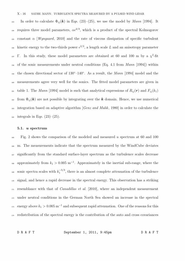
X - 16 SATHE–MANN: TURBULENCE SPECTRA MEASURED BY A PULSED WIND LIDAR
In order to calculate Φij(k) in Eqs. (23)–(25), we use the model by Mann [1994]. It153
requires three model parameters, αε2/3, which is a product of the spectral Kolmogorov154
constant α [Wyngaard , 2010] and the rate of viscous dissipation of specific turbulent155
kinetic energy to the two-thirds power ε2/3, a length scale L and an anisotropy parameter156
Γ. In this study, these model parameters are obtained at 60 and 100 m by a χ2-fit157
of the sonic measurements under neutral conditions (Eq. 4.1 from Mann [1994]) within158
the chosen directional sector of 130◦–140◦. As a result, the Mann [1994] model and the159
measurements agree very well for the sonics. The fitted model parameters are given in160
table 1. The Mann [1994] model is such that analytical expressions of Rij(r) and Fij(k1)161
from Φij(k) are not possible by integrating over the k domain. Hence, we use numerical162
integration based on adaptive algorithm [Genz and Malik , 1980] in order to calculate the163
integrals in Eqs. (23)–(25).164
5.1. u spectrum
Fig. 2 shows the comparison of the modeled and measured u spectrum at 60 and 100165
m. The measurements indicate that the spectrum measured by the WindCube deviates166
significantly from the standard surface-layer spectrum as the turbulence scales decrease167
approximately from k1 > 0.005 m−1. Approximately in the inertial sub-range, where the168
sonic spectra scales with k−5/31 , there is an almost complete attenuation of the turbulence169
signal, and hence a rapid decrease in the spectral energy. This observation has a striking170
resemblance with that of Canadillas et al. [2010], where an independent measurement171
under neutral conditions in the German North Sea showed an increase in the spectral172
energy above k1 > 0.005 m−1 and subsequent rapid attenuation. One of the reasons for this173
redistribution of the spectral energy is the contribution of the auto and cross covariances174
D R A F T September 1, 2011, 9:45pm D R A F T
109

SATHE–MANN: TURBULENCE SPECTRA MEASURED BY A PULSED WIND LIDAR X - 17
of different components of the velocity field, as seen in Eq. (23). At very low wavenumbers175
(< 0.005 m−1), the spectral energy measured by the WindCube is approximately the same176
as that measured by the sonics. This is because very large turbulence eddies are associated177
with very low wavenumbers that cause the volume measurement from the lidar to behave178
essentially like a point measurement.179
At both heights, our model agrees very well with the measurements at almost all180
wavenumbers. The point-like behavior of the WindCube at very low wavenumbers, and181
redistribution of the spectral energy beyond k1 > 0.005 m−1, is captured by the model182
very well. However, there are stark differences in the distribution of the spectral energy183
at 60 and 100 m. This is because of the beam interference phenomenon that occurs for184
certain separation distances at 100 m. This is explained as follows.185
In our model, we have assumed validity of Taylor’s hypothesis, which states that tur-186
bulence is advected by the mean wind field, i.e., the local velocity of the turbulent eddies187
is so small that they essentially move with only the mean velocity. In other words, tur-188
bulence can be considered to be frozen. For the u spectrum, we use only the N-S beams189
that are aligned in the mean wind direction. At 100 m, the mean wind speed is such190
that the North and South beams will investigate the same air (but different components)191
after approximately 3Δx. Looking more closely at Eq. (21), at 3Δx we get ru3 → 0 and192
ru4 → 0. This implies that in Eq. (23), exp(ik · ru3) → 1 and exp(ik · ru4) → 1. This193
will cause an overall decrease in Ruwc(n) at n = 3. From our calculations, we also find194
anomalous behavior of Ruwc(n) at n = 2 and n = 4. Revisiting Eq. (21), we find that at195
n = 2, ru3 → 0 and at n = 4, ru4 → 0. This implies that it will cause some reduction in196
D R A F T September 1, 2011, 9:45pm D R A F T
110

X - 18 SATHE–MANN: TURBULENCE SPECTRA MEASURED BY A PULSED WIND LIDAR
Ruwc(n), but not as much as when n = 3. In order to explain this behavior, we illustrate197
the interference phenomenon of the beams in Fig. 3.198
Since we assume Taylor’s hypothesis, we can either fix the N-S beams and measure the
flow field as it moves past the beams, or freeze the flow field and move the N-S beams
instead. For simplicity, let us freeze the flow field and represent 1–8 as the positions at
which the North and the South beams perform measurements. The difference between
each position is then equal to the separation distance Δx. Let 1, 3, 5, and 7 denote the
measurements of the North beam and 2, 4, 6, and 8 denote those of the South beam.
For now, let us consider only the intersection of beams 2 and 5 at point A, which is
the point where the North and South beams will see the same air. This occurs at a
separation distance of 3Δx corresponding to a height of 104 m. As a result, we will
get unusual covariances whenever there is intersection of beams 2 and 5 in combination
with other beam measurements. Since the WindCube uses one current and one previous
measurement to deduce wind field components, we use the measurement from beam 2
when it is in combination with beam 1 or 3. Similarly, we use beam 5 when it is in
combination with beam 4 or 6. These combinations can be written as[(2, 1) (3, 2)(5, 4) (6, 5)
](28)
The bold numbers in Eq. (28) indicate the current measurement for the respective beams,199
i.e., the set (2, 1) indicates that the current measurement from beam 2 is used in combi-200
nation with the previous measurement from beam 1 to deduce the u component, and so201
on for other sets. In this case, we will obtain unusual covariances at these separation dis-202
tances in the model, which are equal to the difference between beam numbers in bold (Eq.203
28) that correspond to the intersection of beams 2 and 5. This happens at 5− 3, 5− 2,204
D R A F T September 1, 2011, 9:45pm D R A F T
111

SATHE–MANN: TURBULENCE SPECTRA MEASURED BY A PULSED WIND LIDAR X - 19
and 6−2, corresponding to separation distances of 2Δx, 3Δx, and 4Δx, respectively. We205
do not get unusual covariances at 3− 2 because the sets (2, 1) and (3, 2) do not contain206
beam 5, and similarly at 6 − 5, since the sets (5, 4) and (6, 5) do not contain beam 2.207
Thus, in general, we will always obtain unusual covariances at the heights at which the208
distance between the North and the South beams corresponds to separation distances of209
(n − 1)Δx, nΔx, and (n + 1)Δx (where n is odd, since for even n the North and South210
beams never intersect). Thus, if we now consider intersection points B (≈ 35 m) and C211
(≈ 173 m) in Fig. 3, then the separation distances are Δx and 5Δx, respectively. Thus,212
we should expect unusual covariances at 0, Δx, and 2Δx at 35 m, whereas at 173 m, we213
expect the same at 4Δx, 5Δx, and 6Δx.214
In order to verify the above explanation, Ruwc(n)/σ2u (where σ2
u is the true variance of215
the u component) is calculated at two separation distances (100 and 173 m), as shown in216
Fig. 4. We do not calculate Ruwc(n)/σ2u at 35 m because the WindCube reliably measures217
from approximately 40 m (owing to a large measuring volume of about 30 m). σ2u is218
calculated by integrating Eq. (25) over the k1 domain at respective heights. We can now219
clearly see unusual covariances at (n− 1)Δx, nΔx, and (n+1)Δx at both heights, where220
n = 3 at 100 m and n = 5 at 173 m. Fig. 2 indicates that the model captures this beam221
interference phenomenon, which is also present in the measurements at 100 m, very well.222
Thus, it could also be implied that in nature, Taylor’s hypothesis is valid to some extent.223
5.2. v spectrum
Fig. 5 shows the comparison of the modeled and measured v spectrum at 60 and 100m.224
As observed for the u component, the v spectrum measured by the lidar deviates sig-225
nificantly from that of the sonic spectrum. However, at very low wavenumbers, there is226
D R A F T September 1, 2011, 9:45pm D R A F T
112

X - 20 SATHE–MANN: TURBULENCE SPECTRA MEASURED BY A PULSED WIND LIDAR
an offset in the spectral energy between the lidar and the sonic. The behavior in the227
inertial sub-range is the same as that for the u component, where a rapid attenuation228
in the spectral energy is observed. Our model agrees very well with the measurements229
at 60 and 100 m, except at very low wavenumbers (< 0.005 m−1), where the model over230
estimates the spectral energy. One striking feature of this comparison is that as opposed231
to the u component, we do not see any beam interference phenomenon at 100 m because232
of Taylor’s hypothesis. This is because only the E-W beams are used to deduce the v com-233
ponents, which are perpendicular to the mean wind field. Thus, even though we assume234
Taylor’s hypothesis, the beams never interfere with each other at any separation distance.235
Thus, this result indirectly verifies the beam interference phenomenon explanation for the236
u component at 100 m. We give the following explanation for the over estimation of the237
spectral energy at very low wavenumbers.238
From Eq. (24), it is understood that the v spectrum measured by theWindCube contains
contributions from the v and w components of the spectral tensor, i.e., Φ22(k) and Φ33(k),
weighted by the corresponding weighting functions |ϕ(k ·nE)|2 and |ϕ(k ·nW )|2. Due to
the assumption of uniform shear and no effect of the Coriolis force by Mann [1994], the
symmetry group of the spectral tensor model is such that the co-spectral energy between v
and w is zero, i.e., F23(k1) = 0. We observed, using sonic anemometer measurements, that
F23(k1) is not exactly zero, but has some negative spectral energy at all wavenumbers.
We also observed that F23(k1) < F13(k1). On closely analyzing Eq. (24), we note that,
in nature, if F23(k1) contributes to the covariance measured by the lidar, it will result in
overall reduction of Rvwc . Thus, the symmetry group of Mann [1994] may not be entirely
valid. We also find that the contribution of the second term in Eq. (24) is negligible,
D R A F T September 1, 2011, 9:45pm D R A F T
113

SATHE–MANN: TURBULENCE SPECTRA MEASURED BY A PULSED WIND LIDAR X - 21
and only the first and the third terms add to the spectral energy. Let us now consider a
case such that at 60 m, the beam is staring perpendicularly to the mean wind field in a
horizontal plane. It will thus measure only the v component of the velocity field. In this
case, the v spectrum measured by the WindCube is given as
Fvwc∗(k1) =
∫ ∞
−∞
(∫ ∞
−∞Φ22(k) dk3
)|ϕ(k2)|2 dk2, (29)
where ∗ denotes spectra for a staring beam lidar. In Eq. (29), we first integrate over239
the k3 domain, and the resulting two dimensional spectrum Ev(k1, k2) is weighted by the240
filter function |ϕ(k2)|2. The behavior of the weighting function is such that |ϕ(k2)|2 → 1241
as k2 → 0. Thus, if the amount of two dimensional spectral energy increases sharply242
as (k1, k2) → 0, then the contribution of this spectral energy in the one-dimensional243
spectrum will be significant. In order to verify this assumption, we calculate Ev(k1, k2)244
at three values of k1, i.e., k1 = (10−1, 10−2, 10−3) m−1, as shown in Fig. 6. We also245
plot the variation of |ϕ(k2)|2, so that filtering of the spectral energy for the respective246
wavenumbers is clearly evident. From the figure, it is observed that k1 → 0, Ev(k1, k2)247
increases by several orders of magnitude with decreasing |k2| until a certain value of |k2|,248
after which it decreases with k2 → 0. Since Mann [1994] does not assume isotropy in249
the horizontal plane, Ev(k1, k2) � 0 as (k1, k2) → 0 [Wyngaard , 2010]. In our study,250
the WindCube is not horizontal, but at φ = 27.5◦ with the vertical. Hence, for the v251
component, the filter function along the line-of-sight acts over k2 and k3 domains. Its252
influence on averaging of the two and three dimensional spectral energy will be much253
more complicated than that for a horizontally pointing lidar. Nevertheless, we can argue254
similar reasons for the conically scanning case.255
D R A F T September 1, 2011, 9:45pm D R A F T
114

X - 22 SATHE–MANN: TURBULENCE SPECTRA MEASURED BY A PULSED WIND LIDAR
From the above explanation, we can consider four reasons for the over estimation of256
Fvwc(k1) in the model as k1 → 0.257
1. Ev(k1, k2) could be more spread out such that the total energy over the k2 domain258
would still be the same as that predicted by the Mann [1994] model.259
2. The peak in Ev(k1, k2) could be shifted to larger values of |k2|.260
3. Despite anisotropic conditions, Ev(k1, k2) could approach zero as (k1, k2)→ 0.261
4. There could be some contribution by F23(k1).262
As a consequence, the Mann [1994] model would still predict Fv(k1) considerably accu-263
rate. However, when Ev(k1, k2) is weighted by |ϕ(k2)|2, the total energy calculated using264
the Mann [1994] model and that obtained in nature would be different. Thus, it will cause265
overestimation of Fvwc(k1) as k1 → 0, despite observing a good agreement between the266
theoretical and measured Fv(k1) (Fig. 5). Unfortunately, it is very difficult to measure267
the two- and three-dimensional spectra, and hence, we cannot verify our explanation.268
5.3. w spectrum
Fig. 7 shows the comparison of the modeled and measured w spectrum at 60 and 100269
m. Since in the calculation of the w spectrum, we use only the North and South beams,270
we will obtain similar beam interference at 100 m, because of the assumption of Taylor’s271
hypothesis, as that observed for the u spectrum. The measured WindCube spectrum272
agrees quite well with the model at both heights, especially at high wavenumbers. As273
observed for the u component, at 100 m we note the effect of unusual covariances on the274
spectral energies. At very low wavenumbers, there is a slight offset between the model and275
measurements. This offset could be because of the slight deviation in the modeled and276
measured sonic spectrum. The model also shows that at very low wavenumbers, because277
D R A F T September 1, 2011, 9:45pm D R A F T
115

SATHE–MANN: TURBULENCE SPECTRA MEASURED BY A PULSED WIND LIDAR X - 23
of very large turbulence eddies, the volume measurement from the lidar behaves similar278
to a point measurement.279
6. Conclusion
The main objective of this paper is to understand how a pulsed wind lidar measures280
turbulence spectra. For this purpose, we modeled the u, v, and w spectra as measured281
by the WindCube only for a case where the mean wind direction is aligned with the mea-282
surement beams. For an arbitrary wind direction, a similar framework can be used, but283
it is much more complicated. In general, the model agrees very well with the measure-284
ments for all three components at both heights, except at very low wavenumbers for the285
v component.286
For the u and w components at very low wavenumbers (< 0.005 m−1), the volume287
measurement of the lidar behaves similar to a point measurement because of very large288
turbulence eddies. However, redistribution of the spectral energy is noted for all compo-289
nents above 0.005 m−1 , which is captured by the model very well. One of the important290
findings of this study is that for the u and w components the beam interference phe-291
nomenon will be observed at the heights in the mean wind direction at which the distance292
between the beams on the azimuth circle is equal to some odd multiple of the separation293
distance (n − 1)Δx, nΔx and (n + 1)Δx; this is because of the assumption of Taylor’s294
hypothesis. We observe the influence of this beam interference phenomenon at 100 m for295
the u and w components at approximately 2Δx, 3Δx, and 4Δx.296
For the v component, we observe an offset in the spectral energy at very low frequencies297
compared with those measured by the sonics. One of the reasons for this offset is the298
large contribution of Φ22(k) as k → 0. Such an offset is also observed in our model, but299
D R A F T September 1, 2011, 9:45pm D R A F T
116

X - 24 SATHE–MANN: TURBULENCE SPECTRA MEASURED BY A PULSED WIND LIDAR
to a greater degree. We have speculated an explanation based on the difference in the300
shape of the modeled and the true two-dimensional spectrum Ev(k1, k2). Due to lack of301
measurements of Ev(k1, k2), we cannot verify our explanation. Furthermore, there is a302
small contribution of F23(k1) in nature, which is not taken into account in the spectral303
tensor model.304
We theoretically explained the interaction of the spectral tensors that cause redistribu-305
tion of the spectral energy, and thus measurement of turbulence spectra using pulsed wind306
lidars is clarified. This study is particularly relevant for further understanding of how a307
pulsed wind lidar measures turbulent gusts. Given the complications displayed in this308
study, it might be advantageous to abandon the VAD technique for spectral analysis of309
lidar data, and instead analyze time series of individual beams. This approach is currently310
being pursued at Risø DTU, Denmark.311
Acknowledgments. This study is part of a PhD project at Delft University of Tech-312
nology. The experimental results are all based on data collected at the Høvsøre Test313
Station under the auspices of Anders Ramsing Vestergaard and Bjarne Sønderskov. This314
paper has been prepared using resources provided by the European Commission’s FP7315
SafeWind Project, Grant Agreement no. 213740, and by the Center for Computational316
Wind Turbine Aerodynamics and Atmospheric Turbulence funded by the Danish Council317
for Strategic Research grant no. 09-067216. Finally, the authors would like to thank318
Dr. Mike Courtney for useful comments and also checking the manuscript for English319
language errors.320
D R A F T September 1, 2011, 9:45pm D R A F T
117

SATHE–MANN: TURBULENCE SPECTRA MEASURED BY A PULSED WIND LIDAR X - 25
References
Canadillas, B., A. Begue, and T. Neumann (2010), Comparison of turbulence spectra de-321
rived from LiDAR and sonic measurements at the offshore platform FINO1, in DEWEK322
2010, 10th German Wind Energy Conference.323
Courtney, M., R. Wagner, and P. Lindelow (2008), Testing and comparison of lidars for324
profile and turbulence measurements in wind energy, in 14th International Symposium325
for the Advancement of Boudary Layer Remote Sensing, IOP Conference Series Earth326
and Environmental Science, vol. 1, edited by J. Mann et al., p. 012021, IOP Publishing327
LTD., doi:10.1088/1755-1315/1/1/012021.328
Davenport, A. G. (1964), Note on the distribution of the largest value of a random329
function with application to gust loading, ICE Proceedings, 28 (2), 187–196, doi:330
10.1680/iicep.1964.10112.331
Dors, I., J. P. McHugh, G. Y. Jumper, and J. Roadcap (2011), Velocity spectra and tur-332
bulence using direct detection lidar and comparison with thermosonde measurements,333
Journal of Geophysical Research, 116, D01,102, 1–12, doi:10.1029/2010JD014606.334
Drobinski, P., A. M. Dabas, and P. H. Flamant (2000), Remote measurement of turbulent335
wind spectra by heterodyne Doppler lidar technique, Journal of Applied Meteorology,336
39, 2434–2451, doi:10.1175/1520-0450(2000)039<2434:RMOTWS>2.0.CO;2.337
Frehlich, R., S. M. Hannon, and S. W. Henderson (1998), Coherent doppler lidar mea-338
surements on wind field statistics, Boundary-Layer Meteorology, 86 (2), 233–256, doi:339
10.1023/A:1000676021745.340
Genz, A. C., and A. A. Malik (1980), Remarks on algorithm 006: An Adaptive Algorithm341
for Numerical Integration over an N-dimensional Rectangular Region, Journal of Com-342
D R A F T September 1, 2011, 9:45pm D R A F T
118

X - 26 SATHE–MANN: TURBULENCE SPECTRA MEASURED BY A PULSED WIND LIDAR
putational and Applied Mathematics, 6 (4), 295–302, doi:10.1016/0771-050X(80)90039-343
X.344
Gryning, S.-E., E. Batchvarova, B. Brummer, H. Jørgensen, and S. Larsen (2007), On345
the extension of the wind profile over homogeneous terrain beyond the surface layer,346
Boundary-Layer Meteorology, 124 (2), 251–268, doi:10.1007/s10546-007-9166-9.347
Hardesty, R. M., J. A. Korrell, and F. F. Hall (1982), Lidar measurement of wind ve-348
locity turbulence spectra encountered by a rotating turbine blade, Technical Report349
DOE/RL/10236-81/1, National Oceanic and Atmospheric Administration, Boulder, CO350
(USA).351
IEC (2005), IEC 61400-1. Wind turbines – Part 1: Design Requirements.352
Kaimal, J. C., and J. J. Finnigan (1994), Atmospheric Boundary Layer Flows, chap.353
Acquisition and processing of atmospheric boundary layer data, pp. 255–257, Oxford354
University Press, New York.355
Kaimal, J. C., J. C. Wyngaard, Y. Izumi, and O. R. Cote (1972), Spectral characteristics of356
surface-layer turbulence, Quarterly Journal of the Royal Meteorological Society, 98 (417),357
563–589, doi:10.1002/qj.49709841707.358
Kaimal, J. C., J. C. Wyngaard, D. A. Haugen, O. R. Cote, Y. Izumi, S. J.359
Caughey, and C. J. Readings (1976), Turbulence structure in the convective bound-360
ary layer, Journal of Atmospheric Sciences, 33 (11), 2152–2169, doi:10.1175/1520-361
0469(1976)033<2152:TSITCB>2.0.CO;2.362
Kristensen, L., D. H. Lenschow, P. Kirkegaard, and M. Courtney (1989), The spectral ve-363
locity tensor for homogeneous boundary-layer turbulence, Boundary-Layer Meteorology,364
47 (1–4), 149–193, doi:10.1007/BF00122327.365
D R A F T September 1, 2011, 9:45pm D R A F T
119

SATHE–MANN: TURBULENCE SPECTRA MEASURED BY A PULSED WIND LIDAR X - 27
Kristensen, L., M. Casanova, M. S. Courtney, and I. Troen (1991), In search of a gust366
definition, Boundary-Layer Meteorology, 55 (1–2), 91–107, doi:10.1007/BF00119328.367
Kunkel, K. E., E. W. Eloranta, and J. A. Weinman (1980), Remote determination of368
winds, turbulence spectra and energy dissipation rates in the boundary layer from li-369
dar measurements, Journal of Atmospheric Sciences, 37 (5), 978–985, doi:10.1175/1520-370
0469(1980)037<0978:RDOWTS>2.0.CO;2.371
Lindelow, P. (2007), Fibre based coherent lidars for remote wind sensing, PhD thesis,372
Technical University Denmark.373
Lindelow-Marsden, P. (2009), UpWind D1. Uncertainties in wind assessment with LIDAR,374
Tech. Rep. Risø-R-1681(EN), Risø DTU.375
Lothon, M., D. H. Lenschow, and S. D. Mayor (2009), Doppler lidar measurements of376
vertical velocity spectra in the convective planetary boundary layer, Boundary-Layer377
Meteorology, 132 (2), 205–226, doi:10.1007/s10546-009-9398-y.378
Mann, J. (1994), The spatial structure of neutral atmospheric surface-layer turbulence,379
Journal of Fluid Mechanics, 273, 141–168, doi:10.1017/S0022112094001886.380
Mann, J., J. Cariou, M. Courtney, R. Parmentier, T. Mikkelsen, R. Wagner, P. Lindelow,381
M. Sjoholm, and K. Enevoldsen (2009), Comparison of 3D turbulence measurements382
using three staring wind lidars and a sonic anemometer, Meteorologische Zeitschrift,383
18 (2, Sp. Iss. SI), 135–140, doi:10.1127/0941-2948/2009/0370.384
Mayor, S. D., D. H. Lenschow, R. L. Schwiesow, J. Mann, C. L. Frush, and M. K. Simon385
(1997), Validation of NCAR 10.6-μm CO2 Doppler lidar radial velocity measurements386
and comparison with a 915-MHz profiler, Journal of Atmospheric and Oceanic Technol-387
ogy, 14 (5), 1110–1126, doi:10.1175/1520-0426(1997)014<1110:VONMCD>2.0.CO;2.388
D R A F T September 1, 2011, 9:45pm D R A F T
120

X - 28 SATHE–MANN: TURBULENCE SPECTRA MEASURED BY A PULSED WIND LIDAR
Pena, A., C. B. Hasager, S.-E. Gryning, M. Courtney, I. Antoniou, and T. Mikkelsen389
(2009), Offshore wind profiling using light detection and ranging measurements, Wind390
Energy, 12 (2), 105–124, doi:10.1002/we.283.391
Rice, S. O. (1944), Mathematical analysis of random noise, Bell System Tech. J., 23 (3),392
282–332.393
Rice, S. O. (1945), Mathematical analysis of random noise, Bell System Tech. J., 24 (1),394
46–156.395
Sathe, A., J. Mann, J. Gottschall, and M. S. Courtney (2011), Can wind lidars mea-396
sure turbulence?, Journal of Atmospheric and Oceanic Technology, 28 (7), 853–868,397
doi:10.1175/JTECH-D-10-05004.1.398
Sjoholm, M., T. Mikkelsen, J. Mann, K. Enevoldsen, and M. Courtney (2009), Spatial399
averaging-effects on turbulence measured by a continuous-wave coherent lidar, Meteo-400
rologische Zeitschrift, 18 (3, Sp. Iss. SI), 281–287, doi:10.1127/0941-2948/2009/0379.401
Wyngaard, J. C. (2010), Turbulence in the Atmosphere, Cambridge University Press, New402
York.403
Table 1: Mann [1994] model parameters to estimate Φij(k)
Height (m) αε2/3 L (m) Γ60 0.051 46.226 3.158100 0.037 60.867 2.896
D R A F T September 1, 2011, 9:45pm D R A F T
121
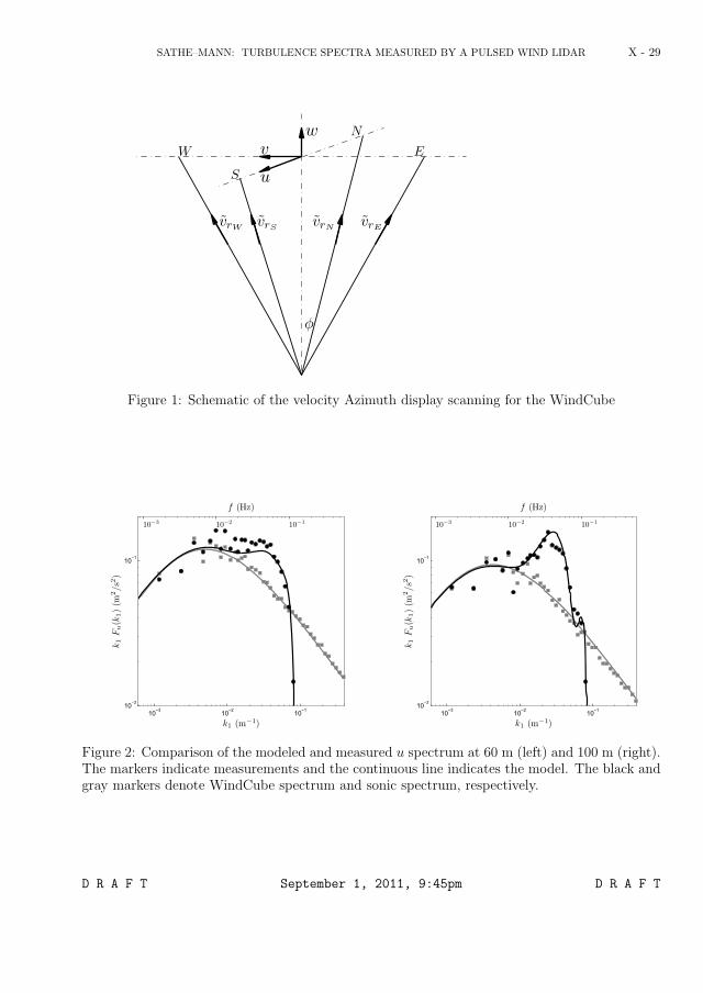
SATHE–MANN: TURBULENCE SPECTRA MEASURED BY A PULSED WIND LIDAR X - 29
u
vw N
E
S
W
vrW vrS vrN vrE
φ
Figure 1: Schematic of the velocity Azimuth display scanning for the WindCube
f (Hz)
10−3 10−2 10−110−2
10−1
k1 (m−1)
k1Fu(k
1)(m
2/s2)
10−3 10−2 10−1
f (Hz)
10−3 10−2 10−110−2
10−1
k1 (m−1)
k1Fu(k
1)(m
2/s2)
10−3 10−2 10−1
Figure 2: Comparison of the modeled and measured u spectrum at 60 m (left) and 100 m (right).The markers indicate measurements and the continuous line indicates the model. The black andgray markers denote WindCube spectrum and sonic spectrum, respectively.
D R A F T September 1, 2011, 9:45pm D R A F T
122

X - 30 SATHE–MANN: TURBULENCE SPECTRA MEASURED BY A PULSED WIND LIDAR
Figure 3: Schematic of the intersection of the North and South Beams. The shaded portionindicates the measurement volume. The black marker indicates a height of 100 m
D R A F T September 1, 2011, 9:45pm D R A F T
123

SATHE–MANN: TURBULENCE SPECTRA MEASURED BY A PULSED WIND LIDAR X - 31
0 5 10 15 20 25 300
0.2
0.4
0.6
0.8
1
1.2
n
Ruwc(n)/σ2 u
100 m173 m
Figure 4: Comparison of Ruwc(n)/σ2u at different heights
f (Hz)
10−3 10−2 10−110−2
10−1
k1 (m−1)
k1Fv(k
1)(m
2/s2)
10−3 10−2 10−1
f (Hz)
10−3 10−2 10−110−2
10−1
k1 (m−1)
k1Fv(k
1)(m
2/s2)
10−3 10−2 10−1
Figure 5: Comparison of the modeled and measured v spectrum at 60 m (left) and 100 m (right).The meaning of the symbols and colors correspond to those in Fig. 2
D R A F T September 1, 2011, 9:45pm D R A F T
124

X - 32 SATHE–MANN: TURBULENCE SPECTRA MEASURED BY A PULSED WIND LIDAR
−0.1 −0.08 −0.06 −0.04 −0.02 0 0.02 0.04 0.06 0.08 0.1100
101
102
103
k2
Ev(k
1,k
2)
k1 = 0.001k1 = 0.01k1 = 0.1
−0.1 −0.08 −0.06 −0.04 −0.02 0 0.02 0.04 0.06 0.08 0.10
0.1
0.2
0.3
0.4
0.5
0.6
0.7
0.8
0.9
1
|ϕ(k
2)|2
Figure 6: Two-Dimensional energy spectrum of the v component. The weighting function |ϕ(k2)|2is plotted on the right y-axis
f (Hz)
10−3 10−2 10−1
10−2
k1 (m−1)
k1Fw(k
1)(m
2/s2)
10−3 10−2 10−1
f (Hz)
10−3 10−2 10−1
10−2
k1 (m−1)
k1Fw(k
1)(m
2/s2)
10−3 10−2 10−1
Figure 7: Comparison of the modeled and measured w spectrum at 60 m (left) and 100 m (right).The meaning of the symbols and colors correspond to those in Fig. 2
D R A F T September 1, 2011, 9:45pm D R A F T
125

126

Chapter 7
How can wind lidars measureturbulence? A preliminaryinvestigation
In chapters 5 and 6 we understood that the VAD scanning technique of measuringturbulence using lidars result in large systematic errors. In this chapter we investigatea new method that in principle has the potential to make turbulence measurementsby lidars possible. The method uses six lidar beams to counter the contaminationof the measured turbulence by other components of the Reynolds stress tensor. Thefoundation for this idea was laid down by Eberhard et al. [1989], Mann et al. [2010],where momentum flux was measured using two beams. As a consequence of using sixarbitrarily chosen lidar beams the random error in the turbulence measurements willincrease. We optimize the beams angles such that these random errors are minimized.Then in principle the only systematic errors that remain in the measurements are theaveraging errors due to the large sampling volume in which lidars measure windspeeds. To model these systematic errors, we make use of the Mann [1994] model todescribe the three-dimensional turbulence structure.
For both, the continuous-wave (ZephIR) and the pulsed (WindCube) lidars onlytheoretical calculations of the systematic errors are carried out, which are comparedwith the calculations for a VAD scanning technique. The measurement using thisconfiguration requires significant hardware changes and are not carried out in thisPhD study. The attached paper compares two methods of measurement, the VADscanning technique and the six-beam method. The description for the VAD scanningtechnique is an overlap of the work carried out in chapter 5, and only the six beamapproach is new work.
111
127

Can the available wind lidars measure turbulence?
A. Sathea,b∗, J. Manna, J. Gottschalla, M. S. Courtneya
aWind Energy Division, Risø DTU, Roskilde, Denmark, [email protected]& R, Section Wind Energy, TU Delft, Delft, The Netherlands, [email protected]
1 INTRODUCTION
It is now well established that wind lidars (henceforth referred to as lidars) measure the 10-min mean wind speed with acceptable accuracy. Several measurement campaigns have beencarried out in this regard, where cup anemometers are used as reference instruments (Kindleret al., 2007; Pena et al., 2009; Smith et al., 2006). Turbulence measurements using lidars isstill a subject of research, and an acceptable method is yet to be established. The turbulencemeasurements that we refer to in this article are the second-order moments of wind speeds. Forwind energy, amongst a whole range of applications, turbulence measurements are useful in theload calculations of wind turbines, power curve measurements and validation of wind profilemodels.
The current standard for the measurement of turbulence for wind energy purposes is thesonic anemometer, which is a compact instrument that can measure all three components ofwind velocity in a relatively small sample volume that for all practical purposes can be consid-ered a point. It needs to be mounted on a meteorological mast (met-mast), such that the flowdistortion due to the mast itself is kept to a minimum. Despite this there are disadvantagesof using sonic anemometers, the most important being that tall met-masts are very expensive,and offshore, the costs increase significantly. We thus have to look for alternatives. Remotesensing methods such as sodars and lidars are viable alternatives. In this article we restrict thediscussion to lidars only.
Although lidars have been introduced in wind energy recently, for meteorology they havebeen investigated previously to measure turbulence using different scanning techniques. Acommon technique is by conical scanning and using the velocity azimuth display (VAD) tech-nique of processing the data. One of the first remote sensing (Doppler radar) turbulence studiesusing a full 360◦ scan in a horizontal plane was carried out by Browning and Wexler (1968),where the limitations of horizontal homogeneity and vertical wind shear are explained in de-tail. Wilson (1970) modified the technique from Browning and Wexler (1968) and performedturbulence measurements over snow. Kropfli (1986) extended the technique to accommodateturbulence scales of motion larger than those described in Wilson (1970) and showed that thesetechniques could be used to make reasonable estimates of turbulent kinetic energy and momen-tum flux by modelling the random errors in the measurements.
Eberhard et al. (1989) studied turbulence using Doppler lidar and using the variances ofthe radial velocity, where they modelled the random errors using a partial Fourier decomposi-tion method, which gave better estimates of the errors than Wilson (1970) and Kropfli (1986).Gal-Chen et al. (1992) presented a technique to analyse lidar data for turbulence measurementsusing the scans at two levels, and produced estimates of fluxes in the mixed layer, and spectraof the horizontal velocity at the surface. Banakh et al. (1995) presented an analysis of estimat-ing the random errors in the measurement of the mean wind speed by lidars using the theory
∗The author is affiliated to Risø DTU and TU Delft
1
128

of isotropic turbulence. Banta et al. (2002) studied the turbulence characteristics under theconditions of low-level jets, using the vertical-slice scans of radial velocities. Smalikho et al.(2005) presented a method to use lidar data for the estimation of turbulent energy dissipationrate to study wake vortices of an aircraft. A comprehensive review is given in Engelbart et al.(2007) that covers different remote sensing techniques for turbulence measurements includinglidars. A review of the use of lidars for wind energy applications is also presented in Emeiset al. (2007). Pichugina et al. (2008) demonstrated the sensitivity of the streamwise velocityvariance to the spatial and temporal averaging, also by using the technique of vertical-slicescans of radial velocities. Recently, studies have been carried out to model the spatial aver-aging effects (Sjoholm et al., 2009) and compare the 3D turbulence measurements using threestaring lidars (Mann et al., 2009). Wagner et al. (2009) modelled the systematic errors by ap-proximating the conical scan and the scan time as a length scale, providing first estimates ofthe variances of the longitudinal component of wind velocity. Mann et al. (2010) estimatedthe momentum fluxes using lidars and modelled the unfiltered turbulence from the CW lidar,where the model compares reasonably well with the measurements.
In this article an attempt is made to answer the research question, ‘Can the available windlidars measure turbulence?’. Two approaches are investigated to answer this question. The firstis the conical scanning and velocity azimuth display (VAD) technique to process the data, underwhich a theoretical model is developed to estimate the systematic errors in the second-ordermoments of wind speeds measured by lidars. The approach is similar to Wyngaard (1968),Citriniti and George (1997), where turbulence measured by the hot-wire anemometer probewas modelled. The systematic errors are the errors that arise due to the averaging effect inthe line-of-sight and the quite large circle in which lidars measure wind speed. The second isconically scanning at six azimuth angles and using the variances of the radial velocities fromthese six beams. This approach has been used previously by (Eberhard et al., 1989), (Mannet al., 2010) to measure momentum flux only. Under our approach, lidar beams are shot at fivedifferent azimuth angles and one beam is vertical.
Two types of lidars are considered, the ZephIR developed by QinetiQ (Natural Power) as acontinuous wave (CW) lidar and the WindCube developed by Leosphere as a pulsed lidar. Theverification is carried out by comparing the variances measured by the ZephIR and WindCubewith that of the sonic anemometers placed at different heights on a met-mast.
2 APPROACH 1 – CONICAL SCANNING AND VAD TECHNIQUE TO PROCESSLIDAR DATA
v
w
uθ
vr
NEW
S
φ
Figure 1: Schematic of the velocity azimuth display scanning
2
129

Fig. 1 shows the lidar emitting the laser beam at different azimuth angles θ. The azimuthangles increase from 0◦–360◦ in the clockwise direction as for the geographical convention.The line-of-sight velocity (also called radial velocity vr) is measured by the lidar at each az-imuth angle. The half-opening angle φ (= 90◦ − elevation angle) is kept constant throughoutthe scan. The CW and pulsed lidars work on the principle of backscattering of the emitted radi-ation, and subsequent detection of the Doppler shift in the frequency of the received radiation.The Doppler shift in the frequency is related to vr by,
δ f = 2vr
λ, (1)
where f and λ are the frequency and wavelength of the emitted radiation. Mathematically, vr isgiven as the dot product of the unit directional vector and the velocity field at the point of focusfor a CW lidar, and the center of the range gate (Lindelow, 2007) for the pulsed lidar,
vr(θ) = n(θ) ·v(d fn(θ)), (2)
where d f is the focus distance for the CW lidar or the distance to the center of the range gatefor the pulsed lidar at which the wind speeds are measured, v = (u,v,w) is the instantaneousvelocity field evaluated at the focus point or the center of the range gate d fn(θ), and n(θ) isthe unit directional vector given as,
n(θ) = (cosθsinφ,sinθsinφ,cosφ). (3)
In practice it is impossible to obtain the backscattered radiation precisely from only the focuspoint, and there is always backscattered radiation of different intensities from different regionsin space along the line-of-sight. Hence, it is necessary to assign appropriate weights to thebackscattered intensity such that the weight corresponding to the focus point or the center ofthe range gate is the highest. Mathematically, the weighted average radial velocity can bewritten as,
vr(θ) =∫ ∞
−∞ϕ(s)n(θ) ·v(sn(θ)+d fn(θ)) ds, (4)
where ϕ(s) is any weighting function, integrating to one, and s is the distance along the beamfrom the focus. For simplicity we assume that s = 0 corresponds to the focus distance. Follow-ing are the main assumptions of our model:
1. The terrain is homogeneous
2. The flow field is frozen during the scan
3. Eq. (4) with an appropriately chosen ϕ(s) models the averaging well
4. The spatial structure of the turbulent flow is described well by the spectral tensor modelof Mann (1994)
We derive the expressions for the CW lidar (ZephIR) only, since the same approach is usedfor the pulsed lidar (Windcube). If we assume the coordinate system such that u is alignedto the mean wind direction, v is perpendicular to the mean wind direction, w is the verticalcomponent, and the mean wind comes from the North then vr(θ) can be expressed as,
vr(θ) = A+Bcosθ+C sinθ, (5)
where the coefficients A = wqq cosφ, B = uqq sinφ and C = vqq sinφ and the sign ambiguityin vr(θ) is neglected (see Mann et al. (2010)). We use the subscript qq to denote the velocitycomponents measured by ZephIR, since they are not the true velocity components u, v and w.The assumption that the mean wind comes from the North is only made for simplicity. For alidar measuring at many points on the azimuth circle the choice of the mean wind direction does
3
130

not matter since averaging over the entire circle is carried out. The values of the coefficients A,B and C are found using least squares method by fitting Eq. (5) to the measured values of vr(θ)at all scanned azimuth angles. The coefficients can be written as Fourier integrals,
A =1
2π
∫ 2π
0vr(θ) dθ, (6)
B =1
π
∫ 2π
0vr(θ) cosθ dθ, (7)
C =1
π
∫ 2π
0vr(θ) sinθ dθ. (8)
We proceed by deriving expressions for the wqq variance. The expressions for the (co-) vari-ances of the remaining components of wind velocity can be derived in a similar manner.
The variance of A is defined as σ2A = 〈A′2〉, where 〈〉 denotes ensemble averaging of a
variable. From the above definition of A we can write,
σ2A = 〈w′2qq〉cos2 φ. (9)
Using Eq. (6) we can also write,
σ2A =
⟨(1
2π
∫ 2π
0v′r(θ) dθ
)2⟩. (10)
Lengthy manipulations allow us to express σ2A in terms of the three-dimensional spectral ve-
locity tensor Φi j(k), which is the Fourier transform of the covariance tensor. Let αi(k) =(∫ ∞−∞ ϕ(s)
[1
2π∫ 2π
0 ni(θ)ei(s+d f )k·n(θ) dθ]
ds)
, which physically represents the line-of-sight and
conical averaging. Eq. (10) can then be written as (using Eq. 9),
〈w′2qq〉cos2 φ =∫
Φi j(k)αi(k)α∗j(k) dk, (11)
where ∗ denotes complex conjugation. Thus the integral reduces to evaluating αi(k), sincethe analytical expressions for Φi j(k) are given in Mann (1994). Eq. (11) can then be estimatednumerically. For a CW lidar, ϕ(s) is well approximated by a Lorentzian function (Sonnenscheinand Horrigan, 1971),
ϕ(s) =1
πl
l2 + s2, (12)
where l is the Rayleigh length (= λbd2f /πr2
b, where λb = 1.55 μm is the wavelength of the emit-
ted radiation, and rb = 19.5 mm is the beam radius). The resulting 〈w′2qq〉 can now be evaluated
and a similar approach is taken for deriving 〈u′2qq〉 and 〈v′2qq〉 variances, and for the variancesmeasured by the Windcube. An additional complication for the ZephIR is that the beam rotatesthree times calling for an extra averaging in time, which is included in the theoretical predictionin Fig. (2a), see Sathe et al. (2011) for details. We present the systematic errors as the ratio ofthe lidar second-order moments and the true second-order moment.
2.1 Comparison of the models with the measurementsThe measurements were performed at the Danish National Test Center for Large Wind Turbinesat Høvsøre, Denmark. The site is about 2 km from the west coast of Denmark. The easternsector is characterized by flat homogeneous terrain, and to the south is a lagoon. Our referencemeasurements for this study are the sonic anemometer measurements taken at 40, 60, 80 and
4
131

100 m. The measured three-dimensional wind speeds are resolved with a frequency of 20 Hzand then reduced to the respective 10-min statistics (mean values and standard deviations orvariances). All sonic anemometers are placed on the North booms of the met-mast, resultingin unusable data when the wind is from the south due to the wake of the mast. In combinationwith the sonic measurements, wind speeds from a ZephIR and a WindCube are used. Refer-ence and lidar data were collected over two different time periods, for the WindCube betweenJanuary and April 2009, and for the ZephIR between April and November 2009. In order tofurther avoid the influence of the wakes from the wind turbines and the met. mast on lidar mea-surements, and inhomogeneities due to the sudden change of roughness (sea-land transition),only data periods with easterly winds (50◦–150◦) are analyzed. For the ZephIr 5530 data pointswere used after using all the filter, whereas for the WindCube 4003 data points were used.
The estimation of Φi j using the model from Mann (1994) requires three input parameters,
αε2/3, which is a product of the spectral Kolmogorov constant α (Monin and Yaglom, 1975)
and the rate of viscous dissipation of specific turbulent kinetic energy ε2/3, a length scale Land an anisotropy parameter Γ. We use these input parameters obtained by fitting the sonicanemometer measurements under different atmospheric stability conditions, at several heightson the meteorological mast in the eastern sector (Pena et al., 2010).
0 0.5 1 1.50
20
40
60
80
100
120
140
160
〈u′iu
′i〉lidar/〈u′
iu′i〉sonic
Hei
ght (
m)
u
v
w
(a) ZephIR
0 0.2 0.4 0.6 0.8 1 1.2 1.4 1.6 1.8 20
20
40
60
80
100
120
140
160
〈u′iu
′i〉lidar/〈u′
iu′i〉sonic
Hei
ght (
m)
u
v
w
(b) WC
Figure 2: ZephIR and WindCube systematic errors under neutral conditions. The markers indicate measure-ments. For the ZephIR, solid lines are the theoretical plots without the low-pass filter, and the dashed lines arewith the low-pass filter. For the WindCube, the model variation with wind direction is plotted as dotted line for0◦, dash-dot line for 15◦, dashed line for 30◦ and solid line for 45◦
Fig. 2 shows the comparison between the modelled systematic error and the measurementsat flat terrain test site in Denmark. Although the results are obtained under different atmo-spheric stability conditions we show the results for only the neutral condition. We infer thefollowing:
• For the ZephIR, the systematic errors increase with height. This is due to a quadraticincrease in the probe length with height (Lindelow, 2007). The diameter of the scanningcircle also increases with height. This results in a greater attenuation of the second-ordermoments with increasing height.
For the WindCube the systematic errors decrease with height for the u and v variances,where the probe length is constant (Lindelow, 2007), and hence, at lower heights thereis a combined averaging effect due to the probe length and the diameter of the scanningcircle. Considering that at lower heights the length scales are smaller than at higherheights, it is likely that the variances are attenuated greater at lower heights than at higher
5
132

heights. For w variance, the systematic error is approximately constant, and is most likelydue to the small length scales.
• The systematic errors in w variance is much larger (approximately 3-5 times) than thatof the u and v variances for both lidars. This is due to the very small length scales ofthe w component as compared to those for u and v, resulting in the attenuation of the wvariance of up to 90%. The u and v variances are attenuated up to 70%.
• For both lidars there is a significant spread (first and third quartiles) in the systematicerrors of u and v variances – These are the random errors and most likely occur due tothe disjunct sampling (Lenschow et al., 1994) for the ZephIR. For the WindCube, thespread in the systematic error (first and third quartiles) of the u and v variances is smallerthan that of the ZephIR. This is most likely because the WindCube updates the velocityvector approximately every 6.5 seconds, whereas the ZephIR updates every 18 seconds.
• In general, the trend of the systematic errors predicted by the models (low-pass fileringfor ZephIR) for both lidars is in agreement with the observations at all heights.
• For the WindCube, the systematic error varies significantly with the wind direction rel-ative to the beam direction for w variance, and to a lesser degree for u and v varianceunder all stability conditions.
2.2 SummaryThe systematic errors of the second-order moments measured by lidars using the conical scan-ning and VAD technique to process the data are quite large due to
1. the spatial separation of the data points along the line-of-sight and
2. the spatial separation of the data points in the conical section.
The general lidar equation for the second-order moments using the VAD data processing tech-nique can be written as,
〈v′mv′n〉lidar =∫
Φi j(k)Xim(k)X∗j
n(k) dk; (13)
Xim(k) =
{ βi(k)∧
bi(k), m = 1γi(k)
∧ci(k), m = 2
αi(k)∧
ai(k), m = 3
The weighting functions αi(k), βi(k), γi(k) are used for the ZephIR and ai(k), bi(k), ci(k)are used for the WindCube. Thus, the measurement of the second-order moment by lidar in-volves interaction of all components of the spectral velocity tensor Φi j(k) weighted by thecorresponding weighting functions Xi
m(k) and Y ∗jn(k). It is to be noted that Eqn. (13) is given
in Einstein summation convention, and hence, in order to explicitly see the contribution of allcomponents of Φi j(k) on the measurement of the second-order moments by lidar, this equationmust be expanded for all values of the subscripts i and j. In most cases, this results in the atten-uation of the second-order moments, whereas in some cases this also results in amplification ofthe second-order moment.
3 APPROACH 2 – A SIX BEAM APPROACH
Having understood that the VAD technique results in large systematic errors in the turbulencemeasurements, we investigate a new method method to measure turbulence using the same
6
133
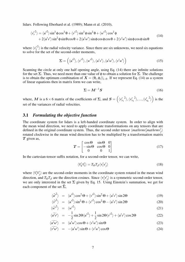
lidars. Following Eberhard et al. (1989); Mann et al. (2010),
〈v′r2〉= 〈u′2〉sin2 φcos2 θ+ 〈v′2〉sin2 φsin2 θ+ 〈w′2〉cos2 φ+2〈u′v′〉sin2 φsinθcosθ+2〈u′w′〉sinφcosφcosθ+2〈v′w′〉sinφcosφsinθ
(14)
where 〈v′r2〉 is the radial velocity variance. Since there are six unknowns, we need six equationsto solve for the set of the second-order moments,
Σ=(〈u′2〉,〈v′2〉,〈w′2〉,〈u′v′〉,〈u′w′〉,〈v′w′〉
)(15)
Scanning the circle at only one half opening angle, using Eq. (14) there are infinite solutionsfor the set Σ. Thus, we need more than one value of φ to obtain a solution for Σ. The challengeis to obtain the optimum combination of X = (θi,φi)|i..6. If we represent Eq. (14) as a systemof linear equations then in matrix form we can write,
Σ=M−1S (16)
where, M is a 6× 6 matrix of the coefficients of Σ, and S =(〈v′r1
2〉,〈v′r2
2〉, ...,〈v′r6
2〉)
is the
set of the variances of radial velocities.
3.1 Formulating the objective functionThe coordinate system for lidars is a left-handed coordinate system. In order to align withthe mean wind direction, we need to apply coordinate transformations on any tensors that aredefined in the original coordinate system. Thus, the second order tensor 〈mathrmv′imathrmv′j〉rotated clockwise in the mean wind direction has to be multiplied by a transformation matrixT given as,
T =
[cosΘ sinΘ 0−sinΘ cosΘ 0
0 0 1
](17)
In the cartesian-tensor suffix notation, for a second-order tensor, we can write,
〈v′kv′l〉= TikTjl〈v′iv′j〉 (18)
where 〈v′iv′j〉 are the second-order moments in the coordinate system rotated in the mean wind
direction, and TikTjl are the direction cosines. Since 〈v′iv′j〉 is a symmetric second-order tensor,
we are only interested in the set Σ given by Eq. 15. Using Einstein’s summation, we get for
each component of the set Σ,
〈u′2〉 = 〈u′2〉cos2 Θ+ 〈v′2〉sin2 Θ+ 〈u′v′〉sin2Θ (19)
〈v′2〉 = 〈u′2〉sin2 Θ+ 〈v′2〉cos2 Θ−〈u′v′〉sin2Θ (20)
〈w′2〉 = 〈w′2〉 (21)
〈u′v′〉 = −1
2sin2Θ〈u′2〉+ 1
2sin2Θ〈v′2〉+ 〈u′v′〉cos2Θ (22)
〈u′w′〉 = 〈u′w′〉cosΘ+ 〈v′w′〉sinΘ (23)
〈v′w′〉 = −〈u′w′〉sinΘ+ 〈v′w′〉cosΘ (24)
7
134

where Σ =(〈u′2〉,〈v′2〉,〈w′2〉,〈u′v′〉,〈u′w′〉,〈v′w′〉
)is the set of second-order moments in the
coordinate system rotated in the mean wind direction. In matrix form, Eqs. (19–24) can bewritten as,⎡⎢⎢⎢⎢⎢⎢⎢⎢⎣
〈u′2〉〈v′2〉〈w′2〉〈u′v′〉〈u′w′〉〈v′w′〉
⎤⎥⎥⎥⎥⎥⎥⎥⎥⎦=
⎡⎢⎢⎢⎢⎢⎢⎣cos2 Θ sin2 Θ 0 sin2Θ 0 0
sin2 Θ cos2 Θ 0 −sin2Θ 0 00 0 1 0 0 0
−12 sin2Θ 1
2 sin2Θ 0 cos2Θ 0 00 0 0 0 cosΘ sinΘ0 0 0 0 −sinΘ cosΘ
⎤⎥⎥⎥⎥⎥⎥⎦
⎡⎢⎢⎢⎢⎢⎢⎣〈u′2〉〈v′2〉〈w′2〉〈u′v′〉〈u′w′〉〈v′w′〉
⎤⎥⎥⎥⎥⎥⎥⎦ (25)
Σ = RΣ (26)
where R is the transformation matrix to be applied on the set Σ to obtain Σ in the rotatedcoordinate system. Using Eq. (16), we can write,
δΣ=RM−1δS (27)
where δΣ and δS are the random errors in the second-order moments and radial velocityvariances respectively. Following lengthy manipulations, we get
〈δΣ ·δΣ〉〈ε2
s 〉= Tr(RN(RN)T ) (28)
where N = M−1, Tr denotes trace of a matrix, T denotes matrix transpose, and 〈ε2s 〉 is the error
variance of the radial velocities. In deriving Eq. (28) we have assumed that the error variance ofthe radial velocity is equal for all six beams. Eq. (28) states that the error variance is dependenton the mean wind direction. In order to make it independent of the mean wind direction, weassume a uniform distribution of the mean wind direction, and estimate the averaged ratio ofthe error variance. Thus,⟨
〈δΣ ·δΣ〉〈ε2
s 〉
⟩=
1
2π
∫ 2π
0Tr(RN(RN)T )dΘ
=1
2π
∫ 2π
0Tr(RNNTRT )dΘ
Using the property of matrix trace that it is invariant under cyclic permutations we get,⟨〈δΣ ·δΣ〉〈ε2
s 〉
⟩=
1
2π
∫ 2π
0Tr(RTRNNT )dΘ (29)
We can also switch the order between integration and matrix trace, i.e. either we can estimatethe trace first and then the integration or vice-versa. Thus,⟨
〈δΣ ·δΣ〉〈ε2
s 〉
⟩= Tr([
1
2π
∫ 2π
0RTRdΘ
]NNT)
(30)
Solving the integral we get,
⟨〈δΣ ·δΣ〉〈ε2
s 〉
⟩= Tr
⎛⎜⎜⎜⎜⎜⎝
⎡⎢⎢⎢⎢⎢⎣78
18 0 0 0 0
18
78 0 0 0 0
0 0 1 0 0 0
0 0 0 32 0 0
0 0 0 0 1 00 0 0 0 0 1
⎤⎥⎥⎥⎥⎥⎦NNT
⎞⎟⎟⎟⎟⎟⎠ (31)
8
135

3.2 Optimizing the objective functionFrom (Eq. 31), it is clear that we need to optimize for 12 variables, i.e. a set X = (θi,φi)|i=1..6.The constraints constitute the range of angles of θi and φi. Thus, the optimization problem canbe stated as follows:
Minimize f (X) = Tr
⎛⎜⎜⎜⎜⎜⎝
⎡⎢⎢⎢⎢⎢⎣78
18 0 0 0 0
18
78 0 0 0 0
0 0 1 0 0 0
0 0 0 32 0 0
0 0 0 0 1 00 0 0 0 0 1
⎤⎥⎥⎥⎥⎥⎦NNT
⎞⎟⎟⎟⎟⎟⎠subject to constraints,
0◦ ≤ θi|i=1..6 ≤ 360◦
0◦ ≤ φi|i=1..6 ≤ 45◦
(32)
We assume that statistical homogeneity in the horizontal direction is valid only for a maximumvalue of φi = 45◦. Analytical optimization of Eq. (32) provides a unique design solution set X .However, Eq. (32) is a very complicated optimization problem, and hence, analytical solutionis not possible1. In that case, the simplest method is to solve Eq. (32) for different combinationsof X . However, this would need very large number of computations. E.g. if we assume thatX take only integer values, the number of computations required are 3606× 906 ≈ O(1027).It is observed that one computation of f (X) takes approximately 0.5 seconds. Thus 1027
computations need approximately 1017 years. Moreover, if X also take real values then thenumber of computations, and hence, the time required increase manyfold. Thus, with thecurrent available computer resources it is seen that evaluating f (X) by directly substituting fordifferent sets of X is not possible. We are thus forced to use available numerical optimizationtechniques.
There are two classes of numerical methods to solve a non-linear optimization problem Rao(2009):
1. Direct search methods
2. Gradient methods
For gradient methods, it is essential that the objective function is differentiable, and ∇ f isdefined at all points, i.e. f (X) is not discontinuous Rao (2009). For simplicity we assume thatf (X) is discontinuous, and hence, we cannot use gradient methods. Thus, we optimize Eq.(32) using direct search methods only. The main advantage of using direct search methods isthat they can be used for discontinuous and non-differentiable functions. The main limitationof such methods is that the found optimum may only be a local optimum.
In principle, any direct search algorithm can be used to find an optimum solution. It isgenerally very cumbersome to write algorithms for all available methods, and hence, we use thealready available algorithms in Mathematica. For a global optimization problem, four differentalgorithms are available in Mathematica:
1. Simplex (NM) Nelder and Mead (1965)
2. Differential Evolution (DE) Storn and Price (1997)
3. Simulated Annealing (SA) Ingber (1993)
4. Random Search (RS) Rao (2009)
Eventually, we have to choose a solution set from one of these algorithms.
1Corresponding attempt is made in Mathematica
9
136

Table 1: Comparison of the optimization methods
Optimization Methods
Nelder-Mead Differential Evolution Simulated Annealing Random Search
〈δΣ ·δΣ〉/〈ε2s 〉 10.2 11.78 10.2 10.2
i θi φi θi φi θi φi θi φi1 0 45 0 44.9999 0 45 0 45
2 284.451 1.087e-7 109.771 0.00087255 72 45 216 45
3 144 45 233.185 43.8284 297.23 6.8733e-6 143.035 6.6121e-15
4 288 45 310.453 44.9993 216 45 144 45
5 72 45 144.495 44.9333 288 45 72 45
6 216 45 89.3294 44.9993 144 45 288 45
Table 1 gives a comparison of different optimization methods, when X is constrained totake real values. It is observed that the NM, SA and RS methods give the same optimumf (X∗). The DE method gives a slightly higher value of the optimum. X is evaluated tomachine precision. However, in reality it is difficult to orient the laser beam at such preciseangles φi. Hence, we rounded X∗ to the nearest integer values and checked its influence onf (X∗). We found that there is no influence of rounding of X∗ on f (X∗).
3.3 ResultsFollowing section 2 we can estimate the second-order moments using the six beam approach.We choose X from the SA method. Since the NM and RS methods also give the same optimumsolution, X could also be chosen from these methods. From Eq. (27) the u variance can bewritten as,
〈u′2〉= 〈v′2r1〉−〈v′2r3
〉−0.085(〈v′2r2
〉+ 〈v′2r5〉)+0.585
(〈v′2r4
〉+ 〈v′2r6〉)
(33)
Following section 2 we get,
〈v′2r1〉=
∫Φi j(k)βi1(k)β∗j1(k)dk (34)
where βi1(k) =(∫ ∞−∞ ϕ(s)ni1ei(s+d f )k·n1ds
)and ∗ denotes complex conjugation. We can then
use appropriate weighting function ϕ(s) to estimate βi1(k). We can estimate the variances ofthe radial velocities in the remaining beam directions in a similar manner and substitute in Eq.(33) to theoretically estimate the u variance measured by the lidar. The remaining second-ordermoments are estimated in a similar manner.
Fig. (3) shows theoretical comparison of the systematic errors using the six beam approachwith that using the VAD technique. Although the results are obtained for all stability conditions,only the neutral conditions are shown. One striking difference between two approaches is thatthe systematic error in the w variance is reduced significantly using the six beam approach. Forthe ZephIR, the systematic errors in u and v variances are the same for both approaches. For theWindcube, a significant improvement is obtained for all variances using the six beam approach.Although, fig. (3b) shows that the VAD technique gives lower systematic error, it is mainly dueto the addition and subtraction of all second-order moments. This effect is less observed usingthe six beam approach. The only form of filtering that remains is the line-of-sight averaging.It has been observed that the Windcube systematic errors remain constant for the neutral andunstable conditions (not shown) using the six beam approach. Such is not the case with theVAD technique, where there is an over estimation of the variances.
3.4 Future workThe theoretical estimations using the six beam approach will be compared with the measure-ments. Currently, the experiment is ongoing to measure the second-order moments using the
10
137

0 0.5 1 1.50
20
40
60
80
100
120
140
160
〈u′iu
′j〉QQ/〈u′
iu′j〉
Height(m
)
neutral
〈u′2〉6 beam
〈v′2〉6 beam
〈w′2〉6 beam
〈u′2〉conical〈v′2〉conical〈w′2〉conical
(a) ZephIR
0 0.2 0.4 0.6 0.8 1 1.2 1.4 1.6 1.8 20
20
40
60
80
100
120
140
160
〈u′iu
′j〉WC/〈u′
iu′j〉
Height(m
)
neutral
〈u′2〉6 beam
〈v′2〉6 beam
〈w′2〉6 beam
(b) Windcube
Figure 3: Comparison of the ZephIR and Windcube systematic errors under neutral conditions
using the six Beam approach and the VAD technique
windscanner developed at Risø DTU. Subsequently, following Mann et al. (2010) a spatial filtermodel that negates the line-of-sight averaging will be used, which in principle will completelyget rid of any filtering of the turbulence.
4 CONCLUSION
Two approaches have been investigated to measure turbulence. Using the VAD technique itis clear that the systematic errors of the second-order moments are quite large, and hence,the ZephIR and WindCube cannot be used to measure turbulence precisely. Using the sixbeam approach, the theoretical results look promising for the Windcube, whereas there is noimprovement for the ZephIR. A final conclusion can only be derived once the measurementsare compared with the theoretical results.
ACKNOWLEDGEMENTS
This study is a part of the PhD project under the We@Sea program, BISK-03041, and spon-sored by the Dutch Ministry of Economic affairs. The experimental results are all based ondata collected at the Høvsøre Test Station under the watchful eyes of Anders Ramsing Vester-gaard and Bjarne Sønderskov. Our thanks to them for their highly professional and good-humoured assistance. This paper has been prepared using resources provided by the EU FP6UpWind project (Project reference 019945 SES6) and by the Center for computational windturbine aerodynamics and atmospheric turbulence funded by the Danish Council for StrategicResearch grant no. 09-067216.We also acknowledge funding for this work under the EuropeanCommissions FP7 SafeWind Project, Grant Agreement no. 213740.
References
Banakh, V. A., Smalikho, I. N., Kopp, F., and Werner, C. (1995). Representativeness of wind measurements witha CW Doppler lidar in the atmospheric boundary layer. Applied optics, 34(12):2055–2067.
Banta, R. M., Newsom, R. K., Lundquist, J. K., Pichugina, Y. L., Coulter, R. L., and Mahrt, L. (2002). Nocturnallow-level jet characteristics over Kansas during CASES-99. Boundary-Layer Meteorology, 105:221–252.
11
138

Browning, K. A. and Wexler, R. (1968). The determination of kinematic properties of a wind field using a Dopplerradar. Journal of Applied Meteorology, 7:105–113.
Citriniti, J. H. and George, W. K. (1997). The reduction of spatial aliasing by long hot-wire anemometer probes.Experiments in Fluids, 23:217–224.
Eberhard, W. L., Cupp, R. E., and Healy, K. R. (1989). Doppler lidar measurements of profiles of turbulence andmomentum flux. Journal of Atmospheric and Oceanic Technology, 6:809–819.
Emeis, S., Harris, M., and Banta, R. M. (2007). Boundary-layer anemometry by optical remote sensing for windenergy applications. Meteorologische Zeitschrift, 16(4):337–347.
Engelbart, D. A. M., Kallistratova, M., and Kouznetsov, R. (2007). Determination of the turbulent fluxes ofheat and momentum in the ABL by ground-based remote-sensing techniques (a review). MeteorologischeZeitschrift, 16(4):325–335.
Gal-Chen, T., Xu, M., and Eberhard, W. L. (1992). Estimation of atmospheric boundary layer fluxes and otherturbulence parameters from Doppler lidar data. Journal of Geophysical Research, 97(D17):18,409–18,423.
Ingber, L. (1993). Simulated annealing: Practice versus theory. Mathematical Computer Modelling, 18(11):29–57.
Kindler, D., Oldroyd, A., Macaskill, A., and Finch, D. (2007). An eight month test campaign of the QinetiQZephIR system: Preliminary results. Meteorologische Zeitschrift, 16(5):479–489.
Kropfli, R. A. (1986). Single Doppler radar measurement of turbulence profiles in the convective boundary layer.Journal of Atmospheric and Oceanic Technology, 3:305–314.
Lenschow, D. H., Mann, J., and Kristensen, L. (1994). How long is long enough when measuring fluxes and otherturbulence statistics? Journal of Atmospheric and Oceanic Technology, 11:661–673.
Lindelow, P. (2007). Fibre Based Coherent Lidars for Remote Wind Sensing. PhD thesis, Technical UniversityDenmark.
Mann, J. (1994). The spatial structure of neutral atmospheric surface-layer turbulence. Journal of Fluid Mechan-ics, 273:141–168.
Mann, J., Cariou, J., Courtney, M., Parmentier, R., Mikkelsen, T., Wagner, R., Lindelow, P., Sjoholm, M., andEnevoldsen, K. (2009). Comparison of 3D turbulence measurements using three staring wind lidars and asonic anemometer. Meteorologische Zeitschrift, 18(2, Sp. Iss. SI):135–140.
Mann, J., Pena, A., Bingol, F., Wagner, R., and Courtney, M. S. (2010). Lidar scanning of momentumflux in and above the surface layer. Journal of Atmospheric and Oceanic Technology, 27(6):792–806.DOI:10.1175/2010JTECHA1389.1.
Monin, A. S. and Yaglom, A. M. (1975). Statistical Fluid Mechanics, volume 2. MIT Press.
Nelder, J. A. and Mead, R. (1965). A simplex method for function minimization. The computer Journal, 7:308–313.
Pena, A., Gryning, S.-E., and Mann, J. (2010). On the length scale of the wind profile. Quarterly Journal of theRoyal Meteorological Society, 136(653):2119–2131.
Pena, A., Hasager, C. B., Gryning, S.-E., Courtney, M., Antoniou, I., and Mikkelsen, T. (2009). Offshore windprofiling using light detection and ranging measurements. Wind Energy, 12(2):105–124.
Pichugina, Y. L., Banta, R. M., Kelly, N. D., Jonkman, B. J., Tucker, S. C., Newsom, R. K., and Brewer, W. A.(2008). Horizontal-velocity and variance measurements in the stable boundary layer using Doppler lidar:Sensitivity to averaging procedures. Journal of Atmospheric and Oceanic Technology, 25:1307–1327.
Rao, S. (2009). Engineering Optimization: Theory and Practice. John Wiley and Sons Inc., Hoboken, New Jersey,fourth edition.
Sathe, A., Mann, J., Gottschall, J., and Courtney, M. S. (2011). Can wind lidars measure turbulence? Journal ofAtmospheric and Oceanic Technology, 28(7):853–868.
12
139

Sjoholm, M., Mikkelsen, T., Mann, J., Enevoldsen, K., and Courtney, M. (2009). Spatial averaging-effects onturbulence measured by a continuous-wave coherent lidar. Meteorologische Zeitschrift, 18(3, Sp. Iss. SI):281–287.
Smalikho, I., Kopp, F., and Rahm, S. (2005). Measurement of atmospheric turbulence by 2-μm Doppler lidar.Journal of Atmospheric and Oceanic Technology, 22(11):1733–1747.
Smith, D. A., Harris, M., Coffey, A. S., Mikkelsen, T., Jørgensen, H. E., Mann, J., and Danielian, R. (2006). Windlidar evaluation at the Danish wind test site in Høvsøre. Wind Energy, 9:87–93.
Sonnenschein, C. M. and Horrigan, F. A. (1971). Signal-to-noise relationships for coaxial systems that heterodynebackscatter from atmosphere. Applied optics, 10(7):1600.
Storn, R. and Price, K. (1997). Differential evolution a simple and efficient heuristic for global optimization overcontinuous spaces. Journal of Global Optimization, 11(4):341–359.
Wagner, R., Mikkelsen, T., and Courtney, M. (2009). Investigation of turbulence measurements with a continuouswave, conically scanning lidar. Technical Report Risø-R-1682(EN), Risø DTU.
Wilson, D. A. (1970). Doppler radar studies of boundary layer wind profiles and turbulence in snow conditions.In Proc. 14th Conf. on Radar Meteorology, pages 191–196.
Wyngaard, J. C. (1968). Measurement of small-scale turbulence structure with hot wires. Journal of ScientificInstruments, 1:1105–1108.
13
140

Chapter 8
Conclusions and future work
8.1 Conclusions
Broadly speaking the original goal at the start of this PhD project was to somehowmake use of the measurements in analyzing wind turbine loads at an offshore site. Ifwe consider what has been achieved, there has been some digression, mainly due tothe opportunities that have been provided to perform research in other interestingtopics. In particular research has been carried out in wind profiles, turbulence, windturbine loads, and measurement of turbulence using wind lidars. The conclusions arebased on the answers to the research questions that were posed in section 1.1. Atfirst an overall conclusion is formulated. Then each question is tackled individuallyand conclusions are drawn accordingly.
8.1.1 Overall conclusions
It is important to quantify the wind conditions as accurately as possible from theperspective of wind turbine loads. This is clearly evident when we compare the loadsobtained using the IEC [2005a] defined wind conditions and those obtained usingsite-specific wind conditions. Especially, the quantification of the wind profiles andturbulence should be carried out as accurately as possible since they have a directinfluence on the fatigue loads. A more physical logarithmic wind shear with a diabaticcorrection term that is valid for the entire boundary layer should be used instead ofthe power law with a shear exponent as suggested in the IEC [2005a] standard. Thedescription of the Mann [1994] model parameters in quantifying turbulence should alsobe site-specific. The IEC [2005a] standard assumes that LM and Γ do not changewith the mean wind speed, whereas observations at Høvsøre indicate the contrary.The αε2/3 parameter according to the IEC [2005a] standard is about 4.5 to 1.5 timeslarger than that observed at Høvsøre. This causes the level of turbulence to increasesignificantly when the IEC [2005a] standard is used as compared to the site-specificturbulence. The use of diabatic wind conditions as input in load calculations isimportant for the tower and rotor loads. However, more investigations are necessaryto consolidate the understanding.
125
141

The use of site-specific wind conditions in load calculations require measurements.Remote-sensing devices like lidars have the potential to measure turbulence, and inthe past have already been proven to measure the mean wind profiles with suffi-cient accuracy. Using the VAD scanning method, lidars cannot measure turbulenceprecisely. It is unwise to use a simple transfer function in order to correct for the sys-tematic errors in the turbulence statistics measured by lidars, primarily because thedistribution of the energy with respect to the wavenumbers is completely different incomparison to what is actually observed in the nature. New methods are required tomeasure turbulence using lidars, and the six-beam approach has the potential to re-duce the systematic errors in the measurements. If lidars are demonstrated to measureturbulence precisely in comparison to the sonic anemometers then it has the potentialto displace traditional meteorological mast anemometry, and potentially change thecurrent methods of wind turbine design.
8.1.2 Specific conclusions
How are diabatic wind profiles characterized?
The diabatic wind profiles are characterized using two different wind profile mod-els. Under stable conditions the model that is strictly valid for the surface layerover-predicts the wind shear significantly (particularly at greater heights) as com-pared to the Gryning et al. [2007] model that is valid for the entire boundary layer.This because for the surface-layer wind profile model the length scale increases infin-itely with height. This is a reasonable assumption in the surface layer but is certainlynot true for the entire boundary layer [Blackadar, 1962]. The boundary-layer heightparameter zi introduced in the Gryning et al. [2007] model restricts the growth ofthe length scale beyond the surface layer, which results in achieving good agreementbetween the model and the measurements at all heights. For unstable conditions bothmodels agree well with the measurements, also observed in an independent study byPena et al. [2008]. Under unstable conditions zi is much larger than that under stableconditions, and consequently the surface layer also extends to greater heights. Hence,surface-layer similarity theory is more applicable under these conditions resulting ingood agreement of the models and the measurements. Thus we do not need to includezi parameter in the models under unstable conditions, also observed independentlyby Pena et al. [2008].
Are wind turbine loads influenced by atmospheric stability?
When diabatic wind profiles are used under steady wind conditions in the load calcu-lations, fatigue loads at the blade root are increased significantly as compared to thoseobtained by assuming neutral conditions only. This is a result of increased wind shearunder stable conditions, and has a direct influence on fatigue damage. Atmosphericstability distribution thus becomes very important. A stable site will induce moreloads as compared to unstable sites.
When diabatic wind conditions are used in load calculations the tower loads aremainly influenced by diabatic turbulence, whereas the rotor loads are influenced by
142

diabatic wind profiles. The blade loads are influenced by both, diabatic wind profileand turbulence, that leads to averaging of the loads, i.e. the calculated loads usingthe diabatic wind conditions are approximately the same as those obtained assumingneutral wind conditions. The distribution of atmospheric stability is quite importantin calculating fatigue loads. For a very stable site the calculated tower loads usingdiabatic wind conditions will decrease significantly, whereas those for the rotor loadswill increase. The choice of a wind profile model will also influence the rotor loadssignificantly. E.g. a surface-layer wind profile model will predict a larger wind shearunder stable conditions as compared to the boundary-layer wind profile model, andhence predict larger rotor loads as compared to those obtained using the boundary-layer wind profile.
The IEC [2005a] standard is extremely conservative for calculating the wind tur-bine loads under normal power production cases. They predict loads which are up to95% larger than those obtained using diabatic input wind conditions.
Can wind lidars measure turbulence?
With the current measurement configuration that uses the VAD scanning techniqueto extract wind field components, lidars cannot measure turbulence precisely. Twomechanisms contribute to imprecise turbulence measurements by lidars. One is theaveraging effect of turbulence due to a large sample volume in which lidars meas-ure wind speeds. The second is the contribution of all components of the Reynoldsstress tensor in the measurement of turbulence that arises due to combining differentlidar beams. The systematic errors behave differently for continuous-wave and pulsedlidars. For pulsed lidars the errors are dependent on wind direction and averagingeffect reduces with height due to constant length of the sample volume, whereas fora continuous-wave lidar the averaging effect increases with height since the length ofthe sample volume increases quadratically with height. The systematic errors due tothe averaging effect are also influenced by atmospheric stability. Under stable cond-itons turbulence length scales are smaller. This results in larger volume averaging incomparison to unstable conditions.
How do pulsed wind lidars measure turbulence spectra?
Approximately in the inertial sub-range there is a complete attenuation of turbu-lent energy, primarily because of the averaging effect in the large sample volume.Close to the inertial sub-range and low frequencies there is a redistribution of theturbulent energy. One of the reasons for this redistribution is the contribution ofall components of the Reynolds stress tensor. It is clearly evident that even if theReynolds stress tensor measured by lidars agrees quite well with that measured bysonics, at least for wind turbine applications it is not recommended to use lidars forturbulence measurements. This is because for wind turbines apart from the Reynoldsstress tensor the distribution of energy at various frequencies is also quite important,and evidently the turbulence spectra measured by lidars does not correspond to thatobserved in the nature.
143

How would it be possible for wind lidars to measure turbulence?
In principle if we directly use the variances of radial velocity then we can elimin-ate the systematic errors due to cross-contamination by other components of theReynolds stress tensor, which requires six lidar beams. The only systematic errorsthat remain are due to the averaging effect in the large sample volume.
8.2 Recommendations for future work
Several ideas have sprung up as result of working on this PhD project. Each idea isa potential research topic of its own. They are listed as follows:
1. Friction velocity u∗ is an important parameter in many meteorological studies,particularly for wind profile and atmospheric turbulence. If we wish to model thewind profile that is valid in the entire boundary layer then we need an accurateestimate of u∗. Gryning et al. [2007] modelled the friction velocity that variedlinearly with height, but non-linear expressions for u∗ have also been suggested[Panofsky, 1973]. This will have significant influence on the wind profile modelsin the boundary layer. Thus more work is needed to model or measure u∗ profileaccurately in the boundary layer. Lidars can be used to measure u∗ profiles.
2. Modelling the wind profile for modern wind turbines must include zi, partic-ularly under stable conditions [Gryning et al., 2007, Pena et al., 2008, Satheet al., 2011a]. The best method to obtain zi is to directly measure it but isquite difficult and expensive. If zi is to be used in the wind profile models it isconvenient if we have some model of zi instead of having to measure it. Thereare lot of uncertainties in the modelling zi, particularly under diabatic condi-tions [Seibert et al., 2000]. Much work is needed to have a robust model forestimating zi.
3. The wind profile model by Gryning et al. [2007] uses the very uncertain resist-ance law constants A and B under diabatic conditions. In this PhD study Aand B vary only with the stability parameters. Zilitinkevich and Esau [2005]observed that A and B are functions of stability parameters, baroclinicity andboundary layer height. More experimental work is needed to verify the findings.
4. In chapter 4 we performed load simulations to investigate the influence of at-mospheric stability. As a next obvious step, comparison of the simulated andmeasured loads should be carried out.
5. A comparison of the load simulations under diabatic conditions should be madebetween onshore and offshore sites. It is well known that wind speeds at offshoresites are higher than at onshore sites. This affects the turbulent structure andconsequently will have an influence on the loads.
6. The 6-beam approach as described in chapter 7 has in principle the potentialto counter the challenges faced by the VAD technique. The theoretical resultsobtained in chapter 7 need to be verified using measurements. This requires
144

significant hardware changes to the existing lidar technology.
7. From Mann et al. [2009] it is observed that at small turbulence scales the radialvelocity spectra measured by lidars coincide with that measured by a sonic an-emometer. This means that at large turbulence scales the averaging effect dueto lidar sampling volume and the influence of the contamination by the cross-components is negligible. There is thus a potential to fit a three-dimensionalspectral tensor model, e.g. [Mann, 1994] to only the low frequency part anddeduce the entire turbulent structure. We can thus make use of lidar measure-ments and turbulence spectral tensor models to measure turbulence.
8. The model of the turbulence spectra as measured by a pulsed wind lidar inchapter 6 is in principle only valid when the mean wind direction is alignedwith the measurement beams. As an obvious next step this model should beextended to arbitrary wind directions.
9. The model in chapter 6 was derived with a view to modelling gusts as measuredby lidars, since the gust factor is a function of turbulence spectral moments.A detailed gust modelling should be carried out using the model developed inchapter 6 in order to understand theoretically how lidars measure gusts.
10. In chapters 5 – 7, for theoretically modelling the turbulence as measured by lid-ars we used the Mann [1994] model under all atmospheric stabilities. However,the Mann [1994] model is strictly valid only under neutral conditions. Bar-ring the model by Hanazaki and Hunt [2004], which is valid only under stableconditions there is no diabatic spectral tensor model of turbulence. A diabaticthree-dimensional turbulent structure model is thus required.
145

146

Appendix A
Appendices
A.1 Uncertainty analysis of Obukhov length
L is estimated using the Rib method Grachev and Fairall [1996],
L =
⎧⎪⎨⎪⎩z
10Ribfor L < 0;
z(1−5Rib)10Rib
for L > 0.
(A.1)
Mathematically, Rib is given as,
Rib =−gz(Tvsea − θv)
θvu2(A.2)
where Tvsea is the virtual temperature at the sea surface. θv is defined as,
θv = Tv
(P0
P
)(RairCp
)
(A.3)
where P is the air pressure at z, Tv is the virtual temperature of air at z, P0 is thereference air pressure, Rair is the gas constant for dry air, and Cp is the specific heatat constant pressure. Tv is defined as,
Tv =T
1− esRHP (1− εa)
(A.4)
where RH and es are the relative humidity and saturation vapour pressure at z,and εa is the ratio of the gas constant of dry air to moist air. Tvsea is obtained bysubstituting T by SST, RH by RHsea, es by essea, and P by P0 in Eq. A.4. es isestimated following Flatau et al. [1992],
es = 6.1117675 + 0.443986062T + 1.43053301× 10⁻²T 2
+ 2.65027242× 10⁻⁴T 3 + 3.02246994× 10⁻⁶T 4
+ 2.03886313× 10⁻⁸T 5 + 6.38780966× 10⁻¹¹T 6
(A.5)
131
147

essea is estimated by substituting T by SST in Eq. A.5. P is defined as,
P = P0 exp
(−Mgz
RT
)(A.6)
where M is the molar mass of air and R is the universal gas constant. Table A.1gives the values of the constants that are used in this analysis. From Eqs. A.1–A.6
Table A.1: Constants used in the uncertainty analysis
g = 9.81 m/s2
Cp = 1005 J/kg-Kεa = 0.622z = 21 m
P0 = 1.01325× 10⁵ N/m2
M = 0.02896 kg/molR = 8.314 J/mol-KRair = 287 J/kg-KRHsea = 100%
and table A.1, it is clear that
L = f(T, Tsea, RH, u) (A.7)
where f() denotes a function. Since L is a function of multiple variables, using thelaw of propagation of uncertainty ISO [1995],
uc(L) =
N∑i=1
(∂L
∂Xi
)2ui(Xi)
2 +
N−1∑i=1
N∑j=i+1
∂L
∂Xi
∂L
∂XjXiXj (A.8)
where uc(L) is the combined uncertainty in the estimation of L, N are the numberof variables (equal to 4 in this analysis), Xi are the variables (T, Tsea, RH, u), ∂/∂Xi
denotes the partial derivative with respect to Xi, ui(Xi) is the standard individualuncertainty of Xi and XiXj is the covariance of Xi and Xj . Since the high frequencyraw measurements of Xi are unavailable, we assume that they are uncorrelated, andhence, the second term in Eq. A.8 vanishes. Thus,
uc(L) =N∑i=1
(∂L
∂Xi
)2ui(Xi)
2 (A.9)
Since 10-min mean measurements are used to estimate L, the partial derivatives areevaluated for each 10–min observation. Eq. A.1 is used to obtain partial derivatives forunstable and stable condition. ui(Xi) is obtained using a Type B evaluation, wherethe use of calibration reports is made. Table A.2 gives the standard uncertainties atOWEZ and Horns Rev,
Fig. A.1a and A.1b (top figure) show the combined uncertainty in the estimationof L. It is observed that uc(L) increases rapidly (top figure) as the difference in θvand Tvsea is reduced (middle figure), in accordance with Vincent et al. [2010]. Thus,
148
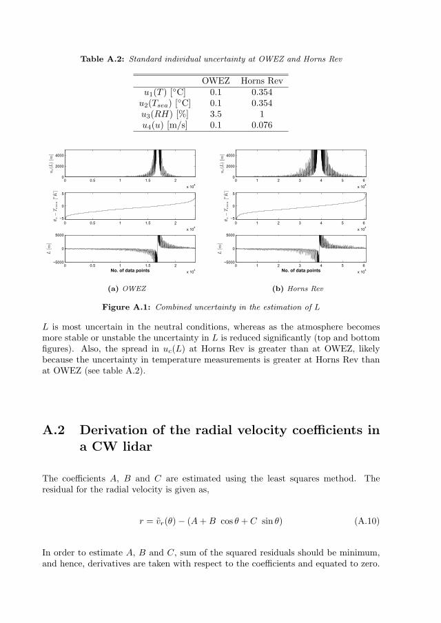
Table A.2: Standard individual uncertainty at OWEZ and Horns Rev
OWEZ Horns Revu1(T ) [
◦C] 0.1 0.354u2(Tsea) [
◦C] 0.1 0.354u3(RH) [%] 3.5 1u4(u) [m/s] 0.1 0.076
0 0.5 1 1.5 2
x 104
0
2000
4000
uc(L
)[m
]
0 0.5 1 1.5 2
x 104
−5
0
5
θ v−Tvsea[◦K]
0 0.5 1 1.5 2
x 104
−5000
0
5000
No. of data points
L[m
]
(a) OWEZ
0 1 2 3 4 5 6
x 104
0
2000
4000
uc(L
)[m
]0 1 2 3 4 5 6
x 104
−5
0
5
θ v−Tvsea[◦K]
0 1 2 3 4 5 6
x 104
−5000
0
5000
No. of data points
L[m
]
(b) Horns Rev
Figure A.1: Combined uncertainty in the estimation of L
L is most uncertain in the neutral conditions, whereas as the atmosphere becomesmore stable or unstable the uncertainty in L is reduced significantly (top and bottomfigures). Also, the spread in uc(L) at Horns Rev is greater than at OWEZ, likelybecause the uncertainty in temperature measurements is greater at Horns Rev thanat OWEZ (see table A.2).
A.2 Derivation of the radial velocity coefficients ina CW lidar
The coefficients A, B and C are estimated using the least squares method. Theresidual for the radial velocity is given as,
r = vr(θ)− (A+B cos θ + C sin θ) (A.10)
In order to estimate A, B and C, sum of the squared residuals should be minimum,and hence, derivatives are taken with respect to the coefficients and equated to zero.
149

Thus,
∂r
∂A=
2π∑θ=0
−2[vr(θ)− (A+B cos θ + C sin θ)] = 0 (A.11)
∂r
∂B=
2π∑θ=0
−2 cos θ[vr(θ)− (A+B cos θ + C sin θ)] = 0 (A.12)
∂r
∂C=
2π∑θ=0
−2 sin θ[vr(θ)− (A+B cos θ + C sin θ)] = 0 (A.13)
Rearranging the above equations,
2π∑θ=0
vr(θ) = A
2π∑θ=0
+B
2π∑θ=0
cos θ + C
2π∑θ=0
sin θ (A.14)
2π∑θ=0
vr(θ) cos θ = A
2π∑θ=0
cos θ +B
2π∑θ=0
cos2 θ + C
2π∑θ=0
sin θ cos θ (A.15)
2π∑θ=0
vr(θ) sin θ = A
2π∑θ=0
sin θ +B
2π∑θ=0
cos θ sin θ + C
2π∑θ=0
sin2 θ (A.16)
Multiplying both sides by dθ and replacing the summation by integrals the aboveequations can be written as,∫ 2π
0
vr(θ) dθ = A
∫ 2π
0
dθ +B
∫ 2π
0
cos θ dθ + C
∫ 2π
0
sin θ dθ (A.17)∫ 2π
0
vr(θ) cos θ dθ = A
∫ 2π
0
cos θ dθ +B
∫ 2π
0
cos2 θ dθ
+ C
∫ 2π
0
sin θ cos θ dθ
(A.18)
∫ 2π
0
vr(θ) sin θ dθ = A
∫ 2π
0
sin θ dθ +B
∫ 2π
0
cos θ sin θ dθ
+ C
∫ 2π
0
sin2 θ dθ
(A.19)
To estimate the coefficients the integrals are estimated;∫ 2π0
cos2 θ dθ = π,∫ 2π0
sin θ cos θ dθ =
0,∫ 2π0
cos θ dθ = 0,∫ 2π0
sin2 θ dθ = π,∫ 2π0
sin θ dθ = 0 and∫ 2π0
dθ = 2π. Substitutingthe integrals in the above equation we get,
A =1
2π
∫ 2π
0
vr(θ) dθ (A.20)
B =1
π
∫ 2π
0
vr(θ) cos θ dθ (A.21)
C =1
π
∫ 2π
0
vr(θ) sin θ dθ (A.22)
150

Bibliography
A K. Blackadar. The vertical distribution of wind and turbulent exchange in a neutralatmosphere. Journal of Geophysical Research, 67(8):3095–3102, 1962. doi: {10.1029/JZ067i008p03095}.
T. Burton, D. Sharpe, N. Jenkins, and E. Bossanyi. Wind Energy Handbook. JohnWiley and Sons, LTD, 2001.
M. Courtney, R. Wagner, and P. Lindelow. Testing and comparison of lidars forprofile and turbulence measurements in wind energy. In J. Mann et al., editor, 14th
International Symposium for the Advancement of Boudary Layer Remote Sensing,volume 1 of IOP Conference Series Earth and Environmental Science, page 012021.IOP Publishing LTD., 2008. doi: 10.1088/1755-1315/1/1/012021.
A G. Davenport. The spectrum of horizntal gustiness near the ground in high winds.Quarterly Journal of the Royal Meteorological Society, 87:194–211, 1961.
W L. Eberhard, R E. Cupp, and K R. Healy. Doppler lidar measurements of profiles ofturbulence and momentum flux. Journal of Atmospheric and Oceanic Technology,6:809–819, 1989. doi: 10.1175/1520-0426(1989)006$〈$0809:DLMOPO$〉$2.0.CO;2.
P J. Flatau, R L. Walko, and W R. Cotton. Polynomial fits to saturation vapourpressure. Journal of Applied Meteorology, 31:1507–1513, 1992.
A A. Grachev and C W. Fairall. Dependence of the Monin-Obukhov stability para-meter on the bulk Richardson number over the ocean. Journal of Applied Meteor-ology, 36:406–414, 1996.
S-E. Gryning, E. Batchvarova, B. Brummer, H. Jørgensen, and S. Larsen. Onthe extension of the wind profile over homogeneous terrain beyond the sur-face layer. Boundary-Layer Meteorology, 124(2):251–268, 2007. doi: 10.1007/s10546-007-9166-9.
H. Hanazaki and J C R. Hunt. Structure of unsteady stably stratified turbulencewith mean shear. Journal of Fluid Mechanics, 507:1–42, 2004. doi: 10.1017/S0022112004007888.
IEC. IEC 61400-1. Wind turbines – Part 1: Design Requirements. 2005a.
IEC. IEC 61400-3. Offshore wind turbines-part 1: Design Requirements. 2005b.
135
151

ISO. Guide to the Expression of Uncertainty in Measurement. Technical report,International Organisation for Standardization, 1995.
J C. Kaimal, J C. Wyngaard, Y. Izumi, and O R. Cote. Spectral characteristics ofsurface-layer turbulence. Quarterly Journal of the Royal Meteorological Society, 98(417):563–589, 1972. doi: 10.1002/qj.49709841707.
H J. Kouwenhoven. User manual data files meteorological mast NoordzeeWind.NoordzeeWind, 2.0 edition, October 2007.
J. Mann. The spatial structure of neutral atmospheric surface-layer turbulence.Journal of Fluid Mechanics, 273:141–168, 1994. ISSN 0022-1120. doi: 10.1017/S0022112094001886.
J. Mann, J. Cariou, M. Courtney, R. Parmentier, T. Mikkelsen, R. Wagner, P. Linde-low, M. Sjoholm, and K. Enevoldsen. Comparison of 3D turbulence measurementsusing three staring wind lidars and a sonic anemometer. Meteorologische Zeitschrift,18(2, Sp. Iss. SI):135–140, 2009. doi: 10.1127/0941-2948/2009/0370.
J. Mann, A. Pena, F. Bingol, R. Wagner, and M S. Courtney. Lidar scanning ofmomentum flux in and above the surface layer. Journal of Atmospheric and OceanicTechnology, 27(6):792–806, 2010. doi: 10.1175/2010JTECHA1389.1.
A S. Monin and A M. Obukhov. Basic laws of turbulent mixing in the atmospherenear the ground. Tr. Akad. Nauk. SSR, Geofiz. Inst., 151:163–187, 1954.
Hans A. Panofsky. Workshop on Micrometeorology, chapter Tower Micrometeorology,pages 151–176. American Meteorological Society, 1973.
A. Pena, S-E. Gryning, and C B. Hasager. Measurement and modelling of the windspeed profile in the marine atmospheric boundary layer. Boundary-Layer Meteor-ology, 129(3):479–495, 2008. doi: 10.1007/s10546-008-9323-9.
A. Pena, C B. Hasager, S-E. Gryning, M. Courtney, I. Antoniou, and T. Mikkelsen.Offshore wind profiling using light detection and ranging measurements. WindEnergy, 12(2):105–124, 2009. doi: 10.1002/we.283.
L. Prandtl. Meteorologische Anwendung der Stromungslehre. Beitrage zur Physik derAtmosphare, 19:188–202, 1932.
S O. Rice. Mathematical analysis of random noise. Bell System Tech. J., 23(3):282–332, 1944.
S O. Rice. Mathematical analysis of random noise. Bell System Tech. J., 24(1):46–156, 1945.
A. Sathe and W. Bierbooms. The influence of different wind profiles due to varyingatmospheric stability on the fatigue life of wind turbines. In M O L. Hansen andK S. Hansen, editors, The Science of Making Torque from Wind, volume 75 ofJournal of Physics: Conference Series, pages 12056–12062, 2007. doi: 10.1088/1742-6596/75/1/012056.
152

A. Sathe and J. Mann. Measurement of turbulence spectra using scanning pulsedwind lidars. 2011. Submitted to Journal of Geophysical Research.
A. Sathe, S-E. Gryning, and A. Pena. Comparison of the atmospheric stability andwind profiles at two wind farm sites over a long marine fetch in the North Sea.Wind Energy, 14(6):767–780, 2011a. doi: 10.1002/we.456.
A. Sathe, J. Mann, T. Barlas, and W. Bierbooms. Influence of atmospheric stabilityon wind turbine loads. 2011b. Submitted to Wind Energy.
A. Sathe, J. Mann, J. Gottschall, and M S. Courtney. Can wind lidars measure tur-bulence? Journal of Atmospheric and Oceanic Technology, 28(7):853–868, 2011c.doi: 10.1175/JTECH-D-10-05004.1.
A. Sathe, J. Mann, J. Gottschall, and M S. Courtney. Can the available wind lidarsmeasure turbulence? In ICWE13 Scientific Proceedings, Amsterdam, The Nether-lands, 11-15 July 2011d.
P. Seibert, F. Beyrich, S-E. Gryning, S. Joffre, A. Rasmussen, and P. Tercier. Reviewand intercomparison of operational methods for the determination of the mixingheight. Atmospheric Environment, 34(7):1001–1027, 2000.
M. Sjoholm, T. Mikkelsen, J. Mann, K. Enevoldsen, and M. Courtney. Spatialaveraging-effects on turbulence measured by a continuous-wave coherent lidar. Met-eorologische Zeitschrift, 18(3, Sp. Iss. SI):281–287, 2009. doi: 10.1127/0941-2948/2009/0379.
D A. Smith, M. Harris, A S. Coffey, T. Mikkelsen, H E. Jørgensen, J. Mann, andR. Danielian. Wind lidar evaluation at the Danish wind test site in Høvsøre. WindEnergy, 9:87–93, 2006. doi: 10.1002/we.193.
C L. Vincent, P. Pinson, and G. Giebel. Wind fluctuations over the North Sea.International Journal of Climatology, 2010. doi: 10.1002/joc.2175.
T. von Karman. Progress in the statistical theory of turbulence. In Proceedings ofNational Academy of Sciences, USA, volume 34, pages 530–539. California Instituteof Technology, Pasadena, June 1948.
S S. Zilitinkevich and I N. Esau. Resistance and heat-transfer laws for stableand neutral planetary boundary layers: Old theory advanced and re-evaluated.Quarterly Journal of the Royal Meteorological Society, 131(609):1863–1892, 2005.doi: 10.1256/qj.04.143.
153

154

Curriculum-vitae
Ameya Sathe was born on 17th June 1981 in Mumbai, India.
He completed his Bachelor of Engineering degree in Mechanical engineering fromMumbai University in 2002. He then competed in the GATE entrance examination in2003 and secured admission for a Masters course in Hydrology at the Indian Instituteof Technology, Roorkee, India. During his Masters he was awarded the DAAD-IITscholarship to pursue his Masters thesis in University of Stuttgart, Germany. He fin-ished Master of Technology from IIT Roorkee in 2005 with highest grades. He thenworked at TATA consultancy services as assistant systems engineer until August 2006.
From October 2006, he began his PhD studies at Delft University of Technology,The Netherlands. During his PhD he closely collaborated with Risø DTU, Denmark,in the EU UPWIND project that concerned turbulence measurements using wind lid-ars. In October 2010 he ended his contract at TU Delft and started working at RisøDTU as a Research Assistant in the EU Safewind project. The goals of this projectcoincided very nicely with his PhD, where he continued working on lidar turbulencemeasurements. In November 2011, his research work culminated into a PhD thesis.
139
155


Het omslag is niet voorzien van lamineerfolie!The cover is not laminated!
Deze afdruk wordt gebruikt voor productie.This printout will be used for production


![elecciones universitarias - rector(a) y vicerrector(a) [2016-2020]](https://static.fdokumen.com/doc/165x107/6328175e6d480576770d993e/elecciones-universitarias-rectora-y-vicerrectora-2016-2020.jpg)