Contents lists available at ScienceDirect

Signal Processing

Signal Processing 99 (2014) 29–47

0165-16http://d

n CorrE-m1 ht

June 12

journal homepage: www.elsevier.com/locate/sigpro

Saliency based mass detection from screening mammograms

Praful Agrawal, Mayank Vatsa n, Richa SinghIIIT-Delhi, India

a r t i c l e i n f o

Article history:Received 24 June 2013Received in revised form28 November 2013Accepted 9 December 2013Available online 17 December 2013

Keywords:MammographySaliencyWavelet transform

84/$ - see front matter & 2013 Elsevier B.V.x.doi.org/10.1016/j.sigpro.2013.12.010

esponding author.ail address: mayank@iiitd.ac.in (M. Vatsa).tp://www.who.int/features/qa/15/en/index.h, 2013.

a b s t r a c t

Screening mammography has been successful in early detection of breast cancer, whichhas been one of the leading causes of death for women worldwide. Among commonlydetected symptoms on mammograms, mass detection is a challenging problem as the taskis affected by high complexity of breast tissues, the presence of pectoral muscles as wellas varying shape and size of masses. In this research, a novel framework is proposedwhich automatically detects mass(es) from mammogram(s) even in the presenceof pectoral muscles. The framework uses saliency based segmentation which does notrequire removal of pectoral muscles, if present. From segmented regions, differentfeatures are extracted followed by Support Vector Machine classification for massdetection. The experiments are performed using an existing experimental protocol onthe MIAS database and the results show that the proposed framework with saliency basedregion segmentation outperforms the state-of-art algorithms.

& 2013 Elsevier B.V. All rights reserved.

1. Introduction

For the past few decades, cancer has been a major cause ofdeaths worldwide. World Health Organization (WHO) haspredicted that the number of deaths due to cancer willincrease by 45% from 2007 to 2030. In 2030, new cases ofcancer are expected to reach 15.5 million from 11.3 millionreported in 2007.1 Detailed statistics from WHO show thatbreast cancer accounts for the maximum number of newlyreported cases and deaths caused due to cancer amongwomen worldwide. The symptoms of breast cancer can bedetected with the help of X-ray of breasts, termed as mammo-grams. Experts have suggested that the best possible cure forbreast cancer is the early prognosis of these symptoms.

With increasing awareness about the disease, thousandsof mammograms are captured annually in the screeningcenters. Even in most of the developed economies such asUSA and Europe, there is a mismatch between the number ofexperts available and the number that is required to analyzethe screening mammograms. Due to the lack of medical

All rights reserved.

tml, last accessed on

experts required to analyze the screening mammograms,scientists have realized the role of Computer Aided Detec-tion/Diagnosis systems to automate the diagnosis of screen-ing mammograms. Computer Aided Detection systems(CADe) are used to detect early symptoms from medicalimages and Computer Aided Diagnosis systems (CADx) areused to diagnose abnormal findings. Some studies [1–3]claim that the use of CAD systems has actually improvedthe diagnosis of breast cancer, however other experiments [4]do not agree with these results. Amid such varied results,scientists emphasize on using CAD systems as secondaryopinion for doctors.

For breast cancer prognosis, a CADe system detectsearly symptoms from screening mammograms. As shownin Fig. 1, the commonly detected symptoms on mammo-grams include

�

clustered micro-calcification, � mass, � architectural distortion, and � bilateral asymmetry.

Clustered micro-calcification is a very prominent symp-tom observed in new cases of breast cancer. As illust-

rated in Fig. 1, they appear as a group of white dots on a

Fig. 1. Sample images: (a) normal mammogram, (b) cluster of micro-calcification, (c) a part of mammogram containing mass, and (d) left and rightmammograms of the same patient showing a case of bilateral asymmetry. Source: MIAS Database [14].

Pectoral Muscles

Masses

Fig. 2. Pectoral muscles indicated on a MLO view mammogram contain-ing masses.

P. Agrawal et al. / Signal Processing 99 (2014) 29–4730

mammogram. A mass is defined as a space-occupyinglesion seen in more than one projection [5]. They vary insize and shape [6], and therefore are difficult to detect inmammograms. Fig. 1 illustrates a case with cancerousmass present in a mammogram. Architectural distortionand bilateral asymmetry are not very common symptomsand multiple images are required to detect these symp-toms. For example, architectural distortion can be detectedby comparing the screening mammograms capturedbefore and after the distortion is developed. Bilateralasymmetry corresponds to any significant difference inthe tissue structure between the two breasts (left andright). Fig. 1 shows a sample case of bilateral asymmetry.

Mammograms are generally captured from multipleviews to collect as much information as possible beforedetection/diagnosis. Some widely captured views areCarnio-caudal (CC) and Multi-lateral Oblique (MLO). A CCview mammogram is taken from above a horizontallycompressed breast and shows as much as possible theglandular tissue, the surrounding fatty tissue, and theoutermost edge of the chest muscle. On the other hand, aMLO view mammogram is captured from the side atan angle of a diagonally compressed breast thus allow-ing more of the breast tissue to be imaged as compared toother views. However, with this procedure, pectoral mus-cles also appear in MLO view mammograms. As shown inFig. 2, these pectoral muscles have high intensity values inthe mammogram and may be misinterpreted as mass.Therefore, algorithms generally involve removing the pec-toral muscles or a segmentation step to suppress pectoral

muscle region followed by detection of symptoms. Evenwith the availability of multiple views, only few automaticmammogram analysis algorithms combine information andperform case based analysis using multiple views simulta-neously [7]. Most of the algorithms consider and processeach view as an individual image.

Many sophisticated algorithms have been proposedto detect the symptoms from screening mammograms[8–10]. As shown in Fig. 1, there are multiple symptomsof breast cancer. While efficient algorithms for detection

Fig. 3. Sample of mass regions from the MIAS database [14].

P. Agrawal et al. / Signal Processing 99 (2014) 29–47 31

and diagnosis of micro-calcification exist [11], the same isnot true for masses [12]. Detection and diagnosis of massesin a mammogram are challenging problems due to thevarying size, shape, and appearance of masses as well asvarying tissue density (Fig. 3). Detection and diagnosiscorrespond to two different stages of the complete diag-nosis. Detection refers to finding the possible location(s) ofmass in the complete mammogram, while diagnosis is thefinal step of finding the exact boundaries of the masspresent and/or classify the segmented mass as benign ormalignant [6]. Even though there are algorithms that canaddress both the problems simultaneously, researchersgenerally try to solve them independently. Successfuldetection is crucial for meaningful diagnosis and therefore,in this research, we focus on mass detection from screen-ing mammograms.

1.1. Literature review

In the literature, several researchers have proposedalgorithms to detect masses in mammograms. Table 1summarizes some of the key contributions for massdetection. Vyborny and Giger [13] discussed the algo-rithms to detect abnormalities such as mass and micro-calcification from mammograms using CAD systems. Theyconcluded that for a fair comparison, the algorithmsshould be evaluated on a public database. However, in

the absence of any such database, existing algorithmscompare their results directly with the radiologist's assess-ment. In the same year, Mammographic Image AnalysisSociety [14] released a public database comprising 322digitally scanned film based mammograms. Later, anotherdatabase known as the Digital Database for ScreeningMammography (DDSM) [15] was published for researchpurpose. These databases and few others have helped theresearchers to identify and solve some key problemsassociated with the development of CAD systems forscreening mammograms. Cheng et al. [16] summarizedthe existing algorithms for one of the key challenges inscreening mammograms i.e, detection and classification ofmasses. They discussed the various steps involved in anautomated approach and the key processing algorithmsproposed in the literature for modeling these steps. Theyalso compared the results of different classifiers withradiologist's performance on the DDSM database. Tanget al. [5] analyzed the advent of CAD systems usingmammography in a more generic way and focused oncomputer aided detection of four major symptoms inscreening mammograms. A categorical review of existingalgorithms was presented and the authors suggested thatCAD systems could assist radiologists in validating theirassessment. They also suggested that further improvementis required if such systems are to be used in an indepen-dent manner. Oliver et al. [6], in their recent survey,

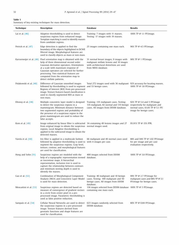
Table 1Summary of key existing techniques for mass detection.

Technique Description Database Results

Lai et al. [46] Adaptive thresholding is used to detectsuspicious regions from enhanced image.Template matching is used to identify massesfrom candidate regions.

Training: 7 images with 11 masses.Testing: 17 images with 19 masses.

100% TP @ 1.1 FP/image.

Petrick et al. [47] Edge detection is applied to find theboundary of the objects highlighted in DCWEfiltered image. Morphological features areused to classify objects as mass or non-mass.

25 images containing one mass each. 96% TP @ 4.5 FP/image.

Karssemeijer et al. [48] Pixel orientation map is obtained with thehelp of three dimensional second orderGaussian derivative operators. Orientationsat a scale with maximum response ofGaussian operators are selected for furtherprocessing. Two statistical features arecomputed from the orientation map todetect stellate patterns.

31 normal breast images, 9 images withmalignant stellate lesions and 10 imageswith architectural distortions are usedfrom MIAS database.

90% TP @ 1 FP/image.

Polakowski et al. [40] Difference of Gaussian smoothed imagesfollowed by thresholding is used to segmentRegions of Interest (ROI) from pre-processedimage. Texture features based classification isused to classify segmented ROI as mass ornon-mass.

Total 272 images used with 36 malignantand 53 benign cases.

92% accuracy for locating masses.100% TP @ 1.8 FP/image.

Eltonsy et al. [38] Multiple concentric layer model is designedto detect the suspicious regions in amammogram. Minimum distance betweentwo segmented regions and probability ofthe presence of a suspicious region in thegiven mammogram are used to reduce thefalse accepts.

Training: 135 malignant cases. Testing:135 malignant, 82 normal and 135 benigncases. All images from DDSM database.

92% TP @ 5.4 and 5 FP/imagerespectively for malignant andnormal cases, 61.6% TP @ 5.1 FP/image for benign cases.

Kom et al. [49] Image enhanced by linear filter is subtractedfrom original image to obtain the suspiciousregions. Local Adaptive thresholding isapplied to the subtracted image to obtain thedetected masses.

34 containing 49 lesions images and 27normal images used.

95.91% TP @ 15% FPR.

Varela et al. [50] Iris filter is applied in a multiscale fashionfollowed by adaptive thresholding is used tosegment the suspicious regions. Gray level,texture, contour, and morphological featuresare used for classification.

66 malignant and 49 normal cases usedwith 4 images per case.

88% and 94% TP @ 1.02 FP/imagefor per image and per caseevaluation respectively.

Hong and Sohn [51] Suspicious regions are modeled with thehelp of a topographic representation termedas isocontour maps. A hierarchialrepresentation, inclusion tree is used tocapture the relationship between contoursand minimum nesting depth is used toidentify the masses.

400 images selected from DDSMdatabase.

100% TP @ 3.8 FP/image.

Gao et al. [52] Combination of Morphological ComponentAnalysis (MCA) and Concentric Layer Modelis used for mass detection.

Training: 40 malignant and 10 benigncases. Testing: 100 malignant and 50benign cases. All images from DDSMdatabase.

99% TP @ 2.7 FP/image formalignant cases and 88% TP @ 3.1FP/image for benign cases.

Mencattini et al. [53] Suspicious regions are detected based onmeasure of convergence of gradient vectorsin a circle from center pixel in a pre-processed image. Parametric thresholding isused as false positive reduction.

136 images selected from DDSM databasecontaining one mass each.

100% TP @ 5 FP/image.

Sampaio et al. [54] Cellular Neural Networks are used to detectthe suspicious regions in a pre-processedimage. Texture features derived fromgeostatic functions and shape features areused for classification.

623 images randomly selected fromDDSM database.

80% TP @ 0.84 FP/image.

P. Agrawal et al. / Signal Processing 99 (2014) 29–4732

Fig. 4. Illustrating the steps involved in the proposed framework.

P. Agrawal et al. / Signal Processing 99 (2014) 29–47 33

analyzed existing algorithms according to various compu-ter vision paradigms used for segmentation of suspiciousregions and the features used to model the variations innormal and cancerous tissue patterns. They also comparedseven key mass detection approaches on a common set ofimages using one experimental protocol and observedthat, in general, the performance varies with shape andsize of masses as well as with the density of breast tissues.

Some commercial systems such as ImageChecker CAD2

and SecondLook Digital3 are also available and are nearlyaccurate in detecting micro-calcifications, however theaccuracies of mass detection require improvement [12].Based on our observation, following are the key challengesin designing an efficient mass detection algorithm:

�

Jun

tal.

Existing databases consist of noisy mammograms. Noisein mammograms is mainly due to the old film basedX-rays, such as mechanical noise in the image back-ground and certain irregularities such as tape markingsand occlusions. Therefore, mammogram analysis startswith an overhead step of image cleaning, which gen-erally involves masking out the breast region. However,this masking disrupts the natural texture on the outerboundary of breast region thereby creating a hard edge.Such hard edges can easily confuse the segmentationalgorithms. In order to develop more useful and efficientalgorithms, such unwanted hard edges on the breastboundary must be diluted before segmentation.

�

In mass detection algorithms, pectoral muscle segmen-tation is an important step as the presence of pectoralmuscles may increase false alarms generated by auto-matic segmentation algorithms [17]. Though severalresearchers have proposed dedicated pectoral musclesegmentation algorithms [17–21], it is still challengingto accurately segment these muscles when the tissuedensity around the muscles is high. Therefore, it isimportant to design more robust algorithms that do notrequire segmenting the pectoral muscle boundaries.

�

False positive reduction is used to remove the falselysegmented regions. Existing algorithms consider thesegmented Regions of Interest (ROI) as a single entityfor the false positive reduction step. Very often theseregions contain mass surrounded by normal tissueregions or mass present in different orientations. Suchregions can lead to ambiguity in feature values andtherefore reduce the performance.

�

Features are generally derived from the properties ofobjects present in an image such as texture, shape,

2 http://www.hologic.com/en/imagechecker-cad, last accessed one 12, 2013.3 http://www.icadmed.com/products/mammography/secondlookdigihtm, last accessed on June 12, 2013.

gradient, and intensity. Many such features have beenproposed/used for mass detection [6,16]. However, onlysubsets of these features have been used by researchersrepeatedly. There is no study that analyzes a compre-hensive feature space in a common framework anddetermine their effectiveness.

1.2. Research contribution

In this research, a framework for mass detection frommammograms is proposed which attempts to answer thekey issues in existing approaches as identified in theprevious subsection:

�

The pre-processing step in the proposed frameworkutilizes image blending to diffuse the hard edgesformed due to masking.

�

Visual saliency is proposed to segment probable masscontaining regions in a pre-processed mammogram.One of the key findings of the study is that the saliencybased segmentation is robust to the presence of pec-toral muscles.

�

For improved mass detection, candidate regions obtainedfrom visual saliency based segmentation are examined.A grid based approach is utilized to examine theregions of interest and different features are extracted,analyzed, and compared individually. Further, featureselection and dimensionality reduction algorithmsare investigated to obtain the optimal set of features.Using the protocol of Oliver et al. [6] on the MIASdatabase, classification results show that the proposedalgorithm yields better performance than existingalgorithms.

2. Proposed framework for mass detection

In this research, a framework for detection of masses fromscreening mammograms is proposed. The proposed frame-work uses visual saliency based segmentation and a set ofoptimal features to detect mass in screening mammograms.Fig. 4 illustrates the steps involved in the proposed frame-work – pre-processing, ROI segmentation, grid based sam-pling of ROI, feature extraction, and classification.

2.1. Pre-processing

The mammogram images are generally low on contrastand have noise in background such as tape markings andlabels (as shown in Fig. 5) which may affect the segmenta-tion results. Therefore, contrast enhancement and back-ground segmentation are crucial pre-processing stepsfor a CAD system to analyze mammograms [22–24].

P. Agrawal et al. / Signal Processing 99 (2014) 29–4734

In this research, a set of completely automated pre-processing steps are used to remove the background noiseand enhance the image quality of mammogram images.The pre-processing steps illustrated in Fig. 6 are as follows:

�

Pre

I

Fig

Figcro

Masking: The first step of pre-processing estimates thebreast boundary using a gradient based approachproposed by Kus and Karagoz [24]. Adaptive globalthresholding followed by histogram stretching are usedto compute the outline of breast region and generate

processed Image

nput Image Generated Mask

Masking

Enhancement

Masked Image

Enhanced Image

Mask Generation

Blending & Cropping

Fig. 6. Steps involved in pre-processing.

. 5. Low contrast mammogram with occlusion and noisy background.

. 7. (a) Enhanced image without cropping, (b) saliency map without cropping, (cpped and enhanced image.

the mask. To ensure that any breast region is notmissed, the mask is dilated using a circular structuringelement of pixel size five. Finally, the dilated mask, asshown in Fig. 6, is used to remove the background noise.

�

Enhancement: In the literature, several contrastenhancement techniques have been proposed for theenhancement of mammograms [23]. In this research,adaptive histogram equalization is applied to enhancethe contrast of masked mammogram image [25]. Fig. 6shows the contrast enhanced image thus obtained.

�

Blending: In masking, the background region pixels areassigned zero intensity, which creates hard edge alongthe border of the segmented region. This artificial hardedge leads to undue saliency accumulation along theborder. Therefore, we utilize the concept of imageblending to dissolve the hard edges. Gaussian–Lapla-cian pyramid [26] based image blending is used toblend the masked image with the original image onlyalong the outer breast boundary. The two images aredecimated into a Gaussian–Laplacian pyramid up toseven levels. Blending is applied at each level of thepyramid and finally the image is reconstructed.

�

Cropping: Though image blending removes the hardedges at the outer boundary, it fails to dissolve the thickvertical edge on one side of the mammogram. Suchedges are obtained when the breast region lies in themiddle of the image; an example is shown in Fig. 7.To address this issue, as shown in Fig. 7, image iscropped such that the breast region is aligned to itsrespective sides.

2.2. Saliency based ROI segmentation

After preprocessing, the region of interest (regionwhere mass is expected) is to be segmented. The anatomyof breast is a complex structure due to the presence ofpectoral muscles as well as the varied density of breastparenchyma. For an expert, it is easy to analyze breasttissues without getting confused with pectoral muscles.However, for an automatic algorithm, it is difficult todifferentiate between pectoral muscles and mass. There-fore, generally, pectoral muscles are removed before seg-menting the ROI. Automatic pectoral muscle segmentation

) enhanced image after cropping, and (d) saliency map pertaining to

P. Agrawal et al. / Signal Processing 99 (2014) 29–47 35

is a difficult task, and it is also an overhead in processingthe mammograms without pectoral muscles such asCarnio-Caudal (CC) view mammograms. Therefore, in thisresearch, we propose the visual saliency based ROI seg-mentation in mammograms which does not require thelocation of pectoral muscles at any time of processing todetect the ROI.

Visual saliency models the ability of humans to per-ceive salient features in an image. In computer vision,visual saliency models are bottom-up techniques whichemphasize on particular image regions such as regionswith different characteristics [27]. Visual saliency modelscan be classified as space-based or object-based models.Object-based models assign higher saliency to the regionscontaining objects. On the other hand, space-based modelsproduce a saliency map of the input image. It is repre-sented as a probabilistic map of an image where the valueat a pixel location corresponds to the saliency of that pixelwith respect to the surroundings. It can also be very usefulin cases where some structures are implicit with respect tothe image such as pectoral muscles in mammograms. Asimple visual saliency based segmentation algorithm canbe designed by applying thresholding on the saliency map(or probabilistic map).

Several visual saliency based algorithms have been pro-posed in the literature [27,28]. Since the screening mammo-grams are gray scale images, algorithms which utilize themulti-channel properties of color images may not be useful.Saliency algorithms which are capable of computing visualsaliency from a graysale image, such as GBVS [29], Liu et al.[30], Hou and Zhang [31], and Esaliency [32], are consideredto segment ROI from the pre-processed mammogram. Any ofthese algorithms can be used for generating saliency maps,however, we experimentally observed that GBVS yields thebest results. Therefore, in this research, we use saliency mapsgenerated by GBVS to extract the ROI.

GBVS computes saliency of a region with respect to itslocal neighbourhood using the directional contrast. Saliencycomputation is directly correlated with the feature mapused. In screening mammograms, it has been observed thatthe contrast of mass containing regions is significantlydifferent from the remaining breast parenchyma. As dis-cussed earlier, mass surrounded by dense tissues is tough todetect, however, the directional contrast with respect to thelocal neighbourhood helps in identifying such masses alongwith the masses present in fatty regions. It is to be noted thatthe fatty regions surrounded by dense tissues may also getfalsely detected, such regions are discarded at the finalclassification stage. The steps involved in computing thesaliency map are explained below4:

1.

GBV

Mass differs in contrast from the neighboring regions,therefore feature maps are computed from contrastvalues along four different orientations of 2D Gaborfilters (01, 451, 901, and 1351).

2.

The saliency maps can be derived in a naïve way by

4 Refer to the original paper by Harel et al. [29] for more details onS algorithm.

in t

size

squaring all the values in the feature map obtained inthe previous step. However, this naïve method canresult in a large number of falsely detected regionsindicated as salient regions. Therefore, activation mapsare computed as the equilibrium distribution of ergodicMarkov chain [33], obtained using the initial featuremaps. The equilibrium distribution will lead to higherweights only for the edges present in salient regions.Moreover, the higher edge weights initialized inregions other than salient regions will get diffused inthe equilibrium distribution. Ergodic Markov chains aremodeled on a fully connected directed graph obtainedfrom feature maps. The graph is generated by connect-ing nodes in a feature map using weighted connections.The weight of an edge connecting node (i,j) to node(p,q) in the graph is assigned as

wðði; jÞ; ðp; qÞÞ9D � Fði�p; j�qÞ; ð1Þ

where F a; bð Þ9exp � a2þb2

2s2

!ð2Þ

D9����log Mði; jÞ

Mðp; qÞ

� ����� ð3Þ

where Mði; jÞ represents a node in the feature map ands is set to 0.15 times the image width5.

3.

Final step in saliency algorithms is generating saliencymap from activation maps. However, in general,some individual activation maps lack accumulation ofweights in salient regions, therefore, an additional stepof normalization of activation map is performed toavoid uniform saliency maps. GBVS normalizes activa-tion maps using a similar approach as used in theprevious step, i.e. the equilibrium distribution of ergo-dic Markov chain to accumulate high activation valuesin salient regions. Markov chains are obtained fromactivation maps in a similar manner as discussed in theprevious step, however, the function D in Eq. (1) nowmaps to the value at location (p,q) in activation map(Eq. (4)) and value of the parameter s in Eq. (2) is 0.06times the image width (see footnote 5):

D9Aðp; qÞ ð4Þwhere Aðp; qÞ represents a node in the activation map.

4.

Finally, normalized activation maps are combined usingsum rule to obtain the saliency map.

Once the saliency map is computed, a threshold equalto half of the maximum value6 in saliency map is used toobtain the ROI. The regions containing less than 100 pixelsare discarded for further analysis. Fig. 8 illustrates someexamples of saliency maps generated from pre-processedimages and ROI segmentation from the saliency maps.

5 We empirically found that s values at step 2 and 3 suits all imageshe MIAS database.6 Threshold¼0.5 is empirically selected to obtain the optimalROIs.

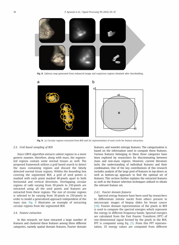
Fig. 8. Saliency map generated from enhanced image and suspicious regions obtained after thresholding.

s1

ci

R

s2

Fig. 9. (a) Circular regions extracted from ROI and (b) representation of each circle for feature extraction.

P. Agrawal et al. / Signal Processing 99 (2014) 29–4736

2.3. Grid based sampling of ROI

Since GBVS algorithm extracts salient regions in a moregeneric manner, therefore, along with mass, the segmen-ted regions contain some normal tissues as well. Theproposed framework utilizes a grid based search to detectthe mass containing regions and discard the falselydetected normal tissue regions. Within the bounding boxcovering the segmented ROI, a grid of seed points ismarked with each point marked 40 pixels apart in bothhorizontal and vertical directions. Overlapping circularregions of radii varying from 30 pixels to 210 pixels areextracted using all the seed points and features areextracted from these regions. The size of circular regionsis selected to be varying from 30 pixels to 210 pixels inorder to model a generalized approach independent of themass size. Fig. 9 illustrates an example of extractingcircular regions from the segmented ROI.

2.4. Feature extraction

In this research, we have extracted a large number offeatures and clustered these features among three differentcategories, namely spatial domain features, Fourier domain

features, and wavelet entropy features. The categorization isbased on the information used to compute these features.Various features belonging to these three categories havebeen explored by researchers for discriminating betweenmass and non-mass regions. However, current literaturelacks the understanding of individual features and theircombination. One of the key contributions of this researchincludes analysis of the large pool of features in top-down aswell as bottom-up approach to find the optimal set offeatures. This section further explains the extracted featuresas well as the feature selection techniques utilized to obtainthe relevant feature set.

2.4.1. Fourier domain featuresSpectral energy features have been used by researchers

to differentiate mitotic nuclei from others present inmicroscopic images of biopsy slides for breast cancer[34]. Fourier domain representation of the pixels in ROIis used to compute the spectral energies which representthe energy in different frequency bands. Spectral energiesare calculated from the Fast Fourier Transform (FFT) ofone-dimensional signal formed by the pixels in the ROI,FFT is computed using Eq. (5). From this FFT represen-tation, 35 energy values are computed from different

Table 2Kernels proposed by Laws [39].

Kernel label Kernel values

l5 [1 4 6 4 1]s5 [�1 0 2 0 �1]e5 [1 �4 6 �4 1]r5 [�1 �2 0 2 1]w5 [�1 2 0 �2 1]

P. Agrawal et al. / Signal Processing 99 (2014) 29–47 37

frequency bands as explained in Appendix A:

FFT_ROI¼ ∑N�1

n ¼ 0xðnÞe� j2πnk=N ; k¼ 0;1;…;N�1 ð5Þ

where x(n) represents the pixels of region R in spatialdomain and N represents the total number of pixels inregion R.

2.4.2. Wavelet entropy featuresIn some cases, the masses may be surrounded with

highly dense tissues along different directions. DiscreteWavelet Transform (DWT) encodes the details present inan image along different directions. Wang et al. [35] haveshown that entropy features computed in wavelet domaincan efficiently differentiate between the masses and nor-mal breast tissues. Nine features encoding the entropy ofup to three level DWT detailed sub-bands are extractedfrom the circular regions. As the ROI size is much smallercompared to the complete mammogram, meaningfuldecimation can be up to level three only. On the otherhand, Redundant Discrete Wavelet Transform (RDWT) [36]is undecimated, therefore it can be used to extract theentropy information even at higher levels. Here, RDWT upto level four is used to extract the entropy features.

Let I be the mammogram image and IHl, IVl, IDl be thedetailed sub-bands at level l representing the horizontal,vertical and diagonal high level coefficients respectively.RHl, RVl, and RDl represent the set of DWT coefficients fromthe detailed sub-bands IHl, IVl, and IDl respectively mappedto the pixels in region R on a mammogram. Entropy iscalculated for each sub-band region as Al

i ¼ �∑pilnlogðpilÞ,where i¼H;V , and D. AH

l, AV

l, and AD

lrepresent the entropy

of horizontal, vertical and diagonal coefficients respec-tively at level l from DWT representation and pil representsthe normalized histogram of values in Ril. In a similarmanner, the entropy features are computed from theRDWT sub-bands, Bl

i ¼ �∑pilnlogðpilÞ, where i¼H;V ;D, i.e. BH

l, BV

l, and BD

lrepresent the entropy of horizontal,

vertical and diagonal coefficients at level l from RDWTrepresentation respectively.

2.4.3. Spatial domain featuresThe spatial domain features include Laws texture fea-

tures, intensity features, run-length texture features, andstatistical texture features commonly used by existingalgorithms [16,37]. To extract the spatial domain features,let us assume circle ci be the set comprising all the boundarypoints of ROI, R be the set containing all points in the regionof interest, square s1 be the square region with area andcenter same as ci, and region s2 be the square with each sideexactly five pixels more than s1 and center same as ci. Thisprovides us two squares and a circle as shown in Fig. 9, wenow extract five different features from the distributionformed by the pixels in these regions:

�

Intensity features: It has been observed that the inten-sity of mass varies with respect to the surroundingtissues. Based on this intuition, researchers have pro-posed some thresholding based and morphology basedalgorithms [5,6,38]. However, we model this variationwith the help of five features computed from the pixel

values within and out of the suspicious regions, namelyMean Intensity, Intensity Variation, Mean IntensityDifference, Skewness, and Kurtosis. Detailed informa-tion about computing these features is available inAppendix B.

�

Laws texture features: Laws [39] proposed five linearkernels for texture based segmentation that representedges, ripples, waves, lines, and spots in a square regionas shown in Table 2. Polakowski et al. [40] studied 25feature masks generated by the combination of thesekernels and found that eight of them are the mostdiscriminating for detecting masses in mammograms.These eight features are used in this experiment to mapthe texture information present in the segmentedregions. Each of these features are computed with thehelp of feature masks described in Appendix C. Thepreprocessed image is convolved with these featuremasks and the mean value corresponding to pixellocations in circular regions is considered as featurevalues.

�

Statistical texture features: Statistical texture features,also known as Spatial Gray-Level Dependence (SGLD)features, use statistical measures to model the patternof intensity values in a region [41]. These features havebeen used by many existing approaches to differentiatebetween breast tissues as normal or cancerous [16]. Thefeatures are computed using the Gray Level Co-occurrence Matrix (GLCM) which quantifies the num-ber of occurrences of gray level i in a spatial relationwith gray level j. The image is discretized into eightgray levels and GLCM matrices are obtained for fourorientations (01, 451, 901, and 1351). The four GLCMmatrices obtained are normalized and 13 features areextracted from each of the four matrices. Appendix Dcontains detailed description of these features. Further,13 additional features are computed as mean of theseindividual features.

�

Run length texture features: Another widely used mea-sure of texture includes features based on the GrayLevel Run Length (GLRL) matrix [42]. These featuresmeasure the simultaneous presence of intensity valuesfor varying continuous lengths in different directions.GLRL matrix Gðx; yjθÞ represents the run length matrixin a given direction θ. These can be helpful in modelingcomplex textures such as breast tissues and have beenused for mass detection in some existing approaches[16]. In total, 20 features are computed from GLRLmatrices in four different directions i.e. 01, 451, 901,and 1351. The features derived from these matrices areexplained in Appendix E.

P. Agrawal et al. / Signal Processing 99 (2014) 29–4738

2.4.4. Feature selection154 features are extracted from each circular region.

These features are evaluated in the proposed frameworkresulting in selection of optimal features to discriminatebetween mass and non-mass regions. The features areanalyzed individually as well as in combination usingfeature selection and dimensionality reduction algorithms.In this research, feature concatenation is used to combineany two feature sets.

Firstly, the performance of all individual set of featuresis evaluated. Mutual information based feature selection[43] is then used to further analyze these feature sets andobtain optimal features out of these individual sets.Features with significant performance are then combinedto seek better classification. The discrimination power offeatures is measured using the mutual information basedfeature selection which uses a minimum RedundancyMaximum Relevance (mRMR) criterion [43]. Mutual infor-mation between two random variables x and y withprobability density functions p(x), p(y) and pðx; yÞ is com-puted using

MI x; yð Þ ¼∬ p x; yð Þlog pðx; yÞpðxÞpðyÞ dx dy ð6Þ

According to the mRMR criteria, optimal features musthave high mutual information with the target labels inorder to represent the maximum dependency. The theo-retical analysis of mRMR based feature selection algorithmis discussed by Peng et al. [43]. The mRMR based featureselection arranges the features in decreasing order of theirdiscrimination ability using the input feature values andoptimal number of features is obtained by evaluatingdifferent number of features selected from top of the list.

Based on the initial results of individual feature sets, acombined set of features is obtained using feature con-catenation. The combined set of features is analyzed withthe help of mRMR feature selection and Principal Compo-nent Analysis (PCA) [44] based dimensionality reduction.

2.5. Classification

The features extracted from circular ROIs are classifiedusing a 2-class SVM with the classes being mass and non-mass. SVM [45] with polynomial kernel of degree three istrained to obtain the decision boundary. The training datafor SVM is fx; yg, where x represents the feature vectorextracted from the circular ROI with training label

Table 3Symptom-wise description of the MIAS database.

Description # Images (# Symptoms)

Fatty

Architectural distortion 6(6)Bilateral asymmetry 4(4)Mass 24(27)Micro-calcification cluster 6(6)Normal 66

Total 106

yAfþ1; �1g. þ1 represents the positive (mass) class and�1 represents the negative (non-mass) class. The actuallabels of circular ROIs are obtained using the ground truthinformation available with the database. Any circular ROI isassigned a positive label if the center of the mass is presentwithin the ROI or there is at least 50% overlap between theground truth and extracted ROI. The classifier trained onoptimal set of features is tested using the remaining(unseen) regions as probe instances.

3. Results and analysis

Images from the MIAS database [14] are used toevaluate the proposed saliency based framework for massdetection. The spatial resolution of images is 50 μm�50 μm and grayscale intensity is quantized to 8 bits. TheMIAS database is one of the most popular public databasesused for evaluating breast cancer detection and diagnosistechniques. Though the database is old and many sophis-ticated algorithms have been applied to detect symptomsusing this challenging database, the intricacy of the data-base is clearly visible from the results in the comparisonstudy by Oliver et al. [6]. The database contains varieddensity mammograms for both mass and non-massclasses, which increases the intra-class variation andmakes the problem even more challenging. There are total322 MLO view mammograms in the database, both leftand right breast images for 161 cases. Among the 322mammograms, 207 are normal and 115 mammogramshave one of the four symptoms of breast cancer. Furtherdetails about the number of images per symptom aresummarized in Table 3.

In order to compare the performance of the proposedframework with existing algorithms, experiments areconducted with the experimental protocol used by Oliveret al. [6] and the performance is compared with sevenstate-of-the-art algorithms. The protocol includes classifi-cation of segmented regions as mass and non-mass usingthree times 10-fold cross-validation. The performance iscompared in terms of mean and standard deviation valuesof Area Under the Curve (AUC) of Receiver OperatingCharacteristic (ROC) curves obtained after classification.Since we have used the same database and experimentalprotocol, performance of the proposed framework isdirectly compared with the results reported by Oliveret al. [6]. The performance of segmentation and

Fatty-glandular Dense-glandular

6(6) 7(7)4(4) 7(7)20(20) 12(12)9(9) 10(15)65 76

104 112

P. Agrawal et al. / Signal Processing 99 (2014) 29–47 39

classification steps of the proposed framework are indivi-dually discussed in the following sub-sections.

3.1. Segmentation results

ROI segmentation using GBVS yields highly accurateresults and does not generate any false alarm due topectoral muscles on the MIAS database. 49 out of total58 masses are detected by the saliency based segmenta-tion, while nine are missed. Some false rejects are due tothe noise in breast region, for example, as shown in Fig. 10,when a label is coinciding with the breast tissues andtherefore cannot be completely removed. This results infalse saliency accumulation at that point, resulting inmissing the mass region as well as adding one falsepositive. The results from GBVS are promising and overallclassification results (described in later subsections)justify the intuition to use saliency based segmentationfor analyzing mammograms.

In this research, we also compare the performance ofGBVS with three existing visual saliency algorithms – Liuet al. [30], Hou and Zhang [31], and Esaliency [32]. Thealgorithms are considered on the basis of their capabilityto generate saliency map from an input grayscale image.Though the effectiveness of GBVS as a generic visualsaliency algorithm can be analyzed in the benchmarkstudy by Borji et al. [27], comparative analysis fromFig. 11 and Table 4 shows that GBVS outperforms othersaliency algorithms for mammogram ROI segmentation. Asshown in Table 4, three algorithms are able to detect morethan half of the masses at the cost of high false positives.Additionally, unlike GBVS, other three algorithms are notable to distinguish between the pectoral muscle regionand other breast parenchyma. The contrast of mass con-taining regions varies from other breast parenchyma,therefore, contrast maps being the basis of saliency map

Fig. 10. Sample results of the proposed saliency based segmentation al

generation in GBVS make it suitable for mammogramanalysis.

3.2. Feature extraction and classification results

In the proposed framework, 30,462 overlapping circularregions are extracted from the probable regions marked byapplying saliency based segmentation on 55 images con-taining 58 masses. 3470 regions contain at least 50% massaccording to the ground truth data; these regions areconsidered as positive class (mass) samples. 154 featuresfrom seven different sets of features are computed toclassify each circular region as mass and non-mass. In theproposed framework, the performance of these features isevaluated thoroughly, starting from classification usingindividual sets of features. Feature selection techniquesare applied on these feature sets to achieve optimalperformance with minimum computational effort. Thefeatures with good classification performance are com-bined using feature concatenation to further enhance theclassification performance. The results obtained from com-plete feature analysis are explained in this section.

3.2.1. Individual feature set resultsThe performance of individual sets of features for mass

vs non-mass classification of extracted regions can becompared in Table 5 and Fig. 12. The results obtained canbe summarized as follows:

�

gori

As compared to other feature sets, spatial domainfeatures do not perform efficiently. One of the majorreasons for the reduced performance could be varyingorientation, shape and size of masses present in thecircular ROIs. The results show that the intensity ortexture information alone may not be sufficient tomodel the highly complex masses.

thm. (a) Successful segmentation and (b) false segmentation.

GBVS [29] Liu [30]et al. Hou & Zhang[31]

Esaliency [32]InputMammogram

Fig. 11. Sample results of the saliency algorithms. Each row corresponds to the output of the four saliency algorithms for corresponding mammogramimage shown in the left most column. The green color in saliency maps denotes the ROI segmented after thresholding on the saliency map and pink colorrepresents the ground truth region containing mass. (For interpretation of the references to color in this figure caption, the reader is referred to the webversion of this paper.)

P. Agrawal et al. / Signal Processing 99 (2014) 29–4740

�

Fourier domain spectral energies also could notyield high performance for the classifying circularregions. Since spatial information is absent in Fourier

representation, spectral energies derived from fre-quency bands alone may not be sufficient, thereforeexploring additional features may be helpful for

Table 4Comparative analysis of saliency algorithms.

Comparison Metric GBVS [29] Liu et al. [30] Hou & Zhang [31] Esaliency [32]

Mass detection ratio(threshold onsaliency map)

49/58 (0.5) 58/58 38/58 (0.4) 40/58 (0.7)

False positives 2–3/image NA 6–7/image 410=image

Observation Results are not affected bythe presence of pectoralmuscles

Entire breast region is theoutput salient object

Incorrect high saliencyvalue in different regionsof mammogram otherthan mass regions such aspectoral muscles and allcorners of the image

It is not able todifferentiate betweenthe pectoral musclesand other breastparenchyma

Table 5Classification results of individual sets of features.

Feature category Features No. of features AUC (Az)

Spatial domain features GLRL features 20 0.54870.016Intensity features 5 0.53270.016Laws texture features 8 0.43670.059SGLD features 65 0.68770.016

Fourier domain features Spectral energy features 35 0.49570.015

Wavelet features DWT entropy features 9 0.87670.001RDWT entropy features 12 0.87070.001

0 0.1 0.2 0.3 0.4 0.5 0.6 0.7 0.8 0.9 10

0.1

0.2

0.3

0.4

0.5

0.6

0.7

0.8

0.9

1

False Positive Rate

True

Pos

itive

Rat

e

RDWTDWTSGLDLawsIntensityGLRLFFT

Fig. 12. ROC curves for the individual sets of features. (For interpretationof the references to color in this figure caption, the reader is referred tothe web version of this paper.)

P. Agrawal et al. / Signal Processing 99 (2014) 29–47 41

performance improvement.

� Entropy features from Discrete Wavelet Transform

show very good classification performance withoutbeing affected by the size or orientation of masses.Wavelet entropies model the randomness in edge mapsalong different orientations of a localized neighbor-hood. Therefore, they may be able to better encode thedifferences between mass and non-mass irrespective oftheir shape and size. Since the performance of DWTand RDWT features is dependent on the mother wave-let used, we have evaluated the results with 12 differ-ent mother wavelets. The results of this comparison arereported in Table 6. The results show that DWT entropyfeatures derived from the first three levels of Bi-orthogonal 2.2 wavelet transform yield the best AUC

of 0.87670.001.

� As discussed earlier, DWT can yield significant entropy

features up to three levels of decimation and beyondthat, the size of some decimated masses is insignificantfor feature computation. Therefore, we have also eval-uated the performance of Redundant Wavelet Trans-form features as there is no decimation step in RDWT.We empirically found that information up to level fouris useful for the MIAS database. As shown in Table 6,the performance of RDWT entropy differs signifi-cantly from the corresponding DWT entropy features,which indicates that RDWT provides some additionalinformation. Out of the 12 mother wavelets used forevaluation, entropy features derived from the RDWTrepresentation using Bi-orthogonal 1.3 mother waveletyield the best performance of AUC ¼ 0:87070:001.

3.2.2. Feature selection resultsFrom the results reported in Table 5, it is clear that the

performance of different feature sets differs significantly.Also, some features in these sets may be providingredundant information. Therefore, to reduce the computa-tional effort and discard the redundant and irrelevantfeatures in these individual feature sets, mRMR basedfeature selection [43] is applied to find the optimalfeatures from these individual sets. The results obtainedafter feature selection are summarized in Table 7. It isobserved that the accuracy improved after applying fea-ture selection for Spatial domain and Fourier domainfeatures. Entropy features derived from DWT and RDWTdepend on edge orientations within the region. However,due to varying shape and size of masses, their relevance

Table 6Comparing the performance of DWT and RDWT entropy features with different mother wavelets. The results are reported in terms of Area Under the Curve(Az) of ROC curves.

Wavelet used DWT RDWT DWTþRDWT

Bi-orthogonal 1.3 0.86370.001 0.87070.001 0.87470.000Bi-orthogonal 2.2 0.87670.001 0.84870.015 0.86470.000Bi-orthogonal 5.5 0.82170.006 0.76770.044 0.86370.020Coiflet 1 0.83270.020 0.79270.064 0.86070.000Coiflet 5 0.81270.022 0.67470.044 0.84770.000Daubechies 2 0.84370.012 0.78470.055 0.86770.001Daubechies 10 0.78870.029 0.74470.052 0.87470.004Discrete Meyer 0.77570.040 0.67170.064 0.84270.005Reverse Bi-orthogonal 1.3 0.79770.009 0.61870.025 0.85170.000Reverse Bi-orthogonal 2.2 0.85570.000 0.70370.051 0.89170.001Reverse Bi-orthogonal 5.5 0.78070.058 0.78670.009 0.85870.008Symlets 2 0.78570.036 0.72170.075 0.86970.001

Table 7Analyzing the effect of mRMR based feature selection on individualfeature sets. Performance of individual set of features after mRMR basedfeature selection.

Feature description No. of selected features AUC (Az)

DWT 9 0.87670.001RDWT 12 0.87070.001Intensity 3 0.56070.047FFT 21 0.52370.016SGLD 52 0.71970.052GLRL 15 0.63170.047Laws 4 0.47970.093

0 0.1 0.2 0.3 0.4 0.5 0.6 0.7 0.8 0.9 10

0.1

0.2

0.3

0.4

0.5

0.6

0.7

0.8

0.9

1

False Positive Rate

True

Pos

itive

Rat

e

Biorthogonal 1.3Biorthogonal 2.2Biorthogonal 5.5Coiflet 1Coiflet 5Daubechies 2Daubechies 10Discrete MeyerReverse Biorthogonal 1.3Reverse Biorthogonal 2.2Reverse Biorthogonal 5.5Symlet 2

Fig. 13. ROC curves for different mother wavelets with combined featuresfrom DWT and RDWT. (For interpretation of the references to color in thisfigure caption, the reader is referred to the web version of this paper.)

P. Agrawal et al. / Signal Processing 99 (2014) 29–4742

can vary. Therefore, to keep the feature set generalizable,no further feature selection is applied on wavelet entropyfeatures.

3.2.3. Feature combination resultsAfter thoroughly evaluating the individual sets of

features, the feature sets are combined and classificationperformance is analyzed. Feature combination is per-formed at two levels – before feature selection and afterfeature selection, further described below:

�

Before feature selection: As shown in Table 5, the entropyvalues from DWT and RDWT representations yield bestresult among all features. Therefore, it is our assertion thatany combination of features should contain these entropyfeatures. Correlation analysis is also used to validate thecombination. The class-wise correlation between thedistance scores obtained after SVM classification is calcu-lated for both the feature sets. The correlation for thepositive class (mass) is found to be 0.33, which indicatesthat True Positive (TP) to False Positive (FP) ratio on theROC curve can be improved when DWT and RDWTfeatures are combined. DWT features from all 12 motherwavelets are combined with their corresponding RDWTfeatures. Comparison results from Table 6 and Fig. 13show that the features extracted using Reverse Bi-orthogonal 2.2 mother wavelet yield the best TP–FP ratiowith AUC ¼ 0:89170:001. The combination of best per-forming DWT and RDWT features from Bi-orthogonal 2.2

and 1.3 mother wavelets respectively could not performbetter than DWT and RDWT features derived fromReverse Bi-orthogonal 2.2 mother wavelet.

�

After feature selection: The feature sets obtained afterfeature selection are concatenated with combination ofDWT and RDWT to analyze the scope for furtherimprovement in the classification performance. Featurecombination results are summarized in Table 8 andFig. 14. Along with evaluating individual features,feature set obtained by combining the individual setsof features is also analyzed using mRMR based featureselection and PCA based dimensionality reduction. Thecombined feature set consists of DWT, RDWT, SGLD,GLRL, and FFT features (intensity and Laws features arediscarded for the combination due to their poor per-formance). The results derived from feature combina-tion, as reported in Table 8, show that the highestclassification performance is achieved using the com-bination of DWT and RDWT features only.

3.2.4. Comparison with existing algorithmsThe proposed framework uses saliency based region

of interest detection. The segmented regions are further

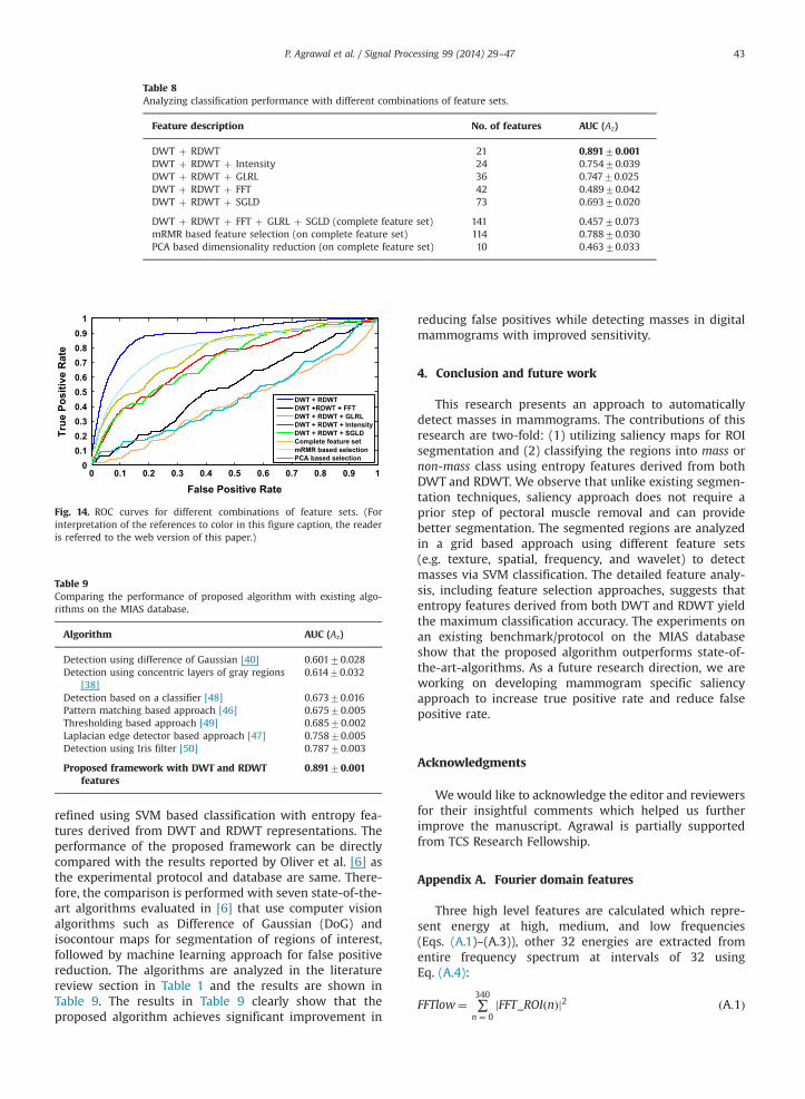
Table 8Analyzing classification performance with different combinations of feature sets.

Feature description No. of features AUC (Az)

DWT þ RDWT 21 0.89170.001DWT þ RDWT þ Intensity 24 0.75470.039DWT þ RDWT þ GLRL 36 0.74770.025DWT þ RDWT þ FFT 42 0.48970.042DWT þ RDWT þ SGLD 73 0.69370.020

DWT þ RDWT þ FFT þ GLRL þ SGLD (complete feature set) 141 0.45770.073mRMR based feature selection (on complete feature set) 114 0.78870.030PCA based dimensionality reduction (on complete feature set) 10 0.46370.033

0 0.1 0.2 0.3 0.4 0.5 0.6 0.7 0.8 0.9 10

0.10.20.30.40.50.60.70.80.9

1

False Positive Rate

True

Pos

itive

Rat

e

DWT + RDWTDWT +RDWT + FFTDWT + RDWT + GLRLDWT + RDWT + IntensityDWT + RDWT + SGLDComplete feature setmRMR based selectionPCA based selection

Fig. 14. ROC curves for different combinations of feature sets. (Forinterpretation of the references to color in this figure caption, the readeris referred to the web version of this paper.)

Table 9Comparing the performance of proposed algorithm with existing algo-rithms on the MIAS database.

Algorithm AUC (Az)

Detection using difference of Gaussian [40] 0.60170.028Detection using concentric layers of gray regions

[38]0.61470.032

Detection based on a classifier [48] 0.67370.016Pattern matching based approach [46] 0.67570.005Thresholding based approach [49] 0.68570.002Laplacian edge detector based approach [47] 0.75870.005Detection using Iris filter [50] 0.78770.003

Proposed framework with DWT and RDWTfeatures

0.89170.001

P. Agrawal et al. / Signal Processing 99 (2014) 29–47 43

refined using SVM based classification with entropy fea-tures derived from DWT and RDWT representations. Theperformance of the proposed framework can be directlycompared with the results reported by Oliver et al. [6] asthe experimental protocol and database are same. There-fore, the comparison is performed with seven state-of-the-art algorithms evaluated in [6] that use computer visionalgorithms such as Difference of Gaussian (DoG) andisocontour maps for segmentation of regions of interest,followed by machine learning approach for false positivereduction. The algorithms are analyzed in the literaturereview section in Table 1 and the results are shown inTable 9. The results in Table 9 clearly show that theproposed algorithm achieves significant improvement in

reducing false positives while detecting masses in digitalmammograms with improved sensitivity.

4. Conclusion and future work

This research presents an approach to automaticallydetect masses in mammograms. The contributions of thisresearch are two-fold: (1) utilizing saliency maps for ROIsegmentation and (2) classifying the regions into mass ornon-mass class using entropy features derived from bothDWT and RDWT. We observe that unlike existing segmen-tation techniques, saliency approach does not require aprior step of pectoral muscle removal and can providebetter segmentation. The segmented regions are analyzedin a grid based approach using different feature sets(e.g. texture, spatial, frequency, and wavelet) to detectmasses via SVM classification. The detailed feature analy-sis, including feature selection approaches, suggests thatentropy features derived from both DWT and RDWT yieldthe maximum classification accuracy. The experiments onan existing benchmark/protocol on the MIAS databaseshow that the proposed algorithm outperforms state-of-the-art-algorithms. As a future research direction, we areworking on developing mammogram specific saliencyapproach to increase true positive rate and reduce falsepositive rate.

Acknowledgments

Wewould like to acknowledge the editor and reviewersfor their insightful comments which helped us furtherimprove the manuscript. Agrawal is partially supportedfrom TCS Research Fellowship.

Appendix A. Fourier domain features

Three high level features are calculated which repre-sent energy at high, medium, and low frequencies(Eqs. (A.1)–(A.3)), other 32 energies are extracted fromentire frequency spectrum at intervals of 32 usingEq. (A.4):

FFTlow¼ ∑340

n ¼ 0jFFT_ROIðnÞj2 ðA:1Þ

P. Agrawal et al. / Signal Processing 99 (2014) 29–4744

FFTmed¼ ∑683

n ¼ 341jFFT_ROIðnÞj2 ðA:2Þ

FFThigh¼ ∑1023

n ¼ 684jFFT_ROIðnÞj2 ðA:3Þ

FFTh¼ ∑32�ðhþ1Þ�1

n ¼ 32�hjFFT_ROIðnÞj2; where h¼ 0;1;…;31

ðA:4Þ

Appendix B. Intensity features

Mean Intensity: Mean intensity corresponds to themean value of pixels in region R [37]:

m¼ 1N

∑ði;jÞAR

I i; jð Þ ðB:1Þ

Intensity variation: Intensity variation corresponds tothe standard deviation of pixels in region R [37]:

var¼ffiffiffiffiffiffiffiffiffiffiffiffiffiffiffiffiffiffiffiffiffiffiffiffiffiffiffiffiffiffiffiffiffi1N∑ðIði; jÞ�mÞ2

r; where ðB:2Þ

m¼ 1N∑I i; jð Þ ðB:3Þ

where Iði; jÞ represents the image pixel value at (i,j) loca-tion and N the number of points in R.

Mean intensity difference: Mean intensity difference isthe difference between the mean intensity of pixels withinthe region R and the mean intensity of pixels in theneighborhood Ne [37]. The neighborhood Ne is defined asthe region obtained after subtracting circular region cifrom square region s2:

Ne¼ s2�ci ðB:4ÞSkewness: Skewness measures the asymmetry among

data around the sample mean. Skewness of the distribu-tion formed by pixels of region R is defined as the third

-1 -2 0 2 1

2 4 0 -4 -2

0 0 0 0 0

-2 -4 0 4 2

1 2 0 -2 -1

-1 -2 0 2 1

-2 -4 0 4 2

0 0 0 0 0

2 4 0 -4 -2

1 2 0 -2 -1

-1 0 2 0 -1

4 0 -8 0 4

-6 0 12 0 -6

4 0 -8 0 4

-1 0 2 0 -1

-1 0 2 0 -1

-4 0 8 0 -4

-6 0 12 0 -6

-4 0 8 0 -4

-1 0 2 0 -1

Fig. 15. Feature masks generated using the kernels proposed by Laws [39]. (a

standardized moment of the distribution:

s¼ Eðx�μÞ3s3

ðB:5Þ

Kurtosis: Kurtosis measures the robustness of the dis-tribution towards outliers. Kurtosis of the distributionformed by pixels of region R is defined as fourth standar-dized moment of the distribution:

k¼ Eðx�μÞ4s4

ðB:6Þ

where μ and s are respectively the mean and standarddeviation of the distribution and E(x) gives expectation ofvariable x.

Appendix C. Laws texture features

Eight feature masks used to compute Laws texturefeatures are illustrated in Fig. 15.

Appendix D. Statistical texture features

Following equations define the notations helpful indescribing features extracted from GLCM matrices:

CxðiÞ ¼ ∑Ng

j ¼ 1Cði; jÞ ðD:1Þ

CyðjÞ ¼ ∑Ng

i ¼ 1Cði; jÞ ðD:2Þ

Cxþy kð Þ ¼∑Ng

i ¼ 1∑Ng

j ¼ 1

iþ j¼ k

Cði; jÞ; k¼ 2;3;…;2Ng ðD:3Þ

Cx�y kð Þ ¼ ∑Ng

i ¼ 1∑Ng

j ¼ 1

ji� jj ¼ kCði; jÞ; k¼ 0;1;…;Ng�1 ðD:4Þ

-1 0 2 0 1

0 0 0 0 0

2 0 -4 0 2

0 0 0 0 0

-1 0 2 0 1

-1 4 -6 4 -1

0 0 0 0 0

2 -8 12 -8 2

0 0 0 0 0

-1 4 -6 4 -1

-1 2 0 -2 1

4 -8 0 8 -4

-6 12 0 -12 6

4 -8 0 8 -4

-1 2 0 -2 1

1 -4 6 -4 1

4 -16 24 -16 4

6 -24 36 -24 6

4 -16 24 -16 4

1 -4 6 -4 1

) w5r5, (b) r5r5, (c) s5s5, (d) s5e5, (e) e5s5, (f) I5s5, (g) e5w5 and I5e5.

P. Agrawal et al. / Signal Processing 99 (2014) 29–47 45

where Ng is the number of distinct gray levels, 8 in ourcase. With the help of notations defined above, 13 featuresare computed using the equations below:

�

Contrast or inertia:

f 1 ¼ ∑Ng �1

n ¼ 0n2 ∑Ng

i ¼ 1∑Ng

j ¼ 1

ji� jj ¼ nCði; j

!ðD:5Þ

�

Correlation:

f 2 ¼∑i∑jijCði; jÞ�μxμy

sxsyðD:6Þ

where μx; μy and sx; sy are the means and standarddeviations of matrices Cx and Cy respectively.

�

Energy or angular second moment:

f 3 ¼∑i∑jCði; jÞ2 ðD:7Þ

�

Sum of squares:

f 4 ¼∑i∑jði�μÞ2Cði; jÞ ðD:8Þ

where μ is the mean of the GLCM matrix.

� Entropy:

f 5 ¼ �∑i∑jCði; jÞlogðCði; jÞÞ ðD:9Þ

�

Inverse difference moment:

f 6 ¼∑i∑j

11þði� jÞ2

C i; jð Þ ðD:10Þ

�

Sum average:

f 7 ¼ ∑2Ng

k ¼ 2kCxþyðkÞ ðD:11Þ

�

Sum variance:

f 8 ¼ ∑2Ng

k ¼ 2ðk� f 7Þ2CxþyðkÞ ðD:12Þ

�

Sum entropy:

f 9 ¼ � ∑2Ng

k ¼ 2CxþyðkÞlogðCxþyðkÞÞ ðD:13Þ

�

Difference variance:

f 10 ¼∑kðk�μx�yÞ2Cx�yðkÞ ðD:14Þ

where μx�y is the mean of Cx�y.

� Difference entropy:

f 11 ¼ � ∑Ng �1

Cx�yðkÞlogðCx�yðkÞÞ ðD:15Þ

k ¼ 0

Information measures of correlation:

� f 12 ¼

HXY�HXY1

maxðHX;HYÞ ðD:16Þ

f 13 ¼ ½1�e�2ðHXY2 �HXYÞ�1=2 ðD:17Þ

HXY ¼ �∑i∑jCði; jÞ logðCði; jÞÞ ðD:18Þ

HX ¼ �∑iCxðiÞ logðCxðiÞÞ ðD:19Þ

HY ¼ �∑jCyðjÞ logðCyðjÞÞ ðD:20Þ

HXY1 ¼ �∑i∑jCði; jÞ logðCxðiÞCyðjÞÞ ðD:21Þ

HXY2 ¼ �∑i∑jCxðiÞCyðjÞ logðCxðiÞCyðjÞÞ ðD:22Þ

where C is one of the four GLCM matrices, similarcomputations are made for all four matrices.

Appendix E. Run length texture features

Run length distribution rðjjθÞ and gray-level distribu-tion gðijθÞ are derived from each of the four GLRL matricesGðx; yjθÞ as follows:

rðjjθÞ ¼∑iGði; jjθÞ ðE:1Þ

gðijθÞ ¼∑jGði; jjθÞ ðE:2Þ

The total number of runs in the image S are computed asfollows:

S¼∑i∑jGði; jjθÞ ðE:3Þ

Following features are extracted from each of the fourGLRL matrices using notations defined in Eqs. (E.1)–(E.3)?,

�

Short runs emphasis (SRE):

SRE¼ 1S∑j

rðjjθÞj2

ðE:4Þ

�

Long runs emphasis (LRE):

LRE¼ 1S∑jrðj θj Þj2 ðE:5Þ

�

Gray level non-uniformity (GLN):

GLN¼ 1S∑igðijθÞ2 ðE:6Þ

�

Run length non-uniformity (RLN):

RLN¼ 1S∑jrðjjθÞ2 ðE:7Þ

P. Agrawal et al. / Signal Processing 99 (2014) 29–4746

Run percentage (RP):

� RP ¼ 1

Area∑jr j θj Þð ðE:8Þ

where Area is given by the number of pixels in region R.

References

[1] C.G. Berman, Recent advances in breast-specific imaging, CancerControl J. 14 (4) (2007) 338–349.

[2] R.F. Brem, J.W. Hoffmeister, G. Zisman, M.P. DeSimio, S.K. Rogers,A computer-aided detection system for the evaluation of breastcancer by mammographic appearance and lesion size, Am. J.Roentgenol. 184 (3) (2005) 893–896.

[3] R.F. Brem, J.A. Rapelyea, G. Zisman, J.W. Hoffmeister, M.P. Desimio,Evaluation of breast cancer with a computer-aided detection systemby mammographic appearance and histopathology, Cancer 104 (5)(2005) 931–935.

[4] E.D. Pisano, C. Gatsonis, E. Hendrick, M. Yaffe, J.K. Baum, S. Acharyya,E.F. Conant, L.L. Fajardo, L. Bassett, C. D'Orsi, R. Jong, M. Rebner,Diagnostic performance of digital versus film mammography forbreast-cancer screening, New Engl. J. Med. 353 (17) (2005)1773–1783.

[5] J. Tang, R.M. Rangayyan, J. Xu, I. El Naqa, Y. Yang, Computer-aideddetection and diagnosis of breast cancer with mammography:recent advances, IEEE Trans. Inf. Technol. Biomed. 13 (2) (2009)236–251.

[6] A. Oliver, J. Freixenet, J. Martí, E. Pérez, J. Pont, E.R.E. Denton,R. Zwiggelaar, A review of automatic mass detection and segmenta-tion in mammographic images, Med. Image Anal. 14 (2) (2010)87–110.

[7] M. Velikova, P.J. Lucas, M. Samulski, N. Karssemeijer, A probabilisticframework for image information fusion with an application tomammographic analysis, Med. Image Anal. 16 (4) (2012) 865–875.

[8] K. Ganesan, U. Acharya, C. Chua, L. Min, K. Abraham, K.-H. Ng,Computer-aided breast cancer detection using mammograms: areview, IEEE Rev. Biomed. Eng. 6 (2013) 77–98.

[9] P. Rahmati, A. Adler, G. Hamarneh, Mammography segmentationwith maximum likelihood active contours, Med. Image Anal. 16 (6)(2012) 1167–1186.

[10] R. Rangayyan, F. Ayres, J. Leo Desautels, A review of computer-aideddiagnosis of breast cancer: toward the detection of subtle signs,J. Frankl. Inst. 344 (2007) 312–348.

[11] S. Halkiotis, T. Botsis, M. Rangoussi, Automatic detection of clusteredmicrocalcifications in digital mammograms using mathematicalmorphology and neural networks, Signal Process. 87 (7) (2007)1559–1568.

[12] B. Senthilkumar, G. Umamaheshwari, A review on computer aideddetection and diagnosis - towards the treatment of breast cancer,Eur. J. Sci. Res. 52 (4) (2011) 437–452.

[13] C.J. Vyborny, M.L. Giger, Computer vision and artificial intelligence inmammography, Am. J. Roentgenol. 162 (3) (1994) 699–708.

[14] J. Suckling, J. Parker, D. Dance, S. Astley, I. Hutt, C. Boggis, I. Ricketts,E. Stamatakis, N. Cerneaz, S. Kok, P. Taylor, D. Betal, J. Savage, Themammographic images analysis society digital mammogram data-base, Experta Med. Int. Congress Ser. 1069 (1994) 375–378.

[15] M. Heath, K. W. Bowyer, D. Kopans, Current status of the digitaldatabase for screening mammography, in: 4th International Work-shop on Digital Mammography, 1998, pp. 457–460.

[16] H. Cheng, X. Shi, R. Min, L. Hu, X. Cai, H. Du, Approaches forautomated detection and classification of masses in mammograms,Pattern Recognit. 39 (4) (2006) 646–668.

[17] K. Ganesan, U.R. Acharya, K.C. Chua, L.C. Min, K.T. Abraham, Pectoralmuscle segmentation: a review, Comput. Methods ProgramsBiomed. 110 (1) (2013) 48–57.

[18] S. Kwok, R. Chandrasekhar, Y. Attikiouzel, Automatic pectoral musclesegmentation on mammograms by straight line estimation and cliffdetection, in: Intelligent Information Systems Conference, 2001,pp. 67–72.

[19] S. Brandt, G. Karemore, N. Karssemeijer, M. Nielsen, An anatomicallyoriented breast coordinate system for mammogram analysis, IEEETrans. Med. Imaging 30 (10) (2011) 1841–1851.

[20] R.J. Ferrari, R.M. Rangayyan, J.E.L. Desautels, R.A. Borges, A.F. Frère,Automatic identification of the pectoral muscle in mammograms,IEEE Trans. Med. Imaging 23 (2) (2004) 232–245.

[21] M. Mustra, M. Grgic, Robust automatic breast and pectoral musclesegmentation from scanned mammograms, Signal Process. 93 (10)(2013) 2817–2827.

[22] R. Rangayyan, L. Shen, Y. Shen, J.E.L. Desautels, H. Bryant, T. Terry,N. Horeczko, M. Rose, Improvement of sensitivity of breast cancerdiagnosis with adaptive neighborhood contrast enhancement ofmammograms, IEEE Trans. Inf. Technol. Biomed. 1 (3) (1997)161–170.

[23] S. Singh, K. Bovis, An evaluation of contrast enhancement techni-ques for mammographic breast masses, IEEE Trans. Inf. Technol.Biomed. 9 (1) (2005) 109–119.

[24] P. Kus, I. Karagoz, Fully automated gradient based breast boundarydetection for digitized X-ray mammograms, Comput. Biol. Med.42 (1) (2012) 75–82.

[25] R.C. Gonzalez, R.E. Woods, Digital Image Processing, 2nd ed., 1992.[26] P. Burt, E. Adelson, The laplacian pyramid as a compact image code,

IEEE Trans. Commun. 31 (4) (1983) 532–540.[27] A. Borji, D.N. Sihite, L. Itti, Quantitative analysis of human-model

agreement in visual saliency modeling: a comparative study, IEEETrans. Image Process. 22 (1) (2013) 55–69.

[28] A. Borji, L. Itti, State-of-the-art in visual attention modeling, IEEETrans. Pattern Anal. Machine Intell. 35 (1) (2013) 185–207.

[29] J. Harel, C. Koch, P. Perona, Graph-based visual saliency, in: Advancesin Neural Information Processing Systems, vol. 19, 2007, pp. 545–552.

[30] T. Liu, Z. Yuan, J. Sun, J. Wang, N. Zheng, X. Tang, H.-Y. Shum,Learning to detect a salient object, IEEE Trans. Pattern Anal. Mach.Intell. 33 (2) (2011) 353–367.

[31] X. Hou, L. Zhang, Saliency detection: a spectral residual approach, in:IEEE Conference on Computer Vision and Pattern Recognition, 2007,pp. 1–8.

[32] T. Avraham, M. Lindenbaum, Esaliency (extended saliency): mean-ingful attention using stochastic image modeling, IEEE Trans.Pattern Anal. Mach. Intell. 32 (4) (2010) 693–708.

[33] D.A. Levin, Y. Peres, E.L. Wilmer, Markov Chains and Mixing Times,American Mathematical Society, 2006.

[34] L.E. Boucheron, Object- and spatial-level quantitative analysis ofmultispectral histopathology images for detection and characteriza-tion of cancer (Ph.D. thesis). University of California, Santa Barbara(2008).

[35] Y. Wang, X. Gao, J. Li, A feature analysis approach to mass detectionin mammography based on RF-SVM, in: International Conference onImage Processing, vol. 5, 2007, pp. 9–12.

[36] J. Fowler, The redundant discrete wavelet transform and additivenoise, IEEE Signal Process. Lett. 12 (9) (2005) 629–632.

[37] H.D. Li, M. Kallergi, L.P. Clarke, V.K. Jain, R.A. Clark, Markov randomfield for tumor detection in digital mammography, IEEE Trans. Med.Imaging 14 (3) (1995) 565–576.

[38] N. Eltonsy, G. Tourassi, A. Elmaghraby, A concentric morphologymodel for the detection of masses in mammography, IEEE Trans.Med. Imaging 26 (6) (2007) 880–889.

[39] K.I. Laws, Textured Image Segmentation, Technical Report, Univer-sity of Southern California, 1980.

[40] W.E. Polakowski, D.A. Cournoyer, S.K. Rogers, M.P. DeSimio,D.W. Ruck, J.W. Hoffmeister, R.A. Raines, Computer-aided breastcancer detection and diagnosis of masses using Difference ofGaussians and derivative-based feature saliency, IEEE Trans. Med.Imaging 16 (6) (1997) 811–819.

[41] R.M. Haralick, K. Shanmugam, I. Dinstein, Textural features for imageclassification, IEEE Trans. Syst. Man Cybern. 6) (1973) 610–621.

[42] X. Tang, Texture information in run-length matrices, IEEE Trans.Image Process. 7 (11) (1998) 1602–1609.

[43] H. Peng, F. Long, C. Ding, Feature selection based on mutualinformation criteria of max-dependency, max-relevance, and min-redundancy, IEEE Trans. Pattern Anal. Mach. Intell. 27 (8) (2005)1226–1238.

[44] P. Belhumeur, J. Hespanha, D. Kriegman, Eigenfaces vs. fisherfaces:recognition using class specific linear projection, IEEE Trans. PatternAnal. Mach. Intell. 19 (7) (1997) 711–720.

[45] C.C. Chang, C.J. Lin, LIBSVM: a library for support vector machines,ACM Trans. Intell. Syst. Technol. 2 (3) (2011) 1–27.

[46] S. Lai, X. Li, W. Biscof, On techniques for detecting circumscribedmasses in mammograms, IEEE Trans. Med. Imaging 8 (4) (1989)377–386.

[47] N. Petrick, H.P. Chan, B. Sahiner, D. Wei, An adaptive density-weighted contrast enhancement filter for mammographic breastmass detection, IEEE Trans. Med. Imaging 15 (1) (1996) 59–67.

P. Agrawal et al. / Signal Processing 99 (2014) 29–47 47

[48] N. Karssemeijer, G. te Brake, Detection of stellate distortions inmammograms, IEEE Trans. Med. Imaging 15 (5) (1996) 611–619.

[49] G. Kom, A. Tiedeu, M. Kom, Automated detection of masses inmammograms by local adaptive thresholding, Comput. Biol. Med.37 (1) (2007) 37–48.

[50] C. Varela, P.G. Tahoces, A.J. Méndez, M. Souto, J.J. Vidal, Computer-ized detection of breast masses in digitized mammograms, Comput.Biol. Med. 37 (2) (2007) 214–226.

[51] B.W. Hong, B.S. Sohn, Segmentation of regions of interest inmammograms in a topographic approach, IEEE Trans. Inf. Technol.Biomed. 14 (1) (2010) 129–139.

[52] X. Gao, Y. Wang, X. Li, D. Tao, On combining morphologicalcomponent analysis and concentric morphology model for mammo-graphic mass detection, IEEE Trans. Inf. Technol. Biomed. 14 (2)(2010) 266–273.

[53] A. Mencattini, G. Rabottino, M. Salmeri, R. Lojacono, Assessment of abreast mass identification procedure using an iris detector, IEEETrans. Instrum. Meas. 59 (10) (2010) 2505–2512.

[54] W. Borges Sampaio, E. Moraes Diniz, A. Corrêa Silva, A. Cardoso dePaiva, M. Gattass, Detection of masses in mammogram images usingCNN, geostatistic functions and SVM, Comput. Biol. Med. 41 (8)(2011) 653–664.