NBER WORKING PAPER SERIES

SCREENING AND SELECTION:THE CASE OF MAMMOGRAMS

Liran EinavAmy FinkelsteinTamar Oostrom

Abigail J. OstrikerHeidi L. Williams

Working Paper 26162http://www.nber.org/papers/w26162

NATIONAL BUREAU OF ECONOMIC RESEARCH 1050 Massachusetts Avenue

Cambridge, MA 02138August 2019

We are grateful to Leila Agha, Emily Oster and participants in the Dartmouth/NIA P01 Reserach Meeting and the NBER Health Care Summer Institute for helpful comments, and to the Laura and John Arnold Foundation for financial support. This material is based upon work supported by the National Institute on Aging through Grant Number T32-AG000186 and the National Science Foundation Graduate Fellowship Program under Grant Number 1122374 (Oostrom). The authors acknowledge the assistance of the Health Care Cost Institute (HCCI) and its data contributors, Aetna, Humana, and UnitedHealthcare, in providing the claims data analyzed in this study. This study also used the linked SEER-Medicare database. The interpretation and reporting of these data are the sole responsibility of the authors. The authors acknowledge the efforts of the National Cancer Institute; the Office of Research, Development and Information, CMS; Information Management Services (IMS), Inc.; and the Surveillance, Epidemiology, and End Results (SEER) Program tumor registries in the creation of the SEER-Medicare database The views expressed herein are those of the authors and do not necessarily reflect the views of the National Bureau of Economic Research.

At least one co-author has disclosed a financial relationship of potential relevance for this research. Further information is available online at http://www.nber.org/papers/w26162.ack

NBER working papers are circulated for discussion and comment purposes. They have not been peer-reviewed or been subject to the review by the NBER Board of Directors that accompanies official NBER publications.

© 2019 by Liran Einav, Amy Finkelstein, Tamar Oostrom, Abigail J. Ostriker, and Heidi L. Williams. All rights reserved. Short sections of text, not to exceed two paragraphs, may be quoted without explicit permission provided that full credit, including © notice, is given to the source.

Screening and Selection: The Case of MammogramsLiran Einav, Amy Finkelstein, Tamar Oostrom, Abigail J. Ostriker, and Heidi L. WilliamsNBER Working Paper No. 26162August 2019JEL No. I11,I18

ABSTRACT

Debates over whether and when to recommend screening for a potential disease focus on the causal impact of screening for a typical individual covered by the recommendation, who may differ from the typical individual who responds to the recommendation. We explore this distinction in the context of recommendations that breast cancer screening start at age 40. The raw data suggest that responders to the age 40 recommendation have less cancer than do women who self-select into screening at earlier ages. Combining these patterns with a clinical oncology model allows us to infer that responders to the age 40 recommendation also have less cancer than women who never screen, suggesting that the benefits of recommending early screening are smaller than if responders were representative of covered individuals. For example, we estimate that shifting the recommendation from age 40 to age 45 results in over three times as many deaths if responders were randomly drawn from the population than under the estimated patterns of selection. These results highlight the importance of considering the characteristics of responders when making and designing recommendations.

Liran EinavStanford UniversityDepartment of Economics579 Serra MallStanford, CA 94305-6072and NBERleinav@stanford.edu

Amy FinkelsteinDepartment of Economics, E52-442 Massachusetts Institute of Technology50 Memorial DriveCambridge, MA 02142and NBERafink@mit.edu

Tamar OostromMassachusetts Institute of Technologyoostrom@mit.edu

Abigail J. OstrikerMassachusetts Institute of Technologyabigail.ostriker@gmail.com

Heidi L. Williams Department of Economics Stanford University579 Serra MallOffice 323Stanford, CA 94305and NBERhlwill@stanford.edu

1 Introduction

Whether and when to recommend screening for potential diseases is a highly controversial and evolving

policy area, with active academic research.1 Much of the debate – both in public policy and in academia –

centers on the causal impact of screening for a typical individual covered by the recommendation. Estimat-

ing this causal impact is challenging for several well-known reasons. First, there are the usual challenges

to causal inference. Second, many of the potential costs and benefits of screening are difficult to measure

and to monetize.2 In this paper, we highlight another important – and, we believe, overlooked – challenge

in analyzing and designing screening policies: the typical individual covered by a recommendation may be

very different from the typical individual who responds to the recommendation. As a result, the estimated

impact of the screening for a randomly selected individual may be quite different from the impact for an

affected individual.

We explore this distinction in the context of the current controversy over whether to recommend annual

mammograms for women starting at age 40. Results from randomized trials have consistently failed to show

statistically significant mortality benefits of mammograms for women in their 40s, and in 2009 this prompted

the US Preventive Services Task Force (USPTF) to change its recommendation for routine mammograms to

begin at age 50 rather than at age 40. This change generated substantial public controversy (Kolata, 2009;

Saad, 2009; Berry, 2013).

This debate has focused on the costs and benefits of mammograms for typical (“average-risk”) 40 year

old women, with little attention paid to what types of women respond to a screening recommendation and

whether the costs and benefits for them may differ from the average woman. To investigate the type of

women who respond, we draw on two primary data sources. The first is insurance claims data on mammo-

gram choices and their results (negative, false positive, or true positive) for privately insured women aged

35-50 from the Health Care Cost Institute (HCCI). The second is cancer registry data, from the National

Cancer Institute’s Surveillance, Epidemiology and End Results (SEER) database, on the size and stage of

detected tumors for women aged 35-50 who were diagnosed with breast cancer.

The visual evidence shows sharp and pronounced changes in behavior and outcomes at age 40. There is

an over 25 percentage point jump in the annual mammogram rate at age 40, from 10 percent to 35 percent of

women. Women who respond to the recommendation have a lower incidence of cancer than do women who

choose screening in the absence of the recommendation: there is a roughly 30 percent decline (from 0.84%

to 0.56%) in the share of screened women diagnosed with cancer (i.e. true positives) at age 40. Given the

high rate of false positives (about 90 percent of initial positive mammograms turn out to be false positives),

the sharp increase in the mammogram rate at age 40 translates into a substantial increase in the number of

women experiencing false positives (from about 10 per thousand women to about 40). This is consistent

1For example, Welch, Schwartz„ and Woloshin (2011) argue that although many medical conditions – such as high bloodpressure, elevated blood glucose levels, low bone density, and high cholesterol – benefit from treatment, there has been a trendover time towards widespread use of medical screening tests and increasingly low diagnostic thresholds that recommend treatingpatients for whom the benefits from treatments are quite small. By contrast, Maciosek et al. (2010) review these same screeningefforts and conclude that they save a large number of lives at relatively low cost .

2The costs and benefits of screening include monetary costs, clinical outcomes, discomfort from unnecessary procedures, andpsychological effects induced by the screening process, including pre-screening apprehension and anxiety due to false positives(e.g Ong and Mandl, 2015; Welch, 2015; Welch and Passow, 2014; Nelson et al., 2009; Brett et al., 2005).

1

with a key concern regarding false positives that motivated moving the recommended age of mammogram

from 40 to 50 (Nelson et al., 2009). Moreover, among those diagnosed with cancer, the registry data show

a sharp decline in the average tumor’s stage and size starting at age 40. For example, the share of detected

tumors that are invasive (i.e. later stage) as opposed to in situ falls by about 6 percentage points (or 7 percent)

at age 40.

These descriptive results indicate that women who respond to the recommendation for a mammogram

have lower risk of cancer than those who seek mammograms in the absence of the recommendation. Inter-

estingly, we find that women who respond to the recommendation also appear to be more likely to comply

with other types of recommended preventive care, such as cervical cancer screening tests and flu shots. This

is consistent with Oster (2018)’s finding that when a health behavior is recommended, those who comply

with the recommendation tend to exhibit other positive health behaviors.

To assess the implications of these findings and to quantify costs and health outcomes under various

counterfactual selection scenarios, we specify a model of mammogram demand that is a function of a

woman’s age, her (undiagnosed) cancer type (no cancer, in situ, or invasive), and whether or not a mam-

mogram is recommended at her age. We estimate the model by method of moments, using two key inputs.

First, we leverage our data on the observed patterns of mammogram decisions and mammogram outcomes

(specifically, cancer type) for women by age. Second, we bring in a clinical oncology model of the underly-

ing rate of onset of breast cancer by age, as well as cancers’ clinical progression in the absence of detection

and treatment. In the absence of a clinical model, these objects are inherently difficult (or impossible) to

observe: cancer incidence is not observed in the non-screened population, and almost all detected cancer

is treated immediately upon detection. The clinical model of breast cancer incidence and progression is

drawn from a large scale, coordinated project funded by the National Cancer Institute (NCI) involving seven

different research groups (Clarke et al., 2006); we show robustness of our findings to a range of alternative

assumptions about the onset and distribution of cancer type by age.

The estimates from our model indicate that women who would select into mammograms in the absence

of the recommendation have much higher rates of both in situ and invasive cancer than the general popula-

tion. We refer to this as “positive selection” into mammograms (positive with respect to cancer incidence).

However, our estimates indicate that the women who select into mammograms due to the recommendation

are much less likely to have invasive cancer – and are no more likely to have in-situ cancer – than women

who do not select into mammograms. The relative degree of selection pre- and post- the age 40 recommen-

dation is identified directly from our data; the clinical model of underlying cancer incidence is needed to

assess whether the observed selection either pre- or post-age 40 is positive with respect to the underlying

population, whose cancer incidence is not directly observed.

We apply our model and its estimates to illustrate how the nature of selection in response to the recom-

mendation affects the impact of the recommendation. Specifically, we estimate that shifting the recommen-

dation from age 40 to age 45 results in more than three times as many deaths – at similar cost savings – if we

assume that those who respond to the recommendation are randomly drawn from the population rather than

drawn based on the estimated selection patterns. We view this as a particularly instructive counterfactual

since assuming the individuals who respond are randomly drawn from the population is conceptually simi-

2

lar to using estimates of the impact of mammography from randomized experiments (with full compliance).

Because in practice those who respond to the recommendation have a much lower rate of invasive cancer

than the underlying population, the mortality cost of moving the recommendation to age 45 is lower than

under random selection. Conversely, our model also illustrates that if it were feasible to target the recom-

mendations to those with higher rates of cancer, the mortality cost of moving the recommendation from

age 40 to 45 could be substantially larger than even the random selection assumption would imply. This is

consistent with recent interest in reducing over-diagnosis by developing targeting, precision screening for

individuals at higher risk (Elmore, 2016; Esserman et al., 2009).

Our paper relates to several distinct literatures. Most narrowly, it speaks to the large body of work

on mammograms. A sizable number of randomized trials has explored the impact of mammograms on

subsequent health outcomes (Alexander et al., 1999; Bjurstam et al., 2003; Habbema et al., 1986; Miller

et al., 2000, 2002; Moss et al., 2006; Nyström et al., 2002). In addition, several studies have examined so-

called “over-diagnosis” – i.e. screening of a cancer that never would become clinically relevant (Jørgensen

and Gøtzsche, 2009); these studies have analyzed the extent to which increased mammogram screening

rates are associated with increased incidence of small or early stage tumors with no corresponding increase

in large or late-stage tumors, suggesting that increased screening may be identifying tumors that would

never have developed into life-threatening cancers (Bleyer and Welch, 2012; Harding et al., 2015; Jørgensen

and Gøtzsche, 2009; Jørgensen et al., 2017; Welch et al., 2016; Zackrisson et al., 2006). Several studies

have combined these existing estimates to quantify the costs and benefits of mammograms (e.g. Welch

and Passow, 2014; Ong and Mandl, 2015). All of these studies have focused on the average effect of

mammograms on the female population, and did not consider the potential selection that is our focus.

A related strand of literature investigates how mammogram rates are influenced by factors such as dis-

tance to women’s health clinics (Lu and Slusky, 2016), health insurance coverage (Bitler and Carpenter,

2016; Cooper et al., 2017; Fedewa et al., 2015; Finkelstein et al., 2012; Habermann et al., 2007; Kelaher

and Stellman, 2000; Mehta et al., 2015), and recommendations (Kadiyala and Strumpf, 2011, 2016; Jacob-

son and Kadiyala, 2017). Most of these studies break out effects by income, education, race, and other

individual-level characteristics, but are not able to link these demographic characteristics to cancer out-

comes. Of these, Kadiyala and Strumpf (2016) is most closely related to our work; they document a sharp

increase in self-reported mammograms at age 40 and estimate that most of the “newly detected” cancers are

early stage cancers.

Beyond the specific application of mammograms, there is a broader health policy debate about whether

and when to recommend medical screening tests (e.g. Welch, Schwartz„ and Woloshin, 2011). A central

challenge that has limited empirical research on this topic is that – in the datasets typically available to

researchers – the testing decision is observed but the outcome of the test is not. An attractive feature of

our setting is that the outcome of the test (i.e. cancer incidence and type of cancer) is measurable both in

claims data and in registry data. In this sense our analysis is similar in spirit to Abaluck et al. (2016), who

are able to measure the outcome of imaging tests for pulmonary embolism in claims data, which they use

to investigate whether and when that imaging test is being “overused.” Both our paper and Abaluck et al.

(2016) share a common feature with the racial profiling literature on stop and frisks (e.g. Anwar and Fang

3

2006; Persico 2009): the object of interest is only observed conditional on an action. This raises an empirical

challenge for analyzing how the action (in our case, screening) relates to the underlying object of interest (in

our case, the underlying incidence of cancer and cancer types). In our setting, we overcome this empirical

challenge by combining two insights. First, the recommendation at age 40 serves as an exogenous source of

variation in the screening rate, allowing us to estimate the cancer type of the marginal person affected by the

recommendation. Second, the clinical oncology model of cancer incidence and growth allows us to use the

observed moments (namely, outcomes conditional on screening under different regimes) to model outcomes

under counterfactual regimes.

More broadly, our paper speaks to the value of complementing reduced form estimates of causal effects

with economic models of behavior, and particularly of selection. Reduced form methods – both quasi-

experimental and randomized experiments – aim to estimate causal effects by shutting down any endogenous

choices. In practice, however, most policies involve an element of choice, so that the ultimate impact of the

policy depends not only on the distribution of causal treatment effects but also on which individuals select

into treatment. In this sense our paper relates broadly to the literature on Roy selection, or selection on gains.

In the healthcare context specifically, Einav et al. (2013) emphasize that the impact on healthcare spending

of offering a high deductible health insurance plan may be very different than what would be estimated from

random assignment of high deductible plans across individuals, because the types of people who choose

high deductible plans can have very different health care utilization responses to cost sharing than a typical

individual. Our analysis speaks to a similar issue, in the context of evaluating recommendations for disease

screening.

The rest of the paper proceeds as follows. Section 2 briefly summarizes the relevant institutional details

of our empirical context (breast cancer and mammography). Section 3 describes our data and presents

descriptive results. Section 4 presents our model of mammogram choice and describes how we estimate

it using the observed descriptive patterns together with a clinical oncology model. Section 5 presents the

model estimates and discusses their implications for the impact of changing the age of recommendation for

mammogram under both observed and counterfactual selection patterns. The last section concludes.

2 Empirical context

2.1 Breast cancer

The earliest stages of breast cancer typically produce no symptoms and are not detectable in the absence of

screening technologies.3 As breast cancer progresses, it can spread within the breast, to adjacent tissues,

to adjacent lymph nodes, and to distant organs (known as metastases). In clinical settings, tumors are

classified according to the size of the tumor, the extent to which it has spread to lymph nodes, and whether it

has metastasized. Public health research typically relies on a standardized classification – namely, the SEER

classification system, which includes four stages: in situ, local, regional, and distant; the last three stages

are collectively referred to as “invasive” tumors.

3Unless otherwise noted, the discussion in this section draws from American Cancer Society (2017a).

4

Our analysis focuses on the distinction between in situ and invasive tumors, because this distinction has

been a key focus of the policy debate around mammography recommendations. In situ refers to abnormal

cells that have not invaded nearby tissues, instead remaining confined to the ducts or glands in which they

originated. Some but not all in situ tumors will become invasive. Expected survival time varies greatly by

stage at diagnosis: patients who are diagnosed with localized breast cancer are 99% as likely as cancer-

free women to survive to 5 years after diagnosis, compared to 85% for regional breast cancer, and 27%

for distant-stage breast cancer.4 Within a stage, survival also varies with tumor size. For example, among

women with regional disease, 5-year survival (again, relative to comparable cancer-free women) is 95%

for tumors smaller than 2 centimeters in diameter, 85% for tumors of 2-5 centimeters, and 72% for tumors

greater than 5 centimeters.5

2.2 Mammography

Asymptomatic breast cancer can be detected by a mammogram, which is a low-dose x-ray procedure that

allows visualization of the internal structure of the breast. If an abnormality is detected on a routine screening

mammogram, the woman is typically called back in for a diagnostic mammogram and – if needed – a

confirmatory biopsy (Cutler, 2008; Hubbard et al., 2011). Once a diagnosis has been confirmed, the patient

may undergo surgery to remove the tumor, as well as other treatments which aim to reduce the risk of

recurrence, such as radiation therapy, chemotherapy, hormone therapy, and/or targeted therapy.

Mammography is based on the theory of early detection of invasive cancer, rather than detection and

removal of precancerous lesions (Humphrey et al., 2002). The efficacy of mammography is the subject

of considerable debate. Mechanically, mammography is most beneficial if machines can detect tumors

in their earliest stages, and if tumors (on average) rapidly become more difficult to treat the longer they

go undetected. The benefits from mammography will be lower if a tumor is slow to advance from stage

to stage, if mortality when treatment begins at a later stage is similar to when tumors are treated earlier,

or if mammogram machines are unlikely to correctly identify tumors. In practice, because most patients

diagnosed with breast cancer are treated immediately upon detection, there is little information about the

natural history of breast cancer tumors, making it difficult to know how an individual tumor would have

progressed had it not been treated (Zahl et al., 2008). This complicates attempts to quantify the benefits of

mammography.

In principle, the major potential health benefit of mammography is reduced mortality. However, in

practice randomized trials of the impact of mammogram on mortality have documented mixed results. There

have been nine trials in total, with the first one dating back to the 1960s (Welch and Black, 2010). Their

estimates of relative risk reduction in breast cancer mortality due to invitation to mammography range

from 0% to 31% (Welch and Passow, 2014), but many of these studies have lacked the statistical power

to separately determine effects in different age groups (Humphrey et al., 2002). In particular, while most

studies indicate that mammography reduces mortality among average-risk women over age 50, recent trials

specifically designed to study mammography in younger women (aged 40-49) have estimated statistically

4These tabulations are drawn from US SEER cancer registry data from 2007-2013, as in American Cancer Society (2017a).5These tabulations are drawn from US SEER cancer registry data from 2000-2014, as in American Cancer Society (2017a).

5

insignificant reductions in breast cancer mortality in this age group (Bjurstam et al., 2003; Moss et al., 2006).

The potential costs of mammography include financial, physical, and psychological costs. These costs

arise from the initial screening, the finding of false positives, and the treatment of cancers that would not

have become clinically relevant in a woman’s lifetime (often referred to as “over-diagnosis”). Some of these

costs, such as the financial cost of a screening, are easy to quantify, while others are much more difficult

to estimate. Estimates of the rate of over-diagnosis of breast cancer (from both observational work and

inferences from randomized control trials) range from less than 5% to more than 50% of diagnosed breast

cancers (Oeffinger et al., 2015). Aggregating observational data and randomized studies, Welch and Passow

(2014) estimate that for every 1,000 women aged 40-49 who undergo annual mammography for 10 years,

0.1-1.6 women will avoid dying from breast cancer, while 510-690 will have at least one false positive result

and up to 11 women will be over-diagnosed and (unnecessarily) treated.

In the 1980s, following the first randomized trials of routine mammography, the National Institutes of

Health (NIH), the National Cancer Institute (NCI), and eleven other health care organizations issued recom-

mendations for routine screenings of women over age 40 (Kolata, 2009). These recommendations became

the subject of controversy over time as more trials were published, and the US federal government subse-

quently reconsidered its position. In 1997, an NIH panel concluded that there was insufficient evidence to

recommend routine screening for women in their 40s, a finding that one radiologist described as a “death

sentence” for women (Taubes, 1997). After public pressure, the Senate encouraged an advisory board to

reject that conclusion (Kolata, 2009). In 2009, following the publication of experimental data that failed to

show statistically significant mortality benefits of mammograms for women in their 40s, the US Preventive

Services Task Force (USPSTF) recommended that women begin screening at age 50. Again, this conclu-

sion generated backlash from patient advocacy groups like the American Cancer Society, which at the time

recommended annual screening for women aged 40 and above (American Cancer Society, 2018).6 This neg-

ative reaction was exacerbated by fears that the Affordable Care Act (ACA, then being drafted) would allow

insurers to refuse to cover mammograms for younger women. The USPSTF stood by its recommendation,

but a poll found that 84% of women aged 35-49 did not plan to follow the new recommendations, and the

ACA was modified to mandate that insurers reimburse mammograms for women aged 40 and over (Saad,

2009). Although in the last few years most patient advocacy organizations have begun to moderate their

stances, the question of whether mammography should be recommended in the 40-49 age group remains

controversial.

Importantly, both the academic literature and the policy debate over the costs and benefits of mam-

mograms has focused on the average impacts of mammograms for specific ages. In contrast, our focus is

on the characteristics of women whose decision to get a mammogram is influenced by the mammogram

recommendation, and how their underlying cancer incidence and characteristics may differ from that of a

randomly selected woman in the population.

6The American Cancer Society currently recommends annual screening for women between ages 45-54 and screening every 2years for women 55 years and older (American Cancer Society, 2018).

6

3 Data and descriptive patterns

3.1 Data and variable construction

Our analysis of mammogram choices and outcomes focuses on women aged 35-50 and draws on two primary

data sources. The first is claim-level data provided by the Health Care Cost Institute (HCCI) consisting of all

claims paid by three large commercial insurers (Aetna, Humana, and UnitedHealthcare) from January 2008

through December 2012. Together, these three insurers represented about one-quarter of individuals under

age 65 with commercial insurance (HCCI, 2012). The data capture the billing-related information contained

in the claims that these insurers pay out to medical providers; this includes the exact date and purpose of

each claim, as well as the amount paid by the insurer and the amount owed out of pocket. The data also

include a (masked) person identifier as well as the individual’s birth year and gender.

The claim-level information in the HCCI data allow us to construct variables measuring whether an indi-

vidual had a screening mammogram,7 whether the result was positive or negative, and whether the positive

result was true positive or false positive. Our coding of screening mammograms (hereafter “mammograms”)

– as well as their outcomes – broadly follows the approach of Segel, Balkrishnan„ and Hirth (2017), which

we cross-validated using Medicare claims data linked to cancer registry data (see Appendix A for more

details).

The original HCCI data contain about 28.7 million privately insured women aged 25-64, and over 70

million woman-years. We limit the data to woman-years aged 35-50 who are covered continuously for

at least three years between January 2008 and December 2012; we keep all the years of coverage except

the first and last (since for every woman-year we need to observe the previous year to define screening

mammograms and the subsequent year to measure outcomes). This results in about 7.4 million woman-

years, and 3.7 million distinct women.

The primary drawback of the HCCI data is that we are not able to observe information on a breast cancer

diagnosis beyond its detection. To overcome this limitation of the HCCI data, we therefore also analyze the

National Cancer Institute’s (NCI) Surveillance, Epidemiology, and End Results (SEER) database. This is

an administrative, patient-level cancer registry of all cancer diagnoses in 13 US states, covering about one

quarter of the US population (SEER, 2019). We analyze all the breast cancer diagnoses in the data between

2000 and 2014 for women aged 35-50 at the time of diagnosis; this covers about 230,000 diagnoses. All

cancer diagnoses are required to be reported, with data collected directly from the cancer patients’ medical

records at the time of diagnosis (rather than self reports).8 For each diagnosed cancer, the SEER data contain

information about the size and stage of each tumor at diagnosis. They also contain basic demographics for

the patient including age at time of diagnosis, race, and insurance coverage, as well as subsequent mortality

information through December 2013.

In our HCCI sample, the average woman’s age is 43 and 27% of woman-years are under 40. In the

7A “screening mammogram” is a routine test that is conceptually different -- and coded differently in the data -- from a “diagnos-tic mammogram,” which would typically follow the emergence of a possible breast cancer symptom (such as a positive screeningmammogram).

8See https://seer.cancer.gov/manuals/2018/SPCSM_2018_maindoc.pdf for more information. SEER registries arerequired to collect data on persons who are diagnosed with cancer and who, at the time of diagnosis, are residents of the geographicarea covered by the SEER registry.

7

SEER data, because cancer risk increases with age, the average age at diagnosis is a bit higher (44.7) and

only 13% of the SEER diagnoses occur in women under 40. In SEER, where we can observe race, slightly

over three-quarters of the sample is white. And unlike the HCCI data where, by construction, everyone is

privately insured, in the SEER data only 84% are privately insured, while 13% are on Medicaid.

Table 1 documents mammogram rates and test results in the HCCI data. About 30% of woman-years are

associated with a mammogram. The vast majority (89.6%) of mammograms are negative, and another 9.7%

are false positives. Only 0.7% are true positives. Among all woman-years with a mammogram, total (insurer

plus out-of-pocket) health care spending in the 12 months starting from (and including) the mammogram

averages $4,900; while it is slightly higher (by ~$1,500) for those with a false positive, it is dramatically

higher for those with true positives, averaging about $47,000. Out-of-pocket spending in the 12 months post

mammogram is about $2,800 for women with a positive mammogram, compared to $710 for women with a

negative mammogram and $915 for women with a false positive.

The SEER data provide more information on tumor stage and tumor size for the 230,000 true positives

(i.e. diagnoses) we observe. Just over 15% are are in situ; the rest are invasive. Of the invasive, about 57%

are localized, 38% are regional, and the remaining 5% are distant.

3.2 Mammograms and outcomes, by age

Figure 1 shows the age profile of annual mammogram rates in the HCCI data. Because we observe birth

year, the mammogram rate at age, say, 40 is the share of women who got a mammogram in the year they

turned 40. Between ages 39 and 41, the mammogram rate jumps by over 25 percentage points, from 8.9%

to 35.2%. This pronounced jump in mammogram rates at age 40 has been previously documented in self-

reported mammograms in survey data (Kadiyala and Strumpf, 2011, 2016).9 One might be concerned that

the existence of a recommendation for mammograms at age 40 could bias upward survey self reports at that

age. However, our analysis using claims data confirms a real change in mammogram behavior at 40. Indeed,

as we show in Appendix Figure A.1, the increase in mammogram rates that we estimate at age 40 in the

HCCI data is very similar to what we estimate using survey self reports (from the Behavioral Risk Factor

Surveillance System Survey, or BRFSS), although – consistent with prior work (Blustein, 1995; Cronin

et al., 2009) – we estimate lower mammogram rates at every age in claims data compared to self-reported

data.

Figure 2 documents the outcomes of these mammograms – negative, false positive, and true positive –

in the HCCI data. Figure 2a documents that the vast majority (on the order of 85-90%) of mammograms are

negative, and that almost all the remainder are false positive. Figure 2b narrows in on the rates of false pos-

itives and true positives by age. Between ages 39 and 41, the share of true positives falls by one-third (from

0.84% to 0.56%). This indicates that the marginal women who choose to have a mammogram because of

the screening recommendation at age 40 have lower underlying rates of cancer (i.e. true positive diagnoses).

The share of mammograms that are false positives is generally declining smoothly in age, because the prob-

9Our data span the time period when the 2009 US Preventive Services Task Force changed its recommendation for routinemammograms to begin at age 50 rather than at age 40. Past analyses such as Block et al. (2013) have documented that this appearsto have had little affect on women’s mammography behavior, which is not surprising given the substantial public controversy overthis recommendation change.

8

ability of a false positive is higher for women with denser breast tissue, and density generally decreases

with age (Susan G. Komen Foundation, 2018). The exception is a small “spike” in false positives around

age 40; this likely is attributable to the fact that the probability of a false positive mammogram is highest

for a woman’s first mammogram (American Cancer Society, 2017b). Note, however, that while the share of

false positives is trending fairly smoothly in age, the number of women experiencing a false positive rises

considerably at age 40, given the 25 percentage point increase in the share of women having mammograms.

Given an approximately 12 percent false positive rate around age 40, the increase in the share of women

having mammograms due to the recommendations implies that the number of women experiencing a false

positive quadruples, from about 10 to 40 per thousand women.

Figure 3 documents the age profile of tumor type among all diagnoses in the SEER data. Between ages

39 and 41, the share of detected tumors that are in situ (as opposed to invasive) rises by 6 percentage points,

from 11.6 percent to 17.7 percent; this is consistent with prior findings from Kadiyala and Strumpf (2016).

The average size of a detected tumor falls by over 9 percent, from 27mm at age 39 to 24.4mm at age 41,

although the pattern is less dramatic since detected tumor size is also falling (albeit less rapidly) at earlier

ages.

Taken together, these descriptive results from both the HCCI and SEER data suggest that the women

brought into screening by the recommendation at age 40 have a lower cancer disease burden than those

who sought screening prior to the age 40 recommendation. This manifests itself in lower rates of cancer,

detection of cancer at earlier stages, and smaller tumors conditional on cancer detection.

In Figure 4 we return to the HCCI data to examine the implications of these findings for the age profile

of spending in the 12 months post mammogram. Figure 4a shows, unsurprisingly, that healthcare spending

increases with age, and is higher for individuals with mammograms than without. More interestingly, it also

shows that the difference in spending between those with and without mammograms exhibits a pronounced

decline at age 40. Figure 4b shows that spending is much higher for true positives than false positives and

negatives, and that spending for true positives is increasing with age, but there is no obvious break at age 40.

Presumably therefore, the several hundred dollar decrease at age 40 in the average spending of those

who get mammograms in Figure 4a reflects selection: those who select into mammograms due to the rec-

ommendation at age 40 have lower healthcare spending than those who choose to have mammograms prior

to age 40. Indeed, we show in Appendix Figure A.2a that prior year spending among those who get mammo-

grams drops precipitously at age 40, consistent with these individuals being healthier overall (in addition to

having lower underlying incidence of cancer). Similarly, Appendix Figure A.2b shows a precipitous decline

in the number of emergency room visits in the prior year for women who get mammograms starting at age

40, which may indicate better health and possibly better health behaviors. Women who select into mammo-

grams following the age 40 recommendation also appear more prone to complying with other recommended

preventive care: they have higher rates of pap tests (that is, cervical cancer screening tests) and flu shots in

the year before the mammogram for those who select into mammograms at age 40 rather than at earlier ages

(see Appendix Figures A.3a and A.3b). These results are consistent with Oster (2018)’s finding that when a

health behavior is recommended, those who take up also tend to exhibit other positive health behaviors.

Finally, Figure 5 documents 5-year mortality post-diagnosis in the SEER data by age of diagnosis,

9

separately for tumors initially diagnosed as in situ and invasive tumors. Mortality is almost three times

higher for invasive tumors compared to in-situ tumors. For example, at age 40, the five-year mortality rate

is 17.2% for invasive tumors compared to 5.6% for in-situ tumors. However, the mortality rate is roughly

flat by age within tumor type.

4 Model and estimation

The empirical patterns documented in the preceding section indicate that the women who respond to the

mammogram recommendation have a lower incidence of cancer than those who seek mammograms in the

absence of a recommendation. To evaluate the implications of this selection for alternative, counterfactual

timings of the screening recommendation (such as at age 45 instead of age 40), we write down a stylized

model of mammogram decision making. We then estimate this model using the observed patterns shown

in Section 3 combined with a clinical oncology model of the underlying cancer incidence in the population

and tumor evolution in the absence of detection. The clinical oncology model provides the (hitherto absent)

crucial information on the cancer disease burden of women who respond to the mammogram recommenda-

tion compared to women who not get mammograms; naturally we explore sensitivity to alternative clinical

assumptions.

4.1 A descriptive model of mammogram choice

We model the annual decision of whether or not to have a mammogram; annual decision frequency seems

natural given that mammogram screening tends not to be done more frequently than once a year. Absent

any recommendation to do so, we assume the “organic” decision to have a mammogram follows a simple

probit, so that

(1) Pr (moit = 1) = Pr (αo + γ

oait +δoc I(cit = c)+ ε

oit > 0) ,

where moit is an indicator for whether woman i had a mammogram in year t, ait is woman i’s age in year t,

cit describes woman i’s undiagnosed cancer status in year t, and εoit is a (standard) normally distributed error

term. Following our discussion in Section 3, our baseline specification summarizes cancer status cit with

two indicator variables, one that indicates an in-situ tumor and another that indicates an invasive tumor; the

omitted category is no cancer.

If it is recommended that woman i obtain a mammogram, we model her response to the recommendation

as a second, subsequent decision that is taken within the same year. That is, if a woman has already decided

to have a mammogram “organically” based on equation (1), a recommendation has no additional impact.

But for women who decided not to have a mammogram organically (that is, moit = 0), a second decision point

arises due to the recommendation, and we model this second decision point in a similar fashion, except that

10

the parameters are allowed to be different:

(2) Pr (mrit = 1|mo

it = 0) = Pr (αr + γrait +δ

rc I(cit = c)+ ε

rit > 0) ,

where εrit is a (standard) normally distributed error term, drawn independently from εo

it .10 This model as-

sumes that the impact of the recommendation is (weakly) monotone for all women. For each woman, it only

increases the probability that she has a mammogram, a feature that seems (to us) natural.

Since we do not directly observe whether a mammogram was taken for organic reasons or in response

to a recommendation, the probability that woman i obtains a mammogram in year t is given by

Pr (mit = 1) =

Pr (moit = 1) if not recommended

Pr (moit = 1)+Pr (mr

it = 1|moit = 0)Pr (mo

it = 0) if recommended.

We use the model’s results to quantify the degree of selection into mammograms in the presence and

absence of a recommendation, and to examine how the nature of this selection affects the impact of recom-

mendations. To do so, we use the model estimates to predict mammogram rates and mammogram outcomes

under the current recommendation to begin mammograms at age 40 as well as under a counterfactual rec-

ommendation to begin at age 45. Consistent with our focus on selection, we also examine how alternative,

counterfactual selection into mammograms in response to the recommendation would change the impact of

changing the recommended age at which to begin mammograms from 40 to 45.

Discussion

Importantly, this is a descriptive, or statistical model of mammogram choice, rather than a behavioral one.

This is most apparent from the fact that we use the cancer status cit as an explanatory variable, when nat-

urally this cancer status is unknown by undiagnosed women. Cancer status cit is also unobserved by the

econometrician; we describe below the clinical model of tumor evolution which we use to “fill in” these

missing data, thus essentially integrating over the population distribution of this cancer status component.

We take this modeling approach for several reasons. First, many of the outcomes in this setting are

difficult to assess or monetize, e.g. the stress and anxiety associated with false positive test results or the

non-monetary costs associated with the breast cancer treatment (even if successful). This makes it difficult

to translate the rich set of outcomes into a single metric of utility. Second, our key focus is on the impact

of the recommendation policy. With a perfectly informed population of patients, recommendations should

have no impact, yet the data in Section 3 show a clear increase in the mammogram rate in response to the

age 40 recommendation. We could try to attribute this recommendation-induced increase in mammogram

rate to improved information, but this would require us to make assumptions about what type of information

is being revealed and how, or why patients did not have such information to begin with. We prefer instead to

remain agnostic about the behavioral channel by which the recommendation affects screening rates. Finally,

10While this independence assumption may appear restrictive, note that equation (2) only applies to those women who electednot to obtain an “organic” mammogram. It is therefore effectively restricted to women with “low enough” εo

it ’s, so that much of thepotential correlation is already conditioned out.

11

a descriptive model of decision making does not require us to try to reconcile observed patterns of decisions

with optimal behavior, or model deviations from optimality. The drawback is, of course, that we will not be

able to engage in other policy changes or in the impact of changes in the recommendation policy on patient

welfare directly, but rather will only evaluate changes in recommendation policies through their effect on

observed outcomes.

Another key feature of our setup is that we model the mammogram decision to be a static – and perhaps

naive – one. The decision is static in the sense that we assume individuals do not take into account, for

example, the time elapsed since their most recent mammogram (if any).11 The decision is naive in the

sense that we assume that women, when deciding to get a mammogram or not, do not explicitly take into

account their propensity to get a mammogram in future years. This assumption seems not unrealistic, and

simplifies the model. This assumption is particularly important in the context of our counterfactual exercise,

which holds the estimated model as given while we change the age at which it is recommended to begin

mammograms. Specifically, in considering the changes that occur when the mammogram recommendation

begins at age 45 instead of 40, our static model assumes this would have no impact on women aged 39

or younger; in a dynamic model with forward looking agents, however, it could increase the propensity of

women below age 40 to get a mammogram. Our current model could in principle capture such dynamics

implicitly by allowing serial correlation in εoit and in εr

it . However, because we have a relatively short

panel, and because we only use age to match the two main data sets, it would be hard to identify such a

serial correlation structure. Consistent with this being a fairly inconsequential assumption, Figure 2 shows

very low rates of pre-recommendation mammograms, and no evidence that mammograms decline in the

year or two years that are right before age 40 (when forward looking women might anticipate their future

mammogram).

4.2 Implementation

A clinical model of tumor appearance and evolution

To complete the empirical specification, we specify a clinical oncology model of tumor appearance and

tumor evolution, which allows us to “fill in” cancer status for women who do not get diagnosed. This

clinical model delivers two key elements. First, it produces the underlying incidence of cancer (and cancer

type) by age; this cannot be directly observed in data since cancer incidence is only observed conditional

on screening. Second, it provides (counterfactual) predictions of the rate at which tumors would progress

in the absence of detection and treatment (the so-called “natural history” of the tumor); since breast cancer

is usually treated once diagnosed, rather than being monitored without treatment, it is difficult (perhaps

impossible) to directly estimate the natural history of tumors from existing data.

For the clinical model, we draw on an active literature creating clinical/biological models of cancer

arrival and growth. Specifically, we draw on the work of the Cancer Intervention and Surveillance Modeling

11While restrictive, there is no strong evidence of such dynamic patterns in the data. We only have a short panel of at most threeyears for each woman, so it is difficult to apply any formal statistical testing. However, conditional on having two mammogramsduring the three years we observe (2009-2011), the frequency of getting a mammogram “every other year” (that is, getting mam-mograms in 2009 and 2011 but not in 2010) is not more likely than getting a mammogram in consecutive years (34%, relative to39% for 2009 and 2010, and 27% for 2010 and 2011).

12

Network (CISNET) project funded by the National Cancer Institute to analyze the role of mammography in

contributing to breast cancer mortality reductions over the last quarter of the 20th century. As part of this

effort, seven different groups12 developed models of breast cancer incidence and progression (Clarke et al.,

2006). For convenience, we focus on one of these models, the Erasmus model (Tan et al., 2006). We also

show robustness of our results below to alternative specifications designed to produce markedly different

estimates for the key objects: namely, the underlying incidence of cancer and cancer types.

We briefly summarize the Erasmus model here; Appendix B describes the model in much more detail.

Starting with a cancer-free population of 20-year-old women, the Erasmus model assumes that breast tumors

appear at a given age-specific rate (that is increasing in age). When they appear, tumors are endowed with

a given invasive potential and initial rate of growth, and then evolve accordingly over time with respect to

those two characteristics. Tumors can either be invasive, leading to death of the patient if not detected early

enough, or be in situ. In-situ tumors are not themselves harmful but may either transform into a harmful

invasive tumor or remain benign. In some sense, a key issue in the debate over mammograms is the extent

to which tumors that are detected early (e.g. in-situ tumors) would have become harmful if not detected or

would have remained benign; Marmot et al. (2013) discusses how, depending on the method of analysis, a

wide variety of estimates can be obtained when trying to answer this question. The Erasmus model further

classifies tumors by whether or not they are detectable by screening, which in the case of invasive tumors

depends on their size and in the case of in-situ tumors depends on their sub type. Finally, the model assumes

that beyond a certain size, invasive tumors are fatal.

The original Erasmus model was calibrated using a combination of Swedish trial data and US (SEER)

population data. To better match the cancer incidence rates from the SEER (birth cohorts 1950-1975), we

introduce a proportional shifter of overall cancer incidence and calibrate this parameter on the SEER data.

Appendix Figure A.4 shows the calibrated model’s predictions – under the assumption of no screening – of

the share of women with cancer at each age, and the share of existing cancers that are in situ (rather than

invasive) by age.

Estimation and Identification

We estimate the model using method of moments. The observed moments we try to match are the mammo-

gram screening rate at each age (Figure 1), the true positive rate at each age (Figure 2b), and the share of

tumors at each age that are in situ conditional on true positive (as in Figure 3).13 Because identification is

primarily driven by the discontinuous change in screening rates at age 40, we weight more heavily moments

that are closer to age 40 than moments that are associated with younger and older ages.14

12The composition of the CISNET consortium has changed over time, but the seven groups who produced models for the originalpublication in 2006 were affiliated with the Dana-Farber Cancer Center, Erasmus University Rotterdam, Georgetown UniversityMedical Center, University of Texas M.D. Anderson Cancer Center, Stanford University, University of Rochester, and Universityof Wisconsin-Madison.

13Figure 3 shows the share of all diagnosed cancers (in the SEER data) that are in situ, but the model produces a different metric:the share of screening mammogram-diagnosed cancers that are in situ. Cancers that are clinically diagnosed are highly unlikely tobe in situ, so the SEER value likely underestimates the true value of share in situ for screening mammogram-diagnosed cancers.Appendix C describes how we adjust the SEER moments to account for this.

14Specifically, the weight on moments associated with ages 39 and 41 is 10/11 of the weight on the age 40 moment, the weighton moments associated with ages 38 and 42 is 9/11 of the weight on the age 40 moment, and so on.

13

To generate the corresponding model-generated moments, we simulate a panel of women starting at

age 20, and use the clinical model described above to generate cancer incidence and tumor growth for

each woman. We then apply our mammogram decision model, by age and recommendation status, to each

simulated woman who is alive and has yet to be diagnosed with cancer. The simulated cohort allows us

to see the fraction of women with a detectable (by mammogram) tumor at each age, and thus generate the

mammogram rate, and the true positive rate (by cancer type) conditional on screening. As mentioned above,

for cancer type, we distinguish only between in-situ and invasive tumors.

With this simulated population of women, an assumed value of parameters associated with the mammo-

gram decisions with and without recommendation (equations 1 and 2) and the observed policy recommen-

dation (40 and above), the model generates an age-specific share of women who are screened, and the tumor

characteristics (in-situ and invasive rates), conditional on getting screened. We then search for the param-

eters that minimize the (weighted) distance between these generated moments and the observed moments

described above.

Although the model is static, it does have a dynamic element because we calculate the model-generated

moments only for women who were not diagnosed with cancer in previous years, and for those who did

not die (from breast cancer or other causes) prior to the given age. Specifically, because the mammogram

decision applies to women who have yet to be diagnosed with cancer, fitting the model requires calculating

the rate of cancer among the population who is eligible to be screened, which includes those who have

currently undiagnosed cancer or no cancer, but does not include those who are dead or already diagnosed.

Appendix C provides more detail on this and other aspects of the estimation.

For our counterfactual exercises, the estimates from the mammogram choice model – and the assumption

that choices would be smooth in age through age 40 in the absence of the recommendation – allow us to

predict mammogram decisions and outcomes under counterfactual scenarios. Crucially, the model estimates

allow us to forecast the cancer characteristics of women who (counterfactually) do not get screened and

whose cancer may therefore progress in the absence of diagnosis. The key parameters are δ o and δ r, which

capture the nature of selection into mammogram screening. Positive selection (i.e. positive δ ) implies that

women with cancer (or with invasive vs. in-situ cancer) are more likely to get a mammogram than are woman

without cancer. A negative δ implies the opposite. Both types of selection are plausible. Positive selection

could arise, for example, if women with a greater risk of breast cancer (e.g. due to family history) are more

likely to get a mammogram; negative selection could arise, for example, if women with certain underlying

characteristics (e.g. risk aversion) are both more likely to get a mammogram and also more likely to avoid

risk factors linked to breast cancer. Importantly, by allowing δ o and δ r to be different, the model allows for

the nature of selection to be different for organic and recommendation-driven mammograms. Identification

of these selection effects is driven by comparing the share of cancer in the population (which is “data”

provided by the clinical oncology model) to the true positive mammogram rates. The extent to which this

relationship changes discretely at age 40, when the recommendation kicks in, allows us to separately identify

δ o and δ r.

14

5 The impact of alternative screening policies

5.1 Model fit and parameter estimates

Figure 6 presents the model fit to the key moments, which we view as quite reasonable. The parameter

estimates are shown in Table 2. It may be easiest to see the implications of these parameters in the context of

our counterfactual results, but one can already infer the general pattern by focusing on the four δ parameters,

which indicate the extent of selection into mammogram. The two δ o parameters are positive and relatively

large, indicating strong positive selection into the “organic” decision to have a mammogram. For example,

for the average woman-year in the sample (that is, using the distribution of ages in the sample), the estimated

coefficients imply that the “organic” mammogram rates for women with either an in-situ or invasive tumor

are much higher (0.30 and 0.57, respectively) relative to the “organic” mammogram rates for cancer-free

women (0.20).

In contrast, the two δ r parameters tell a different story. The estimates suggest that there is no differential

selection into the “recommended” decision for women with in-situ tumors (relative to cancer-free women),

and that essentially no woman with an invasive tumor selects into mammogram due to the recommendation.

This result is driven by precisely the patterns in the data that identify these parameters, and which were

presented in Figure 3. Namely, conditional on diagnosis, the share of in-situ tumors rises sharply at age 40,

so that virtually all the increase in detected cancers reflects in-situ tumors. As we show below, this pattern

has a critical effect on our results, because women without cancer or with in-situ tumors – who constitute the

primary incremental positive mammogram results – may not face drastic health implications if those tumors

would instead be discovered several years later.

We note that the large standard errors on δ oinvasive and δ r

invasive reflect the fact that the estimates imply that

virtually all women with invasive tumors who get screened do so organically, with essentially no women

with invasive tumors getting screened in response to the recommendation; as a result, the likelihood function

is fairly flat for high values of δ oinvasive and low values of δ r

invasive. But for exactly the same reason, these

imprecise estimates of the parameter have little impact on the counterfactual results, as reflected by the

much tighter standard errors associated with the counterfactuals of interest reported in the next section.

5.2 Implications

We apply the estimated parameters from Table 2 to analyze outcomes under various counterfactual recom-

mendations. For concreteness, we focus on outcomes under the current recommendation to begin mammo-

grams at age 40 as well as under a counterfactual recommendation to begin at age 45. Our model is well

suited for such a counterfactual exercise: we simply assume that mammogram decisions are based on the

“organic” decision until age 45, and only at age 45 is there a second, recommendation-induced decision.

Given the static nature of the model, mammogram rates will remain the same until age 40, and would be the

same (conditional on cancer status) from age 45 and on, but will decrease for women aged 40-44 without a

recommendation. We choose a counterfactual recommendation that begins at age 45 because this is not too

far out of sample, and also in the range of realistic policy alternatives; Canada, for instance, recommends

routine screening beginning at age 50 (Kadiyala and Strumpf, 2011).

15

For both the age 40 and age 45 recommendations, we examine how alternative, counterfactual selection

into mammograms in response to the recommendation would change the recommendation’s impact. The

main outcomes we generate under the various counterfactuals are age-specific mammogram rates, mammo-

gram outcomes (specifically, negative, false positive, and true positive, as well as tumor type), total health

care spending, and mortality. We do not attempt to quantify other potential consequences of a change in rec-

ommendation (such as the opportunity to use less invasive treatments for early-stage diagnoses, or increased

anxiety from false positive results, which are more uncertain (Welch and Passow, 2014)).

Throughout the counterfactual exercises, mammogram rates are generated directly from the parameter

estimates in Table 2, and mammogram outcomes are generated based on the the parameter estimates in

Table 2 and the underlying incidence and natural history of breast cancer tumors from the Erasmus model.

We also use the Erasmus model’s parameters in order to map detection of tumors to subsequent mortality,

allowing us to translate the estimated changes in detection into implied changes in mortality. Finally, we use

the auxiliary data from Figure 4 on how healthcare spending varies with age and mammogram outcomes

to translate the estimated change in mammogram rates and mammogram outcomes into implied spending

changes. Appendix D provides more details behind these counterfactual calculations.

5.2.1 Shifting the age of recommendation from 40 to 45

Table 3 shows the implications of shifting the recommendation from age 40 to age 45, given the estimated

response to recommendations from Table 2. We focus on the implications for women ages 35-50.

Panel A summarizes the implications for screening and spending; Figure 7 shows how the age profile of

screening and screening outcomes change with this counterfactual. Changing the recommended age from

40 to 45 reduces the average number of mammograms a woman receives between ages 35 and 50 from 4.7

to 3.8, an almost 20 percent decline. By design, all of the “lost” mammograms occur between ages 40 and

44. Naturally, the vast majority of these “lost” mammograms would have been negative (89.5%) or false

positive (10.4%). Moving the recommendation to age 45 decreases the average number of false positives

a woman experiences over age 30-45 by 0.09. The fraction of true positive mammograms that are “lost”

due to the later recommendation, while small in absolute number (0.0004 per woman), is not negligible,

and it constitutes an approximately 6% reduction in the cancer detection rate. Of the “lost” true positives,

however, all are in situ since our estimates imply that the recommendation effectively induces no additional

women with invasive cancer to get screened. Thus, any changes in mortality are due to in-situ tumors that

go unscreened and later become invasive.

The last row of Panel A shows that changing the recommendation age to 45 reduces total healthcare

spending over ages 35-50 per woman by about $320, or about half a percent. This reduction in spending

arises from a combination of a level and composition effect. The dominant factor is naturally the decline in

the overall number of mammograms. We estimate that women who have a mammogram in a given year are

expected to spend approximately $490 more (on average, averaging over ages 40-44) over the subsequent

12 months relative to women with no mammograms, and that moving the recommendation age to 45 re-

sults in 0.9 fewer mammograms per woman. This would mechanically result in approximately $440 lower

spending. The estimated spending reduction is lower ($320) because of selection. The “lost” mammograms

16

are disproportionally negative or false positive, and the true positive mammogram results are associated

with, by far, the highest expected subsequent spending (see Figure 4b). true positive mammograms account

for a larger share of mammograms in the counterfactual scenario (0.53%, relative to 0.44% under age-40

recommendation).

Panel B documents the implications of this counterfactual for health outcomes. The lower detection rate

of cancers is associated with 5 more women per 100,000 who are dead by the age of 50; all of this increase

in deaths comes from increased breast cancer mortality. The results thus suggest that, relative to an age-45

recommendation, an age-40 recommendation increases spending by about $32 million per 100,000 women

(during their 35-50 age span), and prevents about 5 additional deaths by age 50 per 100,000 women; the

cost per life saved is thus about $6 million.

Naturally, these mortality implications are driven by the assumptions in the clinical oncology model,

about which there is a range of views (Clarke et al., 2006; Welch and Passow, 2014). In addition, our

analysis considers only the costs in terms of health care spending, and does not consider the disutility of

stress and anxiety created by false positives or additional medical care. For both reasons, our goal here is

not to emphasize a specific estimate of the cost per life saved per se, but rather to examine whether and how

this type of counterfactual policy exercise can be affected by the nature of selection into mammograms in

response to the recommendation, a question we turn to in the next section.

5.2.2 Consequences of selection patterns in response to mammogram

Table 4 illustrates the importance of selection in response to the recommendation. To do so, Panel A repli-

cates the results from Table 3, while Panels B and C contrast them with what the results would be under

alternative selection responses to the recommendation. Under both alternative selection models, we maintain

our estimated selection associated with the “organic” mammogram decision, but vary the nature of selection

into mammograms in response to the recommendation. One case (Panel B) assumes no selection, which is

conceptually consistent with the idea of using estimated mammogram treatment effects from randomized

experiments to inform the recommendation policy (as in, for example, Welch and Passow (2014)); in prac-

tice we do this by assuming that δ r = 0.15 The other case (Panel C) assumes that selection in response to the

recommendation is positive, and is the same as in the “organic” decision; we implement this counterfactual

by assuming that δ r is equal to our estimated δ o.

In both counterfactual selection cases we consider, we adjust the model to maintain the same age-specific

mammogram rates under a given recommendation regardless of the assumed selection, so that only the

nature of selection changes; Appendix D provides more detail. By design, therefore, the mammogram

rates (first row of each panel) remain almost the same across all three selection models,16 and therefore

15Note that we here have in mind a conceptual randomized experiment with full compliance. Of course, in practice, full compli-ance is rare, and the complier population to the experiment is itself not random, although it may be differentially selected from thecomplier population to the recommendation. In a recent paper, Kowalski (2018) argues that in practice the women most likely toreceive mammograms when encouraged to do so in a randomized clinical trial are healthier, and hence benefit less from mammo-grams.

16Although not seen in the table due to rounding, the mammogram rates are not exactly the same across the panels because thenature of selection leads to differential mortality (discussed below), which in turn (slightly) affects the set of women “eligible” fora screening mammogram.

17

the spending effect associated with each of these cases also remains almost identical (second row of each

panel). In contrast, the importance of selection is shown in the third row of each panel: different patterns of

selection affect the reduction in deaths from moving the recommendation to age 40 compared to age 45. For

example, while our estimates that are based on observed selection imply that moving the recommendation

from 45 to 40 saves 5 additional lives (by age 50) per 100,000 women, which corresponds to a cost of

about $6.3 million per life saved, random selection would imply over three times as many lives saved (18

per 100,000), corresponding to a cost of about $1.9 million per life saved. At a more extreme case of

selection, assuming that the strong positive selection associated with “organic” selection would also apply

to the selection in response to the recommendation, would imply almost nine times as many lives saved (45

per 100,000 women), corresponding to a cost per life saved of about $0.86 million.

The qualitative results are intuitive. As selection associated with the recommendation is more negative

(i.e. women who respond are less likely to have cancer), the recommendation for earlier mammograms is

less effective in finding tumors that would have not been found otherwise or tumors that would otherwise

be found only later. However, if the selection associated with the recommendation were very positive (i.e.

women who respond are more likely to have cancer), an earlier recommendation would be more effective.

Thus, out of the three selection scenarios considered, earlier recommendation is most beneficial if the se-

lection response to the recommendation is the same as under “organic” selection, which was highly positive

(Panel C). While it is not immediately clear how in practice to achieve such strong positive selection in

response to the recommendation, this result suggests that better targeting of the recommended mammogram

to women with higher a-priori risk of cancer could – if feasible – have dramatic effects on the mortality

benefits from the recommendation.17 The comparison between our estimated selection (panel A) and the

“no selection” case (panel B) is an intermediate case. Because we estimate negative selection for invasive

tumors, an earlier recommendation is more effective (i.e. more women with cancer would be screened)

under random selection, and the cost per life saved is therefore be lower.

5.2.3 Sensitivity

We observe in the data (see Figures 2b and 3) that those who select into screening via the recommendation

are healthier than those get screened organically prior to the recommendation. However, a key question

underlying our results is how women who are screened compare to those who do not get mammograms.

In particular, we need to make assumptions about how the health of these women would have developed

if they were screened at a later age instead. These assumptions depend on the underlying natural history

(“clinical”) model of breast cancer. We therefore examine the sensitivity of our conclusions to changing key

features of this model.

This sensitivity analysis serves to highlight a point we have tried to emphasize throughout: the reader

should not place much (or any) weight on our particular, quantitative estimates of the cost per life saved

17The potential benefits of personalizing breast cancer screening recommendations have been made in the medical literature(e.g. Schousboe et al. (2011)), and current breast cancer screening recommendations often differ across average risk and high riskwomen (where the latter is, e.g., women with a family history of breast cancer). But to the best of our knowledge our point aboutselection responses to recommendations has not been made previously. Our consistent selection model is one way of illustratingthe potential gains from recommendation designs that affect take-up of mammograms based on unobservables.

18

of having the recommended age to start screening at 40 instead of at 45; these are quite sensitive to the

assumptions underlying the clinical model. By contrast, the question we focus on – how the nature of the

selection response to the recommendation affects any estimate of the impact of an earlier recommendation

– is less affected by the specific clinical model.

We focus on three different adjustments to the Erasmus clinical model that we use; the details can be

found in Appendix E. First, as discussed in Section 4.2, in our baseline analysis we adjusted upward the

original Erasmus estimates of the underlying incidence rate of cancer to match the US population, rather

than the combination of Swedish and US data on which it was originally calibrated (see Appendix B); in

our first sensitivity analysis, we undo this adjustment and use the original Erasmus incidence assumptions.

Second, the Erasmus model implies that almost two-thirds of in-situ tumors will become invasive if not

treated; a review of the literature suggests that this is on the high end of model estimates, which range from

14% to 60% (Burstein et al., 2004). We therefore examine sensitivity to adjusting the model so that only

14% or 28% of in-situ tumors will become invasive, rather than the 62.5% in our baseline model. Finally,

the Erasmus model implies that about 6% of all tumors for women aged 35-50 are non-malignant, i.e. have

no potential to be invasive and therefore would never result in a breast cancer mortality. In contrast, another

clinical model – the Wisconsin model (Fryback et al., 2006) – implies a much higher share (42%) of non-

malignant tumors, while an estimate from a randomized control trial (in which women in the control group

were not invited to be screened at the end of the active trial period) suggests that 19% of tumors would not

have become malignant (Marmot et al., 2013). We therefore increase the share of in-situ tumors with no

malignant potential at all ages in a proportional shift so that the share of non-malignant tumors at age 40 is

either 19% or 42%.

For each sensitivity analysis, we first reproduce the Erasmus model natural history with the appropriate

adjustments. We then re-estimate the mammogram decision model using the same data moments (see Figure

6) and the women simulated using the revised natural history model. To construct counterfactuals, we apply

the new parameter estimates to the revised natural history model. Qualitatively, we can anticipate the impact

of these changes: reducing the overall incidence of cancer, reducing the share in situ that will transition to

invasive, and increasing the share non-malignant all serve to make screening less effective, and therefore

delaying screening becomes less consequential.

The results are summarized in Table 5. As we emphasized earlier, the details of the model are critical for

the quantitative results, and indeed the mortality levels vary considerably compared to the baseline model in

all specifications. In addition, the mortality cost of delaying the recommendation falls. This occurs for two

reasons. First, conditional on the same mammogram decision model estimates, screening is less effective

with fewer malignant tumors. Therefore, delaying screening is less costly. In addition, changing the share of

tumors that are non-malignant affects the estimation of δ rin−situ as shown in Appendix Table A.10. In these

sensitivity checks, δ rin−situ is lower than in the baseline estimates. This occurs because the natural history

model now has more in-situ tumors. One of the moments we match is the share of in-situ tumors among

diagnoses. In order to observe the same amount of in-situ diagnoses with more underlying in-situ tumors,

we must be screening fewer in-situ women and more invasive women. The magnitude of this selection

change depends on the magnitude of the change in the sensitivity specification; the last specification is the

19

most aggressive in increasing the in-situ tumor share. Since the women who chose to get screened due to

the recommendation now have fewer in-situ tumors (which could potentially become invasive), screening is

less effective as well.

More importantly, we also examine how these sensitivity analyses affect our selection results, and here

we find that the qualitative conclusions are quite robust. In all cases except one (the incidence shift, reported

in row (1) of Table 5), moving from the estimated selection to no selection (or consistent selection) has

a large (relative) effect on the number of women who die by age 50. The intuition is as in the baseline

model. Under the estimated selection, the women who select into the recommendation are healthier and less

likely to have invasive or in-situ cancer. Therefore, the cost of delaying the recommendation (in terms of

lives lost) is low. If there were no selection, the women who responded to the recommendation would be

more likely to have cancer than in the estimated selection specification. Thus delaying the recommendation

would have a higher cost in terms of an increase in deaths. Finally, if there were consistent selection, the

women who chose to get screened due the recommendation would be more likely to have cancer. In this

case, the recommendation would be highly effective and delaying screening would be very costly in terms

of mortality. The one exercise for which this result does not hold is the incidence shift, since in this case the

re-estimated mammogram decision model has one different parameter sign. As shown in Appendix Table

A.10, in this case δ rin−situ is positive, implying recommendation-induced positive selection.

6 Conclusions

The debate over whether and when to recommend screening for a particular disease involves a host of em-

pirical and conceptual challenges with which the existing literature has grappled, including how to estimate

the “health” return to early screening, how to measure non-health benefits or costs, and how to monetize all

of these factors (Humphrey et al., 2002; Nelson et al., 2009; Marmot et al., 2013; Welch and Passow, 2014;

Ong and Mandl, 2015). We make no pretense of “resolving” these issues. Instead, we suggest an additional

important and largely overlooked factor that can – and should – be considered: the nature of selection in

response to the recommendation.

We illustrate this point in the specific context of the (controversial) recommendation that women should

begin regular mammogram screenings at age 40. We document that this recommendation is associated with

a sharp (25 percentage point) increase in mammogram rates, and that those who respond to the recommen-

dation have substantially lower rates of cancer incidence than those who choose to get mammograms in the

absence of the recommendation (i.e. before age 40); conditional on having cancer, women who respond to

the recommendation also have lower rates of the more lethal invasive cancer, relative to the less lethal in

situ cancer. These data speak directly to the relative cancer risks of women who select mammograms in the

absence and presence of a recommendation. To further assess how the cancer risk of those who select mam-

mograms either pre or post recommendation compare to those who do not select mammograms, we draw on

a clinical oncology model to provide the underlying cancer incidence in the non-screened population (since

this is not directly observed). These results suggest that those who choose mammograms in the absence of a

recommendation have substantially higher rates of both invasive and in situ cancer than women who do not

20

get screened; women who choose mammograms in response to the recommendation have similar rates of in

situ cancer to unscreened women but much lower rates of invasive cancer than unscreened women.

To illustrate the potential consequences of these selection responses to recommendations, we write down

a stylized model of the mammogram decision – which depends on age, cancer status, and recommendation.

We estimate this model using the observed empirical patterns combined with the clinical oncology model,

the latter of which provides both the underlying incidence of cancer and the (counterfactual) tumor evolution

in the absence of detection. We then apply the model to assess the implications for spending and mortality

of changing the recommended age for beginning mammograms from 40 to 45. The specific numbers that

we estimate will be naturally sensitive to the modeling assumptions, and – moreover – our estimates do not

attempt to measure the potential impacts of mammograms on outcomes such as stress.

Our focus instead is on the consequences of the selection response to the recommendation, which our

estimates suggest are non-trivial. Specifically, we consider the impact of moving the recommended age of

mammograms from 45 to 40, and how this varies under alternative selection responses to the recommen-

dation; we hold the change in mammogram rates (and consequently the cost increase) from changing the

recommendation constant, and show that the mortality implications from earlier recommended mammo-

grams vary markedly with selection patterns. For example, under the observed selection pattern, the number

of lives saved by moving the recommendation from age 45 to 40 is less than a third what it would be if those

who responded to the recommendation were instead drawn at random from the population. This difference

arises because we estimate that those who respond to the recommendation have much lower rates of invasive

cancer than the general population. Conversely, our results also suggest that if it were feasible to target the

recommendations to those with higher rates of cancer, shifting the recommendation from age 45 to 40 would

save substantially more lives than either the observed selection patterns or random selection.

Our findings suggest that future work exploring how recommendations can be designed to affect the

behavior of higher risk individuals could have important welfare implications. More broadly, our findings

suggest that the ongoing debates over whether and when to recommend screening for a disease should

consider not only average costs and benefits from screening, but also the nature of selection associated with

those who respond to the recommendation.

21

References

Abaluck, J., L. Agha, C. Kabrhel, A. Raja, and A. Venkatesh, 2016: The Determinants of Productivity in

Medical Testing: Intensity and Allocation of Care. American Economic Review, 106 (12), 3730–3764,

doi:10.1257/aer.20140260, URL https://www.aeaweb.org/articles?id=10.1257/aer.20140260.

Alexander, F., and Coauthors, 1999: 14 years of follow-up from the Edinburgh randomised trial of breast-

cancer screening. The Lancet, 353 (9168), 1903–1908, doi:10.1016/S0140-6736(98)07413-3, URL http:

//www.sciencedirect.com/science/article/pii/S0140673698074133.

American Cancer Society, 2017a: Breast Cancer Facts & Figures 2017-2018. American Cancer

Society, Inc., URL https://www.cancer.org/content/dam/cancer-org/research/cancer-facts-and-statistics/

breast-cancer-facts-and-figures/breast-cancer-facts-and-figures-2017-2018.pdf.

American Cancer Society, 2017b: Limitations of Mammograms. URL https://www.cancer.org/cancer/

breast-cancer/screening-tests-and-early-detection/mammograms/limitations-of-mammograms.html.

American Cancer Society, 2018: History of ACS Recommendations for the Early

Detection of Cancer in People Without Symptoms. URL https://www.cancer.org/

health-care-professionals/american-cancer-society-prevention-early-detection-guidelines/overview/

chronological-history-of-acs-recommendations.html.

Anwar, S., and H. Fang, 2006: An Alternative Test of Racial Prejudice in Motor Vehicle Searches: Theory

and Evidence. American Economic Review, 96 (1), 127–151, doi:10.1257/000282806776157579, URL

https://www.aeaweb.org/articles?id=10.1257/000282806776157579.

Berry, D., 2013: Breast cancer screening: Controversy of impact. Breast (Edinburgh, Scotland),

22 (0 2), S73–S76, doi:10.1016/j.breast.2013.07.013, URL https://www.ncbi.nlm.nih.gov/pmc/articles/

PMC4192714/.

Bitler, M. P., and C. S. Carpenter, 2016: Health Insurance Mandates, Mammography, and Breast Cancer Di-

agnoses. American Economic Journal: Economic Policy, 8 (3), 39–68, doi:10.1257/pol.20120298, URL

https://www.aeaweb.org/articles?id=10.1257/pol.20120298.

Bjurstam, N., and Coauthors, 2003: The Gothenburg Breast Screening Trial. Cancer, 97 (10), 2387–2396,

doi:10.1002/cncr.11361, URL https://onlinelibrary.wiley.com/doi/abs/10.1002/cncr.11361.

Bleyer, A., and H. G. Welch, 2012: Effect of three decades of screening mammography on breast-cancer

incidence. The New England Journal of Medicine, 367 (21), 1998–2005, doi:10.1056/NEJMoa1206809.

Block, L., M. Jarlenski, A. Wu, and W. Bennett, 2013: Mammography use among women ages 40-49 after

the 2009 u.s. preventive services task force recommendation. J Gen Intern Med, 28 (11), 1447–1453.

Blustein, J., 1995: Medicare Coverage, Supplemental Insurance, and the Use of Mammography by Older

Women. New England Journal of Medicine, 332 (17), 1138–1143, doi:10.1056/NEJM199504273321706,

URL https://doi.org/10.1056/NEJM199504273321706.

22

Brett, J., C. Bankhead, B. Henderson, E. Watson, and J. Austoker, 2005: The psycho-

logical impact of mammographic screening. A systematic review. Psycho-Oncology, 14 (11),917–938, URL http://libproxy.mit.edu/login?url=http://search.ebscohost.com/login.aspx?direct=true&

db=mdc&AN=15786514&site=ehost-live&scope=site.

Burstein, H. J., K. Polyak, J. S. Wong, S. C. Lester, and C. M. Kaelin, 2004: Ductal Carcinoma in Situ of

the Breast. New England Journal of Medicine, 350 (14), 1430–1441, doi:10.1056/NEJMra031301, URL

https://doi.org/10.1056/NEJMra031301.

Clarke, L. D., S. K. Plevritis, R. Boer, K. A. Cronin, and E. J. Feuer, 2006: Chapter 13: A Comparative

Review of CISNET Breast Models Used To Analyze U.S. Breast Cancer Incidence and Mortality Trends.

JNCI Monographs, 2006 (36), 96–105, doi:10.1093/jncimonographs/lgj013, URL https://academic.oup.

com/jncimono/article-lookup/doi/10.1093/jncimonographs/lgj013.

Cooper, G. S., T. D. Kou, A. Dor, S. M. Koroukian, and M. D. Schluchter, 2017: Cancer preventive services,

socioeconomic status, and the Affordable Care Act. Cancer, 123 (9), 1585–1589, doi:10.1002/cncr.30476.

Cronin, K. A., and Coauthors, 2009: CEBP Focus on Cancer Surveillance: Bias Associated With Self-

Report of Prior Screening Mammography. Cancer epidemiology, biomarkers & prevention : a publication

of the American Association for Cancer Research, cosponsored by the American Society of Preventive

Oncology, 18 (6), 1699–1705, doi:10.1158/1055-9965.EPI-09-0020, URL https://www.ncbi.nlm.nih.gov/

pmc/articles/PMC2771779/.

Cutler, D. M., 2008: Are We Finally Winning the War on Cancer? Journal of Economic Perspectives, 22 (4),3–26, doi:10.1257/jep.22.4.3, URL https://www.aeaweb.org/articles?id=10.1257/jep.22.4.3.

Einav, L., A. Finkelstein, S. P. Ryan, P. Schrimpf, and M. R. Cullen, 2013: Selection on Moral Hazard

in Health Insurance. American Economic Review, 103 (1), 178–219, doi:10.1257/aer.103.1.178, URL

https://www.aeaweb.org/articles?id=10.1257/aer.103.1.178.

Elmore, J. G., 2016: Solving the problem of overdiagnosis. New England Journal of Medicine,

375 (15), 1483–1486, doi:10.1056/NEJMe1608683, URL https://doi.org/10.1056/NEJMe1608683,

pMID: 27732826, https://doi.org/10.1056/NEJMe1608683.

Ernster, V. L., and Coauthors, 2002: Detection of ductal carcinoma in situ in women undergoing screening

mammography. Journal of the National Cancer Institute, 94 (20), 1546–1554.

Esserman, L., Y. Shieh, and I. Thompson, 2009: Rethinking screening for breast cancer and prostate cancer.

JAMA, 203 (15), 1685–1692.

Eusebi, V., E. Feudale, M. Foschini, A. Micheli, A. Conti, C. Riva, S. DiPalma, and F. Rilke, 1994: Long-

term follow-up of in situ carcinoma of the breast. Seminars in Diagnostic Pathology, 11 (3), 223–235.

Fedewa, S. A., and Coauthors, 2015: Elimination of cost-sharing and receipt of screening for colorectal and

breast cancer. Cancer, 121 (18), 3272–3280, doi:10.1002/cncr.29494.

23

Finkelstein, A., and Coauthors, 2012: The Oregon Health Insurance Experiment: Evidence from the First

Year. The Quarterly Journal of Economics, 127 (3), 1057–1106, doi:10.3386/w17190, URL http://www.

nber.org/papers/w17190.

Freeman, J., C. Klabunde, N. Schussler, J. Warren, B. Virnig, and G. Cooper, 2002: Measur-

ing Breast, Colorectal, and Prostate Cancer Screening with Medicare Claims Data. Medical Care,

40 (8), (Supplement):IV–36–IV–42, URL https://journals.lww.com/lww-medicalcare/Abstract/2002/

08001/Measuring_Breast,_Colorectal,_and_Prostate_Cancer.5.aspx.

Fryback, D. G., N. K. Stout, M. A. Rosenberg, A. Trentham-Dietz, V. Kuruchittham, and P. L. Remington,

2006: The Wisconsin Breast Cancer Epidemiology Simulation Model. Journal of the National Cancer

Institute. Monographs, (36), 37–47, doi:10.1093/jncimonographs/lgj007.

Habbema, J. D. F., G. J. v. Oortmarssen, D. J. van Putten, J. T. Lubbe, and P. J. v. d. Maas, 1986: Age-

Specific Reduction in Breast Cancer Mortality by Screening: An Analysis of the Results of the Health

Insurance Plan of Greater New York Study. JNCI: Journal of the National Cancer Institute, 77 (2), 317–

320, doi:10.1093/jnci/77.2.317, URL https://academic.oup.com/jnci/article/77/2/317/945422.

Habermann, E. B., B. A. Virnig, G. F. Riley, and N. N. Baxter, 2007: The impact of a change in

Medicare reimbursement policy and HEDIS measures on stage at diagnosis among Medicare HMO

and fee-for-service female breast cancer patients. Medical Care, 45 (8), 761–766, doi:10.1097/MLR.

0b013e3180616c51.

Harding, C., F. Pompei, D. Burmistrov, H. G. Welch, R. Abebe, and R. Wilson, 2015: Breast Cancer

Screening, Incidence, and Mortality Across US Counties. JAMA internal medicine, 175 (9), 1483–1489,

doi:10.1001/jamainternmed.2015.3043.

HCCI, 2012: Health Care Cost and Utilization Report: 2011, URL https://www.nahdo.org/sites/nahdo.org/

files/publications/HCCI_HCCUR2011.pdf.

Hubbard, R. A., K. Kerlikowske, C. I. Flowers, B. C. Yankaskas, W. Zhu, and D. L. Miglioretti, 2011:

Cumulative probability of false-positive recall or biopsy recommendation after 10 years of screen-

ing mammography: a cohort study. Annals of Internal Medicine, 155 (8), 481–492, doi:10.7326/

0003-4819-155-8-201110180-00004.

Hubbard, R. A., W. Zhu, S. Balch, T. Onega, and J. J. Fenton, 2015: Identification of abnormal screening

mammogram interpretation using Medicare claims data. Health Services Research, 50 (1), 290–304, doi:

10.1111/1475-6773.12194.

Humphrey, L. L., M. Helfand, B. K. S. Chan, and S. H. Woolf, 2002: Breast cancer screening: A summary

of the evidence for the U.S. Preventive Services Task Force. Annals of Internal Medicine, 137 (5 Part 1),347–360.

Jacobson, M., and S. Kadiyala, 2017: When guidelines conflict: A case study of mammography screening

initiation in the 1990s. Womens Health Issues, 27 (6), 692–699.

24

Jørgensen, K. J., and P. C. Gøtzsche, 2009: Overdiagnosis in publicly organised mammography screening

programmes: Systematic review of incidence trends. BMJ, 339, b2587, doi:10.1136/bmj.b2587, URL

https://www.bmj.com/content/339/bmj.b2587.

Jørgensen, K. J., P. C. Gøtzsche, M. Kalager, and P.-H. Zahl, 2017: Breast Cancer Screening in Denmark.

Annals of Internal Medicine, 167 (7), 524, doi:10.7326/L17-0270, URL http://annals.org/article.aspx?

doi=10.7326/L17-0270.

Kadiyala, S., and E. Strumpf, 2011: Are United States and Canadian cancer screening rates consistent

with guideline information regarding the age of screening initiation? International Journal for Quality

in Health Care: Journal of the International Society for Quality in Health Care, 23 (6), 611–620, doi:

10.1093/intqhc/mzr050.

Kadiyala, S., and E. Strumpf, 2016: How Effective is Population-Based Cancer Screening? Regression

Discontinuity Estimates from the US Guideline Screening Initiation Ages. Forum for Health Economics

& Policy, 19 (1), 87–139, URL https://ideas.repec.org/a/bpj/fhecpo/v19y2016i1p87-139n2.html.

Kelaher, M., and J. M. Stellman, 2000: The impact of medicare funding on the use of mammography among

older women: Implications for improving access to screening. Preventive Medicine, 31 (6), 658–664, doi:

10.1006/pmed.2000.0759.

Kolata, G., 2009: Get a Mammogram. No Don’t. Repeat. New York Times.

Kowalski, A. E., 2018: Behavior within a Clinical Trial and Implications for Mammography Guidelines.

Working Paper 25049, National Bureau of Economic Research. doi:10.3386/w25049, URL http://www.

nber.org/papers/w25049.

Lu, Y., and D. J. G. Slusky, 2016: The Impact of Women’s Health Clinic Closures on Preventive Care.

American Economic Journal: Applied Economics, 8 (3), 100–124, doi:10.1257/app.20140405, URL

https://www.aeaweb.org/articles?id=10.1257/app.20140405.

Maciosek, M. V., A. B. Coffield, T. J. Flottemesch, N. M. Edwards, and L. I. Solberg, 2010: Greater use of

preventive services in u.s. health care could save lives at little or no cost. Health Affairs, 29 (9).

Marmot, M. G., D. G. Altman, D. A. Cameron, J. A. Dewar, S. G. Thompson, and M. Wilcox, 2013:

The benefits and harms of breast cancer screening: An independent review. British Journal of Cancer,

108 (11), 2205–2240, doi:10.1038/bjc.2013.177, URL https://www.nature.com/articles/bjc2013177.

Mehta, S. J., D. Polsky, J. Zhu, J. D. Lewis, J. T. Kolstad, G. Loewenstein, and K. G. Volpp, 2015: ACA-

mandated elimination of cost sharing for preventive screening has had limited early iimpact. The American

Journal of Managed Care, 21 (7), 511–517.

Miller, A. B., T. To, C. J. Baines, and C. Wall, 2000: The Canadian National Breast Screening Study-2: 13-

Year Results of a Randomized Trial in Women Aged 50–59 Years. JNCI: Journal of the National Cancer

25

Institute, 92 (18), 1490–1499, doi:10.1093/jnci/92.18.1490, URL https://academic.oup.com/jnci/article/

92/18/1490/2909588.

Miller, A. B., T. To, C. J. Baines, and C. Wall, 2002: The Canadian National Breast Screening Study-1:

Breast Cancer Mortality after 11 to 16 Years of Follow-up: A Randomized Screening Trial of Mam-

mography in Women Age 40 to 49 Years. Annals of Internal Medicine, 137 (5_Part_1), 305, doi:

10.7326/0003-4819-137-5_Part_1-200209030-00005, URL http://annals.org/article.aspx?doi=10.7326/

0003-4819-137-5_Part_1-200209030-00005.

Moss, S. M., H. Cuckle, A. Evans, L. Johns, M. Waller, and L. Bobrow, 2006: Effect of mammo-

graphic screening from age 40 years on breast cancer mortality at 10 years’ follow-up: A randomised

controlled trial. The Lancet, 368 (9552), 2053–2060, doi:10.1016/S0140-6736(06)69834-6, URL http:

//www.sciencedirect.com/science/article/pii/S0140673606698346.

Nelson, H. D., K. Tyne, A. Naik, C. Bougatsos, B. K. Chan, and L. Humphrey, 2009: Screening for Breast

Cancer: Systematic Evidence Review Update for the U. S. Preventive Services Task Force. Annals of

internal medicine, 151 (10), 727–W242, doi:10.1059/0003-4819-151-10-200911170-00009, URL https:

//www.ncbi.nlm.nih.gov/pmc/articles/PMC2972726/.

Nyström, L., I. Andersson, N. Bjurstam, J. Frisell, B. Nordenskjöld, and L. E. Rutqvist, 2002: Long-term

effects of mammography screening: updated overview of the Swedish randomised trials. The Lancet,

359 (9310), 909–919, doi:10.1016/S0140-6736(02)08020-0, URL http://www.sciencedirect.com/science/

article/pii/S0140673602080200.

Oeffinger, K. C., and Coauthors, 2015: Breast Cancer Screening for Women at Average Risk: 2015 Guide-

line Update From the American Cancer Society. JAMA, 314 (15), 1599–1614, doi:10.1001/jama.2015.

12783, URL https://jamanetwork.com/journals/jama/fullarticle/2463262.

Ong, M.-S., and K. D. Mandl, 2015: National expenditure for false-positive mammograms and breast cancer

overdiagnoses estimated at $4 billion a year. Health Affairs (Project Hope), 34 (4), 576–583, doi:10.1377/

hlthaff.2014.1087.

Oster, E., 2018: Behavioral Feedback: Do Individual Choices Influence Scientific Results? Working Paper

25225, National Bureau of Economic Research. doi:10.3386/w25225, URL http://www.nber.org/papers/

w25225.

Page, D., W. Dupont, L. Rogers, R. Jensen, and P. Schuyler, 1995: Contined local recurrence of carcinoma

15-25 years after a diagnosis of low grade ductal carcinoma in situ of the breast treated only by biopsy.

Cancer, 76 (7), 1197–1200.

Persico, N., 2009: Racial profiling? detecting bias using statistical evidence. Annual Review of Economics,

1 (1), 229–254, doi:10.1146/annurev.economics.050708.143307, URL https://doi.org/10.1146/annurev.

economics.050708.143307, https://doi.org/10.1146/annurev.economics.050708.143307.

26

Rosenberg, M. A., 2006: Competing risks to breast cancer mortality. Journal of the National Cancer Insti-

tute. Monographs, (36), 15–19, doi:10.1093/jncimonographs/lgj004.

Roth, M. Y., J. G. Elmore, J. P. Yi-Frazier, L. M. Reisch, N. V. Oster, and D. L. Miglioretti, 2011: Self-

detection remains a key method of breast cancer detection for U.S. women. Journal of Women’s Health

(2002), 20 (8), 1135–1139, doi:10.1089/jwh.2010.2493.

Saad, L., 2009: Women Disagree with New Mammogram Advice. Gallup, URL http://news.gallup.com/

poll/124463/women-disagree-new-mammogram-advice.aspx.

Schousboe, J., K. Kerlikowske, A. Loh, and S. Cummings, 2011: Personalizing mammography by breast

density and other risk factors for breast cancer: Analysis of health benefits and cost-effectiveness. Annals

of Internal Medicine, 155 (1), 10–20.

SEER, 2019: SEER Incidence Data, 1973-2015. URL https://seer.cancer.gov/data/index.html.

Segel, J., R. Balkrishnan, and R. Hirth, 2017: The Effect of False-positive Mammograms on Antide-

pressant and Anxiolytic Initiation. Medical Care, 55 (8), 752–758, URL https://journals.lww.com/

lww-medicalcare/Abstract/2017/08000/The_Effect_of_False_positive_Mammograms_on.3.aspx.

Susan G. Komen Foundation, 2018: Accuracy of Mammograms. URL https://ww5.komen.org/

BreastCancer/AccuracyofMammograms.html.

Tan, S. Y. G. L., G. J. van Oortmarssen, H. J. de Koning, R. Boer, and J. D. F. Habbema, 2006: The

MISCAN-Fadia Continuous Tumor Growth Model for Breast Cancer. JNCI Monographs, 2006 (36),56–65, doi:10.1093/jncimonographs/lgj009, URL https://academic.oup.com/jncimono/article/2006/36/

56/917299.

Taubes, G., 1997: The Breast-Screening Brawl. Science, 275 (5303), 1056–1059, doi:10.1126/science.275.

5303.1056, URL http://science.sciencemag.org/content/275/5303/1056.

Welch, H. G., 2015: Less Medicine, More Health: 7 Assumptions That Drive Too Much Medical Care.

Beacon Press.

Welch, H. G., and W. C. Black, 2010: Overdiagnosis in Cancer. JNCI: Journal of the National Cancer

Institute, 102 (9), 605–613, doi:10.1093/jnci/djq099, URL https://academic.oup.com/jnci/article/102/9/

605/894608.

Welch, H. G., and H. J. Passow, 2014: Quantifying the benefits and harms of screening mammography.

JAMA Internal Medicine, 174 (3), 448–454, doi:10.1001/jamainternmed.2013.13635.

Welch, H. G., P. C. Prorok, A. J. O’Malley, and B. S. Kramer, 2016: Breast-Cancer Tumor Size, Over-

diagnosis, and Mammography Screening Effectiveness. New England Journal of Medicine, 375 (15),1438–1447, doi:10.1056/NEJMoa1600249, URL https://doi.org/10.1056/NEJMoa1600249.

27

Welch, H. G., L. M. Schwartz, and S. Woloshin, 2011: Overdiagnosed: Making People Sick in the Pursuit

of Health. Beacon Press.

Zackrisson, S., I. Andersson, L. Janzon, J. Manjer, and J. P. Garne, 2006: Rate of over-diagnosis of breast

cancer 15 years after end of Malmö mammographic screening trial: Follow-up study. BMJ, 332 (7543),689–692, doi:10.1136/bmj.38764.572569.7C, URL https://www.bmj.com/content/332/7543/689.

Zahl, P.-H., J. Mæhlen, and H. G. Welch, 2008: The Natural History of Invasive Breast Cancers Detected

by Screening Mammography. Archives of Internal Medicine, 168 (21), 2311–2316, doi:10.1001/archinte.

168.21.2311, URL https://jamanetwork.com/journals/jamainternalmedicine/fullarticle/773446.

28

Figure 1: Mammogram rates by age

0

0.05

0.1

0.15

0.2

0.25

0.3

0.35

0.4

0.45

35 36 37 38 39 40 41 42 43 44 45 46 47 48 49 50

Share who

 had

 a m

ammog

ram

Age

Notes: Figure shows share of women who had a mammogram by age, from insurance claims data on a set of privately insuredwoman-years from 2009- 2011. Because we observe birth year, age is measured as of the start of the calendar year. Thus themammogram rate at age 40 is the share of women who got a mammogram in the year they turned 40. Error bars (small, andtherefore not visible in the figure) reflect 95% confidence intervals. N = 7,373,302 woman-years.

29

Figure 2: Mammogram outcomes by age

0

0.2

0.4

0.6

0.8

1

35 36 37 38 39 40 41 42 43 44 45 46 47 48 49 50

Mam

mog

ram re

sult cond

ition

al on mam

mog

ram

Age

Negative

False positive

True positive

(a) Mammogram Results Conditional on Mammogram

0.08

0.1

0.12

0.14

0.16

0.18

0.2

0.004

0.005

0.006

0.007

0.008

0.009

0.01

35 36 37 38 39 40 41 42 43 44 45 46 47 48 49 50

Share of m

ammog

rams tha

t are fa

lse positive

Share of m

ammog

rams that are true

 positive

Age

True positive False positive

(b) Share True Positive and False Positive

Notes: Sample is limited to the set of privately insured woman-years from the private insurance claims data who had a mammogram.N = 7,373,302 woman-years. For each age (measured by the age at the beginning of the calendar year), panel A shows the sharewith each mammogram outcome. Panel B presents no new information but, for expositional ease, reports on a different scale theshare of mammograms at each age that are true positive (left hand axis) and false positive (right hand axis). Error bars reflect 95%confidence intervals.

30

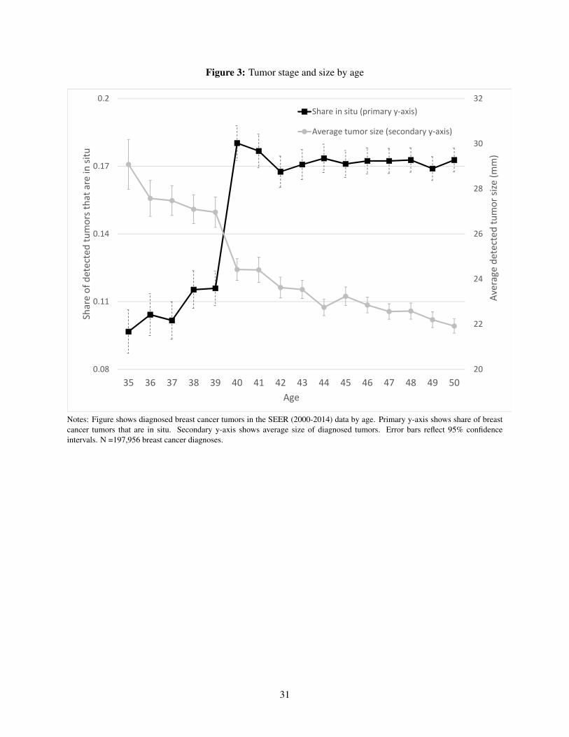
Figure 3: Tumor stage and size by age

20

22

24

26

28

30

32

0.08

0.11

0.14

0.17

0.2

35 36 37 38 39 40 41 42 43 44 45 46 47 48 49 50

Average de

tected

 tumor size (m

m)

Share of detected tumors tha

t are in

 situ

Age

Share in situ (primary y‐axis)

Average tumor size (secondary y‐axis)

Notes: Figure shows diagnosed breast cancer tumors in the SEER (2000-2014) data by age. Primary y-axis shows share of breastcancer tumors that are in situ. Secondary y-axis shows average size of diagnosed tumors. Error bars reflect 95% confidenceintervals. N =197,956 breast cancer diagnoses.

31

Figure 4: Spending by age

4,000

4,200

4,400

4,600

4,800

5,000

5,200

5,400

5,600

5,800

6,000

35 36 37 38 39 40 41 42 43 44 45 46 47 48 49 50

Average 12

‐mon

th sp

ending

Age

No mammogram

Mammogram

(a) Mammogram versus no mammogram

4,000

14,000

24,000

34,000

44,000

54,000

64,000

35 36 37 38 39 40 41 42 43 44 45 46 47 48 49 50

Average 12

‐mon

th sp

ending

Age

Negative

False positive

True positive

(b) By mammogram outcome

Notes: Sample is insurance claims data on a set of privately insured woman-years from 2009- 2011. In Panel A, for each age(defined based on age at the beginning of the calendar year), we report the spending in the 12 months following the mammogram.For those without a mammogram, we draw a reference date from the distribution of actual mammograms in that year. All referencedates are set to be the first of the given month. Spending is measured in the 12 months after this reference date. Panel B focusesonly on the woman-years with mammograms and shows subsequent 12-month spending separately based on mammogram outcome.Error bars (not always visible) reflect 95% confidence intervals. N = 7,373,302 woman-years.

32

Figure 5: Mortality

0.00

0.05

0.10

0.15

0.20

0.25

35 36 37 38 39 40 41 42 43 44 45 46 47 48 49 50

5‐year m

ortality (since diagn

osis)

Age

In situ diagnosis

invasive diagnosis

Notes: Figure shows 5-year mortality for diagnosed breast cancer tumors in the SEER (2000-2014) data. Mortality rates are shownseparately by age of diagnoses and by tumor stage (in situ and invasive). Error bars reflect 95% confidence intervals. N = 147,243diagnoses with non-missing 5-year mortality.

33

Figure 6: Model fit

0

0.1

0.2

0.3

0.4

0.5

35 36 37 38 39 40 41 42 43 44 45 46 47 48 49 50

Share who

 had

 a m

ammog

ram

Age

Observed

Fitted

(a) Share with mammogram

0

0.002

0.004

0.006

0.008

0.01

35 36 37 38 39 40 41 42 43 44 45 46 47 48 49 50

Share of m

ammog

rams that are true

 positive

Age

Observed

Fitted

(b) Share of mammograms that are true positive

0.3

0.4

0.5

0.6

35 36 37 38 39 40 41 42 43 44 45 46 47 48 49 50

Share of diagn

oses th

at are in

 situ

Age

Observed

Fitted

(c) Share of diagnoses in situ

Notes: Figures show model fit by comparing the observed patterns of mammogram rates, outcomes, and types of diagnoses by ageto the fitted values from the model based on the parameter estimates from Table 2. The observed data on mammograms (PanelA) was previously shown in Figure 1; the observed data on share of mammograms that are true positives was previously shown inFigure 2; the observed data on the share of diagnoses that are in situ is a modified version of the data shown in Figure 3. WhileFigure 3 presented the share of all diagnosed cancers that are in situ, we match the share of mammogram-diagnosed cancers thatare in situ, as shown in Panel C. Appendix C provides more detail.34

Figure 7: Impact of changing the mammogram recommendation age from 40 to 45, by age

0

0.1

0.2

0.3

0.4

0.5

35 36 37 38 39 40 41 42 43 44 45 46 47 48 49 50

Share who

 had

 a m

ammog

ram

Age

Age 40 Recommendation

Age 45 Recommendation

(a) Share with mammogram by age

0

0.002

0.004

0.006

0.008

0.01

0.012

35 36 38 39 40 41 42 43 44 45 46 47 48 49 50

Share of m

ammog

rams that are true

 positive

Age

Age 40 Recommendation

Age 45 Recommendation

(b) Share of mammograms that are true positive by age

0.3

0.4

0.5

0.6

35 36 38 39 40 41 42 43 44 45 46 47 48 49 50

Share of true

 positives tha

t are in

 situ

Age

Age 40 Recommendation

Age 45 Recommendation

(c) Share of diagnoses in situ by age

Figure reports the model predictions - by age - for mammogram rates, mammogram outcomes, and the share of diagnoses that arein situ, based on the parameter estimates from Table 2. As in Table 3, we report the model predictions both under the status quorecommendation that mammograms begin at age 40 and the counterfactual recommendation that mammograms begin at age 45.

35

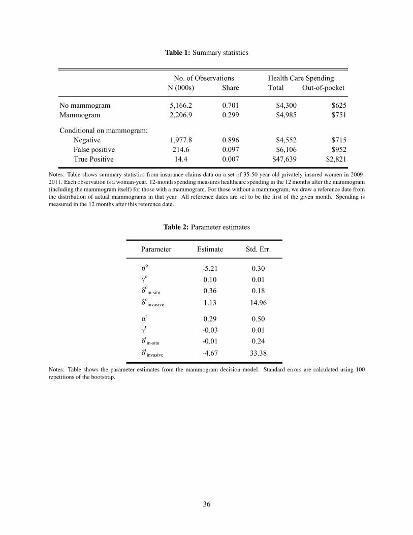
Table 1: Summary statistics

N (000s) Share Total Out-of-pocket

No mammogram 5,166.2 0.701 $4,300 $625Mammogram 2,206.9 0.299 $4,985 $751

Conditional on mammogram:Negative 1,977.8 0.896 $4,552 $715False positive 214.6 0.097 $6,106 $952True Positive 14.4 0.007 $47,639 $2,821

No. of Observations Health Care Spending

Notes: Table shows summary statistics from insurance claims data on a set of 35-50 year old privately insured women in 2009-2011. Each observation is a woman-year. 12-month spending measures healthcare spending in the 12 months after the mammogram(including the mammogram itself) for those with a mammogram. For those without a mammogram, we draw a reference date fromthe distribution of actual mammograms in that year. All reference dates are set to be the first of the given month. Spending ismeasured in the 12 months after this reference date.

Table 2: Parameter estimates

Estimate Std. Err.

αo -5.21 0.30γo 0.10 0.01δo

in-situ 0.36 0.18δo

invasive 1.13 14.96

αr 0.29 0.50γr -0.03 0.01δr

in-situ -0.01 0.24δr

invasive -4.67 33.38

Parameter

Notes: Table shows the parameter estimates from the mammogram decision model. Standard errors are calculated using 100repetitions of the bootstrap.

36

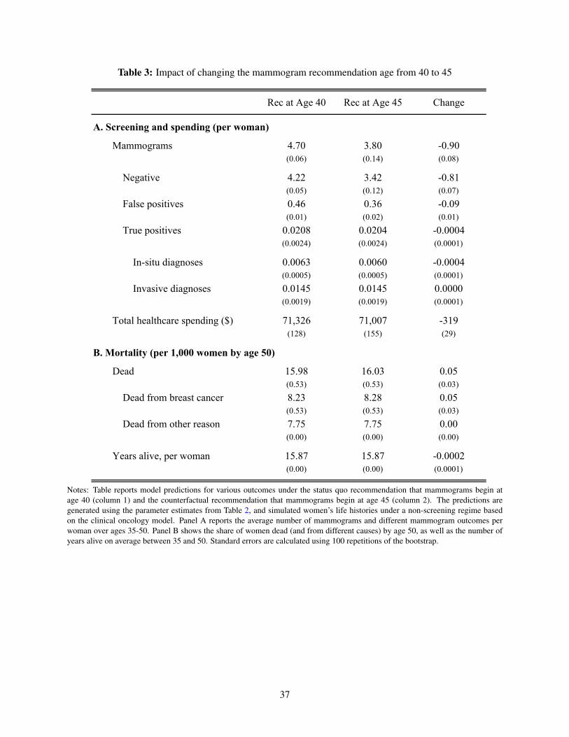
Table 3: Impact of changing the mammogram recommendation age from 40 to 45

Rec at Age 40 Rec at Age 45 Change

A. Screening and spending (per woman)

Mammograms 4.70 3.80 -0.90(0.06) (0.14) (0.08)

Negative 4.22 3.42 -0.81(0.05) (0.12) (0.07)

False positives 0.46 0.36 -0.09(0.01) (0.02) (0.01)

True positives 0.0208 0.0204 -0.0004(0.0024) (0.0024) (0.0001)

In-situ diagnoses 0.0063 0.0060 -0.0004(0.0005) (0.0005) (0.0001)

Invasive diagnoses 0.0145 0.0145 0.0000(0.0019) (0.0019) (0.0001)

Total healthcare spending ($) 71,326 71,007 -319(128) (155) (29)

B. Mortality (per 1,000 women by age 50)

Dead 15.98 16.03 0.05(0.53) (0.53) (0.03)

Dead from breast cancer 8.23 8.28 0.05(0.53) (0.53) (0.03)

Dead from other reason 7.75 7.75 0.00(0.00) (0.00) (0.00)

Years alive, per woman 15.87 15.87 -0.0002(0.00) (0.00) (0.0001)

Notes: Table reports model predictions for various outcomes under the status quo recommendation that mammograms begin atage 40 (column 1) and the counterfactual recommendation that mammograms begin at age 45 (column 2). The predictions aregenerated using the parameter estimates from Table 2, and simulated women’s life histories under a non-screening regime basedon the clinical oncology model. Panel A reports the average number of mammograms and different mammogram outcomes perwoman over ages 35-50. Panel B shows the share of women dead (and from different causes) by age 50, as well as the number ofyears alive on average between 35 and 50. Standard errors are calculated using 100 repetitions of the bootstrap.

37

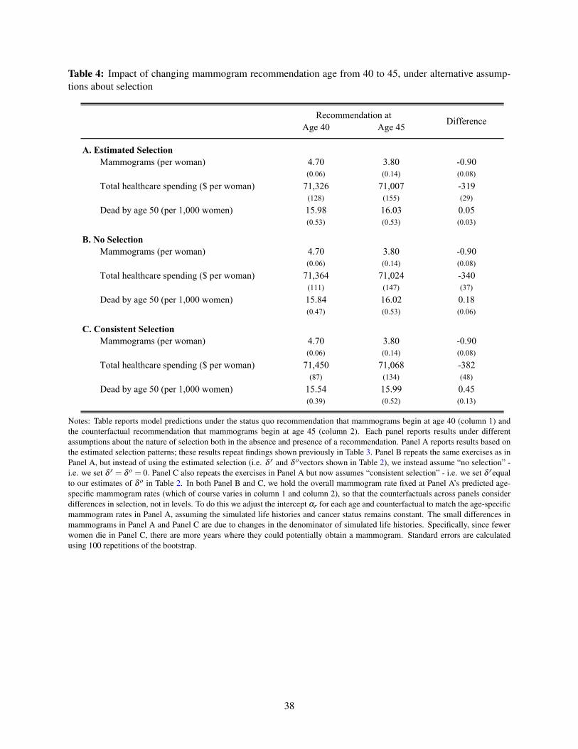
Table 4: Impact of changing mammogram recommendation age from 40 to 45, under alternative assump-tions about selection

Age 40 Age 45

A. Estimated SelectionMammograms (per woman) 4.70 3.80 -0.90

(0.06) (0.14) (0.08)Total healthcare spending ($ per woman) 71,326 71,007 -319

(128) (155) (29)Dead by age 50 (per 1,000 women) 15.98 16.03 0.05

(0.53) (0.53) (0.03)

B. No SelectionMammograms (per woman) 4.70 3.80 -0.90

(0.06) (0.14) (0.08)Total healthcare spending ($ per woman) 71,364 71,024 -340

(111) (147) (37)Dead by age 50 (per 1,000 women) 15.84 16.02 0.18

(0.47) (0.53) (0.06)

C. Consistent SelectionMammograms (per woman) 4.70 3.80 -0.90

(0.06) (0.14) (0.08)Total healthcare spending ($ per woman) 71,450 71,068 -382

(87) (134) (48)Dead by age 50 (per 1,000 women) 15.54 15.99 0.45

(0.39) (0.52) (0.13)

Recommendation at Difference

Notes: Table reports model predictions under the status quo recommendation that mammograms begin at age 40 (column 1) andthe counterfactual recommendation that mammograms begin at age 45 (column 2). Each panel reports results under differentassumptions about the nature of selection both in the absence and presence of a recommendation. Panel A reports results based onthe estimated selection patterns; these results repeat findings shown previously in Table 3. Panel B repeats the same exercises as inPanel A, but instead of using the estimated selection (i.e. δ r and δ ovectors shown in Table 2), we instead assume “no selection” -i.e. we set δ r = δ o = 0. Panel C also repeats the exercises in Panel A but now assumes “consistent selection” - i.e. we set δ requalto our estimates of δ o in Table 2. In both Panel B and C, we hold the overall mammogram rate fixed at Panel A’s predicted age-specific mammogram rates (which of course varies in column 1 and column 2), so that the counterfactuals across panels considerdifferences in selection, not in levels. To do this we adjust the intercept αr for each age and counterfactual to match the age-specificmammogram rates in Panel A, assuming the simulated life histories and cancer status remains constant. The small differences inmammograms in Panel A and Panel C are due to changes in the denominator of simulated life histories. Specifically, since fewerwomen die in Panel C, there are more years where they could potentially obtain a mammogram. Standard errors are calculatedusing 100 repetitions of the bootstrap.

38

Table 5: Sensitivity checks for impact of changing mammogram recommendation age from 40 to 45

Age 40 Age 45 Age 40 Age 45 Age 40 Age 45

Baseline Estimate 15.98 16.03 0.05 15.84 16.02 0.18 15.54 15.99 0.45

(1) Erasmus original level 10.66 10.68 0.02 10.67 10.68 0.01 10.65 10.68 0.03

Decrease share of in-situ tumors that become invasive:(2) from 62.5% to 28% 15.20 15.22 0.02 15.06 15.21 0.15 14.78 15.18 0.41(3) from 62.5% to 14% 14.89 14.90 0.01 14.75 14.89 0.14 14.48 14.86 0.39

Increase share of non-malignant tumors:(4) from 6% to 19% 15.08 15.12 0.03 14.90 15.10 0.20 14.63 15.07 0.44(5) from 6% to 42% 12.69 12.70 0.02 12.53 12.68 0.15 12.36 12.66 0.30

Decrease cancer incidence to:

C. Consistent SelectionA. Estimated Selection B. No Selection

Dead by age 50(per 1,000 women)

Recommendation atDiff

(per 1,000 women) (per 1,000 women)Dead by age 50 Dead by age 50

Recommendation atDiff

Recommendation atDiff

Notes: Table reports model predictions under alternate sensitivity assumptions. The first three columns in the first row replicate theresults from Table 4 Panel A on the impact of changing the mammogram recommendation age from 40 to 45 based on the estimatedselection patterns. We report only the impact on the death rate by age 50. The second three columns replicate the results from Table4 Panel B where we instead assume “no selection” - i.e. we set δ r = δ o = 0. The last set of columns reflect Table 4 Panel C wherewe assume “consistent selection” - i.e. we set δ requal to our estimates of δ o in Table A.10. Each row tests the sensitivity of theseestimates under alternate natural history assumptions, as discussed in Section 5.2.3.

39

Appendix

A Coding Mammograms and Outcomes in Claims Data

We follow Segel, Balkrishnan„ and Hirth (2017) in coding the incidence of screening mammograms (here-

after “mammograms”) and the results of those mammograms in the HCCI claims data.

We code a woman as having a screening mammogram on a given date if she has a claim with ICD-9

procedure code V76.12 or CPT codes 77057 or G0202 on that date, but no claims for any other mammo-

gram within the previous 12 months and no prior claims for breast cancer treatment.18 Previous work has

documented that claims-based measures of mammogram rates tend to be lower than mammogram rates in

self-reported survey data. For example, Freeman et al. (2002) document this pattern in Medicare data, and

Cronin et al. (2009) document similar evidence in a study of Vermont women. Consistent with these studies,

Appendix Figure A.1 documents the age profile of the annual screening mammogram rate, as measured by

both the Behavioral Risk Factor Surveillance System (BRFSS) survey and the algorithm described above

using the HCCI claims data. Between ages 39 and 41, the mammogram rate jumps by approximately the

same amount - 25 percentage points - by both measures, but the survey data describe mammogram rates as

being approximately 10 to 20 percentage points higher than the claims data rate at all ages. Of course the

samples are not perfectly comparable, as the BRFSS sample is of all women with health insurance (public

or private) from 2002-2012, while the HCCI sample is of women privately insured by Aetna, Humana or

United between 2008 and 2012.

We code the outcome of a screening mammogram as negative if there are no subsequent claims for

either follow-up testing or breast cancer treatment within the next twelve months. We code the outcome

as a false positive if there is at least one claim for follow-up testing in the following three months (i.e.

a subsequent mammogram, a breast biopsy, a breast ultrasound, or other radiologic breast testing) in the

following three months, but no claims for breast cancer treatment in the next 12 months. We code the

outcome of a mammogram as true positive if, within twelve months following the mammogram, there is

at least one claim for breast cancer. We consider a women to have a subsequent mammogram if she has a

claim with ICD-9 procedure code V76.12 or CPT codes 77057 or G0202. A women has a breast biopsy

if she has a claim with ICD-9 procedure code 85.11, 85.12, 85.20, or 85.21 or CPT codes 19100, 19101,

or 19120. A breast ultrasound is coded with ICD-9 procedure code 88.73 or CPT code 76645. Radiologic

breast testing is coded with ICD-9 procedure code 87.35, 87.36, 87.73, or 88.85 or CPT codes 76003, 77002,

76095, 77031, 76086, 76087, 76088, 77053, 77054, 76355, 76360, 76362, 77011, 77012, 77013, 76098,

76100, 76101, 76102, 76120, 76125, 76140, 76150, 76350, or 76365. Breast cancer is coded with ICD-9

procedure code 233.0, V103.0, or 174.0 through 174.9 or CPT code 19160, 19162, 19180, 19200, 19220,

19240, 19301, 19303, 19305, 19307, 38740, or 38745.The codes used to identify these claims are provided

in Appendix Table A.1, along with their references.

The linked SEER-Medicare data allows us to cross validate this claims-based coding process against

18Segel, Balkrishnan„ and Hirth (2017) focused on data from 2003-2004, so used the CPT code 76092. In 2007 this code wasreplaced by 77057. In addition, Hubbard et al. (2015) identify CPT code G0202 as indicating a screening mammogram claim.Segel, Balkrishnan„ and Hirth (2017) provide codes for “other” (non-screening) mammograms, which we omit.

40

cancer diagnoses in the cancer registry. The results are very encouraging. Appendix Tables A.2 and A.3

describe the concordance of true positive mammograms as coded using this algorithm with actual diagnoses

as recorded in the SEER-Medicare data. For those who were diagnosed with breast cancer and had a mam-

mogram in the year of diagnosis, 99.8% of mammograms were coded as true positive using our algorithm.

Meanwhile, 93% of mammograms for patients who were never diagnosed with breast cancer were nega-

tive, while 6.5% were false positives. Most patients with true positive mammograms were diagnosed with

breast cancer in the year of or the year following the mammogram, while 83% of those without true positive

mammograms were never diagnosed and a further 13% were not diagnosed until more than 1 year after

the mammogram (4% were diagnosed in the year following the mammogram, but none in the year of the

mammogram).

B Clinical model: the Erasmus model

We use the Erasmus model to generate estimates of the underlying onset rate by age of cancer and cancer

type, as well as the evolution of (untreated) cancers. We adjust the model to better match certain key

moments of the SEER data. This (modified) Erasmus data, together with assumed parameters from the

mammogram decision model (specifically, equations 1 and 2) and the observed policy recommendation (40

and above), generates an age-specific share of women who are screened, as well as the tumor characteristics

(in situ and invasive rates) conditional on getting screened, which we then attempt to match by method

of moments to the observed data on the age-specific share of women who are screened and the tumor

characteristics conditional on getting screened.

As described in the main text, the Erasmus model is one of seven models developed for the Cancer

Intervention and Surveillance Modeling Network (CISNET) as part of a project decomposing breast cancer

mortality reductions from 1975-2000 into effects from the dissemination of mammography versus the de-

velopment of advanced treatment techniques (Clarke et al. 2006). Each of the groups participating in the

project wrote a model of breast cancer incidence and mortality in the US over this time period and then

compared the mortality rates under scenarios with and without mammography and advanced treatment. For

convenience, we focus on one of these models, the Erasmus model (Tan et al., 2006).

In what follows we describe our implementation of the Erasmus model. This implementation directly

follows Tan et al. (2006), with all the assumptions we describe being theirs. We then describe the calibration

changes we make to the model based on some of our own external data and assumptions.

B.1 Model details

Tumor incidence

The model allows us to simulate a cohort of women i, each with a year of birth bi and a year of death from

other causes di which is randomly determined and dependent on the year of birth. Specifically, it assumes

that in each year y the probability that a person born in year b (such that y ≥ b) dies of causes other than

breast cancer is Qby . A woman’s year of death is defined as the lesser of 110 and the first year in which a

41

random draw from a uniform distribution on [0,1] falls below Qby . It assumes that no woman dies from other

causes before age 30.

The model further assumes that there exists a probability Cb that any woman from cohort b will get

cancer before age 85. It defines age aby = y− b as the age in year y of an individual born in year b and

assumes that for every cohort b and year y such that 20 ≤ aby ≤ 85 there exists Sa, the probability that a

woman experiences tumor onset at age a conditional on eventually getting cancer. For each woman i with

any cancer, we can therefore construct the year of tumor onset ti as the lesser of the year in which she turns

85 and the first year in which a random draw from a uniform distribution on [0, 1] falls below Sy−bi .

Tumor type and in situ characteristics

At onset, cancer type is defined to be either an invasive tumor or one of three types of non-invasive tumors.

Non-invasive tumors are also known as as ductal carcinoma in situ (DCIS), which we refer to in the text as in

situ. Invasive tumors are assigned a minimum size and other tumor characteristics (as described in Appendix

Table A.4) at onset and immediately begin growing. DCIS-regressive tumors eventually disappear without

causing any harm; DCIS-invasive tumors eventually transform into a harmful invasive tumor but do no harm

in the meantime, and DCIS-clinical tumors do no harm but are eventually clinically detected. The model

assumes that the outcome of each DCIS tumor (regression, invasion, or detection) occurs wi years after

onset, where wi is generated by random draws from an exponential distribution with mean W . None of the

three types of DCIS tumors can be clinically detected during the duration of this “dwell time”, but they can

be screen-detected with a screening-year-specific probability Ey if screening occurs. The type of tumor is

defined at onset subject to age-specific probabilities Ia (invasive), Va (DCIS-invasive), Ra (DCIS-regressive),

and Ca (DCIS-clinical) such that Ia +Va +Ra +Ca = 1. Values for these and other Erasmus parameters are

given in Appendix Table A.5.

For DCIS tumors that become invasive, onset of invasive disease is defined as the moment when the

tumor size reaches the minimum value of the screening threshold diameter; this threshold varies with the

woman’s age as well as over time (to reflect improvements in screening technology). The dwell time for

DCIS tumors was calibrated in the MISCAN breast cancer model based on the duration from onset of DCIS

to the 1975 screening threshold diameter.

Invasive tumor characteristics

The model assumes that the fundamental characteristic of invasive tumors is their year-dependent size syi .

For all invasive tumors, it defines s0i (the size in the year of onset) to be equal to 0.01 cm. It assume that all

invasive tumors grow exponentially. Tumor size in year y is therefore given by s0i (1+gi)

y where gi is the

individual-specific growth rate (drawn from a lognormal distribution at tumor onset). It further assumes that

diagnosis depends on tumor size and the individual’s “screen detection diameter” rayi (drawn at the time of

screening from an age- and detection-year-specific Weibull distribution) and “clinical diagnosis diameter”

ci (log normally distributed and set at tumor onset). If the patient undergoes screening, the tumor can be

detected if syi > ri. Alternatively, if the tumor grows so large that sy

i > ci, the patient will certainly detect it

due to the appearance of clinical symptoms. Tumor size also determines mortality: if a patient diagnoses

42

her tumor before it reaches its “fatal diameter” fi (drawn at onset from a year-specific Weibull distribution),

she will receive treatment and survive, but if not, she will die regardless of treatment.

The model defines for each invasive tumor the length of time the patient will survive after the tumor

reaches its fatal diameter, called the “survival duration since fatal diameter” and denoted ui (log normally

distributed). It assumes that if the tumor has not been clinically detected by the time 0.9*ui years have

passed since the fatal diameter was reached, it will be clinically detected due to distant metastases at that

time.

Finally, it assumes that the growth rate gi, clinical diagnosis diameter ci, and survival duration ui are

correlated with coefficients ρgc, ρgu, and ρcu. The variables described in this section (syi ,r

ayi , fi gi,ci,ui) ,

combined with the woman’s age and the year of initiation, fully specify the course of the disease for an

invasive tumor, subject to potential screening regimens.

B.2 Parameterizing the Erasmus model

We begin by choosing certain population-specific parameters required as inputs for the Erasmus model: the

other-cause death probability, the overall tumor incidence, and the tumor incidence by age. As in Tan et al.

(2006), the other-cause death probability follows the approach of Rosenberg (2006). However, we adjusted

the tumor incidence parameters (overall cohort incidence and quadratic incidence by age) that are given in

Tan et al. (2006) in order to match the SEER data’s share of diagnoses that are in situ and invasive for those

under 40 and over 40. After establishing these population-specific parameters, we simulate individual life

histories under a no-screening assumption, and use the tumor sizes and types to determine the population

cancer rate by age.

Other-cause death probability

Following Rosenberg (2006), we computed probability of death due to other causes as the difference be-

tween the all-cause mortality and breast cancer specific mortality. We obtained all-cause mortality for ages

0-110 and years 1933-2010 from the Human Mortality Database. Using breast cancer death totals from

the National Center for Health Statistics and female population totals from the Human Mortality Database,

we calculated breast-cancer-specific mortality for ages 0-110 and years 1959-2010. To impute values for

previous years, we assumed that the age-specific breast cancer mortality rate in any year before 1958 was

equal to the rate in 1958. We combined these data to calculate non-breast-cancer mortality rates for all years

between 1933 and 2010.

Age profile of cancer incidence

The Erasmus model provided a CDF of tumor incidence in 5-year increments, implying a step function of

yearly incidence that produces spikes in tumor onset within a cohort every 5 years (see Appendix Table A.6,

first column reproduced from Tan et al. (2006), based on estimates of US population in 1975). We con-

structed a smoothed CDF of tumor incidence by fitting to the Erasmus CDF using a constrained polynomial

43

(quadratic) fit: y = ax2 +bx+ c. We fitted a,b,c, the start age xstart (at which the CDF should be zero), and

the end age xend (at which the CDF should be one). Restrictions included:

ax2start +bxstart + c = 0

ax2end +bxend + c = 1

2axstart +b≥ 0

The values that minimize the error ∑(y−y)2 across each of the fourteen ages in Appendix Table A.6 are

xstart = 24, xend = 85, a = 0.000268, b =−0.01282, c = 0.15327. We assume that the incidence before age

24 is 0. The fit is shown in Appendix Figure A.5.

Adjusting cancer incidence rates

Tan et al. (2006) calculate cumulative tumor incidence by birth cohort based on observed (i.e. diagnosed)

incidence in the US from 1975-1979. Implicitly, this assumes that all tumors are diagnosed. It will therefore

miss any undiagnosed tumors. Not surprisingly, therefore, when we use the original Erasmus parameters and

our calibrated screening policy described below, the model substantially under-predicts observed diagnoses.

To rectify this, we allowed the cohort tumor incidence to vary with a multiplicative shift α which uniformly

affects each cohort’s tumor incidence.

We calibrate α as follows. We define the parameters θ = (α, pscrninv, pscrndcis) where pscrninv is the

probability of a mammogram conditional on having an invasive tumor and pscrninsitu is the probability

of a mammogram conditional on having an in situ tumor. We then estimate θ by maximum likelihood.

Specifically, we maximize the log likelihood of observing SEER tumor types (1973-2013, for women 25-

34). The model’s original incidence and the incidence multiplicatively shifted by α are plotted against the

SEER diagnosis rates in Appendix Figure A.6. We also plot the model’s diagnosis rates with no screening;

with the multiplicative shift this roughly matches with the SEER diagnosis levels.

B.3 Visual representation and results from Erasmus model: Underlying cancer rate

The first panel of Appendix Figure A.7 visualizes the Erasmus model using a flow chart. The second panel

shows example sequences of progression for each of the four types of tumors, in the absence of screening.

The first two rows show the progress of DCIS-regressive and DCIS-clinical tumors, which are harmless

and differ only in their behaviors at the end of their dwell time: DCIS-regressive tumors disappear, while

DCIS-clinical tumors are detected clinically, for example at a routine physical exam. If these tumors are

screened, they will be diagnosed with a probability equal to the “sensitivity” as described in Appendix Table

A.5. Likewise, before it switches to its invasive phase, the DCIS-invasive tumor can also be detected by a

screening mammogram in the same way. After it becomes invasive, the DCIS-invasive tumor (row 3) and the

invasive tumor (row 4) can only be detected if the size exceeds the year- and age-specific screening diameter

44

of the year in which it is screened. If a woman’s tumor is screened (or clinically diagnosed) before it reaches

the fatal diameter, her life is saved, but if not, she will eventually die, regardless of detection or treatment in

later years. In most cases, when a woman’s tumor reaches the fatal diameter without being diagnosed, she

will be clinically diagnosed before death. The flow chart omits deaths due to other causes.

Appendix Figure A.8 plots the share of women in each of five categories when the Erasmus model

is calculated with no screening. The calculation is based on birth cohorts from 1950-1975, and focuses

on women aged 30-50 in 2000-2005. At any given age, the share of women with detectable invasive or

DCIS cancer is substantially smaller than the share of women who have already been diagnosed clinically,

indicating that there is a small window of time during which a cancer can be screened before it is clinically

detected.

Using the calibrated other-cause death probabilities and incidence rates, we solve the Erasmus model

assuming that there is no screening for birth years 1950-1975. We restrict to years 2000-2005 and ages

30-50, producing a set of individual life-histories that can be categorized in every year as dead due to breast

cancer, dead due to other causes, clinically diagnosed, currently undiagnosed invasive cancer, currently

undiagnosed DCIS, or no cancer. (We consider invasive cancer that is too small to be detectable, and

regressed DCIS tumors, to be the same as “no cancer.”)

We take the “population cancer rate” at each age, or the share of women who have a tumor by a certain

age, from the Erasmus model. The Erasmus model assumes that cancers can only be detected by mammo-

gram once they have reached a certain size, so we assume the screening diameter is 1.09 cm – the average

screen-detectable size in the Erasmus model – and count the share of women with detectable invasive cancer

as the share of women with tumors above that size in the Erasmus model. We also count 80% of the women

with DCIS tumors, under the assumption in the Erasmus model that about 80% of technically “detectable”

in situ tumors will be detected in any given year. We do not count DCIS-regressive tumors after they have re-

gressed, and after a DCIS-invasive tumor has transitioned to an invasive tumor we determine its detectability

based on the rules for invasive cancers.19

C Estimation of mammogram model

We estimate our model of mammogram demand by method of moments. The moments are generated from

the Erasmus model combined with our model of screening decisions. We first use the Erasmus model to

generate cancer incidence and tumor growth under a no-screening assumption, as described above. Specifi-

cally, we simulate a panel of ten million women born between 1910 and 1974. We start at age 20 and model

cancer incidence and tumor growth using the Erasmus model, assuming no screening. We use the tumor

sizes and types to determine the population cancer rate by age.

Then, for a given set of parameters αo,γo,δ o,αr,γr,δ r, we apply the mammogram decision model (by

19Note that this leads to an unintuitive model behavior in which DCIS tumors are detectable at smaller sizes than invasive tumors.In the Erasmus model, invasive tumors are initialized at 0.01 mm and are not considered screen-detectable (by us) until they reach1.09 cm. DCIS-invasive tumors are initialized at the screening threshold of the year and age in which they become invasive. Sincethis is sometimes smaller than 1.09 (1.09 is just the average of the distribution of screening thresholds in 2010), the model couldsimulate a DCIS-invasive tumor which is detectable for several years, then becomes undetectable, then becomes detectable again.

45

age and recommendation status) to the cancer rate age profile from the Erasmus model to generate the main

moments by age.

Although the model is static, it does have a dynamic element in it, as we calculate the model-generated

moments only for the women who were not diagnosed with cancer in previous years, or those who did not

die (from breast cancer or other causes) prior to the given age. To do this, we must make an assumption about

what fraction of clinically-diagnosed women under the no-screening assumption overlap with the screen-

diagnosed population when the mammogram decision model is applied. One extreme would be to assume

that there is no overlap (perfect negative correlation between clinical and screen diagnosis), so that if 0.01

of the population were clinically-diagnosed under the no-screening assumption, and 0.02 of the population

were screen-diagnosed for a given set of parameters, a total of 0.03 of the women would be diagnosed with

cancer. We chose to make the other assumption, that there was perfect positive correlation between clinical

and screen diagnosis. In this case, if 0.01 of the population were clinically-diagnosed and 0.02 were screen-

diagnosed, only 0.02 of the women would be diagnosed with cancer. This likely produces an underestimate

of the effects of screening, because it minimizes the number of women who are diagnosed each year.

With this simulated population of women, an assumed value of parameters associated with the mammo-

gram decisions with and without recommendation (equations 1 and 2) and the observed policy recommen-

dation (40 and above), the model generates an age-specific share of women who are screened, and the tumor

characteristics (in situ and invasive rates), conditional on getting screened.

As mentioned in the main text (footnote 13), the in situ rate moment differs from Figure 3 in the main

text. Figure 3 shows the in situ rate of all diagnosed cancers that appear in the SEER database, but the

moment we match with the model is the in situ rate of screen-detected cancers. Cancers that are clinically

diagnosed are highly unlikely to be in situ, so the SEER value likely underestimates the true value of share in

situ for screening mammogram-diagnosed cancers. We adjust the SEER moment at each age using Bayes’

rule:

P(M)∗P(insitu|M)+(1−P(M))∗P(insitu| ∼M) = P(insitu),

where M is the event that a diagnosed tumor was screen-detected. We assume that P(M), the share of

diagnoses detected by screening mammogram, is 0.2 for ages 35-39 and 0.34 for ages 40-49 (following

Roth et al. (2011)). We assume that P(insitu| ∼ M) = 0.08, following Ernster et al. (2002). P(insitu) is

given by the SEER moments in Figure 3, allowing us to back out P(insitu|M), our object of interest, which

is the moment we actually match. The results for P(insitu|M) for ages 40-49 range from 52% to 55%, which

is in line with the 56% reported in this age group by Ernster et al. (2002).

With our 48 moments in hand (16 moments for each of 3 types), we then search for the parameters that

minimize the (weighted) distance between these generated moments and the observed moments. We apply

a linear weight that decreases on each side of age 40, so that the weight on moments associated with ages

39 and 41 is 10/11 of the weight on the age 40 moment, the weight on moments associated with ages 38 and

42 is 9/11 of the weight on the age 40 moment, and so on. To achieve a reasonable fit, we also weight the

moments by the inverse of their standard deviation. We chose 2,000 random starting values in the parameter

46

space defined as follows:

αo ∈ [−10,10],γo ∈ [−0.2,0.2],δ o

insitu ∈ [−2,2], δoinvasive ∈ [−2,2]

αr ∈ [−2,2],γr ∈ [−0.2,0.2],δ r

insitu ∈ [−2,2],δ rinvasive ∈ [−2,2]

and applied the Nelder-Mead algorithm to each of these starting vectors. We then iteratively applied the

Nelder-Mead algorithm to the best starting value to further minimize the objective function.

D Counterfactual simulations of mammogram model

Our counterfactuals analyze the impact of changing the recommendation age as well as the selection re-

sponse. In both cases, we first model the underlying onset rate of cancer and the evolution of cancers using

the Erasmus model described in Section 4.2 and Appendix B. Since we are interested in analyzing the im-

pact of potential future recommendation changes, we apply the most recent year’s value of any time-varying

parameters of the Erasmus model. In practice, this means we use the breast-cancer-specific and non-breast-

cancer mortality for 2010, the scale parameter for fatal diameter βyF from 1975 (see Appendix Table A.5),

the screening sensitivity Ey from 2000, the screening diameter scale parameters from 2000 (see Appendix

Table A.7), and the tumor incidence for the 1970 cohort (see Appendix Table A.8). We simulate this model

for 10 million women’s life histories, and in particular from ages 35-50.

We then apply the screening decision as described in Section 4.2 for each women and year. The baseline

model uses the parameter values given in Table 2, with the recommendation applied starting at age 40. We

change the age of the recommendation in Table 3 and the selection parameters δ r in Table 4.

In all counterfactuals that retain the age-40 recommendation (i.e. the ones that aim to isolate a counter-

factual selection responses), we specify that the age-specific mammogram rates must be the same as in the

baseline specification, while the type of women who respond to the recommendation is allowed to change.

This allows the counterfactuals to consider only differences in selection, not levels. After imposing the

counterfactual selection coefficients, we add an age-specific constant so that the age-specific mammogram

rates are unchanged relative to the baseline. In all counterfactuals that both use the age-45 recommendation

(i.e. the ones that consider a counterfactual policy recommendation) and impose alternative selection pat-

terns, we make a similar adjustment so that the age-specific mammogram rates match those produced by the

age-45 counterfactual with the baseline estimated selection parameters. The screening decisions along with

underlying natural history in the Erasmus model determine whether a given mammogram screen results in

a negative test, a false positive, or true positive based on the cancer type of the screened woman.

The Erasmus model parameters also reveal whether a mammogram detects a cancer early enough to

prevent breast-cancer-related morality. If an invasive tumor is detected before it reaches the fatal diameter

(see Appendix Table A.5 on Erasmus parameters), the person survives to die of natural causes. If the invasive

tumor is detected after the tumor is larger than the fatal diameter, the person dies of breast cancer after

some stochastic period determined by survival duration parameters (see Appendix Table A.5 on Erasmus

parameters). Breast cancer related mortality is driven by invasive tumors; in situ tumors are only fatal if

47

they progress to an invasive tumor.

To estimate total spending under different counterfactuals, we first calculated in the HCCI data, the

total age-specific spending in the twelve months following no mammogram, a negative mammogram, a

false positive mammogram, and a true positive mammogram. At each age, each simulated woman falls into

one of these categories. We add up the spending for a given woman across ages 35-50 based on her relevant

mammogram outcomes in each year. For example, suppose a woman had a true positive mammogram at age

42, and no mammograms at any other age. We would add the average spending in the HCCI data for women

with no mammograms for ages 35-41, the average spending for a woman in the twelve months following

a true positive mammogram at age 42, and the average spending for women with no mammograms at ages

43-50. Note that the screening decision only applies to women who are alive and have never been diagnosed

with breast cancer; once a women receives a true positive diagnosis she is not longer screened.

E Sensitivity Analysis

We explore the robustness of our estimates to changing features of our clinical model. In particular, we

focus on statistics that can be compared with other sources, such as the share of in-situ tumors that become

invasive, and the share of tumors that are non-malignant.

Two specifications test sensitivity to decreasing the share of in-situ tumors that become invasive. The

Erasmus model assumes that 62.5% of in-situ tumors will become invasive, while estimates for the fraction

of DCIS tumors that would become invasive over 10 years if left untreated ranges from 14-60% (Burstein

et al., 2004), putting the Erasmus model at the most conservative end of the spectrum. Alternate estimates

suggest that the share of DCIS-tumors that become invasive is 14% (Eusebi et al., 1994) or 28% (Page et al.,

1995). In these checks, we also shift the tumor type distribution to match these estimates at age 40. This

sensitivity proportionally reduces the share of DCIS-invasive tumors at all ages, and proportionally increases

the share of tumors that are DCIS-regressive and DCIS-clinical at all ages. The share of invasive tumors

remains the same.

Similarly, two specifications test sensitivity to increasing the share of non-malignant tumors. Non-

malignant refers to tumors that have no potential to be invasive and therefore would never result in a breast

cancer mortality. Specifically, in our natural history model, recall that there are invasive tumors as well as

three types of non-invasive tumors (also known as DCIS or in situ): DCIS-regressive, DCIS-clinical and

DCIS-invasive. The invasive and DCIS-invasive tumors are referred to as “malignant” due to their potential

to cause harm, while the DCIS-regressive and DCIS-clinical tumors will never become invasive and are

therefore referred to as “non-malignant”. The Erasmus model’s parameters (see Appendix Table A.9) imply

that 3-9% of all tumors are non-malignant.20 In contrast, estimates of over-diagnosis, or the diagnosis of a

cancer that would not harm a woman in her lifetime, vary from <5% to >30% (American Cancer Society,

2017a). Compared to other models, the Erasmus model seems to have a low estimate of non-malignancy,

or equivalently a high estimate of the share of cancer that is invasive or could become invasive. Therefore,

20The share of cancer that is in situ of any kind (DCIS-clinical, DCIS-regressive, or DCIS-invasive) with no screening is ap-proximately 15% at age 35 and 9% at age 50 (see Appendix Figure A.4). The age gradient is because some of the DCIS invasivebecomes invasive and some of the DCIS regressive regresses.

48

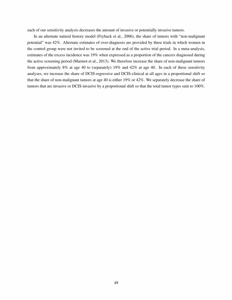
each of our sensitivity analysis decreases the amount of invasive or potentially invasive tumors.

In an alternate natural history model (Fryback et al., 2006), the share of tumors with “non-malignant

potential” was 42%. Alternate estimates of over-diagnosis are provided by three trials in which women in

the control group were not invited to be screened at the end of the active trial period. In a meta-analysis,

estimates of the excess incidence was 19% when expressed as a proportion of the cancers diagnosed during

the active screening period (Marmot et al., 2013). We therefore increase the share of non-malignant tumors

from approximately 8% at age 40 to (separately) 19% and 42% at age 40. In each of these sensitivity

analyses, we increase the share of DCIS-regressive and DCIS-clinical at all ages in a proportional shift so

that the share of non-malignant tumors at age 40 is either 19% or 42%. We separately decrease the share of

tumors that are invasive or DCIS-invasive by a proportional shift so that the total tumor types sum to 100%.

49

Figure A.1: Mammogram rate in survey and claims data, by age

0

0.1

0.2

0.3

0.4

0.5

0.6

0.7

35 36 37 38 39 40 41 42 43 44 45 46 47 48 49 50

Share who

 had

 a m

ammog

ram

Age

BRFSS Survey

HCCI Claims

Notes: This figure shows the share of women who received a screening mammogram each year, by age. Source for survey data:Behavioral Risk Factor Surveillance System Survey (BRFSS), even years 2000-2012, restricted to women with health insurance(public or private). Source for claims data: HCCI data from 2008-2012, for mammograms between 2009-2011. Mammograms arecoded in the HCCI claims data using the algorithm described in Segel, Balkrishnan„ and Hirth (2017). Mammograms are coded inthe BRFSS data based on self-reports. The approximately 15-ppt discrepancy between surveyed and observed mammogram ratesis consistent with the finding of Cronin et al. (2009), who document that self-reported screening rates overstated actual screeningrates by 15 to 27 percentage points in a study of Vermont women.

50

Figure A.2: Health care spending and emergency room use prior to mammogram, by age

3,500

3,700

3,900

4,100

4,300

4,500

35 36 37 38 39 40 41 42 43 44 45 46 47 48 49 50

Average 12

‐mon

th sp

ending

 in Prio

r Year

Age

No Mammogram

Mammogram

(a) Annual spending in year prior to mammogram

0.15

0.16

0.17

0.18

0.19

0.20

0.21

35 36 37 38 39 40 41 42 43 44 45 46 47 48 49 50

Average # of Emergency Ro

om Visits in

 Prio

r Yea

r

Age

No Mammogram

Mammogram

(b) # of emergency room visits in year prior to mammogram

Notes: Sample is insurance claims data on a set of privately insured woman-years from 2009- 2011. The x-axis plots the women’sage at the time of the mammogram. Panel A presents average total spending in the 12 months prior to the mammogram, not includ-ing the mammogram date. Panel B presents average number of emergency room visits in the 12 months prior to a mammogram.For those without a mammogram, we draw a reference date from the distribution of actual mammograms in that year. All referencedates are set to be the first of the given month. N = 5,140,371 woman-years.

51

Figure A.3: Preventive care prior to mammogram by age

0.3

0.4

0.5

0.6

0.7

0.8

0.9

35 36 37 38 39 40 41 42 43 44 45 46 47 48 49 50

Any Pa

p Test in

 Prio

r Year

Age

No Mammogram

Mammogram

(a) Any pap test in year prior to mammogram

0.08

0.09

0.10

0.11

0.12

0.13

0.14

0.15

35 36 37 38 39 40 41 42 43 44 45 46 47 48 49 50

Any Flu Sh

ot in

 Prio

r Year

Age

No Mammogram

Mammogram

(b) Any flu shot in year prior to mammogram

Notes: Sample is insurance claims data on a set of privately insured woman-years from 2009- 2011. In panel A, for each age at thetime of the mammogram, we report the average share of women who obtained a pap test in the 12 months prior to the mammogram.We do not include tests done on the day of the mammogram. Panel B presents the analogous results for any flu shot. For thosewithout a mammogram, we draw a reference date from the distribution of actual mammograms in that year. All reference datesare set to be the first of the given month. Spending is measured in the 12 months prior to this reference date. N = 5,140,371woman-years.

52

Figure A.4: Erasmus model predictions for share with cancer and share in situ (no screening)

0

0.02

0.04

0.06

0.08

0.1

0.12

0.14

0.16

35 36 37 38 39 40 41 42 43 44 45 46 47 48 49 50Age

Share with any cancer

Share of in‐situ cancer, conditional on having cancer

Notes: Figure presents the share with any cancer and the share of cancer in situ in the Erasmus model, with no screening.

53

Figure A.5: Fitted tumor incidence by age

20 30 40 50 60 70 80

0.0

0.2

0.4

0.6

0.8

1.0

Age

Cum

m. I

ncid

ence

Erasmus IncidenceRestricted 2nd Degree Poly

Notes: Figure presents the smoothed CDF of tumor incidence by age, fitted to the original Erasmus incidence in 5-year intervals.

54

Figure A.6: Multiplicative incidence adjustment0

12

34

Num

per

100

0 al

ive

in c

ohor

t

25 30 35 40 45 50 55 60Age at diagnosis/incidence

SEER Dx Sim DxSim Incd

(a) Original incidence

02

46

8N

um p

er 1

000

aliv

e in

coh

ort

25 30 35 40 45 50 55 60Age at diagnosis/incidence

SEER Dx Sim DxSim Incd

(b) Incidence multiplicatively shifted by α

Notes: Figure presents the simulated incidence and diagnosis rates compared with the SEER diagnosis rates. These are presentedfor both the original incidence in panel (a), and for the incidence shifted by α in panel (b). This simulation assumes no screening.

55

Figure A.7: Erasmus model

Tumor Onset

Draw type, dwell time Draw growth rate, fatal diameter

Dwell 1 year

Screened?

Dwell time over?

Tumor type invasive?

Diagnosed (screen)Yes

No

Diagnosed (clinical)Yes

YesNo

Tumor type clinical?

Yes

No

No

Tumor type regressive;Tumor disappears

Grow 1 year

Screened?

Above screening diameter? Above clinical detection diameter?

Yes No

Above fatal diameter?Above fatal diameter?

Yes

No

Above fatal diameter?

No

Eventual death

Yes

No

Diagnosed (screen) + Eventual death

YesDiagnosed (screen) +Tumor treated & disappears

No

Diagnosed (clinical) + Eventual death

YesDiagnosed (clinical) +Tumor treated & disappears

No

(a) Flow chart

DCIS - Regressive

DCIS - Clinical

DCIS - Invasive

Time

Invasive

Invasive

DCIS

Legend

DCIS tumor

Invasive tumor

Fatal diameter

Clinical diagnosis

Death?

Y if not screen-detected by year 4

Y if not screen-detected by year 2

Never

Never

(b) Example sequences

Notes: Panel (a) shows the flow chart of a tumor’s natural history according to the Erasmus model. Panel (b) shows examplesequences of progression for each different type of tumor, in the absence of screening.

56

Figure A.8: Cancer histories in Erasmus model

0.0

2.0

4.0

6.0

8Fr

actio

n of

Coh

ort

30 35 40 45 50Age

Dead Other Causes Dead Breast CancerAlive Dxed Alive Dtctbl - InvasiveAlive Dtctbl - DCIS

Notes: Figure shows the share of women in different categories when the Erasmus model is run without screening for birth cohorts1950-1975, and focuses on years 2000-2005. The categories represented are “Dead Other Causes” (died due to other causes), “DeadBreast Cancer” (died due to breast cancer), “Alive Dxed” (alive and with clinically diagnosed cancer), “Alive Dtctbl - Invasive”(alive and with detectable but not yet detected invasive cancer), and “Alive Dtctbl - DCIS” (alive and with detectable but not yetdetected DCIS cancer). The remainder of the population is cancer-free or has invasive or DCIS cancer that is too small to bedetectable yet.

57

Table A.1: Codes used to identify claims

Event Code type CPT Codes ICD-9 Codes

Screening mammogram CPT procedure 77057*, G0202** V76.12Breast biopsy CPT procedure 19100, 19101, 19120 85.11, 85.12, 85.20, 85.21

Breast ultrasound CPT procedure 76645 88.73**Radiologic breast testing CPT procedure 76003, 77002*, 76095, 77031*, 76086,

76087, 76088, 77053*, 77054*, 76355,76360, 76362, 77011*, 77012*, 77013*,

76098, 76100, 76101, 76102, 76120,76125, 76140, 76150, 76350, 76365

87.35, 87.36, 87.73, 88.85

Breast cancer treatment CPT procedure 19160, 19162, 19180, 19200, 19220,19240, 19301**, 19303**, 19305**,

19307**, 38740, 38745

233.0, V103.0, 174.0-174.9

* indicates this code was not provided by Segel, Balkrishnan„ and Hirth (2017) but is the post-2007 analog of such a code. Seehttp://provider.indianamedicaid.com/ihcp/Bulletins/BT200701.pdf.** indicates this code was provided by Hubbard et al. (2015) rather than Segel, Balkrishnan„ and Hirth (2017).Notes: This table provides the codes used to define mammograms in the HCCI and SEER-Medicare claims data. “CPT codes” arealso known as “HCPCS codes”.

Table A.2: Results of mammograms by diagnosis

Diagnosed in SEER-Medicare

Yes No

Negative 0.001 0.226False Positive 0.001 0.014True Positive 0.501 0.002

No Mammogram 0.497 0.759

N 80,408 3,327,642

Notes: This table summarizes the outcomes of mammograms for SEER-Medicare patients who are diagnosed with breast cancerin that year (column 1) and not diagnosed with breast cancer in that year (column 2). Breast cancer diagnoses are recorded in theSEER linked data. Mammogram outcomes (negative, false positive, true positive, and no mammogram) are coded using the Segelalgorithm as described in Appendix A. We restrict to those who were diagnosed between 2007 and 2013. Sample includes both65+ and disabled.

58

Table A.3: Diagnosis status by true positive result

True positive mammogram(Conditional on screened)

Time of Diagnosis Yes No

Prior to mammogram 0.001 0.000In year of mammogram 0.722 0.000

In year following mammogram 0.145 0.022More than 1 year after mammogram 0.016 0.142

Never diagnosed 0.116 0.836

N 55,799 952,292

Notes: This table summarizes the time of diagnosis in the linked SEER data for patients who were coded as having a true positivemammogram in the SEER-Medicare data. We restrict this analysis to patients who received a screening mammogram in the SEER-Medicare data, as coded in the Segel algorithm as described in Appendix A. For these patients, we use the SEER-Medicare claimsand the Segel algorithm to determine whether the patient had a true positive mammogram. We then compare the timing of thisclaims-related diagnosis with the SEER diagnosis, if any occurred. The rows refer to the year the patient was coded as havingbreast cancer in the SEER linked data. Source: SEER-Medicare data, diagnoses between 2007-2013.

Table A.4: Tumor characteristics

Invasive DCISSize sy

i (cm) Dwell time wi (years)Growth rate gi (1/years) *

Screen detection diameter rayi (cm)

Clinical diagnosis diameter ci (cm) *Fatal diameter fi (cm)

Survival duration since fatal ui (years) *

Note: This table lists the tumor characteristics for invasive and DCIS tumors. Starred variables (*) have correlated distributions- see Table A.5. Parameter values listed in Appendix Table A.4 to A.7 are taken from Tan et al. (2006) or the extended CISNETdescription of the same model.

59

Table A.5: Model parameters

All women Notation Values

Probability of death from othercauses

Qby Derived following Rosenberg (2006)

Probability of any breast cancer Cb Quadratic fit to Table A.8 plus further optimizationAge-specific probability of

onset (given any onset)Sa Quadratic fit to values in Table A.6

Probability of invasive tumor(given tumor onset)

Ia See Table A.9

Probability of DCIS tumorsub-type (summing to 1 - Ia)

Va,Ra,Ca See Table A.9

Invasive Tumors

Mean of log of growth rate gi µG 0.062SD of log of growth rate gi σG 0.87Scale parameter for screen

detection rayi

βayR see Table A.7

Shape parameter for screendetection ray

i

ηR 2.95

Mean of log of clinicaldiagnosis diameter ci

µC 0.97

SD of log of clinical diagnosisdiameter ci

σC 0.63

Scale parameter for fataldiameter fi

βyF Linear between 1915 and 1975 (0.8 in 1915; 4.0 in

1975); 4.0 after 1975Shape parameter for fatal

diameter fi

ηF 0.95

Mean of log of survival durationui

µU 2.43

SD of log of survival duration ui σU 1.13Correlation between gi and ci ρgc +0.41Correlation between gi and ui ρgu -0.90Correlation between ci and ui ρcu -0.43

DCIS Tumors

Mean of tumor dwell time wi21 W 5.22 - (time to grow from 1975 to current year

screening diameter)Screening sensitivity Ey Linear from 1975-2000 (0.4 in 1975, 0.8 in 2000)

and 0.8 from 2001-2010

Note: This table lists the parameters of the tumor growth model, along with their values where applicable.

21Dwell time wi (time from in situ onset to invasive onset) is calculated by subtracting the time it takes the invasive tumor togrow from the 1975 screening threshold to the current screening threshold from a random draw from an exponential distributionwith mean 5.22.

60

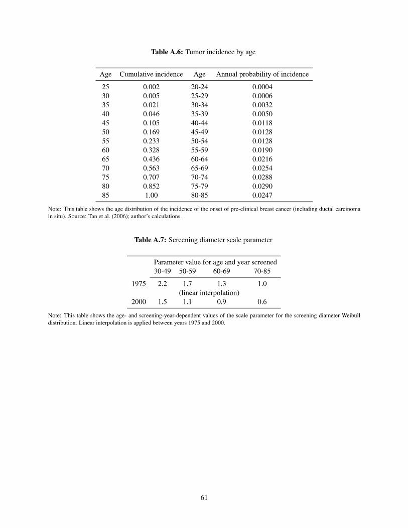
Table A.6: Tumor incidence by age

Age Cumulative incidence Age Annual probability of incidence

25 0.002 20-24 0.000430 0.005 25-29 0.000635 0.021 30-34 0.003240 0.046 35-39 0.005045 0.105 40-44 0.011850 0.169 45-49 0.012855 0.233 50-54 0.012860 0.328 55-59 0.019065 0.436 60-64 0.021670 0.563 65-69 0.025475 0.707 70-74 0.028880 0.852 75-79 0.029085 1.00 80-85 0.0247

Note: This table shows the age distribution of the incidence of the onset of pre-clinical breast cancer (including ductal carcinomain situ). Source: Tan et al. (2006); author’s calculations.

Table A.7: Screening diameter scale parameter

Parameter value for age and year screened30-49 50-59 60-69 70-85

1975 2.2 1.7 1.3 1.0(linear interpolation)

2000 1.5 1.1 0.9 0.6

Note: This table shows the age- and screening-year-dependent values of the scale parameter for the screening diameter Weibulldistribution. Linear interpolation is applied between years 1975 and 2000.

61

Table A.8: Tumor incidence by birth cohort: original Erasmus values

Birth cohort Cumulative incidence

1900-04 0.1221905-09 0.1321910-14 0.1411915-19 0.1541920-24 0.1691925-29 0.1761930-34 0.1821935-39 0.2001940-44 0.2201945-49 0.2231950-54 0.2041955-59 0.1981960-64 0.1931965-69 0.189

1970 0.187

Note: This table shows the cumulative probability (up to age 85) of the onset of pre-clinical breast cancer by birth cohort. Source:Tan et al. (2006)

Table A.9: Tumor type distribution

Age at onset Invasive DCIS-invasive DCIS-regressive DCIS-clinical

20-34 0.76 0.15 0.03 0.0635-79 (linear interpolation)80-85 0.92 0.05 0.01 0.02

Note: This table shows the age-dependent proportions of incident tumor types. Linear interpolation is applied between ages 35 and79.

62

Table A.10: Sensitivity checks for parameter estimates

(1) (2) (3) (4) (5)BaselineEstimate Incidence 28% 14% 19% 42%

αo -5.21 -4.81 -5.20 -5.20 -4.67 -3.33γo 0.10 0.09 0.10 0.10 0.09 0.05δo

in-situ 0.36 1.15 0.36 0.36 0.09 -0.16δo

invasive 1.13 10.89 1.13 1.13 1.15 1.58

αr 0.29 -0.06 0.26 0.26 0.03 -0.73γr -0.03 -0.02 -0.02 -0.02 -0.02 0.00δr

in-situ -0.01 0.58 -0.01 0.00 -0.55 -1.06δr

invasive -4.67 22.28 -5.10 -12.80 -6.67 -13.67

Parameter

Sensitivity Checks

Share In-situ to Invasive Share Non-Malignant

Notes: Table shows the parameter estimates from the mammogram decision model under alternate sensitivity assumptions.Specifics for each of the columns are discussed in Section 5.2.3.

63