Rural Residential Development and Transportation Infrastructure in High Growth Rural Communities

Rural Residential Development and Transportation Infrastructure in High Growth Rural Communities

Prepared for

MONTANA DEPARTMENT OF TRANSPORTATION

And

U.S. DEPARTMENT OF TRANSPORTATION, FEDERAL HIGHWAY ADMINISTRATION

Prepared by

JERRY JOHNSON, BRUCE MAXWELL, MONICA BRELSFORD, FRANK DOUGHER MONTANA STATE UNIVERSITY

In cooperation with

WESTERN TRANSPORTATION INSTITUTE MONTANA STATE UNIVERSITY

BOZEMAN, MONTANA

October 2003

GYRITS Table of Contents

TABLE OF CONTENTS

Table of Contents.............................................................................................................................1 List of Figures ..................................................................................................................................2 List of Tables ...................................................................................................................................2 Summary ..........................................................................................................................................3 Implementation Statement ...............................................................................................................4 Disclaimer ........................................................................................................................................4 Acknowledgements..........................................................................................................................4 1. Introduction..............................................................................................................................5 2. Population Growth in the Rocky Mountain West....................................................................7 3. Sprawl, Rural Communities, and Land Use Change ...............................................................8 4. Efforts to Model Land Use Change .......................................................................................11 5. A Small Scale Model: Land Use/ Land Cover Change Prediction System ...........................13 6. Integrating Land Use and Transportation Infrastructure .......................................................15 7. Modeling Four Corners, MT..................................................................................................17 8. Modeling Teton Valley, ID....................................................................................................21

8.1. Model Prediction:.......................................................................................................... 21 8.2. Model Forecast Scenarios for Teton Valley, ID ........................................................... 25 8.3. Model Applications....................................................................................................... 28

9. Conclusions............................................................................................................................31 10. References..........................................................................................................................32

Western Transportation Institute 1

GYRITS Table of Contents

LIST OF FIGURES

Figure 1: Average East and West Bound Traffic Over Teton Pass ................................................ 9 Figure 2: Hypothetical Probability of Change for Cell in Native Range to Other Land Use ....... 14 Figure 3: Changes in Commuter Capacity form 1995 to 2002, Four Corners, MT...................... 16 Figure 4: Teton County, Idaho study area including the towns of Driggs and Victor.................. 21 Figure 5: Probabilistic Computer Model Parameterized with Land Use Maps ............................ 21 Figure 6: Graph showing the percent matching (accuracy) of the model predicted 1999 map with

the observed 1999 land use map ........................................................................................... 22 Figure 7: Graph showing the percent matching (accuracy) of the model predicted 1999 map with

the observed 1999 land use map. .......................................................................................... 23 Figure 8: The mean number of map cells (~10 acres) in each land use category for the observed

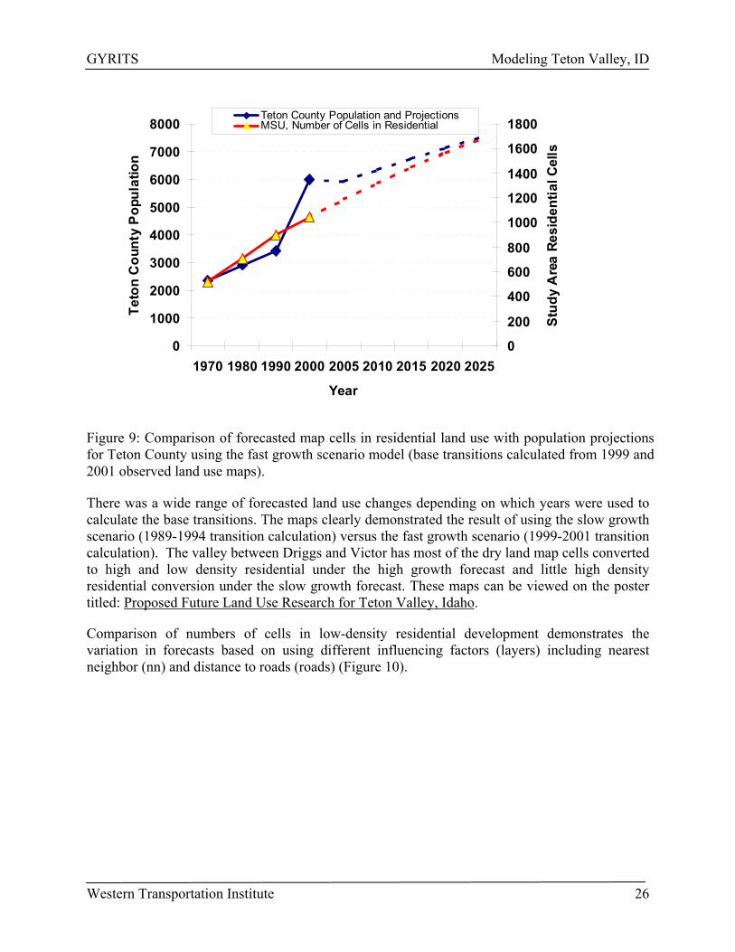
2001 map compared to the 2004 predicted map. .................................................................. 24 Figure 9: Comparison of forecasted map cells in residential land use with population projections

for Teton County using the fast growth scenario model (base transitions calculated from 1999 and 2001 observed land use maps). ............................................................................. 26

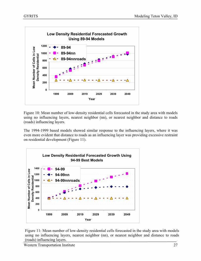
Figure 10: Mean number of low-density residential cells forecasted in the study area with models using no influencing layers, nearest neighbor (nn), or nearest neighbor and distance to roads (roads) influencing layers. .................................................................................................... 27

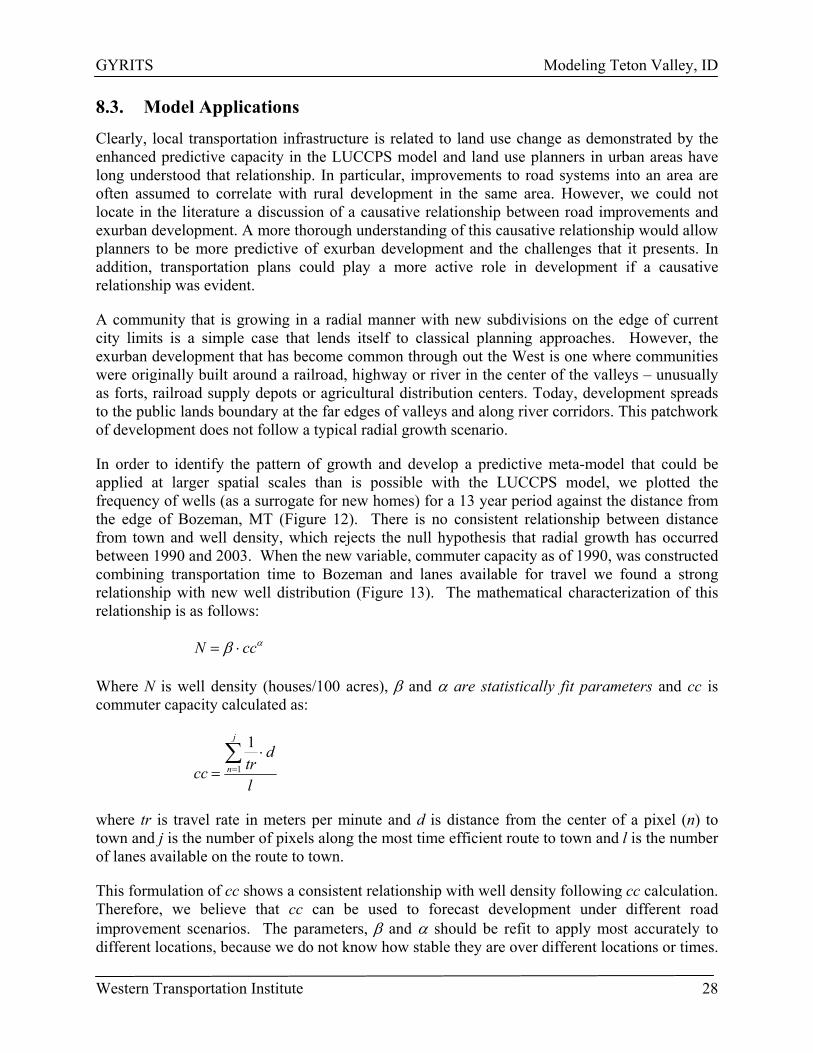
Figure 11: Mean number of low-density residential cells forecasted in the study area with models using no influencing layers, nearest neighbor (nn), or nearest neighbor and distance to roads (roads) influencing layers. .................................................................................................... 27

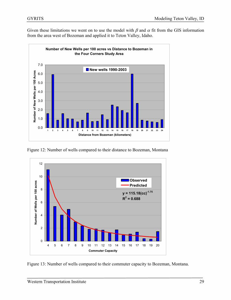
Figure 12: Number of wells compared to their distance to Bozeman, Montana .......................... 29 Figure 13: Number of wells compared to their commuter capacity to Bozeman, Montana......... 29 Figure 14: Potential for development per Commuter Capacity to Jackson .................................. 30

LIST OF TABLES

Table 1: Four LUCCPS models predicting land use change in the Four Corners Area, Montana. Historical land use maps used in these comparisons were the years 1976, 1984, 1987, 1990 and 1995. The historical years were used to predict a future map which was then compared to the observed map 2001. .................................................................................................... 17

Table 2: Calibration of the LUCCPS model using 1987 and 1995 land use layers along with other drivers to predict the observed year 2001. ............................................................................ 18

Table 3: Four LUCCPS models predicting land use change in the Four Corners Area, Montana. Historical land use maps used in this comparison were the years 1987 and 1995. The historical years were used to predict 2003 which was then compared to the closest observed map 2001............................................................................................................................... 19


GYRITS Summary

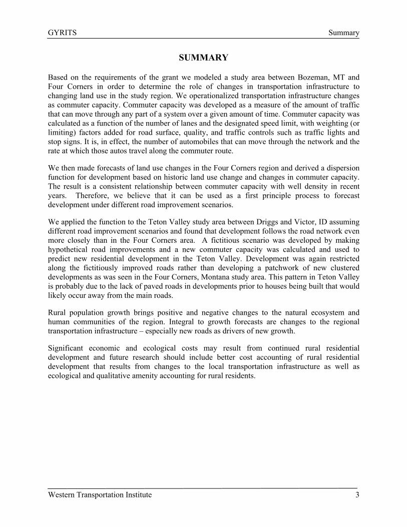
SUMMARY

Based on the requirements of the grant we modeled a study area between Bozeman, MT and Four Corners in order to determine the role of changes in transportation infrastructure to changing land use in the study region. We operationalized transportation infrastructure changes as commuter capacity. Commuter capacity was developed as a measure of the amount of traffic that can move through any part of a system over a given amount of time. Commuter capacity was calculated as a function of the number of lanes and the designated speed limit, with weighting (or limiting) factors added for road surface, quality, and traffic controls such as traffic lights and stop signs. It is, in effect, the number of automobiles that can move through the network and the rate at which those autos travel along the commuter route.

We then made forecasts of land use changes in the Four Corners region and derived a dispersion function for development based on historic land use change and changes in commuter capacity. The result is a consistent relationship between commuter capacity with well density in recent years. Therefore, we believe that it can be used as a first principle process to forecast development under different road improvement scenarios.

We applied the function to the Teton Valley study area between Driggs and Victor, ID assuming different road improvement scenarios and found that development follows the road network even more closely than in the Four Corners area. A fictitious scenario was developed by making hypothetical road improvements and a new commuter capacity was calculated and used to predict new residential development in the Teton Valley. Development was again restricted along the fictitiously improved roads rather than developing a patchwork of new clustered developments as was seen in the Four Corners, Montana study area. This pattern in Teton Valley is probably due to the lack of paved roads in developments prior to houses being built that would likely occur away from the main roads.

Rural population growth brings positive and negative changes to the natural ecosystem and human communities of the region. Integral to growth forecasts are changes to the regional transportation infrastructure – especially new roads as drivers of new growth.

Significant economic and ecological costs may result from continued rural residential development and future research should include better cost accounting of rural residential development that results from changes to the local transportation infrastructure as well as ecological and qualitative amenity accounting for rural residents.


GYRITS Implementation Statement

IMPLEMENTATION STATEMENT

This study is sponsored by the U.S. Department of Transportation, Federal Highway Administration in cooperation with the Montana Department of Transportation, the Wyoming Department of Transportation, the Idaho Transportation Department, and the Yellowstone National Park. The major objective of this document is to summarize GYRITS Work Order II-2E, GIS Land Use Forecasting in Teton County Idaho.

DISCLAIMER

The opinions, findings and conclusions expressed in this publication are those of the authors and not necessarily those of the Wyoming Transportation Department, the Montana Department of Transportation or the U.S. Department of Transportation, Federal Highway Administration. Alternative accessible formats of this document will be provided upon request.

Persons with disabilities who need an alternative accessible format of this information, or who require some other reasonable accommodation to participate, should contact Kate Heidkamp, Western Transportation Institute, PO Box 173910, Montana State University–Bozeman, Bozeman, MT 59717-3910, telephone: (406) 994-7018, fax: (406) 994-1697. For the hearing impaired call (406) 994-4331 TDD.

ACKNOWLEDGEMENTS

Grateful appreciation is extended to the U.S. Department of Transportation, Federal Highway Administration; Montana Department of Transportation; Idaho Transportation Department; Wyoming Department of Transportation; Yellowstone National Park; other partner agencies and the Greater Yellowstone Rural ITS Project Steering Committee members.


GYRITS Introduction

1. INTRODUCTION

This report integrates the complex interaction between land use change and changes to the local transportation infrastructure in rural communities. There are several interconnected reasons why rural sprawl - a pattern of rural residential settlement characterized principally by low densities and scattered development – and transportation infrastructure is one of the most pressing concerns facing amenity rich communities, resort communities and retirement destinations as well as the surrounding countryside. They include a range of social and economic costs to rural resident populations; the loss of open landscapes and productive agricultural lands; and ecological disturbance to environmentally sensitive lands.

Issues related to sprawl maybe substantially different in the rural Rocky Mountains than in close proximity to large urban centers. For example, in general, there is greater demand for private rural homesites on relatively large parcels and thereby less market demand for clustering homes. Western states, as a rule, do not have the intense planning effort aimed at mitigating the effects of large numbers of people commuting into large cities, and there is a less well developed political will toward planning.

Realistically, there is also less attention from researchers and computer modelers on the issues surrounding rural areas than in urban centers where land use and transportation planning enjoy a rich and sophisticated literature, professional training infrastructure, and history. As a result, much of the quality technical work of urban centers is less applicable in micropolitan and rural areas.

The central concern for this project was to understand the connections between the influence of travel patterns and land use change in the rural countryside. The general outline is to provide background on the issue of sprawl and its causes and consequences, to present an effective method of modeling and forecasting land use change and to apply the findings of the model in two similar study areas. The study areas are two tourism dependent rural locations. The first, Four Corners, MT is a rapidly growing high amenity unincorporated community adjacent to Bozeman, MT. The second is Driggs, ID (Teton Valley), a recreational community located near Jackson, WY and the source of some of the tourism service labor force for Jackson Hole.

Specifically, the organization of the report is:

1) introduce the focus of the report,

2) provide background on recent population growth in the Rocky Mountain West,

3) discuss topics of concern stemming from the impacts of population growth and sprawl in high growth rural areas,

4) review the general methods of modeling land use change,

5) present a land use change forecasting model (LUCCPS) and assess the change in accuracy of the forecasts both with and without changes to transportation infrastructure integrated into the model,


GYRITS Introduction

6) develop the connections between transportation infrastructure and land use change,

7) assess the nature of rural residential development with and without changes to transportation infrastructure integrated into the model, and

8) demonstrate how the enhanced modeling capability can be applied in a similar research setting.

The emphasis is on a model that appears to be efficacious to a rural setting and the constraints faced by rural local governments and the political culture in which they operate. The primary GIS model (LUCCPS) is available, user friendly, relatively inexpensive to use, transparent in terms of data and assumptions, and can integrate high levels of community participation. Initially we also thought the model would easily integrate changes to transportation infrastructure as a driving variable of land use change.


GYRITS Population Growth in the Rocky Mountain West

2. POPULATION GROWTH IN THE ROCKY MOUNTAIN WEST

Rural areas in the American West are in the midst of a period of population growth unlike any in the past. According to the recent 2000 census, the West was the fastest growing region of the U.S. over the past decade (U.S. Census 2000). While the national average population growth was 13.2%, the western region of the country grew at an average of 19.7%. During that period the population of the region grew by over 10 million and 67% of the counties in the Rocky Mountain1 axis grew at rates faster than the national average (Beyers and Nelson 2000). Most of the growth continues to be in close proximity to the major urban areas of the West (Denver, Salt Lake City) but high growth areas are also located in regional micropolitan locations - Driggs/Victor and Coeur D’ Alene, ID., Bozeman and Whitefish, MT., Durango and Telluride, CO, and Jackson, WY (Vias, Mulligan and Molin 2002). Many of the smaller towns are heavily dependent on tourism and associated real estate development for their continued economic health and it is the growth taking place in these communities and outlying rural areas that is the focus of this project. The unprecedented rate and nature of recent population growth in the rural countryside attracts the attention of those interested in the maintenance of undeveloped open space, productive agricultural land, and thriving rural communities (Lassila 1999).

The reasons for recent growth in the small towns of the Rocky Mountains are multifaceted and are strongly associated with increased tourism and recreation in amenity rich rural areas and rural economies shifting from extractive economic bases to growth in the non-labor sector and service sectors of the national economy (Johnson, Maxwell and Aspinall 2003). Two views prevail to explain recent population increases (Decker and Crompton 1993). The first is the quality of life argument that states that rural location is a function of a mix of amenities acting as pull factors (see especially Bowers 1999). Examples include a move to a small town in part because of the scenic beauty of the area, low crime rate, a desirable climate, recreation opportunity, or to be close to family and friends. While, the demand model asserts that in-migration is a function of wages and employment - jobs first; then migration. Employment in extractive industries, regional shopping centers, and the construction trades provide acceptable wages for many who are looking to relocate to the West.

In fact, both models have explanatory power and both are probably simultaneously acting to change the social and geographical character of Western communities. What is clear is that the geographical features that provided natural resources in the past now act as powerful attractants to those who would live near mountains, rivers, forests, and protected public lands and engage in the quality outdoor recreation such amenities provide (Johnson, Maxwell and Aspinall 2003; Johnson and Rasker 1995; Williams, White, and Johnson 1981; Power 1996; Riebsame, Gosnell, and Theobald 1996).

1 The Rocky Mountain states include: Idaho, Montana, Wyoming, Utah, Colorado, New Mexico, and Arizona.


GYRITS Sprawl, Rural Communities, and Land Use Change

3. SPRAWL, RURAL COMMUNITIES, AND LAND USE CHANGE

The communities we consider relevant to this modeling exercise and the findings cover a variety of rural communities including those located at or near mountain resorts (i.e. Jackson, WY, Big Sky, MT); recreation driven communities (Moab, UT); amenity communities (Durango, CO, Bozeman, MT), retirement and bedroom communities (St. George, UT, Belgrade, MT, Post Falls, ID). For purposes of brevity we refer to these communities interchangeably as rural or resort communities.

Full discussion of the host of positive and negative effects of rapid in-migration to the recreation and retirement communities of the Rocky Mountains is beyond the scope of this report however, a comprehensive review can be found in: Riebsame, Gosnell, and Theobald (1996); Rasker and Hansen (2000); Johnson, et al. (2003); and Hansen et al. (2003) and Johnson (2004). Two categories of impacts are typically identified in the literature. Social impacts are those that accrue to people and their employment and incomes, power structure within the community, housing, and quality of life. The other set of impacts are to the ecological setting effecting water, land use, native plant and animal populations, and ecological processes.

Two general impacts do merit attention for this analysis however: 1. The spatial distribution and costs of housing, and 2. The impact on public infrastructure such as transportation. Both may significantly affect the quality of life in resort communities.

In many rural and mountain resort communities, the local cost of living precludes the majority of the labor force from living where they work. The result is long commutes from the “downstream” communities. Hartman (2002) identifies a downward economic spiral based on the ever-increasing costs of living for tourism service workers. In the Roaring Fork Valley of Colorado for example tourist service workers drive two hours each way to work in Aspen - a county where the median home price is $2.4 million and there are two- to four-year waiting lists for apartments. A report on Pitkin County’s housing estimated that for every new 6,000-square-foot home, two domestic workers are brought into the work force. However, in Aspen’s current housing shortage, job creation produces a need for affordable housing that doesn't exist. The impacts on the transportation infrastructure and taxpayers can be seen in the highway reengineering necessary to carry the heavy traffic loads of commuters and tourists. In the Roaring Fork Valley Highway 82 between Basalt and Aspen has increased from two to four lanes in the past decade and construction continues.

The latest census data shows an over 2000% increase over ten years in the number of workers who live in Teton County, Idaho (Driggs, Victor) and work in Teton County, Wyoming (Jackson). The long commute over Teton Pass is easily explained by the disparity in the median cost of housing in Teton County, Wyoming ($1.17 million in 2001) as compared to Teton County, Idaho’s $190,908 median cost in 2001. Figure 1 graphically shows the peak travel times over Teton Pass from Idaho to Wyoming as service workers leave early and arrive home late.



Finally, in Big Sky, Montana – a year round destination resort near Bozeman, MT, workers commute over an hour each way to work in the construction and tourist service industry. In this case there is not only a large disparity of housing prices between the two communities but, in addition, the limited amount of private land for development precludes any being used for less profitable employee housing.

0

100

200

300

400

500

600

700

800

900

1000

1100

1200

1300

1400

1500

1600

1700

1800

1900

2000

2100

2200

2300

East Average

0

1000

2000

3000

4000

5000

6000

7000

8000

Number of Vehicles

Hours

Average East and West Bound Traffic Over Teton Pass Jan, Feb, Mar 2002

East Average West Average

Figure 1: Average East and West Bound Traffic Over Teton Pass

The effect of long commutes is that towns near a resort destination, for example, serve as the primary residential location and tend to restrain the sense of community in the resort area. More problematic is that the impacts of sprawl in the resort area are exported and uncoupled from the adjacent communities. Such impacts are not easily assimilated (Johansen and Fuguitt 1990). For example, as people live out of town or in “bedroom communities” adjacent to resort areas, they tend to work, play, and spend money where they work but sleep at their place of residence. Their presence in the resort is a source of income to the resort-based business community, but their home is in a location removed from the resort and thus may impart significant impacts to the residential community in terms of traffic, the flow of labor related income and taxes, demands on public infrastructure (schools, social services, health care). Their home may carry land-based impacts to the residential community in terms of local viewshed and open space depletion (Johnson, et al. 2003; Riebsame, Gosnell, and Theobald 1996).

There are frequently political and economic pressures to, in effect, subsidize the resort community with a quality road system that allows for easy access for incoming tourists and commuters; both groups are needed to sustain the artificial economy inherent in mountain resorts.



Similar population, cost of living, and other dynamics take place in most of the desirable high growth communities throughout the Rocky Mountains. No matter what the major drivers of the local economy may be, high population growth seems to bring with it the same suite of positive and negative impacts (Johnson 2004).


GYRITS Efforts to Model Land Use Change

4. EFFORTS TO MODEL LAND USE CHANGE

The ability to simulate land use change and development is important for better growth management and more efficient and cost-effective use of the transportation system and private land (Oregon DOT 2001) and research efforts aimed at modeling social, economic, and ecological changes taking place on rural land is an active area of research. The overall objective is to assess and predict the rate, nature, and impact of land use change in rural areas at multiple scales; (Hansen, et al. 2003) (see also: http://lcluc.gsfc.nasa.gov/products/index.asp). Predicting land use change in areas with a mosaic of private ownership land uses requires combination of a wide range of driving variables and methods. Land capability can be determined by soil, climate and land cover variables that are often available in geo-referenced form (Berry et al., 1996; Turner et al., 1996). Other variables such as those related to social and economic drivers have not been well-represented in the literature due in some part to the difficulty of data acquisition via electronic or remote sensed means and relatively fewer researchers in the area of study. However, various models have been designed to describe the host of driving variables responsible for land use change. The models fall into three primary categories: multiple regression models, those based on cellular automata theory, and agent based models (Theobald and Hobbs 1998; Hill and Aspinall 2000).

4.1. Multiple Regression Models

Multiple regression is a procedure that analyzes the relationship between several independent variables (IV) and a dependent variable (DV). This form of analysis assumes development patterns (DV) that respond to a relatively few locational factors (IV) such as proximity to towns and highways, and the likelihood that development decreases with increasing distance from urban areas (Wear, Turner and Flamm 1996). This reflects traditional urban and rural development models that are based on the assumption of accessibility – usually through a well-developed transportation corridor (Chen 2000) and the importance of a few predictor variables (Turner et al., 1996). Multiple regression analysis has the benefit of being low cost in terms of time, data and resources, but is limited by dependence on the most powerful drivers or predictors of change to the independent variable. Variables that may not emerge in regression as statistically robust, but may be important predictors at a smaller scale will tend to fall out of the equation. As such, its use in larger spatial scales may tend to miss important subscale predictors.

4.2. Cellular Automata (CA) Models

These models assume that future development patterns respond to local patterns of existing development, and the likelihood of development is higher in areas of higher neighboring change in the variable being measured. Further, these models assume that local processes can influence global patterns; that is, there can be a “ripple effect” through and beyond system boundaries. Briefly, cellular automata models can be thought of as a dynamic system where the state of one cell depends on the previous state of surrounding cells where the change takes place according to a set of transition rules (White, Engelen and Uljee 2000). These rules are typically expressed in terms of probability functions. CA models benefit from computational efficiency because the “cell neighborhood” can be limited to only adjacent cells to conduct the transition analysis but can also be expanded to include cells across the probability space if needed. Further, the set of


GYRITS Efforts to Model Land Use Change

transition rules can be very broad to include “weak” drivers that may be present in only one location of the probability space and permit fine spatial detail (i.e. the influence of a single road). Finally, because the analysis is spatial in nature, findings are easily compatible with GIS applications and are typically written as GIS program extensions.

The CA method assumes that future land use patterns are driven by local patterns of land use change and that local changes strongly influence nearby change. This method differs from a regression approach in several ways. First, the model makes the prediction of future land use change based on the probability of change from surrounding cells. Second, whereas regression approaches tend to drop variables that do not contribute significantly to prediction on a large portion of the map, a probability approach allows a full compliment of the independent driving variables to reflect the potential land use change (Berry et al. 1996). Finally, regression approaches tend to model change based on proximity to geographical features (roads, water) and predict a gradient of change that decreased with distance from these features (Theobald and Hobbs 1998). Thus, the likelihood of development decreases with increasing distance from urban areas. Yet, observation of rural growth suggests that accessibility is perhaps not the driving factor of homes in the rural countryside. Rather, future development patterns are more likely a function of the near or distant views available to potential homeowners, characteristics of the community, or geographical isolation from others (Maxwell, Johnson and Montagne 2000). With respect to transportation, people do not necessarily follow roads (the regression approach) but roads will invariably follow where people live (rules based approach).

The forecasted patterns produced by these two models were compared by Theobald and Hobbs (1998) against historical observed development patterns using both a spatial aggregate and spatial measures. Overall, the cellular automata model outperformed the regression models with respect to observed land use patterns.

Agent based models. An emergent model type in the study of land use change, agent models are analogous to cellular automata models by assigning attributes that describe condition and characteristics of agents or actors in a system (Ferber 1999). Like CA models, agents exist in some “space”. In the context of land use change, that space may be an area of discrete geographical space or behavior constrained by an artificial environment as in the behavior of grazing herds with respect to simulated drought conditions. As in CA models, agent behavior is driven by transition rules. Any number of rules can be devised to govern the activities of agents’ goals that they seek to satisfy (e.g., minimizing travel distance between points, desire to live away from others). However, a unique attribute of agent models is that "preferences" that agents might regard as desirable can be defined (e.g., "likes" and "dislikes" for certain spaces, neighbors, or solutions) http://www.casa.ucl.ac.uk/geosimulation/abms.htm). These preferences can inform new and emergent relationships on the land. Agent based models may be especially useful for understanding and modeling different groups of rural residents based on demographic typologies or psychographic motivates. In other words, if the rules are written specifically, agent based models allow researchers to treat people as discrete individuals rather than over generalized groups.


GYRITS Land Use/Land Cover Change Prediction System

5. A SMALL SCALE MODEL: LAND USE/ LAND COVER CHANGE PREDICTION SYSTEM

The Land Use/Land Cover Change Prediction System (LUCCPS) (Maxwell, Johnson, and Montagne 2000; Johnson and Maxwell 2001) was designed as a cellular automata model that can also be utilized as an agent based model. The design criteria were to be able to assess and predict the rate, nature, and impact of land use change in rural areas. The model was designed to reside on a GIS platform thereby making multidisciplinary investigation and policy analysis feasible as well as high quality visualization possible. The model is based on the history of past land use change, natural features, man-made infrastructure, and land use decisions. Each layer of information is used as an independent driving variable to calculate the transition probabilities for landscapes in private ownership. The LUCCPS model can also be used as an agent based model through manipulation of existing data layers. Likes and dislikes for certain types of spaces or infrastructure, neighborhood density, or various planning solutions such as clustering or open space preservation can be expressed as driving layers thereby allowing artificial conditions to be imposed on the model output.

A complete description of the model and output examples can be found in Maxwell, Johnson, and Montagne (2000) but briefly, the model utilizes aerial photos at appropriate intervals in a study region up to 100 sq. mi. The study region is divided into cells 10 acres in size and each cell is assigned a land use designation. The observed land use information is placed in the GIS system as independent layers of information so they could be used as independent variables in the prediction system. Other data layers are constructed to be included in our eventual model of land use change and may include natural geographical features, manmade infrastructure as well as personal interview data.

The data layers are used to generate a 2+n dimensional probability transition matrix (multiple layers of information through time and space) for land use. The approach used to predict land use/cover change concentrates on identifying and incorporating independent driving variables directly into transition probabilities in landscapes dominated by private ownership.

The model is based on the effects of both past land use change as well as the additional data layers described above. This method assumes that future land use patterns are driven by local patterns of land use change and that local changes strongly influence nearby change (cellular automata logic). Further, various natural geographical and human built features on the landscape may act as either positive or negative drivers of land use change (agent based logic).

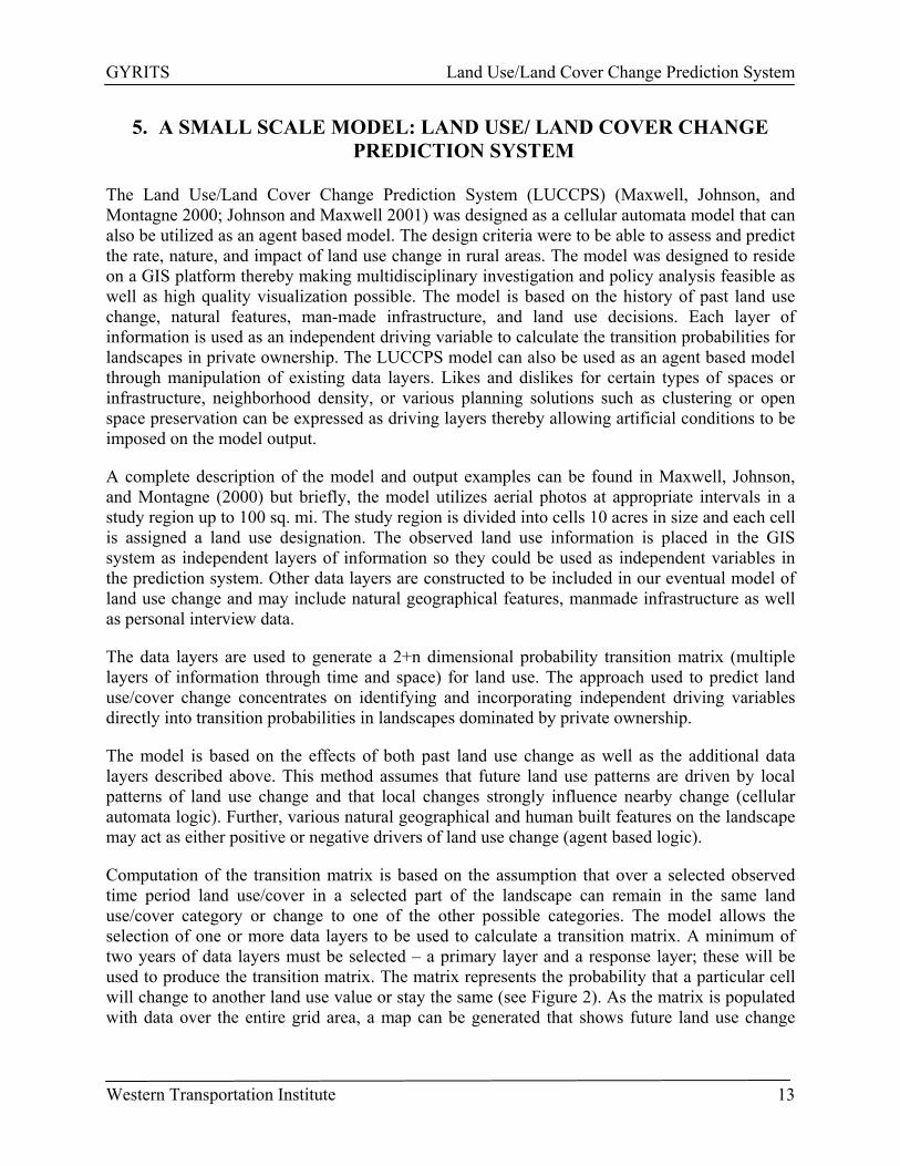
Computation of the transition matrix is based on the assumption that over a selected observed time period land use/cover in a selected part of the landscape can remain in the same land use/cover category or change to one of the other possible categories. The model allows the selection of one or more data layers to be used to calculate a transition matrix. A minimum of two years of data layers must be selected – a primary layer and a response layer; these will be used to produce the transition matrix. The matrix represents the probability that a particular cell will change to another land use value or stay the same (see Figure 2). As the matrix is populated with data over the entire grid area, a map can be generated that shows future land use change


GYRITS Land Use/Land Cover Change Prediction System

scenarios based on the probability of change derived from past land use change and the effects of geographical and socioeconomic features.

Figure 2: Hypothetical Probability of Change for Cell in Native Range to Other Land Use

Accuracy of the model is enhanced by predicting a known mix of land use. Various combinations of the known land use profile in combination with the other driving factors are tested and yield varying prediction accuracy. An aerial land use map from the latest year available is used as the calibration. Accuracy rates of 80%-90%+ are attained given various combinations of data layers.


GYRITS Integrating Land Use and Transp Infrastructure

6. INTEGRATING LAND USE AND TRANSPORTATION INFRASTRUCTURE

Elizabeth Humstone, the Director of the Vermont Forum on Sprawl states:

It is critical to keep in mind the close connection between land use and transportation. Highways provide access to land, which enables the development of that land. Land uses generate vehicle, pedestrian, bicycle, and transit trips. In order to manage traffic along a highway, both land use and transportation strategies are necessary.

Accordingly, over the past decade there has been growing interest in integrating transportation and land use planning, based on a recognition that land use not only influences transportation outcomes, but that transportation investments also influence land use decisions (Waddell 2001).

Following Humstone, we sought to incorporate transportation infrastructure changes into the LUCCPS model as a way to enhance the accuracy of our forecasts. The model was able to integrate the transportation infrastructure layers by operationalizing it as a change in commuter capacity adjusted travel time of the road networks between 1990 and 1995, and between 1995 and 2001.

Commuter capacity (adjusted travel time) was developed as a measure of the amount of traffic that can move through any part of a system over a given amount of time. Commuter capacity was calculated as a function of the number of lanes and the designated speed limit, with weighting (or limiting) factors added for the type of road surface, the quality, and traffic controls such as traffic lights and stop signs. It is, in effect, the time it takes to move an automobile through the network to a designated end point (in this case Bozeman, Montana in the Four Corners study area and Jackson, Wyoming in the Teton Valley study area).

If, for example, a significant portion of roadway was reengineered to include additional lanes of traffic, or the road surface improved from gravel to asphalt, the commuter capacity of that road section and adjacent land would be significantly increased. Furthermore, since the commuter capacity model is sensitive to route efficiency, capacity changes along arterial routes can alter capacity values and best route paths for contributing areas well away from the altered stretch of road. For example, a capacity increase along one route may divert traffic away from a nearby parallel route if the improved route offers more lanes, a better road surface, a higher speed limit, or fewer stoplights.

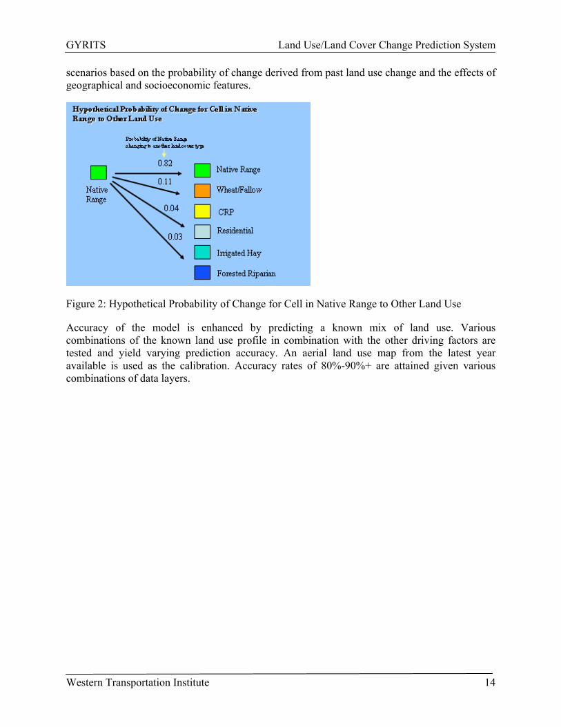
The product of the commuter capacity analysis was a GIS layer for the Four Corners study area that identifies “hot spots” of transportation changes across the landscape. Figure 3 shows the completed digital layer depicting the gradient of no change to the largest change in capacity that was constructed for the model. Hot spots of change are located primarily in areas where new roads have been constructed for rural subdivisions and along existing highways in a general north/south pattern from the Four Corners intersection. The digital layer depicting changes in commuter travel time was imported into the LUCCPS prediction model as one of several influencing variables.


GYRITS Integrating Land Use and Transp Infrastructure

Figure 3: Changes in Commuter Capacity form 1995 to 2002, Four Corners, MT


GYRITS Modeling Four Corners, MT

7. MODELING FOUR CORNERS, MT

The first goal of the modeling exercise is to assess the accuracy of the LUCCPS model in the study area. We created land use layers from aerial photos for the following years: 1976, 1984, 1987, 1990, 1995. We created a 2001 layer by driving the area and visually assessing land use changes. We also attained a GIS residential layer from Gallatin County for 2001. All possible combinations of years were used in the LUCCPS model to find the best predictive years, the four best models are shown in Table 1. From these model runs we found that some combinations of years predicted agricultural lands better (1990-1995), while other combinations predicted residential land better (1987-1995). For this report, the model that predicted residential growth was used.

Table 1: Four LUCCPS models predicting land use change in the Four Corners Area, Montana. Historical land use maps used in these comparisons were the years 1976, 1984, 1987, 1990 and 1995. The historical years were used to predict a future map which was then compared to the observed map 2001. Historical

Change 1976-1990

Historical Change 1987-1995



Land Use Cell Type Observed 2001 Number of cells

Predicted 2004 Number of cells




Farm 73 77 74 74 74 High Density Residential 172 136 158* 124 134 Low Density Residential 371 385 386 383* 343 Commercial 54 55* 60 42 48 Irrigated Crop 1455 1629 1319 1389 1482* Irrigated Hay 708 589 846 834 746* Bottomland Pasture 69 31 58 50 66* Riparian 179 175 180* 182 185 Percent Accuracy of model 68.49 74.39 60.65 92.28

* indicates best prediction in each land use category

The next step in the calibration process is to determine the mix of predictor variables that results in the most accurate prediction for the 2001 land use mozaic. We ran the model using 1987 as the primary land use layer and 1995 as the response layer and the combination of driving variables including nearest neighbor (the cellular automata feature) and change in commuter capacity. Change in commuter capacity layer and nearest neighbor improved our ability to forecast the mosaic of land use changes significantly over using the land use change probabilities alone. The combination of the two layers gave the best result. Table two displays the mix of driving variables and resulting accuracy of the calibration. To statistically evaluate the accuracy of the model we used the Kappa Statistic. Kappa statistic uses the number of categories and the number of cells to create a random chance map and adjusts the accuracy measure by subtracting the estimated contribution by chance (Campbell 1987). For our study area the random model was 29.3% accurate, well below our projected map at 74.39%. To calculate the Kappa Statistic:



1 - expected K = Observed - expected

^

.7439 - .293 = .4509 =

.6378

1 - .293 .707

Therefore, our model is 64% better than would be expected by random chance.

Table 2: Calibration of the LUCCPS model using 1987 and 1995 land use layers along with other drivers to predict the observed year 2001. Model Parameters

Kappa Statistic

Random chance model 29.2 1987-1995 Land use change probabilities only 63.27 1987-1995 Land use change probabilities + nearest neighbor 71.27 1998-1995 Land use change probabilities + change in commuter capacity 71.09 1987-1995 Land use change probabilities + nearest neighbor + commuter capacity 88.50

Many attempts to model land use change are, in fact, attempts to model rural residential development while transitions of other land use categories remain largely ignored. Yet, the transition of agricultural land may be an important aesthetic and economic consideration in resort communities. For example, management of agricultural land from crops to large animal production may result in unpleasant sights and smells to those residing in nearby rural subdivisions. Others may find pleasure in the green irrigated alfalfa field that replaces dryland farming. In both scenarios, local employment and agriculture earning patterns may shift and the type of agricultural land use may act as either an attractant or deterrent for future homesites.

The LUCCPS model has the provision for generating a census of all cells that changed in the study area categorized by land use type. Comparing the census results for the modeling scenarios without transportation in the mix of driving variables and another with transportation in the mix yielded different results. The table below (Table three) indicates that the calibrated LUCCPS model tends to underestimate high and low density residential development and commercial lands. However, by using the combination of driving variables, we are able to predict agricultural land uses.



Table 3: Four LUCCPS models predicting land use change in the Four Corners Area, Montana. Historical land use maps used in this comparison were the years 1987 and 1995. The historical years were used to predict 2003 which was then compared to the closest observed map 2001. Model I

Historical Change

Model II Historical Change + Nearest Neighbor

Model III Historical Change + Change in Road Capacity

Model VI Historical Change + Nearest Neighbor + Change in Road Capacity

Land Use Cell Type Number of Cells

Percent Correct

Percent Correct Percent Correct Percent Correct

Farm 73 99 99 99 99 High Density Residential 172 64 65 64 63 Low Density Residential 371 72 74 75 79 Commercial 54 76 76 76 76 Irrigated Crop 1455 75 77 77 96 Irrigated Hay 708 64 84 84 96 Shrub Land 21 95 95 90 100 Dry Grassland 9 78 89 100 100 Bottomland Pasture 69 77 88 75 100 Riparian 179 98 94 94 100 Kappa Statistic 63.78 71.27 71.09 88.50

The ability to accurately forecast many land uses may be useful as a land use planning tool. Future infrastructure needs, road and bridge maintenance, viewshed analysis can be planned if the future growth of an area can be accurately modeled. Further, a diverse landscape mosaic offers diverse land preservation opportunities schemes that can influence rural residential development. For example, where large intact farms and ranches exist, conservation easements may be negotiated to preserve open space and maintain agricultural earnings (White 1998; Wright 1993)2. Other land conservation strategies might be a local government entity or nonprofit (e.g. open space bonds, Nature Conservancy) to purchase the land and protect it from development. Federal and state conservation programs like the Conservation Reserve Program or those aimed at floodplain or wetlands protection may prove useful (Johnson and Maxwell 2001). The use of these options can be considered if the future mosaic can be anticipated.

The modeling exercise in Four Corners showed that changes to transportation infrastructure was an important driving variable when forecasting a complex mosaic of land uses and further, it was strongly associated with the dispersion of rural residential development from the local population

2 A conservation easement is a legal contract between a land trust, a governmental entity, or other qualified organization and a willing landowner. In exchange for a tax deductible contribution for the value of the protected land, the easement permanently limits uses of the land in order to protect its conservation values. The restrictions run permanently with the land. A conservation easement protects the land from unlimited subdivision and development while also protecting the rights of private ownership. Examples of uses generally permitted by a conservation easement: include: continued agricultural use; sale or gift of the property; or selective timber harvest. Examples of uses generally restricted by a conservation easement are: subdivision for residential development; surface mining; or the elimination of wildlife or fisheries habitat protected by the easement. The landowner continues to own the land and continues to pay taxes on the land.



center. The next question we asked was if the lessons learned from the modeling exercise in Four Corners can be exported to another similar study area?


GYRITS Modeling Teton Valley, ID

8. MODELING TETON VALLEY, ID

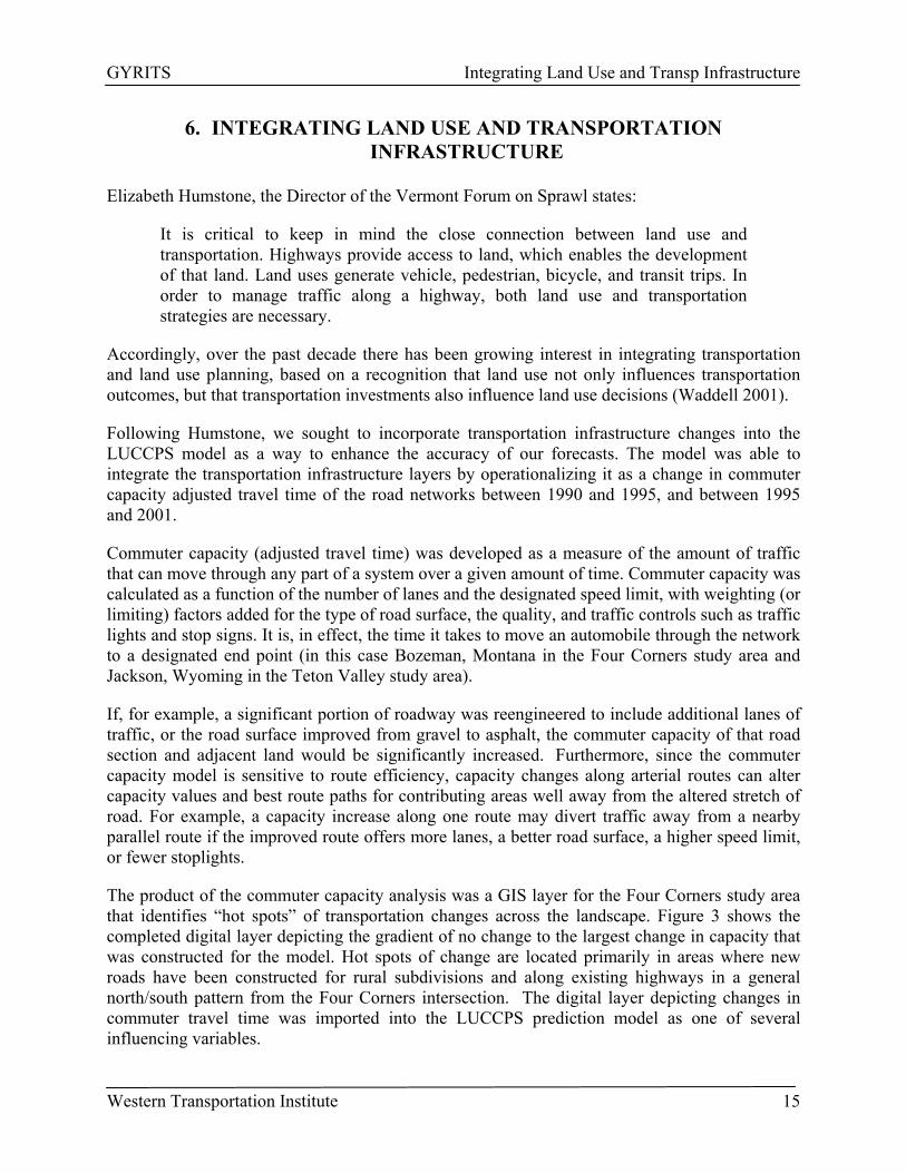
We completed our initial forecasts of land use change for Teton County, ID in 2002. It is the fastest growing county in Idaho over the past 10 years according to the 2000 Census. The county’s rural landscape, small towns, surrounding wildlands, nearby ski resorts and associated service jobs are drawing people to the area. In addition, rising costs of real estate in neighboring Jackson Hole, Wyoming, seems to be encouraging work force commuters from Teton Valley, Idaho. As a result, planning for residential growth and associated development is critical if the rural nature of the valley is to be preserved. The study area is a portion of the Teton Valley between and including Driggs and Victor. The study area is 10 miles on a side and thus included federal lands on the east and west sides of the valley as well as privately owned lands in the valley bottom (Figure 4).

Figure 4: Teton County, Idaho study area including the towns of Driggs and Victor.

8.1. Model Prediction:

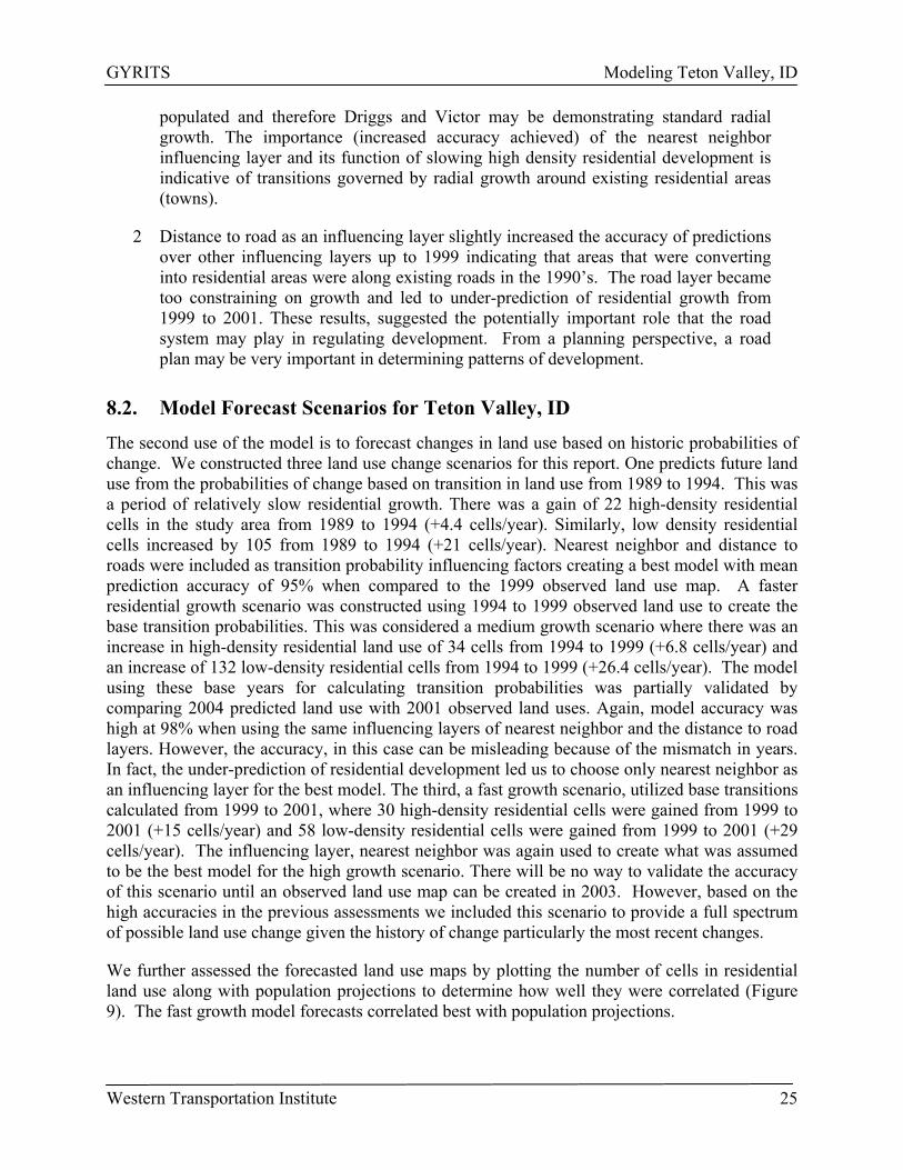
The probabilistic computer model (Maxwell et al., 2000) was parameterized with land use maps classified into the following categories on 1:20,000 aerial photos (USGS NAPP) taken in 1989 and then again in 1994 (Figure 5).

The model was calibrated in the manner similar to the Four Corners example. We compared the 1999 observed land use map, classified from aerial photos, with the predicted 1999 map and found the model to be 91% accurate when no influencing layers were added to the model. That is, 91% of the map

1989

Driggs

Victor

FarmHigh Density ResidentialLow Density ResidentialOpen Space, SchoolIndustrail, CommercialDryland CropIrrigated CropIrrigated HayShrub RangelandDryland PastureBottomland PastureRiparian ZonesCottonwood or AspenConifer ForestMixed Conifer and AspenAspen ForestForestConservation Easements

Land Use Categories

Figure 5: Probabilistic Computer Model Parameterized with Land Use Maps



units (cells) matched between the observed and predicted maps. Accuracy was maximized at 95% when influencing layers were included.

The influencing layers that increased the model prediction accuracy (using the 1999 observed land use map for comparison) were nearest neighbor, distance to Driggs, distance to forest boundary, distance to public lands, distance to roads, distance to streams, distance to Victor, distance to existing subdivision in 2000, distance to platted subdivisions as of 2000 (Figure 6).

90919293949596979899

89-9

4

89-9

4dis

tdrig

gs

89-9

4dis

tvic

tor

89-9

4tow

n

89-9

4pub

licla

nd

89-9

4str

eam

89-9

4roa

ds

89-9

4exi

st

89-9

4sur

vey

89-9

4nn

89-9

4nn+

drig

gs

89-9

4nn+

vict

or

89-9

4nn+

tow

n

89-9

4nn+

publ

ic

89-9

4nn+

stre

am

89-9

4nn+

road

s

89-9

4nn+

surv

ey

89-9

4nn+

exis

t

Models

Perc

ent A

ccur

acy

Estim

ate

Figure 6: Graph showing the percent matching (accuracy) of the model predicted 1999 map with the observed 1999 land use map

Nearest neighbor, which is simply a way to take into account the position of any map cell relative to its neighboring cells and thus is more apt to have cells on the edge of a big block of cells classified the same before it changes the cells more central within a block with a common classification. Increased accuracy with the nearest neighbor influencing layer is consistent with previous predictions in other areas, although it was much less improvement in accuracy in the Teton study area. This result may be due to generally higher fragmentation of land uses in Teton County than in previous study areas in the Greater Yellowstone Region.

In addition to nearest neighbor, the influence of several other layers improved model accuracy equally and thus are probably surrogates for one another. The distance to existing subdivisions, mapped in the Year 2000, did not add accuracy as much as expected. The likely reason for this result is that the majority of the changes that were occurring between 1989 and 1999 were not residential (high or low density) growth, but changes in agricultural land uses, i.e. irrigated hay and crops. Thus, whole map accuracy was more a function of improvements in predicting agricultural land use changes than residential development. Platted lands (as of the Year 2000) were not expected to be very predictive of land use change because a large number occurred after the prediction period (1994 to 1999). Distance to roads and distance to streams improved land use prediction, although, this result must be tempered with the realization that a large proportion



of the study area is in National Forest with the greatest average distances from roads where no change predictably occurs.

The model under-predicted high and low density residential cell numbers and over-predicted cells in irrigated crop and hay, shrub and dry land pasture. When the nearest neighbor influencing layer was removed for prediction, numbers of cells predicted to be in residential development were closer to the number observed, however dry land pasture and bottom lands were way over-predicted leading to an overall less accurate model. The model without nearest neighbor tends to place high density residential all over the map when in fact it tends to transition from low density residential and most often on the edge of past clusters which the nearest neighbor influencing layer encourages. Thus, we selected the best model to include nearest neighbor and distance to roads as the influencing layers that we would leave in the model to maximize accuracy even though there is some risk of under-predicting residential development.

One other accuracy test was conducted using 1994 and 1999 observed land use maps to calculate transition probabilities and then predict a land use map for 2004. Of course, we did not have an observed land use map for 2004, but we did compare the predicted 2004 with the observed 2001 land use map anticipating that the 2004 prediction would over predict the residential development when compared with 2001. The accuracy was maximized at 98% with the same influencing layers as those found to maximize accuracy with the 1989 to 1994 base transitions (Figure 7).

Model Performance for TAAF Study Area,Observed 2001 vs Predicted 2004

90919293949596979899

94-9

9

94-

99di

stdr

iggs

94-

99di

stvi

ctor

94-9

9tow

n

94-

99pu

blic

land

94-9

9str

eam

94-9

9roa

ds

94-9

9exi

st

94-9

9sur

vey

94-9

9nn

94-

99nn

+drig

gs

94-

99nn

+vic

tor

94-9

9nn+

tow

n

94-

99nn

+pub

lic

94-

99nn

+str

eam

94-

99nn

+roa

ds

94-

99nn

+sur

vey

94-9

9nn+

exis

t

Models

Perc

ent A

ccur

acy

Estim

ate

Figure 7: Graph showing the percent matching (accuracy) of the model predicted 1999 map with the observed 1999 land use map.



In addition, the 2004 predicted residential development was very closely matched to the 2001 observed which indicated that the model, again, may be underestimating transitions from non-residential to residential land uses (Figure 8).

0200400600800

100012001400

Farm

Hig

h D

ensi

ty R

es.

Low

Den

sity

Res

.

Ope

n S

pace

Com

mer

cial

Dry

land

Cro

p

Irr. C

rop

Irr. H

ay

Shr

ubla

nd

Dry

land

Pas

ture

Bot

tom

land

Pas

.

Rip

aria

n

Rip

aria

n tre

es

Con

ifer

Mix

ed F

ores

t

Aspe

n

Land Use Categories

Num

ber o

f Cel

ls

2001 Actual2004 Predicted

Figure 8: The mean number of map cells (~10 acres) in each land use category for the observed 2001 map compared to the 2004 predicted map.

Similar to the previous accuracy assessment, high and low density residential development was under-predicted and agricultural types were over-predicted. Again, this is largely a result of how the nearest neighbor influencing layer affects transitions. However, we maintain that it is more important to keep nearest neighbor as an influencing layer to be more spatially precise even when the model under-predicts total cells in residential development. The major difference with this accuracy assessment, was that inclusion of the distance to road influencing layer further constrained residential growth beyond the nearest neighbor affect, thus it was determined that the best model for the most recent years should not include the distance to roads.

The model accuracy assessment and identification of important influencing layers reveals 2 important phenomena that may be useful to county planners.

1 Distance to Driggs and distance to Victor were major influencing factors that improved predicted changes in land use where the majority of changes were from irrigated hay to irrigated crop and from all forms of agriculture to residential in the period from 1994 to 1999. In addition, existing subdivisions (as of 2000) improved land use change prediction that almost certainly relates to residential land use change. Thus, most of the residential growth in the period from 1989 to 1999 was occurring near to Driggs and Victor and a majority of that growth was in low density (2 or less houses per 10 acre map cell) residential development. The increase in low density residential is often indicative of housing developments that have just begun to be



populated and therefore Driggs and Victor may be demonstrating standard radial growth. The importance (increased accuracy achieved) of the nearest neighbor influencing layer and its function of slowing high density residential development is indicative of transitions governed by radial growth around existing residential areas (towns).

2 Distance to road as an influencing layer slightly increased the accuracy of predictions over other influencing layers up to 1999 indicating that areas that were converting into residential areas were along existing roads in the 1990’s. The road layer became too constraining on growth and led to under-prediction of residential growth from 1999 to 2001. These results, suggested the potentially important role that the road system may play in regulating development. From a planning perspective, a road plan may be very important in determining patterns of development.

8.2. Model Forecast Scenarios for Teton Valley, ID

The second use of the model is to forecast changes in land use based on historic probabilities of change. We constructed three land use change scenarios for this report. One predicts future land use from the probabilities of change based on transition in land use from 1989 to 1994. This was a period of relatively slow residential growth. There was a gain of 22 high-density residential cells in the study area from 1989 to 1994 (+4.4 cells/year). Similarly, low density residential cells increased by 105 from 1989 to 1994 (+21 cells/year). Nearest neighbor and distance to roads were included as transition probability influencing factors creating a best model with mean prediction accuracy of 95% when compared to the 1999 observed land use map. A faster residential growth scenario was constructed using 1994 to 1999 observed land use to create the base transition probabilities. This was considered a medium growth scenario where there was an increase in high-density residential land use of 34 cells from 1994 to 1999 (+6.8 cells/year) and an increase of 132 low-density residential cells from 1994 to 1999 (+26.4 cells/year). The model using these base years for calculating transition probabilities was partially validated by comparing 2004 predicted land use with 2001 observed land uses. Again, model accuracy was high at 98% when using the same influencing layers of nearest neighbor and the distance to road layers. However, the accuracy, in this case can be misleading because of the mismatch in years. In fact, the under-prediction of residential development led us to choose only nearest neighbor as an influencing layer for the best model. The third, a fast growth scenario, utilized base transitions calculated from 1999 to 2001, where 30 high-density residential cells were gained from 1999 to 2001 (+15 cells/year) and 58 low-density residential cells were gained from 1999 to 2001 (+29 cells/year). The influencing layer, nearest neighbor was again used to create what was assumed to be the best model for the high growth scenario. There will be no way to validate the accuracy of this scenario until an observed land use map can be created in 2003. However, based on the high accuracies in the previous assessments we included this scenario to provide a full spectrum of possible land use change given the history of change particularly the most recent changes.

We further assessed the forecasted land use maps by plotting the number of cells in residential land use along with population projections to determine how well they were correlated (Figure 9). The fast growth model forecasts correlated best with population projections.



0

1000

2000

3000

4000

5000

6000

7000

8000

1970 1980 1990 2000 2005 2010 2015 2020 2025

Year

Teto

n C

ount

y P

opul

atio

n

0

200

400

600

800

1000

1200

1400

1600

1800

Stud

y A

rea

Resi

dent

ial C

ells

Teton County Population and ProjectionsMSU, Number of Cells in Residential

Figure 9: Comparison of forecasted map cells in residential land use with population projections for Teton County using the fast growth scenario model (base transitions calculated from 1999 and 2001 observed land use maps).

There was a wide range of forecasted land use changes depending on which years were used to calculate the base transitions. The maps clearly demonstrated the result of using the slow growth scenario (1989-1994 transition calculation) versus the fast growth scenario (1999-2001 transition calculation). The valley between Driggs and Victor has most of the dry land map cells converted to high and low density residential under the high growth forecast and little high density residential conversion under the slow growth forecast. These maps can be viewed on the poster titled: Proposed Future Land Use Research for Teton Valley, Idaho.

Comparison of numbers of cells in low-density residential development demonstrates the variation in forecasts based on using different influencing factors (layers) including nearest neighbor (nn) and distance to roads (roads) (Figure 10).



Low Density Residential Forecasted Growth Using 89-94 Models

0

200

400

600

800

1000

1200

1999 2009 2019 2029 2039 2049

Year

Mea

n Nu

mbe

r of C

ells

in L

ow

Den

sity

Res

iden

tial

89-9489-94nn89-94nnroads

Figure 10: Mean number of low-density residential cells forecasted in the study area with models using no influencing layers, nearest neighbor (nn), or nearest neighbor and distance to roads (roads) influencing layers.

The 1994-1999 based models showed similar response to the influencing layers, where it was even more evident that distance to roads as an influencing layer was providing excessive restraint on residential development (Figure 11).

Low Density Residential Forecasted Growth Using 94-99 Best Models

0

200

400

600

800

1000

1200

1400

1999 2009 2019 2029 2039 2049

Year

Mea

n N

umbe

r of C

ells

in L

ow

Den

sity

Res

iden

tial

94-9994-99nn94-99nnroads

Figure 11: Mean number of low-density residential cells forecasted in the study area with models using no influencing layers, nearest neighbor (nn), or nearest neighbor and distance to roads (roads) influencing layers.



8.3. Model Applications

Clearly, local transportation infrastructure is related to land use change as demonstrated by the enhanced predictive capacity in the LUCCPS model and land use planners in urban areas have long understood that relationship. In particular, improvements to road systems into an area are often assumed to correlate with rural development in the same area. However, we could not locate in the literature a discussion of a causative relationship between road improvements and exurban development. A more thorough understanding of this causative relationship would allow planners to be more predictive of exurban development and the challenges that it presents. In addition, transportation plans could play a more active role in development if a causative relationship was evident.

A community that is growing in a radial manner with new subdivisions on the edge of current city limits is a simple case that lends itself to classical planning approaches. However, the exurban development that has become common through out the West is one where communities were originally built around a railroad, highway or river in the center of the valleys – unusually as forts, railroad supply depots or agricultural distribution centers. Today, development spreads to the public lands boundary at the far edges of valleys and along river corridors. This patchwork of development does not follow a typical radial growth scenario.

In order to identify the pattern of growth and develop a predictive meta-model that could be applied at larger spatial scales than is possible with the LUCCPS model, we plotted the frequency of wells (as a surrogate for new homes) for a 13 year period against the distance from the edge of Bozeman, MT (Figure 12). There is no consistent relationship between distance from town and well density, which rejects the null hypothesis that radial growth has occurred between 1990 and 2003. When the new variable, commuter capacity as of 1990, was constructed combining transportation time to Bozeman and lanes available for travel we found a strong relationship with new well distribution (Figure 13). The mathematical characterization of this relationship is as follows:

αβ ccN ⋅=

Where N is well density (houses/100 acres), β and α are statistically fit parameters and cc is commuter capacity calculated as:

l

dtrcc

j

n

⋅=∑=1

1

where tr is travel rate in meters per minute and d is distance from the center of a pixel (n) to town and j is the number of pixels along the most time efficient route to town and l is the number of lanes available on the route to town.

This formulation of cc shows a consistent relationship with well density following cc calculation. Therefore, we believe that cc can be used to forecast development under different road improvement scenarios. The parameters, β and α should be refit to apply most accurately to different locations, because we do not know how stable they are over different locations or times.



Given these limitations we went on to use the model with β and α fit from the GIS information from the area west of Bozeman and applied it to Teton Valley, Idaho.

Number of New Wells per 100 acres vs Distance to Bozeman in the Four Corners Study Area

0.0

1.0

2.0

3.0

4.0

5.0

6.0

7.0

1 2 3 4 5 6 7 8 9 10 11 12 13 14 15 16 17 18 19 20 21 22 23 24

Distance from Bozeman (kilometers)

Num

ber o

f New

Wel

ls p

er 1

00 A

cres

New wells 1990-2003

Figure 12: Number of wells compared to their distance to Bozeman, Montana

0

2

4

6

8

10

12

4 5 6 7 8 9 10 11 12 13 14 15 16 17 18 19 20

Commuter Capacity

Num

ber o

f Wel

ls p

er 1

00 a

cres

ObservedPredicted

y = 115.18(cc)-1.75

R2 = 0.688

Figure 13: Number of wells compared to their commuter capacity to Bozeman, Montana.



Commuter capacity in the Teton Valley study area is in relevance of time to Jackson, Wyoming (Figure 14)3. The findings show that development follows the road network even more closely than in the Four Corners area. A fictitious scenario was developed by making hypothetical road improvements (i.e. the highway between Driggs and Victor to 5 lanes and several other main arterials were paved) and a new commuter capacity was calculated and used to predict new residential development in the Teton Valley. However, most development was again restricted along the fictitiously improved roads rather than developing a patchwork of new clustered developments as was seen in the Four Corners, Montana Study Area. This pattern in Teton Valley is probably due to the lack of paved roads in developments prior to houses being built that would likely occur away from the main roads.

Figure 14: Potential for development per Commuter Capacity to Jackson

3 We recognize that some residents of the Valley also commute to Rexburg, ID. But the model was designed to relate to the commute to Jackson because of the impact tourism service workers are having on real estate development in Teton Valley.


GYRITS Conclusions

9. CONCLUSIONS

Visitors and eventually residents are attracted to rural communities and the rural lands that surround them for a variety of reasons. Rural residential growth in these communities does not follow typical radial growth where distance from town would be a good predictor. Rather, proximity to public lands, river corridors and access to scenic vistas act as attractants for rural homesites. We found that changes to transportation infrastructure play a key role in the pattern of rural development to the extent that it could probably be used to influence rural residential growth in communities where rural conditions are considered an amenity.

Rural population growth brings change to the natural ecosystem and human communities of the region. Integral to growth forecasts are changes to the regional transportation infrastructure – especially new roads as drivers of new growth. Qualitative measures of change related to transportation change are mixed. Clearly, better transportation infrastructure will make rural lands that are marginal for agriculture more valuable as rural subdivisions and better roadways are typically considered safer for commuters. However, significant economic and ecological costs may result from continued rural residential development.

This modeling exercise demonstrates the efficacy of using changes to the local transportation infrastructure as a major driving variable of rural residential development in a small scale model such as LUCCPS. Future research should include better cost accounting of rural residential development that results from changes to the local transportation infrastructure as well as ecological and qualitative amenity accounting for rural residents. In locations such as Teton Valley, ID, commuter preferences for distance traveled vs. the local wage rate could be calculated that would better estimate the future demand for living in a “downstream” community (Hartman 2002).


GYRITS References

10. REFERENCES

Berry, M., Flamm, R.O., Hazen, B.C., & MacIntyre, R.M. (1996). The Land Use Change Analysis System (LUCAS) For Evaluating Landscape Management Decisions. IEEE Computational Science and Engineering, 3, 24-35.

Beyers, W. B., and P. B. Nelson. 2000. Contemporary Development Forces in the Nonmetropolitan West: New Insights From Rapidly Growing Communities Journal of Rural Studies 16: 459-74.

Bowers, D. 1999. Rural Development Perspectives No. 14-2. August. Web Page: http://www.ers.usda.gov/publications/rdp/rdpsept99/

Campbell, James B. (1987) in Introduction to Remote Sensing. The Guilford Press. Pages 334-355.

Chen, H. 2000. “Commiting and Land Use Patterns”. Geographical and Environmental Modeling. 4, no. 2:163-173.

Decker, J. M., and J. L. Crompton. 1993. Attracting Footloose Companies: An Investigation of the Business Location Process Journal of Professional Services Marketing 9, no. 1: 69-94.

Ferber, J. 1999. Multi-Agent Systems: An Introduction to Distributed Artificial Intelligence. Harlow, UK: Addison-Wesley.

Hansen, A.J., R. Rasker, B. Maxwell, J.J. Rotella, J. Johnson, A. Wright Parmenter, U. Langner, W. Cohen, R. Lawrence, and M.V. Kraska 2003. Ecological Causes and Consequences of Demographic Change in the New West. BioScience 52(2) 151-168.

Hartman, R. 2002. “Downstream & Down Valley: Essential Components and Directions of Growth and Change in the Sprawling Resort Landscapes of the Rocky Mountain West”. Mountain Resort Development in an Era of Globalization Conference. Steamboat Springs, CO. September.

Hill, M. and R. Aspinall. 2000. Spatial Information For Land Use Management., Gordon and Breach. Amsterdam, The Netherlands

Humstone, E. 2002. Improving Environmental Policy Through Land Use Planning and Providing Assistance to Communities to Aid in the Redevelopment of Brownfield Sites. Testimony to: Senate committee on environment and public works. Web Page: http://www.vtsprawl.org/Initiatives/research/HPW_testimony.htm

Johansen, H. E., and G. V. Fuguitt. 1990. The Changing Rural Village. Rural Development Perspectives 2, no. 6: 2-6.


GYRITS References

Johnson, J.D (2004) Impacts of tourism-related in-migration: The Greater Yellowstone Region In: R. Buckley Environmental Impacts of Ecotourism. Buckley, R.C. 2003. Case Studies of Ecotourism. CAB International Oxford. In Press

Johnson, J. D., and B. M. Maxwell. 2001. The Role of the Conservation Reserve Program in Controlling Rural Residential Development. Journal of Rural Studies 17: 323-32.

Johnson, J. D., B. M. Maxwell, and R. Aspinall. 2003. Moving Nearer to Heaven: Growth and Change in the Greater Yellowstone Region. Nature Tourism and Environment. Editor R. Buckley, R.C., C. M. Pickering, and D. and WeaverWallingford: CAB International.

Johnson, J. D., and R. Rasker. 1995. The Role Of Economic And Quality Of Life Values In Rural Business Location.Journal of Rural Studies 11, no. 4.

Lassila, K. D. 1999. The New Suburbanites: How American Plants And Animals Are Threatened By The Sprawl The Amicus Journal 21, no. 2: 16-22.

Maxwell, B., J. Johnson, and C. Montagne. 2000. Predicting Land Use Change In And Around A Rural Community. Spatial Information For Land Use Management., Chapter 13. Gordon and Breach. Amsterdam, The Netherlands

Oregon DOT. 2001. Transportation and Land Use Model Integration Program: Overview of the First Generation Models. Report for Oregon Department of Transportation Prepared by: Parsons, Brinkerhoff, Quade, and Douglas, Eugene, Oregon.

Power, T.M. 1996. Lost Landscapes And Failed Economies: The Search For A Value Of Place. Washington DC: Island Press.

Rasker, R., and A. Hansen. 2000. Natural Amenities and Population Growth in the Greater Yellowstone Region. Research in Human Ecology 7, no. 2: 30-40.

Riebsame, W. E., W. Gosnell, and D. M. Theobald. 1996. Land Use and Landscape Change in the Colorado Mountains I: Theory, Scale and Pattern Mountain Research and Development 16, no. 4: 395-405.

Theobald, D.M. and Hobbs, N.T. 1998. Forecasting Rural Land-use Change: A Comparison of Regression and Spatial Transition-Based Models. Geographical and Environmental Modeling 2, no.1:65-82.

Turner, M. G., D. N. Wear, and R. O. Flamm. 1996. Land Ownership and Land-Cover Change in the Southern Appalachian Highlands and the Olympic Peninsula. Ecological Applications 6, no. 4: 1150-1172.

U.S. Bureau of the Census. 1999. Mountain States Show Biggest Increases in Housing; Nevada


GYRITS References

Leads the Way, Census Bureau Reports. Web page Web Page: http://www.census.gov/Press-Release/www/1999/cb99-232.html.

Vias, A. C., G. F. Mulligan, and A. Molin. 2002. Economic Structure and Socioeconomic Change in America's Micropolitan Areas, 1970-1997. The Social Science Journal 39: 399-417.

Wear, D. N., M. G. Turner, and R.O. Flamm. 1996 Ecosystem Management with Multiple Owners: Landscape Dynamics in a Southern Appalachian Watershed. Ecological Applications 6, no. 4: 1173-88.

White, J. S. (1998) Beating Plowshares Into Townhouses: The Loss Of Farmland And Strategies For Slowing Its Conversion To Nonagricultural Uses. Environmental Law 28, 1, 113-143.

White, R., Engelen, G., and Uljee, I. 2000. Modeling Land Use Change With Linked Cellular Automata and Socioeconomic Models: a Tool for Exploring the Impact of Climate Change on the Island of St. Lucia. Spatial Information For Land Use Management., Chapter 14. Gordon and Breach. Amsterdam, The Netherlands

Williams, J. A., L. K. White, and D. R. Johnson. 1981. The Social and Demographic Character Of The Quality Of Life On The Great Plains By The Year 2000. The Great Plains: Perspectives And Prospects. (Eds.) M. P. Lawson, and M. E. Baker. Lincoln, NE: University Of Nebraska Press.

Wright, J.B. (1993) Conservation Easements: An Analysis of Donated Development Rights. Journal of the American Planning Association 59, 487-494.


Rural Residential Development and Transportation Infrastructure in High Growth Rural Communities

Documents

Transcript of Rural Residential Development and Transportation Infrastructure in High Growth Rural Communities