Robust Identification of a Single Axis High Precision Positioning System

Safanah M. Raafat 1 , Wahyudi Martono ,Rini Akmeliawati , and Ari Legowo , 1 2 2

1 Intelligent Mechatronics Research Unit, Department of Mechatronics Engineering, Faculty of Engineering, International Islamic University Malaysia (IIUM)

2Department of Mechatronics Engineering, Faculty of Engineering, International Islamic University Malaysia (IIUM)

PO BOX 10, Kuala Lumpur, 50728,Malaysia Email:sm_raafat@yahoo.com

Abstract- Robust control has been studied in recent years as an efficient methodology for the design of highly performing controllers of positioning systems. However, it is necessary to provide accurate nominal model and associated uncertainty bounds to design this type of controllers. The aim of this paper is to robustly identify a single axis high precision positioning system with uncertainties. For a given data set a nominal model is identified then model error modeling techniques are used to handle uncertainties in modeling. To examine the quality of the identified nominal and modeling error models ∞ is designed based on the identified uncertainties. Computer simulation and experimenting with the high precision positioning system verify that the obtained nominal model and modeling error model are reliable and the implemented approach can be used to develop an integrated identification and robust controller.

H

Keywords- servo system, identification for robust control, model error modeling, control, robust stability and performance analysis.

∞H

I. INTRODUCTION

Recently, research has focused on robust control techniques

to address the control challenges associated with high precision positioning systems. Different design methods of robust controllers were developed [1-4]; the required weighting functions were selected according to the designer knowledge and experience. Although these controllers provide acceptable performance but still there are some important issues that need more attention. The uncertainties need to be studies, identified and analyzed systematically to improve the performance of the system without developing overly conservative robust controller.

∞H

The main concept of applying robust control in practical problems is to consider a physical system as an uncertain model which may be represented as a family of mathematical models. Using robust control techniques, all models in this family will be stabilized in an appropriate manner. This family is described by a nominal model and a bounded uncertainty. Thus it is customary to identify not only a nominal model, but also an uncertainty bound associated to this nominal model. Identification methods producing a

nominal model and its associated uncertainty are known as "Robust Identification" or "(Robust) Control-Oriented Identification" methods [5]. Robust identification algorithms use a priori information on system and its input-output data to produce a nominal model and its associated uncertainty.

Two main philosophies are adopted in literature to describe uncertainty bounds modeling and identification for robust stability and performance: The first one is based on statistical assumptions and the second one relies on deterministic hypotheses, such as the identification error being unknown-but-bounded (UBB) [6].

In standard identification problems, the error originates from two different sources: a “variance” term, due to noise affecting the data, and a “bias” term due to effect of un-modeled dynamics. The nature of these two error terms is quite different: the former is generally uncorrelated with the input signal (when the data is collected in open loop), while the latter strongly depends on the estimated nominal model and on the input used in the identification experiment.

There are three different approaches to robust identification:

1. Stochastic Embedding (SE), 2. Model Error Modeling (MEM) 3. Set Membership Identification (SMI).

Each of these methods explicitly accepts the presence of bias model errors, which may motivate the term “robust identification”.

SE is a frequency domain method which assumes that un-modeled dynamics can be represented adequately by a non-stationary stochastic process whose variance increases with frequency.

MEM employs standard prediction error methods to identify a nominal model from input–output time domain data. Then, one can estimate the un-modeled dynamics by looking at that part of the identification residuals that originates from the input. Identification of residual dynamics (that can be performed using again prediction error methods) provides the so called model error model.

SMI provides efficient algorithms for estimating the set of feasible models, compatible with the available data and the UBB error assumption.

978-1-4244-4152-5/09/$25.00 ©2009 IEEE 78

2009 5th International Colloquium on Signal Processing & Its Applications (CSPA)

The additive and multiplicative model uncertainty bounds are the typical results of the above uncertainty estimation approaches. Generally, given any nominal model, a model uncertainty description can be found to explain the experimental data. In this paper, system identification is viewed as the problem to find the nominal model and model uncertainty description that is best for robust control. More specifically, with as the primary controller design tool, the goal is to find (or approximate) the nominal model that leads to the minimum uncertainty norm. The system identification is tightly integrated with the optimal control design method.

∞H

∞H

The approach in this paper is to identify a simple low order nominal model form experimentally collected data from the system. For the same data apply MEM techniques to define a certain uncertainty structure. In particular MEM identification method is used in order to robustly identify the uncertainties. Fundamentally positioning systems affected by nonlinearities mainly the friction thus linear model can not describe completely the dynamics of the system. To fulfill this problem robust controller is a beneficial tool, so robust identification of the single axes high precision positioning system is an evident necessity. For validation of the obtained weighting functions a robust controller is designed using the identified nominal and uncertainty models. Then robust stability and performance of the resulted controlled system are analyzed.

This paper is organized as follows: modeling and identification of the nominal model and uncertainties of a single axis high precision positioning system for robust control objective is given in section II. Section III describes the ∞ controller design and synthesis. Stability and performance analysis are presented as well. Demonstration of the applied identification and control method is given in section IV. Finally, the conclusions are presented in section V.

H

II. MODELING OF A SINGLE AXIS HIGH PRECISION POSITIONING

SYSTEM

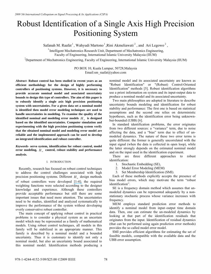
Hardware setup of the overall motion control scheme for the motor-table direct drive system is shown in Fig.1. The basic hardware consists of a host PC, FDA-5001 servo drive, a three phase voltage type PWM drive and the motor-table mechanism. The currently used machine has an operating range of 185mm. It is capable of 1µm resolution for measurements. In the system, position feedback signal is the only sensing available, which is obtained via an incremental encoder.

A. Analytical model

The dynamic behavior of the considered electric AC servomotor driven positioning system can be described by the following second-order nonlinear differential equation [7]:

ft FKuyy −=+ &&& α (1)

where y is the servomotor’s displacement, u is an input to the servomotor drive, is friction force, K and fF tα are positive

constants that relate with motor dynamics and mechanical system. In this paper only the linear part of the mathematical model will be considered, the friction effect will be treated as unstructured uncertainty. B. System Identification Model

Since there is no available information about the systems model parameters it is necessary to obtain the required nominal model by identification. Different model structures, identification methods and input test signals where used to develop a suitable model [8]. In this paper, the input-output data is collected from the positioning system using MATLAB’s xPC Target two PC-type desktop computers in a host-target configuration, and a NI BNC-2110 data acquisition card. MATLAB's System Identification Toolbox is used for identification [9]. Prediction Error Method (PEM) identification method is applied to obtain the following type one second order nominal model of the controlled system

)1()(

sTsKsG

p+= (2)

where K is a constant and T is the time constant in second. pIt should be noticed that the nominal model is used to

design the nominal controller and therefore a low order nominal model is preferable to be obtained.

C. Model Uncertainty Identification Using Model Error Modeling Method

Using linear model parameters identification there is always an associated uncertainty that must be identified for robust control design. "Model Error Modeling" (MEM) is a time domain technique in the area of system identification with various applications such as model validation and direct model error modeling, which will be used in this paper.

Simulink & xPC target

Host PC Target PC

AC Servo- Drive FDA-5001

Single stage positioning table

AC motor Position linear

encoder

RS232c

Fig.1. Experimental setup of single axis high precision positioning system.

978-1-4244-4152-5/09/$25.00 ©2009 IEEE 79

2009 5th International Colloquium on Signal Processing & Its Applications (CSPA)

Consider (2) and let G be the nominal estimated model of the system in (1). Suppose N samples of input-output data that have been generated by real system are available:

ˆ

rG

)()()()( kvkuqGky mrm += (3) where m is the measured displacement, mu is the measured controlled signal and is the measurement noise.

y)(kv

Let "residual" sequence to be computed as follows:

)(ˆ)()( kuGkyk mm −=ε (4) Now, it is possible to consider the "Error System" whose

input and output are respectively andmu ε . Let be this system's identified model. So:

eG

)()()()( kvkuqGk me +=ε (5)

e is also known as Model Error Model and is the estimate of unmodeled dynamics relevant error. It can be identified by any identification method as for nominal model; Using input-output data in (4), the model error model and its associated uncertainty is determined. Having system's nominal model

and e along with its uncertainty, it is possible to obtain a complete model of the system in (1). This can be done by adding up the nominal model and the uncertainty bound of eG . Using this MEM technique, the 99.9% confidence interval of additive model error is identified and used as the uncertainty weighting function aW [6]. It is also obvious that MEM technique has the ability of separating bias and variance errors completely. Due to this fact, recently this approach to robust identification attracts some interests [10, 11].

G

G G

III. ROBUST CONTROLLER DESIGN AND SYNTHESIS

After specifying the nominal model and associated

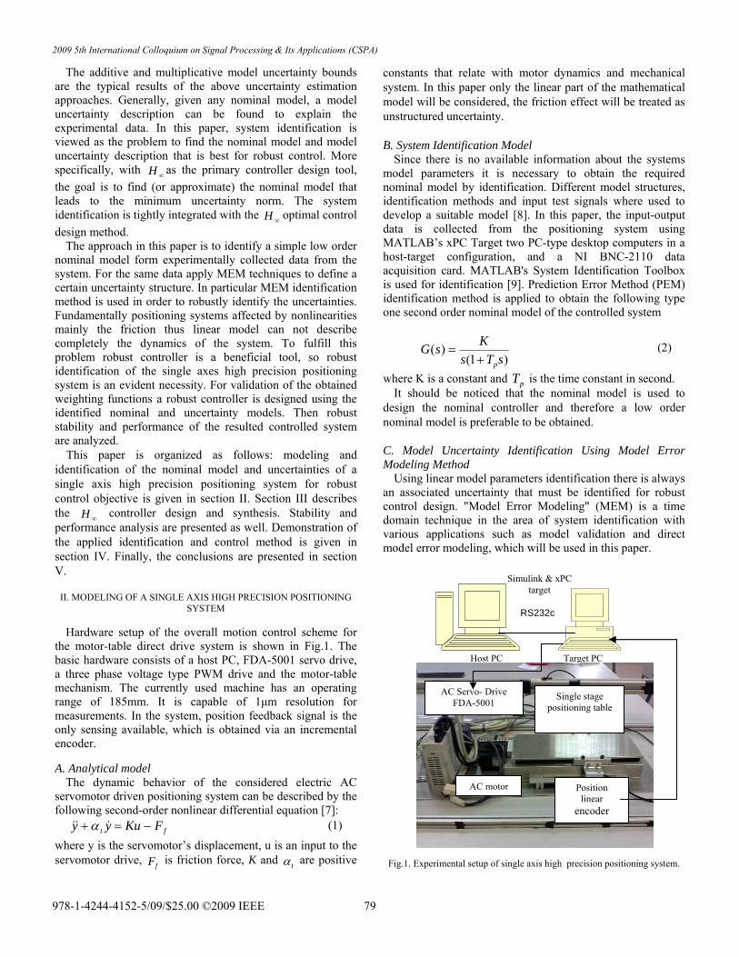
uncertainty bound , the design of nominal ∞ controller will be considered in order to achieve specified performance requirements in the frequency domain. A common approach is used to provide a generalized plant that contains the nominal model augmented with weighting functions. The entire connection of the controlled system will be as shown in Fig. 2. the augmented system is

H

⎪⎧

⎪⎨ ⎩ =

⎥⎦

⎢⎣⎥⎦

⎢⎣

=⎥⎦

⎢⎣

esKuusGsGe

)()()(

1

2221

1211 ⎤⎡⎤⎡⎤⎡ wsGsGz )()(

sK

(6)

where is the exogenous input signal of the augmented system, is the controlled variable vector of the augmented system, and is the tracking error between the reference command and the displacement output.

wz

e

The state space ∞ theory gives the equations to produce a stabilizing feedback controller 1 from output e to input

that minimize the induced norm between w and .

H)(

u ∞H z

Fig .2. The entire-connection of the robustly -controlled system. For the augmented plant

⎥⎥⎥

⎦⎢⎢⎢

⎣

=

22122

12111

21

)(DDCDDCsG

⎤⎡ BBA (7)

the ∞ controller is unique and can be found by solving two Riccati equations. The algorithm can be executed iteratively by appropriate software such as the Robust Control Toolbox in MATLAB.

H

The controller 1 stabilizes the plant with uncertainties, such that the ∞ norm of the closed loop transfer matrix is minimized providing robust performance.

KH

The performance weighting function e is used to reflect the requirements on the shape of the closed loop transfer function as given by the following equation [12]:

W

εωω

b

bse s

MsW

++

=/ (8)

where is the maximum value of the sensitivity function sin all frequencies ,

Mbω is the system bandwidth and ε is a

small number. Similarly, it is desirable to reduce the high frequency

content of the control signal by proper selection of the control weighting function [12]: uW

bc

ubcu s

MsWωε

ω+

+=

1

/ (9)

where bcω is the bandwidth of the controller, u is the maximum value of the control signal, and

M1ε is a small

number. For robust control synthesis, a representation of model

uncertainty is required to bound the difference between the actual plant and the linear model used for control design. These unmodeled uncertainties are best formulated as unstructured uncertainties because they are difficult to express in highly structured parameterized form.

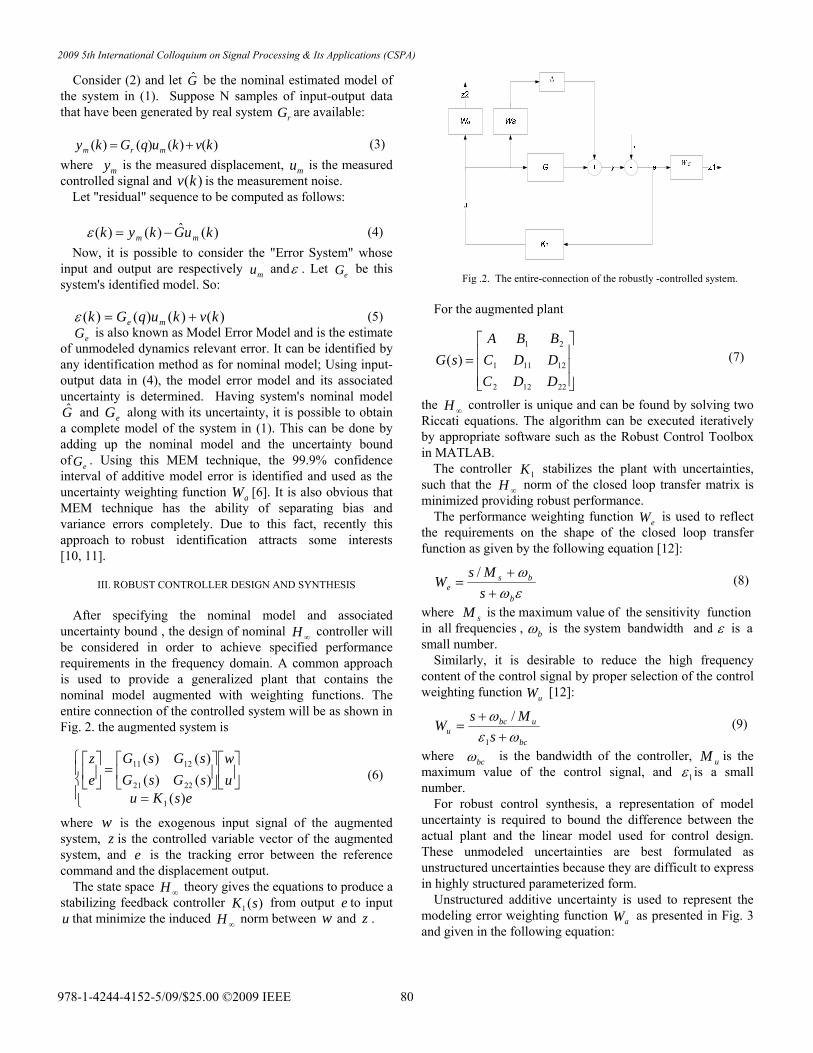
Unstructured additive uncertainty is used to represent the modeling error weighting function as presented in Fig. 3 and given in the following equation:

aW

978-1-4244-4152-5/09/$25.00 ©2009 IEEE 80

2009 5th International Colloquium on Signal Processing & Its Applications (CSPA)

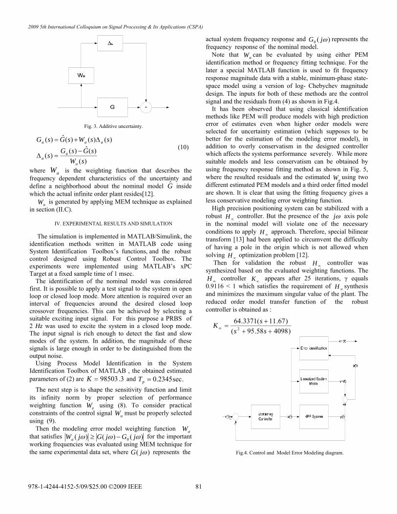
Fig. 3. Additive uncertainty.

)()()(ˆ)( ssWsGsG aaa (10)

∆+=

)()(ˆ)(

)(sW

sGsGsa

aa

−=∆

where a is the weighting function that describes the frequency dependent characteristics of the uncertainty and define a neighborhood about the nominal model G inside which the actual infinite order plant resides[12].

W

ˆ

aW is generated by applying MEM technique as explained in section (II.C).

IV. EXPERIMENTAL RESULTS AND SIMULATION

The simulation is implemented in MATLAB/Simulink, the

identification methods written in MATLAB code using System Identification Toolbox’s functions, and the robust control designed using Robust Control Toolbox. The experiments were implemented using MATLAB’s xPC Target at a fixed sample time of 1 msec.

The identification of the nominal model was considered first. It is possible to apply a test signal to the system in open loop or closed loop mode. More attention is required over an interval of frequencies around the desired closed loop crossover frequencies. This can be achieved by selecting a suitable exciting input signal. For this purpose a PRBS of 2 Hz was used to excite the system in a closed loop mode. The input signal is rich enough to detect the fast and slow modes of the system. In addition, the magnitude of these signals is large enough in order to be distinguished from the output noise.

Using Process Model Identification in the System Identification Toolbox of MATLAB , the obtained estimated parameters of (2) are and 3.98503=K .sec2345.0=pT

The next step is to shape the sensitivity function and limit its infinity norm by proper selection of performance weighting function eW using (8). To consider practical constraints of the control signal must be properly selected using (9).

uW

Then the modeling error model weighting function aW that satisfies )()()( 0 ωωω jGjGjWa −≥ for the important working frequencies was evaluated using MEM technique for the same experimental data set, where )( ωjG represents the

actual system frequency response and )(0 ωjG represents the frequency response of the nominal model.

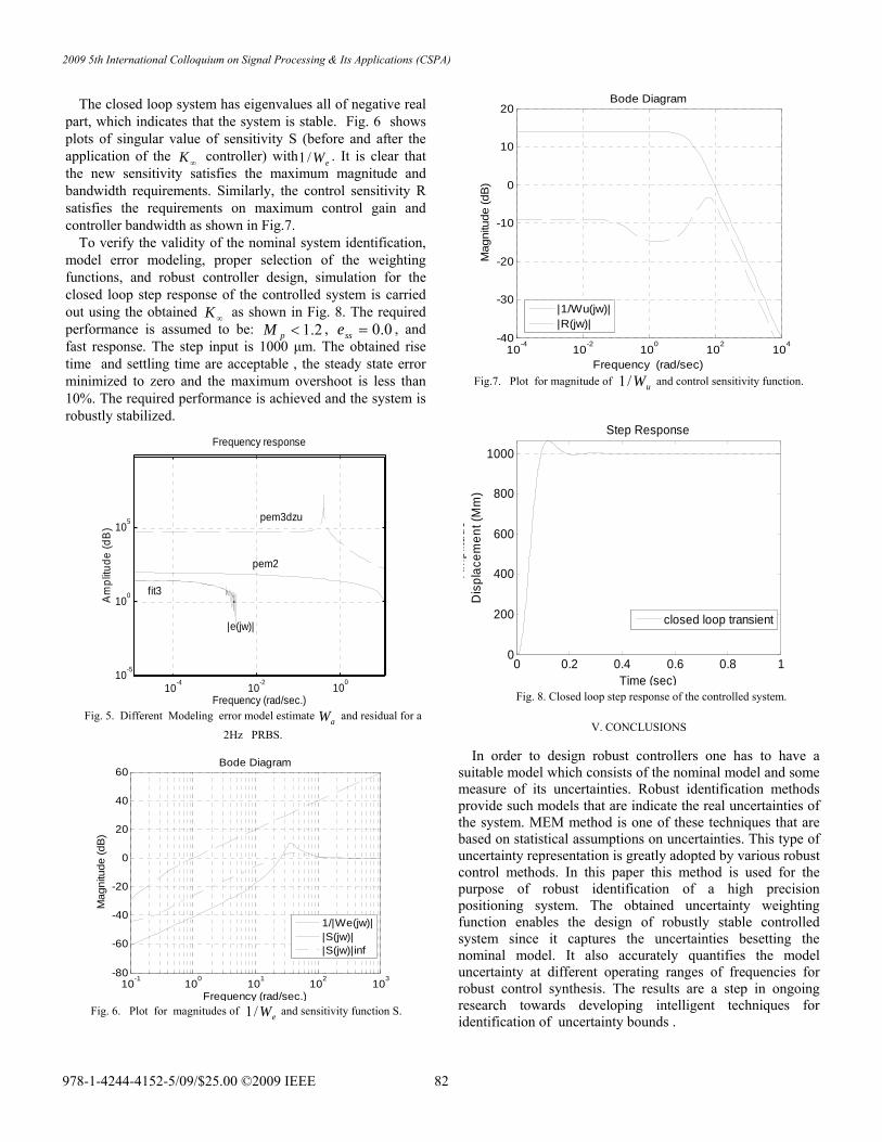
Note that aW can be evaluated by using either PEM identification method or frequency fitting technique. For the later a special MATLAB function is used to fit frequency response magnitude data with a stable, minimum-phase state-space model using a version of log- Chebychev magnitude design. The inputs for both of these methods are the control signal and the residuals from (4) as shown in Fig.4.

It has been observed that using classical identification methods like PEM will produce models with high prediction error of estimates even when higher order models were selected for uncertainty estimation (which supposes to be better for the estimation of the modeling error model), in addition to overly conservatism in the designed controller which affects the systems performance severely. While more suitable models and less conservatism can be obtained by using frequency response fitting method as shown in Fig. 5, where the resulted residuals and the estimated aW using two different estimated PEM models and a third order fitted model are shown. It is clear that using the fitting frequency gives a less conservative modeling error weighting function.

High precision positioning system can be stabilized with a robust ∞ controller. But the presence of the H ωj axis pole in the nominal model will violate one of the necessary conditions to apply ∞H approach. Therefore, special bilinear transform [13] had been applied to circumvent the difficulty of having a pole in the origin which is not allowed when solving optimization problem [12]. ∞

Then for validation the robust ∞ controller was synthesized based on the evaluated weighting functions. The

controller ∞ appears after 25 iterations, γ equals 0.9116 < 1 which satisfies the requirement of synthesis and minimizes the maximum singular value of the plant. The reduced order model transfer function of the robust controller is obtained as :

HH

∞H K∞H

)409858.95()67.11(3371.64

2 +++

=∞ sssK

Fig.4. Control and Model Error Modeling diagram.

978-1-4244-4152-5/09/$25.00 ©2009 IEEE 81

2009 5th International Colloquium on Signal Processing & Its Applications (CSPA)

The closed loop system has eigenvalues all of negative real

part, which indicates that the system is stable. Fig. 6 shows plots of singular value of sensitivity S (before and after the application of the ∞ controller) with e . It is clear that the new sensitivity satisfies the maximum magnitude and bandwidth requirements. Similarly, the control sensitivity R satisfies the requirements on maximum control gain and controller bandwidth as shown in Fig.7.

K W/1

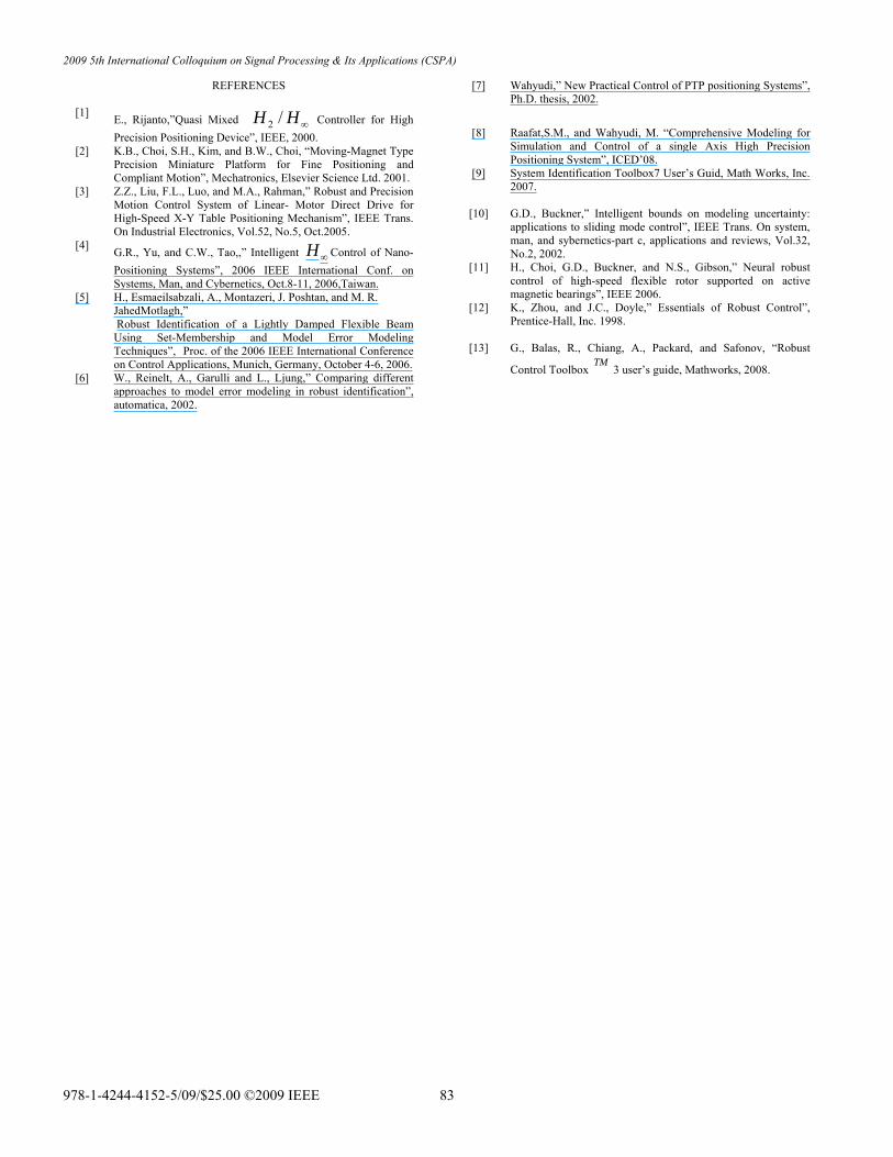
To verify the validity of the nominal system identification, model error modeling, proper selection of the weighting functions, and robust controller design, simulation for the closed loop step response of the controlled system is carried out using the obtained ∞ as shown in Fig. 8. The required performance is assumed to be: ,

K2.1<pM 0.0=sse , and

fast response. The step input is 1000 µm. The obtained rise time and settling time are acceptable , the steady state error minimized to zero and the maximum overshoot is less than 10%. The required performance is achieved and the system is robustly stabilized.

10-4 10-2 10010-5

100

105

Frequency (rad/sec.)

Am

plitu

de (d

B)

Frequency response

pem3dzu

fit3

|e(jw)|

pem2

Fig. 5. Different Modeling error model estimate and residual for a

2Hz PRBS. aW

10-1 100 101 102 103-80

-60

-40

-20

0

20

40

60

Frequency (rad/sec.)

Mag

nitu

de (d

B)

Bode Diagram

1/|We(jw)||S(jw)||S(jw)|inf

Fig. 6. Plot for magnitudes of and sensitivity function S. eW/1

10-4 10-2 100 102 104-40

-30

-20

-10

0

10

20

Mag

nitu

de (d

B)

Bode Diagram

Frequency (rad/sec)

|1/Wu(jw)||R(jw)|

Fig.7. Plot for magnitude of and control sensitivity function. uW/1

0 0.2 0.4 0.6 0.8 10

200

400

600

800

1000

Dis

plac

emen

t (M

m)

Step Response

Time (sec)

Am

plitu

de

closed loop transient

Fig. 8. Closed loop step response of the controlled system.

V. CONCLUSIONS

In order to design robust controllers one has to have a

suitable model which consists of the nominal model and some measure of its uncertainties. Robust identification methods provide such models that are indicate the real uncertainties of the system. MEM method is one of these techniques that are based on statistical assumptions on uncertainties. This type of uncertainty representation is greatly adopted by various robust control methods. In this paper this method is used for the purpose of robust identification of a high precision positioning system. The obtained uncertainty weighting function enables the design of robustly stable controlled system since it captures the uncertainties besetting the nominal model. It also accurately quantifies the model uncertainty at different operating ranges of frequencies for robust control synthesis. The results are a step in ongoing research towards developing intelligent techniques for identification of uncertainty bounds .

978-1-4244-4152-5/09/$25.00 ©2009 IEEE 82

2009 5th International Colloquium on Signal Processing & Its Applications (CSPA)

REFERENCES

[1] E., Rijanto,”Quasi Mixed Controller for High Precision Positioning Device”, IEEE, 2000.

∞HH /2

[2] K.B., Choi, S.H., Kim, and B.W., Choi, “Moving-Magnet Type Precision Miniature Platform for Fine Positioning and Compliant Motion”, Mechatronics, Elsevier Science Ltd. 2001.

[3] Z.Z., Liu, F.L., Luo, and M.A., Rahman,” Robust and Precision Motion Control System of Linear- Motor Direct Drive for High-Speed X-Y Table Positioning Mechanism”, IEEE Trans. On Industrial Electronics, Vol.52, No.5, Oct.2005.

[4] G.R., Yu, and C.W., Tao,,” Intelligent Control of Nano- Positioning Systems”, 2006 IEEE International Conf. on Systems, Man, and Cybernetics, Oct.8-11, 2006,Taiwan.

∞H

[5] H., Esmaeilsabzali, A., Montazeri, J. Poshtan, and M. R. JahedMotlagh,” Robust Identification of a Lightly Damped Flexible Beam Using Set-Membership and Model Error Modeling Techniques”, Proc. of the 2006 IEEE International Conference on Control Applications, Munich, Germany, October 4-6, 2006.

[6] W., Reinelt, A., Garulli and L., Ljung,” Comparing different approaches to model error modeling in robust identification”, automatica, 2002.

[7] Wahyudi,” New Practical Control of PTP positioning Systems”, Ph.D. thesis, 2002.

[8] Raafat,S.M., and Wahyudi, M. “Comprehensive Modeling for Simulation and Control of a single Axis High Precision Positioning System”, ICED’08.

[9] System Identification Toolbox7 User’s Guid, Math Works, Inc. 2007.

[10] G.D., Buckner,” Intelligent bounds on modeling uncertainty: applications to sliding mode control”, IEEE Trans. On system, man, and sybernetics-part c, applications and reviews, Vol.32, No.2, 2002.

[11] H., Choi, G.D., Buckner, and N.S., Gibson,” Neural robust control of high-speed flexible rotor supported on active magnetic bearings”, IEEE 2006.

[12] K., Zhou, and J.C., Doyle,” Essentials of Robust Control”, Prentice-Hall, Inc. 1998.

[13] G., Balas, R., Chiang, A., Packard, and Safonov, “Robust

Control Toolbox 3 user’s guide, Mathworks, 2008. TM

978-1-4244-4152-5/09/$25.00 ©2009 IEEE 83

2009 5th International Colloquium on Signal Processing & Its Applications (CSPA)