Multi–Precision Math
307
Multi–Precision Math Tom St Denis Algonquin College Mads Rasmussen Open Communications Security Greg Rose QUALCOMM Australia August 29, 2017
-
Upload
khangminh22 -
Category
Documents
-
view
0 -
download
0
Transcript of Multi–Precision Math

Multi–Precision Math
Tom St Denis
Algonquin College
Mads Rasmussen
Open Communications Security
Greg Rose
QUALCOMM Australia
August 29, 2017

This text has been placed in the public domain. This text corresponds tothe v0.39 release of the LibTomMath project.
This text is formatted to the international B5 paper size of 176mm wide by250mm tall using the LATEX book macro package and the Perl booker package.
Contents
1 Introduction 11.1 Multiple Precision Arithmetic . . . . . . . . . . . . . . . . . . . . 1
1.1.1 What is Multiple Precision Arithmetic? . . . . . . . . . . 11.1.2 The Need for Multiple Precision Arithmetic . . . . . . . . 11.1.3 Benefits of Multiple Precision Arithmetic . . . . . . . . . 3
1.2 Purpose of This Text . . . . . . . . . . . . . . . . . . . . . . . . . 41.3 Discussion and Notation . . . . . . . . . . . . . . . . . . . . . . . 5
1.3.1 Notation . . . . . . . . . . . . . . . . . . . . . . . . . . . . 51.3.2 Precision Notation . . . . . . . . . . . . . . . . . . . . . . 51.3.3 Algorithm Inputs and Outputs . . . . . . . . . . . . . . . 61.3.4 Mathematical Expressions . . . . . . . . . . . . . . . . . . 61.3.5 Work Effort . . . . . . . . . . . . . . . . . . . . . . . . . . 7
1.4 Exercises . . . . . . . . . . . . . . . . . . . . . . . . . . . . . . . 71.5 Introduction to LibTomMath . . . . . . . . . . . . . . . . . . . . 9
1.5.1 What is LibTomMath? . . . . . . . . . . . . . . . . . . . . 91.5.2 Goals of LibTomMath . . . . . . . . . . . . . . . . . . . . 9
1.6 Choice of LibTomMath . . . . . . . . . . . . . . . . . . . . . . . 101.6.1 Code Base . . . . . . . . . . . . . . . . . . . . . . . . . . . 101.6.2 API Simplicity . . . . . . . . . . . . . . . . . . . . . . . . 111.6.3 Optimizations . . . . . . . . . . . . . . . . . . . . . . . . . 111.6.4 Portability and Stability . . . . . . . . . . . . . . . . . . . 111.6.5 Choice . . . . . . . . . . . . . . . . . . . . . . . . . . . . . 12
2 Getting Started 132.1 Library Basics . . . . . . . . . . . . . . . . . . . . . . . . . . . . 132.2 What is a Multiple Precision Integer? . . . . . . . . . . . . . . . 14
2.2.1 The mp int Structure . . . . . . . . . . . . . . . . . . . . 15
iii
2.3 Argument Passing . . . . . . . . . . . . . . . . . . . . . . . . . . 172.4 Return Values . . . . . . . . . . . . . . . . . . . . . . . . . . . . . 182.5 Initialization and Clearing . . . . . . . . . . . . . . . . . . . . . . 19
2.5.1 Initializing an mp int . . . . . . . . . . . . . . . . . . . . 192.5.2 Clearing an mp int . . . . . . . . . . . . . . . . . . . . . . 22
2.6 Maintenance Algorithms . . . . . . . . . . . . . . . . . . . . . . . 242.6.1 Augmenting an mp int’s Precision . . . . . . . . . . . . . 242.6.2 Initializing Variable Precision mp ints . . . . . . . . . . . 272.6.3 Multiple Integer Initializations and Clearings . . . . . . . 292.6.4 Clamping Excess Digits . . . . . . . . . . . . . . . . . . . 31
3 Basic Operations 353.1 Introduction . . . . . . . . . . . . . . . . . . . . . . . . . . . . . . 353.2 Assigning Values to mp int Structures . . . . . . . . . . . . . . . 35
3.2.1 Copying an mp int . . . . . . . . . . . . . . . . . . . . . . 353.2.2 Creating a Clone . . . . . . . . . . . . . . . . . . . . . . . 40
3.3 Zeroing an Integer . . . . . . . . . . . . . . . . . . . . . . . . . . 413.4 Sign Manipulation . . . . . . . . . . . . . . . . . . . . . . . . . . 42
3.4.1 Absolute Value . . . . . . . . . . . . . . . . . . . . . . . . 423.4.2 Integer Negation . . . . . . . . . . . . . . . . . . . . . . . 43
3.5 Small Constants . . . . . . . . . . . . . . . . . . . . . . . . . . . 453.5.1 Setting Small Constants . . . . . . . . . . . . . . . . . . . 453.5.2 Setting Large Constants . . . . . . . . . . . . . . . . . . . 47
3.6 Comparisons . . . . . . . . . . . . . . . . . . . . . . . . . . . . . 483.6.1 Unsigned Comparisions . . . . . . . . . . . . . . . . . . . 483.6.2 Signed Comparisons . . . . . . . . . . . . . . . . . . . . . 51
4 Basic Arithmetic 554.1 Introduction . . . . . . . . . . . . . . . . . . . . . . . . . . . . . . 554.2 Addition and Subtraction . . . . . . . . . . . . . . . . . . . . . . 56
4.2.1 Low Level Addition . . . . . . . . . . . . . . . . . . . . . 564.2.2 Low Level Subtraction . . . . . . . . . . . . . . . . . . . . 614.2.3 High Level Addition . . . . . . . . . . . . . . . . . . . . . 654.2.4 High Level Subtraction . . . . . . . . . . . . . . . . . . . 68
4.3 Bit and Digit Shifting . . . . . . . . . . . . . . . . . . . . . . . . 714.3.1 Multiplication by Two . . . . . . . . . . . . . . . . . . . . 714.3.2 Division by Two . . . . . . . . . . . . . . . . . . . . . . . 74
4.4 Polynomial Basis Operations . . . . . . . . . . . . . . . . . . . . 774.4.1 Multiplication by x . . . . . . . . . . . . . . . . . . . . . . 77
4.4.2 Division by x . . . . . . . . . . . . . . . . . . . . . . . . . 804.5 Powers of Two . . . . . . . . . . . . . . . . . . . . . . . . . . . . 83
4.5.1 Multiplication by Power of Two . . . . . . . . . . . . . . . 834.5.2 Division by Power of Two . . . . . . . . . . . . . . . . . . 874.5.3 Remainder of Division by Power of Two . . . . . . . . . . 90
5 Multiplication and Squaring 955.1 The Multipliers . . . . . . . . . . . . . . . . . . . . . . . . . . . . 955.2 Multiplication . . . . . . . . . . . . . . . . . . . . . . . . . . . . . 96
5.2.1 The Baseline Multiplication . . . . . . . . . . . . . . . . . 965.2.2 Faster Multiplication by the “Comba” Method . . . . . . 1015.2.3 Polynomial Basis Multiplication . . . . . . . . . . . . . . 1095.2.4 Karatsuba Multiplication . . . . . . . . . . . . . . . . . . 1125.2.5 Toom-Cook 3-Way Multiplication . . . . . . . . . . . . . . 1185.2.6 Signed Multiplication . . . . . . . . . . . . . . . . . . . . 128
5.3 Squaring . . . . . . . . . . . . . . . . . . . . . . . . . . . . . . . . 1305.3.1 The Baseline Squaring Algorithm . . . . . . . . . . . . . . 1315.3.2 Faster Squaring by the “Comba” Method . . . . . . . . . 1345.3.3 Polynomial Basis Squaring . . . . . . . . . . . . . . . . . 1385.3.4 Karatsuba Squaring . . . . . . . . . . . . . . . . . . . . . 1395.3.5 Toom-Cook Squaring . . . . . . . . . . . . . . . . . . . . . 1445.3.6 High Level Squaring . . . . . . . . . . . . . . . . . . . . . 144
6 Modular Reduction 1496.1 Basics of Modular Reduction . . . . . . . . . . . . . . . . . . . . 1496.2 The Barrett Reduction . . . . . . . . . . . . . . . . . . . . . . . . 150
6.2.1 Fixed Point Arithmetic . . . . . . . . . . . . . . . . . . . 1506.2.2 Choosing a Radix Point . . . . . . . . . . . . . . . . . . . 1526.2.3 Trimming the Quotient . . . . . . . . . . . . . . . . . . . 1536.2.4 Trimming the Residue . . . . . . . . . . . . . . . . . . . . 1546.2.5 The Barrett Algorithm . . . . . . . . . . . . . . . . . . . . 1546.2.6 The Barrett Setup Algorithm . . . . . . . . . . . . . . . . 158
6.3 The Montgomery Reduction . . . . . . . . . . . . . . . . . . . . . 1606.3.1 Digit Based Montgomery Reduction . . . . . . . . . . . . 1636.3.2 Baseline Montgomery Reduction . . . . . . . . . . . . . . 1646.3.3 Faster “Comba” Montgomery Reduction . . . . . . . . . . 1696.3.4 Montgomery Setup . . . . . . . . . . . . . . . . . . . . . . 175
6.4 The Diminished Radix Algorithm . . . . . . . . . . . . . . . . . . 1776.4.1 Choice of Moduli . . . . . . . . . . . . . . . . . . . . . . . 179
6.4.2 Choice of k . . . . . . . . . . . . . . . . . . . . . . . . . . 1806.4.3 Restricted Diminished Radix Reduction . . . . . . . . . . 1806.4.4 Unrestricted Diminished Radix Reduction . . . . . . . . . 186
6.5 Algorithm Comparison . . . . . . . . . . . . . . . . . . . . . . . . 191
7 Exponentiation 1937.1 Exponentiation Basics . . . . . . . . . . . . . . . . . . . . . . . . 193
7.1.1 Single Digit Exponentiation . . . . . . . . . . . . . . . . . 1957.2 k-ary Exponentiation . . . . . . . . . . . . . . . . . . . . . . . . . 198
7.2.1 Optimal Values of k . . . . . . . . . . . . . . . . . . . . . 1997.2.2 Sliding-Window Exponentiation . . . . . . . . . . . . . . . 199
7.3 Modular Exponentiation . . . . . . . . . . . . . . . . . . . . . . . 2017.3.1 Barrett Modular Exponentiation . . . . . . . . . . . . . . 205
7.4 Quick Power of Two . . . . . . . . . . . . . . . . . . . . . . . . . 216
8 Higher Level Algorithms 2198.1 Integer Division with Remainder . . . . . . . . . . . . . . . . . . 219
8.1.1 Quotient Estimation . . . . . . . . . . . . . . . . . . . . . 2218.1.2 Normalized Integers . . . . . . . . . . . . . . . . . . . . . 2228.1.3 Radix-β Division with Remainder . . . . . . . . . . . . . 222
8.2 Single Digit Helpers . . . . . . . . . . . . . . . . . . . . . . . . . 2338.2.1 Single Digit Addition and Subtraction . . . . . . . . . . . 2338.2.2 Single Digit Multiplication . . . . . . . . . . . . . . . . . 2368.2.3 Single Digit Division . . . . . . . . . . . . . . . . . . . . . 2398.2.4 Single Digit Root Extraction . . . . . . . . . . . . . . . . 243
8.3 Random Number Generation . . . . . . . . . . . . . . . . . . . . 2458.4 Formatted Representations . . . . . . . . . . . . . . . . . . . . . 248
8.4.1 Reading Radix-n Input . . . . . . . . . . . . . . . . . . . 2488.4.2 Generating Radix-n Output . . . . . . . . . . . . . . . . . 252
9 Number Theoretic Algorithms 2579.1 Greatest Common Divisor . . . . . . . . . . . . . . . . . . . . . . 257
9.1.1 Complete Greatest Common Divisor . . . . . . . . . . . . 2609.2 Least Common Multiple . . . . . . . . . . . . . . . . . . . . . . . 2659.3 Jacobi Symbol Computation . . . . . . . . . . . . . . . . . . . . . 267
9.3.1 Jacobi Symbol . . . . . . . . . . . . . . . . . . . . . . . . 2689.4 Modular Inverse . . . . . . . . . . . . . . . . . . . . . . . . . . . 274
9.4.1 General Case . . . . . . . . . . . . . . . . . . . . . . . . . 2759.5 Primality Tests . . . . . . . . . . . . . . . . . . . . . . . . . . . . 278

9.5.1 Trial Division . . . . . . . . . . . . . . . . . . . . . . . . . 2789.5.2 The Fermat Test . . . . . . . . . . . . . . . . . . . . . . . 2829.5.3 The Miller-Rabin Test . . . . . . . . . . . . . . . . . . . . 284

List of Figures
1.1 Typical Data Types for the C Programming Language . . . . . . 21.2 Exercise Scoring System . . . . . . . . . . . . . . . . . . . . . . . 8
2.1 Design Flow of the First Few Original LibTomMath Functions. . 142.2 The mp int Structure . . . . . . . . . . . . . . . . . . . . . . . . 162.3 LibTomMath Error Codes . . . . . . . . . . . . . . . . . . . . . . 182.4 Algorithm mp init . . . . . . . . . . . . . . . . . . . . . . . . . . 192.5 Algorithm mp clear . . . . . . . . . . . . . . . . . . . . . . . . . . 222.6 Algorithm mp grow . . . . . . . . . . . . . . . . . . . . . . . . . . 252.7 Algorithm mp init size . . . . . . . . . . . . . . . . . . . . . . . . 272.8 Algorithm mp init multi . . . . . . . . . . . . . . . . . . . . . . . 302.9 Algorithm mp clamp . . . . . . . . . . . . . . . . . . . . . . . . . 32
3.1 Algorithm mp copy . . . . . . . . . . . . . . . . . . . . . . . . . . 363.2 Algorithm mp init copy . . . . . . . . . . . . . . . . . . . . . . . 403.3 Algorithm mp zero . . . . . . . . . . . . . . . . . . . . . . . . . . 413.4 Algorithm mp abs . . . . . . . . . . . . . . . . . . . . . . . . . . 423.5 Algorithm mp neg . . . . . . . . . . . . . . . . . . . . . . . . . . 443.6 Algorithm mp set . . . . . . . . . . . . . . . . . . . . . . . . . . . 463.7 Algorithm mp set int . . . . . . . . . . . . . . . . . . . . . . . . . 473.8 Comparison Return Codes . . . . . . . . . . . . . . . . . . . . . . 493.9 Algorithm mp cmp mag . . . . . . . . . . . . . . . . . . . . . . . 493.10 Algorithm mp cmp . . . . . . . . . . . . . . . . . . . . . . . . . . 51
4.1 Algorithm s mp add . . . . . . . . . . . . . . . . . . . . . . . . . 574.2 Algorithm s mp sub . . . . . . . . . . . . . . . . . . . . . . . . . 624.3 Algorithm mp add . . . . . . . . . . . . . . . . . . . . . . . . . . 664.4 Addition Guide Chart . . . . . . . . . . . . . . . . . . . . . . . . 67
ix
4.5 Algorithm mp sub . . . . . . . . . . . . . . . . . . . . . . . . . . 694.6 Subtraction Guide Chart . . . . . . . . . . . . . . . . . . . . . . . 694.7 Algorithm mp mul 2 . . . . . . . . . . . . . . . . . . . . . . . . . 724.8 Algorithm mp div 2 . . . . . . . . . . . . . . . . . . . . . . . . . 754.9 Algorithm mp lshd . . . . . . . . . . . . . . . . . . . . . . . . . . 784.10 Sliding Window Movement . . . . . . . . . . . . . . . . . . . . . 794.11 Algorithm mp rshd . . . . . . . . . . . . . . . . . . . . . . . . . . 814.12 Algorithm mp mul 2d . . . . . . . . . . . . . . . . . . . . . . . . 844.13 Algorithm mp div 2d . . . . . . . . . . . . . . . . . . . . . . . . . 884.14 Algorithm mp mod 2d . . . . . . . . . . . . . . . . . . . . . . . . 91
5.1 Algorithm s mp mul digs . . . . . . . . . . . . . . . . . . . . . . 975.2 Long-Hand Multiplication Diagram . . . . . . . . . . . . . . . . . 985.3 Comba Multiplication Diagram . . . . . . . . . . . . . . . . . . . 1035.4 Algorithm Comba Fixup . . . . . . . . . . . . . . . . . . . . . . . 1035.5 Algorithm fast s mp mul digs . . . . . . . . . . . . . . . . . . . . 1055.6 Asymptotic Running Time of Polynomial Basis Multiplication . . 1105.7 Algorithm mp karatsuba mul . . . . . . . . . . . . . . . . . . . . 1135.8 Algorithm mp toom mul . . . . . . . . . . . . . . . . . . . . . . . 1195.9 Algorithm mp toom mul (continued) . . . . . . . . . . . . . . . . 1205.10 Algorithm mp mul . . . . . . . . . . . . . . . . . . . . . . . . . . 1285.11 Squaring Optimization Diagram . . . . . . . . . . . . . . . . . . . 1305.12 Algorithm s mp sqr . . . . . . . . . . . . . . . . . . . . . . . . . . 1325.13 Algorithm fast s mp sqr . . . . . . . . . . . . . . . . . . . . . . . 1355.14 Algorithm mp karatsuba sqr . . . . . . . . . . . . . . . . . . . . . 1405.15 Algorithm mp sqr . . . . . . . . . . . . . . . . . . . . . . . . . . 145
6.1 Algorithm mp reduce . . . . . . . . . . . . . . . . . . . . . . . . . 1556.2 Algorithm mp reduce setup . . . . . . . . . . . . . . . . . . . . . 1596.3 Algorithm Montgomery Reduction . . . . . . . . . . . . . . . . . 1616.4 Example of Montgomery Reduction (I) . . . . . . . . . . . . . . . 1616.5 Algorithm Montgomery Reduction (modified I) . . . . . . . . . . 1626.6 Example of Montgomery Reduction (II) . . . . . . . . . . . . . . 1626.7 Algorithm Montgomery Reduction (modified II) . . . . . . . . . . 1636.8 Example of Montgomery Reduction . . . . . . . . . . . . . . . . . 1646.9 Algorithm mp montgomery reduce . . . . . . . . . . . . . . . . . 1656.10 Algorithm fast mp montgomery reduce . . . . . . . . . . . . . . . 1706.11 Algorithm mp montgomery setup . . . . . . . . . . . . . . . . . . 1766.12 Algorithm Diminished Radix Reduction . . . . . . . . . . . . . . 178
6.13 Example Diminished Radix Reduction . . . . . . . . . . . . . . . 1796.14 Algorithm mp dr reduce . . . . . . . . . . . . . . . . . . . . . . . 1816.15 Algorithm mp dr setup . . . . . . . . . . . . . . . . . . . . . . . 1846.16 Algorithm mp dr is modulus . . . . . . . . . . . . . . . . . . . . 1856.17 Algorithm mp reduce 2k . . . . . . . . . . . . . . . . . . . . . . . 1876.18 Algorithm mp reduce 2k setup . . . . . . . . . . . . . . . . . . . 1886.19 Algorithm mp reduce is 2k . . . . . . . . . . . . . . . . . . . . . 190
7.1 Left to Right Exponentiation . . . . . . . . . . . . . . . . . . . . 1947.2 Example of Left to Right Exponentiation . . . . . . . . . . . . . 1957.3 Algorithm mp expt d . . . . . . . . . . . . . . . . . . . . . . . . . 1967.4 k-ary Exponentiation . . . . . . . . . . . . . . . . . . . . . . . . . 1997.5 Optimal Values of k for k-ary Exponentiation . . . . . . . . . . . 2007.6 Optimal Values of k for Sliding Window Exponentiation . . . . . 2007.7 Sliding Window k-ary Exponentiation . . . . . . . . . . . . . . . 2017.8 Algorithm mp exptmod . . . . . . . . . . . . . . . . . . . . . . . 2027.9 Algorithm s mp exptmod . . . . . . . . . . . . . . . . . . . . . . 2067.10 Algorithm s mp exptmod (continued) . . . . . . . . . . . . . . . 2077.11 Sliding Window State Diagram . . . . . . . . . . . . . . . . . . . 2097.12 Algorithm mp 2expt . . . . . . . . . . . . . . . . . . . . . . . . . 216
8.1 Algorithm Radix-β Integer Division . . . . . . . . . . . . . . . . 2208.2 Algorithm mp div . . . . . . . . . . . . . . . . . . . . . . . . . . 2238.3 Algorithm mp div (continued) . . . . . . . . . . . . . . . . . . . . 2248.4 Algorithm mp add d . . . . . . . . . . . . . . . . . . . . . . . . . 2348.5 Algorithm mp mul d . . . . . . . . . . . . . . . . . . . . . . . . . 2378.6 Algorithm mp div d . . . . . . . . . . . . . . . . . . . . . . . . . 2408.7 Algorithm mp n root . . . . . . . . . . . . . . . . . . . . . . . . . 2448.8 Algorithm mp rand . . . . . . . . . . . . . . . . . . . . . . . . . . 2468.9 Lower ASCII Map . . . . . . . . . . . . . . . . . . . . . . . . . . 2498.10 Algorithm mp read radix . . . . . . . . . . . . . . . . . . . . . . 2508.11 Algorithm mp toradix . . . . . . . . . . . . . . . . . . . . . . . . 2538.12 Example of Algorithm mp toradix. . . . . . . . . . . . . . . . . . 254
9.1 Algorithm Greatest Common Divisor (I) . . . . . . . . . . . . . . 2589.2 Algorithm Greatest Common Divisor (II) . . . . . . . . . . . . . 2589.3 Algorithm Greatest Common Divisor (III) . . . . . . . . . . . . . 2599.4 Algorithm mp gcd . . . . . . . . . . . . . . . . . . . . . . . . . . 2619.5 Algorithm mp lcm . . . . . . . . . . . . . . . . . . . . . . . . . . 265
9.6 Algorithm mp jacobi . . . . . . . . . . . . . . . . . . . . . . . . . 2709.7 Probability of successful trial division to detect non-primes . . . 2809.8 Algorithm mp prime is divisible . . . . . . . . . . . . . . . . . . . 2819.9 Algorithm mp prime fermat . . . . . . . . . . . . . . . . . . . . . 2839.10 Algorithm mp prime miller rabin . . . . . . . . . . . . . . . . . . 285
Prefaces
When I tell people about my LibTom projects and that I release them as publicdomain they are often puzzled. They ask why I did it and especially why Icontinue to work on them for free. The best I can explain it is “Because I can.”Which seems odd and perhaps too terse for adult conversation. I often qualifyit with “I am able, I am willing.” which perhaps explains it better. I am thefirst to admit there is not anything that special with what I have done. Perhapsothers can see that too and then we would have a society to be proud of. MyLibTom projects are what I am doing to give back to society in the form of toolsand knowledge that can help others in their endeavours.
I started writing this book because it was the most logical task to further mygoal of open academia. The LibTomMath source code itself was written to beeasy to follow and learn from. There are times, however, where pure C sourcecode does not explain the algorithms properly. Hence this book. The bookliterally starts with the foundation of the library and works itself outwards tothe more complicated algorithms. The use of both pseudo–code and verbatimsource code provides a duality of “theory” and “practice” that the computerscience students of the world shall appreciate. I never deviate too far fromrelatively straightforward algebra and I hope that this book can be a valuablelearning asset.
This book and indeed much of the LibTom projects would not exist in theircurrent form if it was not for a plethora of kind people donating their time,resources and kind words to help support my work. Writing a text of significantlength (along with the source code) is a tiresome and lengthy process. Currentlythe LibTom project is four years old, comprises of literally thousands of usersand over 100,000 lines of source code, TeX and other material. People likeMads and Greg were there at the beginning to encourage me to work well. Itis amazing how timely validation from others can boost morale to continue theproject. Definitely my parents were there for me by providing room and board
xiii

during the many months of work in 2003.To my many friends whom I have met through the years I thank you for the
good times and the words of encouragement. I hope I honour your kind gestureswith this project.
Open Source. Open Academia. Open Minds.
Tom St Denis

I found the opportunity to work with Tom appealing for several reasons, notonly could I broaden my own horizons, but also contribute to educate othersfacing the problem of having to handle big number mathematical calculations.
This book is Tom’s child and he has been caring and fostering the projectever since the beginning with a clear mind of how he wanted the project to turnout. I have helped by proofreading the text and we have had several discussionsabout the layout and language used.
I hold a masters degree in cryptography from the University of SouthernDenmark and have always been interested in the practical aspects of cryptog-raphy.
Having worked in the security consultancy business for several years in SaoPaulo, Brazil, I have been in touch with a great deal of work in which multipleprecision mathematics was needed. Understanding the possibilities for speedingup multiple precision calculations is often very important since we deal withoutdated machine architecture where modular reductions, for example, becomepainfully slow.
This text is for people who stop and wonder when first examining algorithmssuch as RSA for the first time and asks themselves, “You tell me this is onlysecure for large numbers, fine; but how do you implement these numbers?”
Mads RasmussenSao Paulo - SP
Brazil
It’s all because I broke my leg. That just happened to be at about thesame time that Tom asked for someone to review the section of the book aboutKaratsuba multiplication. I was laid up, alone and immobile, and thought “Whynot?” I vaguely knew what Karatsuba multiplication was, but not really, so Ithought I could help, learn, and stop myself from watching daytime cable TV,all at once.
At the time of writing this, I’ve still not met Tom or Mads in meatspace. I’vebeen following Tom’s progress since his first splash on the sci.crypt Usenet newsgroup. I watched him go from a clueless newbie, to the cryptographic equivalentof a reformed smoker, to a real contributor to the field, over a period of abouttwo years. I’ve been impressed with his obvious intelligence, and astounded byhis productivity. Of course, he’s young enough to be my own child, so he doesn’thave my problems with staying awake.
When I reviewed that single section of the book, in its very earliest form,I was very pleasantly surprised. So I decided to collaborate more fully, and atleast review all of it, and perhaps write some bits too. There’s still a long wayto go with it, and I have watched a number of close friends go through the millof publication, so I think that the way to go is longer than Tom thinks it is.Nevertheless, it’s a good effort, and I’m pleased to be involved with it.
Greg Rose, Sydney, Australia, June 2003.
Chapter 1
Introduction
1.1 Multiple Precision Arithmetic
1.1.1 What is Multiple Precision Arithmetic?
When we think of long-hand arithmetic such as addition or multiplication werarely consider the fact that we instinctively raise or lower the precision of thenumbers we are dealing with. For example, in decimal we almost immediate canreason that 7 times 6 is 42. However, 42 has two digits of precision as opposedto one digit we started with. Further multiplications of say 3 result in a largerprecision result 126. In these few examples we have multiple precisions for thenumbers we are working with. Despite the various levels of precision a singlesubset1 of algorithms can be designed to accomodate them.
By way of comparison a fixed or single precision operation would lose pre-cision on various operations. For example, in the decimal system with fixedprecision 6 · 7 = 2.
Essentially at the heart of computer based multiple precision arithmetic arethe same long-hand algorithms taught in schools to manually add, subtract,multiply and divide.
1.1.2 The Need for Multiple Precision Arithmetic
The most prevalent need for multiple precision arithmetic, often referred toas “bignum” math, is within the implementation of public-key cryptography
1With the occasional optimization.
1
2 CHAPTER 1. INTRODUCTION
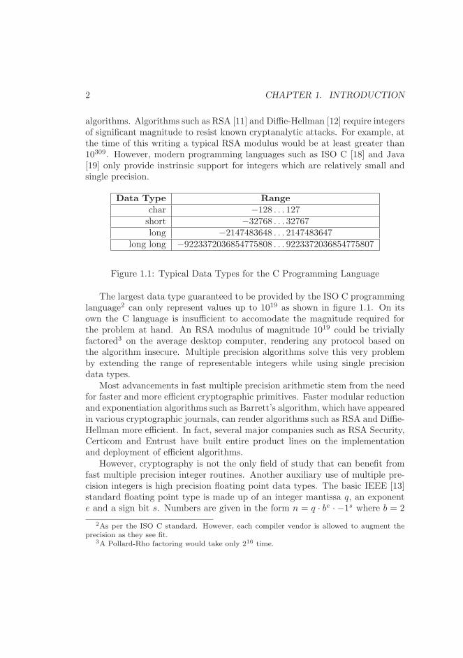
algorithms. Algorithms such as RSA [11] and Diffie-Hellman [12] require integersof significant magnitude to resist known cryptanalytic attacks. For example, atthe time of this writing a typical RSA modulus would be at least greater than10309. However, modern programming languages such as ISO C [18] and Java[19] only provide instrinsic support for integers which are relatively small andsingle precision.
Data Type Rangechar −128 . . . 127short −32768 . . . 32767long −2147483648 . . . 2147483647
long long −9223372036854775808 . . . 9223372036854775807
Figure 1.1: Typical Data Types for the C Programming Language
The largest data type guaranteed to be provided by the ISO C programminglanguage2 can only represent values up to 1019 as shown in figure 1.1. On itsown the C language is insufficient to accomodate the magnitude required forthe problem at hand. An RSA modulus of magnitude 1019 could be triviallyfactored3 on the average desktop computer, rendering any protocol based onthe algorithm insecure. Multiple precision algorithms solve this very problemby extending the range of representable integers while using single precisiondata types.
Most advancements in fast multiple precision arithmetic stem from the needfor faster and more efficient cryptographic primitives. Faster modular reductionand exponentiation algorithms such as Barrett’s algorithm, which have appearedin various cryptographic journals, can render algorithms such as RSA and Diffie-Hellman more efficient. In fact, several major companies such as RSA Security,Certicom and Entrust have built entire product lines on the implementationand deployment of efficient algorithms.
However, cryptography is not the only field of study that can benefit fromfast multiple precision integer routines. Another auxiliary use of multiple pre-cision integers is high precision floating point data types. The basic IEEE [13]standard floating point type is made up of an integer mantissa q, an exponente and a sign bit s. Numbers are given in the form n = q · be · −1s where b = 2
2As per the ISO C standard. However, each compiler vendor is allowed to augment theprecision as they see fit.
3A Pollard-Rho factoring would take only 216 time.
1.1. MULTIPLE PRECISION ARITHMETIC 3
is the most common base for IEEE. Since IEEE floating point is meant to beimplemented in hardware the precision of the mantissa is often fairly small (23,48 and 64 bits). The mantissa is merely an integer and a multiple precision in-teger could be used to create a mantissa of much larger precision than hardwarealone can efficiently support. This approach could be useful where scientificapplications must minimize the total output error over long calculations.
Yet another use for large integers is within arithmetic on polynomials of largecharacteristic (i.e. GF (p)[x] for large p). In fact the library discussed withinthis text has already been used to form a polynomial basis library4.
1.1.3 Benefits of Multiple Precision Arithmetic
The benefit of multiple precision representations over single or fixed precisionrepresentations is that no precision is lost while representing the result of anoperation which requires excess precision. For example, the product of two n-bit integers requires at least 2n bits of precision to be represented faithfully.A multiple precision algorithm would augment the precision of the destinationto accomodate the result while a single precision system would truncate excessbits to maintain a fixed level of precision.
It is possible to implement algorithms which require large integers with fixedprecision algorithms. For example, elliptic curve cryptography (ECC ) is oftenimplemented on smartcards by fixing the precision of the integers to the maxi-mum size the system will ever need. Such an approach can lead to vastly simpleralgorithms which can accomodate the integers required even if the host platformcannot natively accomodate them5. However, as efficient as such an approachmay be, the resulting source code is not normally very flexible. It cannot, atruntime, accomodate inputs of higher magnitude than the designer anticipated.
Multiple precision algorithms have the most overhead of any style of arith-metic. For the the most part the overhead can be kept to a minimum withcareful planning, but overall, it is not well suited for most memory starved plat-forms. However, multiple precision algorithms do offer the most flexibility interms of the magnitude of the inputs. That is, the same algorithms based onmultiple precision integers can accomodate any reasonable size input withoutthe designer’s explicit forethought. This leads to lower cost of ownership for thecode as it only has to be written and tested once.
4See http://poly.libtomcrypt.org for more details.5For example, the average smartcard processor has an 8 bit accumulator.
4 CHAPTER 1. INTRODUCTION
1.2 Purpose of This Text
The purpose of this text is to instruct the reader regarding how to implementefficient multiple precision algorithms. That is to not only explain a limitedsubset of the core theory behind the algorithms but also the various “housekeeping” elements that are neglected by authors of other texts on the subject.Several well reknowned texts [1, 2] give considerably detailed explanations ofthe theoretical aspects of algorithms and often very little information regardingthe practical implementation aspects.
In most cases how an algorithm is explained and how it is actually imple-mented are two very different concepts. For example, the Handbook of AppliedCryptography (HAC ), algorithm 14.7 on page 594, gives a relatively simplealgorithm for performing multiple precision integer addition. However, the de-scription lacks any discussion concerning the fact that the two integer inputsmay be of differing magnitudes. As a result the implementation is not as simpleas the text would lead people to believe. Similarly the division routine (al-gorithm 14.20, pp. 598 ) does not discuss how to handle sign or handle thedividend’s decreasing magnitude in the main loop (step #3 ).
Both texts also do not discuss several key optimal algorithms required suchas “Comba” and Karatsuba multipliers and fast modular inversion, which weconsider practical oversights. These optimal algorithms are vital to achieve anyform of useful performance in non-trivial applications.
To solve this problem the focus of this text is on the practical aspects of im-plementing a multiple precision integer package. As a case study the “LibTom-Math”6 package is used to demonstrate algorithms with real implementations7
that have been field tested and work very well. The LibTomMath library isfreely available on the Internet for all uses and this text discusses a very largeportion of the inner workings of the library.
The algorithms that are presented will always include at least one “pseudo-code” description followed by the actual C source code that implements thealgorithm. The pseudo-code can be used to implement the same algorithm inother programming languages as the reader sees fit.
This text shall also serve as a walkthrough of the creation of multiple preci-sion algorithms from scratch. Showing the reader how the algorithms fit togetheras well as where to start on various taskings.
6Available at http://math.libtomcrypt.com7In the ISO C programming language.
1.3. DISCUSSION AND NOTATION 5
1.3 Discussion and Notation
1.3.1 Notation
Amultiple precision integer of n-digits shall be denoted as x = (xn−1, . . . , x1, x0)βand represent the integer x ≡∑n−1
i=0 xiβi. The elements of the array x are said
to be the radix β digits of the integer. For example, x = (1, 2, 3)10 wouldrepresent the integer 1 · 102 + 2 · 101 + 3 · 100 = 123.
The term “mp int” shall refer to a composite structure which contains thedigits of the integer it represents, as well as auxilary data required to manipulatethe data. These additional members are discussed further in section 2.2.1. Forthe purposes of this text a “multiple precision integer” and an “mp int” areassumed to be synonymous. When an algorithm is specified to accept an mp intvariable it is assumed the various auxliary data members are present as well.An expression of the type variablename.item implies that it should evaluate tothe member named “item” of the variable. For example, a string of charactersmay have a member “length” which would evaluate to the number of charactersin the string. If the string a equals “hello” then it follows that a.length = 5.
For certain discussions more generic algorithms are presented to help thereader understand the final algorithm used to solve a given problem. When analgorithm is described as accepting an integer input it is assumed the input is aplain integer with no additional multiple-precision members. That is, algorithmsthat use integers as opposed to mp ints as inputs do not concern themselveswith the housekeeping operations required such as memory management. Thesealgorithms will be used to establish the relevant theory which will subsequentlybe used to describe a multiple precision algorithm to solve the same problem.
1.3.2 Precision Notation
The variable β represents the radix of a single digit of a multiple precisioninteger and must be of the form qp for q, p ∈ Z
+. A single precision variablemust be able to represent integers in the range 0 ≤ x < qβ while a doubleprecision variable must be able to represent integers in the range 0 ≤ x < qβ2.The extra radix-q factor allows additions and subtractions to proceed withouttruncation of the carry. Since all modern computers are binary, it is assumedthat q is two.
Within the source code that will be presented for each algorithm, the datatypemp digit will represent a single precision integer type, while, the data typemp word will represent a double precision integer type. In several algorithms
6 CHAPTER 1. INTRODUCTION
(notably the Comba routines) temporary results will be stored in arrays ofdouble precision mp words. For the purposes of this text xj will refer to thej’th digit of a single precision array and xj will refer to the j’th digit of adouble precision array. Whenever an expression is to be assigned to a doubleprecision variable it is assumed that all single precision variables are promotedto double precision during the evaluation. Expressions that are assigned to asingle precision variable are truncated to fit within the precision of a singleprecision data type.
For example, if β = 102 a single precision data type may represent a value inthe range 0 ≤ x < 103, while a double precision data type may represent a valuein the range 0 ≤ x < 105. Let a = 23 and b = 49 represent two single precisionvariables. The single precision product shall be written as c ← a · b while thedouble precision product shall be written as c ← a · b. In this particular case,c = 1127 and c = 127. The most significant digit of the product would not fitin a single precision data type and as a result c 6= c.
1.3.3 Algorithm Inputs and Outputs
Within the algorithm descriptions all variables are assumed to be scalars ofeither single or double precision as indicated. The only exception to this ruleis when variables have been indicated to be of type mp int. This distinction isimportant as scalars are often used as array indicies and various other counters.
1.3.4 Mathematical Expressions
The ⌊ ⌋ brackets imply an expression truncated to an integer not greater thanthe expression itself. For example, ⌊5.7⌋ = 5. Similarly the ⌈ ⌉ brackets implyan expression rounded to an integer not less than the expression itself. Forexample, ⌈5.1⌉ = 6. Typically when the / division symbol is used the intentionis to perform an integer division with truncation. For example, 5/2 = 2 whichwill often be written as ⌊5/2⌋ = 2 for clarity. When an expression is written asa fraction a real value division is implied, for example 5
2 = 2.5.
The norm of a multiple precision integer, for example ||x||, will be used torepresent the number of digits in the representation of the integer. For example,||123|| = 3 and ||79452|| = 5.
1.4. EXERCISES 7
1.3.5 Work Effort
To measure the efficiency of the specified algorithms, a modified big-Oh notationis used. In this system all single precision operations are considered to have thesame cost8. That is a single precision addition, multiplication and division areassumed to take the same time to complete. While this is generally not true inpractice, it will simplify the discussions considerably.
Some algorithms have slight advantages over others which is why some con-stants will not be removed in the notation. For example, a normal baselinemultiplication (section 5.2.1) requires O(n2) work while a baseline squaring
(section 5.3) requires O(n2+n2 ) work. In standard big-Oh notation these would
both be said to be equivalent to O(n2). However, in the context of the this textthis is not the case as the magnitude of the inputs will typically be rather small.As a result small constant factors in the work effort will make an observabledifference in algorithm efficiency.
All of the algorithms presented in this text have a polynomial time work level.That is, of the form O(nk) for n, k ∈ Z
+. This will help make useful comparisonsin terms of the speed of the algorithms and how various optimizations will helppay off in the long run.
1.4 Exercises
Within the more advanced chapters a section will be set aside to give the readersome challenging exercises related to the discussion at hand. These exercises arenot designed to be prize winning problems, but instead to be thought provoking.Wherever possible the problems are forward minded, stating problems that willbe answered in subsequent chapters. The reader is encouraged to finish theexercises as they appear to get a better understanding of the subject material.
That being said, the problems are designed to affirm knowledge of a partic-ular subject matter. Students in particular are encouraged to verify they cananswer the problems correctly before moving on.
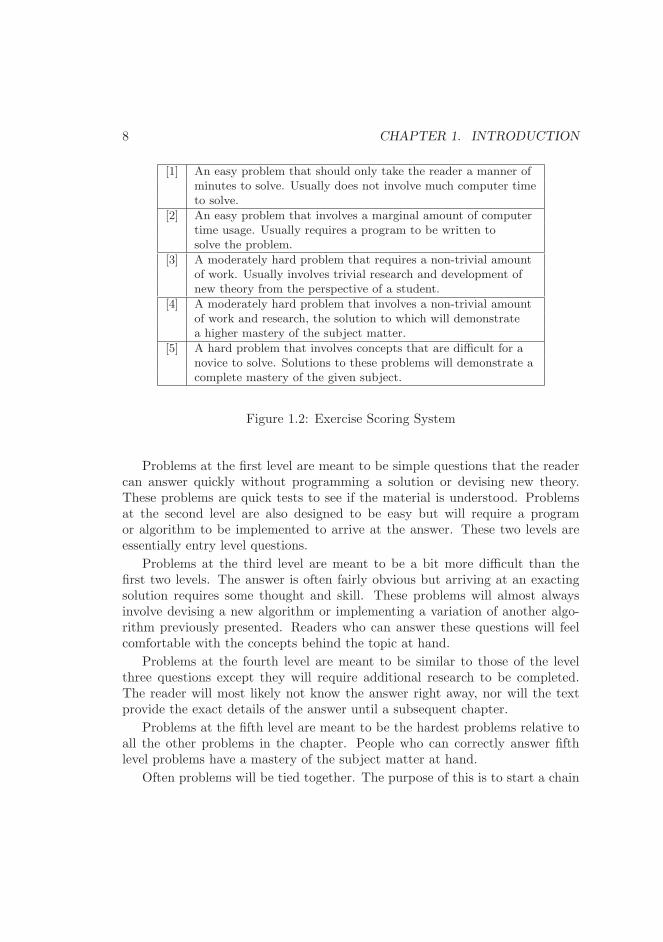
Similar to the exercises of [1, pp. ix] these exercises are given a scoringsystem based on the difficulty of the problem. However, unlike [1] the problemsdo not get nearly as hard. The scoring of these exercises ranges from one (theeasiest) to five (the hardest). The following table sumarizes the scoring systemused.
8Except where explicitly noted.
8 CHAPTER 1. INTRODUCTION
[1] An easy problem that should only take the reader a manner ofminutes to solve. Usually does not involve much computer timeto solve.
[2] An easy problem that involves a marginal amount of computertime usage. Usually requires a program to be written tosolve the problem.
[3] A moderately hard problem that requires a non-trivial amountof work. Usually involves trivial research and development ofnew theory from the perspective of a student.
[4] A moderately hard problem that involves a non-trivial amountof work and research, the solution to which will demonstratea higher mastery of the subject matter.
[5] A hard problem that involves concepts that are difficult for anovice to solve. Solutions to these problems will demonstrate acomplete mastery of the given subject.
Figure 1.2: Exercise Scoring System
Problems at the first level are meant to be simple questions that the readercan answer quickly without programming a solution or devising new theory.These problems are quick tests to see if the material is understood. Problemsat the second level are also designed to be easy but will require a programor algorithm to be implemented to arrive at the answer. These two levels areessentially entry level questions.
Problems at the third level are meant to be a bit more difficult than thefirst two levels. The answer is often fairly obvious but arriving at an exactingsolution requires some thought and skill. These problems will almost alwaysinvolve devising a new algorithm or implementing a variation of another algo-rithm previously presented. Readers who can answer these questions will feelcomfortable with the concepts behind the topic at hand.
Problems at the fourth level are meant to be similar to those of the levelthree questions except they will require additional research to be completed.The reader will most likely not know the answer right away, nor will the textprovide the exact details of the answer until a subsequent chapter.
Problems at the fifth level are meant to be the hardest problems relative toall the other problems in the chapter. People who can correctly answer fifthlevel problems have a mastery of the subject matter at hand.
Often problems will be tied together. The purpose of this is to start a chain
1.5. INTRODUCTION TO LIBTOMMATH 9
of thought that will be discussed in future chapters. The reader is encouragedto answer the follow-up problems and try to draw the relevance of problems.
1.5 Introduction to LibTomMath
1.5.1 What is LibTomMath?
LibTomMath is a free and open source multiple precision integer library writtenentirely in portable ISO C. By portable it is meant that the library does notcontain any code that is computer platform dependent or otherwise problematicto use on any given platform.
The library has been successfully tested under numerous operating systemsincluding Unix9, MacOS, Windows, Linux, PalmOS and on standalone hardwaresuch as the Gameboy Advance. The library is designed to contain enoughfunctionality to be able to develop applications such as public key cryptosystemsand still maintain a relatively small footprint.
1.5.2 Goals of LibTomMath
Libraries which obtain the most efficiency are rarely written in a high levelprogramming language such as C. However, even though this library is writtenentirely in ISO C, considerable care has been taken to optimize the algorithmimplementations within the library. Specifically the code has been written towork well with the GNU C Compiler (GCC ) on both x86 and ARM processors.Wherever possible, highly efficient algorithms, such as Karatsuba multiplication,sliding window exponentiation and Montgomery reduction have been providedto make the library more efficient.
Even with the nearly optimal and specialized algorithms that have been in-cluded the Application Programing Interface (API ) has been kept as simpleas possible. Often generic place holder routines will make use of specializedalgorithms automatically without the developer’s specific attention. One suchexample is the generic multiplication algorithm mp mul() which will automat-ically use Toom–Cook, Karatsuba, Comba or baseline multiplication based onthe magnitude of the inputs and the configuration of the library.
Making LibTomMath as efficient as possible is not the only goal of theLibTomMath project. Ideally the library should be source compatible withanother popular library which makes it more attractive for developers to use.
9All of these trademarks belong to their respective rightful owners.
10 CHAPTER 1. INTRODUCTION
In this case the MPI library was used as a API template for all the basic func-tions. MPI was chosen because it is another library that fits in the same nicheas LibTomMath. Even though LibTomMath uses MPI as the template for thefunction names and argument passing conventions, it has been written fromscratch by Tom St Denis.
The project is also meant to act as a learning tool for students, the logicbeing that no easy-to-follow “bignum” library exists which can be used to teachcomputer science students how to perform fast and reliable multiple precisioninteger arithmetic. To this end the source code has been given quite a fewcomments and algorithm discussion points.
1.6 Choice of LibTomMath
LibTomMath was chosen as the case study of this text not only because theauthor of both projects is one and the same but for more worthy reasons. Otherlibraries such as GMP [14], MPI [15], LIP [17] and OpenSSL [16] have multipleprecision integer arithmetic routines but would not be ideal for this text forreasons that will be explained in the following sub-sections.
1.6.1 Code Base
The LibTomMath code base is all portable ISO C source code. This means thatthere are no platform dependent conditional segments of code littered through-out the source. This clean and uncluttered approach to the library means thata developer can more readily discern the true intent of a given section of sourcecode without trying to keep track of what conditional code will be used.
The code base of LibTomMath is well organized. Each function is in its ownseparate source code file which allows the reader to find a given function veryquickly. On average there are 76 lines of code per source file which makes thesource very easily to follow. By comparison MPI and LIP are single file projectsmaking code tracing very hard. GMP has many conditional code segmentswhich also hinder tracing.
When compiled with GCC for the x86 processor and optimized for speedthe entire library is approximately 100KiB10 which is fairly small compared toGMP (over 250KiB). LibTomMath is slightly larger than MPI (which compilesto about 50KiB) but LibTomMath is also much faster and more complete thanMPI.
10The notation “KiB” means 210 octets, similarly “MiB” means 220 octets.
1.6. CHOICE OF LIBTOMMATH 11
1.6.2 API Simplicity
LibTomMath is designed after the MPI library and shares the API design. Quiteoften programs that use MPI will build with LibTomMath without change. Thefunction names correlate directly to the action they perform. Almost all of thefunctions share the same parameter passing convention. The learning curve isfairly shallow with the API provided which is an extremely valuable benefit forthe student and developer alike.
The LIP library is an example of a library with an API that is awkward towork with. LIP uses function names that are often “compressed” to illegibleshort hand. LibTomMath does not share this characteristic.
The GMP library also does not return error codes. Instead it uses a POSIX.1[23] signal system where errors are signaled to the host application. This hap-pens to be the fastest approach but definitely not the most versatile. In effecta math error (i.e. invalid input, heap error, etc) can cause a program to stopfunctioning which is definitely undersireable in many situations.
1.6.3 Optimizations
While LibTomMath is certainly not the fastest library (GMP often beats LibTom-Math by a factor of two) it does feature a set of optimal algorithms for taskssuch as modular reduction, exponentiation, multiplication and squaring. GMPand LIP also feature such optimizations while MPI only uses baseline algorithmswith no optimizations. GMP lacks a few of the additional modular reductionoptimizations that LibTomMath features11.
LibTomMath is almost always an order of magnitude faster than the MPIlibrary at computationally expensive tasks such as modular exponentiation. Inthe grand scheme of “bignum” libraries LibTomMath is faster than the averagelibrary and usually slower than the best libraries such as GMP and OpenSSLby only a small factor.
1.6.4 Portability and Stability
LibTomMath will build “out of the box” on any platform equipped with a mod-ern version of the GNU C Compiler (GCC ). This means that without changesthe library will build without configuration or setting up any variables. LIP andMPI will build “out of the box” as well but have numerous known bugs. Most
11At the time of this writing GMP only had Barrett and Montgomery modular reductionalgorithms.
12 CHAPTER 1. INTRODUCTION
notably the author of MPI has recently stopped working on his library and LIPhas long since been discontinued.
GMP requires a configuration script to run and will not build out of thebox. GMP and LibTomMath are still in active development and are very stableacross a variety of platforms.
1.6.5 Choice
LibTomMath is a relatively compact, well documented, highly optimized andportable library which seems only natural for the case study of this text. Varioussource files from the LibTomMath project will be included within the text.However, the reader is encouraged to download their own copy of the library toactually be able to work with the library.
Chapter 2
Getting Started
2.1 Library Basics
The trick to writing any useful library of source code is to build a solid founda-tion and work outwards from it. First, a problem along with allowable solutionparameters should be identified and analyzed. In this particular case the in-ability to accomodate multiple precision integers is the problem. Futhermore,the solution must be written as portable source code that is reasonably efficientacross several different computer platforms.
After a foundation is formed the remainder of the library can be designedand implemented in a hierarchical fashion. That is, to implement the lowestlevel dependencies first and work towards the most abstract functions last. Forexample, before implementing a modular exponentiation algorithm one wouldimplement a modular reduction algorithm. By building outwards from a basefoundation instead of using a parallel design methodology the resulting projectis highly modular. Being highly modular is a desirable property of any projectas it often means the resulting product has a small footprint and updates areeasy to perform.
Usually when I start a project I will begin with the header files. I definethe data types I think I will need and prototype the initial functions that arenot dependent on other functions (within the library). After I implement thesebase functions I prototype more dependent functions and implement them. Theprocess repeats until I implement all of the functions I require. For example, inthe case of LibTomMath I implemented functions such as mp init() well before
13
14 CHAPTER 2. GETTING STARTED
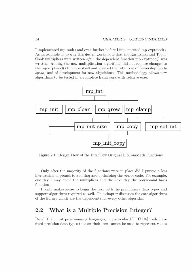
I implemented mp mul() and even further before I implemented mp exptmod().As an example as to why this design works note that the Karatsuba and Toom-Cook multipliers were written after the dependent function mp exptmod() waswritten. Adding the new multiplication algorithms did not require changes tothe mp exptmod() function itself and lowered the total cost of ownership (so to
speak) and of development for new algorithms. This methodology allows newalgorithms to be tested in a complete framework with relative ease.
Figure 2.1: Design Flow of the First Few Original LibTomMath Functions.
Only after the majority of the functions were in place did I pursue a lesshierarchical approach to auditing and optimizing the source code. For example,one day I may audit the multipliers and the next day the polynomial basisfunctions.
It only makes sense to begin the text with the preliminary data types andsupport algorithms required as well. This chapter discusses the core algorithmsof the library which are the dependents for every other algorithm.
2.2 What is a Multiple Precision Integer?
Recall that most programming languages, in particular ISO C [18], only havefixed precision data types that on their own cannot be used to represent values
2.2. WHAT IS A MULTIPLE PRECISION INTEGER? 15
larger than their precision will allow. The purpose of multiple precision algo-rithms is to use fixed precision data types to create and manipulate multipleprecision integers which may represent values that are very large.
As a well known analogy, school children are taught how to form numberslarger than nine by prepending more radix ten digits. In the decimal system thelargest single digit value is 9. However, by concatenating digits together largernumbers may be represented. Newly prepended digits (to the left) are said tobe in a different power of ten column. That is, the number 123 can be describedas having a 1 in the hundreds column, 2 in the tens column and 3 in the onescolumn. Or more formally 123 = 1 · 102 + 2 · 101 + 3 · 100. Computer basedmultiple precision arithmetic is essentially the same concept. Larger integersare represented by adjoining fixed precision computer words with the exceptionthat a different radix is used.
What most people probably do not think about explicitly are the variousother attributes that describe a multiple precision integer. For example, theinteger 15410 has two immediately obvious properties. First, the integer ispositive, that is the sign of this particular integer is positive as opposed tonegative. Second, the integer has three digits in its representation. There isan additional property that the integer posesses that does not concern pencil-and-paper arithmetic. The third property is how many digits placeholders areavailable to hold the integer.
The human analogy of this third property is ensuring there is enough spaceon the paper to write the integer. For example, if one starts writing a largenumber too far to the right on a piece of paper they will have to erase it andmove left. Similarly, computer algorithms must maintain strict control overmemory usage to ensure that the digits of an integer will not exceed the al-lowed boundaries. These three properties make up what is known as a multipleprecision integer or mp int for short.
2.2.1 The mp int Structure
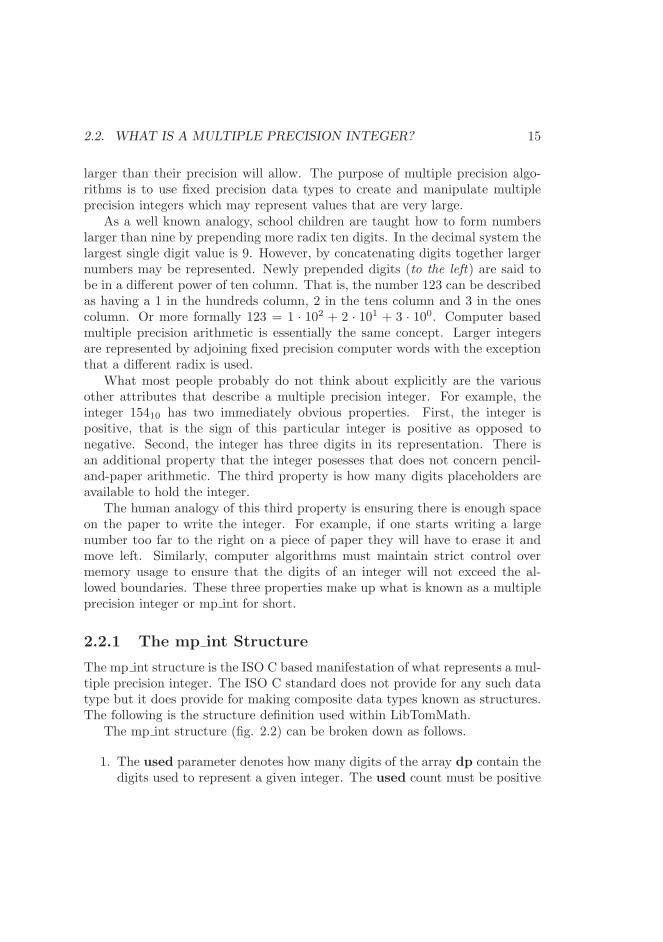
The mp int structure is the ISO C based manifestation of what represents a mul-tiple precision integer. The ISO C standard does not provide for any such datatype but it does provide for making composite data types known as structures.The following is the structure definition used within LibTomMath.
The mp int structure (fig. 2.2) can be broken down as follows.
1. The used parameter denotes how many digits of the array dp contain thedigits used to represent a given integer. The used count must be positive
16 CHAPTER 2. GETTING STARTED
typedef struct {int used, alloc, sign;mp digit *dp;} mp int;
Figure 2.2: The mp int Structure
(or zero) and may not exceed the alloc count.
2. The alloc parameter denotes how many digits are available in the arrayto use by functions before it has to increase in size. When the usedcount of a result would exceed the alloc count all of the algorithms willautomatically increase the size of the array to accommodate the precisionof the result.
3. The pointer dp points to a dynamically allocated array of digits thatrepresent the given multiple precision integer. It is padded with (alloc−used) zero digits. The array is maintained in a least significant digit order.As a pencil and paper analogy the array is organized such that the rightmost digits are stored first starting at the location indexed by zero1 in thearray. For example, if dp contains {a, b, c, . . .} where dp0 = a, dp1 = b,dp2 = c, . . . then it would represent the integer a+ bβ + cβ2 + . . .
4. The sign parameter denotes the sign as either zero/positive (MP ZPOS)or negative (MP NEG).
Valid mp int Structures
Several rules are placed on the state of an mp int structure and are assumed tobe followed for reasons of efficiency. The only exceptions are when the structureis passed to initialization functions such as mp init() and mp init copy().
1. The value of alloc may not be less than one. That is dp always points toa previously allocated array of digits.
2. The value of used may not exceed alloc and must be greater than orequal to zero.
1In C all arrays begin at zero.
2.3. ARGUMENT PASSING 17
3. The value of used implies the digit at index (used − 1) of the dp arrayis non-zero. That is, leading zero digits in the most significant positionsmust be trimmed.
(a) Digits in the dp array at and above the used location must be zero.
4. The value of sign must be MP ZPOS if used is zero; this represents themp int value of zero.
2.3 Argument Passing
A convention of argument passing must be adopted early on in the developmentof any library. Making the function prototypes consistent will help eliminatemany headaches in the future as the library grows to significant complexity. InLibTomMath the multiple precision integer functions accept parameters fromleft to right as pointers to mp int structures. That means that the source(input) operands are placed on the left and the destination (output) on theright. Consider the following examples.
mp_mul(&a, &b, &c); /* c = a * b */
mp_add(&a, &b, &a); /* a = a + b */
mp_sqr(&a, &b); /* b = a * a */
The left to right order is a fairly natural way to implement the functionssince it lets the developer read aloud the functions and make sense of them. Forexample, the first function would read “multiply a and b and store in c”.
Certain libraries (LIP by Lenstra for instance) accept parameters the otherway around, to mimic the order of assignment expressions. That is, the desti-nation (output) is on the left and arguments (inputs) are on the right. In truth,it is entirely a matter of preference. In the case of LibTomMath the conventionfrom the MPI library has been adopted.
Another very useful design consideration, provided for in LibTomMath, iswhether to allow argument sources to also be a destination. For example, thesecond example (mp add) adds a to b and stores in a. This is an importantfeature to implement since it allows the calling functions to cut down on thenumber of variables it must maintain. However, to implement this feature spe-cific care has to be given to ensure the destination is not modified before thesource is fully read.
18 CHAPTER 2. GETTING STARTED
2.4 Return Values
A well implemented application, no matter what its purpose, should trap asmany runtime errors as possible and return them to the caller. By catchingruntime errors a library can be guaranteed to prevent undefined behaviour.However, the end developer can still manage to cause a library to crash. Forexample, by passing an invalid pointer an application may fault by dereferencingmemory not owned by the application.
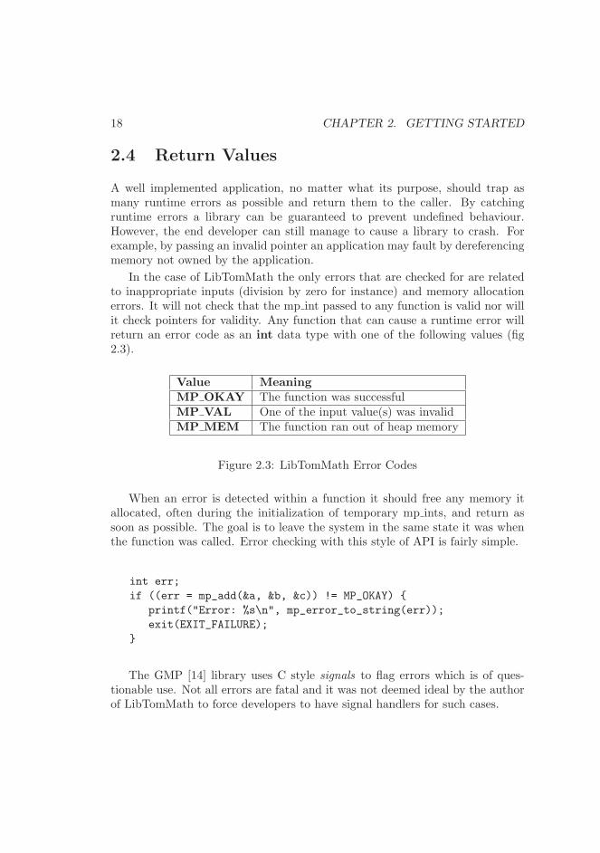
In the case of LibTomMath the only errors that are checked for are relatedto inappropriate inputs (division by zero for instance) and memory allocationerrors. It will not check that the mp int passed to any function is valid nor willit check pointers for validity. Any function that can cause a runtime error willreturn an error code as an int data type with one of the following values (fig2.3).
Value MeaningMP OKAY The function was successfulMP VAL One of the input value(s) was invalidMP MEM The function ran out of heap memory
Figure 2.3: LibTomMath Error Codes
When an error is detected within a function it should free any memory itallocated, often during the initialization of temporary mp ints, and return assoon as possible. The goal is to leave the system in the same state it was whenthe function was called. Error checking with this style of API is fairly simple.
int err;
if ((err = mp_add(&a, &b, &c)) != MP_OKAY) {
printf("Error: %s\n", mp_error_to_string(err));
exit(EXIT_FAILURE);
}
The GMP [14] library uses C style signals to flag errors which is of ques-tionable use. Not all errors are fatal and it was not deemed ideal by the authorof LibTomMath to force developers to have signal handlers for such cases.
2.5. INITIALIZATION AND CLEARING 19
2.5 Initialization and Clearing
The logical starting point when actually writing multiple precision integer func-tions is the initialization and clearing of the mp int structures. These twoalgorithms will be used by the majority of the higher level algorithms.
Given the basic mp int structure an initialization routine must first allocatememory to hold the digits of the integer. Often it is optimal to allocate asufficiently large pre-set number of digits even though the initial integer willrepresent zero. If only a single digit were allocated quite a few subsequent re-allocations would occur when operations are performed on the integers. Thereis a tradeoff between how many default digits to allocate and how many re-allocations are tolerable. Obviously allocating an excessive amount of digitsinitially will waste memory and become unmanageable.
If the memory for the digits has been successfully allocated then the rest ofthe members of the structure must be initialized. Since the initial state of anmp int is to represent the zero integer, the allocated digits must be set to zero.The used count set to zero and sign set to MP ZPOS.
2.5.1 Initializing an mp int
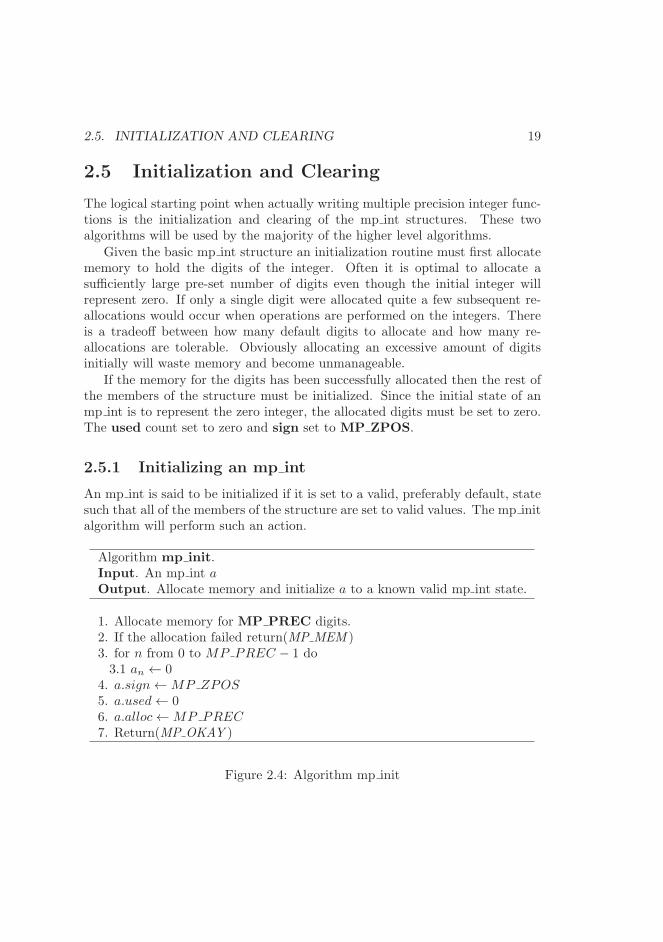
An mp int is said to be initialized if it is set to a valid, preferably default, statesuch that all of the members of the structure are set to valid values. The mp initalgorithm will perform such an action.
Algorithm mp init.Input. An mp int aOutput. Allocate memory and initialize a to a known valid mp int state.
1. Allocate memory for MP PREC digits.2. If the allocation failed return(MP MEM )3. for n from 0 to MP PREC − 1 do3.1 an ← 0
4. a.sign←MP ZPOS5. a.used← 06. a.alloc←MP PREC7. Return(MP OKAY )
Figure 2.4: Algorithm mp init
20 CHAPTER 2. GETTING STARTED
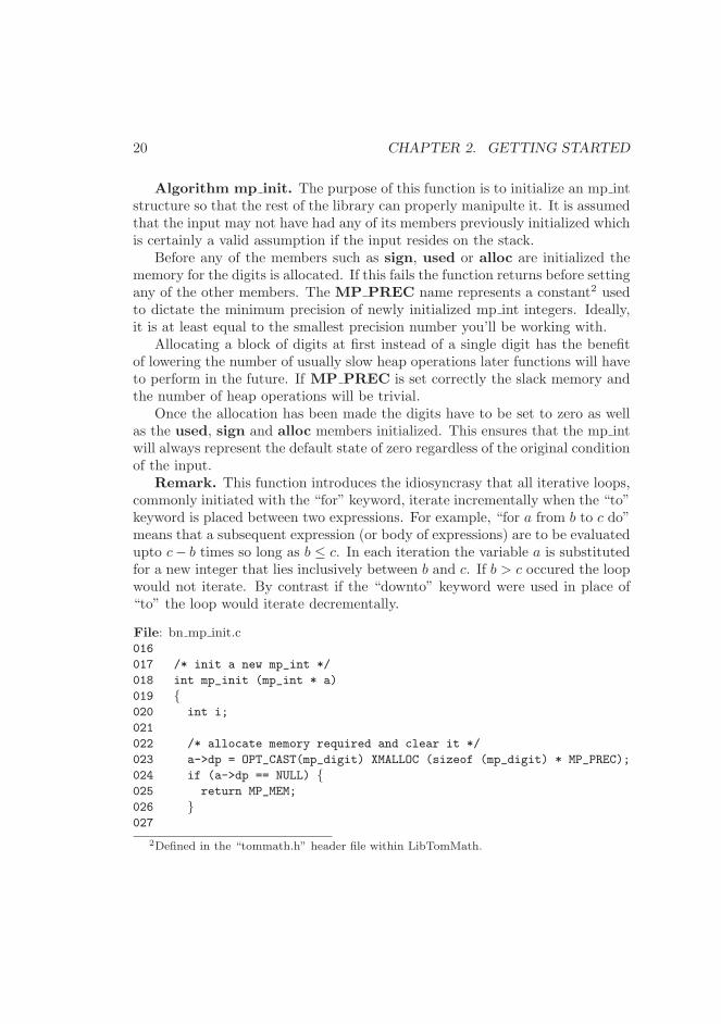
Algorithm mp init. The purpose of this function is to initialize an mp intstructure so that the rest of the library can properly manipulte it. It is assumedthat the input may not have had any of its members previously initialized whichis certainly a valid assumption if the input resides on the stack.
Before any of the members such as sign, used or alloc are initialized thememory for the digits is allocated. If this fails the function returns before settingany of the other members. The MP PREC name represents a constant2 usedto dictate the minimum precision of newly initialized mp int integers. Ideally,it is at least equal to the smallest precision number you’ll be working with.
Allocating a block of digits at first instead of a single digit has the benefitof lowering the number of usually slow heap operations later functions will haveto perform in the future. If MP PREC is set correctly the slack memory andthe number of heap operations will be trivial.
Once the allocation has been made the digits have to be set to zero as wellas the used, sign and alloc members initialized. This ensures that the mp intwill always represent the default state of zero regardless of the original conditionof the input.
Remark. This function introduces the idiosyncrasy that all iterative loops,commonly initiated with the “for” keyword, iterate incrementally when the “to”keyword is placed between two expressions. For example, “for a from b to c do”means that a subsequent expression (or body of expressions) are to be evaluatedupto c− b times so long as b ≤ c. In each iteration the variable a is substitutedfor a new integer that lies inclusively between b and c. If b > c occured the loopwould not iterate. By contrast if the “downto” keyword were used in place of“to” the loop would iterate decrementally.
File: bn mp init.c016
017 /* init a new mp_int */
018 int mp_init (mp_int * a)
019 {020 int i;
021
022 /* allocate memory required and clear it */
023 a->dp = OPT_CAST(mp_digit) XMALLOC (sizeof (mp_digit) * MP_PREC);
024 if (a->dp == NULL) {025 return MP_MEM;
026 }027
2Defined in the “tommath.h” header file within LibTomMath.
2.5. INITIALIZATION AND CLEARING 21
028 /* set the digits to zero */
029 for (i = 0; i < MP_PREC; i++) {030 a->dp[i] = 0;
031 }032
033 /* set the used to zero, allocated digits to the default precision
034 * and sign to positive */
035 a->used = 0;
036 a->alloc = MP_PREC;
037 a->sign = MP_ZPOS;
038
039 return MP_OKAY;
040 }041 #endif
042
043 /* ref: $Format:%D$ */
044 /* git commit: $Format:%H$ */
045 /* commit time: $Format:%ai$ */
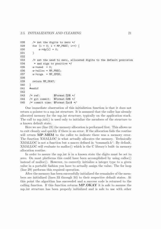
One immediate observation of this initializtion function is that it does notreturn a pointer to a mp int structure. It is assumed that the caller has alreadyallocated memory for the mp int structure, typically on the application stack.The call to mp init() is used only to initialize the members of the structure toa known default state.
Here we see (line 23) the memory allocation is performed first. This allows usto exit cleanly and quickly if there is an error. If the allocation fails the routinewill return MP MEM to the caller to indicate there was a memory error.The function XMALLOC is what actually allocates the memory. TechnicallyXMALLOC is not a function but a macro defined in “tommath.h“. By default,XMALLOC will evaluate to malloc() which is the C library’s built–in memoryallocation routine.
In order to assure the mp int is in a known state the digits must be set tozero. On most platforms this could have been accomplished by using calloc()instead of malloc(). However, to correctly initialize a integer type to a givenvalue in a portable fashion you have to actually assign the value. The for loop(line 29) performs this required operation.
After the memory has been successfully initialized the remainder of the mem-bers are initialized (lines 33 through 34) to their respective default states. Atthis point the algorithm has succeeded and a success code is returned to thecalling function. If this function returns MP OKAY it is safe to assume themp int structure has been properly initialized and is safe to use with other
22 CHAPTER 2. GETTING STARTED
functions within the library.
2.5.2 Clearing an mp int
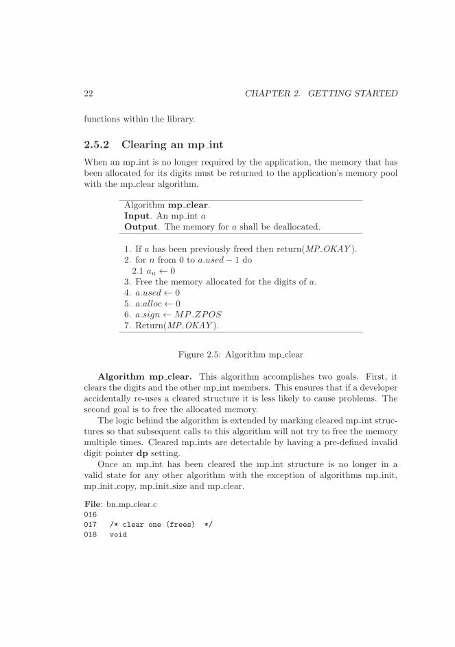
When an mp int is no longer required by the application, the memory that hasbeen allocated for its digits must be returned to the application’s memory poolwith the mp clear algorithm.
Algorithm mp clear.Input. An mp int aOutput. The memory for a shall be deallocated.
1. If a has been previously freed then return(MP OKAY ).2. for n from 0 to a.used− 1 do2.1 an ← 0
3. Free the memory allocated for the digits of a.4. a.used← 05. a.alloc← 06. a.sign←MP ZPOS7. Return(MP OKAY ).
Figure 2.5: Algorithm mp clear
Algorithm mp clear. This algorithm accomplishes two goals. First, itclears the digits and the other mp int members. This ensures that if a developeraccidentally re-uses a cleared structure it is less likely to cause problems. Thesecond goal is to free the allocated memory.
The logic behind the algorithm is extended by marking cleared mp int struc-tures so that subsequent calls to this algorithm will not try to free the memorymultiple times. Cleared mp ints are detectable by having a pre-defined invaliddigit pointer dp setting.
Once an mp int has been cleared the mp int structure is no longer in avalid state for any other algorithm with the exception of algorithms mp init,mp init copy, mp init size and mp clear.
File: bn mp clear.c016
017 /* clear one (frees) */
018 void
2.5. INITIALIZATION AND CLEARING 23
019 mp_clear (mp_int * a)
020 {021 int i;
022
023 /* only do anything if a hasn’t been freed previously */
024 if (a->dp != NULL) {025 /* first zero the digits */
026 for (i = 0; i < a->used; i++) {027 a->dp[i] = 0;
028 }029
030 /* free ram */
031 XFREE(a->dp);
032
033 /* reset members to make debugging easier */
034 a->dp = NULL;
035 a->alloc = a->used = 0;
036 a->sign = MP_ZPOS;
037 }038 }039 #endif
040
041 /* ref: $Format:%D$ */
042 /* git commit: $Format:%H$ */
043 /* commit time: $Format:%ai$ */
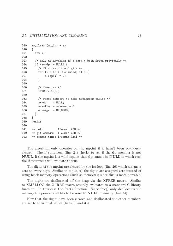
The algorithm only operates on the mp int if it hasn’t been previouslycleared. The if statement (line 24) checks to see if the dp member is notNULL. If the mp int is a valid mp int then dp cannot be NULL in which casethe if statement will evaluate to true.
The digits of the mp int are cleared by the for loop (line 26) which assigns azero to every digit. Similar to mp init() the digits are assigned zero instead ofusing block memory operations (such as memset()) since this is more portable.
The digits are deallocated off the heap via the XFREE macro. Similarto XMALLOC the XFREE macro actually evaluates to a standard C libraryfunction. In this case the free() function. Since free() only deallocates thememory the pointer still has to be reset to NULL manually (line 34).
Now that the digits have been cleared and deallocated the other membersare set to their final values (lines 35 and 36).
24 CHAPTER 2. GETTING STARTED
2.6 Maintenance Algorithms
The previous sections describes how to initialize and clear an mp int structure.To further support operations that are to be performed on mp int structures(such as addition and multiplication) the dependent algorithms must be able toaugment the precision of an mp int and initialize mp ints with differing initialconditions.
These algorithms complete the set of low level algorithms required to workwith mp int structures in the higher level algorithms such as addition, multipli-cation and modular exponentiation.
2.6.1 Augmenting an mp int’s Precision
When storing a value in an mp int structure, a sufficient number of digits mustbe available to accomodate the entire result of an operation without loss ofprecision. Quite often the size of the array given by the alloc member is largeenough to simply increase the used digit count. However, when the size of thearray is too small it must be re-sized appropriately to accomodate the result.The mp grow algorithm will provide this functionality.
2.6. MAINTENANCE ALGORITHMS 25
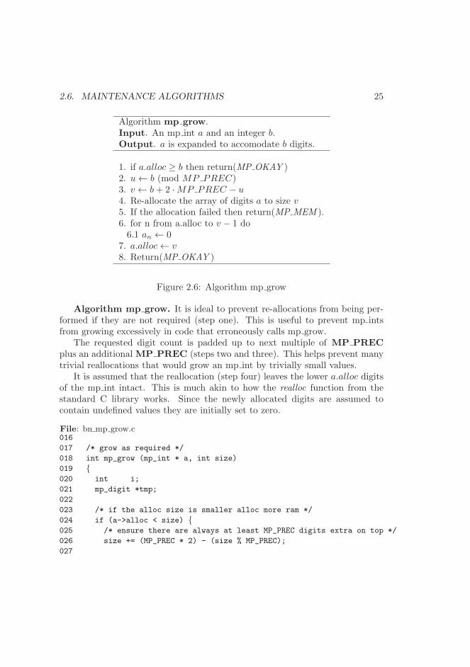
Algorithm mp grow.Input. An mp int a and an integer b.Output. a is expanded to accomodate b digits.
1. if a.alloc ≥ b then return(MP OKAY )2. u← b (mod MP PREC)3. v ← b+ 2 ·MP PREC − u4. Re-allocate the array of digits a to size v5. If the allocation failed then return(MP MEM ).6. for n from a.alloc to v − 1 do6.1 an ← 0
7. a.alloc← v8. Return(MP OKAY )
Figure 2.6: Algorithm mp grow
Algorithm mp grow. It is ideal to prevent re-allocations from being per-formed if they are not required (step one). This is useful to prevent mp intsfrom growing excessively in code that erroneously calls mp grow.
The requested digit count is padded up to next multiple of MP PRECplus an additional MP PREC (steps two and three). This helps prevent manytrivial reallocations that would grow an mp int by trivially small values.
It is assumed that the reallocation (step four) leaves the lower a.alloc digitsof the mp int intact. This is much akin to how the realloc function from thestandard C library works. Since the newly allocated digits are assumed tocontain undefined values they are initially set to zero.
File: bn mp grow.c016
017 /* grow as required */
018 int mp_grow (mp_int * a, int size)
019 {020 int i;
021 mp_digit *tmp;
022
023 /* if the alloc size is smaller alloc more ram */
024 if (a->alloc < size) {025 /* ensure there are always at least MP_PREC digits extra on top */
026 size += (MP_PREC * 2) - (size % MP_PREC);
027
26 CHAPTER 2. GETTING STARTED
028 /* reallocate the array a->dp
029 *
030 * We store the return in a temporary variable
031 * in case the operation failed we don’t want
032 * to overwrite the dp member of a.
033 */
034 tmp = OPT_CAST(mp_digit) XREALLOC (a->dp, sizeof (mp_digit) * size);
035 if (tmp == NULL) {036 /* reallocation failed but "a" is still valid [can be freed] */
037 return MP_MEM;
038 }039
040 /* reallocation succeeded so set a->dp */
041 a->dp = tmp;
042
043 /* zero excess digits */
044 i = a->alloc;
045 a->alloc = size;
046 for (; i < a->alloc; i++) {047 a->dp[i] = 0;
048 }049 }050 return MP_OKAY;
051 }052 #endif
053
054 /* ref: $Format:%D$ */
055 /* git commit: $Format:%H$ */
056 /* commit time: $Format:%ai$ */
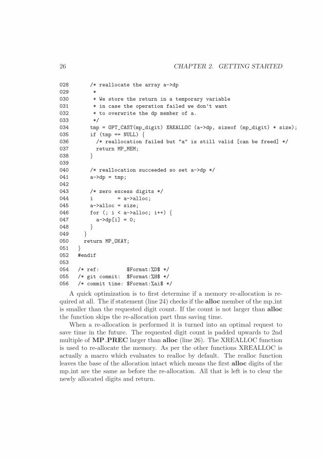
A quick optimization is to first determine if a memory re-allocation is re-quired at all. The if statement (line 24) checks if the allocmember of the mp intis smaller than the requested digit count. If the count is not larger than allocthe function skips the re-allocation part thus saving time.
When a re-allocation is performed it is turned into an optimal request tosave time in the future. The requested digit count is padded upwards to 2ndmultiple of MP PREC larger than alloc (line 26). The XREALLOC functionis used to re-allocate the memory. As per the other functions XREALLOC isactually a macro which evaluates to realloc by default. The realloc functionleaves the base of the allocation intact which means the first alloc digits of themp int are the same as before the re-allocation. All that is left is to clear thenewly allocated digits and return.
2.6. MAINTENANCE ALGORITHMS 27
Note that the re-allocation result is actually stored in a temporary pointertmp. This is to allow this function to return an error with a valid pointer.Earlier releases of the library stored the result of XREALLOC into the mp inta. That would result in a memory leak if XREALLOC ever failed.
2.6.2 Initializing Variable Precision mp ints
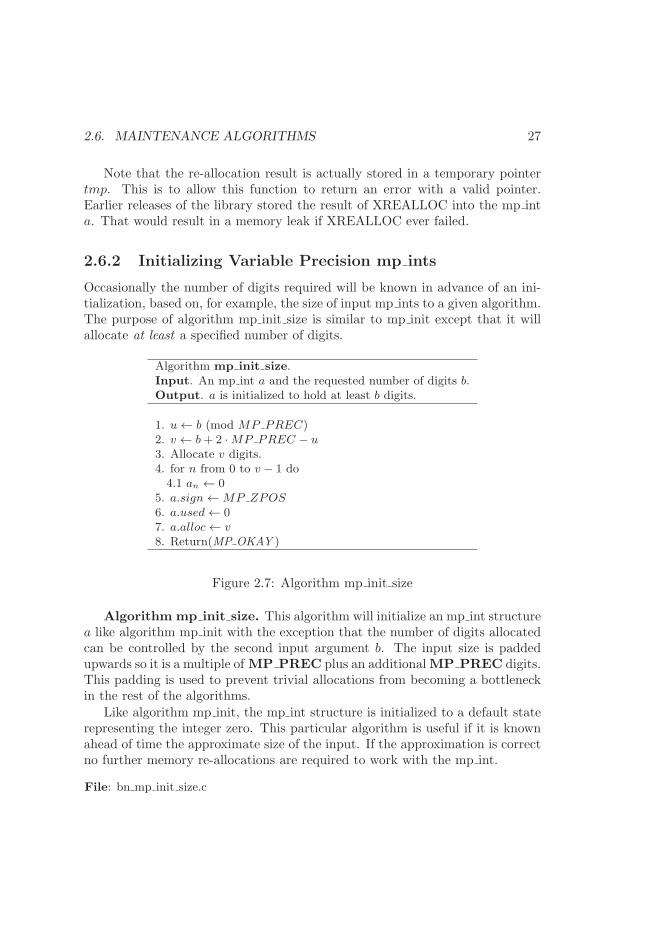
Occasionally the number of digits required will be known in advance of an ini-tialization, based on, for example, the size of input mp ints to a given algorithm.The purpose of algorithm mp init size is similar to mp init except that it willallocate at least a specified number of digits.
Algorithm mp init size.Input. An mp int a and the requested number of digits b.Output. a is initialized to hold at least b digits.
1. u← b (mod MP PREC)2. v ← b+ 2 ·MP PREC − u3. Allocate v digits.4. for n from 0 to v − 1 do4.1 an ← 0
5. a.sign←MP ZPOS6. a.used← 07. a.alloc← v8. Return(MP OKAY )
Figure 2.7: Algorithm mp init size
Algorithm mp init size. This algorithm will initialize an mp int structurea like algorithm mp init with the exception that the number of digits allocatedcan be controlled by the second input argument b. The input size is paddedupwards so it is a multiple of MP PREC plus an additionalMP PREC digits.This padding is used to prevent trivial allocations from becoming a bottleneckin the rest of the algorithms.
Like algorithm mp init, the mp int structure is initialized to a default staterepresenting the integer zero. This particular algorithm is useful if it is knownahead of time the approximate size of the input. If the approximation is correctno further memory re-allocations are required to work with the mp int.
File: bn mp init size.c
28 CHAPTER 2. GETTING STARTED
016
017 /* init an mp_init for a given size */
018 int mp_init_size (mp_int * a, int size)
019 {020 int x;
021
022 /* pad size so there are always extra digits */
023 size += (MP_PREC * 2) - (size % MP_PREC);
024
025 /* alloc mem */
026 a->dp = OPT_CAST(mp_digit) XMALLOC (sizeof (mp_digit) * size);
027 if (a->dp == NULL) {028 return MP_MEM;
029 }030
031 /* set the members */
032 a->used = 0;
033 a->alloc = size;
034 a->sign = MP_ZPOS;
035
036 /* zero the digits */
037 for (x = 0; x < size; x++) {038 a->dp[x] = 0;
039 }040
041 return MP_OKAY;
042 }043 #endif
044
045 /* ref: $Format:%D$ */
046 /* git commit: $Format:%H$ */
047 /* commit time: $Format:%ai$ */
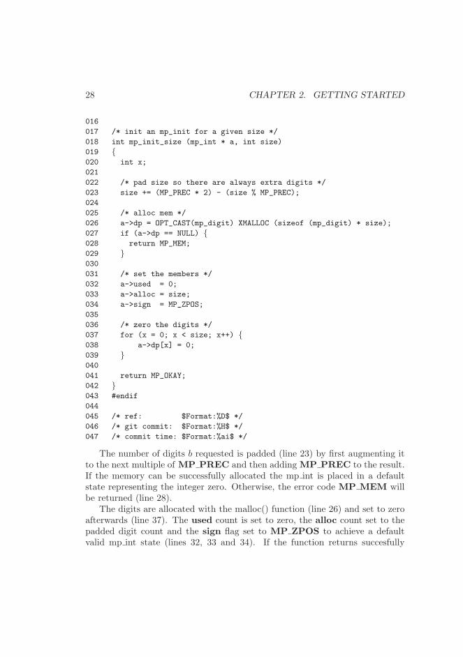
The number of digits b requested is padded (line 23) by first augmenting itto the next multiple of MP PREC and then adding MP PREC to the result.If the memory can be successfully allocated the mp int is placed in a defaultstate representing the integer zero. Otherwise, the error code MP MEM willbe returned (line 28).
The digits are allocated with the malloc() function (line 26) and set to zeroafterwards (line 37). The used count is set to zero, the alloc count set to thepadded digit count and the sign flag set to MP ZPOS to achieve a defaultvalid mp int state (lines 32, 33 and 34). If the function returns succesfully
2.6. MAINTENANCE ALGORITHMS 29
then it is correct to assume that the mp int structure is in a valid state for theremainder of the functions to work with.
2.6.3 Multiple Integer Initializations and Clearings
Occasionally a function will require a series of mp int data types to be madeavailable simultaneously. The purpose of algorithm mp init multi is to initializea variable length array of mp int structures in a single statement. It is essentiallya shortcut to multiple initializations.
30 CHAPTER 2. GETTING STARTED
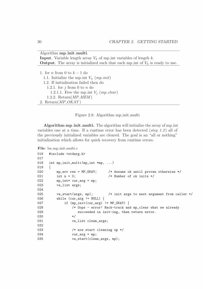
Algorithm mp init multi.Input. Variable length array Vk of mp int variables of length k.Output. The array is initialized such that each mp int of Vk is ready to use.
1. for n from 0 to k − 1 do1.1. Initialize the mp int Vn (mp init)1.2. If initialization failed then do1.2.1. for j from 0 to n do1.2.1.1. Free the mp int Vj (mp clear)
1.2.2. Return(MP MEM )2. Return(MP OKAY )
Figure 2.8: Algorithm mp init multi
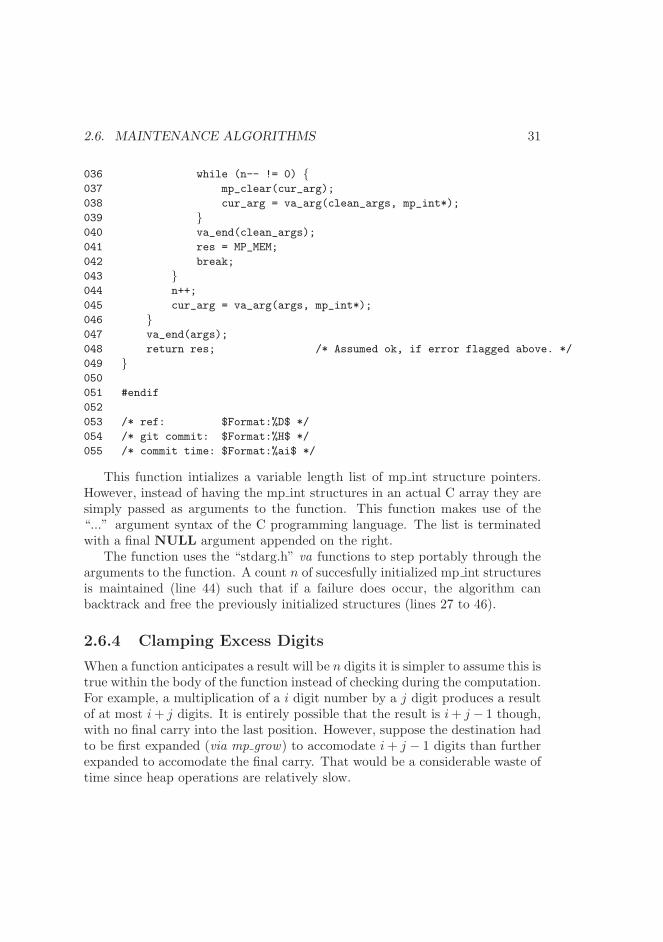
Algorithm mp init multi. The algorithm will initialize the array of mp intvariables one at a time. If a runtime error has been detected (step 1.2 ) all ofthe previously initialized variables are cleared. The goal is an “all or nothing”initialization which allows for quick recovery from runtime errors.
File: bn mp init multi.c
016 #include <stdarg.h>
017
018 int mp_init_multi(mp_int *mp, ...)
019 {020 mp_err res = MP_OKAY; /* Assume ok until proven otherwise */
021 int n = 0; /* Number of ok inits */
022 mp_int* cur_arg = mp;
023 va_list args;
024
025 va_start(args, mp); /* init args to next argument from caller */
026 while (cur_arg != NULL) {027 if (mp_init(cur_arg) != MP_OKAY) {028 /* Oops - error! Back-track and mp_clear what we already
029 succeeded in init-ing, then return error.
030 */
031 va_list clean_args;
032
033 /* now start cleaning up */
034 cur_arg = mp;
035 va_start(clean_args, mp);
2.6. MAINTENANCE ALGORITHMS 31
036 while (n-- != 0) {037 mp_clear(cur_arg);
038 cur_arg = va_arg(clean_args, mp_int*);
039 }040 va_end(clean_args);
041 res = MP_MEM;
042 break;
043 }044 n++;
045 cur_arg = va_arg(args, mp_int*);
046 }047 va_end(args);
048 return res; /* Assumed ok, if error flagged above. */
049 }050
051 #endif
052
053 /* ref: $Format:%D$ */
054 /* git commit: $Format:%H$ */
055 /* commit time: $Format:%ai$ */
This function intializes a variable length list of mp int structure pointers.However, instead of having the mp int structures in an actual C array they aresimply passed as arguments to the function. This function makes use of the“...” argument syntax of the C programming language. The list is terminatedwith a final NULL argument appended on the right.
The function uses the “stdarg.h” va functions to step portably through thearguments to the function. A count n of succesfully initialized mp int structuresis maintained (line 44) such that if a failure does occur, the algorithm canbacktrack and free the previously initialized structures (lines 27 to 46).
2.6.4 Clamping Excess Digits
When a function anticipates a result will be n digits it is simpler to assume this istrue within the body of the function instead of checking during the computation.For example, a multiplication of a i digit number by a j digit produces a resultof at most i+ j digits. It is entirely possible that the result is i+ j − 1 though,with no final carry into the last position. However, suppose the destination hadto be first expanded (via mp grow) to accomodate i+ j − 1 digits than furtherexpanded to accomodate the final carry. That would be a considerable waste oftime since heap operations are relatively slow.
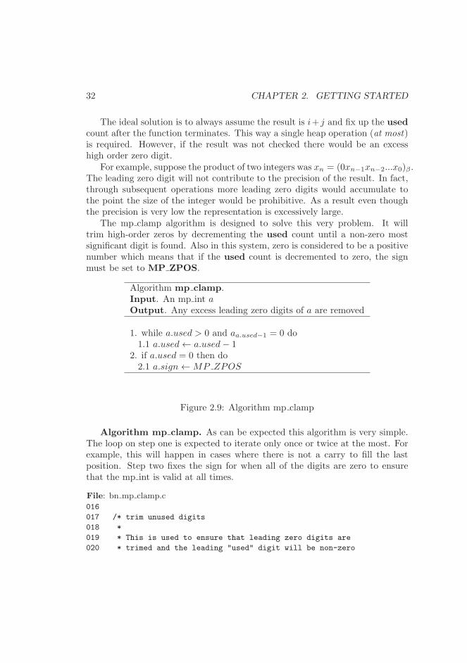
32 CHAPTER 2. GETTING STARTED
The ideal solution is to always assume the result is i+ j and fix up the usedcount after the function terminates. This way a single heap operation (at most)is required. However, if the result was not checked there would be an excesshigh order zero digit.
For example, suppose the product of two integers was xn = (0xn−1xn−2...x0)β .The leading zero digit will not contribute to the precision of the result. In fact,through subsequent operations more leading zero digits would accumulate tothe point the size of the integer would be prohibitive. As a result even thoughthe precision is very low the representation is excessively large.
The mp clamp algorithm is designed to solve this very problem. It willtrim high-order zeros by decrementing the used count until a non-zero mostsignificant digit is found. Also in this system, zero is considered to be a positivenumber which means that if the used count is decremented to zero, the signmust be set to MP ZPOS.
Algorithm mp clamp.Input. An mp int aOutput. Any excess leading zero digits of a are removed
1. while a.used > 0 and aa.used−1 = 0 do1.1 a.used← a.used− 1
2. if a.used = 0 then do2.1 a.sign←MP ZPOS
Figure 2.9: Algorithm mp clamp
Algorithm mp clamp. As can be expected this algorithm is very simple.The loop on step one is expected to iterate only once or twice at the most. Forexample, this will happen in cases where there is not a carry to fill the lastposition. Step two fixes the sign for when all of the digits are zero to ensurethat the mp int is valid at all times.
File: bn mp clamp.c
016
017 /* trim unused digits
018 *
019 * This is used to ensure that leading zero digits are
020 * trimed and the leading "used" digit will be non-zero
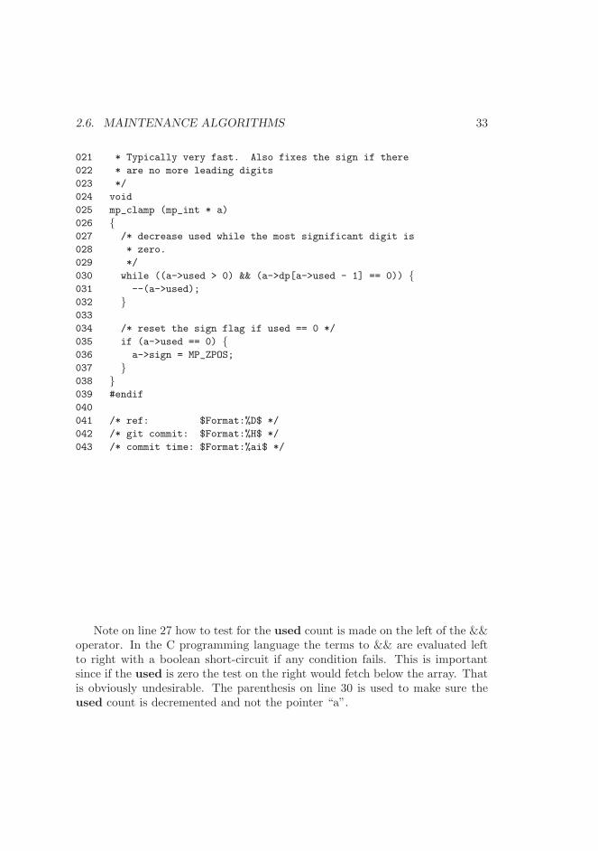
2.6. MAINTENANCE ALGORITHMS 33
021 * Typically very fast. Also fixes the sign if there
022 * are no more leading digits
023 */
024 void
025 mp_clamp (mp_int * a)
026 {027 /* decrease used while the most significant digit is
028 * zero.
029 */
030 while ((a->used > 0) && (a->dp[a->used - 1] == 0)) {031 --(a->used);
032 }033
034 /* reset the sign flag if used == 0 */
035 if (a->used == 0) {036 a->sign = MP_ZPOS;
037 }038 }039 #endif
040
041 /* ref: $Format:%D$ */
042 /* git commit: $Format:%H$ */
043 /* commit time: $Format:%ai$ */
Note on line 27 how to test for the used count is made on the left of the &&operator. In the C programming language the terms to && are evaluated leftto right with a boolean short-circuit if any condition fails. This is importantsince if the used is zero the test on the right would fetch below the array. Thatis obviously undesirable. The parenthesis on line 30 is used to make sure theused count is decremented and not the pointer “a”.
34 CHAPTER 2. GETTING STARTED
Exercises
[1] Discuss the relevance of the used member of the mp int structure.
[1] Discuss the consequences of not using padding when performing allocations.
[2] Estimate an ideal value for MP PREC when performing 1024-bit RSAencryption when β = 228.
[1] Discuss the relevance of the algorithm mp clamp. What does it prevent?
[1] Give an example of when the algorithm mp init copy might be useful.
Chapter 3
Basic Operations
3.1 Introduction
In the previous chapter a series of low level algorithms were established thatdealt with initializing and maintaining mp int structures. This chapter willdiscuss another set of seemingly non-algebraic algorithms which will form thelow level basis of the entire library. While these algorithm are relatively trivialit is important to understand how they work before proceeding since thesealgorithms will be used almost intrinsically in the following chapters.
The algorithms in this chapter deal primarily with more “programmer” re-lated tasks such as creating copies of mp int structures, assigning small valuesto mp int structures and comparisons of the values mp int structures represent.
3.2 Assigning Values to mp int Structures
3.2.1 Copying an mp int
Assigning the value that a given mp int structure represents to another mp intstructure shall be known as making a copy for the purposes of this text. Thecopy of the mp int will be a separate entity that represents the same value as themp int it was copied from. The mp copy algorithm provides this functionality.
35
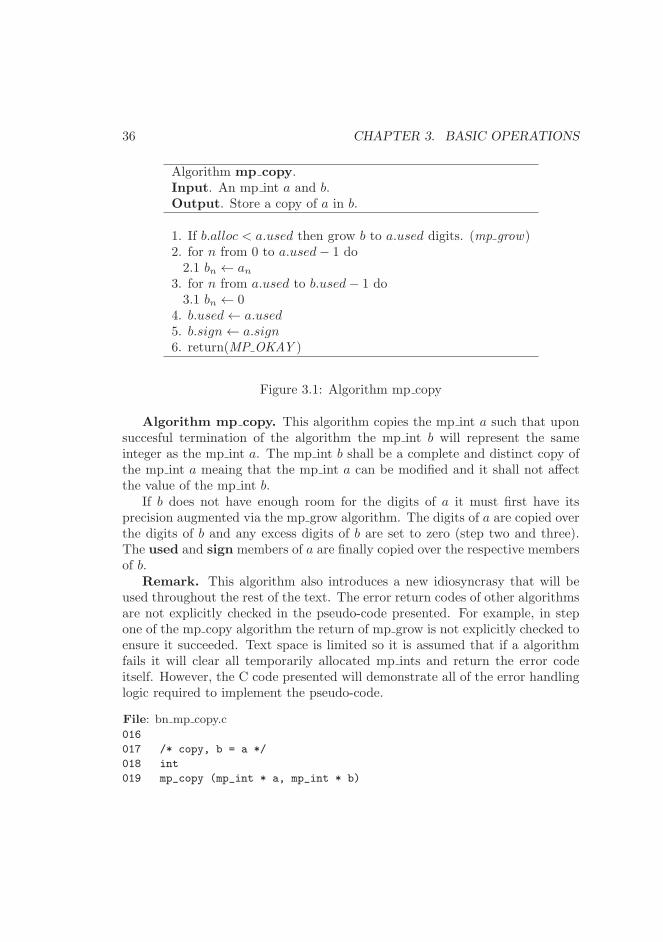
36 CHAPTER 3. BASIC OPERATIONS
Algorithm mp copy.Input. An mp int a and b.Output. Store a copy of a in b.
1. If b.alloc < a.used then grow b to a.used digits. (mp grow)2. for n from 0 to a.used− 1 do2.1 bn ← an
3. for n from a.used to b.used− 1 do3.1 bn ← 0
4. b.used← a.used5. b.sign← a.sign6. return(MP OKAY )
Figure 3.1: Algorithm mp copy
Algorithm mp copy. This algorithm copies the mp int a such that uponsuccesful termination of the algorithm the mp int b will represent the sameinteger as the mp int a. The mp int b shall be a complete and distinct copy ofthe mp int a meaing that the mp int a can be modified and it shall not affectthe value of the mp int b.
If b does not have enough room for the digits of a it must first have itsprecision augmented via the mp grow algorithm. The digits of a are copied overthe digits of b and any excess digits of b are set to zero (step two and three).The used and sign members of a are finally copied over the respective membersof b.
Remark. This algorithm also introduces a new idiosyncrasy that will beused throughout the rest of the text. The error return codes of other algorithmsare not explicitly checked in the pseudo-code presented. For example, in stepone of the mp copy algorithm the return of mp grow is not explicitly checked toensure it succeeded. Text space is limited so it is assumed that if a algorithmfails it will clear all temporarily allocated mp ints and return the error codeitself. However, the C code presented will demonstrate all of the error handlinglogic required to implement the pseudo-code.
File: bn mp copy.c
016
017 /* copy, b = a */
018 int
019 mp_copy (mp_int * a, mp_int * b)
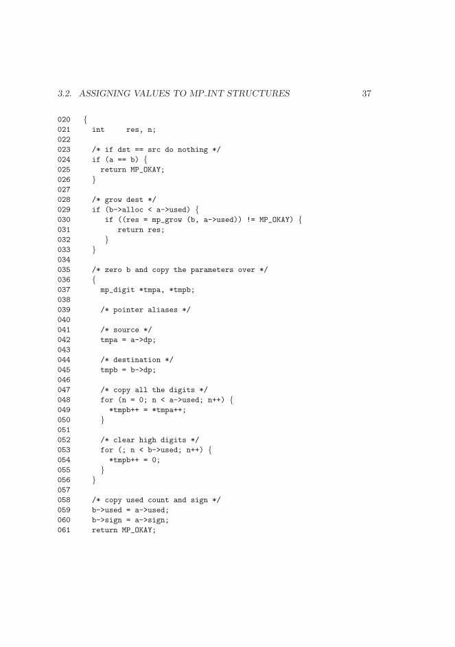
3.2. ASSIGNING VALUES TO MP INT STRUCTURES 37
020 {021 int res, n;
022
023 /* if dst == src do nothing */
024 if (a == b) {025 return MP_OKAY;
026 }027
028 /* grow dest */
029 if (b->alloc < a->used) {030 if ((res = mp_grow (b, a->used)) != MP_OKAY) {031 return res;
032 }033 }034
035 /* zero b and copy the parameters over */
036 {037 mp_digit *tmpa, *tmpb;
038
039 /* pointer aliases */
040
041 /* source */
042 tmpa = a->dp;
043
044 /* destination */
045 tmpb = b->dp;
046
047 /* copy all the digits */
048 for (n = 0; n < a->used; n++) {049 *tmpb++ = *tmpa++;
050 }051
052 /* clear high digits */
053 for (; n < b->used; n++) {054 *tmpb++ = 0;
055 }056 }057
058 /* copy used count and sign */
059 b->used = a->used;
060 b->sign = a->sign;
061 return MP_OKAY;
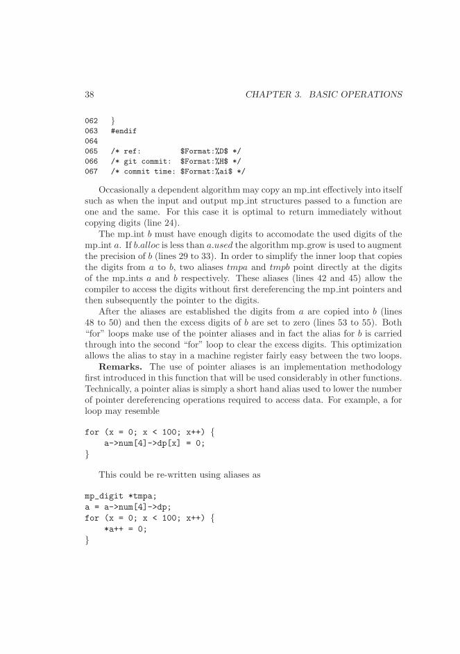
38 CHAPTER 3. BASIC OPERATIONS
062 }063 #endif
064
065 /* ref: $Format:%D$ */
066 /* git commit: $Format:%H$ */
067 /* commit time: $Format:%ai$ */
Occasionally a dependent algorithm may copy an mp int effectively into itselfsuch as when the input and output mp int structures passed to a function areone and the same. For this case it is optimal to return immediately withoutcopying digits (line 24).
The mp int b must have enough digits to accomodate the used digits of themp int a. If b.alloc is less than a.used the algorithm mp grow is used to augmentthe precision of b (lines 29 to 33). In order to simplify the inner loop that copiesthe digits from a to b, two aliases tmpa and tmpb point directly at the digitsof the mp ints a and b respectively. These aliases (lines 42 and 45) allow thecompiler to access the digits without first dereferencing the mp int pointers andthen subsequently the pointer to the digits.
After the aliases are established the digits from a are copied into b (lines48 to 50) and then the excess digits of b are set to zero (lines 53 to 55). Both“for” loops make use of the pointer aliases and in fact the alias for b is carriedthrough into the second “for” loop to clear the excess digits. This optimizationallows the alias to stay in a machine register fairly easy between the two loops.
Remarks. The use of pointer aliases is an implementation methodologyfirst introduced in this function that will be used considerably in other functions.Technically, a pointer alias is simply a short hand alias used to lower the numberof pointer dereferencing operations required to access data. For example, a forloop may resemble
for (x = 0; x < 100; x++) {a->num[4]->dp[x] = 0;
}
This could be re-written using aliases as
mp_digit *tmpa;
a = a->num[4]->dp;
for (x = 0; x < 100; x++) {*a++ = 0;
}
3.2. ASSIGNING VALUES TO MP INT STRUCTURES 39
In this case an alias is used to access the array of digits within an mp intstructure directly. It may seem that a pointer alias is strictly not required asa compiler may optimize out the redundant pointer operations. However, thereare two dominant reasons to use aliases.
The first reason is that most compilers will not effectively optimize pointerarithmetic. For example, some optimizations may work for the Microsoft VisualC++ compiler (MSVC) and not for the GNU C Compiler (GCC). Also someoptimizations may work for GCC and not MSVC. As such it is ideal to find acommon ground for as many compilers as possible. Pointer aliases optimize thecode considerably before the compiler even reads the source code which meansthe end compiled code stands a better chance of being faster.
The second reason is that pointer aliases often can make an algorithm simplerto read. Consider the first “for” loop of the function mp copy() re-written tonot use pointer aliases.
/* copy all the digits */
for (n = 0; n < a->used; n++) {b->dp[n] = a->dp[n];
}
Whether this code is harder to read depends strongly on the individual.However, it is quantifiably slightly more complicated as there are four variableswithin the statement instead of just two.
Nested Statements
Another commonly used technique in the source routines is that certain sectionsof code are nested. This is used in particular with the pointer aliases to highlightcode phases. For example, a Comba multiplier (discussed in chapter six) willtypically have three different phases. First the temporaries are initialized, thenthe columns calculated and finally the carries are propagated. In this examplethe middle column production phase will typically be nested as it uses temporaryvariables and aliases the most.
The nesting also simplies the source code as variables that are nested areonly valid for their scope. As a result the various temporary variables requireddo not propagate into other sections of code.
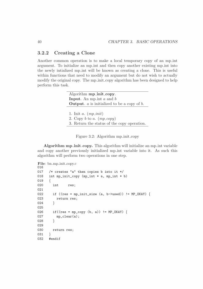
40 CHAPTER 3. BASIC OPERATIONS
3.2.2 Creating a Clone
Another common operation is to make a local temporary copy of an mp intargument. To initialize an mp int and then copy another existing mp int intothe newly intialized mp int will be known as creating a clone. This is usefulwithin functions that need to modify an argument but do not wish to actuallymodify the original copy. The mp init copy algorithm has been designed to helpperform this task.
Algorithm mp init copy.Input. An mp int a and bOutput. a is initialized to be a copy of b.
1. Init a. (mp init)2. Copy b to a. (mp copy)3. Return the status of the copy operation.
Figure 3.2: Algorithm mp init copy
Algorithm mp init copy. This algorithm will initialize an mp int variableand copy another previously initialized mp int variable into it. As such thisalgorithm will perform two operations in one step.
File: bn mp init copy.c016
017 /* creates "a" then copies b into it */
018 int mp_init_copy (mp_int * a, mp_int * b)
019 {020 int res;
021
022 if ((res = mp_init_size (a, b->used)) != MP_OKAY) {023 return res;
024 }025
026 if((res = mp_copy (b, a)) != MP_OKAY) {027 mp_clear(a);
028 }029
030 return res;
031 }032 #endif
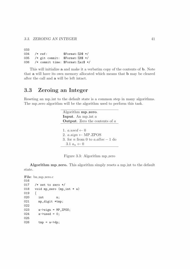
3.3. ZEROING AN INTEGER 41
033
034 /* ref: $Format:%D$ */
035 /* git commit: $Format:%H$ */
036 /* commit time: $Format:%ai$ */
This will initialize a and make it a verbatim copy of the contents of b. Notethat a will have its own memory allocated which means that b may be clearedafter the call and a will be left intact.
3.3 Zeroing an Integer
Reseting an mp int to the default state is a common step in many algorithms.The mp zero algorithm will be the algorithm used to perform this task.
Algorithm mp zero.Input. An mp int aOutput. Zero the contents of a
1. a.used← 02. a.sign← MP ZPOS3. for n from 0 to a.alloc− 1 do3.1 an ← 0
Figure 3.3: Algorithm mp zero
Algorithm mp zero. This algorithm simply resets a mp int to the defaultstate.
File: bn mp zero.c016
017 /* set to zero */
018 void mp_zero (mp_int * a)
019 {020 int n;
021 mp_digit *tmp;
022
023 a->sign = MP_ZPOS;
024 a->used = 0;
025
026 tmp = a->dp;
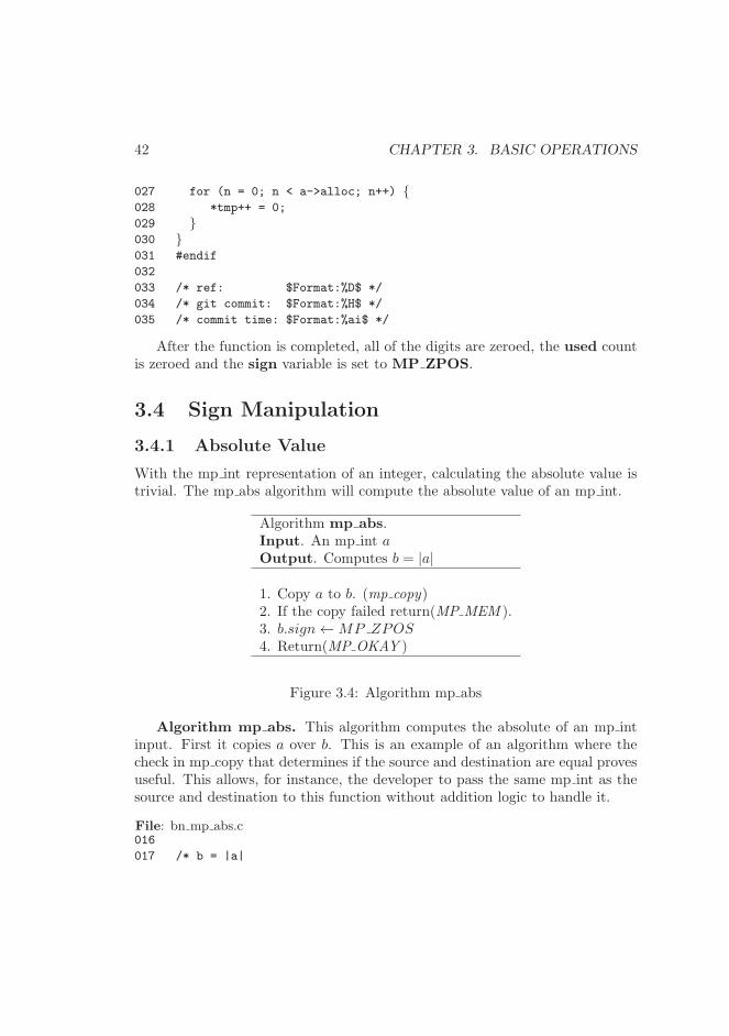
42 CHAPTER 3. BASIC OPERATIONS
027 for (n = 0; n < a->alloc; n++) {028 *tmp++ = 0;
029 }030 }031 #endif
032
033 /* ref: $Format:%D$ */
034 /* git commit: $Format:%H$ */
035 /* commit time: $Format:%ai$ */
After the function is completed, all of the digits are zeroed, the used countis zeroed and the sign variable is set to MP ZPOS.
3.4 Sign Manipulation
3.4.1 Absolute Value
With the mp int representation of an integer, calculating the absolute value istrivial. The mp abs algorithm will compute the absolute value of an mp int.
Algorithm mp abs.Input. An mp int aOutput. Computes b = |a|
1. Copy a to b. (mp copy)2. If the copy failed return(MP MEM ).3. b.sign←MP ZPOS4. Return(MP OKAY )
Figure 3.4: Algorithm mp abs
Algorithm mp abs. This algorithm computes the absolute of an mp intinput. First it copies a over b. This is an example of an algorithm where thecheck in mp copy that determines if the source and destination are equal provesuseful. This allows, for instance, the developer to pass the same mp int as thesource and destination to this function without addition logic to handle it.
File: bn mp abs.c016
017 /* b = |a|
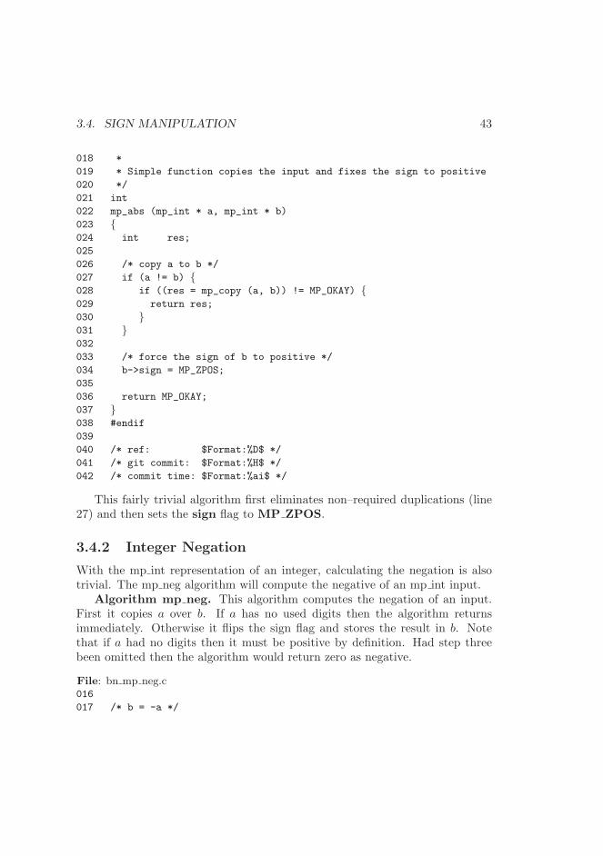
3.4. SIGN MANIPULATION 43
018 *
019 * Simple function copies the input and fixes the sign to positive
020 */
021 int
022 mp_abs (mp_int * a, mp_int * b)
023 {024 int res;
025
026 /* copy a to b */
027 if (a != b) {028 if ((res = mp_copy (a, b)) != MP_OKAY) {029 return res;
030 }031 }032
033 /* force the sign of b to positive */
034 b->sign = MP_ZPOS;
035
036 return MP_OKAY;
037 }038 #endif
039
040 /* ref: $Format:%D$ */
041 /* git commit: $Format:%H$ */
042 /* commit time: $Format:%ai$ */
This fairly trivial algorithm first eliminates non–required duplications (line27) and then sets the sign flag to MP ZPOS.
3.4.2 Integer Negation
With the mp int representation of an integer, calculating the negation is alsotrivial. The mp neg algorithm will compute the negative of an mp int input.
Algorithm mp neg. This algorithm computes the negation of an input.First it copies a over b. If a has no used digits then the algorithm returnsimmediately. Otherwise it flips the sign flag and stores the result in b. Notethat if a had no digits then it must be positive by definition. Had step threebeen omitted then the algorithm would return zero as negative.
File: bn mp neg.c016
017 /* b = -a */
44 CHAPTER 3. BASIC OPERATIONS
Algorithm mp neg.Input. An mp int aOutput. Computes b = −a
1. Copy a to b. (mp copy)2. If the copy failed return(MP MEM ).3. If a.used = 0 then return(MP OKAY ).4. If a.sign = MP ZPOS then do4.1 b.sign = MP NEG.
5. else do5.1 b.sign = MP ZPOS.
6. Return(MP OKAY )
Figure 3.5: Algorithm mp neg
018 int mp_neg (mp_int * a, mp_int * b)
019 {020 int res;
021 if (a != b) {022 if ((res = mp_copy (a, b)) != MP_OKAY) {023 return res;
024 }025 }026
027 if (mp_iszero(b) != MP_YES) {028 b->sign = (a->sign == MP_ZPOS) ? MP_NEG : MP_ZPOS;
029 } else {030 b->sign = MP_ZPOS;
031 }032
033 return MP_OKAY;
034 }035 #endif
036
037 /* ref: $Format:%D$ */
038 /* git commit: $Format:%H$ */
039 /* commit time: $Format:%ai$ */
Like mp abs() this function avoids non–required duplications (line 21) andthen sets the sign. We have to make sure that only non–zero values get a sign
3.5. SMALL CONSTANTS 45
of MP NEG. If the mp int is zero than the sign is hard–coded to MP ZPOS.
3.5 Small Constants
3.5.1 Setting Small Constants
Often a mp int must be set to a relatively small value such as 1 or 2. For thesecases the mp set algorithm is useful.
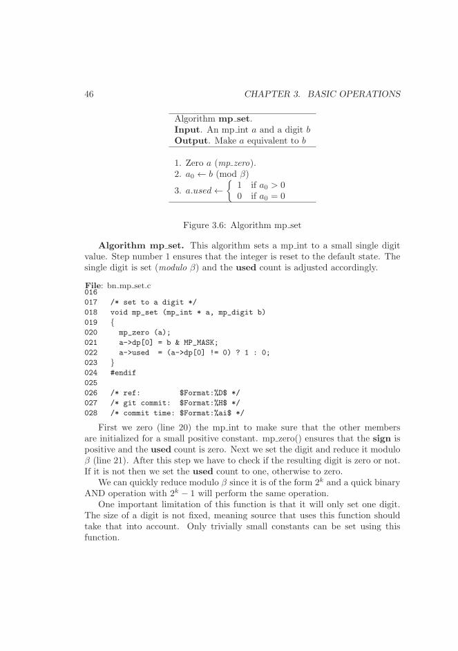
46 CHAPTER 3. BASIC OPERATIONS
Algorithm mp set.Input. An mp int a and a digit bOutput. Make a equivalent to b
1. Zero a (mp zero).2. a0 ← b (mod β)
3. a.used←{
1 if a0 > 00 if a0 = 0
Figure 3.6: Algorithm mp set
Algorithm mp set. This algorithm sets a mp int to a small single digitvalue. Step number 1 ensures that the integer is reset to the default state. Thesingle digit is set (modulo β) and the used count is adjusted accordingly.
File: bn mp set.c016
017 /* set to a digit */
018 void mp_set (mp_int * a, mp_digit b)
019 {020 mp_zero (a);
021 a->dp[0] = b & MP_MASK;
022 a->used = (a->dp[0] != 0) ? 1 : 0;
023 }024 #endif
025
026 /* ref: $Format:%D$ */
027 /* git commit: $Format:%H$ */
028 /* commit time: $Format:%ai$ */
First we zero (line 20) the mp int to make sure that the other membersare initialized for a small positive constant. mp zero() ensures that the sign ispositive and the used count is zero. Next we set the digit and reduce it moduloβ (line 21). After this step we have to check if the resulting digit is zero or not.If it is not then we set the used count to one, otherwise to zero.
We can quickly reduce modulo β since it is of the form 2k and a quick binaryAND operation with 2k − 1 will perform the same operation.
One important limitation of this function is that it will only set one digit.The size of a digit is not fixed, meaning source that uses this function shouldtake that into account. Only trivially small constants can be set using thisfunction.
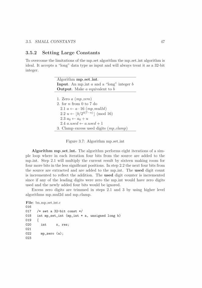
3.5. SMALL CONSTANTS 47
3.5.2 Setting Large Constants
To overcome the limitations of the mp set algorithm the mp set int algorithm isideal. It accepts a “long” data type as input and will always treat it as a 32-bitinteger.
Algorithm mp set int.Input. An mp int a and a “long” integer bOutput. Make a equivalent to b
1. Zero a (mp zero)2. for n from 0 to 7 do2.1 a← a · 16 (mp mul2d)2.2 u← ⌊b/24(7−n)⌋ (mod 16)2.3 a0 ← a0 + u2.4 a.used← a.used+ 1
3. Clamp excess used digits (mp clamp)
Figure 3.7: Algorithm mp set int
Algorithm mp set int. The algorithm performs eight iterations of a sim-ple loop where in each iteration four bits from the source are added to themp int. Step 2.1 will multiply the current result by sixteen making room forfour more bits in the less significant positions. In step 2.2 the next four bits fromthe source are extracted and are added to the mp int. The used digit countis incremented to reflect the addition. The used digit counter is incrementedsince if any of the leading digits were zero the mp int would have zero digitsused and the newly added four bits would be ignored.
Excess zero digits are trimmed in steps 2.1 and 3 by using higher levelalgorithms mp mul2d and mp clamp.
File: bn mp set int.c016
017 /* set a 32-bit const */
018 int mp_set_int (mp_int * a, unsigned long b)
019 {020 int x, res;
021
022 mp_zero (a);
023
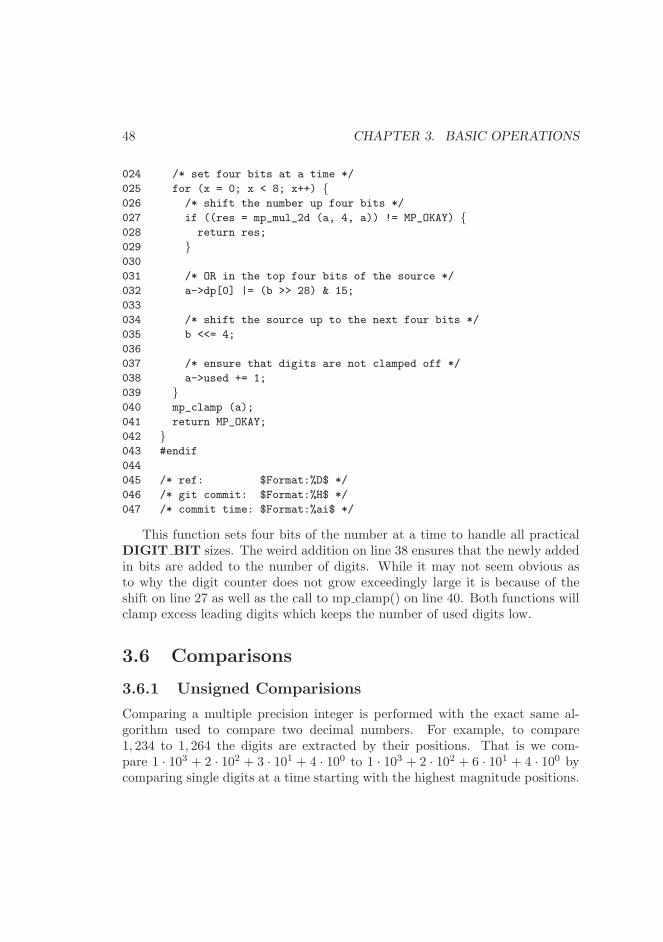
48 CHAPTER 3. BASIC OPERATIONS
024 /* set four bits at a time */
025 for (x = 0; x < 8; x++) {026 /* shift the number up four bits */
027 if ((res = mp_mul_2d (a, 4, a)) != MP_OKAY) {028 return res;
029 }030
031 /* OR in the top four bits of the source */
032 a->dp[0] |= (b >> 28) & 15;
033
034 /* shift the source up to the next four bits */
035 b <<= 4;
036
037 /* ensure that digits are not clamped off */
038 a->used += 1;
039 }040 mp_clamp (a);
041 return MP_OKAY;
042 }043 #endif
044
045 /* ref: $Format:%D$ */
046 /* git commit: $Format:%H$ */
047 /* commit time: $Format:%ai$ */
This function sets four bits of the number at a time to handle all practicalDIGIT BIT sizes. The weird addition on line 38 ensures that the newly addedin bits are added to the number of digits. While it may not seem obvious asto why the digit counter does not grow exceedingly large it is because of theshift on line 27 as well as the call to mp clamp() on line 40. Both functions willclamp excess leading digits which keeps the number of used digits low.
3.6 Comparisons
3.6.1 Unsigned Comparisions
Comparing a multiple precision integer is performed with the exact same al-gorithm used to compare two decimal numbers. For example, to compare1, 234 to 1, 264 the digits are extracted by their positions. That is we com-pare 1 · 103 + 2 · 102 + 3 · 101 + 4 · 100 to 1 · 103 + 2 · 102 + 6 · 101 + 4 · 100 bycomparing single digits at a time starting with the highest magnitude positions.
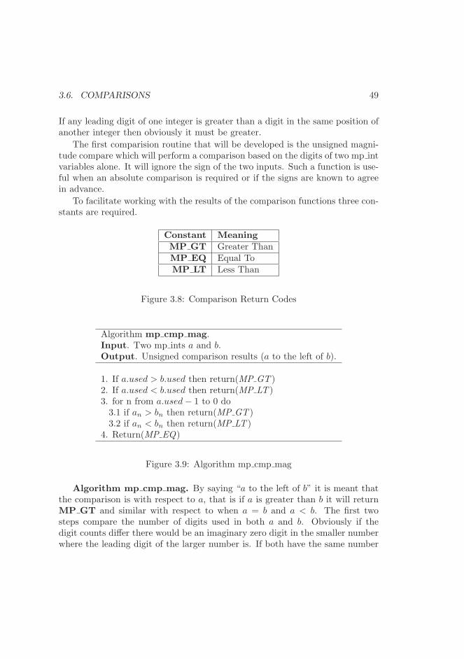
3.6. COMPARISONS 49
If any leading digit of one integer is greater than a digit in the same position ofanother integer then obviously it must be greater.
The first comparision routine that will be developed is the unsigned magni-tude compare which will perform a comparison based on the digits of two mp intvariables alone. It will ignore the sign of the two inputs. Such a function is use-ful when an absolute comparison is required or if the signs are known to agreein advance.
To facilitate working with the results of the comparison functions three con-stants are required.
Constant MeaningMP GT Greater ThanMP EQ Equal ToMP LT Less Than
Figure 3.8: Comparison Return Codes
Algorithm mp cmp mag.Input. Two mp ints a and b.Output. Unsigned comparison results (a to the left of b).
1. If a.used > b.used then return(MP GT )2. If a.used < b.used then return(MP LT )3. for n from a.used− 1 to 0 do3.1 if an > bn then return(MP GT )3.2 if an < bn then return(MP LT )
4. Return(MP EQ)
Figure 3.9: Algorithm mp cmp mag
Algorithm mp cmp mag. By saying “a to the left of b” it is meant thatthe comparison is with respect to a, that is if a is greater than b it will returnMP GT and similar with respect to when a = b and a < b. The first twosteps compare the number of digits used in both a and b. Obviously if thedigit counts differ there would be an imaginary zero digit in the smaller numberwhere the leading digit of the larger number is. If both have the same number
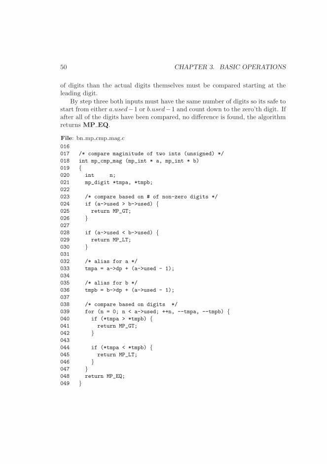
50 CHAPTER 3. BASIC OPERATIONS
of digits than the actual digits themselves must be compared starting at theleading digit.
By step three both inputs must have the same number of digits so its safe tostart from either a.used−1 or b.used−1 and count down to the zero’th digit. Ifafter all of the digits have been compared, no difference is found, the algorithmreturns MP EQ.
File: bn mp cmp mag.c
016
017 /* compare maginitude of two ints (unsigned) */
018 int mp_cmp_mag (mp_int * a, mp_int * b)
019 {020 int n;
021 mp_digit *tmpa, *tmpb;
022
023 /* compare based on # of non-zero digits */
024 if (a->used > b->used) {025 return MP_GT;
026 }027
028 if (a->used < b->used) {029 return MP_LT;
030 }031
032 /* alias for a */
033 tmpa = a->dp + (a->used - 1);
034
035 /* alias for b */
036 tmpb = b->dp + (a->used - 1);
037
038 /* compare based on digits */
039 for (n = 0; n < a->used; ++n, --tmpa, --tmpb) {040 if (*tmpa > *tmpb) {041 return MP_GT;
042 }043
044 if (*tmpa < *tmpb) {045 return MP_LT;
046 }047 }048 return MP_EQ;
049 }
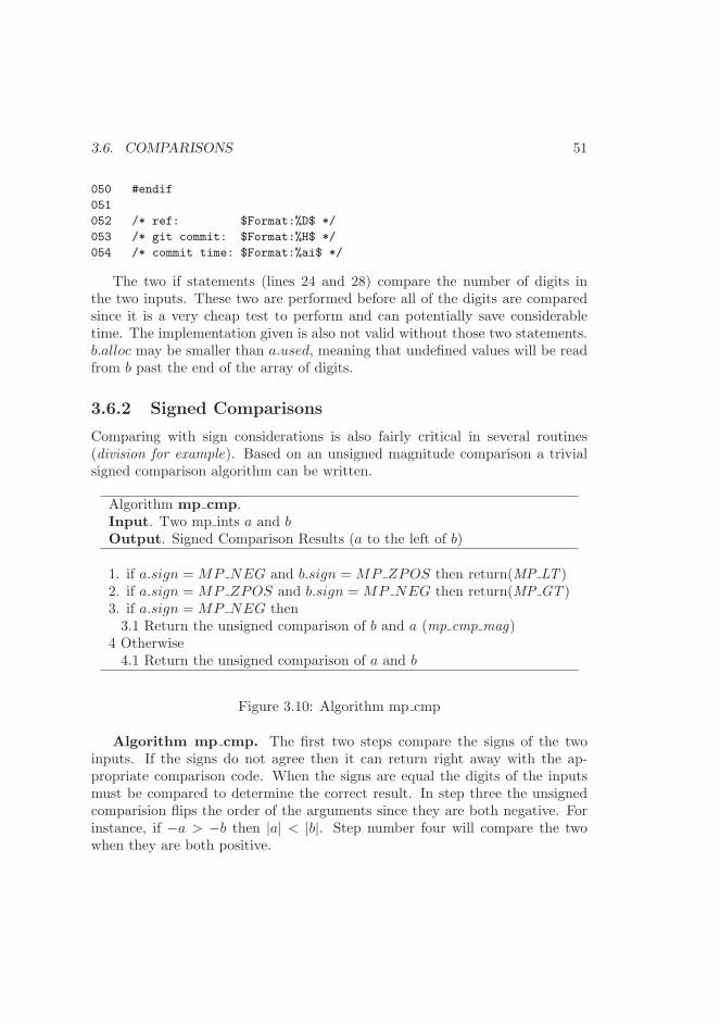
3.6. COMPARISONS 51
050 #endif
051
052 /* ref: $Format:%D$ */
053 /* git commit: $Format:%H$ */
054 /* commit time: $Format:%ai$ */
The two if statements (lines 24 and 28) compare the number of digits inthe two inputs. These two are performed before all of the digits are comparedsince it is a very cheap test to perform and can potentially save considerabletime. The implementation given is also not valid without those two statements.b.alloc may be smaller than a.used, meaning that undefined values will be readfrom b past the end of the array of digits.
3.6.2 Signed Comparisons
Comparing with sign considerations is also fairly critical in several routines(division for example). Based on an unsigned magnitude comparison a trivialsigned comparison algorithm can be written.
Algorithm mp cmp.Input. Two mp ints a and bOutput. Signed Comparison Results (a to the left of b)
1. if a.sign = MP NEG and b.sign = MP ZPOS then return(MP LT )2. if a.sign = MP ZPOS and b.sign = MP NEG then return(MP GT )3. if a.sign = MP NEG then3.1 Return the unsigned comparison of b and a (mp cmp mag)
4 Otherwise4.1 Return the unsigned comparison of a and b
Figure 3.10: Algorithm mp cmp
Algorithm mp cmp. The first two steps compare the signs of the twoinputs. If the signs do not agree then it can return right away with the ap-propriate comparison code. When the signs are equal the digits of the inputsmust be compared to determine the correct result. In step three the unsignedcomparision flips the order of the arguments since they are both negative. Forinstance, if −a > −b then |a| < |b|. Step number four will compare the twowhen they are both positive.
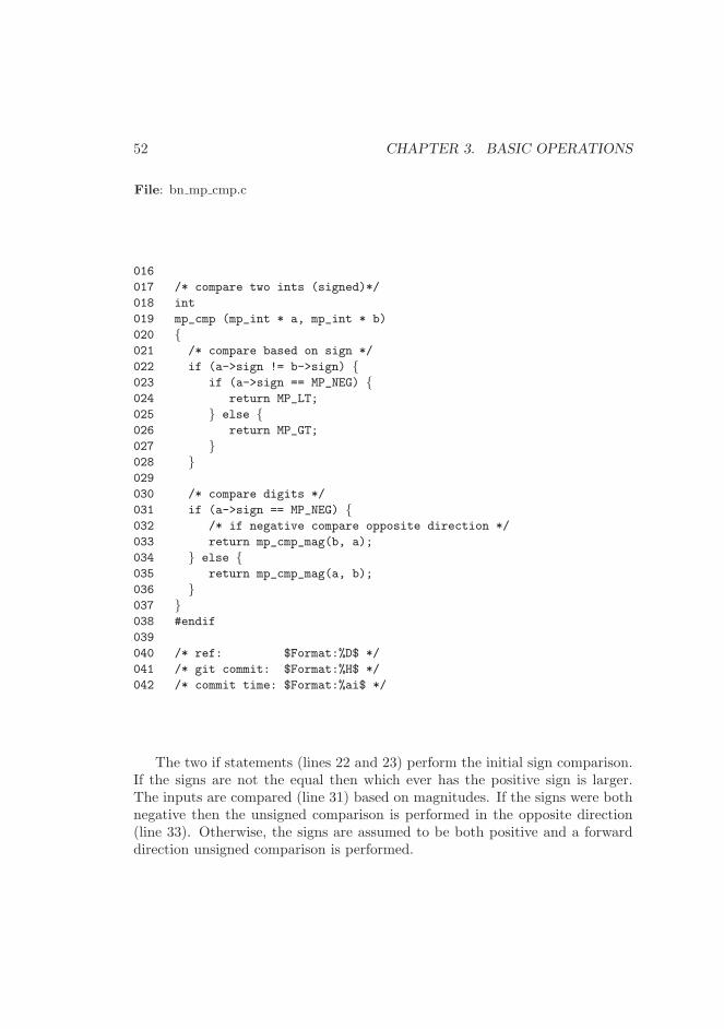
52 CHAPTER 3. BASIC OPERATIONS
File: bn mp cmp.c
016
017 /* compare two ints (signed)*/
018 int
019 mp_cmp (mp_int * a, mp_int * b)
020 {021 /* compare based on sign */
022 if (a->sign != b->sign) {023 if (a->sign == MP_NEG) {024 return MP_LT;
025 } else {026 return MP_GT;
027 }028 }029
030 /* compare digits */
031 if (a->sign == MP_NEG) {032 /* if negative compare opposite direction */
033 return mp_cmp_mag(b, a);
034 } else {035 return mp_cmp_mag(a, b);
036 }037 }038 #endif
039
040 /* ref: $Format:%D$ */
041 /* git commit: $Format:%H$ */
042 /* commit time: $Format:%ai$ */
The two if statements (lines 22 and 23) perform the initial sign comparison.If the signs are not the equal then which ever has the positive sign is larger.The inputs are compared (line 31) based on magnitudes. If the signs were bothnegative then the unsigned comparison is performed in the opposite direction(line 33). Otherwise, the signs are assumed to be both positive and a forwarddirection unsigned comparison is performed.
3.6. COMPARISONS 53
Exercises
[2] Modify algorithm mp set int to accept as input a variable length array of bits.
[3] Give the probability that algorithm mp cmp mag will have to compare k digitsof two random digits (of equal magnitude) before a difference is found.
[1] Suggest a simple method to speed up the implementation of mp cmp mag basedon the observations made in the previous problem.

54 CHAPTER 3. BASIC OPERATIONS
Chapter 4
Basic Arithmetic
4.1 Introduction
At this point algorithms for initialization, clearing, zeroing, copying, compar-ing and setting small constants have been established. The next logical set ofalgorithms to develop are addition, subtraction and digit shifting algorithms.These algorithms make use of the lower level algorithms and are the cruicialbuilding block for the multiplication algorithms. It is very important that thesealgorithms are highly optimized. On their own they are simple O(n) algorithmsbut they can be called from higher level algorithms which easily places them atO(n2) or even O(n3) work levels.
All of the algorithms within this chapter make use of the logical bit shiftoperations denoted by << and >> for left and right logical shifts respectively. Alogical shift is analogous to sliding the decimal point of radix-10 representations.For example, the real number 0.9345 is equivalent to 93.45% which is foundby sliding the the decimal two places to the right (multiplying by β2 = 102).Algebraically a binary logical shift is equivalent to a division or multiplicationby a power of two. For example, a << k = a · 2k while a >> k = ⌊a/2k⌋.
One significant difference between a logical shift and the way decimals areshifted is that digits below the zero’th position are removed from the number.For example, consider 11012 >> 1 using decimal notation this would produce110.12. However, with a logical shift the result is 1102.
55
56 CHAPTER 4. BASIC ARITHMETIC
4.2 Addition and Subtraction
In common twos complement fixed precision arithmetic negative numbers areeasily represented by subtraction from the modulus. For example, with 32-bitintegers a − b (mod 232) is the same as a + (232 − b) (mod 232) since 232 ≡0 (mod 232). As a result subtraction can be performed with a trivial series oflogical operations and an addition.
However, in multiple precision arithmetic negative numbers are not repre-sented in the same way. Instead a sign flag is used to keep track of the sign of theinteger. As a result signed addition and subtraction are actually implementedas conditional usage of lower level addition or subtraction algorithms with thesign fixed up appropriately.
The lower level algorithms will add or subtract integers without regard tothe sign flag. That is they will add or subtract the magnitude of the integersrespectively.
4.2.1 Low Level Addition
An unsigned addition of multiple precision integers is performed with the samelong-hand algorithm used to add decimal numbers. That is to add the trailingdigits first and propagate the resulting carry upwards. Since this is a lower levelalgorithm the name will have a “s ” prefix. Historically that convention stemsfrom the MPI library where “s ” stood for static functions that were hiddenfrom the developer entirely.
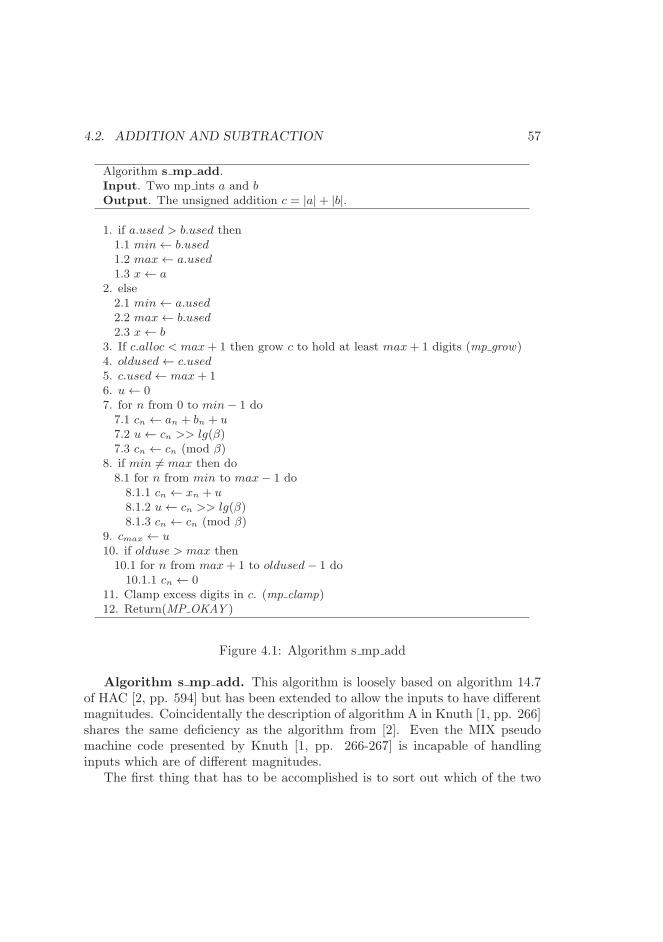
4.2. ADDITION AND SUBTRACTION 57
Algorithm s mp add.Input. Two mp ints a and bOutput. The unsigned addition c = |a|+ |b|.
1. if a.used > b.used then1.1 min← b.used1.2 max← a.used1.3 x← a
2. else2.1 min← a.used2.2 max← b.used2.3 x← b
3. If c.alloc < max+ 1 then grow c to hold at least max+ 1 digits (mp grow)4. oldused← c.used5. c.used← max+ 16. u← 07. for n from 0 to min− 1 do7.1 cn ← an + bn + u7.2 u← cn >> lg(β)7.3 cn ← cn (mod β)
8. if min 6= max then do8.1 for n from min to max− 1 do8.1.1 cn ← xn + u8.1.2 u← cn >> lg(β)8.1.3 cn ← cn (mod β)
9. cmax ← u10. if olduse > max then10.1 for n from max+ 1 to oldused− 1 do10.1.1 cn ← 0
11. Clamp excess digits in c. (mp clamp)12. Return(MP OKAY )
Figure 4.1: Algorithm s mp add
Algorithm s mp add. This algorithm is loosely based on algorithm 14.7of HAC [2, pp. 594] but has been extended to allow the inputs to have differentmagnitudes. Coincidentally the description of algorithm A in Knuth [1, pp. 266]shares the same deficiency as the algorithm from [2]. Even the MIX pseudomachine code presented by Knuth [1, pp. 266-267] is incapable of handlinginputs which are of different magnitudes.
The first thing that has to be accomplished is to sort out which of the two
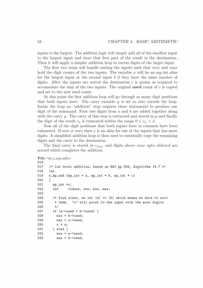
58 CHAPTER 4. BASIC ARITHMETIC
inputs is the largest. The addition logic will simply add all of the smallest inputto the largest input and store that first part of the result in the destination.Then it will apply a simpler addition loop to excess digits of the larger input.
The first two steps will handle sorting the inputs such that min and maxhold the digit counts of the two inputs. The variable x will be an mp int aliasfor the largest input or the second input b if they have the same number ofdigits. After the inputs are sorted the destination c is grown as required toaccomodate the sum of the two inputs. The original used count of c is copiedand set to the new used count.
At this point the first addition loop will go through as many digit positionsthat both inputs have. The carry variable µ is set to zero outside the loop.Inside the loop an “addition” step requires three statements to produce onedigit of the summand. First two digits from a and b are added together alongwith the carry µ. The carry of this step is extracted and stored in µ and finallythe digit of the result cn is truncated within the range 0 ≤ cn < β.
Now all of the digit positions that both inputs have in common have beenexhausted. If min 6= max then x is an alias for one of the inputs that has moredigits. A simplified addition loop is then used to essentially copy the remainingdigits and the carry to the destination.
The final carry is stored in cmax and digits above max upto oldused arezeroed which completes the addition.
File: bn s mp add.c016
017 /* low level addition, based on HAC pp.594, Algorithm 14.7 */
018 int
019 s_mp_add (mp_int * a, mp_int * b, mp_int * c)
020 {021 mp_int *x;
022 int olduse, res, min, max;
023
024 /* find sizes, we let |a| <= |b| which means we have to sort
025 * them. "x" will point to the input with the most digits
026 */
027 if (a->used > b->used) {028 min = b->used;
029 max = a->used;
030 x = a;
031 } else {032 min = a->used;
033 max = b->used;
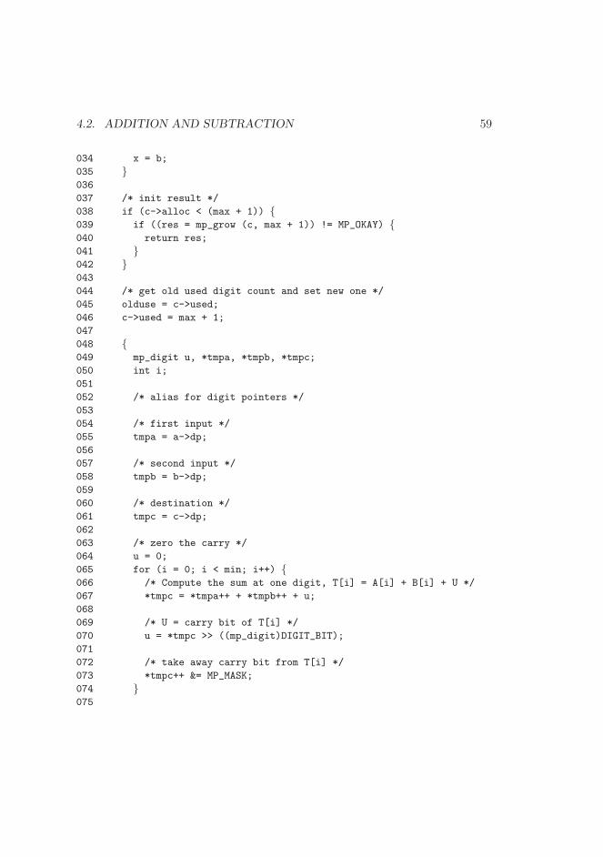
4.2. ADDITION AND SUBTRACTION 59
034 x = b;
035 }036
037 /* init result */
038 if (c->alloc < (max + 1)) {039 if ((res = mp_grow (c, max + 1)) != MP_OKAY) {040 return res;
041 }042 }043
044 /* get old used digit count and set new one */
045 olduse = c->used;
046 c->used = max + 1;
047
048 {049 mp_digit u, *tmpa, *tmpb, *tmpc;
050 int i;
051
052 /* alias for digit pointers */
053
054 /* first input */
055 tmpa = a->dp;
056
057 /* second input */
058 tmpb = b->dp;
059
060 /* destination */
061 tmpc = c->dp;
062
063 /* zero the carry */
064 u = 0;
065 for (i = 0; i < min; i++) {066 /* Compute the sum at one digit, T[i] = A[i] + B[i] + U */
067 *tmpc = *tmpa++ + *tmpb++ + u;
068
069 /* U = carry bit of T[i] */
070 u = *tmpc >> ((mp_digit)DIGIT_BIT);
071
072 /* take away carry bit from T[i] */
073 *tmpc++ &= MP_MASK;
074 }075
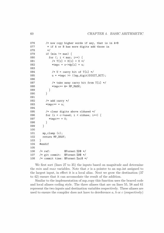
60 CHAPTER 4. BASIC ARITHMETIC
076 /* now copy higher words if any, that is in A+B
077 * if A or B has more digits add those in
078 */
079 if (min != max) {080 for (; i < max; i++) {081 /* T[i] = X[i] + U */
082 *tmpc = x->dp[i] + u;
083
084 /* U = carry bit of T[i] */
085 u = *tmpc >> ((mp_digit)DIGIT_BIT);
086
087 /* take away carry bit from T[i] */
088 *tmpc++ &= MP_MASK;
089 }090 }091
092 /* add carry */
093 *tmpc++ = u;
094
095 /* clear digits above oldused */
096 for (i = c->used; i < olduse; i++) {097 *tmpc++ = 0;
098 }099 }100
101 mp_clamp (c);
102 return MP_OKAY;
103 }104 #endif
105
106 /* ref: $Format:%D$ */
107 /* git commit: $Format:%H$ */
108 /* commit time: $Format:%ai$ */
We first sort (lines 27 to 35) the inputs based on magnitude and determinethe min and max variables. Note that x is a pointer to an mp int assigned tothe largest input, in effect it is a local alias. Next we grow the destination (37to 42) ensure that it can accomodate the result of the addition.
Similar to the implementation of mp copy this function uses the braced codeand local aliases coding style. The three aliases that are on lines 55, 58 and 61represent the two inputs and destination variables respectively. These aliases areused to ensure the compiler does not have to dereference a, b or c (respectively)
4.2. ADDITION AND SUBTRACTION 61
to access the digits of the respective mp int.The initial carry u will be cleared (line 64), note that u is of type mp digit
which ensures type compatibility within the implementation. The initial addi-tion (line 65 to 74) adds digits from both inputs until the smallest input runsout of digits. Similarly the conditional addition loop (line 80 to 90) adds theremaining digits from the larger of the two inputs. The addition is finished withthe final carry being stored in tmpc (line 93). Note the “++” operator withinthe same expression. After line 93, tmpc will point to the c.used’th digit of themp int c. This is useful for the next loop (line 96 to 99) which set any old upperdigits to zero.
4.2.2 Low Level Subtraction
The low level unsigned subtraction algorithm is very similar to the low levelunsigned addition algorithm. The principle difference is that the unsigned sub-traction algorithm requires the result to be positive. That is when computinga − b the condition |a| ≥ |b| must be met for this algorithm to function prop-erly. Keep in mind this low level algorithm is not meant to be used in higherlevel algorithms directly. This algorithm as will be shown can be used to createfunctional signed addition and subtraction algorithms.
For this algorithm a new variable is required to make the description simpler.Recall from section 1.3.1 that a mp digit must be able to represent the range0 ≤ x < 2β for the algorithms to work correctly. However, it is allowable that amp digit represent a larger range of values. For this algorithm we will assumethat the variable γ represents the number of bits available in a mp digit (thisimplies 2γ > β).
For example, the default for LibTomMath is to use a “unsigned long” for themp digit “type” while β = 228. In ISO C an “unsigned long” data type mustbe able to represent 0 ≤ x < 232 meaning that in this case γ ≥ 32.
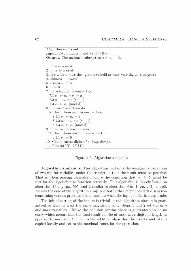
62 CHAPTER 4. BASIC ARITHMETIC
Algorithm s mp sub.Input. Two mp ints a and b (|a| ≥ |b|)Output. The unsigned subtraction c = |a| − |b|.
1. min← b.used2. max← a.used3. If c.alloc < max then grow c to hold at least max digits. (mp grow)4. oldused← c.used5. c.used← max6. u← 07. for n from 0 to min− 1 do7.1 cn ← an − bn − u7.2 u← cn >> (γ − 1)7.3 cn ← cn (mod β)
8. if min < max then do8.1 for n from min to max− 1 do8.1.1 cn ← an − u8.1.2 u← cn >> (γ − 1)8.1.3 cn ← cn (mod β)
9. if oldused > max then do9.1 for n from max to oldused− 1 do9.1.1 cn ← 0
10. Clamp excess digits of c. (mp clamp).11. Return(MP OKAY ).
Figure 4.2: Algorithm s mp sub
Algorithm s mp sub. This algorithm performs the unsigned subtractionof two mp int variables under the restriction that the result must be positive.That is when passing variables a and b the condition that |a| ≥ |b| must bemet for the algorithm to function correctly. This algorithm is loosely based onalgorithm 14.9 [2, pp. 595] and is similar to algorithm S in [1, pp. 267] as well.As was the case of the algorithm s mp add both other references lack discussionconcerning various practical details such as when the inputs differ in magnitude.
The initial sorting of the inputs is trivial in this algorithm since a is guar-anteed to have at least the same magnitude of b. Steps 1 and 2 set the minand max variables. Unlike the addition routine there is guaranteed to be nocarry which means that the final result can be at most max digits in length asopposed to max + 1. Similar to the addition algorithm the used count of c iscopied locally and set to the maximal count for the operation.
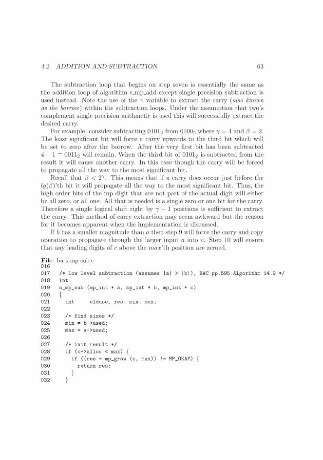
4.2. ADDITION AND SUBTRACTION 63
The subtraction loop that begins on step seven is essentially the same asthe addition loop of algorithm s mp add except single precision subtraction isused instead. Note the use of the γ variable to extract the carry (also known
as the borrow) within the subtraction loops. Under the assumption that two’scomplement single precision arithmetic is used this will successfully extract thedesired carry.
For example, consider subtracting 01012 from 01002 where γ = 4 and β = 2.The least significant bit will force a carry upwards to the third bit which willbe set to zero after the borrow. After the very first bit has been subtracted4 − 1 ≡ 00112 will remain, When the third bit of 01012 is subtracted from theresult it will cause another carry. In this case though the carry will be forcedto propagate all the way to the most significant bit.
Recall that β < 2γ . This means that if a carry does occur just before thelg(β)’th bit it will propagate all the way to the most significant bit. Thus, thehigh order bits of the mp digit that are not part of the actual digit will eitherbe all zero, or all one. All that is needed is a single zero or one bit for the carry.Therefore a single logical shift right by γ − 1 positions is sufficient to extractthe carry. This method of carry extraction may seem awkward but the reasonfor it becomes apparent when the implementation is discussed.
If b has a smaller magnitude than a then step 9 will force the carry and copyoperation to propagate through the larger input a into c. Step 10 will ensurethat any leading digits of c above the max’th position are zeroed.
File: bn s mp sub.c016
017 /* low level subtraction (assumes |a| > |b|), HAC pp.595 Algorithm 14.9 */
018 int
019 s_mp_sub (mp_int * a, mp_int * b, mp_int * c)
020 {021 int olduse, res, min, max;
022
023 /* find sizes */
024 min = b->used;
025 max = a->used;
026
027 /* init result */
028 if (c->alloc < max) {029 if ((res = mp_grow (c, max)) != MP_OKAY) {030 return res;
031 }032 }
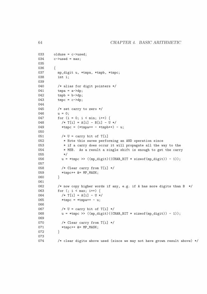
64 CHAPTER 4. BASIC ARITHMETIC
033 olduse = c->used;
034 c->used = max;
035
036 {037 mp_digit u, *tmpa, *tmpb, *tmpc;
038 int i;
039
040 /* alias for digit pointers */
041 tmpa = a->dp;
042 tmpb = b->dp;
043 tmpc = c->dp;
044
045 /* set carry to zero */
046 u = 0;
047 for (i = 0; i < min; i++) {048 /* T[i] = A[i] - B[i] - U */
049 *tmpc = (*tmpa++ - *tmpb++) - u;
050
051 /* U = carry bit of T[i]
052 * Note this saves performing an AND operation since
053 * if a carry does occur it will propagate all the way to the
054 * MSB. As a result a single shift is enough to get the carry
055 */
056 u = *tmpc >> ((mp_digit)((CHAR_BIT * sizeof(mp_digit)) - 1));
057
058 /* Clear carry from T[i] */
059 *tmpc++ &= MP_MASK;
060 }061
062 /* now copy higher words if any, e.g. if A has more digits than B */
063 for (; i < max; i++) {064 /* T[i] = A[i] - U */
065 *tmpc = *tmpa++ - u;
066
067 /* U = carry bit of T[i] */
068 u = *tmpc >> ((mp_digit)((CHAR_BIT * sizeof(mp_digit)) - 1));
069
070 /* Clear carry from T[i] */
071 *tmpc++ &= MP_MASK;
072 }073
074 /* clear digits above used (since we may not have grown result above) */
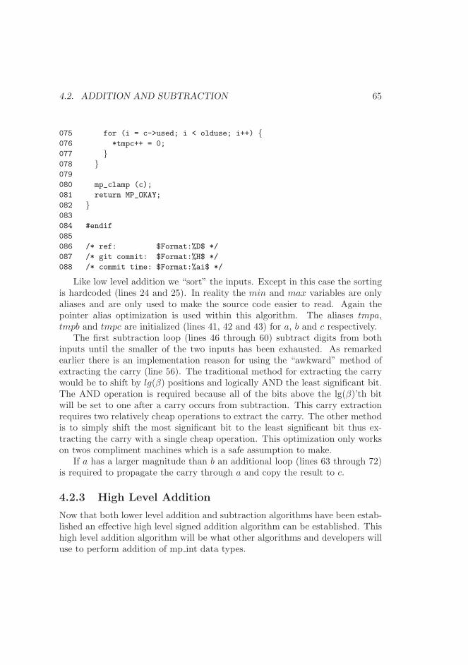
4.2. ADDITION AND SUBTRACTION 65
075 for (i = c->used; i < olduse; i++) {076 *tmpc++ = 0;
077 }078 }079
080 mp_clamp (c);
081 return MP_OKAY;
082 }083
084 #endif
085
086 /* ref: $Format:%D$ */
087 /* git commit: $Format:%H$ */
088 /* commit time: $Format:%ai$ */
Like low level addition we “sort” the inputs. Except in this case the sortingis hardcoded (lines 24 and 25). In reality the min and max variables are onlyaliases and are only used to make the source code easier to read. Again thepointer alias optimization is used within this algorithm. The aliases tmpa,tmpb and tmpc are initialized (lines 41, 42 and 43) for a, b and c respectively.
The first subtraction loop (lines 46 through 60) subtract digits from bothinputs until the smaller of the two inputs has been exhausted. As remarkedearlier there is an implementation reason for using the “awkward” method ofextracting the carry (line 56). The traditional method for extracting the carrywould be to shift by lg(β) positions and logically AND the least significant bit.The AND operation is required because all of the bits above the lg(β)’th bitwill be set to one after a carry occurs from subtraction. This carry extractionrequires two relatively cheap operations to extract the carry. The other methodis to simply shift the most significant bit to the least significant bit thus ex-tracting the carry with a single cheap operation. This optimization only workson twos compliment machines which is a safe assumption to make.
If a has a larger magnitude than b an additional loop (lines 63 through 72)is required to propagate the carry through a and copy the result to c.
4.2.3 High Level Addition
Now that both lower level addition and subtraction algorithms have been estab-lished an effective high level signed addition algorithm can be established. Thishigh level addition algorithm will be what other algorithms and developers willuse to perform addition of mp int data types.
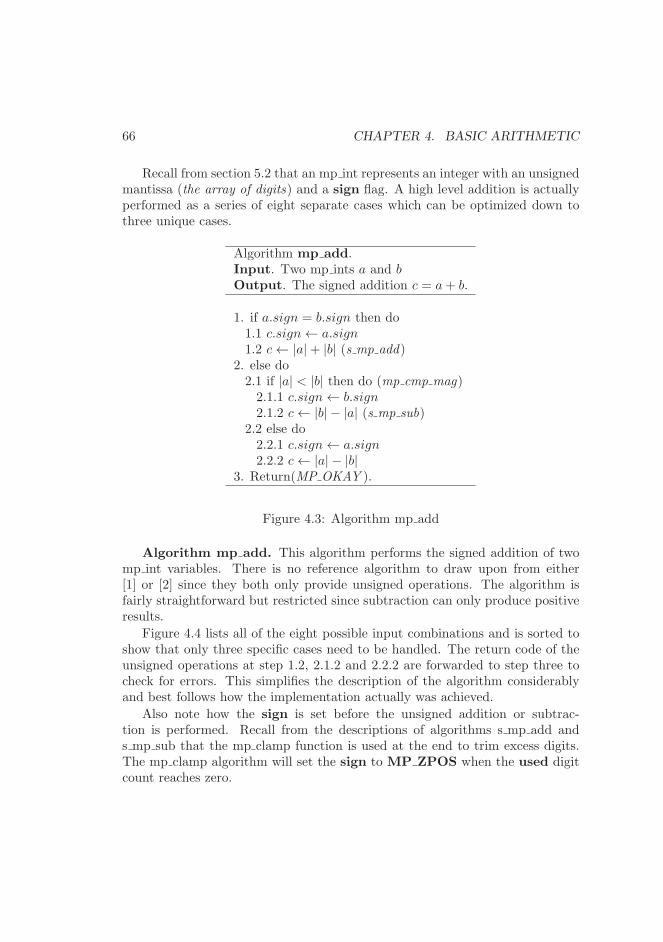
66 CHAPTER 4. BASIC ARITHMETIC
Recall from section 5.2 that an mp int represents an integer with an unsignedmantissa (the array of digits) and a sign flag. A high level addition is actuallyperformed as a series of eight separate cases which can be optimized down tothree unique cases.
Algorithm mp add.Input. Two mp ints a and bOutput. The signed addition c = a+ b.
1. if a.sign = b.sign then do1.1 c.sign← a.sign1.2 c← |a|+ |b| (s mp add)
2. else do2.1 if |a| < |b| then do (mp cmp mag)2.1.1 c.sign← b.sign2.1.2 c← |b| − |a| (s mp sub)
2.2 else do2.2.1 c.sign← a.sign2.2.2 c← |a| − |b|
3. Return(MP OKAY ).
Figure 4.3: Algorithm mp add
Algorithm mp add. This algorithm performs the signed addition of twomp int variables. There is no reference algorithm to draw upon from either[1] or [2] since they both only provide unsigned operations. The algorithm isfairly straightforward but restricted since subtraction can only produce positiveresults.
Figure 4.4 lists all of the eight possible input combinations and is sorted toshow that only three specific cases need to be handled. The return code of theunsigned operations at step 1.2, 2.1.2 and 2.2.2 are forwarded to step three tocheck for errors. This simplifies the description of the algorithm considerablyand best follows how the implementation actually was achieved.
Also note how the sign is set before the unsigned addition or subtrac-tion is performed. Recall from the descriptions of algorithms s mp add ands mp sub that the mp clamp function is used at the end to trim excess digits.The mp clamp algorithm will set the sign to MP ZPOS when the used digitcount reaches zero.
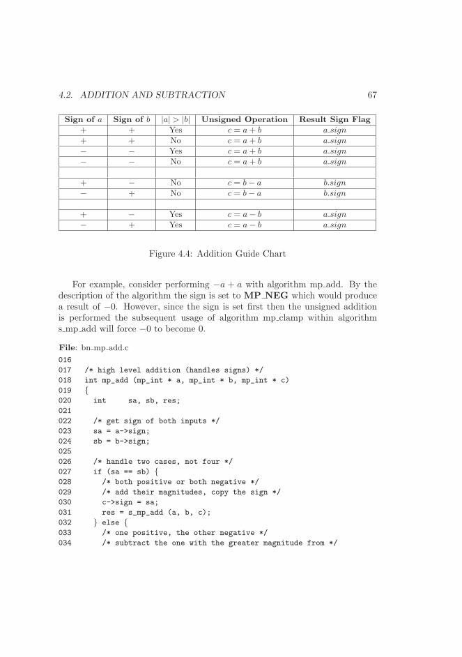
4.2. ADDITION AND SUBTRACTION 67
Sign of a Sign of b |a| > |b| Unsigned Operation Result Sign Flag
+ + Yes c = a+ b a.sign
+ + No c = a+ b a.sign
− − Yes c = a+ b a.sign
− − No c = a+ b a.sign
+ − No c = b− a b.sign
− + No c = b− a b.sign
+ − Yes c = a− b a.sign
− + Yes c = a− b a.sign
Figure 4.4: Addition Guide Chart
For example, consider performing −a + a with algorithm mp add. By thedescription of the algorithm the sign is set to MP NEG which would producea result of −0. However, since the sign is set first then the unsigned additionis performed the subsequent usage of algorithm mp clamp within algorithms mp add will force −0 to become 0.
File: bn mp add.c
016
017 /* high level addition (handles signs) */
018 int mp_add (mp_int * a, mp_int * b, mp_int * c)
019 {020 int sa, sb, res;
021
022 /* get sign of both inputs */
023 sa = a->sign;
024 sb = b->sign;
025
026 /* handle two cases, not four */
027 if (sa == sb) {028 /* both positive or both negative */
029 /* add their magnitudes, copy the sign */
030 c->sign = sa;
031 res = s_mp_add (a, b, c);
032 } else {033 /* one positive, the other negative */
034 /* subtract the one with the greater magnitude from */
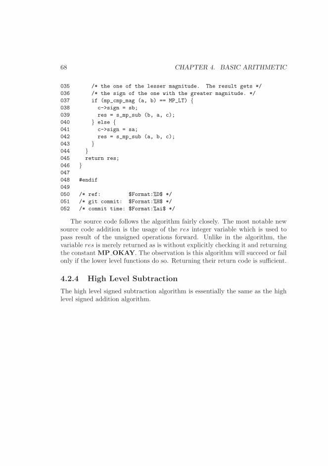
68 CHAPTER 4. BASIC ARITHMETIC
035 /* the one of the lesser magnitude. The result gets */
036 /* the sign of the one with the greater magnitude. */
037 if (mp_cmp_mag (a, b) == MP_LT) {038 c->sign = sb;
039 res = s_mp_sub (b, a, c);
040 } else {041 c->sign = sa;
042 res = s_mp_sub (a, b, c);
043 }044 }045 return res;
046 }047
048 #endif
049
050 /* ref: $Format:%D$ */
051 /* git commit: $Format:%H$ */
052 /* commit time: $Format:%ai$ */
The source code follows the algorithm fairly closely. The most notable newsource code addition is the usage of the res integer variable which is used topass result of the unsigned operations forward. Unlike in the algorithm, thevariable res is merely returned as is without explicitly checking it and returningthe constant MP OKAY. The observation is this algorithm will succeed or failonly if the lower level functions do so. Returning their return code is sufficient.
4.2.4 High Level Subtraction
The high level signed subtraction algorithm is essentially the same as the highlevel signed addition algorithm.
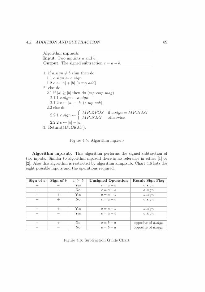
4.2. ADDITION AND SUBTRACTION 69
Algorithm mp sub.Input. Two mp ints a and bOutput. The signed subtraction c = a− b.
1. if a.sign 6= b.sign then do1.1 c.sign← a.sign1.2 c← |a|+ |b| (s mp add)
2. else do2.1 if |a| ≥ |b| then do (mp cmp mag)2.1.1 c.sign← a.sign2.1.2 c← |a| − |b| (s mp sub)
2.2 else do
2.2.1 c.sign←{
MP ZPOS if a.sign = MP NEGMP NEG otherwise
2.2.2 c← |b| − |a|3. Return(MP OKAY ).
Figure 4.5: Algorithm mp sub
Algorithm mp sub. This algorithm performs the signed subtraction oftwo inputs. Similar to algorithm mp add there is no reference in either [1] or[2]. Also this algorithm is restricted by algorithm s mp sub. Chart 4.6 lists theeight possible inputs and the operations required.
Sign of a Sign of b |a| ≥ |b| Unsigned Operation Result Sign Flag
+ − Yes c = a+ b a.sign
+ − No c = a+ b a.sign
− + Yes c = a+ b a.sign
− + No c = a+ b a.sign
+ + Yes c = a− b a.sign
− − Yes c = a− b a.sign
+ + No c = b− a opposite of a.sign
− − No c = b− a opposite of a.sign
Figure 4.6: Subtraction Guide Chart
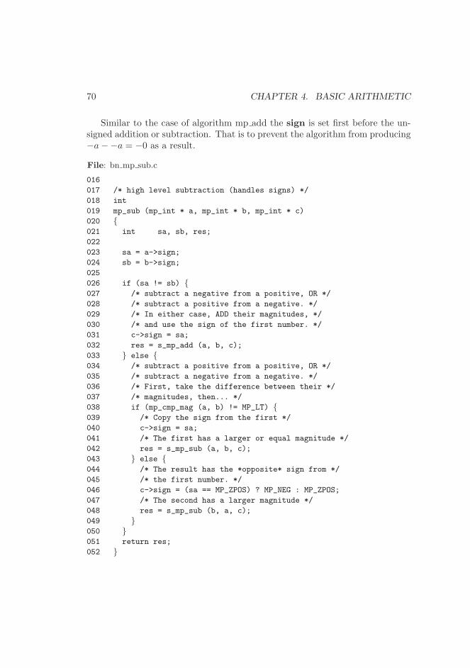
70 CHAPTER 4. BASIC ARITHMETIC
Similar to the case of algorithm mp add the sign is set first before the un-signed addition or subtraction. That is to prevent the algorithm from producing−a−−a = −0 as a result.
File: bn mp sub.c
016
017 /* high level subtraction (handles signs) */
018 int
019 mp_sub (mp_int * a, mp_int * b, mp_int * c)
020 {021 int sa, sb, res;
022
023 sa = a->sign;
024 sb = b->sign;
025
026 if (sa != sb) {027 /* subtract a negative from a positive, OR */
028 /* subtract a positive from a negative. */
029 /* In either case, ADD their magnitudes, */
030 /* and use the sign of the first number. */
031 c->sign = sa;
032 res = s_mp_add (a, b, c);
033 } else {034 /* subtract a positive from a positive, OR */
035 /* subtract a negative from a negative. */
036 /* First, take the difference between their */
037 /* magnitudes, then... */
038 if (mp_cmp_mag (a, b) != MP_LT) {039 /* Copy the sign from the first */
040 c->sign = sa;
041 /* The first has a larger or equal magnitude */
042 res = s_mp_sub (a, b, c);
043 } else {044 /* The result has the *opposite* sign from */
045 /* the first number. */
046 c->sign = (sa == MP_ZPOS) ? MP_NEG : MP_ZPOS;
047 /* The second has a larger magnitude */
048 res = s_mp_sub (b, a, c);
049 }050 }051 return res;
052 }
4.3. BIT AND DIGIT SHIFTING 71
053
054 #endif
055
056 /* ref: $Format:%D$ */
057 /* git commit: $Format:%H$ */
058 /* commit time: $Format:%ai$ */
Much like the implementation of algorithm mp add the variable res is usedto catch the return code of the unsigned addition or subtraction operations andforward it to the end of the function. On line 38 the “not equal to” MP LTexpression is used to emulate a “greater than or equal to” comparison.
4.3 Bit and Digit Shifting
It is quite common to think of a multiple precision integer as a polynomial inx, that is y = f(β) where f(x) =
∑n−1i=0 aix
i. This notation arises within dis-cussion of Montgomery and Diminished Radix Reduction as well as Karatsubamultiplication and squaring.
In order to facilitate operations on polynomials in x as above a series ofsimple “digit” algorithms have to be established. That is to shift the digits leftor right as well to shift individual bits of the digits left and right. It is importantto note that not all “shift” operations are on radix-β digits.
4.3.1 Multiplication by Two
In a binary system where the radix is a power of two multiplication by two notonly arises often in other algorithms it is a fairly efficient operation to perform.A single precision logical shift left is sufficient to multiply a single digit by two.
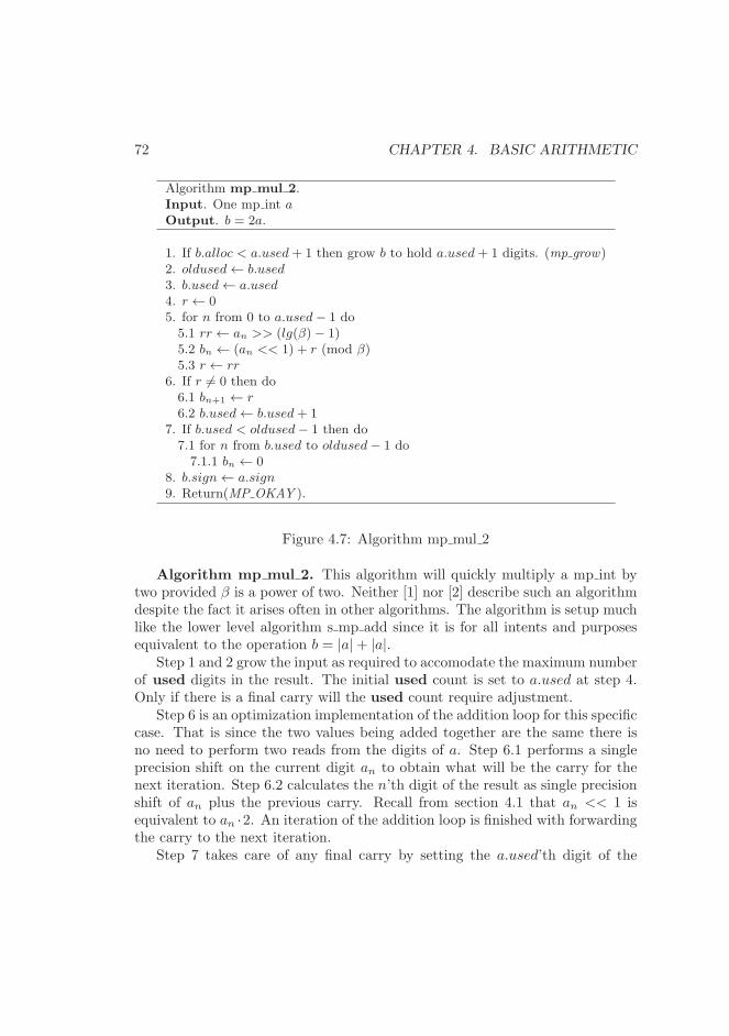
72 CHAPTER 4. BASIC ARITHMETIC
Algorithm mp mul 2.Input. One mp int aOutput. b = 2a.
1. If b.alloc < a.used+ 1 then grow b to hold a.used+ 1 digits. (mp grow)2. oldused← b.used3. b.used← a.used4. r ← 05. for n from 0 to a.used− 1 do5.1 rr ← an >> (lg(β)− 1)5.2 bn ← (an << 1) + r (mod β)5.3 r ← rr
6. If r 6= 0 then do6.1 bn+1 ← r6.2 b.used← b.used+ 1
7. If b.used < oldused− 1 then do7.1 for n from b.used to oldused− 1 do7.1.1 bn ← 0
8. b.sign← a.sign9. Return(MP OKAY ).
Figure 4.7: Algorithm mp mul 2
Algorithm mp mul 2. This algorithm will quickly multiply a mp int bytwo provided β is a power of two. Neither [1] nor [2] describe such an algorithmdespite the fact it arises often in other algorithms. The algorithm is setup muchlike the lower level algorithm s mp add since it is for all intents and purposesequivalent to the operation b = |a|+ |a|.
Step 1 and 2 grow the input as required to accomodate the maximum numberof used digits in the result. The initial used count is set to a.used at step 4.Only if there is a final carry will the used count require adjustment.
Step 6 is an optimization implementation of the addition loop for this specificcase. That is since the two values being added together are the same there isno need to perform two reads from the digits of a. Step 6.1 performs a singleprecision shift on the current digit an to obtain what will be the carry for thenext iteration. Step 6.2 calculates the n’th digit of the result as single precisionshift of an plus the previous carry. Recall from section 4.1 that an << 1 isequivalent to an ·2. An iteration of the addition loop is finished with forwardingthe carry to the next iteration.
Step 7 takes care of any final carry by setting the a.used’th digit of the
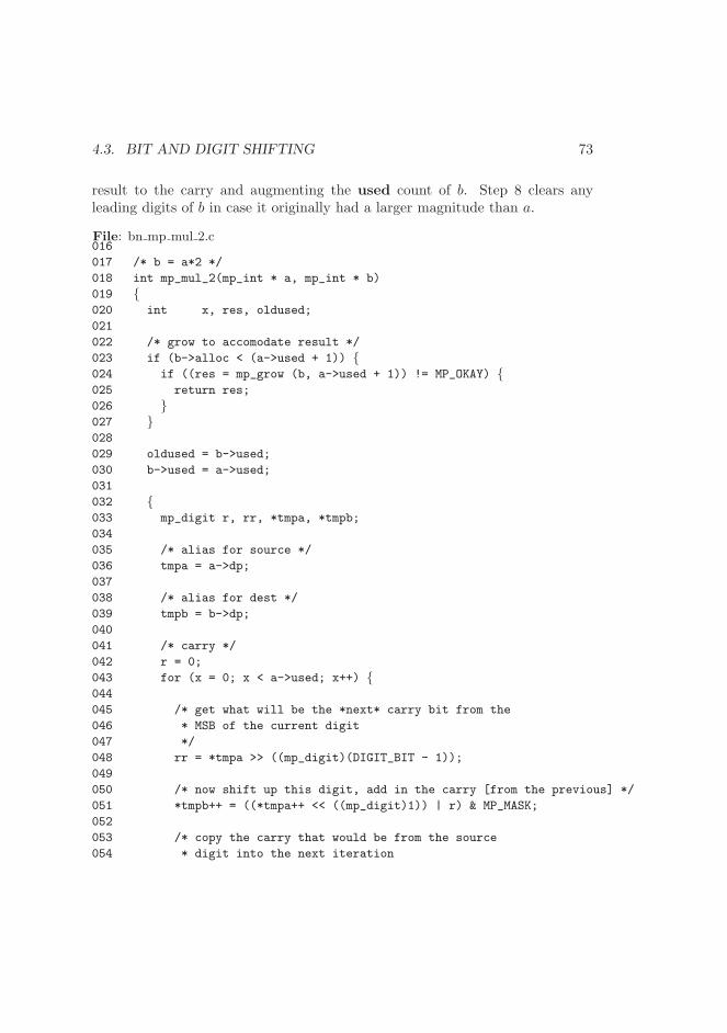
4.3. BIT AND DIGIT SHIFTING 73
result to the carry and augmenting the used count of b. Step 8 clears anyleading digits of b in case it originally had a larger magnitude than a.
File: bn mp mul 2.c016
017 /* b = a*2 */
018 int mp_mul_2(mp_int * a, mp_int * b)
019 {020 int x, res, oldused;
021
022 /* grow to accomodate result */
023 if (b->alloc < (a->used + 1)) {024 if ((res = mp_grow (b, a->used + 1)) != MP_OKAY) {025 return res;
026 }027 }028
029 oldused = b->used;
030 b->used = a->used;
031
032 {033 mp_digit r, rr, *tmpa, *tmpb;
034
035 /* alias for source */
036 tmpa = a->dp;
037
038 /* alias for dest */
039 tmpb = b->dp;
040
041 /* carry */
042 r = 0;
043 for (x = 0; x < a->used; x++) {044
045 /* get what will be the *next* carry bit from the
046 * MSB of the current digit
047 */
048 rr = *tmpa >> ((mp_digit)(DIGIT_BIT - 1));
049
050 /* now shift up this digit, add in the carry [from the previous] */
051 *tmpb++ = ((*tmpa++ << ((mp_digit)1)) | r) & MP_MASK;
052
053 /* copy the carry that would be from the source
054 * digit into the next iteration
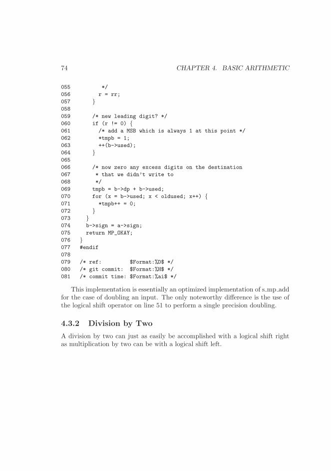
74 CHAPTER 4. BASIC ARITHMETIC
055 */
056 r = rr;
057 }058
059 /* new leading digit? */
060 if (r != 0) {061 /* add a MSB which is always 1 at this point */
062 *tmpb = 1;
063 ++(b->used);
064 }065
066 /* now zero any excess digits on the destination
067 * that we didn’t write to
068 */
069 tmpb = b->dp + b->used;
070 for (x = b->used; x < oldused; x++) {071 *tmpb++ = 0;
072 }073 }074 b->sign = a->sign;
075 return MP_OKAY;
076 }077 #endif
078
079 /* ref: $Format:%D$ */
080 /* git commit: $Format:%H$ */
081 /* commit time: $Format:%ai$ */
This implementation is essentially an optimized implementation of s mp addfor the case of doubling an input. The only noteworthy difference is the use ofthe logical shift operator on line 51 to perform a single precision doubling.
4.3.2 Division by Two
A division by two can just as easily be accomplished with a logical shift rightas multiplication by two can be with a logical shift left.
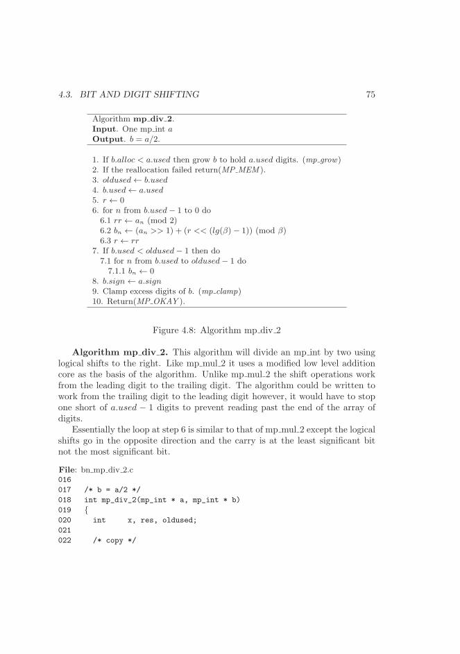
4.3. BIT AND DIGIT SHIFTING 75
Algorithm mp div 2.Input. One mp int aOutput. b = a/2.
1. If b.alloc < a.used then grow b to hold a.used digits. (mp grow)2. If the reallocation failed return(MP MEM ).3. oldused← b.used4. b.used← a.used5. r ← 06. for n from b.used− 1 to 0 do6.1 rr ← an (mod 2)6.2 bn ← (an >> 1) + (r << (lg(β)− 1)) (mod β)6.3 r ← rr
7. If b.used < oldused− 1 then do7.1 for n from b.used to oldused− 1 do7.1.1 bn ← 0
8. b.sign← a.sign9. Clamp excess digits of b. (mp clamp)10. Return(MP OKAY ).
Figure 4.8: Algorithm mp div 2
Algorithm mp div 2. This algorithm will divide an mp int by two usinglogical shifts to the right. Like mp mul 2 it uses a modified low level additioncore as the basis of the algorithm. Unlike mp mul 2 the shift operations workfrom the leading digit to the trailing digit. The algorithm could be written towork from the trailing digit to the leading digit however, it would have to stopone short of a.used − 1 digits to prevent reading past the end of the array ofdigits.
Essentially the loop at step 6 is similar to that of mp mul 2 except the logicalshifts go in the opposite direction and the carry is at the least significant bitnot the most significant bit.
File: bn mp div 2.c016
017 /* b = a/2 */
018 int mp_div_2(mp_int * a, mp_int * b)
019 {020 int x, res, oldused;
021
022 /* copy */
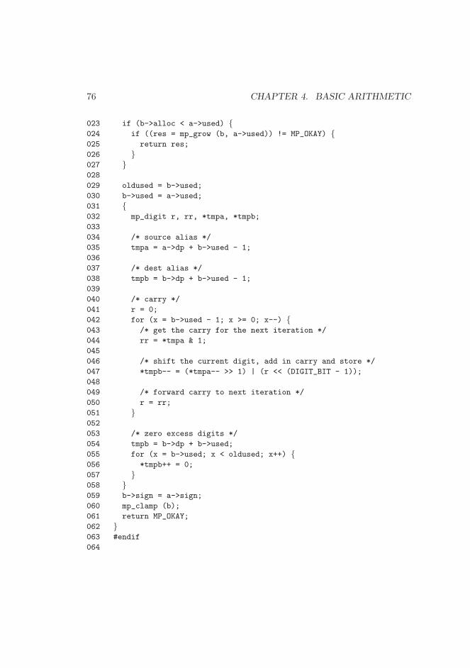
76 CHAPTER 4. BASIC ARITHMETIC
023 if (b->alloc < a->used) {024 if ((res = mp_grow (b, a->used)) != MP_OKAY) {025 return res;
026 }027 }028
029 oldused = b->used;
030 b->used = a->used;
031 {032 mp_digit r, rr, *tmpa, *tmpb;
033
034 /* source alias */
035 tmpa = a->dp + b->used - 1;
036
037 /* dest alias */
038 tmpb = b->dp + b->used - 1;
039
040 /* carry */
041 r = 0;
042 for (x = b->used - 1; x >= 0; x--) {043 /* get the carry for the next iteration */
044 rr = *tmpa & 1;
045
046 /* shift the current digit, add in carry and store */
047 *tmpb-- = (*tmpa-- >> 1) | (r << (DIGIT_BIT - 1));
048
049 /* forward carry to next iteration */
050 r = rr;
051 }052
053 /* zero excess digits */
054 tmpb = b->dp + b->used;
055 for (x = b->used; x < oldused; x++) {056 *tmpb++ = 0;
057 }058 }059 b->sign = a->sign;
060 mp_clamp (b);
061 return MP_OKAY;
062 }063 #endif
064
4.4. POLYNOMIAL BASIS OPERATIONS 77
065 /* ref: $Format:%D$ */
066 /* git commit: $Format:%H$ */
067 /* commit time: $Format:%ai$ */
4.4 Polynomial Basis Operations
Recall from section 4.3 that any integer can be represented as a polynomial inx as y = f(β). Such a representation is also known as the polynomial basis[3, pp. 48]. Given such a notation a multiplication or division by x amountsto shifting whole digits a single place. The need for such operations arises inseveral other higher level algorithms such as Barrett and Montgomery reduction,integer division and Karatsuba multiplication.
Converting from an array of digits to polynomial basis is very simple. Con-sider the integer y ≡ (a2, a1, a0)β and recall that y =
∑2i=0 aiβ
i. Simplyreplace β with x and the expression is in polynomial basis. For example,f(x) = 8x + 9 is the polynomial basis representation for 89 using radix ten.That is, f(10) = 8(10) + 9 = 89.
4.4.1 Multiplication by x
Given a polynomial in x such as f(x) = anxn + an−1x
n−1 + ...+ a0 multiplyingby x amounts to shifting the coefficients up one degree. In this case f(x) · x =anx
n+1 + an−1xn + ...+ a0x. From a scalar basis point of view multiplying by
x is equivalent to multiplying by the integer β.
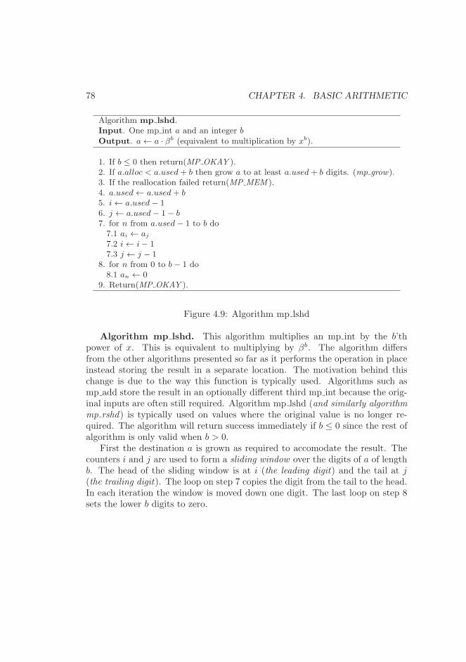
78 CHAPTER 4. BASIC ARITHMETIC
Algorithm mp lshd.Input. One mp int a and an integer b
Output. a← a · βb (equivalent to multiplication by xb).
1. If b ≤ 0 then return(MP OKAY ).2. If a.alloc < a.used+ b then grow a to at least a.used+ b digits. (mp grow).3. If the reallocation failed return(MP MEM ).4. a.used← a.used+ b5. i← a.used− 16. j ← a.used− 1− b7. for n from a.used− 1 to b do7.1 ai ← aj
7.2 i← i− 17.3 j ← j − 1
8. for n from 0 to b− 1 do8.1 an ← 0
9. Return(MP OKAY ).
Figure 4.9: Algorithm mp lshd
Algorithm mp lshd. This algorithm multiplies an mp int by the b’thpower of x. This is equivalent to multiplying by βb. The algorithm differsfrom the other algorithms presented so far as it performs the operation in placeinstead storing the result in a separate location. The motivation behind thischange is due to the way this function is typically used. Algorithms such asmp add store the result in an optionally different third mp int because the orig-inal inputs are often still required. Algorithm mp lshd (and similarly algorithm
mp rshd) is typically used on values where the original value is no longer re-quired. The algorithm will return success immediately if b ≤ 0 since the rest ofalgorithm is only valid when b > 0.
First the destination a is grown as required to accomodate the result. Thecounters i and j are used to form a sliding window over the digits of a of lengthb. The head of the sliding window is at i (the leading digit) and the tail at j(the trailing digit). The loop on step 7 copies the digit from the tail to the head.In each iteration the window is moved down one digit. The last loop on step 8sets the lower b digits to zero.
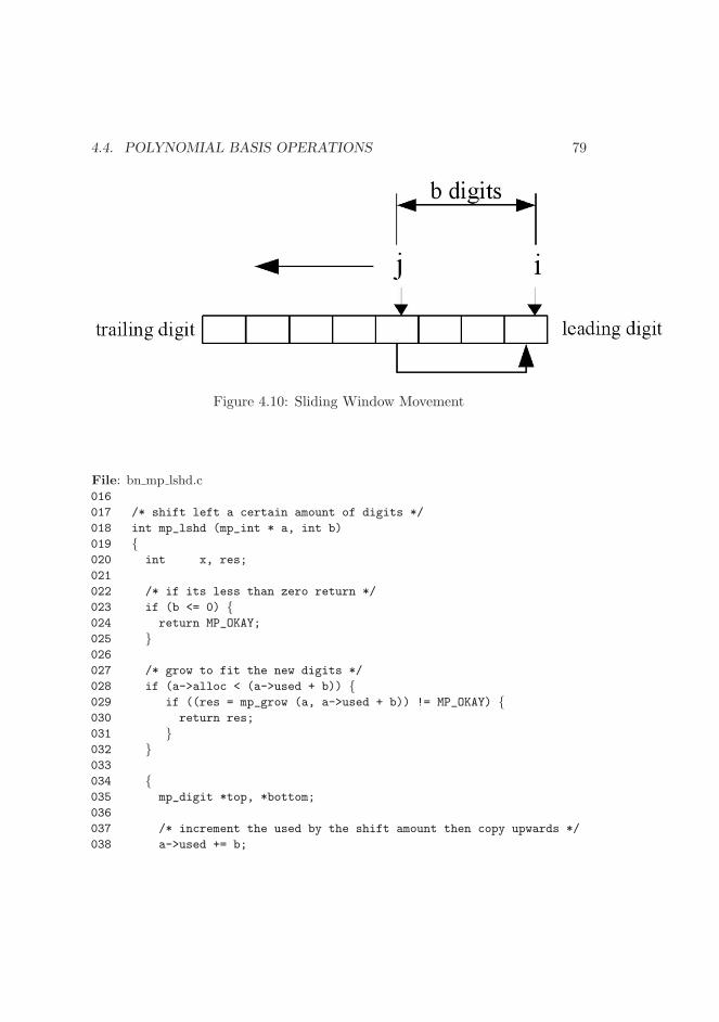
4.4. POLYNOMIAL BASIS OPERATIONS 79
Figure 4.10: Sliding Window Movement
File: bn mp lshd.c016
017 /* shift left a certain amount of digits */
018 int mp_lshd (mp_int * a, int b)
019 {020 int x, res;
021
022 /* if its less than zero return */
023 if (b <= 0) {024 return MP_OKAY;
025 }026
027 /* grow to fit the new digits */
028 if (a->alloc < (a->used + b)) {029 if ((res = mp_grow (a, a->used + b)) != MP_OKAY) {030 return res;
031 }032 }033
034 {035 mp_digit *top, *bottom;
036
037 /* increment the used by the shift amount then copy upwards */
038 a->used += b;
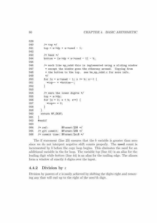
80 CHAPTER 4. BASIC ARITHMETIC
039
040 /* top */
041 top = a->dp + a->used - 1;
042
043 /* base */
044 bottom = (a->dp + a->used - 1) - b;
045
046 /* much like mp_rshd this is implemented using a sliding window
047 * except the window goes the otherway around. Copying from
048 * the bottom to the top. see bn_mp_rshd.c for more info.
049 */
050 for (x = a->used - 1; x >= b; x--) {051 *top-- = *bottom--;
052 }053
054 /* zero the lower digits */
055 top = a->dp;
056 for (x = 0; x < b; x++) {057 *top++ = 0;
058 }059 }060 return MP_OKAY;
061 }062 #endif
063
064 /* ref: $Format:%D$ */
065 /* git commit: $Format:%H$ */
066 /* commit time: $Format:%ai$ */
The if statement (line 23) ensures that the b variable is greater than zerosince we do not interpret negative shift counts properly. The used count isincremented by b before the copy loop begins. This elminates the need for anadditional variable in the for loop. The variable top (line 41) is an alias for theleading digit while bottom (line 44) is an alias for the trailing edge. The aliasesform a window of exactly b digits over the input.
4.4.2 Division by x
Division by powers of x is easily achieved by shifting the digits right and remov-ing any that will end up to the right of the zero’th digit.
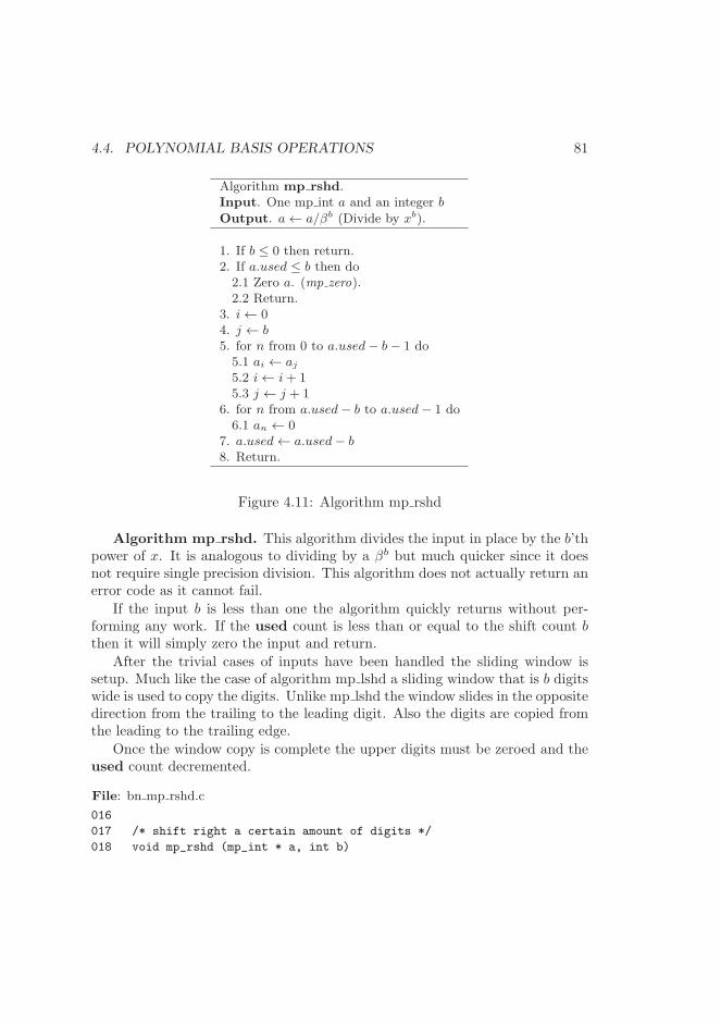
4.4. POLYNOMIAL BASIS OPERATIONS 81
Algorithm mp rshd.Input. One mp int a and an integer b
Output. a← a/βb (Divide by xb).
1. If b ≤ 0 then return.2. If a.used ≤ b then do2.1 Zero a. (mp zero).2.2 Return.
3. i← 04. j ← b5. for n from 0 to a.used− b− 1 do5.1 ai ← aj
5.2 i← i+ 15.3 j ← j + 1
6. for n from a.used− b to a.used− 1 do6.1 an ← 0
7. a.used← a.used− b8. Return.
Figure 4.11: Algorithm mp rshd
Algorithm mp rshd. This algorithm divides the input in place by the b’thpower of x. It is analogous to dividing by a βb but much quicker since it doesnot require single precision division. This algorithm does not actually return anerror code as it cannot fail.
If the input b is less than one the algorithm quickly returns without per-forming any work. If the used count is less than or equal to the shift count bthen it will simply zero the input and return.
After the trivial cases of inputs have been handled the sliding window issetup. Much like the case of algorithm mp lshd a sliding window that is b digitswide is used to copy the digits. Unlike mp lshd the window slides in the oppositedirection from the trailing to the leading digit. Also the digits are copied fromthe leading to the trailing edge.
Once the window copy is complete the upper digits must be zeroed and theused count decremented.
File: bn mp rshd.c
016
017 /* shift right a certain amount of digits */
018 void mp_rshd (mp_int * a, int b)
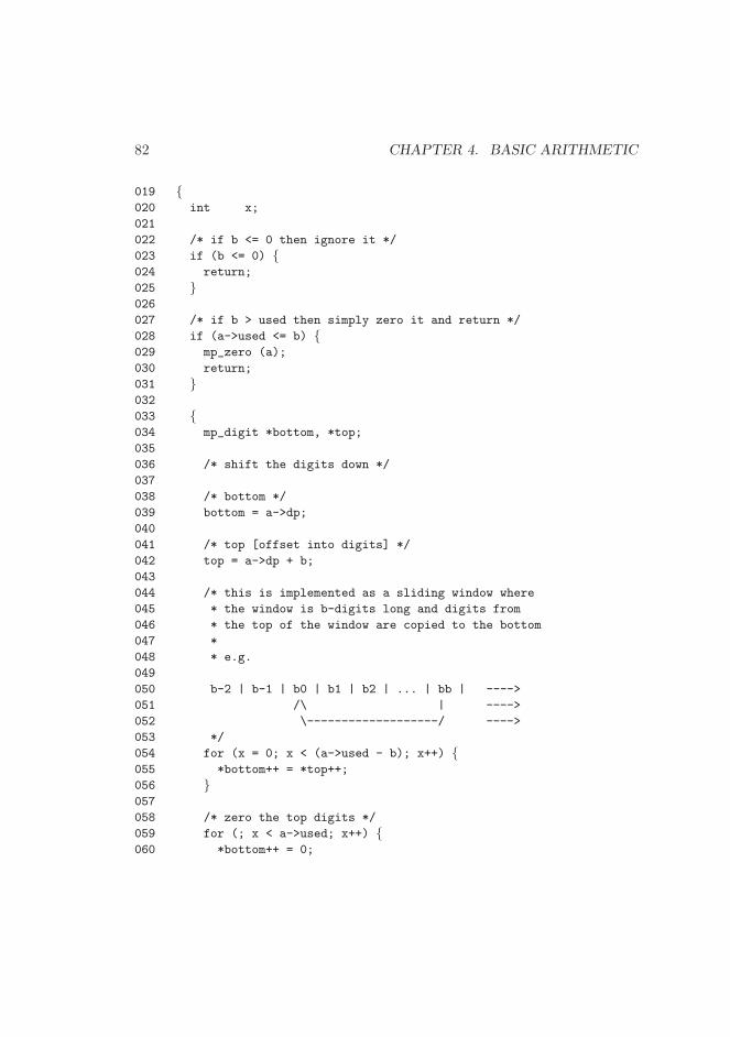
82 CHAPTER 4. BASIC ARITHMETIC
019 {020 int x;
021
022 /* if b <= 0 then ignore it */
023 if (b <= 0) {024 return;
025 }026
027 /* if b > used then simply zero it and return */
028 if (a->used <= b) {029 mp_zero (a);
030 return;
031 }032
033 {034 mp_digit *bottom, *top;
035
036 /* shift the digits down */
037
038 /* bottom */
039 bottom = a->dp;
040
041 /* top [offset into digits] */
042 top = a->dp + b;
043
044 /* this is implemented as a sliding window where
045 * the window is b-digits long and digits from
046 * the top of the window are copied to the bottom
047 *
048 * e.g.
049
050 b-2 | b-1 | b0 | b1 | b2 | ... | bb | ---->
051 /\ | ---->
052 \-------------------/ ---->
053 */
054 for (x = 0; x < (a->used - b); x++) {055 *bottom++ = *top++;
056 }057
058 /* zero the top digits */
059 for (; x < a->used; x++) {060 *bottom++ = 0;
4.5. POWERS OF TWO 83
061 }062 }063
064 /* remove excess digits */
065 a->used -= b;
066 }067 #endif
068
069 /* ref: $Format:%D$ */
070 /* git commit: $Format:%H$ */
071 /* commit time: $Format:%ai$ */
The only noteworthy element of this routine is the lack of a return type sinceit cannot fail. Like mp lshd() we form a sliding window except we copy in theother direction. After the window (line 59) we then zero the upper digits of theinput to make sure the result is correct.
4.5 Powers of Two
Now that algorithms for moving single bits as well as whole digits exist algo-rithms for moving the “in between” distances are required. For example, toquickly multiply by 2k for any k without using a full multiplier algorithm wouldprove useful. Instead of performing single shifts k times to achieve a multi-plication by 2±k a mixture of whole digit shifting and partial digit shifting isemployed.
4.5.1 Multiplication by Power of Two
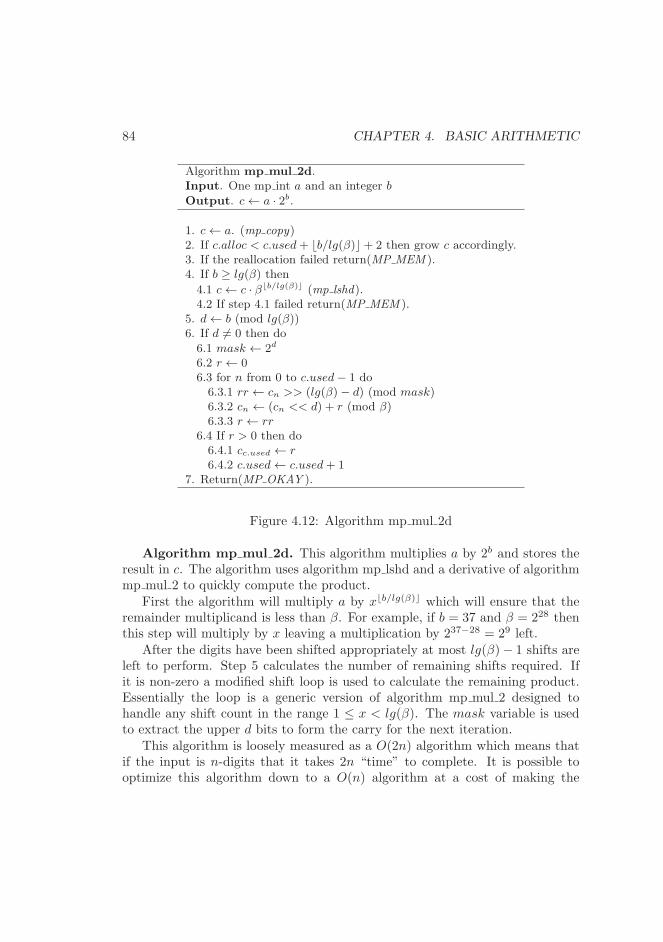
84 CHAPTER 4. BASIC ARITHMETIC
Algorithm mp mul 2d.Input. One mp int a and an integer b
Output. c← a · 2b.
1. c← a. (mp copy)2. If c.alloc < c.used+ ⌊b/lg(β)⌋+ 2 then grow c accordingly.3. If the reallocation failed return(MP MEM ).4. If b ≥ lg(β) then
4.1 c← c · β⌊b/lg(β)⌋ (mp lshd).4.2 If step 4.1 failed return(MP MEM ).
5. d← b (mod lg(β))6. If d 6= 0 then do
6.1 mask ← 2d
6.2 r ← 06.3 for n from 0 to c.used− 1 do6.3.1 rr ← cn >> (lg(β)− d) (mod mask)6.3.2 cn ← (cn << d) + r (mod β)6.3.3 r ← rr
6.4 If r > 0 then do6.4.1 cc.used ← r6.4.2 c.used← c.used+ 1
7. Return(MP OKAY ).
Figure 4.12: Algorithm mp mul 2d
Algorithm mp mul 2d. This algorithm multiplies a by 2b and stores theresult in c. The algorithm uses algorithm mp lshd and a derivative of algorithmmp mul 2 to quickly compute the product.
First the algorithm will multiply a by x⌊b/lg(β)⌋ which will ensure that theremainder multiplicand is less than β. For example, if b = 37 and β = 228 thenthis step will multiply by x leaving a multiplication by 237−28 = 29 left.
After the digits have been shifted appropriately at most lg(β)− 1 shifts areleft to perform. Step 5 calculates the number of remaining shifts required. Ifit is non-zero a modified shift loop is used to calculate the remaining product.Essentially the loop is a generic version of algorithm mp mul 2 designed tohandle any shift count in the range 1 ≤ x < lg(β). The mask variable is usedto extract the upper d bits to form the carry for the next iteration.
This algorithm is loosely measured as a O(2n) algorithm which means thatif the input is n-digits that it takes 2n “time” to complete. It is possible tooptimize this algorithm down to a O(n) algorithm at a cost of making the
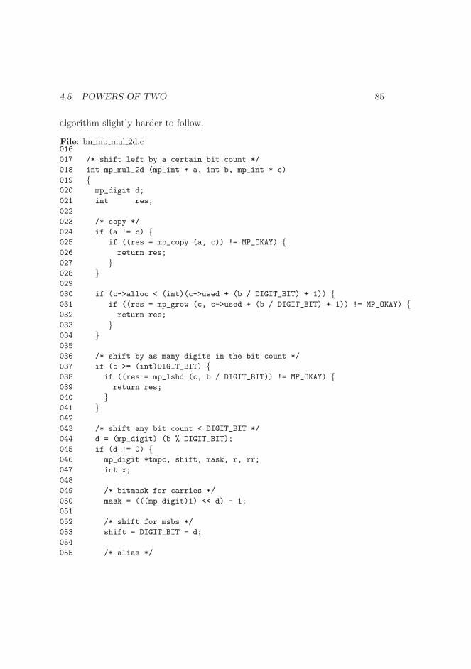
4.5. POWERS OF TWO 85
algorithm slightly harder to follow.
File: bn mp mul 2d.c016
017 /* shift left by a certain bit count */
018 int mp_mul_2d (mp_int * a, int b, mp_int * c)
019 {020 mp_digit d;
021 int res;
022
023 /* copy */
024 if (a != c) {025 if ((res = mp_copy (a, c)) != MP_OKAY) {026 return res;
027 }028 }029
030 if (c->alloc < (int)(c->used + (b / DIGIT_BIT) + 1)) {031 if ((res = mp_grow (c, c->used + (b / DIGIT_BIT) + 1)) != MP_OKAY) {032 return res;
033 }034 }035
036 /* shift by as many digits in the bit count */
037 if (b >= (int)DIGIT_BIT) {038 if ((res = mp_lshd (c, b / DIGIT_BIT)) != MP_OKAY) {039 return res;
040 }041 }042
043 /* shift any bit count < DIGIT_BIT */
044 d = (mp_digit) (b % DIGIT_BIT);
045 if (d != 0) {046 mp_digit *tmpc, shift, mask, r, rr;
047 int x;
048
049 /* bitmask for carries */
050 mask = (((mp_digit)1) << d) - 1;
051
052 /* shift for msbs */
053 shift = DIGIT_BIT - d;
054
055 /* alias */
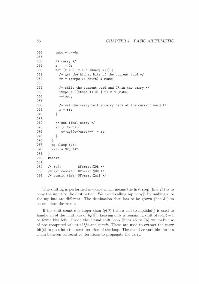
86 CHAPTER 4. BASIC ARITHMETIC
056 tmpc = c->dp;
057
058 /* carry */
059 r = 0;
060 for (x = 0; x < c->used; x++) {061 /* get the higher bits of the current word */
062 rr = (*tmpc >> shift) & mask;
063
064 /* shift the current word and OR in the carry */
065 *tmpc = ((*tmpc << d) | r) & MP_MASK;
066 ++tmpc;
067
068 /* set the carry to the carry bits of the current word */
069 r = rr;
070 }071
072 /* set final carry */
073 if (r != 0) {074 c->dp[(c->used)++] = r;
075 }076 }077 mp_clamp (c);
078 return MP_OKAY;
079 }080 #endif
081
082 /* ref: $Format:%D$ */
083 /* git commit: $Format:%H$ */
084 /* commit time: $Format:%ai$ */
The shifting is performed in–place which means the first step (line 24) is tocopy the input to the destination. We avoid calling mp copy() by making surethe mp ints are different. The destination then has to be grown (line 31) toaccomodate the result.
If the shift count b is larger than lg(β) then a call to mp lshd() is used tohandle all of the multiples of lg(β). Leaving only a remaining shift of lg(β)− 1or fewer bits left. Inside the actual shift loop (lines 45 to 76) we make useof pre–computed values shift and mask. These are used to extract the carrybit(s) to pass into the next iteration of the loop. The r and rr variables form achain between consecutive iterations to propagate the carry.

4.5. POWERS OF TWO 87
4.5.2 Division by Power of Two
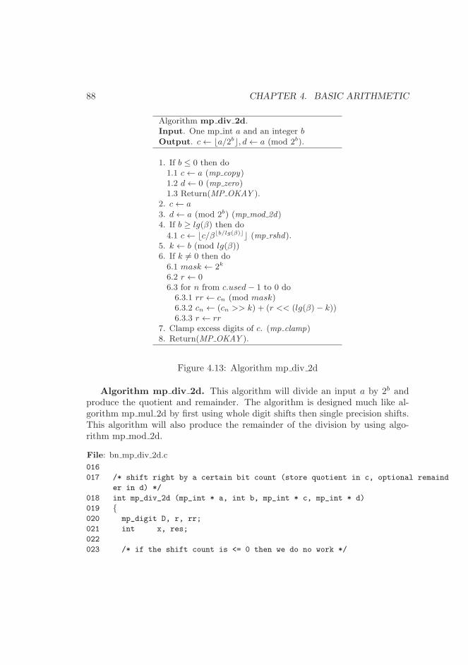
88 CHAPTER 4. BASIC ARITHMETIC
Algorithm mp div 2d.Input. One mp int a and an integer b
Output. c← ⌊a/2b⌋, d← a (mod 2b).
1. If b ≤ 0 then do1.1 c← a (mp copy)1.2 d← 0 (mp zero)1.3 Return(MP OKAY ).
2. c← a
3. d← a (mod 2b) (mp mod 2d)4. If b ≥ lg(β) then do
4.1 c← ⌊c/β⌊b/lg(β)⌋⌋ (mp rshd).5. k ← b (mod lg(β))6. If k 6= 0 then do
6.1 mask ← 2k
6.2 r ← 06.3 for n from c.used− 1 to 0 do6.3.1 rr ← cn (mod mask)6.3.2 cn ← (cn >> k) + (r << (lg(β)− k))6.3.3 r ← rr
7. Clamp excess digits of c. (mp clamp)8. Return(MP OKAY ).
Figure 4.13: Algorithm mp div 2d
Algorithm mp div 2d. This algorithm will divide an input a by 2b andproduce the quotient and remainder. The algorithm is designed much like al-gorithm mp mul 2d by first using whole digit shifts then single precision shifts.This algorithm will also produce the remainder of the division by using algo-rithm mp mod 2d.
File: bn mp div 2d.c
016
017 /* shift right by a certain bit count (store quotient in c, optional remaind
er in d) */
018 int mp_div_2d (mp_int * a, int b, mp_int * c, mp_int * d)
019 {020 mp_digit D, r, rr;
021 int x, res;
022
023 /* if the shift count is <= 0 then we do no work */
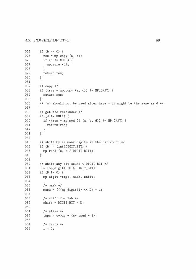
4.5. POWERS OF TWO 89
024 if (b <= 0) {025 res = mp_copy (a, c);
026 if (d != NULL) {027 mp_zero (d);
028 }029 return res;
030 }031
032 /* copy */
033 if ((res = mp_copy (a, c)) != MP_OKAY) {034 return res;
035 }036 /* ’a’ should not be used after here - it might be the same as d */
037
038 /* get the remainder */
039 if (d != NULL) {040 if ((res = mp_mod_2d (a, b, d)) != MP_OKAY) {041 return res;
042 }043 }044
045 /* shift by as many digits in the bit count */
046 if (b >= (int)DIGIT_BIT) {047 mp_rshd (c, b / DIGIT_BIT);
048 }049
050 /* shift any bit count < DIGIT_BIT */
051 D = (mp_digit) (b % DIGIT_BIT);
052 if (D != 0) {053 mp_digit *tmpc, mask, shift;
054
055 /* mask */
056 mask = (((mp_digit)1) << D) - 1;
057
058 /* shift for lsb */
059 shift = DIGIT_BIT - D;
060
061 /* alias */
062 tmpc = c->dp + (c->used - 1);
063
064 /* carry */
065 r = 0;
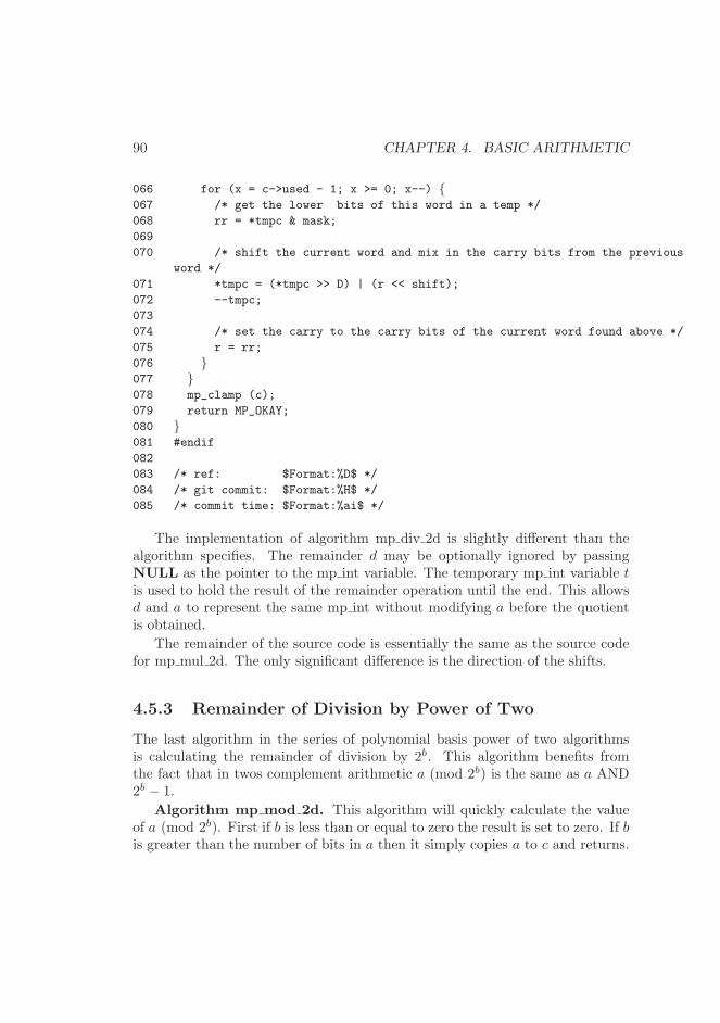
90 CHAPTER 4. BASIC ARITHMETIC
066 for (x = c->used - 1; x >= 0; x--) {067 /* get the lower bits of this word in a temp */
068 rr = *tmpc & mask;
069
070 /* shift the current word and mix in the carry bits from the previous
word */
071 *tmpc = (*tmpc >> D) | (r << shift);
072 --tmpc;
073
074 /* set the carry to the carry bits of the current word found above */
075 r = rr;
076 }077 }078 mp_clamp (c);
079 return MP_OKAY;
080 }081 #endif
082
083 /* ref: $Format:%D$ */
084 /* git commit: $Format:%H$ */
085 /* commit time: $Format:%ai$ */
The implementation of algorithm mp div 2d is slightly different than thealgorithm specifies. The remainder d may be optionally ignored by passingNULL as the pointer to the mp int variable. The temporary mp int variable tis used to hold the result of the remainder operation until the end. This allowsd and a to represent the same mp int without modifying a before the quotientis obtained.
The remainder of the source code is essentially the same as the source codefor mp mul 2d. The only significant difference is the direction of the shifts.
4.5.3 Remainder of Division by Power of Two
The last algorithm in the series of polynomial basis power of two algorithmsis calculating the remainder of division by 2b. This algorithm benefits fromthe fact that in twos complement arithmetic a (mod 2b) is the same as a AND2b − 1.
Algorithm mp mod 2d. This algorithm will quickly calculate the valueof a (mod 2b). First if b is less than or equal to zero the result is set to zero. If bis greater than the number of bits in a then it simply copies a to c and returns.
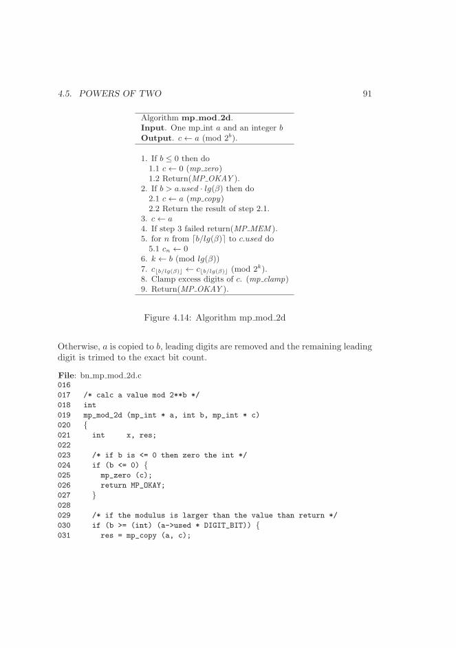
4.5. POWERS OF TWO 91
Algorithm mp mod 2d.Input. One mp int a and an integer b
Output. c← a (mod 2b).
1. If b ≤ 0 then do1.1 c← 0 (mp zero)1.2 Return(MP OKAY ).
2. If b > a.used · lg(β) then do2.1 c← a (mp copy)2.2 Return the result of step 2.1.
3. c← a4. If step 3 failed return(MP MEM ).5. for n from ⌈b/lg(β)⌉ to c.used do5.1 cn ← 0
6. k ← b (mod lg(β))
7. c⌊b/lg(β)⌋ ← c⌊b/lg(β)⌋ (mod 2k).8. Clamp excess digits of c. (mp clamp)9. Return(MP OKAY ).
Figure 4.14: Algorithm mp mod 2d
Otherwise, a is copied to b, leading digits are removed and the remaining leadingdigit is trimed to the exact bit count.
File: bn mp mod 2d.c016
017 /* calc a value mod 2**b */
018 int
019 mp_mod_2d (mp_int * a, int b, mp_int * c)
020 {021 int x, res;
022
023 /* if b is <= 0 then zero the int */
024 if (b <= 0) {025 mp_zero (c);
026 return MP_OKAY;
027 }028
029 /* if the modulus is larger than the value than return */
030 if (b >= (int) (a->used * DIGIT_BIT)) {031 res = mp_copy (a, c);
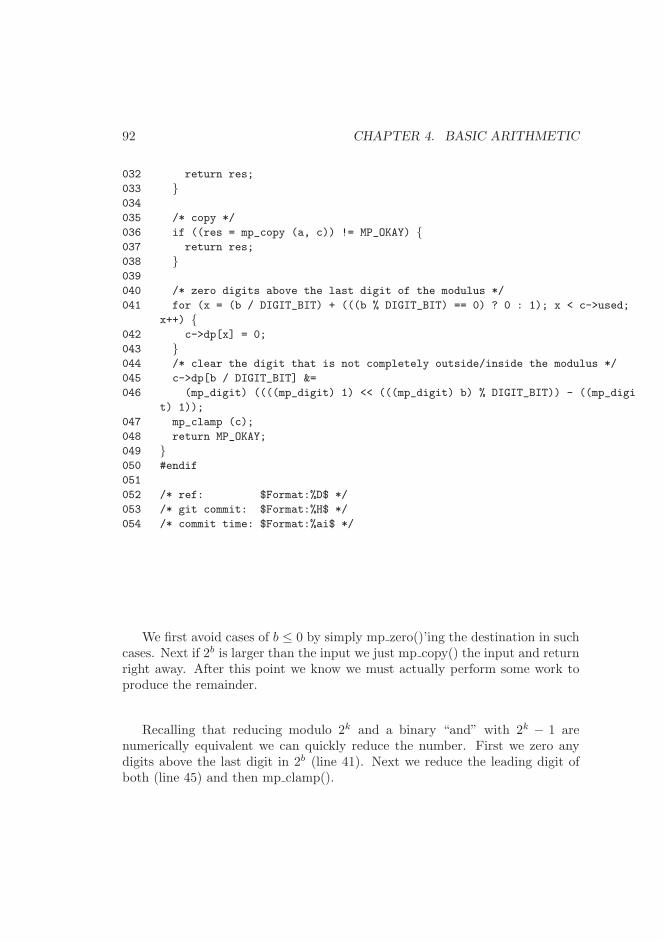
92 CHAPTER 4. BASIC ARITHMETIC
032 return res;
033 }034
035 /* copy */
036 if ((res = mp_copy (a, c)) != MP_OKAY) {037 return res;
038 }039
040 /* zero digits above the last digit of the modulus */
041 for (x = (b / DIGIT_BIT) + (((b % DIGIT_BIT) == 0) ? 0 : 1); x < c->used;
x++) {042 c->dp[x] = 0;
043 }044 /* clear the digit that is not completely outside/inside the modulus */
045 c->dp[b / DIGIT_BIT] &=
046 (mp_digit) ((((mp_digit) 1) << (((mp_digit) b) % DIGIT_BIT)) - ((mp_digi
t) 1));
047 mp_clamp (c);
048 return MP_OKAY;
049 }050 #endif
051
052 /* ref: $Format:%D$ */
053 /* git commit: $Format:%H$ */
054 /* commit time: $Format:%ai$ */
We first avoid cases of b ≤ 0 by simply mp zero()’ing the destination in suchcases. Next if 2b is larger than the input we just mp copy() the input and returnright away. After this point we know we must actually perform some work toproduce the remainder.
Recalling that reducing modulo 2k and a binary “and” with 2k − 1 arenumerically equivalent we can quickly reduce the number. First we zero anydigits above the last digit in 2b (line 41). Next we reduce the leading digit ofboth (line 45) and then mp clamp().
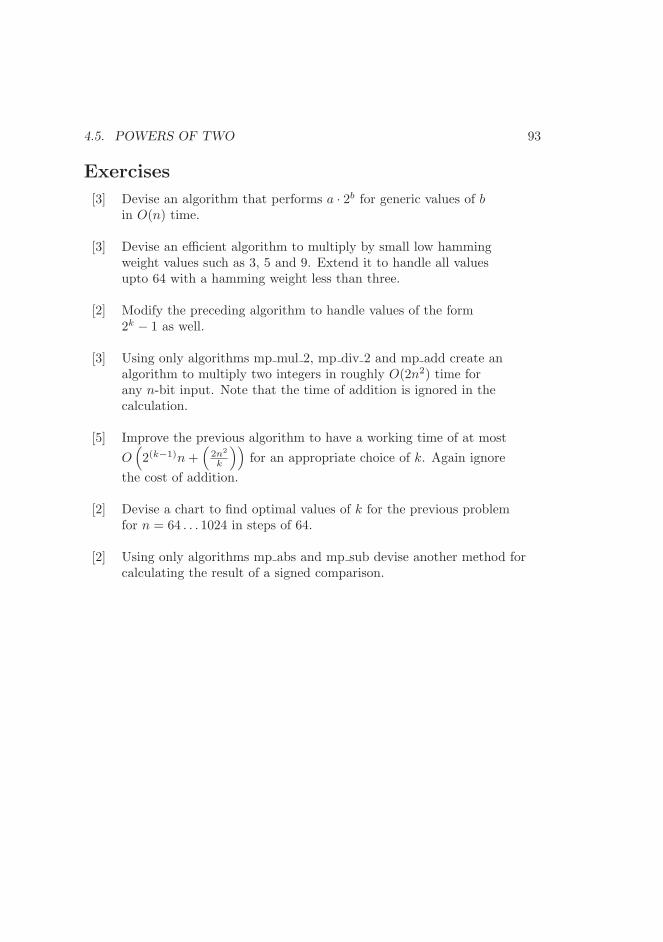
4.5. POWERS OF TWO 93
Exercises
[3] Devise an algorithm that performs a · 2b for generic values of bin O(n) time.
[3] Devise an efficient algorithm to multiply by small low hammingweight values such as 3, 5 and 9. Extend it to handle all valuesupto 64 with a hamming weight less than three.
[2] Modify the preceding algorithm to handle values of the form2k − 1 as well.
[3] Using only algorithms mp mul 2, mp div 2 and mp add create analgorithm to multiply two integers in roughly O(2n2) time forany n-bit input. Note that the time of addition is ignored in thecalculation.
[5] Improve the previous algorithm to have a working time of at most
O(
2(k−1)n+(
2n2
k
))
for an appropriate choice of k. Again ignore
the cost of addition.
[2] Devise a chart to find optimal values of k for the previous problemfor n = 64 . . . 1024 in steps of 64.
[2] Using only algorithms mp abs and mp sub devise another method forcalculating the result of a signed comparison.

94 CHAPTER 4. BASIC ARITHMETIC
Chapter 5
Multiplication and Squaring
5.1 The Multipliers
For most number theoretic problems including certain public key cryptographicalgorithms, the “multipliers” form the most important subset of algorithms ofany multiple precision integer package. The set of multiplier algorithms includeinteger multiplication, squaring and modular reduction where in each of thealgorithms single precision multiplication is the dominant operation performed.This chapter will discuss integer multiplication and squaring, leaving modularreductions for the subsequent chapter.
The importance of the multiplier algorithms is for the most part drivenby the fact that certain popular public key algorithms are based on modularexponentiation, that is computing d ≡ ab (mod c) for some arbitrary choice ofa, b, c and d. During a modular exponentiation the majority1 of the processortime is spent performing single precision multiplications.
For centuries general purpose multiplication has required a lengthly O(n2)process, whereby each digit of one multiplicand has to be multiplied againstevery digit of the other multiplicand. Traditional long-hand multiplication isbased on this process; while the techniques can differ the overall algorithm usedis essentially the same. Only “recently” have faster algorithms been studied.First Karatsuba multiplication was discovered in 1962. This algorithm can
1Roughly speaking a modular exponentiation will spend about 40% of the time performingmodular reductions, 35% of the time performing squaring and 25% of the time performingmultiplications.
95
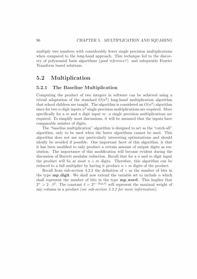
96 CHAPTER 5. MULTIPLICATION AND SQUARING
multiply two numbers with considerably fewer single precision multiplicationswhen compared to the long-hand approach. This technique led to the discov-ery of polynomial basis algorithms (good reference? ) and subquently FourierTransform based solutions.
5.2 Multiplication
5.2.1 The Baseline Multiplication
Computing the product of two integers in software can be achieved using atrivial adaptation of the standard O(n2) long-hand multiplication algorithmthat school children are taught. The algorithm is considered an O(n2) algorithmsince for two n-digit inputs n2 single precision multiplications are required. Morespecifically for a m and n digit input m · n single precision multiplications arerequired. To simplify most discussions, it will be assumed that the inputs havecomparable number of digits.
The “baseline multiplication” algorithm is designed to act as the “catch-all”algorithm, only to be used when the faster algorithms cannot be used. Thisalgorithm does not use any particularly interesting optimizations and shouldideally be avoided if possible. One important facet of this algorithm, is thatit has been modified to only produce a certain amount of output digits as res-olution. The importance of this modification will become evident during thediscussion of Barrett modular reduction. Recall that for a n and m digit inputthe product will be at most n + m digits. Therefore, this algorithm can bereduced to a full multiplier by having it produce n+m digits of the product.
Recall from sub-section 4.2.2 the definition of γ as the number of bits inthe type mp digit. We shall now extend the variable set to include α whichshall represent the number of bits in the type mp word. This implies that2α > 2 · β2. The constant δ = 2α−2lg(β) will represent the maximal weight ofany column in a product (see sub-section 5.2.2 for more information).
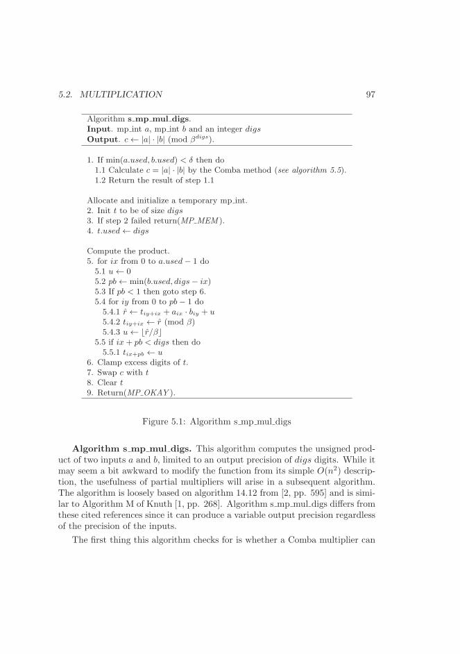
5.2. MULTIPLICATION 97
Algorithm s mp mul digs.Input. mp int a, mp int b and an integer digs
Output. c← |a| · |b| (mod βdigs).
1. If min(a.used, b.used) < δ then do1.1 Calculate c = |a| · |b| by the Comba method (see algorithm 5.5).1.2 Return the result of step 1.1
Allocate and initialize a temporary mp int.2. Init t to be of size digs3. If step 2 failed return(MP MEM ).4. t.used← digs
Compute the product.5. for ix from 0 to a.used− 1 do5.1 u← 05.2 pb← min(b.used, digs− ix)5.3 If pb < 1 then goto step 6.5.4 for iy from 0 to pb− 1 do5.4.1 r ← tiy+ix + aix · biy + u5.4.2 tiy+ix ← r (mod β)5.4.3 u← ⌊r/β⌋
5.5 if ix+ pb < digs then do5.5.1 tix+pb ← u
6. Clamp excess digits of t.7. Swap c with t8. Clear t9. Return(MP OKAY ).
Figure 5.1: Algorithm s mp mul digs
Algorithm s mp mul digs. This algorithm computes the unsigned prod-uct of two inputs a and b, limited to an output precision of digs digits. While itmay seem a bit awkward to modify the function from its simple O(n2) descrip-tion, the usefulness of partial multipliers will arise in a subsequent algorithm.The algorithm is loosely based on algorithm 14.12 from [2, pp. 595] and is simi-lar to Algorithm M of Knuth [1, pp. 268]. Algorithm s mp mul digs differs fromthese cited references since it can produce a variable output precision regardlessof the precision of the inputs.
The first thing this algorithm checks for is whether a Comba multiplier can
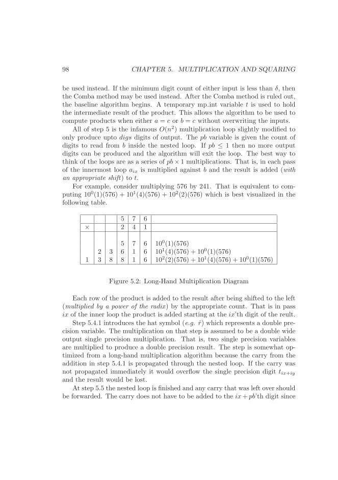
98 CHAPTER 5. MULTIPLICATION AND SQUARING
be used instead. If the minimum digit count of either input is less than δ, thenthe Comba method may be used instead. After the Comba method is ruled out,the baseline algorithm begins. A temporary mp int variable t is used to holdthe intermediate result of the product. This allows the algorithm to be used tocompute products when either a = c or b = c without overwriting the inputs.
All of step 5 is the infamous O(n2) multiplication loop slightly modified toonly produce upto digs digits of output. The pb variable is given the count ofdigits to read from b inside the nested loop. If pb ≤ 1 then no more outputdigits can be produced and the algorithm will exit the loop. The best way tothink of the loops are as a series of pb× 1 multiplications. That is, in each passof the innermost loop aix is multiplied against b and the result is added (withan appropriate shift) to t.
For example, consider multiplying 576 by 241. That is equivalent to com-puting 100(1)(576) + 101(4)(576) + 102(2)(576) which is best visualized in thefollowing table.
5 7 6× 2 4 1
5 7 6 100(1)(576)2 3 6 1 6 101(4)(576) + 100(1)(576)
1 3 8 8 1 6 102(2)(576) + 101(4)(576) + 100(1)(576)
Figure 5.2: Long-Hand Multiplication Diagram
Each row of the product is added to the result after being shifted to the left(multiplied by a power of the radix ) by the appropriate count. That is in passix of the inner loop the product is added starting at the ix’th digit of the reult.
Step 5.4.1 introduces the hat symbol (e.g. r) which represents a double pre-cision variable. The multiplication on that step is assumed to be a double wideoutput single precision multiplication. That is, two single precision variablesare multiplied to produce a double precision result. The step is somewhat op-timized from a long-hand multiplication algorithm because the carry from theaddition in step 5.4.1 is propagated through the nested loop. If the carry wasnot propagated immediately it would overflow the single precision digit tix+iy
and the result would be lost.
At step 5.5 the nested loop is finished and any carry that was left over shouldbe forwarded. The carry does not have to be added to the ix+ pb’th digit since
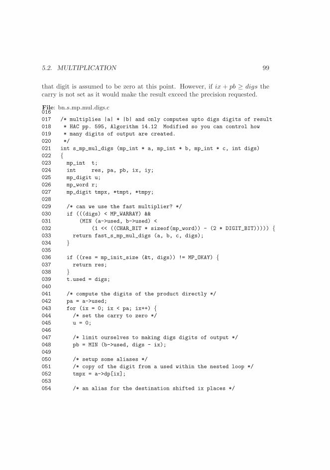
5.2. MULTIPLICATION 99
that digit is assumed to be zero at this point. However, if ix + pb ≥ digs thecarry is not set as it would make the result exceed the precision requested.
File: bn s mp mul digs.c016
017 /* multiplies |a| * |b| and only computes upto digs digits of result
018 * HAC pp. 595, Algorithm 14.12 Modified so you can control how
019 * many digits of output are created.
020 */
021 int s_mp_mul_digs (mp_int * a, mp_int * b, mp_int * c, int digs)
022 {023 mp_int t;
024 int res, pa, pb, ix, iy;
025 mp_digit u;
026 mp_word r;
027 mp_digit tmpx, *tmpt, *tmpy;
028
029 /* can we use the fast multiplier? */
030 if (((digs) < MP_WARRAY) &&
031 (MIN (a->used, b->used) <
032 (1 << ((CHAR_BIT * sizeof(mp_word)) - (2 * DIGIT_BIT))))) {033 return fast_s_mp_mul_digs (a, b, c, digs);
034 }035
036 if ((res = mp_init_size (&t, digs)) != MP_OKAY) {037 return res;
038 }039 t.used = digs;
040
041 /* compute the digits of the product directly */
042 pa = a->used;
043 for (ix = 0; ix < pa; ix++) {044 /* set the carry to zero */
045 u = 0;
046
047 /* limit ourselves to making digs digits of output */
048 pb = MIN (b->used, digs - ix);
049
050 /* setup some aliases */
051 /* copy of the digit from a used within the nested loop */
052 tmpx = a->dp[ix];
053
054 /* an alias for the destination shifted ix places */
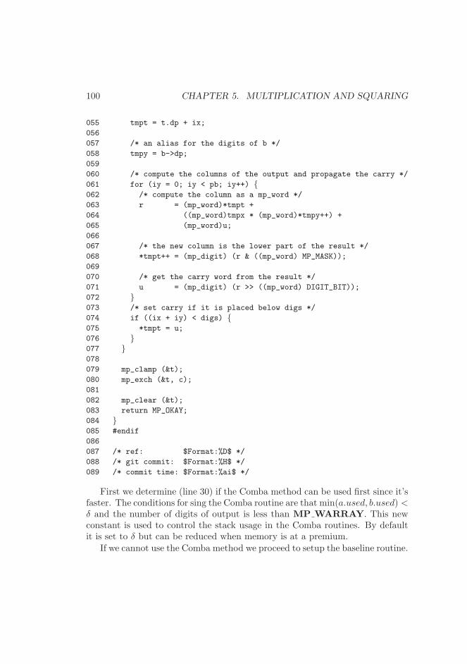
100 CHAPTER 5. MULTIPLICATION AND SQUARING
055 tmpt = t.dp + ix;
056
057 /* an alias for the digits of b */
058 tmpy = b->dp;
059
060 /* compute the columns of the output and propagate the carry */
061 for (iy = 0; iy < pb; iy++) {062 /* compute the column as a mp_word */
063 r = (mp_word)*tmpt +
064 ((mp_word)tmpx * (mp_word)*tmpy++) +
065 (mp_word)u;
066
067 /* the new column is the lower part of the result */
068 *tmpt++ = (mp_digit) (r & ((mp_word) MP_MASK));
069
070 /* get the carry word from the result */
071 u = (mp_digit) (r >> ((mp_word) DIGIT_BIT));
072 }073 /* set carry if it is placed below digs */
074 if ((ix + iy) < digs) {075 *tmpt = u;
076 }077 }078
079 mp_clamp (&t);
080 mp_exch (&t, c);
081
082 mp_clear (&t);
083 return MP_OKAY;
084 }085 #endif
086
087 /* ref: $Format:%D$ */
088 /* git commit: $Format:%H$ */
089 /* commit time: $Format:%ai$ */
First we determine (line 30) if the Comba method can be used first since it’sfaster. The conditions for sing the Comba routine are that min(a.used, b.used) <δ and the number of digits of output is less than MP WARRAY. This newconstant is used to control the stack usage in the Comba routines. By defaultit is set to δ but can be reduced when memory is at a premium.
If we cannot use the Comba method we proceed to setup the baseline routine.
5.2. MULTIPLICATION 101
We allocate the the destination mp int t (line 36) to the exact size of the outputto avoid further re–allocations. At this point we now begin the O(n2) loop.
This implementation of multiplication has the caveat that it can be trimmedto only produce a variable number of digits as output. In each iteration of theouter loop the pb variable is set (line 48) to the maximum number of inner loopiterations.
Inside the inner loop we calculate r as the mp word product of the twomp digits and the addition of the carry from the previous iteration. A particu-larly important observation is that most modern optimizing C compilers (GCCfor instance) can recognize that a N × N → 2N multiplication is all that isrequired for the product. In x86 terms for example, this means using the MULinstruction.
Each digit of the product is stored in turn (line 68) and the carry propagated(line 71) to the next iteration.
5.2.2 Faster Multiplication by the “Comba” Method
One of the huge drawbacks of the “baseline” algorithms is that at the O(n2)level the carry must be computed and propagated upwards. This makes thenested loop very sequential and hard to unroll and implement in parallel. The“Comba” [4] method is named after little known (in cryptographic venues) PaulG. Comba who described a method of implementing fast multipliers that donot require nested carry fixup operations. As an interesting aside it seems thatPaul Barrett describes a similar technique in his 1986 paper [7] written five yearsbefore.
At the heart of the Comba technique is once again the long-hand algorithm.Except in this case a slight twist is placed on how the columns of the result areproduced. In the standard long-hand algorithm rows of products are producedthen added together to form the final result. In the baseline algorithm thecolumns are added together after each iteration to get the result instantaneously.
In the Comba algorithm the columns of the result are produced entirelyindependently of each other. That is at the O(n2) level a simple multiplicationand addition step is performed. The carries of the columns are propagated afterthe nested loop to reduce the amount of work requiored. Succintly the first stepof the algorithm is to compute the product vector ~x as follows.
~xn =∑
i+j=n
aibj , ∀n ∈ {0, 1, 2, . . . , i+ j} (5.1)
102 CHAPTER 5. MULTIPLICATION AND SQUARING
Where ~xn is the n′th column of the output vector. Consider the followingexample which computes the vector ~x for the multiplication of 576 and 241.
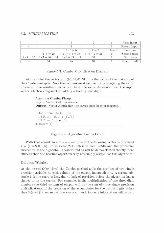
5.2. MULTIPLICATION 103
5 7 6 First Input
× 2 4 1 Second Input
1 · 5 = 5 1 · 7 = 7 1 · 6 = 6 First pass4 · 5 = 20 4 · 7 + 5 = 33 4 · 6 + 7 = 31 6 Second pass
2 · 5 = 10 2 · 7 + 20 = 34 2 · 6 + 33 = 45 31 6 Third pass
10 34 45 31 6 Final Result
Figure 5.3: Comba Multiplication Diagram
At this point the vector x = 〈10, 34, 45, 31, 6〉 is the result of the first step ofthe Comba multipler. Now the columns must be fixed by propagating the carryupwards. The resultant vector will have one extra dimension over the inputvector which is congruent to adding a leading zero digit.
Algorithm Comba Fixup.Input. Vector ~x of dimension kOutput. Vector ~x such that the carries have been propagated.
1. for n from 0 to k − 1 do1.1 ~xn+1 ← ~xn+1 + ⌊~xn/β⌋1.2 ~xn ← ~xn (mod β)
2. Return(~x).
Figure 5.4: Algorithm Comba Fixup
With that algorithm and k = 5 and β = 10 the following vector is produced~x = 〈1, 3, 8, 8, 1, 6〉. In this case 241 · 576 is in fact 138816 and the proceduresucceeded. If the algorithm is correct and as will be demonstrated shortly moreefficient than the baseline algorithm why not simply always use this algorithm?
Column Weight.
At the nested O(n2) level the Comba method adds the product of two singleprecision variables to each column of the output independently. A serious ob-stacle is if the carry is lost, due to lack of precision before the algorithm has achance to fix the carries. For example, in the multiplication of two three-digitnumbers the third column of output will be the sum of three single precisionmultiplications. If the precision of the accumulator for the output digits is lessthen 3·(β−1)2 then an overflow can occur and the carry information will be lost.
104 CHAPTER 5. MULTIPLICATION AND SQUARING
For any m and n digit inputs the maximum weight of any column is min(m,n)which is fairly obvious.
The maximum number of terms in any column of a product is known as the“column weight” and strictly governs when the algorithm can be used. Recallfrom earlier that a double precision type has α bits of resolution and a singleprecision digit has lg(β) bits of precision. Given these two quantities we mustnot violate the following
k · (β − 1)2< 2α (5.2)
Which reduces to
k ·(
β2 − 2β + 1)
< 2α (5.3)
Let ρ = lg(β) represent the number of bits in a single precision digit. Byfurther re-arrangement of the equation the final solution is found.
k <2α
(22ρ − 2ρ+1 + 1)(5.4)
The defaults for LibTomMath are β = 228 and α = 264 which means that k isbounded by k < 257. In this configuration the smaller input may not have morethan 256 digits if the Comba method is to be used. This is quite satisfactoryfor most applications since 256 digits would allow for numbers in the rangeof 0 ≤ x < 27168 which, is much larger than most public key cryptographicalgorithms require.
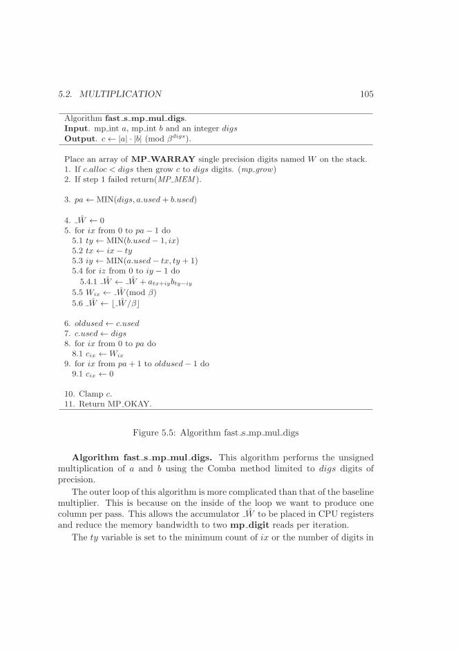
5.2. MULTIPLICATION 105
Algorithm fast s mp mul digs.Input. mp int a, mp int b and an integer digs
Output. c← |a| · |b| (mod βdigs).
Place an array of MP WARRAY single precision digits named W on the stack.1. If c.alloc < digs then grow c to digs digits. (mp grow)2. If step 1 failed return(MP MEM ).
3. pa← MIN(digs, a.used+ b.used)
4. W ← 05. for ix from 0 to pa− 1 do5.1 ty ← MIN(b.used− 1, ix)5.2 tx← ix− ty5.3 iy ← MIN(a.used− tx, ty + 1)5.4 for iz from 0 to iy − 1 do
5.4.1 W ← W + atx+iybty−iy
5.5 Wix ← W (mod β)
5.6 W ← ⌊ W/β⌋
6. oldused← c.used7. c.used← digs8. for ix from 0 to pa do8.1 cix ←Wix
9. for ix from pa+ 1 to oldused− 1 do9.1 cix ← 0
10. Clamp c.11. Return MP OKAY.
Figure 5.5: Algorithm fast s mp mul digs
Algorithm fast s mp mul digs. This algorithm performs the unsignedmultiplication of a and b using the Comba method limited to digs digits ofprecision.
The outer loop of this algorithm is more complicated than that of the baselinemultiplier. This is because on the inside of the loop we want to produce onecolumn per pass. This allows the accumulator W to be placed in CPU registersand reduce the memory bandwidth to two mp digit reads per iteration.
The ty variable is set to the minimum count of ix or the number of digits in
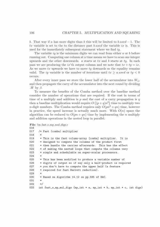
106 CHAPTER 5. MULTIPLICATION AND SQUARING
b. That way if a has more digits than b this will be limited to b.used− 1. Thetx variable is set to the to the distance past b.used the variable ix is. This isused for the immediately subsequent statement where we find iy.
The variable iy is the minimum digits we can read from either a or b beforerunning out. Computing one column at a time means we have to scan one integerupwards and the other downwards. a starts at tx and b starts at ty. In eachpass we are producing the ix’th output column and we note that tx+ ty = ix.As we move tx upwards we have to move ty downards so the equality remainsvalid. The iy variable is the number of iterations until tx ≥ a.used or ty < 0occurs.
After every inner pass we store the lower half of the accumulator into Wix
and then propagate the carry of the accumulator into the next round by dividingW by β.
To measure the benefits of the Comba method over the baseline methodconsider the number of operations that are required. If the cost in terms oftime of a multiply and addition is p and the cost of a carry propagation is qthen a baseline multiplication would require O
(
(p+ q)n2)
time to multiply twon-digit numbers. The Comba method requires only O(pn2 + qn) time, howeverin practice, the speed increase is actually much more. With O(n) space thealgorithm can be reduced to O(pn + qn) time by implementing the n multiplyand addition operations in the nested loop in parallel.
File: bn fast s mp mul digs.c016
017 /* Fast (comba) multiplier
018 *
019 * This is the fast column-array [comba] multiplier. It is
020 * designed to compute the columns of the product first
021 * then handle the carries afterwards. This has the effect
022 * of making the nested loops that compute the columns very
023 * simple and schedulable on super-scalar processors.
024 *
025 * This has been modified to produce a variable number of
026 * digits of output so if say only a half-product is required
027 * you don’t have to compute the upper half (a feature
028 * required for fast Barrett reduction).
029 *
030 * Based on Algorithm 14.12 on pp.595 of HAC.
031 *
032 */
033 int fast_s_mp_mul_digs (mp_int * a, mp_int * b, mp_int * c, int digs)
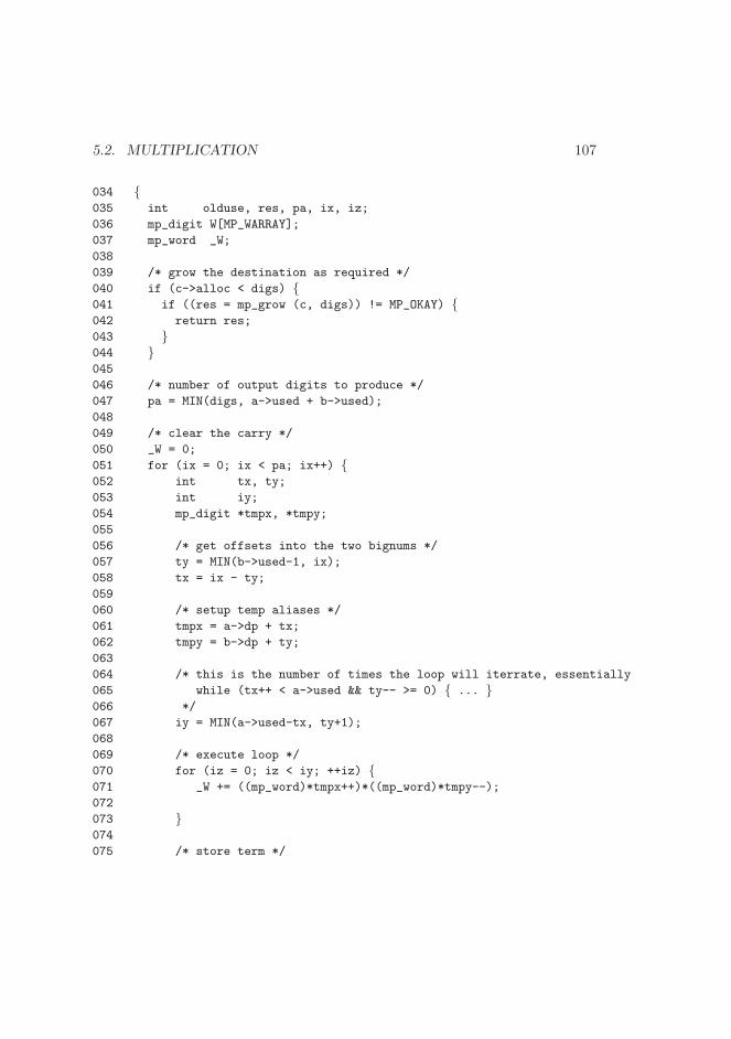
5.2. MULTIPLICATION 107
034 {035 int olduse, res, pa, ix, iz;
036 mp_digit W[MP_WARRAY];
037 mp_word _W;
038
039 /* grow the destination as required */
040 if (c->alloc < digs) {041 if ((res = mp_grow (c, digs)) != MP_OKAY) {042 return res;
043 }044 }045
046 /* number of output digits to produce */
047 pa = MIN(digs, a->used + b->used);
048
049 /* clear the carry */
050 _W = 0;
051 for (ix = 0; ix < pa; ix++) {052 int tx, ty;
053 int iy;
054 mp_digit *tmpx, *tmpy;
055
056 /* get offsets into the two bignums */
057 ty = MIN(b->used-1, ix);
058 tx = ix - ty;
059
060 /* setup temp aliases */
061 tmpx = a->dp + tx;
062 tmpy = b->dp + ty;
063
064 /* this is the number of times the loop will iterrate, essentially
065 while (tx++ < a->used && ty-- >= 0) { ... }066 */
067 iy = MIN(a->used-tx, ty+1);
068
069 /* execute loop */
070 for (iz = 0; iz < iy; ++iz) {071 _W += ((mp_word)*tmpx++)*((mp_word)*tmpy--);
072
073 }074
075 /* store term */
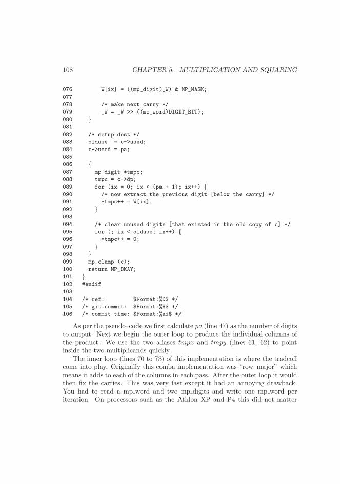
108 CHAPTER 5. MULTIPLICATION AND SQUARING
076 W[ix] = ((mp_digit)_W) & MP_MASK;
077
078 /* make next carry */
079 _W = _W >> ((mp_word)DIGIT_BIT);
080 }081
082 /* setup dest */
083 olduse = c->used;
084 c->used = pa;
085
086 {087 mp_digit *tmpc;
088 tmpc = c->dp;
089 for (ix = 0; ix < (pa + 1); ix++) {090 /* now extract the previous digit [below the carry] */
091 *tmpc++ = W[ix];
092 }093
094 /* clear unused digits [that existed in the old copy of c] */
095 for (; ix < olduse; ix++) {096 *tmpc++ = 0;
097 }098 }099 mp_clamp (c);
100 return MP_OKAY;
101 }102 #endif
103
104 /* ref: $Format:%D$ */
105 /* git commit: $Format:%H$ */
106 /* commit time: $Format:%ai$ */
As per the pseudo–code we first calculate pa (line 47) as the number of digitsto output. Next we begin the outer loop to produce the individual columns ofthe product. We use the two aliases tmpx and tmpy (lines 61, 62) to pointinside the two multiplicands quickly.
The inner loop (lines 70 to 73) of this implementation is where the tradeoffcome into play. Originally this comba implementation was “row–major” whichmeans it adds to each of the columns in each pass. After the outer loop it wouldthen fix the carries. This was very fast except it had an annoying drawback.You had to read a mp word and two mp digits and write one mp word periteration. On processors such as the Athlon XP and P4 this did not matter
5.2. MULTIPLICATION 109
much since the cache bandwidth is very high and it can keep the ALU fed withdata. It did, however, matter on older and embedded cpus where cache is oftenslower and also often doesn’t exist. This new algorithm only performs two readsper iteration under the assumption that the compiler has aliased W to a CPUregister.
After the inner loop we store the current accumulator in W and shift W(lines 76, 79) to forward it as a carry for the next pass. After the outer loop weuse the final carry (line 76) as the last digit of the product.
5.2.3 Polynomial Basis Multiplication
To break the O(n2) barrier in multiplication requires a completely differentlook at integer multiplication. In the following algorithms the use of polynomialbasis representation for two integers a and b as f(x) =
∑ni=0 aix
i and g(x) =∑n
i=0 bixi respectively, is required. In this system both f(x) and g(x) have n+1
terms and are of the n’th degree.The product a · b ≡ f(x)g(x) is the polynomial W (x) =
∑2ni=0 wix
i. Thecoefficients wi will directly yield the desired product when β is substituted forx. The direct solution to solve for the 2n + 1 coefficients requires O(n2) timeand would in practice be slower than the Comba technique.
However, numerical analysis theory indicates that only 2n+1 distinct pointsin W (x) are required to determine the values of the 2n+1 unknown coefficients.This means by finding ζy = W (y) for 2n + 1 small values of y the coefficientsof W (x) can be found with Gaussian elimination. This technique is also occa-sionally refered to as the interpolation technique (references please...) since ineffect an interpolation based on 2n+1 points will yield a polynomial equivalentto W (x).
The coefficients of the polynomial W (x) are unknown which makes findingW (y) for any value of y impossible. However, since W (x) = f(x)g(x) theequivalent ζy = f(y)g(y) can be used in its place. The benefit of this techniquestems from the fact that f(y) and g(y) are much smaller than either a or brespectively. As a result finding the 2n + 1 relations required by multiplyingf(y)g(y) involves multiplying integers that are much smaller than either of theinputs.
When picking points to gather relations there are always three obvious pointsto choose, y = 0, 1 and ∞. The ζ0 term is simply the product W (0) = w0 =a0 · b0. The ζ1 term is the product W (1) = (
∑ni=0 ai) (
∑ni=0 bi). The third
point ζ∞ is less obvious but rather simple to explain. The 2n+ 1’th coefficientof W (x) is numerically equivalent to the most significant column in an integer
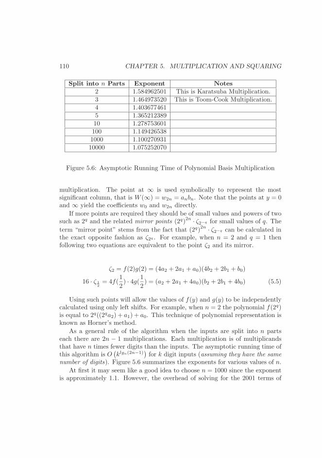
110 CHAPTER 5. MULTIPLICATION AND SQUARING
Split into n Parts Exponent Notes2 1.584962501 This is Karatsuba Multiplication.3 1.464973520 This is Toom-Cook Multiplication.4 1.4036774615 1.36521238910 1.278753601100 1.1494265381000 1.10027093110000 1.075252070
Figure 5.6: Asymptotic Running Time of Polynomial Basis Multiplication
multiplication. The point at ∞ is used symbolically to represent the mostsignificant column, that is W (∞) = w2n = anbn. Note that the points at y = 0and ∞ yield the coefficients w0 and w2n directly.
If more points are required they should be of small values and powers of twosuch as 2q and the related mirror points (2q)
2n · ζ2−q for small values of q. The
term “mirror point” stems from the fact that (2q)2n · ζ2−q can be calculated in
the exact opposite fashion as ζ2q . For example, when n = 2 and q = 1 thenfollowing two equations are equivalent to the point ζ2 and its mirror.
ζ2 = f(2)g(2) = (4a2 + 2a1 + a0)(4b2 + 2b1 + b0)
16 · ζ 12= 4f(
1
2) · 4g(1
2) = (a2 + 2a1 + 4a0)(b2 + 2b1 + 4b0) (5.5)
Using such points will allow the values of f(y) and g(y) to be independentlycalculated using only left shifts. For example, when n = 2 the polynomial f(2q)is equal to 2q((2qa2) + a1) + a0. This technique of polynomial representation isknown as Horner’s method.
As a general rule of the algorithm when the inputs are split into n partseach there are 2n − 1 multiplications. Each multiplication is of multiplicandsthat have n times fewer digits than the inputs. The asymptotic running time ofthis algorithm is O
(
klgn(2n−1))
for k digit inputs (assuming they have the same
number of digits). Figure 5.6 summarizes the exponents for various values of n.
At first it may seem like a good idea to choose n = 1000 since the exponentis approximately 1.1. However, the overhead of solving for the 2001 terms of
5.2. MULTIPLICATION 111
W (x) will certainly consume any savings the algorithm could offer for all butexceedingly large numbers.
Cutoff Point
The polynomial basis multiplication algorithms all require fewer single precisionmultiplications than a straight Comba approach. However, the algorithms incuran overhead (at the O(n) work level) since they require a system of equations tobe solved. This makes the polynomial basis approach more costly to use withsmall inputs.
Let m represent the number of digits in the multiplicands (assume both
multiplicands have the same number of digits). There exists a point y such thatwhen m < y the polynomial basis algorithms are more costly than Comba, whenm = y they are roughly the same cost and when m > y the Comba methodsare slower than the polynomial basis algorithms.
The exact location of y depends on several key architectural elements of thecomputer platform in question.
1. The ratio of clock cycles for single precision multiplication versus othersimpler operations such as addition, shifting, etc. For example on theAMD Athlon the ratio is roughly 17 : 1 while on the Intel P4 it is 29 : 1.The higher the ratio in favour of multiplication the lower the cutoff pointy will be.
2. The complexity of the linear system of equations (for the coefficients of
W (x)) is. Generally speaking as the number of splits grows the complexitygrows substantially. Ideally solving the system will only involve addition,subtraction and shifting of integers. This directly reflects on the ratioprevious mentioned.
3. To a lesser extent memory bandwidth and function call overheads. Pro-vided the values are in the processor cache this is less of an influence overthe cutoff point.
A clean cutoff point separation occurs when a point y is found such thatall of the cutoff point conditions are met. For example, if the point is too lowthen there will be values of m such that m > y and the Comba method is stillfaster. Finding the cutoff points is fairly simple when a high resolution timer isavailable.
112 CHAPTER 5. MULTIPLICATION AND SQUARING
5.2.4 Karatsuba Multiplication
Karatsuba [5] multiplication when originally proposed in 1962 was among thefirst set of algorithms to break the O(n2) barrier for general purpose mul-tiplication. Given two polynomial basis representations f(x) = ax + b andg(x) = cx+ d, Karatsuba proved with light algebra [6] that the following poly-nomial is equivalent to multiplication of the two integers the polynomials rep-resent.
f(x) · g(x) = acx2 + ((a+ b)(c+ d)− (ac+ bd))x+ bd (5.6)
Using the observation that ac and bd could be re-used only three half sizedmultiplications would be required to produce the product. Applying this al-gorithm recursively, the work factor becomes O(nlg(3)) which is substantiallybetter than the work factor O(n2) of the Comba technique. It turns out whatKaratsuba did not know or at least did not publish was that this is simplypolynomial basis multiplication with the points ζ0, ζ∞ and ζ1. Consider theresultant system of equations.
ζ0 = w0
ζ1 = w2 + w1 + w0
ζ∞ = w2
By adding the first and last equation to the equation in the middle the termw1 can be isolated and all three coefficients solved for. The simplicity of thissystem of equations has made Karatsuba fairly popular. In fact the cutoff pointis often fairly low2 making it an ideal algorithm to speed up certain public keycryptosystems such as RSA and Diffie-Hellman.
2With LibTomMath 0.18 it is 70 and 109 digits for the Intel P4 and AMD Athlon respec-tively.
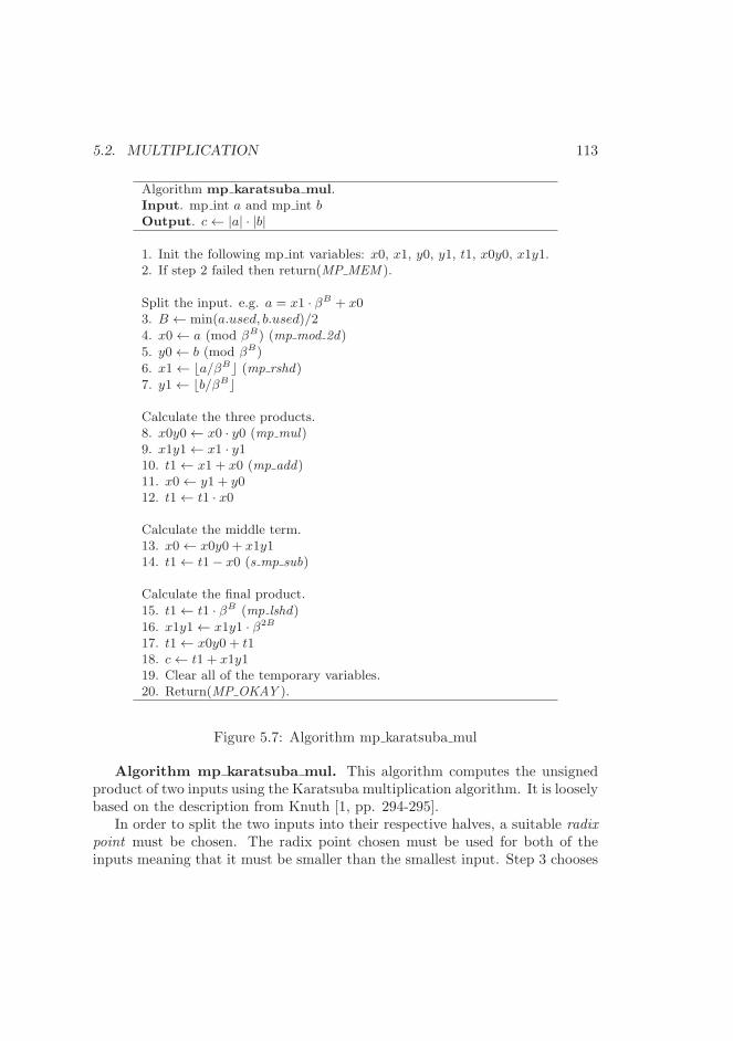
5.2. MULTIPLICATION 113
Algorithm mp karatsuba mul.Input. mp int a and mp int bOutput. c← |a| · |b|
1. Init the following mp int variables: x0, x1, y0, y1, t1, x0y0, x1y1.2. If step 2 failed then return(MP MEM ).
Split the input. e.g. a = x1 · βB + x03. B ← min(a.used, b.used)/24. x0← a (mod βB) (mp mod 2d)5. y0← b (mod βB)6. x1← ⌊a/βB⌋ (mp rshd)7. y1← ⌊b/βB⌋
Calculate the three products.8. x0y0← x0 · y0 (mp mul)9. x1y1← x1 · y110. t1← x1 + x0 (mp add)11. x0← y1 + y012. t1← t1 · x0
Calculate the middle term.13. x0← x0y0 + x1y114. t1← t1− x0 (s mp sub)
Calculate the final product.15. t1← t1 · βB (mp lshd)16. x1y1← x1y1 · β2B
17. t1← x0y0 + t118. c← t1 + x1y119. Clear all of the temporary variables.20. Return(MP OKAY ).
Figure 5.7: Algorithm mp karatsuba mul
Algorithm mp karatsuba mul. This algorithm computes the unsignedproduct of two inputs using the Karatsuba multiplication algorithm. It is looselybased on the description from Knuth [1, pp. 294-295].
In order to split the two inputs into their respective halves, a suitable radix
point must be chosen. The radix point chosen must be used for both of theinputs meaning that it must be smaller than the smallest input. Step 3 chooses
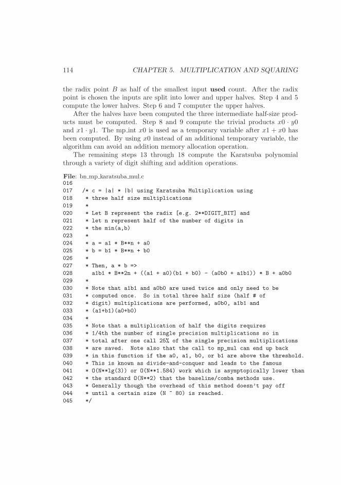
114 CHAPTER 5. MULTIPLICATION AND SQUARING
the radix point B as half of the smallest input used count. After the radixpoint is chosen the inputs are split into lower and upper halves. Step 4 and 5compute the lower halves. Step 6 and 7 computer the upper halves.
After the halves have been computed the three intermediate half-size prod-ucts must be computed. Step 8 and 9 compute the trivial products x0 · y0and x1 · y1. The mp int x0 is used as a temporary variable after x1 + x0 hasbeen computed. By using x0 instead of an additional temporary variable, thealgorithm can avoid an addition memory allocation operation.
The remaining steps 13 through 18 compute the Karatsuba polynomialthrough a variety of digit shifting and addition operations.
File: bn mp karatsuba mul.c016
017 /* c = |a| * |b| using Karatsuba Multiplication using
018 * three half size multiplications
019 *
020 * Let B represent the radix [e.g. 2**DIGIT_BIT] and
021 * let n represent half of the number of digits in
022 * the min(a,b)
023 *
024 * a = a1 * B**n + a0
025 * b = b1 * B**n + b0
026 *
027 * Then, a * b =>
028 a1b1 * B**2n + ((a1 + a0)(b1 + b0) - (a0b0 + a1b1)) * B + a0b0
029 *
030 * Note that a1b1 and a0b0 are used twice and only need to be
031 * computed once. So in total three half size (half # of
032 * digit) multiplications are performed, a0b0, a1b1 and
033 * (a1+b1)(a0+b0)
034 *
035 * Note that a multiplication of half the digits requires
036 * 1/4th the number of single precision multiplications so in
037 * total after one call 25% of the single precision multiplications
038 * are saved. Note also that the call to mp_mul can end up back
039 * in this function if the a0, a1, b0, or b1 are above the threshold.
040 * This is known as divide-and-conquer and leads to the famous
041 * O(N**lg(3)) or O(N**1.584) work which is asymptopically lower than
042 * the standard O(N**2) that the baseline/comba methods use.
043 * Generally though the overhead of this method doesn’t pay off
044 * until a certain size (N ~ 80) is reached.
045 */
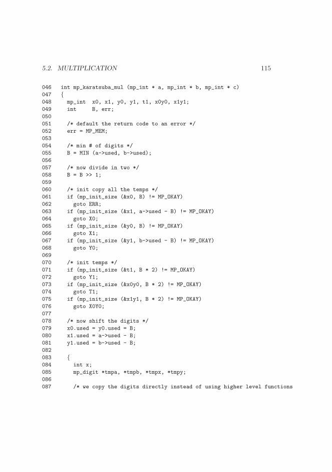
5.2. MULTIPLICATION 115
046 int mp_karatsuba_mul (mp_int * a, mp_int * b, mp_int * c)
047 {048 mp_int x0, x1, y0, y1, t1, x0y0, x1y1;
049 int B, err;
050
051 /* default the return code to an error */
052 err = MP_MEM;
053
054 /* min # of digits */
055 B = MIN (a->used, b->used);
056
057 /* now divide in two */
058 B = B >> 1;
059
060 /* init copy all the temps */
061 if (mp_init_size (&x0, B) != MP_OKAY)
062 goto ERR;
063 if (mp_init_size (&x1, a->used - B) != MP_OKAY)
064 goto X0;
065 if (mp_init_size (&y0, B) != MP_OKAY)
066 goto X1;
067 if (mp_init_size (&y1, b->used - B) != MP_OKAY)
068 goto Y0;
069
070 /* init temps */
071 if (mp_init_size (&t1, B * 2) != MP_OKAY)
072 goto Y1;
073 if (mp_init_size (&x0y0, B * 2) != MP_OKAY)
074 goto T1;
075 if (mp_init_size (&x1y1, B * 2) != MP_OKAY)
076 goto X0Y0;
077
078 /* now shift the digits */
079 x0.used = y0.used = B;
080 x1.used = a->used - B;
081 y1.used = b->used - B;
082
083 {084 int x;
085 mp_digit *tmpa, *tmpb, *tmpx, *tmpy;
086
087 /* we copy the digits directly instead of using higher level functions
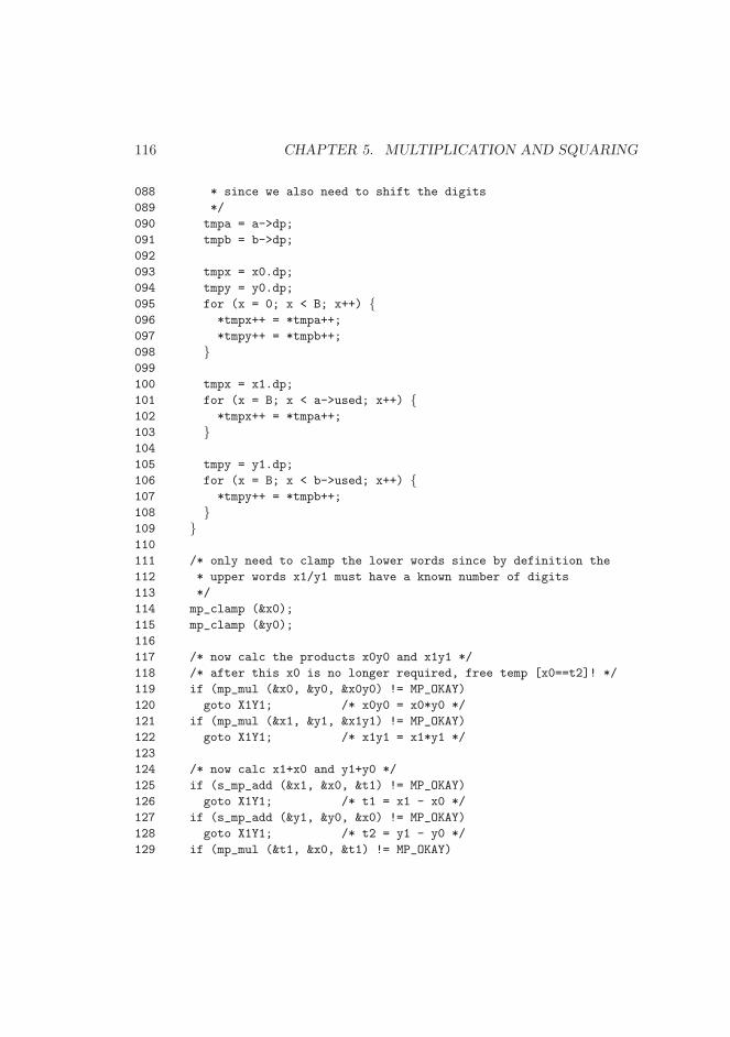
116 CHAPTER 5. MULTIPLICATION AND SQUARING
088 * since we also need to shift the digits
089 */
090 tmpa = a->dp;
091 tmpb = b->dp;
092
093 tmpx = x0.dp;
094 tmpy = y0.dp;
095 for (x = 0; x < B; x++) {096 *tmpx++ = *tmpa++;
097 *tmpy++ = *tmpb++;
098 }099
100 tmpx = x1.dp;
101 for (x = B; x < a->used; x++) {102 *tmpx++ = *tmpa++;
103 }104
105 tmpy = y1.dp;
106 for (x = B; x < b->used; x++) {107 *tmpy++ = *tmpb++;
108 }109 }110
111 /* only need to clamp the lower words since by definition the
112 * upper words x1/y1 must have a known number of digits
113 */
114 mp_clamp (&x0);
115 mp_clamp (&y0);
116
117 /* now calc the products x0y0 and x1y1 */
118 /* after this x0 is no longer required, free temp [x0==t2]! */
119 if (mp_mul (&x0, &y0, &x0y0) != MP_OKAY)
120 goto X1Y1; /* x0y0 = x0*y0 */
121 if (mp_mul (&x1, &y1, &x1y1) != MP_OKAY)
122 goto X1Y1; /* x1y1 = x1*y1 */
123
124 /* now calc x1+x0 and y1+y0 */
125 if (s_mp_add (&x1, &x0, &t1) != MP_OKAY)
126 goto X1Y1; /* t1 = x1 - x0 */
127 if (s_mp_add (&y1, &y0, &x0) != MP_OKAY)
128 goto X1Y1; /* t2 = y1 - y0 */
129 if (mp_mul (&t1, &x0, &t1) != MP_OKAY)
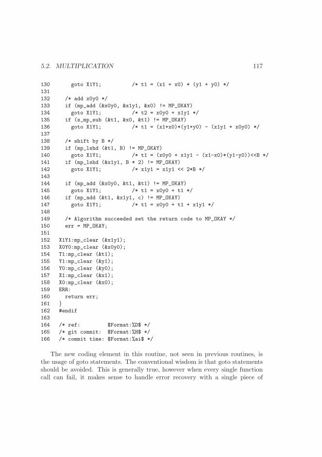
5.2. MULTIPLICATION 117
130 goto X1Y1; /* t1 = (x1 + x0) * (y1 + y0) */
131
132 /* add x0y0 */
133 if (mp_add (&x0y0, &x1y1, &x0) != MP_OKAY)
134 goto X1Y1; /* t2 = x0y0 + x1y1 */
135 if (s_mp_sub (&t1, &x0, &t1) != MP_OKAY)
136 goto X1Y1; /* t1 = (x1+x0)*(y1+y0) - (x1y1 + x0y0) */
137
138 /* shift by B */
139 if (mp_lshd (&t1, B) != MP_OKAY)
140 goto X1Y1; /* t1 = (x0y0 + x1y1 - (x1-x0)*(y1-y0))<<B */
141 if (mp_lshd (&x1y1, B * 2) != MP_OKAY)
142 goto X1Y1; /* x1y1 = x1y1 << 2*B */
143
144 if (mp_add (&x0y0, &t1, &t1) != MP_OKAY)
145 goto X1Y1; /* t1 = x0y0 + t1 */
146 if (mp_add (&t1, &x1y1, c) != MP_OKAY)
147 goto X1Y1; /* t1 = x0y0 + t1 + x1y1 */
148
149 /* Algorithm succeeded set the return code to MP_OKAY */
150 err = MP_OKAY;
151
152 X1Y1:mp_clear (&x1y1);
153 X0Y0:mp_clear (&x0y0);
154 T1:mp_clear (&t1);
155 Y1:mp_clear (&y1);
156 Y0:mp_clear (&y0);
157 X1:mp_clear (&x1);
158 X0:mp_clear (&x0);
159 ERR:
160 return err;
161 }162 #endif
163
164 /* ref: $Format:%D$ */
165 /* git commit: $Format:%H$ */
166 /* commit time: $Format:%ai$ */
The new coding element in this routine, not seen in previous routines, isthe usage of goto statements. The conventional wisdom is that goto statementsshould be avoided. This is generally true, however when every single functioncall can fail, it makes sense to handle error recovery with a single piece of
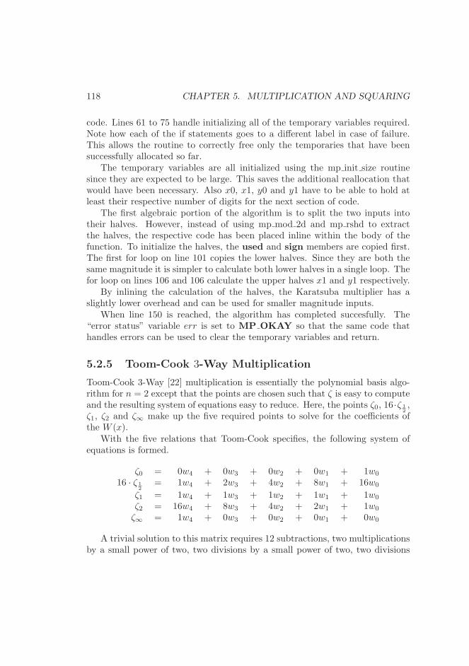
118 CHAPTER 5. MULTIPLICATION AND SQUARING
code. Lines 61 to 75 handle initializing all of the temporary variables required.Note how each of the if statements goes to a different label in case of failure.This allows the routine to correctly free only the temporaries that have beensuccessfully allocated so far.
The temporary variables are all initialized using the mp init size routinesince they are expected to be large. This saves the additional reallocation thatwould have been necessary. Also x0, x1, y0 and y1 have to be able to hold atleast their respective number of digits for the next section of code.
The first algebraic portion of the algorithm is to split the two inputs intotheir halves. However, instead of using mp mod 2d and mp rshd to extractthe halves, the respective code has been placed inline within the body of thefunction. To initialize the halves, the used and sign members are copied first.The first for loop on line 101 copies the lower halves. Since they are both thesame magnitude it is simpler to calculate both lower halves in a single loop. Thefor loop on lines 106 and 106 calculate the upper halves x1 and y1 respectively.
By inlining the calculation of the halves, the Karatsuba multiplier has aslightly lower overhead and can be used for smaller magnitude inputs.
When line 150 is reached, the algorithm has completed succesfully. The“error status” variable err is set to MP OKAY so that the same code thathandles errors can be used to clear the temporary variables and return.
5.2.5 Toom-Cook 3-Way Multiplication
Toom-Cook 3-Way [22] multiplication is essentially the polynomial basis algo-rithm for n = 2 except that the points are chosen such that ζ is easy to computeand the resulting system of equations easy to reduce. Here, the points ζ0, 16·ζ 1
2,
ζ1, ζ2 and ζ∞ make up the five required points to solve for the coefficients ofthe W (x).
With the five relations that Toom-Cook specifies, the following system ofequations is formed.
ζ0 = 0w4 + 0w3 + 0w2 + 0w1 + 1w0
16 · ζ 12
= 1w4 + 2w3 + 4w2 + 8w1 + 16w0
ζ1 = 1w4 + 1w3 + 1w2 + 1w1 + 1w0
ζ2 = 16w4 + 8w3 + 4w2 + 2w1 + 1w0
ζ∞ = 1w4 + 0w3 + 0w2 + 0w1 + 0w0
A trivial solution to this matrix requires 12 subtractions, two multiplicationsby a small power of two, two divisions by a small power of two, two divisions
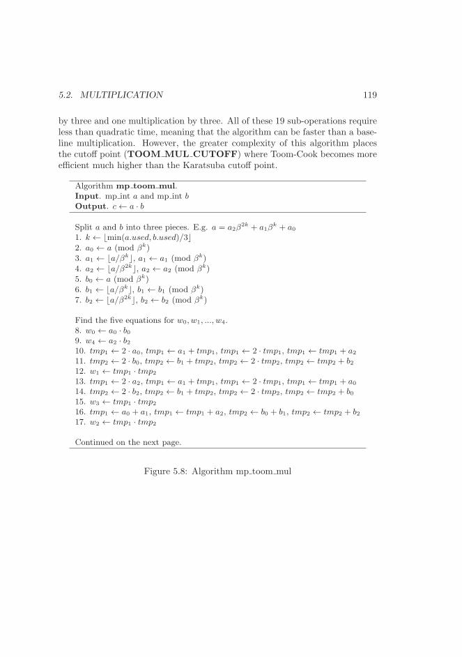
5.2. MULTIPLICATION 119
by three and one multiplication by three. All of these 19 sub-operations requireless than quadratic time, meaning that the algorithm can be faster than a base-line multiplication. However, the greater complexity of this algorithm placesthe cutoff point (TOOM MUL CUTOFF) where Toom-Cook becomes moreefficient much higher than the Karatsuba cutoff point.
Algorithm mp toom mul.Input. mp int a and mp int bOutput. c← a · b
Split a and b into three pieces. E.g. a = a2β2k + a1β
k + a0
1. k ← ⌊min(a.used, b.used)/3⌋
2. a0 ← a (mod βk)
3. a1 ← ⌊a/βk⌋, a1 ← a1 (mod βk)
4. a2 ← ⌊a/β2k⌋, a2 ← a2 (mod βk)
5. b0 ← a (mod βk)
6. b1 ← ⌊a/βk⌋, b1 ← b1 (mod βk)
7. b2 ← ⌊a/β2k⌋, b2 ← b2 (mod βk)
Find the five equations for w0, w1, ..., w4.8. w0 ← a0 · b09. w4 ← a2 · b210. tmp1 ← 2 · a0, tmp1 ← a1 + tmp1, tmp1 ← 2 · tmp1, tmp1 ← tmp1 + a2
11. tmp2 ← 2 · b0, tmp2 ← b1 + tmp2, tmp2 ← 2 · tmp2, tmp2 ← tmp2 + b212. w1 ← tmp1 · tmp213. tmp1 ← 2 · a2, tmp1 ← a1 + tmp1, tmp1 ← 2 · tmp1, tmp1 ← tmp1 + a0
14. tmp2 ← 2 · b2, tmp2 ← b1 + tmp2, tmp2 ← 2 · tmp2, tmp2 ← tmp2 + b015. w3 ← tmp1 · tmp216. tmp1 ← a0 + a1, tmp1 ← tmp1 + a2, tmp2 ← b0 + b1, tmp2 ← tmp2 + b217. w2 ← tmp1 · tmp2
Continued on the next page.
Figure 5.8: Algorithm mp toom mul
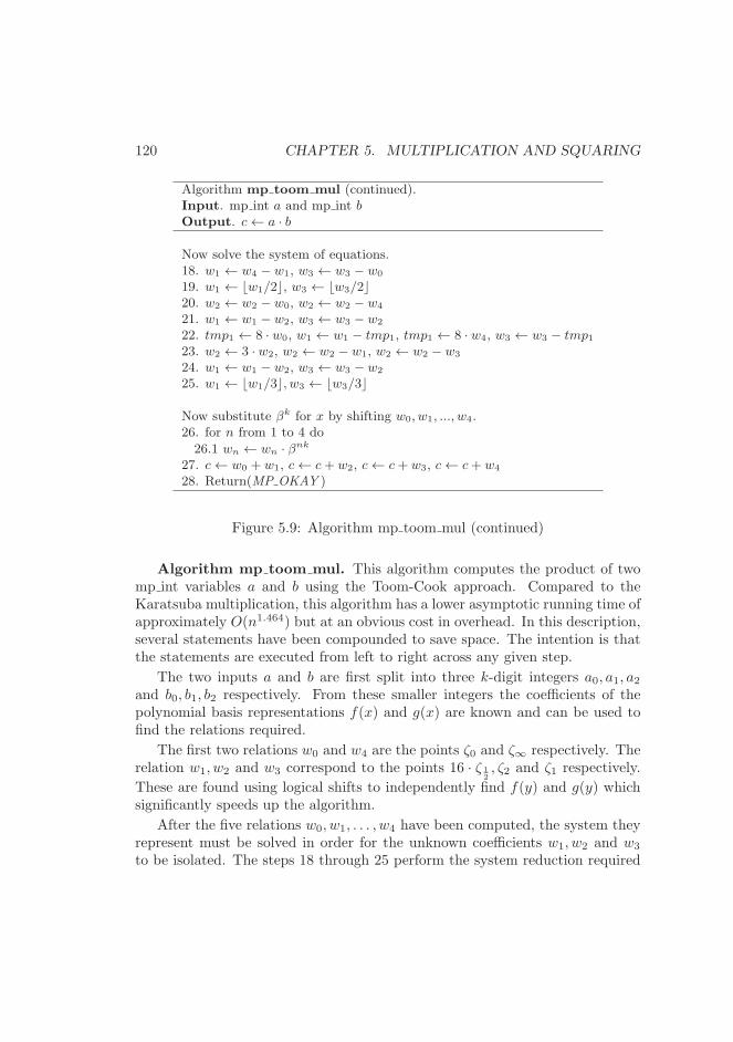
120 CHAPTER 5. MULTIPLICATION AND SQUARING
Algorithm mp toom mul (continued).Input. mp int a and mp int bOutput. c← a · b
Now solve the system of equations.18. w1 ← w4 − w1, w3 ← w3 − w0
19. w1 ← ⌊w1/2⌋, w3 ← ⌊w3/2⌋20. w2 ← w2 − w0, w2 ← w2 − w4
21. w1 ← w1 − w2, w3 ← w3 − w2
22. tmp1 ← 8 · w0, w1 ← w1 − tmp1, tmp1 ← 8 · w4, w3 ← w3 − tmp123. w2 ← 3 · w2, w2 ← w2 − w1, w2 ← w2 − w3
24. w1 ← w1 − w2, w3 ← w3 − w2
25. w1 ← ⌊w1/3⌋, w3 ← ⌊w3/3⌋
Now substitute βk for x by shifting w0, w1, ..., w4.26. for n from 1 to 4 do
26.1 wn ← wn · βnk
27. c← w0 + w1, c← c+ w2, c← c+ w3, c← c+ w4
28. Return(MP OKAY )
Figure 5.9: Algorithm mp toom mul (continued)
Algorithm mp toom mul. This algorithm computes the product of twomp int variables a and b using the Toom-Cook approach. Compared to theKaratsuba multiplication, this algorithm has a lower asymptotic running time ofapproximately O(n1.464) but at an obvious cost in overhead. In this description,several statements have been compounded to save space. The intention is thatthe statements are executed from left to right across any given step.
The two inputs a and b are first split into three k-digit integers a0, a1, a2and b0, b1, b2 respectively. From these smaller integers the coefficients of thepolynomial basis representations f(x) and g(x) are known and can be used tofind the relations required.
The first two relations w0 and w4 are the points ζ0 and ζ∞ respectively. Therelation w1, w2 and w3 correspond to the points 16 · ζ 1
2, ζ2 and ζ1 respectively.
These are found using logical shifts to independently find f(y) and g(y) whichsignificantly speeds up the algorithm.
After the five relations w0, w1, . . . , w4 have been computed, the system theyrepresent must be solved in order for the unknown coefficients w1, w2 and w3
to be isolated. The steps 18 through 25 perform the system reduction required
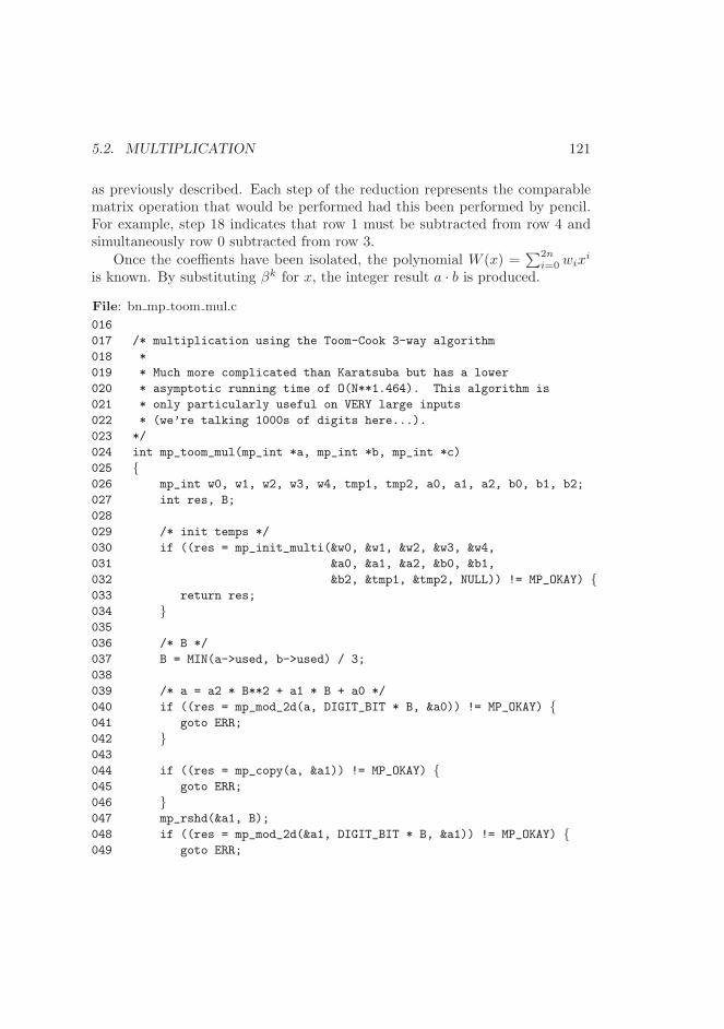
5.2. MULTIPLICATION 121
as previously described. Each step of the reduction represents the comparablematrix operation that would be performed had this been performed by pencil.For example, step 18 indicates that row 1 must be subtracted from row 4 andsimultaneously row 0 subtracted from row 3.
Once the coeffients have been isolated, the polynomial W (x) =∑2n
i=0 wixi
is known. By substituting βk for x, the integer result a · b is produced.
File: bn mp toom mul.c
016
017 /* multiplication using the Toom-Cook 3-way algorithm
018 *
019 * Much more complicated than Karatsuba but has a lower
020 * asymptotic running time of O(N**1.464). This algorithm is
021 * only particularly useful on VERY large inputs
022 * (we’re talking 1000s of digits here...).
023 */
024 int mp_toom_mul(mp_int *a, mp_int *b, mp_int *c)
025 {026 mp_int w0, w1, w2, w3, w4, tmp1, tmp2, a0, a1, a2, b0, b1, b2;
027 int res, B;
028
029 /* init temps */
030 if ((res = mp_init_multi(&w0, &w1, &w2, &w3, &w4,
031 &a0, &a1, &a2, &b0, &b1,
032 &b2, &tmp1, &tmp2, NULL)) != MP_OKAY) {033 return res;
034 }035
036 /* B */
037 B = MIN(a->used, b->used) / 3;
038
039 /* a = a2 * B**2 + a1 * B + a0 */
040 if ((res = mp_mod_2d(a, DIGIT_BIT * B, &a0)) != MP_OKAY) {041 goto ERR;
042 }043
044 if ((res = mp_copy(a, &a1)) != MP_OKAY) {045 goto ERR;
046 }047 mp_rshd(&a1, B);
048 if ((res = mp_mod_2d(&a1, DIGIT_BIT * B, &a1)) != MP_OKAY) {049 goto ERR;
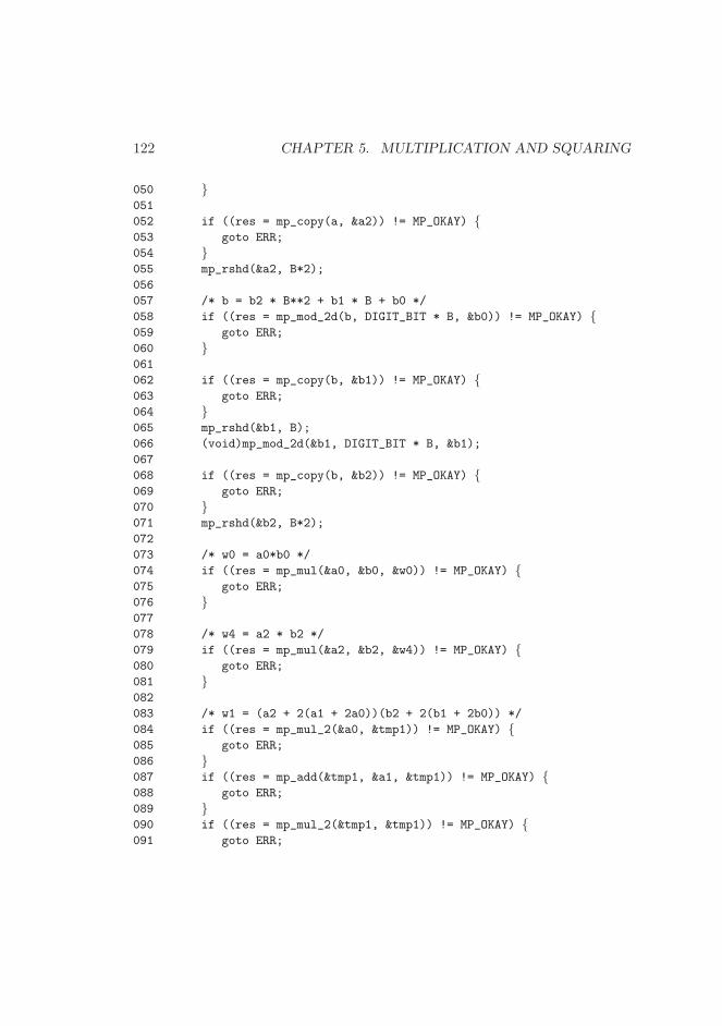
122 CHAPTER 5. MULTIPLICATION AND SQUARING
050 }051
052 if ((res = mp_copy(a, &a2)) != MP_OKAY) {053 goto ERR;
054 }055 mp_rshd(&a2, B*2);
056
057 /* b = b2 * B**2 + b1 * B + b0 */
058 if ((res = mp_mod_2d(b, DIGIT_BIT * B, &b0)) != MP_OKAY) {059 goto ERR;
060 }061
062 if ((res = mp_copy(b, &b1)) != MP_OKAY) {063 goto ERR;
064 }065 mp_rshd(&b1, B);
066 (void)mp_mod_2d(&b1, DIGIT_BIT * B, &b1);
067
068 if ((res = mp_copy(b, &b2)) != MP_OKAY) {069 goto ERR;
070 }071 mp_rshd(&b2, B*2);
072
073 /* w0 = a0*b0 */
074 if ((res = mp_mul(&a0, &b0, &w0)) != MP_OKAY) {075 goto ERR;
076 }077
078 /* w4 = a2 * b2 */
079 if ((res = mp_mul(&a2, &b2, &w4)) != MP_OKAY) {080 goto ERR;
081 }082
083 /* w1 = (a2 + 2(a1 + 2a0))(b2 + 2(b1 + 2b0)) */
084 if ((res = mp_mul_2(&a0, &tmp1)) != MP_OKAY) {085 goto ERR;
086 }087 if ((res = mp_add(&tmp1, &a1, &tmp1)) != MP_OKAY) {088 goto ERR;
089 }090 if ((res = mp_mul_2(&tmp1, &tmp1)) != MP_OKAY) {091 goto ERR;
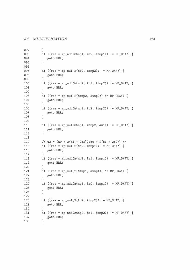
5.2. MULTIPLICATION 123
092 }093 if ((res = mp_add(&tmp1, &a2, &tmp1)) != MP_OKAY) {094 goto ERR;
095 }096
097 if ((res = mp_mul_2(&b0, &tmp2)) != MP_OKAY) {098 goto ERR;
099 }100 if ((res = mp_add(&tmp2, &b1, &tmp2)) != MP_OKAY) {101 goto ERR;
102 }103 if ((res = mp_mul_2(&tmp2, &tmp2)) != MP_OKAY) {104 goto ERR;
105 }106 if ((res = mp_add(&tmp2, &b2, &tmp2)) != MP_OKAY) {107 goto ERR;
108 }109
110 if ((res = mp_mul(&tmp1, &tmp2, &w1)) != MP_OKAY) {111 goto ERR;
112 }113
114 /* w3 = (a0 + 2(a1 + 2a2))(b0 + 2(b1 + 2b2)) */
115 if ((res = mp_mul_2(&a2, &tmp1)) != MP_OKAY) {116 goto ERR;
117 }118 if ((res = mp_add(&tmp1, &a1, &tmp1)) != MP_OKAY) {119 goto ERR;
120 }121 if ((res = mp_mul_2(&tmp1, &tmp1)) != MP_OKAY) {122 goto ERR;
123 }124 if ((res = mp_add(&tmp1, &a0, &tmp1)) != MP_OKAY) {125 goto ERR;
126 }127
128 if ((res = mp_mul_2(&b2, &tmp2)) != MP_OKAY) {129 goto ERR;
130 }131 if ((res = mp_add(&tmp2, &b1, &tmp2)) != MP_OKAY) {132 goto ERR;
133 }
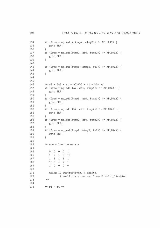
124 CHAPTER 5. MULTIPLICATION AND SQUARING
134 if ((res = mp_mul_2(&tmp2, &tmp2)) != MP_OKAY) {135 goto ERR;
136 }137 if ((res = mp_add(&tmp2, &b0, &tmp2)) != MP_OKAY) {138 goto ERR;
139 }140
141 if ((res = mp_mul(&tmp1, &tmp2, &w3)) != MP_OKAY) {142 goto ERR;
143 }144
145
146 /* w2 = (a2 + a1 + a0)(b2 + b1 + b0) */
147 if ((res = mp_add(&a2, &a1, &tmp1)) != MP_OKAY) {148 goto ERR;
149 }150 if ((res = mp_add(&tmp1, &a0, &tmp1)) != MP_OKAY) {151 goto ERR;
152 }153 if ((res = mp_add(&b2, &b1, &tmp2)) != MP_OKAY) {154 goto ERR;
155 }156 if ((res = mp_add(&tmp2, &b0, &tmp2)) != MP_OKAY) {157 goto ERR;
158 }159 if ((res = mp_mul(&tmp1, &tmp2, &w2)) != MP_OKAY) {160 goto ERR;
161 }162
163 /* now solve the matrix
164
165 0 0 0 0 1
166 1 2 4 8 16
167 1 1 1 1 1
168 16 8 4 2 1
169 1 0 0 0 0
170
171 using 12 subtractions, 4 shifts,
172 2 small divisions and 1 small multiplication
173 */
174
175 /* r1 - r4 */
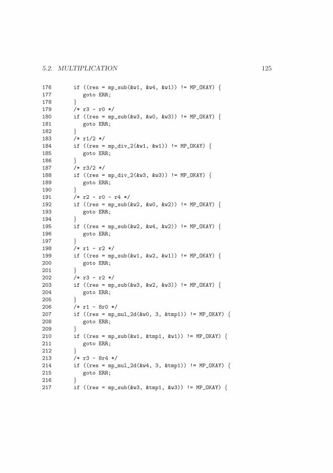
5.2. MULTIPLICATION 125
176 if ((res = mp_sub(&w1, &w4, &w1)) != MP_OKAY) {177 goto ERR;
178 }179 /* r3 - r0 */
180 if ((res = mp_sub(&w3, &w0, &w3)) != MP_OKAY) {181 goto ERR;
182 }183 /* r1/2 */
184 if ((res = mp_div_2(&w1, &w1)) != MP_OKAY) {185 goto ERR;
186 }187 /* r3/2 */
188 if ((res = mp_div_2(&w3, &w3)) != MP_OKAY) {189 goto ERR;
190 }191 /* r2 - r0 - r4 */
192 if ((res = mp_sub(&w2, &w0, &w2)) != MP_OKAY) {193 goto ERR;
194 }195 if ((res = mp_sub(&w2, &w4, &w2)) != MP_OKAY) {196 goto ERR;
197 }198 /* r1 - r2 */
199 if ((res = mp_sub(&w1, &w2, &w1)) != MP_OKAY) {200 goto ERR;
201 }202 /* r3 - r2 */
203 if ((res = mp_sub(&w3, &w2, &w3)) != MP_OKAY) {204 goto ERR;
205 }206 /* r1 - 8r0 */
207 if ((res = mp_mul_2d(&w0, 3, &tmp1)) != MP_OKAY) {208 goto ERR;
209 }210 if ((res = mp_sub(&w1, &tmp1, &w1)) != MP_OKAY) {211 goto ERR;
212 }213 /* r3 - 8r4 */
214 if ((res = mp_mul_2d(&w4, 3, &tmp1)) != MP_OKAY) {215 goto ERR;
216 }217 if ((res = mp_sub(&w3, &tmp1, &w3)) != MP_OKAY) {
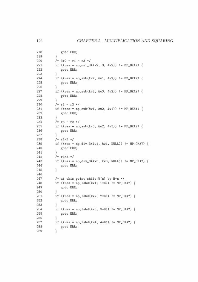
126 CHAPTER 5. MULTIPLICATION AND SQUARING
218 goto ERR;
219 }220 /* 3r2 - r1 - r3 */
221 if ((res = mp_mul_d(&w2, 3, &w2)) != MP_OKAY) {222 goto ERR;
223 }224 if ((res = mp_sub(&w2, &w1, &w2)) != MP_OKAY) {225 goto ERR;
226 }227 if ((res = mp_sub(&w2, &w3, &w2)) != MP_OKAY) {228 goto ERR;
229 }230 /* r1 - r2 */
231 if ((res = mp_sub(&w1, &w2, &w1)) != MP_OKAY) {232 goto ERR;
233 }234 /* r3 - r2 */
235 if ((res = mp_sub(&w3, &w2, &w3)) != MP_OKAY) {236 goto ERR;
237 }238 /* r1/3 */
239 if ((res = mp_div_3(&w1, &w1, NULL)) != MP_OKAY) {240 goto ERR;
241 }242 /* r3/3 */
243 if ((res = mp_div_3(&w3, &w3, NULL)) != MP_OKAY) {244 goto ERR;
245 }246
247 /* at this point shift W[n] by B*n */
248 if ((res = mp_lshd(&w1, 1*B)) != MP_OKAY) {249 goto ERR;
250 }251 if ((res = mp_lshd(&w2, 2*B)) != MP_OKAY) {252 goto ERR;
253 }254 if ((res = mp_lshd(&w3, 3*B)) != MP_OKAY) {255 goto ERR;
256 }257 if ((res = mp_lshd(&w4, 4*B)) != MP_OKAY) {258 goto ERR;
259 }
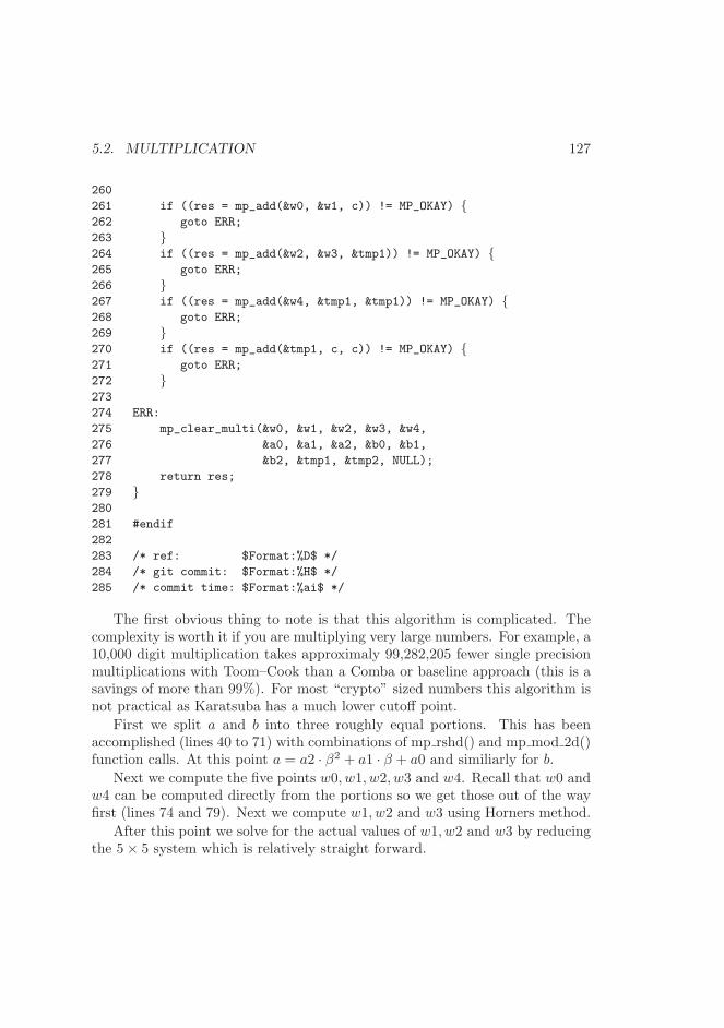
5.2. MULTIPLICATION 127
260
261 if ((res = mp_add(&w0, &w1, c)) != MP_OKAY) {262 goto ERR;
263 }264 if ((res = mp_add(&w2, &w3, &tmp1)) != MP_OKAY) {265 goto ERR;
266 }267 if ((res = mp_add(&w4, &tmp1, &tmp1)) != MP_OKAY) {268 goto ERR;
269 }270 if ((res = mp_add(&tmp1, c, c)) != MP_OKAY) {271 goto ERR;
272 }273
274 ERR:
275 mp_clear_multi(&w0, &w1, &w2, &w3, &w4,
276 &a0, &a1, &a2, &b0, &b1,
277 &b2, &tmp1, &tmp2, NULL);
278 return res;
279 }280
281 #endif
282
283 /* ref: $Format:%D$ */
284 /* git commit: $Format:%H$ */
285 /* commit time: $Format:%ai$ */
The first obvious thing to note is that this algorithm is complicated. Thecomplexity is worth it if you are multiplying very large numbers. For example, a10,000 digit multiplication takes approximaly 99,282,205 fewer single precisionmultiplications with Toom–Cook than a Comba or baseline approach (this is asavings of more than 99%). For most “crypto” sized numbers this algorithm isnot practical as Karatsuba has a much lower cutoff point.
First we split a and b into three roughly equal portions. This has beenaccomplished (lines 40 to 71) with combinations of mp rshd() and mp mod 2d()function calls. At this point a = a2 · β2 + a1 · β + a0 and similiarly for b.
Next we compute the five points w0, w1, w2, w3 and w4. Recall that w0 andw4 can be computed directly from the portions so we get those out of the wayfirst (lines 74 and 79). Next we compute w1, w2 and w3 using Horners method.
After this point we solve for the actual values of w1, w2 and w3 by reducingthe 5× 5 system which is relatively straight forward.
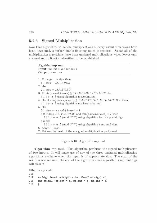
128 CHAPTER 5. MULTIPLICATION AND SQUARING
5.2.6 Signed Multiplication
Now that algorithms to handle multiplications of every useful dimensions havebeen developed, a rather simple finishing touch is required. So far all of themultiplication algorithms have been unsigned multiplications which leaves onlya signed multiplication algorithm to be established.
Algorithm mp mul.Input. mp int a and mp int bOutput. c← a · b
1. If a.sign = b.sign then1.1 sign = MP ZPOS
2. else2.1 sign = MP ZNEG
3. If min(a.used, b.used) ≥ TOOM MUL CUTOFF then3.1 c← a · b using algorithm mp toom mul
4. else if min(a.used, b.used) ≥ KARATSUBA MUL CUTOFF then4.1 c← a · b using algorithm mp karatsuba mul
5. else5.1 digs← a.used+ b.used+ 15.2 If digs < MP ARRAY and min(a.used, b.used) ≤ δ then
5.2.1 c← a · b (mod βdigs) using algorithm fast s mp mul digs.5.3 else
5.3.1 c← a · b (mod βdigs) using algorithm s mp mul digs.6. c.sign← sign7. Return the result of the unsigned multiplication performed.
Figure 5.10: Algorithm mp mul
Algorithm mp mul. This algorithm performs the signed multiplicationof two inputs. It will make use of any of the three unsigned multiplicationalgorithms available when the input is of appropriate size. The sign of theresult is not set until the end of the algorithm since algorithm s mp mul digswill clear it.
File: bn mp mul.c
016
017 /* high level multiplication (handles sign) */
018 int mp_mul (mp_int * a, mp_int * b, mp_int * c)
019 {
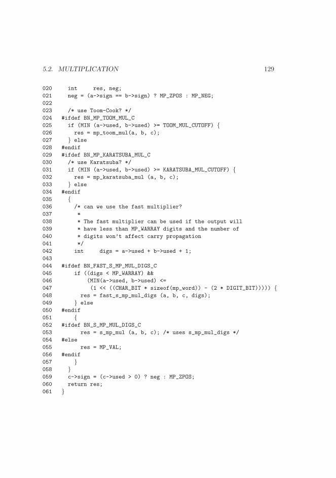
5.2. MULTIPLICATION 129
020 int res, neg;
021 neg = (a->sign == b->sign) ? MP_ZPOS : MP_NEG;
022
023 /* use Toom-Cook? */
024 #ifdef BN_MP_TOOM_MUL_C
025 if (MIN (a->used, b->used) >= TOOM_MUL_CUTOFF) {026 res = mp_toom_mul(a, b, c);
027 } else
028 #endif
029 #ifdef BN_MP_KARATSUBA_MUL_C
030 /* use Karatsuba? */
031 if (MIN (a->used, b->used) >= KARATSUBA_MUL_CUTOFF) {032 res = mp_karatsuba_mul (a, b, c);
033 } else
034 #endif
035 {036 /* can we use the fast multiplier?
037 *
038 * The fast multiplier can be used if the output will
039 * have less than MP_WARRAY digits and the number of
040 * digits won’t affect carry propagation
041 */
042 int digs = a->used + b->used + 1;
043
044 #ifdef BN_FAST_S_MP_MUL_DIGS_C
045 if ((digs < MP_WARRAY) &&
046 (MIN(a->used, b->used) <=
047 (1 << ((CHAR_BIT * sizeof(mp_word)) - (2 * DIGIT_BIT))))) {048 res = fast_s_mp_mul_digs (a, b, c, digs);
049 } else
050 #endif
051 {052 #ifdef BN_S_MP_MUL_DIGS_C
053 res = s_mp_mul (a, b, c); /* uses s_mp_mul_digs */
054 #else
055 res = MP_VAL;
056 #endif
057 }058 }059 c->sign = (c->used > 0) ? neg : MP_ZPOS;
060 return res;
061 }
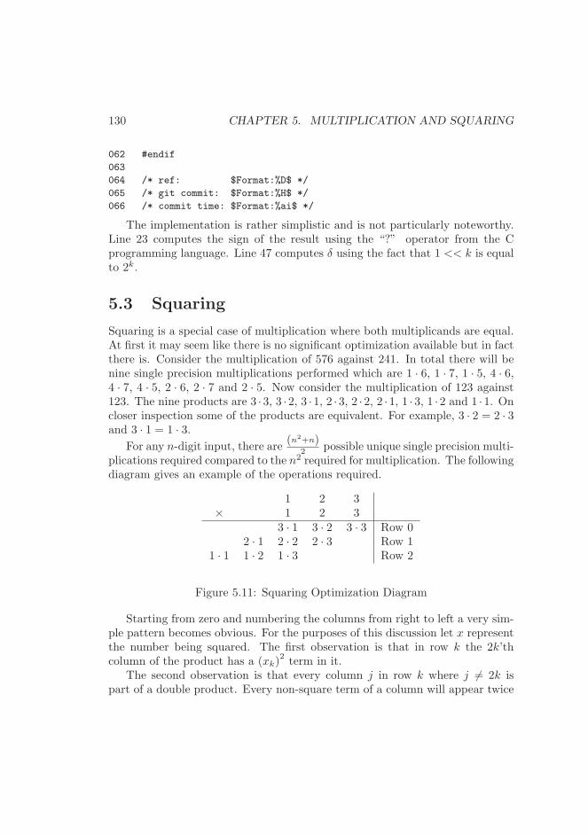
130 CHAPTER 5. MULTIPLICATION AND SQUARING
062 #endif
063
064 /* ref: $Format:%D$ */
065 /* git commit: $Format:%H$ */
066 /* commit time: $Format:%ai$ */
The implementation is rather simplistic and is not particularly noteworthy.Line 23 computes the sign of the result using the “?” operator from the Cprogramming language. Line 47 computes δ using the fact that 1 << k is equalto 2k.
5.3 Squaring
Squaring is a special case of multiplication where both multiplicands are equal.At first it may seem like there is no significant optimization available but in factthere is. Consider the multiplication of 576 against 241. In total there will benine single precision multiplications performed which are 1 · 6, 1 · 7, 1 · 5, 4 · 6,4 · 7, 4 · 5, 2 · 6, 2 · 7 and 2 · 5. Now consider the multiplication of 123 against123. The nine products are 3 ·3, 3 ·2, 3 ·1, 2 ·3, 2 ·2, 2 ·1, 1 ·3, 1 ·2 and 1 ·1. Oncloser inspection some of the products are equivalent. For example, 3 · 2 = 2 · 3and 3 · 1 = 1 · 3.
For any n-digit input, there are(n2+n)
2 possible unique single precision multi-plications required compared to the n2 required for multiplication. The followingdiagram gives an example of the operations required.
1 2 3× 1 2 3
3 · 1 3 · 2 3 · 3 Row 02 · 1 2 · 2 2 · 3 Row 1
1 · 1 1 · 2 1 · 3 Row 2
Figure 5.11: Squaring Optimization Diagram
Starting from zero and numbering the columns from right to left a very sim-ple pattern becomes obvious. For the purposes of this discussion let x representthe number being squared. The first observation is that in row k the 2k’thcolumn of the product has a (xk)
2term in it.
The second observation is that every column j in row k where j 6= 2k ispart of a double product. Every non-square term of a column will appear twice
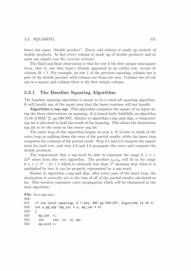
5.3. SQUARING 131
hence the name “double product”. Every odd column is made up entirely ofdouble products. In fact every column is made up of double products and atmost one square (see the exercise section).
The third and final observation is that for row k the first unique non-squareterm, that is, one that hasn’t already appeared in an earlier row, occurs atcolumn 2k + 1. For example, on row 1 of the previous squaring, column one ispart of the double product with column one from row zero. Column two of rowone is a square and column three is the first unique column.
5.3.1 The Baseline Squaring Algorithm
The baseline squaring algorithm is meant to be a catch-all squaring algorithm.It will handle any of the input sizes that the faster routines will not handle.
Algorithm s mp sqr. This algorithm computes the square of an input us-ing the three observations on squaring. It is based fairly faithfully on algorithm14.16 of HAC [2, pp.596-597]. Similar to algorithm s mp mul digs, a temporarymp int is allocated to hold the result of the squaring. This allows the destinationmp int to be the same as the source mp int.
The outer loop of this algorithm begins on step 4. It is best to think of theouter loop as walking down the rows of the partial results, while the inner loopcomputes the columns of the partial result. Step 4.1 and 4.2 compute the squareterm for each row, and step 4.3 and 4.4 propagate the carry and compute thedouble products.
The requirement that a mp word be able to represent the range 0 ≤ x <2β2 arises from this very algorithm. The product aixaiy will lie in the range0 ≤ x ≤ β2 − 2β + 1 which is obviously less than β2 meaning that when it ismultiplied by two, it can be properly represented by a mp word.
Similar to algorithm s mp mul digs, after every pass of the inner loop, thedestination is correctly set to the sum of all of the partial results calculated sofar. This involves expensive carry propagation which will be eliminated in thenext algorithm.
File: bn s mp sqr.c016
017 /* low level squaring, b = a*a, HAC pp.596-597, Algorithm 14.16 */
018 int s_mp_sqr (mp_int * a, mp_int * b)
019 {020 mp_int t;
021 int res, ix, iy, pa;
022 mp_word r;
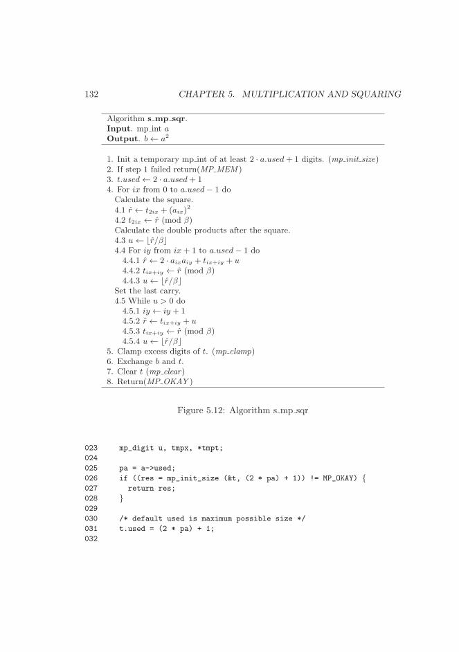
132 CHAPTER 5. MULTIPLICATION AND SQUARING
Algorithm s mp sqr.Input. mp int aOutput. b← a2
1. Init a temporary mp int of at least 2 · a.used+ 1 digits. (mp init size)2. If step 1 failed return(MP MEM )3. t.used← 2 · a.used+ 14. For ix from 0 to a.used− 1 doCalculate the square.
4.1 r ← t2ix + (aix)2
4.2 t2ix ← r (mod β)Calculate the double products after the square.4.3 u← ⌊r/β⌋4.4 For iy from ix+ 1 to a.used− 1 do4.4.1 r ← 2 · aixaiy + tix+iy + u4.4.2 tix+iy ← r (mod β)4.4.3 u← ⌊r/β⌋
Set the last carry.4.5 While u > 0 do4.5.1 iy ← iy + 14.5.2 r ← tix+iy + u4.5.3 tix+iy ← r (mod β)4.5.4 u← ⌊r/β⌋
5. Clamp excess digits of t. (mp clamp)6. Exchange b and t.7. Clear t (mp clear)8. Return(MP OKAY )
Figure 5.12: Algorithm s mp sqr
023 mp_digit u, tmpx, *tmpt;
024
025 pa = a->used;
026 if ((res = mp_init_size (&t, (2 * pa) + 1)) != MP_OKAY) {027 return res;
028 }029
030 /* default used is maximum possible size */
031 t.used = (2 * pa) + 1;
032
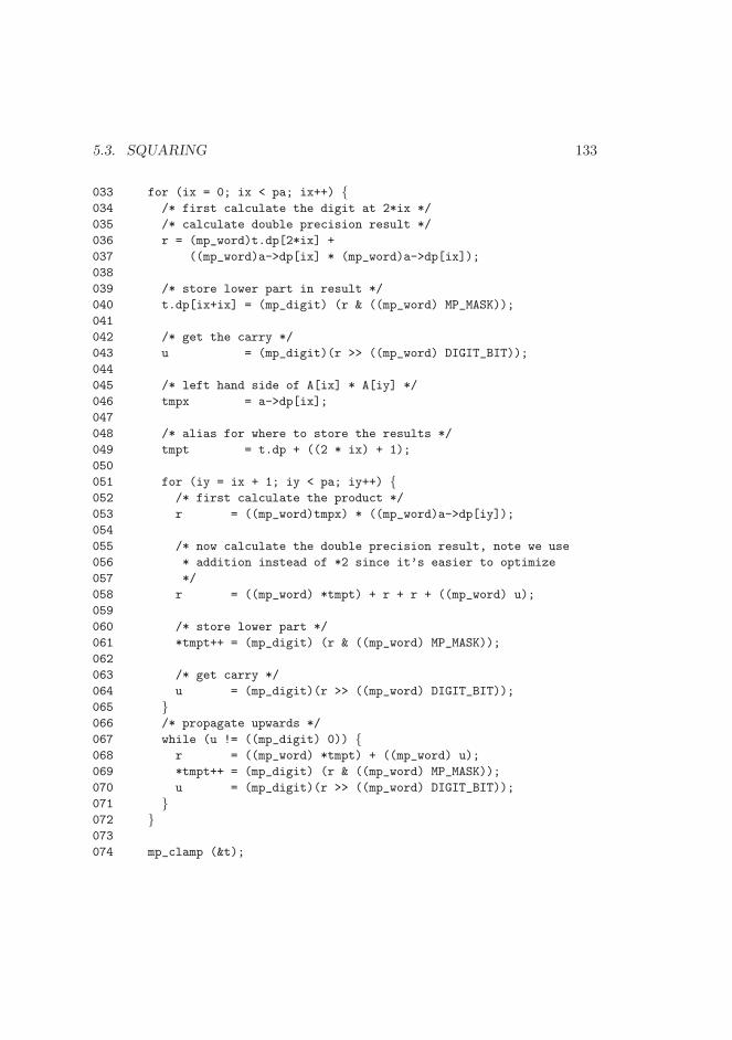
5.3. SQUARING 133
033 for (ix = 0; ix < pa; ix++) {034 /* first calculate the digit at 2*ix */
035 /* calculate double precision result */
036 r = (mp_word)t.dp[2*ix] +
037 ((mp_word)a->dp[ix] * (mp_word)a->dp[ix]);
038
039 /* store lower part in result */
040 t.dp[ix+ix] = (mp_digit) (r & ((mp_word) MP_MASK));
041
042 /* get the carry */
043 u = (mp_digit)(r >> ((mp_word) DIGIT_BIT));
044
045 /* left hand side of A[ix] * A[iy] */
046 tmpx = a->dp[ix];
047
048 /* alias for where to store the results */
049 tmpt = t.dp + ((2 * ix) + 1);
050
051 for (iy = ix + 1; iy < pa; iy++) {052 /* first calculate the product */
053 r = ((mp_word)tmpx) * ((mp_word)a->dp[iy]);
054
055 /* now calculate the double precision result, note we use
056 * addition instead of *2 since it’s easier to optimize
057 */
058 r = ((mp_word) *tmpt) + r + r + ((mp_word) u);
059
060 /* store lower part */
061 *tmpt++ = (mp_digit) (r & ((mp_word) MP_MASK));
062
063 /* get carry */
064 u = (mp_digit)(r >> ((mp_word) DIGIT_BIT));
065 }066 /* propagate upwards */
067 while (u != ((mp_digit) 0)) {068 r = ((mp_word) *tmpt) + ((mp_word) u);
069 *tmpt++ = (mp_digit) (r & ((mp_word) MP_MASK));
070 u = (mp_digit)(r >> ((mp_word) DIGIT_BIT));
071 }072 }073
074 mp_clamp (&t);
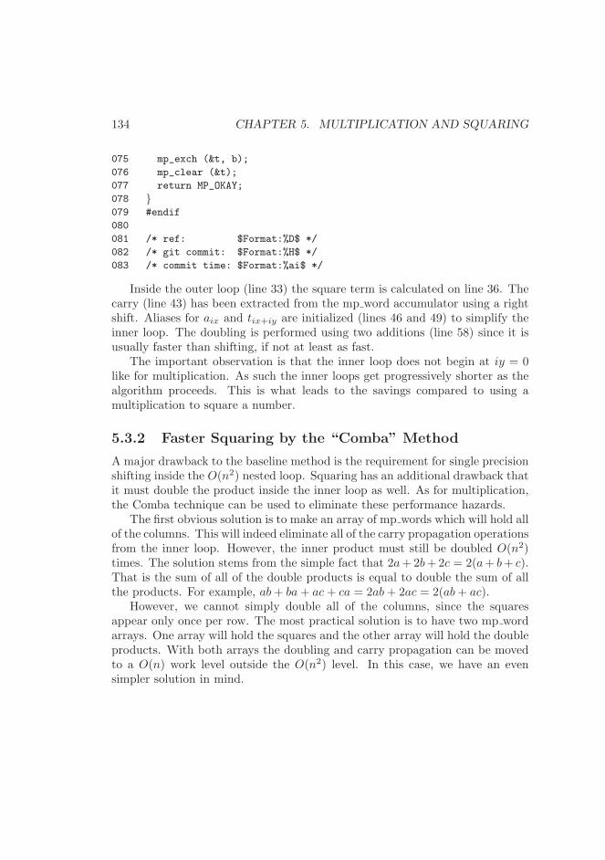
134 CHAPTER 5. MULTIPLICATION AND SQUARING
075 mp_exch (&t, b);
076 mp_clear (&t);
077 return MP_OKAY;
078 }079 #endif
080
081 /* ref: $Format:%D$ */
082 /* git commit: $Format:%H$ */
083 /* commit time: $Format:%ai$ */
Inside the outer loop (line 33) the square term is calculated on line 36. Thecarry (line 43) has been extracted from the mp word accumulator using a rightshift. Aliases for aix and tix+iy are initialized (lines 46 and 49) to simplify theinner loop. The doubling is performed using two additions (line 58) since it isusually faster than shifting, if not at least as fast.
The important observation is that the inner loop does not begin at iy = 0like for multiplication. As such the inner loops get progressively shorter as thealgorithm proceeds. This is what leads to the savings compared to using amultiplication to square a number.
5.3.2 Faster Squaring by the “Comba” Method
A major drawback to the baseline method is the requirement for single precisionshifting inside the O(n2) nested loop. Squaring has an additional drawback thatit must double the product inside the inner loop as well. As for multiplication,the Comba technique can be used to eliminate these performance hazards.
The first obvious solution is to make an array of mp words which will hold allof the columns. This will indeed eliminate all of the carry propagation operationsfrom the inner loop. However, the inner product must still be doubled O(n2)times. The solution stems from the simple fact that 2a+2b+2c = 2(a+ b+ c).That is the sum of all of the double products is equal to double the sum of allthe products. For example, ab+ ba+ ac+ ca = 2ab+ 2ac = 2(ab+ ac).
However, we cannot simply double all of the columns, since the squaresappear only once per row. The most practical solution is to have two mp wordarrays. One array will hold the squares and the other array will hold the doubleproducts. With both arrays the doubling and carry propagation can be movedto a O(n) work level outside the O(n2) level. In this case, we have an evensimpler solution in mind.
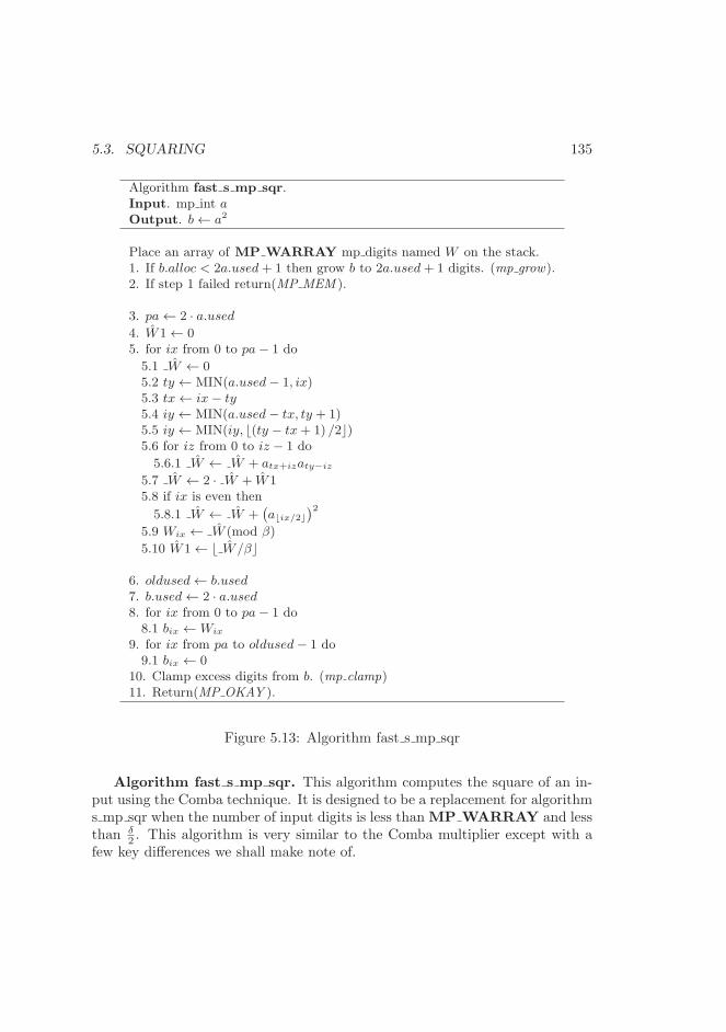
5.3. SQUARING 135
Algorithm fast s mp sqr.Input. mp int aOutput. b← a2
Place an array of MP WARRAY mp digits named W on the stack.1. If b.alloc < 2a.used+ 1 then grow b to 2a.used+ 1 digits. (mp grow).2. If step 1 failed return(MP MEM ).
3. pa← 2 · a.used
4. W1← 05. for ix from 0 to pa− 1 do
5.1 W ← 05.2 ty ← MIN(a.used− 1, ix)5.3 tx← ix− ty5.4 iy ← MIN(a.used− tx, ty + 1)5.5 iy ← MIN(iy, ⌊(ty − tx+ 1) /2⌋)5.6 for iz from 0 to iz − 1 do
5.6.1 W ← W + atx+izaty−iz
5.7 W ← 2 · W + W15.8 if ix is even then
5.8.1 W ← W +(
a⌊ix/2⌋
)2
5.9 Wix ← W (mod β)
5.10 W1← ⌊ W/β⌋
6. oldused← b.used7. b.used← 2 · a.used8. for ix from 0 to pa− 1 do8.1 bix ←Wix
9. for ix from pa to oldused− 1 do9.1 bix ← 0
10. Clamp excess digits from b. (mp clamp)11. Return(MP OKAY ).
Figure 5.13: Algorithm fast s mp sqr
Algorithm fast s mp sqr. This algorithm computes the square of an in-put using the Comba technique. It is designed to be a replacement for algorithms mp sqr when the number of input digits is less than MP WARRAY and lessthan δ
2 . This algorithm is very similar to the Comba multiplier except with afew key differences we shall make note of.
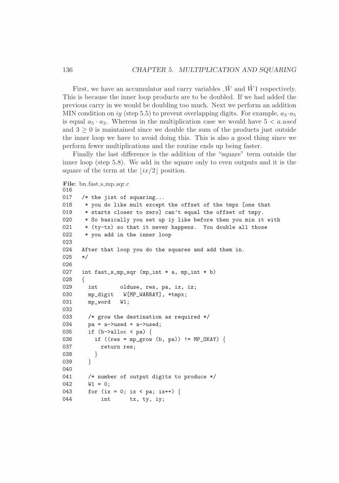
136 CHAPTER 5. MULTIPLICATION AND SQUARING
First, we have an accumulator and carry variables W and W1 respectively.This is because the inner loop products are to be doubled. If we had added theprevious carry in we would be doubling too much. Next we perform an additionMIN condition on iy (step 5.5) to prevent overlapping digits. For example, a3 ·a5is equal a5 · a3. Whereas in the multiplication case we would have 5 < a.usedand 3 ≥ 0 is maintained since we double the sum of the products just outsidethe inner loop we have to avoid doing this. This is also a good thing since weperform fewer multiplications and the routine ends up being faster.
Finally the last difference is the addition of the “square” term outside theinner loop (step 5.8). We add in the square only to even outputs and it is thesquare of the term at the ⌊ix/2⌋ position.
File: bn fast s mp sqr.c016
017 /* the jist of squaring...
018 * you do like mult except the offset of the tmpx [one that
019 * starts closer to zero] can’t equal the offset of tmpy.
020 * So basically you set up iy like before then you min it with
021 * (ty-tx) so that it never happens. You double all those
022 * you add in the inner loop
023
024 After that loop you do the squares and add them in.
025 */
026
027 int fast_s_mp_sqr (mp_int * a, mp_int * b)
028 {029 int olduse, res, pa, ix, iz;
030 mp_digit W[MP_WARRAY], *tmpx;
031 mp_word W1;
032
033 /* grow the destination as required */
034 pa = a->used + a->used;
035 if (b->alloc < pa) {036 if ((res = mp_grow (b, pa)) != MP_OKAY) {037 return res;
038 }039 }040
041 /* number of output digits to produce */
042 W1 = 0;
043 for (ix = 0; ix < pa; ix++) {044 int tx, ty, iy;
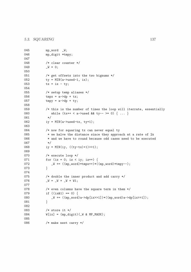
5.3. SQUARING 137
045 mp_word _W;
046 mp_digit *tmpy;
047
048 /* clear counter */
049 _W = 0;
050
051 /* get offsets into the two bignums */
052 ty = MIN(a->used-1, ix);
053 tx = ix - ty;
054
055 /* setup temp aliases */
056 tmpx = a->dp + tx;
057 tmpy = a->dp + ty;
058
059 /* this is the number of times the loop will iterrate, essentially
060 while (tx++ < a->used && ty-- >= 0) { ... }061 */
062 iy = MIN(a->used-tx, ty+1);
063
064 /* now for squaring tx can never equal ty
065 * we halve the distance since they approach at a rate of 2x
066 * and we have to round because odd cases need to be executed
067 */
068 iy = MIN(iy, ((ty-tx)+1)>>1);
069
070 /* execute loop */
071 for (iz = 0; iz < iy; iz++) {072 _W += ((mp_word)*tmpx++)*((mp_word)*tmpy--);
073 }074
075 /* double the inner product and add carry */
076 _W = _W + _W + W1;
077
078 /* even columns have the square term in them */
079 if ((ix&1) == 0) {080 _W += ((mp_word)a->dp[ix>>1])*((mp_word)a->dp[ix>>1]);
081 }082
083 /* store it */
084 W[ix] = (mp_digit)(_W & MP_MASK);
085
086 /* make next carry */
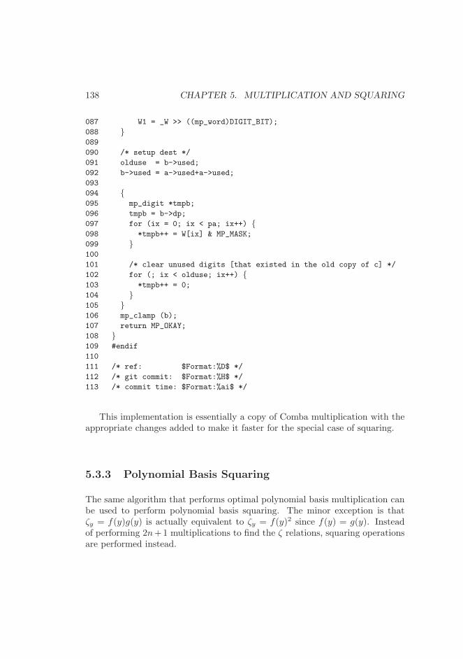
138 CHAPTER 5. MULTIPLICATION AND SQUARING
087 W1 = _W >> ((mp_word)DIGIT_BIT);
088 }089
090 /* setup dest */
091 olduse = b->used;
092 b->used = a->used+a->used;
093
094 {095 mp_digit *tmpb;
096 tmpb = b->dp;
097 for (ix = 0; ix < pa; ix++) {098 *tmpb++ = W[ix] & MP_MASK;
099 }100
101 /* clear unused digits [that existed in the old copy of c] */
102 for (; ix < olduse; ix++) {103 *tmpb++ = 0;
104 }105 }106 mp_clamp (b);
107 return MP_OKAY;
108 }109 #endif
110
111 /* ref: $Format:%D$ */
112 /* git commit: $Format:%H$ */
113 /* commit time: $Format:%ai$ */
This implementation is essentially a copy of Comba multiplication with theappropriate changes added to make it faster for the special case of squaring.
5.3.3 Polynomial Basis Squaring
The same algorithm that performs optimal polynomial basis multiplication canbe used to perform polynomial basis squaring. The minor exception is thatζy = f(y)g(y) is actually equivalent to ζy = f(y)2 since f(y) = g(y). Insteadof performing 2n+1 multiplications to find the ζ relations, squaring operationsare performed instead.
5.3. SQUARING 139
5.3.4 Karatsuba Squaring
Let f(x) = ax + b represent the polynomial basis representation of a number
to square. Let h(x) = (f(x))2represent the square of the polynomial. The
Karatsuba equation can be modified to square a number with the followingequation.
h(x) = a2x2 +(
(a+ b)2 − (a2 + b2))
x+ b2 (5.7)
Upon closer inspection this equation only requires the calculation of threehalf-sized squares: a2, b2 and (a + b)2. As in Karatsuba multiplication, thisalgorithm can be applied recursively on the input and will achieve an asymptoticrunning time of O
(
nlg(3))
.If the asymptotic times of Karatsuba squaring and multiplication are the
same, why not simply use the multiplication algorithm instead? The answer tothis arises from the cutoff point for squaring. As in multiplication there existsa cutoff point, at which the time required for a Comba based squaring and aKaratsuba based squaring meet. Due to the overhead inherent in the Karatsubamethod, the cutoff point is fairly high. For example, on an AMD Athlon XPprocessor with β = 228, the cutoff point is around 127 digits.
Consider squaring a 200 digit number with this technique. It will be splitinto two 100 digit halves which are subsequently squared. The 100 digit halveswill not be squared using Karatsuba, but instead using the faster Comba basedsquaring algorithm. If Karatsuba multiplication were used instead, the 100 digitnumbers would be squared with a slower Comba based multiplication.
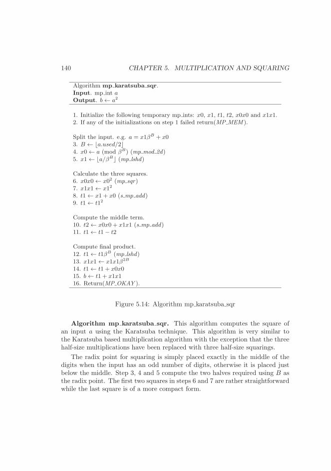
140 CHAPTER 5. MULTIPLICATION AND SQUARING
Algorithm mp karatsuba sqr.Input. mp int aOutput. b← a2
1. Initialize the following temporary mp ints: x0, x1, t1, t2, x0x0 and x1x1.2. If any of the initializations on step 1 failed return(MP MEM ).
Split the input. e.g. a = x1βB + x03. B ← ⌊a.used/2⌋4. x0← a (mod βB) (mp mod 2d)5. x1← ⌊a/βB⌋ (mp lshd)
Calculate the three squares.6. x0x0← x02 (mp sqr)7. x1x1← x12
8. t1← x1 + x0 (s mp add)9. t1← t12
Compute the middle term.10. t2← x0x0 + x1x1 (s mp add)11. t1← t1− t2
Compute final product.12. t1← t1βB (mp lshd)13. x1x1← x1x1β2B
14. t1← t1 + x0x015. b← t1 + x1x116. Return(MP OKAY ).
Figure 5.14: Algorithm mp karatsuba sqr
Algorithm mp karatsuba sqr. This algorithm computes the square ofan input a using the Karatsuba technique. This algorithm is very similar tothe Karatsuba based multiplication algorithm with the exception that the threehalf-size multiplications have been replaced with three half-size squarings.
The radix point for squaring is simply placed exactly in the middle of thedigits when the input has an odd number of digits, otherwise it is placed justbelow the middle. Step 3, 4 and 5 compute the two halves required using B asthe radix point. The first two squares in steps 6 and 7 are rather straightforwardwhile the last square is of a more compact form.
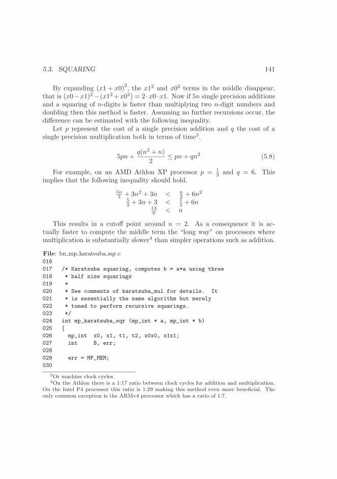
5.3. SQUARING 141
By expanding (x1 + x0)2, the x12 and x02 terms in the middle disappear,
that is (x0−x1)2− (x12+x02) = 2 ·x0 ·x1. Now if 5n single precision additionsand a squaring of n-digits is faster than multiplying two n-digit numbers anddoubling then this method is faster. Assuming no further recursions occur, thedifference can be estimated with the following inequality.
Let p represent the cost of a single precision addition and q the cost of asingle precision multiplication both in terms of time3.
5pn+q(n2 + n)
2≤ pn+ qn2 (5.8)
For example, on an AMD Athlon XP processor p = 13 and q = 6. This
implies that the following inequality should hold.
5n3 + 3n2 + 3n < n
3 + 6n2
53 + 3n+ 3 < 1
3 + 6n139 < n
This results in a cutoff point around n = 2. As a consequence it is ac-tually faster to compute the middle term the “long way” on processors wheremultiplication is substantially slower4 than simpler operations such as addition.
File: bn mp karatsuba sqr.c
016
017 /* Karatsuba squaring, computes b = a*a using three
018 * half size squarings
019 *
020 * See comments of karatsuba_mul for details. It
021 * is essentially the same algorithm but merely
022 * tuned to perform recursive squarings.
023 */
024 int mp_karatsuba_sqr (mp_int * a, mp_int * b)
025 {026 mp_int x0, x1, t1, t2, x0x0, x1x1;
027 int B, err;
028
029 err = MP_MEM;
030
3Or machine clock cycles.4On the Athlon there is a 1:17 ratio between clock cycles for addition and multiplication.
On the Intel P4 processor this ratio is 1:29 making this method even more beneficial. Theonly common exception is the ARMv4 processor which has a ratio of 1:7.
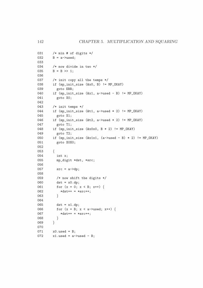
142 CHAPTER 5. MULTIPLICATION AND SQUARING
031 /* min # of digits */
032 B = a->used;
033
034 /* now divide in two */
035 B = B >> 1;
036
037 /* init copy all the temps */
038 if (mp_init_size (&x0, B) != MP_OKAY)
039 goto ERR;
040 if (mp_init_size (&x1, a->used - B) != MP_OKAY)
041 goto X0;
042
043 /* init temps */
044 if (mp_init_size (&t1, a->used * 2) != MP_OKAY)
045 goto X1;
046 if (mp_init_size (&t2, a->used * 2) != MP_OKAY)
047 goto T1;
048 if (mp_init_size (&x0x0, B * 2) != MP_OKAY)
049 goto T2;
050 if (mp_init_size (&x1x1, (a->used - B) * 2) != MP_OKAY)
051 goto X0X0;
052
053 {054 int x;
055 mp_digit *dst, *src;
056
057 src = a->dp;
058
059 /* now shift the digits */
060 dst = x0.dp;
061 for (x = 0; x < B; x++) {062 *dst++ = *src++;
063 }064
065 dst = x1.dp;
066 for (x = B; x < a->used; x++) {067 *dst++ = *src++;
068 }069 }070
071 x0.used = B;
072 x1.used = a->used - B;
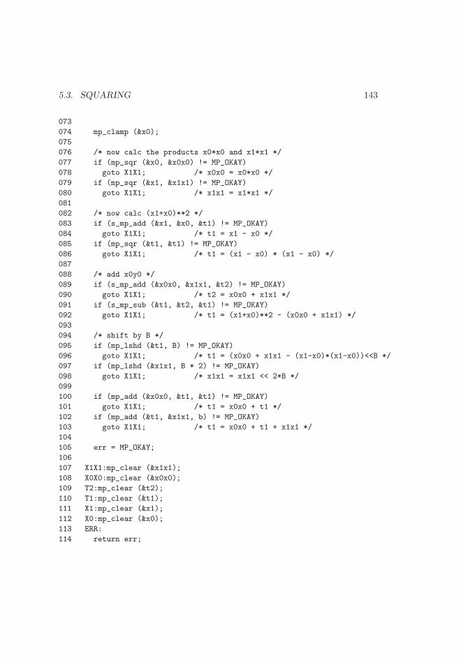
5.3. SQUARING 143
073
074 mp_clamp (&x0);
075
076 /* now calc the products x0*x0 and x1*x1 */
077 if (mp_sqr (&x0, &x0x0) != MP_OKAY)
078 goto X1X1; /* x0x0 = x0*x0 */
079 if (mp_sqr (&x1, &x1x1) != MP_OKAY)
080 goto X1X1; /* x1x1 = x1*x1 */
081
082 /* now calc (x1+x0)**2 */
083 if (s_mp_add (&x1, &x0, &t1) != MP_OKAY)
084 goto X1X1; /* t1 = x1 - x0 */
085 if (mp_sqr (&t1, &t1) != MP_OKAY)
086 goto X1X1; /* t1 = (x1 - x0) * (x1 - x0) */
087
088 /* add x0y0 */
089 if (s_mp_add (&x0x0, &x1x1, &t2) != MP_OKAY)
090 goto X1X1; /* t2 = x0x0 + x1x1 */
091 if (s_mp_sub (&t1, &t2, &t1) != MP_OKAY)
092 goto X1X1; /* t1 = (x1+x0)**2 - (x0x0 + x1x1) */
093
094 /* shift by B */
095 if (mp_lshd (&t1, B) != MP_OKAY)
096 goto X1X1; /* t1 = (x0x0 + x1x1 - (x1-x0)*(x1-x0))<<B */
097 if (mp_lshd (&x1x1, B * 2) != MP_OKAY)
098 goto X1X1; /* x1x1 = x1x1 << 2*B */
099
100 if (mp_add (&x0x0, &t1, &t1) != MP_OKAY)
101 goto X1X1; /* t1 = x0x0 + t1 */
102 if (mp_add (&t1, &x1x1, b) != MP_OKAY)
103 goto X1X1; /* t1 = x0x0 + t1 + x1x1 */
104
105 err = MP_OKAY;
106
107 X1X1:mp_clear (&x1x1);
108 X0X0:mp_clear (&x0x0);
109 T2:mp_clear (&t2);
110 T1:mp_clear (&t1);
111 X1:mp_clear (&x1);
112 X0:mp_clear (&x0);
113 ERR:
114 return err;
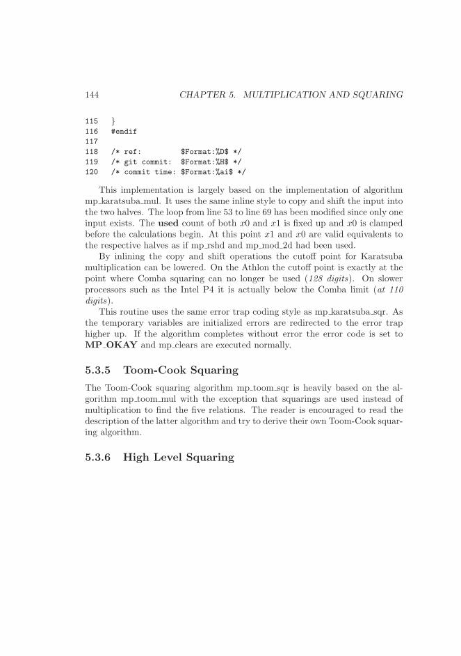
144 CHAPTER 5. MULTIPLICATION AND SQUARING
115 }116 #endif
117
118 /* ref: $Format:%D$ */
119 /* git commit: $Format:%H$ */
120 /* commit time: $Format:%ai$ */
This implementation is largely based on the implementation of algorithmmp karatsuba mul. It uses the same inline style to copy and shift the input intothe two halves. The loop from line 53 to line 69 has been modified since only oneinput exists. The used count of both x0 and x1 is fixed up and x0 is clampedbefore the calculations begin. At this point x1 and x0 are valid equivalents tothe respective halves as if mp rshd and mp mod 2d had been used.
By inlining the copy and shift operations the cutoff point for Karatsubamultiplication can be lowered. On the Athlon the cutoff point is exactly at thepoint where Comba squaring can no longer be used (128 digits). On slowerprocessors such as the Intel P4 it is actually below the Comba limit (at 110
digits).This routine uses the same error trap coding style as mp karatsuba sqr. As
the temporary variables are initialized errors are redirected to the error traphigher up. If the algorithm completes without error the error code is set toMP OKAY and mp clears are executed normally.
5.3.5 Toom-Cook Squaring
The Toom-Cook squaring algorithm mp toom sqr is heavily based on the al-gorithm mp toom mul with the exception that squarings are used instead ofmultiplication to find the five relations. The reader is encouraged to read thedescription of the latter algorithm and try to derive their own Toom-Cook squar-ing algorithm.
5.3.6 High Level Squaring
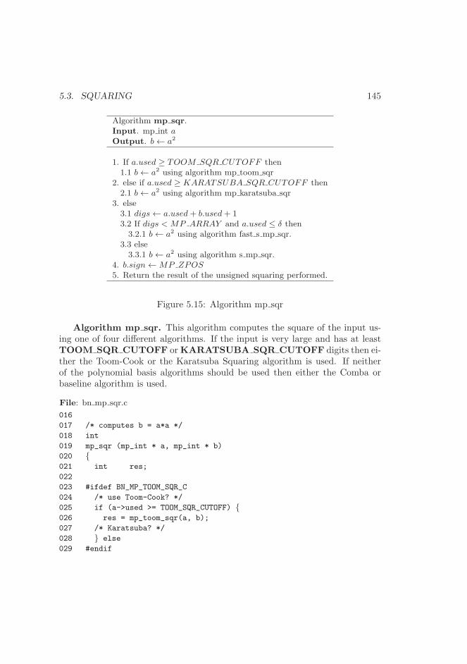
5.3. SQUARING 145
Algorithm mp sqr.Input. mp int aOutput. b← a2
1. If a.used ≥ TOOM SQR CUTOFF then1.1 b← a2 using algorithm mp toom sqr
2. else if a.used ≥ KARATSUBA SQR CUTOFF then2.1 b← a2 using algorithm mp karatsuba sqr
3. else3.1 digs← a.used+ b.used+ 13.2 If digs < MP ARRAY and a.used ≤ δ then3.2.1 b← a2 using algorithm fast s mp sqr.
3.3 else3.3.1 b← a2 using algorithm s mp sqr.
4. b.sign←MP ZPOS5. Return the result of the unsigned squaring performed.
Figure 5.15: Algorithm mp sqr
Algorithm mp sqr. This algorithm computes the square of the input us-ing one of four different algorithms. If the input is very large and has at leastTOOM SQR CUTOFF orKARATSUBA SQR CUTOFF digits then ei-ther the Toom-Cook or the Karatsuba Squaring algorithm is used. If neitherof the polynomial basis algorithms should be used then either the Comba orbaseline algorithm is used.
File: bn mp sqr.c
016
017 /* computes b = a*a */
018 int
019 mp_sqr (mp_int * a, mp_int * b)
020 {021 int res;
022
023 #ifdef BN_MP_TOOM_SQR_C
024 /* use Toom-Cook? */
025 if (a->used >= TOOM_SQR_CUTOFF) {026 res = mp_toom_sqr(a, b);
027 /* Karatsuba? */
028 } else
029 #endif
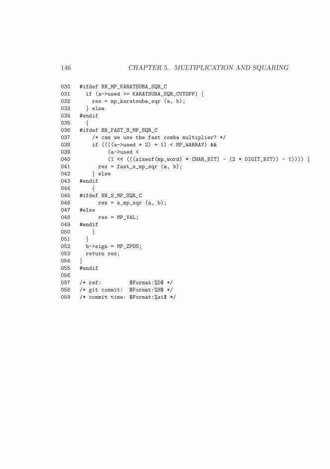
146 CHAPTER 5. MULTIPLICATION AND SQUARING
030 #ifdef BN_MP_KARATSUBA_SQR_C
031 if (a->used >= KARATSUBA_SQR_CUTOFF) {032 res = mp_karatsuba_sqr (a, b);
033 } else
034 #endif
035 {036 #ifdef BN_FAST_S_MP_SQR_C
037 /* can we use the fast comba multiplier? */
038 if ((((a->used * 2) + 1) < MP_WARRAY) &&
039 (a->used <
040 (1 << (((sizeof(mp_word) * CHAR_BIT) - (2 * DIGIT_BIT)) - 1)))) {041 res = fast_s_mp_sqr (a, b);
042 } else
043 #endif
044 {045 #ifdef BN_S_MP_SQR_C
046 res = s_mp_sqr (a, b);
047 #else
048 res = MP_VAL;
049 #endif
050 }051 }052 b->sign = MP_ZPOS;
053 return res;
054 }055 #endif
056
057 /* ref: $Format:%D$ */
058 /* git commit: $Format:%H$ */
059 /* commit time: $Format:%ai$ */
5.3. SQUARING 147
Exercises
[3] Devise an efficient algorithm for selection of the radix point to handle inputsthat have different number of digits in Karatsuba multiplication.
[2] In section 5.3 the fact that every column of a squaring is made upof double products and at most one square is stated. Prove this statement.
[3] Prove the equation for Karatsuba squaring.
[1] Prove that Karatsuba squaring requires O(
nlg(3))
time.
[2] Determine the minimal ratio between addition and multiplication clock cyclesrequired for equation 6.7 to be true.
[3] Implement a threaded version of Comba multiplication (and squaring) where youcompute subsets of the columns in each thread. Determine a cutoff point whereit is effective and add the logic to mp mul() and mp sqr().
[4] Same as the previous but also modify the Karatsuba and Toom-Cook. You mustincrease the throughput of mp exptmod() for random odd moduli in the range512 . . . 4096 bits significantly (> 2x) to complete this challenge.

148 CHAPTER 5. MULTIPLICATION AND SQUARING
Chapter 6
Modular Reduction
6.1 Basics of Modular Reduction
Modular reduction is an operation that arises quite often within public keycryptography algorithms and various number theoretic algorithms, such as fac-toring. Modular reduction algorithms are the third class of algorithms of the“multipliers” set. A number a is said to be reduced modulo another number b byfinding the remainder of the division a/b. Full integer division with remainderis a topic to be covered in 8.1.
Modular reduction is equivalent to solving for r in the following equation.a = bq + r where q = ⌊a/b⌋. The result r is said to be “congruent to a modulob” which is also written as r ≡ a (mod b). In other vernacular r is known asthe “modular residue” which leads to “quadratic residue”1 and other forms ofresidues.
Modular reductions are normally used to create either finite groups, rings orfields. The most common usage for performance driven modular reductions isin modular exponentiation algorithms. That is to compute d = ab (mod c) asfast as possible. This operation is used in the RSA and Diffie-Hellman publickey algorithms, for example. Modular multiplication and squaring also ap-pears as a fundamental operation in elliptic curve cryptographic algorithms.As will be discussed in the subsequent chapter there exist fast algorithms forcomputing modular exponentiations without having to perform (in this exam-
ple) b − 1 multiplications. These algorithms will produce partial results in the
1That’s fancy talk for b ≡ a2 (mod p).
149
150 CHAPTER 6. MODULAR REDUCTION
range 0 ≤ x < c2 which can be taken advantage of to create several efficientalgorithms. They have also been used to create redundancy check algorithmsknown as CRCs, error correction codes such as Reed-Solomon and solve a varietyof number theoeretic problems.
6.2 The Barrett Reduction
The Barrett reduction algorithm [7] was inspired by fast division algorithmswhich multiply by the reciprocal to emulate division. Barretts observation wasthat the residue c of a modulo b is equal to
c = a− b · ⌊a/b⌋ (6.1)
Since algorithms such as modular exponentiation would be using the samemodulus extensively, typical DSP2 intuition would indicate the next step wouldbe to replace a/b by a multiplication by the reciprocal. However, DSP intuitionon its own will not work as these numbers are considerably larger than theprecision of common DSP floating point data types. It would take anothercommon optimization to optimize the algorithm.
6.2.1 Fixed Point Arithmetic
The trick used to optimize the above equation is based on a technique of em-ulating floating point data types with fixed precision integers. Fixed pointarithmetic would become very popular as it greatly optimize the “3d-shooter”genre of games in the mid 1990s when floating point units were fairly slow if notunavailable. The idea behind fixed point arithmetic is to take a normal k-bitinteger data type and break it into p-bit integer and a q-bit fraction part (wherep+ q = k).
In this system a k-bit integer n would actually represent n/2q. For example,with q = 4 the integer n = 37 would actually represent the value 2.3125. Tomultiply two fixed point numbers the integers are multiplied using traditionalarithmetic and subsequently normalized by moving the implied decimal pointback to where it should be. For example, with q = 4 to multiply the integers9 and 5 they must be converted to fixed point first by multiplying by 2q. Leta = 9(2q) represent the fixed point representation of 9 and b = 5(2q) represent
2It is worth noting that Barrett’s paper targeted the DSP56K processor.
6.2. THE BARRETT REDUCTION 151
the fixed point representation of 5. The product ab is equal to 45(22q) whichwhen normalized by dividing by 2q produces 45(2q).
This technique became popular since a normal integer multiplication andlogical shift right are the only required operations to perform a multiplicationof two fixed point numbers. Using fixed point arithmetic, division can be easilyapproximated by multiplying by the reciprocal. If 2q is equivalent to one than2q/b is equivalent to the fixed point approximation of 1/b using real arithmetic.Using this fact dividing an integer a by another integer b can be achieved withthe following expression.
⌊a/b⌋ ∼ ⌊(a · ⌊2q/b⌋)/2q⌋ (6.2)
The precision of the division is proportional to the value of q. If the divisorb is used frequently as is the case with modular exponentiation pre-computing2q/b will allow a division to be performed with a multiplication and a right shift.Both operations are considerably faster than division on most processors.
Consider dividing 19 by 5. The correct result is ⌊19/5⌋ = 3. With q = 3the reciprocal is ⌊2q/5⌋ = 1 which leads to a product of 19 which when dividedby 2q produces 2. However, with q = 4 the reciprocal is ⌊2q/5⌋ = 3 and theresult of the emulated division is ⌊3 · 19/2q⌋ = 3 which is correct. The valueof 2q must be close to or ideally larger than the dividend. In effect if a is thedividend then q should allow 0 ≤ ⌊a/2q⌋ ≤ 1 in order for this approach to workcorrectly. Plugging this form of divison into the original equation the followingmodular residue equation arises.
c = a− b · ⌊(a · ⌊2q/b⌋)/2q⌋ (6.3)
Using the notation from [7] the value of ⌊2q/b⌋ will be represented by the µsymbol. Using the µ variable also helps re-inforce the idea that it is meant tobe computed once and re-used.
c = a− b · ⌊(a · µ)/2q⌋ (6.4)
Provided that 2q ≥ a this algorithm will produce a quotient that is eitherexactly correct or off by a value of one. In the context of Barrett reduction thevalue of a is bound by 0 ≤ a ≤ (b − 1)2 meaning that 2q ≥ b2 is sufficient toensure the reciprocal will have enough precision.
Let n represent the number of digits in b. This algorithm requires approxi-mately 2n2 single precision multiplications to produce the quotient and anothern2 single precision multiplications to find the residue. In total 3n2 single preci-sion multiplications are required to reduce the number.
152 CHAPTER 6. MODULAR REDUCTION
For example, if b = 1179677 and q = 41 (2q > b2), then the reciprocal µis equal to ⌊2q/b⌋ = 1864089. Consider reducing a = 180388626447 modulob using the above reduction equation. The quotient using the new formulais ⌊(a · µ)/2q⌋ = 152913. By subtracting 152913b from a the correct residuea ≡ 677346 (mod b) is found.
6.2.2 Choosing a Radix Point
Using the fixed point representation a modular reduction can be performed with3n2 single precision multiplications. If that were the best that could be achieveda full division3 might as well be used in its place. The key to optimizing thereduction is to reduce the precision of the initial multiplication that finds thequotient.
Let a represent the number of which the residue is sought. Let b representthe modulus used to find the residue. Let m represent the number of digits inb. For the purposes of this discussion we will assume that the number of digitsin a is 2m, which is generally true if two m-digit numbers have been multiplied.Dividing a by b is the same as dividing a 2m digit integer by a m digit integer.Digits below the m− 1’th digit of a will contribute at most a value of 1 to thequotient because βk < b for any 0 ≤ k ≤ m− 1. Another way to express this isby re-writing a as two parts. If a′ ≡ a (mod bm) and a′′ = a−a′ then a
b ≡ a′+a′′
b
which is equivalent to a′
b + a′′
b . Since a′ is bound to be less than b the quotient
is bound by 0 ≤ a′
b < 1.Since the digits of a′ do not contribute much to the quotient the observation
is that they might as well be zero. However, if the digits “might as well be zero”they might as well not be there in the first place. Let q0 = ⌊a/βm−1⌋ representthe input with the irrelevant digits trimmed. Now the modular reduction istrimmed to the almost equivalent equation
c = a− b · ⌊(q0 · µ)/βm+1⌋ (6.5)
Note that the original divisor 2q has been replaced with βm+1 where in thiscase q is a multiple of lg(β). Also note that the exponent on the divisor whenadded to the amount q0 was shifted by equals 2m. If the optimization hadnot been performed the divisor would have the exponent 2m so in the end theexponents do “add up”. Using the above equation the quotient ⌊(q0 · µ)/βm+1⌋can be off from the true quotient by at most two. The original fixed point
3A division requires approximately O(2cn2) single precision multiplications for a smallvalue of c. See 8.1 for further details.
6.2. THE BARRETT REDUCTION 153
quotient can be off by as much as one (provided the radix point is chosen suitably)and now that the lower irrelevent digits have been trimmed the quotient can beoff by an additional value of one for a total of at most two. This implies that0 ≤ a − b · ⌊(q0 · µ)/βm+1⌋ < 3b. By first subtracting b times the quotient andthen conditionally subtracting b once or twice the residue is found.
The quotient is now found using (m + 1)(m) = m2 + m single precisionmultiplications and the residue with an additional m2 single precision multipli-cations, ignoring the subtractions required. In total 2m2 + m single precisionmultiplications are required to find the residue. This is considerably faster thanthe original attempt.
For example, let β = 10 represent the radix of the digits. Let b = 9999represent the modulus which implies m = 4. Let a = 99929878 represent thevalue of which the residue is desired. In this case q = 8 since 107 < 99992
meaning that µ = ⌊βq/b⌋ = 10001. With the new observation the multiplicandfor the quotient is equal to q0 = ⌊a/βm−1⌋ = 99929. The quotient is then⌊(q0 · µ)/βm+1⌋ = 9993. Subtracting 9993b from a and the correct residuea ≡ 9871 (mod b) is found.
6.2.3 Trimming the Quotient
So far the reduction algorithm has been optimized from 3m2 single precisionmultiplications down to 2m2 +m single precision multiplications. As it standsnow the algorithm is already fairly fast compared to a full integer division algo-rithm. However, there is still room for optimization.
After the first multiplication inside the quotient (q0 · µ) the value is shiftedright by m+1 places effectively nullifying the lower half of the product. It wouldbe nice to be able to remove those digits from the product to effectively cut downthe number of single precision multiplications. If the number of digits in themodulus m is far less than β a full product is not required for the algorithm towork properly. In fact the lower m − 2 digits will not affect the upper half ofthe product at all and do not need to be computed.
The value of µ is a m-digit number and q0 is a m + 1 digit number. Usinga full multiplier (m + 1)(m) = m2 + m single precision multiplications wouldbe required. Using a multiplier that will only produce digits at and above the
m − 1’th digit reduces the number of single precision multiplications to m2+m2
single precision multiplications.
154 CHAPTER 6. MODULAR REDUCTION
6.2.4 Trimming the Residue
After the quotient has been calculated it is used to reduce the input. As previ-ously noted the algorithm is not exact and it can be off by a small multiple ofthe modulus, that is 0 ≤ a− b · ⌊(q0 · µ)/βm+1⌋ < 3b. If b is m digits than theresult of reduction equation is a value of at most m+ 1 digits (provided 3 < β)implying that the upper m− 1 digits are implicitly zero.
The next optimization arises from this very fact. Instead of computingb · ⌊(q0 · µ)/βm+1⌋ using a full O(m2) multiplication algorithm only the lowerm + 1 digits of the product have to be computed. Similarly the value of a canbe reduced modulo βm+1 before the multiple of b is subtracted which simplifesthe subtraction as well. A multiplication that produces only the lower m + 1
digits requires m2+3m−22 single precision multiplications.
With both optimizations in place the algorithm is the algorithm Barrettproposed. It requires m2 + 2m − 1 single precision multiplications which isconsiderably faster than the straightforward 3m2 method.
6.2.5 The Barrett Algorithm
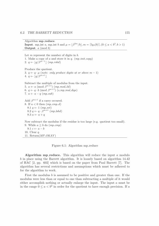
6.2. THE BARRETT REDUCTION 155
Algorithm mp reduce.Input. mp int a, mp int b and µ = ⌊β2m/b⌋,m = ⌈lgβ(b)⌉, (0 ≤ a < b2, b > 1)Output. a (mod b)
Let m represent the number of digits in b.1. Make a copy of a and store it in q. (mp init copy)2. q ← ⌊q/βm−1⌋ (mp rshd)
Produce the quotient.3. q ← q · µ (note: only produce digits at or above m− 1)4. q ← ⌊q/βm+1⌋
Subtract the multiple of modulus from the input.5. a← a (mod βm+1) (mp mod 2d)6. q ← q · b (mod βm+1) (s mp mul digs)7. a← a− q (mp sub)
Add βm+1 if a carry occured.8. If a < 0 then (mp cmp d)8.1 q ← 1 (mp set)8.2 q ← q · βm+1 (mp lshd)8.3 a← a+ q
Now subtract the modulus if the residue is too large (e.g. quotient too small).9. While a ≥ b do (mp cmp)9.1 c← a− b
10. Clear q.11. Return(MP OKAY )
Figure 6.1: Algorithm mp reduce
Algorithm mp reduce. This algorithm will reduce the input a modulob in place using the Barrett algorithm. It is loosely based on algorithm 14.42of HAC [2, pp. 602] which is based on the paper from Paul Barrett [7]. Thealgorithm has several restrictions and assumptions which must be adhered tofor the algorithm to work.
First the modulus b is assumed to be positive and greater than one. If themodulus were less than or equal to one than subtracting a multiple of it wouldeither accomplish nothing or actually enlarge the input. The input a must bein the range 0 ≤ a < b2 in order for the quotient to have enough precision. If a
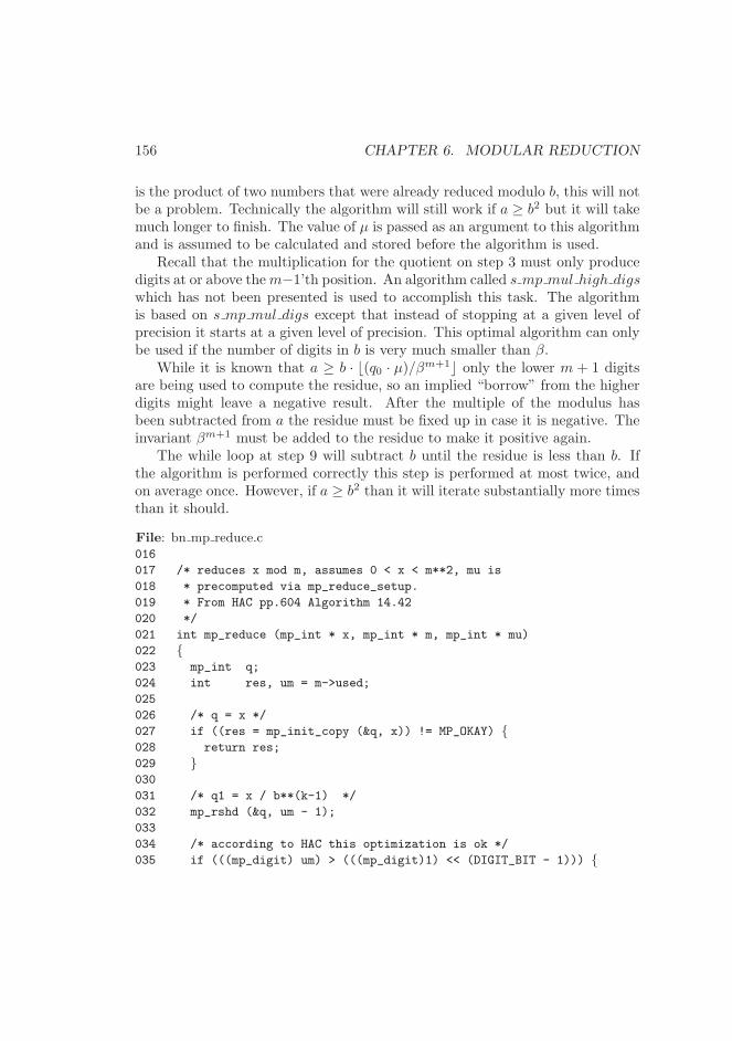
156 CHAPTER 6. MODULAR REDUCTION
is the product of two numbers that were already reduced modulo b, this will notbe a problem. Technically the algorithm will still work if a ≥ b2 but it will takemuch longer to finish. The value of µ is passed as an argument to this algorithmand is assumed to be calculated and stored before the algorithm is used.
Recall that the multiplication for the quotient on step 3 must only producedigits at or above them−1’th position. An algorithm called s mp mul high digswhich has not been presented is used to accomplish this task. The algorithmis based on s mp mul digs except that instead of stopping at a given level ofprecision it starts at a given level of precision. This optimal algorithm can onlybe used if the number of digits in b is very much smaller than β.
While it is known that a ≥ b · ⌊(q0 · µ)/βm+1⌋ only the lower m + 1 digitsare being used to compute the residue, so an implied “borrow” from the higherdigits might leave a negative result. After the multiple of the modulus hasbeen subtracted from a the residue must be fixed up in case it is negative. Theinvariant βm+1 must be added to the residue to make it positive again.
The while loop at step 9 will subtract b until the residue is less than b. Ifthe algorithm is performed correctly this step is performed at most twice, andon average once. However, if a ≥ b2 than it will iterate substantially more timesthan it should.
File: bn mp reduce.c016
017 /* reduces x mod m, assumes 0 < x < m**2, mu is
018 * precomputed via mp_reduce_setup.
019 * From HAC pp.604 Algorithm 14.42
020 */
021 int mp_reduce (mp_int * x, mp_int * m, mp_int * mu)
022 {023 mp_int q;
024 int res, um = m->used;
025
026 /* q = x */
027 if ((res = mp_init_copy (&q, x)) != MP_OKAY) {028 return res;
029 }030
031 /* q1 = x / b**(k-1) */
032 mp_rshd (&q, um - 1);
033
034 /* according to HAC this optimization is ok */
035 if (((mp_digit) um) > (((mp_digit)1) << (DIGIT_BIT - 1))) {
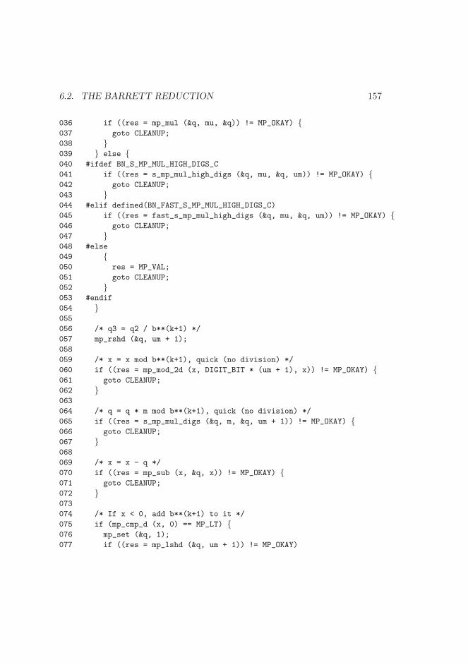
6.2. THE BARRETT REDUCTION 157
036 if ((res = mp_mul (&q, mu, &q)) != MP_OKAY) {037 goto CLEANUP;
038 }039 } else {040 #ifdef BN_S_MP_MUL_HIGH_DIGS_C
041 if ((res = s_mp_mul_high_digs (&q, mu, &q, um)) != MP_OKAY) {042 goto CLEANUP;
043 }044 #elif defined(BN_FAST_S_MP_MUL_HIGH_DIGS_C)
045 if ((res = fast_s_mp_mul_high_digs (&q, mu, &q, um)) != MP_OKAY) {046 goto CLEANUP;
047 }048 #else
049 {050 res = MP_VAL;
051 goto CLEANUP;
052 }053 #endif
054 }055
056 /* q3 = q2 / b**(k+1) */
057 mp_rshd (&q, um + 1);
058
059 /* x = x mod b**(k+1), quick (no division) */
060 if ((res = mp_mod_2d (x, DIGIT_BIT * (um + 1), x)) != MP_OKAY) {061 goto CLEANUP;
062 }063
064 /* q = q * m mod b**(k+1), quick (no division) */
065 if ((res = s_mp_mul_digs (&q, m, &q, um + 1)) != MP_OKAY) {066 goto CLEANUP;
067 }068
069 /* x = x - q */
070 if ((res = mp_sub (x, &q, x)) != MP_OKAY) {071 goto CLEANUP;
072 }073
074 /* If x < 0, add b**(k+1) to it */
075 if (mp_cmp_d (x, 0) == MP_LT) {076 mp_set (&q, 1);
077 if ((res = mp_lshd (&q, um + 1)) != MP_OKAY)
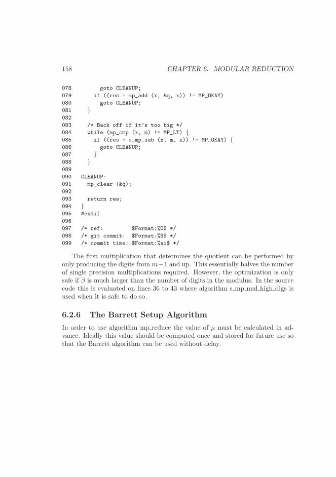
158 CHAPTER 6. MODULAR REDUCTION
078 goto CLEANUP;
079 if ((res = mp_add (x, &q, x)) != MP_OKAY)
080 goto CLEANUP;
081 }082
083 /* Back off if it’s too big */
084 while (mp_cmp (x, m) != MP_LT) {085 if ((res = s_mp_sub (x, m, x)) != MP_OKAY) {086 goto CLEANUP;
087 }088 }089
090 CLEANUP:
091 mp_clear (&q);
092
093 return res;
094 }095 #endif
096
097 /* ref: $Format:%D$ */
098 /* git commit: $Format:%H$ */
099 /* commit time: $Format:%ai$ */
The first multiplication that determines the quotient can be performed byonly producing the digits from m−1 and up. This essentially halves the numberof single precision multiplications required. However, the optimization is onlysafe if β is much larger than the number of digits in the modulus. In the sourcecode this is evaluated on lines 36 to 43 where algorithm s mp mul high digs isused when it is safe to do so.
6.2.6 The Barrett Setup Algorithm
In order to use algorithm mp reduce the value of µ must be calculated in ad-vance. Ideally this value should be computed once and stored for future use sothat the Barrett algorithm can be used without delay.
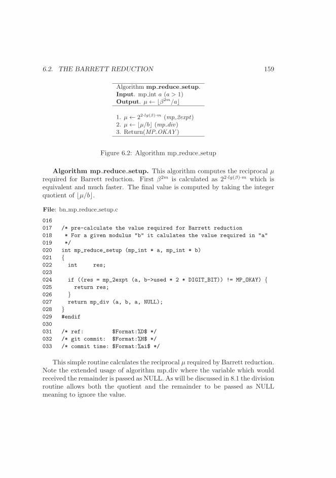
6.2. THE BARRETT REDUCTION 159
Algorithm mp reduce setup.Input. mp int a (a > 1)Output. µ← ⌊β2m/a⌋
1. µ← 22·lg(β)·m (mp 2expt)2. µ← ⌊µ/b⌋ (mp div)3. Return(MP OKAY )
Figure 6.2: Algorithm mp reduce setup
Algorithm mp reduce setup. This algorithm computes the reciprocal µrequired for Barrett reduction. First β2m is calculated as 22·lg(β)·m which isequivalent and much faster. The final value is computed by taking the integerquotient of ⌊µ/b⌋.
File: bn mp reduce setup.c
016
017 /* pre-calculate the value required for Barrett reduction
018 * For a given modulus "b" it calulates the value required in "a"
019 */
020 int mp_reduce_setup (mp_int * a, mp_int * b)
021 {022 int res;
023
024 if ((res = mp_2expt (a, b->used * 2 * DIGIT_BIT)) != MP_OKAY) {025 return res;
026 }027 return mp_div (a, b, a, NULL);
028 }029 #endif
030
031 /* ref: $Format:%D$ */
032 /* git commit: $Format:%H$ */
033 /* commit time: $Format:%ai$ */
This simple routine calculates the reciprocal µ required by Barrett reduction.Note the extended usage of algorithm mp div where the variable which wouldreceived the remainder is passed as NULL. As will be discussed in 8.1 the divisionroutine allows both the quotient and the remainder to be passed as NULLmeaning to ignore the value.
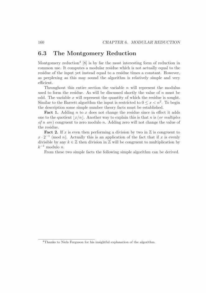
160 CHAPTER 6. MODULAR REDUCTION
6.3 The Montgomery Reduction
Montgomery reduction4 [8] is by far the most interesting form of reduction incommon use. It computes a modular residue which is not actually equal to theresidue of the input yet instead equal to a residue times a constant. However,as perplexing as this may sound the algorithm is relatively simple and veryefficient.
Throughout this entire section the variable n will represent the modulusused to form the residue. As will be discussed shortly the value of n must beodd. The variable x will represent the quantity of which the residue is sought.Similar to the Barrett algorithm the input is restricted to 0 ≤ x < n2. To beginthe description some simple number theory facts must be established.
Fact 1. Adding n to x does not change the residue since in effect it addsone to the quotient ⌊x/n⌋. Another way to explain this is that n is (or multiples
of n are) congruent to zero modulo n. Adding zero will not change the value ofthe residue.
Fact 2. If x is even then performing a division by two in Z is congruent tox · 2−1 (mod n). Actually this is an application of the fact that if x is evenlydivisible by any k ∈ Z then division in Z will be congruent to multiplication byk−1 modulo n.
From these two simple facts the following simple algorithm can be derived.
4Thanks to Niels Ferguson for his insightful explanation of the algorithm.
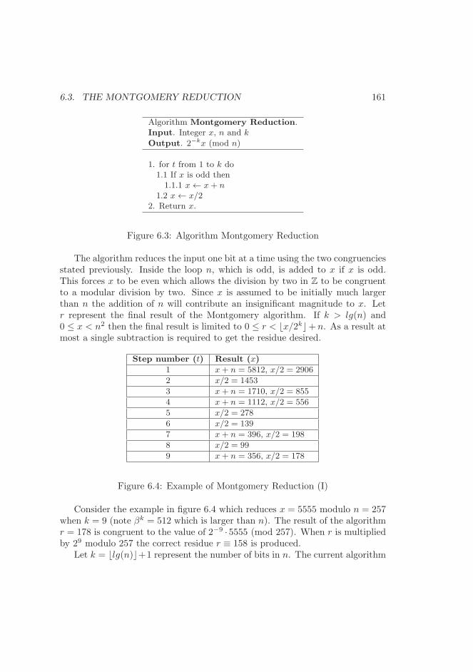
6.3. THE MONTGOMERY REDUCTION 161
Algorithm Montgomery Reduction.Input. Integer x, n and k
Output. 2−kx (mod n)
1. for t from 1 to k do1.1 If x is odd then1.1.1 x← x+ n
1.2 x← x/22. Return x.
Figure 6.3: Algorithm Montgomery Reduction
The algorithm reduces the input one bit at a time using the two congruenciesstated previously. Inside the loop n, which is odd, is added to x if x is odd.This forces x to be even which allows the division by two in Z to be congruentto a modular division by two. Since x is assumed to be initially much largerthan n the addition of n will contribute an insignificant magnitude to x. Letr represent the final result of the Montgomery algorithm. If k > lg(n) and0 ≤ x < n2 then the final result is limited to 0 ≤ r < ⌊x/2k⌋+n. As a result atmost a single subtraction is required to get the residue desired.
Step number (t) Result (x)
1 x+ n = 5812, x/2 = 2906
2 x/2 = 1453
3 x+ n = 1710, x/2 = 855
4 x+ n = 1112, x/2 = 556
5 x/2 = 278
6 x/2 = 139
7 x+ n = 396, x/2 = 198
8 x/2 = 99
9 x+ n = 356, x/2 = 178
Figure 6.4: Example of Montgomery Reduction (I)
Consider the example in figure 6.4 which reduces x = 5555 modulo n = 257when k = 9 (note βk = 512 which is larger than n). The result of the algorithmr = 178 is congruent to the value of 2−9 · 5555 (mod 257). When r is multipliedby 29 modulo 257 the correct residue r ≡ 158 is produced.
Let k = ⌊lg(n)⌋+1 represent the number of bits in n. The current algorithm
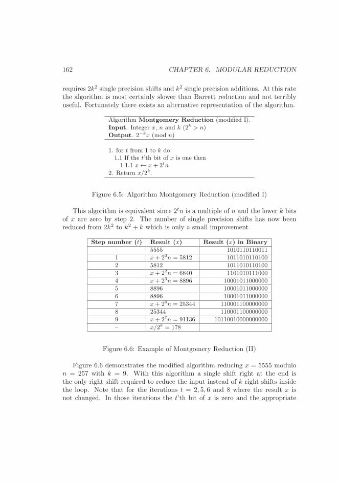
162 CHAPTER 6. MODULAR REDUCTION
requires 2k2 single precision shifts and k2 single precision additions. At this ratethe algorithm is most certainly slower than Barrett reduction and not terriblyuseful. Fortunately there exists an alternative representation of the algorithm.
Algorithm Montgomery Reduction (modified I).
Input. Integer x, n and k (2k > n)
Output. 2−kx (mod n)
1. for t from 1 to k do1.1 If the t’th bit of x is one then1.1.1 x← x+ 2tn
2. Return x/2k.
Figure 6.5: Algorithm Montgomery Reduction (modified I)
This algorithm is equivalent since 2tn is a multiple of n and the lower k bitsof x are zero by step 2. The number of single precision shifts has now beenreduced from 2k2 to k2 + k which is only a small improvement.
Step number (t) Result (x) Result (x) in Binary
– 5555 1010110110011
1 x+ 20n = 5812 1011010110100
2 5812 1011010110100
3 x+ 22n = 6840 1101010111000
4 x+ 23n = 8896 10001011000000
5 8896 10001011000000
6 8896 10001011000000
7 x+ 26n = 25344 110001100000000
8 25344 110001100000000
9 x+ 27n = 91136 10110010000000000
– x/2k = 178
Figure 6.6: Example of Montgomery Reduction (II)
Figure 6.6 demonstrates the modified algorithm reducing x = 5555 modulon = 257 with k = 9. With this algorithm a single shift right at the end isthe only right shift required to reduce the input instead of k right shifts insidethe loop. Note that for the iterations t = 2, 5, 6 and 8 where the result x isnot changed. In those iterations the t’th bit of x is zero and the appropriate
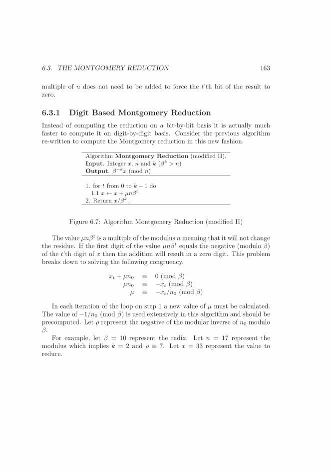
6.3. THE MONTGOMERY REDUCTION 163
multiple of n does not need to be added to force the t’th bit of the result tozero.
6.3.1 Digit Based Montgomery Reduction
Instead of computing the reduction on a bit-by-bit basis it is actually muchfaster to compute it on digit-by-digit basis. Consider the previous algorithmre-written to compute the Montgomery reduction in this new fashion.
Algorithm Montgomery Reduction (modified II).
Input. Integer x, n and k (βk > n)
Output. β−kx (mod n)
1. for t from 0 to k − 1 do1.1 x← x+ µnβt
2. Return x/βk.
Figure 6.7: Algorithm Montgomery Reduction (modified II)
The value µnβt is a multiple of the modulus nmeaning that it will not changethe residue. If the first digit of the value µnβt equals the negative (modulo β)of the t’th digit of x then the addition will result in a zero digit. This problembreaks down to solving the following congruency.
xt + µn0 ≡ 0 (mod β)µn0 ≡ −xt (mod β)
µ ≡ −xt/n0 (mod β)
In each iteration of the loop on step 1 a new value of µ must be calculated.The value of −1/n0 (mod β) is used extensively in this algorithm and should beprecomputed. Let ρ represent the negative of the modular inverse of n0 moduloβ.
For example, let β = 10 represent the radix. Let n = 17 represent themodulus which implies k = 2 and ρ ≡ 7. Let x = 33 represent the value toreduce.
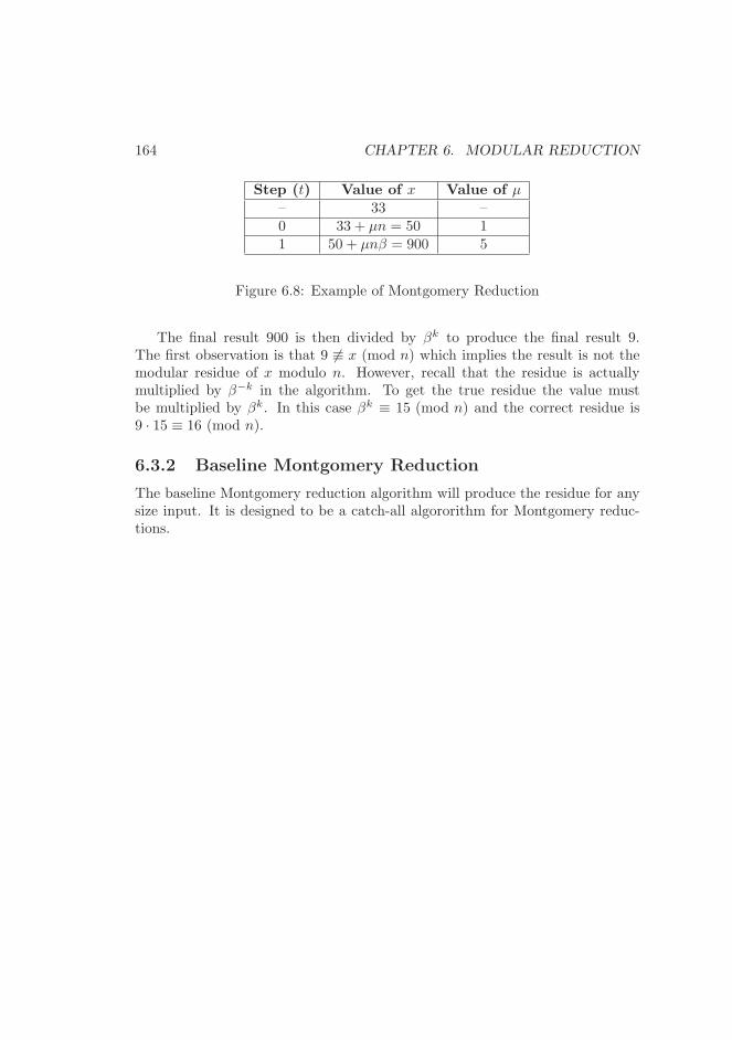
164 CHAPTER 6. MODULAR REDUCTION
Step (t) Value of x Value of µ– 33 –0 33 + µn = 50 11 50 + µnβ = 900 5
Figure 6.8: Example of Montgomery Reduction
The final result 900 is then divided by βk to produce the final result 9.The first observation is that 9 6≡ x (mod n) which implies the result is not themodular residue of x modulo n. However, recall that the residue is actuallymultiplied by β−k in the algorithm. To get the true residue the value mustbe multiplied by βk. In this case βk ≡ 15 (mod n) and the correct residue is9 · 15 ≡ 16 (mod n).
6.3.2 Baseline Montgomery Reduction
The baseline Montgomery reduction algorithm will produce the residue for anysize input. It is designed to be a catch-all algororithm for Montgomery reduc-tions.
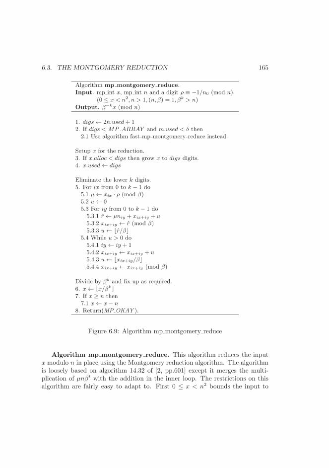
6.3. THE MONTGOMERY REDUCTION 165
Algorithm mp montgomery reduce.Input. mp int x, mp int n and a digit ρ ≡ −1/n0 (mod n).
(0 ≤ x < n2, n > 1, (n, β) = 1, βk > n)
Output. β−kx (mod n)
1. digs← 2n.used+ 12. If digs < MP ARRAY and m.used < δ then2.1 Use algorithm fast mp montgomery reduce instead.
Setup x for the reduction.3. If x.alloc < digs then grow x to digs digits.4. x.used← digs
Eliminate the lower k digits.5. For ix from 0 to k − 1 do5.1 µ← xix · ρ (mod β)5.2 u← 05.3 For iy from 0 to k − 1 do5.3.1 r ← µniy + xix+iy + u5.3.2 xix+iy ← r (mod β)5.3.3 u← ⌊r/β⌋
5.4 While u > 0 do5.4.1 iy ← iy + 15.4.2 xix+iy ← xix+iy + u5.4.3 u← ⌊xix+iy/β⌋5.4.4 xix+iy ← xix+iy (mod β)
Divide by βk and fix up as required.
6. x← ⌊x/βk⌋7. If x ≥ n then7.1 x← x− n
8. Return(MP OKAY ).
Figure 6.9: Algorithm mp montgomery reduce
Algorithm mp montgomery reduce. This algorithm reduces the inputx modulo n in place using the Montgomery reduction algorithm. The algorithmis loosely based on algorithm 14.32 of [2, pp.601] except it merges the multi-plication of µnβt with the addition in the inner loop. The restrictions on thisalgorithm are fairly easy to adapt to. First 0 ≤ x < n2 bounds the input to
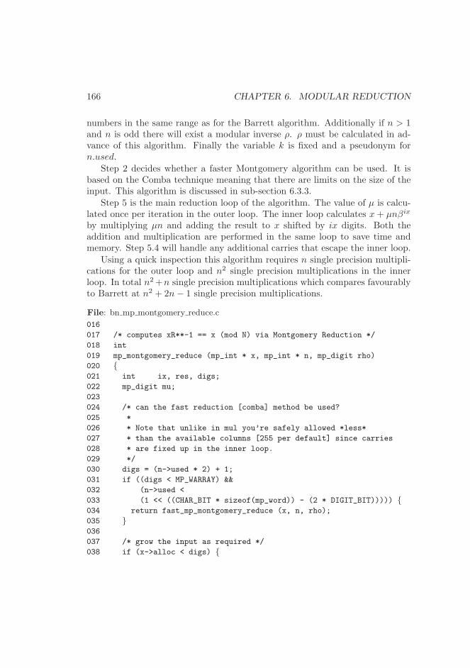
166 CHAPTER 6. MODULAR REDUCTION
numbers in the same range as for the Barrett algorithm. Additionally if n > 1and n is odd there will exist a modular inverse ρ. ρ must be calculated in ad-vance of this algorithm. Finally the variable k is fixed and a pseudonym forn.used.
Step 2 decides whether a faster Montgomery algorithm can be used. It isbased on the Comba technique meaning that there are limits on the size of theinput. This algorithm is discussed in sub-section 6.3.3.
Step 5 is the main reduction loop of the algorithm. The value of µ is calcu-lated once per iteration in the outer loop. The inner loop calculates x+ µnβix
by multiplying µn and adding the result to x shifted by ix digits. Both theaddition and multiplication are performed in the same loop to save time andmemory. Step 5.4 will handle any additional carries that escape the inner loop.
Using a quick inspection this algorithm requires n single precision multipli-cations for the outer loop and n2 single precision multiplications in the innerloop. In total n2+n single precision multiplications which compares favourablyto Barrett at n2 + 2n− 1 single precision multiplications.
File: bn mp montgomery reduce.c
016
017 /* computes xR**-1 == x (mod N) via Montgomery Reduction */
018 int
019 mp_montgomery_reduce (mp_int * x, mp_int * n, mp_digit rho)
020 {021 int ix, res, digs;
022 mp_digit mu;
023
024 /* can the fast reduction [comba] method be used?
025 *
026 * Note that unlike in mul you’re safely allowed *less*
027 * than the available columns [255 per default] since carries
028 * are fixed up in the inner loop.
029 */
030 digs = (n->used * 2) + 1;
031 if ((digs < MP_WARRAY) &&
032 (n->used <
033 (1 << ((CHAR_BIT * sizeof(mp_word)) - (2 * DIGIT_BIT))))) {034 return fast_mp_montgomery_reduce (x, n, rho);
035 }036
037 /* grow the input as required */
038 if (x->alloc < digs) {
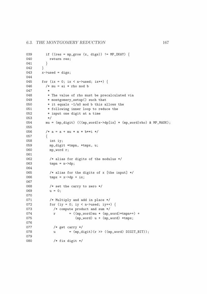
6.3. THE MONTGOMERY REDUCTION 167
039 if ((res = mp_grow (x, digs)) != MP_OKAY) {040 return res;
041 }042 }043 x->used = digs;
044
045 for (ix = 0; ix < n->used; ix++) {046 /* mu = ai * rho mod b
047 *
048 * The value of rho must be precalculated via
049 * montgomery_setup() such that
050 * it equals -1/n0 mod b this allows the
051 * following inner loop to reduce the
052 * input one digit at a time
053 */
054 mu = (mp_digit) (((mp_word)x->dp[ix] * (mp_word)rho) & MP_MASK);
055
056 /* a = a + mu * m * b**i */
057 {058 int iy;
059 mp_digit *tmpn, *tmpx, u;
060 mp_word r;
061
062 /* alias for digits of the modulus */
063 tmpn = n->dp;
064
065 /* alias for the digits of x [the input] */
066 tmpx = x->dp + ix;
067
068 /* set the carry to zero */
069 u = 0;
070
071 /* Multiply and add in place */
072 for (iy = 0; iy < n->used; iy++) {073 /* compute product and sum */
074 r = ((mp_word)mu * (mp_word)*tmpn++) +
075 (mp_word) u + (mp_word) *tmpx;
076
077 /* get carry */
078 u = (mp_digit)(r >> ((mp_word) DIGIT_BIT));
079
080 /* fix digit */
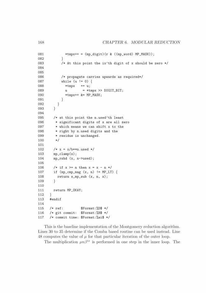
168 CHAPTER 6. MODULAR REDUCTION
081 *tmpx++ = (mp_digit)(r & ((mp_word) MP_MASK));
082 }083 /* At this point the ix’th digit of x should be zero */
084
085
086 /* propagate carries upwards as required*/
087 while (u != 0) {088 *tmpx += u;
089 u = *tmpx >> DIGIT_BIT;
090 *tmpx++ &= MP_MASK;
091 }092 }093 }094
095 /* at this point the n.used’th least
096 * significant digits of x are all zero
097 * which means we can shift x to the
098 * right by n.used digits and the
099 * residue is unchanged.
100 */
101
102 /* x = x/b**n.used */
103 mp_clamp(x);
104 mp_rshd (x, n->used);
105
106 /* if x >= n then x = x - n */
107 if (mp_cmp_mag (x, n) != MP_LT) {108 return s_mp_sub (x, n, x);
109 }110
111 return MP_OKAY;
112 }113 #endif
114
115 /* ref: $Format:%D$ */
116 /* git commit: $Format:%H$ */
117 /* commit time: $Format:%ai$ */
This is the baseline implementation of the Montgomery reduction algorithm.Lines 30 to 35 determine if the Comba based routine can be used instead. Line48 computes the value of µ for that particular iteration of the outer loop.
The multiplication µnβix is performed in one step in the inner loop. The
6.3. THE MONTGOMERY REDUCTION 169
alias tmpx refers to the ix’th digit of x and the alias tmpn refers to the modulusn.
6.3.3 Faster “Comba” Montgomery Reduction
The Montgomery reduction requires fewer single precision multiplications thana Barrett reduction, however it is much slower due to the serial nature of theinner loop. The Barrett reduction algorithm requires two slightly modified mul-tipliers which can be implemented with the Comba technique. The Montgomeryreduction algorithm cannot directly use the Comba technique to any significantadvantage since the inner loop calculates a k × 1 product k times.
The biggest obstacle is that at the ix’th iteration of the outer loop the valueof xix is required to calculate µ. This means the carries from 0 to ix− 1 musthave been propagated upwards to form a valid ix’th digit. The solution as itturns out is very simple. Perform a Comba like multiplier and inside the outerloop just after the inner loop fix up the ix+ 1’th digit by forwarding the carry.
With this change in place the Montgomery reduction algorithm can be per-formed with a Comba style multiplication loop which substantially increases thespeed of the algorithm.
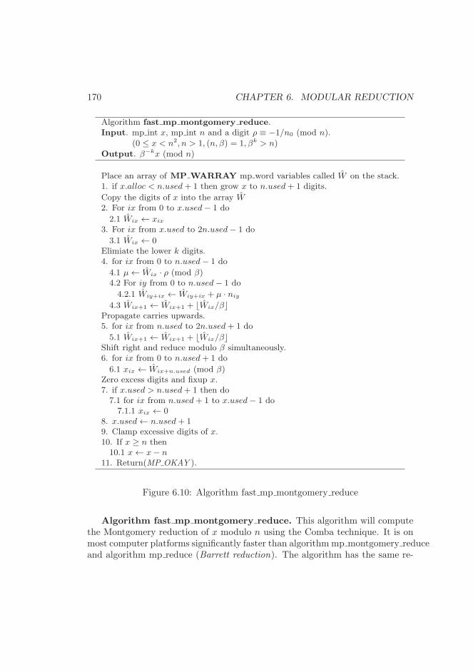
170 CHAPTER 6. MODULAR REDUCTION
Algorithm fast mp montgomery reduce.Input. mp int x, mp int n and a digit ρ ≡ −1/n0 (mod n).
(0 ≤ x < n2, n > 1, (n, β) = 1, βk > n)
Output. β−kx (mod n)
Place an array of MP WARRAY mp word variables called W on the stack.1. if x.alloc < n.used+ 1 then grow x to n.used+ 1 digits.
Copy the digits of x into the array W2. For ix from 0 to x.used− 1 do
2.1 Wix ← xix
3. For ix from x.used to 2n.used− 1 do
3.1 Wix ← 0Elimiate the lower k digits.4. for ix from 0 to n.used− 1 do
4.1 µ← Wix · ρ (mod β)4.2 For iy from 0 to n.used− 1 do
4.2.1 Wiy+ix ← Wiy+ix + µ · niy
4.3 Wix+1 ← Wix+1 + ⌊Wix/β⌋Propagate carries upwards.5. for ix from n.used to 2n.used+ 1 do
5.1 Wix+1 ← Wix+1 + ⌊Wix/β⌋Shift right and reduce modulo β simultaneously.6. for ix from 0 to n.used+ 1 do
6.1 xix ← Wix+n.used (mod β)Zero excess digits and fixup x.7. if x.used > n.used+ 1 then do7.1 for ix from n.used+ 1 to x.used− 1 do7.1.1 xix ← 0
8. x.used← n.used+ 19. Clamp excessive digits of x.10. If x ≥ n then10.1 x← x− n
11. Return(MP OKAY ).
Figure 6.10: Algorithm fast mp montgomery reduce
Algorithm fast mp montgomery reduce. This algorithm will computethe Montgomery reduction of x modulo n using the Comba technique. It is onmost computer platforms significantly faster than algorithm mp montgomery reduceand algorithm mp reduce (Barrett reduction). The algorithm has the same re-
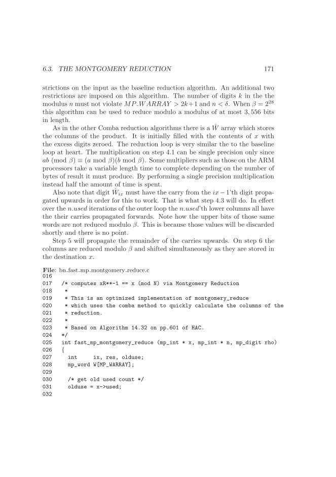
6.3. THE MONTGOMERY REDUCTION 171
strictions on the input as the baseline reduction algorithm. An additional tworestrictions are imposed on this algorithm. The number of digits k in the themodulus n must not violate MP WARRAY > 2k+1 and n < δ. When β = 228
this algorithm can be used to reduce modulo a modulus of at most 3, 556 bitsin length.
As in the other Comba reduction algorithms there is a W array which storesthe columns of the product. It is initially filled with the contents of x withthe excess digits zeroed. The reduction loop is very similar the to the baselineloop at heart. The multiplication on step 4.1 can be single precision only sinceab (mod β) ≡ (a mod β)(b mod β). Some multipliers such as those on the ARMprocessors take a variable length time to complete depending on the number ofbytes of result it must produce. By performing a single precision multiplicationinstead half the amount of time is spent.
Also note that digit Wix must have the carry from the ix− 1’th digit propa-gated upwards in order for this to work. That is what step 4.3 will do. In effectover the n.used iterations of the outer loop the n.used’th lower columns all havethe their carries propagated forwards. Note how the upper bits of those samewords are not reduced modulo β. This is because those values will be discardedshortly and there is no point.
Step 5 will propagate the remainder of the carries upwards. On step 6 thecolumns are reduced modulo β and shifted simultaneously as they are stored inthe destination x.
File: bn fast mp montgomery reduce.c016
017 /* computes xR**-1 == x (mod N) via Montgomery Reduction
018 *
019 * This is an optimized implementation of montgomery_reduce
020 * which uses the comba method to quickly calculate the columns of the
021 * reduction.
022 *
023 * Based on Algorithm 14.32 on pp.601 of HAC.
024 */
025 int fast_mp_montgomery_reduce (mp_int * x, mp_int * n, mp_digit rho)
026 {027 int ix, res, olduse;
028 mp_word W[MP_WARRAY];
029
030 /* get old used count */
031 olduse = x->used;
032
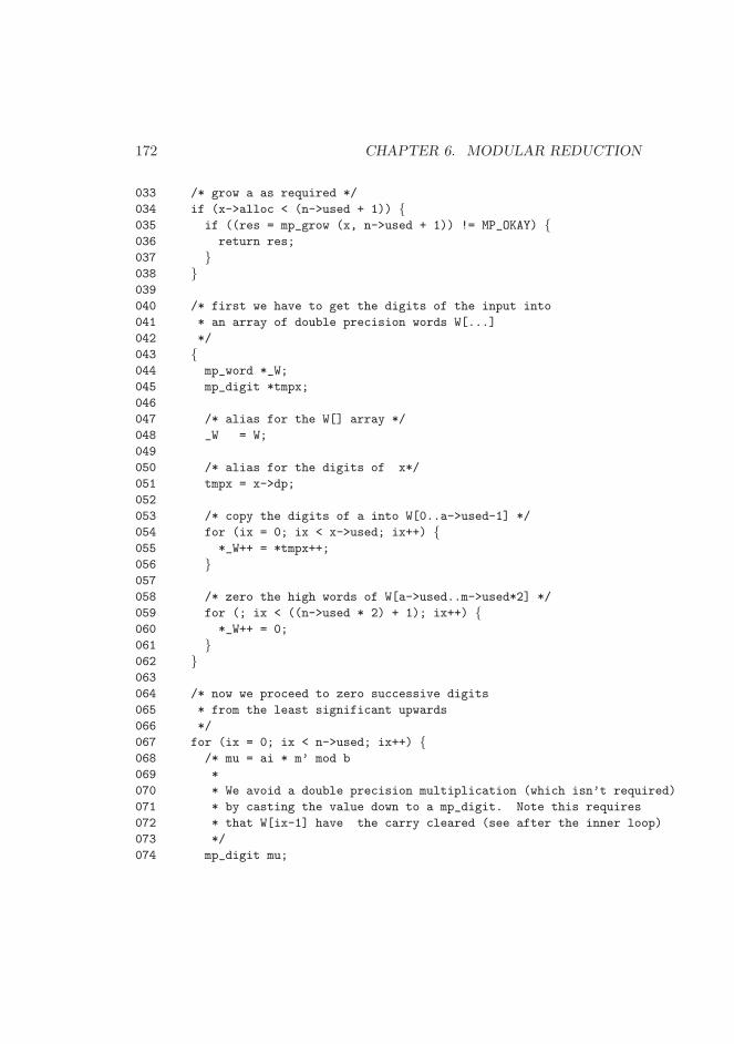
172 CHAPTER 6. MODULAR REDUCTION
033 /* grow a as required */
034 if (x->alloc < (n->used + 1)) {035 if ((res = mp_grow (x, n->used + 1)) != MP_OKAY) {036 return res;
037 }038 }039
040 /* first we have to get the digits of the input into
041 * an array of double precision words W[...]
042 */
043 {044 mp_word *_W;
045 mp_digit *tmpx;
046
047 /* alias for the W[] array */
048 _W = W;
049
050 /* alias for the digits of x*/
051 tmpx = x->dp;
052
053 /* copy the digits of a into W[0..a->used-1] */
054 for (ix = 0; ix < x->used; ix++) {055 *_W++ = *tmpx++;
056 }057
058 /* zero the high words of W[a->used..m->used*2] */
059 for (; ix < ((n->used * 2) + 1); ix++) {060 *_W++ = 0;
061 }062 }063
064 /* now we proceed to zero successive digits
065 * from the least significant upwards
066 */
067 for (ix = 0; ix < n->used; ix++) {068 /* mu = ai * m’ mod b
069 *
070 * We avoid a double precision multiplication (which isn’t required)
071 * by casting the value down to a mp_digit. Note this requires
072 * that W[ix-1] have the carry cleared (see after the inner loop)
073 */
074 mp_digit mu;
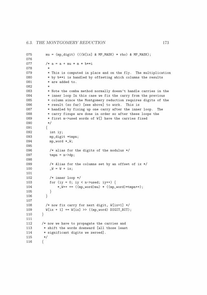
6.3. THE MONTGOMERY REDUCTION 173
075 mu = (mp_digit) (((W[ix] & MP_MASK) * rho) & MP_MASK);
076
077 /* a = a + mu * m * b**i
078 *
079 * This is computed in place and on the fly. The multiplication
080 * by b**i is handled by offseting which columns the results
081 * are added to.
082 *
083 * Note the comba method normally doesn’t handle carries in the
084 * inner loop In this case we fix the carry from the previous
085 * column since the Montgomery reduction requires digits of the
086 * result (so far) [see above] to work. This is
087 * handled by fixing up one carry after the inner loop. The
088 * carry fixups are done in order so after these loops the
089 * first m->used words of W[] have the carries fixed
090 */
091 {092 int iy;
093 mp_digit *tmpn;
094 mp_word *_W;
095
096 /* alias for the digits of the modulus */
097 tmpn = n->dp;
098
099 /* Alias for the columns set by an offset of ix */
100 _W = W + ix;
101
102 /* inner loop */
103 for (iy = 0; iy < n->used; iy++) {104 *_W++ += ((mp_word)mu) * ((mp_word)*tmpn++);
105 }106 }107
108 /* now fix carry for next digit, W[ix+1] */
109 W[ix + 1] += W[ix] >> ((mp_word) DIGIT_BIT);
110 }111
112 /* now we have to propagate the carries and
113 * shift the words downward [all those least
114 * significant digits we zeroed].
115 */
116 {
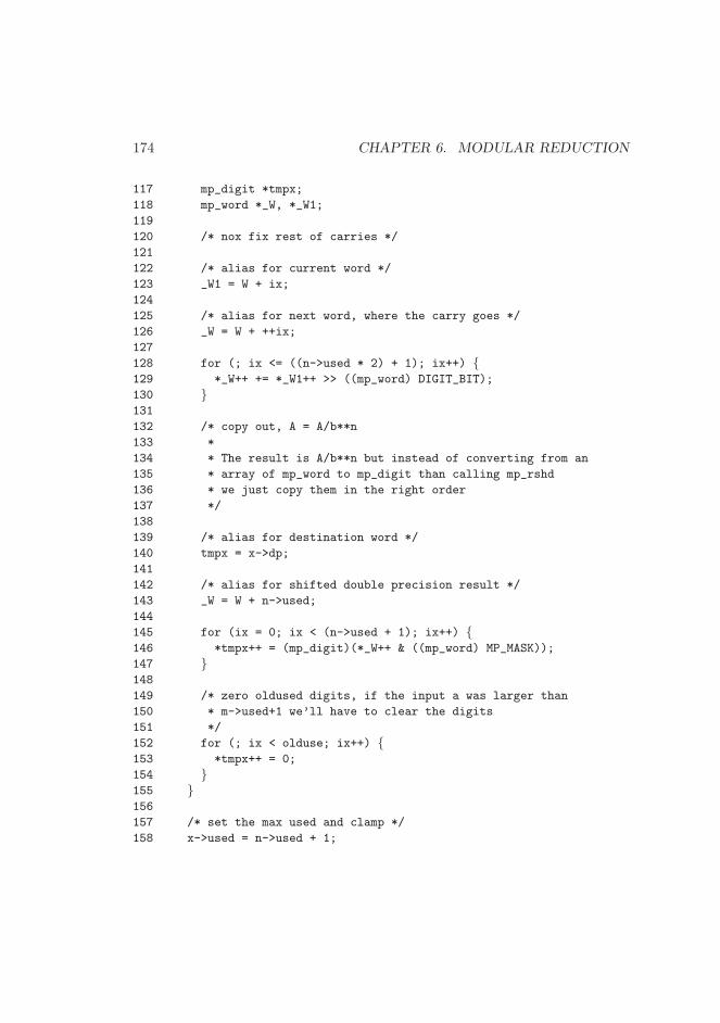
174 CHAPTER 6. MODULAR REDUCTION
117 mp_digit *tmpx;
118 mp_word *_W, *_W1;
119
120 /* nox fix rest of carries */
121
122 /* alias for current word */
123 _W1 = W + ix;
124
125 /* alias for next word, where the carry goes */
126 _W = W + ++ix;
127
128 for (; ix <= ((n->used * 2) + 1); ix++) {129 *_W++ += *_W1++ >> ((mp_word) DIGIT_BIT);
130 }131
132 /* copy out, A = A/b**n
133 *
134 * The result is A/b**n but instead of converting from an
135 * array of mp_word to mp_digit than calling mp_rshd
136 * we just copy them in the right order
137 */
138
139 /* alias for destination word */
140 tmpx = x->dp;
141
142 /* alias for shifted double precision result */
143 _W = W + n->used;
144
145 for (ix = 0; ix < (n->used + 1); ix++) {146 *tmpx++ = (mp_digit)(*_W++ & ((mp_word) MP_MASK));
147 }148
149 /* zero oldused digits, if the input a was larger than
150 * m->used+1 we’ll have to clear the digits
151 */
152 for (; ix < olduse; ix++) {153 *tmpx++ = 0;
154 }155 }156
157 /* set the max used and clamp */
158 x->used = n->used + 1;
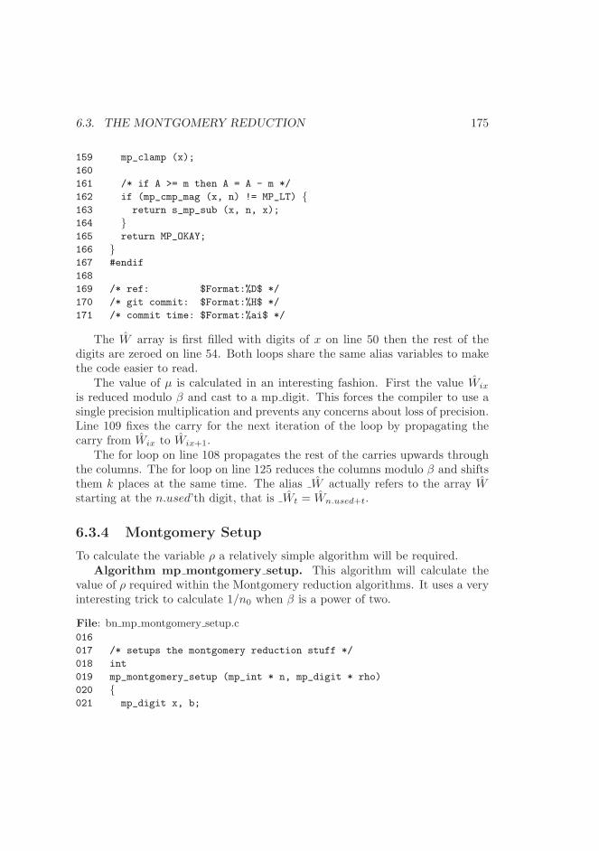
6.3. THE MONTGOMERY REDUCTION 175
159 mp_clamp (x);
160
161 /* if A >= m then A = A - m */
162 if (mp_cmp_mag (x, n) != MP_LT) {163 return s_mp_sub (x, n, x);
164 }165 return MP_OKAY;
166 }167 #endif
168
169 /* ref: $Format:%D$ */
170 /* git commit: $Format:%H$ */
171 /* commit time: $Format:%ai$ */
The W array is first filled with digits of x on line 50 then the rest of thedigits are zeroed on line 54. Both loops share the same alias variables to makethe code easier to read.
The value of µ is calculated in an interesting fashion. First the value Wix
is reduced modulo β and cast to a mp digit. This forces the compiler to use asingle precision multiplication and prevents any concerns about loss of precision.Line 109 fixes the carry for the next iteration of the loop by propagating thecarry from Wix to Wix+1.
The for loop on line 108 propagates the rest of the carries upwards throughthe columns. The for loop on line 125 reduces the columns modulo β and shiftsthem k places at the same time. The alias W actually refers to the array Wstarting at the n.used’th digit, that is Wt = Wn.used+t.
6.3.4 Montgomery Setup
To calculate the variable ρ a relatively simple algorithm will be required.Algorithm mp montgomery setup. This algorithm will calculate the
value of ρ required within the Montgomery reduction algorithms. It uses a veryinteresting trick to calculate 1/n0 when β is a power of two.
File: bn mp montgomery setup.c
016
017 /* setups the montgomery reduction stuff */
018 int
019 mp_montgomery_setup (mp_int * n, mp_digit * rho)
020 {021 mp_digit x, b;
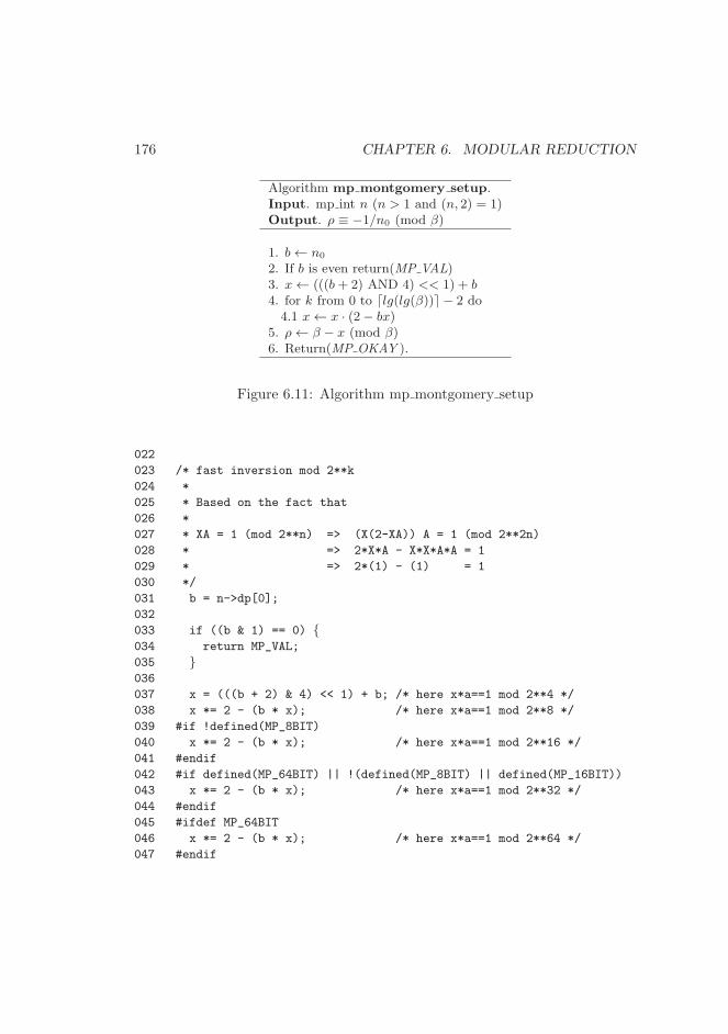
176 CHAPTER 6. MODULAR REDUCTION
Algorithm mp montgomery setup.Input. mp int n (n > 1 and (n, 2) = 1)Output. ρ ≡ −1/n0 (mod β)
1. b← n0
2. If b is even return(MP VAL)3. x← (((b+ 2) AND 4) << 1) + b4. for k from 0 to ⌈lg(lg(β))⌉ − 2 do4.1 x← x · (2− bx)
5. ρ← β − x (mod β)6. Return(MP OKAY ).
Figure 6.11: Algorithm mp montgomery setup
022
023 /* fast inversion mod 2**k
024 *
025 * Based on the fact that
026 *
027 * XA = 1 (mod 2**n) => (X(2-XA)) A = 1 (mod 2**2n)
028 * => 2*X*A - X*X*A*A = 1
029 * => 2*(1) - (1) = 1
030 */
031 b = n->dp[0];
032
033 if ((b & 1) == 0) {034 return MP_VAL;
035 }036
037 x = (((b + 2) & 4) << 1) + b; /* here x*a==1 mod 2**4 */
038 x *= 2 - (b * x); /* here x*a==1 mod 2**8 */
039 #if !defined(MP_8BIT)
040 x *= 2 - (b * x); /* here x*a==1 mod 2**16 */
041 #endif
042 #if defined(MP_64BIT) || !(defined(MP_8BIT) || defined(MP_16BIT))
043 x *= 2 - (b * x); /* here x*a==1 mod 2**32 */
044 #endif
045 #ifdef MP_64BIT
046 x *= 2 - (b * x); /* here x*a==1 mod 2**64 */
047 #endif
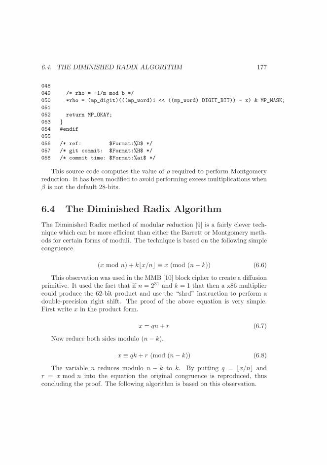
6.4. THE DIMINISHED RADIX ALGORITHM 177
048
049 /* rho = -1/m mod b */
050 *rho = (mp_digit)(((mp_word)1 << ((mp_word) DIGIT_BIT)) - x) & MP_MASK;
051
052 return MP_OKAY;
053 }054 #endif
055
056 /* ref: $Format:%D$ */
057 /* git commit: $Format:%H$ */
058 /* commit time: $Format:%ai$ */
This source code computes the value of ρ required to perform Montgomeryreduction. It has been modified to avoid performing excess multiplications whenβ is not the default 28-bits.
6.4 The Diminished Radix Algorithm
The Diminished Radix method of modular reduction [9] is a fairly clever tech-nique which can be more efficient than either the Barrett or Montgomery meth-ods for certain forms of moduli. The technique is based on the following simplecongruence.
(x mod n) + k⌊x/n⌋ ≡ x (mod (n− k)) (6.6)
This observation was used in the MMB [10] block cipher to create a diffusionprimitive. It used the fact that if n = 231 and k = 1 that then a x86 multipliercould produce the 62-bit product and use the “shrd” instruction to perform adouble-precision right shift. The proof of the above equation is very simple.First write x in the product form.
x = qn+ r (6.7)
Now reduce both sides modulo (n− k).
x ≡ qk + r (mod (n− k)) (6.8)
The variable n reduces modulo n − k to k. By putting q = ⌊x/n⌋ andr = x mod n into the equation the original congruence is reproduced, thusconcluding the proof. The following algorithm is based on this observation.
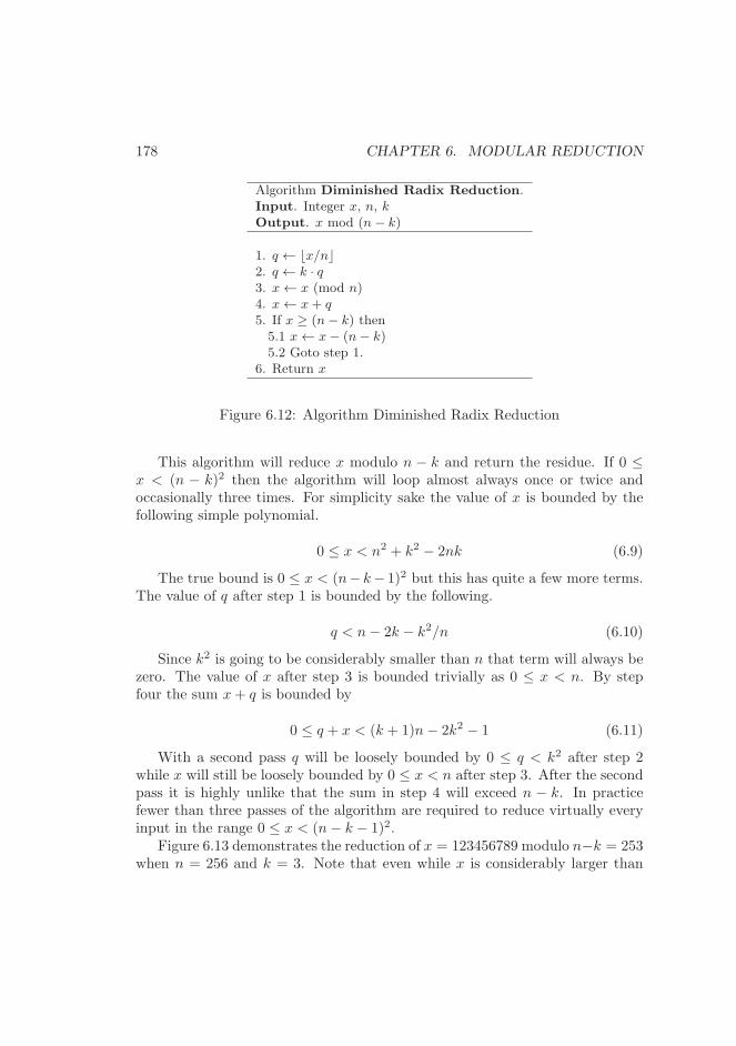
178 CHAPTER 6. MODULAR REDUCTION
Algorithm Diminished Radix Reduction.Input. Integer x, n, kOutput. x mod (n− k)
1. q ← ⌊x/n⌋2. q ← k · q3. x← x (mod n)4. x← x+ q5. If x ≥ (n− k) then5.1 x← x− (n− k)5.2 Goto step 1.
6. Return x
Figure 6.12: Algorithm Diminished Radix Reduction
This algorithm will reduce x modulo n − k and return the residue. If 0 ≤x < (n − k)2 then the algorithm will loop almost always once or twice andoccasionally three times. For simplicity sake the value of x is bounded by thefollowing simple polynomial.
0 ≤ x < n2 + k2 − 2nk (6.9)
The true bound is 0 ≤ x < (n− k− 1)2 but this has quite a few more terms.The value of q after step 1 is bounded by the following.
q < n− 2k − k2/n (6.10)
Since k2 is going to be considerably smaller than n that term will always bezero. The value of x after step 3 is bounded trivially as 0 ≤ x < n. By stepfour the sum x+ q is bounded by
0 ≤ q + x < (k + 1)n− 2k2 − 1 (6.11)
With a second pass q will be loosely bounded by 0 ≤ q < k2 after step 2while x will still be loosely bounded by 0 ≤ x < n after step 3. After the secondpass it is highly unlike that the sum in step 4 will exceed n − k. In practicefewer than three passes of the algorithm are required to reduce virtually everyinput in the range 0 ≤ x < (n− k − 1)2.
Figure 6.13 demonstrates the reduction of x = 123456789 modulo n−k = 253when n = 256 and k = 3. Note that even while x is considerably larger than
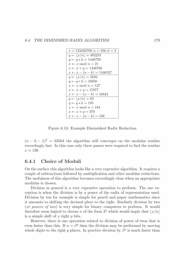
6.4. THE DIMINISHED RADIX ALGORITHM 179
x = 123456789, n = 256, k = 3
q ← ⌊x/n⌋ = 482253q ← q ∗ k = 1446759x← x mod n = 21x← x+ q = 1446780x← x− (n− k) = 1446527
q ← ⌊x/n⌋ = 5650q ← q ∗ k = 16950x← x mod n = 127x← x+ q = 17077x← x− (n− k) = 16824
q ← ⌊x/n⌋ = 65q ← q ∗ k = 195x← x mod n = 184x← x+ q = 379x← x− (n− k) = 126
Figure 6.13: Example Diminished Radix Reduction
(n − k − 1)2 = 63504 the algorithm still converges on the modular residueexceedingly fast. In this case only three passes were required to find the residuex ≡ 126.
6.4.1 Choice of Moduli
On the surface this algorithm looks like a very expensive algorithm. It requires acouple of subtractions followed by multiplication and other modular reductions.The usefulness of this algorithm becomes exceedingly clear when an appropriatemodulus is chosen.
Division in general is a very expensive operation to perform. The one ex-ception is when the division is by a power of the radix of representation used.Division by ten for example is simple for pencil and paper mathematics sinceit amounts to shifting the decimal place to the right. Similarly division by two(or powers of two) is very simple for binary computers to perform. It wouldtherefore seem logical to choose n of the form 2p which would imply that ⌊x/n⌋is a simple shift of x right p bits.
However, there is one operation related to division of power of twos that iseven faster than this. If n = βp then the division may be performed by movingwhole digits to the right p places. In practice division by βp is much faster than
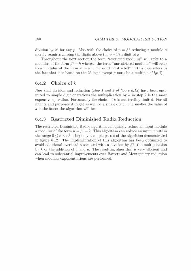
180 CHAPTER 6. MODULAR REDUCTION
division by 2p for any p. Also with the choice of n = βp reducing x modulo nmerely requires zeroing the digits above the p− 1’th digit of x.
Throughout the next section the term “restricted modulus” will refer to amodulus of the form βp− k whereas the term “unrestricted modulus” will referto a modulus of the form 2p − k. The word “restricted” in this case refers tothe fact that it is based on the 2p logic except p must be a multiple of lg(β).
6.4.2 Choice of k
Now that division and reduction (step 1 and 3 of figure 6.12) have been opti-mized to simple digit operations the multiplication by k in step 2 is the mostexpensive operation. Fortunately the choice of k is not terribly limited. For allintents and purposes it might as well be a single digit. The smaller the value ofk is the faster the algorithm will be.
6.4.3 Restricted Diminished Radix Reduction
The restricted Diminished Radix algorithm can quickly reduce an input moduloa modulus of the form n = βp−k. This algorithm can reduce an input x withinthe range 0 ≤ x < n2 using only a couple passes of the algorithm demonstratedin figure 6.12. The implementation of this algorithm has been optimized toavoid additional overhead associated with a division by βp, the multiplicationby k or the addition of x and q. The resulting algorithm is very efficient andcan lead to substantial improvements over Barrett and Montgomery reductionwhen modular exponentiations are performed.
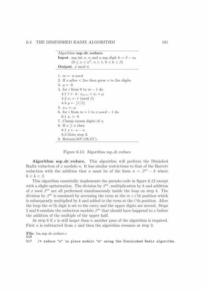
6.4. THE DIMINISHED RADIX ALGORITHM 181
Algorithm mp dr reduce.Input. mp int x, n and a mp digit k = β − n0
(0 ≤ x < n2, n > 1, 0 < k < β)Output. x mod n
1. m← n.used2. If x.alloc < 2m then grow x to 2m digits.3. µ← 04. for i from 0 to m− 1 do4.1 r ← k · xm+i + xi + µ4.2 xi ← r (mod β)4.3 µ← ⌊r/β⌋
5. xm ← µ6. for i from m+ 1 to x.used− 1 do6.1 xi ← 0
7. Clamp excess digits of x.8. If x ≥ n then8.1 x← x− n8.2 Goto step 3.
9. Return(MP OKAY ).
Figure 6.14: Algorithm mp dr reduce
Algorithm mp dr reduce. This algorithm will perform the DimishedRadix reduction of x modulo n. It has similar restrictions to that of the Barrettreduction with the addition that n must be of the form n = βm − k where0 < k < β.
This algorithm essentially implements the pseudo-code in figure 6.12 exceptwith a slight optimization. The division by βm, multiplication by k and additionof x mod βm are all performed simultaneously inside the loop on step 4. Thedivision by βm is emulated by accessing the term at the m+ i’th position whichis subsequently multiplied by k and added to the term at the i’th position. Afterthe loop the m’th digit is set to the carry and the upper digits are zeroed. Steps5 and 6 emulate the reduction modulo βm that should have happend to x beforethe addition of the multiple of the upper half.
At step 8 if x is still larger than n another pass of the algorithm is required.First n is subtracted from x and then the algorithm resumes at step 3.
File: bn mp dr reduce.c016
017 /* reduce "x" in place modulo "n" using the Diminished Radix algorithm.
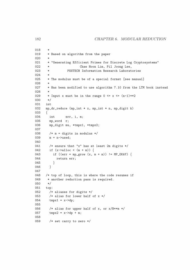
182 CHAPTER 6. MODULAR REDUCTION
018 *
019 * Based on algorithm from the paper
020 *
021 * "Generating Efficient Primes for Discrete Log Cryptosystems"
022 * Chae Hoon Lim, Pil Joong Lee,
023 * POSTECH Information Research Laboratories
024 *
025 * The modulus must be of a special format [see manual]
026 *
027 * Has been modified to use algorithm 7.10 from the LTM book instead
028 *
029 * Input x must be in the range 0 <= x <= (n-1)**2
030 */
031 int
032 mp_dr_reduce (mp_int * x, mp_int * n, mp_digit k)
033 {034 int err, i, m;
035 mp_word r;
036 mp_digit mu, *tmpx1, *tmpx2;
037
038 /* m = digits in modulus */
039 m = n->used;
040
041 /* ensure that "x" has at least 2m digits */
042 if (x->alloc < (m + m)) {043 if ((err = mp_grow (x, m + m)) != MP_OKAY) {044 return err;
045 }046 }047
048 /* top of loop, this is where the code resumes if
049 * another reduction pass is required.
050 */
051 top:
052 /* aliases for digits */
053 /* alias for lower half of x */
054 tmpx1 = x->dp;
055
056 /* alias for upper half of x, or x/B**m */
057 tmpx2 = x->dp + m;
058
059 /* set carry to zero */
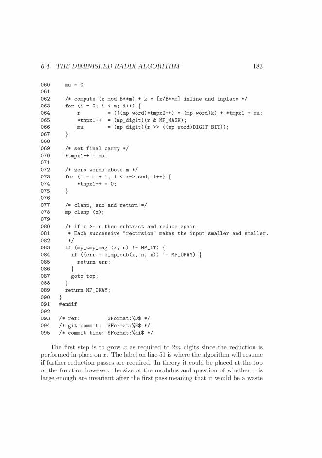
6.4. THE DIMINISHED RADIX ALGORITHM 183
060 mu = 0;
061
062 /* compute (x mod B**m) + k * [x/B**m] inline and inplace */
063 for (i = 0; i < m; i++) {064 r = (((mp_word)*tmpx2++) * (mp_word)k) + *tmpx1 + mu;
065 *tmpx1++ = (mp_digit)(r & MP_MASK);
066 mu = (mp_digit)(r >> ((mp_word)DIGIT_BIT));
067 }068
069 /* set final carry */
070 *tmpx1++ = mu;
071
072 /* zero words above m */
073 for (i = m + 1; i < x->used; i++) {074 *tmpx1++ = 0;
075 }076
077 /* clamp, sub and return */
078 mp_clamp (x);
079
080 /* if x >= n then subtract and reduce again
081 * Each successive "recursion" makes the input smaller and smaller.
082 */
083 if (mp_cmp_mag (x, n) != MP_LT) {084 if ((err = s_mp_sub(x, n, x)) != MP_OKAY) {085 return err;
086 }087 goto top;
088 }089 return MP_OKAY;
090 }091 #endif
092
093 /* ref: $Format:%D$ */
094 /* git commit: $Format:%H$ */
095 /* commit time: $Format:%ai$ */
The first step is to grow x as required to 2m digits since the reduction isperformed in place on x. The label on line 51 is where the algorithm will resumeif further reduction passes are required. In theory it could be placed at the topof the function however, the size of the modulus and question of whether x islarge enough are invariant after the first pass meaning that it would be a waste
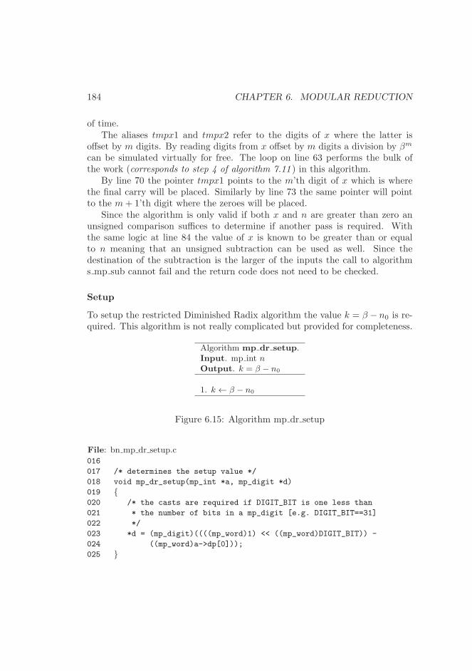
184 CHAPTER 6. MODULAR REDUCTION
of time.The aliases tmpx1 and tmpx2 refer to the digits of x where the latter is
offset by m digits. By reading digits from x offset by m digits a division by βm
can be simulated virtually for free. The loop on line 63 performs the bulk ofthe work (corresponds to step 4 of algorithm 7.11 ) in this algorithm.
By line 70 the pointer tmpx1 points to the m’th digit of x which is wherethe final carry will be placed. Similarly by line 73 the same pointer will pointto the m+ 1’th digit where the zeroes will be placed.
Since the algorithm is only valid if both x and n are greater than zero anunsigned comparison suffices to determine if another pass is required. Withthe same logic at line 84 the value of x is known to be greater than or equalto n meaning that an unsigned subtraction can be used as well. Since thedestination of the subtraction is the larger of the inputs the call to algorithms mp sub cannot fail and the return code does not need to be checked.
Setup
To setup the restricted Diminished Radix algorithm the value k = β − n0 is re-quired. This algorithm is not really complicated but provided for completeness.
Algorithm mp dr setup.Input. mp int nOutput. k = β − n0
1. k ← β − n0
Figure 6.15: Algorithm mp dr setup
File: bn mp dr setup.c
016
017 /* determines the setup value */
018 void mp_dr_setup(mp_int *a, mp_digit *d)
019 {020 /* the casts are required if DIGIT_BIT is one less than
021 * the number of bits in a mp_digit [e.g. DIGIT_BIT==31]
022 */
023 *d = (mp_digit)((((mp_word)1) << ((mp_word)DIGIT_BIT)) -
024 ((mp_word)a->dp[0]));
025 }
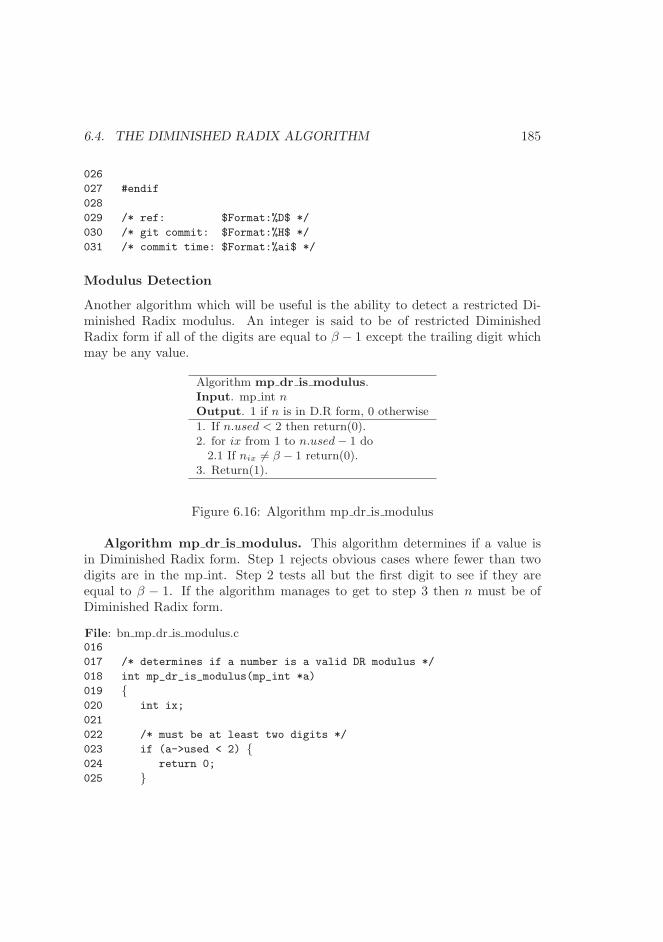
6.4. THE DIMINISHED RADIX ALGORITHM 185
026
027 #endif
028
029 /* ref: $Format:%D$ */
030 /* git commit: $Format:%H$ */
031 /* commit time: $Format:%ai$ */
Modulus Detection
Another algorithm which will be useful is the ability to detect a restricted Di-minished Radix modulus. An integer is said to be of restricted DiminishedRadix form if all of the digits are equal to β − 1 except the trailing digit whichmay be any value.
Algorithm mp dr is modulus.Input. mp int nOutput. 1 if n is in D.R form, 0 otherwise
1. If n.used < 2 then return(0).2. for ix from 1 to n.used− 1 do2.1 If nix 6= β − 1 return(0).
3. Return(1).
Figure 6.16: Algorithm mp dr is modulus
Algorithm mp dr is modulus. This algorithm determines if a value isin Diminished Radix form. Step 1 rejects obvious cases where fewer than twodigits are in the mp int. Step 2 tests all but the first digit to see if they areequal to β − 1. If the algorithm manages to get to step 3 then n must be ofDiminished Radix form.
File: bn mp dr is modulus.c016
017 /* determines if a number is a valid DR modulus */
018 int mp_dr_is_modulus(mp_int *a)
019 {020 int ix;
021
022 /* must be at least two digits */
023 if (a->used < 2) {024 return 0;
025 }
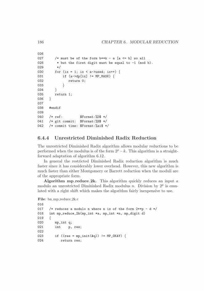
186 CHAPTER 6. MODULAR REDUCTION
026
027 /* must be of the form b**k - a [a <= b] so all
028 * but the first digit must be equal to -1 (mod b).
029 */
030 for (ix = 1; ix < a->used; ix++) {031 if (a->dp[ix] != MP_MASK) {032 return 0;
033 }034 }035 return 1;
036 }037
038 #endif
039
040 /* ref: $Format:%D$ */
041 /* git commit: $Format:%H$ */
042 /* commit time: $Format:%ai$ */
6.4.4 Unrestricted Diminished Radix Reduction
The unrestricted Diminished Radix algorithm allows modular reductions to beperformed when the modulus is of the form 2p−k. This algorithm is a straight-forward adaptation of algorithm 6.12.
In general the restricted Diminished Radix reduction algorithm is muchfaster since it has considerably lower overhead. However, this new algorithm ismuch faster than either Montgomery or Barrett reduction when the moduli areof the appropriate form.
Algorithm mp reduce 2k. This algorithm quickly reduces an input amodulo an unrestricted Diminished Radix modulus n. Division by 2p is emu-lated with a right shift which makes the algorithm fairly inexpensive to use.
File: bn mp reduce 2k.c
016
017 /* reduces a modulo n where n is of the form 2**p - d */
018 int mp_reduce_2k(mp_int *a, mp_int *n, mp_digit d)
019 {020 mp_int q;
021 int p, res;
022
023 if ((res = mp_init(&q)) != MP_OKAY) {024 return res;
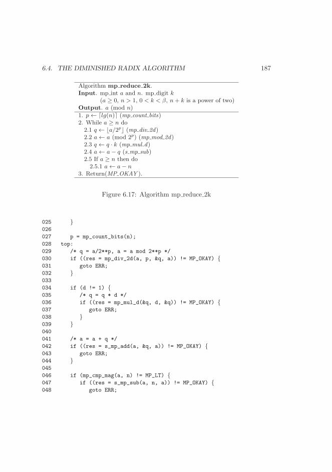
6.4. THE DIMINISHED RADIX ALGORITHM 187
Algorithm mp reduce 2k.Input. mp int a and n. mp digit k
(a ≥ 0, n > 1, 0 < k < β, n+ k is a power of two)Output. a (mod n)
1. p← ⌈lg(n)⌉ (mp count bits)2. While a ≥ n do2.1 q ← ⌊a/2p⌋ (mp div 2d)2.2 a← a (mod 2p) (mp mod 2d)2.3 q ← q · k (mp mul d)2.4 a← a− q (s mp sub)2.5 If a ≥ n then do2.5.1 a← a− n
3. Return(MP OKAY ).
Figure 6.17: Algorithm mp reduce 2k
025 }026
027 p = mp_count_bits(n);
028 top:
029 /* q = a/2**p, a = a mod 2**p */
030 if ((res = mp_div_2d(a, p, &q, a)) != MP_OKAY) {031 goto ERR;
032 }033
034 if (d != 1) {035 /* q = q * d */
036 if ((res = mp_mul_d(&q, d, &q)) != MP_OKAY) {037 goto ERR;
038 }039 }040
041 /* a = a + q */
042 if ((res = s_mp_add(a, &q, a)) != MP_OKAY) {043 goto ERR;
044 }045
046 if (mp_cmp_mag(a, n) != MP_LT) {047 if ((res = s_mp_sub(a, n, a)) != MP_OKAY) {048 goto ERR;
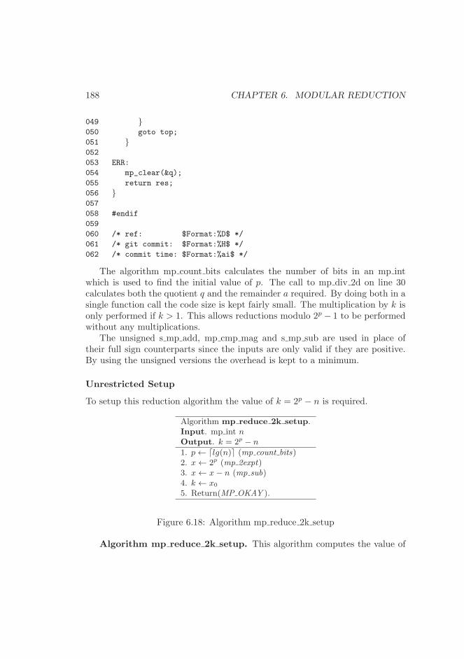
188 CHAPTER 6. MODULAR REDUCTION
049 }050 goto top;
051 }052
053 ERR:
054 mp_clear(&q);
055 return res;
056 }057
058 #endif
059
060 /* ref: $Format:%D$ */
061 /* git commit: $Format:%H$ */
062 /* commit time: $Format:%ai$ */
The algorithm mp count bits calculates the number of bits in an mp intwhich is used to find the initial value of p. The call to mp div 2d on line 30calculates both the quotient q and the remainder a required. By doing both in asingle function call the code size is kept fairly small. The multiplication by k isonly performed if k > 1. This allows reductions modulo 2p − 1 to be performedwithout any multiplications.
The unsigned s mp add, mp cmp mag and s mp sub are used in place oftheir full sign counterparts since the inputs are only valid if they are positive.By using the unsigned versions the overhead is kept to a minimum.
Unrestricted Setup
To setup this reduction algorithm the value of k = 2p − n is required.
Algorithm mp reduce 2k setup.Input. mp int nOutput. k = 2p − n
1. p← ⌈lg(n)⌉ (mp count bits)2. x← 2p (mp 2expt)3. x← x− n (mp sub)4. k ← x0
5. Return(MP OKAY ).
Figure 6.18: Algorithm mp reduce 2k setup
Algorithm mp reduce 2k setup. This algorithm computes the value of
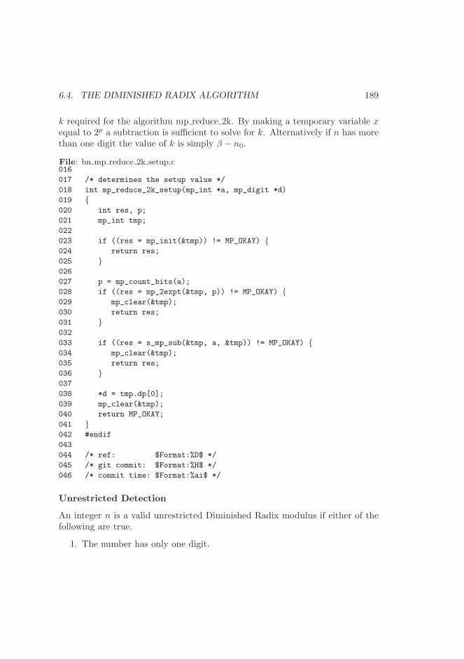
6.4. THE DIMINISHED RADIX ALGORITHM 189
k required for the algorithm mp reduce 2k. By making a temporary variable xequal to 2p a subtraction is sufficient to solve for k. Alternatively if n has morethan one digit the value of k is simply β − n0.
File: bn mp reduce 2k setup.c016
017 /* determines the setup value */
018 int mp_reduce_2k_setup(mp_int *a, mp_digit *d)
019 {020 int res, p;
021 mp_int tmp;
022
023 if ((res = mp_init(&tmp)) != MP_OKAY) {024 return res;
025 }026
027 p = mp_count_bits(a);
028 if ((res = mp_2expt(&tmp, p)) != MP_OKAY) {029 mp_clear(&tmp);
030 return res;
031 }032
033 if ((res = s_mp_sub(&tmp, a, &tmp)) != MP_OKAY) {034 mp_clear(&tmp);
035 return res;
036 }037
038 *d = tmp.dp[0];
039 mp_clear(&tmp);
040 return MP_OKAY;
041 }042 #endif
043
044 /* ref: $Format:%D$ */
045 /* git commit: $Format:%H$ */
046 /* commit time: $Format:%ai$ */
Unrestricted Detection
An integer n is a valid unrestricted Diminished Radix modulus if either of thefollowing are true.
1. The number has only one digit.
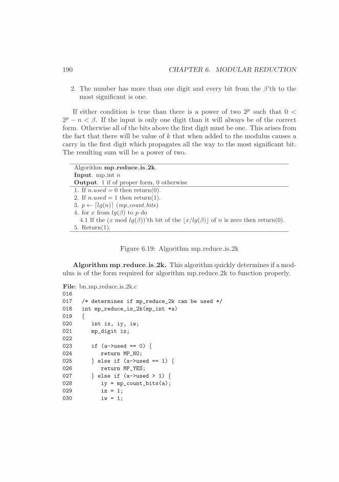
190 CHAPTER 6. MODULAR REDUCTION
2. The number has more than one digit and every bit from the β’th to themost significant is one.
If either condition is true than there is a power of two 2p such that 0 <2p − n < β. If the input is only one digit than it will always be of the correctform. Otherwise all of the bits above the first digit must be one. This arises fromthe fact that there will be value of k that when added to the modulus causes acarry in the first digit which propagates all the way to the most significant bit.The resulting sum will be a power of two.
Algorithm mp reduce is 2k.Input. mp int nOutput. 1 if of proper form, 0 otherwise
1. If n.used = 0 then return(0).2. If n.used = 1 then return(1).3. p← ⌈lg(n)⌉ (mp count bits)4. for x from lg(β) to p do4.1 If the (x mod lg(β))’th bit of the ⌊x/lg(β)⌋ of n is zero then return(0).
5. Return(1).
Figure 6.19: Algorithm mp reduce is 2k
Algorithm mp reduce is 2k. This algorithm quickly determines if a mod-ulus is of the form required for algorithm mp reduce 2k to function properly.
File: bn mp reduce is 2k.c016
017 /* determines if mp_reduce_2k can be used */
018 int mp_reduce_is_2k(mp_int *a)
019 {020 int ix, iy, iw;
021 mp_digit iz;
022
023 if (a->used == 0) {024 return MP_NO;
025 } else if (a->used == 1) {026 return MP_YES;
027 } else if (a->used > 1) {028 iy = mp_count_bits(a);
029 iz = 1;
030 iw = 1;
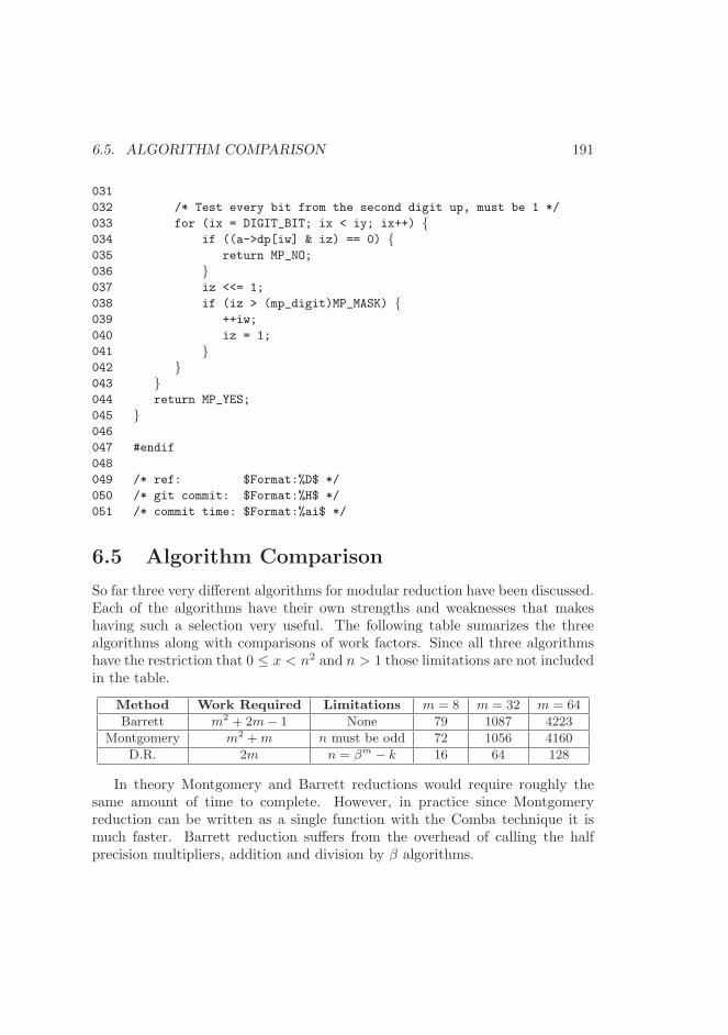
6.5. ALGORITHM COMPARISON 191
031
032 /* Test every bit from the second digit up, must be 1 */
033 for (ix = DIGIT_BIT; ix < iy; ix++) {034 if ((a->dp[iw] & iz) == 0) {035 return MP_NO;
036 }037 iz <<= 1;
038 if (iz > (mp_digit)MP_MASK) {039 ++iw;
040 iz = 1;
041 }042 }043 }044 return MP_YES;
045 }046
047 #endif
048
049 /* ref: $Format:%D$ */
050 /* git commit: $Format:%H$ */
051 /* commit time: $Format:%ai$ */
6.5 Algorithm Comparison
So far three very different algorithms for modular reduction have been discussed.Each of the algorithms have their own strengths and weaknesses that makeshaving such a selection very useful. The following table sumarizes the threealgorithms along with comparisons of work factors. Since all three algorithmshave the restriction that 0 ≤ x < n2 and n > 1 those limitations are not includedin the table.
Method Work Required Limitations m = 8 m = 32 m = 64
Barrett m2 + 2m− 1 None 79 1087 4223
Montgomery m2 +m n must be odd 72 1056 4160
D.R. 2m n = βm − k 16 64 128
In theory Montgomery and Barrett reductions would require roughly thesame amount of time to complete. However, in practice since Montgomeryreduction can be written as a single function with the Comba technique it ismuch faster. Barrett reduction suffers from the overhead of calling the halfprecision multipliers, addition and division by β algorithms.
192 CHAPTER 6. MODULAR REDUCTION
For almost every cryptographic algorithm Montgomery reduction is the al-gorithm of choice. The one set of algorithms where Diminished Radix reductiontruly shines are based on the discrete logarithm problem such as Diffie-Hellman[12] and ElGamal [21]. In these algorithms primes of the form βm − k canbe found and shared amongst users. These primes will allow the DiminishedRadix algorithm to be used in modular exponentiation to greatly speed up theoperation.
Exercises
[3] Prove that the “trick” in algorithm mp montgomery setup actuallycalculates the correct value of ρ.
[2] Devise an algorithm to reduce modulo n+ k for small k quickly.
[4] Prove that the pseudo-code algorithm “Diminished Radix Reduction”(figure 6.12) terminates. Also prove the probability that it willterminate within 1 ≤ k ≤ 10 iterations.
Chapter 7
Exponentiation
Exponentiation is the operation of raising one variable to the power of another,for example, ab. A variant of exponentiation, computed in a finite field or ring,is called modular exponentiation. This latter style of operation is typicallyused in public key cryptosystems such as RSA and Diffie-Hellman. The abilityto quickly compute modular exponentiations is of great benefit to any suchcryptosystem and many methods have been sought to speed it up.
7.1 Exponentiation Basics
A trivial algorithm would simply multiply a against itself b−1 times to computethe exponentiation desired. However, as b grows in size the number of multipli-cations becomes prohibitive. Imagine what would happen if b ∼ 21024 as is thecase when computing an RSA signature with a 1024-bit key. Such a calculationcould never be completed as it would take simply far too long.
Fortunately there is a very simple algorithm based on the laws of exponents.Recall that lga(a
b) = b and that lga(abac) = b + c which are two trivial rela-
tionships between the base and the exponent. Let bi represent the i’th bit of bstarting from the least significant bit. If b is a k-bit integer than the followingequation is true.
ab =
k−1∏
i=0
a2i·bi (7.1)
193
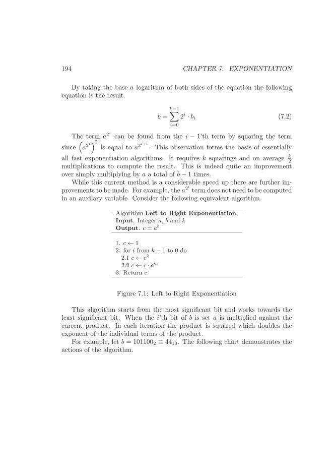
194 CHAPTER 7. EXPONENTIATION
By taking the base a logarithm of both sides of the equation the followingequation is the result.
b =
k−1∑
i=0
2i · bi (7.2)
The term a2i
can be found from the i − 1’th term by squaring the term
since(
a2i)2
is equal to a2i+1
. This observation forms the basis of essentially
all fast exponentiation algorithms. It requires k squarings and on average k2
multiplications to compute the result. This is indeed quite an improvementover simply multiplying by a a total of b− 1 times.
While this current method is a considerable speed up there are further im-provements to be made. For example, the a2
i
term does not need to be computedin an auxilary variable. Consider the following equivalent algorithm.
Algorithm Left to Right Exponentiation.Input. Integer a, b and k
Output. c = ab
1. c← 12. for i from k − 1 to 0 do2.1 c← c2
2.2 c← c · abi
3. Return c.
Figure 7.1: Left to Right Exponentiation
This algorithm starts from the most significant bit and works towards theleast significant bit. When the i’th bit of b is set a is multiplied against thecurrent product. In each iteration the product is squared which doubles theexponent of the individual terms of the product.
For example, let b = 1011002 ≡ 4410. The following chart demonstrates theactions of the algorithm.
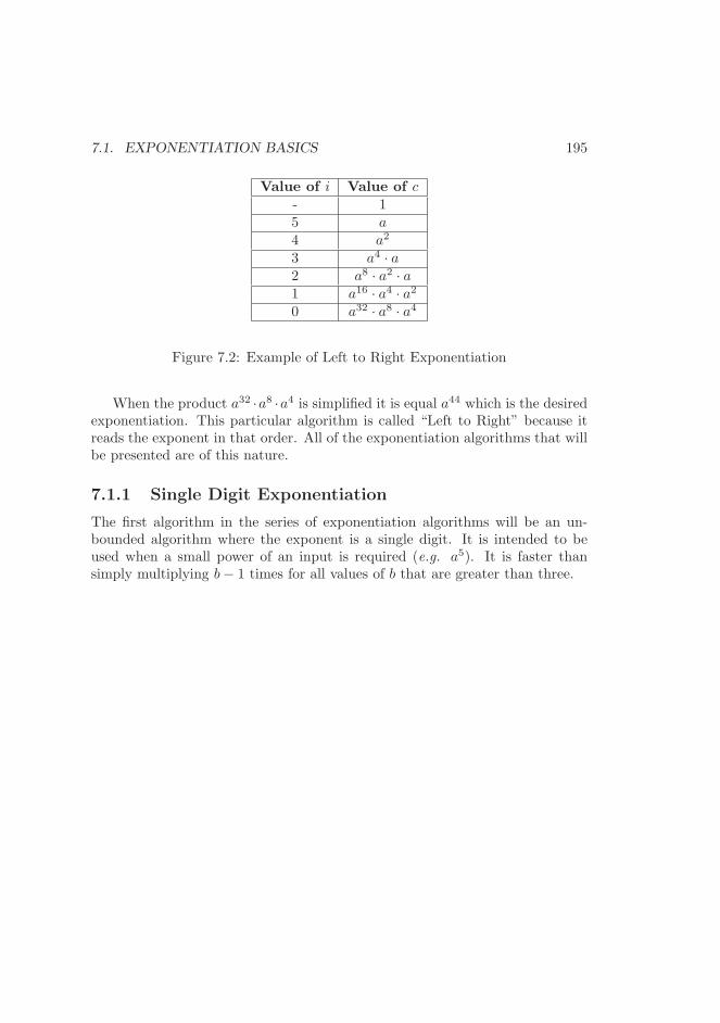
7.1. EXPONENTIATION BASICS 195
Value of i Value of c- 15 a4 a2
3 a4 · a2 a8 · a2 · a1 a16 · a4 · a20 a32 · a8 · a4
Figure 7.2: Example of Left to Right Exponentiation
When the product a32 ·a8 ·a4 is simplified it is equal a44 which is the desiredexponentiation. This particular algorithm is called “Left to Right” because itreads the exponent in that order. All of the exponentiation algorithms that willbe presented are of this nature.
7.1.1 Single Digit Exponentiation
The first algorithm in the series of exponentiation algorithms will be an un-bounded algorithm where the exponent is a single digit. It is intended to beused when a small power of an input is required (e.g. a5). It is faster thansimply multiplying b− 1 times for all values of b that are greater than three.
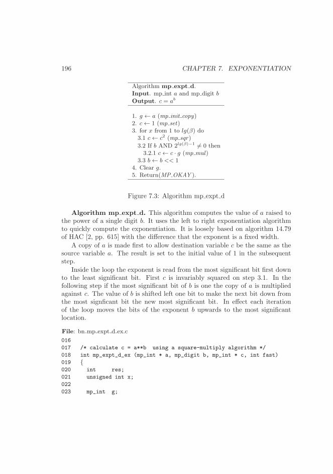
196 CHAPTER 7. EXPONENTIATION
Algorithm mp expt d.Input. mp int a and mp digit b
Output. c = ab
1. g ← a (mp init copy)2. c← 1 (mp set)3. for x from 1 to lg(β) do3.1 c← c2 (mp sqr)
3.2 If b AND 2lg(β)−1 6= 0 then3.2.1 c← c · g (mp mul)
3.3 b← b << 14. Clear g.5. Return(MP OKAY ).
Figure 7.3: Algorithm mp expt d
Algorithm mp expt d. This algorithm computes the value of a raised tothe power of a single digit b. It uses the left to right exponentiation algorithmto quickly compute the exponentiation. It is loosely based on algorithm 14.79of HAC [2, pp. 615] with the difference that the exponent is a fixed width.
A copy of a is made first to allow destination variable c be the same as thesource variable a. The result is set to the initial value of 1 in the subsequentstep.
Inside the loop the exponent is read from the most significant bit first downto the least significant bit. First c is invariably squared on step 3.1. In thefollowing step if the most significant bit of b is one the copy of a is multipliedagainst c. The value of b is shifted left one bit to make the next bit down fromthe most signficant bit the new most significant bit. In effect each iterationof the loop moves the bits of the exponent b upwards to the most significantlocation.
File: bn mp expt d ex.c
016
017 /* calculate c = a**b using a square-multiply algorithm */
018 int mp_expt_d_ex (mp_int * a, mp_digit b, mp_int * c, int fast)
019 {020 int res;
021 unsigned int x;
022
023 mp_int g;
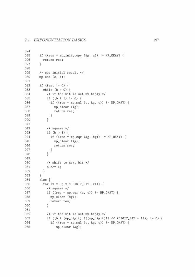
7.1. EXPONENTIATION BASICS 197
024
025 if ((res = mp_init_copy (&g, a)) != MP_OKAY) {026 return res;
027 }028
029 /* set initial result */
030 mp_set (c, 1);
031
032 if (fast != 0) {033 while (b > 0) {034 /* if the bit is set multiply */
035 if ((b & 1) != 0) {036 if ((res = mp_mul (c, &g, c)) != MP_OKAY) {037 mp_clear (&g);
038 return res;
039 }040 }041
042 /* square */
043 if (b > 1) {044 if ((res = mp_sqr (&g, &g)) != MP_OKAY) {045 mp_clear (&g);
046 return res;
047 }048 }049
050 /* shift to next bit */
051 b >>= 1;
052 }053 }054 else {055 for (x = 0; x < DIGIT_BIT; x++) {056 /* square */
057 if ((res = mp_sqr (c, c)) != MP_OKAY) {058 mp_clear (&g);
059 return res;
060 }061
062 /* if the bit is set multiply */
063 if ((b & (mp_digit) (((mp_digit)1) << (DIGIT_BIT - 1))) != 0) {064 if ((res = mp_mul (c, &g, c)) != MP_OKAY) {065 mp_clear (&g);
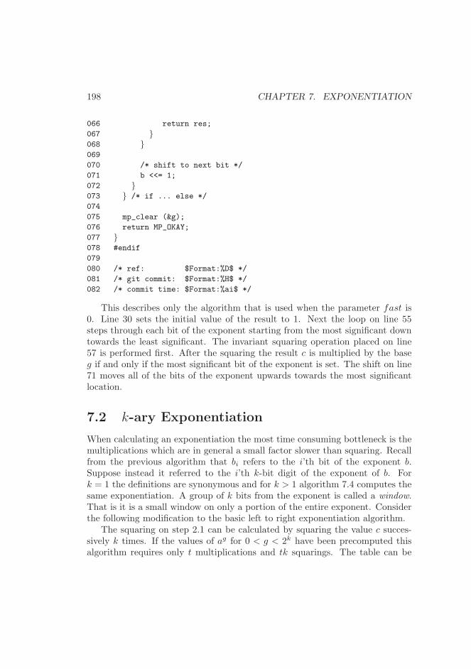
198 CHAPTER 7. EXPONENTIATION
066 return res;
067 }068 }069
070 /* shift to next bit */
071 b <<= 1;
072 }073 } /* if ... else */
074
075 mp_clear (&g);
076 return MP_OKAY;
077 }078 #endif
079
080 /* ref: $Format:%D$ */
081 /* git commit: $Format:%H$ */
082 /* commit time: $Format:%ai$ */
This describes only the algorithm that is used when the parameter fast is0. Line 30 sets the initial value of the result to 1. Next the loop on line 55steps through each bit of the exponent starting from the most significant downtowards the least significant. The invariant squaring operation placed on line57 is performed first. After the squaring the result c is multiplied by the baseg if and only if the most significant bit of the exponent is set. The shift on line71 moves all of the bits of the exponent upwards towards the most significantlocation.
7.2 k-ary Exponentiation
When calculating an exponentiation the most time consuming bottleneck is themultiplications which are in general a small factor slower than squaring. Recallfrom the previous algorithm that bi refers to the i’th bit of the exponent b.Suppose instead it referred to the i’th k-bit digit of the exponent of b. Fork = 1 the definitions are synonymous and for k > 1 algorithm 7.4 computes thesame exponentiation. A group of k bits from the exponent is called a window.That is it is a small window on only a portion of the entire exponent. Considerthe following modification to the basic left to right exponentiation algorithm.
The squaring on step 2.1 can be calculated by squaring the value c succes-sively k times. If the values of ag for 0 < g < 2k have been precomputed thisalgorithm requires only t multiplications and tk squarings. The table can be
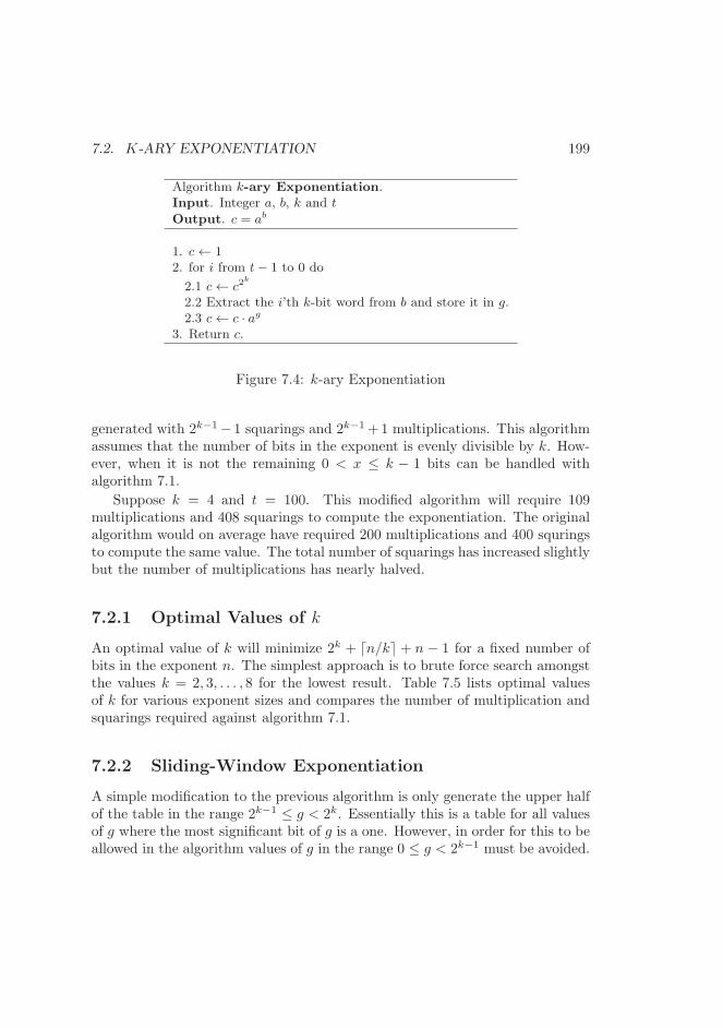
7.2. K-ARY EXPONENTIATION 199
Algorithm k-ary Exponentiation.Input. Integer a, b, k and t
Output. c = ab
1. c← 12. for i from t− 1 to 0 do
2.1 c← c2k
2.2 Extract the i’th k-bit word from b and store it in g.2.3 c← c · ag
3. Return c.
Figure 7.4: k-ary Exponentiation
generated with 2k−1−1 squarings and 2k−1+1 multiplications. This algorithmassumes that the number of bits in the exponent is evenly divisible by k. How-ever, when it is not the remaining 0 < x ≤ k − 1 bits can be handled withalgorithm 7.1.
Suppose k = 4 and t = 100. This modified algorithm will require 109multiplications and 408 squarings to compute the exponentiation. The originalalgorithm would on average have required 200 multiplications and 400 squringsto compute the same value. The total number of squarings has increased slightlybut the number of multiplications has nearly halved.
7.2.1 Optimal Values of k
An optimal value of k will minimize 2k + ⌈n/k⌉ + n − 1 for a fixed number ofbits in the exponent n. The simplest approach is to brute force search amongstthe values k = 2, 3, . . . , 8 for the lowest result. Table 7.5 lists optimal valuesof k for various exponent sizes and compares the number of multiplication andsquarings required against algorithm 7.1.
7.2.2 Sliding-Window Exponentiation
A simple modification to the previous algorithm is only generate the upper halfof the table in the range 2k−1 ≤ g < 2k. Essentially this is a table for all valuesof g where the most significant bit of g is a one. However, in order for this to beallowed in the algorithm values of g in the range 0 ≤ g < 2k−1 must be avoided.
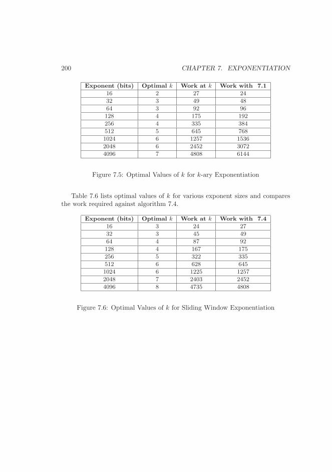
200 CHAPTER 7. EXPONENTIATION
Exponent (bits) Optimal k Work at k Work with 7.1
16 2 27 24
32 3 49 48
64 3 92 96
128 4 175 192
256 4 335 384
512 5 645 768
1024 6 1257 1536
2048 6 2452 3072
4096 7 4808 6144
Figure 7.5: Optimal Values of k for k-ary Exponentiation
Table 7.6 lists optimal values of k for various exponent sizes and comparesthe work required against algorithm 7.4.
Exponent (bits) Optimal k Work at k Work with 7.4
16 3 24 27
32 3 45 49
64 4 87 92
128 4 167 175
256 5 322 335
512 6 628 645
1024 6 1225 1257
2048 7 2403 2452
4096 8 4735 4808
Figure 7.6: Optimal Values of k for Sliding Window Exponentiation
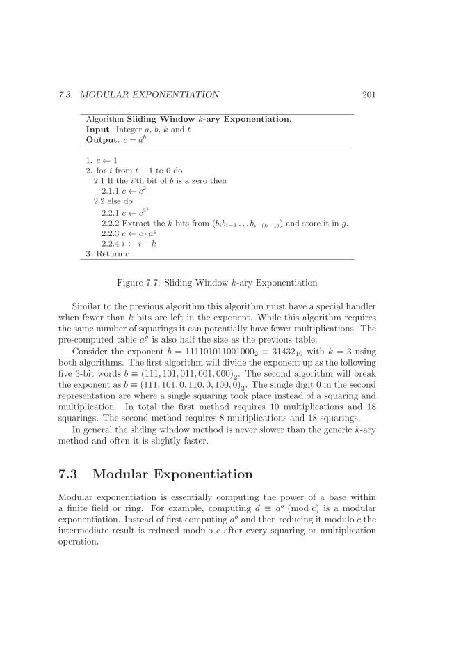
7.3. MODULAR EXPONENTIATION 201
Algorithm Sliding Window k-ary Exponentiation.Input. Integer a, b, k and t
Output. c = ab
1. c← 12. for i from t− 1 to 0 do2.1 If the i’th bit of b is a zero then2.1.1 c← c2
2.2 else do
2.2.1 c← c2k
2.2.2 Extract the k bits from (bibi−1 . . . bi−(k−1)) and store it in g.2.2.3 c← c · ag
2.2.4 i← i− k3. Return c.
Figure 7.7: Sliding Window k-ary Exponentiation
Similar to the previous algorithm this algorithm must have a special handlerwhen fewer than k bits are left in the exponent. While this algorithm requiresthe same number of squarings it can potentially have fewer multiplications. Thepre-computed table ag is also half the size as the previous table.
Consider the exponent b = 1111010110010002 ≡ 3143210 with k = 3 usingboth algorithms. The first algorithm will divide the exponent up as the followingfive 3-bit words b ≡ (111, 101, 011, 001, 000)2. The second algorithm will breakthe exponent as b ≡ (111, 101, 0, 110, 0, 100, 0)2. The single digit 0 in the secondrepresentation are where a single squaring took place instead of a squaring andmultiplication. In total the first method requires 10 multiplications and 18squarings. The second method requires 8 multiplications and 18 squarings.
In general the sliding window method is never slower than the generic k-arymethod and often it is slightly faster.
7.3 Modular Exponentiation
Modular exponentiation is essentially computing the power of a base withina finite field or ring. For example, computing d ≡ ab (mod c) is a modularexponentiation. Instead of first computing ab and then reducing it modulo c theintermediate result is reduced modulo c after every squaring or multiplicationoperation.
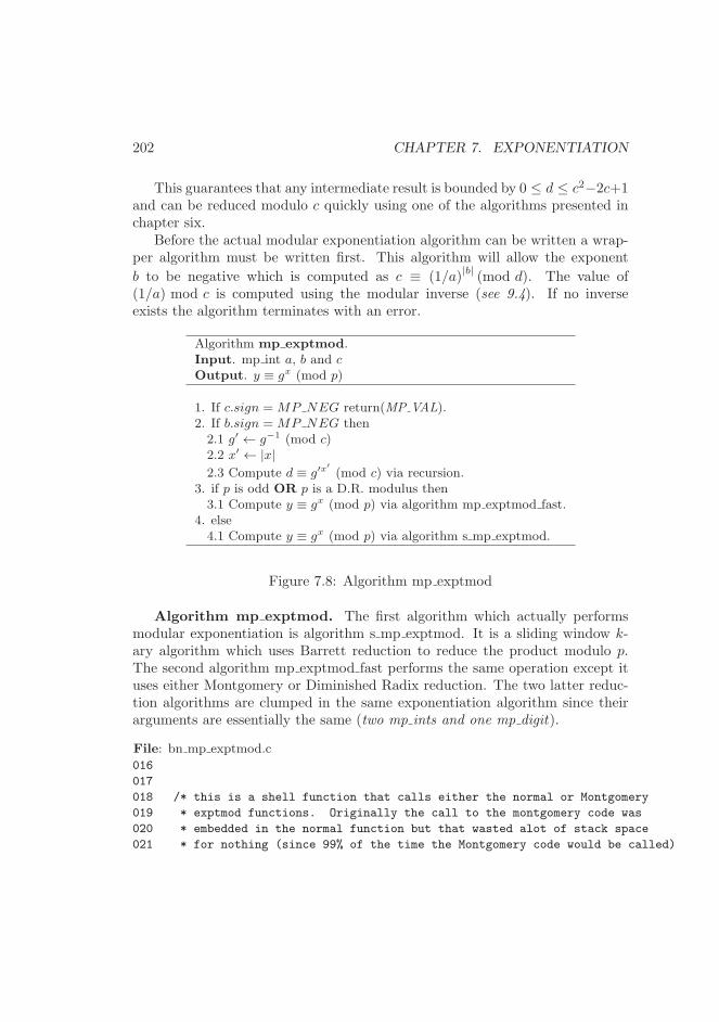
202 CHAPTER 7. EXPONENTIATION
This guarantees that any intermediate result is bounded by 0 ≤ d ≤ c2−2c+1and can be reduced modulo c quickly using one of the algorithms presented inchapter six.
Before the actual modular exponentiation algorithm can be written a wrap-per algorithm must be written first. This algorithm will allow the exponent
b to be negative which is computed as c ≡ (1/a)|b|
(mod d). The value of(1/a) mod c is computed using the modular inverse (see 9.4). If no inverseexists the algorithm terminates with an error.
Algorithm mp exptmod.Input. mp int a, b and cOutput. y ≡ gx (mod p)
1. If c.sign = MP NEG return(MP VAL).2. If b.sign = MP NEG then2.1 g′ ← g−1 (mod c)2.2 x′ ← |x|
2.3 Compute d ≡ g′x′
(mod c) via recursion.3. if p is odd OR p is a D.R. modulus then3.1 Compute y ≡ gx (mod p) via algorithm mp exptmod fast.
4. else4.1 Compute y ≡ gx (mod p) via algorithm s mp exptmod.
Figure 7.8: Algorithm mp exptmod
Algorithm mp exptmod. The first algorithm which actually performsmodular exponentiation is algorithm s mp exptmod. It is a sliding window k-ary algorithm which uses Barrett reduction to reduce the product modulo p.The second algorithm mp exptmod fast performs the same operation except ituses either Montgomery or Diminished Radix reduction. The two latter reduc-tion algorithms are clumped in the same exponentiation algorithm since theirarguments are essentially the same (two mp ints and one mp digit).
File: bn mp exptmod.c
016
017
018 /* this is a shell function that calls either the normal or Montgomery
019 * exptmod functions. Originally the call to the montgomery code was
020 * embedded in the normal function but that wasted alot of stack space
021 * for nothing (since 99% of the time the Montgomery code would be called)
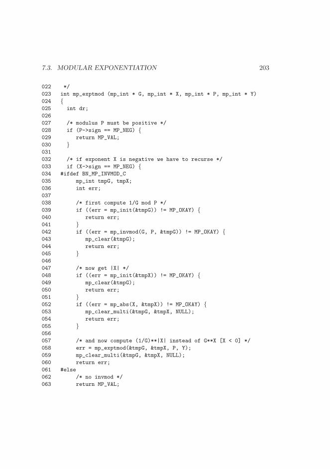
7.3. MODULAR EXPONENTIATION 203
022 */
023 int mp_exptmod (mp_int * G, mp_int * X, mp_int * P, mp_int * Y)
024 {025 int dr;
026
027 /* modulus P must be positive */
028 if (P->sign == MP_NEG) {029 return MP_VAL;
030 }031
032 /* if exponent X is negative we have to recurse */
033 if (X->sign == MP_NEG) {034 #ifdef BN_MP_INVMOD_C
035 mp_int tmpG, tmpX;
036 int err;
037
038 /* first compute 1/G mod P */
039 if ((err = mp_init(&tmpG)) != MP_OKAY) {040 return err;
041 }042 if ((err = mp_invmod(G, P, &tmpG)) != MP_OKAY) {043 mp_clear(&tmpG);
044 return err;
045 }046
047 /* now get |X| */
048 if ((err = mp_init(&tmpX)) != MP_OKAY) {049 mp_clear(&tmpG);
050 return err;
051 }052 if ((err = mp_abs(X, &tmpX)) != MP_OKAY) {053 mp_clear_multi(&tmpG, &tmpX, NULL);
054 return err;
055 }056
057 /* and now compute (1/G)**|X| instead of G**X [X < 0] */
058 err = mp_exptmod(&tmpG, &tmpX, P, Y);
059 mp_clear_multi(&tmpG, &tmpX, NULL);
060 return err;
061 #else
062 /* no invmod */
063 return MP_VAL;
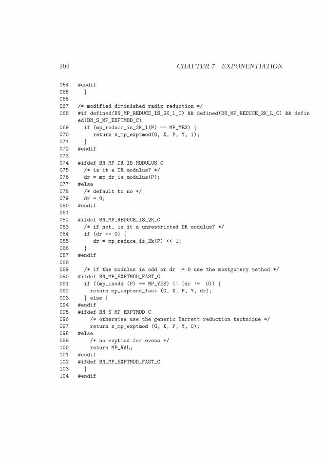
204 CHAPTER 7. EXPONENTIATION
064 #endif
065 }066
067 /* modified diminished radix reduction */
068 #if defined(BN_MP_REDUCE_IS_2K_L_C) && defined(BN_MP_REDUCE_2K_L_C) && defin
ed(BN_S_MP_EXPTMOD_C)
069 if (mp_reduce_is_2k_l(P) == MP_YES) {070 return s_mp_exptmod(G, X, P, Y, 1);
071 }072 #endif
073
074 #ifdef BN_MP_DR_IS_MODULUS_C
075 /* is it a DR modulus? */
076 dr = mp_dr_is_modulus(P);
077 #else
078 /* default to no */
079 dr = 0;
080 #endif
081
082 #ifdef BN_MP_REDUCE_IS_2K_C
083 /* if not, is it a unrestricted DR modulus? */
084 if (dr == 0) {085 dr = mp_reduce_is_2k(P) << 1;
086 }087 #endif
088
089 /* if the modulus is odd or dr != 0 use the montgomery method */
090 #ifdef BN_MP_EXPTMOD_FAST_C
091 if ((mp_isodd (P) == MP_YES) || (dr != 0)) {092 return mp_exptmod_fast (G, X, P, Y, dr);
093 } else {094 #endif
095 #ifdef BN_S_MP_EXPTMOD_C
096 /* otherwise use the generic Barrett reduction technique */
097 return s_mp_exptmod (G, X, P, Y, 0);
098 #else
099 /* no exptmod for evens */
100 return MP_VAL;
101 #endif
102 #ifdef BN_MP_EXPTMOD_FAST_C
103 }104 #endif
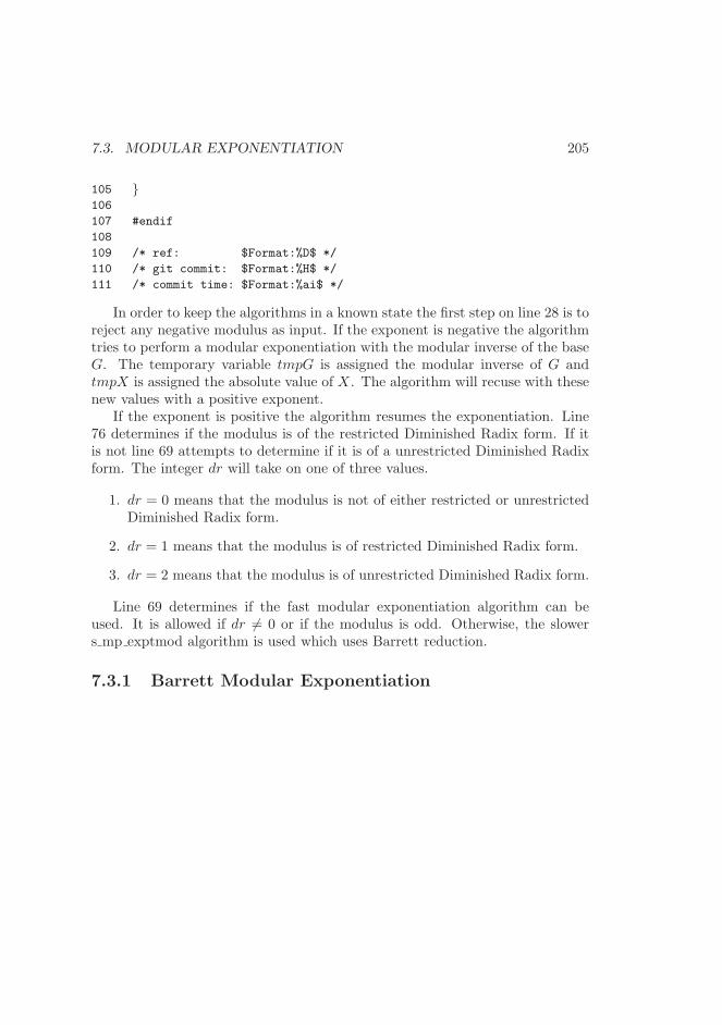
7.3. MODULAR EXPONENTIATION 205
105 }106
107 #endif
108
109 /* ref: $Format:%D$ */
110 /* git commit: $Format:%H$ */
111 /* commit time: $Format:%ai$ */
In order to keep the algorithms in a known state the first step on line 28 is toreject any negative modulus as input. If the exponent is negative the algorithmtries to perform a modular exponentiation with the modular inverse of the baseG. The temporary variable tmpG is assigned the modular inverse of G andtmpX is assigned the absolute value of X. The algorithm will recuse with thesenew values with a positive exponent.
If the exponent is positive the algorithm resumes the exponentiation. Line76 determines if the modulus is of the restricted Diminished Radix form. If itis not line 69 attempts to determine if it is of a unrestricted Diminished Radixform. The integer dr will take on one of three values.
1. dr = 0 means that the modulus is not of either restricted or unrestrictedDiminished Radix form.
2. dr = 1 means that the modulus is of restricted Diminished Radix form.
3. dr = 2 means that the modulus is of unrestricted Diminished Radix form.
Line 69 determines if the fast modular exponentiation algorithm can beused. It is allowed if dr 6= 0 or if the modulus is odd. Otherwise, the slowers mp exptmod algorithm is used which uses Barrett reduction.
7.3.1 Barrett Modular Exponentiation
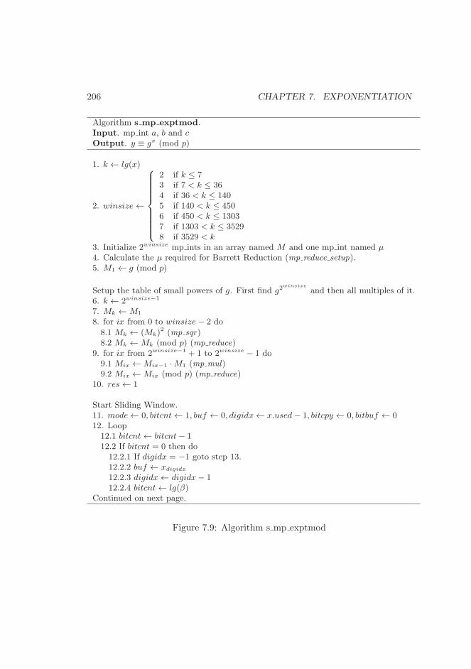
206 CHAPTER 7. EXPONENTIATION
Algorithm s mp exptmod.Input. mp int a, b and cOutput. y ≡ gx (mod p)
1. k ← lg(x)
2. winsize←
2 if k ≤ 73 if 7 < k ≤ 364 if 36 < k ≤ 1405 if 140 < k ≤ 4506 if 450 < k ≤ 13037 if 1303 < k ≤ 35298 if 3529 < k
3. Initialize 2winsize mp ints in an array named M and one mp int named µ4. Calculate the µ required for Barrett Reduction (mp reduce setup).5. M1 ← g (mod p)
Setup the table of small powers of g. First find g2winsize
and then all multiples of it.6. k ← 2winsize−1
7. Mk ←M1
8. for ix from 0 to winsize− 2 do
8.1 Mk ← (Mk)2 (mp sqr)
8.2 Mk ←Mk (mod p) (mp reduce)9. for ix from 2winsize−1 + 1 to 2winsize − 1 do9.1 Mix ←Mix−1 ·M1 (mp mul)9.2 Mix ←Mix (mod p) (mp reduce)
10. res← 1
Start Sliding Window.11. mode← 0, bitcnt← 1, buf ← 0, digidx← x.used− 1, bitcpy ← 0, bitbuf ← 012. Loop12.1 bitcnt← bitcnt− 112.2 If bitcnt = 0 then do12.2.1 If digidx = −1 goto step 13.12.2.2 buf ← xdigidx
12.2.3 digidx← digidx− 112.2.4 bitcnt← lg(β)
Continued on next page.
Figure 7.9: Algorithm s mp exptmod
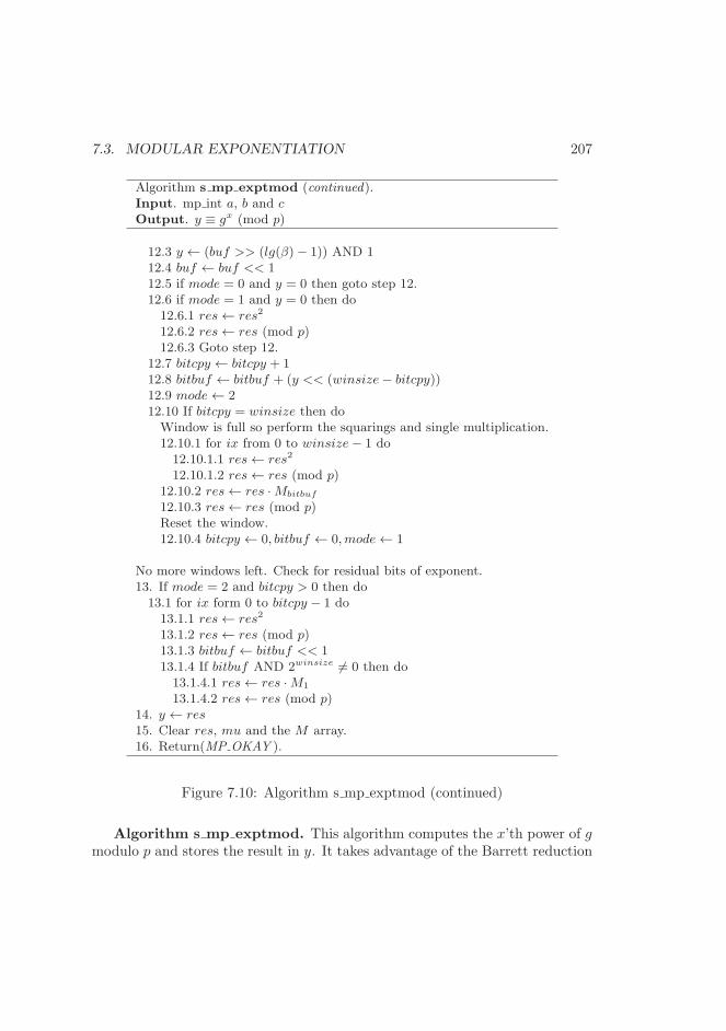
7.3. MODULAR EXPONENTIATION 207
Algorithm s mp exptmod (continued).Input. mp int a, b and cOutput. y ≡ gx (mod p)
12.3 y ← (buf >> (lg(β)− 1)) AND 112.4 buf ← buf << 112.5 if mode = 0 and y = 0 then goto step 12.12.6 if mode = 1 and y = 0 then do12.6.1 res← res2
12.6.2 res← res (mod p)12.6.3 Goto step 12.
12.7 bitcpy ← bitcpy + 112.8 bitbuf ← bitbuf + (y << (winsize− bitcpy))12.9 mode← 212.10 If bitcpy = winsize then doWindow is full so perform the squarings and single multiplication.12.10.1 for ix from 0 to winsize− 1 do12.10.1.1 res← res2
12.10.1.2 res← res (mod p)12.10.2 res← res ·Mbitbuf
12.10.3 res← res (mod p)Reset the window.12.10.4 bitcpy ← 0, bitbuf ← 0,mode← 1
No more windows left. Check for residual bits of exponent.13. If mode = 2 and bitcpy > 0 then do13.1 for ix form 0 to bitcpy − 1 do13.1.1 res← res2
13.1.2 res← res (mod p)13.1.3 bitbuf ← bitbuf << 113.1.4 If bitbuf AND 2winsize 6= 0 then do13.1.4.1 res← res ·M1
13.1.4.2 res← res (mod p)14. y ← res15. Clear res, mu and the M array.16. Return(MP OKAY ).
Figure 7.10: Algorithm s mp exptmod (continued)
Algorithm s mp exptmod. This algorithm computes the x’th power of gmodulo p and stores the result in y. It takes advantage of the Barrett reduction
208 CHAPTER 7. EXPONENTIATION
algorithm to keep the product small throughout the algorithm.The first two steps determine the optimal window size based on the number
of bits in the exponent. The larger the exponent the larger the window sizebecomes. After a window size winsize has been chosen an array of 2winsize
mp int variables is allocated. This table will hold the values of gx (mod p) for2winsize−1 ≤ x < 2winsize.
After the table is allocated the first power of g is found. Since g ≥ p isallowed it must be first reduced modulo p to make the rest of the algorithmmore efficient. The first element of the table at 2winsize−1 is found by squaringM1 successively winsize− 2 times. The rest of the table elements are found bymultiplying the previous element by M1 modulo p.
Now that the table is available the sliding window may begin. The followinglist describes the functions of all the variables in the window.
1. The variable mode dictates how the bits of the exponent are interpreted.
(a) When mode = 0 the bits are ignored since no non-zero bit of theexponent has been seen yet. For example, if the exponent were simply1 then there would be lg(β)−1 zero bits before the first non-zero bit.In this case bits are ignored until a non-zero bit is found.
(b) When mode = 1 a non-zero bit has been seen before and a newwinsize-bit window has not been formed yet. In this mode leading0 bits are read and a single squaring is performed. If a non-zero bitis read a new window is created.
(c) When mode = 2 the algorithm is in the middle of forming a windowand new bits are appended to the window from the most significantbit downwards.
2. The variable bitcnt indicates how many bits are left in the current digit ofthe exponent left to be read. When it reaches zero a new digit is fetchedfrom the exponent.
3. The variable buf holds the currently read digit of the exponent.
4. The variable digidx is an index into the exponents digits. It starts at theleading digit x.used− 1 and moves towards the trailing digit.
5. The variable bitcpy indicates how many bits are in the currently formedwindow. When it reaches winsize the window is flushed and the appro-priate operations performed.
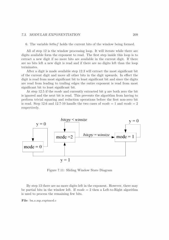
7.3. MODULAR EXPONENTIATION 209
6. The variable bitbuf holds the current bits of the window being formed.
All of step 12 is the window processing loop. It will iterate while there aredigits available form the exponent to read. The first step inside this loop is toextract a new digit if no more bits are available in the current digit. If thereare no bits left a new digit is read and if there are no digits left than the loopterminates.
After a digit is made available step 12.3 will extract the most significant bitof the current digit and move all other bits in the digit upwards. In effect thedigit is read from most significant bit to least significant bit and since the digitsare read from leading to trailing edges the entire exponent is read from mostsignificant bit to least significant bit.
At step 12.5 if the mode and currently extracted bit y are both zero the bitis ignored and the next bit is read. This prevents the algorithm from having toperform trivial squaring and reduction operations before the first non-zero bitis read. Step 12.6 and 12.7-10 handle the two cases of mode = 1 and mode = 2respectively.
Figure 7.11: Sliding Window State Diagram
By step 13 there are no more digits left in the exponent. However, there maybe partial bits in the window left. If mode = 2 then a Left-to-Right algorithmis used to process the remaining few bits.
File: bn s mp exptmod.c
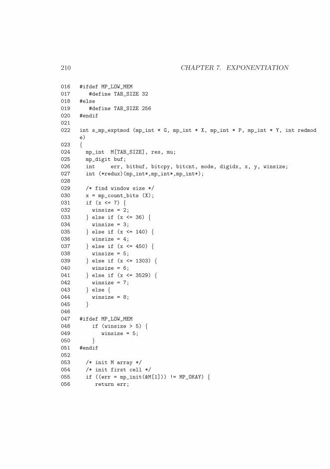
210 CHAPTER 7. EXPONENTIATION
016 #ifdef MP_LOW_MEM
017 #define TAB_SIZE 32
018 #else
019 #define TAB_SIZE 256
020 #endif
021
022 int s_mp_exptmod (mp_int * G, mp_int * X, mp_int * P, mp_int * Y, int redmod
e)
023 {024 mp_int M[TAB_SIZE], res, mu;
025 mp_digit buf;
026 int err, bitbuf, bitcpy, bitcnt, mode, digidx, x, y, winsize;
027 int (*redux)(mp_int*,mp_int*,mp_int*);
028
029 /* find window size */
030 x = mp_count_bits (X);
031 if (x <= 7) {032 winsize = 2;
033 } else if (x <= 36) {034 winsize = 3;
035 } else if (x <= 140) {036 winsize = 4;
037 } else if (x <= 450) {038 winsize = 5;
039 } else if (x <= 1303) {040 winsize = 6;
041 } else if (x <= 3529) {042 winsize = 7;
043 } else {044 winsize = 8;
045 }046
047 #ifdef MP_LOW_MEM
048 if (winsize > 5) {049 winsize = 5;
050 }051 #endif
052
053 /* init M array */
054 /* init first cell */
055 if ((err = mp_init(&M[1])) != MP_OKAY) {056 return err;
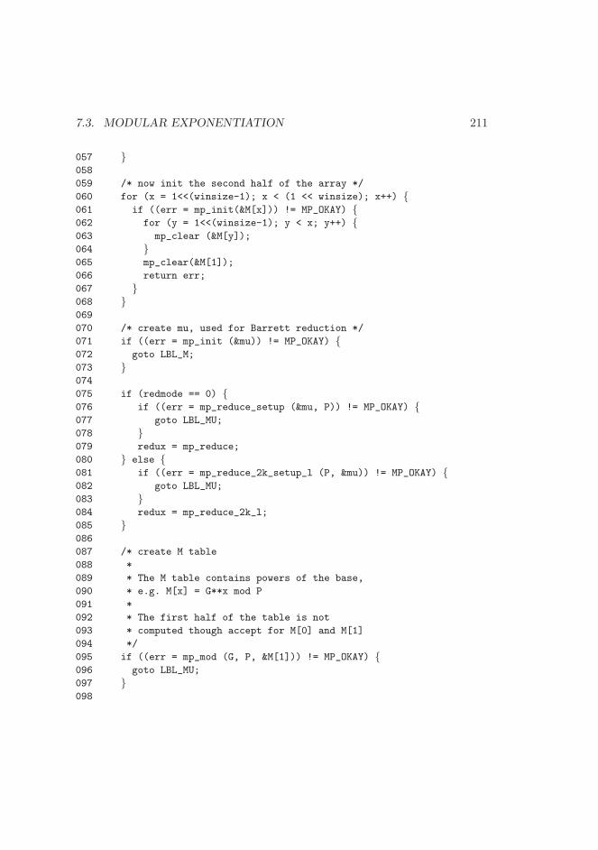
7.3. MODULAR EXPONENTIATION 211
057 }058
059 /* now init the second half of the array */
060 for (x = 1<<(winsize-1); x < (1 << winsize); x++) {061 if ((err = mp_init(&M[x])) != MP_OKAY) {062 for (y = 1<<(winsize-1); y < x; y++) {063 mp_clear (&M[y]);
064 }065 mp_clear(&M[1]);
066 return err;
067 }068 }069
070 /* create mu, used for Barrett reduction */
071 if ((err = mp_init (&mu)) != MP_OKAY) {072 goto LBL_M;
073 }074
075 if (redmode == 0) {076 if ((err = mp_reduce_setup (&mu, P)) != MP_OKAY) {077 goto LBL_MU;
078 }079 redux = mp_reduce;
080 } else {081 if ((err = mp_reduce_2k_setup_l (P, &mu)) != MP_OKAY) {082 goto LBL_MU;
083 }084 redux = mp_reduce_2k_l;
085 }086
087 /* create M table
088 *
089 * The M table contains powers of the base,
090 * e.g. M[x] = G**x mod P
091 *
092 * The first half of the table is not
093 * computed though accept for M[0] and M[1]
094 */
095 if ((err = mp_mod (G, P, &M[1])) != MP_OKAY) {096 goto LBL_MU;
097 }098
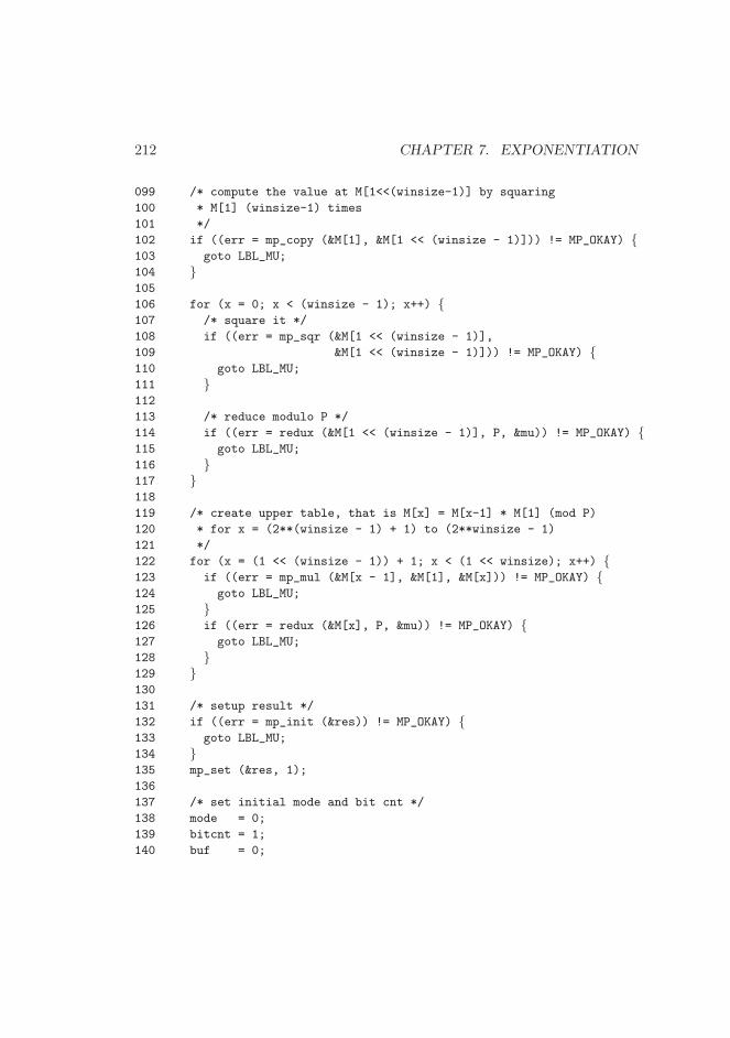
212 CHAPTER 7. EXPONENTIATION
099 /* compute the value at M[1<<(winsize-1)] by squaring
100 * M[1] (winsize-1) times
101 */
102 if ((err = mp_copy (&M[1], &M[1 << (winsize - 1)])) != MP_OKAY) {103 goto LBL_MU;
104 }105
106 for (x = 0; x < (winsize - 1); x++) {107 /* square it */
108 if ((err = mp_sqr (&M[1 << (winsize - 1)],
109 &M[1 << (winsize - 1)])) != MP_OKAY) {110 goto LBL_MU;
111 }112
113 /* reduce modulo P */
114 if ((err = redux (&M[1 << (winsize - 1)], P, &mu)) != MP_OKAY) {115 goto LBL_MU;
116 }117 }118
119 /* create upper table, that is M[x] = M[x-1] * M[1] (mod P)
120 * for x = (2**(winsize - 1) + 1) to (2**winsize - 1)
121 */
122 for (x = (1 << (winsize - 1)) + 1; x < (1 << winsize); x++) {123 if ((err = mp_mul (&M[x - 1], &M[1], &M[x])) != MP_OKAY) {124 goto LBL_MU;
125 }126 if ((err = redux (&M[x], P, &mu)) != MP_OKAY) {127 goto LBL_MU;
128 }129 }130
131 /* setup result */
132 if ((err = mp_init (&res)) != MP_OKAY) {133 goto LBL_MU;
134 }135 mp_set (&res, 1);
136
137 /* set initial mode and bit cnt */
138 mode = 0;
139 bitcnt = 1;
140 buf = 0;
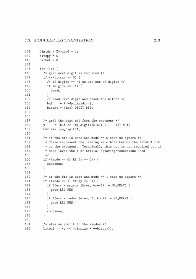
7.3. MODULAR EXPONENTIATION 213
141 digidx = X->used - 1;
142 bitcpy = 0;
143 bitbuf = 0;
144
145 for (;;) {146 /* grab next digit as required */
147 if (--bitcnt == 0) {148 /* if digidx == -1 we are out of digits */
149 if (digidx == -1) {150 break;
151 }152 /* read next digit and reset the bitcnt */
153 buf = X->dp[digidx--];
154 bitcnt = (int) DIGIT_BIT;
155 }156
157 /* grab the next msb from the exponent */
158 y = (buf >> (mp_digit)(DIGIT_BIT - 1)) & 1;
159 buf <<= (mp_digit)1;
160
161 /* if the bit is zero and mode == 0 then we ignore it
162 * These represent the leading zero bits before the first 1 bit
163 * in the exponent. Technically this opt is not required but it
164 * does lower the # of trivial squaring/reductions used
165 */
166 if ((mode == 0) && (y == 0)) {167 continue;
168 }169
170 /* if the bit is zero and mode == 1 then we square */
171 if ((mode == 1) && (y == 0)) {172 if ((err = mp_sqr (&res, &res)) != MP_OKAY) {173 goto LBL_RES;
174 }175 if ((err = redux (&res, P, &mu)) != MP_OKAY) {176 goto LBL_RES;
177 }178 continue;
179 }180
181 /* else we add it to the window */
182 bitbuf |= (y << (winsize - ++bitcpy));
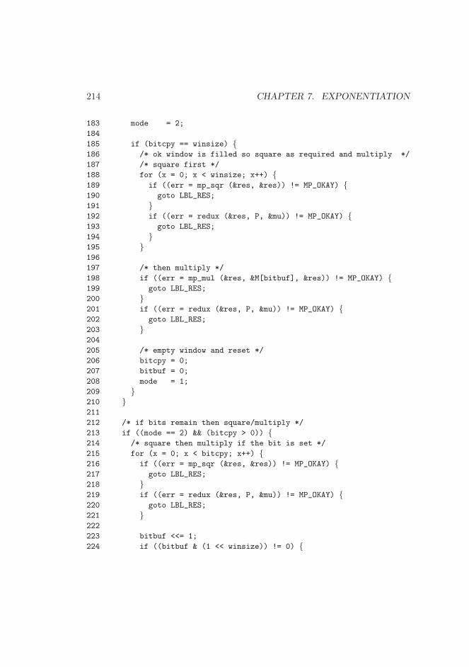
214 CHAPTER 7. EXPONENTIATION
183 mode = 2;
184
185 if (bitcpy == winsize) {186 /* ok window is filled so square as required and multiply */
187 /* square first */
188 for (x = 0; x < winsize; x++) {189 if ((err = mp_sqr (&res, &res)) != MP_OKAY) {190 goto LBL_RES;
191 }192 if ((err = redux (&res, P, &mu)) != MP_OKAY) {193 goto LBL_RES;
194 }195 }196
197 /* then multiply */
198 if ((err = mp_mul (&res, &M[bitbuf], &res)) != MP_OKAY) {199 goto LBL_RES;
200 }201 if ((err = redux (&res, P, &mu)) != MP_OKAY) {202 goto LBL_RES;
203 }204
205 /* empty window and reset */
206 bitcpy = 0;
207 bitbuf = 0;
208 mode = 1;
209 }210 }211
212 /* if bits remain then square/multiply */
213 if ((mode == 2) && (bitcpy > 0)) {214 /* square then multiply if the bit is set */
215 for (x = 0; x < bitcpy; x++) {216 if ((err = mp_sqr (&res, &res)) != MP_OKAY) {217 goto LBL_RES;
218 }219 if ((err = redux (&res, P, &mu)) != MP_OKAY) {220 goto LBL_RES;
221 }222
223 bitbuf <<= 1;
224 if ((bitbuf & (1 << winsize)) != 0) {
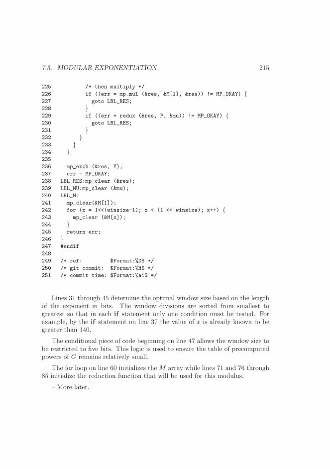
7.3. MODULAR EXPONENTIATION 215
225 /* then multiply */
226 if ((err = mp_mul (&res, &M[1], &res)) != MP_OKAY) {227 goto LBL_RES;
228 }229 if ((err = redux (&res, P, &mu)) != MP_OKAY) {230 goto LBL_RES;
231 }232 }233 }234 }235
236 mp_exch (&res, Y);
237 err = MP_OKAY;
238 LBL_RES:mp_clear (&res);
239 LBL_MU:mp_clear (&mu);
240 LBL_M:
241 mp_clear(&M[1]);
242 for (x = 1<<(winsize-1); x < (1 << winsize); x++) {243 mp_clear (&M[x]);
244 }245 return err;
246 }247 #endif
248
249 /* ref: $Format:%D$ */
250 /* git commit: $Format:%H$ */
251 /* commit time: $Format:%ai$ */
Lines 31 through 45 determine the optimal window size based on the lengthof the exponent in bits. The window divisions are sorted from smallest togreatest so that in each if statement only one condition must be tested. Forexample, by the if statement on line 37 the value of x is already known to begreater than 140.
The conditional piece of code beginning on line 47 allows the window size tobe restricted to five bits. This logic is used to ensure the table of precomputedpowers of G remains relatively small.
The for loop on line 60 initializes the M array while lines 71 and 76 through85 initialize the reduction function that will be used for this modulus.
– More later.
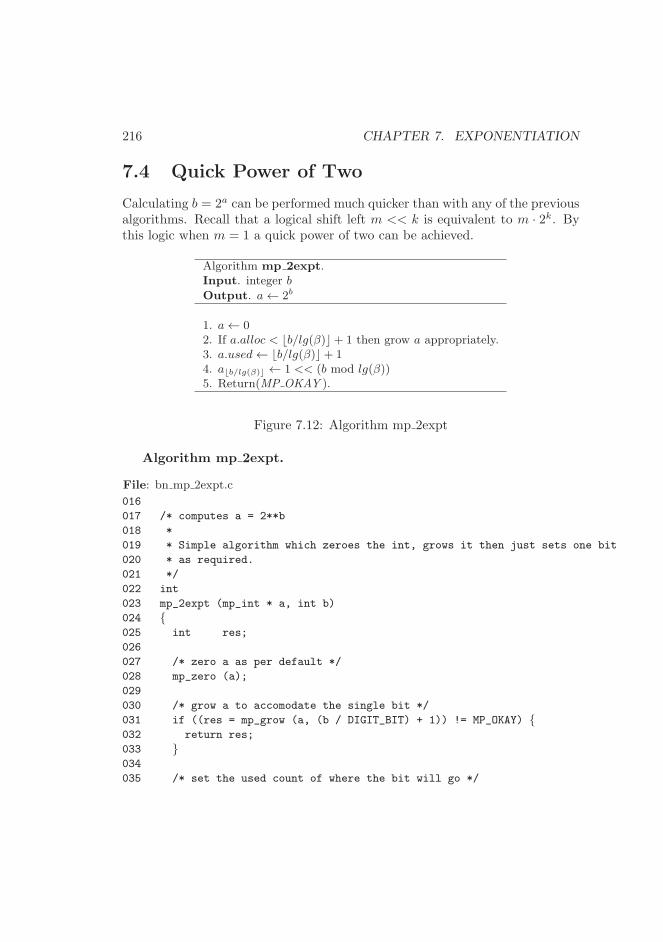
216 CHAPTER 7. EXPONENTIATION
7.4 Quick Power of Two
Calculating b = 2a can be performed much quicker than with any of the previousalgorithms. Recall that a logical shift left m << k is equivalent to m · 2k. Bythis logic when m = 1 a quick power of two can be achieved.
Algorithm mp 2expt.Input. integer b
Output. a← 2b
1. a← 02. If a.alloc < ⌊b/lg(β)⌋+ 1 then grow a appropriately.3. a.used← ⌊b/lg(β)⌋+ 14. a⌊b/lg(β)⌋ ← 1 << (b mod lg(β))5. Return(MP OKAY ).
Figure 7.12: Algorithm mp 2expt
Algorithm mp 2expt.
File: bn mp 2expt.c
016
017 /* computes a = 2**b
018 *
019 * Simple algorithm which zeroes the int, grows it then just sets one bit
020 * as required.
021 */
022 int
023 mp_2expt (mp_int * a, int b)
024 {025 int res;
026
027 /* zero a as per default */
028 mp_zero (a);
029
030 /* grow a to accomodate the single bit */
031 if ((res = mp_grow (a, (b / DIGIT_BIT) + 1)) != MP_OKAY) {032 return res;
033 }034
035 /* set the used count of where the bit will go */
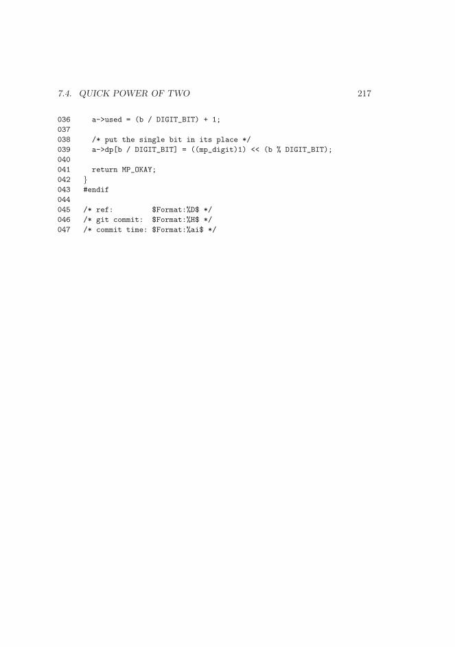
7.4. QUICK POWER OF TWO 217
036 a->used = (b / DIGIT_BIT) + 1;
037
038 /* put the single bit in its place */
039 a->dp[b / DIGIT_BIT] = ((mp_digit)1) << (b % DIGIT_BIT);
040
041 return MP_OKAY;
042 }043 #endif
044
045 /* ref: $Format:%D$ */
046 /* git commit: $Format:%H$ */
047 /* commit time: $Format:%ai$ */

218 CHAPTER 7. EXPONENTIATION
Chapter 8
Higher Level Algorithms
This chapter discusses the various higher level algorithms that are required tocomplete a well rounded multiple precision integer package. These routines areless performance oriented than the algorithms of chapters five, six and sevenbut are no less important.
The first section describes a method of integer division with remainder thatis universally well known. It provides the signed division logic for the package.The subsequent section discusses a set of algorithms which allow a single digitto be the 2nd operand for a variety of operations. These algorithms servemostly to simplify other algorithms where small constants are required. Thelast two sections discuss how to manipulate various representations of integers.For example, converting from an mp int to a string of character.
8.1 Integer Division with Remainder
Integer division aside from modular exponentiation is the most intensive algo-rithm to compute. Like addition, subtraction and multiplication the basis ofthis algorithm is the long-hand division algorithm taught to school children.Throughout this discussion several common variables will be used. Let x rep-resent the divisor and y represent the dividend. Let q represent the integerquotient ⌊y/x⌋ and let r represent the remainder r = y−x⌊y/x⌋. The followingsimple algorithm will be used to start the discussion.
219
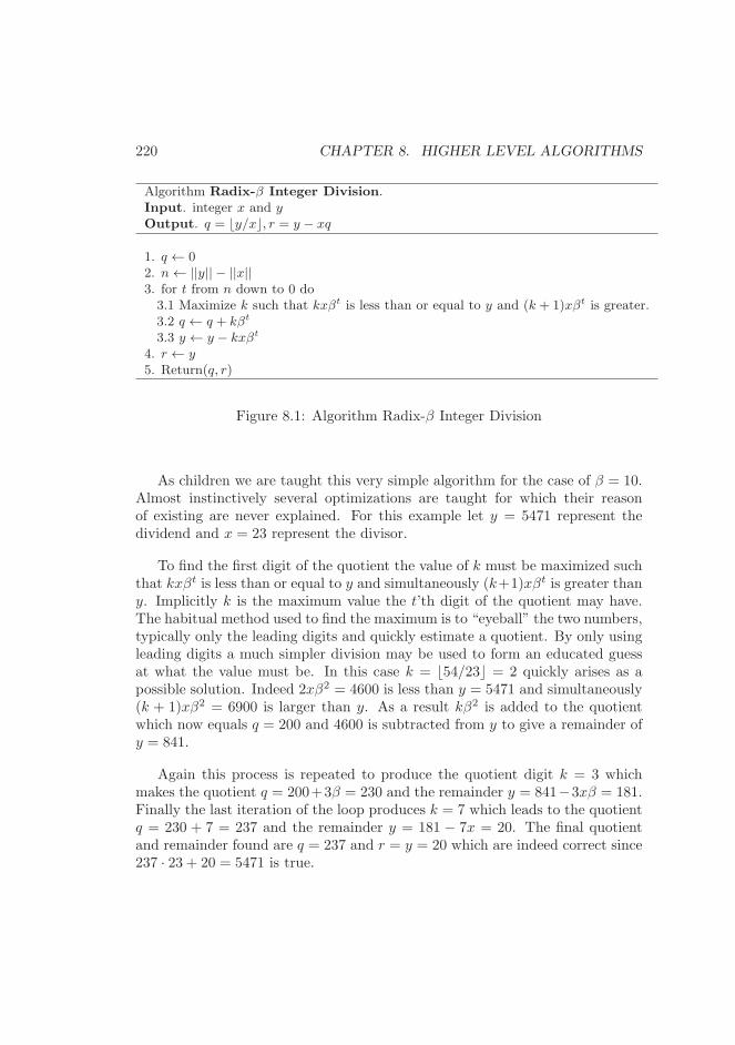
220 CHAPTER 8. HIGHER LEVEL ALGORITHMS
Algorithm Radix-β Integer Division.Input. integer x and yOutput. q = ⌊y/x⌋, r = y − xq
1. q ← 02. n← ||y|| − ||x||3. for t from n down to 0 do3.1 Maximize k such that kxβt is less than or equal to y and (k + 1)xβt is greater.3.2 q ← q + kβt
3.3 y ← y − kxβt
4. r ← y5. Return(q, r)
Figure 8.1: Algorithm Radix-β Integer Division
As children we are taught this very simple algorithm for the case of β = 10.Almost instinctively several optimizations are taught for which their reasonof existing are never explained. For this example let y = 5471 represent thedividend and x = 23 represent the divisor.
To find the first digit of the quotient the value of k must be maximized suchthat kxβt is less than or equal to y and simultaneously (k+1)xβt is greater thany. Implicitly k is the maximum value the t’th digit of the quotient may have.The habitual method used to find the maximum is to “eyeball” the two numbers,typically only the leading digits and quickly estimate a quotient. By only usingleading digits a much simpler division may be used to form an educated guessat what the value must be. In this case k = ⌊54/23⌋ = 2 quickly arises as apossible solution. Indeed 2xβ2 = 4600 is less than y = 5471 and simultaneously(k + 1)xβ2 = 6900 is larger than y. As a result kβ2 is added to the quotientwhich now equals q = 200 and 4600 is subtracted from y to give a remainder ofy = 841.
Again this process is repeated to produce the quotient digit k = 3 whichmakes the quotient q = 200+3β = 230 and the remainder y = 841−3xβ = 181.Finally the last iteration of the loop produces k = 7 which leads to the quotientq = 230 + 7 = 237 and the remainder y = 181 − 7x = 20. The final quotientand remainder found are q = 237 and r = y = 20 which are indeed correct since237 · 23 + 20 = 5471 is true.
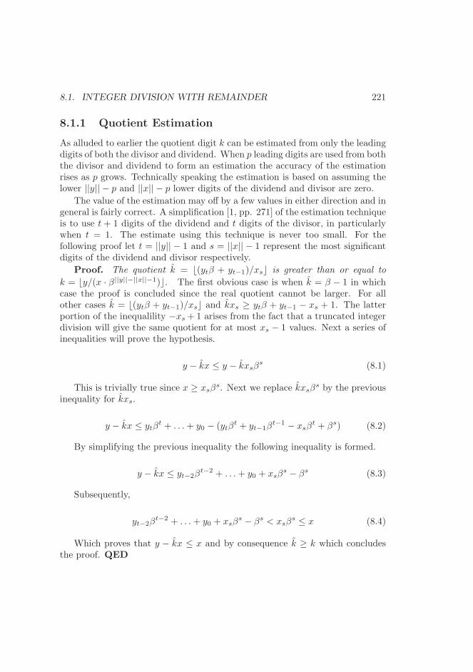
8.1. INTEGER DIVISION WITH REMAINDER 221
8.1.1 Quotient Estimation
As alluded to earlier the quotient digit k can be estimated from only the leadingdigits of both the divisor and dividend. When p leading digits are used from boththe divisor and dividend to form an estimation the accuracy of the estimationrises as p grows. Technically speaking the estimation is based on assuming thelower ||y|| − p and ||x|| − p lower digits of the dividend and divisor are zero.
The value of the estimation may off by a few values in either direction and ingeneral is fairly correct. A simplification [1, pp. 271] of the estimation techniqueis to use t + 1 digits of the dividend and t digits of the divisor, in particularlywhen t = 1. The estimate using this technique is never too small. For thefollowing proof let t = ||y|| − 1 and s = ||x|| − 1 represent the most significantdigits of the dividend and divisor respectively.
Proof. The quotient k = ⌊(ytβ + yt−1)/xs⌋ is greater than or equal to
k = ⌊y/(x · β||y||−||x||−1)⌋. The first obvious case is when k = β − 1 in whichcase the proof is concluded since the real quotient cannot be larger. For allother cases k = ⌊(ytβ + yt−1)/xs⌋ and kxs ≥ ytβ + yt−1 − xs + 1. The latterportion of the inequalility −xs + 1 arises from the fact that a truncated integerdivision will give the same quotient for at most xs − 1 values. Next a series ofinequalities will prove the hypothesis.
y − kx ≤ y − kxsβs (8.1)
This is trivially true since x ≥ xsβs. Next we replace kxsβ
s by the previousinequality for kxs.
y − kx ≤ ytβt + . . .+ y0 − (ytβ
t + yt−1βt−1 − xsβ
t + βs) (8.2)
By simplifying the previous inequality the following inequality is formed.
y − kx ≤ yt−2βt−2 + . . .+ y0 + xsβ
s − βs (8.3)
Subsequently,
yt−2βt−2 + . . .+ y0 + xsβ
s − βs < xsβs ≤ x (8.4)
Which proves that y − kx ≤ x and by consequence k ≥ k which concludesthe proof. QED
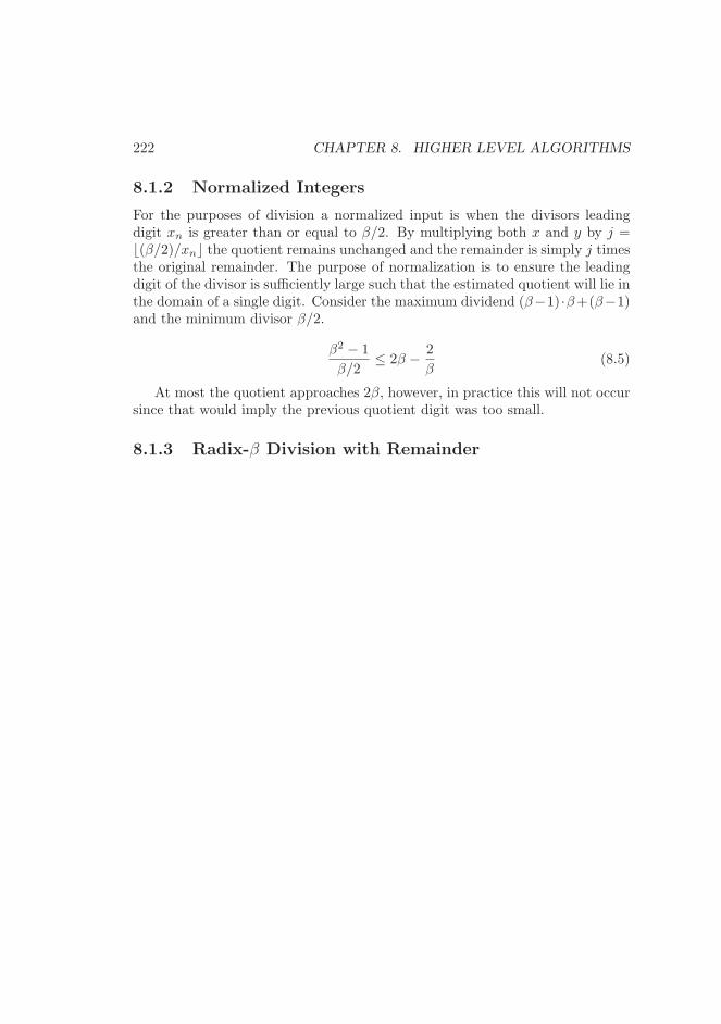
222 CHAPTER 8. HIGHER LEVEL ALGORITHMS
8.1.2 Normalized Integers
For the purposes of division a normalized input is when the divisors leadingdigit xn is greater than or equal to β/2. By multiplying both x and y by j =⌊(β/2)/xn⌋ the quotient remains unchanged and the remainder is simply j timesthe original remainder. The purpose of normalization is to ensure the leadingdigit of the divisor is sufficiently large such that the estimated quotient will lie inthe domain of a single digit. Consider the maximum dividend (β−1) ·β+(β−1)and the minimum divisor β/2.
β2 − 1
β/2≤ 2β − 2
β(8.5)
At most the quotient approaches 2β, however, in practice this will not occursince that would imply the previous quotient digit was too small.
8.1.3 Radix-β Division with Remainder
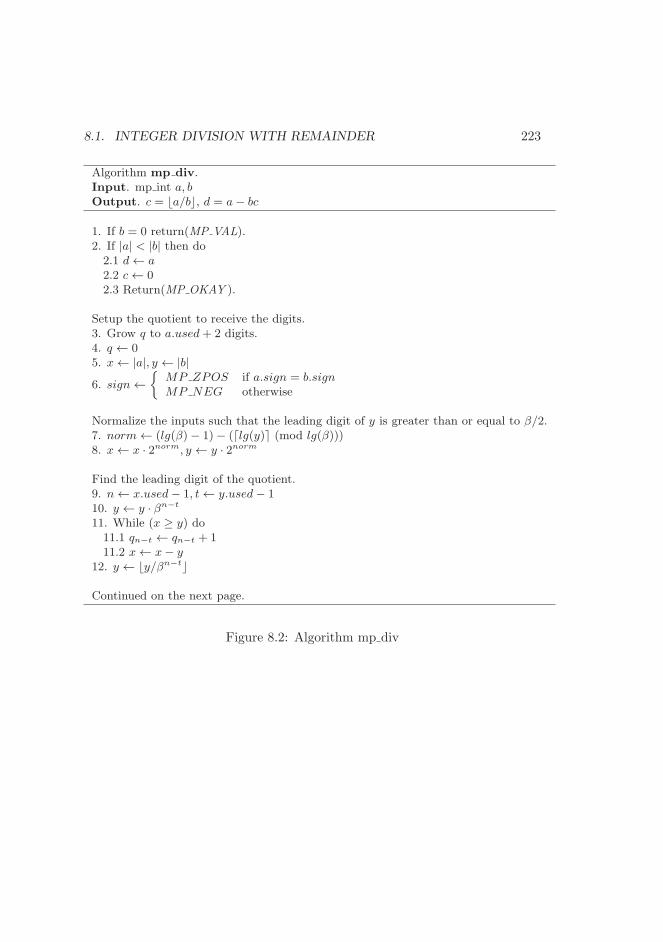
8.1. INTEGER DIVISION WITH REMAINDER 223
Algorithm mp div.Input. mp int a, bOutput. c = ⌊a/b⌋, d = a− bc
1. If b = 0 return(MP VAL).2. If |a| < |b| then do2.1 d← a2.2 c← 02.3 Return(MP OKAY ).
Setup the quotient to receive the digits.3. Grow q to a.used+ 2 digits.4. q ← 05. x← |a|, y ← |b|
6. sign←
{
MP ZPOS if a.sign = b.signMP NEG otherwise
Normalize the inputs such that the leading digit of y is greater than or equal to β/2.7. norm← (lg(β)− 1)− (⌈lg(y)⌉ (mod lg(β)))8. x← x · 2norm, y ← y · 2norm
Find the leading digit of the quotient.9. n← x.used− 1, t← y.used− 110. y ← y · βn−t
11. While (x ≥ y) do11.1 qn−t ← qn−t + 111.2 x← x− y
12. y ← ⌊y/βn−t⌋
Continued on the next page.
Figure 8.2: Algorithm mp div
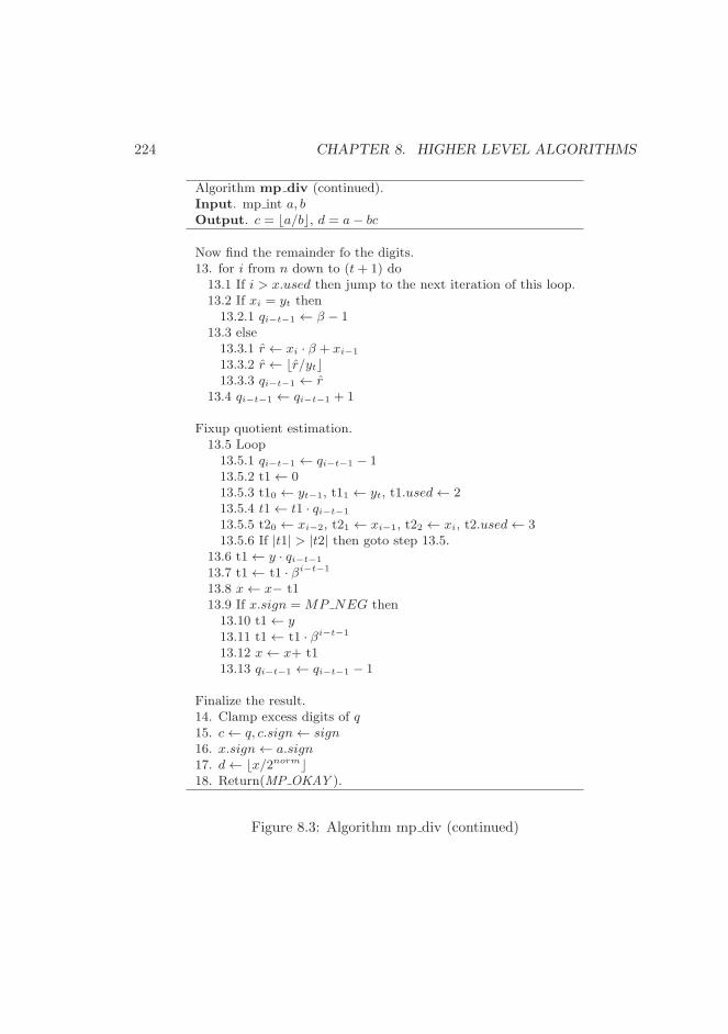
224 CHAPTER 8. HIGHER LEVEL ALGORITHMS
Algorithm mp div (continued).Input. mp int a, bOutput. c = ⌊a/b⌋, d = a− bc
Now find the remainder fo the digits.13. for i from n down to (t+ 1) do13.1 If i > x.used then jump to the next iteration of this loop.13.2 If xi = yt then13.2.1 qi−t−1 ← β − 1
13.3 else13.3.1 r ← xi · β + xi−1
13.3.2 r ← ⌊r/yt⌋13.3.3 qi−t−1 ← r
13.4 qi−t−1 ← qi−t−1 + 1
Fixup quotient estimation.13.5 Loop13.5.1 qi−t−1 ← qi−t−1 − 113.5.2 t1← 013.5.3 t10 ← yt−1, t11 ← yt, t1.used← 213.5.4 t1← t1 · qi−t−1
13.5.5 t20 ← xi−2, t21 ← xi−1, t22 ← xi, t2.used← 313.5.6 If |t1| > |t2| then goto step 13.5.
13.6 t1← y · qi−t−1
13.7 t1← t1 · βi−t−1
13.8 x← x− t113.9 If x.sign = MP NEG then13.10 t1← y13.11 t1← t1 · βi−t−1
13.12 x← x+ t113.13 qi−t−1 ← qi−t−1 − 1
Finalize the result.14. Clamp excess digits of q15. c← q, c.sign← sign16. x.sign← a.sign17. d← ⌊x/2norm⌋18. Return(MP OKAY ).
Figure 8.3: Algorithm mp div (continued)
8.1. INTEGER DIVISION WITH REMAINDER 225
Algorithm mp div. This algorithm will calculate quotient and remainderfrom an integer division given a dividend and divisor. The algorithm is a signeddivision and will produce a fully qualified quotient and remainder.
First the divisor b must be non-zero which is enforced in step one. If thedivisor is larger than the dividend than the quotient is implicitly zero and theremainder is the dividend.
After the first two trivial cases of inputs are handled the variable q is setupto receive the digits of the quotient. Two unsigned copies of the divisor y anddividend x are made as well. The core of the division algorithm is an unsigneddivision and will only work if the values are positive. Now the two values x andy must be normalized such that the leading digit of y is greater than or equalto β/2. This is performed by shifting both to the left by enough bits to get thedesired normalization.
At this point the division algorithm can begin producing digits of the quo-tient. Recall that maximum value of the estimation used is 2β− 2
β which meansthat a digit of the quotient must be first produced by another means. In thiscase y is shifted to the left (step ten) so that it has the same number of digitsas x. The loop on step eleven will subtract multiples of the shifted copy of yuntil x is smaller. Since the leading digit of y is greater than or equal to β/2this loop will iterate at most two times to produce the desired leading digit ofthe quotient.
Now the remainder of the digits can be produced. The equation q =⌊xiβ+xi−1
yt⌋ is used to fairly accurately approximate the true quotient digit. The
estimation can in theory produce an estimation as high as 2β− 2β but by induc-
tion the upper quotient digit is correct (as established on step eleven) and theestimate must be less than β.
Recall from section 8.1.1 that the estimation is never too low but may be toohigh. The next step of the estimation process is to refine the estimation. Theloop on step 13.5 uses xiβ
2 + xi−1β + xi−2 and qi−t−1(ytβ + yt−1) as a higherorder approximation to adjust the quotient digit.
After both phases of estimation the quotient digit may still be off by avalue of one1. Steps 13.6 and 13.7 subtract the multiple of the divisor fromthe dividend (Similar to step 3.3 of algorithm 8.1 and then subsequently add amultiple of the divisor if the quotient was too large.
Now that the quotient has been determine finializing the result is a matterof clamping the quotient, fixing the sizes and de-normalizing the remainder. Animportant aspect of this algorithm seemingly overlooked in other descriptions
1This is similar to the error introduced by optimizing Barrett reduction.
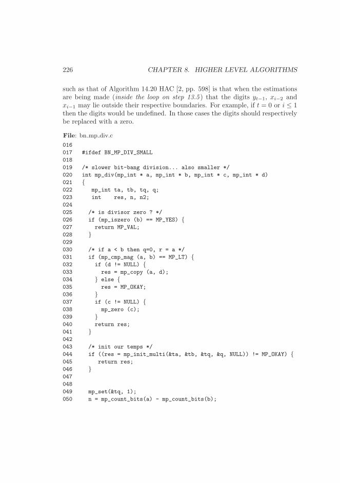
226 CHAPTER 8. HIGHER LEVEL ALGORITHMS
such as that of Algorithm 14.20 HAC [2, pp. 598] is that when the estimationsare being made (inside the loop on step 13.5 ) that the digits yt−1, xi−2 andxi−1 may lie outside their respective boundaries. For example, if t = 0 or i ≤ 1then the digits would be undefined. In those cases the digits should respectivelybe replaced with a zero.
File: bn mp div.c
016
017 #ifdef BN_MP_DIV_SMALL
018
019 /* slower bit-bang division... also smaller */
020 int mp_div(mp_int * a, mp_int * b, mp_int * c, mp_int * d)
021 {022 mp_int ta, tb, tq, q;
023 int res, n, n2;
024
025 /* is divisor zero ? */
026 if (mp_iszero (b) == MP_YES) {027 return MP_VAL;
028 }029
030 /* if a < b then q=0, r = a */
031 if (mp_cmp_mag (a, b) == MP_LT) {032 if (d != NULL) {033 res = mp_copy (a, d);
034 } else {035 res = MP_OKAY;
036 }037 if (c != NULL) {038 mp_zero (c);
039 }040 return res;
041 }042
043 /* init our temps */
044 if ((res = mp_init_multi(&ta, &tb, &tq, &q, NULL)) != MP_OKAY) {045 return res;
046 }047
048
049 mp_set(&tq, 1);
050 n = mp_count_bits(a) - mp_count_bits(b);
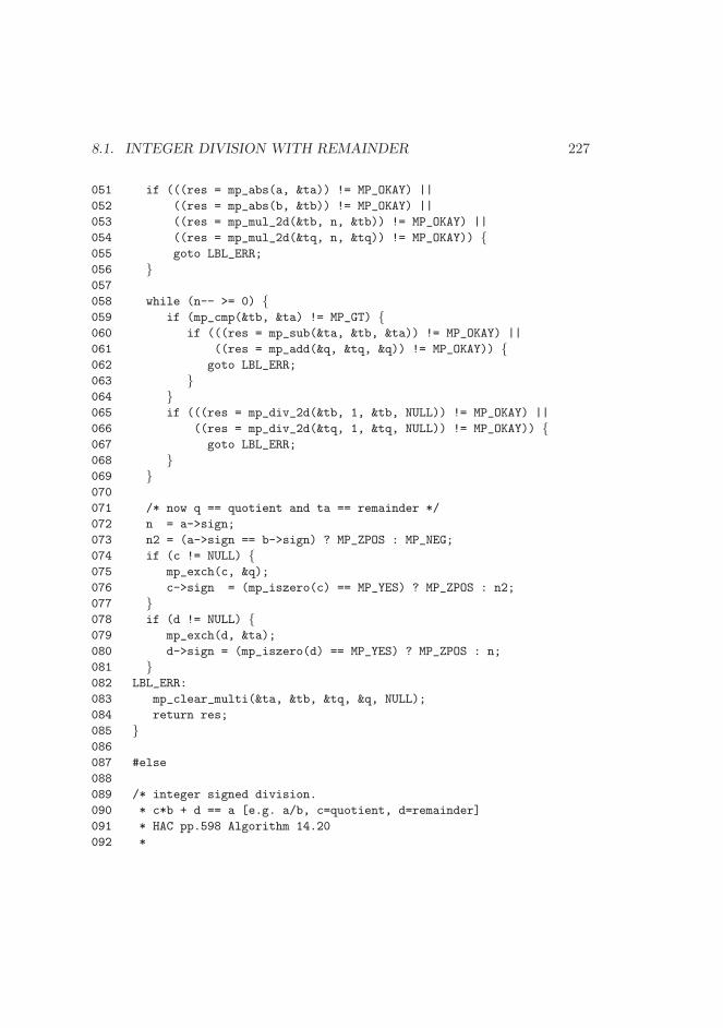
8.1. INTEGER DIVISION WITH REMAINDER 227
051 if (((res = mp_abs(a, &ta)) != MP_OKAY) ||
052 ((res = mp_abs(b, &tb)) != MP_OKAY) ||
053 ((res = mp_mul_2d(&tb, n, &tb)) != MP_OKAY) ||
054 ((res = mp_mul_2d(&tq, n, &tq)) != MP_OKAY)) {055 goto LBL_ERR;
056 }057
058 while (n-- >= 0) {059 if (mp_cmp(&tb, &ta) != MP_GT) {060 if (((res = mp_sub(&ta, &tb, &ta)) != MP_OKAY) ||
061 ((res = mp_add(&q, &tq, &q)) != MP_OKAY)) {062 goto LBL_ERR;
063 }064 }065 if (((res = mp_div_2d(&tb, 1, &tb, NULL)) != MP_OKAY) ||
066 ((res = mp_div_2d(&tq, 1, &tq, NULL)) != MP_OKAY)) {067 goto LBL_ERR;
068 }069 }070
071 /* now q == quotient and ta == remainder */
072 n = a->sign;
073 n2 = (a->sign == b->sign) ? MP_ZPOS : MP_NEG;
074 if (c != NULL) {075 mp_exch(c, &q);
076 c->sign = (mp_iszero(c) == MP_YES) ? MP_ZPOS : n2;
077 }078 if (d != NULL) {079 mp_exch(d, &ta);
080 d->sign = (mp_iszero(d) == MP_YES) ? MP_ZPOS : n;
081 }082 LBL_ERR:
083 mp_clear_multi(&ta, &tb, &tq, &q, NULL);
084 return res;
085 }086
087 #else
088
089 /* integer signed division.
090 * c*b + d == a [e.g. a/b, c=quotient, d=remainder]
091 * HAC pp.598 Algorithm 14.20
092 *
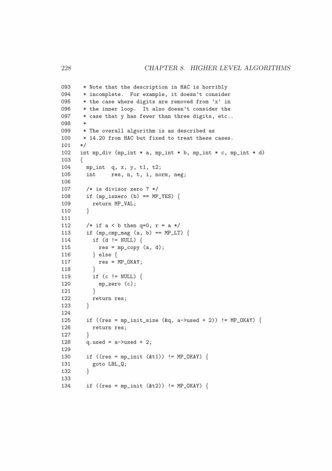
228 CHAPTER 8. HIGHER LEVEL ALGORITHMS
093 * Note that the description in HAC is horribly
094 * incomplete. For example, it doesn’t consider
095 * the case where digits are removed from ’x’ in
096 * the inner loop. It also doesn’t consider the
097 * case that y has fewer than three digits, etc..
098 *
099 * The overall algorithm is as described as
100 * 14.20 from HAC but fixed to treat these cases.
101 */
102 int mp_div (mp_int * a, mp_int * b, mp_int * c, mp_int * d)
103 {104 mp_int q, x, y, t1, t2;
105 int res, n, t, i, norm, neg;
106
107 /* is divisor zero ? */
108 if (mp_iszero (b) == MP_YES) {109 return MP_VAL;
110 }111
112 /* if a < b then q=0, r = a */
113 if (mp_cmp_mag (a, b) == MP_LT) {114 if (d != NULL) {115 res = mp_copy (a, d);
116 } else {117 res = MP_OKAY;
118 }119 if (c != NULL) {120 mp_zero (c);
121 }122 return res;
123 }124
125 if ((res = mp_init_size (&q, a->used + 2)) != MP_OKAY) {126 return res;
127 }128 q.used = a->used + 2;
129
130 if ((res = mp_init (&t1)) != MP_OKAY) {131 goto LBL_Q;
132 }133
134 if ((res = mp_init (&t2)) != MP_OKAY) {
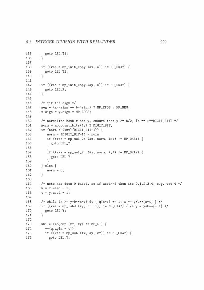
8.1. INTEGER DIVISION WITH REMAINDER 229
135 goto LBL_T1;
136 }137
138 if ((res = mp_init_copy (&x, a)) != MP_OKAY) {139 goto LBL_T2;
140 }141
142 if ((res = mp_init_copy (&y, b)) != MP_OKAY) {143 goto LBL_X;
144 }145
146 /* fix the sign */
147 neg = (a->sign == b->sign) ? MP_ZPOS : MP_NEG;
148 x.sign = y.sign = MP_ZPOS;
149
150 /* normalize both x and y, ensure that y >= b/2, [b == 2**DIGIT_BIT] */
151 norm = mp_count_bits(&y) % DIGIT_BIT;
152 if (norm < (int)(DIGIT_BIT-1)) {153 norm = (DIGIT_BIT-1) - norm;
154 if ((res = mp_mul_2d (&x, norm, &x)) != MP_OKAY) {155 goto LBL_Y;
156 }157 if ((res = mp_mul_2d (&y, norm, &y)) != MP_OKAY) {158 goto LBL_Y;
159 }160 } else {161 norm = 0;
162 }163
164 /* note hac does 0 based, so if used==5 then its 0,1,2,3,4, e.g. use 4 */
165 n = x.used - 1;
166 t = y.used - 1;
167
168 /* while (x >= y*b**n-t) do { q[n-t] += 1; x -= y*b**{n-t} } */
169 if ((res = mp_lshd (&y, n - t)) != MP_OKAY) { /* y = y*b**{n-t} */
170 goto LBL_Y;
171 }172
173 while (mp_cmp (&x, &y) != MP_LT) {174 ++(q.dp[n - t]);
175 if ((res = mp_sub (&x, &y, &x)) != MP_OKAY) {176 goto LBL_Y;
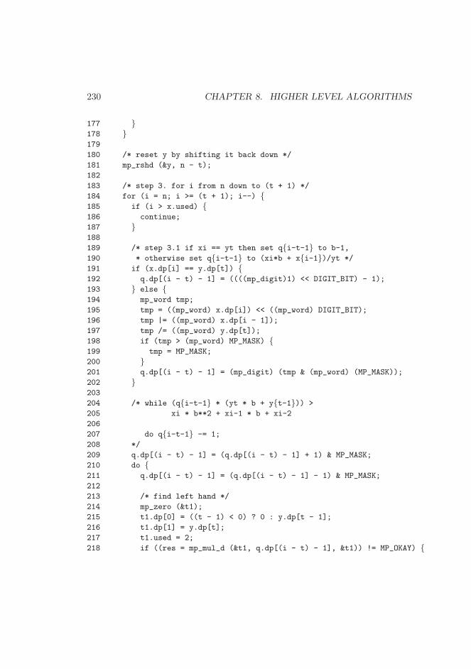
230 CHAPTER 8. HIGHER LEVEL ALGORITHMS
177 }178 }179
180 /* reset y by shifting it back down */
181 mp_rshd (&y, n - t);
182
183 /* step 3. for i from n down to (t + 1) */
184 for (i = n; i >= (t + 1); i--) {185 if (i > x.used) {186 continue;
187 }188
189 /* step 3.1 if xi == yt then set q{i-t-1} to b-1,
190 * otherwise set q{i-t-1} to (xi*b + x{i-1})/yt */
191 if (x.dp[i] == y.dp[t]) {192 q.dp[(i - t) - 1] = ((((mp_digit)1) << DIGIT_BIT) - 1);
193 } else {194 mp_word tmp;
195 tmp = ((mp_word) x.dp[i]) << ((mp_word) DIGIT_BIT);
196 tmp |= ((mp_word) x.dp[i - 1]);
197 tmp /= ((mp_word) y.dp[t]);
198 if (tmp > (mp_word) MP_MASK) {199 tmp = MP_MASK;
200 }201 q.dp[(i - t) - 1] = (mp_digit) (tmp & (mp_word) (MP_MASK));
202 }203
204 /* while (q{i-t-1} * (yt * b + y{t-1})) >
205 xi * b**2 + xi-1 * b + xi-2
206
207 do q{i-t-1} -= 1;
208 */
209 q.dp[(i - t) - 1] = (q.dp[(i - t) - 1] + 1) & MP_MASK;
210 do {211 q.dp[(i - t) - 1] = (q.dp[(i - t) - 1] - 1) & MP_MASK;
212
213 /* find left hand */
214 mp_zero (&t1);
215 t1.dp[0] = ((t - 1) < 0) ? 0 : y.dp[t - 1];
216 t1.dp[1] = y.dp[t];
217 t1.used = 2;
218 if ((res = mp_mul_d (&t1, q.dp[(i - t) - 1], &t1)) != MP_OKAY) {
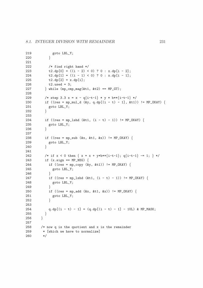
8.1. INTEGER DIVISION WITH REMAINDER 231
219 goto LBL_Y;
220 }221
222 /* find right hand */
223 t2.dp[0] = ((i - 2) < 0) ? 0 : x.dp[i - 2];
224 t2.dp[1] = ((i - 1) < 0) ? 0 : x.dp[i - 1];
225 t2.dp[2] = x.dp[i];
226 t2.used = 3;
227 } while (mp_cmp_mag(&t1, &t2) == MP_GT);
228
229 /* step 3.3 x = x - q{i-t-1} * y * b**{i-t-1} */
230 if ((res = mp_mul_d (&y, q.dp[(i - t) - 1], &t1)) != MP_OKAY) {231 goto LBL_Y;
232 }233
234 if ((res = mp_lshd (&t1, (i - t) - 1)) != MP_OKAY) {235 goto LBL_Y;
236 }237
238 if ((res = mp_sub (&x, &t1, &x)) != MP_OKAY) {239 goto LBL_Y;
240 }241
242 /* if x < 0 then { x = x + y*b**{i-t-1}; q{i-t-1} -= 1; } */
243 if (x.sign == MP_NEG) {244 if ((res = mp_copy (&y, &t1)) != MP_OKAY) {245 goto LBL_Y;
246 }247 if ((res = mp_lshd (&t1, (i - t) - 1)) != MP_OKAY) {248 goto LBL_Y;
249 }250 if ((res = mp_add (&x, &t1, &x)) != MP_OKAY) {251 goto LBL_Y;
252 }253
254 q.dp[(i - t) - 1] = (q.dp[(i - t) - 1] - 1UL) & MP_MASK;
255 }256 }257
258 /* now q is the quotient and x is the remainder
259 * [which we have to normalize]
260 */
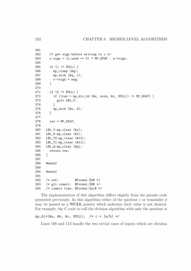
232 CHAPTER 8. HIGHER LEVEL ALGORITHMS
261
262 /* get sign before writing to c */
263 x.sign = (x.used == 0) ? MP_ZPOS : a->sign;
264
265 if (c != NULL) {266 mp_clamp (&q);
267 mp_exch (&q, c);
268 c->sign = neg;
269 }270
271 if (d != NULL) {272 if ((res = mp_div_2d (&x, norm, &x, NULL)) != MP_OKAY) {273 goto LBL_Y;
274 }275 mp_exch (&x, d);
276 }277
278 res = MP_OKAY;
279
280 LBL_Y:mp_clear (&y);
281 LBL_X:mp_clear (&x);
282 LBL_T2:mp_clear (&t2);
283 LBL_T1:mp_clear (&t1);
284 LBL_Q:mp_clear (&q);
285 return res;
286 }287
288 #endif
289
290 #endif
291
292 /* ref: $Format:%D$ */
293 /* git commit: $Format:%H$ */
294 /* commit time: $Format:%ai$ */
The implementation of this algorithm differs slightly from the pseudo codepresented previously. In this algorithm either of the quotient c or remainder dmay be passed as a NULL pointer which indicates their value is not desired.For example, the C code to call the division algorithm with only the quotient is
mp_div(&a, &b, &c, NULL); /* c = [a/b] */
Lines 108 and 113 handle the two trivial cases of inputs which are division
8.2. SINGLE DIGIT HELPERS 233
by zero and dividend smaller than the divisor respectively. After the two trivialcases all of the temporary variables are initialized. Line 147 determines the signof the quotient and line 148 ensures that both x and y are positive.
The number of bits in the leading digit is calculated on line 151. Implictlyan mp int with r digits will require lg(β)(r−1)+k bits of precision which whenreduced modulo lg(β) produces the value of k. In this case k is the number ofbits in the leading digit which is exactly what is required. For the algorithmto operate k must equal lg(β) − 1 and when it does not the inputs must benormalized by shifting them to the left by lg(β)− 1− k bits.
Throughout the variables n and t will represent the highest digit of x and yrespectively. These are first used to produce the leading digit of the quotient.The loop beginning on line 184 will produce the remainder of the quotient digits.
The conditional “continue” on line 186 is used to prevent the algorithmfrom reading past the leading edge of x which can occur when the algorithmeliminates multiple non-zero digits in a single iteration. This ensures that xi isalways non-zero since by definition the digits above the i’th position x must bezero in order for the quotient to be precise2.
Lines 214, 216 and 223 through 225 manually construct the high accuracyestimations by setting the digits of the two mp int variables directly.
8.2 Single Digit Helpers
This section briefly describes a series of single digit helper algorithms whichcome in handy when working with small constants. All of the helper functionsassume the single digit input is positive and will treat them as such.
8.2.1 Single Digit Addition and Subtraction
Both addition and subtraction are performed by “cheating” and using mp setfollowed by the higher level addition or subtraction algorithms. As a result thesealgorithms are subtantially simpler with a slight cost in performance.
2Precise as far as integer division is concerned.
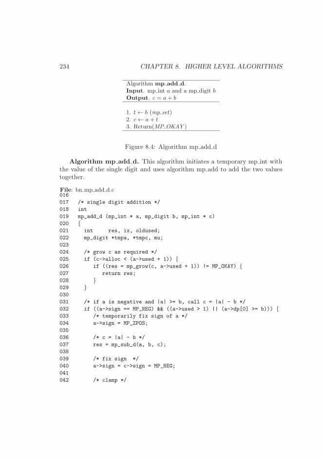
234 CHAPTER 8. HIGHER LEVEL ALGORITHMS
Algorithm mp add d.Input. mp int a and a mp digit bOutput. c = a+ b
1. t← b (mp set)2. c← a+ t3. Return(MP OKAY )
Figure 8.4: Algorithm mp add d
Algorithm mp add d. This algorithm initiates a temporary mp int withthe value of the single digit and uses algorithm mp add to add the two valuestogether.
File: bn mp add d.c016
017 /* single digit addition */
018 int
019 mp_add_d (mp_int * a, mp_digit b, mp_int * c)
020 {021 int res, ix, oldused;
022 mp_digit *tmpa, *tmpc, mu;
023
024 /* grow c as required */
025 if (c->alloc < (a->used + 1)) {026 if ((res = mp_grow(c, a->used + 1)) != MP_OKAY) {027 return res;
028 }029 }030
031 /* if a is negative and |a| >= b, call c = |a| - b */
032 if ((a->sign == MP_NEG) && ((a->used > 1) || (a->dp[0] >= b))) {033 /* temporarily fix sign of a */
034 a->sign = MP_ZPOS;
035
036 /* c = |a| - b */
037 res = mp_sub_d(a, b, c);
038
039 /* fix sign */
040 a->sign = c->sign = MP_NEG;
041
042 /* clamp */
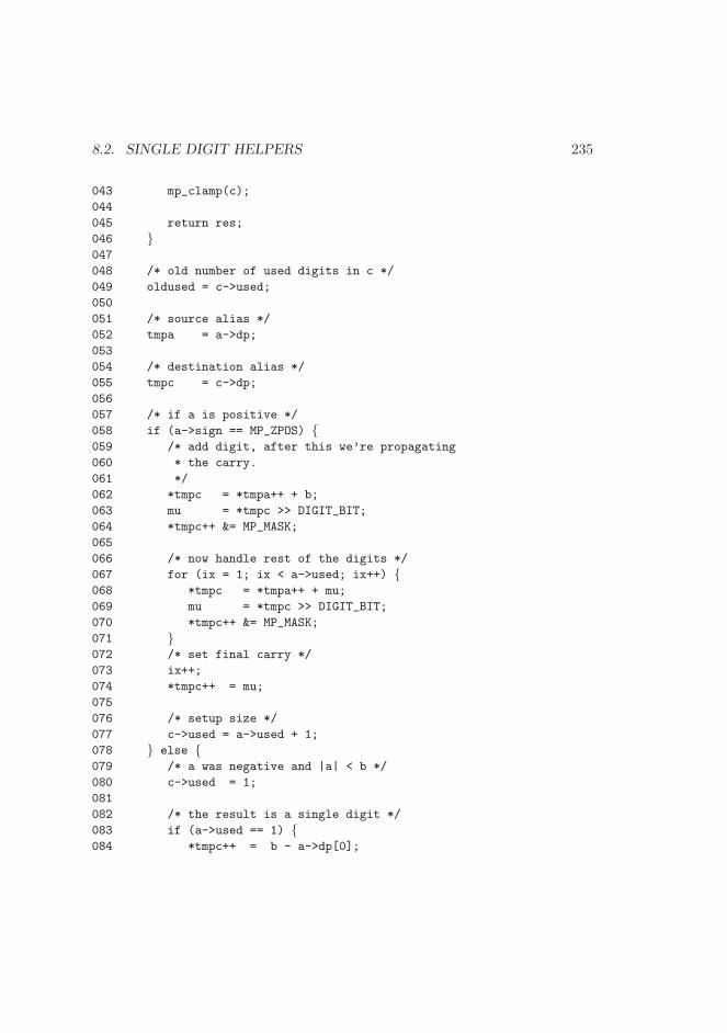
8.2. SINGLE DIGIT HELPERS 235
043 mp_clamp(c);
044
045 return res;
046 }047
048 /* old number of used digits in c */
049 oldused = c->used;
050
051 /* source alias */
052 tmpa = a->dp;
053
054 /* destination alias */
055 tmpc = c->dp;
056
057 /* if a is positive */
058 if (a->sign == MP_ZPOS) {059 /* add digit, after this we’re propagating
060 * the carry.
061 */
062 *tmpc = *tmpa++ + b;
063 mu = *tmpc >> DIGIT_BIT;
064 *tmpc++ &= MP_MASK;
065
066 /* now handle rest of the digits */
067 for (ix = 1; ix < a->used; ix++) {068 *tmpc = *tmpa++ + mu;
069 mu = *tmpc >> DIGIT_BIT;
070 *tmpc++ &= MP_MASK;
071 }072 /* set final carry */
073 ix++;
074 *tmpc++ = mu;
075
076 /* setup size */
077 c->used = a->used + 1;
078 } else {079 /* a was negative and |a| < b */
080 c->used = 1;
081
082 /* the result is a single digit */
083 if (a->used == 1) {084 *tmpc++ = b - a->dp[0];
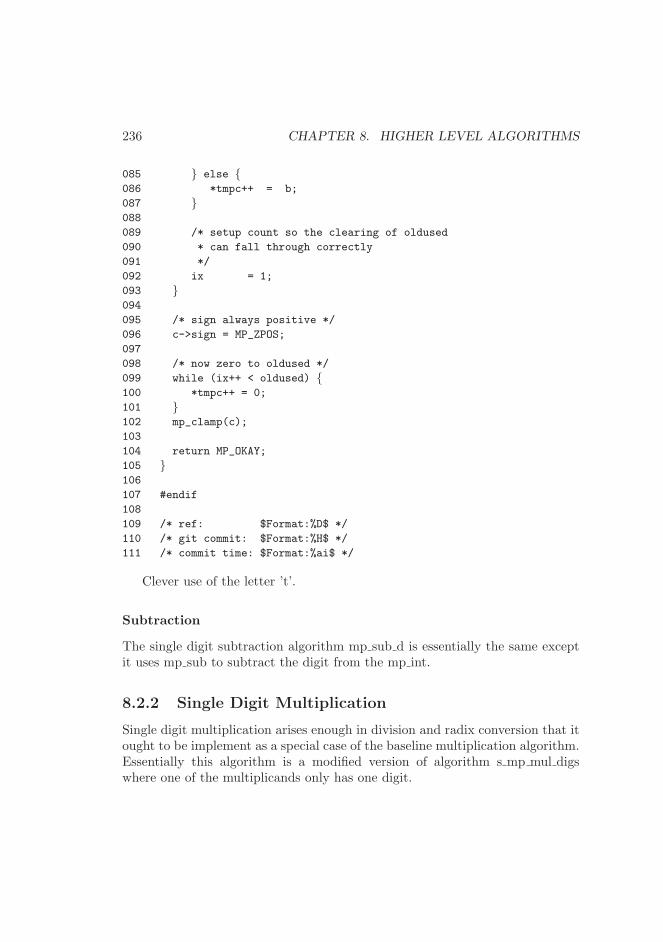
236 CHAPTER 8. HIGHER LEVEL ALGORITHMS
085 } else {086 *tmpc++ = b;
087 }088
089 /* setup count so the clearing of oldused
090 * can fall through correctly
091 */
092 ix = 1;
093 }094
095 /* sign always positive */
096 c->sign = MP_ZPOS;
097
098 /* now zero to oldused */
099 while (ix++ < oldused) {100 *tmpc++ = 0;
101 }102 mp_clamp(c);
103
104 return MP_OKAY;
105 }106
107 #endif
108
109 /* ref: $Format:%D$ */
110 /* git commit: $Format:%H$ */
111 /* commit time: $Format:%ai$ */
Clever use of the letter ’t’.
Subtraction
The single digit subtraction algorithm mp sub d is essentially the same exceptit uses mp sub to subtract the digit from the mp int.
8.2.2 Single Digit Multiplication
Single digit multiplication arises enough in division and radix conversion that itought to be implement as a special case of the baseline multiplication algorithm.Essentially this algorithm is a modified version of algorithm s mp mul digswhere one of the multiplicands only has one digit.
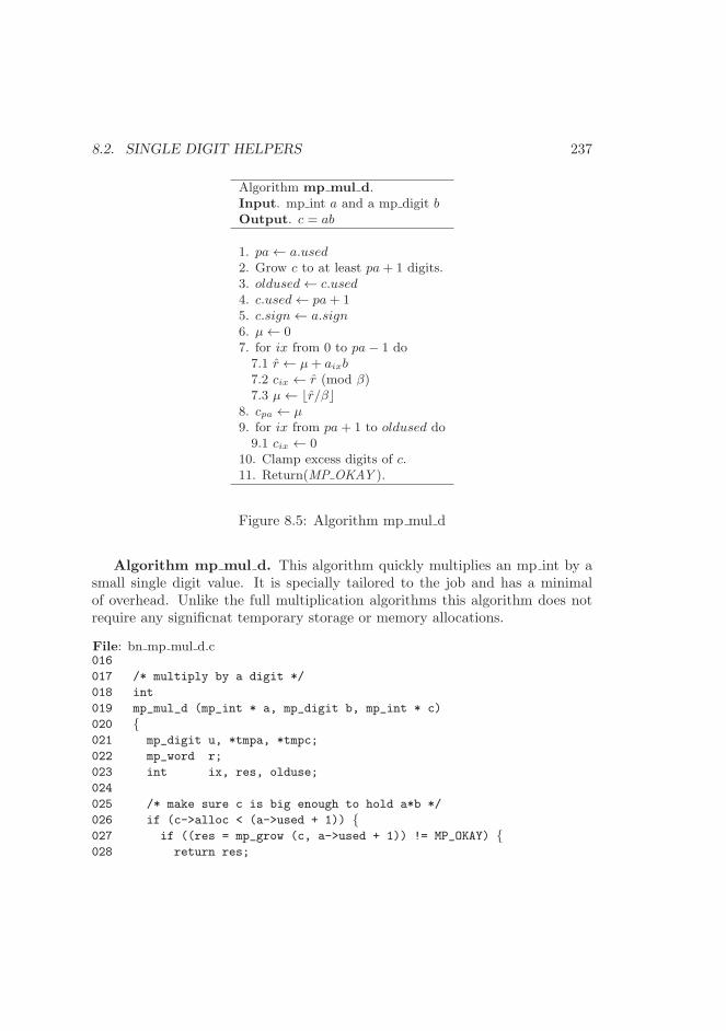
8.2. SINGLE DIGIT HELPERS 237
Algorithm mp mul d.Input. mp int a and a mp digit bOutput. c = ab
1. pa← a.used2. Grow c to at least pa+ 1 digits.3. oldused← c.used4. c.used← pa+ 15. c.sign← a.sign6. µ← 07. for ix from 0 to pa− 1 do7.1 r ← µ+ aixb7.2 cix ← r (mod β)7.3 µ← ⌊r/β⌋
8. cpa ← µ9. for ix from pa+ 1 to oldused do9.1 cix ← 0
10. Clamp excess digits of c.11. Return(MP OKAY ).
Figure 8.5: Algorithm mp mul d
Algorithm mp mul d. This algorithm quickly multiplies an mp int by asmall single digit value. It is specially tailored to the job and has a minimalof overhead. Unlike the full multiplication algorithms this algorithm does notrequire any significnat temporary storage or memory allocations.
File: bn mp mul d.c016
017 /* multiply by a digit */
018 int
019 mp_mul_d (mp_int * a, mp_digit b, mp_int * c)
020 {021 mp_digit u, *tmpa, *tmpc;
022 mp_word r;
023 int ix, res, olduse;
024
025 /* make sure c is big enough to hold a*b */
026 if (c->alloc < (a->used + 1)) {027 if ((res = mp_grow (c, a->used + 1)) != MP_OKAY) {028 return res;
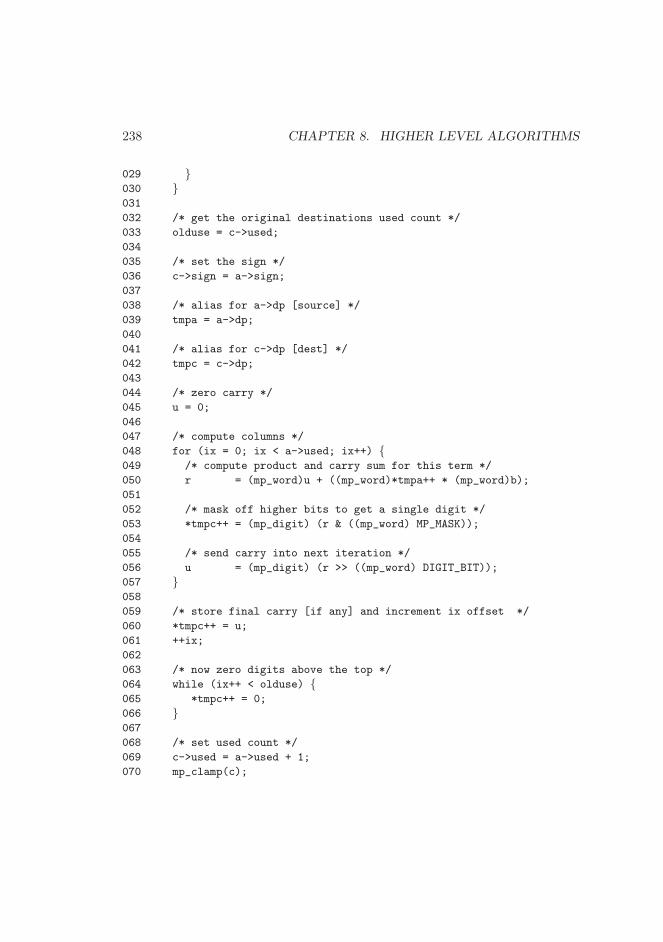
238 CHAPTER 8. HIGHER LEVEL ALGORITHMS
029 }030 }031
032 /* get the original destinations used count */
033 olduse = c->used;
034
035 /* set the sign */
036 c->sign = a->sign;
037
038 /* alias for a->dp [source] */
039 tmpa = a->dp;
040
041 /* alias for c->dp [dest] */
042 tmpc = c->dp;
043
044 /* zero carry */
045 u = 0;
046
047 /* compute columns */
048 for (ix = 0; ix < a->used; ix++) {049 /* compute product and carry sum for this term */
050 r = (mp_word)u + ((mp_word)*tmpa++ * (mp_word)b);
051
052 /* mask off higher bits to get a single digit */
053 *tmpc++ = (mp_digit) (r & ((mp_word) MP_MASK));
054
055 /* send carry into next iteration */
056 u = (mp_digit) (r >> ((mp_word) DIGIT_BIT));
057 }058
059 /* store final carry [if any] and increment ix offset */
060 *tmpc++ = u;
061 ++ix;
062
063 /* now zero digits above the top */
064 while (ix++ < olduse) {065 *tmpc++ = 0;
066 }067
068 /* set used count */
069 c->used = a->used + 1;
070 mp_clamp(c);

8.2. SINGLE DIGIT HELPERS 239
071
072 return MP_OKAY;
073 }074 #endif
075
076 /* ref: $Format:%D$ */
077 /* git commit: $Format:%H$ */
078 /* commit time: $Format:%ai$ */
In this implementation the destination cmay point to the same mp int as thesource a since the result is written after the digit is read from the source. Thisfunction uses pointer aliases tmpa and tmpc for the digits of a and c respectively.
8.2.3 Single Digit Division
Like the single digit multiplication algorithm, single digit division is also a fairlycommon algorithm used in radix conversion. Since the divisor is only a singledigit a specialized variant of the division algorithm can be used to compute thequotient.
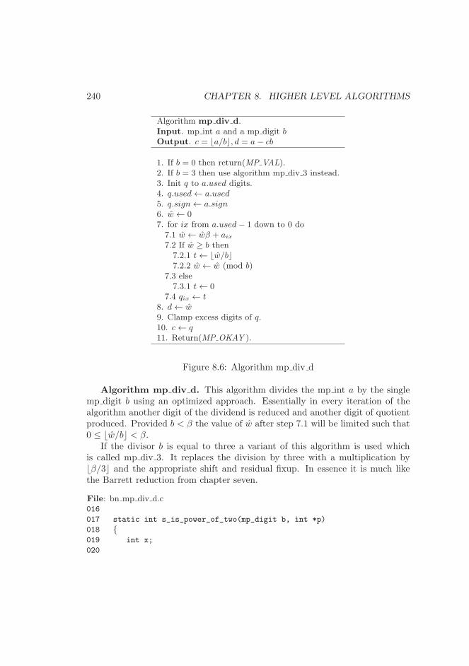
240 CHAPTER 8. HIGHER LEVEL ALGORITHMS
Algorithm mp div d.Input. mp int a and a mp digit bOutput. c = ⌊a/b⌋, d = a− cb
1. If b = 0 then return(MP VAL).2. If b = 3 then use algorithm mp div 3 instead.3. Init q to a.used digits.4. q.used← a.used5. q.sign← a.sign6. w ← 07. for ix from a.used− 1 down to 0 do7.1 w ← wβ + aix
7.2 If w ≥ b then7.2.1 t← ⌊w/b⌋7.2.2 w ← w (mod b)
7.3 else7.3.1 t← 0
7.4 qix ← t8. d← w9. Clamp excess digits of q.10. c← q11. Return(MP OKAY ).
Figure 8.6: Algorithm mp div d
Algorithm mp div d. This algorithm divides the mp int a by the singlemp digit b using an optimized approach. Essentially in every iteration of thealgorithm another digit of the dividend is reduced and another digit of quotientproduced. Provided b < β the value of w after step 7.1 will be limited such that0 ≤ ⌊w/b⌋ < β.
If the divisor b is equal to three a variant of this algorithm is used whichis called mp div 3. It replaces the division by three with a multiplication by⌊β/3⌋ and the appropriate shift and residual fixup. In essence it is much likethe Barrett reduction from chapter seven.
File: bn mp div d.c016
017 static int s_is_power_of_two(mp_digit b, int *p)
018 {019 int x;
020
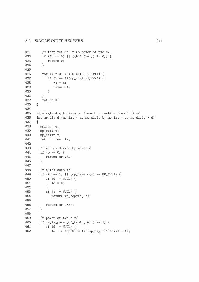
8.2. SINGLE DIGIT HELPERS 241
021 /* fast return if no power of two */
022 if ((b == 0) || ((b & (b-1)) != 0)) {023 return 0;
024 }025
026 for (x = 0; x < DIGIT_BIT; x++) {027 if (b == (((mp_digit)1)<<x)) {028 *p = x;
029 return 1;
030 }031 }032 return 0;
033 }034
035 /* single digit division (based on routine from MPI) */
036 int mp_div_d (mp_int * a, mp_digit b, mp_int * c, mp_digit * d)
037 {038 mp_int q;
039 mp_word w;
040 mp_digit t;
041 int res, ix;
042
043 /* cannot divide by zero */
044 if (b == 0) {045 return MP_VAL;
046 }047
048 /* quick outs */
049 if ((b == 1) || (mp_iszero(a) == MP_YES)) {050 if (d != NULL) {051 *d = 0;
052 }053 if (c != NULL) {054 return mp_copy(a, c);
055 }056 return MP_OKAY;
057 }058
059 /* power of two ? */
060 if (s_is_power_of_two(b, &ix) == 1) {061 if (d != NULL) {062 *d = a->dp[0] & ((((mp_digit)1)<<ix) - 1);
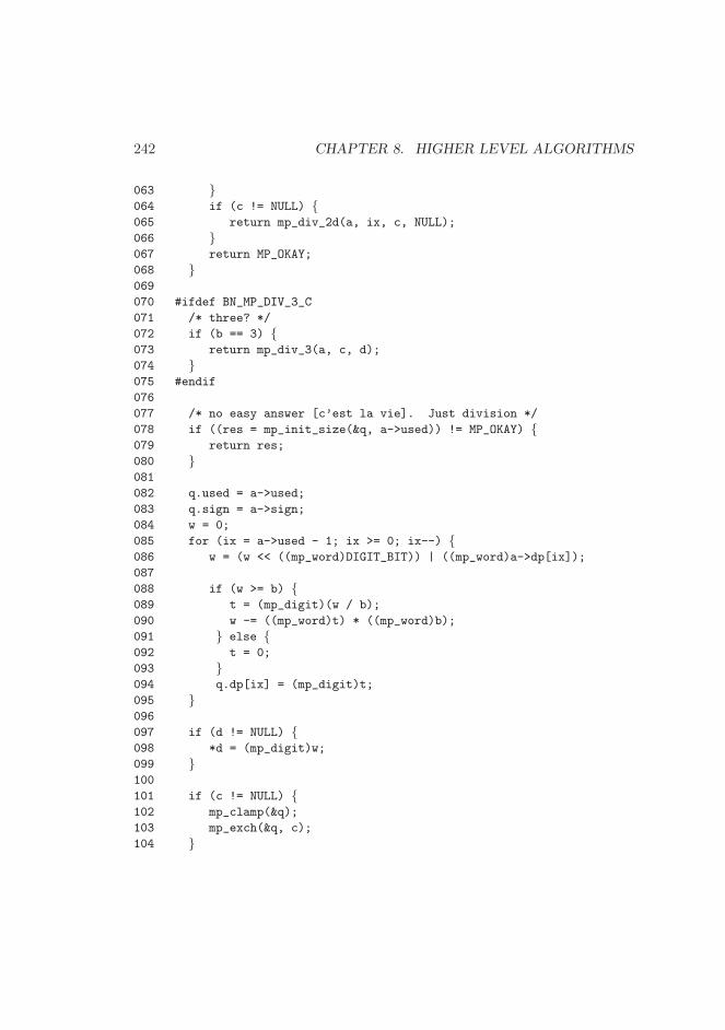
242 CHAPTER 8. HIGHER LEVEL ALGORITHMS
063 }064 if (c != NULL) {065 return mp_div_2d(a, ix, c, NULL);
066 }067 return MP_OKAY;
068 }069
070 #ifdef BN_MP_DIV_3_C
071 /* three? */
072 if (b == 3) {073 return mp_div_3(a, c, d);
074 }075 #endif
076
077 /* no easy answer [c’est la vie]. Just division */
078 if ((res = mp_init_size(&q, a->used)) != MP_OKAY) {079 return res;
080 }081
082 q.used = a->used;
083 q.sign = a->sign;
084 w = 0;
085 for (ix = a->used - 1; ix >= 0; ix--) {086 w = (w << ((mp_word)DIGIT_BIT)) | ((mp_word)a->dp[ix]);
087
088 if (w >= b) {089 t = (mp_digit)(w / b);
090 w -= ((mp_word)t) * ((mp_word)b);
091 } else {092 t = 0;
093 }094 q.dp[ix] = (mp_digit)t;
095 }096
097 if (d != NULL) {098 *d = (mp_digit)w;
099 }100
101 if (c != NULL) {102 mp_clamp(&q);
103 mp_exch(&q, c);
104 }
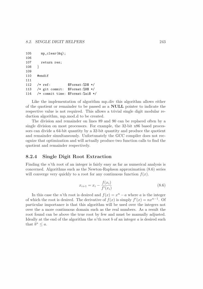
8.2. SINGLE DIGIT HELPERS 243
105 mp_clear(&q);
106
107 return res;
108 }109
110 #endif
111
112 /* ref: $Format:%D$ */
113 /* git commit: $Format:%H$ */
114 /* commit time: $Format:%ai$ */
Like the implementation of algorithm mp div this algorithm allows eitherof the quotient or remainder to be passed as a NULL pointer to indicate therespective value is not required. This allows a trivial single digit modular re-duction algorithm, mp mod d to be created.
The division and remainder on lines 89 and 90 can be replaced often by asingle division on most processors. For example, the 32-bit x86 based proces-sors can divide a 64-bit quantity by a 32-bit quantity and produce the quotientand remainder simultaneously. Unfortunately the GCC compiler does not rec-ognize that optimization and will actually produce two function calls to find thequotient and remainder respectively.
8.2.4 Single Digit Root Extraction
Finding the n’th root of an integer is fairly easy as far as numerical analysis isconcerned. Algorithms such as the Newton-Raphson approximation (8.6) serieswill converge very quickly to a root for any continuous function f(x).
xi+1 = xi −f(xi)
f ′(xi)(8.6)
In this case the n’th root is desired and f(x) = xn−a where a is the integerof which the root is desired. The derivative of f(x) is simply f ′(x) = nxn−1. Ofparticular importance is that this algorithm will be used over the integers notover the a more continuous domain such as the real numbers. As a result theroot found can be above the true root by few and must be manually adjusted.Ideally at the end of the algorithm the n’th root b of an integer a is desired suchthat bn ≤ a.
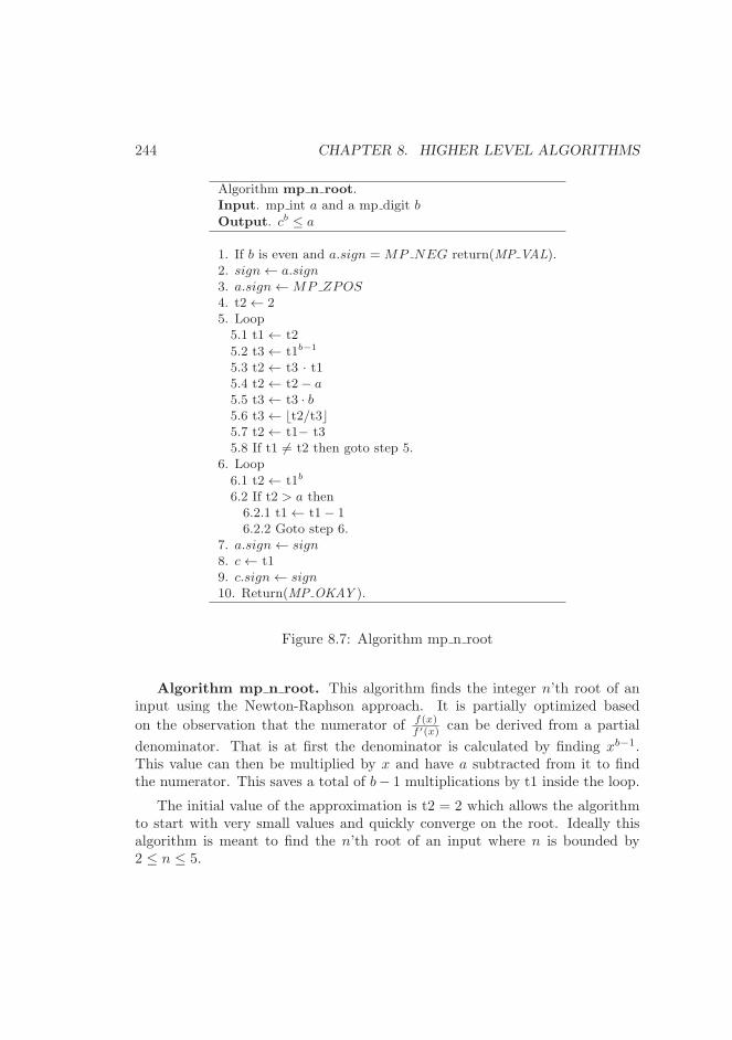
244 CHAPTER 8. HIGHER LEVEL ALGORITHMS
Algorithm mp n root.Input. mp int a and a mp digit b
Output. cb ≤ a
1. If b is even and a.sign = MP NEG return(MP VAL).2. sign← a.sign3. a.sign←MP ZPOS4. t2← 25. Loop5.1 t1← t2
5.2 t3← t1b−1
5.3 t2← t3 · t15.4 t2← t2− a5.5 t3← t3 · b5.6 t3← ⌊t2/t3⌋5.7 t2← t1− t35.8 If t1 6= t2 then goto step 5.
6. Loop
6.1 t2← t1b
6.2 If t2 > a then6.2.1 t1← t1− 16.2.2 Goto step 6.
7. a.sign← sign8. c← t19. c.sign← sign10. Return(MP OKAY ).
Figure 8.7: Algorithm mp n root
Algorithm mp n root. This algorithm finds the integer n’th root of aninput using the Newton-Raphson approach. It is partially optimized based
on the observation that the numerator of f(x)f ′(x) can be derived from a partial
denominator. That is at first the denominator is calculated by finding xb−1.This value can then be multiplied by x and have a subtracted from it to findthe numerator. This saves a total of b− 1 multiplications by t1 inside the loop.
The initial value of the approximation is t2 = 2 which allows the algorithmto start with very small values and quickly converge on the root. Ideally thisalgorithm is meant to find the n’th root of an input where n is bounded by2 ≤ n ≤ 5.
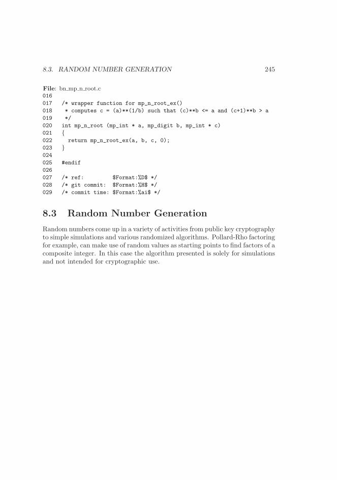
8.3. RANDOM NUMBER GENERATION 245
File: bn mp n root.c016
017 /* wrapper function for mp_n_root_ex()
018 * computes c = (a)**(1/b) such that (c)**b <= a and (c+1)**b > a
019 */
020 int mp_n_root (mp_int * a, mp_digit b, mp_int * c)
021 {022 return mp_n_root_ex(a, b, c, 0);
023 }024
025 #endif
026
027 /* ref: $Format:%D$ */
028 /* git commit: $Format:%H$ */
029 /* commit time: $Format:%ai$ */
8.3 Random Number Generation
Random numbers come up in a variety of activities from public key cryptographyto simple simulations and various randomized algorithms. Pollard-Rho factoringfor example, can make use of random values as starting points to find factors of acomposite integer. In this case the algorithm presented is solely for simulationsand not intended for cryptographic use.
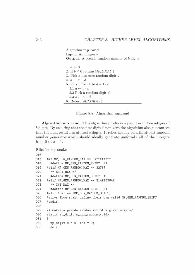
246 CHAPTER 8. HIGHER LEVEL ALGORITHMS
Algorithm mp rand.Input. An integer bOutput. A pseudo-random number of b digits
1. a← 02. If b ≤ 0 return(MP OKAY )3. Pick a non-zero random digit d.4. a← a+ d5. for ix from 1 to d− 1 do5.1 a← a · β5.2 Pick a random digit d.5.3 a← a+ d
6. Return(MP OKAY ).
Figure 8.8: Algorithm mp rand
Algorithm mp rand. This algorithm produces a pseudo-random integer ofb digits. By ensuring that the first digit is non-zero the algorithm also guaranteesthat the final result has at least b digits. It relies heavily on a third-part randomnumber generator which should ideally generate uniformly all of the integersfrom 0 to β − 1.
File: bn mp rand.c
016
017 #if MP_GEN_RANDOM_MAX == 0xffffffff
018 #define MP_GEN_RANDOM_SHIFT 32
019 #elif MP_GEN_RANDOM_MAX == 32767
020 /* SHRT_MAX */
021 #define MP_GEN_RANDOM_SHIFT 15
022 #elif MP_GEN_RANDOM_MAX == 2147483647
023 /* INT_MAX */
024 #define MP_GEN_RANDOM_SHIFT 31
025 #elif !defined(MP_GEN_RANDOM_SHIFT)
026 #error Thou shalt define their own valid MP_GEN_RANDOM_SHIFT
027 #endif
028
029 /* makes a pseudo-random int of a given size */
030 static mp_digit s_gen_random(void)
031 {032 mp_digit d = 0, msk = 0;
033 do {
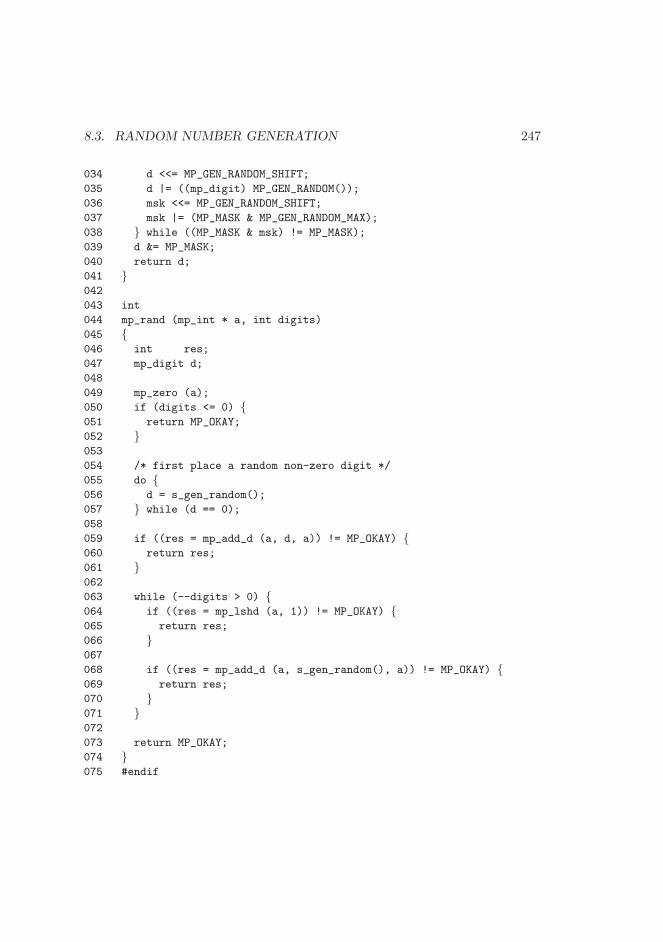
8.3. RANDOM NUMBER GENERATION 247
034 d <<= MP_GEN_RANDOM_SHIFT;
035 d |= ((mp_digit) MP_GEN_RANDOM());
036 msk <<= MP_GEN_RANDOM_SHIFT;
037 msk |= (MP_MASK & MP_GEN_RANDOM_MAX);
038 } while ((MP_MASK & msk) != MP_MASK);
039 d &= MP_MASK;
040 return d;
041 }042
043 int
044 mp_rand (mp_int * a, int digits)
045 {046 int res;
047 mp_digit d;
048
049 mp_zero (a);
050 if (digits <= 0) {051 return MP_OKAY;
052 }053
054 /* first place a random non-zero digit */
055 do {056 d = s_gen_random();
057 } while (d == 0);
058
059 if ((res = mp_add_d (a, d, a)) != MP_OKAY) {060 return res;
061 }062
063 while (--digits > 0) {064 if ((res = mp_lshd (a, 1)) != MP_OKAY) {065 return res;
066 }067
068 if ((res = mp_add_d (a, s_gen_random(), a)) != MP_OKAY) {069 return res;
070 }071 }072
073 return MP_OKAY;
074 }075 #endif
248 CHAPTER 8. HIGHER LEVEL ALGORITHMS
076
077 /* ref: $Format:%D$ */
078 /* git commit: $Format:%H$ */
079 /* commit time: $Format:%ai$ */
8.4 Formatted Representations
The ability to emit a radix-n textual representation of an integer is useful forinteracting with human parties. For example, the ability to be given a string ofcharacters such as “114585” and turn it into the radix-β equivalent would makeit easier to enter numbers into a program.
8.4.1 Reading Radix-n Input
For the purposes of this text we will assume that a simple lower ASCII map (8.9)is used for the values of from 0 to 63 to printable characters. For example, whenthe character “N” is read it represents the integer 23. The first 16 characters ofthe map are for the common representations up to hexadecimal. After that theymatch the “base64” encoding scheme which are suitable chosen such that theyare printable. While outputting as base64 may not be too helpful for humanoperators it does allow communication via non binary mediums.
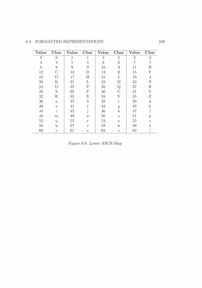
8.4. FORMATTED REPRESENTATIONS 249
Value Char Value Char Value Char Value Char0 0 1 1 2 2 3 34 4 5 5 6 6 7 78 8 9 9 10 A 11 B12 C 13 D 14 E 15 F16 G 17 H 18 I 19 J20 K 21 L 22 M 23 N24 O 25 P 26 Q 27 R28 S 29 T 30 U 31 V32 W 33 X 34 Y 35 Z36 a 37 b 38 c 39 d40 e 41 f 42 g 43 h44 i 45 j 46 k 47 l48 m 49 n 50 o 51 p52 q 53 r 54 s 55 t56 u 57 v 58 w 59 x60 y 61 z 62 + 63 /
Figure 8.9: Lower ASCII Map
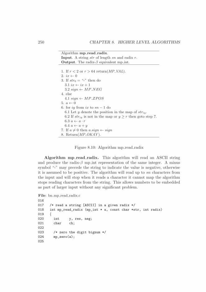
250 CHAPTER 8. HIGHER LEVEL ALGORITHMS
Algorithm mp read radix.Input. A string str of length sn and radix r.Output. The radix-β equivalent mp int.
1. If r < 2 or r > 64 return(MP VAL).2. ix← 03. If str0 = “-” then do3.1 ix← ix+ 13.2 sign←MP NEG
4. else4.1 sign←MP ZPOS
5. a← 06. for iy from ix to sn− 1 do6.1 Let y denote the position in the map of striy.6.2 If striy is not in the map or y ≥ r then goto step 7.6.3 a← a · r6.4 a← a+ y
7. If a 6= 0 then a.sign← sign8. Return(MP OKAY ).
Figure 8.10: Algorithm mp read radix
Algorithm mp read radix. This algorithm will read an ASCII stringand produce the radix-β mp int representation of the same integer. A minussymbol “-” may precede the string to indicate the value is negative, otherwiseit is assumed to be positive. The algorithm will read up to sn characters fromthe input and will stop when it reads a character it cannot map the algorithmstops reading characters from the string. This allows numbers to be embeddedas part of larger input without any significant problem.
File: bn mp read radix.c
016
017 /* read a string [ASCII] in a given radix */
018 int mp_read_radix (mp_int * a, const char *str, int radix)
019 {020 int y, res, neg;
021 char ch;
022
023 /* zero the digit bignum */
024 mp_zero(a);
025
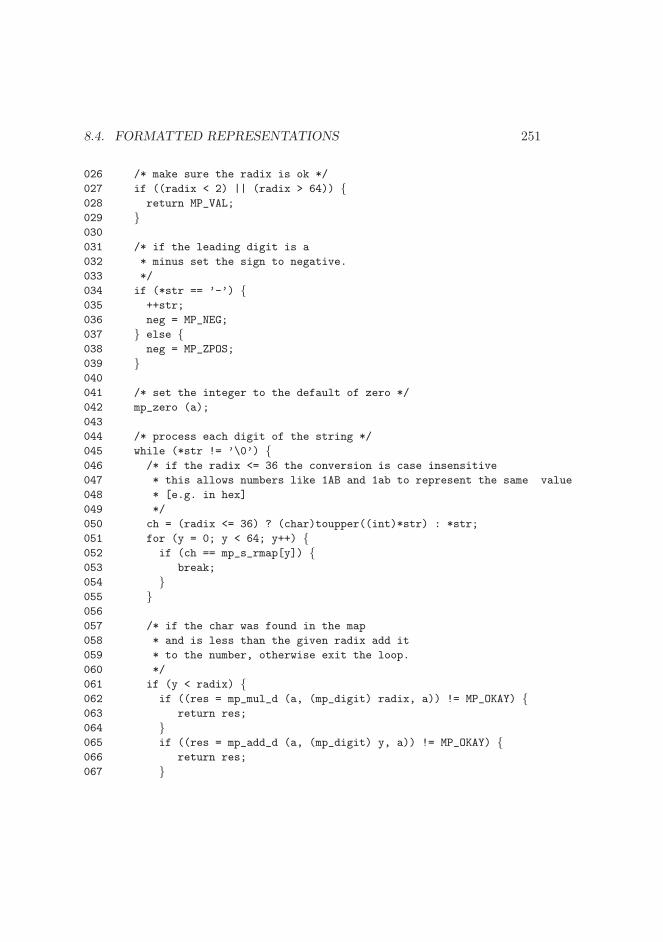
8.4. FORMATTED REPRESENTATIONS 251
026 /* make sure the radix is ok */
027 if ((radix < 2) || (radix > 64)) {028 return MP_VAL;
029 }030
031 /* if the leading digit is a
032 * minus set the sign to negative.
033 */
034 if (*str == ’-’) {035 ++str;
036 neg = MP_NEG;
037 } else {038 neg = MP_ZPOS;
039 }040
041 /* set the integer to the default of zero */
042 mp_zero (a);
043
044 /* process each digit of the string */
045 while (*str != ’\0’) {046 /* if the radix <= 36 the conversion is case insensitive
047 * this allows numbers like 1AB and 1ab to represent the same value
048 * [e.g. in hex]
049 */
050 ch = (radix <= 36) ? (char)toupper((int)*str) : *str;
051 for (y = 0; y < 64; y++) {052 if (ch == mp_s_rmap[y]) {053 break;
054 }055 }056
057 /* if the char was found in the map
058 * and is less than the given radix add it
059 * to the number, otherwise exit the loop.
060 */
061 if (y < radix) {062 if ((res = mp_mul_d (a, (mp_digit) radix, a)) != MP_OKAY) {063 return res;
064 }065 if ((res = mp_add_d (a, (mp_digit) y, a)) != MP_OKAY) {066 return res;
067 }
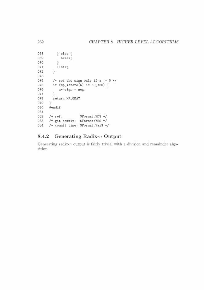
252 CHAPTER 8. HIGHER LEVEL ALGORITHMS
068 } else {069 break;
070 }071 ++str;
072 }073
074 /* set the sign only if a != 0 */
075 if (mp_iszero(a) != MP_YES) {076 a->sign = neg;
077 }078 return MP_OKAY;
079 }080 #endif
081
082 /* ref: $Format:%D$ */
083 /* git commit: $Format:%H$ */
084 /* commit time: $Format:%ai$ */
8.4.2 Generating Radix-n Output
Generating radix-n output is fairly trivial with a division and remainder algo-rithm.
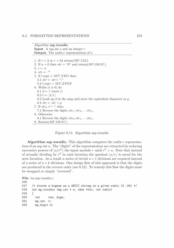
8.4. FORMATTED REPRESENTATIONS 253
Algorithm mp toradix.Input. A mp int a and an integer rOutput. The radix-r representation of a
1. If r < 2 or r > 64 return(MP VAL).2. If a = 0 then str = “0” and return(MP OKAY ).3. t← a4. str ← “”5. if t.sign = MP NEG then5.1 str ← str+ “-”5.2 t.sign = MP ZPOS
6. While (t 6= 0) do6.1 d← t (mod r)6.2 t← ⌊t/r⌋6.3 Look up d in the map and store the equivalent character in y.6.4 str ← str + y
7. If str0 =“−” then7.1 Reverse the digits str1, str2, . . . strn.
8. Otherwise8.1 Reverse the digits str0, str1, . . . strn.
9. Return(MP OKAY ).
Figure 8.11: Algorithm mp toradix
Algorithm mp toradix. This algorithm computes the radix-r representa-tion of an mp int a. The “digits” of the representation are extracted by reducingsuccessive powers of ⌊a/rk⌋ the input modulo r until rk > a. Note that insteadof actually dividing by rk in each iteration the quotient ⌊a/r⌋ is saved for thenext iteration. As a result a series of trivial n× 1 divisions are required insteadof a series of n× k divisions. One design flaw of this approach is that the digitsare produced in the reverse order (see 8.12). To remedy this flaw the digits mustbe swapped or simply “reversed”.
File: bn mp toradix.c016
017 /* stores a bignum as a ASCII string in a given radix (2..64) */
018 int mp_toradix (mp_int * a, char *str, int radix)
019 {020 int res, digs;
021 mp_int t;
022 mp_digit d;
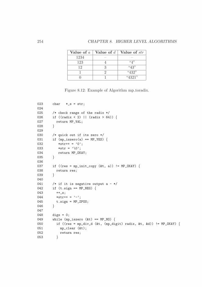
254 CHAPTER 8. HIGHER LEVEL ALGORITHMS
Value of a Value of d Value of str1234 – –123 4 “4”12 3 “43”1 2 “432”0 1 “4321”
Figure 8.12: Example of Algorithm mp toradix.
023 char *_s = str;
024
025 /* check range of the radix */
026 if ((radix < 2) || (radix > 64)) {027 return MP_VAL;
028 }029
030 /* quick out if its zero */
031 if (mp_iszero(a) == MP_YES) {032 *str++ = ’0’;
033 *str = ’\0’;
034 return MP_OKAY;
035 }036
037 if ((res = mp_init_copy (&t, a)) != MP_OKAY) {038 return res;
039 }040
041 /* if it is negative output a - */
042 if (t.sign == MP_NEG) {043 ++_s;
044 *str++ = ’-’;
045 t.sign = MP_ZPOS;
046 }047
048 digs = 0;
049 while (mp_iszero (&t) == MP_NO) {050 if ((res = mp_div_d (&t, (mp_digit) radix, &t, &d)) != MP_OKAY) {051 mp_clear (&t);
052 return res;
053 }
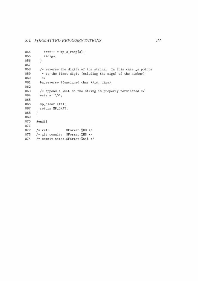
8.4. FORMATTED REPRESENTATIONS 255
054 *str++ = mp_s_rmap[d];
055 ++digs;
056 }057
058 /* reverse the digits of the string. In this case _s points
059 * to the first digit [exluding the sign] of the number]
060 */
061 bn_reverse ((unsigned char *)_s, digs);
062
063 /* append a NULL so the string is properly terminated */
064 *str = ’\0’;
065
066 mp_clear (&t);
067 return MP_OKAY;
068 }069
070 #endif
071
072 /* ref: $Format:%D$ */
073 /* git commit: $Format:%H$ */
074 /* commit time: $Format:%ai$ */

256 CHAPTER 8. HIGHER LEVEL ALGORITHMS
Chapter 9
Number Theoretic
Algorithms
This chapter discusses several fundamental number theoretic algorithms such asthe greatest common divisor, least common multiple and Jacobi symbol com-putation. These algorithms arise as essential components in several key cryp-tographic algorithms such as the RSA public key algorithm and various Sievebased factoring algorithms.
9.1 Greatest Common Divisor
The greatest common divisor of two integers a and b, often denoted as (a, b) isthe largest integer k that is a proper divisor of both a and b. That is, k is thelargest integer such that 0 ≡ a (mod k) and 0 ≡ b (mod k) occur simultaneously.
The most common approach (cite) is to reduce one input modulo another.That is if a and b are divisible by some integer k and if qa+ r = b then r is alsodivisible by k. The reduction pattern follows 〈a, b〉 → 〈b, a mod b〉.
257
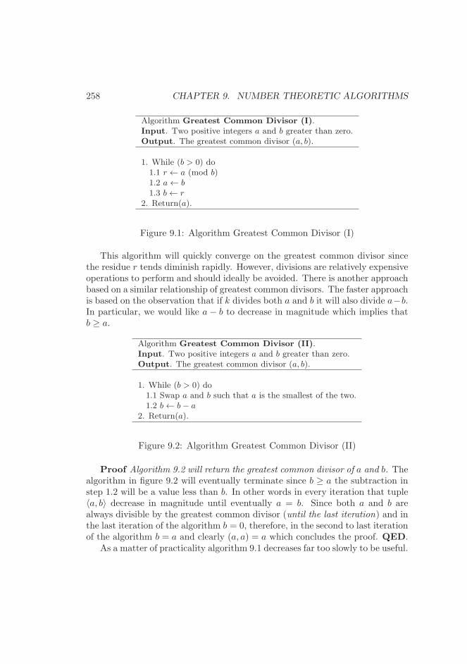
258 CHAPTER 9. NUMBER THEORETIC ALGORITHMS
Algorithm Greatest Common Divisor (I).Input. Two positive integers a and b greater than zero.Output. The greatest common divisor (a, b).
1. While (b > 0) do1.1 r ← a (mod b)1.2 a← b1.3 b← r
2. Return(a).
Figure 9.1: Algorithm Greatest Common Divisor (I)
This algorithm will quickly converge on the greatest common divisor sincethe residue r tends diminish rapidly. However, divisions are relatively expensiveoperations to perform and should ideally be avoided. There is another approachbased on a similar relationship of greatest common divisors. The faster approachis based on the observation that if k divides both a and b it will also divide a−b.In particular, we would like a − b to decrease in magnitude which implies thatb ≥ a.
Algorithm Greatest Common Divisor (II).Input. Two positive integers a and b greater than zero.Output. The greatest common divisor (a, b).
1. While (b > 0) do1.1 Swap a and b such that a is the smallest of the two.1.2 b← b− a
2. Return(a).
Figure 9.2: Algorithm Greatest Common Divisor (II)
Proof Algorithm 9.2 will return the greatest common divisor of a and b. Thealgorithm in figure 9.2 will eventually terminate since b ≥ a the subtraction instep 1.2 will be a value less than b. In other words in every iteration that tuple〈a, b〉 decrease in magnitude until eventually a = b. Since both a and b arealways divisible by the greatest common divisor (until the last iteration) and inthe last iteration of the algorithm b = 0, therefore, in the second to last iterationof the algorithm b = a and clearly (a, a) = a which concludes the proof. QED.
As a matter of practicality algorithm 9.1 decreases far too slowly to be useful.
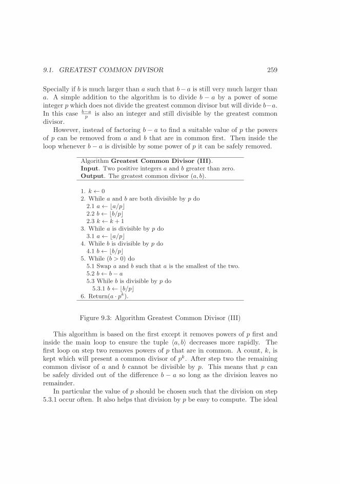
9.1. GREATEST COMMON DIVISOR 259
Specially if b is much larger than a such that b−a is still very much larger thana. A simple addition to the algorithm is to divide b − a by a power of someinteger p which does not divide the greatest common divisor but will divide b−a.In this case b−a
p is also an integer and still divisible by the greatest commondivisor.
However, instead of factoring b − a to find a suitable value of p the powersof p can be removed from a and b that are in common first. Then inside theloop whenever b− a is divisible by some power of p it can be safely removed.
Algorithm Greatest Common Divisor (III).Input. Two positive integers a and b greater than zero.Output. The greatest common divisor (a, b).
1. k ← 02. While a and b are both divisible by p do2.1 a← ⌊a/p⌋2.2 b← ⌊b/p⌋2.3 k ← k + 1
3. While a is divisible by p do3.1 a← ⌊a/p⌋
4. While b is divisible by p do4.1 b← ⌊b/p⌋
5. While (b > 0) do5.1 Swap a and b such that a is the smallest of the two.5.2 b← b− a5.3 While b is divisible by p do5.3.1 b← ⌊b/p⌋
6. Return(a · pk).
Figure 9.3: Algorithm Greatest Common Divisor (III)
This algorithm is based on the first except it removes powers of p first andinside the main loop to ensure the tuple 〈a, b〉 decreases more rapidly. Thefirst loop on step two removes powers of p that are in common. A count, k, iskept which will present a common divisor of pk. After step two the remainingcommon divisor of a and b cannot be divisible by p. This means that p canbe safely divided out of the difference b − a so long as the division leaves noremainder.
In particular the value of p should be chosen such that the division on step5.3.1 occur often. It also helps that division by p be easy to compute. The ideal
260 CHAPTER 9. NUMBER THEORETIC ALGORITHMS
choice of p is two since division by two amounts to a right logical shift. Anotherimportant observation is that by step five both a and b are odd. Therefore, thediffrence b − a must be even which means that each iteration removes one bitfrom the largest of the pair.
9.1.1 Complete Greatest Common Divisor
The algorithms presented so far cannot handle inputs which are zero or negative.The following algorithm can handle all input cases properly and will producethe greatest common divisor.
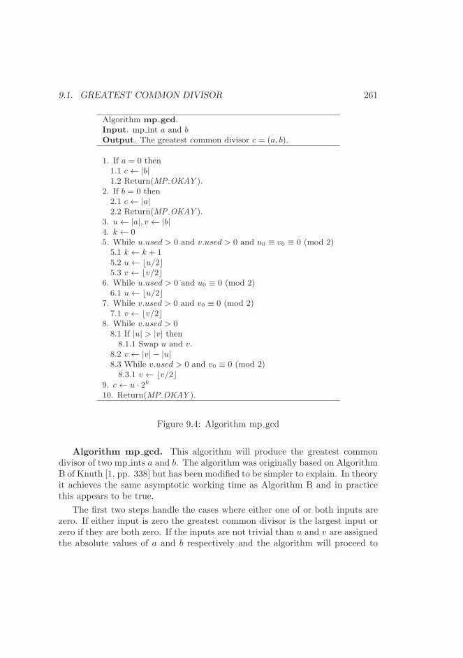
9.1. GREATEST COMMON DIVISOR 261
Algorithm mp gcd.Input. mp int a and bOutput. The greatest common divisor c = (a, b).
1. If a = 0 then1.1 c← |b|1.2 Return(MP OKAY ).
2. If b = 0 then2.1 c← |a|2.2 Return(MP OKAY ).
3. u← |a|, v ← |b|4. k ← 05. While u.used > 0 and v.used > 0 and u0 ≡ v0 ≡ 0 (mod 2)5.1 k ← k + 15.2 u← ⌊u/2⌋5.3 v ← ⌊v/2⌋
6. While u.used > 0 and u0 ≡ 0 (mod 2)6.1 u← ⌊u/2⌋
7. While v.used > 0 and v0 ≡ 0 (mod 2)7.1 v ← ⌊v/2⌋
8. While v.used > 08.1 If |u| > |v| then8.1.1 Swap u and v.
8.2 v ← |v| − |u|8.3 While v.used > 0 and v0 ≡ 0 (mod 2)8.3.1 v ← ⌊v/2⌋
9. c← u · 2k
10. Return(MP OKAY ).
Figure 9.4: Algorithm mp gcd
Algorithm mp gcd. This algorithm will produce the greatest commondivisor of two mp ints a and b. The algorithm was originally based on AlgorithmB of Knuth [1, pp. 338] but has been modified to be simpler to explain. In theoryit achieves the same asymptotic working time as Algorithm B and in practicethis appears to be true.
The first two steps handle the cases where either one of or both inputs arezero. If either input is zero the greatest common divisor is the largest input orzero if they are both zero. If the inputs are not trivial than u and v are assignedthe absolute values of a and b respectively and the algorithm will proceed to
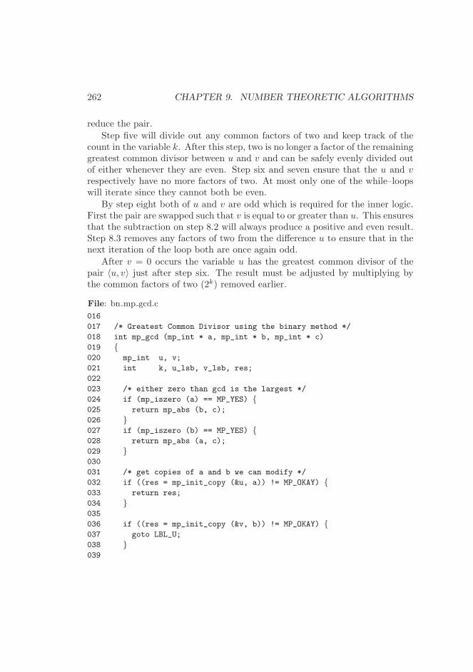
262 CHAPTER 9. NUMBER THEORETIC ALGORITHMS
reduce the pair.
Step five will divide out any common factors of two and keep track of thecount in the variable k. After this step, two is no longer a factor of the remaininggreatest common divisor between u and v and can be safely evenly divided outof either whenever they are even. Step six and seven ensure that the u and vrespectively have no more factors of two. At most only one of the while–loopswill iterate since they cannot both be even.
By step eight both of u and v are odd which is required for the inner logic.First the pair are swapped such that v is equal to or greater than u. This ensuresthat the subtraction on step 8.2 will always produce a positive and even result.Step 8.3 removes any factors of two from the difference u to ensure that in thenext iteration of the loop both are once again odd.
After v = 0 occurs the variable u has the greatest common divisor of thepair 〈u, v〉 just after step six. The result must be adjusted by multiplying bythe common factors of two (2k) removed earlier.
File: bn mp gcd.c
016
017 /* Greatest Common Divisor using the binary method */
018 int mp_gcd (mp_int * a, mp_int * b, mp_int * c)
019 {020 mp_int u, v;
021 int k, u_lsb, v_lsb, res;
022
023 /* either zero than gcd is the largest */
024 if (mp_iszero (a) == MP_YES) {025 return mp_abs (b, c);
026 }027 if (mp_iszero (b) == MP_YES) {028 return mp_abs (a, c);
029 }030
031 /* get copies of a and b we can modify */
032 if ((res = mp_init_copy (&u, a)) != MP_OKAY) {033 return res;
034 }035
036 if ((res = mp_init_copy (&v, b)) != MP_OKAY) {037 goto LBL_U;
038 }039
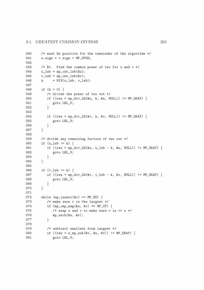
9.1. GREATEST COMMON DIVISOR 263
040 /* must be positive for the remainder of the algorithm */
041 u.sign = v.sign = MP_ZPOS;
042
043 /* B1. Find the common power of two for u and v */
044 u_lsb = mp_cnt_lsb(&u);
045 v_lsb = mp_cnt_lsb(&v);
046 k = MIN(u_lsb, v_lsb);
047
048 if (k > 0) {049 /* divide the power of two out */
050 if ((res = mp_div_2d(&u, k, &u, NULL)) != MP_OKAY) {051 goto LBL_V;
052 }053
054 if ((res = mp_div_2d(&v, k, &v, NULL)) != MP_OKAY) {055 goto LBL_V;
056 }057 }058
059 /* divide any remaining factors of two out */
060 if (u_lsb != k) {061 if ((res = mp_div_2d(&u, u_lsb - k, &u, NULL)) != MP_OKAY) {062 goto LBL_V;
063 }064 }065
066 if (v_lsb != k) {067 if ((res = mp_div_2d(&v, v_lsb - k, &v, NULL)) != MP_OKAY) {068 goto LBL_V;
069 }070 }071
072 while (mp_iszero(&v) == MP_NO) {073 /* make sure v is the largest */
074 if (mp_cmp_mag(&u, &v) == MP_GT) {075 /* swap u and v to make sure v is >= u */
076 mp_exch(&u, &v);
077 }078
079 /* subtract smallest from largest */
080 if ((res = s_mp_sub(&v, &u, &v)) != MP_OKAY) {081 goto LBL_V;
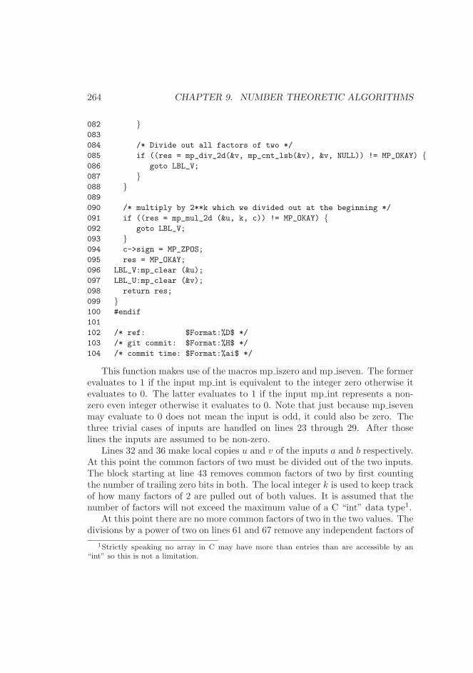
264 CHAPTER 9. NUMBER THEORETIC ALGORITHMS
082 }083
084 /* Divide out all factors of two */
085 if ((res = mp_div_2d(&v, mp_cnt_lsb(&v), &v, NULL)) != MP_OKAY) {086 goto LBL_V;
087 }088 }089
090 /* multiply by 2**k which we divided out at the beginning */
091 if ((res = mp_mul_2d (&u, k, c)) != MP_OKAY) {092 goto LBL_V;
093 }094 c->sign = MP_ZPOS;
095 res = MP_OKAY;
096 LBL_V:mp_clear (&u);
097 LBL_U:mp_clear (&v);
098 return res;
099 }100 #endif
101
102 /* ref: $Format:%D$ */
103 /* git commit: $Format:%H$ */
104 /* commit time: $Format:%ai$ */
This function makes use of the macros mp iszero and mp iseven. The formerevaluates to 1 if the input mp int is equivalent to the integer zero otherwise itevaluates to 0. The latter evaluates to 1 if the input mp int represents a non-zero even integer otherwise it evaluates to 0. Note that just because mp isevenmay evaluate to 0 does not mean the input is odd, it could also be zero. Thethree trivial cases of inputs are handled on lines 23 through 29. After thoselines the inputs are assumed to be non-zero.
Lines 32 and 36 make local copies u and v of the inputs a and b respectively.At this point the common factors of two must be divided out of the two inputs.The block starting at line 43 removes common factors of two by first countingthe number of trailing zero bits in both. The local integer k is used to keep trackof how many factors of 2 are pulled out of both values. It is assumed that thenumber of factors will not exceed the maximum value of a C “int” data type1.
At this point there are no more common factors of two in the two values. Thedivisions by a power of two on lines 61 and 67 remove any independent factors of
1Strictly speaking no array in C may have more than entries than are accessible by an“int” so this is not a limitation.
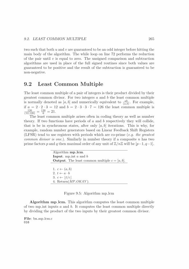
9.2. LEAST COMMON MULTIPLE 265
two such that both u and v are guaranteed to be an odd integer before hitting themain body of the algorithm. The while loop on line 72 performs the reductionof the pair until v is equal to zero. The unsigned comparison and subtractionalgorithms are used in place of the full signed routines since both values areguaranteed to be positive and the result of the subtraction is guaranteed to benon-negative.
9.2 Least Common Multiple
The least common multiple of a pair of integers is their product divided by theirgreatest common divisor. For two integers a and b the least common multipleis normally denoted as [a, b] and numerically equivalent to ab
(a,b) . For example,
if a = 2 · 2 · 3 = 12 and b = 2 · 3 · 3 · 7 = 126 the least common multiple is126
(12,126) =1266 = 21.
The least common multiple arises often in coding theory as well as numbertheory. If two functions have periods of a and b respectively they will collide,that is be in synchronous states, after only [a, b] iterations. This is why, forexample, random number generators based on Linear Feedback Shift Registers(LFSR) tend to use registers with periods which are co-prime (e.g. the greatest
common divisor is one.). Similarly in number theory if a composite n has twoprime factors p and q then maximal order of any unit of Z/nZ will be [p−1, q−1].
Algorithm mp lcm.Input. mp int a and bOutput. The least common multiple c = [a, b].
1. c← (a, b)2. t← a · b3. c← ⌊t/c⌋4. Return(MP OKAY ).
Figure 9.5: Algorithm mp lcm
Algorithm mp lcm. This algorithm computes the least common multipleof two mp int inputs a and b. It computes the least common multiple directlyby dividing the product of the two inputs by their greatest common divisor.
File: bn mp lcm.c016
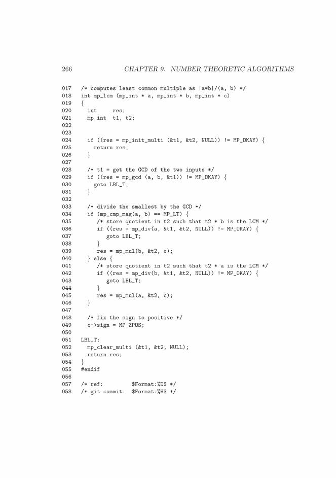
266 CHAPTER 9. NUMBER THEORETIC ALGORITHMS
017 /* computes least common multiple as |a*b|/(a, b) */
018 int mp_lcm (mp_int * a, mp_int * b, mp_int * c)
019 {020 int res;
021 mp_int t1, t2;
022
023
024 if ((res = mp_init_multi (&t1, &t2, NULL)) != MP_OKAY) {025 return res;
026 }027
028 /* t1 = get the GCD of the two inputs */
029 if ((res = mp_gcd (a, b, &t1)) != MP_OKAY) {030 goto LBL_T;
031 }032
033 /* divide the smallest by the GCD */
034 if (mp_cmp_mag(a, b) == MP_LT) {035 /* store quotient in t2 such that t2 * b is the LCM */
036 if ((res = mp_div(a, &t1, &t2, NULL)) != MP_OKAY) {037 goto LBL_T;
038 }039 res = mp_mul(b, &t2, c);
040 } else {041 /* store quotient in t2 such that t2 * a is the LCM */
042 if ((res = mp_div(b, &t1, &t2, NULL)) != MP_OKAY) {043 goto LBL_T;
044 }045 res = mp_mul(a, &t2, c);
046 }047
048 /* fix the sign to positive */
049 c->sign = MP_ZPOS;
050
051 LBL_T:
052 mp_clear_multi (&t1, &t2, NULL);
053 return res;
054 }055 #endif
056
057 /* ref: $Format:%D$ */
058 /* git commit: $Format:%H$ */
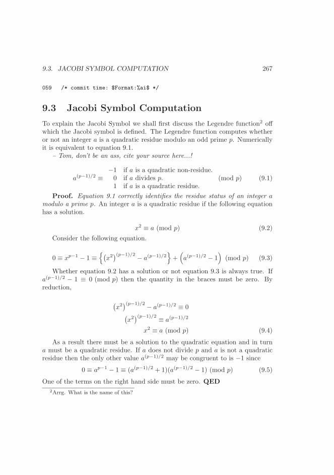
9.3. JACOBI SYMBOL COMPUTATION 267
059 /* commit time: $Format:%ai$ */
9.3 Jacobi Symbol Computation
To explain the Jacobi Symbol we shall first discuss the Legendre function2 offwhich the Jacobi symbol is defined. The Legendre function computes whetheror not an integer a is a quadratic residue modulo an odd prime p. Numericallyit is equivalent to equation 9.1.
– Tom, don’t be an ass, cite your source here...!
a(p−1)/2 ≡−1 if a is a quadratic non-residue.0 if a divides p.1 if a is a quadratic residue.
(mod p) (9.1)
Proof. Equation 9.1 correctly identifies the residue status of an integer amodulo a prime p. An integer a is a quadratic residue if the following equationhas a solution.
x2 ≡ a (mod p) (9.2)
Consider the following equation.
0 ≡ xp−1 − 1 ≡{
(
x2)(p−1)/2 − a(p−1)/2
}
+(
a(p−1)/2 − 1)
(mod p) (9.3)
Whether equation 9.2 has a solution or not equation 9.3 is always true. Ifa(p−1)/2 − 1 ≡ 0 (mod p) then the quantity in the braces must be zero. Byreduction,
(
x2)(p−1)/2 − a(p−1)/2 ≡ 0(
x2)(p−1)/2 ≡ a(p−1)/2
x2 ≡ a (mod p) (9.4)
As a result there must be a solution to the quadratic equation and in turna must be a quadratic residue. If a does not divide p and a is not a quadraticresidue then the only other value a(p−1)/2 may be congruent to is −1 since
0 ≡ ap−1 − 1 ≡ (a(p−1)/2 + 1)(a(p−1)/2 − 1) (mod p) (9.5)
One of the terms on the right hand side must be zero. QED
2Arrg. What is the name of this?
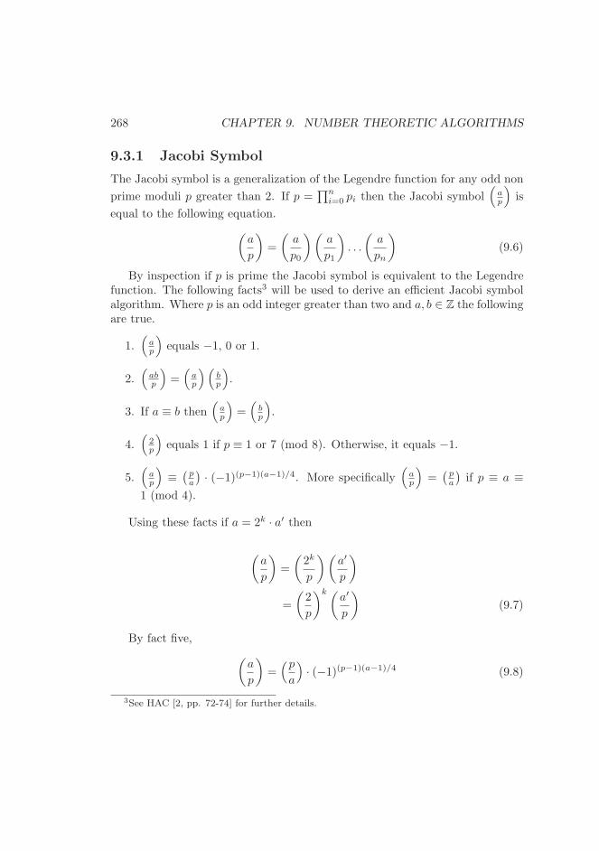
268 CHAPTER 9. NUMBER THEORETIC ALGORITHMS
9.3.1 Jacobi Symbol
The Jacobi symbol is a generalization of the Legendre function for any odd non
prime moduli p greater than 2. If p =∏n
i=0 pi then the Jacobi symbol(
ap
)
is
equal to the following equation.
(
a
p
)
=
(
a
p0
)(
a
p1
)
. . .
(
a
pn
)
(9.6)
By inspection if p is prime the Jacobi symbol is equivalent to the Legendrefunction. The following facts3 will be used to derive an efficient Jacobi symbolalgorithm. Where p is an odd integer greater than two and a, b ∈ Z the followingare true.
1.(
ap
)
equals −1, 0 or 1.
2.(
abp
)
=(
ap
)(
bp
)
.
3. If a ≡ b then(
ap
)
=(
bp
)
.
4.(
2p
)
equals 1 if p ≡ 1 or 7 (mod 8). Otherwise, it equals −1.
5.(
ap
)
≡(
pa
)
· (−1)(p−1)(a−1)/4. More specifically(
ap
)
=(
pa
)
if p ≡ a ≡1 (mod 4).
Using these facts if a = 2k · a′ then
(
a
p
)
=
(
2k
p
)(
a′
p
)
=
(
2
p
)k (a′
p
)
(9.7)
By fact five,
(
a
p
)
=(p
a
)
· (−1)(p−1)(a−1)/4 (9.8)
3See HAC [2, pp. 72-74] for further details.
9.3. JACOBI SYMBOL COMPUTATION 269
Subsequently by fact three since p ≡ (p mod a) (mod a) then
(
a
p
)
=
(
p mod a
a
)
· (−1)(p−1)(a−1)/4 (9.9)
By putting both observations into equation 9.7 the following simplified equa-tion is formed.
(
a
p
)
=
(
2
p
)k (p mod a′
a′
)
· (−1)(p−1)(a′−1)/4 (9.10)
The value of(
p mod a′
a′
)
can be found by using the same equation recur-
sively. The value of(
2p
)k
equals 1 if k is even otherwise it equals(
2p
)
. Using this
approach the factors of p do not have to be known. Furthermore, if (a, p) = 1then the algorithm will terminate when the recursion requests the Jacobi symbolcomputation of
(
1a′
)
which is simply 1.
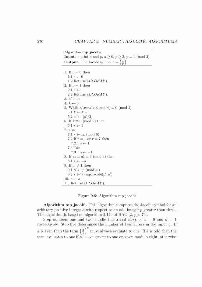
270 CHAPTER 9. NUMBER THEORETIC ALGORITHMS
Algorithm mp jacobi.Input. mp int a and p, a ≥ 0, p ≥ 3, p ≡ 1 (mod 2)
Output. The Jacobi symbol c =(
ap
)
.
1. If a = 0 then1.1 c← 01.2 Return(MP OKAY ).
2. If a = 1 then2.1 c← 12.2 Return(MP OKAY ).
3. a′ ← a4. k ← 05. While a′.used > 0 and a′
0 ≡ 0 (mod 2)5.1 k ← k + 15.2 a′ ← ⌊a′/2⌋
6. If k ≡ 0 (mod 2) then6.1 s← 1
7. else7.1 r ← p0 (mod 8)7.2 If r = 1 or r = 7 then7.2.1 s← 1
7.3 else7.3.1 s← −1
8. If p0 ≡ a′0 ≡ 3 (mod 4) then
8.1 s← −s9. If a′ 6= 1 then9.1 p′ ← p (mod a′)9.2 s← s ·mp jacobi(p′, a′)
10. c← s11. Return(MP OKAY ).
Figure 9.6: Algorithm mp jacobi
Algorithm mp jacobi. This algorithm computes the Jacobi symbol for anarbitrary positive integer a with respect to an odd integer p greater than three.The algorithm is based on algorithm 2.149 of HAC [2, pp. 73].
Step numbers one and two handle the trivial cases of a = 0 and a = 1respectively. Step five determines the number of two factors in the input a. If
k is even than the term(
2p
)k
must always evaluate to one. If k is odd than the
term evaluates to one if p0 is congruent to one or seven modulo eight, otherwise
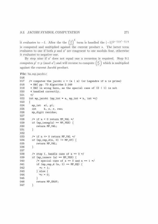
9.3. JACOBI SYMBOL COMPUTATION 271
it evaluates to −1. After the the(
2p
)k
term is handled the (−1)(p−1)(a′−1)/4
is computed and multiplied against the current product s. The latter termevaluates to one if both p and a′ are congruent to one modulo four, otherwiseit evaluates to negative one.
By step nine if a′ does not equal one a recursion is required. Step 9.1
computes p′ ≡ p (mod a′) and will recurse to compute(
p′
a′
)
which is multiplied
against the current Jacobi product.
File: bn mp jacobi.c
016
017 /* computes the jacobi c = (a | n) (or Legendre if n is prime)
018 * HAC pp. 73 Algorithm 2.149
019 * HAC is wrong here, as the special case of (0 | 1) is not
020 * handled correctly.
021 */
022 int mp_jacobi (mp_int * a, mp_int * n, int *c)
023 {024 mp_int a1, p1;
025 int k, s, r, res;
026 mp_digit residue;
027
028 /* if a < 0 return MP_VAL */
029 if (mp_isneg(a) == MP_YES) {030 return MP_VAL;
031 }032
033 /* if n <= 0 return MP_VAL */
034 if (mp_cmp_d(n, 0) != MP_GT) {035 return MP_VAL;
036 }037
038 /* step 1. handle case of a == 0 */
039 if (mp_iszero (a) == MP_YES) {040 /* special case of a == 0 and n == 1 */
041 if (mp_cmp_d (n, 1) == MP_EQ) {042 *c = 1;
043 } else {044 *c = 0;
045 }046 return MP_OKAY;
047 }
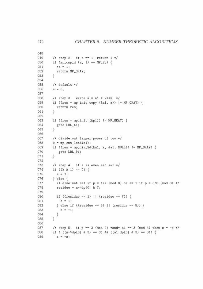
272 CHAPTER 9. NUMBER THEORETIC ALGORITHMS
048
049 /* step 2. if a == 1, return 1 */
050 if (mp_cmp_d (a, 1) == MP_EQ) {051 *c = 1;
052 return MP_OKAY;
053 }054
055 /* default */
056 s = 0;
057
058 /* step 3. write a = a1 * 2**k */
059 if ((res = mp_init_copy (&a1, a)) != MP_OKAY) {060 return res;
061 }062
063 if ((res = mp_init (&p1)) != MP_OKAY) {064 goto LBL_A1;
065 }066
067 /* divide out larger power of two */
068 k = mp_cnt_lsb(&a1);
069 if ((res = mp_div_2d(&a1, k, &a1, NULL)) != MP_OKAY) {070 goto LBL_P1;
071 }072
073 /* step 4. if e is even set s=1 */
074 if ((k & 1) == 0) {075 s = 1;
076 } else {077 /* else set s=1 if p = 1/7 (mod 8) or s=-1 if p = 3/5 (mod 8) */
078 residue = n->dp[0] & 7;
079
080 if ((residue == 1) || (residue == 7)) {081 s = 1;
082 } else if ((residue == 3) || (residue == 5)) {083 s = -1;
084 }085 }086
087 /* step 5. if p == 3 (mod 4) *and* a1 == 3 (mod 4) then s = -s */
088 if ( ((n->dp[0] & 3) == 3) && ((a1.dp[0] & 3) == 3)) {089 s = -s;
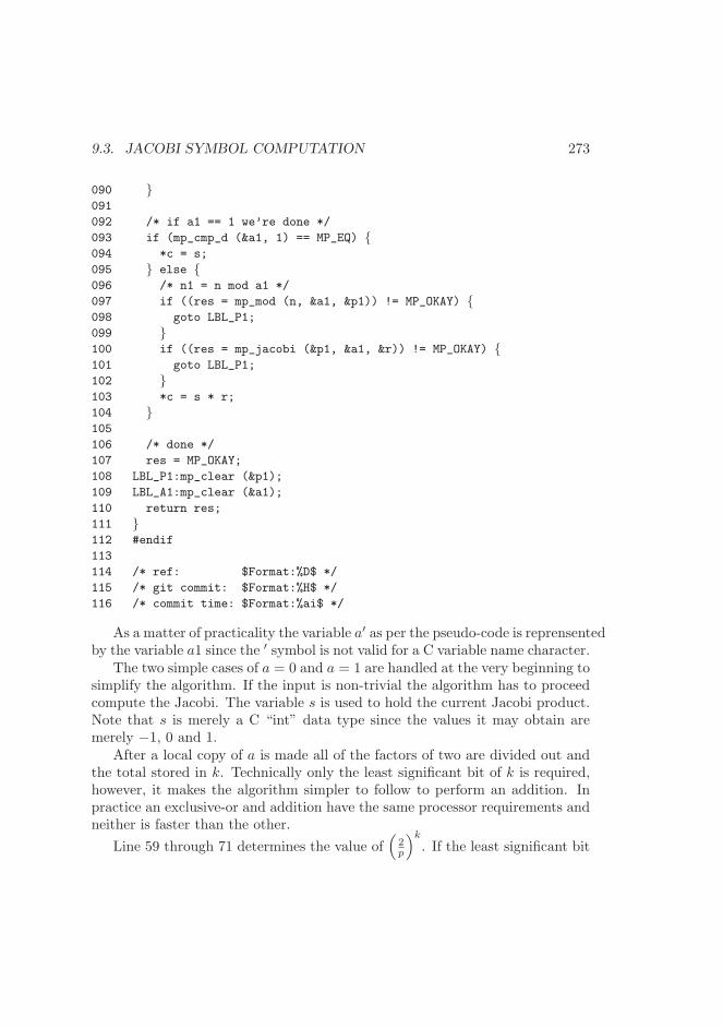
9.3. JACOBI SYMBOL COMPUTATION 273
090 }091
092 /* if a1 == 1 we’re done */
093 if (mp_cmp_d (&a1, 1) == MP_EQ) {094 *c = s;
095 } else {096 /* n1 = n mod a1 */
097 if ((res = mp_mod (n, &a1, &p1)) != MP_OKAY) {098 goto LBL_P1;
099 }100 if ((res = mp_jacobi (&p1, &a1, &r)) != MP_OKAY) {101 goto LBL_P1;
102 }103 *c = s * r;
104 }105
106 /* done */
107 res = MP_OKAY;
108 LBL_P1:mp_clear (&p1);
109 LBL_A1:mp_clear (&a1);
110 return res;
111 }112 #endif
113
114 /* ref: $Format:%D$ */
115 /* git commit: $Format:%H$ */
116 /* commit time: $Format:%ai$ */
As a matter of practicality the variable a′ as per the pseudo-code is reprensentedby the variable a1 since the ′ symbol is not valid for a C variable name character.
The two simple cases of a = 0 and a = 1 are handled at the very beginning tosimplify the algorithm. If the input is non-trivial the algorithm has to proceedcompute the Jacobi. The variable s is used to hold the current Jacobi product.Note that s is merely a C “int” data type since the values it may obtain aremerely −1, 0 and 1.
After a local copy of a is made all of the factors of two are divided out andthe total stored in k. Technically only the least significant bit of k is required,however, it makes the algorithm simpler to follow to perform an addition. Inpractice an exclusive-or and addition have the same processor requirements andneither is faster than the other.
Line 59 through 71 determines the value of(
2p
)k
. If the least significant bit
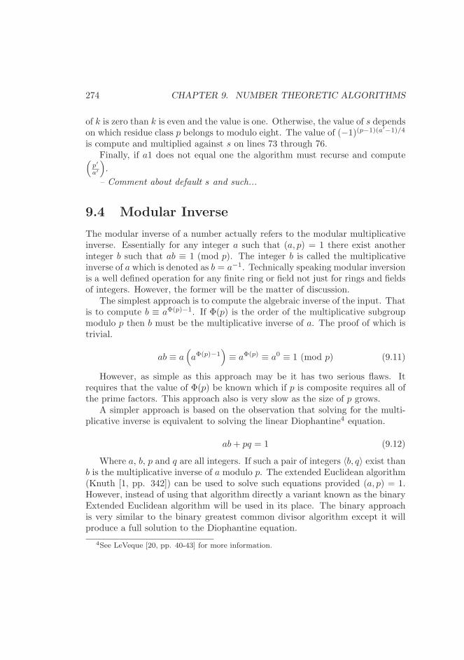
274 CHAPTER 9. NUMBER THEORETIC ALGORITHMS
of k is zero than k is even and the value is one. Otherwise, the value of s dependson which residue class p belongs to modulo eight. The value of (−1)(p−1)(a′−1)/4
is compute and multiplied against s on lines 73 through 76.Finally, if a1 does not equal one the algorithm must recurse and compute
(
p′
a′
)
.
– Comment about default s and such...
9.4 Modular Inverse
The modular inverse of a number actually refers to the modular multiplicativeinverse. Essentially for any integer a such that (a, p) = 1 there exist anotherinteger b such that ab ≡ 1 (mod p). The integer b is called the multiplicativeinverse of a which is denoted as b = a−1. Technically speaking modular inversionis a well defined operation for any finite ring or field not just for rings and fieldsof integers. However, the former will be the matter of discussion.
The simplest approach is to compute the algebraic inverse of the input. Thatis to compute b ≡ aΦ(p)−1. If Φ(p) is the order of the multiplicative subgroupmodulo p then b must be the multiplicative inverse of a. The proof of which istrivial.
ab ≡ a(
aΦ(p)−1)
≡ aΦ(p) ≡ a0 ≡ 1 (mod p) (9.11)
However, as simple as this approach may be it has two serious flaws. Itrequires that the value of Φ(p) be known which if p is composite requires all ofthe prime factors. This approach also is very slow as the size of p grows.
A simpler approach is based on the observation that solving for the multi-plicative inverse is equivalent to solving the linear Diophantine4 equation.
ab+ pq = 1 (9.12)
Where a, b, p and q are all integers. If such a pair of integers 〈b, q〉 exist thanb is the multiplicative inverse of a modulo p. The extended Euclidean algorithm(Knuth [1, pp. 342]) can be used to solve such equations provided (a, p) = 1.However, instead of using that algorithm directly a variant known as the binaryExtended Euclidean algorithm will be used in its place. The binary approachis very similar to the binary greatest common divisor algorithm except it willproduce a full solution to the Diophantine equation.
4See LeVeque [20, pp. 40-43] for more information.

9.4. MODULAR INVERSE 275
9.4.1 General Case
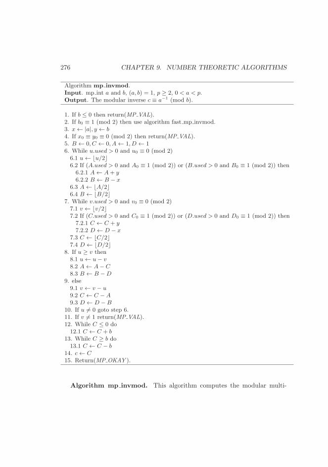
276 CHAPTER 9. NUMBER THEORETIC ALGORITHMS
Algorithm mp invmod.Input. mp int a and b, (a, b) = 1, p ≥ 2, 0 < a < p.Output. The modular inverse c ≡ a−1 (mod b).
1. If b ≤ 0 then return(MP VAL).2. If b0 ≡ 1 (mod 2) then use algorithm fast mp invmod.3. x← |a|, y ← b4. If x0 ≡ y0 ≡ 0 (mod 2) then return(MP VAL).5. B ← 0, C ← 0, A← 1, D ← 16. While u.used > 0 and u0 ≡ 0 (mod 2)6.1 u← ⌊u/2⌋6.2 If (A.used > 0 and A0 ≡ 1 (mod 2)) or (B.used > 0 and B0 ≡ 1 (mod 2)) then6.2.1 A← A+ y6.2.2 B ← B − x
6.3 A← ⌊A/2⌋6.4 B ← ⌊B/2⌋
7. While v.used > 0 and v0 ≡ 0 (mod 2)7.1 v ← ⌊v/2⌋7.2 If (C.used > 0 and C0 ≡ 1 (mod 2)) or (D.used > 0 and D0 ≡ 1 (mod 2)) then7.2.1 C ← C + y7.2.2 D ← D − x
7.3 C ← ⌊C/2⌋7.4 D ← ⌊D/2⌋
8. If u ≥ v then8.1 u← u− v8.2 A← A− C8.3 B ← B −D
9. else9.1 v ← v − u9.2 C ← C −A9.3 D ← D −B
10. If u 6= 0 goto step 6.11. If v 6= 1 return(MP VAL).12. While C ≤ 0 do12.1 C ← C + b
13. While C ≥ b do13.1 C ← C − b
14. c← C15. Return(MP OKAY ).
Algorithm mp invmod. This algorithm computes the modular multi-
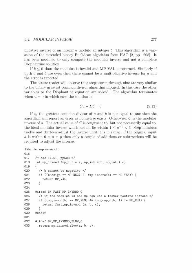
9.4. MODULAR INVERSE 277
plicative inverse of an integer a modulo an integer b. This algorithm is a vari-ation of the extended binary Euclidean algorithm from HAC [2, pp. 608]. Ithas been modified to only compute the modular inverse and not a completeDiophantine solution.
If b ≤ 0 than the modulus is invalid and MP VAL is returned. Similarly ifboth a and b are even then there cannot be a multiplicative inverse for a andthe error is reported.
The astute reader will observe that steps seven through nine are very similarto the binary greatest common divisor algorithm mp gcd. In this case the othervariables to the Diophantine equation are solved. The algorithm terminateswhen u = 0 in which case the solution is
Ca+Db = v (9.13)
If v, the greatest common divisor of a and b is not equal to one then thealgorithm will report an error as no inverse exists. Otherwise, C is the modularinverse of a. The actual value of C is congruent to, but not necessarily equal to,the ideal modular inverse which should lie within 1 ≤ a−1 < b. Step numberstwelve and thirteen adjust the inverse until it is in range. If the original inputa is within 0 < a < p then only a couple of additions or subtractions will berequired to adjust the inverse.
File: bn mp invmod.c
016
017 /* hac 14.61, pp608 */
018 int mp_invmod (mp_int * a, mp_int * b, mp_int * c)
019 {020 /* b cannot be negative */
021 if ((b->sign == MP_NEG) || (mp_iszero(b) == MP_YES)) {022 return MP_VAL;
023 }024
025 #ifdef BN_FAST_MP_INVMOD_C
026 /* if the modulus is odd we can use a faster routine instead */
027 if ((mp_isodd(b) == MP_YES) && (mp_cmp_d(b, 1) != MP_EQ)) {028 return fast_mp_invmod (a, b, c);
029 }030 #endif
031
032 #ifdef BN_MP_INVMOD_SLOW_C
033 return mp_invmod_slow(a, b, c);
278 CHAPTER 9. NUMBER THEORETIC ALGORITHMS
034 #else
035 return MP_VAL;
036 #endif
037 }038 #endif
039
040 /* ref: $Format:%D$ */
041 /* git commit: $Format:%H$ */
042 /* commit time: $Format:%ai$ */
Odd Moduli
When the modulus b is odd the variables A and C are fixed and are not requiredto compute the inverse. In particular by attempting to solve the DiophantineCb+Da = 1 only B and D are required to find the inverse of a.
The algorithm fast mp invmod is a direct adaptation of algorithm mp invmodwith all all steps involving either A or C removed. This optimization will halvethe time required to compute the modular inverse.
9.5 Primality Tests
A non-zero integer a is said to be prime if it is not divisible by any other integerexcluding one and itself. For example, a = 7 is prime since the integers 2 . . . 6do not evenly divide a. By contrast, a = 6 is not prime since a = 6 = 2 · 3.
Prime numbers arise in cryptography considerably as they allow finite fieldsto be formed. The ability to determine whether an integer is prime or not quicklyhas been a viable subject in cryptography and number theory for considerabletime. The algorithms that will be presented are all probablistic algorithms inthat when they report an integer is composite it must be composite. However,when the algorithms report an integer is prime the algorithm may be incorrect.
As will be discussed it is possible to limit the probability of error so wellthat for practical purposes the probablity of error might as well be zero. Forthe purposes of these discussions let n represent the candidate integer of whichthe primality is in question.
9.5.1 Trial Division
Trial division means to attempt to evenly divide a candidate integer by smallprime integers. If the candidate can be evenly divided it obviously cannot be
9.5. PRIMALITY TESTS 279
prime. By dividing by all primes 1 < p ≤ √n this test can actually provewhether an integer is prime. However, such a test would require a prohibitiveamount of time as n grows.
Instead of dividing by every prime, a smaller, more mangeable set of primesmay be used instead. By performing trial division with only a subset of theprimes less than
√n + 1 the algorithm cannot prove if a candidate is prime.
However, often it can prove a candidate is not prime.The benefit of this test is that trial division by small values is fairly efficient.
Specially compared to the other algorithms that will be discussed shortly. Theprobability that this approach correctly identifies a composite candidate whentested with all primes upto q is given by 1− 1.12
ln(q) . The graph (9.7) demonstrates
the probability of success for the range 3 ≤ q ≤ 100.
At approximately q = 30 the gain of performing further tests diminishesfairly quickly. At q = 90 further testing is generally not going to be of anypractical use. In the case of LibTomMath the default limit q = 256 was chosensince it is not too high and will eliminate approximately 80% of all candidateintegers. The constant PRIME SIZE is equal to the number of primes in thetest base. The array prime tab is an array of the first PRIME SIZE primenumbers.
Algorithm mp prime is divisible. This algorithm attempts to deter-mine if a candidate integer n is composite by performing trial divisions.
File: bn mp prime is divisible.c016
017 /* determines if an integers is divisible by one
018 * of the first PRIME_SIZE primes or not
019 *
020 * sets result to 0 if not, 1 if yes
021 */
022 int mp_prime_is_divisible (mp_int * a, int *result)
023 {024 int err, ix;
025 mp_digit res;
026
027 /* default to not */
028 *result = MP_NO;
029
030 for (ix = 0; ix < PRIME_SIZE; ix++) {
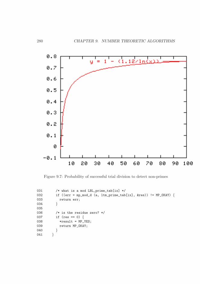
280 CHAPTER 9. NUMBER THEORETIC ALGORITHMS
Figure 9.7: Probability of successful trial division to detect non-primes
031 /* what is a mod LBL_prime_tab[ix] */
032 if ((err = mp_mod_d (a, ltm_prime_tab[ix], &res)) != MP_OKAY) {033 return err;
034 }035
036 /* is the residue zero? */
037 if (res == 0) {038 *result = MP_YES;
039 return MP_OKAY;
040 }041 }
9.5. PRIMALITY TESTS 281
Algorithm mp prime is divisible.Input. mp int aOutput. c = 1 if n is divisible by a small prime, otherwise c = 0.
1. for ix from 0 to PRIME SIZE do1.1 d← n (mod prime tabix)1.2 If d = 0 then1.2.1 c← 11.2.2 Return(MP OKAY ).
2. c← 03. Return(MP OKAY ).
Figure 9.8: Algorithm mp prime is divisible
042
043 return MP_OKAY;
044 }045 #endif
046
047 /* ref: $Format:%D$ */
048 /* git commit: $Format:%H$ */
049 /* commit time: $Format:%ai$ */
The algorithm defaults to a return of 0 in case an error occurs. The valuesin the prime table are all specified to be in the range of a mp digit. The tableprime tab is defined in the following file.
File: bn prime tab.c016 const mp_digit ltm_prime_tab[] = {017 0x0002, 0x0003, 0x0005, 0x0007, 0x000B, 0x000D, 0x0011, 0x0013,
018 0x0017, 0x001D, 0x001F, 0x0025, 0x0029, 0x002B, 0x002F, 0x0035,
019 0x003B, 0x003D, 0x0043, 0x0047, 0x0049, 0x004F, 0x0053, 0x0059,
020 0x0061, 0x0065, 0x0067, 0x006B, 0x006D, 0x0071, 0x007F,
021 #ifndef MP_8BIT
022 0x0083,
023 0x0089, 0x008B, 0x0095, 0x0097, 0x009D, 0x00A3, 0x00A7, 0x00AD,
024 0x00B3, 0x00B5, 0x00BF, 0x00C1, 0x00C5, 0x00C7, 0x00D3, 0x00DF,
025 0x00E3, 0x00E5, 0x00E9, 0x00EF, 0x00F1, 0x00FB, 0x0101, 0x0107,
026 0x010D, 0x010F, 0x0115, 0x0119, 0x011B, 0x0125, 0x0133, 0x0137,
027
028 0x0139, 0x013D, 0x014B, 0x0151, 0x015B, 0x015D, 0x0161, 0x0167,
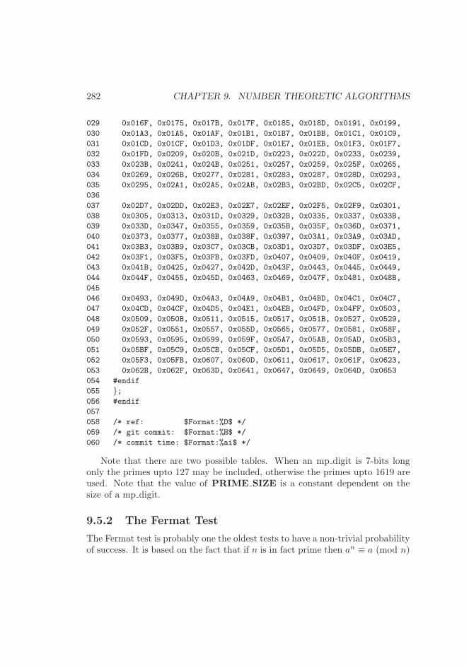
282 CHAPTER 9. NUMBER THEORETIC ALGORITHMS
029 0x016F, 0x0175, 0x017B, 0x017F, 0x0185, 0x018D, 0x0191, 0x0199,
030 0x01A3, 0x01A5, 0x01AF, 0x01B1, 0x01B7, 0x01BB, 0x01C1, 0x01C9,
031 0x01CD, 0x01CF, 0x01D3, 0x01DF, 0x01E7, 0x01EB, 0x01F3, 0x01F7,
032 0x01FD, 0x0209, 0x020B, 0x021D, 0x0223, 0x022D, 0x0233, 0x0239,
033 0x023B, 0x0241, 0x024B, 0x0251, 0x0257, 0x0259, 0x025F, 0x0265,
034 0x0269, 0x026B, 0x0277, 0x0281, 0x0283, 0x0287, 0x028D, 0x0293,
035 0x0295, 0x02A1, 0x02A5, 0x02AB, 0x02B3, 0x02BD, 0x02C5, 0x02CF,
036
037 0x02D7, 0x02DD, 0x02E3, 0x02E7, 0x02EF, 0x02F5, 0x02F9, 0x0301,
038 0x0305, 0x0313, 0x031D, 0x0329, 0x032B, 0x0335, 0x0337, 0x033B,
039 0x033D, 0x0347, 0x0355, 0x0359, 0x035B, 0x035F, 0x036D, 0x0371,
040 0x0373, 0x0377, 0x038B, 0x038F, 0x0397, 0x03A1, 0x03A9, 0x03AD,
041 0x03B3, 0x03B9, 0x03C7, 0x03CB, 0x03D1, 0x03D7, 0x03DF, 0x03E5,
042 0x03F1, 0x03F5, 0x03FB, 0x03FD, 0x0407, 0x0409, 0x040F, 0x0419,
043 0x041B, 0x0425, 0x0427, 0x042D, 0x043F, 0x0443, 0x0445, 0x0449,
044 0x044F, 0x0455, 0x045D, 0x0463, 0x0469, 0x047F, 0x0481, 0x048B,
045
046 0x0493, 0x049D, 0x04A3, 0x04A9, 0x04B1, 0x04BD, 0x04C1, 0x04C7,
047 0x04CD, 0x04CF, 0x04D5, 0x04E1, 0x04EB, 0x04FD, 0x04FF, 0x0503,
048 0x0509, 0x050B, 0x0511, 0x0515, 0x0517, 0x051B, 0x0527, 0x0529,
049 0x052F, 0x0551, 0x0557, 0x055D, 0x0565, 0x0577, 0x0581, 0x058F,
050 0x0593, 0x0595, 0x0599, 0x059F, 0x05A7, 0x05AB, 0x05AD, 0x05B3,
051 0x05BF, 0x05C9, 0x05CB, 0x05CF, 0x05D1, 0x05D5, 0x05DB, 0x05E7,
052 0x05F3, 0x05FB, 0x0607, 0x060D, 0x0611, 0x0617, 0x061F, 0x0623,
053 0x062B, 0x062F, 0x063D, 0x0641, 0x0647, 0x0649, 0x064D, 0x0653
054 #endif
055 };056 #endif
057
058 /* ref: $Format:%D$ */
059 /* git commit: $Format:%H$ */
060 /* commit time: $Format:%ai$ */
Note that there are two possible tables. When an mp digit is 7-bits longonly the primes upto 127 may be included, otherwise the primes upto 1619 areused. Note that the value of PRIME SIZE is a constant dependent on thesize of a mp digit.
9.5.2 The Fermat Test
The Fermat test is probably one the oldest tests to have a non-trivial probabilityof success. It is based on the fact that if n is in fact prime then an ≡ a (mod n)
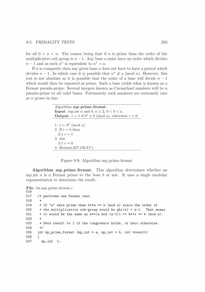
9.5. PRIMALITY TESTS 283
for all 0 < a < n. The reason being that if n is prime than the order of themultiplicative sub group is n− 1. Any base a must have an order which dividesn− 1 and as such an is equivalent to a1 = a.
If n is composite then any given base a does not have to have a period whichdivides n − 1. In which case it is possible that an 6≡ a (mod n). However, thistest is not absolute as it is possible that the order of a base will divide n − 1which would then be reported as prime. Such a base yields what is known as aFermat pseudo-prime. Several integers known as Carmichael numbers will be apseudo-prime to all valid bases. Fortunately such numbers are extremely rareas n grows in size.
Algorithm mp prime fermat.Input. mp int a and b, a ≥ 2, 0 < b < a.Output. c = 1 if ba ≡ b (mod a), otherwise c = 0.
1. t← ba (mod a)2. If t = b then2.1 c = 1
3. else3.1 c = 0
4. Return(MP OKAY ).
Figure 9.9: Algorithm mp prime fermat
Algorithm mp prime fermat. This algorithm determines whether anmp int a is a Fermat prime to the base b or not. It uses a single modularexponentiation to determine the result.
File: bn mp prime fermat.c016
017 /* performs one Fermat test.
018 *
019 * If "a" were prime then b**a == b (mod a) since the order of
020 * the multiplicative sub-group would be phi(a) = a-1. That means
021 * it would be the same as b**(a mod (a-1)) == b**1 == b (mod a).
022 *
023 * Sets result to 1 if the congruence holds, or zero otherwise.
024 */
025 int mp_prime_fermat (mp_int * a, mp_int * b, int *result)
026 {027 mp_int t;
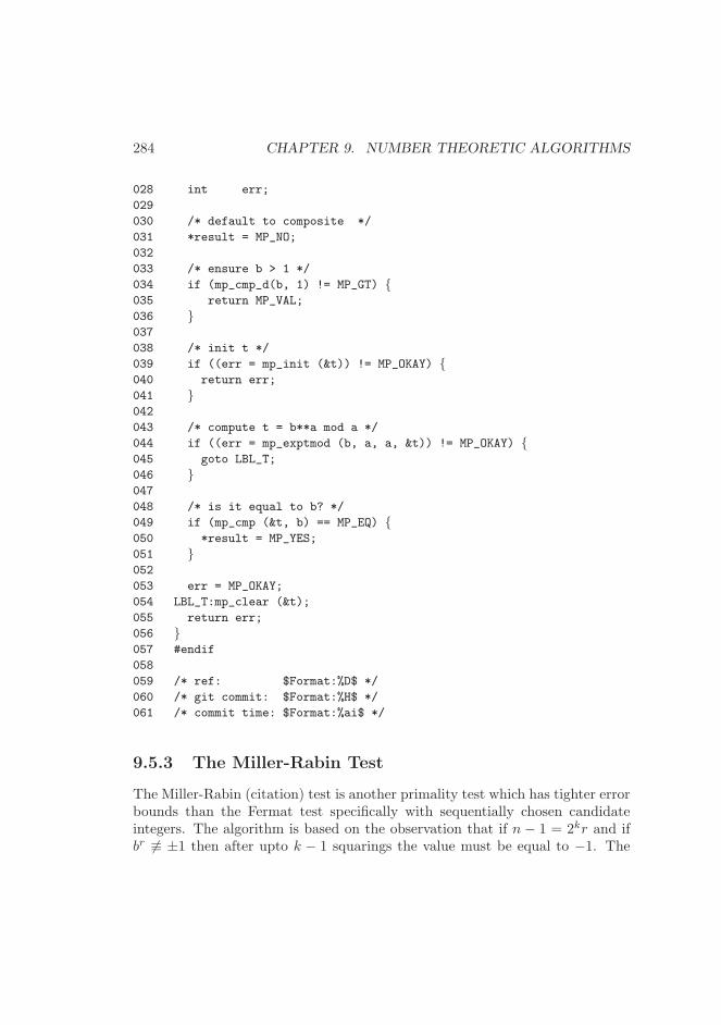
284 CHAPTER 9. NUMBER THEORETIC ALGORITHMS
028 int err;
029
030 /* default to composite */
031 *result = MP_NO;
032
033 /* ensure b > 1 */
034 if (mp_cmp_d(b, 1) != MP_GT) {035 return MP_VAL;
036 }037
038 /* init t */
039 if ((err = mp_init (&t)) != MP_OKAY) {040 return err;
041 }042
043 /* compute t = b**a mod a */
044 if ((err = mp_exptmod (b, a, a, &t)) != MP_OKAY) {045 goto LBL_T;
046 }047
048 /* is it equal to b? */
049 if (mp_cmp (&t, b) == MP_EQ) {050 *result = MP_YES;
051 }052
053 err = MP_OKAY;
054 LBL_T:mp_clear (&t);
055 return err;
056 }057 #endif
058
059 /* ref: $Format:%D$ */
060 /* git commit: $Format:%H$ */
061 /* commit time: $Format:%ai$ */
9.5.3 The Miller-Rabin Test
The Miller-Rabin (citation) test is another primality test which has tighter errorbounds than the Fermat test specifically with sequentially chosen candidateintegers. The algorithm is based on the observation that if n − 1 = 2kr and ifbr 6≡ ±1 then after upto k − 1 squarings the value must be equal to −1. The
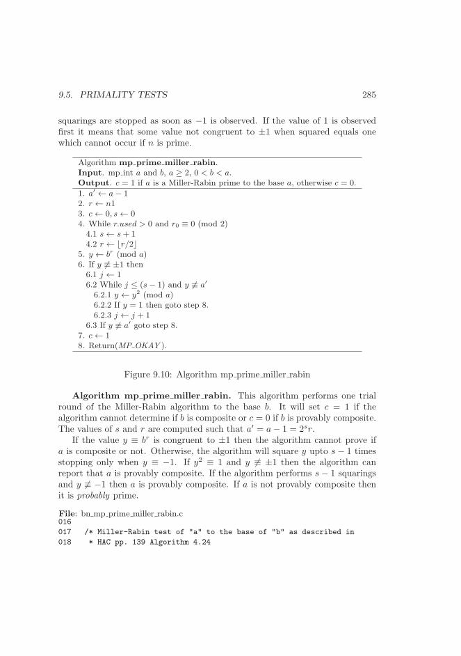
9.5. PRIMALITY TESTS 285
squarings are stopped as soon as −1 is observed. If the value of 1 is observedfirst it means that some value not congruent to ±1 when squared equals onewhich cannot occur if n is prime.
Algorithm mp prime miller rabin.Input. mp int a and b, a ≥ 2, 0 < b < a.Output. c = 1 if a is a Miller-Rabin prime to the base a, otherwise c = 0.
1. a′ ← a− 12. r ← n13. c← 0, s← 04. While r.used > 0 and r0 ≡ 0 (mod 2)4.1 s← s+ 14.2 r ← ⌊r/2⌋
5. y ← br (mod a)6. If y 6≡ ±1 then6.1 j ← 16.2 While j ≤ (s− 1) and y 6≡ a′
6.2.1 y ← y2 (mod a)6.2.2 If y = 1 then goto step 8.6.2.3 j ← j + 1
6.3 If y 6≡ a′ goto step 8.7. c← 18. Return(MP OKAY ).
Figure 9.10: Algorithm mp prime miller rabin
Algorithm mp prime miller rabin. This algorithm performs one trialround of the Miller-Rabin algorithm to the base b. It will set c = 1 if thealgorithm cannot determine if b is composite or c = 0 if b is provably composite.The values of s and r are computed such that a′ = a− 1 = 2sr.
If the value y ≡ br is congruent to ±1 then the algorithm cannot prove ifa is composite or not. Otherwise, the algorithm will square y upto s− 1 timesstopping only when y ≡ −1. If y2 ≡ 1 and y 6≡ ±1 then the algorithm canreport that a is provably composite. If the algorithm performs s− 1 squaringsand y 6≡ −1 then a is provably composite. If a is not provably composite thenit is probably prime.
File: bn mp prime miller rabin.c016
017 /* Miller-Rabin test of "a" to the base of "b" as described in
018 * HAC pp. 139 Algorithm 4.24
286 CHAPTER 9. NUMBER THEORETIC ALGORITHMS
019 *
020 * Sets result to 0 if definitely composite or 1 if probably prime.
021 * Randomly the chance of error is no more than 1/4 and often
022 * very much lower.
023 */
024 int mp_prime_miller_rabin (mp_int * a, mp_int * b, int *result)
025 {026 mp_int n1, y, r;
027 int s, j, err;
028
029 /* default */
030 *result = MP_NO;
031
032 /* ensure b > 1 */
033 if (mp_cmp_d(b, 1) != MP_GT) {034 return MP_VAL;
035 }036
037 /* get n1 = a - 1 */
038 if ((err = mp_init_copy (&n1, a)) != MP_OKAY) {039 return err;
040 }041 if ((err = mp_sub_d (&n1, 1, &n1)) != MP_OKAY) {042 goto LBL_N1;
043 }044
045 /* set 2**s * r = n1 */
046 if ((err = mp_init_copy (&r, &n1)) != MP_OKAY) {047 goto LBL_N1;
048 }049
050 /* count the number of least significant bits
051 * which are zero
052 */
053 s = mp_cnt_lsb(&r);
054
055 /* now divide n - 1 by 2**s */
056 if ((err = mp_div_2d (&r, s, &r, NULL)) != MP_OKAY) {057 goto LBL_R;
058 }059
060 /* compute y = b**r mod a */
9.5. PRIMALITY TESTS 287
061 if ((err = mp_init (&y)) != MP_OKAY) {062 goto LBL_R;
063 }064 if ((err = mp_exptmod (b, &r, a, &y)) != MP_OKAY) {065 goto LBL_Y;
066 }067
068 /* if y != 1 and y != n1 do */
069 if ((mp_cmp_d (&y, 1) != MP_EQ) && (mp_cmp (&y, &n1) != MP_EQ)) {070 j = 1;
071 /* while j <= s-1 and y != n1 */
072 while ((j <= (s - 1)) && (mp_cmp (&y, &n1) != MP_EQ)) {073 if ((err = mp_sqrmod (&y, a, &y)) != MP_OKAY) {074 goto LBL_Y;
075 }076
077 /* if y == 1 then composite */
078 if (mp_cmp_d (&y, 1) == MP_EQ) {079 goto LBL_Y;
080 }081
082 ++j;
083 }084
085 /* if y != n1 then composite */
086 if (mp_cmp (&y, &n1) != MP_EQ) {087 goto LBL_Y;
088 }089 }090
091 /* probably prime now */
092 *result = MP_YES;
093 LBL_Y:mp_clear (&y);
094 LBL_R:mp_clear (&r);
095 LBL_N1:mp_clear (&n1);
096 return err;
097 }098 #endif
099
100 /* ref: $Format:%D$ */
101 /* git commit: $Format:%H$ */
102 /* commit time: $Format:%ai$ */

288 CHAPTER 9. NUMBER THEORETIC ALGORITHMS
Bibliography
[1] Donald Knuth, The Art of Computer Programming, Third Edition,Volume Two, Seminumerical Algorithms, Addison-Wesley, 1998
[2] A. Menezes, P. van Oorschot, S. Vanstone, Handbook of Applied
Cryptography, CRC Press, 1996
[3] Michael Rosing, Implementing Elliptic Curve Cryptography, Man-ning Publications, 1999
[4] Paul G. Comba, Exponentiation Cryptosystems on the IBM PC.IBM Systems Journal 29(4): 526-538 (1990)
[5] A. Karatsuba, Doklay Akad. Nauk SSSR 145 (1962), pp.293-294
[6] Andre Weimerskirch and Christof Paar, Generalizations of the
Karatsuba Algorithm for Polynomial Multiplication, Submitted toDesign, Codes and Cryptography, March 2002
[7] Paul Barrett, Implementing the Rivest Shamir and Adleman Public
Key Encryption Algorithm on a Standard Digital Signal Processor,Advances in Cryptology, Crypto ’86, Springer-Verlag.
[8] P.L.Montgomery. Modular multiplication without trial division.Mathematics of Computation, 44(170):519-521, April 1985.
[9] Chae Hoon Lim and Pil Joong Lee, Generating Efficient Primes
for Discrete Log Cryptosystems, POSTECH Information ResearchLaboratories
[10] J. Daemen and R. Govaerts and J. Vandewalle, Block ciphers based
on Modular Arithmetic, State and Progress in the Research of Cryp-tography, 1993, pp. 80-89
289
290 BIBLIOGRAPHY
[11] R.L. Rivest, A. Shamir, L. Adleman, A Method for Obtaining Dig-
ital Signatures and Public-Key Cryptosystems
[12] Whitfield Diffie, Martin E. Hellman, New Directions in Cryptogra-
phy, IEEE Transactions on Information Theory, 1976
[13] IEEE Standard for Binary Floating-Point Arithmetic (ANSI/IEEEStd 754-1985)
[14] GNU Multiple Precision (GMP), http://www.swox.com/gmp/
[15] Multiple Precision Integer Library (MPI), Michael Fromberger,http://thayer.dartmouth.edu/~sting/mpi/
[16] OpenSSL Cryptographic Toolkit, http://openssl.org
[17] Large Integer Package, http://home.hetnet.nl/~ecstr/LIP.zip
[18] JTC1/SC22/WG14, ISO/IEC 9899:1999, “A draft rationale for theC99 standard.”
[19] The Sun Java Website, http://java.sun.com/
[20] William LeVeque, Fundamentals of Number Theory, Dover Publi-cations, 2014
[21] T. Elgamal, A public key cryptosystem and a signature scheme based
on discrete logarithms, IEEE Transactions on Information Theory,1985, pp. 469-472
[22] D. Knuth, The Art of Computer Programming; Volume 2. Third
Edition, Addison-Wesley, 1997, pg. 294
[23] The Open Group, http://www.opengroup.org/austin/papers/posix_faq.html2017
Index
baseline multiplication, 96big-Oh, 7
modular residue, 149mp digit, 5mp init, 19mp int, 5, 15MP MEM, 18MP NEG, 16MP OKAY, 18MP VAL, 18mp word, 5MP ZPOS, 16
precision, 3
radix point, 113
291