ill PB96-148523 Information is our business.

ROBOT MOTION PLANNING WITH UNCERTAINTY IN CONTROL AND SENSING

STANFORD UNIV., CA worn w ^m-mv?mBmmm

NOV 89

U.S. DEPARTMENT OF COMMERCE National Technical Information Service

DISTRIBUTION STATEMENT A

Approved for public release; Distribution Unlimited

BIBLIOGRAPHIC INFORMATION

RB96-148523

Report Nos: STAN-CS-89-1292

Title: Robot Motion Planning with Uncertainty in Control and Sensing.

Date: Nov 89

Authors: J. C. Latombe, A. Lazanas, and S. Shekhar.

Performing Organization: Stanford Univ., CA. Dept. of Computer Science.

Sponsoring Organization: ^Defense Advanced Research Projects Agency, Arlington, VA.

Contract Nos: DARPA-DAAA21-89-C-0002

Type of Report and Period Covered: Research rept.

NTIS Field/Group Codes: 41C (Robotics/Robots), 62 (Computers, Control & Information iheoryj

Price: PC A03/MF A01

Availability: Available from the National Technical Information Service, Springfield, VA. 221bl

Number of Pages: 48p

Keywords: *Robot control, *Trajectory planning, *Autonomous navigation, Robot dynanncs, Trajectory control, Dynamic control, Adaptive control, Trajectory analysis, Robot sensors. Uncertainty, Two dimensional, Algorithms, Numerical methods and procedures. Robots, Preimage computation.

Abstract: In this paper, we consider the problem of planning motion strategies in the presence of uncertainty in both control and sensing for simple robots described in a two-dimensional configuration space. We consider the preimage backchaining approach to this problem, which was first proposed by Lozano-Perez, Mason and Taylor (1984). Although attractive, the approach raises several difficult computational issues. One • of them, which is directly addressed in this paper, is preimage computation. We describe two practical methods for computing preimages, which we call backprojection from sticking edges and backprojection from goal kernel. In the last sections of the paper, we discuss non-implemented improvements of this planner and present additional results.

November 1989 Report No. STAN-CS-89-1292

illllillllllllllllllllllll PB96-148523

Robot Motion Planning with Uncertainty in Control and Sensing

by

Latombe, Lazanas, and Shekhar

Department of Computer Science

Stanford University Stanford, California 94305

REPRODUCED BY: MS& U.S. Department of Commerce

National Technical Infonmation Sarvice Springfield' Vlrgini» 22WI

PB96-14S523 unclassified

SECURITY CLASSIFICATION OF THIS PAGE

REPORT DOCUMENTATION PAGE

la. REPORT SECURITY CLASSIFICATION

2a. SECURITY CLASSIFICATION AUTHORITY

2b. DECLASSIFICATION / DOWNGRADING SCHEDULE

4. PERFORMING ORGANIZATION REPORT NUMBER(S)

STAN-CS-89-1292 6a. NAME OF PERFORMING ORGANIZATION

Stanford University

6b. OFFICE SYMBOL (If applicable)

6c ADDRESS (City. State, and ZIP Code)

Stanford, CA 94305

8a. NAME OF FUNDING /SPONSORING ORGANIZATION

DARPA/SIMA

8b. OFFICE SYMBOL (If applicable)

8c ADDRESS (City, State, and ZIP Code)

Form Approved OMB No. 0704-0188

lb RESTRICTIVE MARKINGS

3 DISTRIBUTION/AVAILABILITY OF REPORT

5. MONITORING ORGANIZATION REPORT NUMBER(S)

7a. NAME OF MONITORING ORGANIZATION

7b. ADDRESS (City. State, and ZIP Code)

9. PROCUREMENT INSTRUMENT IDENTIFICATION NUMBER

DAAA21-89-C-0002/SIMA Latombe 10 SOURCE OF FUNDING NUMBERS

PROGRAM ELEMENT NO.

PROJECT NO.

TASK NO.

WORK UNIT ACCESSION NO.

11. TITLE (Include Security Classification)

Robot Motion Planning with Uncertainty in Control and Sensing

12. PERSONAL AUTHOR(S) Jean-Claude Latombe, Anthony Lazanas, Shashank Shekhar

,3areYsP4äWORT 13b TIME COVERED FROM TO.

14. DATE OF REPORT (Ye at, Month, Day) 15. PAGEXOUNT w 16. SUPPLEMENTARY NOTATION

17. COSATI CODES

FIELD GROUP SUB-GROUP

18. SUBJECT TERMS (Continue on reverse it necessary and identify by block number)

9 ABSTRACT (Continue on reverse if necessary and identify by block number)

20 DISTRIBUTION/AVAILABILITY OF ABSTRACT

DP UNCLASSIFIED/UNLIMITED D SAME AS RPT D DTIC USERS

22a. NAME Of,RESPONSIBLE INDIVIDUAL Jean-Claude Latombe

21. ABSTRACT SECURITY CLASSIFICATION ABSTRACT SEOJRITJ unclassified

22b TELEPHONE (Include Area Code) 415-723-0350

22c. OFFICE SYMBOL

DD Form 1473. JUN 86 Previous editions are obsolete.

S/N 0102-LF-01A-6603

SECURITY CLASSIFICATION OF THIS PAGE

Robot Motion Planning with Uncertainty in Control and Sensing

Jean-Claude Latombe, Anthony Lazanas, Shashank Shekhar Robotics Laboratory«

Computer Science Department, Stanford University Stanford, CA 94305, USA

Abstract: One of the key topics in robot reasoning is motion planning. Most of the research in this domain has focused on the topological and geometrical problem of finding a collision-free path connecting two configurations of the robot among obstacles, by assuming complete and accurate prior knowledge of the robot workspace and perfect control of the robot. But there exists a variety of robot operations which cannot be achieved reliably by simply executing preplanned paths. These operations require several kinds of uncertainty to be taken into account at the planning stage in order to generate motion strategies, which typically combine motion and sensing commands. In this paper, we consider the problem of planning motion strategies in the presence of uncertainty in both control and sensing for simple robots described in a two-dimensional configuration space. We consider the preimage backchaining approach to this problem, which was first proposed by Lozano-Perez, Mason and Taylor (1984). A preimage of a goal is a region such that if the robot is in this region prior to the execution of a motion command, it is guaranteed that the robot will be in the goal after the execution of the command. Backchaining consists of recursively treating each computed preimage as an intermediate goal, until a computed preimage contains the region in which the initial configuration of the robot is known to be. Although attractive, the approach raises several difficult computational issues. One of them, which is directly addressed in this paper, is preimage computation. We describe two practical methods for computing preimages, which we call backprojection from sticking edges and backprojection from goal kernel. Both methods proceed by separating two basic issues in preimage computation: goal reachability and goal recognizability. They both make use of the notion of backprojection, a concept developed by Erdmann (1984). The second method presents significant advantages over the first, but the two methods can be combined in order to draw the best of each. The combined method is probably the most effective method proposed so far for computing preimages. A motion planner embedding this method has been implemented. In the last sections of the paper, we discuss non-implemented improvements of this

planner and present additional results.

Acknowledgements: This research was funded by DARPA contract DAAA21-89-C0002 (Army), and SIMA (Stanford Institute of Manufacturing and Automation). The authors also thank Randy Wilson for useful

suggestions.

PROTECTED UNDER INTERNATIONAL COPYRIGHT ALL RIGHTS RESERVED. NATIONAL TECHNICAL INFORMATION SERVICE U.S. DEPARTMENT OF COMMERCE

1 Introduction

One of the ultimate goals of robotics research is to create easily instructable autonomous robots. Such robots will accept high-level descriptions of tasks specifying what the user wants done, rather than how to do it, and will execute them without further human assis- tance. Progress toward this goal requires advances in many interrelated domains, including automatic reasoning, perception, and real-time control. One of the key topics in robot rea- soning is motion planning. It is aimed at providing robots with the capability of deciding which motion commands to execute in order to achieve goal arrangements of physical ob- jects During the last ten years, it has emerged as a major research area with ramifications in Artificial Intelligence [Brooks and Lozano-Perez, 1983] [Donald, 1987a], Computational Complexity [Reif, 1979] [Schwartz and Shark, 1988], and Differential Geometry and Topol-

ogy [Schwartz and Shark, 1983] [Canny, 1987].

Most of the research in robot motion planning has focused on the topological and geometri- cal problem of finding a collision-free path connecting two configurations of the robot among obstacles. Today, the mathematical and computational structure of the general path plan- ning problem is reasonably well-understood and practical planners have been implemented in more or less specific cases [Brooks and Lozano-Perez, 1983] [Faverjon and Tournassoud, 1987] [Lozano-Perez, 1987] [Barraquand and Latombe, 1989]. A major limitation of these planners, however, is that they assume complete and accurate prior knowledge of the robot workspace and perfect control of the robot. These assumptions are reasonable as long as the errors in the planning models are small with respect to the tolerances of the task constraints. This is the case, for instance, when the motions are performed in a relatively uncluttered workspace and no delicate contact relation has to be made between objects. But there exists a variety of operations - e.g., grasping a part, mating two mechanical parts, navigating ma cluttered environment, docking and parking a vehicle - which cannot be achieved reliably by simply executing preplanned paths. These operations require uncertainty to be taken into account at the planning stage in order to generate motion strategies that combine motion and sensing commands. At execution time, these commands interact and take advantage of various sources of information to reduce uncertainty and lead the robot to the goal reliably.

During the past few years, a trend in Artificial Intelligence research on autonomous agents interacting with a dynamic and/or uncertain external world has been toward «reactive plan- ning". This trend grew up in reaction to the more traditional approach to planning, which tends to decompose planning and execution between two successive phases. An extreme position related to this trend is to use almost no prediction of future states at all. However, a fundamental difficulty of motion planning with uncertainty, including uncertainty in robot control and sensing, is that uncertainty exists not only at planning time, but also at execu- tion time. In most cases, this difficulty cannot be solved through simple reactive planning schemes, since uncertainty is not simply eliminated at execution time, say, by reading sen- sory inputs. It is necessary for the robot to reason in advance about the knowledge that will be available during motion execution, in order to guarantee that executing the generated plan wiU make enough knowledge available to either guide the robot toward the goal using the current plan, or recognize failure and feedback pertinent data to the planner so that it

can amend the plan appropriately.

a J

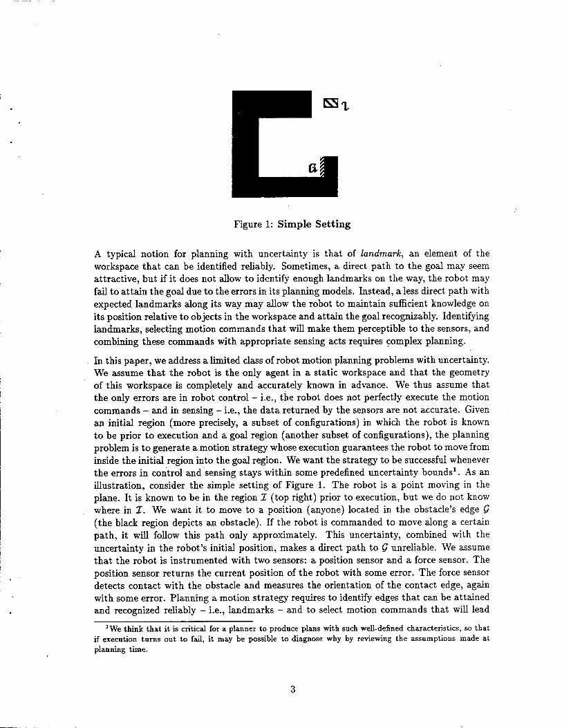
Figure 1: Simple Setting

A typical notion for planning with uncertainty is that of landmark, an element of the workspace that can be identified reliably. Sometimes, a direct path to the goal may seem attractive, but if it does not allow to identify enough landmarks on the way, the robot may fail to attain the goal due to the errors in its planning models. Instead, a less direct path with expected landmarks along its way may allow the robot to maintain sufficient knowledge on its position relative to objects in the workspace and attain the goal recognizably. Identifying landmarks, selecting motion commands that will make them perceptible to the sensors, and combining these commands with appropriate sensing acts requires complex planning.

In this paper, we address a limited class of robot motion planning problems with uncertainty. We assume that the robot is the only agent in a static workspace and that the geometry of this workspace is completely and accurately known in advance. We thus assume that the only errors are in robot control - i.e., the robot does not perfectly execute the motion commands - and in sensing - i.e., the data returned by the sensors are not accurate. Given an initial region (more precisely, a subset of configurations) in which the robot is known to be prior to execution and a goal region (another subset of configurations), the planning problem is to generate a motion strategy whose execution guarantees the robot to move from inside the initial region into the goal region. We want the strategy to be successful whenever the errors in control and sensing stays within some predefined uncertainty bounds1. As an illustration, consider the simple setting of Figure 1. The robot is a point moving in the plane. It is known to be in the region I (top right) prior to execution, but we do not know where in I. We want it to move to a position (anyone) located in the obstacle's edge Q (the black region depicts an obstacle). If the robot is commanded to move along a certain path, it will follow this path only approximately. This uncertainty, combined with the uncertainty in the robot's initial position, makes a direct path to Q unreliable. We assume that the robot is instrumented with two sensors: a position sensor and a force sensor. The position sensor returns the current position of the robot with some error. The force sensor detects contact with the obstacle and measures the orientation of the contact edge, again with some error. Planning a motion strategy requires to identify edges that can be attained and recognized reliably - i.e., landmarks - and to select motion commands that will lead

1 We think that it is critical for a planner to produce plans with such well-defined characteristics, so that if execution turns out to fail, it may be possible to diagnose why by reviewing the assumptions made at planning time.

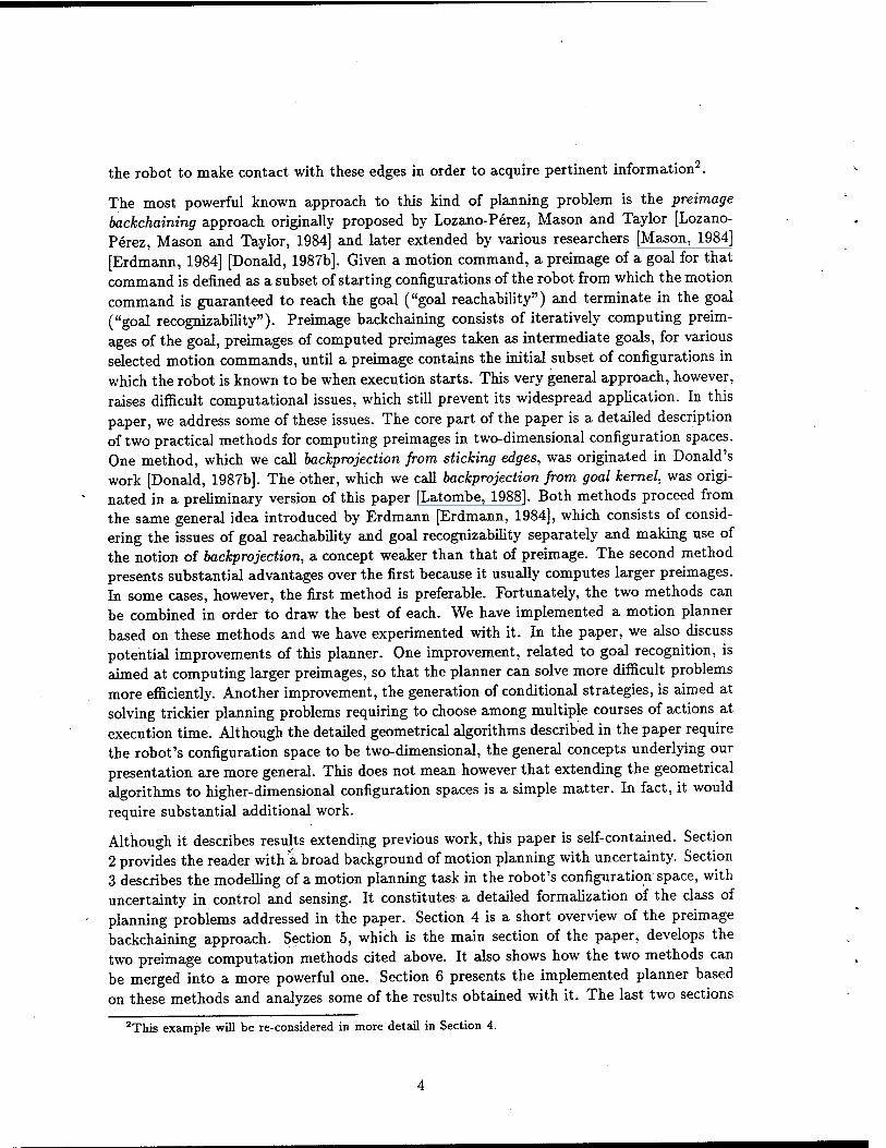
the robot to make contact with these edges in order to acquire pertinent information2.

The most powerful known approach to this kind of planning problem is the preimage backchaining approach originally proposed by Lozano-Perez, Mason and Taylor [Lozano- Perez, Mason and Taylor, 1984] and later extended by various researchers [Mason, 1984] [Erdmann, 1984] [Donald, 1987b]. Given a motion command, a preimage of a goal for that command is defined as a subset of starting configurations of the robot from which the motion command is guaranteed to reach the goal ("goal reachability") and terminate in the goal ("goal recognizability"). Preimage backchaining consists of iteratively computing preim- ages of the goal, preimages of computed preimages taken as intermediate goals, for various selected motion commands, until a preimage contains the initial subset of configurations in which the robot is known to be when execution starts. This very general approach, however, raises difficult computational issues, which still prevent its widespread application. In this paper, we address some of these issues. The core part of the paper is a detailed description of two practical methods for computing preimages in two-dimensional configuration spaces. One method, which we call backprojection from sticking edges, was originated in Donald's work [Donald, 1987b]. The other, which we call backprojection from goal kernel, was origi- nated in a preliminary version of this paper [Latombe, 1988]. Both methods proceed from the same general idea introduced by Erdmann [Erdmann, 1984], which consists of consid- ering the issues of goal reachability and goal recognizability separately and making use of the notion of backprojection, a concept weaker than that of preimage. The second method presents substantial advantages over the first because it usually computes larger preimages. In some cases, however, the first method is preferable. Fortunately, the two methods can be combined in order to draw the best of each. We have implemented a motion planner based on these methods and we have experimented with it. In the paper, we also discuss potential improvements of this planner. One improvement, related to goal recognition, is aimed at computing larger preimages, so that the planner can solve more difficult problems more efficiently. Another improvement, the generation of conditional strategies, is aimed at solving trickier planning problems requiring to choose among multiple courses of actions at execution time. Although the detailed geometrical algorithms described in the paper require the robot's configuration space to be two-dimensional, the general concepts underlying our presentation are more general. This does not mean however that extending the geometrical algorithms to higher-dimensional configuration spaces is a simple matter. In fact, it would require substantial additional work.

Although it describes results extending previous work, this paper is self-contained. Section 2 provides the reader with a broad background of motion planning with uncertainty. Section 3 describes the modelling of a motion planning task in the robot's configuration space, with uncertainty in control and sensing. It constitutes a detailed formalization of the class of planning problems addressed in the paper. Section 4 is a short overview of the preimage backchaining approach. Section 5, which is the main section of the paper, develops the two preimage computation methods cited above. It also shows how the two methods can be merged into a more powerful one. Section 6 presents the implemented planner based on these methods and analyzes some of the results obtained with it. The last two sections

2This example will be re-considered in more detail in Section 4.

discuss several potential improvements of the planner. Section 7 illustrates with a simple example how goal recognition may be improved by embedding more knowledge in a motion command. Section 8 investigates the generation of conditional strategies and extends the methods of Section 5 accordingly. Both sections present novel results related to the preimage backchaining approach.

2 Background

Research on robot motion planning has become active in the mid-seventies, when the goal of automatically programming robots from a geometrical description of the task was first considered attainable [Lozano-Perez, 1976] [Taylor, 1976] [Lieberman and Wesley, 1977]. Since the early eighties, a great deal of effort has been devoted to this domain. Part of this effort was motivated, on the one hand by the difficulties encountered in using explicit robot programming systems [Latombe, 1984] [Latombe et al, 1984], and on the other hand by the goal of introducing autonomous robots in hazardous environments (e.g., nuclear sites, space, undersea, mines). Although automating robot programming has turned out much more difficult than it first appeared, significant results with practical relevance have recently been obtained. A nicely illustrated exposure of why robot programming is difficult can be found in [Mazer, 1987].

During the last ten years, most of the effort has been oriented toward solving the path planning problem, i.e. the problem of planning motions without uncertainty. Over the last few years, it has produced several major results, both theoretical and practical. Theoretical results mostly concern lower and upper bounds of the time complexity of multiple variants of the path finding problem (e.g., see [Reif, 1979] [Canny, 1987] [Schwartz and Sharir, 1988]). In particular, it has been shown that planning the motion of a robot with arbitrarily many degrees of freedom is PSPACE-hard [Reif, 1979]. When the number of degrees of freedom is fixed, algorithms have been proposed, whose time complexity is polynomial in the number of algebraic surfaces bounding the objects and their maximal degree [Schwartz and Sharir, 1983] [Canny, 1987]. Some path planning methods have been produced as a side-effect of these results, but most of them involve very large constants and polynomial exponents and have hardly been implemented. Another important result is the development of the notion of Configuration Space [Arnold, 1978], both as a conceptual tool and as a technique for exploring motion planning problems3. This notion was popularized by Lozano-Perez in the early 80's [Lozano-Perez, 1981] [Lozano-Perez, 1983] and has given birth to various techniques for computing collision-free paths among obstacles (e.g., [Brooks and Lozano-Perez, 1983] [Gouzenes, 1984] [Laugier and Germain, 1985] [Donald, 1987a] [Lozano-Perez, 1987]). Finally, relatively fast path planning algorithms have been defined and implemented. Although these algorithms are usually not complete (they may fail to find a path while one exists), they can solve many practical problems. Lozano-Perez et al. [Lozano-Perez et al, 1987] and Mazer [Mazer, 1987] described an impressive system, Handey, capable of planning all the motions required for assembling simple parts, in the absence of significant uncertainty. Faverjon and Tournassoud [Faverjon and Tournassoud, 1987] reported on a system which uses an adaptation of Khatib's Potential Field method [Khatib,

3It is interesting to note that Configuration Space also becomes a popular tool in Qualitative Reasoning.

1986] for planning the motion of a manipulator with eight degrees of freedom, operating in the complex environment of a nuclear reactor. However, their planner requires human interactive help when it gets stuck into dead-ends (concavities). More recently, Barraquand and Latombe [Barraquand and Latombe, 1989] described another path planner combining hierarchical bitmap representations and numerical potential field techniques. This planner, which escapes local minima by executing Brownian motions, is quite fast in general and solves tricky path planning problems for robots with 10 degrees of freedom. It is also shown to be "probabilistically complete" (i.e., the probability to find a path, if one exists, converges toward 1, when the computing time increases). These practical techniques could bring substantial improvement to the programming of robot operations such as painting,

welding, and riveting.

The problem of planning motions in the presence of uncertainty is conceptually more difficult than the path finding problem. It has attracted less attention so far, and less results have been produced. Two approaches (at least) to this problem have been developed to some extent, in addition to preimage backchaining.

The first of these approaches was proposed independently by Lozano-Perez [Lozano-Perez, 1976] and Taylor [Taylor, 1976], and is known as the skeleton refining approach. It con- sists of: first, retrieving a plan skeleton appropriate to the task at hand and taking it as an initial plan; and second, iteratively modifying the skeleton by inserting complements (typically sensor-based readings). Complements are decided after checking the correctness of the skeleton, either by propagating uncertainty through the steps of the plan skeleton [Taylor, 1976], or by simulating several possible executions [Lozano-Perez, 1976]. Sub- sequent contributions to the approach have been brought by Brooks [Brooks, 1982], who developed a symbolic computation technique for propagating uncertainty forward and back- ward through plan skeletons, and by Pertin-Troccaz and Puget [Pertin-Troccaz and Puget, 1987], who proposed techniques for verifying the correctness of a plan and amending incor- rect plans. Backward propagation of uncertainty in this approach can be regarderd as a particular case of preimage backchaining with predetermined motion commands.

The second approach to motion planning with uncertainty has been proposed by Dufay and Latombe [Dufay and Latombe, 1984], and is known as the inductive learning approach. It consists of assembling input partial strategies into a global one. First, during a training phase the system uses the partial strategies to make on-line decisions and execute several instances of the task at hand. Second, during an induction phase, the system combines the execution traces generated during the training phase, and generalizes them into a global strategy. In fact, the training phase and the induction phase are interweaved. The genera- tion of a strategy for the task ends when new executions do not modify the current strategy. A system based on these principles has been implemented, and experimented successfuUy on several part mating tasks. Some aspects of this approach have been extended by Andreae

[Andreae, 1986].

Both the skeleton refining and inductive learning approaches deal with uncertainty in a second phase of planning. The plan skeleton and the local strategies used during the first phase could be produced using path planning methods assuming zero uncertainty. The second phase takes uncertainty into account, either by analyzing the correctness of

the current plan, or by directly experimenting with the local strategies and combining them into execution traces shaped by actual errors. In contrast, the rationale of preimage backchaining is that uncertainty may affect the overall structure of a plan, in such a way that a motion strategy may not be generated by modifying or composing plans generated assuming no uncertainty. Preimage backchaining is also a much more rigorous approach to motion planning with uncertainty than the other two approaches. In fact, the skeleton refinement and inductive learning approaches are essentially architectural framework to plan motions with uncertainty. Instead, preimage backchaining is a computational framework that can also be regarded as a clean formulation of motion planning with uncertainty.

On the other hand, preimage backchaining raises difficult computational issues. While there have been practical implementations of the skeleton refinement and inductive learning approaches, preimage backchaining is less advanced in that respect. This does not mean that the computational issues, which have to be faced with preimage backchaining, are completely absent from the other approaches. Preimage backchaining only makes explicit issues that are hidden in the other approaches because they are more ad-hoc. Solving these issues is a prerequisite to implementing preimage backchaining, but not to implementing the other aproaches.

The preimage backchaining approach was first presented by Lozano-Perez, Mason, and Taylor [Lozano-Perez, Mason and Taylor, 1984]. This early paper set up most of the basic framework. Large portions of Sections 3 and 4 below are based upon it. Mason [Mason, 1984] investigated several control schemes for searching the graph of preimages, includ- ing control schemes for generating conditional strategies, i.e. plans including conditional branching statements. He also analyzed the correctness and the completeness of the frame- work. Erdmann [Erdmann, 1984] [Erdmann, 1986] contributed to the approach in several ways. In particular, he separated the problem of computing a preimage into two sub- problems, reachability and recognizability. By considering reachability alone, he introduced the notion of "backprojection". (A backprojection of a goal for a given motion command is a subset of starting configurations of the robot from which the motion command is guaran- teed to reach the goal.) The two methods for computing preimages presented in this paper draw upon Erdmann's work. Donald [Donald, 1987b] [Donald, 1988a] extended the preim- age backchaining approach by considering uncertainty in the initial model of the workspace. The proposed extension consists of adding a dimension to the robot's configuration space for every parameter in the workspace whose value is not known accurately. The resulting space is known as the "generalized configuration space". Donald also introduced the notion of Error Detection and Recovery (EDR) strategies. Unlike the strategies considered in this paper, an EDR strategy is not guaranteed to succeed. However, it is guaranteed to either succeed or fail recognizably. Buckley [Buckley, 1986] proposed an application, of preimage backchaining to the analysis of the correctness of a given motion strategy. He also described a procedure for planning motion strategies in the forward direction. This procedure is based on the notion of "forward projection" (a more appropriate term would probably be "post- image"). The procedure discretizes the robot's configuration space into atomic regions based upon the consistent sensory data they should generate, and builds a transition graph between these regions. Buckley implemented a planner operating in a three-dimensional configuration space corresponding to a robot with three translations. The generation of

sensorless motion strategies using techniques inspired from preimage backchaining has been investigated by Erdmann and Mason [Erdmann and Mason, 1986]. Canny and Reif [Canny and Reif, 1987] [Canny, 1987] proved ihat the three-dimensional compliant motion plan- ning problem (the kind of problem attacked by the preimage backchaining approach) is non-deterministic exponential time hard (NEXPTIME-hard). Canny [Canny, 1989] gave an algorithm that computes motion strategies using the preimage backchaining approach when the envelope of the trajectories generated by the robot controller is described algebraically (this excludes illimited rotations). However, the algorithm takes time double exponential in the number of motion commands in the generated strategy. Donald [Donald, 1988b] described a less general algorithm for planning motion strategies in the plane, which takes time simple exponential in the number of commands.

In parallel to the research mentioned above, there has been an increasing interest in planning motions of objects in contact with other1 objects (e.g., [Hopcroft and Wilfong, 1986] [Valade, 1984] [Laugier and Theveneau, 1986] [Koutsou, 1986]). Like the research on path planning in collision-free space, most of this work has assumed accurate and complete prior knowledge of the workspace and perfect control o{ the robot motions. Recently, however, some of the methods developed for planning motions in contact space have been extended to handle some uncertainty [Desai, 1987] [Laugfer, 1989], in a way similar to that introduced by

Buckley [Buckley, 1986].

3 Task Modelling

3.1 Configuration Space

We are interested in planning the motion of an object A - the robot - in a workspace W populated by obstacles Bu i € [l,q]. A configuration of A is a specification of the position of every point in A with respect to a coordinate system embedded in W [Arnold, 1978]. The configuration space of A, denoted by C, is the set of all the possible configurations

of A

Each obstacle Bi maps in C to the subset CBi of configurations where A has no intersection

with Bi, i.e.: CBi = {q e CI A(q) C)Bi^9}

where A(q) denotes the subset of W occupied by A at configuration q. The region CBi is

called C-obstacle.

In general, C is a curved manifold. For instance, if A is a rigid planar object moving freely in >V = R2, then C = R2 x 5\ where 51 denotes the unit circle. If A is a rigid three- dimensional'object moving freely in W = R3, C = R3 x 50(3), where 50(3) denotes the Special Orthogonal Group of orthonormal matrices with determinant +1 [Arnold, 1978].

However, in the rest of the paper, things are much simpler from the geometrical point of view. We assume that A is a two-dimensional object that can only translate in the plane R2, e.g. an omnidirectional mobile robot that cannot rotate. A configuration is represented as q = (x,y), where x and y are the coordinates of a specific point of A, known as the reference point, with respect to the coordinate system embedded in W.

8

■q

|CB|

a

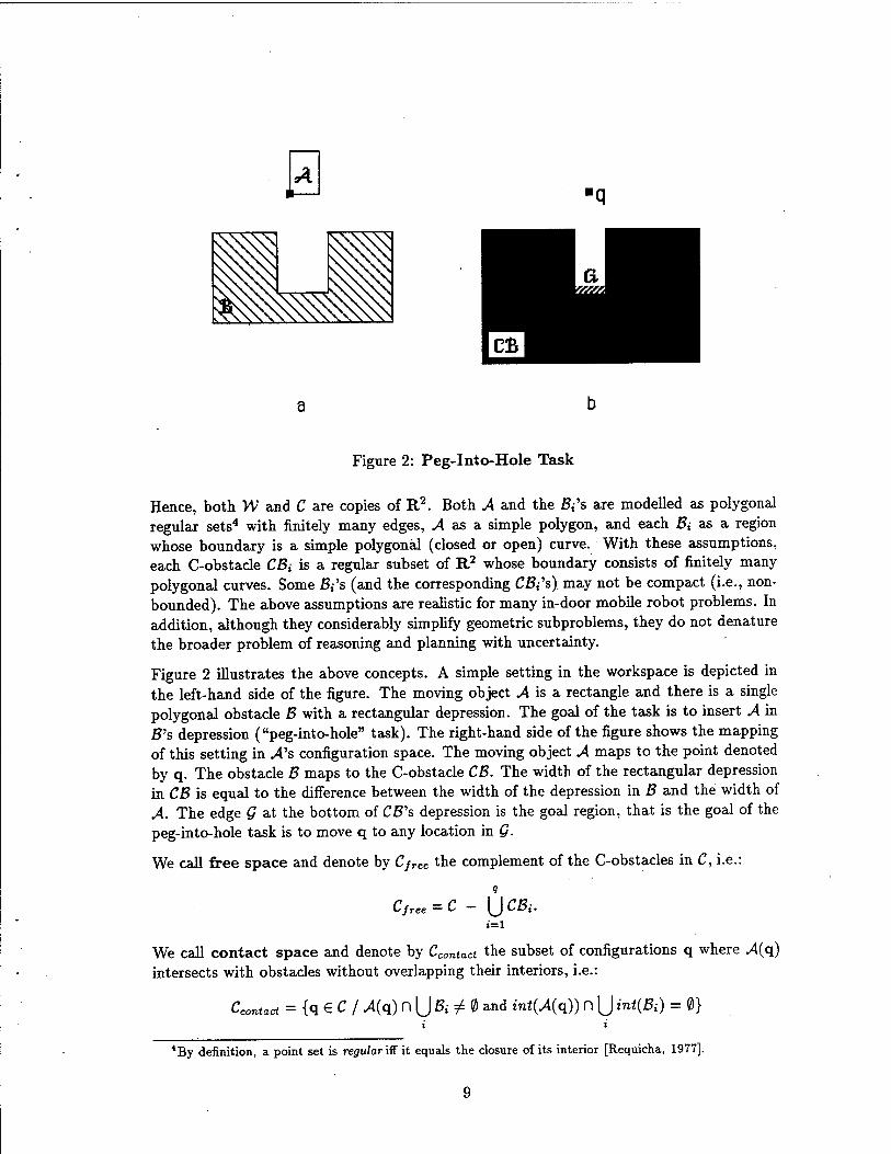
Figure 2: Peg-Into-Hole Task

Hence, both W and C are copies of R2. Both A and the 5,'s are modelled as polygonal regular sets4 with finitely many edges, A as a simple polygon, and each #, as a region whose boundary is a simple polygonal (closed or open) curve. With these assumptions, each C-obstacle CZ5, is a regular subset of R2 whose boundary consists of finitely many polygonal curves. Some Z?,'s (and the corresponding CZJ.'s) may not be compact (i.e., non- bounded). The above assumptions are realistic for many in-door mobile robot problems. In addition, although they considerably simplify geometric subproblems, they do not denature the broader problem of reasoning and planning with uncertainty.

Figure 2 illustrates the above concepts. A simple setting in the workspace is depicted in the left-hand side of the figure. The moving object A is a rectangle and there is a single polygonal obstacle B with a rectangular depression. The goal of the task is to insert A in ß's depression ("peg-into-hole" task). The right-hand side of the figure shows the mapping of this setting in ,4's configuration space. The moving object A maps to the point denoted by q. The obstacle B maps to the C-obstacle CB. The width of the rectangular depression in CB is equal to the difference between the width of the depression in B and the width of A. The edge Q at the bottom of Cß's depression is the goal region, that is the goal of the peg-into-hole task is to move q to any location in Q.

We call free space and denote by C/ree the complement of the C-obstacles in C, i.e.:

9

CjTee = C - \JCBi- t=l

We call contact space and denote by Ccontact the subset of configurations q where A(q) intersects with obstacles without overlapping their interiors, i.e.:

Ccontact = {q € C 1.4(q) n U B,-..± 0 and tn*(.A(q)) n |J ini(ft) = 0}

4By definition, a point set is regular iß it equals the closure of its interior [Requicha, 1977].

where int(S) denotes the interior of the set S.

We call valid space and denote by Cvaud the union of C/ree and Ccontact- A valid path between two configurations q! and q2 in Cvaiid is a continuous map r : [0,1] -»■ Cvaiid such

that r(0) = qi and r(l) = q2-

C/7.ee is an open subset of C, whose boundary, denoted by 0C/ree, is a finite set of polygonal curves. Ccontact is also a finite set of polygonal curves. It can be shown that dCJTee C Ccontact [Hopcroft and Wilfong, 1986]. In Figure 2, the strict inclusion of dCJree in Ccontact would occur iM's width was exactly equal to the width of ß's depression. Then, the depression in CB would degenerate to a line segment contained in Ccontact, but not in 9C/ree- In the rest of the paper, We also impose that each maximal connected subset of U?=1Cß; be homeomorphic to a closed disc, hence bounded by a simple curve [Massey, 1967] [Guillemin and Pollack, 1974]. This entails, in particular, that Ccontact = d{\Jq

i=1CBi) and Ccontact - dCfree- It also excludes the case where several subsets of C-obstacles "touch" each other at isolated points. More generally, it implies that Ccontact consists of a finite set of disjoint polygonal lines We call the outgoing (resp. ingoing) normal of an edge of Ccontact the unit vector normal of that edge pointing toward Cjree (resp. toward the interior of Uq

i=1CBi).

Let nA be the number of edges of A and nB the number of edges of all the obstacles. Ccontact contains 0(nAn2

B) edges, which can be computed in 0{n2An%log nAnB) time [Avnaim and

Boissonnat, 1987] [Sharir, 1987].

3.2 Motion Commands

We describe a motion command M as a pair (CS,TC). CS is called the control state- ment. Given a starting configuration qs, it determines a nominal trajectory of A, i.e. a

curve: r : t e [0, +00) ■-»■ r(t) € Cvaiid

with r(0) = qs and t denoting time. TC is called the termination condition. The controller stops the motion when TC evaluates to true. TC's arguments may be sensory inputs during the execution of the motion and the elapsed time since the beginning of the motion. In the following, we assume that the controller continuously monitors TC during execution and that the motion of A can be stopped instantaneously5.

We assume that .4's mode of control is "generalized damper" [Raibert and Craig, 1981] [Mason, 1981]. This basically means that CS is parameterized by a unit vector v called the commanded direction of motion6 in R2. As long as .4's configuration is m the free space, A moves along the direction v. When .4's configuration is in the contact space at a point other than a vertex, it may move away from the edge, slide along it, or stick to it. If v projects positively along the outgoing normal of the edge, it moves away. Otherwise, assuming a frictionless contact space, A's configuration slides along the projection of v on

sThe fact that these requirements cannot be exactly met by a real system should be taken into account in the specification of the uncertainty.

«Actually, v represents the commanded velocity of A But, for amplifying our presentation, we assume that the magnitude of the velocity is 1 and that it can be attained instantaneously.

10

the edge if this projection is non-zero and sticks to the edge if v points perpendicularly to it.

Friction in the contact space simply results in increasing the range of motion directions that stick to edges. If the friction coefficient is p > 0 (Coulomb law) and assuming no uncertainty in robot control, a generalized damper motion along v sticks to an edge if the magnitude of the angle between —v and the outgoing normal of the edge is less or equal to 4> = tan-1 ft (0 < <j> < x/2), i.e. if — v lies in the half-cone of angle 2</> whose axis points •along the outgoing normal of the edge (this half-cone is called the friction cone). The frictionless case corresponds to <f> = 0. The representation of friction in higher-dimensional spaces is investigated in [Erdmann, 1984].

Finally, for completeness, we must consider the case when «4's configuration is in the contact space at a vertex. A has reached the vertex either by coming from the free space and directly hitting the vertex, or by sliding along an edge abutting at the vertex. In the first case, A behaves as if it had hit one or the other of the two edges abutting at the vertex; hence, its motion may not be deterministic. In the second case, A moves (or sticks) as if its configuration was in the other edge abutting at the vertex.

3.3 Uncertainty in Control

Uncertainty in control is modelled as follows. Let v be the commanded direction of motion. At any instant during the motion, the actual direction of motion is a unit vector v*, such that the magnitude of the angle between v and v* is less than a fixed angle 0 < 7r/2. In other words, v* lies in a half-cone of angle 29 whose axis points along v. This half-cone is called the control uncertainty cone.

During motion, v* may vary arbitrarily between the two extreme orientations determined by v and 6. Thus, if A is in the free space, it moves along a trajectory whose tangent at any configuration is contained in the control uncertainty cone anchored at this configuration. If A's configuration is in the contact space, at a point other than a vertex, it may move away, slide, or stick, depending on the actual direction of motion v* relatively to the contact edge. In particular, if all unit vectors v* lying in the control uncertainty cone project positively on the outgoing normal of the edge, then A is guaranteed to move away from the edge. Instead, if the inverted control uncertainty cone is entirely contained in the friction cone, A sticks to the edge; if it is completely outside the friction cone and all the vectors in the control uncertainty cone project positively on the ingoing normal of the edge, A is guaranteed to slide in the direction of the projection of v on the edge.

3.4 Uncertainty in Sensing

We assume that the robot A is instrumented with two sensors - a position sensor and a force sensor - which we model below. Other sensors could be modelled in a similar fashion.

The position sensor measures the current configuration q of A. The uncertainty in the measurement is modelled as an open disc S(q, p) C R2 of fixed radius p centered at the measured configuration q. This means that if the position sensor gives q as the current con-

11

figuration of A, the actual configuration, denoted7 q*, may be anywhere in the disc E(q,p). Reciprocally, if the actual configuration is known to be q*, the measured configuration q may be anywhere in the disc £(q*,p). S is called the position uncertainty disc. Note that although q* can only be in Cvaiid, the measured configuration q may be in C - Cvaiid.

The force sensor measures the reaction force exerted on A. Under the current assumption that A can only translate, this force maps to an identical vector in C applied at the config- uration of A. (See [Erdmann, 1984] for a discussion of the notion of force in configuration space.) The force sensor is used to acquire information on whether A touches obstacles, or not, and if it touches an obstacle, on the orientation of the outgoing normal of contact space at the contact configuration. Thus, we assume that the output of the sensor at any instant is either the null vector or a unit vector.

At a certain instant, let q* be the actual configuration of A and v* the actual direction of motion. We denote by fj.(q*) the actual reaction force exerted on A at the same instant and we model the physical reality by the following definitions:

- if q* € Cfree, then fv.(q*) = 0;

- if q* € Cconuct, q* is in an edge E, not at a vertex, and v* projects positively on the outgoing normal of E, then f£.(q*) = 0;

- if q* € Ccontact, q* is in an edge E, not at a vertex, and -v* lies in the friction cone at the contact point, then f£.(q*) = — v*;

- if q* € Ccontact, q* is in an edge E, not at a vertex, and -v* projects positively on the outgoing normal of E, but lies outside the friction cone at the contact configuration, then f*,(q*) = f*, with f* being the solution of the following system of equations:

\angle{y,V)\ = <f>

v. r = v ■ (-v*)

sign{angle{y,f*)) = sign(angle{v,-\*))

where:

- v is the outgoing normal of E,

- angle(ni,n2) denotes the angle between vectors nx and n2,

- \a\ denotes the magnitude of a,

- ni -n2 denotes the inner product of vectors na and n2,

- sign(a) denotes the sign (-, 0, +) of a.

- if q* € Ccontact and q* is at a vertex, then let 1J and f2* be the reaction forces that would be generated by the two edges abutting at this vertex; fy«(q*) = f? + *2-

7Our convention is to denote a "nominal" quantity (e.g., a commanded direction of motion, a measured position, a measured force) by a bold letter (e.g., v, q, f) and the corresponding actual quantity by the same letter with superscript * (e.g., v*, q*, f).

12

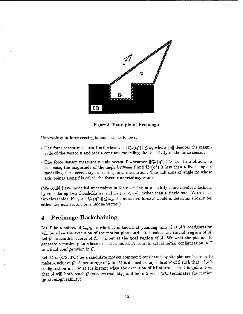
Figure 3: Example of Preimage

Uncertainty in force sensing is modelled as follows:

- The force sensor measures f = 0 whenever ||fv.(q*)|| <u, where ||'n|| denotes the magni- tude of the vector n and u> is a constant modelling the sensitivity of the force sensor.

- The force sensor measures a unit vector f whenever ||f^.(q*)|| > u. In addition, in this case, the magnitude of the angle between f and fy«(q*) is less than a fixed angle s modelling the uncertainty in sensing force orientation. The half-cone of angle 2e whose axis points along f is called the force uncertainty cone.

(We could have modelled uncertainty in force sensing in a slightly more involved fashion, by considering two thresholds u>i and u2 (wi < U2), rather than a single one. With these two thresholds, if u\ < ||fv.(q*)|| < u;2, the measured force F would undeterministically be, either the null vector, or a unique vector.)

4 Preimage Backchaining

Let I be a subset of Cvaiid in which it is known at planning time that A's configuration will be when the execution of the motion plan starts. 1 is called the initial region of A. Let G be another subset of Cvaiid input as the goal region of A. We want the planner to generate a motion plan whose execution moves A from its actual initial configuration in 1 to a final configuration in Q.

Let M = (CS,TC) be a candidate motion command considered by the planner in order to make A achieve Q. A preimage of Q for M is defined as any subset V of C such that: if -4's configuration is in V at the instant when the execution of M starts, then it is guaranteed that A will both reach Q (goal reachability) and be in Q when TC terminates the motion (goal recognizability).

13

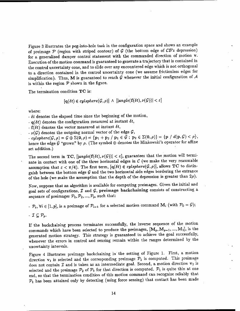
Figure 3 illustrates the peg-into-hole task in the configuration space and shows an example of preimage V (region with striped contour) of G (the bottom edge of CB's depression) for a generalized damper control statement with the commanded direction of motion v. Execution of the motion command is guaranteed to generate a trajectory that is contained in the control uncertainty cone, and to slide over any encountered edge which is not orthogonal to a direction contained in the control uncertainty cone (we assume frictionless edges for simplification). Thus, M is guaranteed to reach Q whenever the initial configuration of A is within the region V shown in the figure.

The termination condition TC is:

[q(6t)€cylsphere(G,p)] A [\angle{i{St),u{G))\< e)

where: - 8t denotes the elapsed time since the beginning of the motion, - q(St) denotes the configuration measured at instant St, - f(St) denotes the vector measured at instant St, - v\G) denotes the outgoing normal vector of the edge G-, - cylsphere(G,f>) = S0S(O,p)= {pi + p2 / Pi € G ; P2 6 S(0,p)} = {p / d{p,G) < p}, hence the edge G "grown" by p. (The symbol © denotes the Minkowski's operator for affine

set addition.)

The second term in TC, [\angle(t(6t),v(G))\ < e], guarantees that the motion wiU termi- nate in contact with one of the three horizontal edges in C (we make the very reasonable assumption that e < TT/4). The first term, [q(St) € cylsphere(G,p)], allows TC to distin- guish between the bottom edge G and the two horizontal side edges bordering the entrance of the hole (we make the assumption that the depth of the depression is greater than 2p).

Now, suppose that an algorithm is available for computing preimages. Given the initial and goal sets of configurations, X and G, preimage backchaining consists of constructing a sequence of preimages V\,Vi, ...,VP, such that:

- Vi, Vi € [l,p], is a preimage of 7?,_i for a selected motion command M, (with V0 = G);

-IQVp-

If the backchaining process terminates successfully, the inverse sequence of the motion commands which have been selected to produce the preimages, [Mp,Mp_i, ....MJ, is the generated motion strategy. This strategy is guaranteed to achieve the goal successfully, whenever the errors in control and sensing remain within the ranges determined by the uncertainty intervals.

Figure 4 illustrates preimage backchaining in the setting of Figure 1. First, a motion direction va is selected and the corresponding preimage V\ is computed. This preimage does not contain 1 and is taken as an intermediate goal. Second, a motion direction v2 is selected and the preimage V2 of Vi for that direction is computed. V\ is quite thin at one end, so that the termination condition of this motion command can recognize reliably that V\ has been attained only by detecting (using force sensing) that contact has been made

14

Figure 4: Illustration of Preimage Backchaining

with the edge denoted by E, which is part of Pi. Since V2 contains 1, the planning problem is solved with a sequence of two motions. Interestingly, the preimage backchaining process has resulted in identifying and using E as an intermediate "landmark" to help the reliable progression of the robot toward Q. Adding other types of sensors than position and force would make it possible to consider more landmarks.

The problem of generating the sequence of preimages can be transformed into the com- binatorial problem of searching a graph by selecting motion commands from a discretized set. The root of this graph is the goal region G, and each other node is a preimage region; each arc is a motion command, connecting a region to a preimage for this command. The construction of this graph requires the set of possible control statements to be discretized. With generalized damper control, this means discretizing the set of motion directions.

Searching the graph of preimages introduced above leads to generate sequential motion strategies, i.e. sequence of motion commands. In some cases, it is necessary or preferable to generate conditional strategies. We will address this issue in Section 8.

It is interesting to notice the relation between preimage backchaining and "goal regression" a classical planning method [Waldinger, 1975] [Nilsson, 1980]. Both methods consist of computing the precondition (ideally, the weakest one) whose satisfaction before executing an action guarantees that some goal condition will be satisfied after the action is executed. However, while preimage backchaining has a strong geometric flavor, goal regression is more logic-oriented.

15

5 Computation of Preimages

In the following, the word "goal" designates either the goal region Q of the motion planning problem, or any preimage taken recursively as an intermediate goal. A goal is generically

denoted by T.

5.1 Computational Issue

The notion of preimage combines two basic concepts, known as goal reachability and goal recognizability [Erdmann, 1984].

Goal reachability concerns only CS and relates to the fact that any trajectory obtained by executing CS from a preimage of a goal T should be guaranteed to reach T. Due to uncertainty in control, given a starting configuration, CS only specifies a nominal trajectory, but any execution of CS will produce an actual trajectory that is slightly different. The planner must be certain that all the possible actual trajectories consistent with both CS and control uncertainty will traverse T at some instant.

Reaching T, however, is not enough. The planner must also be certain that the termination condition TC will stop A in T (goal recognizability). This is a much more subtle notion. One can regard TC as an observer of the actual trajectory being executed. Since sensing is imperfect, TC perceives the actual trajectory as an observed trajectory, which is most likely to be neither the nominal one, nor the actual one. Thus, the problem for the planner is to: (1) infer the set of all the possible actual trajectories from both CS and the specified uncertainty in control; (2) infer the set of all the possible observed trajectories from both the possible actual trajectories and the specified uncertainty in sensing; (3) verify that, for every possible observed trajectory r, TC becomes true at some instant and when TC first becomes true, all the actual trajectories r* consistent with r (i.e., the trajectories which may be observed as r) have reached the goal. Then, it is guaranteed that the execution of

M will terminate in T.

Preimage computation has been investigated in depth in [Erdmann, 1984] and [Latombe, 1988]. For a given commanded direction of motion v, the ideal method would compute the maximal preimage of T, i.e. a preimage that is not contained in another preimage of T for v, and the method would also return the termination condition for the maximal preimage. Indeed, intuitively, a large preimage has more chance to include the initial region 1 than a small one; in addition, if it is considered recursively as an intermediate goal, a large preimage has more chance to admit large preimages than a small one (a goal which includes another goal definitely has a bigger preimage). Thus, considering larger preimages may reduce the size of the search graph; it may also produce "simpler" strategies, i.e. strategies made up of less motion commands. However, Erdmann [Erdmann, 1984] showed that: (1) there does not always exist a maximal preimage; (2) assuming there exists one, it may not be unique; and (3) if there exists a unique maximal preimage, it may depend in a subtle fashion on sensing history, the elapsed time since the beginning of the motion, and the knowledge embedded in the termination predicate (the predicate of TC).

8By definition, any subset of a preimage is also a preimage of the same goal.

16

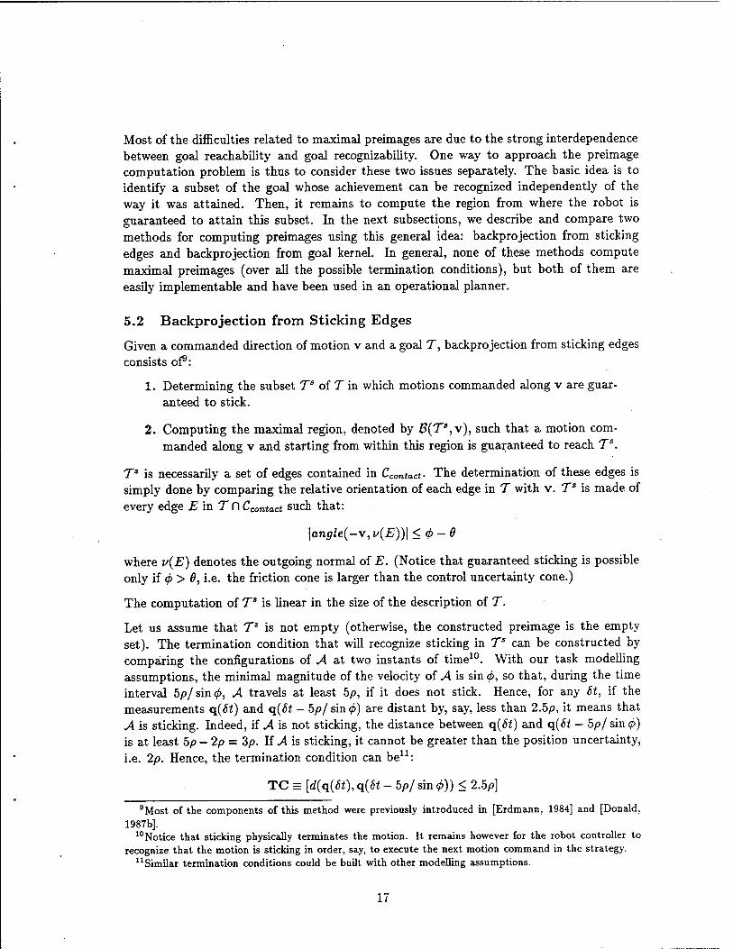
Most of the difficulties related to maximal preimages are due to the strong interdependence between goal reachability and goal recognizability. One way to approach the preimage computation problem is thus to consider these two issues separately. The basic idea is to identify a subset of the goal whose achievement can be recognized independently of the way it was attained. Then, it remains to compute the region from where the robot is guaranteed to attain this subset. In the next subsections, we describe and compare two methods for computing preimages using this general idea: backprojection from sticking edges and backprojection from goal kernel. In general, none of these methods compute maximal preimages (over all the possible termination conditions), but both of them are easily implementable and have been used in an operational planner.

5.2 Backprojection from Sticking Edges

Given a commanded direction of motion v and a goal 7", backprojection from sticking edges consists of9:

1. Determining the subset Ts of T in which motions commanded along v are guar- anteed to stick.

2. Computing the maximal region, denoted by #(Ts,v), such that a motion com- manded along v and starting from within this region is guaranteed to reach Ts.

Ts is necessarily a set of edges contained in Ccontact- The determination of these edges is simply done by comparing the relative orientation of each edge in T with v. Ts is made of every edge E in T C\ Ccontact such that:

\angle{-v,v{E))\<4>-9

where v(E) denotes the outgoing normal of E. (Notice that guaranteed sticking is possible only if <f> > 0, i.e. the friction cone is larger than the control uncertainty cone.)

The computation of Ts is linear in the size of the description of T.

Let us assume that Ts is not empty (otherwise, the constructed preimage is the empty set). The termination condition that will recognize sticking in Ts can be constructed by comparing the configurations of A at two instants of time10. With our task modelling assumptions, the minimal magnitude of the velocity of A is sin <f>, so that, during the time interval 5p/sin<£, A travels at least 5p, if it does not stick. Hence, for any St, if the measurements q(6t) and q(St - 5p/sin<£) are distant by, say, less than 2.5p, it means that A is sticking. Indeed, if A is not sticking, the distance between q(6t) and q(St - hpj sin</>) is at least 5p — 2p = dp. If A is sticking, it cannot be greater than the position uncertainty, i.e. 2/9. Hence, the termination condition can be11:

TC = [d(q(6t), q{8t - hpj sin <f>)) < 2.5/>]

9Most of the components of this method were previously introduced in [Erdmann, 1984] and [Donald, 1987b].

10 Notice that sticking physically terminates the motion. It remains however for the robot controller to recognize that the motion is sticking in order, say, to execute the next motion command in the strategy.

11 Similar termination conditions could be built with other modelling assumptions.

17

A

Figure 5: Computation of a Backprojection

where d denotes the Euclidean distance between two points in R2. The recording of position measurements can be discretized by only considering the instants St = k(5p/ sm<f>), with k = 0,1,2,..., since sticking is a stationary situation.

The region B{TS, v) is called the maximal backprojection of Ta for v. Erdmann [Erd- mann, 1984] gave the following simple algorithm to compute the maximal backprojection

of a single edge:

1. Mark every non-goal vertex such that at least one of the abutting edges is sticking (for v). Mark every non-goal vertex such that A may slide non-deterministically on any of the two abutting edges. Mark every goal vertex such that it is possible

. to slide away from the vertex on the non-goal abutting edge.

2. At every marked vertex erect two rays parallel to the edges of the inverted control uncertainty cone. Compute the intersection of these rays among themselves and with Ccontact- Interrupt each ray beyond the first intersection.

3. Beginning at the goal edge trace out the backprojection region.

The operations of this algorithm are iUustrated in Figure 5. There are three C-obstacles and the goal is the edge denoted by Ts. The vertices marked at step 1 are depicted as thick grey points. The computed backprojection is the region depicted with a striped contour.

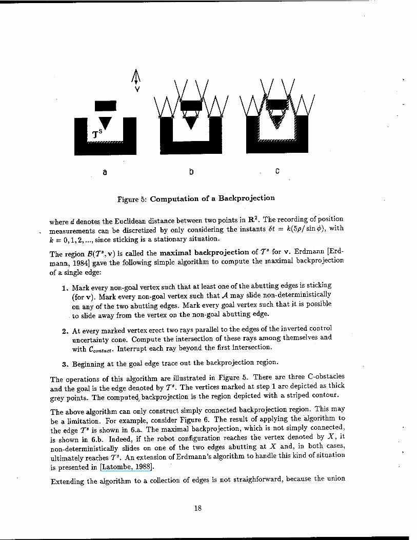
The above algorithm can only construct simply connected backprojection region. This may be a limitation. For example, consider Figure 6. The result of applying the algorithm to the edge Ts is shown in 6.a. The maximal backprojection, which is not simply connected, is shown in 6.b. Indeed, if the robot configuration reaches the vertex denoted by X, it non-deterministically slides on one of the two edges abutting at X and, in both cases, ultimately reaches Ts. An extension of Erdmann's algorithm to handle this kind of situation

is presented in [Latombe, 1988].

Extending the algorithm to a collection of edges is not straighforward, because the union

18

Figure 6: Multiply-Connected Backprojection

of the maximal backprojections of several edges considered individually may not be the maximal backprojection of the union of the edges, but a subset of it. Indeed, there niay be configurations from which a motion commanded along v is guaranteed to reach one of two edges, without knowing which one in advance.

The above algorithm has been generalized by Donald [Donald, 1987b] to an algorithm that generates the maximal backpro jection of any region T' described as the union of segments and polygonal regions in Cvaiid- Donald's algorithm first marks vertices in Ccontact as Erd- mann's algorithm does and then applies a line-sweep technique [Preparata and Shamos, 1985]. A line L is swept accross the plane, perpendicularly to v. The sweep starts at a position of L where it is tangent to T', with T' entirely lying on the side of L pointed by the vector —v. The sweep proceeds in the direction of the vector —v. During the sweep, the algorithm maintains the "status" of the sweeping line - i.e., the description of its intersection with Ccontact, T and the rays erected from the marked vertices. This status changes qualitatively only at discrete positions of the line, called "events". An event occurs whenever the line passes through a vertex of Ccontact, a vertex of T', the intersection of two rays, the intersection of a ray and Ccontact, or the intersection of a ray and T'. At each event, the algorithm updates the status of the line and the list of future events. Both the status of the line and the list of events can be represented in height-balanced trees [Aho, Hopcroft and Ullman, 1983]. During line sweeping, the algorithm traces out the contour of the backpro jection (which does not have to be simply connected). Sweep stops when the last point of the backpro jection contour has been encountered ("closing event").

The algorithm requires the backprojection to be bounded (so that the closing event ex- ists). This is achieved by imposing Cfree or all the C-obstacles to be bounded. Since it is monotonic, the algorithm also requires the actual direction of motion to never project negatively on the v direction. This is achieved if </> > 0, an assumption previously made so that guaranteed sticking be possible. Another algorithm is proposed in [Latombe, 1988], which is computationally less efficient, but does not require that <f> > 6.

The line-sweep algorithm computes B{T', v) in time O((n + m)log(n + m)), where n denotes

19

the total number of edges in Ccontact and m denotes the total number of edges of V. The contour of B(T', v) contains 0{n + m) edges.

Therefore, if m is the size of T, the computation of the preimage of T by backprojecting from the sticking edges in T takes 0((n + m)log(n + m)) time. In general, m < n.

5.3 Backprojection from Goal Kernel

Given a commanded direction of motion v and a goal T, backprojection from goal kernel

consists of:

1, Identifying the maximal subset of T, denoted by Xv(T), such that if it is attained by a motion commanded along v then the achievement of T is recognizable by a termination condition using instantaneous sensing only.

2. Determining the maximal region, denoted by ß(xv(T),v), such that a motion commanded along v starting from within this region is guaranteed to reach

Xv(T).

The subset Xv(X) is called the v-kernel of T. The region B(xv(T),v) is the maximal backprojection of Xv(^) for v (see Subsection 5.2).

The formal definition of the notion of v-kernel requires the two notions of v- consistency and v-distinguishability to be first introduced.

Let W(v) denote the control uncertainty cone for the commanded direction of motion v. We denote by ^(q*) the set of all the possible reaction forces that can be generated at configuration q* when the commanded direction of motion is v. By definition:

KW= U fv-(<i*)- vew(v)

(f£.(q*) has been defined in Subsection 3.4.) A straightforward algorithm computes ^'(q*) inV0(l) time. For example, let q* be in an edge E of Ccontacf, let the angle a between -v and the outgoing normal of E be such that the friction cone and the inverted control uncertainty cone at q* intersect, none of the two cones being fully contained in the other. The set ^(q") includes all the unit vectors originating at q* and lying inside the intersection of the two cones. It also includes vectors pointing along the ray of the friction cone which is closest from the vector -v. These vectors have magnitudes comprised between max{0, cos(a + 0)/ cos<£)

and 1.

We say that a configuration q* € Cmiid is v-consistent with a position measurement q and a force measurement f iff, when the robot commanded along v is at configuration q*, the measurements q and fare possible given the input workspace geometry and the model of uncertainty. The direction v plays an important role in v-consistency because the force that is measured in contact space depends on it. More formally, q» is v-consistent with q and f iff q* € £• (q, f), where /C;(q, f) is defined as follows:

- If f = 0, then:

20

LJ

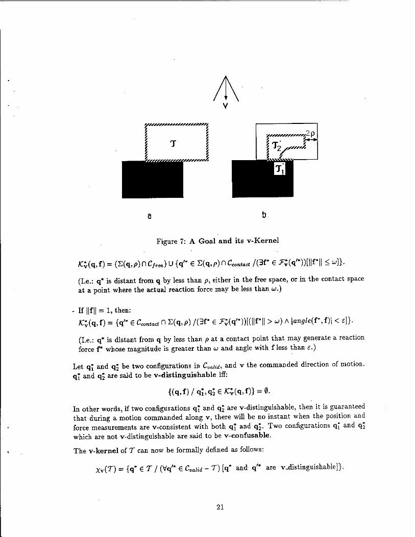
Figure 7: A Goal and its v-Kernel

A:;(q,f)= (S(q,/>)nC/ree)U{q'* € S(q,p)D Contact /(3T e ^v(q'*))[||r|| < «]}.

(I.e.: q* is distant from q by less than p, either in the free space, or in the contact space at a point where the actual reaction force may be less than w.)

- If ||f || = 1, then:

/Cy(q,f) = W* € Ccontact n E(q,p) /(3F € ^(q'*))[(||f|| > w) A |on5Zc(r,f)| < e]}.

(I.e.: q* is distant from q by less than p at a contact point that may generate a reaction force f* whose magnitude is greater than u and angle with f less than e.)

Let qj and q£ be two configurations in Cvaud, and v the commanded direction of motion. qj and q£ are said to be v-distinguishable iff:

{(q,f)/qI,q5€/C;(q,f)} = 0.

In other words, if two configurations qj and q? are v-distinguishable, then it is guaranteed that during a motion commanded along v, there will be no instant when the position and force measurements are v-consistent with both q^ and q£. Two configurations qj and q2 which are not v-distinguishable are said to be v-confusable.

The v-kernel of T can now be formally defined as follows:

Xv(T) = {q* € T / (Vq'* € Cvalid - T) [q* and q" are v_distinguishable]}.

21

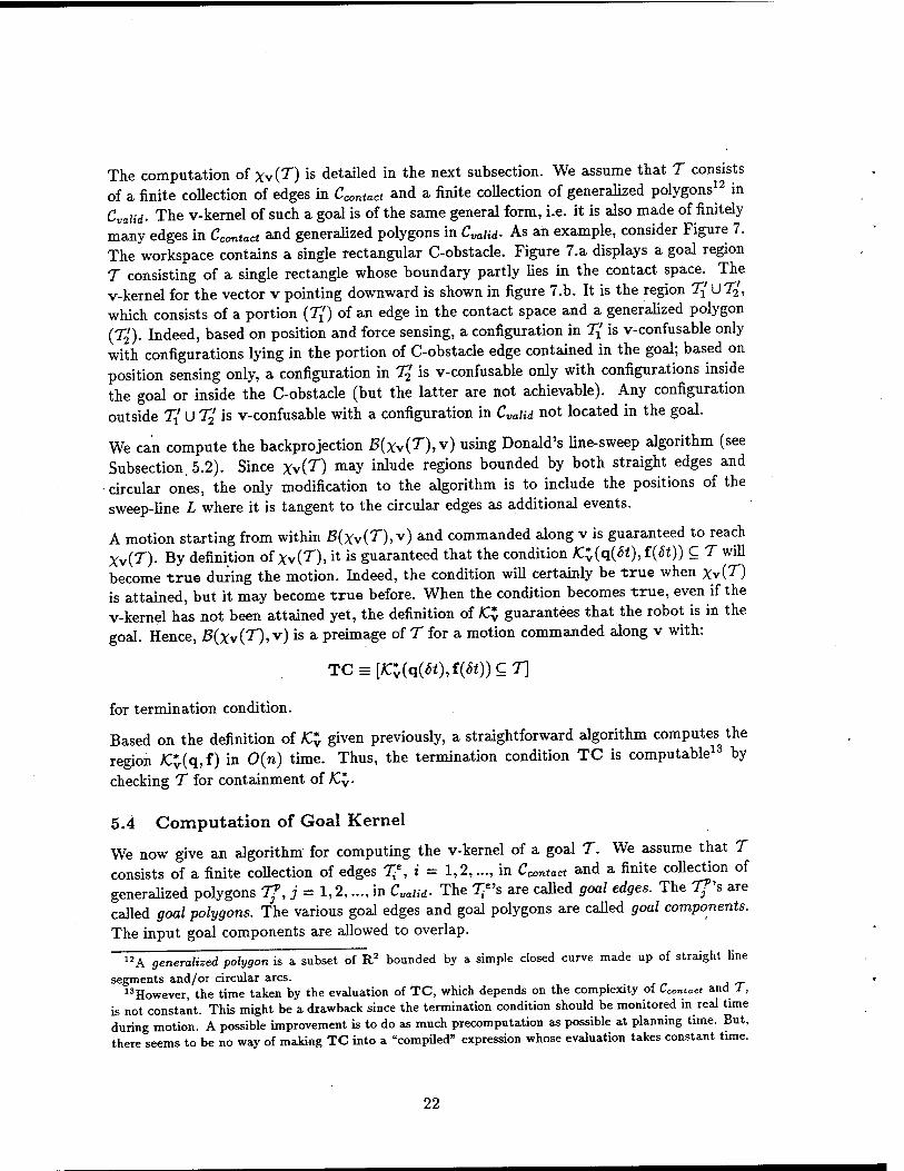
The computation of Xv(T) is detailed in the next subsection. We assume that T consists of a finite collection of edges in CC0Titact and a finite collection of generalized polygons*2 in Cvalid- The v-kernel of such a goal is of the same general form, i.e. it is also made of finitely many edges in Ccontaci and generalized polygons in £*/«. As an example, consider Figure 7. The workspace contains a single rectangular C-obstacle. Figure 7.a displays a goal region T consisting of a single rectangle whose boundary partly lies in the contact space. The v-kernel for the vector v pointing downward is shown in figure 7.b. It is the region Tx UT2, which consists of a portion (T{) of an edge in the contact space and a generalized polygon (7jf). Indeed, based on position and force sensing, a configuration in T{ is v-confusable only with configurations lying in the portion of C-obstacle edge contained in the goal; based on position sensing only, a configuration in % is v-confusable only with configurations inside the goal or inside the C-obstacle (but the latter are not achievable). Any configuration outside T{ U 7^' is v-confusable with a configuration in Cvaiid not located in the goal.

We can compute the backprojection B{xv(X),\) using Donald's line-sweep algorithm (see Subsection, 5.2). Since Xv(D may inlude regions bounded by both straight edges and

• circular ones, the only modification to the algorithm is to include the positions of the sweep-line L where it is tangent to the circular edges as additional events.

A motion starting from within B(xv(T),v) and commanded along v is guaranteed to reach Xv(T). By definition of Xv(T), it is guaranteed that the condition K.^{q(6t),f{St)) C T will become true during the motion. Indeed, the condition will certainly be true when Xy{T) is attained, but it may become true before. When the condition becomes true, even if the v-kernel has not been attained yet, the definition of K% guarantees that the robot is in the goal. Hence, £(XvCO, v) is a preimage of T for a motion commanded along v with:

TC = [JCl(q{6t),f(6t))CT]

for termination condition.

Based on the definition of £* given previously, a straightforward algorithm computes the region JC${q,f) in 0(n) time. Thus, the termination condition TC is computable13 by checking T for containment of fCy.

5.4 Computation of Goal Kernel

We now give an algorithm for computing the v-kernel of a goal T. We assume that T consists of a finite collection of edges Tf, i = 1,2,..., in Ccontact and a finite collection of generalized polygons 7j, j = 1,2,..., in Cvaiid. The %e's are called goal edges. The Ij's are called goal polygons. The various goal edges and goal polygons are called goal components. The input goal components are allowed to overlap.

12 A generalized polygon is a subset of R2 bounded by a simple closed curve made up of straight line

segments and/or circular arcs. "However, the time taken by the evaluation of TC, which depends on the complexity of Contact and T,

is not constant. This might be a drawback since the termination condition should be monitored in real time during motion. A possible improvement is to do as much precomputation as possible at planning time. But, there seems to be no way of making TC into a "compiled" expression whose evaluation takes constant time.

22

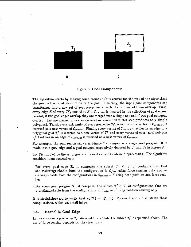
Figure 8: Goal Components

The algorithm starts by making some cosmetic (but crucial for the rest of the algorithm) changes to the input description of the goal. Basically, the input goal components are transformed into a new set of goal components, such that no two of them overlap. First, every edge E of every Tf, such that E C Ccontact-, is inserted in the collection of goal edges. Second, if two goal edges overlap they are merged into a single one and if two goal polygons overlap, they are merged into a single one (we assume that this step produces only simple polygons). Third, every extremity of every goal edge 7^e, which is not a vertex in Ccontact, is inserted as a new vertex of Ccontact- Finally, every vertex of Ccontact that lies in an edge of a polygonal goal Tf is inserted as a new vertex of Tf and every vertex of every goal polygon Tf that lies in an edge of Ccontact is inserted as a new vertex of Ccontact-

For example, the goal region shown in Figure 7.a is input as a single goal polygon. It is made into a goal edge and a goal polygon respectively denoted by 7i and T? in Figure 8.

Let {7i,..., TN) be the set of goal components after the above preprocessing. The algorithm considers them successively:

- For every goal edge 7;, it computes the subset T( C % of configurations that are v-distinguishable from the configuration in CjTee using force sensing only and v- distinguishable from the configurations in Contact — T using both position and force sens- ing.

- For every goal polygon Tj, it computes the subset TJ C Tj of configurations that are v-distinguishable from the configurations in Cvaiid — T using position sensing only.

It is straightforward to verify that XviT) = ULi V- Figures 8 and 7.b illustrate these computations, which we detail below.

5.4.1 Kernel in Goal Edge

Let us consider a goal edge %. We want to compute the subset T{, as specified above. The use of force sensing depends on the direction v.

23

Let us denote by ^v(q*) the set of all the possible force measurements that can be obtained at configuration q*, when the commanded direction of motion is v. This set can be derived

from -Fv(q*) a8 follows:

- If J\J(q"") contains a vector f* such that ||f*|| < u, then 0 € ^v(q*)-

- Let f be a unit length vector. If Fv(q*) contains a vector F such that ||F|| > u and

\angle(f,F)| < e, then f € ^v(q*)-

Although it is easy to construct :Fv(q*) explicitly, we will see below that this is not necessary.

We denote by Tv(%) the set JFv(q*) for any q* € %. A configuration in % \s v- distinguishable from a configuration in CfTee iff 0 g ?*{!$. Hence, if 0 € ^V(^), ^ - 0-

Assume that 0 $ Tv{%). Then, a configuration q* € % is v-distinguishable from any configuration in CfTee. It is v-distinguishable from a configuration q" contained in an edge

hi C ^contact *"•

- either q" £ S(q*,2p), i.e. the two configurations are sufficiently far apart,

- or TV(E) n Fv{Ti) = 0> i-e- the two edges have sufficiently different orientations.

Therefore, the algorithm for computing 7? is the following:

if 0 € Fv(Tl) then return 0; else S <— T{\

for every edge E € Cconfact, .£ £ 7", do

if Fy{E)nrvpi)?Q then S *-S- cylsphere(E,2p);

endif; enddo; return 51;

endif;

where cylsphere{E,2p) = {p / <*(p,£) < 2p} (see Section 4).

The above algorithm does not require the explicit computation of rv{?i)- The test 0 € Tv(7l) can easily be performed by computing the minimal force in F$(7i). The test Tv{E)n Tv(Ti) j- 0 requires the cones spanned by the forces in T*(E) and T*{T{) to be first computed, next "grown" by s, and finally intersected.

77 is computed in 0(n) time.

5.4.2 Kernel in Goal Polygon

Let us consider a goal polygon Tj. We want to compute the subset 7J of configurations that are v-distinguishable from the configurations in CvaHd - T using position sensing only.

24

2E|T.' i

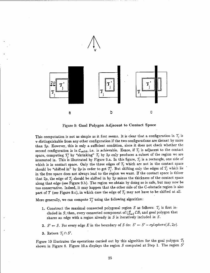
Figure 9: Goal Polygon Adjacent to Contact Space

This computation is not as simple as it first seems. It is clear that a configuration in Tj is v-distinguishable from any other configuration if the two configurations are distant by more than 2p. However, this is only a sufficient condition, since it does not check whether the second configuration is in Cvaiid, i-e. is achievable. Hence, if Tj is adjacent to the contact space, computing Tj by "shrinking" Tj by 2/9 only produces a subset of the region we are interested in. This is illustrated by Figure 9.a. In this figure, TJ is a rectangle, one side of which is in contact space. Only the three edges of Tj which are not in the contact space should be "shifted in" by 2/9 in order to get T[. But shifting only the edges of Tj which lie in the free space does not always lead to the region we want. If the contact space is thiner that 2p, the edge of Tj should be shifted in by 2/9 minus the thickness of the contact space along that edge (see Figure 9.b). The region we obtain by doing so is safe, but may now be too conservative. Indeed, it may happen that the other side of the C-obstacle region is also part of T (see Figure 9.c), in which case the edge of Tj may not have to be shifted at all.

More generally, we can compute 7J using the following algorithm:

1. Construct the maximal connected polygonal region S as follows: Tj is first in- cluded in 5; then, every connected component of ULiC^' and §oal Polyg°n that

shares an edge with a region already in 5 is iteratively included in S.

2. S' <- S. For every edge E in the boundary of S do: S' «- S' - cylsphere{E, 1p).

3. Return Tj D S'.

Figure 10 illustrates the operations carried out by this algorithm for the goal polygon T2

shown in Figure 8. Figure lO.a displays the region 5 computed at Step 1. The region S'

25

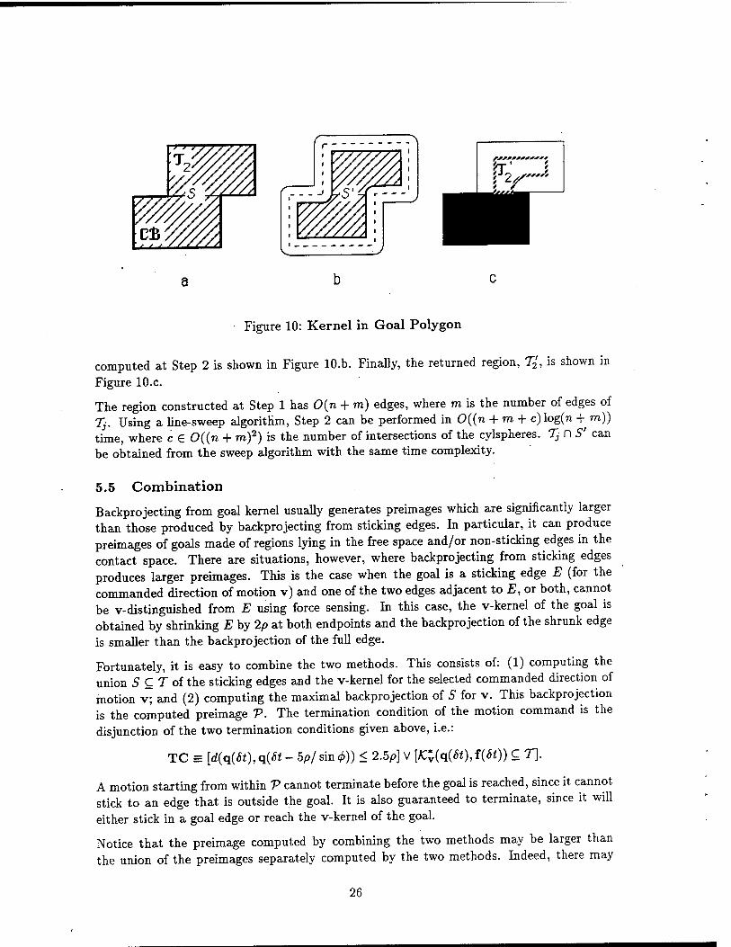
(r

^^ r i VS'%

r ■

'WB. \ • )

m Figure 10: Kernel in Goal Polygon

computed at Step 2 is shown in Figure lO.b. Finally, the returned region, T2', is shown in

Figure lO.c.

The region constructed at Step 1 has 0{n + m) edges, where m is the number of edges of Tj. Using a line-sweep algorithm, Step 2 can be performed in 0((n + m + c)log(n + m)) time, where c 6 0((n + m)2) is the number of intersections of the cylspheres. Tj f~l S' can be obtained from the sweep algorithm with the same time complexity.

5.5 Combination

Backprojecting from goal kernel usually generates preimages which are significantly larger than those produced by backprojecting from sticking edges. In particular, it can produce preimages of goals made of regions lying in the free space and/or non-sticking edges in the contact space. There are situations, however, where backprojecting from sticking edges produces larger preimages. This is the case when the goal is a sticking edge E (for the commanded direction of motion v) and one of the two edges adjacent to E, or both, cannot be v-distinguished from E using force sensing. In this case, the v-kernel of the goal is obtained by shrinking E by 2/9 at both endpoints and the backprojection of the shrunk edge is smaller than the backprojection of the full edge.

Fortunately, it is easy to combine the two methods. This consists of: (1) computing the union 5 C T of the sticking edges and the v-kernel for the selected commanded direction of motion v; and (2) computing the maximal backprojection of S for v. This backprojection is the computed preimage V. The termination condition of the motion command is the disjunction of the two termination conditions given above, i.e.:

TC = [d(q(8t),q(6t- 5p/sm<f>)) < 2.5p] V [IC*y(q(6t),f(6t)) C T\.

A motion starting from within V cannot terminate before the goal is reached, since it cannot stick to an edge that is outside the goal. It is also guaranteed to terminate, since it will either stick in a goal edge or reach the v-kernel of the goal.

Notice that the preimage computed by combining the two methods may be larger than the union of the preimages separately computed by the two methods. Indeed, there may

26

exist starting configurations from where the motion commanded along v is guaranteed to reach either a sticking edge in the goal or the goal v-kernel, without knowing which one in advance.

6 Implementation and Experimentation

We have implemented a motion planner based on the preimage backchaining approach. This planner computes preimages using either the backprojection-from-sticking-edge method, the backprojection-from-kernel method, or the combination of the two. The user inputs the description of the configuration space, the goal region Q, and the initial region X. If successful, the planner returns a motion plan in the form of a sequence of commanded directions of motion and the associated sequence of computed preimages. The method used for computing the preimages determines the termination condition of every motion command in the plan. The planner is implemented in Allegro Common Lisp on an Apple Macintosh II computer.

The planner constructs a graph of preimages by considering commanded motion directions with the orientations {kir/K}k=o,...,2K-i, where K is input by the user. In our experiments, we used K = 2 or 4. The planner searches the graph in a breadth-first fashion, but various (and probably better) other search techniques could have been used instead (e.g., A*).

The algorithms implemented in the planner are essentially those described above, with some variations. In particular, the backprojection of a region is computed using an algorithm similar to that described in [Latombe, 1988], rather than the line-sweep-based algorithm (which would be faster). The planner also approximates conservatively the generalized polygonal v-kernels by regular polygons. These changes have no major impact on the visible operations of the planner.

Below we describe experimental results obtained with the planner. In this decription, we call method 1 (resp. 2, 3) the backprojection-from-sticking-edges method (resp. the backprojection-from-kernel method, the combination of the two methods). In all the exam- ples shown, the initial region is a single point; in the figures it is the center of a disc that depicts position uncertainty. The control uncertainty cone and force uncertainty cone are not depicted. The figures are generated by the planner and are of a slightly different style than the figures in the rest of the paper.

Figures ll.ä and ll.b illustrate motion plans generated by the planner, using method 1 and method 2, respectively. None of them shows the computed preimages. The goal is the rectangular region Q. The plan constructed using method 1 consists-of 5 steps, defined by the commanded directions of motion vx through v5. The corresponding sticking edges are T\ through T5. (More precisely, % is the intersection of the preimage of %+i and the sticking subset of Ccontact- A motion along v,- issued from within 7i_i is guaranteed to stop in Ti, but some configurations in % may not be reachable.) The plan constructed using method 2 is simpler and only consists of a single motion commanded along v.

Figure 12 shows an example where method 1 (Figure 12.a) produceds a simpler plan than method 2 (Figure 12.b). Figure 12.b displays two intermediate preimages. The third preim-

27

vx

Figure 11: Example 1

28

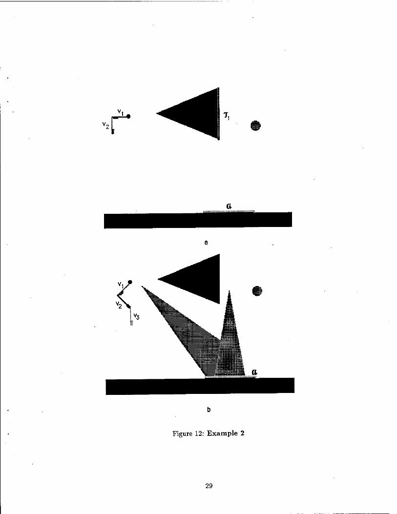
r

Figure 12: Example 2

29

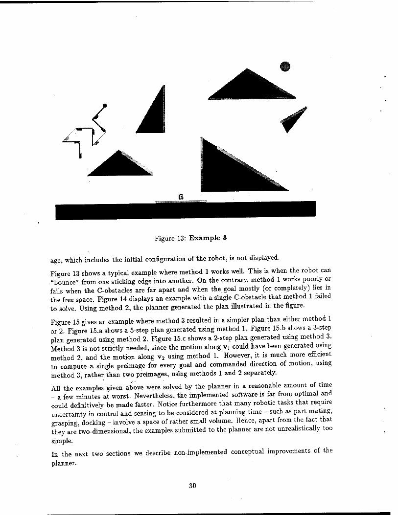
Figure 13: Example 3

age, which includes the initial configuration of the robot, is not displayed.

Figure 13 shows a typical example where method 1 works well. This is when the robot can "bounce" from one sticking edge into another. On the contrary, method 1 works poorly or fails when the C-obstacles are far apart and when the goal mostly (or completely) lies in the free space. Figure 14 displays an example with a single C-obstacle that method 1 failed to solve. Using method 2, the planner generated the plan illustrated in the figure.

Figure 15 gives an example where method 3 resulted in a simpler plan than either method 1 or 2. Figure 15.a shows a 5-step plan generated using method 1. Figure 15.b shows a 3-step plan generated using method 2. Figure 15.c shows a 2-step plan generated using method 3. Method 3 is not strictly needed, since the motion along Vi could have been generated using method 2, and the motion along v2 using method 1. However, it is much more efficient to compute a single preimage for every goal and commanded direction of motion, using method 3, rather than two preimages, using methods 1 and 2 separately.

All the examples given above were solved by the planner in a reasonable amount of time - a few minutes at worst. Nevertheless, the implemented software is far from optimal and could definitively be made faster. Notice furthermore that many robotic tasks that require uncertainty in control and sensing to be considered at planning time - such as part mating, grasping, docking - involve a space of rather small volume. Hence, apart from the fact that they are two-dimensional, the examples submitted to the planner are not unrealistically too

simple.

In the next two sections we describe non-implemented conceptual improvements of the

planner.

30

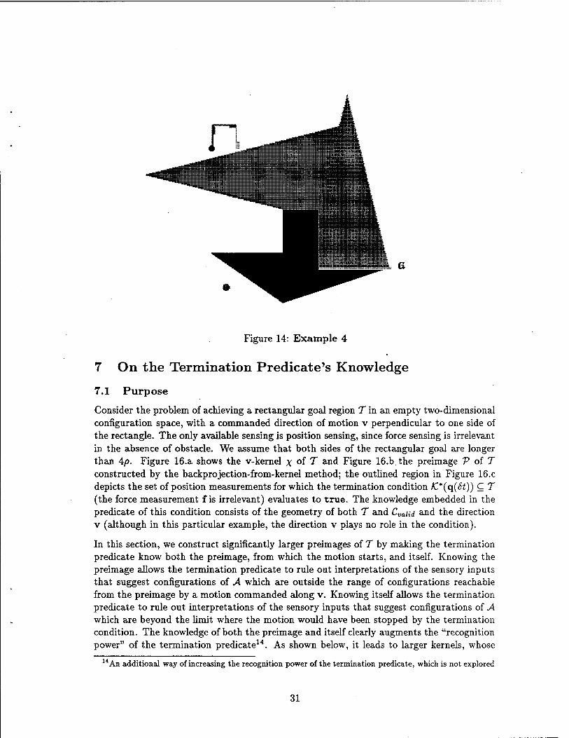
a

Figure 14: Example 4

7 On the Termination Predicate's Knowledge

7.1 Purpose

Consider the problem of achieving a rectangular goal region T in an empty two-dimensional configuration space, with a commanded direction of motion v perpendicular to one side of the rectangle. The only available sensing is position sensing, since force sensing is irrelevant in the absence of obstacle. We assume that both sides of the rectangular goal are longer than 4/). Figure 16.a shows the v-kernel x °f T aQd Figure 16.b.the preimage V of T constructed by the backprojection-from-kernel method; the outlined region in Figure 16.c depicts the set of position measurements for which the termination condition K."(q(6t)) C T (the force measurement f is irrelevant) evaluates to true. The knowledge embedded in the predicate of this condition consists of the geometry of both T and Cvaud and the direction v (although in this particular example, the direction v plays no role in the condition).

In this section, we construct significantly larger preimages of T by making the termination predicate know both the preimage, from which the motion starts, and itself. Knowing the preimage allows the termination predicate to rule out interpretations of the sensory inputs that suggest configurations of A which are outside the range of configurations reachable from the preimage by a motion commanded along v. Knowing itself allows the termination predicate to rule out interpretations of the sensory inputs that suggest configurations of A which are beyond the limit where the motion would have been stopped by the termination condition. The knowledge of both the preimage and itself clearly augments the "recognition power" of the termination predicate14. As shown below, it leads to larger kernels, whose

4 An additional way of increasing the recognition power of the termination predicate, which is not explored

31

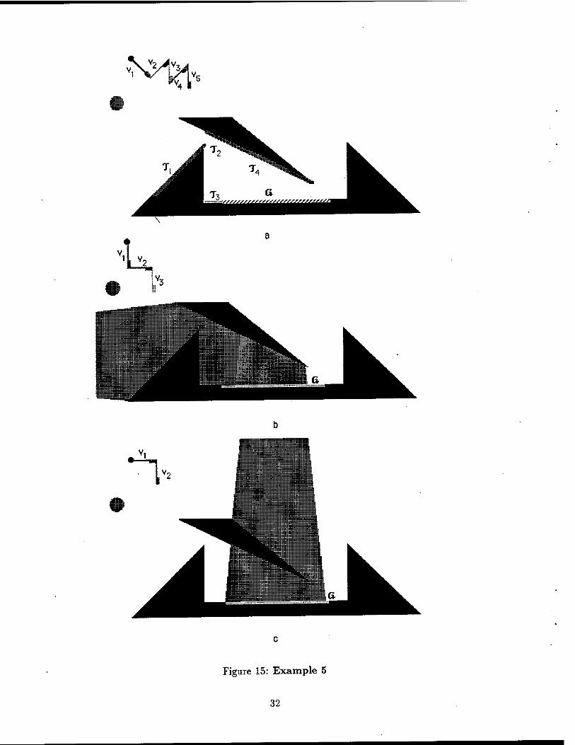
V2^V3j

H v

Figure 15: Example 5

32

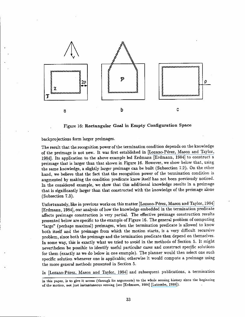
Figure 16: Rectangular Goal in Empty Configuration Space

backprojections form larger preimages.

The result that the recognition power of the termination condition depends on the knowledge of the preimage is not new. It was first established in [Lozano-Perez, Mason and Taylor, 1984]. Its application to the above example led Erdmann [Erdmann, 1984] to construct a preimage that is larger than that shown in Figure 16. However, we show below that, using the same knowledge, a slightly larger preimage can be built (Subsection 7.2). On the other hand, we believe that the fact that the recognition power of the termination condition is augmented by making the condition predicate know itself has not been previously noticed. In the considered example, we show that this additional knowledge results in a preimage that is significantly larger than that constructed with the knowledge of the preimage alone (Subsection 7.3).

Unfortunately, like in previous works on this matter [Lozano-Perez, Mason and Taylor, 1984] [Erdmann, 1984], our analysis of how the knowledge embedded in the termination predicate affects preimage construction is very partial. The effective preimage construction results presented below are specific to the example of Figure 16. The general problem of computing "large" (perhaps maximal) preimages, when the termination predicate is allowed to know both itself and the preimage from which the motion starts, is a very difficult recursive problem, since both the preimage and the termination predicate then depend on themselves. In some way, this is exactly what we tried to avoid in the methods of Section 5. It might nevertheless be possible to identify useful particular cases and construct specific solutions for them (exactly as we do below in one example). The planner would then select one such specific solution whenever one is applicable; otherwise it would compute a preimage using the more general methods presented in Section 5.

In [Lozano-Perez, Mason and Taylor, 1984] and subsequent publications, a termination

in this paper, is to give it access (through its arguments) to the whole sensing history since the beginning of the motion, not just instantaneous sensing (see [Erdmann, 1984] [Latombe, 1988]).

33

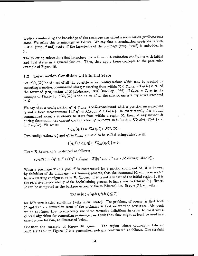
predicate embedding the knowledge of the preimage was called a termination predicate with state. We refine this terminology as follows. We say that a termination predicate is with initial (resp. final) state iff the knowledge of the preimage (resp. itself) is embedded in

it.

The following subsections first introduce the notions of termination conditions with initial and final states in a general fashion. Then, they apply these concepts to the particular

example of Figure 16.

7.2 Termination Condition with Initial State

Let TVvilZ) be the set of all the possible actual configurations which may be reached by executing a motion commanded along v starting from within H C Cvaiid- FVv(U) is called the forward projection of K [Erdmann, 1984] [Buckley, 1986].' If Cvaiid = C, as in the example of Figure 16, TVv(Tl) is the union of all the control uncertainty cones anchored

in 11.

We say that a configuration q* G Cvaiid is v-ft-consistent with a position measurement q and a force measurement f iff q* G K%(q,t) n TVv(1l). In other words, if a motion commanded along v is known to start from within a region 11, then, at any instant St during the motion, the current configuration q* is known to be both in fCy(q{St), f(St)) and

in TVV(1Z). We write: £;,*(q, *) = £v(q. *)n FPv(K).

Two configurations qj and qj in Cvaiid are said to be v-ft-distinguishable iff:

{(q,f)/qi,q;e£O,*(q,f)} = 0-

The v-7£-kernel of T is defined as follows:

Xv,n(T) = {q* € T / (Vq" € Cvaiid - T)[q" and q'* are v_ft_distinguishable]}.

When a preimage V of a goal T is constructed for a motion command M, it is known, by definition of the preimage backchaining process, that the command M win be executed from a starting configuration in V. (Indeed, if V is not a subset of the initial region I, it is the recursive responsibility of the backchaining process to find a way to achieve V.). Hence, V can be computed as the backprojection of the v-P-kernel, i.e. B{xv,v(J)>v), with:

TC = [/C;i7>(q(^),f(^))CT]

for M's termination condition (with initial state). The problem, of course, is that both V and TC are defined in term of the preimage V that we want to construct. Although we do not know how to effectively use these recursive definitions in order to construct a general algorithm for computing preimages, we think that they might at least be used in a case-by-case fashion, as illustrated below.

Consider the example of Figure 16 again. The region whose contour is labelled ABCDEFGH in Figure 17 is a generalized polygon constructed as follows. The straight

34

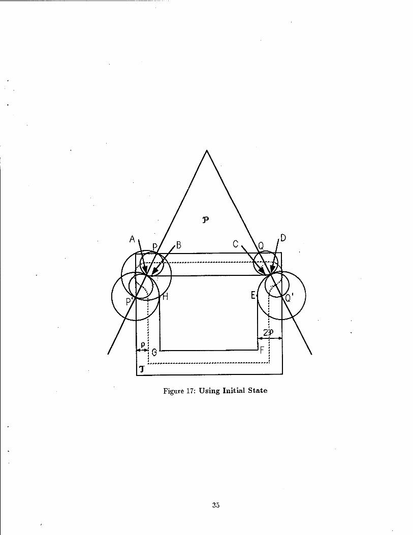
Figure 17: Using Initial State

35

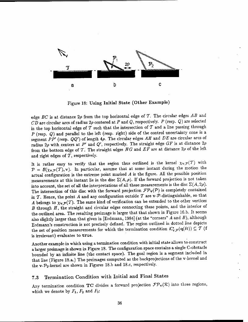
Figure 18: Using Initial State (Other Example)

edge BC is at distance 2p from the top horizontal edge of T. The circular edges AB and CD are circular arcs of radius 2p centered at P and Q, respectively. P (resp. Q) are selected in the top horizontal edge of T such that the intersection of 7 and a line passing through P (resp. Q) and parallel to the left (resp. right) side of the control uncertainty cone is a segment PP' (resp. QQ') of length 4/>. The circular edges AH and DE are circular arcs of radius 2p with centers at P' and Q', respectively. The straight edge GF is at distance 2/3 from the bottom edge of T. The straight edges EG and EF are at distance 2p of the left and right edges of T, respectively.

It is rather easy to verify that the region thus outlined is the kernel Xv,v{T) with •p _ ß(xv,-p(^'),v). In particular, assume that at some instant during the motion the actual configuration is the extreme point marked A is the figure. All the possible position measurements at this instant lie in the disc X(A,p). If the forward projection is not taken into account, the set of all the interpretations of all these measurements is the disc T,(A,2p). The intersection of this disc with the forward projection TVV{V) is completely contained in T. Hence, the point A and any configuration outside T are v-V-distinguishable, so that A belongs to Xv,v(J)- The same kind of verification can be extended to the other vertices B through H, the straight and circular edges connecting these points, and the interior of the outlined area. The resulting preimage is larger that that shown in Figure 16.b. It seems also slightly larger than that given in [Erdmann, 1984] (at the "corners" A and B), although Erdmann's construction is not precisely defined. The region outlined in dotted line depicts the set of position measurements for which the termination condition IC*T(q(6t)) C T (f is irrelevant) evaluates to true.

Another example in which using a termination condition with initial state allows to construct a larger preimage is shown in Figure 18. The configuration space contains a single C-obstacle bounded by an infinite line (the contact space). The goal region is a segment included in that line (Figure 18.a.) The preimages computed as the backprojections of the v-kernel and the v-7Vkernel are shown in Figures 18.b and 18.c, respectively.

7.3 Termination Condition with Initial and Final States

Any termination condition TC divides a forward projection TV^{Tl) into three regions,

which we denote by Fi, Fi and F^:

36

- J\ consists of all the configurations q* such that, for every measurements (q,f) satisfying q* e £*.£(q,f), TC evaluates to false.

- F2 consists of all the configurations q* such that, for every measurements (q,f) satisfying q* e /C*)7J(q,f), TC evaluates to true.

- F3 = FVv(ll) -F\- F2, i.e. any configuration in F3 may non-deterministically produce measurements for which TC evaluates to either true or false.

At every instant during a motion commanded along v and issued from within U, if the current configuration is in Ji, the motion continues; if it is in F2, the motion stops; if it is in F3, the motion may either continue or stop. In general, there exist subsets of Fu F2

and F3 that are inaccessible from H because reaching them would require to previously traverse F2, where the motion would have been terminated. This is precisely why making the termination condition know itself increases its recognition power.

Given a termination condition TC, a motion commanded along v and starting from within 11 can attain a configuration q* iff there exist a configuration q* € U and a valid path compatible with v, which connects q* to q£ without traversing F2, except at q* itself. Let us denote by Qy.TcW ^ FPv(R) the set of all such configurations q£.

We say that a configuration q* € Cvaiid is v-ft-TC-consistent with a position measurement

q and a force measurement f iff q* € £v,rc(<l>f)n öy.TcW- We write:

£v,7z,Tc(q,f) = £v,*(q, f) n Q;,TC W-

Two configurations q? and q£ in Cvaiid are said to be v-ft-TC-distinguishable iff:

{(q,f)/qt,q2€/C;^)TC(q,f)} = 0.

The v-fö-TC-kernel of a goal T is defined as follows:

Xv,w,Tc(^) = {q* € T I (VqM € CvaHd - T)[q* and q'* are v_7e.TC_distinguishable]}.

A preimage V of a goal T can be constructed as the backprojection of the v-P-TC-kernel,

with: TC = [/c;i?iTC(#),P))cr]

for termination condition (with both initial and final •states). The problem here is that TC is defined by a recursive function of itself. But its application to a variety of particular cases might be possible as illustrated below.

The region with striped contour shown in Figure 19 is a generalized polygon constructed as follows. Let R (resp. 5) the points in the top horizontal edge of T such that the intersection of T and a line passing through R (resp. S) and parallel to the left (resp. right) side of the control uncertainty cone is a segment RR' (resp. SS') of length 2/>. The line R'S' that forms the upper portion of the striped contour consists of two circular arcs of radius 2/>, with respective centers R and 5, and a straight segment at distance 1p from the top edge of the goal T. The rest of the striped contour is the lower part of T's boundary. It is rather easy

37

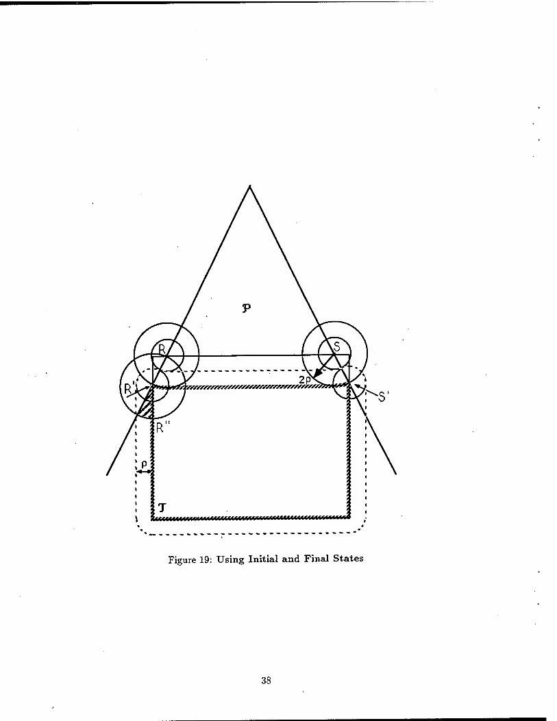
Figure 19: Using Initial and Final States

38

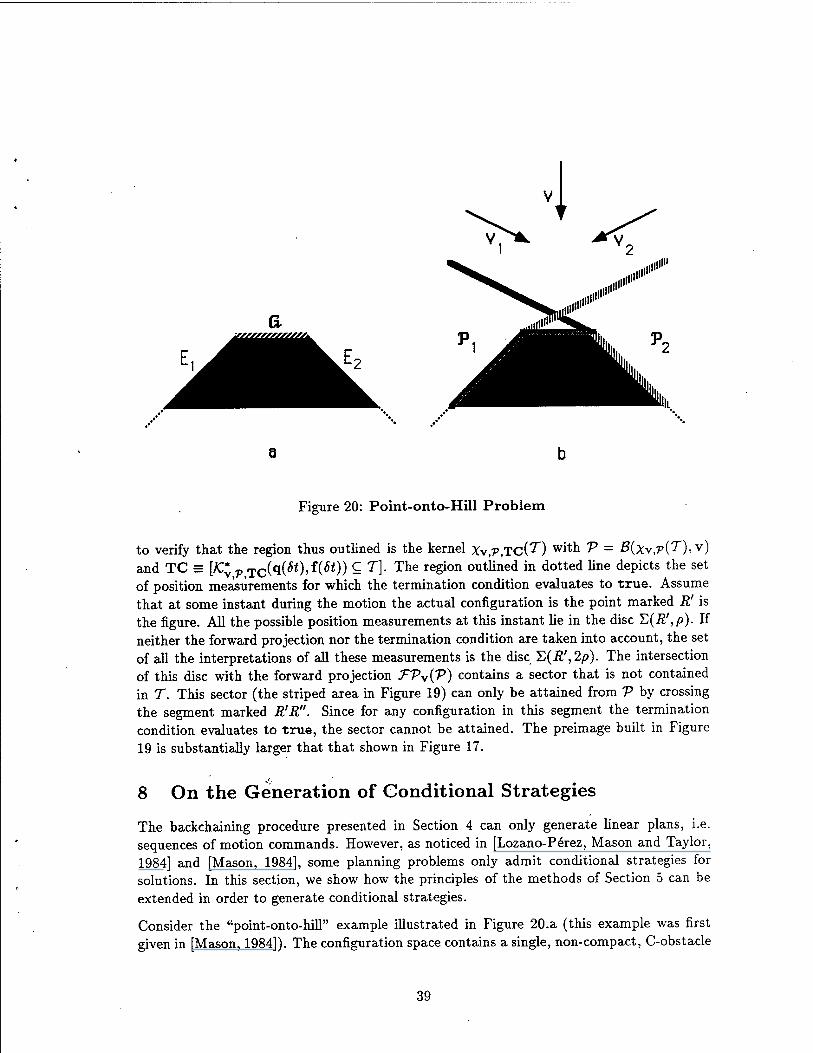
Figure 20: Point-onto-Hill Problem

to verify that the region thus outlined is the kernel Xv,v,Tc(T) w*tn ^ = B{X\,v{T)->v) and TC = [K^v TC(q(6t),i(St)) C T\. The region outlined in dotted line depicts the set of position measurements for which the termination condition evaluates to true. Assume that at some instant during the motion the actual configuration is the point marked R' is the figure. All the possible position measurements at this instant lie in the disc Y,(R',p). If neither the forward projection nor the termination condition are taken into account, the set of all the interpretations of all these measurements is the disc S(Ä',2p). The intersection of this disc with the forward projection TVy{V) contains a sector that is not contained in T. This sector (the striped area in Figure 19) can only be attained from V by crossing the segment marked R'R". Since for any configuration in this segment the termination condition evaluates to true, the sector cannot be attained. The preimage built in Figure 19 is substantially larger that that shown in Figure 17.

8 On the Generation of Conditional Strategies

The backchaining procedure presented in Section 4 can only generate linear plans, i.e. sequences of motion commands. However, as noticed in [Lozano-Perez, Mason and Taylor, 1984] and [Mason, 1984], some planning problems only admit conditional strategies for solutions. In this section, we show how the principles of the methods of Section 5 can be extended in order to generate conditional strategies.

Consider the "point-onto-hill" example illustrated in Figure 20.a (this example was first given in [Mason, 1984]). The configuration space contains a single, non-compact, C-obstacle

39

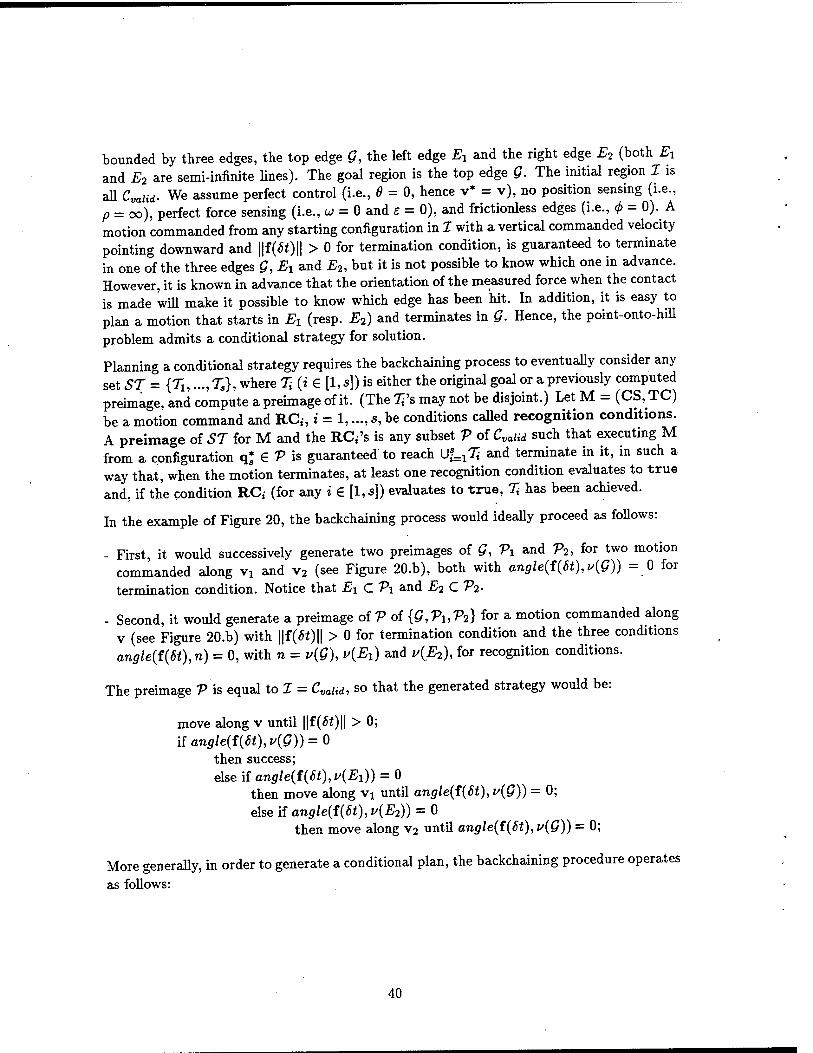
bounded by three edges, the top edge G, the left edge Ex and the right edge E2 (both £1 and E2 are semi-infinite lines). The goal region is the top edge Q. The initial region I is all Cva,id. We assume perfect control (i.e., 0 = 0, hence v* = v), no position sensing (i.e., p = oo), perfect force sensing (i.e., u = 0 and e = 0), and frictionless edges (i.e., <p = 0). A motion commanded from any starting configuration in I with a vertical commanded velocity pointing downward and ||f(«)ll > 0 for termination condition, is guaranteed to terminate in one of the three edges G, Ex and E2, but it is not possible to know which one in advance. However, it is known in advance that the orientation of the measured force when the contact is made will make it possible to know which edge has been hit. In addition, it is easy to plan a motion that starts in E1 (resp. E2) and terminates in Q. Hence, the point-onto-hill problem admits a conditional strategy for solution.

Planning a conditional strategy requires the backchaining process to eventually consider any set ST = {7i,..., TJ, where T{ (i e [1, s]) is either the original goal or a previously computed preimage, and compute a preimage of it. (The %'s may not be disjoint.) Let M = (CS, TC) be a motion command and RC„ i = 1, ...,*, be conditions called recognition conditions. A preimage of ST for M and the RC.'s is any subset V of Cvaiid such that executing M from a configuration q^ € V is guaranteed to reach Uf=17^ and terminate in it, in such a way that, when the motion terminates, at least one recognition condition evaluates to true and, if the condition RC, (for any i € [1,*]) evaluates to true, % has been achieved.

In the example of Figure 20, the backchaining process would ideally proceed as follows:

- First, it would successively generate two preimages of G, V\ and V2, for two motion commanded along vi and v2 (see Figure 20.b), both with angle(f(6t),v(G)) = 0 for termination condition. Notice that Ei C V\ and E2CV2.

- Second, it would generate a preimage of V of {G,VUV2} for a motion commanded along v (see Figure 20.b) with ||f(«)ll > ° for termination condition and the three conditions angle(f(6t),n) = 0, with n = v{G), v(Ex) and v(E2), for recognition conditions.

The preimage V is equal to I = Cvalid, so that the generated strategy would be:

move along v until ||f(£f)|| > 0; if angle(f(6t),v(G))=0

then success; else if angle(t(6t),v(Ei)) = 0

then move along vx until angle(f(8t),v(G)) = 0;

elseifan^e(f(«0.K^2)) = 0

then move along v2 until angle(f(St),i/(G)) = 0;

More generally, in order to generate a conditional plan, the backchaining procedure operates

as follows:

40

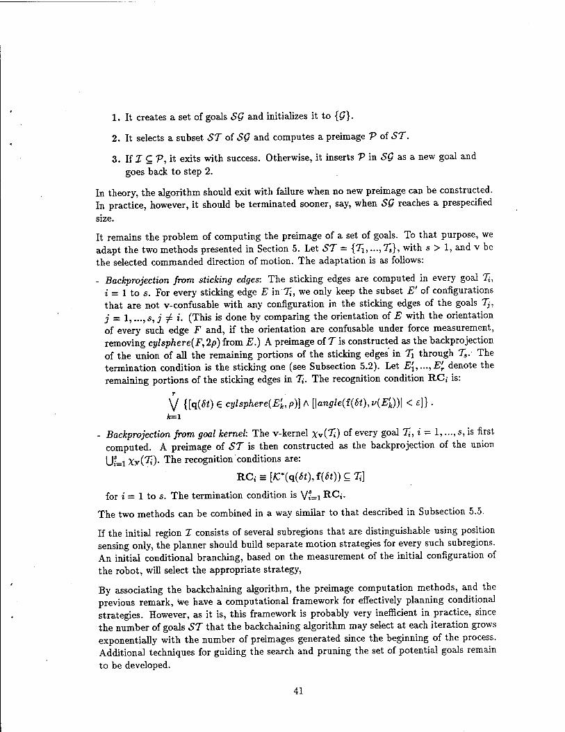
1. It creates a set of goals SQ and initializes it to {$}.

2. It selects a subset ST of SQ and computes a preimage V of ST.

3. If I C V, it exits with success. Otherwise, it inserts V in SQ as a new goal and goes back to step 2.

In theory, the algorithm should exit with failure when no new preimage can be constructed. In practice, however, it should be terminated sooner, say, when SQ reaches a prespecified

size.

It remains the problem of computing the preimage of a set of goals. To that purpose, we adapt the two methods presented in Section 5. Let ST = {%., ...,TS}, with s > 1, and v be the selected commanded direction of motion. The adaptation is as follows:

- Backprojection from sticking edges: The sticking edges are computed in every goal %, i = 1 to s. For every sticking edge E in %, we only keep the subset E' of configurations that are not v-confusable with any configuration in the sticking edges of the goals Tj, j = 1, ...,s, j ^ i. (This is done by comparing the orientation of E with the orientation of every such edge F and, if the orientation are confusable under force measurement, removing cylsphere(F, 2p) from E.) A preimage of T is constructed as the backprojection of the union of all the remaining portions of the sticking edges in Ty through T3. The termination condition is the sticking one (see Subsection 5.2). Let E[,...,E'r denote the remaining portions of the sticking edges in %. The recognition condition RC, is:

V {[q(«) € cylsphere(E'k,p)) A [\angle(f(8t),v(E'k))\ < *]} • k=i

- Backprojection from goal kernel: The v-kernel Xv(7f) of every goal T, i = 1,..., s, is first computed. A preimage of ST is then constructed as the backprojection of the union Ui=iXy(^)- The recognition conditions are:

RCi = [Km{q(6t),i(St))C%\

for i — 1 to s. The termination condition is V*=i RC,-.

The two methods can be combined in a way similar to that described in Subsection 5.5.

If the initial region 1 consists of several subregions that are distinguishable using position sensing only, the planner should build separate motion strategies for every such subregions. An initial conditional branching, based on the measurement of the initial configuration of the robot, will select the appropriate strategy,

By associating the backchaining algorithm, the preimage computation methods, and the previous remark, we have a computational framework for effectively planning conditional strategies. However, as it is, this framework is probably very inefficient in practice, since the number of goals ST that the backchaining algorithm may select at each iteration grows exponentially with the number of preimages generated since the beginning of the process. Additional techniques for guiding the search and pruning the set of potential goals remain to be developed.

41

9 Conclusion

In this paper, we addressed the problem of planning motion strategies in a two-dimensional configuration space in the presence of uncertainty in robot control and sensing. We estab- lished a precise formalization of the problem and we considered the preimage backchaining approach to this problem. In response to one of the main difficulties raised by this general approach, we described in detail two effective methods for computing preimages: back- projection from sticking edges and backprojection from goal kernel. In general, the second method computes larger preimages than the first. In fewer cases, however, it is the contrary. The two methods can be combined into what we think is the most powerful effective method developed so far for computing preimages. A motion planner based on these methods was implemented and we experimented with it in simulation on reasonably simple problems. We discussed two non-implemented improvements of the planner. One improvement consists of increasing the recognition power of the termination predicate of a motion command by embedding the knowledge of both the preimage and itself in it (termination predicate with initial and final states). On a specific example, we showed how this knowledge makes it possible to construct significanty larger preimages. The other improvement extends the preimage backchaining approach to the generation of conditional strategies. We proposed a full computational framework for effectively planning such strategies.

An important shortcoming of the implemented planner is that it blindly discretizes motion directions in order to build the preimage graph and that it uses no heuristics to guide the search of this graph. This is acceptable only for rather simple problems. Although there exist some straightforward heuristics - e.g., move in priority in the direction of the goal - they would probably be easily deceived (but we did not experiment with any of them). Donald [Donald, 1988b] proposed a method based on the notion of "non-directional backprojection" for computing a motion command whose execution is guaranteed to reach a goal from a given region, if one such command exists. The method relies on the fact that the topology of the backprojection of a region can change at a finite number of "critical" orientations of the commanded direction of motion, and that the containment of the initial region in a backprojection changes at a finite number of "pseudo-critical" orientations where an edge of the current backprojection makes contact with the initial region. It computes the backprojections at these critical and pseudo-critical orientations, and test the backprojection for containment of the initial region at each pseudo-critical orientation. Briggs [Briggs, 1988] reduced the time complexity of Donald's original algorithm to 0(n2 log n), where n is the number of edges in the contact space (and assuming that the goal region has constant size). The method can be used in connection with the preimage computation methods described in Section 5 in order to generate a 1-step motion strategy, without bünd discretization and search, whenever one exists. This is done by noticing that both the set of sticking edges in the goal and the v-kernel of the goal change at a finite number of orientations of the commanded direction of motion. Hence, one can compute all the intervals of motion directions in which the sticking edges and the v-kernel remain constant, and determine for each interval if there is a backprojection of the region formed by the corresponding sticking edges and v-kernel, which contains the initial region. However, extending the approach to r-step strategies would require to deal with (pseudo-)critical (r - l)-dimensional surfaces rather than orientations, which might be quite complex in

42

practice. Another interesting approach for constructing r-step strategies is proposed in [Friedman, Hershberger and Snoeyink, 1989]. The approach basically consists of assuming perfect control and determining the range of directions in which the robot should move from an initial region in order to attain a goal in a single step. But, so far, the approach is only applicable when the workspace is the interior of a simple polygon and the goal is an edge

or a vertex of this polygon.

Another major limitation of the planner is that it requires the robot's configuration space to be two-dimensional. The general principles of the planning methods immediately extend to higher-dimensional spaces, but the detailed geometric algorithms do not. One can devise "exact" algorithms in the vein of those described in [Schwartz and Sharir, 1983] and [Canny, 1987] - that is, reducing planning to an algebraic decision problem. Such algorithms will certainly provide upper bounds for the complexity of motion planning with uncertainty,

but they are unlikely to be practical solutions to this problem (e.g., see [Canny, 1989]). More pragmatic, but still systematic methods - perhaps in the vein of those described in

[Barraquand and Latombe, 1989] - remain to be developed.

References

Aho, A.V., Hopcroft, J.E. and Ullman, J.D. (1983) Data Structures and Algorithms, Addison-Wesley, Reading, MA.

Andreae, P.M. (1986) Justified Generalization: Acquiring Procedures from Examples. Ph.D. Disser- tation, Technical Report 834, Artificial Intelligence Laboratory, MIT.

Arnold, V.l. (1978) Mathematical Methods of Classical Mechanics, Springer-Verlag, New York.

Avnaim, F. and Boissonnat, J.D. (1987) "Simultaneous Containment of Several Polygons," Third ACM Symposium on Computational Geometry, Waterloo, Canada.

Barraquand, J. and Latombe, J.C. (1989) Robot Motion Planning: A Distributed Representation Approach, Report No. STAN-CS-89-1257, Department of Computer Science, Stanford University.

Briggs, A.J. (1988) An Efficient Algorithm for One-Step Planar Compliant Motion Planning with Uncertainty, Department of Computer Science, Cornell University, Ithaca, NY.

Brooks, R.A. (1982) "Symbolic Error Analysis and Robot Planning," International Journal of Robotics Research, 1(4), 29-68.

Brooks, R.A. and Lozano-Perez, T. (1983) "A Subdivision Algorithm in Configuration Space for Findpath with Rotation," Eighth International Joint Conference on Artificial Intelligence, Karl-

sruhe, FRG, 799-806.

Buckley, S.J. (1986) Planning and Teaching Compliant Motion Strategies, Ph.D. Dissertation, De- partment of Electrical Engineering and Computer Science, MIT, Cambridge, MA.

Canny, J.F. and Reif, J. (1987) "New Lower Bound Techniques for Robot Motion Planning Prob- lems," 27th IEEE Symposium on Foundations of Computer Science, Los Angeles, CA.

Canny, J.F. (1987) The Complexity of Robot Motion Planning, Ph.D. Dissertation, Department of Electrical Engineering and Computer Science, MIT, Cambridge, MA.

Canny, J.F. (1989) "On Computability of Fine Motion Plans," IEEE International Conference on Robotics and Automation, Scottsdale, AZ, 177-182.

43

Desai, R.S. (1988) On Fine Motion in Mechanical Assembly in Presence of Uncertainty, Ph.D. Dissertation, Department of Mechanical Engineering, University of Michigan.

Donald, B.R. (1987a) A Search Algorithm for Motion Planning With Six Degrees of Freedom, Arti- ficial Intelligence Journal, 31(3), 295-353.

Donald, B.R. (1987b) Error Detection and Recovery for Robot Motion Planning with Uncertainty. Ph.D. Dissertation, Department of Electrical Engineering and Computer Science, MIT.

Donald, B.R. (1988a) "A Geometric Approach to Error Detection and Recovery for Robot Motion Planning with Uncertainty," Artificial Intelligence Journal, 37 (1-3), 223-271.

Donald, B.R. (1988b) "The Complexity of Planar Compliant Motion Planning Under Uncertainty," ACM Symposium on Computational geometry, Urbana, IL.

Dufay, B. and Latombe, J.C. (1984) "A Approach to Automatic Robot Programming Based on Inductive Learning," International Journal of Robotics Research, 3(4), 3-20.

Erdmann, M. (1984) On Motion Planning With Uncertainty, Technical Report 810, AI Laboratory,

MIT.

Erdmann, M. (1986) "Using Backprojections for the Fine Motion Planning With Uncertainty," International Journal of Robotics Research (IJRR), 5(1).

Erdmann, M. and Mason, M.T. (1986) "An Exploration of Sensorless Manipulation," IEEE Inter- national Conference of Robotics and Automation, San Francisco, CA, 1569-1574.

Faverjon, B. and Tournassoud, P. (1987) "A Local Based Approach for Path Planning of Manipula- tors with a High Number of Degrees of Freedom," IEEE International Conference on Robotics and Automation, Raleigh, NC, 1152-1159.

Friedman, J., Hershberger, J. and Snoeyink, J. (1989) "Compliant Motion in a Simple Polygon," ACM Symposium on Computational Geometry.

Gouzenes, L. (1984) "Strategies for Solving Collision-Free Trajectories Problems for Mobile and Manipulator Robots," International Journal of Robotics Research, 3(4), 51-65.

Guillemin, V. and Pollack, A. (1974) Differential Topology, Prentice-Hall, Englewood Cliffs, NJ.

Hopcroft, J.E. and Wilfong, G. (1986) "Motion of Objects in Contact," International Journal of Robotics Research, 4(4), 32-46.

Khatib, O. (1986) "Real-Time Obstacle Avoidance for Manipulators and Mobile Robots," Interna- tional Journal of Robotics Research, 5(1), 90-98.

Koutsou, A. (1986) Planning Motion in Contact to Achieve Paris Mating. Ph.D. Dissertation, Department of Computer Science, University of Edinburgh.

Latombe, J.C. (1984) "Automatic Synthesis of Robot Programs from CAD Specifications," in Robotics and Artificial Intelligence, edited by Brady, M., Gerhardt, L.A. and Davidson, H.F., NATO ASI Series, Springer-Verlag, New York.

Latombe, J.C, Laugier, C, Lefebvre, J.M., Mazer, E. and Miribel, J.F. (1984) "The LM Robot Programming System," in Robotics Research, edited by H. Hanafusa and H. Inoue, MIT Press.

Latombe, J.C. (1988) Motion Planning with Uncertainty: The Preimage Backchaining Approach, Report No. STAN-CS-88-1196, Department of Computer Science, Stanford University, Stanford,

CA.

44

Laugier, C. and Germain, F. (1985) "An Adaptative Collision-Free Trajectory Planner," Interna- tional Conference on Advanced Robotics, Tokyo, Japan.

Laugier, C. and Theveneau, P. (1986) "Planning Sensor-Based Motions for Part-Mating Using Ge- ometric Reasoning Techniques," European Conference on Artificial Intelligence, Brighton, UK.

Laugier, C. (1989) "Planning Fine Motion Strategies by Reasoning in the Contact Space," Proeedings of the IEEE International Conference on Robotics and Automation, Scottsdale, AZ, 653-659.

Liebermann, L.I. and Wesley, M.A. (1977) "AUTOPASS: An Automatic Programming System for Computer Controlled Mechanical Assembly," IBM Journal of Research and Development, 21(4),

321-333.

Lozano-Perez, T. (1976) The Design of a Mechanical Assembly System. Technical Report AI-TR 397, Artificial Intelligence Laboratory, MIT, Cambridge, MA.

Lozano-Perez, T. (1981) "Automatic Planning of Manipulator Transfer Movements," IEEE Trans- actions on Systems, Man and Cybernetics, SMC-ll(lO), 681-698.

Lozano-Perez, T. (1983) "Spatial Planning: A Configuration Space Approach," IEEE Transactions on Computers, C-32(2), 108-120.

Lozano-Perez, T., Mason, M.T. and Taylor, R.H. (1984) "Automatic Synthesis of Fine-Motion Strategies for Robots," International Journal of Robotics Research, 3(1), 3-24.

Lozano-Perez, T. (1987) "A Simple Motion-Planning Algorithm for General Robot Manipulators," IEEE Journal of Robotics and Automation, RA-3(3), 224-238.

Lozano-Perez, T. et al. (1987) "Handey: A Robot System that Recognizes, Plans, and Manipulates," IEEE International Conference on Robotics and Automation, Raleigh, North Carolina, 843-849.

Mason, M.T. (1981) "Compliance and Force Control for Computer Controlled Manipulators," IEEE Transactions on Systems, Man, and Cybernetics, SMC-11, 6, 418-432.

Mason, M.T. (1984) "Automatic Planning of Fine Motions: Correctness and Completeness," IEEE International Conference on Robotics and Automation, Atlanta, GA.

Massey, W.S. (1967) Algebraic Topology: An Introduction, Springer-Verlag, New York.

Mazer, E. (1987). Handey: A Planner for Task-Level Robot Command. Thesis Dissertation, Uni-

versity of Grenoble, France.

Nilsson, N.J. (1980) Principles of Artificial Intelligence, Morgan Kaufmann, Los Altos, CA.

Pertin-Troccaz, J. and Puget, P. (1987) "Dealing with Uncertainty in Robot Planning Using Program Proving Techniques," Robotics Research, edited by Bolles, R.C. and Roth B., MIT Press, 455-466.

Preparata, F.P. and Shamos, M.I. (1985) Computational Geometry: An Introduction. Springer-

Verlag, New York.

Raibert, M.H. and Craig,J.J. (1981) "Hybrid Position/Force Control of Manipulators," Journal of Dynamic Systems, Measurement and Control, 102.

Reif, J.H. (1979) "Complexity of the Mover's Problem and Generalizations," 20th Symposium on the Foundations of Computer Science (FOCS), 421-427.

Requicha, A. (1977) Mathematical Models of Rigid Solid Objects, Technical Memo No. 28, Produc- tion Automation Project, University of Rochester, Rochester, NY.

45

Sharir, M. (1987) "Efficient Algorithms for Planning Purely Translational Collision-Free Motion in Two and Three Dimensions," IEEE International Conference on Robotics and Automation, Raleigh,

NC, 1326-1331.

Schwartz, J.T. and Sharir, M. (1983) "On the Piano Movers' Problem: I. The Case if a Two- Dimensional Rigid Polygonal Body Moving Amidst Polygonal Barriers," Communications on Pure

and Applied Mathematics, 36, 345-398.

Schwartz, J.T. and Sharir, M. (1988) "A Survey of Motion Planning and Related Geometric Algo- rithms," Artificial Intelligence Journal, 37(1-3), 157-169.

Taylor, R.H. (1976) Synthesis of Manipulator Control Programs from Task-Level Specifications, Ph.D. Dissertation, Department of Computer Science, Stanford University, CA.

Valade, J. (1984) "Automatic Generation of Trajectories for Assembly Tasks," Sixth European Con-

ference on Artificial Intelligence, Pisa, Italy.

Waldinger.R. (1975) "Achieving Several Goals Simultaneously," in Elcock, E. and Michie, D. (edi- tors.), Machine Intelligence 8, Ellis Horwood, Chichester, UK.

46

u

u a ft

QJ

© u u

s es

• pa

'S"

o

U

eS

E

V

5*1 o s

^**

5-

QJ S^Äv

B

es

Si o B <s

pfi

s- ™ © ©

5 °

B fi

O

5Z5

o

H Z

s

Or i-

C

s • pp

es s

es s es

Reproduced by NTIS National Technical Information Service U.S. Department of Commerce Springfield, VA 22161

This report was printed specifically for your order from our collection of more than 2 million technical reports.

For economy and efficiency, NTIS does not maintain stock of its vast collection of technical reports. Rather, most documents are printed for each order. Your copy is the best possible reproduction available from our master archive. If you have any questions concerning this document or any order you placed with NTIS, please call our Customer Services Department at (703) 387-4660.

Always think of NTIS when you want: • Access to the technical, scientific, and engineering results generated by the ongoing multibillion dollar R&D program of the U.S. Government. • R&D results from Japan, West Germany, Great Britain, and some 20 other countries, most of it reported in English.

NTIS also operates two centers that can provide you with valuable information: • The Federal Computer Products Center - offers software and datafiles produced by Federal agencies. • The Center for the Utilization of Federal Technology - gives you access to the best of Federal technologies and laboratory resources.

For more information about NTIS, send for our FREE NTIS Products and Services Catalog which describes how you can access this U.S. and

foreign Government technology. Call (703) 487-4650 or send this sheet to NTIS, U.S. Department of Commerce, Springfield, VA 22161. Ask for catalog, PR-827.

Name Address

Telephone,

- Your Source to U.S. and Foreign Government Research and Technology

U.S. DEPARTMENT OF COMMERCE Technology Administration

National Technical Information Service Springfield, VA 22161 (703) 487-4650