Robot Motion Planning and Control - J.P. Laumond.pdf
354
Lecture Notes in Control and Information Sciences 229 Editor: M. Thoma
-
Upload
khangminh22 -
Category
Documents
-
view
0 -
download
0
Transcript of Robot Motion Planning and Control - J.P. Laumond.pdf
Lecture Notes in Control and Information Sciences 229
Editor: M. Thoma
J.-P. Laumond (Ed.)
Robot Motion Planning and Control
I/
i
~ Springer
Series A d v i s o r y B o a r d
A. Bensoussan • M.J. Grimble • P. Kokotovic. H. Kwakernaak J.L. Massey • Y.Z. Tsypkin
E d i t o r
Dr J.-P. Laumond C e n t r e N a t i o n a l d e la R e c h e r c h e S c i e n t i f i q u e
L a b o r a t o i r e d ' A n a l y s e e t d ' A r c h i t e c t u r e d e s S y s t e m e s
7, a v e n u e d u C o l o n e l R o c h e
31077 T o u l o u s e C e d e x
F R A N C E
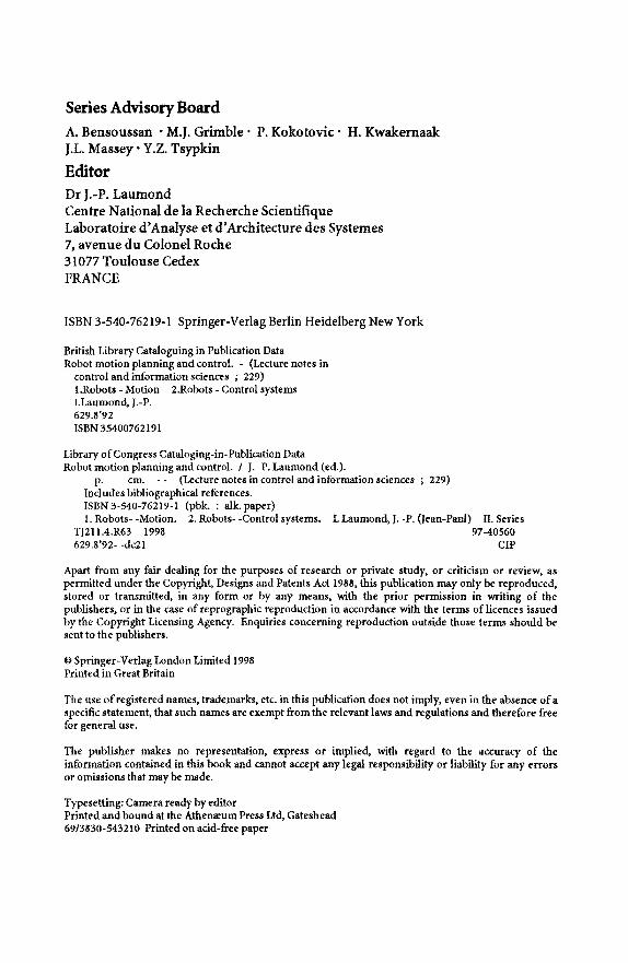
ISBN 3-540-76219-1 Spr inge r -Ver lag Berlin H e i d e l b e r g New York
British Library Cataloguing in Publication Data Robot motion planning and control. - (Lecture notes in
control and information sciences ; 229) 1.Robots - Motion 2.Robots - Control systems I.Laumond, J.-P. 629.8'92 ISBN 35400762191
Library of Congress Cataloging-in-Publication Data Robot motion planning and control. / J. -P. Laumond (ed.).
p. crr~ - - (Lecture notes in control and information sciences ; 229) Includes bibliographical references. ISBN3-540-76219-1 (pbk. : alk, paper) 1. Robots- -Motion. 2. Robots- -Control systems. L Laumond, J. -P. (Jean-Paul) IL Series
TJ211.4.R63 1998 97-40560 629.8'92- -dc21 CIP
Apart from any fair dealing for the purposes of research or private study, or criticism or review, as permitted under the Copyright, Designs and Patents Act 19S8, this publication may only be reproduced, stored or transmitted, in any form or by any means, with the prior permission in writing of the publishers, or in the case of reprographic reproduction in accordance with the terms of licences issued by the Copyright Licensing Agency. Enquiries concerning reproduction outside those terms should be sent to the publishers.
Springer-Verlag London Limited 1998 Printed in Great Britain
The use of registered names, trademarks, etc. in this publication does not imply, even in the absence of a specific statement, that such names are exempt from the relevant laws and regulations and therefore free for general use.
The publisher makes no representation, express or implied, with regard to the accuracy of the information contained in this book and cannot accept any legal responsibility or liability for any errors or omissions that may be made.
Typesetting: Camera ready by editor Printed and bound at the Athenaeum Press Ltd, Gateshead 6913830-543210 Printed on acid-free paper
Foreword
How can a robot decide what motions to perform in order to achieve tasks in the physical world ?
The existing industrial robot programming systems still have very limited motion planning capabilities. Moreover the field of robotics is growing: space exploration, undersea work, intervention in hazardous environments, servicing robotics . . . Motion planning appears as one of the components for the neces- sary autonomy of the robots in such real contexts. It is also a fundamental issue in robot simulation software to help work cell designers to determine collision free paths for robots performing specific tasks.
R o b o t M o t i o n Planning and Cont ro l requi res interdisciplinarity
The research in robot motion planning can be traced back to the late 60's, during the early stages of the development of computer-controlled robots. Nev- ertheless, most of the effort is more recent and has been conducted during the 80's (Robot Motion Planning, J.C. Latombe's book constitutes the reference in the domain).
The position (configuration) of a robot is normally described by a number of variables. For mobile robots these typically are the position and orientation of the robot (i.e. 3 variables in the plane). For articulated robots (robot arms) these variables are the positions of the different joints of the robot arm. A motion for a robot can, hence, be considered as a path in the configuration space. Such a path should remain in the subspace of configurations in which there is no collision between the robot and the obstacles, the so-called free space. The motion planning problem asks for determining such a path through the free space in an efficient way.
Motion planning can be split into two classes. When all degrees of freedom can be changed independently (like in a fully actuated arm) we talk about hotonomic motion planning. In this case, the existence of a collision-free path is characterized by the existence of a connected component in the free config- uration space. In this context, motion planning consists in building the free configuration space, and in finding a path in its connected components.
Within the 80's, Roboticians addressed the problem by devising a variety of heuristics and approximate methods. Such methods decompose the config- uration space into simple cells lying inside, partially inside or outside the free space. A collision-free path is then searched by exploring the adjacency graph of free cells.
VI
In the early 80's, pioneering works showed how to describe the free config- uration space by algebraic equalities and inequalities with integer coefficients (i.e. as being a semi-algebraic set). Due to the properties of the semi-algebraic sets induced by the Tarski-Seidenberg Theorem, the connectivity of the free configuration space can be described in a combinatorial way. From there, the road towards methods based on Real Algebraic Geometry was open. At the same time, Computational Geometry has been concerned with combinatorial bounds and complexity issues. It provided various exact and efficient meth- ods for specific robot systems, taking into account practical constraints (like environment changes).
More recently, with the 90's, a new instance of the motion planning problem has been considered: planning motions in the presence of kinematic constraints (and always amidst obstacles). When the degrees of freedom of a robot sys- tem are not independent (like e.g. a car that cannot rotate around its axis without also changing its position) we talk about nonholonomic motion plan- ning. In this case, any path in the free configuration space does not necessarily correspond to a feasible one. Nonholonomic motion planning turns out to be much more difficult than holonomic motion planning. This is a fundamental issue for most types of mobile robots. This issue attracted the interest of an increasing number of research groups. The first results have pointed out the necessity of introducing a Differential Geometric Control Theory framework in nonholonomic motion planning.
On the other hand, at the motion execution level, nonholonomy raises an- other difficulty: the existence of stabilizing smooth feedback is no more guaran- teed for nonholonomic systems. Tracking of a given reference trajectory com- puted at the planning level and reaching a goal with accuracy require non- standard feedback techniques.
Four main disciplines are then involved in motion planning and control. However they have been developed along quite different directions with only little interaction. The coherence and the originality that make motion plan- ning and control a so exciting research area come from its interdisciplinarity. It is necessary to take advantage from a common knowledge of the different theoretical issues in order to extend the state of the art in the domain.
A b o u t the bo ok
The purpose of this book is not to present a current state of the art in motion planning and control. We have chosen to emphasize on recent issues which have been developed within the 90's. In this sense, it completes Latombe's book published in 1991. Moreover an objective of this book is to illustrate the necessary interdisciplinarity of the domain: the authors come from Robotics,
VII
Computational Geometry, Control Theory and Mathematics. All of them share a common understanding of the robotic problem.
The chapters cover recent and fruitful results in motion planning and con- trol. Four of them deal with nonholonomic systems; another one is dedicated to probabilistic algorithms; the last one addresses collision detection, a critical operation in algorithmic motion planning.
Nonholonomic Systems The research devoted to nonholonomic systems is mo- tivated mainly by mobile robotics. The first chapter of the book is dedicated to nonholonomic path planning. It shows how to combine geometric algorithms and control techniques to account for the nonholonomic constraints of most mobile robots. The second chapter develops the mathematical machinery nec- essary to the understanding of the nonholonomic system geometry; it puts emphasis on the nonholonomic metrics and their interest in evaluating the combinatorial complexity of nonholonomic motion planning. In the third chap- ter, optimal control techniques are applied to compute the optimal paths for car-like robots; it shows that a clever combination of the maximum principle and a geometric viewpoint has permitted to solve a very difficult problem. The fourth chapter highlights the interactions between feedback control and motion planning primitives; it presents innovative types of feedback controllers facing nonholonomy.
Probabilistic Approaches While complete and deterministic algorithms for mo- tion planning are very time-consuming as the dimension of the configuration space increases, it is now possible to address complicated problems in high di- mension thanks to alternative methods that relax the completeness constraint for the benefit of practical efficiency and probabilistic completeness. The fifth chapter of the book is devoted to probabilistic algorithms.
Collision Detection Collision checkers constitute the main bottleneck to con- ceive efficient motion planners. Static interference detection and collision detec- tion can be viewed as instances of the same problem, where objects are tested for interference at a particular position, and along a trajectory. Chapter six presents recent algorithms benefiting from this unified viewpoint.
The chapters are self-contained. Nevertheless, many results just mentioned in some given chapter may be developed in another one. This choice leads to repetitions but facilitates the reading according to the interest or the back- ground of the reader.
VIII
On the origin of the book
All the authors of the book have been involved in PROMotion. PROMotion was a European Project dedicated to robot motion planning and control. It has progressed from September 1992 to August 1995 in the framework of the Basic Research Action of ESPRIT 3, a program of research and development in In- formation Technologies supported by the European Commission (DG III). The work undertaken under the project has been aimed at solving concrete prob- lems. Theoretical studies have been mainly motivated by a practical efficiency. Research in PROMotion has then provided methods and their prototype im- plementations which have the potential of becoming key components of recent programs in advanced robotics.
In few numbers, PROMotion is a project whose cost has been 1.9 MEcus 1 (1.1 MEcus supported by European Community), for a total effort of more than 70 men-year, 179 research reports (most them have been published in international conferences and journals), 10 experiments on real robot platforms, an International Spring school and 3 International Workshops. This project has been managed by LAAS-CNRS in Toulouse; it has involved the "Universitat Politecnica de Catalunya" in Barcelona, the "Ecole Normale Sup@rieure" in Paris, the University "La Sapienza" in Roma, the Institute INRIA in Sophia- Antipolis and the University of Utrecht.
J.D. Boissonnat (INRIA, Sophia-Antipolis), A. De Luca (University "La Sapienza" of Roma), M. Overmars (Utrecht University), J.J. Risler (Ecole Nor- male Sup6rieure and Paris 6 University), C. Torras (Universitat Politecnica de Catalunya, Barcelona) and the author make up the steering committee of PRO- Motion. This book benefits from contributions of all these members and their co-authors and of the work of many people involved in the project.
On behalf of the project committee, I thank J. Wejchert (Project oflicier of PROMotion for the European Community), A. Blake (Oxford University), H. Chochon (Alcatel) and F. Wahl (Brannschweig University) who acted as reviewers of the project during three years. Finally I thank J. Som for her efficient help in managing the project and M. Herrb for his help in editing this book.
Jean-Paul Laumond LAAS-CNRS, Toulouse
August 1997
1 US $ 1 ~ 1 Ecu
List of Contributors
A. Bella'iche D4partement de Math@matiques Universit4 de Paris 7 2 Place Jussieu 75251 Paris Cedex 5 France abellaic©mathp7, j u s s i e u , f r
A. De Luca Dipartimento di Informatica e Sistemistica UniversitA di Roma "La Sapienza" Via Eudossiana 18 00184 Roma Italy adeluca©giannutri, caspur, it
P. Jim@nez Institut de Robbtica i Inform~tica Industrial Gran Capita, 2 08034-Barcelona Spain j imenez©iri, upc. es
J.P. Laumond LAAS-CNRS 7 Avenue du Colonel Roche 31077 Toulouse Cedex 4 France jpl©laas, fr
J.D. Boissonnat INRIA Centre de Sophia Antipolis 2004, Route des Lucioles BP 93 06902 Sophia Antipolis Cedex, France boissonn©sophia, inria, fr
F. Jean Institut de Math@matiques Universit@ Pierre et Marie Curie Tour 46, 5~me @tage, Boite 247 4 Place Jussieu 75252 Paris Cedex 5 France j ean~math, j u s s i e u , fr
F. Lamiraux LAAS-CNRS 7 Avenue du Colonel Roche 31077 Toulouse Cedex 4 France lamiraux©laas, f r
G. Oriolo Dipartimento di Informatica e Sistemistica Universit£ di Roma "La Sapienza" Via Eudossiana 18 00184 Roma Italy oriolo@giannutri, caspur, it

X
M. H. Overmars Department of Computer Science, Utrecht University P.O.Box 80.089, 3508 TB Utrecht, the Netherlands markov@cs, ruu. nl
C. Samson INRIA Centre de Sophia Antipolis 2004, Route des Lucioles BP 93 06902 Sophia Antipolis Cedex, France Claude. Samson@sophia. inria, fr
P. Sou~res LAAS-CNRS 7 Avenue du Colonel Roche 31077 Toulouse Cedex 4 France soueres@laas, f r
F. Thomas Institut de Robbtica i Informatica Industrial Gran Capita, 2 08034-Barcelona Spain thomas©iri, upc. es
J.J. Risler Institut de Math@matiques Universit4 Pierre et Marie Curie Tour 46, 5~me e~age, Boite 247 4 Place Jussieu 75252 Paris Cedex 5 France risler@math, jussieu, fr
S. Sekhavat LAAS-CNRS 7 Avenue du Colonel Roche 31077 Toulouse Cedex 4 France sepanta©laas, fr
P. Svestka Department of Computer Science, Utrecht University P.O.Box 80.089, 3508 TB Utrecht, the Netherlands petr@cs, ruu.nl
C. Torras Institut de Robbtica i Informatica Industrial Gran Capita, 2 08034-Barcelona Spain torras@iri, upc. es
Table of Contents
G u i d e l i n e s in N o n h o l o n o m i c M o t i o n P l a n n i n g for M o b i l e R o b o t s 1
J.P. Laumond, S. Sekhavat, F. Lamiraux 1 Introduction . . . . . . . . . . . . . . . . . . . . . . . . . . . . . . . . . . . . . . . . . . . . . . . . . . . 1
2 Controllabilities of mobile robots . . . . . . . . . . . . . . . . . . . . . . . . . . . . . . . . . 2
3 Path planning and small-time controllability . . . . . . . . . . . . . . . . . . . . . . . 10
4 Steering methods . . . . . . . . . . . . . . . . . . . . . . . . . . . . . . . . . . . . . . . . . . . . . . 13
5 Nonholonomic path planning for small-time controllable systems . . . . . 23
6 Other approaches, other systems . . . . . . . . . . . . . . . . . . . . . . . . . . . . . . . . . 42
7 Conclusions . . . . . . . . . . . . . . . . . . . . . . . . . . . . . . . . . . . . . . . . . . . . . . . . . . . 44
G e o m e t r y o f N o n h o l o n o m i c S y s t e m s . . . . . . . . . . . . . . . . . . . . . . . . . . . 55
A. BeUa~'che, F. Jean, J.-J. Risler 1 Symmetric control systems: an introduction . . . . . . . . . . . . . . . . . . . . . . . 55
2 The car with n trailers . . . . . . . . . . . . . . . . . . . . . . . . . . . . . . . . . . . . . . . . . 73
3 Polynomial systems . . . . . . . . . . . . . . . . . . . . . . . . . . . . . . . . . . . . . . . . . . . . 82
O p t i m a l T r a j e c t o r i e s for N o n h o l o n o m i c M o b i l e R o b o t s . . . . . . . . 93
P. Sou~res, J.-D. Boissonnat 1 Introduction . . . . . . . . . . . . . . . . . . . . . . . . . . . . . . . . . . . . . . . . . . . . . . . . . . . 93
2 Models and optimization problems . . . . . . . . . . . . . . . . . . . . . . . . . . . . . . . 94
3 Some results from Optimal Control Theory . . . . . . . . . . . . . . . . . . . . . . . . 97
4 Shortest paths for the Reeds-Shepp car . . . . . . . . . . . . . . . . . . . . . . . . . . . 107
5 Shortest paths for Dubins' Car . . . . . . . . . . . . . . . . . . . . . . . . . . . . . . . . . . 141
6 Dubins model with inertial control law . . . . . . . . . . . . . . . . . . . . . . . . . . . . 153
7 Time-optimal trajectories for Hilare-tike mobile robots . . . . . . . . . . . . . . 161
8 Conclusions . . . . . . . . . . . . . . . . . . . . . . . . . . . . . . . . . . . . . . . . . . . . . . . . . . . 166
F e e d b a c k C o n t r o l o f a N o n h o l o n o m i c C a r - L i k e R o b o t . . . . . . . . . . 171 A. De Luca, G. Oriolo, C. Samson
1 Introduction . . . . . . . . . . . . . . . . . . . . . . . . . . . . . . . . . . . . . . . . . . . . . . . . . . . 171
2 Modeling and analysis of the car-like robot . . . . . . . . . . . . . . . . . . . . . . . . 179
3 Trajectory tracking . . . . . . . . . . . . . . . . . . . . . . . . . . . . . . . . . . . . . . . . . . . . . 189
4 Pa th following and point stabilization . . . . . . . . . . . . . . . . . . . . . . . . . . . . 213
5 Conclusions . . . . . . . . . . . . . . . . . . . . . . . . . . . . . . . . . . . . . . . . . . . . . . . . . . . 247
6 Further reading . . . . . . . . . . . . . . . . . . . . . . . . . . . . . . . . . . . . . . . . . . . . . . . . 249
XII
Probabi l i s t ic P a t h P lann ing . . . . . . . . . . . . . . . . . . . . . . . . . . . . . . . . . . . P. Svestka, M. 1t. Overmars
255
1 I n t r o d u c t i o n . . . . . . . . . . . . . . . . . . . . . . . . . . . . . . . . . . . . . . . . . . . . . . . . . . . 255 2 T h e P robab i l i s t i c P a t h P l anne r . . . . . . . . . . . . . . . . . . . . . . . . . . . . . . . . . . 258 3 App l i ca t i on to holonomic robo t s . . . . . . . . . . . . . . . . . . . . . . . . . . . . . . . . . 266 4 App l i ca t i on to nonholonomic robo t s . . . . . . . . . . . . . . . . . . . . . . . . . . . . . . 270 5 On probab i l i s t i c comple teness of p robab i l i s t i c p a t h p lann ing . . . . . . . . . 279 6 On the expec ted complex i ty of p robab i l i s t i c p a t h p l ann ing . . . . . . . . . . 285 7 A m u l t i - r o b o t ex tens ion . . . . . . . . . . . . . . . . . . . . . . . . . . . . . . . . . . . . . . . . 291 8 Conclusions . . . . . . . . . . . . . . . . . . . . . . . . . . . . . . . . . . . . . . . . . . . . . . . . . . . 300
Coll i s ion D e t e c t i o n Algor i thms for M o t i o n P l a nn i n g . . . . . . . . . . . 305 P. Jimdnez, F. Thomas, C. Torras
1 I n t r o d u c t i o n . . . . . . . . . . . . . . . . . . . . . . . . . . . . . . . . . . . . . . . . . . . . . . . . . . . 305 2 In te r fe rence de tec t ion . . . . . . . . . . . . . . . . . . . . . . . . . . . . . . . . . . . . . . . . . . . 306 3 Coll is ion de tec t ion . . . . . . . . . . . . . . . . . . . . . . . . . . . . . . . . . . . . . . . . . . . . . 317 4 Coll is ion de t ec t ion in mo t ion p l ann ing . . . . . . . . . . . . . . . . . . . . . . . . . . . . 335 5 Conclus ions . . . . . . . . . . . . . . . . . . . . . . . . . . . . . . . . . . . . . . . . . . . . . . . . . . . 338
Guidelines in Nonholonomic Motion Planning for Mobile Robots
J.P. Laumond, S. Sekhavat and F. Lamiraux
LAAS-CNRS, Toulouse
1 I n t r o d u c t i o n
Mobile robots did not wait to know that they were nonholonomic to plan and execute their motions autonomously. It is interesting to notice that the first navigation systems have been published in the very first International Joint Conferences on Artificial Intelligence from the end of the 60's. These systems were based on seminal ideas which have been very fruitful in the development of robot motion planning: as examples, in 1969, the mobile robot Shakey used a grid-based approach to model and explore its environment [61]; in 1977 Jason used a visibility graph built from the corners of the obstacles [88]; in 1979 Hilare decomposed its environment into collision-free convex cells [30].
At the end of the 70's the studies of robot manipulators popularized the notion of configuration space of a mechanical system [53]; in this space the "piano" becomes a point. The motion planning for a mechanical system is reduced to path finding for a point in the configuration space. The way was open to extend the seminal ideas and to develop new and well-grounded algorithms (see Latombe's book [42]).
One more decade, and the notion of nonholonomy (also borrowed from Mechanics) appears in the literature [44] on robot motion planning through the problem of car parking which was not solved by the pioneering mobile robot navigation systems. Nonholonomic Motion Planning then becomes an attractive research field [52].
This chapter gives an account of the recent developments of the research in this area by focusing on its application to mobile robots.
Nonholonomic systems are characterized by constraint equations involving the time derivatives of the system configuration variables. These equations are non integrable; they typically arise when the system has less controls than configuration variables. For instance a car-like robot has two controls (linear and angular velocities) while it moves in a 3-dimensional configuration space. As a consequence, any path in the configuration space does not necessarily correspond to a feasible path for the system. This is basically why the purely geometric techniques developed in motion planning for holonomic systems do not apply directly to nonholonomic ones.
2 J.P. Laumond, S. Sekhavat and F. Lamiraux
While the constraints due to the obstacles are expressed directly in the man- ifold of configurations, nonholonomic constraints deal with the tangent space. In the presence of a link between the robot parameters and their derivatives, the first question to be addressed is: does such a link reduce the accessible con- figuration space ? This question may be answered by studying the structure of the distribution spanned by the Lie algebra of the system controls.
Now, even in the absence of obstacle, planning nonholonomic motions is not an easy task. Today there is no general algorithm to plan motions for any nonholonomic system so that the system is guaranteed to exactly reach a given goal. The only existing results are for approximate methods (which guarantee only that the system reaches a neighborhood of the goal) or exact methods for special classes of systems; fortunately, these classes cover almost all the existing mobile robots.
Obstacle avoidance adds a second level of difficulty. At this level we should take into account both the constraints due to the obstacles (i.e., dealing with the configuration parameters of the system) and the nonholonomic constraints linking the parameter derivatives. It appears necessary to combine geometric techniques addressing the obstacle avoidance together with control theory tech- niques addressing the special structure of the nonholonomic motions. Such a combination is possible through topological arguments.
The chapter may be considered as self-contained; nevertheless, the basic necessary concepts in differential geometric control theory are more developed in Bella'iche-Jean-Risler's chapter.
Finally, notice that Nonholonomic Motion Planning may be consider as the problem of planning open loop controls; the problem of the feedback control is the purpose of DeLuca-Oriolo-Samson's chapter.
2 Controllabilities of mobile robots
The goal of this section is to state precisely what kind of controllability and what level of mobile robot modeling are concerned by motion planning.
2.1 Controllabilities
Let us consider a n-dimensional manifold, U a class of functions of time t taking their values in some compact sub-domain/~ of R m. The control systems
considered in this chapter are differential systems such that
= f (Z)u + g(X).
u is the control of the system. The i - t h column of the matrix f (X) is a vector field denoted by fi. g(X) is called the drift. An admissible trajectory is a
Guidelines in Nonholonomic Motion Planning for Mobile Robots 3
solution of the differential system with given initial and final conditions and u belonging to L/.
The following definitions use Sussmann's terminology [83].
Definit ion 1. ~ is locally controllable from X if the set of points reachable from X by an admissible trajectory contains a neighborhood of X . It is small- time controllable from X if the set of points reachable from X before a given time T contains a neighborhood o] X for any T.
A control system will be said to be small-time controllable if it is small-time controllable from everywhere.
Small-time controllability clearly implies local controllability. The converse is false.
Checking the controllability properties of a system requires the analysis of the control Lie algebra associated with the system. Considering two vector fields ] and g, the Lie bracket [f, g] is defined as being the vector field Of.g - Og..f 1 The following theorem (see [82]) gives a powerful result for symmetric systems (i.e.,/C is symmetric with respect to the origin) without drift (i.e, g(X) = 0).
Theor e m 2.1. A symmetric system without drift is small-time controllable from X iff the rank of the vector space spanned by the family of vector fields fi together with all their brackets is n at X .
Checking the Lie algebra rank condition (LARC) on a control system con- sists in trying to build a basis of the tangent space from a basis (e.g., a P. Hall family) of the free Lie algebra spanned by the control vector fields. An algo- rithm appears in [46,50].
2.2 Mobi le robots: from dynamics to kinematics
Modeling mobile robots with wheels as control systems may be addressed with a differential geometric point of view by considering only the classical hypoth- esis of "rolling without slipping". Such a modeling provides directly kinematic models of the robots. Nevertheless, the complete chain from motion planning to motion execution requires to consider the ultimate controls that should be applied to the true system. With this point of view, the kinematic model should be derived from the dynamic one. Both view points converge to the same mod- eling (e.g., [47]) but the later enlightens on practical issues more clearly than the former.
1 The k-th coordinate of If, g] is
ts, gt[kl = (g[il Slkl - Stil glkl)
4 J.P. Laumond, S. 8ekhavat and F. Lamiraux
Let us consider two systems: a two-driving wheel mobile robot and a car (in [17] other mechanical structure of mobile robots are considered).
T w o - d r i v i n g w h e e l m o b i l e r o b o t s A classical locomotion system for mobile robot is constituted by two parallel driving wheels, the acceleration of each being controlled by an independent motor. The stability of the platform is insured by castors. The reference point of the robot is the midpoint of the two wheels; its coordinates, with respect to a fixed frame are denoted by (x, y); the main direction of the vehicle is the direction 0 of the driving wheels. With t designating the distance between the driving wheels the dynamic model is:
o j / ( / (vl + v2)cosO o o
• o ° U = ~(Vl V2) "~ ~1 + u2 (1) ?iX 10 01 ~2
with lull _< Ut,max, lull ___ u~,,~a~ and vl and v2 as the respective wheel speeds. Of course vl and v2 are also bounded; these bounds appear at this level as "obstacles" to avoid in the 5-dimensional manifold. This 5-dimensional system is not small-time controllable from any point (this is due to the presence of the drift and to the bounds on ul and u2).
By setting v = ½(Vl + v2) and w = ~(Vl - v2) we get the kinematic model which is expressed as the following 3-dimensional system:
(i) ( o0) (i) = si 0 0 v + w (2)
The bounds on Vl and v2 induce bounds vmax .and Wm,~ on the new controls v and w. This system is symmetric without drift; applying the LARC condition shows that it is small-time controllable from everywhere. Notice that v and w should be C 1.
Ca r - l ike r o b o t s From the driver's point of view, a car has two controls: the accelerator and the steering wheel. The reference point with coordinates (x, y) is the midpoint of the rear wheels. We assume that the distance between both rear and front axles is 1. We denote w as the speed of the front wheels of the car and ~ as the angle between the front wheels and the main direction 0 of the car 2. Moreover a mechanical constraint imposes [~t -< ~max and consequently a
2 More precisely, the front wheels are not exactly parallel; we use the average of their angles as the turning angle.
Guidelines in Nonholonomic Motion Planning for Mobile Robots 5
minimum turning radius. Simple computation shows that the dynamic model of the car is:
(i) ,,,wcos cos0 , (i)Ill • i w c o s e s i n e / ° ° + : / / + '<' u2 (3)
with lull _< ul ,m,: and lu21 _< u2,m::. This 5-dimensional system is not small- time controllable from everywhere.
A first simplification consists in considering w as a control; it gives a 4- dimensional system:
/ cos ~ sin 0 /
= t si0~ ) w-i- u2 (4)
This new system is symmetric without drift; applying the LARC condition shows that it is small4ime controllable from everywhere. Notice that w should be C 1. Up to some coordinate changes, we may show that this system is equiv- alent to the kinematic model of a two-driving wheel mobile robot pulling a "trailer" which is the rear axle of the car (see below). The mechanical con- straint [~] < ~ma~ < "~ appears as an "obstacle" in R 2 x ($1) 2.
Let us assume that we do not care about the direction of the front wheels. We may still simplify the model. By setting v = w cos ~ and w = w sin ~ we get a 3-dimensionated control system:
(i) ( o 0)0 (i) = sin 0 v + w (5)
By construction v and w are C 1 and their values axe bounded. This system looks like the kinematic model of the two-driving wheel mobile robot. The main difference lies on the admissible control domains. Here the constraints on v and w are no longer independent. Indeed, by setting wmax = vf2 and ¢ , ~ = ~ we get: 0 <_ lwl < Ivl <_ 1. This means that the admissible control domain is no longer convex. It remains symmetric; we can still apply the LARC condition to prove that this system is small-time controllable from everywhere. The main difference with the two-driving wheel mobile robot is that the feasible paths of the car should have a curvature lesser than 1.
A last simplification consists in putting Ivl - 1 and even v _= 1; by ref- erence to the work in [65] and [22] on the shortest paths in the plane with
6 J.P. Laumond, S. Sekhavat and F. Lamiraux
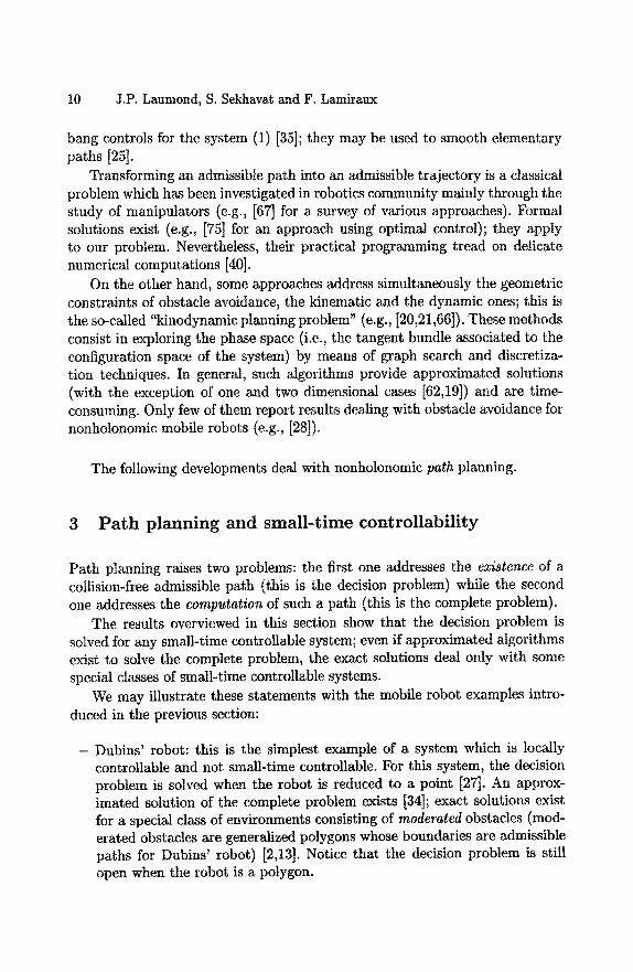
bounded curvature such systems will be called Reeds&Shepp's car and Dubins' car respectively (see Sou~res-Boissonnat's chapter for an overview of recent results on shortest paths for car-like robots). The admissible control domain of Reeds&Shepp's car is symmetric; LARC condition shows that it is small-time controllable from everywhere 3. Dubins' car is a system with drift; it is locally controllable but not small-time controllable from everywhere; for instance, to go from (0, 0, 0) to (1 - cos e, sin e, 0) with Dubins car takes at least 27r - c unity of time.
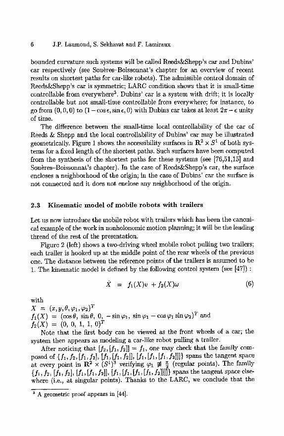
The difference between the small-time local controllability of the car of Reeds & Shepp and the local controllability of Dubins' car may be illustrated geometrically. Figure 1 shows the accessibility surfaces in R 2 x S 1 of both sys- tems for a fixed length of the shortest paths. Such surfaces have been computed from the synthesis of the shortest paths for these systems (see [76,51,15] and Sou~res-Boissonnat's chapter). In the case of Reeds&Shepp's car, the surface encloses a neighborhood of the origin; in the case of Dubins' car the surface is not connected and it does not enclose any neighborhood of the origin.
2.3 Kinematic model of mobi le robots with t rai lers
Let us now introduce the mobile robot with trailers which has been the canoni- cal example of the work in nonholonomic motion planning; it will be the leading thread of the rest of the presentation.
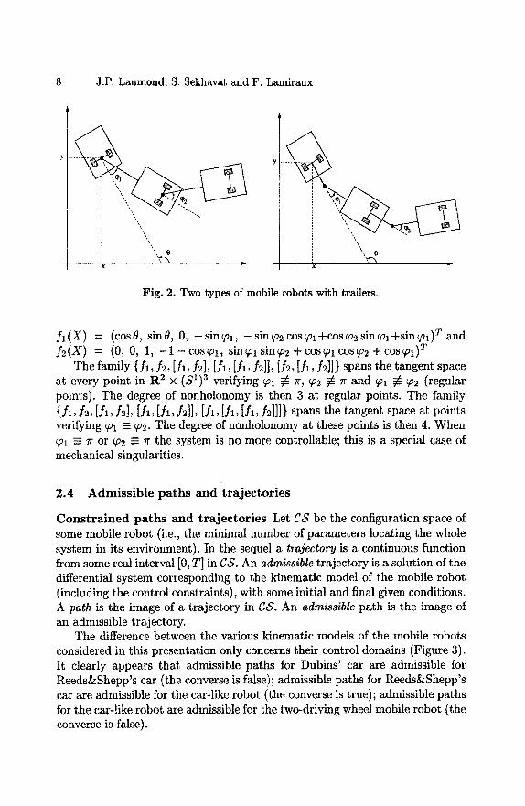
Figure 2 (left) shows a two-driving wheel mobile robot pulling two trailers; each trailer is hooked up at the middle point of the rear wheels of the previous one. The distance between the reference points of the trailers is assumed to be 1. The kinematic model is defined by the following control system (see [47]) :
2 = f l ( x ) v (6)
with X -- ( x , y , O , ~ l , ~ 2 ) T f l ( X ) = (cos~, sin6, 0, - s i n ~ l , s i n a i - c o s ~ l sin~2) T and /2(x) = (0, 0, 1, 1, 0) r
Note that the first body can be viewed as the front wheels of a car; the system then appears as modeling a car-like robot pulling a trailer.
After noticing that [f2, If1, f2]] = fl, one may check that the family com- posed of {fl, f2, [fl, f2], Ill, [f l , f2]], Ill, I l l , Ill, f2]]]} spans the tangent space at every point in R 2 x ($1) 3 verifying ~1 ~ ~ (regular points). The family {]1, f2, [fl, f2], [fl, [£, f2]], [£, If1, [•, [fl, f2]]]]) spans the tangent space else- where (i.e., at singular points). Thanks to the LARC, we conclude that the
a A geometric proof appears in [44].
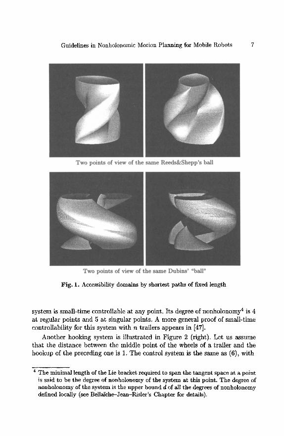
Guidelines in Nonholonomic Motion Planning for Mobile Robots 7
Fig. 1. Accessibility domains by shortest paths of fixed length
system is small-time controllable at any point. Its degree of nonholonomy 4 is 4 at regular points and 5 at singular points. A more general proof of small-time controllability for this system with n trailers appears in [47].
Another hooking system is illustrated in Figure 2 (right). Let us assume that the distance between the middle point of the wheels of a trailer and the hookup of the preceding one is 1. The control system is the same as (6), with
4 The minimal length of the Lie bracket required to span the tangent space at a point is said to be the degree of nonholonomy of the system at this point. The degree of nonholonomy of the system is the upper bound d of all the degrees of nonholonomy defined locally (see Bellai'che-Jean-Pdsler's Chapter for details).
8 J.P. Laumond, S. Sekhavat and F. Lamiraux
Y [-- '\\\\\ "
\,\ ,, e
Fig. 2. Two types of mobile robots with trailers.
f l ( X ) = (cosS, sin0, 0, - s ina i , - sin~o2 cos~l+cos~o2 sin~l+sin~al) T and f2 (X) = (0, 0, 1, - 1 - cos~l , sin~al sin~o2 + cos~al cos~o2 + cos~al) T
The family { f l , f2, [/1, f2], [fl, [fl, f2]], [f2, [fl, f2]]} spans the tangent space at every point in R 2 x ($1) 3 verifying ~al ~ ~r, ~a2 ~ r and ~ol ~ ~2 (regular points). The degree of nonholonomy is then 3 at regular points. The family { f l , f2, If1, ]2], If1, If1, f2]], If1, [fl, If1, ]2]]]} spans the tangent space at points verifying ~Ol -= ~2. The degree of nonholonomy at these points is then 4. When ~1 - 7r or ~2 = 7r the system is no more controllable; this is a special case of mechanical singularities.
2.4 A d m i s s i b l e p a t h s and t r a j e c t o r i e s
Constrained paths and trajectories Let C$ be the configuration space of some mobile robot (i.e., the minimal number of parameters locating the whole system in its environment). In the sequel a trajectory is a continuous function from some real interval [0, T] in C$. An admissible trajectory is a solution of the differential system corresponding to the kinematic model of the mobile robot (including the control constraints), with some initial and final given conditions. A path is the image of a trajectory in CS. An admissible path is the image of an admissible trajectory.
The difference between the various kinematic models of the mobile robots considered in this presentation only concerns their control domains (Figure 3). It clearly appears that admissible paths for Dubins' car are admissible for Reeds&Shepp's car (the converse is false); admissible paths for Reeds&Shepp's car are admissible for the car-like robot (the converse is true); admissible paths for the car-like robot are admissible for the two-driving wheel mobile robot (the converse is false).
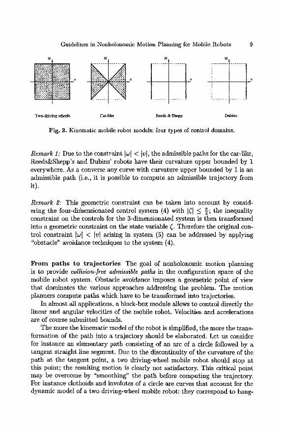
Two-driving wheels
Guidelines in Nonholonomic Motion Planning for Mobile Robots
Car-like
fD
Reeds & Shepp Dubins
Fig. 3. Kinematic mobile robot models: four types of control domains.
Remark 1: Due to the constraint [w] < Iv[, the admissible paths for the car-like, Reeds&Shepp's and Dubins' robots have their curvature upper bounded by 1 everywhere. As a converse any curve with curvature upper bounded by 1 is an admissible path (i.e., it is possible to compute an admissible trajectory from it).
Remark 2: This geometric constraint can be taken into account by consid- ering the four-dihmnsionated control system (4) with I~] < ~" _ ~, the inequality constraint on the controls for the 3-dimensionated system is then transformed into a geometric constraint on the state variable ~. Therefore the original con- trol constraint [w[ < Iv[ arising in system (5) can be addressed by applying "obstacle" avoidance techniques to the system (4).
F r o m pa ths to t r a jec to r ies The goal of nonholonomic motion planning is to provide collision-free admissible paths in the configuration space of the mobile robot system. Obstacle avoidance imposes a geometric point of view that dominates the various approaches addressing the problem. The motion planners compute paths which have to be transformed into trajectories.
In almost all applications, a black-box module allows to control directly the linear and angular velocities of the mobile robot. Velocities and accelerations are of course submitted bounds.
The more the kinematic model of the robot is simplified, the more the trans- formation of the path into a trajectory should be elaborated. Let us consider for instance an elementary path consisting of an arc of a circle followed by a tangent straight line segment. Due to the discontinuity of the curvature of the path at the tangent point, a two driving-wheel mobile robot should stop at this point; the resulting motion is clearly not satisfactory. This critical point may be overcome by "smoothing" the path before computing the trajectory. For instance clothoids and involutes of a circle are curves that account for the dynamic model of a two driving-wheel mobile robot: they correspond to bang-
10 J.P. Laumond, S. Sekhavat and F. Lamiraux
bang controls for the system (1) [35]; they may be used to smooth elementary paths [25].
Transforming an admissible path into an admissible trajectory is a classical problem which has been investigated in robotics community mainly through the study of manipulators (e.g., [67] for a survey of various approaches). Formal solutions exist (e.g., [75] for an approach using optimal control); they apply to our problem. Nevertheless, their practical programming tread on delicate numerical computations [40].
On the other hand, some approaches address simultaneously the geometric constraints of obstacle avoidance, the kinematic and the dynamic ones; this is the so-called "kinodynamic planning problem" (e.g., [20,21,66]). These methods consist in exploring the phase space (i.e., the tangent bundle associated to the configuration space of the system) by means of graph search and discretiza- tion techniques. In general, such algorithms provide approximated solutions (with the exception of one and two dimensional cases [62,19]) and are time- consuming. Only few of them report results dealing with obstacle avoidance for nonholonomic mobile robots (e.g., [28]).
The following developments deal with nonholonomic path planning.
3 P a t h p l a n n i n g a n d s m a l l - t i m e c o n t r o l l a b i l i t y
Path planning raises two problems: the first one addresses the existence of a collision-free admissible path (this is the decision problem) while the second one addresses the computation of such a path (this is the complete problem).
The results overviewed in this section show that the decision problem is solved for any small-time controllable system; even if approximated algorithms exist to solve the complete problem, the exact solutions deal only with some special classes of small-time controllable systems.
We may illustrate these statements with the mobile robot examples intro- duced in the previous section:
- Dubins' robot: this is the simplest example of a system which is locally controllable and not small-time controllable. For this system, the decision problem is solved when the robot is reduced to a point [27]. An approx- imated solution of the complete problem exists [34]; exact solutions exist for a special class of environments consisting of moderated obstacles (mod- erated obstacles are generalized polygons whose boundaries are admissible paths for Dubins' robot) [2,13]. Notice that the decision problem is still open when the robot is a polygon.
Guidelines in Nonholonomic Motion Planning for Mobile Robots 11
- Reeds&Shepp's, car-like and two-driving wheel robots: these systems are small-time controllable. We will see below that exact solutions exist for both problems.
- Mobile robots with trailers: the two systems considered in the previous section are generic of the class of small-time controllable systems. For both of them the decision problem is solved. For the system appearing in Figure 2 (left) we will see that the complete problem is solved; it remains open for the system in Figure 2 (right).
Small-time controllability (Definition 1) has been introduced with a control theory perspective. To make this definition operational for path planning, we should translate it in purely geometric terms.
Let us consider a small-time controllable system, with H a class of control functions taking their values in some compact domain ]C of R m. We assume that the system is symmetric 5. As a consequence, for any admissible path between two configurations X1 and X2, there are two types of admissible trajectories: the first ones go from X1 to X2, the second ones go from X2 to XI.
Let X be some given configuration. For a fixed time T, let T~eachx (T) be the set of configurations reachable from X by an admissible trajectory before the time T. K: being compact, Tteachx(T) tends to {X} when T tends to 0.
Because the system is small-time controllable, Tieachx (T) contains a neigh- borhood of X. We assume that the configuration space is equipped with a (Riemannian) metric: any neighborhood of a point contains a ball centered at this point with a strictly positive radius. Then there exists a positive real num- ber r/such that the ball B(X, rl) centered at X with radius ~/is included in 7~eachx(T).
Now, let us consider a (not necessarily admissible) collision-free path 7 with finite length linking two configurations Xstart and Xgoal. 7 being compact, it is possible to define the clearance e of the path as the minimum distance of 7 to the obstacles 6, e is strictly positive. Then for any X on 7, there exists Tx > 0 such that ~eachx(Tx) does not intersect any obstacle. Let ~/Tx be the radius of the ball centered at X whose points are all reachable from X by admissible trajectories that do not escape T~eachx (Tx). The set of all the balls B(X, rlTx), X E 7, constitutes a covering of % 7 being compact, it is possible to get a finite sequence of configurations (Xi)l<i<k (with X1 = Xsta~t, Xk = X~oal), such that the balls B(XI, rlTx, ) cover 7-
Consider a point Yi,i+l lying on 7 and in B(Xi,rlTx, )f l B(Xi+l, ~Txi+l ). Between Xi and Y/,i+l (respectively Xi+a and Y/,i+I) there is an admissible
5 Notice that, with the exception of Dubins' robot, all the mobile robots introduced in the previous section are symmetric. We consider that a configuration where the robot touches an obstacle is not collision-free.
12 J.P. Laumond, S. Sekhavat and F. Lamiraux
trajectory (and then an admissible path) that does not escape ~eachx~ (Tx~) (respectively 7~eachx~+l (Tx,+I)). Then there is an admissible path between Xi and Xi+l that does not escape Tteachx, (Tx~)U ~eachx~+~ (Tx,+~); this path is then collision-free. The sequence (Xi)l_<i<k is finite and we can conclude that there exists a collision-free admissible path between Xstart and Xgoat.
T h e o r e m 3.1. For symmetric small-time controllable systems the existence o] an admissible collision-free path between two given configurations is equivalent to the existence of any collision-free path between these configurations.
Remark 3: We have tried to reduce the hypothesis required by the proof to a minimum. They are realistic for practical applications. For instance the com- pactness of E holds for all the mobile robots considered in this presentation. Moreover we assume that we are looking for admissible paths without contact with the obstacles: this hypothesis is realistic in mobile robotics (it does not hold any more for manipulation problems). On the other hand we suggest that two configurations belonging to the same connected component of the collision- free path can be linked by a finite length path; this hypothesis does not hold for any space (e.g., think to space with a fractal structure); nevertheless it holds for realistic workspaces where the obstacles are compact, where their shape is simple (e.g., semi-algebraic) and where their number is finite.
Consequence 1: Theorem 3.1 shows that the decision problem of motion plan- ning for a symmetric small-time controllable nonholonomic system is the same as the decision problem for the holonomic associated one (i.e., when the kine- matics constraints are ignored): it is decidable. Notice that deciding whether some general symmetric system is small-time controllable (from everywhere) can be done by a only semi-decidable procedure [50]. The combinatorial com- plexity of the problem is addressed in [77]. Explicit bounds of complexity have been recently provided for polynomial systems in the plane (see [68] and refer- ences therein).
Consequence 2: Theorem 3.1 suggests an approach to solve the complete prob- lem. First, one may plan a collision-free path (by means of any standard meth- ods applying to the classical piano mover problem); then, one approximates this first path by a finite sequence of admissible and collision-free ones. This idea is at the origin of a nonholonomic path planner which is presented below (Section 5.3). It requires effective procedures to steer a nonholonomic system from a configuration to another. The problem has been first attacked by ignor- ing the presence of obstacles (Section 4); numerous methods have been mainly developed within the control theory community; most of them account only for local controllability. Nevertheless, the planning scheme suggested by Theo- rem 3.1 requires steering methods that accounts for small-time controllability
Guidelines in Nonholonomic Motion Planning for Mobile Robots 13
(i.e., not only for local controllability). In Section 5.1 we introduce a topological property which is required by steering methods in order to apply the planning scheme. We show that some among those presented in Section 4 verify this property, another one does not, and finally a third one may be extended to guaranty the property.
4 Steering methods
What we call a steering method is an algorithm that solves the path planning problem without taking into account the geometric constraints on the state. Even in the absence of obstacles, computing an admissible path between two configurations of a nonholonomic system is not an easy task. Today there is no algorithm that guarantees any nonholonomic system to reach an accessible goal exactly. In this section we present the main approaches which have been applied to mobile robotics.
4.1 F r o m vec tor fields to effective paths
The concepts from differential geometry that we want to introduce here are thoroughly studied in [79,90,80,81] and in Bella'iche-Jean-Risler's Chapter. They give a combinatorial and geometric point of view of the path planning problem.
Choose a point X on a manifold and a vector field f defined around this point. There is exactly one path 7(~-) starting at this point and following f . That is, it satisfies 7(0) = X and ~/(T) = f(7(Z)). One defines the exponential of f at point X to be the point 7(1) denoted by e f . X . Therefore e f appears as an operation on the manifold, meaning "slide from the given point along the vector field f for unit time". This is a diffeomorphism. With a being a real number, applying eaf amounts to follow f for a time a. In the same way, applying J + g is equivalent to follow f + g for unit time.
It remains that, whenever [f, g] ~ 0, following directly a f + fig or following first a f , then fig, are no longer equivalent. Intuitively, the bracket If, g] mea- sures the variation of g along the paths of f ; in some sense, the vector field g we follow in a f + fig is not the same as the vector field g we follow after having followed a f first (indeed g is not evaluated at the same points in both cases).
Assume that f l , . . . , fn are vector fields defined in a neighborhood Af of a point X such that at each point of A/', { f l , . . . ,fn} constitutes a basis of the tangent space. Then there is a smaller neighborhood of X on which the maps ( a l , . . . , an) ~-~ e alfl'k'''-t'°~"'f" • X and ( a l , . . . , an) ~-> e c~'J'' ". . e c~Ifl • X are two coordinate systems, called the first and the second normal coordinate system associated to ( f l , . . . , f ,} .
14 J.P. Laumond, S. Sekhavat and F. Lamiraux
The Campbell-Baker-Hausdorff-Dynkin formula states precisely the differ- ence between the two systems: for a sufficiently small T, one has:
eVf . erg _~ evf÷rg - lr2[f,g]'~r2e(T)
where e(r) --+ 0 when 7 -+ 0. Actually, the whole formula as proved in [90] gives an explicit form for the
e function. More precisely, e yields a formal series whose coefficients ch of ~.k are combinations of brackets of degree k, 7 i.e.
o o
k-~.3
Roughly speaking, the Campbell-Baker-Hansdorff-Dynkin formula tells us how a small-time nonholonomic system can reach any point in a neighborhood of a starting point. This formula is the hard core of the local controllability concept. It yields methods for explicitly computing admissible paths in a neigh- borhood of a point.
4.2 Nilpotent systems and nilpotentization
One method among the very first ones has been defined by Lafferiere and Sussmann [39] in the context of nilpotent system. A control system is nilpotent as soon as the Lie brackets of the control vector fields vanish from some given length.
For small-time controllable nilpotent systems it is possible to compute a basis Y of the Control Lie Algebra L A ( A ) from a Philipp Hall family (see for instance [46]). The method assumes that a holonomic path 7 is given. If we express locally this path on B, i.e., if we write the tangent vector ~/(t) as a linear combination of vectors in B(7(t)), the resulting coefficients define a control that steers the holonomic system along 7. Because the system is nilpotent, each exponential of Lie bracket can be developed exactly as a finite combination of the control vector fields: such an operation can be done by using the Campbell-Baker-Hausdorff-Dynkin formula above. An introduction to this machinery through the example of a car-like robot appears in [48]. It is then possible to compute an admissible and piecewise constant control u for the nonholonomic system that steers the system exactly to the goal.
For a general system, Lafferiere and Sussmann reason as if the system were nilpotent of order k. In this case, the synthesized path deviates from the goal. Nevertheless, thanks to a topological property, the basic method may be used
T As an example the degree of [[f, g], If, [g, If, g]l]] is 6.
Guidelines in Nonhotonomic Motion Planning for Mobile Robots 15
in an iterated algorithm that produces a path ending as close to the goal as wanted.
In [33], Jacob gives an account of Lafferiere and Sussmann's strategy by using another coordinate system. This system is built from a Lyndon basis of the free Lie algebra [93] instead of a P. Hall basis. This choice reduces the number of pieces of the solution.
In [11], Bella'/che et al apply the nilpotentization techniques developed in [10] (see also [31]). They show how to transform any controllable system into a canonical form corresponding to a nilpotent system approximating the original one. Its special triangular form allows to apply sinusoidal inputs (see below) to steer the system locally. Moreover, it is possible to derive from the proposed canonical form an estimation of the metrics induced by the shortest feasible paths. This estimation holds at regular points (as in [92]) as welt as at singular points. These results are critical to evaluate the combinatorial complexity of the approximation of holonomic paths by a sequence of admissible ones (see Section 5.7).
The mobile robots considered in this presentation are not nilpotent s. A uilpotentization of this system appear in [39]. We conclude this section by the nilpotentization of a mobile robot pulling a trailer [11].
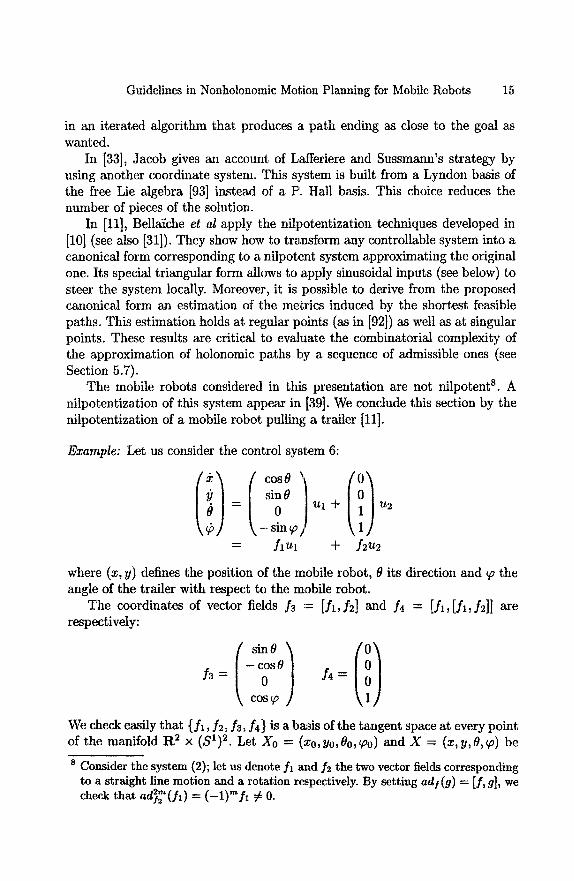
Example: Let us consider the control system 6:
\_~ / ul + u2
= f l U l -I- f2u2
where (x, y) defines the position of the mobile robot, 8 its direction and 9 the angle of the trailer with respect to the mobile robot.
The coordinates of vector fields f3 := [fl, f2] and f4 = [fl, [fl, f2]] are respectively:
=
sin0 -oS J s4: cos ~ /
We check easily that {fl, f2, f3, f4} is a basis of the tangent space at every point of the manifold R 2 x ($1) 2. Let Xo = (xo,yo,O0,9o) and X = (x,y,O,~o) be
s Consider the system (2); let us denote fl and f~ the two vector fields corresponding to a straight line motion and a rotation respectively. By setting adI(g ) -.-- [f, g], we check that a d ~ ( f l ) = (-1)'~fl # 0.
16 J.P. Laumond, S. Sekhavat and F. Lamiraux
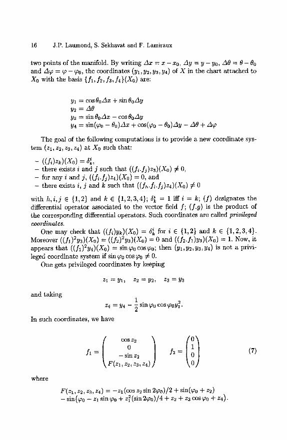
two points of the manifold. By writing Ax = x - Xo, Ay = y - Yo, A0 = 0 - 8o and Aqv = ~v - ~ o , the coordinates (YI,Y2,Y3,Y4) of X in the chart a t tached to Xo with the basis {f l , f2, f3, f4}(Xo) are:
Yl = cos 0oAx + sin OoAy Y2 --- AO Y3 = sin~o Ax - cos~oAy Y4 = sin(~vo - 00)Ax + cos(~oo - ~o)Ay - A0 + A~v
The goal of the following computat ions is to provide a new coordinate sys- t em (zl,z2,z3,z4) at Xo such that:
- k ,
- there exists i and j such that ((fi.fj)z3)(Xo) ~ O, - for any i and j, ((£.fj)z4)(Xo) = O, and - there exists i, j and k such that ((fh.fi.fj)z4)(Xo) ~ 0
with h, i , j e {1,2} and k e {1,2,3,4}; 5~ = 1 iff i = k; ( f ) designates the differential operator associated to the vector field f ; (f.g) is the product of the corresponding differential operators. Such coordinates axe called privileged coordinates.
One may check tha t ((]~)yk)(Xo) = ~ik for i e {1,2} and k e {1,2,3,4}. Moreover ((fl)2y3)(Xo) : ((f2)2y3)(Xo) -- 0 and ((f2.£)y3)(Xo) = 1. Now, it appears tha t ((fl)2y4)(Xo) = sin ~Vo cos ~o0; then (Yl, Y:, Y3, Y4) is not a privi- leged coordinate system if sin ~o cos ~o ~ 0.
One gets privileged coordinates by keeping
z l = y l , z 2 = y ~ , z3=ya
and taking 1
z4 = Y4 - ~ sin ~o cos ~oy 2.
In such coordinates, we have
where
( C°o 2 ) f l = | - sinz2 f2 =
\ F(zl, z3, z4)
F(zl, z2, z3, z4) = - z l (cos z2 sin 2~Vo)/2 + sin(~vo + z2) - sin(~o - zl s in~o + z12(sin 2~vo)/4 + z2 + z3 cos ~oo + z4).
Guidelines in Nonholonomic Motion Planning for Mobile Robots 17
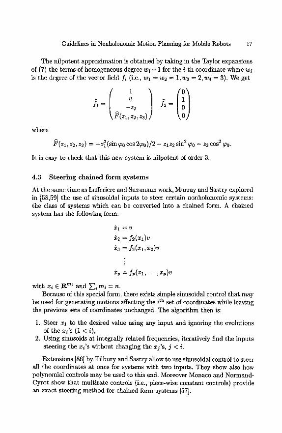
The nilpotent approximation is obtained by taking in the Taylor expansions of (7) the terms of homogeneous degree wi - 1 for the i-th coordinate where wi is the degree of the vector field fi (i.e., W 1 = W 2 = 1,w3 = 2, w4 = 3). We get
where
L= --Z 2
l~(Zl, Z2, Z3)
F ( z 1 , z2, z3) ~-- -z~(sin ~0 cos 2~0)/2 - zlz2 sin 2 ~o0 - z3 cos 2 ~o0.
It is easy to check that this new system is nilpotent of order 3.
4.3 Steering chained form systems
At the same time as Lafferiere and Sussmann work, Murray and Sastry explored in [58,59] the use of sinusoidal inputs to steer certain nonholonomic systems: the class of systems which can be converted into a chained form. A chained system has the following form:
Xl = V
~2 = Y2(zl)v
It3 -'~ f3(Xi, :r2)V
Xp = f p ( X i , . . . , xp)v
with xi E R m~ and ~ mi = n. Because of this special form, there exists simple sinusoidal control that may
be used for generating motions affecting the ith set of coordinates while leaving the previous sets of coordinates unchanged. The algorithm then is:
1. Steer Xl to the desired value using any input and ignoring the evolutions of the x~'s (1 < i),
2. Using sinusoids at integrally related frequencies, iteratively find the inputs steering the xi's without changing the xj's, j < i.
Extensions [86] by Tilbury and Sastry allow to use sinusoidal control to steer all the coordinates at once for systems with two inputs. They show also how polynomial controls may be used to this end. Moreover Monaco and Normand- Cyrot show that multirate controls (i.e., piece-wise constant controls) provide an exact steering method for chained form systems [57].
18 J.P. Laumond, S. Sekhavat and F. Lamiraux
Even if a system is not triangular, it may be possible to transform it into a triangular one by feedback transformations (see [59,60]). Moreover, notice that the nilpotentization techniques introduced in the previous section leads to approximated systems which are in chained form.
E x a m p l e : Let us consider our canonical example of a mobile robot with two trailers (Figure 2, left). The clever idea which enables the transformation of the system into a chained form was to consider a frame attached to the last trailer rather than attached to the robot [86]. Denoting by 01 and 02 the angle of the trailers, and by x2 and Y2 the coordinates of the middle point of the last trailer, the system (6) may be re-written as:
{ ~ ----- C0802C08(01 -- 82)C08(00 -- 81)u l iJ = s i n O 2 c o s ( 0 1 - 02)cos(00 - 01)ul ~0 ---- U2
01 = sin(0o - 01)Ul 02 = sin(01 - 02)cos(0o - 01)ul
Let us consider the following change of coordinates:
r Z 1 m X 1 tan(Oo--O1)
z2 = ~ . cos(ol-eD × (1 + tan2(01 - 82)) + ~ x tan(01 - 02)(3tan(01 - 02)tan82 - (1 - tan2(81 - 82)))
tan(Ol--$2) Z3 m C083~2
z4 = tan02
Z5 m y
This transformation is a local diffeomorphism around configurations for which the angle between bodies are not equal to y." In this new coordinates, the kinematic model of the system has the following chained form:
Z2 ---- V2 ~3 = z 2 . v l (8) Z4 Z3 .Vl Z5 ~- Z4.Vl
Notice that Sordalen generalizes this result by providing a conversion of the car with an arbitrary number of trailers into a chained form [78].
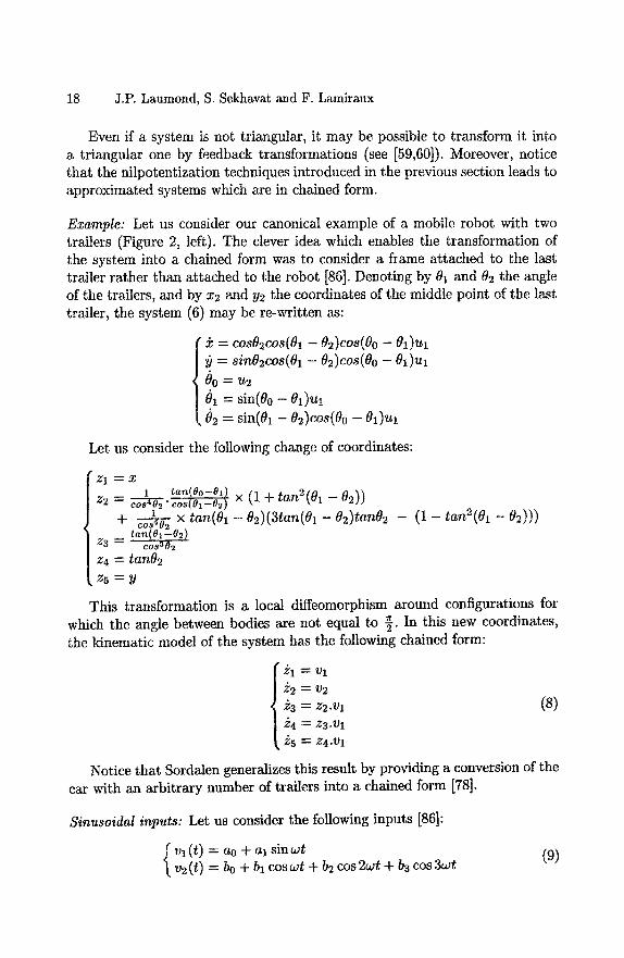
S inuso ida l inputs : Let us consider the following inputs [86]:
I v1 (t) = ao + al sin w t v2 (t) bo + bl cos w t + b2 cos 2wt + b3 cos 3wt
(9)
Guidelines in Nonholonomic Motion Planning for Mobile Robots 19
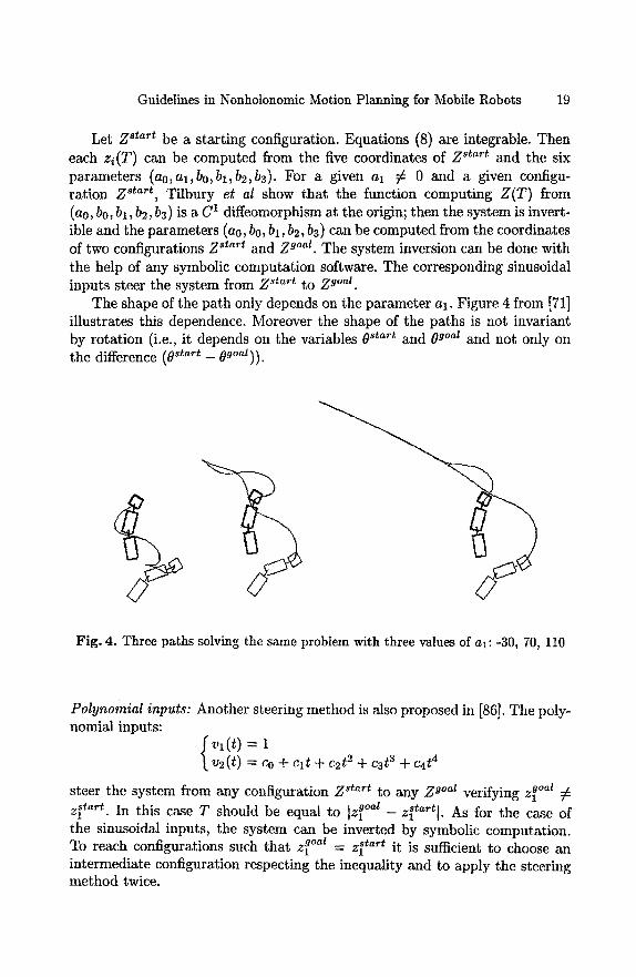
Let Z start be a starting configuration. Equations (8) are integrable. Then each z i (T) can be computed from the five coordinates of Z start and the six parameters (ao,al,bo,b:,b2,b3). For a given al ¢ 0 and a given configu- ration Z ~t~rt, Tilbury et al show that the function computing Z ( T ) from (ao, bo, b:, b2, b3) is a C 1 diffeomorphism at the origin; then the system is invert- ible and the parameters (ao, b0, bl, b2, b3) can be computed from the coordinates of two configurations Z st~r~ and Z g°al. The system inversion can be done with the help of any symbolic computation software. The corresponding sinusoidal inputs steer the system from Z ~ta~t to Z 9°at.
The shape of the path only depends on the parameter a:. Figure 4 from [71] illustrates this dependence. Moreover the shape of the paths is not invariant by rotation (i.e., it depends on the variables 0 star~ and 0 g°at and not only on the difference (0 start - Og°al) ).
Fig. 4. Three paths solving the same problem with three values of a:: -30, 70, 110
Polynomial inputs: Another steering method is also proposed in [86]. The poly- nomial inputs:
Vl(t) = I
V2(t) CO -b Cl t -{- C2 t2 -t- C3 t3 q- C4 t4
goal steer the system from any configuration Z 8tart to any Z g°al verifying z 1 z l tart. In this case T should be equal to ]z~ °al - zltart t. As for the case of the sinusoidal inputs, the system can be inverted by symbolic computation. To reach configurations such that ~:'g°at = z~t~rt it is sufficient to choose an intermediate configuration respecting the inequality and to apply the steering method twice.
20 J.P. Laumond, S. Sekhavat and F. Lamiraux
Extensions: The previous steering methods deal with two-input chained form systems. In [16] Bushnell, Tilbury and Sastry extend these results to three-input nonholonomic systems with the fire-truck system as a canonical example 9. They give sufficient conditions to convert such a system to two-chain, single generator chained forms. Then they show that multirate digital controls, sinusoidal inputs and polynomial inputs may be used as steering methods.
4.4 S t ee r ing fiat systems
The concept of flatness has been introduced by Fliess, Ldvine, Martin and Rouchon [26,63].
A flat system is a system such that there exists a finite set of variables Yi differentially independent which appear as differential functions of the system variables (state variables and inputs) and of a finite number of their derivatives, each system variable being itself a function of the yi's and of a finite number of their derivatives. The variables yi's are called the linearizing outputs of the system.
Example: In [63] Rouchon et al show that mobile robots with trailers are flat as soon as the trailers are hitched to the middle point of the wheels of the previous ones. The proof is based on the same idea allowing to transform the system into a chained form: it consists in modeling the system by starting from the last trailer.
Let us consider the system (6) (Figure 2, left). Let us denote the coordinates of the robot and the two trailers by (x, y, O), (xl, Yl, 81) and (x2, Y2, 82) respec- tively. Remind that the distance between the reference points of the bodies is 1. The holonomic equations allow to compute x, y, Xl and Yl from x2, Y2, 81 and 82:
Xl --~ x2 --~ c0882 x = x 2 -~- cos82 -[- cosSl
Yl = Y2 -k sin 82 Y : Y2 q- sin 82 + sin 81
The rolling without slipping conditions lead to three nonholonomic equations xisin0i -~)icosSi = 0 allowing to compute 62 (resp. 81 and 8) from (i2,~/2) (resp. (~h,yh) and (J/2,~/2)). Finally the controls v and w are given by v = cos0
A_ =~. (or V = sin 8 ) and w Therefore any variable of the system can be computed from x2 and y2 and
their derivatives. The system is flat with x2 and Y2 as linearizing outputs.
9 The fire-truck system is a car-hke robot (two inputs) with one trailer whose direc- tion of the wheels is controllable (third input).
Guidelines in Nonholonomic Motion Planning for Mobile Robots 21
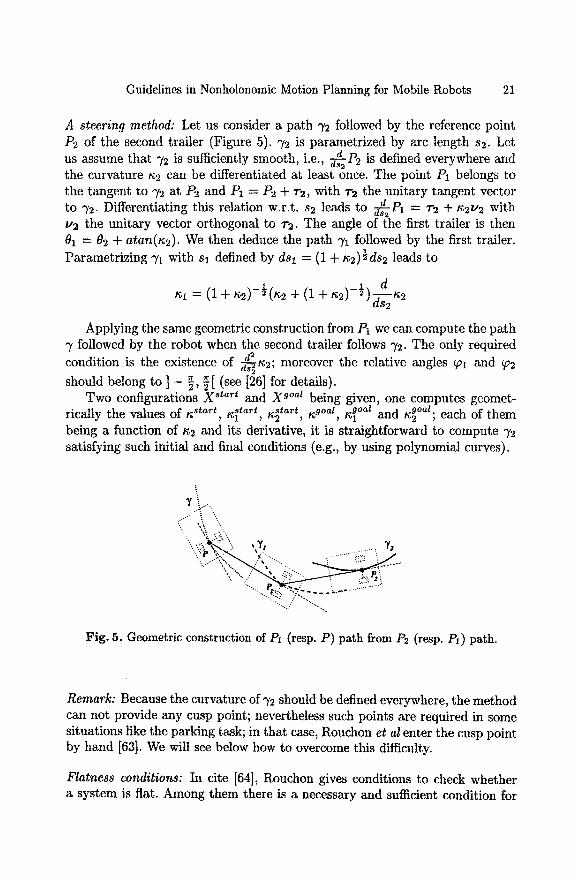
A steering method: Let us consider a path ~/2 followed by the reference point P2 of the second trailer (Figure 5). ~/2 is parametrized by arc length s2. Let
d us assume that 72 is sufficiently smooth, i.e., d-~P2 is defined everywhere and the curvature t~2 can be differentiated at least once. The point P1 belongs to the tangent to ~/2 at P2 and P1 = P2 + ~'2, with v2 the unitary tangent vector
d to 72. Differentiating this relation w.r.t, s2 leads to d--~2Pl = r2 + a2v2 with ~'2 the unitary vector orthogonal to 1"2. The angle of the first trailer is then O~ = 82 + atan(a2). We then deduce the path 71 followed by the first trailer. Parametrizing ~ with s~ defined by ds~ = (1 + g2)½ds2 leads to
1 1 d
as2
Applying the same geometric construction from P1 we can compute the path 7 followed by the robot when the second trailer follows ~'2- The only required
d 2 . condition is the existence of ~ a 2 , moreover the relative angles ~Pl and ~2
should belong to ] - ~, ~[ (see [26] for details). Two configurations X s~art and X g°al being given, one computes geomet-
goat rically the values of ~start ~s~a~tl , ~ ta~t ~aoa~, '~l~g°at and ~2 ; each of them being a function of a2 and its derivative, it is straightforward to compute 72 satisfying such initial and final conditions (e.g., by using polynomial curves).
'.: ,~ :~ :~(..
Fig. 5. Geometric construction of P1 (resp. P) path from P2 (resp. P1) path.
Remark: Because the curvature of "?2 should be defined everywhere, the method can not provide any cusp point; nevertheless such points are required in some situations like the parking task; in that case, Rouchon et al enter the cusp point by hand [63]. We will see below how to overcome this difficulty.
Flatness conditions: In cite [64], Rouchon gives conditions to check whether a system is flat. Among them there is a necessary and sufficient condition for
22 J.P. Laumond, S. Sekhavat and F. Lamiraux
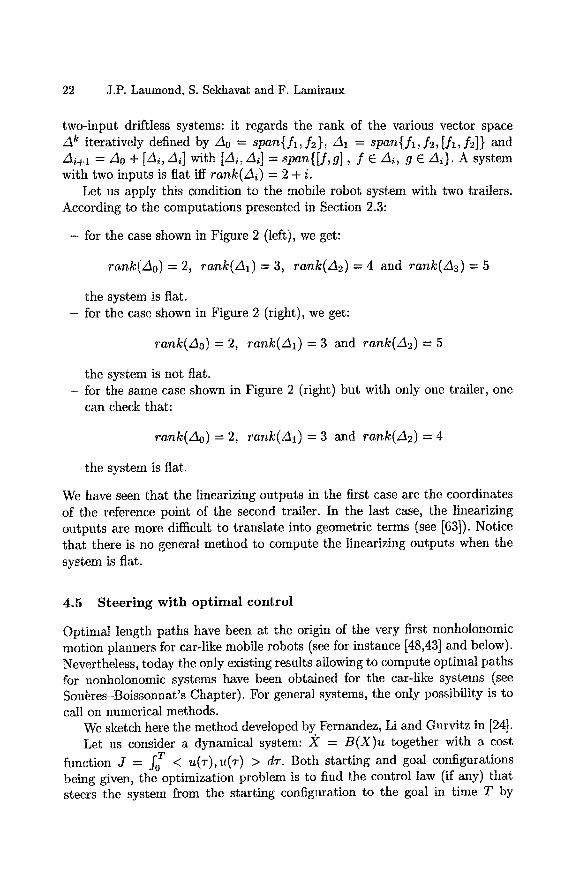
two-input driftless systems: it regards the rank of the various vector space A k iteratively defined by glo = span{f1, f2}, A1 = span{f1, f2, [fl, f2]} and A/+I = Ao + [Ai, Ai] with [Ai, Ai] = span{[f,g] , f E A~, g E Ai}. A system with two inputs is flat iff rank(Ai) = 2 + i.
Let us apply this condition to the mobile robot system with two trailers. According to the computations presented in Section 2.3:
- for the case shown in Figure 2 (left), we get:
rank(Ao) = 2, rank(A1) = 3, rank(A2) = 4 and rank(A3) = 5
the system is fiat. - for the case shown in Figure 2 (right), we get:
rank(Ao) = 2, rank(Z~l) = 3 and rank(A2) = 5
the system is not flat. - for the same case shown in Figure 2 (right) but with only one trailer, one
can check that:
rank(Ao) = 2, rank(A1) = 3 and rank(A2) = 4
the system is flat.
We have seen that the linearizing outputs in the first case are the coordinates of the reference point of the second trailer. In the last case, the linearizing outputs are more difficult to translate into geometric terms (see [63]). Notice that there is no general method to compute the tinearizing outputs when the system is flat.
4.5 Steer ing wi th op t imal control
Optimal length paths have been at the origin of the very first nonholonomic motion planners for car-like mobile robots (see for instance [48,43] and below). Nevertheless, today the only existing results allowing to compute optimal paths for nonholonomic systems have been obtained for the car-like systems (see Sou~res-Boissonnat's Chapter). For general systems, the only possibility is to call on numerical methods.
We sketch here the method developed by Fernandez, Li and Gurvitz in [24]. Let us consider a dynamical system: J( = B ( X ) u together with a cost
function J = f J < u(r), u(~-) > dT. Both starting and goal configurations being given, the optimization problem is to find the control law (if any) that steers the system from the starting configuration to the goal in time T by
Guidelines in Nonholonomic Motion Planning for Mobile Robots 23
minimizing the cost function J. The path corresponding to an optimal control law is said to be an optimal path.
Let us consider a continuous and piecewise C 1 control law u defined over [0, T]. We denote by fi the periodic extension of u over R. We may write fi in terms of a Fourier basis:
oo i2k?rt i2k~
k = 0
We then approximate fi by truncating its expansion up to some rank N. N
The new control law ~ is then defined by N real numbers 1° ~ = ~-,k=l akek, i 2_2__~ e k e {e r , p e Z}. The choice of the reals ak being given, the point X(T)
reached after a time T with the control law fi appears as a function f ( a ) from R N to R n.
Now, we get a new cost function
N
J(a) = ~ [akl 2 + 71IX(T) - XgoatH 2. k = l
The new optimization problem becomes: for a fixed time T, an initial point Xinit and a final point Xgoat , find ~ E R N such as
N
: I kl + 7llf( ) - Xgoatll k = l
is minimum. One proves (e.g., see [24]) that the solutions of the new finite-dimensional
problem converge to the solutions of the original problem as N and 7 go to infinity.
Because we do not know f and 6f /Sa explicitly we use numerical methods (numerical integration of the differential equations and numerical optimization like Newton's algorithm) to compute a solution of the problem. Such a solution is said to be a near-optimal solution of the original problem.
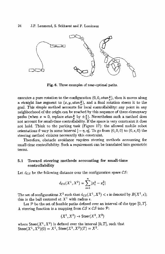
Figure 6 from [71] shows three examples of near-optimal paths computed from this method for a mobile robot with two trailers [49].
5 Nonholonomic path planning for small-time controllable s y s t e m s
Consider the following steering method for a two-driving wheel mobile robot. To go from the origin (0,0,0) to some configuration (x,y, 8) the robot first
10 This approximation restricts the family of the admissible control laws.
24 J.P. Laumond, S. Sekhavat and F. Lamiraux
Fig. 6. Three examples of near-optimal paths.
executes a pure rotation to the configuration (0, 0, atan~), then it moves along a straight line segment to (x,y, atan~), and a final rotation steers it to the goal. This simple method accounts for local controllability: any point in any neighborhood of the origin can be reached by this sequence of three elementary paths (when x = 0, replace atan~ by ~ ) . Nevertheless such a method does not account for small-time controllability. If the space is very constraint it does not hold. Think to the parking task (Figure 17): the allowed mobile robot orientations 0 vary in some interval ] - ~/, 7[. To go from (0, 0, 0) to (0, e, 0) the steering method violates necessarily this constraint.
Therefore, obstacle avoidance requires steering methods accounting for small-time controllability. Such a requirement can be translated into geometric terms.
5.1 Toward steering methods accounting for small-time controllability
Let des be the following distance over the configuration space gS:
n
dc (x',x = Z l x { - i = 1
The set of configurations X 2 such that dcs (X 1 , X 2) < e is denoted by B(X', e); this is the ball centered at X 1 with radius e.
Let ~' be the set of feasible paths defined over an interval of the type [0, T]. A steering function is a mapping from gS x gS into :P:
(X 1 , X 2) -+ Steer(X 1 , X 2 )
where Steer(X 1, X 2) is defined over the interval [0, T], such that Steer(X 1 , X 2 ) (0) = X 1 , Steer(X 1 , X 2 ) (T) = X 2.
Guidelines in Nonholonomic Motion Planning for Mobile Robots 25
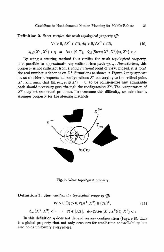
Def ini t ion 2. Steer verifies the weak topological property iff:
Ve > 0,VX 1 E CS, 3/] > 0,VX 2 E CS, (10)
dcs(X1,X 2) < ~7 ~ Vte [0,T], dcs(Steer(X1,X2)(t),X 1) < e
By using a steering method that verifies the weak topological property, it is possible to approximate any collision-free path 7Iree. Nevertheless, this property is not sufficient from a computational point of view. Indeed, it is local: the real number ~/depends on X 1 . Situations as shown in Figure 7 may appear: let us consider a sequence of configurations X i converging to the critical point X c, and such that limx~-~x¢ ~I(X i) = 0; to be collision-free any admissible path should necessary goes through the configuration X c. The computation of X c may set numerical problems. To overcome this difficulty, we introduce a stronger property for the steering methods.
X~
B(X, cE)
Fig. 7. Weak topological property
Definit ion 3. Steer verifies the topological property iff:
Ve > 0,3~/> 0,V(XI,X 2) E (C8) 2, (11)
dcs(X1,X 2) < T/ ~ Vt E [0,T], dcs(Steer(X1,X2)(t),X 1) < e
In this definition ~/does not depend on any configuration (Figure 8). This is a global property that not only accounts for small-time controllability but also holds uniformly everywhere.
26 J.P. Laumond, S. Sekhavat and F. Lamiraux
X goal
X start
% / t X \
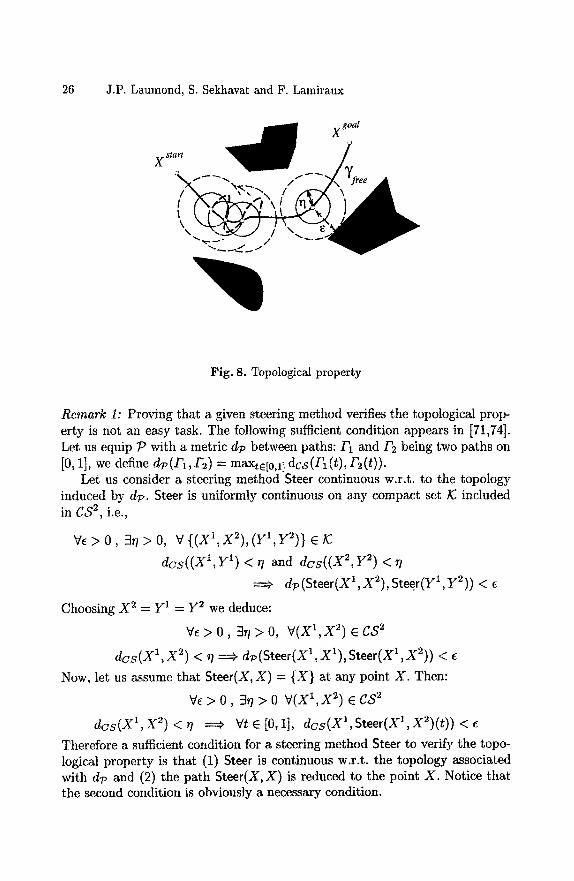
Fig. 8. Topological property
Remark 1: Proving that a given steering method verifies the topological prop- erty is not an easy task. The following sufficient condition appears in [71,74]. Let us equip 7 ~ with a metric d~, between paths:/"1 and F2 being two paths on [0, 1], we define 47, (/"1, F2) = max~e[0j] dcs (1"1 (t), F2 (t)).
Let us consider a steering method Steer continuous w.r.t, to the topology induced by dT,. Steer is uniformly continuous on any compact set ]C included in CS 2, i.e.,
Vc> 0, 3r/> 0, V{(X 1,X2),(Y1,Y2)} eK:
dcs((X 1, y1) < r/ and dcs((X 2, y2) < ~/
dp(Steer(X 1, X2), Steer(Y1, y2)) < e
Choosing X 2 = Y' = y2 we deduce:
V~ > 0 ,3 ,1 > 0, V(X1,X 2) e CS 2
d c s ( X 1 , X 2) < r/===tr dTa(Steer(X1,X1),Steer(X1,X2)) < e
Now, let us assume that Steer(X, X) = {X} at any point X. Then:
V£ > 0, ~] ~> 0 V(X1,X 2) E C8 2
d c s ( X z , X 2) < r/ ~ Vte [0,1], dcs(Xl,Steer(XZ,X~)(t)) < e Therefore a sufficient condition for a steering method Steer to verify the topo- logical property is that (1) Steer is continuous w.r.t, the topology associated with d~ and (2) the path Steer(X, X) is reduced to the point X. Notice that the second condition is obviously a necessary condition.
Guidelines in Nonholonomic Motion Planning for Mobile Robots 27
Remark 2: The first general result taking into account the necessary uniform convergence of steering methods is due to Sussmann and Liu [84]: the authors propose an algorithm providing a sequence of feasible paths that uni]ormty con- verge to any given path. This guarantees that one can choose a feasible path arbitrarily close to a given collision-free path. The method uses high frequency sinusoidal inputs. Though this approach is general, it is quite hard to imple- ment in practice. In [87], Tilbury et al exploit the idea for a mobile robot with two trailers. Nevertheless, experimental results show that the approach cannot be applied in practice, mainly because the paths are highly oscillatory. There- fore this method has never been connected to a geometric planner in order to get a global planner which would take into account both environmental and kinematic constraints.
5.2 Steering methods and topological property
In this section we review the steering methods of Section 4 with respect to the topological property.
Optimal pa ths Let us denote by Steeropt the steering method using optimal control. Steeropt naturally verifies the weak topological property. Indeed the cost of the optimal paths induce a special metric in the configuration space; such a metric is said to be a nonholonomic [92], or singular [14], or Carnot- Caratheory [56], or sub-Riemannian [80] metric. By definition any optimal path with cost r does not escape the nonholonomic ball centered at the starting point with radius r. A general result states that the nonholonomic metrics induce the same topology as the "natural" metrics des. This means that for any nonholonomic ball Bah(X, r) with radius r, there are two real numbers e and ~ strictly positive such that B(X,y) C Bnh(X,r) C B ( X , @
The nonholonomic distance being continuous, to get the topological prop- erty, it suffices to restrict the application of Steeropt to a compact domain of the configuration space 11.
There is no general result that gives the exact shape of the nonholonomic balls; nevertheless the approximated shape of these balls is well understood (e.g., see Bella'iche-Jean-PSsler's chapter).
The metric induced by the length of the shortest paths for Reeds&Shepp's car is close to a nonholonomic metric; car-like robots are the only known cases where it is possible to compute the exact shape of the balls (see Figure 1).
11 Notice that the steering method Steeropt is not necessarily continuous w.r.t, the topology induced by d~,.
28 J.P. Laumond, S. Sekhavat and F. Lamiraux
Sinusoidal inputs and chained form systems Let us consider the two- input chained form system (8) together with the sinusoidal inputs (9) presented in Section 4.3. We have seen that the shape of the paths depends on al (Fig- ure 4). The only constraint on the choice of al is that it should be different from zero.
The steering method using such inputs is denoted by a~ Steersi n. For a fixed a l value of al, Steersi n does not verify the topological property. Indeed, for any
a l configuration Z, the path Steersin(Z, Z) is not reduced to a point 12. Therefore, the only way to build a steering method based on sinusoidal
inputs and verifying the topological property is not to keep al constant. One has to prove the existence of a continuous expression of al (Z 1, Z 2) such that:
lim at(Z I , Z 2 ) = 0
lim ao(Z 1, Z2 ,a l (Z 1, Z2)) = 0 Z2 --~. Z 1
lim bi(Zl ,Z2,a l (Z1,Z2)) = 0 Z2~Z 1
The proof appears in [73]. It first states that, for a fixed value of al, Steers~ n is continuous w.r.t, to the topology induced by dp. This implies that when the final configuration Z 2 tends to the initial configuration Z 1, the path Steera~n(Z 1, Z 2) tends to the path Steera~n(Z I, Z1). Moreover, for any
a l Z, Steersin(Z, Z) tends to {Z} when al tends to zero. Combining these two of Steers~ n to a compact domain/C statements and restricting the application ~1
of CS 2, one may conclude that:
Ve > 0 , 3A1 > 0 Val < A1, 3y(al), V ( Z I , Z 2) E Y~,
d c s ( Z l , Z 2) < ~?(al), ~ Vte [0,1], dcs(Zl ,S teer~n(Zl ,Z2)( t ) ) < e
Then, by tuning al, it is a priori possible to design a steering method Steersi,~ based on sinusoidal inputs and verifying the topological property. It remains to define a constructive way to tune the parameter al. The problem is not easy. Indeed the general expression of parameters ao and bi are unknown. Then we do not dispose of a unique expression of Steersin. Nevertheless, it is possible to "simulate" a steering method verifying the topological property, by
Steersi n according to the distance between the start switching between different al and goal configurations. The principle of the construction presented in Annex consists in introducing the possibility to iteratively compute subgoals and then a sequence of subpaths that reaches the final goal without escaping a bounded domain.
12 The first coordinate of points lying on the path is zl(t) = zx + ~-(1 -coswt).
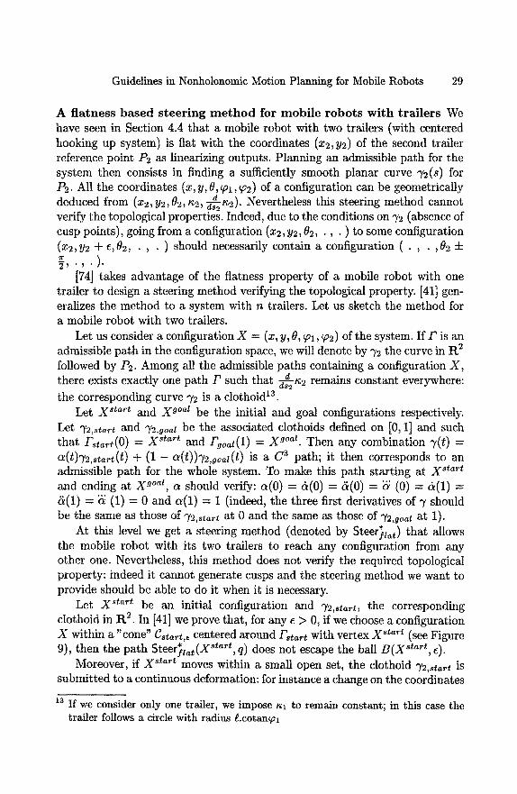
Guidelines in Nonholonomic Motion Planning for Mobile Robots 29
A flatness based steering m e t h o d for mobi le robots wi th trailers We have seen in Section 4.4 that a mobile robot with two trailers (with centered hooking up system) is flat with the coordinates (x2, Y2) of the second trailer reference point P2 as linearizing outputs. Planning an admissible path for the system then consists in finding a sufficiently smooth planar curve 72(s) for P2- All the coordinates (x, y, 0, ~1, ~2) of a configuration can be geometrically
d ~ deduced from (x2,y2,02, ~2, ~ 2). Nevertheless this steering method cannot verify the topological properties. Indeed, due to the conditions on ~/2 (absence of cusp points), going from a configuration (x2, Y2,82, . , . ) to some configuration (x2,y2 + e,02, . , • ) should necessarily contain a configuration ( . , . ,82 4- 7r ~ , . , . ) .
[74] takes advantage of the flatness property of a mobile robot with one trailer to design a steering method verifying the topological property. [41] gen- eralizes the method to a system with n trailers. Let us sketch the method for a mobile robot with two trailers.
Let us consider a configuration X = (x, y, O, ~Ol, ~2) of the system. If F is an admissible path in the configuration space, we will denote by ~/2 the curve in R 2 followed by P2. Among all the admissible paths containing a configuration X,
d there exists exactly one path F such that ~7~2a2 remains constant everywhere: the corresponding curve 72 is a clothoid 13.
Let X s~ar~ and X g°at be the initial and goal configurations respectively. Let 72,s~r~ and 72,~oal be the associated clothoids defined on [0,1] and such that Fstart(O ) -~- X start and Fgoal(1) = X g°al. Then any combination 7(t) = a(t)72,s~r~(t) ÷ (1 - a(t))72,goal(t ) is a C 3 path; it then corresponds to an admissible path for the whole system. To make this path starting at X start
and ending at X 9°~1, a should verify: a(0) = &(0) = &(0) = ~ (0) = &(1) = 5(1) = K (1) = 0 and a(1) = 1 (indeed, the three first derivatives of 7 should be the same as those of 72,~t~rt at 0 and the same as those of 72,go~l at 1).
At this level we get a steering method (denoted by Steer~la~ ) that allows the mobile robot with its two trailers to reach any configuration from any other one. Nevertheless, this method does not verify the required topological property: indeed it cannot generate cusps and the steering method we want to provide should be able to do it when it is necessary.
Let X s~ar~ be an initial configuration and 72,sta~, the corresponding elothoid in R 2. In [41] we prove that, for any e > 0, if we choose a configuration X within a "cone" Cs~ar~,~ centered around Fs~ar~ with vertex X st~r~ (see Figure 9), then the path Steer~la~(X st~r~, q) does not escape the ball B ( X star~, e).
Moreover, if X s~ar~ moves within a small open set, the clothoid ^/2,s~a~ is submitted to a continuous deformation: for instance a change on the coordinates
13 If we consider only one trailer, we impose m to remain constant; in this case the trailer follows a circle with radius Lcota.nTh
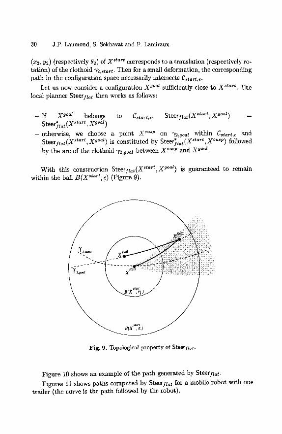
30 J.P. Laumond, S. Sekhavat and F. Lamiraux
(x2, y2) (respectively 82) of X st~t corresponds to a translation (respectively ro- tation) of the clothoid 72,st~t. Then for a small deformation, the corresponding path in the configuration space necessarily intersects Cst~t,e.
Let us now consider a configuration X g°~t sufficiently close to X ~ta~t. The local planner Steer/t~t then works as follows:
- If X 9°al belongs to Cuart,e, Steeryg~t (X 8tar~, X g°al) = S÷~r,~* { y s t a r t ygoal~
-o therwise , we choose a point X cusp on 72,goaZ within Cstart, e and Steer* { X start X cusp] SteerIlat(Xstart,x g°al) is constituted by Ilat~ , j followed
by the arc of the clothoid 72,go~t between X c~'p and X g°~t.
With this construction Steerflat(XStart,X g°al) is guaranteed to remain within the ball B ( X s~art, ~) (Figure 9).
M
J
Fig. 9. Topological property of Steer/~at.
Figure 10 shows an example of the path generated by Steerllat.
Figures 11 shows paths computed by Steer flat for a mobile robot with one traiier (the curve is the path followed by the robot).
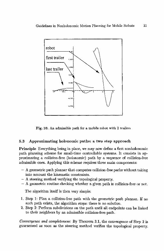
Guidelines in Nonholonomic Motion Planning for Mobile Robots 31
robot ~ ~ ~
first traile_..._ r °°°~I
last trailer ~ ° ~
~0.002
-Q.0O6
Fig. 10. An admissible path for a mobile robot with 2 trailers
5.3 Approximating holonomic paths: a two step approach
Principle Everything being in place, we may now define a first nonholonomic path planning scheme for small-time controllable systems. It consists in ap- proximating a collision-free (holonomic) path by a sequence of collision-free admissible ones. Applying this scheme requires three main components:
- A geometric path planner that computes collision-free paths without taking into account the kinematic constraints.
- A steering method verifying the topological property. - A geometric routine checking whether a given path is collision-free or not.
The algorithm itself is then very simple:
1. Step 1: Plan a collision-free path with the geometric path planner. If no such path exists, the algorithm stops: there is no solution.
2. Step 2: Perform subdivisions on the path until all endpoints can be linked to their neighbors by an admissible collision-free path.
Convergence and completeness: By Theorem 3.1, the convergence of Step 2 is guaranteed as soon as the steering method verifies the topological property.
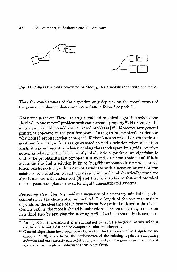
32 J.P. Laumond, S. Sekhavat and F. Lamiraux
Fig. 11. Admissible paths computed by Steer/l~t for a mobile robot with one trailer
Then the completeness of the algorithm only depends on the completeness of the geometric planner that computes a first collision-free path 14.
Geometric planner: There are no general and practical algorithm solving the classical "piano mover" problem with completeness property 15. Numerous tech- niques are available to address dedicated problems [42]. Moreover new general principles appeared in the past few years. Among them one should notice the "distributed representation approach" [5] that leads to resolution-complete al- gorithms (such algorithms are guaranteed to find a solution when a solution exists at a given resolution when modeling the search space by a grid). Another notion is related to the behavior of probabilistic algorithms: an algorithm is said to be probabilistically complete if it includes random choices and if it is guaranteed to find a solution in finite (possibly unbounded) time when a so- lution exists; such algorithms cannot terminate with a negative answer on the existence of a solution. Nevertheless resolution and probabilistically complete algorithms are well understood [8] and they lead today to fast and practical motion geometric planners even for highly dimensionated systems.
Smoothing step: Step 2 provides a sequence of elementary admissible paths computed by the chosen steering method. The length of the sequence mainly depends on the clearance of the first collision-free path: the closer to the obsta- cles the path is, the more it should be subdivided. The sequence may be shorten in a third step by applying the steering method to link randomly chosen pairs
14 An algorithm is complete if it is guaranteed to report a negative answer when a solution does not exist and to compute a solution otherwise.
15 General algorithms have been provided within the framework of real algebraic ge- ometry [69,18]; nevertheless the performance of the existing algebraic computing software and the intrinsic computational complexity of the general problem do not allow effective implementations of these algorithms.
Guidelines in Nonholonomic Motion Planning for Mobile Robots 33
of points lying on the first solution path. Unfortunately there is today no result insuring the convergence of this third step to any "optimal" sequence.
Several nonholonomic path planners have been designed in this way. Here is a review of the main ones.
Application to mobi le robo t s (wi thout trai ler) The seminal ideas of the algorithm above have been introduced in [48]. This reference deals with car-like robots. When the robot is a polygon, the geometric planner is derived from the algorithm based on an analytical representation of the configuration space of a polygon moving amidst polygonal obstacles [4]. When the robot is a disk, the geometric planner works from the Voronoi diagram of the environment. In both cases, the steering method is Steeropt: it consists in computing the shortest length admissible paths for a car-like robot as characterized in [65]. Due to the completeness of the geometric planners the proposed algorithms are complete. Nevertheless they are delicate to implement and fragile in practice (indeed the basic geometric routines are sensitive to numerical computations; a robust implementation could be done by using software computing with rational numbers).
Another version of this algorithm appears in [43] where the geometric plan- ner has been replaced by a distributed representation approach; the search consists in exploring the discretized configuration space with an A* algorithm heuristically guided by a potential function. It is then resolution-complete, less fragile than the original version, and sufficiently efficient to be integrated on real robots. Figure 12 shows an example of a solution from a software developed for the mobile robots Hilare at LAAS.
A clever idea appears in [55]. It tends to minimize the length of the short- est path sequence approximating the geometric path. It consists in computing a skeleton gathering the set of points with maximum clearance with respect to the obstacles. The key point is that the clearance is measured with the metric induced by the length of the shortest admissible paths (the so-called Reeds&Shepp metric). Then the geometric planner works by retracting the ini- tial and goal configurations on the skeleton and by exploring it. Even if one cannot conclude to any optimality of the solution, the sequence of shortest paths provided the approximation step is shorter than a sequence approximating a path that would lie closer to the obstacles. A critical point of the approach is the computation of the metric. The distance between two configurations being inwriant by translation and rotation, the authors use a lookup table storing all the distance value over a discretized compact region around the origin. This table is computed off-line once and may be used to compute the skeleton of various environments.
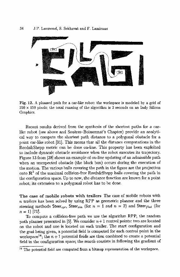
34 J.P. Laumond, S. Sekhavat and F. Lamiraux
r
Fig. 12. A planned path for a car-like robot: the workspace is modeled by a grid of 250 x 150 pixels; the total running of the algorithm is 2 seconds on an Indy Silicon Graphics.
Recent results derived from the synthesis of the shortest paths for a car- like robot (see above and Sou~res-Boissonnat's Chapter) provide an analyti- cal way to compute the shortest path distance to a polygonal obstacle for a point car-like robot [91]. This means that all the distance computations in the Reeds&Shepp metric can be done on-line. This property has been exploited to include dynamic obstacle avoidance when the robot executes its trajectory. Figure 13 from [38] shows an example of on-line updating of an admissible path when an unexpected obstacle (the black box) occurs during the execution of the motion. The various balls covering the path in the figure are the projection onto R 2 of the maximal collision-free Reeds&Shepp balls covering the path in the configuration space. Up to now, the distance function are known for a point robot; its extension to a polygonal robot has to be done.
T h e case of mobi le r obo t s w i t h t ra i le rs The case of mobile robots with n trailers has been solved by using RPP as geometric planner and the three steering methods Steeropt, Steersin (for n = 1 and n = 2) and Steerftat (for n = 1) [71].
To compute a collision-free path we use the algorithm RPP, the random path planner presented in [5]. We consider n + 1 control points: two are located on the robot and one is located on each trailer. The start configuration and the goal being given, a potential field is computed for each control point in the workspacel~; the n + 1 potential fields are then combined to create a potential field in the configuration space; the search consists in following the gradient of
~6 The potential field are computed from a bitmap representation of the workspace.
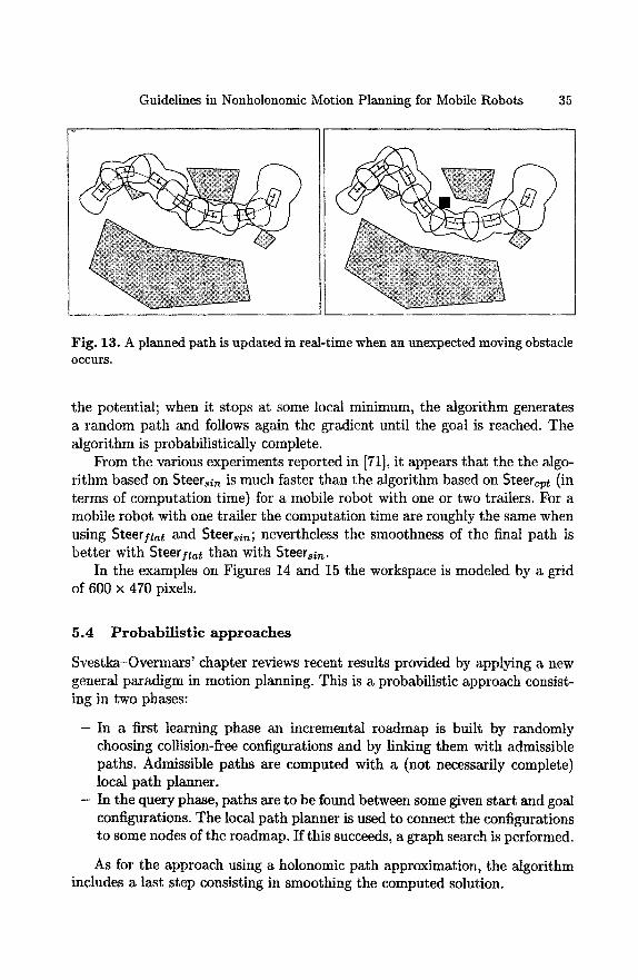
Guidelines in Nonholonomic Motion Planning for Mobile Robots 35
Fig. 13. A planned path is updated in real-time when an unexpected moving obstacle O c c u r s .
the potential; when it stops at some local minimum, the algorithm generates a random path and follows again the gradient until the goal is reached. The algorithm is probabilistically complete.
From the various experiments reported in [71], it appears that the the algo- rithm based on Steers~n is much faster than the algorithm based on Steerop~ (in terms of computation time) for a mobile robot with one or two trailers. For a mobile robot with one trailer the computation time are roughly the same when using Steerilat and Steers/n; nevertheless the smoothness of the final path is better with Steer/la~ than with Steersin.
In the examples on Figures 14 and 15 the workspace is modeled by a grid of 600 x 470 pixels.
5 . 4 P r o b a b i l i s t i c a p p r o a c h e s
Svestka-Overmars' chapter reviews recent results provided by applying a new general paradigm in motion planning. This is a probabilistic approach consist- ing in two phases:
- In a first learning phase an incremental roadmap is built by randomly choosing collision-free configurations and by linking them with admissible paths. Admissible paths are computed with a (not necessarily complete) local path planner.
- In the query phase, paths are to be found between some given start and goal configurations. The local path planner is used to connect the configurations to some nodes of the roadmap. If this succeeds, a graph search is performed.
As for the approach using a holonomic path approximation, the algorithm includes a last step consisting in smoothing the computed solution.
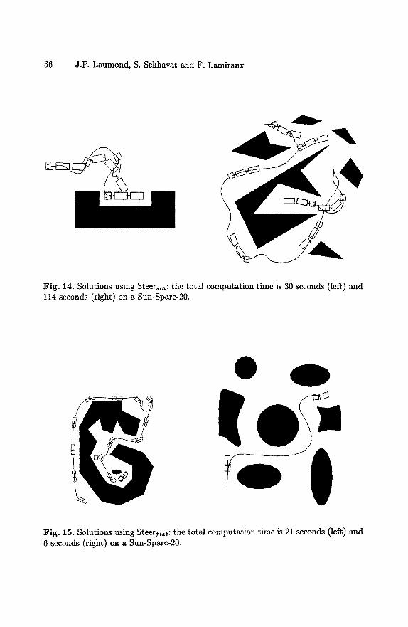
36 J.P. Laumond, S. Sekhavat and F. Lamiraux
Fig. 14. Solutions using Steersi~: the total computation time is 30 seconds (left) and 114 seconds (right) on a Sun-Sparc-20.
Fig. 15. Solutions using Steerfzat: the total computation time is 21 seconds (left) and 6 seconds (right) on a Sun-Sparc-20.
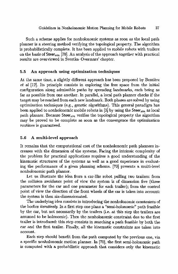
Guidelines in Nonholonomic Motion Planning for Mobile Robots 37
Such a scheme applies for nonholonomic systems as soon as the local path planner is a steering method verifying the topological property. The algorithm is probabilistically complete. It has been applied to mobile robots with trailers on the basis of Steersln [70]. An analysis of the approach together with practical results are overviewed in Svestka-Overmars' chapter.
5.5 An approach using opt imiza t ion techniques
At the same time, a slightly different approach has been proposed by Bessi~re et al [12]. Its principle consists in exploring the free space from the initial configuration along admissible paths by spreading landmarks, each being as far as possible from one another. In parallel, a local path planner checks if the target may be reached from each new landmark. Both phases are solved by using optimisation techniques (e.g., genetic algorithms). This general paradigm has been applied to nonholonomic mobile robots in [3] by using the Steersin as local path planner. Because Steersin verifies the topological property the algorithm may be proved to be complete as soon as the convergence the optimization routines is guaranteed.
5.6 A multi-level approach
It remains that the computational cost of the nonholonomic path planners in- creases with the dimension of the systems. Facing the intrinsic complexity of the problem for practical applications requires a good understanding of the kinematic structures of the systems as well as a good experience in evaluat- ing the performance of a given planning scheme. [70] presents a multi-level nonholonomic path planner.
Let us illustrate the idea from a car-like robot pulling two trailers: from the collision avoidance point of view the system is of dimension five (three parameters for the car and one parameter for each trailer); from the control point of view the direction of the front wheels of the car is taken into account: the system is then six-dimensionated.
The underlying idea consists in introducing the nonholonomic constraints of the bodies iteratively. In a first step one plans a "semi-holonomic" path feasible by the car, but not necessarily by the trailers (i.e. at this step the trailers are assumed to be holonomic). Then the nonholonomic constraint due to the first trailer is introduced: this step consists in searching a path feasible by both the car and the first trailer. Finally, all the kinematic constraints are taken into account.
Each step should benefit from the path computed by the previous one, via a specific nonholonomic motion planner. In [70], the first semi-holonomic path is computed with a probabilistic approach that considers only the kinematic

38 J.P. Laumond, S. Sekhavat and F. Lamiraux
constraints of the car. Then a probabilistic search using Steersin is applied within a tube surrounding the path; it provides a second semi-holonomic path that takes into account the first three kinematic constraints. Finally the second path is approximated via Steersin accounting for all the constraints. The global algorithm is then based on a combination of the holonomic path approximation scheme and the probabilistic one.
Three examples of solutions provided by the algorithm appear in Fig- ure 16: the left column shows the first "semi-holonomic" paths (the two trailers "slide"); the right column shows the corresponding final paths. The total time to compute the solutions ranges from less than one minute for the first example to around three minutes for the third one, on a 136 MIPS workstation.
5.7 On the computational complexity of nonholonomic path planning
Evaluating the computational complexity of the approaches introduced above is a difficult task. More generally, the complexity of the nonholonomic path planning problem is an open problem.
For small-time controllable systems, we have seen that the existence of a solution is characterized by the existence of any collision-free path for the associated holonomic system. The complexity of deciding whether a solution exists is then equivalent to the complexity of the classical piano mover problem (see [42] for an overview). The complexity for other systems (e.g., with drift) is an open problem.
In this section we give an account of results providing lower bounds on the complexity of nonholonomic paths for small-time controllable mobile robots. By reference to the approximation scheme, we may define the complexity of a collision-free nonholonomic path by the length of the sequence of admissi- ble paths approximating a holonomic one. This definition depends a priori on the steering method used to approximate a holonomic path. A more intrinsic definition consists in considering the approximation scheme that uses $teero~. Indeed the cost of the optimal paths induces a (nonholonomic) metric in the configuration space. A possible definition of the complexity of a path is the minimum number of balls computed with the nonholonomic metric and cover- ing the path. For instance the complexity of the paths appearing in Figure 13 is 7 in both cases. This definition allows to link the complexity of nonholonomic path planning with the clearance of the free-space.
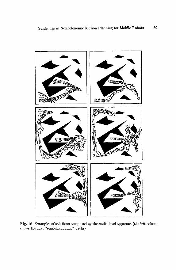
Guidelines in Nonholonomic Motion Planning for Mobile Robots 39
-%
Fig. 16. Examples of solutions computed by the multi-level approach (the left column shows the first "semi-holonomic" paths)
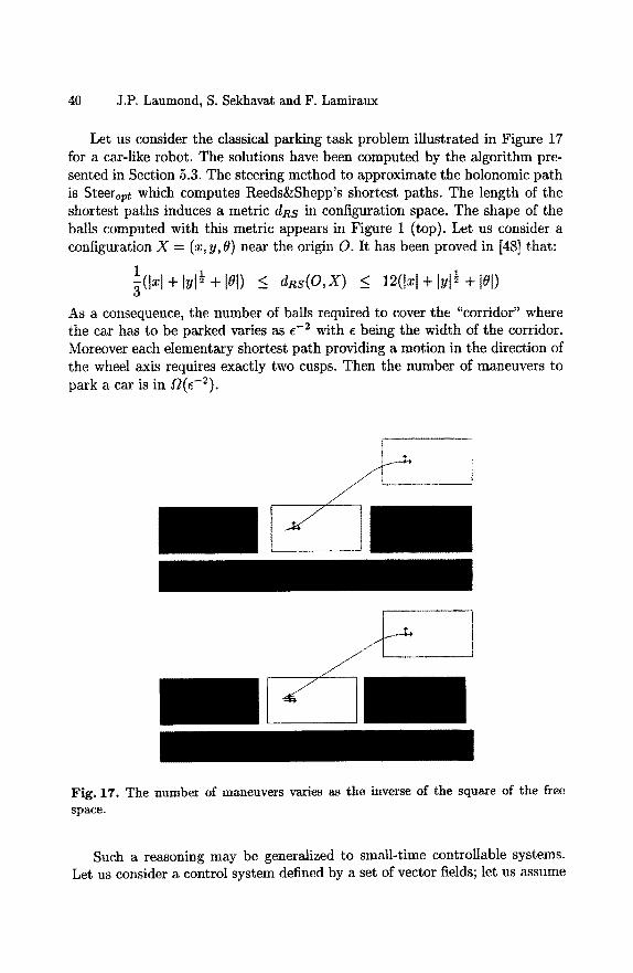
40 J.P. Laumond, S. Sekhavat and F. Lamiraux
Let us consider the classical parking task problem illustrated in Figure 17 for a car-like robot. The solutions have been computed by the algorithm pre- sented in Section 5.3. The steering method to approximate the holonomic path is Steeropt which computes Reeds&Shepp's shortest paths. The length of the shortest paths induces a metric dRs in configuration space. The shape of the balls computed with this metric appears in Figure 1 (top). Let us consider a configuration X = (x, y, 8) near the origin O. It has been proved in [48] that:
~(lxl + + 181) < ~Rs(O,Z) < 12(1xl + + I81) lyt ½
As a consequence, the number of balls required to cover the "corridor" where the car has to be parked varies as e -2 with e being the width of the corridor. Moreover each elementary shortest path providing a motion in the direction of the wheel axis requires exactly two cusps. Then the number of maneuvers to park a car is in ~(e-2) .
m
Fig. 17. The number of maneuvers varies as the inverse of the square of the free space.
Such a reasoning may be generalized to small-time controllable systems. Let us consider a control system defined by a set of vector fields; let us assume
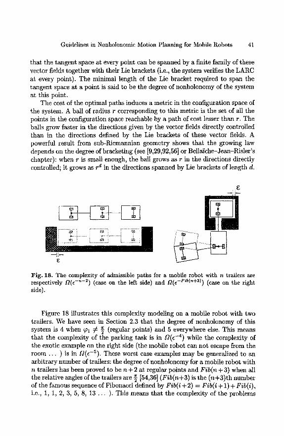
Guidelines in Nonholonomic Motion Planning for Mobile Robots 41
that the tangent space at every point can be spanned by a finite family of these vector fields together with their Lie brackets (i.e., the system verifies the LARC at every point). The minimal length of the Lie bracket required to span the tangent space at a point is said to be the degree of nonholonomy of the system at this point.
The cost of the optimal paths induces a metric in the configuration space of the system. A ball of radius r corresponding to this metric is the set of all the points in the configuration space reachable by a path of cost lesser than r. The balls grow faster in the directions given by the vector fields directly controlled than in the directions defined by the Lie brackets of these vector fields. A powerful result from sub-Riemannian geometry shows that the growing law depends on the degree of bracketing (see [9,29,92,56] or Bella'iche-Jean-Risler's chapter): when r is small enough, the ball grows as r in the directions directly controlled; it grows as r d in the directions spanned by Lie brackets of length d.
E
, ,S
C2 Fig. 18. The complexity of admissible paths for a mobile robot with n trailers are respectively f2(e -~-s) (case on the left side) and J'-~(e -Fib(rid-3)) (case Oil the right side).
Figure 18 illustrates this complexity modeling on a mobile robot with two trailers. We have seen in Section 2.3 that the degree of nonholonomy of this system is 4 when ~ol ¢ ~ (regular points) and 5 everywhere else. This means that the complexity of the parking task is i n / 2 ( C 4) while the complexity of the exotic example on the right side (the mobile robot can not escape from the room . . . ) is in JT(e-5). These worst case examples may be generalized to an arbitrary number of trailers: the degree of nonholonomy for a mobile robot with n trailers has been proved to be n + 2 at regular points and Fib(n -t- 3) when all the relative angles of the trailers are ~ [54,36] (Fib(n+3) is the (n+3)th number of the famous sequence of Fibonacci defined by Fib(i + 2) = Fib(i + 1) + Fib(i), i.e., 1, 1, 2, 3, 5, 8, 13 . . . ). This means that the complexity of the problems
42 J.P. Laumond, S. Sekhavat and F. Lamiraux
appearing in Figure 18 and generalized to n trailers are respectively ~(e -n-2) (simply exponential in n) and/2(e -Fib('~+3)) (doubly exponential in n).
6 O t h e r a p p r o a c h e s , o t h e r s y s t e m s
This section overviews other works related to nonholonomic path planning for mobile robots. They deal either with direct approaches based on dynamic programming techniques, or with specific systems.
Combining discrete configuration space and piece-urise constant inputs: Bar- raquand and Latombe propose in [6,7] a direct approach to nonholonomic path planning. It applies to car-like robots with trailers. The model of the car cor- responds to the control system (4) introduced in Section 2.2. Four input types are chosen in {-1, 1} x {~min, ~max}; they correspond to backward or forward motions with an extremal steering angle. The admissible paths are generated by a sequence of these constant inputs, each of them being applied over a fixed interval of time fit. Starting from the initial configuration the search generates a tree: the successors of a given configuration X are obtained by setting the input to one of the four values and integrating the differential system over St. The configuration space is discretized into an array of cells of equal size (i.e. hyperparallelepipeds). A successor X ~ of a configuration X is inserted in the search tree if and only if the computed path from X to X ~ is collision-free and X ~ does not belong to a cell containing an already generated configuration. The algorithm stops when it generates a configuration belonging to the same cell as the goal (i.e., it does not necessarily reach the goal exactly).
The algorithm is proved to be asymptotically complete w.r.t, to both 5t and the size of the cells. As a brute force method, it remains quite time-consuming in practice. Its main interest is that the search is based on Dijkstra's algorithm which allows to take into account optimality criteria such that the path length or the number of reversals. Asymptotical optimality to generate the minimum of reversals is proved for the car-like robot alone.
Progressive constraints: In [23] Ferbach combines the two step approach pre- sented in Section 5.3 and a so-called variational approach. It applies for small- time controllable system. First, a collision-free path is generated. Then the nonholonomic constraints are introduced progressively. At each iteration, a path is generated from the previous one to satisfy more severe nonholonomic constraints. The search explores the neighborhood of the current path accord- ing to a dynamic programming procedure. The progressiveness of the search is obtained by taking random tangent vectors chosen in neighborhoods of the admissible ones and by making these neighborhoods decreasing to the set of admissible tangent vectors.
Guidelines in Nonholonomic Motion Planning for Mobile Robots 43
The method is neither complete nor asymptotically complete. Completeness would require back-tracking that would be expensive. Nevertheless simulations have been performed with success for a mobile robot with three trailers and for two tractor-trailer robots sharing the same environment.
Car-like robots moving forward: After the pioneering work of Dubins who char- acterized the shortest paths for a particle moving with bounded curvature [22], attempts have been done to attack the path planning for car-like robots moving only forward. Except some algorithms that do not verify any general complete- ness properties (e.g., [45,89,94]), they are only few results addressing the gen- eral problem. All of them assume that the robot is reduced to a point. In [27], Fortune and Wilfong propose an algorithm running in exponential time and space to decide if a path exists; the algorithm does not generate the solution. Jacobs and Canny's algorithm [34] is a provably good approximation algorithm that generates a sequence of elementary feasible paths linking configurations in contact with the obstacles. According to the resolution of a contact space discretization, the algorithm is proved to compute a path which is as close as possible to the minimal length path. More recent results solve the problem ex- actly when the obstacles are bounded by curves corresponding to admissible paths (i.e., the so-called moderate obstacles) [2,13].
Nonholonomic path planning for Dubins' car then remains a difficult and open problem 17.
Multiple mobile robots: Nonholonomic path planning for the coordination of multiple mobiles robots sharing the same environment has been addressed along two main axis: centralized and decentralized approaches is.
In the centralized approaches the search is performed within the Cartesian product of the configuration spaces of all the robots. While the problem is PSPACE-complete [32], recent results by Svestka and Overmars show that it is possible to design planners which are efficient in practice (until five mobile robots) while being probabilistically complete [85]: the underlying idea of the algorithm is to compute a probabilistic roadmap constituted by elementary (nonholonomic) paths admissible for all the robots considered separately; then the coordination of the robots is performed by exploring the Cartesian product of the roadmaps. The more dense is the initial roadmap, the higher is the probability to find a solution in very cluttered environments.
In [1], Alami reports experiments involving ten mobile robots on the basis of a fully decentralized approach: each robot builds and executes its own plan by
lr Notice that Barraquand and Latombe's algorithm [6] may be applied to provide an approximated solution of the problem.
is We refer the reader to Svestka-Overmars' chapter for a more detailed overview on this topic.
44 J.P. Laumond, S. Sekhavat and F. Lamiraux
merging it into a set of already coordinated plans involving other robots. In such a context, planning is performed in parallel with plan execution. At any time, robots exchange information about their current state and their current paths. Geometric computations provide the required synchronization along the paths. If the approach is not complete (as a decentralized schemes), it is sufficiently well grounded to detect deadlocks. Such deadlocks usually involve only few robots among the fleet; then they may be overcome by applying a centralized approach locally.
7 C o n c l u s i o n s
The algorithmic tools presented in this chapter show that the research in motion planning for mobile robots reaches today a level of maturity that allows their transfer on real platforms facing difficult motion tasks.
Numerous challenging questions remain open at a formal level. First of all, there is no nonholonomic path planner working for any small-time controllable system. The case of the mobile robot with trailers shown in Figure 2 (right) is the simplest canonical example which can conduce new developments. A second issue is path planning for controllable and not small-time controllable systems; Dubins' car appears as another canonical example illustrating the difficulty of the research on nonhonomic systems. Sou~res-Boissonnat's chapter emphasizes on recent results dealing with the computation of optimal controls for car-like robots; it appears that extending these tools to simple systems like two-driving wheel mobile robots is today out of reach.
Perhaps the most exciting issues come from practical applications. The mo- tion of the robot should be performed in the physical world. The gap between the world modeling and the real world is critical. Usually, path planning as- sumes a two-steps approach consisting in planning a path and then executing it via feedback control. This assumption holds under the condition that the geometric model of the environment is accurate and that the robot's Cartesian coordinates are directly and exactly measured. Designing a control law that executes a planed path defined in a robot centered frame may be sufficient in manufacturing applications; it is not when dealing with applications such as mobile robot outdoor navigation for instance. In practice, the geometric model of the world and the localisation of the robot should be often performed through the use of embarked extereoceptive sensors (ultrasonic proximeters, infrared or laser range finder, laser or video cameras . . . ).
Uncertainties and sensor-based motions are certainly the two main key- words to be considered to reach the ultimate objectives of the motion plan- ning. Addressing these issues requires to revisit the motion planning problem statement: the problem is to plan not a robot-centered path but a sequence of
Guidelines in Nonholonomic Motion Planning for Mobile Robots 45
sensor-based motions that guaranty the convergence to the goal. The solution is no more given by a simple search in the collision-free configuration space. This way is explored in manufacturing applications for several years; it is difficult in mobile robotics where nonholonomy adds another difficulty degree.
46 J.P. Laumond, S. Sekhavat and F. Lamiraux
Annex: Sinusoidal inputs and obstacle avoidance (comments on the tuning of al)
As we have seen in Section 5.2, we do not dispose of a unique expression of Steersin verifying the topological property. In this annex we show that it is possible to switch between " al different Steersi n to integrate such a steering method within a general nonholonomic path planning scheme.
Let us consider the two input chained form system (8) introduced in Sec- tion 4.3:
{ '~'1 = Vl
~2 v2 Z3 Z2 .Vl
i : Zn Zn--1 .Vl
a l Steersi n is defined by:
vl ( t ) = a0 + al sin wt v2(t) = b0 + bl coswt + b2 cos 2wt + . . . bn-2 cos(n - 2)wt
We have proved that for a given al small enough, the maximal gap between Z start~ a n d t h e al start goal path Steers~ n (Z , Z ) decreases when Z g°al tends to Z start. But this gap do not tends to zero. In other words, for a fixed value of al , trying to reach closer configurations on the geometric path decreases the risk of collision but does not eliminate it. Moreover to tend this gap to zero we have also to decrease Jail. But these two decreasings are not independent. Indeed,
Steersi n and so we by changing the value of al we change the steering method al change the family of the paths. For a given couple of extremal configurations, a decreasing of al increases in most of the cases the extremal gap between the start point and the path. In other words, in order to reduce the risk of collision we have to choose close goal configurations but we also have to reduce al. Which in turn increase again the clearance between the path and the start point. So we have again to bring the goal closer . . . If the decreasing of lall is too fast with respect to the one of the distance between the start configuration and the current goal, the approximation algorithm will not converge.
A strategy for tuning these two decreasings can be integrated in the approx- imation algorithm (Section 5.3) while respecting its completeness. The follow- ing approach has been implemented; it is described with details in [72,71]. It is based on a lemma giving an account of the distance between a path generated by al o by ~i(t). Steers~ n and its starting point Z °. Let us denote z~(t) - z~
Guidelines in Nonholonomic Motion Planning for Mobile Robots 47
a l L e m m a 7.1. For any path computed by Steersin, for any t E [0,T] :
I(~l(t)l ~_ laoTI + ]alTI = A 1 152(t)l <- F, [b~Tt = A2 (12) [Sk+l(t) I < [z~[A1 q_ . . . .~ [Zu[AI0 k-~ + ([zO[ + A~)A k-1 withk > 2
Proof : By definition ~1 (t) = ao + al sinwt. Then:
I~l(t)l <_ I$1(r)ldr <_ (1~ol + la~l) dr < laoTt + la~TI
By setting A1 = [aoT I + [alT] we have the intermediate result that for all t, f~ I$1(T)ld~- <_ Ai. The same reasoning holds to prove that 152(t)1 < ~ IbiTI.
Now, for any k > 2:
An upper bound Ak on I~k(t)l being given, we get:
Then z~k+l <_ (z~k + Iz°l)z~l
And by recurrence:
[~k+l(t)l _< tz°lz~ + . . . + Iz°lal k-2 + (Iz°l + A2)Alk-1 1-1
Given a start configuration Z s~art, we first fix the value of al and two other parameters A'~ in and A~ in to some arbitrary values (see [71] for details on initialization). Then we choose a goal configuration on the straight line segment [Z start, Z g°~l] (or on any collision-free path linking Z start and zg°al]) closer and closer to Z start. This operation decreases the parameters a0, b0 , . . . , bn so it decreases A~ and A2 (the detailed proof of this statement appears in [71,74]). We continue to bring the goal closer to the initial configuration until a collision- free path is found or until A 1 _< A~ in and A2 < A'~irL In the second case, we substitute al, A'~ in and A ~ in respectively by k.al, k.A'~ in and k . A ~ i'~, with k < 1 and we start the above operations again. The new starting path may or may not go further away from Z start than the previous one but in any case, from equations (12) we have the guarantee that following this strategy, the computed path will lie closer and closer to Z 8tart. We have then the guarantee of finding a collision-free path.
48 J.P. Laumond, S. Sekhavat and F. Lamiranx
References
1. R. Alami, "Multi-robot cooperation based on a distributed and incremental plan merging paradigm," Algorithms for Robotic Motion and Manipulation, WAFR '96, J.P. Laumond and M. Overmars Eds, A.K. Peters, 1997.
2. P.K. Agarwal, P. Raghavan and H. Tamaki, "Motion planning for a steering- constrained robot through moderate obstacles," ACM Symp. on Computational Geometry, 1995.
3. J.M. Ahuactzin, " Le Fil d'Ariane: une m6thode de planification g6n6rale. Appli- cation ~ la planification automatique de trajectoires," PhD Thesis, INP, Grenoble, 1994.
4. F. Avnaim, J. Boissonnat and B. Faverjon, "A practical exact motion planning algorithm for polygonal objects amidst polygonal obstacles," IEEE Int. Conf. on Robotics and Automation, pp. 1656-1661, Philadelphia, 1988.
5. J. Barraquand and J.C. Latombe, "Robot motion planning: a distributed repre- sentation approach," International Journal of Robotics Research, 1991.
6. J. Barraquand and J.-C. Latombe, "On non-holonomic mobile robots and optimal maneuvering," Revue d'Intelligence Artificielle, Vol. 3 (2), pp. 77-103, 1989.
7. J. Barraquand and J.C. Latombe, "Nonholonomic multibody mobile robots: con- trollability and motion planning in the presence of obstacles," Algorithmiea, Springer Verlag, Vol. 10, pp. 121-155, 1993.
8. J. Barraquand, L. Kavraki, J.C. Latombe, T.Y. Li, R. Motvani and P. Raghavan, "A random sampling scheme for path planning," Robotics Research, the Seventh International Symposium, G. Giralt and G. Hirzinger Eds, Springer Verlag, 1996.
9. A. Bella'iche, J.P. Laumond and P. 3acobs, "Controllability of car-like robots and complexity of the motion planning problem," Int. Symposium on Intelligent Robotics, pp. 322-337, Bangalore, 1991.
10. A. Bellai'che, J.P. Laumond and J.J. Risler, "Nilpotent infinitesimal approxima- tions to a control Lie algebra," IFA C Nonlinear Control Systems Design Sympo- sium, pp. 174-181, Bordeaux, 1992.
11. A. Bella~che, J.P. Lanmond and M. Chyba, "Canonical nilpotent approximation of control systems: application to nonholonomic motion planning," 32nd IEEE Con]. on Decision and Control, San Antonio, 1993.
12. P. Bessi~re, J.M. Ahuactzin, E. Talbi and E. Mazer, "The Ariadne's clew algo- rithm: global planning with local methods," Algorithmic Foundations of Robotics, K. Goldberg et al Eds, A.K. Peters, 1995.
13. J.D. Boissonnat and S. Lazard, "A polynomial-time algorithm for computing a shortest path of bounded curvature amidst moderate obstacle," ACId Syrup. on Computational Geometry, 1996.
14. R.W. Brockett, "Control theory and singular Riemannian geometry," New Direc- tions in Applied Mathematics, Springer-Verlag, 1981.
15. X.N. Bui, P. Sou~res, J.D. Boissonnat and J.P. Laumond, "The shortest path syn- thesis for nonholonomic robots moving fordwards," IEEE Int. Conf. on Robotics and Automation, Atlanta, 1994.
16. L. Bushnell, D. Tilbury and S. Sastry, "Steering three-input nonholonomic sys- tems: the fire-truck example," International Journal of Robotics Research, Vol. 14 (4), pp. 366-381, 1995.
Guidelines in Nonholonomic Motion Planning for Mobile Robots 49
17. G. Campion, G. Bastin and B. d'Andr6a-Novel, "Structural properties and clas- sification of kinematic and dynamic models of wheeled mobile robots," IEEE Trans. on Robotics and Automation, Vol. 12 (1), 1996.
18. J. Canny, The Complexity of Robot Motion Planning, MIT Press, 1988. 19. J. Canny, A. Rege and J. Reif, "An exact algorithm for kinodynamic planning in
the plane," Discrete and Computational Geometry, Vol. 6, pp. 461-484, 1991. 20. B. Donald, P. Xavier, J. Canny and J. Reif, "Kinodynamic motion planning," J.
of the ACM, Vol. 40, pp. 1048-1066, 1993. 21. B. Donald and P. Xavier, "Provably good approximation algorithms for optimal
kinodynamic planning: robots with decoupled dynamic bounds," Algorithmica, Vol. 14, pp. 443-479, 1995.
22. L. E. Dubins, "On curves of minimal length with a constraint on average curva- ture and with prescribed initial and terminal positions and tangents," American Journal of Mathematics, Vol. 79, pp. 497-516, 1957.
23. P. Ferbach, "A method of progressive constraints for nonholonomic motion plan- ning," IEEE Int. Conf. on Robotics and Automation, pp. 2929-2955, Minneapolis, 1996.
24. C. Fernandes, L. Gurvits and Z.X. Li, "A variational approach to optimal non- holonomic motion planning," IEEE Int. Conf. on Robotics and Automation, pp. 680-685, Sacramento, 1991.
25. S. Fleury, P. Sou~res, J.P. Lanmond and R. Chatila, "Primitives for smooth- ing mobile robot trajectories," IEEE Transactions on Robotics and Automation, Vol. 11 (3), pp. 441-448, 1995.
26. M. Fliess, J. L~vine, P. Martin and P. Rouchon, "Flatness and defect of non-linear systems: introductory theory and examples," Int. Journal of Control, Vol. 61 (6), pp. 1327-1361, 1995.
27. S.3. Fortune and G.T. Wilfong, "Planning constrained motions," ACM STOCS, pp. 445-459, Chicago, 1988.
28. T. Fraichard, "Dynamic trajectory planning with dynamic constraints: a 'state- time space' approach," IEEE//RSJ Int. Conf. on Intelligent Robots and Systems, pp. 1393-1400, Yokohama, 1993.
29. V. Y. Gershkovich, "Two-sided estimates of metrics generated by absolutely non- holonomic distributions on Riemannian manifolds," Soviet Math. Dokl., Vol. 30 (2), 1984.
30. G. Giralt, R. Sobek and R. ChatiIa, "A multi-level planning and navigation sys- tem for a mobile robot: a first approach to Hilare," 6th Int. Joint Conf. on Arti- ficial Intelligence, pp. 335-337, Tokyo, 1979.
31. H. Hermes, A. Lundell and D. Sullivan, "Nilpotent bases for distributions and control systems," J. of Differential Equations, Vol. 55, pp. 385-400, 1984.
32. J. Hopcroft, J.T. Schwartz and M. Sharir, "On the complexity of motion plan- ning for multiple independent objects: PSPACE-hardness of the warehouseman's problem," International Journal of Robotics Research, Vol. 3, pp. 76-88, 1984.
33. G. Jacob, "Lyndon discretization and exact motion planning," European Control Conference, pp. 1507-1512, Grenoble, 1991.
34. P. Jacobs and J. Canny, " Planning smooth paths for mobile robots," IEEE Int. Conf. on Robotics and Automation, Scottsdale, 1989.
50 J.P. Laumond, S. Sekhavat and F. Lamiraux
35. P. Jacobs, A. Rege and J.P. Laumond, "Non-holonomic motion planning for Hilare-like robots," Int. Symposium on Intelligent Robotics, pp. 338-347, Ban- galore, 1991.
36. F. Jean, "The car with N trailers: characterization of the singular configurations," ESAIM: COCV, http://www.emath.fr/cocv/, Vol. 1, pp. 241-266, 1996.
37. Y. Kanayama and N. Miyake, "Trajectory generation for mobile robots," Robotics Research, Vol. 3, MIT Press, pp. 333-340, 1986.
38. M. Khatib, H. Jaouni, R. Chatila and J.P. Lanmond, " Dynamic path modifica- tion for car-like nonholonomic mobile robots," IEEE Int. Conf. on Robotics and Automation, Albuquerque, 1997.
39. G. Lafferrier'e and H.J. Sussmann, "A differential geometric approach to motion planning," Nonholonomic Motion Planning, Zexiang Li and J.F. Canny Eds, The Kluwer International Series in Engineering and Computer Science 192, 1992.
40. F. Lamiranx and J.P. Laumond, "From paths to trajectories for multi-body mo- bile robots," Int. Symposium on Experimental Robotics, Lecture Notes on Control and Information Science, Springer-Verlag, (to appear) 1997.
41. F. Lamiraux and J.P. Lanmond, "Flatness and small-time controllability of multi- body mobile robots: applications to motion planning," European Conference on Control, Brussels, 1997.
42. J.C. Latombe, Robot Motion Planning, Kluwer Academic Publishers, 1991. 43. J.C. Latombe, "A Fast Path Planner for a Car-Like Indoor Mobile Robot," Ninth
National Conference on Artificial Intelligence, AAAI, pp. 659-665, Anaheim, 1991.
44. J.P. Lanmond, "Feasible trajectories for mobile robots with kinematic and envi- ronment constraints," Intelligent Autonomous Systems, L.O. Hertzberger, F.C.A. Groen Edts, North-Holland, pp. 346-354, 1987.
45. J.P. Laumond, "Finding collision-free smooth trajectories for a non-holonomic mobile robot," lOth International Joint Conference on Artificial Intelligence, pp. 1120-1123, Milano, 1987.
46. J.P. Lanmond, " Singularities and topological aspects in nonholonomic motion planning," Nonholonomic Motion Planning, Zexiang Li and J.F. Canny Eds, The Kluwer International Series in Engineering and Computer Science 192, 1992.
47. J.P. Lanmond, "Controllability of a Multibody Mobile Robot," IEEE Transac- tions Robotics and Automation, pp. 755-763, Vol. 9 (6), 1993.
48. J.P. Lanmond, P. Jacobs, M. Ta~x and R. Murray, ~'A motion planner for non- holonomic mobile robot," IEEE Trans. on Robotics and Automation, Vol. 10, 1994.
49. J.P. Laumond, S. Sekhavat and M. Vaisset, "CoUision-free motion planning for a nonholonomic mobile robotwith trailers," 4th IFAC Syrup. on Robot Control, pp. 171-177, Capri, 1994.
50. J.P. Laumond and J.J. Risler, "Nonholonomic systems: controllability and com- plexity," Theoretical Computer Scienee~ Vol. 157, pp. 101-114, 1996.
51. J.P. Laumond and P. Souhres, "Metric induced by the shortest paths for a car-like robot," IEEE/RSJ Int. Conf. on Intelligent Robots and Systems, Yokoama, 1993.
52. Z. Li and J.F. Canny Eds, Nonholonomic Motion Planning, Kluwer Academic Publishers, 1992.
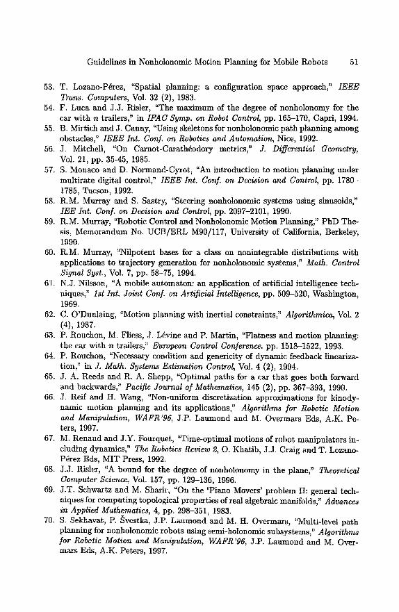
Guidelines in Nonholonomic Motion Planning for Mobile Robots 51
53. T. Lozano-P4rez, "Spatial planning: a configuration space approach," IEEE Trans. Computers, Vol. 32 (2), 1983.
54. F. Luca and J.J. Risler, "The maximum of the degree of nonholonomy for the car with n trailers," in IFAC Syrup. on Robot Control, pp. 165-170, Capri, 1994.
55. B. Mirtich and J. Canny, "Using skeletons for nonholonomic path planning among obstacles," IEEE Int. Conf. on Robotics and Automation, Nice, 1992.
56. J. Mitchell, "On Carnot-Carath6odory metrics," J. Differential Geometry, Vol. 21, pp. 35-45, 1985.
57. S. Monaco and D. Normand-Cyrot, "An introduction to motion planning under multirate digital control," IEEE Int. Conf. on Decision and Control, pp. 1780- 1785, Tucson, 1992.
58. R.M. Murray and S. Sastry, "Steering nonholonomic systems using sinusoids," IEE Int. Conf. on Decision and Control, pp. 2097-2101, 1990.
59. R.M. Murray, "Robotic Control and Nonholonomic Motion Planning," PhD The- sis, Memorandum No. UCB/ERL M90/117, University of California, Berkeley, 1990.
60. R.M. Murray, "Nilpotent bases for a class on nonintegrable distributions with applications to trajectory generation for nonhotonomic systems," Math. Control Signal Syst., Vol. 7, pp. 58-75, 1994.
61. N.J. Nilsson, "A mobile automaton: an application of artificial intelligence tech- niques," 1st Int. Joint Conf. on Artificial Intelligence, pp. 509-520, Washington, 1969.
62. C. O'Dunlaing, "Motion planning with inertial constraints," Algorithmica, Vol. 2 (4), 1987.
63. P. Rouchon, M. Fliess, J. L6vine and P. Martin, "Flatness and motion planning: the car with n trailers," European Control Conference. pp. 1518-1522, 1993.
64. P. Rouchon, "Necessary condition and genericity of dynamic feedback lineariza- tion," in J. Math. Systems Estimation Control, Vot. 4 (2), 1994.
65. J. A. Reeds and R. A. Shepp, "Optimal paths for a car that goes both forward and backwards," Pacific Journal of Mathematics, 145 (2), pp. 367-393, 1990.
66. J. Reif and H. Wang, "Non-uniform discretization approximations for kinody- namic motion planning and its applications," Algorithms for Robotic Motion and Manipulation, WAFR'96, J.P. Laumond and M. Overmars Eds, A.K. Pe- ters, 1997.
67. M. Renaud and J.Y. Fourquet, "Time-optimal motions of robot manipulators in- cluding dynamics," The Robotics Review 2, O. Khatib, J.J. Craig and T. Lozano- P6rez Eds, MIT Press, 1992.
68. J.J. Risler, "A bound for the degree of nonholonomy in the plane," Theoretical Computer Science, Vol. 157, pp. 129-136, 1996.
69. J.T. Schwartz and M. Sharir, "On the 'Piano Movers' problem II: general tech- niques for computing topological properties of real algebraic manifolds," Advances in Applied Mathematics, 4, pp. 298-351, 1983.
70. S. Sekhavat, P. ~vestka, J.P. Laumond and M. H. Overmars, "Multi-level path planning for nonholonomic robots using semi-holonomic subsystems," Algorithms for Robotic Motion and Manipulation, WAFR'96, J.P. Laumond and M. Over- mars Eds, A.K. Peters, 1997.
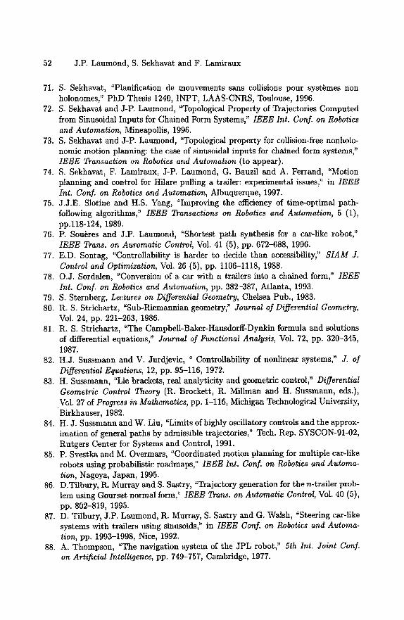
52 J.P. Laumond, S. Sekhavat and F. Lamiranx
71. S. Sekhavat, "Planification de mouvements sans collisions pour syst~mes non holonomes," PhD Thesis 1240, INPT, LAAS-CNRS, Toulouse, 1996.
72. S. Sekhavat and J-P. Laumond, "Topological Property of Trajectories Computed from Sinusoidal Inputs for Chained Form Systems," IEEE Int. Conf. on Robotics and Automation, Mineapollis, 1996.
73. S. Sekhavat and J-P. Laumond, "Topological property for collision-free nonholo- nomic motion planning: the case of sinusoidal inputs for chained form systems," tEEE Transaction on Robotics and Automation (to appear).
74. S. Sekhavat, F. Lamiranx, J-P. Laumond, G. Bauzil and A. Ferrand, "Motion planning and control for Hilare pulling a trailer: experimental issues," in IEEE Int. Conf. on Robotics and Automation, Albuquerque, 1997.
75. J.J.E. Slotine and H.S. Yang, "Improving the efficiency of time-optimal path- following algorithms," IEEE Transactions on Robotics and Automation, 5 (1), pp.118-124, 1989.
76. P. Sou~res and J.P. Laumond, "Shortest path synthesis for a car-like robot," IEEE Trans. on Automatic Contro~ Vol. 41 (5), pp. 672-688, 1996.
77. E.D. Sontag, "Controllability is harder to decide than accessibility," SIAM J. Control and Optimization, Vol. 26 (5), pp. 1106-1118, 1988.
78. O.J. Sordalen, "Conversion of a car with n trailers into a chained form," IEEE Int. Conf. on Robotics and Automation, pp. 382-387, Atlanta, 1993.
79. S. Sternberg, Lectures on Differential Geometry, Chelsea Pub., 1983. 80. R. S. Strichartz, "Sub-Riemannian geometry," Journal of Differential Geometry,
Vol. 24, pp. 221-263, 1986. 81. R. S. Strichartz, "The Campbell-Baker-Hausdorff-Dynkin formula and solutions
of differential equations," Journal of Functional Analysis, Vol. 72, pp. 320-345, 1987.
82. H.J. Sussmann and V. Jurdjevic, " Controllability of nonlinear systems," J. of Differential Equations, 12, pp..95-116, 1972.
83. H. Sussmann, "Lie brackets, real analyticity and geometric control," Differential Geometric Control Theory (R. Brockett, R. Millman and H. Sussmann, eds.), Vol. 27 of Progress in Mathematics, pp. 1-116, Michigan Technological University, Birkhanser, 1982.
84. H.J. Sussmann and W. Liu, "Limits of highly oscillatory controls and the approx- imation of general paths by admissible trajectories," Tech. Rep. SYSCON-91-02, Rutgers Center for Systems and Control, 1991.
85. P. Svestka and M. Overmars, "Coordinated motion planning for multiple car-like robots using probabilistic roadmaps," IEEE Int. Conf. on Robotics and Automa- tion, Nagoya, Japan, 1995.
86. D.Tilbury, l=t. Murray and S. Sastry, "Trajectory generation for the n-trailer prob- lem using Goursat normal form," IEEE Trans. on Automatic Control, Vol. 40 (5), pp. 802-819, 1995.
87. D. Tilbury, J.P. Laumond, R. Murray, S. Sastry and G. Walsh, "Steering car-like systems with trailers using sinnsoids," in IEEE Conf. on Robotics and Automa- tion, pp. 1993-1998, Nice, 1992.
88. A. Thompson, "The navigation system of the JPL robot," 5th Int. Joint Conf. on Artificial Intelligence, pp. 749-757, Cambridge, 1977.
Guidelines in Nonholonomic Motion Planning for Mobile Robots 53
89. P. Tournassoud, " Motion planning for a mobile robot with a kinematic con- straint," Geometry and Robotics, J.D. Boissonnat and J.P. Laumond Eds, pp. 150-171, Lecture Notes in Computer Science, Vol 391, Springer Verlag, 1989.
90. V.S. Varadarajan, Lie Groups, Lie Algebra and their Representations, Springer- Verlag, 1984.
91. M. Vendittelti and J.P. Laumond, "Visible positions for a car-like robot amidst obstacles," Algorithms for Robotic Motion and Manipulation, J.P. Laumond and M. Overmars Eds, A.K. Peters, 1997.
92. A.M. Vershik and V.Ya. Gershkovich, "Nonholonomic problems and the theory of distributions," Acta Applicandae Mathematicae, Vol. 12, pp. 181-209, 1988.
93. X. Viennot, Alg~bres de Lie fibres et mono[des fibres. Lecture Notes in Mathe- matics, 691, Springer Verlag, 1978.
94. G.T. Wilfong, " Motion planning for an autonomous vehicle," IEEE Int. Conf. on Robotics and Automation, pp. 529-533, 1988.
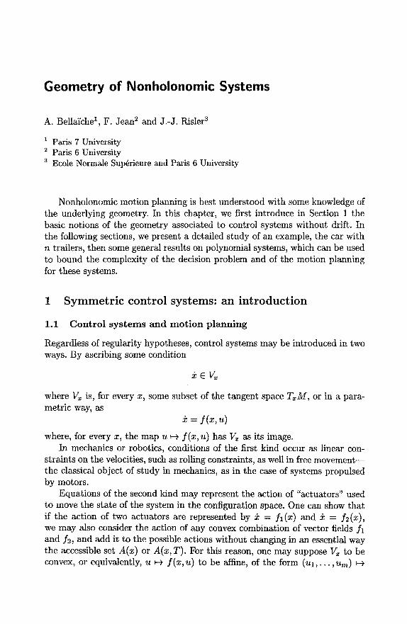
Geometry of Nonholonomic Systems
A. Bellgiche 1, F. Jean 2 and J.-J. Risler 3
1 Paris 7 University 2 Paris 6 University 3 Ecole Normale Sup~rieure and Paris 6 University
Nonholonomic motion planning is best understood with some knowledge of the underlying geometry. In this chapter, we first introduce in Section 1 the basic notions of the geometry associated to control systems without drift. In the following sections, we present a detailed study of an example, the car with n trailers, then some general results on polynomial systems, which can be used to bound the complexity of the decision problem and of the motion planning for these systems.
1 Symmetr ic control systems: an introduct ion
1.1 Control systems and motion planning
Regardless of regularity hypotheses, control systems may be introduced in two ways. By ascribing some condition
where V~ is, for every x, some subset of the tangent space %M, or in a para- metric way, as
= f ( x , u)
where, for every x, the map u ~ f(x,u) has V~ as its image. In mechanics or robotics, conditions of the first kind occur as linear con-
straints on the velocities, such as rolling constraints, as well in free movement - - the classical object of study in mechanics, as in the case of systems propulsed by motors.
Equations of the second kind may represent the action of "actuators" used to move the state of the system in the configuration space. One can show that if the action of two actuators are represented by ~ = f l (x) and ~ = f2(x), we may also consider the action of any convex combination of vector fields f l and f2, and add it to the possible actions without changing in an essential way the accessible set A(x) or A(x, T). For this reason, one may suppose Vx to be convex, or equivalently, u ~-~ ] (x , u) to be affine, of the form ( u l , . . . , urn)
56 A. Bella'iche, F. Jean and a.-J. Risler
Xo(x) + ulXl(x) +"" + umX,~(x), and defined on some convex subset Ks of R 'n, for some m. This is responsible for the form
-~ Xo(x) ' - ~- ? ~ l X l ( X ) 2 t - . . - 7 t- u r n X m ( x )
under which control systems are often encountered in the literature. (It makes no harm to suppose m and Kx to be independent of x, and to suppose that the origin is an interior point of K = Kx.) The vector field Xo is called the drift.
Now, we will use only systems without drift, that is with Xo = 0, for the study of the problem of motion planning for robots. We may content with such systems as long as no dynamics is involved. That is, if the state of the system represents its position, and if we control directly its velocity. As opposed to a system whose state would represent position and velocities, and where the control is exerted on accelerations. Consider the simplest possible of such a system: a mobile point on a line, submitted to the control equation
~=u.
Introducing the velocity y = 2, we see that this system is equivalent to a system governed by the equation
2 = y
~l=u
which can be written as
that is: with a non-zero drift X0. For some applications, our study will be valid in the case of slow motion only,
and resemble to the thermodynamics of equilibriums, where all transformation are supposed to be infinitely slow.
1.2 Definitions. Basic problems
To sum up, we shall be intereste'd in control systems of the form
m
= ~ uiXi(x), x E M, (Z) i=l
where the configuration space M of the system is a C °O manifold, X 1 , . . . , Xm are Coo vector fields on M, and the control function u(t) = ( u l ( t ) , . . . , ut(t)) takes values in a fixed compact convex K of R TM, with nonempty interior, and
Geometry of Nonholonomic Systems 57
symmetric with respect to the origin. Such systems are called symmetric (or driftless). One also says that controls enter linearly in (Z).
For any choice of u as a measurable function defined on some interval [0, T], with value in K , equation (Z) becomes a differential equation
ic = ~ ui(t)X~(x). (1) i=1
Given any point xo on M, we can integrate (1), taking
x(0)=x0 (2)
as an initial condition. For the sake of simplicity, we shall suppose that this equation has a well-defined solution on [0, T] for all choices of u (this is guaran- teed if M is compact or if M = R n, and vector fields X~ are bounded). Call this solution x~. One says that xu is the path with initial point x0 and controlled by u. We shall mainly be interested in its final value x~(T). Classically, points in M are called the states of the system. One says for example that the system is steered from state Xo to state xu(T) by means of the control function u.
One also says that xu (T) is accessible, or reachable, in time T from Xo. We shall denote by A(x, T) the set of points of M accessible from x in time T (or in time < T, it is the same thing for symmetric systems), and by A(x) the set of points accessible from x, that is
A(x) = U A(x,T). T>0
Basic problems of Control Theory are:
- determine the accessible set A(x); - given a point y, accessible from x, find control functions steering the system
from x to y; - do the preceding in minimal time; - more generally, find control function u ensuring any given property of xu (t),
the path controlled by u.
Given xo, the control function u(t) is considered as the input of the system, and xu(t) as the output. In a more general setting, the output is only some function h(x) of the state x, h being called the observation: the state is only partially known. Here we will take as observation h = Id, and call indifferently x the state or the output.
We can now state another basic problem:
58 A. Bella'iche, F. Jean and J.-J. Risler
- can one find a map k : M - ~ / ( such that the differential equation
= f (x , k(x)) (3)
has a determined behaviour, for example, has a given point xo as an at- t ractor?
Since in this problem, the output is reused as an input, such a map k is called a feedback control law, or a closed-loop control. If (3) has xo as an attractor, one says that k is a stabilizing feedback at x0.
1.3 T h e c o n t r o l distance
Return to the control system (Z). For x, y E M, define d(x, y) as the infimum of times T such that y is accessible from x in time T, so d(x, y) = +co if y is not accessible from x. It is immediate to prove that d(x, y) is a distance [distance function] on M. Of course, this is the case only because we supposed that K is symmetric with respect to the origin in R m.
Distance d will be called the control distance. We can define d in a different way. First, observe that since K is convex,
symmetric, with nonempty interior, we can associate to it a norm I1' IlK on R TM, such that K is the unit ball llu[[g ___ 1. Now, for a controlled path c = x~ : [a, b] ~ M obtained by means of a control function u e Ll([a, b], Rm), we set
length(e) = IJu(t) Hg dt. (4)
If c carl be obtained in such a way from several different u's, we take the infimum of the corresponding integrals. Then, d(x, y) is the infimum of the lengths of controlled paths joining x to y (and, of course, this is intended in the definition of an infimum, +co if no such path exists).
A slightly variant construction may be useful. ~5:ansfer the function I1" IlK to T~M, by setting
IlVllK = inf{ II(ul, . . . , Um)NK I V ---- Ul X I (X) ~" " " + u m X m ( x ) }.
We get in this way a function on T x M which is a norm on span(Xl (X) , . . . , Xm(x)) and takes the value +co for vector not in this subspace. We can now define the length of any absolutely continuous path e : [a, b] -¢ M as
b
length(c) = ]a lla(t)ilK dt
and the distance d(x, y) as the infimum of length of paths joining x and y.
Geometry of Nonholonomic Systems 59
Note that distances corresponding to different K, say K1 and/(2, are equiv- alent: there exists some positive constants A and B such that
Adl (x, y) <_ d2 (x, y) < Bdl (x, y).
The most convenient version of the control distance is obtained by taking for K the unit ball of R m, which gives
2 i/2 Ilull = (u~ + - . . + Urn) •
In this case, the distance d is called the sub-Riemannian distance attached to the system of vector fields X1, . . . , Xm. As a justification for this name, observe that, locally, any Riemannian distance can be recovered in such a way by taking m = n, and as Xl (x) , . . . , Xn(x) an orthonormal basis, depending on x, of the tangent space TxM. A more general, more abstract, definition of sub-Riemannian metrics can be given, but we shall not use it in this book.
Now, observe that d(x, y) < oo if and only if x and y are reachable from one another, that A(x, T) is nothing else that the ball of center x and radius T (for d), and that controlled paths joining x to y in minimal time are simply minimizing geodesics.
Many problems of control theory, or path planning, get in this way a geo- metric interpretation. For another example, one could think to obtain a feed- back law k(x) stabilizing the system at x = Xo by choosing k so as to ensure ](x,k(x)) to be the gradient of d(x, xo). Unfortunately, this does not work, even if we take the good version of the gradient, i.e., the sub-Riemannian one:
g r a d . f = + . . . + (x .f)xm.
and take k(x) = (Xl.f , . . . ,Xmf) for that purpose. But studying the reasons of this failure is very instructive. Such a geometric interpretation, using the sub-Riemaniann distance, really brings a new insight in theory, and it will in several occasions be very useful to us.
1.4 Accessibility. The theorems of Chow and Sussmann
We shall deduce-the classical theorem of Chow (Chow [7], Rashevskii [28]) from a more precise result by Sussmann. Sussmann's theorem will be proved using L 1 controls. However, it can be shown that the results obtained are, to a great extend, independent of the class of control used (see Bella'iche [2]).
Consider a symmetric control system, as described above,
m
= E u ' X i ( x ) ' x E M , u E K . (Z) i = 1
60 A. Bella~che, F. Jean and J.-J. Risler
Recall the configuration space M is a C ~ manifold, X1, . . . , Xm are C ~ vector fields on M, and K, the control set, or parameter set, is a fixed compact convex of R m, with nonempty interior, symmetric with respect to the origin.
In all this section, we fix a point x0 E M, the initial point, and a positive time T. Set
nT = L 1 ([0, T], am).
We shall call this space the space o] controls. It may be considered as a normed space by setting
// Ilull = Ilu(t)llK dt.
Given u E 7/T, we consider the differential equation
{ ~ = ~i~=1 ui(t)Xi(x), 0 < t < T x(0) = x0 (5)
Under suitable hypotheses, the differential equation (5) has a well defined so- lution x~(t). We will denote by
Endxo,T : 7/T -+ M
the mapping wich maps u to x~(T). We will call End~o,T, or End for short, the end-point map.
Now, the accessible set A(xo) (the set of points accessible from Xo for the system ~ , regardless of time) is exactly the image of Endxo,T. Indeed, every controlled path c : [0, T'] -~ M, defined by the control u : [0, T t] ~ M may be reparametrized by [0, T]. Conversely, if u E 7/, and L = length(x~), the control function
u(¢(t)) 0 < t < L, v( t ) =
where ¢ is defined as a right inverse to the mapping
// s ~+ []U(T)llK dT
from [0, T] to [0, L] takes its values in K, and defines the same geometric path as u.
T h e o r e m 1.1 (Sussmann [36], Stefan [35]). The set A(xo) of points ac- cessible from a given point Xo in M is an immersed submanifold.
We shall prove this theorem using arguments from differential calculus in Banach spaces, taking advantage from the fact that the end-point map is a differentiable mapping from 7i to M, a finite dimensional manifold.
Geometry of Nonholonomic Systems 61
Recall the rank of a differentiable mapping at a given point is by definition the rank of its differential at that point. The theorem of the constant rank asserts that the image of a differential map with constant rank is an immersed submanifold (for more details about this part of the proof, see Bella'iche [2]).
Defini t ion. Let p the maximal rank of the end-point map Endz0,T : 7-/T --+ M. We say that a control function u E "]'IT is normal if the rank of End~o,T at u is equal to p. We shall say that the path xu defined by u is a normal path. Otherwise, u is said to be an abnormal control, and Xu an abnormal path. A point which can be joined to xo by a normal path is said to be normally accessible from Xo.
L e m m a 1.2. Every point accessible from Xo is normally accessible from xo.
Proof. Let y be a point accessible from x0, and let u E 7-/T a control steering x0 to y. Choose a normal control z E 7/T, steering x0 to some point z. Such a control exists by definition. We claim that the control function w E ~'/3T defined by
fv( t ) if0 < t < T [
w(t) = ~ v(2T - t) i f T < t < 2 T
( u ( t - 2 T ) i f 2 T < t < 3 T
is normal and steers x0 to y. The second part of our assertion is evident: the path xw steers x0, first to
z, then back to x0, then to y. Now, the image of DEndxo,3T consists of the infinitesimal variations ~xw(3T) obtained from infinitesimal variations 6w of w. We can consider special variations of w, namely variations of the first part of w only, leaving the two other parts unchanged. In other words, we consider tile control functions
f v(t) + ~v(t) i f 0 < t < T
w(t) + ~w(t) = ~ v(2T - t) if T < t < 2T |
( u ( t - 2T) if 2T < t < 3T
Since v is a normal control, these variations yield infinitesimal variations of Jx~(T) = x,~+~(T) - xw(T) which form a subspace of dimension p at that point. Now, the corresponding variations of xw(3T) are obtained from those of xw (T) by applying the flow of the time-dependent vector field ~ l< i<m wi(t)Xi(x) between time T and time 3T. Since this flow is a diffeo- mor'pl~ism of M, these variations of x,v(3T) form a subspace of dimension p of the tangent space TyM. The space formed by variations of the xw(3T) caused by unrestricted variations of the control w has thus dimension > p, an so has dimension p. This proves that w is normal.
Of course, the fact that w is in ~f~3T instead of being in "~T is harmless. •
62 A. Bellai'che, F. Jean and J.-J. Risler
Proof of Sussmann's theorem. The normal controls form an open subset N~o,T of 74T. From Theorem 1.2, the accessible set A(xo) is the image of N~o,T by a constant rank map. By using the Theorem of constant rank, the proof is done. m
T h e o r e m 1.3 (Chow [7], Rashevski i [28]). If M is connected (for its orig- inal topology), and if the vector fields X1,. . . , Xm and their iterated brackets [Xi, Xj], [[Zi, Xj], Xk], etc. span the tangent space TxM at every point of M, then any two points of M are accessible from one another.
Proof. Since the relation y E A(x) is clearly an equivalence relation, we can speak of accessibility components. Since
y E A(x) ¢=~ d(x, y) < c~,
the set A(x) is the union of open balls B(x, R) (for d), so it is itself an open set. Whence it results that the accessibility components are also the connected component of M for the topology defined by d.
It is clear that the accessibility components of M axe stable under the flow exp tX~ of vector field Xi (i = 1, . . . , m). Therefore, the vector fields X1, . . . , Xm are, at any point, tangent to the accessibility component through that point (see [2] for details). And so are their brackets [Xi, Xj], their iterated brackets [[X~, Xj], Xk], etc.
If the condition on the brackets is fulfilled, then
T~A(x) = T~M
at every point x, as the preceding discussion shows. In that case, the acces- sibility components are open. Since M is connected, there can be only one accessibility component. []
Definit ion. The following condition
(C) The vector fields X1, . . . ,Xm and their iterated brackets [Xi, Xj], [[Xi, Xj], Xk], etc. span the tangent space TxM at every point of M,
is called Chow's Condition.
When the Chow's Condition holds, one says that system (Z) is controllable. The reciprocal of Chow's theorem, that is, if (Z:) is controllable, the Xi's and their iterated brackets span the tangent space at every point of M, is true if M and the vector fields are analytic, and false in the C ¢~ case (see Sussmann [36]).
Chow's Condition is also known under the name of Lie Algebra Rank Con- dition (LARC) since it states that the rank at every point x of the Lie algebra generated by the Xi's is full (self-evident definition). In the context of PDE, it is known under the name of HSrmander's Condition: if it is verified, the differential operator X~ + . . - + X2m is hypoelliptic (HSrmander's Theorem).
Geometry of Nonholonomic Systems 63
1.5 The shape of the accessible set in t ime 6
The purpose of this section is to study the geometric structure of A(x, ~) for small ~. Let us recall that A(x, E) denotes the set of points accessible from x in time ~ (or in time < ~, it is the same thing) by means of control ui such that ~ u~ < 1. In other words, A(x, s) is equal to B(x, ~), the sub-Riemaniann closed ball centered at x with radius e.
We suppose in the sequel that Chow's condition is satisfied for the control system (~). Choosing some chart in a neighbourhood of x0, we may write (1) a s
m
i----1
The differential equation (1) thus appear as a perturbation of the trivial equa- tion
iTS
= (7)
Classical arguments on perturbation of differential equations show that the solution of (6) is given by
x(T) = x(O) + ui(t) dt Xi(O) + O(llull2), (8)
where, for u, we use the L 1 norm. Thus, with a linear change of coordinates, the set of points accessible from x(0) = 0 in time T < ~ satisfies, for small
A(x, e) C C[-~, e]~' x [-E 2, ~2]~-~1,
where nl is the rank of the family XI (0) , . . . ,Xm(0). As a first step, the set A(x, E) is then included in a flat pancake.
The expression (8) implies also that the differential of the end-point map- ping at the origin in 7 / i s the linear map
u ~-~ ~=l (~oTu~(t) dt) X~(O) •
Since, typically, we suppose m < n, this linear map has rank nl < n and the end-point mapping is not a submersion at 0 E 7-/. Following our definition, this means that the constant path at Xo is an abnormal path. This result has a lot of consequences.
64 A. Bella'/che, F. Jean and J.-J. Risler
Given a neighbourhood U of xo, there may not exist a smooth mapping x ~ u ~ of U into 7/ such that the control u ~ steers xo to x, or, as well, x to xo. A stronger result is Brockett 's theorem asserting the non-existence of a continuous feedback law, stabilizing system (Z) at a given point Xo, when m<n.
To go further in the description of the set A(x, ~) we can use the so-called iterated integrals. For example, the system
Xl = Ul
X2 = u2 (9) X3 ~ Xl~t2 - - X2Ul x l ( 0 ) = x (0) = 3(0) = o
is solved by
T
xi(T)= fo ul(t) dt T
x2(T) = ~o u2(t) dt (I0)
x 3 ( T ) = ]i T (~otl Ui (t2) dt2) u2(tl) dti - ~0 T ( fot' U2(t2) dt2) ui (ti) dtl
This scheme works for chained or triangular systems, that is, 2j depends only on the controls and x i , . . . , x j - i . But we shall see that it can be put to work for any system. To begin with, let us rewrite (9) as
.T ---- U l X l ( x ) -{- u2X2(x), x(O) : O.
Then (10) can be read as
x(T) = x(O) + ul(t)dt XI(O)+ u~(t)dt X2(O)+
Put this way, the formula for x(T) can readily be generalized to any control
system of the form x" = E uiXi(x).
i<~<m
Geometry of Nonholonomic Systems 65
One gets (the proof is not hard, cf. Brockett [5])
(L" ) z(r) = z(O) + ~ u~(t) dt + O(llnll ~) X~(O) + i_<i<m
loT (/otlUj(t2) dt2) ui(tx)dtl) [Xi, Xj](O)-~'O(llul,3), or, written in a more civilized manner
x(T) = x(O) + ~ (AT(u) + O(llull2))X~(O) + l < i < r a
AT (u)[Xi,X~]( 0 ) + O(llull 3) l <i<j<rn which can, for given T, be considered as a limited expansion of order 2 of the end-point mapping about 0 in 7-/. Observe that AT(u) is a linear function with respect to u E 7-/, and AT(u) is a quadratic function on 7-/. This expansion generalizes the expansion (8) and the set A(x, e) satisfies now
A(x,e) C C[-a,e] m × [-e2,e2] "2-"1 x [-ea,ez] '~-n2. (11)
Having shown that A(x, ~) is contained in some box, one can ask whether it contains some other box of the same kind. Of course, before this question can be taken seriously, one has to replace inclusion (11) by
A(x, e) C C[-e, el" ' x [ -e 2, e2] n=-"l x [ -e a, ca] "a-"= x . . .
where the integers nl , n2, na, . . . are the best possible. Now, except for the case n2 = n which can be dealt with directly, the proof
of an estimate like
C'[-a,e] m x [-e2,e2] nz-nl x [-ea,e3] ha-ha x . . . c A(x,e)
requires new techniques and special sets of coordinates. Instead of computing limited expansion up to order r, we will compute an expansion to order 1 only, but by assigning weights to the coordinates. This will be done in §§1.6-1.8.
1.6 Regular and singular points
In the sequel we will fix a manifold M, of dimension n, a system of vector fields X 1 , . . . , Xrn on M. We will suppose that X1 , . . . , Xm verify the condition
66 A. Bella~che, F. Jean and J.-J. Risler
of Chow. We will denote by d the distance defined on M by means of vector fields X1, . . . , Xm.
Let £1 = £ 1 ( X 1 , . . " ,Xm) be the set of linear combinations, with real coefficients, of the vector fields X 1 , . . . , Xm. We define recursively £s = £s(X1, . . . , Xm) by setting
Ls= £s-1 + I t ,e f t iq-j=s
for s = 2 , 3 , . . . , as well as L ° = 0. The union £ = £ ( X I , . . . , X m ) of all £s is a Lie subalgebra of the Lie algebra of vector fields on M which is called the control Lie algebra associated to (E).
Now, for p in M, let LS(p) be the subspace of TpM which consists of the values X(p) taken, at the point p, by the vector fields X belonging to £s. Chow's condition states that for each point p E M, there is a smallest integer r = r(p) such that L r(p) (p) = TpM. This integer is called the degree of nonholonomy at p. It is worth noticing that r(q) < r(p) for q near p. For each point p E M, there is in fact an increasing sequence of vector subspaces, or flag:
{0} = L°(p) C LI(p) C , . . C LS(p) C , - " C Lr(P)(p) = TpM.
We shall denote this flag by ~T(p). Points of the control system split into two categories: regular states, around
which the behaviour of the system does not change in a qualitative way, and singular states, where some qualitative changes occur.
De f in i t i on . We say that p is a regular point if the integers dimLS(q) (s = 1, 2, . . . ) remain constant for q in some neighbourhood of p. Otherwise we say that p is a singular point.
Let us give an example. Take M = R 2, and
(0) X1 = ,X2 = x ~
(k is some integer). Then for c = (x,y) we have dimLX(c) = 1 if x = 0, dim L 1 (c) = 2 if x ~ 0, so all points on the line x = 0 are singular and the others are regular. For other examples, arising in the context of mobile robot with trailers, see Section 2.
It is worth to notice that , when M and vector fields X 1 , . . . , X m are an- alytic, regular points form an open dense set in M. Moreover, the sequence dim LS(p), s = 0, 1, 2 , . . . , is the same for all regular points in a same connected component of M and is streactly increasing for 0 < s < r(p). Thus the degree

Geometry of Nonholonomic Systems 67
of nonholonomy at a regular point is bounded by n - m + 1 (if we suppose that no one of the Xi's is at each point a linear combination of the other vector fields). It may be easily computed when the definition of the Xi's allows sym- bolic computation, as for an analytic function, being non-zero at the formal level is equivalent to being non-zero at almost every point.
Computing, or even bounding the degree of nonholonomy at singular points is much harder, and motivated, for some part, sections 2 and 3 (see also [9,11,19,24]).
1.7 D i s t a n c e e s t i m a t e s a n d p r iv i l eged c o o r d i n a t e s
Now, fix a point p in M, regular or singular. We set n8 = dim LS(p) (s = 0 , 1 , . . . , r ) .
Consider a system of coordinates centered at p, such that the differentials dyl , . . . , dyn form a basis of T~,M adapted to Y(p) (we will see below how to build such coordinates). If r = 1 or 2, then it is easy to prove the following local estimate for the sub-Riemannian distance. For y closed enough to 0, we have
d(0, (Yl,..., Yn)) X lYl ]-'~-''" + lYnl I ''~ ]Ynl+l I 1/2 or' '" q-[y.[ 1/2 (12)
where nt = dim L l(p) (the notation f(y) × g(y) means that there exists con- stants c, C > 0 such that cg(y) < f(y) <_ Cg(y)). Coordinates y l , . . . , y m are said to be of weight 1, and coordinates Ynl+l,... ,Yn are said to be of weight 2.
In the general case, we define the weight wj as the smallest integer s such tha t dyj is non identically zero on LS(p). (So that wj = s if ns-1 < j < ns.) Then the proper generalization of (12) would be
d(0,(yl,... ,y~))xlYll 1/wl +- - .+ ly , l 1/~-. (13)
It turns out that this estimate is generically ]alse as soon as r > 3. A simple counter-example is given by the system
(i) (°1) X1 = , X 2 = x 2 + y
(14)
on R 3. We have
L I ( 0 ) = L 2 ( 0 ) = R 2×{0} , L a ( 0 ) = R a,
68 A. Bellaiche, F. Jean and J.-J. Risler
so that yl = x, y2 = Y, y3 = z are adapted coordinates and have weight 1, 1 and 3. In this case, the estimates (13) cannot be true. Indeed, this would imply
Izl const.(d(0, (x,y, z)) 3,
whence z (exp(tX2)p)] <const. t 3,
but this is impossible since
)h - ~ z exp(tX2)(p) = (X~z)(p) = 1. t=O
However a slight nonlinear change of coordinates allows for (13) to hold. It is sufficient to replace yl, y2, Y3 by zl = x, z2 = y, z3 = z - y2/2.
In the above example, the point under consideration is singular, but one can give similar examples with regular p in dimension > 4. To formulate conditions on coordinate systems under which estimates like (13) may hold, we introduce some definitions.
Call X l f , . . . , X m f the nonholonomic partial derivatives of order 1 of f relative to the considered system (compare to O~lf, . . . ,Ox, f) . Call further X i X j f , X i X j X k f , . . . the nonholonomic derivatives of order 2, 3, . . . of f .
P r o p o s i t i o n 1.4. For a smooth function f defined near p, the following con- ditions are equivalent:
(i) One has f(q) = 0 (d(p, q)S) for q near p. (ii) The nonholonomic derivatives of order < s - 1 of f vanish at p
This is proven by the same kind of computations as in the study of example (14).
Def in i t ion . If Condition (i), or (ii), holds, we say that f is of order >__ s at p.
Def in i t ion . We call local coordinates z l , . . . , zn centered at p a system of privileged coordinates if the order of zj at p is equal to wj (j = 1 , . . . , n).
If z l , . . . ,zn are privileged coordinates, then dzl , . . . ,dzn form a basis of T i M adapted to ~'(p). The converse is not true. Indeed, if dzl , . . . ,dzn form an adapted basis, one can show that the order of zj is < wj, but it may be < wj: for the system (14), the order of coordinate ys = z at 0 is 2, while w3 = 3.
To prove the existence, in an effective way, of privileged coordinates, we first choose vector fields Y1,. . . , Y, whose values at p form a basis of TpM in the following way.
Geometry of Nonholonomic Systems 69
First, choose among X 1 , . . . , Xm a number nl of vector fields such that their values form a basis of Ll(p). Call them Y1, . . . , Y,~I. Then for each s (s = 2 , . . . , r) choose vector fields of the form
Y~.~. , . _ . . = [x~l, [ x ~ , . . . [x~._l, x~.] ...]] (15)
which form a basis of LS(p) mod LS-l(p), and call them Yn,_~+I,. . . , ym. Choose now any system of coordinates y l , . . . , yn centered at p such that
the differentials dy l , . . . ,dyn form a basis dual to YI(P), . . . ,Yn~) . (Starting from any system of coordinates x t , . . . ,xn centered at p, one can obtain such a system Yt , . . . , Y, by a linear change of coordinates.)
T h e o r e m 1.5. The functions z l , . . . , zn recursively defined by
Zq = yq - E 1 . . . . . Zq_ 1 (~1[. . .aq-l! (Y~I "Y:Jl~Yq)(P) z?~ "q-~ (16)
form a system of privileged coordinates near p. (We have set w(a) = wla l + • . . + wna..)
The proof is based on the following lemma.
L e m m a 1.6. For a function f to be of order > s at p, it is necessary and sufficient that
( Y ~ . . . Yr'" f ) (P) = 0
for all ~ = ( a t , . . . ,an) such that wta t + - . . + wnan <_ s.
This is is an immediate consequence of the following, proved by J.-J. Risler [4]: any product Xi~Xi2 . . . X i . , where i t , . . . , is are integers, can be rearranged as a sum of ordered monomials
E c,~..., . ( x l Y ~ . . . Yg"
with Wlal + --. + wnOln <~ 8, and where the ca~...a.'s are smooth functions. This result reminds of the Poincarfi-Birkhoff-Witt theorem.
Observe tha t the coordinates zl, • . . , zn supplied by the construction of The- orem 1.5 are given from original coordinates by expressions of the form
Zl = Yl
z2 -- y~ + pol (y~)
z , = Yn + pol (y l , . . . , Y , - I )
70 A. Bella~che, F. Jean and J.-J. Risler
where pol denotes a polynomial, without constant or linear term, and that the reciprocal change of coordinates has exactly the same form.
Other ways of getting privileged coordinates are to use the mappings
( z l , . . . , z n ) ~ exp(zlY1 + ... +znYn)p (see [14]),
(z l , . . . , zn) ~-~ exp(znYn) ' "exp(z lY1)p (see [18]).
Following the usage in Lie group theory, such coordinates are called canonical coordinates of the first (resp. second) kind.
1.8 Ball-Box T h e o r e m
Using privileged coordinates, the control system (Z) may be rewritten near p a s
m
(j= i = l
where the functions fij are weighted homogeneous polynomials of degree wj - 1. By dropping the o(llzll ;), we get a control system (~)
Zj-~- ~Ui[f i j(Z1, . . . ,Zj_l) ] (j = 1 , . . . ,n ) , i = 1
or, in short, m
by setting Xi = ~j~=l fij(2"l,..., Zn)Ozj. This system is nilpotent and the vec-
tor fields )(i are homogeneous of degree -1 under the non-isotropic dilations (z l , . . . , zn) ~ (A~.lzl,..., Aw~ zn). The system (~) is called the nitpotent ho- mogeneous approximation of the system (Z). For the sub-Riemaniann distance
associated to the nilpotent approximation, the estimate (17) below can be shown by homogeneity arguments. The following theorem is then proved by comparing the distances d and d (for a detailed proof, see Bella'/che [2]).
T h e o r e m 1.7. The estimate
d (O, ( Z l , . . . , Zn) ) x 12"1t 1 /w' - 1 - ' " Jr Iznl x/wn (17)
holds near p if and only if 2'1, . . . , 2"n form a system of privileged coordinates at p.
Geometry of Nonholonomic Systems 71
The estimate (17) of the sub-Riemannian distance allows to describe the shape of the accessible set in time ~. A(x, ~) can indeed be viewed as the sub- Riemannian ball of radius ~ and Theorem 1.7 implies
A(x,e) × [_e~1,¢~1] × . . . × [_Ew.,e~.].
Then A(x, ~) looks like a box, the sides of the box being of length proportionnal to cu'~,..., ew'. By the fact, Theorem 1.7 is called the Ball-Box Theorem (see Gromov [16]).
1 . 9 A p p l i c a t i o n t o c o m p l e x i t y o f n o n h o l o n o m i c m o t i o n p l a n n i n g
The Ball-Box Theorem can be used to address some issues in complexity of motion planning. The problem of nonholonomic motion planning with obstacle avoidance has been presented in Chapter [Laumond-Sekhavat]. It can be for- mulated as follows. Let us consider a nonholonomic system of control in the form (Z). We assume that Chow's Condition is satisfied. The constraints due to the obstacles can be seen as closed subsets F of the configuration space M. The open set M - F is called the free space. Let a, b E M - F. The motion planning problem is to find a trajectory of the system linking a and b contained in the free space.
From Chow's Theorem (§1.4), deciding the existence of a trajectory linking a and b is the same thing as deciding if a and b are in the same connected component of M - F. Since M - F is an open seL the connexity is equivalent to the arc connexity. Then the problem is to decide the existence of a path in M - F linking a and b. In particular this implies that the decision part of the motion planning problem is the same for nonholonomic controllable systems as for holonomic ones.
For the complete problem, some algorithms are presented in Chapter [Lanmond-Sekhavat]. In particular we see that there is a general method (called "Approximation of a collision-free holonomic path"). It consists in dividing the problem in two parts:
- find a path in the free space linking the configurations a and b (this path is called also the collision-free holonomic path);
- approximate this path by a trajectory of the system close enough to be contained in the free space.
The existence of a trajectory approximating a given path can be shown as follows. Choose an open neighbourhood U of the holonomic path small enough to be contained in M - F. We can assume that U is connected and then, from Chow's Theorem, there is a trajectory lying in U and linking a and b.
72 A. Bella'iche, F. Jean and J.-J. Risler
What is the complexity of this method?
The complexity of the first part (i.e., the motion planning problem for holonomic systems) is very well modeled and understood. It depends on the geometric complexity of the environment, that is on the complexity of the geometric primitives modeling the obstacles and the robot in the real world (see [6,30]).
The complexity of the second part requires more developments. It can be seen actually as the "complexity" of the output trajectory. We have then to define this complexity for a trajectory approximating a given path.
Let 7 be a collision-free path (provided by solving the first part of the problem). For a given p, we denote by Tube(% p) the reunion of the balls of radius p centered at q, for any point q of 7. Let e be the biggest radius p such that Tube(y, p) is contained in the free space. We call e the size of the free space around the path 7. The output trajectories will be the trajectories following 7 to within e, that is the trajectories contained in Tube(% e).
Let us assume that we have already defined a complexity a(c) of a trajectory c. We denote by a(7, e) the infimum of a(c) for c trajectory of the system linking a and b and contained in Tube(7, s). a(7, e) gives a complexity of an output trajectory. Thus we can choose it as a definition of the complexity of the second part of our method.
It remains to define the complexity of a trajectory. We will present here some possibilities.
Let us consider first bang-bang trajectories, that is trajectories obtained with controls in the form (ul,.. . ,Um) = (0, . . . , : t :1 , . . . ,0) . For such a tra- jectory the complexity a(c) can be defined as the number of switches in the controls associated to c.
We will now extend this definition to any kind of trajectory. Following [3], a complexity can be derived from the topological complexity of a real- valued function (i.e., the number of changes in the sign of variation of the function). The complexity a(c) appears then as the total number of sign changes for all the controls associated to the trajectory c. Notice that, for a bang- bang trajectory, this definition coincides with the previous one. We will call topological complexity the complexity at(7, ~) obtained with this definition.
Let us recall that the complexity of an algorithm is the number of elemen- tary steps needed to get the result. For the topological complexity, we have chosen as elementary step the construction of a piece of trajectory without change of sign in the controls (that is without manoeuvring, if we think to a car-like robot).
Geometry of Nonholonomic Systems 73
Another way to define the complexity is to use the length introduced in §1.3 (see Formula (4)). For a trajectory c contained in Tube(7, ~), we set
length(c) o (c) - g
and we call metric complexity the complexity am(V, ~) obtained with aE(c). Let us justify this definition on an example. Consider a path 7 such that, for any q E 7 and any i E {1,.. . ,m}, the angle between Tq7 and Xi(q) is greater than a given 0 ~ 0. Then, for a bang-bang trajectory without switches contained in Tube(7, ~), the length cannot exceed ~/sin 0. Thus, the number of switches in a bang-bang trajectory (C Tube(7, ~)) is not greater than the length of the trajectory divided by ~ (up to a constant). This links ae(c) and am(7, ~) to the topological complexity.
Let us give an estimation of these complexities for the system of the car-like robot (see Chapter [Laumond-Sekhavat]). The configurations are parametrized by q = (x, y, ~)T E R 2 × 81 and the system is given by:
~=u lX l+u2X2 , with X I = ~si00 ) , X2= •
It is well-known that, for all q E R 2 × S 1, the space Le(q) has rank 3 (see Section 2).
Let us consider a non-feasible path 7 C R 2 x 31. When 7 is C 1 and its tangent vector is never in Ll(q), one can link the complexity am(V,E) to the number of e-balls needed to cover 7. By the Ball-Box Theorem (§1.8), this number is greater than Kc -2, where the constant depends on 7.
More precise results have been proven by F. Jean (see also [22] for weaker estimates). Let T(q) (I]TH = 1) be the tangent vector to 7. Assume that T(q) belongs to L2(q) - Ll(q) almost everywhere and that 7 is parametrized by its arclength s. Then we have, for small ~ ~ 0:
// at(V,e) and am(7, s) × e -2 det(X1,X2,T)(7(s)) ds
(let us recall that the notation a(7, ~) × f(7, ~) means that there exist c, C > 0 independant on 7 and e such that c](7, e) < a(7, e) < C](7, e)).
2 T h e car w i t h n t r a i l e r s
2.1 Introduction
This section is devoted to the study of an example of nonholonomic control system: the car with n trailers. This system is nonholonomic since it is subject
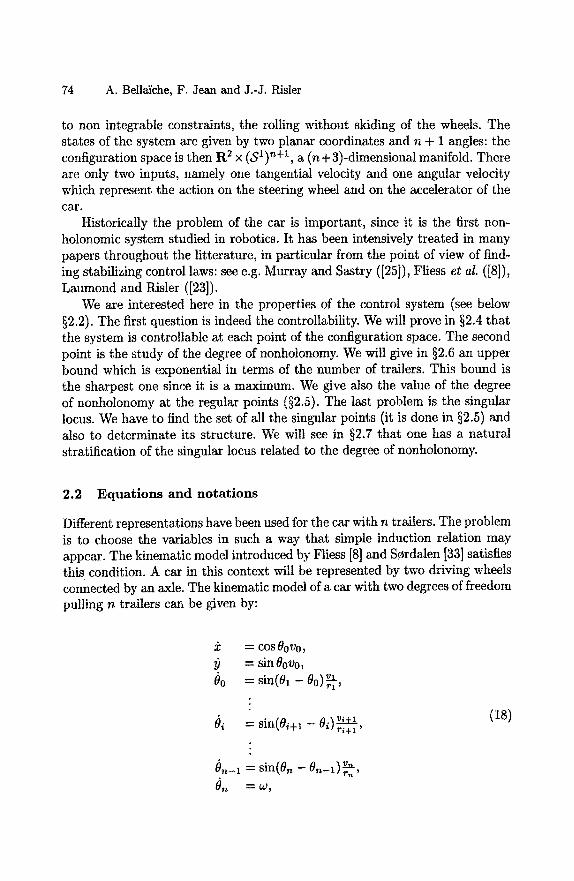
74 A. Bella~che, F. Jean and J.-J. Risler
to non integrable constraints, the rolling without skiding of the wheels. The states of the system are given by two planar coordinates and n + 1 angles: the configuration space is then R 2 x (S 1)n+1, a (n + 3)-dimensional manifold. There are only two inputs, namely one tangential velocity and one angular velocity which represent the action on the steering wheel and on the accelerator of the c a r .
Historically the problem of the car is important, since it is the first non- holonomic system studied in robotics. It has been intensively treated in many papers throughout the litterature, in particular from the point of view of find- ing stabilizing control laws: see e.g. Murray and Sastry ([25]), Fliess et al. ([8]), Laumond and Risler ([23])•
We are interested here in the properties of the control system (see below §2.2). The first question is indeed the controllability. We will prove in §2.4 that the system is controllable at each point of the configuration space. The second point is the study of the degree of nonholonomy. We will give in §2.6 an upper bound which is exponential in terms of the number of trailers. This bound is the sharpest one since it is a maximum. We give also the value of the degree of nonholonomy at the regular points (§2.5). The last problem is the singular locus. We have to find the set of all the singular points (it is done in §2.5) and also to determinate its structure. We wilt see in §2.7 that one has a natural stratification of the singular locus related to the degree of nonholonomy.
2.2 Equations and notations
Different representations have been used for the car with n trailers. The problem is to choose the variables in such a way that simple induction relation may appear. The kinematic model introduced by Fliess [8] and Scrdalen [33] satisfies this condition. A car in this context will be represented by two driving wheels connected by an axle. The kinematic model of a car with two degrees of freedom pulling n trailers can be given by:
:~ = COS OOVO, = sin Oovo,
/~o = sin(01 - Oo) ~ ,
v l / r i + l '
0 . - 1 = sin(O. - O . - 1 ) k , ~n. = 02,
(18)
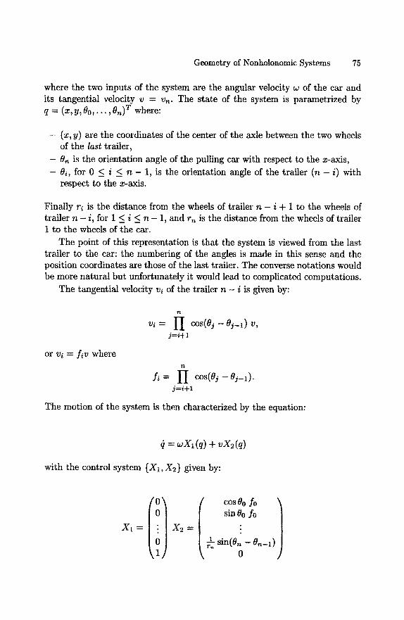
Geometry of Nonholonomic Systems 75
where the two inputs of the system are the angular velocity w of the car and its tangential velocity v = v n . The state of the system is parametrized by q = (x,y, O0,... ,On) T where:
- (x, y) are the coordinates of the center of the axle between the two wheels of the l a s t trailer,
- On is the orientation angle of the pulling car with respect to the x-axis, - 8i, for 0 < i < n - 1, is the orientation angle of the trailer (n - i) with
respect to the x-axis.
Finally ri is the distance from the wheels of trailer n - i + 1 to the wheels of trailer n - i, for 1 < i < n - 1, and rn is the distance from the wheels of trailer 1 to the wheels of the car.
The point of this representation is that the system is viewed from the last trailer to the car: the numbering of the angles is made in this sense and the position coordinates are those of the last trailer. The converse notations would be more natural but unfortunately it would lead to complicated computations.
The tangential velocity vi of the trailer n - i is given by:
or vi = f i v where
n
j= i+ l
= f l cos(0j - 0 j - l ) . j= i+ l
The motion of the system is then characterized by the equation:
(t = (q) + vX2(q)
with the control system {X1, X2) given by:
X x = X 2 =
cos Oo fo ) sin 8o fo
¼ sin(O,, - 0
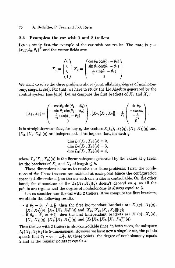
76 A. Bella~che, F. Jean and J.-J. Risler
2.3 Examples : t he car wi th 1 and 2 t r a i l e r s
Let us study first the example of the car with one trailer. The state is q = (x, y, 00, 01) T and the vector fields are:
If) /cos,cos,,) [ sin 9o cos(01 - 00) X1 = X2-- I 1_.sin(01_00)
,1 0
We want to solve the three problems above (controllability, degree of nonholon- omy, singular set). For that, we have to study the Lie Algebra generated by the control system (see §1.6). Let us compute the first brackets of X1 and X2:
/ - cosgo sin(01 - 0o) ~ [ singo
It is straightforward that, for any q, the vectors Xl(q), X~(q), [X1, Xe](q) and IX2, [X1, X2]](q) are independant. This implies that, for each q:
dim LI(X1, X2)(q) = 2, dim L2 (X1, X2) (q) = 3, dim L3(X1, X2)(q) = 4,
where Lk(X1, X2)(q) is the linear subspace generated by the values at q taken by the brackets of X1 and X2 of length _< k.
These dimensions allow us to resolve our three problems. First, the condi- tions of the Chow theorem are satisfied at each point (since the configuration space is 4-dimensional), so the ear with one trailer is controllable. On the other hand, the dimensions of the Lk(X1,X2)(q) doesn't depend on q, so all the points are regular and the degree of nonholonomy is always equal to 3.
Let us consider now the car with 2 trailers. If we compute the first brackets, we obtain the following results:
- i f 0 2 - 01 # 4-~, then the first independant brackets are X1 (q), X2(q), IX1, x2l(q), IX2, x l](q) and [X2, IX2, [X1, x2lll(q);
- if 05 - 01 = 4-~, then the first independant brackets are X1 (q), X2(q), [Xx, X~](q), [X2, IX1, X2l](q) and [Xl[X2, [X~, IX1, X~]]]](q).
Thus the car with 2 trailers is also controllable since, in both cases, the subspaee L5 (X1, X2)(q) is 5-dimensional. However we have now a singular set, the points q such that 02 - 0 1 = :t:~. At these points, the degree of nonholonomy equals 5 and at the regular points it equals 4.
Geometry of Nonholonomic Systems 77
2.4 Control labi l i ty
The controllability of the car with n trailers has first been proved by Lau- mond ([21]) in 1991. He used the kinematic model (18) but a slightly different parametrization where the equation were given in terms of ~i = 0i - 8i-1 and (x ~, y~) ((x ~, y~) is the position of the pulling car). The proof of the controllabil- ity given here is an adaptation of the proof of Laumond for our parametrization. This adaptation has been presented by Sordalen ([33]).
T h e o r e m 2.1. The kinematic model of a car with n trailers is controllable.
Proof. Let us recall some notations introduced in §1.6. Let L:I(X1,X2) be the set of linear combinations with real coefficients of
X1 and X2. We define recursively the distribution £k = ~.k(X1,X2) by:
£k = /:k-1 + Z [L:i,~:j] (19) i+j=k
where [~i, l:j] denotes the set of all brackets [V, W] for V E L:i and W E Ej. The union L:(X1, )(2) of all ~k (X1, X2) is the Control Lie Algebra of the system
Let us now denote L~(X1,X2) the set of linear combinations of X1 and )(2 which coefficients are smooth ]unctions. By the induction (19) we construct from L:~ (X1, X2) the sets £~(X1, X2) and L'(XI, X2).
For a given state q, we denote by Lk(X1,X2)(q), resp. L~(X1,X2)(q), the subspace of Tq(R 2 x (81) n+l) wich consists of tile values at q taken by the vector fields belonging to Lk (X1, X2), resp. £~ (X1,)(2).
Obviously, the sets/:k (X1, X2) and £~ (X1, X2) are different. However, for each k _ 1 and each q, the linear subspaces Lk(X1, X2)(q) and L~(X1, X2)(q) are equal. We are going to prove this equality for k = 2 (the proof for any k can be easily deduced from this case). By definition L2 (X1, X2)(qo) is the linear subspace generated by X1 (qo), X2 (q o) and [X1,X2](qo). L~2(Zl,X2)(qo) is generated by Xl(qo), X2(qo) and all the [f(q)Xl,g(q)X2](qo) with f and g smooth functions. Then L2(XI,X2)(qo) C L~ (X1,3(2) (qo). From the other hand a bracket [fX1, gX2](qo) is equal to:
fg[X1, X2](q0) - g(X2.f)Xl(qo) + f(Xl.g)X2(qo).
Thus [fXl,gX2](qo) is a linear combination with real coefficients of X1(q0), X2(q0) and [X1,X2](qo). Then i~(X1,X2)(qo) = i2(X1,X2)(qo), which prove our statement for k -- 2.
To establish the controllability, we want to apply Chow's theorem (see §1.4): we have then to show that the dimension of L(X1,X2)(q) is n + 3. For that,
78 A. Bella~che, F. Jean and J.-J. Risler
we are going to prove that LI(X1,X2)(q) is n + 3-dimensionnal and use the relation L'(X1, X2)(q) = L(X1, X2)(q).
Let us introduce the following vector fields, for i E {0, . . . , n - 1}, which belong to L'(X1, X2):
Wo = X1 Wi+1 = ri+x (sin ~oir~ + cos ~iZi) Vo = X2 V/+I = cos ~oiV/- sin~iZi) z0 = Ix1, x2] z +l =
The form of these vector fields can be computed by induction. We give only the expression of the interesting ones:
Wi = (0 , . . . , 0 , 1 , 0 , . . . ,0) T, i = 0 , . . . , n
. - i + 2 i (20) ~/Vn = (cos qOo, I sin ~o, 0 , . . . , O) T, l Zn = ( - s i n tool r~ costa0,0, . . . ,0) T.
We have n + 3 vector fields which values at each point of the configu- ration space are independant since their determinant equals l/r1. Therefore L'(Xa, X2)(q), and then L(X1, X2)(q), are equal to Tq(R 2 x (s1)n+l). We can then apply Chow's theorem and get the result. •
R e m a r k . A stronger concept than controllability is given by the following definition: the system {XI, X2} is called well-controllable if there exists a basis of n + 3 vector fields in L(X1, X2)(q) such that the determinant of the basis is constant for each point q of the configuration space. The n + 3 vector fields that we have constructed in the proof satisfy this con- dition. So the car with n trailers is well-controllable.
2.5 R e g u l a r p o i n t s
Let us denote fin(q) the degree of nonholonomy of the car with n trailers. It can be defined as:
fin(q) = min{k I dimLk(Xl,X2)(q) = n + 3}.
We have already computed (§2.3) the values of this degree for n = 1 and 2:
(q) = 3, 2(q) = 4 or 5.
It appears, for n = 2, that the configurations where the car and the first trailer are perpendicular have particular properties. This fact can be generalized as follows ([19]):
Geometry of Nonholonomic Systems 79
T h e o r e m 2.2. The singular locus of the system is the set of the points for which there exists k E [2,n] such that Ok -- Ok-1 = ±~.
The regular points are then the configuration where no two consecutives trailers (except maybe the last two) are perpendicular. It results from §1.6 that the degree of nonholonomy at regular points is < n + 2. In fact this degree is exactly n + 2. It can be shown for instance by converting the system into the so-called chained form as in Scrdalen ([33]). This gives us a first result on the degree of nonholonomy:
Theorem 2.3. At a regular point, i.e., a point such that Ok -- Ok-1 ~ q-~ Vk = 2 , . . . , n, the degree of nonholonomy equals n + 2.
2.6 B o u n d for the degree of nonho lonomy
A first bound for this degree has been given by Laumond ([21]) as a direct consequence of the proof of controllability: we just have to remark that the vector fields (20) belong to/:~.+1 (X1, X2). Thus the degree of nonholonomy is bounded by 2 n+l. However this bound is too large, as it can be seen in the examples with 1 or 2 trailers.
It has been proved in 1993 ([24,34]) that a better bound is the (n+3)-th Fibonacci number, which is defined by F0 = 0, F1 = 1, Fn+3 = Fn+2 + Fn+a. Luca and Risler have also proved that this bound is a maximum which is reached if and only if each trailer (except the last one) is perpendicular to the previous one.
Theorem 2.4. satisfies:
The degree of nonholonomy /3'*(q) for the car with n trailers
~n(q) < Fn+3.
Moreover, the equality happens if and only i] Oi -0 i -1 = 4-~, i = 2, . . . ,n.
Let us remark that this bound is exponential in n since the value of the n-th Fibonacci number is given by:
2.7 Fo rm of the singular locus
The last problem is to determinate the form of the singular locus, which is given in Theorem 2.2. We already know the values of the degree of nonholonomy in two extremal cases:
80 A. Bellaiche, F. Jean and J.-J. Risler
- if no two consecutive trailers are perpendicular, Bin(q) = n + 2; - if each trailer is perpendicular to the previous one, f=(q) = Fn+3.
We have now to characterize the states intermediate between these both cases. For a given state q, we have the following sequence of dimensions:
2 = dimLl(X1,X2)(q) <_... <_ dimLk(X1,X2)(q) _<... _ n + 3. (21)
Let us recall that, if this sequence stays the same in an open neighbourhood of q, the state q is a regular point of the control system; otherwise, q is a singular point (see §1.6). Thus to give the sequence (21) at any state q allows to characterize the singular locus.
To determinate the sequence (21), we only need the dimensions of the spaces Lk(Zl, X2)(q) such that Lk (X1, X2)(q) • Lk-1 (X1, X2) (q). For that we define, for i e {1, n + 3}:
f~(q) = min{k I dimLk(X1,X2)(q) >_ i}
In other words, the fact that k = / ~ ( q ) is equivalent to:
dimLk(X1,X2)(q) >_ i dim Lk-I(X1, X2)(q) < i
(22)
The sequence (21) can be entirely deduced from the sequence fl~(q), i = 1 , . . . , n + 3. Hence the singular locus is completly characterized by the f~(q) 's which we are going to study. Let us remark that f~+3 (q) is the degree of non- holonomy f n (q).
According to its definition, /~(q) increases with respect to i, for i lesser than dim L(X1, X2)(q) (when i is strictly greater than this dimension, f~ (q) is equal to -co) . In fact we will establish (in Theorem 2.5) that this sequence is strictly increasing with respect to i for 2 < i < n + 3. In other words, we will prove that, for 2 < i < n + 3, f~(q) > -o0 and that k = f~(q) is equivalent to (compare with (22)):
dimLk(X1,X2)(q) = i dimLk- l (X1, X2)(q) = i - 1
We can also calculate easily the first values of these sequences. It is clear that the family X1, X2, [X1, X2] is three dimensional for all q (see the examples u = 1 and 2). Then the dimensions of LI(X1,X2)(q) and L2(Xi,X2)(q) are respectively 2 and 3 and we have, for all state q:
,~ (23) f ~ ( q ) = 1 f ~ ( q ) = 1 83 (q) = 2.
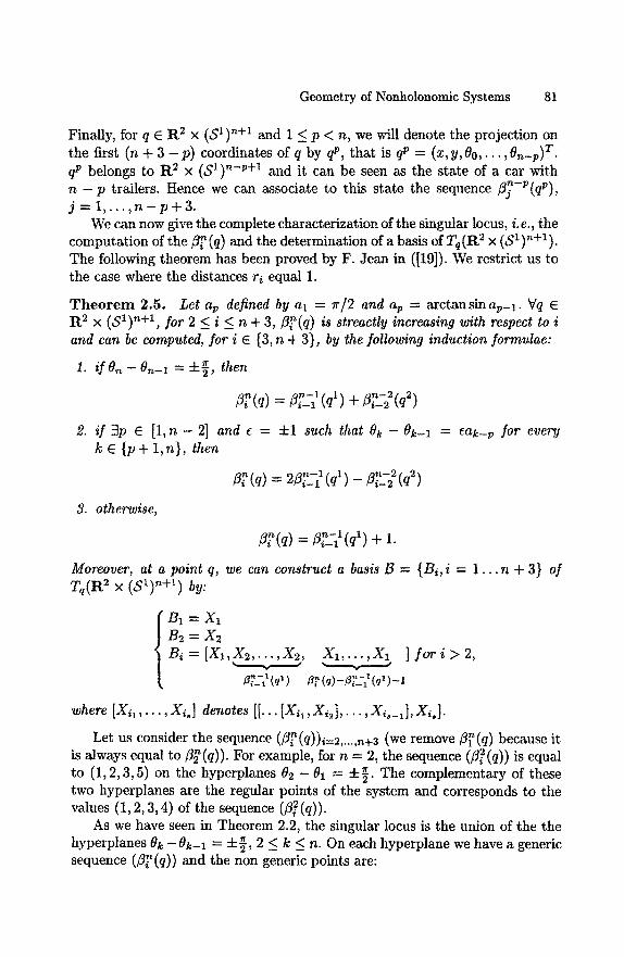
Geometry of Nonholonomic Systems 81
Finally, for q E R 2 × (S 1)n+1 and 1 g p < n, we will denote the projection on the first (n + 3 - p ) coordinates of q by qP, that is qT = (X, y, 00 , . . . , On-T) T. qV belongs to R 2 × (S 1)"-p+I and it can be seen as the state of a car with n - p trailers. Hence we can associate to this state the sequence f~-P(qT), j = 1 , . . . , n - - p + 3 .
We can now give the complete characterization of the singular locus, i.e., the computation of the/3~(q) and the determination of a basis of Tq(R 2 × (S1)n+l). The following theorem has been proved by F. Jean in ([19]). We restrict us to the case where the distances ri equal 1.
T h e o r e m 2.5. Let a T defined by at = 7r/2 and a T = arctansinaT_l. Vq E R 2 × (S1) n+l, for 2 < i < n + 3 , /~ (q ) is streactly increasing with respect to i and can be computed, for i e {3, n + 3}, by the following induction formulae:
I. if On - 0n-1 = ± ~ , then
Z~(q) = Z~_ -1 (qt) + ZT:~(q~)
2. i f 2 p E [1, n - 2 ] and e = ±1 such that Ok --Ok-1 = eak-p for every k E {p+ 1,n}, then
3. otherwise,
~.~(q) n-1 t n-2 2 = ~i-2 ( q ) 2~_~ (q ) -
Moreover, Tq(R 2 × (Sl) ~+1) by:
B1 = Xt B2 = X~ Bi = [X1 ,X2 , . . . , Z2,
~ n - - l ~ 1 ~ Pi -1 (q )
~ ( q ) n-1 1 = / ~ - 1 ( q ) + 1 .
at a point q, we can construct a basis B = {B~,i = 1 . . . n + 3} of
Xt , . . . ,X 1 ] f o r i > 2,
~' (q) - ~7---~ (q~) - 1
where [X,1,..., X,.] aenotes [[... [X,1, X,~],..., X,._I], X,.].
Let us consider the sequence (~(q)) i=2 ..... ~+~ (we remove fl~(q) because it is always equal t o /~ (q ) ) . For example, for n = 2, the sequence (/~i2(q)) is equal to (1, 2, 3, 5) on the hyperplanes 02 - 0 1 = :t:{. The complementary of these two hyperplanes are the regular points of the system and corresponds to the values (1, 2, 3, 4) of the sequence (/32(q)).
As we have seen in Theorem 2.2, the singular locus is the union of the the hyperplanes 0k - 0k-1 = ±~ , 2 < k < n. On each hyperplane we have a generic sequence (j3~(q)) and the non generic points are:
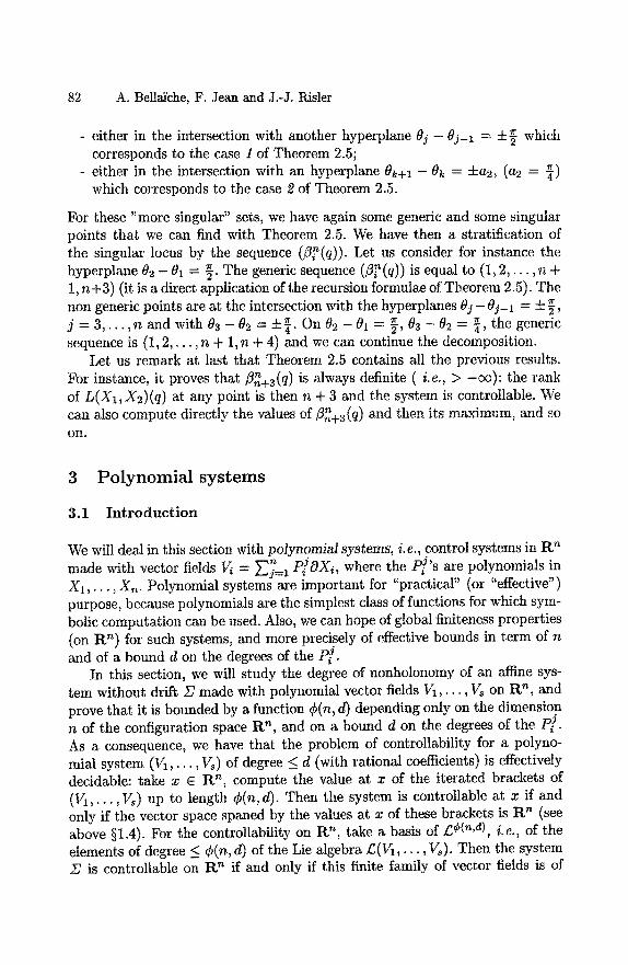
82 A. Bellaiche, F. Jean and J.-J. Risler
- either in the intersection with another hyperplane 0j - 0j-1 = =t:~ which corresponds to the case 1 of Theorem 2.5;
- either in the intersection with an hyperplane 8~+1 - 8h = ±a2, (a2 = ~) which corresponds to the case 2 of Theorem 2.5.
For these "more singular" sets, we have again some generic and some singular points that we can find with Theorem 2.5. We have then a stratification of the singular locus by the sequence (fl~(q)). Let us consider for instance the hyperplane ~2 - 81 = ~. The generic sequence (jJ~(q)) is equal to (1, 2 , . . . , n + 1, n+3) (it is a direct application of the recursion formulae of Theorem 2.5). The non generic points are at the intersection with the hyperplanes 8j - 8 j - 1 = ~= ~, j = 3 , . . . , n and with 83 - 8 2 = =t:~. On 82 - 8 1 = y ~, 83 - 8 2 = ~ " , the generic sequence is (1, 2 , . . . , n + 1, n + 4) and we can continue the decomposition.
Let us remark at last that Theorem 2.5 contains all the previous results. For instance, it proves that ~nn+3(q) is always definite ( i.e., > -co) : the rank of L(X1, X2)(q) at any point is then n + 3 and the system is controllable. We
O n can also compute directly the values f ~n+3(q) and then its maximum, and so o n .
3 P o l y n o m i a l s y s t e m s
3.1 I n t r o d u c t i o n
We will deal in this section with polynomial systems, i.e., control systems in R n made with vector fields V~ = ~=1 P~OX{, where the P~'s are polynomials in X 1 , . . . , Xn. Polynomial systems are important for "practical" (or "effective") purpose, because polynomials are the simplest class of functions for which sym- bolic computation can be used. Also, we can hope of global finiteness properties (on R n) for such systems, and more precisely of effective bounds in term of n and of a bound d on the degrees of the P~.
In this section, we will study the degree of nonholonomy of an affme sys- tem without drift Z made with polynomial vector fields V1, . . . , Vs on R n, and prove that it is bounded by a function ¢(n, d) depending only on the dimension n of the configuration space R ' , and on a bound d on the degrees of the P / . As a consequence, we have that the problem of controllability for a polyno- mial system (V1,. . . , Vs) of degree < d (with rational coefficients) is effectively decidable: take x E R n, compute the value at x of the iterated brackets of (V1, . . . , Vs) up to length ¢(n, d). Then the system is controllable at x if and only if the vector space spaned by the values at x of these brackets is R n (see above §1.4). For the controllability on R n, take a basis of £¢(n,d), i.e., of the elements of degree < ¢(n, d) Of the Lie algebra £.(V1,..., Vs). Then the system Z is controllable on R n if and only if this finite family of vector fields is of
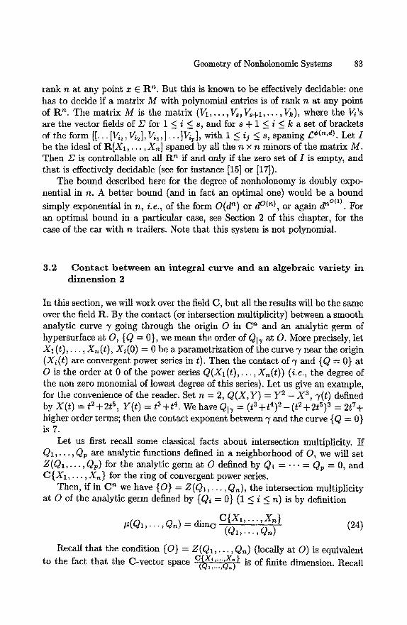
Geometry of Nonholonomic Systems 83
rank n at any point x E R ~. But this is known to be effectively decidable: one has to decide if a matrix M with polynomial entries is of rank n at any point of R n. The matrix M is the matrix (VI, . . . , V~, V8+t,.. . , Vk), where the V~'s are the vector fields of 2Y for 1 < i < s, and for s + 1 < i < k a set of brackets of the form [[... [Vii, V~2], V~3,] ...]Vip], with 1 < ij < s, spaning ~¢(n,d) Let I be the ideal of R[X1, . . . , X,~] spaned by all the n × n minors of the matrix M. Then ~ is controllable on all R n if and only if the zero set of I is empty, and that is effectively decidable (see for instance [15] or [17]).
The bound described here for the degree of nonholonomy is doubly expo- nential in n. A better bound (and in fact an optimal one) would be a bound
simply exponential in n, i.e., of the form O(d n) or d °(n), or again d n°(1) . For an optimal bound in a particular case, see Section 2 of this chapter, for the case of the car with n trailers. Note that this system is not polynomial.
3.2 Contac t b e t w e e n an integral curve and an algebraic variety in d i m e n s i o n 2
In this section, we will work over the field C, but all the results will be the same over the field R. By the contact (or intersection multiplicity) between a smooth analytic curve q' going through the origin O in C n and an analytic germ of hypersurface at O, {Q = 0}, we mean the order of QI~ at O. More precisely, let X1 ( t ) , . . . , Xn(t), Xi(0) = 0 be a parametrization of the curve 7 near the origin (Xi ( t ) are convergent power series in t). Then the contact of 7 and {Q = 0} at O is the order at 0 of the power series Q ( X l ( t ) , . . . , X n ( t ) ) (i.e., the degree of the non zero monomial of lowest degree of this series). Let us give an example, for the convenience of the reader. Set n = 2, Q ( X , Y ) = y 2 _ X 3, 7(t) defined by X ( t ) = t2 + 2t 5, Y ( t ) = t3 + t 4. We have Q]7 = (t3 + t 4 ) 2 - ( t 2 + 2th) 3 "~ 2t7+ higher order terms; then the contact exponent between V and the curve {Q = 0) is 7.
Let us first recall some classical facts about intersection multiplicity. If Q t , - . - , Qv are analytic functions defined in a neighborhood of O, we will set Z ( Q I , . . . , Qv) for the analytic germ at O defined by Q1 = " " = QB = O, and C{X1, . . . , X~} for the ring of convergent power series.
Then, if in C n we have {O} = Z ( Q 1 , . . . , Qn), the intersection multiplicity at O of the analytic germ defined by {Qi = 0} (1 < i < n) is by definition
C{Xl,...,xn) #(Q1,...,Q,~) = dime (Q1,. ~Q--~ (24)
Recall that the condition {O} = Z ( Q 1 , . . . , Qn) (locally at O) is equivalent to the fact that the C-vector space c(xl ..... xn } (Q1 ..... Q,) is of finite dimension. Recall
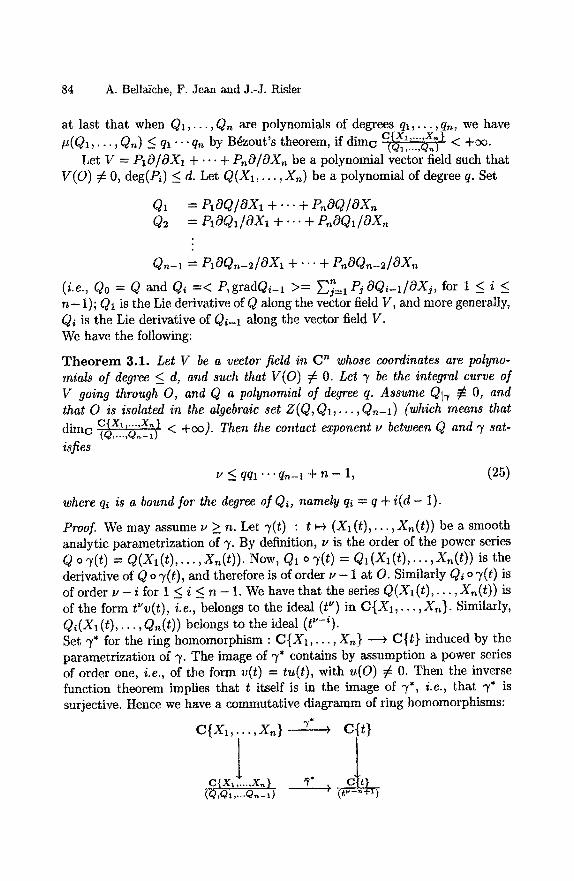
84 A. Bellai'che, F. Jean and J.-J. Risler
at last that when Q1, . - . , Qn are polynomials of degrees q l , . . . , qn , we have #(Q1,. . •, Qn) _< q l ' " "qn by Bdzout's theorem, if dime c(XI(Q1 ..... ..... Q.)x"} < +c~.
Let V = PIO/aXI + . . . + PnO/OXn be a polynomial vector field such that V(O) ~ O, deg(Pi) _< d. Let Q(X1, . . . , Xn) be a polynomial of degree q. Set
Q1 = PtOQ/OX1 + . . . + P , OQ/OXn Q2 = PIOQ1/OX1 + . . . + PnOQ1/OX~
Q~-I = PIOQn-2/OX1 + . . . + PnOQn_2/OXn
(i.e., Qo = Q and Qi = < P, gradQi-1 > = ~j=IPjOQi-1 /OXj , for 1 < i < n - 1); Q1 is the Lie derivative of Q along the vector field V, and more generally, Qi is the Lie derivative of Qi-1 along the vector field V. We have the following:
T h e o r e m 3.1. Let V be a vector field in C n whose coordinates are polyno- mials of degree < d, and such that V(O) ~ O. Let ~/ be the integral curve of V going through O, and Q a polynomial of degree q. Assume QI~ ~ O, and that 0 is isolated in the algebraic set Z(Q, Q1,. . . ,Qn-1) (which means that dime c(x l ..... x~} (Q ..... Q._~) < +co). Then the contact exponent y between Q and 9' sat-
isfies
v < qql""qn-1 + n - 1, (25)
where qi is a bound ]or the degree of Qi, namely qi = q + i(d - 1).
Proof. We may assume u >_ n. Let -y(t) : t ~ (Xl ( t ) , . . . ,Xn(t)) be a smooth analytic parametrization of % By definition, v is the order of the power series Q o 7(t) = Q(X1(t) , . . . ,Xn(t)). Now, Q1 o 7(t) = Ql(Z l ( t ) , . . . ,Xn(t)) is the derivative of Q o 7(t), and therefore is of order u - 1 at O. Similarly Qi o 7(t) is of order u - i for 1 < i < n - 1. We have that the series Q(Xl( t ) , . . . ,Xn(t)) is of the form t~v(t), i.e., belongs to the ideal (t v) in C{X1 , . . . , Xn}. Similarly, Qi(Xt ( t ) , . . . , Qn(t)) belongs to the ideal (tv-i). Set 7* for the ring homomorphism : C{X1 , . . . , Xn} ---+ C{t) induced by the parametrization of 7. The image of ~'* contains by assumption a power series of order one, i.e., of the form v(t) = tu(t), with u(O) ¢ O. Then the inverse function theorem implies that t itself is in the image of 7*, i.e., that 7" is surjective. Hence we have a commutative diagramm of ring homomorphisms:
C{Xl,...,X,} ~" - c { t }
2 c{x~ ..... x~} ~*
( Q , Q I , . . . Q ~ - I ) ~ -
Geometry of Nonholonomic Systems 85
where the vertical arrows represent the canonical maps. Since V* is surjective, we have also that 9" is surjective.
This implies that
c{t} c{xl , . . . ,x,} u - n + 1 = dimc (t ,_n+l) < dimc (Q, . . . ,Qn-1) <- qql"" "q,~-I
or v _< qql -'" q , - I + n - 1 as asserted, the last inequality coming from B~zout's theorem. •
R e m a r k . One may conjecture that such a kind of result is valid (may be with a slightly different bound) without the hypothesis d ime c{x1 ..... x~} finite. This (Q ..... Qn-1) would imply a simply exponential bound (i.e., of the form C(n)d n, or d n°(1)) for the degree of nonholonomy.
Notice that for Theorem 3.1, we may always assume that the polynomial Q(X1 , . . . , Xn) is reduced (or even irreducible), because if Q = R 1 . . . Rs, the bound (25) for the R~'s implies the same bound for Q. In fact, it is enough to prove that if Q = RS, r = degR, s = degS, q = r + s, then
r(r+ d - 1) . . . (r + ( n - 1) (d- 1))+ s(s + d - 1 ) . . - ( s + ( n - 1) (d- 1 ) ) + 2 ( n - 1) <
q(q+ d - 1 ) . . . ( q + ( n - 1 ) ( d - 1)) + n - 1
which is immediate by induction on n. If A is a C-algebra, let us denote by dim A its dimension as a ring (it is its
"Krull dimension"), and dime A its dimension as a C-vector space. If A is an analytic algebra, i.e., A = c(x1 ..... I x~} where I is an ideal, I = ( S t , . . . , Sq), then its dimension as a ring is the dimension (over C) of the germ at O of the analytic space defined by Z(S I , . . . , Sq). We have that dime A < +oc if and only if dim A = 0.
Notice that Q1 cannot be divisible by Q (since Q o 7(t) is of order u, and Q1 o 7(t) of order u - 1). Therefore, if Q is irreducible, we have
dim C{X1, . . . ,X~} = n - 2. (Q,Q1)
This implies that in Theorem 3.1, we may always assume that we have dim C(xl ..... xn) (Q ..... Q~,~) _< n - 2 .
In particular, (25) is true in dimension 2 without additional hypothesis:
C o r o l l a r y 3.2. Let V = Pla/OX + P20/OY be a polynomial vector field in the plane o] degree < d, such that V(O) i~ O, V the integral curve of V by O, and Q(X, Y) a polynomial o] degree q such that QI~ ~ O. Then the contact exponent u of Q and V satisfies
< q(q+ d - 1) + 1.
86 A. Bella~che, F. Jean and J.-J. Risler
This corollary has first been proved by A. Gabrielov, J.-M. Lion and R. Moussu, [10].
3.3 The case of d imension n
We have the following result, due to Gabrielov ([12])
Theorem 3.3. Let V = ~ PiO/OXi be a polynomial vector field, with P~ C C [ Z l , . . . , Zn] of degree <_ d, such that V(O) # O, Q(X1, . . . , Xn) a polynomial of degree ~_ q such that Qf~ ~ O. Then the contact exponent v between Q and 7 satisfies
< 2 + (k - 1)(d - 1)] (26) k = l
Remark . This bound is polynomial in d and q and simply exponential in n. It is optimal (up to constants) since it comes from Example 2) below that there exists a lower bound also polynomial in d and q and simply exponential in n.
R e m a r k . In 1988 Nesterenko ([27]) found a bound ~f the form
v ~ c(n)dn2q n,
namely simply exponential in n when d is fixed, but doubly exponential in the general case.
R e m a r k . In dimension 3, the following bound has been found by A. Gabrielov, F. Jean and J.-J. Risler, [9]:
v < q + 2q(q + d - 1) 2.
3.4 Bound for the degree of nonholonomy in the plane
In the two-dimensional case, we have the following bound for the degree of non-holonomy (see [29]):
Theor e m 3.4. Let Z = (~/~,..., Vs) be a control system made with polynomial vector fields on R 2 of degree <_ d; let r(x) be the degree o] nonholonomy o] E at x E R 2. Then,
r(x) < 6d 2 - 2d + 2 (27)
Geometry of Nonholonomic Systems 87
Proof. Take x = O. Let as above (see §1.6) Li(O) be the vector space spaned by the values at O of the brackets of elements of Z of length _< i. We may assume d imLl(O) = 1, because otherwise the problem of computing r(O) is trivial (if d imLl(O) = 0, then Ls(O) = {0} Vs > 1, and if d imLl(O) = 2, we have LI(O) = R 2 and r(O) = 1 by definition). We therefore assume that V 1(O) ~ 0, and set V = V1. •
L e m m a 3.5. Assume r(O) > 1, which in our case implies that the system Z is controllable at 0 . Then there exists Y E Z such that det(V,Y)i, r ~ 0.
Proof. Assume that det(V,Y)l ~ -- 0 VY E Z. Then, in some neighborhood of O, any vector field Y E Z is tangent to the integral curve ~, of V from O. This implies that the system cannot be controllable at O, since in some neighborhood of O the accessible set from O would be contained in % •
Let us now state a Lemma in dimension n.
L e m m a 3.6. Let V, Y1, . . . , Yn be vector fields on R n. Then
n
V.det(Y1,.. . , Y,~) -- ~ det(Y1,. . . , [V, Yi] , . . . , Yn) + i=1 Div(V).det(Y1,. . . , yn).
Let us recall that Div(V) = OP1/OXi + OP:/OX2 + ... + OPn/OXn, where V = PlO/OXl + . . . -t- PnO/OX,~.
Proof. This formula is classical. See for instance [13, Exercice page 93], or [26, Lemma 2.6]. •
of Theorem 3.4, continued. Let -y be the integral curve of V by O. By Lemma 3.5, there exists Y E ~U such that det(V,Y)l ~ ~ 0. Set Q = det(V, Y)I ~.
By Lemma 3.6, we have V.det (V, Y) = det(V, [V, Y]) + DivVdet(V, Y). Let v be the order of contact of Q and % We have that QI~ = avtV + ' " , with a~ ~ 0, and that (V.Q)i~ = vast v-1 + . . . because V~ can be identified with O/Ot. Then det(V, [V, Y])I~ is of order v - 1 in t, and we see that when differentiating v times in relation to t, we find that
det(V, [V[V,... [V, Y] . . . ]])(O) ~ 0,
the bracket inside the parenthesis being of length v+ 1. This means by definition of r(O) that r(O) ~ ~ + 1. The polynomial Q is of degree < 2d, and V is a polynomial vector field of degree < d. Then Corollary 3.2 gives v < 2 d ( 2 d + d - 1 ) + 1 = 6d 2 - 2 d + 1. •
88 A. Bellgiche, F. Jean and 3.-3. Risler
E x a m p l e . 1) Set v1 = O/OX + x d o / O Y
z v~ = YaO/OX
Then it should be easily seen that for this system, r(O) = d 2 + 2d + 1. The inequality r(O) _> d 2 + 2d + 1 has been checked by F. Jean. This proves that the estimation (27) is asymptotically optimal in term of d, up to the constant 6.
2) Let in R n
{ v1 = O/OXl v~ = x ~ a / a x ~
27
d X G = X._~O/O , ,
We see easily that for this system, r(O) = d n- l , which means that in general ¢(n, d) is at least exponential in n.
3.5 T h e gene ra l case
We have the following result, where for simplicity, and because it is the most important case, we assume the system controllable.
T h e o r e m 3.7. Let n > 3. With the above notation, let r(x) be the degree of non-holonomy at x E R n for the control system Z made with polynomial vector fields of degree <_ d. Let us assume that the system E is controllable. Then we have the following upper bound:
n+3
r(x) G¢(n ,d ) , with¢(n,d) < 2"-2(l + 22n(n-2)-2d2n y~.k2n). (28) k=4
Proof. We first state without proof a result of Gabrielov [11].
L e m m a 3.8. Let (V1, . . . , 17,) be a system of analytic vector fields controllable at 0 such that V1 (0) ~6 0. Let f be a germ of an analytic function such that f (O) = 0 and fl~(yl) ~ 0 (v(V1) denotes the trajectory oJV1 going through 0 ) . Then there exists n vector fields X1, . . . , X , satisfying
- X1 = 1/'1, X2 is one of the Vi, and, for 2 < k G n, Xk is either one of the Vi or belongs to the linear subspace generated by [Xt, ]Xm], for l, m < k;
- there exists a vector field Xe = X1 + e2X2 + "'" + en-lXn-1 such that
de t (x l , . . . , Xn)l,(x.) ~ o.
Geometry of Nonholonomic Systems 89
Let us assume x = O. For a generic linear function f , the conditions f(O) = 0 and f[~(yl) ~ 0 are ensured. We can then apply the lemma and obtain n vector fields X1,..-, Xn. From the first point of Lemma 3.8, Xk is a polynomial vector field of degree not exceeding 2k-2d. Thus the vector field X~ is polynomial of degree not exceeding 2n-ad and the determinant Q = det(x1, . . . , Xn) is also polynomial. Its degree does not exceed d + d + . . . + 2'~-2d = 2n-ld.
The second point of Lemma 3.8 ensures that Q and Xe fulfill the conditions of Theorem 3.3. Then, applying (26), the contact exponent v between Q and 7(X~) satisfies
n
v < 22n3-4n-1 ~ ( 4 d + k - 1) 2n.
k = l
Each derivation of Q along X~ decreases this multiplicity by 1. Hence the result of v consecutives derivations of Q along x~ does not vanish at O. By using Lemma 3.6, that means that there exists n brackets ~k = [X~,..., [XE, Xk]... ], with at most v occurences of Xe, such that:
det(~l(O),. . . ,~n(O)) ~ O.
/,From the first point of Lemma 3.8, each Xk is a linear combination with polynomial coefficient of brackets of the vector fields V/of length not exceeding 2 k-2. This implies Xk(O) e L2k-2(Z)(O) (this is the same reasoning as in the proof of Theorem 2.1). We have then x~(O) E L2~-~(z~)(O) and, Vk, ~k(O) E L2.-~+~2.-3 (Z)(O).
Since det(~l , . . . , ~ ) ~ 0, the subspace L2~-2+v2.-3(Z)(O) is of dimension n and then
n-b3
r(O) < 2~-2(1 + 2~n(~-2)-2d 2n ~ k2n). k----4
90 A. Bellaiche, F. Jean and J.-J. Risler
References
1. A. A. Agrachev and R. V. Gamkrelidze, "Tile exponential representation of flows and the chronological calculus," Mat. Sbornik (N.S.), 107 (149), 467-532, 639, 1978. English transl.: Math. USSR Sbornik, 35, 727-785, 1979.
2. A. Bella'iche, "The tangent space in sub-Riemannian Geometry," in Sub- Riemannian Geometry, A. Bellaiche and J.-J. Risler Ed., Progress in Mathe- matics, Birkh~user, 1996.
3. A. Beltaiche, J.-P. Laumond and J. Jacobs, "Controllability of car-like robots and complexity of the motion planning problem," in International Symposium on Intelligent Robotics, 322-337, Bangalore, India, 1991.
4. A. Bella~che, J.-P. Laumond and J.-J. Risler, "Nilpotent infinitesimal approxi- mations to a control Lie algebra," in Proceedings of the IFAC Nonlinear Control Systems Design Symposium, 174-181, Bordeaux, France, June 1992.
5. R. W. Brockett, "Control theory and singular Riemannian geometry," in New directions in applied mathematics, P. J. Hilton and G. J. Young Ed., Springer- Vertag, 1982.
6. J. F. Canny, The complexity of robot motion planning, MIT Press, 1998. 7. W. L. Chow, "Uber Systeme von linearen partiellen Differentialgleichungen erster
Ordnung," Math. Ann., 117, 98-115, 1940. 8. M. Fliess, J. Levine, P. Martin and P. Rouchon, "On differential flat nonlinear
systems," in Proceedings of the IFA C Non linear Control Systems Design Sympo- sium, 408-412, Bordeaux, France, 1992.
9. A. Gabrielov, F. Jean and J.-J. Risler, Multiplicity of Polynomials on Trajectories of Polynomials Vector Fields in C a, Preprint, Institut de Math~matiques, Univ. Paris VI, 1997.
10. A. Gabrielov, J.-M. Lion and R. Moussu, "Ordre de contact de courbes int~grales du plan," CR Acad. Sci. Paris, 319,219-221, 1994.
11. A. Gabrielov, "Multiplicities of Zeroes of Polynomials on Trajectories of Poly- nomial Vector Fields and Bounds on Degree of Nonholonomy," Mathematical Research Letters, 2, 437-451, 1995.
12. A. Gabrielov, Multiplicity of a zero o] an analytic function on a trajectory of a vector field, Preprint, Purdue University, March 1997.
13. C. Godbillon, Gdomdtrie diffdrentielle et Mdcanique analytique, Hermann, Paris, 1969.
14. N. Goodman, Nilpotent Lie groups, Springer Lecture Notes in Mathematics, 562, 1976.
15. S. Grigoriev, "Complexity of deciding Tarski algebra," J. Symb. Comp., 5, 37-64, 1988.
16. M. Gromov, "Carnot-Carath~odory spaces seen from within," in Sub-Riemannian Geometry, A. Bella~che and J.-J. Risler Ed., Progress in Mathematics, Birkh~user, 1996.
17. J. Heinz, M.-F. Roy and P. Solerno, "Sur la complexit~ du principe de Tarski- Seidenberg," Bull. Soc. Math. Ft., 118, 101-126, 1990.
18. H. Hermes, "Nilpotent and high-order approximations of vector field systems," SIAM Review, 33 (2), 238-264.
Geometry of Nonholonomic Systems 91
19. F. Jean, "The car with N trailers: characterization of the singular configurations," ESAIM: COCV, http://www.emath.fr/cocv/, 1,241-266, 1996.
20. J.-P. Lanmond, "Singularities and Topological Aspects in Nonholonomic Motion Planning," in Nonholonomic Motion Planning, 149-199, Z. Li and J. Canny Ed., Klumer Academic Publishers, 1993.
21. J.-P. Laumond, "Controllability of a multibody mobile robot," in Proceedings of the International Conference on Advanced robotics and Automation, 1033-1038, Pisa, Italy, 1991.
22. J-P. Laumond, P. E. Jacobs, M. Taix and R. M. Murray, "A motion planner for nonholonomic mobile robot," in LAAS-CNRS Report, oct. 1992.
23. J.-P. Laumond and J.-J. Risler, "Nonholonomics systems: Controllability and complexity," Theoretical Computer Science, 157, 101-114, 1996.
24. F. Luca and J.-J. Risler, "The maximum of the degree of nonholonomy for the car with n trailers," 4th IFAC Symposium on Robot Control, 165-170, Capri, 1994.
25. R. M. Murray and S. S. Sastry, "Nonholonomic Motion Planning: Steering using sinusoids," IEEE Transactions on Automatic Control, 38 (5), 700-716, May 1993.
26. A. Nagel, E. M. Stein and S. Wainger, "Metrics defined by vector fields," Acta Math., 155, 103-147, 1985.
27. Y. V. Nesterenko, "Estimates for the number of zeros of certain functions," New Advances in transcendance Theor, 263-269, A. Baker Ed., Cambridge, 1988.
28. P. K. Rashevsky, "Any two points of a totally nonholonomic space may be con- nected by an admissible line," Ueh. Zap. Ped. Inst. ira. Liebknechta, Set. Phys. Math., 2, 83-94, 1938 (Russian).
29. J.-J. Risler, "A bound for the degree of nonholonomy in the plane," Theoretical Computer Science, 157, 129-136, 1996.
30. J. T. Schwartz and M. Sharir, "On the 'Piano Movers' problem II: general tech- niques for computing topological properties of real algebraic manifolds," Advances in Applied Mathematics, 4, 298-351, 1983.
31. A. Seidenberg, "On the length of Hilbert ascending chain," Proc. Amer. Math. Soc., 29, 443-450, 1971.
32. E. Sontag, "Some complexity questions regarding controllability," Proc. of the 27-th IEEE Conf. on Decision and Control, 1326-1329, Austin, 1988.
33. O. J. S0rdalen, "Conversion of the kinematics of a car with n trailers into a chain form," IEEE International Conference on Robotics and Automation, 1993.
34. O. J. Sordalen, "On the global degree of non holonomy of a car with n trailers," 4th IFAC Symposium on Robot Control, 343-348, Capri, 1994.
35. P. Stefan, "Accessible sets, orbits, and foliations with singularities," Proc. London Math. Soe., 29 (3), 699-713, 1974.
36. H. J. Sussmann, "Orbits of families of vector fields and integrability of distribu- tions," Trans. Amer. Math. Soc., 180, 171-188, 1973.
37. H. J. Sussmann, "Lie brackets, Real Analyticity and Geometric control," in Differential Geometric Control Theory, Brockett, Millman, Sussmann Ed., Birk~iuser, 1-116, 1982.
Optimal Trajectories for Nonholonomic Mobile Robots
P. Sou~res 1 and J.-D. Boissonnat 2
1 LAAS- CNRS, Toulouse 2 INRIA, Sophia Antipolis
1 I n t r o d u c t i o n
From a kinematic point of view, the main characteristic of wheeled robots is the nonholonomic rolling without slipping constraint of the wheels on the floor, which forces the vehicle to move tangentially to its main axis. This reduction of the set of accessible velocities at each time makes the path planning problem particularly difficult. Among the different methods devoted to solve this prob- lem we want to focus on those based on the characterization of shortest paths or time-optimal paths, which turn out to be particularly efficient. Indeed, the knowledge of an optimal strategy for linking any two configurations allows to determine simple canonical paths and provides a topological modeling of the problem by defining a new "distance function" taking into account the non- holonomic nature of the system. Unfortunately, the characterization of optimal paths for this class of nonlinear systems is not an easy task.
The works presented in this chapter are based on Pontryagin's Maximum Principle (PMP) which constitutes a generalization of Lagrange's problem of the calculus of variation. PMP is a local reasoning based on the comparison of trajectories corresponding to infinitesimally close control laws. It provides nec- essary conditions for paths to be optimal. Nevertheless, though this condition brings a very strong information about the nature of optimal paths for certain kind of systems, it turns out to be insufficient to solve the optimal control problems we are interested on.
Indeed, on the one hand the nonlinear nature of these systems makes the adjoint differential equations seldom integrable. Therefore, in the most part of cases, the necessary condition of PMP only provides a local characterization of optimal trajectories. On the other hand, the study of such systems has shown that the set of accessible configurations at each time, is neither smooth nor convex. More precisely, it appears that the boundary of this set is made up by several smooth pieces corresponding to the propagation of several wave fronts. This is due at one and the same time to the difficulty of moving sideways and the natural symmetries of the problem.
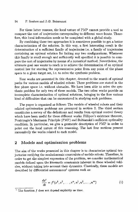
94 P. Sou~res and J.-D. Boissonnat
For these latter reasons, the local nature of PMP cannot provide a tool to compare the cost of trajectories corresponding to different wave fronts. There- fore, this local information needs to be completed with a global study.
By combining these two approaches it is sometimes possible to get a better characterization of the solution. In this way, a first interesting result is the determination of a sufficient family of trajectories i.e. a family of trajectories containing an optimal solution for linking any two configurations. Whenever this family is small enough and sufficiently well specified it is possible to com- pare the cost of trajectories by means of a numerical method. Nevertheless, the ultimate goal one wants to reach is to achieve the determination of an optimal control law for steering the representative point from any point of the phase space to a given target set, i.e. to solve the synthesis problem.
Four works are presented in this chapter, devoted to the search of optimal paths for various models of wheeled robots. These problems are stated in the free phase space i.e. without obstacles. We have been able to solve the syn- thesis problem for only two of these models. The two other works provide an incomplete characterization of optimal solutions, bringing to the fore various kind of difficulties that can be encountered in studying such problems.
The paper is organized as follows: The models of wheeled robots and their related optimization problems are presented in section 2. The third section constitutes a survey of the definitions and results from optimal control theory which have been useful for these different works: Fillipov's existence theorem, Pontryagin's Maximum Principle (PMP) and Boltianskii's sufficient optimality condition. In particular, we give a geometric description of PMP in order to point out the local nature of this reasoning. The last four sections present successively the works related to each model.
2 M o d e l s a n d o p t i m i z a t i o n p r o b l e m s
The aim of the works presented in this chapter is to characterize optimal tra- jectories verifying the nonholonomic constraints of mobile robots. Therefore, in order to get the simplest expression of the problem, we consider mathematical models defined upon the kinematic constraints inherent in these wheeled vehi- cles, without taking into account their dynamics. Classically, these models are described by differential autonomous 1 systems such as:
dxi = fi(x 1,x2,..o , x n , u 1 u2,. . , u m) (1) d t ' "
1 The function f does not depend explicitly on time.
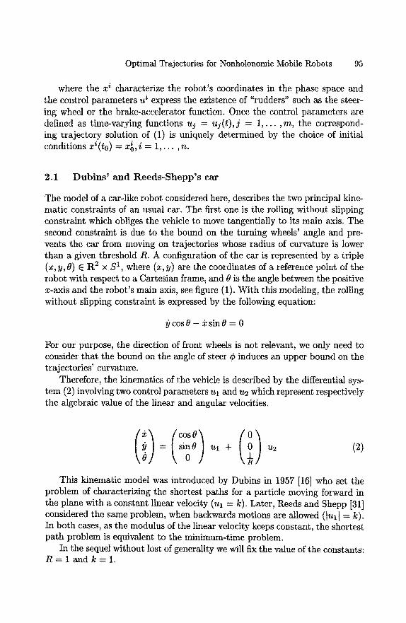
Optimal Trajectories for Nonholonomic Mobile Robots 95
where the x i characterize the robot's coordinates in the phase space and the control parameters u i express the existence of "rudders" such as the steer- ing wheel or the brake-accelerator function. Once the control parameters are defined as time-varying functions u j = u j ( t ) , j = 1,. . . ,m, the correspond- ing trajectory solution of (1) is uniquely determined by the choice of initial conditions x i ( t o ) = Xio,i = 1 , . . . , n .
2.1 Dubins ~ and Reeds-Shepp 's car
The model of a car-like robot considered here, describes the two principal kine- matic constraints of an usual car. The first one is the rolling without slipping constraint which obliges the vehicle to move tangentially to its main axis. The second constraint is due to the bound on the turning wheels' angle and pre- vents the car from moving on trajectories whose radius of curvature is lower than a given threshold R. A configuration of the car is represented by a triple (x, y, 0) E R 2 x S 1, where (x, y) are the coordinates of a reference point of the robot with respect to a Cartesian frame, and 0 is the angle between the positive x-axis and the robot's main axis, see figure (1). With this modeling, the rolling without slipping constraint is expressed by the following equation:
y c o s 0 - &sin0 = 0
For our purpose, the direction of front wheels is not relevant, we only need to consider that the bound on the angle of steer ¢ induces an upper bound on the trajectories' curvature.
Therefore, the kinematics of the vehicle is described by the differential sys- tem (2) involving two control parameters ul and u2 which represent respectively the algebraic value of the linear and angular velocities.
(cos0) = si; 0 ul + u2 (2)
This kinematic model was introduced by Dubins in 1957 [16] who set the problem of characterizing the shortest paths for a particle moving forward in the plane with a constant linear velocity (Ul = k). Later, Reeds and Shepp [31] considered the same problem, when backwards motions are allowed (tult = k). In both cases, as the modulus of the linear velocity keeps constant, the shortest path problem is equivalent to the minimum-time problem.
In the sequel without lost of generality we will fix the value of the constants: R = I and k = 1.
96 P. Sou~res and J.-D. Boissonnat
/
la
Fig. 1. The car-like model
2.2 Dubins ' car wi th inert ial angular velocity
As we will see later in detail, the optimal solutions of Dubins' problem are sequences of line segments and arcs of circle of minimal radius. Therefore, the curvature along the trajectory does not vary continuously. As a consequence, any real robot following such a trajectory would be constrained to stop at each curvature discontinuity.
In order to avoid this problem, Boissonnat, Cerezo and Leblond [3] have proposed a dynamic extension of Dubins' problem by controlling the angular acceleration of the car instead of its angular velocity. The curvature ~ is now considered as a new phase variable, and the angular acceleration v is bounded inside a compact interval I -B, B].
= + v (3 )
For this problem, as for Dubins problem, minimizing the time comes to the same as minimizing the length.
2.3 The robot H I L A R E
The locomotion system of Hilare the robot of LAAS-CNRS consists of two parallel independently driven wheels and four slave castors. The velocities vr and vl of the right and left driven wheels are considered as phase variables and
Optimal Trajectories for Nonholonomic Mobile Robots 97
a configuration of the robot is a 5-uple (x, y, 0, vr, vt). The accelerations ar and at of each driven wheel are the inputs to the following control system:
(// cos0, (i/ • o °
= / / + ar + al (4)
where at, a~ E [-amax, a~x], and d > 0 is the distance between the wheels. In this case the trajectories' curvature is not bounded and the robot can turn about its reference point.
For this model, we consider the problem of characterizing minimum-time trajectories linking any pair of configurations where the robot is at rest i.e verifying vr = vt = 0.
3 S o m e r e s u l t s f r o m O p t i m a l C o n t r o l T h e o r y
3.1 Definit ions
Let us now define the notion of dynamical system in a more precise way. Let M be a n-dimensional manifold, and U a subspace o f R m. We study the motion of a representative point x(t) = (x l(t), . .. , xn(t)) in the phase space M, depending on the control law u(t) = (u 1 ( t) , . . . , urn(t)) taking its values in the control set U. In this chapter, we define the set of admissible control laws as the class of measurable functions from the real time interval [t0,h] to U. As we said in the previous section, the motion of the representative point is described by an autonomous differential system of the form:
dx i - - ~ = f i ( x ( t ) , u ( t ) ) i = 1 , . . . , n (5)
We consider now a function L(x , u) defined on the product M x U, contin- uously differentiable with respect to its arguments. Given any two points Xo and xl in the phase space M, we want to characterize, among all the control laws steering the representative point from x ° to x 1, one (if exists) minimizing the functional:
~o 1 J = L(x(r , u), u(T))dr
98 P. Sou~res and J.-D. Boissonnat
R e m a r k 1. The initial and final time to and tt are not fixed a priori, they depend on the control law u(t).
D e f i n i t i o n 1. Two trajectories are said to be equivalent for transferring the representative point from Xo to xl if they their respective costs are equal.
In the sequel we restrict our study to the minimum-time problem. In this case L(x, u) _-- 1 and J = tl - to.
In chapter 1 it has been shown that the models described in the previ- ous section are fully controllable in their phase space M, i.e. given any two configurations xo and xl in M there always exists a trajectory, solution of (5), linking x0 to xl . Nevertheless it is not possible to deduce from this result whether a minimum-time feasible path from Xo to xl exists or not. This last question constitutes an important field of interest of optimal control theory (cf [13] for a detailed survey). In particular, there exist some general theorems due to Fitlipov, ensuring the existence of optimal paths under some convexity hypotheses. The next subsection presents two theorems that will be sufficient for our purpose'.
3.2 E x i s t e n c e o f o p t i m a l p a t h s
Let M be an open subset of R ~ or a n-dimensional smooth manifold, and U a subset of R m.
T h e o r e m 1. (Fillipov's general theorem for minimum-time problems) Let x0, xl be two points in M. Under the following hypotheses there exists
a time-optimal t rajectory solution of (5) linking x0 to xl .
H1 - f is a continuous function of t, u, x and a continuously differentiable function of x.
H2 - the control set U is a c o m p a c t subset of R m. Furthermore, when u varies in U, the image set F(t,x) described by f(x(t), u(t)) is c o n v e x for
all t ,x E [t0,tl] x M. Hs - there exists a constant C such that for all (t, x) E [to, tl] x M:
< x , f ( t , x , u ) > < C ( l + l x [ 2) /-/4 - there exists an admissible trajectory from x0 to xl
R e m a r k 2. - The hypothesis Ha prevents from a finite escape time of the phase variable x for any admissible control law u(.).
When f is a linear function of the control parameters ui of the form:
f (X,~) = gl(~) Ul + - . . + gin(X) Urn, (6)
there exists a simpler version of this result given by the next theorem.
Optimal Trajectories for Nonholonomic Mobile Robots 99
T h e o r e m 2. Let xo and xl be two points in M. Under the following hypothe- ses there exists an optimal t rajectory solution of (6) linking x0 to xl .
//1 - the gl are locally lipschitzian functions of x. //2 - the control set U is a c o m p a c t convex subset of R m //3 - there exists an admissible t rajectory from xo to xl //4 - The system is complete, in the sense that given any point Xo E M, and any
admissible control law u(.), there exists a corresponding t rajectory x(t, u) defined on the whole time interval [to, tl] and verifying x(to, u) = Xo.
3.3 N e c e s s a r y cond i t i ons : P o n t r y a g i n ' s M a x i m u m P r i n c i p l e
Pontryagin's Maximum Principle (PMP) provides a method for studying vari- ational problems in a more general way than the classical calculus of variation does. Indeed, when the control set U is a closed subset of R m, the Weierstrass' condition characterizing the minimum of the cost functional is no more valid. The case of closed control set is yet the most interesting one for modeling con- crete optimal control problems. PMP provides a necessary condition for the solutions of a general control systems to be optimal for various kind of cost functional. In this chapter we restrict our statement of PMP to minimum-time problems.
We consider the dynamical system (5) where x belongs to an open subset C R n or a smooth n-dimensional manifold M.
D e f i n i t i o n 2. - Let ¢ be a n-dimensional real vector, we define the Hamittonian of system
(5) as the R-valued function H defined on the set Rn. x t? x U by:
H ( ¢ , u) =< ¢, I(x, > (7)
where R . n -- R n \ {0}, and < .,. > is the usual inner product of R n. - / ] u(.) : [to, tl] --~ U is an admissible control law and x(t) : [to, tl] -4 J?
the corresponding trajectory, we define the adjoint vector for the pair (x, u) as the absolutely continuous vector function ¢ defined on [to, tl ], taking its values in R~. which verifies the following adjoint equation at each time t E [to, tl]:
OH ¢(t ) = - x(t) , u(t)) (8)
R e m a r k 3. As H is a linear function of ¢, ~h is also a linear function of ¢. Therefore, either ¢( t ) i~ 0 Vt E [to, tl], or ¢( t ) - 0 on the whole interval [to, tl]; in the latter case, the vector ¢ is said to be trivial.
100 P. Sou~res and J.-D. Boissonnat
T h e o r e m 3. (Pontryagin's Maximum Principle) Let u(.) be an admissible con- trol law defined on the closed interval [t0,tl] and x(t) the corresponding tra- jectory. A necessary condition for x(t) to be time-optimal is that there exists an absolutely continuous non trivial adjoint vector ¢(t) associated to the pair (x, y), and a constant Co _< 0 such that Vt E [to, tl]:
H(¢( t ) , x(t), u(t)) = mea~(H(¢(t), x(t), v(t)) = - ¢ 0 (9)
De f in i t i on 3. - A control law u(t) satisfying the necessary condition of PMP is called an
extremal control law. Let x(t, u) be the corresponding trajectory and ¢(t) the adjoint vector corresponding to the pair (x, u); the triple (x, u, ¢) is also called extremal.
- To study the variations of the Hamiltonian H = S~ ~( t ) ¢~(t) one can rewrite H in the form: H = ~i¢i(t) ui(t) where the ¢i, called switching func- tions determine the sign changes of ui.
Sometimes the maximization of the function H does not define a unique control law. In that case the corresponding control is called singular.
Def in i t i on 4. A control u(t) is singular if there exists a nonempty subset W C U and a non empty interval I C [to, tl] such that Vt E I, Vw(t) E W:
H(¢( t ) , x(t), u(t)) = H(¢( t ) , x(t), w(t))
In particular, when a switching function vanishes over a non empty open interval of time, the corresponding control law comes singular. In that case, all the derivatives of the switching function also vanish on this time interval, providing a sequence of equations. From these relations, it is sometimes possible to characterize the value of the corresponding singular control.
The following theorem allows to compute easily those derivatives in terms of Lie brackets.
T h e o r e m 4. Let Z be a smooth vector field defined on the manifold M and (x, u, ¢) an extremal triple for the system (6).
The derivative of the function ¢z(.) : t r < ¢(t) , Z(x(t)) > is defined by:
Cz(t) = < ¢ , Z]x(t) > i = 1
Let us now define the notion of reachable set"
Optimal Trajectories for Nonholonomic Mobile Robots 101
Defini t ion 5. - We denote by T6(xo,T), and we call set of accessibility from xo in time T, the set of points x E M such that there exists a trajectory solution of (5) transferring the representative point from xo to x in a time t < T.
- The set T~(xo) = (Jo<T<~ ~(xo, T) is called set of accessibility from xo.
When the system is fully controllable (controllable from any point) the set of accessibility T~(Xo) from any point Xo is equal to the whole manifold M. Otherwise, T~(x0) is restricted to a closed subset of M. In this latter case there exists another version of PMP.
T h e o r e m 5. (PMP for boundary trajectories) Let u(.) : [to, tl] -~ U be an admissible control law, and x(t) the corresponding trajectory transferring the representative point from Xo to a point xl belonging to the boundary OTi(Xo) of the set 7~(x0). A necessary condition for the trajectory x(t, u) to be time- optimal, is that there exists a non-trivial adjoint vector ¢ verifying relation (9) with Co = 0
Defini t ion 6. An extremal triple (x, u, ¢) such that Co = 0 is called abnormal
Commentary about PMP: It is often difficult to extract a precise information from PMP. Indeed, it is seldom possible to integrate the adjoint equations or to characterize the singular control laws. Furthermore, one can never be sure to have got all the information it was possible to deduce from PMP. Sometimes, the information obtained is very poor, and the set of potential solutions too large.
An interesting expected result is the characterization of a sufficient fam- ily of trajectory i.e. a family of trajectory containing an optimal solution for linking any pair of points (x0,xl) E M. When this family is small enough, and sufficiently well specified the optimal path may be selected by means of a numerical test.
Nevertheless, the ultimate goal one wants to reach is the exact characteri- zation of the optimal control law allowing to steer the point between any two states of M. However, though it is possible to deduce directly the structure of minimum-time trajectories from PMP for linear systems, the local information is generally insufficient to conclude the study in the case of nonlinear systems. As we will see in the sequel, it is yet sometimes possible to complete the local information provided by PMP by making a geometric study of the problem. When the characterization of optimal path is complete, a synthetic way of rep- resenting the solution is to describe a network of optimal paths linking any point of the state space to a given target point. The following definition due to Pontryagin states this concept in a more precise way.
102 P. Sou~res and J.-D. Boissonnat
Defini t ion 7. For a given optimization problem, we call synthesis function, a ]unction v(x) (if it exists) defined in the phase space M and taking its values in the control set U, such that the solutions of the equation:
dx d-7 =/(x, v(x))
are optimal trajectories linking any point of M to the origin. The problem o/characterizing a synthesis function is called synthesis problem and the cor- responding network of optimal paths is called a synthesis of optimal paths on M.
A geometric illustration o] PMP: In the statement of PMP, optimal control laws are specified by the maximization of the inner product of two vectors. In the rest of this section, drawing our inspiration from a work by H. Halkin [21], we try to give a geometric interpretation of this idea by pointing out the analogy between optimal control and propagation phenomena. In this, we want to focus on the local character of PMP in order to point out its insufficiency for achieving the characterization of shortest paths for nonholonomic problems. This remark emphasizes the necessity to complete the local reasoning by making use of global arguments.
At the basis of the mathematical theory of optimal process stands the prin- ciple o] optimal evolution which can be stated as follows:
"I /x( t , u) is an optimal trajectory starting from Xo at time to, then at each time t >_ to the representative point must belong to the boundary OT~(xo, t) o/ the set 7~(xo, t)"
For some physical propagation phenomena, such as the isotropic propaga- tion of a punctual perturbation on the surface of water, the wave]font associated with the propagation coincides at each time with the boundary of the set of accessibility. Let us consider first the simple propagation of a signal starting at a point x0 such that the set of accessibility 7~(Xo, t) at each time t be smooth and convex with a unique tangent hyperplane defined at each boundary point.
As in geometrical optics, at each time t and at each boundary point x, we can define the wavefront velocity as a nonzero vector V(x, t) = V(x, t) k(x, t) where V(x, t) is a R-valued function of x and t, and k(x, t) a unit vector outward normal to the hyperplane tangent to T~(x0, t) at x. Now, according to the principle of optimal evolution, if x(t, u) is an optimal trajectory starting at x0, the following two conditions must be verified:
- For any admissible motion, corresponding to a control w(t), the projection of the representative point velocity &(t, w) = ](x,w) on the line passing through x(t, w) and whose direction is given by the vector k(x, t), is at most equal to the wavefront speed V(x, t).
Optimal Trajectories for Nonholonomic Mobile Robots 103
< f(x(t) , k(x, t) > < t)
- With the optimal control u, the representative point must keep up with the wavefront OTC(Xo, t) i.e. the projection of the representative point's velocity on the normal vector k(x, t) determines the wavefront velocity.
< f(x(t) ,u(t)) ,k(x, t) > = V(x,t) (11)
Now, by identifying the adjoint vector ¢(x, t) with V(x, t) we can make a link between relations (10, 11) and the maximization of the Hamiltonian defined by (9).
Though this analogy with propagation phenomena provides a good ge- ometric meaning of this principle of optimization, it is not easy to gener- alize this idea to any dynamical system. Indeed, for a general system, the set Ti(xo,t) is not necessarily convex and its boundaries are not necessar- ily smooth. In order to get a geometric meaning of Pontryagin's result in the general case, it is convenient to consider the cost functional J as a new phase variable x °, and to manage our reasoning in the augmented phase space t t x ~ C R n+l. Therefore, at each time, the velocity vector of the representa- tive point X = (x °, x) = (x °, x l , . . . . x n) corresponding to the control law u(.) is given by ](X, u) = (L(x, u), f l (x, u ) , . . . , fn(x, u)). With this representation the optimization problem becomes:
"Let g) be the line passing through (O, xl) parallel to the x°-axis. Among all the trajectories starting at Xo = (0,x0) and reaching g), find one, i/ exists, which minimizes the first coordinate x ° of the point of intersection X1 = (x°,xl) with 2)."
As before we define the set of accessibility TO(X0, t) from Xo in the aug- mented phase space. Now, it is easy to prove that any optimal path must verify the principle of optimality. Indeed, if the point X1 of g~, reached at time tl with control u, lies in the interior of 7~(X0, tl), there exists necessarily a neigh- bourhood of X1 containing a point of 9 located "under" X1 and the control u cannot be optimal. Furthermore, due to the smoothness properties of the func- tion ] , if the point X, reached at time v E [to, tl] with u, is in the interior of TO(X0, r), then for all t >_ T the representative point will belong to the interior of re(Xo, t).
Now, let X(t ,u) be a trajectory starting at X0, optimal for reaching the line T~. In order to use the same reasoning as before, Pontryagin's et al have proven that it is still possible to construct a separating hyperplaae by using the following idea: By replacing u(.) by other admissible control laws on "small" time intervals they define new admissible control laws fi infinitesimaly close to
104 P. Sou~res and J.-D. Boissonnat
u. Then, a part of their proof consists in showing that the set of point X(t, ~) reached at each time t by the "perturbed" trajectories constitutes a convex cone g with vertex X(t,u), contained in T~(X0, t). This cone locally approximates the set TC(Xo,t) and does not contain the half-line 7)- starting at X(t,u) in the direction of the decreasing x °. It is then possible to find an hyperplane 7/tangent to g at X(t,u), separating g and the half-line 7)-, and containing the vector ](t, u). Now, the reasoning is the same as before; the adjoint vector
= (¢0, ¢1 , . . . , Cn) is defined, up to a multiplicative constant, as the vector outward orthogonal to this hyperplane at each time. Following the principle of optimal evolution, the projection of the vector ](t , u) on the line parallel to ¢(t), passing through x(t, u), must be maximal for the control u.
The case o/nonholonomic systems: As we will see later, the nonhotonomic rolling without slipping constraint, characteristic of wheeled robots, makes their displacement anisotropic. Indeed, although forwards motion can be easily per- formed, moving sideways may require numerous manoeuvres. For this reason, and due to the symmetry properties of such systems, the set of accessibility (in time) is generally not convex and its boundary does not coincide every- where with the wavefront associated with the propagation. Instead of this, we will show later that the boundary is made up by the propagation of sev- eral intersecting wavefronts. Therefore, a local method like PMP, based on the comparison of very close control laws cannot be a sufficient tool to compare the cost of trajectories corresponding to different wavefronts. This very important point will be illustrated in section 4 through the construction of a synthesis of optimal paths for the Reeds-Shepp car.
So far, we only have stated necessary conditions for trajectories to be op- timal. We now present a theorem by V. Boltyanskii which states sufficient optimality conditions under very strong hypotheses.
3.4 Bol tyanski i ' s sufficient conditions
In this section we recall Boltianskii's definition of a regular synthesis as stated in [4]. This concept is based on the definition of a piecewise-smooth set.
Let M be a n-dimensional vector space, and f2 an open subset of M. Let E an s-dimensional vector space (s < n) and K C E a bounded, s-dimensional convex polyhedron. Assume that in a certain open set of E containing K are given n continuously differentiable functions ~o ~ (41, 42,... , 4 s), (i = 1, 2, . . . , n)
o such that the rank of the matrix of partial derivatives ( ~ ) , (i = 1, 2 , . . . , n), (j = 1,2, . . . ,s) be equal to s at every point 4 E K.

Optimal Trajectories for Nonholonomic Mobile Robots 105
~~( x~ x~ ) ~ Jo~ Fig. 2. Hyperplane 7-/separating the half-line D - and the convex cone C.
106 P. Sou~res and J.-D. Boissonnat
Def in i t ion 8. - If the smooth vector mapping ~o = (~o1,~o2,... ,~o n) from K to M is injective, the image L = ~o(K) is called a s-dimensional curvilinear polyhedron in M.
- Any set X C [2 which is the union of a finite or countable number of eurvilinear ployhedra, such that only a finite number of these polyhedra intersect every closed bounded set lying in [2, will be called a piecewise-smooth set in [2. The dimension of this set will be the highest dimension of polyhedra involved in the construction.
R e m a r k 4. It has been proven in [12] that any non-singular smooth surface of dimension less than n, closed in [2, can be decomposed in a finite number of eurvilinear polyhedra. Therefore, such a surface is is a pieeewise-smooth set in [2.
Now let us state the problem: In the n-dimensional space M, we consider the following system:
- p ( x l , . . , z n , u ) i = 1 , . . , n (12) dt
where the control u = ( u l , . . . ,Urn) belongs to an open set U C Rrn. The problem is the following one: Given any two points Xo and xl E [2, among all the piecewise continuous controls u(t) transferring the point from xo to xl find
the one which minimizes the Junctional J = fito f ° (x( t ) , u(t))dt. Now, let us assume that are given a piecewise-smooth set N of dimension
lower or equal to n - l , and n + l piecewise-smooth sets p0, p 1 . . . , pn verifying
pO C P~ C p2 C . . . C pn = [2, (13)
and a function v defined in [2 and taking its values in U. Now, we can introduce Boltianskii's definition of a regular synthesis.
De f in i t i on 9. The sets, N, pO, . . . , pn and the Junction v effect a regular syn- thesis for (12) in the region [2, if the following conditions are satisfied.
A The set po is the target point. Every smooth component o f P i \ ( p i - 1 U N ) , i = 1 , . . . , n, is an i-dimensional smooth manifold in [2; these components will be called/-dimensional cells. The function v is continuously differen- tiable on each cell and can be extended into a continuously differentiable function on the neighbourhood of the cell.
B All the cells are grouped into cells of the first or second type ~1 or T2) in the following manner:
(1) If cr is a 1-dim cell of type T1, then it is a segment of a phase trajectory solution of (12) approaching the target po with a nonzero phase velocity.
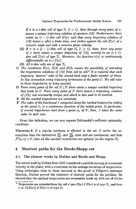
Optimal Trajectories for Nonholonomic Mobile Robots 107
If a is a i-dim cell of type T1 (i > 1), then through every point of a, passes a unique trajectory solution of equation (12). Furthermore, there exists an (i - 1)-dim cell II(a) such that every trajectory solution of (12) leaves a after a finite time, and strikes against the cell II(a) at a nonzero angle and with a nonzero phase velocity.
(2) If a is a ( i - 1)-dim cell of type T2 (i >_ 1), then, from any point of a there issues a unique trajectory of (12), moving in an (i + 1)- dim cell Z(a) of type T1. Moreover, the function v(x) is continuously differentiable on a U Z(a).
(3) All 3-dim cells are of type T1. C The conditions B(1), B(2) and B(3) ensure the possibility of extending
the trajectories solutions of (12) from cell to cell. 2 It is required that each trajectory "pierces" cells of the second kind only a finite number of times. In this connection every trajectory terminates at the point O. We will refer to these trajectories as being marked.
D From every point of the set [2 \ N there exists a unique marked trajectory that leads to O. From every point of N there issues a trajectory, solution of (12), not necessarily unique and which is also said to be marked.
E All the marked trajectories are extremals. F The value of the functional J computed along the marked trajectories ending
at the point O, is a continuous function of the initial point. In particular, if several trajectories start from a point xo of N, then, J takes the same value in each ease.
From this definition, we can now express Boltianskii's sufficient optimality condition:
Theorem 6. If a regular synthesis is effected in the set /2 under the as- sumption that the derivatives ~ and ~ exist and are continuous, and that f ° (x ,u) > 0, then all the marked trajectories are optimal (in the region ~2).
4 S h o r t e s t p a t h s f o r t h e R e e d s - S h e p p c a r
4.1 The pioneer works by Dubins and Reeds and Shepp
The initial work by Dubins from 1957 considered a particle moving at a constant velocity in the plane, with a constraint on the average curvature of trajectories. Using techniques close to those involved in the proof of Fillipov's existence theorem, Dubins proved the existence of shortest paths for his problem. He showed that the optimal trajectories are necessarily made up with arc of circles
2 Trajectories are extended from the cell a into lI(a) if H(a) is of type T1, and from a to ,U(H(a)) if H(a) is of type T2.
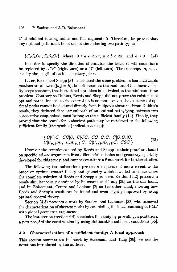
108 P. Sou~res and J.-D. Boissonnat
C of minimal turning radius and line segments S. Therefore, he proved that any optimal path must be of one of the following two path types:
[CaCbCe , CaSdCe} where: 0 <: a, e < 2r, ~r < b < 27r, and d > 0 (14)
In order to specify the direction of rotation the letter C will sometimes be replaced by a "r" (right turn) or a "/" (left turn). The subscripts a, e , . . . specify the length of each elementary piece.
Later, Reeds and Shepp [31] considered the same problem, when backwards motions are allowed (lull = k). In both cases, as the modulus of the linear veloc- ity keeps constant, the shortest path problem is equivalent to the minimum-time problem. Contrary to Dubins, Reeds and Shepp did not prove the existence of optimal paths. Indeed, as the control set is no more convex the existence of op- timal paths cannot be deduced directly from Fillipov's theorem. From Dubins's result, they deduced that any subpath of an optimal path, lying between two consecutive cusp-points, must belong to the sufficient family (14). Finally, they proved that the search for a shortest path may be restricted to the following sufficient family (the symbol I indicates a cusp):
{ ClClC, ccjc, ctcc, ccotc c, clc, colc, (15) ClC=/=sc, csc=/=lC, ClC /2sc=/=lC, c s c }
However the techniques used by Reeds and Shepp in their proof are based on specific ad hoc arguments from differential calculus and geometry, specially developed for this study, and cannot constitute a framework for further studies.
The following two subsections present a sequence of more recent works based on optimal control theory and geometry which have led to characterize the complete solution of Reeds and Shepp's problem. Section (4.2) presents a result simultaneously obtained by Sussmann and Tang [36] on the one hand, and by Boissonnat, Cerezo and Leblond [2] on the other hand, showing how Reeds and Shepp's result can be found and even slightly improved by using optimal control theory.
Section (4.3) presents a work by Sou~res and Laumond [33] who achieved the characterization of shortest paths by completing the local reasoning of PMP with global geometric arguments.
The last section (section 4.4) concludes the study by providing, a posteriori, a new proof of the construction by using Boltianskii's sufficient conditions [35].
4.2 Characterization of a sufficient family: A local approach
This section summarizes the work by Sussmann and Tang [36]; we use the notations introduced by the authors.
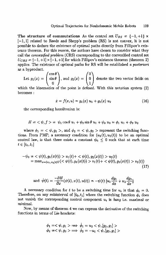
Optimal Trajectories for Nonholonomic Mobile Robots 109
T h e s t r u c t u r e of commuta t i ons As the control set URs = {-1, +1} x [-1, 1] related to Reeds and Shepp's problem (RS) is not convex, it is not possible to deduce the existence of optimal paths directly from Fillipov's exis- tence theorem. For this reason, the authors have chosen to consider what they call the convexified problem (CRS) corresponding to the convexified control set UcRs = [-1, +1] x [-1, +1] for which Fillipov's existence theorem (theorem 2) applies. The existence of optimal paths for RS will be established a posteriori as a byproduct.
Let gl(x) -- [ sinn0 ) , and g2(x) ---- denote the two vector fields on
which the kinematics of the point is defined. With this notation system (2) becomes :
= f ( ~ , u ) = g l ( ~ ) ~1+g~(~) u~
the corresponding hamiltonian is:
(16)
H = < ¢ , f > = ¢ l c o s O u 1 + ¢ 2 s i n O u l + ¢ 3 u 2 = C l u l + ¢ 2 u 2
where ¢1 = < ¢,gl >, and ¢2 = < ¢,g2 > represent the switching func- tions. From PMP, a necessary condition for (ul(t),u2(t)) to be an optimal control law, is that there exists a constant ¢o _< 0 such that at each time t e [~o, t,]
- ¢ 0 = < ¢(t) ,g l (x(~)) > ~ l ( t )+ < ¢(t) ,g2(x(t)) > ~2(t) = max~=(vl,.2)eu(< ¢( t ) , gl (x(~)) > v 1 (~)--~ < ~b(~), g2 (x(~)) > v 2 (~))
(17)
- O H
A necessary condition for t to be a switching time for ui is that ¢i = 0. Therefore, on any subinterval of [to, tl] where the switching function ¢i does not vanish the corresponding control component ui is bang i.e. maximal or minimal.
Now, by means of theorem 4 we can express the derivative of the switching functions in terms of Lie brackets:
¢~ = < ¢, m > ~ ¢~ = u2 < ¢, [g2, m] > ¢2 = < ¢,g2 > = ~ ¢2 = -u~ < ¢,[g~,m] >
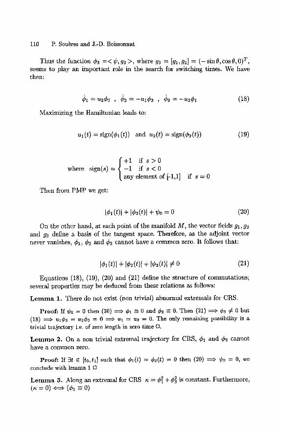
110 P. Sou~res and J.-D. Boissonnat
Thus the function ¢3 = < ¢ , g a >, where g3 = [gl ,g2] = ( - sin~,cosO,0) T, seems to play an important role in the search for switching times. We have then:
Maximizing the Hamiltonian leads to:
(18)
ul( t) = sign(¢l(t)) and us(t) -- sign(¢2(t)) (19)
where / +~ if s > 0 s ign(s )= - if s < 0
I. any element of [-1,1]
Then from PMP we get:
i f s = 0
I¢l(t)l + t¢2(t)l + ¢0 = 0 (20)
On the other hand, at each point of the manifold M, the vector fields gl, g2
and g3 define a basis of the tangent space. Therefore, as the adjoint vector never vanishes, ¢1, ¢2 and ¢3 cannot have a common zero. It follows that:
[¢1(t)[ 4 [¢2(t)[ + [¢3(t)1 ~ 0 (21)
Equations (18), (19), (20) and (21) define the structure of commutations; several properties may be deduced from these relations as follows:
L e m m a 1. There do not exist (non trivial) abnormal extremals for CRS.
Proof: If ¢o = 0 then (20) ==~ ¢1 ~ 0 and q~2 - 0. Then (21) ~ ¢3 ~ 0 but (18) ==~ u1¢~ = u2¢3 = 0 ==~ u~ = u2 = 0. The only remaining possibility is a trivial trajectory i.e. of zero length in zero time D.
L e m m a 2. On a non trivial extremal trajectory for CRS, ¢1 and ¢2 cannot have a common zero.
Proof: If 3t E [to, t~] such that (~ l ( t ) = (~2(t) = 0 then (20) ==# ¢o = 0, we conclude with lemma 1 []
.~2 -b ¢2 is constant. Furthermore, L e r n m a 3. Along an extremal for CRS a = ~'i 3 = 0) ¢ = . (¢1 - 0)
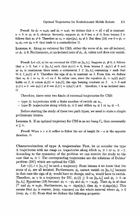
Optimal Trajectories for Nonholonomic Mobile Robots 111
P roo f : As ¢1 -- u~53 and ¢3 -- u251 we deduce that ~ -- 52 + 523 is constant. ,~ = 0 =~ 51 -- 0, obvious. Inversely, suppose ¢1 - 0 but ,¢ ~ 0; from lemma 2 it follows that 52 ¢ 0. Therefore as u2 --- s ign(52), us ¢ O. But then (18) ==~ 0 = ¢1 = u2.53 ==~ 53 = 0 that leads to a contradiction [3.
L e m m a 4. Along an ex t remal for CRS, ei ther the zeros of ¢1 are all isolated, or 51 - 0. Fur the rmore , a t an isolated zero of ¢1, ¢1 exists and does not vanish.
P roo f : Let x(t , u) be an extreinal for CRS on [to, hi . Suppose ¢1 ~ 0; it follows that ,~ > 0. Let r E ] t0 ,h[ such that e l ( r ) = 0, from lemma 2 ¢2(r) ~ 0 and as ¢2 is continuous there exists a subinterval I C ]to, t1[ containing r such that Vt e I , ¢2(t) ~ 0. Therefore the sign of ¢2 is constant on I . From this, we deduce that u2 - 1 or u2 - - 1 on I . In either case, since the equation ¢1 = u2(t) ¢3(t) holds on I , it comes ¢1(t) = =t=¢3(t), the sign keeping constant on I. s > 0 and 51(T) ---- 0 ~ ¢a(r) ¢ 0 ~ ¢1(r) = :t:¢3(r) ¢ 0. therefore, r is an isolated zero. []
Therefore , there exist two kinds of ex t remal t ra jec tor ies for CRS:
- type A: t ra jec tor ies with a finite number of switch on u l , - t ype B: t ra jec tor ies along which ¢1 - 0 and ei ther us - 1 or Us - - 1 .
Before s ta r t ing the s tudy of these two p a t h types , we need to s ta te a s imple p re l imina ry lemma.
L e m m a 5. I f an op t ima l t r a j ec to ry for CRS is an arc bang Ca then necessari ly a <~ 7r.
P r o o f : When a > Ir it suffice to follow the arc of length 2~ - a in the opposite direction. Zt
C h a r a c t e r i z a t i o n o f t y p e A t r a j e c t o r i e s First , let us consider the t ype A t ra jec tor ies wi th n o c u s p i.e. t ra jec tor ies along which ul -= 1 or ul - - 1 . According to the s y m m e t r y of the p rob lem we can restr ic t the s tudy to the case t h a t Ul - 1. T h e corresponding t ra jec tor ies are the solutions of Dubins ' p rob l em (DU) which are op t imal for CRS.
Let 7 ( t ) , t E [t0,tl] be such a t ra jec tory . F rom l e m m a 4 we know t h a t the zeros of ¢1 are all isolated. Fur thermore , ¢1 cannot vanish on ]to, t l [ because in t h a t case the sign of ¢1 would have to change, and u l would have to switch. Therefore , as 7 is a t r a j ec to ry for DU, ¢1(t) > 0 on [ to ,h i and ¢, > 0 on ]to, t l[ . E..quations (18) become: ¢2 = - ¢ 3 and ¢3 = -u2¢.1. T h e n ¢2 is of class C 1 and ¢2 = u2¢1. Fur thermore , u2 = sign(C2), then ¢2 = ¢ls ign(¢2) . This means t h a t ¢2 is convex, (resp. concave) on the whole interval where ¢2 > 0 (resp. ¢2 < 0). F rom t h a t we deduce the following proper ty :
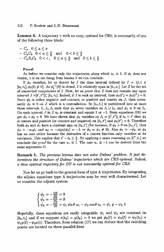
112 P. Sou~res and J.-D. Boissonnat
L e m m a 6. A t r a j ec to ry 7 wi th no cusp, op t imal for CRS, is necessari ly of one of the following three kinds:
- C~ O < a < T r -CaCb O < a < ~ and O < b < ~ -CaS~Cb O < c , O < a < ~ and 0<b<i
Proo f : As before we consider only the trajectories along which ul - 1. If ¢2 does not
vanish, 7 is an arc bang; from lemma 5 we can conclude. If ~b2 vanishes, let us denote by I the time interval defined by I = it , t E
[to, tl], ¢2(t) # 0}. As ¢21(0) is closed, I is relatively open in [to, tl]. Let/7 be the set of connected components of I . First, let us prove that 2: does not contain any open interval J =]t', t"[C [to, tl]. Indeed, if J is such an interval, then ¢2(t') = ¢2(t") = 0. Since ¢2 is either negative and concave, or positive and convex on J , then neces- sarily ¢2 = 0 on J which is a contradiction. So [t0,tl] is partitioned into at most three intervals Ii,I2,Ia such that ¢2 never vanishes on /1 U I3, and ¢2 -- 0 on I2. On each interval J in 17 u2 is constant and equals 1 or -1 . From equations (18) we get ¢'3 + q~3 = 0. We have shown that ¢2 vanishes o n / 2 = [t ' ,t"]; if to < t ' then ¢2 is convex and positive (or concave and negative) on [to, t '[ and ¢2(t') = 0. Therefore both q~a and q~a have a constant sign on ]to, t '[ !for instance, if ¢2 > 0 on [t0,f[, then ¢3 = -u2¢1 and u2 = -sign(¢2) = - 1 = v ¢ a = ¢1 # 0). Also ¢a = -¢2 , so ¢a has no zero either because the derivative of a convex function only vanishes at its minimum. This implies that t ' - t o < {. By applying a same reasoning on ]t", tl] we conclude the proof for the case ul - 1. The case ul -= - 1 can be derived from the same arguments [:3.
R e m a r k 5, The previous lemma does not solve Dubins' problem. It just de- termines the structure of Dubins' trajectories which are CRS-optimal. Indeed, a time optimal trajectory for DU is not necessarily optimal for CRS.
Now let us go back to the general form of t ype A t ra jector ies . B y in tegra t ing the adjoint equat ions type A t ra jec tor ies m a y be very well character ized. Let us consider the adjoint system:
l ~l OH ---- ---g~- = 0 42 -- 0,OH 0
3 -- ~ 0 R ¢1 sin 8 ul -- ~b2 cos ~ ul = ¢1 Y - ¢2
Hopefully, these equat ions are easily integrable: ¢1 and ¢2 are cons tan t on [to, t1] and if we suppose x(to) --- y(to) -= 0 we get ¢2(t) = ¢3(t) -- Ca(to) + ¢ l y ( t ) - ¢2x( t ) . Therefore , f rom relat ion (17) we can deduce t ha t the switching points are loca ted on three paral lel lines.
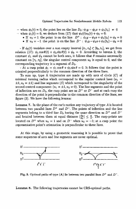
Optimal Trajectories for Nonholonomic Mobile Robots 113
- when Cs(t) = 0, the point lies on the line Do: ¢1Y - Csx + ¢3(t0) = 0 - when ¢1(t) = 0, we deduce from (17) that ¢3(t)u2(t) + ¢0 = 0:
• If us = 1 the point is on the line D + : ¢1Y - Csx + ¢3(t0) + ¢o = 0 • If u2 = - 1 the point is on the line D - : ¢ly-¢sx+¢3(to)-¢o = 0
- If ¢2(t) vanishes over a non empty interval [rl,r2] C [t0,ta], we get from relation (17): Cx c o s 0 ( t ) + ¢ 2 s i n 0 ( t ) + Co = 0. According to lemma 2, the constant ¢1 and ¢2 cannot be both zero, it follows that 0 remains necessarily constant on [TI,~'2], the singular control component u2 is equal to 0, and the corresponding trajectory is a segment of Do.
- At a cusp point ¢1 = ¢1 cos 0 + Cs sin 0 = 0. It follows that the point is oriented perpendicularly to the common direction of the three lines.
To sum up, type A trajectories are made up with arcs of circle (C) of minimal turning radius which correspond to the regular control laws (ul = +1, u2 = +1) and line segments (S) which correspond to the singularity of the second control component: (ul = 4-1, us = 0). The line segments and the point of inflection are on Do, the cusp point are on D + or D - and at each cusp the direction of the point is perpendicular to the common direction of the lines, see figure (3). We have the following lemma:
L e m m a 7. In the plane of the car's motion any trajectory of type A is located between two parallel lines D + and D - . The points of inflection and the line segments belong to a third line Do having the same direction as D + and D - and located between them at equal distance I¢~1 < ~. The cusp-points are
located on D + when u2 = 1 and on D - when u2 = -1 ; at a cusp point the representative point 's orientation is perpendicular to these lines.
At this stage, by using a geometric reasoning it is possible to prove that some sequences of arcs and line segments are never optimal.
D" D"
Do
D + D +
r+r - 1" r+r~ s - r -
Fig. 3. Optimal paths of type (A) lie between two parallel lines D + and D - .
L e m m a 8. The following trajectories cannot be CRS-optimal paths.
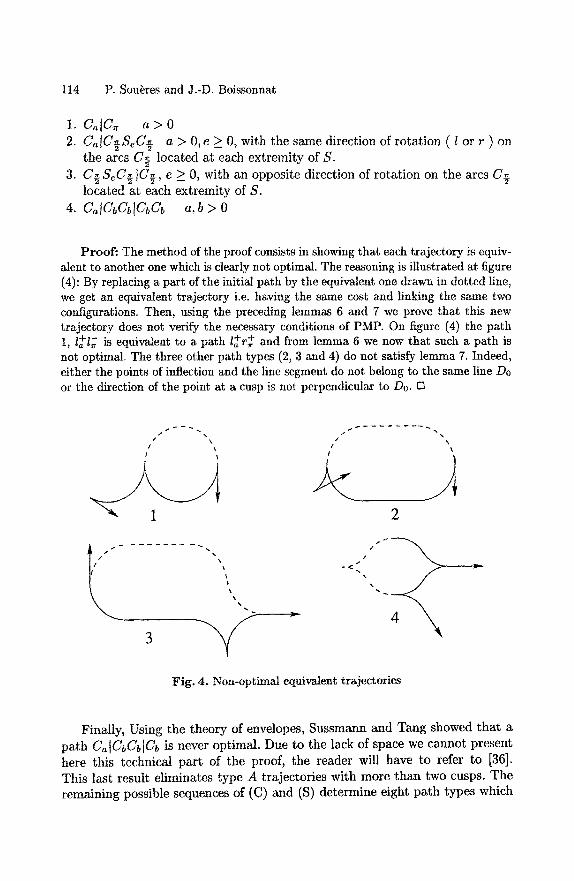
114 P. Sou~res and J.-D. Boissonnat
1. c~tc~ a>O 2. CalC~SeC~ a > 0,e > 0, with the same direction of rotation ( I or r ) on
the arcs C_- located at each extremity of S. 2
3. C-~ SeC~ tC~, e _> 0, with an opposite direction of rotation on the arcs C-_2 located at each extremity of S.
4. CalC'bCbICbCb a,b > 0
Proofi The method of the proof consists in showing that each trajectory is equiv- alent to another one which is clearly not optimal. The reasoning is illustrated at figure (4): By replacing a part of the initial path by the equivalent one drawn in dotted line, we get an equivalent trajectory i.e. having the same cost and linking the same two configurations. Then, using the preceding lemmas 6 and 7 we prove that this new trajectory does not verify the necessary conditions of PMP. On figure (4) the path 1, l+l~ is equivalent to a path + + l~ r , and from lemma 6 we now that such a path is not optimal. The three other path types (2, 3 and 4) do not satisfy lemma 7. Indeed, either the points of inflection and the line segment do not belong to the same line Do or the direction of the point at a cusp is not perpendicular to Do. []
t 't ~
1 2
\
Fig. 4. Non-optimal equivalent trajectories
Finally, Using the theory of envelopes, Sussmann and Tang showed that a path C~[CbCbiCb is never optimal. Due to the lack of space we cannot present here this technical part of the proof, the reader will have to refer to [36]. This last result eliminates type A trajectories with more than two cusps. The remaining possible sequences of (C) and (S) determine eight path types which
Optimal Trajectories for Nonholonomic Mobile Robots 115
are represented by the types (II) to (IX) of the sufficient family (22) presented at section 4.2.
Charac te r i za t ion of t y p e B t ra jec to r ies Let us first consider the case that u2 - 1; we call this subproblem LTV (Left Turn Velocity). In order to lead their reasoning the authors considered what they called the lifted problem LLTV (Lifted Left Turn Velocity) obtained from LTV by regarding the variable 8 as a real number x3. For this last problem, as x3 - 1, any trajectory ~/linking the point x0 at time to to the point xl at time tl has the cost: At = x3(tl) -x3(t0). The same phenomenon occurs for LTV, but only for trajectories whose duration is lower or equal to Iv. For this reason the problem LLTV is called degenerate whereas the problem LTV is locally degenerate.
Using the techniques presented in chapter 1 it is straight forward to deduce from the structure of the Lie algebra L = Lie(gl,g2) generated by the vector fields gl and g2, that the problem LTV has the accessibility property. Neverthe- less, as the corresponding system is not symmetric (i.e. an admissible trajectory followed backwards is not necessary admissible) we cannot deduce directly the controllability of LTV. This can be done by considering the "bang-bang" sys- tem (BB) corresponding to the control set (ul,u2) E { -1 ,+1} x {-1, +1}. As the BB system has the accessibility property and is symmetric on the connected manifold R 2 x S 1 it is controllable. Any admissible trajectory for BB is a se- quences of tangent arcs C. By replacing every arc ra by the complementary part 12.-a followed backwards, we can transform any BB trajectory into an admissible trajectory for LTV. Therefore, we deduce the controllability of the problem LTV. This is no more true for the problem LLTV in R 3. It suffice to note that no point (x, y, 0) verifying (x, y) ¢ (0, 0) is reachable from the origin.
By using the Ascoli-Arzel~ theorem, Sussmann and Tang proved that the reachable set for LLTV from x0, 7~(xo), is a closed subset of R 3. Now, let Lo be the ideal of the lie algebra L generated by gl- As L0 is the smallest linear subspace S of L, such that VX e S, VY E L, [X, Y] E S. It follows that Lo -= Lie(g1, g3)-
Def ini t ion 10. (Sussmann) - Lo is called strong accessibility Lie algebra. - Let x E R 3, Lo(x) = span(gl(x),g2(x)); a trajectory of L L T V is called a
strong extremal if the corresponding adjoint vector ¢ is not trivial on Lo(v( t) ), i.e. the projection ore( t ) on L0(v(t)) never vanishes.
- We will call boundary trajectory of L L T V any trajectory V: [to, tl] -+ R 3 such that v(tl) belongs to the boundary O~(xo) of 7~(Xo).
L e m m a 9. Any boundary trajectory of LLTV is a strong extremal of the form laSo l~Sl .. "°~18~Is~+'°b where 0 _< a,b _< ~- and the signs si E { + , - } alternate.
116 P. Sou~res and J.-D. Boissonnat
Proof." Let 7 : [to,t1] --+ R 3 be a boundary trajectory for LLTV, xo = 7(to) and xl = 7(tl) e OTi(xo). From theorem 5 we know that there exists a nontrivial adjoint vector ¢ = (¢0, ¢1, . . . , Cn) verifying ¢0 - 0. From relation (20) we get I¢11+1¢zl = 0. On the other hand, ~ = ¢1(t) ~ + ¢3(t) 2 ¢ 0 otherwise ¢1 = ¢2 = Cs = 0. It follows that < ¢, gl > = ¢1 and < ¢, g~ > = ¢3 do not vanish simultaneously and therefore 7 is a strong extremal for LLTV. Now, as uz -- 1 we know from equations (18) that ¢1 must be a nontrivial solution of ~1 + ¢1 = 0. Therefore, the distance between two consecutive zeros of ¢1 is exactly 7r and the sign of ¢1 changes at each switch. [:3
L e m m a 10. Given any pa th 7 solution of LLTV, there exists an equivalent solution 71 of LLTV which is a concatenation of a boundary t ra jectory and an arc bang of LLTV for the control ul - 1.
Proof." Let 7 be defined on [to, tl], 7(t0) = zo and 7(tl) = xl a trajectory solution of LLTV. If xl E OTi(xo) the conclusion follows. Suppose now that Xl E Int(Ti(xo)). let us consider an arc bang for LLTV corresponding to the control ul - 1, ending at xl. As the set T~(xo) is closed, by following this path backwards from xl the representative point reaches, after a finite time, a point x~ belonging to the boundary. The problem being degenerate, the trajectory 7 made up by the boundary trajectory from xo to x~ followed by the arc bang from x~ to xl is equivalent to 7. []
Now Suppose 7 : [to, tl] -4 R 2 x S 1 is an LTV trajectory t ime optimal for CRS. Let rr : R 3 -4 R 2 x S 1 be the canonical projection, then ^ / = 7r o 7" where 7* : [to, tl] -4 R 3 is a t rajectory of LLTV. From the previous lemma we can replace 7* by the concatenation * 7new of a boundary t ra jectory 7~ and a bang t ra jectory 73 for ul = 1, and then project these down to trajectories 7new, 71,72 in R 2 x S z. Then 71 is of the form lS°l sl IS~ts~+l -~ -~ . . . . ~ "b . But from lemma 8 a pa th CalC~ with a > 0 cannot be optimal. I t follows that 71 contains at most one cusp, and the length of 72 is lower or equal to ~r. Therefore, 7new is a pa th I a+l b-1 c+ or I a-l d +l e + = l~l++~ with a, b, c and d + e at most equal to 7r. Hence, the
type l+ I~ l +, 0 < a, b, c <_ 7r constitutes a sufficient family for LLTV. Using the same reasoning for the dual problem RTV (Right Turn Velocity),
the pa th type r + r b r + with 0 < a, b, c _< 7r appears to be also sufficient.
R e m a r k 6. The reasoning above cannot be directly held in R 2 x S 1 for L T V because in this case the length of a trajectory steering the point from xo to xl is not necessarily equal to O(tl) - O(to).
Suff ic ien t f a m i l y for R S From the reasoning above it appears tha t the search for optimal trajectories for CRS may be restricted to the following sufficient family containing nine pa th types:
Optimal Trajectories for Nonholonomic Mobile Robots 117
(I) q l ; 1 + or r~+~fr$ 0 < a < ~ , 0 < b < ~ , 0 < e < ( I I ) ( I I I ) Ca]CbC~ or CaCb[Ce O < a < b , O < e < b , O < b < (IV) CaCb]CbCe O ~ a < b , O<_e<b, O<_b<~ (V) C~ICbCb]C~ 0 < a < b , O <_ e < b , 0 < b < ~ (VI) C~lC~S~C~lCb O_<a<~, O_<b<-~, O_<l (VII)(VIII) C~[C~S~Cb or CbS:C~]C~ O < a < ~r , O < b < ~ , O <_ l ( IX) C~SzCb 0 < a < ~ , 0 ~ l , 0 < b < ~
(22)
However, all the path contained in this family are obtained for ul = 1 or ul = -1 , and by this, are admissible for RS. Therefore, this family constitutes also a sufficient family for RS which contains 46 path types. This result improves slightly the preceding statement by Reeds and Shepp of a sufficient family containing 48 path types.
On the other hand, as Fillipov's existence theorem guarantees the existence of optimal trajectories for the convexified problem CRS, it ensures the existence of shortest paths with bounded curvature radius for linking any two configura- tions of Reeds and Shepp's car. Applying PMP to Reeds and Shepp's problem we deduce the following lemma that will be useful in the sequel.
L e m m a 11. (Necessary conditions of PMP) Optimal trajectories for RS are of two types:
- A / P a t h s lying between two parallel lines D + and D- such that the straight line segments and the points of inflection lie on the median line Do of both lines, and the cusp points lie on D + or D- . At a cusp the point's orientation is perpendicular to the common direction of the lines (see figure 3),
- B / P a t h s C]C l . . . IC with length(C) < 7r for any C.
4.3 A geometr ic approach: cons truc t ion of a synthesis of op t imal pa ths
S y m m e t r y and reduct ion propert ies In order to analyse the variation of the car's orientation along the trajectories let us consider the variable 8 as a real number. To a point q = (x,y,8*) in R 2 x S I correspond a set Q = { ( x , y , 8 ) / 8 6 8*} in R 3 where 8* is the class of congruence modulus 27r. Therefore, the search for a shortest path from q to the origin in R 2 x S 1 is equivalent to the search for a shortest path from Q to the origin in R 3. By considering the problem in R 3 instead of R 2 x S 1 we can point out some interesting symmetry properties. First let us consider trajectories starting from each horizontal plane P0 = {(x,y,8), x , y 6 R 2} C R 3.
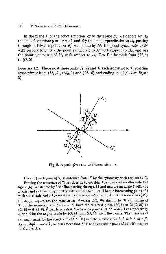
118 P. Sou~res and J.-D. Boissonnat
In the plane P of the robot 's motion, or in the plane P0, we denote by A0 the line of equation: y = - x cot ~ and A~ the line perpendicular to Ao passing through 0. Given a point (M,0), we denote by M1 the point symmetric to M with respect to O, M2 the point symmetric to M with respect to A0, and M3 the point symmetric of M1 with respect to Ao. Let T a be path from (M, 0) to (o, 0).
L e m m a 12. There exist three paths ~ , T2 and T3 each isometric to T, starting respectively from (M1,0), (M2, 0) and (M3,0) and ending at (O,0) (see figure 5).
A o
M2
Fig. 5. A path gives rise to 3 isometric ones.
Proofi (see Figure 5) 7~ is obtained from T by the symmetry with respect to O. Proving the existence of T2 requires us to consider the construction illustrated at
figure (6): We denote by 5 the line passing through M and making an angle 8 with the x-axis, and s the axial symmetry with respect to g. Let A be the intersecting point of with the x-axis and r the rotation by the angle - 8 around A. Let us note L = r(M).
Finally, t, represents the translation of vector LO. We denoteby 7~ the image of T by the isometry .~ = t o r o s. 7~ links the directed point (M, 8) = -~((O, 0)) to (O, 0) = .~(M, 8). 0 clearly equals 0. We have to prove that M = M2. Let respectively
and/~ be the angles made by (O,M) and (O,/~/) with the x-axis. The measure of
the angle made by the bisector of (M, O, ]vl) and the x-axis is: (1+ ~ = ~ = ~2 --A. As tan ~-~ = - cot ~, we can assert that ~/ is the symmetric point of M with respect to Ale, i.e. M2.
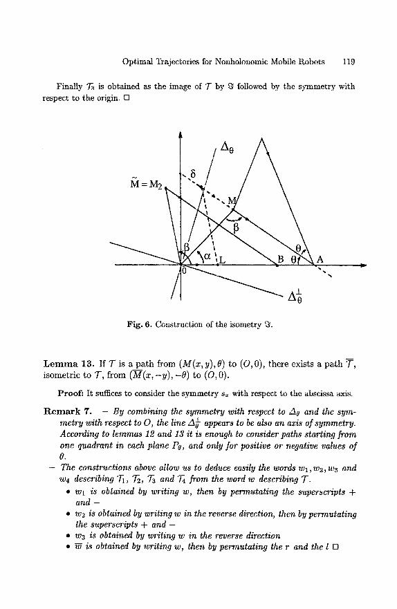
Optimal Trajectories for Nonholonomic Mobile Robots 119
Finally 73 is obtained as the image of 7" by ~ followed by the symmetry with respect to the origin. [:]
M=M2
Fig. 6. Construction of the isometry ~.
L e m m a 13. If T is a pa th from (M(x,y),O) to (O,0), there exists a pa th T , isometric to T , from ( M ( x , - y ) , - 8 ) to (0 , 0).
Proof : It suffices to consider the symmetry s~ with respect to the abscissa axis.
R e m a r k 7. - By combining the symmetry with respect to Ao and the sym- metry with respect to O, the line A~ appears to be also an axis of symmetry. According to lemmas 12 and 13 it is enough to consider paths starting from one quadrant in each plane Po, and only for positive or negative values of O.
- The constructions above allow us to deduce easily the words wl, w2, w3 and w4 describing ~ , 7-2, 7-3 and 7-4 from the word w describing T.
• wl is obtained by writing w, then by permutating the superscripts + and -
• w2 is obtained by writing w in the reverse direction, then by permutating the superscripts + and -
• w3 is obtained by writing w in the reverse direction • ~ is obtained by writing w, then by permutating the r and the t []
120 P. Sou~res and J.-D. Boissonnat
As a consequence of both lemmas above a last symmetry property holds in the case that 0 -- q-zr:
L e m m a 14. If 7" is a path from (M(x, y), ~r) (resp. (M(x, y), -Tr)) to (0 , 0), there exists an isometric path T ~ from (M(x, y) , -~r) (resp. (M(x, y), lr) ) to (o, 0).
The word w ~ describing 7 "1 is obtained by writing w in the opposite direction, then by permutating on the one hand the r and the l, and on the other hand the + and - .
R e m a r k 8. The points (M(x,y),Tr) and (M(x,y),-Tr) represent the same configuration in R 2 x S 1 but are different in R 3. This means that the tra- jectories 7" and T I are isometric and have the same initial and final points, but along these trajectories the car's orientation varies with opposite direction.
P r o o f of l emma 14: We use the notation of lemma 12 and 13. Let (M(x,y),1r) be a directed point and T a trajectory from (M, zr) to (0, 0). When 0 = :klr the axis Ao is aligned with the x-axis. By lemma 12, there exists a trajectory 7~ = ~(T), isometric to T, starting at (M2(x,-y),rc) and ending at (O,0). Then by lemma 12 there exists a trajectory ~ -- sx (7~), isometric to T2, starting at ("~2(x, y),-Tr) and ending at (O, 0). Let us call T' the trajectory ~ , then T' = s, o .~(T) is isometric to T and by combining the rules defining the words w2 and ~ we obtain the rule characterizing ~-~ = w r (the same reasoning holds when 0 = -zr.) D
Now by using lemma 14 we are going to prove that it suffice to consider paths starting from points (x, y, 0) when 0 E [-lr , ~r]. In the family (22) three types of path may start with an initial orientation 0 that does not belong to [-~r, ~r]. These types are (I) and (VII) &~ (VIII). Combining lemma 14 with the necessary condition given by PMP we are going to refine the sufficient family (22) by rejecting those paths along which the total angular variation is greater than ~.
L e m m a 15. In the family (22), types (I), (VII) and (VIII) may be refined as
follows:
(I) l+lbl+ or r+rb r+ O < a + b + e < ~ r
(VII) (VIII) { 0 < a < ~ , 0 < b < 9 , 0 < d CalC~SdCb or CbSdC~ICa and a+b<_ ~ if u2 is constant
on every arc C
Proof: Our method is as follows:
1. We consider a path T linking a point (M, 0) to the origin, such that Igl > ~r.
Optimal Trajectories for Nonholonomic Mobile Robots 121
2. We select a part of T located between two configurations (M1,01) and (M2, 02) such that [01-021 = ~r. According to lemma 14 we replace this part by an isometric one, along which the point's orientation rotates in the opposite direction. In this way we construct a trajectory equivalent to 7" i.e having the same length and linking (M, 0) to the origin.
3. We prove that this new trajectory does not verify the necessary conditions given by PMP. As 7" is equivalent to this non optimal path we deduce that it is not optimal.
Let us consider first a type (I) path. Due to the symmetry properties it suffices to regard a path l+l~l + with a + b + e = ~r + e, (e > 0) and a > e. If we keep in place a piece of length e and replace the final part using lemma 14, we obtain an equivalent path l+r[r+r~_~ which is obviously not optimal because the robot goes twice to the same configuration.
We use the same reasoning to show that a path C~IC~Sd with d # 0 cannot be optimal if a > ~. Without lost of generality we consider a path l + +l~_ s d . According
to lemma 14 we can replace the initial piece l + . l~ by the isometric one r+ r~+ .
The initial path is then equivalent to the path r+_~r~+J[s - which cannot be optimal
as the point of inflection do not belong to the line supporting the line segment. Consider now a path C~]C~SdCb or CbSdC~IC~ with u2 constant on the arcs.
We show that such a path cannot be optimal if a+b > ~. Consider a path l+l~_Sdlb 2
with a + b = ~ + e and a > e. We keep in place a piece of length e and replace the final part by an isometric one according to lemma 14. We obtain an equivalent path l+r+bS+dl+ra_ ~. As the point of inflection does not lie on the line D0, this path
2
violates both necessary conditions A and B of PMP (see lemma 11) and therefore is not optimal. [3
R e m a r k 9. In the sufficient family (22) refined by lemma 15, the orientation of initial points is defined in [-~r, 7r]. So, to solve the shortest path problem in R 2 x S 1, we only have to consider paths starting from R 2 x [ - ~ , 7r] in R 3.
C o n s t r u c t i o n o f d o m a i n s For each type of pa th in the new sufficient family, we want to compute the domains of all possible s tar t ing points for paths ending at the origin. According to the symmet ry properties it suffices to consider paths s tar t ing from one of the four quadrants made by A0 and A~, in each plane Po, and only for positive or negative values of 0. We have chosen to construct domains covering the first quadrant (i.e. x tan 2°- < y ~ - x cot ~), for e e o].
As any pa th in the sufficient family is described by three parameters , each domain is the image of the product of three real intervals by a continuous mapping. I t follows tha t such domains are connected in the configuration space.
To represent the domains, we compute their restriction to planes Po. As 0 is fixed, the cross section of the domain in Po is defined by two parameters . By
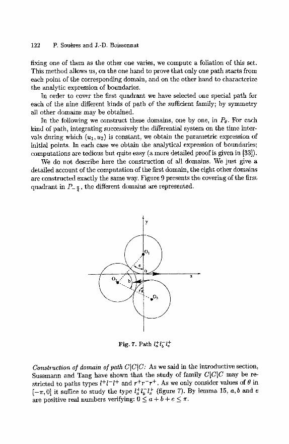
122 P. Sou~res and J.-D. Boissonnat
fixing one of them as the other one varies, we compute a foliation of this set. This method allows us, on the one hand to prove that only one path starts from each point of the corresponding domain, and on the other hand to characterize the analytic expression of boundaries.
In order to cover the first quadrant we have selected one special path for each of the nine different kinds of path of the sufficient family; by symmetry all other domains may be obtained.
In the following we construct these domains, one by one, in Pe. For each kind of path, integrating successively the differential system on the time inter- vals during which (ul, u2) is constant, we obtain the parametric expression of initial points. In each case we obtain the analytical expression of boundaries; computations are tedious but quite easy (a more detailed proof is given in [33]).
We do not describe here the construction of all domains. We just give a detailed account of the computation of the first domain, the eight other domains are constructed exactly the same way. Figure 9 presents the covering of the first quadrant in P_ ~, the different domains are represented.
, /
~y
r X
F i g . 7 . P a t h + - +
Construction of domain of path CICIC: As we said in the introductive section, Sussmann and Tang have shown that the study of family CICIC may be re- stricted to paths types l+l-l + and r+r-r +. As we only consider values of 8 in [-7r, 0] it suffice to study the type l+l[l + (figure 7). By lemma 15, a, b and e are positive real numbers verifying: 0 < a + b + e < r.

Optimal Trajectories for Nonholonomic Mobile Robots 123
Along this trajectories the control (ul,u2) takes successively the values ( + 1 , + 1 ) , ( - 1 , + 1 ) and (+1,+1) . By integrating the system (4) for each of these successive constant values of ul and u2, from the initial configuration (x, y, 8) to the final configuration (0, 0, 0) we get:
[ i-sinS + 2sin(b +e) -2sine - cos 8 + 2 cos(b + e) - 2 cos e + 1 - a - b - e
(23)
Let us now consider that the value of 8 is fixed. The arclength parameter e varies in [0,-8]; given a value of e, b varies in [ 0 , - 8 - e]. When e is fixed as b varies, the initial point traces an arc of the circle ~e of radius 2 centered at Pe (sin 8 + 2 sin e, - cos 8 - 2 cos e + 1)
One end point of this arc is the point E ( s i n S , - c o s 8 + 1) (when b = 0), depending on the value of e the other end point (corresponding to b = - 8 - e) describes an arc of circle of radius 2 centered at the point H ( - sin 8, cos 8 + 1) and delimited by the point E (when e = -8 ) and its symmetric F with respect to the origin O (when e = 0).
For different values of e the arcs of ~e make a foliation of the domain; this ensures the existence of a unique trajectory of this type starting form every point of the domain. Figure (8) represents this construction for two different values of 8. The cross section of this domain appears at figure (9) with the eight other domains making the covering of the first quadrant in P_ ~.
- As this domain is symmetric about the two axes A0 and A~, it follows from lemma 12 that the domain of path 1-1+l - is exactly the same one. This point corroborates the result by Sussmann and Tang which states that the search for an optimal path of the family CICIC (when 8 < 0) may be limited to one of these two path types.
- When 8 = -~r the domain is the disc of radius 2 centered at the origin.
Following the same method the eight other domains are easily computed (see [33]), they are represented at figure 9 in the plane P_~. The domain's boundaries are piecewise smooth curves of simple sort: arcs of circle, line seg- ments, arcs of conchoids of circle or arcs of cardioids.
Ana l y s i s o f the cons truct ion As we know exactly the equations of the piecewise smooth boundary curves, we can precisely describe the domains in each plane P0. This construction insures the complete covering of the first quadrant, and by symmetry the covering of the whole plane. All types in the
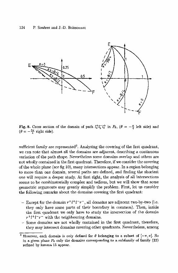
124 P. Sou~res and J.-D. Boissonnat
E e=O 0.25
0~5
I ¢ , ,
, , j \
x
\ \
Fig. 8. Cross section of the domain of path l+l[l + in 1:>o, (0 = - ~ left side) and (0 = - ~ right side).
sufficient family are represented 3. Analysing the covering of the first quadrant, we can note that almost all the domains are adjacent, describing a continuous variation of the path shape. Nevertheless some domains overlap and others are not wholly contained in the first quadrant. Therefore, if we consider the covering of the whole plane (see fig 10), many intersections appear. In a region belonging to more than one domain, several paths are defined, and finding the shortest one will require a deeper study. At first sight, the analysis of all intersections seems to be combinatorially complex and tedious, but we will show that some geometric arguments may greatly simplify the problem. First, let us consider the following remarks about the domains covering the first quadrant:
- Except for the domain r + l + l - r - , all domains are adjacent two-by-two (i.e. they only have some parts of their boundary in common). Then, inside the first quadrant we only have to study the intersection of the domain r + l + l - r - with the neighbouring domains.
- Some domains are not wholly contained in the first quadrant, therefore, they may intersect domains covering other quadrants. Nevertheless, among
3 However, each domain is only defined for 0 belonging to a subset of [-~r, r]. So in a given plane Pe only the domains corresponding to a subfamily of family (22) refined by lemma 15 appear.
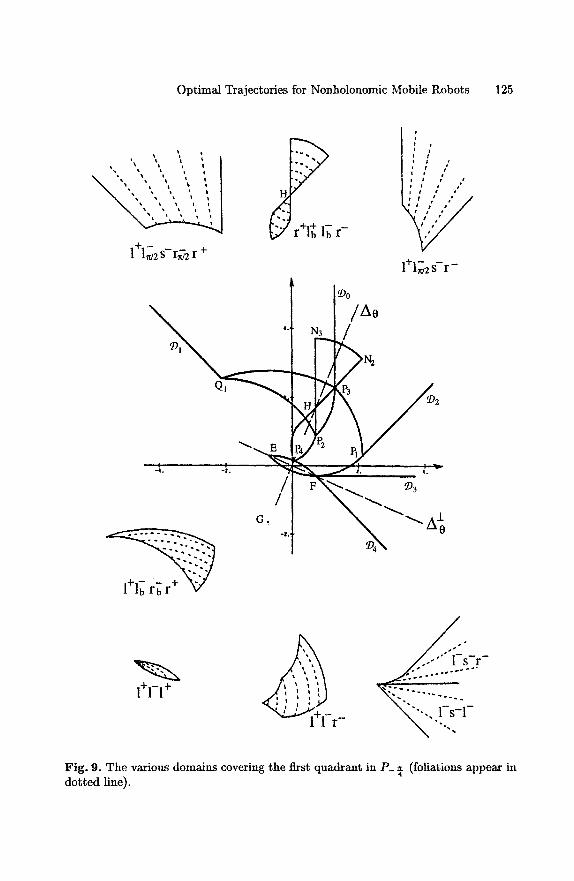
Optimal Trajectories for Nonholonomic Mobile Robots 125
t
-]- _ _
] lrv2S r~2r +
r+l lb r-
i
e I e •
i I t I
I i •
l+l~v2 s - r -
E t e2 . i p ~ . ' , . r
l+l-1 +
Fig. 9. The various domains covering the first quadrant in P_ ~ (foliations appear in dotted line).
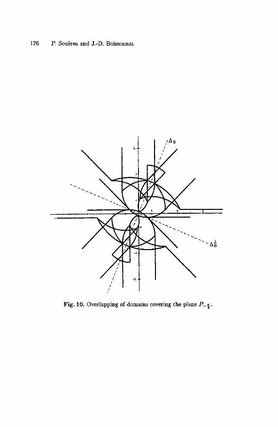
126 P. Sou~res and J.-D. Boissonnat
I /AO I
t I
I
Fig. 10. Overlapping of domains covering the plane P_ ~_. 4
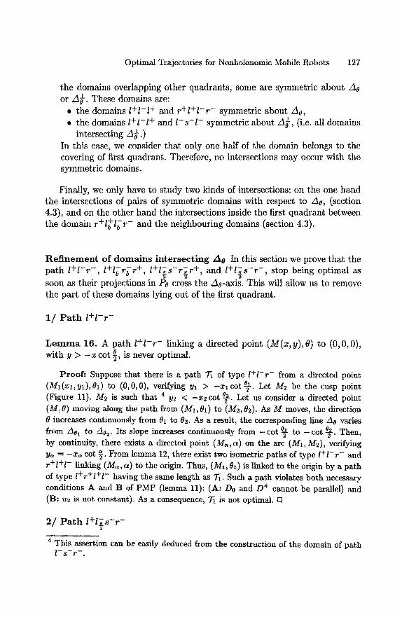
Optimal Trajectories for Nonholonomic Mobile Robots 127
the domains overlapping other quadrants, some are symmetric about A0 or A~-. These domains are:
* the domains l + l - l + and r + l + l - r - symmetric about Ao, , the domains l + l - l + and 1 - s - l - symmetric about A~, (i.e. all domains
intersecting A~-.) In this case, we consider that only one half of the domain belongs to the covering of first quadrant. Therefore, no intersections may occur with the symmetric domains.
Finally, we only have to study two kinds of intersections: on the one hand the intersections of pairs of symmetric domains with respect to A0, (section 4.3), and on the other hand the intersections inside the first quadrant between the domain r+l+bl~r - and the neighbouring domains (section 4.3).
R e f i n e m e n t o f d o m a i n s i n t e r s ec t i ng Ao In this section we prove that the path l + l - r - , l + I b r b r + , l + l ~ s - r ~ r +, and l + l T s r stop being optimal as soon as their projections in Pe cross the Ae-axis. This will allow us to remove the part of these domains lying out of the first quadrant.
1 / P a t h l+ l - r -
L e m m a 16. A path l + l - r - linking a directed point (M(x, y), 0) to (0, 0, 0), with y > - x cot ~, is never optimal.
Proof: Suppose that there is a path 7~ of type l + l - r - from a directed point ( M 1 ( x l , y l ) , 8 1 ) to (0,0,0), verifying yl > - x l c o t ~ . Let /1//2 be the cusp point (Figure 11). M2 is such that 4 ys < -x2cot ~ . Let us consider a directed point (M,0) moving along the path from (M1,81) to (Ms,02). As M moves, the direction 8 increases continuously from 01 to 0s. As a result, the corresponding line Ao varies from A01 to A0:. Its slope increases continuously from --cot ~ to --cot ~ . Then, by continuity, there exists a directed point (M~,a) on the arc (M1, Ms), verifying y~ = -x~ cot 8" From lemma 12, there exist two isometric paths of type l + l - r - and r+l+l - linking (M~,a) to the origin. Thus, (M1,81) is linked to the origin by a path of type l+r+l+l - having the same length as 7i. Such a path violates both necessary conditions A and B of PMP (lemma 11): (A: Do and D + cannot be parallel) and (B: us is not constant). As a consequence, 7~ is not optimal.
2 / P a t h l + l T s r
4 This assertion can be easily deduced from the construction of the domain of path l - s r .
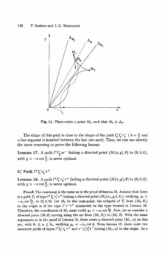
128 P. Sou~res and J.-D. Boissonnat
Y /Ae2 /,As A01
0 ".,', x
Fig. 11. There exists a point M~ such that M~ E Am.
The shape of this path is close to the shape of the pa th l+Ibr [ ( b = ~ and a line segment is inserted between the last two arcs). Then, we can use exactly the same reasoning to prove the following lemma:
L e m m a 17. A path I+lZsr - linking a directed point (M(x,y) ,O) to (0, 0,0), 2
with y > - x cot ~, is never optimal.
3 / P a t h l+lbrbr+
L e m m a 18. A path t+lbrbr+ linking a directed point (M(x, y), 8) to (0, 0, 0), with y > - x c o t ~, is never optimal.
Proof- The reasoning is the same as in the proof of lemma 16. Assume that there is a path 71 of type l+Ibrbr + linking a directed point (Ml(xl, yl), 81), verifying yl > - x l cot 9 , to (0,0,0). Let M2 be the cusp-point; the subpath of 7~ from (M2,01) to the origin is of the type l - r - r + symmetric to the type treated in Lemma 16. Therefore, the coordinates of M2 must verify y2 < -x2 cot s2~. Now, let us consider a directed point (M, 8) moving along the arc from (M1, 81) to (M2, 8). With the same arguments as in the proof of Lemma 16, there exists a directed point (Ma, a) on this arc, with 8t _<: a _< 82, verifying ya ---- - x ~ cot ~. From lemma 12, there exist two isometric paths of types l+l[rb r+ and r-r+l+l - linking (Ma, a) to the origin. As a
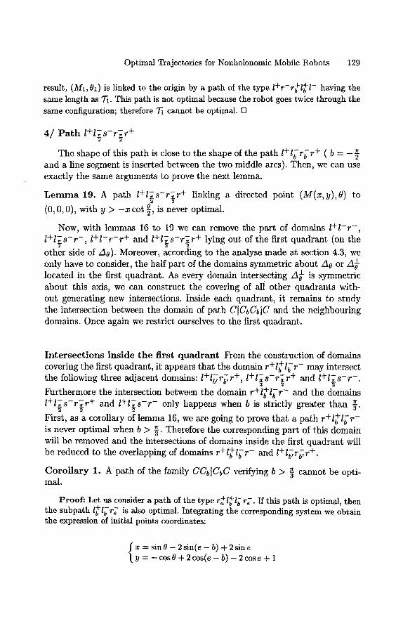
Optimal Trajectories for Nonholonomic Mobile Robots 129
result, (M1,01) is linked to the origin by a path of the type l+r-r+l+l - having the same length as 7]. This path is not optimal because the robot goes twice through the same configuration; therefore 7] cannot be optimal. []
4 / P a t h l+lT_s-rT_r + 2 2
The shape of this path is close to the shape of the path l+lbrbr+ ( b - " and a line segment is inserted between the two middle arcs). Then, we can use exactly the same arguments to prove the next lemma.
L e m m a 19. A path l + l T s - r T r + linking a directed point (M(x ,y ) ,O) to 2 2
(0,0,0), with y > - x c o t ~, is never optimal.
Now, with lemmas 16 to 19 we can remove the part of domains l+l -r - , l+tT_s-r - , t + l - r - r + and l + l T s - r T r + lying out of the first quadrant (on the
2 2 2
other side of A0). Moreover, according to the analyse made at section 4.3, we only have to consider, the half part of the domains symmetric about A9 or A~ located in the first quadrant. As every domain intersecting A~ is symmetric about this axis, we can construct the covering of all other quadrants with- out generating new intersections. Inside each quadrant, it remains to study the intersection between the domain of path CICbCb]C and the neighbouring domains. Once again we restrict ourselves to the first quadrant.
I n t e r s e c t i o n s i n s i d e t h e f i r s t q u a d r a n t From the construction of domains covering the first quadrant, it appears that the domain r+l+lb r - may intersect the following three adjacent domains:/+/~r~r +, l + l T s - r T r + and l+lTs r .
Furthermore the intersection between the domain r+l+lb r - and the domains l + l T s - r T r + and l+lTs r only happens when b is strictly greater than "
2 2 2
First, as a corollary of lemma 16, we are going to prove that a path r+l+l[r - is never optimal when b > ~. Therefore the corresponding part of this domain will be removed and the intersections of domains inside the first quadrant will be reduced to the overlapping of domains r+l+lb r - and l+l~,r~r +.
Corol lary 1. A path of the family CCb[CbC verifying b > ~ cannot be opti- mal.
Proof: Let us consider a path of the type r+l+lbr[. If this path is optimal, then the subpath l+Ibr~ is also optimal. Integrating the corresponding system we obtain the expression of initial points coordinates:
x = sin 0 - 2 s in(e - b) + 2 sin e y = - cos 0 + 2 cos(e - b) - 2 cos e + 1

130 P. Sou~res and J.-D. Boissonnat
with ~ = e - 2b (since the first two arcs of circles have the same length) and from lemma 16 the coordinates must verify y _< - c o t ~x. Replacing x and y by their parametric expression, we obtain after computation:
~T e 7r (since 0 < e < ~ ) [] s i n ~ ( 2 c o s b - 1 ) > 0 then b < ~
Therefore according to the previous construct ion we may remove the part, of the domain r+l+l[r - located beyond the point H with respect to O. (see figure 9).
Now, only one intersection remains inside the first quadrant , between the + - - + .
domains r+l+lbr[ and la, lb, rvre, , let us call Z this region. In order to deter- mine which pa ths are opt imal in this region, we compute in each plane Po the set of points t ha t may be linked to the origin by a pa th of each kind having the same length. Initial point of these two paths are respectively defined by the following paramet r ic systems:
( r+ l+l [ r : ) { Y = - s i n O + 2(2 cosb - 1) sin(e - b) cos0 - 2(2 cosb - 1)cos(e - b) + 1
+ _ _ + { x = s i n ~ - 4 s i n e t + 2 s i n ( e ~ + b l) (2a) (la'lb'rb're') y = -- COS~ + 4COSd -- 2 cos(e I + b r) - 1
the length of these paths are respectively:
L = a + 2 b ÷ e = 4 b + 6 with ~ = e - 2 b + a (25) L t = e I + 2b I + a t = 2(b t + e I ) - 8 with 8 = e I - d
The required condit ion L = L ~ implies t ha t ~ + 2 b - b r - e t = 0. By replacing e I + b ~ by ~ + 2b in the second system, then writ ing tha t b o t h systems are
equivalent we obtain:
siu(e - b)(1 - 2 cos b) + s i n O - 2 s i n e r + sin(~ + 2b) = 0 cos(e - b)(1 2 cos b) + cos ~ - 2 cos e r +cos(O + 2b) + 1 = 0
we eliminate the parameter d writing tha t sin 2 (d) + cos 2 (d ) = 1; then after computa t ion , we obtain the following relation between e and b:
4cos 2 b - 2cosb ÷ (1 - 2 cos b)(2 cos(e - 2b - 8) cosb
+ cos(e - b)) + cos ~ + cos(~ + 2b) - 1 = 0 (26)
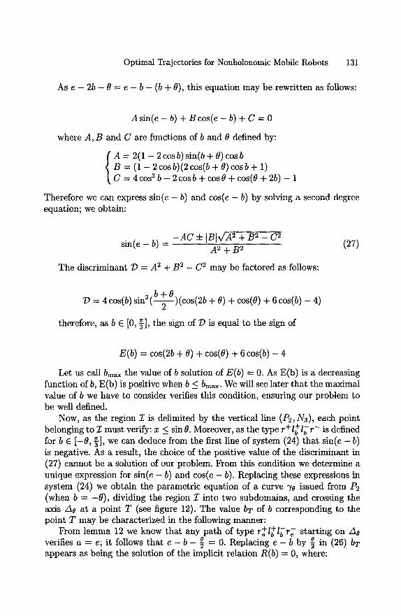
Optimal Trajectories for Nonholonomic Mobile Robots 131
As e - 25 - 0 = e - b - (b + 0), this equation may be rewritten as follows:
A sin(e - b) + B cos(e - b) + C = 0
where A, B and C are functions of b and 0 defined by:
A = 2(1 - 2 cos b) sin(b + 8) cos b B -- (1 - 2 cos 5)(2 cos(b + 0) cos b ÷ 1) C = 4 cos 2 b - 2 cos b + cos 0 + cos(~ + 2b) - 1
Therefore we can express sin(e - b) and cos(e - b) by solving a second degree equation; we obtain:
- A C d: tBI~/A2 + B 2 - C 2 sin(e - b) = A2 + B2
The discriminant D = A 2 ÷ B 2 - C 2 may be factored as follows:
(27)
7) = 4 cos(b) s i n 2 ( : - ~ ) ( c o s ( 2 b + 0) + cos(0) ÷ 6 cos(b) - 4)
therefore, as b E [0, ~], the sign of 7) is equal to the sign of
E(b) = cos(2b + 0) + cos(0) + 6 cos(b) - 4
Let us call bmax the value of b solution of E(b) = O. As E(b) is a decreasing function of b, E(b) is positive when b < bmax. We will see later that the maximal value of b we have to consider verifies this condition, ensuring our problem to be well defined.
Now, as the region 1: is delimited by the vertical line (P2, N3), each point belonging to 2: must verify: x < sin 0. Moreover, as the type r+l+Ib r - is defined for b E [ -0 , §], we can deduce from the first line of system (24) that sin(e - b) is negative. As a result, the choice of the positive value of the discriminant in (27) cannot be a solution of our problem. From this condition we determine a unique expression for sin(e - b) and cos(e - b). Replacing these expressions in system (24) we obtain the parametric equation of a curve ~/0 issued from P2 (when b = - 0 ) , dividing the region Z into two subdomains, and crossing the axis A0 at a point T (see figure 12). The value bT of b corresponding to the point T may be characterized in the following manner:
From lemma 12 we know that any path of type r+l + I - ~ - starting on A0 a b ~b " e verifies a ---- e; it follows that e - b - ~ = 0. Replacing e - b by ~ in (26) bT appears as being the solution of the implicit relation R(b) = 0, where:
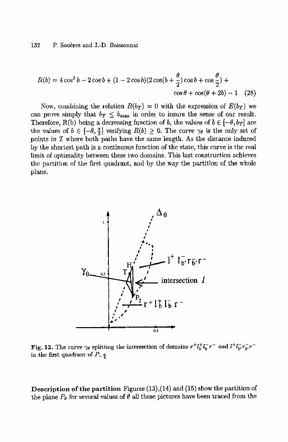
132 P. Sou~res and J.-D. Boissonnat
0 0 R(b) = 4 cos 2 b - 2 cos b + (1 - 2 cos b)(2 cos(b + 5) cos b + cos 5) +
cos0 + cos(0 + 2b) - 1 (28)
Now, combining the relation R(bT) = 0 with the expression of E(bT) we can prove simply that bT <bmax in order to insure the sense of our result. Therefore, R(b) being a decreasing function of b, the values of b e [-8, bT] are the values of b e [-8, ~] verifying R(b) >_ O. The curve 7a is the only set of points in I where both paths have the same length. As the distance induced by the shortest path is a continuous function of the state, this curve is the real limit of optimality between these two domains. This last construction achieves the partition of the first quadrant, and by the way the partition of the whole plane.
A 0
Q #
/
I f
/ l 1 + 1-~-~- HI' ~ 1 lb,~tb,l
~ T ~ intersection I
/ ,,=/ ~r÷l; lgr -
t I
Fig. 12. The curve 7a splitting the intersection of domains r+l+i[r - and l+l~,r~,r - in the first quadrant of P_
Descr ipt ion of the par t i t ion Figures (13),(14) and (15) show the partition of the plane P0 for several values of 0 all these pictures have been traced from the
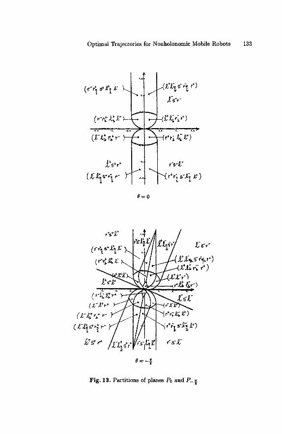
Optimal Trajectories for Nonholonomic Mobile Robots 133
4.IJ (~-,~ : .q J.- ).
4 4 - ~
r~,, + 1_ I ,-,'~. ( ~ , ' , , , - , ~ r'7.,, t " -~ . , . ; , ~ . . ~ , )
0 = 0
+ , ' <J :~ l : l / i z , t , ~ , - I .
- ~ " " -.Z-d..'T~L---~ J.'Jx ,.: ,-+ ) , ~ x . 71"7;/'"F,,/Az+x.',-'l
, ~ . . . . %~_~K ~ 2 r >
(.~-x~,,,:,.-yf t-A ~,+;:,--Qi,~')
~'s+t • L,,_++~,Jz;.~ ~-;z l .¢ ,x ,~s r " " - I i . -
$
Fig. 13. Partitions of planes Po and P_
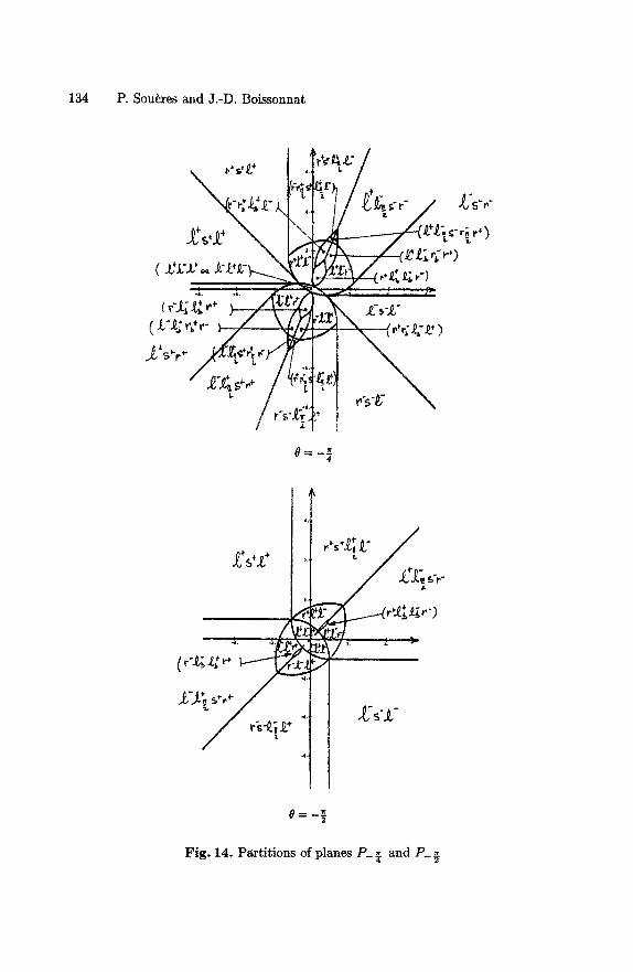
134 P. Sou~res and J.-D. Boissonnat
\ ~ ' ~ ' I " t /
~,,j, \ I ~4~----~r~i<-,t,'> • ~ L<i.,q,tf'././-k----/--~ ~: £; ¢ ' - ' )
( x,'J: J,~:,,- J,'z+~,-~,._ xl** VY;I'zA _ / , , , ~ . ,+ , . ~, ,.;.,
NZ,2+.~.'r",#/ t 1 \
4
. . . . . . i /
1'~k~+'// ... Z ' s ' ± -
4 .
Fig. 14. Partitions of planes P_ ~-4 a n d P _
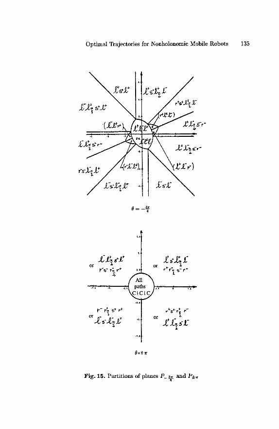
Optimal Trajectories for Nonholonomic Mobile Robots 135
S'r"
3~r n . = - -
4
0 " 0 + ¢ ~ /)4"
p -S " 1'~ r +
A . ,h .l. .I.,
*I.
or . ~" 1" .Z~I~ ~ '
Of ¢ ~ r ~ S - r -
",. +
r+~;+- r; ,-- 01' ~*
1 + £ + ~ z
0=-+~
Fig. 15. Partitions of planes P_ m and P ~ 4
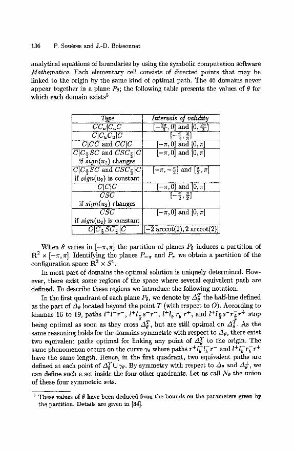
136 P. Sou~res and J.-D. Boissonnat
analytical equations of boundaries by using the symbolic computation software Mathematica. Each elementary cell consists of directed points that may be linked to the origin by the same kind of optimal path. The 46 domains never appear together in a plane Po; the following table presents the values of 0 for which each domain exists 5
Type cc,,IC,,C ctc.c. lc
Intervals o] validity [-~--~ 0] and 'z~ , [O,,,T]
and P , d
CtC~SC and CSC~ tC if sign(u2) is constant
CiCC and CCiC CIC]SC and CSC~IC [-~r,0] and [0,r]
if sign(u2) changes 71" [-~r,-~] and [y, ]
ClClC CSC
if sign(u2 ) changes
' o] and [0 , . ]
CSC [-~r, 0] and [0, ~r] if sign(u2) is constant
CIC ~ SC~ IV [-2 arccot(2), 2 arccot(2)]
When 0 varies in [-Tr, ~] the partition of planes P0 induces a partition of R 2 x [ - r , ~r]. Identifying the planes P_~ and P , we obtain a partition of the configuration space R 2 x S 1.
In most part of domains the optimal solution is uniquely determined. How- ever, there exist some regions of the space where several equivalent path are defined. To describe these regions we introduce the following notation.
In the first quadrant of each plane P0, we denote by A T the half-line defined as the part of A0 located beyond the point T (with respect to O). According to lemmas 16 to 19, paths l+l-r -, l+lTs-r -, t+l-~rbr +, and l+l~s-rTr + stop
being optimal as soon as they cross AT, but are still optimal on A T. As the same reasoning holds for the domains symmetric with respect to Ao, there exist two equivalent paths optimal for linking any point of A T to the origin. The same phenomenon occurs on the curve T0 where paths r+l+blb r- and l+l~rb r+ have the same length. Hence, in the first quadrant, two equivalent paths are defined at each point of A T U 70. By symmetry with respect to A0 and A~, we can define such a set inside the four other quadrants. Let us call No the union of these four symmetric sets.
5 These values of 0 have been deduced from the bounds on the parameters given by the partition. Details are given in [34].
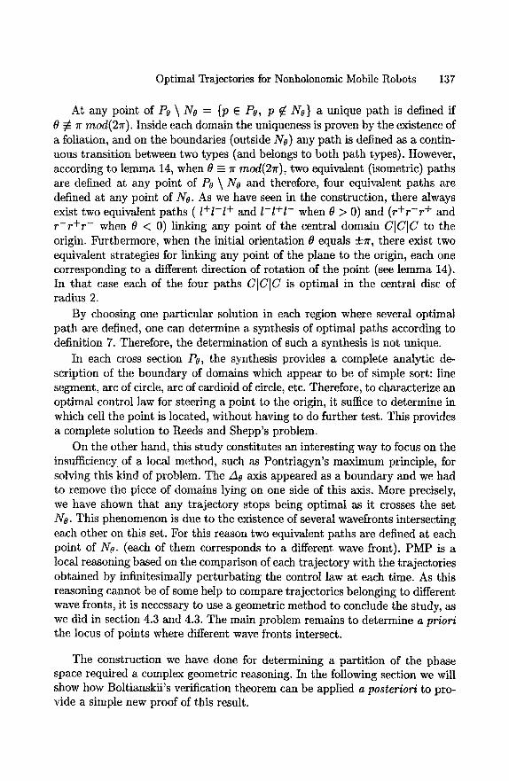
Optimal Trajectories for Nonholonomic Mobile Robots 137
At any point of Po \ No = {p E Po, P ~. No} a unique path is defined if 0 ~ zc mod(2zc). Inside each domain the uniqueness is proven by the existence of a foliation, and on the boundaries (outside No) any path is defined as a contin- uous transition between two types (and belongs to both path types). However, according to lemma 14, when ~ - 7r mod(21r), two equivalent (isometric) paths are defined at any point of Po \ No and therefore, four equivalent paths are defined at any point of No. As we have seen in the construction, there always exist two equivalent paths ( l+l-l + and l-l+l - when 0 > 0) and ( r + r - r + and r - r + r - when 0 < 0) linking any point of the central domain C[C[C to the origin. Furthermore, when the initial orientation 9 equals +r , there exist two equivalent strategies for linking any point of the plane to the origin, each one corresponding to a different direction of rotation of the point (see lemma 14). In that case each of the four paths CICIC is optimal in the central disc of radius 2.
By choosing one particular solution in each region where several optimal path are defined, one can determine a synthesis of optimal paths according to definition 7. Therefore, the determination of such a synthesis is not unique.
In each cross section Po, the synthesis provides a complete analytic de- scription of the boundary of domains which appear to be of simple sort: line segment, arc of circle, arc of cardioid of circle, etc. Therefore, to characterize an optimal control law for steering a point to the origin, it suffice to determine in which cell the point is located, without having to do further test. This provides a complete solution to Reeds and Shepp's problem.
On the other hand, this study constitutes an interesting way to focus on the insufficiency of a local method, such as Pontriagyn's maximum principle, for solving this kind of problem. The A0 axis appeared as a boundary and we had to remove the piece of domains lying on one side of this axis. More precisely, we have shown that any trajectory stops being optimal as it crosses the set No. This phenomenon is due to the existence of several wavefronts intersecting each other on this set. For this reason two equivalent paths are defined at each point of No. (each of them corresponds to a different wave front). PMP is a local reasoning based on the comparison of each trajectory with the trajectories obtained by infinitesimally perturbating the control law at each time. As this reasoning cannot be of some help to compare trajectories belonging to different wave fronts, it is necessary to use a geometric method to conclude the study, as we did in section 4.3 and 4.3. The main problem remains to determine a priori the locus of points where different wave fronts intersect.
The construction we have done for determining a partition of the phase space required a complex geometric reasoning. In the following section we will show how Boltianskii's verification theorem can be applied a posteriori to pro- vide a simple new proof of this result.
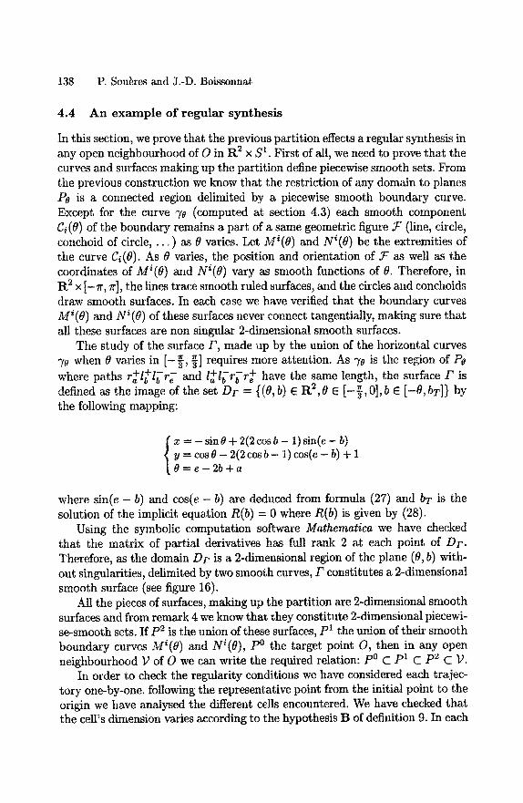
138 P. Sou~res and J.-D. Boissonnat
4.4 A n e x a m p l e o f r egu la r syn thes i s
In this section, we prove that the previous partition effects a regular synthesis in any open neighbourhood of O in R 2 × S 1. First of all, we need to prove that the curves and surfaces making up the partition define piecewise smooth sets. From the previous construction we know that the restriction of any domain to planes Po is a connected region delimited by a piecewise smooth boundary curve. Except for the curve T0 (computed at section 4.3) each smooth component Ci(0) of the boundary remains a part of a same geometric figure Y (line, circle, conchoid of circle, . . . ) as 0 varies. Let Mi(0) and Ni(0) be the extremities of the curve C~(0). As 0 varies, the position and orientation of Y" as well as the coordinates of M~(0) and Ni(8) vary as smooth functions of 0. Therefore, in R 2 × [-Tr, ~r], the lines trace smooth ruled surfaces, and the circles and conchoids draw smooth surfaces. In each case we have verified that the boundary curves Mi(0) and Ni(0) of these surfaces never connect tangentially, making sure that all these surfaces are non singular 2-dimensional smooth surfaces.
The study of the surface T', made up by the union of the horizontal curves "~0 when 0 varies in [ - ~ , -~] requires more attention. As ?'0 is the region of P0 where paths r+l+'-a "b ~b re- and l+lbrbr+ have the same length, the surface/" is defined as the image of the set D r = {(0,b) e R2,0 E [ -~ ,0 ] ,b E [-O, bT]} by the following mapping:
x ---- - sin 0 + 2(2 cos b - 1) sin(e - b) y = cos0 - 2(2 cosb - 1) cos(e - b) 4- 1 O--e-2b+a
where sin(e - b) and cos(e - b) are deduced from formula (27) and bT is the solution of the implicit equation R(b) = 0 where R(b) is given by (28).
U s i n g the symbolic computation software Mathematica we have checked that the matrix of partial derivatives has full rank 2 at each point of D r . Therefore, as the domain D r is a 2-dimensional region of the plane (8, b) with- out singularities, delimited by two smooth curves, F constitutes a 2-dimensional smooth surface (see figure 16).
All the pieces of surfaces, making up the partition are 2-dimensional smooth surfaces and from remark 4 we know that they constitute 2-dimensional piecewi- se-smooth sets. If p2 is the union of these surfaces, p1 the union of their smooth boundary curves Mi(O) and Ni(0), po the target point O, then in any open neighbourhood 1) of O we can write the required relation: p0 C p1 C p2 C 1).
In order to check the regularity conditions we have considered each trajec- tory one-by-one, following the representative point from the initial point to the origin we have analysed the different cells encountered. We have checked that the cell's dimension varies according to the hypothesis B of definition 9. In each
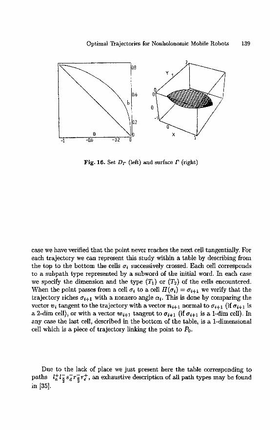
Optimal Trajectories for Nonholonomic Mobile Robots 139
0
.2 I 0
8 -i -0.6 -o12 o
Fig. 16. Set Dr (left) and surface/' (right)
case we have verified that the point never reaches the next cell tangentially. For each trajectory we can represent this study within a table by describing from the top to the bottom the cells ai successively crossed. Each cell corresponds to a subpath type represented by a subword of the initial word. In each case we specify the dimension and the type (T1) or (T2) of the cells encountered. When the point passes from a cell ai to a cell H(ai) = ai+l we verify that the trajectory riches ai+l with a nonzero angle ai. This is done by comparing the vector vi tangent to the trajectory with a vector ni+l normal to ai+l (if ai+l is a 2-dim cell), or with a vector wi+l tangent to ai+l (if ai+l is a 1-dim celt). In any case the last cell, described in the bottom of the table, is a 1-dimensional cell which is a piece of trajectory linking the point to Po.
Due to the lack of place we just present here the table corresponding to paths l+17 s-~rTr +, an exhaustive description of all path types may be found in [35].
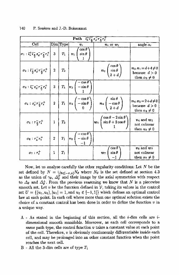
140 P. Sou~res and J.-D. Boissonnat
P a t h l+i~_s~r~re + 2 2 ................ ceil . . . . Dim Type v~ n~ or o~
/cosek 0"1 :l+al~Sdrire+ 3 T1 Vltsi~0 )
/cosek
t3+ / [-cose
1 /
/-cose k /r sin6 ,,4: ~,~r:_,¢ 2 T~ n,~ [ - c o s e /
2 \ 2 + d ]
/ cos8 - 2 sin ~ as : r~r+2 1 T 2 os tsinO+2cosO )
/ - c o s 6 ~
a7 : r + 1 T1
angle t~i
n2.vl = d + 4 ~ 0 because d ) 0
then c~2 ~ 0
n4.v3=2+d¢O because d :> 0
then a4 ~ 0
v4 and o5 not colinear then a5 ¢ 0
/cos e~ v~ and o7 oTtsin_/) not colinear
then (~7 ~ 0 ....
Now, let us analyse carefully the other regularity conditions: Let N be the set defined by N = tA0e[_~,~]Ne where No is the set defined at section 4.3 as the union of 7e, A T and their image by the axial symmetries with respect to A6 and A~. From the previous reasoning we know that N is a piecewise smooth set. Let v be the function defined in 1;, taking its values in the control set U = {(ul ,u2), lull = 1,and u2 E [ -1 , 1]} which defines an optimal control law at each point. In each cell where more than one optimal solution exists the choice of a constant control has been done in order to define the function v in a unique way.
A - As stated in the beginning of this section, all the /-dim cells are i- dimensional smooth manifolds. Moreover, as each cell corresponds to a same path type, the control function v takes a constant value at each point of the cell. Therefore, v is obviously continuously differentiable inside each cell, and may be prolonged into an other constant function when the point reaches the next cell.
B - All the 3-dim cells are of type TI
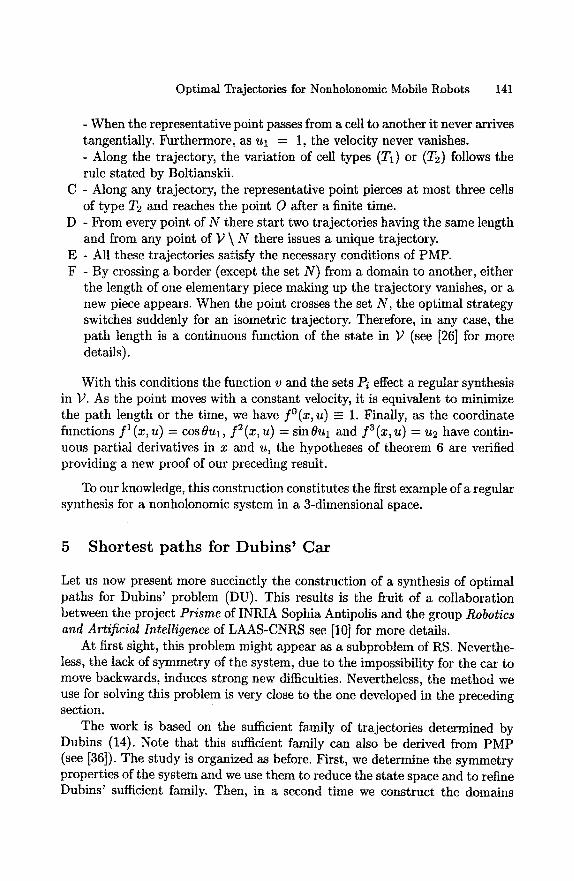
Optimal Trajectories for Nonholonomic Mobile Robots 141
- When the representative point passes from a cell to another it never arrives tangentially. Furthermore, as ul = 1, the velocity never vanishes. - Along the trajectory, the variation of cell types (T1) or (T2) follows the rule stated by Boltianskii.
C - Along any trajectory, the representative point pierces at most three cells of type T2 and reaches the point O after a finite time.
D - From every point of N there start two trajectories having the same length and from any point of ]) \ N there issues a unique trajectory.
E - All these trajectories satisfy the necessary conditions of PMP. F - By crossing a border (except the set N) from a domain to another, either
the length of one elementary piece making up the trajectory vanishes, or a new piece appears. When the point crosses the set N, the optimal strategy switches suddenly for an isometric trajectory. Therefore, in any case, the path length is a continuous function of the state in ]) (see [26] for more details).
With this conditions the function v and the sets Pi effect a regular synthesis in ];. As the point moves with a constant velocity, it is equivalent to minimize the path length or the time, we have f°(x,u) - 1. Finally, as the coordinate functions f l (x, u) = cos ~Ul, f2 (X, U) = sin 8Ul and f3 (x, u) = u2 have contin- uous partial derivatives in x and u, the hypotheses of theorem 6 are verified providing a new proof of our preceding result.
To our knowledge, this construction constitutes the first example of a regular synthesis for a nonholonomic system in a 3-dimensional space.
5 S h o r t e s t p a t h s f o r D u b i n s ' C a r
Let us now present more succinctly the construction of a synthesis of optimal paths for Dubins' problem (DU). This results is the fruit of a collaboration between the project Prisme of INRIA Sophia Antipolis and the group Robotics and Artificial Intelligence of LAAS-CNRS see [10] for more details.
At first sight, this problem might appear as a subproblem of RS. Neverthe- less, the lack of symmetry of the system, due to the impossibility for the car to move backwards, induces strong new difficulties. Nevertheless, the method we use for solving this problem is very close to the one developed in the preceding section.
The work is based on the sufficient family of trajectories determined by Dubins (14). Note that this sufficient family can also be derived from PMP (see [36]). The study is organized as before. First, we determine the symmetry properties of the system and we use them to reduce the state space and to refine Dubins' sufficient family. Then, in a second time we construct the domains
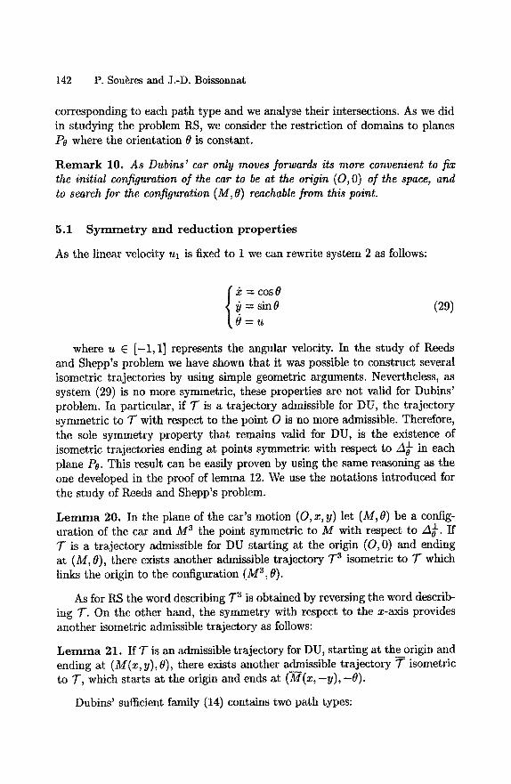
142 P. Sou~res and J.-D. Boissonnat
corresponding to each path type and we analyse their intersections. As we did in studying the problem RS, we consider the restriction of domains to planes P0 where the orientation O is constant.
R e m a r k 10. As Dubins' ear only moves forwards its more convenient to fix the initial configuration of the car to be at the origin (0, O) of the space, and to search for the configuration (M, 0) reachable from this point.
5.1 Symmetry and reduction properties
As the linear velocity Ul is fixed to 1 we can rewrite system 2 as follows:
{ 2 = cos 0 = sin 0
O = u (29)
where u E [-1,1] represents the angular velocity. In the study of Reeds and Shepp's problem we have shown that it was possible to construct several isometric trajectories by using simple geometric arguments. Nevertheless, as system (29) is no more symmetric, these properties are not valid for Dubins' problem. In particular, if T is a trajectory admissible for DU, the trajectory symmetric to T with respect to the point O is no more admissible. Therefore, the sole symmetry property that remains valid for DU, is the existence of isometric trajectories ending at points symmetric with respect to A0~ in each plane Pc. This result can be easily proven by using the same reasoning as the one developed in the proof of lemma 12. We use the notations introduced for the study of Reeds and Shepp's problem.
L e m m a 20. In the plane of the car's motion (O, x, y) let (M, 0) be a config- uration of the car and M 3 the point symmetric to M with respect to A~-. If T is a trajectory admissible for DU starting at the origin (O, 0) and ending at (M, 0), there exists another admissible trajectory 7 -a isometric to T which links the origin to the configuration (M a, 0).
As for RS the word describing T 3 is obtained by reversing the word describ- ing T. On the other hand, the symmetry with respect to the x-axis provides another isometric admissible trajectory as follows:
L e m m a 21. If T is an admissible trajectory for DU, starting at the origin and ending at (M(x, y), 0), there exists another admissible trajectory T isometric to T, which starts at the origin and ends at ( M ( x , - y ) , - 0 ) .
Dubins' sufficient family (14) contains two path types:
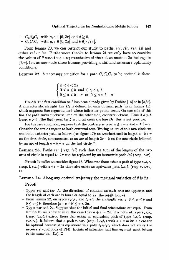
Optimal Trajectories for Nonholonomic Mobile Robots 143
- CaSdCe wi th a, e G [0, 2~r[ and d > 0, - CaCbCe wi th a, e e [0, 2~r[ and b el~r, 2~r[.
F r o m l e m m a 20, we can res t r i c t our s t u d y to pa ths : lrl, rlr, rsr, 1st a n d e i ther rsl or Isr. F u r t h e r m o r e t h a n k s to l e m m a 21 we only have to consider t he values of 0 such t h a t a r ep resen ta t ive of the i r class modu lo 2~r belongs to [0, 7r]. Le t us now s t a t e t h r ee l emmas p rov id ing add i t i ona l necessary o p t i m a l i t y condi t ions .
L e m m a 22. A necessary condi t ion for a p a t h CaCbCe to be o p t i m a l is t ha t :
{ Tr < b < 2~r
0 < a < b and 0 < e < b O ~ a < b - T r or O ~ e < b - T r
P r o o f : The first condition on b has been already given by Dubins [16] or in [2,36]. A characteristic straight line Do is defined for each optimal pa th (as in lemma 11), which supports line segments and where inflection points occur. On one side of this line the path turns clockwise, and on the other side, counterclockwise. Thus if a > b (resp. e > b), the first (resp. last) arc must cross the line Do; this is not possible.
For the last condition, suppose tha t the contrary is true: a :> b - ~r and e > b - ~r. Consider the circle tangent to both extremal arcs. Tracing an arc of this new circle we can build a shorter pa th as follows (see figure 17): an arc shortened to length a - b + Ir
on the first circle, concatenated to an arc of length 2~r - b on the new circle followed by an arc of length e - b -t- ~r on the last circle.[]
L e m m a 23. P a t h s r s r (resp. lsl) such t h a t the sum of the l eng th of t he two arcs of circle is equal to 2Ir can be rep laced by an i somet r ic p a t h lsl (resp. r s r ) .
P r o o f : I t suffice to consider figure 18. Whenever there exists a pa th of type rasdre (resp. laSdl~) with a+e = 2 r there also exists an equivalent path lesdl~ (resp. r~sdra) []
L e m m a 24. Along any op t ima l t r a j e c t o r y the m a x i m a l var ia t ion of 0 is 2 r .
P r o o f :
- Types rsl and lsr: As the directions of rotat ion on each arcs are opposite and the length of each arc is lower or equal to 21r, the result follows.
- From lemma 22, on types r~Ibr~ and larbl~ the arclength verify: 0 < a < b and 0 < e < b. therefore la - e + b I < v < 2m
- Types rsr and lsl: Suppose that the initial and final orientations axe equal. From lemma 23 we know that in the case that a + e --- 2~r, if a path of type r~s~re (resp. l~sdl¢) exists, there also exists an equivalent pa th of type I~sdl~ (resp. reSdra). I t follows tha t a pa th ras~r~ (resp. lasdl~) with a + e ---- 21r + e cannot be optimal because it is equivalent to a path lesdlar~ which does not verify the necessary conditions of PMP (points of inflection and line segment must belong to the same line Do). []
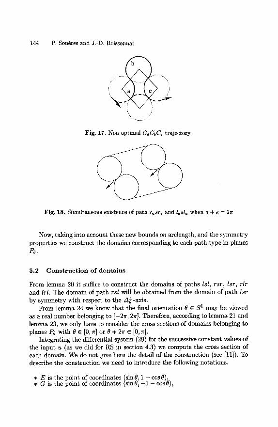
144 P. Sou~res and J.-D. Boissonnat
(\_! °
Fig. 17. Non optimal CaCbCe trajectory
Fig. 18. Simultaneous existence of path r~sr~ and l~sl~ when a + e = 2~r
Now, taking into account these new bounds on arclength, and the symmetry properties we construct the domains corresponding to each path type in planes Pe.
5.2 C o n s t r u c t i o n of d o m a i n s
From lemma 20 it suffice to construct the domains of paths tsl, rsr, lsr, rlr and lrl. The domain of path rsl will be obtained from the domain of path lsr by symmetry with respect to the A~-axis.
From lemma 24 we know that the final orientation ~ E S I may be viewed as a real number belonging to [-2zr, 2zr]. Therefore, according to lemma 21 and lemma 23, we only have to consider the cross sections of domains belonging to planes Pe with t? E [0, v] or t~ + 27r E [0, 7r].
Integrating the differential system (29) for the successive constant values of the input u (as we did for RS in section 4.3) we compute the cross section of each domain. We do not give here the detail of the construction (see [11]). To describe the construction we need to introduce the following notations.
* E is the point of coordinates (sin 8, 1 - cos 8), * G is the point of coordinates (sinO, - 1 - cosS),
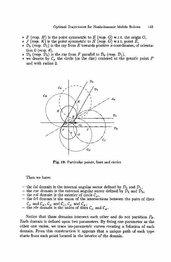
Optimal Trajectories for Nonholonomic Mobile Robots 145
* F (resp. H ) is the point symmetric to E (resp. G) w.r.t, the origin O, , J (resp. K ) is the point symmetric to H (resp. G) w.r.t, point E, * /)o (resp./)1) is the ray from E towards positive x-coordinates, of orienta-
tion 0 (resp. 0), * /)2 (resp./)3) is the ray from F parallel to/)0 (resp./)1), , we denote by Cp the circle (or the disc) centered at the generic point P
and with radius 2.
CK//
...... /" ..... " , / ./ Z~o /" ~ ~ " K /
~f\ V W/:Jf-"-.
- " ( \ ) /
"I-~ ............ " CG
Fig. 19. Particular points, lines and circles
Then we have:
- the Isl domain is the internal angular sector defined by Do and/)1, - the rsr domain is the external angular sector defined by/)2 and/)3, - the rsl domain is the exterior'of circle C a , - the lrl domain is the union of the intersections between the pairs of discs
C o and C., C a and C j, C. and CK, - the rlr domain is the union of discs C o and C H .
Notice that these domains intersect each other and do not partition P0. Each domain is defined upon two parameters. By fixing one parameter as the other one varies, we trace iso-parametric curves creating a foliation of each domain. From this construction it appears that a unique path of each type starts from each point located in the interior of the domain.
146 P. Sou~res and J.-D. Boissonnat
5.3 Cons t ruc t ion o f t h e par t i t ion
At this stage, we have to determine which path type is actually optimal in each region of P0 covered by more than one domain. We are sure of the optimality of the whole Isl domain for the Isl type, even if other domains intersect it. Indeed, this domain is optimal for RS, and Dubins' sufficient family is included in the Reeds and Shepp one (except for CCC paths, which are shortened by CICIC paths). Clearly, a path type with no cusp which is optimal for RS is afortiori optimal for DU.
So, let us consider the other intersections. Due to the lack of the symmetry with respect to the A0-axis, we cannot use a geometric reasoning to compare isometric trajectories, as we did in section 4.3 for RS. Therefore, in each region where more than one path type occur (see fig. 19), we use the method developed at section 4.3 for RS to compute the boundaries of the subdomains in which each path type is optimal. This method is based on the computation of the set of points reachable by a path of each type having the same length and starting at the origin. We conclude with arguments of continuity based on the foliation of domains by iso-length curves.
We will only present here the final equations of these boundary curves, since the calculation are really tedious (see [11] for more details).
In te rsec t ion rsr / rsl The intersection of these two domains, is defined by the complementary in Pe to the set made by the union of the disc ga and the internal angular sector defined by the rays l)2 and :D3. Writing that the final point are identical~ and that both curves have the same length, we get a system of three equations with four variables. Fixing one variable as a parameter, we obtain the parametric expression of a curve ~ :
{y= ) ~cosa+ 2s i na+ s i nO :To -As ina + 2cosa - cos~ - 1
p(a+e-~)~+2(cos(a+0)-l) where A = - sin(a+O)-(a+0-~) , and a is the length of the first arc in the rsl path. This parameter varies within the interval ]~r - 0, #] for 0 E [0, ~[ where p is defined as follows:
- for t? < ~ + ~, # = ~r - 0 + y where y is the solution of the non-algebraic equation cost = t,
- for ~ >_ ~ + r , # is the value of a obtained when Io and :D2 intersect. This value can be computed by equating the parametric system of both curves.
This curve divides the region of intersection into two sub-domains, and admits the line of orientation 0, passing through G, as asymptote. We define the symmetric curve I1 for the intersection between rsr and Isr.
Optimal Trajectories for Nonholonomic Mobile Robots 147
In te r sec t ion rs l / Isr Let ~? defined as in section 5.3. For 8 _< ~ + ~ we deduce from the analysis of iso-distance curves of each type that Isr paths are always shorter than rsl paths in the infinite region delimited by DI, :/)3, and the arc (E, K) of circle CH. Symmetrically with respect to the A~- axis, in the infinite region delimited by Do, D2, and the arc (E, J) of circle Ca the paths rsl are shorter than the lsr ones.
For ~ > ~ + ~r a new boundary curve :/6 appears; it is the locus of points reachable from the origin by a path rsl and Isr having the same length. This curve is determined by equating the parametric system of both curves. The curve/:7 is obtained by symmetry with respect to A~- (see fig. 24)
In te r sec t ion r s r / r l r This region of intersection is made up by the parts of the discs C c and C H lying inside the external angular sector defined by D~ and D3. We find geometrically that the set of points reachable from the origin by a path of each type rsr and r/r having the same length belongs to a circle called Z2 of radius 4~/ and centered at F. Thus, this set is made of two arcs of the circle :/2 respectively defined by the interval of polar angles: [max(0, ~r/2 - ~), min(~, ~r/2 + ~)] and the symmetric interval w.r.t. 8/2. This intersection only occurs if ~ < ~r/2 + ~/.
In te r sec t ion r l r / lrl Using the same reasoning as in the study of the first intersection, we deduce that inside the region determined by the union of the intersections of discs C c and C j , and the intersection of discs C, and CK, rlr paths are always shorter than IrI paths. However, for 8 > r /2 , the region of intersection of discs C c and C, is divided into two subdomains by a curve called ~ . Paths rlr are optimal in the first subdomain, whereas paths Irl are optimal in the other one.
After a change of variables, due to the rotation of angle 8/2, we obtain the following parametric equations for Z3:
X = c,°sv + cos(v + 8) sin e
:/3 y2 = (4 sin~)2 ~_ ( X - 2sin~)2
where v is the length of the middle arc of the lrl path. See [11] for the detail relative to the determination of the interval in which v varies.
In te r sec t ion r l r / r s l This last intersection occurs in the region of the disc C, located outside the disc C a and inside the internal angular sector delimited by D2 and D3. Using the same method as before we determine a curve Z4 delimiting two subdomains in which rlr and rsl are respectively optimal. The
148 P. Sou~res and J.-D. Boissonnat
curve Z5 symmetric of 1:4 with respect to A~- determines the boundary between the subdomains of paths rlr and lsr in the symmetric region. The parametric equations of 2:4 are:
y -- 2 ( a c o s a + s i n a ) + s i n 0 Z4 2 ( g s i n a - cosa) - c o s 0 - 1
with a = 2~r - arccos a a 2 A + B ~/4 (l+cos 0")2+4 (a+sin q)2_a4
O~ = 2 ( A 2 T B ~)
A = cos0 (1 + cosa) - sin0 (a + sing) B = cos 0 (a + sin a) + sin 0 (1 + cos a)
where a is the length of the first arc and 2g the length of the line segment in the rsl path. We can notice that, here again, equations are non-algebraic. This intersection only occurs for 0 >_ 7r/2 - ~. See [11] for the determination of the range of a.
5 . 4 D e s c r i p t i o n o f t h e p a r t i t i o n
With the refinement provided by the previous section we finally obtain a par- tition of P0, for values of 0 having a representative modulus 2~r in [0, 7r]. Using the symmetry properties given by lemmas 20 and 21 we obtain the partition for any 0 E S 1. The shape of domains varies continuously with respect to 0. In the sequel we describe four successive states of the partition according to four successive intervals of 0. We also describe the cross sections corresponding to two particular values: 0 = 0 and zr:
- 0 = 0 (Figure 20) All the domains are represented but notice that, for three of them, not only one but two equivalent optimal paths are defined at each point. Notice also that, in fact, the Irl and Isl domains are not connected: the initial configuration O can be viewed as a point of the domain Irl (isolated in Po), and the horizontal half-line (x >_ 0, y = 0) also belongs to the domain 1st.
- 0 e]0, ~r/2 - 7] (Figure 21) For 0 ~ 0, a unique path type is defined in each domain, but some domains are not connected (rlr, rsl and lsr). For 0 = ~r/2 - 7, the segment of :D2 (resp. 7)3) and Z2 intersect each other on ga (resp. gn).
- e e]~/2 - 7, ~r/2] (Figure 22) Here, the intersection curves 2:4 and 2:5 appear, and for 0 = ~r/2 the two crescents of the rlr domain are connected at one point on the A~/~ axis.
- 0 e]~r/2, 7r/2 + ~] (Figure 23) The intersection curve Z3 has appeared between rlr and Irl. Everything varies continuously until 2:2 disappear when 0 = r / 2 + 7, since the segment
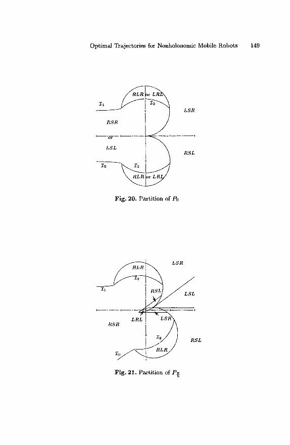
Optimal Trajectories for Nonholonomic Mobile Robots 149
RSR
i o r ~ " - - } ~ . - - ~ - - -
LSR
RSL
Fig. 20. Partition of Po
LSR
S ] " ns\ RSR / t
I2 RSL
Fig. 21. Partition of P~
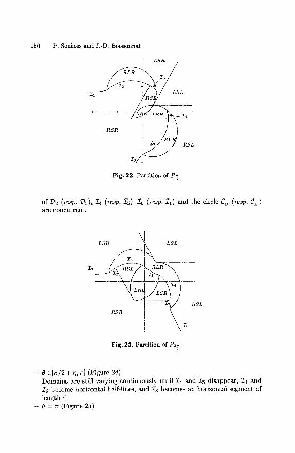
150 P. Sou~res and J.-D. Boissonnat
- LSR
Z~'-~ LSL
. . . . . . . . . . 4
~ RSL
Zo/ l
Fig. 22. Partition of P~
of / )2 (resp. ~)3), 274 (resp. Zs), Zo (resp. Z1) and the circle C a (resp. CH) are concurrent.
L S R ~ LSL
. . . .
J Z2~, / RSL
Fig. 23. Partition of P2_~ 3
- 9 e]lr/2 + ~, 7r[ (Figure 24) Domains are still varying continuously until 1:4 and 5[5 disappear, $4 and 275 become horizontal half-lines, and I3 becomes an horizontal segment of length 4.
- 0 = r (Figure 25)
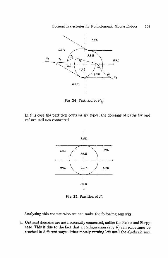
Optimal Trajectories for Nonholonomic Mobile Robots 151
R S R I
Fig. 24. Partition of P ~ 6
In this case the parti t ion contains six types; the domains of paths lsr and rsl are still not connected.
L: ~L
1,
R S L
R" 'R
R S L
4
L S R
Fig. 25. Partition of P~
Analysing this construction we can make the following remarks:
1. Optimal domains are not necessarily connected, unlike the Reeds and Shepp case. This is due to the fact that a configuration (x, y, 0) can sometimes be reached in different ways: either mostly turning left until the algebraic sum
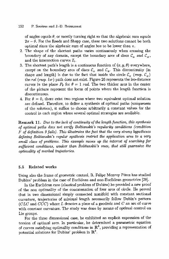
152 P. Sou~res and J.-D. Boissonnat
of angles equals 0, or mostly turning right so that the algebraic sum equals 2~r - 0. For the Reeds and Shepp case, these two solutions cannot be both optimal since the algebraic sum of angles has to be lower than 7r.
2. The shape of the shortest paths varies continuously when crossing the boundary of any domain, except the boundary arcs of discs ga and gxx, and the intersection curves Zi.
3. The shortest path's length is a continuous function of (x, y, 8) everywhere, except on the boundary arcs of discs ga and gn. This discontinuity (in shape and length) is due to the fact that inside the circle ga (resp. gu) the rsl (resp. Isr) path does not exist. Figure 26 represents the iso-distance curves in the plane P0 for 0 = 1 tad. The two thicker arcs in the center of the picture represent the locus of points where the length function is discontinuous.
4. For 0 = 0, there exist two regions where two equivalent optimal solution are defined. Therefore, to define a synthesis of optimal paths (uniqueness of the solution), it suffice to choose arbitrarily a constant values for the control in each region where several optimal strategies are available.
R e m a r k 11. Due to the lack of continuity of the length function, this synthesis of optimal paths does not verify Boltianskii's regularity conditions (condition F of definition g fails). This illustrates the fact that the very strong hypotheses defining Boltianskii's regular synthesis restrict the application area to a very small class of problems. This example raises up the interest of searching for sufficient conditions, weaker than Bolitanskii's ones, that still guarantee the optimality of marked trajectories.
5.5 R e l a t e d works
Using also the frame of geometric control, R. Felipe Monroy P@rez has studied Dubins' problem in the case of Euclidean and non-Euclidean geometries [28].
In the Euclidean case (classical problem of Dubins) he provided a new proof of the non optimality of the concatenation of four arcs of circle. He proved that in two dimensional simply connected manifold with constant sectional curvature, trajectories of minimal length necessarily follow Dubin's pattern (CLC and CCC) where L denotes a piece of a geodesic and C an arc of curve with constant curvature. The study was done by means of optimal control on Lie groups.
For the three dimensional case, he exhibited an explicit expression of the torsion of optimal arcs. In particular, he determined a parametric equation of curves satisfying optimality conditions in R 3, providing a representation of potentiM solutions for Dubins' problem in R 3.
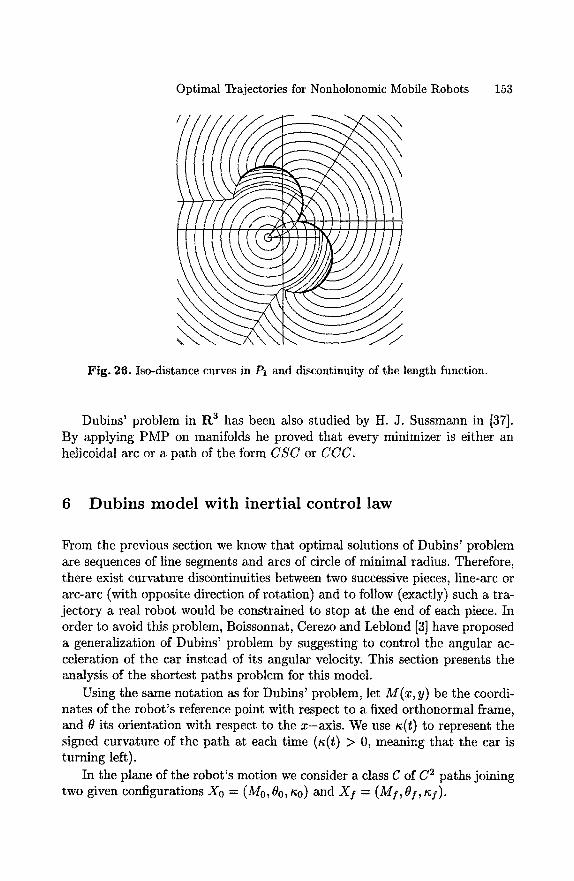
Optimal Trajectories for Nonholonomic Mobile Robots 153
Fig. 26. Iso-distance curves in P1 and discontinuity of the length function.
Dubins' problem in R 3 has been also studied by H. J. Sussmann in [37]. By applying PMP on manifolds he proved that every minimizer is either an helicoidal arc or a path of the form CSC or CCC.
6 D u b i n s m o d e l w i t h i n e r t i a l c o n t r o l l a w
From the previous section we know that optimal solutions of Dubins' problem are sequences of line segments and arcs of circle of minimal radius. Therefore, there exist curvature discontinuities between two successive pieces, line-arc or arc-arc (with opposite direction of rotation) and to follow (exactly) such a tra- jectory a real robot would be constrained to stop at the end of each piece. In order to avoid this problem, Boissonnat, Cerezo and Leblond [3] have proposed a generalization of Dubins' problem by suggesting to control the angular ac- celeration of the car instead of its angular velocity. This section presents the analysis of the shortest paths problem for this model.
Using the same notation as for Dubins' problem, let M(x, y) be the coordi- nates of the robot's reference point with respect to a fixed orthonormal frame, and t? its orientation with respect to the x-axis. We use ~(t) to represent the signed curvature of the path at each time (t~(t) > 0, meaning that the car is turning left).
In the plane of the robot's motion we consider a class g of C 2 paths joining two given configurations X0 = (M0,00, n0) and Xf = (Mr, Of, t~f).
154 P. Sou~res and J.-D. Boissonnat
Definit ion 11. A path belongs to class C if it satisfies the following two prop- erties:
1. Regularity: the path is a C 2 concatenation of an at most countable number o[ open C 3 arcs of finite length, and the set of endpoints of these arcs, also called the switching points, admits at most a finite number of accumulation points.
2. Constraint: along the path, the absolute value of the derivative of the cur- vature, with respect to the arc length, is upper bounded by a given constant B > O, at every point where it is defined.
With these notations and the above definition, the motion of the oriented point M(t) = (x(t) ,y(t) ,O(t) ,~(t)) along paths of class C in R 2 x S 1 x R is well-defined and continuous.
In the sequel we consider that the robot moves at constant speed 1, so that time and arc length coincide.
A path in class g between any two configurations X0 = (xo, Yo,/9o, no) and X ! = (x I, yf , Oy, ~f ), if it exists, is entirely determined by the function v(t) = k(t), defined and continuous everywhere, except at the switching points, by the following differential system:
{~(t) = cos o(t) ) ( ( t ) = ~I:I =sin0(t)= •(t) (30)
~(t) = v(t)
If we add the boundary conditions X(0) = X0, X ( f ) = XI , and the constraint:
Vt e [0,T], iv(t) I </3, (31)
and if we search for a path of minimum length in class C, we have turned the geometric problem into a classical question of optimal control theory where the functional:
// J(v) = T = dt (32)
is to be minimized among the set of control functions v satisfying (31).
6.1 Exis tence of an optimal solution
System (30) may be written as:
= F ( Z , v) = f ( X ) + v g ( Z ) ,
Optimal Trajectories for Nonholonomic Mobile Robots
where the analytic vector fields f and g are given by:
/ ( x ) = , g ( x ) = .
155
C o m p l e t e control labi l i ty of the sys t em We first observe that the Lie algebra £(f , g) generated by f and g is, at each point, of dimension 4. Indeed, v x e R 4,
and
det
cos 0 0 0 - sin 8" sin ~ 0 0 cos
a 01 0 0 10 0
Moreover, the solutions of the associated autonomous system X = f (X) are circles (of radius l /a ) , thus periodic. Hence, Bonnard's theorem [27, thm.III.4] applies, to establish the complete controllability of (30) under the constraint (31). This means that any Xo and X l can always be joined by a path satisfying (30) and (31).
Exis tence of an o p t i m a l control The existence of an optimal control for the problem (30), (31), (32), with given X0 and XI, is ensured by Fillipov's ex- istence theorem (see [13, 5.1.ii] for example). Indeed, the hypotheses of the the- orem are satisfied. The dynamic F(X, v) and the cost J(v) are smooth enough, the set I -B, +B] of control is convex, and the initial and final configurations X0 and Xf are fixed. Finally, one can easily check the existence of a constant C such that t X F ( X , v ) <_ C(IXI 2 + 1) for all t e [0,T], X E R 2 x S 1 x R, v e I - B , + B ] .
Fillipov's theorem then asserts the existence of some T* > 0 and of an optimal control v* (t) which is a measurable (thus locally integrable) function which satisfies (31) on [0, T*]. The solution of (30) for v = v* is a path from X0 to X/which minimizes cost (32) under constraint (31).
156 P. Sou~res and J.-D. Boissonnat
6.2 Necessary conditions for a solution to be optimal
Pontryagin's Maximum Principle We are going to apply Pontryagin's Maximum Principle in order to obtain necessary conditions for a solution to be optimal (i.e. a measurable control v and a trajectory X) minimizing cost (32).
Let us denote by q7 tko = (¢1,¢2,¢3,¢4) , the adjoint state associated to X. For this minimum time problem, the Hamiltonian H is defined for every t e [0, T] by
H(~(t), X(t), v(t)) = < ~P(t), F(X(t) , v(t)) >
This yields in the case of system (30):
H(O(t) ,X(t) ,v(t)) = ¢ 1 ( t ) c o s 0 ( t ) + ¢ 2 ( t ) s i n 0 ( t ) + ¢3(t)a(t) + ¢4(t)v(t). (33)
The adjoint state ~ is defined on [0, T] as a solution to the adjoint system OH which is here:
{ ¢ 1 ( t ) = 0 ~ ¢ 1 ( t ) = ¢1
~(t) = ¢2(t) 0 ~ ¢2(t) = ¢2 (34) ¢3(t) ¢1(t) sin0(t) - ¢2(t) cos0(t) = ¢1?~(t) - ¢22(t)
~J4 ( t ) - - ¢ 3 ( t ) •
Therefore, as ¢1 and ¢2 are constant on [0, T] there exists A >_ 0 and ¢ E [0, 2~r[ such that, Vt E [0, T]:
¢ 1 ( t ) - ¢1 = ~ cos ¢
¢2 (t) -- ¢2 = A sin ¢ (35) ¢ 3 ( t ) = ~ s i n ( 0 ( t ) - ¢) ~J4(t) --~ - - ¢ 3 ( t ) •
The Hamiltonian (33) can now be written as:
H(k~, X, v) = A cos(0 - ¢) + ¢3a + Ctv. (36)
Now, according to theorem 3, a necessary condition for X(T) to be an extremal trajectory for the minimum-time problem is that ~(t) define a nonzero absolutely continuous function such that Yt E [0, T]:
H(~(t) ,X(t) ,v( t )) =
where ¢o _< 0 is a constant.
m a x uE[--B,+B]
H(~(t), X(t), u(t)) = - ¢ o . (37)
Optimal Trajectories for Nonholonomic Mobile Robots 157
Characterization of extremal arcs From equation (37) we deduce that:
¢4(t)v(t) > 0 for almost every t E [0,T]. (38)
As X belongs to class C, on each open C 3 portion of the trajectory, v(t) = :I:B with the sign of ¢4 if ¢4(t) # 0 or, otherwise, that OH = ¢4 ( t ) = 0. If ¢ 4 ( t ) ---- 0
over some interval [tl,t2] C [0,T], (35) implies that ¢3(t) - 0 and ¢3(t) ~- 0. As 0 is continuous and A # 0 (otherwise ¢1 = ¢2 = ¢3 = 0 and therefore ¢0 = 0 which is not possible), it follows that O(t) _~ ¢ (rood ~r). Of course then, ~ - v - 0 on It1, t2]. Hence, on each open C 3 portion of the path, v(t) E { - B , + B , 0 } , and since v has to be continuous on such a portion, it is of one of the three kinds:
1. Cl+: v(t) - B, ¢4(t) > 0 2. CI- : v(t) = - B , ¢4(t) < 0 3. S: v(t) -~ 0, ¢4(t) = 0
Arcs C1 ± are finite portions of clothoids. A clothoid 6 (see figure (27)), also known as a "Cornu spiral", is a curve along which the curvature a depends linearly on the arc length (here equal to t) and varies continuously from - o o to +oo. Hence, all clothoids C1 + (where v(t) = B) are translated and rotated copies of a unique clothoid F while all clothoids C1- (where v(t) = - B ) are translated, rotated and reflected copies of F. Clothoids C1 + will be called direct clothoids and clothoids C1- will be called indirect clothoids. The canonical clothoid F is chosen as the one defined by the following equations:
// B_ x(t) = cos( 2 r )dr
~ t B 2 y(t) = s in (~ r )dT.
Arcs S are line segments, all with the same orientation ¢ (mod ~r). From the above discussion, we have:
Propos i t ion 1. Any extremal path in class C is the C 2 concatenation of line segments (with the same orientation) and of arcs of clothoids (with k = ~:B), all of finite length. The control function v is constant on each piece: v = B on a direct clothoid C1 +, - B on an indirect one CI- , and 0 on a line segment S.
In the sequel, we denote by "CI" an arc of clothoid, by "S" an open line seg- ment, and by "." a switching point. "CI~" will further specify, when necessary, the length # of the arc.
6 More details about clothoiods are given in the next section
158 P. Sou~res and J.-D. Boissonnat
In order to character ize the ex t remal pa ths , and, a m o n g them, the shor tes t ones, we consider the following problem: how are these arcs C1 and S arranged together along an extremal trajectory of class C ? We provide in the next section a par t ia l answer to this question.
C o n c a t e n a t i o n o f a r c s
L e m m a 25. ¢4 = 0 a t any switching point (C1.C1, C1.S or S.C1).
P roo f : That ¢4 = 0 at a switching point CI.S or S.Cl follows from the fact that ¢4 ~- 0 on S and that ¢4 is continuous. At a switching point CI.C1, the sign of v changes and, by (38), also the sign of ¢4. []
L e m m a 26. I f A = 0, the ex t remal p a t h consists of one or two arcs and is of type C1 or C1.C1.
P roo f : If )~ = 0, ¢3 is constant on [0, T] by (35). If ¢3 = 0, ¢4 is constant on [0, T] by (35). Moreover, ¢4 cannot be identically 0, since, otherwise, (~', ¢0) --- (0, 0), which contradicts the necessary conditions of PMP. Hence, it follows from Lemma 25 that the extremal path cannot contain a line segment nor a switching point and thus reduces to a single arc CI.
If ¢3 ¢ 0, ¢4(t) is a linear function of t by (35) and then vanishes at most at one isolated point. Hence the extremal path is of type C1 or C1.C1, by Lemma 25. [3
Note t h a t such pa ths are not generic: f rom any given initial conf igurat ion X0 in R 2 x S 1 x R , the set of final configurations {Xf} one can reach th rough such pa ths is only 1 or 2-dimensional.
L e m m a 27. I f an ex t remal p a t h contains a line segment S, )~ = - ¢ 0 > 0.
P roo f : along a line segment ¢4 - ¢3 ~ 0 and 0 -- ¢ (rood ~r). Hence, H -- eA -- - ¢ o _> 0, with c = :t=1. As Co _< 0 and :~ :> O (from Lemma 26), we must have e = +1 and )~ = - ¢ o . [:3
F rom the p roof of l e m m a 27, ¢ = cos(~ - ¢) = +1 on S, and we have:
C o r o l l a r y 1. Along a line segment S, ~ - ¢ (mod 2~r).
L e m m a 28. ¢3 - ¢1 Y + ¢2 x is cons tant along any ex t remal pa th . I f A > 0, for any given c E R., all the points of an ex t remal p a t h where ¢3 = c lie on the same s t ra ight line De, of direction ¢ (mod ~r).
Proof: Ca -- ¢1 y - ¢2 x from (34), and ¢i and ¢2 are constant. Thus there exists a constant co such that ¢ 1 y - ¢2x = Ca + co, which proves the first part of the lemma. If A ¢ 0, ¢i and ¢2 cannot be both equal to 0 and ¢ l y - ¢ 2 x = c-t-co is the equation of a line of direction 0 = ¢ (rood ~r). [3
As a consequence, we have:
Optimal Trajectories for Nonholonomic Mobile Robots 159
C o r o l l a r y 2. Any line segment S of an extremal pa th is contained in Do and is run with O _= ¢ (mod 2 ~r).
Proof i since ¢3 - 0 on S, it follows from Lemma 28 that S is contained in the line Do of direction ¢. By Corollary 1, 0 - ¢ (rood 2~r). []
L e m m a 29. If A > 0, each open arc of clothoid CI , with/~ > 0 of an extremal path, except possibly the initial and the final ones, intersects Do at least once.
Proof : let CI~ be an arc of length # of an extremal path which is not the initial nor the final arc. Both endpoints of such an intermediate arc are switching points. Let ]tl,t2[ denote the time interval during which this intermediate arc Cl~ is run. By Lemma 25, ~)4( t l ) = ¢4(~2) - - 0. As t2 - tl = # > 0, there exists at least one t E]tl,t2[, say t3, such that ¢4(ts) = 0 and thus, from (35), ¢3(ts) --- 0. Finally, it follows from Lemma 28 that M(ta) belongs to Do. n
Observe tha t the hypothesis )~ > 0 along an extremal pa th is true as soon as it contains either a line segment (Lemma 27) or more than only two arcs of clothoid (Lemma 26).
L e m m a 30. An extremal path contains no portion of type S.CI~.C1 or of sym- metric type C1.C1,.S with # > 0.
Proof: assume that there exists such a portion S.CI~.C1 and let ]tl, t2[ denote the time interval during which Cl~ is run, with t2 - tl =/~ > 0. From Lemma 2, S C Do, and since the variables (x,y,~, ~;) are continuous on [tl,t2], Cl~ is tangent to Do at M(t i ) and ~(~1) = O. Hence, M(tl) is the inflection point of the clothoid supporting CI~ and Do is the tangent to the clothoid at M(tl ) . This implies that Cl~ \ {M(tl)} is entirely contained in an open half-plane delimited by Do, see figure (27), which contradicts Lemma 29. []
The last l emma is in fact superseded by the following one, due to H.J. Sussmann.
L e m m a 31. An extremal pa th contains no portion of type S.Cl~ (or Cl~.S) with # > 0.
Proof : assume that there is a portion of type S.CI~, with # > 0, in an extremal trajectory and let tl be the switching time between S and Cir. From (35) and (36) we obtain the following expressions of the four first derivatives of ¢4 (valid on S as well as on C1,):
{ ¢4 = -,k sin(O- ¢)
~; - ~ cos(0- ¢)
¢4 AI¢ 2 sin(0 - ¢) + (¢3 t¢ + ¢4 v + ¢o) v.
160 P. Sou~res and J.-D. Boissonnat
Hence, the adjoint variable ¢4 is of class C a in the neighbourhood of tl. Moreover, on S, ¢4 = ~J4 -- 0, 0 ~ ¢ (mod 27r), Cs - 0, a = 0. From the above equations, we also have ~'4 =¢4= 0 on S, and, by continuity, at tl. Moreover, ¢'4 (tl) = ¢ o v . Thus, there exists an e, 0 < z < p, such that for t E [tl,tl +e[ we have:
¢ 4 ( t ) = ¢o v( t ) (t - t l ) 4 4! + o ( ( t - tl)5).
Now, from Lemma 27, ¢o < 0, so that ¢4 and v have opposite signs on [tl, tl + ~[ which contradicts (38). []
A consequence of Lemmas 30 and 31 is the following proposition:
P r o p o s i t i o n 2. If an extremal path of class C contains but is not reduced to a line segment, then it contains an infinite number of concatenated clothoid arcs which accumulate towards each endpoint of the segment which is a switching point.
Proposition 2 together with the fact that a clothoid C1 is contained in a ball of bounded diameter Dvt (depending on the parameter B) implies the following:
P r o p o s i t i o n 3. The number n of C 3 pieces contained in a generic extremal path cannot be uniformly bounded from above (with respect to Xo, Xf). How- ever, if d(Mo, Mr) denotes the Euclidean distance in the plane between M0 and My, we have that:
d(Mo,M~) n >_ Dcl
Proof-. either the shortest path contains (and is generically not reduced to) a line segment, and Proposition 2 implies that there are infinitely many arcs of clothoid, or it is made only with arcs of clothoid, the number of which clearly depends on (and increases with) the distance between Xo and Xf. The bound from below is obvious. D
6.3 C o n c l u s i o n
Note that it is not clear whether or not extremal trajectories described in Proposition 2, and, among them, the optimal ones, belongs to class C: indeed, the set of switching points on an optimal trajectory (points where the control v is undefined) might even be uncountable. Moreover, we don' t know yet if the statement of this proposition remains true without the assumption that the path contains a line segment.
Optimal Trajectories for Nonholonomic Mobile Robots 161
However, Propositions 2 and 3 already indicate that the optimal control associated to problem (30), (31), (32) has a complex behavior. Contrarily to what occurs for Dubins or Reeds and Shepp problems, for which every optimal trajectory contains at most a prescribed (finite) number of line segment and arcs of circles, the number of switching points is unbounded here and might be infinite.
6.4 Re l a t ed works
Lemma 31 is due to H.J. Sussmann who provided a complete study of this problem described as "Markov-Dubins problem with angular acceleration con- trol" [38]. In this paper, the author uses results by Zelikin and Borisov [39] to show that there exist extremals involving infinite chattering.
7' Time-optimal trajectories for Hilare-like mobile robots
The last model we consider is the model of Hilare the robot of LAAS-CNRS whose locomotion system consists of two parallel driven wheels and four slave castors.
Let (x, y) be the coordinates of the reference point located between the driven wheels, and 8 the robot's orientation with respect to the x-axis, vr and 'vl denote respectively the velocities of the contact point of the right and left driven wheel with the floor. These virtual point velocities are considered as two state variables while their acceleration ar and al constitute the two system inputs. Therefore, a configuration of the robot is a 5-uple (x, y, 8, vr, vl). Using d to denote the distance between the driven wheels we get the following dynamic representation:
• | ~ sin~ / e =I I vr "6z
+ O o a r + O o a l (39)
Each wheel is driven by an independent motor and the power limitation is expressed by the constraint: ar,al E [-a,a] ,a > 0. For this model there is no curvature constraint and the robot can turn about its reference point.
We consider the problem of characterizing minimum-time trajectories link- ing any pair of configurations where the robot is at rest i.e verifying vr -= vl = O.
This problem has been initially studied by Jacobs et al [25]. After having shown that the system is controllable, the authors have proven that minimum- time trajectories are necessarily made up with bang-bang pieces• To illustrate
162 P. Sou~res and J.-D. Boissonnat
the reasoning of their proof let us suppose that the first control a~ is singular while the second control al is bang-bang.
For this minimum-time problem, denoting by ¢ = (¢1, ¢2, ¢3, ¢4, ¢5) T the adjoint vector, the Hamiltonian corresponding to system (39) is:
and therefore,
Vr + Vl .~ Vr + Vl . ~ . , Vr -- Vl H = ¢1 - - T - - cos ~ + ¢2 ~ sm . ~3 - - - T - - + ¢4 a~ + ¢5 al
As we suppose ar to be singular, the corresponding switching function ¢4 vanishes over a nonzero interval of time. From the adjoint equation we get:
Ovr = cos 0 + sin 0 + --~ = 0
d ¢3 = - 2 ( ¢ 1 cos ~ + ¢2 sin 8)
Taking the derivative of ¢3 and replacing/~ by its expression given by (39) we get:
Vr -- Vl ) ¢3 = (¢1 sin~ - ¢2 c o s ~ ) ( ~ ) (40)
The expression of 43 can also be deduced directly from the adjoint equation:
¢3 = O H . . . . v~ + v l ) , 0t9 -- (¢1 sin~ - ~2 c o s e ) t ~ ) (41)
Equating (40) and (41) we deduce that
1. either v2 -- 0 2. either ¢1 sin 8 - ¢2 cos ~ = 0
As al is supposed to be bang-bang the first case leads to a contradiction. On the other hand, as ~ = ~v g = 0, we deduce from the adjoint equation that ¢1 and ¢2 are constant. Thus, in the second case, the car is moving on a straight line, but a necessary condition for such a motion to be time-optimal is that the acceleration of wheels be both maximal or both minimal, and therefore correspond to bang-bang control.
Using the same reasoning in the case that at is singular and a r regular, or in the case that both control are singular, one can prove that extremal controls are necessarily bang-bang.
Therefore, optimal trajectories are obtained for larl = lall = a; these ex- tremal curves are of two types.
Optimal Trajectories for Nonholonomic Mobile Robots 163
• a r - ~ - a l - - ~ a In this case the robot 's linear acceleration is null: ~)(t) = ½(~)d + ~)g) = 0. v(t) is constant equal to vo, therefore the curvilinear abscissa s(t) = vot. ~)r(t) = :t:a while 7)l(t) .-- Ta. Integrating we get: vr(t) = ± a t + vro, vz(t) = T a t + Vto and 03(t) O(t) 2a = = d=--£t + 030. The curvature ~ is then:
03O n(t) = :t:~-t + wo = +kcs(t) + - - (42) V0 V0
where kc 2a = dv--~o. In the (x, y ) -p lane , the curve is a clothoid with charac-
teristic constant kc. When Xo --- Yo = 03o = 0o the curve is expressed by the following parametric expression in terms of Fresnel sine and cosine.
x( t ) = s i g n ( v o ) v ~ S o V ~ t c o s ( ~T2)dT (43 ) ~ 2]~a2a t
y(t) = 8ign(Voar) Jo
Figure (27) shows a clothoid obtained for ar "- - a l -- a. The part located above the x - a x i s describes the robot 's motion for Vo > 0, while the part located under the x - axis corresponds to v0 < 0. A curve symmetric with respect to the x - a x i s is obtained for ar ( O.
R e m a r k 12. When vo = 0 the curve is reduced to a pure rotation about the origin.
In this case the angular velocity is null: 5~(t) = ~(Or(t) - ~)l(t)) = 0. Therefore w(t) = wo, and O(t) = wot + Oo. The linear acceleration is iJ(t) = sign(a~)a, thus v(t) = s ign(a t )a t + vo. The curvature radius p(t) is given by:
v(t) = sign(a~)k.(O(t) - 0o) + Vo (44) p(t) = 03(t) 030
where ka = ~oo" In the (x, y ) - p l a n e the curve is an involute of a c i rc l J
whose characteristic constant is k~. When xo = Yo = Vo = Oo the curve is expressed by the following parametric expression:
x( t ) = sign(ar)ka(cos(wot) + wot sin(wot) - 1) (45) y( t ) = sign(ar)ka (sin(wot) - wot cos(w0t))
The involute of a circle is the curve described by the end of a thread as it is unwound from a stationary spool.
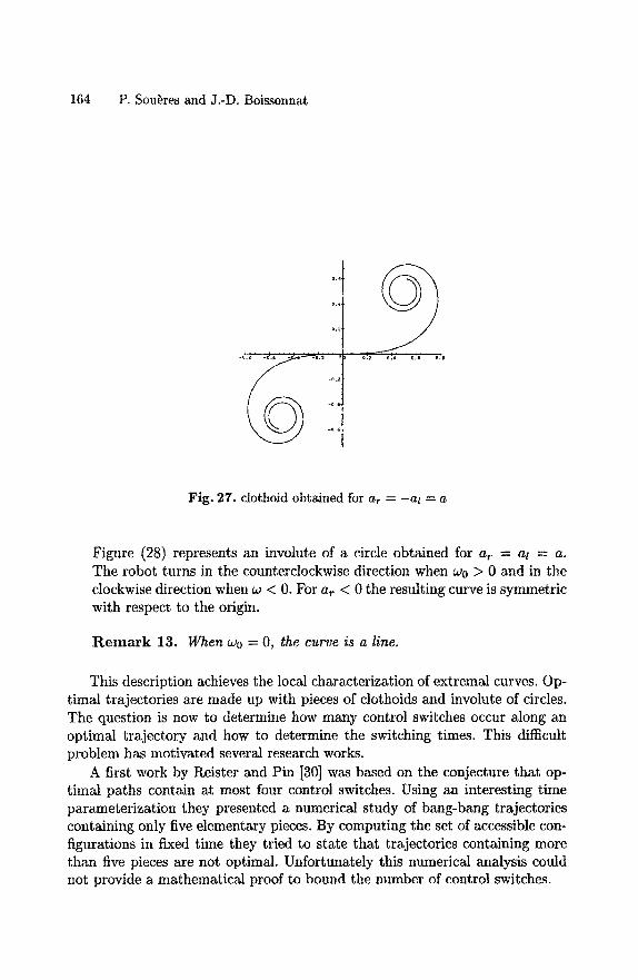
164 P. Sou~res and J,-D. Boissonnat
Fig. 27. clothoid obtained for a~ = -at = a
Figure (28) represents an involute of a circle obtained for a r = at = a .
The robot turns in the counterclockwise direction when wo > 0 and in the clockwise direction when w < 0. For a r < 0 the resulting curve is symmetric with respect to the origin.
R e m a r k 13. W h e n wo = O, t h e c u r v e is a l i ne ,
This description achieves the local characterization of extremal curves. Op- timal trajectories are made up with pieces of clothoids and involute of circles. The question is now to determine how many control switches occur along an optimal trajectory and how to determine the switching times. This difficult problem has motivated several research works.
A first work by Reister and Pin [30] was based on the conjecture that op- timal paths contain at most four control switches. Using an interesting time parameterization they presented a numerical study of bang-bang trajectories containing only five elementary pieces. By computing the set of accessible con- figurations in fixed time they tried to state that trajectories containing more than five pieces are not optimal. Unfortunately this numerical analysis could not provide a mathematical proof to bound the number of control switches.
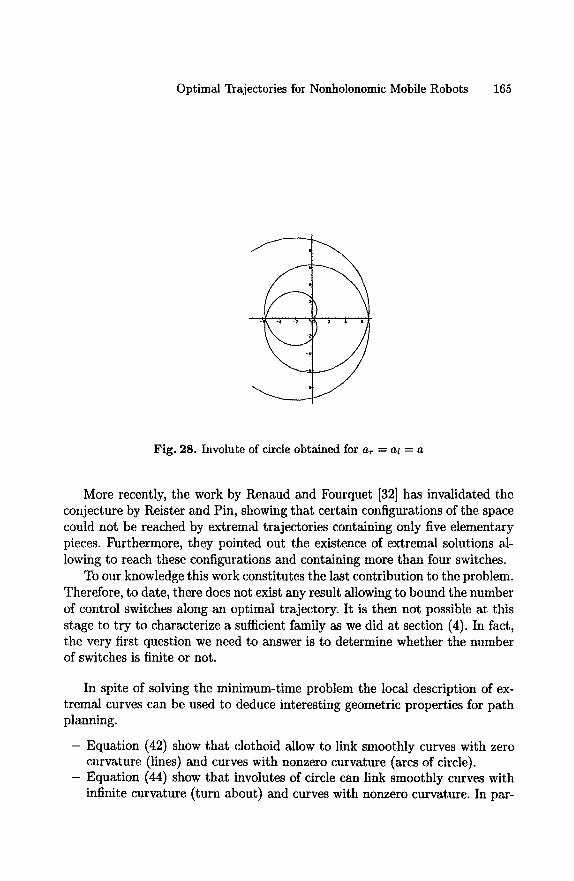
Optimal Trajectories for Nonholonomic Mobile Robots 165
Fig. 28. Involute of circle obtained for ar -- al = a
More recently, the work by Renaud and Fourquet [32] has invalidated the conjecture by Reister and Pin, showing that certain configurations of the space could not be reached by extremal trajectories containing only five elementary pieces. Furthermore, they pointed out the existence of extremal solutions al- lowing to reach these configurations and containing more than four switches.
To our knowledge this work constitutes the last contribution to the problem. Therefore, to date, there does not exist any result allowing to bound the number of control switches along an optimal trajectory. It is then not possible at this stage to try to characterize a sufficient family as we did at section (4). In fact, the very first question we need to answer is to determine whether the number of switches is finite or not.
In spite of solving the minimum-time problem the local description of ex- tremal curves can be used to deduce interesting geometric properties for path planning.
- Equation (42) show that clothoid allow to link smoothly curves with zero curvature (lines) and curves with nonzero curvature (arcs of circle).
- Equation (44) show that involutes of circle can link smoothly curves with infinite curvature (turn about) and curves with nonzero curvature. In par-
166 P. Sou~res and J.-D. Boissonnat
ticular, following this curve the robot can make a cusps while keeping a nonzero angular velocity.
This result has been used by Fleury et al [17] to design primitives for smoothing mobile robots' trajectories. In this work several sub-optimal strate- gies are proposed to smooth broken lines trajectories in a cluttered environ- ment.
8 Conclusions
The study of these four problems corresponding to different models of wheeled robots illustrates the strengths and weaknesses of the use of optimal control for path planning.
By constructing a shortest paths synthesis for the models of Reeds and shepp and the model of Dubins, we have definitely solved the path planning problem for a car-like robot moving in a plane free of obstacles. Obviously, as the vehicle is supposed to move at a constant speed along arcs of circle and line segments this result does not constitute a real feedback control for the robot. However, it constitutes a canonical way to determine a path, for linking any two configurations, upon which path following techniques can be developed.
Furthermore, from this construction, it has been possible to determine a dis- tance function providing a topological analysis of the path planning problem. In particular, for the Reeds and Shepp problem, we have proven that the dis- tance induced by the shortest path is Lipschitz equivalent to a sub-Riemannian metric. Such a metric constitutes a very useful tool to compute the distance between the robot and its environment.
However, whereas optimal control may provide a very complete result for a small number of systems, the characterization of optimal path is in general incomplete. This is illustrated by the last two problems. In such cases, the local characterization of extremals can be used to determine suboptimal strategies for planning.
Beyond solving the path planing problem, this study has permitted to get very interesting results.
First, we have shown the existence of symmetry properties common to the different models of wheeled robots. On this basis, by constructing the set of reachable configuration for the model of Reeds and Shepp and for the model of Dubins, we have shown the existence of several propagating wave fronts in- tersecting each other. From this, we have proven the insufficiency of the local information provided by PMP and the need to be compare the cost of trajecto- ries corresponding to different wave fronts, by means of global arguments. Using this reasoning we have completely solved the problem of Reeds and Shepp as well as the problem of Dubins.
Optimal Trajectories for Nonholonomic Mobile Robots 167
On the other hand, by showing that the synthesis constructed for the Reeds and Shepp problem verifies the required regularity conditions we have found another proof to confirm this result a posteriori by applying Boltianskii's suf- ficient optimality conditions. Though this theorem allows to prove very strong results in a very simple way, we have shown the narrowness of its application area by considering the neighbouring example of Dubins for which the regular- ity conditions no longer apply because of the discontinuity of path length.
The last two examples illustrate the difficulty very often encountered in studying of optimal control problems. First, the adjoint equations are seldom integrable making only possible the local characterization of optimal paths. The search for switching times is then a very difficult problem. Furthermore, as we have seen in studying the problem of Dubins with inertial control, it is possible to face Fuller-like phenomenon though the solution could seem to be a priori intuitively simple.
168 P. Sou~res and J.-D. Boissonnat
References
1. L.D Berkovitz, "Optimal Control Theory," Springer-Verlag, New York, 1974. 2. J.D. Boissonnat, A. Cerezo and J. Leblond, "Shortest paths of bounded curvature
in the plane," in IEEE Int. Conf. on Robotics and Automation, Nice, France, 1992. 3. J.D. Boissonnat, A. Cerezo and J. Leblond, "A Note on Shortest Paths in the
Plane Subject to a Constraint on the Derivative of the Curvature," INRIA Report No 2160, january 1993
4. V.G. Boltyanskii, " Sufficient conditions for optimality and the justification of the dynamic programming method," J.Siam Control, vol 4, No 2, 1966.
5. R.W Brockett, " Control Theory and Singular Riemannian Geometry," New Di- rection in Applied mathematics (P.J. Hilton and G.S. Young, eds), Springer, pp 11-27, Berlin, 1981.
6. I.N. Bronhstein and K.A. Semendyayev, "A guide-book to Mathematics for tech- nologists and engineers," Pergamon Press, 1964.
7. P. Brunovsky, "Every normal linear system has a regular synthesis," J. Diff. Equations, 28, pp 81-100, 1978.
8. P. Brunovsky, "Existence of regular synthesis for general problems," J. Diff. Equa- tions 38 pp 317-343, 1980.
9. X-N. Bui, P. Sou~res, J-D. Boissonnat and J-P Lanmond, "The Shortest Path Synthesis for Non-Holonomic Robots Moving Forwards", INRIA Report N ~ 2153, january 1994.
10. X-N. Bui, P. Sou~res, J-D. Boissonnat and J-P Laumond, "Shortest Path Syn- thesis for Dubins Nonholonomic Robot", IEEE Int. Conf. on Robotics and Au- tomation, San Diego California, 1994.
11. X-N. Bui, "Planification de trajectoires pour un robot polygonal non-holonome dans un environement polygonal," PhD Thesis, Ecole Nationate Supgrieure des Mines de Paris, France 1994.
12. S.S Cairns, "On the triangulation of regular loci", Ann. of Math., 35, pp 579-587 (1934)
13. L. Cesari " Optimization, theory and applications," Springer-Verlag, New york, 1983.
14. R. Chatila, "Mobile robot navigation: space modeling and decisional processes," in Robotics Research : The Third International Symposium (O. Faugeras and G. Giralt, eds.), MIT Press, pp. 373-378, 1986.
15. E.J. Cockayne and G.W.C. Hall, "Plane motion of a particle subject to curvature constraints," SIAM J. Control, 13 (1), 1975.
16. L. E. Dubins, "On curves of minimal length with a constraint on average curva- ture and with prescribed initial and terminal positions and tangents," American Journal of Mathematics, Vol. 79, pp. 497-516, 1957.
17. S. Fleury, P. Sou~res, J-P. Laumond, R. Chatila, " Primitives for Smoothing Mobile Robot Trajectories," IEEE Transactions on Robotics and Automation Vol. 11, No 3, June 1995.
18. M. Fliess, J. Levine, Ph. Martin, and P. Rouchon. " Sur les systhmes non lin~aires diff~rentiellement plats," C.R. Acad. Sci Paris, 1-315:619-624, 1992.
Optimal Trajectories for Nonholonomic Mobile Robots 169
19. J-Y.Fourquet "Mouvements en temps minimal pour les robots manipulateurs en tenant compte de leur dynamique non lin~aire." PhD Thesis, Universitg P.Sabatier N ° 800, France, 1990.
20. G. Giralt, R. Chatila, and M. Vaisset, "An integrated navigation and motion control system for autonomous multisensory mobile robots," in Robotics Research : The First International Symposium (M. Brady and R. P. Paul, eds.), MIT Press, pp. 191-214, 1984.
21. H. Halkin " Mathematical Foundation of System Optimization" in Topics in Optimization, edited by G. Leitmann, Academic Press, 1967.
22. P. Hartman. "The highway spiral for combining curves of different radii." Trans. Amer. Soc. Civil Engin., 1957
23. A. Isidori, "Nonlinear Control Systems," (second edition) Springer-Verlag, 1989. 24. G. Jacob "Lyndon discretization and exact motion planning," in European Con-
trol Conference, pp. 1507-1512 Grenoble, France, 1991. 25. P. Jacobs, A Rege and J-P. Laumond, "Non-Holonomic Motion Planning for
Hilare-Like Mobile Robots," Proceedings of the International Symposium on in- telligent Robotics, Bangalore, 1991.
26. J.P. Laumond and P. Sou~res, "Metric induced by the shortest paths for a car-like mobile robot", in IEEE IROS'93, Yokohama, July 1993.
27. C. Lobry, "Controlabilit~ des syst~mes non line,aires," outils et modules mathd- matiques pour l'automatique, l'analyse des syst~mes et le iraitement du signal, 1: pp 187-214, CNRS, 1981.
28. R. Felipe Monroy P~rez, "Non-Euclidian Dubin's problem: A control theoretic approach", PhD thesis, Department of Mathematics, University of Toronto, 1995.
29. L.S Pontryagin, V.G. Boltianskii, R.V. Gamkrelidze, and E.F. Mishenko. "The mathematical Theory of Optimal Processes," Interscience Publishers, 1962.
30. D.B. Reister and F.G. Pin, "Time-optimal trajectories for mobile robots with two independently driven wheels." International Journal of Robotics Research, Vol 13, No 1, pp 38-54, February 1994.
31. J. A. Reeds and R. A. Shepp, "Optimal paths for a car that goes both forwards and backwards, " Pacific Journal of Mathematics, 145 (2), 1990.
32. M. Renand and Jean-Yves Fourquet, "Minimum-time motion of a mobile robot with two independent acceleration-driven wheels," IEEE International Confer- ence on Robotics and Automation, Albuquerque, USA, April 1997.
33. P. Soubres and J.P. Laumond, " Shortest paths synthesis for a car-like robot" IEEE Transaction on Automatic Control, Vol 41, No 5 May 1996.
34. P. Sou~res, "Comande optimale et robots mobiles non holonomes," PhD Thesis, Universit'e Paul Sabatier, N ° 1554, France, 1993.
35. P. Sou~res, " Applying Boltianskii's sufficient optimality conditions to the char- acterization of shortest paths for the Reeds-Shepp car," third European Control Conference ECC'95, Roma, Italia, Sept. 1995.
36. H.J. Sussmann and W. Tang, "Shortest paths for the Reeds-Shepp car : a worked out example of the use of geometric techniques in nonlinear optimal control," Report SYCON-91-10, Rutgers University, 1991.
37. H.J. Sussmann, ~'Shortest 3-dimensional paths with a prescribed curvature bound", Proc. of the 34th Conference on Decision and Control, New Orleans, LA - December 1995.
170 P. Sou~res and J.-D. Boissonnat
38. H.J. Sussmann, "The Markov-Dubins problem with angular acceleration control", Proe. of the 36th Conference on Decision and Control, San Diego, CA - December 1997.
39. M.I. Zelikin and V.F. Borisov, "Theory of Chattering Control, with applications to astronotics, robotics, economics and engineering", Birkh~user, Boston, 1994.
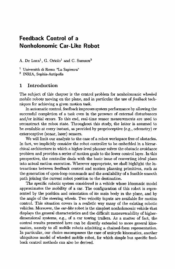
Feedback Control of a Nonholonomic Car-Like Robot
A. De Luca 1, G. Oriolo 1 and C. Samson 2
1 Universit~ di Roma "La Sapienza" INRIA, Sophia-Antipolis
1 I n t r o d u c t i o n
The subject of this chapter is the control problem for nonholonomic wheeled mobile robots moving on the plane, and in particular the use of ]eedback tech- niques for achieving a given motion task.
In automatic control, feedback improves system performance by allowing the successful completion of a task even in the presence of external disturbances and/or initial errors. To this end, real-time sensor measurements are used to reconstruct the robot state. Throughout this study, the latter is assumed to be available at every instant, as provided by proprioceptive (e.g., odometry) or exteroceptive (sonar, laser) sensors.
We will limit our analysis to the case of a robot workspace free of obstacles. In fact, we implicitly consider the robot controller to be embedded in a hierar- chical architecture in which a higher-level planner solves the obstacle avoidance problem and provides a series of motion goals to the lower control layer. In this perspective, the controller deals with the basic issue of converting ideal plans into actual motion execution. Wherever appropriate, we shall highlight the in- teractions between feedback control and motion planning primitives, such as the generation of open-loop commands and the availability of a feasible smooth path joining the current robot position to the destination.
The specific robotic system considered is a vehicle whose kinematic model approximates the mobility of a car. The configuration of this robot is repre- sented by the position and orientation of its main body in the plane, and by the angle of the steering wheels. Two velocity inputs are available for motion control. This situation covers in a realistic way many of the existing robotic vehicles. Moreover, the car-like robot is the simplest nonholonomic vehicle that displays the general characteristics and the difficult maneuverability of higher- dimensional systems, e.g., of a car towing trailers. As a matter of fact, the control results presented here can be directly extended to more general kine- matics, namely to all mobile robots admitting a chained-form representation. In particular, our choice encompasses the case of unicycle kinematics, another ubiquitous model of wheeled mobile robot, for which simple but specific feed- back control methods can also be derived.
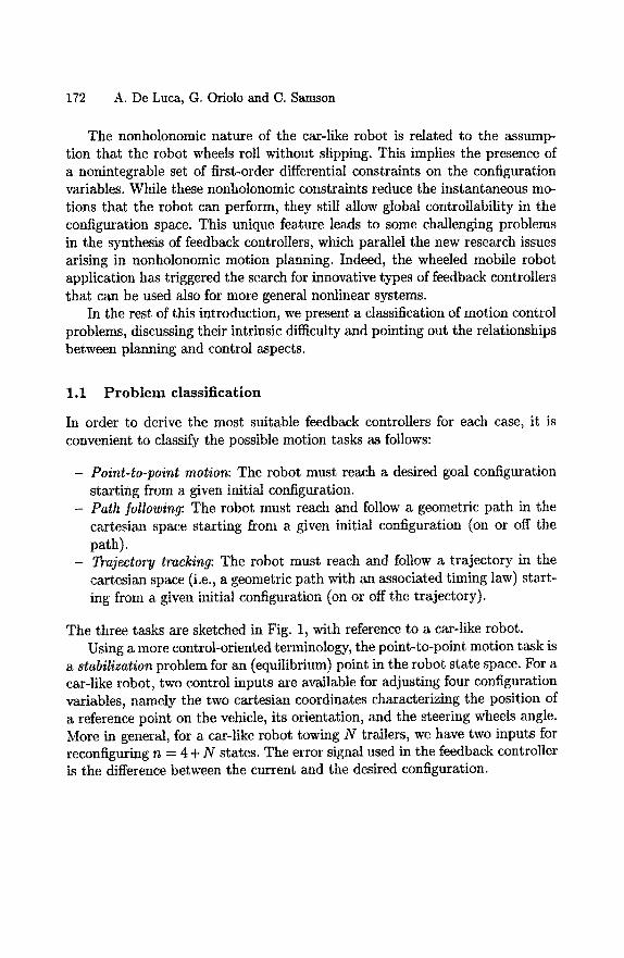
172 A. De Luca, G. Oriolo and C. Samson
The nonholonomic nature of the car-like robot is related to the assump- tion that the robot wheels roll without slipping. This implies the presence of a nonintegrable set of first-order differential constraints on the configuration variables. While these nonholonomic constraints reduce the instantaneous mo- tions that the robot can perform, they still allow global controllability in the configuration space. This unique feature leads to some challenging problems in the synthesis of feedback controllers, which parallel the new research issues arising in nonholonomic motion planning. Indeed, the wheeled mobile robot application has triggered the search for innovative types of feedback controllers that can be used also for more general nonlinear systems.
In the rest of this introduction, we present a classification of motion control problems, discussing their intrinsic difficulty and pointing out the relationships between planning and control aspects.
1.1 P r o b l e m classification
In order to derive the most suitable feedback controllers for each case, it is convenient to classify the possible motion tasks as follows:
- P o i n t - t o - p o i n t m o t i o n : The robot must reach a desired goal configuration starting from a given initial configuration.
- P a t h f o l l o w i n g : The robot must reach and follow a geometric path in the cartesian space starting from a given initial configuration (on or off the path).
- T r a j e c t o r y t r a c k i n g : The robot must reach and follow a trajectory in the cartesian space (i.e., a geometric path with an associated timing law) start- ing from a given initial configuration (on or off the trajectory).
The three tasks are sketched in Fig. 1, with reference to a car-like robot. Using a more control-oriented terminology, the point-to-point motion task is
a s t a b i l i z a t i o n problem for an (equilibrium) point in the robot state space. For a car-like robot, two control inputs are available for adjusting four configuration variables~ namely the two cartesian coordinates characterizing the position of a reference point on the vehicle, its orientation, and the steering wheels angle. More in general, for a car-like robot towing N trailers, we have two inputs for reconfiguring n = 4 + N states. The error signal used in the feedback controller is the difference between the current and the desired configuration.
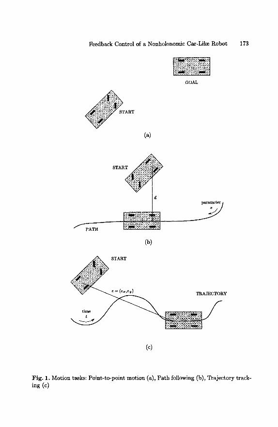
Feedback Control of a Nonholonomic Car-Like Robot 173
START
GOAL
Ca)
START
PATH
START
(b)
parameter ~
TRAJECTORY
time t
(c)
Fig. 1. Motion tasks: Point-to-point motion (a), Path following (b), Trajectory track- ing (c)
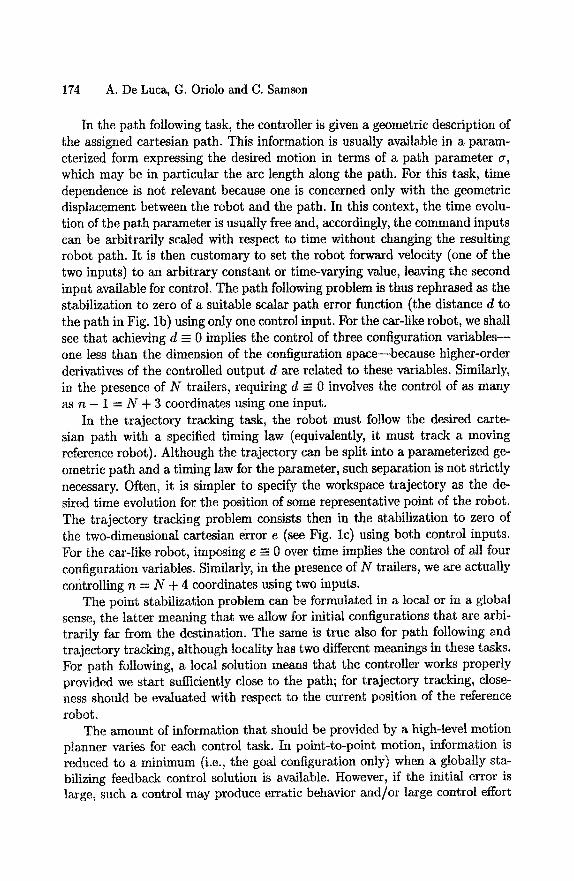
174 A. De Luca, G. Oriolo and C. Samson
In the path following task, the controller is given a geometric description of the assigned cartesian path. This information is usually available in a param- eterized form expressing the desired motion in terms of a path parameter a, which may be in particular the arc length along the path. For this task, time dependence is not relevant because one is concerned only with the geometric displacement between the robot and the path. In this context, the time evolu- tion of the path parameter is usually free and, accordingly, the command inputs can be arbitrarily scaled with respect to time without changing the resulting robot path. It is then customary to set the robot forward velocity (one of the two inputs) to an arbitrary constant or time-varying value, leaving the second input available for control. The path following problem is thus rephrased as the stabilization to zero of a suitable scalar path error function (the distance d to the path in Fig. lb) using only one control input. For the car-like robot, we shall see that achieving d = 0 implies the control of three configuration variables-- one less than the dimension of the configuration space--because higher-order derivatives of the controlled output d are related to these variables. Similarly, in the presence of N trailers, requiring d - 0 involves the control of as many as n - 1 = N + 3 coordinates using one input.
In the trajectory tracking task, the robot must follow the desired carte- sian path with a specified timing law (equivalently, it must track a moving reference robot). Although the trajectory can be split into a parameterized ge- ometric path and a timing law for the parameter, such separation is not strictly necessary. Often, it is simpler to specify the workspace trajectory as the de- sired time evolution for the position of some representative point of the robot. The trajectory tracking problem consists then in the stabilization to zero of the two-dimensional cartesian error e (see Fig. lc) using both control inputs. For the car-like robot, imposing e - 0 over time implies the control of all four configuration variables. Similarly, in the presence of N trailers, we are actually controlling n = N + 4 coordinates using two inputs.
The point stabilization problem can be formulated in a local or in a global sense, the latter meaning that we allow for initial configurations that are arbi- trarily far from the destination. The same is true also for path following and trajectory tracking, although locality has two different meanings in these tasks. For path following, a local solution means that the controller works properly provided we start sufficiently close to the path; for trajectory tracking, close- ness should be evaluated with respect to the current position of the reference robot.
The amount of information that should be provided by a high-level motion planner varies for each control task. In point-to-point motion, information is reduced to a minimum (i.e., the goal configuration only) when a globally sta- bilizing feedback control solution is available. However, if the initial error is large, such a control may produce erratic behavior and/or large control effort

Feedback Control of a Nonholonomic Car-Like Robot 175
which are unacceptable in practice. On the other hand, a local feedback solu- tion requires the definition of intermediate subgoals at the task planning level in order to get closer to the final desired configuration.
For the other two motion tasks, the planner should provide a path which is kinematically feasible (namely, which complies with the nonholonomic con- straints of the specific vehicle), so as to allow its perfect execution in nominal conditions. While for an omnidirectional robot any path is feasible, some degree of geometric smoothness is in general required for nonhotonomic robots. Nev- ertheless, the intrinsic feedback structure of the driving commands enables to recover transient errors due to isolated path discontinuities. Note also that the unfeasibility arising from a lack of continuity in some higher-order derivative of the path may be overcome by appropriate motion timing. For example, paths with discontinuous curvature (like the Reeds and Shepp optimal paths under maximum curvature constraint) can be executed by the real axle midpoint of a car-like vehicle provided that the robot is allowed to stop, whereas paths with discontinuous tangent are not feasible. In this analysis, the selection of the robot representative point for path/trajectory planning is critical.
The timing profile is the additional item needed in trajectory tracking con- trol tasks. This information is seldom provided by current motion planners, also because the actual dynamics of the specific robot are typically neglected at this level. The above example suggests that it may be reasonable to enforce already at the planning stage requirements such as 'move slower where the path curvature is higher'.
1.2 Cont ro l issues
From a control point of view, the previously described motion tasks are defined for the nonlinear system
q=G(q)v , (1)
representing the kinematic model of the robot. Here, q is the n-vector of robot generalized coordinates, v is the m-vector of input velocities (m < n), and the columns gi (i = 1 , . . . , m) of matrix G are smooth vector fields. For the car-like robot, it is n = 4 and m = 2.
The above model can be directly derived from the nonintegrable rolling constraints governing the system kinematic behavior. System (1) is driftless, a characteristic of first-order kinematic models. Besides, its nonlinear nature is intrinsically related to the nonholonomy of the original Pfaffian constraints. In turn, it can be shown that this is equivalent to the global accessibility of the n-dimensional robot configuration space in spite of the reduced number of inputs.
176 A. De Luca, G. Oriolo and C. Samson
Interestingly, the nonholonomy of system (1) reverses the usual order of dif- ficulty of robot control tasks. For articulated manipulators, and in general for all mechanical systems with as malay control inputs as generalized coordinates, stabilization to a fixed configuration is simpler than tracking a trajectory. In- stead, stabilizing a wheeled mobile robot to a point is more difficult than path following or trajectory tracking.
A simple way to appreciate such a difference follows from the general discus- sion of the previous section. The point-to-point task is actually an input-state problem with m = 2 inputs and n controlled states. The path following task is an input-output problem with m = 1 input and p = 1 controlled output, implying the indirect control of n - 1 states. The trajectory tracking task is again an input-output problem with m = 2 inputs and p = 2 controlled out- puts, implying the indirect control of n states. As a result, the point-to-point motion task gives rise to the most difficult control problem, since we are try- ing to control n independent variables using only two input commands. The path following and trajectory tracking tasks have a similar level of difficulty, being 'square' control problems (same number of control inputs and controlled variables).
This conclusion can be supported by a more rigorous controllability analysis. In particular, one can test whether the above problems admit an approximate solution in terms of linear control design techniques. We shall see that if the system (1) is linearized at a fixed configuration, the resulting linear system is not controllable. On the other hand, the linearization of eq. (1) about a smooth trajectory gives rise to a linear time-varying system that is controllable, provided some persistency conditions are satisfied by the reference trajectory.
The search for a feedback solution to the point stabilization problem is further complicated by a general theoretical obstruction. Although the kine- matic model (1) can be shown to be controllable using nonlinear tools from differential geometry, it fails to satisfy a necessary condition for stabilizabil- ity via smooth time-invariant feedback (Brockett's theorem). This means that the class of stabilizing controllers should be suitably enlarged so as to include nonsmooth and/or time-varying feedback control laws.
We finally point out that the design of feedback controllers for the path following task can be tackled from two opposite directions. In fact, by separat- ing the geometric and timing information of a trajectory, path following may be seen as a subproblem of trajectory tracking. On the other hand, looking at the problem from the point of view of controlled states (in the proper coordi- nates), path following appears as part of a point stabilization task. The latter philosophy will be adopted in this chapter.
Feedback Control of a Nonholonomic Car-Like Robot 177
1.3 Open- loop vs. closed-loop control
Some comments are now appropriate concerning the relationships between the planning and control phases in robot motion execution.
Essentially, we regard planning and open-loop (or feedforward) control as synonyms, as opposed to feedback control. In a general setting, a closed-loop controller results from the superposition of a feedback action to a coherent feedforward term. The latter is determined based on a priori knowledge about the motion task and the environment, which may have been previously acquired by exteroceptive sensors. Feedback control is instead computed in real-time based on external/internal sensor data.
However, the borderline between open-loop and closed-loop control solu- tions may not be so sharp. In fact, we may use repeated open-loop phases, replanned at higher rates using new sensor data to gather information on the actual state. In the limit, continuous sensing and replanning leads to a feedback solution. Although this scheme is conceptually simple, its convergence analysis may not be easy. Thus, we prefer to consider the planning and control phases separately.
For wheeled mobile robots, the usual output of the planning phase, which takes into account the obstacle avoidance requirement, is a kinematically fea- sible path with associated nominal open-loop commands. To guarantee fea- sibility, the planner may either take directly into account the nonholonomic constraints in the generation of a path, or create a preliminary holonomic path with standard techniques and then approximate it with a concatenation of feasible subpaths.
In the planning phase, it is also possible to include an optimality criterion together with system state and input constraints. It is often possible to obtain a solution by applying optimal (open-loop) control results. A typical cost cri- terion for the car-like robot is the total length of the collision-free path joining source to destination, while constraints include bounds on the steering angle as well as on the linear and angular velocity. In any case, the resulting com- mands are computed off-line. Hence, unmodeled events at running time, such as occasional slipping of the wheels or erroneous initial localization, will prevent the successful completion of a point-to-point motion or the correct tracing of a desired path.
The well-known answer to such problems is resorting to a feedback con- troller, driven by the current task error, so as to achieve some degree of ro- bustness. However, this should by no means imply the abdication to the use of the nominal open-loop command computed in the planning phase, which is included as the feedforward term in the closed-loop controller. As soon as the task error is zero, the feedback signal is not in action and the output command of the controller coincides with the feedforward term.
178 A. De Luca, G. Oriolo and C. Samson
The path and trajectory tracking controllers presented in this chapter agree with this combined approach. In fact, the feedforward represents the anticipa- tive action needed to drive the robot along the desired nominal motion. We point out that a shortcoming arises when the planner generates optimal feed- forward commands that are at their saturation level, because this leaves no room for the correcting feedback action. This is a common problem in open- loop optimal control; unfortunately, optimal feedback control laws for nonlinear systems are quite difficult to obtain in explicit form.
On the other hand, it follows from the discussion in Sect. 1.1 that no feedfor- ward is required in principle for the point stabilization task, so that the executed trajectory results from the feedback action alone. While this approach may be satisfactory for fine motion tasks, in gross motion a pure feedback control may drive the mobile robot toward the goal in an unpredictable way. In this case, a closer integration of planning and control would certainly improve the overall performance.
1.4 Organiza t ion of contents
We will present some of the most significant feedback control strategies for the different robot motion tasks. For each method, we discuss the single design steps and illustrate the typical performance by simulations. Results are presented in a consistent way in order to allow for comparisons. The organization of the rest of the chapter is as follows.
Section 2 is devoted to preliminary material. The kinematic model of the car-like robot is introduced, stating the main assumptions and distinguishing the cases of rear-wheel and front-wheel driving. We analyze the local control- lability properties at a configuration and about a trajectory. Global controlla- bility is proved in a nonlinear setting and a negative result concerning smooth feedback stabilizability is recalled. This section is concluded by presenting the chained-form transformation of the model and its essential features.
In Sect. 3 we address the trajectory tracking problem. The generation of suitable feedforward commands for a given smooth trajectory is discussed. In particular, we point out how geometric and timing information can be handled separately. A simple linear controller is devised for the chained-form represen- tation of the car-like robot, using the approximate system linearization around the nominal trajectory. Then, we present two nonlinear controllers based on exact feedback linearization. The first uses static feedback to achieve input- output linearization for the original kinematic model of the car-like robot. The second is a full-state linearizing dynamic feedback designed on the chained-form representation. Both guarantee global tracking with prescribed linear error dy- namics.
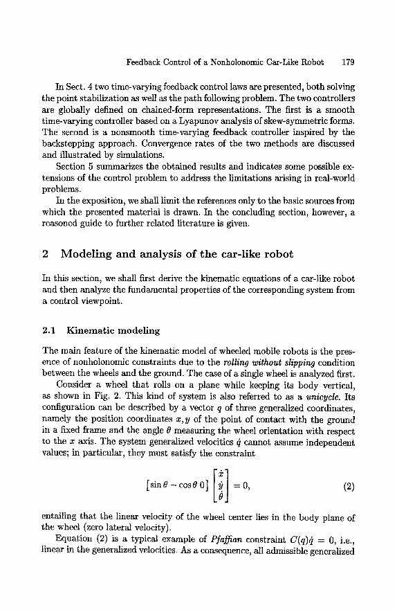
Feedback Control of a Nonholonomic Car-Like Robot 179
In Sect. 4 two time-varying feedback control laws are presented, both solving the point stabilization as well as the path following problem. The two controllers are globally defined on chained-form representations. The first is a smooth time-varying controller based on a Lyapunov analysis of skew-symmetric forms. The second is a nonsmooth time-varying feedback controller inspired by the backstepping approach. Convergence rates of the two methods are discussed and illustrated by simulations.
Section 5 summarizes the obtained results and indicates some possible ex- tensions of the control problem to address the limitations arising in real-world problems.
In the exposition, we shall limit the references only to the basic sources from which the presented material is drawn. In the concluding section, however, a reasoned guide to further related literature is given.
2 M o d e l i n g a n d a n a l y s i s o f t h e c a r - l i k e r o b o t
In this section, we shall first derive the kinematic equations of a car-like robot and then analyze the fundamental properties of the corresponding system from a control viewpoint.
2.1 K inema t i c mode l ing
The main feature of the kinematic model of wheeled mobile robots is the pres- ence of nonholonomic constraints due to the rolling without slipping condition between the wheels and the ground. The case of a single wheel is analyzed first.
Consider a wheel that rolls on a plane while keeping its body vertical, as shown in Fig. 2. This kind of system is also referred to as a unicycle. Its configuration can be described by a vector q of three generalized coordinates, namely the position coordinates x, y of the point of contact with the ground in a fixed frame and the angle ~ measuring the wheel orientation with respect to the x axis. The system generalized velocities q cannot assume independent values; in particular, they must satisfy the constraint
[ sin ~ - cos 8 0 ] -= 0, (2)
entailing that the linear velocity of the wheel center lies in the body plane of the wheel (zero lateral velocity).
Equation (2) is a typical example of P]aJfian constraint C(q)(l = O, i.e., linear in the generalized velocities. As a consequence, all admissible generalized
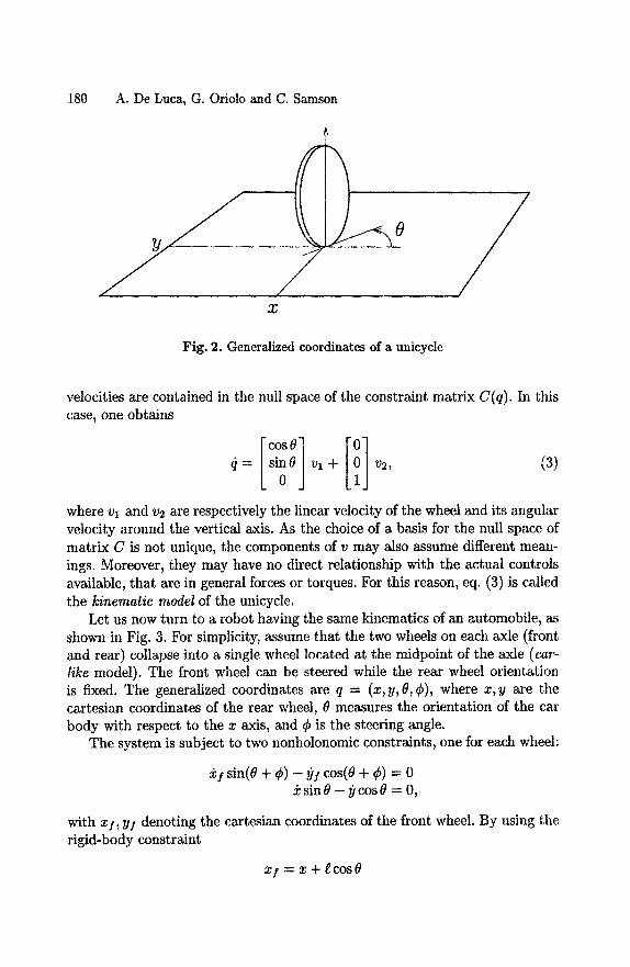
180 A. De Luca, G. Oriolo and C. Samson
~ "0 "
/ X
f Fig. 2. Generalized coordinates of a unicycle
velocities are contained in the null space of the constraint matrix C(q). In this case, one obtains
rcosol [ ioOj v,-,- ,,2, (3)
where vl and v2 are respectively the linear velocity of the wheel and its angular velocity around the vertical axis. As the choice of a basis for the null space of matr ix C is not unique, the components of v may also assume different mean- ings. Moreover, they may have no direct relationship with the actual controls available, that are in general forces or torques. For this reason, eq. (3) is called the kinematic model of the unicycle.
Let us now turn to a robot having the same kinematics of an automobile, as shown in Fig. 3. For simplicity, assume that the two wheels on each axle (front and rear) collapse into a single wheel located at the midpoint of the axle (car- like model). The front wheel can be steered while the rear wheel orientation is fixed. The generalized coordinates are q = (x,y,O,¢), where x ,y are the cartesian coordinates of the rear wheel, 0 measures the orientation of the car body with respect to the x axis, and ¢ is the steering angle.
The system is subject to two nonholonomic constraints, one for each wheel:
:~I sin(O+ ¢) - ~)I cos(O+ ~b) = 0 ksinO - ycos0 = O,
with xi, yf denoting the cartesian coordinates of the front wheel. By using the rigid-body constraint
x! = x + ~cos0
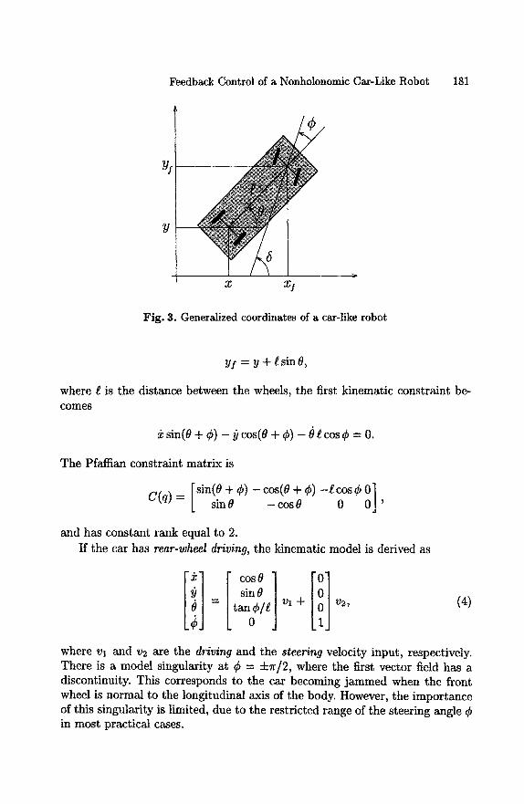
Feedback Control of a Nonholonomic Car-Like Robot 181
yf
Y
Fig. 3. Generalized coordinates of a car-like robot
YI = Y + l sin 0,
where g is the distance between the wheels, the first kinematic constraint be- comes
5:sin(0 + ¢) - 9 cos(0 + ¢) - 0 g cos ¢ = O.
The Pfaffian constraint matrix is
[sin(0 + ¢) - cos(0 + ¢) - t c o s ¢ ~] C(q)= [ sin/9 - c o s O 0 '
and has constant rank equal to 2. If the car has rear-wheel driving, the kinematic model is derived as
/ sin/? /
= Lto,/, j v,÷ v2, (4)
where vl and v2 are the driving and the steering velocity input, respectively. There is a model singularity at ¢ = 4-~r/2, where the first vector field has a discontinuity. This corresponds to the car becoming jammed when the front wheel is normal to the longitudinal axis of the body. However, the importance of this singularity is limited, due to the restricted range of the steering angle ¢ in most practical cases.
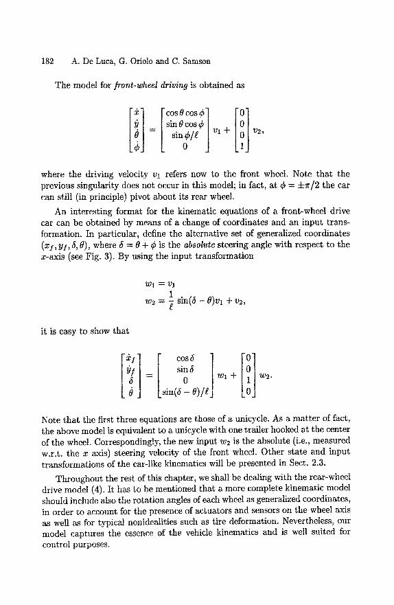
182 A. De Luca, G. Oriolo and C. Samson
The model for front-wheel driving is obtained as
[i] rcos0cos l [i] = | s i n 0 c o s ¢ | V2,
where the driving velocity Vl refers now to the front wheel. Note that the previous singularity does not occur in this model; in fact, at ¢ = 4-r/2 the car can still (in principle) pivot about its rear wheel.
An interesting format for the kinematic equations of a front-wheel drive car can be obtained by means of a change of coordinates and an input trans- formation. In particular, define the alternative set of generalized coordinates (x], y / , 5, 0), where 5 = 0 + ¢ is the absolute steering angle with respect to the x-axis (see Fig. 3). By using the input transformation
Wl --'= Vl
1 w2 = ~ sin(~ - O)vl + v2,
it is easy to show that
[i] ---- Wl + W2-
L sin(5 - e ) /eJ
Note that the first three equations are those of a unicycle. As a mat ter of fact, the above model is equivalent to a unicycle with one trailer hooked at the center of the wheel. Correspondingly, the new input w2 is the absolute (i.e., measured w.r.t, the x axis) steering velocity of the front wheel. Other state and input transformations of the car-like kinematics will be presented in Sect. 2.3.
Throughout the rest of this chapter, we shall be dealing with the rear-wheel drive model (4). It has to be mentioned that a more complete kinematic model should include also the rotation angles of each wheel as generalized coordinates, in order to account for the presence of actuators and sensors on the wheel axis as well as for typical nonidealities such as tire deformation. Nevertheless, our model captures the essence of the vehicle kinematics and is well suited for control purposes.
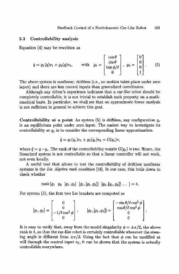
Feedback Control of a Nonholonomic Car-Like Robot 183
2.2 C o n t r o l l a b i l i t y ana lys i s
Equation (4) may be rewritten as
q=gl(q)vl÷g2(q)v2, with
r cos01 | sine |
g l = [tano¢/gj' g2= " (5)
The above system is nonlinear, driftless (i.e., no motion takes place under zero input) and there are less control inputs than generalized coordinates.
Although any driver's experience indicates that a car-like robot should be completely controllable, it is not trivial to establish such property on a math- ematical basis. In particular, we shall see that an approximate linear analysis is not sufficient in general to achieve this goal.
C o n t r o l l a b i l i t y a t a p o i n t As system (5) is driftless, any configuration qe is an equilibrium point under zero input. The easiest way to investigate its controllability at qe is to consider the corresponding linear approximation
~=gl(qe)vl-t-g2(qe)v2=G(qe)v,
where ~ = q-qe. The rank of the controllability matrix G(qe) is two. Hence, the tinearized system is not controllable so that a linear controller will not work, not even locally.
A useful tool that allows to test the controllability of driftless nonlinear systems is the Lie Algebra rank condition [18]. In our case, this boils down to check whether
rank[gl g2 [gl,g2] [gl, [gl,g2]] [g2,[gl,g2]]... ] = 4.
For system (5), the first two Lie brackets are computed as
[gl, g2] = 0
- 1 / ~ c o s 2 '
0
[gl, [gl, g2]] :
" - sin O/g cos 2 ¢] c°sO/ic°s2 ¢ ] "
It is easy to verify that, away from the model singularity ¢ = =k~r/2, the above rank is 4, so that the car-like robot is certainly controllable whenever the steer- ing angle is different from :kr/2. Using the fact that ¢ can be modified at will through the control input v2, it can be shown that the system is actually controllable everywhere.
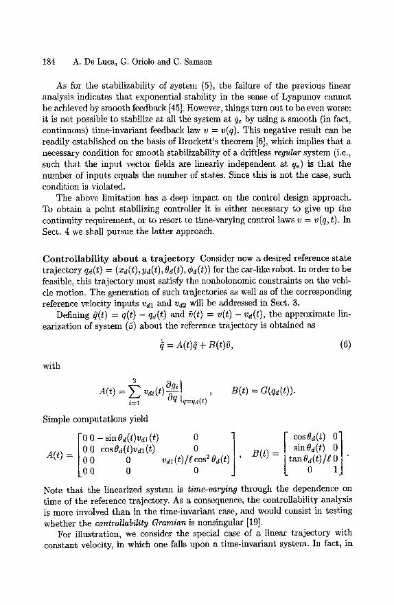
184 A. De Luca, G. Oriolo and C. Samson
As for the stabilizability of system (5), the failure of the previous linear analysis indicates that exponential stability in the sense of Lyapunov cannot be achieved by smooth feedback [45]. However, things turn out to be even worse: it is not possible to stabilize at all the system at qe by using a smooth (in fact, continuous) time-invariant feedback law v = v(q). This negative result can be readily established on the basis of Brockett's theorem [6], which implies that a necessary condition for smooth stabilizability of a driftless regular system (i.e., such that the input vector fields are linearly independent at qe) is that the number of inputs equals the number of states. Since this is not the case, such condition is violated.
The above limitation has a deep impact on the control design approach. To obtain a point stabilizing controller it is either necessary to give up the continuity requirement, or to resort to time-varying control laws v = v(q, t). In Sect. 4 we shall pursue the latter approach.
Control labi l i ty abou t a t r a j ec to ry Consider now a desired reference state trajectory qd(t) = (xd(t), yd(t), Od(t), Cd(t)) for the car-like robot. In order to be feasible, this trajectory must satisfy the nonholonomic constraints on the vehi- cle motion. The generation of such trajectories as well as of the corresponding reference velocity inputs Vdl and vd2 will be addressed in Sect. 3.
Defining ~(t) = q(t) - qd(t) and ~(t) = v(t) - va(t), the approximate lin- earization of system (5) about the reference trajectory is obtained as
= A(t)q + B(t)~, (6)
with
2 Ogi t A(t) = E Vdi(t)~q q=qd( )' i=1
B(t) = G(qd(t)).
Simple computations yield
i 0 - sin Od(t)vdl (t) 0 ] A(t) = 0 0 cosOd(t)vdl(t) 0
0 0 (t)/e cos 2 On(t) ' 0 0 0
B(t) = cos0d(t) i] sinOd(t)
tan0d(t)/~ " 0
Note that the linearized system is t ime-varying through the dependence on time of the reference trajectory. As a consequence, the controllability analysis is more involved than in the time-invariant case, and would consist in testing whether the controllability Gramian is nonsingular [19].
For illustration, we consider the special case of a linear trajectory with constant velocity, in which one falls upon a time-invariant system. In fact, in
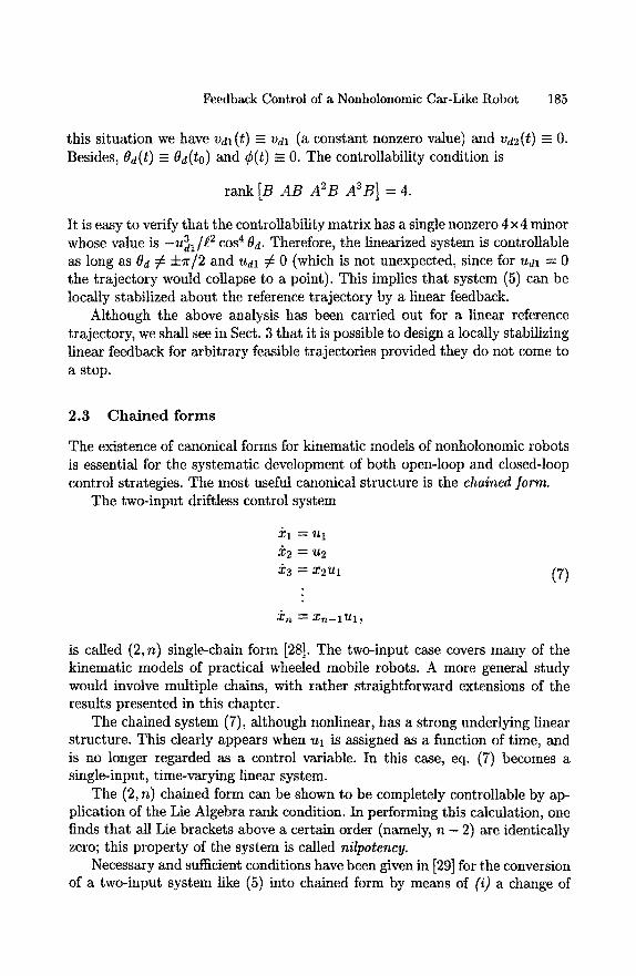
Feedback Control of a Nonholonomic Car-Like Robot 185
this situation we have vdl (t) =_ Vdl (a constant nonzero value) and vd~ (t) = 0. Besides, Od(t) =-- Od(tO) and ¢(t) = 0. The controllability condition is
rank [B A B A2B A3B] = 4.
It is easy to verify that the controllability matrix has a single nonzero 4×4 minor whose value is -u31/g 2 cos 40d. Therefore, the linearized system is controllable as long as Od ~ ±~r/2 and Udl ~ 0 (which is not unexpected, since for udl = 0 the trajectory would collapse to a point). This implies that system (5) can be locally stabilized about the reference trajectory by a linear feedback.
Although the above analysis has been carried out for a linear reference trajectory, we shall see in Sect. 3 that it is possible to design a locally stabilizing linear feedback for arbitrary feasible trajectories provided they do not come to a stop.
2.3 Cha ined forms
The existence of canonical forms for kinematic models of nonhotonomic robots is essential for the systematic development of both open-loop and closed-loop control strategies. The most useful canonical structure is the chained ]orm.
The two-input driftless control system
Xl = Ul
X2 = U2
X3 "~ X2Ul
:~n = :~n- - lUl ,
(7)
is called (2, n) single-chain form [28]. The two-input case covers many of the kinematic models of practical wheeled mobile robots. A more general study would involve multiple chains, with rather straightforward extensions of the results presented in this chapter.
The chained system (7), although nonlinear, has a strong underlying linear structure. This clearly appears when ua is assigned as a function of time, and is no longer regarded as a control variable. In this case, eq. (7) becomes a single-input, time-varying linear system.
The (2, n) chained form can be shown to be completely controllable by ap- plication of the Lie Algebra rank condition. In performing this calculation, one finds that all Lie brackets above a certain order (namely, n - 2) are identically zero; this property of the system is called nilpotency.
Necessary and sufficient conditions have been given in [29] for the conversion of a two-input system like (5) into chained form by means of (i) a change of
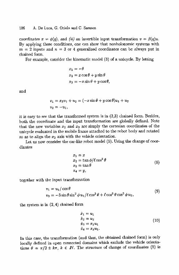
186 A. De Luca, G. Oriolo and C. Samson
coordinates x -- ¢(q), and (ii) an invertible input transformation v -- ~(q)u. By applying these conditions, one can show that nonholonomic systems with m -- 2 inputs and n = 3 or 4 generalized coordinates can be always put in chained form.
For example, consider the kinematic model (3) of a unicycle. By letting
xl ---- --9
x2 = xcos9 + y s i n 9
x3 = --xsin9 + ycosg,
and
vl = x3ul + u2 = ( - x sin 9 + y cos 0)ul + u2
Y 2 -~- - - U 1 ,
it is easy to see that the transformed system is in (2,3) chained form. Besides, both the coordinate and the input transformation are globally defined. Note that the new variables x2 and x3 are simply the cartesian coordinates of the unicycle evaluated in the mobile frame attached to the robot body and rotated so as to align the x2 axis with the vehicle orientation.
Let us now consider the car-like robot model (5). Using the change of coor-
dinates
Xl ----~ x2 = t an¢ /gcosa9 x3 = tan 9 X4 = y ,
(s)
together with the input transformation
vl = u l / cos9
v2 = - 3 singsin 2 C u l / g c o s 2 9 + gcos 3 9cos 2 ¢u2, (9)
the system is in (2, 4) chained form
X2 ~ U2
X 3 " - X 2 U l
X 4 - . . ~ X 3 U l .
(10)
In this case, the transformation (and thus, the obtained chained form) is only locally defined in open connected domains which exclude the vehicle orienta- tions 9 = ~r/2 =t= k~r, k E ~W. The structure of change of coordinates (8) is
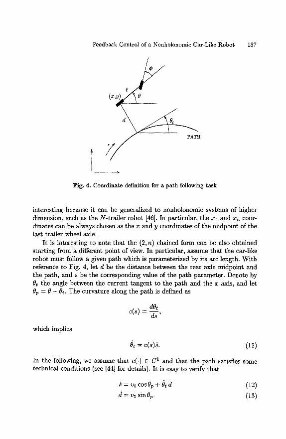
Feedback Control of a Nonholonomic Car-Like Robot 187
PATH
J/
Fig. 4. Coordinate definition for a path following task
interesting because it can be generalized to nonholonomic systems of higher dimension, such as the N-trailer robot [46]. In particular, the xl and xn coor- dinates can be always chosen as the x and y coordinates of the midpoint of the last trailer wheel axle.
It is interesting to note that the (2, n) chained form can be also obtained starting from a different point of view. In particular, assume that the car-like robot must follow a given path which is parameterized by its arc length. With reference to Fig. 4, let d be the distance between the rear axle midpoint and the path, and s be the corresponding value of the path parameter. Denote by Ot the angle between the current tangent to the path and the x axis, and let Op = 0 - Or. The curvature along the path is defined as
dot
= Z 2 '
which implies
Ot =c(s)a. (11)
In the following, we assume that c(-) E C 1 and that the path satisfies some technical conditions (see [44] for details). It is easy to verify that
--~ L~I COS Op q- 0 t d (12)
d = Vl s i n 0 p . (13)
188 A. De Luca, G. Oriolo and C. Samson
Equations (12-13) may be COmbined with model (4) in order to derive the kinematic equations in terms of path coordinates qp = (s, d, 8p, ¢):
Ii] 1 - de(s)
sin 0p
( ~ . . ¢ _ c(s )cosO, ) i - dc(s) / 0
Vl + v2. (14)
The above model can be put in the (2, 4) chained form by using the change of coordinates
• 1 ~ 8
x2 = - d ( s ) d t a n O v - c(s)(1 - de(s)) 1 + sin2 0p (1 - de(s)) 2 tan ¢ cos 20p + ~ cos 30p (15)
x3 = (1 - dc(s)) tan ~p x4 = d,
together with the input transformation
1 - de(s) Vl = COS Op Ul
V2 = a 2 ( q p ) ( U 2 -- O~l(qp)Ul) .
In the above formulas, d ( s ) denotes the derivative of c with respect to s, and we have set
Ox2 ( t a n ¢ ( 1 - dc(s))
t cos 30p cos 2 ¢ a2(qp) = ( 1 - d e ( s ) ) 2 "
Also this chained-form transformation is locally defined in open connected do- mains, because 0p = ~r/2 :k k~r, k E ~V, must be excluded. Note that in the particular case c(s) - O, one recovers the previous expressions (8) and (9). In fact, in this situation the path may be taken as the x-axis of the world frame, and (s, d, 0p) become the coordinates (x, y, ~) of the vehicle.
We conclude this section by pointing out that there are other canonical forms that can be successfully used in connection with nonholonomic systems, namely the Caplygin form and the power form. It is noteworthy that, for m = 2 inputs, the three canonical forms are mathematically equivalent, since there exist global coordinate transformations that allow to convert one into the oth- ers [211 •
Feedback Control of a Nonholonomic Car-Like Robot 189
3 Trajectory tracking
In this section, we consider the problem of tracking a given cartesian trajec- tory with the car-like robot using feedback control. Both a local and a global approach will be presented. In the first, we use a standard linear control design and obtain convergence provided that the car starts sufficiently close to the desired trajectory. In the second, we pursue a feedback linearization approach, achieving asymptotic stability for arbitrary initial states via static as well as dynamic nonlinear feedback.
In the following, extensive use is made of the chained-form representation. Such system transformation is not strictly necessary, but simplifies considerably the control design and provides at the same time a framework for the direct extension of the controllers to vehicles with more complex kinematics. In any case, the methods presented here can be applied to more general mobile robots, even those which cannot be put in chained form.
Before moving to the control design, we discuss the problem of generating state reference trajectories for the car-like robot, both in the original kinematic description (5) and in the chained form (10).
3.1 Re fe rence t r a j e c t o r y genera t ion
Assume that a feasible and smooth desired output trajectory is given in terms of the cartesian position of the car rear wheel, i.e.,
xd = xd( t ) , Yd = yd( t ) , t >_ tO. (16)
This natural way of specifying the motion of a car-like robot has an appealing property. In fact, from this information we are able to derive the corresponding time evolution of the remaining coordinates (state trajectory) as well as of the associated input commands (input trajectory) as shown hereafter.
The desired output trajectory (16) is feasible when it can be obtained from the evolution of a reference car-like robot
~d = COS0d Vdl (17)
~)d = sin Od vm (18)
Od -~ tan Cd Vm/t (19)
& = v~2, (20)
for suitable initial conditions (Xd (to), Yd (to), Od (to), d~d (to)) and piecewise-conti- nuous inputs vd(t), for t > to.
Solving for vm from eqs. (17) and (18) gives for the first input
vdl(t) = • ~ /~ ( t ) + y~(t), (21)
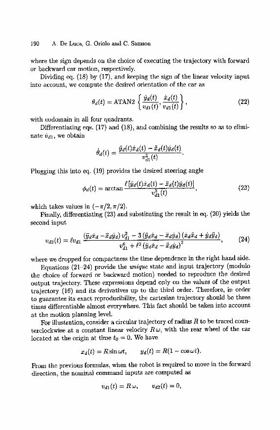
190 A. De Luca, G. Onolo and C. Samson
where the sign depends on the choice of executing the trajectory with forward or backward car motion, respectively.
Dividing eq. (18) by (17), and keeping the sign of the linear velocity input into account, we compute the desired orientation of the car as
0a(t) = ATAN2 { yd(t) 2a(t) } (22) Vdl( t ) ' Vdl(t) '
with codomain in all four quadrants. Differentiating eqs. (17) and (18), and combining the results so as to elimi-
nate ~)dl, we obtain
~d(t) = ~)d(t)2d(t) -- ~d(t)~)d(t) v l(t)
Plugging this into eq. (19) provides the desired steering angle
Cd(t) = arctan ~ [{jd(t)xd(t) -- Xd(t)~ld(t)] (23) V]l(t)
which takes values in ( -0 /2 , r /2) . Finally, differentiating (23) and substituting the result in eq. (20) yields the
second input
Vd2 (t) = ~val (ijdkd --Xd~ld) V21 -- 3 (~)dXd -- X~yd) (XdXd + Ydfta) (24) V61 -1- t 2 (ydXd - - ~d~]d) 2
where we dropped for compactness the time dependence in the right hand side. Equations (21-24) provide the unique state and input trajectory (modulo
the choice of forward or backward motion) needed to reproduce the desired output trajectory. These expressions depend only on the values of the output trajectory (16) and its derivatives up to the third order. Therefore, in order to guarantee its exact reproducibility, the cartesian trajectory should be three times differentiable almost everywhere. This fact should be taken into account at the motion planning level.
For illustration, consider a circular trajectory of radius R to be traced coun- terclockwise at a constant linear velocity R w , with the rear wheel of the car located at the origin at time to = 0. We have
xd(t) = Rsinwt, yd(t) = R(1 - cos~t).
From the previous formulas, when the robot is required to move in the forward direction, the nominal command inputs are computed as
v d l ( t ) = vd2(t) = 0 ,
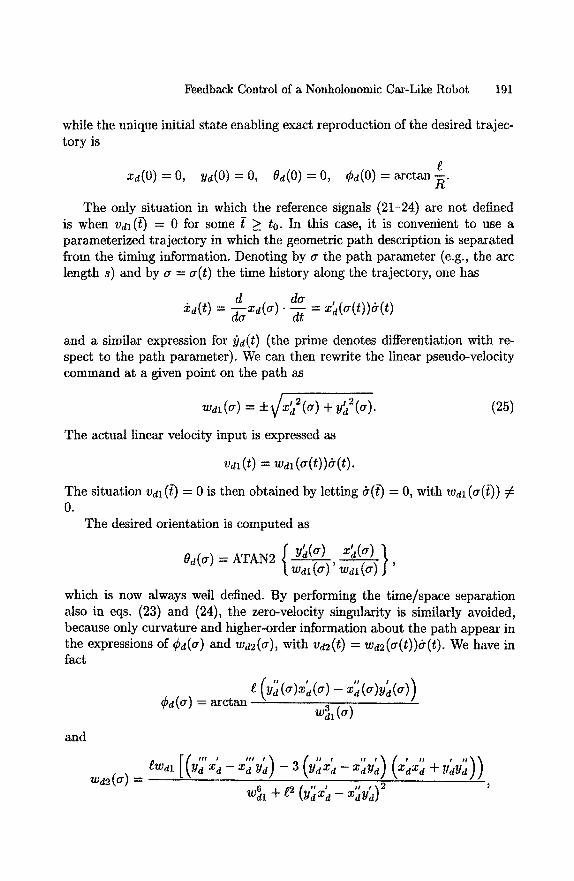
Feedback Control of a Nonholonomic Car-Like Robot 191
while the unique initial state enabling exact reproduction of the desired trajec- tory is
Xd(O) = O, yd(O) = 0, ~d(0) = 0, ¢d(0) = arctan ~ .
The only situation in which the reference signals (21-24) are not defined is when Vdl(t-) = 0 for some t > to. In this case, it is convenient to use a parameterized trajectory in which the geometric path description is separated from the timing information. Denoting by cr the path parameter (e.g., the arc length s) and by a = a ( t ) the time history along the trajectory, one has
de ~d(t ) = x e ( a ) . --~ = x '~(a( t ) )O(t )
and a similar expression for ~)a(t) (the prime denotes differentiation with re- spect to the path parameter). We can then rewrite the linear pseudo-velocity command at a given point on the path as
~1(~) = ±~/~2(~) + y~2(~). (25)
The actual linear velocity input is expressed as
Vdl(t) =Wdl (a(t))d(t).
The situation Vd~(t-) = 0 is then obtained by letting h(t-) = O, with Wdl(a(t-)) ~t O.
The desired orientation is computed as
Od(a) = ATAN2 ~" y~(a) , X~(ff)
t ~(~) ~--~) J' which is now always well defined. By performing the time/space separation also in eqs. (23) and (24), the zero-velocity singularity is similarly avoided, because only curvature and higher-order information about the path appear in the expressions of ~bd(a) and Wd2(cr), with Vd2(t) = Wd2(a(t))gr(t) . We have in fact
Cd(a) = arctan ~(~)
wd~(~) =
and
- XdYd)
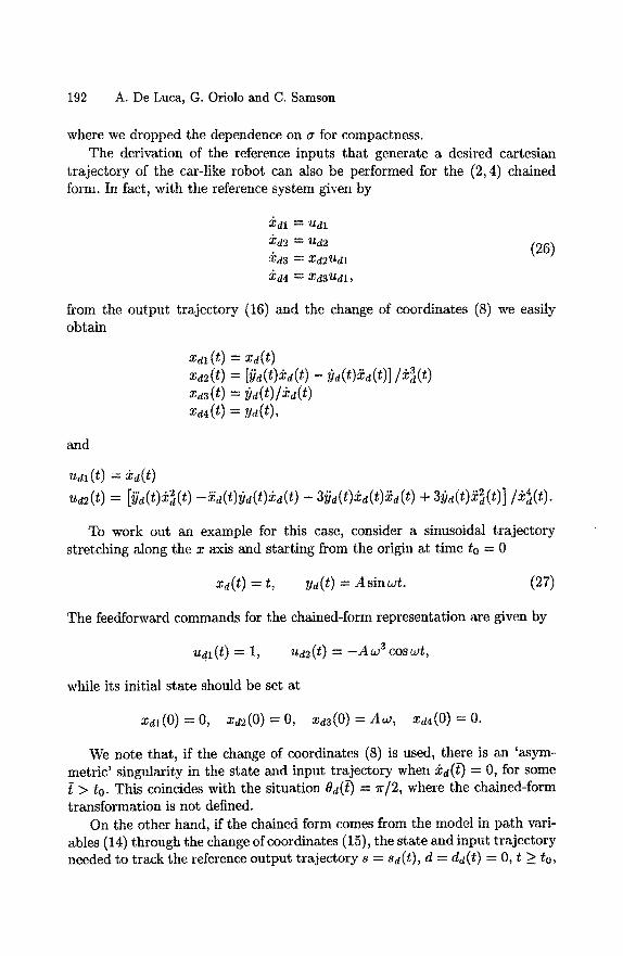
192 A. De Luca, G. Oriolo and C. Samson
where we dropped the dependence on a for compactness. The derivation of the reference inputs that generate a desired cartesian
trajectory of the car-like robot can also be performed for the (2, 4) chained form. In fact, with the reference system given by
Xdl ~ ~tdl
Xd2 : Ud2
Xd3 "~" Xd2Udl
:Bd4 : Xd3 l td l ,
(26)
from the output trajectory (16) and the change of coordinates (8) we easily obtain
x~ l ( t ) = xd(t) x~2 (t) = [/Jd (t)~d (t) - Yd(t)~d ( t ) ] / ~ ] (t) Xd3(t) = ~ld(t)/xd(t) Xd4(t) = yd(t),
and
~dl ( t ) = xd(t) Ud2(t) = [y'd(t)x2(t) --xd(t)yd(t)xd(t) - 3~d(t)~d(t)Xd(t) + 3!]d(t)X2d(t)] /x4(t) .
To work out an example for this case, consider a sinusoidal trajectory stretching along the x axis and starting from the origin at time to = 0
Xd(t) = t, yd(t) = A s i n w t . (27)
The feedforward commands for the chained-form representation are given by
Udl(t) = 1, Ud2(t) = - A w 3 coswt,
while its initial state should be set at
Xdt(O) =0 , Xd~(O) = O, xd3(O) = A w , Xd4(O) = 0 .
We note that, if the change of coordinates (8) is used, there is an 'asym- metric' singularity in the state and input trajectory when &d(t-) = 0, for some
> to. This coincides with the situation 8d(t-') = ~r/2, where the chained-form transformation is not defined.
On the other hand, if the chained form comes from the model in path vari- ables (14) through the change of coordinates (15), the state and input trajectory needed to track the reference output trajectory s = s d ( t ) , d = d d ( t ) -~ O, t > to,
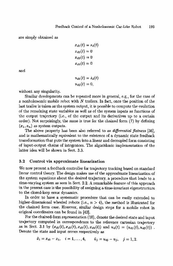
Feedback Control of a Nonholonomic Car-Like Robot 193
are simply obtained as
and
Xdl( t ) : Sd(t)
Xd2(t) = 0
Xd3(t) -~ 0
Xd4(t) = 0
Udl (t) = Sd(t)
Ud2(t) = O,
without any singularity. Similar developments can be repeated more in general, e.g., for the case of
a nonholonomic mobile robot with N trailers. In fact, once the position of the last trailer is taken as the system output, it is possible to compute the evolution of the remaining state variables as well as of the system inputs as functions of the output trajectory (i.e., of the output and its derivatives up to a certain order). Not surprisingly, the same is true for the chained form (7) by defining (xl, x,~) as system outputs.
The above property has been also referred to as differential flatness [36], and is mathematically equivalent to the existence of a dynamic state feedback transformation that puts the system into a linear and decoupled form consisting of input-output chains of integrators. The algorithmic implementation of the latter idea will be shown in Sect. 3.3.
3.2 Control via approximate linearization
We now present a feedback controller for trajectory tracking based on standard linear control theory. The design makes use of the approximate linearization of the system equations about the desired trajectory, a procedure that leads to a time-varying system as seen in Sect. 2.2. A remarkable feature of this approach in the present case is the possibility of assigning a time-invariant eigenstructure to the closed-loop error dynamics.
In order to have a systematic procedure that can be easily extended to higher-dimensional wheeled robots (i.e., n > 4), the method is illustrated for the chained form case. However, similar design steps for a mobile robot in original coordinates can be found in [42].
For the chained-form representation (10), denote the desired state and input trajectory computed in correspondence to the reference cartesian trajectory as in Sect. 3.1 by (Xdl (t), Xd2 (t), Xd3 (t), Xd4(t)) and ud(t) : (Udl (t), Ud2(t)) .
Denote the state and input errors respectively as
~i=Xd~--xi, i = 1 , . . . , 4 , f i j=u@--uj , j = l , 2 .
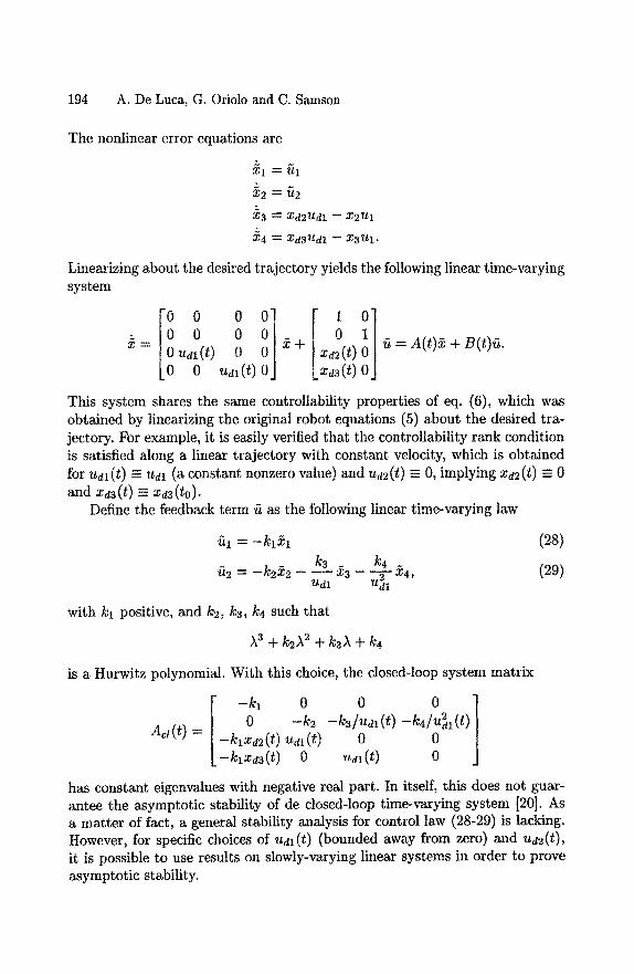
194 A. De Luca, G. Oriolo and C. Samson
The nonlinear error equations are
Xl ---- ?~1 5 X2 = U2
X 3 = X d 2 ~ d l -- X2U 1
X 4 --~ Xd3Udl - - X3~t 1.
Linearizing about the desired trajectory yields the following linear time-varying
[ 00 = 0 0 x = udl( t ) 0
0 Udl(t)
system
2 + 0 xd2(t) ~ = A( t )2 + B(t)~t.
d3(t)
This system shares the same controllability properties of eq. (6), which was obtained by linearizing the original robot equations (5) about the desired tra- jectory. For example, it is easily verified that the controllability rank condition is satisfied along a linear trajectory with constant velocity, which is obtained for Ud1(t) =--- Udl (a constant nonzero value) and Ud2(t) -~ 0, implying Xd2(t) -- 0 and Xda(t) = Xd3(to).
Define the feedback term fi as the following linear time-varying law
~1 ---~ --klXl (28)
~2 = -k222 k3 X3 k4 - ud-7 - 1124' (29)
with kl positive, and k2, k3, k4 such that
.~z + ku)~2 + k3,k + k4
is a Hurwitz polynomial. With this choice, the closed-loop system matrix
A a ( t ) =
- k l 0 0 - k 2
- - k l X d a ( t ) 0
0 0] 0° -- k 3 / U d l ( t ) - -~4/U2dl ( t )
0
has constant eigenvalues with negative real part. In itself, this does not guar- antee the asymptotic stability of de closed-loop time-varying system [20]. As a matter of fact, a general stability analysis for control law (28-29) is lacking. However, for specific choices of udl(t) (bounded away from zero) and Ud2(t), it is possible to use results on slowly-varying linear systems in order to prove asymptotic stability.
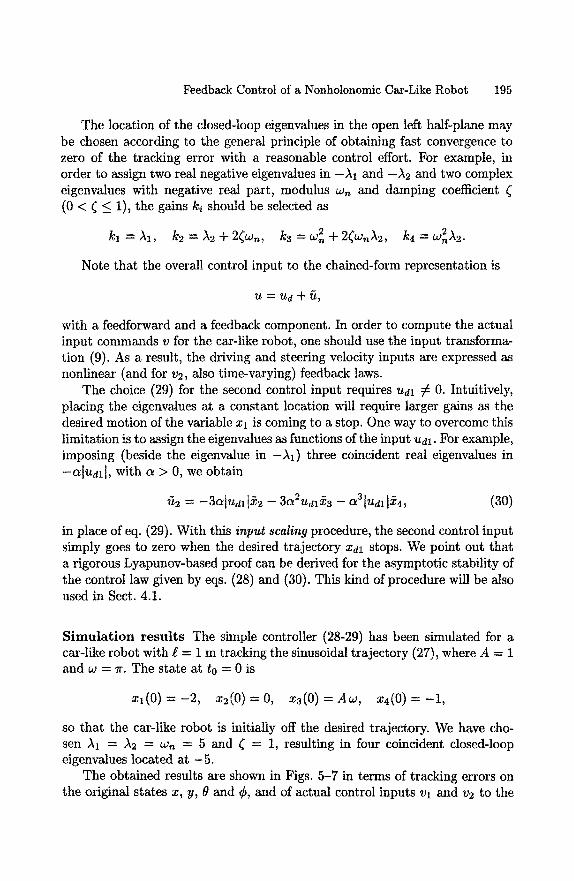
Feedback Control of a Nonholonomic Car-Like Robot 195
The location of the closed-loop eigenvalues in the open left half-plane may be chosen according to the general principle of obtaining fast convergence to zero of the tracking error with a reasonable control effort. For example, in order to assign two real negative eigenvalues in -A1 and -A2 and two complex eigenvalues with negative real part, modulus w, and damping coefficient (0 < ¢ < 1), the gains ki should be selected as
_ 2 2 kl = A1, k2 = A2 + 2(w~, k3 - wn + 2(w,,A2, k4 -- WnA2.
Note that the overall control input to the chained-form representation is
U : U d Jc U,
with a feedforward and a feedback component. In order to compute the actual input commands v for the car-like robot, one should use the input transforma- tion (9). As a result, the driving and steering velocity inputs are expressed as nonlinear (and for v2, also time-varying) feedback laws.
The choice (29) for the second control input requires Udl ~ 0. Intuitively, placing the eigenvalues at a constant location will require larger gains as the desired motion of the variable xl is coming to a stop. One way to overcome this limitation is to assign the eigenvalues as functions of the input udl. For example, imposing (beside the eigenvalue in -)~1) three coincident real eigenvalues in -a[udl l , with ~ > 0, we obtain
£~2 = - -3a tud115c2 - - 3012Udl X,3 - - C~ 3 IUd l I-~4, (30)
in place of eq. (29). With this input scaling procedure, the second control input simply goes to zero when the desired trajectory Xdl stops. We point out that a rigorous Lyapunov-based proof can be derived for the asymptotic stability of the control law given by eqs. (28) and (30). This kind of procedure will be also used in Sect. 4.1.
S imula t ion results The simple controller (28-29) has been simulated for a car-like robot with l = 1 m tracking the sinusoidal trajectory (27), where A = 1 and w = 7r. The state at to = 0 is
Xl(0)=--2, X2(0)=0, x 3 ( O ) = A w , x4(0)=-l,
so that the car-like robot is initially off the desired trajectory. We have cho- sen A1 = )~2 = wn = 5 and ~ = 1, resulting in four coincident closed-loop eigenvalues located at -5.
The obtained results are shown in Figs. 5-7 in terms of tracking errors on the original states x, y, 0 and ¢, and of actual control inputs Vl and v2 to the
196 A. De Luca, G. Oriolo and C. Samson
car-like robot. Once convergence is achieved (approximately, after 2.5 sec), the control inputs virtually coincide with the feedforward commands associated to the nominal sinusoidal trajectory, as computed from eqs. (21) and (24).
Since the control design is based on approximate linearization, the con- trolled system is only locally asymptotically stable. However, extensive simula- tion shows that, also in view of the chained-form transformation, the region of asymptotic stability is quite large--although its accurate determination may be difficult. As a consequence, the car-like robot converges to the desired trajectory even for large initial errors. The transient behavior, however, may deteriorate in an unacceptable way.
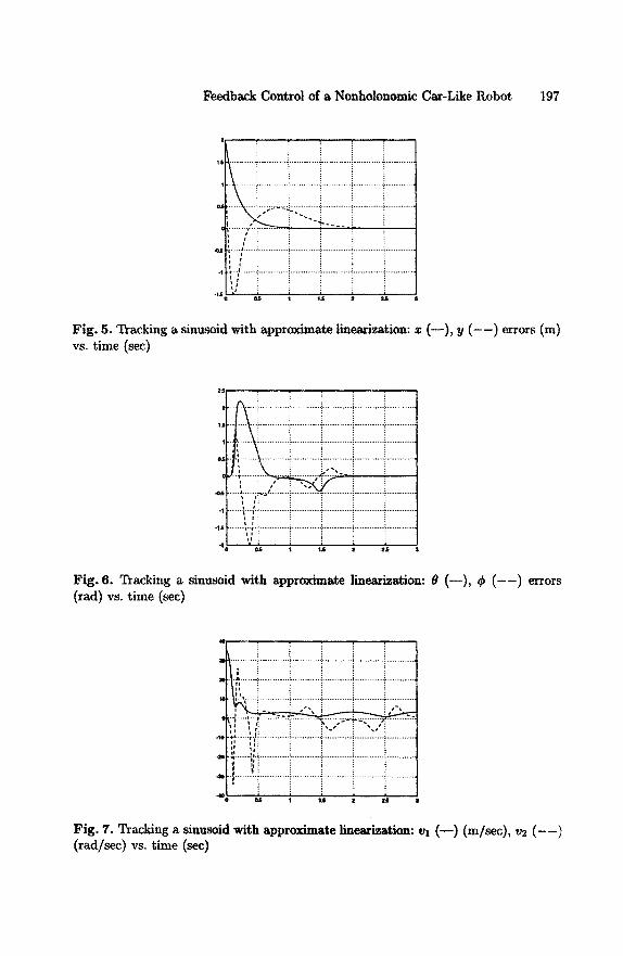
Feedback Control of a Nonholonomic Car-Like Robot 197
2
........ Y l .......... i
.~ , ...---.-~ ............... ~ . . . . . . . . . . . . . . . . . . . . . . . . . . . . . . . . . . . . . . . . . . . . . . . . . . . . . . . . . . . . . . .
Fig. 5. Tracking a sinusoid with approximate linearization: z (--) , y ( - - ) errors (m) vs. time (sec)
(
- I
. . . . . . . . ~ V I . . . . . . . . . . . . . . . . . . . . . . . . . . . . . . . . . . . . . . . . . . . . . . . . . i . . . . . . . . . . . . . . . . . . . . . . . . . . . . . . . .
Fig. 6. Tracking a sinusoid with approximate linearization: 0 (--) , ~b ( - - ) errors (tad) vs. time (sec)
i i i i i
p, ~ ~ ~ .
-- ! , ! i X
Fig. 7. Tracking a sinusoid with approximate linearization: (rad/sec) vs. time (sec)
v, ( - - ) (toltec), v., ( - - )
198 A. De Luca, G. Oriolo and C. Samson
3.3 Cont ro l via exact feedback l inearization
We now turn to the use of nonlinear feedback design for achieving global sta- bilization of the trajectory tracking error to zero.
It is well known in robotics that, if the number of generalized coordinates equals the number of input commands, one can use a nonlinear static (i.e., memoryless) state feedback law in order to transform exactly the nonlinear robot kinematics and/or dynamics into a linear system. In general, the linearity of the system equations is displayed only after a coordinate transformation in the state space. On the linear side of the problem, it is rather straightforward to complete the synthesis of a stabilizing controller. For example, this is the principle of the computed torque control method for articulated manipulators.
Actually, two types of exact linearization problems can be considered for a nonlinear system with outputs. Beside the possibility of transforming via feedback the whole set of differential equations into a linear system (full-state Iinearization), one may seek a weaker result in which only the input-output differential map is made linear (input-output linearization). Necessary and suf- ficient conditions exist for the solvability of both problems via static feedback, while only sufficient (but constructive) conditions can be given for the dynamic feedback case [18].
Consider a generic nonlinear system
= f(x) + G(x)u, z = h(x), (31)
where x is the system state, u is the input, and z is the output to which we wish to assign a desired behavior (e.g., track a given trajectory). Assume the system is square, i.e., the number of inputs equals the number of outputs.
The input-output linearization problem via static feedback consists in look- ing for a control law of the form
u=a(x )+B(x ) r , (32)
with B(x) nonsingular and r an external auxiliary input of the same dimension as u, in such a way that the input-output response of the closed-loop system (i.e., between the new inputs r and the outputs z) is linear. In the multi-input multi-output case, the solution to this problem automatically yields input- output decoupling, namely, each component of the output z will depend only on a single component of the input r.
In general, a nonlinear internal dynamics which does not affect the input- output behavior may be left in the closed-loop system. This internal dynamics reduces to the so-called clamped dynamics when the output z is constrained to follow a desired trajectory zd(t). In the absence of internal dynamics, full-state linearization is achieved. Conversely, when only input-output linearization is
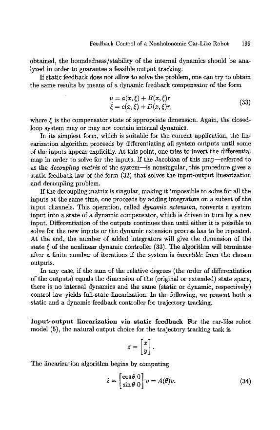
Feedback Control of a Nonholonomic Car-Like Robot 199
obtained, the boundedness/stability of the internal dynamics should be ana- lyzed in order to guarantee a feasible output tracking.
If static feedback does not allow to solve the problem, one can try to obtain the same results by means of a dynamic feedback compensator of the form
u = a(x, ~) + B(x, ~)r (33) = c(x, ~) + D(x, ~)r,
where ~ is the compensator state of appropriate dimension. Again, the closed- loop system may or may not contain internal dynamics.
In its simplest form, which is suitable for the current application, the lin- earization algorithm proceeds by differentiating all system outputs until some of the inputs appear explicitly. At this point, one tries to invert the differential map in order to solve for the inputs. If the Jacobian of this map--referred to as the decoupling matrix of the system--is nonsingular, this procedure gives a static feedback law of the form (32) that solves the input-output linearization and decoupling problem.
If the decoupling matrix is singular, making it impossible to solve for all the inputs at the same time, one proceeds by adding integrators on a subset of the input channels. This operation, called dynamic extension, converts a system input into a state of a dynamic compensator, which is driven in turn by a new input. Differentiation of the outputs continues then until either it is possible to solve for the new inputs or the dynamic extension process has to be repeated. At the end, the number of added integrators will give the dimension of the state ~ of the nonlinear dynamic controller (33). The algorithm will terminate after a finite number of iterations if the system is invertible from the chosen outputs.
In any case, if the sum of the relative degrees (the order of differentiation of the outputs) equals the dimension of the (original or extended) state space, there is no internal dynamics and the same (static or dynamic, respectively) control law yields full-state linearization. In the following, we present both a static and a dynamic feedback controller for trajectory tracking.
Input-output linearization via static feedback For the car-like robot model (5), the natural output choice for the trajectory tracking task is
The linearization algorithm begins by computing
z = [ sin 0 v = A(O)v. (34)
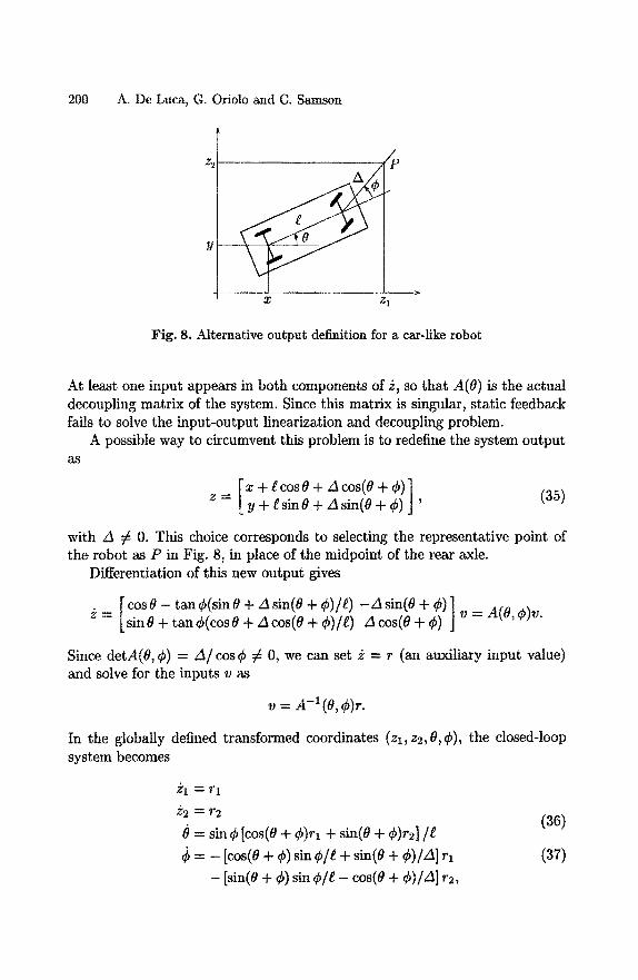
200 A. De Luca, G. Oriolo and C. Samson
X Z
Z2
y
Fig. 8. Alternative output definition for a car-like robot
At least one input appears in both components of ~, so that A(8) is the actual decoupling matrix of the system. Since this matrix is singular, static feedback fails to solve the input-output linearization and decoupling problem.
A possible way to circumvent this problem is to redefine the system output a s
Ix + ~cose + A cos(e + ¢)] z = [ Y + t sin 8 + A sin(8 + ¢) J ' (35)
with A ¢ 0. This choice corresponds to selecting the representative point of the robot as P in Fig. 8, in place of the midpoint of the rear axle.
Differentiation of this new output gives
[cos8 - tan¢(s in8 + Asin(8 + ¢)/~) --A sin(8 + ¢) ] = A(8,¢)v. = Lsin8 + tan~b(cos8 + Acos(8 + ¢) / t ) Acos(8 + ¢) J v
Since detA(8, ¢) = A~ cos ¢ ~ 0, we can set ~ = r (an auxiliary input value) and solve for the inputs v as
v = A -1(8, ¢)r.
In the globally defined transformed coordinates (zl ,z2,8,¢) , the closed-loop system becomes
Zl ---- rl
z2 = r2 (36)
= sin ¢ [cos(8 + ¢)rl + s~(8 + ¢)r2]/e = - [cos(0 + ~b) sin ~b//+ sin(0 + ¢)/A] rl (37)
- [sin(8 + ¢) sin ¢/~ -- cos(8 + ¢)/A] r2,
Feedback Control of a Nonholonomic Car-Like Robot 201
which is input-output linear and decoupled (one integrator on each channel). We note that there exists a two-dimensional internal dynamics expressed by the differential equations for/9 and ¢.
In order to solve the trajectory tracking problem, we choose then
ri = Zdi + kpi(Zdi -- zi), kpi > 0, i = 1, 2, (38)
obtaining exponential convergence of the output tracking error to zero, for any initial condition ( Zl (t0), z2 (to), 0 (t0), ¢(t0) ). A series of remarks is now in order.
- While the two output variables converge to their reference trajectory with arbitrary exponential rate (depending on the choice of the kpi'S in eq. (38)), the behavior of the variables 0 and ¢ cannot be specified at will because it follows from the last two equations of (36).
- A complete analysis would require the study of the stability of the time- varying closed-loop system (36), with r given by eq. (38). In practice, one is interested in the boundedness of/9 and ¢ along the nominal output trajec- tory. This study may not be trivial for higher-dimensional wheeled mobile robots, where the internal dynamics has dimension n - 2.
- Having redefined the system outputs as in eq. (35), one has two options for generating the reference output trajectory. The simplest choice is to directly plan a cartesian motion to be executed by the point P. On the other hand, if the planner generates a desired motion X d ( t ) , y d ( t ) for the rear axle midpoint (with associated Vdl( t ) ,Vd2( t ) computed from eqs. (21) and (24)), this must be converted into a reference motion for P by forward integration of the car-like equations, with v = Vd(t) and use of the output equation (35). In both cases, there is no smoothness requirement for Zd(t) which may contain also discontinuities in the path tangent.
- The output choice (35) is not the only one leading to input-output lin- earization and decoupling by static feedback. As a matter of fact, the first two variables of the chained-form transformation (8) are another example of linearizing outputs, with static feedback given by (9).
Ful l -s ta te l i n e a r i z a t i o n v i a d y n a m i c feedback In order to design a track- ing controller directly for the cartesian outputs (x, y) of the car-like robot, dynamic extension is required in order to overcome the singularity of the de- coupling matrix in eq. (34). Although the linearization procedure can be con- tinued using the original kinematic description (5), we will apply it here to the chained-form representation (10) as a first step toward the extension to higher-dimensional systems.
In accordance with the task definition, choose the two system outputs as
X4 ~
202 A. De Luca, G. Oriolo and C. Samson
namely the x and y coordinates of the robot. Differentiating z with respect to time gives
= x4 x3
where the input u2 does not appear, so that the decoupling matrix is singular. In order to proceed with the differentiation, an integrator (with state denoted by ~1) is added on the first input
Ul = ~1, ~1 = u~, (39)
with u~ a new auxiliary input. Using eq. (39), we can rewrite the first derivative of the output as
which is independent from the inputs u~ and u2 of the extended system. In this way, differentiation of the original input signal at the next step of the procedure is avoided. We have
As u2 does not appear yet, we add another integrator (with state denoted by (2) on the input u~
' " ( 4 0 ) u l = =
obtaining
Finally, the last differentiation gives
~ = 3x26(2 + z3(~ t.u21"
The matrix weighting the inputs is nonsingular provided that (1 # 0. Under such assumption--on which we will come back later--we set~" = r (an auxiliary input value) and solve eq. (41) for
[u~'] = rl u2j [ (r~ - x3r, - 3x2~l~2)/~21] " (42)
Feedback Control of a Nonholonomic Car-Like Robot 203
Putting together the dynamic extensions (39) and (40) with eq. (42), the resulting nonlinear dynamic feedback controller
Ul = ~I
=
~2 =7"1
(43)
transforms the original system into two decoupled chains of three input-output integrators
Z'I ----rl
z'2 ----r2.
The original system in chained form had four states, whereas the dynamic controller has two additional states. All these six states are found in the above input-output description, and hence there is no internal dynamics left. Thus, full-state linearization has been obtained.
On the linear and decoupled system, it is easy to complete the control design with a globally stabilizing feedback for the desired trajectory (independently on each integrator chain). To this end, let
r i -~'Z'di ~- kai (Zdi -- Zi) -~ kv i (Zdi -- Zi) ~- kpi(Zdi -- Zi) , i = 1, 2, (44)
where the feedback gains are such that the polynomials
A3+kai~2+kviA+kpi, i = 1,2,
are Hurwitz, and z, ~, 5 are computed from the intermediate steps of the dynamic extension algorithm as
(2
(45)
In order to initialize the chained-form system and the associated dynamic controller for exact reproduction of the desired output trajectory, we can set
204 A. De Luca, G. Oriolo and C. Samson
z = zd(t) and solve eqs. (45) at time t = to:
xl(tO) = Zdl(tO) (= Xd(tO))
X2(tO) = [Zdl (to)Zd2(to) -- J~dl (tO)~'dZ(to)] /Z]l(to)
x3(to) = /~d2(to)/~dl(tO)
x4(to) = Zdz(to) (= yd(tO)) =
2(to) =
Any other initialization of the robot and/or the dynamic controller will pro- duce a transient state error that converges exponentiaUy to zero, with the rate specified by the chosen gains in eq. (44).
As mentioned in Sect. 3.1, only trajectories zd(t) = (Xd(t), yd(t)) with con- tinuous second time derivatives are exactly reproducible. In the presence of lesser smoothness, the car-like robot will deviate from the desired trajectory. Nonetheless, after the occurrence of isolated discontinuities, the feedback con- troller (43-44) will be able to drive the vehicle back to the remaining part of the smooth trajectory at an exponential rate.
The above approach can be easily extended to the general case of the (2, n) chained form (7). In fact, such representation can be fully transformed via dynamic feedback into decoupled strings of input-output integrators by defin- ing the system output as (xl ,Xn). This result is summarized in the following proposition.
P ropos i t i on 3.1. Consider the (2,n) chained-form system (7) and define its output as
[xl] z = . (46) Xn
By using a nonlinear dynamic feedback controller of dimension n - 2, the system can be fully transformed into a linear one consisting of two decoupled chains of n - 1 integrators, provided that ul ~ O.
Proof We will provide a constructive solution. Let the dynamic extension be composed of n - 2 integrators added on input ul
u l n -2 ) = (47)

Feedback Control of a Nonholonomic Car-Like Robot 205
with the input u2 unchanged. Denote the states of these integrators by f l , . - . , f~-2, so that a state-space representation of eq. (47) is
u: = f l
~1 = ~
-- ?21 .
(7) and (48) is
X2 ---- U2
~3 = x2~i
~4 = x3~1
Xn--1 ------ Xn--2~l
~1 = ~ ~ 2 = ~
~n--3 = ~n--2
~n--2
The extended system consisting of eqs.
(48)
(49)
~n--2 ---- '/1'1.
By applying the linearization algorithm, we have for the first few derivatives of the output (46):
s = [ x . _ ~ ~ + x.-1~2 ]
[ ] ~' = x,~-3(i a + x,~-1(3 + 3(1(2x,~-2
[ ,4 ] z(4) = x,~_4~ + x,~_~4 + (6~(2x,~_3 + 4 ~ 3 x . _ ~ + 3~x._~) '
so that the structure of the (n - 2)-th derivative is
z('~-2) = x2(I ~-~ + x , - l ( ,~_~ + I(~1,~2,..., (,-~,x3, x4,.. . , x , - 2 ) '
206 A. De Luca, G. Oriolo and C. Samson
where f is a polynomial function of its arguments. The expressions of the output (46) together with its derivatives up to the (n - 2)-th order induce a diffeomorphism between (Xl,.. . , xn, ~1,... , ~n-2) and (z, ~, . . . , z(n-2)), which is globally defined except for the manifold ~1 = 0.
We obtain finally
0 g(~l,~2,- . . . . ,~n--2,3~2,Z3, ",Xn--2) "~ Xn_l ~ 2 U2 ,
where g is a polynomial function of its arguments. The decoupling matrix of the extended system is nonsingular provided that ~1 ¢ 0 or, equivalently, that ul ~ 0. Under this assumption, we can set z (n-l) = r and solve eq. (50) for (Ul, u2). Reorganizing with eq. (48), we conclude that the following nonlinear dynamic controller of dimension n - 2
u: = f l
= [ r = - X _lrl -
~n--3 = ~n--2 ~n--2 = rl
(51)
transforms the original chained-form system (7) with output (46) into the input- output linear and decoupled system
IX~n--1)l [ rl ] z(n-1) = { (n-l)! = = r.
Since the number of the input-output integrators (2(n - 1)) equals the number of states of the extended system (n + (n - 2)), there is no internal dynamics in the closed-loop system and thus we have obtained full-state linearization and input-output decoupling.
The above result indicates that dynamic feedback linearization offers a vi- able control design tool for trajectory tracking, even for higher-dimensional kinematic models of wheeled mobile robots (e.g., the N-trailer system). The same dynamic extension technique can be directly applied to the original kine- matic equations of the wheeled mobile robot, without resorting to the chained- form transformation. In particular, for the c~r-like robot (5), similar computa-

Feedback Control of a Nonholonomic Car-Like Robot 207
tions show that the dynamic controller takes the form:
Vl ---- ~1 v2 = --3~2 cos 2 ¢ tan ¢/~1 -- [rl cos 2 • sin 0 / ~ + gr2 cos 2 ¢ cos 0/~12
= e2 (52)
~2 = ~3 tan 2 ¢/i2 + rl cos 0 + r2 sin 0.
The external inputs rl and r2 are chosen as in (44), with the values of z, ~ and 5 given by
z=[:] cosol
= sin 0 J (53)
[-~2 tan Csin 0/[ + ~2 cos 0] = L tan ¢ cos 0 / e + sin 0 ]"
The derivation of the initial conditions on (x, y, 0, ¢) and (~1, ~2) allowing for exact reproduction of a smooth trajectory is straightforward using eqs. (53).
The main limitation of the dynamic feedback linearization approach is the requirement that the compensator state variable ~1 (which corresponds to Vl if linearization is performed on the original car-like equations, or to ul if it is performed on its chained-form representation) should never be zero. In fact, in this case the second control input (i.e., v2 in eq. (52) and us in eq. (43) or, more in general, in eq. (51)) could diverge. It has been shown that the occurrence of this singularity in the dynamic extension process is structural for nonholonomic systems [14]. Therefore, this approach as such is feasible only for trajectory tracking.
In addition, we note the following facts with specific reference to the con- troller (52-53) for the car-like robot.
- If the desired trajectory is smooth and persistent, the nominal control input Vdl does not decay to zero. As the robot is guaranteed to converge exponen- tially to the desired trajectory, also the actual command Vl will eventually be bounded away from zero. On the other hand, exact reproduction of trajectories with linear velocity vanishing to zero (e.g., trajectories with cusps, where the robot should stop and reverse the direction of motion) is not allowed with this control scheme.
- Even for smooth persistent trajectories, problems may arise if the command vl crosses zero during an initial transient. However, this situation can be avoided by suitably choosing the initialization of the dynamic controller (i.e., the states ~1 and ~2), which is in practice an additional degree of
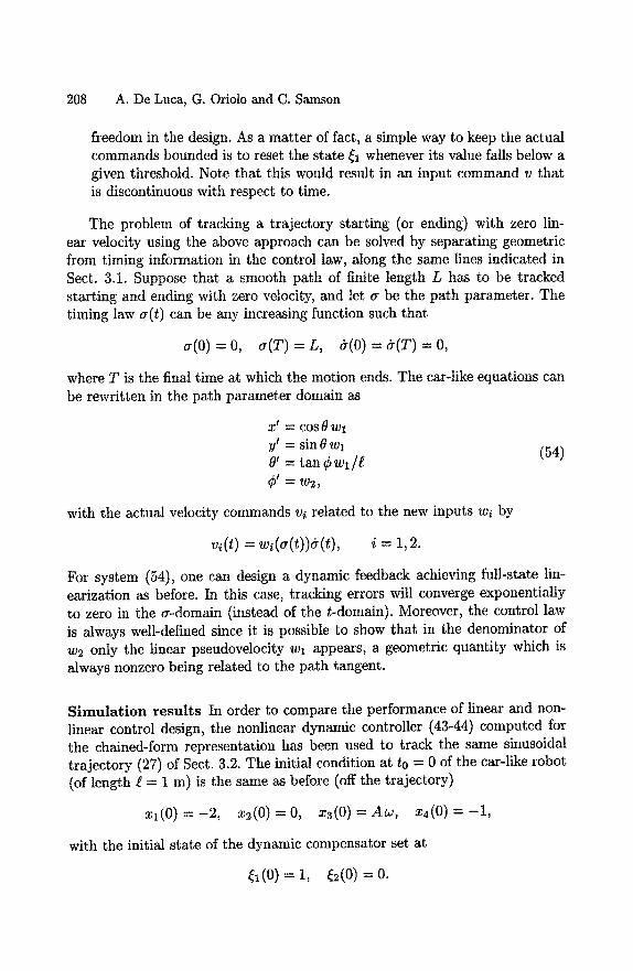
208 A. De Luca, G. Oriolo and C, Samson
freedom in the design. As a matter of fact, a simple way to keep the actual commands bounded is to reset the state ~1 whenever its value falls below a given threshold. Note that this would result in an input command v that is discontinuous with respect to time.
The problem of tracking a trajectory starting (or ending) with zero lin- ear velocity using the above approach can be solved by separating geometric from timing information in the control law, along the same lines indicated in Sect. 3.1. Suppose that a smooth path of finite length L has to be tracked starting and ending with zero velocity, and let a be the path parameter. The timing law a(t) can be any increasing function such that
a(O) = O, a(T) = L, &(O) = &(T) = O,
where T is the final time at which the motion ends. The car-like equations can be rewritten in the path parameter domain as
X t ~ COS 0 W l
yl = sin 0 wl 0' = tan ¢ wl/~
I ~ W2,
with the actual velocity commands vi related to the new inputs wi by
v (t) = i = 1, 2.
(54)
For system (54), one can design a dynamic feedback achieving full-state lin- earization as before. In this case, tracking errors will converge exponentially to zero in the a-domain (instead of the t-domain). Moreover, the control law is always well-defined since it is possible to show that in the denominator of w2 only the linear pseudovelocity wl appears, a geometric quantity which is always nonzero being related to the path tangent.
S imula t ion resul t s In order to compare the performance of linear and non- linear control design, the nonlinear dynamic controller (43-44) computed for the chained-form representation has been used to track the same sinusoidal trajectory (27) of Sect. 3.2. The initial condition at to = 0 of the car-like robot (of length ~ = 1 m) is the same as before (off the trajectory)
x 1 ( 0 ) = - 2 , x2(O)=O, x 3 ( O ) = A w , x 4 ( 0 ) = - l ,
with the initial state of the dynamic compensator set at
= 1, 2(o) = o .

Feedback Control of a Nonholonomic Car-Like Robot 209
As for the stabilizing part of the controller, we have chosen the same gains for both input-output channels, with three coincident closed-loop eigenvalues located at - 5 (kai = 15, kvi = 75, kpi = 125, i = 1, 2).
The results are shown in Figs. 9-11, again in terms of errors on the original states x, y, 0 and ¢, and of the actual control inputs vl, v2 for the car-like robot. A comparison with the analogous plots in Figs. 5-7 shows that the peaks of the transient errors are approximately halved in this particular case. Also, the control effort on the linear velocity vl in Fig. 11 does not reach the large initial value of Fig. 7, while the control input v2 has a lower average value. After achieving convergence, the input commands of the nonlinear dynamic controller are identical to those of the linear one, for they both reduce to the nominal feedforward needed to execute the desired trajectory. Moreover, as a result of the imposed linear dynamics of the feedback controlled system, the transient behavior of the errors is globally exponentially converging to zero, i.e., for any initial conditions of the car-like robot and of the dynamic compensator.
We have also simulated the dynamic feedback controller (52-53) designed directly on the car-like model. Results for a circular and an eight-shaped tra- jectory are reported in Figs. 12-19, assuming a length ~ = 0.1 m for the car. Note that the small peak of the x error in Fig. 13 is only due to an initial mis- match of the robot state with respect to the value specified by the higher-order derivatives of xd( t ) (in particular, of ~d(0)). In fact, in view of the decoupling property induced by the controller, the value of the initial error along each cartesian direction does not affect the error behavior and the control action in the other direction.
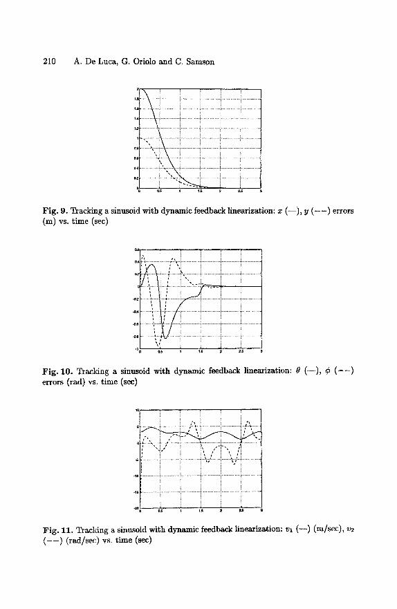
210 A. De Luca, G. Oriolo and C. Samson
Fig. 9. Tracking a sinusoid with dynamic feedback linearization: x (--) , y ( - - ) errors (m) vs. time (sec)
0.(
0.;
I
-02
-0,8
-0~8
: i ' . i i I ~: i ' - ' 7 i
t t 5 ~ [ i
l i ~ ! ! i i . . . . . . . . . i . . . . . . . . . . . .
i i i , i i O.S 1 I J; ~ 2~
Fig. 10. Tracking a sinusoid with dynamic feedback linearization: 0 (--) , ¢ ( - - ) errors (tad) vs. time (sec)
F ~ •
i • #
? 2
Fig. 11. Tracking a sinusoid with dynamic feedback linearization: vl ( - - ) (m/sec), v~ ( - - ) (rad/sec) vs. time (sec)

Feedback Control of a Nonholonomic Car-Like Robot 211
, . . . . . ~ . . . . . . . . . . . . . i . . . . . . . . . . . . . . . . . . . . . . . . . L
i
. . . . t ! ................................... 7" .......................... T o ~ . . .~ . . . . . . . . . . . . . . . . . . . . . . . . . . . . . . . . . . . . . . . . . . . . . . . . . . . . . . . . . . . . . . . . . . ~!,.,.
..... ~'- ................................. ! ............................... /i.,.
.... i x ................... i ...................... :i
. . . . . } .......... ~, i ................. i ................. ~ ............ .+--
i i i i . ! *~s o o~s 1
Fig. 12. Tracking a circle with dynamic feedback linearization: stroboscopic view of the cartesian motion
i I£1111ilIILIIIZIIIIIIIIII~IIIIIIIIIIIIIIII£111ZIIIIIIIIIIIIZIIIII o . 6 ' ~ - " ' : • : . . . . . . . . . . . . . ~ . . . . . . . . . . . . . T . . . . . . . . . . . . . ~ . . . . . . . . . . . . . " . . . . . . . . . . . . . :: . . . . . . . . . . . . .
• i i ~ ! i i
i !
Fig. 13. Tracking a circle with dynamic feedback linearization: x (--), y ( - - ) errors (m) vs. time (sec)
1 2 3 4 ~ 8
F i g . 1 4 . T r a c k i n g a c i r c le w i t h d y n a m i c f e e d b a c k ] i n e a r i z a t i o n : 0 ( - - ) ~ ¢ ( - - ) ( r a d ) vs. time (sec)
212 A. De Luca, G. Oriolo and C. Samson
ZI;III Z Z i Z Z I I Z I i IIIIZZ I Z Z Z;II / i i i i i i 1 1 s I $ •
Fig. 15. Tracking a circle with dynamic feedback linearization: vl ( - - ) (m/sec), v2 ( - - ) (rad/sec) vs. time (see)
r'"~ . . . . . . . . . . ~ ~ " ~ " ' " " ~ . . . . . . . . . . . ~ . . . . . . . . . . . . . i ....
0.1 ~ . . . . . . . . . . . . . . . . . . . i . . . . . . . . . . . . . . . . . '.' . . . . . . . . . . . . . . . . . ! . . . . . . . . . . . . . . . . . . . i i i ~
" " i ................. ) ................ ~ ............. ! ' N " ~ ....
........................................ i ................. i ................. i ....
........................................ i ................. i ................. i ....
........................................ ! . . . . . . . . . . . . . . . . i . . . . . . . . . . . . . . . . . i ....
i i i i 4 @S 0 OJ 1
Fig. 16. Tracking an eight figure with dynamic feedback linearization: stroboscopic view of the cartesian motion
4
" , i
....................... i ! i ............ ............. ........................................
.......... i i i i i i ............. ............. ............. ............. ............. ............ i i i i ~ i
Fig. 17. Tracking an eight figure with dynamic feedback linearization: z (--) , y ( - - ) errors (m) vs. time (see)

Feedback Control of a Nonholonomic Car-Like Robot 213
A +,,,, T
- 4
. $
Fig. 18. Tracking an eight figure with a dynamic feedback linearization: £~ (--), ¢ ( - - ) (tad) vs. time (sec)
. . . . . . . . . . i . . . . . . . . . . . . . . . . . . . . . . . . . . . . . . . . . . . . . . . . . . . . . . . . . . . . . . . . . . . . . . . . . . . . . . . . . . . . . . . . . . .
Fig. 19. Tracking an eight figure with a dynamic feedback linearization: Vl (--) (m/sec), v2 ( - - ) (rad/sec) vs. time (sec)
4 P a t h f o l l o w i n g a n d p o i n t s t a b i l i z a t i o n
In this section, we address the problem of driving the car-like robot to a desired, fixed configuration by using only the current error information, without the need of planning a trajectory joining the initial point to the final destination. In doing this, a control solution for the path following task is obtained as an intermediate step.
As shown in Sect. 2, for nonholonomic mobile robots the point stabiliza- tion problem is considerably more difficult than trajectory tracking and path
214 A. De Luca, G. Oriolo and C. Samson
following. In particular, smooth pure state feedback does not solve the prob- lem. Recently, the idea of including an exogenous time-varying signal in the controller has proven to be successful for achieving asymptotic stability [38]. Roughly speaking, the underlying logic is that such a signal allows all compo- nents of the configuration error to be reflected on the control inputs, so that the error itself can be asymptotically reduced to zero.
Some physical insight on the role of time-varying feedback can be gained by thinking about a parallel parking maneuver of a real car. We can reasonably assume that a human driver controls the vehicle through a front wheel steering command and a linear velocity command. In order to bring to zero the error in the lateral direction--along which the car cannot move directly--experience indicates that an approximately periodic forward/backward motion should be imposed to the car. This motion is somewhat independent from the lateral position error with respect to the goal and is used only to sustain the generation of a net side motion through the combined action of the steering command, which is instead a function of the position error.
Although natural, this strategy is hard to generalize to more complex vehi- cle kinematics, whose maneuverability is less intuitive. For this reason, we have chosen to present here two methods of wide applicability that are designed on the chained-form representation of the system. In order to emphasize the gener- ality of the controller design, the case of an n-dimensional system is considered. We give, however, some details for the case n = 4.
Both the presented feedback laws are time-varying, but they differ in their dependence from the current state as well as in some methodological aspects. The first control is either smooth or at least continuous with respect to the robot state. The second is nonsmooth, in the sense that the state is mea- sured and fed back only at discrete instants of time. Nevertheless, discarding this time-discretization aspect, it is also basically continuous with respect to the state at the desired configuration, contrary to other time-invariant discon- tinuous feedback laws (see Sect. 6). Both controllers provide inputs that are continuous with respect to time and are globally defined on the chained-form representation.
Throughout this section, it will be assumed without loss of generality that the desired configuration coincides with the origin of the state space.
4.1 Control via smooth time-varying feedback
The smooth feedback stabilization method presented here was proposed in [44]. It exploits the internal structure of chained systems in order to decompose the solution approach in two design phases. In the first phase, it is assumed that one control input is given and satisfies some general requirements. The other control is then designed for achieving stabilization of an (n - 1)-dimensional
Feedback Control of a Nonholonomic Car-Like Robot 215
subvector of the system state. At this stage, a solution to the path following problem has already been obtained. In the second phase, the design is completed by specifying the first control so as to guarantee convergence of the remaining variable while preserving the overall closed-loop stability.
As a preliminary step, reorder for convenience the variables of the chained form by letting
,3¢' = ( X 1 , X 2 , - • • , Xn-1, Xn) ----" ( Z l , X n , • • • , X 3 , X 2 ) .
As a consequence, the chained form system (7) becomes
~2 = X3ul
~3 = X4u,
Xn--i = Xn~l
~n ~ U2,
(55)
or equivalently
,'~ = h l ( X ) u l + h2u2, X4 1
h i ( X ) = ' h2 =
01 01 01
(56)
01 11
For the car-like robot, the above reordering is simply an exchange between the second and fourth coordinates. Therefore, the cartesian position of the rear wheel is (X1, X2)- Analogously, for an N-trailer robot, Xl and X2 represent the cartesian coordinates of the midpoint of the last trailer axle.
Let X = (X1, X2), with 2(2 = (X2, X3,. . . , Xn). In the following, we shall first pursue the stabilization of X2 to zero, and then the complete stabilization of X' to the origin.
216 A. De Luca, G. Oriolo and C. Samson
P a t h following via input scaling When ul is assigned as a function of time, the chained system (56) can be written as
~:1 = 0 " O u l ( t ) 0 . . . . . .
0 0 ul(t) 0 . . .
,i~2 = : O . . ,
. • ,
0 0
. . . . . . ~1 (t) • * . . . . 0
. . . , . . . . .
0 0
0 ~ l ( t )
0
& +
'0' 0
• U2, 0 0
' 1
(57)
having set
~0 ~ 21 = X l - u l ( r ) d r .
The first equation in (57) clearly shows that, when the input ul is a pri- ori assigned, the system is no more controllable• However, the structure of the differential equations for 2(2 is reminiscent of the controllable canonical form for linear systems. In particular, when ul is constant and nonzero, system (57) becomes time-invariant and its second part is clearly controllable. As a matter of fact, controllability holds whenever ul (t) is a piecewise-continuous, bounded, and strictly positive (or negative) function. Under these assumptions, Xl varies monotonically with time and differentiation with respect to time can be re- placed by differentiation with respect to X1, being
d d d d~ = dx1 'X1 = dx1 ut ,
and thus
d 1 d sign(ul) dx t = lUll" ~"
This change of variable is equivalent to an input Sect. 3.2). Then, the second part of the system may be rewritten as
X~ 1] -- sign(ut)x3 x[ll = sign(ul)x4 3
xffl_l = sign( l)Xn X~ 1 = sign(ul)u~,
scaling procedure (see
(58)
Feedback Control of a Nonholonomic Car-Like Robot 217
with the definitions
X" ] = sign(u1 and u2 = u'T" 1
Equation (58) is a linear time-invariant system, an equivalent input-output representation of which is
~ n - l ] --~ s i g n ( u l ) n - l u ~ .
Such system is controllable and admits an exponentially stable linear feedback in the form
n - 1 u~(X2) = -sign(u1) n-1 Z kix~i-1]' (59)
i----1
where the gains ki > 0 are chosen so as to satisfy the Hurwitz stability criterion. Hence, the time-varying control
U2 ("~'2, t) = U 1 (~)U~ (¢~2) (60)
globally asymptotically stabilizes the origin A'2 = 0. The above approach provides a solution to the path following problem.
Consider in particular the case of a car-like robot. We have seen at the end of Sect. 2.3 that the system equations (14) in path coordinates can be transformed in chained form. By reordering the variables as in eq. (55), X1 represents the arc length s along the path, X2 is the distance d between the car and the path, while X3 and X4 are related to the car steering angle ¢ and to the relative orientation/gp between the path and the car. Path following requires zeroing the X2, X3 and X4 variables (i.e., 2(2 = 0), independently from X1. Then, for any piecewise-continuous, bounded, and strictly positive (or negative) ul, eq. (59) is particularized as
u~ (X2, X3, X4) -= -sign(ul)[kl X2 + k2 sign(ul)x3 + k3x4].
Using eq. (60), the path following feedback control law is
II2 (X2, ~3, ~4 , t ) ~--- - k I lu l (~)[~2 - k2u4 (~)/~3 - k3 [Ul ( t )1~4,
which can be compared with eq. (30) to appreciate the analogy. Such an ap- proach was originally proposed in [42] for the path following of a unicycle. From the above developments, it is clear that it can be applied to any mobile robot which can be converted into chained form.
218 A. De Luca, G. Oriolo and C. Samson
S k e w - s y m m e t r i c cha ined f o r m s a n d Lyapunov control des ign We show now, by introducing a modified chained form, that it is possible to stabilize globally the origin X2 = 0 under more general hypotheses, namely that [Ul (t)t, f~t (t)[ are bounded and ul (t) does not asymptotically tend to zero. An impor- tant difference with respect to the previous analysis is that Ul (t) is allowed to pass through zero. From there, it will be relatively simple to derive a class of smooth time-varying feedback laws which stabilize globally the origin X = 0 of the complete system (point stabilization).
Consider the following change of coordinates
Zl = X1 z2 = X2 (61) Z3 = X3
zj+3 = kjzj+l + Lh~zj+2, j = 1, . . . , n - 3,
where k s (j = 1 , . . . ,n - 3) is a real positive number and Lh~zj = - ~ h l ( X ) is the Lie derivative of zj along the vector field hi. One easily verifies that eq. (61) is a linear, invertible change of coordinates, since the associated Jaco- bian matrix is of full rank. In particular, X = 0 and X2 = 0 are respectively equivalent to Z = 0 and Z2 = 0, having set Z = (Zl, Z2), Z2 = (z2,z3,... ,Zn) .
Moreover, it is Lh2zi = 0 (i -- 1 , . . . ,n - 1) and Lh2zn = 1. Taking the time derivative of zj+3 and using eq. (56) gives
OZj+3 ~ = ( L h l z j + 3 ) u 1 q_ (Lh2Zj+3)u2,
and from eq. (61)
Lh~Zj+s = -k j+lz j+2 + zj+4.
As a result, we obtain
~j+3 = (-k~+~zj+2 + zj+4)Ul
and for the last differential equation
j = O , . . . , n - 4
Zn = Lhl ZnUl q" u2.
The original chained system (55) has thus been converted into the following skew-symmetric chained form
~'1 = Ul Z'2 = Ul Z3
~j+3 = - k ~ + l u l z j + 2 + ulzj+4, Zn ~ --]gn--21$1Zn--1 -[-W2,
j = 0 , . . . , n - 4 , (62)
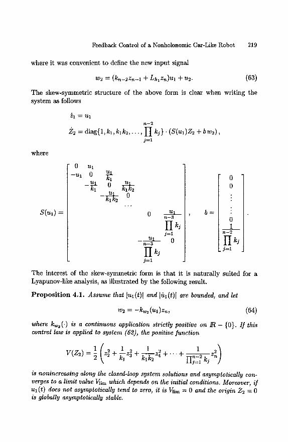
Feedback Control of a Nonholonomic Car-Like Robot 219
where it was convenient to define the new input signal
w2 = (kn-2zn-1 + Lhlzn)ul + U2. (63)
The skew-symmetric structure of the above form is clear when writing the system as follows
Zl = Ul r~--2
2~ = d iag{1 , k l , klk2,.. . , ~ I k j} . ( S ( U l ) Z 2 -}- bw2) , j : l
where
S(Ul ) : -
0 Ul
- u l 0 ~1
-~;~ 0
ul n--3
j=l
ul n--3
j = l 0
b =
0 q 0 I
• I
I i 0
The interest of the skew-symmetric form is that it is naturally suited for a Lyapunov-like analysis, as illustrated by the following result.
P ropos i t i on 4.1. Assume that lul(t)l and litl(t)t are bounded, and let
w2 = - k w 2 ( u l ) z n , (64)
where kw2 (') is a continuous application strictly positive on 1R - {0}. If this control law is applied to system (62), the positive function
1(z +1 t 2 _ 1 ) v(z2) = ~ k, z3 + k-[g~, + . . . + 1.i~\_2 k j n
is nonincreasing along the closed-loop system solutions and asymptotically con- verges to a limit value V]im which depends on the initial conditions. Moreover, if ul (t) does not asymptotically tend to zero, it is VIim = 0 and the origin Z2 = 0 is globally asymptotically stable.
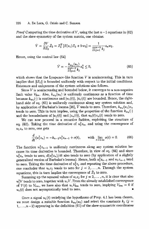
220 A. De Luca, G. Oriolo and C. Samson
Proof Computing the time derivative of V, using the last n - 1 equations in (62) and the skew-symmetry of the system matrix, one obtains:
OV. = = z[ + = - -
OZ2 n--2 Hj: kj Zn W 2 .
Hence, using the control law (64)
? = kw2(ul) 2 < 0, (65) YIL- kj -
which shows that the Lyapunov-like function V is nonincreasing. This in turn implies that IIZ2[[ is bounded uniformly with respect to the initial conditions. Existence and uniqueness of the system solutions also follows.
Since V is nonincreasing and bounded below, it converges to a non-negative limit value Vlim. Also, kw2(ul) is uniformly continuous as a function of time because kw: (-) is continuous and lul (t) l, lul (t) l are bounded. Hence, the right- hand side of eq. (65) is uniformly continuous along any system solution and, by application of Barbalat's lemma [20], V tends to zero. Therefore, k~ 2 (uJzn tends to zero. This in turn implies, using the properties of the function kw: (') and the boundedness of Jut(t)] and [zn(t)h that Ul(t)zn(t) tends to zero.
We can now proceed in a recursive fashion, exploiting the structure of eq. (62). Taking the time derivative of u2zn, and using the convergence of UlZn to zero, one gets
d 2 - ~ ( u l Z n ) = -kn_2U31Zn_l -~ o( t ) , with lim o(t) = 0. (66)
t--4+oo
The function U3Zn--1 is uniformly continuous along any system solution be- cause its time derivative is bounded. Therefore, in view of eq. (66) and since u2zn tends to zero, d(u~zn)/dt also tends to zero (by application of a slightly generalized version of Barbalat's lemma). Hence, both u~zn-1 and UlZn-1 tend to zero. Taking the time derivative of u2zj and repeating the above procedure, one concludes that ulzj tends to zero for j = 2, . . . ,n. Through the system equations, this in turn implies the convergence of Z2 to zero.
Summing up the squared values of ulzj for j = 2, . . . , n, it is clear that also u2V tends to zero, together with ulV. From the already established convergence of V(t) to Vlim, we have also that ul~im tends to zero, implying Vlim : 0 if Ul(t) does not asymptotically tend to zero. •
Once a signal ul (t) satisfying the hypotheses of Prop. 4.1 h~s been chosen, we must design a suitable function kw2(Ul) and select the constants kj (j = 1 , . . . , n - 2 ) appearing in the definition (61) of the skew-symmetric coordinates
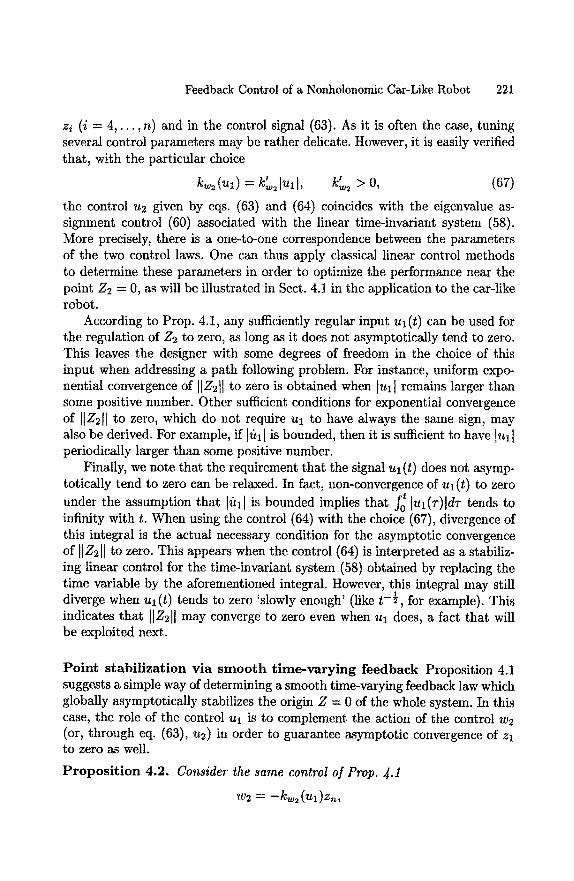
Feedback Control of a Nonholonomic Car-Like Robot 221
z~ (i = 4 , . . . , n) and in the control signal (63). As it is often the case, tuning several control parameters may be rather delicate. However, it is easily verified that, with the particular choice
k (ul) = k'21 lt, > o, (67)
the control u2 given by eqs. (63) and (64) coincides with the eigenvalue as- signment control (60) associated with the linear time-invariant system (58). More precisely, there is a one-to-one correspondence between the parameters of the two control laws. One can thus apply classical linear control methods to determine these parameters in order to optimize the performance near the point Z2 = 0, as will be illustrated in Sect. 4.1 in the application to the car-like robot.
According to Prop. 4.1, any sufficiently regular input ul(t) can be used for the regulation of Z2 to zero, as long as it does not asymptotically tend to zero. This leaves the designer with some degrees of freedom in the choice of this input when addressing a path following problem. For instance, uniform expo- nential convergence of H Z2H to zero is obtained when ]Ul[ remains larger than some positive number. Other sufficient conditions for exponential convergence of [[Z2[I to zero, which do not require ul to have always the same sign, may also be derived. For example, if [ul [ is bounded, then it is sufficient to have lull periodically larger than some positive number.
Finally, we note that the requirement that the signal ul (t) does not asymp- totically tend to zero can be relaxed. In fact, non-convergence of ul(t) to zero
under the assumption that [ull is bounded implies that fo [Ul(T)[dT tends to infinity with t. When using the control (64) with the choice (67), divergence of this integral is the actual necessary condition for the asymptotic convergence of [[Z21[ to zero. This appears when the control (64) is interpreted as a stabiliz- ing linear control for the time-invariant system (58) obtained by replacing the time variable by the aforementioned integral. However, this integral may still diverge when ul (t) tends to zero 'slowly enough' (like t-½, for example). This indicates that [IZ21[ may converge to zero even when ul does, a fact that will be exploited next.
Point stabilization via smooth t ime-vary ing feedback Proposition 4.1 suggests a simple way of determining a smooth time-varying feedback law which globally asymptotically stabilizes the origin Z = 0 of the whole system. In this case, the role of the control Ul is to complement the action of the control w2 (or, through eq. (63), u2) in order to guarantee asymptotic convergence of Zl to zero as well.
Proposition 4.2. Consider the same control of Prop. 4.1
w 2 =
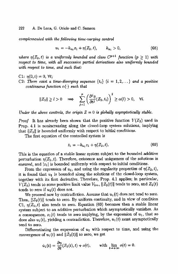
222 A. De Luca, G. Oriolo and C. Samson
complemented with the following time-varying control
Ul = -ku, Zl -F q(Z2, t), kul > O, (68)
where rl(Z2,t) is a uniformly bounded and class C v+l function (19 > 1) with respect to time, with all successive partial derivatives also uniformly bounded with respect to time, and such that:
CI: 7(0, t) = o, vt; C2: There exist a time-diverging sequence {ti} (i = 1, 2, . . . ) and a positive
continuous function c~(. ) such that
• 2
> > o, v i . j = l
Under the above controls, the origin Z = 0 is globally asymptotically stable.
Proof It has already been shown that the positive function V(Z2) used in Prop. 4.1 is nonincreasing along the closed-loop system solutions, implying that tIZ211 is bounded uniformly with respect to initial conditions.
The first equation of the controlled system is
= -k izl + v ( z 2 , t ) . (69)
This is the equation of a stable linear system subject to the bounded additive perturbation r/(Z~, t). Therefore, existence and uniqueness of the solutions is ensured, and Izll is bounded uniformly with respect to initial conditions.
From the expression of ul, and using the regularity properties of z/(Z2,t), it is found that Ul is bounded along the solutions of the closed-loop system, together with its first derivative. Therefore, Prop. 4.1 applies; in particular, V(Z2) tends to some positive limit value Vlim, IIZ2(t)H tends to zero, and Z2(t) tends to zero if ul(t) does not.
We proceed now by contradiction. Assume that ul (t) does not tend to zero. Then, IIZ2(t)ll tends to zero. By uniform continuity, and in view of condition C1, rl(Z2,t) also tends to zero. Equation (69) becomes then a stable linear system subject to an additive perturbation which asymptotically vanishes. As a consequence, zl(t) tends to zero implying, by the expression of ul, that so does also ul (t), yielding a contradiction. Therefore, ul(t) must asymptotically tend to zero.
Differentiating the expression of Ul with respect to time, and using the convergence of ul(t) and IIZ2(t)ll to zero, we get
1(t) = + o(t), with lim o(t) = O. t--~+co
Feedback Control of a Nonholonomic Car-Like Robot 223
Since (Oy/Ot)(Z2, t) is uniformly continuous (its time derivative is bounded), both ~l(t) and (Oy/Ot)(Z2,t) converge to zero (Barbalat's lemma). By us- ing similar arguments, one can also show that the total time derivative of (O~l/Ot)(Z2(t),t) and (027]/Ot2)(Z2(t),t) tend to zero. By repeating the same procedure as many times as necessary, one obtains that (OJ~l/OtJ)(Z2,t) (j = 1, . . . ,p) tends to zero. Hence,
P(0J )5 lim Z -~-~f(Z2(t),t) = O.
t -~oo j=l
(70) Assume now that Vlim is different from zero. This would imply that [[Z2(t)[[ remains larger that some positive real number I (which can be calculated from Vlim). Eq. (70) is then incompatible with the condition C2 imposed on the function r/(Z2, t). Hence, Him is equal to zero and Z2 asymptotically converges to zero. Then, by uniform continuity and using condition C1, r/(Z2, t) also tends to zero. Finally, in view of the expression of Ul, asymptotic convergence of Zl to zero follows immediately. •
We point out that controls ul and u2 resulting from Prop. 4.2 are smooth with respect to the state provided that the functions T/(Z2, t) and kw2(ul) are themselves smooth. On the other hand, if kw2 (ul) is chosen as in eq. (67), u2 is only continuous.
In the overall controller, the choices related to u2 (or w2) can be made along the same lines indicated at the end of Sect. 4.1. In particular, the same control law (60) based on input scaling can be used. As for ul, the gain k~l is typically chosen on the basis of an approximate linearization at the origin. Its second component 71(Z2,t), which introduces an explicit time dependence, is referred to as the heat function in order to establish a parallel with probabilistic global minimization methods. The role of y(Z2,t) in the control strategy is fundamental, for it 'forces motion' until the system has not reached the desired configuration, thus preventing the state from converging to other equilibrium points.
The conditions imposed by Prop. 4.2 on the heat function ~/can be easily met. For example, the three following functions
T ] l ( Z 2 , t ) = [[Z2112 sint n--2
'/2(Z2, t) = E aj sin(/~jt) z2+j j=O
n-2
~/3(Z2, t) = ~ aj exp(bjz2+j) - 1 sin(f/it), j=o exp(bjz2+j) -+ 1
(71)
(72)
(73)
224 A. De Luca, G. Oriolo and C. Samson
satisfy the conditions whenever a d • 0, bj # 0, flj # O, and fli # flj for i ~ j . For the first function, this is obvious. For the second function, the proof can be found in [43]. The same proof basically applies to the third function, which has the additional feature of being uniformly bounded with respect to all its arguments. It should be noted that it is not strictly necessary to use time-periodic functions.
The choice of a suitable heat function is critical for the overall control performance. In general, it is observed that functions (72) and (73) behave better than (71) with respect to the induced asymptotic convergence rate. For the last two functions, the parameters aj and bj (which characterize the 'slope' of ~/~(Z2,t) and 7/3(Z2,t) near the origin Z2 = 0) have much influence on the transient time needed for the solutions to converge to zero.
Appl ica t ion to the car-like robo t For the (2, 4) chained form (10) that per- tains to the car-like robot, the non-trivial part of the change of coordinates (61) is defined by
since we have from eq. (56)
z 4 = k l X 2 q ' X 4 ,
LhlZ3 : LhlX3 : X4"
The skew-symmetric form (62) becomes in this case
'~1 : U l
Z2 "~ Ul Z3
Z3 = -k lU lZ2 ~ UlZ4
~a = -k2ulz3 + w2,
with
w2 ---- (kl + k2)UlZ3 + u2.
In view of Prop. 4.1 and eq. (67), the control input u2 for the skew-symmetric form is chosen as
: -- 21UlIZ4 -- (]gl -}- ]g2) 1Z3 : - k l k : 2 i u l I x 2 - (k l + k 2 ) u l x 3 - k : 2 [ u l I x 4 . (74 )
The value of the three gains kl, k2, and k~: can be selected on the basis of the aforementioned correspondence between the structure of eq. (74) and the
Feedback Control of a Nonholonomic Car-Like Robot 225
eigenvalue assignment control (60). In particular, by comparing the expression of u2 with the input-scaled version (30) of the linear tracking controller, which assigns three coincident eigenvalues in -~ lu l l (with ~ > 0), we can solve for the three gains as
kl -- ~2/3, k2 = 8c~2/3, k" 2 = 3c~.
In this association, one should remember that X2 = x4, X3 = x3, and X4 = x2. In particular, the following gain parameters have been used
k 1 = 1 / 3 , k 2 = 8 / 3 , k~ 2 = 3 ,
corresponding to three eigenvalues in - 1 for the input-scaled linear approxi- mation.
As for the control input ul , which is given by eq. (68), we have set k~ 1 = 10, corresponding to an eigenvalue in -10 for the linear approximation of the x- error dynamics, and we have used the heat function ~/2 with the following parameters
a 0 = 40, al = 20, a2 = 20, ~ o = 1 , /~1=2, & = 3 .
The above controller has been simulated for a car-like robot with £ = 1 m executing a parallel parking maneuver. The desired configuration is the origin of the state space, while the initial configuration at to = 0 is
x ( 0 ) = 0 , y ( 0 ) = - 5 , 0 ( 0 ) = 0 , ¢ ( 0 ) = 0 .
Figures 20-26 show respectively the cartesian motion of the vehicle, the time evolution of x, y, 8 and ¢, and the actual commands vl and v2 applied to the car-like robot, obtained from ul and u2 via the chained-form input transfor- mation (9).
After performing several other numerical tests, we can conclude that:
- The motion is quite natural in the first phase of approaching. - For any stabilization task, the final part of the motion resembles a parallel
parking maneuver. - Basically, the larger are the aj parameters of the heat function Y2, the
shorter is the transient time. On the other hand, more control effort is required far from the goal.
- The final convergence close to the goal is rather slow.
In order to achieve practical convergence to a small ball around the origin in finite time, a simpler, discontinuous heat function can be used. For example,
226 A. De Luca, G. Oriolo and C. Samson
we have chosen
~4(z~, z3, z 4 , t ) = ~kn sin t ifz 2 + z 2 + z 2 >_~ [0 ifz22 + z 2 + z 2 < e,
with e = 10 -~, kn = 20, and modified one of the previous gains by setting k~ 1 = 5. The obtained results are illustrated in Figs. 27-33. The norm of the final cartesian error is equal to 3 .35 .10 -2 m (only due to the y-coordinate), while the final values of~ and ¢ are 2.5-10 -3 rad and 5.5-10 -3 rad, respectively. This condition is reached in about 17 sec.
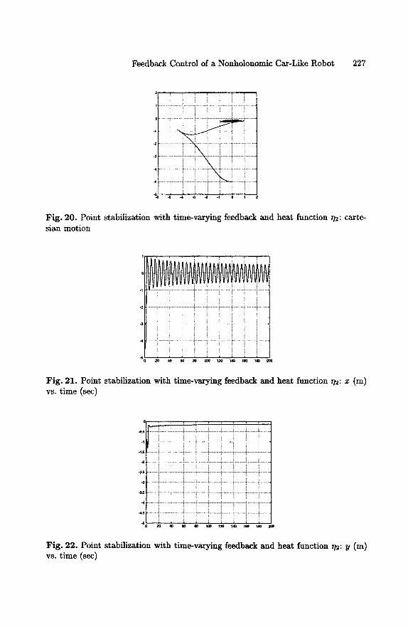
Feedback Control of a Nonholonomic Car-Like Robot 227
J ' i ! i ! : .... i - i .......
Fig. 20. Point stabilization with time-varying feedback sian motion
and heat function ~]~: carte-
i : ~ i ! i ! i l
! ~ i ! i i ! i l
: : : : : :
i i i i i i i i i
Fig. 21. Point stabilization with time-varying feedback and heat function T/2: x (m) vs. time (sec)
o: t : : : i i A i i i i ......... i:::::' i , l i i i i i i
4 ~
i i i ! g i i i l ~ l i i i l l i i i i , ,
Fig. 22. Point stabilization with time-varying feedback and heat function ~/2: y (m) vs. time (sec)
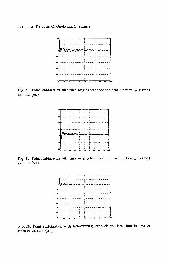
228 A. De Luca, G. Oriolo and C. Samson
.......... i ................... i l - i - i i - + i i . . . . . . . . . . . . . . . . . . . . . . . . . . . .
i ~ i i ! ! ! i i
! i i i i ! i l l
~.~ ! i i i i ! i
i i i i i i l l i
Fig. 23. Point stabilization with time-varying feedback and heat function ~/2:8 (rad) vs. time (sec)
i i i ~ i l i l i
.................. i .................. i++i+++i+-i++i ..........
+ i i i ............... i i i i ) i i i i i
Fig. 24. Point stabilization with time-varying feedback and heat function ~/2: ~ (rad) vs. time (sec)
Io
........ i ......... i ......... ! ......... i ......... L+i__I ......... i ......... i ........
-S
i ! ! i i i i i i
........... ! ......... N I ......... !-T-!+I ......... ! ......... !
i i i i i i i i i
Fig. 25. Point stabilization with time-varying feedback and heat function ~}2: vl (m/sec) vs. time (sec)
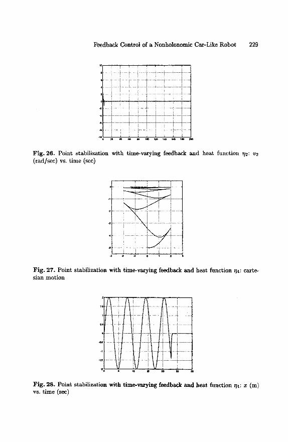
Feedback Control of a Nonholonomic Car-Like Robot 229
........ i ......... i - i ......... i ......... ! T I ......... i ......... i : : : : : : : : :
: : = : : = = : :
Fig. 26. Point stabilization with time-varying feedback and heat function z/z: v2 (rad/sec) vs. time (sec)
.1
4
i i
Fig. 27. Point stabilization with time-varying feedback sian motion
and heat function ~/4: carte-
2 . . ,
i ........ i ......... i ....................
o . . . . ÷..~ i . . . . . . . . . . . . . . . .
"2 m S ~.0
Fig. 28. Point stabilization with time-varying feedb~..k and heat function q4: x (m) vs. time (sec)
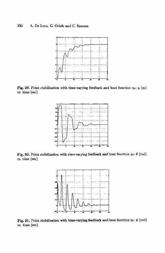
230 A. De Luca, G. Oriolo and C. Samson
i . . . . i
S 10 15 20 ~S 30
Fig. 29. Point stabilization with time-varying feedback and heat function 7/4: y (m) vs. time (sec)
I
OJ
0.4
C
-02
- 04
,OJ
-O8
-1
~ iiii iiiiiiiiiiiiiiiiiiiiiiiiiiiiiiiiiiiil iiiiiiiiiiiiiiiiiiiiiiiiiiiiiiil iiiiiiiiiiiii
iiiili Fig. 30. Point stabilization with time-varying feedback and heat function ~/4: O (rad) vs. time (sec)
S l o lS 2o ~S 30
Fig. 31. Point stabilization with time-varying feedback and heat function ~/4: ~ (rad) vs. time (sec)
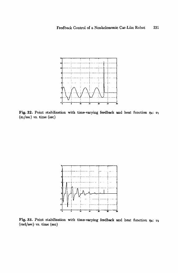
Feedback Control of a Nonholonomic Car-Like Robot 231
Fig. 32. Point stabilization with time-varying feedback and heat function 74: vl (m/sec) vs. time (sec)
s lO m ~ ~ ao
Fig. 33. Point stabilization with time-varying feedback and heat function r/4:v2 (rad/sec) vs. time (sec)
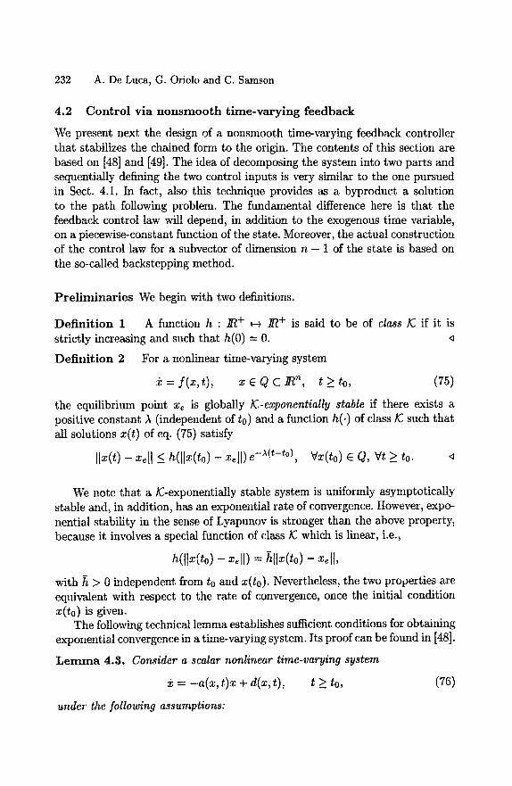
232 A. De Luca, G. Oriolo and C. Samson
4.2 Control via nonsmooth time-varying feedback
We present next the design of a nonsmooth time-varying feedback controller that stabilizes the chained form to the origin. The contents of this section are based on [48] and [49]. The idea of decomposing the system into two parts and sequentially defining the two control inputs is very similar to the one pursued in Sect. 4.1. In fact, also this technique provides as a byproduct a solution to the path following problem. The fundamental difference here is that the feedback control law will depend, in addition to the exogenous time variable, on a piecewise-constant function of the state. Moreover, the actual construction of the control law for a subvector of dimension n - 1 of the state is based on the so-called backstepping method.
Preliminaries We begin with two definitions.
Definition 1 h function h : ~ + ~ ~ + is said to be of class E if it is strictly increasing and such that h(0) = 0.
Defini t ion 2 For a nonlinear time-varying system
= / ( x , t ) , x e Q c t > to, ( 7 5 )
the equilibrium point xe is globally /C-exponentially stable if there exists a positive constant A (independent of to) and a function h(.) of class ]C such that all solutions x(t) of eq. (75) satisfy
Ilx(t) - x~[I < h([lx(to) - xeJ[)e -x(t-t°), Vx(to) e Q, Vt > to.
We note that a ]C-exponentially stable system is uniformly asymptotically stable and, in addition, has an exponential rate of convergence. However, expo- nential stability in the sense of Lyapunov is stronger than the above property, because it involves a special function of class/C which is linear, i.e.,
h ( l l x ( t o ) - x e l l ) = h l l x ( t o ) - xe t l ,
with tt > 0 independent from to and x(to). Nevertheless, the two properties are equivalent with respect to the rate of convergence, once the initial condition x(to) is given.
The following technical lemma establishes sufficient conditions for obtaining exponential convergence in a time-varying system. Its proof can be found in [48].
Lemma 4.3. Consider a scalar nonlinear time-varying system
= -a (x , t)x + d(x, t), t > to, (76)
under the following assumptions:
Feedback Control of a Nonholonomic Car-Like Robot 233
- there exists a solution x(t) of eq. (76) for any x(to) and t > to; - a(x, t) is such that for all x(t)
(a(x(r), T) -- #) dr <_ P, Vt >_ to,
where # and P are some positive constants; - a ( x , t ) i s bouneeefor all x(t) as
Id(x(r), r)l < De -'Y(t-t°), Vt >__ to,
/or some positive constants D and 7.
Then,
Ix(t)l < e(lx(to)l + D)e -(p-~)(t-t°), Vs > O,
where/~ = rain{#, 7} > 0 and c = max{e P, e2P/s}.
B a c k s t e p p i n g con t ro l des ign For convenience, we rewrite here the chained system (7)
X'I ~ Ul X2 ~ U2 X3 ~--- X2Ul
Xn ~ Xn--lUl~
and partition its state as X = (xl,X2), with X2 = (x2,x3, . . . ,xn). As previously noted, when Ul is a predefined fimcti0n of time, X2 satisfies
a linear time-varying equation driven by the input u2. In the following, we will assume that a structure is assigned for the signal ul(t) and address the design of a feedback control law for u2 so as to make X2 = 0 a ]C-exponentially stable equilibrium point. Later, we will add the variable xl to the picture and choose the specific form of control Ul so as to obtain ]C-exponential stability of X -- 0 for the complete system.
The structure of ul is chosen by combining the simplicity of an open-loop command, which is updated as a function of the state only at discrete time instants, with the benefits of adding a time-varying exogenous signal. In par- ticular, let a sequence of equidistant time instants {to,t1, t2 , . . . } be defined as
th = hT, T -- th+l -- th > 0,
234 A. De Luca, G. Oriolo and C. Samson
and define the control Ul as
ul(t) = k(X(th))f(t), for t E [th,th+l). (78)
This structure implies that the input is a function of the state X at time t = th, while during the interval (th,th+l) it is defined in an open-loop fashion. For the time being, no restrictions are put on the form of the function k(.) beside its boundedness. On the other hand, some assumptions are needed for function f(t).
h l : f(t) E C~; h 2 : 0 _< f(t) <_ 1, Vt > to; A3: /(th) = 0, Vth e };
v j e {3 , . . . ,n ) , Vth e {t0,t l , . . . },
where #j and Pj are positive constants. Assumption A3 implies that ul(th) = 0 for all th E (to, t1 , . . . }, and thus
guarantees continuity of Ul (t) with respect to time, even if function k is nons- mooth with respect to the state. Assumption A4 is more technical and is used to guarantee controllability of the linear time-varying subsystem and for proving exponential convergence of X2 to zero by means of Lemma 4.3.
A simple periodic function satisfying the above assumptions is
1 - cos wt 21r f ( t ) = 2 , w = --~-. (79)
This function has a nonzero mean value, a fact which turns out to be important in order to have some 'control energy' sustaining the robot motion as long as an error is present, i.e., X ~t 0 (see the related remarks in Sect 4.1). However, f(t) is not restricted to be periodic.
Using eq. (78), the lower part of system (77) becomes
=
~ 3
Xn.--1 LX ,~J
U2
k(X(th))f(t)x,_~ k(XCth))fC0x.-1
tE[th,th+l), h=O, 1 , . . . . (80)
In the following, we will often write k = k(X(th)) for compactness. A feedback law for u2 that renders X2 = 0 exponentially convergent to
zero (in fact, ~-exponentially stable) is now derived based on a backstepping method--a general technique for controlling systems in cascaded form [22].
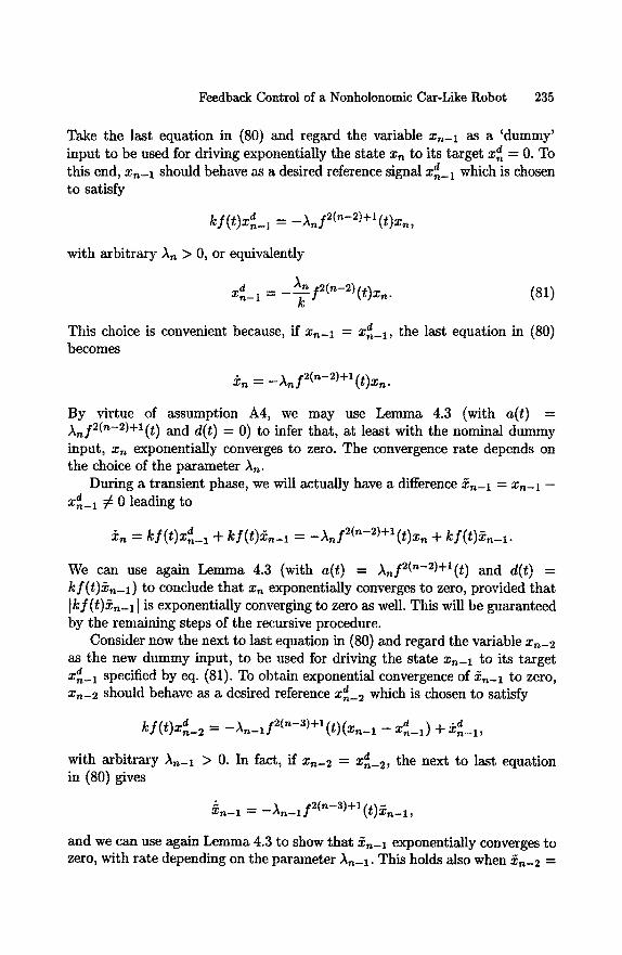
Feedback Control of a Nonholonomic Car-Like Robot 235
Take the last equation in (80) and regard the variable x n - 1 as a 'dummy' input to be used for driving exponentially the state Xn to its target x d = 0. To this end, x n - 1 should behave as a desired reference signal x a which is chosen n--1 to satisfy
k i ( t ) z d l = _ ~ . f ( n - 2 ) + ~ ( t ) x n ,
with arbitrary An > 0, or equivalently
d ~ f 2 ( n - 2 ) xn-1 = - (t)xn. (81)
This choice is convenient because, if x n - 1 = x ~ _ l , the last equation in (80) becomes
Xn = --Anf2(n--2)+l(t)Xn.
By virtue of assumption A4, we may use Lemma 4.3 (with a( t ) = A n f 2 ( n - 2 ) + l ( t ) and d(t ) = 0) to infer that, at least with the nominal dummy input, x n exponentially converges to zero. The convergence rate depends on the choice of the parameter An.
During a transient phase, we will actually have a difference ~ n - 1 = x n - x - x~_ 1 ~ 0 leading to
~n = k l ( t ) ~ _ ~ + k l ( t )~n-~ = - A . f (n-2)+~(t)x" + k l ( t )~n-~ .
We can use again Lemma 4.3 (with a(t ) = Anf2(n-2)-bl (~) and d(t ) = k f (t)~n_l) to conclude that x n exponentially converges to zero, provided that I k f ( t ) ~ n _ l l is exponentially converging to zero as well. This will be guaranteed by the remaining steps of the recursive procedure.
Consider now the next to last equation in (80) and regard the variable x n - 2 as the new dummy input, to be used for driving the state Xn-1 to its target xd n -1 specified by eq. (81). To obtain exponential convergence of xn-1 to zero, Xn-2 should behave as a desired reference x~_2 which is chosen to satisfy
kI( t )x~_2 = - A . _ l f ( " - 3 ) + l ( t ) ( x n _ l - Z._l)d + ~dn_x,
with arbitrary An-1 > 0. In fact, if x n - 2 = x ~ _ 2, the next to last equation in (80) gives
5~n_ 1 : --An_lf2(n--3) +l(t)xn_l,
and we can use again Lemma 4.3 to show that xn-1 exponentially converges to zero, with rate depending on the parameter An-1. This holds also when xn-2 =
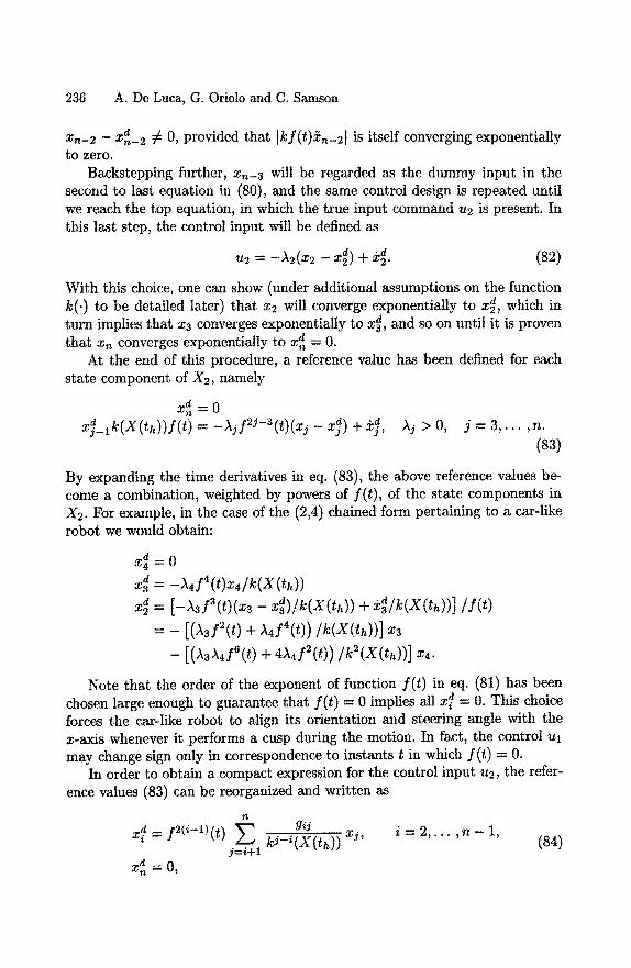
236 A. De Luca, G. Oriolo and C. Samson
X n _ 2 - - X d ~-2 i ~ 0, provided that Ikf(t)Ycn_21 is itself converging exponentially to zero.
Backstepping further, x n - 3 will be regarded as the dummy input in the second to last equation in (80), and the same control design is repeated until we reach the top equation, in which the true input command u2 is present. In this last step, the control input will be defined as
u2 = - + ( 8 2 )
With this choice, one can show (under additional assumptions on the function k(.) to be detailed later) that x2 will converge exponentially to x d, which in turn implies that x3 converges exponentially to xz a, and so on until it is proven that xn converges exponentially to x d = 0.
At the end of this procedure, a reference value has been defined for each state component of X2, namely
x d = 0 x d _ l k ( X ( t h ) ) f ( t ) = - ) ~ j f 2 J - 3 ( t ) ( x j - x ]) + 2 ] , )~j > 0, j = 3, . . . ,n.
( 8 3 )
By expanding the time derivatives in eq. (83), the above reference values be- come a combination, weighted by powers of f ( t ) , of the state components in X2. For example, in the case of the (2,4) chained form pertaining to a car-like robot we would obtain:
= o
x d = - A 4 f 4 ( t ) x 4 / k ( X ( t h ) )
x d = [ - ~ 3 f 3 ( t ) ( x 3 - 2cd ) / k (X( th ) ) -I- x d / k ( X ( t h ) ) ] I f ( t )
= -- [(/~3f2(t) + ~4f4(t))/k(X(th))] x3
- [()~3A4f6(t) + 4A4f2(t))/k2(X(th))] xa.
Note that the order of the exponent of function f ( t ) in eq. (81) has been chosen large enough to guarantee that f ( t ) = 0 implies all x/a = 0. This choice forces the car-like robot to align its orientation and steering angle with the x-axis whenever it performs a cusp during the motion. In fact, the control ul may change sign only in correspondence to instants t in which f ( t ) = O.
In order to obtain a compact expression for the control input u2, the refer- ence values (83) can be reorganized and written as
n
d f2(i-1)(t) Z g~J xj, i = 2,. , n - 1, X i = . . j=i+l k J - i ( Z ( t h ) ) (84) d x n = O,
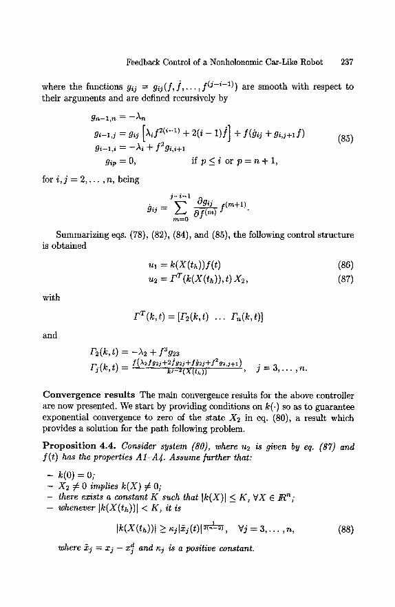
Feedback Control of a Nonholonomic Car-Like Robot 237
where the functions gij = g i j ( f , ] , . . . , f ( J - i - 1 ) ) are smooth with respect to their arguments and are defined recursively by
gn-l ,n = - A n
g,-1,j = gij [,kif 2('-1) + 2 ( i - 1)1] + S(gij + g, , j+If)
g i - l , i = - -h i + f2g l , i+l
gip = O,
for i , j = 2, . . . ,n, being
i f p < i or p = n + l ,
~ - i - 1 0 g i ~ f(m+l). gij = ~ Of(m )
m----0
(85)
and
with
Ul = k ( X ( t h ) ) f ( t )
u2 = F T ( k ( X ( t h ) ) , t) X2,
(86) (87)
FT(k , t ) = [F2(k,t) . . . Fn(k,t)]
F2(k, t) = - ~ 2 + lag23
k~-2(X(th)) , j = 3 , . . . ,n.
Convergence resul ts The main convergence results for the above controller are now presented. We start by providing conditions on k(-) so as to guarantee exponential convergence to zero of the state X2 in eq. (80), a result which provides a solution for the path following problem.
Proposition 4.4. Consider system (80), where u2 is given by eq. (87) and f ( t ) has the properties A1-A~. Assume further that:
- k ( o ) = o ;
- X2 7 £ 0 implies k ( X ) ~ O; - there exists a constant K such that Ik(X)t < K , V X E J~ln; - whenever [k(X(th))[ < K , it is
Ik(X(th))l > ~t:~j(t)l~-r2~, Vj = 3 , . . . ,n, (88)
where ~,j = xj - x] and ~j is a positive constant.
Summarizing eqs. (78), (82), (84), and (85), the following control structure is obtained
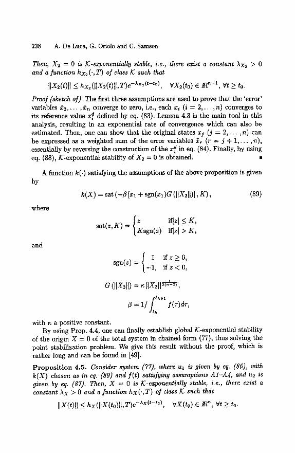
238 A. De Luca, G. Oriolo and C. Samson
Then, X2 : 0 is IC-exponentially stable, i.e., there exist a constant Ax2 > 0 and a function hx2(.,T) of class 1C such that
tlx2(t)[t _< hx2(llX2(t)ll,T)e VX2(to) e ~n-1 , Vt ~ to.
Proof (sketch of) The first three assumptions are used to prove that the 'error' variables 22,. . . ,xn converge to zero, i.e., each xi (i = 2, . . . ,n) converges to
d defined by eq. (83). Lemma 4.3 is the main tool in this its reference value xi analysis, resulting in an exponential rate of convergence which can also be estimated. Then, one can show that the original states xj (j = 2, . . . , n) can be expressed as a weighted sum of the error variables xr (r = j + 1,. . . ,n),
d in eq. (84). Finally, by using essentially by reversing the construction of the xi eq. (88),/C-exponential stability of )(2 = 0 is obtained.
by
where
and
A function k(.) satisfying the assumptions of the above proposition is given
k ( X ) -~- sat ( - ~ Ix 1 -[- sgn(xl)G (ltX2H)], K ) ,
f if[z[ _< K, sat(z, K) = {z
gsgn(z) ifN > K, [
(89)
1 ifz_>0, sgn(z)= -1, if z < 0 ,
1 G ([[X2[I) -- ~ [[x2[l ~-c~,
f th+l
/~ = 1/ f(T)d~, dth
with ~ a positive constant. By using Prop. 4.4, one can finally establish global/(:-exponential stability
of the origin X = 0 of the total system in chained form (77), thus solving the point stabilization problem. We give this result without the proof, which is rather long and can be found in [49].
Propos i t ion 4.5. Consider system (77), where Ul is given by eq. (86), with k(X) chosen as in eq. (89) and f(t) satisfying assumptions A1-A4, and u2 is given by eq. (87). Then, X = 0 is lC-exponentially stable, i.e., there exist a constant Ax > 0 and a function hx( . ,T) of class ]C such that
[IX(t)tl _< hx(iiX(to)ll,T) e-~x(t-t°), VX(to) e ~'~, Vt > to.
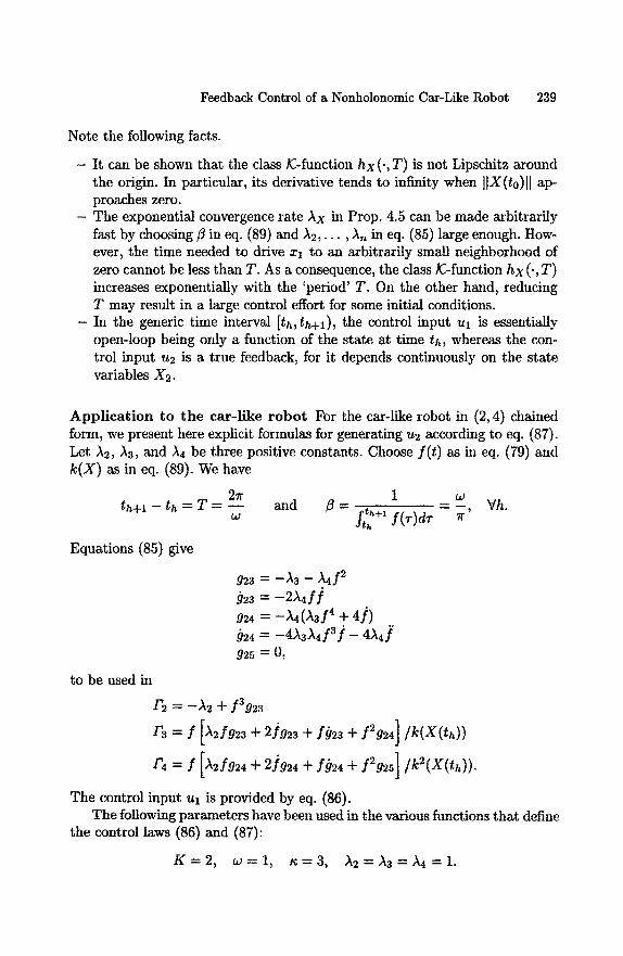
Feedback Control of a Nonholonomic Car-Like Robot 239
Note the following facts.
- It can be shown that the class K-function h x ( . , T ) is not Lipschitz around the origin. In particular, its derivative tends to infinity when IlX(t0)H ap- proaches zero.
- The exponential convergence rate Ax in Prop. 4.5 can be made arbitrarily fast by choosing ~ in eq. (89) and A2,... , An in eq. (85) large enough. How- ever, the time needed to drive xl to an arbitrarily small neighborhood of zero cannot be less than T. As a consequence, the class E-function hx ( . , T ) increases exponentially with the 'period' T. On the other hand, reducing T may result in a large control effort for some initial conditions.
- In the generic time interval [th, th+l), the control input ul is essentially open-loop being only a function of the state at time th, whereas the con- trol input u2 is a true feedback, for it depends continuously on the state variables )(2.
A p p l i c a t i o n to t h e car-l ike r o b o t For the car-like robot in (2, 4) chained form, we present here explicit formulas for generating u2 according to eq. (87). Let A2, A3, and Aa be three positive constants. Choose f ( t ) as in eq. (79) and k ( X ) as in eq. (89). We have
21r 1 w - Vh. th+l -- th = T = --w and j3 = fth+~ f(7)d~" : r '
dth
Equations (85) give
g23 = -;~3 - ~4Y 2 g23 = --2A4fj ~ g24 = --)~4(~3f 4 + 4]) 924 = -4A3A4f 3] - 4A4] g25 = 0,
to be used in
/'2 : -A2 + f3g23
F3 ---- f [)~2fg23 + 2]g23 -1- fg23 + f2ff24] /k(x (th))
r, = y [a Sg2, + 2/9 , + Sg , + S2g s]/k2(X(th)).
The control input Ul is provided by eq. (86). The following parameters have been used in the various functions tha t define
the control laws (86) and (87):
K = 2 , w = l , ~ : 3 , ~ 2 = ) ~ a = ~ 4 = 1 .
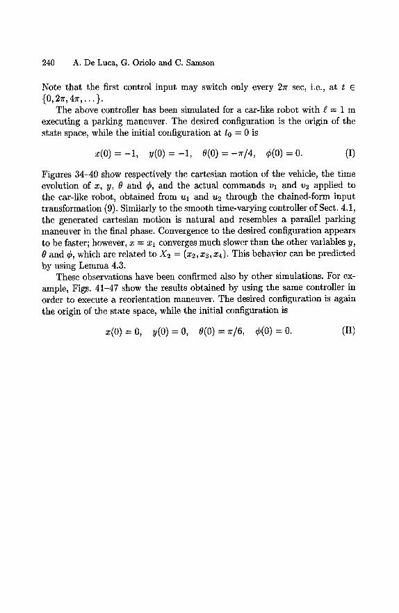
240 A. De Luca, G. Oriolo and C. Samson
Note that the first control input may switch only every 2~r sec, i.e., at t E {0, 2~r, 4 r , . . . }.
The above controller has been simulated for a car-like robot with ~ = 1 m executing a parking maneuver. The desired configuration is the origin of the state space, while the initial configuration at to = 0 is
x(O)=-l, y(O)=-l, O(O)=-r/4, ¢ ( 0 ) = 0 . (I)
Figures 34-40 show respectively the cartesian motion of the vehicle, the time evolution of x, y, 0 and ¢, and the actual commands vl and v2 applied to the car-like robot, obtained from ut and u2 through the chained-form input transformation (9). Similarly to the smooth time-varying controller of Sect. 4.1, the generated cartesian motion is natural and resembles a parallel parking maneuver in the final phase. Convergence to the desired configuration appears to be faster; however, x = xt converges much slower than the other variables y,
and ¢, which are related to X2 = (x2, x3, x4). This behavior can be predicted by using Lemma 4.3.
These observations have been confirmed also by other simulations. For ex- ample, Figs. 41-47 show the results obtained by using the same controller in order to execute a reorientation maneuver. The desired configuration is again the origin of the state space, while the initial configuration is
x ( 0 ) = 0 , y ( 0 ) = 0 , e ( 0 ) = ~ / 6 , ¢ ( 0 ) = 0 . (II)
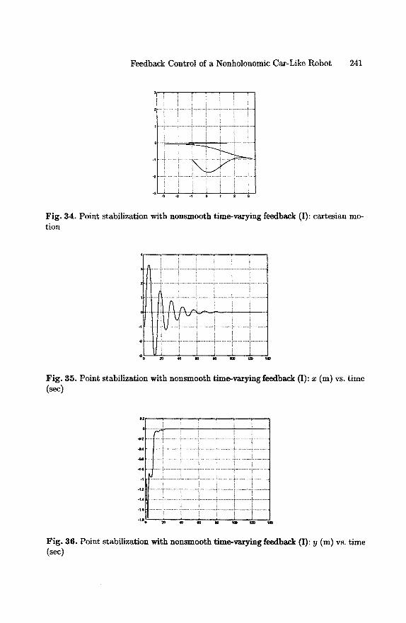
F e e d b a c k C o n t r o l of a N o n h o l o n o m i c C a r - L i k e R o b o t 241
3 , ,
÷ .......... i .......... ) .......... i .......... ! .......... ~ ........... i .... )
o , . ~ , . . . . . : i :: : :, i . . . . ~ . . . . . . . . . . i , -
. , ~ . . . . . . i . . . . . . : . . . . . . i . . . . . . . . i . . . . . . . ! . . . . . . . ) . . . .
F i g . 3 4 . P o i n t s t a b i l i z a t i o n w i t h n o n s m o o t h t i m e - v a r y i n g f e e d b a c k (I): c a r t e s i a n mo-
t i o n
. . . . . . . . . . . . . . . i . . . . . . . . . . . . . . . . . . . . . . . . . . . . . . . . . . . . . . . . . . . . . . . . . . . . . . . . .
F i g . 3 5 . P o i n t s t a b i l i z a t i o n w i t h n o n s m o o t h t i m e - v a r y i n g f e e d b a c k (I) : x ( m ) vs. t i m e (see)
-OA
)
) )
F i g . 3 6 . P o i n t s t a b i l i z a t i o n w i t h n o n s m o o t h t i m e - v a r y i n g f e e d b a c k (I) : y (m) vs. t i m e (sec)
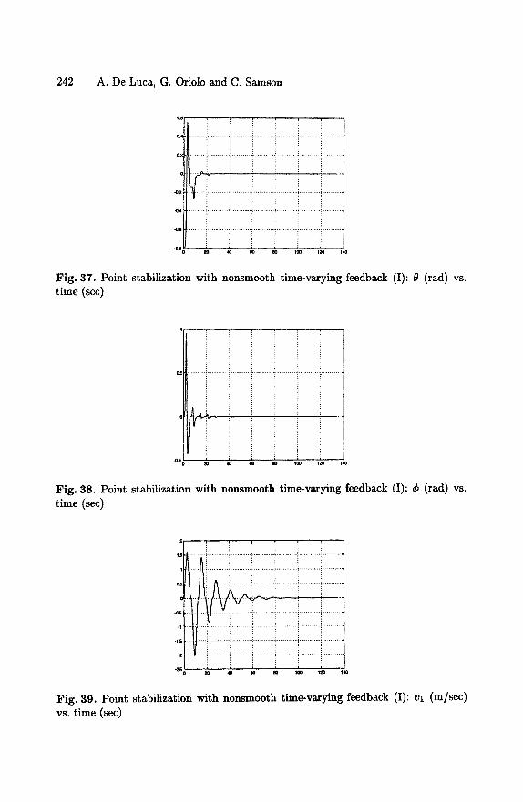
242 A. De Luca, G. Oriolo and C. Samson
Fig, 37. Point stabilization with nonsmooth time-varying feedback (I): ~ (tad) vs. time (sec)
Z
o 2o 4o m m lOO izo 14o
Fig. 38. Point stabilization with nonsmooth time-varying feedback (I): ¢ (red) vs. time (see)
I i )
o
.1
.2
iiiiiiiill iiiiiiii Ill ~o 4o eo m loo Izo i,lo
Fig. 39. Point stabilization with nonsmooth time-varying feedback (I): vl (m/sec) vs, time (sec)
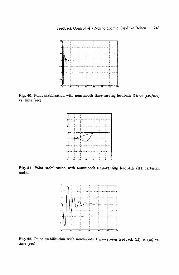
Feedback Control of a Nonholonomic Car-Like Robot 243
. !
-2
Fig. 40. Point stabilization with nonsmooth time-varying feedback (I): v2 (rad/sec) vs. time (sec)
.............................. i .......... i .............................
. . . . . . . . . . . i ....... i ....... i ................. ! .......
Fig. 41. Point stabilization with nonsmooth time-varying feedback (II): cartesian motion
2O 40 e3 m ~ o t ~
Fig. 42. Point stabilization with nonsmooth time-varying feedback (II): x (m) vs. time (sec)

244 A De Luca, G. Oriolo and C. Samson
. . . . . . i . . . . . . . . .
i .............. i. ............... i ................ i ............... i ............... i ...............
. t . . . . . . . . . . . . . . i . . . . . . . . . . !. . . . . . . . . . . i . . . . . . . . . . . . . i . . . . . . . . . . . . . .
~ = . . . . . . . . . . . . . . . . . . . . . . . . . . . . . i . . . . . . . . . . . . . . . . i . . . . . . . . . . . . . . . i . . . . . . . . . . . . . . . . i . . . . . . . . . . . . . . .
! 4
Fig. 43. Point stabilization with nonsmooth time-varying feedback (II): y (m) vs. time (sec)
i
. . . . . . . . . . . . . i ............... i ................ i ............... i ............... i ...............
| , , , , | , . o . i i
Fig. 44. Point stabilization with nonsmooth time-varying feedback (II): 0 (rad) vs. time (see)
t
! ! ! ! !
oJ . . . . . . . . . . . . . ~ . . . . . . . . . . . . . . . . ! . . . . . . . . . . . . . . . 4 . . . . . . . . . . . . . . . i . . . . . . . . . . . . . . . . ! . . . . . . . . . . . . . . .
* , ............. ................ i ................ i ................ i ............... ~ ...............
/
Fig. 45. Point stabilization with nonsmooth time-varying feedback (II): ¢ (rad) vs. time (sec)
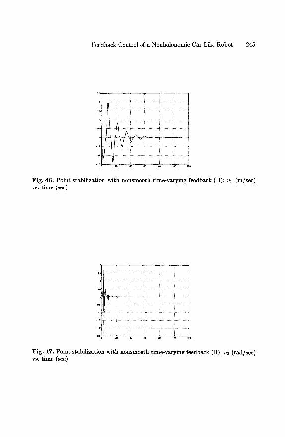
Feedback C o n t r o l o f a N o n h o l o n o m i c C a r - L i k e R o b o t 2 4 5
2 . ' . - ,
2 . . . . . . . . . . . . . . . . . . . . . . . . . . ! . . . . . . . . . . . . . . . ? . . . . . . . . . . . . . . . i . . . . . . . . . . . . . . . . ? . . . . . . . . . . . . . . .
1: . . . . . . . . . ................ i ..... i i
o ~ . . . . . . . . . . : . . . . . . . . . . . i . . . . . . . . . . . . . . . 4 . . . . . . . . . . . . . i . . . . . . . . . . . . . . . . i . . . . . . . . . . . . . .
o . . . . . . . . . . . i . . . . . . . i i . . . .
. ~ . . . . . . . . . . . . . . . ; . . . . . . . . . . . . . . . . . . . . . . . . . . . . ~ . . . . . . . . . . . . . . :~ . . . . . . . . . . . .
- 1 s ~2o
Fig. 46. Point stabilization with nonsmooth time-varying feedback (II): vl (m/sec) vs. time (see)
2
Q
....., 212211'i ii122112112112121112121112121212211211211111121121Ziiil;ii211111212i21121121211111 ~~ ...... ; ,o ® ,,o , & ' ,~o
Fig. 4?. Point stabilization with nonsmooth time-varying feedback (II): v2 (rad/sec) vs. time (sec)
246 A. De Luca, G. Oriolo and C. Samson
4.3 A b o u t exponent ia l convergence
The peculiar convergence behavior of both presented stabilizing methods de- serves some comments. We have already pointed out in Sect. 2.2 that the failure of the linear controllability test for the car-like robot indicates that smooth ex- ponential stability in the sense of Lyapunov cannot be obtained. Recall that (local) exponential stability means that the system trajectories X(t) satisfy the following inequality
HX(t)H <_ KlJX(to)lle -~(t-t°), VX(to) ~ B, Vt > to, (90)
with K, A positive real numbers and B a neighborhood of the origin. The prac- tical significance of this relationship is twofold: (i) small initial errors cannot produce arbitrarily large transient deviations since IIX(t)ll < KIIX(to)l I, and (ii) all solutions converge to zero exponentially.
While it is still unclear whether both properties can be simultaneously achieved for nonholonomic systems, one can still design a control law that guarantees at least one of the two. In the case of smooth time-varying feedback laws, such as the one presented in Sect. 4.1, it may be easily verified that
tlX(t)l I _< KllX(to)ll, VX(to), Vt ___ to, (91)
holds for some positive constant K. However, when using the control law w2 of Prop. 4.2, convergence to zero of ]lZ[I (and hence, of IIXIf) cannot be exponen- tial. In fact, if this were the case, ul would itself converge to zero exponentially, and thus the integral f t o lul('r)]dT would not diverge. This is in contradiction with the fact that divergence of this integral is necessary for the asymptotic convergence of tIZ2ll to zero. As a matter of fact, it is only possible to show that
[[X(t)[] _< K[IX(to)[lP(t), with p(O) = 1, thin p(t) = 0, (92)
where p(t) is a decreasing function whose convergence rate is strictly less than exponential. This theoretical expectation is confirmed by the simulations results of Sect. 4.1. In particular, it has been observed [41] that smooth time-varying feedback control applied to a unicycle yields a convergence rate slower than t -1/2 for most initial configurations, a fact that can be proven using center manifold theory.
On the other hand, existing nonsmooth feedback laws for nonholonomic systems do not guarantee uniform boundedness of the transient error ratio IIX(t)ll/llx(to)ll. For example, the piecewise-continuous time-invariant feed- back law proposed in [8] for the stabilization of a unicycle yields
Hx(t)l[ <_ (K1 + K21lX(to)N)e -~'(t-t°), VX(to), Vt >__ to, (93)
Feedback Control of a Nonholonomic Car-Like Robot 247
with K1, K2 positive real numbers. All solutions converge to zero exponentially, but a small initial error or perturbation may produce transient deviations whose size is larger than some constant.
Similarly, we have seen that the nonsmooth time-varying feedback of Sect. 4.2 guarantees ]~-exponential stability for general chained-form systems. Even if all solutions converge to zero exponentially, this type of asymptotic stability is weaker than property (90), in the sense that small initial errors or perturbations can produce transient deviations of much larger amplitude. Nev- ertheless, it is stronger than (93), for such deviations are not bounded below by some positive constant.
The above discussion may suggest that smooth time-varying feedback laws are somewhat less sensitive to initial errors than nonsmooth feedback laws. This degree of robustness is paid in terms of the asymptotic rate of conver- gence, which is not exponential. However, smooth time-varying feedback may be modified to achieve practical exponential stability, in the sense that the sys- tem state may be steered to any desired small neighborhood of the origin in arbitrary time. This fact is illustrated by the simulation results obtained with the heat function qa in Sect. 4.1.
5 Conclusions
We have presented and compared several feedback solutions for point stabiliza- tion, path following and trajectory tracking control tasks executed by a mobile robot with car-like kinematics.
The problem of accurate tracking of a persistent trajectory can be solved using either linear control synthesis, based on the approximate linearization of the system around the nominal trajectory, or nonlinear (static or dynamic) control synthesis, achieving exact linearization of the (input-output or full- state) closed-loop equations. Local exponential convergence to zero tracking error is obtained in the linear case, while global exponential convergence with prescribed error dynamics is guaranteed in the nonlinear case. In both ap- proaches, the closed-loop controller consists of a nominal feedforward term and of an error feedback action.
For the stabilization to a fixed configuration, the use of new classes of time- varying nonlinear controllers has proven to be effective. From a theoretical point of view, time-varying feedback overcomes the obstruction on the existence of smooth time-invariant stabilizing control laws for nonholonomic systems. Two types of time-varying control laws were presented, respectively expressed by a smooth and a nonsmooth function of the robot state. In both cases, we have recognized that path following can be formulated as a subproblem of point stabilization. The asymptotic rate of convergence of the smooth controller is
248 A. De Luca, G. Oriolo and C. Samson
lower than the exponential orie obtained in the nonsmooth case. However, it may be questioned whether the theoretical convergence rate alone is a good measure of the overall control performance. In practice, what really matters is a rapid initial decay of the error to a small neighborhood of zero under realistic experimental conditions.
The reported numerical simulations have shown the benefit of feedback control in recovering from initial errors with respect to the desired fixed or moving target. In order to fully appreciate these results, we remark that errors (at the initial time or later) can be interpreted as the effect of an instantaneous disturbance acting on the system. Therefore, the robot motion under feedback control is robust with respect to such non-persistent disturbances.
Most of the results have been presented using a canonical transformation of the system into chained form. Although the use of chained forms is not needed in principle, it allows to obtain systematic results that can be extended beyond the considered case study of a car-like mobile robot. For example, the control results hold true also for a car towing N trailers, each attached at the midpoint of the rear axle of the previous one (zero hooking). On the other hand, the control problem for the general case of N trailers with nonzero hooking is still open, because a chained-form transformation is not available for this system.
Throughout this study, we have dealt with a first-order kinematic model of the mobile robot, in which velocities were assumed to be the control in- puts. Extension to second-order kinematics, with accelerations as inputs, and inclusion of vehicle dynamics, with generalized forces as inputs, are possible. In particular, we point out that the nominal dynamics of the vehicle can be completely canceled by means of a nonlinear state feedback so as to obtain a second-order, purely kinematic problem.
Concerning the application of the proposed feedback controllers to real mo- bile robot systems, there are several non-ideal conditions that may affect the actual behavior of the controlled robot, notably: uncertain kinematic parame- ters of the vehicle (including, e.g., the wheels' radius); mechanical limitations such as backlash at the steering wheels and limited range of the steering an- gle; actuator saturation and dead-zone; noise and biases in the transformation from physical sensor data to the robot state; quantization errors in a digital implementation. Control robustness with respect to these kinds of uncertainties and/or disturbances is an open and challenging subject of research. For linear as well as nonlinear systems, Lyapunov exponential stability implies some degree of robustness with respect to perturbations. However, since this kind of stability has not been demonstrated for the point stabilization problem of nonholonomic systems, the connection between robustness properties and asymptotic (even exponential) rate of convergence is not yet well understood.
It should also be noted that perturbations acting on nonholonomic mobile robots are not of equal importance, depending on which component of the state
Feedback Control of a Nonholonomic Car-Like Robot 249
is primarily affected. A deviation in a direction compatible with the vehicle mobility (e.g., sliding of the wheels on the ground) is clearly not as severe as a deviation which violates the kinematic constraints of the system (e.g., lateral skidding of the car-like robot). In any case, proprioceptive sensors may not reveal these perturbing actions and all the controllers presented in this chapter--which assume that the exact robot state is available--would fail in completing their task. A possible solution would be to close the feedback loop using exteroceptive sensor measurements, which provide absolute information about the robot location in its workspace. Currently, it is not clear whether the best solution would be to estimate the robot state from these measurements and then use the previous controllers, or to design new control laws aimed at zeroing the task error directly at the sensor-space level.
6 F u r t h e r r e a d i n g
In addition to the references cited to support the results so far presented, many other related works have appeared in the literature. Hereafter, we mention some of the most significant ones.
A detailed reference on the kinematics of wheeled mobile robots is [2]. The dynamics of general nonholonomic systems was thoroughly analyzed in [31]. A controllability study for kinematic models of car-like robots with trailers was presented in [24], while stabilizability results for both kinematic and dynamic models of nonholonomic systems were given in [5,7].
The problem of designing input commands that drive a nonholonomic mobile robot to a desired configuration has been first addressed through open-loop techniques. Purely differential-geometric approaches were followed in [23,50], while the most effective solutions have been obtained by resort- ing to chained-form transformations and sinusoidal steering [28], or by using piecewise-constant functions as control inputs [26]. In [36] it was shown how the existence of differentially flat outputs can be exploited in order to design efficiently open-loop controls.
A number of works have dealt with the problem of controlling via feedback the motion of a unicycle. In fact, both discontinuous and time-varying feedback controllers were first proposed and analyzed for this specific kinematics. The trajectory tracking problem was solved in [39] by means of a local feedback action. Use of dynamic feedback linearization was proposed in [14]. A piecewise- continuous feedback with an exponential rate of convergence was presented in [8] for the point stabilization task, and later extended to the path following problem in [47]. Another piecewise-continuous controller, obtained through an appropriate switching sequence, was devised in [5]. The explicit inclusion of the exogenous time variable in a smooth feedback law was proposed in [38].
250 A. De Luca, G. Oriolo and C. Samson
In [34], a hybrid stabilization strategy was introduced that makes use of a time-invariant feedback law far from the destination and of a time-varying law in its vicinity. The use of a discontinuous transformation in polar coordinates allowing to overcome the limitation of Brockett's theorem was independently proposed in [1] and [3] for the point stabilization problem; strictly speaking, these schemes are not proven to be stable in the sense of Lyapunov, for they only ensure exponential convergence of the error to zero. A survey of control techniques for the unicycle can be found in [9].
For car-like robots, the trajectory tracking problem was also addressed in [13] through the use of dynamic feedback linearization, and in [16] via flat outputs design and time-scaling. Path following via input scaling was proposed in [15,37]. As for the point stabilization problem, the successful application of time-varying feedback to the case of car-like robots [43] has subsequently moti- vated basic research work aimed at exploring the potentialities of this approach. In particular, results have been obtained for the whole class of controllable drift- less nonlinear systems in [11,12], while general synthesis procedures were given in [33] for chained-form systems and in [35] for power-form systems; in the lat- ter, the use of a nonsmooth but continuous time-varying feedback guarantees exponential convergence to the desired equilibrium point. Using an analysis based on homogeneous norms, similar results were obtained for driftless sys- tems in [30], and for chained-form systems in [27] by means of a backstepping technique. Other related works include [17] and [51]. In the first, the problem of approximating a holonomic path via a nonholonomic one is solved by using time-periodic feedback control. In the second, the open-loop sinusoidal steer- ing method is converted to a stabilization strategy, by adding to the nominal command a mixed discontinuous/time-varying feedback action.
Very few papers have explicitly addressed robustness issues in the control of nonholonomic systems. The robustness of a particular class of nonsmooth controllers based on invariant manifolds was analyzed in [10]. Robust stabiliza- tion of car-like robots in chained form was obtained in [4] and [25] by applying iteratively a contracting open-loop controller; exponential convergence to the desired equilibrium is obtained for small model perturbations. Another possible approach to the design of effective control laws in the presence of nonidealities and uncertainties is represented by learning control, as shown in [32].
Finally, the design of sensor-level controllers for nonholonomic mobile robots is at the beginning stage. The general concept of task-driven feedback control for holonomic manipulators is described in [40]. A first attempt to extend this idea to the point stabilization problem of a mobile robotic system can be found in [52].
Feedback Control of a Nonholonomic Car-Like Robot 251
References
1. M. Aicardi, G. Casalino, A. Bicchi, and A. Balestrino, "Closed loop steering of unicycle-like vehicles via Lyapunov techniques," IEEE Robotics 6J Automation Mag., vol. 2, no. 1, pp. 27-35, 1995.
2. J. C. Alexander and J. H. Maddocks, "On the kinematics of wheeled mobile robots," Int. J. of Robotics Research, vol. 8, no. 5, pp. 15-27, 1989.
3. A. Astolfi, "Exponential stabilization of a mobile robot," 3rd European Control Conf., Roma, I, pp. 3092-3097, 1995.
4. M. K. Bennani and P. Rouchon, "Robust stabilization of flat and chained sys- tems," 3rd European Control Conf., Roma, I, pp. 2642-2646, 1995.
5. A. M. Bloch, M. Reyhanoglu, and N. H. McClamroch, "Control and stabilization of nonholonomic dynamic systems," IEEE Trans. on Automatic Control, vol. 37, no. 11, pp. 1746-1757, 1992.
6. R.W. Brockett, "Asymptotic stability and feedback stabilization," in Differential Geometric Control Theory, R. W. Brockett, R. S. Millman, H. J. Sussmann (Eds.), Birkh~iuser, Boston, MA, pp. 181-191, 1983.
7. G. Campion, B. d'Andrea-Novel, and G. Bastin, "Modeling and state feedback control of nonholonomic mechanical systems," 30th IEEE Conf. on Decision and Control, Brighton, UK, pp. 1184-1189, 1991.
8. C. Canudas de Wit and O. J. Sordalen, "Exponential stabilization of mobile robots with nonholonomic constraints," IEEE Trans. on Automatic Control, vol. 37, no. 11, pp. 1791-1797, 1992.
9. C. Canudas de Wit, H. Khennouf, C. Samson, and O. J. Sordalen, "Nonlinear control design for mobile robots," in Recent Trends in Mobile Robots, Y. F. Zheng (Ed.), World Scientific Publisher, 1993.
10. C. Canudas de Wit and H. Khennouf, "Quasi-continuous stabilizing controllers for nonholonomic systems: Design and robustness considerations," 3rd European Control Conf., Roma, I, pp. 2630-2635, 1995.
11. J.-M. Coron, "Global asymptotic stabilization for controllable systems without drift," Mathematics of Control, Signals, and Systems, vol. 5, pp. 295-312, 1992.
12. J.-M. Coron, "Links between local controllability and local continuous stabi- lization," 2nd IFAC Syrup. on Nonlinear Control System Design, Bordeaux, F, pp. 477-482, 1992.
13. B. d'Andrea-Novel, G. Bastin, and G. Campion, "Dynamic feedback linearization of nonholonomic wheeled mobile robots," 1992 IEEE Int. Conf. on Robotics and Automation, Nice, F, pp. 2527-2532, 1992.
14. A. De Luca and M. D. Di Benedetto, "Control of nonholonomic systems via dynamic compensation," Kybernetica, vol. 29, no. 6, pp. 593-608, 1993.
15. E. D. Dickmanns and A. Zapp, "Autonomous high speed road vehicle guidance by computer vision," lOth IFAC World Congr., Miinchen, D, pp. 221-226, 1987.
16. M. Fliess, J. Ldvine, P. Martin, and P. Rouchon, "Design of trajectory stabiliz- ing feedback for driftless flat systems," 3rd European Control Conf., Roma, I, pp. 1882-1887, 1995.
17. L. Gurvits and Z. Li, "Smooth time-periodic feedback solutions for nonholonomic motion planning," in Nonholonomic Motion Planning, Z. Li, J. Canny (Eds.), Kluwer Academic Publishers, Norwell, MA, pp. 53-108, 1992.
252 A. De Luca, G. Oriolo and C. Samson
18. A. Isidori, Nonlinear Control Systems, 3rd Edition, Springer-Verlag, London, UK, 1995.
19. T. Kailath, Linear Systems, Prentice-Hall, Englewood Cliffs, NJ, 1980. 20. H. K. Khalil, Nonlinear Systems, Macmillan, New York, NY, 1992. 21. I. V. Kolmanovsky, M. Reyhanoglu, and N. H. McClamroch, "Discontinuous feed-
back stabilization of nonholonomic systems in extended power form," 33rd IEEE Conf. on Decision and Control, Lake Buena Vista, FL, pp. 3469-3474, 1994.
22. M. Krstid, I. Kanellakopoulos, and P. Kokotovid, Nonlinear and Adaptive Control Design, John Wiley • Sons, New York, NY, 1995.
23. G. Lafferriere and H. J. Sussmann, "Motion planning for controllable systems without drift," 1991 IEEE Int. Conf. on Robotics and Automation, Sacramento, CA, pp. 1148-1153, 1991.
24. J.-P. Laumond, '~Controllability of a multibody mobile robot," IEEE Trans. on Robotics and Automation, vol. 9, no. 6, pp. 755-763, 1993.
25. P. Lucibello and G. Oriolo, "Stabilization via iterative state steering with ap- plication to chained-form systems," 35th IEEE Conf. on Decision and Control, Kobe, J, pp. 2614-2619, 1996.
26. S. Monaco and D. Normand-Cyrot, "An introduction to motion planning under multirate digital control," 31st IEEE Conf. on Decision and Control, Tucson, AZ, pp. 1780-1785, 1992.
27. P. Morin and C. Samson, "Time-varying exponential stabilization of chained sys- tems based on a backstepping technique," 35th IEEE Conf. on Decision and Control, Kobe, J, pp. 1449-1454, 1996.
28. 1%. M. Murray and S. S. Sastry, "Nonholonomic motion planning: Steering using sinusoids," IEEE Trans. on Automatic Control, vol. 38, no. 5, pp. 700-716, 1993.
29. 1%. M. Murray, "Control of nonholonomic systems using chained forms," Fields Institute Communications, vol. 1, pp. 219-245, 1993.
30. R. M. Murray and R. T. M'Closkey, "Converting smooth, time-varying, asymp- totic stabilizers for driftless systems to homogeneous, exponential stabilizers," 3rd European Control Conf., Roma, t, pp. 2620-2625, 1995.
31. J. I. Neimark and F. A. Fufaev, Dynamics of Nonholonomie Systems, American Mathematical Society, Providence, RI, 1972.
32. G. Oriolo, S. Panzieri, and G. Ulivi, "An iterative learning controller for nonholo- nomic robots," I996 IEEE Int. Conf. on Robotics and Automation, Minneapolis, MN, pp. 2676-2681, 1996.
33. J.-B. Pomet, "Explicit design of time-varying stabilizing control laws for a class of controllable systems without drift," Systems gJ Control Left., vol. 18, pp. 147-158, 1992.
34. J.-B. Pomet, B. Thuilot, G. Bastin, and G. Campion, "A hybrid strategy for the feedback stabilization of nonholonomic mobile robots," 1992 IEEE Int. Conf. on Robotics and Automation, Nice, F, pp. 129-134, 1992.
35. J.-B. Pomet and C. Samson, "Time-varying exponential stabilization of nonholo- nomic systems in power form," INR/A Rep. 2126, Dec. 1993.
36. P. Rouchon, M. Fliess, J. Ldvine, and P. Martin, "Flatness and motion planning: The car with n trailers," Pnd European Control Conf., GrSningen, NL, pp. 1518- 1522, 1993.
Feedback Control of a Nonholonomic Car-Like Robot 253
37. M. Sampei, T. Tamura, T. Itoh, and M. Nakamichi, "Path tracking control of trailer-like mobile robot," 1991 IEEE/RSJ Int. Work. on Intelligent Robots and Systems, Osaka, J, pp. 193-198, 1991.
38. C. Samson, "Velocity and torque feedback control of a nonholonomic cart," in Advanced Robot Control, C. Canudas de Wit (Ed.), Birkh~iuser, Boston, MA, pp. 125-151, 1991.
39. C. Samson and K. Ait-Abderrahim, "Feedback control of a nonholonomic wheeled cart in cartesian space," 1991 IEEE Int. Conf. on Robotics and Automation, Sacramento, CA, pp. 1136-1141, 1991.
40. C. Samson, M. Le Borgne, B. Espian, Robot Control: The Task Function Ap- proach," Oxford Science Publications, Oxford, UK, 1991.
41. C. Samson and K. Ait-Abderrahim, "Feedback stabilization of a nonholonomic wheeled mobile robot, 1991 IEEE/RSJ Int. Work. on Intelligent Robots and Sys- tems," Osaka, J, pp. 1242-1247, 1991.
42. C. Samson, "Path following and time-varying feedback stabilization of a wheeled mobile robot~" 2nd Int. Conf. on Automation, Robotics and Computer Vision, Singapore, 1992.
43. C. Samson, "Time-varying feedback stabilization of car-like wheeled mobile robots," Int. J. of Robotics Research, vol. 12, no. 1, pp. 55-64, 1993.
44. C. Samson, "Control of chained systems. Application to path following and time- varying point-stabilization of mobile robots," IEEE Trans. on Automatic Control, vol. 40, no. 1, pp. 64-77, 1995.
45. E. D. Sontag, "Feedback stabilization of nonlinear systems," in Robust Control of Linear Systems and Nonlinear Control, M. A. Kaashoek, J. H. van Schuppen, A. C. M. Ran (Eds.), Birkh/iuser, Cambridge, MA, pp. 61-81, 1990.
46. O. J. Sordalen, "Conversion of the kinematics of a car with n trailers into a chained form," 1993 IEEE Int. Conf. on Robotics and Automation, Atlanta, GA, vol. 1, pp. 382-387, 1993.
47. O . J . Sordalen and C. Canudas de Wit, "Exponential control law for a mobile robot: Extension to path following," IEEE Trans. on Robotics and Automation, vol. 9, no. 6, pp. 837-842, 1993.
48. O.J. Sordalen, "Feedback control of nonholonomic mobile robots," Ph.D. Thesis, The Norwegian Institute of Technology, Trondheim, NOt Mar. 1993.
49. O. J. Strdalen and O. Egeland, "Exponential stabilization of nonholonomic chained systems," IEEE Trans. on Automatic Control, vol. 40, no. 1, pp. 35- 49, 1995.
50. H. J. Sussmann and W. Liu, "Limits of highly oscillatory controls and the approx- imation of general paths by admissible trajectories," Tech. Rep. SYCON-91-02, Rutgers University, Feb. 1991.
51. A. R. Teel, R. M. Murray, and G. Walsh, "Nonholonomic control systemsi From steering to stabilization with sinusoids," 31st IEEE Conf. on Decision and Con- trol, ~hcson, AZ, pp. 1603-1609, 1992.
52. D. Tsakiris, C. Samson, and P. Rives, "Vision-based time-varying stabilization of a mobile manipulator," 6th Int. Conf. on Control, Automation, Robotics and Vision, Singapore, 1996.
Probabilistic Path Planning
P. Svestka and M. H. Overmars
Utrecht University
1 I n t r o d u c t i o n
The robot path planning problem, which asks for the computation of colli- sion free paths in environments containing obstacles, has received a great deal of attention in the last decades [25,15]. In the basic problem, there is one robot present in a static and known environment, and the task is to compute a collision-free path describing a motion that brings the robot from its current position to some desired goal position. Variations and extensions of this basic problem statement are numerous.
To start with, for a large class of robots (i.e., nonholonomic robots) compu- tation of collision-free paths is not sufficient. Not only are the admissible robot placements constrained by obstacles and the robot geometry, but also are the directions of motion subject to constraints. For example, mobile robots moving on wheels have such nonholonomic constraints, due to the fact that their wheels are not allowed to slide. Another realistic scenario is that of multiple robots acting in the same environment. In this case, apart from the restrictions im- posed by the obstacles, robot geometry, and possible nonholonomic constraints, one also has to avoid collisions between the robots mutually. Moving obstacles, uncertainties in sensing, and inexact control add further levels of difficulty.
In order to build robots that can autonomously act in real-life environ- ments, path planning problems as sketched above need to be solved. However, it has been proven that, in general, solving even the basic path planning prob- lem requires time exponential in the robots number of degrees of freedom. In spite of this discouraging problem complexity, various such complete planners have been proposed. Their high complexity however makes them impractical for most applications. And every extension of the basic path planning prob- lem adds in computational complexity. For example, if we have n robots of d degrees of freedom each, the complexity becomes exponential in nd. Or if we allow for moving obstacles, the problem becomes exponential in their number [9,35]. Assuming uncertainties in the robots sensing and control, leads to an exponential dependency on the complexity of the obstacles [9].
The above bounds deal with the exact problem, and therefore apply to complete planners. These are planners that solve any solvable problem, and return failure for each non-solvable one. So for most practical problems it seems
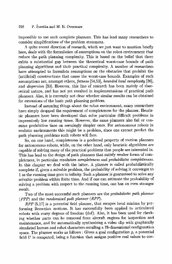
256 P. Svestka and M. H. Overmars
impossible to use such complete planners. This has lead many researchers to consider simplifications of the problem statement.
A quite recent direction of research, which we just want to mention briefly here, deals with the formulation of assumptions on the robot environment that reduce the path planning complexity. This is based on the belief that there exists a substantial gap between the theoretical worst-case bounds of path planning algorithms and their practical complexity. A number of researchers have attempted to formulate assumptions on the obstacles that prohibit the (artificial) constructions that cause the worst-case bounds. Examples of such assumptions are, amongst others, fatness [54,53], bounded local complexity [36], and dispersion [33]. However, this line of research has been mainly of theo- retical nature, and has not yet resulted in implementations of practical path planners. Also, it is currently not clear whether similar results can be obtained for extensions of the basic path planning problem.
Instead of assuming things about the robot environment, many researchers have simply dropped the requirement of completeness for the planner. Heuris- tic planners have been developed that solve particular difficult problems in impressively low running times. However, the same planners also fail or con- sume prohibitive time on seemingly simpler ones. For autonomous robots in realistic environments this might be a problem, since one cannot predict the path planning problems such robots will face.
So, on one hand, completeness is a preferred property of motion planners for autonomous robots, while, on the other hand, only heuristic algorithms are capable of solving many of the practical problems that people are interested in. This has lead to the design of path planners that satisfy weaker forms of com- pleteness, in particular resolution completeness and probabilistic completeness. In this chapter we deal with the latter. A planner is called probabilistically complete if, given a solvable problem, the probability of solving it converges to I as the running time goes to infinity. Such a planner is guaranteed to solve any solvable problem within finite time. And if one can estimate the probability of solving a problem with respect to the running time, one has an even stronger result.
Two of the most successful such planners are the probabilistic path planner (PPP) and the randomized path planner (RPP).
RPP [5,17] is a potential field planner, that escapes local minima by per- forming Brownian motions. It has successfully been applied to articulated robots with many degrees of freedom (dof). Also, it has been used for check- ing whether parts can be removed from aircraft engines for inspection and maintenance, and for automatically synthesising a video clip with graphically simulated human and robot characters entailing a 78-dimensional configuration space. The planner works as follows : Given a goal configuration g, a potential field U is computed, being a function that assigns positive real values to con-
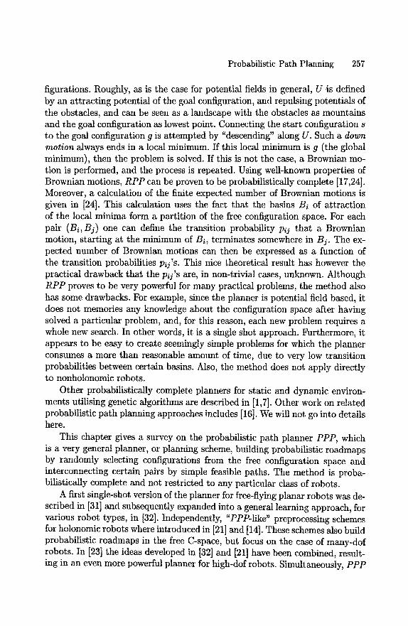
Probabilistic Path Planning 257
figurations. Roughly, as is the case for potential fields in general, U 4s defined by an attracting potential of the goal configuration, and repulsing potentials of the obstacles, and can be seen as a landscape with the obstacles as mountains and the goal configuration as lowest point. Connecting the start configuration s to the goal configuration g is attempted by "descending" along U. Such a down motion always ends in a local minimum. If this local minimum is g (the global minimum), then the problem is solved. If this is not the case, a Brownian mo- tion is performed, and the process is repeated. Using well-known properties of Brownian motions, RPP can be proven to be probabilistically complete [17,24]. Moreover, a calculation of the finite expected number of Brownian motions is given in [24]. This calculation uses the fact that the basins Bi of attraction of the local minima form a partition of the free configuration space. For each pair (Bi, Bj) one can define the transition probability pij that a Brownian motion, starting at the minimum of Bi, terminates somewhere in Bj. The ex- pected number of Brownian motions can then be expressed as a function of the transition probabilities pij's. This nice theoretical result has however the practical drawback that the pq's are, in non-trivial cases, unknown. Although RPP proves to be very powerful for many practical problems, the method also has some drawbacks. For example, since the planner is potential field based, it does not memories any knowledge about the configuration space after having solved a particular problem, and, for this reason, each new problem requires a whole new search. In other words, it is a single shot approach. Furthermore, it appears to be easy to create seemingly simple problems for which the planner consumes a more than reasonable amount of time, due to very low transition probabilities between certain basins. Also, the method does not apply directly to nonholonomic robots.
Other probabilistically complete planners for static and dynamic environ- ments utilising genetic algorithms are described in [1,7]. Other work on related probabilistic path planning approaches includes [16]. We will not go into details here.
This chapter gives a survey on the probabilistic path planner PPP, which is a very general planner, or planning scheme, building probabilistic roadmaps by randomly selecting configurations from the free configuration space and interconnecting certain pairs by simple feasible paths. The method is proba- bilistically complete and not restricted to any particular class of robots.
A first single-shot version of the planner for free-flying planar robots was de- scribed in [31] and subsequently expanded into a general learning approach, for various robot types, in [32]. Independently, "PPP-like" preprocessing schemes for holonomic robots where introduced in [21] and [14]. These schemes also build probabilistic roadmaps in the free C-space, but focus on the case of many-dof robots. In [23] the ideas developed in [32] and [21] have been combined, result- ing in an even more powerful planner for high-dof robots. Simultaneously, PPP
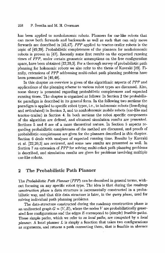
258 P. Svestka and M. H. Overmars
has been applied to nonholonomic robots. Planners for car-like robots that can move both forwards and backwards as well as such that can only move forwards are described in [45,47]. PPP applied to tractor-trailer robots is the topic of [49,39]. Probabilistic completeness of the planners for nonholonomic robots is proven in [47]. Recently some first results on the expected running times of PPP, under certain geometric assumptions on the free configuration space, have been obtained [22,20,3]. For a thorough survey of probabilistic path planning for holonomic robots we also refer to the thesis of Kavraki [19]. Fi- nally, extensions of PPP addressing multi-robot path planning problems have been presented in [46,48].
In this chapter an overview is given of the algorithmic aspects of PPP and applications of the planning scheme to various robot types are discussed. Also, some theory is presented regarding probabilistic completeness and expected running times. The chapter is organised as follows: In Section 2 the probabilis- tic paradigm is described in its general form. In the following two sections the paradigm is applied to specific robot types, i.e., to holonomic robots (free-flying and articulated) in Section 3, and to nonholonomic mobile robots (car-like and tractor-trailer) in Section 4. In both sections the robot specific components of the algorithm are defined, and obtained simulation results are presented. Sections 5 and 6 are of a more theoretical nature. In Section 5 aspects re- garding probabilistic completeness of the method are discussed, and proofs of probabilistic completeness are given for the planners described in this chapter. Section 6 deals with analyses of expected running time. Results by Kavraki et al. [22,20,3] are reviewed, and some new results are presented as well. In Section 7 an extension of PPP for solving multi-robot path planning problems is described, and simulation results are given for problems involving multiple car-like robots.
2 T h e P r o b a b i l i s t i c P a t h P l a n n e r
The Probabilistic Path Planner (PPP) can be described in general terms, with- out focusing on any specific robot type. The idea is that during the roadmap construction phase a data structure is incrementally constructed in a proba- bilistic way, and that this data structure is later, in the query phase, used for solving individual path planning problems.
The data-structure constructed during the roadn'lap construction phase is an undirected graph G = (l/, E), where the nodes V are probabilistically gener- ated free configurations and the edges E correspond to (simple) feasible paths. These simple paths, which we refer to as local paths, are computed by a local planner. A local planner L is simply a function that takes two configurations as axguments, and returns a path connecting them~ that is feasible in absence
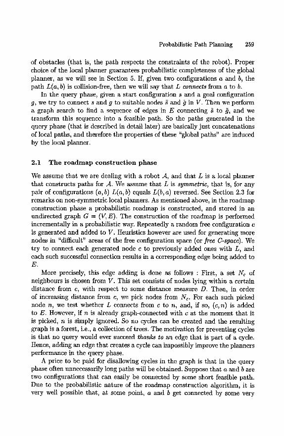
Probabilistic Path Planning 259
of obstacles (that is, the path respects the constraints of the robot). Proper choice of the local planner guarantees probabilistic completeness of the global planner, as we will see in Section 5. If, given two configurations a and b, the path L(a, b) is collision-free, then we will say that L connects from a to b.
In the query phase, given a start configuration s and a goal configuration g, we try to connect s and g to suitable nodes ~ and ~ in V. Then we perform a graph search to find a sequence of edges in E connecting ~ to ~, and we transform this sequence into a feasible path. So the paths generated in the query phase (that is described in detail later) are basically just concatenations of local paths, and therefore the properties of these "global paths" are induced by the local planner.
2.1 The roadmap construction phase
We assume that we are dealing with a robot .4, and that L is a local planner that constructs paths for ,4. We assume that L is symmetric, that is, for any pair of configurations (a, b) L(a, b) equals L(b, a) reversed. See Section 2.3 for remarks on non-symmetric local planners. As mentioned above, in the roadmap construction phase a probabilistic roadmap is constructed, and stored in an undirected graph G = (V, E). The construction of the roadmap is performed incrementally in a probabilistic way. Repeatedly a random free configuration c is generated and added to V. Heuristics however are used for generating more nodes in "difficult" areas of the free configuration space (or ]ree C-space). We try to connect each generated node c to previously added ones with L, and each such successful connection results in a corresponding edge being added to E.
More precisely, this edge adding is done as follows : First, a set Nc of neighbours is chosen from V. This set consists of nodes lying within a certain distance from c, with respect to some distance measure D. Then, in order of increasing distance from c, we pick nodes from No. For each such picked node n, we test whether L connects from c to n, and, if so, (c, n) is added to E. However, if n is already graph-connected with c at the moment that it is picked, n is simply ignored. So no cycles can be created and the resulting graph is a forest, i.e., a collection of trees. The motivation for preventing cycles is that no query would ever succeed thanks to an edge that is part of a cycle. Hence, adding an edge that creates a cycle can impossibly improve the planners performance in the query phase.
A price to be paid for disallowing cycles in the graph is that in the query phase often unnecessarily long paths will be obtained. Suppose that a and b are two configurations that can easily be connected by some short feasible path. Due to the probabilistic nature of the roadmap construction algorithm, it is very well possible that, at some point, a and b get connected by some very
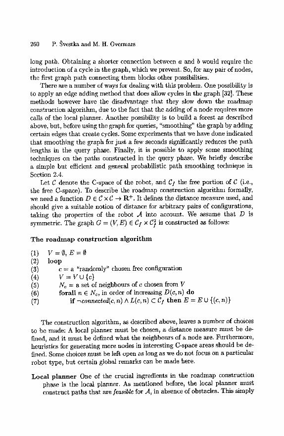
260 P. Svestka and M. H. Overmars
long path. Obtaining a shorter connection between a and b would require the introduction of a cycle in the graph, which we prevent. So, for any pair of nodes, the first graph path connecting them blocks other possibilities.
There are a number of ways for dealing with this problem. One possibility is to apply an edge adding method that does allow cycles in the graph [32]. These methods however have the disadvantage that they slow down the roadmap construction algorithm, due to the fact that the adding of a node requires more calls of the local planner. Another possibility is to build a forest as described above, but, before using the graph for queries, "smoothing" the graph by adding certain edges that create cycles. Some experiments that we have done indicated that smoothing the graph for just a few seconds significantly reduces the path lengths in the query phase. Finally, it is possible to apply some smoothing techniques on the paths constructed in the query phase. We briefly describe a simple but efficient and general probabilistic path smoothing technique in Section 2.4.
Let C denote the C-space of the robot, and C / the free portion of C (i.e., the free C-space). To describe the roadmap construction algorithm formally, we need a function D E g x C --+ R +. It defines the distance measure used, and should give a suitable notion of distance for arbitrary pairs of configurations, taking the properties of the robot ,4 into account. We assume that D is symmetric. The graph G = (V, E) E gf × g~ is constructed as follows:
The r o a d m a p cons t ruc t ion algorithm
(1) V= ,E=0 (2) loop (3) c = a "randomly" chosen free configuration (4) v = y u {c} (5) Nc = a set of neighbours of c chosen from V (6) forall n e No, in order of increasing D(c, n) do (7) if -~connected(c,n) A L(c,n) C C! then E = E tJ {(c,n))
The construction algorithm, as described above, leaves a number of choices to be made: A local planner must be chosen, a distance measure must be de- fined, and it must be defined what the neighbours of a node are. ~rthermore, heuristics for generating more nodes in interesting C-space areas should be de- fined. Some choices must be left open as long as we do not focus on a particular robot type, but certain global remarks can be made here.
Local planner One of the crucial ingredients in the roadmap construction phase is the local planner. As mentioned before, the local planner must construct paths that are ]casiblc for A, in absence of obstacles. This simply
Probabilistic Path Planning 261
means that the paths it constructs describe motions that are performable by the robot, that is, motions that respect the robots constraints. For example, assume the robot is a car-like vehicle moving on wheels, then a local planner that just connects the two argument configurations with a straight-line segment (in C-space) is not suitable, since it describes motions that force the wheels of the robot to slide. Furthermore, we want the roa~lmap construction algorithm to be fast. For this, it is important that (1) the local planner constructs its paths in a time efficient manner and (2) the probability that local paths intersect with obstacles is low. The first requirement can be met by keeping the path con- structs as simple as possible. For obtaining low intersection probabilities, the local planner should construct paths with relatively small sweep vol- umes. That is, the volumes (in workspace) swept by the robot when moving along local paths should preferably be small. Clearly, local planners min- imising these sweep volumes also minimise the probabilities of the local paths intersecting obstacles. Finally, the local planner should guarantee probabilistic completeness of PPP. In Section 5 we give sufficient properties.
Ne ighbour s and edge adding m e t h o d s Another important choice to be made is that of the neighbours Nc of a (new) node c. As is the case for the choice of the local planner, the definition of Nc has large impact on the performance of the roadmap construction algorithm. Reasons for this are that the choice of the neighbours strongly influences the overall structure of the graph, and that, regardless of how the local planner is exactly defined, the calls of the local planner are by far the most time-consuming operations of the roadmap construction algorithm (due to the collision tests that must be performed). So it is clear that calls of the local planner that do not effectively extend the knowledge stored in the roadmap should be avoided as much as possible. Firstly, as mentioned before, attempts to connect to nodes that are already in c's connected component are useless. For this reason the roadmap con- struction algorithm builds a forest. Secondly, local planner calls that fail add no knowledge to the roadmap. To avoid too many local planner fail- ures we only submit pairs of configurations whose relative distance (with respect to D) is small, that is, less than some constant threshold maxdist. Thus:
Nc C {5 E v ln(c , 5) <_ maxdist} (1)
This criterion still leaves many possibilities regarding the actual choice for No. We have decided on taking all nodes within distance maxdist as neighbours. Experiments with various definitions for Nc on a wide range of problems lea~ to this choice.
262 P. ~vestka and M. H. Overmars
Hence, according to the algorithm outline given above, we try to connect to all "nearby" nodes of c, in order of increasing distance D, but we skip those nodes that are already in c's connected component at the moment that the connection is to be attempted. By considering elements of Nc in this order we expect to maximise the chances of quickly connecting c to other configurations and, consequently, reduce the number of calls to the local planner (since every successful connection results in merging two connected components into one). We refer to the described edge adding method as the forest method.
Dis tance We have seen that a distance function D is used for choosing and sorting the neighbours Nc of a new node c. It should be defined in such a way that D(a, b) (for arbitrary a and b) somehow reflects the chance that the lo- cal planner will fail to connect a to b. For example, given two configurations a and b, a possibility is to define D(a, b) as the size of the sweep volume (in the workspace) of L(a, b), that is, as the volume of the area swept by the robot when moving along L(a, b). In this way each local planner L induces its own distance measure, that reflects the described "failure-chance" very well. In fact, if the obstacles were randomly distributed points, then this definition would reflect the local planner's failure chance exactly. However, in the general case, exact computations of the described sweep-volumes tend to be rather expensive, and in practice it turns out that certain rough but cheap to evaluate approximations of the sweep volumes are to be preferred.
N o d e adding heuris t ics If the number of nodes generated during the road- map construction phase is large enough, the set V gives a fairly uniform covering of the free C-space. In easy cases, for example for holonomic robots with few degrees of freedom (say not more than 4), G is then well connected. But in more complicated cases where the free C-space is actually connected, G tends to remain disconnected for a long time in certain narrow (and hence difficult) areas of the free C-space. Due to the probabilistic completeness of the method, we are sure that even- tually G will grasp the connectivity of the free space, but to prevent exor- bitant running times, it is wise to guide the node generation by heuristics that create higher node densities in the difficult areas. To identify these, there are a number of possibilities. In some cases, one can use the geometry of the workspace obstacles. For example, for car-like robots adding (extra) configurations that correspond to placements of the robot "parallel" to obstacle edges and "around" con- vex obstacle corners boosts the performance of the roadmap construction algorithm significantly. A more general criterion is to use the (run-time) structure of the roadmap G. Given a node c E V, one can count the number of nodes of V lying within some predefined distance of c. If this number is low, the obstacle
Probabilistic Path Planning 263
region probably occupies a large subset of c's neighbourhood. This suggests that c lies in a difficult area. Another possibility is to look at the distance from c to the nearest connected component not containing c. If this distance is small, then c lies in a region where two components failed to connect, which indicates that this region might be a difficult one (it may also be actually obstructed). Alternatively, rather than using the structure of the obstacles or the road- map to identify difficult regions, one can look at the run-time behaviour of the local planner. For example, if the local planner often fails to connect c to other nodes, this is also an indication that c lies in a difficult region. Which particular heuristic function should be used depends to some extent on the input scene.
2.2 The que ry phase
During the query phase, paths are to be found between arbitrary start and goal configurations, using the graph G computed in the roadmap construction phase. The idea is that, given a start configuration s and a goal configuration g, we try to find feasible paths Ps and Pg, such that P8 connects s to a graph node $, and Pg connects g to a graph node ~, with ~ graph-connected to (that is, they lie in the same connected component of G). If this succeeds, we perform a graph search to obtain a path Pa in G connecting ~ to ~. A feasible path (in C-space) from s to g is then constructed by concatenating Ps, the subpaths constructed by the local planner when applied to pairs of consecutive nodes in PG, and Pg reversed. Otherwise, the query fails. The queries should preferably terminate 'instantaneously', so no expensive algorithm is allowed for computing Ps and Pg.
For finding the nodes ~ and ~ we use the function query_mapping E C x C -¢ V x V, defined as follows:
query_mapping(a, b) =(~, b), such that h and b are connected, and n(a, 5) + n(b, b) = MIN(=,u)e W : D(a, x) + n(y, b)
where W = {(x, y) E V x VIconnected(x,y)}
So query_mapping(a, b) returns the pair of connected graph nodes (5, b) that minimise the total distance from a to 5 and from b to b. We will refer to 5 as a's graph retraction, and to b ~ b's graph retraction.
The most straightforward way for performing a query with start configu- ration s and goal configuration g is to compute (~, ~) = query_mapping(s, g), and to try to connect with the local planner from s to $ and from ~ to g. However, since no obstacle avoidance is incorporated in the local planner, it
264 P. Svestka and M. H. Overmars
may, in unlucky cases, fail find the connections even if the graph captures the connectivity of free C-space well.
Experiments with different robot types indicated that simple probabilistic methods that repeatedly perform short random walks from s and g, and try to connect to the graph retractions of the end-points of those walks with the local planner, achieve significantly better results. These random walks should aim at maneuvering the robot out of narrow C-space areas (that is, areas where the robot is tightly surrounded by obstacles), and hereby improving the chances for the local planner to succeed. For holonomic robots very good performance is obtained by what we refer to as the random bounce walk (see also [32]). The idea is that repeatedly a random direction (in C-space) is chosen, and the robot is moved in this direction until a collision occurs (or time runs out). When a collision occurs, a new random direction is chosen. This method performs much better than for example pure Brownian motion in C-space. For nonholonomic robots walks of a similar nature can be performed, but care must of course be taken to respect the nonholonomic constraints.
2.3 Using a di rected graph
In the algorithm outline of PPP, as described in the previous section, the computed roadmaps are stored in undirected graphs. For many path planning problems this is sufficient, and it appears that the method is easier and more efficient to implement when based on undirected graphs. For example, path planning problems involving free-flying robots, articulated robots, and (normal) car-like robots can all be dealt With using undirected underlying graphs. There are however path planning problems for which undirected underlying graphs not sufficient, and directed ones are required instead. For example, problems in- volving car-like robots that can only move forwards require directed underlying graphs.
The existence of an edge (a, b) in the underlying graph G corresponds to the statement that the local planner constructs a feasible path from a to b. If however G is undirected, then the edge contains no information about the direction in which the local planner can compute the path, and, hence, it must correspond to the statement that the local planner constructs a feasible path from a to b, as well as one from b to a. So an edge (a, b) can be added only if the local planner connects in both directions. Doing so, useful information might be thrown away. This will happen in those cases where the local planner connects in exactly one direction, and the fact that it has successfully constructed a feasible path will not be stored. If however the local planner is symmetric, which means that it connects from say a to b whenever it connects from b to a, then obviously this problem will never occur. So if the local planner is
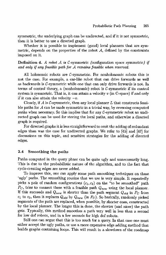
Probabilistic Path Planning 265
symmetric, the underlying graph can be undirected, and if it is not symmetric, then it is better to use a directed graph.
Whether it is possible to implement (good) local planners that are sym- metric, depends on the properties of the robot A, defined by the constraints imposed on it.
Def ini t ion 4. A robot A is C-symmetric (configuration space symmetric) i] and only if any feasible path ]or A remains feasible when reversed.
All holonomic robots are C-symmetric. For nonholonomic robots this is not the case. For example, a car-like robot that can drive forwards as well as backwards is C-symmetric while one that can only drive forwards is not. In terms of control theory, a (nonholonomic) robot is C-symmetric if its control system is symmetric. That is, it can attain a velocity v (in C-space) if and only if it can also attain the velocity -v .
Clearly, if ,4 is C-symmetric, then any local planner L that constructs feasi- ble paths for A can be made symmetric in a trivial way, by reversing computed paths when necessary. So this implies that for any C-symmetric robot an undi- rected graph can be used for storing the local paths, and otherwise a directed graph is required.
For directed graphs it is less straightforward to omit the adding of redundant edges than was the case for undirected graphs. We refer to [45] and [47] for discussions on this topic, and sensitive strategies for the adding of directed edges.
2.4 S m o o t h i n g the pa ths
Paths computed in the query phase can be quite ugly and unnecessarily long. This is due to the probabilistic nature of the algorithm, and to the fact that cycle-creating edges are never added.
To improve this, one can apply some path smoothing techniques on these 'ugly' paths. The smoothing routine that we use is very simple. It repeatedly picks a pair of random configurations (Cl,C2) on the "to be smoothed" path Pc, tries to connect these with a feasible path Qnew using the local planner. If this succeeds and Qnew is shorter than the path segment Qotd in Pc from cl to c2, then it replaces Qolg by Q~ew (in Pc). So basically, randomly picked segments of the path are replaced, when possible, by shorter ones, constructed by the local planner. The longer this is done, the shorter (and nicer) the path gets. Typically, this method smoothes a path very well in less than a second for low dof robots, and in a few seconds for high dof robots.
Still one can argue that this is too much for a query. In that case one must either accept the ugly paths, or use a more expensive edge adding method that builds graphs containing loops. This will result in a slowdown of the roadmap
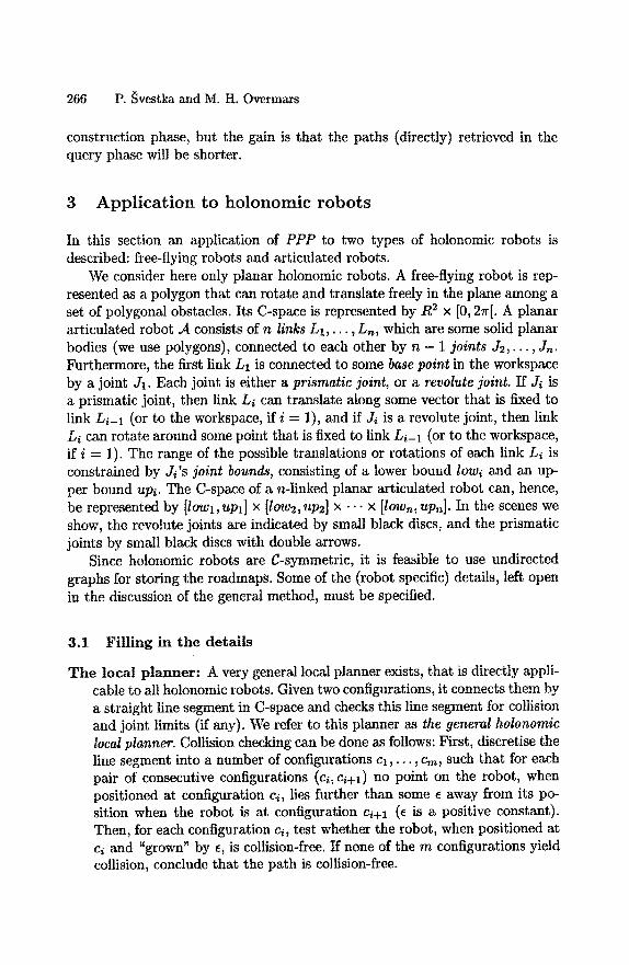
266 P. Svestka and M. H. Overmars
construction phase, but the gain is that the paths (directly) retrieved in the query phase will be shorter.
3 A p p l i c a t i o n t o h o l o n o m i c r o b o t s
In this section an application of PPP to two types of holonomic robots is described: free-flying robots and articulated robots.
We consider here only planar holonomic robots. A free-flying robot is rep- resented as a polygon that can rotate and translate freely in the plane among a set of polygonal obstacles. Its C-space is represented by R 2 x [0, 2r[. A planar articulated robot .4 consists of n links L1 , . . . , Ln, which are some solid planar bodies (we use polygons), connected to each other by n - 1 joints J2, . . . , jn. Furthermore, the first link L1 is connected to some base point in the workspace by a joint J1. Each joint is either a prismatic joint, or a revolute joint. If Ji is a prismatic joint, then link Li can translate along some vector that is fixed to link Li-1 (or to the workspace, if i = 1), and if Ji is a revolute joint, then link Li can rotate around some point that is fixed to link Li-1 (or to the workspace, if i = 1). The range of the possible translations or rotations of each link Li is constrained by Ji's joint bounds, consisting of a lower bound lowi and an up- per bound upi. The C-space of a n-linked planar articulated robot can, hence, be represented by [low1, up1] x [low2, up2] x . . . x [lown, upn]. In the scenes we show, the revolute joints are indicated by small black discs, and the prismatic joints by small black discs with double arrows.
Since holonomic robots are g-symmetric, it is feasible to use undirected graphs for storing the roadmaps. Some of the (robot specific) details, left open in the discussion of the general method, must be specified.
3.1 F i l l ing in t h e de ta i l s
The local planner: A very general local planner exists, that is directly appli- cable to all holonomic robots. Given two configurations, it connects them by a straight line segment in C-space and checks this line segment for collision and joint limits (if any). We refer to this planner as the general holonomic local planner. Collision checking can be done as follows: First, discretise the line segment into a number of configurations Cl , . . . , cm, such that for each pair of consecutive configurations (ci, ci+l) no point on the robot, when positioned at configuration ci, lies further than some e away from its po- sition when the robot is at configuration Ci+l (e is a positive constant). Then, for each configuration c~, test whether the robot, when positioned at ci and "grown" by e, is collision-free. If none of the m configurations yield collision, conclude that the path is collision-free.
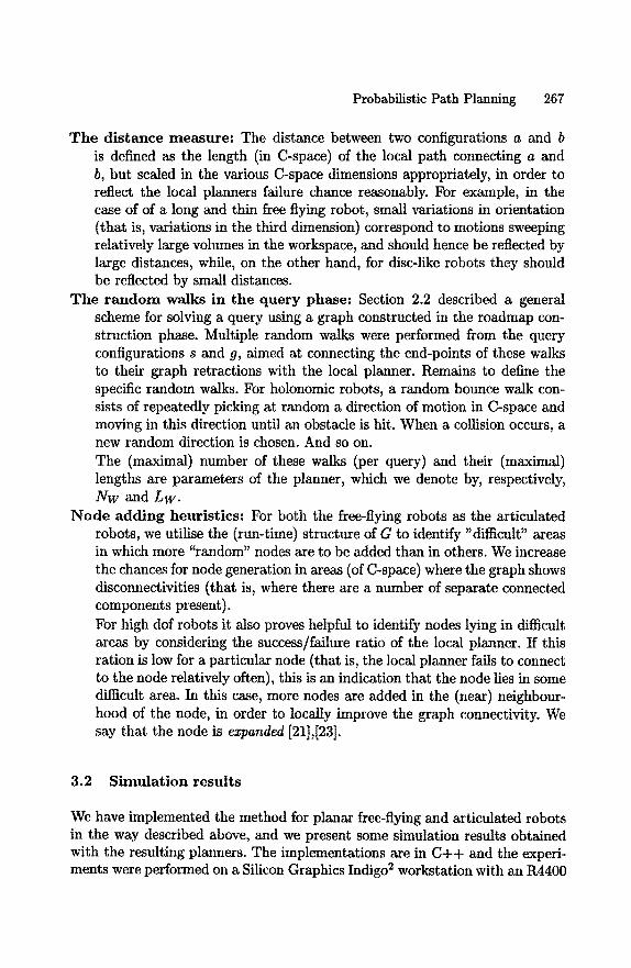
Probabilistic Path Planning 267
The d is tance measure : The distance between two configurations a and b is defined as the length (in C-space) of the local path connecting a and b, but scaled in the various C-space dimensions appropriately, in order to reflect the local planners failure chance reasonably. For example, in the case of of a long and thin free flying robot, small variations in orientation (that is, variations in the third dimension) correspond to motions sweeping relatively large volumes in the workspace, and should hence be reflected by large distances, while, on the other hand, for disc-like robots they should be reflected by small distances.
The r a n d o m walks in the que ry phase: Section 2.2 described a general scheme for solving a query using a graph constructed in the roadmap con- struction phase. Multiple random walks were performed from the query configurations s and g, aimed at connecting the end-points of these walks to their graph retractions with the local planner. Remains to define the specific random walks. For holonomic robots, a random bounce walk con- sists of repeatedly picking at random a direction of motion in C-space and moving in this direction until an obstacle is hit. When a collision occurs, a new random direction is chosen. And so on. The (maximal) number of these walks (per query) and their (maximal) lengths are parameters of the planner, which we denote by, respectively, Nw and Lw.
N o d e adding heurist ics: For both the free-flying robots as the articulated robots, we utilise the (run-time) structure of G to identify "difficult" areas in which more "random" nodes are to be added than in others. We increase the chances for node generation in areas (of C-space) where the graph shows disconnectivities (that is, where there are a number of separate connected components present). For high dof robots it also proves helpful to identify nodes lying in difficult areas by considering the success/failure ratio of the local planner. If this ration is low for a particular node (that is, the local planner fails to connect to the node relatively often), this is an indication that the node lies in some difficult area. In this case, more nodes are added in the (near) neighbour- hood of the node, in order to locally improve the graph connectivity. We say that the node is expanded [21],[23].
3.2 Simula t ion results
We have implemented the method for planar free-flying and articulated robots in the way described above, and we present some simulation results obtained with the resulting planners. The implementations are in C + + and the experi- ments were performed on a Silicon Graphics Indigo 2 workstation with an R4400

268 P. ~vestka and M. H. Overmars
processor running at 150 MHZ. This machine is rated with 96.5 SPECfp92 and 90.4 SPECint92.
In the test scenes used, the coordinates of all workspace obstacles lie in the unit square. Furthermore, in all scenes we have added an obstacle boundary around the unit square, hence no part of the robot can move outside this square.
The experiments are aimed at measuring the "knowledge" acquired by the method after having constructed roadmaps for certain periods of time. This is done by testing how well the method solves certain (interesting) queries. For each scene S we define a query test set TO. = {(sl, sl), (s2,g2),... , (sra,gm)}, consisting of a number of configuration pairs (that is, queries). Then, we re- peatedly construct a graph for some specified time t, and we count how many of these graphs solve the different queries in TQ. This experiment is repeated for a number of different construction times t. The results are presented in the tables under the figures. The numbers in the boxes indicate the percentage of the runs that solve the corresponding query within the given time bound.
The values for the random walk parameters Nw and Lw are, respectively, 10 and 0.05. This guarantees that the time spent per query is bounded by approximately 0.3 seconds (on our machine). Clearly, if we allow more time per query, the method will be more successful in the query phase, and vice versa. Hence there is a trade-off between the construction time and the time allowed for a query.
In Figure 1 we have a free flying L-shaped robot, placed at the configurations a, b, and c. Simulation results are shown for the three corresponding queries, and two paths are shown, both smoothed in 1 second. We see that around 1 second of roadmap construction is required for obtaining roadmaps that solve the queries. These roadmaps consist of approximately 125 nodes.
In Figures 2 to 4 results are given for articulated robots. In the first two scenes, just one query is tested, and well the query (a, b).
In both figures, several robot configurations along a path solving the query are displayed using various grey levels. The results of the experiments are given in the two tables. We see that the query in Figure 2 is solved in all cases after 10 seconds of construction time. Roadmap construction for 5 seconds however suffices to successfully answer the query in more than 90% of the cases. In Figure 3 we observe something similar. For both scenes the roadmaps constructed in 10 seconds contain around 500 nodes.
Figure 4 is a very difficult one. We have a seven dof robot in a very con- strained environment. The configurations a, b, c, and d define 6 different queries, for which the results are shown. These where obtained by a customised imple- mentation by Kavraki et al. [23]. In this implementation, optimised collision

Probabilistic Path Planning 269
Fig. 1. An L-shaped free-flying robot and its test configurations are shown. At the top right, we see two paths computed by the planner and smoothed in 1 second.
Fig. 2. A four dof articulated robot, and a path.
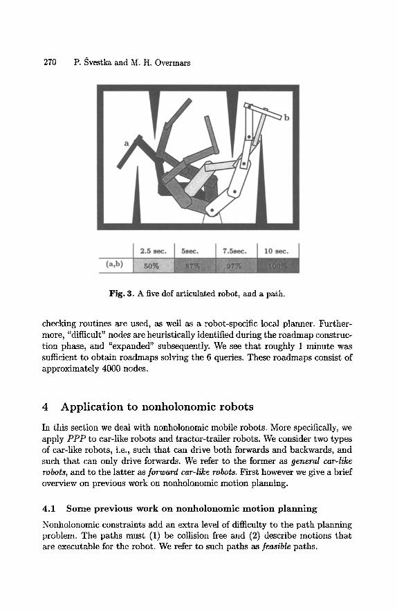
270 P. Svestka and M. H. Overmars
Fig. 3. A five dof articulated robot, and a path.
checking routines are used, as well as a robot-specific local planner. ~ r ther - more, "difficult" nodes are heuristically identified during the roadmap construc- tion phase, and "expanded" subsequently. We see that roughly 1 minute was sufficient to obtain roadmaps solving the 6 queries. These roadmaps consist of approximately 4000 nodes.
4 A p p l i c a t i o n t o n o n h o l o n o m i c r o b o t s
In this section we deal with nonholonomic mobile robots. More specifically, we apply PPP to car-like robots and tractor-trailer robots. We consider two types of car-like robots, i.e., such that can drive both forwards and backwards, and such that can only drive forwards. We refer to the former as general car-like robots, and to the latter as forward car-like robots. First however we give a brief overview on previous work on nonholonomic motion planning.
4.1 Some previous work on nonholonomic mot ion planning
Nonholonomic constraints add an extra level of difficulty to the path planning problem. The paths must (1) be collision free and (2) describe motions that are executable for the robot. We refer to such paths as feasible paths.
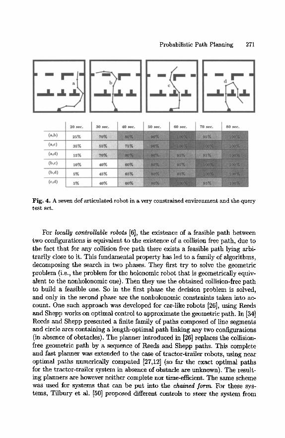
Probabilistic Path Planning 271
Fig. 4. A seven dof articulated robot in a very constrained environment and the query test set.
For locally controllable robots [6], the existence of a feasible path between two configurations is equivalent to the existence of a collision free path, due to the fact that for any collision free path there exists a feasible path lying arbi- trarily close to it. This fundamental property has led to a family of algorithms, decomposing the search in two phases. They first try to solve the geometric problem (i.e., the problem for the holonomic robot that is geometrically equiv- alent to the nonholonomic one). Then they use the obtained collision-free path to build a feasible one. So in the first phase the decision problem is solved, and only in the second phase are the nonholonomic constraints taken into ac- count. One such approach was developed for car-like robots [26], using Reeds and Shepp works on optimal control to approximate the geometric path. In [34] Reeds and Shepp presented a finite family of paths composed of line segments and circle arcs containing a length-optimal path linking any two configurations (in absence of obstacles). The planner introduced in [26] replaces the collision- free geometric path by a sequence of Reeds and Shepp paths. This complete and fast planner was extended to the case of tractor-trailer robots, using near optimal paths numerically computed [27,12] (so far the exact optimal paths for the tractor-trailer system in absence of obstacle are unknown). The result- ing planners are however neither complete nor time-efficient. The same scheme was used for systems that can be put into the chained form. For these sys- tems, Tilbury et al. [50] proposed different controls to steer the system from
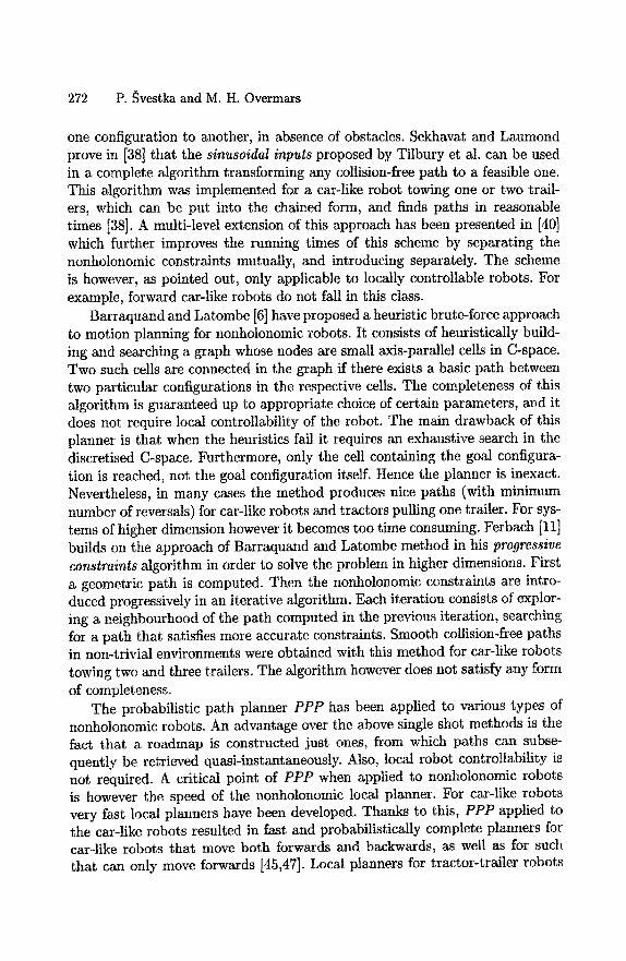
272 P. ~vestka and M. H. Overmars
one configuration to another, in absence of obstacles. Sekhavat and Laumond prove in [38] that the sinusoidal inputs proposed by Tilbury et al. can be used in a complete algorithm transforming any collision-free path to a feasible one. This algorithm was implemented for a car-like robot towing one or two trail- ers, which can be put into the chained form, and finds paths in reasonable times [38]. A multi-level extension of this approach has been presented in [40] which further improves the running times of this scheme by separating the nonholonomic constraints mutually, and introducing separately. The scheme is however, as pointed out, only applicable to locally controllable robots. For example, forward car-like robots do not fall in this class.
Barraquand and Latombe [6] have proposed a heuristic brute-force approach to motion planning for nonholonomic robots. It consists of heuristically build- ing and searching a graph whose nodes are small axis-parallel cells in C-space. Two such cells are connected in the graph if there exists a basic path between two particular configurations in the respective cells. The completeness of this algorithm is guaranteed up to appropriate choice of certain parameters, and it does not require local controllability of the robot. The main drawback of this planner is that when the heuristics fail it requires an exhaustive search in the discretised C-space. Furthermore, only the cell containing the goal configura- tion is reached, not the goal configuration itself. Hence the planner is inexact. Nevertheless, in many cases the method produces nice paths (with minimum number of reversals) for car-like robots and tractors pulling one trailer. For sys- tems of higher dimension however it becomes too time consuming. Ferbach [11] builds on the approach of Barraqua.nd and Latombe method in his progressive constraints algorithm in order to solve the problem in higher dimensions. First a geometric path is computed. Then the nonholonomic constraints are intro- duced progressively in an iterative algorithm. Each iteration consists of explor- ing a neighbourhood of the path computed in the previous iteration, searching for a path that satisfies more accurate constraints. Smooth collision-free paths in non-trivial environments were obtained with this method for car-like robots towing two and three trailers. The algorithm however does not satisfy any form of completeness.
The probabilistic path planner PPP has been applied to various types of nonholonomic robots. An advantage over the above single shot methods is the fact that a roadmap is constructed just ones, from which paths can subse- quently be retrieved quasi-instantaneously. Also, local robot controllability is not required. A critical point of PPP when applied to nonholonomic robots is however the speed of the nonholonomic local planner. For car-like robots very fast local planners have been developed. Thanks to this, PPP applied to the car-like robots resulted in fast and probabilistically complete planners for car-like robots that move both forwards and backwards, as well as for such that can only move forwards [45,47]. Local planners for tractor-trailer robots
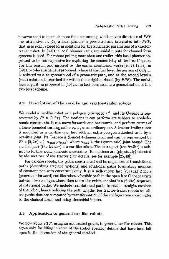
Probabilistic Path Planning 273
however tend to be much more time-consuming, which makes direct use of PPP less attractive. In [49] a local planner is presented and integrated into PPP, that uses exact closed form solutions for the kinematic parameters of a tractor- trailer robot. In [39] the local planner using sinusoidal inputs for chained form systems is used. For robots pulling more than one trailer, this local planner ap- peared to be too expensive for capturing the connectivity of the free C-space. For this reason, and inspired by the earlier mentioned works [26,27,12,38], in [39] a two-level scheme is proposed, where at the first level the portion of CSf~ee is reduced to a neighbourhood of a geometric path, and at the second level a (real) solution is searched for within this neighbourhood (by PPP). The multi- level algorithm proposed in [40] can in fact been seen as a generalisation of this two level scheme.
4.2 Descr ip t ion of the car-like and tractor-trailer robots
We model a car-like robot as a polygon moving in R 2, and its C-space is rep- resented by R 2 x [0, 27r). The motions it can perform are subject to nonholo- nomic constraints. It can move forwards and backwards, and perform curves of a lower bounded turning radius rmi,~, as an ordinary car. A tractor-trailer robot is modelled as a car-like one, but with an extra polygon attached to it by a revolute joint. Its C-space is (hence) 4-dimensional, and can be represented by R 2 x [0, 21r) x [ - a m ~ , ama~], where ama~ is the (symmetric) joint bound. The car-like part (the tractor) is a car-like robot. The extra part (the trailer) is sub- ject to further nonholonomic constraints. Its motions are (physically) dictated by the motions of the tractor (For details, see for example [25,40]).
For car-like robots, the paths constructed will be sequences of translational paths (describing straight motions) and rotational paths (describing motions of constant non-zero curvature) only. It is a well-known fact [25] that if for a (general or forward) car-like robot a feasible path in the open free C-space exists between two configurations, then there also exists one that is a (finite) sequence of rotational paths. We include translational paths to enable straight motions of the robot, hence reducing the path lengths. For tractor-trailer robots we will use paths that are computed by transformation of the configuration coordinates to the chained form, and using sinusoidal inputs.
4.3 Application to general car-like robots
We now apply PPP, using an undirected graph, to general car-like robots. This again asks for filling in some of the (robot specific) details that have been left open in the discussion of the general method.
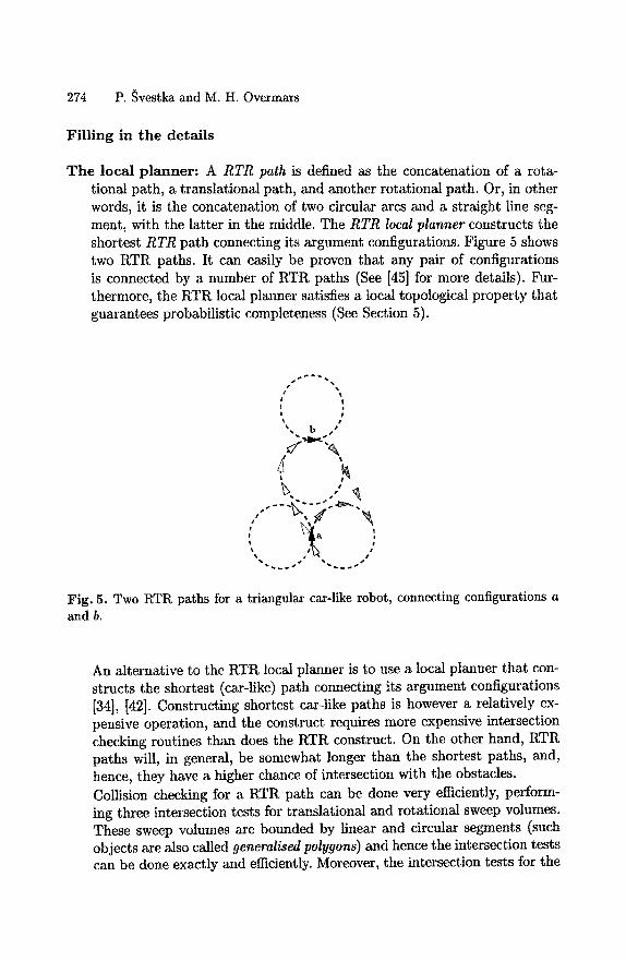
274 P. ~vestka and M. H. Overmars
Filling in the detai ls
The local planner: A RTR path is defined as the concatenation of a rota- tional path, a translational path, and another rotational path. Or, in other words, it is the concatenation of two circular arcs and a straight line seg- ment, with the latter in the middle. The RTR local planner constructs the shortest RTR path connecting its argument configurations. Figure 5 shows two RTR paths. It can easily be proven that any pair of configurations is connected by a number of RTR paths (See [45] for more details). Fur- thermore, the RTR local planner satisfies a local topological property that guarantees probabilistic completeness (See Section 5).
e S •
!
i el I
Fig. 5. Two RTR paths for a triangular car-like robot, connecting configurations a and b.
An alternative to the RTR local planner is to use a local planner that con- structs the shortest (car-like) path connecting its argument configurations [34], [42]. Constructing shortest car-like paths is however a relatively ex- pensive operation, and the construct requires more expensive intersection checking routines than does the RTR construct. On the other hand, RTR paths will, in general, be somewhat longer than the shortest paths, and, hence, they have a higher chance of intersection with the obstacles. Collision checking for a RTR path can be done very efficiently, perform- ing three intersection tests for translational and rotational sweep volumes. These sweep volumes are bounded by linear and circular segments (such objects are also called generalised polygons) and hence the intersection tests can be done exactly and efficiently. Moreover, the intersection tests for the
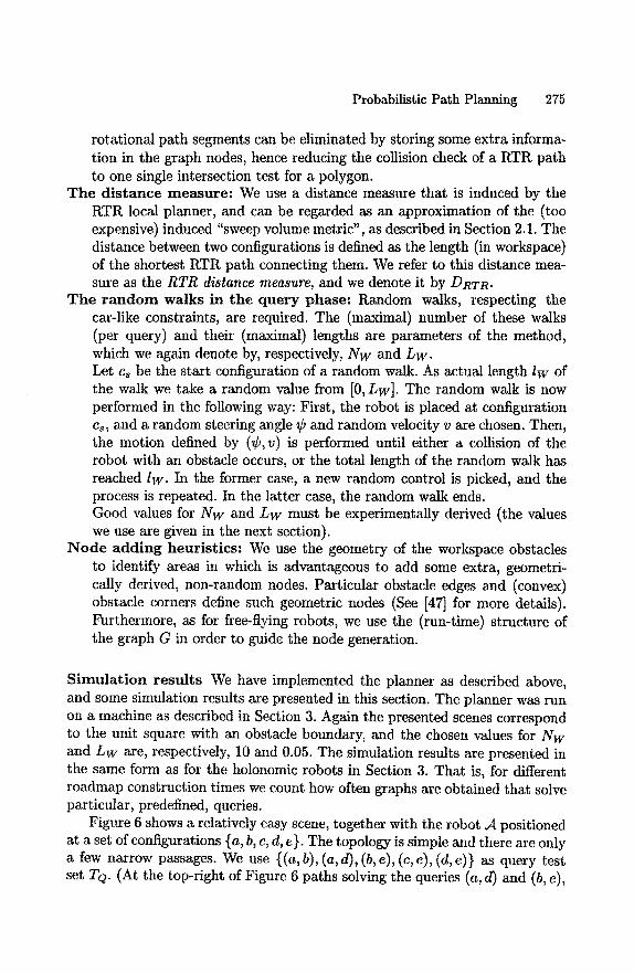
Probabilistic Path Planning 275
rotational path segments can be eliminated by storing some extra informa- tion in the graph nodes, hence reducing the collision check of a RTR path to one single intersection test for a polygon.
The d is tance measure : We use a distance measure that is induced by the RTR local planner, and can be regarded as an approximation of the (too expensive) induced "sweep volume metric", as described in Section 2.1. The distance between two configurations is defined as the length (in workspace) of the shortest RTR path connecting them. We refer to this distance mea- sure as the RTR distance measure, and we denote it by DRTR.
The r a n d o m walks in the que ry phase: Random walks, respecting the car-like constraints, are required. The (maximal) number of these walks (per query) and their (maximal) lengths are parameters of the method, which we again denote by, respectively, Nw and Lw. Let cs be the start configuration of a random walk. As actual length Iw of the walk we take a random value from [0, Lw]. The random walk is now performed in the following way: First, the robot is placed at configuration cs, and a random steering angle ¢ and random velocity v are chosen. Then, the motion defined by (¢, v) is performed until either a collision of the robot with an obstacle occurs, or the total length of the random walk has reached Iw. In the former case, a new random control is picked, and the process is repeated. In the latter case, the random walk ends. Good values for Nw and Lw must be experimentally derived (the values we use are given in the next section).
N o d e adding heurist ics: We use the geometry of the workspace obstacles to identify areas in which is advantageous to add some extra, geometri- cally derived, non-random nodes. Particular obstacle edges and (convex) obstacle corners define such geometric nodes (See [47] for more details). Furthermore, as for free-flying robots, we use the (run-time) structure of the graph G in order to guide the node generation.
S imula t ion resul ts We have implemented the planner as described above, and some simulation results are presented in this section. The planner was run on a machine as described in Section 3. Again the presented scenes correspond to the unit square with an obstacle boundary, and the chosen values for Nw and Lw are, respectively, 10 and 0.05. The simulation results are presented in the same form as for the holonomic robots in Section 3. That is, for different roadmap construction times we count how often graphs are obtained that solve particular, predefined, queries.
Figure 6 shows a relatively easy scene, together with the robot ,4 positioned at a set of configurations {a, b, c, d, e}. The topology is simple and there are only a few narrow passages. We use ((a, b), (a, d), (b, e), (c, e), (d, e)} as query test set TQ. (At the top-right of Figure 6 paths solving the queries (a, d) and (b, e),
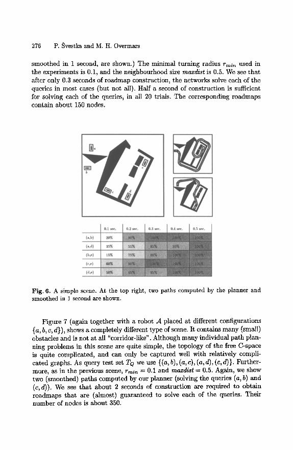
276 P. Svestka and M. H. Overmars
smoothed in 1 second, are shown.) The minimal turning radius rmin used in the experiments is 0.1, and the neighbourhood size maxdist is 0.5. We see that after only 0.3 seconds of roadmap construction, the networks solve each of the queries in most cases (but not all). Half a second of construction is sufficient for solving each of the queries, in all 20 trials. The corresponding roadmaps contain about 150 nodes.
Fig. 6. A simple scene. At the top right, two paths computed by the planner and smoothed in 1 second are shown.
Figure 7 (again together with a robot .4 placed at different configurations {a, b, c, d}), shows a completely different type of scene. It contains many (small) obstacles and is not at all "corridor-like". Although many individual path plan- ning problems in this scene are quite simple, the topology of the free C-space is quite complicated, and can only be captured well with relatively compli- cated graphs. As query test set TQ we use {(a, b), (a, c), (a, d), (c, d)}. Further- more, as in the previous scene, rmin --- 0.1 and maxdist -- 0.5. Again, we show two (smoothed) paths computed by our planner (solving the queries (a, b) and (c, d)). We see that about 2 seconds of construction are required to obtain roadmaps that are (almost) guaranteed to solve each of the queries. Their number of nodes is about 350.

Probabilistic Path Planning 277
Fig. 7. A more complicated scene, and its test configurations. At the top right, two paths computed by the planner and smoothed in 1 second are shown.
4.4 Application to forward car-like robots
Forward car-like robots, as pointed out before, are not C-symmetric. Hence, as explained in Section 2.3, directed instead of undirected graphs are used for storing the roadmaps. For details regarding the exact definition of the roadmap construction algorithm we refer to [32].
The robot specific components, such as the local planner, the metric, and the random walks are quite similar to those used for general car-like robots, as described in Section 4.3. The local planner constructs the shortest forward RTR path connecting its argument configurations. A forward RTR path is defined exactly as a normal RTR path, except that the rotational and translational paths are required to describe forward robot motions. The distance between two configurations is defined as the (workspace) length of the shortest forward RTR path connecting them. A random walk is performed as for general car- like robots, with the difference that the randomly picked velocity must be positive, and that, when collision occurs, the random walk is resumed from a random configuration on the previously followed trajectory (instead of from the configuration where collision occurred).
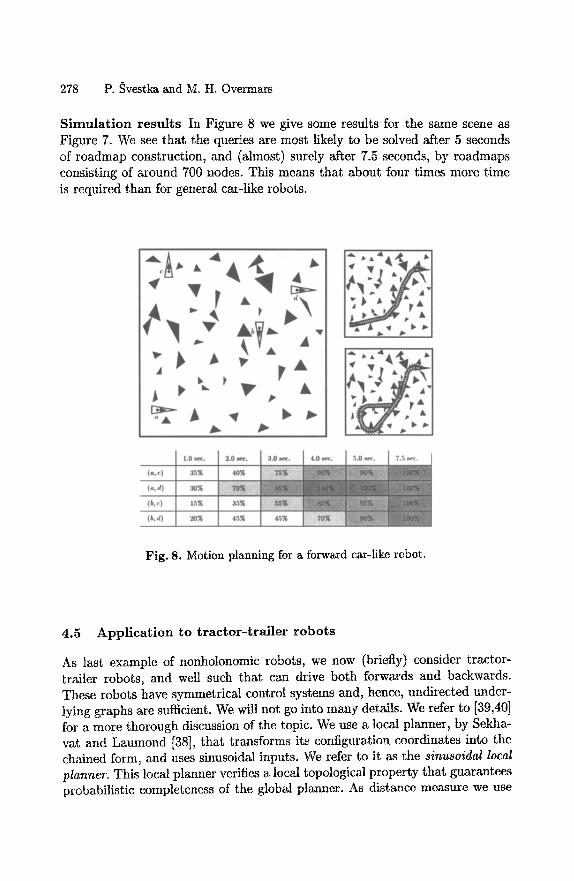
278 P. Svestka and M. H. Overmars
S i m u l a t i o n resu l t s In Figure 8 we give some results for the same scene as Figure 7. We see that the queries are most likely to be solved after 5 seconds of roadmap construction, and (almost) surely after 7.5 seconds, by roadmaps consisting of around 700 nodes. This means that about four times more time is required than for general car-like robots.
Fig. 8. Motion planning for a forward car-like robot.
4.5 A p p l i c a t i o n to t r a c t o r - t r a i l e r r o b o t s
As last example of nonholonomic robots, we now (briefly) consider tractor- trailer robots, and well such that can drive both forwards and backwards. These robots have symmetrical control systems and, hence, undirected under- lying graphs are sufficient. We will not go into many details. We refer to [39,40] for a more thorough discussion of the topic. We use a local planner, by Sekha- vat and Laumond [38], that transforms its configuration coordinates into the chained form, and uses sinusoidal inputs. We refer to it as the sinusoidal local planner. This local planner verifies a local topological property that guarantees probabilistic completeness of the global planner. As distance measure we use
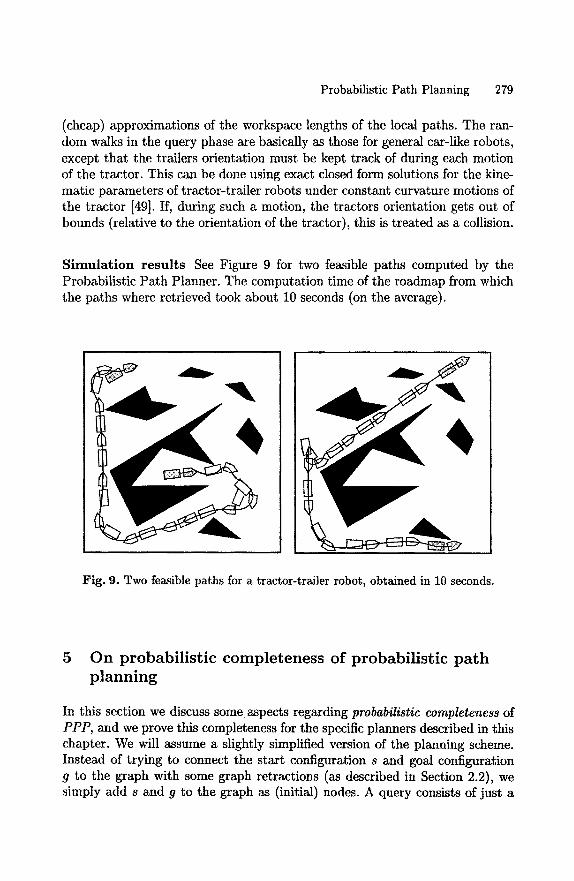
Probabilistic Path Planning 279
(cheap) approximations of the workspace lengths of the local paths. The ran- dom walks in the query phase are basically as those for general car-like robots, except that the trailers orientation must be kept track of during each motion of the tractor. This can be done using exact closed form solutions for the kine- matic parameters of tractor-trailer robots under constant curvature motions of the tractor [49]. If, during such a motion, the tractors orientation gets out of bounds (relative to the orientation of the tractor), this is treated as a collision.
S imula t ion resul ts See Figure 9 for two feasible paths computed by the Probabilistic Path Planner. The computation time of the roadmap from which the paths where retrieved took about 10 seconds (on the average).
d
Fig. 9. Two feasible paths for a tractor-trailer robot, obtained in 10 seconds.
5 On probabilistic completeness of probabilistic path planning
In this section we discuss some aspects regarding probabiIistic completeness of PPP, and we prove this completeness for the specific planners described in this chapter. We will assume a slightly simplified version of the planning scheme. Instead of trying to connect the start configuration s and goal configuration g to the graph with some graph retractions (as described in Section 2.2), we simply add s and g to the graph as (initial) nodes. A query consists of just a
280 P. Svestka and M. H. Overmars
graph search. This simplification of the query phase is for ease of presentation. All results presented in this section directly hold for the case where queries are performed as described earlier (in Section 2.2), using graph retractions and random walks.
A path planner is called probabilistically complete if, given any problem that is solvable in the open free C-space, the probability that the planner solves the problem goes to 1 as the running time goes to infinity. Hence, a probabilisti- cally complete path planner is guaranteed to solve such a problem, provided that it is executed for a sufficient amount of time. For ease of presentation we introduce some shorthand notations. We denote the version of PPP using undi- rected underlying graphs (respectively directed graphs) by PPP~, (respectively PPPd). The notation PPPu(L) (respectively PPPd(L)) is used for referring to PPPu (respectively PPPd) with a specific local planner L. We say L is sym- metric iff, for arbitrary configurations a and b, L(a, b) equals L(b, a) reversed. Furthermore, we again denote the C-space, respectively the free C-space, by C, respectively g/.
We point out that with PPP one obtains a probabilistically complete plan- ner for any robot that is locally controllable (see below), provided that one defines the local planner properly. If, in addition to the local controllability, the robot also has a symmetric control system then PPP~(L) is suitable, oth- erwise PPPd(L) must be used. In Section 5.1 we define a general property for local planners that is sufficient for probabilistic completeness of PPP, and we point out that, given the local controllability of the robot, a local planner satisfying this property always exists (but it must be found). We also men- tion a relaxation of the property, that guarantees probabilistic completeness of PPPu(L) as well, for locally controllable robots with symmetric control sys- tems. All holonomic robots, as well as for example general car-like robots and tractor-trailer robots, fall into this class. Forward car-like robots however are not locally controllable (and neither symmetric). In Section 5.2 we show that all the planners described in this chapter are probabilistically, complete.
First we define the concept local controllability (in the literature also re- ferred to as small-time local controllability or local-local controllability), adopt- ing the terminology introduced by Sussman [43]. Given a robot A, let Z.4 be its control system. That is, ZA describes the velocities that ,4 can attain in C-space. For a configuration c of a robot A, the set of configurations that .4 can reach within time T is denoted by AE, (_< T, c). A is defined to be locally controllable iff for any configuration c E C A~.~(<_ T,c) contains a neighbour- hood of c (or, equivalently, a ball centred at c) for all T > 0. It is a well-known fact that, given a configuration c, the area a locally controllable robot ¢4 can reach without leaving the e-ball around c (for any e > 0) is the entire open e-ball around c.
Probabilistic Path Planning 281
5.1 The general local topology property
We assume now that robot A is locally controllable. For probabilistic complete- ness of PPP a local planner L is required that exploits the local controllability of A. This will be the case if L has what we call the general local topologi- cal property, or GLT-property, as defined in Definition fi using the notion of e-teachability introduced in Definition 5. We denote the ball (in C-space) of radius e centred at configuration c by Be(c).
Defini t ion 5. Let L be a local planner for .A. Furthermore let ~ > 0 and c 6 C be given. The e-reachable area of c by L, denoted by RL,e(c), is defined by
RL,~(c) = {5 6 B~(c)lL(c, 5) is entirely contained in Be(c)}
Def ini t ion 6. Let L be a local planner for A. We say L has the GLT-property
V~ > 0 : 35 > 0 :Vc 6 g : B~(c) C RL,~(c)
We refer to B~ (c) as the e-reachable g-ball of c.
A local planner verifying the GLT-property, at least in theory, always ex- ists, due to the robots local controllability. Theorem 5.1 now states that this property is sufficient to guarantee probabilistic completeness of PPP. That is, of PPPu(L) if L is symmetric, and of PPPd(L) otherwise.
T h e o r e m 5.1. If L is a local planner verifying the GLT-propcrty, then PPP(L) is probabilistically complete.
Proof. The theorem can be proven quite straightforwardly (for both PPPu(L) and PPPd(L)). Assume L verifies the GLT-property. Given two configurations s and g, lying in the same connected component of the open free C-space, take a path P that connects s and g and lies in the open free C-space as well. Let e be the C-space clearance of P (that is, the minimal distance between P and a C-space obstacle), and take 5 > 0 such that Vc 6 C : B~(c) C RL,¼e(c). Then,
consider a covering of P by balls B1 , . . . , Bk of radius ¼6, such that balls Bi and Bi+l, for i 6 {1, . . . , k - 1}, partially overlap. Assume each such ball Bi contains a node vi of G. Then, ]vi - Vi+l] < 5, and each node v~ has a C-space clearance of at least e - ¼5 > 43-e (since 5 <_ e). Hence, due to the definition of 6, we have
L(vi, vi+l) C B¼~(vi) C gl
It follows that if all the balls B1, . . . , Bk contain a node of G, s and g will be graph-connected. Since, due to the random node adding, this is guaranteed to be the case within a finite amount of time, this concludes the proof. See also Figure 10. •
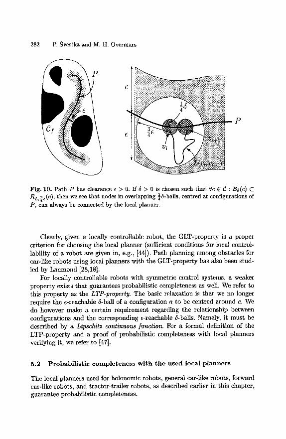
282 P. Svestka and M. H. Overmaxs
P
Fig. 10. Path P has clearance e > 0. If 5 > 0 is chosen such that Vc E C : B~(c) C RL, ~e (C), then we see that nodes in overlapping ¼5-balls, centred at configurations of P, can always be connected by the local planner.
Clearly, given a locally controllable robot, the GLT-property is a proper criterion for choosing the local planner (sufficient conditions for local control- lability of a robot are given in, e.g., [44]). Path planning among obstacles for car-like robots using local planners with the GLT-property has also been stud- ied by Laumond [28,18].
For locally controllable robots with symmetric control systems, a weaker property exists that guarantees probabilistic completeness as well. We refer to this property as the LTP-property. The basic relaxation is that we no longer require the e-reachable J-ball of a configuration a to be centred around c. We do however make a certain requirement regarding the relationship between configurations and the corresponding e-reachable (f-balls. Namely, it must be described by a Lipschitz continuous function. For a formal definition of the LTP-property and a proof of probabilistic completeness with local planners verifying it, we refer to [47].
5.2 Probabi l ls t lc completeness wi th the used local p lanners
The local planners used for holonomic robots, general car-like robots, forward car-like robots, and tractor-trailer robots, as described earlier in this chapter, guarantee probabilistic completeness.
Probabilistic Path Planning 283
Locally controllable robots The general holonomic local planner b for holo- nomic robots constructs the straight line path (in C-space) connecting its ar- gument configurations. It immediately follows that RE,L(C) = BE(c), for any configuration c and any ~ > 0. Hence, L verifies the GLT-property.
T h e o r e m 5.2. PPPu(L), with L being the general holonomie local planner, is probabilistically complete for all holonomic robots.
The planner for general car-like robots uses the RTR local planner. One can prove that this planner verifies the LTP-property [47]. Again, as stated in the following theorem, this guarantees probabilistic completeness.
T h e o r e m 5.3. PPP~(L), with L being the RTR local planner, is probabilisti- cally complete for general car-like robots.
Regarding tractor-trailer robots, Sekhavat and Lanmond prove in [38] that the sinusoidal local planner, used for the tractor-trailer robots, verifies the GLT-property. Hence, for tractor-trailer robots we also have probabilistic com- pleteness.
T h e o r e m 5.4. PPP~(L), with L being the sinusoidal local planner, is proba- bilistically complete for tractor-trailer robots (with arbitrary number of trailers).
Forward car-like robots As pointed out before, the theory of the previous sections applies only to robots that are locally controllable. If a robot does not have this property, a local planner verifying the GLT-property will not exist. A local planner verifying the weaker LTP-property may exist, but this planner will not be symmetric (this would imply the existence of a local planner verifying GTP).
Forward car-like robots are not locally controllable. One can nevertheless prove probabilistic completeness of PPPd(L), with L being the RTR forward local planner. That is, one can prove that, given two configurations s and g such that there exists a feasible path in the open free C-space connecting them, PPPd(L) will surely solve the problem within finite time. The proof, which does not directly generalise to other cases, uses a property of RTR forward paths stated in Lemma 5.5.
Lemma 5.5. Let L be the RTR forward local planner, and let Q be a RTR forward path connecting configurations a and b with a straight line path of non- zero length and both arc paths of total curvature less than 17r. Then:
Ve > 0 : 3 5 > 0 : V(h,b) e Bz(a) × B6(b) : L(h,b) lies within distance c o fQ 1
1 We say a path P lies within distance e of a path Q, iff Vp E P : 3q E Q : Ip - ql < e (in C-space)
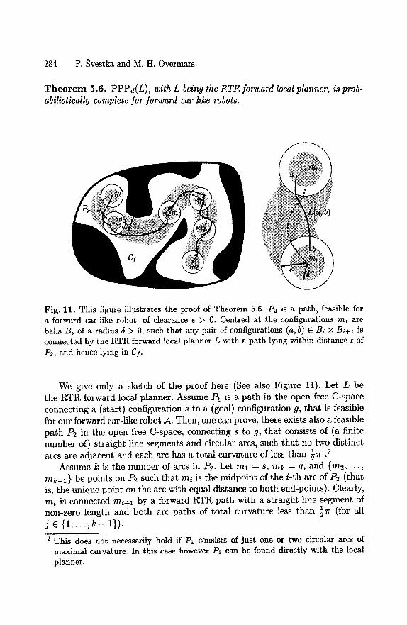
284 P. Svestka and M. H. Overmars
T h e o r e m 5.6. PPPd(L) , with L being the RTR forward local planner, is prob- abilistieally complete for forward car-like robots.
Fig. 11. This figure illustrates the proof of Theorem 5.6. P2 is a path~ feasible for a forward car-like robot, of clearance e > 0. Centred at the configurations mi are balls Bi of a radius 5 > 0, such that any pair of configurations (a, b) E Bi × B~+I is connected by the RTR forward local planner L with a path lying within distance e of P2, and hence lying in Of.
We give only a sketch of the proof here (See also Figure 11). Let L be the RTR forward local planner. Assume PI is a path in the open free C-space connecting a (start) configuration s to a (goal) configuration g, that is feasible for our forward car-like robot A. Then, one can prove, there exists also a feasible path P2 in the open free C-space, connecting s to g, that consists of (a finite number of) straight line segments and circular arcs, such that no two distinct arcs are adjacent and each arc has a total curvature of less than ½7r 2
Assume k is the number of arcs in P2. Let ml = s, m k = g, and { m 2 , . . . , ink - l ) be points on P2 such that mi is the midpoint of the i-th arc of P2 (that is, the unique point on the arc with equal distance to both end-points). Clearly, mi is connected mi+l by a forward RTR path with a straight line segment of non-zero length and both arc paths of total curvature less than ½r (for all j e { 1 , . . . , k - 1}).
2 This does not necessarily hold if P1 consists of just one or two circular arcs of maximal curvature. In this case however P1 can be found directly with the local planner.
Probabilistic Path Planning 285
Let e > 0 be the clearance of P2, and take 5 > 0 such that, for all j E ( 1 , . . . , k - 1}:
V(a,b) E B~(mj) x B~(mj+l) :L(a,b) lies within distance e of Q
It follows from Lemma 5.5 that such a 5 > 0 always exists. When a node of G is present in every ball B~(mj) for 2 _~ j < k, G will contain a path connecting s to g. We know, due to the probabilistic nature of the node adding, that the probability of obtaining such a graph grows to I when the roadmap construction time goes to infinity.
6 On the expected complexity of probabilistic path planning
In the previous section we have formulated properties of local planners that guarantee probabilistic completeness of PPP for locally controllable robots. If these properties are satisfied, we know that as the running time of P P P goes to infinity, the probability of solving any solvable problem goes to 1. However, nothing formal has yet been said about (expected) convergence times of the algorithm. In practice, one will not be satisfied with the guarantee that "eventually a path will be found". For real life applications, some estimate of the running time beforehand is desirable.
Simulation results obtained by the application of PPP on certain "typical" problems can increase our trust in the planners performance and robustness, but they do not describe a formal relation between the probabilities of fail- ure and running times in general, and neither do they provide a theoretical explanation for the empirically observed success of the probabilistic planner. Recently some first theoretical results on expected running times of probabitis- tic planners have been obtained.
Kavraki et al. [22,20,3] show that, under certain geometric assumptions about the free C-space C f, it is possible to establish a relation between the probability that probabilistic planners like pppa find paths solving particular problems, and their running times. They suggest two such assumptions, i.e., the visibility volume assumption and the path clearance assumption. We will discuss these assumptions and present the main results obtained by Kavraki et al.. Also, we will discuss to what extent these results hold for nonholonomic robots, and, where possible, we will adapt them appropriately. Furthermore, we introduce a new assumption on configuration space, the e-complexity assumption, under which it is possible to relate the success probabilities and running times of PPP to the complexity of the problems that are to be solved.
a Kavraki et al. refer to PPP by the name PRM (Probabilistic RoadMap planner).
286 P. Svestka and M. H. Overmars
Throughout this section we use the notations introduced in the previous section, and, unless stated otherwise, we will assume that PPP with undirected underlying graphs (i.e., PPPu) is used.
6.1 The visibil i ty vo lume assumption
The visibility volume assumption uses a notion of "visibility" defined by the used local planner. A free configuration a is said to "see" a free configuration b if the local path L(a, b) lies entirely in gf. The visibility volume assumption now states that every free configuration "sees" a subset of C I whose volume is at least an e fraction of the total volume of gl. If this holds, C I is called e-good.
The analyses assumes a somewhat more complex planner than PPP as de- fined in Section 2. It differs from PPP in that after a probabilistic roadmap G = (V, E) has been constructed (by the roadmap construction algorithm in Section 2.1), an extra post-processing step is performed, referred to by the au- thors as Permeation. Permeation assumes the existence of a complete planner, that is~ a planner solving any solvable problem, and returning failure for any non-solvable one. What permeation does, is invoking the complete planner for certain pairs (a, b) E V × V that are not graph connected. Planners based on this scheme have been implemented by Kavraki et al. (E.g., [21]). However, instead of a complete planner (which, in general, is not available) the poten- tial field planner RPP has been utilised. Since RPP is only probabilistically complete, the mentioned planners are merely approximations of the algorithm sketched above.
Due to the assumed completeness of the invoked planner, provided that the complete planner is invoked for enough pairs of nodes in V, permeation leads to a roadmap where every connected component of gl contains at most one connected component of the roadmap G. For convenience, we will say that such roadmaps have perfect connectivity.
Let us now assume that Gp has such perfect connectivity. Then, if both s and g "see" a node of Gp, the planner will return a path solving this problem if it is solvable, and return failure otherwise. In other words, on the portion of C I that "sees" some node of the roadmap~ the planner is complete. Note that during the permeation step, no nodes are added to G. Hence, the question whether a solvable query will be answered coITectly depends solely on the set of nodes V in G. Theorem 6.1 addresses this question. V is called adequate if the portion of g/ , not visible from any c E V, has a volume of at most 1 Volume(gl). The theorem gives a lower bound for the probability of V being adequate.
T h e o r e m 6.1. (Kavraki et aL [22], Barraquand et al, [3]) Assume G = (V, E) is a roadmap generated by PPP in a ]ree C-space that is e-good. Let
Probabilistic Path Planning 287
E (0, 1] be a real constant, and let C be a positive constant large enough such
thatVx • (0,1] : ( l - x ) (-c-'°g ~) < x { Now, illVI > ~log 1 - - 7, then V is adequate with probability at least 1 - 8.
Regarding the complexity of the roadmap construction, one must estimate the number of calls to the complete planner during the permeation step, re- quired for obtaining a roadmap Gp of perfect connectivity. Theorem 6.2 pro- vides such an estimate.
T h e o r e m 6.2. (Kavraki et al. [22], Barraquand et al. [3]) Let wl >_ w2 >_ .. . >_ Wk be the sizes of the connected components of the roadmap G = (V, E). There exists a (randomised) algorithm that extends G to a roadmap Gp of perfect connectivity, whose expected number of calls of the complete planner is at most:
k
2 ~ i . w, - I Y l - k i=1
Furthermore, with high probability, the number of calls is at most:
0 y ~ i . wi. log(lVl) i = I
Symmetry of the local planner L is required and assumed in the above. However, apart from this, the e-goodness assumption is very general, and the given analysis is not only valid for holonomic robots (on which the authors focus), but also for nonholonomic ones.
However, the question arises in how far the theoretical results are "practical" for nonholonomie robots, since the "visibility" induced by a nonholonomic local planner will be a quite hard to grasp concept that can hardly be regarded as a geometric property of C I. There does not seem to be much hope that we will ever be able to measure the e-goodness of C I for nonholonomic robots, in non-trivial cases (insofar as there is such hope for holonomic ones).
6.2 The p a t h clearance a s sumpt ion
In the path clearance assumption, there exists a collision-free path 79 between the start configuration s and goal configuration g, that has some clearance e > 0 with the C-space obstacles. Throughout this section we denote the volume of an object A by ];(A). In [20], Kavraki et al. study the dependence of the failure probability of PPP (the normal version) to connect s and g on (1) the length of :P, (2) the clearance e, and (3) the number of nodes in the probabilistic roadmap G. Their main result is described by the following theorem:

288 P. Svestka and M. H. Overmars
T h e o r e m 6.3. ( K a v r a k i et aL [20], B a r r a q u a n d et al. [3]) Let .4 be a holonomic robot, L be the general holonomie local planner (for .4), and G = (V, E) be a graph constructed by PPP(L) . Assume configurations s and g are connectable by a path "P of length A, that has a clearance e > 0 with the (C- space) obstacles. Let a E (0,1] be a real constant, and let a be the constant ~Ac)?(B1)/~;(g]), where 131 denotes the unit ball in the C-space ]~n Now i~ IV I is such that
2~(1 - a ~ ) lvt < a g
then, with probability at least 1 - a, s and g will be graph-connected in G (See also Figure 12).
m m w ~ m u ~ m ~ m ~ m m m
c ~s I | | | |
p ' |
|
i i !
|
|
|
Fig. 12. We see that configuration s is connectable to configuration g by a P of clearance e. Let x0 = s, x l , . . . , xk = g be points on P, such that [xj - x j - b l [ _< ~e,1 for all j . If each ball B½~(xj) contains a node of G, then s and g will be graph-connected.
The proof of this theorem is quite straightforward. Given a pa th P of clear- ance e > 0, one can consider a covering of P by balls of radius 1 ~e as shown in Figure 12, and bound the probability tha t one of these balls contains no node of G. Since, if each of these balls does contain a node, G is guaranteed to contain a pa th connecting the s tar t and goal configuration, this gives an upper bound for the failure probabili ty of PPP.
A number of important facts are implied by Theorem 6.3. E.g., the number of nodes required to be generated, in order for the planner to succeed with
1 probabil i ty at least 1 - a , is logarithmic in ~ and )~, and polynomial in 7" Furthermore, the failure probability c~ is linear in the pa th length A.
Probabilistic Path Planning 289
The analyses assumes the use of the general holonomic local planner (as described in Section 3.1). Hence it is assumed that the robot is holonomic. An underlying assumption is namely that the e-reachable area of any configuration e consists of the entire e-ball B~ (c), surrounding e. From theoretical point of view, as pointed out in the previous section, for any locally controllable robot a local planner exists for which the e-reachable area of any configuration c con- sists of the entire open e-ball centred at c. Such a local planner would allow for the result assuming the path clearance to be directly applied to such robots. However, it is not realistic to assume the "e-ball reachability" for a nonholo- nomic local planner, since for most robots we are not able to construct such local planners, and, if we could, they would probably be vastly outperformed (in terms of computation time) by simple local planners verifying only weaker (but sufficient) topological properties, such as those presented in the previ- ous section. However, the analyses presented in [20] can be extended to the case where the local planner verifies only the GLT-property. Through this, we can give running time estimates for locally controllable nonholonomic robots that are realistic in the sense that we can actually build the planners that we analyse. Corollary 6.4 extends the result of Theorem 6.3 to locally controllable nonholonomic robots with local planners verifying the GLT-property.
Corol la ry 6.4. Let A be a fully controllable robot, L be a local planner for A verifying the GLT-property, and G = (V, E) be a graph constructed by PPP(L). Assume configurations s and g are connectable by a path 7 ) of length ~, that has a clearance e > 0 with the (configuration space) obstacles. Take 5 > 0 such that
Vc e C: B~ (c) c RL,~ (c)
Let a E (0, 1] be a real constant, and 1)1 be the volume of the unit ball in the C-space ~'~. Now if tVI is such that
2A ( l;1 -n \ IVl
then, with probability at least 1 - ~, s and g will be graph-connected in G.
Since, by definition of the GLT-property, 5 is a constant with respect to e, the dependencies implied by Theorem 6.3 hold for nonholonomic robots as well.
6.3 The e-complexity assumption
A drawback of Theorem 6.3 and the above corollary is that no relation is established between the failure probability and the complexity of a particular
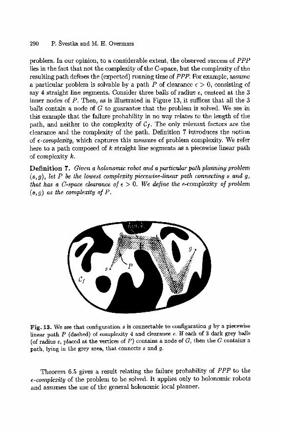
290 P. Svestka and M. H. Overmars
problem. In our opinion, to a considerable extent, the observed success of PPP lies in the fact that not the complexity of the C-space, but the complexity of the resulting path defines the (expected) running time of PPP. For example, assume a particular problem is solvable by a path P of clearance e > 0, consisting of say 4 straight line segments. Consider three balls of radius e, centred at the 3 inner nodes of P. Then, as is illustrated in Figure 13, it suffices that all the 3 balls contain a node of G to guarantee that the problem is solved. We see in this example that the failure probability in no way relates to the length of the path, and neither to the complexity of g I. The only relevant factors are the clearance and the complexity of the path. Definition 7 introduces the notion of e-complexity, which captures this measure of problem complexity. We refer here to a path composed of k straight line segments as a piecewise linear path of complexity k.
Defini t ion 7. Given a holonomic robot and a particular path planning problem (s, g), let P be the lowest complexity piecewise-linear path connecting s and g, that has a C-space clearance of e > O. We define the e-complexity of problem (s, g) as the complexity of P.
Fig. 13. We see that configuration s is connectable to configuration g by a piecewise linear path P (dashed) of complexity 4 and clearance e. If each of 3 dark grey balls (of radius e, placed at the vertices of P) contains a node of G, then the G contains a path, lying in the grey area, that connects s and g.
Theorem 6.5 gives a result relating the failure probability of PPP to the e-complexity of the problem to be solved. It applies only to holonomic robots and assumes the use of the general hotonomic local planner.
Probabilistic Path Planning 291
T h e o r e m 6.5. Let A be a holonomic robot, L be the general holonomic local planner (for A), and G = (V, E) be a graph constructed by PPP(L). Assume (s, 9) is a problem of e-complexity ~. Let a E (0, 1] be a real constant, and ~1 be the volume of the unit ball in the C-space R n . Now if IV[ is such that
( ¢ - 1) (1 "~1 ) IV' V(Cs ) e~ <_
then, with probability at least 1 - a, s and g will be graph-connected in G.
This theorem can be proven quite easily. Given a problem of e-complexity (, there exists a piecewise linear path P of complexity ( and clearance e > 0 solving it. We can place balls of radius e at the vertices of P, and bound the probability the one of these balls contains no node of G. Since, if each of these balls does contain a node, G is guaranteed to contain a path connecting the start and goal configuration, this gives us an upper bound for the failure probability of PPP.
So we now also have a linear dependence of the failure probability, and a logarithmic dependence of lvI, on the complezity ~ of the path P, that is, on the e-complexity of the problem. We note that the existence of a path of a certain clearance e > 0 and implies the existence of a piecewise linear path of a similar clearance.
7 A multi-robot extension
We conclude this chapter with an extension of PPP for solving multi-robot path planning problems. That is, problems involving a number of robots, present in the same workspace, that are to change their positions while avoiding (mu- tual) collisions. Important contributions on multi-robot path planning include [37,13,10,51,41,8,30,29,4,5,17,2,52]. For overviews we refer to [25] and [15].
Most previous successful planners fall into the class of decoupled planners, that is, planners that first plan separate paths for the individual robots more or less independently, and only in a later stage, in case of collisions, try to adapt the paths locally to prevent the collisions. This however inherently leads to planners that are not complete, that is, that can lead to deadlocks. To obtain some form of completeness, one must consider the separate robots as one composite system, and perform the planning for this entire system. However, this tends to be very expensive, since the composite C-space is typically of high dimension, and the constraints of all separate add up.
For example, multi-robot problems could be tackled by direct application of PPP. The robot considered would be composed of the separate "simple" robots, and the local planner would construct paths for this composite robot.
292 P. Svestka and M. H. Overmars
This is a very simple way of obtaining (probabilistically complete) multi-robot planners. However, as mentioned above, a drawback is the high dimension of the configuration space, which, in non-trivial scenes, will force PPP to construct very large roadmaps for capturing the structure of Cf. Moreover, each local path in such a roadmap will consists of a number of local paths for the simple robots, causing the collision checking to be rather expensive.
In this section we describe a scheme where a roadmap for the composite robot is constructed only after a discretisation step that allows for disregarding the actual C-space of the composite robot. See Figure 14 for an example of a multi-robot path planning problem, and a solution to it, computed by a planner based on the scheme.
We will refer to the separate robots AI , . . . , An as the simple robots. One can also consider the simple robots together to be one robot (with many degrees of freedom), the so-called composite robot. A feasible path for the composite robot will be referred to as a coordinated path. We assume in this paper that the simple robots are identical, although, with minor adaptions, the presented concepts are applicable to problems involving non-identical robots as well.
A roadmap for the composite robot is constructed in two steps. First, a simple roadmap is constructed for just one robot with PPP. Then n of such roadmaps are combined into a roadmap for the composite robot (consisting of n simple robots). We will refer to such a composite roadmap as a super-graph. After such a super-graph has been constructed, which needs to be done just once for a given static environment, it can be used for retrieval of coordinated paths. We will present two super-graph structures: fiat super-graphs and multi- level super-graphs. The latter are a generalisation of flat super-graphs, that consume much less memory for problems involving more than 3 robots.
The scheme is a flexible one, in the sense that it is easily applicable to various robot types, provided that one is able to construct simple roadmaps for one such robot. Furthermore, proper construction of the simple roadmaps guarantees probabilistic completeness of the resulting multi-robot planners [46]. In this paper we apply the super-graph approach to car-like robots. We give simulation results for problems involving up to 5 robots moving in the same constrained environment.
7.1 Discre t i sa t ion of the mul t i - robo t planning p r o b l e m
The first step of our multi-robot planning scheme consists of computing a simple roadmap, that is, a roadmap for the simple robot A. We assume that this roadmap is stored as a graph G = (V, E), with the nodes V corresponding to collision-free configurations, and the edges E to feasible paths, also referred to as local paths. We say a node blocks a local path, if the volume occupied by ,4
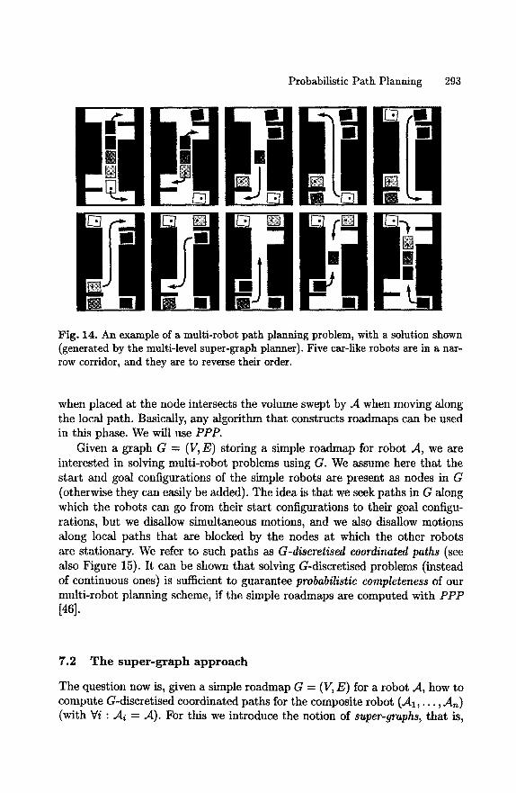
Probabilistic Path Planning 293
Fig. 14. An example of a multi-robot path planning problem, with a solution shown (generated by the multi-level super-graph planner). Five car-like robots are in a nar- row corridor, and they are to reverse their order.
when placed at the node intersects the volume swept by ,4 when moving along the local path. Basically, any algorithm that constructs roadmaps can be used in this phase. We will use PPP.
Given a graph G = (V, E) storing a simple roadmap for robot A, we are interested in solving multi-robot problems using G. We assume here that the start and goal configurations of the simple robots are present as nodes in G (otherwise they can easily be added). The idea is that we seek paths in G along which the robots can go from their start configurations to their goal configu- rations, but we disallow simultaneous motions, and we also disallow motions along local paths that are blocked by the nodes at which the other robots are stationary: We refer to such paths as G-discretised coordinated paths (see also Figure 15). It can be shown that solving G-discretised problems (instead of continuous ones) is sufficient to guarantee probabilistic completeness of our multi-robot planning scheme, if the simple roadmaps are computed with PPP [46].
7.2 The supe r -g raph approach
The question now is, given a simple roadmap G = (V, E) for a robot A, how to compute G-discretised coordinated paths for the composite robot (`41,.-., An) (with Vi : Ai = ,4). For this we introduce the notion of super-graphs, that is,
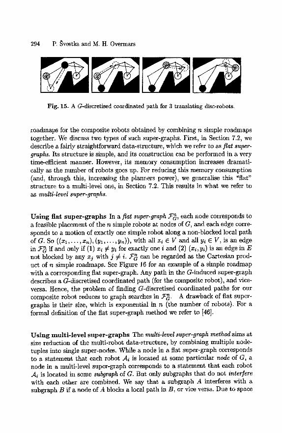
294 P. ~vestka and M. H. Overmars
Fig. 15. A G-discretised coordinated path for 3 translating disc-robots.
roadmaps for the composite robots obtained by combining n simple roadmaps together. We discuss two types of such super-graphs. First, in Section 7.2, we describe a fairly straightforward data-structure, which we refer to as fiat super- graphs. Its structure is simple, and its construction can be performed in a very time-efficient manner. However, its memory consumption increases dramati- cally as the number of robots goes up. For reducing this memory consumption (and, through this, increasing the planners power), we generalise this "flat" structure to a multi-level one, in Section 7.2. This results in what we refer to as multi-level super-graphs.
Using fiat super -g raphs In a fiat super-graph 9v~, each node corresponds to a feasible placement of the n simple robots at nodes of G, and each edge corre- sponds to a motion of exactly one simple robot along a non-blocked local path of G. So ((xl , . . . ,xr~),(yl , . . . ,yn)) , with all x~ E V and all yi E V, is an edge in ~'~ if and only if (1) xi # yi for exactly one i and (2) (xi, Yi) is an edge in E not blocked by any xj with j ~ i. ~'~ can be regarded as the Cartesian prod- uct of n simple roadmaps. See Figure 16 for an example of a simple roadmap with a corresponding flat super-graph. Any path in the G-induced super-graph describes a G-discretised coordinated path (for the composite robot), and vice- versa. Hence, the problem of finding G-discretised coordinated paths for our composite robot reduces to graph searches in ~'~. A drawback of flat super- graphs is their size, which is exponential in n (the number of robots). For a formal definition of the flat super-graph method we refer to [46].
Using mult i - level super -g raphs The multi-level super-graph method aims at size reduction of the multi-robot data-structure, by combining multiple node- tuples into single super-nodes. While a node in a flat super-graph corresponds to a statement that each robot J[i is located at some particular node of G, a node in a multi-level super-graph corresponds to a statement that each robot A~ is located in some subgraph of G. But only subgraphs that do not interfere with each other are combined. We say that a subgraph A interferes with a subgraph B if a node of A blocks a local path in B, or vice versa. Due to space
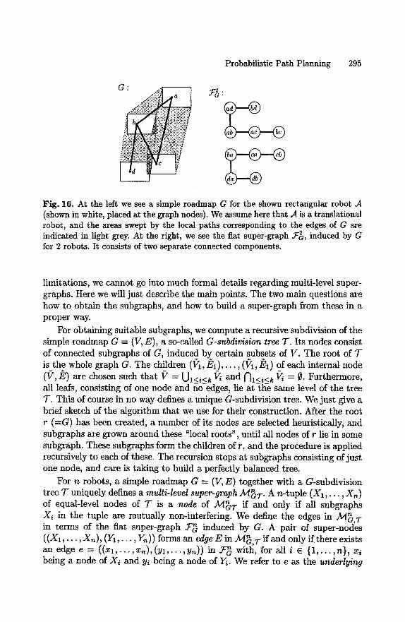
Probabilistic Path Planning 295
C
Fig. 16. At the left we see a simple roadmap G for the shown rectangular robot A (shown in white, placed at the graph nodes). We assume here that .4 is a translational robot, and the areas swept by the local paths corresponding to the edges of G are indicated in light grey. At the right, we see the flat super-graph ~'~, induced by G for 2 robots. It consists of two separate connected components.
limitations, we cannot go into much formal details regarding multi-level super- graphs. Here we will just describe the main points. The two main questions are how to obtain the subgraphs, and how to build a super-graph from these in a proper way.
For obtaining suitable subgraphs, we compute a recursive subdivision of the simple roadmap G = (V, E), a so-called G-subdivision tree T. Its nodes consist of connected subgraphs of G, induced by certain subsets of V. The root of T is the whole graph G. The children (V1, El ) , . . . , (V1,/~1) of each internal node (t ~,/~) are chosen such that V = Ul<i<k Vi and Nl<i<k ~ = ~. Furthermore, all leafs, consisting of one node and no-edges, lie a t t h e same level of the tree T. This of course in no way defines a unique G-subdivision tree. We just give a brief sketch of the algorithm that we use for their construction. After the root r (=G) has been created, a number of its nodes are selected heuristically, and subgraphs are grown around these "local roots", until all nodes of r lie in some subgraph. These subgraphs form the children of r, and the procedure is applied recursively to each of these. The recursion stops at subgraphs consisting of just one node, and care is taking to build a perfectly balanced tree.
For n robots, a simple roadmap G = (V, E) together with a G-subdivision tree 7" uniquely defines a multi-level super-graph M~T. A n-tuple (X1 , . . . , Xn) of equal-level nodes of T is a node of .k,t~T if and only if all subgraphs Xi in the tuple are mutually non-interfering. We define the edges in M~, T in terms of the fiat super-graph ~'~ induced by G. A pair of super-nodes ((X1,. . . , X,) , (Y1, • • •, Yn)) forms an edge E in Jt4~, 7- if and only if there exists an edge e = ( ( x l , . . . , xn ) , ( y l , . . . , yn ) ) in ~'~ with, for all i e {1 , . . . ,n} , x~ being a node of Xi and yi being a node of Y~. We refer to e as the underlying
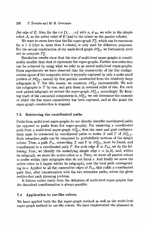
296 P. Svestka and M. H. Overmars
fiat edge of E. Also, for the i E {1, . . . , n} with xi ~ Yi, we refer to the simple robot Ai as the active robot of E (and to the others as the passive robots).
We want to stress here that the flat super-graph 5c~, which can be enormous ibr n > 3 (that is, more than 3 robots), is only used for definition purposes. For the actual construction of our multi-level graph A4~T we fortunately need not to compute ~ .
Simulation results show that the size of multi-level super-graphs is consid- erably smaller than that of equivalent fiat super-graphs. Further size-reduction can be achieved by using what we refer to as sieved multi-level super-graphs. From experiments we have observed that the connectivity of the free configu- rations space of the composite robot is typically captured by only a quite small portion of AJ~T, namely by that portion constructed from the relatively large
n subgraphs in 7". For this reason, we construct A4G. T incrementally. We sort the subgraphs in T by size, and pick them in reversed order of size. For each such picked subgraph we extend the super-graph ~/[~,T accordingly. By keep- ing track of the connected components in ~z[~7- we can determine the moment at which the free space connectivity has been captured, and at this point the super-graph construction is stopped.
7.3 Retrieving the coordinated paths
Paths from multi-level super-graphs do not directly describe coordinated paths (as opposed to paths from fiat super-graphs). For retrieving a coordinated path from a multi-level super-graph fl4~7-, first the start and goal configura- tions must be connected by coordinated paths to nodes X and Y of 2¢I~,7-. Such retraction paths can be computed by probabilistic motions of the simple robots. Then, a path P ~ , connecting X and Y in jk4~T , must be found, and transformed to a coordinated path P. For each edge E in P ~ , we do the fol- lowing: First, we identify the underlying simple edge e = (a,b), and, within its subgraph, we move the active robot to a. Then, we move all passive robots to nodes within their subgraphs that do not block e. And finally we move the active robot to b (again within its subgraph), over the local path correspond- ing to e. Applied to all the consecutive edges of PM, this yields a coordinated path that, after concatenation with the two retraction paths, solves the given multi-robot path planning problem.
It follows rather easily from the definition of multi-level super-graphs that the described transformation is always possible.
7.4 Application to car-like robots
We have applied both the flat super-graph method as well as the multi-level super-graph method to car-like robots. We have implemented the planners in
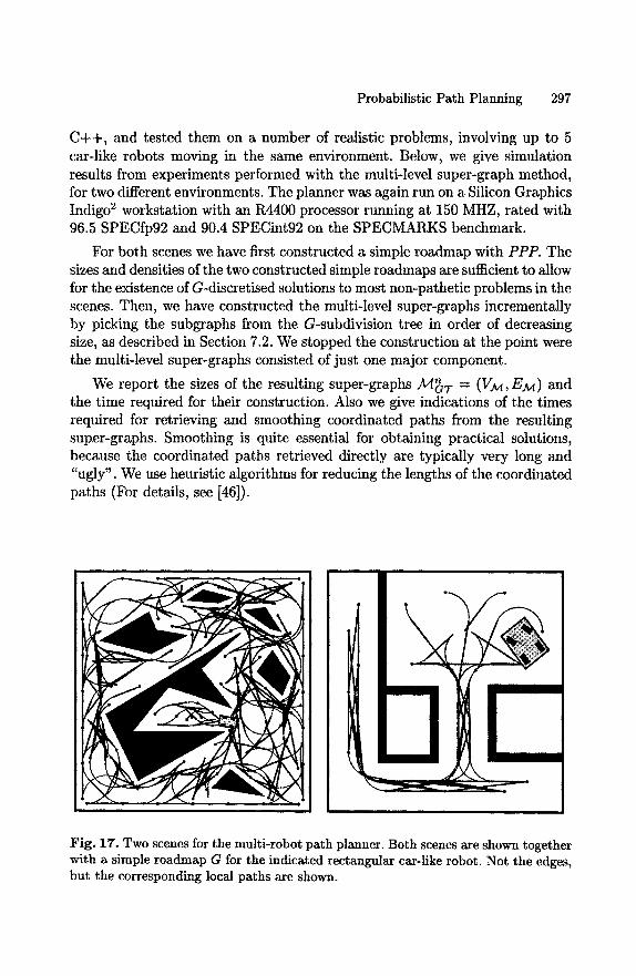
Probabilistic Path Planning 297
C++, and tested them on a number of realistic problems, involving up to 5 car-like robots moving in the same environment. Below, we give simulation results from experiments performed with the multi-level super-graph method, for two different environments. The planner was again run on a Silicon Graphics Indigo 2 workstation with an R4400 processor running at 150 MHZ, rated with 96.5 SPECfp92 and 90.4 SPECint92 on the SPECMARKS benchmark.
For both scenes we have first constructed a simple roadmap with PPP. The sizes and densities of the two constructed simple roadmaps are sufficient to allow for the existence of G-discretised solutions to most non-pathetic problems in the scenes. Then, we have constructed the multi-level super-graphs incrementally by picking the subgraphs from the G-subdivision tree in order of decreasing size, as described in Section 7.2. We stopped the construction at the point were the multi-level super-graphs consisted of just one major component.
n = ( V ~ , E ~ ) and We report the sizes of the resulting super-graphs MaT the time required for their construction. Also we give indications of the times required for retrieving and smoothing coordinated paths from the resulting super-graphs. Smoothing is quite essential for obtaining practical solutions, because the coordinated paths retrieved directly are typically very long and "ugly". We use heuristic algorithms for reducing the lengths of the coordinated paths (For details, see [46]).
V
Fig. 17. Two scenes for the multi-robot path planner. Both scenes are shown together with a simple roadmap G for the indicated rectangular car-like robot. Not the edges, but the corresponding local paths are shown.
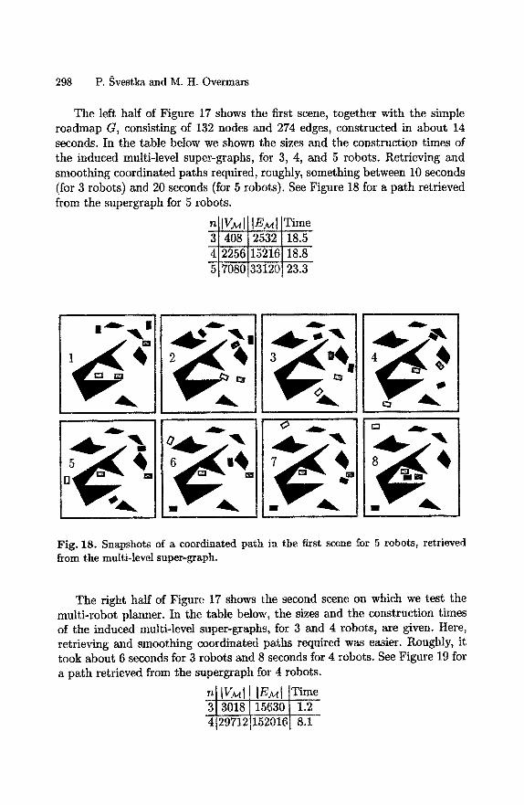
298 P. Svestka and M. H. Overmars
The left half of Figure 17 shows the first scene, together with the simple roadmap G, consisting of 132 nodes and 274 edges, constructed in about 14 seconds. In the table below we shown the sizes and the construction times of the induced multi-level super-graphs, for 3, 4, and 5 robots. Retrieving and smoothing coordinated paths required, roughly, something between 10 seconds (for 3 robots) and 20 seconds (for 5 robots). See Figure 18 for a path retrieved from the supergraph for 5 robots.
n Time -3 408 2532 18.5 -4 2256i152i6 18.8
23.3
L ]! Fig. 18. Snapshots of a coordinated path in the first scene for 5 robots, retrieved from the multi-level super-graph.
The right half of Figure 17 shows the second scene on which we test the multi-robot planner. In the table below, the sizes and the construction times of the induced multi-level super-graphs, for 3 and 4 robots, are given. Here, retrieving and smoothing coordinated paths required was easier. Roughly, it took about 6 seconds for 3 robots and 8 seconds for 4 robots. See Figure 19 for a path retrieved from the supergraph for 4 robots.
n[ [V]~I I [E.M I ]Time '31 3018] 15630 I !:2 .......... 4i29712115201 1 8.1
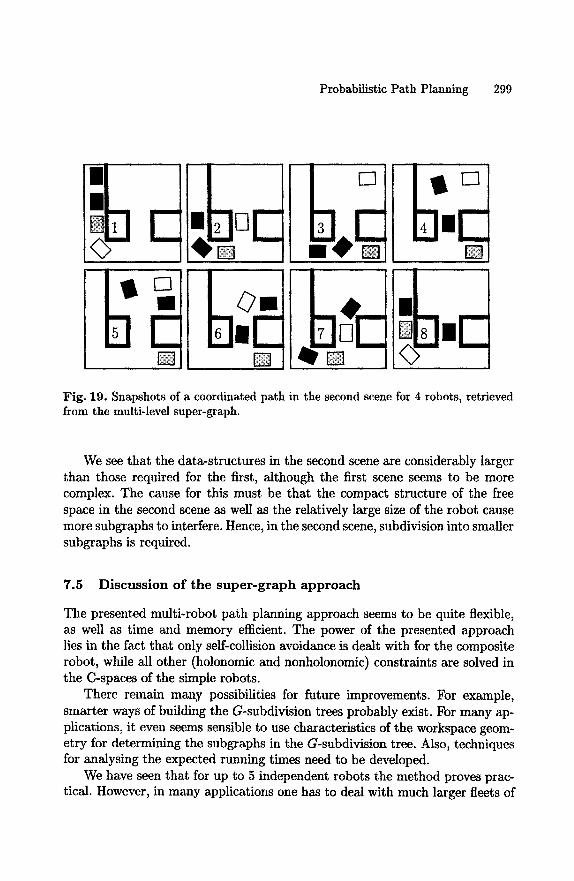
Probabilistic Path Planning 299
Fig. 19. Snapshots of a coordinated path in the second scene for 4 robots, retrieved from the multi-level super-graph.
We see that the data-structures in the second scene are considerably larger than those required for the first, although the first scene seems to be more complex. The cause for this must be that the compact structure of the free space in the second scene as well as the relatively large size of the robot cause more subgraphs to interfere. Hence, in the second scene, subdivision into smaller subgraphs is required.
7.5 Discussion of the super-graph approach
The presented multi-robot path planning approach seems to be quite flexible, as well as time and memory efficient. The power of the presented approach lies in the fact that only self-collision avoidance is dealt with for the composite robot, while all other (holonomic and nonholonomic) constraints are solved in the C-spaces of the simple robots.
There remain many possibilities for future improvements. For example, smarter ways of building the G-subdivision trees probably exist. For many ap- plications, it even seems sensible to use characteristics of the workspace geom- etry for determining the subgraphs in the G-subdivision tree. Also, techniques for analysing the expected running times need to be developed.
We have seen that for up to 5 independent robots the method proves prac- tical. However, in many applications one has to deal with much larger fleets of
300 P. ~vestka and M. H. Overmars
mobile robots. Due to the enormous complexity of such systems, only decoupled planners can be used here. Decoupled planners however can fall into deadlocks. Centralised planners could be integrated into existing large scale decoupled planners for resolving deadlock situations in specific (local) workspace areas where these could arise. For example, if T~ is such an area, the global decoupled planner could enforce a simple rule stating that, at any time instant, no more than say 4 robots are allowed to be present in 7%. Path planning within 7% can then be done by a centralised planner, like for example the planner presented in this section.
8 Conclusions
In this chapter an overview has been given on a general probabilistic scheme PPP for robot path planning. It consists of two phases. In the roadmap con- struction phase a probabilistic roadmap is incrementally constructed, and can subsequently, in the query phase, be used for solving individual path planning problems in the given robot environment. So, unlike other probabilistically complete methods, it is a learning approach. Experiments with applications of PPP to a wide variety of path planning problems show that the method is very powerful and fast. Another strong point of PPP is its flexibility. In order to apply it to some particular robot type, it suffices to define (and implement) a robot specific local planner and some (induced) metric. The performance of the resulting path planner can, if desired, be further improved by tailoring particular components of the algorithm to some specific robot type.
Important is that probabilistic completeness, for holonomic as well as non- holonomic robots, can be obtained by the use of local planners that respect certain general topological properties. Furthermore, there exist some recent re- sults that, under certain geometric assumptions on the free C-space, link the expected running time and failure probability of the planner to the size of the roadmap and characteristics of paths solving the particular problem. For exam- ple, under one such assumption, it can been shown that the expected size of a probabilistic roadmap required for solving a problem grows only logarithmically in the complexity of the problem.
Numerous extensions of the approach are possible. One such extension has been described in this chapter, dealing with the multi-robot path planning problem. Other possibilities include, for example, path planning in partially unknown environments, path planning in dynamic environments (e.g., amidst moving obstacles), and path planning in the presence of movable obstacles.
Probabilistic Path Planning 301
References
1. J.M. Ahuactzin. Le Fil d'Ariadne: Une Mgthode de Planifleation Gdngrale. Ap- plication d la Planifieation Automatique de Trajectoires. PhD thesis, l'Institut National Polytechnique de Grenoble, Grenoble, France, September 1994.
2. R. Alami, F. Robert, F. Ingrand, and S. Suzuki. Multi-robot cooperation through incremental plan-merging. In Proc. IEEE Internat. Conf. on Robotics and Au- tomation, pages 2573-2578, Nagoya, Japan, 1995.
3. J. Barraquand, L. Kavraki, J.-C. Latombe, T.-Y. Li, R. Motwani, and P. Ragha- van. A random sampling scheme for path planning. To appear in Intern. Journal of Rob. Research.
4. J. Barraquand and J.-C. Latombe. A Monte-Carlo algorithm for path planning with many degrees of freedom. In Proc. IEEE Intern. Conf. on Robotics and Automation, pages 1712-1717, Cincinnati, OH, USA, 1990.
5. J. Barraquand and J.-C. Latombe. Robot motion planning: A distributed repre- sentation approach. Internat. Journal Robotics Research., 10(6):628-649, 1991.
6. J. Barraquand and J.°C. Latombe. Nonholonomic multibody mobile robots: Controllability and motion planning in the presence of obstacles. Algorithmiea, 10:121-155, 1993.
7. P. Bessi~re, J.M. Ahuactzin, E.-G. Talbi, and E. Mazer. The Ariadne's clew algorithm: Global planning with local methods. In Proc. The First Workshop on the Algorithmic Foundations of Robotics, pages 39-47. A. K. Peters, Boston, MA, 1995.
8. S.J. Buckley. Fast motion planning for multiple moving robots. In Proceedings of the IEEE International Conference on Robotics and Au$omation, pages 322-326, Scottsdale, Arizona, USA, 1989.
9. J.F. Canny. The Complexity of Robot Path Planning. MIT Press, Cambridge, USA, 1988.
10. M. Erdmann and T. Lozano-P~rez. On multiple moving objects. In Proceedings of the IEEE International Conference on Robotics and Automation, pages 1419- 1424, San Francisco, CA, USA, 1986.
11. P. Ferbach. A method of progressive constraints for nonholonomic motion plan- ning. Technical report, Electricit~ de France. SDM Dept., Chatou, France, September 1995.
12. C. Fernandes, L. Gurvits, and Z.X. Li. Optimal nonholonomic motion planning for a falling cat. In Z. Li and J.F. Canny, editors, Nonholonomic Motion Planning, Boston, USA, 1993. Kluwer Academic Publishers.
13. J. Hopcroft, J.T. Schwartz, and M. Sharir. On the complexity of motion plan- ning for multiple independent objects; PSPACE-hardness of the warehouseman's problem. International Journal of Robotics Research, 3(4):76-88, 1984.
14. Th. Horsch, F. Schwarz, and H. Tolle. Motion planning for many degrees of freedom - random reflections at C-space obstacles. In Proc. IEEE Internat. Conf. on Robotics and Automation, pages 3318-3323, San Diego, USA, 1994.
15. Y. Hwang and N. Ahuja. Gross motion planning--a survey. ACM Comput. Surv., 24(3):219-291, 1992.
302 P. ~vestka and M. H. Overmars
16. Y.K. Hwang and P.C. Chen. A heuristic and complete planner for the classical mover's problem. In Proc. IEEE Inter~nat. Conf. on Robotics and Automation, pages 729-736, Nagoya, Japan, 1995.
17. B. Langlois J. Barraquand and J.-C. Latombe. Numerical potential field tech- niques for robot path planning. IEEE Trans. on Syst., Man., and Cybern.~ 22(2):224-241, 1992.
18. P. Jacobs, J.-P. Laumond, and M. Tai'x. A complete iterative motion planner for a car-like robot. Journees Geometrie Algorithmique, 1990.
19. L. Kavraki. Random networks in configuration space for fast path planning. Ph.D. thesis, Department of Computer Science, Stanford University, Stanford, Califor- nia, USA, January 1995.
20. L. Kavraki, M.N. Kolountzakis, and J.-C. Latombe. Analysis of probabilistic roadmaps for path planning. In IEEE International Conference on Robotics and Automation, pages 3020-3026, Minneapolis, MN, USA, 1996.
21. L. Kavraki and J.-C. Latombe. Randomized preprocessing of configuration space for fast path planning. In Proc. IEEE Internat. Conf. on Robotics and Automa- tion, pages 2138-2145, San Diego, USA, 1994.
22. L. Kavraki, J.-C. Latombe, R. Motwani~ and P. Raghavan. Randomized query processing in robot path planning. In Proc. 27th Annual ACM Syrup. on Theory of Computing (STOC), pages 353-362, Los Vegas, NV, USA, 1995.
23. L. Kavraki, P. Svestka, J.-C. Latombe, and M.H. Overmars. Probabilistic roadmaps for path planning in high dimensional configuration spaces. IEEE Trans. Robot. Aurora., 12:566-580, 1996.
24. F. Lamiraux and J.-P. Lanmond. On the expected complexity of random path planning. In Proc. IEEE Intern. Conf. on Robotics and Automation, pages 3014- 3019, Mineapolis, USA, 1996.
25. J.-C. Latombe. Robot Motion Planning. Kluwer Academic Publishers, Boston, USA, 1991.
26. J.-P. Laumond, P.E. Jacobs, M. Tai'x, and R.M. Murray. A motion planner for nonholonomic mobile robots. IEEE Trans. Robot. Aurora., 10(5), October 1994.
27. J.-P. Lanmond, S. Sekhavat, and M. Vaisset. Collision-free motion planning for a nonholonomic mobile robot with trailers. In ,~th IFAC Syrup. on Robot Control, pages 171-177, Capri, Italy, September 1994.
28. J.-P. Laumond, M. Tai'x, and P. Jacobs. A motion planner for car-like robots based on a mixed global/local approach. In IEEE IROS~ July 1990.
29. Y.H. Liu, S. Kuroda, T. Naniwa, H. Noborio, and S. Arimoto. A practical algo- rithm for planning collision-free coordinated motion of multiple mobile robots. In Proceedings of the IEEE International Conference on Robotics and Automation, pages 1427-1432, Scottsdale, Arizona, USA, 1989.
30. P.A. O'Donnetl and T. Lozano~P~rez. Deadlock-free and collision-free coordina- tion of two robotic manipulators. In Proceedings of the IEEE International Con- ]erence on Robotics and Automation~ pages 484-489~ Scottsdale, Arizona, USA, 1989.
31. M.H. Overmars. A random approach to motion planning. Technical Report RUU- CS-92-32, Dept. Comput. Sci., Utrecht Univ., Utrecht, the Netherlands, October 1992.
Probabilistic Path Planning 303
32. M.H. Overmars and P. Svestka. A probabitistic learning approach to motion plan- ning. In Proc. The First Workshop on the Algorithmic Foundations of Robotics, pages 19-37. A. K. Peters, Boston, MA, 1994.
33. P. Pignon. Structuration de l'Espace pour une Planification Hidrarchisge des Trajectoires de Robots Mobiles. Ph.D. thesis, LAAS-CNRS and Universit6 Paul Sabatier de Toulouse, Toulouse, France, 1993. Report LAAS No. 93395 (in French).
34. J.A. Reeds and R.A. Shepp. Optimal paths for a car that goes both forward and backward. Pacific Journal of Mathematics, 145(2):367-393, 1991.
35. J.H. Reif and M. Sharir. Motion planning in the presence of moving obstacles. In Proc. 25th IEEE Syrup. on Foundations of Computer Science, pages 144-154, 1985.
36. J.T. Schwartz and M. Sharir. Efficient motion planning algorithms in environ- ments of bounded local complexity. Report 164, Dept. Comput. Sci., Courant Inst. Math. Sci., New York Univ., New York, NY, 1985.
37. J.T. Schwartz and M. Shark. On the 'piano movers' problem: III. coordinating the motion of several independent bodies: The special case of circular bodies moving amidst polygonal obstacles. International Journal of Robotics Research, 2(3):46-75, 1983.
38. S. Sekhavat and J.-P. Lanmond. Topological property of trajectories computed from sinusoidal inputs for nonholonomic chained form systems. In Proc. IEEE Internat. Conf. on Robotics and Automation, pages 3383-3388, April 1996.
39. S. Sekhavat, P. Svestka, J.-P. Laumond, and M.H. Overmars. Probabflistic path planning for tractor-trailer robots. Technical Report 96007, LAAS-CNRS, Toulouse, France, 1995.
40. S. Sekhavat, P. ~vestka, J.-P. Laumond, and M.H. Overmars. Multi-level path planning for nonholonomic robots using semi-holonomic subsystems. To appear in Intern. Journal of Rob Research.
41. M. Sharir and S. Sifrony. Coordinated motion planning for two independent robots. In Proceedings of the Fourth ACM Symposium on Computational Geom- etry, 1988.
42. P. Sou~res and J.-P. Laumond. Shortest paths synthesis for a car-like robot. IEEE Trans. Automatic Control, 41:672-688, 1996.
43. H.J. Sussmann. Lie brackets, real analyticity and geometric control. In R.W. Brockett, R.S. Milkman, and H.J. Sussmann, editors, Dij~erential Geometric Con- trol Theory. Birkhanser, 1983.
44. H.J. Sussmann. A general theorem on local controllability. SIAM Journal on Control and Optimization, 25(1):158-194, January 1987.
45. P. Svestka. A probabilistic approach to motion planning for car-like robots. Technical Report RUU-CS-93-18, Dept. Comput. Sci., Utrecht Univ., Utrecht, the Netherlands, April 1993.
46. P. Svestka and M.H. Overmars. Coordinated motion planning for multiple car-like robots using probabilistic roadmaps. In Proc. IEEE Internat. Conf. on Robotics and Automation~ pages 1631-1636, Nagoya, Japan, 1995.
47. P. Svestka and M.H. Overmars. Motion planning for car-like robots using a probabilistic learning approach. Intern. Journal of Rob Research, 16:119-143, 1995.
304 P. ~vestka and M. H. Overmars
48. P. Svestka and M.H. Overmars. Multi-robot path planning with super-graphs. In Proc. CESA '96 IMACS Multieonference, Lille, France, July 1996.
49. P. Svestka and J. Vleugels. Exact motion planning for tractor-trailer robots. In Proe. IEEE Internat. Conf. on Robotics and Automation, pages 2445-2450, Nagoya, Japan, 1995.
50. D. Tilbury, R. Murray, and S. Sastry. Trajectory generation for the n-trailer problem using goursat normal form. In Proc. IEEB Internat. Conf. on Decision and Control, San Antonio, Texas, 1993.
51. P. Tournassoud. A strategy for obstacle avoidance and its application to multi- robot systems. In Proceedings of the IEEE International Conference on Robotics and Automation, pages 1224-1229, San Francisco, CA, USA, 1986.
52. S.M. La Valle and S.A. Hutchinson. Multiple-robot motion planning under inde- pendent objectives. To appear in IEEE Trans. Robot. Autom..
53. F. van der Stappen. Motion Planning amidst Fat Obstacles. Ph.D. thesis, Dept. Comput. Sci., Utrecht Univ., Utrecht, the Netherlands, October 1994.
54. F. van der Stappen, D. Halperin, and M.H. Overmars. The complexity of the free space for a robot moving amidst fat obstacles. Comput. Geom. Theory Appl., 3:353-373, 1993.
Collision Detection Algorithms for Motion Planning
P. Jimdnez, F. Thomas and C. Torras
Institut de Robbtica i Informktica Industrial, Barcelona
1 I n t r o d u c t i o n
Collision detection is a basic tool whose performance is of capital importance in order to achieve efficiency in many robotics and computer graphics applica- tions, such as motion planning, obstacle avoidance, virtual prototyping, com- puter animation, physical-based modeling, dynamic simulation, and, in general, all those tasks involving the simulated motion of solids which cannot penetrate one another. In these applications, collision detection appears as a module or procedure which exchanges information with other parts of the system concern- ing motion, kinematic and dynamic behaviour, etc. It is a widespread opinion to consider collision detection as the main bottleneck in these kinds of appli- cations.
In fact, static interference detection, collision detection and the generation of configuration-space obstacles can be viewed as instances of the same prob- lem, where objects are tested for interference at a particular position, along a trajectory and throughout the whole workspace, respectively. The structure of this chapter reflects this fact.
Thus, the main guidelines in static interference detection are presented in Section 2. It is shown how hierarchical representations allow to focus on relevant regions where interference is most likely to occur, speeding up the whole inter- ference test procedure. Some interference tests reduce to detecting intersections between simple enclosing shapes, such as spheres or boxes aligned with the co- ordinate axes. However, in some situations, this approximate approach does not suffice, and exact basic interference tests (for polyhedral environments) are re- quired. The most widely used such test is that involving a segment (standing for an edge) and a polygon in 3D space (standing for a face of a polyhedron). In this context, it has recently been proved that interference detection between non- convex polyhedra can be reduced, like many other problems in Computational Geometry, to checking some signs of vertex determinants, without computing new geometric entities.
Interference tests lie at the base of most collision detection algorithms, which are the subject of Section 3. These algorithms can be grouped into four approaches: multiple interference detection, swept volume interference, space-
306 P. Jimdnez, F. Thomas and C. Torras
time volume intersection, and trajectory parameterization. The multiple inter- ference detection approach has been the most widely used under a variety of sampling strategies, reducing the collision detection problem to multiple calls to static interference tests. The efficiency of a basic interference test does not guarantee that a collision detection algorithm based on it is in turn efficient. The other key factor is the number of times that this test is applied. Therefore, it is important to restrict the application of the interference test to those in- stants and object parts at which a collision can truly occur. Several strategies have been developed: 1) to find a lower time bound for the first collision, 2) to reduce the pairs of primitives within objects susceptible of interfering, and 3) to cut down the number of object pairs to be considered for interference. These strategies rely on distance computation algorithms, orientation-based pruning criteria and space partitioning schemes.
Section 4 describes how motion planners adopt different strategies with respect to the use of static interference and collision detection procedures, de- pending on their global or local nature. While global planners use static in- terference tests, or their generalizations, to generate a detailed description of either configuration-space obstacles or free-space connectivity, incremental and local path planners avoid this costly computation by fully relying on collision detection tests during the search process.
Finally, some conclusions are sketched in Section 5.
2 I n t e r f e r e n c e d e t e c t i o n
Objects to be checked for interference are usually modeled by composing sim- ple shapes. Hierarchies of spheres (or other primitive volumes) and polyhedral approximations are the most commonly used. The former exploit the low cost of detecting interference between spheres, which reduces to comparing the dis- tance between their centers and the sum of their radii. This type of model is particularly adequate in situations not demanding high accuracy, since achiev- ing that would require going down many levels in the hierarchy. Objects with planar faces and subject to small tolerances are usually dealt with using poly- hedral representations of their boundaries.
Hierarchical approximations permit focusing on the regions susceptible of interfering, as described in Section 2.1. Then, basic interference tests, which are the subject of Section 2.2, need only be applied within the focused regions.
2.1 Focusing on relevant regions
The two main approaches to confine the search for interferences to particular portions of the solids are representation dependent. On the one hand, there are
Collision Detection Algorithms for Motion Planning 307
algorithms that bound volume portions, and they are suited for volume repre- sentations, like Constructive Solid Geometry (CSG), octrees, or representations based on spheres. On the other hand, there are procedures that restrict the el- ements of the boundary of the objects that can intersect, and these algorithms are of course used together with boundary representations.
Hierarchica l vo lume represen ta t ions Two advantages of hierarchical rep- resentations must be highlighted:
- In many cases an interference or a non-interference situation can be easily detected at the first levels of the hierarchy. This leads to substantial savings under all interference detection schemes.
- The refinement of the representation is only necessary in the parts where collision may occur.
There are two types of bounding techniques for hierarchical volume rep- resentations, those that are based on an object partition hierarchy, and those where subregions of a space partition are considered.
O b j e c t pa r t i t ion hierarchies The so called "S-bounds" were developed and used in [8] for bounding spatially the part of the CSG tree that represents an intersection between two solids. S-bounds are simple enclosing volumes of the primitives at the leaves of the CSG tree: two examples are shown and discussed in [8] where rectangular parallelepipeds aligned with the coordinate axes and spheres are used as S-bounds. According to the set operations attached to every node in the tree, the S-bound corresponding to the root of the CSG intersection tree can be obtained after a number of pseudo-union and intersection operations of S-bounds. An algorithm that runs upwards and downwards on the tree performs all these operations (see Figs. 1 and 2). The main advantages of this procedure are the cut- off of subtrees included in empty bounds, leading to possibly important computational savings, and the focusing of intersection searching on zones where intersection can actually occur. The "successive spherical approximation" described in [6] allows focusing on the region of possible interference by checking intersection of spherical sectors at different levels in the hierarchy (Fig. 3). Hierarchies based on spheres that bound objects at different levels of refinement are also used in [50] and in [52].
Space pa r t i t i on hierarchies The octree representation allows to avoid checking for collision in those parts of the workspace where octants are labelled empty, that is, where no part of any object exists. H a full (to- tally occupied by the solid) or mixed (partially occupied) octant is inside a full one of the other solid, interference occurs. Only if a full or mixed
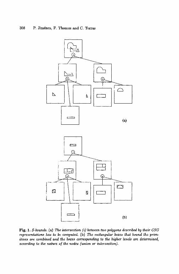
308 P. Jimdnez, F. Thomas and C. Torras
W'--3
(a)
J
[]
/
f : : j
1
(b)
Fig. 1. S-bounds. (a) The intersection (i) between two polygons described by their CSG representations has to be computed. (b) The rectangular boxes that bound the prim- itives are combined and the boxes corresponding to the higher levels are determined, according to the nature of the nodes (union or intersection).
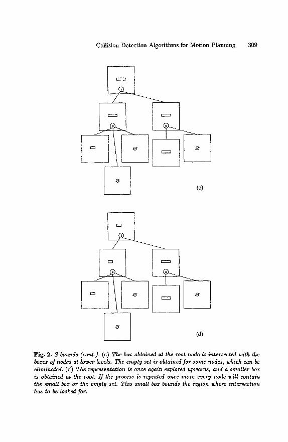
Collision Detection Algorithms for Motion Planning 309
(c)
(d)
Fig. 2. S-bounds (cont.). (c) The box obtained at the root node is intersected with the boxes of nodes at lower levels. The empty set is obtained for some nodes, which can be eliminated. (d) The representation is once again explored upwards, and a smaller box is obtained at the root. I f the process is repeated once more every node will contain the small box or the empty set. This small box bounds the region where intersection has to be looked for.
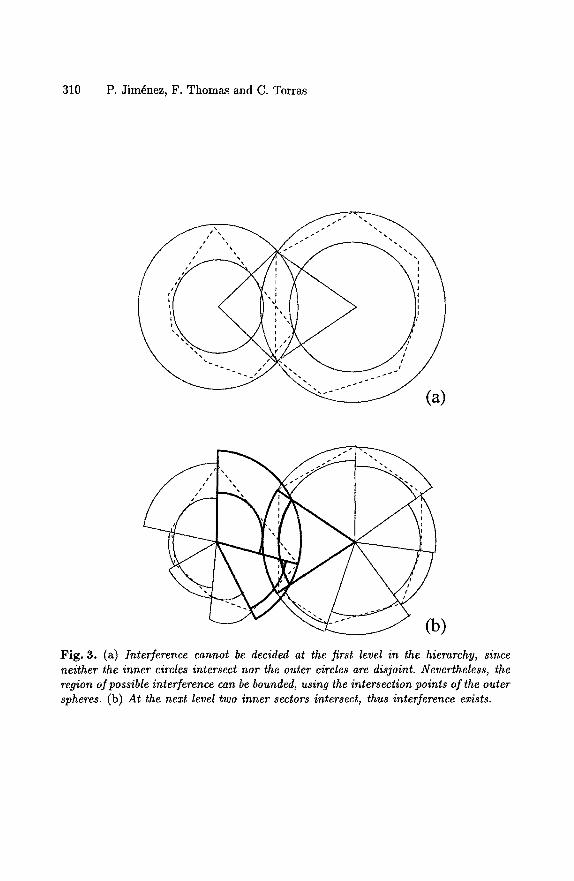
310 P. Jim~nez, F. Thomas and C. Torras
t S ~ ~ ~
ill Id
(a)
ps~ S~'t~ " ' ' ~
) Fig. 3. (a) Interference cannot be decided at the first level in the hierarchy, since neither the inner circles intersect nor the outer circles are disjoint. Nevertheless, the region of possible interference can be bounded, using the intersection points of the outer spheres. (b) At the next level two inner sectors intersect, thus interference exists.
Collision Detection Algorithms for Motion Planning 311
octant is inside a mixed one, the representation has to be further refined. The "natural" octree primitive is a cube [1,27], but there exist also mod- els based on the same idea where spheres are used, as octant-including volumes [31] or within a different space subdivision technique, where the subdivision branching is 13 instead of 8 [39]. In the binary space partition tree [56], a binary tree is constructed that represents a recursive partition- ing of space by hyperplanes. The authors describe such representation as a "crossing between octrees and boundary representations", but partition- ing is not restricted to be axis-aligned, as in the octree representation, and therefore transformations (a change in orientation, for example) can be sim- ply computed by applying the transformation to each hyperplane, without rebuilding the whole representation.
B o u n d a r y r ep resen ta t ions Hierarchical representations associated to bounding volumes that contain boundary features allow to restrict the effort of determining which parts of the objects boundaries may intersect to the most "promising" parts. Octrees have been used for subdividing axis aligned bounding boxes and constructing a bounding box hierarchy for the hull features (features of the polyhedron also appearing on its convex hull) and concavities of non-convex polyhedra [51]. Once penetration has been detected between the convex hulls of two polyhedra, a sweep and prune algorithm is applied to tra- verse the hierarchies down to the leaf level, where overlapping boxes indicate which faces may intersect, and exact contact points can be quickly determined.
In dense, cluttered environments, Oriented Bounding Boxes (OBB) perform better than axis aligned boxes or spheres, as they do fit more tightly to the objects and therefore less interferences between bounding volumes are reported. A hierarchical structure called OBB-Tree is used in [25] to represent polyhedra whose surfaces have been triangulated. Overlaps between OBBs are rapidly determined by performing 15 simple axis projection tests (about 200 arithmetic operations), as proved by the authors through their separating axis theorem.
2.2 Basic interference tests
Convexity plays a very important role in the performance of interference de- tection algorithms, and it is therefore used as classification criterion in the description below.
Convex p o l y h e d r a As pointed out in [37], intersection detection for two convex polyhedra can be done in linear time in the worst case. The proof is by reduction to linear programming, which is solvable in linear time for any fixed number of variables. If two point sets have disjoint convex hulls, then there is a
312 P. Jim@nez, F. Thomas and C. Torras
plane which separates the two sets. The three parameters that define the plane are considered as variables. Then, a linear inequality is attached to each vertex of one polyhedron, which specifies that the point is on one side of the plane, and the same is done for the other polyhedron (specifying now the location on the other side of the plane).
Moreover, convex polyhedra can be properly preprocessed, as described in [17], to make the complexity of intersection detection drop to O(logn logm). Preprocessing takes O(n + m) time to build a hierarchical representation of two polyhedra with n and m vertices. The lowest level in the hierarchical represen- tation is a tetrahedron. At each level of the hierarchy, vertices of the original polyhedron are added, such that they form an independent set (i.e. , are not adjacent) in the polyhedron corresponding to this hierarchical level, and the corresponding edge and face adjacency relationships are updated.
In fact, this algorithm computes the distance between two convex polyhedra. Likewise, all algorithms developed for distance computation can be adapted to detect interference. We refer the reader to Section 3.2.
One convex a n d o n e o n e n o n - c o n v e x An algorithm for computing the intersection between a convex and a non-convex polyhedron is described in [45]. A by-product of intersection computation is interference detection. Let P and Q be the surface of P (convex, n edges) and of Q (possibly non convex, m edges), respectively. The algorithm needs to solve the support problem, that is, to determine at least one point of each connected component of P f3 Q (this set of points will be called S). The methods for interference detection between convex polyhedra and linear subspaces developed by Dobkin and Kirkpatrick [16] are used for determining the intersections of P with edges and faces of Q: a hierarchical representation is used for P , so that the intersection between a line l, supporting an edge of Q, and P is computed in time O(log n), and a point in h N P , where h is a plane supporting a face of Q, can also be computed in time O(logn). Therefore, an algorithm can be constructed that solves the support problem in O(m log n). The next step consists in determining C = P f3 Q, by taking points of S, which are intersections between a face and an edge, and determining the intersections between the face and the two faces which are adjacent to the edge. Finally, the segments of edges of P and Q which are inside the intersection have to be determined. Figure 4 illustrates the main steps of the strategy. The overall complexity is O((n + m + s) log(n + m + s)), where s is the number of edges in the intersection.
Non-convex p o l y h e d r a : D e c o m p o s i t i o n i n t o c o n v e x p a r t s It is possible to extend the usage of the above algorithms to non-convex polyhedra just by decomposing these polyhedra into convex entities. Typically, decomposition
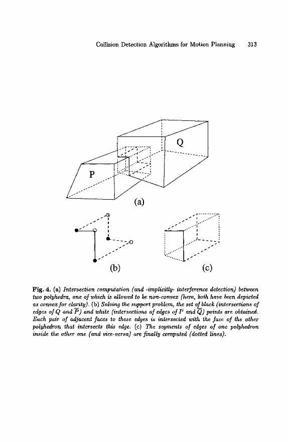
Collision Detection Algorithms for Motion Planning 313
- i t s ! , , ° . ~ ,
(a)
s ~ S s t I . . " " " t | s I , . ' "
s I t t . . * ' ! a l A ~ ¢'~ ! " " I "i : o I
i . . . ...... 2-: ~ . . ° " s t
; . . ° •
s S ~ " - . . ° . . . s ~ , S
(b) (c)
Fig. 4. (a) Intersection computation (and -implicitly- interference detection) between two polyhedra, one of which is allowed to be non-convex (here, both have been depicted as convex for clarity). (b) Solving the support problem, the set of black (intersections of edges of Q and P) and white (intersections of edges of P and Q)points are obtained. Each pair of adjacent faces to these edges is intersected with the face of the other polyhedron that intersects this edge. (c) The segments of edges of one polyhedron inside the other one (and vice-versa) are finally computed (dotted lines).
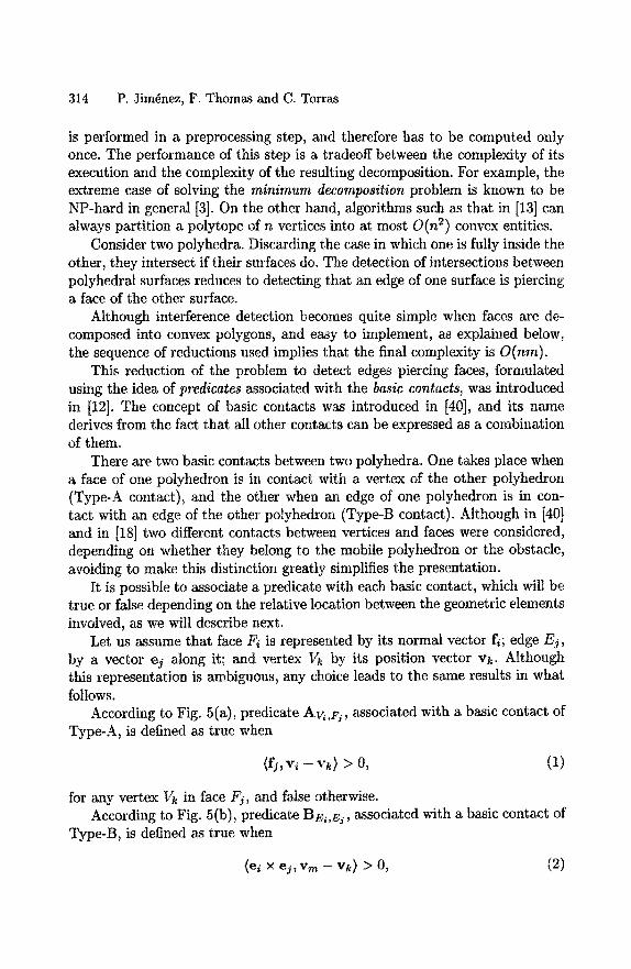
314 P. Jim~nez, F. Thomas and C. Torras
is performed in a preprocessing step, and therefore has to be computed only once. The performance of this step is a tradeoff between the complexity of its execution and the complexity of the resulting decomposition. For example, the extreme case of solving the minimum decomposition problem is known to be NP-hard in general [3]. On the other hand, algorithms such as that in [13] can always partition a polytope of n vertices into at most O(n 2) convex entities.
Consider two polyhedra. Discarding the case in which one is fully inside the other, they intersect if their surfaces do. The detection of intersections between polyhedral surfaces reduces to detecting that an edge of one surface is piercing a face of the other sm'face.
Although interference detection becomes quite simple when faces are de- composed into convex polygons, and easy to implement, as explained below, the sequence of reductions used implies that the final complexity is O(nm).
This reduction of the problem to detect edges piercing faces, formulated using the idea of predicates associated with the basic contacts, was introduced in [12]. The concept of basic contacts was introduced in [40], and its name derives from the fact that all other contacts can be expressed as a combination of them.
There are two basic contacts between two polyhedra. One takes place when a face of one polyhedron is in contact with a vertex of the other polyhedron (Type-A contact), and the other when an edge of one polyhedron is in con- tact with an edge of the other polyhedron (Type-B contact). Although in [40] and in [18] two different contacts between vertices and faces were considered, depending on whether they belong to the mobile polyhedron or the obstacle, avoiding to make this distinction greatly simplifies the presentation.
It is possible to associate a predicate with each basic contact, which will be true or false depending on the relative location between the geometric elements involved, as we will describe next.
Let us assume that face Fi is represented by its normal vector fi; edge Ej, by a vector ej along it; and vertex V~ by its position vector vk. Although this representation is ambiguous, any choice leads to the same results in what follows.
According to Fig. 5(a), predicate Ave,F~, associated with a basic contact of Type-A, is defined as true when
(fj,vi - v k ) > 0, (1)
for any vertex Vk in face Fj, and false otherwise. According to Fig. 5(b), predicate BE, Ej, associated with a basic contact of
Type-B, is defined as true when
(ei × ej,Vm -- vk) > O, (2)
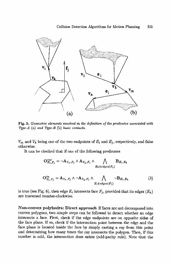
Collision Detection Algorithms for Motion Planning 315
vi fj
f \ (a) (b)
Fig. 5. Geometric elements involved in the definition of the predicates associated with Type-A (a) and Type-B (b) basic contacts.
Vm and Vk being one of the two endpoints of Ei and Ej, respectively, and false otherwise.
It can be checked that if one of the following predicates
OOUt E~,Fi = -~Av~ ,Fj A A%,v~ A A BE~ ,Ek E~ Eedges( Fj )
OE~ ,Fj ---" Av . ,Fj A "~Avt t ,Fj A A -~BE~,E~ EiEedges(Fj)
(a)
is true (see Fig. 6), then edge Ei intersects face Fj, provided that its edges (Ek) are traversed counter-clockwise.
Non-convex po lyhedra : Direc t approach If faces are not decomposed into convex polygons, two simple steps can be followed to detect whether an edge intersects a face. First, check if the edge endpoints are on opposite sides of the face plane. If so, check if the intersection point between the edge and the face plane is located inside the face by simply casting a ray from this point and determining how many times the ray intersects the polygon. Then, if this number is odd, the intersection does exists (odd-parity rule). Note that the
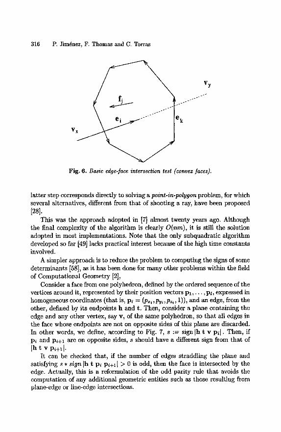
316 P. Jim6nez, F. Thomas and C. Torras
rj
ei y "
Yy
Fig. 6. Basic edge-face intersection test (convex faces).
latter step corresponds directly to solving a point-in-polygon problem, for which several alternatives, different from that of shooting a ray, have been proposed [281.
This was the approach adopted in [7] almost twenty years ago. Although the final complexity of the algorithm is clearly O(nm), it is still the solution adopted in most implementations. Note that the only subquadratic algorithm developed so far [49] lacks practical interest because of the high time constants involved.
A simpler approach is to reduce the problem to computing the signs of some determinants [58], as it has been done for many other problems within the field of Computational Geometry [2],
Consider a face from one polyhedron, defined by the ordered sequence of the vertices around it, represented by their position vectors P l , . . . , Pt, expressed in homogeneous coordinates (that is, pi = (pz~ ,Py~,Pz,, 1)), and an edge, from the other, defined by its endpoints h and t. Then, consider a plane containing the edge and any other vertex, say v, of the same polyhedron, so that all edges in the face whose endpoints are not on opposite sides of this plane are discarded. In other words, we define, according to Fig. 7, s := sign Ih t v Pit- Then, if Pi and Pi+l are on opposite sides, s should have a different sign from that of lh t v Pi+t I.
It can be checked that, if the number of edges straddling the plane and satisfying s * sign Ih t Pi Pi+I I > 0 is odd, then the face is intersected by the edge. Actually, this is a reformulation of the odd parity rule that avoids the computation of any additional geometric entities such as those resulting from plane-edge or line-edge intersections.
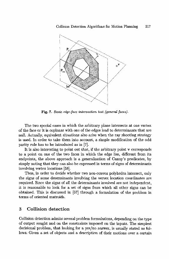
Collision Detection Algorithms for Motion Planning 317
j f j J~
j J
4-44
O ¥ ,:"
j J"
J j J"
~'"~ • 4 7"" 4 "'-4 "~'~'"
Fig. 7. Basic edge-face intersection test (general faces).
The two special cases in which the arbitrary plane intersects at one vertex of the face or it is coplanar with one of the edges lead to determinants that are null. Actually, equivalent situations also arise when the ray shooting strategy is used. In order to take them into account, a simple modification of the odd parity rule has to be introduced as in [7].
It is also interesting to point out that, if the arbitrary point v corresponds to a point on one of the two faces in which the edge lies, different from its endpoints, the above approach is a generalization of Canny's predicates, by simply noting that they can also be expressed in terms of signs of determinants involving vertex locations [58].
Thus, in order to decide whether two non-convex polyhedra intersect, only the signs of some determinants involving the vertex location coordinates are required. Since the signs of all the determinants involved are not independent, it is reasonable to look for a set of signs from which all other signs can be obtained. This is discussed in [57] through a formulation of the problem in terms of oriented matroids.
3 C o l l i s i o n d e t e c t i o n
Collision detection admits several problem formulations, depending on the type of output sought and on the constraints imposed on the inputs. The simplest decisional problem, that looking for a yes/no answer, is usually stated as fol- lows: Given a set of objects and a description of their motions over a certain
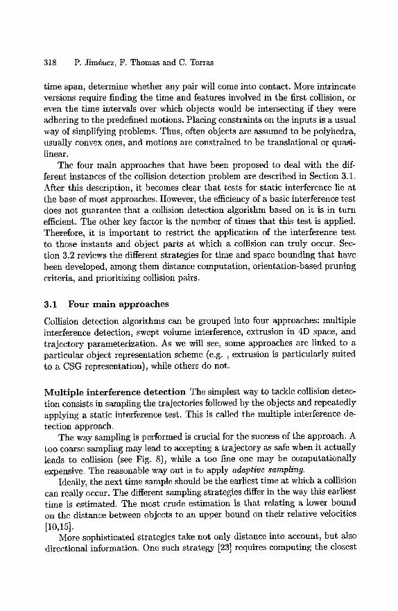
318 P. Jim@nez, F. Thomas and C. Torras
time span, determine whether any pair will come into contact. More intrincate versions require finding the time and features involved in the first collision, or even the time intervals over which objects would be intersecting if they were adhering to the predefined motions. Placing constraints on the inputs is a usual way of simplifying problems. Thus, often objects are assumed to be polyhedra, usually convex ones, and motions are constrained to be translational or quasi- linear.
The four main approaches that have been proposed to deal with the dif- ferent instances of the collision detection problem are described in Section 3.1. After this description, it becomes clear that tests for static interference lie at the base of most approaches. However, the efficiency of a basic interference test does not guarantee that a collision detection algorithm based on it is in turn efficient. The other key factor is the number of times that this test is applied. Therefore, it is important to restrict the application of the interference test to those instants and object parts at which a collision can truly occur. Sec- tion 3.2 reviews the different strategies for time and space bounding that have been developed, among them distance computation, orientation-based pruning criteria, and prioritizing collision pairs.
3.1 Four main approaches
Collision detection algorithms can be grouped into four approaches: multiple interference detection, swept volume interference, extrusion in 4D space, and trajectory parameterization. As we will see, some approaches are linked to a particular object representation scheme (e.g. , extrusion is particularly suited to a CSG representation), while others do not.
Mul t ip le interference de tec t ion The simplest way to tackle collision detec- tion consists in sampling the trajectories followed by the objects and repeatedly applying a static interference test. This is called the multiple interference de- tection approach.
The way sampling is performed is crucial for the success of the approach. A too coarse sampling may lead to accepting a trajectory as safe when it actually leads to collision (see Fig. 8), while a too fine one may be computationally expensive. The reasonable way out is to apply adaptive sampling.
Ideally, the next time sample should be the earliest time at which a collision can really occur. The different sampling strategies differ in the way this earliest time is estimated. The most crude estimation is that relating a lower bound on the distance between objects to an upper bound on their relative velocities [10,15].
More sophisticated strategies take not only distance into account, but also directional information. One such strategy [23] requires computing the closest
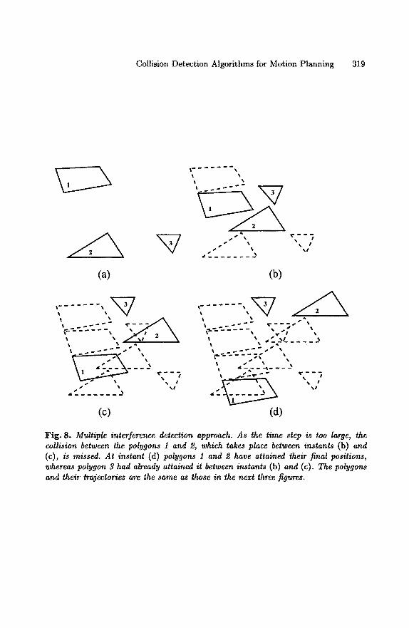
Collision Detection Algorithms for Motion Planning 319
(a) (b)
. . . . . . , , 7 ,, . . . . . . .
%V *"I
L - - ~ " - - " ~ - - - - - - "~
s L S _ . . . . . ,,t _ ~
(c) (d)
Fig. 8. Multiple interference detection approach. As the time step is too large, the collision between the polygons 1 and 2, which takes place between instants (b) and (c), is missed. At instant (d) polygons 1 and 2 have attained their final positions, whereas polygon 3 had already attained it between instants (b) and (c). The polygons and their trajectories are the same as those in the next three figures.
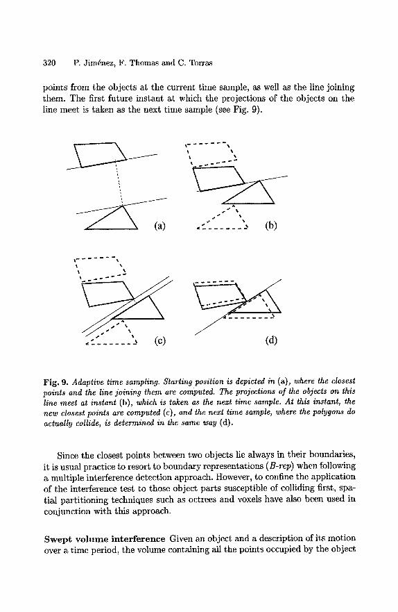
320 P. Jim@nez, F. Thomas and C. Torras
points from the objects at the current time sample, as well as the line joining them. The first future instant at which the projections of the objects on the line meet is taken as the next time sample (see Fig. 9).
I •
t •
i i
.-_ . . . . . . _ , (b)
, : . . . . . . ~ (C) (d)
Fig. 9. Adaptive time sampling. Starting position is depicted in (a), where the closest points and the line joining them are computed. The projections of the objects on this line meet at instant (b), which is taken as the next time sample. At this instant, the new closest points are computed (c), and the next time sample, where the polygons do actually collide, is determined in the same way (d).
Since the closest points between two objects lie always in their boundaries, it is usual practice to resort to boundary representations (B-rep) when following a multiple interference detection approach. However, to confine the application of the interference test to those object parts susceptible of colliding first, spa- tial partitioning techniques such as octrees and voxels have also been used in conjunction with this approach.
Swept vo lume interference Given an object and a description of its motion over a time period, the volume containing all the points occupied by the object
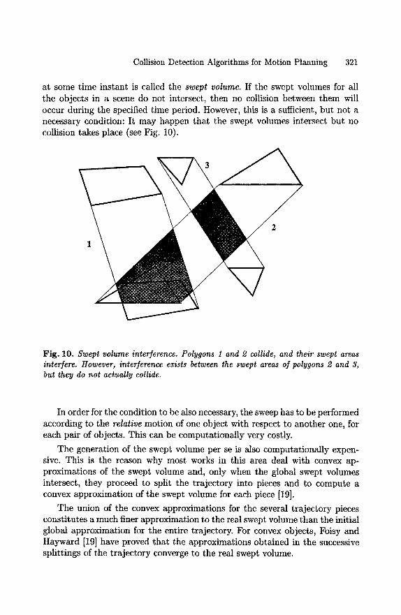
Collision Detection Algorithms for Motion Planning 321
at some time instant is called the swept volume. If the swept volumes for all the objects in a scene do not intersect, then no collision between them will occur during the specified time period. However, this is a sufficient, but not a necessary condition: It may happen that the swept volumes intersect but no collision takes place (see Fig. 10).
Fig. 10. Swept volume interference. Polygons 1 and 2 collide, and their swept areas interfere. However, interference exists between the swept areas of polygons 2 and 3, but they do not actually collide.
In order for the condition to be also necessary, the sweep has to be performed according to the relative motion of one object with respect to another one, for each pair of objects. This can be computationally very costly.
The generation of the swept volume per se is also computationalty expen- sive. This is the reason why most works in this area deal with convex ap- proximations of the swept volume and, only when the global swept volumes intersect, they proceed to split the trajectory into pieces and to compute a convex approximation of the swept volume for each piece [19].
The union of the convex approximations for the several trajectory pieces constitutes a much finer approximation to the real swept volume than the initial global approximation for the entire trajectory. For convex objects, Foisy and Hayward [19] have proved that the approximations obtained in the successive splittings of the trajectory converge to the real swept volume.
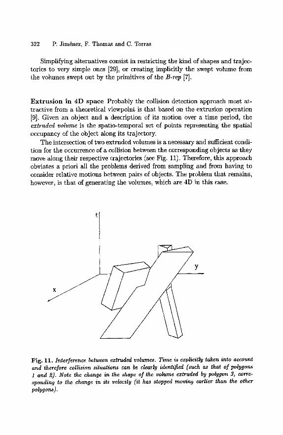
322 P. Jim@nez, F. Thomas and C. Torras
Simplifying alternatives consist in restricting the kind of shapes and trajec- tories to very simple ones [29], or creating implicitly the swept volume from the volumes swept out by the primitives of the B-rep [7].
Ex t rus ion in 4D space Probably the collision detection approach most at- tractive from a theoretical viewpoint is that based on the extrusion operation [9]. Given an object and a description of its motion over a time period, the extruded volume is the spatio-temporal set of points representing the spatial occupancy of the object along its trajectory.
The intersection of two extruded volumes is a necessary and sufficient condi- tion for the occurrence of a collision between the corresponding objects as they move along their respective trajectories (see Fig. 11). Therefore, this approach obviates a priori all the problems derived from sampling and from having to consider relative motions between pairs of objects. The problem that remains, however, is that of generating the volumes, which are 4D in this case.
/
Fig. 11. Interference between eztruded volumes. Time is ezplieitly taken into account and therefore collision situations can be clearly identified (such as that of polygons i and 2). Note the change in the shape of the volume e~truded by polygon 3, corre- sponding to the change in its velocity (it has stopped moving earlier than the other polygon#.
Collision Detection Algorithms for Motion Planning 323
The extrusion operation is distributive with respect to the union, inter- section and set difference operations. This motivated the development of the extrusion approach in the context of CSG representations. The mentioned dis- tributive property guarantees that an object and its extruded volume can be represented through the same boolean combination of volumetric primitives and extrusions of these primitives, respectively.
The formal beauty of this approach is partially occluded by the high cost of its practical implementation. Thus, for example, the extrusion of a linear subspace subject to a constant angular velocity is bounded by a helicoidal hy- persurface. For this reason, the implementation deals only with linear subspaces subject to piecewise translational motions [9].
T r a j e c t o r y pa rame te r i za t i on The collision instant can be analytically de- termined if the object trajectories are expressed as functions of a parameter (time) and the collision condition is formulated as a semialgebraic set involv- ing the locations of object features (faces, edges and vertices). This requires to perform a change of variable in order to obtain an algebraic expression for rota- tion, instead of equations in terms of trascendent functions. By replacing those locations by the corresponding parameterized trajectories, a semialgebraic set in terms of a single variable (time) is obtained. Once this set is explicitly com- puted, the time instants at which objects establish and lose contact are known.
The trajectory parameterization approach has been followed in [12,33,54], where a polyhedra interference test is expressed as a combination of param- eterized basic contact functions. These functions reflect the spatial relation- ships between the primitives of the B-rep of the polyhedra. The zeros of these functions delimit several time intervals, whose combination according to the interference test provides the desired set of intervals over which objects would be intersecting, if they were ~lhering to the predefined trajectories.
3.2 St ra tegies for space and t ime bound ing
The first three approaches described in the preceding section eventually re- quire to apply a static interference test between either 3D volumes or 4D ones. However, even if a basic interference test is made very efficient, the collision de- tection algorithm can still be computationally expensive if the basic test has to be applied many times. Thus, the key aspect of any collision detection scheme is to restrict as much as possible when and where this test is applied. Knowing how the objects are moving and how far away they are from one another, it is possible to bound the time interval where the collision is likely to occur. Therefore, it is important to determine quickly the distance between the ob- jects. On the other hand, if the direction of motion is known, the search for
324 P. Jim@nez, F. Thomas and C. Torras
possible collisions can be restrained to those object parts which may first come into contact. Finally, if there are many moving objects in the scene, means to avoid having to check every pair of objects for collision need to be provided. These are the issues discussed in the next subsections.
Dis tance computation for collision t ime bound ing Spherical represen- tations are appealing because the elementary distance calculation between two spheres is trivial. The problem rather consists in determining which spheres of the representation have to be tested. In [59] the objects are described in terms of spherical cones (generated by translating a sphere along a line and changing its radius) and spherical planes (which are obtained by translating a sphere in two dimensions, and eventually changing also its radius). These primitives can also be viewed as a collection of spheres. Any distance can be expressed as a combination of the distances between two spherical cones and between a sphere and a spherical plane. The distance between two spherical cones is deter- mined in two steps: first, compute the direction where the minimum distance occurs, then compute the involved spheres (locate their centers on the axes of the spherical cones). The distance between a sphere and a spherical plane is found by projecting the sphere perpendicularly on the plane, and calculating the sphere on the plane that corresponds to this projection. In any case, once the spheres are located, the distance is easily found as the distance between their centers minus the sum of their radius.
Most distance computation algorithms have been developed for convex poly- hedra. Some exploit specific features of the polyhedra and therefore cannot be used for other type of geometric models. Others, like the method explained in [24], can be used with spherical [26] or other non-polytopal surface descriptions [22].
There are two main streams in the way that the distance computation problem is treated, namely the geometric and the optimization approaches.
The geometric approach The closest points of two polyhedra are obtained, under this approach, by expanding a hierarchical (incremental) representation in a given direction or by navigating along the boundaries of the polyhedra. The euclidean distance between these closest points is then computed. The methods differ in the way that the closest points are obtained:
- An adequate representation may justify the effort spent in obtaining it, as a preprocessing step is done only once, if it allows important computa- tional savings in subsequent operations. This is the idea behind Dobkin and
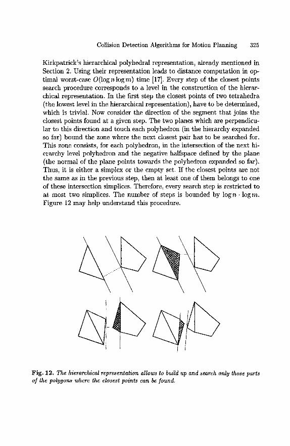
Collision Detection Algorithms for Motion Planning 325
Kirkpatrick's hierarchical polyhedral representation, already mentioned in Section 2. Using their representation leads to distance computation in op- timal worst-case O(log n log m) time [17]. Every step of the closest points search procedure corresponds to a level in the construction of the hierar- chical representation. In the first step the closest points of two tetrahedra (the lowest level in the hierarchical representation), have to be determined, which is trivial. Now consider the direction of the segment that joins the closest points found at a given step. The two planes which are perpendicu- lar to this direction and touch each polyhedron (in the hierarchy expanded so far) bound the zone where the next closest pair has to be searched for. This zone consists, for each polyhedron, in the intersection of the next hi- erarchy level polyhedron and the negative halfspace defined by the plane (the normal of the plane points towards the polyhedron expanded so far). Thus, it is either a simplex or the empty set. If the closest points are not the same as in the previous step, then at least one of them belongs to one of these intersection simptices. Therefore, every search step is restricted to at most two simplices. The number of steps is bounded by log n • log m. Figure 12 may help understand this procedure.
Fig. 12. The hierarchical representation allows to build up and search only those parts of the polygons where the closest points can be found.
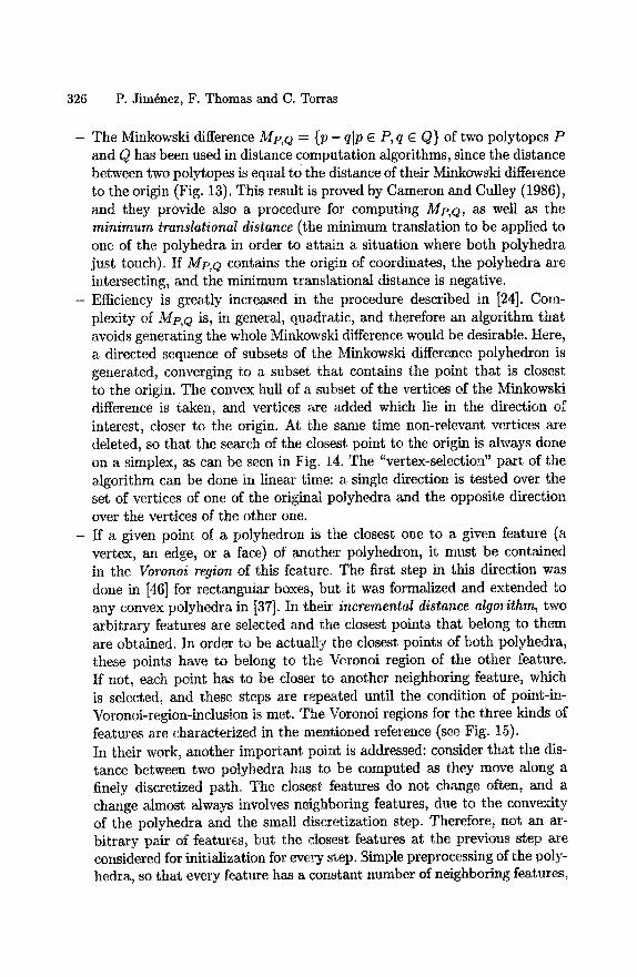
326 P. Jim6nez, F. Thomas and C. Torras
- The Minkowski difference Mp, Q ---. {p - q[p E P, q E Q} of two polytopes P and Q has been used in distance computation algorithms, since the distance between two polytopes is equal to the distance of their Minkowski difference to the origin (Fig. 13). This result is proved by Cameron and Culley (1986), and they provide also a procedure for computing Mp, Q, as well as the minimum translational distance (the minimum translation to be applied to one of the polyhedra in order to attain a situation where both polyhedra just touch). If Mp, Q contains the origin of coordinates, the polyhedra are intersecting, and the minimum translational distance is negative.
- Efficiency is greatly increased in the procedure described in [24]. Com- plexity of Mp, Q is, in general, quadratic, and therefore an algorithm that avoids generating the whole Minkowski difference would be desirable. Here, a directed sequence of subsets of the Minkowski difference polyhedron is generated, converging to a subset that contains the point that is closest to the origin. The convex hull of a subset of the vertices of the Minkowski difference is taken, and vertices are added which lie in the direction of interest, closer to the origin. At the same time non-relevant vertices are deleted, so that the search of the closest point to the origin is always done on a simplex, as can be seen in Fig. 14. The "vertex-selection" part of the algorithm can be done in linear time: a single direction is tested over the set of vertices of one of the original polyhedra and the opposite direction over the vertices of the other one.
- If a given point of a polyhedron is the closest one to a given feature (a vertex, an edge, or a face) of another polyhedron, it must be contained in the Voronoi region of this feature. The first step in this direction was done in [46] for rectangular boxes, but it was formalized and extended to any convex polyhedra in [37]. In their incremental distance algorithm, two arbitrary features are selected and the closest points that belong to them are obtained. In order to be actually the closest points of both polyhedra, these points have to belong to the Voronoi region of the other feature. If not, each point has to be closer to another neighboring feature, which is selected, and these steps are repeated until the condition of point-in- Voronoi-region-inclusion is met. The Voronoi regions for the three kinds of features are characterized in the mentioned reference (see Fig. 15). In their work, another important point is addressed: consider that the dis- taace between two polyhedra has to be computed as they move along a finely discretized path. The closest features do not change often, and a change almost always involves neighboring features, due to the convexity of the polyhedra and the small discretization step. Therefore, not an ar- bitrary pair of features, but the closest features at the previous step are considered for initialization for every step. Simple preprocessing of the poly- hedra, so that every feature has a constant number of neighboring features,
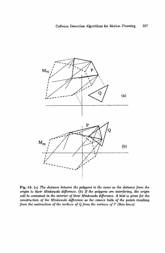
Collision Detection Algorithms for Motion Planning 327
M
| ",. | ~ ' .
i . - (a)
M~ ! / i / j f f . y,/./
/ / / /- 2./" (b)
Fig. 13. (a) The distance between the polygons is the same as the distance from the origin to their Minkowski difference. (b) I f the polygons are interfering, the origin will be contained in the interior of their Minkowski difference. A hint is given for the construction of the Minkowski difference as the convex hulls of the points resulting from the subtraction of the vertices of Q from the vertices of P (thin lines).
328 P. Jim~nez, F. Thomas and C. Torras
2 (a) (b) 1 ................ "...
9 "\'4
0 7 ~ 5 4 + 6 0
~ """ (d) ,, (c) , .
9."" \" 4 ~ ,' ,,,";
Fig. 14. The closest poini of the original Minkowski polygon (a) to the origin (0) has to be determined. The first simplex (b) has been chosen arbitrarily. A subset of vertices, whose convex hull contains the closest point of the simplex to the origin, is taken (4 and 9, although in this case also 1 and 9 could have been chosen), and a new vertex is selected (c). Note that this new vertex, 6, has the minimum projection onto the direction to the closest point found in (b). At the same time, the non-relevant vertex 1 is deleted. The direction to the closest point of the simplex in (c) is computed, and in the next step the closest point of the polygon to the origin (7 in this ease) is determined (d).
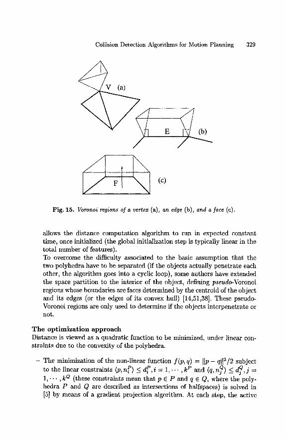
Collision Detection Algorithms for Motion Planning 329
< v (a)
E
(c)
Fig. 15. Voronoi regions o] a vertex (a), an edge (b), and a face (c).
allows the distance computation algorithm to run in expected constant time, once initialized (the global initialization step is typically linear in the total number of features). To overcome the difficulty associated to the basic assumption that the two polyhedra have to be separated (if the objects actually penetrate each other, the algorithm goes into a cyclic loop), some authors have extended the space partition to the interior of the object, defining pseudo-Voronoi
regions whose boundaries are faces determined by the centroid of the object and its edges (or the edges of its convex hull) [14,51,38]. These pseudo- Voronoi regions are only used to determine if the objects interpenetrate or not.
The optimization approach Distance is viewed as a quadratic function to be minimized, under linear con- straints due to the convexity of the polyhedra.
- The minimization of the non-linear function f ( p , q) = HP - q[12/2 subject to the linear constraints (p, n P) < d R, i = 1 , . . . , k p and (q, n?) < d~j, j = 1 , . - - , k Q (these constraints mean that p E P and q E Q, where the poly- hedra P and Q are described as intersections of halfspaces) is solved in [5] by means of a gradient projection algorithm. At each step, the active
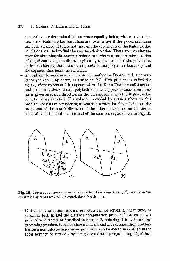
330 P. Jim~nez, F. Thomas and C. Torras
constraints are determined (those where equality holds, with certain toler- ance) and Kuhn-Tucker conditions are used to test if the global minimum has been attained. If this is not the case, the coefficients of the Kuhn-Tucker conditions are used to find the new search direction. There are two alterna- tives for obtaining the starting points: to perform a simplex minimization subalgorithm along the direction given by the centroids of the polyhedra, or by considering the intersection points of the polyhedra boundary and the segment that joins the centroids.
- In applying Rosen's gradient projection method as Bobrow did, a conver- gence problem may occur, as stated in [62]. This problem is called the zig-zag phenomenon and it appears when the Kuhn-Tucker conditions are satisfied alternatively at each polyhedron. This happens because a zero vec- tor is given as search direction on the polyhedron where the Kuhn-Tucker conditions are satisfied. The solution provided by these authors to this problem consists in considering as search direction for this polyhedron the projection of the search direction of the other polyhedron on the active constraints of the first one, instead of the zero vector, as shown in Fig. 16.
(a) (b)
Fig. 16. The zig-zag phenomenon (a) is avoided if the projection of S~l on the active constraint of B is taken as the search direction Sbl (b).
- Certain quadratic optimization problems can be solved in linear time, as shown in [44]. In [36] the distance computation problem between convex polyhedra is stated as described in Section 2, reducing it to a linear pro- gramming problem. It can be shown that the distance computation problem between non-intersecting convex polyhedra can be solved in O(n) (n is the total number of vertices) by using a quadratic programming algorithm.
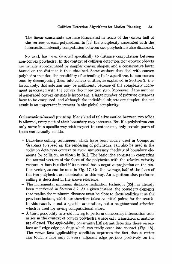
Collision Detection Algorithms for Motion Planning 331
The linear constraints are here formulated in terms of the convex hull of the vertices of each polyhedron. In [53] the complexity associated with the intersection intensity computation between two polyhedra is also discussed.
No work has been devoted specifically to distance computation between non-convex polyhedra. In the context of collision detection, non-convex objects are usually approximated by simpler convex shapes, and a conservative lower bound on the distance is thus obtained. Some authors that deal with convex polyhedra mention the possibility of extending their algorithms to non-convex ones by decomposing them into convex entities, as explained in Section 2. Un- fortunately, this solution may be inefficient, because of the complexity incre- ment associated with the convex decomposition step. Moreover, if the number of generated convex entities is important, a large number of pairwise distances have to be computed, and although the individual objects are simpler, the net result is an important increment in the global complexity.
Or ien ta t ion-based p run ing If any kind of relative motion between two solids is allowed, every part of their boundary may intersect. But if a polyhedron can only move in a specific way with respect to another one, only certain parts of them can actually collide.
- Back-face culling techniques, which have been widely used in Computer Graphics to speed up the rendering of polyhedra, can also be used in the collision detection context to avoid unnecessary checking of boundary ele- ments for collision, as shown in [61]. The basic idea consists in comparing the normal vectors of the faces of the polyhedra with the relative velocity vectors. A face is culled if its normal has a negative projection on the mo- tion vector, as can be seen in Fig. 17. On the average, half of the faces of the two polyhedra are eliminated in this way. An algorithm that performs culling is described in the above reference.
- The incremental minimum distance realization technique [36] has already been mentioned in Section 3.2. At a given instant, the boundary elements that realize the minimum distance must be close to those realizing it at the previous instant, which are therefore taken as initial points for the search. In this case it is not a specific orientation, but a neighborhood criterion which is used for saving computational effort.
- A third possibility to avoid having to perform unnecesary intersection tests arises in the context of convex polyhedra where only translational motions are allowed. The applicability constraints [18] permit detecting those vertex- face and edge-edge pairings which can really come into contact (Fig. 18). The vertex-face applicability condition expresses the fact that a vertex can touch a face only if every adjacent edge projects positively on the
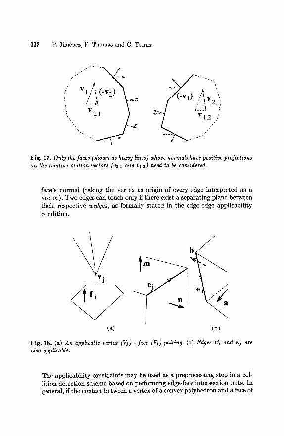
332 P. Jim~nez, F. Thomas and C. Torras
Fig. 17. Only the faces (shown as heavy lines) whose normals have positive projections on the relative motion vectors (v~,l and vl,2) need to be considered.
face's normal (taking the vertex as origin of every edge interpreted as a vector). Two edges can touch only if there exist a separating plane between their respective wedges, as formally stated in the edge-edge applicability condition.
(a) (b)
Fig. 18. (a) An applicable vertex (Vj) - face (Fi) pairing. (b) Edges Ei and Ej are also applicable.
The applicability constraints may be used as a preprocessing step in a col- lision detection scheme based on performing edge-face intersection tests. In general, ff the contact between a vertex of a convex polyhedron and a face of

Collision Detection Algorithms for Motion Planning 333
another polyhedron is applicable, only one of the edges which are adjacent to the vertex have to be considered for intersection with this face to report collision. Any other edge-face test with this face can be cut off. In a similar way one can bound the number of edges to be considered with respect to a given face resulting from edge-edge applicability constraints. In [32] an efficient algorithm for geometric pruning based on applicability constraints for convex potyhedra is described. Experimental results show that, by using this pruning technique, collision detection based on the edge-face intersec- tion test has an expected O(n) complexity, where n is the total number of edges, and the constant of linearity is close to 1. The algorithm is based on a face orientation graph representation, where face adjacency relations are explicitly depicted. The authors are currently working on extensions of the algorithm to non-convex polyhedra.
Pr ior i t iz ing collision pairs The algorithms that try to avoid having to test for collision every possible pairing between solids in a given workspace are only useful if there is a large number of solids that may collide. Candidates for col- lision checking are prioritized in order to test only those pairs which are more likely to collide. The first criterion one may consider is distance, but it is not enough if the relative velocities are not taken into account, as pointed out in [20]. These authors introduce the concept of awareness or imminence of a col- lision. The shortest possible time at which a collision may occur is computed, considering mutual distance, instantaneous relative velocity, and velocity and acceleration bounds. This calculation is initially done for every pair, and after- wards the updating is done more frequently for those pairs whose awareness is larger. According to their value of awareness, the pairs are partitioned into equivalence classes whose collision imminence is similar. A binary partition scheme is used, where the cardinality of each class (called "bucket") is an in- creasing power of 2, and the value of the measure of awareness for all elements of a given class is greater than that for any other element in a lower bucket (of greater cardinality). At every time step, only one pair within each bucket is updated. Since the higher the bucket, the less pairs it contains, higher buckets are updated more frequently than lower ones. As their measures of awareness change, pairs can percolate from bucket to bucket.
In [47] a heap is used to store object pairs and soonest possible collision times, so that the pair on the top is the nearest to collide. This soonest col- lision time is computed from the distance between the closest points of the objects, current velocities and accelerations, and acceleration bounds assuming a ballistic trajectory for the objects. At each time step, integration of the dy- namic state is done up to the time of collision for the pair on the top. Collision detection is performed for this pair, and if no collision actually occurs, the time
334 P. Jim@nez, F. Thomas and C. Torras
of impact is recomputed and the heap updated. Only the objects whose bound- ing boxes for their swept volumes during the frame period intersect with other boxes are selected and included in the heap. The intersections between these n boxes can be done in O(n(1 + logR)) (R is the ratio of largest to smallest box size), as shown in [48].
The same idea is followed in [35,14,51,38], where the concept of geometric and temporal coherence is emphasized, not only to speed up pairwise intersec- tion detection (as done in [36] and whose algorithm is also used here) but also to perform less of these pairwise tests. If time steps (frames) are small enough, the position and orientation of the objects undergo only small changes, and it has already been mentioned how this fact can be used to keep track for the closest feature pair of two convex polyhedra. But it also means that there will be little changes in the position of the bounding boxes 1, and, of course, in the sequence of intervals that these bounding boxes project onto the coordinate axes, and which overlap (in the three axes) if and only if the corresponding bounding boxes intersect. Interval sorting techniques exist that take into ac- count the sorted lists of interval endpoints in the previous frame, and allow to lower the effort to determine the projection intervals overlap to expected linear instead of O(n log n) (for n boxes). The computational cost of keeping track of changes in overlap status of interval pairs, following this line, is O(n + s) (where s is the number of pairwise overlaps).
The so called sweep algorithms in [60] are along the same line: at a given instant, a plane is swept through the scene and only pairs of objects simultane- ously intersecting the plane are tested for possible interference, thus avoiding to test every pair. The algorithm mentioned in this reference due to [30] does not find all intersections, although it reports at least one intersection if any exists, in O(nlog 2 n) time between n spheres.
It is also possible to use such a sweep algorithm in 2D for bounding collision pairs in 3D, as done in [31]. 4D hyper-trapezoids are used to bound the object during its motion. If one intersection between two hyper-trapezoids occurs, the corresponding objects are tested for collision. These intersections are computed from intersections between their faces. The problem is reduced, by succesive projections, to a 2D segment intersection detection problem. The 2D sweep algorithm is described in [4] and runs in O((m + k) log m) time for m segments that intersect k times. Although for N objects the worst case value of k is O(N2), empirical evidence shows that the average value of k is much lower (0.07~).
1 Two kinds of axis aligned bounding boxes are used in [14], fixed bounding cubes and dynamically rectangular boxes; for the latter, object orientation changes translate into changes in the dimensions of the bounding box.
Collision Detection Algorithms for Motion Planning 335
4 Collision detection in motion planning
The goal of motion planning is to generate a collision-free path for a robot. Thus, collision-free trajectory planners must be able to perform some kind of geometric reasoning concerning collision detection between the robot and the obstacles [5,12]. In the generation of the path from the initial to the final robot configuration other criteria than mere collision avoidance may intervene, in order to optimize the resulting path in terms of its length, distances to obstacles, or orientation changes. Not to speak about extensions of the basic motion planning problem, that include uncertainty, kinematic constraints, or movable objects [34].
Depending on whether the static interference or collision detection tests are performed in a preprocessing step or during the path planning process, three kinds of planners can be distinguished: global, incremental, and local planners.
4.1 Global p lanners
In general, the configuration of a robot is given by a set of parameters, or degrees of freedom, that determine its location and orientation. The space defined by the ranges of allowed values for these parameters is usually called C-space.
An obstacle in C-space (C-obstacle, for short) is defined as the connected set of configurations where a given mobile object intersects with an obstacle in workspace. C-obstacles can be interpreted as the intersection of halfspaces bounded by C-surfaces, each C-surface being associated with a basic contact (see Section 2.2).
It can be shown that when working with polyhedra (and vertex, edge and face locations are expressed in terms of the degrees of freedom of the moving polyhedron), expressions (1) and (2) in Section 2.2 lead to the above-mentioned halfspaces, and using the predicate formalism in expression (3) a proper descrip- tion of the C-obstacles can be obtained.
The collection of all C-obstacles constitutes the C-obstacle region. Some properties of the C-obstacles concerning compactness, connectedness and regu- larity are shown in [34]. C-obstacle generation can be viewed as a further gener- alization of the static interference and collision detection problems: here objects are not tested for interference at a particular configuration nor even along a given parameterized trajectory, but rather at all possible configurations in the workspace. Thus, once the C-obstacles are obtained, all information concerning interferences is captured.
Global planners construct a complete representation of the connectivity of free space (the complementary of the C-obstacle region) for their planning purposes. Several techniques have been devised to this end, depending on the
336 P. Jim~nez, F. Thomas and C. Torras
degrees of freedom of the robot as well as on its shape and the shape of the obstacles. Nevertheless, they are only of practical interest in low-dimensional configuration spaces. Pioneer work in this direction was done in [42,40] for polytopal environments. As a result of applying these techniques, a graph-based representation of free space is obtained: a roadmap or the connectivity graph of a cell decomposition. Afterwards a graph search algorithm can be applied in order to find the path that connects the initial and the final configurations.
In some simple cases, the configuration of a robot can be expressed in terms of the workspace coordinates of a given robot's point: for example, if the robot is a sphere (a disc in 2D) this reference point will be its center. The C-obstacles are trivially obtained from the obstacles in the workspace by performing an isotropic growth by the radius of the robot. Another simple case consists in a polytopal robot translating amidst polytopal obstacles. Any vertex of the robot can be taken as reference point. In this particular case, C-obstacles can also be interpreted as the Minkowski difference between the obstacle and the robot at a fixed orientation (as already mentioned in the context of distance computation in Section 3.2). This fact can be used for constructing the C-obstacle itself. This alternative representation is obviously related to the general predicate-based one, in the sense that the differences between the vertices corresponding to the features related to basic contacts are vertices of the C-obstacle. Both represen- tations have been developed for convex polytopes. Non-convex obstacles can be treated in the same way by representing them as overlapping convex parts.
When the robot polytope is allowed to rotate, the computation of the C- obstacles becomes much more difficult. Although an approximate solution can be readily obtained by sampling the involved rotations, in general C-obstacles can only be accurately described using the aforementioned predicates, which can be formally interpreted as semialgebraic sets (see [11] for more details). Note that when all degrees of freedom but one are sampled, the problem be- comes one of detecting intervals of interference, as many times as needed, de- pending on the sampling rate. This technique is used with up to three degrees of freedom in [41].
4.2 Inc rementa l planners
While global path planners generate a detailed description of the connectivity of the whole free space, incremental path planners avoid this costly compu- tation by obtaining this description in an incremental fashion. In this case, the construction of the free-space representation is carried out simultaneously with the path planning process. A paradigmatic example of this strategy can be found in [21], where a restricted visibility graph in C-space is built up it- eratively. This subset of the whole visibility graph is granted to contain the optimal path. It is constructed by determining which C-obstacles intersect the
Collision Detection Algorithms for Motion Planning 337
segments of the shortest path found so far (a straight line joining the initial and final positions at the first step), and rearranging the visibility graph with these new C-obstacles.
Randomized path planning methods might work in a similar way: points are randomly generated and those lying in free space are retained. Then, attempts are made to link these points by means of collision-free line segments. In this wa3; a representation of free space is gradually built up by locally testing for collisions, while generating a path from the initial to the final configurations. The same applies to those techniques that combine a potential field approach with randomization to escape from local minima. More details on this kind of algorithms can be found in Chapter 5.
4.3 Local planners
Local planners use collision detection as a subroutine whose output is used on- line to guide the search of a collision-free trajectory. The main difference with respect to incremental strategies is that local methods perform path planning by applying motion operators that act locally. In [18] these operators are used for sliding on C-surfaces and along their intersections without computing an explicit representation of free-space. They also allow to jump in free-space be- tween obstacles. In any case, each time a C-surface is traversed, an interference test is performed to ensure that the motion is collision-free. These operators are the building blocks of more sophisticated local experts, which are strategies for deciding which trajectory to follow, based on the local geometry as well as on the history of the current planning process. This combination of motion in free space with motion in contact (or up to a safety distance from the obsta- cles) is used by other local motion planners. This is the case of the algorithms developed for planar articulated and 3D cartesian robot arms in [43,55]. The intersection points of the obstacles with the main line joining the initial and final positions are found, and motions along the obstacle boundaries between these points are computed.
Some local planners, as well as some incremental ones, can be applied in a recursive way: starting from an initial guess for a path between the initial and the final position, intermediate points are determined as collisions are detected, and the algorithm is recursively applied to the resulting path segments until a collision-free trajectory is detected or the conclusion is drawn that no such path exists.
While global path planners are always complete, that is, they are able to find a solution if one exists, those based on local techniques only ensure completeness at a resolution level. In [18] a partition of C-space based on neighborhoods is adopted, which are marked as visited if they are traversed by a trajectory
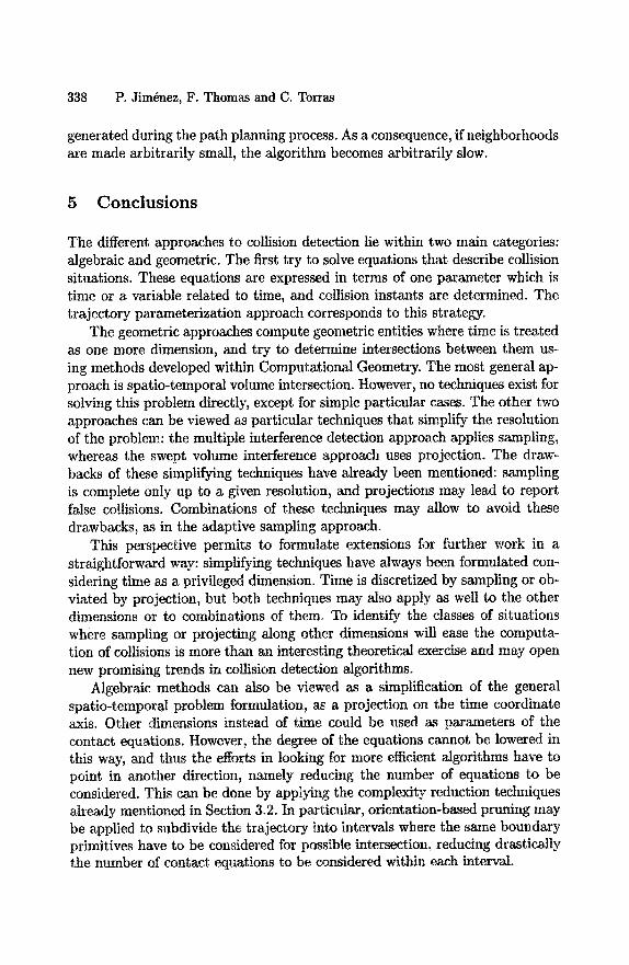
338 P. Jim~nez, F. Thomas and C. Torras
generated during the path planning process. As a consequence, if neighborhoods are made arbitrarily small, the algorithm becomes arbitrarily slow.
5 C o n c l u s i o n s
The different approaches to collision detection lie within two main categories: algebraic and geometric. The first try to solve equations that describe collision situations. These equations are expressed in terms of one parameter which is time or a variable related to time, and collision instants are determined. The trajectory parameterization approach corresponds to this strategy.
The geometric approaches compute geometric entities where time is treated as one more dimension, and try to determine intersections between them us- ing methods developed within Computational Geometry. The most general ap- proach is spatio-temporal volume intersection. However, no techniques exist for solving this problem directly, except for simple particular cases. The other two approaches can be viewed as particular techniques that simplify the resolution of the problem: the multiple interference detection approach applies sampling, whereas the swept volume interference approach uses projection. The draw- backs of these simplifying techniques have already been mentioned: sampling is complete only up to a given resolution, and projections may lead to report false collisions. Combinations of these techniques may allow to avoid these drawbacks, as in the adaptive sampling approach.
This perspective permits to formulate extensions for further work in a straightforward way: simplifying techniques have always been formulated con- sidering time as a privileged dimension. Time is discretized by sampling or ob- viated by projection, but both techniques may also apply as well to the other dimensions or to combinations of them. To identify the classes of situations where sampling or projecting along other dimensions will ease the computa- tion of collisions is more than an interesting theoretical exercise and may open new promising trends in collision detection algorithms.
Algebraic methods can also be viewed as a simplification of the general spatio-temporal problem formulation, as a projection on the time coordinate axis. Other dimensions instead of time could be used as parameters of the contact equations. However, the degree of the equations cannot be lowered in this way, and thus the efforts in looking for more efficient algorithms have to point in another direction, namely reducing the number of equations to be considered. This can be done by applying the complexity reduction techniques already mentioned in Section 3.2. In particular, orientation-based pruning may be applied to subdivide the trajectory into intervals where the same boundary primitives have to be considered for possible intersection, reducing drastically the number of contact equations to be considered within each interval.

Collision Detection Algorithms for Motion Planning 339
In the line of developing complexity reduction techniques for interference detection we have centered our contribution to the PROMotion Project. Little work had previously been done on algorithms that deal directly with non-convex polyhedra, without decomposing them into convex parts. We have developed one such algorithm, based on a boolean combination of signs of vertex determi- nants [58]. Thus, neither line-plane intersections, nor ficticious edges and faces arising from a decomposition are required. Only the signs of determinants, for which there exist very efficient and robust algorithms, need to be computed. Moreover, we have developed a representation that captures the applicability relationships between the boundary features of two general polyhedra, that is, it allows to determine quickly which contacts can arise under translational mo- tions [32]. In the case of non-convex polyhedra a large subset of all contacts that cannot take place for a given relative orientation are pruned off (all of them in the case of convex polyhedra). As these relationships hold over whole ranges of orientations, this technique can also be used to perform pruning along a trajectory that includes rotation[33], as mentioned above in the context of algebraic techniques for collision detection.
The speed-up of the basic interference and collision detection tests will nec- essarily improve the performance of motion planners, thus making the famous bottleneck a little bit wider.
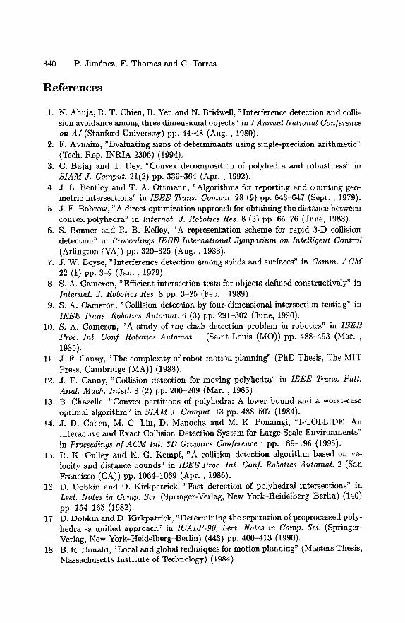
340 P. Jim@nez, F. Thomas and C. Torras
References
1. N. Ahuja, R. T. Chien, R. Yen and N. Bridwell, "Interference detection and colli- sion avoidance among three dimensional objects" in I Annual National Conference on AI (Stanford University) pp. 44-48 (Aug. , 1980).
2. F. Avnaim, "Evaluating signs of determinants using single-precision arithmetic" (Tech. aep. INRIA 2306) (1994).
3. C. Bajaj and T. Dey, "Convex decomposition of polyhedra and robustness" in SIAM J. Comput. 21(2) pp. 339-364 (Apr., 1992).
4. J. L. Bentley and T. A. Ottmann, "Algorithms for reporting and counting geo- metric intersections" in IEEE Trans. Comput. 28 (9) pp. 643-647 (Sept. , 1979).
5. J .E. Bobrow, "A direct optimization approach for obtaining the distance between convex polyhedra" in Internat. J. Robotics Res. 8 (3) pp. 65-76 (June, 1983).
6. S. Bonner and R. B. Kelley, "A representation scheme for rapid 3-D collision detection" in Proceedings IEEE International Symposium on Intelligent Control (Arlington (VA)) pp. 320-325 (Aug., 1988).
7. J. W. Boyse, "Interference detection among solids and surfaces" in Comm. ACM 22 (1) pp. 3-9 (Jan. , 1979).
8. S. A. Cameron, "Efficient intersection tests for objects defined constructively" in Internat. J. Robotics Res. 8 pp. 3-25 (Feb. , 1989).
9. S. A. Cameron, "Collision detection by four-dimensional intersection testing" in IEEE Trans. Robotics Automat. 6 (3) pp. 291-302 (June, 1990).
10. S. A. Cameron, "A study of the clash detection problem in robotics" in IEEE Proc. Int. Conf. Robotics Automat. 1 (Saint Louis (MO)) pp. 488-493 (Mar. , 1985).
11. J. F. Canny, "The complexity of robot motion planning" (PhD Thesis, The MIT Press, Cambridge (MA)) (1988).
12. J. F. Canny, "Collision detection for moving polyhedra" in IEEE Trans. Patt. Anal. Maeh. Intell. 8 (2) pp. 200-209 (Mar., 1986).
13. B. Chazelle, "Convex partitions of polyhedra: A lower bound and a worst-case optimal algorithm" in SIAM J. Comput. 13 pp. 488-507 (1984).
14. J. D. Cohen, M. C. Lin, D. Manocha and M. K. Ponamgi, "I-COLLIDE: An Interactive and Exact Collision Detection System for Large-Scale Environments" in Proceedings of ACM Int. 31) Graphics Conference 1 pp. 189-196 (1995).
15. R. K. Culley and K. G. Kempf, "A collision detection algorithm based on ve- locity and distance bounds" in IEEE Proc. Int. Con]. Robotics Automat. 2 (San Francisco (CA)) pp. 1064-1069 (Apr., 1986).
16. D. Dobkin and D. Kirkpatrick, "Fast detection of polyhedral intersections" in Leer. Notes in Comp. Sci. (Springer-Verlag, New York-Heidelberg-Berlin) (140) pp. 154-165 (1982).
17. D. Dobkin and D. Kirkpatrick, "Determining the separation of preprocessed poly- hedra -a unified approach" in ICALP-90, Leer. Notes in Comp. Sci. (Springer- Verlag, New York-tteidelberg-Berlin) (443) pp. 400-413 (1990).
18. B. R. Donald, "Local and global techniques for motion planning" (Masters Thesis, Massachusetts Institute of Technology) (1984).
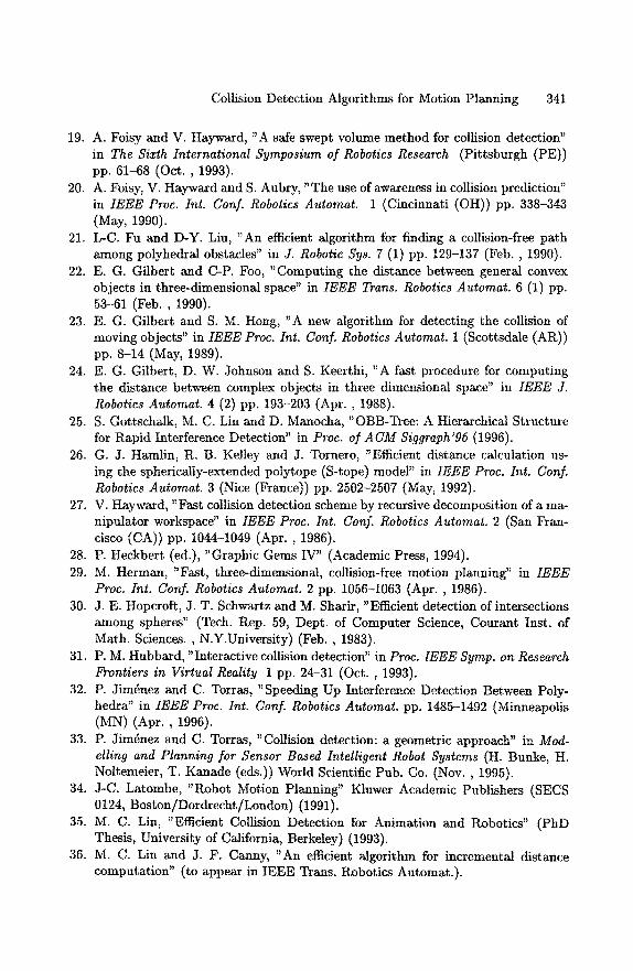
Collision Detection Algorithms for Motion Planning 341
19. A. Foisy and V. Hayward, "A safe swept volume method for collision detection" in The Sixth International Symposium of Robotics Research (Pittsburgh (PE)) pp. 61-68 (Oct. , 1993).
20. A. Foisy, V. Hayward and S. Aubry, "The use of awareness in collision prediction" in IEEE Proc. Int. Conf. Robotics Automat. 1 (Cincinnati (OH)) pp. 338-343 (May, 1990).
21. L-C. Fu and D-Y. Liu, "An efficient algorithm for finding a collision-free path among polyhedral obstacles" in J. Robotic Sys. 7 (1) pp. 129-137 (Feb., 1990).
22. E. G. Gilbert and C-P. Foo, "Computing the distance between general convex objects in three-dimensional space" in IEEE Trans. Robotics Automat. 6 (1) pp. 53-61 (Feb., 1990).
23. E. G. Gilbert and S. M. Hong, "A new algorithm for detecting the collision of moving objects" in IEEE Proe. Int. Conf. Robotics Automat. 1 (Scottsdale (AR)) pp. 8-14 (May, 1989).
24. E. G. Gilbert, D. W. Johnson and S. Keerthi, "A fast procedure for computing the distance between complex objects in three dimensional space" in IEEE J. Robotics Automat. 4 (2) pp. 193-203 (Apr., 1988).
25. S. Gottschalk, M. C. Lin and D. Manocha, "OBB-Tree: A Hierarchical Structure for Rapid Interference Detection" in Proc. of ACM Siggraph'96 (1996).
26. G. J. Hamtin, R. B. Kelley and 3. Tornero, "Efficient distance calculation us- ing the spherically-extended polytope (S-tope) model" in IEEE Proc. Int. Conf. Robotics Automat. 3 (Nice (France)) pp. 2502-2507 (May, 1992).
27. V. Hayward, "Fast collision detection scheme by recursive decomposition of a ma- nipulator workspace" in IEEE Proc. Int. Conf. Robotics Automat. 2 (San Fran- cisco (CA)) pp. 1044-1049 (Apr., 1986).
28. P. Heckbert (ed.), "Graphic Gems IV" (Academic Press, 1994). 29. M. Herman, "Fast, three-dimensional, collision-free motion planning" in IEEE
Proe. Int. Conf. Robotics Automat. 2 pp. 1056-1063 (Apr. , 1986). 30. J. E. Hopcroft, J. T. Schwartz and M. Sharir, "Efficient detection of intersections
among spheres" (Tech. Rep. 59, Dept. of Computer Science, Courant Inst. of Math. Sciences. , N.Y.University) (Feb. , 1983).
31. P.M. Hubbard, "Interactive collision detection" in Proe. IEEE Symp. on Research Frontiers in Virtual Reality 1 pp. 24-31 (Oct. , 1993).
32. P. Jim~nez and C. Torras, "Speeding Up Interference Detection Between Poly- hedra" in IEEE Proc. Int. Conf. Robotics Automat. pp. 1485-1492 (Minneapolis (MN) (Apr., 1996).
33. P. Jim~nez and C. Torras, "Collision detection: a geometric approach" in Mod- elling and Planning for Sensor Based Intelligent Robot Systems (H. Bunke, H. Noltemeier, T. Kanade (eds.)) World Scientific Pub. Co. (Nov. , 1995).
34. J-C. Latombe, "Robot Motion Planning" Kluwer Academic Publishers (SECS 0124, Boston/Dordrecht/London) (1991).
35. M. C. Lin, "Efficient Collision Detection for Animation and Robotics" (PhD Thesis, University of California, Berkeley) (1993).
36. M. C. Lin and J. F. Canny, "An efficient algorithm for incremental distance computation" (to appear in IEEE Trans. Robotics Automat.).
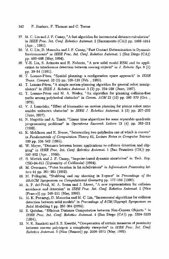
342 P. Jim6nez, F. Thomas and C. Torras
37. M. C. Lin and J. F. Canny, "A fast algorithm for incremental distance calculation" in IEEE Proc. Int. Conf. Robotics Automat. 2 (Sacramento (CA)) pp. 1008-1014 (Apr., 1991).
38. M. C. Lin, D. Manocha and J. F. Canny, "Fast Contact Determination in Dynamic Environments" in IEEE Proc. Int. Conf. Robotics Automat. 1 (San Diego (CA)) pp. 602-608 (May, 1994).
39. Y-H. Liu, S. Arimoto and H. Noborio, "A new solid model HSM and its appli- cation to interference detection between moving objects" in J. Robotic Sys. 8 (1) pp. 39-54 (1991).
40. T. Lozano-P6rez, "Spatial planning: a configuration space approach" in IEEE Trans. Comput. 32 (2) pp. 108-120 (Feb., 1983).
41. T. Lozano-P6rez, "A simple motion-planning algorithm for general robot manip- ulators" in IEEE J. Robotics Automat. 3 (3) pp. 224-238 (June, 1987).
42. T. Lozano-P6rez and M. A. Wesley, "An algorithm for planning collision-free paths among polyhedral obstacles" in Comm. ACId 22 (10) pp. 560-570 (Oct. , 1979).
43. V. J. Lumelsky, "Effect of kinematics on motion planning for planar robot arms amidst unknown obstacles" in IEEE J. Robotics Automat. 3 (3) pp. 207-223 (June, 1987).
44. N. Megiddo and A. Tamir, "Linear time algorithms for some separable quadratic programming problems" in Operations Research Letters 13 (4) pp. 203-211 (1993).
45. K. Mehlhorn and K. Simon, "Intersecting two polyhedra one of which is convex" in Fundamentals of Computation Theory 85, Lecture Notes in Computer Science 199 pp. 534-542 (1985).
46. W. Meyer, "Distance between boxes: applications to collision detection and clip- ping" in IEEE Proc. Int. Conf. Robotics Automat. 1 (San Francisco (CA)) pp. 597-602 (Apr., 1986).
47. B. Mirtich and J. F. Canny, "Impulse-based dynamic simulation" in Tech. Rep. CSD-94-815 (University of California) (1994).
48. M. Overmars, "Point location in fat subdivisions" in Information Processing let- ters 44 pp. 261-265 (1992).
49. M. Pellegrini, "Stabbing and ray shooting in 3-spacd ~ in Proceedings of the 6thACM Symposium on Computational Geometry pp. 177-186 (1990).
50. A. P. del-Pobil, M. A. Serna and J. Llovet, "A new representation for collision avoidance and detection" in IEEE Proc~ Int. Conf. Robotics Automat. 1 (Nice (France)) pp. 246-251 (May, 1992).
51. M.K. Ponamgi, D. Manocha and M. C. Lin, "Incremental algorithms for collision detection between solid models" in Proceedings of A CM/Siggraph Symposium on Solid Modelling 1 pp. 293-304 (1995).
52. S. Quinlan, "Efficient Distance Computation between Non-Convex Objects " in IEEE Proe. Int. Conf. Robotics Automat. 4 (San Diego (CA)) pp. 3324-3329 (1994).
53. N. K. Sancheti and S. S. Keerthi, "Computation of certain measures of proximity between convex polytopes: a complexity viewpoint" in IEEE Proe. Int. Conf. Robotics Automat. 3 (Nice (France)) pp. 2508-2513 (May, 1992).
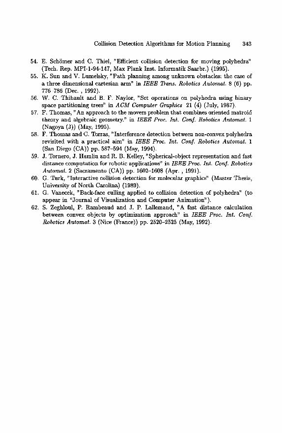
Collision Detection Algorithms for Motion Planning 343
54. E. SchSmer and C. Thiel, "Efficient collision detection for moving polyhedra" (Tech. l~ep. MPI-1-94-147, Max Plank Inst. Informatik Saarbr.) (1995).
55. K. Sun and V. Lumelsky, "Path planning among unknown obstacles: the case of a three dimensional cartesian arm" in IEEE Trans. Robotics Automat. 8 (6) pp. 776-786 (Dec. , 1992).
56. W. C. Thibanlt and B. F. Naylor, "Set operations on polyhedra using binary space partitioning trees" in ACM Computer Graphics 21 (4) (July, 1987).
57. F. Thomas, "An approach to the movers problem that combines oriented matroid theory and algebraic geometry." in IEEE Proc. Int. Conf. Robotics Automat. 1 (Nagoya (J)) (May, 1995).
58. F. Thomas and C. Torras, "Interference detection between non-convex polyhedra revisited with a practical aim" in IEBE Proe. Int. Conf. Robotics Automat. 1 (San Diego (CA)) pp. 587-594 (May, 1994).
59. J. Tornero, J. Hamlin and R. B. Kelley, "Spherical-object representation and fast distance computation for robotic applications" in 1EEE Proc. Int. Conf. Robotics Automat. 2 (Sacramento (CA)) pp. 1602-1608 (Apr., 1991).
60. G. Turk, "Interactive collision detection for molecular graphics" (Master Thesis, University of North Carolina) (1989).
61. G. Vanecek, "Back-face culling applied to collision detection of polyhedra" (to appear in "Journal of Visualization and Computer Animation").
62. S. Zeghloul, P. Rambeand and J. P. Lallemand, "A fast distance calculation between convex objects by optimization approach" in IEEE Proc. Int. Conf. Robotics Automat. 3 (Nice (France)) pp. 2520-2525 (May, 1992).

Lecture Notes in Control and Information Sciences
Edited by M, Thoma
1993-1997 Published Titles:
Vol. 186: Sresnath, N. Systems Representation of Global Climate Change Models. Foundation for a Systems Science Approach. 288 pp. 1993 [3-540-19824-5]
Vol. 187: Moreoki, A.; Bianchi, G.; Jaworeck, K. (Eds) RoManSy 9: Proceedings of the Ninth CISM-IFToMM Symposium on Theory and Practice of Robots and Manipulators. 476 pp. 1993 [3-540-19834-2]
Vol, 188: Naidu, D. Subbaram Aeroassisted Orbital Transfer: Guidance and Control Strategies 192 pp. 1993 [3-540-19819-9]
Vol, 189: Ilchmann, A. Non-ldentif'ter-Based High-Gain Adaptive Control 220 pp. 1993 [3-540-19845-8]
Vol. 190: Chatila, R.; Hirzinger, G. (Eds) Experimental Robotics th The 2nd International Symposium, Toulouse, France, June 25-27 1991 580 pp. 1993 [3-540-19851-2]
Vol. 191: Blondel, V. Simultaneous Stabilization of Unear Systems 212 pp. 1993 [3-540-19862-8]
Vol. 192: Smith, R.S.; Dahleh, M. (Eds) The Modeling of Uncertainty in Control Systems 412 pp. 1993 [3-540-19870-9]
Vol. 193: Zinober, A.S.I. (Ed.) Variable Structure and Lyapunov Control 428 pp. 1993 [3-540-19869-5]
Vol. 194: Cao, Xi-Ran Realization Probabilities: The Dynamics of Queuing Systems 336 pp. 1993 [3-540-19872-5]
Vol. 195: Uu, D.; Michel, A.N. Dynamical Systems with Saturation Nonlinearities: Analysis and Design 212 pp. 1994 [3-540-19888-1]
Vol. 196: Bat'dlotti, S. Noninteracting Control with Stability for Nonlinear Systems 196 pp. 1994 [3-540-19891-1]
Voi. 197: Henry, J.; Yvon, J.P. (Eds) System Modelling and Optimization 975 pp approx. 1994 [3-540-19893-8]
Vol. 198: Winter, H.; NQSer, H.-G. (Eds) Advanced Technologies for Air Traffic Row Management 225 pp approx. 1994 [3-540-19895-4]
Vol. 199: Cohen, G.; Quadrat, J.-P. (Eds) 1 l th International Conference on Ar~lysis and Optimization of Systems - Discrete Event Systems: Sophia-Antipolis, June 15-16-17, 1994 648 pp. 1994 [3-540-19896-2]
VoL 200: Yoshikawa, T.; Miyazaki, F. (Eds) Experimental Robotics I11: The 3rd Intematior~l Symposium, Kyoto, Japan, October 28-30, 1993 624 pp. 1994 [3-540-19905-5]
Vol. 201: Kogan, J. Robust Stability and Convexity 192 pp. 1994 [3-540-19919-5]
Vol. 202: Francis, B.A.; Tannenbaum, A.R. (Eds) Feedback Control, Nonlinear Systems, and Complexity 288 pp. 1995 [3-540-19943-8]
Vol. 203: Popkov, Y.S. Macrosystems Theory and its Applications: Equilibrium Models 344 pp. 1995 [3-540-19955-1]
Vol. 204: Takahashi, S.; Takahara, Y. Logical Approach to Systems Theory 192 pp. 1995 [3-540-19956-X]
Vol. 205: Kotta, U. Inversion Method in the Discrete-time Nonlinear Control Systems Synthesis Problems 168 pp. 1995 [3-540-19966-7]
Vol. 206: Aganovic, Z.;.Gajic, Z. Unear Optimal Control of Bilinear Systems with Applications to Singular Perturbations and Weak Coupling 133 pp. 1995 [3-540-19976-4]
Vol. 207: Gabasov, R.; Kirillova, FM.; Prischepova, S.V. Optimal Feedback Control 224 pp. 1995 [3-540-19991-8]
Vol. 200: Khalil, H.K.; Chow, J.H.; Ioannou, P.A. (Eds) Proceedings of Workshop on Advances inControl and its Applications 300 pp. 1995 [3-540-19993-4]
Vol. 209: Foias, C.; C)zbay, H.; Tannenbaum, A. Robust Control of Infinite Dimensional Systems: Frequency Domain Methods 230 pp. 1996 [3-540-19994-2]
Vol. 210: De Wilde, P. Neural Network Models: An Analysis 164 pp. 1996 [3-540-19995-0]
Vol. 211: Gawronski, W. Balanced Control of Flexible Structures 280 pp. 1996 [3-540-76017-2]
Vol. 212: Sanchez, A. Formal Specification and Synthesis of Procedural Controllers for Process Systems 248 pp. 1996 [3-540-76021-0]
Vol. 213: Patra, A.; Rao, G.P. General Hybrid Orthogonal Functions and their Applications in Systems and Control 144 pp. 1996 [3-540-76039-3]
Vol. 214: Yin, G.; Zhang, Q. (Eds) Recent Advances in Control and Optimization of Manufacturing Systems 240 pp. 1996 [3-540-76055-5]
Vol. 215: Bonivento, C.; Marro, G.; Zanasi, R. (Eds) Colloquium on Automatic Control 240 pp. 1996 [3-540-76060-1]
Vol. 216: Kulhavy, R. Recursive Nonlinear Estimation: A Geometric Approach 244 pp. 1996 [3-540-76063-6]
Vol. 217: Garofalo, F.; Glielmo, L. (Eds) Robust Control via Variable Structure and Lyapunov Techniques 336 pp. 1996 [3-540-76067-9]
Vol. 218: van der Schaft, A. L~ Gain and Passivity Techniques in Nonlinear Control 176 pp. 1996 [3-540-76074-1]
Vol. 219: Berger, M.-O.; Deriche, R.; Herlin, I.; Jaffr6, J.; Morel, J.-M. (Eds) ICAOS '96: 12th International Conference on Analysis and Optimization of Systems - Images, Wavelets and PDEs: Paris, June 26-28 1996 378 pp. 1996 [3-540-76076-8]

Vol. 220: Brogliato, B. Nonsmooth Impact Mechanics: Models, Dynamics and Control 420 pp. 1996 [3-540-76079-2]
VoL 221: Kelkar, A.; Joshi, S. Control of Nonlinear Multibody Flexible Space Structures 160 pp. t996 ['3-540-76093-8]
Vol. 222: Morse, A.S. Control Using Logic-Based Switching 288 pp. 1997 [3-540-76097-0]
Vol. 223: Khatib, O.; Salisbury, J.K. Experimental Robotics IV: The 4th International Symposium, Stanford, California, June 30 - July 2, 1995 596 pp. 1997 [3-540-76133-0]
Vol. 224: Magni, J.-F.; Bennani, S.; Terlouw, J. (Eds) Robust Flight Control: A Design Challenge 664 pp. 1997 [3-540-76151-9]
Vol. 225: Poznyak, A.S.; Najim, K. Learning Automata and Stochastic Optimization 219 pp. 1997 [3-540-76154-3]
Vol. 226: Cooperman, G.; Michler, G.; Vinck, H. (Eds) Workshop on High Performance Computing and Gigabit Local Area Networks 248 pp. 1997 [3-540-76169-1]
Vol. 227: Tarboudech, S.; Garcia, G. (Eds) Control of Uncertain Systems with Bounded Inputs 203 pp. 1997 [3-540-76183-7]
Vol, 228: Dugard, L.; Verrlest, E.I. (Eds) Stability and Control of Time-delay Systems 337 pp. 1998 [3-540-76193-4]