35th AMual Ccm~ of the AlUtratJm Ar,nculturaJ Econ~ Soddy

Unh~itycf New England, Annldatf!'# 11",t4 ~ry* 199J

Returns hom the Aculuat.ion of Agricultural Reseudt

R Gros!, V . Kneebone" R..Ltakt Victmun ~\eftt 01 Agkulwre and Rurll AtW,"

In September 1988 the Victottln Govemmtnt reJe.ak'd an «OM"*, s.tra~ for IlfkUJturewl~cb" amongstotlwr thin~ pnrridedan inJtctio.n of fundinstn addition to ~ depr1:mtnw bud .. aJloatiOn to manyaJrleultu1'lll tat.rm and exteNlon projectt. The ~.~ 01 ttw i~ of funding is e&timated in thiJ pipet Inr ~ PtDlllditsn of Hith Qu41ity \w.at fDr "idm. proj«1.

Two dittinct e1timItion ptca.dum ate empliOytd. rustly, ABAR£'s compu~ vadon of au: Edwards and Fmbafm «onomit surpluJ mode! wa ~ to tvalu.ate the n1iIp\itude and distribution of the benefits ttNnlting fromtad\ of tht fetfNlm .nd dtvtIopmanproj«l" A change hatnewo:rk was then .ppUed 1iJ"J(V 1tm timing ofbolh the costs lind ~t. differ. attttrding to the fundjng ~riG, The Nt" Praelt Vll:ae (NJ'V) of the re~propams with the injection of funding wa, comp;tred with the NPV without the tn.jediun of tund:i.ng. 1'll\e dUfertnce between the two reflects the earl1er raltMtiOn of the ~b whrn the ~th ~afM ~ a«tltrated 50 tNt the adoptiOn Gf~arthftsull1 is soon. Bther tM.n Iller. Tht tow mt&fCft (ost$ (in reAl terms) and the adoption rate and 1e\'e'J .are ~ to be the .s..une i1'ftip«tive of the funding tamlno.

~)t t j • ,. ,f'. j 1 ~, j

1

------------------------------------------------------I. INTRODUcnON

In ~b:T, t9M# U. \l'tct.oriln Go~1 mr&illC!dan E(m~: StrAtCI,Y 1« A~"1I1~~(A5) which wa$ dtMttd at ~~. (1lmptUtJ'~.~ and p'~wth ~nU" The AS P'fOF.tm. ~1d" ~ tft ~~tiCn to the DtpM~, o,f ~I.tuft: 1M Rutal At,*, (DARA'bud~ ~tt.ttt 0fI ~ ... N.J ~ wm ~ \mdfr the ,c;m4ititt·n tNt the ASJU~ ~ bt f~3, nJl~ tn M'J"rM of ma~t amt ~i pedormlfa'

In thl, Plptr u..1 bawfit IAIIPl tiS ·UMd ttl ~ ·the ftMndl1pai~ 01 .~.M of N&M1' Qu~ity \~t b Vl;tw p." AD btnd$tI .hd ~ 1ft! ~. f1'om Vk'kml~i y~ftt1l (to on • two .,.M btf.tt .~ ., VktMia ·lftdtht 1ft, 01 t" workS .hkbtnduda· the ·othfr ,taws cI A.QSU'ltiJ) •

. 1ht ~~ ttl me ptp6 it U ~\I. In ~ ,2 e. ...-.11 .~ QMd to ... ·tho projKt baw.fib and (osb tJ d~ n. ~ crptm btMfit fti&Mdcft ed\f"~ it dttIDfd SftUoft., ,dttliiJ It. ~~t ,~ .~. tor Prodt.tdiencf Ulah auln., ",..,tifi,1 Vittm.

2

U. METHOD

In\'Utmf:nt in agricultural ~rth i~ output thtoup improvtme'nb lO ex:bttnS input,; the d~l of new inputs., and through incmued IwowWp whkh tnlbks prodtKUJ .m ~fOrs to td«t" combine and ~ their mp.:t$ more ~tJl'. In this contat, tr..nowledp can be exmddf!ftCI as pu1 01 the ("apitll IlOdt of the apkUlturaJ ~, j1Dt mu:·othu pbytbl inputs. Lib othu forms 01 (lpluJ. bowled. mull W CfNted throup in~t, 1$ -bf«t to deprt:d.ation and it' tAte of uQisuton (adoption) vlrieso'W'f' timt.

EVihuting the costs and btneIitJ freat agicultulaJ ~ is not an easy.tMk. ~ a»ts·iUV Nghly viS1*: and 0IXUt,. at poinb in timeo. weU ~ lIlybaleflUltan to flow. In addJ" .n .. ~tth, by tts Ul'lCYlrUJn na~ft', is a hip risk tnvestmtnt. Further; even Utheretle'i&~ i$ ~u1. slow rate of adoptiCn or utWsItion (ofMW knowledp) can ft!duce'benditJ rnarbdly.

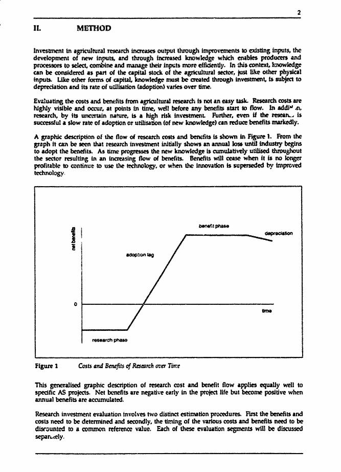
A graphic delW:.riptinn 01 theftow 01 ~h CO$U IJld bm.~ 1$ shown in ft~ 1. From ~ Ult.ph it can be Ren that fet'41'Ch inves-tment iNti.Ii, $hows In IMUII .Ioa until tndUltfy begins to adopt the benefit,$. At. tinw ~~ the new knowledp is aunuLtttvtly utWsed duwghout theMdor multing In an ~si. flow of benefits. BeNfil$ wUl 0!':Ut when ,it II no longer profit4bleto contint.::.t to use the tfChno1o&Y .. or when the iMOV"tion is JU~ by impnwed ted'lnology .

II I

o ~----------~--------------------------

flpre 1

This generalised grapbk defaiption of research cost and benriitflow applies equally well to ~fic AS projects_ Net benefits are negatf'\l'e urly in the protect life but b«o:me. positive when annual benefits are accumul.ated.

Research investment evaluation involves two dbtind estimation protedum. First the benefits and costs need to be determined and secondly .. the timing of the variou$ costs and benefits need to be disrtlunted to a common reference value. Each of these ev:&1uation segments will be discussed sepm.~ly.

3

A. The Effects of Researdl

A supply and demand framework can be used to estimate the dfeds of a re5e1n:n .. ln<iuccd prcdudivity increase. A supply-enlumdng change shifts the supply CUM to the right, low'cnng unit costs. Such 4 shift permits more of that good t.o be produced at .. lower price. A demand .. enhandng chl.nse leacb to an increase in product demand from fllttors such IS promotion Ind advertising. This shifts the demand curve to the right and f6ultsin an ~in the price offered (or that product.

Generally agricultural research is directed at reducing the costs of production, ptOceJJing or marketing, thus~ shifting the supply curve to the right. DAM hAS tended, in the put, to concentr4te on fann level research Wned at redudng the costs Of production tJuouah the Idopdon of new management technique$, crop varieties or input allQaltions. However, a numbttr of the projects under the AS hive a different focus.

The basic model used to determine the research benefits is shown in Figure 2. The graphlhows a demand and supply schedule for a J*ticular agricultural OUlF' At point e and pritt " mukets clear and the supply of the good ~ls the demand of thD c:POd. Any pomt on the demand curve reprersents what consumers are willing to pay for different qU&ntities of <X.lmmodlty Q.

Investment in agricultural research which produces new knowledge then shifts the supply curve to the right (52) by a un.it cost reduction of R (equal to the newknowJedge). The new COlit reduction knowledge has lowered the equllibrium price (8) and incrf~ the equilibrium quantity produced (h) <Figure 2).

PRICE

a

p

g

b

F

S1

S2

Q h QUANTITY

To measure the benefits of a unit cost reduction (that is, a shlft in !he JUppJyC'UJ'Ve to the right> an economic technique known as econo!1tic surplus is employed. Economic surplus has been used extensively to evaluate the magnitude and the distributitm of meud\ benefits tEdwltds and Freebaim 1981, Ffftbai~ .. f a1 1982, Alston and Freebairn 1986, and Alston and Mullen 1988).

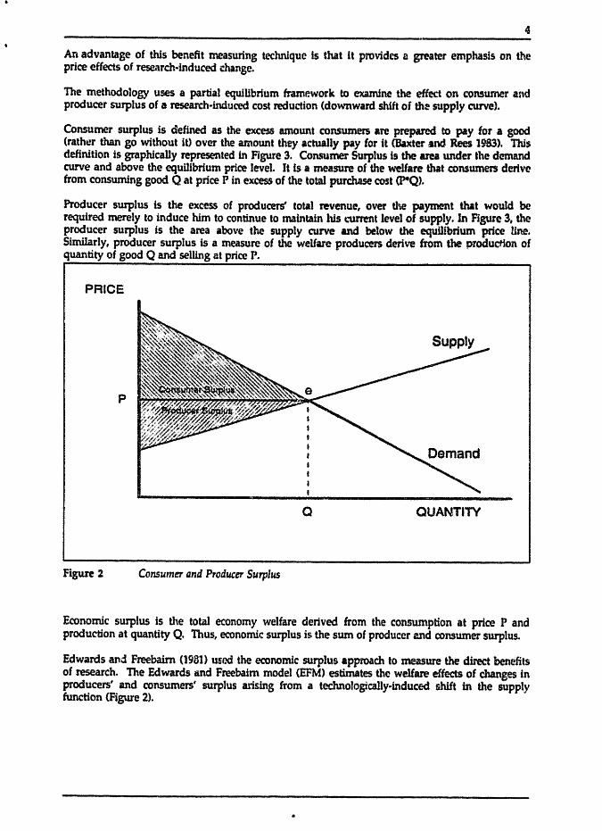
" An advantage of this benefit measuring teclmique is that it provides a pter emphasis on the price effects of research-induced change.

The methodology uses a partial equilibrium framework to ewnlne the effed on consumer and producer surplus of a research-induced cost reduction (downward shift of the supply curve).

Consumer surplus is defined as the exCeJ5 amount consumers are prepared top.ty for a good (rather than go without it) over the amount they actually pay for it (Baxter M\d Reel 1983). This definition is graphically represented in Figure 3. Consumer Surplus iathe area und« the demand curve and above the equilibrium price level. It is I measure of the wellare that consumers derive from consuming good Q at price P in excess of the total purclwe cost (lMQ).

Producer surplus is the excess of producers' total tevenue, over the payment that would be required merely to induce him to continue to maintain his wrrent level of supply. In Figure 3, the producer surplus tsthe area above the supply curve and below the equilibrium price line. Similarly, producer surplus is a measure of the welfare producers derive from the produc.tion of quantity of good Q and selling at price P.

PRICE

p

a QUANTITY

Figure 2 Consumer and Producer Surplus

Economic surplus is the total economy welfare derived from the consumption at price P and production at quantity Q. Thus, economic surplus is the sum of producer and consumer surplus.

Edwards and Freebaim (1981) used the economic surplus approach to measure the direct benefits of research. The Edwards and Freebaim model (EFM) estimates the welfare effects of changes in producers' and consumers' surplus arising from a technologically"Induced shift in the supply function <Figure 2).

5

In Figure 2 consumer and producer surplus before the technological change is the area bounded by aPe and bPe respedively. The technological change reduces unit costs by Rand shifts the supply curve to 52, lowering the price to 8 and increasing the quantity produced to h. The post innovation consumer and producer surplus is Qgz and Fgz. The change in economic surplus is the difference between the initial total surplus and the post·research total surplus1 that is (agz-aPe)+(Fgz-bPe) :: Fha.

The EFM has been used to assess plant disease research in Australia (McLeish and Wonder 1982.), is currently being applied in a major ABARE study evaluating the cost and benefits 01 aU CSIRO research projects.

Past studies using the EFM framework identified three key factors which detcnnined the magnitude of the benefits:

extent and rate of adoption: size of industry of which the cost reduction is applicable; magnitude of cost reduction.

The Au.stralian Bureau of Agricultural and Resource Economics (ABARE) computeri:;ed the EFM. The EFM adapted by ABARE has been used in this analysts to estimate (where appropriate') the benefits from research investment. Full detaUs of the model are found in Edwards .nd Fretbairn (1981, 1984).

The EFM a.ssumes linear supply and demand curves and research-induced parallel shifts.. That is, any reduction in costs affects all units by equal absolute amo\lnts; The analysis reqUires the estimation of demand and supply elasticities and the measurement of a shift para.rneter (R). The approach itself is static in nature and does not incorporate the lags involved in the research process.

B. Research Costs

The research costs for the various projects are actual budget allocations for 1988 and 1989 and forecast expenditures for the life of the project. Ful1 details of project costs are prov,ided lor each specific project.

All Figures in this study are expressed in 1989 dollars. The analyses are perfonned in real tenns (inflation removed).

C. Cash Flow Analysis

In a cost benefit framework, there is a need to consider the fact that different stages of the fe!farch and development process occur at different points in time. Different costs may occur at different stages of the project life and adoption is spread over .. number of years. Discounting procedures bring the estimated streams of costs and benefits to a common reierenc:epoint. In this study the common reference point is 1989 doDar values.

The discounting technique known as net present value <NPV) is used to estimate the present value of the research projects. Discounting involves calculating todays (or the preeent) value of • sum of money spent or received in the future.

The fonnula for calculating the NPV is:

" NPV=

t-1

where Y, C, r n

1:

;; total benefits ($) incurred in year t ;; total costs ($) incurred in year t ;: discount rate 11: number years of the investment

6

Projects are classified as profitable if they have positive NPVs. That is the value of the research benefits expressed in today dollars exceeds thetosts of the investment. In addition to NPV, the ratios of project benefits to costs (OCR) are presented.

D. Discount Rate

Cash flow analysis is very sensitive to the discount rate employed. As such ill wide l'Al\ae of discount rates is found in the economic literature.

The Department of Management and Budget has determined that for the Vidorian Covernment and semi government authorities the appropriate discount rate lor new capital works is 4.0% real. AOt (1989) using a weighted average cost of capital and the Capital Asset Pricing Model (to determine the supply price of equity capital) e$timated the real cost of capital in the Victorian eeonomy to be in the order of 8.0% real. Tht Commonwealth Treasury adopts A teJt discount rate of 10.0% real for evaluating public $eCtor investment projects with sensitivity tests at 7.0% and 13.0%. The NSW Treasury requests evalllltions .to be undertaken u.ing 7.0~ with sensitivity tcsts at ,.&.0% and 10.0%.

A major cost benefit study into CSIROdivision of entomology uied real discount rates of 10.0% (Marsden et 41 1980). Current ABARE studies estimating the returns to CSIRO research are also using real discount rates of 10%.

In accordance with the economic literature this anaJysis uses a Teal discount fate of 10.0%. This discount rate is more appropriate to the evaluation of research. As the ViCtOrim Government reqUires a 4% real return, sensitivity i, conducted at 6.0l; and 12.0%.

E. The AS Evaluation Approach

The previous sections describe a general methodology to evaluate the coN and ~efits of research investtnent. However, most of the projeds funded through AS were projects already being researched by DARA. The additional AS resources effectively provided a stimulus to speed up the projects. The injection of AS hlnds. boosted the existing projects thus allowing the ttream of benefits to flow sooner rather than liter.

Figure " shows the effects of the AS stimulus. The shaded area. is the net benefit from spe«il"S up the project- If the discounted CQst for speeding up the project is JeiS than the discount-ed benefit then it is profitable to increase the project speed. In this analysls,tl\e shaded area in Figure .4 is the area which we int~d to measure. The lbaded area i$ a meuureof the net benefits from speeding up the project. Therefore, the benefits of speeding up the project equate to the net benefit of the AS injection of funds.

7

In this analysis the AS project is assessed within a change framework. That is, the benefit of AS is determined by the difference in the rerums 01 the 'with AS' to the 'without AS'. The total cost of the research is assumed to be the same in real terms (inflation removed) inlxQlh the 'with AS' and the 'wi~hout AS' tiCenarios. The only difference in costs appears in the timing of the respective cost flows. In the 'without AS' case the research would have proceeded, but at a much slower rate. The 'without AS' project would still have produced the benefits but it would occur at some time further in the future.

An advantage 01 evaluating the projects withln a change framework is that any research costs that otCUrred prior to 1988 (commencement of AS) an be ignofed. It would be virtually impossible to quantify the historical inputs :metdUng back over many years.

To account for the difference in timing of the flow of costs and benefits a discounted CAsh flow analysis is used. In terms of NPVs, the retum to the injection of AS funds is equaJ to the NPV 01 the project with AS minus the NPV 01 the project without AS. 11 the difference is positive then the AS funds have been invested profitably.

nelben,fI,. benefttpha'lt

o

WITH AS

rnoarch phase

figure 4 A change approach

8

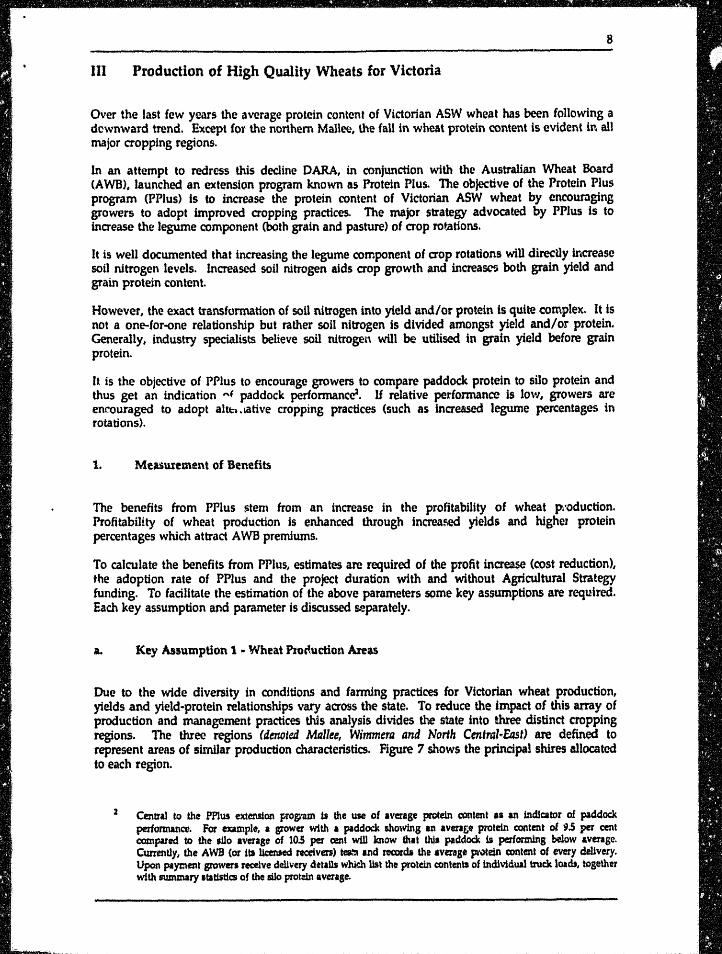
111 Production of High Quality Wheats for Victoria

Over the last few years the average protein content of Victorian ASW wheat has been following a dcwnward trend. Except for the northern Malice, the fall in wheat protein content is evident in all major cropping regions.

In an attempt to redress this decline DARA, in conjunction with the Australian Wheat Board (A WB). launched an extension program known as Protein Plus. The obJective of the Protein Plus program (PPlus) is to increase the protein content of Victorian ASW wheat by encouraging growers to adopt improved cropping practices. The major strategy advocated by PPlus is to increase the legume component (both grain and pasture) of crop rotations.

It is well documented that increasing the legume component of crop rotations will direcUy tr,crease soil nitrogen levels. Increased soil nitrogen aids aop growth and increaS('5 both grain yield and grain protein content.

However, the exact transformation of soU nitrogen into yield and/or protein is quite complex. It is not a one-for-one relationship but rather soil nitrogen is divided amongst yield and/or protein. Generally, industry specialiSts believe soU nitrogen will be utilised in grain yield before grain protein.

It is the objective of PPlus to encourage growers to compare paddock protein to sUo protem and thus get an indication ,,{ paddock performance2. If relative performance is low, growers are encouraged to adopt altb .&,ati\'e cropping p.ractices (such as increased legume percentages in rotations).

1. Meuurement of Benefits

The benefits from Prius ~tem from an increase in the profitability of wheat p'oduction. Profitability of wheat production is enhanced through increa!led yields and higheJ protein percentages which attract A WB premiums.

To calculate the benefits from PP1U5, estimates are required of the profit increase (cost reduction), the adoption rate of PPlus and the project duration with and without Agricultural Strategy funding. To fadUtate the estimation of the above parameters 5Pme key assumptions are required. Each key assumption and parameter is discussed separately.

Key Assumption 1 • Wheat Pro~uctiO!\ Areas

Due to the wide diversity in conditions and tanning practices for Victorian wheat production, yields and yield-protein relationships vary across the state. To reduce the impact of this array of production and management practices this analysis divides tht state into three distinct cropping regions. The three regions (denoted Mallee, WimmerQ and North Central-East) are defined to represent areas of similar production characteristics. Figure 7 shows the prind~ shires allocated to each region.

2 Centta1 to the PPlus extCNion f1081'il1n 11 the use of average protein content II an indicator of paddock performanc;'t. for ew:nple. I grower With • piddock showing In &VeRst protein content of 9.5 per ""t compared to the ..no awrage of 10.5 per amt wU1 know that tN.a paddock is pe:rfonning below average. Currently, Ute AWB (or itl Jic:enMd rec:elvm) teI.':'t and rt!lCOfdI the avms. P'»dn eontent of every delivery. Upon pa~t grower. rece1ve dtl\very detl1ll which UJ\ the protein contents of tndlv1dUll truck loads, toge\her wfth suuu:na:ry .tatiJtic:s of the sUo protd.n averlSe.

9

~~ ~ .

• ~I'tll ttnt,,"'·lu' ~ 1r-".-t..JI\..t'"o,..,...~~.- ....... ",:,

."---/'

~'

Figure 7 Principal wheat growing shires selected for analysis The particular production characteristics u~d to select the above shires are:

CI shires in which whe~! production is a major enterprise; and • shires which are predominantly under crop production.

Shires such as Walpeup and Mildura, although producing large amounts of wheat, were not included because they also contain large uncropped areas.

b. Key Assumption 2 • Crop Proportions

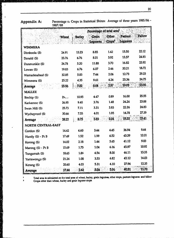
This analysis assumes the average proportion of crops represents the average agronomic profile of each region'. The crops or enterprises considered are wheat, barley, grain legumes, pasture legumes, other crops and fallow (Appendix A).

The total fanned area is assumed to equal the total area of wheat, barley, grain legumes I other crops, pasture legumes and fallow, as presented in Table 12. That is, the six enterprises are assumed to occupy 100 per cent of farmed land. The area of the different enterprises (expressed as a percentage> are averages for the three years 1985/86 to 1987/88. The fallow area percentages are DARA estimates'. DARA industry experts estimate the fallow area for the Wimmera and Mallee to be 84 per cent of the combined area of wheat and other crops. Due to the high percentage of

, Conducting the analys.ts this WI, avoids the problem 01 using 'avenge' or 'sWlcUlrd' rotations. Such gen~c rotations are llleaningless at best.

AUJtnl1#n Bureau of SfAtistic:s no longer coU~ statlstfcs on fann area und~ tallow.

10

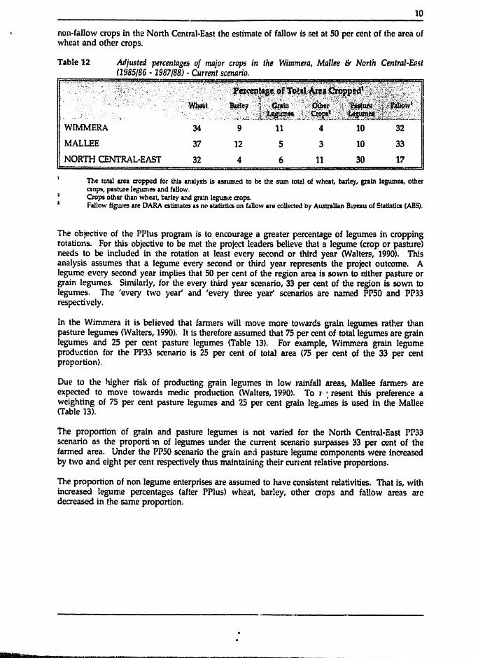
non-fallow crops in the North Central-East the estimate of fallow is set at 50 per cent of the area of wheat and other crops.

Table 12.

WIMMERA

MALLEE

Adjusted percentages of rruljor crops in the Wimmera, Mallee & North Central-East (1985/86 - 1987/88) • Current scenario.

~",::""~:, .. ;,,.,\ .. :;; :':::: i_~, .. ~~~,~~~3·~~\f:i::}~1~$;·~~:~; ;~': ' ....... ~~ ' .. ~! J~3::::.j:!;_:;~L;

9 11 4 10 32

12 5 3 10 33

NORTH CENTRAL-EAST

34

37

32 4 6 11 30 17

The total area aopped for this analysis is ISNlned to be the sum totAl of wheat, barley, pin legumes, other aops. pasture legumes and fallow. Crops other thin wheat, barley and grain 1egtUl'le aops.. Fallow Bgwes are DARA estiJ:nates .5 nt' stitUtics on fanow are collected oy AWltral1an Bweau 01 Statistics (ADS).

The objective of the PPlus program is to encourage a greater percentage of legumes in cropping rotations. For this objective to be met the project leaders believe that a legume (crop or pasture) needs to be included in the rotation at least every second or third year (Walters, 1990). This analysis assumes that a legume every second or third year represents the project outcome. A legume every second year implies that 50 per cent of the region area is sown to either pasture or grain legumes. Similarly, for the every third year scenario, 33 per cent of the region is sown to legumes. The 'every two year' and 'every three year' scenarios are named PPSO and PP33 respecti vely.

In the Wimmera it is believed that fanners will move more towards grain legumes rather than pasture legumes (Walters, 1990). It is therefore assumed that 75 per cent of tota11egumes are grain legumes and 25 per cent pasture legumes (Table 13). For example, Wimmera grain legume proch.,ction for the PP33 scenario is 2S per cent of total area (75 per cent of the 33 per cent proportion).

Due to the higher risk of producting grain legumes in low rainfall areas, Mallee farmers are expected to mOve towards medic production (Walters, 1990). To J.: resent this preference a weighting of 75 per cent pasture legumes and ?..5 per cent grain leg..unes is used in the Mallee <Table 13).

The proportion of grain and pasture legumes is not varied for the North Central-East PP33 scenario as the proporti,)n of legumes under the current scenario surpasses 33 per cent of the fanned area. Under the PP50 scenario the grain and pasture legume components were increased by two and eight per cent respectively thus maintaining their current relative proportions.

The proportion of non legume enterprises are assumed to have consistent relativities. That is, with increased legume percentages (after PPlus) wheat, barley, other crops and fallow areas are decreased in the same proportion.

11

Table 13 Proport. m 01 crops in Wimmera, Malia and North Central·East with a 33 and 50 per cent leL.ume camponent

, . " ..

,p~ .. ~@ ~QW '(!ro,ppt4 ,~~f

.... __ ................................ _ ............. ~ ..... ".~~~ ...... ~~: .. ;;.~ ....... ;&~ .. , .. ,~ .. ,.L:~~~.: .... . PP33

WIMMER-\

MALLEE

NORTH CENTRAL-EASTJ

28

29

32

8

9

4

25

8

6

3

2

11

8

25

30

27

26

17 •· .. •• .... "" .. ····"'''·'·~ .. I· ...... '· .. ••• ........ ' .. ···' ............. _ ........................ « ..... ,.. ............................ , ............. /< ....... - .,.." ... ".w ... : .... t .. ':?7~.! ... ~:·:': .. .'."~·:·~ .. ' ..

+.- ,_ ".' .". , ": ,"~: ':. ',~.·.t·, ... ;~,\<~· ""'·h~'; u~, .. nll"'.'''1f'''1r\o ...... It ...... , • •• I<li# ••• ~. -.f ...... fI ............. , .• , , ... • ... ..,l ......... Uhn.U, ......... ~f' ~u •• n ..... 'lfH" ...... ' ................ u •••• ";t ... ~\"''"''\l ....... ''v .. " .. I .. uill;t,,.-.. 't\\,{ .. \1>.\.h .. ',,'''' ..... \''''''""\U""U''"''U-''t,. .. __ i~'\ ...

PPSO

WJ.M:MERA

MALLEE

NORTH CENTRAL-EAST

21

22

25

6

7

3

38

13

S

2

2

8

13

38

42

20

20

13

The total area cropped for thls analysis 11 assumed to be the sum twl of whClt, barley, grain legumes, other crops, pasture Iflgnll'lefl and b,Uow Crops other than wheat, buley and grain legume aops The combined proportion of legume aops and pastures an the North Central-East amounted to 36 per cent of total arCA under the current sc:enari.l) and lS therefore not adjusted for the 33 per cent legume scenario (PP13).

2. Cost Reduction • R Factor

As indicated earlier, the benefits from PPIus arise from increased wheat yields and higher protein premiums. To estimate the change in on-farm costs and returns involved in increasing legume production to the proportio\\s shown in Table 13 a partial budget technique is applied.

a. Change in Costs

PPlus is primarily directed at incl'(~sing the legume <both pasture and grain) component of farm paddock rotationsS. Obviously, such a change does not come without cost. The introduction of improved agronomic practices will require some additional costs to be met by individual fanners.

In this analysis, on-fann costs are estimated by calculating the total weighted variable cost for each region. Total weighted variable costs are determined by summing the weighted variable costs for all enterprises in each region. That is, the variable costs for ead\ enterprise (from D.ARA gross margins) are weighted accordmg to the proportion of the enterprise in each region and then added together to calculate a total weighted variable cost.

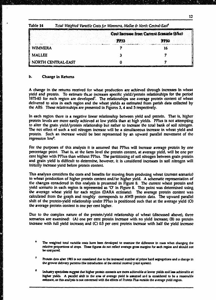
The total cost to producers of increasing grain and pasture legumes to PP33 and PPSO proportions are estimated by comparing the total weighted variable costs for the three scenarios crable 14). The change from the current scenario to PP33 or PP50 increases the total weighted variable costs in the Wimmera by between seven and sixteen dollars per hectare, by three to seven dollars in the Mallee and by zero to seven dollars in the North Central-East (Table 14).

Alternative strategies, such AI the appUation of nll:rOge:n fertil1Jer. are also advocated by PPIWl

12

Tabl,14

\¥I"'f'MERA "1

3

o

16

1

"1

'-fALLEE

NORTHCEM'RAL"EAST

A change In tM returns ~ved for wheat production are achieved throup ~ in wheat yield and protein. To atirn.ate thtie inaeues specific yield/protein rdatiomhiPJ for the period 1975-85 for each ~on are developed'. The relationships use average pro~in content of wheat deli\~ to llIos in each region and the wheat yields at e&ttmated from piUUh data coUected by the ADS. These re1lttoNJdps are presented in FiguftlS 3." and 5 respectiveJy.

In each region there is a negative linear relationship betweett yield and protein. That {s,highe'r protein levels are more easiJy ach1eved at low yields than at high yields. PPlus is not attempting to .lter the gr~dn yield/protein re:lationmip but rather to tnaease the total bank 01 soil nitrogen. The net effect of such a soil nitrogen ~se will be a $lm\lltlneoU$ increase in wheat yield and protein. Such an inc:reasc would be betSt re:pTe$ented by an upward par,Uel movement of the ~o.nbne·.

For the purpo$eS of thu analysis it is assumed that PPlus will Increase average protein by one percentage point. That is, at the farm level the protein content, at average yield, will be one per cent higher with PJ11u, thln without PPlu$. The partitioning of soil nitrogen between grain protein and grain yield is difficult to determine, howevtr, it is umsidered increases in soil nitrogen win initially increase yield before protein content.

Thi$ analysts COMidert the costs and benefits for moving from produdng wheat (current scenario) Ii) w~t prodUdion of higher protein content and I or higher yJeld. A schematic representation of tl~ ehanges conl\.dered in this analysis is presented in Figure 8. The curre.nt wheat protein and yield tilCenario in ~ach reston is Kpl'e$enttd as 'cr in Figure 8. This point was detennlned using the average wb~.t yield for each region (DARA es1imate). The average protein content was akulated from the graph and roughly corresponds to AWB protein data. The upward parallel ,tuft of the proteitr)1eld relationship und~ PPlus is positioned such that at the averag., yield to} the average p'rotein content is one per cent higher.

Due to the t.-omplex nature of the protein/yield relationship of wheat (discussed above); three scenarios are eumined: (Alone per cent protein in~ with n.o yield i.naease; (B) no protein increase with full yield ~; and (C) 05 per cent protein increase with half the ~eld increase

•

1

,

the wet&hltd total vwbJe COIt$ hi" ben devdoped to ~ the ~ in COIiiU when c:ha.npS the II'llt,tvt ~ot (lopl, ThIN 81'R' do not nfl«taYllf.p IfOlI' marsw lor .. dl ~ and Ibould not N~partd.

PrQkln &11 __ nIB" fIOt·cgMkl...s due to 1M. ~ aumber of prime h&td Itp'fIlttlOlUtand a dwlge in 1M power dtltivay pat«IJN (the illtmd&dOll 01 the «ntnd I1.'t'I!vaJ paint tp.ttm).

~~ 1'U(PIt tbat htpla' protein ~ Ilt more .clUwablt at)owet )it1d1 wi_ tdUw.ble at Np. ~ A pIl'IUt! INIt in tM I1U 01 'wnt' )'Sekt k UlUtnid ud tI <onttdftfd to be • fWONble "It" ... thb aNlJYiU ts _.~ wUh Ik· dlCdS o! J\'Oldn Plu. outside the ,"Wlst yidd ~on.

13

under (8), Points A and B ~t the potu ICfm.Mi05 which may arise from PPlu$, and point (Cl l'I'J'f'~b the fnos! libely outcotnC. being a mixture of both a yie.ld increase and a protein i~ (Figure 8).

/ .. ,. ..... r~=:::==. ..... 01

••• __ ••• A / ... _ .. _-_ ..... -

.. ---_.-. ---

Yield (Vha)

Uling thi, approach the avmge yield and protein valuet .are estimated fo,T tM Wimmer., MalJce and North Central-East from FIgure 9# 10&00 11 respectively and are presented in Table 1S.

Table 15

t\'tMWEAA

MAU.EE

~u, '1aN1'RAL«EAST

rk .. ft":~ It. .:1

~ .~ .~ ;~. )1M ~. ~i'~ 1

_ + ____ ~ .. ;!l:.:~.~,.""""'._ "',.4<~_~H..q::~ ......... _......, .... ~, ........ ...;;....~~~~~\ti..._~~ ... ~~~,.;!;::u:, .... ;;.~>T'.,;..~,;'; ..... ~~...:,.~,~ .. ~~."....,.,...:/iio ... ,-.!; __ ~ ~

25

1.6

2.0

9:/

11.9

10.0

2.S

1.6

2n

10.7

12.9

11.0

3..4

2.4

3.0

9:1

119

10.0

2.9 10.3

2.0 12.4

2.5 10.5

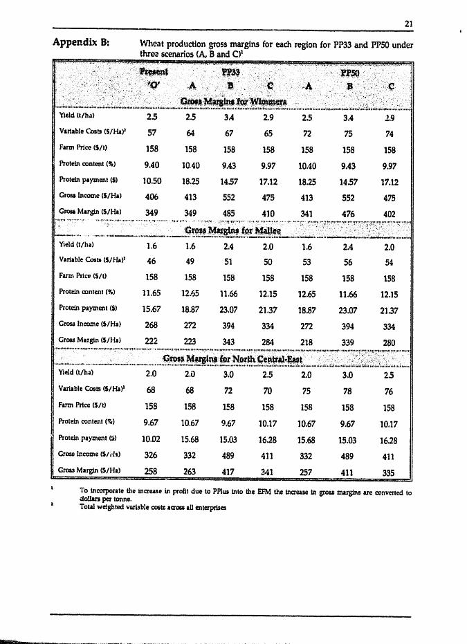
The protein and yield levels from ra!tle 15 are used' to calculate gross m.argins for each region fAppmdbt B)t. Changes in profit ($/tonne) for the three SC'eNUios (A, 8, and 0 for PP33 and PPSO Weft then calcUlated from the gross margins for each retPonlO• The weishtedlVefAge tncrnstin profit mu.tting from PPlus range from .. 52.19 per toMe for PP50 to $47.15 per to~ for PP33 (Table 16) .

• In fJIK.h ...... tlw )Wld ..... ..s vww. (OIfa Wfft ~ted when ~ inc:rustd. PrmtWN k# hl~ P"*IfA wen alto tadudtd.

113 1M ettap In profil 'or 4IIICtl ~ ~ the f1CII INfP lor whut tU1nJ mto ICalUnt van~ U1I11 for Nfl.." pt ~ .. 'aopI. puturl ad &.DowWfiphd ~ ~ the '.rea ~ of each crop m each ~ Thec:h.M,. tn pofit •• at. wtdpttd .~ 10 tht amount 01 what prodUdkla in eu.h ~

fJpre 9 Prottif% and yield reUtticmship for the Wimmtm

"1IUItn "Il~ to! a1',....-------------· _____ --___ '"

• • •

fipRIO

,t

U

at

u

It

• •

l.t

Protein and yield rt14tionships for the Malla

.~ .. --~----~------~----~----~~----.. -----• I.'

Fipre 11

u

1 1.' • .., , ).,

QuLIn Y'fIl14 (LIMa)

Ptofein and yield rtlafitmShtps for the North Centml·£4$t

14

Pr« ... 1.UO· 1m '* YiIU

~n .. 12.10 • l,m. rid" m!..o:S3)

Pr«d" • U.76 • 1.32 " YII14 (~.o.65J

Prr.tttm • lJ .6.7 eJt'.o.2J)

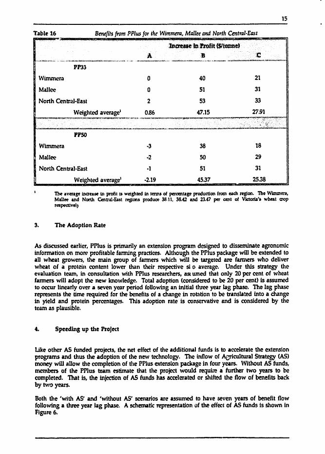
TAble 16

\Vimmera

Mallee

P133

North CentrDJ·East

Btn£fi15 from PPlus {Of lhe Wimmem~ Mallet and North Central-East

o o 2

40

S1

53

21

31

33

Weighted average' 0.86 47.15 21.91

15

t .. "~· .. ~-.,.' .... -··-., ........ -·" __ ' .. r ..... ,." .... -,.. ............ ".-~---~ ............. " ... HAA';"'~ ... ·~ .. ·~:'~··:·~:j~~7 .. ·':."· .. ' .. · ~~~.M~ ..... ,~.~.'~ ... ~.fj,"'if.l~~~u.u ... ~*.n .. ~~4t~,(I.u-'" .. '1:.1r, ........... "".u"'i-"n ...... ~ .... ~~** .. .t.~,~ ..... "'......,..~~"~~ ... ''''"~ •• u;.u ..........

P'5O

Wimmera ·3 38 18

Mal lee ·2 50 29

North Central-East ·1 51 31

Weighted averagel .. 2.19 45.37 25.38

The IVUlp inac&:.te in proBt 1$ weighted in ttnnl of pe:centap production from uch reston. Tho WimJnm. MaUte &ltd North Cmtr&1·ust restonl produce 3811. 38.42 and 23.41 per cent of Victoria'. wheat aop rapoc:tive!)

3. The Adoption Rate

As discussed eArlier, PPlus is primarily an extension program designed to disseminate agronomic informiltion on more profitable fanning practices. Although the .PFluG package will be extended to all wheal growers, the Ir.ain group of fanners which will be targeted are fanners who deliver wheat of a protein content lower than their respective si 0 average. Under this strategy the evaluation team, in consultation with PPlus research...-rs, ast umed that only 20 per cent of wheat farmers will adopt the new knowledge. Total adoption (considered to be 20 per cent) is assumed to ocxur linearly over a seven ymr period following an initial three year Jag phase. The lag phase represents the time required for the benefits of a change in rotation to be translated into a change in yield and protein percentages. This adoption rate is conservative and is considered by the tcam as plausible.

S~ed1n1 up the Project

Uke other AS funded projects, the net effed of the additional funds is to accelerate the extension programs and thus the adoption of the new technology. The inflow of Aericu1tu.ral Strategy (AS) money will allow the completion of tbe WIllS exter.ston package in four years. Without AS funds, members of the W)llS team estimate that the project would requh'e a further two years to be completed. That is, the injection of AS funds has accelerated or shifted the flow of benefits back by tw~ years.

Both the 'with AS and 'without AS' scenarios are assumed to have seven years of benefit flow following a three year lag phase. A schematic representation of the effect of AS funds is shown in Figure 6.

16

o ~------~~~~~~~~---------~------

WITHOUTM

figure 12 The bmtfits frum Prolein Plus under a duange IZpprooch (not 10 sa':Ule)

In this analysis acceleration (II the PPlus program by two years is assumed to be the optimistic ~o. Acceleration by onc year is assu.med to represent the pessimistic scenario.

TM variabJes used in the Edwards Freeblim Model are Usted in Table 17. The variables are the $Arne for both the 'with AS' and 'without AS' stenarios, except for the length of the project p'ha5e. The two cues for the Q)5\ i'eductlon of the project are also investigated (Pr33 and PP50 so..~rios).

Table 11 Variables 1M PPlus used in E.dwards Frttbairn Model

t'~Y.u&le Commodity price (S/toMe)

Cost saving ($/tonne)

Qua.ntity produced in Victoria (tonnes)

Quantity produced in ROW' (tonnes)

Quantity consumed in Victoria (tonnes)

Elasticity of supply for Victoria

Elasticity of supply ROW

Elasticity of demand for Victoria

Elastidty of demand HOWl

PP33

FPSO

ABARE t$timated IcrtQst prta!' for mediwn tmn

;~~ 140

21.91

25.38

2,230,000

514,800~

332,000

1

1

'().35

-20

ROW • Rat of World (l.e, all oth. coWltri.1JId the .... of AUltnliI)

5. Project Costs

.... J:SAM~ ABARE' (1990)

From gross margins

From gross margins A'WB (19ss.90)

ABARE (1969)

AWB (1985--90)

DARA eatimate

DARA estimate

DARA estimate

DATtA estimate

The costs for the PPJus PfOJec:t have been calculated over I three year period from 1988-89 to 1990-91. To account for the extra year required to complete the Projectl the avmge aMual expenditure for the first three years is assumed to equal the fourth year of funding. The total

•

17

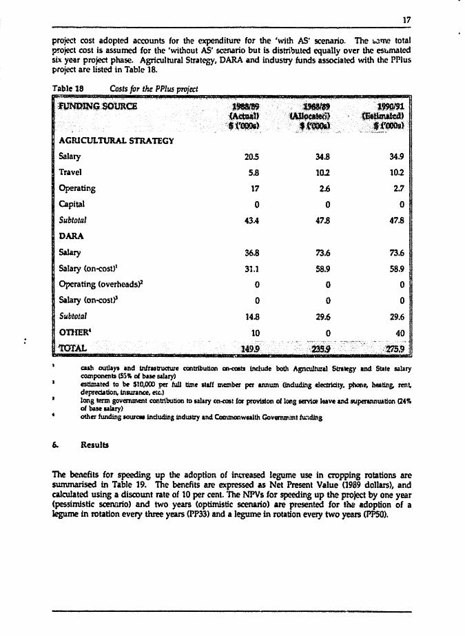
project cost adopted accounts for the expenditure for the 'with AS' scenario. The b.lmt? total p!oject cost is assumed for the 'without AS' scenario but is distributed equally over the cstdnated six year project phase. Agricultural Strategy~ DAM and industry funds associated with the PPlus pr0fect are listed in Table 18.

Table 18 Costs for the PPlus project

•

AGRICULTURAL STRATEGY

Salary

Travel

Operating

Capital

Subtotal

DARA

Salary

Salary (on~ost)l

Operating (overheads)l

Salary (on<ost)'

Subtolal

ODlER'

~rorAL

""

205

S.8

17

o 43.4

36.8

31.1

o o

14.8

10

149~9

34.8

10.2

2.6

o 47.8

73.6

58.9

o o

29.6

o

34.9

10.2

2.7

o 47.8

73.6

58.9

o o

29.6

40

·;:~.9

cuh outlays and tn.frat1fucture cxl'unbution ~ tndude both Agncultural Strategy and State salary eomponmts (55" of bile mary) estimated to ~ 510,(XO per tuU tUne stall member per annum (lndu.dmS electricity. phone, heating.. rent, depredation. insurance. etc.) long t2nn IOVenu:nmtcontribution to Nlary OlHDt for provision cl WPS SCI'\'tce kaYe and IUpaannuation <24,. 01 base Nlary) othC'l funding SOUfcas inch.sdma industry and Cownonwtalth CoVGI1'Ul'Imtt N.'1dinS

Results

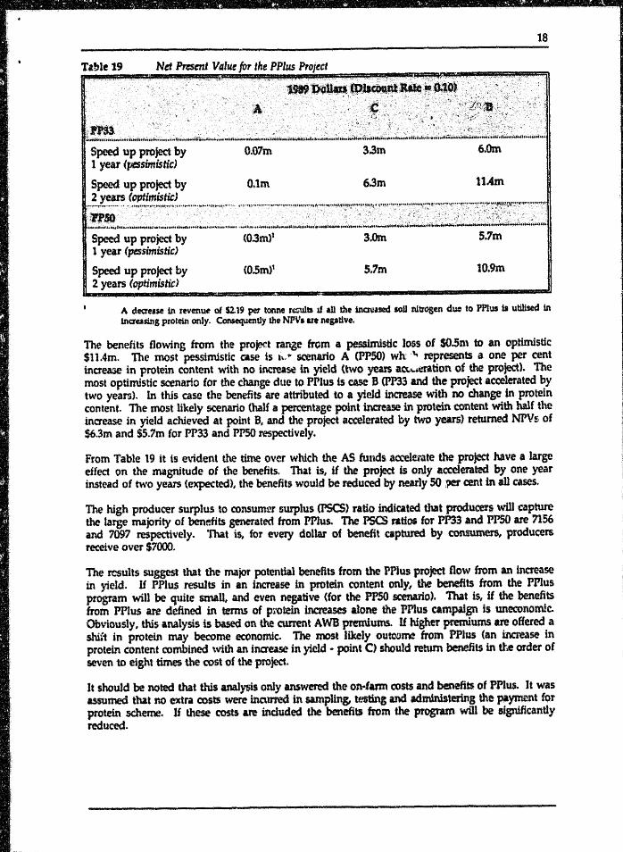
The benefits for speeding up the adoptiDn of ina'eased legume use in cropping rotations are summarised in Table 19. The benefits are expressed as Net Present Value (1989 doUars), and calculated using a discount rate of 10 per cent. The NPVs for speeding up the project by one year (pessimistic scenario) and two years (optimistic scenario) are presented for the adoption of a legume in rotation every three years (PP33) and A legume in rotation every two years (PPSO).

18

Table 19 Net Present Value for the PPlus Project 1 .,' '" " ,'~' '/, •• f,f "";" ,-'~.~'. .",.,

,,1$.. . .. ....... '.. .~. ·:-:7t,~?~,,!~:~~.~: .i ~.""' ••• :"''' •• '''''W .... iu .... l>.~.''''.,,*$.''-$l''.'''."~'',,","''''''''''.'''.* ..... n."¥Hjj~".;f'4~W .... '~ .... j4·~" .. ~ .......... , ........ .,".tI.J'h""' •• It.~,,,~,,.AA~ ......................... , ... .,.: ...... .

Speed up proJect by O.tl7m 33m 6.Om 1 year (pessimistic)

Speedup project by O.1m 6.3m llAm 2 years (optimistic)

.'.if), .. , .. "":""""~""""""""":~""t"·".'··C··~~~~··: •• ~.·, ... ,» •• ".~~>~~.~~ .. \~,~,.l':::'~".~,"~' t'»"'7':':~':'0'~;';~'~?~":~:'7';'~~;?~:~~~:;~:'~'1~""'j,m"~

~~~"'Uri .... t#.~ .. "~"*".~*,,,n~."""'.iI""~"""IfII" •• ItU .. ...,.# .. # ..... ~".'"~~"".lt~ •• ~ .... ~1t~tj~.;" .......... '~ •••• ~.~ ... ~.;.;-~ .. ' .... ~~ .. n. ............ ~ .. -.101t>>"1\of

Speed up project by 1 year (pessimistic)

Speed up project by 2 years (optimistic~

(O.5m)'

3.Om 5.7m

5.1m lO.9rn

A d~"$e in r~venut 01 52.19 per tonne r¢!lUllS if aU the 1ncnlamd soU nitrogen dut to PPlr» 11 ut:W.sed in mcraMS prottin only. ConaequmtJy the NPV.I1" Nptlve.

The benefits flowing from the pro~t range from a pessimistic loss of 505ft' to an Optimistic $1l.4m. The most pessimistic case is ,~," scenario A <PPSO) wh'~ represents a one per cent inttease in protein content with no increase in yield (two years aa,\'ieration of the project). The most optimistic scenario for the change due to PPlus is case B (PP33 and the project accelerAted by two years), In this case the benefits are attributed to a yield increase with no change in protein content. The most Ukely scenario (half a percentage point increase in protein t.antent with half the increase in yield achieved at point B, and the project accelerated by two )"eUS) returned NPVs of $6.3m and 55.7m for W33 and PP50 n!Spectively.

From Table 19 it is evident the time over which the AS funds .cce1mte the projea have a large eifecton the magnitude 01 the benefits. That iSI it the project is only accelerated by one year instead of two years (expected), the benefits would be reduced by nearly 50 ,';)er amt in all cases.

'!'he high producer surplus to consumt'r 6urplus (FSCS) ratio indicated that producer, will capture the large majority of benefits generated from WIllS. ThePSCS ratios for PP33 .and PPSO are 7156 and 1097 respectively. That is, for every dollar of benefit captured by con&Ume1'$, producers receive over $7000.

The results suggest that the tna)otpotenrtal benefits from the PPlus project flow from an increase in yield. If PPlus .results in an increase in protein content only, the benefits from the PPlus program will be quite small, and even negative (for the PP50 scenario). That is, If the benefits from PPlus are defined in terms of p~oteln irtc:reaseJ alone the PPlus campalgn is unecononUc. Ob\'1ously # this analysis is based on the current AWB premiums. If higher premiums ate offered a shSJ1 in protein may become economic. The most likely outoamt: from PPh15 (an ~se in protein content combined with aninc:rease in yield .. point C) should re:Mn benefits in tl'~ order of seven to eight times the cost of the project.

It should be noted that this anaJy$is only answered theon-farm costs and benefib of PPlu5. It was usumed that no extra cos'ts were inam-ed in sampling, tetting and adrniniJ,tering the pa~nt for protein scheme. U these costs are included the benefits &om the progrunwiU be significantly reduced.

19

7. Sensitivity Analyais

Sensitivity analyses were performed on some of the key variables (details are shown in Appendix C).

The results are extremely sensitive to the choice of R factor used in the analysis. The size of the benefits from the PPlus project are highly sensitive to whether the soil fertility improvements achieved through increasc..'<i use of grain and pasture legumes are utilised in increAsed protein content or increased yield. If the improvement in soil fertility results purely in an increase in protein c:onterlt the benefits from AS funds may be as low as SO.1m for PP33 and a 105s of over $O.5m for PPSO. Conversely, if the tmproved fertility is consumed in increased yield (CQnsidered to be the most probable outcome) benefits from the project could be as large as 510.9m for PPSO and $11.4m for PP33.

As shown in Table 19, the benefits are very sensitive to the time over which the project is accelerated (that is, the number of years over which the project is speeded up). If the project is accelerated by only one year the benefits from PPJus an! reduced by approximately 50 per cent for all scenarios.

TI-tC benefits from PPlus are relatively senSltive to a change in the discount rate. Decreasing the dIscount rate from ten per cent to six per cent increased the benefits by five per cent. An increase in the discount rate to twelve per cent decreased the benefits by eight per cent.

The results were relatively insensitive to the other variables used in the model. For example, sensitivity on the elasticity of supply (:50%) only showed a varialion in the result of less than five per cent for aU scenarios.

Appendix A:

WlMMERA

Dimboola (5)

Donald (S)

Dunmunkle (5)

Lowan (5)

Warracknabeal (5)

Wimmera (5)

~f,~1~~ MALLEE

Birchip (5)

Karkarooc (S)

Swan Hill {S)

Wycheproof (S)

A.v~e

20

Percentage OJ Crops in Statistical Shires: Average of three years 1985/86 -1987/88

24.91 13.23

25.76 6.76

24.78 5.20

19.83 6.76

32.85 5.83

25.22 4.35

25~ ~:::~,;~: .. ~ ~,. -~' .. :o I<c,c:'" .,; 'w,.'"

2~_..: 10.95

26.95 9.40

25.13 7.11

30.66 7.55

.. ~,22 • ~~15 ! .j

8.85

8.01

11.88

6.07

7.44

9.61

4.47

3.76

3.31

1.4:?

3.92

3.70

2.46

2.06

4.24

0.89

1.48

3.83

15.50

13.57

16.82

30.21

12.73

25.36

16.00

24.24

22.26

22.12

24.93

23.92

18.72

29.33

24.75

25.55

23.88

24.83

4.01 1.95 14.78 27.39

c .• ·.·;,~~:. ··~j;;f ~\r:i~g.$~;:)·;~;~E~.~l. NORTH CENTRAL-EAST

Gordon (5) 14.42 4,60 3.44 4.45 36.94 9.44

Huntly (5) - Pt B 17.49 1.52 1.99 6.52 43.39 12.01

Korong (5) 14.02 2.18 1.44 5.65 41.12 9.83

Marong (5) - Pt B 15.69 1.75 1.04 6.16 45.97 10.92

Tungamah (5) 18.65 1.86 4.54 8.00 46.11 13.33

Yarrawonga (S) 21.24 1.00 3.53 6.82 42.12 14.03

Kerang (5) 20.60 4.03 5.31 4.10 2.7.94 12.35

.A~ ';J7M '~ , >:,'., .. ~ ~\:,'"> ~~> t~\:·;!~·.· •. ·:,~':~i~~~~;iii·: , Total ana is ~cul.ted .. the totalll'Q of wheat. barley. sraJn l~ other crops, pasture ITlU1el and fallow Crops other than wheat. barley and grain l!gw:ne crops.

Appendix B:

Yield (t/h~)

Vanable C.osts (S/I-b)2

Fmn Price (s/t>

Protein content (90)

Protein payment ($)

GrOll Inc:om~ (S/H.)

Grosa Margin (S/H.)

Yield (t/ha)

Variable Costs (S/ Ha)~

Farm Price (SIt>

ProreJ.n contenl (cr.)

Protein paymmt (5)

Grosa Income (5/Ha)

Groas Margin (S/Ha)

21

Wheat production gross margins for each region for PP33 and PP50 under threa scenarios (A, B and C)'

2.5 2.5 3.4 2.9 2.5 3.4 l.9

57 64 67 65 72 75 74

158 158 158 158 158 158 158

9.40 10.40 9.43 9.97 10.40 9.43 9.97

10.50 18.25 1457 17.12 18.25 14.57 17.12

406 413 552 475 413 552 475

349 349 485 410 341 476 402

1.6 1.6 2.4 2.0 1.6 2.4 2.0

46 49 51 50 53 56 54

158 158 158 158 158 158 158

11.65 12.65 11.66 12.15 12.65 11.66 12.15

15.67 18.87 23.07 21.37 18.87 23.07 21.37

268 272 394 334 272 394 334

222 223 343 284 218 339 280 . ~'t ••• '."n ~ .tt. ~~~" .... ~t'."'I'H~.'~~~I;~'~::~"'.f~.'~" ~ •••• ~ .~.~t~ ._~,.tt~~ ~., ••. ~tt~ •• ft"~ .{~'~:f ~.i!II',~'~~ ••• !'I~,.~lI.f ~."~,~~~~,~~~:~,~"~H'~!~~.~~:'~~'~'r;,t'~ ~~"u";':~;~?~:~?r~~, ~~"~~ "~~,,.t •• ,~~v~

',' .. ' 'QJ'Q.'M~n,\fo.rNonh,Ctlm:r~'!'l.Mt.: : ... ·,·:~:>~;:,i·"~:::\;' '. ~~ ... ,,. ............... It .... ,. ........................... , .............. "' ...... u. .... ,. ....... , ..... '" , ....... ,11., ......... v. ......... , •• n-fi ...... ,. t.u .. ~h.* 41 .. -.. • i •............... ;.,~ ........ , ..... i ..... h ..... ' ....... ,.!. , .. d .. , ••• h.u " ••• ,. '-'4 ......... u

Yield (t/ha) 2.0 2.0 3.0 2.5 2.0 3.0 2.5

Variable CosL1 (S/Ha)2 68 68 72 70 75 78 76

Farm Price (SIt) 158 158 158 158 158 158 158

Protein content (,.) 9.67 10.67 9.67 10.17 10.67 9.67 10.17

Protein payment (lI) 10.02 15.68 15.03 16.28 15.68 15.03 16.28

Gross Income (SIal) 326 332 489 411 332 489 411

CraN Margin (5/Ha) 258 263 417 341 257 411 335

To incorporate the mereue in profit due to PPlus into the EFM the increase in grON margins are converted to dollara per tonne. Tot&! weighted vi.Tiable co.sts aaOSi all enterprises

22

Appendix C: Sensitivity Analyses

Table 1 Net Present Benefits (NPVs) with Varying Discount Rates and R foctors (PP33)

Speed up project by 1 year (pessimistiC>

Speed up protect by 2 years (aptnnistic)

Speed up project by 1 year (pessimistic)

Speed up project by 2 years (optimistic)

Speed up project by 1 year (pessimistic)

Speed up project by 2 years (optimistic)

O.OOm 3.4m 6.1m

0.2 6.6m U.9m

F'~""""~"""""\"'''''' '~"\"A~"'J~'~':""',"'I·:\·"r,~ .. ,··~~?t>·~~'!""·!;·r"!~,:\"!"~'~~"1',~:1!"':":"'~;'\?~':::!!:;~;~1::!::j,~.~!;.:.,'l:"". $, , 'n~drtt:a~~:{J.'lO ., ", .,ii,>J .. ,.::, ';::"':,:";'~'" l\~.~ ... ~ .... ~~ .... i.".~ ... ~wnuu'nn.t.lo."\~" .1~.""h" "\"~"~:::l.~:' ~j.,~:'t"J '." •• :~~c~f''':''.~~~:~;' .i;.~~~, .. ~ .. u •• :.~).). ;~.t4'~f~"i1:.i;; •• ;i;;. ;,~,'ou~'i::;f,\i~,;u~tu'~'

O.07m 3.3m 6.Om

O.1m 6.3m 11.4m

f ..... ··~····"·· .. ·····'':~:., .. <> ... ".n •.•• :,~~" ••••••. " ... ": •• !.': •••• :".:.~.:.,.~:) •• ' .. ·", .. ~···'.,"' .. ·(· ... • .. '" .... ··"7~;7~7'!·~:·:"'!Jr':·' .. ·· .. r ' . , ~$PQJmt~,.t~J2 ',,' :.:,<'.;~ ;:", ." ... ,.,. ................ u,_ .... .w. • .<: ... 4 .... " ........ , •• llh.'.~ ... , ........ l,>Io .... , ...... ,;.t.I.I ... f .... ""' ...... h.li't" ........ ..,. ...... ' •• HlIi.~~""i'1~ .... • ... l.)ln,h.'~n' ......... h

O.06m

Oolm

. .

3.Om 5.5m

S.arn 10.5m

23

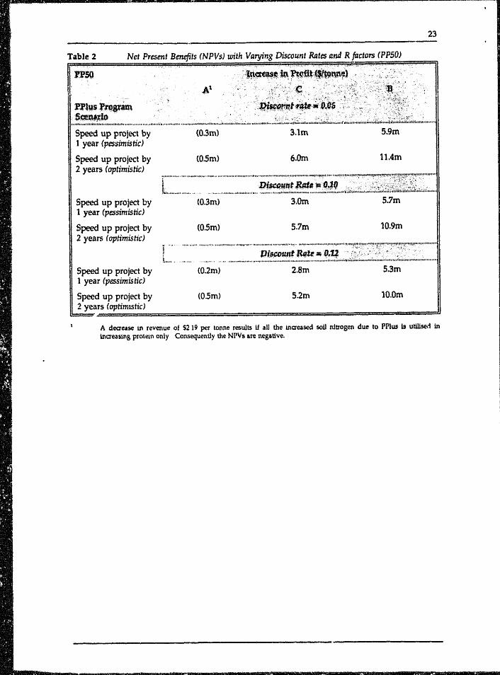
Table 2 Net Present Benefits (NPVs) with Varying Discount Rates and R factors (PP50)

Speed up project by 1 year (pes!1>Unistic)

Speed up project by 2 years (optimistic)

Speed up project by 1 year (pessimistic)

Speed up project by 2 years (optimistic)

Speed up project by 1 year (pesSimistic)

Speed up project by 2 years (optimIStic)

~ ......

(O.3m) 3.1m S.9m

(O.5m) 6.Om 11.4m

<O.3m) 3.Om S.7m

(O.5m) 5.7m 10.9m

......... ···:::::·:·····::··::::.=~:~::~:::~~~~!::~:;.:i;,ij::::~::~~;i;:~~~~:~~~:~~::~:~~~::~~~~::;:~::::::::::::::· <O.2m) 2.8m 5.3m

<OSm) S.2m lO.Om

A decrease tn revenue of 52 19 per tonne results if all the tnaeased soU nitrogen due to PPlus is utilised in ina-easing prohnn oniy Consequently the NPVs Ilre negative.

Mttm •

Tab! .. 3 Stltttt4 NPV, 1?.'rrI ,Ir.t ,..~ $'tIlIIra PP3l .114 pm crilh ,~:i cdtf4tQ f:y t;;':p

ytUf'I

Y~"i~t."" ,-;,e. ,.....,tiIIl~: ....

154

126

~,,:~"'ot'WoM

-55b

-11.16

. illMUdty«aml1 O,S

1.5

:11MddtyofJ)cDJaM

0.18

0.52

:E1.tkit.y·cfS~"lr·Ht· .. ~WOdd 0.5

1.5

':ElJDft~;Clfl)_lmllteltofW.ld

10

30

63m

6Am

63m

62m

6.otn

6.6m

6.3m

6.3m

6.3m

6.3m

63m

63m

,"~ .. I.,I '.,' ,Ill . It! lil.J

S.1m

S.1m

5.6m

5.6m

55m

S.7m

5.1n1

5.'m S.1m

S.1m

5.1m

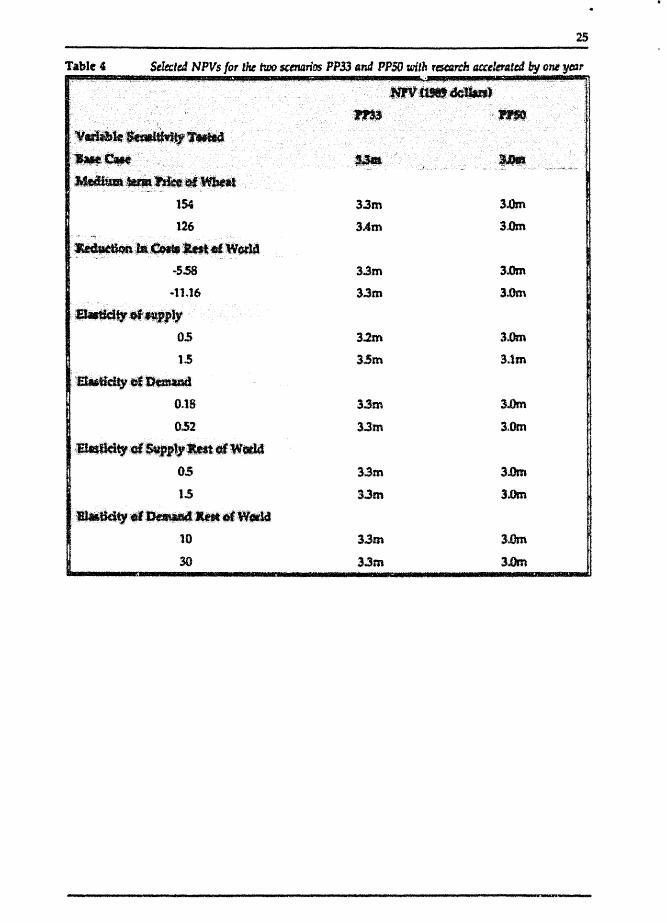
Table' Seltcle4 NPVs for the two sctnarios PP33 and PPSO r.uith ~rrh acakr4ltd by one yc::r

;".lc;~_~ .... c.. ·~,"':t,ab·"·;Wlw.t

154

126

·~:".eo. __ ·.,W~ .. 5.58

-11.16

! .... t1It,·,~,lt

0.5

15

)m.sdty_'~

0.18

052

i1MUdtr:of'$tI",.,lI$tOfWOdd 05

IS

:"'~!",~:"oI'WIdd

10

30

;lirV:,ttM,t:acu.Dl .,. '.:r:no

. .... 33m

lAm

33m

33m

32m

35m

33m

33m

33m

33m

33m

33m

:tOm S,Qrn

3.om

3.Om

3Dm

3.1m

3Dm

3.6m

----------------------------------------------------

IV REfERENCES

AustralianBurtau of Agricultural and Raoula' EaJDOmio ('1990), Ptnanat Communkatiun

Australian Bumu of AgricUltum and ~ &onornks (959), ~il, St6tl1tD Jultl,'tm;, Australian Com'lUnelltPubrtshlna Stnke. CI~4I~

AustraJJan Damn of Stlt:istia (1990), c,..IM P.'run VlacritJ9:!8119, ClWogut' No. 1321.2" Australian Gowm.'TC'nl Publishing Sm"b, CutbaT.,

AuJtrl1ianSureau ofStltistks (l9t19). C. ,,,u ".tum VicttrillS"ll9, CI~ No. 7321.2. Aus.trali&n Co~t Publi$hi1"f6 Sen"ke .. Ctnbtrr""

Australian Bureau 01 Stltistb (1958), Cmps 11114 '.tuNJ V~ J981[!9. ClbJope No. 73l1.2~ Australian Qw-erMtent Publlshing Srerric:r. Cl.nb«ra,

Australian Bureau of Statistia (1987). C""" ani P-.tu:rlS Vlt~ 1988J'89, O&ulogue No~ 7321.2. Australi.Gl Govenurte\t Pubb$hins Smi«,,,Ca~a

Au.straUan Bureau of SGtbUcs (1966), Uw$tod W Ul18t«l PnJSIlU, Vtctorf,a. Clt.ltogue No. 7221.2, AustraUm Covmunem PubtisNng Stnict. Ctnbftu~

AustraliAn DatI)' Corporation (draft, 1989), Milktln4D4try Pro;Ium Co~Ih1t,.

Australian Dairy Corporation (Dec 1989)~ GE.N (monthly $tltist~.l pubUcation),

Australian Oiliry Corporation Oln 1990). lMtrysUtJ (monthly statistiCal publication).

AustrAlian Meat and Uvatock C01'pOfltion (1989). Sesmticfl RttV-tN of .fJw A.KStnlliln Mtai lind Uttt:JtO'd ~1iItiDn* AMLC, Sydney.

Australian \\'be •• Board (1989). 1988 .. 89 Anruud RtpJn,

Austrahan Wheat Board (1988), 1987 .. 88 An~ .Rtpmt

Australian \YheatBoarJ (1981). 1986-87 Anmud Rtpmt.

Australian 'Nheat Board (1986). 1985·86 Annud Rtport

AustraUan Wheat Board (1985). 1984 ... 85 Anrwll Rtp:wf.

ACl (1989), nt Rml Cost of Orpit/d in fM VkWliln £tonomy~ Supplementary paper submiHtd to the st«ring committee of the stlte plantJtiollS impact ItUdy, Melbourne.

Baxter, R E and Rees. R (1983), Tht Penguin Dich~ of Eomomio, Penguin Boob Ltm.itcd, ~fiddlesex, London.

Davidson, Bj> MacAulay, G and Powell, R (1989), "The estimation of the dem&ndfor market milk .. cheese and butter ~n New South Wales, Vidorla and QueeNland/' lltiry Eamtn:rks Rt:uDrch Report, No.2, Deputment of Agricultural Economks and Business Management" UnivmJty of New England, Armidale.

Oepa.rtment of Agriculture and Rural Affairs" Australian Wheat Board (1989), ImprotVtg tht Value of Vidona'sWheal,

27

Edwards, C W and Freebaim, J W (1984), 'The gains from researd\ into tradeable commodities," American Journal 0/ Agricultural Economics, Vol. 66, pp.41-49.

Edwards, G W and Freeba.im. J W (982), 'The social benefits from an i.nau5e in productivity in part of an industry," Review of Marketing and Agrlcultu1'l21 Economics, Vol. 50, pp. 193-210.

Edwards, G W and i\-eebairo, J W (1981), Measuring It Country'$ Gains from ksem'ch: Theory and Appliazt~n I,. Rural Rtstarch in Australia. Australian Government Publishing Service, CanbeJTa.

Elliott, B. (1990), personal communication

Freebairo, J W, Davis, J S and Edwards, G W (1982), "Distribution of ~h pins in multistage production systems," American /ourMl of Agricultural £amomics, Vol. 64, pp. 39--46.

Gruen, F H et al (1961), Long Term Projections of Agricultural Supply lind Dem/usd : Australia 1965 • 1980. Department of Economics, Monash University.

Herd Improvement Organisation of Victoria (1989), Dairy Cattle ProdudiDn Report IS88/89.

Industries Assistance Commission (1983), The Dairy Industry.

Johnson, B G (1989), "Economic criteria and proceedings for allocating resources to research." Paper presented to Workshop on Research Priorities and Resource Allocation fo.t Rural Research, Standing Committee on Agriculture, Canberra, NOVeri"lber.

Johnson, B G (1981), Public and private interests in government fundtd restnrch. Phd thesis, Australian National University, Canberra.

Lembit, M and Hall, N (1987) Supply Response in AU5tralian Dairy Farms, Paper presented to the 31st Annual Conference of AAEC, February, 1987.

Marsden, JIe Martin, G, Parham, 0, RisdelJ Smith, T and Johnson, B G (1980), Returns on Agricultural &stare/a, CSIRO and lAC, Canberra.

Mcleish, R A and Wonder. B S (1982.), "CSIRO review of plant disease research in Australia", Working Paper 82, Bureau of Agricultural Economics, Canberra.

Mullen, J D, Alston, J M and Wohlgenant, M K (1988), "Th,e impact of multlmge roI!Search on Australian wool growers." Contributed paper presented at 32nd Annual Conference of the Australian Agricultural Economics Society, La Trobe University, Melbourne.

Mullen, J D (1987), 'The impact of research on the Australian wool industry." rrrimeo, NSW Department of Agrk:Wture, Sydney.

Reed, K (1990), personal communication.

Walters, L. (1990), personal communication

Wi.lIiamoon, G, Topp, V, and Lembit, M (1987>, A suz,..,egiQnallinear programming mod~l of the NSW 44iry industry: ttd1.niad docume;rJatitm. A contributed paper to the 1988 Ausa-allan Economics Congress, ANU, Canberra.