Physica D 268 (2014) 79–90

Contents lists available at ScienceDirect

Physica D

journal homepage: www.elsevier.com/locate/physd

Response of the parameters of a neural network to pseudoperiodictime seriesYi Zhaoa,⇤, Tongfeng Wenga, Michael Small ba Shenzhen Graduate School, Harbin Institute of Technology, Shenzhen, People’s Republic of Chinab School of Mathematics and Statistics, The University of Western Australia, Crawley, WA 6009, Australia

h i g h l i g h t s

• We provide a method for identifying the dynamics of pseudoperiodic time series.• The method can directly distinguish periodic dynamics from the chaotic counterparts.• The method shows great advantage of robustness against strong observational noise.• Both experimental and theoretical evidences give positive support to our method.

a r t i c l e i n f o

Article history:Received 9 January 2013Received in revised form6 August 2013Accepted 8 November 2013Available online 15 November 2013Communicated by Y. Nishiura

Keywords:Pseudoperiodic time seriesChaosNeural network

a b s t r a c t

We propose a representation plane constructed from parameters of a multilayer neural network, withthe aim of characterizing the dynamical character of a learned time series. We find that fluctuation of thisplane reveals distinct features of the time series. Specifically, a periodic representation plane correspondsto a periodic time series, even when contaminated with strong observational noise or dynamical noise.Wepresent a theoretical explanation for how the neural network training algorithmadjusts parameters ofthis representation plane and thereby encodes the specific characteristics of the underlying system. Thisability, which is intrinsic to the architecture of the neural network, can be employed to distinguish thechaotic time series from periodic counterparts. It provides a new path toward identifying the dynamics ofpseudoperiodic time series. Furthermore, we extract statistics from the representation plane to quantifyits character. We then validate this idea with various numerical data generated by the known periodicand chaotic dynamics and experimentally recorded human electrocardiogram data.

© 2013 Elsevier B.V. All rights reserved.

1. Introduction

Chaos in nonlinear dynamical systems has become a widely-known phenomenon and its presence has been found in variousfields of science over decades [1–3]. Techniques for chaosidentification have received substantial attention in recent years,especially with the objective of exploring chaotic dynamics frompseudoperiodic time series. Pseudoperiodic time series widelyexists in nature, such as annual sunspot numbers, laser outputs,and human biomedical signals [3]. To facilitate the analysisof such pseudoperiodic time series, it is necessary to discovertheir underlying dynamics [4]. The available methods includethe estimation of various quantitative invariants of the attractor[5,6] and time–frequency representation analysis [7]. However,computation of these quantities for noisy experimental data is notalways reliable. For example, filtered noise can also mimic low-dimensional chaotic attractors [8]. Moreover, some quantitative

⇤ Corresponding author. Tel.: +86 75526035689.E-mail addresses: zhao.yi@hitsz.edu.cn, zhyky@msn.com (Y. Zhao).

criteria, such as Lyapunov exponent and correlation dimensionrely heavily on the proper phase space reconstruction, and aimto quantify the geometric information of the attractors when itis confirmed to be present [9]. In addition, there is no uniqueway to select accurate embedding dimension and time delay fora given time series [10]. For these reasons, Zhang et al. [11]constructed the complex network from pseudoperiodic timeseries through the separation of cycles as nodes, and from theperspective of the complex network regime. They were then ableto identify the dynamics of corresponding time series. Howeverthe relationship between the dynamics of the time series andtopology of the corresponding network constructed is still open tosome interpretation. Moreover, their approach to divide cycles isbased on local minima, which is quite sensitive to noise or at leastan appropriate criteria for separating cycles. Later, Pukenas et al.proposed another similar algorithm for detecting pseudoperiodicdynamics [12], in which their statistical criterion was Lyapunovexponent. Cvitanovi¢ et al. summarized developments on chaosidentification and consideration about cycle decomposition [13].

Surrogate data methods provide indirect evidence of nonlinearcharacteristics with statistical significance for pseudoperiodic

0167-2789/$ – see front matter© 2013 Elsevier B.V. All rights reserved.http://dx.doi.org/10.1016/j.physd.2013.11.002

80 Y. Zhao et al. / Physica D 268 (2014) 79–90

time series. Theiler first presented the cycle shuffling algorithmto generate surrogate data for pseudoperiodic time series [14].However, it may give spurious results in the event that time cyclesare not properly separated. Dolan et al. therefore introduced asimple recurrence method to improve the cycle shuffling so as toavoid the discontinuity and instability of the surrogate data [15].Small et al. proposed the pseudoperiodic surrogate algorithm,which first achieved surrogate data by means of the phase spaceconstruction of the original time series [16]. Luo et al. describeda surrogate algorithm for continuous dynamical systems, whichmade use of linear stochastic dependence between the cycles ofthe pseudoperiodic orbits [17]. However, Shiro et al. pointed outLuo’s method may give incorrect results in some cases [18]. Morerecently, Nakamura [19] and Coelho et al. [20] claimed differentalgorithms for testing intercycle determinism in pseudoperiodictime series respectively. Like all statistical testing, the surrogatedata method merely excludes the given hypothesis but cannotconfirm the specific dynamics of the given data. Besides thesemethods involved in nonlinear time series analysis, spectrumtechniques (Fourier and wavelet analysis) are also popular toolsin this area [21]. However, these tools are usually used in signalprocessing [22], and seldom applied directly for the dynamicalidentification of time series due to their inherent linearity.

Artificial neural networks, as a biologically inspired compu-tation, have been widely applied for time series classification,modeling, and prediction [23–25]. They have useful ability of cap-turing the dynamics hidden in the data with no prior knowledgeof the data structure. Furthermore, there have been relatively fewattempts at applying this modeling idea to characterize the pseu-doperiodic data. Thework described here ismotivated by the use offorecasting of a nonparametric model to detect chaotic dynamics,as proposed by Sugihara and May [26]. Sugihara and May showedthat the short-term prediction is feasible and can be used to qual-itatively detect the dynamical character of a system. In this paper,we show that pseudoperiodic time series can also be investigatedfrom the parameters of a class of highly parametric models: neuralnetworks. During the training process, the neural network updatesits parameters to capture the underlying dynamics of the time se-ries. We show how the parameters of the neural network encodethe dynamics into their adjustments. A representation plane com-posed of certain parameters from the neural networkmodel-fit canthen be used to reveal the corresponding characteristics. We applythe multilayer neural network to pseudoperiodic time series fore-casting and seek to detect their underlying dynamics.

By pseudoperiodic time series we mean that they are eitherperiodic or chaotic—in the presence of noise. Of course, there areother possibilities. Here, we only focused on the identification ofthese two types of dynamics through the representation plane.Specifically, noisy periodic signals correspond to the periodic rep-resentation plane and chaotic time series result in the representa-tion planes exhibiting an irregular character. Thereby, it providesa new path toward distinguishing the chaotic time series from pe-riodic counterparts.

2. Identification principle based on neural network architec-

ture

The basic architecture of a neural network is that somecollection of input vectors, hidden neurons and then the outputoperator are connected via numerous interconnected pathwaysfrom input to output. The multilayer neural network we adoptcomprises an input layer, a single hidden (neuron) layer, and alinear output layer. It is known that this multilayer neural networkcan accurately approximate any nonlinear function [27]. Considerthat there are K neurons in the hidden layer and g(·) denotesthe sigmoid activation function of each neuron. The input vector,

p = {p1, p2, . . . , pR} of which pi is a row vector, is fed to theneural network, and then the network gives its output denoted byy. W = {!ij|i = 1, 2, . . . , K , j = 1, 2, . . . , R} denotes weightsassociated with connections between the input and hidden layers;V = {vi|i = 1, 2, . . . , K} denotes weights associated withconnections between the hidden and output layers; b = {bi|i =1, 2, . . . , K} and b0 are the biases assigned to neurons and theoutput layer respectively. So the transfer function of a multilayerneural network is given by

y = b0 +KX

i=1

vig

RX

j=1

(!ijpj + bi)

!

. (1)

In the weight matrix of W, the matrix element !ij reflects theconnection strength between the ith neuron and jth input data.When the network adjusts its parameters to model the character-istic (such as periodicity) of the training sample, such informationis expected to be encoded by these parameters. However, exactlyhow these parameters encode this information has never previ-ously been addressed. In the current work, we consider probingsuch a process and identify an intrinsic law related to the neuralnetwork architecture.

2.1. Training process

Here, we take a general training algorithm, the Levenberg Mar-quardt (LM) algorithm, as an example. The LM algorithm has beenwidely used as an optimization algorithm for dealing with nonlin-ear least squares minimization problems [28]. It is introduced tothe feed-forward networks for improving the training speed. Com-pared to the Gauss–Newton method, it has an extra term to avoid-ing ill-conditioning, which will ensure the good performance forstrongly nonlinear problems. Hence, it is generally the algorithmof choice for training feed-forward neural networks. Consider thata function f (z) need to be minimized with the following form:

f (z) = 12

mX

j=1

r2j (z) (2)

where z = (z1, z2, . . . , zn) is a vector composed of the model pa-rameters and rj is the model residual. Here, rj represents the errorterm in the neural network training process, reflecting the trainingperformance. TheGauss–Newtonmethod adjusts its parameters asfollows:

�z = [JT (z)J(z)]�1JT (z)r(z) (3)

where the Jacobian matrix J defined as J(z) = { @rj@zi

|1 j m, 1 i n}, r(z) = (r1(z), r2(z), . . . , rm(z)).

The LM algorithm further modifies the Gauss–Newton methodas follows:

�z = [JT (z)J(z) + µI]�1JT (z)r(z). (4)

The new parameter µ guarantees the inverse operation ofexpression {JT (z)J(z) + µI} is meaningful. In addition, due toits value varying in each training iteration, it can enhance theconvergence rate in the training process.

2.2. Representation plane and its response

Now,we deduce the corresponding response of the defined rep-resentation plane of the neural network to the data. The treatmentis equivalent for any other algorithms as such a response is intrinsicto the architecture of theneural network. Suppose thatX = {xi, i =1, 2, . . . ,N} is the training data set under consideration. We use Rsuccessive data to predict the next forward (R + 1)th data. There-fore, the training data set is split into a series of successive subsets,

Y. Zhao et al. / Physica D 268 (2014) 79–90 81

Fig. 1. Free-run prediction on a periodic sine obtained by the neural network. The blue line represents the original signal and the dotted red line is the prediction (panel(a)) and its corresponding representation plane (panel (b)).

which constructs a matrix {xi,j |1 i R, 1 j N �R}, the tar-get output vector is Op = {xj |j = R + 1, . . . ,N} . Therefore, the in-put vector {pi |i = 1, 2, . . . , R} . is fed to the neural network, wherepi is a row vector (xi,1, xi,2, . . . , xi,N�R). For any neuron of the neu-ral network under consideration, its associated parameter vectoris ⇤ = [!1, !2, . . . ,!R, b1, v1, b0]T and we neglect the subscriptdenoting the neuron index. After the (k � 1)th training step, thetraining performance of the neural network can be expressed by

Ek�1 = 12

N�RX

i=1

e2i = 12(Op � Ok�1

p )2 (5)

where Ok�1p is the prediction on the target data Op.

According to Eq. (4), the adaptive weight vector �! =[�!1, �!2, . . . , �!R] can be achieved by the following equation:

�! = [JT J + µI]�1JT Ek�1 (6)where J = [Ck�1 · p1, . . . , Ck�1 · pR, fk�1, gk�1, hk�1] is theJacobian matrix with its components expressed as Ck�1 =(@Ek�1/@(

PRi=1 !ixi,j)|j = 1, . . . ,N�R), fk�1 = @Ek�1/@b1, gk�1 =

@Ek�1/@v1, hk�1 = @Ek�1/@b0, andµ is an adaptive parameter thatcan be considered as a constant in each iteration.

By examining the components of �!, one intriguing result isthat if the input vectors pm and pn are equal, �!m and �!n arealso the same as follows:

�!m = �!n = Ck�1 · pmRP

i=1C2k�1p

2i + f 2k�1 + g2

k�1 + h2k�1 + µEk�1

. (7)

Since pm and pn are equal, changes to the weights associated withpm and pn are the same over the whole training process. Hence, thefinal weight distribution for periodic data has a periodic character.

As a particular case, we consider a simplified situation withjust five input data {a1, a2, a3, a4, a5} fed to the neural network.According to the LM algorithm, we obtain their associated weightadjustments �!1 and �!5 after the (k� 1)th training step, whichare explicitly expressed by�!1

= Ek�1ca1

µ(c2a21 + c2a22 + c2a23 + c2a24 + c2a25 + µ + f 2k�1 + g2k�1 + h2

k�1)

� c3a22 + c3a23 + c3a24 + c3a25 + cf 2k�1 + ch2

k�1 + cg2k�1

µa1+ c3a31

µ

!

Ek�1 (8)

�!5

= Ek�1ca5

µ(c2a21 + c2a22 + c2a23 + c2a24 + c2a25 + µ + f 2k�1 + g2k�1 + h2

k�1)

� c3a21 + c3a22 + c3a23 + c3a24 + cf 2k�1 + ch2

k�1 + cg2k�1

µa5+ c3a35

µ

!

Ek�1 (9)

where

c = @Ek�1

@(!1a1 + !2a2 + !3a3 + !4a4 + !5a5)and the other parameters are defined as before. We observe thatthe adjustment of weight parameters presents linear relationshipto the input data in Eqs. (8) and (9). When a1 = a5, �!1 iscorrespondingly equal to �!5. So a pair of the same input bringabout the same weight updating. If this pair of inputs remains thesame, then theirweight adjustments are also consistent. Eq. (7) canbe regarded as the generalization of this case given any R inputvectors. Normally, the training strategy of neural network is thatthe parameters are updated to minimize the mean square errorstep by step. So, if we can guarantee that the final error sequence{Op�Ok�1

p } is small enough, thenweobtain the optimal parametersin the representation plane.

In fact, the input vectors can be considered as different trajecto-ries calculated with different initial conditions. Then, for periodicsystems, the approximately same initial values lead to the identicalshape. Based on the above analysis, the periodic data can theoreti-cally lead to the periodic representation plane. But for chaotic sys-tems, due to the nature of sensitivity to initial conditions, the smalldeviation of initial values can trigger dramatically different shapes.Thereby, for input vector pi, (i = 1, 2, . . . , R), its behavior maydiffer significantly from the remaining input vectors pj, (j 6= i).The striking dissimilarity among these input vectors disrupts ordestroys the consistent weight adjustments, resulting in an irreg-ular character shown on the representation plane. As a result, thestructure evident on the representation plane actually reflects thefeature of the learned time series generated from either periodic orchaotic systems. Therefore, we define the weight matrix as a rep-resentation plane to embody the underlying dynamics. For a faircomparison, we normalize the matrix of weight values.

3. Characterization of pseudoperiodic time series by the

representation plane

We first use a simple sine signal to illustrate this approach. Thesine signal is generated from the interval [�150⇡ , 150⇡ ] with the

82 Y. Zhao et al. / Physica D 268 (2014) 79–90

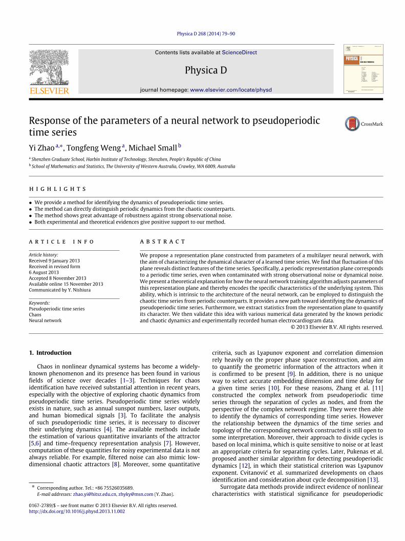
Fig. 2. Free-run prediction on periodic (a) and chaotic (c) Rössler data. The period of the periodic data is 24. The blue line represents the original signal and the dotted redline is its prediction. Panel (b) and (d) give two representation planes of neural networks for the periodic and chaotic data, respectively.

step size ⇡/8, whose period is 16. Therefore, we get 2400 periodicpoints, where the first 1950 points is selected as training data withthe rest points for testing. Fig. 1 shows the free-run prediction ofthewell-trained neural network and corresponding representationplane. By free-run prediction, we mean that the future is predictediteratively by the current and previous predicted values, in con-trast to the one-step prediction. Clearly, such a plane has a periodiccharacter, which shows the same property as the original data.

Next, we validate this method with pseudoperiodic time seriesfrom the Rössler system and Logistic map in both periodic andchaotic regimes. The Rössler system is given by x = �(y +z), y = x + ay, z = b + z(x � c), where a, b and c arecoefficients. We generate periodic and chaotic data by setting a =b = 0.1, c = 6 and a = b = 0.1, c = 9 respectively.We select 2000 successive x-component data points, in which thefirst 1800 points are used as the training data and the rest isthe test data. Fig. 2 presents the free-run prediction on the testdata by neural networks and their representation planes. FromFig. 2, it is obvious that the representation plane of the neuralnetwork exhibits a periodic shape with the same period as theoriginal data, while the representation plane of the neural network

for modeling the chaotic counterpart displays distinct irregularfluctuation. Therefore, the representation plane, which reflectsthe dynamical character hidden in the given data, shows strikingdistinction for periodic and chaotic data.

Chaotic attractors are known to be the closure of infinite setof unstable periodic orbits (UPOs) [13,29,30]. So each subset,{xi, xi+1, . . . , xi+R}N�R

i=1 , intersects a diverse set of UPOs and thuscontains segments from that set. It is impossible to make consis-tent adjustments to theweights associatedwith two ormore inputindexes given these successive input vectors, and thus the accu-mulated weight adjustments (i.e. the final weight values) appearto be irregular. On the other hand, we can say that the accumu-latedweight adjustments are robust against stochastic disturbance(noise) by taking periodic time series into consideration. As a re-sult, the accumulated weight adjustments not only eliminate thepossible coincidence or disturbance in the chaotic data but also en-hance the regular character of the periodic data.

We now examine the logistic map given by xn+1 = Cxn(1 �xn), where C is a constant. Here we set C = 3.74 and 3.60respectively to generate periodic and chaotic data. In the periodiccase with periodicity of 5 contaminated by small observational

Y. Zhao et al. / Physica D 268 (2014) 79–90 83

Fig. 3. Free-run prediction on periodic (a) and chaotic (c) Logistic data. The blue line represents the original signal and the dotted red line is the prediction. Panel (b) and(d) are corresponding representation planes of two neural networks for the periodic and chaotic data, respectively.

noise. The signal to noise ratio (SNR) of the noisy data is 22 dB. Fig. 3presents the free-run prediction on the test periodic and chaoticLogistic data by two neural networks and their own representationplanes. As shown in Fig. 3(b), the representation plane of neuralnetwork for the periodic time series takes the periodic picture,suggesting that the representation plane can reflect the noisyperiodic dynamics. Since chaotic training data usually includesvarious UPOs in the phase–space, the representation plane for thechaotic Logistic data thereby takes an irregular distribution, whichis attributed to the subtle variation between any two input subsets.

Finally, we test the utility of our approach when applied to thenonstationary data. Here, we generate a periodic nonstationarysignal consisting of 2000 data points by the Sine function plus aquadratic function. We then repeat the experiment and obtain itsfree-run prediction as well as the representation plane in Fig. 4.Apparently periodic fluctuation shown in the representation planeimplies that the considered data has periodic character, as we ex-pected. This result further suggests that our approach is also appli-cable to detect the periodic dynamics for nonstationary signals.

4. Robustness analysis

4.1. Robustness against the observational noise

The preceding simulated chaotic data can also be distinguishedfrom its periodic counterparts by means of quantitative invariants

based on the phase space reconstruction. But these criteria aresensitive to noise, and thus they may misjudge the periodicdynamics. To address the robustness of the proposed method, weadd white and colored random noise to these data, and repeatthe previous procedure. Fig. 5 illustrates the result of the periodicRössler data with observational noise (SNR = 27 dB). Fig. 6gives the free-run prediction of two neural networks and theirrepresentation planes for the periodic Logistic data contaminatedby white and colored noise with SNR = 22 dB. It indicates that,given the LM training algorithm, this newmethod can tolerate low-level noise.

The representation plane, therefore, can identify and furtherhighlight periodic characteristics, which may not be perceivedthrough the time series itself or by common quantitative criteria.Correlation dimension of the previous periodic and chaotic Rösslerdata calculated by Gaussian kernel algorithm [31] is 1.209 and1.921 respectively, and correlation dimension of the same chaoticdata contaminatedwith small noise is close to the value of periodiccounterpart. So a direct comparison of correlation dimensionvalues is rarely sufficient to differentiate the periodic time seriesfrom the chaotic counterpart.

4.2. Compared to other techniques

We now consider the application of the pseudoperiodic surro-gate (PPS) method to the previous time series as a comparison.

84 Y. Zhao et al. / Physica D 268 (2014) 79–90

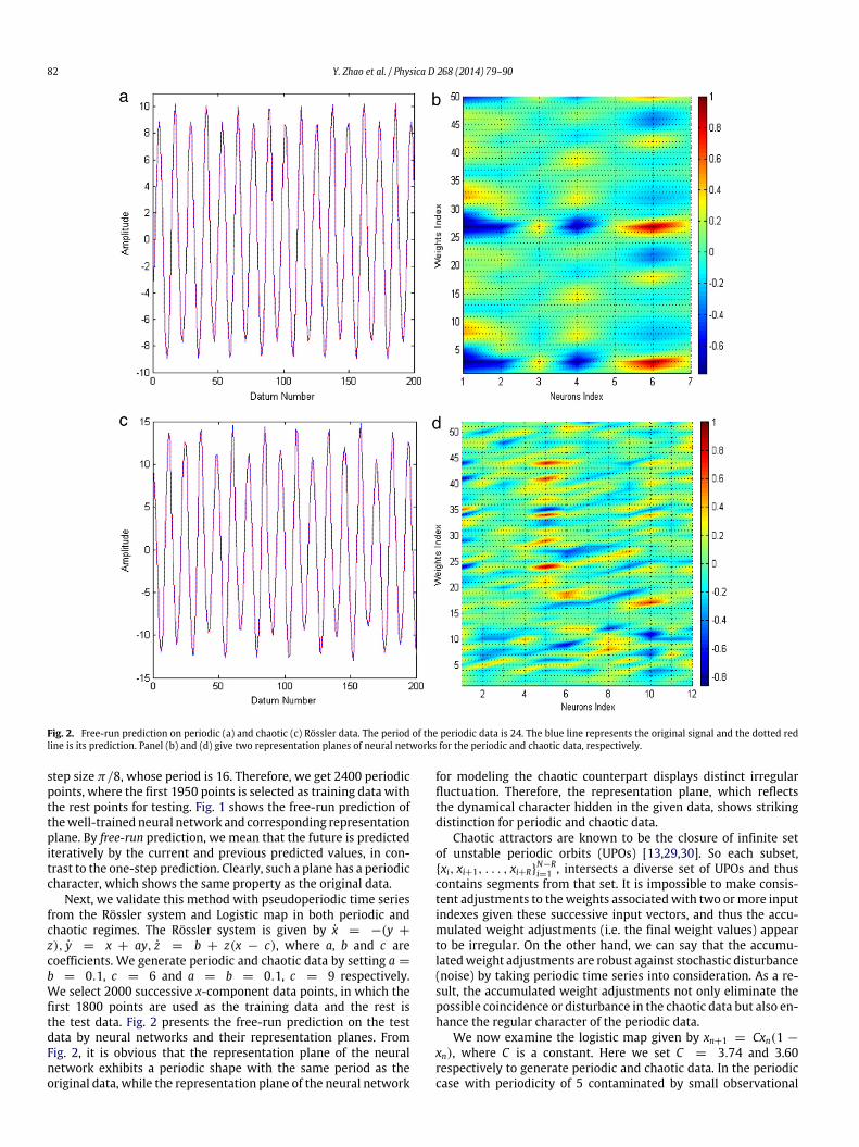
Fig. 4. Free-run prediction on nonstationary data (a) and its related representation plane (b). The blue line represents the original signal and the dotted red line is theprediction.

Fig. 5. Representation planes of periodic Rössler data contaminated by white (a) and colored (b) noise, and chaotic Rössler data contaminated by white (c) and colored (d)noise, respectively.

Y. Zhao et al. / Physica D 268 (2014) 79–90 85

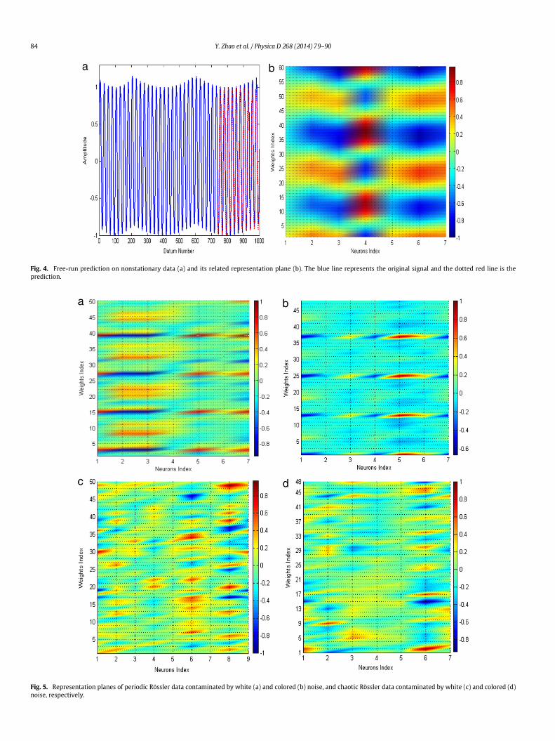
Fig. 6. Free-run prediction on periodic Logistic data contaminated by white (a) and colored (c) noise. The blue line represents the original signal and the dotted red line isthe predicted signal. Panel (b) and (d) give their corresponding representation planes.

The PPS method can test whether an observed time series is con-sistent with the periodic process contaminated by uncorrelatednoise [16]. Hence, this algorithm generates surrogate time seriesthat are both statistically similar to the original data and also con-sistent with a noise periodic or pseudoperiodic source. The pro-cess of this method is that it first reconstructs the time series intheir phase space and then randomly picks up an initial point inthe constructed phase space. The next point is then iteratively se-lected from neighbors covered by the given radius of the currentpoint. Hence, the deviation between the original data and its PPSsurrogate data is determined by this radius. When the radius in-creases gradually, such deviation will obliterate the fine dynam-ics. For example, the chaotic Rössler data can be destroyed by thesmall deviation in terms of the statistical measurements, while theperiodic orbits have to be obliterated by the larger deviation (i.e.larger radius). Different dynamics which exist in chaotic and peri-odic data lead to distinct trends of their surrogates produced by thePPS method with increasing noise radius. Trends of surrogates forchaotic andperiodic time series, therefore, are distinguishable [32].In practical realizations the surrogate generation algorithmdefinesa probability with which the next point to be chosen in the sur-rogate is not the next point of the original data. The value of the

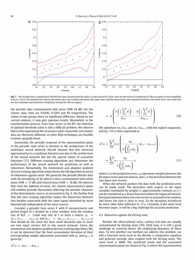
radius is deduced according to the given probability. The lowerprobability means the next point of the surrogate is the originalnext data point with higher chance (i.e. the radius is smaller), andvice versa. We apply this method to the previous periodic Rösslerdata added with white noise (SNR 26 dB) and colored noise (SNR26 dB). The statistical criterion is complexity [33]. The results arepresented in Fig. 7, where the hypothesis of periodic orbits is sig-nificantly rejected. That is, the periodic Rössler data with small ob-servational noise is rejected to be periodic data with reference tothe PPS method.

In addition, another powerful tool for the analysis andvisualization of dynamical characteristics hidden in time seriesis the recurrence plot (RP) method [34]. By transforming timeseries into the RP regime, we can measure various statisticalvalues from the RP based on recurrence quantification analysis(RQA) [35], including the percent determinism (DET), average linelength of diagonal lines (L) and the maximum diagonal line length(Lmax). Simultaneously, an amount of dynamical invariants can alsobe derived from the RP [36], such as the correlation dimension,Shannon entropy and mutual information. Here, we employ theRQA to characterize the previous periodic and chaotic Logisticdata. DET, L and Lmax are 0.9417, 9.0236 and 50 respectively for

86 Y. Zhao et al. / Physica D 268 (2014) 79–90

Fig. 7. The straight line is complexity of the Rössler data contaminated bywhite (a) and colored (b) noise; dots are themean of complexity of 100 surrogates at the probabilityfrom 0.1 to 0.9; two dashed lines denote the means plus one standard deviation (the upper line) and the meanminus one standard deviation (the lower line); two solid linesare the maximum and minimum complexity among the 100 surrogates.

the periodic data contaminated with noise (SNR 24 dB). For thechaotic data, they are 0.9249, 9.3203 and 68 respectively. Thevalues in two groups show no significant difference. Based on ourcurrent analysis, it may give spurious results. Meanwhile, in thetransformation process, from time series to the RP, the selectionof optimal threshold value is still a difficult problem. We observethat in this experiment the recurrence plots of periodic and chaoticdata are obviously different, so other RQA techniques are feasibleto better quantify them.

Essentially, the periodic response of the representation planeto the periodic time series is intrinsic to the architecture of themultilayer neural network. Hornik showed that this universalapproximation to a nonlinear function was due to the architectureof the neural network but not the special choice of activationfunctions [37]. Different training algorithms just determine theperformance of the neural network for prediction as well asrobustness. Remarkably, the momentum and adaptive gradientdescent training algorithm outperforms the LM algorithm in termsof robustness against noise. We generate the periodic Rössler datawith the periodicity of 30, which is then contaminated with whitenoise (SNR = 17 dB) and colored noise (SNR = 18 dB).We observethat with the addition of noise, the related representation planestill exhibits periodic fluctuation reflecting the periodic characterof the deterministic source, as presented in Fig. 8. We further findthat this new training algorithm makes the distinction betweentwo weights associated with the same inputs disturbed by noisetheoretically independent of the noise sources.

Consider a periodic time series X with N measurements andperiod length of L divided by a time window with the windowsize of R(R > L)and step size of 1 to form a matrix. p1 ={x1,1, x1,2, . . . , x1,N�R} and pL+1 = {xL+1,1, xL+1,2, . . . , xL+1,N�R}that should be the same but have small deviation due to noiseare two input vectors fed to the neural network. Given themomentum and adaptive gradient descent training algorithm [38],it can be observed that the final accumulated deviation of theircorresponding weight adjustment associated with p1 and pL+1 isgiven by:

�2! = �!1 � �!L+1

= �

0

BBB@

@

✓12

N�RPi=1

e2i

◆

@!1�

@

✓12

N�RPi=1

e2i

◆

@!L+1

1

CCCA. (10)

We substitute @ei/@!1 and @ei/@!L+1 with the explicit expansion,and Eq. (10) is then expressed as

�2! =N�RX

i=1

ei�

0

BBBB@@ei

@

RP

j=1!jxj,i

! (x1,i � xL+1,i)

1

CCCCA

=N�RX

i=1

ei@ei

@

RP

j=1!jxj,i

!"i (11)

where ei is the prediction error,!j represents weights between thejth input vector and oneneuron, and "i is the deviation between thetwo input row vectors.

When the network predicts the data well, the prediction errorcan be made small. The derivative with respect to the inputvariables multiplied by weights is approximately constant as f (·)can be considered as a linear function within the region of interest.Deviation between these two rowvectors is assumed to be random,and hence the sum is close to zero. So the deviation introducedby noise takes little influence to �2!. Certainly, if the noise levelbecomes larger, it will be a big challenge for accurate prediction.

4.3. Robustness against the driving noise

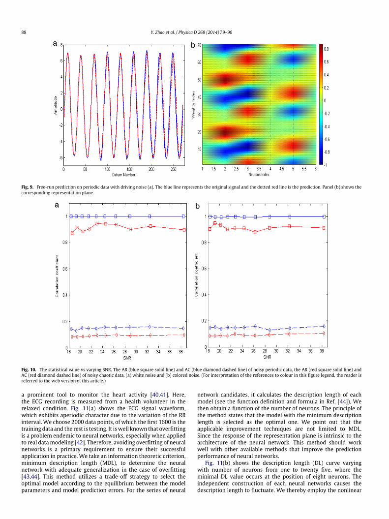
Besides the observational noise, various real data are usuallycontaminated by driving noise [39]. Until now, it is still a greatchallenge to correctly detect the underlying dynamics of thesedata. To test whether our method can address this problem, weadd a Gaussian noise term to the Rössler x-component equationand generate periodic data coupled with the driving noise. Thenoise level is 40dB. The predicted result and the associatedrepresentation plane are shown in Fig. 9, where the representation

Y. Zhao et al. / Physica D 268 (2014) 79–90 87

Fig. 8. Free-run prediction on periodic data with white noise (a) and colored noise (c). The blue line represents the original signal and the dotted red line is the prediction.Panel (b) and (d) present corresponding representation planes.

plane presents apparently periodic character, correctly reflectingthe underlying dynamics of the considered signal. The findingsuggests that the described method is feasible to identify theperiodic dynamics with weak dynamical noise.

4.4. Quantitative analysis of the representation plane

We follow the spirit of the RQA approach to extract statis-tics from the representation plane. Consider that the represen-tation plane is denoted by a weight matrix W = {!ij|i =1, 2, . . . , K , j = 1, 2, . . . , R}, where K represents the total num-ber of neurons in the hidden layer and R is the size of in-put vector. We give three statistical measurements to quan-tify the representation plane, specially, the average weight valueAW = 1

RK

PR,Ki,j=1 !ij, the average row vector similarity AR =

1R

PRi=1 maxj6=i{cov[!i,1:K , !j,1:K ]}j=K

j=1 and the average column vec-tor similarity AC = 1

K

PKi=1 maxj6=i{cov[!1:R,i, !1:R,j]}j=R

j=1, wherecov represents the cross correlation coefficient between two dif-ferent vectors. Note that given the above definition, the AR valueis equal to one for the periodic data. We employ these statistics tocharacterize the previous representation plane of the Logistic map

in both periodic and chaotic regimes. The AW, AR and AC valuesare 0.22, 1 and 0.15 respectively for the periodic data while for thechaotic data they correspondingly are 0.07, 0.88 and 0.08. Thesemeasurements provide us with a quantitative analysis of the rep-resentation plane, and can unfold the intrinsic difference betweentwo representation planes for periodic and chaotic dynamics.

In addition, we examine the robustness of the proposedstatistics against noise. Fig. 10 shows the AR and AC values versusnoise levels for the previous Logistic data. Again, AC and AR givegood quantification of the representation plane and distinguishthe periodic representation plane from the chaotic counterpartunder noise disturbance. These results further indicate that therepresentation plane captures the dynamics of the given timeseries. Note that, we omit the corresponding results for the AWmeasure since it is not robust to noise.

5. Application to human ECG data

As an example of application to practical time series, we employthe representation plane to investigate the dynamical characterof human ECG recording. The ECG recording contains abundantinformation reflecting the cardiac state, which is considered as

88 Y. Zhao et al. / Physica D 268 (2014) 79–90

Fig. 9. Free-run prediction on periodic data with driving noise (a). The blue line represents the original signal and the dotted red line is the prediction. Panel (b) shows thecorresponding representation plane.

Fig. 10. The statistical value vs varying SNR. The AR (blue square solid line) and AC (blue diamond dashed line) of noisy periodic data, the AR (red square solid line) andAC (red diamond dashed line) of noisy chaotic data. (a) white noise and (b) colored noise. (For interpretation of the references to colour in this figure legend, the reader isreferred to the web version of this article.)

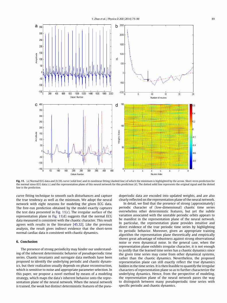
a prominent tool to monitor the heart activity [40,41]. Here,the ECG recording is measured from a health volunteer in therelaxed condition. Fig. 11(a) shows the ECG signal waveform,which exhibits aperiodic character due to the variation of the RRinterval. We choose 2000 data points, of which the first 1600 is thetraining data and the rest is testing. It iswell known that overfittingis a problem endemic to neural networks, especially when appliedto real datamodeling [42]. Therefore, avoiding overfitting of neuralnetworks is a primary requirement to ensure their successfulapplication in practice. We take an information theoretic criterion,minimum description length (MDL), to determine the neuralnetwork with adequate generalization in the case of overfitting[43,44]. This method utilizes a trade-off strategy to select theoptimal model according to the equilibrium between the modelparameters and model prediction errors. For the series of neural

network candidates, it calculates the description length of eachmodel (see the function definition and formula in Ref. [44]). Wethen obtain a function of the number of neurons. The principle ofthe method states that the model with the minimum descriptionlength is selected as the optimal one. We point out that theapplicable improvement techniques are not limited to MDL.Since the response of the representation plane is intrinsic to thearchitecture of the neural network. This method should workwell with other available methods that improve the predictionperformance of neural networks.

Fig. 11(b) shows the description length (DL) curve varyingwith number of neurons from one to twenty five, where theminimal DL value occurs at the position of eight neurons. Theindependent construction of each neural networks causes thedescription length to fluctuate. We thereby employ the nonlinear

Y. Zhao et al. / Physica D 268 (2014) 79–90 89

Fig. 11. (a) Normal ECG data and (b) DL curve (solid line) and its nonlinear fitting (dashed line) of which theminimum is highlighted by the arrow. Short-term prediction forthe normal sinus ECG data (c) and the representation plane of this neural network for this prediction (d). The dotted solid line represents the original signal and the dottedline is the prediction.

curve fitting technique to smooth such disturbances and capturethe true tendency as well as the minimum. We adopt the neuralnetwork with eight neurons for modeling the given ECG data.The free-run prediction obtained by the model exactly capturesthe test data presented in Fig. 11(c). The irregular surface of therepresentation plane in Fig. 11(d) suggests that the normal ECGdata measured is consistent with the chaotic character. This resultagrees with results in the literature [45,32]. Like the previousanalysis, the result gives indirect evidence that the short-termnormal cardiac data is consistent with chaotic dynamics.

6. Conclusion

The presence of strong periodicity may hinder our understand-ing of the inherent deterministic behavior of pseudoperiodic timeseries. Chaotic invariants and surrogate data methods have beenproposed to identify the underlying periodic and chaotic dynam-ics, but their realization usually depends on phase reconstruction,which is sensitive to noise and appropriate parameter selection. Inthis paper, we propose a novel method by means of a modelingstrategy, which maps the data’s inherent behavior onto the repre-sentation plane of the neural network. When the neural networkis trained, the weak but distinct deterministic features of the pseu-

doperiodic data are encoded into updated weights, and are alsoclearly reflected on the representation plane of the neural network.

In detail, we find that the presence of strong (approximately)periodic character of (low-dimensional) chaotic time seriesoverwhelms other deterministic features, but yet the subtlevariation associated with the unstable periodic orbits appears tobe manifest in the representation plane of the neural network.In particular, the representation plane provides intuitive anddirect evidence of the true periodic time series by highlightingits periodic behavior. Moreover, given an appropriate trainingalgorithm the representation plane theoretically and empiricallyshows great advantage of robustness against strong observationalnoise or even dynamical noise. In the general case, when therepresentation plane exhibits irregular character, it is not enoughto justify that the learned time series has a chaotic dynamics sincethe given time series may come from other dynamical systems,rather than the chaotic dynamics. Nevertheless, the proposedrepresentation plane can still exactly reflect the true dynamicshidden in the time series. It is then feasible to quantify the irregularcharacters of representation plane so as to further characterize theunderlying dynamics. Hence, from the perspective of modeling,the representation plane of the neural network paves the wayto distinguish between many pseudoperiodic time series withspecific periodic and chaotic dynamics.

90 Y. Zhao et al. / Physica D 268 (2014) 79–90

Acknowledgments

This research was funded by China National Scientific Foun-dation Grant, No. 608001014, and Scientific Foundation Grant ofGuang Dong province, China, No 9451805707002363.

References

[1] S.N. Rasband, Chaotic Dynamics of Nonlinear Systems,Wiley, New York, 1990.[2] E. Ott, T. Sauer, J.A. Yorke, Coping with Chaos: Analysis of Chaotic Data and the

Exploitation of Chaotic Systems, Wiley-Interscience, 1994.[3] G. Nicolis, C. Nicolis, Foundations of Complex Systems, World Scientific, 2007.[4] W.A. Sethares, Tatra Mt. Math. Publ. 23 (2001) 1–16.[5] K. Judd, Physica D 56 (1992) 216–228.[6] M. Small, K. Judd, A. Mees, Stat. Comput. 11 (2001) 257–268.[7] C. Capus, K. Brown, J. Acoust. Soc. Am. 113 (2003) 3253–3263.[8] N.J. Corron, S.T. Hayes, S.D. Pethel, J.N. Blakely, Phys. Rev. Lett. 97 (2006)

024101.[9] H. Kantz, T. Schreiber, Nonlinear Time Series Analysis, Cambridge University

Press, 2004.[10] L.M. Pecora, L. Moniz, J. Nichols, T.L. Carroll, Chaos 17 (2007) 013110.[11] J. Zhang, M. Small, Phys. Rev. Lett. 96 (2006) 238701.[12] K. Pukenas, K. Muckus, Electron. Electr. Eng. 8 (2007) 53–56.[13] P. Cvitanovi¢, R. Artuso, R. Mainieri, G. Tanner, G. Vattay, Chaos: Classical and

Quantum, Niels Bohr Institute, 2010.[14] J. Theiler, Phys. Lett. A. 196 (1995) 335–341.[15] K. Dolan, A. Witt, M.L. Spano, A. Neiman, F. Moss, Phys. Rev. E. 59 (1999)

5235–5241.[16] M. Small, D.J. Yu, R.G. Harrison, Phys. Rev. Lett. 87 (2001) 188101.[17] X.D. Luo, T. Nakamura, M. Small, Phys. Rev. E. 71 (2005) 026230.

[18] M. Shiro, Y. Hirata, K. Aihara, Artifical Life Robot. 15 (2010) 496–499.[19] T. Nakamura, M. Small, Phys. Rev. E. 72 (2005) 056216.[20] M.C.S. Coelho, E.M.A.M. Mendes, L.A. Aguirre, Chaos 18 (2008) 023125.[21] J.S. Walker, Not. AMS 44 (1997) 658–670.[22] M. Sifuzzaman, M.R. Islam, M.Z. Ali, J. Phys. Sci. 13 (2009) 121–134.[23] K.L. Priddy, P.E. Keller, Artifical Neural Networks: An Introduction, SPIE Press,

2005.[24] V.M. Krasnopolsky, H. Schiller, Neural Netw. 16 (2003) 321–334.[25] A. Jain, A.M. Kumar, Appl. Soft. Comput. 7 (2007) 585–592.[26] G. Sugihara, R.M. May, Nature 344 (1990) 734–741.[27] G. Cybenko, Math. Control Signals Systems 2 (1989) 303–314.[28] M.T. Hagan, M. Menhaj, IEEE Trans. Neural Netw. 5 (1994) 989–993.[29] B.R. Hunt, E. Ott, Phys. Rev. Lett. 76 (1996) 2254–2257.[30] K. Narayanan, R.B. Govindan, M.S. Gopinathan, Phys. Rev. E. 57 (1998)

4594–4603.[31] D. Yu, M. Small, R.G. Harrison, C. Diks, Phys. Rev. E. 61 (2000) 3750–3756.[32] Y. Zhao, J.F. Sun, M. Small, Internat. J. Bifur. Chaos 18 (2008) 141–160.[33] A. Lempel, J. Ziv, IEEE Trans. Inform. Theory 22 (1976) 75–81.[34] N. Marwan, M.C. Romano, M. Thiel, J. Kurths, Phys. Rep. 438 (2007) 237–329.[35] L.L. Trulla, A. Giuliani, J.P. Zbilut, C.L.Webber, Phys. Lett. A. 223 (1996) 255–260.[36] M. Thiel, M.C. Romano, P.L. Read, J. Kurths, Chaos 14 (2004) 234–243.[37] K. Hornik, Neural Netw. 4 (1991) 251–257.[38] M. Moreira, E. Fiesler, IDIAP Technical Report, 1995.[39] T. Nakamura, M. Small, Physica D 223 (2006) 54–68.[40] M. Richter, T. Schreiber, Phys. Rev. E. 58 (1998) 6392–6398.[41] U.R. Acharya, O. Faust, N. Kannathal, T.L. Chua, S. Laxminarayan, Comput.

Methods Programs Biomed. 80 (2005) 37–45.[42] D.M. Hawkins, J. Chem. Inf. Comput. Sci. 44 (2004) 1–12.[43] M. Small, C.K. Tse, Phys. Rev. E. 66 (2002) 066701.[44] Y. Zhao, M. Small, IEEE Trans. Circuits Syst. 53 (2006) 722–732.[45] R.B. Govindan, K. Narayanan, M.S. Gopinathan, Chaos 8 (1998) 495–502.