Resolution issues in numerical models of oceanic and coastal circulation
27
Continental Shelf Research 27 (2007) 1317–1343 Resolution issues in numerical models of oceanic and coastal circulation David A. Greenberg a, ,1 , Fre´de´ric Dupont b , Florent H. Lyard c , Daniel R. Lynch d , Francisco E. Werner e a Fisheries and Oceans Canada, Bedford Institute of Oceanography, Dartmouth, Nova Scotia, Canada b Que´bec-Oce´an,Universite´Laval,Que´bec,Que´bec,Canada c LEGOS, CNRS, Toulouse, France d Dartmouth College, Hanover, New Hampshire, USA e University of North Carolina, Chapel Hill, North Carolina, USA Received 1 February 2006; received in revised form 29 September 2006; accepted 9 October 2006 Available online 7 February 2007 Abstract The baroclinic and barotropic properties of ocean processes vary on many scales. These scales are determined by various factors such as the variations in coastline and bottom topography, the forcing meteorology, the latitudinal dependence of the Coriolis force, and the Rossby radius of deformation among others. In this paper we attempt to qualify and quantify scales of these processes, with particular attention to the horizontal resolution necessary to accurately reproduce physical processes in numerical ocean models. We also discuss approaches taken in nesting or down-scaling from global/basin-scale models to regional-scale or shelf-scale models. Finally we offer comments on how vertical resolution affects the representation of stratification in these numerical models. r 2007 Elsevier Ltd. All rights reserved. Keywords: Numerical ocean; Model; Resolution; Finite difference; Finite element; Coastline; Assimilation; Open boundary conditions; Topography 1. Introduction Modelling the ocean will always involve compro- mises of scale. Even with increases in computation speed and available memory, any model is subject to practical limits on its resolution. This is true for all models, not just those with fixed resolution, but also those based on mapped Cartesian coordinates such as finite difference (FD) models, or variable triangle finite element (FE) or finite volume (FV) models. Increasing the spatial resolution, i.e. making the model’s spatial grid size ðDxÞ smaller, generally increases requirements for computer storage space, memory and computation time. The increase in computational time results not only from the increased number of computation points, but also from the requirement to decrease the model time step ðDtÞ to satisfy various well known computa- tional fluid dynamic stability criteria (e.g. Richt- meyer and Morton, 1967; Roache, 1976; Haidvogel ARTICLE IN PRESS www.elsevier.com/locate/csr 0278-4343/$ - see front matter r 2007 Elsevier Ltd. All rights reserved. doi:10.1016/j.csr.2007.01.023 Corresponding author. Tel.: +1 902 426 2431; fax: +1 902 426 6927. E-mail address: [email protected] (D.A. Greenberg). 1 Manuscript prepared while on research leave at LEGOS, CNRS, Toulouse, France.
Transcript of Resolution issues in numerical models of oceanic and coastal circulation
ARTICLE IN PRESS
0278-4343/$ - see
doi:10.1016/j.csr
�Correspondifax: +1902 426
E-mail addre
(D.A. Greenber1Manuscript
CNRS, Toulous
Continental Shelf Research 27 (2007) 1317–1343
www.elsevier.com/locate/csr
Resolution issues in numerical models of oceanicand coastal circulation
David A. Greenberga,�,1, Frederic Dupontb, Florent H. Lyardc,Daniel R. Lynchd, Francisco E. Wernere
aFisheries and Oceans Canada, Bedford Institute of Oceanography, Dartmouth, Nova Scotia, CanadabQuebec-Ocean, Universite Laval, Quebec, Quebec, Canada
cLEGOS, CNRS, Toulouse, FrancedDartmouth College, Hanover, New Hampshire, USA
eUniversity of North Carolina, Chapel Hill, North Carolina, USA
Received 1 February 2006; received in revised form 29 September 2006; accepted 9 October 2006
Available online 7 February 2007
Abstract
The baroclinic and barotropic properties of ocean processes vary on many scales. These scales are determined by various
factors such as the variations in coastline and bottom topography, the forcing meteorology, the latitudinal dependence of
the Coriolis force, and the Rossby radius of deformation among others. In this paper we attempt to qualify and quantify
scales of these processes, with particular attention to the horizontal resolution necessary to accurately reproduce physical
processes in numerical ocean models. We also discuss approaches taken in nesting or down-scaling from global/basin-scale
models to regional-scale or shelf-scale models. Finally we offer comments on how vertical resolution affects the
representation of stratification in these numerical models.
r 2007 Elsevier Ltd. All rights reserved.
Keywords: Numerical ocean; Model; Resolution; Finite difference; Finite element; Coastline; Assimilation; Open boundary conditions;
Topography
1. Introduction
Modelling the ocean will always involve compro-mises of scale. Even with increases in computationspeed and available memory, any model is subject topractical limits on its resolution. This is true for allmodels, not just those with fixed resolution, but also
front matter r 2007 Elsevier Ltd. All rights reserved
.2007.01.023
ng author. Tel.: +1902 426 2431;
6927.
g).
prepared while on research leave at LEGOS,
e, France.
those based on mapped Cartesian coordinates suchas finite difference (FD) models, or variable trianglefinite element (FE) or finite volume (FV) models.Increasing the spatial resolution, i.e. making themodel’s spatial grid size ðDxÞ smaller, generallyincreases requirements for computer storage space,memory and computation time. The increase incomputational time results not only from theincreased number of computation points, but alsofrom the requirement to decrease the model timestep ðDtÞ to satisfy various well known computa-tional fluid dynamic stability criteria (e.g. Richt-meyer and Morton, 1967; Roache, 1976; Haidvogel
.

ARTICLE IN PRESSD.A. Greenberg et al. / Continental Shelf Research 27 (2007) 1317–13431318
and Beckmann, 1999; Kantha and Clayson, 2000;Lynch, 2005). For surface gravity wave problemspropagating in a region of depth h, explicit in timecomputations are limited by the CFL stabilityrequirement (DtoDx=
ffiffiffiffiffigh
p, where g is the gravita-
tional acceleration andffiffiffiffiffigh
pis the gravity wave
speed) and implicit in time computations are limitedby the Courant condition (vDtoDx, where v is thefluid velocity).
The scales important to an accurate numericalsolution of a problem are not generally uniformover the domain of a model. Changes in bottomtopography and coastline over small scales, as wellas the presence of density fronts, eddies, etc., canhave a critical influence over the processes through-out a domain that determine the required resolu-tion. Similarly, if regular spacing in latitude andlongitude is used in an ocean model covering higherlatitude seas, the contraction of longitude linestowards the poles leads to distorted grid cells anddifferent resolved scales in the north–south versuseast–west directions.
In this paper we review certain aspects of spatialresolution requirements of oceanic circulation mod-els and the approaches taken in specific applica-tions. An issue related to the problem of resolutionthat we feel needs to be addressed first is theproblem of open boundary conditions and nestedgrids. These arise when the small spatial scalesaddressed by regional models necessitate the trun-cation of larger domains, despite the large increasein computing power seen in the last four decades.Nested and variable resolution models are oftenpart of the solution (Section 2). The second issue weaddress is the importance of properly resolvingsmall channels and sills connecting larger bodies ofwater (Section 3). The third aspect is related toresolution problems found in models employingstructured grids in resolving coastlines, i.e. the so-called staircase problem (Section 4). The fourthaspect is related to the bottom topography whichneeds to be accurately represented to properlysimulate wave speed, steep slope processes andobstructions to flow (Section 5). Fifth, we discusshow resolving the baroclinic Rossby radius influ-ences model solutions at basin-scales with anexample of the North Atlantic (Section 6). Sixth,we present how data assimilation can yield mislead-ing results when the important physical propertiesare not spatially resolved (Section 7). Seventh, wehighlight aspects of mesh generation techniquespresently used to prescribe model resolution re-
quirements (Section 8). And finally, we look at someof the factors that make it difficult to resolvevertical ocean dynamics (Section 9). In our sum-mary, we make a list of factors we suggest need tobe considered in determining the resolution ofcirculation models (Sections 10 and 11).
2. Open boundaries and nested grids
The study of open boundaries and nesting meshesencompasses much more material than couldreasonably be included in this review. Here we limitour discussion to pointing out different importantaspects of the subjects and giving some entry pointsto the literature.
The treatment of open boundaries is an importantissue, indirectly related to the models’ resolutionrequirements. While numerical models of coastaland shelf regions may be capable of capturingdetails of the flow in domains of interest, theycannot afford to explicitly include the simultaneoussolution of the larger neighboring basin-scaledomain at appropriate levels of resolution. Simi-larly, basin-scale models cannot easily or affordablydownscale to resolve the coastal regions. Presently,common practice is either to impose open boundaryconditions on the regional models that allow foroutward non-reflecting radiation of the computedsolution (e.g. Orlanski, 1976; Chapman, 1985),implement ‘‘sponge-layers’’ along the open bound-aries where the outward propagating signals aredissipated without reflection (e.g. Foreman et al.,2000), impose direct forcing on the open boundaryfrom observations (e.g. Greenberg, 1979), or insome cases a combination of these (e.g. Flather,1981; Werner et al., 1993b). Alternatively, boundaryconditions extracted from basin-scale models areused to force (Hermann et al., 2002) or to providebest-prior estimates for the regional model (e.g.Lynch et al., 2001). An expanded domain usingvariable resolution, mapped coordinates (e.g. Haid-vogel et al., 1991) or nested grids (e.g. Oey andChen, 1992; Greenberg, 1979) is often used tofurther isolate the boundary effects from the corearea, although nesting needs to be treated carefully(Davies and Hall, 2002). A different approach toconsidering the unmodelled ocean is taken inGarrett and Greenberg (1977) and Garrett andToulaney (1979) where Green’s functions are usedto integrate model predictions with Platzman’s(1975) normal modes for the Atlantic Ocean. Thisproduced a correction to the computations done

ARTICLE IN PRESS
Model Boundary
Real Boundary
Discretized strait
Real strait
Fig. 1. Effect of a poor resolution on the geometry of a strait.
This one is widened by about 100%. Straits are of great
importance because they control the exchange of water between
ocean basins.
x
xy
y
yz
Fig. 2. Depending on the numerical scheme used, under-resolved
channels in both finite element (below) and finite difference
(above) schemes have problems representing simultaneously the
depth and the cross-sectional area (center) leading to inaccurate
determination of the transport.
D.A. Greenberg et al. / Continental Shelf Research 27 (2007) 1317–1343 1319
within the limited model domain and error estimatesfor remaining uncertainties.
The treatment of open boundaries in limited-domain models has been a persistent theme in oceanmodelling (Orlanski, 1976; Camerlengo andO’Brien, 1980; Flather, 1981; Roed and Smedstad,1984; Blumberg and Kantha, 1985; Chapman, 1985;Johnsen and Lynch, 1995; Lynch and Holboke,1997; Palma and Matano, 1998; Penduff et al., 2000;Davies et al., 2003; Blayo and Debreu, 2005).Methods advanced in these papers have been fairlysuccessful in keeping disturbances generated withinthe domain from reflecting at the boundaries andcontaminating the solutions. However, care has tobe taken to treat transient, oscillating and steadycomponents correctly. Transient and periodic sig-nals are often treated in some form of radiationcondition that needs an outgoing speed for thecomponent crossing the boundary. Steady and low-frequency components are frequently dealt with byconsidering across boundary gradients of elevationor currents that are in near geostrophic balance (e.g.Lynch et al., 1992; Werner et al., 1993a).
None of the above techniques will account fortrue interaction with the ocean outside the modeldomain or for forcing on the exterior ocean (e.g.meteorology) that will impact the boundary of thedomain. The study of Hayashi et al. (1986)addressed the question of boundary influences onsteady wind driven circulation in coastal oceanmodels. They showed that influences from anupstream boundary (in the sense of a shelf-wave),can be significant throughout the model and thatassuming an infinite shelf upstream implies anunrealistic length of uniform shelf adjacent to thatboundary.
The further the open boundary is from the area ofinterest, the less impact it will have on the desiredsolutions due to later arrival and increased dampingin transit of errors propagated. Variable resolutionand nested mesh models are often used to accom-plish this. This is done by using a graded mesh of(usually triangular) elements where large elements inthe far-field grade ‘‘smoothly’’ into the more highlyresolved region of interest. Another approach isto use assimilation. By using assimilation techni-ques, boundary conditions as well as modelparameters can be inferred using available data.This can be very powerful in hindcasting andnowcasting and with care, in prediction. Howeveras will be shown in Section 7, this approach is notwithout pitfalls.
3. Channels and sills
Accurate representation of channels and sills thatconnect different bodies of water within a modeldomain is of critical, even fundamental, importanceto obtaining meaningful simulations. In limitingsituations of Cartesian discretization only oneor two grid cells are available to describe a strait(Fig. 1). In this situation, the strait width must takevalues in a set of discrete numbers at the price ofmisrepresenting the width. (A different aspect ofshoreline resolution is dealt with in Section 4.)
Even when the model coastline has a better fit,but is represented with minimal resolution (Fig. 2),it is difficult to simultaneously compute theappropriate water depth and cross-sectional area

ARTICLE IN PRESSD.A. Greenberg et al. / Continental Shelf Research 27 (2007) 1317–13431320
correctly, leading to errors in phase speed and/ortransport. As an example, in the Canadian ArcticArchipelago, Kliem and Greenberg (2003) foundthat the smaller channels make a significantcontribution to the transport from the Arctic tothe North Atlantic (Fig. 3). This requires resolutionof order 1 km in a domain that spans 2000–3000 km.
The importance of resolution is also illustrated incases where partially enclosed seas are linked to theocean through restricted channels. Lake Maracaibo,in Venezuela, is an example of such a system. Thelake is joined to the Gulf of Venezuela throughnarrow natural (and now also dredged) channelsthrough Tablazo Bay and the Maracaibo Strait. Tomodel the tides in this region, Molines et al. (1989)used three grids (one each for the Gulf of Venezuela,Tablazo Bay and Lake Maracaibo), with differentmesh sizes and orientations, run independently, butusing common tidal boundary conditions derivedfrom observations. The system’s tidal responseobtained by Molines et al. (1989) was a compositeof the three grids’ solution, and found to quantita-tively agree with observations only if different
Fig. 3. In the Arctic Archipelago, Kliem and Greenberg (2003) found sig
Strait (bottom) and Hellgate (top) channels.
values of the bottom drag coefficient were specifiedin the various model sub-domains. Using a series ofharmonic and time stepping FE models, Lynch andWerner (1987, 1991) and Lynch et al. (1990)considered tidal and baroclinic processes. Theirmodel was able to concentrate high (and variable)resolution through the narrow straits, recoveringthe system’s tidal response without requiring thatdifferent bottom drag coefficients be imposed.Lynch et al. (1990) showed that decoupling theGulf from the Bay and the Lake produced afundamentally different result for each sub-domain,than if the system were run as one single unit, thusestablishing the importance of the explicit inclusionand resolution of the channels connecting the Gulfand Lake. A comprehensive study of exchange inthe system was carried out by Laval et al. (2003)employing a FD model. To accommodate thevariation in scales, they used some geometricstraightening of the bathymetry to align with themesh, and used a stretched computational gridfocusing on the narrows. This permitted resolutionas fine as 250m and as large as 6 km. With this
nificant transport through the minimally resolved Fury and Hecla
ARTICLE IN PRESSD.A. Greenberg et al. / Continental Shelf Research 27 (2007) 1317–1343 1321
model configuration they were able to produce agood picture of the balance between barotropic andbaroclinic processes.
A situation physically similar to Lake Maracaibois seen in the Bras d’Or Lakes, Nova Scotia,Canada. The Lakes are connected to the CabotStrait and Atlantic Ocean via a shallow narrowpassage. Within the Lakes, various basins areseparated by sills and constrictions. Petrie (1999)and Petrie and Bugden (2002) have demonstratedthat the frictional effects of the constricted channelseffectively damp the diurnal and semi-diurnal tidalfrequencies, but the longer period motions, mostlymeteorological, originating outside the Lakes,propagate into the system largely unaffected. Tidalmixing is important to the observed hydrography.Dupont et al. (2003a) constructed a FE tidal modelof the Lakes producing detailed solutions for fiveconstituents, although some of the comparisonswith the observations were not good, possibly dueto short records and other data problems. Ofinterest, Petrie’s (1999) simple model combiningone-dimensional FD sections with rectangularbasins gave a good qualitative picture of theresponse characteristics, damping the high frequen-cies and letting low frequency signals pass withminimal effect.
Whitehead (1998) identifies many deep passagesand straits important to global ocean circulation. Byconsidering the balance of the forces of pressure,Coriolis and inertia, together with hydrographicdata, he was able to obtain a ‘‘crude firstapproximation’’ of some inter-basin fluxes. He feltthat more realistic bathymetry is needed for betterprecision and posed several questions that should beaddressed to better understand the local dynamicsand therefore the larger picture. Similarly, Gille etal. (2004) commented on the problems ocean
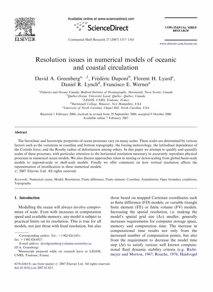
Fig. 4. Effect of the rotation on the discretization of a square domain
occur along the walls.
models have reproducing dense water overflowsand the need for high-resolution bathymetry toaccurately simulate them. They noted two areas, theMid-Atlantic Ridge and the Indonesia Seas, whereobservations indicated fine scale processes leadingto inter-basin exchange and found in some criticalpassages there have been no bathymetric surveys.Metzger and Hurlburt (2001) showed that whenmodelling the South China Sea at 1=16� resolution,the inclusion of two shoals represented by indivi-dual topography grid points, had a major impact onthe circulation through the Luzon Strait.
4. Resolving the coastline: the staircase problem
Some of the early studies advancing our funda-mental understanding of large scale ocean dynamicswere based on simple, most often rectangular,geometric forms—whereas the true basin geometryand coastline are more complicated. In FD models,the complexity of the geometry translates into theoccurrence of steps along the discretized domainanywhere the orientation of the boundary does notcorrespond to that of the grid (Fig. 4). We hereafterlimit ourselves to the case of the occurrence of stepsalong the lateral boundaries of the model.
It is important to note that for circular or smoothgeometries it is possible to use curvilinear grids forFD methods and hence, avoid the occurrence ofsteps along the boundaries. Curvilinear grids canbetter fit irregular coastlines and can provide somevariable resolution capabilities, such as implemen-ted in the POM (Blumberg and Herring, 1987) andSPEM (Song and Haidvogel, 1994) models. How-ever, for a realistic representation of lateral bound-aries, step-like features would still appear sincecurvilinear grids only accommodate the large scalefeatures of the coastline.
Real Boundary
Model Boundary
. When the sides are not aligned with the axes, step-like features

ARTICLE IN PRESSD.A. Greenberg et al. / Continental Shelf Research 27 (2007) 1317–13431322
We first review the propagation of Kelvin wavesin a rotated square basin. Then we review conver-gence problems found in the typical wind drivenMunk problem but in a rotated square basin.Finally we show convergence rates for a winddriven circulation in a circular basin, for which ananalytical solution can be derived.
4.1. The shallow water equations
We propose to solve idealized shallow water (SW)equations. While these equations are considerablysimplified compared to the primitive equations, thedynamical processes involved in the formation ofwind-driven circulation and the interaction withirregular coastlines are similar enough that we canrestrict ourselves to these equations as an introduc-tory study. The equations are
qtuþ u � =uþ f k� uþ g=Z ¼s
hþ nr2u, ð1Þ
qtZþ = � ðuhÞ ¼ 0, ð2Þ
where symbols are defined in Table 1. Theseequations correspond to a Boussinesq, hydrostatic,homogeneous ocean in which we assume that thereis no vertical structure, reducing the real three-dimensional (3D) problem to a simpler two-dimen-sional (2D) problem. The acceleration due togravity is here reduced with the goal of mimickingthe first baroclinic mode dynamics, i.e. the dynamicsof the upper layer of the ocean. The interlayer stressis taken to be zero, therefore no drag or bottomfriction appears in Eq. (1). The wind stress s is theonly external forcing applied.
4.2. Kelvin wave propagation along a steplike wall
From theoretical arguments, Mysak and Tang(1974) showed that Kelvin waves can be retarded by
Table 1
Definition of variables in Eqs. (1) and (2)
ðx; y; zÞ The coordinate system (east, north, upward)
u ¼ ðu; vÞ Vertically averaged velocity
Z Elevation of the water surface taken from rest
hb Depth of the undisturbed water
h ¼ Zþ hb Total depth of water
k ¼ ð0; 0; 1Þ Unit vector in the vertical
= Horizontal gradient operator
f ¼ f 0 þ by Coriolis parameter, f 0 and b defined at 45�
n Dynamic eddy viscosity
s ¼ ðtx; tyÞ Wind stress in m2 s�2
irregularities along a coastline. The effect is strongerfor larger scale irregularities and not very significantfor small scales. Pedersen (1996) studied theinfluence of steps on gravity waves and found thisretardation effect at coarse resolution. This effectwas also noted in circular lakes by Beletsky et al.(1997) for different kinds of staggering of the gridand vertical representations. Using different hier-archy of ocean models, Schwab and Beletsky (1998)found the same for Kelvin waves, the effectdiminishing with higher resolution. These resultsare reproduced in Fig. 5 using a SW C-grid modelbased on Sadourny (1975). Four grids in total wereused: two grids with no rotation of the basinshowing no step along the boundaries at 10 and5 km resolution and two grids with a 30� rotation ofthe basin relative to the discretization axes showingsteps along the walls at also 10 and 5 km resolution.The finding that higher resolution decreases theretardation effect is consistent with the idea thatKelvin waves should not be sensitive to coastlinedetails, at scales small compared to the Rossbyradius of deformation. In Fig. 5, for the highestresolution runs (5 km), the retardation effect is stillnoticeable but it is much weaker compared to theruns at 10 km resolution. Since the radius ofdeformation is 31 km in these runs, these resultsimply that we should resolve the Rossby radius withabout 10 points (when using a second-orderformulation). One consequence for modelling theocean is that the fast modes of an ocean basin (theKelvin modes) will be misrepresented, especially ifthe model resolution is coarse. Therefore, transientresponses of the ocean, such as the El Nino Kelvinwave along the Western America may be retarded,which may have consequences on the period ofoccurrences of El Nino events according to thedelayed oscillator theory (Schopf and Suarez, 1988).For instance, in the study of Soares et al. (1999),there are only two points to represent the Rossbyradius of deformation at 20� North.
In the context of the Munk problem, it is notclear how retarded Kelvin waves affect the steadystate of the ocean. We propose to further investigatethese issues in the context of the single gyre Munkproblem in the next section.
4.3. Single gyre Munk problem in presence of
steplike walls
In the classic single gyre Munk circulation with aconstant wind, the sphericity and rotation of the

ARTICLE IN PRESS
a
c
b
d
Fig. 5. Elevation field for the Kelvin retardation problem in the presence of steps along the walls at two different resolutions. a represents
the rotation angle of the grid relative to the discretization axes. (a) 10 km, a ¼ 0; (b) 10 km, a ¼ 30�; (c) 5 km, a ¼ 0; (d) 5 km, a ¼ 30�. The
dashed line is the �0:01m contour, the solid lines are contours from 0.1 to 1.0m with an increment of 0.1m.
D.A. Greenberg et al. / Continental Shelf Research 27 (2007) 1317–1343 1323
earth yield a strong return flow along the westernwall (tx ¼ �10
�4 sinðpðy=LyÞÞ and ty ¼ 0). Theenergy put into the ocean by the winds is dissipatedmainly in a viscous sublayer along the boundarybecause of the strong return flow there. A strongrecirculation forms in the northwestern part of thedomain, evidence of the non-linear effects in thesolution.
Cox (1979), in the broader context of thecirculation of the Indian Ocean, implemented somerotating experiments which showed that under no-slip boundary condition the circulation is notsignificantly modified by the presence of steplikewalls. Adcroft and Marshall (1998), hereafter AM,conducted a thorough study of the impact of
steplike walls for the single gyre Munk problem inpresence of no-slip or free-slip dynamical boundaryconditions using a C-grid SW model. Their resultsessentially confirmed Cox’s results that the hor-izontal circulation under the no-slip boundarycondition is not very sensitive to the presence ofsteps along the coastline. This may be explained bythe fact that the core of the boundary current underno-slip is located a few grid points inside the interiorof the basin.
For free-slip, however, they compared resultsfrom non-rotated and rotated square basin experi-ments and showed the circulation to be highlysensitive to the presence of steps along the walls. Inrotated basin experiments, the basin was rotated

ARTICLE IN PRESSD.A. Greenberg et al. / Continental Shelf Research 27 (2007) 1317–13431324
relative to the grid axes (see Fig. 4), but the windforcing and north–south axis were kept constantrelative to the basin, so that the only differencesbetween the experiments are due to the discretiza-tion. The presence of steps along the boundarytends to reduce the strength of the circulation to theextent that results obtained using free-slip boundaryconditions with step-like boundaries more closelyresemble those with no-slip boundary conditionsthan free-slip solutions without steps.
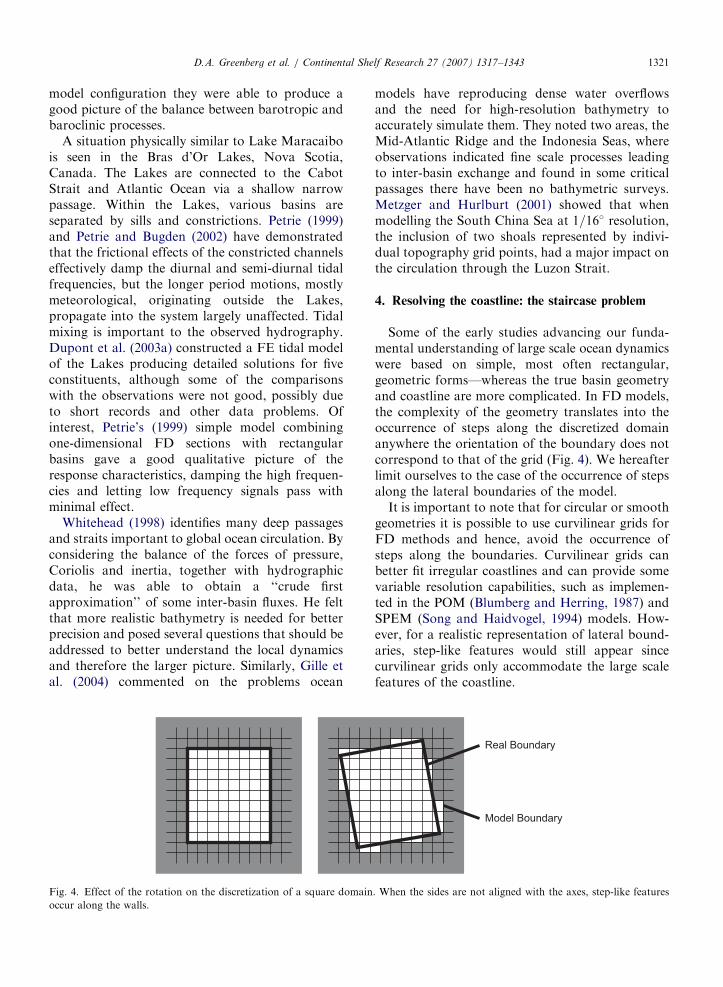
Moreover, they showed that, at least for smallrotation angles, sensitivity to steps under free-slipconditions could be greatly reduced by using avorticity–divergence formulation of the viscousstress tensor (Madec et al., 1991) instead of theconventional five-point Laplacian operator. Thetwo tensor formulations are equivalent in a non-rotated basin, but are different in presence of steps.Around steps, the vorticity–divergence formulationtends to accelerate the fluid parcels compared to theconventional stress formulation. Fig. 6 reproducesthe basic ideas of AM after 6 years of integrationfrom rest. The combinations are for the FD modelwith the enstrophy conserving advective scheme ofSadourny (1975) and with, respectively (A) theconventional stress tensor (five-point) and (B) thevorticity–divergence stress tensor of Madec et al.(1991). The figure shows the elevation fields for theA and B cases and for no rotation and a smallrotation angle of 3:4�. Clearly, the A case showscirculation patterns collapsing as the number ofsteps along the walls increases whereas, for the Bcase, the circulation is quite similar to the originalnon-rotated circulation.
Dupont et al. (2003b) investigated further theproblem by computing vorticity budgets for thewhole basin in presence of steplike walls. Thenumerical budget is actually not defined up to themodel coastline due to the large footprint of themodel vorticity equation used in the C-grid stagger-ing. Without going into excessive detail, this meansthe model vorticity budget allows for some advec-tive flux to leave or enter the domain. This advectiveflux can then be used as a measure of theconvergence of the model since it usually tends tozero in non-rotated domains following the discreti-zation order given by the vorticity (1 for a second-order accurate FD model). However, due to theincreased number of steps and the high value of theadvective flux around steps, it is no longer obviousthat the advective contribution to the vorticitybudget goes to zero as the resolution is increased
in rotated square basins. They found that combina-tion A (and other combinations) do not showevidence of convergence, contrary to combinationB. In the latter case, the convergence order of theadvective contribution is close to one (the maximumallowable for vorticity in a primitive second-orderFD model, and by extension any residual present inthe vorticity budget of such a model) irrespective ofthe rotation angle but with the curve shifted tolarger values.
The effect of staircases on the coastal dynamicscan also be felt via the appearance of spuriousvorticity/divergence extrema. Spiky vorticity/diver-gence may imply spurious local upwelling/down-welling. Dupont et al. (2003b) discussed therelevance of their results in the perspective of 3Dmodelling. One application is to large scale z-levelmodels where the lateral walls can be significant (forinstance at a sharp shelf slope between a shallowshelf and a deep ocean) and may be sufficient for themechanism introduced herein to dominate even inthe presence of a whole variety of other physicalprocesses. Section 9 examines further, the problemof representing the local dynamics in the presence oflateral and vertical staircases, which may wellexplain the relative difficulty z-level models havein representing some slope dynamics (Mellor et al.,2002).
4.4. An inviscid wind-driven circulation in a circular
domain
A linear analytical solution can be found for thewind-driven problem in a circular domain withCoriolis forces and damped by a linear bottomfriction. No viscosity is included. There is a no-normal flow condition at the model boundary andthe wind forcing is similar to the Munk gyre case.The steady state for the linearized SW solution inpolar coordinates is
Z ¼W
4gHRxy (3)
and with Coriolis force:
Z ¼Wf
RgHkR2
8þ
1
4
kf
xy� ðx2 þ y2Þ
� �� �. (4)
We perform a one year run from rest for all modelswith windstress, W ¼ 10�4 m2 s�2, f ¼ 10�4 s�1 orzero, g ¼ 10�2 m s�2, the basin radius, R ¼ 500�103 m, uniform depth, H ¼ 1000m and linearbottom friction coefficient k ¼ 10�3 s�1. This is
ARTIC
LEIN
PRES
S
0
0
100200
300
400
A,B 20 km
0
0
100
100
200
A 20 km
0
0
100
200
300
400
A,B 10 km
0
0
100
100200
A 10 km
0
0
100
200
300
400
B 20 km
0
0
100
200
300
400
B 10 km
Fig. 6. Layer thickness in meters after a 6 year spin-up for 20 and 10 km resolution. Shown are results from the A and B combination (see text) with or without a 3:44� rotation angle of
the basin. Note that the B case tends to resemble the A,B case with no rotation, but the A case does not.
D.A
.G
reenb
erget
al.
/C
on
tinen
tal
Sh
elfR
esearch
27
(2
00
7)
13
17
–1
34
31325

ARTICLE IN PRESS
0.0001
0.001
0.01
0.1
1
1 10 100
Norm
aliz
ed e
rror
in e
ta
Resolution (number of points in the x-direction)
slope 2
C-grid FD
LW
HT
PZM
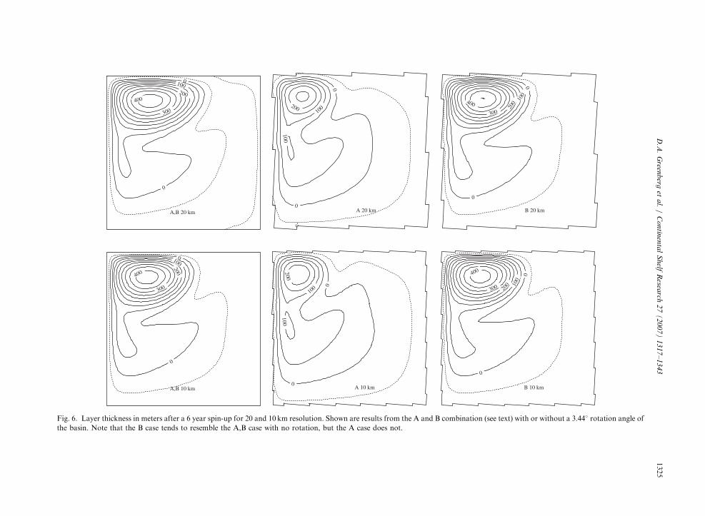
Fig. 8. Convergence with resolution of the normalized elevation
error in a circular domain for three FE models (LW, HT, PZM)
and the C-grid FD for comparison.
D.A. Greenberg et al. / Continental Shelf Research 27 (2007) 1317–13431326
enough to converge to a steady state. The normal-ized error is computed as
EðZmod Þ ¼
R RjZmod � ZjdxdyR R
dxdy
ffiffiffiffiffiffiffiffiffiffiffiffiffiffiffiffiffiffiffiffiffiffiffiffiR RdxdyR R
Z2 dxdy
s. (5)
We first analyze the results from the C-grid model.For brevity, we only show the results for one case,at f ¼ 0, since convergence properties are notsignificantly different than those at fa0. Fig. 7shows the convergence of the normalized error in Zwith increasing resolution. It appears that theconvergence order of the C-grid FD model is closerto one (1.1 when f ¼ 0 and 1.3 when f ¼ 10�4 s�1)than two, the maximum for this second-order FDformulation.
We also consider the solution from a fourth-orderA-grid model (Dietrich, 1998). The original for-mulation, hereafter O-FDM4, however, uses sec-ond-order numerics close to the boundary. Amodified version, R-FDM4, remains fourth-orderby use of non-centered operators in the vicinity ofthe walls for derivatives oriented perpendicular tothe walls. This modification was motivated by moreaccurate (and depending on the test-case, morestable) results when using this fourth-order exten-sion. We now compare the solution from the C-gridFD model with the O-FDM4 and R-FDM4 models.Fig. 7 shows that the order of the A-grid model isactually less than two in the presence of step-likewalls. Furthermore, there is no longer a difference,in terms of truncation order, between the second-order C-grid and the fourth-order A-grid models—
0.0001
0.001
0.01
0.1
1
10 100 1000
Norm
aliz
ed e
rror
in e
ta
Resolution (number of points in the x-direction)
slope 1
slope 2
Cgrid FD
O-FDM 4
R-FDM 4
Fig. 7. Convergence with resolution of the normalized elevation
error for the second order C-grid FD, O-FDM4 and R-FDM4
models in a circular domain.
unlike the case with straight walls. Therefore, thepresence of steps along irregular boundaries has adetrimental effect on the accuracy of high order FDformulations if the flow is allowed to slip along thewalls.
We now compare three FE models to the C-gridmodel. This first FE model (Lynch and Werner,1991) is based on equal order basis functions forpressure and velocity (also known as P12P1Þ and onthe generalized wave equation, hereafter referred asthe LW model. The second (Hua and Thomasset,1984) is based on non-conformal basis function forvelocity (also known as PNC
1 2P1), hereafter referredas the HT model. The last (Peraire et al., 1986) isbased on a Taylor–Galerkin approximation using aP12P1 approach, hereafter referred as the PZMmodel. In this circular geometry, all FE models havethe advantage that the representation of theboundary improves as the resolution is increased.Therefore, it should be possible to observe conver-gence order close to two. Fig. 8 shows that all FEmodels have a convergence rate close to second-order. Hence in terms of accuracy, all FE modelsappear to perform better than FD models in non-rectangular geometries for linear inviscid problems.
5. Bottom topography and slope
5.1. The open ocean
The most elementary numerical considerationslead one to conclude that resolution of the operativehorizontal wavelength must be respected. In SW
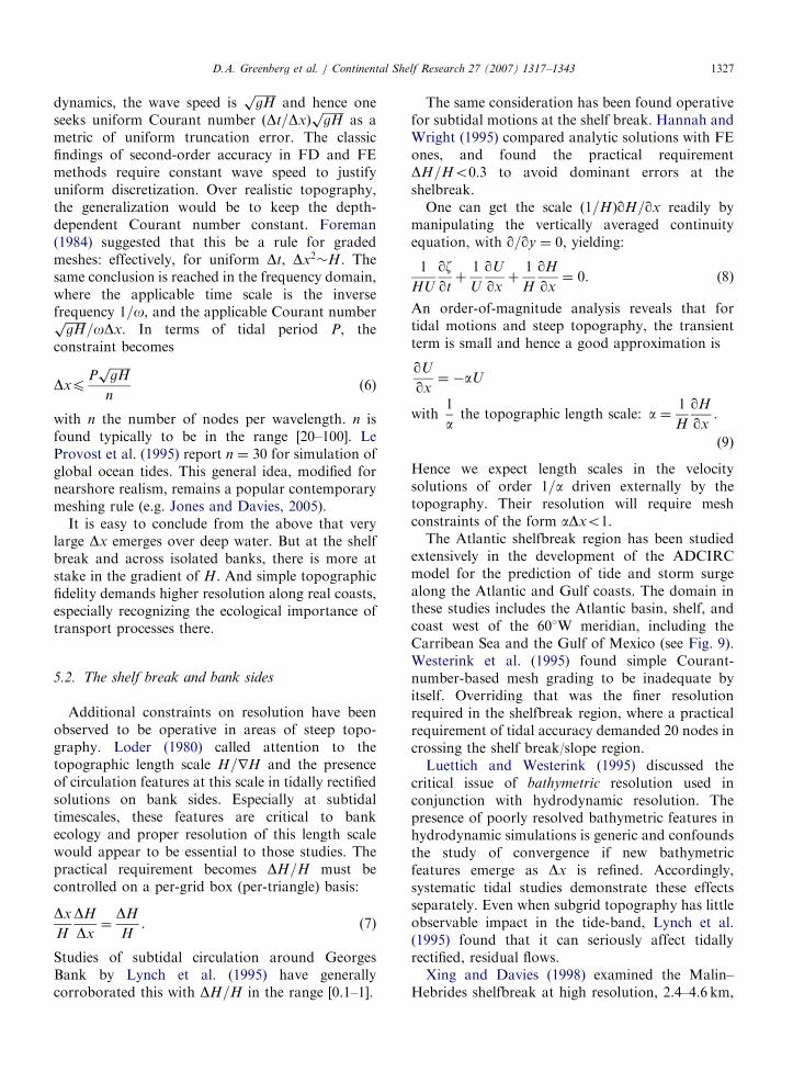
ARTICLE IN PRESSD.A. Greenberg et al. / Continental Shelf Research 27 (2007) 1317–1343 1327
dynamics, the wave speed isffiffiffiffiffiffiffigHp
and hence oneseeks uniform Courant number ðDt=DxÞ
ffiffiffiffiffiffiffigHp
as ametric of uniform truncation error. The classicfindings of second-order accuracy in FD and FEmethods require constant wave speed to justifyuniform discretization. Over realistic topography,the generalization would be to keep the depth-dependent Courant number constant. Foreman(1984) suggested that this be a rule for gradedmeshes: effectively, for uniform Dt, Dx2�H. Thesame conclusion is reached in the frequency domain,where the applicable time scale is the inversefrequency 1=o, and the applicable Courant numberffiffiffiffiffiffiffi
gHp
=oDx. In terms of tidal period P, theconstraint becomes
DxpPffiffiffiffiffiffiffigHp
n(6)
with n the number of nodes per wavelength. n isfound typically to be in the range [20–100]. LeProvost et al. (1995) report n ¼ 30 for simulation ofglobal ocean tides. This general idea, modified fornearshore realism, remains a popular contemporarymeshing rule (e.g. Jones and Davies, 2005).
It is easy to conclude from the above that verylarge Dx emerges over deep water. But at the shelfbreak and across isolated banks, there is more atstake in the gradient of H. And simple topographicfidelity demands higher resolution along real coasts,especially recognizing the ecological importance oftransport processes there.
5.2. The shelf break and bank sides
Additional constraints on resolution have beenobserved to be operative in areas of steep topo-graphy. Loder (1980) called attention to thetopographic length scale H=rH and the presenceof circulation features at this scale in tidally rectifiedsolutions on bank sides. Especially at subtidaltimescales, these features are critical to bankecology and proper resolution of this length scalewould appear to be essential to those studies. Thepractical requirement becomes DH=H must becontrolled on a per-grid box (per-triangle) basis:
Dx
H
DH
Dx¼
DH
H. (7)
Studies of subtidal circulation around GeorgesBank by Lynch et al. (1995) have generallycorroborated this with DH=H in the range [0.1–1].
The same consideration has been found operativefor subtidal motions at the shelf break. Hannah andWright (1995) compared analytic solutions with FEones, and found the practical requirementDH=Ho0:3 to avoid dominant errors at theshelbreak.
One can get the scale ð1=HÞqH=qx readily bymanipulating the vertically averaged continuityequation, with q=qy ¼ 0, yielding:
1
HU
qzqtþ
1
U
qU
qxþ
1
H
qH
qx¼ 0. (8)
An order-of-magnitude analysis reveals that fortidal motions and steep topography, the transientterm is small and hence a good approximation is
qU
qx¼ �aU
with1
athe topographic length scale: a ¼
1
H
qH
qx.
ð9Þ
Hence we expect length scales in the velocitysolutions of order 1=a driven externally by thetopography. Their resolution will require meshconstraints of the form aDxo1.
The Atlantic shelfbreak region has been studiedextensively in the development of the ADCIRCmodel for the prediction of tide and storm surgealong the Atlantic and Gulf coasts. The domain inthese studies includes the Atlantic basin, shelf, andcoast west of the 60�W meridian, including theCarribean Sea and the Gulf of Mexico (see Fig. 9).Westerink et al. (1995) found simple Courant-number-based mesh grading to be inadequate byitself. Overriding that was the finer resolutionrequired in the shelfbreak region, where a practicalrequirement of tidal accuracy demanded 20 nodes incrossing the shelf break/slope region.
Luettich and Westerink (1995) discussed thecritical issue of bathymetric resolution used inconjunction with hydrodynamic resolution. Thepresence of poorly resolved bathymetric features inhydrodynamic simulations is generic and confoundsthe study of convergence if new bathymetricfeatures emerge as Dx is refined. Accordingly,systematic tidal studies demonstrate these effectsseparately. Even when subgrid topography has littleobservable impact in the tide-band, Lynch et al.(1995) found that it can seriously affect tidallyrectified, residual flows.
Xing and Davies (1998) examined the Malin–Hebrides shelfbreak at high resolution, 2.4–4.6 km,

ARTICLE IN PRESS
Fig. 9. The ADCIRC domain for tide and surge prediction. Approximate latitudinal range is 7�–46�N, and longitudinal range is
60�–97�W.
D.A. Greenberg et al. / Continental Shelf Research 27 (2007) 1317–13431328
in order to describe internal tides generated there.Further studies on 2D cross-shelf transects used0.6 km resolution to examine these phenomena indetail, and the interaction of tidal rectifaction andwind, and mixing (Xing and Davies, 2001, 1997).Hall and Davies (2005b) highlighted the value ofvariable resolution in this context. In addition theycalled attention to the importance of mesh-depen-dent subgrid-scale closure. Three-dimensional FEresults demonstrate these effects on realistic MalinShelf geometry (Hall and Davies, 2005a).
Blain et al. (1998) provide additional resolutionstudies which generally corroborate the ADCIRCfindings; the context of hurricane prediction addsthe requirement of resolving the scale of the stormmodel forcing, which can be severe on otherwiselarge Dx over deep water.
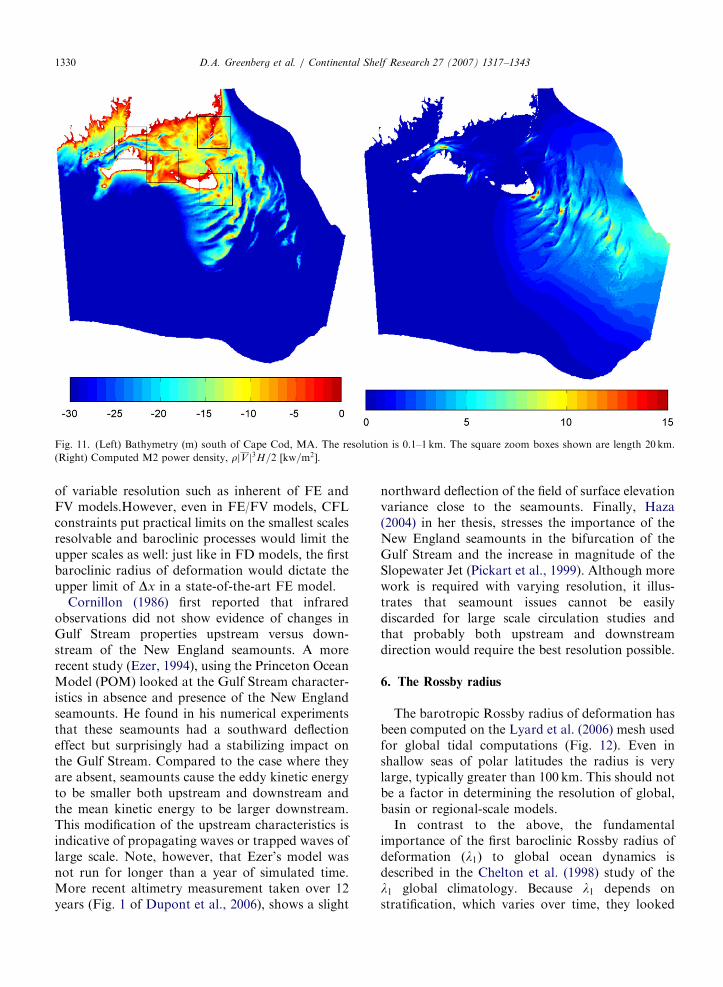
Smith (2005) found it necessary to resolve localridges and troughs under 1 km in width, in order tocapture the tide power distribution ðjvj3Þ suitable forpower generation studies. An example appears inFig. 11 wherein this effect is resolved within aregional (far-field) tidal context.
5.3. At the coast
As one approaches the shore, the bottom shoalsand horizontal shear is generated via variablebottom stress in very SW. In reality this is themechanism of ‘‘horizontal stress’’. The latter mustbe either mimicked by compensating horizontalboundary conditions on an imaginary sea wall, orthe actual physics simulated by proper resolution ofthe actual topography. The resolution demands sogenerated far exceed those from the wavelength-resolution in the open ocean or from the topo-graphic length scale on steep topography. Implied intopographic realism is fidelity to along-shore as wellas cross-shore topography.
The nearshore area is in fact where much of theoperational data are located. Blanton et al. (2004)studied the ADCIRC domain with both coarse andfine nearshore resolution along the Georgia/SouthCarolina coast. There, the presence of a denseestuary/tidal inlet complex (ETIC, Fig. 14) wasfound to be highly dissipative and affects theregional energy balance for the semidiurnal tides

ARTICLE IN PRESS
Fig. 10. Portion of ADCIRC mesh covering the city of New Orleans. This local resolution provides quality hurricane surge prediction
when appended to the wide-area domain illustrated in Fig. 9. The horizontal scale of the figure is approximately 30 km per side.
D.A. Greenberg et al. / Continental Shelf Research 27 (2007) 1317–1343 1329
(Fig. 15). This was found to affect regional skillassessment and to confound the interpretation oftidal data there unless properly resolved (Fig. 16).
Prediction of hurricane surge has been demon-strated using the collection of the expertise repre-sented here (large domain, resolution of barotropicand topographic length scales, coastal resolution) inBlain et al. (1998). The significant extra demand isthe propagation of tide and storm surge inland,which requires unusual topographic resolution foreffective prediction. An example of this meshing isillustrated in Fig. 10.
5.4. Shelfbreak and seamounts—baroclinic
Resolution issues where topography varies ra-pidly were already addressed above in the context ofbarotropic flows. In the broader context of thebaroclinic (density driven) flows, topographic fea-tures generate much smaller flow scales at the orderof the deformation radius (see next section) andsmaller, e.g. internal waves and tides, flow rectifica-tion due to tides (Wright and Loder, 1985) or
interactions with the large scale circulation as inTaylor columns (Haza, 2004). At the shelf edge,internal waves and tides are generated and propa-gate both offshore and inshore. Those propagatingoffshore are the main concern here as they cantravel long distances before being damped orbreaking (e.g. Alford, 2003). These features aredifficult to resolve and poses a major challenge torealistic state-of-the-art basin-scale circulation mod-els since they still cannot afford to resolve thenecessary 10 (or more) points for wavelike struc-tures at the scale of the first deformation radius(Treguier et al., 2005). For the foreseeable future,selective filters—e.g. the Smagorinsky viscosityscheme for variable or stretched grids, where theviscosity essentially varies with the local resolution(Hall and Davies 2005a, b)—might be necessary toensure model stability in regions of strong barocli-nic process generation and/or propagation. As Halland Davies (2005b) also show the improvements ofthe baroclinic tidal flow as the resolution isincreased locally around seamounts and shelfbreaks, it provides an interesting argument in favor
ARTICLE IN PRESS
Fig. 11. (Left) Bathymetry (m) south of Cape Cod, MA. The resolution is 0.1–1 km. The square zoom boxes shown are length 20 km.
(Right) Computed M2 power density, rjV j3H=2 ½kw=m2�.
D.A. Greenberg et al. / Continental Shelf Research 27 (2007) 1317–13431330
of variable resolution such as inherent of FE andFV models.However, even in FE/FV models, CFLconstraints put practical limits on the smallest scalesresolvable and baroclinic processes would limit theupper scales as well: just like in FD models, the firstbaroclinic radius of deformation would dictate theupper limit of Dx in a state-of-the-art FE model.
Cornillon (1986) first reported that infraredobservations did not show evidence of changes inGulf Stream properties upstream versus down-stream of the New England seamounts. A morerecent study (Ezer, 1994), using the Princeton OceanModel (POM) looked at the Gulf Stream character-istics in absence and presence of the New Englandseamounts. He found in his numerical experimentsthat these seamounts had a southward deflectioneffect but surprisingly had a stabilizing impact onthe Gulf Stream. Compared to the case where theyare absent, seamounts cause the eddy kinetic energyto be smaller both upstream and downstream andthe mean kinetic energy to be larger downstream.This modification of the upstream characteristics isindicative of propagating waves or trapped waves oflarge scale. Note, however, that Ezer’s model wasnot run for longer than a year of simulated time.More recent altimetry measurement taken over 12years (Fig. 1 of Dupont et al., 2006), shows a slight
northward deflection of the field of surface elevationvariance close to the seamounts. Finally, Haza(2004) in her thesis, stresses the importance of theNew England seamounts in the bifurcation of theGulf Stream and the increase in magnitude of theSlopewater Jet (Pickart et al., 1999). Although morework is required with varying resolution, it illus-trates that seamount issues cannot be easilydiscarded for large scale circulation studies andthat probably both upstream and downstreamdirection would require the best resolution possible.
6. The Rossby radius
The barotropic Rossby radius of deformation hasbeen computed on the Lyard et al. (2006) mesh usedfor global tidal computations (Fig. 12). Even inshallow seas of polar latitudes the radius is verylarge, typically greater than 100 km. This should notbe a factor in determining the resolution of global,basin or regional-scale models.
In contrast to the above, the fundamentalimportance of the first baroclinic Rossby radius ofdeformation ðl1Þ to global ocean dynamics isdescribed in the Chelton et al. (1998) study of thel1 global climatology. Because l1 depends onstratification, which varies over time, they looked

ARTICLE IN PRESS
Fig. 12. The barotropic Rossby radius (km) as calculated on the global FE mesh of Lyard et al. (2006). For most computations, this would
not be a factor in determining model resolution.
D.A. Greenberg et al. / Continental Shelf Research 27 (2007) 1317–1343 1331
at the significance of this variation to the oceandynamical computations. They found that the largerrange variability in stratification was limited to thetop few hundred meters so the full depth integral ofthe buoyancy frequency, used in l1 computation,was not greatly changed. They concluded thattemporal variability was not significant for mostconsiderations. They computed l1 on a global 1� �1� mesh. Of interest is that the lowest contourshown is 10 km (� 0:09� latitude) and that in thecritical Gulf Stream–North Atlantic Current areabetween 40� and50� l1 was close to 20 km (� 0:18�
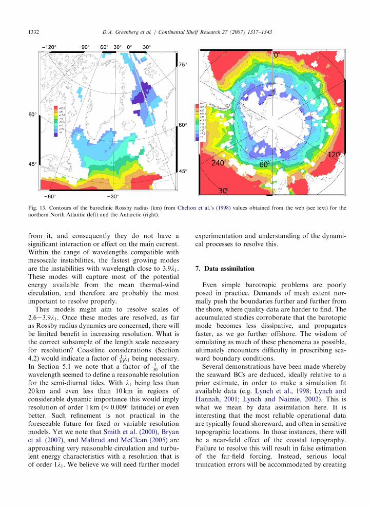
latitude). Because we are interested in resolving theshorter length scales, we would like to look in moredetail at the near polar values. Chelton et al. (1998)computational results are available online (http://www.coas.oregonstate.edu/research/po/research/chelton/index.html). We have plotted these inFig. 13 for the northern North Atlantic andAntarctic. (Not all values are represented in theseplots due to artifacts in the graphical display thatshrink the domain around boundaries and missinggrid points.) In the North Atlantic, l1 is seen todecrease to less than 5 km east of Greenland beforeincreasing again northward. Around Antarctica, l1is seen to be less than 7.5 km over a large area.
Smith et al. (2000) and Bryan et al. (2007) lookedat how resolution affected computations of theNorth Atlantic Ocean. They showed how their 0:1�
model greatly improved the eddy characteristics and
the time averaged currents in comparisons with thesimulations made with model resolutions of 1
2
�and
16
�. The Gulf Stream and North Atlantic Current
(see note added in Proof in Smith et al., 2000)separate from the continental shelf topography inthe correct areas. Similarly, Maltrud and McClean(2005), using a global model with the same 0:1�
resolution were able to produce good global eddycharacteristics, but there were some anomalies andthey had poorer results with the separation of theGulf Stream.
The resolution necessary to include properrepresentation of l1’s influence in ocean models iscomplex. Stammer (1997), looking at satellite data,found a strong empirical relationship between eddyscales at all latitudes and l1. A zonal average ofeddy scales estimated from TOPEX data betweenlatitudes �60� and þ60� indicated the largest eddyscales were close to 100 km around the equator anddiminished to 50–60 km near 60�. Cushman-Roisin (1994) points out how the relationshipbetween the first Rossby radius and the meso-scalebaroclinic instability typically has ratio of ordergreater than 1. He describes how in the case of thethermal wind flowing inside an ocean with constantBrunt–Vaisala frequency, N, i.e. the density islogarithmic, the stability limit is close to 2:6l1.Under this limit, perturbations are not able to takethe main stream circulation away from equilibrium,thus they are not able to capture potential energy
ARTICLE IN PRESS
Fig. 13. Contours of the baroclinic Rossby radius (km) from Chelton et al.’s (1998) values obtained from the web (see text) for the
northern North Atlantic (left) and the Antarctic (right).
D.A. Greenberg et al. / Continental Shelf Research 27 (2007) 1317–13431332
from it, and consequently they do not have asignificant interaction or effect on the main current.Within the range of wavelengths compatible withmesoscale instabilities, the fastest growing modesare the instabilities with wavelength close to 3:9l1.These modes will capture most of the potentialenergy available from the mean thermal-windcirculation, and therefore are probably the mostimportant to resolve properly.
Thus models might aim to resolve scales of2:623:9l1. Once these modes are resolved, as faras Rossby radius dynamics are concerned, there willbe limited benefit in increasing resolution. What isthe correct subsample of the length scale necessaryfor resolution? Coastline considerations (Section4.2) would indicate a factor of 1
10l1 being necessary.
In Section 5.1 we note that a factor of 130
of thewavelength seemed to define a reasonable resolutionfor the semi-diurnal tides. With l1 being less than20 km and even less than 10 km in regions ofconsiderable dynamic importance this would implyresolution of order 1 km (� 0:009� latitude) or evenbetter. Such refinement is not practical in theforeseeable future for fixed or variable resolutionmodels. Yet we note that Smith et al. (2000), Bryanet al. (2007), and Maltrud and McClean (2005) areapproaching very reasonable circulation and turbu-lent energy characteristics with a resolution that isof order 1l1. We believe we will need further model
experimentation and understanding of the dynami-cal processes to resolve this.
7. Data assimilation
Even simple barotropic problems are poorlyposed in practice. Demands of mesh extent nor-mally push the boundaries further and further fromthe shore, where quality data are harder to find. Theaccumulated studies corroborate that the barotopicmode becomes less dissipative, and propagatesfaster, as we go further offshore. The wisdom ofsimulating as much of these phenomena as possible,ultimately encounters difficulty in prescribing sea-ward boundary conditions.
Several demonstrations have been made wherebythe seaward BCs are deduced, ideally relative to aprior estimate, in order to make a simulation fitavailable data (e.g. Lynch et al., 1998; Lynch andHannah, 2001; Lynch and Naimie, 2002). This iswhat we mean by data assimilation here. It isinteresting that the most reliable operational dataare typically found shoreward, and often in sensitivetopographic locations. In those instances, there willbe a near-field effect of the coastal topography.Failure to resolve this will result in false estimationof the far-field forcing. Instead, serious localtruncation errors will be accommodated by creating

ARTICLE IN PRESSD.A. Greenberg et al. / Continental Shelf Research 27 (2007) 1317–1343 1333
far-field, boundary-forced errors which permeatethe shelf.
The ETIC region of the South Atlantic Bight(mentioned above in Section 5.3) is a classicexample. In Lynch et al. (2004), it was found thatsub-km coastal resolution was required in order tomake valid inference of boundary conditions as faroffshore as the 70m isobath. Failure to resolvethe ETIC resulted in forecast errors equal inmagnitude to the subtidal phenomena under study(Figs. 14–16). Worse, these errors are masked by afalse confidence gained from ‘fitting’ a poorlyresolved model to available data—errors are anni-hilated by the data assimilation at the observationpoints, but created elsewhere, all over the shelf.
8. Mesh generation
Since the recognition that variable resolution iswithin reach, there has been considerable interest inalgorithms for mesh generation.
The FD method has been adapted by firstinventing a mapping from the original Cartesian orpolar coordinate system to a more natural, curvedcoordinate system (e.g. Blumberg et al., 1985, 1993).The mapping terms are then embedded in thegoverning PDE, which is discretized on regular grid
Fig. 14. Nearfield mesh resolving t
in the mapped space. The problem of mesh genera-tion is transferred to that of generating the coordinatetransformation. As typically conceived, this approachinvolves a global coordinate transformation, aformidable task for all but the simplest transforma-tions; and a numerical challenge in itself.
In the FE arena, this mapping approach isembedded in essentially all methods which useunstructured grids. The formalism developed inthe FE arena is the ‘‘isoparametric transformation’’,and the principles here are (a) make the mappinglocal, definable on each FE independently of theothers; (b) start in the natural numerical space (e.g.the triangle) and map outwards to the physicalspace; (c) concentrate on the level of continuity atthe triangle boundaries; and (d) make the mappingeasily automated at the element level. The mostcommon form of this requires C0 continuity, i.e. apolynomial map which is continuous across elementboundaries, with first derivatives non-continuousthere. And the most elementary form of thisamounts to linear mapping over each triangle. Thegenius of this idea is that the map is conceived at thelocal, discrete level, and hence computable, in termsof simple local functions; while alternate ideasconceive a continuous global map which is thendiscretized along with the PDE.
he ETIC, and data locations.

ARTICLE IN PRESS
Fig. 15. Data-assimilative solution for nearfield M2 tidal amplitude (m) for the numbered areas identified in Fig. 16.
D.A. Greenberg et al. / Continental Shelf Research 27 (2007) 1317–13431334
With unstructured grids, most common is the useof Delaunay triangulation of generated nodes, andsubsequent refinement in various ways. This arearemains a subjective art, as no extant algorithmprovides fully satisfactory, reproducible results, andall attempts rely in the last analysis on heuristic,interactive adjustment.
An early example of unstructured mesh genera-tion was presented by Henry and Walters (1993).This method generated triangles with the Courantconstraint operative, resulting in uniform gravitywave resolution over variable topography. Exam-ples of more complex generation of meshes onvastly different scales can be seen in Greenberg et al.(2005), Kliem and Greenberg (2003), and Lyard etal. (2006) which used unpublished software (Lyard)derived initially from the Henry and Walters (1993)TriGrid package.
More recently, Bilgili et al. (2005) describe agenerator which incorporates a user-directed selec-tion of several refinement criteria. Included are
Element area. Topographic length scale resolution (H=rH). H: shallow refinement. Uniform 1=rH. Wavelength resolution. Peclet number. Maximum slope. Relaxation by local averaging.Like other methods in its class, this approach istypical in that it proceeds from coarse to fine grid,through selective refinement.
Hagen (2001), Hagen et al. (2000, 2001, 2002),and Hagen and Parrish (2003) have contributed thelocal truncation error analysis (LTEA) approach. Inthis approach, one seeks to make the truncationerror uniform across the whole domain. Required isa high-resolution solution U , capable of beingdifferentiated up to fifth-order. With these deriva-tives everywhere, one estimates the leading trunca-tion error as
� ¼ Dx2 q5Uqx5
; . . .
� �(10)
which is different everywhere. By setting this to aconstant everywhere, one gets a recipe for the localDx, and proceeds to generate a coarser mesh. The

ARTICLE IN PRESS
Fig. 16. Difference (m) between the ETIC-resolving and non-resolving solutions, following data assimilation. The results are plotted on
the coarser mesh, which covers roughly 420 km along-shelf and 100 km cross-shelf. The difference is of order 20 cm over a significant
portion of the shelf. The difference is vanishingly small at the data locations (green filled hexagons), as these points are fit to the model.
D.A. Greenberg et al. / Continental Shelf Research 27 (2007) 1317–1343 1335
ARTICLE IN PRESS
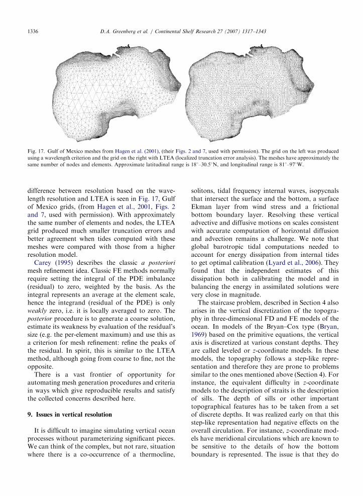
Fig. 17. Gulf of Mexico meshes from Hagen et al. (2001), (their Figs. 2 and 7, used with permission). The grid on the left was produced
using a wavelength criterion and the grid on the right with LTEA (localized truncation error analysis). The meshes have approximately the
same number of nodes and elements. Approximate latitudinal range is 18�–30:5�N, and longitudinal range is 81�–97�W.
D.A. Greenberg et al. / Continental Shelf Research 27 (2007) 1317–13431336
difference between resolution based on the wave-length resolution and LTEA is seen in Fig. 17, Gulfof Mexico grids, (from Hagen et al., 2001, Figs. 2and 7, used with permission). With approximatelythe same number of elements and nodes, the LTEAgrid produced much smaller truncation errors andbetter agreement when tides computed with thesemeshes were compared with those from a higherresolution model.
Carey (1995) describes the classic a posteriori
mesh refinement idea. Classic FE methods normallyrequire setting the integral of the PDE imbalance(residual) to zero, weighted by the basis. As theintegral represents an average at the element scale,hence the integrand (residual of the PDE) is onlyweakly zero, i.e. it is locally averaged to zero. Theposterior procedure is to generate a coarse solution,estimate its weakness by evaluation of the residual’ssize (e.g. the per-element maximum) and use this asa criterion for mesh refinement: refine the peaks ofthe residual. In spirit, this is similar to the LTEAmethod, although going from coarse to fine, not theopposite.
There is a vast frontier of opportunity forautomating mesh generation procedures and criteriain ways which give reproducible results and satisfythe collected concerns described here.
9. Issues in vertical resolution
It is difficult to imagine simulating vertical oceanprocesses without parameterizing significant pieces.We can think of the complex, but not rare, situationwhere there is a co-occurrence of a thermocline,
solitons, tidal frequency internal waves, isopycnalsthat intersect the surface and the bottom, a surfaceEkman layer from wind stress and a frictionalbottom boundary layer. Resolving these verticaladvective and diffusive motions on scales consistentwith accurate computation of horizontal diffusionand advection remains a challenge. We note thatglobal barotropic tidal computations needed toaccount for energy dissipation from internal tidesto get optimal calibration (Lyard et al., 2006). Theyfound that the independent estimates of thisdissipation both in calibrating the model and inbalancing the energy in assimilated solutions werevery close in magnitude.
The staircase problem, described in Section 4 alsoarises in the vertical discretization of the topogra-phy in three-dimensional FD and FE models of theocean. In models of the Bryan–Cox type (Bryan,1969) based on the primitive equations, the verticalaxis is discretized at various constant depths. Theyare called leveled or z-coordinate models. In thesemodels, the topography follows a step-like repre-sentation and therefore they are prone to problemssimilar to the ones mentioned above (Section 4). Forinstance, the equivalent difficulty in z-coordinatemodels to the description of straits is the descriptionof sills. The depth of sills or other importanttopographical features has to be taken from a setof discrete depths. It was realized early on that thisstep-like representation had negative effects on theoverall circulation. For instance, z-coordinate mod-els have meridional circulations which are known tobe sensitive to the details of how the bottomboundary is represented. The issue is that they do
ARTICLE IN PRESSD.A. Greenberg et al. / Continental Shelf Research 27 (2007) 1317–1343 1337
not accurately advect denser waters along slopesand overestimate diapycnal mixing (Gerdes, 1993;Roberts et al., 1996; Roberts and Wood, 1997).
Different strategies have been proposed tocircumvent the problem. One strategy was to changethe vertical coordinate, z, to a terrain followingcoordinate, s (Phillips, 1957; Blumberg and Mellor,1983), Song and Haidvogel (1994). But s-coordinatemodels encounter other known limitations, such aspressure gradient errors and artificial diapycnalmixing (e.g. Haney, 1991; Mellor et al., 1994). Asecond strategy is to use a layered (or r-coordinate)model (Bleck, 1978; Bleck and Boudra, 1981).Roberts et al. (1996) compared the behavior of thesimulated North Atlantic in a z-model and in anisopycnal model (r-model). In particular, theynoted that the z-model has more trouble inrepresenting a realistic outflow from the Greenlandbasin (GIN). Roberts and Wood (1997) extendedthe study by systematically studying the effect ofmodifying the topography of the sill at the outflowof GIN and noted the high sensitivity of the model.The same observation was made by Winton (1997)in a more idealized geometry of the North Atlantic.Winton et al. (1998) finally demonstrated that it is aresolution problem. When the resolution was highenough to resolve the bottom boundary layer and toresolve the slope, the flow is realistic enough.However, the required resolution is unrealistic evenfor modern z-models; therefore, they recommendedthe use of explicit bottom boundary layer models orthe use of isopycnal models (although these alsohave their limitations, namely relating to disappear-ing layers and lack of vertical resolution in weaklystratified regions such as the deep mixed layer foundin the winter season in the North Atlantic).
Shchepetkin and McWilliams (2003) developed ahigher-order pressure gradient algorithm for s-coordinate type models. When tested over anidealized seamount, they were able to diminish theerrors. Similarly, a test application to the NorthAtlantic with a flat density field drastically reducedthe spurious currents that arise from the non-alignment of the vertical pressure field with thehorizontal. They also split the compressibility termsin a manner that allowed them to more accuratelyrepresent the physics without degrading the hydro-static error.
From a different perspective, Hirst and McDou-gall (1996) noted that, in coarse resolution z-models,the Gent and McWilliams (1990) turbulence schemeremarkably enhances the conservation of water
properties along topographic slopes. Another ap-proach was proposed by Adcroft et al. (1997). Theyshowed interesting use of ‘‘shaved’’ cells in z-models. The topography is then piecewise linear,instead of being piecewise constant at discrete levelsas in typical z-models.
More recently, Chassignet et al. (2003) showedthe viability of a hybrid vertical coordinate FDmodel based on ideas developed by Bleck andBoudra (1981) and Bleck and Benjamin (1993). Themain goal of the hybrid vertical coordinate is toremedy the lack of vertical resolution of isopycnalmodels in critical locations such as deep mixedlayers, i.e. the upper surface dynamics where thehybrid coordinate relaxes to a z-coordinate. Eachhybrid level is essentially constrained to follow asmuch as possible an isopycnal surface unless it hitsthe mixed layer or the topography. This enables theuse of more sophisticated parameterization ofmixing in the mixed layer than the simple Kraus–Turner-type bulk formulae otherwise used inisopycnal-models (Treguier et al., 2005). Allowanceswere made as well to relax the hybrid coordinate tosigma coordinate on the shelves where resolving thebottom layer is crucial to the representation ofvertical mixing. Whereas the isopycnal models tendto have too little diapycnal mixing, the hybridcoordinate would allow some in the boundary layersat the price that some spurious diapycnal mixingand pressure gradient errors may occur in steeptopographic regions where the hybrid coordinatechanges to another form.
High vertical resolution rarely leads to stabilityissues, as the vertical Courant number is usuallysmall. Some exceptions may occur close to steeptopography. For a hydrostatic model, this wouldcorrespond to a case where the hydrostatic approx-imation is probably no longer fully valid. Mostmodels are hydrostatic, and generally speakingmodels treat the vertical diffusion implicitly due tothe large value of the diffusion coefficients obtainedfrom turbulence schemes. The vertical advectionproblem is usually treated explicitly in an Eulerianfashion. It is possible to treat the vertical advectionproblem implicitly which leads to the same tri-diagonal matrix problem as the one arising from thediffusion problem. However, this would give rise toan inconsistency in local conservation, with oneadvection problem being treated implicitly and oneexplicitly.
A possible stability limitation of z-levels modelsrelates to the treatment of the free-surface. If the top

ARTICLE IN PRESSD.A. Greenberg et al. / Continental Shelf Research 27 (2007) 1317–13431338
layer is treated as having varying-depth, tides oratmospheric processes may create rapid variationsin sea surface height (i.e. large vertical velocity) inthe thin layers close to the surface. This problem isnot present in sigma models for instance because thesigma velocity converges to zero as it gets close tothe surface, whatever the variations in sea surface.
Ideally, a 3D circulation model should haveenough vertical levels to represent the physics ofthe surface and bottom boundary layers wherestrong gradients are found with coarser resolutionin between. The present state-of-the-art models with40–50 levels are actually still behind these basicrequirements.
10. Discussion
The resolution requirements described here canlead to multiple requirements in the different partsof a model. For example the consistent wavelengthresolution (proportional to
ffiffiffiffiffigh
p) will give very
different cell density over a shelf break from thatneeded to satisfy the resolution of steep slopes(DH=H small). Other differences with the criteriawill of course be seen when there is high resolutionin an area of particular interest. We expect theLTEA approach will see continued developmentand application with the ability to specify differenterror criteria for different regions depending on thefocus of study.
Numerical models of coastal and shelf regionsmay be capable of capturing details of the flow indomains of interest, but they cannot afford toexplicitly include the solution of the larger neigh-boring basin-scale domain. As such, regionalmodels face a complication not found in globalmodels namely the complexities of open boundaries.The transfer of energy into and out of the modeldomain via these boundaries can involve assump-tions on the interaction of the modelled area withthe adjacent unmodelled ocean. Frequently, theassumption is made that these boundaries are‘‘small enough’’ and ‘‘far enough away’’ that theinteractions do not impact the solution in the areaof interest. However, establishing that this is thecase remains a challenge. Variable resolution andnested grids or mapped coordinates are frequentlyused to help distance open boundaries from theprincipal area of interest.
The baroclinic Rossby radius of deformation isfundamentally related to the dynamics of globalocean circulation. It clearly needs to be resolved,
but to what precision remains unclear. Improvedmodel efficiencies and greater computer capacityhave permitted models to move from resolutions of41� � 1� (no eddies—Roberts et al., 2004) and 1
3
��
13
�(eddy permitting—Gordon et al., 2000) to 0:1� �
0:1� (approaching eddy resolving—Smith et al.,2000; Bryan et al., 2007; Maltrud and McClean,2005). These latter simulations at 0:1�are beginningto reasonably reproduce fundamental eddy char-acteristics of the circulation. In part, this isattributed to better resolution of l1, even thoughthis radius is at best minimally resolved inimportant parts of the model domains.
The occurrence of step-like features along thecoastline of finite difference (FD) models is inevi-table when modelling the real ocean. Curvilineargrids allow some flexibility in following the largescale features of the coastlines but do not preventsteps from occurring at small scales. A known effectof steps at coarse resolution in inviscid flows is toretard the propagation of waves along the modelboundary. However, at higher resolution theproblem disappears. In a circular domain, we foundthat FD models of different convergence order tendto be first-order only, which explains the retardationeffect.
In presence of winds and viscous stresses, the free-slip boundary condition is problematic and yieldssolutions converging to too viscous circulations. Aremedy found by Adcroft and Marshall (1998) wasto replace the conventional viscous stress formula-tion based on the five-point Laplacian operator by adivergence–vorticity stress formulation. Note, how-ever, that this solution is only applicable insituations where the steps are known to be artificial.Dupont (2001), in his thesis, reports problems whenusing this approach to the more general case of anundulating but otherwise circular basin. Therefore,the no-slip boundary condition seems to be moreadequate in FD models even though the assumptionthat no-slip applies to large scale flows is not welljustified.
The issues of vertical resolution have only brieflybeen touched upon here. The problems are complex,but different solutions are showing some promise.Hybrid vertical coordinates have the ability to avoidthe larger diapycnal diffusion seen in z-level modelsand to increase the resolution in weakly stratifiedregions, which have been the main drawbacks ofisopycnal models, while the interior of much of theocean remains isopycnal (Chassignet et al., 2003).Similarly, using higher order equations to compute

ARTICLE IN PRESSD.A. Greenberg et al. / Continental Shelf Research 27 (2007) 1317–1343 1339
horizontal gradients in terrain following coordinatemodels may alleviate problems seen in this type ofcomputation (Shchepetkin and McWilliams, 2003).
In the context of tidal data assimilation, it wasfound that in coarse models the absence ofimportant dissipative and/or resonant estuarieswas detrimental to the accuracy of the assimilatedsolution away from the location of the observations.Modellers interested in using data assimilationtechniques in models with omitted/underesolved,but nonetheless potentially significant, portions ofthe focussed region need to be aware of this.
There have been recent investigations where meshgeneration is part of the model, with resolutionbeing increased or decreased on the basis of someaspect of the dynamics included (Blayo and Debreu,1998; Pain et al., 2005; Gorman et al., 2006). So farthese adaptive mesh models have been tested inidealized cases and for particular processes. Thisflexibility comes at the expense of very largecomputer demands.
10.1. Resolution issues—a list
Our review has covered several resolution issuesthat can affect the adequacy of model solutions.Briefly, these are:
(1)
Small scale processes that interact with the largescale circulation need to be resolved if theycannot be parameterized.(2)
Model coastlines need to accurately represent thevariations that can reflect and modify thecoastal trapped motions.(3)
Channels and sills [barotropic] need cross sec-tional area and depth resolved to get the currentphase speed and transport correct.(4)
Channels and sills [baroclinic] need the sill heightaccurately represented to get the right volumeand density of overflow waters.(5)
Topography needs to be resolved. Convergenceis enhanced with grid resolution matching wavespeed. Steep bottom slopes need special atten-tion to ensure that the change in depth over agrid cell ðDH=HÞ is small.(6)
The baroclinic Rossby radius needs to beresolved at some level to properly reproducelarge scale ocean dynamics. As one approachesthe poles, this could be a challenge.(7)
Open boundary specification of regional modelswill always require proper justification. Variableresolution and nested grid models can be used tomove boundaries further from the domain ofinterest.
(8)
Assimilation requires an understanding of thephysics being modified to avoid using data toattempt to correct an improperly resolvedsolution.(9)
Mesh generation techniques are still developingand can now be used to meet specific modelrequirements.11. Concluding remarks
The above discussion would appear to imply thatthe ocean modelling community is facing animpossible task in trying to meet all the require-ments as outlined here. It seems clear that the use ofunstructured grids may provide a better opportunityto resolve channels, sills, coastlines, critical slopesand localized areas of interest. However, even withthis flexibility, these requirements are often not met,requiring additional advances in approaches such asadaptive mesh refinement (e.g. Blayo and Debreu,1998, among others). However, all classes ofcirculation models have continued to provide robustsolutions even with less than perfect numerics. Asan example, Arakawa and Lamb (1981) havedescribed techniques for properly accounting forthe energy in non-linear models. The techniques arecomplicated and expensive to implement. Manymodels do not follow such a methodology yet stillproduce reliable answers to the questions posed.
Resolution is but one of the factors that comesinto play when one chooses a model to apply to aparticular application. Other dominant factorsinclude stability, convergence and efficiency. Amodel’s deficiency in any of these could quicklyeliminate it from application to different problems.When the above are satisfactory, other factors suchas available expertise and model support infrastruc-ture can be considered. This paper predominantlyaddresses just one of these critical factors—resolu-tion. We hope that this review will help the modelleridentify weaknesses in solutions and enable morerobust model design and discretization. Similarly, itis hoped that non-modellers, who use ‘‘off the shelf’’modelling packages as basic tools, will do so awareof some the many issues that remain to be resolved.
Acknowledgments
We would like to thank Brian Blanton andRick Luettich (University of North Carolina) for

ARTICLE IN PRESSD.A. Greenberg et al. / Continental Shelf Research 27 (2007) 1317–13431340
providing Figs. 9 and 10 and Scott Hagen (Uni-versity of Central Florida) and coauthors forpermission to use their work in Fig. 17. We alsobenefited from input from Joannes Westerink(Notre Dame), Keston Smith (Dartmouth College)and Jason Chaffey (Bedford Institute of Oceano-graphy). F.E. Werner acknowledges support fromthe SEACOOS project.
References
Adcroft, A., Marshall, D., 1998. How slippery are piecewise-
constant coastlines in numerical ocean models? Tellus 50A,
95–108.
Adcroft, A., Hill, C., Marshall, D., 1997. Representation of
topography by shaved cells in a height coordinate ocean
model. Monthly Weather Review 125, 2293–2315.
Alford, M.H., 2003. Redistribution of energy available for ocean
mixing by long-range propagation of internal waves. Nature
423 (6936), 159–162.
Arakawa, A., Lamb, V.R., 1981. A potential enstrophy conser-
ving scheme for shallow water equations. Monthly Weather
Review 109 (1), 18–36.
Beletsky, D., O’Connor, W.P., Schwab, D.J., Dietrich, D.E.,
1997. Numerical simulation of internal Kelvin waves and
coastal upwelling fronts. Journal of Physical Oceanography
27, 1197–1215.
Bilgili, A., Smith, K., Lynch, D., 2005. Battri: a two-dimensional
bathymetry-based unstructured triangular grid generator for
finite element circulation modeling. Computers and Geos-
ciences 32 (5), 632–642.
Blain, C., Westerink, J., Luettich, R., 1998. Grid convergence
studies for the prediction of hurricane storm surge. Interna-
tional Journal for Numerical methods in Fluids 26, 369–401.
Blanton, B., Werner, F., Seim, H., Luettich Jr., R., Lynch, D.,
Smith, K., Voulgaris, G., Bingham, F., Way, F., 2004.
Barotropic tides in the South Atlantic Bight. Journal of
Geophysical Research 109 (C12), C12024.
Blayo, E., Debreu, L., 1998. Adaptive mesh refinement for finite
difference ocean models: first experiments. Journal of Physical
Oceanography 29, 1239–1250.
Blayo, E., Debreu, L., 2005. Revisiting open boundary conditions
from the point of view of characteristic variables. Ocean
Modelling 9, 231–252.
Bleck, R., 1978. Simulation of coastal upwelling frontogenesis
with an isopycnic coordinate model. Journal of Geophysical
Research 83, 6163–6172.
Bleck, R., Benjamin, S., 1993. Regional weather prediction with a
model combining terrain-following and isentropic coordi-
nates. Part I: model description. Monthly Weather Review
121, 1770–1785.
Bleck, R., Boudra, D.B., 1981. Initial testing of a numerical ocean
circulation model using a hybrid quasi-isopycnal vertical
coordinate. Journal of Physical Oceanography 11, 755–770.
Blumberg, A., Herring, H., 1987. Circulation modelling using
orthogonal curvilinear coordinates. In: Nihoul, J., Jamart, B.
(Eds.), Three-Dimensional Models of Marine and Estuarine
Dynamics, Elsevier Oceanography, vol. 45. Elsevier, Amster-
dam, pp. 55–88.
Blumberg, A., Kantha, L., 1985. Open boundary condition for
circulation models. Journal of Hydraulic Engineering 111,
237–255.
Blumberg, A., Mellor, G., 1983. Diagnostic and prognostic
numerical circulation studies of the South Atlantic Bight.
Journal of Geophysical Research 88, 4579–4592.
Blumberg, A., Herring, H., Kantha, L., Mellor, G., 1985. 3-D
orthogonal curvilinear circulation modelling. In: Hydraulics and
Hydrology in the Small Computer Age. Hydraulics Division,
ASCE, Lake Buena Vista, FL, August 12–17, pp. 1088–1094.
Blumberg, A., Signell, R., Jenter, H., 1993. Modelling transport
processes in the coastal ocean. Journal of Marine Environ-
mental Engineering 1, 31–52.
Bryan, F.O., Hecht, M.W., Smith, R.D., 2007. Resolution
convergence and sensitivity studies with North Atlantic
circulation models. Part I: the western boundary current
system. Ocean Modelling 16, 141–159.
Bryan, K., 1969. A numerical method for the study of the
circulation of the world ocean. Journal of Computational
Physics 4, 347–376.
Camerlengo, A.L., O’Brien, J.J., 1980. Open boundary condi-
tions in rotating fluids. Journal of Computational Physics 35
(1), 12–35.
Carey, G., 1995. Mesh generation, a posteriori error estimation,
and mesh refinement. In: Lynch, D.R., Davies, A.M. (Eds.),
Quantitative Skill Assessment for Coastal Ocean Models.
Coastal and Estuarine Series, vol. 47. American Geophysical
Union, Washington, DC, pp. 15–29.
Chapman, D., 1985. Numerical treatment of cross-shelf open
boundaries in a barotropic coastal ocean model. Journal of
Physical Oceanography 15 (8), 1060–1075.
Chassignet, E.P., Smith, L.T., Halliwell, G.R., 2003. North
Atlantic simulations with the hybrid coordinate ocean model
(HYCOM): impact of the vertical coordinate choice, reference
pressure and thermobaricity. Journal of Physical Oceanogra-
phy 33, 2504–2526.
Chelton, D.B., deSzoeke, R.A., Schlax, M.G., Naggar, K.E.,
Siwertz, N., 1998. Geographical variability of the first-
baroclinic Rossby radius of deformation. Journal of Physical
Oceanography 28, 433–460.
Cornillon, P., 1986. The effect of the New England Seamounts on
Gulf Stream meandering as observed from satellite IR
imagery. Journal of Physical Oceanography 16, 386–389.
Cox, M.D., 1979. A numerical study of Somali Currents eddies.
Journal of Physical Oceanography 29, 311–326.
Cushman-Roisin, B., 1994. Introduction to Geophysical Fluid
Dynamics. Prentice-Hall, New Jersey.
Davies, A.M., Hall, P., 2002. Numerical problems associated
with coupling hydrodynamic models in shelf edge regions: the
surge event of February 1994. Applied Mathematical Model-
ling 26, 807–831.
Davies, A.M., Xing, J., Gjevik, B., 2003. Barotropic eddy
generation by flow instability at the shelf edge: sensitivity to
open boundary conditions, inflow and diffusion. Journal of
Geophysical Research 108 (C2), 17-1–17-15.
Dietrich, D.E., 1998. Application of a modified A-grid ocean
model having reduced numerical dispersion to the Gulf of
Mexico fronts circulation. Dynamics of Atmospheres and
Oceans 27, 201–217.
Dupont, F., 2001. Comparison of numerical methods for
modelling ocean circulation in basins with irregular coasts.
Ph.D. Thesis, McGill University, Montreal, Canada.

ARTICLE IN PRESSD.A. Greenberg et al. / Continental Shelf Research 27 (2007) 1317–1343 1341
Dupont, F., Petrie, B., Chaffey, J., 2003a. Modelling the tides of
the Bras d’Or Lakes. Canadian Technical Report of the
Hydrogen Ocean Science 230 Fisheries and Oceans Canada,
Bedford Institute of Oceanography, Dartmouth, Nova Scotia.
Dupont, F., Straub, D.N., Lin, C.A., 2003b. Influence of a step-
like coastline on the basin scale vorticity budget of mid-
latitude gyre models. Tellus 55A (3), 255–272.
Dupont, F., Hannah, C.G., Wright, D.G., 2006. Model
investigation of the slope water, north of the Gulf Stream.
Geophysical Research Letters 33 (L05604).
Ezer, T., 1994. On the interaction between the Gulf Stream and
the New England Seamount Chain. Journal of Physical
Oceanography 24, 191–204.
Flather, R., 1981. Results from a model of the northeast Atlantic
relating to the Norwegian Coastal Current. In: Saetre, R.,
Mork, M. (Eds.), The Norwegian Coastal Current, vol. 2.
Bergen, Norway, pp. 427–458.
Foreman, M.G.G., 1984. A two-dimensional dispersion analysis
of selected methods for solving the linearized shallow
water equations. Journal of Computational Physics 56 (2),
287–323.
Foreman, M.G.G., Thomson, R.E., Smith, C.L., 2000. Seasonal
current simulations for the western continental margin of
Vancouver Island. Journal of Geophysical Research 105 (C8),
19665–19698.
Garrett, C., Greenberg, D., 1977. Predicting changes in tidal
regime: the open boundary problem. Journal of Physical
Oceanography 7 (2), 171–181.
Garrett, C., Toulaney, B., 1979. A variable-depth Green’s
function for shelf edge tides. Journal of Physical Oceano-
graphy 9, 1258.
Gent, P.R., McWilliams, J.C., 1990. Isopycnal mixing in ocean
circulation models. Journal of Physical Oceanography 20,
150–155.
Gerdes, R., 1993. A primitive equation ocean general circulation
model using a general vertical coordinate transformation.
Journal of Geophysical Research 98, 14683–14701.
Gille, S.T., Metzger, E.J., Tokmakian, R., 2004. Seafloor
topography and ocean circulation. Oceanography 17 (1),
47–54.
Gordon, C., Cooper, C., Senior, C.A., Banks, H., Gregory, J.M.,
Johns, T.C., Mitchell, J.F.B., Wood, R.A., 2000. The
simulation of SST, sea ice extents and ocean heat transports
in a version of the Hadley Centre coupled model without flux
adjustments. Climate Dynamics 16 (2–3), 147–168.
Gorman, G., Piggott, M., Pain, C., de Oliveira, C., Umpleby, A.,
Goddard, A., 2006. Optimisation based bathymetry approx-
imation through constrained unstructured mesh adaptivity.
Ocean Modelling 12, 436–452.
Greenberg, D.A., 1979. A numerical model investigation of tidal
phenomena in the Bay of Fundy and Gulf of Maine. Marine
Geodesy 2 (2), 161–187.
Greenberg, D.A., Shore, J.A., Page, F.H., Dowd, M., 2005. A
finite element circulation model for embayments with drying
intertidal areas and its application to the Quoddy region of
the Bay of Fundy. Ocean Modelling 10, 211–231.
Hagen, S., 2001. Estimation of the truncation error for the
linearized shallow water momentum equations. Engineering
with Computers 17, 354–362.
Hagen, S., Parrish, D., 2003. Meshing requirements for tidal
modeling in the western North Atlantic. International Journal
of Computational Fluid Dynamics 18 (7), 585–595.
Hagen, S., Westerink, J., Kolar, R., 2000. One-dimensional finite
element grids based on localized truncation error analysis.
International Journal for Numerical Methods in Fluids 32,
241–261.
Hagen, S., Westerink, J., Kolar, R., Horstmann, O., 2001. Two
dimensional unstructured mesh generation for tidal models.
International Journal for Numerical Methods in Fluids 35,
669–686.
Hagen, S.C., Horstmann, O., Bennett, R.J., 2002. An unstruc-
tured mesh generation algorithm for shallow water modeling.
International Journal of Computational Fluid Dynamics 16
(2), 83–91.
Haidvogel, D., Wilkin, J., Young, R., 1991. A semi-spectral
primitive equation ocean circulation model using vertical
sigma and orthogonal curvilinear horizontal coordinates.
Journal of Computational Physics 94, 151–185.
Haidvogel, D.B., Beckmann, A., 1999. Numerical Ocean
Circulation Modeling. Imperial College Press, London.
Hall, P., Davies, A.M., 2005a. Comparison of finite difference
and element models of internal tides on the Malin-Hebrides
shelf. Ocean Dynamics 55, 272–293.
Hall, P., Davies, A.M., 2005b. Effect of coastal boundary
resolution and mixing upon internal wave generation
and propagation in coastal regions. Ocean Dynamics 55,
248–271.
Haney, R.L., 1991. On the pressure gradient force over steep
topography in sigma coordinate ocean models. Journal of
Physical Oceanography 21, 610–619.
Hannah, C.G., Wright, D.G., 1995. Depth dependent analytical
and numerical solutions for wind-driven flow in the coastal
ocean. In: Lynch, D.R., Davies, A.M. (Eds.), Quantitative
Skill Assessment for Coastal Ocean Models. Coastal and
Estuarine Studies, vol. 47. AGU, Washington, DC, pp.
125–152.
Hayashi, T., Greenberg, D., Garrett, C., 1986. A note on open
boundary conditions for numerical models of shelf circula-
tion. Continental Shelf Research 5 (4), 487–497.
Haza, A.C., 2004. Study of the gulf stream-slopewater system.
Ph.D. Thesis, University of Miami, Miami, Florida.
Henry, R., Walters, R., 1993. Geometrically based, automatic
generator for irregular triangular networks. Numerical
Methods in Engineering 9, 555–566.
Hermann, A., Haidvogel, D.B., Dobbins, E.L., Stabeno, P.J.,
2002. Coupling global and regional circulation models in
the coastal gulf of alaska. Progress in Oceanography 53,
335–367.
Hirst, A., McDougall, T.J., 1996. Deep-water properties and
surface buoyancy flux as simulated by a z-coordinate model
including eddy-induced advection. Journal of Physical Ocea-
nography 26, 1320–1343.
Hua, B., Thomasset, F., 1984. A noise free finite element scheme
for the two layer shallow equations. Tellus, 157–165.
Johnsen, M., Lynch, D., 1995. Assessment of a second-order
radiation boundary condition for tidal and wind-driven flows.
In: Lynch, D., Davies, A. (Eds.), Quantitative Skill Assess-
ment for Coastal Ocean Models. Coastal and Estuarine
Studies, vol. 47. American Geophysical Union, Washington,
DC.
Jones, J.E., Davies, A.M., 2005. An intercomparison between
finite difference and finite element (telemac) approaches to
modeling west coast of Britain tides. Ocean Dynamics 55,
178–198.

ARTICLE IN PRESSD.A. Greenberg et al. / Continental Shelf Research 27 (2007) 1317–13431342
Kantha, L., Clayson, C., 2000. Numerical models of Oceans and
Oceanic Processes. International Geophysics, vol. 66. Aca-
demic Press, New York.
Kliem, N., Greenberg, D.A., 2003. Diagnostic simulations of the
summer circulation in the Canadian Arctic Archipelago.
Atmosphere-Ocean 41 (4), 273–289.
Laval, B., Imberger, J., Findikakis, A.N., 2003. Mass transport
between a semi-enclosed basin and the ocean: Lake Mar-
acaibo. Journal of Geophysical Research 108 (C7), 3234.
Le Provost, C., Genco, M.-L., Lyard, F., 1995. Modeling and
predicting tides over the world ocean. In: Lynch, D.R.,
Davies, A.M. (Eds.), Quantitative Skill Assessment for
Coastal Ocean Models. Coastal and Estuarine Series, vol.
47. American Geophysical Union, Washington, DC, pp.
175–201.
Loder, J.W., 1980. Topographic rectification of tidal currents on
the sides of Georges Bank. Journal of Physical Oceanography
10, 1399–1416.
Luettich, R., Westerink, J., 1995. Continental shelf scale
convergence studies with a barotropic tidal model. In: Lynch,
D.R., Davies, A.M. (Eds.), Quantitative Skill Assessment for
Coastal Ocean Models. Coastal and Estuarine Series, vol. 47.
American Geophysical Union, Washington, DC, pp. 349–371.
Lyard, F., Lefevre, F., Letellier, T., Francis, O., 2006. Modelling
the global ocean tides: a modern insight from FES2004.
Ocean Dynamics 56, 394–415.
Lynch, D., 2005. Numerical Partial Differential Equations for
Environmental Scientists and Engineers. Springer, New York.
Lynch, D., Hannah, C., 2001. Inverse model for limited-area
hindcasts on the continental shelf. Journal of Atmospheric
and Oceanic Technology 18, 962–981.
Lynch, D., Naimie, C., 2002. Hindcasting the Georges Bank
circulation, part II: wind-band inversion. Continental Shelf
Research 22, 2191–2224.
Lynch, D., Werner, F., Molines, J., Fornerino, M., 1990. Tidal
dynamics in a coupled ocean–lake system. Estuarine, Coastal
and Shelf Science 31, 319–343.
Lynch, D., Ip, J., Naimie, C., Werner, F., 1995. Convergence
studies of tidally-rectified circulation on Georges Bank. In:
Lynch, D., Davies, A. (Eds.), Quantitative Skill Assessment
for Coastal Ocean Models, vol. 47. American Geophysical
Union, pp. 153–174.
Lynch, D., Naimie, C., Hannah, C., 1998. Hindcasting the
Georges Bank circulation, part: I detiding. Continental Shelf
Research 18, 607–639.
Lynch, D., Naimie, C., Ip, J., Lewis, C., Werner, F., Luettich Jr.,
R.A., Blanton, B., Quinlan, J., McGillicuddy, D., Ledwell, J.,
Churchill, J., Kosnyrev, V., Davis, C., Gallager, S., Ashjian,
C., Lough, R., Manning, J., Flagg, C., Hannah, C., Groman,
R., 2001. Real-time data assimilative modeling on Georges
Bank. Oceanography 14, 65–77.
Lynch, D.R., Holboke, M.J., 1997. Normal flow boundary
conditions in 3d circulation models. International Journal for
Numerical Methods in Fluids 25, 1185–1205.
Lynch, D.R., Werner, F.E., 1987. Three-dimensional hydrody-
namics on finite elements. Part I: linearized harmonic model.
International Journal for Numerical Methods in Fluids 7,
871–909.
Lynch, D.R., Werner, F.E., 1991. Three-dimensional hydrody-
namics on finite elements. Part II: nonlinear time-stepping
model. International Journal for Numerical Methods in
Fluids 12, 507–533.
Lynch, D.R., Werner, F.E., Greenberg, D.A., Loder, J.W., 1992.
Diagnostic model for baroclinic, wind-driven and tidal circula-
tion in shallow seas. Continental Shelf Research 12, 37–64.
Lynch, D.R., Smith, K.W., Blanton, B.O., Luettich, R.A.,
Werner, F.E., 2004. Forecasting the coastal ocean: resolution,
tide and operational data in the South Atlantic Bight. Journal
of Oceanic and Atmospheric Technology 21 (7), 1074–1085.
Madec, G., Chartier, M., Delecluse, P., Crepon, M., 1991. A
three-dimensional numerical study of deep-water formation in
the northwestern Mediterranean Sea. Journal of Physical
Oceanography 21, 1349–1371.
Maltrud, M.E., McClean, J.L., 2005. An eddy resolving global
1=10� ocean simulation. Ocean Modelling 8, 31–54.
Mellor, G., Hakkinen, S., Ezer, T., Patchen, R., 2002. A
generalization of a sigma coordinate ocean model and an
intercomparison of model vertical grids. In: Pinardi, N.,
Woods, J. (Eds.), Ocean Forecasting: Conceptual Basis and
Applications. Springer, Berlin, pp. 55–72.
Mellor, G.L., Ezer, T., Oey, L.Y., 1994. The pressure gradient
conundrum of sigma coordinate ocean models. Journal of
Atmospheric and Oceanic Technology 11, 1126–1134.
Metzger, E.J., Hurlburt, H.E., 2001. The importance of high
horizontal resolution and accurate coastline geometry in
modeling South China Sea inflow. Geophysical Research
Letters 28 (6), 1059–1062.
Molines, J., Fornerino, M., le Provost, C., 1989. Tidal spectro-
scopy of a coastal area: observed and simulated tides of the
Lake Maracaibo system. Continental Shelf Research 9 (4),
301–323.
Mysak, L.A., Tang, C.L., 1974. Kelvin wave propagation along
an irregular coastline. Journal of Fluid Mechanics 64,
241–261.
Oey, L.-Y., Chen, P., 1992. A nested-grid ocean model: with
application to the simulation of meanders and eddies in the
Norwegian Coastal Current. Journal of Geophysical Re-
search 97 (C12), 20,087–20,115.
Orlanski, I., 1976. A simple boundary condition for unbounded
hyperbolic flows. Journal of Computational Physics 21,
251–269.
Pain, C., Piggott, M., Goddard, A., Fang, F., Gorman, G.,
Marshall, D., Eaton, M., Power, P., de Oliveira, C.R.E., 2005.
Three-dimensional unstructured mesh ocean modelling.
Ocean Modelling 10, 5–33.
Palma, E.D., Matano, R.P., 1998. On the implementation of
passive open boundary conditions for a general circulation
model: the barotropic mode. Journal of Geophysical Re-
search 103 (C1), 1319–1341.
Pedersen, G., 1996. On the effect of irregular boundaries in finite
difference models. International Journal for Numerical
Methods in Fluids 6, 497–505.
Penduff, T., Barnier, B., de Verdiere, A.C., 2000. Self-adapting
open boundaries for regional models: application to the
eastern North Atlantic. Journal of Geophysical Research 105,
11279–11297.
Peraire, J., Zienkiewicz, O.C., Morgan, K., 1986. Shallow water
problems: a general explicit formulation. International
Journal for Numerical Methods in Engineering 22, 547–574.
Petrie, B., 1999. Sea level variability in the Bras d’Or Lakes.
Atmosphere-Ocean 37 (2), 221–239.
Petrie, B., Bugden, G., 2002. The physical oceanography of the
Bras d’Or Lakes. Proceedings of the Nova Scotia Institute of
Science 42 (1), 9–36.
ARTICLE IN PRESSD.A. Greenberg et al. / Continental Shelf Research 27 (2007) 1317–1343 1343
Phillips, N.A., 1957. A coordinate system having some special
advantages for numerical forecasting. Journal of Meteorology
14, 184–185.
Pickart, R.S., McKee, T.K., Torres, D.J., Harrington, S.A., 1999.
Mean structure and interannual variability of the slopewater
system south of Newfoundland. Journal of Physical Oceano-
graphy 29 (10), 2541–2558.
Platzman, G.W., 1975. Normal modes of the Atlantic and Indian
Oceans. Journal of Physical Oceanography 5 (2), 201–221.
Richtmeyer, R., Morton, K., 1967. Difference Methods for Initial
Value Problems. Interscience Publishers, New York.
Roache, P., 1976. Computational Fluid Dynamics. Hermosa
Publishing, Albuquerque, NM.
Roberts, M.J., Wood, R.A., 1997. Topographic sensitivity studies
with a Bryan–Cox type ocean model. Journal of Physical
Oceanography 27, 823–836.
Roberts, M.J., Marsh, R., New, A.L., Wood, R.A., 1996. An
intercomparison of a Bryan–Cox-type ocean model and an
isopycnic ocean model. Part I: the subpolar gyre and high
latitude processes. Journal of Physical Oceanography 26,
1495–1527.
Roberts, M.J., Banks, H.N.G., Gregory, J., Hill, R., Muller-
worth, S., Pardaens, A., Rickard, G., Thorpe, R., Wood, R.,
2004. Impact of an eddy-permitting ocean resolution on
control and climate change simulations with a global coupled
GCM. Journal of Climate 17 (1), 3–20.
Roed, L.P., Smedstad, O.M., 1984. Open boundary conditions
for forced waves in a rotating fluid. SIAM Journal on
Scientific and Statistical Computing 5 (2), 414–426.
Sadourny, R., 1975. The dynamics of finite difference models of
the shallow water equations. Journal of Atmospheric Sciences
32, 680–689.
Schopf, P.S., Suarez, M.J., 1988. Vacillations in a coupled
ocean–atmosphere model. Journal of Atmospheric Science 45,
549–566.
Schwab, D.J., Beletsky, D., 1998. Propagation of Kelvin waves
along irregular coastlines in finite-difference models. Ad-
vances in Water Resources 22 (3), 239–245.
Shchepetkin, A.F., McWilliams, J.C., 2003. A method for
computing horizontal pressure-gradient force in an oceanic
model with a nonaligned vertical coordinate. Journal of
Geophysical Research 108 (C3), 3090.
Smith, K., 2005. M2 tides and power generation in Vineyard
Sound, Nantucket Sound, and Nantucket Shoals. Internal
Report NML-05-10, Dartmouth College, Hanover, NH, USA.
Smith, R., Maltrud, M., Bryan, F., Hecht, M., 2000. Numerical
simulation of the North Atlantic Ocean at 1=10�. Journal ofPhysical Oceanography 30, 1532–1561.
Soares, J., Wainer, I., Wells, N., 1999. Reflection of equatorial
Kelvin waves at eastern ocean boundaries, part I: hypothe-
tical boundaries. Annales Geophysicae 17, 812–826.
Song, Y., Haidvogel, D.B., 1994. A semi-implicit ocean circula-
tion model using a generalized topography-following coordi-
nate system. Journal of Computational Physics 115, 228–244.
Stammer, D., 1997. Global characteristics of ocean variability
from regional TOPEX/POSEIDON altimeter measurements.
Journal of Physical Oceanography 27, 1743–1769.
Treguier, A.M., Theetten, S., Chassignet, E.P., Penduff, T.,
Smith, R., Talley, L., Beismann, J.O., Boning, C., 2005. The
North Atlantic subpolar gyre in four high-resolution models.
Journal of Physical Oceanography 35, 757–774.
Werner, F.E., Blanton, J.O., Lynch, D.R., Savidge, D.K., 1993a.
A numerical study of the continental shelf circulation of the
U.S. South Atlantic Bight during autumn of 1987. Con-
tinental Shelf Research 13, 971–997.
Werner, F.E., Page, F.H., Lynch, D.R., Loder, J.W., Lough,
R.G., Perry, R.I., Greenberg, D.A., Sinclair, M.M., 1993b.
Influences of mean advection and simple behavior on the
distribution of cod and haddock early life stages on Georges
Bank. Fisheries Oceanography 2, 43–64.
Westerink, J., Luettich, R., Blain, C., Hagen, S., 1995. Surface
elevation and circulation in continental margin waters. In:
Carey, G. (Ed.), Finite Element Modeling of Environmental
Problems. Wiley, Chichester, pp. 39–60.
Whitehead, J.A., 1998. Topographic control of oceanic flows
in deep passages and straits. Reviews of Geophysics 36,
423–440.
Winton, M., 1997. The damping effect of bottom topography on
internal decadal-scale oscillations of the thermohaline circula-
tion. Journal of Physical Oceanography 27, 203–208.
Winton, M., Hallberg, R., Gnanadesikan, A., 1998. Simulation
of density-driven frictional downslope flow in z-coordinate
ocean models. Journal of Physical Oceanography 27,
2163–2174.
Wright, D.G., Loder, J.W., 1985. A depth-dependent study of the
topographic rectification of tidal currents. Geophysical and
Astrophysical Fluid Dynamics 31, 169–220.
Xing, J., Davies, A., 1997. The influence of wind effects upon
internal tides in shelf edge regions. Journal of Physical
Oceanography 27, 2100–2125.
Xing, J., Davies, A., 1998. A three-dimensional model of internal
tides on the Malin-Hebrides shelf and shelf edge. Journal of
Geophysical Research 103, 27,821–27,847.
Xing, J., Davies, A., 2001. Non-linear effects of internal tides on
the generation of the tidal mean flow at the Hebrides shelf
edge. Geophysical Research Letters 28 (20), 3939–3942.