Reproductive Biology and Life History Strategy

Reproductive Biology and Life History Strategy

of Bithynia tentaculata (Linnaeus, 1758) and

Bithynia leachii (Sheppard, 1823)

Vom Fachbereich Biologie der Universität Hannover

zur Erlangung des Grades

Doktor der Naturwissenschaften

Dr. rer. nat.

genehmigte Dissertation

von

Diplom-Biologe Torsten Richter

geboren am 19. 10. 1966 in Hannover

2001

Referent: Prof. Dr. K. Wächtler

Korreferent: Prof. Dr. H. Brendelberger

Tag der Promotion: 16. 2. 2001

Abstract: I studied the life histories of 6 populations of the iteroparous prosobranch snail B. tentaculataand 1 sympatric population of B. leachii for 3 years. Males and females out of 4 populations were kept incages in the field during their entire lifespan. Data were collected on the principal life history traits.Reproductive traits studied were egg size and - number, spawn size and - number, oviposition sitechoice, hatching success of eggs and sex ratio of offspring, and the temporal aspects of reproduction.Differences were apparent for all examined traits and at 3 different levels: between species, betweenpopulations and also within populations. Additionally, I found several trade-offs between conflictingreproductive demands that differed in their outcome between species and populations.

Species level: Compared to B. leachii, B. tentaculata shows some differences in the overall growthpattern, is larger at maturity, attains a larger body size and shows only a slight sexual dimorphism, ifany. The females lay fewer but larger spawns containing large eggs. They have a potential longer lifespan, but are more susceptible to parasitation by trematode larva. In direct comparison of thesympatric populations, B. leachii laid more eggs per reproducing female that had also a higherhatchability.Population level: The populations of B. tentaculata showed several differences that seem to be localadaptations, differing with regard to mean shell height, shell height at maturity, sexual dimorphism andoverall growth patterns. They also differed in size and number of eggs and spawns produced, egghatchability and their reproductive pattern over time. In general, river snails were smaller than snailsfrom standing waters and showed a trade-off with regard to egg number and egg size (producing manybut smaller eggs and many but smaller spawns) that resembled the trade-off observed for B. leachii.Individual females also showed different life history strategies within populations. Mostly I observeddifferent reproductive patterns in space and time. Some females had a long reproductive period layingmany small spawns, others laid few large spawns within short time and had therefore a longpostbreeding period.

Key Words: Bithynia, life history, reproduction

Abstract: Ich habe 6 B. tentaculata Populationen und eine sympatrische B. leachii Population über einenZeitraum von 3 Jahren beobachtet. Männchen und Weibchen aus 4 Populationen wurden bis zu ihrem Todindividuell in Käfigen am Entnahmestandort gehältert. Ich habe Daten zu den wichtigsten Aspekten desLebenszyklus der Tiere gesammelt wie zur Reproduktionsbiologie, u.a. Lebenserwartung, Größe beiGeschlechtsreife, Eigröße und Eizahl, Laichschnurgröße und Laichschnurzahl, Wahl des Eiablageplatzes,Schlupferfolg, Geschlechterverhältnis des Nachwuches und zeitlicher Verlauf der Reproduktionsperiode.Signifikante Unterschiede traten sowohl zwischen den Arten, zwischen den Populationen als auchinnerhalb der Populationen auf.Verglichen mit B. leachii hat B. tentaculata einen etwas anderen Wachstumsverlauf, ist bei derGeschlechtsreife als auch als Adulttier größer und zeigt einen schwach ausgeprägten Geschlechts-dimorphismus. Die Weibchen legen wenige, dafür große Laichschnüre mit großen Eiern. Sie haben einepotentiell höhere Lebenserwartung, sind aber auch häufiger parasitiert. Im Vergleich der beidensympatrischen Populationen legte B. leachii im Verlauf einer längeren Reproduktionsperiode mehr Eierals die größere B. tentaculata.Auch die 6 B. tentaculata Populationen zeigten erhebliche Unterschiede. Sie unterschieden sich in derDurchschnittsgröße, der Größe bei Geschlechtsreife, dem Wachstumsverlauf und dem Vorhandenseineines Sexualdimorphismus. Eizahl und -größe, Laichschnurzahl - und größe, Schlupfraten und zeitlicherVerlauf der Reproduktion waren verschieden. Schnecken aus Fließgewässern waren kleiner und zeigteneinen Trade-off, der an B. leachii erinnerte, indem sie ihre reproduktive Investition in zahlreichere,aber kleinere Eier in zahlreichen, aber kleinen Laichschnüren aufteilten.Innerhalb der Populationen zeigten einzelne Weibchen abweichende Reproduktionsverläufe. Zumeistunterschied sich das raumzeitliche Muster der Reproduktion. Es gab Weibchen mit einer langenLaichperiode, in deren Verlauf zahlreiche Laichschnüre mit wenigen Eiern produziert wurden undWeibchen mit kurzer Reproduktionsperiode, in deren Verlauf wenige Laichschnüre mit vielen Eiern gelegtwurden. Dies hatte auch Auswirkungen auf die Dauer der postreproduktiven Phase vor derÜberwinterung.Schlagworte: Bithynia, Lebenszyklus, Fortpflanzung

Table of Contents

I. INTRODUCTION........................................................................................................................ 1

II. MATERIAL AND METHODS...................................................................................................... 5

1. STUDY AREA AND SAMPLING METHOD ......................................................................... 5

2. FIELD STUDY ................................................................................................................ 8

2.1. Population dynamics, sex-ratio and parasitic load............................................. 8

2.2. Population structure and sex-ratio..................................................................... 8

2.3. Parasitic load ....................................................................................................... 9

2.4. Individual life histories and reproduction........................................................... 9

2.5. Size of eggs and juveniles...................................................................................10

2.6. Transplant experiment ......................................................................................11

2.7. Temperature.......................................................................................................11

3. LABORATORY STUDIES................................................................................................11

3.1. Individual life histories and reproduction.........................................................11

3.2. Critical shell height for reproduction...............................................................12

3.3. Sex-ratio of progeny..........................................................................................12

3.4. Shell growth marks and age determination........................................................12

3.5. Female choice of oviposition site .......................................................................13

3.6. Reproductive success of Bithynia tentaculata under the influence of Lymnaea

stagnalis ..............................................................................................................14

3.7. A simulation of severe dry periods.................................................................... 14

3.8. Parasitation and reproduction ...........................................................................15

4. STATISTICS.................................................................................................................15

III. RESULTS.............................................................................................................................17

1. HABITAT CONDITIONS.................................................................................................17

1.1. Utilizable habitat size........................................................................................17

1.2. Temperature.......................................................................................................18

1.3. Predators............................................................................................................20

1.4. Co-occuring molluscan species..........................................................................20

1.5. Abundance of the molluscan species in different habitats .................................22

2. GROWTH PATTERN, POPULATION DYNAMICS AND SEX-RATIO OF FIELD

POPULATIONS .............................................................................................................23

2.1. Some remarks on field sample data.................................................................... 23

2.2. Growth pattern and population dynamics...........................................................23

2.2.1. Introductory remarks.....................................................................................23

2.2.2. Habitats...........................................................................................................24

2.2.3. Years ...............................................................................................................36

2.2.4. Gender effects on growth.................................................................................39

2.2.5. A comparison of gender and habitat ................................................................40

Table of Contents

2.3. Snail abundance..................................................................................................42

2.4. Sex ratio.............................................................................................................43

2.4.1. Overall sex ratio of the different habitats......................................................43

2.4.2. Temporal fluctuations in gender abundance ...................................................44

2.4.3. Sex-ratio of progeny under laboratory conditions ........................................47

3. PARASITES..................................................................................................................48

3.1. Habitats ..............................................................................................................49

3.1.1. Dümmer ..........................................................................................................49

3.1.2. Small Pond ......................................................................................................49

3.1.3. Pond................................................................................................................51

3.1.4. Leine................................................................................................................52

3.2. Parasitation and gigantism.................................................................................52

4. INDIVIDUAL LIFE HISTORIES AND REPRODUCTION....................................................52

4.1. Individual life histories and reproduction of females in the field.....................52

4.1.1. Minimal female height for reproduction........................................................53

4.1.2. Start of reproduction......................................................................................53

4.1.3. Egg number .....................................................................................................53

4.1.4. Number of spawns...........................................................................................54

4.1.5. Eggs per spawn................................................................................................55

4.1.6. Range of eggs per spawn and other spawn characteristics.............................57

4.1.7. Size of eggs and juveniles ...............................................................................60

4.1.8. Length of reproductive period ........................................................................61

4.1.9. Hatching rates of eggs .....................................................................................62

4.1.10. Variance within populations between years.................................................63

4.1.11. Correlations..................................................................................................66

4.1.12. An analysis of cumulative egg numbers .......................................................68

4.1.13. Differences between years ...........................................................................71

4.2. Trait combinations and individual reproductive strategies ..............................74

4.3. Transplant experiment ......................................................................................75

4.4. Reproduction and parasitation ...........................................................................76

4.5. Individual life histories and reproduction of females in laboratory culture.... 76

4.5.1. Minimal female height for reproduction........................................................76

4.5.2. Shell height of females....................................................................................77

4.5.3. Egg number .....................................................................................................78

4.5.4. Hatching rate of eggs.......................................................................................78

4.5.5. Length of reproductive period ........................................................................79

4.5.6. Differences between years..............................................................................80

5. OVIPOSITION SITE CHOICE..........................................................................................81

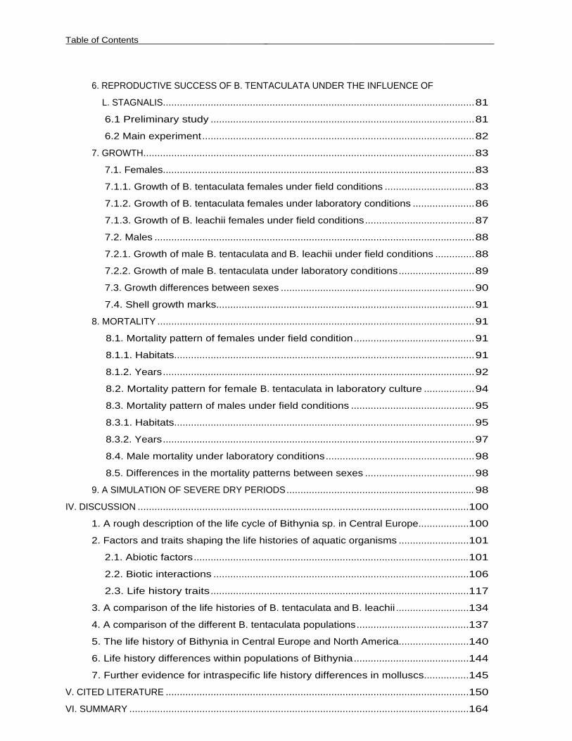
Table of Contents

6. REPRODUCTIVE SUCCESS OF B. TENTACULATA UNDER THE INFLUENCE OF

L. STAGNALIS...............................................................................................................81

6.1 Preliminary study ..............................................................................................81

6.2 Main experiment.................................................................................................82

7. GROWTH......................................................................................................................83

7.1. Females...............................................................................................................83

7.1.1. Growth of B. tentaculata females under field conditions ................................83

7.1.2. Growth of B. tentaculata females under laboratory conditions ......................86

7.1.3. Growth of B. leachii females under field conditions.......................................87

7.2. Males ..................................................................................................................88

7.2.1. Growth of male B. tentaculata and B. leachii under field conditions ..............88

7.2.2. Growth of male B. tentaculata under laboratory conditions...........................89

7.3. Growth differences between sexes .....................................................................90

7.4. Shell growth marks............................................................................................91

8. MORTALITY .................................................................................................................91

8.1. Mortality pattern of females under field condition...........................................91

8.1.1. Habitats...........................................................................................................91

8.1.2. Years...............................................................................................................92

8.2. Mortality pattern for female B. tentaculata in laboratory culture ..................94

8.3. Mortality pattern of males under field conditions ............................................95

8.3.1. Habitats...........................................................................................................95

8.3.2. Years...............................................................................................................97

8.4. Male mortality under laboratory conditions.....................................................98

8.5. Differences in the mortality patterns between sexes .......................................98

9. A SIMULATION OF SEVERE DRY PERIODS................................................................... 98

IV. DISCUSSION ......................................................................................................................100

1. A rough description of the life cycle of Bithynia sp. in Central Europe..................100

2. Factors and traits shaping the life histories of aquatic organisms .........................101

2.1. Abiotic factors..................................................................................................101

2.2. Biotic interactions ...........................................................................................106

2.3. Life history traits............................................................................................117

3. A comparison of the life histories of B. tentaculata and B. leachii ..........................134

4. A comparison of the different B. tentaculata populations........................................137

5. The life history of Bithynia in Central Europe and North America.........................140

6. Life history differences within populations of Bithynia .........................................144

7. Further evidence for intraspecific life history differences in molluscs................145

V. CITED LITERATURE ............................................................................................................150

VI. SUMMARY .........................................................................................................................164

Introduction 1

I. INTRODUCTION

Scientists today agree that there exist several millions of different species, most of them as

yet undescribed. They all differ to at least some extent in appearance, physiology, behaviour

and life history. How this diversity did arise (and is maintained) is a challenging question

for evolutionary thinking.

Life history theory is a comparatively new line of research that is deeply rooted in ecology

and evolution. Living things in their bewildering array of extremely diverse life histories

have something in common: They stand in a line of ancestors that reproduced successfully.

Most organisms start their life as a zygote. Generally spoken, a lot of opportunities are open

from this starting point to reach a condition where reproduction is possible. Which size and

age should the organism reach before it reproduces? When mature, organisms can reproduce

once, several times or continuously throughout their lifes.

Organisms differ in their allocation of resources to growth, maintenance and reproduction.

They also differ how the allocation pattern to the conflicting demands changes during their

lifetime. They can divide their limited resources to produce few, large offspring of high

quality or numerous, small offspring that are more mortality-prone. In the end, the general

problems faced are the same for oaks, elephants, snails or seals; but the answers differ.

The principal life history traits are (following Stearns, 1992):

-Size at birth

-Growth pattern

-Age at maturity

-Size at maturity

-Number, size, and sex ratio of offspring

-Age- and size-specific reproductive investments

-Age- and size-specific mortality schedules

-Length of life

Trade-offs between conflicting demands link these traits. Some important trade-offs are:

-Reproduction versus growth

-Current versus future reproduction

-Current reproduction versus survival

-Number versus size of offspring

Introduction 2

The possible outcome of trade-offs as the phenotypic plasticity an organism can show in its

life history traits are constrained by lineage specific effects (its evolutionary past).

Life history theory sets out to analyse all those aspects of the life history of organisms. The

set of traits that characterizes a particular life cycle is called a life history strategy. The

field is in itself controversial. This is not in the least astonishing because the exploration of

life histories lies at the heart of evolutionary thinking. Therefore it is a battle ground for

very diverse concepts ranging from strictly mechanistic adaptationists views over

epigenetics to Neo-Lamarckian ideas.

Long-term studies on the life-histories of individual invertebrates under natural conditions

are sparse, but empirical data are needed to test the predictions of general life history

theory. Especially data on intraspecific and individual variation in populations in the field

are missing for invertebrates. A lot of empirical and theoretical work on general life history

theory, life history variability and evolution of life histories has been carried out on

molluscs and especially on freshwater snails in recent years (e.g. Aldridge 1982; Brown

1983, 1991; Calow 1978, 1981, 1983; Hart and Begon 1982; Lam 1994; Lam and Calow

1989a,b; Ribi and Gebhardt 1986; Tompa et al. 1984).

In studies based on population means or mass culture of animals the individual variation

within the population is either not assessed or underestimated. In order to gain a more

detailed insight into the underlying patterns that are shaping life cycles and population

dynamics, I followed up the life histories of individuals in this study. Even if this study

consists therefore out of many solely descriptive observations, this is not seen as a

disadvantage. In my opinion a profound knowledge of the species' autecology is indespensible

for further research. Autecology provides the firm ground for a meaningful analysis of

complex systems like biocoenoses or ecosystems where numerous species interact.

The genus Bithynia is represented by two species in Central Europe. Bithynia tentaculata is

an iteroparous snail common in European and West Asian inland waters that has successfully

invaded North America since the last century (Frömming 1956; Harman 1968). It is a

sexually reproducing dioecious prosobranch that lives up to 4 years (Fig. 1).

B. tentaculata was chosen because of its common occurrence and its broad habitat use

(rivers, streams, lakes, permanent and temporary water bodies of diverse quality) and

because more studies concentrated on short-lived and semelparous pulmonates than on

prosobranchs so far (Brown 1983; review in Costil and Daguzan 1995a).

Introduction 3

ab

c

d

e

Fig.1a): Crawling adult snail of B. tentaculata; b): Shell and operculum of B. tentaculata;c): Shell and operculum of B. leachii; d): B. tentaculata spawn and cross-section of spawn(redrawn after Hss 1971); e): Spawn with hatching juveniles

B. leachii is somewhat smaller and less common than B. tentaculata and is, in contrast to B.

tentaculata, restricted to water bodies with fairly good water quality (Fig. 1). Its life-cycle

is less well known and there exist only a few more or less anecdotal observations in the older

literature. B. leachii is only found in still waters and, most interestingly, seems to occur

always sympatric with B. tentaculata (Boycott 1936; Frömming 1956; Grabow 1994;

Heitkamp 1982; Macan 1977; Nottbohm 1984; Wesenberg-Lund 1939). In general terms,

B. tentaculata is eurytopic compared to a stenotopic B. leachii.

The autecology of B. tentaculata has been investigated in detail in Great Britain, the St.

Lawrence River, Quebec/Canada and in Oneida Lake, upstate New York/USA (Lilly 1953;

Tashiro 1982; Tashiro and Colman 1982; Vincent et al. 1981; Vincent and Harvey 1985;

Young 1975). Vincent and Gaucher (1983) already discussed interpopulation and spatio-

temporal variations of the life cycle, but they worked with grouped snails for only one

reproductive season. The reproductive biology, development of spawn and hatching rates

under the influence of different temperatures were studied in 1995 in the laboratory and

under field conditions (Richter and Wächtler 1999).

Introduction 4

My study has the following aims:

A) To investigate the virtually unknown autecology of B. leachii

B) To improve our knowledge of the autecology of B. tentaculata

C) To understand why B. tentaculata is eurytopic and successful compared to a stenotopic and

rare B. leachii

D) To test the hypothesis that different environmental conditions should lead to discernible

differences in the life history traits between populations of the same species even in close

spatial proximity

E) To investigate if there is evidence that different female life histories exist simultaneously

even within a population

F) To delineate biotic and abiotic factors shaping the life histories of the species

G) To assess the impact of trematode parasites on snail reproduction

Material and Methods 5

II. MATERIAL AND METHODS

1. STUDY AREA AND SAMPLING METHOD

During this study, I examined six populations of B. tentaculata and one coexisting population

of B. leachii. All populations lived in Lower Saxonia, Northern Germany (Fig. 2). Three

populations were in very close spatial proximity to each other near the southern shore of the

Dümmer, a shallow lake of post-glacial origin (Fig. 2c). These populations were chosen

because they live under conditions that differ strongly in regard to limnological and

biological factors but otherwise are subject to the same climatic conditions.

The first of these populations lived in the river Hunte, which is a medium sized lowland

river running to the river Weser. The second lived in an artificial canal built to divert

highly eutrophic waters coming from intensively cultured marshland from the Dümmer (it

crosses beneath the Hunte) and the third in a ditch running parallel to the canal at the edge of

a meadow. Marshland without any trees or shrubs is surrounding the habitats.

At the sample site the Hunte is approx. 20 m wide and 1 m deep. It is slowly streaming with

some floating vegetation (Ceratophyllum demersum, Potamogeton natans), the steep banks

are dominated by Glyceria maxima. Snails were sampled by sweeping a pond net through the

vegetation, mainly the stems of G. maxima which were preferred by B. tentaculata. Snails

were restricted to areas with vegetation, the river bed and bank sections free of vegetation

were not populated by B. tentaculata.

The canal (referred to as the Canal further on) is about 7 m wide and about 1 m deep with a

very thick layer of mud on the bottom. The water is slowly streaming. Submerse and floating

vegetation (Ceratophyllum demersum, Callitriche palustris, Nuphar lutea) grows

throughout the whole water body. The bank is dominated by Carex gracilis and some Glyceria

maxima. Snails were sampled using a pond net or by direct examination of submerse

vegetation. Sampling by net was difficult because of large amounts of detritus. Snails were

limited to the upper waters because of frequent oxygen depletion in deeper water levels in

late spring and summer.

The ditch (referred to as the Ditch further on) is about 150 m long without any drain. It is

approximately 1,5 m wide and the water level is very variable, depending on weather and

season. In dry summers the Ditch may dry up for several weeks. It is surrounded by dense-

growing Carex gracilis. The bottom is covered by a thick layer of plant debris consisting


Fig. 2a): Map of Northern Germany; b): Map of Hannover, arrow indicates sampling site inthe river Leine, cross indicates location of the Veterinary School where the Pond and theSmall Pond are located; c): Map of the Dümmer, numbers mark sampling sites: 1 = Hunte, 2= Canal, 3 = Ditch

mainly of C. gracilis stems and leaves. Due to high concentrations of humic components the

colour of the water is brown. When active, B. tentaculata stayed near the water surface

because of frequent oxygen depletion in deeper water. Ceratophyllum demersum, Polygonum

amphibium and Lemna minor are the most common macrophytes. Snail sampling followed the

routine as described above.


3 other populations of B. tentaculata studied were located in Hannover, the capital city of

Lower Saxonia (Fig. 2b). They lived in a further lowland river, the Leine, a pond and a small

pond both of an artificial origin (referred to as the Pond and the Small Pond further on). The

population of B. leachii studied shared its habitat with B. tentaculata in the Pond. All habitats

are persistent and eutrophic, elevation above sea level (approx. 55 m) is the same for all of

them.

The Leine is a lowland river typical for densely populated areas with its river bed influenced

by man for centuries. At the sampling site the river, approx. 50 m wide and several meters

deep, splits into a running section and a canal for industrial purposes. It is met by a brook

(the Fösse) that starts at the slag heaps of a salt mine near the outskirts of Hannover and

runs further through the city to the Leine.

The B. tentaculata population studied lived in a layer of solid stones tipped into the river as a

reinforcement of its bank. The water is always muddy and there are no macrophytes in it.

Some nettles and a Salix sp. grow on the river bank. Water velocity fluctuates greatly

throughout the year with maxima during winter or spring floods, but is normally low in

summer and autumn. Water velocity is further reduced beneath the stones were layers of

mud aggregate. Snails were sampled by lifting stones out of the water and examining their

bottom surface to which B. tentaculata was restricted.

The Pond was built around 1930 and covers an area of approximately 2700 m2 with an

average depth of 1 m. It is located in the botanical garden of the Tierärztliche Hochschule

(Veterinary School) Hannover. The shores are lined by full grown trees and dense vegetation.

The sample site for both the populations of B. tentaculata and B. leachii was an area where

gravel was tipped from the shore. The submerse vegetation consisted mainly of

Ceratophyllum demersum, Elodea canadiensis, Nuphar lutea and green algae forming dense

mats in summer. Sampling was by pond net and direct examination of vegetation and gravel.

During summer, dense vegetation made sampling difficult.

The Small Pond is an artificial garden pond near the department of zoology which covers an

area of approx. 40 m2. It is about 0,5 m deep with a thick layer of mud and rotting plant

debris on the bottom. It is made of black plastic foil and was built in the eighties. The

vegetation is dominated by Stratiotes aloides and Lemna minor, which cover the entire water

surface during summer and autumn. Dense mats consisting of Elodea canadensis and green

algae form in summer in the upper water body. Due to frequent oxygen depletion, B.

tentaculata is restricted to the upper 20-30 cm of the water during most part of summer

and autumn. Snails were sampled by pond net, directly from the plastic foil and by examining

the vegetation.


2. FIELD STUDY

2.1. Population dynamics, sex-ratio and parasitic load

The populations were sampled monthly from March/April, when snails become active after

overwintering until September/October when snails migrate from shallow waters into

greater depths where they rest inactive in the mud, beneath plant debris or under stones

over the winter period. Exact timing of these events depends to a great extent on weather

conditions and can vary for several weeks between years. Although some snails can be

present later than October in shallow waters, sampling was stopped because older and/or

bigger snails tend to migrate earlier than juveniles. Therefore late sampling would not

reflect the true population structure.

On several occasions high water and flooding prevented sampling. Sample size varied greatly

depending on season, population, weather, water level and abundance of vegetation, but

normally between 50 and 100 snails were sampled each time. The 3 Dümmer populations

were sampled in 1997 and 1998, the 4 populations in Hannover in 1997, 1998 and 1999.

After sampling, snails were transported to the laboratory at the Tierärztliche Hochschule,

Hannover and were examined under a stereo microscope.

On some occasions (at least twice per habitat) all molluscs present were sampled, the

species determined and the level of abundance recorded.

2.2. Population structure and sex-ratio

When snails are lying on their "back" and the operculum is in view of the observer, one can

see the penis of the males behind the right tentacle when the snails are stretching out of their

shells in an attempt to regain contact to the bottom surface with their foot. Depending on the

population, a precursory structure developing into a penis in later life may be seen with

males as small as 2 or 3 mm.

Snails were grouped as males, females or gender unknown and the shell height was measured

to the nearest tenth of a millimetre using vernier callipers. With these data length-

frequency graphs were calculated. At times when small snails of unknown gender dominated

the samples, additional adults were sampled. This additional snails were used to determine

the sex-ratio and parasitic load of the population under study, but were not used in length-

frequency graphs.


2.3. Parasitic load

Infection with larval trematodes was examined by cracking the snails using tweezers and

looking for sporocysts, rediae or cercariae in the snail tissues under a stereo microscope

(magnification up to 40x). These stages are normally located in the digestive gland and/or

the reproductive organs and lead to castration of snails. Progressive infections may involve

the whole body of snails, tissues are then severely damaged and the snails can contain several

thousand cercaria.

Obviously, very early (cryptic) infection stages could not be detected by this method. Since

it was the aim of this study to detect the influence of parasitic castration on reproduction for

different populations and to assess the probability for an individual snail to loose its

reproductive capacity due to castration during its lifetime, this omission does not seem very

serious. In fact, the level of cryptic infections in a population shows itself in the pattern of

snails infected over time. On the same token, trematode larval stages were not classified

because the observed effect under study (loss of reproductive ability) was the same

regardless of trematode species.

In 1997, only preliminary studies on parasitation were carried out. In 1998 all 6

B. tentaculata populations and in 1999 the 3 populations in Hannover were checked

regularly.

2.4. Individual life histories and reproduction

Females of B. tentaculata and B. leachii were kept caged in the field. Each female inhabited an

individual cage of approximately 425 cm3 made of plastic mesh. Each cage contained a device

of acrylic glass for spawn deposition and as a foot-rest for filter-feeding. 30 female snails

sampled in March/April some weeks before the onset of the reproductive period were used

per population. Snails were sampled, sexed, caged and kept afterwards at the sampling sites.

1997 30 female B. tentaculata per population were kept in the Ditch, the Leine, the Pond and

the Small Pond (Tab. 1). 1998 and 1999 30 male and female B. tentaculata per population

were kept in the Leine, the Pond and the Small Pond. 1998 and 1999 28 male and female

B. leachii were kept in the Pond. Because of their smaller size permitting escape out of the

mesh cages made for B. tentaculata, B. leachii inhabited cages made out of acrylic tubes closed

by fine-meshed cloth at both ends.


Tab. 1: Number of snails in field experimentsB. tentaculata B. leachii

Origin Ditch Leine Pond Small Pond Pond

Females1997

30 30 30 30 -

Females1998/1999

- 30 30 30 28

Males1998/1999

- 30 30 30 28

Cages were controlled at least once a week until the end of reproductive activity. Each time

new spawns were counted, marked individually and their development was observed. The

number of dead eggs and of hatching juveniles was counted. Due to the transparent egg

membrane, the embryonic development inside the egg is easily observed (Fig. 1d). Hatching

juveniles leave a characteristic hole in the egg membrane (Fig. 1e; Lilly 1953; Richter and

Wächtler 1999). After the reproductive season controls were shifted to a biweekly pattern.

The controls stopped with the onset of overwintering in October/November and started again

in March/April the following years.

The shell height of the caged snails was measured every four weeks using vernier callipers,

dead snails were removed weekly. If the body condition of dead snails permitted, they were

examined for signs of parasitation. Snails were observed until they died. The last observation

period ended with the onset of overwintering in 1999.

2.5. Size of eggs and juveniles

Eggs sampled on one (B. tentaculata and B. leachii from the Pond) or two (Small Pond and

Leine) occasions in 1999 were measured under a stereo microscope. Since the eggs, which

have a round shape when laid singly, are fairly rectangular when laid in rows, length and

breadth were measured and multiplicated. This approximation of the area covered by the eggs

was used in comparisons. It was the aim to compare mean egg size between populations and to

test the hypothesis that egg size diminishes over time. Theoretical work suggests that females

should make greater investments per individual egg in the early than in the late reproductive

period (Begon and Parker 1986). In 1999, newly hatched juveniles of the populations in

Hannover (except the Leine population) were measured under a stereo microscope to

compare mean juvenile shell height.


2.6. Transplant experiment

In 1998, 5 pairs of B. leachii were transplanted within their cages into the Leine, where

this species, at least in the area of the sampling site, does not occur. It was the aim of this

experiment to show if reproduction of B. leachii was possible in running waters.

2.7. Temperature

Since temperature is the most important single abiotic factor, it was recorded weekly

(reproductive period) to monthly (rest of the year) for the habitats under study using min-

max thermometers. All other abiotic factors were not observed since there were no means

for any permanent recordings of water chemistry and related parameters. Occasional

measurements are regarded as being of limited ecological value by the author.

3. LABORATORY STUDIES

3.1. Individual life histories and reproduction

Snails of all habitats were maintained in laboratory culture. In 1997 females of the 6

B. tentaculata populations were kept individually in 500 ml beakers that were filled with tap

water (Tab. 2). Water was changed bimonthly. Snails were sampled before the onset of the

reproductive period. They were fed with dried green algae and Mikromin© by Tetra once or

twice a week. Mikromin© is a product normally used for raising fish fry but has also some

tradition in molluscan studies.

The temperature and light regime followed within limits conditions experienced in the field.

Due to problems with temperature regulation (temperatures below 12° C could not be

maintained), a proper overwintering could not be simulated. After air temperatures were

above freezing point in late winter 1998, snails were maintained outdoors for 3 weeks

instead and returned to the laboratory afterwards.

Beakers were controlled 2 or 3 times a week during the reproductive period. New spawns

were marked individually and eggs counted. The spawns were observed until the juveniles

hatched. Females were measured every 2 or 3 months with vernier callipers until they died.

Females not reproducing were sexed a second time to prevent that males were mistaken as

females.

After the first reproductive period, 1 or 2 males were added to every living female in

autumn, and, in some cases, in spring 1998. During the second reproductive period in


1998, procedures followed the routine of 1997. Females and males were marked with nail

varnish. Males were also measured every 2 or 3 months to detect differences in the growth

pattern between sexes.

Tab. 2: Number of snails in laboratory cultureDümmer Hannover

Hunte Canal Ditch Leine Pond Small Pond

Females1997

40 30 18 50 33 32

Males1997/1998

30/15 0/23 29 28 28 27

3.2. Critical shell height for reproduction

Since observations in the field and the laboratory suggested that females below a critical

shell height in early spring were not able to reproduce the entire year irrespective of any

growth later on, females below this size were sampled in March/April 1998 and kept with

males in 500 ml beakers. Snails were measured bimonthly and beakers were checked for

spawns regularly. 10 pairs from the Leine with females < 6,7 mm and 9 from the Pond with

females < 6,9 mm were used.

3.3. Sex-ratio of progeny

It was the aim of this experiment to find out if the sex-ratio of the snails's progeny is 1:1 or

different.

10-20 adult females per population and species were kept in the laboratory in 1997. Snails

were maintained in 1 litre aquaria to lessen food competition between females and their

progeny. When the juvenile snails had reached a sufficient size, they were sexed under a

stereo microscope and measured with vernier callipers.

Additionally, on 3 occasions in the summer of 1997, some 100 young snails sampled in the

Pond too small for immediate sex and species determination were kept in 5 l aquaria until

they reached a sexable size. Then they were sexed and the sex- and species ratio established.

The same was done with juveniles from the Leine once in 1997.

3.4. Shell growth marks and age determination

To test the hypothesis that growth marks on the shells of B. tentaculata, which some

scientists use for age determination, are formed during the process of overwintering, 46

juveniles from the Ditch too small for sex determination were sampled in October 1997 and


kept at room temperature during the winter period. In February 1998, the snails were

sexed and the number of growth rings counted.

3.5. Female choice of oviposition site

The aim of this experiment was to find out if female B. tentaculata show any substrat

preferences for egg laying when a choice of several naturally occurring substrata is given.

Experimental set-up:

Four round areas with a diameter of 35 cm were separated by plastic mesh in an aquarium.

The plastic protruded from the water so that the snails could not leave the areas. Snails could

move uninhibited within each area. Each area was divided into 8 segments of identical size. 2

segments per area contained one out of four different substrata (Fig. 3). Tested substrata

were wood, gravel, tree leaves and aquatic macrophytes (Nuphar lutea stems and leaves). All

substrata were sampled in the Pond and checked for spawns before the experiment.

Females were sampled in June 1997. Each of the 4 areas contained females of a different

population. 9 females from the Canal, 11 from the Ditch, 13 from the Pond and 15 from the

Small Pond were used. The females were left in the areas for 2 weeks, then they were

recovered and it was recorded on which substrata they were found. The substrata were

checked for spawns afterwards and spawns and eggs were counted.

Macrophytes

Macrophytes

Gravel Leaves

Leaves

Wood

Wood

Gravel

35 cm

Fig. 3: Experimental set-up for the oviposition site choice of female B. tentaculata


3.6. Reproductive success of Bithynia tentaculata under the influence of Lymnaea stagnalis

B. tentaculata and L. stagnalis often coexist in their habitats. In this study, L. stagnalis was

found in 3 out of 6 habitats. A detrimental influence through grazing by the much larger and

mobile L. stagnalis on spawns and early juvenile stages of B. tentaculata was assumed. On the

other hand, the smaller B. tentaculata is able to use habitat structures not accessible by the

larger L. stagnalis. The negative influence of L. stagnalis should therefore be reduced by

increasing structural diversity of the habitat.

Preliminary study

Ten aquaria containing 5 l of tap water were used in the laboratory in 1998. Each aquarium

contained 6 females and 4 males of B. tentaculata. Two aquaria were used as controls and

contained only B. tentaculata and a mud layer on the bottom, the other 8 contained 2 adult L.

stagnalis each. Two of the aquaria had only a mud layer on the bottom, 2 additionally a gravel

layer, 2 mud and macrophytes (Elodea canadiensis, Ceratophyllum demersum and Stratiotes

aloides) and 2 mud, gravel and macrophytes. Dead L. stagnalis were replaced when necessary.

Visible spawns on the glass were marked and observed. After the reproductive period aquaria

were examined for juveniles.

Experimental set-up

In April 1999 8 plastic tubs with a capacity of 50 l were filled with tap water and some pond

water. They all had a layer of mud on the bottom, 4 had an additional layer of gravel. Only

gravel was used since the preliminary study showed no pronounced difference between gravel

and macrophytes. Gravel has also the advantage that it can be easily examined for juvenile

snails. The tubs were left for some weeks to allow colonisation by algae and bacteria. The tubs

were located outside, evaporation was compensated for by rainfall.

10 males and 10 females of B. tentaculata were added per tub. 2 tubs contained only

B. tentaculata and served as controls. 2 tubs contained B. tentaculata and 10 adult L.

stagnalis, two tubs 5 L. stagnalis and a gravel layer, two tubs 10 L. stagnalis and a gravel

layer. After 6 months the tubs were searched for juveniles and adults of both species and

their number was recorded.

3.7. A simulation of severe dry periods

The Ditch at the Dümmer frequently dries up in hot summers with poor rainfall and

therefore the population of B. tentaculata is obviously adapted to survive this unfavourable


periods. It seemed interesting to test whether this is a special adaptation of this population or

whether the species as a whole is capable to survive dry periods.

14 aquaria with a capacity of approximately 1,5 l were filled with pond water in June

1997. They had a layer of mud and gravel on the bottom. 2 of them were used for each of the

6 B. tentaculata populations and 2 contained B. leachii from the Pond. They contained 10-12

B. tentaculata and 28 B. leachii; altogether 66 female and 61 male B. tentaculata and 31

female and 25 male B. leachii. The water evaporated gradually until the aquaria fell dry in

October. 4 weeks later water was added and the living snails were counted. To avoid any

disturbances during the drying process, the number of surviving snails was not determined

prior to desiccation.

3.8. Parasitation and reproduction

During this study I frequently observed that a certain percentage of adult females did not

reproduce. Because there obviously seems to be no advantage in fitness terms related to not

reproducing, I assumed that non-reproducing females were castrated by parasites. To test if

parasitation is the only cause for reproductive failure, 33 adult females from the Hunte

population were kept in 0,5 l beakers from May 1998 to late August 1998. Then the non-

reproducing females were crushed and searched for parasitic stages.

4. STATISTICS

All statistics throughout this study were made with StatView 5.0 (1998), SAS Institute

using a Macintosh Power PC. Due to the nature of the data which often did not allow the use of

parametric statistics because of different variances between groups and/or data lacking

normal distribution, non-parametric tests (Kruskal-Wallis One-Way ANOVA, Wilcoxon

Rank Sum Test, Fisher's Exact Test) were applied several times.

Non-parametric tests were preferred over data transformation. Statistical significance is

claimed when the P-value is at least < 0,05 or smaller. Smaller P-values are not marked

differently for non-parametric tests in this study because of the comparatively small

number of 30 or less per group.

After finding significant differences using a Kruskall-Wallis-Test, a posteriori comparisons

were made using U-Tests.

A posteriori comparisons after a significant ANOVA normally used Bonferroni/Dunn Tests

that controlled for number of comparisons. In some instances the less conservative Fisher's

Post-Hoc Test was preferred.


For the comparison of egg number of first spawn to egg number of last spawn a paired T-Test

was used. In cases when the exact number was not clear because 2 or more spawns had been

laid between controls, the mean egg number of spawns was used in analysis. All T-Tests in

this study are two-tailed.

To compare the shell height at maturity between populations, the heights of the 5 smallest

reproducing snails per year were used in analysis.

The tendency for larger females to lay larger spawns at the onset of breeding than small

females predicted by Begon and Parker (1986) was examined in a correlation analysis using

the mean of the spawns laid in the first 3 weeks for females that reproduced at least for 5

weeks.

Throughout the text the term significant is always used in the sense of statistically

significant in regard to the applied statistical methods. For better readability, the term

significant may lack when there is direct reference to a significant P-value in the text.

Box Plots: In the results section, variables are often displayed as box plots. Each box plot is

composed of 5 horizontal lines that display the 10th, 25th, 50th, 75th and 90th percentiles

of a variable (this means, for example, that half of all data points are contained within the

box between the second and the forth horizontal line. The 50th percentile is equal to the

median of a distribution). All values above the 90th percentile and below the 10th percentile

are plotted separately as small open circles to display outliers. Since my interest was on

individuals showing divergent traits, box plots were often chosen to present data.

Results 17

III. RESULTS

1. HABITAT CONDITIONS

1.1. Utilizable habitat size

Water velocity and oxygen

Because of the special requirements of any living organism, the physical size of a habitat and

its utilizable size for a given organism are mostly not the same. A rough assessment of the 6

habitats leads to following classification:

A) The rivers:

High water velocity makes it impossible for B. tentaculata to adhere to the surface of

vegetation or stones. As a result, sites with strong water currents like the river bed were

not populated by snails. Snails living in the Hunte used solely the vegetation on both river

banks, preferring areas near the water surface. The snails in the Leine were living more or

less densely clustered on the underside of stones. This structures reduced water velocity

effectively so that fine detritus and mud settled down. Oxygen supply seemed sufficient since

even very muddy parts were populated in summer.

B) Habitats with oxygen depletion in summer:

Oxygen depletion and long periods with anaerobic conditions and H2S formation occurred

regularly in the Canal, the Ditch and the Small Pond each summer. This was due to the heavy

load of plant debris and organic detritus in the habitats. As a consequence, B. tentaculata

lived near the water surface during summer and avoided all parts deeper than 30-50 cm.

Snails reentered bottom parts only when water temperatures decreased in autumn.

The failure to keep caged snails alive at the Dümmer was due to a long-lasting oxygen

depletion in all but the upmost water levels in the Canal and the Ditch during the summer of

1997.

At the end of the reproductive period in July 1998 one containment with about 50

B. tentaculata dropped into the anaerobic zone at the bottom of the Small Pond. Since controls

happened on a weekly basis, snails were exposed at maximum for seven days to hypoxic

conditions. About 80% of the snails were dead at recovery of the containment and most others

Results 18

died the following week. All eggs that had remained at the season's end were also dead. This

illustrates the pronounced effect of oxygen availability on the gill-breathing Bithynia.

C) Habitats without oxygen depletion:

The Pond was the only habitat with standing water that was populated in all depth during

summer. B. tentaculata and B. leachii were found directly beneath the water surface and in

depths of approximately 1,5 m. Except for deeper layers of rotting plant debris, the whole

habitat was utilizable the year round even when snails preferred the parts near the water

surface in summer.

1.2. Temperature

The temperature profiles of the three habitats in Hannover resembled each other very

closely. The water temperature rised steadily from mid-March to June, being more or less

stable in the range of 15°C to 22°C during summer until autumn. Temperatures started to

decrease slowly then, reaching their minimum during winter (Fig. 4).

Neither the maxima (ANOVA, P = ,1875) nor the minima (ANOVA, P = ,1685) differed

significantly between the habitats, but there was a trend towards the Pond being slightly

warmer than the Small Pond. The highest temperatures were frequently measured in the

Pond but never exceeded 24°C. The lowest temperatures were encountered in the Leine

where the temperature dropped to 1°C in winter. In contrast, the temperature in the ponds

seldom dropped below 4°C and periods of ice cover were short in both winters.

To search for differences in temperature fluctuations between habitats, the weekly

differences between the minima and maxima for any given temperature measurement were

used in an analysis of variance, but there was no difference found (ANOVA, P = ,8788). The

temperature regime in the habitats therefore seems homogenous on a long-time scale.

Results 19

0

5

10

15

20

25 9

.4.-

15

.4.

7.5

.-13.5

.

4.6

.-1

0.6

.

2.7

.-8.7

.

30

.7.-

5.8

.

27

.8.-

2.9

.

24.9

.-30.9

.

22

.10

.-2

8.1

0.

19

.11

.-2

5.1

1.

17

.12

.-2

4.1

2.

15.1

.-21.1

.

12.2

.-18.2

.

13.3

.-19.3

.

10.4

.-16.4

.

8.5

.-1

4.5

.

5.6

.-1

1.6

.

3.7

.-9.7

.

31.7

.-6.8

.

28.8

.-3.9

.

25

.9.-

1.1

0.

23.1

0.-

29.1

0.

20.1

1.-

26.1

1

18.1

2.-

24.1

2.

15

.1.-

21

.1.

12

.2.-

18

.2.

12

.3.-

18

.3.

9.4

.-15.4

.

7.5

.-13.5

.

5.6

.-11.6

.

3.7

.-9.7

.

31.7

.-6.8

.

28.8

.-3.9

.

25

.9.-

1.1

0.

23.1

0.-

30.1

0.

Small Pond max.Small Pond min.

0

5

10

15

20

25

9.4

.-1

5.4

.

7.5

.-13.5

.

4.6

.-1

0.6

.

2.7

.-8.7

.

30

.7.-

5.8

.

27

.8.-

2.9

.

24.9

.-30.9

.

22

.10

.-2

8.1

0.

19

.11

.-2

5.1

1.

17

.12

.-2

4.1

2.

15.1

.-21.1

.

12.2

.-18.2

.

13.3

.-19.3

.

10.4

.-16.4

.

8.5

.-1

4.5

.

5.6

.-1

1.6

.

3.7

.-9.7

.

31.7

.-6.8

.

28.8

.-3.9

.

25

.9.-

1.1

0.

23.1

0.-

29.1

0.

20.1

1.-

26.1

1

18.1

2.-

24.1

2.

15

.1.-

21

.1.

12

.2.-

18

.2.

12

.3.-

18

.3.

9.4

.-15.4

.

7.5

.-13.5

.

5.6

.-11.6

.

3.7

.-9.7

.

31.7

.-6.8

.

28.8

.-3.9

.

25

.9.-

1.1

0.

23.1

0.-

30.1

0.

Pond max.Pond min.

0

5

10

15

20

25

9.4

.-1

5.4

.

7.5

.-13.5

.

4.6

.-1

0.6

. 2

.7.-

8.7

.

30

.7.-

5.8

.

27

.8.-

2.9

. 2

4.9

.-30.9

.

22

.10

.-2

8.1

0.

19

.11

.-2

5.1

1.

17

.12

.-2

4.1

2.

15.1

.-21.1

.

12.2

.-18.2

.

13.3

.-19.3

.

10.4

.-16.4

.

8.5

.-1

4.5

.

5.6

.-1

1.6

.

3.7

.-9.7

.

31.7

.-6.8

.

28.8

.-3.9

.

25

.9.-

1.1

0.

23.1

0.-

29.1

0.

20.1

1.-

26.1

1

18.1

2.-

24.1

2.

15

.1.-

21

.1.

12

.2.-

18

.2.

12

.3.-

18

.3.

9.4

.-15.4

.

7.5

.-13.5

.

5.6

.-11.6

.

3.7

.-9.7

.

31.7

.-6.8

.

28.8

.-3.9

.

25

.9.-

1.1

0.

23.1

0.-

30.1

0.

Leine max.Leine min.

1997 1998 1999

1997 1998 1999

1997 1998 1999

Fig. 4: Temperature regime of the three habitats in Hannover (y-axis in °C)

Results 20

1.3. Predators

The presence or absence of predators deeply influences the living conditions for any

organism and may alter the size of the utilizable habitat.

A) Shell invading predators: Leeches, water bugs and beetles were present in all habitats.

Chaetogaster sp. was especially common in the Ditch.

B) Shell breaking predators: Crayfish (Orconectes sp.) were present in the Leine and in the

Pond. Fish were absent in the Small Pond and in the Ditch with the exception of nine-spined

stickleback in 1998 in the latter habitat. All other habitats had a diverse fish fauna which

could not be classified any further.

Dabbling ducks were commonly present on the Leine and the Canal and to a lesser degree on

the Pond and the Small Pond.

1.4. Co-occuring molluscan species

Overall 20 gastropod and 5 bivalve species were found (Tab. 3; the genus Pisidium is not

included). The most diverse were the 3 habitats at the Dümmer whereas in Hannover only

few molluscan species were present. Prosobranch diversity was generally low with 4

species out of 6 present in only 1 of the habitats. Only in one habitat, the Leine, lived more

than 2 different prosobranch species. Pulmonate diversity was generally higher than that of

prosobranchs with exception of the Leine where only Radix ovata was found. 11 pulmonate

species occurred in the Canal, 10 in the Ditch and 9 in the Hunte.

Members of the Unionidae were found in three habitats with three species living in the Hunte

and one species in the Canal and the Pond. Sphaerium corneum was quite common and found in

4 habitats whereas Dreissena polymorpha was only found in the Leine.

Several species were altogether rare and only few individuals were found. This is the case

with Viviparus contectus, Potamopyrgus antipodarum, Valvata cristata , Acroloxus

lacustris, Galba truncatula, Radix auricularia, Gyraulus albus and Hippeutis complanatus.

Anisus vortex was very abundant in all its habitats. All other gastropod species showed

intermediate patterns, rare in some habitats and common elsewhere.

Results 21

Tab. 3: Species composition of the different habitatsHunte Canal Ditch Small

PondPond Leine

GASTROPODA

Viviparus contectus * *

Potamopyrgus antipodarum *

Bithynia tentaculata * * * * * *

Bithynia leachii *

Valvata piscinalis *

Valvata cristata *

Acroloxus lacustris * * * *

Lymnaea stagnalis * * *

Stagnicola sp. * * * * *

Galba truncatula *

Radix ovata * * * *

Radix auricularia * *

Planorbis planorbis * * *

Planorbis carinatus * * *

Anisus vortex * * * *

Bathyomphalus contortus * * *

Gyraulus albus * *

Hippeutis complanatus * *

Planorbarius corneus * *

Physa fontinalis * *

BIVALVIA

Unio pictorum *

Anodonta cygnea * *

Anodonta anatina * *

Sphaerium corneum * * * *

Dreissena polymorpha *

Results 22

1.5. Abundance of the molluscan species in different habitats

Hunte

B. tentaculata was by far the most common species and dominant most time. In spring 1997

Valvata piscinalis was dominant and three times as abundant as B. tentaculata but numbers

receded during summer. Anisus vortex, Physa fontinalis and Sphaerium corneum could be

common sometimes, all other species were rare.

Canal

B. tentaculata and A. vortex were the most abundant species but their presence was strongly

fluctuating. Common were Planorbis planorbis and P. fontinalis, all other species were rare.

Ditch

The Ditch was clearly dominated by pulmonate species. P. planorbis, P. carinatus, A. vortex,

Bathyomphalus contortus and Planorbarius corneus were very common with a maximum in

late summer/autumn. B. tentaculata was most common in spring and early summer when the

pulmonates had not yet reached high numbers. The other pulmonates were rare.

Small Pond

With exception of Stagnicola sp. all molluscan species were common but their abundance was

fluctuating with time of year. B. tentaculata was mostly present in large numbers but in late

summer A. vortex was sometimes predominant. Lymnaea stagnalis was rare in early spring

but numbers increased dramatically when juvenile hatching started in late spring/summer.

Sphaerium corneum was always common but never predominant.

Pond

B. tentaculata was common in spring, rare after the die-off in summer and common again in

late summer/autumn when juveniles were grown. B. leachii was rare the first 2 years and

predominant over B. tentaculata in the second half of 1999. All other snail species were

mostly rare. The number of species was low for a comparatively large habitat as the Pond.

Results 23

Leine

B. tentaculata was the dominant snail species comprising more than 80% of all snails in all

the years. Only Radix ovata was also common during 1998, all other prosobranchs were rare

to non-existent. In the summer 1998 Dreissena polymorpha was the predominant mollusc

species comprising more than 50% of all individuals but its numbers decreased rapidly

during winter.

2. GROWTH PATTERN, POPULATION DYNAMICS AND SEX-RATIO OF FIELD POPULATIONS

2.1. Some remarks on field sample data

Following sample data are biased, simply because large snails are more easily found than

smaller ones. Fortunately, this bias is in the same direction for all populations. Dense

submerse vegetation presented the major obstacle for sampling, regardless of sampling

technique, so sampling data from habitats without macrophytes like the Leine are more

accurate than data from habitats with extensive vegetation like the Canal, the Ditch or the

Pond. For latter habitats difficulties increased from spring to summer with increasing plant

growth, in some instances making it impossible to search successfully for snails during

summer months. This explains most of the lacking data points in graphs.

As a further consequence, newly hatched snails smaller than 2,5 mm could not be sampled

appropriately and were therefore excluded from analysis. This leads to the effect that mean

shell size in diagrams drops with a delay of approximately one month to the start of juvenile

hatching in the field. In my opinion this poses no problems for comparisons because this

shift is encountered in all habitats and for both species.

2.2. Growth pattern and population dynamics

2.2.1. Introductory remarks

First, there is a comparison of the population means for shell height for every habitat and

species separately, combined with evidence from the length-frequency diagrams. The first

part is followed by the same data viewed under the angle of different years for all observed

populations simultaneously. The same procedure is employed on the temporal fluctuations of

sex-ratio within and between populations.

Sample size for individual data points is not included in the figures showing mean shell

height and sex-ratio, but can be seen in the length-frequency diagrams (which use the same

data sets).

Results 24

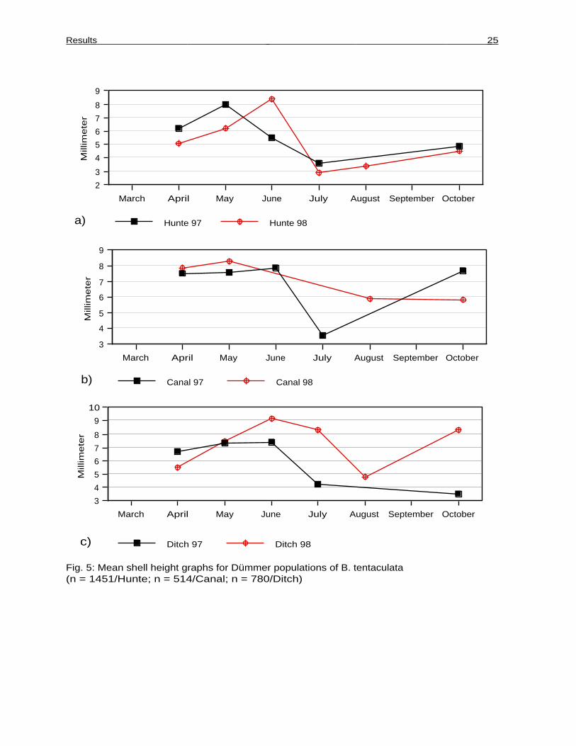
2.2.2. Habitats

Hunte

On the whole, the curves for both years are fairly congruent. Mean shell height in early

spring was different in 1997 and 1998 (T-Test, P < ,0001), the population consisting of

larger size classes in 1997 than the following year when there were a lot of snails well

below adult size (Figs. 5a and 8).

In both years there was an increase in mean shell height during spring to early summer

followed by a steep decline which marks the hatching of juveniles. Juvenile hatching started

4 weeks earlier in 1997 than in 1998. In contrast to 1998 there were already juveniles

present in June 1997. In both years the population consisted mainly of young individuals by

July. In 1998 there was almost a complete replacement of elder individuals during summer

months.

There was moderate shell growth in both years from late summer onwards till the onset of

overwintering. The slope of the curve was much steeper in spring than in autumn in both

years. The mean shell height before and after overwintering as the length-frequency data of

the population were in correspondence.

Canal

The population was already very large in early spring both years, consisting almost

exclusively of adult animals and showing only very moderate growth until summer (Figs. 5b

and 8). In 1997 there was a steep decline in July when juveniles hatched and adults

vanished, followed by rapid growth of juvenile snails. The newborns already reached mean

adult sizes before winter.

The mean shell height before and after overwintering corresponded directly as did the

length-frequency distributions of the population. Intense vegetation made sampling

impossible in the summer of 1998. In August there was a mixture of very small to large

snails with no size class overproportionally present. Until October there was apparently no

growth and the population mean was below the value for 1997, but this may be an artefact

due to the small sample size (n =16).

Results 25

2

3

4

5

6

7

8

9M

illim

ete

r

March April May June July August September October

Hunte 98Hunte 97

3

4

5

6

7

8

9

Mill

imete

r


Canal 98Canal 97

3

4

5

6

7

8

9

10

Mill

imete

r


Ditch 98Ditch 97

a)

b)

c)

Fig. 5: Mean shell height graphs for Dümmer populations of B. tentaculata(n = 1451/Hunte; n = 514/Canal; n = 780/Ditch)

Results 26

5

6

7

8

9

10

11M

illim

ete

r


Small Pond 99Small Pond 98Small Pond 97

4

5

6

7

8

9

10

Mill

imete

r


Pond 99Pond 98Pond 97

2

3

4

5

6

7

8

9

Mill

imete

r


Leine 99Leine 98Leine 97

a)

b)

c)

Fig. 6: Mean shell height graphs for B. tentaculata populations in Hannover (n =2304/Small Pond; n = 1046/Pond; n = 2825/Leine)

Ditch

The graphs for both years are very different (Figs. 5c and 8). Mean shell height in April

was different in both years (U-Test, Tied P = ,0001), the population consisting mainly of

subadult snails in 1998.

Results 27

In 1997 there was only moderate growth after overwintering with a great part of the

population retaining a size below the critical shell size for reproduction. Juvenile hatching

started in July. The population seemingly did not grow afterwards until overwintering. In

October nearly the whole population was represented by very small individuals. Mean height

before and after overwintering did not correspond.

In 1998 there was initially a rapid increase in shell size during spring with all individuals

reaching adult sizes in summer. Juveniles first appeared in July again but main juvenile

hatching occured a month later than the previous year. After the reproductive period the

population grew very fast reaching a maximum in the adult size classes in autumn.

Small Pond

The population structure in the Small Pond showed some peculiarities as the population

almost completely failed to reproduce in 1997 and 1999 (Figs. 6a and 9). In April 1997

mean shell height was already near 9 mm. There was a small, but constant increase until

July when the population mean reached 10 mm. Almost all animals were in the size classes 9

to 11 mm by then. Mean shell height remained on this high level until autumn with a small

decline in October. This was due to the appearance of very few juveniles in this month.

In March 1998 the mean shell height was already well above 9 mm. The population

structure was in correspondence with that of the previous October, the whole population

comprised of the size classes 9 to 11 mm with only very few smaller juveniles present. The

mean shell height increased to 10 mm in May and stayed on this level until August. In August

the population consisted of nearly 80% of newly hatched snails. Mean shell size dropped to

5 mm and increased about 1mm per month until October.

In March 1999 mean shell height was below March 1998 (U-Test, Tied P = ,0222) and

well above the level of the previous October (T-Test, P = ,0003). This points in the

direction that mortality is higher in smaller size classes during winter. The population grew

very fast until May when 90% of all snails were 10 mm or larger, some reaching

exceptionally large shell sizes of 13 mm and above. Juveniles were always present in

samples from July onwards but they comprised only a small fraction of the population and

size classes of 10 mm and above remained dominant until autumn.

Results 28

Pond

The population means were different in all years in April (ANOVA, P < ,0001;

Bonferroni/Dunn post hoc test, P < ,0001 for all three comparisons between years).

In 1997, the population started from a low level with no prevalent size class and grew until

June when half the snails were in the 9 mm size class (Figs. 6b and 10). Juveniles appeared

in July comprising 60% of the total population. At the same time a fungal disease started

killing the adult snails (most likely a pathogenic member of the family of Saprolegniales

(Oomycota), pers. com. by A. de Cock, Bureau for Schimmelculturen, the Netherlands).

Mean shell height increased until September again and dropped a bit in October when a

second autumnal rush of juveniles entered the population.

In April 1998 the mean shell height was already 8 mm and increased to above 9 mm in one

month. In June and July the population was dominated by small size classes when juveniles

hatched and the fungus killed large numbers of adult snails. Until August mean shell height

increased for more than 3 mm in just one month and increased further in autumn. In

September 75% of the population was in or above the 9 mm size class.

In March 1999 the population set out from this high level and in April 85% of all snails had

a shell height of 9 mm or above. Due to a very early and severe fungal infection this year,

the population declined drastically in early summer 1999. Nearly no snails were found until

July when the newly hatched snails had reached searchable sizes. Growth again was rapid

until August but came to a halt later on. It should be mentioned that the fungal infection

started earlier every year, but never occurred again after July, thereby not affecting the

new generations.

Leine

This population showed the most uniform course throughout the years (Figs. 6c and 9). After

overwintering the mean shell height increased slowly to its maximum in June, then dropped

to its minimum in July when juveniles hatched in large numbers. Hatching was followed by

rapid growth in late summer that slowed down in autumn and came to a halt at the end of the

season.

The population composition was different in spring 1998 when the mean shell height was

well below that of the other years (March: U-test, Tied P = ,0010; April: Kruskall-Wallis-

Test, Tied P < ,0001). There were differences in the population composition before and after

overwintering. Population means were slightly above the October values in March 1998 and

1999. The differences were only significant between October 1998 and March 1999 when

Results 29

the mean shell height difference was 0,5 mm (T-Test, P = ,0385). This underlines the

aforementioned trend that winter mortality is higher in the smaller size classes.

B. leachii

Data for B. leachii are sparse as a consequence of the rareness of this species that only

became abundant in 1999. Compared to B. tentaculata the length-frequency distribution was

more homogeneous because B. leachii curbs growth at a smaller size (Figs. 7 and 10). Most

snails remained in the 5 mm size class or below, with the exception of spring 1999 when

40% were in the 6 mm and some females even in the 7 mm size class.

2

3

4

5

6

Mill

imete

r


B. leachii 99B. leachii 98B. leachii 97

Fig. 7: Mean shell height graph for B. leachii (n = 317)

Only 1999 is discussed in detail when nearly 200 B. leachii were sampled. Being slightly

above 5 mm, the mean shell height in April 1999 was nearly 1 mm above the previous years

(Difference was significant, ANOVA P < ,0001; Bonferroni/Dunn P < ,0001 for comparisons

between years). The population grew moderately in spring and juveniles dominated from

July onwards. The mean shell size was 3 mm in July. The increase in shell size was only

moderate during autumn in 1999.

Results 30

2468

101214

2468

101214

2468

101214

2468

101214

2468

101214

2468

101214

2468

101214

April n = 76 May n = 91 June n = 59

HUNTE1997

HUNTE1998

July n = 199

2468

101214

2468

101214

2468

101214

April n = 119

2468

101214

April n = 76

April n = 71

April n = 176

April n = 67

2468

101214

2468

101214

2468

101214

2468

101214

2468

101214

2468

101214

2468

101214

2468

101214

2468

101214

May n = 115 June n = 73

CANAL1997

CANAL1998

May n = 63 June n = 10 July n = 89

May n = 32

DITCH1997

DITCH1998



2468

101214

2468

101214

July n = 222(different X-axis!)

Fig. 8: Length-frequency graphs for the Dümmer populations of B. tentaculata

Results 31

2468

101214

October n = 153

August n = 232 October n = 112

2468

101214

2468

101214

2468

101214

2468

101214

2468

101214

2468

101214

HUNTE1997

HUNTE1998

CANAL1997

CANAL1998

October n = 86


DITCH1997

DITCH1998

October n = 52 (different X-axis)


2468

101214

2468

101214

Results 32

2468

101214

2468

101214

2468

101214

2468

101214

2468

101214

2468

101214

2468

101214

2468

101214

2468

101214


March n = 76 April n = 88 May n = 65

March n = 130 April n = 336 May n = 117

SMALLPOND1997

SMALLPOND1998

SMALLPOND1999

2468

101214

2468

101214

2468

101214

2468

101214

2468

101214

2468

101214

2468

101214

2468

101214

2468

101214

2468

101214

2468

101214

LEINE1997

LEINE1998

LEINE1999


March n = 85 April n = 216 May n = 96 June n = 119

March n = 84 April n = 204 May n = 96 June n = 71

Fig. 9: Length-frequency graphs for the Small Pond and Leine populations of B. tentaculata

Results 33

2468

101214

2468

101214

2468

101214

2468

101214

2468

101214

2468

101214

2468

101214

2468

101214

2468

101214

2468

101214

2468

101214

July n = 74 August n = 62 September n = 58 October n = 75


July n = 102 August n = 121 September n = 96

SMALLPOND1997

SMALLPOND1998

SMALLPOND1999

2468

101214

2468

101214

2468

101214

2468

101214

2468

101214

2468

101214

2468

101214

2468

101214

2468

101214


2468

101214

July n = 188 (dif. X-axis) August n = 99 September n = 141 October n = 91

July n = 169 August n = 132

2468

101214

September n = 128

LEINE1997

LEINE1998

LEINE1999

Results 34

2468

101214

2468

101214

2468

101214

2468

101214

2468

101214

2468

101214

2468

101214

2468

101214

2468

101214

2468

101214

2468

101214

2468

101214

2468

101214



March n = 89 April n = 41

April n = 28

April n = 29

June n = 9April n = 51 May n = 51

POND1999

POND1998

POND 1997

B. leachii1997

B. leachii1998

B. leachii1999

Fig. 10: Length-frequency graphs for the Pond populations of B. tentaculata and B. leachii

Results 35

2468

101214

2468

101214

2468

101214

2468

101214

2468

101214

2468

101214

2468

101214

2468

101214

2468

101214

2468

101214

2468

101214

2468

101214

2468

101214

2468

101214

2468

101214

July n = 75 September n = 44 October n = 43


July n = 87 August n = 39

POND1997

POND1998

POND1999

July n = 8 October n = 16

August n = 17 September n = 28


B. leachii1997

B. leachii1998

B. leachii1999

2468

101214

September n = 20

Results 36

2.2.3. Years

1997

This was a year with fairly homogeneous tendencies (Fig. 11a). In April the mean shell

heights of most populations were between 6 mm and 7 mm. However, there were significant

differences (ANOVA, P < ,0001). The Canal population lay somewhat above average and the

Small Pond population was clearly larger than all others (Bonferroni/Dunn, P < ,0001).

The Small Pond population remained larger than the other populations throughout the year.

This was in part due to its lack of reproductive success.

All populations grew moderately during spring. The first juveniles appeared in the Hunte

already in June and one month later in the other habitats. With exception of the Ditch there

was considerable growth in late summer and autumn. However, the rate of increase in shell

height differed between habitats to the effect that in October there were pronounced

differences in mean shell height between the populations (Kruskall-Wallis-Test, P <

,0001, a non-parametric test was employed because shell height distribution was bimodal

in some cases).

Shell heights fell into 4 groups at the end of the season, the Small Pond population being

larger and the Ditch population smaller than all others (Fig. 11a). The Canal and Pond

populations were of the same mean height and fairly large with 7,5 mm but their length-

frequencies showed differences (Figs. 8 and 10). The Canal population was dominated by the

size class of 8 mm which comprised nearly 50% of all snails whereas the Pond population

was more evenly distributed and had its maximum with 30% in the 9 mm size class. The

river populations (Leine and Hunte) were clearly smaller and lay between them and the

Ditch.

1998

This year the course of the mean shell heights was inhomogenous (Fig. 11b). The population

differences visible the previous October prevailed throughout overwintering. Only the mean

shell height in the Ditch closed up to the river populations, leaving 3 groups of significantly

different shell heights (ANOVA, P < ,0001; Bonferroni/Dunn P < ,0001 for differences

between groups). The Small Pond snails were by far the largest, the Pond and Canal snails

were of intermediate height and the group with the smallest mean heights consisted of the

Hunte, Leine and Ditch populations.

Results 37

3 populations showed rapid growth in spring with an increase of at least 1 mm per month

for 1 (Pond) or 2 months (Hunte and Ditch), the others showed a more restrained increase.

Juveniles were first present in the Pond, making up the majority of the population from

June onwards. Differences were pronounced in July, the river populations of Leine and

Hunte consisting almost completely out of juveniles by now whereas hatching commenced

only slowly in the other Dümmer populations and no juveniles were found in the Small Pond.

Here newborn snails appeared during autumn, comprising now more than 75% of the

population.

The mean shell height reached its minimum in August for 2 populations (Ditch and Small

Pond), whereas it increased for more than 3 mm in the Pond and the Leine. During autumn

the increase in shell size ranged from zero (Canal and Leine) over moderate (Hunte, Small

Pond and Pond) to rapid in the Ditch.

At the end of the season the mean shell heights fell again within 3 groups clearly separated

from each other (Kruskall-Wallis-Test, P < ,0001). However, the grouping differed from

the spring situation. The population in the Ditch had now by far the largest mean shell size,

the Hunte snails were the smallest and the other 4 populations were intermediate. The

picture was even further complicated because of the different size class distributions (uni-

and bimodal) within the 6 populations (Figs. 8, 9 and 10).

1999

This year the mean shell heights were again different between the 3 remaining populations

(Fig. 11c). Shell heights differed in March (Kruskall-Wallis-Test, P < ,0001) when Pond

and Leine showed a unimodal size-frequency distribution with a maximum in the 10 mm and

8 mm class, respectively. The Small Pond showed a bimodal distribution with clearly

separated juvenile- and adult-sized snails (Fig. 9).

Growth in spring was zero in the Pond, moderate for three months in the Leine and fast until

May in the Small Pond population, the latter reaching the mean shell size of the Pond

population already in April. The Small Pond population failed successful reproduction again

this year. In contrast, the Leine population consisted mainly of juveniles by July (Fig. 9).

Because most snails were killed by the fungal infection in the Pond, sampling was

unsuccessful in May and June. In July the Pond population consisted of fast-growing

juveniles with no apparent maximum in any size-class (Fig. 10). During late summer rapid

Results 38

23456789

1011


Leine 97

Pond 97

Small Pond 97

Ditch 97

Canal 97

Hunte 97

Mill

imete

r

23456789

1011

Mill

imete

r


Leine 98

Pond 98

Small Pond 98

Ditch 98

Canal 98

Hunte 98

23456789

1011

Mill

imete

r


Leine 99Pond 99Small Pond 99

a)

b)

c)

Fig. 11: Mean shell heights for all years and all B. tentaculata populations (n = 8920)

growth took place in the Pond and the Leine that stopped already in autumn. In the Small Pond

some juveniles were found in September, the adult snails showing no further increase in

shell size before winter.

Results 39

2.2.4. Gender effects on growth

The effect of gender on growth was of minor importance. When the growth data were splitted

for gender, the resulting mean shell height graphs were mostly in parallel (Fig. 12). At the

Dümmer, only the Canal population showed minor differences between males and females

(Fig. 12a). However, this seems to be an artefact of the small sample sizes (Because the

sex-ratio fluctuates in time, the number of snails of a given gender was low at some

sampling dates. Several samples had to be excluded for this reason).

3

4

5

6

7

8

9

10

Mill

imete

r

April May June July Aug Sep Oct April May June July Aug Sep Oct

Ditch Males

Ditch Females

Canal Males

Canal Females

Hunte Males

Hunte Females

4

6

8

10

12

Mill

imete

r

Apr May Jun Jul AugSep Oct Mar Apr May Jun Jul AugSep Oct Mar Apr May Jun Jul AugSep

Leine Males

Leine Females

Pond Males

Pond Females

Small Pond Males

Small Pond Females

1997 1998

1997 1998 1999

a)

b)

Fig. 12: Mean shell height graphs for all B. tentaculata populations, data splitted by gender(n = 8920)

The graphs for the Leine population in Hannover were in parallel for the three years under

study (Fig. 12b). Differences between male and female curves are most pronounced in the

Pond population. This is most obvious in spring/early summer 1997 and 1999.

Results 40

Some differences were apparent in the Small Pond (Fig. 12b). During spring 1997 only

males grew while females remained on a high level throughout the season. In spring 1998

females started growing a month before males. In 1999 the mean shell height of males

increased earlier than that of females. However, this year females reached mean shell

heights equal to males for the first time (see next section for further details).

2.2.5. A comparison of gender and habitat

Sexual dimorphism

There is no easy way to answer the question whether there is any sexual dimorphism in the

genus Bithynia. The data are quite ambiguous. In three B. tentaculata populations females

were overall bigger than males, in two populations males and females had overall identical

mean shell heights and in one population males were larger than females (Tab. 4).

Height differences were most pronounced for the Canal and the Pond populations where the

mean shell height of females lay 5% above males. The Small Pond was the only habitat where

males were larger than females.

With B. leachii gender differences were more pronounced. The mean shell height of females

lay 20% above male shell height in this species (Tab. 4).

Tab. 4: Height relations of males to females for all populations (heights of all sampled and sexedindividuals > 3,5 mm were pooled for analysis)

Females > Males Females = Males Males > Females

Canal, T-Test P = ,020Female: 7,9 mm ± 1,3 (n = 156)Male: 7,5 mm ± 1,3 (n = 155)

Hunte, T-Test P = ,15Female: 6,0 mm ± 2,0 (n = 505)Male: 5,9 mm ± 1,8 (n = 432)

Small Pond, U-Test P < ,0001Female: 9,1 mm ± 1,9 (n = 1039)Male: 9,4 mm ± 2,1 (n = 1063)

Pond, T-Test P = ,0005Female: 8,1 mm ± 2,0 (n = 415)Male: 7,7 mm ± 2,0 (n = 507)

Ditch, T-Test P = ,47Female: 7,3 mm ± 2,2 (n = 318)Male: 7,4 mm ± 2,1 (n = 354)

Leine, T-Test P = ,017Female: 6,9 mm ± 1,6 (n = 969)Male: 6,7 mm ± 1,6 (n = 1239)B. leachii, U-Test P < ,0001Female: 4,8 mm ± 1,2 (n = 159)Male: 4,0 mm ± 0,9 (n = 132)

An analysis of the height to breadth ratio revealed no significant differences between male

and female B. tentaculata. This means that the height to breadth ratio increases

symmetrically with growth for both genders (Fig. 13). This holds true for all 6 habitats. An

ANOVA of the height to breadth ratio between habitats (height divided by breadth was used for

comparisons) showed that snails originating from the Leine were slimmer than other snails

Results 41

(ANOVA, P < ,0001; Bonferroni/Dunn, P < ,0033 or smaller for the a posteriori

comparisons).

2

3

4

5

6

7

Bre

adth

2 3 4 5 6 7 8 9 10 11Height (mm)

Males

Females

Breadth = 1,067 + ,511 * Height; R^2 = ,867 (Males)Breadth = ,857 + ,56 * Height; R^2 = ,87 (Females)

Fig. 13: Regression of breadth on height for B. tentaculata, splitted by gender (n = 554)

An ANOVA showed differences between the habitats and the mean shell height of populations

(Fig. 14; Tab. 5). The overall smallest snails were found in the rivers with the Hunte

population (6,0 mm) being even smaller than the Leine population (6,8 mm). Snails from

the Ditch (7,4 mm) were on average larger than river snails but smaller than snails from

the Pond (7,9 mm) and the Canal (7,7 mm) which were of equal size. By far the largest

snails inhabited the Small Pond (9,3 mm).

0

2

4

6

8

10

Hunte Canal Ditch Small Pond Pond Leine

Mill

ime

ter

Fig. 14: Mean shell height of the different B. tentaculata populations (n = 10920)

When the data are splitted by gender, the ranking between habitats remains unchanged with

only one exception: the mean shell height of the Ditch males is equal to that of Canal and Pond

males (Tab. 5). This is a consequence of the differences in sexual dimorphism between the

populations. The Canal and Pond females were on average larger than males whereas in the

Ditch both genders were of equal size.

Results 42

Tab. 5: Ranking of the mean height of males and females and the population means (for meanheight values and n see Tab. 4)ANOVA: Mean height of whole population/males/females from the different habitats(Bonferroni/Dunn post hoc test, = difference not significant; < difference significant)

Population

P < ,0001Hunte < Leine < Ditch < Canal = Pond < Small Pond

Females

P < ,0001Hunte < Leine < Ditch < Canal = Pond < Small Pond

Males

P < ,0001Hunte < Leine < Ditch = Canal = Pond < Small Pond

To compare the maximum shell heights between the 6 habitats, an ANOVA for the mean shell

height of the largest individuals was calculated (Tab. 6). Individuals from the Small Pond

were clearly larger than any other snails. Pond individuals remained on the second position

but Canal snails had smaller maximum sizes and fell below the Ditch and even the Leine

(males). This signifies that even though the Canal population was a population consisting of

large animals, individual snails did not attain maximum sizes above 10 mm. Shell heights of

10 mm and above were frequently encountered in other habitats where the overall

population means were lower than in the Canal.

Tab. 6: Ranking of the mean values of the largest male/female B. tentaculata per populationANOVA: Mean height of the largest males/females from the different habitats (n = 20), in millimetre(Bonferroni/Dunn post hoc test, = difference not significant; < difference significant)

Females

P < ,0001Leine (9,5) = Canal (9,6) = Hunte (9,8) < Ditch (10,5) = Pond (11,1) < Small Pond (12,1)

Males

P < ,0001Hunte (9,3) = Canal (9,3) < Leine (10,0) < Ditch (10,9) = Pond (11,1) < Small Pond (12,1)

2.3. Snail abundance

Different habitat size, habitat structures and varying sampling techniques made it

impossible to strictly compare population size between habitats. Instead a comparison based

on sampling time is used to rank habitats (Fig. 15). This seems the more reasonable as

population size itself is strongly fluctuating and dependent on time of year. Using the mean

sample size for one hour of sampling effort is levelling off the seasonal influence.

B. tentaculata was most abundant in the Leine with a mean sample size of 382 snails per

hour sampling effort, followed by the second river population, the Hunte, with a mean

sample size of 295 snails. The Small Pond population is intermediate with a mean of 189

snails per hour sampling effort. In the other habitats, B. tentaculata was far less abundant

Results 43

with a mean sample size of 66 snails in the Canal, 54 snails in the Ditch and 36 in the Pond

(Fig. 15). B. leachii was even less common than B. tentaculata in the Pond, its low numbers

preventing any useful calculation of a mean sample size.

0

100

200

300

400

Nu

mb

er

of

sna

ils

Hunte Canal Ditch Small Pond Pond Leine

Fig. 15: Number of B. tentaculata per hour sampling effort for the different habitats(n = 6754)

Abundance of B. leachii in relation to B. tentaculata in the Pond

B. leachii was far less abundant than B. tentaculata in 1997 and 1998 (Tab. 7). Its numbers

increased significantly during 1999 (Fisher's Exact P-Value < ,0001).

Tab. 7: Number of sampled individuals of both co-occuring speciesin the Pond samples (percentage of total individuals in brakes)Year B. leachii B. tentaculata

1997 58 (15%) 323 (85%)1998 84 (16%) 455 (84%)1999 190 (38%) 313 (62%)

2.4. Sex ratio

2.4.1. Overall sex ratio of the different habitats

The sex-ratio of B. tentaculata was balanced (Canal and Small Pond) or males predominated

(Fig. 16). Only in the Hunte lived slightly more females than males. Differences between

habitats were significant and the overall sex-ratio for B. tentaculata is dissimilar from 1:1

(Contingency Table, Chi Square P < ,0001). The predominance of males is clearly visible in

the Pond and in the Leine. In contrast to B. tentaculata, with B. leachii females were more

abundant.

Results 44

0 10 20 30 40 50 60

B. leachii (n = 329)

Leine (n = 2442)

Pond (n = 1039)

Small Pond (n = 2191)

Ditch (n = 688)

Canal (n = 424)

Hunte (n = 1101)

MalesFemales

Fig. 16: Sex-ratio of populations of both species, data pooled for all years

2.4.2. Temporal fluctuations in gender abundance

The sex-ratio of male to female B. tentaculata was not stable in time but exhibited more or

less pronounced fluctuations within years (Figs. 17 and 18).

Hunte

The Hunte population was the only one where there were slightly more females than males

(Fig. 16). In the first half of 1997 the percentage of females showed great fluctuations,

starting slightly above 50% in April, reaching a maximum in May and a minimum in June

(Fig. 17a). After June the percentage of females increased steadily until October.

In 1998 the curve is very smooth, the percentage of females starting with a maximum of

56% in March, decreasing steadily to a low in June and increasing thereafter again above

50% in October.

Canal

Fluctuations in gender abundance were not pronounced. There was a trend towards females

being less abundant than males at the end of the season (Fig. 17b).

Results 45

Ditch

Females made up clearly more than half of the population in April 1997 but then their

percentage declined rapidly to below 30% in June (Fig. 17c). Data is lacking afterwards

because the population consisted mainly of juveniles to small for sex determination.

In March 1998 females made up 60% of the population. Their percentage dropped to 40% in

April and May and increased again to 50% for the rest of the year.

25

50

75

Pe

rce

nt


Hunte 1998Hunte 1997

25

50

75

Pe

rce

nt


Canal 1998Canal 1997

25

50

75

Pe

rce

nt


Ditch 1998Ditch 1997

a)

b)

c)

Fig. 17: Percentage of females in samples from the Dümmer

Small Pond

In accordance with an overall sex-ratio of 1:1, the percentage of females in the samples was

mostly near 50% (Fig. 18a). The major deviations occured in spring 1997 and in April

Results 46

25

50

75P

erc

en

t


Small Pond Fem. 1999Small Pond Fem. 1998Small Pond Fem. 1997

20

50

80

Pe

rce

nt


Pond Fem. 1999Pond Fem. 1998Pond Fem. 1997

25

50

75

Pe

rce

nt


Leine Fem. 1999Leine Fem. 1998Leine Fem. 1997

a)

b)

c)

Fig. 18: Percentage of females in samples from Hannover

1998 when there were overproportionally many females in the samples. By far the fewest

females were sampled in September 1999. The percentage of females before and after

overwintering is in good accordance both times.

Pond

In most samples there were clearly less than 50% females present (Fig. 18b). In general,

the percentage of females was higher in spring, diminished during summer and rised again in

autumn when it lay above 50% in 1997 and 1998. The lowest number of females was

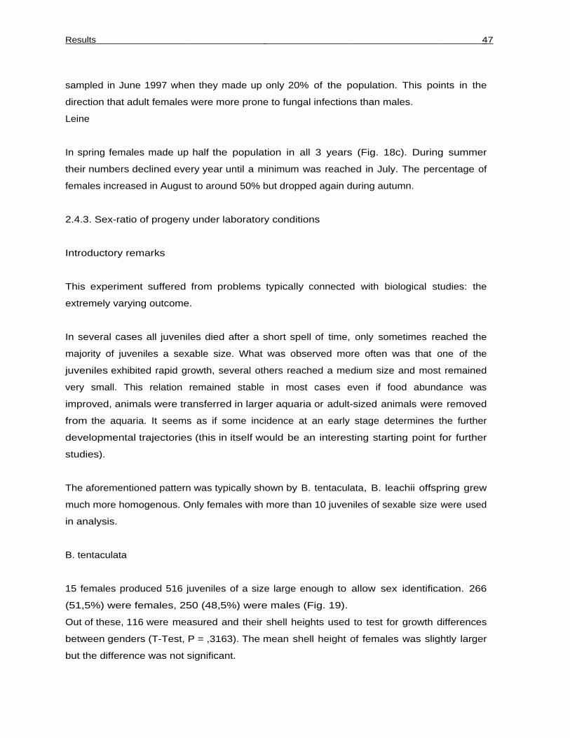
Results 47

sampled in June 1997 when they made up only 20% of the population. This points in the

direction that adult females were more prone to fungal infections than males.

Leine

In spring females made up half the population in all 3 years (Fig. 18c). During summer

their numbers declined every year until a minimum was reached in July. The percentage of

females increased in August to around 50% but dropped again during autumn.

2.4.3. Sex-ratio of progeny under laboratory conditions

Introductory remarks

This experiment suffered from problems typically connected with biological studies: the

extremely varying outcome.

In several cases all juveniles died after a short spell of time, only sometimes reached the

majority of juveniles a sexable size. What was observed more often was that one of the

juveniles exhibited rapid growth, several others reached a medium size and most remained

very small. This relation remained stable in most cases even if food abundance was

improved, animals were transferred in larger aquaria or adult-sized animals were removed

from the aquaria. It seems as if some incidence at an early stage determines the further

developmental trajectories (this in itself would be an interesting starting point for further

studies).

The aforementioned pattern was typically shown by B. tentaculata, B. leachii offspring grew

much more homogenous. Only females with more than 10 juveniles of sexable size were used

in analysis.

B. tentaculata

15 females produced 516 juveniles of a size large enough to allow sex identification. 266

(51,5%) were females, 250 (48,5%) were males (Fig. 19).

Out of these, 116 were measured and their shell heights used to test for growth differences

between genders (T-Test, P = ,3163). The mean shell height of females was slightly larger

but the difference was not significant.

Results 48

B. leachii

16 females produced 506 juveniles, 260 (51,4%) were females and 246 (48,6%) males

(Fig. 19). All juveniles were measured, the females having a mean shell size of 3,1 mm and

the males of 2,6 mm. Females grew significantly faster than males (U-test Tied P < ,0001).

0 10 20 30 40 50 60

B. tentaculata (n = 516)

B. leachii (n = 506)

MalesFemales

Fig. 19: Sex-ratio of laboratory offspring

The outcome is consistent with the hypothesis that both species have a sex-ratio of 1:1 at

birth and there is no bias in favour of one gender. Only for B. leachii gender had a significant

influence on juvenile growth rate. This is consistent with the pronounced sexual dimorphism

encountered in field sample data for B. leachii.

Juveniles sampled in the Pond and the Leine in summer 1997

Of several hundred juvenile snails sampled in the Pond 83 reached a size sufficient for sex

and species determination in February 1998. 69 (31 females, 38 males) belonged to B.

tentaculata, 14 (6 females, 8 males) to B. leachii. This relation of juveniles (69/14;

83%/17%) is in good agreement with the relation for relative abundance of the two species

found throughout direct sampling of the Pond populations in 1997 (323 B. tentaculata /58

B. leachii ; 85%/15%).

From the juveniles sampled in the Leine, 78 were females and 68 males. This adds up to 109

female and 106 male B. tentaculata.

3. PARASITES

The percentage of snails parasitized by trematodes fluctuated with time in all habitats (Figs.

20 and 21). The grade of parasitic infection was examined separately for males and females

but differences were only significant in the Small Pond. Here more females than males were

Results 49

infected (Fisher's Exact Test, P = ,0008). Data for males and females are therefore

combined for statistical analysis in the other 5 populations.

3.1. Habitats

3.1.1. Dümmer

In the spring of 1998 the percentage of snails parasitized was low in the Hunte and the Ditch

and high in the Canal (Fig. 20). The percentage of infected snails increased more or less

rapidly until July when approximately 25% of the populations were infected. There are no

data for the Canal due to sampling problems. In August percentage of parasitized snails was

below 5% in the Canal and the Ditch but remained high in the Hunte. In late autumn

parasitation was low in all habitats. Overall parasitation levels were highest in the Hunte

(15%), intermediate in the Canal (11%) and low in the Ditch (8%) (Tab. 8).

0

10

20

30

40

Pe

rce

nt


Ditch 1998Canal 1998Hunte 1998

Fig. 20: Percentage of parasitized B. tentaculata in the Dümmer populations (n = 550)

3.1.2. Small Pond

The Small Pond exhibited some unusual features. It was the only population showing a gender

effect. Furthermore was it possible in 1999 to compare infection levels of older snails to

that of snails born the previous year (Fig. 21a). This was possible because of

aforementioned differences in the shell structure.

Gender and parasitation

The gender effect was first observed in autumn 1998. In 1997 and in spring/summer 1998

infection levels for males and females were the same. In autumn 1998, out of 62 examined

females 47 (76%) were parasitized, but out of 85 males only 44 (52%), the difference

being statistically significant (Fisher's Exact Test, P = ,0035). The effect persisted for the

Results 50

older snails (born in 1997 or earlier) in 1999. This year, out of 43 examined females 32

(74%) and out of 62 males 17 (27%) were infected (Fisher's Exact Test, P < ,0001).

Interestingly, the number of parasitized snails showed no significant difference between

genders for the snails born the previous year (12 parasitized females out of 71 examined

and 4 parasitized males out of 70).

Seasonal fluctuations and stage specific parasitation

In July 1997 24% of the Small Pond snails were parasitized and this number doubled until

October (Fig. 21a). In May 1998 the number of parasitized snails (25%) was lower than

the previous autumn, pointing towards a higher winter mortality of parasitized snails. The

infection level increased steadily during summer and autumn until in October more than

70% of the adult population were parasitized (and 24 out of 26 examined adult females!).

In 1999 several processes interact. Old snails started on a high level of parasitation in April

(60%) that is retained in May (55%). Then the infection level dropped to 24% in July.

This was mostly due to the mortality scheme, almost all of the highly parasitized old females

being dead by now. The surviving old males showed a moderate infection level compared to

females.

The young snails started on a very low infection level in spring 1999, but the percentage of

infected animals increased during summer until 22% are parasitized in August. Because

most of the older snails were dead by now, younger snails contributed increasingly to the

overall infection level from summer onwards. These interactions led to the observed scheme

of parasitic infections with its decline from April to July and its levelling off around 20% in

late summer.

The overall infection level (37% of all examined snails) was by far the highest for all

habitats under study (Tab. 8).

Tab. 8: Parasitation of snails in per cent (number of parasitized snails/ number of examined snails)Hunte Canal Ditch

Parasitized % Parasitized % Parasitized %

1998 38/261 15 7/66 11 18/223 8

Small Pond Pond LeineParasitized % Parasitized % Parasitized %

1997 35/96 37 3/11 8/46 171998 147/292 50 11/90 12 33/399 81999 72/292 25 8/93 9 17/248 7

Sum: 254/680 37 22/194 11 58/693 8

Results 51

3.1.3. Pond

Parasitation was low in spring in both years (Fig. 21b). Data are very sparse until August

because the fungal infection killed nearly all adult snails during spring/early summer and

there is no point in examining newly hatched snails for trematode larva.

In 1998 the number of infected snails increased in autumn up to 20%. In 1999 quite a large

number of the new generation was parasitized by July. However, no infected snails were

found later on. With 11% the overall infection level is moderate in the Pond (Tab. 8).

0

20

40

60

80

Pe

rce

nt


Pond 1999Pond 1998

0

20

40

60

80

Pe

rce

nt


Leine 1997 Leine 1999Leine 1998

0

20

40

60

80

Pe

rce

nt


Small Pond 1999Young Snails 1999

Older Snails 1999

Small Pond 1998

Small Pond 1997

1997

a)

b)

c)

Fig 21: Percentage of parasitized B. tentaculata in the populations in Hannover (n: a = 680;b = 194; c = 693)

Results 52

3.1.4. Leine

The course of parasitation levels was identical in both years. With 3% the infection level

was very low in March (Fig. 21c). It remained low until May and increased towards June,

reaching nearly 20% in July as in July 1997. The infection level dropped in late summer

and was low to zero (September 1999) until overwintering. With 8% the overall infection

level of the population was low (Tab. 8).

3.2. Parasitation and gigantism

The mean shell sizes of parasitized and non-parasitized snails were compared to test for

increased shell growth in reaction to parasitation. This mechanism is repeatedly documented

in the literature. Only snails > 7 mm were used in the analysis since trematode parasitation

is often occult in smaller animals. The outcome is equivocal: In the Small Pond and the Leine

the mean shell size for both groups is exactly the same; in the Hunte, the Ditch and the Pond

the parasitized snails belong to a significantly larger subgroup of the population (Tab. 9).

The number of Canal snails examined was too low to allow any statistical analysis.

Tab. 9: Comparison of the mean shell height of parasitized and non-parasitized snailsOrigin Parasitized Non-parasitized P-value

Hunte Ø = 9,0 mm ± 1,2 (n = 27) Ø = 8,1 mm ± 0,7 (n = 115) < ,0001; U-testDitch Ø = 9,6 mm ± 1,5 (n = 23) Ø = 9,0 mm ± 1,0 (n = 131) ,0066; U-testSmall Pond Ø = 10,1 mm ± 0,8 (n = 181) Ø = 10,1 mm ± 0,7 (n = 204) ,6485; T-TestPond Ø = 10,5 mm ± 1,0 (n = 21) Ø = 9,3 mm ± 1,2 (n = 156) < ,0001; T-TestLeine Ø = 7,9 mm ± 0,8 (n = 40) Ø = 8,0 mm ± 0,6 (n = 279) ,5196; T-Test

4. INDIVIDUAL LIFE HISTORIES AND REPRODUCTION

4.1. Individual life histories and reproduction of females in the field

Introductory remark

To structure the following section there is first a comparison on the population respective

species level which gives a picture of the general outline. Field data of all years is pooled for

statistical analysis. Afterwards the variance within each population for the 3 (2) years

under study is analysed and the legitimacy of the data being pooled will be post hoc

established. To round the picture off each years data will be analysed shortly in the

concluding section. For a short explanation of box plot graphs used frequently throughout

this section, see page 16 in Material and Methods.

Results 53

4.1.1. Minimal female height for reproduction

Females in the Small Pond (8,6 mm) and the Pond (8,2 mm) attained significantly larger

sizes before reproducing than Leine females (7,4 mm) (Fig. 22; ANOVA, P < ,0001;

Bonferroni/Dunn post hoc test, P < ,0001 -Small Pond/Leine-; P = ,0010 -Pond/Leine-).

Height of B. leachii females (4,4 mm) was clearly below that of B. tentaculata females (T-

Test, P < ,0001).

3

4

5

6

7

8

9

10

Mill

imete

r

B. leachii Leine Pond Small Pond

<______ B. tentaculata ______>

Fig. 22: Height of smallest reproducing females (n = 55)

4.1.2. Start of reproduction

The starting point for reproduction differed for 2 to 4 weeks (that corresponds to

differences in water temperature of 2 to 4 °C) between females within each population. The

differences were most pronounced for old and young females in the Small Pond in 1999. Here

the old females (aged 2 years or older) started to reproduce in April, approximately 1

month earlier than females born the previous summer.

4.1.3. Egg number

The mean number of eggs laid per reproducing female was in the range of 188 to 400 and

differed significantly between the populations (Fig. 23; Tabs. 10, 19 and 21).

The mean egg number per female for the Leine population (400 eggs) lay above the other

B. tentaculata populations and B. leachii . The mean egg number for the Small Pond (188

eggs) and the Pond (189 eggs) were the same. The mean egg number for B. leachii (228

eggs) lay significantly above the mean for the Small Pond, but the difference to the Pond was

not significant (Tab. 10).

Results 54

The differences between females with a high and a low output of eggs were most pronounced

in the Leine population. The total egg number of individual females per reproductive period

was below 100 eggs for some females and nearly 900 eggs for others.

The differences between females were in the same order of magnitude in the other 3

populations (Fig. 23).

0

100

200

300

400

500

600

700

800

900

Num

ber

of eggs


<______ B. tentaculata _______>

Fig. 23: Mean egg number of reproducing females (n = 221)

Tab. 10: Egg number statistics (The Kruskall-Wallis-Test tested the whole data set for significantdifferences; the U-Tests are a-posteriori tests to establish significant differences between 2groups within the data set after a positive Kruskall-Wallis-Test was calculated)Egg number (n = 221) Kruskall-Wallis-Test, Tied P < ,0001

Small Pond = Pond U-Test, Tied P = ,9499Small Pond < Leine U-Test, Tied P < ,0001Small Pond < B. leachii U-Test, Tied P = ,0171Pond < Leine U-Test, Tied P < ,0001Pond = B. leachii U-Test, Tied P = ,0750Leine > B. leachii U-Test, Tied P = ,0001

4.1.4. Number of spawns

The mean number of spawns per reproducing female was statistically different between the

populations (Tabs. 11, 19 and 21; Fig. 24). B. leachii females laid on average more spawns

(36,2 spawns) than any of the 3 B. tentaculata populations. Leine females laid significantly

more spawns (29,1 spawns) than females from the Small Pond (11,3 spawns) or the Pond

(11,8 spawns). There was no difference between the Small Pond and the Pond.

Differences between individual females for the number of spawns laid per reproductive

period were most pronounced within the Leine population, intermediate for B. leachii and

low for the Small Pond and Pond populations (Fig. 24).

Results 55

0

10

20

30

40

50

60

70N

um

be

r o

f sp

aw

ns


<_______ B. tentaculata _______>

Fig. 24: Mean number of spawns per reproducing female (n = 221)

Tab. 11: Spawn number statistics (The Kruskall-Wallis-Test tested the whole data set forsignificant differences; the U-Tests are a-posteriori tests to establish significant differencesbetween 2 groups within the data set after a positive Kruskall-Wallis-Test was calculated)Spawn number (n = 221) Kruskall-Wallis-Test, Tied P < ,0001

Small Pond = Pond U-Test, Tied P = ,9332Small Pond < Leine U-Test, Tied P < ,0001Small Pond < B. leachii U-Test, Tied P < ,0001Pond < Leine U-Test, Tied P < ,0001Pond < B. leachii U-Test, Tied P < ,0001Leine < B. leachii U-Test, Tied P = ,0294

4.1.5. Eggs per spawn

The mean number of eggs per spawn was statistically different between the populations

(Tabs. 12, 19 and 21; Fig. 25). B. leachii had on average less eggs per spawn (6,7 eggs)

than any of the 3 B. tentaculata populations. Leine spawns contained on average significantly

fewer eggs (14,5 eggs) than spawns from the Small Pond (18,1 eggs) or the Pond (18,9

eggs). Again there was no significant difference between the Small Pond and the Pond

populations.

The differences between individual females with regard to mean number of eggs per spawn

were low for B. leachii and pronounced for the Small Pond and Pond populations (Fig. 25).

Results 56

0

5

10

15

20

25

30

35

40

45

50Ø

of

eg

gs

pe

r sp

aw

n


<_______ B. tentaculata _______>

Fig. 25: Mean number of eggs per spawn (n = 221)

Tab. 12: Eggs per spawn statistics (The Kruskall-Wallis-Test tested the whole data set forsignificant differences; the U-Tests are a-posteriori tests to establish significant differencesbetween 2 groups within the data set after a positive Kruskall-Wallis-Test was calculated)Eggs per spawn (n = 221) Kruskall-Wallis-Test, Tied P < ,0001

Small Pond = Pond U-Test, Tied P = ,9404Small Pond > Leine U-Test, Tied P = ,0004Small Pond > B. leachii U-Test, Tied P < ,0001Pond > Leine U-Test, Tied P = ,0022Pond > B. leachii U-Test, Tied P < ,0001Leine > B. leachii U-Test, Tied P < ,0001

In all populations of both species the number of eggs per spawn decreased significantly

between the onset and the end of the breeding season (Tab. 13). The mean difference between

first and last spawns was most pronounced in the Small Pond but also clearly visible in the

Pond and the Leine. The decline in egg number per spawn within the breeding period was

least distinctive for B. leachii.

Table 13: Paired T-Test, egg number of first spawn compared to egg number of last spawnper breeding season for individual femalesOrigin Mean difference

between first andlast spawn

P-value n

Small Pond 33,68 ± 25,81 < ,0001 59Pond 23,45 ± 20,87 < ,0001 56Leine 16,52 ± 13,21 < ,0001 56B. leachii 9,30 ± 7,42 < ,0001 56

The mean egg number of spawns declined constantly throughout all months of each

reproductive season. This is even obvious when mean egg number per spawn started on a low

level as is the case with B. leachii (Tab. 14).

Results 57

Tab. 14: Mean egg numbers per spawn for the consecutive months of the reproductive period (thenumbers in brackets show egg number of the smallest and biggest spawns)Origin 1. Month 2. Month 3. Month 4. Month 5. Month 6. Month

Small Pond1997

Ø: 16,7(1-79)n = 132

Ø: 13,8(2-36)n = 90

Ø: 7,4(2-18)n = 14

Small Pond1998

Ø: 30,9(1-121)n = 55

Ø: 19,3(2-67)n = 81

Ø: 9,9(1-34)n = 68

Small Pond1999

Ø: 24,8(4-60)n = 35

Ø: 22,0(1-69)n = 92

Ø: 10,9(2-25)n = 52

Ø: 4,6(1-13)n = 30

Pond 1997 Ø: 31,0(1-78)n = 19

Ø: 12,2(1-36)n = 170

Ø: 9,0(3-22)n = 87

Ø: 8,1(3-14)n = 13

Pond 1998 Ø: 20,6(1-83)n = 78

Ø: 15,2(1-29)n = 37

Ø: 6,5(3-12)n = 10

Pond 1999 Ø: 24,5(1-123)n = 121

Ø: 15,2(1-30)n = 118

Leine 1997 Ø: 15,7(1-44)n = 68

Ø: 13,9(2-34)n = 162

Ø: 9,1(1-22)n = 67

Leine 1998 Ø: 18,1(1-60)n = 107

Ø: 11,6(1-32)n = 124

Ø: 10,7(3-21)n = 11

Leine 1999 Ø: 19,6(5-64)n = 82

Ø: 15,9(1-31)n = 303

Ø: 13,5(1-37)n = 264

Ø: 10,7(1-25)n = 339

Ø: 13,5(5-24)n = 38

Ø: 23,7(2-46)n = 10

B. leachii1998

Ø: 10,3(1-29)n = 52

Ø: 8,3(1-52)n = 320

Ø: 4,9(1-19)n = 224

Ø: 3,4(1-10)n = 87

B. leachii1999

Ø: 8,3(1-41)n = 223

Ø: 6,2(1-17)n = 619

Ø: 4,6(1-21)n = 141

Ø: 3,1(1-5)n = 10

In every year and for all populations the mean egg number per spawn was highest in the

first month of the reproductive period. It declined more or less rapidly afterwards. The only

exception is the unusual long reproductive period in the Leine in 1999. Mean egg numbers

increased during autumn again after a minimum in summer, but only few females took part

in the autumnal reproduction (Tab. 14).

4.1.6. Range of eggs per spawn and other spawn characteristics

Mean range of eggs per spawn

The mean range of eggs per spawn was significantly different between the populations (Tab.

15; Fig. 26). This parameter measures the difference between the biggest and smallest

Results 58

spawn for any reproductive female. By this it allows to compare the extent of seasonal shifts

in egg number per spawn within and between populations during the course of the

reproductive period.

The mean range of eggs per spawn for B. leachii (17,1) was less than the mean range for the

3 B. tentaculata populations (Tab. 20). The mean range of Small Pond females (44,3) lay

significantly above the level in the Leine (29,8) and the Pond (36,1). The difference

between the Pond and the Leine was not significant.

Tab. 15: Range of eggs per spawn statistics (The Kruskall-Wallis-Test tested the whole data set forsignificant differences; the U-Tests are a-posteriori tests to establish significant differencesbetween 2 groups within the data set after a positive Kruskall-Wallis-Test was calculated)Range of eggs per spawn (n = 221) Kruskall-Wallis-Test, Tied P < ,0001

Small Pond > Pond U-Test, Tied P = ,0311Small Pond > Leine U-Test, Tied P < ,0001Small Pond > B. leachii U-Test, Tied P < ,0001Pond = Leine U-Test, Tied P = ,1976Pond > B. leachii U-Test, Tied P < ,0001Leine > B. leachii U-Test, Tied P < ,0001

The mean range of eggs per spawn declined continuously alongside with mean egg number of

spawns throughout the reproductive period (Tab. 14). The only exceptions were the Small

Pond in 1999 when the young snails started to reproduce with a delay of 1 month compared

to old snails and the B. leachii population in 1998. But in general big spawns were laid in the

beginning of each season and no more at its end. Nonetheless most spawns laid were small

spawns independent of population, year or time of season. Spawns containing few eggs to only

1 were laid continuously throughout the reproductive period in all populations. (Tab. 14).

0

20

40

60

80

100

120

140

Range o

f egg n

um

ber


<_______ B. tentaculata _______>

Fig. 26: Mean range of eggs per spawn (n = 221)

Results 59

Egg number of first spawns

It was of interest to find out wether the first spawn a given female produced during the

reproductive period was also the biggest spawn (and therefore the female's biggest per cent

investment in reproductive terms).

This was the case more often in the Small Pond and the Pond than in the Leine (Tab. 16; Chi

Square P = ,0262). B. leachii laid less often the biggest spawn at the start of the

reproductive period than B. tentaculata, but this was statistically just not significant (Tab.

16; Fisher's Exact P-Value = ,0504). The difference became significant when only the

sympatric populations of both species were compared (Fisher's Exact P-Value = ,0048).

Tab. 16: Number of females that laid their biggest spawn at the start of the reproductive seasonOrigin First spawn = Biggest spawn First spawn ≠ Biggest spawn

Small Pond 40 14Pond 42 10Leine 42 29

Sum B. tentaculata 124 53

B. leachii 24 21

In general, B. tentaculata females laid biggest spawns containing more eggs than B. leachii

females (Fig. 27; Kruskall-Wallis Test, P < ,0001). Big spawns in the Small Pond and the

Pond could contain more than a hundred eggs whereas egg numbers never exceeded 65 eggs in

the Leine and 52 eggs for B. leachii spawns.

By the same token B. leachii females laid on average smallest spawns containing less eggs

(1,3 eggs) than B. tentaculata females (5,6 eggs) (Kruskall-Wallis-Test; P < ,0001).

0

20

40

60

80

100

120

140

Egg

s


<_______ B. tentaculata _______>

Fig. 27: Egg number of biggest spawn (n = 221)

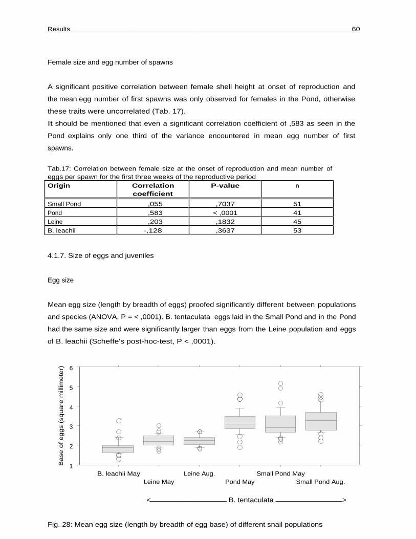
Results 60

Female size and egg number of spawns

A significant positive correlation between female shell height at onset of reproduction and

the mean egg number of first spawns was only observed for females in the Pond, otherwise

these traits were uncorrelated (Tab. 17).

It should be mentioned that even a significant correlation coefficient of ,583 as seen in the

Pond explains only one third of the variance encountered in mean egg number of first

spawns.

Tab.17: Correlation between female size at the onset of reproduction and mean number ofeggs per spawn for the first three weeks of the reproductive periodOrigin Correlation

coefficientP-value n

Small Pond ,055 ,7037 51Pond ,583 < ,0001 41Leine ,203 ,1832 45B. leachii -,128 ,3637 53

4.1.7. Size of eggs and juveniles

Egg size

Mean egg size (length by breadth of eggs) proofed significantly different between populations

and species (ANOVA, P = < ,0001). B. tentaculata eggs laid in the Small Pond and in the Pond

had the same size and were significantly larger than eggs from the Leine population and eggs

of B. leachii (Scheffe's post-hoc-test, P < ,0001).

1

2

3

4

5

6

Base

of eggs

(square

mill

imete

r)

B. leachii MayLeine May

Leine Aug.Pond May

Small Pond MaySmall Pond Aug.

<________________ B. tentaculata ______________>

Fig. 28: Mean egg size (length by breadth of egg base) of different snail populations

Results 61

Most interestingly, eggs of the Leine population and of B. leachii were almost the same size

with only a small difference that was not statistically significant (Fig. 28).

The mean egg size at the beginning and the end of the reproductive period remained the same

for the Small Pond and the Leine.

Juvenile shell height at hatching

An ANOVA revealed significant differences (P = <, 0001) in juvenile shell height at

hatching. The hatchlings of B. tentaculata in the Pond and the Small Pond were of the same

height (about 1,2 mm; Fig. 29) and both were significantly larger than hatchlings from B.

leachii (Scheffe's post hoc test, P = <,0001). Unfortunately, the situation in the Leine did

not allow for sampling of freshly hatched juveniles. Since mean egg size of the Leine

population was in the range of B. leachii eggs used in analysis, it seems a reasonable

interpolation that shell height of juveniles in the Leine should be smaller than in the other

habitats of B. tentaculata.

,5

,7

,9

1,1

1,3

1,5

Mill

imete

r

B. leachii Pond Small Pond

<______ B. tentaculata ______>

Fig. 29: Juvenile shell height at hatching in millimeter(n = 30)

4.1.8. Length of reproductive period

The mean length of the reproductive period was significantly different between the

populations (Fig. 30; Tabs. 18 and 19). Leine females had, with a mean value of 86,7 days,

on average the longest reproductive periods. For several females its duration exceeded 4

months. Pond females had a significantly shorter mean length of the reproductive period

(37,6 days) than any other population (Tab. 19). This was due to the high mortality caused

by the fungal infections every year.

Results 62

There was no significant difference in the mean length of the reproductive period between

the Small Pond (57,7 days) and B. leachii (64,4 days).

0

20

40

60

80

100

120

140

160

Days

B.leachii Leine Pond Small Pond

<______ B. tentaculata _______>

Fig. 30: Mean length of reproductive period in days (n = 191)

Tab. 18: Statistics for length of reproductive period (The ANOVA tested the whole data setfor significant differences; the Bonferroni/Dunn tests are a-posteriori tests to establishsignificant differences between 2 groups within the data set after a positive ANOVA wascalculated)Length of reproductive period (n = 191) ANOVA, P < ,0001

Small Pond > Pond Bonferroni/Dunn, P = ,0075Small Pond < Leine Bonferroni/Dunn, P < ,0001Small Pond = B. leachii Bonferroni/Dunn, P = ,2522Pond < Leine Bonferroni/Dunn, P < ,0001Pond < B. leachii Bonferroni/Dunn, P = ,0001Leine > B. leachii Bonferroni/Dunn, P = ,0006

4.1.9. Hatching rates of eggs

The hatching rate of eggs was generally high in all habitats (Fig. 31; Tab. 19). With more

than 97% of all eggs hatched the mean hatching rate was highest for B. leachii and with

90,6% it was somewhat lower for the coexisting B. tentaculata population in the Pond. The

hatching rate of B. leachii females never dropped below 90% in a single case with data for

more than 50 females included (Tab. 19).

Differences between the hatching rates of individual females were most pronounced in the

Small Pond, but also in this population more than 85% of all eggs hatched on average.

Hatching rates were not obtained for the Leine population because of aforementioned

difficulties due to silt sedimentation in the cages.

Results 63

0

20

40

60

80

100P

erc

en

t

B. leachii Small Pond Pond

<____ B. tentaculata ____>

Fig. 31: Mean hatching rates of eggs in per cent, data for all reproductive females pooled perpopulation (n = 151)

Tab. 19: Population means ± 1 standard deviation for several parameters connected to reproduction(the first 2 numbers in the boxes are the lowest and highest data points of observed parameters)Origin Egg number Spawn

numberØ of eggsper spawn

Range ofeggs perspawn

Hatchingrate in per

cent

Length ofreproductiveseason (days)

Small Pond 23 - 460Ø: 188,0± 85,6(n = 59)

2 - 22Ø: 11,0± 4,6(n = 59)

6,2 - 35,5Ø: 17,7± 6,0(n = 59)

10 - 118Ø: 49,0± 22,2(n = 59)

0,0 - 100Ø: 85,7(n = 43)

9 - 107Ø: 57,7± 24,5(n = 48)

Pond 20 - 403Ø: 189,4± 91,6(n = 56)

5 - 29Ø: 11,7± 7,0(n = 56)

3,8 - 45,0Ø: 18,6± 7,7(n = 56)

6 - 109Ø: 35,7± 20,7(n = 56)

0,0 - 100Ø: 90,6(n = 56)

9 - 92Ø: 37,6± 25,8(n = 56)

Leine 50 - 862Ø: 400,1± 229,9(n = 54)

2 - 67Ø: 29,0± 17,4(n = 54)

9,1 - 26,5Ø: 16,7± 3,1(n = 54)

14 - 61Ø: 29,0± 10,8(n = 54)

7 - 148Ø: 86,7± 37,5(n = 37)

B. leachii 31-453Ø: 228,4± 84,0(n = 52)

7 - 66Ø: 35,6± 14,2(n = 52)

3,5 - 13,1Ø: 6,8± 1,9(n = 52)

6 - 51Ø: 17,2± 6,8(n = 52)

92,2 - 100Ø: 97,4(n = 52)

13 - 125Ø: 64,4± 28,0(n = 50)

4.1.10. Variance within populations between years

Annotation:

Box plots showing descriptive statistics for each discussed parameter, population and year

are included in the concluding section "Years" (4.1.13.). For reasons of clarity there are no

further references to individual graphs in this section.

Results 64

Small Pond

There were very few significant differences between years observed in this population (Tab.

21). Spawn number as mean number of eggs per spawn and range of eggs per spawn were,

within some limits, the same in all years. The mean number of eggs was highest in 1999 but

this was not significant either.

There was a difference for length of reproductive period (ANOVA, P = ,0230), the

reproductive season of 1999 being longer than that of 1997 (Bonferroni/Dunn, P =

,0065). The hatching rate was lowest in 1997.

Small Pond 1999

This year it was possible to tell apart snails born the previous year and older ones by

differences in shell features. Generally being of equal sizes, young snails had thin,

transparent shells whereas shells of older snails were thick, opaque and corroded. 15 of the

caged females were born in 1998 (called younger) and 15 were at least one year older

(called older).

Tab. 20: Means of reproductive traits for older and younger females from the Small Pond in 1999Old females (n = 5) Young females (n = 11)

Egg number 257,4 ± 54,9 209,5 ± 149,1 U-test, P = ,4615Spawn number 16,2 ± 2,2 11,6 ± 6,7 U-test, P = ,1731Ø eggs per spawn 15,9 ± 2,1 17,0 ± 5,6 U-test, P = ,6917Range 38,2 ± 12,1 38,3 ± 20,0 T-Test, P = ,9942Length of reproduction(days)

84 ± 23,8 58 ± 31,5 T-Test, P = ,1234

Hatching rate (%) 94,7 88,5

Out of the 16 reproducing snails, 5 were older and 11 younger females. Younger females

started to reproduce about 4 weeks later than older ones. There was a strong tendency

towards older females having a longer reproductive period and producing more spawns and

eggs than younger females but this tendency was not significant (Tab. 20). This was

partially due to the low numbers of reproducing old females, most older females being

castrated by trematodes. Mean egg number per spawn and range of eggs per spawn were the

same for both groups. Hatching rate of older females lay slightly above that for younger ones.

Results 65

Tab. 21: Yearly population means ± 1 standard deviation for several reproductive traits (the first 2numbers in the boxes are the lowest and highest data points of observed parameters)Origin Egg number Spawn

numberØ of eggsper spawn

Range ofeggs perspawn

Hatching ratein per cent

Length ofreproductive

season(days)

Small Pond1997

23 - 305Ø: 161,7± 75,0(n = 22)

2 - 22Ø: 10,7± 4,8(n = 22)

7,7 - 35,5Ø: 15,7± 6,0(n = 22)

17 - 72Ø: 41,7± 16,8(n = 22)

0,0 - 97,1Ø: 82,6(n = 20)

9 - 84Ø: 49± 22,2(n = 23)

Small Pond1998

68 - 300Ø: 187,4± 62,1(n = 21)

4 - 19Ø: 9,7± 3,5(n = 21)

6,8 - 30,3Ø: 20,5± 6,4(n = 21)

16 - 118Ø: 51,0± 27,8(n = 21)

72,2 - 93,2Ø: 84,1(n = 7)

27 - 85Ø: 59± 19,8(n = 10)

Small Pond1999

28 - 460Ø: 224,8± 126,5(n = 16)

2 - 22Ø: 13,1± 6,0(n = 16)

6,2 - 19,3Ø: 16,7± 4,7(n = 16)

10 - 65Ø: 38,3± 17,5(n = 16)

75,7 - 100Ø: 90,4(n = 16)

23 - 107Ø: 70± 26,7(n = 15)

Pond 1997 20 - 326Ø: 209,0± 81,8(n = 17)

5 - 29Ø: 17,0± 5,8(n = 17)

3,8 - 16,8Ø: 12,0± 3,3(n = 17)

6 - 75Ø: 32,8± 17,0(n = 17)

92,3 - 100Ø: 97,3(n = 17)

13 - 92Ø: 49± 17,3(n = 17)

Pond 1998 28 - 324Ø: 117,5± 78,2(n = 19)

2 - 24Ø: 6,6± 6,0(n = 19)

10,3 - 45,0Ø: 21,6± 9,7(n = 19)

6 - 64Ø: 25,1± 15,7(n = 19)

56,5 - 97,8Ø: 90,0(n = 19)

9 - 77Ø: 25± 20,2(n = 19)

Pond 1999 96 - 403Ø: 241,1± 75,1(n = 20)

6 - 28Ø: 12,1± 5,4(n = 20)

9,1 - 33,6Ø: 21,4± 5,5(n = 20)

23 - 109Ø: 48,1± 22,5(n = 20)

0,0 - 98,0Ø: 85,5(n = 20)

14 - 51Ø: 42± 6,4(n = 20)

Leine 1997 53 - 633Ø: 325,1± 152,0(n = 12)

2 - 48Ø: 24,8± 12,8(n = 12)

10,5 - 26,5Ø: 14,5± 4,7(n = 12)

17 - 41Ø: 27,2± 7,1(n = 12)

7 - 102Ø: 61± 28,0(n = 12)

Leine 1998 50 - 441Ø: 204,0± 119,1(n = 17)

3 - 31Ø: 13,8± 8,5(n = 17)

10,1 - 19,0Ø: 15,3± 2,3(n = 17)

14 - 47Ø: 28,5± 9,6(n = 17)

Leine 1999 185 - 862Ø: 569,6± 196,3(n = 25)

11 - 67Ø: 41,3± 15,1(n = 25)

9,1 - 17,8Ø: 14,1± 2,4(n = 25)

14 - 61Ø: 30,2± 11,5(n = 25)

28 -148Ø: 101± 31,8(n = 25)

B. leachii1998

31 - 453Ø: 214,9± 104,6(n = 26)

7 - 66Ø; 33,4± 18,2(n = 26)

3,5 - 13,1Ø: 7,0± 2,3(n = 26)

6 - 51Ø: 19,3± 8,0(n = 26)

92,4 - 100Ø: 97,4(n = 26)

13 - 125Ø: 67± 38,2(n = 24)

B. leachii1999

142 - 366Ø: 241,8± 55,2(n = 26)

18 - 57Ø: 37,8± 8,7(n = 26)

4,3 - 9,2Ø: 6,5± 1,2(n = 26)

8 - 22Ø: 15,0± 4,2(n = 26)

92,2 - 99,5Ø: 97,3(n = 26)

35 - 108Ø: 62± 13,4(n = 26)

Results 66

Pond

The mean length of the reproductive period, the mean spawn number and the mean egg

number were lower in 1998 than in both other years (Tab. 21; ANOVA, P = ,0001 for each

of 3 comparisons).

The mean spawn number in 1999 was also lower than the mean number in 1997. The mean

number of eggs per spawn was lower in 1997 than in both other years (Kruskall-Wallis-

Test, Tied P < ,0001). The hatching rate declined from 97,3% in 1997 over 90,0% in

1998 to 85,5% in 1999 (Tab. 21).

Leine

The mean egg number and the mean number of spawns were exceptionally high in 1999, the

differences being significant (Tab. 21; ANOVA, P < ,0001 for mean egg number; Kruskall-

Wallis-Test, Tied P < ,0001 for mean spawn number). The reproductive period lasted

longer in 1999 than in 1997 (T-Test, P = ,0002). Due to building activities at the site

which led to major disturbances, data for 1998 are not included.

Although differences between 1997 and 1998 were pronounced (these are to some extent a

consequence of the building activities), these differences are not statistically significant. The

mean number of eggs per spawn and the range of eggs per spawn were the same in all years.

B. leachii

There were no apparent differences between both years (Tab. 21). Only the mean range of

eggs per spawn lay slightly higher in 1998 (U-test, P = ,0169).

4.1.11. Correlations

Only few parameters are correlated in any meaningful way. Unexpectedly, the egg number of

females is only weakly positive (B. tentaculata) or not at all (B. leachii) correlated to shell

height of females (Tabs. 22-25). This means that larger females did not lay significantly

more eggs than smaller females.

The only real strong positive correlations existing for the populations of both species are

between egg number, number of spawns and length of reproductive period. The correlation

coefficients are near or above ,8 in all cases (Fisher's r to z P-value < ,0001 for every

single correlation between these three parameters). Are partial correlation coefficients

calculated instead of correlation coefficients, coefficient values decline clearly showing that

Results 67

Tab. 22: Small Pond, correlation matrix (n = 46)

1,000 ,382 ,275 ,198 ,288 ,303

,382 1,000 ,787 ,220 ,623 ,796

,275 ,787 1,000 -,331 ,374 ,789

,198 ,220 -,331 1,000 ,254 -,009

,288 ,623 ,374 ,254 1,000 ,417

,303 ,796 ,789 -,009 ,417 1,000

Height May Egg number Spawns Ø per spawn Range Length/rep. period

Height May

Egg number

Spawns

Ø per spawn

Range

Length/rep. period

46 observations were used in this computation.

Tab. 23: Pond, correlation matrix (n = 59)

1,000 ,429 -,003 ,381 ,563 ,015

,429 1,000 ,772 ,102 ,645 ,787

-,003 ,772 1,000 -,407 ,308 ,853

,381 ,102 -,407 1,000 ,270 -,211

,563 ,645 ,308 ,270 1,000 ,318

,015 ,787 ,853 -,211 ,318 1,000

Height April Egg number Spawns Ø per spawn Range Lenght/rep. period

Height April

Egg number

Spawns

Ø per spawn

Range

Lenght/rep. period


Tab. 24: Leine, correlation matrix (n = 56)

1,000 ,308 ,277 ,141 ,432 ,034

,308 1,000 ,951 -,018 ,287 ,845

,277 ,951 1,000 -,228 ,156 ,811

,141 -,018 -,228 1,000 ,432 -,094

,432 ,287 ,156 ,432 1,000 ,286

,034 ,845 ,811 -,094 ,286 1,000

Height April Egg number Spawns Ø per spawn Range Length/rep. period

Height April

Egg number

Spawns

Ø per spawn

Range

Length/rep. period

Tab. 25: B. leachii, correlation matrix (n = 50)

1,000 ,192 ,007 ,202 -,152 -,127

,192 1,000 ,819 ,037 ,138 ,805

,007 ,819 1,000 -,451 -,042 ,864

,202 ,037 -,451 1,000 ,380 -,250

-,152 ,138 -,042 ,380 1,000 -,025

-,127 ,805 ,864 -,250 -,025 1,000

Height May Egg number Spawns Ø per spawn Range Length/rep. period

Height May

Egg number

Spawns

Ø per spawn

Range

Length/rep. period


Results 68

the 3 parameters are closely interconnected. In the end this has no further meaning than that

an increasing length of the reproductive period leads to increasing spawn and egg numbers.

The range of eggs per spawn is positively correlated with number of eggs in the Small Pond

and the Pond (Fisher's r to z P-value < ,0001), but there is no correlation for the Leine and

B. leachii (Tabs. 22-25).

The only other interesting correlation is a weak but significant negative correlation between

number of spawns and mean number of eggs per spawn. This confirms a trend for females

laying many spawns to decrease the egg number per single spawn.

4.1.12. An analysis of cumulative egg numbers

Small Pond

The curves are of a different shape each year (Fig. 32a). In 1997 it was a parabolic curve,

its slope diminishing with time. One third of all eggs were laid in the first week, after 2

weeks 50% were laid. The egg number per week then decreased steadily. 90% of all eggs

were laid within the first 7 weeks, contributions to total egg number later on were only

marginal. The breeding period was short and lasted for 12 weeks.

In 1998 the curve has a more or less linear appearance. 18% of all eggs were laid during

the first week, nearly no eggs during the second and 20% during the third. 50% of all eggs

were laid within the first 4 weeks. After that there is a more or less steady weekly increase

of approximately 10% until more than 90% of all eggs have been laid in week 9. The last 4

weeks contribute nearly nothing to the total egg number.

In 1999 the curve was sigmoid with a slope that increases steadily until it is steepest

between weeks 6 and 8 and decreases afterwards. In the first 4 weeks only 25% of all eggs

were laid. 50% were reached after 6 weeks. Another 25% of eggs were laid after week 8.

With 16 weeks the reproductive period lasted longer than the other years.

Pond

The curves are more or less linear in all years (Fig. 32b). The slope largely remained the

same throughout most of the time. An interesting detail is the contribution of the first week

to the total egg number which increased throughout the years from 14% (1997) over 20%

(1998) to more than 30% in 1999. The last value is the major exception from linearity

within the first weeks. 50% of all eggs were laid after 2-3 weeks (1998 and 1999) or 3-4

Results 69

0

25

50

75

100P

erc

en

t

Start 1 2 3 4 5 6 7 8 9 10 11 12 13 14 15 16 17 18 19 20 21 22 23 24

Small Pond 99Small Pond 98Small Pond 97

0

25

50

75

100

Pe

rce

nt

Start 1 2 3 4 5 6 7 8 9 10 11 12 13 14 15 16 17 18 19 20 21 22 23 24

Pond 99Pond 98Pond 97

0

25

50

75

100

Pe

rce

nt

Start 1 2 3 4 5 6 7 8 9 10 11 12 13 14 15 16 17 18 19 20 21 22 23 24

Leine 99Leine 98Leine 97

a)

b)

c)

Fig. 32: Cumulative egg numbers for the B. tentaculata populations in Hannover (numberssignify consecutive weeks of the reproductive period)

weeks (1997). Egg numbers decreased quite abruptly after 6 or 7 weeks when the die-off

of snails started.

With a duration of only 8 weeks, the reproductive period was shortest in 1999. The longest

reproductive period lasted for 14 weeks in 1997 while the contributions to total egg number

was near zero during the last 5 weeks.

Results 70

0

25

50

75

100P

erc

en

t

Start 1 2 3 4 5 6 7 8 9 10 11 12 13 14 15 16 17 18 19 20 21 22 23 24

B. leachii 99B. leachii 98

Fig. 33: Cumulative egg numbers for the B. leachii population (numbers signify consecutiveweeks of the reproductive period)

Leine

The curves were sigmoid every year but were differentiated by their slopes (Fig. 32c). In

1997 egg numbers increased steadily for the first 6 weeks with 25% of all eggs laid after 4

weeks. The steepest slope was reached during weeks 6 and 7 after which nearly 70% of all

eggs were laid. The slope gradually decreased afterwards until almost all eggs were laid after

11 weeks. Reproduction continued for one month but the number of eggs was nearly zero.

In 1998 the slope increased faster than in 1997, reaching its maximum already between

weeks 3 and 5. Nearly half the eggs were laid during the first month. Egg numbers decreased

with week 6 and 90% of all eggs were laid within two months. The reproductive period lasted

13 weeks while in the last weeks almost no further eggs were laid.

In 1999 egg laying started very restrained. It took 6 weeks for 25% of all eggs to be laid and

only after 9 weeks the 50% mark was reached. Maximum egg laying occurred during week 8

and it continued on a medium level for another 10 weeks. Due to this, weekly contributions

to total egg number were extremely low this year, never exceeding 10% per week with

exception of week 8 (11,5%). It took 18 weeks for more than 95% of all eggs to be laid. The

reproductive period continued for a further 6 weeks. With more than 5 months this year's

reproductive period was by far the longest observed in the field.

B. leachii

Egg laying started restrained in 1998 but increased after week 2 (Fig. 33). The weekly

output lay around 10% for the following 5 weeks. After week 7 the slope decreased but egg

Results 71

laying continued steadily on a lower level for another 8 weeks. The reproductive period

lasted altogether 21 weeks with the last 6 weeks not contributing much to total egg number.

In 1999 egg laying started more rapidly than the previous year and it took one week less

until half the eggs were laid. The slope remained on a high level throughout most of the

reproductive period and only went down when more than 95% of all eggs were laid after

week 9. Reproduction continued for another 5 weeks but almost no further eggs were laid.

The reproductive period lasted for only 14 weeks this year.

4.1.13. Differences between years

Number of reproducing females

A higher percentage of adult B. leachii (98%) than B. tentaculata females (69%)

reproduced (Tab. 26). The percentage of reproducing females showed differences between

years for all populations with exception of B. leachii. A higher percentage than usual

reproduced in the Small Pond in 1997 (85%) and in the Leine in 1999 (93%). In 1999

fewer females reproduced in the Pond (70%) than in the other years.

Tab. 26: Number of reproductive females as portion of adult females for the different years andmortality of females from one reproductive period to the nextOrigin Reproductive females Living at overwintering Living at next year's

reproductive period

Small Pond 1997 24/28 17/30 7/17last years in 1998 6/7 0/7 -Small Pond 1998 15/30Small Pond 1999 16/30 13/30 11/13Pond 1997 17/22 0/30 -Pond 1998 22/25 0/30 -Pond 1999 21/30 0/30 -Leine 1997 16/26 7/30 6/7Last years in 1998 3/6 0/6 -Leine 1998 15/30 1/30 1/1Leine 1999 25/27 21/27B. leachii 1998 26/26 4/26 2/4last years in 1999 1/2 0/2 -B. leachii 1999 28/28 1/28

Origin Reproductive females Living atoverwintering

Living at next year'sreproductive period

Small Pond 61/95 30/60 18/30Pond 60/77 0/90 -Leine 59/89 29/87B. leachii 55/56 5/54 2/4

Results 72

There was a trend towards more female B. tentaculata reproducing in the Pond (78%) than

in the other habitats (Small Pond: 64%; Leine: 66%), but the overall percentage of

reproducing females was not significantly different between the populations (Chi Square P-

Value = ,1263).

Egg number

The mean egg number of reproducing Leine females was higher than that of the other

B. tentaculata populations and B. leachii in 1997 (325,1 eggs) and 1999 (569,6 eggs)

(Tabs. 21 and 27). Egg number was generally high in all populations in 1999 (Fig. 34).

The lowest mean egg numbers had the Small Pond population in 1997 (161,7 eggs) and the

Pond population in 1998 (117,5 eggs).

Tab. 27: Comparison of mean egg numbers per year and population (n = 221)Year Kruskall-Wallis-Test

Egg number 1997 Small Pond < Pond < Leine Tied P = ,00311998 Pond < Small Pond = Leine = B. leachii Tied P = ,00411999 Small Pond = Pond = B. leachii < Leine Tied P < ,0001

0

100

200

300

400

500

600

700

800

900

Num

ber

of eggs

B. l. 98 B. l. 99 L. 97 L. 98 L. 99 P. 97 P. 98 P. 99 S.P. 97 S.P. 98 S.P. 99

<_______________ B. tentaculata ________________>

Fig. 34: Egg number of females (n = 221) (B. l. = B. leachii; L. = Leine; P. = Pond; S.P. = SmallPond)

Spawn number

The mean spawn number was highest in 1997 for the Leine population (24,8), 1998 for

B. leachii (33,4) and 1999 for B. leachii (37,8) and the Leine population (41,3) (Tabs.

21 and 28). The number of spawns was generally low in the Small Pond and also in the Pond

population (Fig. 35).

Results 73

0

10

20

30

40

50

60

70N

um

be

r o

f sp

aw

ns


<_______________ B. tentaculata ________________>

Fig. 35: Number of spawns (n = 221) (B. l. = B. leachii; L. = Leine; P. = Pond; S.P. = Small Pond)

Tab. 28: Comparison of mean spawn number per year and population (n = 221)Year Kruskall-Wallis-Test

Spawn number 1997 Small Pond < Pond < Leine Tied P = ,00021998 Small Pond = Pond = Leine < B. leachii Tied P < ,00011999 Small Pond = Pond < Leine = B. leachii Tied P < ,0001

Mean number of eggs per spawn

The mean number of eggs per spawn was generally highest for the Small Pond and/or Pond

populations in all years (Tabs. 21 and 29; Fig. 36). It was lowest for B. leachii in both

years, the Leine population being on an intermediate level.

0

5

10

15

20

25

30

35

40

45

50

Ø o

f e

gg

s p

er

spa

wn


<_______________ B. tentaculata ________________>

Fig. 36: Mean number of eggs per spawn (n = 221) (B. l. = B. leachii; L. = Leine; P. = Pond;S.P. = Small Pond)

Results 74

Tab. 29: Comparison of mean number of eggs per spawn (n = 221)Year Kruskall-Wallis-Test

Ø of eggs perspawn

1997 Small Pond > Pond; Small Pond = Leine;Pond = Leine

Tied P = ,0436

1998 Small Pond = Pond > Leine > B. leachii Tied P < ,00011999 Pond > Small Pond = Leine > B. leachii Tied P < ,0001

Length of reproductive period

The mean length of the reproductive period was shortest in the Pond in 1998 (25 days) and

1999 (42 days) (Tabs. 21 and 30; Fig. 37). The duration of the reproductive period was

exceptionally long in the Leine in 1999 (101 days) and for B. leachii in 1998 (67 days).

Tab. 30: Comparison of mean length of reproductive period between years and populations (n = 161)Year Kruskall-Wallis-Test

Mean length of 1997 Small Pond = Pond = Leine Tied P = ,4278reproductive 1998 Small Pond = B. leachii > Pond Tied P = ,0001period 1999 Pond < Small Pond = B. leachii < Leine Tied P < ,0001

0

20

40

60

80

100

120

140

160

Days

B. l. 98 B. l. 99 L. 97 L. 99 P. 97 P. 98 P. 99 S.P. 97 S.P. 98 S.P. 99

<_________________ B. tentaculata __________________>

Fig. 37: Length of reproductive period in days (n = 161) (B. l. = B. leachii; L. = Leine;P. = Pond; S.P. = Small Pond)

4.2. Trait combinations and individual reproductive strategies

The females exhibited differences in their individual strategies within the populations. In

direct comparison within the populations, there were females that laid many spawns with

few eggs, others that laid few spawns containing many eggs and females adopting a strategy

inbetween. This trade-off between spawn size and -number combined with other traits like

start of reproduction, range of spawn size and length of the reproductive period led to

individual trait combinations. I have compiled some of the data for different years (Tab. 31).

Results 75

I used egg number as the common denominator since it demonstrates most convincingly that

any given investment in a similar number of eggs can be partitioned in a different spatio-

temporal pattern.

Tab. 31: Combinations of reproductive traits in several individual femalesOrigin Egg

numberSpawnnumber

Ø of eggsper spawn

Range ofspawn size

Length ofreproductive

period

First spawn isgreatestspawn

of season

Small Pond 186 15 12,4 58 (5-63) 56 Yes1997 197 15 13,1 49 (3-52) 71 Yes

196 11 17,8 47 (5-52) 56 Yes194 9 21,6 46 (5-52) 63 Yes

Small Pond 307 22 14,0 32 (2-34) 86 Yes1999 334 18 18,6 58 (1-59) 100 No

330 14 23,6 61 (6-67) 78 Yes

Pond 254 28 9,1 23 (1-24) 48 No1999 275 19 14,5 37 (5-42) 41 Yes

250 11 22,7 81 (7-88) 41 Yes237 10 23,7 39 (16-55) 48 Yes251 9 27,9 36 (14-50) 48 Yes

Leine 366 32 11,4 21 (2-23) 102 No1997 333 28 11,9 24 (1-25) 102 No

327 22 14,9 21 (2-23) 51 No363 23 15,8 33 (2-35) 65 No348 17 20,5 41 (3-44) 49 Yes

Leine 435 48 9,1 14 (1-15) 84 No1999 455 31 14,7 27 (6-33) 84 Yes

451 28 16,1 27 (3-30) 112 Yes408 25 16,3 27 (3-30) 77 No

4.3. Transplant experiment

Of the 10 transplanted B. leachii snails (5 females/5 males) one female was lost and one died

before the onset of the reproductive period. The remaining 3 females reproduced. All females

grew during the reproductive period and died in late summer of 1998.

One male died shortly after the start of the experiment, the others grew during the summer.

Two males died in late summer of 1998, the remaining 2 in early spring of 1999. Mean

shell height at death was similar to the pond population.

The mean egg number per reproducing females in the Leine lay slightly higher than the egg

number of B. leachii females in the Pond, but the difference was not significant (T-Test; P =

,5796). All other reproductive parameters like spawn number etc. showed no major

differences between transplanted and Pond females (Tab. 32). The eggs developed into

Results 76

hatchable juveniles in the Leine and hatching was observed but not quantified due to

aforementioned problems with silt sedimentation in the cages.

Tab. 32: Mean values ± 1 standard deviation for some reproductive parameters of transplantfemales (n = 3)

Egg number Spawnnumber

Ø of eggs perspawn

Range of eggsper spawn

Length ofreproductiveperiod (days)

B. leachii

Transplant 1998

236 - 284Ø: 261,7± 24,2

27 - 30Ø: 29,0± 1,7

7,9 - 10,5Ø. 9,1± 1,3

21 - 30Ø: 24,0± 5,2

50 - 93Ø: 69,7± 21,7

4.4. Reproduction and parasitation

Field evidence

Of all females recovered dead during field experiments, 16 were in a condition good enough to

be examined for trematode larval stages. Of these snails 9 were not parasitized and had

successfully reproduced. 6 females were strongly parasitized. 5 of these snails had not

reproduced at all and 1 had made an attempt at egg laying but the eggs were not viable. 1 of

the parasitized females belonged to B. leachii and was the only female of this species in the

field experiments that did not reproduce.

Laboratory evidence

Out of the 33 Hunte females kept in the laboratory in this experiment, 2 died in the first 2

weeks and 1 non-reproductive female in August. An unusual high number of 27 out of the 30

living females reproduced, leaving only 3 non-reproductive females. Of this 3 females 1 was

severely parasitized, the others were not parasitized and had normally developed gonads. The

result is therefore not in agreement with the hypothesis that non-reproducing females are

always parasitized.

4.5. Individual life histories and reproduction of females in laboratory culture

4.5.1. Minimal female height for reproduction

The mean height of the smallest reproducing snails was different between habitats (Fig. 38).

With the height of the 5 smallest reproducing snails per habitat an ANOVA analysis was

calculated showing significant differences between groups (P < ,0001). Because of the small

number a Fisher's PLSD was preferred over more conservative post-hoc tests in this case.

Snails from the Leine (Ø: 6,8 mm) and the Hunte (Ø: 7,0 mm) started reproducing at the

Results 77

smallest size. They were significantly smaller than those from the Canal (Ø: 7,6 mm),

which were themselves smaller than those from the Pond (Ø: 8,1 mm). Snails from the

Small Pond (Ø: 8,8mm) and the Ditch (Ø: 9,2 mm) had to reach a significantly larger size

than all others before being able to reproduce.

6

7

8

9

10

Mill

imete

r


Fig. 38: Shell height of smallest reproducing B. tentaculata females under laboratoryconditions (n = 30)

Critical shell height for reproduction in further laboratory experiments

Pond

All males and females grew throughout spring and summer and reached normal adult sizes.

None of the 9 females reproduced. It seems reasonable to argue that Pond females must have

reached a shell height of at least 7,0 mm in early spring to be able to reproduce.

Leine

8 males and 5 females grew during the experiment. 3 out of the 10 females reproduced. The

reproducing females were the largest ones, being of a shell height of 6,4 mm (2x) and 6,6

mm. All females smaller than 6,4 mm in early spring failed to reproduce irrespective of the

size they attained during spring and summer. Therefore the critical shell height for Leine

females seems to be 6,4 mm.

4.5.2. Shell height of females

The mean height of females at start of laboratory culture (which largely reflects the

population's composition in the field in spring 1997) was different (Kruskall-Wallis-Test:

P < ,0001) between habitats (Tab. 33).

Results 78

Females from the Ditch (Ø: 8,1 mm) and the Small Pond (Ø: 8,9 mm) were largest, females

from the Canal (Ø: 7,7 mm) and the Leine (Ø: 7,4 mm) were of a medium size and Pond (Ø:

6,6 mm) and Hunte (Ø: 6,2 mm) females were the smallest.

Tab. 33: Shell height of B. tentaculata females at start of experiment and at their deathsStart (April 1997) Death

FEMALES Ø min max Ø min max

Hunte (n = 40) 6,2 3,3 9,2 7,7 6,0 9,3Canal (n = 30) 7,7 4,7 9,0 8,4 7,1 10,0Ditch (n = 18) 8,1 4,7 10,1 9,6 8,7 10,6Small Pond (n =32) 8,9 6,3 10,7 9,2 7,7 10,7Pond (n = 33) 6,6 3,5 10,1 8,5 6,4 10,4Leine (n = 50) 7,4 4,6 9,0 7,7 5,0 9,1

The mean shell height at death showed significant differences between habitats (Tab. 33;

ANOVA, P = ,0001). Females from the Ditch (Ø: 9,6 mm) and the Small Pond (Ø: 9,2 mm)

grew up to equal sizes and were significantly larger than females from the Canal (Ø: 8,4

mm) and the Pond (Ø: 8,5 mm). Females from all 4 population were significantly larger

than females from the river populations (Hunte and Leine Ø: 7,7 mm; Bonferroni/Dunn

post-hoc test, P = ,0033).

4.5.3. Egg number

The mean egg number of reproducing females was significantly different between populations

(ANOVA, P = ,0001). The females from the Ditch (Ø: 101 eggs) and the Small Pond (Ø: 105

eggs) laid significantly more eggs in 1997 than those of the other populations which showed

no significant differences between each other (Tab. 34; Bonferroni/Dunn post-hoc-test, P =

,0033).

No significant differences were found for mean number of spawns (Tab. 34; Kruskall-

Wallis-Test, P = ,336)

4.5.4. Hatching rate of eggs

The hatching rates of B. tentaculata females originating from Dümmer populations were

higher than those of females originating from populations out of Hannover (Tab. 34). The

hatching rates of the latter were dramatically lower than those observed in the field for this

populations (see Tab. 19).

Results 79

Tab. 34: Population mean values ± 1 standard deviation for several reproductive traits (the first 2numbers in the boxes are the minimum and maximum values of observed parameters)Origin Egg

number1997

Eggnumber1998

Spawnnumber1997

Spawnnumber1998

Ø perspawn1997

Ø perspawn1998

Hatchingrate

1997 (%)

Hunte 12 - 100Ø: 61,4± 24,8(n = 13)

4 - 126Ø: 37,4± 40,6(n = 12)

1 - 11Ø: 7,1± 3,3(n = 13)

1 - 24Ø: 5,6± 6,6(n = 12)

5,2 - 21,0Ø. 9,8± 4,5(n = 12)

2,0 - 11,5Ø: 6,9± 3,1(n = 9)

4,9 - 100Ø. 83,1(n = 13)

Canal 36 - 115Ø: 63,1± 23,4(n = 16)

55 - 110Ø: 78,2± 23,8(n = 5)

1 - 10Ø: 5,8± 3,2(n = 16)

5 - 31Ø: 12,6± 10,5(n = 5)

5,0 - 34,5Ø: 12,9± 7,2(n = 15)

3,1 - 13,8Ø: 8,6± 4,4(n = 5)

13,9 - 100Ø: 61,3(n = 16)

Ditch 8 - 194Ø: 101,2± 60,2(n = 6)

-1-25Ø: 10,5± 8,4(n = 6)

-4,4 - 19,8Ø: 12,5± 6,8(n = 5)

-90,7 - 98,7Ø: 95,9(n = 6)

SmallPond

50 - 187Ø: 105,0± 38,7(n = 21)

34 - 63Ø: 48,0± 11,9(n = 4)

1 - 15Ø: 6,8± 3,2(n = 21)

3 - 5Ø: 3,8± 1,0(n = 4)

7,2 - 16,7Ø: 16,9± 6,1(n = 20)

8,5 - 21Ø: 13,7± 5,9(n = 4)

0 - 78,2Ø: 21,1(n = 20)

Pond 10 - 120Ø: 61,5± 34,9(n = 10)

14 - 64Ø: 46,6± 20,8(n = 7)

2 - 16Ø: 6,4± 4,0(n = 10)

1 - 9Ø: 4,1± 2,8(n = 7)

2,0 - 29,5Ø: 11,5± 8,1(n = 10)

6,9 - 15,0Ø: 9,7± 3,0(n = 9)

0 - 90,0Ø: 52,0(n = 10)

Leine 13 -115Ø: 50,8± 23,2(n = 27)

14 - 105Ø: 54,4± 28,4(n = 8)

1 - 13Ø: 7,8± 3,4(n = 27)

1 - 17Ø: 7,1± 5,2(n = 8)

2,8 - 16,0Ø: 7,2± 3,4(n = 26)

4,6 - 26,5Ø: 10,1± 7,8(n = 7)

0 - 95,7Ø: 54,5(n = 27)

4.5.5. Length of reproductive period

No significant differences were found for mean length of reproductive period (ANOVA, P =

,903; Fig. 39; Tab. 35).

0102030405060708090

100

Days


Fig. 39: Length of reproductive period for laboratory B. tentaculata females in 1997 (for nsee Tab. 35)

Results 80

Tab. 35: Length of the reproductive period ± 1 standard deviation in laboratory culture in daysHunte 97 Hunte 98 Canal 97 Canal 98 Ditch 97 Ditch 98

Ø = 46 ± 23(1-65)(n = 13)

Ø = 13 ± 18(1-60)(n = 12)

Ø = 46 ± 31(1-86)(n = 16)

Ø = 34 ± 21(1-52)(n = 5)

Ø = 49 ± 30(1-75)(n = 6)

-

Small Pond 97 Small Pond 98 Pond 97 Pond 98 Leine 97 Leine 98

Ø = 51 ± 27(1-93)(n = 21)

Ø = 24 ± 12(14-38)(n = 4)

Ø = 50 ± 27(4 - 84)(n = 10)

Ø = 33 ± 34(1 - 89)(n = 7)

Ø = 52 ± 23(1 - 90)(n = 27)

Ø = 20 ± 20(1 - 52)(n = 8)

Out of these observations a common pattern emerges (Tab. 36). The females from the

smallest and most ephemeral habitats delay their reproductive activity until they reach a

shell size well above that of most of the females from other populations. This difference in

shell size found at the turning point from exclusive investment in somatic growth to

investment both in growth and reproduction is preserved throughout further live. Females of

this habitat type remain significantly larger than females from other habitats until death.

This larger size pays off in a significantly larger number of eggs.

Tab. 36: Statistical tests for several traits connected with reproduction under laboratoryconditions (ANOVA, P < ,0001 for each analysis; Bonferroni/Dunn Post Hoc Test, = no significantdifference; < significant difference, P < ,0033 at least)

Smallest reproducing females Leine = Hunte < Canal < Pond < Small Pond = Ditch

Height at death (Females) Leine = Hunte < Canal = Pond < Small Pond = Ditch

Height at death (Males) Hunte < Leine < Ditch = Canal = Pond < Small Pond

Egg number of females (1997) Leine = Hunte = Canal = Pond < Small Pond = Ditch

With regard to the size at first reproduction and the shell size at death the females from the

Pond and the Canal (which clearly resembles a pond) were in a medium position. However,

their larger size did not pay off in egg numbers compared to river populations. The females

from both river habitats started to reproduce at the smallest size and showed only moderate

growth afterwards. They attained only smaller adult sizes than females from other

populations. This smaller size did not lessen their reproductive output compared to the pond

type of habitat.

4.5.6. Differences between years

The significant differences in egg number found in 1997 between populations did not persist

in laboratory culture in 1998 (ANOVA, P = ,192; Tab. 34). In contrast to females from the

other populations, the females from the Ditch did not reproduce a second time in the

laboratory. Due to the small number of reproducing females no further statistics were

performed with the data from 1998, but it seems remarkable that in almost every case

Results 81

reproductive success and related traits were lower in 1998 than in 1997. It seems also

obvious that laboratory culture levelled off differences between populations (Tab. 34). The

only exception were the females from the Canal, which laid more spawns with more eggs in

1998 than in 1997 (but notice that number of reproducing snails was very low in 1998).

5. OVIPOSITION SITE CHOICE

The females of the 4 populations clearly preferred macrophytes for spawn deposition (Tab.

37). Wood and gravel were not used by 3 populations. Dead leaves were used for spawn

deposition by 3 populations, but egg numbers were sparse. This is even more remarkable

since females preferred other substrata than macrophytes for foraging (Tab. 38). Egg laying

behaviour therefore does not simply reflect the feeding preferences of females. Females are

discriminating actively between sites for foraging and locations for egg laying.

Tab. 37: Egg numbers on different substrat typesOrigin Egg number/

woodEgg number/

gravelEgg number/macrophytes

Egg number/dead leaves

Pond - - 195 21Small Pond - 31 309 -Canal - - 229 10Ditch 18 - 148 23

Count: 18 31 881 54

Tab. 38: Location of females at recoveryOrigin Wood Gravel Macrophytes Dead

leavesWater

surfaceDead

females

Pond 1 - 6 6 - -Small Pond 2 2 2 2 1 6Canal 4 3 1 1 - -Ditch 4 1 - 4 2 -

Count: 11 6 9 13 3 6

6. REPRODUCTIVE SUCCESS OF B. TENTACULATA UNDER THE INFLUENCE OF L. STAGNALIS

6.1 Preliminary study

Spawn deposition by B. tentaculata was observed in all aquaria. However, juveniles were

only found in the controls without L. stagnalis and also in one aquarium containing gravel and

one containing gravel and macrophytes.

Direct consumption of spawns laid by B. tentaculata was observed in several cases but

L. stagnalis did not feed on spawns systematically. This means that snails encountering a

Results 82

spawn did not consume it as a whole, but consumed that part of the spawns that lay in their

way during grazing movements. In the long run, due to intensive grazing activities of L.

stagnalis, most spawns were consumed completely during several chance encounters.

Direct consumption of juveniles was not observed. In consideration of the observation that at

least some juveniles hatched in aquaria containing L. stagnalis, but mostly could not be found

at the end of the experiment and the large size difference between adult L. stagnalis and

B. tentaculata juveniles, consumption should be a common cause of mortality for the latter.

6.2 Main experiment

Out of 160 adult B. tentaculata present at the start of the experiment, 136 (85%) were

recovered after 6 months. Of these snails 91 (33 males, 33 females, 25 gender unknown)

were alive and 45 (19 males, 17 females, 9 gender unknown) were dead.

Living juveniles of B. tentaculata were found in 4 tubs, living juveniles of L. stagnalis in all

tubs where this species was established. Altogether 142 juvenile B. tentaculata were found

in the 2 control tubs. In the 6 tubs containing L. stagnalis there were 20 juvenile

B. tentaculata and 526 juvenile L. stagnalis (Tab. 39).

The outcome showed clearly that the reproductive success of B. tentaculata is influenced

negatively by L. stagnalis and that this influence is a strong one. Surprisingly, experimental

conditions (habitat diversity, number of adult L. stagnalis) seemed not to influence the

reproductive success in the presence of L. stagnalis (Tab. 39). Reproduction was low to zero

in all cases. This is not in favour of the hypothesis that predicted increasing numbers of

surviving juveniles under lower feeding pressure and higher structural habitat diversity. A

possible explanation is that the feeding pressure by L. stagnalis on small juvenile stages was

underestimated and that the gravel layer at the bottom of the tubs did not improve habitat

structure sufficiently to offer B. tentaculata protection from L. stagnalis.

Tab. 39: Number of living juvenile B. tentaculata at end of experiment Experimental conditions

Controls 10 L. stagnalis, no gravel

5 L. stagnalis,with gravel

10 L. stagnalis,with gravel

Number of 133 12 - -juveniles 9 - - 8

Count: 142 12 - 8

Results 83

7. GROWTH

7.1. Females

7.1.1. Growth of B. tentaculata females under field conditions

The females of the 3 populations showed overall more similarities than differences in regard

to their growth pattern.

In the Small Pond and the Leine 20% of all females grew, whereas in the Pond 30% grew,

but this difference was not significant. On the other hand it should not be overlooked that

differences within the 3 populations between years can be pronounced (Tab. 40).

Reproduction and growth are correlated traits. Significantly more non-reproducing females

grew than reproducing ones (Fisher's exact test, P = ,0005), but in all populations a

substantial fraction (every sixth female) grew while reproducing (Tab. 40). This comes

close to the laboratory data, were every fifth reproducing female grew (see chapter 7.1.2.).

Overall only 35% of the non-reproducing females grew, but there is a difference between

populations: In the Pond a larger fraction (57%) grew than in the Small Pond (27%) and

the Leine (24%) (Contingency Table, Chi Square P = ,0140). There is one further

difference: Subadult females grow more often than adult ones. Out of a total number of 20

females below the critical shell height for reproduction, 17 grew whereas only 17 out of 77

adult-sized females grew.

Overall 63 (23%) out of a total of 275 observed individuals grew. It is obvious that most

females grew in the period from spring to early summer (49 out of 63), some during

summer until autumn (14 out of 63) and none grew in autumn or during winter (Tab. 41).

An even smaller fraction of those females observed a second year after successful

overwintering grew. This makes it clear that the main increase in shell size occurs directly

after birth until the first winter, some during the following spring and only a little bit later

on.

When comparing mean shell height at start and at death of females, it is apparent that in

most habitats and years there is almost no to only moderate increase (Tab. 42). Exceptions

are the Small Pond in 1999, the year when there was a substantial fraction of young snails

after a successful reproductive period the year before, the Pond in 1997 when there were

more small females in the spring than usual and the Leine in 1999 when females reached

unusual large shell heights during summer.

Results 84

Tab. 40: Number of females with a given trait as fraction of females that could show this traitOrigin Growing females Growing reproductive

femalesGrowing non-

reproductive femalesSmall Pond 1997 4/30 1/24 3/6last years in 1998 0/7 0/6 0/1Small Pond 1998 2/30 1/15 1/15Small Pond 1999 13/30 7/16 6/14Pond 1997 17/28 8/17 9/11Pond 1998 6/28 1/22 5/8Pond 1999 3/30 1/21 2/9Leine 1997 6/30 3/16 3/14Last years in 1998 1/6 0/3 1/3Leine 1998 3/29 0/15 3/14Leine 1999 8/27 7/25 1/2B. leachii 1998 25/26 25/26 -last years in 1999 1/2 0/1 1/1B. leachii 1999 12/28 12/28 -

Origin Growing females Growing reproductivefemales

Growing non-reproductive females

Small Pond 19/97 9/61 10/36Pond 26/86 10/60 16/28Leine 18/92 10/59 8/33B. leachii 38/55 37/55 1/1

Small Pond 1999

This year 13 out of 30 females grew. Out of the growing females 11 were born the previous

year and only 2 were older snails. All the 4 non-reproducing younger females grew also.

Out of 16 reproducing females 7 grew which were all younger individuals.The growth of

young snails led to the result that 1999 was the only year when mean shell height increased

in the Small Pond between the start of experiment and the death of females (Tab. 42). These

findings underline the former notion that most increment in shell size occurs directly after

birth until the first winter, some during the following spring or early summer and only few

females grow when more than 1 year old.

Results 85

Tab. 41: Growth patterns of females for all years and populationsDate Small Pond 1997 Small Pond 1998 Small Pond 1999Start Grown Not

grownDead Grown Not

grownDead Grown Not

grown->May - 11 9 21 5->June 2 26 1 1 10 1 7 18 -->July 2 25 1 - 10 8 - 25 4->August 2 23 2 - 2 1 1 20 2->Sept. - 24 7 - 1 - 2 17 3->Oct. - 17 1 - 1 - - 16 3->March - 16 9 - 1 1 - 13 2

Sum: 4 24 21 1 10 11 13 17 19

Date Pond 1997 Pond 1998 Pond 1999Start Grown Not

grownDead Grown Not

grownDead Grown Not

grownDead

->May 5 24 26 3 27 17->June 17 13 20 1 2 1 3 10 13->July - 10 10 - 2 2

Sum: 17 13 30 6 23 29 3 27 30

Date Leine 1997 Leine 1998 Leine 1999Start Grown Not

grownDead Grown Not

grownDead Grown Not

grownDead

->May 1 35 15 - 27 2->June 2 23 10 2 19 9 3 22 1->July 2 13 5 1 11 10 1 23 1->August 2 8 2 - 2 1 3 20 -->Sept. 1 7 1 - 1 - - 23 1->Oct. - 7 - - 1 - - 22 1->March - 7 1 - 1 -

Sum: 6 19 19 3 33 35 7 20 6

Date B. leachii 1998 B. leachii 1999Start Grown Not

grownDead Grown Not

grownDead

->May 17 7 6 10 18 2->June 12 6 6 - 26 24->July - 12 1 - 2 1->August - 11 5 - 1 -->Sept. 4 2 1 1 - -->Oct. 2 3 1->March - 4 1

Sum: 20 1 21 11 17 27

Results 86

Tab. 42: Shell height of females in millimeter at start of experiment and at their deaths (n = 30;exceptions: B. leachii 1998, n = 27; B. leachii 1999, n = 28)

Start Death

FEMALES Ø min max Ø min maxSmall Pond 1997 9,2 5,6 10,4 9,2 7,9 10,3Small Pond 1998 9,6 8,4 11,1 9,5 8,3 11,1Small Pond 1999 9,5 7,6 11,0 10,2 8,8 11,6Pond 1997 7,7 4,9 12,5 8,8 7,8 12,5Pond 1998 8,4 6,1 10,1 8,8 7,3 10,4Pond 1999 10,0 9,1 12,0 10,0 9,1 12,0Leine 1997 7,8 4,9 9,0 8,0 5,4 10,0Leine 1998 7,7 6,6 8,7 7,8 6,6 10,0Leine 1999 8,2 7,5 9,1 8,6 7,5 11,8B. leachii 1998 4,5 3,8 5,7 5,5 4,7 6,9B. leachii 1999 5,7 4,4 6,6 5,9 5,1 6,7

7.1.2. Growth of B. tentaculata females under laboratory conditions

The populations exhibited significant differences in their overall growth patterns during the

experiment (Contingency Table, Chi Square P < ,0001). On average more females from the

Hunte, the Ditch and the Pond grew until their deaths while growth for the Leine population

was significantly below average (Tab. 43). This also can be seen when comparing the mean

shell height at start and at death for the 6 populations. The mean shell height of the Hunte,

the Ditch and the Pond is increasing most profoundly (Tab. 44).

It is also obvious that most females grew in the period from mid-April to early summer (80

females out of an overall sum of 97 growing females), some in late summer to autumn and

almost none grew between mid-September and April (Tab. 43).

In 1997, 67 out of a total of 203 females proofed to be below the critical shell size for

reproduction. Out of the 67 small females, almost all (93%, 62 females) grew in 1997. The

same year 130 females reproduced while only 19% (25 females) grew.

Fewer females grew during their second spring (23 out of 102) than during their first (80

females out of 203; Fisher's Exact Test, P = ,0032).

These results point out two things: First, nutrition during lab culture was good enough to

allow for growth. Second, most females curbed their growth in favour of reproduction when

reaching an adult size. However, a substantial fraction of females (every fifth female)

continued to grow.

Results 87

Tab. 43: Growth patterns for females under laboratory conditions (n = 203)Date Hunte Canal DitchStart:16.4.97

Grown Notgrown

Dead Grown Notgrown

Dead Grown Notgrown

Dead

-> 9.7. 20 18 2 9 21 3 13 3 2-> 16.9. 11 25 4 8 19 5 4 12 --> 16.12. 1 33 6 2 20 4 - 16 3-> 11.4. - 28 3 - 18 4 - 13 4-> Death 7 18 25 3 11 14 1 8 9

Sum: 25 15 40 13 17 30 14 2 18

Date Small Pond Pond LeineStart:26.4.97

Grown Notgrown

Dead Grown Notgrown

Dead Grown Notgrown

Dead

-> 7.7 9 22 3 21 10 2 8 42 9-> 15.9. 2 25 4 7 23 4 4 37 10-> 16.12. 1 23 2 1 26 5 - 31 6-> 11.4. 1 22 2 - 22 4 - 25 10-> Death 2 19 21 5 13 18 5 10 15

Sum: 12 20 32 22 11 33 11 39 50

Tab. 44: Shell height of B. tentaculata females at start of experiment and at their deaths (n = 203)Start (April 1997) Death

FEMALES Ø min max Ø min max

Hunte (n = 40) 6,2 3,3 9,2 7,7 6,0 9,3Canal (n = 30) 7,7 4,7 9,0 8,4 7,1 10,0Ditch (n = 18) 8,1 4,7 10,1 9,6 8,7 10,6Small Pond (n =32) 8,9 6,3 10,7 9,2 7,7 10,7Pond (n = 33) 6,6 3,5 10,1 8,5 6,4 10,4Leine (n = 50) 7,4 4,6 9,0 7,7 5,0 9,1

7.1.3. Growth of B. leachii females under field conditions

The females of this species exhibited a different growth pattern. They started their growth

earlier in spring than females of B. tentaculata and curbed their growth completely during

the reproductive period (Tab. 41). For the females surviving the summer, there was a

second growth period after they stopped to reproduce.

In general, there were significantly more growing B. leachii females compared to

B. tentaculata (Fisher's Exact Test, P < ,0001). With one exception, all females that grew

also reproduced (Tab. 40) and this one female was severely parasitized. This is significantly

different from B. tentaculata, too (Fisher's Exact Test, P < ,0001).

Results 88

7.2. Males

7.2.1. Growth of male B. tentaculata and B. leachii under field conditions

In the Small Pond only 11% of the observed males grew whereas 42% of the Pond and 38%

of the Leine male population grew. The difference between habitats was significant

(Contingency Table, Chi Square P = ,0004). Differences between years can be pronounced as

is seen for the Leine population (Tab. 45).

Tab. 45: Number of males with a given trait as fraction of males that could show that traitOrigin Growing males Living at overwintering Living at next years

reproductive period

Small Pond 1998 6/30 3/30 2/3last years in 1999 0/2 2/2 2/2Small Pond 1999 1/30 16/30 12/16Pond 1998 11/30 1/30 1/1Pond 1999 14/30 2/30Leine 1998 3/30 1/30 1/1Leine 1999 18/26 22/26B. leachii 1998 16/21 9/27 6/9last years in 1999 0/6 0/6 -B. leachii 1999 2/21 1/25

Origin Growing males Living at overwintering Living at next yearsreproductive period

Small Pond 7/62 21/62 16/21Pond 25/60 3/60 1/1Leine 21/56 23/56B. leachii 18/48 10/52 6/9

The overall growth pattern of males was mostly similar to that of females in that most

growth took place during spring and summer (Tab. 46).

When comparing mean shell height at start and at death of males, it is apparent that there

was almost no increase in the Small Pond in both years (Tab. 47). For the Pond and the

Leine, differences between years are obvious (there is a strong temporal component

involved). During 1998 there was nearly no growth increment whereas in 1999 males from

both populations showed rapid growth. The latter year females also reached shell heights

well above average values in both populations (Tab. 41).

Results 89

Tab. 46: Growth patterns of males for all years and populationsDate Small Pond 1998 Small Pond 1999 Pond 1998 Pond 1999Start Grown Not

grownDead Grown Not

grownDead Grown Not

grownDead Grown Not

grownDead

->May 3 38 5 2 30 2 9 20 24 12 18 9->June 6 30 15 1 29 2 2 3 3 7 14 19->July 4 17 8 - 28 1 - 2 1 1 1 -->Aug. 2 11 8 - 27 6 - 1 - - 2 -->Sept. - 5 1 - 21 1 - 1 - - 2 -->Oct. - 4 - - 20 1 - 1 - - 2 -->Mar. - 4 - 1 18 4 - 1 - - 2 -

Sum: 8 33 37 3 29 17 10 19 28 14 16 28

Date Leine 1998 Leine 1999 B. leachii 1998 B. leachii 1999Start Grown Not

grownDead Grown Not

grownDead Grown Not

grownDead Grown Not

grownDead

->May - 29 12 - 25 - 10 10 6 1 26 4->June 3 14 8 11 14 - 8 6 - - 23 22->July 1 8 6 13 12 1 1 13 4 - 1 -->Aug. - 3 2 1 23 - 2 8 - - 1 -->Sept. - 1 - - 24 1 8 2 1 1 - -->Oct. - 1 - - 23 - - 9 -->Mar. - 1 - - 9 5

Sum: 3 26 28 18 7 2 16 4 16 2 25 26

Tab. 47: Shell height of males at start of experiment and at their deathsStart Death

MALES Ø min max Ø min max

Small Pond 98 (30) 10,0 8,8 11,3 10,1 8,8 11,4Small Pond 99 (30) 10,3 8,6 11,6 10,3 8,9 11,6Pond 98 (n = 30) 7,8 6,4 9,7 8,2 6,4 10,0Pond 99 (n = 30) 8,8 6,4 10,3 9,7 8,1 11,5Leine 98 (n = 30) 8,0 6,9 10,2 8,2 7,0 10,2Leine 99 (n = 30) 7,8 6,6 8,8 9,2 7,6 10,3B. leachii (n = 27) 3,9 3,4 4,7 4,7 3,5 5,8B. leachii (n = 28) 4,6 3,7 5,7 4,8 3,8 5,8

7.2.2. Growth of male B. tentaculata under laboratory conditions

Growth patterns of males were more homogenous than those of females. Males from most

habitats did not grow until death (108 males out of 125) with exception of Hunte males were

13 out of 30 grew (Tab. 48). The Hunte population is also the only one where an increase in

mean shell height between the start and the death was observed (Tab. 49). No contingency

table could be calculated for differences between male groups because the expected value for

several cells lay below the required minimum value of 5.

The result seems to be mostly a consequence of the starting point of laboratory culture and

hence of limited scientific value. Males were sampled in autumn, and, as was seen for

Results 90

females, almost all growth occurs during spring and summer within the first year of an

individual's life. Seen in retrospect, only limited growth could be expected therefore. The

few growing males grew almost all in the spring and summer of 1998 (Tab. 48). This is in

good agreement with the growth pattern observed for females.

Tab. 48: Growth patterns for males in laboratory culture (n = 125)Date Hunte Canal DitchStart:3.10.97

Grown Notgrown

Dead Grown Notgrown

Dead Grown Notgrown

Dead

-> 16.12. 3 27 8 2 19 5 1 25 2-> 11.4. 7 15 3 1 15 4 - 24 7-> Death 7 12 19 1 11 12 2 15 17

Sum: 13 17 30 3 18 21 3 23 26

Date Small Pond Pond LeineStart:18.9.97

Grown Notgrown

Dead Grown Notgrown

Dead Grown Notgrown

Dead

-> 16.12. - 24 2 - 26 2 - 28 1-> 11.4. - 22 4 - 24 9 - 27 3-> Death 5 13 18 2 13 15 4 20 24

Sum: 5 19 24 2 24 26 4 24 28

Tab. 49: Shell height of males at start of experiment and at their deaths in laboratory culture (n =125)

Start (September/October 1997) DeathMALES Ø min max Ø min max

Hunte (n = 30) 5,3 4,0 7,1 6,2 4,1 8,9Canal (n = 21) 8,1 7,1 9,4 8,2 7,2 9,5Ditch (n = 26) 8,0 6,1 9,6 8,1 6,1 9,7Sm. Pond (n =24) 9,9 8,0 11,6 9,9 8,2 11,6Pond (n = 26) 8,5 7,6 9,3 8,5 7,7 9,3Leine (n = 28) 7,0 5,7 8,0 7,0 5,7 8,2

7.3. Growth differences between sexes

B. tentaculata

For the Small Pond and the Pond populations there were no significant differences in regard

to growth regime between males and females (Fisher's Exact Test, P = ,19 and P = ,16;

respectively). In the Leine more males grew than females (Fisher's Exact Test, P = ,0210).

This difference is due to an unusual high number of growing males in 1999 (Tabs. 41 and

46).

Results 91

B. leachii

More females grew than males (Fisher's Exact Test, P = ,0016). This is in accordance with

the pronounced sexual dimorphism in this species (Tab. 4).

7.4. Shell growth marks

Of the 46 juvenile snails without growth marks sampled in October 1997, 28 snails > 5 mm

(11 females, 17 males) could be recovered after 20 weeks at constant room temperature.

Out of these, the shells of 15 snails showed 1, the shells of 5 snails 2 and the shells of 8

snails no growth marks. Therefore growth marks do not seem to be reliable markers for age

determination in B. tentaculata.

8. MORTALITY

8.1. Mortality pattern of females under field condition

8.1.1. Habitats

Small Pond

The survival of females was high throughout the reproductive season in 1997 but numbers

dropped at its end in August (Fig. 40a). More than half of the females lived at the onset of

overwintering but a substantial fraction died during winter. 20% of the females lived for a

second reproductive season in 1998 but were all dead towards its end (Tab. 26).

The curve for 1998 is missing because most of the females died when their containment

dropped accidentally in the anaerobic zone at the end of the reproductive season.

In 1999 survival was good during spring but the numbers started declining steadily from

June onwards. 40% of the females lived in October and nearly all overwintered successfully.

Pond

The survival curves are characterised by the sudden death of all females in early summer

(Tab. 26; Fig. 40b). This die-off was caused by an aquatic fungus, supposedly a member of

the Saprolegniales. The hyphae were already protruding out of still living animals, showing

that the fungus was a real pathogen and not just infesting dead snails. The sectioning of dead

snails under a stereomicroscope revealed that they were mostly healthy and not particularly

Results 92

weakened individuals. Females were not over proportionally often parasitized. Most females

carried a yolk supply, showing that they died well before the end of reproductive activities.

In no year any females were alive after July.

The only major difference between years was the timing of the die-off. Numbers declined

later in 1997 than the other years whereas the die-off started already in April in 1998

leading to an exceptionally low reproductive success. All females died within 1 month in

1999, bringing reproduction to an end within May. As a consequence, no females lived

through the entire reproductive season.

Leine

In 1997 and 1998 numbers of females declined profoundly after a short delay in early

spring (Fig. 40c). As a consequence, 3 out of 4 females were dead at the end of August in

1997 and virtually all in August 1998. In 1997, every fifth female survived for another

breeding season in 1998 (Tab. 26).

The survival curve for 1999 is completely different. Numbers were stable throughout

spring, followed by a very moderate decline during summer and autumn. 80% of the females

were alive at the onset of overwintering.

B. leachii

Survival curves were different in 1998 and 1999 (Fig. 41). 1998 approximately 20% of

the females died per month from April onwards till August. Numbers were then stable during

autumn and winter. 15% of the females survived to a second reproductive period but all

were dead by July (Tab. 26).

In 1999 virtually no females died in spring but then 90% died within 4 weeks leading to an

unusual short reproductive period.

8.1.2. Years

1997

Pond and Leine snails showed a more or less rapid decline during late spring/early summer

with no or few females alive after July (Fig. 42a). In contrast, survival was high in the

Small Pond with more than half of the females alive at the end of the season.

Results 93

0

20

40

60

80

100P

erc

en

t

M A M J J A S O N D J F M A M J J A S O N D J F

Small Pond Males 99

Small Pond Males 98

Small Pond Females 99

Small Pond Females 97

0

20

40

60

80

100

Pe

rce

nt


Pond Males 99

Pond Males 98

Pond Females 99

Pond Females 98

Pond Females 97

0

20

40

60

80

100

Pe

rce

nt


Leine Males 99

Leine Males 98

Leine Females 99

Leine Females 98

Leine Females 97

a)

b)

c)

Fig. 40: Mortality scheme of B. tentaculata in Hannover under field conditions (n = 420)

1998

Pond and Leine snails again showed a rapid decline in numbers which was somewhat faster in

the Pond (Fig. 42b). Here all females were dead by June whereas it took 2 months longer in

the Leine until all females were dead. B. leachii numbers declined steadily but less rapid and

nearly 20% of the females survived till winter.

Results 94

0

20

40

60

80

100P

erc

en

t


B. leachii Males 99

B. leachii Males 98

B. leachii Females 99


Fig. 41: Mortality scheme of B. leachii under field conditions (n = 102)

1999

This year both B. tentaculata and B. leachii numbers collapsed in the Pond during May and

June (Fig. 42c). Survival was unusual high in the Leine and also good for Small Pond

females.

8.2. Mortality pattern for female B. tentaculata in laboratory culture

The survival curves of all 6 populations were congruent with a minor deviation for the

Leine. Here the mortality in July was above-average (Fig. 43). The mortality was moderate

throughout the season and was also low during winter.

Females from the populations in Hannover lived significantly longer in the laboratory than

under field conditions (ANOVA, P < ,0001). More than half of all females survived their

first breeding season and from 30% to 60% took part in a second one. The number of females

surviving to a second reproductive season was highest for the Hunte and the Small Pond and

lowest for the Ditch and the Leine. Nearly all females died after their second reproductive

season. No fungal infections as observed each year in the Pond were observed under

laboratory conditions.

Results 95

0

20

40

60

80

100P

erc

en

t


Leine Females 97Pond Females 97Small Pond Females 97

0

20

40

60

80

100

Pe

rce

nt



Leine Females 99Pond Females 99Small Pond Females 99

0

20

40

60

80

100

Pe

rce

nt



Leine Females 98Pond Females 98

a)

b)

c)

Fig. 42: A comparison of yearly female mortality patterns under field conditions for bothspecies (n = 295)

8.3. Mortality pattern of males under field conditions

8.3.1. Habitats

Small Pond

In 1998 20% of all males died within the first 4 weeks (Fig. 40a). This rapid decline then

stopped until June but continued during July and August. The few males left in autumn lived

until the end of the experiment in December 1999.

Results 96

In 1999 there was a much more slow decline in the number of surviving males. Within the

first 4 months 20% died and during August another 20%. Numbers were stable then and at

the onset of overwintering more than half of all males were living (Tab. 45).

0

20

40

60

80

100

Pe

rce

nt


Ditch Females

Canal Females

Hunte Females

Leine Laboratory Females

Pond Laboratory Females

Small Pond Laboratory Females

Fig. 43: Mortality scheme for B. tentaculata females in laboratory culture

Pond

In both years there was a rapid decline after fungal infections started in spring/early

summer (Tab. 45; Fig. 40b). Male mortality matched female mortality patterns. All males

were dead by July 1998. The following year the impact of the die-off was as hard during May

and June but a small fraction of males survived until the end of the experiment.

Leine

In 1998 the number of males declined fast and in July almost all snails were dead (Fig.

40c). No males were alive at the end of the season.

In 1999 the mortality pattern was totally different. There was a steady but very moderate

decline from April onwards. At the end of October more than 80% of all males were alive

(Tab. 45).

B. leachii

The curves were different for both years (Fig. 41). After a rapid decline in April 1998 the

number of dead snails lessened and no males died from August onwards until next year's

spring. The remaining males died during the summer of 1999.

Results 97

In contrast, there was at first a modest decline in the spring of 1999 followed by a collapse

of the population during May. Almost all males were dead by June. The few surviving males

stayed alive until the onset of overwintering (Tab. 45).

8.3.2. Years

1998

Differences between habitats were pronounced this year (Fig. 44a). The course of events

ranged from a rapid spring decline of B. tentaculata males from the Pond population over a

nearly as rapid decline in the Leine during early summer to a more steady die-off in the

Small Pond.

B. leachii numbers were stable from August onwards and 40% of the males survived until

winter.

0

20

40

60

80

100

Pe

rce

nt


B. leachii Males 98

Leine Males 98

Pond Males 98

Small Pond Males 98

0

20

40

60

80

100

Pe

rce

nt


B. leachii Males 99

Leine Males 99

Pond Males 99

Small Pond Males 99

a)

b)

Fig. 44: Mortality pattern of males under field conditions (n = 225)

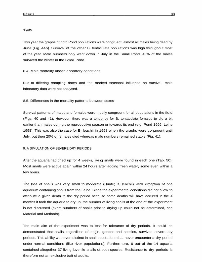
Results 98

1999

This year the graphs of both Pond populations were congruent, almost all males being dead by

June (Fig. 44b). Survival of the other B. tentaculata populations was high throughout most

of the year. Male numbers only went down in July in the Small Pond. 40% of the males

survived the winter in the Small Pond.

8.4. Male mortality under laboratory conditions

Due to differing sampling dates and the marked seasonal influence on survival, male

laboratory data were not analysed.

8.5. Differences in the mortality patterns between sexes

Survival patterns of males and females were mostly congruent for all populations in the field

(Figs. 40 and 41). However, there was a tendency for B. tentaculata females to die a bit

earlier than males during the reproductive season or towards its end (e.g. Pond 1999, Leine

1998). This was also the case for B. leachii in 1998 when the graphs were congruent until

July, but then 20% of females died whereas male numbers remained stable (Fig. 41).

9. A SIMULATION OF SEVERE DRY PERIODS

After the aquaria had dried up for 4 weeks, living snails were found in each one (Tab. 50).

Most snails were active again within 24 hours after adding fresh water, some even within a

few hours.

The loss of snails was very small to moderate (Hunte; B. leachii) with exception of one

aquarium containing snails from the Leine. Since the experimental conditions did not allow to

attribute a given death to the dry period because some deaths will have occured in the 4

months it took the aquaria to dry up, the number of living snails at the end of the experiment

is not discussed (exact numbers of snails prior to drying up could not be determined, see

Material and Methods).

The main aim of the experiment was to test for tolerance of dry periods. It could be

demonstrated that snails, regardless of origin, gender and species, survived severe dry

periods. This ability was even distinct in snail populations that never encounter a dry period

under normal conditions (like river populations). Furthermore, 6 out of the 14 aquaria

contained altogether 37 living juvenile snails of both species. Resistance to dry periods is

therefore not an exclusive trait of adults.

Results 99

For B. tentaculata, there were no significant differences between sexes with regard to

mortality (Tab. 51: Contingency Table, Fisher's exact P-value = ,28). However, there was a

significant difference for B. leachii (Tab. 52: Contingency Table, Fisher's exact P-value =

,035). B. leachii females showed a higher mortality during the dry period than males

Tab. 50: Number of living snails in the aquaria at the beginning and the end of the experiment (A, B:Ditch; C, D: Canal; E, F: Pond; G, H: Small Pond; I, J: Leine; K, L: Hunte; M, N: B. leachii)

A B C D E F G H I J K L M N

Start 11 12 10 10 12 12 10 10 10 9 11 10 28 28End 11 11 9 7 11 11 8 9 10 1 7 5 17 12

Tab. 51: Number of living and dead B. tentaculata at end of experimentFemales Males

Living 49 51Dead 17 10

Tab. 52: Number of living and dead B. leachii at end of experimentFemales Males

Living 12 17Dead 19 8

Discussion 100

IV. DISCUSSION

Introductory remarks

The principal concerns of this study are an in-depth description of the life histories of

Bithynia tentaculata and Bithynia leachii, to bring out the differences in the life cycle

strategies of both species and to discuss the differences in female life histories between and

within populations.

It is self-evident that data could not be collected at all levels and for all processes involved

and that the following section sets off from rather firm ground were reasoning is supported

by data over areas were this basis is dwindling to fields that are more or less speculative.

Since the interdependence of the patterns and processes involved can not be described

conclusively in a simple way, I have decided to present things in a modular manner: First, as

a foundation, there will be a rough description of the life cycle of Bithynia in Central Europe

followed by the main factors and traits shaping the life cycle. In succession, factors and

traits are then discussed separately, observed and possible consequences are mentioned and

interactions and feed-back mechanisms with other factors are discussed. As a synthesis based

on the first section follows a detailed description of the similarities and differences in the

life histories of both species and of the observed populations. In conclusion, these findings

are then discussed under the focus of molluscan life histories and current thinking in life

history theory.

1. A ROUGH DESCRIPTION OF THE LIFE CYCLE OF BITHYNIA SP. IN CENTRAL EUROPE

Snails surviving the winter at the bottom of water bodies end their inactivity with rising

water temperatures in spring. They reenter the upper, warmer water levels in the following

weeks. Shell heigth increases markedly during spring.

The reproductive period starts when water temperatures rise to 12°C or above for some

days. This happens mostly during late April or early May. Spawning activities increase

rapidly with rising temperatures and continue on a high level during May and June. The

spawning can continue with decreasing intensity during July and August.

The mortality of adult snails increases in the course of the reproductive period and decreases

in autumn. Juvenile hatching starts in June and has its peak in late June and July. Depending

on the length of the reproductive period, newly hatched snails may be present also in autumn.

While juveniles grow rapidly during late summer and autumn, adults mostly show no

further shell growth after the reproductive period.

Discussion 101

With decreasing water temperatures in autumn, the snails leave the upper water levels and

move towards the bottom of the water body. The snails withdraw within their shells and close

the shell opening with their operculum. They remain inactive approximately from November

to March. Snails live for 1 to 3 years under natural conditions.

2. FACTORS AND TRAITS SHAPING THE LIFE HISTORIES OF AQUATIC ORGANISMS

There are several important abiotic factors. In general, there exists no feed-back mechanism

from the organism onto this factors. I will mention temperature, oxygen content of water,

habitat structure and - size, water level and desiccation, water current/velocity and

catastrophic events.

Biotic interactions are typically characterised by their feed-back mechanisms. I will discuss

predation, parasitation, competition. Food abundance, foraging and co-occurring molluscan

species are shortly mentioned.

Discussed traits of the life cycle include growth, reproduction, paternal effects, population

structure and sex ratio, mortality and related topics like the distribution of snails in space

and time.

2.1. ABIOTIC FACTORS

Temperature

Traditionally, freshwater snail distributions have been explained by physicochemical factors

like calcium concentration of waters, but this concept was challenged recently (Lodge et al.

1987) after several studies failed to find meaningful correlations between water chemistry

and snail abundance (e.g. Dussart 1979). Former authors strongly emphasised the

importance of abiotic factors as temperature and oxygen in combination with biotic ones in

explaning snail distributions. Temperature is thought to be the single most influential factor

in ecology (Begon et al. 1998). Most biological processes show a more or less linear

relationship to temperature throughout a favourable temperature range (Laudien 1973).

Winter temperatures determine the length of inactivity for both Bithynia species and

thereby strongly influence mortality during overwintering. A sometimes apparent shift in

the size frequency distributions of populations towards larger shells between the onset and

the end of overwintering was several times attributed to slow shell growth during winter

(Lilly 1953; Pinel-Alloul and Magnin 1971). This shift in size frequencies is more

reasonably explained by higher winter mortality of small snails since none of the

Discussion 102

individually caged snails showed any growth during winter. Thereby low temperatures in

winter cause size-specific mortality. Winter mortality was also higher for smaller

individuals in helicid land snails (Baur 1990).

Rising water temperatures end the inactivity of snails and lead to a shift in the habitat used

since snails leave the bottom regions and enter the upper, warmer water levels. In general,

rising temperatures increase activity in Bithynia and other freshwater snails (e.g. Costil

and Bailey 1998; MacRae and Leptizki 1994). The filtration rate of B. tentaculata increases

with increasing temperatures (Brendelberger and Jürgens 1993).

Rising temperatures exceeding a certain threshold have been confirmed as the major trigger

for reproduction in diverse molluscs (e.g. Aldridge 1983; Cáceres-Martínez and Figueras

1998, Costil and Daguzan 1995b; Fretter 1984; Russel-Hunter 1964), but in Littorina

brevicula spawning is triggered by decreasing temperatures in winter (Son and Hong

1998). In aquatic environments, temperature seems more reliable than photo period

whereas for insects photo period is dominant over temperature in timing life history events

(Albrecht et al. 1999; Gotthard et al. 1999).

Temperatures of approximately 12°C trigger the start of spawning in B. tentaculata.

Temperature (and not day-length) is the single cause to trigger spawning since a population

in an underground water supply of a large chemical plant started to reproduce when water

temperatures rose above 12°C, even in complete absence of light (Richter 1996). The

temperature effects were also clearly more important for reproductive stimulation than

photo period in Helix aspersa (Jess and Marks 1998).

The length of embryonic development is dependent on temperature in B. tentaculata. Time

between egg laying and hatching drops from 35-45 days in April and May over 20-30 days

in June to 10-15 days in July and August. Hatching success was not influenced by different

temperatures (Richter and Wächtler 1999).

In the St. Lawrence River, Canada, varying temperatures lead to a change between a long and

a short developmental cycle in B. tentaculata (Vincent and Harvey 1985).

Temperature was only measured on a regular basis in the 3 habitats in Hannover. There were

strong fluctuations between summer maxima and winter minima, but temperatures never

exceeded 24°C and seldom dropped below 4°C. The coldest temperatures (1°C) were

encountered in the Leine whereas the Pond had the highest temperatures during summer. The

temperature profiles were not significantly different between habitats and the temperature

regime is fairly homogenous for all populations.

Discussion 103

Oxygen

The oxygen demands of organisms generally increase with rising temperatures. This is

especially important in aquatic environments since the oxygen tension in water decreases

with increasing temperature (Wetzel 1983). The availability of oxygen determines the

usable habitat size for prosobranch snails. Since they respire by means of their ctenidium

(and to some degree via their epithelia), they depend on sufficiently aerated water. Under

low oxygen levels or anaerobic conditions pulmonate snails have a clear advantage over

prosobranchs since they can respire atmospheric air via their lung cavity (e.g. Aldridge

1983; Boycott 1936). Oxygen had a major effect on Bithynia mortality as was seen by the

deaths of caged snails due to hypoxic conditions in the Ditch, Canal and Small Pond.

Sufficient dissolved oxygen is necessary for embryonic development. Lack of oxygen leads to a

developmental arrest and lengthens time till hatching. Longer periods of lacking oxygen

increase egg mortality of aquatic snails dramatically (Lee and Strathmann 1998). Older

embryonic stages are more sensitive to hypoxygenation than younger ones. Death of Bithynia

spawns occurred as a consequence of oxygen depletion in all habitats. This leads to a strong

selection pressure on females to find appropriate places for spawn deposition.

The time needed for oxygen to diffuse through egg capsules constrains their maximum size

and influences the spacing of eggs in capsules. Increasing capsule size leads to an increase in

the percentage of resources per egg that has to be invested in the costly matrix of the capsule

and limits thereby capsule size (Lee and Strathmann 1998).

Habitat structure and -size

Parasitation is strongly influenced by size and structure of aquatic habitats. Both determine

the spectrum of definite trematode hosts shedding eggs into the water body. Definite hosts that

discriminate strongly by the size and structure of water bodies include mammals like

muskrat, beaver and smaller rodents, birds, amphibians and fish.

It is known that both prevalence of parasites and parasitic load can vary strongly on a small

scale within habitats (Coy et al. 1982; Fernandez and Esch 1991b). For B. tentaculata,

infection levels differed approximately 1000 times between 3 sites within 20 m (Lepitzki

and Scott 1994). Infection levels differed with the type of vegetation for Lymnaea elodes

(Sorensen and Minchella 1998).

Habitat structure has an influence on the amount of sites suitable for spawn deposition,

probability of predator contact and overwintering possibilities. Due to their size difference,

B. tentaculata and B. leachii differ in their ability of habitat use. The smaller B. leachii can

Discussion 104

use a higher percentage of the total surface area. As was demonstrated in this study, Lymnea

stagnalis has a severe negative influence on Bithynia spawns and juveniles. Habitat structure

mediates the outcome of this interaction by excluding the large-bodied Lymnea from fine-

scaled parts of the habitat that are usable by the smaller Bithynia. The same holds true for

predators as fish and crayfish that can be limited by their size in entering hollow spaces and

crevices under stones and rocks. The effect of predation on freshwater snails is known to be

dependent on the type of habitat (Lodge et al. 1987).

Habitat size further influences the degree of mobility that is necessary for Bithynia, because

the snails use different parts of the habitat for feeding, mating, egg laying and overwintering.

Water levels and habitat desiccation

Varying water levels lead to changes in the usable habitat size. They force strictly aquatic

organisms to migrate with their fluctuations. Falling water levels pose a severe threat to

immobile life cycle stages as spawns. Bithynia spawns can withstand desiccation only for

very short periods and are irreversibly damaged after few hours of exposition to air.

Periods of draught can lead to a complete desiccation of a habitat, this being the most extreme

form of changing water levels. Complete desiccation forms a strong selection pressure on

aquatic organisms to develop resting stages capable of surviving dry periods (Williams

1987). Desiccation increased mortality and decreased fecundity in Biomphalaria glabrata

(Vianey-Liaud 1996). Biomphalaria snails were able to survive desiccation for up to 6

weeks and resumed egg-laying shortly after desiccation ended (Simões and Lopes 1996).

Both Bithynia species can withstand desiccation for more than a month in dry mud. Even

river populations of B. tentaculata that never experience desiccation were able to survive in

numbers equal to the only ephemeral habitat, the Ditch. B. tentaculata is known to occur in

temporal ponds in Germany and Northern India (Heitkamp 1982; Mattison et al. 1995).

Water currents and water velocity

Habitats with standing and running waters show some fundamental differences. In general,

running waters are better aerated, but the aggregation of nutrients is impeded or prevented

that is typical for standing waters. Most running waters experience periods of high waters

and flood that can differ in predictability and affect habitat stability negatively (Brehm and

Meijering 1990; Lampert and Sommer 1993). Both the Leine and the Hunte experienced

high waters and floods during the observation period. During flood, all three Dümmer

Discussion 105

habitats were connected in spring 1998. Flooding may thereby facilitate the transport of

individuals between populations that are separated otherwise.

Both water currents and -velocity influence the usable habitat size. Increasing water

velocity increases energetic demands of surface adherence for snails and increases the risk of

drifting. Above a threshold, snails lose surface contact and are subject to drift. Due to this,

snail distribution is patchy in rivers. Most parts of the river habitats were devoid of

B. tentaculata whereas areas with reduced water velocity were the most densely populated of

all habitat types. Shells of the Leine population were significantly slimmer than those of the

other ones. This is likely to be an adaptation to reduce resistance to water currents.

Perturbations of the substrate in running waters select for thicker snail shells that are able

to withstand the abrasive and crushing action of pebbles and stones. This is also known for

habitats with different degrees of wave exposition.

Because of their small size even in only moderately flowing waters trematode eggs and

miracidia are subject to drift. This reduces the risk of becoming parasitized for snails in

streams and rivers and hot spots of trematode infections (e.g. muskrat dens, breeding

colonies of birds) are of a more limited size compared to standing waters. By this, infection

levels fluctuate on a very small scale in running waters (Lepitzki and Scott 1994).

Disturbance

Disturbance plays a major role in structuring biocoenoses (Sousa 1984). Examples relevant

for aquatic molluscs include periods of severe draught or flood, prolonged frost and ice cover

in winter, reductions in macrophyte abundance, food shortage and pollution (Lodge et al.

1987). Pollution has been recognised to change the life histories of gastropods (e.g. Liu and

Morton 1998). Detrimental effects of fungicides and other chemical substances on

B. tentaculata are documented ( van Wijngarden et al. 1998).

Disturbance played a major role in both rivers where every year there was at least one

flood. The occurrence of disturbance is therefore highly predictable in the rivers, but timing

and duration of these events is highly unpredictable. The Ditch did not dry out in the

observation period, but water levels fluctuated strongly with temperature and the intensity

of precipitation. In addition, there were long periods with anoxic conditions during summer.

In the other habitats, water levels were fairly stable (in spring 1998, the high water at the

Dümmer flooded also the Ditch and the Canal) and winters were generally mild.

Discussion 106

2.2. BIOTIC INTERACTIONS

Predation

There is a vast amount of literature concerned with predation and predator-prey

interactions in ecology (e.g. Begon et al. 1998). Predation risk is known to change almost

every single life history trait. Most features of the sometimes bizarre shaped and commonly

thick-walled shells of marine prosobranchs are considered as antipredator structures as are

the thick shells of freshwater prosobranchs which mostly lack sculpturing (Vermeij and

Covich 1978). These authors attribute the thin shells of pulmonates and the thicker shells of

prosobranchs to differences in longevity and general life history strategy.

Constitution of shells strongly influences the outcome of predation pressure by crayfish. Two

crayfish species fed predominantly on Lymnaea stagnalis and Lymnaea (Radix) peregra when

B. tentaculata was also present (Nyström et al. 1999). Because a decrease in L. stagnalis

abundance lessens the predation of Bithynia spawns, crayfish may even have a positive

influence on B. tentaculata abundance and may alter the outcome of competition between both

species. Molluscivorous fish can also change the species composition from thin-shelled

L. stagnalis to thick-shelled B. tentaculata (Brönmark and Weisner 1996).

In freshwater systems, predator presence has been observed to change age and size at

maturity of snails via changes in their energy allocation (Crowl and Covich 1990; Lam

1994). Snail behaviour also changes with presence or absence of predators. Snails show

escape reactions in the presence of predatory crayfish and leeches (Alexander and Covich

1991; Crowl and Covich 1990). Snails can even distinguish between the presence or absence

of different types of predators and behave accordingly, in this case between fish and crayfish

(Turner et al. 1999).

In this study, the effect of predation was only circumstantially investigated. Habitats differed

in predator presence. Predatory fish were absent from the Ditch and the Small Pond.

Crayfish and fish were present in the Leine and the Pond and may have been a cause for low

pulmonate numbers. Dabbling ducks were common on the Leine, present in small numbers in

the other habitats but never observed on the Ditch. From the shore of the smaller water

bodies thrushes fed on pulmonates that often forage attached to the water surface.

Invertebrate predators were common in all habitats.

In general, prosobranchs can escape shell-invading predators like leeches better than

pulmonates. I found commonly small hemolymphe-sucking Glossiphonia sp. inside Bithynia

shells, but due to their small size they are rather parasites than predators. Nothing is known

Discussion 107

about their possible role as vectors for snail diseases. Cerfolli and Rossi (1995) found that

the survival of B. tentaculata under predation pressure by leeches increased when a second

predator level (represented by fish) was introduced in experiments.

The very small oligochaet Chaetogaster limnaei consumed not only trematode miracidia and

cercaria, but also caused erosion of the mantle and gill epithelia in Dreissena sp. (Conn et al.

1996). I found Chaetogaster sp. regularly when crushing snails to look for trematode stages,

most often in snails from the Canal and the Ditch. Ditch snails could harbour up to 30

specimen within their shells. I can not say whether their presence was detrimental or

beneficial to snails, but it is an interesting coincidence that the lowest infection level in

standing waters was correlated with the highest prevalence of Chaetogaster sp.. Cercaria

were seen in their stomachs on several occasions.

On the level of the individual, growth can be of special significance. In some cases, when

predators forage preferably on juvenile and small individuals, rapid growth facilitated by

delayed sexual maturity helps to escape predation pressure in pulmonates (Crowl and Covich

1990; Lam 1994). Mean shell height of B. tentaculata was larger when predatory crayfish

were present in experiments in plastic pools. This was most likely due to size-selective

predation of crayfish and not to a growth response by Bithynia (Nyström et al. 1999).

Increased mobility due to mate searching and active site selection for mating, reproduction

and egg laying increases the predation risk. Foraging possibilities also influence mobility and

thereby predation risk. In Bithynia, individuals with a sufficient supply of algae and detritus

for filter feeding should in general be in lower danger by predators than more mobile grazing

snails. Apart from the energetic plus of filter feeding over grazing this would be a second

advantage.

Parasitation

-Parasitation

Parasitates have only more recently become a focus of interest in life history and ecological

studies (Zander 1998). For several decades, competition and predation were predominant

and parasites were virtually absent from the ecological agenda (Lauckner 1986). Several

scientists who claimed the general importance of parasites for ecological thinking were

concerned with marine and freshwater molluscs (Brown 1991; Lauckner 1984; Lodge et al.

1987). Today, parasites are well integrated in modern ecological thinking. Their role in

shaping the life histories of their hosts, host-parasite coevolution, the invention and

maintenance of sex in natural populations and their costs and possible benefits to their hosts

Discussion 108

are investigated (e.g. Begon et al. 1998; Dobson et al. 1992; Huxham et al. 1993;

Michalakis et al. 1992; Toft and Karter 1990).

The success of invasive species can be partially attributed to their incompatibility to local

parasites as was demonstrated in invading Mytilus galloprovencalis in South Africa (Calvo-

Ugarteburu and McQuaid 1998).

Bithynia is a host for a broad variety of trematode species (e.g. Mattison et al. 1995; Pike

1967). In Bithynia as in other molluscs, infections with larval stages of trematodes most

often lead to irreversible castration and reproductive death of infected individuals by direct

destruction of the gonad (via ingestion by redia or pressure caused by larval stages) and/or

gonadal atrophy due to energetic demands of the parasites (e.g. Goater et al. 1989; Gorbushin

and Levakin 1999; Lauckner 1986; Mouritsen and Jensen 1994; Taskinen et al. 1997).

After early researchers thought invasion of the gonad and castration to be a rare event

(review in Wright 1966), the castration of the host has long been seen as a strategy of the

parasite (review in Baudoin 1975). The complete castration of hosts is mostly achieved

within few weeks post infectionem. The reproductive investments of the host can be altered

by chemical interference by the parasite within days (e.g. Hodasi 1972; Sorensen and

Minchella 1998; Wilson and Denison 1980). Due to parasitic castration, several potentially

iteroparous molluscan species were found to be effectively semelparous under field

conditions (Holopainen et al. 1997). Among other effects, the preference of the gonad over

other host organs enhances host and therefore parasite survival. The longer the potential

life-span of the host, the more often the gonad was the site mainly infected (review in

Taskinen et al. 1997).

The histological and pathological consequences of infections in Bithynia were investigated in

several studies (Adam et al. 1995; Neuhaus 1949; Reader 1971a,b, 1976). When snails

are crushed under a dissection microscope, it can be seen that in the terminal stages of an

infection almost the whole body consists of parasitic stages. The only exceptions are the foot

region and the head. In heavy infected populations, a great deal of the biomass attributed to

the host should therefore be attributed to the biomass of the parasite. It is clear that

trematode infections thereby can change trophic interactions in ecosystems dramatically

(Lauckner 1984, 1986).

The prevalence of infections fluctuated strongly with time in the 6 habitats. Prevalence

showed also significant differences between the populations with the Small Pond being the

most affected habitat of all. Here nearly 4 out of 10 adult snails were parasitised. The

infection levels reached their high in October 1998 when three quarters of the adult snails

were parasitized. All other habitats showed an overall infection level close to 10% of the

Discussion 109

adult population. This number becomes more dramatic when it is taken into account that

infection levels rised to their high during the reproductive period of B. tentaculata. They lay

above 20% in July for the Hunte and the Ditch (data for the Canal are missing due to

sampling difficulties). The prevalence was near 20% in all 3 years in June and July in the

Leine that had otherwise very low infection levels. Data for the Pond are sparse but one third

of all snails were parasitized in July 1999.

These results show unequivocally that parasites have a profound effect on the reproductive

capacity of B. tentaculata individuals and populations. Infection levels for B. tentaculata

range from 2% from a Spanish population, 10% - 35% in Berlin, Germany, 18% - 37% in

Northern India to 57% in Quebec, Canada (Emmel 1942; Mattison et al. 1995; Ménard and

Scott 1987; Toledo et al. 1998). According to Mattison et al. (1995); B. tentaculata was the

heaviest infected snail in their survey in Northern India. Infection levels for B. leachii were

1,2% in Brandenburg and 5% - 35% in Berlin and are thought to be generally low (Emmel

1942; Hering-Hagenbeck and Schuster 1996). In sympatric populations of both species,

B. leachii was less parasitized (Emmel 1942). Ménard and Scott (1987) and also Emmel

(1942) found that infection levels fluctuated strongly between seasons for Bithynia. A

strong seasonality of infections was also found for other snail and bivalve species (e.g.

Fernandez and Esch 1991a; Taskinen and Valtonen 1995; Woolhouse 1989).

When it is taken into account that infections persist in snails and that infection levels mostly

dropped markedly during autumn, it becomes clear that parasitation has also a major

influence on snail mortality and thereby on population structure. Infections seem to

negatively influence winter survival of snails since I found that infection levels in spring lay

in every case below the pre-winter levels. Reader (1976) also found higher winter

mortality in parasitized B. tentaculata. This is not astonishing since parasites deplete the

energy stores of their hosts. However, Goater et al. (1989) found no effect of parasites on

winter survival of Helisoma anceps (Pulmonata).

Minchella and Loverde (1981) found that parasites increased mortality in Biomphalaria

glabrata and Lauckner (1986) found mortality to increase with parasitic load for Littorina

and Hydrobia in the Baltic Sea. Infection decreased survival of desiccation for Biomphalaria

pfeifferi (Badger and Oyerinde 1996). In general, most studies showed that mortality is

increased due to parasitation (e.g. Huxham et al. 1993; Robson and Williams 1971;

Sorensen and Minchella 1998; Webster and Woolhouse 1999), but Hodasi (1972) found

increased survival of parasitized Lymnaea truncatula in mass laboratory culture. Snails can

also be killed by cercaria shed by conspecifics that penetrate into the snails to transform

into metacercaria (Campbell 1997).

Discussion 110

With exception of an incident in the Small Pond, I found no differences in prevalence between

genders. In 1998, infection levels of females but not of males increased dramatically during

autumn from an already high level in summer. I can offer no explanation why this sexual

bias was observed in autumn 1998/spring 1999. Since the Small Pond population failed to

reproduce in 1997, these snails were at least born in 1996. The prevalence with females

was around 75%, excluding three out of four older females from reproduction. This

emphasises my point that parasites can have a marked negative influence on reproductive

capacity and may even pose a threat to whole populations under special circumstances.

In a 2 year survey on B. tentaculata in Canada, Ménard and Scott (1987) found no sex-bias

for metacercarial infection, but other authors found sexually biased infection levels in

molluscs. Males were predominantly parasitized in the snail Cerithidea californica, whereas

females were preferred by parasites in the bivalve Anodonta piscinalis (Lafferty 1993b;

Taskinen and Valtonen 1995).

The mechanism by which miracidia find snail hosts are a much debated topic in parasitology

but are often more or less speculative so far. Under the proposed mechanisms are random

movement of miracidia, orientation along gradients into conditions favourable for the hosts

and chemical cues from the host (e.g. Campbell 1997; Kalbe et al. 1996). Under the

discussed chemical cues are, among others, sexual hormones from snails. This would account

for the observation that often only sexually mature hosts are attacked (e.g. Lauckner 1986;

Robson and Williams 1971). But it should be mentioned that at least some trematodes infect

also premature snails and it is very feasible that different trematode species (or even

strains of trematode species) evolved different strategies for host location and, subsequent,

infection.

This point is supported by evidence that different trematodes affect growth patterns of the

same snail species differently and that different snail species and even different populations

of the same snail species react differently on the same trematode (Gorbushin and Levakin

1999; Mouritsen et al. 1999).

It is also possible that the early trematode stages remain cryptic inside immature hosts after

infection until their development is triggered by signals of the sexual maturation of their

host. Appropriate selection of snail host species by miracidia and cercaria has frequently

been demonstrated in the field and the laboratory (e.g. Campbell 1997; Coy et al. 1982).

The increasing infection levels with increasing age that were exhibited by the Small Pond

population after reproductive failure in 1997 point in the direction that infections are

acquired over time and accumulate in ageing populations of B. tentaculata. I found also a

constant increase of infections in young snails in the Small Pond in 1999. They set out near

zero per cent infections in spring and reached 20% in August.

Discussion 111

That infections accumulate with age was earlier demonstrated for marine snails, freshwater

bivalves and metacercarial stages in B. tentaculata (e.g. Curtis 1996; Holopainen et al.

1997; Lafferty 1993a,b; Lepitzki and Scott 1994; Ménard and Scott 1987; Sousa 1983).

However, Mattison et al. (1995) found that infections were more prevalent in smaller size

classes of B. tentaculata in Northern India. Selection should therefore favour early

reproduction under a high risk of parasitation and increasing infection levels with age. This

was demonstrated for a marine and a freshwater snail that matured earlier in habitats where

trematodes were abundant (Jokela and Lively 1995; Lafferty 1993a).

Another consequence of increasing infections with age should be that there is no positive

selection for snail longevity. In this context I find it remarkable that a substantial amount of

Bithynia females that reached maturity within a year died after their first reproductive

period. However, the longest-lived population inhabited the water body (Small Pond) where

parasites were most abundant.

It would be very interesting to study the effect of size (which is closely correlated with age

in organisms with indeterminate growth) on the probability of becoming infected. Since the

body surface increases with size, this should lead to a higher probability both of a chance

encounter with parasites as well as being located by a parasite searching along a gradient of a

chemical stimulus originating from the host. Larger animals should be stronger

transmitters.

Another way of trematode transmission is the direct ingestion of eggs by hosts. Because

larger animals are known to consume larger food quantities, this should also lead to a higher

infection probability with increasing size. In combination, this could lead to selection against

larger size and for smaller size at maturity even if, in general, size and reproductive output

show a strong positive correlation. It could also be one cause of determinate growth and/or

semelparity at least in species were the biomass of the parasite is of the same magnitude as

the biomass of the host. To my knowledge, no study testing this hypotheses exists so far.

Distribution patterns and number of individuals in groups influence the risk of parasitation.

A patchy irregular distribution of animals in their habitat and increasing numbers of

individuals in groups decreased the risk of becoming parasitized for a bivalve (Grosholz

1994).

An effect termed reproductive compensation was observed in snails. In this case mature

snails freshly infected by trematodes increased their reproductive effort above that of non-

infected individuals to compensate for future loss of reproductive capacity (Gérard and

Théron 1997; Minchella and Loverde 1981; Minchella 1985; Thornhill et al. 1986), but

Sorensen and Minchella (1998) found no reproductive compensation in Lymnaea elodes. A

shortening of the prereproductive life span was also found in other host-parasite systems

Discussion 112

(Agnew et al. 1999; Michalakis and Hochberg 1994). Theoretical models on parasitism and

host reproductive effort are presented by Forbes (1993, 1996) and Perrin and Christe

(1996).

That sexual reproduction is maintained under severe parasitic pressure was demonstrated

with Potamopyrgus antipodarum. With this species, clonal strains and sexual populations can

coexist. Since parthenogenesis has a twofold advantage over sexual reproduction (since no

males are produced), clonal strains should replace sexual populations. But in the presence of

castrating parasites, sexually reproducing individuals predominate whereas with decreasing

prevalence of trematodes clonal individuals predominate (Jokela and Lively 1995; Jokela et

al. 1997). These findings are in favour of the Red Queen hypothesis for the maintenance of

sex which states that sexual reproduction is a counteradaption to parasites and is selected for

since it produces genetically diverse offspring and rare, resistant genotypes (Fox et al.

1996; Lively and Howard 1994). Interestingly, clonal diversity was also higher in the

presence than in the absence of parasites.

Further support for the Red Queen hypothesis came from a study using a bivalve species that

demonstrated heritability for resistance to parasites (Grosholz 1994). Resistance to

Schistosoma mansoni was also heritable in Biomphalaria glabrata (Webster and Woolhouse

1999).

Parasites can profoundly alter the behaviour of their hosts (e.g. Thompson 1990). Parasites

can, at least in some cases, influence habitat choice of hosts. In the freshwater snail

Potamopyrgus antipodarum, infection with a trematode species changed the temporal-spatial

pattern of habitat use. Infected snails preferred areas where dabbling ducks (the definite

hosts of the trematode) were foraging, but left those areas, when a second predator, a snail-

eating fish, appeared during the day. Further development of the trematode was only possible

in the ducks (Levri 1998; 1999).

The neuropeptide gene expression of Lymnaea stagnalis was already changed few hours post

infectionem. The parasite influenced host behaviour and inhibited egg laying and

accompanying behaviour. The manipulation of the host by the parasite changed according to

the parasitic stages inside the host (Hoek et al. 1997). Castration early in infection by

chemical factors was also observed in Lymnaea elodes (Sorensen and Minchella 1998).

Other factors influencing parasitation were already mentioned above. Habitat size and

-structure as well as other abiotic factors attract or repel different types of definite hosts

for trematodes and thereby define the species composition of the parasite guild. The

composition of the parasite guild within the host is mediated by competition between

different trematode species. There are examples for intense competition inside the host that

include indirect and direct evidence (Sousa 1983).

Discussion 113

In general, multiple infections of hosts are much less often observed during field studies than

statistically predicted (Emmel 1942; Fernandez and Esch 1991a; Goater et al. 1989), but

Curtis (1997) found high levels of multispecies infections in a marine snail. Direct

evidence includes field studies were individual snails changed the species of trematode

cercaria they shed and laboratory studies were established infections in snails were

substituted by a second infection with eggs or miracidia of another trematode species

(Fernandez and Esch 1991b). Cercaria of certain trematode species are even known to be

hyperparasites of other trematodes inside the snail hosts (Campbell 1997).

Genetic structure and mating system of host populations and genotypes of parasites

introduced by migrating species will also have a profound effect on host-parasite

interactions. Temporal fluctuations in species and strains of parasites as well as the

structure of the parasitic guild and their interactions affect host-parasite coevolution. Host-

parasite coevolution should be impossible when too many trematode species are present.

Immunocompetence is an interesting, but mostly overlooked life history trait. New models of

host-parasite coevolution have shown that coevolution must not necessarily lead to decreased

virulence of the parasite towards its host, the outcome of host and parasite coevolution

proposed by older models (Owens and Wilson 1999; Toft and Karter 1990).

Other studies have found evidence that resistance against parasites is costly (Michalakis and

Hochberg 1994). Susceptible Biomphalaria glabrata had a higher fertility than resistant

snails (Webster and Woolhouse 1999). Counter-intuitively, a reduced immunocompetence

may also be adaptive when parasites are virulent and common. If resistance is futile, then

potential hosts should withdraw their resources from an immune response and enhance

reproduction instead (Baalan and Jukela, cit. in Owens and Wilson 1999).

In my opinion this could explain some of the differences between Bithynia species.

B. tentaculata is infected by too many different trematode species with too many different

strategies and high virulence that successful coevolution is impossible and sufficient

immunocompetence and resistance is futile. I assume that B. tentaculata gave up the combat

with the parasites in its evolutionary past and instead relocated its resources to growth and

reproduction.

B. leachii is the first host of fewer trematode species belonging to a smaller range of

trematode families. This could be the result of successful active parasite resistance by

B. leachii. B. leachii kept on in its battle with the parasites, defeats most and is defeated by

few. Since immunocompetence and immune responses are costly, B. leachii has fewer

resources left for growth and therefore is smaller. This hypothesis would account for the

greater range of parasites and their higher prevalence as also the higher susceptibility to

fungal diseases in the larger B. tentaculata. To test this hypothesis, an assessment of the costs

Discussion 114

of resistance would be crucial. To explain the observed differences, the costs should be quite

high.

-Gigantism

Gigantism (the increased shell growth in response to parasitism) is a topic much debated in

molluscan life histories since it has been reported early in the century. Several scientists

like Wesenberg-Lund and Rothschild have described gigantism in various snail species in the

first half of the last century. Two explanations were formulated: Minchella (1985) saw

gigantism as a host adaptation to trematode parasitism, whereas Sousa (1983) explained

gigantism as a side effect of parasitic castration or an adaptation of the parasite.

Minchella postulated that due to the increased growth snails enhanced their survival and

could thereby outlive parasites and reproduce after infections, but most infections persist in

snails during their entire live. There are only very few cases were a loss of trematode

infection could be demonstrated (Fernandez and Esch 1991a; Goater et al. 1989). Thereby

Sousa's explanation is favoured that gigantism is either a side effect of parasitation because

host castration sets free energy for growth otherwise needed for reproduction or gigantism is

an adaptation of the parasite to overcome spatial constraints within the host.

Several studies found gigantism in marine and freshwater snails (e.g. Mouritsen and Jensen

1994; Sorensen and Minchella 1998; Wilson and Denison 1980). Other studies failed to

demonstrate gigantism or even found "dwarfism" (e.g. Curtis 1997; Fernandez and Esch

1991a; Goater et al. 1989; Huxham et al. 1993; Mouritsen et al. 1999).

Growth rates were enhanced in Lymnaea truncatula and Biomphalaria glabrata when infected

as premature snails and unaltered when infected as adults (Gérard and Théron 1997; Hodasi

1972). Loker (1979) found that infected Lymnaea catascopium grew faster the first 2

months post exposure and thereafter more slowly than uninfected controls. Minchella et al.

(1985) found the same response for L. elodes.

Gorbushin (1997) found that trematode-induced gigantism in Hydrobia sp. depended on the

trematode species, some trematodes increasing growth rates whereas others had no effect.

Alteration of growth rates was also dependent on the origin of host populations. Gorbushin and

Levakin (1999) found that infection with Microphallus sp. stunted growth in Littorina

obtusata, had no effect on growth of L. saxatilis and enhanced growth in Onoba aculeus from

the same habitat.

Often growth rates of infected snails were continually below those of uninfected ones

(Fernandez and Esch 1991a; Lauckner 1986; Sousa 1983). Mouritsen et al. (1999) and

Sousa (1983) assume that gigantism is a phenomenon more likely in short-lived and/or

semelparous snails and unlikely in long-lived species due to their differences in life history

and resource allocation.

Discussion 115

With B. tentaculata, evidence is equivocal. Whereas in 2 populations there was no observable

size difference, in 3 populations infected snails belonged to a significantly larger subgroup.

It should be mentioned that gigantism could not be demonstrated in both populations with the

highest number of examined infected snails. Thereby gigantism in B. tentaculata may be an

artefact due to rather small sample sizes.

On the other hand, Mouritsen et al. (1999) demonstrated that the outcome in regard to

changes in growth pattern was not only influenced by the trematode species, but also by the

population of Littorina littorea observed. Snails from some populations had lower growth

rates, whereas other snails did not alter their growth rates when infected with the same

trematode. This stresses the necessity of a very regional focus in ecological studies and

underlines the difficulties connected with generalizations.

Intra- and interspecific competition and coexisting molluscs

Competition has been a major focus of ecological studies in the past century, but its

importance to explain freshwater snail communities has lately been challenged in favour of

disturbance and predator-prey interactions (Lodge et al. 1987).

The concept of competition itself poses several difficulties (e.g. Begon et al. 1998; Rohde

1991). Among other reasons, this has to do with the peculiarities of the niche concept in

ecology (its unlimited multidimensionality and thereby the implicit impossibility to test it

by falsification) and the temporal aspects of competition and evolution ("The ghost of

competition past", Connell 1980, cit. in Begon et al. 1998). This means that an apparent

lack of competition observed in the present between coexisting species can be a consequence

of the extinction of poorer competitors in the past, a consequence of competition in the past

that led to coevolution of the species and in the end to the extinction of competition between

the coevolving species or that there was never competition at all because the species are

simply different. In retrospect it is impossible to decide if competition was or was not

involved.

In a study on interspecific competition Fenchel (1975) found character displacement in

mudsnails (Hydrobia sp.) in sympatric populations compared to allopatric ones. Being of

equal size in allopatric populations, in sympatric ones H. ventrosa was smaller and H. ulvae

bigger. Thereby resource overlap and competition should be lessened.

In recent years several studies claimed that the observed patterns are better explained as a

consequence of environmental factors acting differently on the species (e.g. Cherrill and

James 1987), but Gorbushin (1996) found evidence for intra- and interspecific

competition in a field experiment with Hydrobia. Most interestingly, the outcome of

competition between Hydrobia species was influenced by overall snail density. The

Discussion 116

successfully competing Hydrobia species changed when snail density was manipulated in the

field experiments.

Barnes and Gandolfi (1998) found evidence for both intra- and interspecific competition in

Hydrobia neglecta. Increasing numbers of H. neglecta decreased egg number per female, but

egg production decreased even further when H. ulvae was present.

In a field experiment Brönmark et al. (1991) found that food competition by grazing

tadpoles had a negative influence on fecundity and growth of 2 pulmonate snail species.

L. stagnalis has a higher grazing efficiency compared to B. tentaculata (Nyström et al.

1999). Grazing effects on algae growing on a hard substrate by 5 pulmonate species were

identical but a coexisting prosobranch was less effective (Barnese et al. 1990).

Snails of the genus Lymnaea are known to forage on spawns of co-occurring snail species

(Michelson and DuBois 1974; Vermeij and Covich 1978) as are some other large

prosobranchs that also feed on juveniles (Aldridge 1983).

L. emarginata consumed egg masses of Biomphalaria glabrata in the laboratory and thereby

strongly reduced population growth of the latter species (Michelson and DuBois 1974).

Brown (1982) found a negative influence of L. elodes on Physa gyrina fecundity, but

intraspecific competition had a more dramatic effect on growth rates. Since growth rates in

P. gyrina increased and reproductive success decreased dramatically when kept together with

L. elodes, I conclude that this was due to intense egg predation overlooked by the authors.

In this study L. stagnalis had a strong negative influence on B. tentaculata populations in

experimental pond communities because snails consumed or damaged spawns and juveniles.

In general, interspecific competition should be lessened by increasing the habitat

heterogeneity (Lodge et al. 1987). However, increasing the structural diversity of the

habitat did not increase juvenile survival in the competiton experiments with B. tentaculata

and L. stagnalis.

In the field, L. stagnalis occurred in 3 out of 6 habitats, but was most abundant in the Small

Pond. Here lived only few other gastropod species which could be a consequence of long-time

competition by L. stagnalis. The Small Pond was fairly stable, highly productive and lacked

efficient vertebrate predators which should increase the level of competition (Lodge et al.

1987). Its small habitat size was even more reduced by regular oxygen depletion. Thereby

the habitats used by B. tentaculata and L. stagnalis overlapped, increasing the probability

that L. stagnalis encountered spawns or juveniles of Bithynia during foraging.

The reproductive failure observed in 1997 and low numbers of juveniles in 1999 therefore

could be caused by predation of L. stagnalis on B. tentaculata.

Species composition of the Canal and the Ditch demonstrated a clear competitive advantage for

pulmonate snails in both habitats. This is a common picture in habitats with low oxygen

Discussion 117

(Lodge et al. 1987). B. tentaculata dominated clearly in both rivers where also the most

prosobranch species existed.

Intraspecific competition was several times demonstrated for gastropods, higher densities

leading to reduced growth and/or decreasing fecundity and changes in size at maturity (e.g.

Brown 1985; Carter and Ashdown 1984; Cherrill and James 1987; Lazaridou-Dimitriadou

et al. 1998). In my opinion intraspecific competition accounts for the pronounced

differences in juvenile growth during laboratory culture of B. tentaculata, but should not

play a major role under densities encountered in the field.

Foraging

Bithynia is able to forage in two different modes, by grazing and via filter-feeding (Meier-

Brook and Kim 1977). Filtration of organic matter out of the water leads to a higher

energetic net gain than grazing (Brendelberger 1997a; Tashiro 1982). Filtration of green

algae or diatoms led to a more rapid growth than grazing on several different food items

(Brendelberger 1997a). Food filtration also allows Bithynia to remain unmoving for long

time periods and to live in fairly large groups that lead to the commonly observed clumped

distribution in the field (e.g. Meier-Brook and Kim 1977; Schäfer 1953). By this

behaviour both predation and parasitation risks should be lessened.

Bithynia is highly selective and only forages on food of a high energy content in contrast to

other freshwater snails (Brendelberger 1995, 1997a). Freshwater snails choose their

habitat in accordance to the presence of appropriate food sources (Lodge et al. 1987). Aquatic

snails also show different sets of enzymes and enzymatic activities and are thereby

differently equipped to use diverse food items (Brendelberger 1997c). Therefore

coprophagy can be a food source for some snails, but not for B. tentaculata (Brendelberger

1997b). The activity of digestive enzymes in B. tentaculata changes with different feeding

regimes (Brendelberger 1997c).

2.3. LIFE HISTORY TRAITS

Growth

Growth as a key feature of every life history is affected by gender, age, reproductive

investment and other energetic demands (mobility, predator avoidance and phenotypic

plasticity, immune responses etc.), climate, food quality and habitat productivity,

competition, parasitation, diseases and sex- and size-related mortality.

Discussion 118

-Growth pattern

The growth patterns of organisms determine their age at maturity when size at maturity is

fixed. Different growth and maturation rates can be an important isolating mechanism in

speciation processes in snails (Aldridge 1983). The overall growth pattern of both Bithynia

species was to some degree different. The growth patterns of the 6 B. tentaculata populations

showed several differences and some similarities.

The populations also showed different growth patterns in consecutive years. Even individuals

within the same population showed differences with regard to growth. The individuals showed

no tendency to grow up to equal maximum sizes. Some females grew further after becoming

sexually mature, others did not grow any further after starting to reproduce.

However, both in the field and the laboratory, clearly more non-reproductive females grew

than reproducing ones. On the other hand, a substantial fraction (approximately 20%) of the

females grew after they started to reproduce under both conditions. Likewise, the probability

of a given adult female to grow after overwintering did not depend on female size. This means

there existed no common pattern like small adult females growing and larger females not

growing further.

-Age effects

It is well known that the age of an individual influences its growth pattern. In most cases,

growth decreases with age and size. This negative relation between growth rate and size is the

most common observation on gastropod growth (e.g. Aldridge 1983; Mouritsen et al. 1999).

Growth was most rapid in newly hatched snails during late summer/autumn. Young

B. tentaculata had higher weight-specific filtration rates than older snails and young

B. graeca had the highest daily consumption and assimilation rates (Brendelberger and

Jürgens 1993; Eleutheriadis and Lazaridou-Dimitriadou 1996). Caquet (1993) found that

shell growth differed between seasons for Physa fontinalis, growth being most rapid for

juveniles directly after hatching. Growth decreased with size in Hydrobia ulvae and Helisoma

anceps (Fernandez and Esch 1991a; Mouritsen and Jensen 1994).

Bithynia can reach an adult shell size before their first winter. The intensity of growth

decreased in all populations for sexually mature snails. In general, most shell growth

occurred in the first months of the life span, some after the first overwintering during

spring and summer but only few snails grew after their second winter. This was supported

by the growth patterns in laboratory culture.

Discussion 119

Growth rates of prereproductive Helisoma anceps were faster than those of equally sized

reproductive snails in summer (Fernandez and Esch 1991a). This is in good agreement with

theory that predicts a trade-off between somatic and gonadal demands (Roff 1992; Stearns

1992). However, in Biomphalaria glabrata reaching maturity, growth was not reduced after

egg laying started in laboratory experiments (Gérard and Théron 1997).

-Gender effects and sexual dimorphism

Growth patterns can be influenced by gender and thereby lead to sexual dimorphic species.

This is often the case in prosobranchs (Aldridge 1983). Sex-specific growth rates are

common in the genus Viviparus with females attaining larger shell heights (e.g. Buckley

1986; Eleutheriadis and Lazaridou-Dimitriadou 1995; Ribi 1999). A more rapid growth of

juvenile females has been reported several times for marine prosobranchs (e.g. Sousa

1983).

B. leachii has a pronounced sexual dimorphism, females being on average 20% higher than

males. In laboratory experiments, B. leachii females grew more rapid than males after

hatching. In the field experiments, females grew more often and more rapid than males.

A less pronounced dimorphism (approx. 5%) was found in 4 of the 6 B. tentaculata

populations. Females were larger in 3 populations, but males were larger in the fourth. The

ratio of shell height to shell width was not different between sexes.

B. tentaculata showed no growth differences between males and females in the laboratory.

Growth patterns of males and females were mostly the same in field experiments with caged

snails with the exception of the Leine in 1999 when an unusual high number of males grew.

There were some differences between sexes in field sample data with regard to growth

pattern. Mostly those were differences in the timing of shell growth in the field, but on the

whole similarities dominated.

-Shell height at maturity

Size at maturity is one of the key life history traits since it is a central turning point during

ontogeny that marks a profound switch in resource allocation.

B. leachii females started to reproduce with approximately 4 mm shell height. Pond and

Small Pond females had the largest shell height at maturity with 8 to 9 mm, Leine females

were significantly smaller. Laboratory experiments confirmed that river populations

mature at smaller shell heights.

Discussion 120

Population differences in shell height at maturity did not translate into differences in age at

maturity since all females born during summer reached maturity the following year. Shell

height at maturity is not known for males, but observations on dissected individuals suggests

that males reach maturity at smaller sizes than females.

-Mean shell height

The mean shell height curves showed differences between populations and years. 1997 was a

year with homogenous growth curves when only the Small Pond population differed due to its

reproductive failure.

On the other hand, differences were pronounced in 1998 and also 1999. The differences had

2 major causes: Populations with low mean shell sizes showed an increased shell growth in

spring and the timing of juvenile hatching and subsequent growth differed between

populations. In addition, the snails in all populations reached larger shell heights than usual

in 1999.

A ranking of the mean shell heights showed clear trends. The river populations contained by

far the smallest snails with the Hunte population being even smaller than the one in the

Leine. Even large animals seldom reached shell heights above 1 cm. The Ditch population is

on average larger than the river populations and the biggest animals can reach 11 mm. By

far the largest snails were encountered in the Small Pond where individuals may measure up

to 13 mm. Mean shell heights in the Pond and the Canal were the same and lay between the

Small Pond and the Ditch.

Reproduction

Life history theory centres on reproduction. All other traits of an organism relate to it in one

or the other way. For Bithynia, habitat structure and -persistency together with oxygen

content of water limit suitable places for spawn deposition. Habitat productivity influences

the growth regime, size at maturity and the amount of resources being spent on reproduction.

Sex-ratio and population structure influence mating chances and the overall reproductive

output of the population. The prevalence of parasites regulates reproductive capability of

snails and changes mortality patterns.

Coexisting species like Lymnaea stagnalis decrease reproductive success, others may

facilitate it. Among others, predation and density-dependent factors modulate the mortality

scheme and thereby the number of reproductive seasons per snail. Random events like flood,

desiccation, water regulation and pollution also have a severe effect on reproduction.

Discussion 121

-Egg number and -size

One of the most fundamental trade-offs is between egg number and egg size. With a limited

amount of resources that can be allocated to egg production, a female can produce more

smaller eggs or fewer larger eggs. This alternative has a profound effect on type and duration

of embryonic development, juvenile size and number etc. (e.g. Roff 1992; Stearns 1992). In

general, egg size is positively correlated with developmental time (Chester 1996).

This trade-off was observed twice in this study. B. tentaculata females in the Small Pond and

the Pond produced larger eggs than the Leine females. As expected, egg number in the Leine

lay above the other populations. Egg size therefore explains some of the differences in egg

number between the 3 populations.

B. leachii eggs were of the same size as those of the Leine population, but smaller than the

eggs of the sympatric B. tentaculata population in the Pond. Egg size in the coexisting

Bithynia populations therefore explains to some degree why the much smaller B. leachii laid

as many or more eggs than B. tentaculata females.

Egg number per female of both Bithynia species lay well above those for a semelparous

population of Bithynia graeca in an artificial lake in northern Greece (109 ± 19,1 eggs;

Eleutheriadis and Lazaridou-Dimitriadou 1996).

-Egg development

Bithynia shows direct larval development with suppression of planctonic stages as all other

freshwater snails. It is an interesting side effect of the embryonic developmental type that it

strongly influences the genotypic diversity of populations. Direct development increases the

likelihood for local adaptations (Lafferty 1993a). Hoskin (1997) found that the genotypic

diversity of two direct developing prosobranchs was lower than that of a sympatric

prosobranch with planktonic development in Australia. He found that even under marine

conditions, different populations of direct developing snails were effectively closed and

evolved largely without genetic influences from other populations.

If such segregation works even under marine conditions, where habitats are at least

connected by a common water body, the effect on freshwater populations should be more

dramatic. One may speculate if the invasion capability of Dreissena polymorpha, which was

able to settle successfully in very diverse habitats in very short time, is at least partially

due to a higher genetic diversity maintained by the unique mode of planktonic development in

this freshwater species.

Discussion 122

A change in developmental type from planktonic to direct development or vice versa has lead

to speciation events quite frequently in marine prosobranchs (Oliverio 1996). There are

some examples of poecilogony in marine animals. Poecilogenous females produce offspring

with different developmental modes, e.g. the polychaete Streblospio benedicti (Bridges and

Heppel 1996). In an opisthobranch snail species, individual females produce planktonic and

also direct developing offspring (Gibson and Chia 1995).

-Spawn number and -size

Another interesting trade-off can be observed between spawn number and spawn size. When

at least a substantial part of the resources for egg production is acquired prior to

reproduction as is the case with Bithynia, a given capital breeder (= investing mostly stored

resources) can produce few large or many small spawns. A female producing many small

spawns is hedging their bets compared to a female that lays few large spawns. Bet hedging

should be advantageous in unstable and unpredictable environments or when predation on

eggs is severe.

Again this trade-off was observed twice and in the same combinations as for egg size and

-number. The Leine females laid more spawns containing on average fewer eggs than both

other B. tentaculata populations. B. leachii laid the highest number of spawns containing the

fewest eggs. B. leachii females laid three times more spawns than the sympatric

B. tentaculata females. Spawns of the latter contained on average a 2,5 fold higher egg

number. This is not just an allometrical artefact due to the smaller size of B. leachii females

since they were able to lay as many eggs per day as B. tentaculata females.

The same trade-off between few large and many small clutches was found for a spider

(Schneider and Lubin 1998). In Cepaea nemoralis, young snails laid fewer and larger

clutches than older snails of the same size and origin (Carter and Ashdown 1984). In the land

snail Arianta arbustorum, clutch size and egg size increased with snails size (Baur 1990).

A surprising constraint on the size of snail egg masses has been shown by several scientists:

Embryos within larger egg masses show slower development due to a slowed down gas

exchange than embryos from smaller egg masses. Therefore their stage-specific mortality is

increased due to the prolonged development (Chaffee and Strathmann 1984; Lee and

Strathmann 1998; Marois and Croll 1991). This is a consequence of the increasing diameter

of egg masses.

This relationship does not hold true for Bithynia since these snails lay their egg masses as

long parallel rows of 2 to 4 eggs lacking a common jelly matrix and tertiary egg membrane

that is characteristic for pulmonate freshwater snails (Hess 1971; Nekrassow 1929). The

gas exchange is not slowed down because with growing egg number only the length of the

Discussion 123

spawn increases. Developmental time of spawn is therefore only correlated to temperature

and not to spawn size (Richter and Wächtler 1999).

Hatchability of spawn is independent from egg number. Offspring fitness does not decrease

with increasing clutch size at least when hatchability is taken as a fitness measure for

different sized spawns. Effects of crowding on growth and survival of hatchlings could not be

assessed in the field. However, there is circumstantial evidence that crowding is not

detrimental to Bithynia because adults as well as hatchlings strongly tend towards a patchy

distribution under field conditions. A possible benefit of larger clutch size could be a

decreased risk of becoming parasitized due to a patchy distribution.

-Mean number of eggs per spawn

The number of eggs per spawn decreased significantly in all three populations and for both

species between the onset and the end of the reproductive season. This was observed even for

females which did not begin the breeding season with the biggest spawns. A similar decrease

in egg number per spawn and also mean egg size during the breeding season was observed by

Ito (1997) for individual females of the semelparous opisthobranch snail Haloa japonica

(Pilsbry) and Carter and Ashdown (1984) for Cepaea nemoralis, but Gibson and Chia

(1995) found that clutch size increased throughout the breeding season in an opisthobranch

snail. Clutch size increased during the first weeks of reproductive activity and decreased

afterwards in laboratory cultured Lymnaea truncatula and in field populations of the land

snail Arianta arbustorum (Baur 1990; Hodasi 1972).

Ito (1997) interpreted his findings in the theoretical framework proposed by Begon and

Parker (1986) for an optimal allocation of limited resources to reproduction under random

mortality. In their model they suggest as ultimate cause of the decline in size and number of

offspring during the reproductive period, that females should produce higher numbers of

larger eggs at the onset of reproduction because of the reduced probability of surviving to lay

further clutches at a later date. This pattern was observed several times for diverse groups

like annual plants, lepidoptera and other invertebrates that shared the feature of

semelparity (Begon and Parker 1986; Ito 1997).

Even if Parker and Begon (1986) assumed in their model that females do not feed or only

feed little as adults, are semelparous and experience random mortality, the general

conclusions based on the declining probability of surviving from one reproductive event to

the next seems to be of a broader applicability.

It is interesting that in the case of B. tentaculata, the trait of declining egg numbers per

spawn was observed in a potentially iteroparous species that feeds and, to some extent, even

Discussion 124

grows during reproduction. The trend to declining egg numbers per spawn is even shown in

consecutive breeding seasons by the same females. But it must be emphasised that the linear

decrease of clutch size with age (biggest clutch in the beginning followed by a steady decline

of egg number) predicted by Begon and Parker's optimality model (1986) was in no case

true when spawns were examined on the individual level, where eggs per spawn exhibited

wide variation. A large fraction of females started reproduction even with small spawns. The

trend toward smaller spawns is therefore an overall tendency when the whole reproductive

period is taken into account.

I think this has two causes: First, Bithynia seems to be a mixture of capital and income

breeder. At the start of the reproductive period, predominantly stored resources are

allocated to reproduction and reproductive output is therefore high, but these stores become

more and more depleted with time and only newly acquired resources can be allocated to

reproduction at the end of the season.

This is supported by laboratory data. It is known that the numerical fecundity of Bithynia in

laboratory culture is significantly decreased compared to wild populations (Tashiro 1980,

this study). In the beginning, the egg laying process in the laboratory is not distinguishable

from field observations, but after some weeks there is a steep decline in egg number. So it

seems plausible that the costs of reproduction are divided between storage gained in the

prebreeding state and acquired resources during the reproductive period, a mixture between

capital and income breeding.

Second, an investment early in the season has a higher pay-off in fitness terms than a late

investment (Baur 1990). Juveniles from early eggs hatch before the majority of their

conspecifics and have the longest time for growth and development before winter. Juveniles

from late eggs may be more mortality prone during winter because of their smaller size and

limited resources. They also may fail to reach the critical shell size for reproduction the

following year. Thereby the pay-off on reproductive investments decreases throughout the

season and from a certain time onwards an iteroparous female can expect higher rewards in

fitness terms when she stores acquired resources for her own survival and subsequent

reproduction the following year (Calow and Sibly 1983; but see also "First spawns").

-Range of egg number per spawn

This parameter illustrates to which extent the egg number of the smallest and the biggest

spawn per season differed. B. leachii had a low range meaning differences were not

pronounced in this species. In contrast, the population in the Small Pond had a high range of

eggs per spawn. The differences in egg number between small and large spawns were the most

pronounced of all populations. Females in the Small Pond often laid spawns containing more

Discussion 125

than 100 eggs at the start of reproduction, followed by much smaller spawns for the rest of

the season. Pond and Leine females were on a medium level.

-First spawns

A female can start the reproductive season with small or big spawns. When the starting point

for reproductive activities marks an especially favourable season for the production of

progeny, it should increase the fitness of a female to make large investments.

I therefore expected females to lay their biggest spawns (and hence biggest per cent

investment of the reproductive season) directly at the beginning. Approximately 4 out of 5

females in the Small Pond (which also had the heighest range of eggs per spawn) and Pond

followed this pattern, their first spawns being also the biggest spawns of the season. In the

Leine, 42 females showed this trait, but 29 females laid their biggest spawn later on in the

season. Only a few more than half of the B. leachii females started with their biggest spawn,

the difference being significant compared to the sympatric B. tentaculata population.

A lot of variation is therefore maintained in the populations and there should be other factors

influencing the increase in fitness through the timing of reproductive investments than those

mentioned under "Mean number of eggs per spawn". In this context it is interesting that

females differ up to 4 weeks (that translates in 2°-4° Celsius in temperature terms) with

regard to the time they start to reproduce. Obviously there is no stable "optimal time" for

reproduction that can be selected for (see also "Cumulative egg number").

The egg number of the first spawns had only a weak positive correlation with shell height for

the Pond population, but not for the other ones. This signifies that larger females did not

start reproduction laying larger spawns than smaller females as proposed by the model of

Begon and Parker (1986). Larger females laid larger spawns in an opisthobranch snail

(Gibson and Chia 1995).

-Length of reproductive period

As was stated several times by now, reproduction is costly to all organisms. A female with a

long reproductive period has therefore fewer time to replenish her storage for

overwintering than a female with a short reproductive period. As a consequence,

overwintering success should be better for females with a short reproductive period

compared to long-time spawners. Although numbers of overwintering snails were too low for

statistical analysis, such a tendency was not observed in the field. It seemed again as if good

performers survived better even with a long reproductive period (and high reproductive

effort).

Discussion 126

On other grounds, it is reasonable to assume that selection should shape the length of

reproductive periods in such a way that their lengths are congruent with the time frame

most appropriate for reproduction in a given habitat. Thereby a long versus a short

reproductive period should tell us something about the selective patterns of the habitats.

Leine females had by far the longest reproductive periods, sometimes up to 4 months. Pond

females on average had the shortest reproductive periods, but this was mostly due to the

rapid die-off after the fungal disease spread. Mean length of reproductive period was 2

months for the Small Pond and B. leachii. Obviously a much broader time frame for

successful reproduction exists in the river than in the still water populations.

-Hatching rate

The egg number of a given female does not tell us much about its actual reproductive success.

This is particularly true for gastropods that often lay extra eggs for nutrition of juveniles

and are known to have varying rates of hatching success (Fretter 1984). Other factors may

influence hatching rate as well. Hatching rate was on average 86% for Pomacea canaliculata

(Ampullariidae) and clutch size had no effect on hatching success (Estebenet and Cazzaniga

1993). Hatching rate was negatively influenced by crowding in Cepaea nemoralis (Carter

and Ashdown 1984). Hatching rate varied greatly with time but was lowest at the end of the

reproductive season in a land snail (Baur 1990).

It is interesting that the hatching rate was very high in both Bithynia species. With

B. leachii, almost all eggs that were laid hatched successfully. This is the more interesting

when one recalls that eggs are costly in energetic terms and thereby very good food items,

but egg predation by invertebrates (invertebrates like leeches, turbellaria and aquatic

larvae of insects were able to enter the cages) was not observed in this study.

Hatching rates in the Small Pond and the Pond were also high but lower than for B. leachii.

Differences between females were most pronounced in the Small Pond. Hatching success was

often low for females that laid over proportionally few eggs. As all cages were kept under the

same environmental conditions, hatching failure seems more likely due to poorly performing

females than to abiotic factors.

Freshwaters are known to carry very large numbers of planktonic organisms including

fungal spores, bacteria and viruses (Lampert and Sommer 1993). It is an interesting detail

that spawns did not become infected by any of aforementioned pathogens. An analysis of the

outer egg membranes for their antibiotic potential seems to me very rewarding. Only

mechanically damaged eggs or eggs with dead embryos were successfully attacked by

pathogens.

Discussion 127

-Correlations

Trade-off theory predicts that several life history traits should be negatively correlated

(e.g. Roff 1992; Stearns 1992). Current reproduction should influence both future

reproduction and survival negatively (Calow and Sibly 1983). In the same line of reasoning

should a higher egg number decrease the viability of the individual egg, but empirical

evidence is often contrary.

Lepage et al. (1998) manipulated clutch size in the greater snow goose and found that

experimentally enlarged clutch sizes enhanced offspring quality instead of decreasing it like

they expected. Crowl and Covich (1990) found that Physella virgata individuals that started

to reproduce at a younger age and smaller size had a shorter life span than snails with

delayed maturity. However, researchers often found positive correlations between the

aforementioned traits on the individual level when negative ones are predicted. In short, this

means nothing more than the somewhat banal notion that some animals perform better than

others and good performers can invest more into conflicting demands (Noordwijk and Jong

1986). Examples include the breeding frequency of the King Penguin Aptenodytes

patagonicus where current reproduction influences future reproductive success positively

and the amphipod Gammarus minus where reproductive output and growth were positively

correlated (Glazier 2000; Jiguet and Jouventin 1999).

This pattern holds also true for Bithynia: A high reproductive investment was associated with

a high probability of winter survival and mortality was higher with non-reproductive

females or poor reproducers. Likewise, large egg numbers did not influence hatching success

negatively, to the contrary, hatching success was inferior for females that laid fewer eggs.

Glazier (2000) pointed out that the often overlooked positive correlations should stimulate

further research and should be integrated into ecological models. Individual variations in

resource acquisition leading to positive correlations have been neglected in favour of the

study of resource allocations leading to the predicted negative correlations in theoretical

models.

An interesting detail of this study showed that the number of eggs produced by a given female

was not positively correlated to the size of the female. A positive correlation between size of

parent and number of offspring seems self-evident and has been found throughout the plant

and animal kingdoms quite regularly for very diverse organisms and several times for land

and freshwater snail species (Aldridge 1982, Begon et al. 1998; Cepaea nemoralis: Carter

and Ashdown 1984; Helix aspersa: Dupont-Nivet et al. 1998; Lazaridou-Dimitriadou et al.

1998; Semisulcospira libertina (Prosobranchia): Nakano and Izawa 1996; Viviparus ater:

Ribi and Gebhardt 1986; Littorina rudis: Roberts and Hughes 1980; Thais sp.: Spight and

Discussion 128

Emlen 1976). However, Ito (1997) found no significant positive correlation between female

size and egg number in the opisthobranch snail Haloa japonica.

As a consequence, at least in some cases, it is not possible to extrapolate the contribution of a

given size class to further generations out of the size class distribution of a population. One

possible explanation despite different live history strategies could be the increasing risk of

parasitation and host castration with age.

The only strong positive correlation found on the population level for all 4 populations is

between length of reproductive period, number of spawns and egg number. In other words,

this is the trivial notion that within a longer reproductive period, more spawns are laid

leading to a higher egg number.

The most interesting correlation is a weak, but significant correlation between number of

spawns and mean number of eggs per spawn. This shows a tendency towards a trade-off

between the number of spawns and the eggs per spawn. Females laying more spawns invest

less eggs per spawn.

-Cumulative egg numbers

Cumulative egg numbers are a graphical representation of the egg laying process over time.

By the slope of the curve one can tell how the egg laying process began, when it was most

intense and when intensity started to fade.

The curves were linear in all years for the Pond population. About half of all eggs were laid

within the first 3 weeks and about 90% within 6 weeks. Egg laying stopped rapidly because

of the spreading fungal disease. It is an interesting detail that the contributions of the first

week to total egg number increased from year to year. This is expected when mortality is

very high during the reproductive period. Under the observed mortality scheme the highest

pay-off in fitness terms should be rewarded to females reproducing early and intensely.

Since they will have the most progeny, the trait of early and intense reproduction will

become more frequent every year in the population. The fungal disease therefore led to a shift

in the life histories of Pond snails within a short time period.

The shape of curves in the Leine was sigmoid. Egg laying began very slowly in all years and

was most intense after 3 to 7 weeks and decreased slowly afterwards.

Curves were very different for the Small Pond females. Egg laying started rapidly in 1997

and slowed down continuously afterwards. Half of all eggs were laid after just 2 weeks. In

1998, the curve was more or less linear with a restrained start. In 1999, the curve had a

Discussion 129

sigmoid shape as in the Leine population. This was partially caused by the younger females

starting to reproduce 4 weeks later than older females.

In 1998, the curve for the B. leachii females was sigmoid with a restrained start and most

intense egg laying between weeks 3 and 6. Egg laying activity decreased only slowly

afterwards since some females had a very long reproductive period of up to 20 weeks. In

1999, the curve was linear for the most part of the reproductive season.

Parental effects

Parental effects are phenotypic effects of individuals on the phenotype of their progeny that

are unrelated to the genotype of the offspring. They have become a major interest in ecology

lately (e.g. Bernardo 1996a, Carrière 1994) and are now also well documented in

freshwater snails (Lam 1999). They can be mediated by environmental cues that relate, for

example, to season, presence of predators and predation pressure or they can be a direct

consequence of the maternal phenotype like the influence of female nutrition on the

trajectories of foetal growth in humans (Woods 1989) or on egg size in vertebrates

(Reznick et al. 1996) and in invertebrates (Bernardo 1996b).

Significant differences between the egg sizes of females were found in an opisthobranch snail

(Gibson and Chia 1995). Food deprived snails produced exclusively offspring with planctonic

development whereas snails under normal conditions produced also direct developing

offspring. The same observation was made by Chester (1996) in the nudibranch Tenellia

adspersa where egg size was plastic and related to adult nutrition.

Maternal effects are often mediated through phenotypic plasticity. An example is that good

nutritive conditions of mothers lead to a gradual increase of size of progeny over several

generations. The evidence for mammals was reviewed by Geist (1989). Another example is

reported in an article by Lazaridou-Dimitriadou et al. (1998) on Helix aspersa under

indoor culture conditions, but the authors failed to recognise the maternal effect.

-Egg size

The size of eggs directly influences juvenile size and fitness and may fluctuate with season or

may be fixed. Increasing egg size with season was found for a land snail in alpine populations

and a marine polychaete (Baur 1990; Bridges and Heppell 1996). In both cases, larger eggs

increased hatchling survival.

In the Leine and Small Pond populations of B. tentaculata, where data were collected at the

beginning and the end of reproduction, egg size was fixed.

Discussion 130

-Oviposition site choice

By choosing the right places for the deposition of eggs or juveniles, a female contributes

crucially to successful embryonic development and juvenile survival and thereby to its own

fitness. Oviposition site choice has been overlooked traditionally by scientists in favour of

"hard" life history components like egg size and egg number (Resetarits 1996). But the

ability to detect suitable sites for oviposition should be a major trait of the adaptation of an

organism to its environment and therefore is expected to be under strong selection.

For example, Hyla chrysoscelis females discriminate between ponds with different degrees of

predators and competitors present, avoiding actively predators and conspecific competition

(Resetarits and Wilbur 1989). Oviposition site choice is a crucial life history trait in land

snails (Baur 1990).

In a choice experiment females of 4 populations of B. tentaculata clearly preferred

macrophytes for spawn deposition. They discriminated strongly against wood, gravel and, to a

lesser extent, dead leaves. This pattern does not reflect foraging preferences of females,

since females were found on all 4 substrata and were most often found on dead leaves.

Population structure and sex-ratio

-Population structure

The population structure is influenced by the growth regime, the sex-ratio, the reproductive

strategy and the mortality scheme. Mortality schemes have a most profound influence via

their size-, age- and sex-related effects. Population density influences the degree of

intraspecific competition that has via changes in fitness a feed-back mechanism on

population structure. The population structure itself influences reproduction.

The populations in this study were structured differently. This was mainly due to differences

in growth regime and maximum shell height, sex-specific mortality and longevity of snails.

-Sex-ratio

The sex-ratio of a population is a consequence of the sex-ratio of the progeny and sex-

specific mortality. Although the sex-ratio has far-reaching consequences, its importance is

often overlooked in invertebrate studies. Mostly the sex-ratio is assumed to be 1:1.

Sex-ratios in prosobranchs are often female-biased (Hyman 1967). Sex-ratios of adults

were female biased in 2 Viviparus species but the sex-ratio of juveniles was 1:1, suggesting

a sex-specific mortality pattern as in some Bithynia populations (Ribi 1999). A Greek

Discussion 131

population of Viviparus contectus had a 1:1 sex-ratio with females being larger than males

(Eleutheriadis and Lazaridou-Dimitriadou 1995).

The overall sex-ratio for Littorina rudis was 1:1, but the sex-ratio was found to fluctuate

erratically in time with no clear seasonal trend (Roberts and Hughes 1980). Robson and

Williams (1971) found an overall sex-ratio of 1:1 for Littorina littorea in North

Yorkshire, but some size classes showed significantly different sex-ratios.

Morton (1991) found different sex-ratios between populations of the same species. He

investigated 14 bivalve species in southern China and found several times populations with

female-biased sex-ratios and male-biased in others. Sex-ratios also varied with age for

some species (and were stable in others), but in contrast to B. tentaculata, sex-ratios were

biased in younger stages and were 1:1 in older ones.

The sex-ratio of B. tentaculata was approximately 1:1 in the Canal, the Hunte and the Small

Pond. In the other habitats, males predominated, most pronounced in the Pond and the Leine.

With B. leachii, females predominated. Since the progeny of both species consisted to equal

parts of males and females in the laboratory, a sex-specific mortality is concluded for the

populations with differing adult ratios.

Sex-specific mortality schemes are also supported by seasonal fluctuations in gender

abundances. There was a general tendency in all populations with exception of the Small Pond

that females set out from a level near 50% in spring to a sometimes pronounced low during

summer. This points in the direction of sex-specific mortality.

Findings support the hypothesis that reproduction is more costly to females and that these

costs are paid earlier in comparison to males (Tashiro 1982). However, there are several

examples in the literature where this reasoning is contradicted. In the Viviparidae females

are longer lived than males irrespective of their high energetic investment in reproduction

(Eleutheriadis and Lazaridou-Dimitriadou 1995; Ribi 1999).

In conclusion, either the proposed trade-off between reproduction and survival is overrated

or the methods to measure reproductive effort are not accurate. Personally I'm quite sure

that the simple idea of gender investments in reproduction, - eggs costly, sperms cheap -, is

inaccurate.

Several other aspects, especially of male reproduction, should bear costs (like increased

mobility, less foraging time, structures for mate finding and gender recognition, courtship,

cannibalism) that are not easily measured or even observed in invertebrates, but have at

least been demonstrated in spiders and freshwater snails (Schneider and Lubin 1998).

Males in Viviparus actively searched for mates and could discriminate conspecific over

allospecific females before direct contact, whereas females accepted copulations of both con-

and allospecific males. Males in Viviparus also produce oligopyrene sperm that are absorbed

Discussion 132

by females and males stopped feeding while copulating (Ribi and Katoh 1998). This

demonstrates that males had costs due to mobility, devices for mate recognition and

production of different sperm types. Viable models for reproductive effort should try to

incorporate those costs.

Mortality

The mortality of organisms is influenced by their age, gender and size. Low food levels, high

reproductive investment and higher mobility increase mortality. Biotic interactions like

predation, parasitation, diseases and competition have a profound effect on mortality as have

abiotic factors like habitat persistency, catastrophes, climate, oxygen depletion etc.

Sex-specific mortality rates are known in diverse invertebrate species. Mortality was

higher in male Hydrobia neglecta (Barnes and Gandolfi 1998). In the butterfly Pararge

aegeria mortality rates are sex-specific and the male mortality rates vary between

populations due to different patterns in female emergence under varying climates (Gotthard

et al. 2000).

There were only slight gender differences observed in B. tentaculata. In general, females died

somewhat earlier in summer in the field, but mortality curves met again in autumn.

Mortality was intensified by parasites and small size in winter. Irrespective of their high

parasitic load, the Small Pond snails were clearly the longest-lived in the field, living up to

3 years. On the contrary, Pond snails only lived for approximately 10 months in all years.

This potentially iteroparous population was de facto semelparous since a fungal disease killed

almost all adults during spring and summer.

Mortality patterns in the Leine showed the largest annual differences. In 1998, no snails

survived whereas in 1997 every fourth female lived for a second breeding season. In 1999

more than 80% of all snails lived at overwintering. This is the more remarkable since this

was a year with an exceptionally high reproductive effort, an unusual large number of

reproducing females and a very long reproductive period. This is contrary to the often

proposed trade-off that a higher reproductive effort should increase mortality. This trade-

off is so far seldom proven beyond doubt (Stearns 1992).

For Bithynia it is known that reproduction is costly in terms of invested protein and

overwintering reduces significantly the carbohydrate stores of snails (Tashiro 1980,

1982). It is also known that the numerical fecundity of Bithynia in laboratory culture is

significantly decreased compared to wild populations (Tashiro 1980, this study). So it seems

plausible that the costs of reproduction are divided between storage gained in the prebreeding

Discussion 133

state and acquired biomass during reproduction. A female with a long reproductive period

should therefore have fewer time to replenish her resources for overwintering than a female

with a short reproductive period, but the observed trend was opposite to expectations based

on life history theory. Good reproductive performers also had better survival.

20% of the B. leachii females and 40% of the males lived at overwintering in 1998. Winter

mortality was higher for males and 15% of both sexes lived for a second breeding period. In

1999, there was a die-off in June comparable to that of the sympatric B. tentaculata

population.

Females of all populations lived clearly longer in the laboratory than under field conditions.

This shows that mortality is mainly caused by extrinsic factors in the field. Laboratory

snails were not exposed to pathogens to the extent of snails in the field and could not aquire

new trematode infections. This resulted in a very low level of infected females in the

laboratory as was seen for Hunte females.

Spatial and temporal distribution

-Overwintering

Winter survival is positively influenced by snail size and snail nutrition and negatively by

length of winter, unusual low temperatures and parasites. Females must replenish their

energy stores after reproduction in autumn (Tashiro 1982). Hibernating Leptoxis carinata

(Prosobranchia) lost 10 - 25 % of their biomass in winter (Aldridge 1982). Winter

survival is thereby negatively affected when temperatures start to decrease early in autumn.

It is typical for Bithynia to overwinter at the bottom of water bodies (Emmel 1942; Vincent

et al. 1981; Young 1975). Due to the density anomaly of water, here the temperatures will

not drop below 4°C during winters of normal strength.

Overwintering in the mud at the bottom of the habitat is also displayed by other prosobranchs

like Viviparus sp. (e.g. Eleutheriadis and Lazaridou-Dimitriadou 1995; Vail 1978).

-Mobility

Snail movement is influenced by temperature, habitat size and the distance between the

different habitat parts that are needed for overwintering, foraging, mating etc. In addition,

habitat use depends on sex and age of individuals. In general, males are regarded as being

more mobile than females because of their more active role in mate searching. In Bithynia,

Discussion 134

the ability for filter feeding and the clumped distribution lessens the need for moving with

regard to mating and foraging.

B. tentaculata has been found to move quite large distances during both day and night in

artificial ponds (MacRae and Lepitzki 1994). This high mobility seems to be partly an

artefact since food sources were rare and unevenly distributed during the experiment.

Furthermore, it is in disagreement with observations of the snails' field distributions.

3. A COMPARISON OF THE LIFE HISTORIES OF B. TENTACULATA AND B. LEACHII

Both species differ in size, B. leachii being smaller when reaching maturity and as fully

grown adult. Whereas adult B. tentaculata reach shell heights of 8 to 12 mm, B. leachii

females rarely exceed 6 mm and males reach on average only 4 mm. This pronounced sexual

dimorphism in B. leachii is only detectable to a much lesser extent in 3 of the 6

B. tentaculata populations.

Female B. leachii show a different growth pattern than B. tentaculata females. Females of

both species grow during spring and some B. tentaculata females continue to grow while

reproducing whereas B. leachii stops growth when reproducing. Growth stops for all adult

B. tentaculata by August, but B. leachii females surviving reproduction start to grow again in

autumn. On the whole, more adult B. leachii females grew than B. tentaculata females.

B. tentaculata is more often parasitized and has a wider array of trematode parasites than

B. leachii (for a discussion of possible causes and life history consequences, see last

paragraphs of "Parasitation"). Whereas 30 adult B. leachii harboured no infections and only

1 out of 56 female B. leachii did not reproduce (and was parasitized), the number of non-

reproductive B. tentaculata females lay much higher (17 out of 77 adult females in the

Pond). Several of them were found to be parasitized when dissected after death. Unfortunately

this was not possible with most females due to rapid decay of dead snails.

Contrary to B. tentaculata, B. leachii was also resistant to the fungal disease in 1998, but the

following year numbers of both species declined rapidly.

B. leachii egg size is smaller than the egg size of the coexisting B. tentaculata population, but

B. leachii eggs were of equal size to the Leine population of B. tentaculata. Consistent with egg

size, hatchling size of B. leachii is smaller in the Pond. Total egg number per reproducing

female showed a trend to higher numbers for B. leachii in the coexisting populations. Since

more B. leachii females reproduced and B. leachii had a higher hatching rate than

B. tentaculata, number of living offspring per adult individual in the Pond is higher for

Discussion 135

B. leachii. This becomes even more pronounced since B. leachii showed a female-biased

population structure whereas B. tentaculata was male-biased in the Pond.

B. leachii females laid more spawns containing on average fewer eggs. Therefore both species

show different trade-offs with regard to the partitioning of reproductive effort: B. leachii

produces more and smaller eggs than co-occurring B. tentaculata. B. leachii lays a lot of

spawns with few eggs whereas B. tentaculata lays fewer spawns containing higher egg

numbers. Since the first spawn of the reproductive period is also less often the biggest spawn

for B. leachii, the species shows a reproductive strategy that is more in line with bet-

hedging than that of the co-occurring B. tentaculata population. A negative side-effect of a

high spawn number is that females have to find more places suitable for spawn deposition.

Therefore they spend more time for searching and more energy on mobility than females

with fewer, bigger spawns (Lee and Strathmann 1998). In addition, Aldridge (1983)

assumes that small eggs and spawns are an antipredator strategy in freshwater ecosystems.

The course of cumulative egg numbers is different in 1998 and equal in 1999. Both curves

show a linear increase for nearly the whole reproductive period in 1999. In 1998, the

curve was also linear for B. tentaculata and of a stretched sigmoid shape for B. leachii

resembling the curves of the Leine population of B. tentaculata.

The different shapes are at least partially explained by the mortality scheme. The

B. tentaculata population in the Pond suffered from a severe die-off due to a fungal disease

during the reproductive period in all years. B. leachii showed no such die-off in 1998 and

had therefore a long reproductive period with a slow start that lead to a sigmoid curve. In

1999 B. leachii snails died in large numbers in early summer and the curve is compressed

towards a more linear shape.

On the whole, the reproductive strategy of B. leachii in the Pond is clearly different from

that of the coexisting B. tentaculata population. Surprisingly, B. leachii shows several

similarities to the Leine population of B. tentaculata (egg and juvenile size, the trade-off to

produce more spawns with fewer eggs, the shape of the cumulative egg number curves).

The findings do not explain the dominance and broader occurrence of B. tentaculata, to the

contrary, dominance relations should be rather in favour of B. leachii. This point is

supported by the successful reproduction of transplanted B. leachii snails in the Leine.

Why then do we find a different picture in the field? One point is that this ecological study

regards only a short period in time, but the ratio of both species shifted markedly in favour

of B. leachii between 1997 and 1999. Therefore B. leachii may become dominant in the Pond

over the next years.

Discussion 136

Tab. 53: A comparison of the life histories of the sympatric Bithynia populations

B. tentaculata B. leachii

Adult size

8 - 12 mm Females: 4 - 6 mm / Males: 2,5 - 4,5 mm

Size at maturity

Females: ca 8 mm

Males: ?

Females: ca 4 mm

Males: ca 2,5 mm (?)

Sexual dimorphism

Females slightly bigger than males Pronounced

Growth pattern

Intense during spring, growth continues while

reproducing and stops in late summer

Intense during spring, growth stops while

reproducing, second growth period afterwards

Parasites

Often parasitized Seldom parasitized

Susceptability to fungal disease

High Medium (?)

Life expectancy

1 - 3 years 1 - 2 years

Egg size

Large Small

Egg number

Ø = 180 eggs per reproducing female Ø = 230 eggs per reproducing female

Hatchability of eggs

High (> 85%) Very high (> 95%)

Spawns

Fewer spawns with many eggs Many spawns with few eggs

First spawn = biggest spawn

42 out of 52 first spawns observed 24 out of 45 first spawns observed

It is also a possibility that the smaller B. leachii suffers over proportionally from winter

mortality since winter survival is size related. The smaller size may facilitate predation

compared to B. tentaculata, but direct evidence is missing to support this hypothesis.

Discussion 137

A further point could be different migration capabilities. Since migration between habitats is

passive, I would expect behavioural causes to change migration probability. When small

B. tentaculata prefer foraging attached to the water surface and B. leachii juveniles do not,

chance encounters and transport by waterfowl should favour the spreading of B. tentaculata.

4. A COMPARISON OF THE DIFFERENT B. TENTACULATA POPULATIONS

DÜMMER POPULATIONS

HUNTE

Hunte snails were the smallest of the 6 populations. They had a balanced sex-ratio and

showed no sexual dimorphism. They were numerous and also the dominant snail species in

their habitat. The overall parasitation level was 15% with its high in summer when 2 out of

10 adult snails were affected during the reproductive period.

Adult snails were almost completely replaced by juveniles in late summer/autumn, the mean

life expectancy therefore being 12-14 months. Juveniles grew slower during summer and

autumn than in spring.

Habitat stability was low because of irregular high waters and floods and because the

vegetation on the river banks where snails lived died in winter.

CANAL

Canal snails were quite large and of the same mean size as Pond snails. On average, females

were larger than males, the sex-ratio was balanced. They were frequently encountered but

never common in their habitat.

The overall parasitation level was low. Juveniles replaced adult snails almost completely in

the summer of 1997 (data for 1998 are missing). Juveniles grew very fast in autumn

reaching adult sizes already in October and grew almost no further after overwintering.

Bottom parts of the habitat were frequently anaerobe. There were a lot of sympatric

pulmonates.

DITCH

Ditch snails were on average larger than the river but smaller than the other still water

populations, but some individuals reached very large sizes. Males predominated but the

population showed no sexual dimorphism. Snail abundance was fluctuating irregularly as was

juvenile presence. The population structure therefore showed no consistent trends.

Discussion 138

Parasitation was normally clearly below 10%, but 25% of the adults were affected in July.

The average parasitation level was the same as for the Leine and the lowest observed.

The habitat experienced frequent periods of oxygen depletion and changing water levels. It

was clearly suboptimal for B. tentaculata. No juveniles hatched in 1998 until August.

Pulmonates were by far dominating and no other prosobranchs existed in the Ditch.

POPULATIONS IN HANNOVER

SMALL POND

On average Small Pond snails were by far the largest ones, some individuals reaching a shell

height of 13 mm. The sex-ratio was balanced but males were larger than females, this being

the only case observed for B. tentaculata.

Snails were always common, but sometimes sympatric pulmonates were predominant.

Lymnaea stagnalis was present in high numbers in later summer. The life expectancy was

high with snails living for 2-3 reproductive periods.

The parasitation level lay clearly above all other populations, 4 out of 10 adult snails being

parasitized on average. A substantial part of the potentially iteroparous population was

therefore functionally semelparous due to parasitic castration. In autumn 1998, 3 out of 4

adults contained parasites.

The population failed almost completely to reproduce in 1997 and also had a poor juvenile

recruitment in 1999. Juveniles grew rapidly in autumn and also in spring. They reached

maturity at a size well above that for river populations.

Females laid few, big eggs in few, large spawns. The largest spawns were found in this

population. The eggs had the lowest hatching success. The length of the reproductive period

was intermediate. Deeper habitat parts were anaerobe during the summer season, the

vegetation died off in winter.

POND

Pond snails were smaller than Small Pond and larger than Leine snails. Size at maturity was

equal to the Small Pond. The population showed a sexual dimorphism with females being

larger than males, but the sex-ratio was male biased.

The life expectancy was low and snails were de facto semelparous. The adult snails died

almost completely due to a fungal disease in late spring/early summer and were replaced by

juveniles in June/July. Juveniles grew rapidly in summer and autumn and again in spring.

Females laid few, big eggs in few, large spawns, the hatching success being very good for

most females. The length of the reproductive period was short due to the die-off. On average

parasitation levels were low, but could increase in summer.

Discussion 139

Snails were clearly less common compared to all other populations. Oxygenation was

sufficient throughout the year and the habitat fairly stable. The population was the only one

living sympatric with B. leachii.

Tab. 54: Life history differences of the 3 B. tentaculata populations in Hannover

Mean shell height Leine < Pond < Small Pond

Shell height at maturity Leine < Pond = Small Pond

Snail abundance Leine > Small Pond > Pond

Egg number Leine > Pond = Small Pond

Size of eggs Leine < Pond = Small Pond

Spawn number Leine > Pond = Small Pond

Mean number of eggs per spawn Leine < Pond = Small Pond

Range of egg number Leine = Pond < Small Pond

Length of reproductive period Leine > Small Pond > Pond

Life expectancy Small Pond > Leine > Pond

LEINE

Leine snails were small on average and also reached maturity at a small size. They had a

different height-width-ratio, being slenderer than the other populations. The sex-ratio was

male-biased, females being on average larger than males. Life expectancy was intermediate

with great variation in number of females taking part in 2 reproductive periods.

In general, most adult snails were replaced by numerous juveniles in late summer.

Juveniles were rapidly growing in late summer but not in autumn and again, but somewhat

slower, in the following spring. Parasitation was very low but had its high during the

reproductive period as in other populations. 2 out of 10 adult snails were parasitized then.

Females laid many, small eggs in many, small spawns. The reproductive period was long,

some females even reproducing in autumn.

Snails were more abundant in the Leine than in the 5 other habitats. They were always very

common and dominant in all years, the habitat obviously very suitable for B. tentaculata.

Water velocity fluctuated greatly and floods happened on an irregular basis. Otherwise the

habitat was more stable than the others since the snails lived permanently on the underside

of stones and vegetation was absent.

Discussion 140

Trends and tendencies

In spite of the discussed dissimilarities, some habitats have some trends in common. The

river snails are smaller than those from still water, the Leine snails even slenderer than

others. I think this is a way to decrease shell resistance to water currents. B. tentaculata was

most abundant and also the dominant snail species in the rivers, showing that these habitats

were very suitable for the species and less suitable for pulmonates. B. tentaculata is also the

dominant species in the river and estuary section of the St. Lawrence River (Vincent et al.

1981).

It is evident that the Pond and the Small Pond share some common features. Snails from both

populations have large sizes at maturity and they grow to large adult sizes. Snails are less

abundant than in the rivers. They share several features of their reproductive strategy,

namely egg size and -number, mean spawn number and mean number of eggs per spawn.

In most populations the maximum of parasitation is reached during summer when snails are

reproducing.

5. THE LIFE HISTORY OF BITHYNIA IN CENTRAL EUROPE AND NORTH AMERICA

Early references on the autecology of B. tentaculata and B. leachii are in general agreement

with the description of the life cycle given above (Boycott 1936; Frömming 1956;

Wesenberg-Lund 1939).

More detailed work was done on populations in the United States and Canada. Mattice (1971)

and Tashiro (1980, 1982) investigated the same population in Lake Oneida, upstate New

York. The size at maturity was 7 mm and the general pattern of the reproductive period is

similar to my results. Mattice (1971) found great variation in the number of eggs per

female. He found values from 60 up to 1000 eggs per female per reproductive period, but he

kept his snails in groups and has no data on individuals. He regarded B. tentaculata as a

semelparous species.

Tashiro (1980, 1982) proofed that the population was iteroparous and snails lived for up to

3 years. He found somewhat lower egg numbers per female, 158 eggs per two-year old

female and 175 per three-year old female. Younger females did not reproduce. He used

growth marks for age determination, a method that is afflicted with difficulties as I have

shown above. Other authors have also challenged the realiability of growth marks for age

determination in Bithynia (Chung 1983; Young 1975; but see Vincent and Vaillaincourt

1981).

The evidence that one-year old females are not reproducing is based on measurements of

nitrogen content of field-sampled snails and not on direct observations. I think it possible

that a larger number of females do not reach the critical shell height for reproduction in

Discussion 141

their first year due to the more continental climate with harder winters in upstate New

York. However, I'm sceptical about the notion that all females need 2 years of development.

Females can reach sexual maturity within 1 year in a section of the St. Lawrence River 250

km north of Oneida Lake (Vincent and Gaucher 1983). Since a smaller shell size at maturity

that would generally allow reproduction in the first year should be adaptive for a mortality-

prone organism as a small freshwater snail, it is most interesting that such a trend was not

observed in this long established population.

Vincent et al. (1981), Vincent and Gaucher (1983) and Vincent and Harvey (1985)

described 2 different life cycles in the St. Lawrence River, Canada. In colder years the

hatchlings failed to reach the critical shell height for reproduction before overwintering and

had to overwinter a second time until first reproduction. In warmer seasons, hatchlings

reached the critical shell height before overwintering and reproduced at an age of

approximately 11 months. They reproduced with some delay compared to older females. This

delay was also found in the Small Pond population.

In the St. Lawrence River, snails may live up to 4 years and have 2-3 reproductive periods

per lifetime. Two-year old females showed the highest reproductive investment. Both life

cycles exist simultaneously in German populations, depending on the date of egg laying and

hatching.

The general life cycle pattern of the Canadian populations is similar to the populations in this

study, but there are also apparent differences. Both the growth and reproductive season in

Canada are 1 to 3 months shorter, the differences caused by the colder climate limiting snail

activity to a shorter time period.

Vincent and Vaillancourt (1981) found that snail growth was most intense in the second

year. On average, snails grew 3,0 mm between hatching and overwintering, 4,0 mm in their

second and 0,7 mm in their third season, reaching an average shell height of 8,5 mm (annual

growth increment + size at hatching). Shell growth of snails started simultaneously with

reproduction in May (Vincent and Harvey 1985).

Shell heights of older snails overlapped broadly and showed great variability. The mean adult

size is in good agreement with my river populations, but shell growth after hatching is

clearly more intense in Europe as is supported by Frömming (1956).

The age distribution and snail density varied significantly between years in several

populations with no clear trend, this being due to changing mortality rates (Vincent et al

1981). I made similar observations for the Leine population. Vincent et al. (1981) found

also great variability in juvenile recruitment between years with nearly complete failure in

some years, a pattern that I observed only in the Small Pond population.

Discussion 142

Vincent and Gaucher (1983) found interpopulation differences in mean shell height of

adults, shell height at maturity, sex-ratio, fecundity and mortality that show similar trends

to my data. They examined the reproductive period of 3 populations in the St. Lawrence River

for one summer season but had data on growth pattern due to aforementioned studies for a

period of several years.

The minimal shell size at maturity was 6 mm for 2 populations and 8 mm for the third.

Nearly all females larger than 8 mm took part in reproduction in all populations.

Parasitation was regarded as being of minor influence, but this was not studied

systematically. The mean adult shell size of the population with the largest shell height at

maturity lay also above that of the other populations.

The sex-ratio in one population was clearly female-biased for all age classes whereas in the

others percentage of females decreased significantly with age. One population had an overall

balanced sex-ratio with a trend to male dominance and the third was clearly male-biased.

Such clear shifts in female abundance with age were not observed by me and the sex-ratio for

B. tentaculata was never female biased. Likewise, mortality rates were not sex-specific in

my populations as in the Canada.

The populations were sexual dimorphic with males being higher than females in all cases.

This is contrary to my observations with exception of the Small Pond.

Growth patterns of hatchlings were also different between populations leading to varying

length-frequencies after overwintering.

The findings of Vincent and Gaucher (1983) in regard to fecundity are most interesting in

this context. After classifying their populations in age classes by the growth mark method,

they found 3 different generations reproducing in all populations. Egg number was generally

lowest for females reproducing the first time which had the largest growth increment during

the reproductive period. Mean egg numbers of 2 and 3 year old females were the same in 1

population and decreased with age in the others. The population with the largest shell size

laid also the most eggs per female. On the other hand, the smallest females laid more eggs

than the medium-sized population and had in the 2 year age class the highest mean egg

number of all age classes and populations. Due to their abundance and fecundity, the 2 year

old females contributed the most offspring in all populations. Mean egg number per spawn

was fairly stable within populations but showed differences between populations.

On the whole, data from the St. Lawrence River are in good agreement with interpopulation

differences in Northern Germany, but there are also several deviations apparent. I can not

discuss the effects of different age classes since I'm sceptical about the growth mark method.

Anyway, only Small Pond females lived long enough for some to take part in 3 reproductive

periods. Here I found a trend similar to conditions in the St. Lawrence with younger females

producing less eggs than older ones.

Discussion 143

Contrary to the situation in the St. Lawrence, the biggest females did not have the highest egg

number, quite the reverse, the smallest females laid the most eggs. Since Vincent and

Gaucher (1983) did not measure egg size, I can not say if the Canadian populations showed

different trade-offs as was apparent for populations in Hannover.

The overall egg number per female in the St. Lawrence is in very good agreement with my

still water populations, but on average only half as much as in the Leine. The mean egg

number per spawn is clearly below the values for populations in Hannover, even below the

Leine population. The largest spawns were comparable to the Leine and markedly below still

water populations.

This supports a common trade-off in the reproductive strategy of river populations in

Europe and America: In running waters B. tentaculata produces many spawns with low mean

egg numbers. The authors did not offer any furhter data on reproduction or the temporal

dynamic of the reproductive period, so these patterns can not be discussed.

Lilly (1953) reports on a broad habitat use of B. tentaculata in England. It has a preference

for at least slightly flowing waters, but avoids fast flowing parts of rivers where the species

withdraws in the weeds lining the river bank.

She found a reproductive period largely similar to Northern Germany with egg laying

starting in late April and ending in July. All juveniles had hatched in August. In winter the

snails collected in the mud, preferably at places with reduced water flow. Juveniles reached

sexual maturity in their first spring at a shell height of roughly 7 mm and could live for

more than a year. B. tentaculata was coexisting with other prosobranch species as

Potamopyrgus antipodarum, Valvata piscinalis and Viviparus viviparus .

Young (1975) gives rough descriptions of the life cycles of several snails in the Worcester-

Birmingham Canal, England. His description of the life cycle of B. tentaculata is in agreement

with my data. He assumes a shell height of 6 mm at maturity. Egg laying started at

approximately 12°C water temperature in 2 consecutive years.

In view of the evidence, I regard the general life cycle of B. tentaculata as very conservative.

This can be seen by the similarities in its life history in different parts of Europe and

America. B. tentaculata became established in America as a neozoon in the later part of the

19. century, but its life cycle remained mostly unchanged despite the long period of time.

This stands in contrast to the pronounced regional life cycle differences of other invasive

molluscs like Dreissena polymorpha in Europe and America, a species which became

established much later than B. tentaculata in North America (Nichols 1996).

Discussion 144

This general conservatism on a large scale stands in marked contrast to the plasticity on a

local level. My data combined with the evidence gathered by Vincent and Gaucher (1983)

demonstrate different trade-offs and reproductive strategies between and within populations.

6. LIFE HISTORY DIFFERENCES WITHIN POPULATIONS OF BITHYNIA

Marked individual differences with respect to several key live-history traits are apparent

even for different individuals within populations that live under exactly the same

environmental conditions. Therefore it seems unlikely that these differences are caused

solely by enviromental factors and it is supposed that they have at least some genetic basis

and should be seen as different life history strategies resulting from microevolutionary

adjustments in the populations. However, as in every study in evolutionary biology, it is

extremely difficult to separate phenotypic responses to environmental cues from differences

caused by different genotypes in the populations under study and to distinguish between

phenotypic plasticity, alternative life-history styles due to epigenetic influences on

ontogenetic traits via maternal influences and/or environmental cues and microevolutionary

genetic adjustments due to natural selection acting on different genotypes (e.g. Bruton 1989;

Lam 1999; Stearns 1992).

The variations within populations are a consequence of the reproductive investments a snail

makes. In a given year a potentially iteroparous female can reproduce or skip one

reproductive period. When reproducing, a female making an investment of, for example, 350

eggs in one reproductive period can do so by rapidly producing a small number of large

spawns within a few weeks at the start of the breeding season, by producing a large number

of small spawns over several months or by adopting a strategy in between. The female can

start reproduction with the biggest spawn or with rather small ones (for data, see Tab. 31).

These alternative strategies have a lasting influence on several key life history features of

the females' progeny:

1) the probability of egg hatching (via egg predation, temperature for embryonic

development and possible lack of dissolved oxygen in summer, the major cause of egg

mortality)

2) juvenile survival and juvenile growth rates

3) time until first reproduction of offspring.

Discussion 145

Growth rates are important because they relate crucially to age at first reproduction, are

fluctuating in time and are therefore related to the date of hatching (Brendelberger and

Jürgens 1993). Growth is also only possible during a limited favourable season and stops

with overwintering. Juvenile snails not reaching a critical shell heigth before overwintering

fail to reproduce the following spring. This happens to eggs laid in July/August by females

with a long reproductive period. For Viviparus contectus (Millet) Eleutheriadis and

Lazaridou-Dimitriadou (1995) found an increase in time needed to reach maturity from 3

months for spring born to 8 months for autumn born juveniles. As the costs are obvious in

both cases, the benefits are not.

One possible benefit for females with long reproductive periods could be the higher

probability of their offspring for colonising new habitats through dispersal via waterfowl

(Boerger 1975; Brown 1991). For freshwater snails it is a common way to be dispersed as

young while attached to the feet or plumage of waterfowl. The chance of such a thing to happen

to the offspring of a given female should increase with the length of her reproductive period.

Since freshwater snail populations live under, at least in evolutionary terms, a high risk of

frequent extinctions, such a trait may enhance individual fitness in the long run.

It would be very interesting to investigate if B. leachii is the more conservative species on

the local level. If B. tentaculata has a higher phenotypic plasticity and/or ability or scope to

evolve, this would be a conclusive explanation for its wider and eurytopic distribution, its

numerical dominance in comparison to B. leachii and its imigration abilities.

7. FURTHER EVIDENCE FOR INTRASPECIFIC LIFE HISTORY DIFFERENCES IN MOLLUSCS

Intraspecific life history differences that include traits as growth, age and/or size at

maturity, egg-number, number of spawns and number of eggs per spawn have been found for

several mollusc species (e.g. Aldridge 1982, 1983; Brown 1985, Calow 1981; Costil and

Daguzan 1995a, Dupont-Nivet et al. 1998; Lam 1994; Lam and Calow 1989a,b; Lassen

1979; Morton 1991; Vincent and Gaucher 1983); other scientists found intrapopulation

variation in egg size (Chester 1996; Estebenet and Cazzaniga 1993) and variation in larval

developmental type for marine snails (Ito 1997). Gibson and Chia (1995) found even

different larval developmental types within the spawns of individuals in an opisthobranch

snail. Differences between populations are often attributable to geographic, climatic and/or

nutritional differences and habitat productivity (e.g. Bailey and Mackie 1986; Brown et al.

1985; Carter and Ashdown 1984; Lafferty 1993a; Nichols 1996).

Not all molluscs exhibit different reproductive patterns. Uniform reproductive patterns

were found for cultured and wild Mytilus galloprovencalis in Spain (Cáceres-Martínez and

Discussion 146

Figueras 1998), but Bayne et al. (1983) found interpopulation differences with regard to

reproduction for Mytilus edulis on English coasts.

The evidence for different intraspecific and intrapopulation life cycle strategies (meaning

that there is a definite genetic basis for the observed variability) so far is ambiguous. In one

of the first thorough studies on this subject, Russel-Hunter (1961) found interpopulation

variation in the life cycles of 5 freshwater snails in a Scottish lake: Planorbis albus and

Valvata piscinalis showed differences in growth rates and Physa fontinalis, Lymnaea peregra

and Ancylus fluviatilis showed differences in growth rates as well as in reproductive

patterns.

Russel-Hunter thought most differences to be environmentally evoked due to the plasticity of

snail life cycles, but assumed also a genetic basis in some. He already pointed out that the

pecularities of the freshwater environment as there are its small-scale isolation, its

transience and rather harsh and fluctuating conditions should lead to a strong selection

pressure on adaptive plasticity per se.

Calow (1981) and Lam and Calow (1989b, 1990) interpreted life-history differences for

populations of Lymnea peregra (Müller) as being microevolutionary adaptations to local

selection pressures, meaning they have at least some genetic basis. On the other hand, the

number of traits that showed significant interpopulation differences decreased during

laboratory culture and a maternal influence was concluded (Lam and Calow 1989b).

In a further study Lam (1994) found differences in several life-history traits for two

neighbouring populations of the pulmonate Radix plicatulus (Benson) in a Hong Kong stream.

Under the influence of a predatory snail almost absent from one habitat, he found differences

predicted by general life history theory in regard of age at maturity, length of recruitment

period and mean egg number per egg capsule. But during subsequent laboratory culture only

the trait mean egg number per capsule was persistently different in the F1-generation and in

the F2 no differences were apparent. Hence he favours the idea that the observed life history

differences are due to maternal influences that diminuish during the course of laboratory

culture. The notion that phenotypic plasticity per se may be heritable and therefore adaptive

brings no solution to this problem unless the genetic basis can be demonstrated (Lam 1994).

Baur (1990) found profound variations in several life history traits (egg size, clutch size

and -number, length of reproductive period, hatching success) between populations of the

land snail Arianta arbustorum living at different altitudes in the Alps. Most of the variation

was an environmental effect caused by the differences in altitude, but transplant

experiments showed also a certain level of a population and hence genetic effect.

In Viviparus ater , two populations in different alpine lakes showed a different reproductive

trade-off, one producing relatively fewer but larger offspring than the other. The lakes

Discussion 147

differed in their selection regimes but the authors could not attribute life history differences

to genetic causes or phenotypic plasticity (Ribi and Gebhardt 1986).

Different life histories exist for Potamopyrgus antipodarum (Gray) in New Zealand. In this

species there are mixed populations of sexually reproducing and clonal individuals. This is at

least partially due to parasitic pressure of the environment, increasing levels of trematode

parasitism leading to predominance of sexual reproduction (Jokela and Lively 1995; Jokela

et al. 1997). Turner et al. (1999) found interpopulation differences in behavioural

reactions to predator presence in Physella gyrina.

The coexistence of different mating systems (selfing versus outcrossing) within and among

populations was found for the tropical planorbid genus Bulinus and the stream limpet

Ancylus fluviatilis (Städler and Jarne 1997). Lymnaea (Radix) peregra had self-sterile and

self-fertile individuals within the same populations. The individual reproductive

performances at sexual maturity were heterogenous among self-fertile lineages (Coutellec-

Vreto et al. 1998). The authors stressed the necessity to focus on the variation within

populations for a better understanding of the evolution of freshwater snail mating systems.

Corbicula fluminea is sexually polymorphic, populations are comprised of males, females

and hermaphrodites in some environments whereas males are absent in others (Morton

1991). This is observed quite frequently in freshwater mussels.

Some authors explain the simultaneous existence of separate sexes and hermaphrodites as a

passing effect of sex change with increasing size in older mussels. Since sex reversal seems

not to be quantitative in mussel populations as is seen by the existence of large males, small

females and different-sized hermaphrodites, the observed pattern would be better explained

by the existence of different reproductive strategies within populations (a permanent

male/female and permanent hermaphrodite strategy and a sex-reversal strategy).

Semelparity and iteroparity are thought not to be stable and mutual exclusive alternative life

history strategies in Pisidium, but to be plastic responses to the prevailing environment of

the bivalves (Holopainen et al. 1997).

Dupont-Nivet et al. (1998), in a study on the quantitative genetics of reproductive traits in

Helix aspersa (Müller), found low to medium heritabilities of several traits (egg number,

mean egg weight, time from hibernating to mating and time from mating to egg laying). They

observed a notable variation in all traits (range of eggs in first clutch was 320, range for

mating after hibernation was 60 days) that persisted in the first two generations in culture.

Differences in growth patterns between populations were found for Littorina rudis and

frequently for Littorina littorea (e.g. Huxham et al. 1993; Mouritsen et al. 1999; Roberts

and Hughes 1980). Mouritsen et al. (1999) found different growth patterns for three

Discussion 148

Danish populations, two of them only 3 km apart. The populations showed also significant

differences when infected by parasites. The trematode Renicola reduced growth in one

population but had no effect on another population. Gorbushin (1997) found also a

population-specific effect in the alteration of growth rates after trematode infection in

Hydrobia.

Shell height at maturity differed between 15 mm and 19 mm between 3 Lymnaea elodes

populations in Indiana depending on habitat permanence and productivity, but transplant

experiments revealed that there was also a genetic component involved (Brown 1985).

Three river populations of the freshwater prosobranch Leptoxis carinatain upstate New York

had different sizes at maturity with females maturing at a smaller size laying proportionally

more eggs. Eggs showed interpopulation differences in the C:N ratio and developmental time

(Aldridge 1982).

Lafferty (1993a,b) found differences in size at maturity between marine snail populations

with high and low incidence of parasitic infections, snails maturing at smaller sizes under

high parasitic pressure. In a reciprocal transplant experiment, source population had a

detectable influence on size at maturity and therefore he assumes a genetic basis in

combination with extent phenotypic plasticity, but he can not rule out a maternal effect or an

environmentally induced switch in early snail development.

Literature 150

V. CITED LITERATURE

Adam, R., Pipitgool, V., Sithithaworn, P., Hinz, E. and Storch, V. (1995).Morphology and ultrastructure of the digestive gland of Bithynia siamensis goniomphalus(Prosobranchia: Bithyniidae) and alterations induced by infection with the liver flukeOpisthorchis viverrini (Trematoda: Digenea). Parasitological Research 81, 684-692.

Agnew, P., Bedhomme, S., Haussy, C. and Michalakis, Y. (1999). Age and size atmaturity of the mosquito Culex pipiens infected by the microsporidian parasite Vavraiaculicis. Proc. R. Soc. Lond. B 266, 947-952.

Albrecht, E. A., Carreño, N. B. and Castro-Vasquez, A. (1999). A quantitativestudy of environmental factors influencing the seasonal onset of reproductive behaviour inthe South American apple snail Pomacea canaliculata (Gastropoda: Ampullariidae). Journal ofMolluscan Studies 65, 241-250.

Aldridge, D. W. (1982). Reproductive tactics in relation to life-cycle bioenergetics inthree natural populations of the freshwater snail, Leptoxis carinata. Ecology 63, 196-208.

Aldridge, D. W. (1983). Physiological Ecology of Freshwater Prosobranchs. In Ecology,vol. 6 (ed. W. D. Russel-Hunter), pp. 329-358. New York: Academic Press.

Alexander, J. and Covich, A. P. (1991). Predation risk and avoidance behaviour in twofreshwater snails. Biological Bulletin 180, 387-393.

Badger, L. I. and Oyerinde, J. P. O. (1996). Schistosoma mansoni: effect of aestivationon the intra-molluscan stages and the survival rate of infected Biomphalaria pfeifferi.Annals of Tropical Medicine and Parasitology 90, 617-620.

Bailey, R. C. and Mackie, G. L. (1986). Reproduction of a fingernail clam incontrasting habitats: life-history tactics? Canadian Journal of Zoology 64, 1701-1704.

Barnes, R. S. K. and Gandolfi, S. M. (1998). Is the lagoonal mudsnail Hydrobianeglecta rare because of competitively-induced reproductive depression and, if so, what arethe implications for its conservation? Aquatic Conservation: Marine and FreshwaterEcosystems 8, 737-744.

Barnese, L. E., Lowe, R. L. and Hunter, R. D. (1990). Comparative grazingefficiency of pulmonate and prosobranch snails. J. N. Am. Benthol. Soc. 9, 35-44.

Baudoin, M. (1975). Host castration as a parasitic strategy. Evolution 29, 335-352.

Baur, B. (1990). Seasonal Changes in Clutch Size, Egg Size and Mode of Oviposition inArianta arbustorum L. (Gastropoda) from Alpine Populations. Zoologischer Anzeiger 225,253-264.

Bayne, B. L., Salkeld, P. N. and Worrall, C. M. (1983). Reproductive effort andvalue in different populations of the marine mussel, Mytilus edulis L. Oecologia 59, 18-26.

Begon, M. and Parker, G. A. (1986). Should egg size and clutch size decrease with age?Oikos 47, 293-302.

Begon, M.; Harper J.l. and Townsend, C.R. (1998). Ökologie. Spektrum AkademischerVerlag Heidelberg

Literature 151

Bernardo, J. (1996a). The Particular Maternal Effect of Propagule Size, Especially EggSize: Patterns, Models, Quality of Evidence and Interpretations. American Zoologist 36,216-236.

Bernardo, J. (1996b). Maternal Effects in Animal Ecology. American Zoologist 36, 83-105.

Boerger, H. (1975). A comparison of the life cycles, reproductive ecologies, and size-weight relationships of Helisoma anceps, H. campanulatum, and H. trivolvis (Gastropoda,Planorbidae). Canadian Journal of Zoology 53, 1812-1824.

Boycott, A. E. (1936). The habitats of freshwater Mollusca in Britain. Journal of AnimalEcology 5, 117-186.

Brehm, J. and Meijering, M. P. D. (1990). Fließgewässerkunde, pp. 295. Heidelberg:Quelle & Meyer Verlag.

Brendelberger, H. and Jürgens, S. (1993). Suspension feeding in Bithynia tentaculata(Prosobranchia, Bithyniidae), as affected by body size, food and temperature. Oecologia 94,36-42.

Brendelberger, H. (1995). Dietary preference of three freshwater gatropods for eightnatural foods of different energetic content. Malacologia 36, 147-153.

Brendelberger, H. (1997a). Contrasting feeding strategies of two freshwater gastropods,Radix peregra (Lymnaeidae) and Bithynia tentaculata (Bithyniidae). Archiv fuerHydrobiologie 140, 1-21.

Brendelberger, H. (1997b). Coprophagy: a supplementary food source for twofreshwater gastropods? Freshwater Biology 38, 145-157.

Brendelberger, H. (1997c). Determination of digestive enzyme kinetics: a new method todefine trophic niches in freshwater snails. Oecologia 109, 34-40.

Bridges, T. S. and Heppell, S. (1996). Fitness Consequences of Maternal Effects inStreblospio benedicti (Annelida: Polychaeta). American Zoologist 36, 132-146.

Brown, K. M. (1982). Resource overlap and competition in pond snails: an experimentalanalysis. Ecology 63, 412-422.

Brown, K. M. (1983). Do life history tactics exist at the intraspecific level? Data fromfreshwater snails. The American Naturalist 121, 871-879.

Brown, K. M. (1985). Intraspecific life history variation in a pond snail: the roles ofpopulation divergence and phenotypic plasticity. Evolution 39, 387-395.

Brown, K. M. (1985). Mechanisms of life history adaptation in the temporary pond snailLymnaea elodes (Say). American Malacological Bulletin 3, 143-150.

Brown, K. M. (1991). Mollusca: Gastropoda. In Ecology and Classification of NorthAmerican Freshwater Invertebrates (ed. J. H. Thorp and A. P. Covich), pp. 285-314.Orlando San Diego San Francisco: Academic Press.

Brown, K. M., Devries, D. R. and Leathers, B. K. (1985). Causes of life historyvariation in the freshwater snail Lymnea elodes. Malacologia 26, 191-200.

Brönmark, C., Rundle, S. D. and Erlandsson, A. (1991). Interactions betweenfreshwater snails and tadpoles: competition and facilitation. Oecologia 87, 8-18.

Literature 152

Brönmark, C. and Weisner, S. E. B. (1996). Decoupling the cascading trophicinteractions in a freshwater benthic food chain. Oecologia 108, 534-541.

Bruton, M. N. (1989). Alternative Life-History Styles of Animals. In Perspectives invertebrate science, vol. 6 (ed. E. K. Balon). Dordrecht Boston London: Kluwer AcademicPublishers.

Buckley, D. E. (1986). Bioenergetics of age-related versus size-related reproductivetactics in female Viviparous georgianus. Biological Journal of the Linnean Society 27, 293-309.

Cáceres-Martínez, J. and Figueras, A. (1998). Long-term survey on wild andcultured mussels (Mytilus galloprovencalis Lmk) reproductive cycles in the Ria de Vigo(NW Spain). Aquaculture 162, 141-156.

Calow, P. (1978). The Evolution of Life-Cycle Strategies in Fresh-Water Gastropods.Malacologia 17, 351-364.

Calow, P. (1981). Adaptational aspects of growth and reproduction in Lymnea peregra(Gastopoda: Pulmonata) from exposed and sheltered aquatic habitats. Malacologia 21, 5-13.

Calow, P. (1983). Life-Cycle Patterns and Evolution. In Ecology, vol. 6 (ed. W. D. Russel-Hunter), pp. 649-678. Orlando San Diego San Francisco: Academic Press.

Calow, P. and Sibly, R. M. (1983). Physiological trade-offs and the evolution of lifecycles. Sci. Prog., Oxf. 68, 177-188.

Calvo-Ugarteburu, G. and McQuaid, C. D. (1998). Parasitism and invasive species:effects of digenetic trematodes on mussels. Marine Ecology Progress Series 169, 149-163.

Campbell, R. A. (1997). Host-finding behaviour of Cotylurus flabelliformis (Trematoda:Strigeidae) cercariae for snail hosts. Folia Parasitologica 44, 199-204.

Caquet, T. (1993). Comparative life-cycle, biomass and secondary production of threesympatric freshwater gastropod species. Journal of Molluscan Studies 59, 43-50.

Carrière, Y. (1994). Evolution of phenotypic variance: non-Mendelian parentalinfluences on phenotypic and genotypic components of life-history traits in a generalistherbivore. Heredity 72, 420-430.

Carter, M. A. and Ashdown, M. (1984). Experimental studies on the effects of density,size and shell colour and banding phenotypes on the fecundity of Cepaea nemoralis.Malacologia 25, 291-302.

Cerfolli, F. and Rossi, L. (1995). Numerical variation in three coexistingmacrodetritivore species (Proasellus coxalis, Planorbarius corneus and Bithyniatentaculata) under different levels of vertical forces in aquatic microcosms. Hydrobiologia302, 103-112.

Chaffee, C. and Strathmann, R. R. (1984). Constraints on egg masses. I. Retardeddevelopment within thick egg masses. J. Exp. Mar. Biol. Ecol. 84, 73-83.

Cherrill, A. J. and James, R. (1987). Evidence for competition between mudsnails(Hydrodiidae): a field experiment. Hydrobiologia 150, 25-31.

Chester, C. M. (1996). The effect of adult nutrition on the reproduction and developmentof the estuarine nudibranch, Tenellia adspersa (Nordmann, 1845). Journal of ExperimentalMarine Biology and Ecology 198, 113-130.

Literature 153

Chung, P.-R. (1983). A comparative study of three species of Bithyniidae (Mollusca:Prosobranchia): Parafossarulus manchouricus, Bithynia tentaculata and B. (Gabbia)misella, pp. 243: University of Michigan.

Conn, D. B., Ricciardi, A., Babapulle, M. N., Klein, K. A. and Rosen, D. A.(1996). Chaetogaster limnaei (Annelida: Oligochaeta) as a parasite of the zebra musselDreissena polymorpha, and the quagga mussel Dreissena bugensis (Mollusca: Bivalvia).Parasitology Research 82, 1-7.

Costil, K. and Daguzan, J. (1995a). Comparative life cycle and growth of two freshwatergatropod species, Planorbarius corneus (L.) and Planorbis planorbis (L.). Malacologia 37,53-68.

Costil, K. and Daguzan, J. (1995b). Effect of temperature on reproduction inPlanorbarius corneus (L.) and Planorbis planorbis (L.) throughout the life span.Malacologia 36, 79-89.

Costil, K. and Bailey, S. E. R. (1998). Influence of water temperature on the activity ofPlanorbarius corneus (L.) (Pulmonata, Planorbidae). Malacologia 39, 141-150.

Coutellec-Vreto, M.-A., Jarne, P., Guiller, A. and Madec, L. (1998). Inbreedingand fitness in the freshwater snail Lymnea peregra: an evaluation over two generations ofself-fertilization. Evolution 52, 1635-1647.

Coy, K. B., Blankespoor, H. D. and Ulmer, M. J. (1982). Recruitment of digenetictrematodes using caged snails. J. Parasitol. 68, 496-500.

Crowl, T. A. and Covich, A. P. (1990). Predator-Induced Life-History Shifts in aFreshwater Snail. Science 24?, 949-951.

Curtis, L. A. (1996). The Probability of a Marine Gastropod Being Infected by aTrematode. Journal of Parasitology 82, 830-833.

Curtis, L. A. (1997). Ilyanassa obsoleta (Gastropoda) as a host for trematodes inDelaware estuaries. The Journal of Parasitology 83, 793-803.

Dobson, A. P., Hudson, P. J. and Lyles, A. M. (1992). Macroparasites: Worms andothers. In Natural Enemies - The population biology of predators, parasites and diseases (ed.M. J. Crawley), pp. 329-348. Oxford: Blackwell Scientific Publications.

Dupont-Nivet, M., Mallard, J., Bonnet, J. C. and Blanc, J. M. (1998).Quantitative Genetics of Reproductive Traits in the Edible Snail Helix aspersa Müller. TheJournal of Experimental Zoology 281, 220-227.

Dussart, G. B. J. (1979). Life cycles and distribution of the aquatic gastropod molluscsBithynia tentaculata (L.), Gyraulus albus (Muller), Planorbis planorbis (L.) and Lymnaeaperegra (Muller) in relation to water chemistry. Hydrobiologia 67, 223-239.

Eleutheriadis, N. and Lazaridou-Dimitriadou, M. (1995). The life-cycle,population dynamics, growth and secondary production of the snail Viviparus contectus(Millet) (Gastropoda; Prosobranchia) in the marshes of the river Strymonas, Serres,Macedonia, Northern Greece. Malacologia 37, 41-52.

Eleutheriadis, N. and Lazaridou-Dimitriadou, M. (1996). Nutritional budget forthe freshwater snail Bithynia graeca (Gastropoda: Bithyniidae). Journal of Molluscan Studies62, 177-184.

Literature 154

Emmel, L. (1942). Die Cercarien von Bithynia tentaculata L. und B. leachi Leach aus einemBerliner Standort, ihre jahreszeitliche Verteilung und die Spezifität ihrer Anpassung an denZwischenwirt. Zentralblatt für Bakteriologie und Parasitenkunde 149, 81-98.

Estebenet, A. L. and Cazzaniga, N. J. (1993). Egg variability and the reproductivestrategy of Pomacea canaliculata (Gastropoda: Ampullariidae). Apex 8, 129-138.

Fenchel, T. (1975). Character Displacement and Coexistence in Mud Snails (Hydrobiidae).Oecologia 20, 19-32.

Fernandez, J. and Esch, G. W. (1991a). Effect of parasitism on the growth rate of thepulmonate snail Helisoma anceps. The Journal of Parasitology 77, 937-944.

Fernandez, J. and Esch, G. W. (1991b). Guild structure of larval trematodes in thesnail Helisoma anceps: patterns and processes at the individual host level. The Journal ofParasitology 77, 528-539.

Forbes, M. R. L. (1993). Parasitism and host reproductive effort. Oikos 67, 444-450.

Forbes, M. R. L. (1996). More on parasitism and host reproductive effort. Oikos 75,321-322.

Fox, J. A., Dybdahl, M. F., Jokela, J. and Lively, C. M. (1996). Genetic structureof coexisting sexual and clonal subpopulations in a freshwater snail (Potamopyrgusantipodarum). Evolution 50, 1541-1548.

Fretter, V. (1984). Prosobranchs. In Reproduction, vol. 7 (ed. A. S. Tompa, N. H. Verdonkand J. A. M. v. d. Biggelaar), pp. 1-45: Academic Press.

Frömming, E. (1956). Biologie der mitteleuropäischen Süßwasserschnecken. Berlin:Duncker & Humblot.

Geist, V. (1989). Environmentally guided phenotype plasticity in mammals and some of itsconsequences to theoretical and applied biology. In Alternative life-history styles of animals,vol. 6 (ed. M. N. Bruton), pp. 153-176. Dordrecht: Kluwer Academic Publishers.

Gérard, C. and Théron, A. (1997). Age/size- and time-specific effects of Schistosomamansoni on energy allocation patterns of its snail host Biomphalaria glabrata. Oecologia 112,447-452.

Gibson, G. D. and Chia, F.-S. (1995). Developmental variability in the poecilogonousopisthobranch Haminaea callidegenita: life-history traits and effects of environmentalparameters. Marine Ecology Progress Series 121, 139-155.

Glazier, D. S. (2000). Is fatter fitter? Body storage and reproduction in ten populationsof the freshwater amphipod Gammarus minus. Oecologia 122, 335-345.

Goater, T. M., Shostak, A. W., Williams, J. A. and Esch, G. W. (1989). A mark-recapture study of trematode parasitism in overwintered Helisoma anceps (Pulmonata),with special reference to Halipegus occidualis (Hemiuridae). The Journal of Parasitology75, 553-560.

Gorbushin, A. M. (1996). The enigma of mud snail shell growth: asymmetricalcompetition or character displacement? Oikos 77, 85-92.

Gorbushin, A. M. (1997). Field evidence of trematode-induced gigantism in Hydrobia spp.(Gastropoda: Prosobranchia). J. mar. biol. Ass. U.K. 77, 785-800.

Literature 155

Gorbushin, A. M. and Levakin, I. A. (1999). The effect of trematode parthenitae on thegrowth of Onoba aculeus, Littorina saxatilis and L. obtusata (Gastropoda: Prosobranchia).Journal of the Marine Biological Association of the United Kingdom 79, 273-279.

Gotthard, K., Nylin, S. and Wiklund, C. (1999). Seasonal plasticity in two satyrinebutterflies: state-dependent decision making in relation to daylength. Oikos 84, 453-462.

Gotthard, K., Nylin, S. and Wiklund, C. (2000). Mating opportunity and the evolutionof sex-specific mortality rates in a butterfly. Oecologia 122, 36-43.

Grabow, K. (1994). Die Mollusken des Salzgitter-Stichkanals (Mittellandkanal) beiBraunschweig, Niedersachsen. Braunschweiger naturkundliche Schriften 4, 485-496.

Grosholz, E. D. (1994). The effects of host genotype and spatial distribution on trematodeparasitism in a bivalve population. Evolution 48, 1514-1524.

Harman, W. N. (1968). Replacement of pleurocerids by Bithynia in polluted waters ofCentral New York. Nautilus 81, 77-83.

Hart, A. and Begon, M. (1982). The Status of General Reproductive-Strategy Theories,Illustrated in Winkles. Oecologia 52, 37-42.

Heitkamp, U. (1982). Phänologie und Ökologie der Mollusken stagnierenderKleingewässer Süd-Niedersachsens. Faunistische Mitteilungen aus Süd-Niedersachsen 4/5,1-39.

Hering-Hagenbeck, S. and Schuster, R. (1996). A focus of opisthorchiidosis inGermany. Applied Parasitology 37, 260-265.

Hess, O. (1971). Fresh water gastropoda. In Experimental embryology of marine andfresh-water invertebrates (ed. G. Reverberi), pp. 213-: North-Holland Publ. Co.

Hodasi, J. K. M. (1972). The effects of Fasciola hepatica on Lymnaea truncatula.Parasitology 65, 359-369.

Hoek, R. M., van Kesteren, R. E., Smit, A. B., de Jong-Brink, M. and Geraerts,W. P. M. (1997). Altered gene expression in the host brain caused by a trematode parasite:Neuropeptide genes are preferentially affected during parasitosis. Proc. Natl. Acad. Sci. USA94, 14072-14076.

Holopainen, I. J., Lamberg, S., Valtonen, E. T. and Ratanen, J. (1997). Effects ofparasites on life history of the freshwater bivalve, Pisidium amnicum, in Eastern Finland.Archiv fuer Hydrobiologie 139, 461-477.

Hoskin, M. G. (1997). Effects of contrasting modes of larval development on the geneticstructures of populations of three species of prosobranch gastropods. Marine Biology 127,647-656.

Huxham, M., Raffaeli, D. and Pike, A. (1993). The influence of Cryptocotyle lingua(Digenea: Platyhelminthes) infections on the survival and fecundity of Littorina littorea(Gastropoda: Prosobranchia); an ecological approach. Journal of Experimental MarineBiology and Ecology 168, 223-238.

Hyman, L. (1967). Mollusca I. In The invertebrates, vol. 6 (ed. L. Hyman). New York:Mc-Graw-hill Book company.

Literature 156

Ito, K. (1997). Egg-size and -number variations related to maternal size and age, and therelationship between egg size and larval characteristics in an annual marine gastropod, Haloajaponica (Opisthobranchia; Cephalaspidea). Marine Ecology Progress Series 152, 187-195.

Jess, S. and Marks, R. J. (1998). Effect of temperature and photoperiod on growth andreproduction of Helix aspersa var. maxima. Journal of Agricultural Science, Cambridge 130,367-372.

Jiguet, F. and Jouventin, P. (1999). Individual breeding decisions and long-termreproductive strategy in the King Penguin Aptenodytes patagonicus. Ibis 141, 428-433.

Jokela, J. and Lively, C. M. (1995). Parasites. sex, and early reproduction in a mixedpopulation of freshwater snails. Evolution 49, 1268-1271.

Jokela, J., Lively, C. M., Dybdahl, M. F. and Fox, J. A. (1997). Evidence for a costof sex in the freshwater snail Potamopyrgus antipodarum. Ecology 78, 452-460.

Kalbe, M., Haberl, B. and Haas, W. (1996). Schistosoma mansoni miracidial host-finding: species specifity of an Egyptian strain. Parasitological Research 82, 8-13.

Lafferty, K. D. (1993a). The marine snail, Cerithidea californica, matures at smallersizes where parasitism is high. Oikos 68, 3-11.

Lafferty, K. D. (1993b). Effects of parasitic castration on growth, reproduction andpopulation dynamics of a marine snail. Marine Ecology Progress Series 96, 229-237.

Lam, P. K. S. (1994). Intraspecific life-history variation in Radix plicatulus(Gastropoda: Pulmonata: Lymnaeidae). Journal of Zoology, London 232, 435-446.

Lam, P. K. S. (1999). Methods for distinguishing genetic and environmental variance instress tolerance. Ecological Applications 9, 449-455.

Lam, P. K. S. and Calow, P. (1989a). Intraspecific life-history variation in Lymneaperegra (Gastropoda: Pulmonata) 1. Field study. Journal of Animal Ecology 58, 571-588.

Lam, P. K. S. and Calow, P. (1989b). Intraspecific life-history variation in Lymneaperegra (Gastopoda: Pulmonata) 2. Environmental or genetic variance? Journal of AnimalEcology 58, 589-602.

Lam, P. K. S. and Calow, P. (1990). Interpopulation variation in juvenile survival andgrowth rates of Lymnea peregra (Gastropoda: Pulmonata); Temperature at recruitment as aselection pressure? Journal of Molluscan Studies 56, 17-23

Lampert, W. and Sommer, U. (1993). Limnoökologie, pp. 440. Stuttgart: Thieme.

Lassen, H. H. (1979). Reproductive Effort in Danish Mudsnails (Hydrobiidae). Oecologia40, 365-369

Lauckner, G. (1984). Impact of trematode parasitism on a North Sea tidal flat. Helgol.Wiss. Meeresunters. 37, 185-199.

Lauckner, G. (1986). Analysis of parasite-host systems in the Western Baltic Sea.Ophelia Supplement 4.

Laudien, H. (1973). Changing Reaction Systems: A. Effect of Temperature on Processes ofGrowth and Development. In Temperature and Life (ed. H. Precht, J. Christophersen, H.Hensel and W. Larcher), pp. 355-377. Berlin: Springer.

Literature 157

Lazaridou-Dimitriadou, M., Alpoyanni, E., Baka, M., Brouziotis, T.,Kifonidis, N., Mihaloudi, E., Sioula, D. and Vellis, G. (1998). Growth, mortalityand fecundity in successive generations of Helix aspersa Müller cultured indoors andcrowding effects on fast- medium- and slow-growing snails of the same clutch. Journal ofMolluscan Studies 64, 67-74.

Lee, C. E. and Strathmann, R. R. (1998). Scaling of Gelatinous Clutches: Effects ofSiblings` Competition for Oxygen on Clutch Size and Parental Investment per Offspring. TheAmerican Naturalist 151, 293-310.

Lepage, D., Gauthier, G. and Desrochers, A. (1998). Larger clutch sizes increasefledging success and offspring quality in a precocial species. Journal of Animal Ecology 67,210-216.

Lepitzki, D. A. W. and Scott, M. E. (1994). Assessing cercarial transmission ofCyathocotyle bushiensis and Sphaeridiotrema pseudoglobulus by use of sentinel snails. Can. J.Zool. 72, 885-891.

Levri, E. P. (1998). The influence of non-host predators on parasite-induced behavioralchanges in a freshwater snail. Oikos 81, 531-537.

Levri, E. P. (1999). Parasite-induced change in host behavior of a freshwater snail:parasitic manipulation or byproduct of infection? Behavioral Ecology 10, 234-241.

Lilly, M. M. (1953). The mode of life and the structure and functioning of thereproductive ducts of Bithynia tentaculata (L.). Proceedings of the Malacological Society ofLondon 30, 87-110.

Liu, J. H. and Morton, B. (1998). The Impacts of Pollution on the Growth, Reproductionand Population Structure of Hong Kong Limpets. Marine Pollution Bulletin 36, 152-158.

Lively, C. M. and Howard, R. S. (1994). Selection by parasites for clonal diversity andmixed mating. Phil. Trans. R. Soc. Lond. B 346, 271-281.

Lodge, D. M., Brown, K. M., Klosiewski, S. P., Stein, R. A., Covich, A. L.,Leathers, B. K. and Brönmark, C. (1987). Distribution of freshwater snails: Spatialscale and the relative importance of physicochemical and biotic factors. Amer. Malac. Bull. 5,73-84.

Loker, E. S. (1979). Effects of Schistosomatium douthitti Infection on the Growth,Survival, and Reproduction of Lymnaea catascopium. Journal of Invertebrate Pathology 34,138-144.

Macan, T. T. (1977). A key to the British fresh- and brackish-water gastropods.Ambleside, Cumbria: Freshwater Biological Association.

MacRae, M. and Lepitzki, D. A. W. (1994). Population Estimation of the Snail Bithyniatentaculata (Gastropoda: Prosobranchia) Using Mark-recapture and the Examination of SnailMovements in Pools. Canadian Field-Naturalist 108, 58-66.

Marois, R. and Croll, R. P. (1991). Hatching asynchrony within the egg mass of thepond snail, Lymnea stagnalis. Invertebrate Reproduction and Development 19, 139-146.

Mattice, J. S. (1971). Trophic biology of a natural population of Bithynia tentaculata (L.)in terms of ecological energetics. Syracuse: Syracuse University, USA.

Mattison, R. G., Dunn, T. S., Hanna, R. E. B., Nizami, W. A. and Ali, Q. M.(1995). Population dynamics of freshwater gastropods and epidemiology of their helminth

Literature 158

infections with emphasis on larval paramphistomes in northern India. Journal ofHelminthology 69, 125-138.

Meier-Brook, C. and Kim, C. H. (1977). Notes on ciliary feeding in two KoreanBithynia species. Malacologia 16, 159-163.

Ménard, L. and Scott, M. E. (1987). Seasonal occurence of Cyathocotyle bushiensisKhan, 1962 (Digenea: Cyathocotylidae) metacercariae in the intermediate host Bithyniatentaculata L. (Gastropoda: Prosobranchia). Canadian Journal of Zoology 65, 2980-2992.

Michalakis, Y., Olivieri, I., Renaud, F. and Raymond, M. (1992). PleiotropicAction of Parasites: How to be Good for the Host. TREE 7, 59-62.

Michalakis, Y. and Hochberg, M. E. (1994). Parasitic effects on host life-historytraits: A review of recent studies. Parasite 1, 291-294.

Michelson, E. H. and DuBois, L. (1974). Lymnaea emarginata, a possible agent for thecontrol of the schistosome snail host, Biomphalaria glabrata. The Nautilus 88, 101-108.

Minchella, D. J. (1985). Host life-history variation in response to parasitism.Parasitology 90, 205-216.

Minchella, D. J. and Loverde, P. T. (1981). A cost of increased early reproductiveeffort in the snail Biomphalaria glabrata. The American Naturalist 118, 876-881

Minchella, D. J., Leathers, B. K., Brown, K. M. and McNair, J. N. (1985). Hostand parasite counteradaptations: an example from a freshwater snail. The AmericanNaturalist 126, 843-854.

Morton, B. (1991). Do the Bivalvia demonstrate environment-specific sexual strategies?A Hong Kong model. J. Zool., Lond. 223, 131-142.

Mouritsen, K. N. and Jensen, K. T. (1994). The enigma of gigantism: effect of larvaltrematodes on growth, fecundity, egestion and locomotion in Hydrobia ulvae (Pennant)(Gastropoda: Prosobranchia). Journal of Experimental Marine Biology and Ecology 181, 53-66.

Mouritsen, K. N., Gorbushin, A. and Jensen, K. T. (1999). Influence of trematodeinfections on in situ growth rates of Littorina littorea. Journal of the Marine BiologicalAssociation of the United Kingdom 79, 425-430.

Nakano, D. and Izawa, K. (1996). Reproductive Biology of Semisulcospira libertina(Prosobranchia: Pleuroceridae) in Iga Basin, Mie Prefecture. Venus (Jap. Jour. Malac.) 55,235-241.

Nekrassow, A. D. (1929). Vergleichende Morphologie der Laiche vonSüßwassergastropoden. Z. f. Morphol. u. Ökol. d. Tiere 13, 1-35.

Neuhaus, W. (1949). Hungerversuche zur Frage der parasitären Kastration bei Bithyniatentaculata. Z. f. Parasitenkunde 14, 300-319.

Nichols, S. J. (1996). Variations in the Reproductive Cycle of Dreissena polymorpha inEurope, Russia and North America. American Zoologist 36, 311-325.

Noordwijk, A. J. and de Jong, G. (1986). Acquisition and allocation of resources: theirinfluence on variation in life history tactics. The American Naturalist 128, 137-142.

Literature 159

Nottbohm, G. (1984). Beiträge zur Molluskenfauna des nördlichen Leineberglandes (I.Süßwassermollusken). Beitr. Naturk. Niedersachsens 37, 220-236.

Nyström, P., Brönmark, C. and Granéli, W. (1999). Influence of an exotic and anative crayfish species on a littoral benthic community. Oikos 85, 545-553.

Oliverio, M. (1996). Life-histories, speciation, and biodiversity in mediteraneanprosobranch gastropods. Vie Milieu 46, 163-169.

Owens, I. P. F. and Wilson, K. (1999). Immunocompetence: a neglected life historytrait or conspicuous red herring? TREE 14, 170-172.

Parker, G. A. and Begon, M. (1986). Optimal egg size and clutch size: effects ofenvironment and maternal phenotype. The American Naturalist 128, 573-592.

Perrin, N. and Christe, P. (1996). On host life-history response to parasitism. Oikos75, 317-320.

Pike, A. W. (1967). Some stylet cercariae and a microphallid type in British freshwatermolluscs. Parasitology 57, 729-754.

Pinel-Alloul, B. and Magnin, E. (1971). Cycle vital et croissance de Bithyniatentaculata L. (Mollusca, Gastropoda, Prosobranchia) du Lac St-Louis près de Montréal. Can.J. Zool. 49, 759-766.

Reader, T. A. J. (1971a). Histochemical observations on carbohydrates, lipids andenzymes in digenean parasites and host tissues of Bithynia tentaculata. Parasitology 63,125-136.

Reader, T. A. J. (1971b). The pathological effects of sporocysts, rediae and metacercariaeon the digestive gland of Bithynia tentaculata (Mollusca: Gastropoda). Parasitology 63, 483-489.

Reader, T. A. J. (1976). Studies on the Ultrastructure, Histochemistry andCytochemistry of the Uninfected Digestive Gland of Bithynia tentaculata (Mollusca:Gastropoda) and on the Ultrastructure of this Host Organ in Snails Infected with LarvalDigeneans. Z. Parasitenkunde 50, 11-30.

Resetarits, W. J., Jr. (1996). Oviposition Site Choice and Life History Evolution. Amer.Zool. 36, 205-215.

Resetarits , W. J., Jr. and Wilbur, H. M. (1989). Choice of oviposition site in Hylachrysoscelis: Role of predators and competitors. Ecology 70, 220-228.

Reznick, D., Callahan, H. and Llauredo, R. (1996). Maternal effects on offspringquality in poeciliid fishes. Amer. Zool. 36, 147-156.

Ribi, G. (1999). Habitat segregation between the hybridizing snails Viviparus ater and V.contectus. Heldia 4, 39-46.

Ribi, G. and Gebhardt, M. (1986). Age specific fecundity and size of offspring in theprosobranch snail, Viviparus ater. Oecologia 71, 18-24.

Ribi, G. and Katoh, M. (1998). Weak preference for conspecific mates in the hybridizingsnails Viviparus ater and V. contectus (Mollusca Prosobranchia). Ethology Ecology &Evolution 10, 383-392.

Literature 160

Richter, T. and Wächtler, K. (1999). Zur Reproduktionsbiologie von Bithyniatentaculata (L. 1758) in Norddeutschland. Heldia 4.

Roberts, D. J. and Hughes, R. N. (1980). Growth and Reproductive Rates of Littorinarudis from Three Contrasted Shores in North Wales, UK. Marine Biology 58, 47-54.

Robson, E. M. and Williams, I. C. (1971). Relationships of Some Species of Digeneawith the Marine Prosobranch Littorina littorea (L.) II. The Effect of Larval Digenea on theReproductive Biology of L. littorea. Journal of Helminthology 45, 145-159.

Roff, D. A. (1992). The Evolution of Life Histories, pp. 535. New York: Chapman & Hall.

Rohde, K. (1991). Intra- and interspecific interactions in low density populations inresource-rich habitats. Oikos 60, 91-104.

Russel-Hunter, W. (1961). Life cycles of four freshwater snails in limited populationsin Loch Lomond, with a discussion of intraspecific variation. Proceedings of the RoyalAcademy of Scotland 136, 135-171.

Schäfer, H. (1953). Untersuchungen zur Ökologie von Bithynia tentaculata. Archiv fürMolluskenkunde 82, 67-70.

Schneider, J. M. and Lubin, Y. (1998). Intersexual conflict in spiders. Oikos 83,496-506.

Simões, L. C. G. and Lopes, C. E. (1996). Desiccation and gamete survival inBiomphalaria. Malacological Review, Suppl. 6: Molluscan Reproduction , 137-141.

Son, M. H. and Hong, S. Y. (1998). Reproduction of Littorina brevicula in Koreanwaters. Marine Ecology Progress Series 172, 215-223.

Sorensen, R. E. and Minchella, D. J. (1998). Parasite influences on host life history:Echinostoma revolutum parasitism of Lymnaea elodes snails. Oecologia 115, 188-195.

Sousa, W. P. (1983). Host life history and the effect of parasitic castration on growth: afield study of Cerithidea californica (Haldeman) (Gastropoda: Prosobranchia) and itstrematode parasites. Journal of Experimental Marine Biology and Ecology 73, 273-296.

Sousa, W. P. (1984). The role of disturbance in natural communities. Ann. Rev. Ecol.Syst. 15, 353-391.

Spight, T. M. and Emlen, J. (1976). Clutch size of two marine snails with a changingfood supply. Ecology 57, 1162-1178.

Städler, T. and Jarne, P. (1997). Population biology, genetic structure, and matingsystem parameters in freshwater snails. In Evolutionary Ecology of Freshwater Animals (ed.B. Streit, T. Städler and C. M. Lively). Basel: Birkhäuser Verlag.

Stearns, S. C. (1992). The Evolution of Life Histories, pp. 249. Oxford: OxfordUniversity Press.

Tashiro, J. S. (1980). Bioenergetic background to reproductive partitionong in aniteroparous population of the freshwater prosobranch, Bithynia tentaculata. Syracuse:Syracuse University, USA .

Tashiro, J. S. (1982). Grazing in Bithynia tentaculata: age-specific bioenergetic patternsin reproductive partitioning of ingested carbon and nitrogen. The American MidlandNaturalist 107, 133-150.

Literature 161

Tashiro, J. S. and Colman, S. D. (1982). Filter-feeding in the freshwater prosobranchsnail Bithynia tentaculata: bioenergetic partitioning of ingested carbon and nitrogen. TheAmerican Midland Naturalist 109, 114-125.

Taskinen, J. and Valtonen, E. T. (1995). Age-, size-, and sex-specific infection ofAnodonta piscinalis (Bivalvia: Unionidae) with Rhipidocotyle fennica (Digenea:Bucephalidae) and its influence on host reproduction. Canadian Journal of Zoology 73, 887-897.

Taskinen, J., Mäkelä, T. and Valtonen, E. T. (1997). Exploitation of Anodontapiscinalis (Bivalvia) by trematodes: parasite tactics and host longevity. Ann. Zool. Fennici34, 37-46.

Thompson, S. N. (1990). Physiological alterations during parasitism and their effects onhost behaviour. In Parasitism and host behaviour (ed. C. J. Barnard and J. M. Behnke), pp.65-94. London New York Philadelphia: Taylor & Francis.

Thornhill, J. A., Jones, J. T. and Kusel, J. R. (1986). Increased oviposition andgrowth in immature Biomphalaria glabrata after exposure to Schistosoma mansoni.Parasitology 93, 443-450.

Toft, C. A. and Karter, A. J. (1990). Parasite-Host Coevolution. TREE 5, 326-329.

Toledo, R., Muñoz-Antolí, C., Pérez, M. and Esteban, J. G. (1998). Larvaltrematode infections in freshwater gastropods from the Albufera Natural Park in Spain.Journal of Helminthology 72, 79-82.

Tompa, A. S., Verdonk, N. H. and Biggelaar, J. A. M. v. d. (1984). Reproduction.In The Mollusca, vol. 7 (ed. K. M. Wilbur). New York: Academic Press.

Turner, A. M., Fetterolf, S. A. and Bernot, R. J. (1999). Predator identity andconsumer behavior: differential effects of fish and crayfish on the habitat use of a freswatersnail. Oecologia 118, 242-247.

Vail, V. A. (1978). Seasonal reproductive patterns in 3 viviparid gastropods. Malacologia17, 73-97.

van Wijngaarden, R. P. A., Crum, S. J. H., Decraene, K., Hattink, J. and vanKammen, A. (1998). Toxicity of derosal (active ingredient Carbendazim) to aquaticinvertebrates. Chemosphere 37, 673-683.

Vermeij, G. J. and Covich, A. P. (1978). Coevolution of freshwater gastropods andtheir predators. The American Naturalist 112, 833-843.

Vianey-Liaud, M. (1996). Nutritional and hydrous stress in Biomphalaria glabrata(Gastropoda: Pulmonata). Malacological Review, Suppl. 6: Molluscan Reproduction , 129-135.

Vincent, B. and Vaillancourt, G. (1981). Méthode de détermination de l`âge, longévitéet croissance annuelle de Bithynia tentaculata L. (Gastropoda: Prosobranchia) dans le Saint-Laurent (Québec). Canadian Journal of Zoology 59, 982-985.

Vincent, B., Vaillancourt, G. and Harvey, M. (1981). Cycle de dévelopment,croissance, effectifs, biomasse et production de Bithynia tentaculata L. (Gastropoda:Prosobranchia) dans le Saint-Laurent (Québec). Canadian Journal of Zoology 59, 1237-1250.

Literature 162

Vincent, B. and Gaucher, M. (1983). Variations de la fecondite et de la structure despopulations chez Bithynia tentaculata L. Canadian Journal of Zoology 61, 2417-2423.

Vincent, B. and Harvey, M. (1985). Dynamique de deux populations du GasteropodeBithynia tentaculata. Verh. Internat. Verein. Limnol. 22, 3288-3291.

Webster, J. P. and Woolhouse, M. E. J. (1999). Cost of resistance: relationshipbetween reduced fertility and increased resistance in a snail-schistosome host-parasitesystem. Proc. R. Soc. Lond. B 266, 391-396.

Wesenberg-Lund, C. (1939). Biologie der Süßwassertiere - Wirbellose Tiere. Berlin:Julius Springer.

Wetzel, R. G. (1983). Limnology, pp. 767: Saunders College Publishing.

Williams, D. D. (1987). The ecology of temporary waters. London & Sydney: Croom Helm.

Wilson, R. A. and Denison, J. (1980). The Parasitic Castration and Gigantism ofLymnaea truncatula Infected with the Larval Stages of Fasciola hepatica. Zeitschrift fürParasitenkunde 61, 109-119.

Woods, D. L. (1989). The constraint of maternal nutrition on the trajectory of fetalgrowth in humans. In Alternative life-history styles of animals (ed. M. N. Bruton), pp.459-464. Dordrecht: Kluwer Academic Publishers.

Woolhouse, M. E. J. (1989). On the interpretation of age-prevalence curves forschistosome infections of host snails. Parasitology 99, 47-56.

Wright, C. A. (1966). The Pathogenesis of Helminths in the Mollusca. HelminthologicalAbstracts 35, 207-224.

Young, M. R. (1975). The life cycles of six species of freshwater molluscs in theWorcester-Birmingham Canal. Proc. malac. Soc. Lond. 41, 533-548.

Zander, C. D. (1998). Parasit-Wirt-Beziehungen. Berlin: Springer.

Summary 164

VI. SUMMARY

The genus Bithynia is represented by two species in Central Europe. Bithynia tentaculata

(L.) is an iteroparous snail common in European inland waters. It is a sexually reproducing

dioecious prosobranch that lives up to 4 years showing a broad habitat use (rivers, streams,

lakes, permanent and temporary water bodies of diverse quality). Bithynia leachii

(Sheppard) is somewhat smaller and less common than B. tentaculata and is restricted to

water bodies with fairly good water quality. B. leachii is only found in still waters and seems

to occur always sympatric with B. tentaculata . In general terms, B. tentaculata is eurytopic

compared to a stenotopic B. leachii.

I studied the life histories of 6 populations of B. tentaculata and 1 sympatric population of

B. leachii for 3 years in Lower Saxonia, Germany. All populations were regularly sampled

and males and females out of 4 populations were kept in individual cages in the field during

their entire lifespan. Data were collected on the principal life history traits as size and age

at maturity, growth pattern and mortality schemes, parasitation and, most important,

reproduction. Reproductive traits studied were egg size and - number, spawn size and -

number, oviposition site choice, hatching success of eggs and sex ratio of offspring, and the

temporal aspects of reproduction. Differences were apparent at 3 levels: between species,

between populations and also within populations. Additionally, I found several trade-offs

between conflicting demands connected to reproduction that differed in their outcome between

species and populations.

Species level: Compared to B. leachii, B. tentaculata shows some differences in the overall

growth pattern, is larger at maturity, attains a larger body size and shows only a slight

sexual dimorphism, if any. The females lay fewer but larger spawns containing large eggs.

They have a potential longer life span, but are more susceptible to parasitation by trematode

larva. B. leachii females are approx. 20% larger than males and lay small eggs in many

small spawns during a long reproductive period. In direct comparison of the sympatric

populations, B. leachii laid more eggs per reproducing female that had also a higher

hatchability.

Population level: The populations of B. tentaculata showed several differences that seem to be

local adaptations. Populations differed with regard to mean shell height of populations, shell

height at maturity, sexual dimorphism and overall growth patterns. Snail abundance,

parasitic infections and life expectancy differed. They also differed in size and number of eggs

and spawns produced, egg hatchability and their reproductive pattern over time. In general,

river snails were smaller than snails from standing waters and showed a trade-off with

regard to egg number and egg size (producing many but smaller eggs and many but smaller

spawns) that resembled the trade-off observed for B. leachii.

Individual females also showed different life history strategies within populations. Mostly I

observed different reproductive patterns in space and time. Some females had a long

Summary 165

reproductive period laying many small spawns, others laid few large spawns within short

time and had therefore a long postbreeding period.

In conclusion, I compared my data with observations on B. tentaculata populations in North

America, where the species was introduced during the last century. In general, the life

history of B. tentaculata seems conservative on a large scale, but shows some plasticity on

the local level.

ZUSAMMENFASSUNG

Die Gattung Bithynia ist mit 2 Arten in Mitteleuropa vertreten. Bithynia tentaculata (L.) ist

ein im Süßwasser häufig vorkommender, sich sexuell vermehrender und getrennt-

geschlechtlicher iteroparer Prosobranchier, der bis zu 4 Jahre alt werden kann. Die Art

bewohnt ein breites Spektrum unterschiedlicher Habitate auch schlechter Wasserqualität

(Flüsse, Bäche, Gräben, Seen, Teiche als auch temporäre Gewässer). Bithynia leachii

(Sheppard) ist etwas kleiner, ebenfalls getrenntgeschlechtlich und iteropar, weniger weit

verbreitet und auf Stillgewässer mit besserer Wasserqualität beschränkt. Interessanter-

weise scheint die Art stets sympatrisch mit B. tentaculata aufzutreten. B. tentaculata ist

euryök verglichen mit der stenöken B. leachii.

Ich habe 6 B. tentaculata Populationen und eine sympatrische B. leachii Population über

einen Zeitraum von 3 Jahren in Niedersachsen, Deutschland, beobachtet. Die Populationen

wurden regelmäßig beprobt und Männchen und Weibchen aus 4 Populationen wurden bis zu

ihrem Tod individuell in Käfigen am Entnahmestandort gehältert. Ich habe Daten zu den

wichtigsten Aspekten des Lebenszyklus der Tiere gesammelt wie Alter und Größe bei der

Geschlechtsreife, Wachstumsverlauf, Mortalität, Parasitierung und vor allem zur

Reproduktionsbiologie. Aspekte der Reproduktionsbiologie waren u.a. Eigröße und Eizahl,

Laichschnurgröße und Laichschnurzahl, Wahl des Eiablageplatzes, Schlupferfolg,

Geschlechterverhältnis des Nachwuches und der zeitliche Verlauf der Reproduktionsperiode.

Signifikante Unterschiede traten sowohl zwischen den Arten, zwischen den Populationen als

auch innerhalb der Populationen auf.

Verglichen mit B. leachii hat B. tentaculata einen etwas anderen Wachstumsverlauf, ist bei

der Geschlechtsreife als auch als Adulttier größer und zeigt in einigen Populationen einen

schwach ausgeprägten Geschlechtsdimorphismus. Die Weibchen legen wenige, dafür große

Laichschnüre mit großen Eiern. Sie haben eine potentiell höhere Lebenserwartung, sind aber

auch häufiger parasitiert. Die Weibchen von B. leachii sind ca. 20% größer als die Männchen

und legen kleine Eier in Eischnüren, die zumeist nur wenige Eier enthalten. Im Vergleich der

beiden sympatrischen Populationen legte B. leachii im Verlauf einer längeren

Reproduktionsperiode mehr Eier als die größere B. tentaculata.

Summary 166

Auch die 6 B. tentaculata Populationen zeigten erhebliche Unterschiede. Sie unterschieden

sich in der Durchschnittsgröße, der Größe bei Geschlechtsreife, dem Wachstumsverlauf und

dem Vorhandensein eines Sexualdimorphismus. Auch Häufigkeit der Art, Parasitierungsgrad

und Lebenserwartung waren unterschiedlich. Eizahl und -größe, Laichschnurzahl - und

größe, Schlupfraten und zeitlicher Verlauf der Reproduktion waren verschieden. Schnecken

aus Fließgewässern waren kleiner und zeigten einen Trade-off, der an B. leachii erinnerte,

indem sie ihre reproduktive Investition in zahlreichere, aber kleinere Eier in zahlreichen,

aber kleinen Laichschnüren aufteilten.

Innerhalb der Populationen zeigten einzelne Weibchen abweichende Reproduktionsverläufe.

Zumeist unterschied sich das raumzeitliche Muster der Reproduktion. Es gab Weibchen mit

einer langen Laichperiode, in deren Verlauf zahlreiche Laichschnüre mit wenigen Eiern

produziert wurden und Weibchen mit kurzer Reproduktionsperiode, in deren Verlauf wenige

Laichschnüre mit vielen Eiern gelegt wurden. Dies hatte auch Auswirkungen auf die Dauer

der postreproduktiven Phase vor der Überwinterung.

Im Vergleich mit Befunden aus Nordamerika, wo B. tentaculata im letzten Jahrhundert

eingeschleppt wurde, ergibt sich abschließend, daß der Lebenszyklus der Art weiträumig

gesehen sehr konservativ ist, dem aber eine nicht unerhebliche kleinräumige Plastizität

entgegensteht.

167

ACKNOWLEDGEMENTS

Prof. Dr. K. Wächtler for countless conversations on, in retrospect, an astonishing array oftopics in biology and (far) beyond.

H. Breitrück and M. Pohlmann for their kind support and their help in all those trickysituations that arise during scientific work.

Dr. M. Beyerbach for help with statistics.

R. Brüning helped with scanns and some of the graphics.

U. Thönissen provided the drawings and knew how to handle me even in the darker passages ofthis work.

My family was, as ever, generous and supportive.

The Studienstiftung des deutschen Volkes for the financial support and their team forgraduated students for some of the most stimulating breaks during the last years.

Reproductive Biology and Life History Strategy

Documents

Transcript of Reproductive Biology and Life History Strategy