REMOVAL OF REACTIVE DYES FROM DYE LIQUOR

USING ACTIVATED CARBON FOR THE REUSE OF

WATER, SALT AND ENERGY

BY

Z. MBOLEKWA

SUBMITTED IN PARTIAL FULFILLMENT OF THE

REQUIREMENTS FOR THE DEGREE OF

MASTERS OF SCIENCE IN ENGINEERING

UNIVERSITY OF KWAZULU-NATAL, DURBAN

2007

i

PREFACE

I, the undersigned, declare that this dissertation submitted to the University of KwaZulu-Natal

for the degree of Master of Science in Engineering and the work contained herein is my original

work unless cited and has not been submitted at any other university for any degree.

____________________ Signature

Date of submission: 10 August 2007

PROF CA BUCKLEY SUPERVISOR As the candidate’s Supervisor I have approved this thesis/dissertation for submission

____________________ Signature ____________________ Name ____________________ Date

ii

ACKNOWLEDGEMENTS

Firstly and foremost I’d like to thank Lord God for blessing me with this opportunity. Thank

you for being my light throughout my darkness and my life throughout my death. To the Creator

of the universe I give all the honour, glory and praise.

I would like to express my appreciation to Prof CA Buckley for his untiring support and

seemingly unlimited belief in me. I will always be grateful to you for giving me this

opportunity.

To my family, thank you for always being there and always encouraging me. I cannot thank you

enough for what you have done for me. You are an incredible family and God could not have

chosen a better family for me.

I am grateful to WRC and CCETSA, without their financial assistance this project would never

have begun.

My special thanks go to Mr CJ Brouckaert and the PRG research team for their kindness and all

the great work they have done.

Last but definitely not least, I would like to thank the staff and colleagues of the Department of

Chemistry, Biological Sciences, Dyefin (Pinetown) and Sugar Milling Research Institute

(Durban). Thank you for your support that had made all of this incredible study possible. If

there is anyone I have left out thank you all I really appreciate.

iii

ABSTRACT

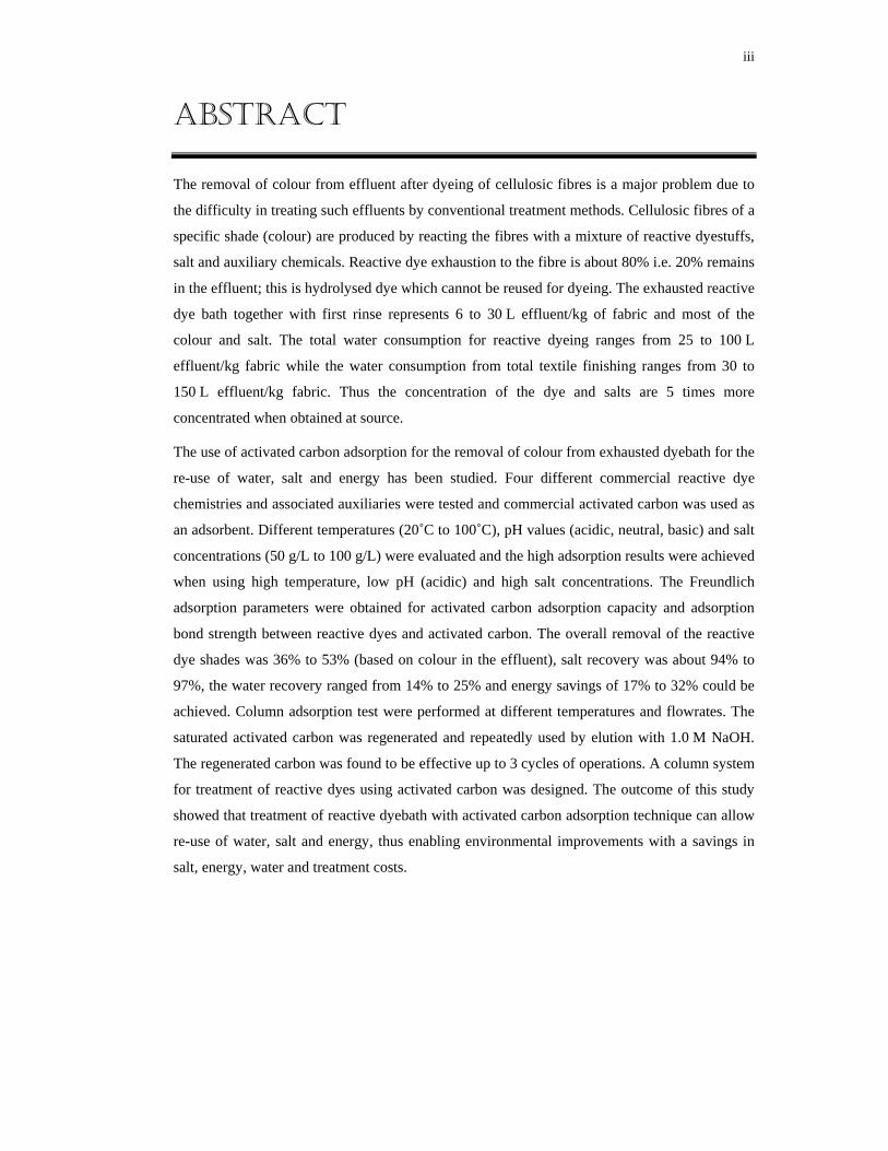
The removal of colour from effluent after dyeing of cellulosic fibres is a major problem due to

the difficulty in treating such effluents by conventional treatment methods. Cellulosic fibres of a

specific shade (colour) are produced by reacting the fibres with a mixture of reactive dyestuffs,

salt and auxiliary chemicals. Reactive dye exhaustion to the fibre is about 80% i.e. 20% remains

in the effluent; this is hydrolysed dye which cannot be reused for dyeing. The exhausted reactive

dye bath together with first rinse represents 6 to 30 L effluent/kg of fabric and most of the

colour and salt. The total water consumption for reactive dyeing ranges from 25 to 100 L

effluent/kg fabric while the water consumption from total textile finishing ranges from 30 to

150 L effluent/kg fabric. Thus the concentration of the dye and salts are 5 times more

concentrated when obtained at source.

The use of activated carbon adsorption for the removal of colour from exhausted dyebath for the

re-use of water, salt and energy has been studied. Four different commercial reactive dye

chemistries and associated auxiliaries were tested and commercial activated carbon was used as

an adsorbent. Different temperatures (20˚C to 100˚C), pH values (acidic, neutral, basic) and salt

concentrations (50 g/L to 100 g/L) were evaluated and the high adsorption results were achieved

when using high temperature, low pH (acidic) and high salt concentrations. The Freundlich

adsorption parameters were obtained for activated carbon adsorption capacity and adsorption

bond strength between reactive dyes and activated carbon. The overall removal of the reactive

dye shades was 36% to 53% (based on colour in the effluent), salt recovery was about 94% to

97%, the water recovery ranged from 14% to 25% and energy savings of 17% to 32% could be

achieved. Column adsorption test were performed at different temperatures and flowrates. The

saturated activated carbon was regenerated and repeatedly used by elution with 1.0 M NaOH.

The regenerated carbon was found to be effective up to 3 cycles of operations. A column system

for treatment of reactive dyes using activated carbon was designed. The outcome of this study

showed that treatment of reactive dyebath with activated carbon adsorption technique can allow

re-use of water, salt and energy, thus enabling environmental improvements with a savings in

salt, energy, water and treatment costs.

iv

TABLE OF CONTENTS

PREFACE ......................................................................................................................................... i ACKNOWLEDGEMENTS .............................................................................................................ii ABSTRACT....................................................................................................................................iii TABLE OF CONTENTS................................................................................................................ iv LIST OF FIGURES .......................................................................................................................vii LIST OF TABLES ........................................................................................................................... x LIST OF SYMBOLS .....................................................................................................................xii

GLOSSARY..................................................................................................................................xiv

CHAPTER 1: INTRODUCTION..............................................................................................1-1

1.1. TEXTILE INDUSTRY..........................................................................................................1-1 1.2. TEXTILE WASTEWATER TREATMENT ..............................................................................1-3 1.3. PROJECT OUTLINE ...........................................................................................................1-4 1.4. THESIS OUTLINE............................................................................................................1-6

CHAPTER 2: LITERATURE REVIEW..................................................................................2-1

2.1. REACTIVE DYES~AN OVERVIEW ................................................................................2-1 2.1.1. Development of reactive dyes..................................................................................2-1 2.1.2. Reactive dye chemistry ............................................................................................2-2 2.1.3. Reactive dye classes ................................................................................................2-4 2.1.4. Reactive dye reactivity.............................................................................................2-5 2.1.5. Basic principle of dyeing cotton with reactive dyes ................................................2-5 2.1.6. Reactive dye application and storage .....................................................................2-6 2.1.7. Colour measurement ...............................................................................................2-6 2.1.8. Treatment of reactive dyeing effluent ......................................................................2-6

2.2. ACTIVATED CARBON ......................................................................................................2-8 2.2.1. Background .............................................................................................................2-8 2.2.2. Characterisation of activated carbon......................................................................2-9 2.2.3. Adsorption on activated carbon ............................................................................2-10 2.2.4. Factors affecting adsorption capacity...................................................................2-11 2.2.5. Factors affecting adsorption rate..........................................................................2-12 2.2.6. Adsorption isotherms.............................................................................................2-12 2.2.7. Breakthrough behaviour of activated carbon........................................................2-14 2.2.8. System design ........................................................................................................2-14 2.2.9. Activated carbon adsorption as a reclamation technique .....................................2-15

2.3. WATER QUALITY FOR REUSE ........................................................................................2-17

v

2.4. SYSTEM DESIGN ............................................................................................................2-18 2.4.1. Scale-up and similitude .........................................................................................2-18

2.5. CLOSURE .......................................................................................................................2-19

CHAPTER 3: REACTIVE DYEING........................................................................................3-1

3.1. REACTIVE DYE CHEMISTRY ............................................................................................3-1 3.2. PRINCIPLE OF REACTIVE DYEING....................................................................................3-1

3.2.1. Specialty chemicals .................................................................................................3-2 3.2.2. Commodity chemicals..............................................................................................3-3

3.3. EXPERIMENTATION ..................................................................................................3-3 3.3.1. Preparation of dyeing solution................................................................................3-3 3.3.2. Colour measurement ...............................................................................................3-5

3.4. RESULTS.......................................................................................................................3-5 3.4.1. Laboratory test dyeings ...........................................................................................3-5 3.4.2. Total dyeing process mass balance .........................................................................3-7

3.5. DISCUSSION.................................................................................................................3-9 3.5.1. Laboratory test dyeings ...........................................................................................3-9 3.5.2. Total dyeing process mass balance .......................................................................3-10

3.6. CONCLUSION ............................................................................................................3-10

CHAPTER 4: CARBON EQUILIBRIUM TEST ....................................................................4-1

4.1. INTRODUCTION ...............................................................................................................4-1 4.1.1. Characteristics of activated carbon ........................................................................4-1

4.2. EXPERIMENTATION .........................................................................................................4-2 4.3. RESULTS..........................................................................................................................4-3

4.3.1. Adsorption isotherms...............................................................................................4-4 4.3.2. Adsorption isotherm model parameters ..................................................................4-8 4.3.3. Mass Balance ........................................................................................................4-11

4.4. DISCUSSION...................................................................................................................4-13 4.5. CONCLUSION .................................................................................................................4-15

CHAPTER 5: COLUMN TEST ................................................................................................5-1

5.1. EXPERIMENTATION.........................................................................................................5-1 5.1.1. Column calculations................................................................................................5-2

5.2. RESULTS .........................................................................................................................5-3 5.2.1. Column Breakthrough Curves.................................................................................5-4

5.3. DISCUSSION.....................................................................................................................5-6 5.4. CONCLUSION ...................................................................................................................5-8

CHAPTER 6: REGENERATION .............................................................................................6-1

6.1. BACKGROUND .................................................................................................................6-1

vi

6.2. EXPERIMENTATION .........................................................................................................6-2 6.3. RESULTS .........................................................................................................................6-2 6.4. DISCUSSION ....................................................................................................................6-4 6.5. CONCLUSION...................................................................................................................6-5

CHAPTER 7: SYSTEM DESIGN .............................................................................................7-1

7.1. DESIGN .........................................................................................................................7-1 7.1.1. Small column design................................................................................................7-1 7.1.2. Pilot-scale design ....................................................................................................7-3

CHAPTER 8: CONCLUSIONS AND RECOMMENDATIONS ...........................................8-1

REFERENCES...........................................................................................................................R-1 APPENDIX A: THE DYEING PROCESSES .........................................................................A-1 APPENDIX B: ACTIVATED CARBON ADSORPTION ..................................................... B-1 APPENDIX C: ERROR ANALYSIS .......................................................................................C-1 APPENDIX D: COLUMN TEST..............................................................................................D-1 APPENDIX E: REGENERATION .......................................................................................... E-1

vii

LIST OF FIGURES

Fig 1.1 : Sequence for reactive dyeing of cotton ..........................................................................1-2

Fig 1.2 : Overall sketch of dye machine close-coupled with proposed activated carbon process..

.......................................................................................................................................................1-5

Fig 3.1: Dye and salt concentrations before and after dyeing of Navy shade. .............................3-6

Fig 3.2: Dye and salt concentrations before and after dyeing of Black shade..............................3-6

Fig 3.3: Dye and salt concentrations before and after dyeing of Beige shade..............................3-6

Fig 3.4: Dye and salt concentrations before and after dyeing of Turquoise shade. ......................3-6

Fig 3.5: Dye and salt ratios after dyeing of Navy shade..............................................................3-7

Fig 3.6: Dye and salt ratios after dyeing of Black shade. .............................................................3-7

Fig 3.7: Dye and salt ratios after dyeing of Beige shade. .............................................................3-7

Fig 3.8: Dye and salt ratios after dyeing of Turquoise shade. ......................................................3-7

Fig 3.9: Flow diagram and mass balance for dyeing of Navy shade ............................................3-8

Fig 4.1 : Metal flasks where test dye solution was poured ...........................................................4-4

Fig 4.2 : Front view of the shaker with a temperature controller used .........................................4-4

Fig 4.3 : Back view of the shaker .................................................................................................4-4

Fig 4.4 : Stirrers inside the shaker where metal flasks are clamped .............................................4-4

Fig 4.5 : Different time interval at 60˚C-Navy shade ...................................................................4-5

Fig 4.6 : Different time interval at 60˚C-Black shade...................................................................4-5

Fig 4.7 : Different time interval at 60˚C-Beige shade ..................................................................4-5

Fig 4.8 : Different time interval at 60˚C- Turquoise shade ..........................................................4-5

Fig 4.9 : Effect of temperature on adsorption of Navy shade at pH 11 and 70 g/L NaCl ............4-6

Fig 4.10 : Effect of temperature on adsorption of Black shade at pH 11 and 80 g/L Na2SO4 ......4-6

Fig 4.11 : Effect of temperature on adsorption of Beige shade at pH 11 and 60 g/L NaCl..........4-6

Fig 4.12 : Effect of temperature on adsorption of Turquoise shade at pH 10 and 50 g/L Na2SO4 ....

………………………………………………………………………………………………….4-6

viii

Fig 4.13 : Effect of pH on adsorption of Navy shade at 100°C and 70 g/L NaCl .......................4-7

Fig 4.14 : Effect of pH on the adsorption of Black shade at 100°C and 80 g/L Na2SO4..........…4-7

Fig 4.15 : Effect of pH on the adsorption of Beige shade at 100ºC and 60 g/L NaCl ..................4-7

Fig 4.16 : Effect of pH on the adsorption of Turquoise shade at 100ºC and 50 g/L Na2SO4 .......4-7

Fig 4.17 : Effect of electrolyte concentrations on adsorption of Navy shade at 100°C and pH 11…

………………………………………………………………………………………………….4-7

Fig 4.18 : Effect of electrolyte concentrations on the adsorption of Black shade at 100°C and

pH 11.............................................................................................................................................4-7

Fig 4.19 : Effect of electrolyte concentrations on the adsorption of Beige shade at 100°C and

pH 11.............................................................................................................................................4-8

Fig 4.20 : Effect of electrolyte concentrations on the adsorption of Turquoise shade at 100°C

and pH 10 ......................................................................................................................................4-8

Fig 4.21 : Flow diagram and mass balance for dyeing of Navy shade .......................................4-12

Fig 5.1 : Schematic set-up diagram of column experiment ..........................................................5-2

Fig 5.2 : Navy breakthrough curve at different temperatures. ......................................................5-4

Fig 5.3 : Black breakthrough curve at different temperatures. .....................................................5-4

Fig 5.4 : Beige breakthrough curve at different temperatures. .....................................................5-4

Fig 5.5 : Turquoise breakthrough curve at different temperatures. ..............................................5-4

Fig 5.6 : Navy breakthrough curve at different flowrates and 60˚C.............................................5-5

Fig 5.7 : Black breakthrough curve at different flowrates and 60˚C ............................................5-5

Fig 5.8 : Beige breakthrough curve at different flowrates and 60˚C ............................................5-5

Fig 5.9 : Turquoise breakthrough curve at different flowrates and 60˚C .....................................5-5

Fig 6.1: Desorption of shades from granular activated column using NaOH...............................6-3

Fig 6.2: Regeneration of GAC-Navy shade at 60˚C.....................................................................6-3

Fig 6.3: Regeneration of GAC-Black shade at 60˚C ....................................................................6-3

Fig 6.4: Regeneration of GAC-Beige shade at 60˚C ....................................................................6-3

Fig 6.5: Regeneration of GAC-Turquoise shade at 60˚C .............................................................6-3

ix

Fig 7.2 : Navy breakthrough curve at 60˚C for column design ....................................................7-2

Fig A.1: Navy shade dyeing process ...........................................................................................A-2

Fig A.2: Black shade dyeing process...........................................................................................A-3

Fig A.3: Beige shade dyeing process...........................................................................................A-4

Fig A.4: Turquoise shade dyeing process....................................................................................A-5

Fig A.5: Flow diagram and mass balance for dyeing of Navy shade ..........................................A-6

Fig A.6: Flow diagram and mass balance for dyeing of Black shade..........................................A-7

Fig A.7: Flow diagram and mass balance for dyeing of Beige shade..........................................A-8

Fig A.8: Flow diagram and mass balance for dyeing of Turquoise shade...................................A-9

Fig B.1: Flow diagram and mass balance for dyeing of Navy shade .......................................... B-8

Fig B.2: Flow diagram and mass balance for dyeing of Black shade.......................................... B-9

Fig B.3: Flow diagram and mass balance for dyeing of Beige shade........................................ B-10

Fig B.4: Flow diagram and mass balance for dyeing of Turquoise shade................................. B-11

x

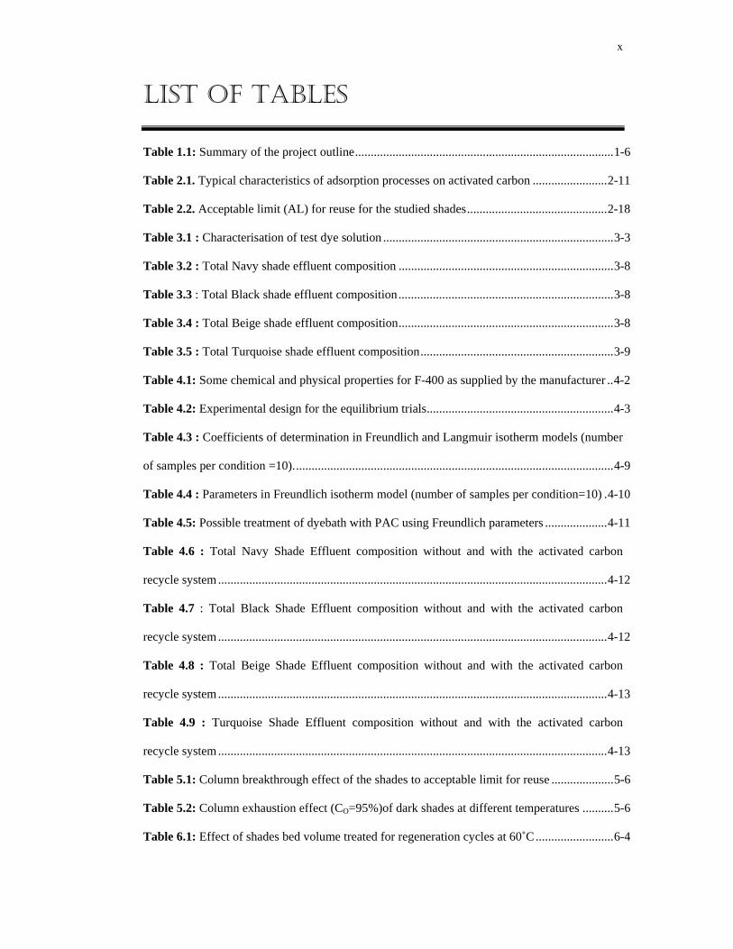
LIST OF TABLES

Table 1.1: Summary of the project outline...................................................................................1-6

Table 2.1. Typical characteristics of adsorption processes on activated carbon ........................2-11

Table 2.2. Acceptable limit (AL) for reuse for the studied shades.............................................2-18

Table 3.1 : Characterisation of test dye solution ..........................................................................3-3

Table 3.2 : Total Navy shade effluent composition .....................................................................3-8

Table 3.3 : Total Black shade effluent composition.....................................................................3-8

Table 3.4 : Total Beige shade effluent composition.....................................................................3-8

Table 3.5 : Total Turquoise shade effluent composition..............................................................3-9

Table 4.1: Some chemical and physical properties for F-400 as supplied by the manufacturer ..4-2

Table 4.2: Experimental design for the equilibrium trials............................................................4-3

Table 4.3 : Coefficients of determination in Freundlich and Langmuir isotherm models (number

of samples per condition =10).......................................................................................................4-9

Table 4.4 : Parameters in Freundlich isotherm model (number of samples per condition=10) .4-10

Table 4.5: Possible treatment of dyebath with PAC using Freundlich parameters ....................4-11

Table 4.6 : Total Navy Shade Effluent composition without and with the activated carbon

recycle system.............................................................................................................................4-12

Table 4.7 : Total Black Shade Effluent composition without and with the activated carbon

recycle system.............................................................................................................................4-12

Table 4.8 : Total Beige Shade Effluent composition without and with the activated carbon

recycle system.............................................................................................................................4-13

Table 4.9 : Turquoise Shade Effluent composition without and with the activated carbon

recycle system.............................................................................................................................4-13

Table 5.1: Column breakthrough effect of the shades to acceptable limit for reuse ....................5-6

Table 5.2: Column exhaustion effect (CO=95%)of dark shades at different temperatures ..........5-6

Table 6.1: Effect of shades bed volume treated for regeneration cycles at 60˚C.........................6-4

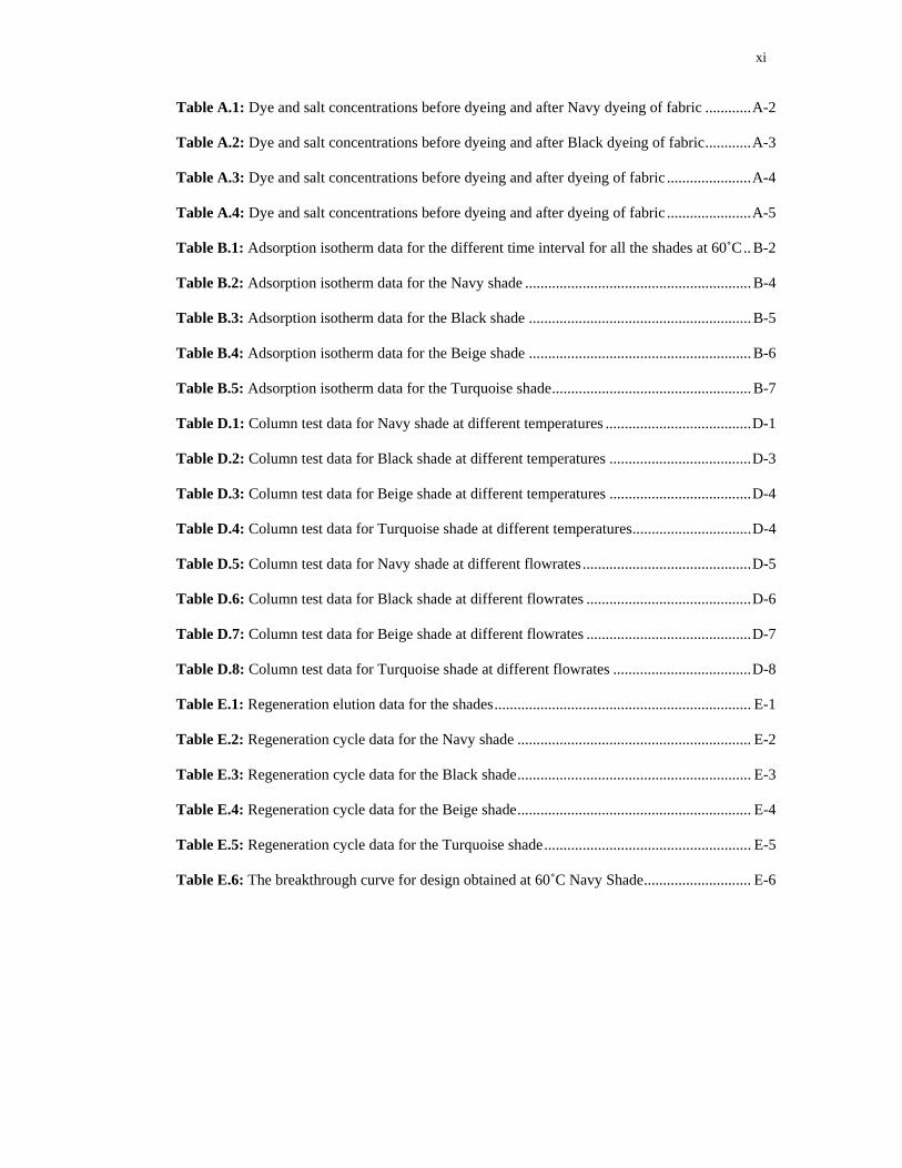
xi

Table A.1: Dye and salt concentrations before dyeing and after Navy dyeing of fabric ............A-2

Table A.2: Dye and salt concentrations before dyeing and after Black dyeing of fabric............A-3

Table A.3: Dye and salt concentrations before dyeing and after dyeing of fabric ......................A-4

Table A.4: Dye and salt concentrations before dyeing and after dyeing of fabric ......................A-5

Table B.1: Adsorption isotherm data for the different time interval for all the shades at 60˚C.. B-2

Table B.2: Adsorption isotherm data for the Navy shade ........................................................... B-4

Table B.3: Adsorption isotherm data for the Black shade .......................................................... B-5

Table B.4: Adsorption isotherm data for the Beige shade .......................................................... B-6

Table B.5: Adsorption isotherm data for the Turquoise shade.................................................... B-7

Table D.1: Column test data for Navy shade at different temperatures ......................................D-1

Table D.2: Column test data for Black shade at different temperatures .....................................D-3

Table D.3: Column test data for Beige shade at different temperatures .....................................D-4

Table D.4: Column test data for Turquoise shade at different temperatures...............................D-4

Table D.5: Column test data for Navy shade at different flowrates............................................D-5

Table D.6: Column test data for Black shade at different flowrates ...........................................D-6

Table D.7: Column test data for Beige shade at different flowrates ...........................................D-7

Table D.8: Column test data for Turquoise shade at different flowrates ....................................D-8

Table E.1: Regeneration elution data for the shades................................................................... E-1

Table E.2: Regeneration cycle data for the Navy shade ............................................................. E-2

Table E.3: Regeneration cycle data for the Black shade............................................................. E-3

Table E.4: Regeneration cycle data for the Beige shade............................................................. E-4

Table E.5: Regeneration cycle data for the Turquoise shade...................................................... E-5

Table E.6: The breakthrough curve for design obtained at 60˚C Navy Shade............................ E-6

xii

LIST OF SYMBOLS

Langmuir constant related to the area occupied by a monolayer of adsorbate reflecting the adsorption capacityAL Acceptable limit for

a

water reuse for dyeing (75 ADMI) Pilot-scale column surface area Small-scale column surface area

Langmuir direct measure for the i

L

S

AAb

O

t

ntensity of adsorptionC Dye residual concentration for equilibruim tests (mg dye/L)C Initial dye feed concentration-column testC Residual dye concentration in the effluent-column test

Pilot-scale column carbon particle Small-scale column carbon particle diameter

Ca

L

S

ddε rbon bed void fraction

Pilot-scale empty bed contact time Small-scale empty bed contact time

Pilot-scale column internal diameter

L

S

L

S

EBCTEBCTIDID Small-scale column internal diameter

Small-scale column lengthM Mass of carbon

Pilot-scale mass of carbon

S

CL

CS

L

MM Small-scale mass of carbon

Carbon particle density Pilot-scale flow rate Small-scale flow rate

Re Pilot-scale Rey

L

S

L

pbQQ

nold's numbersRe Small-scale Reynold's numbers

Pilot-scale time to breakthrough Small-scale time to breakthrough

S

L

S

tbtbν Water viscocity

xiii

bL

bS

V Volume of dye solution-column test Pilot-scale volume of carbon bed Small-scale volume of carbon bed Pilot-L

VVV

O

scale hydraulic loading rateV Volume of carbon bed-column test

Pilot-scale feed volume Small-scale hydraulic loading rate

L

S

L

VoVV Pilot-scale hydraulic loading rateX Amount of dye adsorbed (mg)

xiv

GLOSSARY

Adsorbate A substance that becomes adsorbed at the interface or into the

interfacial layer of another material, or adsorbent.

Adsorbent The substrate material onto which a substance is adsorbed

Adsorption The adhesion of the molecules of dissolved substances, or

liquids known as adsorbate in more or less concentrated form,

to the surface of solids or liquids known as adsorbent with

which they are in contact.

Activated carbon A carbon material produced by roasting of cellulose base

substances, such as wood, coal or coconut shell to promote

active sites that yield a porous structure, creating a very large

internal surface area, which can adsorb pollutants.

Anchor Reactive group that form a covalent bond with the textile

material

Anthraquinone dye Dye based on the structure of 9, 10-anthraquinone, with

powerful electron donor groups in one or more of the four alpha

positions.

Azo dye Dye which contain a least one azo group (-N=N-), and can

contain up to four azo bonds.

Cellulose A complex carbohydrate that is composed of glucose units,

forms the main constituent of the cell wall in most plants, and is

important in the manufacture of numerous products, such as

paper, textiles, pharmaceuticals, and explosives.

Chromogen A compound not itself a dye but containing a chromophore and

so capable of becoming a dye.

Chromophore The chemical group that gives colour to a molecule

Dye A colouring substance used to colour cloth, paper etc.

Electrophile A chemical species (an ion or a molecule) which is strongly

attracted to a region of negative charge and tends to attract or

accept electrons.

Exhaust To use up all the colour potential of a dyebath

xv

Fibre A fine thread used to make textiles, which is flexible and fine.

A general name for the raw material, such as cotton, flax,

hemp, etc., used in textile manufactures.

Hue Quality of a colour as determined by its dominant wavelength.

Nucleophile A chemical species (an ion or a molecule) which is strongly

attracted to a region of positive charge and tends to donate or

share electrons.

Nucleophilic addition Addition of a nucleophile to a chemical compound

Nucleophilic substitution Substitution of a halogen by a nucleophile in a chemical

compound

Reactivation Restoration of the activated carbon to a state where it is

virtually identical to the properties of the virgin pre-cursor

Reactive dye A dye which is capable of reacting chemically with a substrate

to form a covalent dye-substrate bond.

Substantivity The attraction between a substrate and a dye or other substance

under the precise conditions of test whereby the latter is

selectively extracted from the application medium by the

substrate.

1-1

CHAPTER 1 INTRODUCTION

Water is life. The provision and supply of adequate water quality and quantity for economic and public health purposes remain a continuous challenge. Water use and wastewater management in South Africa is a key factor for social and economic growth, as well as our environment (WRC, 2003).

Water resources management has become an important operational and environmental issue

especially in the context of South Africa as water is becoming incrementally scarce. Even

though it appears to be in plentiful supply on the earth’s surface, water is a rare and precious

commodity, and only an infinitesimal part of the earth’s water reserves (approx. 0.03%)

constitutes the water resource, which is available for human activities (Allegre et al., 2004).

South Africa is a semi-arid country. It is predicted that in future, increasing demands will be

made on our dwindling water resources. It is therefore imperative that all water use sectors use

water optimally and efficiently to ensure that the needs of both the environment and people are

satisfied for now and future generations (DWAF, 1998). Due to the limited water resources in

South Africa, it is important to encourage industries to implement water and effluent

management strategies and reduce waste at source (Barclay and Buckley, 2002).

Increasingly stringent environmental legislation and generally enhanced intensity, efficiency

and diversity of treatment technologies have made the reuse of water more viable in many

industrial processes. Wastewater reclamation and reuse are effective tools for sustainable

industrial development programmes. The use and re-use of industrial wastewater is a common

activity throughout the industrial sector in South Africa today. The reality is that discharge of

wastewater through the municipal sewer system is costly to industries, which must pay the

relevant municipal authority to receive and treat this wastewater. Alternatively, for industries

who wish to discharge directly into water resource they are required to treat the wastewater to

acceptable standards in terms of the water use authorisation issued. The treatment costs of crude

water supplies, and wastewater disposal have increased the economic incentive for

implementing water reuse and recycle processes in industry (Dvarioneine et al., 2003). Thus the

way industries think about and use water is an important factor in determining the country’s

future.

1.1. TEXTILE INDUSTRY The textile industry is characterised by high water consumption and as one of the largest

industrial producers of wastewaters. Textile effluents from cotton dyeing represent severe

environmental problems as they contain highly coloured and high conductivity wastewater

1-2

resulting from dye baths and dye rinse waters, which contain unfixed dyes (Faria et al., 2004).

Reactive dyes are the major cause for complaint. Exhaust reactive dyeing requires high salt

concentrations (up to 80 g/L of Na2SO4/NaCl). Reactive dye bath and first rinse represent 6 to

30 L effluent per kg of fabric and most of the colour and salt. The main challenges that textile

industries face from dyeing of cellulose with reactive dyes is to reduce water consumption and

high salinity coloured effluents. Fig 1.1 is a schematic representation of the main stages

involved in the reactive dyeing of cotton. This section will describe the three different stages

used in the colouration of fabric by reactive dyeing namely: preparation, dyeing and finishing.

Fig 1.1 : Sequence for reactive dyeing of cotton

The cotton contains a significant amount of contamination resulting from fertilizers, insecticides

and fungicides. Preparation removes all the natural impurities from the cotton and chemical

residues from previous processing. Natural impurities include waxes, oils, proteins, mineral

matter, and residual seeds. All the impurities on the cotton must be removed before dyeing

because they can interfere with dyeing process resulting in uneven dyeing, spotting and

permanently damaging the cotton fibre. The processes involved in preparation are desizing,

scouring and bleaching. The second stage in colouration of cotton is dyeing. Different reactive

dye classes require specific dyeing procedures; however a common factor is that high volumes

of water, auxiliaries, salt and alkali are required to produce a dyed cotton fabric. The total

volume of water from the dyeing process is determined by a liquor ratio, which is the volume of

dye solution required to dye a mass of fabric. The liquor ratio ranges from 30:1

L effluent/kg fabric in old equipment or short runs to 3:1 in ultramodern airflow equipment. A

typical value for the liquor ratio is 10:1. Subsequent rinsing of the reactive dyed cotton fabric

gives rise to large volumes of coloured effluent with high salts. The third stage is finishing,

which improves the quality of the cotton fabric after dyeing (Hendrickx and Boardman, 1995).

The water consumption resulting from the dyeing process from reactive dyeing ranges from 75

to 150 L effluent per kg of fabric.

PREPARATION 1. Weaving 2. Desizing 3. Scouring 4. Bleaching

DYEING

FINISHING

1-3

1.2. TEXTILE WASTEWATER TREATMENT The rapid development of textile industries has given rise to multiple environmental problems

which led to the development of cleaner technologies and waste minimisation techniques.

Sustainability assessment is the approach to evaluate the cleaner technologies and waste

minimisation for waste discharges. The sustainability of any technology or technique is assessed

from three points of view: economic, environmental and social impacts. Waste minimisation

techniques can be grouped into four major categories: inventory management and improved

operations, modification of equipment, production process changes, and recycling and reuse

(Eckenfelder, 2000; Barclay and Buckley, 2002).

The main challenge that textile industries face from dyeing of cellulose with reactive dyes is to

reduce water consumption and the highly saline coloured effluents. Coloured effluent disposed

by textile industries into Sterkspruit River was observed in the Hammarsdale area of KwaZulu-

Natal in the last decade. The inadequate treatment of Hammarsdale Wastewater Treatment

Works resulted in poor quality final effluents, which have an adverse environmental impact on

Sterkspruit river. The eThekwini municipality is encouraging the textile industries to be

involved in waste minimisation and cleaner production technologies. The removal of colour

from dyeing of cellulose effluent is a major problem due to the difficulty in treating such

effluents by conventional treatment methods. Biological treatment, chemical precipitation,

membrane technology, activated carbon adsorption and evaporation are the common wastewater

treatment techniques of textile industry effluents (Wenzel et al., 1996). Removing colour from

reactive dyebath for reuse by conventional processes such as chemical precipitation, evaporation

and biological treatment have been ineffective because of the high salt content resulting from

reactive dyeing. This is because only water can be reclaimed and not the salt and energy

(Wenzel et al., 1996; Allegre et al., 2004). Membrane filtration techniques such as reverse

osmosis can reclaim water, salt and energy (Dvarioniene et al., 2003) but high concentrations of

salt used in reactive dyeing will increase osmotic pressure which reduces the net pressure

driving force and permeate flow (Allegre et al., 2004).The salt and the residual dye still need to

be separated.

Activated carbon adsorption is the one promising technique for recovery of water, salt and

energy from exhausted dyebath. The advantage of using this stream is that the high salt

concentration could shift the dye equilibrium towards the carbon resulting in very high removal

efficiencies. It is hypothesised that dye removal using activated carbon will be more complete in

the presence of high concentration of salt and the decolourised dye solution can be reused

preventing the discharge of large masses of salts and water. Much work has been done on

activated carbon for the treatment of combined dye effluent; however there has been very little

work on the treatment of the reactive dye bath effluent using activated carbon. Furthermore the

1-4

hot saline decolourised dye bath is suitable for direct reuse thus reducing the total dissolved

solids load from the textile mill and allowing for direct energy reuse. Cleaner Textile Production

Project funded by Danida supported Dyefin Textiles and Vivendi Water Treatment (equipment

suppliers) in the pilot assessment of the system. The cost of the system is directly related to the

capacity of the carbon for dyestuffs and the amount of unexhausted dye in the effluent.

Continuous pilot-scale activated carbon trials on exhausted reactive dyebath effluent which

were undertaken by Vivendi Plant on Dyefin Textile industry effluent concluded that

Chemviron F-400 carbon could treat 68 L effluent per kg carbon i.e. 147 g carbon/kg fabric and

the performance of thermally regenerated carbon was similar to that of virgin carbon (Hoffman,

2004). Further tests were needed to quantify the effect of temperature, salt and pH on the

adsorption characteristics. Investigation of new high performance dyes with greater exhaustion

is allowing a trade-off between more expensive high performance dyes and the cost of activated

carbon.

1.3. PROJECT OUTLINE There are a large number of studies describing the use of activated carbon for the removal of

colour from textile effluents but these studies have been unsuccessful for a number of reasons:

• The studies focused on the combined dye house or factory effluent. The dye

concentrations are low, and the volumes are large. This resulted in low driving forces

and large carbon inventories (Wenzel et al., 1996; Santhy and Selvapathy, 2006).

• The salt concentrations were low. Dyeing with reactive dyes requires a high electrolyte

concentration (up to 80 g/L) in order to force the dye equilibrium towards the fabric.

This will improve the driving force of the dye onto the carbon Treatment of the dilute

dye house effluent reduces the salting out effect (Wenzel et al., 1996).

• Modern reactive dyes have bifunctional or more bonding groups and thus have a much

higher affinity for the fabric, thus there is less residual dye in the dye effluent hence the

mass of carbon required per mass of textiles is reduced (Allegre et al., 2006).

• The proposed activated carbon process will be close-coupled to the dye machine and

will treat the hot dye liquor. Fig 1.2 shows an overall sketch of activated carbon process

close-coupled to the dye machine. The dye will be removed and the hot water

containing the electrolyte will be recycled directly to the dye bath for the subsequent

dyeing.

The most important parameter is the amount of carbon to treat the exhausted dyebath for each

type of dye chemistry for a fixed shade. The feed concentration to the activated carbon column

should be the exhausted dyebath from each shade.

1-5

Fig 1.2 : Overall sketch of dye machine close-coupled with proposed activated carbon process.

The objective of this study is to establish the process parameters governing the recovery of

water and chemicals for reuse from reactive dye baths using activated carbon and to investigate

a process for recovering water and chemicals from reactive dyeing. The following approach was

adopted to achieve these aims:

• The first phase of this project involved researching of the relevant literature on reactive

dyes and activated carbon adsorption. The reactive dye chemistry and the factors that

affect adsorption equilibrium were investigated.

• The experimental work on dyeing a range of shades using different dye chemistries being

undertaken in terms of WRC Project K5/1363 - The promotion of biodegradable

chemicals in the textile industry using the score system: phase 1 - pilot study, was of

particular relevance to this project in selecting dye chemistries and dyestuffs to be

evaluated. The four selected dye chemistries represent almost all reactive dye chemistries

used in Dyefin textile factory. Four reactive dye classes of Drimarene HF, Cibacron S,

Procion HE and Remazol L with different dye chemistries were selected from the WRC

Project K5/1363 to produce four different laboratory shades. Laboratory dyeing for four

different shades (Navy, Black, Beige and Turquoise) with associated auxiliaries and salts

Cotton

Preparation

Dyebath

Rinsing

Neutralisation

Finishing

Rinsing

Activated carbon column

Hot decolourised water with salt

Regeneration

1-6

were undertaken following a specific dye recipe for each of the shades. Each shade

consisted of up to 3 dyestuffs. The Navy shade was made of three Drimarene HF reactive

dyes, Black shade consisted of two Cibacron S reactive dyes, Beige shade made of three

Procion HE reactive dyes and Turquoise shade consisted of two Remazol and one Levafix

reactive dyes.

• The dye bath liquor from each of these laboratory dyeings was then tested against

activated carbon. One grade of F-400 activated carbon from Chemviron was selected.

Adsorption isotherm experiments were undertaken on the dye liquor bath. The effect of

three different salt concentrations, three pH values and four different temperatures on the

adsorption isotherm was determined for all four shades. Column tests were undertaken

using the exhausted dye bath at three different temperatures to determine the kinetics of

dye adsorption. The results would be used to determine the parameters for standard

adsorption theory.

• Finally, the carbon was chemically regenerated at a laboratory scale under a range of

conditions. Column experiments for the regenerated carbon were performed to determine

the performance of the regenerated carbon. This procedure was repeated for a number of

cycles to evaluate the regenerated carbon adsorption capacity. The results were used to

assess the overall performance of the reuse system. The possible system for removal of

colour for the reuse of salt, water and energy was designed. Table 1.1 shows the overall

summary of the project.

Table 1.1: Summary of the project outline Class Drimarene HF Cibacron S Procion HE Remazol L *Shades Navy Black Navy Black Navy Beige Navy Black Beige Turquoise Selected shades

X X X X

Dyeing X X X X Isotherms X X X X Column evaluation

X X X X

Column Regeneration

X X X X

System design

X X X X

*Possible shades from Score study (WRC Project K5/1363)

1.4. THESIS OUTLINE The thesis begins with a literature survey on reactive dyes and activated carbon adsorption

presented in Chapter 2. Chapter 3 presents results on the reactive dyeing for all four shades.

Chapter 4 presents results on activated adsorption isotherms. In Chapter 5, the column results

of the dye adsorption are explained and in Chapter 6 the regeneration of activated carbon

results are presented. Chapter 7 explains the system design of the adsorption of dye by

1-7

activated carbon. An overall conclusion of the results obtained and recommendations are

presented in Chapter 8.

2-1

CHAPTER 2 LITERATURE REVIEW

From Chapter 1, the main objective of this investigation is to establish the process parameters

governing the recovery of water and chemicals for reuse from reactive dye baths using activated

carbon. The textile industry plays an important role in our economy in increasing consumer

interests by producing cotton fabric with value, comfort and styling using reactive dyes. At the

same time large volumes of water are used for reactive dyeing and large quantities of coloured

wastewater with high salt contents are generated. Treatment of textile effluent resulting from

reactive dyeing is major problem facing textile industries today. The failure of most

conventional treatment process resulted in the need to develop alternative treatment methods

such as activated carbon adsorption. Activated carbon adsorption has been studied in more

detail than the other treatment methods in this chapter. In this chapter the relevant literature on

reactive dyes and activated carbon has been reviewed. Section 2.1 discusses an overview of

reactive dyes while Section 2.2 discusses the activated carbon and its adsorption characteristics.

Water quality for reuse and system design for activated carbon treatment is discussed in Section

2.3 and 2.4 respectively.

2.1. REACTIVE DYES~AN OVERVIEW Reactive dyes gained popularity in the 20th century as dyes that give a permanent colouration to

cellulosic textile substrates, and an important criterion was that the colour did not fade or

discolour on laundering. Reactive dyes are dyes which have groups capable of forming bonds

between a carbon or phosphorus atom of the dye ion or molecule and oxygen, nitrogen or

sulphur atom of a hydroxyl, an amino or mercapto group respectively of the textile substrate.

This section discusses the development of reactive dyes of cotton, their chemistry, chemical

constitution, classes, reactivity, application and storage.

2.1.1. Development of reactive dyes The most important distinguishing characteristics of reactive dyes are that they form covalent

bonds with the substrate that is to be coloured during the application process. Thus, the dye

molecule contains specific functional groups that can undergo addition or substitution reactions

with the OH, SH and NH2 groups present in textile fibres (Hunger, 2003).

The concept of immobilising a dye molecule by covalent bond formation with reactive groups in

a fibre originated in the early 1900s (Broadbent, 2001). Cross and Bevan first succeeded in

fixing dyes covalently onto cellulose fibres, but their multi-step process was too complicated for

practical application. Early work by Schroter with sulfonyl chloride-based dyes was

2-2

unsuccessful, but Gunther later did succeed in fixing derivatives of isatoic anhydride onto

cellulose fibres. Haller and Heckendorn, and Heyna and Schumacher in the 1940s also

contributed in the approach of modifying the fibres and introduced coloration (Hunger, 2003).

In 1955, Rattee and Stephen, working for ICI in England, developed a procedure for dyeing

cotton with fibre-reactive dyes containing dichlorotriazine groups. They established that dyeing

cotton with these dyes under mild alkaline conditions resulted in a reactive chlorine atom on the

triazine ring being substituted by an oxygen atom from the cellulose hydroxyl group

(Broadbent, 2001).

The discovery of reactive dyes was an event of great technical and commercial importance. Not

only did this class of dye function by the complete new fixation method of covalent bonding

with the substrate, but it also offered the cotton dyer a desirable blend of properties such as high

wet fastness, brilliance and variety of hue and versatility of application (Hunter and Renfrew,

1999).

2.1.2. Reactive dye chemistry A dye is dissolved in the application medium, usually water, at some point during colouration. It

will also usually exhibit some substantivity for the material being dyed and be absorbed from

the aqueous solution (Hunger, 2003). The molecular structures of reactive dyes resemble those

of acid and simple direct cotton dyes, but with an added reactive group. Reactive groups are of

two main types:

• Those reacting with cellulose by nucleophilic substitution of a labile chlorine, fluorine,

methyl sulphone or nicotinyl leaving group activated by an adjacent nitrogen atom in a

hetero-cyclic ring (Broadbent, 2001). The reaction is called hetero-aromatic nucleophilic

substitution (Hunter and Renfrew, 1999).

• Those reacting with cellulose by nucleophilic addition to a carbon-carbon double bond,

usually activated by an adjacent electron-attracting sulphone group (Broadbent, 2001).

Overwhelmingly, sulphonyl has emerged as the preferred activating group with α-halo-

amido group playing a minor role. While vinyl sulphones are applied to all cellulosic and

protein fibres, the α-haloacrylamido types are largely confined to the latter, especially

wool (Hunter and Renfrew, 1999).

The dyes can also react with water and these reactions compete with one another. The reactive

group must exhibit adequate reactivity towards cotton, but have lower reactivity towards water

molecules which can deactivate the dye by hydrolysis. The hydrolysis of the reactive group of

the dye is similar to its reaction with cellulose but involves a hydroxyl ion in water rather than a

cellulosate ion in the fibre (Broadbent, 2001). All dyes are hydrolysed, the extent of which

determines the efficiency of dyeing, and as a result 100% efficiency (or fixation) is never

2-3

achieved. Commercial reactive dyes vary in molecular mass and complexity in that they contain

one, two and/or three chromophoric units and up to three different reactive groups, which will

be discussed in subsequent sections.

Chemical constitution of reactive dyes In a dye molecule, a chromophore is combined with one or more functional groups, the so called

anchors that can react with cotton. Under suitable conditions, covalent bonds are formed

between dye and cotton fibre (Hunger, 2003). Reactive groups increase the molecular mass of a

dye but do not enhance chromogenic strength (Hunter and Renfrew, 1999).

Monofunctional Most mono-anchor dyes are derivatives of cyanuric chloride (2,4,6-trichloro-1,3,5-triazine), a

molecule of wide synthetic potential because the three chlorine atoms on the triazine ring differ

in their reactivity. The first chlorine atom exchanges with nucleophiles in water at 0 to 5°C, the

second at 35 to 40°C and the third at 80 to 85°C (Hunger, 2003).

Bifunctional dyes The concept of reactive dyes with two reactive groups was well established in the early years of

reactive dyeing but at that time fixation efficiency was not a major issue and bifunctional dyes

were the exception rather than the rule until textile industries observed that more that 50% of the

monofunctional dyes could be lost to hydrolysis and discarded in the dye effluent (Hunter and

Renfrew, 1999). Since the 1980s considerable interest has been shown in strongly fixing

reactive dyes, and the required high fixation values have increasingly been achieved with the aid

of double anchors (Hunger, 2003).

Double-anchor dyes can be divided into two categories: those containing two equivalent

reactive groups called homo-bifunctional dyes (e.g. bis-β-sulphatoethylsulphone (CI Reactive

Black 5)) and those with mixed-anchor systems called hetero-bifunctional dyes (e.g. CI

Reactive Red 194). A homo-bifunctional reactive dye encompasses products containing two

vinylsulfonyls or sulfoxyethylsulfonyl group, which increase the probability of reaction with the

fibre. Introduction of homo-bifunctionality into cellulose reactive dyes is achieved by different

molecular structures: mono azo bis-monochlorotriazinyl, dis azo bis-monochlorotriazinyl, non-

azo-bis-monochlorotriazinyl, Procion H-EXL and bis-vinylsulphonyl reactive dyes (Hunger,

2003; Hunter and Renfrew, 1999).

In a mixed-anchor system the two reactive groups have different reactivities: a more reactive 2-

sulfohydroxyethysulfonyl group and a less reactive monochlorotriazinyl residue (Hunger,

2003). Hetero-bifunctional reactive dyes , which have different optimal fixation towards cotton

gives a more uniform degree of fixation over a wide range of dyeing temperature and fixation

pH values than homo-bifunctional reactive dyes (Broadbent, 2001).

2-4

Multifunctional dyes The introduction of more than two anchor groups has only a minor influence on dye fixation

characteristics, so multiple-anchor dyes play only a subordinate role in world markets (Hunger,

2003), increasingly this has been an area of patent interest (Hunter and Renfrew, 1999). A

number of tri-functional dyes containing bis-vinyl sulphone/monochlorotriazine and bis-vinyl

sulphone/monofluorotriazine reactive groups have been disclosed by dye suppliers (e.g. Ciba

etc.). Four (tetra-functional dyes) and five (penta-functional dyes) independent reactive groups

have been developed (Hunter and Renfrew, 1999).

2.1.3. Reactive dye classes Virtually every conceivable chromophore has been used in the synthesis of reactive dyes.

Azo dyes Most reactive dyes fall in the category of azo dyes. Virtually every hue in the dye spectrum can

be achieved by appropriate structural modifications (mono- and di-azo dyes, combinations

involving either single or multiple aromatic and heterocyclic ring systems) (Hunger, 2003).

Metal-Complex (formazan) dyes Exceptionally lightfast colours are obtained with metal-complexed azo dyes. Copper complexes

of disubstituted azo compounds produce a wide range of colours (yellow, ruby, violet, blue,

brown, olive, black) (Hunger, 2003).

Anthraquinone dyes Anthraquinone-based dyes are significant because of their brilliance, good light fastness and

chromophore stability under both acidic and basic conditions. Recently, in the 21st century, they

dominated the market for brilliant blue reactive dyes in spite of their relatively low colour

strength and comparatively high cost. The shades of commercial reactive anthraquinone dyes

range from violet to blue, e.g. C.I. Reactive Blue 19 (Hunger, 2003).

Triphenodiaxazine dyes Dyes derived from triphenodioxazine ring system have been commercially available since 1928

when Kranzlein and co-workers discovered dyes with this basic structure augmented by sulfonic

acid groups. The triphenodioxazine chromophore was tested in almost every class of dyes, but

only recently has it been introduced into reactive dyes. Until the 21st century, anthraquinone

dyes were predominant in most applications requiring brilliant blue dyes, but the much stronger

triphenodioxazine dyes now represent a less expensive choice in many applications (Hunger,

2003).

2-5

Phthalocyanine dyes The water-soluble reactive phthalocyanine dyes yield brilliant turquoise and green shades not

available in any other dye category. The most important reactive phthalocyanine dyes contain

copper or nickel as their central atom; they are substituted with sulfonic acid groups and also

with reactive groups joined via sulphonamide bridges, e.g. C.I. Reactive Blue 15 (Hunger,

2003).

2.1.4. Reactive dye reactivity The reactive groups of various types of reactive dye have different chemical structures and show

a wide range of reactivity. Reactive dyes reactivity is classified into the following:

• Alkali-controllable dyes, which have high reactivity and only moderate substantivity.

They are applied at low temperatures and level dyeing requires careful control of the

addition of alkali to initiate the fixation stage e.g. dichlorotriazine,

difluorochloropyrimidine and vinylsulphone reactive dyes.

• Salt-controllable dyes. These dyes have low reactivity towards cellulose under alkaline

conditions and therefore the dyeing temperature will be as high as 80°C. They have

appreciable substantivity and level dyeing requires careful addition of electrolyte to

promote exhaustion e.g. trichloropyrimidine, monochlorotriazine and monofluorotriazine

reactive dyes.

• Temperature-controllable dyes, which undergo fixation at high temperatures even under

neutral conditions e.g. nicotinyltriazine (Broadbent, 2001).

2.1.5. Basic principle of dyeing cotton with reactive dyes The relatively simple procedure for batch dyeing of cotton materials with reactive dyes,

developed by Rattee and Stephen (Broadbent, 2001), is still used for all types of reactive dyes

irrespective of their particular reactive group. Dyeing is commenced in neutral solution, in the

presence of electrolyte to promote exhaustion of the dye onto the cotton. During this period, the

dye does not react with the fibre and migration from fibre to fibre is possible. An appropriate

alkali is added gradually to the dyebath to increase the pH, this initiates the desired dye-fibre

reaction. The hydroxyl groups in cellulose are weakly acidic and absorption of hydroxide ions

causes some dissociation, forming cellulosate ions, which react with the dye by nucleophilic

addition or substitution. In general, the lower the reactivity of the reactive group of the dye

towards alkaline cellulose, the higher the final dyeing temperature and the higher the final pH of

the dyebath (Broadbent, 2001; Hunger, 2003). After dyeing, any unreacted and hydrolysed dye

present in the cotton must be removed by thorough washing to ensure no colour bleed from the

cotton on subsequent washing during use (Broadbent, 2001).

2-6

2.1.6. Reactive dye application and storage Reactive dyes are water soluble anionic electrophiles, which react to a greater or lesser degree

with nucleophilic fibres during dyeing. Fixation to cellulose presents a number of special

problems. Application disadvantages of reactive dyeing of cellulose include the following:

• Hydrolysis accompanies fixation, resulting in incomplete utilisation of dye

• Relatively large amounts of electrolyte are required for exhaust and pad steam

applications

• Laborious removal of unreacted and hydrolysed dye is required- often a longer operation

than the dyeing step itself and not always entirely satisfactory

• Hydrolysed dye is discharged as coloured effluent

• Colour is not easily removed by effluent treatment processes and in many cases the dyes

are not readily biodegradable

• Unhydrolysed, unfixed haloheterocyclic reactive dyes may pose an environmental hazard

(Hunter and Renfrew, 1999).

Because most reactive dyes are prone to hydrolysis, their handling and use requires care. Once a

dye is prepared, it cannot be stored for later use without some risk of hydrolysis of the reactive

group. This decreases its fixation ability and is a particular problem with the most reactive types

of dye. Many commercial reactive dyes are dusty powders but all physical forms must be

handled with care. These dyes react with the amino groups in proteins in the skin and on

mucous surfaces. Inhalation of the dust is dangerous and a dust mask is obligatory during

handling. Reactive dye powders and grains are sometimes hygroscopic and drums must be

carefully re-sealed. Most reactive dyes have a limited storage period, after which some

deterioration can be expected (Broadbent, 2001).

2.1.7. Colour measurement The colour from dyeing can be expressed on a scale developed by the American Dye

Manufacturers Institute (ADMI). This scale uses a spectral or a tristimulus method to calculate a

single colour value that is independent of hue (dominant wavelength). Therefore if two colours,

A and B, are judged visually to differ from colourless to the same degree, their ADMI colour

values will be the same (Allen et al., 1973; Greenberg et al., 1995). It is a very sensitive scale.

For example the ADMI value for tap water is ~75.

2.1.8. Treatment of reactive dyeing effluent The importance of colour and salinity pollution control has been significantly increased since

the introduction of reactive dyes. Environmentalists are concerned with the presence of colour

2-7

from reactive dyeing due to their incomplete exhaustion and high salt concentration used in

reactive dyeing. Failure of conventional treatment processes for removal of colour from reactive

dyebaths with high salt content resulted in alternative treatment processes. Among all treatment

processes for textile wastewater, activated carbon adsorption seems to be promising in the

removal of reactive dyes from reactive dyebath effluent with high salt content and is explained

in more detail in section 2.2. In the subsequent sections the failure of common conventional

processes is explained.

Biological treatment Biological treatments reproduce artificially or otherwise, the phenomena of self-purification that

exists in nature. As a result of the low biodegradability of most of the dyes and chemicals used

in the textile industry, their biological treatment by activated sludge does not always meet with

great success: in fact most of these dyes resist aerobic biological treatment. Coagulation-

flocculation treatment is generally used to eliminate organic substances. The products normally

used have no effect on the elimination of soluble dyestuffs, even though this process is widely

used in some countries. It makes it possible to effectively eliminate insoluble dyes (Allegre et

al., 2004).

Evaporation Evaporation is technically feasible when the water contains highly water-soluble compounds

with low vapour pressure. High salinity of the dye-bath has been a limiting factor in evaporation

for the test equipment, due to the increase of boiling point and the capacity of the vacuum

pump. However, costs for evaporation are much higher than for membrane filtration. For the

dye-bath treatment, evaporation does not allow the salt content to be re-used, as the activated

carbon adsorption does, thus making evaporation economically unfavourable. The evaporation

technique reclaims water and leaves a residue of salt, dye-stuffs and chemical oxygen demand

together (Wenzel et al., 1996).

Chemical precipitation Removal of reactive dyes by precipitation with various precipitants has been shown to be

possible by other researchers. Precipitation has been found to leave a certain amount of

impurities from precipitants and dyestuffs and in some case surplus precipitants, in the water

phase. This increased the need for fresh water renewal in case of re-circulation, or activates the

need for a secondary treatment such as activated carbon (Wenzel et al., 1996).

Membrane technology The use of membrane filters in the textile industry was one of the most promising technologies

available for the purification of process water for reuse but high salt concentrations resulting

from reactive dyeing have limited its use. Membrane technology has emerged as a reliable and

2-8

applicable technology in the treatment of various industrial process effluent streams with low

salt concentrations (Dvarioniene et al., 2003). Care is needed when using membranes to avoid

membrane clogging or fouling, which appears to occur rapidly (Marmagne and Coste, 1996).

The problem associated with using membranes is that the higher the concentration of salt, the

more important the osmotic pressure becomes and; therefore the greater the energy required

(Allegre et al., 2004).

2.2. ACTIVATED CARBON Removal of colour from reactive dye bearing wastewaters is one of the major environmental

problems because of difficulty in treating such wastewaters by conventional treatment methods,

as most of the reactive dyes are resistant to biological degradation and oxidizing agents. This

section discusses the activated carbon adsorption as a remedial technique, which offers great

potential for the removal of colour from reactive dye wastewaters and producing quality

effluent. The type of carbon tests (equilibrium, column and regeneration) that will be evaluated

for this study will be briefly explained in this section with their advantages and disadvantages.

The adsorption experiments are detailed in Chapter 4 for equilibrium, Chapter 5 for column

and Chapter 6 for regeneration.

2.2.1. Background Water insoluble dyes (e.g. disperse and vat dyes) generally exhibit good exhaustion properties

i.e. most of the dyes bonds to the fibre and have been reported to be removed by physical means

such as flocculation (Shaul et al., 1986; 1988). Since the introduction of water soluble (reactive

dyes), which are used extensively by the textile industries, conventional biological treatment

processes are no longer able to achieve adequate colour removal. The use of adsorption as an

alternative technique for removal reactive dyes is as a result of the failure of conventional

physicochemical coagulation/flocculation methods (Juang et al., 1996).

Adsorption on porous carbon was described as early as 1550 BC in an ancient Egyptian papyrus

and later by Hippocrates and Pliny the Elder, as an adsorbent for medicinal purposes (Bansal et

al., 1988; Allen et al., 1998). In the 19th century, powdered carbons made from blood, wood and

animals were used for the purification of liquids. At the beginning of the 20th century, the use of

bone char available as granular material was used for decolourisation in the sugar industry,

where the liquid to be treated was continuously passed through a column (Hassler, 1974).

Currently, activated carbons are produced commercially from precursor materials such as

coconut shells, coal, peat, nutshells, wood and lignite by either chemical or physical activation

or a combination of both of these methods (Bansal et al., 1988).

Activated carbons are unique and versatile adsorbents because of their extended surface area,

microporous structure (Allen and Koumanova, 2005), high adsorption capacity, and high degree

2-9

of surface reactivity. They are extensively used to purify, decolourise, deodorise, dechlorinate,

and detoxify potable waters; for solvent recovery and air purification in inhabited spaces such as

restaurants, food processing and chemical industries. According to Bansal et al.(1988), the

characterisation of activated carbon is carried out on the basis of several physical and chemical

properties, commonly including their total surface, pore size distribution, impact hardness and

ability to adsorb selected substances.

During the 20th century, the first processes were developed to produce activated carbons with

defined properties on an industrial scale. The use of activated carbons in an adsorption process

is increasing towards recycling and waste minimisation, thereby reducing the use of the water

resources.

2.2.2. Characterisation of activated carbon The effectiveness of activated carbon as an adsorbent is attributed to its unique properties. A

given type or sample of activated carbon is usually quantified based on four primary criteria:

total carbon surface area, carbon density, particle size distribution and adsorptive capacity. Of

course, all these factors influence the adsorption rate and capacity.

Total carbon surface area and carbon density Total surface area is measured by the adsorption of nitrogen gas onto carbon and is expressed in

area per mass of carbon. Because the gas molecules used to measure adsorption are small, it

should be noted that this measurement of surface area may be misleading when considering the

adsorptive capacity of a carbon for large organic macromolecules (Ford, 1981; Patrick, 1995).

Typical samples of activated carbon possess a high surface area in the range from 500 to 1 400

m2/g (Hassler, 1974) and a well defined microporous structure (average pore opening is about

1.5 nm) (Streat et al., 1995).

Particle size distribution Particle size distribution is important in carbon systems as it influences the handling of the

activated carbon material. For example, in granular activated carbon (GAC), the particle size

affects the hydraulic loading, backwash rates for a filter and adsorption rates (Patrick, 1995).

The particle size distribution of GAC is best obtained by sieve analysis, whereas for the analysis

of powdered activated carbon (PAC) a Coulter Counter is a suitable device (Zolfl et al., 2000)

Adsorptive capacity Adsorptive capacity is characterised by the effectiveness of activated carbon in removing a

given contaminant. For example, the commonly used iodine number describes the capacity of

carbon to adsorb low-molecular mass substances, while molasses number characterises a

capacity of carbon for more complex compounds (Patrick, 1995) and methylene blue numbers

2-10

represent the amount of large micropores and mesopores in the activated carbon (Clements,

2002).

2.2.3. Adsorption on activated carbon Each activated carbon has a unique set of physical and chemical characteristics that are

dependent on the type of raw material and the processing methods (physical, chemical or a

combination) employed in its manufacture (Allen et al., 1998). Adsorption is defined as a

process where the adsorbate is attached to the surface of the adsorbent. The kinetics of

adsorption onto the activated carbon are controlled by the process of diffusion. The transfer of

the impurities from the bulk solution to the internal surface of the carbon proceeds through three

stages:

• Bulk diffusion of the compound from the liquid to the film around the carbon particle

• Diffusion through this surface film, this is usually the rate determining step

• Diffusion through the internal structure to the adsorption sites in the carbon (van Lier,

1989).

Molecules can bind to the surface by two types of binding forces namely, physical and chemical

forces. Physiosorption or physical adsorption is the result of intermolecular van der Waals

forces or hydrogen bonds of attraction between molecules of the solid and the substance

adsorbed. The physical adsorption is relatively weak and the adsorbed particles are assumed to

be free to move on the surface of the adsorbent. There is no significant redistribution of electron

density in either the molecule or at the substrate surface (Kumar et al., 2004). Chemisorption or

activated adsorption is associated with the transfer and sharing of electrons between adsorbate

and adsorbent resulting in a chemisorptive bond, a chemical bond stronger than van der Waals

forces (Suffet and McGuire, 1981; Hunger, 2003). The process is irreversible and on desorption

the original substance will often be found to have undergone a chemical change. In general, the

adsorbability of a compound on activated carbon increases with

• Increasing molecular mass

• A higher number of functional groups such as double bonds or halogen compounds

• Increasing polarisability of the molecule. This is related to electron clouds of the

molecule.

2-11

Table 2.1. Typical characteristics of adsorption processes on activated carbon (Kumar et al., 2004) Characteristics Physical Adsorption Chemical Adsorption Binding force Due to physical force of attraction,

thus this process is also called as Van der Waal’s adsorption

Due to chemical forces or bonding, thus this process is also called as activated adsorption.

Saturation uptake Multilayer phenomena Single layer phenomena Activation Energy No activation energy involved May be involved Temperature Range (over which adsorption occurs)

Adsorption is appreciable at lower temperature below boiling point of adsorbate

Adsorption can take place even at higher temperature

Nature of adsorbate Amount of adsorbate removed depends more on adsorbate than on adsorbent

Depends on both adsorbent and adsorbate

Heat of adsorption 1 kcal/mole 50 to 100 kcal/mole

2.2.4. Factors affecting adsorption capacity One of the factors that influences adsorption on activated carbon is the adsorptive capacity of a

given amount of carbon for a particular solute. Factors that can affect adsorptive capacity are as

follows: surface area of activated carbon, pore size of carbon, solubility of solute in aqueous

solution, pH and temperature.

Branch-chain organics are more easily adsorbed than straight-chain organics, while the type of

attached functional group affects adsorption. Double- or triple-carbon bond (unsaturated)

organics are adsorbed more easily than single-carbon bond (saturated) organics. These

phenomena are attributed to the influence of the molecular structure on the polarity and/or

solubility of the compound of interest. The aqueous solubility of a solute is inversely related to

its adsorption onto carbon. Less soluble compounds are adsorbed more easily than more soluble

compounds (Pope, 1998).

The porosity of activated carbon, which is classified by the size of the diameter of the pores,

varies from micropores (2 nm), to mesopores (2 to 50 nm), to macropores (greater than 50 nm).

During treatment, particles of the same size as the pores tend to get stuck and retained by the

carbon. Volatile organic chemicals, metals, and some non-polar inorganic chemicals are

captured and held strongly by the activated carbon (Hassler, 1974). Less polar (or weakly

ionized) organics are more easily adsorbed than polar (or strongly ionized) organics.

Adsorption reactions are usually exothermic. High temperatures would seem to inhibit or slow

down adsorption but this is not usually found to be a factor in most systems. An explanation for

this may be revealed by considering the rate-limiting factor for adsorption. In carbon, adsorption

is limited primarily by the diffusion of solute onto the carbon particle. Higher temperatures may

impede adsorption at the adsorption site, but they significantly speed up the pace of diffusion,

offsetting any negative temperature effect (Mattson and Harry, 1971).

2-12

2.2.5. Factors affecting adsorption rate Adsorption rate is limited by diffusion; variables that influence diffusion have a significant

effect on adsorption rate. High concentration gradient across the surface of the carbon particle

will increase the rate of adsorption, though a high concentration of solute can eventually have a

negative effect on adsorptive capacity. Larger molecules are generally more easily adsorbed

than smaller molecules. However, when pore diffusion governs the adsorption process, the

adsorption rate decreases with molecular mass above values specific to each type of carbon and

within a given class of organics (Parker and Hughes, 1998).

According to van Lier (1989), the rate of adsorption depends on:

• The nature and relative concentrations of the substances to be removed.

• The presence of compounds which are not to be removed, but interfere with adsorption of

a compound to be removed.

• The pH and temperature of the solution containing compounds.

• The carbon type used.

2.2.6. Adsorption isotherms Adsorption is most generally described in terms of isotherms which show the relationship

between the adsorbate concentration and the amount of adsorbate adsorbed at a constant

temperature (Osipow, 1962). An adsorption isotherm gives the concentration of a substance

adsorbed on a surface in relation to its concentration in the surrounding fluid when the system is

at equilibrium at a constant temperature (Broadbent, 2001). A liquid phase isotherm shows

distribution of impurities between adsorbed phase and bulk solution at equilibrium. There are

many liquid phase isotherm for adsorption but in these study only two (Freundlich and

Langmuir isotherms) will be explained.

Freundlich isotherm Freundlich, a German physical chemist, presented an empirical adsorption isotherm for non-

ideal sorption on heterogeneous surfaces as well as multilayer sorption. A Freundlich isotherm

can be used to determine the effect of solubility on the adsorptive capacity of activated carbon

over a range of different concentrations. Under standard conditions, the adsorptive capacity of

activated carbon will increase as the concentration increases, until the maximum saturation

capacity is reached (Kumar et al., 2004).

A Freundlich isotherm is commonly used to describe the adsorption characteristics of activated

carbon in water and wastewater treatment. The empirical derived equation of a Freundlich

adsorption isotherm for this work is defined as:

2-13

1X CM

nFk=

where X/M is the amount of dye adsorbed per gram of carbon (mg dye/g carbon), C is the

residual concentration (mg dye/L) and kF and n are Freundlich parameters (Jusoh et al., 2005).

The adsorption isotherm model can be expressed in the linear form as:

X 1log log logCM Fk

n⎛ ⎞ ⎛ ⎞= +⎜ ⎟ ⎜ ⎟⎝ ⎠ ⎝ ⎠

Plotting log (X/M) against log (C) should give rise to a straight line to indicate the validity of

the Freundlich model. The n and kF values are obtained from the slope and intercept

respectively. The constant kF, partition coefficient in equilibrium, is positively related to the

degree of adsorption or adsorption capacity, while constant, n, provides estimation of the

intensity or strength of adsorption (Albanis et al., 2000).

Langmuir isotherm A theoretical model for monolayer adsorption, which involves the assumption that forces acting

in adsorption are of a similar kind to those involved in chemical combination, was proposed by

Langmuir in the 20th century (Mantell, 1951). The model was originally developed to represent

chemisorption on a set of distinct localized adsorption sites. The basic assumptions on which the

model is based are:

• Molecules are adsorbed at a fixed number of well-defined localised sites

• Each site can hold one adsorbate molecule

• All sites are energetically equivalent

• There is no interaction between molecules adsorbed on neighbouring sites

The Langmuir model has a limited success in predicting mixture equilibria (Ruthven, 1984).

The Langmuir adsorption isotherm is defined as:

X CM 1 + C

aba

=

where (X/M) is the amount of dye adsorbed per gram of carbon (mg dye/g carbon), C is the

residual concentration and a, b are Langmuir parameters.

the model can also be expressed as:

1 1 1X CM

ab b= +

⎛ ⎞⎜ ⎟⎝ ⎠

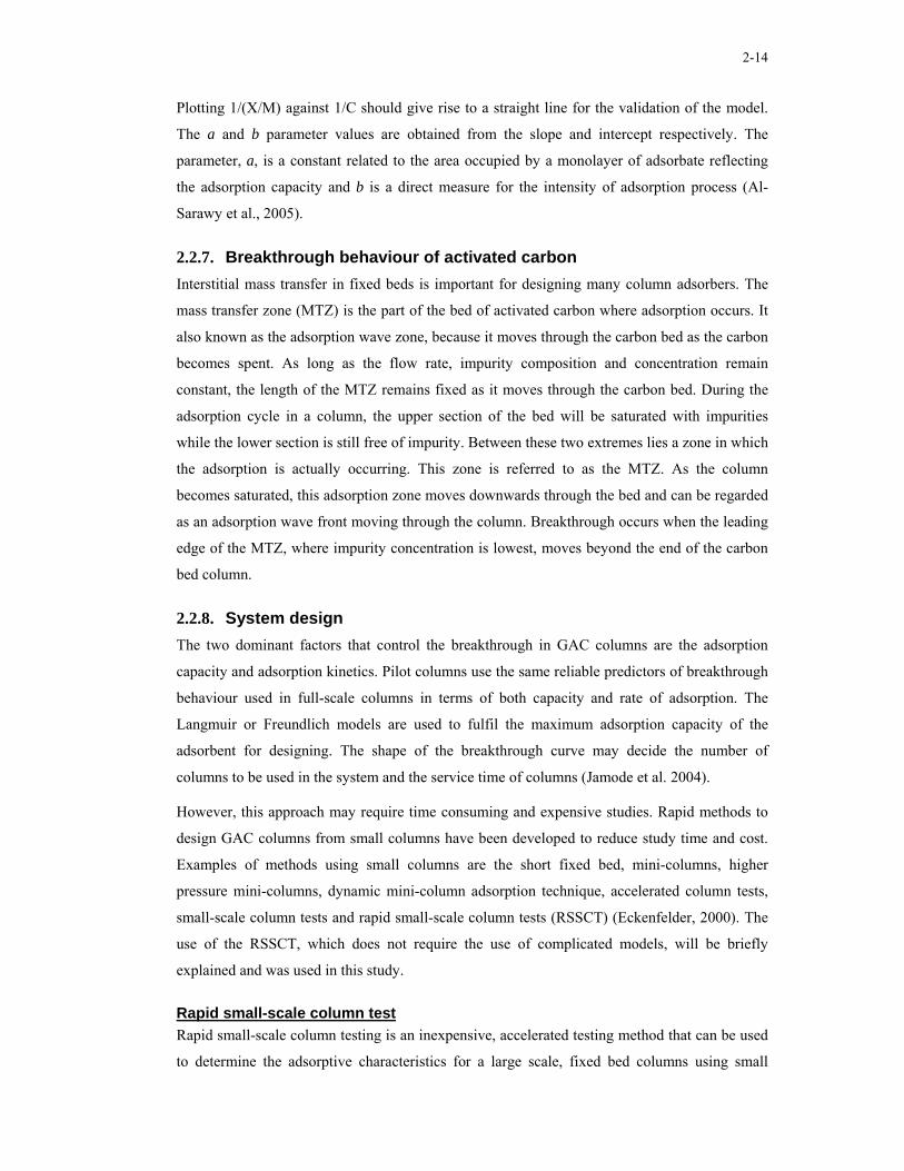
2-14

Plotting 1/(X/M) against 1/C should give rise to a straight line for the validation of the model.

The a and b parameter values are obtained from the slope and intercept respectively. The

parameter, a, is a constant related to the area occupied by a monolayer of adsorbate reflecting

the adsorption capacity and b is a direct measure for the intensity of adsorption process (Al-

Sarawy et al., 2005).

2.2.7. Breakthrough behaviour of activated carbon Interstitial mass transfer in fixed beds is important for designing many column adsorbers. The

mass transfer zone (MTZ) is the part of the bed of activated carbon where adsorption occurs. It

also known as the adsorption wave zone, because it moves through the carbon bed as the carbon

becomes spent. As long as the flow rate, impurity composition and concentration remain

constant, the length of the MTZ remains fixed as it moves through the carbon bed. During the

adsorption cycle in a column, the upper section of the bed will be saturated with impurities

while the lower section is still free of impurity. Between these two extremes lies a zone in which

the adsorption is actually occurring. This zone is referred to as the MTZ. As the column

becomes saturated, this adsorption zone moves downwards through the bed and can be regarded

as an adsorption wave front moving through the column. Breakthrough occurs when the leading

edge of the MTZ, where impurity concentration is lowest, moves beyond the end of the carbon

bed column.

2.2.8. System design The two dominant factors that control the breakthrough in GAC columns are the adsorption

capacity and adsorption kinetics. Pilot columns use the same reliable predictors of breakthrough

behaviour used in full-scale columns in terms of both capacity and rate of adsorption. The

Langmuir or Freundlich models are used to fulfil the maximum adsorption capacity of the

adsorbent for designing. The shape of the breakthrough curve may decide the number of

columns to be used in the system and the service time of columns (Jamode et al. 2004).

However, this approach may require time consuming and expensive studies. Rapid methods to

design GAC columns from small columns have been developed to reduce study time and cost.

Examples of methods using small columns are the short fixed bed, mini-columns, higher

pressure mini-columns, dynamic mini-column adsorption technique, accelerated column tests,

small-scale column tests and rapid small-scale column tests (RSSCT) (Eckenfelder, 2000). The

use of the RSSCT, which does not require the use of complicated models, will be briefly

explained and was used in this study.

Rapid small-scale column test Rapid small-scale column testing is an inexpensive, accelerated testing method that can be used

to determine the adsorptive characteristics for a large scale, fixed bed columns using small

2-15

column studies. The primary advantage of using RSSCT over pilot testing is the time savings.

Other major advantages are cost savings, reduced water requirements and the fact that extensive

isotherm and kinetic studies are not necessary. Mass transfer models can be used to determine

dimensional parameters. These parameters are used to maintain similitude between small and

large-scale columns. Subsequent to determining similitude, the RSSCT can be scaled up to aid

in the design of full-scale treatment operation.

2.2.9. Activated carbon adsorption as a reclamation technique Activated carbons are the most important commercial adsorbents. Their high surface area

together with their surface chemical structure allows them to be used in a wide variety of

industrial applications, some of the most important dealing with the environment field and

particularly with water purification and industrial wastewater cleaning (Jankowska et al., 1981;

Gonzalez-Serrano et al., 2004). Most forms of activated carbon are non-polar in nature; they

have the greatest affinity for other non-polar substances.

Powdered activated carbon (PAC) and granular activated carbon (GAC) are the forms of

activated carbon used in water and wastewater treatment. PAC is added to the actual wastewater

stream to adsorb contaminants, then removed later from the stream and discarded. PAC was

often used in the past because of its faster adsorption rate, but disposal costs and handling

concerns have made GAC a more popular alternative for most applications. GAC is used in

water treatment, and then regenerated when it becomes less effective due to saturation with

chemicals. GAC is also usually much easier to handle and transport than PAC (Ford, 1981;

Brady and McKay, 1996).

Benefits of activated carbon treatment (Ford, 1981; Wagner and Jula, 1981) are:

• Highly effective at removing non-polar organic chemicals from water

• Applicable to a wide variety of organic compounds

• Very effective at removing colours from waste streams

• Effective at removing low levels (ppb range) of metal pollutants

• Thermal regeneration of the carbon destroys the adsorbed waste solute

• Very flexible system allows rapid start-up and shut down as needed

• System can be designed so that it is portable to be taken to waste sites

Limitations of activated carbon treatment (Ford, 1981; Wagner and Jula, 1981):

• Limited to wastes with low organic concentrations (<5%)

• Limited to wastes with very low inorganic concentrations (<1%)

2-16

• Unable to remove highly soluble organics, or those with low molecular weights

• Systems cannot tolerate suspended solids in the influent stream (due to clogging)

• High operating costs due to carbon costs and system requirements

• Disposal of contaminated carbon can be problematic if it is not regenerated

Regeneration of granular activated carbon Activated carbons that are used for the removal of organic compounds from liquid phase

systems will gradually become saturated, due to the concentration of contaminants on the

surface of the adsorbent. When this occurs a decision must be made on how to deal with the

spent material (Clark and Lykins, 1989). Due to the high manufacturing costs and the recovery

of components adsorbed on the surface of activated carbon, regeneration is the preferred option.

The possibility of regeneration is one of the main reasons for the wide-spread use of activated

carbon as an adsorbent (Zolfl et al., 2000).

Regarding the regeneration of activated carbon, a careful distinction between reactivation and

regeneration is of importance. Volatile components or substances with lower energy can be

removed fairly easily, whereas non-volatile compounds or substances adsorbed with high

energy and so-called irreversible residues resulting from polycondensation and polymerisation

product formation can hardly be desorbed. Reactivation restores the activated carbon to a state

where it is virtually identical to the properties of the virgin pre-cursor. Regeneration combines

both the adsorptive regeneration and reactivation. However, for simplification all methods will

be referred as regeneration methods (Zolfl et al., 2000).

There are three potential regeneration techniques: chemical, steam and thermal. Both chemical

and steam are used primarily in industrial systems designed to recover the adsorbate (Clark and

Lykins, 1989).

Thermal regeneration The thermal reactivation of activated carbon is usually carried out in a multiple hearth furnace.

Thermal regeneration is made up of four stages: drying, desorption, pyrolysis and gasification.

Drying occurs in the entry zone of the furnace as the carbon is heated from ambient temperature

to 100°C. The thermal desorption followed by pyrolysis of organic adsorbate occurs as the

temperature increases beyond the drying temperature. Gasification occurs between 649°C and

1 038°C (Clark and Lykins, 1989).

The three main parameters influencing the regeneration success are the temperature gradient

within the furnace, the retention time and the level of exhaustion of the activated carbon. A

further increase in temperature would lead to an unacceptable and expensive burn-out of

activated carbon which causes enlargement of micropores. Further carbon loss (up to 15 percent

2-17

mass) occurs as a result of attrition caused by inevitable removal of the carbon from the column

into the furnace. Another disadvantage of thermal regeneration is that the adsorbed compounds,

which may be useful, are destroyed (Zolfl et al., 2000). Thermal regeneration is the most widely

used regeneration method despite its energy demand which result high costs (Alvarez et al.,

2004; Ferro-Garcia et al., 1993).

Activated carbon is a valuable commodity which is capable of being recycled using thermal

reactivation or regeneration techniques. This process offers significant advantages:

• Removal of expensive waste disposal costs.

• Reduction in operating costs as regenerated material is often less expensive than virgin

adsorbent.

• The regeneration of activated carbon makes it the less polluted environmental option

(Clark and Lykins, 1989).

Chemical regeneration Chemical regeneration is based on the transformation of the adsorbed components into water

soluble salts by adding diluted acids or bases. Although this method is unharmful to the

activated carbon, both the used chemicals and the desorbed substances need to be reprocessed in

order to reduce chemical waste and costs (Zolfl et al., 2000). Chemical regeneration can be

carried out by desorption of the adsorbates using specific solvents or by decomposition using

oxidizing chemical agents (Alvarez et al., 2004). Desorption can take place by a pH change

which allow the adsorbate to change their ionic nature and thus be released from the carbon

surface. The desorption process needs to be followed by a neutralisation and rinsing stages

(Santhy and Selvapathy, 2006).

2.3. WATER QUALITY FOR REUSE The required water quality used for textile processes depends on where it will be reused. The

textile industry uses water of drinking quality although some processes do not require water of

this quality. The use of reclaimed water for textile processes has been studied by various

researchers and in their studies they proved that the use of reclaimed water for textile dyeing

processes was possible. A study performed by Harker in 1980 showed that there was no

difference observed between fabric processed with drinking water quality and fabric prepared

with reclaimed water. Another research study by Inoue and co-workers (1977) and Tworeck

(1984) showed that there was a slight difference which was observed when dyeing a fabric with

reclaimed water and these effects were considered significant and were fully acceptable to the

textile mill investigated.

2-18

For this study the acceptable limit (AL) for reuse were selected on basis that the textile

industries are using water of drinking quality for their dyeing processes i.e. the ADMI value of

75. When dyeing a medium shades such as Turquoise and dark shades such as Navy and Black,

reclaimed water need not be of drinking water quality. According to studies mentioned on the

previous paragraph, dyeing using reclaimed water with a very low colour produced acceptable

results to the textile mills. Dyeing of light shades such as Beige with reclaimed water from dark

shade effluent has to be of acceptable limit (thus 75 ADMI). Table 2.2 shows the summary of

the acceptable limit for reuse with corresponding dye removed in percentages and dye

concentration used for this study.

Table 2.2. Acceptable limit (AL) for reuse for the studied shades Shades Navy Black Beige Turquoise FEED ADMI 17650 19010 345 10100 AL (ADMI) 75 75 75 75 % dye rem 99 99 78 99 AL dye conc (mg dye/L) 3 3 41 5

2.4. SYSTEM DESIGN The design of a GAC pilot-scale involves time-consuming and expensive studies. The use of

Rapid Small Scale Column Test (RSSCT), based on fixed-bed mass transfer models, which does

not require use of complicated models, was developed by Frick and Crittenden et al to solve this

problem of time-consuming and expensive methods. The three primary advantages of using

RSSCT for design are:

• The RSSCT can be conducted in less time that is required for pilot studies.

• Extensive isotherm or kinetic studies are not required for the performance prediction of

the pilot-scale, unlike predictive mathematical models.

• A small volume of water is needed for the test (Crittenden et al., 1991).

2.4.1. Scale-up and similitude Scale-up is based on similitude between small and large-scale columns considering equilibrium

capacity, bed volumes treated, particle densities and solute concentration. Results from RSSCT

can be scaled up to predict the performance of full-scale treatment systems. Similarity of

operation between small and large-scale column is assured by properly selecting the particle

size, hydraulic loading rate and empty bed contact time (EBCT) for the RSSCT. Perfect

similarity is achieved if the large and small systems have equal surface diffusivities, isotherm

capacities, bulk densities, operating temperature and influent concentration. Then, the RSSCT

and the full-scale plant will have identical breakthrough profiles (Crittenden et al., 1986;

Crittenden et al., 1991). If the adsorption process is controlled by multi- adsorbate competition,

then particular care should be given in estimating the following design parameters.

2-19

GAC particle size: Smaller GAC particle sizes increase the rate of adsorption. But if the particles become very

small, such as powdered activated carbon (PAC), then they could not be used in fixed-bed

applications.

Type of GAC: GAC with an appropriate pore size distribution suitable for the removal of identified target

compound should be selected. Pore size distribution of GAC can be controlled by the degree of

activation and choice of base materials (e.g. bitumen, wood, coconut etc.)

Empty bed contact time The empty bed contact time of the RSSCT is determined from intraparticle mass transfer

resistances. If the void fractions, bulk densities and the capacities are identical for the carbons

used in RSSCT and pilot-scale processes, the proper scaling between the small and large

column EBCTs can be determined from the following equation:

2 X

S S S

L L L

EBCT d tEBCT d t

−⎡ ⎤

= =⎢ ⎥⎣ ⎦

Where SEBCT and LEBCT are the EBCTs, Sd and Ld are GAC particle sizes and St and Lt

are the corresponding operational times for the small and large columns respectively. The

dependence of the intraparticle diffusion coefficient on particle size is defined by X . If the

intraparticle diffusion coefficient do not change with particle size ( 0X = ), then the exact

similarity between RSSCT and pilot-scale effluent profiles can be maintained. If the

intraparticle diffusion is assumed to cause most of the spreading in the mass transfer zone then

the intraparticle diffusivity is proportional to particle size ( 1X = ).Columns with larger EBCTs

will yield larger specific volumes of water treated per unit mass of GAC. This is because the

ratio of length of active mass transfer zone to the length of the column decreases with increasing

column length (Crittenden et al., 1991).

2.5. CLOSURE In this chapter, the relevant literature on reactive dyes has been reviewed, to highlight the

different reactive dye chemistries, classes and the basic principle of the reactive dyeing process.

Different treatment technologies for the removal of colour from exhausted reactive dyebath

have also been highlighted and the emphasis was on activated carbon adsorption. The

incapability of the existing conventional treatment processes resulted in activated carbon

adsorption being the promising technology in the removal of colour from exhausted reactive

dyebath. Reactive dyeing of cellulose, such as cotton in this case study is performed at high

temperatures, high salt concentration and high volumes of water (from dyeing, rinsing etc.) and

2-20

this results in high colour and high salt concentrations in the effluent. This is the main challenge

that the textile industries are concerned about. Reactive dyeing of cotton and the parameters

involved in the activated carbon adsorption process of reactive dyes will be evaluated in the

subsequent chapters. The evaluating parameter such as different temperatures, pH values, salt

concentrations in the removal of colour were necessary for recovery of water, salt and energy

from reactive dyebath.

3-1

CHAPTER 3 REACTIVE DYEING

As described in Chapter 1, reactive dyes will always have a significant place in textile dyeing

because of their high colour fastness and the wide spectrum they possess. In the last decade the

consumption of reactive dyes has been 4 to 5 times more than other dye groups. Cellulosic

fibres such as cotton of a specific shade (colour) are produced by reacting the fibres with a

mixture of reactive dyestuffs, salt and auxiliary chemicals. The reactive dyestuff can contain

different functional groups (chemistries). Reactive dyeing of cotton was undertaken to estimate

the amount of dye and salt that remains in the effluent before activated carbon studies.

Laboratory reactive dyeing trials for different dye chemistries/classes operated at Dyefin Textile

factory were undertaken. This chapter describe the selected dye chemistries and classes (section

3.1) used for this study with their dyeing process and recipes presented in sections 3.2 and 3.3.1.

The discussion and conclusion of results are discussed.

3.1. REACTIVE DYE CHEMISTRY The reactive groups found in reactive dyes increase the molecular weight of a dye but do not

enhance chromogenic strength. Four different reactive dye shades were used in this study;

Navy, Black, Beige and Turquoise shades and were obtained using Drimarene HF, Cibacron S,

Procion HE and Remazol L dye classes respectively. According to manufacturers’ specifications

(Table 3.1) the Drimarene HF (from Clariant) belongs to trifluoropyrimidine reactive chemistry,

the chemistry for Cibacron S (from Ciba) is not divulged, while Procion HE (from Dystar)

belongs to monochlorotriazine and Remazol (from Dystar) belongs to vinylsulphone reactive

chemistry. Drimarene HF dyes are trifunctional reactive dyes with three halogens attached to a

pyrimidine ring. Procion HE dyes are bifunctional reactive dyes which were launched in the late

1960s and early 1970s. Procion were designed to have substantially increased substantivity

exhaustion and fixation values compared with corresponding products carrying one

chlorotriazinyl. Remazol L dyes are also bifunctional reactive dyes which were established in

mid 1980s. The synthesis involves a vinyl sulphone attached to a triazine ring (Hunter and

Renfrew, 1999).

3.2. PRINCIPLE OF REACTIVE DYEING The preparation, dyeing and finishing of textile products with reactive dyes consumes large

amounts of energy, chemicals and water. These wet-processing operations require the use of

several chemical baths that are often at elevated temperatures to achieve the desired

3-2

characteristics to the dyed fabric. Exhaust reactive dyeing of cotton has three consecutive

distinct phases:

• The initial exhaustion phase – During this stage there is migration of reactive dye to the

cotton fibre. The amount of dye absorbed by the fibre depends on substantivity. The salt

such as sodium chloride and sodium sulphate are added to promote migration of dye to

the fibre. This phase is usually performed by gradually increasing the temperature of the

dyebath, this aids in the penetration and migration of dye into the fibre (Broadbent 2001).

The increase in temperature allows swelling of the cotton fibre which leads to a higher

dye uptake (El-Shishtawy et al., 2007)

• The fixation phase – At this stage the pH of the dyebath is increased by adding alkali,

which causes dissociation of some hydroxyl group in the cotton fibre. This allows

nucleophilic cotton ions to react with the dye ions. Dye absorption reaction progresses

until no further dye can be taken by the cotton fibre (i.e. reach equilibrium).

• The post-dyeing washing – The cotton fibre after dyeing contains unfixed dye as well as

hydrolysed dye, residual alkali and salt that are bonded on the surface of fibre. The latter

are removed by successive rinsing in cold and warm water. The cold rinse removes most

of the electrolyte and the unfixed dyes. The removal of electrolyte shifts the dye

equilibrium back to the aqueous phase and eases removal in the cold rinse. The

hydrolysed dye which is adsorbed on the fibres is partially removed by warm rinse and

more completely by hot soaping. Rinsing aims at removing hydrolysed and unfixed

reactive dyes from the cotton fibre. Depending on the dye recipe of the reactive dye used,

neutralisation can follow the cold rinse before warm rinse. Sodium hydroxide is adsorbed

within the cotton fibres, a neutralisation step is needed to release the residual alkali as a

neutral salt. The final last cold rinse removes the last traces of dye (Broadbent, 2001).

Several auxiliary chemicals are added to the bath during dyeing processes. These chemicals can

be divided into two groups: commodity and specialty chemicals and will be discussed in the

subsequent sections.

3.2.1. Specialty chemicals Specialty chemicals are mixtures which have an unknown composition due to proprietary

information. The mixtures are often developed to solve problems specific to the process and to

counteract or enhance the effects of other chemicals (Hendrickx and Boardman, 1995).

Examples of specialty chemicals used in this study are Dekol (from BASF plc), Tebolan (from

Dr. Th. Bohme KG, Chem. Fabrik GmbH), Avcoson from (Avco Chemicals Ltd) and Subitol.

In dyeing of cotton, Dekol is used as a dispersing agent and protective colloid, Avcoson is used

for minimising primary fibre fibrillation and Tebolan to prevent unwanted reduction of sensitive

3-3

dyestuffs. Avcoson, Subitol, Tebolan are used in the reactive dyeing dyebath. Dekol solution is

used for soaping process of the cotton fibre and also in the reactive dyeing bath. Specialty

chemicals can cause side effects that are detrimental to the overall process (This information

was taken from Material Safety Data Sheet (MSDS). Their composition and chemistries were

not divulged by the Manufacturer.

3.2.2. Commodity chemicals Commodity chemicals are mixtures or chemical mixtures that have known composition.

Examples of commodity chemicals used in this study are sodium hydroxide, sodium sulphate,

sodium carbonate and acetic acid. The presence of hydroxide and sulphate ions opens the

structure of the cotton and shifts the equilibrium of dye from the aqueous phase to the solid

(fibre) phase thus controls or retards the rate of dyeing. The sodium carbonate (alkali) is

necessary for the sufficient exhaustion of the dyebath to promote the dye-cotton reaction. The

acetic acid is added to control the acidity of the dyebath.

3.3. EXPERIMENTATION Four different dye shades were evaluated (Table 3.1). Each shade consisted of three dyestuffs

and associated auxiliaries. The dyeing recipes for the four shades are presented in section 3.3.1.

The salt concentration and pH were measured using Jenway conductivity meter 4310 and pH

meter 3310 by Jenway. The colour measurement of the dye solution presented in section 3.3.2

was performed using a Cary UV/Visible Spectrophotometer.

Table 3.1 : Characterisation of test dye solution Dye Shade

Class Chemistry Supplier Initial concentration (mg/L) Navy* Drimarene HF Trifluoropymidine Clariant 3 850 Black** Cibacron S Not available Ciba 3 912 Beige* Procion HE Monochlorotriazine Dystar 945 Turquoise** Remazol L Vinylsulphone Dystar 3 464 * - NaCl salt used, ** - Na2SO4 salt used

3.3.1. Preparation of dyeing solution The dye recipes used for this study were taken from the unpublished WRC Project K5/1363 and

are representative of the shades dyed at Dyefin Textile factory. Other reactive dyeing results for

all reactive dyes used in Dyefin Textiles are presented under unpublished WRC Project reports.

The reactive dyes used for the selected four shades are supplied as a powder form and the

auxiliaries in liquid form were obtained from Dyefin Textile industry. Preparation of stock

solution for the dyes and auxiliaries, and the shades dye solution was then subjected to the

dyeing procedures outlined in Appendix A. The recipe for each shade is explained in the

subsequent sections. Prior to the dyeing process, the textile was wetted to facilitate an even

3-4

intake of dyestuff and dyeing water. For all the shades the exhausted dyebath effluent (S1) was

set aside for later analysis.

Navy Shade Dyeing liquor (S0) for 10 g fabric was prepared from the relevant stock solutions (Appendix A)

according to a dyeing recipe: 30 mL Drimarene Navy, 6.6 mL Drimarene Red, 1.9 mL

Drimarene Yellow, 2 mL Tebolan, 6 mL Dekol, 8 mL Avcoson, 7 g sodium chloride and 10 mL

sodium carbonate into 100 mL volumetric flask and filled up to the mark with distilled water.

The dyebath temperature was 60˚C with a pH value of 11. After dyeing the fabric (S1) was

subjected to a cold (25˚C) water rinse (S2) followed with hot (100˚C) soaping with Dekol (S3)

and lastly cold (25˚C) water rinse (S4). The dyeing procedure is shown in Fig A.1 of

Appendices.

Black Shade Dyeing liquor (S0) for 10 g fabric was prepared according to a dyeing recipe: 21 mL Cibacron

Black R, 18 mL Cibacron Black G, 2 mL Tebolan, 6 mL Dekol, 8 mL Avcoson, 2.7 mL of 95%

sodium hydroxide, 8 g sodium sulphate and 10 mL sodium carbonate into 100 mL volumetric

flask and filled up to the mark with distilled water. The dyebath temperature was 60˚C with a

pH value of 11. After dyeing the fabric (S1) was subjected to a warm (50˚C)water rinse (S2)

followed by cold (25˚C) neutralisation (S3) then with hot (100˚C) soaping with Dekol (S4)

followed by hot (75˚C)water rinse (S5), warm (50˚C)water rinse (S6) and lastly cold (25˚C)

water rinse (S7). The dyeing procedure is shown in Fig A.2 of Appendices.

Beige Shade Dyeing liquor (S0) for 10 g fabric was prepared according to a dyeing recipe: 5 mL Procion

Yellow H-E4R, 1.5 mL Procion Red H-E7B, 2.9 mL Procion Blue H-ERD, 1.5 mL Tebolan,

2.5 mL Subitol, 60% Acetic acid to control pH between 5.5 to 6.5, 6 g sodium chloride and

7.5 mL sodium carbonate into 100 mL volumetric flask and filled up to the mark with distilled

water. The dyebath temperature was 60˚C with a pH value of 11. After dyeing the fabric (S1)

was subjected to a hot (100˚C) water rinse (S2) followed by cold (25˚C) water rinse (S3) then

with hot (100˚C) soaping with Dekol (S4) and lastly cold (25˚C) water rinse (S5). The dyeing

procedure is shown in Fig A.3 of Appendices.

Turquoise Shade Dyeing liquor (S0) for 10 g fabric was prepared according to a dyeing recipe: 0.24 mL Remazol

Brilliant Yellow 3GL granules, 33 mL Remazol Turquoise Blue G 133%, 1.4 mL Levafix Blue

CA granules, 1.5 mL Tebolan, 2.5 mL Subitol, 5 g sodium sulphate and 6.5 mL sodium

carbonate into 100 mL volumetric flask and filled up to the mark with distilled water. The

dyebath temperature was 60˚C with a pH value of 11. After dyeing the fabric (S1) was subjected

3-5

to a hot (100˚C) water rinse (S2) followed by cold (25˚C) neutralisation (S3) then with hot

(100˚C) soaping with Dekol (S4) and lastly cold (25˚C) water rinse (S5). The dyeing procedure

is shown in Fig A.4 of Appendices.

3.3.2. Colour measurement Transmittance values at each wavelength value were determined between 400 nm to 700 nm

(visible range) at 10 nm intervals. The 1-cm absorption cell was thoroughly cleaned with

detergent and rinsed with distilled water. The cell was rinsed twice with the sample to be

analysed. The cell was filled with the sample to be analysed and the external surface of the cell

was wiped clean using lens paper. The instrument was set to read 100% transmittance on the

distilled water blank and the samples were analysed.

3.4. RESULTS This section (3.4.1) presents results obtained from the laboratory reactive dyeing of fabric for

four different shades; Navy (trifloropyrimidine chemistry), Black (not divulged chemistry),

Beige (monochlorotriazine chemistry) and Turquoise (vinylsulphone). The final section contains

the mass balances for the total dyeing process of the selected shades. All results are discussed in

the discussion section (Section 3.5). Experimental data is presented in Appendix A and the

error analysis is presented in Appendix C.

3.4.1. Laboratory test dyeings Figs 3.1 to 3.4 shows the dye and salt concentrations measured before and after laboratory

dyeing trials of the four reactive dye shades. Dye and salt recovered after dyeing are presented

in Figs 3.5 to 3.8.

3-6

0

500

1000

1500

2000

2500

3000

3500

4000

4500

S0 S1 S2 S3 S4

Dye

conc

(mg

dye/

L)

0

10

20

30

40

50

60

70

80

Salt

conc

(g/L

)

Dye concentration Salt concentration

Fig 3.1: Dye and salt concentrations before and after dyeing of Navy shade. S0-unexhausted dyebath, S1-exhausted dyebath, S2-cold water rinse, S3-hot soaping and S4-cold water rinse.

0

500

1000

1500

2000

2500

3000

3500

4000

4500

S0 S1 S2 S3 S4 S5 S6 S7

Dye

con

c (m

g dy

e/L)

0

10

20

30

40

50

60

70

80

90

Salt

conc

(g/L

)

Dye concentration Salt concentration

Fig 3.2: Dye and salt concentrations before and after dyeing of Black shade. S0-unexhausted dyebath, S1-exhausted dyebath, S2-warm water rinse, S3-cold neutralisation, S4-hot soaping and S5-hot water rinse, S6-warm water rinse and S7-cold water rinse.

0

100

200300400

500

600700800900

1000

S0 S1 S2 S3 S4 S5

Dye

con

c (m

g dy

e/L)

0

10

20

30

40

50

60

70

Salt

conc

(g/L

)

Dye concentration Salt concentration

Fig 3.3: Dye and salt concentrations before and after dyeing of Beige shade. S0-unexhausted dyebath, S1-exhausted dyebath, S2-hot water rinse, S3-cold water rinse, S4-hot soaping and S5-cold water rinse.

0

500

1000

1500

2000

2500

3000

3500

4000

S0 S1 S2 S3 S4 S5

Dye

con

c (m

g dy

e/L)

0

10

20

30

40

50

60

Salt

con

c (g

/L)

Dye concentration Salt concentration

Fig 3.4: Dye and salt concentrations before and after dyeing of Turquoise shade. S0-unexhausted dyebath, S1-exhausted dyebath, S2-cold water rinse, S3-cold neutralisation, S4-hot soaping and S5-cold water rinse.

3-7

0

0.02

0.04

0.06

0.08

0.1

0.12

S1 S2 S3 S4

Dye

(C/C

o)

0

0.2

0.4

0.6

0.8

1

1.2

Sal

t (C

/Co)

Dye recovered Salt recovered

Fig 3.5: Dye and salt ratios after dyeing of Navy shade. S1-exhausted dyebath, S2-cold water rinse, S3-hot soaping and S4-cold water rinse.

0

0.02

0.04

0.06

0.08

0.1

0.12

S1 S2 S3 S4 S5 S6 S7

Dye

(C/C

o)

0

0.2

0.4

0.6

0.8

1

1.2

Sal

t (C

/Co)

Dye recovered Salt recovered

Fig 3.6: Dye and salt ratios after dyeing of Black shade. S1-exhausted dyebath, S2-warm water rinse, S3-cold neutralisation, S4-hot soaping and S5-hot water rinse, S6-warm water rinse and S7-cold water rinse.

0

0.02

0.04

0.06

0.08

0.1

0.12

S1 S2 S3 S4 S5

Dye

(C/C

o)

0

0.2

0.4

0.6

0.8

1

1.2

Sal

t (C/

Co)

Dye recovered Salt recovered

Fig 3.7: Dye and salt ratios after dyeing of Beige shade. S1-exhausted dyebath, S2-hot water rinse, S3-cold water rinse, S4-hot soaping and S5-cold water rinse

0

0.02

0.04

0.06

0.08

0.1

0.12

S1 S2 S3 S4 S5

Dye

(C/C

o)

0

0.2

0.4

0.6

0.8

1

1.2

Sal

t (C/

Co)

Dye recovered Salt recovered

Fig 3.8: Dye and salt ratios after dyeing of Turquoise shade. S1-exhausted dyebath, S2-cold water rinse, S3-cold neutralisation, S4-hot soaping and S5-cold water rinse.

3.4.2. Total dyeing process mass balance The possibility for treatment of dyebath in terms of mass balance is shown in Table 3.2 to 3.5

for all four shades. The flow diagrams of the mass balance for all four shades are listed in

Appendix A, only Navy shade is presented in Fig 3.9.

3-8

25°C pH 738.5g dye /kg fabric

10 L water/kg fabric700 g salt/ kg fabric1 050 kJ/kg fabric

60°CpH 114.3 g dye/kg fabric682 g salt/kg fabric

10 L water/kg fabric1 460 kJ/kg fabric

1st Rinse

Final Rinse

Dyebath

25°C

1.2 g dye/kg fabric~18 g salt/kg fabric10 L water/kg fabric

100°C

1.8 g dye/kg fabric<0.1g salt/kg fabric10 L water/kg fabric3 140 kJ/kg fabric

25°C0.8 g dye/kg fabric<0.1 g salt/kg fabric10 L water/kg fabric

IN

1 kg fabric1.5 L water

Soaping

S2

S3

S4

S1

25°C10 L water/kg fabric

Wet fabric

Wet fabric

Wet fabric

25°C10 L water/kg fabric

100°C10 L water/kg fabric0.04 L Dekol/kg fabric

3 140 kJ/kg fabric

Wet fabric

1 kg dyed fabric1.5 L water

25°C pH 738.5g dye /kg fabric

10 L water/kg fabric700 g salt/ kg fabric1 050 kJ/kg fabric

60°CpH 114.3 g dye/kg fabric682 g salt/kg fabric

10 L water/kg fabric1 460 kJ/kg fabric

1st Rinse

Final Rinse

Dyebath

25°C

1.2 g dye/kg fabric~18 g salt/kg fabric10 L water/kg fabric

100°C

1.8 g dye/kg fabric<0.1g salt/kg fabric10 L water/kg fabric3 140 kJ/kg fabric

25°C0.8 g dye/kg fabric<0.1 g salt/kg fabric10 L water/kg fabric

IN

1 kg fabric1.5 L water

Soaping

S2

S3

S4

S1

25°C10 L water/kg fabric

Wet fabric

Wet fabric

Wet fabric

25°C10 L water/kg fabric

100°C10 L water/kg fabric0.04 L Dekol/kg fabric

3 140 kJ/kg fabric

Wet fabric

1 kg dyed fabric1.5 L water

Fig 3.9: Flow diagram and mass balance for dyeing of Navy shade

Table 3.2 : Total Navy shade effluent composition Components Units Total composition (in %) Dyebath (in %) Water L/kg fabric 40 (100) 10 (25) Salt g/kg fabric 700 (100) 682 (97) Dye g/kg fabric 8.1 (21) 4.3 (53) Energy kJ/kg fabric 4 600 (100) 1 460 (32)

Table 3.3 : Total Black shade effluent composition Components Units Total composition (in %) Dyebath (in %) Water L/kg fabric 70 (100) 10 (14) Salt g/kg fabric 800 (100) 770 (96) Dye g/kg fabric 8.7 (22) 3.7 (43) Energy kJ/kg fabric 8 800 (100) 1 460 (17)

Table 3.4 : Total Beige shade effluent composition Components Units Total composition (in %) Dyebath (in %) Water L/kg fabric 50 10 (20) Salt g/kg fabric 600 565 (94) Dye g/kg fabric 1.81 0.65 (36) Energy kJ/kg fabric 8 160 1 880 (23)

3-9

Table 3.5 : Total Turquoise shade effluent composition Components Units Total composition (in %) Dyebath (in %) Water L/kg fabric 50 10 (20) Salt g/kg fabric 500 480 (96) Dye g/kg fabric 7.31 2.7 (37) Energy kJ/kg fabric 4 600 1460 (32)

3.5. DISCUSSION This section discusses the experimental results in section 3.4 of Chapter 3, beginning with

laboratory test dyeings, followed by mass balances for total dyeing process of all four selected

shades.

3.5.1. Laboratory test dyeings The reactive dyeing of four shades (Figs 3.1 to 3.4) was performed to estimate the amount of

dye that remains in the effluent before adsorption tests were conducted. Fig 3.1 to 3.4 shows the

reactive dyeing of Navy, Black, Beige and Turquoise shades, about 3 850, 3 912, 945 and

3 464 mg/L of dye concentrations and 70, 80, 60 and 50 g/L salt is used respectively when

dyeing a fabric. According to the dye recipes higher salt concentrations were used for Navy and

Black Shades than for Beige and Turquoise. This is because lower salt concentrations are

required for dyeing light shades and higher salt concentrations for darker shades (Shu et al.,

2005). Different dye chemistries used for this study exhibit different fixation ratios. This may

be due to the types of reactive dyes used and their associated dye recipes. The efficiency of

dyeing process for a specific shade is associated with various parameters such as substantivity

and diffusion rate of dyes, auxiliaries, hardness of water, pH of the dye liquor, type and the

concentration of reactive dye used.

According to results obtained from dyebath, high colour and high salt concentration are

recovered for all the shades. Dye concentration recovered for all the shades after dyeing were in

the following order dyebath > soaping > rinsing and neutralisation steps (Figs 3.5 to 3.8). The

main source of residual colour in the reactive dyebath is the result of their incomplete

exhaustion during the dyeing process (Golob et al., 2005). The remainder of most unfixed dye

on the surface and inside of the fabric was eliminated by soaping using boiling detergent

solution. The recovered dye concentration after dyeing (includes from dyebath effluent up until

final rinse) ranged from 19% to 22% for the studied shades. According to Allegre et al., (2006),

the hydrolysed and unfixed reactive dyes after dyeing represents 20 to 30% of the reactive dyes

applied. This is the colour that is in the effluent and needs to be treated.

The salt concentration recovered was dyebath > 1st rinse> other dyeing processes (e.g. soaping,

neutralisation, final rinse etc). All the salt used was found in the dyebath with traces of salt

measured in the first rinse. The salts (NaCl and Na2SO4) used gave a better exhaustion of dye

migration to fabric, the overall fixation ratio of reactive dyes ranged from 78% to 81% for the

3-10

studied chemistries. NaCl and Na2SO4 are neutral salts that act as catalysts in the reactive

dyeing; the need for alkali is for covalent bond fixation between dye and the fabric. From the

study results obtained by Ahmed (2005), it was shown that both sodium chloride and sodium

sulphate were effective exhaust agents in the presence of alkali.

3.5.2. Total dyeing process mass balance Tables 3.2 to 3.5 (page 3-8 to 3-9) shows the mass balance for the dyeing of the four different

shades. The effluent composition of the shades ranges from 19% to 22% of the dye with all the

salt used for dyeing. The dyebath has the most dye of about 36% to 53% of the total colour in

the effluent and almost all the salt ranging between 94% to 97% for all the selected shades. The

most energy is used in dyebath, soaping and rinsing (depending on the desired shade) stages.

The volumes of water used are the same for all stages of dyeing.

3.6. CONCLUSION • Dye exhaustion to the fabric for Navy (trifloropyrimidine chemistry), Black (chemistry not

divulged), Beige (monochlorotriazine chemistry) and Turquoise (vinylsulphone) shades

was about 79%, 78%, 81% and 79% respectively. Therefore 19% up to 22% is discharged

in the effluent resulting in high colour effluent from reactive dyeing operations. No

significant relation was observed between the shade and fibre exhaustion for light as well as

dark shades.

• High dye concentration liquor with all the salt used was obtained in the dyebath effluent.

Treatment of dyebath with activated carbon compared to other treatment technologies is

necessary because of high colour and high salt effluent.

• Moderate dye and low salt concentrations were found in the first rinse effluent. Thus

treatment of the first rinse effluent with membrane filtration may be possible.

• Effluent with high dye concentrations and no salt were measured in the soaping process and

traces of dye concentration with no salt were obtained in the neutralisation, second and final

rinse effluents.

• Mass balance estimates show that the removal of colour for the studied reactive dye shades

from the exhausted dyebath is necessary. Water recovery ranging from 14 to 25%, salt

recovery of about 94 to 97% and energy savings of 17 to 32% could be achieved.

These results obtained from this chapter were able to provide the predictions of the amount of

dye and salt remaining in the dyebath effluent before adsorption studies were undertaken.

4-1

CHAPTER 4 CARBON EQUILIBRIUM TESTS

According to reactive dyeing studies performed (Chapter 3) reactive dye effluent consist of an

average of 20% of the unexhausted dyebath with all the electrolyte. After dyeing, the exhausted

dyebath contains about 53% of the discharged dye and 97% of the salt. The main aim of this

part of the investigation was to evaluate the effect of different temperatures, pH values and

electrolyte concentrations on the removal of reactive dyes using activated carbon. The

possibility of using activated carbon for the removal of colour and the effect of dye equilibrium

on different experimental conditions was evaluated. This chapter discusses the carbon

equilibrium test for this study, beginning with a brief introduction on adsorption models and

experimental methods used, followed by experimental details and the discussion of the results

obtained, and lastly the conclusion.

4.1. INTRODUCTION Equilibrium studies are used to determine the capacity of the activated carbon adsorbent. The

equilibrium relationships between adsorbent and adsorbate are described by adsorption

isotherms, usually the equilibrium ratio between the quantity adsorbed and that remaining in

solution at a fixed temperature. The adsorption equilibrium data can be correlated with various

adsorption isotherm models mentioned in the literature (Chapter 2). The equilibrium adsorption

isotherms are of importance in the design of adsorption system (Chapter 7).

Chapter 2 introduced the two adsorption models for which the experimental data was

interpreted; Langmuir and Freundlich adsorption isotherms respectively. The two parameter

models, namely Freundlich and Langmuir, can be readily linearised and hence the parameter

values can be easily obtained. When performing the adsorption process the characteristics of the

adsorbent are of fundamental importance and characteristics of the granular activated carbon

used for this study are explained in Section 4.1.1.

4.1.1. Characteristics of activated carbon The selection of suitable activated carbon is of fundamental importance when designing a

carbon treatment plant. The activated carbon can be classified by adsorption capacity and

physical properties. Table 4.1 lists the F-400 specifications which illustrate the adsorptive

character of the activated carbon selected for this study. Some of the important characteristics

are explained in the subsequent paragraph.

4-2

Iodine number provides an indication of the amount of micropores in the carbon i.e. indicate

adsorption capacity for smaller molecules. Molasses number represents the amount of larger

pores in the carbon i.e. indicate adsorption capacity for larger molecules. Methylene blue

numbers represent the amount of large micropores and mesopores in the activated carbon.

Apparent density is the mass of carbon per unit volume, which can be packed in an empty

column (Clements, 2002). Discussion with the supplier indicated that the Chemviron F-400 has

a high adsorption capacity and would be the most appropriate quality and it is readily available

in South Africa. The F-400 has amphoteric properties (Allen and Koumanova, 2005), which is

an advantage for the adsorption of dyes which may exist in solution as either anions or as

cations.

Table 4.1: Some chemical and physical specifications for F-400 compared to other activated carbons as supplied by the manufacturers (Clements, 2002) Adsorptive character F-400 F-200 Norit 1240 Diahope DC 106 Origin Bituminous coal NA NA NA Iodine number (mg/g) 1 050 850 1 020 1 050 Molasses number 243 177 230 280 Methylene blue numbers (mg/g) 260 200 200 190 Apparent density (kg/m3) 425 500 440 475 Moisture content (%) 2 2 2 2 Ash content (%) (on dry basis) 10 10 7 5 Surface area (m2/g) based on BET 1 100 NA NA NA

Note: NA- unknown

4.2. EXPERIMENTATION The experimentation design for the carbon equilibrium study is explained in Section 4.2.1 and

the procedure followed is discussed in Section 4.2.2.

4.2.1. Experimental Design The dye solution is made up under neutral conditions so as to reduce the degree of dye

hydrolysis. Alkali, to pH 11, is added just prior to dyeing. Thus if the salt solution is to be

reused, it will need to be at a neutral to acidic pH value. Thus three pH conditions were

investigated (pH 11; 7 and 4). Under certain conditions reactive dyeing can be undertaken at

100˚C although for the dyes considered for this study, 60˚C is more usual. As the proposed

system may cool down to room temperature, additional temperatures of 40˚C and 20˚C were

investigated. The recommended salt concentrations for the different shades were all different

(Navy - 70 g/L; Black – 80 g/L; Beige – 60 g/L; Turquoise – 50 g/L). Higher salt concentrations

would result in greater dye exhaustion hence dye concentrations about 30 g/L above and below

the recommended values were investigated. A matrix of experimental conditions is given in

Table 4.2. Each condition was evaluated (in duplicate) for 5 different ratios of carbon/dye.

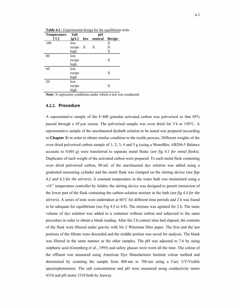
4-3

Table 4.2 : Experimental design for the equilibrium trials pH Temperature

[˚C] Salt [g/L] low neutral Recipe

100 low X recipe X X X high X 80 low recipe X high 60 low recipe X high 20 low recipe X high Note: X represents conditions under which a test was conducted

4.2.2. Procedure

A representative sample of the F-400 granular activated carbon was pulverised so that 95%

passed through a 45 µm screen. The pulverised sample was oven dried for 3 h at 150°C. A

representative sample of the unexhausted dyebath solution to be tested was prepared (according

to Chapter 3) in order to obtain similar condition to the textile process. Different weights of the

oven dried pulverised carbon sample of 1; 2; 3; 4 and 5 g (using a MonoBloc AB204-5 Balance

accurate to 0.001 g) were transferred to separate metal flasks (see fig 4.1 for metal flasks).

Duplicates of each weight of the activated carbon were prepared. To each metal flask containing

oven dried pulverised carbon, 80 mL of the unexhausted dye solution was added using a

graduated measuring cylinder and the metal flask was clamped on the stirring device (see figs

4.2 and 4.3 for the stirrers). A constant temperature in the water bath was maintained using a

±1C˚ temperature controller by Julabo; the stirring device was designed to permit immersion of

the lower part of the flask containing the carbon-solution mixture in the bath (see fig 4.4 for the

stirrers). A series of tests were undertaken at 60˚C for different time periods and 2 h was found

to be adequate for equilibrium (see Fig 4.5 to 4.8). The mixture was agitated for 2 h. The same

volume of dye solution was added to a container without carbon and subjected to the same

procedure in order to obtain a blank reading. After the 2 h contact time had elapsed, the contents

of the flask were filtered under gravity with No 2 Whatman filter paper. The first and the last

portions of the filtrate were discarded and the middle portion was saved for analysis. The blank

was filtered in the same manner as the other samples. The pH was adjusted to 7.6 by using

sulphuric acid (Greenberg et al., 1995) and safety glasses were worn all the time. The colour of

the effluent was measured using American Dye Manufacturer Institute colour method and

determined by scanning the sample from 400 nm to 700 nm using a Cary UV/Visible

spectrophotometer. The salt concentration and pH were measured using conductivity meter

4310 and pH meter 3310 both by Jenway.

4-4

Fig 4.1 : Metal flasks where test dye solution was poured

Fig 4.2 : Front view of the stirrers with a temperature controller used

Fig 4.3 : Back view of the shaker

Fig 4.4 : Stirrers view where metal flasks are clamped

4.3. RESULTS This section presents results obtained from the decolourisation equilibrium tests of four different

shades; Navy, Black, Beige and Turquoise using powdered activated carbon. The section begins

with different time interval to reach equilibrium followed by the adsorption isotherms obtained

using the Freundlich model (Section 4.3.1) at different temperatures, pH values and electrolyte

concentrations. Section 4.3.2 presents parameters obtained from Freundlich and Langmuir to

give indication why Freundlich was the selected model. Section 4.3.3. contains mass balances

for the dyeing of the four shades of which the mass balance diagrams are presented in

Appendix B. All the results of this section are discussed in Section 4.4 and the error analysis is

presented in Appendix C.

4.3.1. Adsorption isotherms Adsorption isotherm data for the different time interval for all the shades at 60˚C are presented

in Fig 4.5 to 4.8. Experimental data is presented in Table B.1 of Appendix B. Figs 4.9 to 4.20

show the Freundlich model isotherms plotted from the mass of dye adsorbed per gram of carbon

[log (X/M)] against residual dye concentration [log (C)]. The straight lines were plotted at four

4-5

different temperatures (20, 60, 80 and 100˚C), three different pH values (basic, neutral and

acidic conditions) and three different electrolyte concentrations for all the four shades and

presented in Figs 4.9 to 4.12, Figs 4.13 to 4.16 and Figs 4.17 to 4.20 respectively. Experimental

data is presented in Appendix B. Each graph was constructed from 10 data points (5

duplicates).

0

50

100

150

200

250

300

0 1 2 3 4 5

Time (hours)

X/M

(mg

dye/

g ca

rbon

)

1g carbon 2g carbon 3g carbon4g carbon 5g carbon

Fig 4.5 : Different time interval at 60˚C-Navy shade

0

50

100

150

200

250

300

0 1 2 3 4 5

Time (hours)

X/M

(mg

dye/

g ca

rbon

)

1g carbon 2g carbon 3g carbon4g carbon 5g carbon

Fig 4.6 : Different time interval at 60˚C-Black shade

0

10

20

30

40

50

60

0 1 2 3 4 5

Time (hours)

X/M

(mg

dye/

g ca

rbon

)

1g carbon 2g carbon 3g carbon4g carbon 5g carbon

Fig 4.7 : Different time interval at 60˚C-Beige shade

0

50

100

150

200

250

0 1 2 3 4 5

Time (hours)

X/M

(mg

dye/

g ca

rbon

)

1g carbon 2g carbon 3g carbon4g carbon 5g carbon

Fig 4.8 : Different time interval at 60˚C-Turquoise shade

4-6

1.6

1.8

2

2.2

2.4

2.6

-1 0 1 2 3 4

log(C)

log

(X/M

)

20 degC 60 deg C 80 degC 100 degC

Fig 4.9 : Effect of temperature on adsorption of Navy shade at pH 11 and 70 g/L NaCl

1.6

1.8

2

2.2

2.4

2.6

-1 0 1 2 3 4

log(C)

log

(X/M

)

20 degC 60 deg C 80 degC 100 degC

Fig 4.10 : Effect of temperature on adsorption of Black shade at pH 11 and 80 g/L Na2SO4

1

1.2

1.4

1.6

1.8

2

0 1 2 3 4

log(C)

log

(X/M

)

20 degC 60 deg C 80 degC 100 degC

Fig 4.11 : Effect of temperature on adsorption of Beige shade at pH 11 and 60 g/L NaCl

1.6

1.8

2

2.2

2.4

2.6

0 1 2 3 4

log(C)

log

(X/M

)

20 degC 60 deg C 80 degC 100 degC

Fig 4.12 : Effect of temperature on adsorption of Turquoise shade at pH 10 and 50 g/L Na2SO4

4-7

1.7

1.8

1.9

2

2.1

2.2

2.3

2.4

2.5

-1 0 1 2 3 4

log (C)

log

(X/M

)

pH 4 pH 7 pH 11

Fig 4.13 : Effect of pH on adsorption of Navy shade at 100°C and 70 g/L NaCl

1.7

1.8

1.9

2

2.1

2.2

2.3

2.4

2.5

-1 0 1 2 3 4

log (C)

log

(X/M

)

pH 4 pH 7 pH 11

Fig 4.14 : Effect of pH on the adsorption of Black shade at 100°C and 80 g/L Na2SO4

1.1

1.2

1.3

1.4

1.5

1.6

1.7

1.8

1.9

0 1 2 3 4

log (C)

log

(X/M

)

pH 4 pH 7 pH 11

Fig 4.15 : Effect of pH on the adsorption of Beige shade at 100ºC and 60 g/L NaCl

1.7

1.8

1.9

2

2.1

2.2

2.3

2.4

2.5

-1 0 1 2 3 4

log (C)

log

(X/M

)

pH 3 pH 6 pH 10

Fig 4.16 : Effect of pH on the adsorption of Turquoise shade at 100ºC and 50 g/L Na2SO4

1.7

1.8

1.9

2

2.1

2.2

2.3

2.4

2.5

-1 0 1 2 3 4

log (C)

log

(X/M

)

40 g/L 70 g/L 100 g/L

Fig 4.17 : Effect of electrolyte concentrations on adsorption of Navy shade at 100°C and pH 11

1.7

1.8

1.9

2

2.1

2.2

2.3

2.4

2.5

-1 0 1 2 3 4

log (C)

log

(X/M

)

50 g/L 80 g/L 110 g/L

Fig 4.18 : Effect of electrolyte concentrations on the adsorption of Black shade at 100°C and pH 11

4-8

1.1

1.2

1.3

1.4

1.5

1.6

1.7

1.8

1.9

0 1 2 3 4

log (C)

log

(X/M

)

30 g/L 60 g/L 100 g/L

Fig 4.19 : Effect of electrolyte concentrations on the adsorption of Beige shade at 100°C and pH 11

1.7

1.8

1.9

2

2.1

2.2

2.3

2.4

2.5

0 1 2 3 4

log (C)

log

(X/M

)

30 g/L 50 g/L 80 g/L

Fig 4.20 : Effect of electrolyte concentrations on the adsorption of Turquoise shade at 100°C and pH 10

4.3.2. Adsorption isotherm model parameters The coefficients of determination obtained from Freundlich and Langmuir models are presented

in Table 4.3 and the Freundlich model parameters are listed in Table 4.4 for all the four shades

at different temperatures, pH values and electrolyte concentrations. The curves showing the

validation calculated and experimental data of Freundlich model are presented in Appendix B.

4-9

Table 4.3 : Coefficients of determination in Freundlich and Langmuir isotherm models (number of samples per condition =10).

Freundlich model

Langmuir model

Shades Temp (°C) Salt (g/L) pH

r r 20 70 11 0.747 0.591 60 70 11 0.924 0.671 80 70 11 0.973 0.699

100 70 11 0.995 0.734 100 70 4 0.981 0.826 100 70 7 0.992 0.771 100 70 11 0.995 0.734 100 40 11 0.993 0.603 100 70 11 0.995 0.734

Navy

100 100 11 0.997 0.549 20 80 11 0.964 0.876 60 80 11 0.981 0.851 80 80 11 0.983 0.840

100 80 11 0.984 0.723 100 80 4 0.986 0.682 100 80 7 0.978 0.742 100 80 11 0.984 0.723 100 50 11 0.994 0.616 100 80 11 0.984 0.723

Black

100 110 11 0.966 0.835 20 60 11 0.949 0.521 60 60 11 0.978 0.586 80 60 11 0.922 0.638

100 60 11 0.978 0.392 100 60 4 0.983 0.446 100 60 7 0.991 0.451 100 60 11 0.978 0.392 100 30 11 0.865 0.331 100 60 11 0.978 0.392

Beige

100 100 11 0.977 0.385 20 50 10 0.796 0.602 60 50 10 0.862 0.713 80 50 10 0.924 0.771

100 50 10 0.954 0.786 100 50 3 0.959 0.812 100 50 6 0.954 0.764 100 50 10 0.954 0.786 100 30 10 0.938 0.872 100 50 10 0.954 0.786

Turquoise

100 80 10 0.949 0.819

4-10

Table 4.4 : Parameters in Freundlich isotherm model (number of samples per condition =10) Shades Temp

(°C) Salt (g/L)

pH kF (mg dye/g carbon) /

(mg dye/L)

n r

20 70 11 61.54 5.941 0.747 60 70 11 62.43 4.716 0.924 80 70 11 68.35 4.364 0.973

100 70 11 78.16 3.594 0.995 100 70 4 84.83 3.521 0.981 100 70 7 81.09 3.580 0.992 100 70 11 78.16 3.594 0.995 100 40 11 61.85 3.518 0.993 100 70 11 78.16 3.594 0.995

Navy

100 100 11 94.20 3.547 0.997 20 80 11 55.99 4.222 0.964 60 80 11 56.28 3.681 0.981 80 80 11 63.79 3.734 0.983

100 80 11 72.02 3.543 0.984 100 80 4 84.53 3.785 0.986 100 80 7 74.09 3.516 0.978 100 80 11 72.02 3.543 0.984 100 50 11 57.94 3.455 0.994 100 80 11 72.02 3.543 0.984

Black

100 110 11 89.04 3.672 0.966 20 60 11 2.096 1.866 0.949 60 60 11 2.282 1.772 0.978 80 60 11 3.100 2.175 0.922

100 60 11 3.873 1.480 0.978 100 60 4 3.950 1.263 0.983 100 60 7 4.085 1.391 0.991 100 60 11 3.873 1.480 0.978 100 30 11 3.129 1.559 0.865 100 60 11 3.873 1.480 0.978

Beige

100 100 11 5.061 1.468 0.977 20 50 10 33.13 3.542 0.796 60 50 10 38.51 3.524 0.862 80 50 10 42.34 3.203 0.924

100 50 10 53.18 2.840 0.954 100 50 3 64.79 2.886 0.959 100 50 6 57.61 2.840 0.954 100 50 10 53.18 2.840 0.954 100 30 10 39.93 2.696 0.938 100 50 10 53.18 2.840 0.954

Turquoise

100 80 10 60.74 2.738 0.949

4-11

Table 4.5: Possible treatment of dyebath with PAC using Freundlich parameters Shades Temp

(°C) Salt (g/L)

pH X/M (mg dye/g carbon) /

kg fabric/ g carbon

L effluent/ g carbon

20 70 11 171 0.04 0.40 60 70 11 226 0.05 0.53 80 70 11 274 0.06 0.63

100 70 11 422 0.10 1.00 100 70 4 475 0.11 1.11 100 70 7 441 0.10 1.00 100 70 11 422 0.10 1.00 100 40 11 347 0.08 0.83 100 70 11 422 0.10 1.00

Navy

100 100 11 521 0.13 1.25 20 80 11 227 0.06 0.63 60 80 11 281 0.08 0.78 80 80 11 311 0.08 0.83

100 80 11 382 0.10 1.00 100 80 4 403 0.11 1.11 100 80 7 398 0.11 1.11 100 80 11 382 0.10 1.00 100 50 11 321 0.08 0.83 100 80 11 382 0.10 1.00

Black

100 110 11 446 0.13 1.25 20 60 11 20 0.03 0.30 60 60 11 24 0.04 0.37 80 60 11 21 0.03 0.32

100 60 11 65 0.10 1.00 100 60 4 108 0.16 1.67 100 60 7 82 0.13 1.25 100 60 11 65 0.10 1.00 100 30 11 46 0.07 2.50 100 60 11 65 0.10 1.00

Beige

100 100 11 87 0.14 1.43 20 50 10 161 0.06 0.59 60 50 10 189 0.07 0.71 80 50 10 243 0.09 0.91

100 50 10 382 0.14 1.43 100 50 3 451 0.16 1.67 100 50 6 414 0.14 1.43 100 50 10 382 0.14 1.43 100 30 10 319 0.13 1.25 100 50 10 382 0.14 1.43

Turquoise

100 80 10 469 0.16 1.67

4.3.3. Mass Balance The possibility for treatment of dyebath with activated carbon in terms of mass balance which

could result in cost savings is shown in Table 4.6 to 4.9 for all the four shades. The flow

diagram of the mass balance of the Navy shade is shown in Fig 4.21 and the other three shades

are listed in Appendix B. The sample calculation for energy savings is presented in

Appendix B (Page B-11).

4-12

25°C pH 738.5g dye /kg fabric

10 L water/kg fabric700 g salt/ kg fabric1 050 kJ/kg fabric

60°CpH 114.3 g dye/kg fabric682 g salt/kg fabric

10 L water/kg fabric1 460 kJ/kg fabric

1st Rinse

Final Rinse

Activated carbon

Dyebath

25°C

1.2 g dye/kg fabric~18 g salt/kg fabric10 L water/kg fabric

100°C

1.8 g dye/kg fabric<0.1g salt/kg fabric10 L water/kg fabric3 140 kJ/kg fabric

25°C0.8 g dye/kg fabric<0.1 g salt/kg fabric10 L water/kg fabric

IN

Savings60°C682 g salt/kg fabric10 L water/ kg fabric1 460 kJ/kg fabric

1 kg fabric1.5 L water

Soaping

S2

S3

S4

S1

25°C10 L water/kg fabric

Wet fabric

Wet fabric

Wet fabric

25°C10 L water/kg fabric

100°C10 L water/kg fabric0.04 L Dekol/kg fabric

3 140 kJ/kg fabric

Neutralize to pH 7

Dyebath

Wet fabric

1 kg dyed fabric1.5 L water

25°C pH 738.5g dye /kg fabric

10 L water/kg fabric700 g salt/ kg fabric1 050 kJ/kg fabric

60°CpH 114.3 g dye/kg fabric682 g salt/kg fabric

10 L water/kg fabric1 460 kJ/kg fabric

1st Rinse

Final Rinse

Activated carbon

Dyebath

25°C

1.2 g dye/kg fabric~18 g salt/kg fabric10 L water/kg fabric

100°C

1.8 g dye/kg fabric<0.1g salt/kg fabric10 L water/kg fabric3 140 kJ/kg fabric

25°C0.8 g dye/kg fabric<0.1 g salt/kg fabric10 L water/kg fabric

IN

Savings60°C682 g salt/kg fabric10 L water/ kg fabric1 460 kJ/kg fabric

1 kg fabric1.5 L water

Soaping

S2

S3

S4

S1

25°C10 L water/kg fabric

Wet fabric

Wet fabric

Wet fabric

25°C10 L water/kg fabric

100°C10 L water/kg fabric0.04 L Dekol/kg fabric

3 140 kJ/kg fabric

Neutralize to pH 7

Dyebath

Wet fabric

1 kg dyed fabric1.5 L water

Fig 4.21: Flow diagram and mass balance for dyeing of Navy shade

Table 4.6 : Total Navy Shade Effluent composition without and with the activated carbon recycle system Components Units No recovery Activated carbon

recovery Savings (%)

Effluent 25˚C L/kg fabric 20 20 Effluent 60˚C L/kg fabric 10 0 Effluent 100˚C L/kg fabric 10 10

25

Salt g/kg fabric 700 18 97 Dye g/kg fabric 8.1 3.8 53 Energy kJ/kg fabric 4 600 3 140 32

Table 4.7 : Total Black Shade Effluent composition without and with the activated carbon recycle system Components Units No recovery Activated carbon

recovery Savings (%)

Effluent 25˚C L/kg fabric 20 20 Effluent 50˚C L/kg fabric 20 20 Effluent 60˚C L/kg fabric 10 0 Effluent 75˚C L/kg fabric 10 10 Effluent 100˚C L/kg fabric 10 10

14

Salt g/kg fabric 800 30 96 Dye g/kg fabric 8.7 5.0 43 Energy kJ/kg fabric 8 800 7 340 17

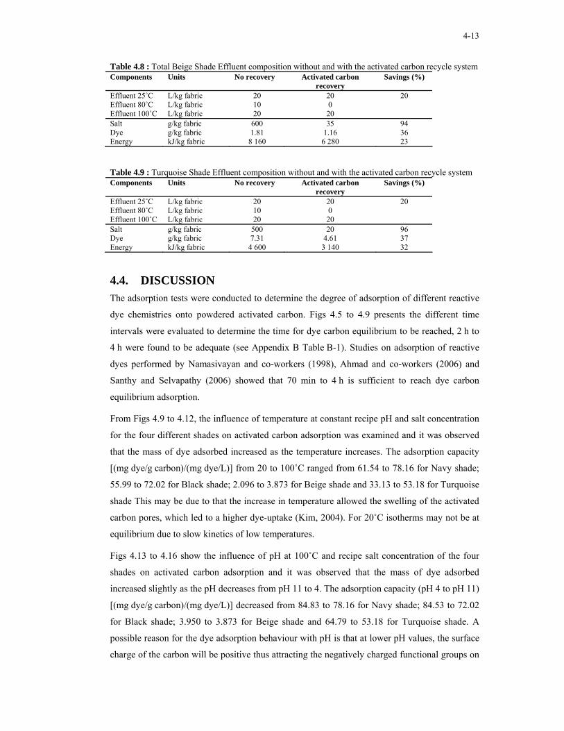
4-13

Table 4.8 : Total Beige Shade Effluent composition without and with the activated carbon recycle system Components Units No recovery Activated carbon

recovery Savings (%)

Effluent 25˚C L/kg fabric 20 20 Effluent 80˚C L/kg fabric 10 0 Effluent 100˚C L/kg fabric 20 20

20

Salt g/kg fabric 600 35 94 Dye g/kg fabric 1.81 1.16 36 Energy kJ/kg fabric 8 160 6 280 23

Table 4.9 : Turquoise Shade Effluent composition without and with the activated carbon recycle system Components Units No recovery Activated carbon

recovery Savings (%)

Effluent 25˚C L/kg fabric 20 20 Effluent 80˚C L/kg fabric 10 0 Effluent 100˚C L/kg fabric 20 20

20

Salt g/kg fabric 500 20 96 Dye g/kg fabric 7.31 4.61 37 Energy kJ/kg fabric 4 600 3 140 32

4.4. DISCUSSION The adsorption tests were conducted to determine the degree of adsorption of different reactive

dye chemistries onto powdered activated carbon. Figs 4.5 to 4.9 presents the different time

intervals were evaluated to determine the time for dye carbon equilibrium to be reached, 2 h to

4 h were found to be adequate (see Appendix B Table B-1). Studies on adsorption of reactive

dyes performed by Namasivayan and co-workers (1998), Ahmad and co-workers (2006) and

Santhy and Selvapathy (2006) showed that 70 min to 4 h is sufficient to reach dye carbon

equilibrium adsorption.

From Figs 4.9 to 4.12, the influence of temperature at constant recipe pH and salt concentration

for the four different shades on activated carbon adsorption was examined and it was observed

that the mass of dye adsorbed increased as the temperature increases. The adsorption capacity

[(mg dye/g carbon)/(mg dye/L)] from 20 to 100˚C ranged from 61.54 to 78.16 for Navy shade;

55.99 to 72.02 for Black shade; 2.096 to 3.873 for Beige shade and 33.13 to 53.18 for Turquoise

shade This may be due to that the increase in temperature allowed the swelling of the activated

carbon pores, which led to a higher dye-uptake (Kim, 2004). For 20˚C isotherms may not be at

equilibrium due to slow kinetics of low temperatures.

Figs 4.13 to 4.16 show the influence of pH at 100˚C and recipe salt concentration of the four

shades on activated carbon adsorption and it was observed that the mass of dye adsorbed

increased slightly as the pH decreases from pH 11 to 4. The adsorption capacity (pH 4 to pH 11)

[(mg dye/g carbon)/(mg dye/L)] decreased from 84.83 to 78.16 for Navy shade; 84.53 to 72.02

for Black shade; 3.950 to 3.873 for Beige shade and 64.79 to 53.18 for Turquoise shade. A

possible reason for the dye adsorption behaviour with pH is that at lower pH values, the surface

charge of the carbon will be positive thus attracting the negatively charged functional groups on

4-14

the reactive dye causing an increase in amount of dye adsorbed (Al-Degs et al., 2000; Santhy

and Selvapathy, 2006; Vadivelan and Kumar, 2005).

Figs 4.17 to 4.20 presents the influence of electrolyte concentration at 100˚C and recipe pH

value of the shades on activated carbon adsorption and it was observed that the mass of dye

adsorbed increased as the electrolyte concentration increases. The increase in adsorption

capacity [(mg dye/g carbon)/(mg dye/L)] ranged from 61.85 to 98.20 for Navy shade; 57.94 to

89.04 for Black shade; 3.129 to 5.061 for Beige shade and 39.93 to 60.74 for Turquoise shade.

NaCl and Na2SO4 are neutral salts that act as catalysts in the reactive dyeing; the need for pH

change to basic (pH 11) for higher adsorption between dye and the carbon is necessary (Ahmed,

2005).

High amount of dye uptake by powdered activated carbon was observed at high temperature,

high electrolyte concentration and low pH values.

Table 4.3 showed that in every case the r-value for the Freundlich model was greater than the

corresponding value for the Langmuir model. The r value for Freundlich model was greater than

0.90 for 87% of the tests and greater than 0.95 for 72% of the tests; while for the Langmuir

model the highest r value was 0.88. According to Arslanoglu and co-workers (2004) and Kim

(2004) higher coefficients of determination of isotherm are used to determine the best fit model.

The Freundlich adsorption parameters and r values using linear regression analysis for the

different shades are presented in Table 4.3 for different temperatures, pH values and electrolyte

concentrations respectively. In the Freundlich isotherm model, the parameter kF is a measure of

adsorption capacity, whereas the parameter n is a measure of adsorption bond strength. A large

kF value [(in mg dye per gram of carbon) / (mg dye per litre)] indicates a larger adsorption

capacity and a higher n value indicates a stronger adsorption bond (Kim, 2004). According to

the results obtained in Table 4.4 similar results were observed in all the four shades; the kF

values obtained increased as the temperature increases, increased as the pH value decreases

(from pH 11 to pH 4) and increased as the electrolyte increases). Large kF values of about 94,

89, 5 and 61 [(mg dye/g carbon)/(mg dye/L)]for Navy, Black, Beige and Turquoise shades

respectively, were observed at 100˚C, pH 4 and high electrolyte concentrations. There was not

much difference in bond strength between activated carbon and reactive dyes at different

temperatures, pH values and electrolyte concentrations. Bond strength for Navy, Black and

Turquoise (ranged from 2.738 to 5.941) were higher that Beige (ranged from 1.263 to 2.175).

All the n values obtained for all the studied shades were between 1 and 10, this indicated

favourable adsorption (Arslanoglu et al., 2004; Santhy and Selvapathy, 2006). The adsorption

results obtained for the removal of the four shades showed the possibility of decreasing the pH

or using higher concentrations of salt to achieve higher dye removals. If the pH value were to be

decreased to around a value of 4, it would have to be neutralised to a value of 7 before reuse.

4-15

The amount of salt discharged to drain would need to be evaluated before dyeing in higher salt

concentrations could be considered. The use of dyeing at higher temperatures (above 60˚C) need

to be carefully considered due to the adverse effect on the ability to control shade consistency.

The treatment of dyebath with activated carbon is presented in Table 4.5. From Chapter 3 it was

shown that the dyebath effluent contains about 430 mg/L for Navy shade, 370 mg/L for Black

shade, 65 mg/L for Beige shade and 270 mg/L for Turquoise shade. In all the selected shades

the dyebath effluent is at 60˚C. The treatment of the 60˚C Navy shade effluent with a gram

activated carbon will treat 0.05 kg fabric i.e. about 0.53 L effluent. For treatment of Black,

Beige and Turquoise shades effluent, a gram of carbon will treat about 0.08 kg fabric i.e. 0.78 L

effluent; 0.04 kg fabric i.e. 0.37 L effluent and 0.07 kg fabric i.e. 0.71 L effluent respectively. A

colour removal of above 95% was observed starting from 3 g to 5 g carbon for all the studied

shades in the adsorption equilibrium tests undertaken.

Tables 4.6 to 4.9 and Fig 4.21 show the mass balance for the dyeing and adsorption of the four

different shades. The treatment of dyebath with activated carbon showed dyebath effluent can

be reclaimed. The possibility exist for re-use of 97% salt, 25% water and 32% energy

(Table 4.5); 96% salt, 14% water and 17% energy (Table 4.6); 94% salt, 20% water and 23%

energy (Table 4.7); and 96% salt, 20% water and 32% energy (Table 4.8) for Navy; Black;

Beige and Turquoise shades respectively. The removal of colour from dyebath using activated

carbon of all the shades represents 36% up to 53% of the total colour in the effluent. First rinse

stream (S2) has a low salt concentration. The possibility exists for the further concentration of

the S2 effluent by a membrane process. The permeate from membrane process can be re-used

for the first rinse and the concentrate can join exhausted dye bath effluent (S1) (see figs B.1 to

B.4, Appendix B).

4.5. CONCLUSION • The best adsorption for the four reactive dye shades studied occurred at high temperature,

low pH and high electrolyte concentration.

• Based on determination of coefficients, the adsorption of the reactive dyes studied was

better fitted by the Freundlich isotherm model.

• Hot decolourised water with salt was recovered after adsorption of the reactive dyes and

this implies significant water, salt and energy savings.

From the textile industry perspective the discharged dye is at 60˚C and high pH of about 11.

Advantage of neutralising the effluent and heating to 100˚C with high salt concentrations is

needed for best possible adsorption of the reactive dyes shades studied. The results obtained in

this chapter predicted the performance of PAC in the removal of colour from reactive dyebath

4-16

for re-use purposes. The adsorption kinetics of the selected reactive dye shades were

subsequently evaluated using GAC in a packed column (Chapter 5). The temperature had to be

evaluated since it was the major factor that influenced the adsorption of the reactive dyes

studied in this chapter. The results obtained form a basis for evaluating the temperature effect on

column systems, which is presented in the subsequent chapter.

5-1

CHAPTER 5 COLUMN TEST

As stated in the previous chapter temperature and salt concentration were the major factors that

influenced adsorption equilibrium with pH a minor factor. The possibility of reuse of recovered

hot decolourised water with salt was observed from Chapter 4. Due to poor handling, transport

and disposal concerns of PAC, GAC has been used for column plants because of its advantages.

The carbon of the same type as in Chapter 4 was used in this chapter; the only difference was

that the carbon used in Chapter 4 was in powder form. The performance of GAC on column

system was evaluated to determine the reactive dye kinetics involved in the adsorption process.

The study of column adsorption behaviour and kinetics is necessary for the information required

for the design and operation of adsorption equipment for wastewater treatment. Column

adsorption behaviour is a prerequisite during modelling of the adsorption kinetics and the

behaviour of the adsorbent. This was done to determine the breakthrough conditions for a dye

solution. This chapter discusses the adsorption behaviour of F-400 granular activated carbon

studied in column test. The experimental methods used, followed by experimental work and the

discussion of the results obtained and lastly the conclusion of the experimental results are

presented in this chapter.

5.1. EXPERIMENTATION A representative sample of the appropriate granular activated carbon was sieved with -1 mm and

+0.95 mm screen. The average 1 mm GAC sample was oven dried for 3 h at 150°C. The 30 g

sample of oven dried GAC was boiled for 2 h, to ensure removal of air and then closely packed

into a jacketed glass column of 200 mm length and 26 mm internal diameter. The bed was

supported and closed off with glass wool, which also ensures good liquid distribution. The

column was sealed with rubber bungs and silicone sealer to avoid leaking of liquid. The column

was clamped to a burette stand and water from the water bath was pumped through the outer

walls of the column to maintain a constant temperature. A temperature controller with an

accuracy of ±3 C˚, manufactured by Labcon was used. Polystyrene chips were distributed on top

of the water bath to avoid loss in heat. A representative dye solution to be tested was

continuously fed into a column at a constant flow rate. A digital flow control peristaltic pump

(Watson- Marlow 101U/R) was calibrated and used to feed the column. The pump flowrate was

measured before and after each test. The difference never exceeded 0.003mL/min. The pump

has a maximum flow of up to 53 mL/min at 32 rpm (maximum recommended speed). The 102R

pump head accept continuous tubing or elements. The dye solution was fed through a bed of

granular activated carbon in down flow. Samples of the effluent were collected periodically and

5-2

analyzed for the remaining dye concentration using a Cary UV/Visible spectrophotometer

(model with curvette of 1 cm). The salt concentration and pH were measured using Jenway

conductivity meter 4310 and a Jenway pH meter 3310. Fresh carbon was used for each

experiment.

Two experiments were undertaken in parallel, first Navy and Black and then Turquoise and

Beige. A single batch (20 L) of dye solution was made for each test. It was stored in plastic

buckets with lids a cold room (4˚C). The column loading took between 10 and 14 days and the

column was immediately regenerated. Elluent samples were analysed for colour (ADMI) on the

day of sampling. Regeneration took 1 day. After standing overnight the next loading cycle

commenced.

A schematic diagram of the experimental set-up is shown in Fig 5.1. Column calculations

(specifications) for this study are explained in Section 5.2.1.

Fig 5.1 : Schematic set-up diagram of column experiment

5.1.1. Column calculations Column calculation parameters for the four shades are presented in this section.

Column parameters (small column internal diameter) 0.026 m

(small column length) 0.2 m (particle diameter-small column) 1 mm (carbon bulk density) 0.425 g/mL

(bed void) 0.4 (flow rate-small column) 0.625 m

S

S

S

S

IDLdpb

Qε

==

==

== L/min

(mass of carbon-small column) 30 gCSM =

Effluent

GAC

Glass wool

Rubber bungs

Feed Tank Pump Water Bath

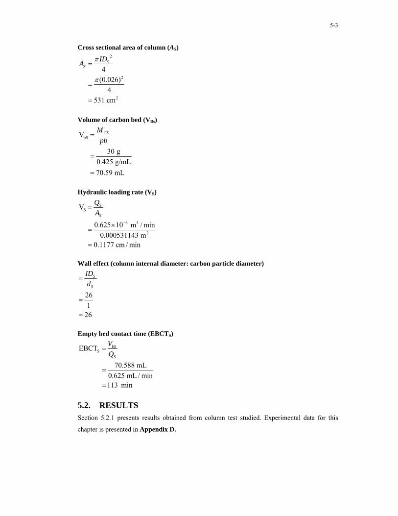
5-3

Cross sectional area of column (AS) 2

2

2

4(0.026)

4531 cm

SS

IDA π

π

=

=

=

Volume of carbon bed (VBs)

bSV

30 g0.425 g/mL70.59 mL

CSMpb

=

=

=

Hydraulic loading rate (VS)

S

6 3

2

V

0.625 10 m / min0.000531143 m

0.1177 cm / min

S

S

QA

−

=

×=

=

Wall effect (column internal diameter: carbon particle diameter)

261

26

S

S

IDd

=

=

=

Empty bed contact time (EBCTS)

EBCT

70.588 mL0.625 mL / min113 min

bSS

S

VQ

=

=

=

5.2. RESULTS Section 5.2.1 presents results obtained from column test studied. Experimental data for this

chapter is presented in Appendix D.

5-4

5.2.1. Column Breakthrough Curves The breakthrough curves obtained at different temperatures and different flowrates are

presented in Figs 5.1 to 5.8 for the four shades studied. The results of the breakthrough curves

and exhaustion are listed in Tables 5.1 to 5.2 respectively. The sample calculation for

exhaustion data is presented in Appendix D.

0.0

0.1

0.2

0.3

0.4

0.5

0.6

0.7

0.8

0.9

1.0

0 20 40 60 80 100 120 140 160

Bed volumes

Ct/C

o

20 degC 40 degC 60 degC AL

0.000

0.005

0.010

0 10 20Bed volumes

Ct/C

o

Fig 5.2 : Navy breakthrough curve at different temperatures.

0.0

0.1

0.2

0.3

0.4

0.5

0.6

0.7

0.8

0.9

1.0

0 20 40 60 80 100 120 140 160 180 200

Bed volumes

Ct/C

o 20 degC 40 degC 60 degC AL

0.000

0.005

0.010

0 10 20

Bed volumes

Ct/C

o

Fig 5.3 : Black breakthrough curve at different temperatures.

0.0

0.1

0.2

0.3

0.4

0.5

0.6

0.7

0.8

0.9

1.0

0 10 20 30 40 50 60 70 80 90 100

Bed volumes

Ct/C

o

20 degC 40 degC 60 degC AL

Fig 5.4 : Beige breakthrough curve at different temperatures.

0.0

0.1

0.2

0.3

0.4

0.5

0.6

0.7

0.8

0.9

1.0

0 20 40 60 80 100 120 140 160

Bed volumes

Ct/C

o

20 degC 40 degC 60 degC AL

0.000

0.005

0.010

0 10 20

Bed volumes

Ct/C

o

Fig 5.5 : Turquoise breakthrough curve at different temperatures.

AL-Acceptable Limit for reuse

5-5

0.0

0.1

0.2

0.3

0.4

0.5

0.6

0.7

0.8

0.9

1.0

0 20 40 60 80 100 120 140 160

Bed volumes

Ct/C

o

0.625 mL/min 6 mL/min AL

0.000

0.005

0.010

0 10 20

Bed volumes

Ct/C

o

Fig 5.6 : Navy breakthrough curve at different flowrates and 60˚C

0.0

0.1

0.2

0.3

0.4

0.5

0.6

0.7

0.8

0.9

1.0

0 20 40 60 80 100 120 140 160 180Bed volumes

Ct/C

o

0.625 mL/min 6 mL/min AL

0.000

0.005

0.010

0 10 20Bed volumes

Ct/C

o

Fig 5.7 : Black breakthrough curve at different flowrates and 60˚C

0.0

0.1

0.2

0.3

0.4

0.5

0.6

0.7

0.8

0.9

1.0

0 10 20 30 40 50 60 70 80 90 100

Bed volumes

Ct/C

o

0.625 mL/min 6 mL/min AL

Fig 5.8 : Beige breakthrough curve at different flowrates and 60˚C

0.0

0.1

0.2

0.3

0.4

0.5

0.6

0.7

0.8

0.9

1.0

0 20 40 60 80 100 120 140 160

Bed volumes

Ct/C

o

0.625 mL/min 6 mL/min AL

0.000

0.005

0.010

0 10 20

Bed volumes

Ct/C

o

Fig 5.9 : Turquoise breakthrough curve at different flowrates and 60˚C

AL-Acceptable Limit for reuse

5-6

Table 5.1: Column breakthrough effect of the shades to acceptable limit for reuse Shade Temp

(˚C) Flow rate (mL/min)

Acceptable Limit for reuse (V/Vo)

Acceptable Limit for reuse (mg dye/g carbon)

Acceptable Limit for reuse (kg fabric/g carbon)

Navy 20 0.625 1 2 0.02 40 0.625 11 20 0.25 60 0.625 14 25 0.33 60 6 11 20 0.25 Black 20 0.625 8 15 0.20 40 0.625 14 26 0.33 60 0.625 21 37 0.50 60 6 10 18 0.25 Beige 20 0.625 35 16 1.00 40 0.625 40 18 1.00 60 0.625 45 20 1.00 60 6 34 15 1.00 Turquoise 20 0.625 7 11 0.16 40 0.625 17 28 0.50 60 0.625 24 39 0.50 60 6 10 16 0.25

Table 5.2: Column exhaustion effect (CO=95%)of the shades at different temperatures Shade Temp (˚C) Flow rate (mL/min) V/Vo X/M (mg dye/g carbon) kg fabric/ g carbon Navy 20 0.625 94 72 1.69 40 0.625 94 70 1.65 60 0.625 81 65 1.54 60 6 65 52 1.22 Black 20 0.625 102 92 2.17 40 0.625 102 97 2.28 60 0.625 89 97 2.29 60 6 75 78 1.83 Beige 20 0.625 85 21 0.47 40 0.625 78 21 0.47 60 0.625 71 20 0.47 60 6 62 17 0.38 Turquoise 20 0.625 101 80 1.88 40 0.625 88 75 1.76 60 0.625 88 76 1.79 60 6 65 57 1.35

5.3. DISCUSSION Breakthrough curves of Ct/C0 versus volume treated were obtained at constant flowrate

(0.625 mL/min) for all four shades at different temperatures (20, 40, 60˚C) and are shown in

Figs 5.2 to 5.5. The two temperatures 20˚C and 40˚C were evaluated to check the effect of

column temperature but only 60˚C temperature results will be discussed in terms of

breakthrough and exhaustion of the column (see Table 5.1 and 5.2). The reason for choosing

60˚C is that all the dyeing of the four shades selected is performed at 60˚C. Thus the effluent to

be treated will be at the same temperature, provided it is treated immediately as there might be a

possibility of a drop in temperature if it is not treated immediately (thus the reason for

evaluating 20˚C and 40˚C).

The breakthrough time and volume increased as the temperature increased and it was observed

that the exhaustion point decreased as the temperature increased. This maybe due to that the

increase in temperature allowed the swelling of the activated carbon pores, which led to a higher

dye-uptake. The acceptable limit (AL) (75 ADMI) for reuse for all the shades in terms of

5-7

concentrations are summarised in Table 2.2 of Chapter 2. The acceptable concentrations based

on 75 ADMI for Navy and Black shades are 3 mg dye/L, for Beige and Turquoise are 41, 5 mg

dye/L respectively. For treatment at 60˚C for Navy and Black shades, the AL was at 14 and 21

bed volumes respectively. Treatment of Beige and Turquoise shades, the AL was at 45 and 24

bed volumes respectively. The flow through the test column was continued until the dye

concentration of column effluent (Ct) was about 0.95C0, which indicated the exhaustion point

(Eckenfelder, 2000) and exhaustion capacity results are shown in Table 5.2.

Changes in flowrates were evaluated at 0.625 and 6 mL/min flowrates at 60˚C and the

breakthrough curves are shown in Figs 5.6 to 5.9. It is evident from the results obtained in

Tables 5.2 to 5.3 that as the flow rate increased, the service times were shortened. As the

flowrate decreased, the breakthrough time increased and longer service times were achieved.

The AL for reuse for Navy, Black, Beige and Turquoise shades were at 11, 10, 34 and 10 bed

volumes respectively. The variation in the breakthrough curve and adsorption capacity may be

explained on the basis of mass transfer zone. Increase in flowrates caused the increase in zone

speed, which resulted in decrease in time required to achieve breakthrough (Perry and Chilton,

1973).

At 60˚C and a flowrate of 0.625 mL/min to AL, a gram of activated carbon, will treat

0.33 kg fabric of Navy shades, 0.50 kg fabric of Black shade, 1 kg of Beige shade fabric and

0.50 kg fabric Turquoise shade before breakthrough occurs. The values of carbon capacity per

kg of fabric (Table 5.1) and exhaustion capacity (Table 5.2) obtained from column test (ranged

from 17 to 97 mg dye per gram carbon) are much lower than those of adsorption equilibrium

tests (ranged from 20 to 521 mg dye per gram carbon) ( see Chapter 4). This indicates that the

column tests were not run under equilibrium conditions.

An important factor that had affected the column test results was the influence of the wall effect

(ratio of column inner diameter to average particle diameter). According to Couteau and

Mathaly (1997), the minimum value of 39 was considered to be sufficient to eliminate the wall

effect problem although Crittenden and co-workers (1991), the minimum value to avoid

channelling was 50. For the column tests evaluated the wall effect ratio was too low (26). Small

particles of activated carbon are appropriate for the operation but some operational requirements

such as ease of handling and low pressure drop in adsorption bed define the lower limit of

particle size. For the system design discussed in Chapter 7 one column test was repeated

correcting the shortcomings of the methodology used in this Chapter. The wall effect ratio was

taken into account following Crittenden and co-workers design model (Crittenden et al., 1991).

5-8

5.4. CONCLUSION • For a fixed flow, higher temperatures delay the breakthrough for all the selected shades.

High adsorptive capacities for AL ranging from 20 to 39 mg dye per gram carbon were

observed for 60˚C (highest temperature for this column study) for all the shades evaluated.

For low temperature (20˚C), the adsorptive capacity ranged from 2 to 16 mg dye per gram

carbon.

• Higher temperatures exhaust the carbon quicker than low temperatures. The dye volumes

for 95% exhaustion ranged from 81 to 89 bed volumes for high temperature (60˚C) while

for low temperature (20˚C) was 85 to 102 bed volumes.

• A decrease in flow rate increases the adsorption capacity of the column for AL. The carbon

capacity at low flow rate ranged from 20 to 37 mg dye per gram carbon while at high flow

rate ranged from 15 to 20 mg dye per gram carbon.

In this chapter the adsorption dye kinetics on activated carbon were investigated and the effect

of temperature on breakthrough curve and exhaustion point was observed. The advantage of

using granular activated carbon for treatment of wastewater is the possibility of regeneration.

The granular activated carbon exhausted with reactive dye was chemically regenerated for re-

adsorption processes. The information from column test was useful for the design of column for

pilot-scale use, which is presented in Chapter 7.

6-1

CHAPTER 6 REGENERATION

The main objective of the regeneration treatment process is to re-establish the adsorptive

capacity of the carbon for the adsorption of reactive dye, increase the usefulness of GAC and

reduce costs for GAC and waste treatment. Regeneration of the adsorbent material is of crucial

importance in the economic development. The saturated granular activated carbon which was

used for dye removal in Chapter 5 was subjected to regeneration. This chapter discusses the

chemical regeneration of saturated F-400 granular activated carbon used in the column tests. A

brief background on regeneration, experimental methods used, followed by discussion of the

results and lastly conclusion that can be drawn from the experimental results are presented in

this chapter.

6.1. BACKGROUND Activated carbons that are used for the removal of organic compounds from liquid phase

systems will gradually become saturated, due to the concentration of contaminants on the

surface of the adsorbent. When this occurs a decision must be made on how to deal with the

spent material (Clark and Lykins, 1989). Due to the high manufacturing costs and the recovery

of components adsorbed on the surface of activated carbon, regeneration is the preferred option.

The possibility of regeneration is one of the main reasons for the wide-spread use of activated

carbon as an adsorbent (Zolfl et al., 2000). There are three potential regeneration techniques:

chemical, steam and thermal. Advantages of having a regeneration system are as follows:

• System is reliable from a process standpoint

• Reduces solid waste handling problems caused by disposal of spent carbon

• Saves up to 50% of the carbon cost (EPA, 2000)

Thermal regeneration is the mostly common applied regeneration method but due to high costs

resulting from energy used and effluent gas treatment further alternative regeneration processes

have been investigated. Thermal regeneration studies performed by Abdul and Campbell (1996)

showed that a significant deterioration of the GAC pore structure resulted in reduced adsorption

surface area. Due to this, many chemicals have been tested for the regeneration of activated

carbon to treat wastewater. Studies by Huling and co-workers (2005) concluded that chemical

regeneration of activated carbon was not an economically viable process and the overall

feasibility of the process was based on chemical costs and disposal of concentrated effluent.

Studies performed by Sorlini and Collivignarelli (2005) proved that base-acid regeneration for

6-2

granular activated carbon system was the best amongst base, acid and thermal regeneration

process for the removal of organics. The removal efficiency ranged from 50% to 60% for base-

acid regeneration, 40% to 50% for thermal regeneration and about 20% for base and acid

regeneration

6.2. EXPERIMENTATION The chemical regeneration procedure used for this study was developed by Santhy and

Selvapathy (Santhy and Selvapathy, 2005). Experiments were carried out for the desorption of

the four shades studied using 1 M NaOH as the eluent. The influent was allowed to percolate

through the saturated carbon bed of 70.6 mL at a flow rate of 0.625 mL/min (see Fig 6.1 for first

regeneration). From these results it was assumed that 3 bed volumes of 1 M NaOH would be

sufficient. After the desorption of the shades, the carbon bed was washed with volumes of

distilled water three times to remove the free alkali. A volume of 50 mL of 1 M HCl at a flow

rate of 0.625 mL/min was washed through the column to neutralize any residual alkalinity. The

carbon bed was finally washed with distilled water and the next cycle of operation of removal of

dye from solution was performed. The process of adsorption and regeneration of carbon beds

were repeated over 4 cycles of operation. The adsorption process was performed as described in

Chapter 5.

6.3. RESULTS This section presents results obtained from the chemical regeneration of granular activated

carbon tests for four different shades; Navy, Black, Beige and Turquoise. Fig 6.1 presents

elution using 1 M NaOH. The column breakthrough curves obtained using regenerated granular

activated carbon is shown in Figs 6.2 to 6.5. Table 6.1 presents the exhaustion time for the

regenerated carbon for the 1st, 2nd, 3rd and 4th cycles. Experimental data for regeneration is

presented in Appendix E.

6-3

0

0.0001

0.0002

0.0003

0 1 2 3 4 5

NaOH bed volume

Dye

elut

ed (g

/mL)

Navy Black Beige Turquoise

Fig 6.1: Desorption of shades from granular activated column using NaOH

0

0.1

0.2

0.3

0.4

0.5

0.6

0.7

0.8

0.9

1

0 10 20 30 40 50 60 70 80 90 100Bed volumes

Ct/C

o

1st Cycle 2nd Cycle 3rd Cycle4th Cycle AL

Fig 6.2: Regeneration of GAC-Navy shade at 60˚C

0

0.1

0.2

0.3

0.4

0.5

0.6

0.7

0.8

0.9

1

0 10 20 30 40 50 60 70 80 90 100Bed volumes

Ct/C

o

1st Cycle 2nd Cycle 3rd Cycle4th Cycle AL

Fig 6.3: Regeneration of GAC-Black shade at 60˚C

0

0.1

0.2

0.3

0.4

0.5

0.6

0.7

0.8

0.9

1

0 10 20 30 40 50 60 70 80Bed volumes

Ct/C

o

1st Cycle 2nd Cycle 3rd Cycle4th Cycle AL

Fig 6.4: Regeneration of GAC-Beige shade at 60˚C

0

0.1

0.2

0.3

0.4

0.5

0.6

0.7

0.8

0.9

1

0 10 20 30 40 50 60 70 80 90 100Bed volumes

Ct/C

o

1st Cycle 2nd Cycle 3rd Cycle4th Cycle AL

Fig 6.5: Regeneration of GAC-Turquoise shade at 60˚C

AL-Acceptable Limit for reuse

6-4

Table 6.1: Effect of shades bed volume treated for regeneration cycles at 60˚C Shades Regeneration cycles AL

(V/Vo) AL (mg dye/g carbon)

AL (g carbon/kg fabric)

Navy 1st cycle 14 25 3 2nd cycle 11 20 4 3rd cycle 1 2 42 4th cycle ― ― ― Black 1st cycle 21 55 39 2nd cycle 14 39 28 3rd cycle 8 29 22 4th cycle ― ― ― Beige 1st cycle 45 20 1 2nd cycle 35 16 1 3rd cycle 30 13 1 4th cycle ― ― ― Turquoise 1st cycle 24 39 2 2nd cycle 15 24 3 3rd cycle 7 11 6 4th cycle ― ― ―

6.4. DISCUSSION The flow through the tested column was continued until the dye concentration of column

effluent (Ct) was about 0.95C0, which indicated the exhaustion point (Eckenfelder, 2000).The

elution of granular activated carbon was achieved using 1 M NaOH followed by 1 M HCl (Fig

6.1). About 3 bed volumes were sufficient for almost complete desorption of the four shades.

From the results shown in Table E.1 of Appendix E, the dye recovery for Navy, Black, Beige

and Turquoise shades was 748, 765, 187 and 675 mg dye/L respectively. The percent recovery

for the first cycle at 60˚C for Navy, Black, Beige and Turquoise was 97, 98, 99 and 97 %

respectively. The column tests with regenerated carbon were performed at 60˚C. According to

Table 6.1, the bed volumes treated for Navy and Black shades, the AL were at 14; 11 and 1; and

21, 14 and 8 for the first, second and third cycles respectively. The bed volumes treated for AL

for Beige shade were at 45; 35 and 30 for the first, second and third cycles respectively. The AL

for reuse for Turquoise shade were at 24, 15 and 7 bed volumes treated for the first, second and

third cycles respectively.

At least three cycles of regeneration were carried out within the standard limit for reuse.

Significant deterioration of the carbon was observed at the fourth cycle. A small decline in GAC

adsorption capacity was observed from the first to the third regeneration cycles. The role of dye

auxiliaries on the activated carbon were not evaluated in the study and it is possible that they

could have major effects that are detrimental on the performance of activated carbon. The

auxiliary mixtures are often developed to solve problems specific to the process and to

counteract or enhance the effects of other chemicals (Hendrickx and Boardman, 1995).

According to Huling et al. (2005) there are two general mechanisms that could adversely affect

the adsorption capacity of the regenerated carbon. The first mechanism is the change in physical

and chemical characteristics of GAC because of oxidative treatment. The second mechanism is

the accumulation of by-products caused by incomplete transformation of the target compounds

6-5

at adsorption sites. The change in adsorption capacity of regenerated carbon was postulated to

be due to the accumulation of reactive dyes and possibly reaction by-products, which may have

blocked adsorption sites.

6.5. CONCLUSION • NaOH elution can regenerate the spent F-400 granular activated carbon exhausted with

reactive dyes up to 3 regeneration cycles.

• Fewer bed volumes were treated as the regenerated carbon was used. As regenerated

carbon was used less carbon capacity was observed.

• The removal of dyes with regenerated carbon within the limit for reuse was observed up

to 3 cycles of operation.

The effectiveness of chemical regeneration of saturated carbon using NaOH was not satisfactory

in terms of industrial application because of the number of cycles achieved. The results obtained

showed that the use NaOH compared to other chemical regenerants need to be investigated for

the implementation of activated carbon for removal of reactive dyes. The overall results from

Chapter 3 to 6 showed the possibility of designing a pilot scale system, which is presented in

Chapter 7.

7-1

CHAPTER 7 SYSTEM DESIGN

From Chapter 4 and Chapter 5, the possibility of recovery of hot decolourised water with salt

from reactive dyebath was shown to be possible by adsorption studies and chemical

regeneration (Chapter 6). A laboratory-scale column with a small diameter, filled with carbon

was tested and the dye solution was run through the column to obtain data that were used for

adsorption and design. The rapid small-scale column test methodology which uses mass transfer

similarity criteria to allow scale up of the test results to the full size column was evaluated for

design purposes. The design of adsorption systems requires column tests similar to the actual

operation of full-scale systems.

In Chapter 5 the wall effect of the particle diameter to column diameter ratio was not taken into

account, thus before designing an adsorption column for this study. One column test for Navy

shade at 60˚C was performed with column internal diameter to particle diameter ratio of 50. The

main objective of this chapter is to design an adsorption plant using the information obtained

from the improved column (column: particle ratio of 50) adsorption study.

The column effluent was monitored for the contaminant of interest. For water treatment

applications, the attainment of a specific effluent concentration is more critical than

breakthrough. Thus, both the dye effluent and initial breakthrough are employed to analyze the

data. The first information from the breakthrough curve is the cumulative number of bed

volumes to breakthrough. In this chapter; mostly comparison of small-scale to full-scale

operation will be made. A brief introduction on scaling up using RSSCT was presented in

Chapter 2 and the design methodology using the information collected is shown in Section 7.1.

7.1. DESIGN The RSSCT design of one of the four shades is presented in section 7.1.1 and the design is

shown in section 7.1.2.

7.1.1. Small column design The calculations presented are for the Navy shade only. Design calculations for the other three

shades can be done using a similar method. The breakthrough curve for design obtained at 60˚C

Navy Shade is shown in Fig 7.1 and the experimental data presented in Table E.6 in

Appendix E.

7-2

Navy Shade

Column parameters 0.026 m0.2 mm0.425 g/mL0.4120 min952 min

T 60 degC26 520.2

S

S

S

S

S

S

IDdpb

EBCTtb

IDd

ε

=======

= =

The minimum column-diameter-to-particle-size ratio should be 50 to avoid channelling

(i.e. ID=26 mm) (Crittenden et al., 1991).

0.00

0.01

0.01

0 5 10 15

Bed volumes

Ct/C

o

60 degC AL

Fig 7.1: Navy breakthrough curve at 60˚C for column design

Small-scale: Column surface area 2

S

2

2

4(2.6 cm)

45.309 cm

SIDA π

π

=

=

=

In this study the minimum value of superficial Reynolds number ( ReS ) of 1 was selected.

According to Crittenden and co-workers (1991), a value of 1 for ReS usually yields good

results but lower values can be selected if head loss and column length are unacceptable. The

7-3

minimum Reynolds number guarantees the effects of dispersion and the external mass transfer

of the large column must be greater than in the RSSCT

Small-scale: Hydraulic loading rate (superficial velocity) using Re 1s =

Water viscosity (ν )= 0.89 cP

S

S

Re

Re

1 0.00089996 0.02 0.0045 cm/s0.27 cm/min

Ss

s

S

gV d

Vgd

νν

=

=

×=

×==

Small scale: Flowrate

2

3

0.27 cm/min 5.31 cm1.43 cm /min

S S SQ V A=

= ×

=

Small-scale: Volume of the carbon bed

bS3

3

120 min 1.43 cm /min172 cm

S SV EBCT Q= ×

= ×

=

Small-scale: Mass of carbon

3 3172 cm 0.425 g/cm73 g

CS bSM V pb= ×

= ×=

7.1.2. Full-scale design Suppose a column with 1 m internal diameter (assumption) packed with 500 kg granular

activated carbon of 2 mm particle diameter was used for pilot-scale study.

Pilot-scale for Navy shade The diffusion of adsorbate onto GAC was assumed to be controlled by proportional diffusivity

where most of the mass transfer zone spreading was caused by intraparticle diffusion ( 1X = )

(Crittenden et al. 1991)

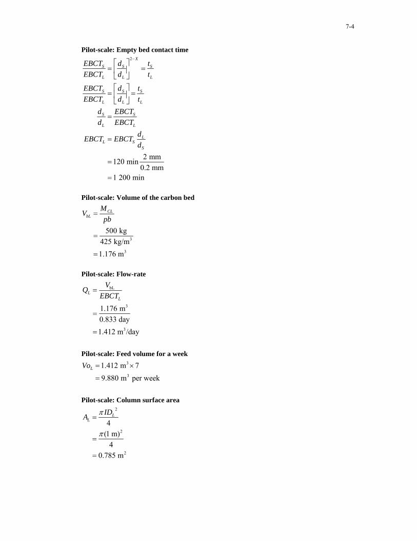
7-4

Pilot-scale: Empty bed contact time 2

2 mm120 min0.2 mm

1 200 min

X

S S S

L L L

S S S

L L L

S S

L L

LL S

S

EBCT d tEBCT d t

EBCT d tEBCT d t

d EBCTd EBCT

dEBCT EBCTd

−⎡ ⎤

= =⎢ ⎥⎣ ⎦⎡ ⎤

= =⎢ ⎥⎣ ⎦

=

=

=

=

Pilot-scale: Volume of the carbon bed

3

3

500 kg425 kg/m1.176 m

CLbL

MVpb

=

=

=

Pilot-scale: Flow-rate

bL

3

3

1.176 m0.833 day1.412 m /day

LL

VQEBCT

=

=

=

Pilot-scale: Feed volume for a week 3

3

1.412 m 79.880 m per week

LVo = ×

=

Pilot-scale: Column surface area 2

2

2

4(1 m)

40.785 m

LL

IDA π

π

=

=

=

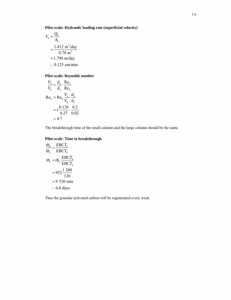
7-5

Pilot-scale: Hydraulic loading rate (superficial velocity)

3

2

1.412 m /day0.78 m

1.798 m/day0.125 cm/min

LL

L

QVA

=

=

=∴

Pilot-scale: Reynolds number ReRe

Re Re

0.126 0.210.27 0.02

4.7

S SL

L S L

L LL S

S S

V dV d

V dV d

= ⋅

= ⋅

= ⋅

=

The breakthrough time of the small column and the large column should be the same.

Pilot-scale: Time to breakthrough

1 200952120

9 520 min6.6 days

S S

L L

LL S

S

tb EBCTtb EBCT

EBCTtb tbEBCT

=

=

=

=∴

Thus the granular activated carbon will be regenerated every week.

8-1

CHAPTER 8 CONCLUSIONS AND RECOMMENDATIONS

In this study four different dye classes were investigated (Drimarene HF, Cibacron S, Procion

HE and Remazol Levafix using four standard shades (Navy, Black, Beige and Turquoise). The

reactive dyestuffs contained different functional groups (chemistries). Reactive dye exhaustion

to the fibre for the four reactive dye classes was about 80% i.e. 20% remains in the effluent.

Reactive dyeing of the four studied shades resulted in salt concentrations over 90% and hot

coloured water remaining in the dyebath effluent. The efficiency of the dyeing process for a

specific shade is associated with various parameters such as substantivity and diffusion rate of

dyes, hardness of water, pH and temperature of the dye liquor, type and concentration of

reactive dye used. The use of granular activated carbon for the adsorption of reactive dyes has

been examined and results obtained indicated that activated carbon could effectively remove

colour from exhausted reactive dyebath effluent and allow re-use of hot decolourised water with

high concentration of salt.

From the adsorption results obtained using activated carbon it was concluded that the most

important factor influencing the adsorption rate and capacity for the reactive dye shades studied

is the adsorption temperature. Textile processes require hot water for reactive dyeing of cotton.

There is great potential in the textile industry for hot water recovery. The use of heat exchangers

to transfer heat to the incoming dyeing feed water can be eliminated when using granular

activated carbon columns. The pH values and electrolyte concentration also played a vital role

in the whole adsorption process and particularly in adsorption capacity. Colour removal of

100%, salt recovery of 94 to 97% and energy savings 17 to 32% in the dyebath effluent were

achieved. Reactive dyeing of cotton is performed at high temperatures and in this study the

results were discussed based on 60˚C, which was the common temperature used for dyeing for

all four shades selected.

The breakthrough time from column breakthrough curves for 60˚C were at 14, 21, 45 and 24

bed volumes for Navy, Black, Beige and Turquoise shades respectively. The exhaustion or

saturation times for the granular activated carbon were at 24, 41, 45 and 35 bed volumes for

Navy, Black, Beige and Turquoise shades respectively. The variation in the slope of the

breakthrough curve may be explained on the basis of mass transfer fundamentals of adsorption

capacity of granular activated carbon. Increase in flowrate caused an increase in zone speed,

resulting in decrease in the time required to achieve breakthrough, while a decrease in flowrate

resulted in an increased breakthrough time. This was due to decreased contact time between the

dye and carbon at higher flow rates.

8-2

From the column test results shown, the values of carbon capacity per kilogram of fabric

obtained from the column test were much lower than those of the adsorption equilibrium test.

The reason is that more of the adsorption sites are exposed in PAC than in the GAC and the

process is faster when using PAC. The Freundlich isotherms measured in the adsorption

equilibrium experiments do not apply to the column tests, perhaps due to that the equilibrium is

not reached in column tests. One of the advantages of using GAC in the column test is the

possibility of regeneration. From studies presented in the literature; it was shown that the

required water quality for textile process is not stated. The textile industries are using drinking

water quality for dyeing, therefore the 75 ADMI could be used as the standard limit when

treating water for reactive dyeing reuse. Dyeing of the same shades or dyeing of a darker shade

with treated light shade effluent would not need drinking water quality.

The regenerated carbon for this study was found to be effective up to 3 cycles of operation

within the acceptable limit for reuse. Significant deterioration of the carbon was observed at the

fourth cycle. The poor performance could be associated with role of dye auxiliaries in the

overall adsorption process because of their unknown composition and chemistry (this was not

divulged by the manufacturer for confidentiality. This led to the activated carbon not

economically feasible for industrial application. Fewer bed volumes were treated when using

regenerated carbon compared to virgin carbon. The possibility of savings exists when using

regenerated GAC for treatment. Regeneration should also ensure that the eluted solution is not

posing any disposal problems in terms of high acidity and high colour concentration. A further

investigation of thermal regeneration of the spent granular activated carbon for the removal of

reactive dyes is needed to determine its advantages and disadvantages over chemical

regeneration. The design, operation and maintenance of carbon adsorption and regeneration

processes depend on costs and characteristics of textile water to be treated and the capacity of

the plant. Therefore the designer is responsible for selecting a system that will meet the

discharge permit requirements at the lowest cost possible. Once the optimum flowrate, bed

depth and operating capacity of GAC is determined, the carbon contactors configurations can be

estimated. The use of RSSCT method for designing in this study has the major potential

advantage over other methods in predicting the performance of pilot-scale. The carbon particle

must be at least 1/50 of the column diameter to overcome the wall effect problem. Small

particles of activated carbon are appropriate for the operation but some operational requirements

such as ease of handling and low pressure drop in adsorption bed define the lower limit of

particle size.

Further research in this area should concentrate on evaluating different activated carbons and

role of auxiliaries in activated carbon adsorption studies. When implementing the laboratory-

scale plant in textile industry, the effect change in temperature, pH and electrolyte concentration

8-3

should be noted and the chemical parameters should also be researched. The first rinse stream

has a moderate colour with low salt concentration effluent. If further colour removal is required,

this stream could be treated by reverse osmosis. The permeate can be used for the first rinse and

the concentrate can join dyebath effluent. The further investigation should also be expanded to

the evaluation of other chemical regenerants and thermal regeneration of saturated activated

carbon. The use of GAC adsorption and the regeneration of GAC should also be taken into

account for water, salt and energy savings for the textile industry. This study proved that the

activated carbon adsorption technique is the solution in reactive dyeing textile industries

because of the possibility for re-use of water, salt and energy; thus enabling environmental

improvements with savings in salt, energy and water.

R-1

REFERENCES

ABDUL HM AND CAMPBELL WR (1996) Pentachlorophenol adsorption and desorption

characteristics of granular activated carbon-II. Kinetics. Water Research 30 12. 2907-2913.

AHMAD AA, HAMEED BH AND AZIZ N (2006) Adsorption of direct dye on palm ash:

Kinetic and equilibrium modeliing University of Science Malaysia, Malaysia.

AHMED NSE (2005) The use of sodium edate in the dyeing of cotton with reactive dyes. Dyes

and Pigments 65. 221-225.

AL-DEGS Y, KHRAISHEH MAM, ALLEN SJ AND AHMAD MN (2000) Effect of carbon

surface chemistry on the removal of rective dyes from textile effluent. Water Research 34 3.

927-935.

AL-SARAWY A, RASHED IG, HANNA MA AND WALI FKM (2005) Removal of some 4-

pyrazolone dyes from aqueous solutions by adsorption onto different types of carbon.

Desalination 186. 129-153.

ALBANIS TA, HELA DG, SAKELLARIDES TM AND DANIS TG (2000) Removal of dyes

from aqueous solutions by adsorption on mixtures of fly ash and soil in batch and column

techniques. Global Nest: TheInternational Journal 2 3. 237-244.

ALLEGRE C, MOULIN P, MAISSEU M AND CHARBIT F (2004) Savings and re-use of salts

and water present in dye house effluents. Desalination 162 13-22.

ALLEGRE C, MOULIN P, MAISSEU M AND CHARBIT F (2006) Treatment and reuse of

reactive dyeing effluents. Journal of Membrane Science 269 15-34.

ALLEN SJ AND KOUMANOVA B (2005) Decolourisation of water/wastewater using

adsorption (Review). Journal of the University of Chemical Technology and Metallurgy 40 3.

175-192.

ALLEN SJ, WHITTEN L AND MCKAY G (1998) The Production and Characterization of

Activated Carbons: A Review. Development in Chemical Engineering And Mineral Processes 6

5. 231-261.

ALLEN W, PRESCOTT WB, DERBY RE, GARLAND CE, PERET JM AND SALTZMAN M

(1973) Determination of colour of water and wastewater by means of ADMI colour values.

Proceedings of the 28th Industrial Waste Conference, England. 661.

R-2

ALVAREZ PM, BELTRAN FJ, GOMEZ-SERRANO V, JARAMILLO J AND RODRIGUEZ

EM (2004) Comparison between thermal and ozone regenerations of spent activated carbon

exhausted with phenol. Water Research 38 8. 2155-2165.

ARSLANOGLU FN, KAR F AND ARSLAN N (2004) Adsorption of dark coloured

compounds from peach pulp by using granular activated carbon Journal of Food Engineering 1-

8.

BANSAL RC, DONNET JB AND STOECKLI F (1988) Active carbon. Marcel Dekker Inc,

New York.

BARCLAY S AND BUCKLEY CA (2002) Waste Minimisation Guide for Textile Industry: A

Step towards Cleaner Production Water Research Commision 1 Report No TT 139/00, Durban.

BRADY M AND MCKAY G (1996) Characterization of Adsorbents: Use of Adsorbents for the

removal of Pollutants from Wastewater. CRC Press, Inc., Florida. 39-48.

BROADBENT AD (2001) Basic Principles of Textile Coloration. Society of Dyers and

Colourists, West Yorkshire, England. 332-353.

CLARK RM AND LYKINS BW JR (1989) Granular Activated Carbon: Design, Operation and

Cost. Lewis Publishers, Inc. Michigan

CLEMENTS M (2002) Granular Activated Carbon Management at a Water Treatment Plant.

Department of Civil Engineering, Rand Afrikaans University., Johannesburg.

COUTEAU D AND MATHALY P (1997) Purification of ferulic acid by adsorption after

enzymic release from sugar-beet pulp extract. Industrial Crops and Products 6 3-4. 237-252.

CRITTENDEN JC, BERRIGAN JK, HAND DW AND LYKINS B (1987) Design of Rapid

Fixed-Bed Adsorption Tests for a constant diffusivity. Journal of Environmental

Engineering 113 2. 243-259.

CRITTENDEN JC, REDDY PS, ARORA H, TRYNOSKI J, HAND DW, PERRAM DL AND

SUMMERS RS (1991) Predicting GAC Performance with Rapid Small-Scale Column Tests.

Journal of the American Water Works Association 83 1. 77-87.

DVARIONIENE J, STASISKIENE Z AND KNUDSEN HH (2003) Pilot-Scale Membrane

Filtration Study on Water Reuse of Rinsing Water after Reactive Cotton Dyeing. Environmental

Research Engineering and Management 3 25. 3-10.

ECKENFELDER WW JR (2000) Industrial Water Pollution Control 3rd edition. The McGraw-

Hill Companies, Inc. United States of America.

R-3

EL-SHISHTAWY RM, YOUSSEF YA, AHMED NSE AND MOUSA AA (2007) The use of

sodium edate in dyeing: Union dyeing of cotton/wool blend with hetero bi-functional reactive

dyes. Dyes and Pigments 72 57-65.

ENVIRONMENTAL PROTECTION AGENCY (2000) Wastewater Technology Fact

Sheet:Granular Activated Carbon Absorption and Regeneration, Office of Water Washington,

DC.

FARIA PCC, ORFAO JJM AND PEREIRA MFR (2004) Adsorption of anionic and cationic

dyes on activated carbons with different surface chemistries Water Research 38 2043-2052.

FERRO-GARCIA MA, UTRERA-HIDALGO E, RIVERA-UTRILLA J, MORENO-

CASTILLA C AND JOLY JP (1993) Regeneration of activated carbons exhausted with

chlorophenols. Carbon 31 6. 857-863.

FORD DL (1981) Wastewater Characteristics and Treatment. CRC Press, Inc., New York.

GOLOB V, VINDER A AND SIMONIC M (2005) Efficiency of the coagulation/flocculation

method for the treatment of dyebath effluents. Dyes and Pigments 67 93-97.

GONZALEZ-SERRANO E, CORDERO T, RODRIGUEZ-MIRASOL J, COTORAELO L

AND RODRIGUEZ JJ (2004) Removal of water pollutants with activated carbons prepared

from H3PO4 activation of lignin from kraft black liquors. Water Research 38 13. 3043-3050

GREENBERG AE, TRUSSEL RR AND CLESCERI LS (1995) Standard Methods for

Examination of Water and Wastewater. American Public Health Association.

HARKER RP (1980) Recycling sewage water for scouring and dyeing. American Dyestuff

Manufacturer 69 1. 28-46.

HASSLER JW (1974) Purification with Activated Carbon. Chemical Publishing Company Inc.,

New York.

HENDRICKX I AND BOARDMAN GD (1995) Pollution Prevention Studies in the Textile

Wet Processing Industry. Department of Civil Engineering, Blacksburg, Virginia.

HOFFMAN J (2004) Decolourisation of textile effluent. Proceedings of WISA Biennial

Conference and Exhibition, Cape Town. 529-535.

HULING SG, JONES PK, WENDELL PE AND ARNOLD RG (2005) Fenton-driven chemical

regeneration of MTBE-spent GAC. Water Research 39 2145-2153.

HUNGER K (2003) Industrial Dyes Chemistry, Properties, Applications. WILEY-VCH Verlag

GmbH and Co, Weinheim.

R-4

HUNTER A AND RENFREW M (1999) Reactive Dyes for Textile Fibres, The chemistry of

activated Π-bonds as reactive groups and miscellaneous topics. Society of Dyers and Colourists.

West Yorkshire, England. 1-174.

INOUE G AND NAGASAWA S (1977) Water reuse in fiber dyeing industry. Desalination 23

12. 133-140.

JAMODE AV, SAPKAL VS, JAMODE VS AND DESHMUKH SK (2004) Adsorption

Kinetics of Defluoridation Using Low-cost Adsorbent. Adsorption Science and Technology 22

1. 65-73.

JANKOWSKA H, NEFFE S AND SWIATKOWSKI A (1981) Investigations of the

electrochemical properties of activated carbon and carbon black. Electrochimica Acta 26 12.

1861-1866.

JUANG RS, TSENG RL AND WU FC (1996) Use of Chitin and Chitosan in Lobster Shell

Wastes for Colour Removal from Aqueous Solutions. Journal of Environmental Science Health

31 2. 325-339.

JUSOH A, CHENG WH, LOW WM, NORA'AINI A AND NOOR MJMM (2005) Study on the

removal of iron and manganese in ground water by granular activated carbon. Desalination 182

1-3. 347-353.

KIM DS (2004) Adsorption characteristics of Fe (III) and Fe (III)-NTA complex on granular

activated carbon. Journal of Hazardous Materials 106 B. 67-84.

KUMAR VK, SUBANANDAM K, RAMAMURTHI V AND SIVANESAN S (2004) Solid

Liquid Adsorption for Wastewater Treatment: Principle Design and Operation. Anna

University, Chennai, India.

MANTELL CL (1951) Adsorption. McGraw-Hill Book Co., Inc., London.

MARMAGNE O AND COSTE C (1996) Removal from Textile Plant Effluents. American

Dyestuff Reporter 15-21.

MATTSON JS AND HARRY BM JR (1971) Activated carbon: Surface Chemistry and

Adsorption from Solution. Marcel Dekker, Inc., New York.

NAMASIVAYAN C, PRABHA D AND KUMUTHA M (1998) Removal of Direct Red and

Acid Brilliant Blue by adsorption onto banana pith. Bioresource Technology 64 77-79.

OSIPOW LI (1962) Surface Chemistry: Theory and Industrial Application. Reinhold Publishing

Corporation, New York.

PARKER I AND HUGHES D (1998) Water Treatment Primer CE 4124: Environmental

Information Management. Civil Engineering Department, Virginia.

R-5

PATRICK JW (1995) Porosity in Carbons: Characterisation and Applications. Edward Arnold,

Inc., London.

POPE JP (1998) Groundwater Pollution Primer CE 4594: Soil and Groundwater Pollution. Civil

Engineering Department, Virginia.

RUTHVEN DM (1984) Principles of adsorption and adsorption processes. Wiley, New York.

SANTHY K AND SELVAPATHY P (2006) Removal of reactive dyes by adsorption on coir

pith activated carbon. Bioresource Technology 97 11. 1329-1336.

SHAUL G, DEMPSEY CR AND DOSTAL KA (1988) Fate of water soluble azo dyes in the

activated sludge process. Water Engineering, Research Laboratory, Cincinnati.

SHAUL G, DEMPSEY CR, DOSTAL KA AND LIEBERMAN RJ (1986) Fate of azo dyes in

the activated sludge process. Lewis Publisher Inc., Michigan.

SHU L, WAITE TD, BLISS PJ, FANE A AND JEGATHEESAN V (2005) Nanofiltration for

the possible reuse of water and recovery of sodium chloride salt from textile effluent.

Desalination 172 235-243.

SMITH JM, VAN NESS HC AND ABBOTT MM (2001) Introduction to chemical engineering

thermodynamics 6th edition. McGraw-Hill International edition. United States of America.

SORLINI S AND COLLIVIGNARELLI C (2005) Chlorite removal with granular activated

carbon. Desalination 176 255-265.

STREAT M, PATRICK JW AND CAMPORRO P AND SAHA B (1995) Sorption of phenol

and para-chlorophenol from water using conventional and novel activated carbon.

Water Research 29 2. 467-472.

SUFFET IH AND MCGUIRE MJ (1981) Activated Carbon Adsorption I, II. Ann Arbor

Science Publishers, Michigan.

TWORECK WC, ROSS WR AND RENSBURG NJJ (1984) The use of reclaimed water in the

textile industry. Textile Dyegest SA 2-6.

VADIVELAN V AND KUMAR VK (2005) Equilibrium, kinetics, mechanism, and process

design for the sorption of methylene blue onto rice husk. Journal of Colloid and Interface

Science 286 90-100.

VAN LIER WC (1989) Mass transfer to activated carbon in aqueous solutions. Drukkerij

Elinkwijk BV, Utrecht. 1-2.

WAGNER NJ AND JULA RJ (1981) Activated Carbon Adsorption for Wastewater Treatment.

CRC Press, Inc. . 41-60.

R-6

WATER RESEARCH COMMISSION (2003) KSA3: Water Use and Wastewater Management.

WENZEL H, KNUDSEN HH, KRISTENSEN GH AND HANSEN J (1996) Reclamation and

Reuse of Process water from Reactive Dyeing of Cotton. Desalination 106 192-203.

ZOLFL CM, STEENKAMP CJH AND BREET ELJ (2000) Supercritical fluid Regeneration of

Exhausted Granular Activated Carbon- Potential application to water purification. Water

Research Commision 923/1/00

A-1

APPENDIX A

THE DYEING PROCESSES Appendix A contains dyeing procedures for all the four shades with experimental data for

Chapter 3. Preparation of reactive dyestuff stock solution, auxiliaries and chemicals are

explained in the subsequent sections. The chemicals used were taken from Dyefin Textile

factory.

Preparation of 1% dyestuff solutions: Weigh 1 g of dry reactive dyestuff powder or granules. Put it in a beaker and add little warm

distilled water. Paste up well and wash into a 100 mL flat bottom volumetric flask, preferably at

20ºC, to bring total volume to 100 mL.

Preparation of auxiliary solutions

10 % Dekol AA-D solution. Measure 10 mL of concentrated Dekol AA-D solution from BASF plc and add water to make up

a total volume of 100 mL.

10% Tebolan UFN Measure 10 mL of concentrated Tebolan UFN solution from Dr. Th. Bohme KG, Chem. Fabrik

GmbH and add water to make up a total volume of 100 mL

10% Avcoson LL Measure 10 mL of concentrated Avcoson LL solution from Avco Chemicals Ltd and add water

to make up a total volume of 100 mL.

10% Subitol Measure 10 mL of concentrated Subitol solution and add water to make up a total volume of

100 mL.

20% Sodium carbonate Weigh 20 g of Sodium carbonate powder and add water to make up a total volume of 100 mL.

95% (36 Be˚) Sodium hydroxide Measure 19 mL of 100% (38 Be˚) concentrated sodium hydroxide solution; add 1 ml water to

make a total volume of 20 mL. In the textile industry a 100 % (38 Be˚) caustic solution relates

to the as purchased concentration. Be˚ is an old German density measure.

A-2

60% Acetic Acid Measure 60 mL of glacial acetic acid and fill up to 100 mL with distilled water.

Dyeing Procedures

Drimarene HF (Navy shade) Supplier: Clariant

Substrate: 10 g of 100 % cotton single jersey knit, bleached.

Liquor ratio: 10:1 (mL liquor / g fabric)

Dye type: Reactive Dyes

Dye class: Drimarene HF

Chemistry: Trifloropyrimidine (TFP)

Procedure: Exhaust

Fig A.1: Navy shade dyeing process

Table A.1: Dye and salt concentrations before dyeing and after Navy dyeing of fabric Sample No. Dye (mg/L) Salt (g/L) S0 3 850 70.0 S1 430 68.2 S2 120 1.80 S3 180 <0.01 S4 80 <0.01

Aux. / Dye / NaCl / Fabric (S0)

25ºC

80oC for 30 min

60ºC for 30 min

Na2CO3

>2ºC / min

Soap in 100 mL Dekol solution

Rinse (100 mL water, pH 6)

25ºC for 10 min

100oC for 10 min

Rinse (100 mL water, pH 6)

25ºC for 10 min

S1 S2 S3 S4

Drop to < 26ºC

A-3

Cibacron S (Black shade) Supplier: Ciba

Substrate: 10g of 100 % cotton single jersey knit, bleached

Liquor ratio: 10:1 (mL liquor / g fabric)

Dye type: Reactive Dyes

Dye class: Cibacron LS

Chemistry: Not available

Procedure: Exhaust

Fig A.2: Black shade dyeing process

Table A.2: Dye and salt concentrations before dyeing and after Black dyeing of fabric Sample No. Dye (mg/L) Salt (g/L) S0 3912 80 S1 370 77 S2 130 2.9 S3 80 0.1 S4 220 <0.01 S5 40 <0.01 S6 22 <0.01 S7 10 <0.01

Drop to < 26ºC

Rinse (100 mL water)

50ºC for 10 min

S1 S2 S3

Soap in 100 mL Dekol solution

100oC for 10 min

Rinse (100 mL

water)

75ºC for 10 min

S4 S5

Neutralise (100 mL water, final pH 5.5)

25ºC

Rinse (100 mL water)

50ºC for 10 min

25ºC for 10 min

Rinse (100 mL water)

S6

Aux/ Salt/ Fabric (S0)

Dyes Na2CO3 NaOH

60ºC for 10min

60ºC for 25min

60ºC for 10min

60ºC for 45min

S7

A-4

Procion HE ( Beige shade) Supplier: Dystar

Substrate: 10g of 100 % cotton single jersey knit, bleached

Liquor ratio: 10:1 (mL liquor / g fabric)

Dye type: Reactive Dyes

Dye class: Procion HE

Chemistry: Monochlorotriazine (MCT)

Procedure: Exhaust

Fig A.3: Beige shade dyeing process

Table A.3: Dye and salt concentrations before dyeing and after dyeing of fabric Sample No. Dye (mg/L) Salt (g/L) S0 945 60 S1 65 57 S2 31 2.8 S3 27 0.2 S4 34 <0.01 S5 24 <0.01

25°C Aux. / Dye / Salt /

Acetic acid / Fabric (S0)

(pH 5.5 – 6.5)

80oC for 60min

50oC for 10min

> 1.5oC / min

80oC for 20min

Na2CO3

70oC

Drop to 30oC (pH 10.6 – 11.0)

S5 S3

Rinse (100 mL water)

25ºC for 10 min

S2

Soap in 100 mL Dekol solution

100oC for 10 min

Rinse (100mL water)

25ºC for 10 min

S4 S1

Rinse (100mL water)

100ºC for 10 min

A-5

Remazol / Levafix (Turquoise shade) Supplier: Dystar

Substrate: 10g of 100 % cotton single jersey knit, bleached

Liquor ratio: 10:1 (mL liquor / g fabric)

Dye type: Reactive Dyes

Dye class: Remazol

Chemistry: Vinylsulphone (VS)

Procedure: Exhaust

Fig A.4: Turquoise shade dyeing process

Table A.4: Dye and salt concentrations before dyeing and after dyeing of fabric Sample No. Dye (mg/L) Salt (g/L) S0 3464 50 S1 270 48 S2 95 1.9 S3 90 0.1 S4 192 <0.01 S5 84 <0.01

60oC for 80min

Aux. /Dye / Salt / Na2CO3 /

Fabric (S0)

Drop to < 26ºC

25ºC > 2ºC / min

S1 S5

Rinse (100 mL water)

25ºC for 10 min

S2 S3

Soap in 100 mL Dekol solution

100oC for 10 min

Rinse (100 mL water)

25ºC for 10 min

S4

Neutralise (100 mL water, final pH 7.0)

25ºC

A-6

25°C pH 738.5g dye /kg fabric

10 L water/kg fabric700 g salt/ kg fabric1 050 kJ/kg fabric

60°CpH 114.3 g dye/kg fabric682 g salt/kg fabric

10 L water/kg fabric1 460 kJ/kg fabric

1st Rinse

Final Rinse

Dyebath

25°C

1.2 g dye/kg fabric~18 g salt/kg fabric10 L water/kg fabric

100°C

1.8 g dye/kg fabric<0.1g salt/kg fabric10 L water/kg fabric3 140 kJ/kg fabric

25°C0.8 g dye/kg fabric<0.1 g salt/kg fabric10 L water/kg fabric

IN

1 kg fabric1.5 L water

Soaping

S2

S3

S4

S1

25°C10 L water/kg fabric

Wet fabric

Wet fabric

Wet fabric

25°C10 L water/kg fabric

100°C10 L water/kg fabric0.04 L Dekol/kg fabric

3 140 kJ/kg fabric

Wet fabric

1 kg dyed fabric1.5 L water

25°C pH 738.5g dye /kg fabric

10 L water/kg fabric700 g salt/ kg fabric1 050 kJ/kg fabric

60°CpH 114.3 g dye/kg fabric682 g salt/kg fabric

10 L water/kg fabric1 460 kJ/kg fabric

1st Rinse

Final Rinse

Dyebath

25°C

1.2 g dye/kg fabric~18 g salt/kg fabric10 L water/kg fabric

100°C

1.8 g dye/kg fabric<0.1g salt/kg fabric10 L water/kg fabric3 140 kJ/kg fabric

25°C0.8 g dye/kg fabric<0.1 g salt/kg fabric10 L water/kg fabric

IN

1 kg fabric1.5 L water

Soaping

S2

S3

S4

S1

25°C10 L water/kg fabric

Wet fabric

Wet fabric

Wet fabric

25°C10 L water/kg fabric

100°C10 L water/kg fabric0.04 L Dekol/kg fabric

3 140 kJ/kg fabric

Wet fabric

1 kg dyed fabric1.5 L water

Fig A.5: Flow diagram and mass balance for dyeing of Navy shade without recovery

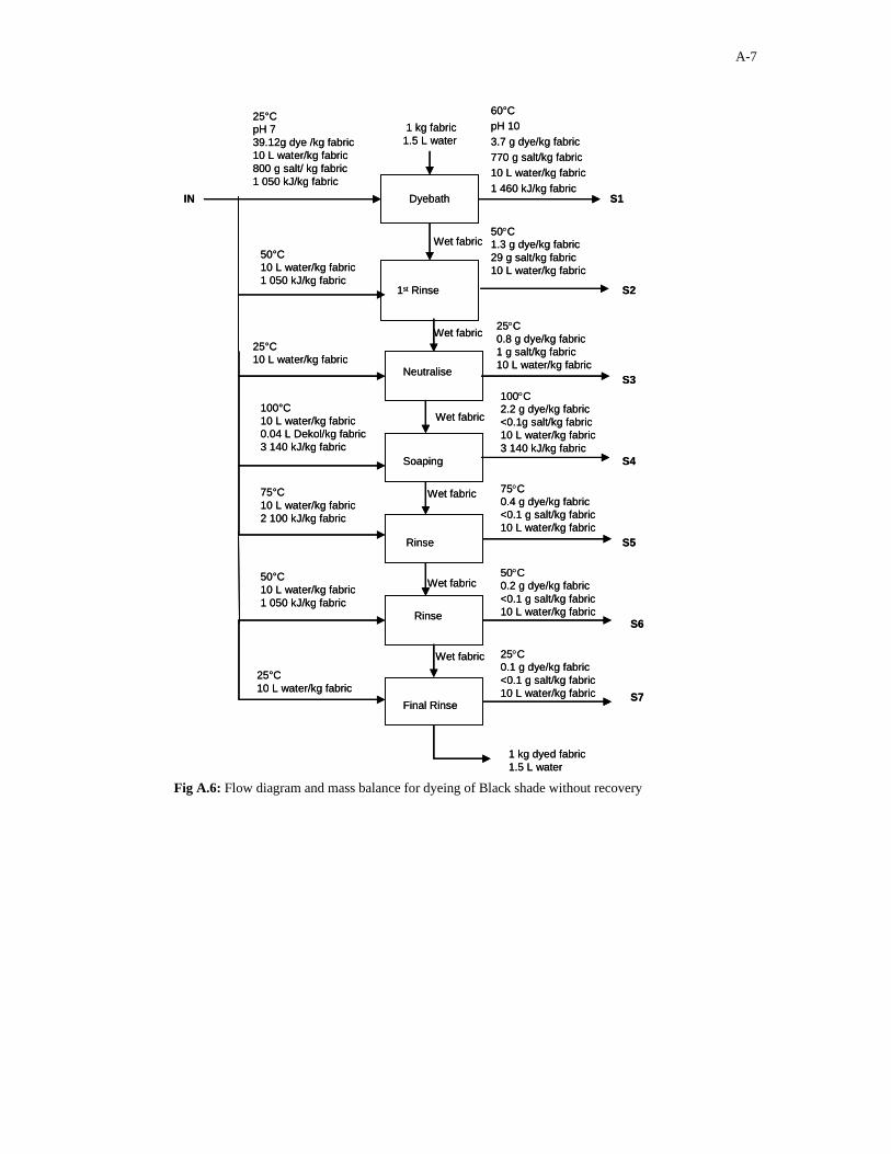
A-7

25°C pH 739.12g dye /kg fabric10 L water/kg fabric800 g salt/ kg fabric1 050 kJ/kg fabric

60°CpH 103.7 g dye/kg fabric770 g salt/kg fabric10 L water/kg fabric1 460 kJ/kg fabric

1st Rinse

Final Rinse

Dyebath

50°C1.3 g dye/kg fabric29 g salt/kg fabric10 L water/kg fabric

75°C0.4 g dye/kg fabric<0.1 g salt/kg fabric10 L water/kg fabric

IN

1 kg fabric1.5 L water

Soaping

S2

S3

S5

S1

50°C10 L water/kg fabric1 050 kJ/kg fabric

Wet fabric

Wet fabric

Wet fabric75°C10 L water/kg fabric2 100 kJ/kg fabric

100°C10 L water/kg fabric0.04 L Dekol/kg fabric3 140 kJ/kg fabric

Wet fabric

1 kg dyed fabric1.5 L water

Wet fabric

100°C2.2 g dye/kg fabric<0.1g salt/kg fabric10 L water/kg fabric3 140 kJ/kg fabric

Neutralise

S4

25°C10 L water/kg fabric

25°C0.8 g dye/kg fabric1 g salt/kg fabric10 L water/kg fabric

Wet fabric

Rinse

Rinse

S6

S7

50°C10 L water/kg fabric1 050 kJ/kg fabric

25°C10 L water/kg fabric

50°C0.2 g dye/kg fabric<0.1 g salt/kg fabric10 L water/kg fabric

25°C0.1 g dye/kg fabric<0.1 g salt/kg fabric10 L water/kg fabric

25°C pH 739.12g dye /kg fabric10 L water/kg fabric800 g salt/ kg fabric1 050 kJ/kg fabric

60°CpH 103.7 g dye/kg fabric770 g salt/kg fabric10 L water/kg fabric1 460 kJ/kg fabric

1st Rinse

Final Rinse

Dyebath

50°C1.3 g dye/kg fabric29 g salt/kg fabric10 L water/kg fabric

75°C0.4 g dye/kg fabric<0.1 g salt/kg fabric10 L water/kg fabric

IN

1 kg fabric1.5 L water

Soaping

S2

S3

S5

S1

50°C10 L water/kg fabric1 050 kJ/kg fabric

Wet fabric

Wet fabric

Wet fabric75°C10 L water/kg fabric2 100 kJ/kg fabric

100°C10 L water/kg fabric0.04 L Dekol/kg fabric3 140 kJ/kg fabric

Wet fabric

1 kg dyed fabric1.5 L water

Wet fabric

100°C2.2 g dye/kg fabric<0.1g salt/kg fabric10 L water/kg fabric3 140 kJ/kg fabric

Neutralise

S4

25°C10 L water/kg fabric

25°C0.8 g dye/kg fabric1 g salt/kg fabric10 L water/kg fabric

Wet fabric

Rinse

Rinse

S6

S7

50°C10 L water/kg fabric1 050 kJ/kg fabric

25°C10 L water/kg fabric

50°C0.2 g dye/kg fabric<0.1 g salt/kg fabric10 L water/kg fabric

25°C0.1 g dye/kg fabric<0.1 g salt/kg fabric10 L water/kg fabric

Fig A.6: Flow diagram and mass balance for dyeing of Black shade without recovery

A-8

25°C pH 734.64g dye /kg fabric10 L water/kg fabric500 g salt/ kg fabric1 050 kJ/kg fabric

60°CpH 102.7 g dye/kg fabric480 g salt/kg fabric10 L water/kg fabric1 460 kJ/kg fabric

1st Rinse

Final Rinse

Dyebath

25°C0.95 g dye/kg fabric19 g salt/kg fabric10 L water/kg fabric

25°C0.84 g dye/kg fabric<0.1 g salt/kg fabric10 L water/kg fabric

IN

1 kg fabric1.5 L water

Soaping

S2

S3

S5

S1

25°C10 L water/kg fabric

Wet fabric

Wet fabric

Wet fabric25°C10 L water/kg fabric

100°C10 L water/kg fabric0.04 L Dekol/kg fabric3 140 kJ/kg fabric

Wet fabric1 kg dyed fabric1.5 L water

Wet fabric

100°C1.92 g dye/kg fabric<0.1g salt/kg fabric10 L water/kg fabric3 140 kJ/kg fabric

Neutralise

S4

25°C10 L water/kg fabric

25°C0.9 g dye/kg fabric1 g salt/kg fabric10 L water/kg fabric

25°C pH 734.64g dye /kg fabric10 L water/kg fabric500 g salt/ kg fabric1 050 kJ/kg fabric

60°CpH 102.7 g dye/kg fabric480 g salt/kg fabric10 L water/kg fabric1 460 kJ/kg fabric

1st Rinse

Final Rinse

Dyebath

25°C0.95 g dye/kg fabric19 g salt/kg fabric10 L water/kg fabric

25°C0.84 g dye/kg fabric<0.1 g salt/kg fabric10 L water/kg fabric

IN

1 kg fabric1.5 L water

Soaping

S2

S3

S5

S1

25°C10 L water/kg fabric

Wet fabric

Wet fabric

Wet fabric25°C10 L water/kg fabric

100°C10 L water/kg fabric0.04 L Dekol/kg fabric3 140 kJ/kg fabric

Wet fabric1 kg dyed fabric1.5 L water

Wet fabric

100°C1.92 g dye/kg fabric<0.1g salt/kg fabric10 L water/kg fabric3 140 kJ/kg fabric

Neutralise

S4

25°C10 L water/kg fabric

25°C0.9 g dye/kg fabric1 g salt/kg fabric10 L water/kg fabric

Fig A.7: Flow diagram and mass balance for dyeing of Turquoise shade without recovery

A-9

25°C pH 5.5 to 6.59.45 g dye /kg fabric10 L water/kg fabric600 g salt/ kg fabric1 050 kJ/kg fabric

80°CpH 100.65 g dye/kg fabric565 g salt/kg fabric10 L water/kg fabric1 880 kJ/kg fabric

1st Rinse

Final Rinse

Dyebath

100°C0.31 g dye/kg fabric28 g salt/kg fabric10 L water/kg fabric3 140 kJ/kg fabric

25°C0.24 g dye/kg fabric<0.1 g salt/kg fabric10 L water/kg fabric

IN

1 kg fabric1.5 L water

Soaping

S2

S3

S5

S1

100°C10 L water/kg fabric3 140 kJ/kg fabric

Wet fabric

Wet fabric

Wet fabric25°C10 L water/kg fabric

100°C10 L water/kg fabric0.04 L Dekol/kg fabric3 140 kJ/kg fabric

Wet fabric1 kg dyed fabric1.5 L water

Wet fabric

100°C0.34 g dye/kg fabric<0.1g salt/kg fabric10 L water/kg fabric3 140 kJ/kg fabric

2nd Rinse

S4

25°C10 L water/kg fabric

25°C0.27 g dye/kg fabric~7 g salt/kg fabric10 L water/kg fabric

25°C pH 5.5 to 6.59.45 g dye /kg fabric10 L water/kg fabric600 g salt/ kg fabric1 050 kJ/kg fabric

80°CpH 100.65 g dye/kg fabric565 g salt/kg fabric10 L water/kg fabric1 880 kJ/kg fabric

1st Rinse

Final Rinse

Dyebath

100°C0.31 g dye/kg fabric28 g salt/kg fabric10 L water/kg fabric3 140 kJ/kg fabric

25°C0.24 g dye/kg fabric<0.1 g salt/kg fabric10 L water/kg fabric

IN

1 kg fabric1.5 L water

Soaping

S2

S3

S5

S1

100°C10 L water/kg fabric3 140 kJ/kg fabric

Wet fabric

Wet fabric

Wet fabric25°C10 L water/kg fabric

100°C10 L water/kg fabric0.04 L Dekol/kg fabric3 140 kJ/kg fabric

Wet fabric1 kg dyed fabric1.5 L water

Wet fabric

100°C0.34 g dye/kg fabric<0.1g salt/kg fabric10 L water/kg fabric3 140 kJ/kg fabric

2nd Rinse

S4

25°C10 L water/kg fabric

25°C0.27 g dye/kg fabric~7 g salt/kg fabric10 L water/kg fabric

Fig A.8: Flow diagram and mass balance for dyeing of Beige shade without recovery

B-1

APPENDIX B

ACTIVATED CARBON ADSORPTION Appendix B contains experimental data and calculations for equilibrium test shown in Chapter 4.

B-2

Table B.1: Adsorption isotherm data for the different time interval for all the shades at 60˚C Shade Hours Mass of carbon (g) 1 1 2 2 3 3 4 4 5 5 Navy 1 ADMI (-) 74531 75244 7382 7993 463 452 276 274 194 193 X/M (mg dye/g carbon) 191 190 148 148 102 102 77 77 62 62 C (mg dye/L) 1464 1467 145 157 9.10 8.87 5.42 5.39 3.81 3.79 2 ADMI (-) 34771 39760 3513 3716 227 221 138 133 99 95 X/M (mg dye/g carbon) 253 246 151 151 103 103 77 77 62 62 C (mg dye/L) 683 781 69 73 4.46 4.34 2.71 2.61 1.94 1.87 3 ADMI (-) 35585 39098 3309 3818 227 225 137 134 96 97 X/M (mg dye/g carbon) 252 247 151 151 103 103 77 77 62 62 C (mg dye/L) 699 768 65 75 4.45 4.42 2.69 2.64 1.89 1.91 4 ADMI (-) 35178 39429 3411 3767 227 223 137 134 97 96 X/M (mg dye/g carbon) 253 246 151 151 103 103 77 77 62 62 C (mg dye/L) 691 775 67 74 4.46 4.38 2.70 2.63 1.92 1.89 Black 1 ADMI (-) 38920 39358 3781 3462 362 379 216 214 250 270 X/M (mg dye/g carbon) 235 234 153 153 104 104 78 78 62 62 C (mg dye/L) 978 989 95 87 9.10 9.52 5.42 5.39 6.28 6.79 2 ADMI (-) 17424 17502 1185 1230 197 181 140 147 121 129 X/M (mg dye/g carbon) 278 278 155 155 104 104 78 78 63 63 C (mg dye/L) 438 440 30 31 4.95 4.55 3.52 3.69 3.04 3.24 3 ADMI (-) 17629 17351 1114 1154 194 185 145 144 127 124 X/M (mg dye/g carbon) 278 278 155 155 104 104 78 78 63 63 C (mg dye/L) 443 436 28 29 4.87 4.65 3.65 3.61 3.18 3.12 4 ADMI (-) 17530 17430 1154 1194 195 183 143 145 124 127 X/M (mg dye/g carbon) 278 278 155 155 104 104 78 78 63 63 C (mg dye/L) 441 438 29 30 4.91 4.6 3.59 3.65 3.11 3.18 Beige 1 ADMI (-) 1278 1260 528 507 224 235 185 194 149 142 X/M (mg dye/g carbon) 31 32 29 29 23 22 17 17 14 14 C (mg dye/L) 559 551 231 222 98 103 81 85 65 62 2 ADMI (-) 658 634 256 250 110 115 96 90 76 74 X/M (mg dye/g carbon) 53 53 33 33 24 24 18 18 15 15 C (mg dye/L) 288 277 112 109 48 50 42 39 33 32 3 ADMI (-) 647 651 244 263 119 117 103 87 71 75 X/M (mg dye/g carbon) 53 53 34 33 24 24 18 18 15 15 C (mg dye/L) 283 285 107 115 52 51 45 38 31 33 4 ADMI (-) 652 642 250 256 114 115 99 88 73 74 X/M (mg dye/g carbon) 53 53 33 33 24 24 18 18 15 15 C (mg dye/L) 285 281 109 112 50 50 43 38 32 32

B-3

Shade Hours Mass of carbon (g) 1 1 2 2 3 3 4 4 5 5 Turquoise 1 ADMI (-) 13378 13511 1199 1235 339 375 206 218 170 157 X/M (mg dye/g carbon) 189 188 135 134 92 92 69 69 55 55 C (mg dye/L) 1105 1116 99 102 28 31 17 18 14 13 2 ADMI (-) 8162 7998 616 627 168 165 103 106 75 79 X/M (mg dye/g carbon) 223 224 137 136 92 92 69 69 55 55 C (mg dye/L) 674 661 51 52 14 14 8.51 8.76 6.20 6.53 3 ADMI (-) 8101 8126 593 642 182 157 105 105 78 76 X/M (mg dye/g carbon) 224 223 137 136 92 92 69 69 55 55 C (mg dye/L) 669 671 49 53 15 13 9 9 6 6 4 ADMI (-) 8132 8065 605 636 176 163 104 105 76 78 X/M (mg dye/g carbon) 223 224 137 136 92 92 69 69 55 55 C (mg dye/L) 672 666 50 53 15 14 9 9 6 6

B-4

Navy Shade Dye Class: Drimarene HF

Dye Chemistry: Trifluoropyrimidine (TFP)

Electrolyte: Sodium chloride

Initial ADMI: 196000

Initial dye mass: 0.385 g /100 mL

Solution volume used: 80 mL

Table B.2: Adsorption isotherm data for the Navy shade Parameters Mass of carbon (g) 1 1 2 2 3 3 4 4 5 5 20˚C ADMI (-) 72839 71633 6228 6440 340 329 207 211 164 160 X/M (mg dye/g carbon) 194 195 149 149 102 102 77 77 62 62 C (mg dye/L) 1431 1407 122 127 6.68 6.46 4.07 4.14 3.22 3.14 60˚C ADMI (-) 34784 39744 3531 3726 227 221 138 133 99 95 X/M (mg dye/g carbon) 253 246 151 151 103 103 77 77 62 62 C (mg dye/L) 683 781 69 73 4.46 4.34 2.71 2.61 1.94 1.87 80˚C ADMI (-) 22800 22432 1783 1919 147 144 83 82 59 60 X/M (mg dye/g carbon) 272 273 153 152 103 103 77 77 62 62 C (mg dye/L) 448 441 35 38 2.89 2.83 1.63 1.61 1.16 1.18 100˚C ADMI (-) 6937 6765 519 570 97 94 40 41 34 36 pH 11 X/M (mg dye/g carbon) 297 297 154 154 103 103 77 77 62 62 7 g NaCl C (mg dye/L) 136 133 10 11 1.95 1.81 0.79 0.81 0.68 0.71 pH 7 ADMI (-) 13602 13264 953 971 225 209 132 137 62 61 X/M (mg dye/g carbon) 287 287 153 153 103 103 77 77 62 62 C (mg dye/L) 267 261 19 19 4.42 4.11 2.59 2.69 1.22 1.20 pH 4 ADMI (-) 5530 5319 280 293 65 69 36 37 29 27 X/M (mg dye/g carbon) 299 300 154 154 103 103 77 77 62 62 C (mg dye/L) 109 104 5.50 5.76 1.28 1.36 0.71 0.73 0.57 0.53 4 g NaCl ADMI (-) 13602 13264 953 971 225 209 132 137 62 61 X/M (mg dye/g carbon) 287 287 153 153 103 103 77 77 62 62 C (mg dye/L) 267 261 19 19 4.42 4.11 2.59 2.69 1.22 1.20 10 g NaCl ADMI (-) 3560 3304 285 269 59 49 28 25 16 11 X/M (mg dye/g carbon) 302 303 154 154 103 103 77 77 62 62 C (mg dye/L) 70 65 5.60 5.28 1.16 0.96 0.55 0.49 0.31 0.22

B-5

Black Shade Dye Class: Cibacron S

Dye Chemistry: Undivulged

Electrolyte: Sodium sulphate

Initial ADMI: 155680

Initial dye mass: 0.391 g /100 mL

Solution volume: 80 mL

Table B.3: Adsorption isotherm data for the Black shade Parameters Mass of carbon (g) 1 1 2 2 3 3 4 4 5 5 20˚C ADMI (-) 29040 29270 2193 2154 234 207 195 186 143 148 X/M (mg dye/g carbon) 255 254 154 154 104 104 78 78 63 63 C (mg dye/L) 730 736 55 54 5.88 5.20 4.90 4.67 3.59 3.72 60˚C ADMI (-) 17424 17502 1185 1230 197 181 140 147 121 129 X/M (mg dye/g carbon) 278 278 155 155 104 104 78 78 63 63 C (mg dye/L) 438 440 30 31 4.95 4.55 3.52 3.69 3.04 3.24 80˚C ADMI (-) 13956 13980 657 738 146 140 98 99 67 69 X/M (mg dye/g carbon) 285 285 156 156 104 104 78 78 63 63 C (mg dye/L) 351 351 17 19 3.67 3.52 2.46 2.49 1.68 1.73 100˚C ADMI (-) 7556 7603 429 432 90 93 68 69 32 38 pH 11 X/M (mg dye/g carbon) 298 298 156 156 104 104 78 78 63 63 7 g Na2SO4 C (mg dye/L) 190 191 11 11 2.26 2.34 1.71 1.73 0.80 0.95 pH 7 ADMI (-) 6889 6675 361 372 75 79 66 68 30 36 X/M (mg dye/g carbon) 299 300 156 156 104 104 78 78 63 63 C (mg dye/L) 173 168 9.07 9.35 1.88 1.99 1.66 1.71 0.75 0.90 pH 4 ADMI (-) 6151 5962 290 296 58 57 34 36 17 20 X/M (mg dye/g carbon) 301 301 156 156 104 104 78 78 63 63 C (mg dye/L) 155 150 7.29 7.44 1.46 1.43 0.85 0.90 0.43 0.50 4 g Na2SO4 ADMI (-) 12187 12453 890 894 224 228 139 137 64 62 X/M (mg dye/g carbon) 288 288 156 156 104 104 78 78 63 63 C (mg dye/L) 306 313 22 22 5.63 5.73 3.49 3.44 1.61 1.56 10 g Na2SO4 ADMI (-) 4703 4745 181 183 40 42 30 35 18 20 X/M (mg dye/g carbon) 304 303 156 156 104 104 78 78 63 63 C (mg dye/L) 118 119 4.55 4.60 1.01 1.06 0.75 0.88 0.45 0.50

B-6

Beige Shade Dye Class: Procion HE

Dye Chemistry: Monochlorotriazine

Electrolyte: Sodium chloride

Initial ADMI: 2160

Initial dye mass: 0.095 g /100 mL

Solution volume: 80 mL

Table B.4: Adsorption isotherm data for the Beige shade Parameters mass of carbon (g) 1 1 2 2 3 3 4 4 5 5 20˚C ADMI (-) 754 738 429 418 158 145 135 133 95 92 X/M (mg dye/g carbon) 49 50 30 30 23 24 18 18 14 14 C (mg dye/L) 330 323 188 183 69 63 59 58 42 40 60˚C ADMI (-) 658 634 256 250 110 115 96 90 76 74 X/M (mg dye/g carbon) 53 53 33 33 24 24 18 18 15 15 C (mg dye/L) 288 277 112 109 48 50 42 39 33 32 80˚C ADMI (-) 518 546 108 105 54 50 43 40 37 34 X/M (mg dye/g carbon) 57 56 36 36 25 25 19 19 15 15 C (mg dye/L) 227 239 47 46 24 22 19 18 16 15 100˚C ADMI (-) 156 148 78 70 36 35 21 20 18 19 pH 11 X/M (mg dye/g carbon) 70 70 36 37 25 25 19 19 15 15 7 g NaCl C (mg dye/L) 68 65 34 31 16 15 9.19 8.75 7.88 8.31 pH 7 ADMI (-) 120 126 50 52 25 22 19 18 16 17 X/M (mg dye/g carbon) 71 71 37 37 25 25 19 19 15 15 C (mg dye/L) 53 55 220 23 11 9.63 8.31 7.88 7.00 7.44 pH 4 ADMI (-) 96 91 38 37 19 18 17 16 16 15 X/M (mg dye/g carbon) 72 72 37 37 25 25 19 19 15 15 C (mg dye/L) 42 40 17 16 8.31 7.88 7.44 7.00 7.00 6.56 4 g NaCl ADMI (-) 208 200 143 146 59 57 38 35 24 25 X/M (mg dye/g carbon) 68 69 35 35 25 25 19 19 15 15 C (mg dye/L) 91 88 63 64 26 25 17 15 11 11 10 g NaCl ADMI (-) 103 101 51 49 24 23 14 13 12 13 X/M (mg dye/g carbon) 72 72 37 37 25 25 19 19 15 15 C (mg dye/L) 45 44 22 21 11 10 6.13 5.69 5.25 5.69

B-7

Turquoise Shade Dye Class: Remazol and Levafix

Dye Chemistry: Vinylsulphone

Electrolyte: Sodium sulphate

Initial ADMI: 41936

Initial dye mass: 0.346 g /100 mL

Solution volume: 80 mL

Table B.5: Adsorption isotherm data for the Turquoise shade Parameters Mass of carbon (g) 1 1 2 2 3 3 4 4 5 5 20˚C ADMI (-) 10582 10494 1176 1212 305 300 156 159 122 130 X/M (mg dye/g carbon) 207 208 135 135 92 92 69 69 55 55 C (mg dye/L) 874 867 97 100 25 25 13 13 11 11 60˚C ADMI (-) 8162 7998 616 627 168 165 103 106 75 79 X/M (mg dye/g carbon) 223 224 137 136 92 92 69 69 55 55 C (mg dye/L) 674 661 51 52 14 14 8.51 8.76 6.20 6.53 80˚C ADMI (-) 4452 4341 336 375 93 90 68 69 46 45 X/M (mg dye/g carbon) 248 248 137 137 92 92 69 69 55 55 C (mg dye/L) 368 359 28 31 7.68 7.43 5.62 5.70 3.80 3.72 100˚C ADMI (-) 1484 1447 112 125 51 50 26 23 20 21 pH 11 X/M (mg dye/g carbon) 267 268 138 138 92 92 69 69 55 55 7 g Na2SO4 C (mg dye/L) 123 120 9.25 10 4.21 4.13 2.15 1.90 1.65 1.73 pH 7 ADMI (-) 1188 1175 91 95 41 45 18 19 16 17 X/M (mg dye/g carbon) 269 269 138 138 92 92 69 69 55 55 C (mg dye/L) 98 97 7.52 7.85 3.39 3.72 1.49 1.57 1.32 1.40 pH 4 ADMI (-) 936 902 73 77 26 28 14 15 11 12 X/M (mg dye/g carbon) 271 271 138 138 92 92 69 69 55 55 C (mg dye/L) 77 75 6.03 6.36 2.15 2.31 1.16 1.24 0.91 0.99 4 g Na2SO4 ADMI (-) 2442 2381 184 206 104 102 53 58 43 45 X/M (mg dye/g carbon) 261 261 138 138 92 92 69 69 55 55 C (mg dye/L) 202 197 15 17 8.59 8.43 4.38 4.79 3.55 3.72 10 g Na2SO4 ADMI (-) 915 892 69 67 31 39 17 18 15 13 X/M (mg dye/g carbon) 271 271 138 138 92 92 69 69 55 55 C (mg dye/L) 76 74 5.70 5.53 2.56 3.22 1.40 1.49 1.24 1.07

B-8

25°C pH 738.5g dye /kg fabric

10 L water/kg fabric700 g salt/ kg fabric1 050 kJ/kg fabric

60°CpH 114.3 g dye/kg fabric682 g salt/kg fabric

10 L water/kg fabric1 460 kJ/kg fabric

1st Rinse

Final Rinse

Activated carbon

Dyebath

25°C

1.2 g dye/kg fabric~18 g salt/kg fabric10 L water/kg fabric

100°C

1.8 g dye/kg fabric<0.1g salt/kg fabric10 L water/kg fabric3 140 kJ/kg fabric

25°C0.8 g dye/kg fabric<0.1 g salt/kg fabric10 L water/kg fabric

IN

Savings60°C682 g salt/kg fabric10 L water/ kg fabric1 460 kJ/kg fabric

1 kg fabric1.5 L water

Soaping

S2

S3

S4

S1

25°C10 L water/kg fabric

Wet fabric

Wet fabric

Wet fabric

25°C10 L water/kg fabric

100°C10 L water/kg fabric0.04 L Dekol/kg fabric

3 140 kJ/kg fabric

Neutralize to pH 7

Dyebath

Wet fabric

1 kg dyed fabric1.5 L water

25°C pH 738.5g dye /kg fabric

10 L water/kg fabric700 g salt/ kg fabric1 050 kJ/kg fabric

60°CpH 114.3 g dye/kg fabric682 g salt/kg fabric

10 L water/kg fabric1 460 kJ/kg fabric

1st Rinse

Final Rinse

Activated carbon

Dyebath

25°C

1.2 g dye/kg fabric~18 g salt/kg fabric10 L water/kg fabric

100°C

1.8 g dye/kg fabric<0.1g salt/kg fabric10 L water/kg fabric3 140 kJ/kg fabric

25°C0.8 g dye/kg fabric<0.1 g salt/kg fabric10 L water/kg fabric

IN

Savings60°C682 g salt/kg fabric10 L water/ kg fabric1 460 kJ/kg fabric

1 kg fabric1.5 L water

Soaping

S2

S3

S4

S1

25°C10 L water/kg fabric

Wet fabric

Wet fabric

Wet fabric

25°C10 L water/kg fabric

100°C10 L water/kg fabric0.04 L Dekol/kg fabric

3 140 kJ/kg fabric

Neutralize to pH 7

Dyebath

Wet fabric

1 kg dyed fabric1.5 L water

Fig B.1: Flow diagram and mass balance for dyeing of Navy shade with recovery

B-9

25°C pH 739.12g dye /kg fabric10 L water/kg fabric800 g salt/ kg fabric1 050 kJ/kg fabric

60°CpH 103.7 g dye/kg fabric770 g salt/kg fabric10 L water/kg fabric1 460 kJ/kg fabric

1st Rinse

Final Rinse

Activated carbonDyebath

50°C1.3 g dye/kg fabric29 g salt/kg fabric10 L water/kg fabric

75°C0.4 g dye/kg fabric<0.1 g salt/kg fabric10 L water/kg fabric

IN

Savings60°C770 g salt/kg fabric10 L water/ kg fabric1 460 kJ/kg fabric

1 kg fabric1.5 L water

Soaping

S2

S3

S5

S1

50°C10 L water/kg fabric1 050 kJ/kg fabric

Wet fabric

Wet fabric

Wet fabric75°C10 L water/kg fabric2 100 kJ/kg fabric

100°C10 L water/kg fabric0.04 L Dekol/kg fabric3 140 kJ/kg fabric

Neutralize to pH 7

Dyebath

Wet fabric

1 kg dyed fabric1.5 L water

Wet fabric

100°C2.2 g dye/kg fabric<0.1g salt/kg fabric10 L water/kg fabric3 140 kJ/kg fabric

Neutralise

S4

25°C10 L water/kg fabric

25°C0.8 g dye/kg fabric1 g salt/kg fabric10 L water/kg fabric

Wet fabric

Rinse

Rinse

S6

S7

50°C10 L water/kg fabric1 050 kJ/kg fabric

25°C10 L water/kg fabric

50°C0.2 g dye/kg fabric<0.1 g salt/kg fabric10 L water/kg fabric

25°C0.1 g dye/kg fabric<0.1 g salt/kg fabric10 L water/kg fabric

25°C pH 739.12g dye /kg fabric10 L water/kg fabric800 g salt/ kg fabric1 050 kJ/kg fabric

60°CpH 103.7 g dye/kg fabric770 g salt/kg fabric10 L water/kg fabric1 460 kJ/kg fabric

1st Rinse

Final Rinse

Activated carbonDyebath

50°C1.3 g dye/kg fabric29 g salt/kg fabric10 L water/kg fabric

75°C0.4 g dye/kg fabric<0.1 g salt/kg fabric10 L water/kg fabric

IN

Savings60°C770 g salt/kg fabric10 L water/ kg fabric1 460 kJ/kg fabric

1 kg fabric1.5 L water

Soaping

S2

S3

S5

S1

50°C10 L water/kg fabric1 050 kJ/kg fabric

Wet fabric

Wet fabric

Wet fabric75°C10 L water/kg fabric2 100 kJ/kg fabric

100°C10 L water/kg fabric0.04 L Dekol/kg fabric3 140 kJ/kg fabric

Neutralize to pH 7

Dyebath

Wet fabric

1 kg dyed fabric1.5 L water

Wet fabric

100°C2.2 g dye/kg fabric<0.1g salt/kg fabric10 L water/kg fabric3 140 kJ/kg fabric

Neutralise

S4

25°C10 L water/kg fabric

25°C0.8 g dye/kg fabric1 g salt/kg fabric10 L water/kg fabric

Wet fabric

Rinse

Rinse

S6

S7

50°C10 L water/kg fabric1 050 kJ/kg fabric

25°C10 L water/kg fabric

50°C0.2 g dye/kg fabric<0.1 g salt/kg fabric10 L water/kg fabric

25°C0.1 g dye/kg fabric<0.1 g salt/kg fabric10 L water/kg fabric

Fig B.2: Flow diagram and mass balance for dyeing of Black shade with recovery

B-10

25°C pH 5.5 to 6.59.45 g dye /kg fabric10 L water/kg fabric600 g salt/ kg fabric1 050 kJ/kg fabric

80°CpH 100.65 g dye/kg fabric565 g salt/kg fabric10 L water/kg fabric1 880 kJ/kg fabric

1st Rinse

Final Rinse

Activated carbonDyebath

100°C0.31 g dye/kg fabric28 g salt/kg fabric10 L water/kg fabric3 140 kJ/kg fabric

25°C0.24 g dye/kg fabric<0.1 g salt/kg fabric10 L water/kg fabric

IN

Savings60°C565 g salt/kg fabric10 L water/ kg fabric1 880 kJ/kg fabric

1 kg fabric1.5 L water

Soaping

S2

S3

S5

S1

100°C10 L water/kg fabric3 140 kJ/kg fabric

Wet fabric

Wet fabric

Wet fabric25°C10 L water/kg fabric

100°C10 L water/kg fabric0.04 L Dekol/kg fabric3 140 kJ/kg fabric

Neutralize to pH 5.5 to 6.5

Dyebath

Wet fabric1 kg dyed fabric1.5 L water

Wet fabric

100°C0.34 g dye/kg fabric<0.1g salt/kg fabric10 L water/kg fabric3 140 kJ/kg fabric

2nd Rinse

S4

25°C10 L water/kg fabric

25°C0.27 g dye/kg fabric~7 g salt/kg fabric10 L water/kg fabric

25°C pH 5.5 to 6.59.45 g dye /kg fabric10 L water/kg fabric600 g salt/ kg fabric1 050 kJ/kg fabric

80°CpH 100.65 g dye/kg fabric565 g salt/kg fabric10 L water/kg fabric1 880 kJ/kg fabric

1st Rinse

Final Rinse

Activated carbonDyebath

100°C0.31 g dye/kg fabric28 g salt/kg fabric10 L water/kg fabric3 140 kJ/kg fabric

25°C0.24 g dye/kg fabric<0.1 g salt/kg fabric10 L water/kg fabric

IN

Savings60°C565 g salt/kg fabric10 L water/ kg fabric1 880 kJ/kg fabric

1 kg fabric1.5 L water

Soaping

S2

S3

S5

S1

100°C10 L water/kg fabric3 140 kJ/kg fabric

Wet fabric

Wet fabric

Wet fabric25°C10 L water/kg fabric

100°C10 L water/kg fabric0.04 L Dekol/kg fabric3 140 kJ/kg fabric

Neutralize to pH 5.5 to 6.5

Dyebath

Wet fabric1 kg dyed fabric1.5 L water

Wet fabric

100°C0.34 g dye/kg fabric<0.1g salt/kg fabric10 L water/kg fabric3 140 kJ/kg fabric

2nd Rinse

S4

25°C10 L water/kg fabric

25°C0.27 g dye/kg fabric~7 g salt/kg fabric10 L water/kg fabric

Fig B.3: Flow diagram and mass balance for dyeing of Turquoise shade with recovery

B-11

25°C pH 5.5 to 6.59.45 g dye /kg fabric10 L water/kg fabric600 g salt/ kg fabric1 050 kJ/kg fabric

80°CpH 100.65 g dye/kg fabric565 g salt/kg fabric10 L water/kg fabric1 880 kJ/kg fabric

1st Rinse

Final Rinse

Activated carbonDyebath

100°C0.31 g dye/kg fabric28 g salt/kg fabric10 L water/kg fabric3 140 kJ/kg fabric

25°C0.24 g dye/kg fabric<0.1 g salt/kg fabric10 L water/kg fabric

IN

Savings60°C565 g salt/kg fabric10 L water/ kg fabric1 880 kJ/kg fabric

1 kg fabric1.5 L water

Soaping

S2

S3

S5

S1

100°C10 L water/kg fabric3 140 kJ/kg fabric

Wet fabric

Wet fabric

Wet fabric25°C10 L water/kg fabric

100°C10 L water/kg fabric0.04 L Dekol/kg fabric3 140 kJ/kg fabric

Neutralize to pH 5.5 to 6.5

Dyebath

Wet fabric1 kg dyed fabric1.5 L water

Wet fabric

100°C0.34 g dye/kg fabric<0.1g salt/kg fabric10 L water/kg fabric3 140 kJ/kg fabric

2nd Rinse

S4

25°C10 L water/kg fabric

25°C0.27 g dye/kg fabric~7 g salt/kg fabric10 L water/kg fabric

25°C pH 5.5 to 6.59.45 g dye /kg fabric10 L water/kg fabric600 g salt/ kg fabric1 050 kJ/kg fabric

80°CpH 100.65 g dye/kg fabric565 g salt/kg fabric10 L water/kg fabric1 880 kJ/kg fabric

1st Rinse

Final Rinse

Activated carbonDyebath

100°C0.31 g dye/kg fabric28 g salt/kg fabric10 L water/kg fabric3 140 kJ/kg fabric

25°C0.24 g dye/kg fabric<0.1 g salt/kg fabric10 L water/kg fabric

IN

Savings60°C565 g salt/kg fabric10 L water/ kg fabric1 880 kJ/kg fabric

1 kg fabric1.5 L water

Soaping

S2

S3

S5

S1

100°C10 L water/kg fabric3 140 kJ/kg fabric

Wet fabric

Wet fabric

Wet fabric25°C10 L water/kg fabric

100°C10 L water/kg fabric0.04 L Dekol/kg fabric3 140 kJ/kg fabric

Neutralize to pH 5.5 to 6.5

Dyebath

Wet fabric1 kg dyed fabric1.5 L water

Wet fabric

100°C0.34 g dye/kg fabric<0.1g salt/kg fabric10 L water/kg fabric3 140 kJ/kg fabric

2nd Rinse

S4

25°C10 L water/kg fabric

25°C0.27 g dye/kg fabric~7 g salt/kg fabric10 L water/kg fabric

Fig B.4: Flow diagram and mass balance for dyeing of Beige shade with recovery

Energy Calculations Liquor ratio= 10 L/kg fabric

Water feed temperature = 25˚C

Effluent temperature = 60˚C

Enthalpy water at 25˚C = 105 kJ/kg (Smith et al., 2001)

Enthalpy water at 60˚C = 252 kJ/kg

Enthalpy water at 100˚C = 420 kJ/kg

Recoverable Energy at 60˚C = 10 L/kg fabric . (252-105) kJ/kg . 1kg/L

= 1 470 kJ

Recoverable Energy at 100˚C = 10 L/kg fabric . (420-105) kJ/kg . 1kg/L

= 3 150 kJ

Effluent Energy savings= 1 470 kJ

1 470 kJ+3 150 kJ= 0.32 32%∴

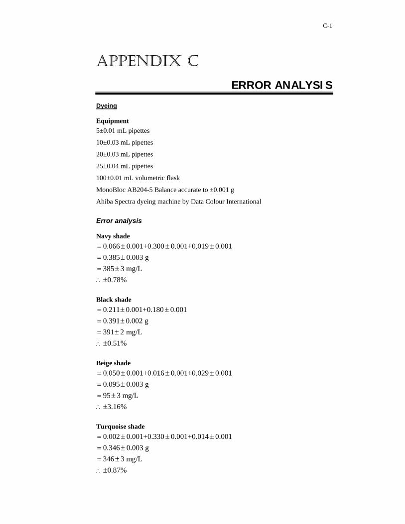
C-1

APPENDIX C

ERROR ANALYSIS

Dyeing

Equipment 5±0.01 mL pipettes

10±0.03 mL pipettes

20±0.03 mL pipettes

25±0.04 mL pipettes

100±0.01 mL volumetric flask

MonoBloc AB204-5 Balance accurate to ±0.001 g

Ahiba Spectra dyeing machine by Data Colour International

Error analysis

Navy shade 0.066 0.001+0.300 0.001+0.019 0.0010.385 0.003 g385 3 mg/L

0.78%

= ± ± ±= ±= ±∴±

Black shade 0.211 0.001+0.180 0.0010.391 0.002 g391 2 mg/L

0.51%

= ± ±= ±= ±∴±

Beige shade 0.050 0.001+0.016 0.001+0.029 0.0010.095 0.003 g95 3 mg/L

3.16%

= ± ± ±= ±= ±∴±

Turquoise shade 0.002 0.001+0.330 0.001+0.014 0.0010.346 0.003 g346 3 mg/L

0.87%

= ± ± ±= ±= ±∴±

C-2

Dye isotherms Equipment:

Grinding/pulverising equipment

Standard screen ASTM = 45µm

Oven set at 150˚C

Whatman No. 2 filter paper

10 x Filter funnels and stands

100±0.15 mL plastic measuring cylinders

MonoBloc AB204-5 Balance accurate to 0.001 g

Labcon temperature controller ±3˚C

Parvalux Electric motors model S15water bath with stirrers and 10 metal flasks

Cary 50 U/V Visible spectrophotometer, 1 mm cell

Error analysis:

Navy shade = 385 mg/L±3 mg/L

Black shade = 391 mg/L±2 mg/L

Beige shade = 95 mg/L±3 mg/L

Turquoise shade = 346 mg/L±3 mg/L

Column test

Equipment: Column with 26 mm diameter and 200 mm length

Standard screen ASTM = 1000µm and 720µm

Hot plate for boiling

10±0.02 mL plastic samples vials for collecting

5000±0.02 mL volumetric flasks for sample feeding

MonoBloc AB204-5 Balance accurate to 0.001 g

Julabo temperature controller ±1˚C

Cary 50 U/V Visible spectrophotometer, 1 mm cell

Error analysis

5 0.02 mL5 0.015 mg/L0.3%

= ±= ±∴

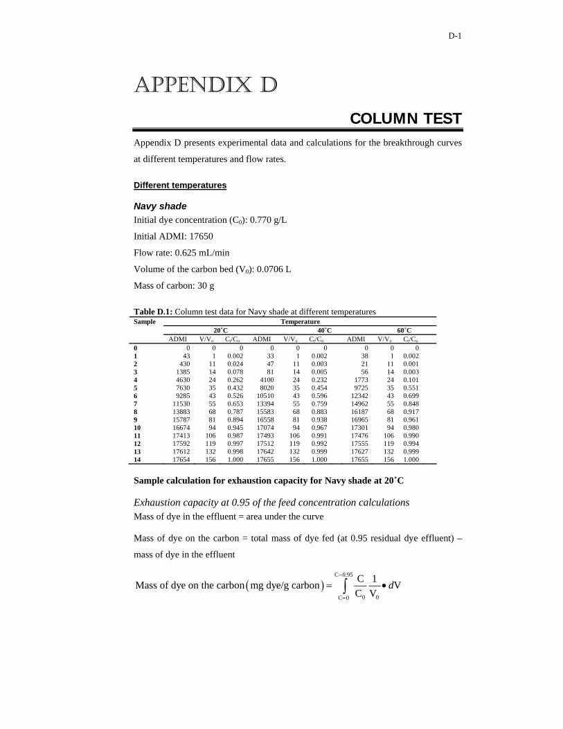
D-1

APPENDIX D

COLUMN TEST Appendix D presents experimental data and calculations for the breakthrough curves

at different temperatures and flow rates.

Different temperatures

Navy shade Initial dye concentration (C0): 0.770 g/L

Initial ADMI: 17650

Flow rate: 0.625 mL/min

Volume of the carbon bed (V0): 0.0706 L

Mass of carbon: 30 g

Table D.1: Column test data for Navy shade at different temperatures Temperature

20˚C 40˚C 60˚C Sample

ADMI V/Vo Ct/Co ADMI V/Vo Ct/Co ADMI V/Vo Ct/Co 0 0 0 0 0 0 0 0 0 0 1 43 1 0.002 33 1 0.002 38 1 0.002 2 430 11 0.024 47 11 0.003 21 11 0.001 3 1385 14 0.078 81 14 0.005 56 14 0.003 4 4630 24 0.262 4100 24 0.232 1773 24 0.101 5 7630 35 0.432 8020 35 0.454 9725 35 0.551 6 9285 43 0.526 10510 43 0.596 12342 43 0.699 7 11530 55 0.653 13394 55 0.759 14962 55 0.848 8 13883 68 0.787 15583 68 0.883 16187 68 0.917 9 15787 81 0.894 16558 81 0.938 16965 81 0.961 10 16674 94 0.945 17074 94 0.967 17301 94 0.980 11 17413 106 0.987 17493 106 0.991 17476 106 0.990 12 17592 119 0.997 17512 119 0.992 17555 119 0.994 13 17612 132 0.998 17642 132 0.999 17627 132 0.999 14 17654 156 1.000 17655 156 1.000 17655 156 1.000

Sample calculation for exhaustion capacity for Navy shade at 20˚C

Exhaustion capacity at 0.95 of the feed concentration calculations Mass of dye in the effluent = area under the curve

Mass of dye on the carbon = total mass of dye fed (at 0.95 residual dye effluent) –

mass of dye in the effluent

( )C 0.95

0 0C 0

C 1Mass of dye on the carbon mg dye/g carbon VC V

d=

=

= •∫

D-2

Total mass of dye fed at 0.95 of feed concentration

(94 0.0706)*(0.94 0.770)4.8 g dye4 800 mg dye30 g carbon

160 mg dye/g carbon

= • •=

=

=

Mass of dye in the effluent at 0.95 of feed concentration

1calculate using l b for rectangle and (l b) for traingle22.63 g dye2 633 mg dye30 g carbon

87 mg dye/g carbon

= × ×

=

=

=

Exhaustion capacity of dye at 0.95 of the feed concentration Mass of dye on the carbon = total mass of dye fed (at 0.95 residual dye effluent) –

mass of dye in the effluent

160 mg dye/g carbon-87 mg dye/g carbon=72 mg dye/g carbon=

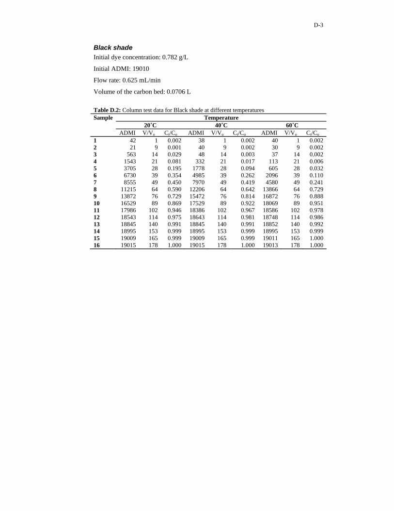
D-3

Black shade Initial dye concentration: 0.782 g/L

Initial ADMI: 19010

Flow rate: 0.625 mL/min

Volume of the carbon bed: 0.0706 L

Table D.2: Column test data for Black shade at different temperatures Temperature

20˚C 40˚C 60˚C Sample

ADMI V/Vo Ct/Co ADMI V/Vo Ct/Co ADMI V/Vo Ct/Co 1 42 1 0.002 38 1 0.002 40 1 0.002 2 21 9 0.001 40 9 0.002 30 9 0.002 3 563 14 0.029 48 14 0.003 37 14 0.002 4 1543 21 0.081 332 21 0.017 113 21 0.006 5 3705 28 0.195 1778 28 0.094 605 28 0.032 6 6730 39 0.354 4985 39 0.262 2096 39 0.110 7 8555 49 0.450 7970 49 0.419 4580 49 0.241 8 11215 64 0.590 12206 64 0.642 13866 64 0.729 9 13872 76 0.729 15472 76 0.814 16872 76 0.888 10 16529 89 0.869 17529 89 0.922 18069 89 0.951 11 17986 102 0.946 18386 102 0.967 18586 102 0.978 12 18543 114 0.975 18643 114 0.981 18748 114 0.986 13 18845 140 0.991 18845 140 0.991 18852 140 0.992 14 18995 153 0.999 18995 153 0.999 18995 153 0.999 15 19009 165 0.999 19009 165 0.999 19011 165 1.000 16 19015 178 1.000 19015 178 1.000 19013 178 1.000

D-4

Beige shade Initial dye concentration: 0.189 g/L

Initial ADMI: 345

Flow rate: 0.625 mL/min

Volume of the carbon bed: 0.706 L

Table D.3: Column test data for Beige shade at different temperatures Temperature

20˚C 40˚C 60˚C Sample

ADMI V/Vo Ct/Co ADMI V/Vo Ct/Co ADMI V/Vo Ct/Co 1 15 1 0.043 14 1 0.041 13 1 0.038 2 20 7 0.058 19 7 0.055 19 7 0.055 3 34 14 0.099 22 14 0.064 20 14 0.058 4 45 21 0.130 33 21 0.096 21 21 0.061 5 66 28 0.191 44 28 0.128 23 28 0.067 6 88 35 0.255 64 35 0.186 39 35 0.113 7 111 43 0.322 88 43 0.255 64 43 0.186 8 148 50 0.429 150 50 0.435 153 50 0.443 9 191 57 0.554 209 57 0.606 227 57 0.658 10 239 64 0.693 262 64 0.759 284 64 0.823 11 280 71 0.812 303 71 0.878 325 71 0.942 12 315 78 0.913 329 78 0.954 343 78 0.994 13 335 85 0.971 341 85 0.988 344 85 0.997 14 345 92 1.000 345 92 1.000 345 92 1.000 15 345 99 1.000 345 99 1.000 345 99 1.000

Turquoise shade Initial dye concentration: 0.693 g/L

Initial ADMI: 10100

Flow rate: 0.625 mL/min

Volume of the carbon bed: 0.706 L

Table D.4: Column test data for Turquoise shade at different temperatures Temperature

20˚C 40˚C 60˚C Sample

ADMI V/Vo Ct/Co ADMI V/Vo Ct/Co ADMI V/Vo Ct/Co 1 44 1 0.004 40 1 0.004 42 1 0.004 2 47 7 0.005 38 7 0.003 43 7 0.004 3 359 11 0.036 44 11 0.004 39 11 0.004 4 794 17 0.079 36 17 0.004 51 17 0.005 5 1283 24 0.127 895 24 0.089 191 24 0.019 6 3612 45 0.358 3840 45 0.380 4298 45 0.426 7 4855 52 0.481 5605 52 0.555 6543 52 0.648 8 7745 69 0.767 8145 69 0.806 8835 69 0.875 9 8366 75 0.828 8676 75 0.859 9124 75 0.923 10 9293 88 0.920 9493 88 0.939 9865 88 0.977 11 9706 101 0.961 9806 101 0.971 9912 101 0.984 12 9995 112 0.989 9998 112 0.989 9998 112 0.989 13 10080 126 0.998 10091 126 0.999 10091 126 0.999 14 10088 139 0.999 10095 139 0.999 10095 139 0.999 15 10099 152 0.999 10099 152 0.999 10099 152 1.000

D-5

Different flowrates

Navy shade Initial dye concentration: 770 mg/L

Initial ADMI: 17650

Temperature: 60˚C

Volume of the carbon bed: 70.6 mL

Table D.5: Column test data for Navy shade at different flowrates Flowrates

0.625 mL/min 6 mL/min Sample

ADMI V/Vo Ct/Co ADMI V/Vo Ct/Co 1 38 1 0.002 38 5 0.002 2 21 11 0.001 360 10 0.020 3 56 14 0.003 1580 15 0.089 4 1773 24 0.101 5975 24 0.339 5 9725 35 0.551 12325 35 0.698 6 12342 43 0.699 14646 45 0.829 7 14962 55 0.848 16785 65 0.951 8 16187 68 0.917 17179 75 0.973 9 16965 81 0.961 17343 86 0.983 10 17301 94 0.980 17598 106 0.997 11 17476 106 0.990 17601 126 0.997 12 17555 119 0.994 17635 134 0.999 13 17627 132 0.999 17660 142 1.000 14 17655 156 1.000 17655 156 1.000

D-6

Black shade Initial dye concentration: 782 mg/L

Initial ADMI: 19010

Temperature: 60˚C

Volume of the carbon bed: 70.6 mL

Table D.6: Column test data for Black shade at different flowrates Flowrates

0.625 mL/min 6 mL/min Sample

ADMI V/Vo Ct/Co ADMI V/Vo Ct/Co 1 40 1 0.002 29 5 0.002 2 30 9 0.002 35 10 0.002 3 37 14 0.002 458 15 0.024 4 113 21 0.006 1819 24 0.096 5 605 28 0.032 3976 35 0.209 6 2096 39 0.110 9883 45 0.519 7 4580 49 0.241 17459 65 0.918 8 13866 64 0.729 18335 75 0.964 9 16872 76 0.888 18675 86 0.982 10 18069 89 0.951 18939 106 0.996 11 18586 102 0.978 18946 126 0.997 12 18748 114 0.986 18948 134 0.997 13 18852 140 0.992 18951 142 0.997 14 18995 153 0.999 18999 156 0.999 15 19011 165 1.000 19011 166 1.000 16 19013 178 1.000 19013 178 1.000

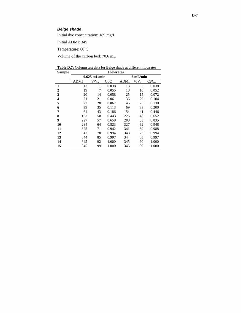
D-7

Beige shade Initial dye concentration: 189 mg/L

Initial ADMI: 345

Temperature: 60˚C

Volume of the carbon bed: 70.6 mL

Table D.7: Column test data for Beige shade at different flowrates Flowrates

0.625 mL/min 6 mL/min Sample

ADMI V/Vo Ct/Co ADMI V/Vo Ct/Co 1 13 1 0.038 13 5 0.038 2 19 7 0.055 18 10 0.052 3 20 14 0.058 25 15 0.072 4 21 21 0.061 36 20 0.104 5 23 28 0.067 45 26 0.130 6 39 35 0.113 69 33 0.200 7 64 43 0.186 154 41 0.446 8 153 50 0.443 225 48 0.652 9 227 57 0.658 288 55 0.835 10 284 64 0.823 327 62 0.948 11 325 71 0.942 341 69 0.988 12 343 78 0.994 343 76 0.994 13 344 85 0.997 344 83 0.997 14 345 92 1.000 345 90 1.000 15 345 99 1.000 345 99 1.000

D-8

Turquoise shade Initial dye concentration: 693 mg/L

Initial ADMI: 10100

Temperature: 60˚C

Volume of the carbon bed: 70.6 mL

Table D.8: Column test data for Turquoise shade at different flowrates Flowrates

0.625 mL/min 6 mL/min Sample

ADMI V/Vo Ct/Co ADMI V/Vo Ct/Co 1 42 1 0.004 45 5 0.004 2 43 7 0.004 33 10 0.003 3 39 11 0.004 397 15 0.039 4 51 17 0.005 2058 24 0.204 5 191 24 0.019 4375 35 0.433 6 4298 45 0.426 6995 45 0.693 7 6543 52 0.648 9583 65 0.949 8 8835 69 0.875 9835 75 0.974 9 9124 75 0.923 10024 86 0.992 10 9865 88 0.977 10075 106 0.998 11 9912 101 0.984 10082 126 0.998 12 9998 112 0.989 10090 134 0.999 13 10091 126 0.999 10091 142 0.999 14 10095 139 0.999 10095 149 0.999 15 10099 152 1.000 10099 156 0.999

E-1

APPENDIX E

REGENERATION Appendix E contains the experimental data for regeneration (Chapter 6)

Regeneration elution Flow rate: 0.625 mL/min

Volume of the carbon bed: 70.6 mL

Table E.1: Regeneration elution data for the shades Shades

Navy Black Beige Turquoise Sample V/Vo

ADMI Conc (mg/L)

ADMI Conc (mg/L)

ADMI Conc (mg/L)

ADMI Conc (mg/L)

1 0 0 0 0 0 0 0 0 0 2 0.425 6295 275 7016 289 86 47.1 3537 243 3 0.850 4098 179 4382 180 50 27.4 2553 175 4 1.276 2756 120 2820 116 37 20.3 1519 104 5 1.701 1962 85.6 1705 70.1 32 17.5 1056 72.4 6 2.126 1166 50.9 1242 51.1 28 15.3 504 34.6 7 2.551 463 20.2 874 35.9 25 13.7 365 25.0 8 2.976 285 12.4 418 17.2 23 12.6 182 12.5 9 3.401 47 2.05 59 2.43 21 11.5 45 3.09 10 3.827 40 1.75 45 1.85 20 10.9 41 2.81 11 4.252 35 1.53 38 1.56 20 10.9 35 2.40 Total 748 765 187 675 Initial dye concentration 770 782 189 693

E-2

REGENERATION CYCLES

Navy shade Initial dye concentration: 770 mg/L

Initial ADMI: 17650

Flow rate: 0.625 mL/min

Volume of the carbon bed: 70.6 mL

Table E.2: Regeneration cycle data for the Navy shade Regeneration cycle

1st cycle 2nd cycle 3rd cycle 4th cycle Sample

ADMI V/Vo Ct/Co ADMI V/Vo Ct/Co ADMI V/Vo Ct/Co ADMI V/Vo Ct/Co 1 38 1 0.002 40 1 0.002 45 1 0.003 9265 1 0.525 2 21 11 0.001 70 11 0.004 455 11 0.026 11456 11 0.649 3 56 14 0.003 482 14 0.027 1508 14 0.085 12208 14 0.691 4 1773 24 0.100 3976 24 0.225 6179 24 0.350 14579 24 0.826 5 9725 35 0.551 11224 35 0.636 12723 35 0.721 17553 35 0.995 6 12342 43 0.699 13665 43 0.774 14988 43 0.849 7 14962 55 0.848 15775 55 0.894 16988 55 0.962 8 16187 68 0.917 16875 68 0.956 9 16965 81 0.961

E-3

Black shade Initial dye concentration: 782 mg/L

Initial ADMI: 19010

Flow rate: 0.625 mL/min

Volume of the carbon bed: 70.6 mL

Table E.3: Regeneration cycle data for the Black shade Regeneration cycle

1st cycle 2nd cycle 3rd cycle 4th cycle Sample

ADMI V/Vo Ct/Co ADMI V/Vo Ct/Co ADMI V/Vo Ct/Co ADMI V/Vo Ct/Co 1 40 1 0.002 35 1 0.002 37 1 0.002 8976 1 0.472 2 30 9 0.002 31 9 0.002 35 9 0.002 10179 9 0.535 3 37 14 0.002 93 14 0.005 654 14 0.034 11597 14 0.610 4 113 21 0.006 668 21 0.035 1623 21 0.085 13423 21 0.706 5 605 28 0.032 1976 28 0.104 3347 28 0.176 16047 28 0.844 6 2096 39 0.110 4376 39 0.230 6656 39 0.350 18996 39 0.999 7 4580 49 0.241 9459 49 0.498 13338 49 0.702 8 13866 64 0.729 15535 64 0.817 18096 64 0.952 9 16872 76 0.888 18175 76 0.956 10 18069 89 0.951

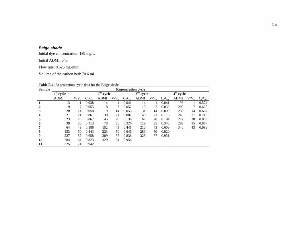
E-4

Beige shade Initial dye concentration: 189 mg/L

Initial ADMI: 345

Flow rate: 0.625 mL/min

Volume of the carbon bed: 70.6 mL

Table E.4: Regeneration cycle data for the Beige shade Regeneration cycle

1st cycle 2nd cycle 3rd cycle 4th cycle Sample

ADMI V/Vo Ct/Co ADMI V/Vo Ct/Co ADMI V/Vo Ct/Co ADMI V/Vo Ct/Co 1 13 1 0.038 14 1 0.041 14 1 0.041 198 1 0.574 2 19 7 0.055 18 7 0.052 19 7 0.055 209 7 0.606 3 20 14 0.058 19 14 0.055 31 14 0.090 230 14 0.667 4 21 21 0.061 30 21 0.087 40 21 0.116 248 21 0.719 5 23 28 0.067 45 28 0.130 67 28 0.194 277 28 0.803 6 39 35 0.113 78 35 0.226 119 35 0.345 299 35 0.867 7 64 43 0.186 152 43 0.441 210 43 0.609 340 43 0.986 8 153 50 0.443 223 50 0.646 283 50 0.820 9 227 57 0.658 289 57 0.838 328 57 0.951 10 284 64 0.823 329 64 0.954 11 325 71 0.942

E-5

Turquoise shade Initial dye concentration: 693 mg/L

Initial ADMI: 10100

Flow rate: 0.625 mL/min

Volume of the carbon bed: 70.6 mL

Table E.5: Regeneration cycle data for the Turquoise shade Regeneration cycle

1st cycle 2nd cycle 3rd cycle 4th cycle Sample

ADMI V/Vo Ct/Co ADMI V/Vo Ct/Co ADMI V/Vo Ct/Co ADMI V/Vo Ct/Co 1 42 1 0.004 40 1 0.004 41 1 0.004 5123 1 0.507 2 43 7 0.004 47 7 0.005 54 7 0.005 6254 7 0.619 3 39 11 0.004 57 11 0.006 234 11 0.023 6875 11 0.681 4 51 17 0.005 126 17 0.012 353 17 0.035 7589 17 0.751 5 191 24 0.019 555 24 0.055 959 24 0.095 8566 24 0.848 6 4298 45 0.426 5592 45 0.554 6886 45 0.682 10098 45 1.000 7 6543 52 0.648 7488 52 0.741 8433 52 0.835 8 8835 69 0.875 9334 69 0.924 9735 69 0.964 9 9124 75 0.923 9724 75 0.963 10 9865 88 0.977

E-6

System design column data

Table E.6: The breakthrough curve for design obtained at 60˚C Navy Shade Navy shade Sample ADMI V/Vo Ct/Co

1 40 0.58 0.0023 2 41 1.16 0.0023 3 39 2.33 0.0022 4 40 3.49 0.0023 5 41 4.65 0.0023 6 50 5.81 0.0028 7 66 7.27 0.0037 8 73 7.91 0.0041 9 97 9.30 0.0055