Reliable CFD-based estimation of flow rate in

haemodynamics measures

R. Ponzini1,2, C. Vergara3, A. Redaelli1, A. Veneziani3

30th January 2006

1-Department of Bioengineering, Politecnico di Milano, Italy

2-CILEA (Consorzio Interuniversitario Lombardo per l’Elaborazione e l’Automazione),

Segrate (MI), Italy

3-MOX (Modeling and Scientific Computing) - Department of Mathematics,

Politecnico di Milano, Italy

Keywords: Flow rate estimation, Doppler technique, Computational Fluid Dy-namics, flow rate boundary conditions, Womersley number.

AMS Subject Classification: 62G99

Abstract

Physical useful measures in current clinical practice refer often to theblood flow rate, that is related to the mean velocity. However, the directmeasure of the latter is currently not possible using a Doppler velocimetrytechnique. Therefore, the usual approach to calculate the flow rate with thistechnique consists in measuring the maximum velocity and in estimating themean velocity, making the hypothesis of parabolic profile, that in realisticsituations brings to strongly inaccurate estimates.

In this paper, we propose a different way for estimating the flow rateregarded as a function of maximum velocity and Womersley number. Thisrelation is obtained by fixing a parametrized representation and by evalu-ating the parameters by means of a least square approach working on thenumerical results of CFD simulations (about 200). Numerical simulationsare carried out by prescribing the flow rate, not the velocity profile. Inthis way, no bias are implicitly induced in prescribing boundary conditions.Validation tests based on numerical simulations show that the proposedrelation improves the flow rate estimation.

1 Introduction

The correct knowledge of the blood flow rate Q in a vascular district is a majorissue in many clinical situations for estimating the perfusion state of a certain

1

tissue and for decision-making when a cardiovascular disease occurs. For exam-ple, the evaluation of the flow reserve, defined as the ratio between the maximalflow obtained in vasodilation conditions and the baseline conditions, is one ofthe most important parameters used to characterize the haemodynamics impactof a luminal obstruction. If Γ denotes a section of the vascular district at hand,the flow rate Q through Γ is given by:

Q =

∫

Γ

ρv · ndγ (1)

where ρ is the blood density, v the velocity and n the normal unit vector.In principle the knowledge of the whole velocity field on Γ is needed for thecomputation of Q. However, this information cannot be obtained in ordinaryDoppler velocimetry analysis. A different way for representing Q is to resort toa mean velocity value V such that

Q(t) = ρV (t)A(t), (2)

where A is the measure of Γ. The problem with this formulation is still that Vcannot be directly measured, therefore it is currently estimated by the measureof the maximum value of velocity VM on Γ by means of an appropriate relationlinking VM to V . In particular, it is usually assumed (see Doucette et al. 1992)that

V =1

2VM . (3)

This equation stems from the hypothesis of a parabolic spatial profile for thevelocity. According to this assumption, blood is considered a steady, laminarNewtonian fluid in a cylindrical vessel (see e.g. Nichols and O’Rourke 1990).In real situations, blood flow is far from fulfilling these features. Several works(see e.g. Robertson et al. 2001, Perktold et al. 1998, Sheada et al. 1993,Ponzini et al. 2006) pointed out that a non parabolic profile can be computedin simulating realistic conditions even when the considered morphologies werethe same of those studied in the validation protocol of the Doppler guide wire(see e.g. Doucette et al. 1992, Savader et al . 1997).

In particular, the relevance of blood pulsatility on velocity profiles has beenclearly pointed out since a long time by Womersley (1955) and among the others,we quote Hale et al. (1955) and Nichols and O’Rourke (1990). These workshighlight that the hypothesis that blood is quasi-static (i.e. that at each instantthe velocity profile is the same as for a steady fluid featuring the flow rateprescribed at that instant) is not realistic, in particular when the Womersleynumber W = r

√2πf/µ =

√2Af/µ (where r =

√A/π is the vessel radius, f

the frequency of blood impulse and µ the blood viscosity) increases. The limitedvalidity of the parabolic profile assumption has been clearly pointed out alsoin Jenni et al. (2000 and 2004) and in Porenta et al. (1999). In these works,the authors found that the use of (3) to estimate the mean velocity value is too

2

simplistic and can lead to misleading results in the coronary CFR (CoronaryFunctional Reserve) evaluation of the flux. Starting from this observation, theypropose to modify the acquisition procedure at the operator’s level according tothe Hottinger and Meindl principle (see Hottinger and Meindl 1979).

In order to obtain a more realistic relation linking VM to V taking into ac-count the pulsatility of the blood flow rate, a first possibility is to utilize theanalytical relationship that He et al. (1993) proposed for a cylindrical domainfor a sinusoidal signal. This approach can be extended to general physiologicalwaveforms by application of the superimposition effects principle that holds forlinear problems. However, this approach has two major drawbacks. On onehand it has been devised for cylindrical morphologies and its extension to morerealistic geometries seems not trivial and somehow problematic. On the otherone, the problem at hand is driven by the non-linear Navier-Stokes equations,so the superimposition of effects is strictly non applicable. When the Reynoldsnumber increases, that means that the non linearity becomes more relevant, thiscan induces some inaccuracies. For these reasons, alternatively some works de-veloped different relations between the maximum and the mean velocity, usingComputational Fluid Dynamics (CFD) for specific cases. In this context, ap-proximations have been found by Pennati et al. (1996 and 1998) for the case ofthe ductus venosus and by Ponzini et al. (2006) for coronary Y-graft bypass.

In the present work, we propose an “operator independent” approach, basedon CFD, for improving blood flow estimates from maximum velocity measuresthat basically relies on the mean velocity/vessel area method (consisting in mea-suring the lumen area and the maximum value of velocity and in computing themean velocity as a function of this value) and on a generalization of (3). Inprinciple, we could think to extend this formula by introducing a relation of theform

V = g(VM , r, f, µ, . . .),

where all significant parameters (such as the vessel curvature or torsion) canbe included for improving the accuracy of the mean velocity. However, themanagement in the clinical practice of all these parameters could be somehowproblematic and even unnecessary. We decide therefore to select only one signifi-cant parameter besides the maximum velocity. As a matter of fact, we introducethe relation

V = g(VM ,W ), (4)

establishing a link between the V (and then the flow rate) and VM as a functionof the Womersley number W summarizing in a synthetic way some geometrical,fluid dynamical and rheological features. Function g will be fixed by specifyingsome parameters, depending on its specific functional form. The quantitative de-termination of these parameters can be carried out by fitting available data witha least squares approach. These data could be provided by “in vitro” measurestaken in realistic experimental set up. Alternatively, fitting can be carried outby exploiting numerical simulations (see Pennati et al. 1998 and Ponzini et al.

3

2006). So far, haemodynamics computations with flow rate boundary conditionshave been carried out by specifying an arbitrary velocity profile. The reason ofthis is that from the mathematical viewpoint flow rate boundary conditions arenot enough to have a well posed problem and the available conditions are com-pleted by selecting a velocity profile compatible with the prescribed flow rate.In the context of the present work, the prescription of a velocity profile wouldbe equivalent to select a priori for each value of W a functional relation like(4) and this would reduce the significance of numerical simulations (see Redaelliet al. 1997) and definitely the accuracy of (4) in recovering the flow rate fromthe maximum velocity. Recently, new numerical techniques have been howeverdevised for solving haemodynamics flow rates problems without the prescriptionof a velocity profile (see Heywood et al. 1996, Formaggia et al. 2002, Venezianiand Vergara 2005a). The potential bias in using numerical simulations speci-fying the velocity profile can be therefore avoided. Several accurate numericalsimulations in different realistic situations have been therefore carried out forcollecting data useful for the least squares estimate of the parameters in (4). Byso doing, we firstly derive two different equations in the form (4) well suited forrepresenting the link between VM and V for two different representative groupsof vessels. Afterwards, by an appropriate combination of these formulae, we ob-tain a unique equation covering different geometrical features and a physiologicalrange of Womersley numbers.

The effectiveness of the formula has been validated by resorting again tonumerical simulations. By computing blood flow in geometries and conditionsdifferent than the ones used for the least squares fitting, we observed that ourformula yields a (sometimes strong) improvement of the flow rate estimationbased on the (3). We think therefore that this result can be potentially of biginterest in clinical practice. However, successive in vitro and in vivo validationto confirm the present study are mandatory.

The outline of the paper is as follows. In Section 2 we present the basicfeatures of model (4). We firstly present models used for the two significantgroups of vessel and give details about the least squares fitting. We avoid math-ematical details about CFD methods for getting reliable numerical simulations,referring the interested reader to Formaggia et al. (2002) and to Veneziani andVergara (2005a). Then, we illustrate how the two formulae have been collectedin a unique equation of the form (4). Validation is presented in Section 3. Con-clusions and perpectives are drawn in Section 4.

2 Materials and Methods

2.1 Basic features of the mathematical model

The specific features of the flow patterns in a vascular district, once boundaryconditions have been assigned, are basically the morphology, the pulsatility andthe rheology. On one hand, one would set up an accurate equation linking the

4

mean and the maximum velocities, taking into account all these aspects. On theother hand, the usage of this equation is subordinated to the possibility of gettingreliable estimates of all these features in the clinical practice. As pointed outin the Introduction, as a reasonable compromise between the accuracy and thefeasibility, we summarize the dependence on all these features by resorting to theWomersley number (see equation (4). In this way, we synthetically account forthe radius of the vessel, the blood viscosity and in particular for the pulsatility.W can be in practice estimated on the basis of available clinical measures. Weactually are assuming that it is possible to define locally a vessel radius. Thiswill be the only geometrical parameter in our equation. More complex (and moredifficult to implement) equations could be considered in a future development ofthe present work.

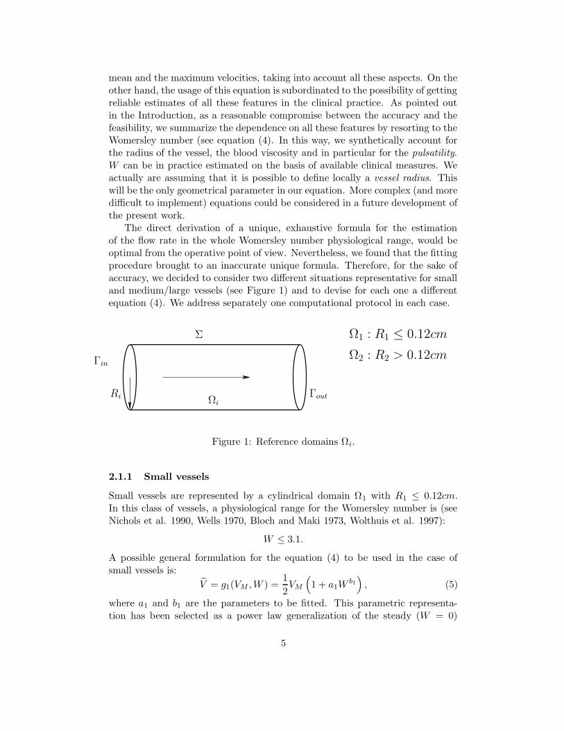
The direct derivation of a unique, exhaustive formula for the estimationof the flow rate in the whole Womersley number physiological range, would beoptimal from the operative point of view. Nevertheless, we found that the fittingprocedure brought to an inaccurate unique formula. Therefore, for the sake ofaccuracy, we decided to consider two different situations representative for smalland medium/large vessels (see Figure 1) and to devise for each one a differentequation (4). We address separately one computational protocol in each case.

Σ

Γin

Ri Ωi

Γout

Ω1 : R1 ≤ 0.12cm

Ω2 : R2 > 0.12cm

Figure 1: Reference domains Ωi.

2.1.1 Small vessels

Small vessels are represented by a cylindrical domain Ω1 with R1 ≤ 0.12cm.In this class of vessels, a physiological range for the Womersley number is (seeNichols et al. 1990, Wells 1970, Bloch and Maki 1973, Wolthuis et al. 1997):

W ≤ 3.1.

A possible general formulation for the equation (4) to be used in the case ofsmall vessels is:

V = g1(VM ,W ) =1

2VM

(1 + a1W

b1)

, (5)

where a1 and b1 are the parameters to be fitted. This parametric representa-tion has been selected as a power law generalization of the steady (W = 0)

5

equation (3). In the numerical simulations carried out for fitting a1 and b1, wedistinguished two situations that can be referred to “small vessels”:

1. small arteries

2. coronaries.

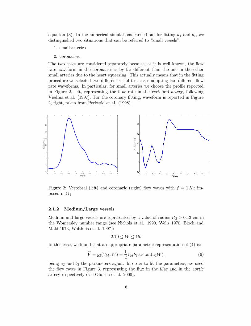
The two cases are considered separately because, as it is well known, the flowrate waveform in the coronaries is by far different than the one in the othersmall arteries due to the heart squeezing. This actually means that in the fittingprocedure we selected two different set of test cases adopting two different flowrate waveforms. In particular, for small arteries we choose the profile reportedin Figure 2, left, representing the flow rate in the vertebral artery, followingViedma et al. (1997). For the coronary fitting, waveform is reported in Figure2, right, taken from Perktold et al. (1998).

0 0.1 0.2 0.3 0.4 0.5 0.6 0.7 0.8 0.9 11.4

1.6

1.8

2

2.2

2.4

2.6

2.8

3

time(sec)

flux(

cm3 /

sec)

Figure 2: Vertebral (left) and coronaric (right) flow waves with f = 1Hz im-posed in Ω1

2.1.2 Medium/Large vessels

Medium and large vessels are represented by a value of radius R2 > 0.12 cm inthe Womersley number range (see Nichols et al. 1990, Wells 1970, Bloch andMaki 1973, Wolthuis et al. 1997):

2.70 ≤ W ≤ 15.

In this case, we found that an appropriate parametric representation of (4) is:

V = g2(VM ,W ) =1

2VMb2 arctan(a2W ), (6)

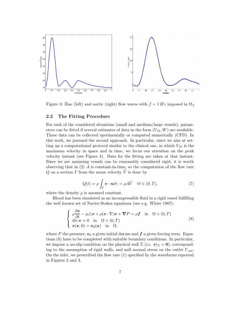
being a2 and b2 the parameters again. In order to fit the parameters, we usedthe flow rates in Figure 3, representing the flux in the iliac and in the aorticartery respectively (see Olufsen et al. 2000).

6

0 0.1 0.2 0.3 0.4 0.5 0.6 0.7 0.8 0.9 115

20

25

30

35

40

45

50

time(sec)

flux(

cm3 /s

ec)

Figure 3: Iliac (left) and aortic (right) flow waves with f = 1Hz imposed in Ω2

2.2 The Fitting Procedure

For each of the considered situations (small and medium/large vessels), param-eters can be fitted if several estimates of data in the form (VM ,W ) are available.These data can be collected sperimentally or computed numerically (CFD). Inthis work, we pursued the second approach. In particular, since we aim at set-ting up a computational protocol similar to the clinical one, in which VM is themaximum velocity in space and in time, we focus our attention on the peakvelocity instant (see Figure 4). Data for the fitting are taken at that instant.Since we are assuming vessels can be reasonably considered rigid, it is worthobserving that in (2) A is constant-in-time, so the computation of the flow rateQ on a section Γ from the mean velocity V is done by

Q(t) = ρ

∫

Γ

v · ndγ = ρAV ∀t ∈ (0, T ), (7)

where the density ρ is assumed constant.Blood has been simulated as an incompressible fluid in a rigid vessel fulfilling

the well known set of Navier-Stokes equations (see e.g. White 1987):

ρ∂v

∂t− µ4v + ρ(v · ∇)v + ∇P = ρf in Ω × (0, T )

div v = 0 in Ω × (0, T )v(x, 0) = v0(x) in Ω,

(8)

where P the pressure, v0 a given initial datum and f a given forcing term. Equa-tions (8) have to be completed with suitable boundary conditions. In particular,we impose a no-slip condition on the physical wall Σ (i.e. v|Σ = 0), correspond-ing to the assumption of rigid walls, and null normal stress on the outlet Γout.On the inlet, we prescribed the flow rate (1) specified by the waveforms reportedin Figures 2 and 3.

7

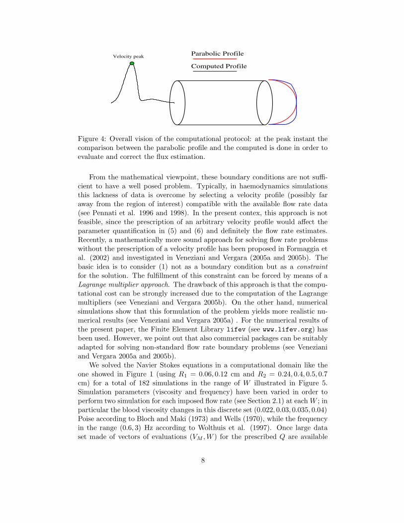
Computed Profile

Parabolic ProfileVelocity peak

Figure 4: Overall vision of the computational protocol: at the peak instant thecomparison between the parabolic profile and the computed is done in order toevaluate and correct the flux estimation.

From the mathematical viewpoint, these boundary conditions are not suffi-cient to have a well posed problem. Typically, in haemodynamics simulationsthis lackness of data is overcome by selecting a velocity profile (possibly faraway from the region of interest) compatible with the available flow rate data(see Pennati et al. 1996 and 1998). In the present contex, this approach is notfeasible, since the prescription of an arbitrary velocity profile would affect theparameter quantification in (5) and (6) and definitely the flow rate estimates.Recently, a mathematically more sound approach for solving flow rate problemswithout the prescription of a velocity profile has been proposed in Formaggia etal. (2002) and investigated in Veneziani and Vergara (2005a and 2005b). Thebasic idea is to consider (1) not as a boundary condition but as a constraint

for the solution. The fulfillment of this constraint can be forced by means of aLagrange multiplier approach. The drawback of this approach is that the compu-tational cost can be strongly increased due to the computation of the Lagrangemultipliers (see Veneziani and Vergara 2005b). On the other hand, numericalsimulations show that this formulation of the problem yields more realistic nu-merical results (see Veneziani and Vergara 2005a) . For the numerical results ofthe present paper, the Finite Element Library lifev (see www.lifev.org) hasbeen used. However, we point out that also commercial packages can be suitablyadapted for solving non-standard flow rate boundary problems (see Venezianiand Vergara 2005a and 2005b).

We solved the Navier Stokes equations in a computational domain like theone showed in Figure 1 (using R1 = 0.06, 0.12 cm and R2 = 0.24, 0.4, 0.5, 0.7cm) for a total of 182 simulations in the range of W illustrated in Figure 5.Simulation parameters (viscosity and frequency) have been varied in order toperform two simulation for each imposed flow rate (see Section 2.1) at each W ; inparticular the blood viscosity changes in this discrete set (0.022, 0.03, 0.035, 0.04)Poise according to Bloch and Maki (1973) and Wells (1970), while the frequencyin the range (0.6, 3) Hz according to Wolthuis et al. (1997). Once large dataset made of vectors of evaluations (VM ,W ) for the prescribed Q are available

8

from numerical simulations, parameters in (5), (6) are obtained by means ofa non-linear least-square fitting optimization. In particular, we have used theLeast Squares module present in the package Scientific-Python. We do notdwell here with further mathematical details. The interested reader is referredto Langtangen (2004).

2.3 A unified approach

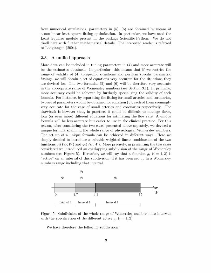
More data can be included in tuning parameters in (4) and more accurate willbe the estimates obtained. In particular, this means that if we restrict therange of validity of (4) to specific situations and perform specific parametricfittings, we will obtain a set of equations very accurate for the situations theyare devised for. The two formulae (5) and (6) will be therefore very accuratein the appropriate range of Womersley numbers (see Section 3.1). In principle,more accuracy could be achieved by furtherly specializing the validity of eachformula. For instance, by separating the fitting for small arteries and coronaries,two set of parameters would be obtained for equation (5), each of them seeminglyvery accurate for the case of small arteries and coronaries respectively. Thedrawback is however that, in practice, it could be difficult to manage three,four (or even more) different equations for estimating the flow rate. A uniqueformula will be less accurate but easier to use in the clinical practice. For thisreason, after considering the two cases presented above seprately, we devised aunique formula spanning the whole range of phyisological Womersley numbers.The set up of a unique formula can be achieved in different ways. Here wesimply decided to introduce a suitable weighted linear combination of the twofunctions g1(VM ,W ) and g2(VM ,W ). More precisely, in presenting the two casesconsidered we introduced an overlapping subdivision of the range of Womersleynumbers (see Figure 5). Hereafter, we will say that a function gi (i = 1, 2) is“active” on an interval of this subdivision, if it has been set up in a Womersleynumbers range including that interval.

Interval 1 Interval 2 Interval 3

W

g1 g2

g1

g2

153.12.70

Figure 5: Subdivision of the whole range of Womersley numbers into intervalswith the specification of the different active gi (i = 1, 2).

We have therefore the following subdivision:

9

Interval 1 For W < 2.70 the only active function is g1;

Interval 2 For 2.70 ≤ W < 3.1 the active functions are both g1 and g2;

Interval 3 For 3.1 < W ≤ 15 only g2 is active.

2 3 4 5 6 7 80

0.1

0.2

0.3

0.4

0.5

0.6

0.7

0.8

0.9

1

W

w

Figure 6: Weight function w

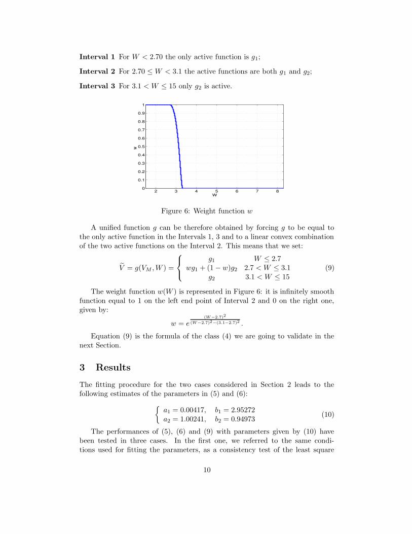
A unified function g can be therefore obtained by forcing g to be equal tothe only active function in the Intervals 1, 3 and to a linear convex combinationof the two active functions on the Interval 2. This means that we set:

V = g(VM ,W ) =

g1 W ≤ 2.7wg1 + (1 − w)g2 2.7 < W ≤ 3.1

g2 3.1 < W ≤ 15(9)

The weight function w(W ) is represented in Figure 6: it is infinitely smoothfunction equal to 1 on the left end point of Interval 2 and 0 on the right one,given by:

w = e(W−2.7)2

(W−2.7)2−(3.1−2.7)2 .

Equation (9) is the formula of the class (4) we are going to validate in thenext Section.

3 Results

The fitting procedure for the two cases considered in Section 2 leads to thefollowing estimates of the parameters in (5) and (6):

a1 = 0.00417, b1 = 2.95272a2 = 1.00241, b2 = 0.94973

(10)

The performances of (5), (6) and (9) with parameters given by (10) havebeen tested in three cases. In the first one, we referred to the same condi-tions used for fitting the parameters, as a consistency test of the least square

10

approach adopted for the parameters estimation. In the second test cases set,we retained the same geometries used for the parameters fitting and changedthe inlet flow rate waveforms used. In the last class of benchmarks, we applied(9) to completely different geometries and flow rate waveforms. In each case,we compare the mean velocity estimated by (5), (6) or (9) with (10), startingfrom the outlet maximum velocity, with the exact prescribed value and with theparabolic estimate (3). Finally, in order to compare our new method with theparabolic one, we applied the Bland-Altman test (see Bland and Altman 1986)to the validation test cases described in Section 3.2 and 3.3. This statistical testis usually performed in clinical practice to evaluate the level of agreement of anew measurement technique with an established one.

3.1 A consistency test

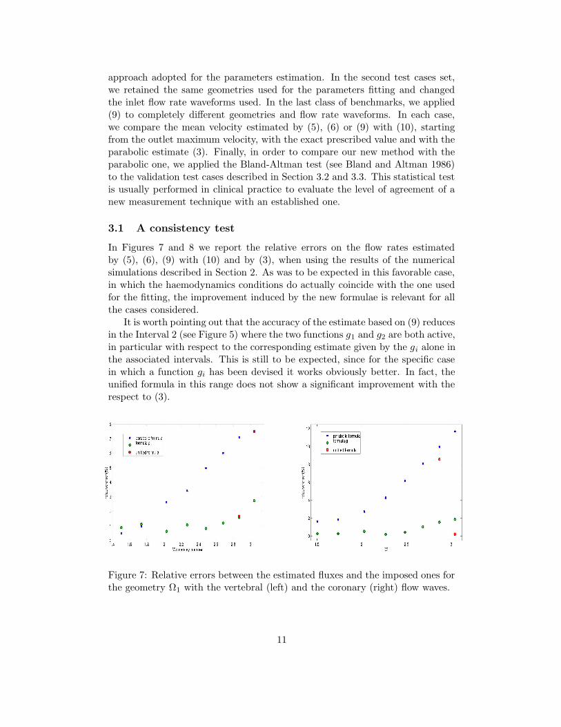
In Figures 7 and 8 we report the relative errors on the flow rates estimatedby (5), (6), (9) with (10) and by (3), when using the results of the numericalsimulations described in Section 2. As was to be expected in this favorable case,in which the haemodynamics conditions do actually coincide with the one usedfor the fitting, the improvement induced by the new formulae is relevant for allthe cases considered.

It is worth pointing out that the accuracy of the estimate based on (9) reducesin the Interval 2 (see Figure 5) where the two functions g1 and g2 are both active,in particular with respect to the corresponding estimate given by the gi alone inthe associated intervals. This is still to be expected, since for the specific casein which a function gi has been devised it works obviously better. In fact, theunified formula in this range does not show a significant improvement with therespect to (3).

Figure 7: Relative errors between the estimated fluxes and the imposed ones forthe geometry Ω1 with the vertebral (left) and the coronary (right) flow waves.

11

5 6 7 8 9 10 11 12 13 140

5

10

15

20

25

30

35

Womersley number

Rel

ativ

e er

ror(

%)

Errors comparision for the aortic flow rate

parabolic formulaformula g2

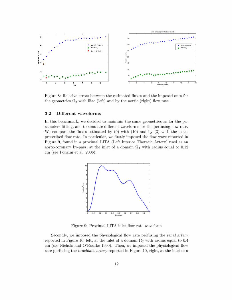
Figure 8: Relative errors between the estimated fluxes and the imposed ones forthe geometries Ω2 with iliac (left) and by the aortic (right) flow rate.

3.2 Different waveforms

In this benchmark, we decided to maintain the same geometries as for the pa-rameters fitting, and to simulate different waveforms for the perfusing flow rate.We compare the fluxes estimated by (9) with (10) and by (3) with the exactprescribed flow rate. In particular, we firstly imposed the flow wave reported inFigure 9, found in a proximal LITA (Left Interior Thoracic Artery) used as anaorto-coronary by-pass, at the inlet of a domain Ω1 with radius equal to 0.12cm (see Ponzini et al. 2006).

0 0.1 0.2 0.3 0.4 0.5 0.6 0.7 0.8 0.9 10

1

2

3

4

5

6

7

8

9

10

time(sec)

flux(

cm3 /s

ec)

Figure 9: Proximal LITA inlet flow rate waveform

Secondly, we imposed the physiological flow rate perfusing the renal arteryreported in Figure 10, left, at the inlet of a domain Ω2 with radius equal to 0.4cm (see Nichols and O’Rourke 1990). Then, we imposed the physiological flowrate perfusing the brachialis artery reported in Figure 10, right, at the inlet of a

12

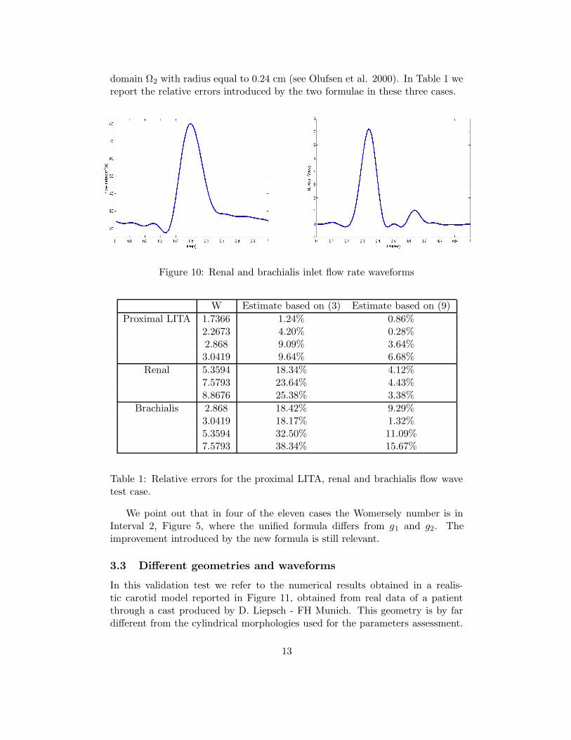
domain Ω2 with radius equal to 0.24 cm (see Olufsen et al. 2000). In Table 1 wereport the relative errors introduced by the two formulae in these three cases.

Figure 10: Renal and brachialis inlet flow rate waveforms

W Estimate based on (3) Estimate based on (9)

Proximal LITA 1.7366 1.24% 0.86%2.2673 4.20% 0.28%2.868 9.09% 3.64%3.0419 9.64% 6.68%

Renal 5.3594 18.34% 4.12%7.5793 23.64% 4.43%8.8676 25.38% 3.38%

Brachialis 2.868 18.42% 9.29%3.0419 18.17% 1.32%5.3594 32.50% 11.09%7.5793 38.34% 15.67%

Table 1: Relative errors for the proximal LITA, renal and brachialis flow wavetest case.

We point out that in four of the eleven cases the Womersely number is inInterval 2, Figure 5, where the unified formula differs from g1 and g2. Theimprovement introduced by the new formula is still relevant.

3.3 Different geometries and waveforms

In this validation test we refer to the numerical results obtained in a realis-tic carotid model reported in Figure 11, obtained from real data of a patientthrough a cast produced by D. Liepsch - FH Munich. This geometry is by fardifferent from the cylindrical morphologies used for the parameters assessment.

13

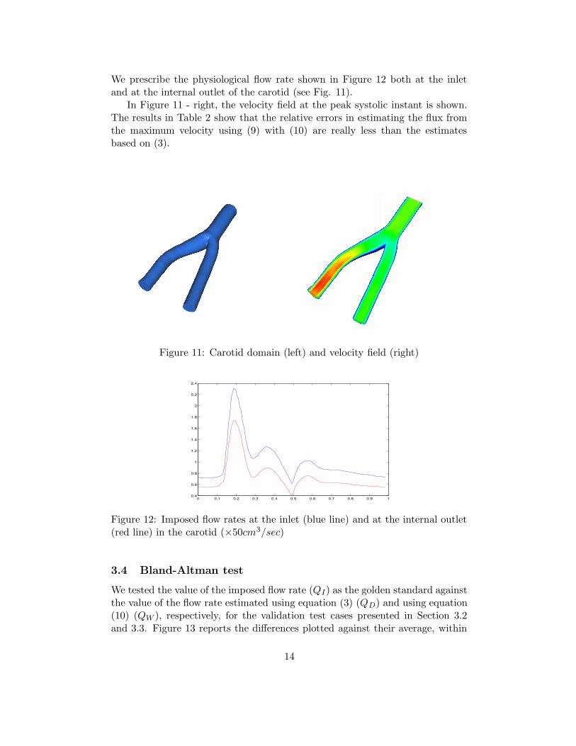
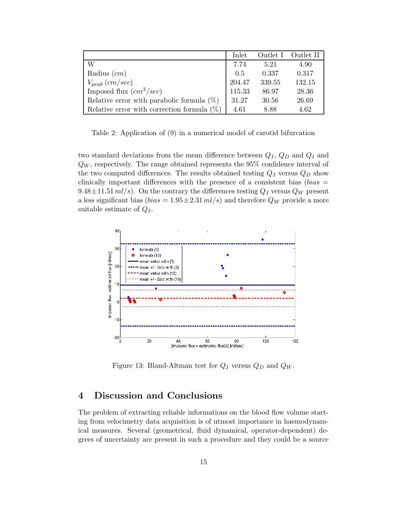
We prescribe the physiological flow rate shown in Figure 12 both at the inletand at the internal outlet of the carotid (see Fig. 11).

In Figure 11 - right, the velocity field at the peak systolic instant is shown.The results in Table 2 show that the relative errors in estimating the flux fromthe maximum velocity using (9) with (10) are really less than the estimatesbased on (3).

Figure 11: Carotid domain (left) and velocity field (right)

0 0.1 0.2 0.3 0.4 0.5 0.6 0.7 0.8 0.9 10.4

0.6

0.8

1

1.2

1.4

1.6

1.8

2

2.2

2.4

Figure 12: Imposed flow rates at the inlet (blue line) and at the internal outlet(red line) in the carotid (×50cm3/sec)

3.4 Bland-Altman test

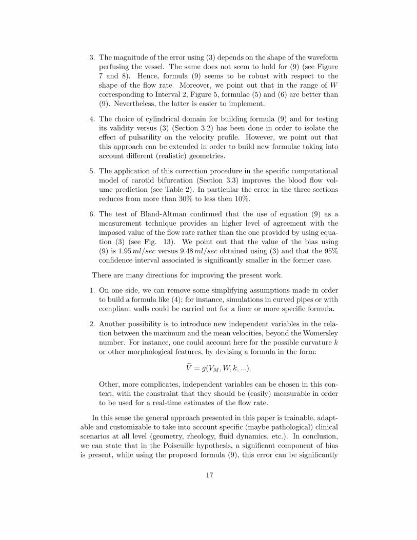
We tested the value of the imposed flow rate (QI) as the golden standard againstthe value of the flow rate estimated using equation (3) (QD) and using equation(10) (QW ), respectively, for the validation test cases presented in Section 3.2and 3.3. Figure 13 reports the differences plotted against their average, within

14

Inlet Outlet I Outlet II

W 7.74 5.21 4.90Radius (cm) 0.5 0.337 0.317Vpeak (cm/sec) 204.47 339.55 132.15Imposed flux (cm3/sec) 115.33 86.97 28.36Relative error with parabolic formula (%) 31.27 30.56 26.69Relative error with correction formula (%) 4.61 8.88 4.62

Table 2: Application of (9) in a numerical model of carotid bifurcation

two standard deviations from the mean difference between QI , QD and QI andQW , respectively. The range obtained represents the 95% confidence interval ofthe two computed differences. The results obtained testing QI versus QD showclinically important differences with the presence of a consistent bias (bias =9.48±11.51ml/s). On the contrary the differences testing QI versus QW presenta less significant bias (bias = 1.95±2.31ml/s) and therefore QW provide a moresuitable estimate of QI .

Figure 13: Bland-Altman test for QI versus QD and QW .

4 Discussion and Conclusions

The problem of extracting reliable informations on the blood flow volume start-ing from velocimetry data acquisition is of utmost importance in haemodynam-ical measures. Several (geometrical, fluid dynamical, operator-dependent) de-grees of uncertainty are present in such a procedure and they could be a source

15

of bias and/or random errors.In this work we have presented how the extensive use of numerical simula-

tions can enhance currently in use procedures, based on analytical solutions ofthe flow field like the Poiseuille one. Actually, some of the hypotheses assumedfor analytical solutions can be removed thanks to numerical simulations, yield-ing definitely better estimates of relevant quantities starting from velocimetrydata. In particular, in the present work, we removed the unrealistic parabolicassumption implicitly introduced in (3) for the flow rate estimates from maxi-mum velocity measures. In devising new relations for the blood flow estimate,we therefore chose the Womersley number as a measure of the fluid unsteadi-ness. Numerical simulations have provided data for the fitting of the parametersselected in the specification of the new formula. The data collection has beenfirstly differentiated into two representative cases, corresponding to small andmedium/large vessels, and then a unique equation (9) has been computed bylinear combination.

Using CFD for this aim has many advantages:

1. The so called mean velocity/vessel area method used in velocimetry dataacquisition can be accurately reproduced;

2. Simplifying assumptions present in previous methods can be removed in acontrolled manner, possibly identifying the most relevant ones;

3. Collection of data for the parameters fitting is quite fast and cheap;

4. Validation and benchmarking can still be based (at least partially) onnumerical simulations carried out in configurations different form the onesused for the fitting.

5. The previous advantages are related to general CFD. Moreover, in our par-ticular case, we point out that the prescription of the flow rate boundarycondition without prescribing a priori the velocity profile through a La-grange multipliers approach, leads to meaningful numerical results avoid-ing the bias induced by the prescription of the inlet velocity profile.

The results obtained by our formula show clearly the systematic incorrectnessof the parabolic hypothesis used in daily clinical velocimetry analysis. Therelative error of the parabolic formula increase with the Womersley number.More precisely, it is worth pointing out that:

1. The relative error associated with the parabolic prediction formula (3)in the consistency test (Section 3.1) shows a systematic underestimation(mean = 22.01%, stdv = 11.08%) ;

2. The relative error associated with the prediction formula (9), in the con-sistency test, is bounded in a very small range as a consequence of theaccounting for the pulsatile nature of blood (mean = 3.73%, stdv = 2.51%);

16

3. The magnitude of the error using (3) depends on the shape of the waveformperfusing the vessel. The same does not seem to hold for (9) (see Figure7 and 8). Hence, formula (9) seems to be robust with respect to theshape of the flow rate. Moreover, we point out that in the range of Wcorresponding to Interval 2, Figure 5, formulae (5) and (6) are better than(9). Nevertheless, the latter is easier to implement.

4. The choice of cylindrical domain for building formula (9) and for testingits validity versus (3) (Section 3.2) has been done in order to isolate theeffect of pulsatility on the velocity profile. However, we point out thatthis approach can be extended in order to build new formulae taking intoaccount different (realistic) geometries.

5. The application of this correction procedure in the specific computationalmodel of carotid bifurcation (Section 3.3) improves the blood flow vol-ume prediction (see Table 2). In particular the error in the three sectionsreduces from more than 30% to less then 10%.

6. The test of Bland-Altman confirmed that the use of equation (9) as ameasurement technique provides an higher level of agreement with theimposed value of the flow rate rather than the one provided by using equa-tion (3) (see Fig. 13). We point out that the value of the bias using(9) is 1.95ml/sec versus 9.48ml/sec obtained using (3) and that the 95%confidence interval associated is significantly smaller in the former case.

There are many directions for improving the present work.

1. On one side, we can remove some simplifying assumptions made in orderto build a formula like (4); for instance, simulations in curved pipes or withcompliant walls could be carried out for a finer or more specific formula.

2. Another possibility is to introduce new independent variables in the rela-tion between the maximum and the mean velocities, beyond the Womersleynumber. For instance, one could account here for the possible curvature kor other morphological features, by devising a formula in the form:

V = g(VM ,W, k, ...).

Other, more complicates, independent variables can be chosen in this con-text, with the constraint that they should be (easily) measurable in orderto be used for a real-time estimates of the flow rate.

In this sense the general approach presented in this paper is trainable, adapt-able and customizable to take into account specific (maybe pathological) clinicalscenarios at all level (geometry, rheology, fluid dynamics, etc.). In conclusion,we can state that in the Poiseuille hypothesis, a significant component of biasis present, while using the proposed formula (9), this error can be significantly

17

reduced. An extensive “in vitro” and “in vivo” validation activity is now manda-tory as a necessary phase for confirming the strong improvements found here,before incorporating this formula into clinical devices.

Acknowledgments

Numerical results of this work have been obtained with the finite element codesLifeV (developed at MOX - Dipartimento di Matematica - Politecnico di Mi-lano, at EPFL in Lausanne and at INRIA at Paris, see www.lifev.org)). Theauthors gratefully acknowledge M. Prosi who provided the bifurcation computa-tional domain and in particular G.Pennati at Laboratory of Biological StructureMechanics (LaBS), Politecnico di Milano, for many friutful discussions and sug-gestions.

References

[1] Bland J.M., Altman D.G., Statistical methods for assessing agreement be-tween two methods of clinical measurement,Lancet ; 1(8476):307-310, 1986.

[2] Bloch K.J. and Maki D.G., Hyperviscosity syndrome associated with im-munoglobulin abnormalities, J. Sem. Hematol. ;10:113126 , 1973.

[3] Doucette J.W., Corl P.D., Payne H.M., Flynn A.E., Goto M., Nassi M.,Segal J., Validation of a Doppler guide wire for intravascular measurementof coronary artery flow velocity, Circulation; 85, 1899-1911 , 1992.

[4] Formaggia L., Gerbeau J.F., Nobile F., Quarteroni A., Numerical treatmentof Defective Boundary Conditions for the Navier-Stokes equation, SIAM J.

Num. Anal.; 40(1):376-401, 2002

[5] Hale J.F., McDonald D.A., Womersley J.R., Velocity profiles of oscillatingarterial flow, with some calculations of viscous drag and the Reynolds num-bers, J. Physiol.; 128 (3):629-40 1955.

[6] He X., Ku D.N., Moore J.E. Jr, Simple calculation of the velocity profiles forpulatile flow in a blood vessel using Mathematica, Ann. Biomed. Eng.; 21,45-49,1993.

[7] Heywood, Rannacher and Turek, Artificial Boundary and Flux and PressureConditions for the Incompressible Navier-Stokes Equations, Int. Journ. Num.

Meth. Fluids; 22, 325-352,1996.

[8] Hottinger C.F., Meindl J.D., Blood flow mesaurements using the attenuation-compensated volume flowmeter, Ultrasound Imaging ; 1(1):1-15, 1979.

18

[9] Jenni R., Kaufmann P.A., Jiang Z., Attenhofer C., Linka A., Mandinov L.,In vitro validation of volumetric blood flow measurement using Doppler flowwire, Ultrasound Med Biol.; 26(8):1301-10, 2000.

[10] Jenni R., Matthews F., Aschkenasy S.V., Lachat M., van Der Loo B., Oech-slin E., Namdar M., Jiang Z., Kaufmann P.A., A novel in vivo procedure forvolumetric flow measurements. Ultrasound Med Biol.; 30(5):633-7, 2004.

[11] Langtangen H. P., Python Scripting for Computational Science, Springer,2004.

[12] Nichols W.W., O’Rourke M.F. , McDonald’s blood flow in arteries, (V Ed.),Hodder Arnold (Eds.), 1990.

[13] Olufsen M.S., Peskin C.S., Kim W.Y., Pedersen E.M., Nadim A., Larsen J.,Numerical Simulation and Experimental Validation of Blood Flow in Arterieswith Structured-Tree Outflow Conditions Annals of Biomedical Engineering ;28:1281-1299, 2000

[14] Pennati G., Bellotti M., Ferrazzi E., Bozzo M., Pardi G., Fumero R.,Blood flow through the ductus venosus in human fetus: calculation usingDoppler velocimetry and computational findings, Ultrasound in Med. and

Biol.;24(4):477-487, 1998.

[15] Pennati G., Redaelli A., Bellotti M., Ferrazzi E., Computational analysisof the ductus venosus fluid-dynamics based on Doppler measurements, Ul-

trasound in Med. and Biol.;22(8):1017-1029, 1996.

[16] Perktold K., Hofer M., Rappitsch G., Loew M., Kuban B.D., FriedmanM.H., Validated computation of physiologic flow in a realistic coronary arterybranch,J. Biomech.; 31 Mar(3):217-28.1998

[17] Ponzini R., Lemma M., Morbiducci U., Antona C., Montevecchi F., RedaelliA., Doppler derived quantitative flow estimate in coronary artery bypassgraft: a computational multi-scale model for the evaluation of the currenttheory. Submitted, 2006.

[18] Porenta G., Schima H., Pentaris A., Tsangaris S., Moertl D., Probst P.,Maurer G., Baumgartner H., Assessment of coronary stenoses by Dopplerwires: a validation study using in vitro modeling and computer simulations.Ultrasound Med Biol.; 25 (5):793-801, 1999 .

[19] Quarteroni A., Valli A., Numerical Approximation of Partial Differential

Equations, Springer, 1994.

[20] Redaelli A., Boschetti F., Inzoli F. The assignement of velocity profiles infinite element simulations of pulsatile flow in arteries Comput. Biol. Med.

27(3):233-247, 1997.

19

[21] Robertson M. B., Khler U., Hoskins P. R., Marshall I., Flow in Ellipti-cal Vessels Calculated for a Physiological Waveform Journal Of Vascular

research ; 38:73-82, 2001.

[22] Savader S.J., Lund G.B., Osterman F.A., Volumetric evaluation of bloodflow in normal renal arteries with a Doppler flow wire: a feasibility studyJournal of Vascular and Interventional Radiology ; 8(2): 209-214, 1997.

[23] Sheada R.E., Cobbold R.S., Johnston K.W.,Aarnink R. Three-dimensionaldisplay of calculated velocity profiles for physiological flow waveforms. J.

Vasc. Surg. 17(4):656-60, 1993.

[24] Veneziani A., Vergara C., Flow rate defective boundary conditions inhaemodinamics simulations, Int. Journ. Num. Meth. Fluids; 47, 803-816,2005.

[25] Veneziani A., Vergara C., An approximate method for solving incompress-ible Navier-Stokes problem with flow rate conditions. Submitted, 2005.

[26] Viedma A., Jimnez-Ortiz C. and Marco V., Extended Willis Circle modelto explain clinical observations in periorbital arterial flow,Journal of Biome-

chanics; 30 (3): 265272, 1997.

[27] Weiman A.E., Principles and Practice of echocardiography (second edition),Lea & Febiger, 1994.

[28] Wells R., Syndromes of hyperviscosity, N. Engl. J. Med.; 283 (4):183-186,1970.

[29] F. White, Viscous Fluid Flow, McGraw Hill, NY, 1987

[30] RA. Wolthuis, VF. Froelicher Jr, J. Fischer and JH. Triebwasser, The re-sponse of healthy men to treadmill exercise Circulation; 55:153-157, 1977.

[31] Womersley J.R., Method for the calculation of velocity, rate of flowand viscous drag in arteries when the pressure gradient is known,J Phys-

iol.;127(3):553-63,1955.

20