Relevance of sampling schemes in light of Ruelle’s

linear response theory

Valerio Lucarini†∗

v.lucarini@reading.ac.uk,Tobias Kuna∗

t.kuna@reading.ac.uk,J. Wouters∗

j.wouters@reading.ac.uk,D. Faranda∗

d.faranda@pgr.reading.ac.uk

May 13, 2011

†Department of Meteorology, University of Reading, Reading, UK∗Department of Mathematics, University of Reading, Reading, UK

Abstract

We reconsider the theory of the linear response of non-equilibriumsteady states to perturbations. We first show that by using a generalfunctional decomposition for space-time dependent forcings, we candefine elementary susceptibilities that allow to construct the responseof the system to general perturbations. Starting from the definition ofSRB measure, we then study the consequence of taking different sam-pling schemes for analysing the response of the system. We show thatonly a specific choice of the time horizon for evaluating the response ofthe system to a general time-dependent perturbation allows to obtainthe formula first presented by Ruelle. We also discuss the special caseof periodic perturbations, showing that when they are taken into con-sideration the sampling can be fine-tuned to make the definition of thecorrect time horizon immaterial. Finally, we discuss the implicationsof our results in terms of strategies for analyzing the outputs of numer-ical experiments by providing a critical review of a formula proposedby Reick.

1 Introduction

The study of how the properties of general non-equilibrium statisticalmechanical systems change when considering a generic perturbation,usually related to variations either in the value of some internal param-eters or in the external forcing, is of great relevance, both in purely

1

arX

iv:1

105.

2527

v1 [

cond

-mat

.sta

t-m

ech]

12

May

201

1

mathematical terms and with regards to applications to the naturaland social sciences. Whereas in quasi-equilibrium statistical mechan-ics it is possible to link the response of a system to perturbations toits unforced fluctuations thanks to the fluctuation-dissipation theorem[9, 28], in the general non-equilibrium case it is not possible to framerigorously an equivalence between internal fluctuations and forcings.At a fundamental level, this is closely related to the fact that forcedand dissipative systems feature a singular invariant measure. Whereasnatural fluctuations of the system are restricted to the unstable mani-fold, because, by definition, asymptotically there is no dynamics alongthe stable manifold, perturbations will induce motions - of exponen-tially decaying amplitude - out of the attractor with probability one,as discussed in, e.g., [24, 22, 13]. It is worth noting that Lorenz antic-ipated some of these ideas when studying the difference between freeand forced variability of the climate system [12]. This crucial difficultyinherent to out-of-equilibrium systems is lifted if the external perturba-tion is, rather artificially, everywhere tangent to the unstable manifold,or if the system includes some stochastic forcing, which smooths outthe resulting the invariant measure [10].

Recently, Ruelle [21, 22, 24] paved the way to the study of the re-sponse of general non-equilibrium systems to perturbations by present-ing rigorous results leading to the formulation of a response theory forAxiom A dynamical systems [20], which possess a Sinai-Ruelle-Boweninvariant measure [26]. Given a measurable observable of the system,the change in its expectation value due to an ε-perturbation in theflow (or in the map, in the case of discrete dynamics) can be writtenas a perturbative series of terms proportional to εn, where each term ofthe series can be written as the expectation value of some well-definedobservable over the unperturbed state. Ruelle’s formula is identical toKubo’s classical formula [8] when a Hamiltonian system is considered[13].

Whereas Axiom A systems are mathematically non-generic, theapplicability of the Ruelle theory to a variety of actual models is sup-ported by the so-called chaotic hypothesis [6], which states that systemswith many degrees of freedom behave as if they were Axiom A systemswhen macroscopic statistical properties are considered. The chaotichypothesis has been interpreted as the natural extension of the classicergodic hypothesis to non-Hamiltonian systems [5].

In the last decade great efforts have been directed at extendingand clarifying the degree of applicability of the response theory fornon-equilibrium systems along five main lines:

• extension of the theory for more general classes of dynamicalsystems [4, 2];

• introduction of effective algorithms for computing the responsein dynamical systems with many degrees of freedom [1], in orderto support the numerical analyses pioneered by [19, 3];

• investigation of the frequency-dependent response - the suscep-tibility - for the linear and nonlinear cases, with the ensuing in-troduction of a new theory of Kramers-Kronig relations and sum

2

rules for non-equilibrium systems [13, 25] supported by numericalexperiments [14];

• study of the response to external perturbations of non-equilib-rium systems undergoing stochastic dynamics [17, 27];

• use of Ruelle’s response theory to study the impact of addingstochastic forcing to otherwise deterministic systems [15].

In particular, the response theory seems especially promising for tack-ling notoriously complex problems such as those related to studyingthe response of geophysical systems to perturbations, which includethe investigation of climate change; see discussions in [1, 14, 16]. Inparticular, in [16], it is discussed that by deriving from the linear sus-ceptibility the time-dependent Green function, it is possible to devisea strategy to compute climate change for a general observable and fora general time-dependent pattern of forcing. Recently, response theoryis becoming of great interest also in social sciences such as economics[7].

When developing a response theory, there are two possible waysto frame the temporal impact of the additional perturbation to thedynamics. Either one considers the impact at a given time t of aperturbation affecting the system since a very distant past, or oneconsiders the impact in the distant future of perturbations starting atthe present time. When deriving the response formula, Ruelle takes thefirst approach and delivers the correct formula [21]. Taking a differentpoint of view and considering the specific case of periodic perturbations– which, anyway, tell us the whole story about the response by linearity–, Reick [19] derives a formula that is well suited for analyzing theoutput of numerical experiments [14, 16].

Given the great relevance and increasing popularity in applicationsof the response theory introduced by Ruelle, in this paper, we recon-sider the theory of the linear response of non-equilibrium steady statesto perturbations and try to bridge rigorously the theoretical derivationsand the strategies for designing numerical experiments and analyzingefficiently their outputs.

In Section 2, we study the relevance of the choice of the time hori-zon for evaluating the impact of the perturbation and we demonstratewhy the Ruelle approach is the correct one. We clarify some of theassumptions implicitly considered in his derivations. We then discussthe special case of periodic perturbations, showing that using them asbasis for a response theory greatly simplifies the formulas and the con-ditions under which the formulas are derived. In Section 3, we discussthe implications of our results in terms of strategies for improving thequality of numerical simulations and of the analysis of their outputsignals and reconsider Reick’s formula [19]. In Section 4 we presentour conclusions and perspectives for future work.

3

2 Linear Response Theory, revised

2.1 Separable perturbations

We study the linear response of a discrete dynamical system to generaltime-dependent perturbations. All calculations are formal, in the sensethat we neglect all higher orders in the perturbation without derivingan estimate for these terms and we assume that all sums converge inall senses necessary.

The unperturbed dynamical system is given by

xt+1 = f(xt) ,

with t ∈ Z, xt ∈ M , M being a smooth manifold and f : M → Ma differentiable map. For simplicity we consider a time-independentunperturbed dynamics, although the following can be extended to atime-dependent case in a straightforward manner. Moreover, the anal-ysis of the case of a continuous time flow x = f(x) is perfectly analo-gous to what is presented in the following and the main correspondingresults will be mentioned in Appendix A.

The dynamical system is perturbed by a time-dependent forcingX(t, x) as follows:

xt+1 = ft+1(xt) := f(xt) +X(t+ 1, f(xt)) . (1)

The effect of the perturbation on individual trajectories is in generaldifficult to describe. More can however be said about the statisticalproperties of the system. One can look at the expectation values ofobservables under invariant states of the dynamical system:

ρ(A) :=

∫ρ(dx)A(x) ,

where ρ(dx) is an invariant measure of the unperturbed dynamics i.e.

ρ(A f) = ρ(A) .

for any observable A. In general, a dynamical system can possess manyinvariant measures. The physically relevant measure for dynamicalsystems is the SRB measure [26]. This measure is physical in the sensethat for a set of initial conditions of full Lebesgue measure the timeaverages limt→∞

1t

∑tk=1A(fk(x)) converge to the expectation value

under ρ. In other words, for any measure l(dx) that is absolutelycontinuous w.r.t. Lebesgue, we have that

ρ(A) = limt→∞

1

t

t∑k=1

∫l(dx)A(fk(x)) . (2)

We want to determine the linear response of expectation valuesunder the SRB measure to perturbations of the dynamical system asin Eq. 1. We denote by δT ρ the difference in the expectation valuebetween the perturbed and unperturbed system at time T . In [24],

4

Ruelle presents a formula for the linear response due to perturbationsthat are separable in time and space:

X(t, x) = φ(t)χ(x) .

The leading order term of the expansion of δT ρ(A) in X is given by

δT ρ(A) ≈∑j∈Z

GA(j)φ(T − j) , (3)

with

GA(j) = θ(j)

∫ρ(dx)χ(x)D(A f j)(x) , (4)

where θ is the Heaviside function. Since δT ρ(A) is expressed as a con-volution product of GA and φ, the Fourier transform of the responseδωρ(A) =

∑T∈Z e

iTωδT ρ(A) is given by a product of the Fourier trans-

form φ(ω) of the time factor φ(t) and a susceptibility function κA(ω):

δωρ(A) ≈ κA(ω)φ(ω) . (5)

where

φ(ω) =∑j∈Z

eijωφ(j) ,

κA(ω) =∑j∈Z

eijωGA(j)

=∑j≥0

eijω∫ρ(dx)χ(x)D(A f j)(x) . (6)

Due to the causality of the response function GA(j) (i.e. GA(j) = 0,j < 0)), the susceptibility κA(ω) is analytic in the upper complex planeand satisfies Kramers-Kronig relations [22, 13].

2.2 General perturbations

If the perturbation is of a more general nature (i.e. not separable), wecan deduce a linear response formula from Eq. 5, solely based on lin-earity in the following way. Let φr(t) be a Schauder basis [11] of time-dependent functions and ψs(x) a Schauder basis of space-dependentfunctions. One can take for example the Fourier basis in time anda wavelet basis in space, or whatever basis may be suitable for thesystem at hand. The product functions φr(t)ψs(x) then form a basisof the time and space dependent functions as a tensor product [18].More concretely, we may for an appropriate sense of convergence as-sume that any function X(t, x) can be decomposed in the product basisφr(t)ψs(x) with coefficients ar,s:

X(t, x) =∑r,s≥0

ar,sφr(t)ψs(x) .

5

Since each of the factors in this sum is separable, we can use Eq. 5 andthe linearity of the response to get that the response is given by

δωρ(A) ≈∑r,s≥0

ar,sφr(ω)κs,A(ω) , (7)

where κs,a is the susceptibility function of observable A, correspondingto the forcing pattern given by ψs(x). Since the vectors ψs(x) consti-tute a basis, the functions κs,a are elementary linear susceptibilitiesthat allow to construct the response of the system to any pattern offorcing.

By inserting the expression of κs,A(ω) from Eq. 6 into Eq. 7, itis possible to deduce the frequency-dependent response of the system.It is expressed as an ensemble average of a dot product of Fouriertransforms, namely the transforms of the perturbation term and of thelinear tangent of the observable, ΓA(ω, x):

δωρ(A) ≈∑r,s≥0

ar,sφr(ω)∑j≥0

eijω∫ρ(dx)ψs(x)D(A f j)(x)

=∑j≥0

eijω∫ρ(dx)X(ω, x)D(A f j)(x)

=

∫ρ(dx)X(ω, x)ΓA(ω, x) , (8)

with

GA(ω, x) =∑j≥0

eijωD(A f j)(x)

X(ω, x) =∑T∈Z

X(T, x)eiωT

=∑r,s≥0

ar,sφr(ω)ψs(x). (9)

Instead from Eqs. 3-4 in the time domain

δT ρ(A) ≈∫ρ(dx)

∑j≥0

X(T − j, x)D(A f j)(x) . (10)

For the case of a periodic perturbation X(t + τ, x) = X(t, x), we getas linear response

δT ρ(A) ≈∫ρ(dx)

τ∑n=1

∞∑m=0

X(T + n+mτ, x)D(A fn+mτ )(x)

=

∫ρ(dx)

τ∑n=1

X(T + n, x)

∞∑m=0

D(A fn+mτ )(x)

=

∫ρ(dx)

τ∑n=1

X(T + n, x)GA,n(x) , (11)

6

with

GA,n(x) =

∞∑m=0

D(A fn+mτ )(x) .

In order to elucidate some crucial aspects of the Ruelle’s responsetheory, we now propose a direct derivation of the linear response tothe perturbation X(t, x) by considering the history of the perturbedand unperturbed trajectory of the system and verify under which con-ditions we find agreement with Eqs. 8-10. Our goal is to derive theleading order term of the expansion of δT ρ(A) with respect to X fromfirst principle, i.e. without resorting to the Schauder decomposition asabove. Such a derivation should of course arrive at the same results asthose in Eqs. 8-10.

2.2.1 Response at a moving time horizon

We describe the perturbed measure ρT (A) such that the system isinitialized at time T in an initial condition according to the measure l.We move the time horizon at which we observe forward and average thetime-evolved measurements. The system is prepared and then observedwhile it is evolving over a sufficiently long time. The measure ρT istime-dependent as the dynamics f is also time-dependent. Formallywe take ρT to be the ergodic mean of the expectation values of A,starting at time T :

ρT (A) = limt→∞

1

t

t∑k=1

∫l(dx)A(fkT (x)) . (12)

Here l(dx) is an initial measure that is absolutely continuous withrespect to Lebesgue and fkT represents k iterations of the perturbeddynamics from time T to T + k:

fkT (x) = fT+k . . . fT+1(x) . (13)

The difference in expectation values δT ρ is the given by

δT ρ(A) = ρT (A)− ρ(A). (14)

Following the computation presented in [24] for the separable case,we can expand the perturbed dynamics f around the unperturbeddynamics f . We then try to rewrite the response of the perturbedsystem in terms of the SRB measure of the unperturbed system byfinding an expression for A(fkT (x)) in terms of A(fk(x)).

We can approximate up to first order in X the two time step futureevolution by expanding around the unperturbed dynamics f2(x):

xT+2 = fT+2 fT+1(xT )

≈ f2(xT ) +X(T + 1, f(xT )).Df(f(xT )) +X(T + 2, f2(xT )) .

7

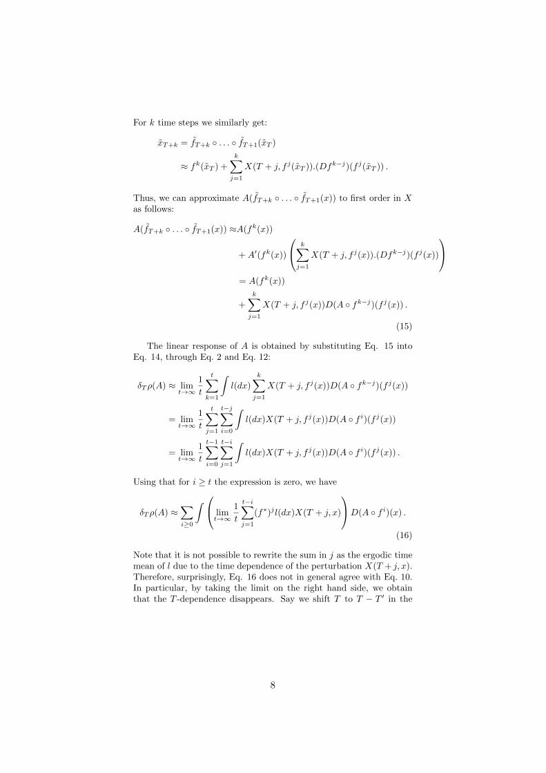
For k time steps we similarly get:

xT+k = fT+k . . . fT+1(xT )

≈ fk(xT ) +

k∑j=1

X(T + j, f j(xT )).(Dfk−j)(f j(xT )) .

Thus, we can approximate A(fT+k . . . fT+1(x)) to first order in Xas follows:

A(fT+k . . . fT+1(x)) ≈A(fk(x))

+A′(fk(x))

k∑j=1

X(T + j, f j(x)).(Dfk−j)(f j(x))

= A(fk(x))

+

k∑j=1

X(T + j, f j(x))D(A fk−j)(f j(x)) .

(15)

The linear response of A is obtained by substituting Eq. 15 intoEq. 14, through Eq. 2 and Eq. 12:

δT ρ(A) ≈ limt→∞

1

t

t∑k=1

∫l(dx)

k∑j=1

X(T + j, f j(x))D(A fk−j)(f j(x))

= limt→∞

1

t

t∑j=1

t−j∑i=0

∫l(dx)X(T + j, f j(x))D(A f i)(f j(x))

= limt→∞

1

t

t−1∑i=0

t−i∑j=1

∫l(dx)X(T + j, f j(x))D(A f i)(f j(x)) .

Using that for i ≥ t the expression is zero, we have

δT ρ(A) ≈∑i≥0

∫ limt→∞

1

t

t−i∑j=1

(f∗)j l(dx)X(T + j, x)

D(A f i)(x) .

(16)

Note that it is not possible to rewrite the sum in j as the ergodic timemean of l due to the time dependence of the perturbation X(T + j, x).Therefore, surprisingly, Eq. 16 does not in general agree with Eq. 10.In particular, by taking the limit on the right hand side, we obtainthat the T -dependence disappears. Say we shift T to T − T ′ in the

8

limit appearing in the above equation:

limt→∞

1

t

t−i∑j=1

(f∗)j l(dx)X(T − T ′ + j, x)

= limt→∞

1

t

t−i−T ′∑j′=1−T ′

(f∗)j′+T ′

l(dx)X(T + j′, x)

= limt→∞

1

t

t−i∑j′=1

(f∗)j′(

(f∗)T′l(dx)

)X(T + j′, x) .

Taking the reasonable assumption that the result in Eq. 16 does notdepend on the initial measure l(dx) (this cannot be obtained from theuniqueness of the SRB measure), the obtained response of the systemis time-independent even if the forcing is time-dependent.

Let us compare the result contained in Eq. 16 with Eq. 3 in thespecial case of a time-independent perturbation X(t, x) = χ(x). NowEq. 16 and Eq. 3 agree since Eq. 16 simplifies to:

δT ρ(A) ≈∑i≥0

∫ρ(dx)χ(x)D(A f i)(x) ,

because limt→∞ 1/t∑t−ij=1(f∗)j l(dx)) = ρ(dx), by the definition of the

SRB measure. The formula given by Ruelle [22] is recovered, as canbe seen by substituting φ(t) = 1 into Eq. 3.

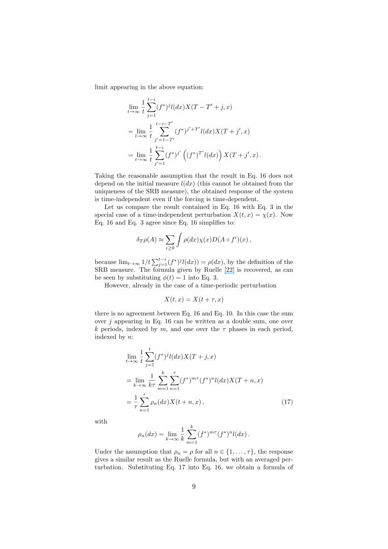
However, already in the case of a time-periodic perturbation

X(t, x) = X(t+ τ, x)

there is no agreement between Eq. 16 and Eq. 10. In this case the sumover j appearing in Eq. 16 can be written as a double sum, one overk periods, indexed by m, and one over the τ phases in each period,indexed by n:

limt→∞

1

t

t∑j=1

(f∗)j l(dx)X(T + j, x)

= limk→∞

1

kτ

k∑m=1

τ∑n=1

(f∗)mτ (f∗)nl(dx)X(T + n, x)

=1

τ

τ∑n=1

ρn(dx)X(t+ n, x) , (17)

with

ρn(dx) = limk→∞

1

k

k∑m=1

(f∗)mτ (f∗)nl(dx) .

Under the assumption that ρn = ρ for all n ∈ 1, . . . , τ, the responsegives a similar result as the Ruelle formula, but with an averaged per-turbation. Substituting Eq. 17 into Eq. 16, we obtain a formula of

9

the form of Eq. 10, with the difference that instead of the true forcingX(t, x) the averaged forcing

1

τ

τ∑n=1

X(t+ n, x)

appears in the formula. The disagreement is apparent, e.g. when oneconsiders a perturbation of the form X(t, x) = sin( 2πl

τ t)χ(x), whichobviously results in a zero response.

One way to obtain agreement with Formula 11 is to choose a spe-cific sampling procedure. We sample with the same periodicity of theforcing, thus altering the definition of the response. We define themeasures for the perturbed and unperturbed system as

ρ′T (dx) := limN→∞

1

N

N∑k=1

(fkτ+pT )∗l(dx)

ρ′(dx) := limN→∞

1

N

N∑k=1

(fkτ+pT )∗l(dx),

for p ∈ 0, . . . , τ − 1. With this definition we obtain Eq. 11:

δρ′T = ρ′T − ρ′

≈ limN→∞

1

N

N∑k=1

∫l(dx)

τ∑n=1

k∑m=1

X(T + n+mτ, fn+mτ (x))

D(A fkτ−n−mτ )(fn+mτ (x))

and by the periodicity of X

δρ′T ≈τ∑n=1

limN→∞

1

N

N−1∑m=0

N−m∑i=1

∫(fn+mτ )∗l(dx)X(T + n, x)D(A f iτ−n)(x)

=

τ∑n=1

limN→∞

1

N

∑i≥1

N−i∑m=0

∫(fn+mτ )∗l(dx)X(T + n, x)D(A f iτ−n)(x)

=

τ∑n=1

∫ (limN→∞

1

N

N−i∑m=0

(fn+mτ )∗l(dx)

)X(T + n, x)

∑i≥1

D(A f iτ−n)(x)

=

τ∑n=1

∫ρn(dx)X(T + n, x)

∑i≥1

D(A f iτ−n)(x)

.

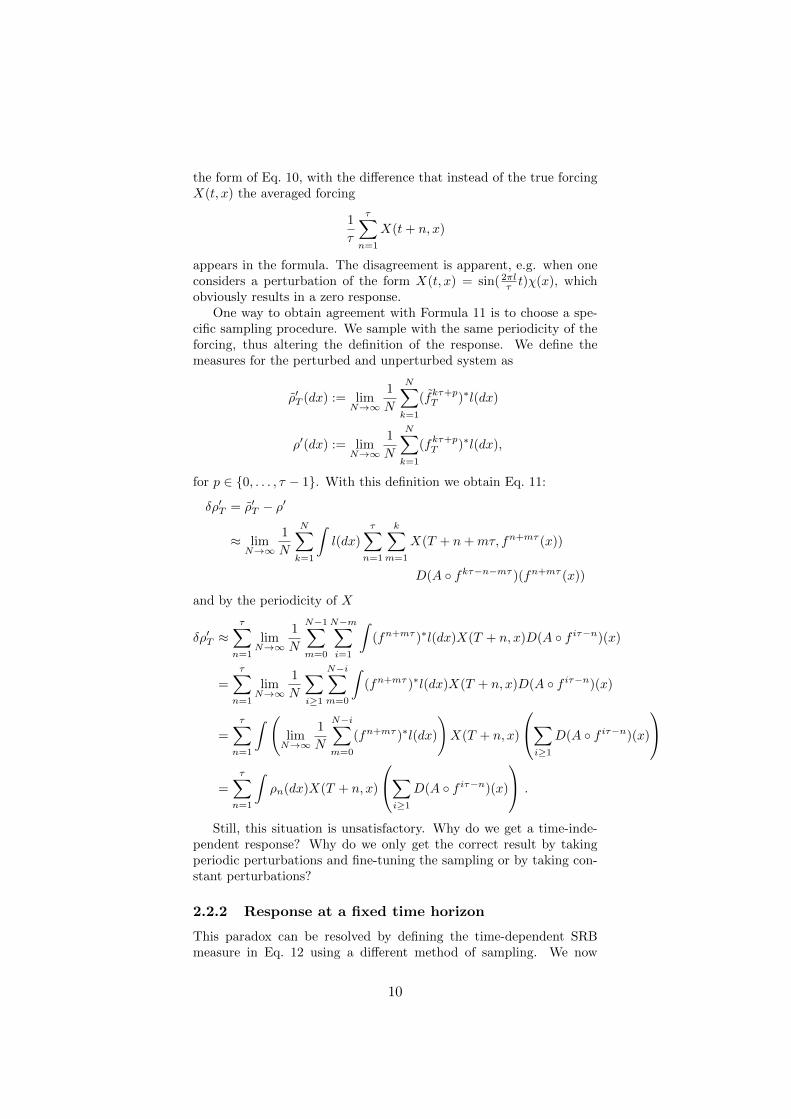
Still, this situation is unsatisfactory. Why do we get a time-inde-pendent response? Why do we only get the correct result by takingperiodic perturbations and fine-tuning the sampling or by taking con-stant perturbations?

2.2.2 Response at a fixed time horizon

This paradox can be resolved by defining the time-dependent SRBmeasure in Eq. 12 using a different method of sampling. We now

10

consider the time evolution fkT in this definition to go from time T − kin the past up to the fixed time horizon T , so instead of Eq. 13, wehave:

fkT = fT . . . fT−k . (18)

Note that this approach does not use the reversed time dynamics butrather a different time perspective in which the final time is fixed asthe current time and the perturbation starts in the remote past.

The expansion to first order in X around the dynamics of f nowbecomes:

xT = fT . . . fT−k+1(xT−k)

≈ fk(xT−k) +

k−1∑j=0

X(T − j, fk−j(xT−k)).(Df j)(fk−j(xT−k)) .

Hence, the linear response of ρ(A) at time T is given by

δT ρ(A) ≈ limt→∞

1

t

t∑k=1

∫l(dx)

k−1∑j=0

X(T − j, fk−j(x))D(A f j)(fk−j(x))

= limt→∞

1

t

t−1∑j=0

t−j∑i=1

∫l(dx)X(T − j, f i(x))D(A f j)(f i(x))

= limt→∞

1

t

∑j≥0

∫ t−j∑i=1

(f∗)il(dx)X(T − j, x)D(A f j)(x) .

Note that in contrast to Eq. 16 the indices are such that the time aver-age of the measure and the perturbation are decoupled. This cruciallydepends on the choice of the sampling. This allows us to use the def-inition of the SRB measure in Eq. 2 and replace the time average inthe limit by ρ:

δT ρ(A) ≈∑j≥0

∫ρ(dx)X(T − j, x)D(A f j)(x) . (19)

This agrees with Eq. 10.Here we do get the anticipated result. Note that this expression

gives also a non-zero response for a perturbation which is non-zero fora finite time as opposed to Eq. 16.

This sampling is the natural one fore deducing the general linearresponse theory. Doing the calculation for constant forcing does notelucidate the relevance of the choice of sampling. This sampling cor-responds to a Gedankenexperiment where the system is prepared inthe distant past and we observe the difference of the perturbed andunperturbed evolution up to a given instant T .

11

3 Numerics

For perturbations that are separable (X(t, x) = φ(t)χ(x)) and have asingle driving frequency Ω (φ(t) = εcos(Ωt)), the following samplingscheme for computing the susceptibility for a given observable A hasbeen proposed by Reick [19]:

κA(Ω) = limε→0

limN→∞

1

Nε

N∑t=1

eiΩt∫ρ(dx)

(A(f t0(x))−A(f t(x))

). (20)

This formula has been later adopted to analyze the output of a simpleclimate model [16] and a generalization has been proposed to study thenonlinear susceptibilities describing harmonic generation [14]. Appli-cability of this formula depends on performing numerical experimentswhere the initial samples approximate the unperturbed SRB measureρ.

Using our previous calculations, we want to circumstantiate the va-lidity of the formula. We apply Ruelle’s response theory to obtain aperturbative expression of Eq. 20 in terms of quantities of the unper-turbed dynamics.

limN→∞

1

N

N∑t=1

eiΩt∫l(dx)

(A(f t0(x))−A(f t(x))

)≈ limN→∞

1

N

N∑t=1

eiΩt∫ t∑

j=1

(f j)∗l(dx)X(j, f j(x))D(A f t−j)(x) .

Here we encounter the same problem as in Eq. 16, namely the couplingof the averages of the measure and the perturbation. Indeed, usingReick’s formula sampling from an initial measure different from theunperturbed SRB measure, one does not get a reasonable response, asreported in [16].

By sampling according to the unperturbed SRB measure ρ insteadof l, the above equation becomes

limN→∞

1

N

N∑j=1

N−j∑k=0

eiΩkeiΩj∫ρ(dx)X(j, x)D(A fk)(x)

= limN→∞

1

N

∫ρ(dx)GA(ω, x)

N−k∑j=1

eiΩjX(j, x) . (21)

We insert the inverse discrete time Fourier transform

X(j, x) =1

2π

∫ π

−πX(ω, x)e−iωjdω

12

into Eq. 21:∫ρ(dx)ΓA(ω, x) lim

N→∞

1

N

N∑j=1

eiΩjX(j, x)

=

∫ρ(dx)ΓA(ω, x) lim

N→∞

1

N

N∑j=1

eiΩj1

2π

∫ π

−πX(ω, x)e−iωjdω

=

∫ρ(dx)ΓA(ω, x) lim

N→∞

1

2π

∫ π

−πX(ω, x)

1

N

N∑j=1

ei(Ω−ω)jdω . (22)

The sum over j can be rewritten by making use of

x+ . . .+ xN = x1− xN

1− x.

as

1

Nei(Ω−ω)j 1− eiN(Ω−ω)j

1− ei(Ω−ω)j,

which converges to 0 as N goes to infinity, except for Ω = ω. At Ω = ωthe sum over j gives N . Hence, if X(ω, x) is continuous, we can takethe limit in Eq. 22 inside the integral

1

2π

∫ π

−πX(ω, x)1Ω(ω)dω = 0 ,

where 1Ω is the indicator function on Ω. We deduce that in the caseof a general perturbation with a continuous Fourier spectrum, Reick’snumerical approach cannot be applied. Note also that for finite timesteps N (as is always the case for numerical experiments), there is anadditional broadening of the signal of order 1/N , as is apparent fromEq. 22.

If on the other hand the Fourier transform is singular, for example

X(ω, x) = δ(Ω− ω)χ(x) ,

which corresponds to the monochromatic signal

X(j, x) =1

2πe−iΩjχ(x) ,

we have that

limN→∞

1

N

N−k∑j=1

eiΩjX(j, x) = limN→∞

N − k2πN

χ(x)

=χ(x)

2π.

Such that Eq. 21 becomes∫ρ(dx)GA(ω, x)χ(x) = κA(Ω) ,

as predicted by Reick. The above calculation gives a straightforwardderivation of Reicks formula.

13

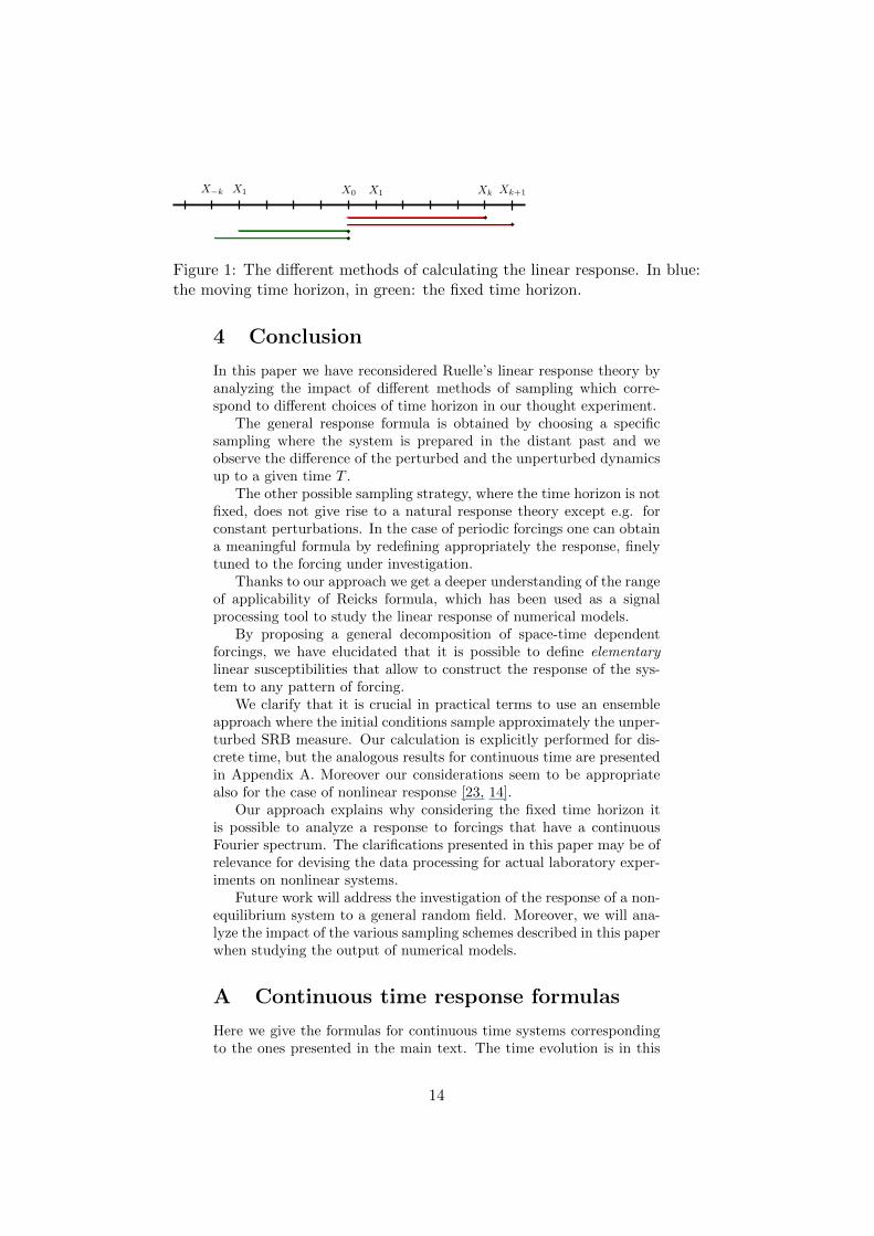
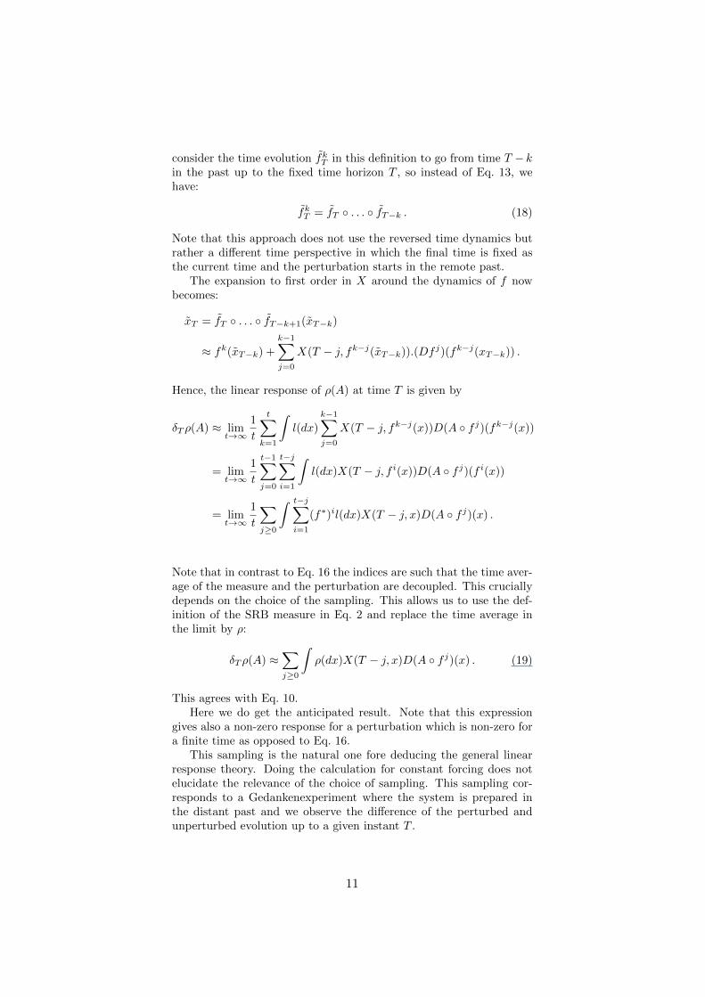
Figure 1: The different methods of calculating the linear response. In blue:the moving time horizon, in green: the fixed time horizon.

4 Conclusion

In this paper we have reconsidered Ruelle’s linear response theory byanalyzing the impact of different methods of sampling which corre-spond to different choices of time horizon in our thought experiment.

The general response formula is obtained by choosing a specificsampling where the system is prepared in the distant past and weobserve the difference of the perturbed and the unperturbed dynamicsup to a given time T .

The other possible sampling strategy, where the time horizon is notfixed, does not give rise to a natural response theory except e.g. forconstant perturbations. In the case of periodic forcings one can obtaina meaningful formula by redefining appropriately the response, finelytuned to the forcing under investigation.

Thanks to our approach we get a deeper understanding of the rangeof applicability of Reicks formula, which has been used as a signalprocessing tool to study the linear response of numerical models.

By proposing a general decomposition of space-time dependentforcings, we have elucidated that it is possible to define elementarylinear susceptibilities that allow to construct the response of the sys-tem to any pattern of forcing.

We clarify that it is crucial in practical terms to use an ensembleapproach where the initial conditions sample approximately the unper-turbed SRB measure. Our calculation is explicitly performed for dis-crete time, but the analogous results for continuous time are presentedin Appendix A. Moreover our considerations seem to be appropriatealso for the case of nonlinear response [23, 14].

Our approach explains why considering the fixed time horizon itis possible to analyze a response to forcings that have a continuousFourier spectrum. The clarifications presented in this paper may be ofrelevance for devising the data processing for actual laboratory exper-iments on nonlinear systems.

Future work will address the investigation of the response of a non-equilibrium system to a general random field. Moreover, we will ana-lyze the impact of the various sampling schemes described in this paperwhen studying the output of numerical models.

A Continuous time response formulas

Here we give the formulas for continuous time systems correspondingto the ones presented in the main text. The time evolution is in this

14

setting given by a differential equation

dx

dt= F (x) ,

resulting in a flow x(t+ s) = fs(x(t)). The SRB measure is given by

ρ(A) = limt→∞

1

t

∫ t

0

ds

∫l(dx)A(fs(x)) .

For a separable perturbation

dx

dt= F (x) + χ(x)φ(t)

the susceptibility is given by

κA(ω) =

∫ ∞0

dteiωt∫ρ(dx)χ(x)D(A f t)(x) .

In case of a general perturbation F (x) → F (x) + X(t, x) the linearresponse becomes:

δT ρ(A) ≈∫ ∞

0

dτ

∫ρ(dx)X(T − τ, x)D(A fτ )(x)

The SRB measure with a moving time horizon is:

ρT = limt→∞

1

t

∫ t

0

ds

∫l(dx)A(fT+t

T (x))

and the SRB measure with a fixed time horizon:

ρT = limt→∞

1

t

∫ t

0

ds

∫l(dx)A(fTT−t(x))

where f t2t1 (x) is a trajectory of the perturbed system, starting at timet1 in x and evolving up to time t2.

Reick’s formula now becomes:

κA(ω) = limε→0

limν→∞

1

νε

∫ ν

0

dteiΩt∫ρ(dx)

(A(f t0(x))−A(f t0(x))

)References

[1] R. Abramov and A.J. Majda. Blended response algorithms for lin-ear fluctuation-dissipation for complex nonlinear dynamical sys-tems. Nonlinearity, 20:2793–2821, 2007.

[2] V. Baladi. On the susceptibility function of piecewise expandinginterval maps. Comm. Math. Phys., 275:839–859, 2007.

[3] B. Cessac and J.-A. Sepulchre. Linear response, susceptibility andresonances in chaotic toy models. Physica D, 225:13–28, 2007.

15

[4] D. Dolgopyat. On differentiability of SRB states for partiallyhyperbolic systems. Invent. Math., 155:389–449, 2004.

[5] G. Gallavotti. In J.P. Francoise, G.L. Naber, and T. S.Tsun, editors, Nonequilibrium Statistical Mechanics (Stationary):Overview, volume 3 of Encyclopedia of Mathematical Physics,pages 530–539. Elsevier Amsterdam, 2006.

[6] G. Gallavotti and E.G.D. Cohen. Dynamical ensembles in sta-tionary states. J. Stat. Phys., 80:931–970, 1995.

[7] R.S. Hawkins and M. Aoki. Macroeconomic relaxation: Adjust-ment processes of hierarchical economic structures. Economics:The Open-Access, Open-Assessment E-Journal, 3:1–21, 2009.

[8] R. Kubo. Statistical-mechanical theory of irreversible processes.i. J. Phys. Soc. Jpn., 12:570–586, 1957.

[9] R. Kubo. The fluctuation dissipation theorem. Rep. Prog. Phys.,29:255–284, 1966.

[10] G. Lacorata and A. Vulpiani. Fluctuation-response relation andmodeling in systems with fast and slow dynamics. Nonlin. Pro-cesses Geophys., 14:681–694, 2007.

[11] J. Lindenstrauss and L. Tzafriri. Classical Banach spaces.Springer, 1996.

[12] E.N. Lorenz. Forced and free variations of weather and climate.J. Atmos. Sci., 36:1367–1376, 1979.

[13] V. Lucarini. Response theory for equilibrium and non-equilibriumstatistical mechanics: Causality and generalized Kramers-Kronigrelations. J. Stat. Phys., 131:543–558, 2008.

[14] V. Lucarini. Evidence of dispersion relations for the nonlinearresponse of Lorenz 63 system. J. Stat. Phys., 134:381–400, 2009.

[15] V. Lucarini. Stochastic perturbations to dynamical systems: aresponse theory approach. Physical Review E, submitted, 2011.

[16] V. Lucarini and S. Sarno. A statistical mechanical approach forthe computation of the climatic response to general forcings. Non-lin. Processes Geophys., 18:7–28, 2011.

[17] A.J. Majda and X. Wang. Linear response theory for statisticalensembles in complex systems with time-periodic forcing. Comm.Math. Sci., 8:142–172, 2010.

[18] M. Reed and B. Simon. Modern Methods of Mathematical Physics.Vol. 1. Functional Analysis. Academic Press, New York, 1972.

[19] C. H. Reick. Linear response of the Lorenz system. PhysicalReview E, 66(3):036103, 2002.

[20] D. Ruelle. Chaotic evolution and strange attractors. CambridgeUniversity Press Cambridge, 1989.

[21] D. Ruelle. Differentiation of SRB states. Communications inMathematical Physics, 187(1):227–241, 1997.

16

[22] D. Ruelle. General linear response formula in statistical mechan-ics, and the fluctuation-dissipation theorem far from equilibrium.Phys. Letters A, 245:220–224, 1998.

[23] D. Ruelle. Nonequilibrium statistical mechanics near equilibrium:computing higher-order terms. Nonlinearity, 11:5–18, 1998.

[24] D. Ruelle. A review of linear response theory for general differen-tiable dynamical systems. Nonlinearity, 22(4):855–870, 2009.

[25] A. Shimizu. Universal properties of nonlinear response functionsof nonequilibrium steady states. Journal of the Physical Societyof Japan, 79:113001, 2010.

[26] L.-S. Young. What are SRB measures, and which dynamical sys-tems have them? Journal of Statistical Physics, 108:733–754,2002. 10.1023/A:1019762724717.

[27] T. Yuge. Sum rule for response function in nonequilibriumLangevin systems. Phys. Rev. E, 82:051130, 2010.

[28] D.N. Zubarev. Nonequilibrium Statistical Thermodynamics. Con-sultant Bureau New York, 1974.

17