arX

iv:g

r-qc

/041

2011

v1 2

Dec

200

4

Relating Spin Foams and Canonical Quantum

Gravity: (n − 1) + 1 formulation of nD spin

foams.

Suresh K MaranDepartment of Physics and Astronomy

University of PittsburghPittsburgh PA-15260

February 7, 2008

Abstract

In this article we lay foundations for a formal relationship of spin foam

models of gravity and BF theory to their continuum canonical formula-

tions. First the derivation of the spin foam model of the BF theory from

the discrete BF theory action in n dimensions is reviewed briefly. By

foliating the underlying n dimensional simplicial manifold using n − 1 di-

mensional simplicial hypersurfaces, the spin foam model is reformulated.

Then it is shown that spin network functionals arise naturally on the fo-

liations. The graphs of these spin network functionals are dual to the

triangulations of the foliating hypersurfaces. Quantum Transition ampli-

tudes are defined. I calculate the transition amplitudes related to 2D BF

theory explicitly and show that these amplitudes are triangulation inde-

pendent. The application to the spin foam models of gravity is discussed

briefly.

1 Introduction

During the late part of the last decade, there has been a vigorous activity in thearea of combinatorial quantization of the theories such as BF theory1 [1] andgravity, generally referred to as the spin foam quantization. The general notionof a spin foam model was motivated by at least three examples: the Regge-Ponzano model, which is a construction of simplicial quantum geometries using6J symbols of the group SU(2) [2]; the abstract spin networks of Roger Penrose,who derives spatial structures from the interchange of angular momentum [3]

1A BF theory in n dimensions and for a group G refers to field theory defined by the actionS =

∫

B ∧ F . Here B is a n − 2 form which takes values in dual Lie algebra of G and F isa 2-form is the cartan curvature of a G-connection A. The free variables of the theory are Band A.

1

and the evolutions of the Rovelli-Smolin spin network functionals, which are thekinematical quantum states of canonical quantum gravity [4]. Casual evolutionand dual formulation of spin foams were proposed by Fotini Markopoulou [5],[6] and Lee Smolin [5]. I refer to Baez [7] for a nice introduction to spin foammodels and we refer to Perez [8] for an up-to-date review of the spin foam modelsand a comprehensive set of references.

The concept of spin foam is very general and there are various specific spinfoam models that are available in the research literature [8]. A spin foam modelof the four dimensional SO(4) BF theory called the Ooguri model [9] can bederived directly from its discretized action. From this model a spin foam modelof Riemannian gravity can be derived by imposing a set of constraints called theBarrett-Crane constraints [10]. Here by ‘the spin foam models’ we specificallyrefer to these models of BF theory, gravity and their variations.

One of the interesting problems in quantum gravity is how to relate the spinfoam models of gravity to its canonical formulation of gravity [11], [12], [13],[14]. Here we take the point of view of seeing how close we can bring a spin foammodel to it’s canonical quantum formulation, instead of assuming the existenceof a precise relation between them. Canonical quantum gravity is formulated oncontinuum manifolds, while the spin foams are formulated on simplicial man-ifolds (or on 2-complexes [7]). In general the canonical formulation requiresthe underlying n dimensional manifold of the theory to be expressible in an(n − 1) + 1 form. In the same spirit, here we foliate the n dimensional simpli-cial manifold. The foliation is made up of a one parameter family of simplicial(n−1) dimensional hypersurfaces2. Between any two consecutive hypersurfaceswe have a one-simplex thick slice of the simplicial manifold.

To each edge ((n − 1)-simplex) of the simplicial manifold is associated aparallel propagator g which plays the role of a discrete connection. To makea parallel to the canonical quantization we make an important identification.I find that the parallel propagators associated with the edges in the foliatinghypersurfaces can be thought of as the analog of the continuum connection inthe (coordinate) time direction. In the canonical quantization, the field equa-tion corresponding to this component of the connection is the Gauss constraint[11], which on quantization leads to spin network functionals [12]. Remarkablythe same idea works in the spin foam quantization obtained by the path inte-gral quantization of the theory defined by the discretized BF action S. It justhappens that the integration of the Feynman weight eiS with respect to theparallel propagators associated with the edges of the hypersurfaces results ina product of spin network functionals. These spin network functionals are de-fined on the parallel propagators associated with the edges that go between thehypersurfaces and the graphs that are dual to the triangulation of the foliatinghypersurfaces. All our work is built around this observation of the appearanceof spin network functionals. Since the spin foam model of gravity is obtained byimposing the Barrett-Crane constraints on the BF spin foam model, we believe

2We restrict ourselves to manifolds that are foliatable by a one parameter family of sim-plicial hypersurfaces.

2

we can carry over this result to gravity.Each of the one-simplex thick slices of the simplicial manifold can be consid-

ered to define a discrete coordinate time instant. The set of parallel propagatorswhich are associated with the edges that go between two consecutive foliatinghypersurface can be considered to contain the physical (connection) informa-tion of the theory at a particular discrete time for a given triangulation. Spinnetwork states can be defined as functions of these discrete connections. Usingthe path integral formulation, we define a spin network state to spin networkstate elementary transition amplitude matrix.

This article has been made as self-contained as possible. In this article wefirst focus on BF theory for an arbitrary compact group and discuss gravityafterwards. In section two we review the derivation of BF spin foam model.

In section three we discuss how the partition function of the BF theorycan be expressed in terms of the spin network functionals that are obtainedby integrating the Feynman weight eiS with respect to the parallel propagatorsassociated with the edges in the foliating simplicial hypersurfaces. In sectionfour we discuss the details of these spin network functionals. I show that thesespin network functionals are orthonormal in the obvious inner product.

In section five we discuss the elementary transition amplitudes using thepath integral formulation. I discuss this in the form of a connection formulationand spin network formulation.

In section six we discuss two dimensional BF theory. I explicitly calculate theelementary transition amplitudes. I find that the transition matrix is symmetric,non-unitary and is independent of triangulation.

In section seven we discuss 2+1 BF theory (2+1 Riemannian) gravity verybriefly.

In section five we define the elementary transition amplitude matrix forgravity by including the Barrett-Crane constraints in the definition of BF ele-mentary transition amplitude matrix. This is similar to that of Reisenberger[20] defined in an unfoliated context. In section six, we observe that, in thecase of Lorentzian Barrett-Crane model, in the asymptotic limit, the foliatinghypersurfaces behave as spatial hypersurfaces.

2 Review of the spin foam derivation

The review in this section follows that of Baez [7]. Advanced readers may skipor quickly glance through this section. The term ‘edge integral’ is introduced inthis section and is used widely in this article.

Consider an n dimensional manifold M and a G-connection A, where G is acompact linear group. Let F be a curvature 2-form of the connection A. Alsolet B be a dual Lie algebra valued n− 2 form. Then the continuum BF theoryis defined by the following action:

Sc =

∫

M

Tr(B ∧ F ). (1)

3

The spin foam model for this action is derived by calculating the partitionfunction corresponding to the discretized version of this action [7], [9], [16]. Letthe manifold be triangulated by a simplicial lattice. Each n-simplex s is boundedby n+ 1 (n− 1)-simplices called the edges e of s. In turn each (n− 1)-simplexis bounded by n (n− 2)-simplices called the bones.

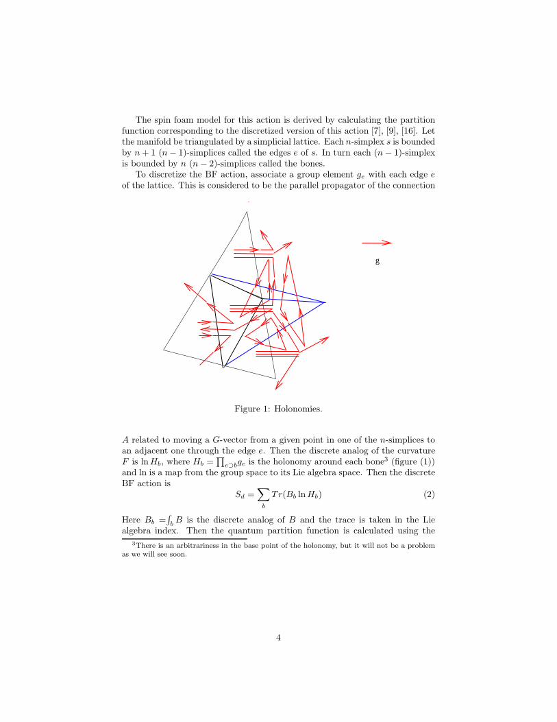
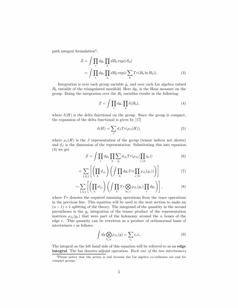
To discretize the BF action, associate a group element ge with each edge eof the lattice. This is considered to be the parallel propagator of the connection

g

Figure 1: Holonomies.

A related to moving a G-vector from a given point in one of the n-simplices toan adjacent one through the edge e. Then the discrete analog of the curvatureF is lnHb, where Hb =

∏

e⊃bge is the holonomy around each bone3 (figure (1))and ln is a map from the group space to its Lie algebra space. Then the discreteBF action is

Sd =∑

b

Tr(Bb lnHb) (2)

Here Bb =∫

bB is the discrete analog of B and the trace is taken in the Lie

algebra index. Then the quantum partition function is calculated using the

3There is an arbitrariness in the base point of the holonomy, but it will not be a problemas we will see soon.

4

path integral formulation4:

Z =

∫

∏

e

dge

∏

b

dBb exp(iSd)

=

∫

∏

e

dge

∏

b

dBb exp(i∑

b

Tr(Bb lnHb)). (3)

Integration is over each group variable ge and over each Lie algebra valuedBb variable of the triangulated manifold. Here dge is the Haar measure on thegroup. Doing the integration over the Bb variables results in the following:

Z =

∫

∏

e

dge

∏

b

δ(Hb), (4)

where δ(H) is the delta functional on the group. Since the group is compact,the expansion of the delta functional is given by [17]

δ(H) =∑

J

dJTr(ρJ(H)), (5)

where ρJ(H) is the J representation of the group (tensor indices not shown)and dJ is the dimension of the representation. Substituting this into equation(4) we get

Z =

∫

∏

e

dge

∏

b

∑

Jb

dJbTr(ρJb

(∏

e⊃b

ge)) (6)

=∑

Jb

[(

∏

b

dJb

)(

∫

∏

b

dgeTr(∏

e⊃b

ρJb(ge))

)]

(7)

=∑

Jb

[(

∏

b

dJb

)(

∫

∏

b

Tr⊗

b⊂e

ρJb(ge)

∏

e

dge

)]

, (8)

where Tr denotes the required summing operations from the trace operationsin the previous line. This equation will be used in the next section to make an(n− 1) + 1 splitting of the theory. The integrand of the quantity in the secondparentheses is the ge integration of the tensor product of the representationmatrices ρJb

(ge) that were part of the holonomy around the n bones of theedge e. This quantity can be rewritten as a product of orthonormal basis ofintertwiners i as follows:

∫

dg⊗

b⊃e

ρJb(g) =

∑

ie

ieıe. (9)

The integral on the left hand side of this equation will be referred to as an edge

integral. The bar denotes adjoint operation. Each one of the two intertwiners4Please notice that the action is real because the Lie algebra co-ordinates are real for

compact groups.

5

corresponds to one of the two sides of an edge of a simplex. Please refer to theappendices for more information about the edge integrals.

The mathematical fact that the edge integral splits into two intertwiners is acritical reason for the emergence of the spin foam models from the path integralformulation of the discretized BF theory. Each of the intertwiners is associatedwith one of two sides of the edge.When this edge integral formula is used inequation (8) and all the required summations are performed, it is seen thateach index of each intertwiner corresponding to an inner side of an edge of eachsimplex only sums with an index of an intertwiner corresponding to an innerside of another edge of the same simplex. Because of this the partition functionZ splits into a product of terms, with each term interpreted as a quantumamplitude associated with a simplex in the triangulation.

Finally the formula for the partition function in n dimensions is given by

Z =∑

Jb,ie

(

∏

b

dJb

)

∏

s

Z(s), (10)

where Z(s) is the quantum amplitude associated with the n-simplex s and dJbis

interpreted as the quantum amplitude associated with the bone b. This partitionfunction may not be finite in general. The set Jb,ie of all Jb’s and ie’s is calleda coloring of the bones and the edges.

3 The (n − 1) + 1 splitting of the n dimensional

BF spin foam models.

Consider a smooth n dimensional manifold M triangulated by a simplicial lat-tice. I assume that the following properties hold for the triangulation56:

1. The simplicial manifold can be foliated by a discrete one parameter familyof n − 1 dimensional simplicial hypersurfaces made of the edges of thetriangulation,

2. The foliation is such that there are no vertices of the lattice in betweenthe hypersurfaces of the family,

3. The hypersurfaces do not intersect or touch each other at any point, and

4. The slice of the manifold in between any two consecutive hypersurfaces isalways one-simplex thick.

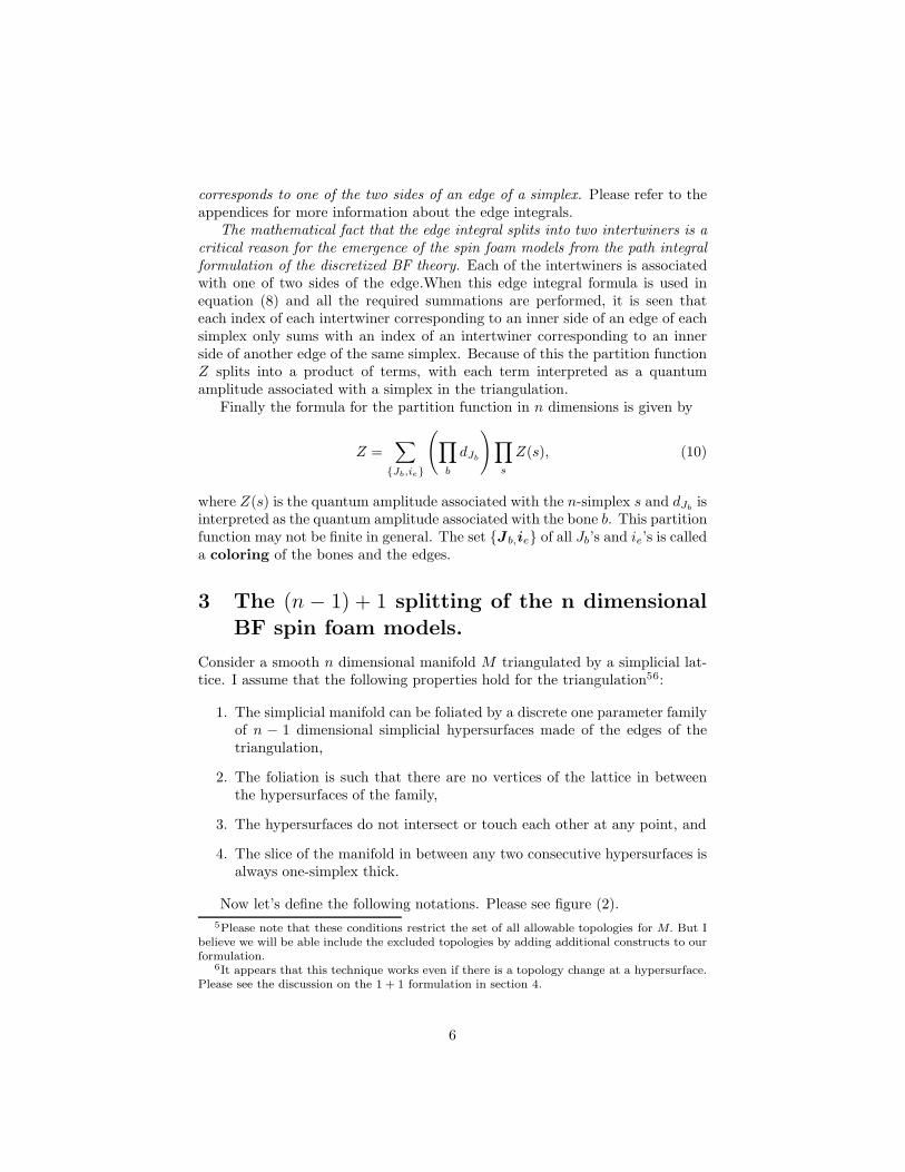
Now let’s define the following notations. Please see figure (2).

5Please note that these conditions restrict the set of all allowable topologies for M. But Ibelieve we will be able include the excluded topologies by adding additional constructs to ourformulation.

6It appears that this technique works even if there is a topology change at a hypersurface.Please see the discussion on the 1 + 1 formulation in section 4.

6

Notation 1 Let Σi be a sequence of simplicial hypersurfaces, ordered by aninteger i, which is a foliation of the triangulation of M such that the aboveproperties hold.

Notation 2 Let Ωi be the piece of the simplicial manifold M between Σi andΣi+1. This Ωi has the thickness of a one-simplex.

Now there are two types of edges and bones in the lattice, those that whichlie on the hypersurfaces and those that go between the hypersurfaces.

Notation 3 Let the edges which lie on the hypersurfaces be represented with acap on them, as in e, and those that go between the foliating hypersurfaces berepresented with a tilde on them, as in e. If we want to refer to the both types ofthese edges by a single variable, then we use the e notation as before. I assumethe same conventions apply for bones also.

Consider the expression for the partition function:

Z =∑

Jb

[(

∏

b

dJb

)

Tr

(

∫

∏

b

⊗

b⊂e

ρJb(ge)

∏

e

dge

)]

(11)

Let us do the integration in the ge variables of the edges e that lie on the foliatingsurfaces only. Then the product of the edge integrals of these edges in the aboveequation is replaced by a product of the intertwiners. The resulting integrandin the right hand side of the above equation is made up of a product of spinnetwork functionals [12] with parallel propagators constructed out of certainproducts of the ρJ

b(ge)’s and the intertwiners ie’s intertwining them. In figure

(2) this process has been explained and many of the notations are illustrated in1 + 1 dimensions.

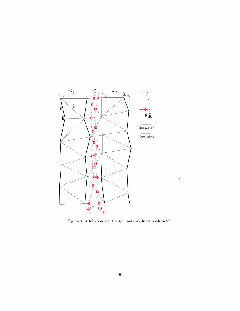
There are two spin network functionals for each Ωi. One of them, ψ+i (the

other is ψ−i ) is made up of the intertwiners associated with the sides of all the

edges e of Σi facing Ωi (Ωi−1) and the ρJb( ge)’s of the edges e in Ωi(Ωi−1).

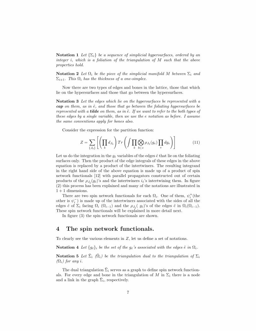
These spin network functionals will be explained in more detail next.In figure (3) the spin network functionals are shown.

4 The spin network functionals.

To clearly see the various elements in Z, let us define a set of notations.

Notation 4 Let gei be the set of the ge’s associated with the edges e in Ωi.

Notation 5 Let Σi (Ωi) be the triangulation dual to the triangulation of Σi

(Ωi) for any i.

The dual triangulation Σi serves as a graph to define spin network function-als. For every edge and bone in the triangulation of M in Σi there is a nodeand a link in the graph Σi, respectively.

7

e

Σ iΣ i−1

Σi+1

ee

Σ iΣ i−1

Σi+1

e

eΩ i−1 Ω i

Ω i−1 Ωi

~~

ι

ρ (g)~

Hypersurface

Triangulation

Figure 2: Before and after integration with respect to dge, e ∈ Σi.

8

ee

Σ i+2

e

Ω i Σi+1Σ i

Ω i+1Ω i−1Σ i−1

ΨΨi i+1

b

~ι

ρ (g)~

Hypersurface

Triangulation

+ −

Σ

Figure 3: A foliation and the spin network functionals in 2D.

9

Notation 6 Let the coloring Jb, o

b, ieΣ be the set of representations J

b’s, ori-

entations ob’s assigned to the bones b’s and intertwiners ie associated with the

edges e’s of the manifold on any hypersurface Σ.

Notice that the bones b’s of the simplicial manifold M are actually the edgesof the hypersurface on which they are lying. But we will refer to the simplices asedges or bones with respect to the simplicial manifold M to keep our notationssimple.

The orientation ob’s can be used to assign directions (arrows) to the links

dual to the bones b’s. The arrows assigned to the links can be used to restrictthe choice of the intertwiner ie assigned to the node corresponding to the edgee ⊂ Σi, as a linear map from the tensor product of the representations assignedto the links with incoming arrows converging at the node, to the tensor productof the representations assigned to the links with outgoing arrows diverging outof the node. If all the arrows are incoming or outgoing then the intertwinerlinearly maps to or from the identity representation, respectively.

Definition 7 Given a hypersurface Σi and any bone b on it, we can associateparallel propagators G±

bto the bone, defined as follows:

G+

b=

∏

∀eb,e∈Ωi

ge. (12)

G−

b=

∏

∀eb,e∈Ωi−1

ge. (13)

where, the multiplications are done in the sequential order of edges e ∋ b aroundthe bone b. The starting edge for G+

b(G−

b) is given by orientation o

b(o

b=opposite

orientation to ob). Let the collection of these G±

b’s for all b on Σi be denoted as

G±

bΣi

.

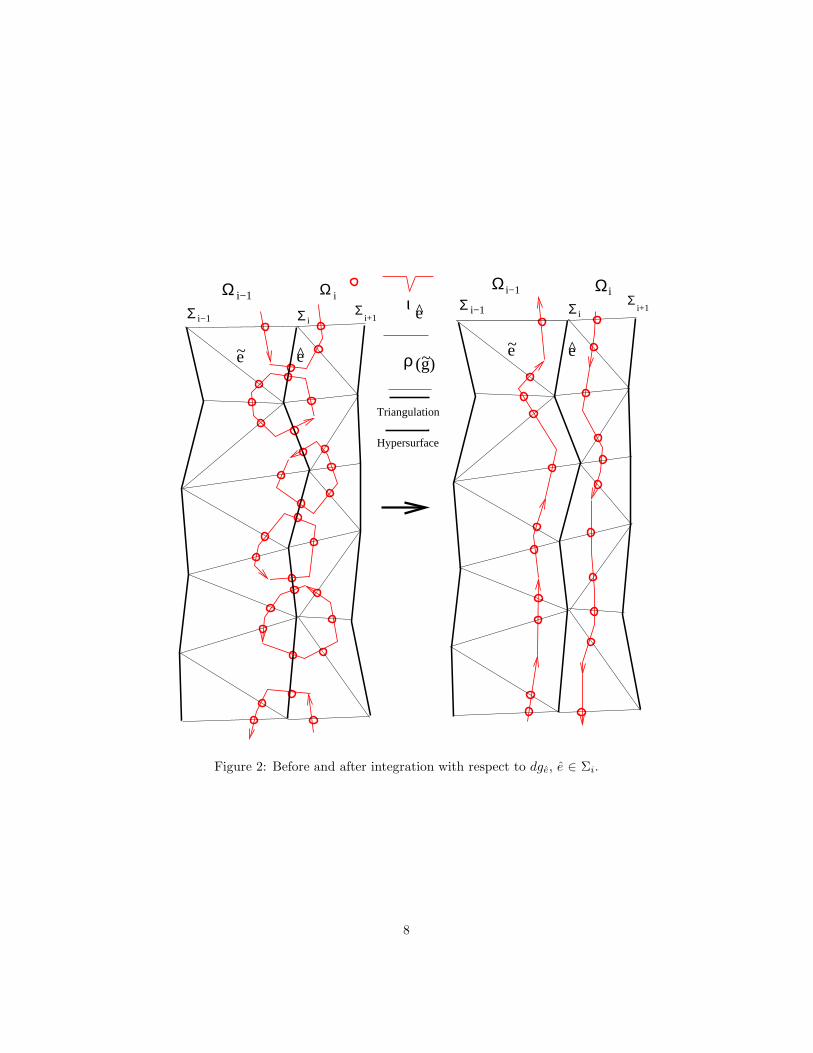
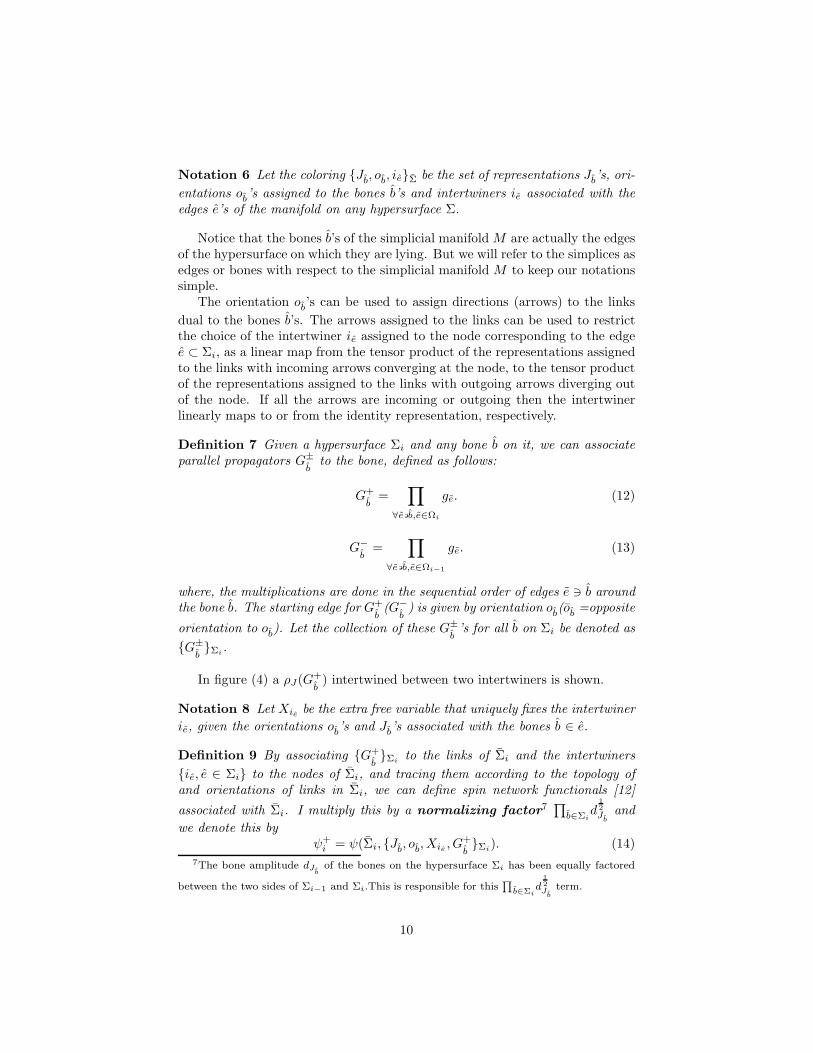
In figure (4) a ρJ(G+

b) intertwined between two intertwiners is shown.

Notation 8 Let Xiebe the extra free variable that uniquely fixes the intertwiner

ie, given the orientations ob’s and J

b’s associated with the bones b ∈ e.

Definition 9 By associating G+

bΣi

to the links of Σi and the intertwiners

ie, e ∈ Σi to the nodes of Σi, and tracing them according to the topology ofand orientations of links in Σi, we can define spin network functionals [12]

associated with Σi. I multiply this by a normalizing factor7∏

b∈Σid

12

Jb

and

we denote this byψ+

i = ψ(Σi, Jb, o

b, Xie

, G+

bΣi

). (14)

7The bone amplitude dJb

of the bones on the hypersurface Σi has been equally factored

between the two sides of Σi−1 and Σi.This is responsible for this∏

b∈Σid

12

Jb

term.

10

~g

ρRepresentation

J

eιIntertwiner

e

b

e~

e~

~g

eι

~g

b

ι

Ω iΣi

+G

Figure 4: A ρJ (G+

b) intertwined between two intertwiners.

This spin network functional associated with the side of Σi that faces Ωi. Sim-ilarly, by using G−

bΣi

we can define another spin network functional

ψ−i = ψ(Σi, Jb

, ob, Xıe

, G−

bΣi

). (15)

associated with the other side of Σi that faces Ωi−1. In ψ−i we have used the

adjoints ıe’s of the intertwiners ie’s and opposite orientations ob’s to o

b’s. These

spin network functionals so defined capture the gauge invariant information inthe discretized connection ge, e ∈ Ωi.

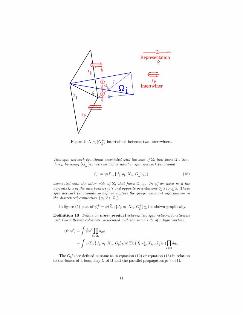
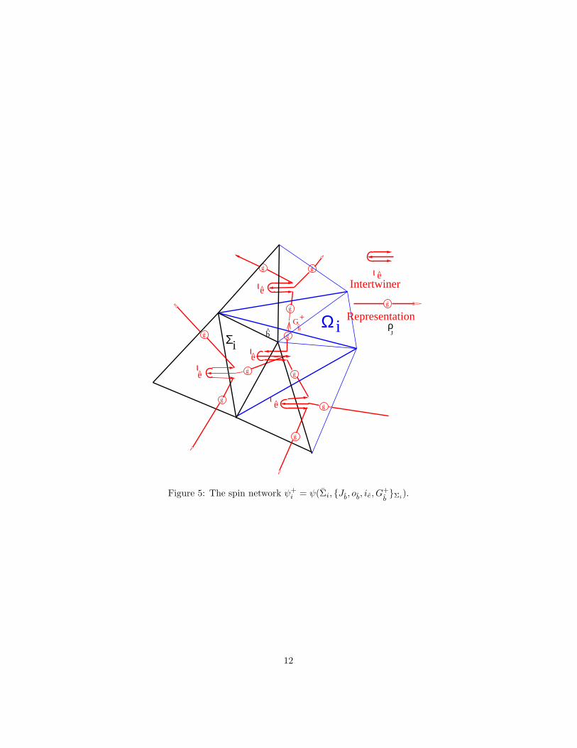
In figure (5) part of ψ+i = ψ(Σi, Jb

, ob, Xie

, G+

bΣi

) is shown graphically.

Definition 10 Define an inner product between two spin network functionalswith two different colorings, associated with the same side of a hypersurface.

(ψ, ψ′) ≡∫

ψψ′∏

e∈Ωi

dge

=

∫

ψ(Σ, Jb, o

b, Xie

, GbΣ)ψ(Σ, J ′

b, o′

b, Xıe

, GbΣ)∏

e∈Ω

dge.

The Gb’s are defined as same as in equation (12) or equation (13) in relation

to the bones of a boundary Σ of Ω and the parallel propagators ge’s of Ω.

11

e

e

e

~g~g

~g

~g

~g

e

e

~g

~g

~g

~g

b ~g

~g

b

Intertwiner

RepresentationρJ

ιι

ι

Ω i

ι

ι

−

+

Σi

G

Figure 5: The spin network ψ+i = ψ(Σi, Jb

, ob, ie, G

+

bΣi

).

12

It can be shown that these spin network functionals are orthonormal in theinner product.

(ψ, ψ′)

=

∫

ψ(Σ, Jb, o

b, Xie

, GbΣ)ψ(Σ, J ′

b, o′

b, Xıe

, GbΣ)∏

e∈Ω

dge

=∏

b∈Σ

δJbJ′

b

∏

e∈Ω

δXieXı′

e

∏

b|Jb≇J

b

δobo′

b,

where the last product in above equation is only over bones whose associatedrepresentations are not conjugate equivalent. This is because in case the repre-sentation J

bis conjugate equivalent then the spin network state does not change

under the change of orientation ob, in other words, for the corresponding state,

ob

is physically redundant.

Proposition 11 The spin network functionals ψ+i and ψ−

i are gauge invariant.

Proof. Now let us demonstrate the gauge invariance of the spin network func-tionals those we obtained from the BF spin foam evaluation. Let us gaugetransform the discrete connection ge, e ∈ M. This requires associating agauge transformation matrix ts ∈ G to each n-simplex s. Let us denote thetwo simplices between which a edge e of M lies, as se,1 and se,2, the num-bers 1 and 2 are chosen such that the parallel propagator ge propagates vectorsfrom se,1 to se,2. After the gauge transformation, the new discrete connectionis g′e, e ∈ M, where g′e = tse,2

get−1se,1

. Let us denote the two edges between

which each bone b ∈ Σi lies as eb,1 and e

b,2, the numbers 1 and 2 are cho-sen such that the orientation o

bpoints from e

b,1 to eb,2. Now if se

b,1and se

b,2

are the simplices of Ωi that touch Σi at eb,1 and e

b,2 respectively, then under

gauge transformation we have G+

bbecome G′+

b= tse

b,1G+

bt−1se

b,2

and our ψ+i

transforms to ψ′+i = ψ(Σi, Jb

, ob, Xie

, G′+

bΣi

). But since we have traced the

G′+

bwith the intertwiners and the intertwiners are invariant under the action

of group elements of G, the gauge transformation matrices t′ss are absorbedby the intertwiners and we get back the original state. This proves the gaugeinvariance of ψ+

i . The gauge invariance of ψ−i can be proved in the similar way.

Definition 12 Let us define a functional⟨

ψ+i , ψ

−i+1

⟩

as follows,

⟨

ψ+i , ψ

−i+1

⟩

Ωi=

∫

ψ+i ψ

−i+1

∏

b∈Ωi

δ(Hb)∏

e∈Ωi

dge. (16)

Now it is straight forward to show that Z can be rewritten as

Z =∑

Jb,o

b,Xie

∏

i

⟨

ψ+, ψ−i+1

⟩

Ωi, (17)

where Jb, o

b, Xie

is the collection of Jb, o

b, Xie

i for all i.

13

5 The elementary transition amplitudes

Let us first fix a triangulation M of the manifold M that satisfies the propertiesenlisted in the previous section. Let us first calculate a connection to connectiontransition amplitude using the path integral formulation of quantum mechanics.The order of the hypersurfaces i can be considered to define a discrete coordinatetime variable.

Notation 13 Let geA (geB) associated with ΩA (ΩB) be the initial (final)connection information, where A and B are integers such that A < B.

Notation 14 Let ΩAB be the simplicial manifold between ΣA and ΣB.

Definition 15 A transition amplitude from geA to geB can be defined basedon the path integral formulation as follows,

〈geA|geB〉 =

∫

exp[iSAB]∏

e∈ΩA+1,B−1

dge

∏

b∈ΩAB

dBb, (18)

where SAB is defined to be

SAB =∑

b∈ΩA+1,B−1

Tr(Bb lnHb).

Our definition of the transition amplitudes has been chosen such that it satisfies:

• the relationship

〈geA|geC〉 =

∫

〈geA|geB〉

〈geB|geC〉∏

b∈ΩB

δ(Hb)∏

e∈ΩB

dge,

where the A, B and C are three consecutive integers in the increasingorder,

• and leads to the result,

〈geA|geB〉 =∑

Jb,o

b,Xie

ψ−A+1

B−1∏

i=A+1

(

ψ+i , ψ

−i+1

)

ψ+B (19)

on integration over ge’s.

The above two properties can be checked explicitly by calculations.For BF theory the physical states require only flat connections. If the ge

are restricted to flat connections gfe (Hb = 1), then δ(Hb) can be removed in

14

the definition of the transition amplitudes8. Then the first condition simply ex-presses an abstract quantum mechanical property that any quantum transitionamplitudes have to satisfy:

⟨

gfe A|gf

e C

⟩

=

∫

⟨

gfe A|gf

e B

⟩

⟨

gfe B|gf

e C

⟩

∏

e∈ΩB

dgfe .

This tells us that the transition amplitudes are intuitively well defined.

Definition 16 Let us define S =

|Jb, o

b, Xie

Σ, Σ >

to be an orthonormalbasis of quantum states, each quantum state identified by a graph Σ and theassociated coloring of bones and edges by J

b, o

b, Xie

Σ. The S defines a basisof abstract spin network states [12].

Definition 17 Equation (19) suggests the following two interpretations:

1. The functional ψ−i+1 is the connection gei to the spin network state

∣

∣

∣J

b, o

b, Xie

Σi+1, Σi+1

⟩

transition amplitude,

ψ−i+1 =ψ(Σi+1, Jb

, ob, Xıe

, G−

bΣi+1

) =⟨

gei|Jb, o

b, Xie

Σi+1, Σi

⟩

Ωi

,

and similarly, functional ψ+i is the spin network state |J

b, o

b, Xie

i, Σi >to the connection gei transition amplitude

ψ+i =ψ(Σi, Jb

, ob, Xie

, G+bΣi

) =⟨

Jb, o

b, Xie

Σi, Σi|gei

⟩

Ωi

Please notice that the above equations are consistent with the orthonor-malities of ψ±

i and the |Jb, o

b, Xie

Σ, Σ >’s. I have the suffix Ωi in theleft-hand sides of the last two equations indicate the dependence on Ωi.

2. Our⟨

ψ+i , ψ

−i+1

⟩

is the spin network state to spin network state transitionamplitude 9,

⟨

ψ+i , ψ

−i+1

⟩

=⟨

Jb, o

b, Xie

Σi, Σi|Jb

, ob, Xie

Σi+1, Σi+1

⟩

Ωi

(20)

Equation(20) defines an elementary transition amplitude. The suffix hasbeen added in the right side above equation because the elementary tran-sition amplitude depends on the triangulation of Ωi.

8An appropriate measure factor may need to be introduced in the integrand.9Using 16 we can show that the elementary transition amplitude

⟨

ψ−

i, ψ+

i

⟩

is simply the

product of the quantum amplitudes of the n-simplices in Ωi, of the bones b ∈ Ωi and thesquare root of the quantum amplitudes of the bones on Σi and Σi+1.

15

Definition 18 The graphs Σi and Σi+1 do not uniquely determine Ωi. Toremove the triangulation dependence of

⟨

ψ+i , ψ

−i+1

⟩

Ωi, let us define a new ele-

mentary transition amplitude, by summing over all possible one-simplex thicktriangulations of Ωi that sandwich between Σi and Σi+1 as follows:

⟨

Jb, o

b, Xie

Σi, Σi|Jb

, ob, iei+1, Σi+1

⟩

(21)

=∑

Ωi

⟨

Jb, o

b, Xie

Σi, Σi|Jb

, ob, Xie

Σi+1, Σi+1

⟩

Ωi

.

Proposition 19 Given any two abstract spin network states∣

∣Jb, o

b, Xie

ΣA, ΣA

⟩

and∣

∣Jb, o

b, Xie

ΣB, ΣB

⟩

, one can immediately calculate an elementary transi-tion amplitude between them.

Proof. The new elementary transition amplitude defined in equation (21) de-pends only on the (J

b, o

b, Xie

Σi,Σi) and the (J

b, o

b, Xie

Σi+1, Σi+1). Because

of this, given any two spin network states∣

∣Jb, o

b, Xie

ΣA, ΣA

⟩

and∣

∣Jb, o

b, Xie

ΣB, ΣB

⟩

,one can immediately calculate a transition amplitude between them, by con-structing a one simplex-thick simplicial manifold ΩAB that sandwiches be-tween ΣA and ΣB, constructing the functions ψ−

A(ΣA, Jb, o

b, Xıe

, G−e ΣA

) andψ+

B(ΣB, Jb, o

b, Xie

, G+e ΣB

), using equation (21) to calculate⟨

Jb, o

b, Xie

ΣA, ΣA|Jb

, XıeΣB

, ΣB

⟩

.If there is no ΩAB that fit between ΣA and ΣB then the elementary transitionamplitude has to be defined to be zero.

The elementary transition amplitudes defined above can be further gener-alized as follows. Let H be an abstract Hilbert space linearly spanned by thespin network state basis defined earlier, S then for any two |ψ〉 , |φ〉 ∈ H , thetransition amplitude 〈ψ|φ〉 can be defined by extending the elementary tran-sition amplitude by linearity. So our elementary transition amplitudes definesa transition matrix. Then if the index i is considered to represent a coordi-nate time, the transition matrix evolves any state |ψi〉 ∈ H at a discrete timeinstant i to its next time instant i + 1. In the case of an arbitrary group GBF theory i may be just an arbitrary parameter to help explore its quantumtheory. But in the case of the Lorentzian quantum gravity, the index i doeshave some physical relation to time. (Please see the discussion near the endof the section on the 3 + 1 Formulation of Gravity). The elementary transi-

tion matrix⟨

Jb, o

b, Xie

Σi, Σi|Jb

, ob, Xie

Σi+1, Σi+1

⟩

so defined helps define

a discrete co-ordinate time evolution scheme of BF theory. In section six, wewill explain how to adapt this scheme to gravity by redefining the elementarytransition amplitudes.

A close analysis indicates that the topology change is built into this for-malism. Please see the section on 1 + 1 BF theory for an illustration.

Our spin network functionals in four dimensions for the BF theory and thosefor gravity that will be discussed later are similar to those in canonical quantumgravity on a triangulated three manifold formulated by Thiemann [13], [14]. InThiemann’s formulation, the spin networks are constructed using parallel prop-agators associated with the edges of the three-simplices of a triangulation of a

16

three manifold. These parallel propagators are constructed out of the path or-dered integral P exp(−

∫

A) of the Ashtekar-Sen connection [11] on the manifold.Our spin network functionals are constructed using the parallel propagators ge

associated with the edges e of the four-simplices in the four dimensional slicesΩi. The four dimensional slices Ωi can be considered as thickened 3D simplicialsurfaces. In our formulation the physical meaning of the parallel propagatorsg’s is clear.

Further work that needs to be done on the theoretical constructions devel-oped in this section will be discussed at the end of this article.

6 The 1 + 1 splitting of the 2D gravity.

In 1 + 1 dimensions the spin network functionals are mathematically simple.Here the 2D manifold is foliated by 1D curves. To simplify our discussion,let us restrict ourselves to conjugate equivalent representations, but conjugateinequivalent representations can be easily included by adding additional deltafunctions in the transition amplitude calculations.

6.1 The one circle to one circle elementary transition am-

plitude.

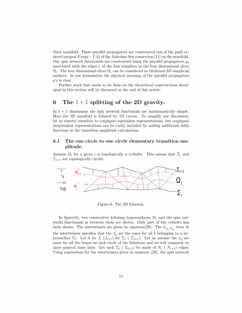
Assume Ωi for a given i is topologically a cylinder. This means that Σi andΣi+1 are topologically circles.

ΩΣ

i

Σ i

Ψ

Ψ

+

−i+1

i+1

i

ι e

ρ (g)

^

~

Figure 6: The 2D foliation.

In figure(6), two consecutive foliating hypersurfaces, Ωi and the spin net-works functionals in between them are shown. Only part of the cylinder hasbeen shown. The intertwiners are given by equation(29). The δJ

b1J

b2term in

the intertwiners specifies that the Jb

are the same for all b belonging to a hy-persurface Σi. Let it be Ji (Ji+1) for Σi ( Σi+1). Let us assume the o

bare

same for all the bones on each circle of the foliations and we will comment onmore general cases later. Let each Σi ( Σi+1) be made of Ni ( Ni+1) edges.Using expressions for the intertwiners given in equation (29), the spin network

17

functionals can be calculated as

ψ+i = Tr(ρJi

(∏

e∈Ωi

ge))

andψ−

i+1 = Tr(ρJi+1(∏

e∈Ωi

ge)),

where the powers of d12

J in ψ+i , ψ−

i+1 in equation (14) and equation (15) from thebone amplitudes and intertwiners cancel each other. The gei are multipliedaccording to the order defined by the topological continuity of Ωi and orientationoi. But since we restricted ourselves to conjugate equivalent representations, thespin network functionals are independent of the orientations ob.

In the 1 + 1 formalism there is no internal holonomy between the foliations.The elementary transition amplitudes can be calculated using equation (16) asfollows:

⟨

ψ+i , ψ

−i+1

⟩

=

∫

ψ+i ψ

−i+1

∏

e∈Ωi

dge

=

∫

Tr(ρJi(∏

e∈Ωi

ge))Tr(ρJi+1(∏

e∈Ωi

ge))∏

e∈Ωi

dge

= δJiJi+1,

whereMi is the number of edges in Ωi. It is interesting to see that the elementarytransition amplitude does not depend on the triangulation.

6.2 The n-circle to m-circle elementary transition ampli-

tude

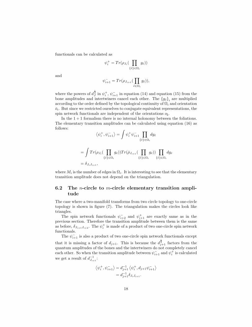
The case where a two-manifold transforms from two circle topology to one-circletopology is shown in figure (7). The triangulation makes the circles look liketriangles.

The spin network functionals ψ−i+2 and ψ+

i+1 are exactly same as in theprevious section. Therefore the transition amplitude between them is the sameas before, δJi+1Ji+2

. The ψ+i is made of a product of two one-circle spin network

functionals.The ψ−

i+1 is also a product of two one-circle spin network functionals except

that it is missing a factor of dj+1. This is because the d12

j+1 factors from thequantum amplitudes of the bones and the intertwiners do not completely canceleach other. So when the transition amplitude between ψ−

i+1 and ψ+i is calculated

we get a result of d−1Ji+1

:

⟨

ψ+i , ψ

−i+1

⟩

= d−1j+1

⟨

ψ+i , dj+1ψ

−i+1

⟩

= d−1j+1δJiJi+1

.

18

ψ i+1+

ψi+1−

ψi+

Σ i

Σ i+1

Σi+2

ψ i+2−

a

b

Figure 7: A topology change.

The topologies of Σi+1 and Σi are not the same. This suggests that the aboveresult is a quantum amplitude for a topology change from one circle to twocircles. The intertwiner of the edge ab in figure(7) at which the two circlesintersect contributed a factor of d−1

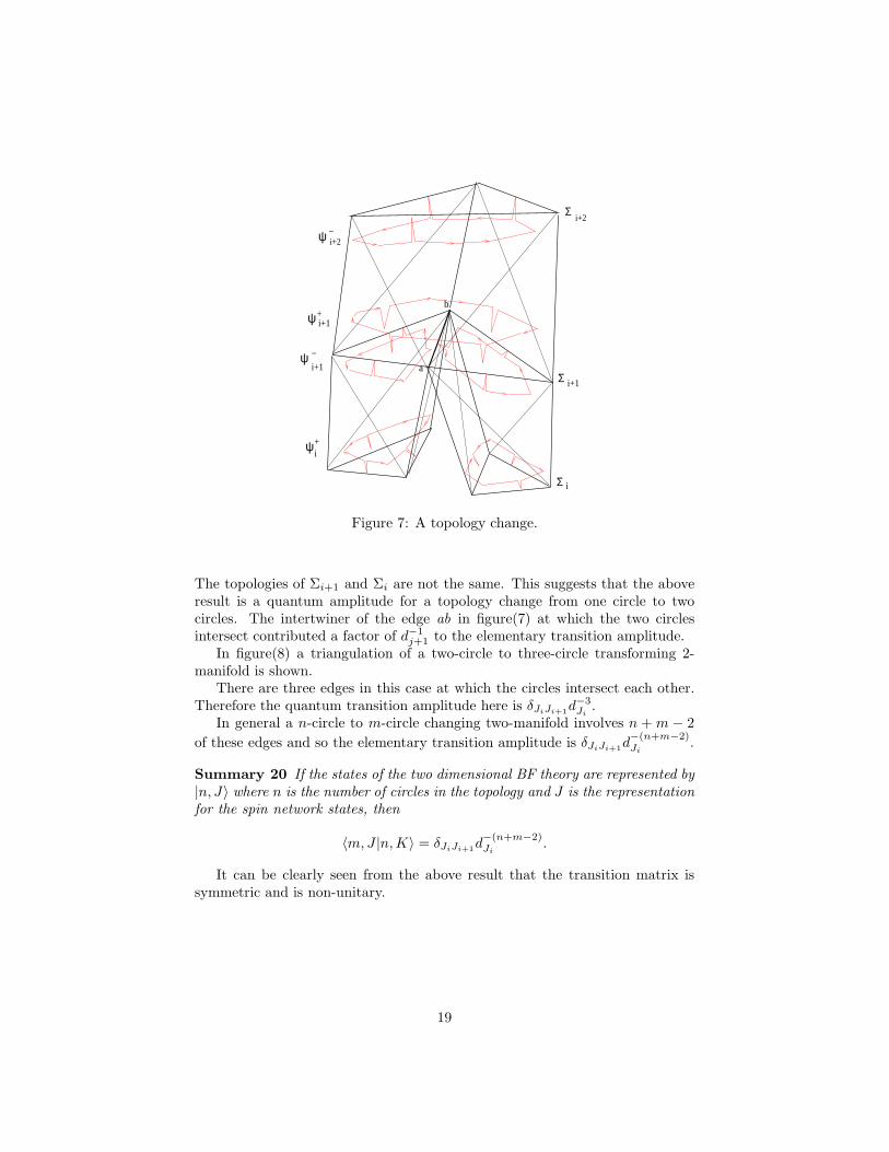
j+1 to the elementary transition amplitude.In figure(8) a triangulation of a two-circle to three-circle transforming 2-

manifold is shown.There are three edges in this case at which the circles intersect each other.

Therefore the quantum transition amplitude here is δJiJi+1d−3

Ji.

In general a n-circle to m-circle changing two-manifold involves n + m − 2

of these edges and so the elementary transition amplitude is δJiJi+1d−(n+m−2)Ji

.

Summary 20 If the states of the two dimensional BF theory are represented by|n, J〉 where n is the number of circles in the topology and J is the representationfor the spin network states, then

〈m,J |n,K〉 = δJiJi+1d−(n+m−2)Ji

.

It can be clearly seen from the above result that the transition matrix issymmetric and is non-unitary.

19

c

a

e

fd

b

Figure 8: A more complicated topology change.

6.3 Topological invariance of the 2D transition amplitudes

In case of 2D manifolds, the partition function is [7], [18]

Z =∑

J

dχ(M)J (22)

where, χ is the Euler characteristic of M , a topological invariant.Let ΣA and ΣB are two closed 1D manifolds. Let M be a simplicial 2-

manifold foliated by N hypersurfaces Σi such that ΣA = Σ1 and ΣB =ΣN . Then the transition amplitude 〈ΣA, JA|ΣB, JB〉M can be calculated bymultiplying the elementary transition amplitudes 〈Σi, Ji|Σi+1, Ji+1〉. Since for2-manifolds the intertwiners require that all the Jb’s are the same we have

〈ΣA, JA|ΣB, JB〉M = δJAJB

N−1∏

i=1

〈Σi, JA|Σi+1, JA〉Ωi.

Now consider we have two copies of M, and splice them at their identicalends. Let the resultant manifold be M

′

. Then, we can show using the calcula-tions leading to equation(22) as done in [7] and [18] that 〈ΣA, JA|ΣB, JB〉M 〈ΣB, JB|ΣA, JA〉Mis nothing but the partition function associated with M ′ with J fixed to valueJA

〈ΣA, JA|ΣB, JB〉2M = 〈ΣA, JA|ΣB, JB〉M 〈ΣB, JB|ΣA, JA〉M= d

χ(M ′)JA

δJAJB.

20

Now, since the above result is a topological invariant, and the 2-D transitionamplitudes are always positive real, we can conclude 〈ΣA, JA|ΣB, JB〉M is atopological invariant. This means that the transition amplitude

〈ΣA, JA|ΣB, JB〉 =∑

M

〈ΣA, JA|ΣB, JB〉M

where the summation is over all possible M (an arbitrary triangulation foreach topology used) that sandwich between ΣA and ΣB, is independent of thetriangulations of M .

The generalization of this result to higher dimensions is being analyzed andwill be published elsewhere.

7 The 3 + 1 formulation of gravity.

Lets go the four dimensional cases after a brief discussion of the 3D Riemanniancase. The 3D Riemannian gravity is equivalent to the 3D BF theory for thegroup SU(2). The intertwiners are just the 3J symbols of SU(2). The spinnetwork functionals are essentially the same as that of the Ashtekar-BarberoEuclidean canonical quantum gravity formalism [19]. Here the spin networkfunctionals live on the two dimensional foliating surfaces.

In the case of the SO(4) Riemannian gravity, the most popular proposal isthe Barrett-Crane model [10], which was derived by imposing the Barrett-Craneconstraints on the spin foam model of the SO(4) BF theory. The Barrett-Craneconstraints are basically the discretized Plebanski constraints.

The Barrett-Crane constraints are implemented on the SO(4) BF theorygiven by equation (10) by using the following conditions10:

1. The Jb are restricted to the simple representations of SO(4) [10], [41].

2. The intertwiners are restricted to the Barrett-Crane intertwiners given inequation (34) [10].

Please see appendix C for the definitions of the simple representations andthe Barrett-Crane intertwiner.

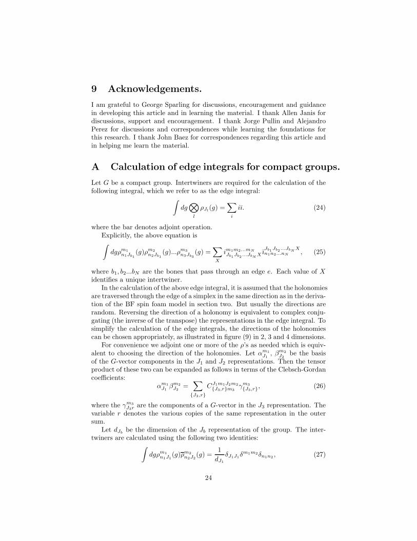
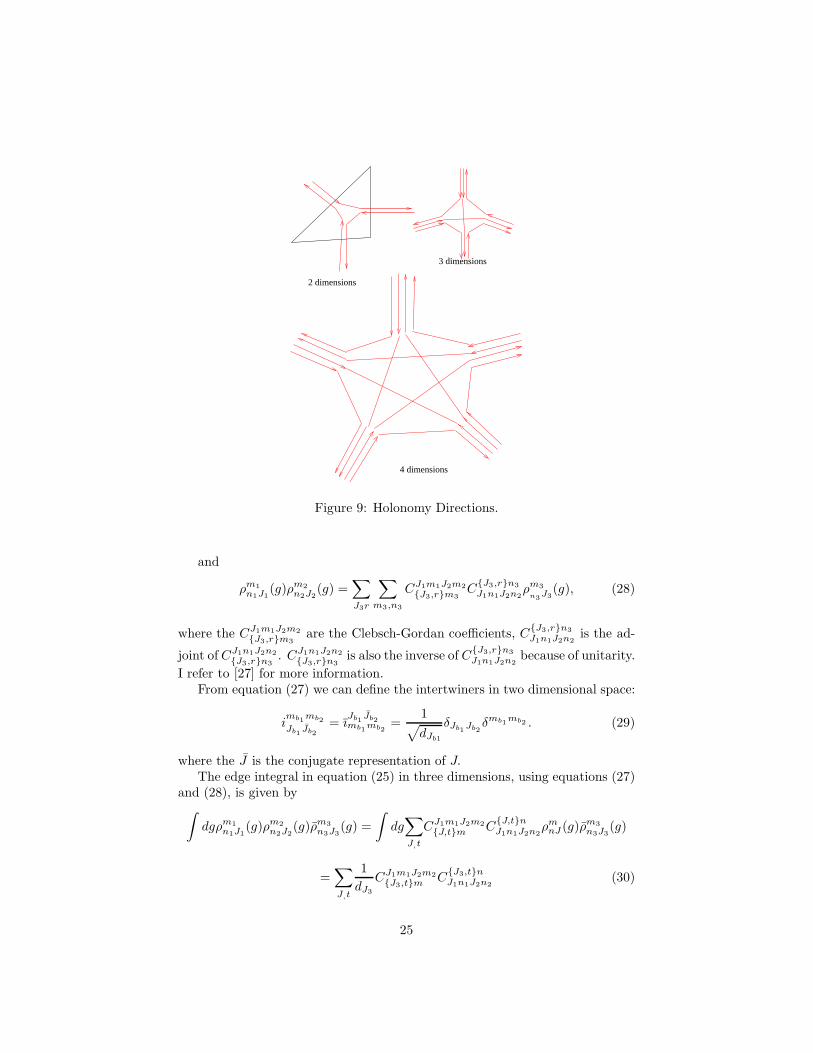
To simplify the calculation of the edge integrals, the directions of the holonomiesin the derivation of the spin foam model can be chosen as illustrated in figure(9). The parallel sets of arrows indicate the direction in which the holonomiesare traversed through the edges of a four-simplex. Please refer to appendix Aand B for more information.

10The model so obtained may differ from the Barrett-Crane model by the amplitudes ofthe lower dimensional (< 4) simplices. We believe that the imposition of the Barrett-Craneconstraints are not yet derived in a way that can be rigorously related to any discretized formof the gravity Lagrangian. Because of this the amplitudes of the lower dimensional simplicesare not yet fixed. For simplicity, here we assume that these quantum amplitude are same asthat of the BF spin foam model.

21

The spin network functionals ψ±i = ψ±(Σi, Jb

, ob, Xie

, G±bΣi

) of the SO(4)BF theory can be adapted to gravity by restricting the Jb’s to the simple rep-resentations and the intertwiners ie to the Barrett-Crane intertwiners [10] Leth : S3 → SU(2) be a mapping and ρJ be the J representation of SU(2). Thenthe Barrett-Crane intertwiner can be rewritten as (derived in appendix C)

iJ1J2J3J4

l1r1l2r2l3r3l4r4=

∫

S3

dxρl1r1J1

(h(x))ρl2r2J2

(h(x))ρr3

l3J3(h−1(x))ρr4

l4J4(h−1(x)).

Definition 21 The elementary transition amplitudes(

ψ+i , ψ

−i+1

)

defined in equa-tion (16) can be reformulated for Riemannian gravity as

(

ψ+i , ψ

−i+1

)

= PBC

∫

ψ+i ψ

−i+1

∏

b∈Ωi

δ(Hb)∏

e∈Ωi

dge, (23)

where PBC is the projector which imposes the Barrett-Crane constraints on theintertwiners associated with the edges e.

Any three-simplicial hypersurface Σ with the J ’s interpreted as the sizes ofthe edges of its three-simplices, which are assumed to be flat [21], describes adiscrete geometry. In this sense the above equation assigns quantum amplitudesfor a history of geometries [7].

In the case of Riemannian gravity the final spin network functional has beenconstructed on the homogenous space S3 = SO(4)/SU(2) corresponding to thesubgroup SU(2).

In the case of SO(3, 1) ≈ SL(2, C), imposing the Barrett-Crane constraintscan potentially lead to three different types of spin foam models relating to thethree different homogenous space of SO(3, 1) corresponding to the subgroupsSO(3), SU(1, 1) or E(2) [22]. The first case has been more investigated than theother two and is the most interesting in the context of our 3+1 formulation. Inthis case, the theory is defined [22] by replacing S3 in the Euclidean formalismdefined above by H+ the homogenous space SL(2, C)/SU(2). H+ is the spaceof the upper sheet of the two-sheeted hyperboloid of 4D Minkowski space-time.The related spin network functional of the 3 + 1 formulation is made of theinfinite dimensional representations of the Lorentz group. Here the Jb valuesare continuous (more precisely, imaginary). An element x of H+, is assignedto each side of each edge of the 4-simplices. The asymptotic limit [23] of thetheory is controlled by the Einstein-Regge action [21] of gravity [23]. In theasymptotic limit the dominant contribution (non-degenerate sector) to the spinfoam amplitude is when the x values are normals to the edges in the simplicialgeometry defined by the Jb values as before. This means in the asymptoticlimit the foliating simplicial 3-surfaces act as space-like simplicial 3-surfaces ofa simplicial 4-geometry defined by the Jb values. This suggests that in theasymptotic limit a certain sense of time exists in the order of the foliatinghypersurfaces.

In case of a H− ≈ SL(2, C)/SU(1, 1) based spin foam model the Jb are bothdiscrete and continuous [24]. The spin network functionals for the Lorentzianquantum gravity are being currently studied and will be published elsewhere.

22

8 Discussion and comments.

Now let us compare our formalism in the previous section to that of the canonicalquantum formulation.

• The Gauss constraint has been implemented in our formalism by the useof the gauge invariant spin network functionals for the quantum states.There is an important difference between the two formulations in the caseof the Lorentzian quantum gravity. It is that the spin network functionalsare made of the finite dimensional representations [12] in the canonicalformalism, while here they are made of infinite dimensional representations[22]. This difference needs to be investigated.

• The coordinate independence has been implemented here at the classicallevel by the use of the discretized action.

• The Hamiltonian constraint of canonical quantum gravity contains evolu-tion information. So it essentially should be contained in the definition ofthe elementary transition amplitudes given in equation (23).

Our formulation has brought the spin foams closer to canonical quantumgravity in the formal set up and in certain details. Our formulation has boththe features of spin foam models and the canonical formulation. Since the spinfoams are derived from the discretized action, it is reasonable to say that thecanonical formulation can be further related to the spin foam model of gravityby studying the continuum limit. But before that, we believe the impositionof Barrett-Crane constraints on the BF spin foams has to be rigorously derivedfrom a discrete action and the amplitudes of the lower dimensional simplicesfixed (please see [25] for more discussion on this).

One of the problems with canonical quantum gravity is in defining a properHamiltonian constraint operator. The proposal by Thiemann [13] for a Hamil-tonian constraint operator appears to be set back by anomalies [26]. By study-ing the continuum limit of our elementary transition amplitudes one might beable to get a useful physical Hamiltonian operator (physical inner product) forcanonical quantum gravity.

There are many open questions that need to be addressed, such as:

• What can we learn from this approach about the physics of quantumgravity? For example, is quantum gravity unitary?

• What are the potential applications to the physical problems?

• What is the continuum limit?

• How to include the topologies in our theory that were excluded by theconditions that were specified in the beginning of section three?

• How to include matter?

23

9 Acknowledgements.

I am grateful to George Sparling for discussions, encouragement and guidancein developing this article and in learning the material. I thank Allen Janis fordiscussions, support and encouragement. I thank Jorge Pullin and AlejandroPerez for discussions and correspondences while learning the foundations forthis research. I thank John Baez for correspondences regarding this article andin helping me learn the material.

A Calculation of edge integrals for compact groups.

Let G be a compact group. Intertwiners are required for the calculation of thefollowing integral, which we refer to as the edge integral:

∫

dg⊗

l

ρJl(g) =

∑

i

iı. (24)

where the bar denotes adjoint operation.Explicitly, the above equation is∫

dgρm1

n1Jb1(g)ρm2

n2Jb1(g)...ρm3

n3Jb3(g) =

∑

X

im1m2...mN

Jb1Jb2

...JbNX ı

Jb1Jb2

...JbNX

n1n2...nN , (25)

where b1, b2...bN are the bones that pass through an edge e. Each value of Xidentifies a unique intertwiner.

In the calculation of the above edge integral, it is assumed that the holonomiesare traversed through the edge of a simplex in the same direction as in the deriva-tion of the BF spin foam model in section two. But usually the directions arerandom. Reversing the direction of a holonomy is equivalent to complex conju-gating (the inverse of the transpose) the representations in the edge integral. Tosimplify the calculation of the edge integrals, the directions of the holonomiescan be chosen appropriately, as illustrated in figure (9) in 2, 3 and 4 dimensions.

For convenience we adjoint one or more of the ρ’s as needed which is equiv-alent to choosing the direction of the holonomies. Let αm1

J1, βm2

J2be the basis

of the G-vector components in the J1 and J2 representations. Then the tensorproduct of these two can be expanded as follows in terms of the Clebsch-Gordancoefficients:

αm1

J1βm2

J2=∑

J3,r

CJ1m1J2m2

J3,rm3γm3

J3,r, (26)

where the γm3

J3r are the components of a G-vector in the J3 representation. Thevariable r denotes the various copies of the same representation in the outersum.

Let dJbbe the dimension of the Jb representation of the group. The inter-

twiners are calculated using the following two identities:∫

dgρm1

n1J1(g)ρm2

n2J2(g) =

1

dJ1

δJ1J1δm1m2δn1n2

, (27)

24

2 dimensions

3 dimensions

4 dimensions

Figure 9: Holonomy Directions.

and

ρm1

n1J1(g)ρm2

n2J2(g) =

∑

J3r

∑

m3,n3

CJ1m1J2m2

J3,rm3C

J3,rn3

J1n1J2n2ρm3

n3J3

(g), (28)

where the CJ1m1J2m2

J3,rm3are the Clebsch-Gordan coefficients, C

J3,rn3

J1n1J2n2is the ad-

joint of CJ1n1J2n2

J3,rn3. CJ1n1J2n2

J3,rn3is also the inverse of C

J3,rn3

J1n1J2n2because of unitarity.

I refer to [27] for more information.From equation (27) we can define the intertwiners in two dimensional space:

imb1

mb2

Jb1Jb2

= ıJb1

Jb2mb1

mb2=

1√

dJb1

δJb1Jb2δmb1

mb2 . (29)

where the J is the conjugate representation of J.The edge integral in equation (25) in three dimensions, using equations (27)

and (28), is given by∫

dgρm1

n1J1(g)ρm2

n2J2(g)ρm3

n3J3(g) =

∫

dg∑

J,t

CJ1m1J2m2

J,tmC

J,tn

J1n1J2n2ρm

nJ (g)ρm3

n3J3(g)

=∑

J,t

1

dJ3

CJ1m1J2m2

J3,tmC

J3,tn

J1n1J2n2(30)

25

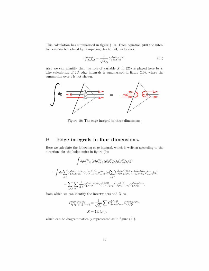
This calculation has summarised in figure (10). From equation (30) the inter-twiners can be defined by comparing this to (24) as follows:

im1m2m

J1J2J3,t=

1√

dJ3

CJ1m1J2m2

J3,tm. (31)

Also we can identify that the role of variable X in (25) is played here by t.The calculation of 2D edge integrals is summarised in figure (10), where thesummation over t is not shown.

=g

g

gdg

Figure 10: The edge integral in three dimensions.

B Edge integrals in four dimensions.

Here we calculate the following edge integral, which is written according to thedirections for the holonomies in figure (9):

∫

dgρm1

n1J1(g)ρm2

n2J2(g)ρm3

n3J3(g)ρm4

n4J4(g)

=

∫

dg∑

J5,t

CJ1m1J2m2

J5,tm5C

J5,tn5

J1n1J2n2ρm5

n5J5

(g)∑

J6,r

CJ6,rm6r

J3m3J4m4CJ3n3J4n4

J6,rn6ρm6

n6J6

(g)

=∑

J,r,t

∑

k,l

1

dJ

CJ1m1J2m2

J,tkC

J,tl

J1n1J2n2C

J,rk

J3m3J4m4CJ3n3J4n4

J,rl,

from which we can identify the intertwiners and X as

im1m2m3m4

J1J2J3J4J,t,r=

1√dJ

∑

l

CJ,rl

J1m1J2m2CJ3m3J4m4

J,tl

X = J, t, r,

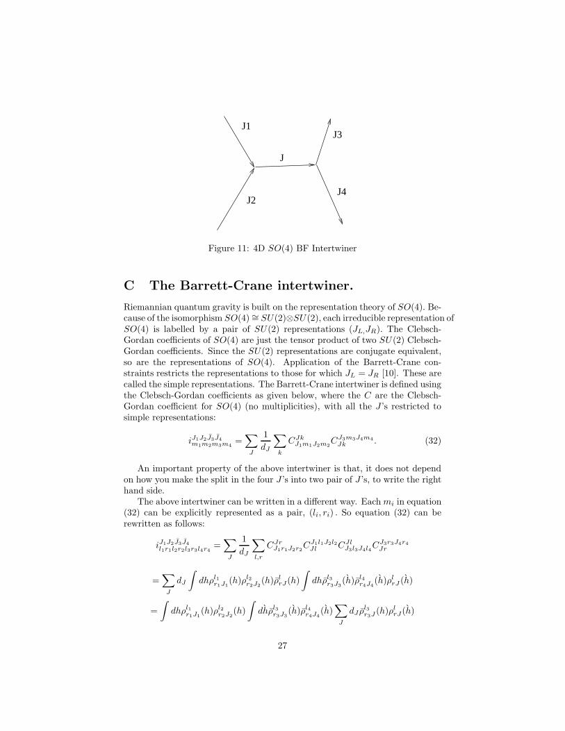
which can be diagrammatically represented as in figure (11).

26

J1

J2J4

J3

J

Figure 11: 4D SO(4) BF Intertwiner

C The Barrett-Crane intertwiner.

Riemannian quantum gravity is built on the representation theory of SO(4). Be-cause of the isomorphism SO(4) ∼= SU(2)⊗SU(2), each irreducible representation ofSO(4) is labelled by a pair of SU(2) representations (JL,JR). The Clebsch-Gordan coefficients of SO(4) are just the tensor product of two SU(2) Clebsch-Gordan coefficients. Since the SU(2) representations are conjugate equivalent,so are the representations of SO(4). Application of the Barrett-Crane con-straints restricts the representations to those for which JL = JR [10]. These arecalled the simple representations. The Barrett-Crane intertwiner is defined usingthe Clebsch-Gordan coefficients as given below, where the C are the Clebsch-Gordan coefficient for SO(4) (no multiplicities), with all the J ’s restricted tosimple representations:

iJ1J2J3J4

m1m2m3m4=∑

J

1

dJ

∑

k

CJkJ1m1J2m2

CJ3m3J4m4

Jk . (32)

An important property of the above intertwiner is that, it does not dependon how you make the split in the four J ’s into two pair of J ’s, to write the righthand side.

The above intertwiner can be written in a different way. Eachmi in equation(32) can be explicitly represented as a pair, (li, ri) . So equation (32) can berewritten as follows:

iJ1J2J3J4

l1r1l2r2l3r3l4r4=∑

J

1

dJ

∑

l,r

CJrJ1r1J2r2

CJ1l1J2l2Jl CJl

J3l3J4l4CJ3r3J4r4

Jr

=∑

J

dJ

∫

dhρl1r1J1

(h)ρl2r2J2

(h)ρlrJ(h)

∫

dhρl3r3J3

(h)ρl4r4J4

(h)ρlrJ (h)

=

∫

dhρl1r1J1

(h)ρl2r2J2

(h)

∫

dhρl3r3J3

(h)ρl4r4J4

(h)∑

J

dJ ρl3r3J (h)ρl

rJ(h)

27

=

∫

dhρl1r1J1

(h)ρl2r2J2

(h)

∫

dhρl3r3J3

(h)ρl4r4J4

(h)δ(h−1h)

=

∫

dhρl1r1J1

(h)ρl2r2J2

(h)ρl3r3J3

(h)ρl4r4J4

(h)

=

∫

dhρl1r1J1

(h)ρl2r2J2

(h)ρr3

l3J3(h−1)ρr4

l4J4(h−1), (33)

where h and h belong to SU(2).Restricting the representation to simple ones effectively reduces the harmonic

analysis on SO(4) to S3.In the last equation, h must be seen as an element of S3 instead of SU(2).

Let h : S3 → SU(2) is a bijective mapping. Then the Barrett-Crane intertwinercan be rewritten as

iJ1J2J3J4

l1r1l2r2l3r3l4r4=

∫

S3

dxρl1r1J1

(h(x))ρl2r2J2

(h(x))ρr3

l3J3(h−1(x))ρr4

l4J4(h−1(x)).

(34)

References

[1] A.S. Schwarz, Lett. Math. Phys. 2 (1978) 247; Commun. Math. Phys. 67(1979) 1; G. Horowitz, Commun. Math. Phys. 125 (1989) 417; M. Blau andG. Thompson, Ann. Phys. 209 (1991) 129.

[2] G. Ponzano and T. Regge, Semiclassical Limit of Racah Coefficients, Spec-troscopy and Group Theoretical Methods in Physics, F. Block et al (Eds),North-Holland, Amsterdam, 1968.

[3] R. Penrose-Angular momentum: an approach to combinatorial space-time,Quantum Theory and Beyond, essays and discussions arising from a collo-quium, Edited by Ted Bastin, Cambridge University Press, 1971.

[4] C. Rovelli, The projector on physical states in loop quantum grav-ity, Preprint available as arXiv:gr-qc/9806121; C. Rovelli and M. P.Reisenberger, ”Sum over Surfaces” form of Loop Quantum Gravity,arXiv:gr-qc/9612035.

[5] F. Markopoulou and L. Smolin, Causal evolution of spin networks,Nucl.Phys. B,508:409–430, 1997.

[6] F. Markopoulou, Dual formulation of spin network evolution, Preprintavailable as gr-qc/9704013.

[7] J. C. Baez, An Introduction to Spin Foam Models of Quantum Gravity andBF Theory, Lect.Notes.Phys., 543:25–94, 2000

[8] A. Perez, Spin Foam Models for Quantum Gravity, Preprint available asarXiv:gr-qc/0301113.

28

[9] H. Ooguri, Topological Lattice Models in Four Dimensions, Mod.Phys.Lett.A, 7:2799–2810, 1992.

[10] J. W. Barrett and L. Crane, Relativistic Spin Networks and QuantumGravity. J.Math.Phys., 39:3296–3302, 1998.

[11] A. Ashtekar, Lectures on non Perturbative Canonical Gravity, Word Sci-entific, 1991.

[12] C. Rovelli and L. Smolin, Spin Networks and Quantum Gravity, Preprintavailable as gr-qc 9505006.

[13] T. Thiemann, Anomaly-free formulation of non-perturbative, four-dimensional Lorentzian quantum gravity, Preprint available asarXiv:gr-qc/9606088.

[14] R. Borissov, R. Pietri and C. Rovelli, Matrix Elements of Thiemann’sHamiltonian Constraint in Loop Quantum Gravity, Preprint available asarXiv:gr-qc/9703090.

[15] M. P. Reisenberger, On Relativistic Spin Network Vertices, J. Math. Phys.,40:2046–2054, 1999.

[16] R. De. Pietri and L. Freidel, SO(4) Plebanski Action and Relativistic SpinFoam Model. Class.Quant.Grav., 16:2187–2196, 1999.

[17] N. Ja. Vilenkin and A. U. Klimyk, Representation theory of Lie groups andSpecial Functions. Volume 1, Kluwer Academic Publisher, Dordrecht, TheNetherlands, 1993.

[18] A. Perez, Spin Foam Models for Quantum Gravity, Ph.D. Thesis, Universityof Pittsburgh, Pittsburgh, USA 2001.

[19] J. F. Barbero, Real Ashtekar Variables for Lorentzian Signature SpaceTimes. Phys. Rev., D51:5507–5510, 1995.

[20] M. P. Reisenberger, Worldsheet formulations of gauge theories and grav-ity”, gr-qc/9412035

[21] T. Regge, General Relativity without Coordinates, Nuovo Cimento 19(1961) 558-571.

[22] J. W. Barrett and L. Crane, A Lorentzian Signature Model for QuantumGeneral Relativity, Class.Quant.Grav., 17:3101–3118, 2000.

[23] J. W. Barrett and C. Steele, Asymptotics of relativistic spin networks,Preprint available as arXiv:gr-qc/0209023..

[24] A. Perez and C. Rovelli, 3+1 Spin foam Model of Quantum grav-ity with Spacelike and Timelike Components, Preprint available asarXiv:gr-qc/0011037.

29

[25] M. Bojowald and A. Perez, Spin Foam Quantization and Anomalies,Preprint gr–qc/0303026

[26] R. Gambini, J. Lewandowski, D. Marolf and G. Pullin, On the consistencyof the constraint algebra in spin network quantum gravity, Preprint avail-able as arXiv:gr-qc/9710018

[27] N. Ja. Vilenkin and A. U. Klimyk Representation theory of Lie groupsand Special Functions, Recent advances, Kluwer Academic Publisher, Dor-drecht, The Netherlands, 1995.

[28] J. C. Baez, Spin Foam Models, Class Quant Grav 15 (1998) 1827-1858;gr-qc/9709052.

[29] J. C. Baez, J. D. Christenson, Thomas R. Halford, and D. C.Tsang, Spin foam models of Riemannian quantum gravity, PreprintarXiv:gr-qc/0202017.

[30] C. Rovelli, The basis of the Ponzano-Regge-Turaev-Viro-Ooguri quantum-gravity model is the Loop Representation basis, Preprint available asarXiv:hep-th/9304164.

[31] D. Oriti and R. M.Williams, Gluing 4-simplices: a derivation of the Barrett-Crane spin foam model for Euclidean quantum gravity, Preprint available:arXiv:gr-qc/0010031.

[32] D. A. Varshalovich, A. N. Moskalev and V. K. Khersonskii, Quantum The-ory of Angular Momentum, World Scientific, 1988.

[33] V. Turaev and O. Viro, State sum invariants of 3-manifolds and quantum6j symbols, Topology 31(1992), 865-902.

[34] M. P. Reisenberger, Worldsheet formulations of gauge theories and gravity,arXiv:gr-qc/9412035.

[35] A. Perez, C. Rovelli, Observables in quantum gravity, PreprintarXiv:gr-qc/0104034.

[36] M. Arnsdorf, Relating canonical and covariant approaches to triangulatedmodels of quantum gravity, Preprint arXiv:gr-qc/0110026.

[37] E. R. Livine, Projected Spin Networks for Lorentz connection: LinkingSpin Foams and Loop Gravity, Preprint arXiv:gr-qc/0207084.

[38] A. Perez and C. Rovelli, Spin foam model for Lorentzian General Relativity,Preprint arXiv:gr-qc/0009021

[39] L. Freidel and K. Krasnov, Simple Spin Networks as Feynman Graphs,Preprint available as hep-th/9903192.

30

[40] H. Ooguri, Partition Functions and Topology-Changing Amplitudes inthe 3D Lattice Gravity of Ponzano and Regge, Preprint available asarXiv:hep-th/9112072.

[41] M. P. Reisenberger, Classical Euclidean general relativity from ”left-handedarea = right-handed area”, arXiv:gr-qc/9804061.

31