Regional sea level change in Northwest Pacific: Process, characteristic and prediction

J. Geogr. Sci. 2011, 21(3): 387-400

DOI: 10.1007/s11442-011-0852-7

© 2011 Science Press Springer-Verlag

Received: 2010-11-19 Accepted: 2010-12-27 Foundation: Key Project of National Natural Science Foundation of China, No.40730527 Author: Luo Wen (1987–), Master, specialized in sea level change and spatiotemporal analysis in GIS.

E-mail: [email protected] *Corresponding author: Yuan Linwang (1973–), Ph.D and Professor, specialized in geographic modeling and GIS.

E-mail: [email protected]

www.geogsci.com springerlink.com/content/1009-637X

Regional sea level change in Northwest Pacific: Process, characteristic and prediction

LUO Wen, YUAN Linwang, YU Zhaoyuan, YI Lin, XIE Zhiren

Key Laboratory of Virtual Geographic Environment, Ministry of Education, Nanjing Normal University, Nanjing 210046, China

Abstract: Based on 22 sparse-distributed tide gauge records in the Northwest Pacific Ocean marginal sea, the process, characteristic and prediction of regional sea level change are discussed by the integration of the following methods. Firstly, the regularized EM algorithm (RegEM) and the Multi-taper Spectral Method (MTM) are adopted to interpret their multiscale fluctuation processes and their spatial-temporal variations. Secondly, the orderly cluster method is introduced to classify these tidal stations, and with the consideration of the space adjacent relation, we obtain five sub-regions (the coasts of Bohai Sea-northern Yellow Sea, Yellow Sea-East China Sea along Chinese coast, the East China Sea along Japanese coast, the southern East China Sea and the northwestern South China Sea). Furthermore, the Mean Generation Function (MGF) is explored to predict the medium- and long-term trends of each tide station. Finally, the Principal Component Analysis (PCA) is employed to obtain re-gional-scale sea level change trends, sea level rise rates of the above five sub-regions from 2001 to 2030 are 1.23–1.27 mm/a, 3.30–3.34 mm/a, 2.72–2.76 mm/a, 1.43–1.47 mm/a and 1.13–1.15 mm/a respectively, and the whole region sea level rise rate is between 2.01 mm/a and 2.11 mm/a. The aim of our work is to conduct an integrated research on regional sea level change.

Keywords: regional sea level change; spatial-temporal variation; MTM; prediction; Northwest Pacific

Global and regional sea level predictions are the focus of sea level research in the 21st cen-tury. Many of the previous researches have utilized the statistic-based models (Zhang, 1997; Li et al., 1998; Chambers et al., 2002; Wu et al., 2003), and the reliability of analyses were ascribed to the inconsistent data timespan, heterogeneous spatial distribution, and complex-ity and uncertainty of sea level changes. Physical process-based models which aim to cap-ture major factors and processes controlling sea level changes, are sensitive to the factors selections, action processes, and parameters, etc. (Solomon et al., 2007, Knutti et al., 2000; Collins et al., 2002). Because the relative contributions of the main components are still

388 Journal of Geographical Sciences

highly uncertain, therefore, physical process-based models are tentative and primitive (Raper et al., 2006; Rahmstorf et al., 2007). Rahmstorf (2007) proposed a semi-empirical model to predict global sea level rise during the 21st century. Grinsted et al. (2009) intro-duced a Monte-Carlo inversion method to find out the possible scenarios of sea level changes during the 21st century, these new advances have argued the results given by IPCC AR4 report. It also means that statistical models still play an important role in sea level re-search.

Significant spatial non-uniform characteristics of the regional sea level change have been revealed by tide gauges and satellite altimetry (Church et al., 2004; Prandi et al., 2009; Yuan et al., 2009; Yuan et al., 2010). Tide gauge data are strongly affected by local topography, climate, hydrological process, human activity and vertical land movement. Data preprocess-ing and analysis method selection is very important when using tide gauge data (Douglas, 1997). Recently, methods (e.g. PCA and virtual site method) are introduced to time series imputation and interpolation in climate and sea level fields (Grinsted et al., 2009; Jevrejeva et al., 2006). The sensitivities of spatial structures and the uncertainties of restored series have limited their applications (Siddall et al., 2009). The irregular distributions and spa-tial-temporal multiscale characteristics also lead to the difficulty of regional sea level pre-diction. Here, we apply six mathematic methods to explore the process, characteristic and prediction of regional sea level change. The integration use of these methods can make full use of the existing available data, help discuss the variation characteristics, comprehensive prediction and change rate of different regions. Our work also provides a new integrated perspective on regional sea level change.

1 Data and methods

1.1 Data

The Northwest Pacific Ocean marginal seas, which near the Inter-tropical Convergence Zone (ITCZ), are strongly influenced by many factors, such as monsoon, ocean currents, ENSO and human activities. We select monthly mean sea level anomaly data from 22 tide gauge stations in this area, with timespans ranging from January 1954 to December 2009. Data of Qinhuangdao, Yantai, Incheon, Tai Po Kau and Macau stations are from the Revised Local Reference (RLR) data from Permanent Service for Mean Sea Level (PSMSL) (Specer et al., 1993). Other data are from UH Sea Level Center1. The spatial distribution of research sta-tions are shown in Figure 1.

1.2 Methods

RegEM method can estimate the covariance matrix, spatial-temporal distributions and re-construction of error distributions from incomplete data accurately and effectively, which also leads to more accurate estimates of the missing values than conventional EM imputa-tion techniques, especially in recurring small-scale variations (Schneider, 2001, Mann et al., 2009). In the RegEM method, interpolations utilize the ridge regression to recover the miss-ing value and the covariance information with generalized cross-validation. With the impu-

1 http://ilikai.soest.hawaii.edu/uhslc/data.html

LUO Wen et al.: Regional sea level change in Northwest Pacific: Process, characteristic and prediction 389

tation series, sea level change rate of different periods, and their spa-tial-temporal distribution can be further discussed.

The frequency methods, such as spectrum analysis, can provide the periods and energetic characteristics of time series with different lengths (Mann et al., 1998; Moberg et al., 2005). The MTM approach, firstly proposed by Thomson (1982), is a low variance, high-resolution spec-trum analysis method (Lanzerotti et al., 1986; Percival et al., 1993; Riedel et al., 1994). The property of nearly zero spectral leakage makes it suitable for weak signal detection and reconstruction from nonlinear short-length data series with high noise background. So we introduce it to explore the detailed multiscale frequency characteristics.

For those samples with the tem-poral or spatial order, the ordered cluster method, also named as opti-mal segmentation method (Luo et al., 2009), can classify these ordered samples without changing their original orders. We introduce it to classify the 22 stations together with the consideration of spatial adjacency, and with the help of optimal segmentations of the sea level change characteristics along certain directions, we can discuss their spatial heterogeneity.

The MGF method is then used to predict sea level change until 2030 of each station. The MGF method derives dependent variables from original time series as prediction variables. Optimal subset regression models and the couple score criterion (CSC) can take both details and trend forecasting into account. The MGF method can forecast the variation characteris-tics of various periods, the change of extreme values and long-term trend changes from original time series, and multistep forecasting is also supported (Cao et al., 1993; Yuan et al., 2008).

The Empirical Mode Decomposition (EMD) method is an effective multiscale analysis method for nonlinear and non-stationery time series. The trend extracted by EMD has much better logical foundation and adaptive characteristics, which makes it to be one of the most effective trend separation methods (Huang et al., 1998; Wu et al., 2007). In order to filter out high frequency fluctuation components in sea level series, we introduce EMD to extract trend components, and calculate sea level change rates.

PCA is usually used in data compression and feature extraction. By introducing it to inte-

Figure 1 Spatial distribution of tide gauge stations


grate proxy indexes at different time periods and resolutions, Mann et al. (1998) recon-structed the global temperature time series. Church et al. (2004) and Chambers et al. (2002) have used it to integrate globally satellite altimetry data and sparse-distributed tide gauge data, and computed the sea level change rate.

2 Process reconstruction of sea level change

2.1 Data imputation

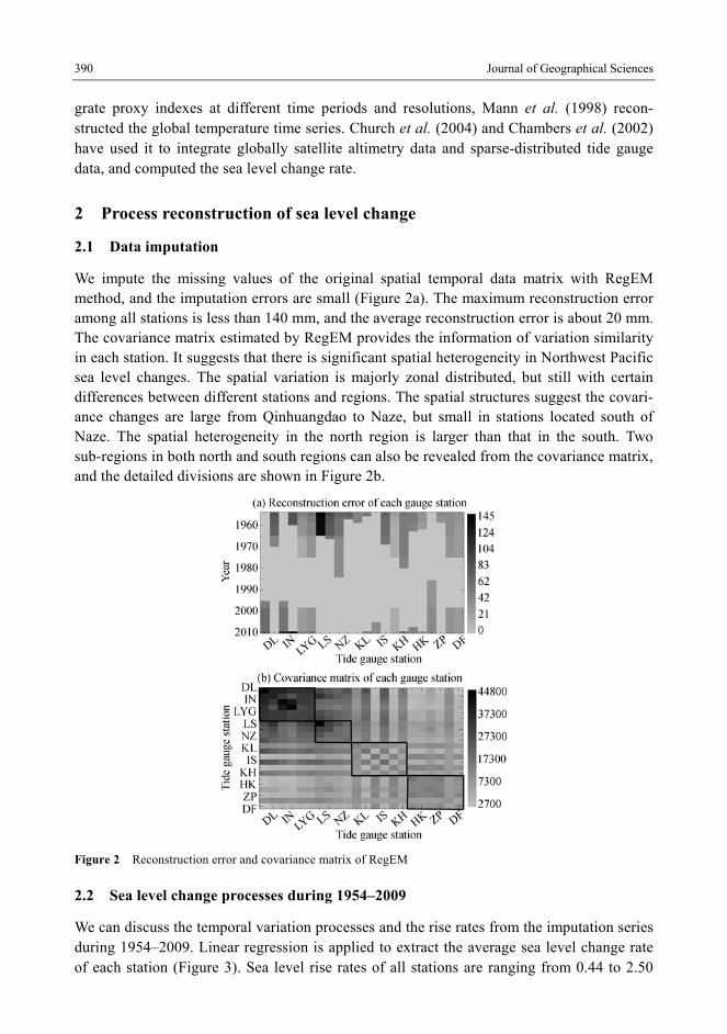
We impute the missing values of the original spatial temporal data matrix with RegEM method, and the imputation errors are small (Figure 2a). The maximum reconstruction error among all stations is less than 140 mm, and the average reconstruction error is about 20 mm. The covariance matrix estimated by RegEM provides the information of variation similarity in each station. It suggests that there is significant spatial heterogeneity in Northwest Pacific sea level changes. The spatial variation is majorly zonal distributed, but still with certain differences between different stations and regions. The spatial structures suggest the covari-ance changes are large from Qinhuangdao to Naze, but small in stations located south of Naze. The spatial heterogeneity in the north region is larger than that in the south. Two sub-regions in both north and south regions can also be revealed from the covariance matrix, and the detailed divisions are shown in Figure 2b.

Figure 2 Reconstruction error and covariance matrix of RegEM

2.2 Sea level change processes during 1954–2009

We can discuss the temporal variation processes and the rise rates from the imputation series during 1954–2009. Linear regression is applied to extract the average sea level change rate of each station (Figure 3). Sea level rise rates of all stations are ranging from 0.44 to 2.50


Figure 3 Imputed series of each gauge and its linear regression series

mm/a. The similar spatial heterogeneity revealed by covariance matrix can also be seen from the change rates clearly. The sea level rise rates from Qinhuangdao to Lusi are between 1.0 and 2.5 mm/a, and Lusi have the largest rise rate among all stations. The smallest rise rate in Naze, is about 0.5 mm/a. In the regions south of Kanmen, the rise rates are smaller than the northern regions. The rise rates in the stations south of Kaohsiung are complex, their trends are fluctuating.

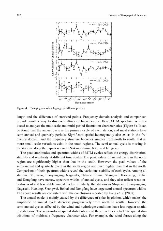
The sea level height in each station rises in a fluctuating way, we compute the average change rates and their confidence intervals to reveal sea level variation processes during 1954 to 2009. Comparisons of rate variations among all stations are shown in Figure 4. The change rates also present variation characteristics associated with the time stage. The change rates for 1954–1974, 1975–1990 and 1991–2009 range between –5.2–2.75 mm/a and –6.82–8.1 mm/a and 0.91–5.3 mm/a respectively, the change rates during 1954 to 2009 are only from 0.44 to 2.5 mm/a. The spatial heterogeneity began to decline after 1975. However, the average rise rates increased after 1975. The average change rates of all stations during 1954–1974, 1975–1990, 1991–2009 and 1954–2009 are –1.16 mm/a, 1.49 mm/a, 3.26 mm/a and 1.44 mm/a, respectively.

3 Spectrum characteristic-based region classifications

3.1 Comparison of spectrum structure

Multi-station comparisons, which commonly operated in temporal domain, are unable to reveal the multiscale characteristics clearly, because they are often affected by the series


Figure 4 Changing rate of each gauge in different periods

length and the difference of start/end points. Frequency domain analysis and comparison provide another way to discuss multiscale characteristics. Here, MTM spectrum is intro-duced to analyze the multiscale and multi-period fluctuation characteristics (Figure 5). It can be found that the annual cycle is the primary cycle of each station, and most stations have semi-annual and quarterly periods. Significant spatial heterogeneity also exists in the fre-quency domain, and the frequency structure becomes simpler from north to south, that is, more small scale variations exist in the south regions. The semi-annual cycle is missing in the stations along the Japanese coast (Nakano Shima, Naze and Ishigaki).

The peak amplitudes and spectrum widths of MTM cycles reflect the energy distribution, stability and regularity at different time scales. The peak values of annual cycle in the north region are significantly higher than that in the south. However, the peak values of the semi-annual and quarterly cycle in the south region are much higher than that in the north. Comparison of their spectrum widths reveal the variations stability of each cycle. Among all stations, Shijiusuo, Lianyungang, Nagasaki, Nakano Shima, Shangwei, Kaohsung, Beihai and Dongfang have narrow spectrum widths of annual cycle, and they also reflect weak or-derliness of and less stable annual cycles. Similarly, the stations as Shijiusuo, Lianyungang, Nagasaki, Keelung, Shangwei, Beihai and Dongfang have large semi-annual spectrum widths. The above results are consistent with the conclusions reported by Kang et al. (2008).

The annual cycle is mainly caused by the difference of solar insolation, which makes the amplitude of annual cycle decrease progressively from north to south. However, the semi-annual cycles affected by the wind and hydrologic conditions have less regular spatial distributions. The non-uniform spatial distributions of these factors control the spatial dis-tributions of multiscale frequency characteristics. For example, the wind forces along the


Figure 5 The MTM power spectrum of each station and cluster analysis of the original spectrum

Chinese coast are much larger than other areas, and the sea level along the Chinese coast are strongly affected by discharges of big rivers, which makes the semi-annual cycles along the


Chinese coast more special and unstable. Interrupted climate events such as ENSO are also important factors that affect the frequency characteristics (Liu et al., 2010).

3.2 Coastal region classification

We use ordered cluster to further reveal the zonal variation of the multiscale frequency characteristics. The ordered cluster results of MTM spectrums are shown in Figure 5. With the consideration of latitudinal distribution of stations, we can modify the classification of ordered cluster and get the coastal region classifications finally. The modifications are as follows: (1) separating the cluster from Shijiusuo to Keelung into Chinese coastal region and Japanese coastal region; (2) merging the Beihai and Dongfang stations into the class of their spatial neighborhood groups. In total, we classify all 22 stations into five sub-regions. Re-gion I is near Bohai Sea and the north Yellow Sea, including Qinghuangdao, Dalian, Yantai and Incheon. Region II is the Chinese coast of Yellow Sea and East China Sea, including Shijiusuo, Lianyungang, Lusi, Kanmen and Keelung. Region III is along Japanese coast, including Nagasaki, Nakano Shima and Naze. Region IV is in the south of East China Sea, including Xiamen, Ishigaki, Shangwei and Kaohsjung. Region V is located in the north-western coast of South China Sea, including the rest six stations.

The differences of spectrum structures are related to the difference of the principal con-tribution factors and forcing mechanism at different regions. The latitude of Region I is rela-tively higher, and their spectrums are more regular with significant annual changes and non-significant semi-annual cycles. The spectrum distributions of Region II are more com-plex in both annual and semi-annual cycles. Especially Shijiusuo and Lianyungang have wider spectrum widths. The fluctuations with the periods longer than semi-annual in Region III are insignificant and irregular. Region IV is strongly affected by Taiwan Island, Kuroshio Current and its branches. The spectrums in this region are complex and unstable. The annual, semi-annual and seasonal cycles are significant in Region V, which reflect the characteristics of low latitude sea level changes. MTM spectrum-based ordered cluster considers not only the spatial heterogeneities but also the spatial adjacency of stations, which can effectively reveal the spatial temporal variations of regional sea level changes.

4 Regional sea level prediction and integration

4.1 MGF-based sea level prediction

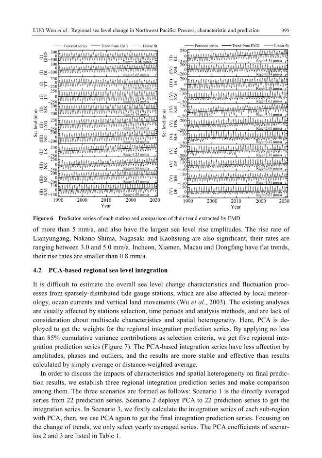
We predict monthly average mean sea level of each station until 2030 using MGF, and the trend components extracted by EMD and their linear fitting lines are also provided (Figure 6). The prediction series explicitly show the multiscale characteristics of original time series and the spatial heterogeneity. Among these predictions, Qinghuangdao, Incheon, Shijiusuo and Nagasaki have a flat and unique trend, their prediction series have little amplitude of variations. The variations of Xiamen, Macau and Hong Kong are significantly complex. Sea levels of the rest stations are predicted to rise except Qinhuangdao and Yantai. The declined trends of these two stations, with an average rate about –0.04 mm/a and –0.86 mm/a, are mainly caused by the vertical rise of the earth’s crust at their regions (Zhang et al., 1997). The stations with maximum sea level rise values are Lusi and Keelung, they both have a rate


Figure 6 Prediction series of each station and comparison of their trend extracted by EMD

of more than 5 mm/a, and also have the largest sea level rise amplitudes. The rise rate of Lianyungang, Nakano Shima, Nagasaki and Kaohsiung are also significant, their rates are ranging between 3.0 and 5.0 mm/a. Incheon, Xiamen, Macau and Dongfang have flat trends, their rise rates are smaller than 0.8 mm/a.

4.2 PCA-based regional sea level integration

It is difficult to estimate the overall sea level change characteristics and fluctuation proc-esses from sparsely-distributed tide gauge stations, which are also affected by local meteor-ology, ocean currents and vertical land movements (Wu et al., 2003). The existing analyses are usually affected by stations selection, time periods and analysis methods, and are lack of consideration about multiscale characteristics and spatial heterogeneity. Here, PCA is de-ployed to get the weights for the regional integration prediction series. By applying no less than 85% cumulative variance contributions as selection criteria, we get five regional inte-gration prediction series (Figure 7). The PCA-based integration series have less affection by amplitudes, phases and outliers, and the results are more stable and effective than results calculated by simply average or distance-weighted average.

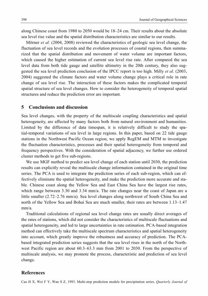
In order to discuss the impacts of characteristics and spatial heterogeneity on final predic-tion results, we establish three regional integration prediction series and make comparison among them. The three scenarios are formed as follows: Scenario 1 is the directly averaged series from 22 prediction series. Scenario 2 deploys PCA to 22 prediction series to get the integration series. In Scenario 3, we firstly calculate the integration series of each sub-region with PCA, then, we use PCA again to get the final integration prediction series. Focusing on the change of trends, we only select yearly averaged series. The PCA coefficients of scenar-ios 2 and 3 are listed in Table 1.


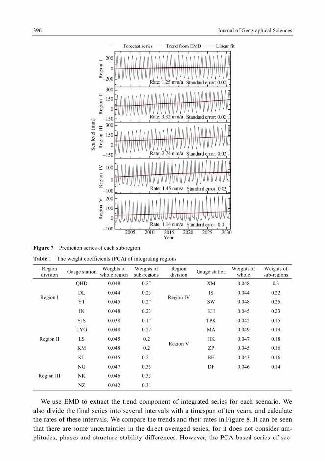
Figure 7 Prediction series of each sub-region

Table 1 The weight coefficients (PCA) of integrating regions

Region division

Gauge stationWeights of

whole regionWeights of sub-regions

Region division

Gauge stationWeights of

whole Weights of sub-regions

QHD 0.048 0.27 XM 0.048 0.3

DL 0.044 0.23 IS 0.044 0.22

YT 0.045 0.27 SW 0.048 0.25 Region I

IN 0.048 0.23

Region IV

KH 0.045 0.23

SJS 0.038 0.17 TPK 0.042 0.15

LYG 0.048 0.22 MA 0.049 0.19

LS 0.045 0.2 HK 0.047 0.18

KM 0.048 0.2 ZP 0.045 0.16

Region II

KL 0.045 0.21 BH 0.043 0.16

NG 0.047 0.35

Region V

DF 0.046 0.14

NK 0.046 0.33 Region III

NZ 0.042 0.31

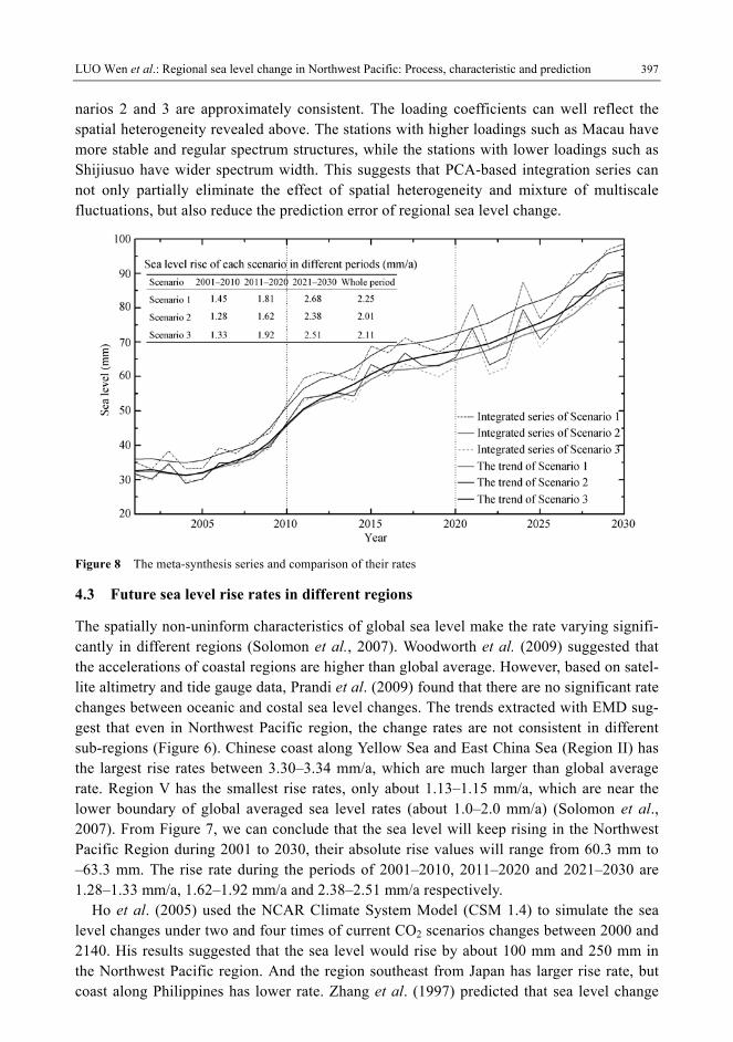
We use EMD to extract the trend component of integrated series for each scenario. We also divide the final series into several intervals with a timespan of ten years, and calculate the rates of these intervals. We compare the trends and their rates in Figure 8. It can be seen that there are some uncertainties in the direct averaged series, for it does not consider am-plitudes, phases and structure stability differences. However, the PCA-based series of sce-


narios 2 and 3 are approximately consistent. The loading coefficients can well reflect the spatial heterogeneity revealed above. The stations with higher loadings such as Macau have more stable and regular spectrum structures, while the stations with lower loadings such as Shijiusuo have wider spectrum width. This suggests that PCA-based integration series can not only partially eliminate the effect of spatial heterogeneity and mixture of multiscale fluctuations, but also reduce the prediction error of regional sea level change.

Figure 8 The meta-synthesis series and comparison of their rates

4.3 Future sea level rise rates in different regions

The spatially non-uninform characteristics of global sea level make the rate varying signifi-cantly in different regions (Solomon et al., 2007). Woodworth et al. (2009) suggested that the accelerations of coastal regions are higher than global average. However, based on satel-lite altimetry and tide gauge data, Prandi et al. (2009) found that there are no significant rate changes between oceanic and costal sea level changes. The trends extracted with EMD sug-gest that even in Northwest Pacific region, the change rates are not consistent in different sub-regions (Figure 6). Chinese coast along Yellow Sea and East China Sea (Region II) has the largest rise rates between 3.30–3.34 mm/a, which are much larger than global average rate. Region V has the smallest rise rates, only about 1.13–1.15 mm/a, which are near the lower boundary of global averaged sea level rates (about 1.0–2.0 mm/a) (Solomon et al., 2007). From Figure 7, we can conclude that the sea level will keep rising in the Northwest Pacific Region during 2001 to 2030, their absolute rise values will range from 60.3 mm to –63.3 mm. The rise rate during the periods of 2001–2010, 2011–2020 and 2021–2030 are 1.28–1.33 mm/a, 1.62–1.92 mm/a and 2.38–2.51 mm/a respectively.

Ho et al. (2005) used the NCAR Climate System Model (CSM 1.4) to simulate the sea level changes under two and four times of current CO2 scenarios changes between 2000 and 2140. His results suggested that the sea level would rise by about 100 mm and 250 mm in the Northwest Pacific region. And the region southeast from Japan has larger rise rate, but coast along Philippines has lower rate. Zhang et al. (1997) predicted that sea level change


along Chinese coast from 1980 to 2050 would be 18–24 cm. Their results about the absolute sea level rise value and the spatial distribution characteristics are similar to our results.

Mörner et al. (2004, 2008) reviewed the characteristics of geologic sea level change, the fluctuation of sea level records and the evolution processes of coastal regions, then summa-rized that the spatial distribution and movement of water volume are important factors, which caused the higher estimation of current sea level rise rate. After compared the sea level data from both tide gauge and satellite altimetry in the 20th century, they also sug-gested the sea level prediction conclusion of the IPCC report is too high. Milly et al. (2003, 2004) suggested the climate factors and water volume change plays a critical role in rate change of sea level rise. The interaction of these factors makes the complicated temporal spatial structure of sea level changes. How to consider the heterogeneity of temporal spatial structures and reduce the prediction error are important.

5 Conclusions and discussion

Sea level changes, with the property of the multiscale coupling characteristics and spatial heterogeneity, are affected by many factors both from natural environment and humanities. Limited by the difference of data timespan, it is relatively difficult to study the spa-tial-temporal variations of sea level in large regions. In this paper, based on 22 tide gauge stations in the Northwest Pacific Ocean region, we apply RegEM and MTM to investigate the fluctuation characteristics, processes and their spatial heterogeneity from temporal and frequency perspectives. With the consideration of spatial adjacency, we further use ordered cluster methods to get five sub-regions.

We use MGF method to predict sea level change of each station until 2030, the prediction results can explicitly reveal the multiscale change information contained in the original time series. The PCA is used to integrate the prediction series of each sub-region, which can ef-fectively eliminate the spatial heterogeneity, and make the prediction more accurate and sta-ble. Chinese coast along the Yellow Sea and East China Sea have the largest rise rates, which range between 3.30 and 3.34 mm/a. The rate changes near the coast of Japan are a little smaller (2.72–2.76 mm/a). Sea level changes along northwest of South China Sea and north of the Yellow Sea and Bohai Sea are much smaller, their rates are between 1.13–1.47 mm/a.

Traditional calculations of regional sea level change rates are usually direct averages of the rates of stations, which did not consider the characteristics of multiscale fluctuations and spatial heterogeneity, and led to large uncertainties in rate estimation. PCA-based integration method can effectively take the multiscale spectrum characteristics and spatial heterogeneity into account, which greatly improve the robustness and accuracy of prediction. The PCA- based integrated prediction series suggests that the sea level rises in the north of the North-west Pacific region are about 60.3–63.3 mm from 2001 to 2030. From the perspective of multiscale analysis, we may promote the process, characteristic and prediction of sea level change.

References

Cao H X, Wei F Y, Wan S Z, 1993. Multi-step prediction models for precipitation series. Quarterly Journal of


Applied Meteorology, 4: 198–204. (in Chinese)

Chambers D P, Mehlhaff C A, Urban T J et al., 2002. Low-frequency variations in global mean sea level:

1950–2000. Journal of Geophysical Research, 107(C4): 3026.

Church J A, White N J, 2004. Estimates of the regional distribution of sea level rise over the 1950–2000 period.

Journal of Climate, 17: 2609–2625.

Collins M, Allen M R, 2002. Assessing the relative roles of initial and boundary conditions in inter-annual to

decadal climate predictability. Journal of Climate, 15: 3104–3109.

Douglas B C, 1997. Global sea rise: A redetermination. Surveys in Geophysics, 18(2/3): 279–292.

Grinsted A, Moore J C, Jevrejeva S, 2009. Reconstructing sea level from paleo and projected temperatures 200 to

2100AD. Climate Dynamics, 34(4): 461–472.

Ho C B，Hoon K D Jin C Y et al., 2005. Projections of ocean climate for northwestern Pacific Ocean. Acta

Oceanologica Sinica, 24(1): 134–145.

Huang N E, Shen Z, Long S R et al., 1998. The empirical mode decomposition and the Hilbert spectrum for

nonlinear and non-stationary series analysis. Proceedings of the Royal Society of London Series A: Mathe-

matical, Physical and Engineering Sciences, 454: 903–995.

Jevrejeva S, Grinsted A, Moore J C et al., 2006. Nonlinear trends and multiyear cycles in sea level records. Jour-

nal of Geophysical Research, 111: C09012.

Kang S K, Chemiawsky J Y, Foreman M G et al., 2008. Spatial variability in annual sea level variations around

the Korean Peninsula. Geophysical Research Letters, 35: L03603.

Knutti R, Stocker T F, 2000. Influence of the thermohaline circulation on projected sea level rise. Journal of Cli-

mate, 13: 1997–2001.

Lanzerotti L J, Thomson D J, Medford L V et al., 1986. Electromagnetic study of the Atlantic continental margin

using a section of a transatlantic cable. Journal of Geophysical Research, 91: 7417–7428.

Li Y P, Qin Z H, Duan Y H, 1998. Research and prediction of mean sea level of Shanghai area. Acta Geographica

Sinica, 53(5): 393–403. (in Chinese)

Liu X Y, Liu Y G, Guo L et al., 2010. Interannual changes of sea level in the two regions of East China Sea and

different responses to ENSO. Global and Planetary Change, 72 (3): 215–226.

Luo D J, Wang X W, Liu W, 2009. Automatic separate layer model based on the phase-space reconstruction and

improved optimum division method. Progress in Geophysics, 24(2): 675–679. (in Chinese)

Mann M E, Bradley R S, Hughes M K, 1998. Global-scale temperature patterns and climate forcing over the past

six centuries. Nature, 392: 779–787.

Mann M E, Zhang Z, Rutherford S et al., 2009. Global signatures and dynamical origins of the little ice age and

medieval climate anomaly. Science, 326: 1256–1260.

Miller L, Douglas B C, 2004. Mass and volume contributions to twentieth-century global sea level rise. Nature,

428(6981): 406–409.

Milly P C D, Cazenave A, Gennero C, 2003. Contribution of climate-driven change in continental water storage

to recent sea-level rise. PNAS, 100(23): 13158–13161.

Moberg A, Sonechkin D, Holmgren K et al., 2005. Highly variable Northern Hemisphere temperatures recon-

structed from low- and high-resolution proxy data. Nature, 433: 613–617.

Mörner N, 2004. Estimating future sea level changes from past records. Global and Planetary Change, 40(1/2):

49–54.

Mörner N, 2008. Comment on comment by Nerem et al. (2007) on “Estimating future sea level changes from past

records” by Nils-Axel Mörner (2004). Global and Planetary Change, 62(3/4): 219–220.

Percival D B, Walden A T, 1993. Spectral Analysis for Physical Applications: Multitaper and Conventional Uni-

variate Techniques. Cambridge: Cambridge University Press.

Prandi P, Cazenave A, Becker M, 2009. Is coastal mean sea level rising faster than the global mean? A compari-

son between tide gauges and satellite altimetry over 1993–2007. Geophysical Research Letters, 36: L05602.

Rahmstorf S, 2007. A semi-empirical approach to projecting future sea-level rise. Science, 315: 368–370.

Rahmstorf S, Cazenave A, Church J A et al., 2007. Recent climate observations compared to projections. Science,


316: 709.

Raper S C B, Braithwaite R J, 2006. Low sea level rise projections from mountain glaciers and ice caps under

global warming. Nature, 439: 311–213.

Riedel K S, Sidorenko A, 1994. Smoothed multiple taper spectral analysis and adaptive implementation. IEEE

Transactions on Signal Processing, 44: 464–467.

Schneider T, 2001. Analysis of incomplete climate data: Estimation of mean values and covariance matrices and

imputation of missing values. Journal of Climate, 14: 853–871.

Siddall M, Stocker T F, Clark P U, 2009. Constraints on future sea-level rise from past sea-level change. Nature

Geoscience, 2(8): 571–575.

Solomon S, Qin D, Manning M et al., 2007. Intergovernmental Panel on Climate Change (IPCC). In: Climate

Change 2007: The Physical Science Basis. Cambridge: Intergovernmental Panel on Climate Change, 1–18.

Spencer N E, Woodworth P L, 1993. Data holdings of the permanent service of mean sea level. PSMSL Data

Holdings, 5: 1–81.

Thomson D J, 1982. Spectrum estimation and harmonic analysis. Proceeding of the IEEE, 70(9): 1055–1096.

Woodworth P L, White N J, Jevrejeva S et al., 2009. Evidence for the accelerations of sea level on multi-decade

and century timescales. International Journal of Climatology, 29: 777–789.

Wu Z, Huang N E, Long S R et al., 2007. On the trend, detrending, and variability of nonlinear and nonstationary

time series. Proceedings of the National Academy of Sciences, 104(38): 14889–14894.

Wu Z D, Li Z Q, Zhao M C, 2003. The process and prediction of sea level change of China offshore waters in 50

years. Hydrographic Surveying and Charting, 23(2): 17–19. (in Chinese)

Yuan L W, Luo W, Yu Z Y et al., 2010. Scale coupling and fluctuation transformation of interannual to interde-

cadal sea-level variations in Northwest Pacific Region. Geographical Research, 29(12): 2201-2211. (in Chi-

nese)

Yuan L W, Xie Z R, Yu Z Y, 2008. Long-term prediction and comparison of sea-level change based on the SSA

and MGF model. Geographical Research, 27(2): 305–313. (in Chinese)

Yuan L W, Yu Z Y, Xie Z R et al., 2009. ENSO signals and their spatial-temporal variation characteristics re-

corded by the sea-level changes in the Northwest Pacific margin during 1965–2005. Science China (Series D),

52(6): 869–882.

Zhang J W, 1997. Estimate model of MSL change along the coast of China. Marine Science Bulletin, 16(4): 3–11.

(in Chinese)

Regional sea level change in Northwest Pacific: Process, characteristic and prediction

Documents

Transcript of Regional sea level change in Northwest Pacific: Process, characteristic and prediction