Refinery short-term scheduling with tank farm, inventory and distillation management: An integrated...

European Journal of Operational Research 166 (2005) 812–827

www.elsevier.com/locate/dsw

Refinery short-term scheduling with tank farm,inventory and distillation management:An integrated simulation-based approach

George Chryssolouris *, Nikolaos Papakostas, Dimitris Mourtzis

Laboratory for Manufacturing Systems and Automation, Department of Mechanical Engineering and Aeronautics,

University of Patras, 26110 Rio, Patras, Greece

Received 1 September 2002; accepted 1 March 2004Available online 26 August 2004

Abstract

This work addresses primarily the scheduling of a refinery importing various types of crude oil. The refinery oper-ation discussed in this paper involves the unloading of crude oil to storage tanks, the transfer and blending from storagetanks to charging tanks and crude oil distillation units, and the arrangement of the temperature cut-points for each dis-tillation unit. The paper describes a simulation-based approach to the refinery operation, which is modelled as a poolingproblem. The proposed approach uses a random-search formulation, which allows for controlling search depth,breadth and solution quality, as well as computational effort. An implementation of the proposed approach is presentedin a real case scenario.� 2004 Elsevier B.V. All rights reserved.

Keywords: Decision support systems; Scheduling; Simulation; Pooling problem; Petroleum industry

1. Introduction

The short-term oil refinery scheduling problemis one of the most challenging problems in opera-tional research due to the complexity of the refin-ery scheduling operations (Pinto et al., 2000) andthe corresponding process models (Zhang and

0377-2217/$ - see front matter � 2004 Elsevier B.V. All rights reservdoi:10.1016/j.ejor.2004.03.046

* Corresponding author. Tel.: +30 2610 997262; fax: +302610 997744.

E-mail address: [email protected] (G. Chryssolouris).

Zhu, 2000). In a refinery, a number of operationstake place for turning raw material (crude oils)into higher value end (petroleum) products. De-mand drives the definition of the production tar-gets (quantities of final products with specificproperties within specified time periods) to a refin-ery. The first steps for achieving these targets in-volve the processing of the different crude oils ontheir own, or as blends, in the distillation units.Crudes are usually delivered to storage tanksby vessels. In a typical refinery, there is often an

ed.

mailto:[email protected]

Nomenclature

Indicesc = 1, . . . ,NR crude oild = 1, . . . ,ND crude distillation unitg = 1, . . . ,n node in sampleh = 1, . . . ,NT tanki 2 ½1;MNGA� \N alternativej 2 ½1; SR� \N samplek(s) indexing function denoting the tank feeding stream s

n 2 ½1;DH � 1� \N last node of path (sample)rg,j node for period g of path (sample) jp = 1, . . . ,NC temperature cut point, distillate, CDU output streams = 1, . . . ,NS streamt 2 [0, time] time representation in a time intervalu = 1, . . . ,NK docking stationv = 1, . . . ,NV vesselz = 1, . . . ,NM CDU mode of operation, depending on blend type of input (e.g., MS or LS)

Variables

qp density of distillate p

ATv the time the vth docked vessel remains docked without unloadingCc,d total volumetric quantity of crude oil c, transferred to CDU d

Ds stream s densityE(rgj) returns 1 when the node ogj is feasible and 0 otherwiseFp,c the quantity of distillate p produced, due to a fraction of crude oil c in the input blendFp,d,tot total production of product p in CDU d during a time intervalIC the total tank inventory cost_minc;h input mass transfer rate of crude oil c in tank h

Mh total mass of oil stored in tank h_Mout

h total mass output transfer rate of tank h

NDV the number of docked vesselsqc,h mass fraction of crude oil c in tank h

RC the total oil transfer costSs volumetric transfer rate of stream sTC total costTT v 2 ½0;NK� \N variable to denote the docking station allocated to vessel v; 0 if no docking station

is allocatedVh volume stored in tank h

VC the cost due to the vessels waiting timeVSh, VEh the initial and final volume of the hth tank during a time intervalWd,p temperature cut point p (upper cut point of CDU stream p) of CDU d

Wp temperature cut point pY ins;h equal to 1 when tank h feeds stream s and 0 otherwise

Y outs;h equal to 1 when stream s feeds tank h and 0 otherwise

G. Chryssolouris et al. / European Journal of Operational Research 166 (2005) 812–827 813

Crude Oil "Captain"

05

10152025303540

0-175 175-232 232-342 342-369 369-509 509-550 550-800Temperature (°C)

Evap

orat

ion

(%)

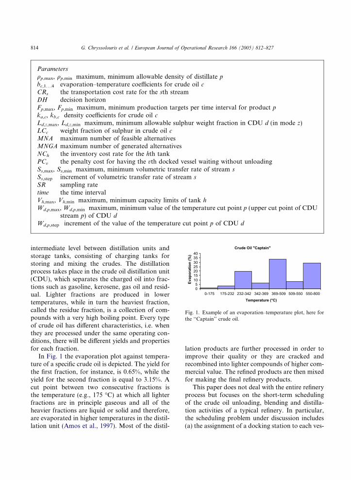
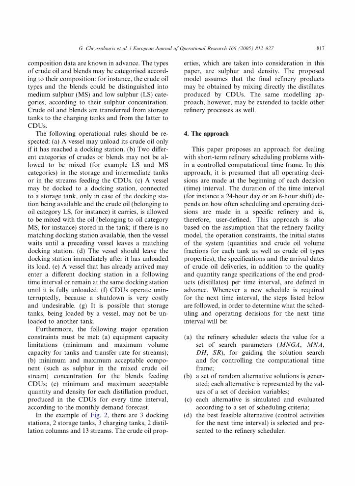
Fig. 1. Example of an evaporation–temperature plot, here forthe ‘‘Captain’’ crude oil.

Parameters

qp,max, qp,min maximum, minimum allowable density of distillate p

bc,1. . .4 evaporation–temperature coefficients for crude oil cCRs the transportation cost rate for the sth streamDH decision horizonFp,max, Fp,min maximum, minimum production targets per time interval for product pka,c, kb,c density coefficients for crude oil cLd,z,max, Ld,z,min maximum, minimum allowable sulphur weight fraction in CDU d (in mode z)LCc weight fraction of sulphur in crude oil cMNA maximum number of feasible alternativesMNGA maximum number of generated alternativesNCh the inventory cost rate for the hth tankPCv the penalty cost for having the vth docked vessel waiting without unloadingSs,max, Ss,min maximum, minimum volumetric transfer rate of stream s

Ss,step increment of volumetric transfer rate of stream s

SR sampling ratetime the time intervalVh,max, Vh,min maximum, minimum capacity limits of tank h

Wd,p,max, Wd,p,min maximum, minimum value of the temperature cut point p (upper cut point of CDUstream p) of CDU d

Wd,p,step increment of the value of the temperature cut point p of CDU d

814 G. Chryssolouris et al. / European Journal of Operational Research 166 (2005) 812–827

intermediate level between distillation units andstorage tanks, consisting of charging tanks forstoring and mixing the crudes. The distillationprocess takes place in the crude oil distillation unit(CDU), which separates the charged oil into frac-tions such as gasoline, kerosene, gas oil and resid-ual. Lighter fractions are produced in lowertemperatures, while in turn the heaviest fraction,called the residue fraction, is a collection of com-pounds with a very high boiling point. Every typeof crude oil has different characteristics, i.e. whenthey are processed under the same operating con-ditions, there will be different yields and propertiesfor each fraction.

In Fig. 1 the evaporation plot against tempera-ture of a specific crude oil is depicted. The yield forthe first fraction, for instance, is 0.65%, while theyield for the second fraction is equal to 3.15%. Acut point between two consecutive fractions isthe temperature (e.g., 175 �C) at which all lighterfractions are in principle gaseous and all of theheavier fractions are liquid or solid and therefore,are evaporated in higher temperatures in the distil-lation unit (Amos et al., 1997). Most of the distil-

lation products are further processed in order toimprove their quality or they are cracked andrecombined into lighter compounds of higher com-mercial value. The refined products are then mixedfor making the final refinery products.

This paper does not deal with the entire refineryprocess but focuses on the short-term schedulingof the crude oil unloading, blending and distilla-tion activities of a typical refinery. In particular,the scheduling problem under discussion includes(a) the assignment of a docking station to each ves-


sel, (b) the specification of the volume flow transferamong storage tanks, charging tanks and distilla-tion units per time interval and (c) the determina-tion of the temperature cut points for eachdistillation unit per time interval.

2. Overview of scheduling in oil refineries

Long-term and plant-wide planning problemsin the Petrochemical Industry have been mainlyaddressed by mathematical programming tech-niques (Bodington and Baker, 1990). Pure LinearProgramming (LP) methods have been used forlong-term planning, but are not applicable toshort-term scheduling and on-line optimisation,since they are based on simplified correlations,without being able to represent both continuous(and often non-linear) processes and discrete deci-sions accurately (Zhang and Zhu, 2000). In fact,short-term refinery scheduling combines a set ofproblems that have been mainly addressed in liter-ature as cost/profit optimisation problems, such asthe allocation of crude oil to tanks, the problem ofdetermining the flows from several input tanks,mixed together in one or several storage tanks,and then transferred towards one or several outputtanks (pooling problem), and the determination ofthe distillation cut-points.

Paolucci et al. (2002) proposed a simulation-based decision support system for allocating crudeoil supply to port and refinery tanks. Fieldhouse(1993) proposed a technique, known as distribu-tive recursion––a form of successive linear approx-imation––for addressing the pooling problemalone. The combined crude allocation/poolingproblem has been examined by Lee et al. (1996)with the development of a mixed integer linearprogramming (MILP) multi-period model for pro-posing a short-term crude oil unloading, tankinventory management, and CDU charging sched-ule, having as production target the CDU feedingwith specific quantities of blends of predeterminedspecification. In this approach, time is representedby dividing the scheduling horizon into equal timeslots. Pinto et al. (2000) present the results of theapplication of a mixed integer optimisation modelin a similar real world problem. In their model,

time is represented by variable length time slots,which correspond to crude oil receiving operations(vessels unloading) as well as to periods betweentwo receiving tasks. Ballintijn (1993) proposed aMILP model for finding a minimum cost sequenceof daily activities for the units and the oil-move-ment systems in a refinery, in order to meet theoverall production targets. In this multi-periodmodel, only pure crudes may be processed in thedistillation units. Shah (1996) proposed a mathe-matical programming approach, in which, tanksmay store only one crude type and each CDU runsexactly one crude type from one tank at a time.

Amos et al. (1997) dealt with the combinedpooling/distillation problem as applied to a spe-cific refinery case. They proposed a non-linearmathematical model for determining the flows ofthe input tanks towards the distillation units, aswell as the temperature cut points for each distilla-tion unit. Their model focuses on the distillationprocess, without taking into account any capacitylimitations in the storage tanks. Zhang and Zhu(2000) present a two-level decomposition strategyfor tackling large-scale refinery optimisation prob-lems. The site level model determines common is-sues among processes, such as allocation of rawmaterials and utilities, whilst the process levelmodel optimises individual processes. The resultsfrom the process level optimisation are then fedback to the site level model for further optimisa-tion until convergence criteria between the twomodels are met.

In general, the availability of LP-based com-mercial software for refinery production planninghas allowed the development of general, long-term(Paolucci et al., 2002) production plans of thewhole refinery (Pinto et al., 2000). On the otherhand, the refinery short-term scheduling processes(requiring fast decisions) are affected by stochasticdisturbances (Paolucci et al., 2002), such as shiparrivals that are confirmed about a few daysahead, without knowing with certainty the exactarrival time, the production fluctuations, which af-fect blend and stream properties and, finally, themarket variations, which may affect productiontargets. Feasible solutions, which incorporate LP-based plans and real-life disturbances, are usuallycalculated by human schedulers, relying on


manual/spreadsheet calculations, which, however,require ample time and effort (Pinto et al., 2000).

Interestingly, commercial tools for short-termproduction scheduling are few and these do notallow for a rigorous representation of plant partic-ularities (Pinto et al., 2000). For that reason, some-times refineries are developing in-house toolsstrongly based on simulation (Pinto et al., 2000;Magalhaes et al., 1998; Hofferl and Steinschorn,1998). These tools, however, are not generic en-ough, neither do they tackle successfully all model-ling problems in an integrated manner.

The optimisation based formulations for short-term scheduling in literature are very few (Pintoet al., 2000) and those presented in the paragraphsabove, do not incorporate the model complexity ofthe entire unloading, blending and distillationprocess. They also show that there are still a num-ber of issues to address in order to be applicable:(a) the difficulty of controlling the computationaltime frame, because of the highly combinatorialfeatures of the MILP models, these formulationsare based on (Pinto et al., 2000); (b) the difficultyof imposing directly the time structure in themodel, which in the non-linear approach leads tounder-optimisation (Simons, 1995); (c) the optimi-sation criteria, which are usually expressed in costor profit terms, while units operation and the over-

T2

T1

VesselsStorageTanks

D1

D2

DockingStations

D3

S1

S2

S

S

S3

Fig. 2. Example of a

all plant objectives may not always be directlyrepresented with cost/profit terms and (d) the dif-ficulty of understanding the rationale underlyingthe solutions proposed by a ‘‘black box’’ mathe-matical programming model, in contrast to a sim-ulation-based decision support approach (Paolucciet al., 2002).

The approach described in the present paperemploys an integrated simulation-based mecha-nism, for evaluating the performance of a numberof generated alternatives, using multiple criteria.This new approach has been implemented into asoftware system, for the purpose of solving theshort-term scheduling problem in a specific refin-ery case, allowing for user interaction and theinvestigation of what-if scenarios.

3. The refinery model

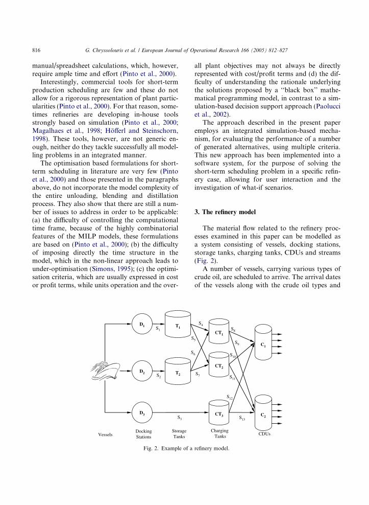
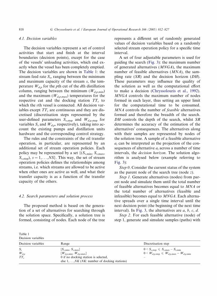
The material flow related to the refinery proc-esses examined in this paper can be modelled asa system consisting of vessels, docking stations,storage tanks, charging tanks, CDUs and streams(Fig. 2).

A number of vessels, carrying various types ofcrude oil, are scheduled to arrive. The arrival datesof the vessels along with the crude oil types and

CT1

C1

Charging Tanks CDUs

CT2

C2CT3

S4

5

6

S7

S8

S9

S10

S11

S12

S13

refinery model.


composition data are known in advance. The typesof crude oil and blends may be categorised accord-ing to their composition: for instance, the crude oiltypes and the blends could be distinguished intomedium sulphur (MS) and low sulphur (LS) cate-gories, according to their sulphur concentration.Crude oil and blends are transferred from storagetanks to the charging tanks and from the latter toCDUs.

The following operational rules should be re-spected: (a) A vessel may unload its crude oil onlyif it has reached a docking station. (b) Two differ-ent categories of crudes or blends may not be al-lowed to be mixed (for example LS and MScategories) in the storage and intermediate tanksor in the streams feeding the CDUs. (c) A vesselmay be docked to a docking station, connectedto a storage tank, only in case of the docking sta-tion being available and the crude oil (belonging tooil category LS, for instance) it carries, is allowedto be mixed with the oil (belonging to oil categoryMS, for instance) stored in the tank; if there is nomatching docking station available, then the vesselwaits until a preceding vessel leaves a matchingdocking station. (d) The vessel should leave thedocking station immediately after it has unloadedits load. (e) A vessel that has already arrived mayenter a different docking station in a followingtime interval or remain at the same docking stationuntil it is fully unloaded. (f) CDUs operate unin-terruptedly, because a shutdown is very costlyand undesirable. (g) It is possible that storagetanks, being loaded by a vessel, may not be un-loaded to another tank.

Furthermore, the following major operationconstraints must be met: (a) equipment capacitylimitations (minimum and maximum volumecapacity for tanks and transfer rate for streams);(b) minimum and maximum acceptable compo-nent (such as sulphur in the mixed crude oilstream) concentration for the blends feedingCDUs; (c) minimum and maximum acceptablequantity and density for each distillation product,produced in the CDUs for every time interval,according to the monthly demand forecast.

In the example of Fig. 2, there are 3 dockingstations, 2 storage tanks, 3 charging tanks, 2 distil-lation columns and 13 streams. The crude oil prop-

erties, which are taken into consideration in thispaper, are sulphur and density. The proposedmodel assumes that the final refinery productsmay be obtained by mixing directly the distillatesproduced by CDUs. The same modelling ap-proach, however, may be extended to tackle otherrefinery processes as well.

4. The approach

This paper proposes an approach for dealingwith short-term refinery scheduling problems with-in a controlled computational time frame. In thisapproach, it is presumed that all operating deci-sions are made at the beginning of each decision(time) interval. The duration of the time interval(for instance a 24-hour day or an 8-hour shift) de-pends on how often scheduling and operating deci-sions are made in a specific refinery and is,therefore, user-defined. This approach is alsobased on the assumption that the refinery facilitymodel, the operation constraints, the initial statusof the system (quantities and crude oil volumefractions for each tank as well as crude oil typesproperties), the specifications and the arrival datesof crude oil deliveries, in addition to the qualityand quantity range specifications of the end prod-ucts (distillates) per time interval, are defined inadvance. Whenever a new schedule is requiredfor the next time interval, the steps listed beloware followed, in order to determine what the sched-uling and operating decisions for the next timeinterval will be:

(a) the refinery scheduler selects the value for aset of search parameters (MNGA, MNA,DH, SR), for guiding the solution searchand for controlling the computational timeframe;

(b) a set of random alternative solutions is gener-ated; each alternative is represented by the val-ues of a set of decision variables;

(c) each alternative is simulated and evaluatedaccording to a set of scheduling criteria;

(d) the best feasible alternative (control activitiesfor the next time interval) is selected and pre-sented to the refinery scheduler.

l of Operational Research 166 (2005) 812–827

4.1. Decision variables

818 G. Chryssolouris et al. / European Journa

The decision variables represent a set of controlactivities that start and finish at the intervalboundaries (decision points), except for the caseof the vessels� unloading activities, which end ex-actly when the vessel has been completely emptied.The decision variables are shown in Table 1: thestream feed rate Ss, ranging between the minimumand maximum capacity of the stream s, the tem-perature Wd,p for the pth cut of the dth distillationcolumn, ranging between the minimum (Wd,p,min)and the maximum (Wd,p,max) temperatures for therespective cut and the docking station TTv towhich the vth vessel is connected. All decision var-iables except TTv are continuous and they are dis-cretised (discretisation steps represented by theuser-defined parameters Ss,step and Wd,p,step forvariables Ss and Wd,p, respectively), taking into ac-count the existing pumps and distillation unitshardware and the corresponding control strategy.

The rules and the constraints of the oil transferoperation, in particular, are represented by anadditional set of stream operation policies. Eachpolicy may be represented by a set {(Ss,min, Ss,max,Ss,step), s = 1, . . . ,NS}. This way, the set of streamoperation policies defines the relationships amongstreams, i.e. which streams are allowed to be activewhen other ones are active as well, and what theirtransfer capacity is as a function of the transfercapacity of the others.

4.2. Search parameters and solution process

The proposed method is based on the genera-tion of a set of alternatives for searching throughthe solution space. Specifically, a solution tree isformed, consisting of nodes. Each node of the tree

Table 1Decision variables

Decision variables Range

Ss [Ss,min, Ss,max]Wd,p [Wd,p,min, Wd,p,max]TTv 0 if no docking station is selected,

else 1, . . . ,NK (NK: number of docking

represents a different set of randomly generatedvalues of decision variables based on a randomlyselected stream operation policy for a specific timeinterval.

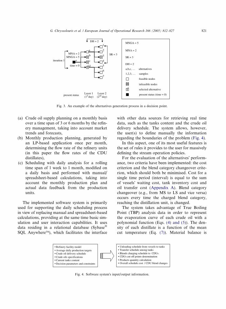
A set of four adjustable parameters is used forguiding the search (Fig. 3): the maximum numberof generated alternatives (MNGA), the maximumnumber of feasible alternatives (MNA), the sam-pling rate (SR) and the decision horizon (DH).These parameters may influence the quality ofthe solution as well as the computational effortto make a decision (Chryssolouris et al., 1992).MNGA controls the maximum number of nodesformed in each layer, thus setting an upper limitfor the computational time to be consumed.MNA controls the number of feasible alternativesformed and therefore the breadth of the search.DH controls the depth of the search, whilst SR

determines the accuracy of the estimation of thealternatives� consequences. The alternatives alongwith their samples are represented by nodes ofthe solution tree. A sample of a feasible alternativeai can be interpreted as the projection of the con-sequences of alternative ai across a number of timeintervals, the decision horizon. The solution algo-rithm is analysed below (example referring toFig. 3):

Step 0. Consider the current status of the systemas the parent node of the search tree (node z).

Step 1. Generate alternatives (nodes) from par-ent node and simulate them until the total numberof feasible alternatives becomes equal to MNA orthe total number of alternatives (feasible andinfeasible) becomes equal toMNGA. Each alterna-tive spreads over a single time interval until thenext decision point (the beginning of the next timeinterval). In Fig. 3, the alternatives are a, b, c, d.

Step 2. For each feasible alternative (node) ofstep 1, generate and simulate samples (paths) with

Discretisation step

0 < Ss,step 6 Ss,max � Ss,min

0 < Wd,p,step 6 Wd,p,max � Wd,p,min

stations)–


maximum length (including the feasible alternativeof step 1) equal to DH, until the number of the fea-sible paths becomes equal to SR, complying withthe following rule: for each node of the path nomore than one feasible and no more than MNGAinfeasible nodes are generated for the next levelof the path. Formally, a sample j of a feasiblealternative ai may be defined as a path Uj = {ai,r1,j, r2,j, . . . ,rn,j}, 16 n6DH � 1, Eðrg;jÞ ¼ 1 8g 2½1; n� \N, where

• rg,j: a node expressing a set of decision variablesvalues for period g of sample (path) j of the par-ent alternative (node ai),

• E(rg,j): returns 1 when node rg,j is feasible and 0otherwise.

In Fig. 3, alternative a has 3 samples: a-1, a-2and a-4. An example of the stream operation pol-icies and the decision variables values of an alter-native sample are depicted in Tables 2 and 3,respectively, for a decision horizon of 2 time inter-vals (e.g., days). In this example, policies 1 and 2were randomly selected from the entire set of pol-icies for the 1st (day 1) and 2nd node (day 2) of thesample, respectively.

Step 3. Sort out the alternatives with the sam-ples (paths) being of the maximum length. Theconsequences (e.g., cost) for each feasible alterna-tive are then calculated as the mean value of theconsequences of these ‘‘maximum length’’ sam-ples. The consequence of an alternative, with re-

Table 2Stream operation policies example

Policy S8 S10

S8,min S8,max S8,step S10,min S

1 2400 3600 240 2400 32 0 0 0 0

Table 3An alternative example

� � � S8 S10 S12 � � � TT1

Period 1 (day 1) 2640 3600 0 0Period 2 (day 2) 0 0 5040 0

spect to a scheduling criterion, is the estimatedvalue of that criterion if the alternative is imple-mented (Chryssolouris, 1992).

Step 4. In the last stage, the utility of each alter-native is calculated, taking into account the conse-quences calculated in the previous stage and thecriteria weights, which express the relative impor-tance of different criteria. The simple additiveweighting method with linear scale transformation(Hwang and Yoon, 1981) is used in this paper forcalculating the utility of each alternative and forranking the alternatives according to their utility.The alternative with the highest utility value isthen selected.

4.3. Simulation

During the solution process, every node is sim-ulated and checked for feasibility. For each node,the simulation mechanism takes as input the initialstatus of the system (at the beginning of the timeinterval), as well as the values of the decision var-iables of the node, utilising a set of material bal-ance and crude oil evaporation–temperatureequations. The simulation mechanism calculatesalso the content of each tank (blend composition)at the end of each time interval, as well as thequantity of the distillates, produced in the distilla-tion columns during the time interval. In this pa-per, material balance is modelled by a set ofdifferential equations (Himmelblau, 1992), assum-ing instantaneous uniform mixing in tanks and

S12

10,max S10,step S12,min S12,max S12,step

600 240 0 0 00 0 4800 7200 240

TT2 TT3 W1,1 W1,2 W1,3 W1,4 W2,1 � � �1 0 160 220 464 700 1801 0 186 232 466 700 170


streams and insignificant stream capacities com-pared to tanks capacities.

dðqc;hMhÞ=dt ¼ _minc;h � _M

out

h qc;h; ð1Þ

whereqc,h mass fraction of crude oil c in tank h,Mh total mass of oil stored in tank h,_minc;h input mass transfer rate of crude oil c in

tank h,_Mout

h total mass output transfer rate of tank h.These equations are related to the decision var-

iables according to the following equations:

_minc;h ¼

XNS

s¼1

½SsY outs;h qc;kðsÞDs�; ð2Þ

_Mout

h ¼XNS

s¼1

½SsY ins;hDs�; ð3Þ

wherek(s) indexing function denoting the tank feed-

ing stream s,Ds stream s density, as per tank k(s) content,Y outs;h equal to 1 when stream s feeds tank h and

0 otherwise,Y ins;h equal to 1 when tank h feeds stream s and

0 otherwise.The model introduced by Amos et al. (1997) is

employed for determining the functions that repre-sent the density and the sulphur concentrationthroughout the distillates of a crude oil blend,fed to a CDU. According to this model, the den-sity is assumed to be proportional to the boilingpoint, whilst sulphur is assumed to be distributeduniformly throughout the fractions of a crude oilor blend. The cumulative function that representsthe evaporation–temperature function of a crudeoil is described below (denoting temperature asW):

F cumðW Þ ¼ bc;1W þ bc;2W 2 þ bc;3W 3 þ bc;4W 4; ð4Þ

where the coefficients bc,1. . .4 are calculated by solv-ing a constrained least square problem and are as-sumed to be known in advance for each crude oil.Therefore, the quantity Fp,c of distillate p due to afraction of crude oil c reaching a distillation unit isequal to

F p;c ¼ Cc½bc;1ðW p � W p�1Þ þ bc;2ðW 2p � W 2

p�1Þ

þ bc;3ðW 3p � W 3

p�1Þ þ bc;4ðW 4p � W 4

p�1Þ� 8p;

ð5Þ

where Wp�1 and Wp stand for the low andupper temperature cut points (decision variables)for distillate p (with W0 = 0) and Cc is the totalvolumetric quantity of crude oil c transferred tothe distillation unit. The total quantity Fp,tot ofdistillate p for a distillation unit is thereforeequal to

F p;tot ¼XNRc¼1

F p;c; ð6Þ

where NR denotes the total number of crude oiltypes.

For a time period, density qp of distillate p in adistillation column is represented by the followingfunction (Amos et al., 1997):

qp ¼XNRc¼1

½F p;cðka;c þ kb;cðW p þ W p�1Þ=2Þ�XNRc¼1

F p;c

,;

ð7Þ

where ka,c and kb,c are constants assumed to beknown in advance for the crude oil c.

Nodes not satisfying one or more constraints(Appendix B), such as the tanks capacity limits,the production targets and the CDU streams spec-ifications, are considered infeasible and are dis-carded. In Fig. 3, for instance, node 3 foralternative a is discarded.

5. Implementation

The proposed methodology has been imple-mented in a client/server software system thatoperates under the Windows� 2000 operating sys-tem, for the purpose of tackling the refinery short-term scheduling problem in a specific refinery. Inthat particular plant, as in a large number of refin-eries, the standard scheduling practice includes thefollowing stages:

MNGA = 5

MNA = 2

SR = 3

DH = 2

feasible nodes

infeasible nodes

DH = 2

time = 0

Layer 1(1stday)

Layer 2(2nd day)

present status (time = 0)

SR = 3

iteration 1

present status

a

b

d

c

1

2

3

4

5

6

7

z

a,b,c, … alternatives

1,2,3, … samples

MNA = 2MNGA = 5

selected alternative

Fig. 3. An example of the alternatives generation process in a decision point.


(a) Crude oil supply planning on a monthly basisover a time span of 3 or 6 months by the refin-ery management, taking into account markettrends and forecasts,

(b) Monthly production planning, generated byan LP-based application once per month,determining the flow rate of the refinery units(in this paper the flow rates of the CDUdistillates),

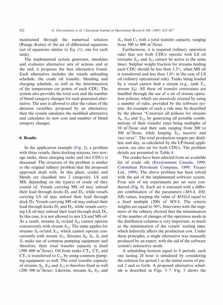
(c) Scheduling with daily analysis for a rollingtime span of 1 week to 1 month, modified ona daily basis and performed with manual/spreadsheet-based calculations, taking intoaccount the monthly production plan andactual data feedback from the productionunits.

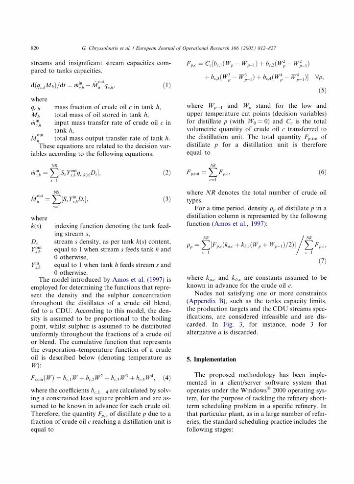
The implemented software system is primarilyused for supporting the daily scheduling processin view of replacing manual and spreadsheet-basedcalculations, providing at the same time basic sim-ulation and user interaction capabilities. It usesdata residing in a relational database (Sybase�

SQL AnywhereTM), which facilitates the interface

• Refinery facility model• Average daily production targets• Crude oil delivery schedule• Crude oils specifications• Current tanks content• Decision parameters and constraints

Fig. 4. Software system�s inp

with other data sources for retrieving real timedata, such as the tanks content and the crude oildelivery schedule. The system allows, however,the user(s) to define manually the informationregarding the boundaries of the problem (Fig. 4).

In this aspect, one of its most useful features isthe set of rules it provides to the user for massivelydefining the stream operation policies.

For the evaluation of the alternatives� perform-ance, two criteria have been implemented: the costcriterion and the blend category changeover crite-rion, which should both be minimised. Cost for asingle time period (interval) is equal to the sumof vessels� waiting cost, tank inventory cost andoil transfer cost (Appendix A). Blend categorychangeover (e.g., from MS to LS and vice versa)occurs every time the charged blend category,reaching the distillation unit, is changed.

The system takes advantage of True BoilingPoint (TBP) analysis data in order to representthe evaporation curve of each crude oil with apolynomial function (Eqs. (4) and (5)). The den-sity of each distillate is a function of the meancut temperature (Eq. (7)). Material balance is

• Unloading schedule from vessels to tanks• Transfer schedule among tanks• Blends charging schedule to CDUs• CDUs cut off points determination • Products quantity calculation• Overall schedule cost / CDU blend changes

ut/output information.


maintained through the numerical solution(Runge–Kutta) of the set of differential equations(set of equations similar to Eq. (1), one for eachtank).

The implemented system generates, simulatesand evaluates alternative sets of actions and atthe end, it proposes the best alternative found.Each alternative includes the vessels unloadingschedule, the crude oil transfer, blending andcharging schedule, as well as the determinationof the temperature cut points of each CDU. Thesystem also provides the total cost and the numberof blend category changes for each generated alter-native. The user is allowed to alter the values of thedecision variables, proposed by an alternative;then the system simulates the modified alternativeand calculates its new cost and number of blendcategory changes.

6. Results

In the application example (Fig. 2), a problemwith three vessels, three docking stations, two stor-age tanks, three charging tanks and two CDUs isdiscussed. The structure of the problem is similarto the original refinery problem that the proposedapproach dealt with. In this plant, crudes andblends are classified into 2 categories: LS andMS, depending on the type(s) of crude oil theyconsist of. Vessels carrying MS oil may unloadtheir load through docks D1 and D2, while vesselscarrying LS oil may unload their load throughdock D3. Vessels carrying MS oil may unload theirload through docks D1 and D2, while vessels carry-ing LS oil may unload their load through dock D3.In this case, it is not allowed to mix LS and MS oil.As a result, streams S8 or/and S10 cannot operateconcurrently with stream S12. The same applies forstreams S9 or/and S11, which cannot operate con-currently with stream S13. Streams S4, S5, S6 andS7 make use of common pumping equipment andtherefore, their total transfer capacity is fixed(500–600 m3/hour). Oil from tanks CT1, CT2 andCT3 is transferred to C1, by using common pump-ing equipment as well. The total transfer capacityof streams S8, S10 and S12 is therefore fixed as well(200–300 m3/hour). Likewise, streams S9, S11 and

S13 feed C2 with a total transfer capacity, rangingfrom 500 to 600 m3/hour.

Furthermore, it is required (refinery operationrule) that not both CDUs operate with LS oil(streams S12 and S13 cannot be active at the sametime). Sulphur weight fraction for streams feedingeach CDU should be less than 3.2%, when MS oilis transferred and less than 1.0% in the case of LSoil (refinery operational rule). Tanks being loadedby a vessel cannot feed a stream (e.g., tank T1,stream S4). All these oil transfer constraints arehandled through the use of a set of stream opera-tion policies, which are massively created by usinga number of rules, provided by the software sys-tem. An example of such a rule may be describedby the phrase ‘‘Construct all policies for streamsS8, S10 and S12, by generating all possible combi-nations of their transfer rates being multiples of10 m3/hour and their sum ranging from 200 to300 m3/hour, while keeping S12 inactive andvice versa’’. The total production targets per distil-late and day, as calculated by the LP-based appli-cation, are also set for both CDUs. The problemdetails are presented in Table 4.

The crudes have been selected from an availablelist of crude oils (Environment Canada, 1999;Colombian Petroleum Company, 1999; TexacoLtd., 1999). The above problem has been solvedwith the aid of the implemented software system.Four sets of ten experiments per set were con-ducted (Fig. 8). Each set is executed with a differ-ent combination of the parameters (MNA, DH,SR) values, keeping the value of MNGA equal toa fixed multiple (200) of MNA. The criteriaweights are equal to 50%. Interviews with the engi-neers of the refinery showed that the minimisationof the number of changes of the operation mode inthe distillation columns is very important, as muchas the minimisation of the vessels� waiting time,which indirectly affects the production cost. Underthese principles, a single alternative was manuallyproduced by an expert, with the aid of the softwaresystem�s interactive mode.

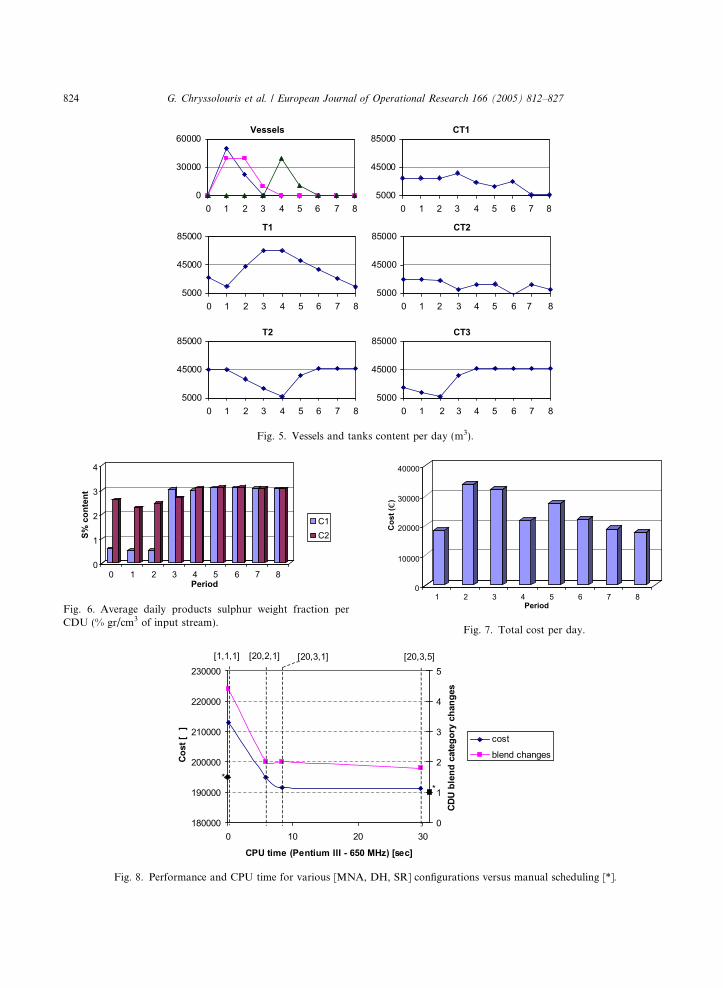
A scheduling horizon equal to 8 periods, eachone lasting 24 hour is simulated by consideringthe solution for period 1 as the initial status of per-iod 2 and so forth. A proposed alternative sched-ule is described in Figs. 5–7. Fig. 5 shows the

Table 4System information for the application example

Crude oil Type LC% (kg/m3 of crude) Density (kg/l)

A Medium sulphur (MS) 3.45 0.90B Medium sulphur (MS) 1.74 0.87C Low sulphur (LS) 0.53 0.88

Vessels Arrival (day) Load (m3) Crude oil type Wait cost (€/hour)

Vessel 1 1 50,000 A 200Vessel 2 1 40,000 C 350Vessel 3 4 40,000 B 300

Stream(s) Rate (m3/hour) Rate step (m3/hour) Blend constraints Rate cost (€/m3)

S1�3 1150–1300 10 – 0.25S4 + S5 + S6 + S7 500–600 10 – 0.55S8 + S10 + (S12) 200–300 10 L% < 3.2% (1.0%) 0.25S9 + S11 + (S13) 500–600 10 L% < 3.2% (1.0%) 0.25

Storage tank Capacity (m3) Initial amount (m3) Initial content (vol.%) Inventory cost (€/(hourm3))

T1 5000–80,000 27,000 100% B 0.002T2 5000–70,000 45,000 100% A 0.002

Charging tank Capacity (m3) Initial amount (m3) Initial content (vol.%) Inventory cost (€/(hourm3))

CT1 4000–50,000 30,000 70%A + 30%B 0.002CT2 4000–50,000 25,000 40%A + 60%B 0.002CT3 5000–50,000 20,000 100% C 0.002

CDU Products cut-off points range (�C) Step (�C) Initial blend

C1 (1) 150–180, (2) 220–240, (3) 450–500,(4) 700

2 LS

C2 (1) 150–190, (2) 230–260, (3) 440–500,(4) 700

10 MS

Prod. target (m3/day) Product 1 Product 2 Product 3 Product 4 (residue)

3000–5000 1200–2200 5900–7200 5000–7800

Density (kg/l) 0.65–0.85 0.70–0.95 0.75–1.05 0.80–1.10


contents of the vessels, the storage and chargingtanks for each period of the scheduling horizonfor an 8-days proposed schedule. Vessels 1 and 3,carrying MS crude oil, deliver their load withoutwaiting. Vessel 2, the one carrying the LS crudeoil, waits for one day only and unloads directlyto the charging tank CT3. The sulphur weight frac-tion of the input streams (and therefore the meansulphur weight fraction in the distillation prod-ucts) for each distillation unit is depicted in Fig.6. LS oil is processed in periods 1 and 2 by columnC1. It is observed that the software system pro-

poses a schedule, keeping low the number ofchanges of the distillation units operation modefrom LS to MS and vice versa, by allowing the dis-tillation units to process the same crude categoryin continuous time periods. This is accomplishedby having kept vessel 2 waiting during period 2:this way, CT3 is emptied by feeding C1 (CT3 can-not be fed while feeding) and vessel 2 may then un-load its load to CT3.

The 2nd and 3rd periods contribute most of theoverall schedule cost (Fig. 7) due to unloading(transportation cost) of vessel 1 (periods 2 and 3)

T1

5000

45000

85000

0 1 2 3 4 5 6 7 8

T2

5000

45000

85000

0 1 2 3 4 5 6 7 8

CT1

5000

45000

85000

0 1 2 3 4 5 6 7 8

CT2

5000

45000

85000

0 1 2 3 4 5 6 7 8

CT3

5000

45000

85000

0 1 2 3 4 5 6 7 8

Vessels

0

30000

60000

0 1 2 3 4 5 6 7 8

Fig. 5. Vessels and tanks content per day (m3).

0

10000

20000

30000

40000

1 2 3 4 5 6 7 8

Cos

t ()

Period

Fig. 7. Total cost per day.

0

1

2

3

4

0 1 2 3 4 5 6 7 8

S% c

onte

nt

C1C2

Period

Fig. 6. Average daily products sulphur weight fraction perCDU (% gr/cm3 of input stream).

180000

190000

200000

210000

220000

230000

0 10 20 30

CPU time (Pentium III - 650 MHz) [sec]

Cost

[]

0

1

2

3

4

5

CDU

blen

d ca

tego

ry c

hang

es

cost

blend changes

[1,1,1] [20,2,1] [20,3,1] [20,3,5]

**

Fig. 8. Performance and CPU time for various [MNA, DH, SR] configurations versus manual scheduling [*].



and vessel 2 (period 3) and due to the waiting ofvessel 2 (period 2).

Based on the results (mean performance valuesper experiment) presented in Fig. 8, it is shownthat different combinations of the parameters val-ues may lead to solutions of different quality ex-pressed in terms of production cost and CDUblend category changes in this particular probleminstance.

Compared with the performance (194,630€and 1 blend change) of the solution producedmanually (which would normally require a fewtens of minutes time with spreadsheet-based cal-culations), it is obvious that the proposed ap-proach leads to promising results, and allowsthe user to interact with the implemented system,by testing what-if scenarios as well as alternativesolutions.

7. Conclusion

The proposed approach takes into account thecharacteristics of the crude oil storage, distillationand transportation system of a typical refinery, byestablishing a close to human rationale way tomodel the resources, the logic relationships amongthem, the constraints as well as the scheduling cri-teria. This approach emulates to some extent thehuman decision making process and generatesalternatives in the decision points, formed throughthe discretisation of the decision horizon into timeintervals of equal duration.

The conclusions drawn from the implementa-tion/installation phase in the refinery, show thatthe proposed approach, compared with manualspreadsheet-based calculations, may acceleratethe scheduling process, proposing alternative solu-tions of comparable quality, while increasing theaccuracy of computations and allowing the inves-tigation of what-if scenarios. New blending recipesmay be investigated and proposed thus, reachingbetter optimisation levels. The implemented sys-tem may also be used for training purposes. Con-trary to other software packages, the proposedsystem tackles the vessels unloading, crude blend-ing and distillation processes in a unified way, thusbeing able to yield faster and more realistic results.

Furthermore, it may make use of multiple criteria,reflecting the production objectives in terms of auser.

On the other hand, it should be noted that dueto the entire process complexity and the stochasticdisturbances taking place in the production level,the model is not completely accurate and, there-fore, the simulation of the proposed control activ-ities does not reflect exactly the actual status of thesystem, after the proposed control decisions havebeen implemented. In addition, the data are not al-ways precisely correct–for instance, the actualspecifications of the crude oil loads to be deliveredas well as the arrival dates of the vessels are oftenquite different from those taken into considerationin simulation time. Moreover, units� response timeis not always negligible (about 30 minutes, in thecase of CDUs), and is not modelled. Nevertheless,since the primary purpose of the implemented sys-tem is to operate as a decision support system,replacing manual spreadsheet-based calculations,while providing basic simulation and user interac-tion capabilities, the simulation error probability isaccepted as is. On the other hand, it is quite truethat since data are not always correct and the pro-posed model is not capable of simulating produc-tion disturbances and inaccurate or uncertaindata, without significant experimentation withwhat-if scenarios, refinery schedulers are, in princi-ple, in favour of simple scheduling scenarios,where, for instance, only a few streams are mixedand operational changes are minimised. At thesame time, the requirement for near real-time datafeedback from the production units in order to ad-just initial status data and to monitor the imple-mentation of the proposed schedule has becomemore imperative.

Regarding the evaluation process and thescheduling objectives, other criteria may also beconsidered, such as the vessels� waiting time, espe-cially in cases where the penalty cost cannot beeasily estimated, as well as the quality of the distil-lation products as a function of their properties.Additionally, the performance of the proposed ap-proach could be improved by taking advantage ofother modelling and optimisation strategies, suchas mathematical programming techniques or rulebased models. Specifically, simpler mathematical


programming formulations, modelling, for in-stance, local blending and transfer constraints,could be utilized in order to generate alternativesthat would be locally feasible. Another option isto incorporate LP-based models, tackling otherrefinery operations, such as the gasoline-blendingprocess, thus, addressing broader optimisationproblems. Additionally, rule-based systems couldbe exploited for reducing the search space, usingsimple sets of rules, based on the experience ofthe refinery schedulers, consequently acceleratingthe solution process. A further appealing issue isthat the solutions, favoured by the proposed ap-proach, are the ones the projections of which (sam-ples) exhibit feasibility and best average score overthe entire decision horizon. Therefore, it is quiteinteresting to prove whether the use of the pro-posed sampling approach leads to solutions thatare less sensitive to stochastic disturbances andinaccurate data. The ideas above are subject to fur-ther research.

Appendix A. Cost function

Cost (TC) for a single time period (interval) iscalculated according to the following equations:

TC ¼ VC þ IC þ RC; ðA:1Þ

VC ¼XNDVv¼1

½AT v � PCv�; ðA:2Þ

IC ¼XNTh¼1

½time � NCh � ðVSh þ VEhÞ=2�; ðA:3Þ

RC ¼XNSs¼1

½time � Ss � CRs�: ðA:4Þ

Appendix B. Constraints

For each time interval, the following constraintsare valid (time considered equal to 0 at the begin-ning of the interval):

V h;min 6 V hðtÞ6 V h;max 8h; 8t 2 ½0; time�; ðB:1Þ

F p;min 6

XNDd¼1

F p;d;tot 6 F p;max 8p; p ¼ 1; . . . ;NC;

ðB:2Þ

Ld;z;min 6

XNRc¼1

½Cc;dLCc�XNRc¼1

Cc;d

,6 Ld;z;max

8d; 8z; 8t 2 ½0; time�; ðB:3Þ

qp;min 6 qpðtÞ6 qp;max 8p; 8t 2 ½0; time�: ðB:4Þ

References

Amos, F., Ronnqvist, M., Gill, G., 1997. Modelling the poolingproblem at the New Zealand Refining Company. Journal ofthe Operational Research Society 48, 767–778.

Ballintijn, K., 1993. Optimization in refinery scheduling:Modeling and solution, Chapter 10. In: Ciriani, T.A.,Leachman, R.C. (Eds.), Optimization in Industry. Wiley,Chichester, pp. 191–199.

Bodington, C.E., Baker, T.E., 1990. A history of mathematicalprogramming in the petroleum industry. Interfaces 20, 117–127.

Chryssolouris, G., 1992. Manufacturing Systems: Theory andPractice. Springer-Verlag, New York.

Chryssolouris, G., Dicke, K., Lee, M., 1992. On the resourcesallocation problem. International Journal of ProductionResearch 30, 2773–2795.

Colombian Petroleum Company, 1999. Colombian Crude Oiland Products. June. Available from <http://www.ecopetrol.com.co>.

Environment Canada, Environmental Technology Center, July1999. Oil Properties Database. Available from <http://www.etcentre.org/>.

Fieldhouse, M., 1993. The pooling problem, Chapter 13. In:Ciriani, T.A., Leachman, R.C. (Eds.), Optimization inIndustry. Wiley, Chichester, pp. 223–230.

Himmelblau, D.M., 1992. Basic Principles and Calculations inChemical Engineering, fifth ed. Prentice-Hall, India.

Hofferl, F., Steinschorn, D., 1998. Raffinerie scheduling alsDynamisches Optimierungsproblem. Erdol Erdgas Kohle114 (5), 244–246.

Hwang, C.L., Yoon, K., 1981. Multiple Attribute DecisionMaking. Springer-Verlag, Berlin.

Lee, H., Pinto, J.M., Grossmann, I.E., Park, S., 1996. Mixed-integer linear programming model for refinery short-termscheduling of crude oil unloading with inventory manage-ment. Industrial Engineering Chemistry Research 35, 1630–1641.

Magalhaes, M.V.O., Moro, L.F.L., Smania, P., Hassimoto,M.K., Pinto, J.M., Abadia, G.J., 1998. SIPP––A solutionfor refinery scheduling. In: 1998 NPRA Computer Confer-

http://www.ecopetrol.com.co

http://www.ecopetrol.com.co

http://www.etcentre.org/

http://www.etcentre.org/


ence, National Petroleum Refiners� Association, November15–18, San Antonio, TX.

Paolucci,M., Sacile, R., Boccalatte, A., 2002. Allocating crude oilsupply to port and refinery tanks: A simulation-baseddecision support system. Decision Support Systems 33, 39–54.

Pinto, J.M., Joly, M., Moro, L.F.L., 2000. Planning andscheduling models for refinery operations. Computers andChemical Engineering 24, 2259–2276.

Shah, N., 1996. Mathematical programming techniques forcrude oil scheduling. Computers and Chemical Engineering20, S1227–S1232.

Simons, R., February 1995. Planning and scheduling BP�s oilrefineries––new and old approaches, MP in Action––TheNewsletter of Mathematical Programming in Industry andCommerce. Available from <http://www.eudoxus.com/mpac9502.pdf>.

Texaco Ltd., UK, June 1999. Selected Texaco Equity Crudes.Available from <http://www.uk.texaco.com/>.

Zhang, N., Zhu, X.X., 2000. A novel modelling anddecomposition strategy for overall refinery optimisa-tion. Computers and Chemical Engineering 24, 1543–1548.

http://www.eudoxus.com/mpac9502.pdf

http://www.eudoxus.com/mpac9502.pdf

http://www.uk.texaco.com/

Refinery short-term scheduling with tank farm, inventory and distillation management: An integrated...

Documents

Transcript of Refinery short-term scheduling with tank farm, inventory and distillation management: An integrated...