Reference Guide - Frontline Systems
504
Version 2020 For Use With Excel 2010-2019 Reference Guide
-
Upload
khangminh22 -
Category
Documents
-
view
1 -
download
0
Transcript of Reference Guide - Frontline Systems

Version 2020 For Use With Excel 2010-2019
Reference Guide

Copyright
Software copyright 1991-2019 by Frontline Systems, Inc.
User Guide copyright 2019 by Frontline Systems, Inc.
GRG/LSGRG Solver: Portions copyright 1989 by Optimal Methods, Inc. SOCP Barrier Solver: Portions
copyright 2002 by Masakazu Muramatsu. LP/QP Solver: Portions copyright 2000-2010 by International
Business Machines Corp. and others. Neither the Software nor this User Guide may be copied, photocopied, reproduced, translated, or reduced to any electronic medium or machine-readable form without the express
written consent of Frontline Systems, Inc., except as permitted by the Software License agreement below.
Trademarks Frontline Solvers®, XLMiner®, Analytic Solver®, Risk Solver®, Premium Solver®, Solver SDK®, and RASON®
are trademarks of Frontline Systems, Inc. Windows and Excel are trademarks of Microsoft Corp. Gurobi is a
trademark of Gurobi Optimization, Inc. Knitro is a trademark of Artelys. MOSEK is a trademark of MOSEK
ApS. OptQuest is a trademark of OptTek Systems, Inc. XpressMP is a trademark of FICO, Inc.
Acknowledgements
Thanks to Dan Fylstra and the Frontline Systems development team for a 25-year cumulative effort to build the
best possible optimization and simulation software for Microsoft Excel. Thanks to Frontline’s customers who
have built many thousands of successful applications, and have given us many suggestions for improvements.
Risk Solver Pro and Risk Solver Platform have benefited from reviews, critiques, and suggestions from several risk analysis experts:
• Sam Savage (Stanford Univ. and AnalyCorp Inc.) for Probability Management concepts including SIPs,
SLURPs, DISTs, and Certified Distributions.
• Sam Sugiyama (EC Risk USA & Europe LLC) for evaluation of advanced distributions, correlations, and
alternate parameters for continuous distributions.
• Savvakis C. Savvides for global bounds, censor bounds, base case values, the Normal Skewed distribution
and new risk measures.
How to Order
Contact Frontline Systems, Inc., P.O. Box 4288, Incline Village, NV 89450.
Tel (775) 831-0300 Fax (775) 831-0314 Email [email protected] Web http://www.solver.com
Frontline Solvers 2020 Reference Guide Page 3
Contents
Start Here: V2020 Essentials 15
Getting the Most from This Reference Guide ............................................................... 15 Start with the User Guide ............................................................................... 15 Understand Product Subsets ........................................................................... 15 Desktop and Cloud Versions .......................................................................... 15 Using the Ribbon and Task Pane .................................................................... 15 Understanding Solver Result Messages .......................................................... 16 Using Solver Engine Options ......................................................................... 16 Using PSI Functions ...................................................................................... 16 Using the Object-Oriented API....................................................................... 16 Using the Traditional VBA Functions............................................................. 16 Using Large-Scale Solver Engines ................................................................. 16
Using the Ribbon and Task Pane 17
Introduction ................................................................................................................. 17 Using the Ribbon ......................................................................................................... 17 Right-Click Context Menus ......................................................................................... 21 Context-Sensitive Charts ............................................................................................. 21 Using the Distribution Galleries ................................................................................... 24
Common Distributions ................................................................................... 24 Advanced Distributions .................................................................................. 25 Exotic Distributions ....................................................................................... 25 Discrete Distributions .................................................................................... 26 Custom Distributions ..................................................................................... 26
Using the Results Galleries .......................................................................................... 27 Output Menu ................................................................................................. 28 Statistics Functions ........................................................................................ 29 Risk Measure Functions ................................................................................. 30 Range Functions ............................................................................................ 31 Six Sigma Functions ...................................................................................... 32
Using the Uncertain Variable Dialog ............................................................................ 33 Title Toolbar .................................................................................................. 35 Tabs and Panes .............................................................................................. 35 Editable Confidence Intervals......................................................................... 37 Parameters View ............................................................................................ 37 Analytic Moments View ................................................................................ 38 Compound Distributions ................................................................................ 39 Percentiles View ............................................................................................ 40 Chart Settings Views...................................................................................... 41 PDF Tab ........................................................................................................ 42 CDF / Reverse CDF Tabs ............................................................................... 42 Navigating Among Variable Cells .................................................................. 43 Overlay Charts of Variables ........................................................................... 44
Using the Uncertain Function Dialog ........................................................................... 45 Chart Settings Views...................................................................................... 60 Overlay Charts of Functions ........................................................................... 61 Distribution Fitting ........................................................................................ 62
Distribution Fitting ...................................................................................................... 62 Distribution Fitting for PsiMetalog ................................................................. 66

Frontline Solvers 2020 Reference Guide Page 4
Fitting an Uncertain Function using PsiData() ................................................ 69 Charts and Graphs for Presentations ............................................................................. 71 Exporting Data to Microsoft's Power BI ....................................................................... 72 Exporting Data to Tableau ........................................................................................... 75
Tableau Data Extract...................................................................................... 76 Tableau Web Connector ................................................................................. 77
Using the Decisions Menu ........................................................................................... 81 Decision Variable Plot ................................................................................... 81 Normal .......................................................................................................... 84 Recourse ........................................................................................................ 84
Using the Optimize Menu ............................................................................................ 84 Chart Formatting, Copy/Paste and Printing .................................................................. 86
Chart Type..................................................................................................... 87 Chart Options ................................................................................................ 90 Axis Options .................................................................................................. 92 Chart Markers ................................................................................................ 94 Copying and Pasting Charts ........................................................................... 96 Printing Charts ............................................................................................... 97
Using the Publish Icon for Solver Apps and Add-ons ................................................... 98 Load or Start Solver App in Excel for the Web ............................................... 99 Load or Start the Solver App in Excel 2013/2016 ......................................... 100
Managing Your License............................................................................................. 100 Product Selection Wizard .......................................................................................... 103 Getting Help .............................................................................................................. 105
Examples ..................................................................................................... 106 Knowledge Base .......................................................................................... 106 User Guide .................................................................................................. 106 Submit a Support Ticket ............................................................................... 106 Operating Mode ........................................................................................... 107 Solver Academy .......................................................................................... 107 Video Tutorials/Live Webinars .................................................................... 107 Learn more! ................................................................................................. 107
Using the Options Dialog........................................................................................... 108 Simulation Tab ............................................................................................ 108 Trials, Simulations, and Random Seed ......................................................... 109 Value to Display .......................................................................................... 110 Random Number Generation and Sampling .................................................. 111 Using Correlations ....................................................................................... 112 Using PSI Technology or Excel for Trials .................................................... 113 CLT Threshold ............................................................................................ 113 Optimization tab .......................................................................................... 114 General Options ........................................................................................... 115 Transformation Options ............................................................................... 116 Advanced Options ....................................................................................... 118 General Options Tab .................................................................................... 121 Tree Options Tab ......................................................................................... 123 Bounds Options Tab .................................................................................... 125 Chart Options Tab........................................................................................ 126 Setting Default Chart Properties ................................................................... 127 Controlling Pop-Up Charts and Dialogs........................................................ 128 Markers Tab ................................................................................................ 128 Problem Tab ................................................................................................ 130
Controlling Use of Multiple Processor Cores.............................................................. 130
Solver Result Messages 132

Frontline Solvers 2020 Reference Guide Page 5
Introduction ............................................................................................................... 132 Result Messages and Codes ....................................................................................... 132
Standard Solver Result Messages ................................................................. 133 Large Scale Frontline Engines ...................................................................... 133 Analytic Solver Result Messages.................................................................. 140 Interval Global Solver Result Messages........................................................ 148
Problems with Poorly Scaled Models ......................................................................... 149 Dealing with Poor Scaling ............................................................................ 149
The Tolerance Option and Integer Constraints ............................................................ 150 Limitations on Smooth Nonlinear Optimization ......................................................... 150
GRG Solver Stopping Conditions ................................................................. 151 GRG Solver with Multistart Methods ........................................................... 152 GRG Solver and Integer Constraints ............................................................. 152
Limitations on Global Optimization ........................................................................... 153 Rounding and Possible Loss of Solutions ..................................................... 153 Interval Global Solver Stopping Conditions .................................................. 154 Interval Global Solver and Integer Constraints.............................................. 155
Limitations on Non-Smooth Optimization .................................................................. 155 Effect on the GRG and LP/Quadratic Solvers ............................................... 156 Evolutionary Solver Stopping Conditions ..................................................... 156
Platform Option Reference 159
Setting Options Programmatically .............................................................................. 159 Object-Oriented API .................................................................................... 159
Platform Solver Options ............................................................................................ 161 Optimization Model ..................................................................................... 161 Optimizations to Run ................................................................................... 162 Run Specific Optimization ........................................................................... 162 Optimization Interpreter ............................................................................... 162 Solve Mode ................................................................................................. 163 Solve Uncertain Models ............................................................................... 163 Use Psi Functions to Define Model on Worksheet ........................................ 163 Use Interactive Optimization ........................................................................ 163 Number of Threads ...................................................................................... 164 Simulation Model ........................................................................................ 164 Simulations to Run ...................................................................................... 165 Run Specific Simulation .............................................................................. 165 Trials per Simulation.................................................................................... 165 Simulation Interpreter .................................................................................. 165 Use Correlations .......................................................................................... 166 Value to Display .......................................................................................... 166 Trial to Display ............................................................................................ 167 Number of Threads ...................................................................................... 167 Decision Tree .............................................................................................. 168 Certainty Equivalents ................................................................................... 168 Decision Node EV/CE ................................................................................. 168 Risk Tolerance ............................................................................................. 168 Scalar A....................................................................................................... 169 Scalar B ....................................................................................................... 169 Diagnosis..................................................................................................... 169 Intended Model Type ................................................................................... 169 Intended Use of Uncertainty ......................................................................... 170 Transformation ............................................................................................ 170 Nonsmooth Model Transformation ............................................................... 171 Big M Value ................................................................................................ 172

Frontline Solvers 2020 Reference Guide Page 6
Stochastic Transformation ............................................................................ 172 Chance Constraints Use ............................................................................... 173 Auto Adjust Chance Constraints ................................................................... 173 Default Bounds ............................................................................................ 173 Decision Vars Lower ................................................................................... 174 Decision Vars Upper .................................................................................... 175 Cutoff Measure ............................................................................................ 175 Lower Cutoff ............................................................................................... 175 Upper Cutoff ............................................................................................... 176 Censure Measure ......................................................................................... 176 Lower Censure ............................................................................................ 176 Upper Censure ............................................................................................. 177 Advanced .................................................................................................... 177 Supply Engine with ...................................................................................... 178 Use Incremental Parsing .............................................................................. 178 Use Sparse Variables ................................................................................... 178 Only Parse Active Sheet ............................................................................... 179 Scan for Bounds .......................................................................................... 179 Formula Dependency Test............................................................................ 180 General ........................................................................................................ 180 Log Level .................................................................................................... 181 Wrap Text in Output Pane ............................................................................ 181 Solver Parameters Dialog ............................................................................. 181 Operating Mode ........................................................................................... 182 Support Mode .............................................................................................. 182 Autoselect Plug-in Solvers ........................................................................... 182
Solver Engine Option Reference 183
Setting Options Programmatically .............................................................................. 183 Object-Oriented API .................................................................................... 183
The Basic Microsoft Excel Solver .............................................................................. 185 Common Solver Options ........................................................................................... 185
Max Time and Iterations .............................................................................. 186 Precision ...................................................................................................... 187 Tolerance and Convergence ......................................................................... 188 Use Automatic Scaling / Scaling .................................................................. 188 Assume Non-Negative / AssumeNonNeg ..................................................... 188 Show Iteration ............................................................................................. 189 Bypass Solver Reports / Bypass Reports ....................................................... 189
LP/Quadratic Solver Options ..................................................................................... 190 Primal Tolerance / PrimalTolerance and Dual Tolerance / DualTolerance ..... 190 Presolve ....................................................................................................... 191 Derivatives for the Quadratic Solver ............................................................. 191 Max Subproblems/ MaxSubProblems ........................................................... 191 Max Feasible (Integer) Solutions / MaxFeasibleSols ..................................... 192 Integer Tolerance / IntTolerance ................................................................... 192 Integer Cutoff / IntCutoff ............................................................................. 193 Preprocessing .............................................................................................. 193 Cuts & Heuristics......................................................................................... 193 Tau .............................................................................................................. 195 Tolerance..................................................................................................... 195 Compute Confidence Interval ....................................................................... 195 Objective Error ............................................................................................ 195 Objective Improvement ................................................................................ 195 Compute Recourse Statistics ........................................................................ 195

Frontline Solvers 2020 Reference Guide Page 7
SOCP Barrier Solver Options .................................................................................... 196 Gap Tolerance / GapTolerance ..................................................................... 196 Step Size Factor / StepSizeFactor ................................................................. 197 Feasibility Tolerance / FeasiblityTolerance ................................................... 197 Search Direction / SearchDirection ............................................................... 197 Power Index ................................................................................................ 197
GRG Nonlinear Solver Options.................................................................................. 198 Convergence ................................................................................................ 199 Recognize Linear Variables / RecognizeLinear ............................................. 200 Derivatives and Other Nonlinear Options ..................................................... 201
Multistart Search Options .......................................................................................... 202 Multistart Search / Multistart ........................................................................ 203 Topographic Search / TopoSearch ............................................................... 203 Require Bounds on Variables / RequireBounds............................................. 203 Population Size / PopulationSize .................................................................. 204 Random Seed / RandomSeed ...................................................................... 204
Interval Global Solver Options................................................................................... 204 Accuracy ..................................................................................................... 205 Resolution ................................................................................................... 205 Max Time w/o Improvement / MaxTimeNoImp ........................................... 206 Absolute vs. Relative Stop / AbsRelStep ...................................................... 206 Assume Stationary / AssumeStationary ........................................................ 206 Method Options Group / Method .................................................................. 206
Evolutionary Solver Options ...................................................................................... 208 Convergence ................................................................................................ 209 Population Size / PopulationSize .................................................................. 209 Mutation Rate / MutationRate ...................................................................... 210 Random Seed / RandomSeed ....................................................................... 210 Require Bounds on Variables / RequireBounds............................................. 211 Local Search / LocalSearch .......................................................................... 211 Fix Nonsmooth Variables / FixNonSmooth .................................................. 213 Global Search / GlobalSearch ....................................................................... 214 Model Based Search / ModelBasedSearch .................................................... 214 Feasibility Pump / FeasibilityPump .............................................................. 214 Max Subproblems / MaxSubProblems .......................................................... 215 Max Feasible Solutions / MaxFeasibleSols ................................................... 215 Tolerance / IntTolerance .............................................................................. 215 Max Time without Improvement / MaxTimeNoImprove ............................... 216
Integer Section of the Engine Tab Options ................................................................. 216 Max Subproblems / MaxSubProblems .......................................................... 216 Max Feasible Solutions / MaxFeasibleSols ................................................... 217 Integer Tolerance / IntTolerance ................................................................... 217 Integer Cutoff / IntCutoff ............................................................................. 217
The Current Problem and Engine Limits Sections ...................................................... 218 Loading, Saving and Merging Solver Models ............................................................. 218
Saved Model Formats .................................................................................. 219 Using Multiple Solver Models...................................................................... 223 Merging Solver Models................................................................................ 223
PSI Function Reference 225
Using PSI Functions .................................................................................................. 225 Using PSI Optimization Functions ............................................................... 225 PsiCalcValue ............................................................................................... 226 PsiCon ......................................................................................................... 226 PsiCurrentOpt .............................................................................................. 226

Frontline Solvers 2020 Reference Guide Page 8
PsiEngine .................................................................................................... 226 PsiInput ....................................................................................................... 227 PsiModel ..................................................................................................... 227 PsiObj ......................................................................................................... 227 PsiOption..................................................................................................... 227 PsiOptParam ................................................................................................ 227 PsiOptStatus ................................................................................................ 228 PsiOptValue ................................................................................................ 228 PsiSenParam ................................................................................................ 228 PsiSenValue ................................................................................................ 229 PsiVar ......................................................................................................... 229 Using PSI Distribution Functions ................................................................. 229 Using PSI Property Functions ...................................................................... 230 Using PSI Statistics Functions ...................................................................... 230
Continuous Analytic Distributions ............................................................................. 231 PsiBeta ........................................................................................................ 231 PsiBetaGen .................................................................................................. 233 PsiBetaSubj ................................................................................................. 234 PsiBurr12 .................................................................................................... 236 PsiCauchy.................................................................................................... 237 PsiChiSquare ............................................................................................... 237 PsiDagum .................................................................................................... 239 PsiDblTriang ............................................................................................... 240 PsiErf .......................................................................................................... 240 PsiErlang ..................................................................................................... 241 PsiExponential ............................................................................................. 242 PsiFatigueLife ............................................................................................. 243 PsiFDist ....................................................................................................... 244 PsiFrechet .................................................................................................... 245 PsiGamma ................................................................................................... 246 PsiHypSecant .............................................................................................. 247 PsiInvNormal .............................................................................................. 248 PsiJohnsonSB .............................................................................................. 249 PsiJohnsonSU .............................................................................................. 250 PsiKumaraswamy ........................................................................................ 251 PsiLaplace ................................................................................................... 251 PsiLevy ....................................................................................................... 252 PsiLogistic ................................................................................................... 253 PsiLogLogistic............................................................................................. 254 PsiLogNormal ............................................................................................. 255 PsiLogNorm2 .............................................................................................. 257 PsiMaxExtreme ........................................................................................... 258 PsiMetalog .................................................................................................. 259 PsiMetalogFit .............................................................................................. 260 PsiMetalogSPT ............................................................................................ 260 PsiMinExtreme ............................................................................................ 262 PsiMyerson .................................................................................................. 262 PsiNormal.................................................................................................... 266 PsiNormalSkew ........................................................................................... 267 PsiPareto ..................................................................................................... 270 PsiPareto2.................................................................................................... 271 PsiPearson5 ................................................................................................. 272 PsiPearson6 ................................................................................................. 273 PsiPert ......................................................................................................... 274 PsiRayleigh ................................................................................................. 276 PsiReciprocal ............................................................................................... 277

Frontline Solvers 2020 Reference Guide Page 9
PsiStudent.................................................................................................... 278 PsiTriangGen ............................................................................................... 279 PsiTriangular ............................................................................................... 281 PsiUniform .................................................................................................. 282 PsiWeibull ................................................................................................... 283
Discrete Analytic Distributions .................................................................................. 285 PsiBernoulli ................................................................................................. 285 PsiBinomial ................................................................................................. 286 PsiGeometric ............................................................................................... 287 PsiHyperGeo ............................................................................................... 289 PsiIntUniform .............................................................................................. 290 PsiLogarithmic ............................................................................................ 291 PsiNegBinomial ........................................................................................... 292 PsiPoisson ................................................................................................... 293
Custom Distributions ................................................................................................. 295 PsiCumul ..................................................................................................... 295 PsiCumulD .................................................................................................. 296 PsiDiscrete .................................................................................................. 296 PsiDisUniform ............................................................................................. 297 PsiEmpirical ................................................................................................ 298 PsiGeneral ................................................................................................... 298 PsiHistogram ............................................................................................... 299
Special Distributions ................................................................................................. 301 PsiCertified .................................................................................................. 301 PsiFit ........................................................................................................... 301 PsiMVLogNormal ....................................................................................... 301 PsiMVNormal ............................................................................................. 303 PsiResample ................................................................................................ 304 PsiMVResample .......................................................................................... 304 PsiMVShuffle .............................................................................................. 304 PsiSip .......................................................................................................... 305 PsiSlurp ....................................................................................................... 305
PSI Property Functions .............................................................................................. 305 PsiBaseCase ................................................................................................ 305 PsiCertify .................................................................................................... 306 PsiCensor .................................................................................................... 306 PsiCollect .................................................................................................... 306 PsiCompound .............................................................................................. 306 PsiCopula .................................................................................................... 307 PsiCopulaGauss ........................................................................................... 311 PsiCopulaStudent......................................................................................... 312 PsiCorrMatrix .............................................................................................. 313 PsiCorrDepen .............................................................................................. 313 PsiCorrIndep................................................................................................ 313 PsiLock ....................................................................................................... 314 PsiName ...................................................................................................... 314 PsiSeed ........................................................................................................ 314 PsiShift ........................................................................................................ 314 PsiTruncate .................................................................................................. 314 PsiTruncateP................................................................................................ 315
PSI Statistics Functions ............................................................................................. 315 PsiAbsDev ................................................................................................... 316 PsiBVaR ...................................................................................................... 316 PsiCITrials .................................................................................................. 316 PsiCoeffVar ................................................................................................. 317 PsiStdErr ..................................................................................................... 317
Frontline Solvers 2020 Reference Guide Page 10
PsiCorrelation .............................................................................................. 317 PsiCount ...................................................................................................... 318 PsiCVaR ...................................................................................................... 318 PsiData ........................................................................................................ 318 PsiExpGain .................................................................................................. 319 PsiExpGainRatio ......................................................................................... 319 PsiExpLoss .................................................................................................. 319 PsiExpLossRatio .......................................................................................... 319 PsiExpValMargin ........................................................................................ 319 PsiFrequency ............................................................................................... 320 PsiKendallTau ............................................................................................. 320 PsiKurtosis .................................................................................................. 321 PsiMax ........................................................................................................ 321 PsiMean ...................................................................................................... 321 PsiMeanCI ................................................................................................... 321 PsiMedian.................................................................................................... 322 PsiMin ......................................................................................................... 322 PsiMode ...................................................................................................... 322 PsiOutput..................................................................................................... 323 PsiPercentile/PsiPtoX .................................................................................. 323 PsiPercentileD/PsiQtoX ............................................................................... 323 PsiRange ..................................................................................................... 324 PsiSemiDev ................................................................................................. 324 PsiSemiVar .................................................................................................. 324 PsiSimData .................................................................................................. 324 PsiSimOutput .............................................................................................. 325 PsiSkewness ................................................................................................ 325 PsiSpearmanRho .......................................................................................... 326 PsiStdDev .................................................................................................... 326 PsiStdDevCI ................................................................................................ 326 PsiTarget ..................................................................................................... 327 PsiTargetD .................................................................................................. 327 A Note on PsiTheo Functions ....................................................................... 327 PsiTheoKurtosis .......................................................................................... 327 PsiTheoMax ................................................................................................ 327 PsiTheoMean ............................................................................................... 328 PsiTheoMedian ............................................................................................ 328 PsiTheoMin ................................................................................................. 328 PsiTheoMode .............................................................................................. 328 PsiTheoPercentile/PsiTheoPtoX ................................................................... 328 PsiTheoPercentileD/PsiTheoQtoX................................................................ 328 PsiTheoRange .............................................................................................. 329 PsiTheoSkewness ........................................................................................ 329 PsiTheoStdDev ............................................................................................ 329 PsiTheoTarget/PsiTheoXtoP ........................................................................ 329 PsiTheoTargetD/PsiTheoXtoQ ..................................................................... 330 PsiTheoVariance .......................................................................................... 330 PsiTheoXtoY ............................................................................................... 330 PsiVariance ................................................................................................. 330
Psi Six Sigma Functions ............................................................................................ 331 PsiSigmaCP ................................................................................................. 331 PsiSigmaCPK .............................................................................................. 331 PsiSigmaCPKLower .................................................................................... 331 PsiSigmaCPKUpper..................................................................................... 331 PsiSigmaCPM ............................................................................................. 332 PsiSigmaDefectPPM .................................................................................... 332

Frontline Solvers 2020 Reference Guide Page 11
PsiSigmaDefectShiftPPM ............................................................................ 332 PsiSigmaDefectShiftPPMLower .................................................................. 333 PsiSigmaDefectShiftPPMUpper ................................................................... 333 PsiSigmaK ................................................................................................... 333 PsiSigmaLowerBound ................................................................................. 333 PsiSigmaProbDefectShift ............................................................................. 334 PsiSigmaProbDefectShiftLower ................................................................... 334 PsiSigmaProbDefectShiftUpper ................................................................... 334 PsiSigmaSigmaLevel ................................................................................... 334 PsiSigmaUpperBound .................................................................................. 335 PsiSigmaYield ............................................................................................. 335 PsiSigmaZLower ......................................................................................... 335 PsiSigmaZMin ............................................................................................. 336 PsiSigmaZUpper .......................................................................................... 336
Functions for Multiple Simulations ............................................................................ 336 PsiCurrentTrial ............................................................................................ 336 PsiCurrentSim ............................................................................................. 336 PsiSimParam ............................................................................................... 337
Functions for Classification, Prediction & Forecasting ............................................... 337 PsiForecast() ................................................................................................ 337 PsiPosteriors() ............................................................................................. 339 PsiPredict() .................................................................................................. 340 PsiTransform()............................................................................................. 342
About Microsoft Excel 2016 Functions ...................................................................... 343 Using PsiForecastETS() and PsiForecastLinear() .......................................... 343 PsiForecastETS() ......................................................................................... 343 PsiForecastLinear() ...................................................................................... 344
Solver Add-in Math Functions 346
Introduction ............................................................................................................... 346 Functions .................................................................................................................. 347
MSOLVE .................................................................................................... 347 MTRACE .................................................................................................... 347 MNORM ..................................................................................................... 348 MEIGENVEC ............................................................................................. 348 MEIGENVAL ............................................................................................. 348 DOTPRODUCT .......................................................................................... 349 QUADPRODUCT ....................................................................................... 350
Dimensional Modeling Psi Functions 352
Introduction ............................................................................................................... 352 Psi Cube Functions .................................................................................................... 352
PsiCube ....................................................................................................... 352 PsiCubeData ................................................................................................ 355 PsiCubeOutput............................................................................................. 357 PsiDim ........................................................................................................ 359 PsiOptData .................................................................................................. 361 PsiOptValue ................................................................................................ 364 PsiParamDim ............................................................................................... 368 PsiPivotCube ............................................................................................... 371 PsiPivotDim ................................................................................................ 372 PsiReduce .................................................................................................... 375 Psi Statistics Functions................................................................................. 380
RASON Conversion Functions .................................................................................. 384

Frontline Solvers 2020 Reference Guide Page 12
PsiDataSrc ................................................................................................... 384 PsiModelSrc ................................................................................................ 384
Psi Decision Table Functions ..................................................................................... 385 PsiDecTable ................................................................................................ 385 PsiCalcValue ............................................................................................... 386 PsiJoin ......................................................................................................... 386
Solver Reports 388
Introduction ............................................................................................................... 388 Report Types ............................................................................................................. 388
Structure and Transformation Reports .......................................................... 388 Answer, Sensitivity and Limits Reports ........................................................ 388 Scaling Report ............................................................................................. 389 Structure and Feasibility Reports .................................................................. 389 Solutions Report .......................................................................................... 389 Population Report ........................................................................................ 390 Selecting the Reports ................................................................................... 390
The Scaling Report .................................................................................................... 392 An Example Model ................................................................................................... 395 The Answer Report ................................................................................................... 396 The Sensitivity Report ............................................................................................... 397
Interpreting Reduced Costs and Shadow Prices............................................. 397 Interpreting Reduced Gradients and Lagrange Multipliers............................. 399
The Limits Report ..................................................................................................... 399 The Feasibility Report ............................................................................................... 400 The Structure Report ................................................................................................. 401 The Population Report ............................................................................................... 402 The Solutions Report ................................................................................................. 404
Integer Programming Problems .................................................................... 404 Global Optimization Problems ..................................................................... 405 Non-Smooth Optimization Problems ............................................................ 405 Solutions for Systems of Inequalities ............................................................ 406 Solutions for Systems of Equations .............................................................. 406
VBA Object Model Reference 411
Introduction ............................................................................................................... 411 Adding a Reference in the VBA Editor ......................................................... 411 Analytic Solver Object Model ...................................................................... 412 Using the VBA Object Browser ................................................................... 413
Object-Oriented API Structure ................................................................................... 413 Primary Objects ........................................................................................... 413 Secondary Objects ....................................................................................... 415
Primary Objects ......................................................................................................... 415 Problem Object ............................................................................................ 416 Solver Object ............................................................................................... 419 Engine Object .............................................................................................. 422 Evaluator Object .......................................................................................... 424 Model Object ............................................................................................... 427 Variable Object ............................................................................................ 430 Function Object ........................................................................................... 434
Secondary Objects ..................................................................................................... 439 ModelParam Object ..................................................................................... 439 EngineParam Object .................................................................................... 440 EngineLimit Object...................................................................................... 441

Frontline Solvers 2020 Reference Guide Page 13
EngineStat Object ........................................................................................ 442 OptIIS Object .............................................................................................. 443 Statistics Object ........................................................................................... 443 DoubleMatrix Object ................................................................................... 445 DependMatrix Object ................................................................................... 447 Distribution Object ...................................................................................... 447
Traditional VBA Function Reference 451
Controlling the Solver’s Operation ............................................................................. 451 Running Predefined Solver Models .............................................................. 451 Using the Macro Recorder ........................................................................... 451 Using Microsoft Excel Help ......................................................................... 452 Referencing Functions in Visual Basic ......................................................... 452 Checking Function Return Values ................................................................ 452 Standard, Model and Premium Macro Functions........................................... 453
Standard VBA Functions ........................................................................................... 453 SolverAdd (Form 1) ..................................................................................... 453 SolverAdd (Form 2) ..................................................................................... 454 SolverChange (Form 1) ................................................................................ 455 SolverChange (Form 2) ................................................................................ 455 SolverDelete (Form 1) ................................................................................. 456 SolverDelete (Form 2) ................................................................................. 456 SolverFinish ................................................................................................ 456 SolverFinishDialog ...................................................................................... 458 SolverGet .................................................................................................... 459 SolverLoad .................................................................................................. 461 SolverOk ..................................................................................................... 462 SolverOkDialog ........................................................................................... 463 SolverOptions .............................................................................................. 463 SolverReset ................................................................................................. 465 SolverSave .................................................................................................. 465 SolverSolve ................................................................................................. 466
Solver Model VBA Functions .................................................................................... 468 SolverModel ................................................................................................ 468 SolverModelCheck ...................................................................................... 471 SolverModelGet .......................................................................................... 471 SolverDependents ........................................................................................ 473 SolverFormulas............................................................................................ 473
Premium VBA Functions ........................................................................................... 473 SolverEVGet ............................................................................................... 474 SolverEVOptions ......................................................................................... 475 SolverGRGGet ............................................................................................ 476 SolverGRGOptions ...................................................................................... 477 SolverIGGet ................................................................................................ 479 SolverIGOptions .......................................................................................... 479 SolverIntGet ................................................................................................ 481 SolverIntOptions .......................................................................................... 483 SolverLimGet .............................................................................................. 486 SolverLimOptions........................................................................................ 487 SolverLPGet ................................................................................................ 487 SolverLPOptions ......................................................................................... 488 SolverOkGet ................................................................................................ 490 SolverSizeGet .............................................................................................. 491
RASON Error Codes 492
Frontline Solvers 2020 Reference Guide Page 14
Introduction ............................................................................................................... 492 Error Messages .......................................................................................................... 492
Appendix: Differences between Analytic Solver Desktop and Analytic Solver Cloud 498
Introduction ............................................................................................................... 498 Differences ................................................................................................................ 498
General ........................................................................................................ 498 Dimensional Cubes ...................................................................................... 499 Simulation ................................................................................................... 499 Optimization ................................................................................................ 501 Parameters ................................................................................................... 503 Create App for Rason ................................................................................... 503 Tools ........................................................................................................... 504
Frontline Solvers 2020 Reference Guide Page 15
Start Here: V2020 Essentials
Getting the Most from This Reference Guide
Start with the User Guide
The Analytic Solver User Guide covers installation, licensing, using Help and
example models, using transition aids for Excel Solver and previous version
users, and other topics to help you use the software effectively. This Reference
Guide contains detailed reference information about advanced features of the
software.
Understand Product Subsets
Read the overview of our Frontline Solvers including Analytic Solver
Comprehensive and its subset products: Analytic Solver Optimization, Analytic
Solver Simulation, Analytic Solver Upgrade and Analytic Solver Basic in the
User Guide.
Desktop and Cloud Versions
Analytic Solver V2020 comes in two versions: Analytic Solver Desktop – a
traditional “COM add-in” that works only in Microsoft Excel for Windows PCs
(desktops and laptops), and Analytic Solver Cloud – a modern “JavaScript add-
in” that works in Excel for Windows and Excel for Macintosh (desktops and
laptops), and also in Excel for the Web using Web browsers such as Chrome,
FireFox and Safari. Your license gives you access to both versions, and your
Excel workbooks and optimization, simulation and data mining models work in
both versions, no matter where you save them (though OneDrive is most
convenient).
Your license also gives you access to Frontline Systems’ web application
AnalyticSolver.com – a third way to create and solve models, if you don’t have an Office 365 subscription and you don’t have a Windows PC. But we highly
recommend an Office 365 subscription to make your work easier and faster.
Using the Ribbon and Task Pane
The chapter “Using the Ribbon and Task Pane” covers the features of Analytic
Solver’s graphical user interface. There are many capabilities in the GUI that
aren’t covered in the User Guide, due to space limits, that you can learn about in
this chapter.

Frontline Solvers 2020 Reference Guide Page 16
Understanding Solver Result Messages
The chapter “Solver Result Messages” documents in detail the meaning of the
various Solver Result Messages. Note that these descriptions are also available
in online Help, when you click the hyperlinked Result Message that appears in
the Task Pane Output tab.
Using Solver Engine Options
The chapter “Solver Engine Option Reference” documents all of the options of
Analytic Solver’s five built-in Solver Engines for optimization, and Risk Solver
Engine for simulation. Note that these descriptions are also available in online
Help, when you click the hyperlinked option names at the bottom of the Task
Pane Engine tab.
Using PSI Functions
The topic “Using Psi Functions” within the chapter, “PSI Function Reference,”
documents all of the PSI functions that you can use in formula cells for
optimization and for simulation (PSI Distribution functions, PSI Property
functions, and PSI Statistics functions).
Using the Object-Oriented API
For use in Analytic Solver Desktop only, the chapter “VBA Object Model
Reference” documents the objects, properties and methods supported by
Analytic Solver’s Objected-Oriented API. You should read this chapter in
conjunction with the chapters “Automating Optimization in VBA” and
“Automating Simulation in VBA” in the Analytic Solver User Guide, which
provide programming hints and examples.
Using the Traditional VBA Functions
For use in Analytic Solver Desktop only, the chapter “Traditional VBA Function
Reference” documents functions such as SolverOK and SolverSolve, that
Analytic Solver supports for upward compatibility with the standard Excel
Solver and older versions of Analytic Solver, Risk Solver Platform and Premium Solver Platform. Note that VBA (Visual Basic for Applications) is available
only in traditional desktop Excel; Microsoft has no plans to offer VBA in Excel
for the Web, and VBA cannot be used on AnalyticSolver.com.
Using Large-Scale Solver Engines
Read the Platform Solver Engines Guide to learn more about Frontline’s eight
large-scale Solver Engines for optimization, including their Solver Options and
special Solver Result Messages. All Large-Scale Engines are installed via the
SolverSetup installation program.

Frontline Solvers 2020 Reference Guide Page 17
Using the Ribbon and Task Pane
Introduction Analytic Solver was designed from the ground up with the “Ribbon-based” graphical user interface first introduced in Excel 2007 – in mind. You can select
input probability distributions and output statistics from dropdown galleries that
work just like the galleries in Excel 2010 - 2019. Just click, drag and drop to
create a formula that computes a statistic or risk measure for one of your
uncertain functions. Double-click a cell in your model to immediately display
Risk Solver’s charts and graphs. Or just hover over an uncertain variable or
function cell to see a pop-up miniature chart of its PDF or frequency
distribution.
Since your risk analysis model is defined by functions such as PsiNormal() and
PsiMean() in worksheet cells, you can create or edit your model by working
with formulas in Excel, if you like. But visual aids are at your fingertips! This chapter describes the graphical user interface features of Analytic Solver and it's
subset products.
Using the Ribbon The Ribbon is your ‘gateway’ to the Analytic Solver’s graphical user interface.
Most often, you simply click a button on the Ribbon to open a dropdown gallery
with more buttons, then you click one of these choices.
In Excel 2010 - 2019 and in Excel for the Web, the Analytic Solver Ribbon
appears as a tab on the standard Ribbon at the top of the Excel application
window, and it stays in this position:
The small downward pointing arrow below most of the buttons indicates that you can open a dropdown gallery of options related to that button. If no arrow
exists, simply click the button to open a cascading menu (shown below). For
example, clicking on the Distributions button opens a menu containing options
for different types of probability distributions built into Analytic Solver:
Frontline Solvers 2020 Reference Guide Page 18
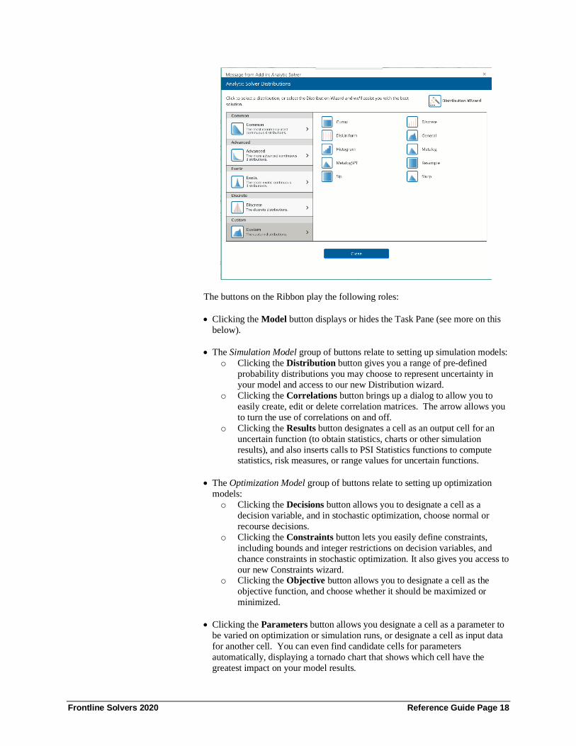
The buttons on the Ribbon play the following roles:
• Clicking the Model button displays or hides the Task Pane (see more on this
below).
• The Simulation Model group of buttons relate to setting up simulation models:
o Clicking the Distribution button gives you a range of pre-defined
probability distributions you may choose to represent uncertainty in
your model and access to our new Distribution wizard.
o Clicking the Correlations button brings up a dialog to allow you to
easily create, edit or delete correlation matrices. The arrow allows you
to turn the use of correlations on and off.
o Clicking the Results button designates a cell as an output cell for an
uncertain function (to obtain statistics, charts or other simulation
results), and also inserts calls to PSI Statistics functions to compute statistics, risk measures, or range values for uncertain functions.
• The Optimization Model group of buttons relate to setting up optimization
models:
o Clicking the Decisions button allows you to designate a cell as a
decision variable, and in stochastic optimization, choose normal or
recourse decisions.
o Clicking the Constraints button lets you easily define constraints,
including bounds and integer restrictions on decision variables, and
chance constraints in stochastic optimization. It also gives you access to
our new Constraints wizard. o Clicking the Objective button allows you to designate a cell as the
objective function, and choose whether it should be maximized or
minimized.
• Clicking the Parameters button allows you designate a cell as a parameter to
be varied on optimization or simulation runs, or designate a cell as input data
for another cell. You can even find candidate cells for parameters
automatically, displaying a tornado chart that shows which cell have the
greatest impact on your model results.
Frontline Solvers 2020 Reference Guide Page 19
• The Solve Action group of buttons relate to solving your optimization or
simulation model:
o Clicking the Simulate button turns on Interactive Simulation, and
lights up the bulb; clicking it again turns off Interactive Simulation and the bulb. The arrow allows you to run a single simulation at a time.
o Clicking the Optimize button runs an optimization, while clicking the
downward arrow gives you a list of choices for how to solve the model.
You can use the Analyze Original Model option to find out what type
of model (linear, nonlinear, etc.) you’ve defined, and what Solver
Engine can be used to solve it.
o Clicking the Create App button drops down a menu with a list of
choices that automatically convert your existing optimization,
simulation or simulation optimization model into a RASON model to
be solved using either the RASON Desk IDE, the Web IDE on
RASON.com or from within a customized Web application. Select
RASON IDE or RASON.com to automatically open either the RASON Desk IDE or RASON Web IDE containing your model written
in the RASON modeling language. Select Web Page to create a web
application that will solve your model, which has been converted to a
RASON model, by calling the RASON Interpreter from within a
customized web app. This feature reduces months of development
work to a single button click!
Analytic Solver includes the ability to turn your Excel-based
optimization or simulation model into a Microsoft Power BI Custom
Visual. Simply select rows or columns of data in your Excel model to
serve as changeable parameters, then choose Create App – Power BI, and save the file created by Analytic Solver. Afterwards, you will click
the Load Custom Visual icon in Power BI, and select the file you just
saved. Then, simply drag and drop appropriate Power BI datasets into
the “well” of inputs to match your model parameters to create your full
optimization or simulation model in Power BI! For more information,
see the chapter, “Creating Power BI Custom Visuals” within the
Analytic Solver User Guide.
Analytic Solver includes the ability to turn your Excel-based
optimization or simulation model into a Tableau Dashboard
Extension! This is quite similar to the ability to create Power BI
Custom Visuals. Note: This new feature works (only) with Tableau version
2018.2 or later.
You simply select rows or columns of data to serve as changeable
parameters, then choose Create App – Tableau, and save the file
created by Analytic Solver. In Tableau, you’ll see the newly-created
file under Extensions on the left side of the dashboard, where you can
drag it onto your dashboard. You’ll be prompted to match the
parameters your model needs with data in Tableau. Much like with
Power BI, what you get isn’t just a chart – it’s your full optimization or
simulation model, ready to accept Tableau data, run on demand (using our RASON server), and display visual results in Tableau! For more

Frontline Solvers 2020 Reference Guide Page 20
information, see the chapter, “Creating Tableau Extensions” within the
Analytic Solver User Guide.
• The Analysis group of buttons relate to analyzing your results:
o Clicking the Reports button gives you access to a full range of reports
for optimization, simulation and sensitivity analysis.
o Clicking the Charts button similarly lets you create and manipulate
charts related to your optimization, simulation, or sensitivity analysis
results – including charts that cover multiple optimization or simulation
runs, with varying parameters.
• The Tools group of buttons are covered more fully in the User Guide. They
allow you to set up decision trees, create probability distributions that fit
historical data, see the results of specific simulations or optimization, manage
results and publish an optimization or simulation model to the new Excel for
the Web (now referred to as Excel Online) Solver app or Google Sheets
Solver add-on.
• Use the Get Data button to draw a random sample of data, or summarize data
from a (i) an Excel worksheet, (ii) the PowerPivot “spreadsheet data model”
which can hold 10 to 100 million rows of data in Excel, (iii) an external SQL
database such as Oracle, DB2 or SQL Server, or (iv) a dataset with up to billions of rows, stored across many hard disks in a compute cluster running
Apache Spark (https://spark.apache.org/), using the new Big Data feature. See
the Analytic Solver Data Mining User Guide for help with this new feature.
• Clicking the Options button displays a dialog of options for controlling the
optimization and simulation processes as well as for formatting charts and
graphs.
• Clicking the Help button displays online Help. The arrow allows you to open
examples or an online tutorial, access the User and Reference Guides, check
your version and license status, or enter a license code.
Each of these GUI functions is described in later sections of this chapter.
Solver Home Tab Removed in V2020
The Solver Home tab has been removed from Analytic Solver Desktop V2020.
You can use the License menu to Login and Logout, browse to
www.solver.com, start a Live Chat, etc. See the section below for more information.

Frontline Solvers 2020 Reference Guide Page 21
Right-Click Context Menus With the Ribbon, you can easily ‘discover’ and access the function you want
with a few mouse clicks. But you can access most of the same functions without
using the Ribbon: Just select any worksheet cell, and right-click to display the
Excel context menu. At the bottom of this menu, select the Analytic Solver
choice, as shown on the next page. (Neither AnalyticSolver.com nor Analytic
Solver Cloud support a right-click menu.)
The choices on the Analytic Solver context submenu correspond one-for-one
with most of the buttons on the Ribbon. Cascading submenus appear for each
option, corresponding one-for-one with the dropdown galleries and menu choices that appear for the buttons on the Ribbon. Just select (left-click) the one
you want.
Context-Sensitive Charts With the Ribbon, you can access many GUI functions with a few mouse clicks.
But you can work with existing uncertain variables and functions without even
using the Ribbon.
• Hold the mouse pointer over an uncertain variable cell (any cell
containing a PSI Distribution function call) for about one second to
display a pop-up miniature probability density function (PDF) chart for
that variable, whenever Interactive Simulation is enabled. (Supported
only in Analytic Solver Desktop.)

Frontline Solvers 2020 Reference Guide Page 22
• Double-click an uncertain variable cell to display the Uncertain
Variable dialog in Analytic Solver Desktop or AnalyticSolver.com.
This dialog displays a chart of the distribution and allows you to
change the distribution type and parameters, fit a distribution to your
data, and view statistics and percentiles.
When using Anlaytic Solver Cloud, double click the uncertain variable
cell in the Model tab of the Solver task pane to open the Uncertain
Variable dialog.

Frontline Solvers 2020 Reference Guide Page 23
• Hold the mouse pointer over an uncertain function cell (any cell
containing a PsiOutput() call, or any cell referenced by a PSI Statistics
function call) for about one second to display a pop-up miniature fre-
quency distribution chart, whenever Interactive Simulation is enabled.
(Supported only in Analytic Solver Desktop.)
• Double-click an uncertain function cell to display the Uncertain
Function dialog (shown below), which displays a chart of simulation
results and sensitivity analysis, and allows you to adjust bounds, fit an
analytic distribution to the results, and view statistics and percentiles.
When using Anlaytic Solver Cloud, double click the Uncertain
Function cell in the Model tab of the Solver task pane to open the
Uncertain Function dialog.
The Uncertain Variable and Uncertain Function dialogs are described in later
sections of this chapter. When using both dialogs in Analytic Solver Desktop,
you can right-click the mouse over the chart and select from the context menu
to add or remove a Lower Cut, Upper Cut, or Marker to the chart.

Frontline Solvers 2020 Reference Guide Page 24
Using the Distribution Galleries The Distribution Button on the Ribbon allows you to access a comprehensive set
of distributions in six groups: Common, Advanced, Exotic, Discrete, Custom,
and Certified. These are used to create new uncertain variables in your model,
by selecting a type of probability distribution to be placed into the currently
selected cell on the worksheet. In Analytic Solver Desktop or
AnalyticSolver.com, you simply click one of these buttons or menus to drop
down a gallery of available distributions, then click on one of the buttons in the
gallery to select one.
This will open the Uncertain Variables dialog, with the selected distribution
charted with default parameters. You can then adjust parameters, add ‘control’
parameters that will truncate and/or shift the distribution, and perform other
actions to obtain exactly what you want. When you click the Save icon in the
Uncertain Variables dialog title toolbar, a formula such as =PsiNormal(0,1) is
written to the currently selected (active) cell.
Common Distributions
Clicking Common will display a gallery of common probability distributions.

Frontline Solvers 2020 Reference Guide Page 25
You can select any of the 10 common probability distributions shown above.
For an explanation of continuous versus discrete distributions, see the section
“Uncertain Variables and Probability Distributions” in the Frontline Solver
User Guide chapter “Mastering Simulation and Risk Analysis Concepts.”
Advanced Distributions
Clicking Advanced displays the gallery of Advanced probability distributions
shown below:
For an explanation of these advanced distributions, see the section “Uncertain
Variables and Probability Distributions” in the Frontline Solver User Guide
chapter “Mastering Simulation and Risk Analysis Concepts.”
Exotic Distributions
Clicking Exotic displays the gallery of custom probability distributions shown
below:

Frontline Solvers 2020 Reference Guide Page 26
For an explanation of these Exotic distributions, see the “Psi Function
Reference” chapter within this guide.
Discrete Distributions
Clicking Discrete displays the gallery of custom probability distributions shown
below:
For an explanation of continuous versus discrete distributions, see the section
“Uncertain Variables and Probability Distributions” in the Frontline Solver
User Guide chapter “Mastering Simulation and Risk Analysis Concepts.”
Custom Distributions
Scolling down and clicking Custom displays the gallery of custom probability
distributions shown below.

Frontline Solvers 2020 Reference Guide Page 27
Analytic Solver Cloud
For an explanation of analytic versus custom distributions, see the section
“Uncertain Variables and Probability Distributions” in the Analytic Solver User
Guide chapter “Mastering Simulation and Risk Analysis Concepts.” For a
description of the Resample, Sip and Slurp choices, see “Stochastic Libraries:
SIPs and SLURPs” in the same chapter. For hints and mathematical forms of
each of these distributions, see the section “Custom Distributions” in the chapter
“PSI Function Reference” within this guide.
Using the Results Galleries The Results button on the Ribbon allows you to access a full range of statistics
in four groups – Output, Statistic, Measure, and Range – which are used to
compute statistics over the full range of outcomes for the uncertain functions in your model, by placing a PSI Statistics function call into a cell on the worksheet.
Click the Results button, then select the desired group on the left (Output,
Statistic, Measure and Range) and the desired statistic, measure, or range, on the
right. A second dialog will appear asking for the output cell for which to
compute the result and also a cell address where you'd like to place the statistic.
Click Insert.

Frontline Solvers 2020 Reference Guide Page 28
Output Menu
The Output menu is used to specify that a worksheet cell contains an uncertain
function. Any formula cell that depends, directly or indirectly, on an uncertain
variable cell contains a distribution of outcomes, but Analytic Solver saves the
outcomes – so they can be reported, charted, or summarized by statistics – only
for formula cells that are referenced by PSI Statistics functions, or that either
contain or are referenced by a PsiOutput() function.
You can tell Analytic Solver that a cell (for example B11) is an uncertain
function either by adding a call to PsiOutput() to the formula already in the cell
– so it reads for example =B4*(B5-B6)-B7 + PsiOutput() – or by placing a formula =PsiOutput(cell) in some other cell, so it reads for example
=PsiOutput(B11). You can also tell Solver that cell is an uncertain function by
simply using cell as the first argument of a PSI Statistics function call in some
other cell – for example =PsiMean(B11) or =PsiFrequency(B11,0,n).
When you click the Output button, a special ‘gallery’ of two choices appears:

Frontline Solvers 2020 Reference Guide Page 29
The first choice, “In Cell,” adds PsiOutput() to the formula in the active cell.
This can be done by simply clicking the Results button. The second choice,
“Referred Cell,” displays a small dialog, like the one shown on the previous
page, where you can enter the cell address. The formula =PsiOutput(activecell)
is written to that cell.
Statistics Functions
Clicking the Statistic gallery/menu displays the PSI Statistics functions.
These fnctions compute classical statistics – measures of central tendency or
measures of dispersion:
• PsiMean, the average of all the values
• PsiMode, the most frequently occurring single value
• PsiVariance, which describes the spread of the distribution of values
• PsiStdDev for standard deviation, the square root of variance
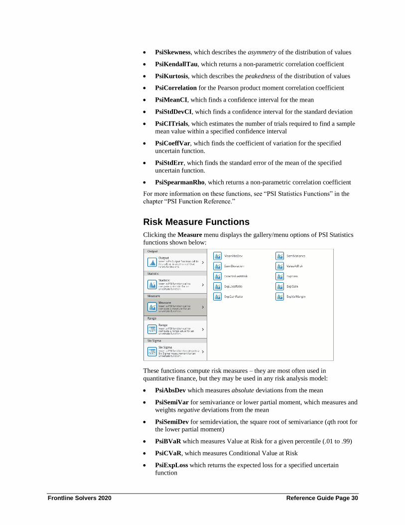
Frontline Solvers 2020 Reference Guide Page 30
• PsiSkewness, which describes the asymmetry of the distribution of values
• PsiKendallTau, which returns a non-parametric correlation coefficient
• PsiKurtosis, which describes the peakedness of the distribution of values
• PsiCorrelation for the Pearson product moment correlation coefficient
• PsiMeanCI, which finds a confidence interval for the mean
• PsiStdDevCI, which finds a confidence interval for the standard deviation
• PsiCITrials, which estimates the number of trials required to find a sample
mean value within a specified confidence interval
• PsiCoeffVar, which finds the coefficient of variation for the specified
uncertain function.
• PsiStdErr, which finds the standard error of the mean of the specified
uncertain function.
• PsiSpearmanRho, which returns a non-parametric correlation coefficient
For more information on these functions, see “PSI Statistics Functions” in the
chapter “PSI Function Reference.”
Risk Measure Functions
Clicking the Measure menu displays the gallery/menu options of PSI Statistics
functions shown below:
These functions compute risk measures – they are most often used in
quantitative finance, but they may be used in any risk analysis model:
• PsiAbsDev which measures absolute deviations from the mean
• PsiSemiVar for semivariance or lower partial moment, which measures and
weights negative deviations from the mean
• PsiSemiDev for semideviation, the square root of semivariance (qth root for the lower partial moment)
• PsiBVaR which measures Value at Risk for a given percentile (.01 to .99)
• PsiCVaR, which measures Conditional Value at Risk
• PsiExpLoss which returns the expected loss for a specified uncertain
function

Frontline Solvers 2020 Reference Guide Page 31
• PsiExpLossRatio which returns the expected loss ratio for a specified
uncertain function
• PsiExpGain which returns the expected gain for a specified uncertain
function
• PsiExpGainRatio which returns the expected gain ratio for a specified
uncertain function
• PsiExpValMargin which returns the expected value margin for a specified
uncertain function
For more information on these functions, see “PSI Statistics Functions” in the
chapter “PSI Function Reference.”
Range Functions
Clicking the Range menu displays the menu/gallery of PSI Statistics functions
shown on the next page.
These functions compute values related to the full range of outcomes of the
uncertain function:
• PsiMax, the maximum value across all the trials
• PsiMin, the minimum value across all the trials
• PsiPercentile, which provides percentile values from 1% to 99%
• PsiRange, the difference between PsiMax and PsiMin
• PsiTarget, the proportion of values less than or equal to a target value
• PsiFrequency, which returns an array of frequencies with which values fall
into a number of “bins” that you specify
• PsiData, which returns an array of raw trial values from the Monte Carlo simulation process
• PsiCount, which returns a count of all, successful, or failed trials

Frontline Solvers 2020 Reference Guide Page 32
For more information on these functions, see “PSI Statistics Functions” in the
chapter “PSI Function Reference.”
Six Sigma Functions
Clicking the Six Sigma menu displays the gallery/menu options of PSI Statistics
functions shown below.
These functions (introduced in Analytic Solver V2015) compute values related
to the Six Sigma indices used in manufacturing and process control.
• PsiSigmaCP calculates the Process Capability.
• PsiSigmaCPK calculates the Process Capability Index.
• PsiSigmaCPKLower calculates the one-sided Process Capability Index
based on the Lower Specification Limit.
• PsiSigmaCPKUpper calculates the one-sided Process Capability Index
based on the Upper Specification Limit.
• PsiSigmaCPM calculates the Taguchi Capability Index.
• PsiSigmaDefectPPM calculates the Defect Parts per Million statistic.
• PsiSigmaDefectShiftPPM calculates the Defective Parts per Million
statistic with a Shift.
• PsiSigmaDefectShiftPPMLower calculates the Defective Parts per Million
statistic with a Shift below the Lower Specification Limit.
• PsiSigmaDefectShiftPPMUpper calculates the Defective Parts per Million
statistic with a Shift above the Upper Specification Limit.
• PsiSigmaK calculates the Measure of Process Center.
• PsiSigmaLowerBound calculates the Lower Bound as a specific number of
standard deviations below the mean.
• PsiSigmaProbDefectShift calculates the Probability of Defect with a Shift
outside the limits.
• PsiSigmaProbDefectShiftLower calculates the Probability of Defect with
a Shift below the lower limit.
• PsiSigmaPRobDefectShiftUpper calculates the Probability of Defect with
a Shift above the upper limit.

Frontline Solvers 2020 Reference Guide Page 33
• PsiSigmaSigmaLevel calculates the Process Sigma Level with a Shift.
• PsiSigmaUpperBound calculates the Upper Bound as a specific number of
standard deviations above the mean.
• PsiSigmaYield calculates the Six Sigma Yield with a shift, i.e. the fraction of the process that is free of defects.
• PsiSigmaZLower calculates the number of standard deviations of the
process that the lower limit is below the mean of the process.
• PsiSigmaZMin calculates the minimum of ZLower and ZUpper.
• PsiSigmaZUpper calculates the number of standard deviations of the
process that the upper limit is above the mean of the process.
For more information on these functions, see “PSI Six Sigma Functions” in the
chapter “PSI Function Reference.”
Using the Uncertain Variable Dialog The Uncertain Variable dialog, pictured below in its simplest form and its most
comprehensive form, offers an easy way to create or edit an uncertain variable
with an analytic or custom probability distribution.
Analytic Solver Desktop – Uncertain Variable Dialog with Chart Options Pane Closed
Analytic Solver Desktop – Uncertain Variable Dialog with Chart Options Pane Open
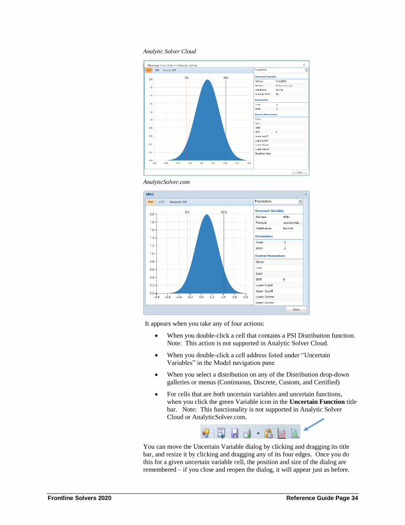
Frontline Solvers 2020 Reference Guide Page 34
Analytic Solver Cloud
AnalyticSolver.com
It appears when you take any of four actions:
• When you double-click a cell that contains a PSI Distribution function.
Note: This action is not supported in Analytic Solver Cloud.
• When you double-click a cell address listed under “Uncertain
Variables” in the Model navigation pane
• When you select a distribution on any of the Distribution drop-down
galleries or menus (Continuous, Discrete, Custom, and Certified)
• For cells that are both uncertain variables and uncertain functions,
when you click the green Variable icon in the Uncertain Function title
bar. Note: This functionality is not supported in Analytic Solver
Cloud or AnalyticSolver.com.
You can move the Uncertain Variable dialog by clicking and dragging its title
bar, and resize it by clicking and dragging any of its four edges. Once you do
this for a given uncertain variable cell, the position and size of the dialog are
remembered – if you close and reopen the dialog, it will appear just as before.

Frontline Solvers 2020 Reference Guide Page 35
Title Toolbar
The toolbar, supported in Analytic Solver Desktop only, alongside the title of
the Uncertain Variable dialog provides quick tools to work with uncertain
variables. ToolTips appear for each one if you hover the mouse over the icon.
The role of each tool is explained below.
• The Variables tool (leftmost) displays a dropdown outline with check
boxes of all the uncertain variable cell addresses in your model. If you click
one of these cell addresses, the Excel selection will move to that cell, and
the Uncertain Variable dialog will display and edit the uncertain variable in
that cell. If you check boxes next to several uncertain variables, the dialog
displays Overlay charts that include all of these variables.
• The Save tool writes a PSI Distribution function call into the currently
selected cell that reflects the distribution type, parameters, and property functions currently chosen in the Uncertain Variable dialog.
• The Print tool prints the chart, statistics or percentiles currently shown in
the Uncertain Variable dialog on the default printer. The arrow next to this
tool displays Print Preview, Printer Settings, and Page Settings choices.
• The Copy tool copies the chart currently shown in the Uncertain Variable
dialog to the Windows Clipboard. Use Edit Paste in almost any Windows
application to paste the chart image into another document.
• The Fitting tool displays the Distribution Fitting dialog, used to automati-
cally fit a distribution type and parameters to user-supplied data. For more
information, see “Distribution Fitting” at the end of this section.
• If the active cell is both an uncertain variable and an uncertain function, a
blue Show Output tool appears on the title bar. Click this tool to display
the Uncertain Function dialog for this cell.
• The Chart View Control toolbar can be used to convert the chart to a 3D
chart, rotate the chart up, down, left or right, or reset the chart back to its
default settings.
Tabs and Panes
Tabs: The Uncertain Variable dialog in all versions of Analytic Solver has
three tabs: PDF (Probability Density Function), CDF (Cumulative Distribution
Function), and Reverse CDF. Each tab displays different information about the
distribution.
Panes: In Analytic Solver Desktop, the border at the right can be clicked to
show additional information. The following sections explain the role of each
pane.
The Uncertain Variable dialog with the right pane closed is pictured immediately below. The dialog with the right pane open is the subsequent
picture. See above for the Uncertain Variable dialogs in Analytic Solver Cloud
and AnalyticSolver.com.

Frontline Solvers 2020 Reference Guide Page 36
Analytic Solver Desktop - Uncertain Variable dialog with right pane closed
Analytic Solver Desktop - Uncertain Variable dialog with right pane open:

Frontline Solvers 2020 Reference Guide Page 37
The drop down menu in the right pane showing additional views:
Note: Neither the Axis Options nor Markers menu options are currently
supported in Analytic Solver Cloud or AnalyticSolver.com.
Editable Confidence Intervals
Introduced in Analytic Solver Desktop V2015, confidence intervals appearing at
the top of the chart are now editable. In all versions of Analytic Solver, by
default, red vertical lines will appear, for most distributions, at the 5% and 95%
cutoff values, effectively displaying the 90th confidence interval.
In all versions of Analytic Solver, percentile or cutoff values can be altered by
moving the red vertical lines to the left or right. In Analytic Solver Desktop,
percentile or cutoff values may also be altered by typing in the desired value or percentile.
Regardless of how a cutoff value is changed, the remaining cutoff value will
automatically change accordingly. Likewise, when a percentile value is
changed, the remaining percentiles will automatically update.
Parameters View
The parameters specific to the currently selected distribution type are displayed
when the Parameters view is selected in the right pane. The Parameters section
of the pane displays both “English” and “mathematical” names for each
parameter. In the Value column (the column where the values for the
distribution are entered such as minimum value, likely value and maximum value), you can enter or select a value for the parameter, by either:
• Typing a numeric value or a cell address into the field. The chart is
redrawn as soon as you finish and move away from the field.
• Clicking the cell reference button at the right edge of the Value field,
then point and click to select a worksheet cell with the mouse. You can
select a cell on the current worksheet or on another worksheet. This
option is not supported in Analytic Solver Cloud or
AnalyticSolver.com.
Some parameter values may be invalid for the current distribution type (for
example, a negative number for the Standard Deviation, or a negative Mean for

Frontline Solvers 2020 Reference Guide Page 38
a LogNormal distribution), or may be inconsistent with other parameter values
(for example, a lower bound that’s greater than an upper bound for the
Triangular distribution). The box will show in the distribution area of the dialog
to warn you:
You can proceed to change the upper bound of a Triangular distribution so it is
greater than a newly entered lower bound. If the parameters are still invalid
when you try and save the distribution or close the dialog, Analytic Solver will warn you:
In Analytic Solver Desktop, you can still accept the invalid parameters and
continue – but the uncertain variable’s value will display as #VALUE! in this case. Analytic Solver Cloud and AnalyticSolver.com will not allow you to save
a distribution with invalid parameters.
Analytic Moments View
The Analytic Moments view displays numeric values for several summary
statistics that describe the current distribution. These are ‘analytic’ statistics,
computed entirely from the distribution type and parameters (most of the
formulas are shown in the chapter “PSI Function Reference”); they do not
require a Monte Carlo simulation or sampling of values from the distribution.
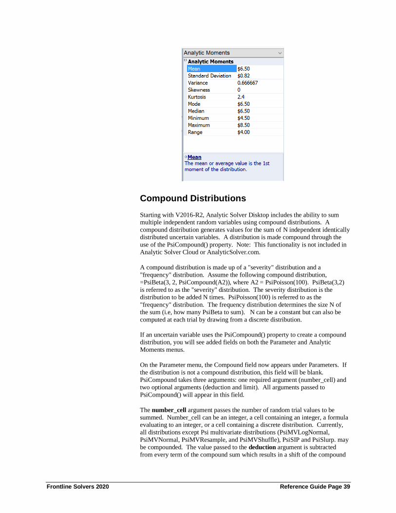
Frontline Solvers 2020 Reference Guide Page 39
Compound Distributions
Starting with V2016-R2, Analytic Solver Disktop includes the ability to sum multiple independent random variables using compound distributions. A
compound distribution generates values for the sum of N independent identically
distributed uncertain variables. A distribution is made compound through the
use of the PsiCompound() property. Note: This functionality is not included in
Analytic Solver Cloud or AnalyticSolver.com.
A compound distribution is made up of a "severity" distribution and a
"frequency" distribution. Assume the following compound distribution,
=PsiBeta(3, 2, PsiCompound(A2)), where A2 = PsiPoisson(100). PsiBeta(3,2)
is referred to as the "severity" distribution. The severity distribution is the
distribution to be added N times. PsiPoisson(100) is referred to as the
"frequency" distribution. The frequency distribution determines the size N of
the sum (i.e, how many PsiBeta to sum). N can be a constant but can also be
computed at each trial by drawing from a discrete distribution.
If an uncertain variable uses the PsiCompound() property to create a compound
distribution, you will see added fields on both the Parameter and Analytic
Moments menus.
On the Parameter menu, the Compound field now appears under Parameters. If
the distribution is not a compound distribution, this field will be blank.
PsiCompound takes three arguments: one required argument (number_cell) and
two optional arguments (deduction and limit). All arguments passed to
PsiCompound() will appear in this field.
The number_cell argument passes the number of random trial values to be
summed. Number_cell can be an integer, a cell containing an integer, a formula evaluating to an integer, or a cell containing a discrete distribution. Currently,
all distributions except Psi multivariate distributions (PsiMVLogNormal,
PsiMVNormal, PsiMVResample, and PsiMVShuffle), PsiSIP and PsiSlurp. may
be compounded. The value passed to the deduction argument is subtracted
from every term of the compound sum which results in a shift of the compound

Frontline Solvers 2020 Reference Guide Page 40
distribution by -N * deduction. If a trial value is larger than a specified limit,
then the trial value is reset to the limit.
Note: If a discrete distribution is passed to the number_cell argument, the
frequency distribution must be formulated in such a way that the trial values
generated by the distribution must be greater than 1. If not, trial values < 1 will
be set equal to 1.
On the Analytic Moments menu, four additional statistics will appear under
Compund Analytic Moments: Mean, Variance, Standard Deviation and
Skewness. For a complete example of a compound distribution, see the chapter
Examples: Simulation and Risk Analysis in the Analytic Solver User Guide.
Percentiles View
The Percentiles view, shown on the next page, displays numeric percentile
values (from 1% to 99%) for the current distribution. Like the values on the
Statistics tab, these percentiles are computed entirely from the distribution type
and parameters; they do not require a Monte Carlo simulation or sampling of
values from the distribution.
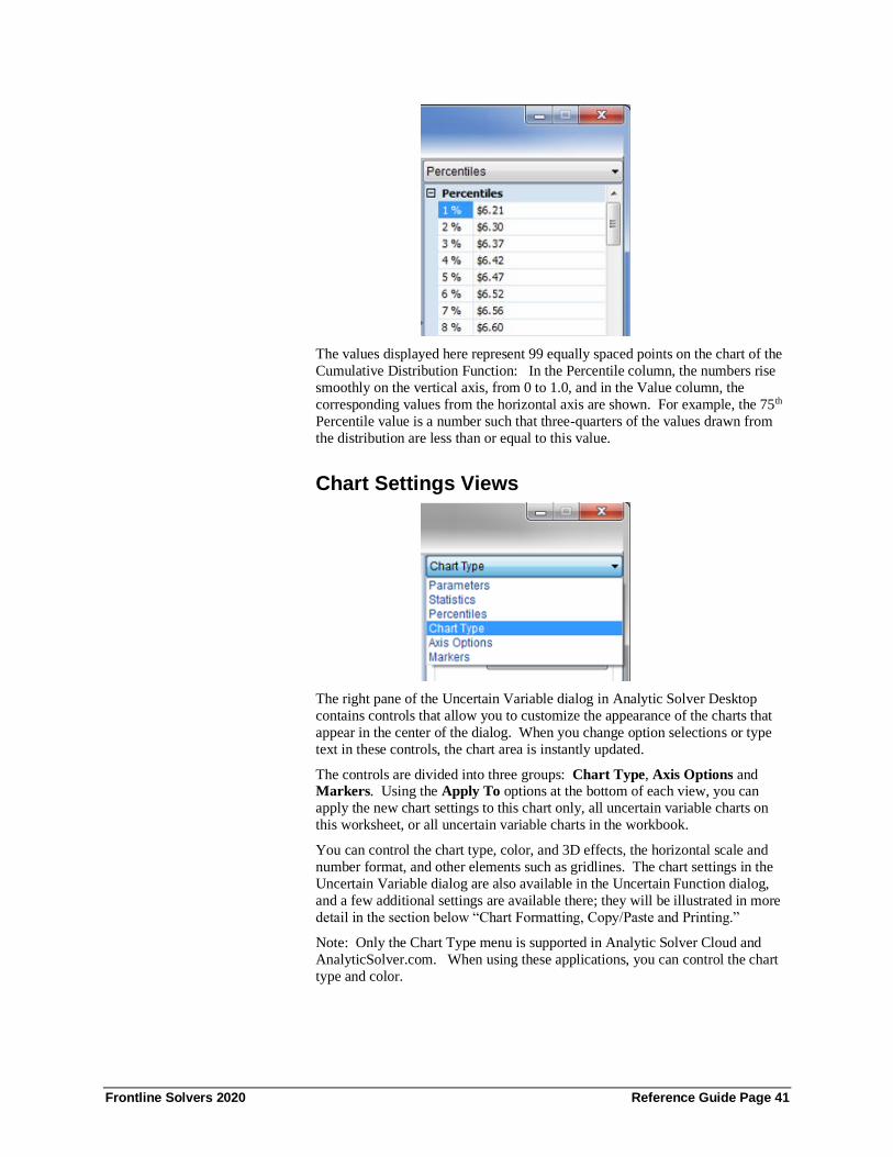
Frontline Solvers 2020 Reference Guide Page 41
The values displayed here represent 99 equally spaced points on the chart of the
Cumulative Distribution Function: In the Percentile column, the numbers rise
smoothly on the vertical axis, from 0 to 1.0, and in the Value column, the
corresponding values from the horizontal axis are shown. For example, the 75th
Percentile value is a number such that three-quarters of the values drawn from
the distribution are less than or equal to this value.
Chart Settings Views
The right pane of the Uncertain Variable dialog in Analytic Solver Desktop
contains controls that allow you to customize the appearance of the charts that
appear in the center of the dialog. When you change option selections or type
text in these controls, the chart area is instantly updated.
The controls are divided into three groups: Chart Type, Axis Options and Markers. Using the Apply To options at the bottom of each view, you can
apply the new chart settings to this chart only, all uncertain variable charts on
this worksheet, or all uncertain variable charts in the workbook.
You can control the chart type, color, and 3D effects, the horizontal scale and
number format, and other elements such as gridlines. The chart settings in the
Uncertain Variable dialog are also available in the Uncertain Function dialog,
and a few additional settings are available there; they will be illustrated in more
detail in the section below “Chart Formatting, Copy/Paste and Printing.”
Note: Only the Chart Type menu is supported in Analytic Solver Cloud and
AnalyticSolver.com. When using these applications, you can control the chart
type and color.
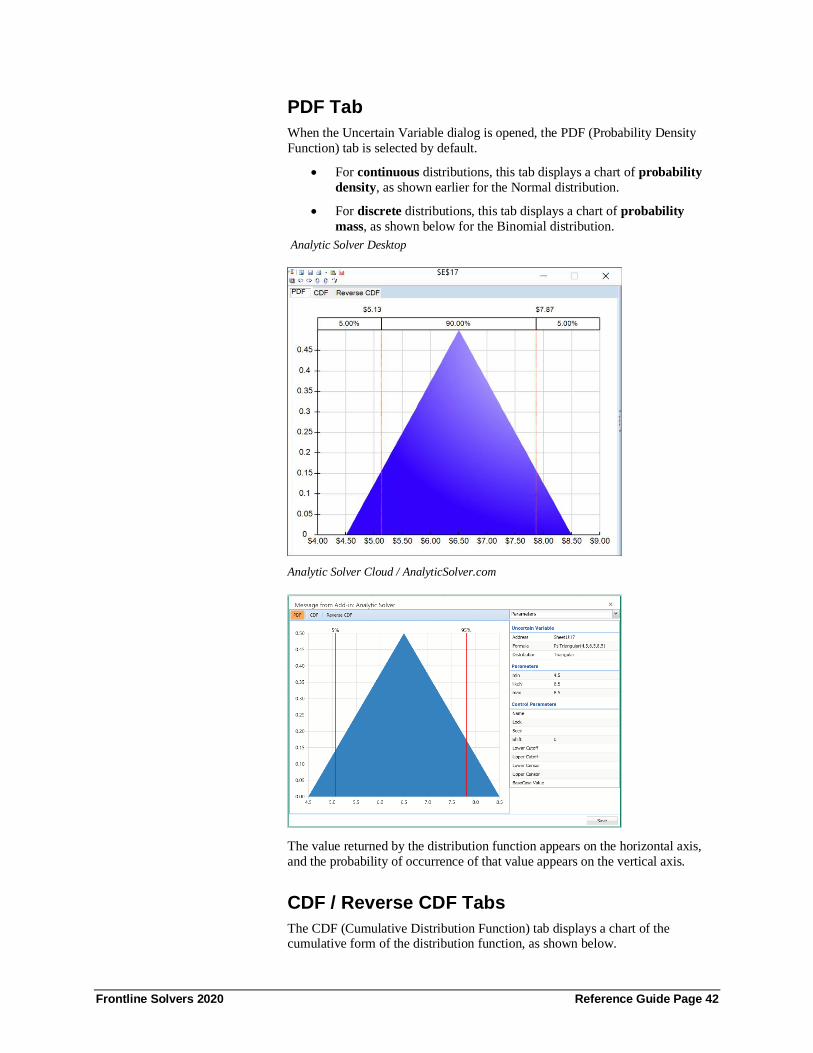
Frontline Solvers 2020 Reference Guide Page 42
PDF Tab
When the Uncertain Variable dialog is opened, the PDF (Probability Density
Function) tab is selected by default.
• For continuous distributions, this tab displays a chart of probability
density, as shown earlier for the Normal distribution.
• For discrete distributions, this tab displays a chart of probability
mass, as shown below for the Binomial distribution.
Analytic Solver Desktop
Analytic Solver Cloud / AnalyticSolver.com
The value returned by the distribution function appears on the horizontal axis,
and the probability of occurrence of that value appears on the vertical axis.
CDF / Reverse CDF Tabs
The CDF (Cumulative Distribution Function) tab displays a chart of the cumulative form of the distribution function, as shown below.

Frontline Solvers 2020 Reference Guide Page 43
Analytic Solver Desktop
Analytic Solver Cloud / AnalyticSolver.com
The value returned by the distribution function appears on the horizontal axis,
and the vertical axis shows the cumulative probability that a sample from this
distribution is less than or equal (on the CDF tab), or greater than or equal (on
the Reverse CDF tab) to the horizontal axis value.
Navigating Among Variable Cells
An easy way to navigate through your variables is to use the Task Pane at the
right of the workbook. Your entire model can be easily viewed and you can add,
delete, or even change variables by clicking on the green “+” sign below the
Model tab label to add, double-clicking on an existing variable to change it in a
dialog box which will pop-open, and by clicking once on a variable and then
clicking on red “X” below the Model tab label to delete it.

Frontline Solvers 2020 Reference Guide Page 44
Analytic Solver Desktop Analytic Solver Cloud AnalyticSolver.com
Overlay Charts of Variables
You can also use the Variables tool to select several uncertain variable cells, and
display Overlay charts of the PDF, CDF, or Reverse CDF of all of the selected
variable cells. Simply open the outline by clicking the Uncertain Variables tool
on the top of the Uncertain Variable dialog, and check the boxes next to the
uncertain variables that you want to include.
Note: This functionality is not supported in Analytic Solver Cloud or
AnalyticSolver.com.
Below is an example of the PDF tab of the Uncertain Variable dialog with three
variables selected – a Normal distribution, Triangular distribution, and Uniform
distribution. You can improve the appearance of an Overlay chart by setting the
Transparency in the right-hand Chart Options pane, and by rotating a 3D version
of the chart using the Chart View Control toolbar.

Frontline Solvers 2020 Reference Guide Page 45
When you do this, the first uncertain variable cell you choose is the “primary”
variable. (In this case the primary variable is the uncertain variable in cell B6.)
The Statistics and Percentiles tabs will display information for this variable, and
distribution fitting will work with this variable. You won’t be able to “uncheck the box” for this variable unless you uncheck all the others, or alternatively click
the cell address of a different variable, which makes that cell the “primary”
uncertain variable.
Using the Uncertain Function Dialog The Uncertain Function dialog gives you easy access to the full range of
outcomes, as well as summary statistics, percentiles, and sensitivity analysis, for
an uncertain function. It appears when you take any of three actions:
• When you double-click a cell that contains a PsiOutput() function
call, or is referenced by a PSI Statistic function call in another cell
(This functionality is not supported in Analytic Solver Cloud.)
• When you double-click a cell address listed under “Functions” in the
Model navigation pane
• For cells that are uncertain variables and uncertain functions, when
you click the blue Function icon in the Uncertain Variable title bar.
(Not supported in Analytic Solver Cloud or AnalyticSolver.com.)
You can move the Uncertain Function dialog by clicking and dragging its title
bar, and in Analytic Solver Desktop or AnalyticSolver.com, resize it by clicking
and dragging any of its four edges. In Analytic Solver Desktop, once you do this
for a given uncertain variable cell, the position and size of the dialog are
remembered – if you close and reopen the dialog, it will appear just as before.
Unlike the Uncertain Variable dialog, where the chart is drawn, and statistics
and percentiles are computed analytically based on the distribution type and
parameters, the Uncertain Function dialog always reflects the results of the most
recent Monte Carlo simulation, based on trial values drawn in that simulation.
The charts show the frequencies with which uncertain function sample values fall into certain ranges, called “bins;” the frequencies provide estimates of the
probabilities of occurrence of these values for the function. Similarly, the
statistics and percentiles are estimates of the true values for the function.

Frontline Solvers 2020 Reference Guide Page 46
Title Toolbar
The toolbar alongside the title of the Uncertain Function dialog in Analytic
Solver Desktop provides quick tools to work with uncertain functions. ToolTips
appear for each one if you hover the mouse over the icon. The role of each tool
is explained below.
Note: This toolbar does not currently appear in Analytic Solver Cloud or
AnalyticSolver.com.
• The Functions tool (leftmost) displays a dropdown outline of all the
uncertain function cell addresses in your model. If you click one of
these cell addresses, the selection will move to that cell, and the
Uncertain Function dialog will update to display and edit the uncertain
function in that cell.
• The Save and Close tool saves all changes made to the chart and then
closes the uncertain function dialog.
• The Print tool prints the chart, statistics or percentiles currently
shown in the Uncertain Function dialog on the default printer. The
arrow next to this tool displays Print Preview, Printer Settings, and
Page Settings choices.
• The Copy tool copies the chart currently shown in the Uncertain
Function dialog to the Windows Clipboard. Use Edit Paste in almost
any Windows application to paste the chart image into another
document.
• The Fitting tool displays the Distribution Fitting dialog, used to automatically fit a distribution type and parameters to the simulation
result sample. For more information, see “Distribution Fitting” at the
end of this section.
• The PowerBI icon uploads the uncertain function distribution values
and statistics into Microsoft's Power BI. This applicaton converts data
into readable charts to allow you to visualize your data.
• The Tableau icon uploads the uncertain function distribution values
and statistics into Tableau, a popular interactive software package that
allows you to visually explore and analyze your data.
• If the active cell is both an uncertain function and an uncertain
variable, the Power BI icon is replaced with the Show Output tool.
Click this tool to display the Uncertain Variable dialog for this
cell.
Multiple Simulations
Risk Solver can perform multiple simulations on command, or – when
Interactive Simulation is activated in Analytic Solver Desktop – each time you
change a number on the spreadsheet. To do this, you simply set the number of

Frontline Solvers 2020 Reference Guide Page 47
Simulation to Run option on the Platform tab of the Solver Task Pane to a value
greater than 1. (If using Analytic Solver Desktop, you can also set this option on
the Options dialog by clicking Options on the Ribbon. This option appears on
the Simulation tab which opens by default.
Analytic Solver Desktop Analytic Solver Cloud AnalyticSolver.com
When you do this, a dropdown list of simulations appears in the Uncertain
Function dialog title bar. Results from all simulations are available all the time
– just select the simulation you want from this list, and the Uncertain Function
dialog will instantly update to show you the results from that simulation.
Tabs and Panes
Tabs. The Uncertain Function dialog has five tabs: Frequency, Cumulative
Frequency, Reverse Cumulative Frequency, Sensitivity, and Scatter Plots. Each
tab displays different information about the outcomes of the most recent
simulation for this uncertain function.
Panes: In Analytic Solver Desktop, the border at the right can be clicked to
show additional information. In Analytic Solver Cloud and AnalyticSolver.com,
the pane is automatically open by default. The following sections explain the
role of each pane.
The Uncertain Function dialog in Analytic Solver Desktop, with the right pane closed, is pictured immediately below. The dialog with the right pane open is
the subsequent picture. The following two pictures show the Uncertain Function
dialog in Analytic Solver Cloud and AnalyticSolver.com, respectively.

Frontline Solvers 2020 Reference Guide Page 48
Analytic Solver Desktop Uncertain Function dialog with right pane closed

Frontline Solvers 2020 Reference Guide Page 49
Analytic Solver Desktop Uncertain Function dialog with right pane open
Analytic Solver Cloud
AnalyticSolver.com
Frequency Tab
The Frequency tab appears in the dialog by default; an example is shown below.
The values sampled for the uncertain function on the Monte Carlo trials appear

Frontline Solvers 2020 Reference Guide Page 50
on the horizontal axis, and the vertical axis shows the frequency of occurrence
of values falling in each ‘bin’ reflecting the width of each vertical bar. This
example chart reflects 1,000 Monte Carlo trials; the right scale shows the actual
frequencies of computed values for this set of trials, and the right scale shows
the inferred relative probabilities of each outcome.
Analytic Solver Desktop
Analytic Solver Cloud / AnalyticSolver.com
Editable Confidence Intervals and Legend
Introduced in Analytic Solver Desktop V2015, confidence intervals appearing at
the top of the Frequency, Cumulative Frequency and Reverse Cumulative
Frequency charts are now editable.
By default, red vertical lines will appear, in all version of Analytic Solver, at the
5% and 95% cutoff values, effectively displaying the 90th confidence interval.
The middle percentage is the percentage of all the trial values that lie within the

Frontline Solvers 2020 Reference Guide Page 51
‘included’ area. The two percentages on each end are the percentage of all trial
values that lie outside of the ‘included’ area.
In Analytic Solver Desktop, percentile or cutoff values can be altered in two
ways, by moving the red vertical lines to the left or right or by clicking the
cutoff or percentile value and typing in the desired value or percentile. A change made on one chart will also be reflected in the charts on the remaining
two tabs.
In Analytic Solver Cloud or AnalyticSolver.com, percentile or cutoff values can
be altered by moving the red vertical lines to the left or right. A change made on
one chart will also be reflected in the charts on the remaining two tabs.
The uncertain function legend, introduced in Analytic Solver V2015, contains
the Mean, Standard Deviation, 5th percentile and 95th percentile values for the
uncertain function. All are updated automatically when a change is made to the
percentile or cutoff values.
Cumul / Rev Cumul Frequency Tabs
The Cumul. (Cumulative) Frequency tab shows the values sampled for the
uncertain function on each Monte Carlo trial on the horizontal axis, and the
cumulative frequency of trial values less than or equal to that value on the vertical axis. An example of the Cum. Frequency tab is shown below.

Frontline Solvers 2020 Reference Guide Page 52
The Rev. Cumul. (Reverse Cumulative) Frequency tab is similar: It shows the values sampled for the uncertain function on each Monte Carlo trial on the
horizontal axis, and the cumulative frequency of trial values greater than or
equal to that value on the vertical axis.
The 90th percentile also appears at the top of the Cumulative and Reverse
Cumulative Frequency charts. In Analytic Solver Desktop, percentile or cutoff
values can be altered in two ways, by moving the red vertical lines to the left or right or by clicking the cutoff or percentile value and typing in the desired value
or percentile. In Analytic Solver Cloud or AnalyticSolver.com, percentile or
cutoff values can be altered by moving the red vertical lines to the left or right.
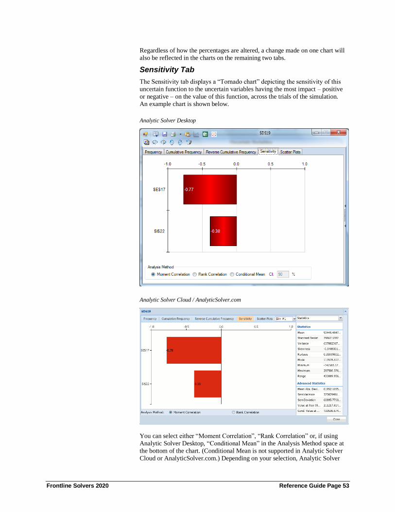
Frontline Solvers 2020 Reference Guide Page 53
Regardless of how the percentages are altered, a change made on one chart will
also be reflected in the charts on the remaining two tabs.
Sensitivity Tab
The Sensitivity tab displays a “Tornado chart” depicting the sensitivity of this
uncertain function to the uncertain variables having the most impact – positive
or negative – on the value of this function, across the trials of the simulation.
An example chart is shown below.
Analytic Solver Desktop
Analytic Solver Cloud / AnalyticSolver.com
You can select either “Moment Correlation”, “Rank Correlation” or, if using
Analytic Solver Desktop, “Conditional Mean” in the Analysis Method space at
the bottom of the chart. (Conditional Mean is not supported in Analytic Solver
Cloud or AnalyticSolver.com.) Depending on your selection, Analytic Solver

Frontline Solvers 2020 Reference Guide Page 54
computes either the Pearson product moment correlation coefficients (Moment
Correlation), Spearman rank order correlation coefficients (Rank Correlation) or
the conditional mean between this uncertain function and all of the uncertain
variables in the model. It then displays the variables on the chart, from top to
bottom, in decreasing order of the absolute value of this coefficient; this gives the chart its “tornado” appearance. For an explanation of Pearson and Spearman
correlation coefficients, consult the section “Dependence and Correlation” in the
chapter “Mastering Simulation and Risk Analysis Concepts” in the Analytic
Solver User Guide.
When Conditional Mean is selected (supported only in Analytic Solver
Desktop), the CI edit box is enabled with a default value of 90%. The mean is
calculated for all trial values for the 5th and 95th percentiles. The numbers on the
left of the chart ($23,089 and $33,081) are the mean values for the 5th percentile
for each uncertain variable located in cells E17 and I22, respectively. The
numbers on the right of the chart ($214,682 and $139,465) are the mean values
for the 95th percentile for each uncertain variable. The red line in the center of the chart designates the mean value of the Uncertain Function across all the
trials. For a given Confidence Interval setting such as the default of 90%, each
bar shows the range of the mean value of the Uncertain Function, conditional on
the Uncertain Variable next to that bar having values within the interval (i.e. it’s
5th and 95th percentiles).
Scatter Plots Tab
The Scatter Plots tab, shown on the next page, gives us a different view of the
relationship of the uncertain function to our uncertain variables.
Notice that the scatter plot for the uncertain variable in cell B6 has three
downward-sloping lines. If each line corresponded to a different market
scenario (Hot, OK or Slow), then we could infer that as the uncertain variable in
cell B6 rises, the value for the uncertain function drops – dropping fastest in the Hot Market scenario (far left line).

Frontline Solvers 2020 Reference Guide Page 55
In Analytic Solver Desktop, you can easily add or remove variables from this tab by clicking the Multiple Variables drop down menu. Select the checkbox
next to the uncertain variable or uncertain function to add to the dialog and
uncheck to remove. This menu does not appear in Analytic Solver Cloud or
AnalyticSolver.com.
Statistics View
The Statistics tab displays numeric values for several summary statistics,
computed from the trials of the most recent Monte Carlo simulation. Unlike the
Statistics tab values in the Uncertain Variables dialog, which are computed
analytically from the distribution type and parameters, the values on this tab are
estimates of the true statistics, computed from the sample of possible outcomes
drawn in the most recent simulation. An example is shown below.

Frontline Solvers 2020 Reference Guide Page 56
All statistics appearing on the Statistics pane are described in the Psi Function
Reference chapter under the corresponding Psi function. See below for a short
description of each.
Statistics
• Mean, the average of all the values. For more information, see PsiMean.
• Standard Deviation, the square root of variance. For more information,
see PsiStdDev.
• Variance, describes the spread of the distribution of values. For more
information, see PsiVariance.
• Skewness, which describes the asymmetry of the distribution of values. For
more information, see PsiSkewness.
• Kurtosis, which describes the peakedness of the distribution of values. For
more information, see PsiKurtosis.
• Mode, the most frequently occurring single value. For more information,
see PsiMode.
• Median, the 50th percentile of the distribution of trials. For more information, see PsiMedian.
• Minimum, the minimum value attained. For more information, see PsiMin.
• Maximum, the maximum value attained. For more information, see
PsiMax.

Frontline Solvers 2020 Reference Guide Page 57
• Range, the difference between the maximum and minimum values. For
more information, see PsiRange.
Clustering, not supported in Analytic Solver Cloud or AnalyticSolver.com,
performs k-Means clustering on the simulation trial data. For more information
on this feature, see the section on Clustering, below.
• Show Clusters, determines if clustering information is shown. Select either
"No Clustering", "Cluster Outputs" (to use only the trial data from the
uncertain function as the input data for k-Means clustering algorithm) or
"Cluster Inputs and Outputs" (to use the trial data for both the uncertain
variables and uncertain function as the input data for k-Means clustering
algorithm).
• Number of Clusters, the value of k, i.e. the number of clusters to form.
• Cluster to Show, the cluster to overlay on the output chart.
Advanced Statistics
• Mean Abs. Deviation, returns the average of the absolute deviations. For
more information, see PsiAbsDev.
• SemiVariance, measure of the dispersion of values. For more information,
see PsiSemiVar.
• SemiDeviation, one-sided measure of dispersion of values. For more
information, see PsiSemiDev.
• Value at Risk 95%, the maximum loss that can occur at a given confidence
level. For more information see PsiBVaR.
• Cond. Value at Risk, is defined as the expected value of a loss given that a
loss at the specified percentile occurs. For more information, see PsiCVaR.
• Mean Confidence, returns the confidence “half-interval” for the estimated
mean value (returned by the PsiMean() function. For more information see
PsiMeanCI.
• Std. Dev. Confidence 95%, returns the confidence ‘half-interval’ for the
estimated standard deviation of the simulation trials (returned by the
PsiStdDev() function). For more information, see PsiStdDevCI.
• Coefficient of Variation, is defined as the ratio of the standard deviation to
the mean. For more information, see PsiCoeffVar.
• Standard Error, defined as the standard deviation of the sample mean. For
more information, see PsiStdErr.
• Expected Loss, returns the average of all negative data multiplied by the
percentrank of 0 among all data. For more information, see PsiExpLoss.
• Expected Loss Ratio, returns the expected loss ratio. For more
information, see PsiExpLossRatio.
• Expected Gain returns the average of all positive data multiplied by 1 -
percentrank of 0 among all data. For more information, see PsiExpGain.
• Expected Gain Ratio, returns the expected gain ratio. For more information, see PsiExpGainRatio.
• Expected Value Margin, returns the expected value margin. For more
information, see PsiExpValMargin.
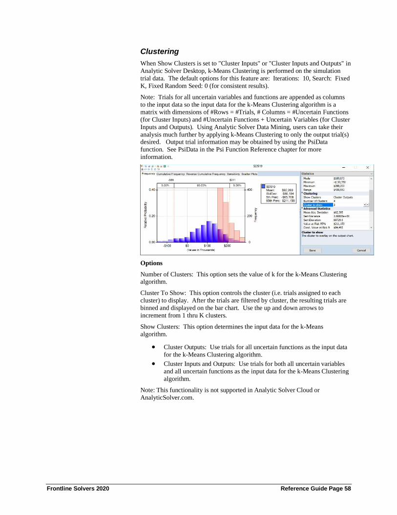
Frontline Solvers 2020 Reference Guide Page 58
Clustering
When Show Clusters is set to "Cluster Inputs" or "Cluster Inputs and Outputs" in
Analytic Solver Desktop, k-Means Clustering is performed on the simulation
trial data. The default options for this feature are: Iterations: 10, Search: Fixed
K, Fixed Random Seed: 0 (for consistent results).
Note: Trials for all uncertain variables and functions are appended as columns
to the input data so the input data for the k-Means Clustering algorithm is a
matrix with dimensions of #Rows = #Trials, # Columns = #Uncertain Functions
(for Cluster Inputs) and #Uncertain Functions + Uncertain Variables (for Cluster
Inputs and Outputs). Using Analytic Solver Data Mining, users can take their
analysis much further by applying k-Means Clustering to only the output trial(s) desired. Output trial information may be obtained by using the PsiData
function. See PsiData in the Psi Function Reference chapter for more
information.
Options
Number of Clusters: This option sets the value of k for the k-Means Clustering algorithm.
Cluster To Show: This option controls the cluster (i.e. trials assigned to each
cluster) to display. After the trials are filtered by cluster, the resulting trials are
binned and displayed on the bar chart. Use the up and down arrows to
increment from 1 thru K clusters.
Show Clusters: This option determines the input data for the k-Means
algorithm.
• Cluster Outputs: Use trials for all uncertain functions as the input data
for the k-Means Clustering algorithm.
• Cluster Inputs and Outputs: Use trials for both all uncertain variables
and all uncertain functions as the input data for the k-Means Clustering
algorithm.
Note: This functionality is not supported in Analytic Solver Cloud or
AnalyticSolver.com.

Frontline Solvers 2020 Reference Guide Page 59
Percentiles View
Selecting Percentiles from either the Analytic Solver Desktop or Cloud menu
displays numeric percentile values (from 1% to 99%) computed from the trials
of the most recent Monte Carlo simulation. Unlike the Percentiles tab values in
the Uncertain Variables dialog, which are computed analytically from the
distribution type and parameters, the values on this tab are estimates of the true
percentiles, computed from the sample of outcomes drawn in the most recent simulation. An example is shown below.
The values displayed here represent 99 equally spaced points on the Cumulative
Frequency chart: In the Percentile column, the numbers rise smoothly on the
vertical axis, from 0 to 1.0, and in the Value column, the corresponding values
from the horizontal axis are shown. For example, the 75th Percentile value is a
number such that three-quarters of the values occurring in the last simulation are less than or equal to this value.
This functionality is not supported in AnalyticSolver.com.

Frontline Solvers 2020 Reference Guide Page 60
Six Sigma View
Selecting Six Sigma from the menu in Analytic Solver Desktop or Cloud
displays Six Sigma measures computed from the trials of the most recent Monte
Carlo simulation. (This functionality is not supported in AnalyticSolver.com.)
In this display, the red vertical lines on the chart, which can be dragged left and
right are the Lower Specification Limit (LSL) and the Upper Specification Limit
(USL) which are initially set equal to the 5th and 95th percentile values,
respectively. An example is shown below. This functionality is not supported in AnalyticSolver.com.
Chart Settings Views
The Chart Type pane in Analytic Solver Desktop or Cloud contains controls that
allow you to customize the appearance of the charts that appear in the center of
the dialog. When you change option selections or type text in these controls
(Analytic Solver Desktop only), the chart area is instantly updated.
The controls are divided into three groups in Analytic Solver Desktop: Chart
Type, Axis Options and Markers. Using the Apply To options at the bottom

Frontline Solvers 2020 Reference Guide Page 61
of each view, you can apply the new chart settings to this chart only, all
uncertain variable charts on this worksheet, or all uncertain variable charts in the
workbook.
When using Analytic Solver Desktop, you can control the chart type, color, and
3D effects, the horizontal scale and number format, and other elements such as gridlines. The chart settings in the Uncertain Function dialog are also available
in the Uncertain Variable dialog, and a few additional settings are available
there; they will be illustrated in more detail in the section below “Chart
Formatting, Copy/Paste and Printing.”
Note: At present, you can only change the color of the shaded area in an
uncertain function chart in Analytic Solver Cloud. It is currently not possible to
customize an uncertain function chart in AnalyticSolver.com
Overlay Charts of Functions
You can also use the Functions tool to select several uncertain variable cells,
and display Overlay charts of the PDF, CDF, or Reverse CDF of all of the selected variable cells when using Analytic Solver Desktop. (This functionality
is not supported in Analytic Solver Cloud or AnalyticSolver.com) Simply open
the outline by clicking the Uncertain Functions tool on the top of the Uncertain
Function dialog, and check the boxes next to the uncertain functions (or
uncertain variables) that you want to include.
Below is an example of the PDF tab of the Uncertain Function dialog with three
uncertain functions selected. You can improve the appearance of an Overlay
chart by setting the Transparency in the right-hand Chart Options pane, and by
rotating a 3D version of the chart using the Chart View Control toolbar.
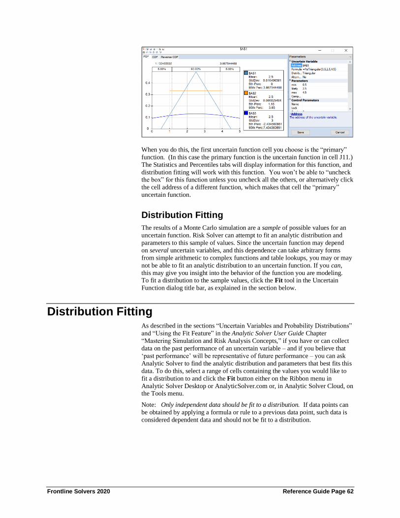
Frontline Solvers 2020 Reference Guide Page 62
When you do this, the first uncertain function cell you choose is the “primary”
function. (In this case the primary function is the uncertain function in cell J11.)
The Statistics and Percentiles tabs will display information for this function, and
distribution fitting will work with this function. You won’t be able to “uncheck the box” for this function unless you uncheck all the others, or alternatively click
the cell address of a different function, which makes that cell the “primary”
uncertain function.
Distribution Fitting
The results of a Monte Carlo simulation are a sample of possible values for an
uncertain function. Risk Solver can attempt to fit an analytic distribution and
parameters to this sample of values. Since the uncertain function may depend
on several uncertain variables, and this dependence can take arbitrary forms
from simple arithmetic to complex functions and table lookups, you may or may
not be able to fit an analytic distribution to an uncertain function. If you can,
this may give you insight into the behavior of the function you are modeling. To fit a distribution to the sample values, click the Fit tool in the Uncertain
Function dialog title bar, as explained in the section below.
Distribution Fitting As described in the sections “Uncertain Variables and Probability Distributions”
and “Using the Fit Feature” in the Analytic Solver User Guide Chapter
“Mastering Simulation and Risk Analysis Concepts,” if you have or can collect
data on the past performance of an uncertain variable – and if you believe that
‘past performance’ will be representative of future performance – you can ask
Analytic Solver to find the analytic distribution and parameters that best fits this
data. To do this, select a range of cells containing the values you would like to
fit a distribution to and click the Fit button either on the Ribbon menu in
Analytic Solver Desktop or AnalyticSolver.com or, in Analytic Solver Cloud, on the Tools menu.
Note: Only independent data should be fit to a distribution. If data points can
be obtained by applying a formula or rule to a previous data point, such data is
considered dependent data and should not be fit to a distribution.

Frontline Solvers 2020 Reference Guide Page 63
Analytic Solver Desktop Analytic Solver Cloud AnalyticSolver.com
This will display the Fit Options dialog. In the Location edit box you will see
the cell range containing the sample data (past observations of the uncertain
variable) you selected to be fitted. You can edit this information if you wish.
For the Type, select Continuous if the uncertain variable’s values are highly divisible – such as most prices, volumes, interest rates, exchange rates, weights,
and distances – or Discrete if the underlying physical process involves discrete,
countable entities.
The checkbox Allow Shifted Distributions allows Analytic Solver to shift the
center of analytic distribution (equivalent to using the PsiShift() property
function) to better fit the sample data; sometimes this is not desirable, so the box
may be unchecked.
When fitting a sample to a distribution, it is important that the trial values are
not in any way correlated with each other. In other words it is important that
each trial is independent. If the checkbox Run Sample Independence Test is

Frontline Solvers 2020 Reference Guide Page 64
checked, the Psi Interpreter will run an independence test and will report an
error if the trial values are found to be dependent. (See note above on
independent data.) Note: This option is not available in Analytic Solver Cloud.
In the Cloud app, this feature is always on.
For Continuous data, you can choose to rank the fitted distributions by AIC/BIC, Chi Square, Kolmogorov-Smirnoff, or Anderson-Darling
statistics. For Discrete data, AIC/BIC and Chi Square statistics are meaningful
(and may be selected). An in-depth description of each goodness of fit test
statistic is beyond the scope of this guide. However, a short description of each
follows. For each specified distribution a hypothesis test is used to determine
how well the distribution fits your data. The Fit Statistic used during the fitting
process is printed at the top right of the Fit Dialog (shown below).
H0: The data is derived from the specified distribution. (Null)
HA: The data is not derived from the specified distribution. (Alternate)
• AIC/BIC (Default) – The AIC test is a Chi Squared test corrected for the number of distribution parameters and sample size.
AIC = Chi-Square Statistic + 2 * k + 2 * k * (k + 1) / (n – k – 1)
where k is the number of distribyution parameters and n is the sample
size.
• Chi Square – Uses the chi-square statistic and distribution to rank either
continuous or discrete distributions. Sample data is first divided into
intervals using either equal probability, then the number of points that
fall into each interval are compared with the expected number of points
in each interval. The null hypotheses is rejected using a 90%
significance level, if the the chi-squared test statistic is greater than the critical value statistic.
Note: The Chi Square test is used indirectly in continuous fitting as a
support in the AIC test. The AIC test must succeed in both discrete and
continuous fitting as this is a necassary condition. When fitting a
discrete function, the Chi Square test must also succeed. When fitting a
continuous function, at least one of the tests, Chi Squared,
Kolmogorov-Smirnoff, or Anderson-Darling, must succeed as well.
• Kolmogorov-Smirnoff – For use with continuous distributions. This
test computes the difference (D) between the continuous distribution
function (CDF) and the empirical cumulative distribution function (ECDF). The null hypothesis is rejected if, at the 90% significance
level, D is larger than the critical value statistic.
• Anderson-Darling – For use with continuous distributions. Ranks the
fitted distribution using the Anderson Darling statistic, A2. The null
hypothesis is rejected using a 90% significance level, if A2 is larger
than the critical value statistic. This test awards more weight to the
distribution tails then the Kolmogorov-Smirnoff test.
Analytic Solver computes and displays a ranked list of candidate fitted
distributions, as shown below. Initially, the distribution with the best fit statistic
(selected in the above dialog) is shown in a chart that overlays the sample data.

Frontline Solvers 2020 Reference Guide Page 65
You can select one or multiple distributions on the left side of the dialog to
display their PDFs overlaid with the sample data in the center chart area, and
show its fitted parameters, analytic moments, and fit statistics in the right pane.
You can display a P-P (Probability-Probability) chart, a Q-Q (Quantile-Quan-
tile) chart, or a CDF Differences chart to get a better idea of how well the
selected distribution(s) fit the sample data.
• P – P Plot – A probability plot which allows you to determine how
closely two or more data sets agree with one another.
• Q – Q Plot – A probability plot which allows you to compare two or
more probability distributions by plotting their quantiles.
• CDF Differences – Note: This functionality is not supported in
Analytic Solver Cloud.
When you dismiss the Distribution Fitting dialog by clicking the X in its upper
right corner, Analytic Solver asks whether you want to accept the currently
selected fitted distribution:
If you click "Yes", Analytic Solver will place a blue balloon on your cursor asking you to select a cell in which to place the fitted distribution. Once you
click a blank cell, a PSI Distribution call with this distribution type and
parameters is written to the current cell.
If you are using Analytic Solver Desktop and you clicked the Fit button on the
Uncertain Variable dialog, you should also click the "X" in the upper right hand
corner to close the dialog and "Yes" to accept the fitted distribution. Analytic
Solver will replace the distribution currently in the Uncertain Variable dialog with the selected distribution type and parameters.
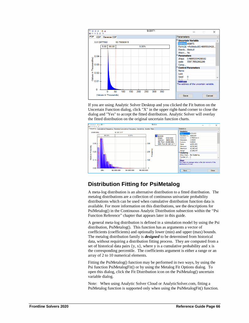
Frontline Solvers 2020 Reference Guide Page 66
If you are using Analytic Solver Desktop and you clicked the Fit button on the Uncertain Function dialog, click "X" in the upper right-hand corner to close the
dialog and "Yes" to accept the fitted distribution. Analytic Solver will overlay
the fitted distribution on the original uncertain function charts.
Distribution Fitting for PsiMetalog
A meta-log distribution is an alternative distribution to a fitted distribution. The metalog distributions are a collection of continuous univariate probability
distributions which can be used when cumulative distribution function data is
available. For more information on this distributions, see the descriptions for
PsiMetalog() in the Continuous Analytic Distribution subsection within the “Psi
Function Reference” chapter that appears later in this guide.
A general meta-log distribution is defined in a simulation model by using the Psi
distribution, PsiMetalog(). This function has as arguments a vector of
coefficients (coefficients) and optionally lower (min) and upper (max) bounds.
The metalog distribution family is designed to be determined from historical
data, without requiring a distribution fitting process. They are computed from a
set of historical data pairs {y, x}, where y is a cumulative probability and x is the corresponding percentile. The coefficients argument is either a range or an
array of 2 to 10 numerical elements.
Fitting the PsiMetalog() function may be performed in two ways, by using the
Psi function PsiMetalogFit() or by using the Metalog Fit Options dialog. To
open this dialog, click the Fit Distribution icon on the PsiMetalog() uncertain
variable dialog.
Note: When using Analytic Solver Cloud or AnalyticSolver.com, fitting a
PsiMetalog function is supported only when using the PsiMetalogFit() function.

Frontline Solvers 2020 Reference Guide Page 67
When used in the Cloud apps, the first argument, numCoef, is a scalar, the
number of coefficients to produce.
PsiMetalog Fit Option Descriptions
• Cumulative Probabilities - This is an Excel range containing the
historical cumulative probabilities (y values).
• Percentiles – Type or select the Excel range containing the percentile
values (x values).

Frontline Solvers 2020 Reference Guide Page 68
• Rank – If omitted, the rank is equal to 3. The value entered for Rank
must be greater than or equal to 2 and less than or equal to 10. In
addition, this value should be less or equal to the number of historical
pairs given in the Cumulative probability and Percentiles aguments.
• Upper Bound – The function may be limited on the right by the upper bound. If omitted, positive infinity is used for the upper bound.
• Lower Bound – The function may be limited on the left by the lower
bound. If omitted, negative infinity isused for the lower bound.
Click Fit to fit the Meta-log distribution. (Click Cancel to close the dialog
without performing the distribution fitting.) Analytic Solver replaces the
distribution currently in the Uncertain Variable dialog with the PsiMetalog()
distribution parameters. If you click the Save button or close the dialog by
clicking the “X” in the upper right hand corner in the title bar of this dialog, the
PSIMetalog() distribution function with the fitted parameters is written to the
current cell.
For example, given the following input parameters.
The arguments in the Metalog Fit Options dialog would be as follows. Note that
since the Upper and Lower Bound fields are empty, the fitted distribution will be
unbounded. Distributions may be bounded on both sides, semi-bounded
(bounded on one side) or unbouded. Note: Rank is equal to 2 which falls

Frontline Solvers 2020 Reference Guide Page 69
between the rank argument lower bound, which is equal to 2, and the number of
historical pairs passed for Cumulative probability and Percentiles, or 5.
After clicking Fit, the uncertain variable dialog changes to the following.
Click Save to close the uncertain variable dialog and save the fitted parameters
to the Excel cell. To inspect the coefficients obtained by the fitting, see the resultant PsiMetalog() function that was saved to this cell. In this example, the
coefficients are 31.6 and 4.43177.
If using Analytic Solver Cloud or AnalyticSolver.com, you can directly type this
function into a blank cell.
Fitting an Uncertain Function using PsiData()
It's still possible to fit a distribution to an uncertain function if using Analytic
Solver Cloud or AnalyticSolver.com. To do so, you'll need to use the PsiData()

Frontline Solvers 2020 Reference Guide Page 70
function to list the trial values for the uncertain function. In the Business
Forecast with Uncertainty Example below, the PsiData() function has been used
in cells D13:D22 to display the first ten simulation trials for the Net Profit
uncertain function in cell D10.
Click the green arrow on the Solver task pane to run a simulation. After the
simulation completes, cells D13:D22 will display the Net Profit (cell D10) for
the first 10 simulation trials.
You can confirm by incrementing through the Trial to Display spinner on the
Tools tab on the Solver task pane. If Trial to Display is equal to 1, then the first simulation trial values will be inserted into the worksheet. If Trial to Display is
equal to 2, then the second simulation trial values will be inserted into the
worksheet, and so on. Notice in the screenshot below, that Trial to Display is set
to 2 and the value in Net Profit is equal to the value in cell D14 (Net Profit for
the 2nd simulation trial).
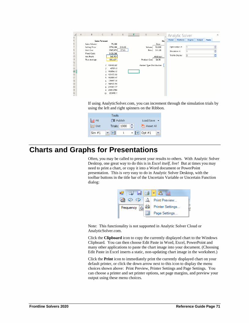
Frontline Solvers 2020 Reference Guide Page 71
If using AnalyticSolver.com, you can increment through the simulation trials by
using the left and right spinners on the Ribbon.
Charts and Graphs for Presentations Often, you may be called to present your results to others. With Analytic Solver
Desktop, one great way to do this is in Excel itself, live! But at times you may
need to print a chart, or copy it into a Word document or PowerPoint
presentation. This is very easy to do in Analytic Solver Desktop, with the
toolbar buttons in the title bar of the Uncertain Variable or Uncertain Function
dialog:
Note: This functionality is not supported in Analytic Solver Cloud or
AnalyticSolver.com.
Click the Clipboard icon to copy the currently displayed chart to the Windows
Clipboard. You can then choose Edit Paste in Word, Excel, PowerPoint and
many other applications to paste the chart image into your document. (Choosing
Edit Paste in Excel inserts a static, non-updating chart image in the worksheet.)
Click the Print icon to immediately print the currently displayed chart on your
default printer, or click the down arrow next to this icon to display the menu
choices shown above: Print Preview, Printer Settings and Page Settings. You
can choose a printer and set printer options, set page margins, and preview your
output using these menu choices.
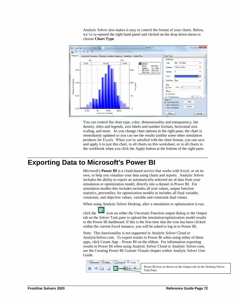
Frontline Solvers 2020 Reference Guide Page 72
Analytic Solver also makes it easy to control the format of your charts. Below,
we’ve re-opened the right hand panel and clicked on the drop down menu to
choose Chart Type.
You can control the chart type, color, dimensionality and transparency, bin
density, titles and legends, axis labels and number formats, horizontal axis
scaling, and more. As you change chart options in the right pane, the chart is
immediately updated so you can see the results (unlike some other simulation
products for Excel). When you’re satisfied with the chart format, you can save and apply it to just this chart, to all charts on this worksheet, or to all charts in
the workbook when you click the Apply button at the bottom of the right pane.
Exporting Data to Microsoft's Power BI Microsoft's Power BI is a cloud-based service that works with Excel, or on its
own, to help you visualize your data using charts and reports. Analytic Solver
includes the ability to export an automatically-selected set of data from your
simulation or optimization model, directly into a dataset in Power BI. For
simulation modles this includes includes all trial values, output function
statistics, percentiles; for optimization models in includes all final variable,
constraint, and objective values, variable and constraint dual values.
When using Analytic Solver Desktop, after a simulation or optimization is run,
click the icon on either the Uncertain Function output dialog or the Output
tab on the Solver Task pane to upload the simulation/optimization model results
to the Power BI dashboard. If this is the first time that the icon has been clicked
within the current Excel instance, you will be asked to log in to Power BI.
Note: This functionality is not supported in Analytic Solver Cloud or
AnalyticSolver.com. To export results to Power Bi when using either of these
apps, click Create App – Power BI on the ribbon. For information exporting
results to Power BI when using Analytic Solver Cloud or Analytic Solver.com, see the Creating Power BI Custom Visuals chapter within Analytic Solver User
Guide.
Power BI Icon as shown on the Output tab on the Desktop Solver
Task Pane.

Frontline Solvers 2020 Reference Guide Page 73
Once logged in, you will be asked to either update an existing dataset or create a
new dataset.
In the screenshot above, we see an existing datset "Product Mix 1" that we could
have updated by selecting and clicking OK. Rather, we chose to create a new
dataset, BusinessForecast. Once the upload is complete, the following message
will appear.
Power BI Icon as shown on the Desktop Solver Uncertain Function
dialog

Frontline Solvers 2020 Reference Guide Page 74
This message signifies that our data has been updated to Power BI successfully.
In your web browser, login to Power BI (http://powerbi.microsoft.com/). The
newly created dataset, along with the existing "ProductMix1" dataset, are listed
under Datasets.
Select the BusinessForecast dataset, then determine the components to be
included in the graph. In this example, we have created a bar chart by clicking
(to the right of the graph) and selecting the Maximum, Mean, Minimum,
and Mode Output Statistics.
Use the icon to pin this graph to the Dashboard.

Frontline Solvers 2020 Reference Guide Page 75
Now, each time the model is solved, the results may be uploaded to your Power
BI dashboard. Click back to Excel and change the Price of the Slow Market from $11 to $15, then run a 2nd simulation either by clicking the green arrow on
the Model tab in the Solver Task Pane or by clicking the Simulate icon on the
Analytic Solver ribbon. Once Solver stops, click the icon on the
Uncertain Function dialog to upload the most recent results. Note: We are not
asked to log in to the Power BI site a second time since we are using the same
instance of Excel. However, we are asked if we would like to select an existing
dataset to update. Select BusinessForecast and then click OK. Click back to
Power BI in your browser and refresh, the chart will update automatically with the new final variable values, as shown below.
Exporting Data to Tableau Tableau is a popular interactive software package that allows you to visually
explore and analyze your data. Tableau can import data from a wide range of sources, including Excel workbooks, and it is often used in conjunction with
Excel. Because Tableau is designed to import data in table form, it hasn’t been
easy to import the results of an optimization or simulation model (such as final
values of the uncertain variables, uncertain functions, percentiles and statistic
values in a simulation model and final values for the variables, constraints, and

Frontline Solvers 2020 Reference Guide Page 76
objective function in an optimization model) into Tableau, unless those model
elements occur in table form by themselves in your spreadsheet (which usually
isn’t the case).
Analytic Solver Desktop simplifies this process considerably. With a single
click, you can convert the results of your optimization or simulation model into a set of Tableau Data Extract files (*.tde). You can open these files directly in
Tableau, and visualize them with a few clicks.
Note: This functionality is not supported in Analytic Solver Cloud or
AnalyticSolver.com. To export results to Tableu when using either of these
apps, click Create App – Tableau on the ribbon. For information exporting
results to Tableau when using Analytic Solver Cloud or Analytic Solver.com,
see the Creating Custom Extensions in Tableau chapter within Analytic Solver
User Guide.
Once Solver has stopped with a final result message, click the icon on the
Task Pane Output tab or uncertain function dialog to save the values for the
uncertain functions, uncertain variables, percentiles and statistics in a simulation
model or variables, constraints, and objective function in an optimization model
to *.tde files. You will be prompted to select a folder where the Tableau files
will be saved along with the type of Tableau export desired: Tableau Data
Extract or Tableau Web Connector.
Note: If exporting to an existing .tde file, data will be appended rather than
overwritten. As a result, when exporting to an existing .tde file, all data must be
of the same structure as when the .tde file was first created.
Tableau Data Extract
If Tableau Data Extract is selected, static data is exported to files saved on your
hard drive.

Frontline Solvers 2020 Reference Guide Page 77
If running an optimization,0 three files will be saved in the folder you
selected: Constraints.tde, Objective.tde and Variables.tde. (Although .tde files
are designed to hold multiple tables, currently Tableau’s software allows only
one table per file.) When you import this data into Tableau, Variables.tde will
have one row for each decision variable, Constraints.tde will have one row for each constraint and Objective.tde will have just one row for the objective.
• Each row of Variables.tde will contain the Excel cell address, the
values of the variables at the time of extraction, the lower and upper
bound of each variable, the optimization index and sensitivity
information such as the reduced cost and allowable increase/decrease.
• Each row of Constraints.tde will contain the Excel cell address where
the constraint is located, the value of each constraint at time of
extraction, the constraint lower and upper bounds, and information that
would appear on a sensitivity report such as the shadow price, slack
value, a 1 or 0 to indicate if the constraint was binding (1) or not (0), and the allowable increase/decrease.
• Objective.tde will contain the Excel cell address where the objective is
located, the value of the objective function at the time of extraction,
and the optimization index.
If running a simulation, four files will be saved in the folder you
selected: InputTrials.tde, OutputStatistics.tde, OutputTrials.tde, and
Percentiles.tde. (Although .tde files are designed to hold multiple tables,
currently Tableau’s software allows only one table per file.) When you import
this data into Tableau, InputTrials.tde and Output Trials.tde will have one row
for each trial, Percentiles.tde will have one row for percentile and
OutputStatistics.tde will have one row for each output function.
• Each row of InputTrials.tde will contain the trial value for each
uncertain variable and the simulation index. The number of rows will
equal the number of trials.
• Each row of OutputTrials.tde will contain the trial value for each
uncertain function and the simulation index. The number of rows will
equal the number of trials.
• Each row of Percentiles.tde will contain the percentile value for each
uncertain function and the simulation index. The number of rows will
equal 99, ranging from the 1st to 99th percentiles.
• Each row of OutputStatistics.tde will contain the Excel cell address,
where the uncertain function is located along with 9 statistical functions
(mean, standard deviation, variance, kurtosis, skewness, mode,
minimum, maximum, and range) and the simulation index.
To open the files in Tableau, either double-click each file (if using Desktop
Tableau), or click Other Files under Connect and open the desired file(s).
Note: If exporting to an existing .tde file, data will be appended rather than
overwritten. As a result, when exporting to an existing .tde file, all data must be
of the same structure as when the .tde file was first created.
Tableau Web Connector
The Tableau Web Connector offers much more flexibility over Tableau Data
Extract by allowing you to refresh your data dynamically inside of Tableau.

Frontline Solvers 2020 Reference Guide Page 78
If Tableau Web Connector is selected, you will be prompted to select a folder
where the files will be saved.
If running an optimization, once the folder is selected and Select Folder is
clicked, OptimizationResults.html will be created and saved to that directory,
then the following message will appear. This file will hold all contents
described above for Constraints.tde, Objective.tde and Variables.tde.
If running a simulation, SimulationResults.html will be saved to the selected
directory, then the following message will appear. This file will hold all
contents described above for InputTrials.tde, OutputStatistics.tde,
OutputTrials.tde, and Percentiles.tde.
Note: If exporting to an existing .tde file, data will be appended rather than
overwritten. As a result, when exporting to an existing .tde file, all data must be
of the same structure as when the .tde file was first created.

Frontline Solvers 2020 Reference Guide Page 79
To open the files in Tableau, open a new workbook in Tableau, and click
Connect to Data.
On the Connect menu, select More Servers – Web Data Connector on the
Connect menu.

Frontline Solvers 2020 Reference Guide Page 80
On the Web Data Connector dialog, enter the location displayed on the dialog
shown above, i.e. http://localhost:8080/, and press Enter.
When the following dialog appears, click Constraints.html.
Note: The error highlighted in red is a simple warning that the URL is not
pointing to a Tableau Web Data Connector file. If you had entered a file name,
such as http://localhost:8080/Constraints.html or
http://localhost:8080/InputTrials.html, the results would have immediately been
uploaded to Tableau.
To add more data, click Data – New Data Source on the Tableau ribbon, then repeat the actions described above.

Frontline Solvers 2020 Reference Guide Page 81
If your Solver results have changed, refresh the results within the Tableau Web
Connector HTML files using the following steps:
1. In ASP, re-run your optimization or simulation model
Click the Tableau icon on the Output tab in the Solver Task Pane.
2. Select Tableau Web Connector and the folder where the files should
be saved.
3. Click OK.
4. In Tableau, click Data – Refresh All Extracts to update your data.
For more information on using Tableau, please refer to the Tableau
documentation found at http://www.tableau.com/.
Using the Decisions Menu When you click the Decisions icon on the Ribbon when using any version of
Analytic Solver, a dropdown menu appears.
From here you can either create a plot of the variables or add Normal or
Recourse variables to your optimization or stochastic optimization model.
Decision Variable Plot
A decision variable plot charts various decision variable characteristics, such as
the lower bound, upper bound, midpoints, current values, etc.
The chart below shows the variable plot from the ProductMix(Opt).xlsx. To
create, click Help – Examples – Optimization and open ProductMix(Opt).xlsx. Select cell G24 (the objective, Total_profit) and then click Decisions – Plot on
the ribbon. Note that the computation of this cell is dependent on the variables.
When creating this plot, Analytic Solver divided the difference of each variables'
upper and lower bound (default selections on the Chart Options tab) and divided
that difference by 50 (the Number of Data Points). For example, the upper

Frontline Solvers 2020 Reference Guide Page 82
bound on each variable is 300 and the lower bound on each variable is 0
resulting in a range of 300. After dividing by the number of data points, we can
calculate that each data point will be a multiple of 6 as shown in the table below.
Note: If a variable does not have an upper bound, then a value of positive
infinity (1E+50) will be used and if a variable does not have a lower bound, then a value of negative infinity (-1e+50) will be used.
Variable Values Value of Cell G24
0 $0
6 $960
12 $1,920
…
300 $48,000
When these points are plotted, the result is the graph below. The Y axis plots
the value of cell G24 while the x axis plots the data points 1 thru 50.
If you change Point B's selection to "Variables at midpoints", the graph will
update to:

Frontline Solvers 2020 Reference Guide Page 83
Notice that the Y axis now shows 0 thru $25,000 to reflect the change in value
of cell G24. To calculate the data points: take the midpoint of each variable and
divide through by the Number of Data Points or (300-0)/2 = 150/50 = 3.
Variable Values Value of Cell G24
0 $0
3 $480
9 $1,440
…
150 $24,000
If you were to leave Point B's selection at "Variables at Upper Bounds" and
instead change Point A's selection to "Variables at Midpoints", then the first,
second, and third data points would be: 150, 153, 159, …. 300.
If you change the variable values to C14 = 25, D14 = 50, and E14 = 75, and then
select "Variables at current values" for Point B, the graph will update
immediately to:
Analytic Solver calculated each data point by subtracting Point A (Lower Bounds) from Point B (Current Values) and dividing by the Number of Data
Points (50).
Value of C14 Value of D14 Value of E14 Value of G24
0 0 0 $0
0.5 1 1.5 $140
1 2 3 $243
1.5 3 4.5 $420
2 4 6.0 $523
… … …
25 50 75 $7,000
If Randomly Chosen values is selected for Point A or Point B, a random value
will be selected between the variables upper and lower bounds.
If you are using AnalyticSolver.com, you’ll notice that you can add/change the
Lower and Upper bounds of variables through the Decision Plot dialog, rather
than having to add such bounds through the Task Pane or Ribbon; but you
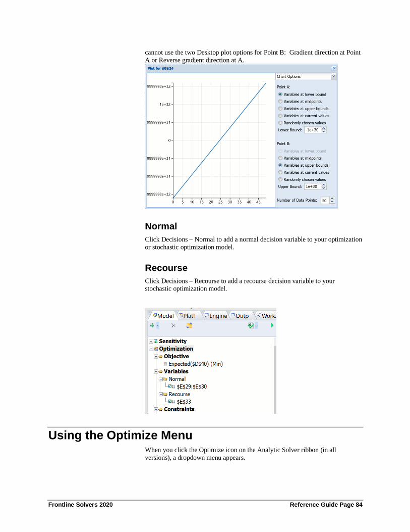
Frontline Solvers 2020 Reference Guide Page 84
cannot use the two Desktop plot options for Point B: Gradient direction at Point
A or Reverse gradient direction at A.
Normal
Click Decisions – Normal to add a normal decision variable to your optimization
or stochastic optimization model.
Recourse
Click Decisions – Recourse to add a recourse decision variable to your stochastic optimization model.
Using the Optimize Menu When you click the Optimize icon on the Analytic Solver ribbon (in all
versions), a dropdown menu appears.

Frontline Solvers 2020 Reference Guide Page 85
From here you can either solve the complete problem or the relaxation of a
mixed – integer problem, solve only for recourse variables or simply analyze either the original or the transformed models.
Solve Complete Problem
Select this menu item if Solver is to solve the optimization model as it appears
in the Task Pane Model tab. If Interpreter is set to Psi Interpreter or Always (the
default setting) on the Task Pane Platform tab, the steps described under
“Analyze Original Problem” will be performed first. If your model is diagnosed as non-smooth, and Non-Smooth Model Transformation is set to Automatic (the
default setting) or Always on the Task Pane Platform tab, the steps described
under “Analyze Transformed Model” will be performed next. If the transformed
model is linear, it will be used to solve the problem, otherwise the original
model will be used. Next, if Automatically Select Solver Engine is checked on
the Task Pane Engine tab, the best available Solver Engine will be used,
otherwise your choice in the Engine tab dropdown list will be used to solve the
problem. When the solution process is complete, the worksheet will show the
best solution found, and reports can be selected from the Reports – Optimization
dropdown list.
For more information on the above options, see the topics “Optimization Interpreter,” “Nonsmooth Model Transformation,” and “Automatically Select
Solver Engine” in the chapter “Platform Option Reference.” For information on
optimization reports, see the “Solver Reports” chapter.
Analyze Original Problem
Select this menu item to run the Interpreter to diagnose your model as a linear
programming, quadratic or conic, smooth nonlinear, or non-smooth optimization model, and determine the convexity of your model. When this option is
selected, the interpreter will pinpoint formulas that are causing your model to be
nonlinear or non-smooth (see the Structure Report in the “Solver Reports”
chapter) or are causing your model to be poorly scaled (see the Structure Report
in the “Solver Reports” chapter).
Analyze Transformed Model
Select this menu item to run the Interpreter to diagnose the transformed model
as a linear programming, quadratic or conic, smooth nonlinear, or non-smooth
optimization model and determine the convexity of your model. If your model
contains non-smooth functions with arguments that depend on the decision

Frontline Solvers 2020 Reference Guide Page 86
variables, the Analytic Solver products will automatically transform your
model, replacing IF, MIN, MAX, ABS, AND, OR, and NOT functions and <=
and >= operators with additional variables and linear constraints that achieve the
same effect, for optimization purposes, as these functions. A Linearization
Report will be available under Reports – Optimization containing a list of these additional variables and constraints.
Solve without Integer Constraints
Select this menu item to solve the “relaxation” of the mixed integer problem (or
MIP) temporarily ignoring the integer constraints. It’s meaningful to Solve with
Integer Constraints only if you have integer constraints in your model.
Solve for Recourse Variables
Select this menu item to solve only for the Recourse variables in your Stochastic
Optimization model. Normal decision variables will remain unchanged. It’s
meaningful to Solve for Recourse variables only if you have recourse decision
variables in an optimization model with uncertainty. Note: Solve for Recourse
Variables is available in all Analytic Solver products up to your licensed
problem limits.
Run on a Solver Server
Select this menu item to solve your optimization or simulation model on a
corporate server or a cloud-based virtual server, with results appearing in your
spreadsheet, just as if you had solved the model locally.
Chart Formatting, Copy/Paste and Printing The right pane of the Uncertain Variable dialog in Analytic Solver Desktop
contains controls that allow you to customize the appearance of the charts that appear in the center of the dialog. When you change option selections or type
text in these controls, the chart area is instantly updated.
Note: This functionality is not currently supported in Analytic Solver Cloud or
AnalyticSolver.com. Currently, in either of these products, you are only able to
customize the chart type and color of the shaded region on the Chart Type pane.
The controls are divided into three groups: Chart Type, Axis Options and
Markers. Using the Apply To options at the bottom of each view, you can
apply the new chart settings to this chart only, all uncertain variable charts on
this worksheet, or all uncertain variable charts in the workbook.
You can control the chart type, color, and 3D effects, the horizontal scale and number format, and the chart title, legend and gridlines. You can also ‘fix’ the
vertical scale of Frequency charts, so that the scale doesn’t change from one
simulation to the next. When you change options or type text in these controls,
the chart area is updated immediately, so you see the results of your changes.
To display a list of chart group of chart settings, simply click on the drop down
menu at the top of the right pane:

Frontline Solvers 2020 Reference Guide Page 87
To save and apply the new chart settings to this chart only, all uncertain function
charts on this worksheet, or all uncertain function charts in the workbook, just
select the option you want and click the Apply button. You can click the Revert
button to return the chart to Risk Solver’s default settings.
Chart Type
The Chart Type settings determine the basic chart type, color and gridlines, the
number and form of bins for frequency charts (uncertain functions only), and 3D
and transparency effects.
Chart Type
Type: You may select any of eight variants of Line, Bar, and Area charts.
Examples of these chart types are shown on the next page.
• Bar – No Gaps
• Bar – With Gaps
• Line – Step
• Line – Midpoint
• Line – Smooth

Frontline Solvers 2020 Reference Guide Page 88
• Area – Step
• Area – Midpoint
• Area – Smooth
Each of these chart variants may be drawn in either two or three dimensions. For 3D, check the box “3D Chart” as described in the next section.
For uncertain functions, a Bar – No Gaps chart is drawn by default. For
uncertain variables, an Area – Midpoint chart is drawn for continuous
distributions, and a Bar – No Gaps charts is drawn for discrete distributions.
Bar – No Gaps
Bar – With Gaps
Line – Step
Area – Step
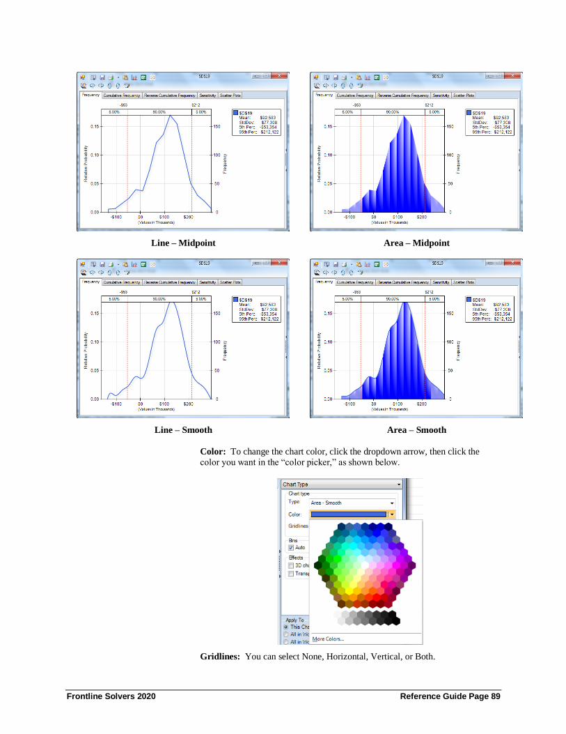
Frontline Solvers 2020 Reference Guide Page 89
Line – Midpoint
Area – Midpoint
Line – Smooth
Area – Smooth
Color: To change the chart color, click the dropdown arrow, then click the
color you want in the “color picker,” as shown below.
Gridlines: You can select None, Horizontal, Vertical, or Both.

Frontline Solvers 2020 Reference Guide Page 90
Bins
Auto: When this box is checked (the default), Analytic Solver automatically
chooses the number of bins (columns for a bar chart), based on the data and the
number of trials. When the box is unchecked, you choose the number of bins,
using the Bins edit box.
Bins: You can enter the exact number of bins you want in the edit box. By
clicking the spinner control, you can increase or decrease the number of bins.
Effects
3D: If this box is checked, a three-dimensional perspective chart is drawn. If it
is unchecked, a two-dimensional chart is drawn.
Transparency: By clicking the spinner control, you can increase or decrease
the degree of transparency in the colors used to draw the chart.
Below is an example of the Uncertain Function dialog, showing how the chart
appears when some of these options are changed.
Chart Options
The Chart Options settings determine the chart title, subtitle, and legend position
and contents.
Chart Display
Starting in Version 12, users have the ability to choose to have the simulation
results dialog automatically open after a simulation is run. Simply click on
“Show chart after each simulation”.
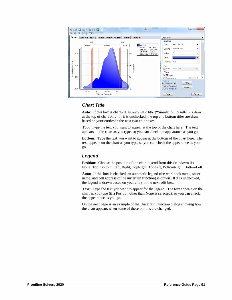
Frontline Solvers 2020 Reference Guide Page 91
Chart Title
Auto: If this box is checked, an automatic title (“Simulation Results”) is drawn
at the top of chart only. If it is unchecked, the top and bottom titles are drawn based on your entries in the next two edit boxes.
Top: Type the text you want to appear at the top of the chart here. The text
appears on the chart as you type, so you can check the appearance as you go.
Bottom: Type the text you want to appear at the bottom of the chart here. The
text appears on the chart as you type, so you can check the appearance as you
go.
Legend
Position: Choose the position of the chart legend from this dropdown list:
None, Top, Bottom, Left, Right, TopRight, TopLeft, BottomRight, BottomLeft.
Auto: If this box is checked, an automatic legend (the workbook name, sheet
name, and cell address of the uncertain function) is drawn. If it is unchecked,
the legend is drawn based on your entry in the next edit box.
Text: Type the text you want to appear for the legend. The text appears on the
chart as you type (if a Position other than None is selected), so you can check
the appearance as you go.
On the next page is an example of the Uncertain Function dialog showing how
the chart appears when some of these options are changed.
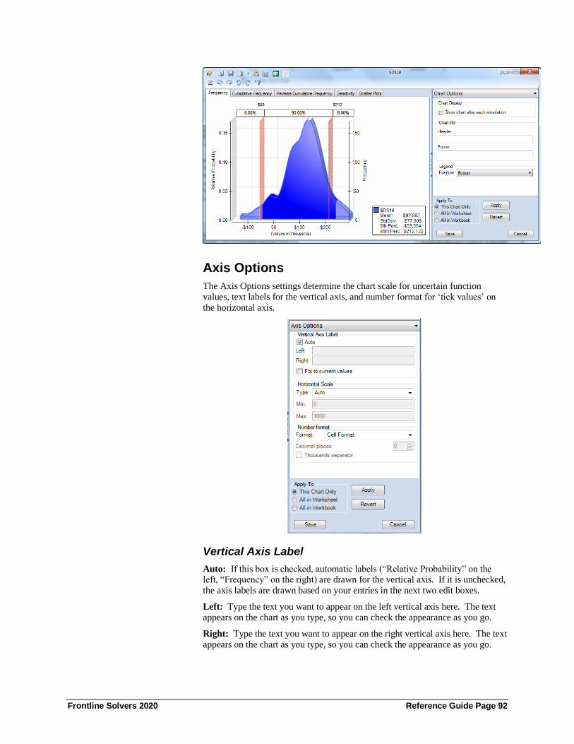
Frontline Solvers 2020 Reference Guide Page 92
Axis Options
The Axis Options settings determine the chart scale for uncertain function
values, text labels for the vertical axis, and number format for ‘tick values’ on
the horizontal axis.
Vertical Axis Label
Auto: If this box is checked, automatic labels (“Relative Probability” on the left, “Frequency” on the right) are drawn for the vertical axis. If it is unchecked,
the axis labels are drawn based on your entries in the next two edit boxes.
Left: Type the text you want to appear on the left vertical axis here. The text
appears on the chart as you type, so you can check the appearance as you go.
Right: Type the text you want to appear on the right vertical axis here. The text
appears on the chart as you type, so you can check the appearance as you go.

Frontline Solvers 2020 Reference Guide Page 93
Fix to Current Values
This check box, which appears only for uncertain functions, affects the vertical
axis scale. Normally, Analytic Solver chooses the scale (lowest and highest
values) on the vertical axis based on the frequencies of outcomes in the most
recent simulation. When Interactive Simulation is on, these values can change
each time you press F9 or change a number on the spreadsheet. This approach
allows Risk Solver to make maximum use of “chart real estate,” adjusting the
vertical axis so that the tallest bars or highest lines almost fill the chart area.
At times, however, you may want to see how the frequency distribution changes
shape as you change numbers on the spreadsheet, without any change to the
scale. If you check the box Fix to current values, the vertical axis is fixed to its current lowest and highest values, until you uncheck the box later. As you
perform more simulations and the frequencies of outcomes change, you may see
charts drawn where the tallest bars or highest lines don’t fill the chart area, or
charts where they overflow the chart area. In the latter case, a vertical scroll bar
will appear automatically, so that you can adjust the view to see the tallest bars
or highest lines if you wish.
Horizontal Scale
Type: Choose the type of scale for function values from this dropdown list:
• Auto: The scale will be determined automatically, based on the values of
the uncertain function in the simulation.
• Fixed: The scale extends from the minimum to the maximum value for the
uncertain function that you enter in the following two edit boxes.
• Std. Deviation: The scale extends below and above the mean value by a
number of standard deviations, that you enter in the first following edit box.
• Percentile: The scale ends from a low percentile to a high percentile that you enter in the following two edit boxes.
Min: Enter the low value for the uncertain function or percentile, or the number
of standard deviations here.
Max: Enter the high value for the uncertain function or percentile here.
Number Format
Format: Choose the type of number format from this dropdown list: General,
Number, Currency, Scientific, Percentage, or Cell Format. The last choice,
which is the default, uses the format of the uncertain function cell for the
horizontal axis tick values.
Decimal Places: For Number and Currency formats, click the spinner (or type a
value) for the number of decimal places you want to appear.
Thousands Separator: For Number and Currency formats, separators (commas
when in U.S. English locale) appear every three digits if this box is checked.
On the next page is an example of the Uncertain Function dialog showing how
the chart appears when some of these options are changed. Notice that the horizontal axis is Fixed to the range -100 to 200 (the numbers are in thousands
so you only need to enter -100, 200 – so that some extreme occurrences may not
be included on the chart. Also, the vertical axis was Fixed to current values on
an earlier simulation, to a range from 0.0 to 0.12 – and on the current simulation,
the two tallest bars exceeded this range, so a vertical scroll bar appears.

Frontline Solvers 2020 Reference Guide Page 94
Chart Markers
You can create a variety of chart Markers to mark and annotate points of interest
on charts of both uncertain variables and uncertain functions. When you create
a Marker, you can apply it to the current chart, all charts in the current
worksheet, or all charts in the workbook. It is often useful to create a few
‘standard’ Markers that apply to all charts, as well as custom Markers for
specific charts. If you have a worksheet or workbook level Marker that you
don’t want to appear on a specific chart, you can make it invisible on that chart.
To create and edit chart Markers, click the Markers tab in the right pane of the
Uncertain Variable or Uncertain Function dialog. You can also create workbook
level Markers via the Risk Solver Options dialog, as illustrated later.
To create a new Marker, click the ++ button at the top left of the option area in
the right panel. To delete an existing Marker, select it in the dropdown list, and
click the x button at the top left.
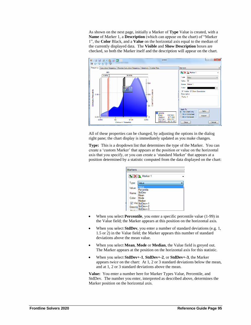
Frontline Solvers 2020 Reference Guide Page 95
As shown on the next page, initially a Marker of Type Value is created, with a
Name of Marker 1, a Description (which can appear on the chart) of “Marker
1”, the Color Black, and a Value on the horizontal axis equal to the median of
the currently displayed data. The Visible and Show Description boxes are
checked, so both the Marker itself and the description will appear on the chart.
All of these properties can be changed, by adjusting the options in the dialog
right pane; the chart display is immediately updated as you make changes.
Type: This is a dropdown list that determines the type of the Marker. You can
create a ‘custom Marker’ that appears at the position or value on the horizontal
axis that you specify, or you can create a ‘standard Marker’ that appears at a
position determined by a statistic computed from the data displayed on the chart:
• When you select Percentile, you enter a specific percentile value (1-99) in the Value field; the Marker appears at this position on the horizontal axis.
• When you select StdDev, you enter a number of standard deviations (e.g. 1,
1.5 or 2) in the Value field; the Marker appears this number of standard
deviations above the mean value.
• When you select Mean, Mode or Median, the Value field is greyed out.
The Marker appears at the position on the horizontal axis for this statistic.
• When you select StdDev+-1, StdDev+-2, or StdDev+-3, the Marker
appears twice on the chart: At 1, 2 or 3 standard deviations below the mean,
and at 1, 2 or 3 standard deviations above the mean.
Value: You enter a number here for Marker Types Value, Percentile, and
StdDev. The number you enter, interpreted as described above, determines the
Marker position on the horizontal axis.

Frontline Solvers 2020 Reference Guide Page 96
Name: The Marker Name appears in the dropdown list next to the Add and
Delete buttons; it is used to select the Marker when the same Marker is used in
multiple charts. You can accept the default names “Marker 1”, “Marker 2”, etc.
or type your own names into the Name edit box.
Color: To change the chart color, click the dropdown arrow, then click the color you want in the “color picker,” as shown below.
Visible: If this box is checked, the Marker appears on the chart; if it is
unchecked, the Marker doesn’t appear. Using this option, you can control
whether a worksheet- or workbook-level Marker appears on a specific chart.
Show Description: If the Marker is Visible and this box is checked, the text in
the Description edit box appears as a label attached to the Marker on the chart.
Description: The text you type in this edit box appears as a label attached to the
Marker, if the Show Description box is checked.
Copying and Pasting Charts
In Analytic Solver Desktop, you can easily copy a chart from the Uncertain
Variable or Uncertain Function dialog to the Windows Clipboard, and paste it
into almost any Windows application that accepts graphic images. To do this,
just click the Clipboard icon in the title bar of the dialog.
On the next page is an example of an Analytic Solver chart pasted into a
PowerPoint slide. Analytic Solver can render the copied chart in Windows
Bitmap, Device Independent Bitmap, and Windows Enhanced Metafile formats.

Frontline Solvers 2020 Reference Guide Page 97
Note: This functionality is not currently supported in Analytic Solver Cloud or
AnalyticSolver.com.
Printing Charts
You can easily print an Analytic Solver Desktop chart: Just click the Print icon
on the Uncertain Variable or Uncertain Function dialog title bar to immediately print the currently displayed chart on your default printer, or click the down
arrow next to this icon to display the menu choices shown below: Print
Preview, Printer Settings and Page Settings. You can choose a printer and set
printer options, set page margins, and preview your output using these menu
choices.
An example of the Print Preview dialog in Risk Solver is shown on the next
page. You can magnify and examine the print image or send it to the currently
selected printer from this dialog.
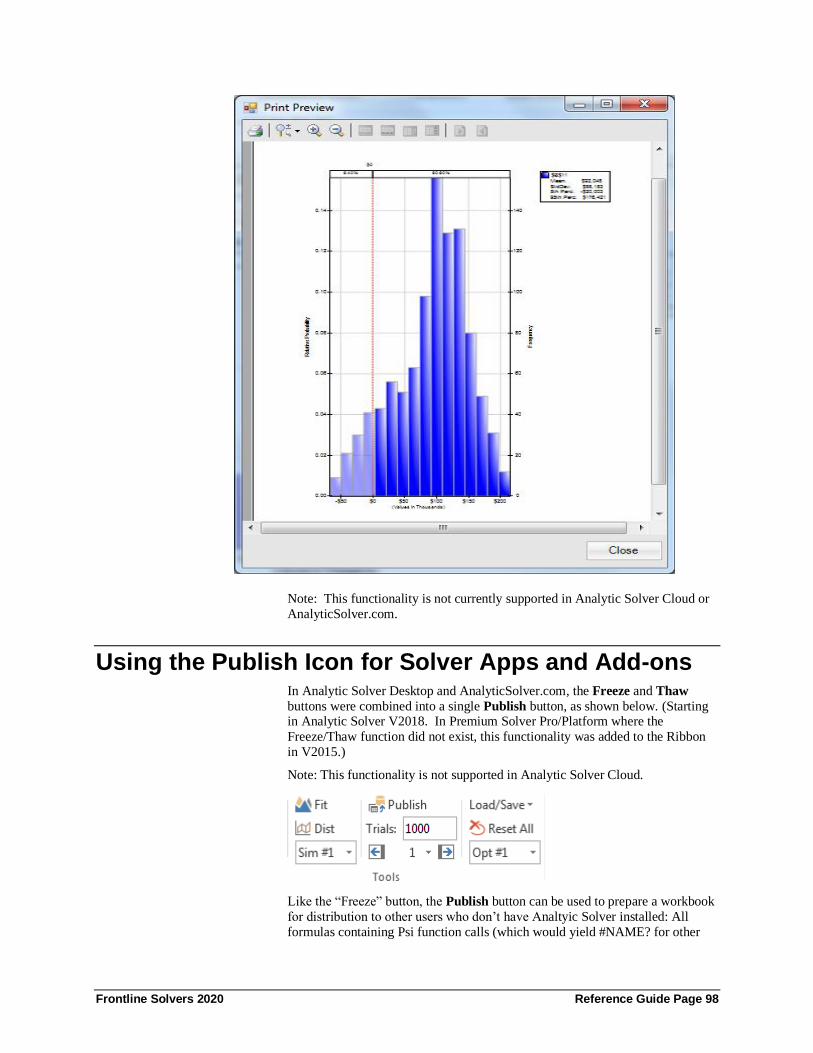
Frontline Solvers 2020 Reference Guide Page 98
Note: This functionality is not currently supported in Analytic Solver Cloud or
AnalyticSolver.com.
Using the Publish Icon for Solver Apps and Add-ons In Analytic Solver Desktop and AnalyticSolver.com, the Freeze and Thaw
buttons were combined into a single Publish button, as shown below. (Starting in Analytic Solver V2018. In Premium Solver Pro/Platform where the
Freeze/Thaw function did not exist, this functionality was added to the Ribbon
in V2015.)
Note: This functionality is not supported in Analytic Solver Cloud.
Like the “Freeze” button, the Publish button can be used to prepare a workbook
for distribution to other users who don’t have Analtyic Solver installed: All
formulas containing Psi function calls (which would yield #NAME? for other
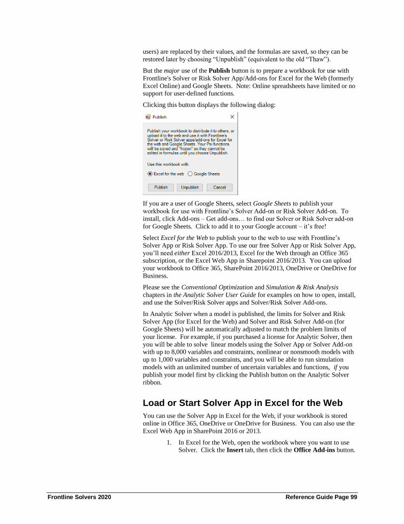
Frontline Solvers 2020 Reference Guide Page 99
users) are replaced by their values, and the formulas are saved, so they can be
restored later by choosing “Unpublish” (equivalent to the old “Thaw”).
But the major use of the Publish button is to prepare a workbook for use with
Frontline's Solver or Risk Solver App/Add-ons for Excel for the Web (formerly
Excel Online) and Google Sheets. Note: Online spreadsheets have limited or no support for user-defined functions.
Clicking this button displays the following dialog:
If you are a user of Google Sheets, select Google Sheets to publish your
workbook for use with Frontline’s Solver Add-on or Risk Solver Add-on. To
install, click Add-ons – Get add-ons… to find our Solver or Risk Solver add-on
for Google Sheets. Click to add it to your Google account – it’s free!
Select Excel for the Web to publish your to the web to use with Frontline’s
Solver App or Risk Solver App. To use our free Solver App or Risk Solver App,
you’ll need either Excel 2016/2013, Excel for the Web through an Office 365 subscription, or the Excel Web App in Sharepoint 2016/2013. You can upload
your workbook to Office 365, SharePoint 2016/2013, OneDrive or OneDrive for
Business.
Please see the Conventional Optimization and Simulation & Risk Analysis
chapters in the Analytic Solver User Guide for examples on how to open, install,
and use the Solver/Risk Solver apps and Solver/Risk Solver Add-ons.
In Analytic Solver when a model is published, the limits for Solver and Risk
Solver App (for Excel for the Web) and Solver and Risk Solver Add-on (for
Google Sheets) will be automatically adjusted to match the problem limits of
your license. For example, if you purchased a license for Analytic Solver, then
you will be able to solve linear models using the Solver App or Solver Add-on with up to 8,000 variables and constraints, nonlinear or nonsmooth models with
up to 1,000 variables and constraints, and you will be able to run simulation
models with an unlimited number of uncertain variables and functions, if you
publish your model first by clicking the Publish button on the Analytic Solver
ribbon.
Load or Start Solver App in Excel for the Web
You can use the Solver App in Excel for the Web, if your workbook is stored
online in Office 365, OneDrive or OneDrive for Business. You can also use the
Excel Web App in SharePoint 2016 or 2013.
1. In Excel for the Web, open the workbook where you want to use Solver. Click the Insert tab, then click the Office Add-ins button.

Frontline Solvers 2020 Reference Guide Page 100
2. In the Office Add-ins dialog, click on the Store tab, and search for
Solver. Click on the Solver App. When prompted, click the Trust
It button, to allow Solver to read and optimize your model.
3. The Solver Parameters dialog should appear, as a pane embedded
in the worksheet. If a Solver model has been created on this worksheet, its selections (objective, variables, constraints and
Solver options) should automatically appear in the dialog.
4. You can modify the Solver model selections, or create a new
Solver model from scratch, by using the dialog options, very much
like the basic Excel Solver. Click the Solve button to find the
optimal solution.
Load or Start the Solver App in Excel 2013/2016
You can use the Solver App in desktop Excel 2013 or 2016, if your workbook is
stored online in Office 365, SharePoint 2013/2016, OneDrive or OneDrive for
Business.
1. In Excel 2013 or 2016, open the workbook where you want to use
Solver. Click the Insert tab, then click the Office Add-ins button.
Note: Your workbook must use the .xlsx or .xlsm extension,
otherwise the My Apps icon on the Ribbon will be disabled.
2. If Solver appears in the Recently Used Apps dropdown list, select
it there, and skip to step 4.
3. Select See All... from the dropdown menu. In the Office Add-ins
dialog, find and select Solver under My Apps or My Organization.
If this is your first time using the Solver App, click find more apps
at the Office Store, and look in the Data Visualization + BI category. Click to see the Solver App listing in the Office Store.
4. The Solver Parameters dialog should appear. Click File Save As,
and save to your online document library.
5. If you later open this workbook in Excel for the Web or the Excel
Web App in a browser, the Solver Parameters dialog should
appear.
NOTE: Although the Solver App can be used in both Excel 2013 or 2016 and
Excel for the Web, because your model is solved "in the cloud," the Solver App
works only with Excel workbooks that are stored online. If you want to solve
a workbook model that is stored on your local PC, use the Solver add-in included with Excel, or desktop Analytic Solver.
See the Analytic Solver User Guide for a step-by-step example of how to
publish an optimization (in the Conventional Optimization chapter) and
simulation (in the Simulation & Risk Analysis chapter) example to both Excel
for the Web and Google Sheets.
Managing Your License Click the License button to open the License Manager where you can manage
your current licenses and accounts, open our Product Selection Wizard, connect
to Live Chat or peruse through a list of FAQs. Click License – Manage
License/Manage Account to open the Licensing Center.

Frontline Solvers 2020 Reference Guide Page 101
The "MyLicenses" tab displays your current license and license type, along with
the expiration date.
Click About Analytic Solver to open the following dialog containing information
on this release.
Click Support Live Chat to open a Live Chat window. If you run into any issues
when using the software, the best way to get help is to start a Live Chat with our
support specialists This will start a Live Chat during our business hours (or send
us a message at other hours), just as if you were to start a Live Chat on
www.solver.com – but it saves you and our tech support rep a lot of time –
because the software reports your latest error message, model diagnosis, license
issue or other problem, without you having to type anything or explain verbally
what’s happened. You’ll see a dialog like this:
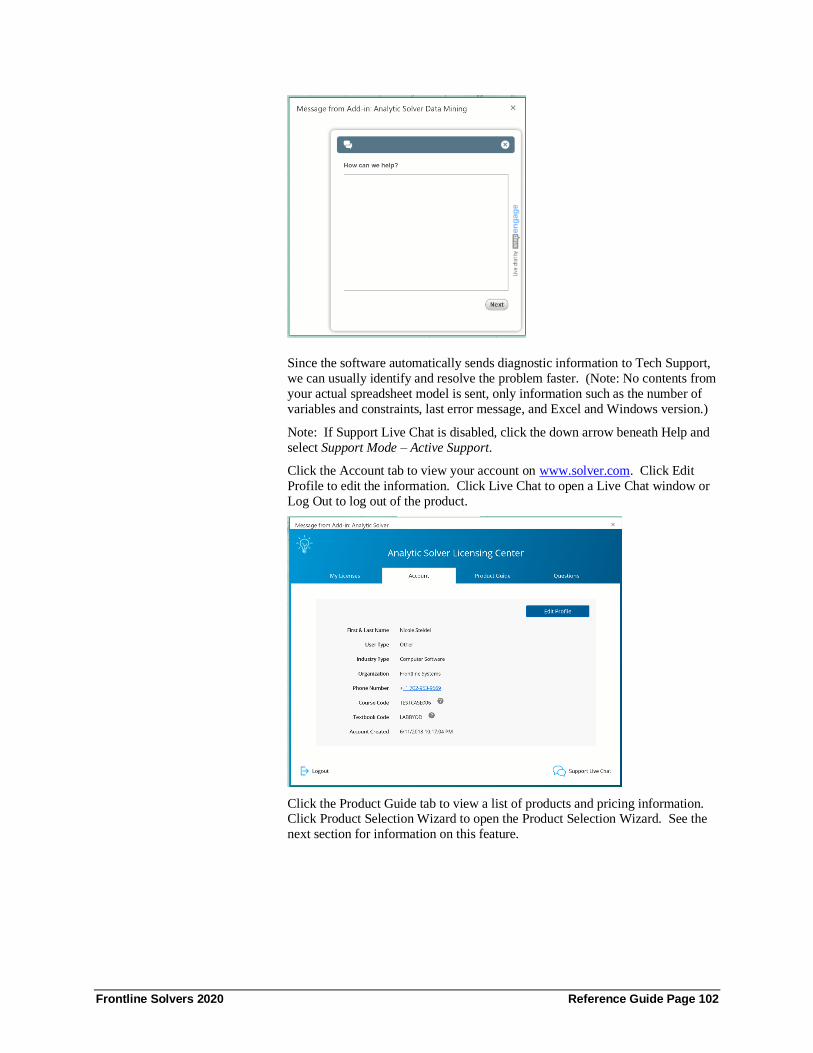
Frontline Solvers 2020 Reference Guide Page 102
Since the software automatically sends diagnostic information to Tech Support,
we can usually identify and resolve the problem faster. (Note: No contents from
your actual spreadsheet model is sent, only information such as the number of
variables and constraints, last error message, and Excel and Windows version.)
Note: If Support Live Chat is disabled, click the down arrow beneath Help and
select Support Mode – Active Support.
Click the Account tab to view your account on www.solver.com. Click Edit
Profile to edit the information. Click Live Chat to open a Live Chat window or
Log Out to log out of the product.
Click the Product Guide tab to view a list of products and pricing information. Click Product Selection Wizard to open the Product Selection Wizard. See the
next section for information on this feature.

Frontline Solvers 2020 Reference Guide Page 103
Click the Questions tab to review a list of FAQs, submit a support ticket or start
a live chat.
Product Selection Wizard Select Product Selection Wizard from the Licensing Center to open a series of
dialogs that will help you determine which product will best meet your needs
based on your recent pattern of use.
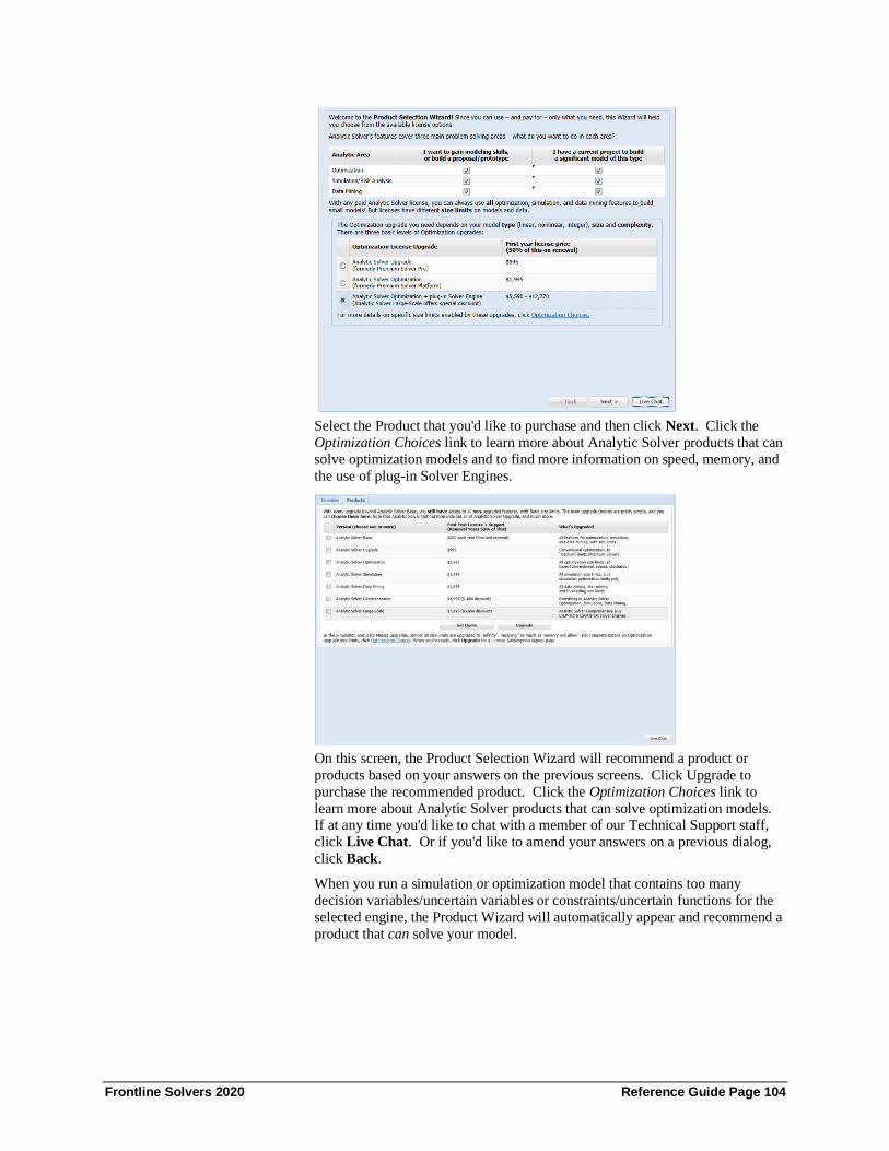
Frontline Solvers 2020 Reference Guide Page 104
Select the Product that you'd like to purchase and then click Next. Click the
Optimization Choices link to learn more about Analytic Solver products that can
solve optimization models and to find more information on speed, memory, and
the use of plug-in Solver Engines.
On this screen, the Product Selection Wizard will recommend a product or
products based on your answers on the previous screens. Click Upgrade to
purchase the recommended product. Click the Optimization Choices link to
learn more about Analytic Solver products that can solve optimization models. If at any time you'd like to chat with a member of our Technical Support staff,
click Live Chat. Or if you'd like to amend your answers on a previous dialog,
click Back.
When you run a simulation or optimization model that contains too many
decision variables/uncertain variables or constraints/uncertain functions for the
selected engine, the Product Wizard will automatically appear and recommend a
product that can solve your model.
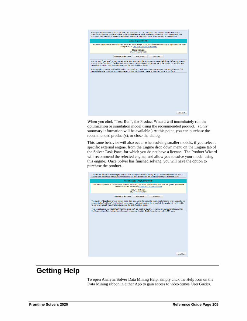
Frontline Solvers 2020 Reference Guide Page 105
When you click “Test Run”, the Product Wizard will immediately run the
optimization or simulation model using the recommended product. (Only
summary information will be available.) At this point, you can purchase the
recommended product(s), or close the dialog.
This same behavior will also occur when solving smaller models, if you select a
specific external engine, from the Engine drop down menu on the Engine tab of
the Solver Task Pane, for which you do not have a license. The Product Wizard
will recommend the selected engine, and allow you to solve your model using
this engine. Once Solver has finished solving, you will have the option to
purchase the product.
Getting Help To open Analytic Solver Data Mining Help, simply click the Help icon on the
Data Mining ribbon in either App to gain access to video demos, User Guides,

Frontline Solvers 2020 Reference Guide Page 106
online Help, example models, and Website support pages to learn how to use our
software tools, and how to build an effective model.
Examples
Clicking this menu item will open a browser pointing to the workbook, Frontline
Example Models Overview.xlsx. In the Desktop app, this file is copied to
C:\Program Files\Frontline Systems\ Analytic Solver Platform\Examples during
installation.
Knowledge Base
Click Knowledge Base to peruse a multitude of online articles related to support and installation issues or to locate articles that will help you to quickly build
accurate, efficient optimization, simulation, and data mining models.
User Guide Click the User Guides menu choice to open PDF files of the Analytic Solver
Optimization and Simulation User and Reference Guides, Analytic Solver Data
Mining User or Reference Guides, or our Quick Start Guides.
Submit a Support Ticket
If you're having installation, technical, or modeling issues, submit a Support
Ticket to open an online support request form. Submit your email address and a
short, concise description of the issue that you are experiencing. You'll receive
a reply from one of Frontline's highly trained Support Specialists within 24 hours, and generally much sooner.
Our technical support service is designed to supplement your own efforts: Getting you
over stumbling blocks, pointing out relevant sections of our User Guides or example
models, helping you fix a modeling error, or -- in rare cases -- working around an issue
with our software (always at our expense).

Frontline Solvers 2020 Reference Guide Page 107
Operating Mode
Click Operating Mode to switch between three different levels of help.
• Guided Mode prompts you step-by-step when solving, with dialogs.
• Auto-Help Mode shows dialogs or Help only when there’s a problem or
error condition.
• Expert Mode provides only messages in the Task Pane Output tab. (This
mode not supported when using a trial license.)
Click the Education & Training tab to visit Solver Academy – Frontline's online
training academy, watch video tutorials or live webinars, or learn more about
optimization, simulation or data mining.
Solver Academy
Solver Academy is Frontline Systems' own learning platform. It's the place
where business analysts can gain expertise in advanced analytics: forecasting,
data mining, text mining, mathematical optimization, simulation and risk
analysis, and stochastic optimization.
Video Tutorials/Live Webinars
Click Video Tutorials to be directed to Frontline's You Tube Channel. Browse
videos on how to create an optimization or simulation model or construct a data
mining or prediction model using Analytic Solver.
Click Live Webinars to be redirected to www.solver.com to join a live or pre-recorded webinar. Topics include Using Analytic Solver Data Mining to Gain
Insights from your Excel Data, Overview of Monte Carlo Simulation
Applications, Applications of Optimization in Excel, etc.
Learn more!
Click any of the three Learn More buttons to learn more about how you can
solve large-scale optimization, simulation, and data mining models, reduce

Frontline Solvers 2020 Reference Guide Page 108
costs, quantify and mitigate risk, and create forecasting, data mining and text
mining models using Analytic Solver.
Using the Options Dialog The Options dialog (supported in Analytic Solver Desktop only) lets you
examine and change Analytic Solver options that apply to your entire model. It appears when you click the Options button on the Analytic Solver Desktop
Ribbon. These settings are stored in the workbook with your model – if you
save the workbook and open it later, on the same or a different PC, the settings
will have the last values you specified in this dialog. The Options dialog has
tabs labeled Simulation, Optimization, General, Tree, Bounds, Charts,
Markers, and Problem.
Note: If using Analytic Solver Cloud or AnalyticSolver.com. See the chapter,
"Platform Solver Reference" that appears later on in this guide.
Simulation Tab
You can set these options in either the Analytic Solver Options dialog or, in
some cases, in the Task Pane, either on the Platform tab or the Engine tab when
Risk Solver Engine is selected in the Engine Selection drop-down menu –
changing them in one will also update them in the other.

Frontline Solvers 2020 Reference Guide Page 109
Trials, Simulations, and Random Seed
Trials per Simulation
This is perhaps the most frequently used option, since it determines the number
of Monte Carlo trials per simulation. You can type the number of trials you
want into the edit box, or click the spinner next to increase or decrease the
number of trials (by 100 trials at a time). Starting in V2015, you can enter the
number of trials on the Analytic Solver ribbon directly above the spinner
control. (See figure below.)
Simulations to Run
Risk Solver can perform multiple simulations whenever you change a number
on the spreadsheet, or whenever you trigger the simulation process in your
custom application. To set the number of simulations, click the spinner next to
the Simulations to Run edit box, or type the number you want into the edit box.
For multiple simulations to be useful, some parameter of the model – normally
something you can control – must have a different value in each individual
simulation. You can do this with the function PsiSimParam(). For more information, see the section “Multiple Parameterized Simulations” in the
Analytic Solver User Guide chapter “Getting Results: Simulation.”

Frontline Solvers 2020 Reference Guide Page 110
Only Run or Run Specific Simulation
Use this option to run a specific simulation when multiple simulations are being
run, for example simulation 10 out of 20 total simulations. PsiSimParam
parameters will be set for this index.
Random Seed
Setting the random number seed to a nonzero value (any number of your choice
is OK) ensures that the same sequence of random numbers is used for each
simulation. When the seed is zero, the random number generator is initialized
from the system clock, so the sequence of random numbers will be different in
each simulation. If you need the results from one simulation to another to be
strictly comparable, you should set the seed. To do this, click the spinner next to
the Random Seed edit box, or type the number you want into the box.
You can specify a random seed for each uncertain variable if you wish, by
including the PsiSeed() property function as an argument in the PSI Distribution function call for that variable. The seed value you set in the Options dialog
affects only uncertain variables that do not have PsiSeed() property functions.
Value to Display
Whenever your spreadsheet is calculated by the Excel Interpreter or the Psi
Interpreter and displayed, each PSI Distribution function returns a value. If no
simulation has been performed, the function returns a random sample from its
distribution. If a simulation has been performed, all of the trial values from that
simulation are available at once. You can specify what value you want to see
with the options in this group.
Type of Value
In the left hand dropdown list, you have a range of choices. When you select
Sample Mean, the Trial Index field is ignored, and each PSI Distribution
function returns the mean of the trial values in the last simulation.
Trial Index
When Value on Trial is selected in the left hand dropdown list, you can specify
which trial you want – from 1 to the value of the Trials per Simulation field.
You can type a number into the edit box, or use the spinner control to increase
or decrease the trial index. Starting in V2015, you can specify the number of
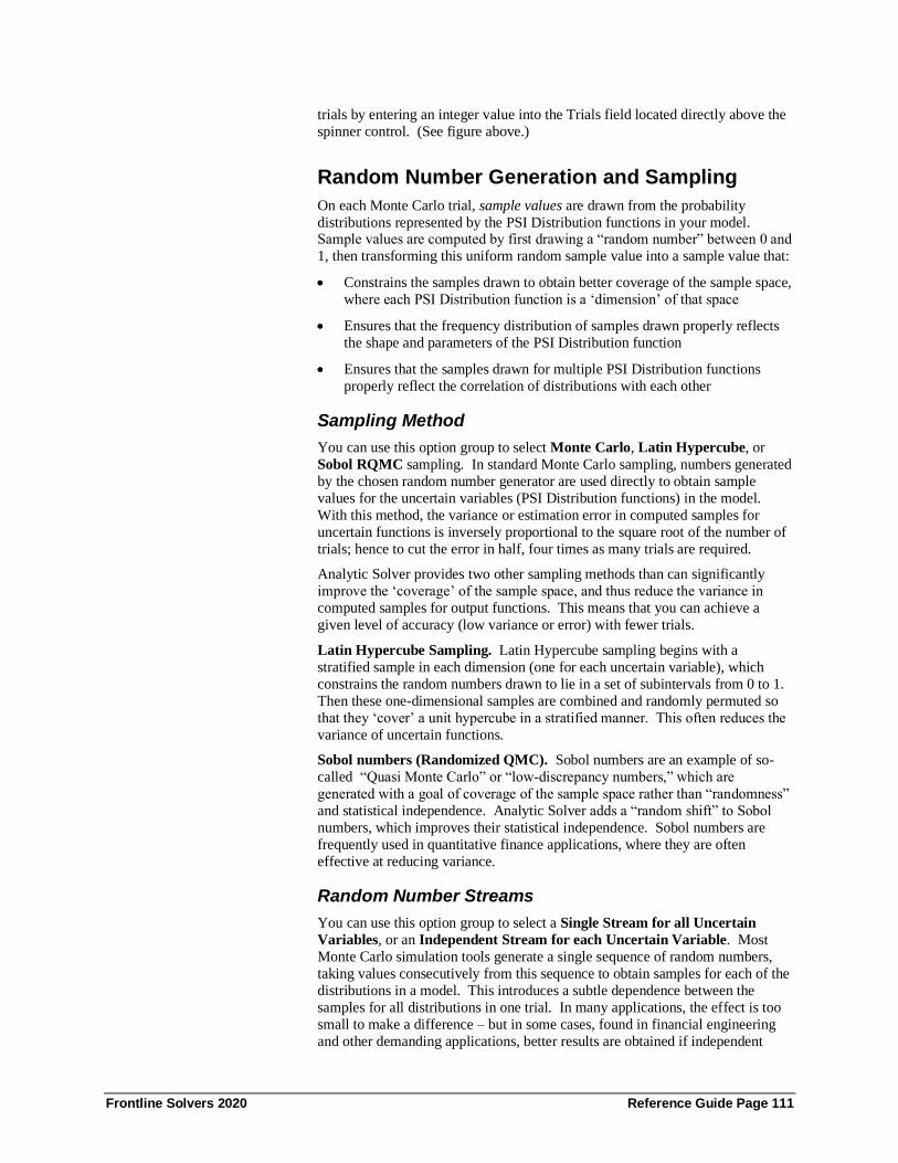
Frontline Solvers 2020 Reference Guide Page 111
trials by entering an integer value into the Trials field located directly above the
spinner control. (See figure above.)
Random Number Generation and Sampling
On each Monte Carlo trial, sample values are drawn from the probability
distributions represented by the PSI Distribution functions in your model. Sample values are computed by first drawing a “random number” between 0 and
1, then transforming this uniform random sample value into a sample value that:
• Constrains the samples drawn to obtain better coverage of the sample space,
where each PSI Distribution function is a ‘dimension’ of that space
• Ensures that the frequency distribution of samples drawn properly reflects
the shape and parameters of the PSI Distribution function
• Ensures that the samples drawn for multiple PSI Distribution functions
properly reflect the correlation of distributions with each other
Sampling Method
You can use this option group to select Monte Carlo, Latin Hypercube, or
Sobol RQMC sampling. In standard Monte Carlo sampling, numbers generated
by the chosen random number generator are used directly to obtain sample
values for the uncertain variables (PSI Distribution functions) in the model.
With this method, the variance or estimation error in computed samples for
uncertain functions is inversely proportional to the square root of the number of
trials; hence to cut the error in half, four times as many trials are required.
Analytic Solver provides two other sampling methods than can significantly
improve the ‘coverage’ of the sample space, and thus reduce the variance in
computed samples for output functions. This means that you can achieve a
given level of accuracy (low variance or error) with fewer trials.
Latin Hypercube Sampling. Latin Hypercube sampling begins with a
stratified sample in each dimension (one for each uncertain variable), which
constrains the random numbers drawn to lie in a set of subintervals from 0 to 1.
Then these one-dimensional samples are combined and randomly permuted so
that they ‘cover’ a unit hypercube in a stratified manner. This often reduces the
variance of uncertain functions.
Sobol numbers (Randomized QMC). Sobol numbers are an example of so-
called “Quasi Monte Carlo” or “low-discrepancy numbers,” which are
generated with a goal of coverage of the sample space rather than “randomness”
and statistical independence. Analytic Solver adds a “random shift” to Sobol
numbers, which improves their statistical independence. Sobol numbers are
frequently used in quantitative finance applications, where they are often
effective at reducing variance.
Random Number Streams
You can use this option group to select a Single Stream for all Uncertain
Variables, or an Independent Stream for each Uncertain Variable. Most
Monte Carlo simulation tools generate a single sequence of random numbers,
taking values consecutively from this sequence to obtain samples for each of the
distributions in a model. This introduces a subtle dependence between the
samples for all distributions in one trial. In many applications, the effect is too
small to make a difference – but in some cases, found in financial engineering
and other demanding applications, better results are obtained if independent

Frontline Solvers 2020 Reference Guide Page 112
random number sequences (streams) are used for each distribution in the model.
Analytic Solver offers this capability for Monte Carlo sampling and Latin
Hypercube sampling; it does not apply to Sobol numbers.
If you use a PsiSeed() property function as an argument to a PSI Distribution
function call, the uncertain variable defined by that distribution always has an independent stream of random numbers, regardless of the setting of this option.
Random Number Generator
You can use this option group to select a random number generation algorithm.
Analytic Solver includes an advanced set of random number generation
capabilities – well beyond those found in other Monte Carlo products for
Microsoft Excel. In common applications, any good random number generator is sufficient – but for challenging applications (for example in financial
engineering) that involve many uncertain variables and many thousands of trials,
the advanced features of Analytic Solver can make a real difference.
Computer-generated numbers are never truly “random,” since they are always
computed by an algorithm – they are called pseudorandom numbers. A random
number generator is designed to quickly generate sequences of numbers that are
as close to statistically independent as possible. Eventually, an algorithm will
generate the same number seen sometime earlier in the sequence, and at this
point the sequence will begin to repeat. The period of the random number
generator is the number of values it can generate before repeating.
A long period is desirable, but there is a tradeoff between the length of the
period and the degree of statistical independence achieved within the period.
Hence Risk Solver offers a choice of four random number generators:
• Park-Miller “Minimal” Generator with Bayes-Durham shuffle and
safeguards. This generator has a period of 231-2. Its properties are good,
but the following choices are usually better.
• Combined Multiple Recursive Generator (CMRG) of L’Ecuyer. This
generator has a period of 2191, and excellent statistical independence of
samples within the period.
• Well Equidistributed Long-period Linear (WELL1024) generator of Panneton, L’Ecuyer and Matsumoto. This very new generator combines a
long period of 21024 with very good statistical independence.
• Mersenne Twister generator of Matsumoto and Nishimura. This generator
has the longest period of 219937-1, but the samples are not as “equidistrib-
uted” as for the WELL1024 and CMRG generators.
Using Correlations
As described in the Frontline Solver User Guide chapter, “Mastering Simulation
and Risk Analysis Concepts,” you can specify that certain uncertain variables in
your model are correlated with other uncertain variables. This means that, on
each simulation trial, samples drawn for each uncertain variable will not be independent of each other, but will be related – for example, if one variable is
positively correlated with another, large (or small) sample values for both
variables will tend to be drawn on the same trial. To define correlations
between uncertain variables, you use PSI Property functions such as
PsiCorrDepen(), PsiCorrMatrix() or the new copula functions, PsiCopula,
PsiCopulaStudent, PsiCopulaGauss, passed as arguments to PSI Distribution
functions such as PsiNormal() or PsiUniform().

Frontline Solvers 2020 Reference Guide Page 113
On a given run, the correlations you’ve defined for all uncertain variables can be
activated or deactivated, depending whether the Use Correlations check box is
checked or unchecked. You’ll normally want to leave this box checked, but by
unchecking the box and performing a run where all uncertain variables are
sampled independently of each other, you can see the difference – and assess the impact of correlation on your model results.
To quickly change this option, you can click the downward pointing arrow
below the Correlate button on the Ribbon and select the Use Correlations
choice. The check mark on this menu choice corresponds to the checked box in
the Options dialog – changing one will change the other. Each time you click
this menu choice, it changes state, from checked to unchecked and vice versa.
Using PSI Technology or Excel for Trials
Analytic Solver uses its own Polymorphic Spreadsheet Interpreter (PSI
Technology) to perform Monte Carlo simulation trials at high speed – often 100
times faster or more than performing the trials by allowing Microsoft Excel to
recalculate the spreadsheet. Normally, you’ll want to use the PSI Interpreter for
simulation trials, since it is designed to compute the same values as Excel does,
but much faster than the Excel Interpreter. However, there are a few features of
Excel formulas and functions that the PSI Interpreter does not handle; if you use
these features in your model, you’ll see an error message when you try to run a
simulation. If your model requires the use of Excel features that are not
supported by the PSI Interpreter, you may have to use the Excel Interpreter
instead. To do this, simply click the radio button Use Excel Interpreter in the Interpreter options group.
Interpreter
You can switch between the PSI Interpreter and Excel Interpreter using this
option. If you wish, you can use this option to check that you’re getting the
same simulation results from both interpreters. Note that small differences from
arithmetic roundoff error are to be expected; bear in mind that if no Random Seed is set, the samples drawn on each run, and hence the results, will vary.
CLT Threshold
VBA / SDK: Parameter Names "CLTThreshold", 1 <= integer value <= 1000
Starting with V2016-R2, Analytic Solver includes the ability to sum multiple
independent random variables using compound distributions. A compound
distribution generates values for the sum of N independent identically
distributed uncertain variables. A distribution is made compound through the
use of the PsiCompound() property.

Frontline Solvers 2020 Reference Guide Page 114
When calculating a compound distribution, Analytic Solver first tries to
compute the distribution analytically. For example "=PsiExponential(par,
PsiCompund(N))" can be computed as PsiGamma(N, par) If Analytic Solver is
unable to compute a compound distribution analytically, but the frequency of the
severity function (N) is greater than the value for the CLT Threshold option, then the distribution will be computed according to the Central Limit Theorem
as PsiNormal(m, s). (The parameters m and s will be computed analytically
from the corresponding analytical moments of the severity distribution.)
Othewise, the compound distribution will be computed using Monte Carlo
simulation to sum up N independent variates of the severity distribution. The
maximum value allowed for this option is 1000 while the minimum value
allowed is 1. The default setting is 100.
For more information on compound distributions, see the Examples: Simulation
and Risk Analysis chapter in the Analytic Solver User Guide.
Optimization tab
You can set these options in either the Analytic Solver Options dialog or, in
some cases, in the Task Pane – changing them in one will also update them in
the other.

Frontline Solvers 2020 Reference Guide Page 115
General Options
Optimizations to Run
Use this property to set the number of optimizations to run when you click the
Optimize button on the Ribbon, or the green arrow (“Solve”) in the Task Pane.
This is useful only if you’ve defined one or more optimization parameters, using
the Parameters Optimization choice on the Ribbon.
Only Run
The specific optimization the Solver will perform, if multiple optimizations are defined. PsiOptParam parameters will be set for this index.
Interpreter
Analytic Solver uses its own Polymorphic Spreadsheet Interpreter (PSI
Technology) to parse the formulas on the worksheet(s) which is often 100 times
faster or more than allowing Microsoft Excel to recalculate the spreadsheet.
Normally, you’ll want to use the PSI Interpreter for optimization, since it is designed to compute the same values as Excel does, but much faster than the
Excel Interpreter. However, there are a few features of Excel formulas and
functions that the PSI Interpreter does not handle; if you use these features in
your model, you’ll see an error message when you try to run an optimization. If
your model requires the use of Excel features that are not supported by the PSI
Interpreter, you may have to use the Excel Interpreter.
You can switch between the PSI Interpreter and Excel Interpreter using this
option. If you wish, you can use this option to check that you’re getting the
same simulation results from both interpreters. Note that small differences from
arithmetic roundoff error are to be expected; bear in mind that if no Random
Seed is set, the samples drawn on each run, and hence the results, will vary.
Solve Mode
Use this option to determine what action will be taken when you click the
Optimize button on the Ribbon, or the green arrow (“Solve”) in the Task Pane.
Select from Solve Complete Problem, Analyze without Solving, Solve
without Integer Constraints, or Solve for Recourse Variables. It’s
meaningful to Solve with Integer Constraints only if you have integer constraints in your model. Similarly, it’s meaningful to Solve for Recourse
variables only if you have recourse decision variables in an optimization model
with uncertainty.
Solve Uncertain Models
Use this option to determine how an optimization model with uncertainty will be
solved when you click the Optimize button on the Ribbon, or the green arrow
(“Solve”) in the Task Pane. Your optimization includes uncertainty if the formula for the objective, or any constraint, depends (directly or indirectly) on
an uncertain variable cell, where you’ve entered a PSI distribution function
(such as PsiNormal). Select from Simulation Optimization, Stochastic
Transformation, Stochastic Decomposition, or Automatic. Automatic (the
default choice) allows Analytic Solver to choose the solution method
automatically.

Frontline Solvers 2020 Reference Guide Page 116
Use Psi Functions to Define Model on Worksheet
Set this option to True if you want to use optimization-specific PSI functions to
define the objective, variables or constraints of your model. These are functions
such as PsiVar() to define decision variables, PsiCon() to define constraints, and
PsiObj() to define the objective. Please see the section, Using Psi Optimization
Functions, later in this guide, for a complete description of each Psi function.
Use Interactive Optimization
Set this option to True if you want to run an optimization automatically
whenever you make a change to your spreadsheet. This is primarily useful (i) on
modest-size models where the optimization completes very quickly and (ii) after
you’ve finished developing and testing your optimization model. You can ask
‘what if’ by changing a number on the spreadsheet, and see how the optimal
solution changes with Interactive Optimization.
Transformation Options
Nonsmooth Model Transformation
Use this option to choose whether Analytic Solver will attempt to transform
constraints in your model that are non-smooth functions of the decision variables
into equivalent linear constraints that depend on newly-introduced binary integer
and continuous decision variables.
You can choose Always, Never, and Automatic. Automatic is the default
choice: Analytic Solver will automatically diagnose your model, and if it
contains non-smooth functions that are candidates for transformation, Analytic
Solver will attempt the transformation and will diagnose the resulting expanded model. This takes the most time, but is completely automatic. If your model is
successfully transformed, you should be sure to check, and probably adjust, the
Big M Value option.
Always is useful only when you know that your model uses non-smooth
functions and that the transformations will succeed. Never is useful if you are
certain that your model doesn’t use non-smooth functions, and you’d like to
save some time, or if you just don’t want the transformation to be attempted.
A simple example is a constraint A1 <= 100 where A1 contains
=IF(B1=0,C1,D1). If B1 is (or depends on) a decision variable, this constraint is
non-smooth – in fact discontinuous – which means that the model cannot be
solved to optimality by either linear programming (fastest and most reliable) or smooth nonlinear optimization.
Assuming for simplicity that B1 is a decision variable that is non-negative, this
constraint can be transformed by introducing a new binary integer variable Y1,
and a new constraint B1 <= BigM * Y1, where BigM is a constant larger than
any possible value for B1 (you can set this value with the Big M Value option).
The IF function in A1 is replaced with =D1*Y1+C1*(1-Y1). Now when Y1=0,
B1 is forced to be = 0, and A1=C1; when Y1=1, B1 can have any positive value,
and A1=D1. The non-smooth IF function is transformed into a set of linear
functions, so a faster and more reliable linear programming Solver can
potentially be used – but the overall size of the model is increased.
Analytic Solver can perform much more complex transformations automatically,
for constraints involving the Excel functions IF, AND, OR, NOT, MIN, MAX,
and the relational operators <=, = and >=. Such transformations can result in a

Frontline Solvers 2020 Reference Guide Page 117
significantly larger model, but if the resulting model is entirely linear, this can
be more than offset by the faster speed and reliability of a linear programming
Solver.
Big M Value
Use this option to set a “Big M” constant value to be used in newly generated
constraints that result from a Nonsmooth Model Transformation. The default
value is 1E6 or 1 million – but if you are using Analytic Solver's transformation
features, you should ensure that this value is correct for your model: It must be
bigger than any numeric value that may appear in your intermediate calculations
(for example, bigger than any value a in an expression IF(a>=b,…)) but it
should not be excessively large.
If your value for the Big M option is smaller than the largest value that occurs in
your intermediate calculations, the generated constraints will not have the
desired effect, and your solution will not be valid for your original problem. If
your Big M value is too large, the transformed model will be poorly scaled, and
the Solver will likely encounter problems with numerical stability as it performs
computations with your too-large values. So it pays to investigate the results
computed by your what-if spreadsheet model, and set the Big M option
appropriately.
Stochastic Transformation
This option has an effect only if the Solve Uncertain Models option is set to
Stochastic Transformation. You can choose Deterministic Equivalent, Robust
Counterpart, or Automatic. This transformation can succeed only if your
objective and constraints are linear functions of the decision variables (they can
also depend on uncertain variables).
Use this option to determine whether Analytic Solver will attempt to transform
your optimization model with uncertainty into a conventional optimization
model without uncertainty: either the Deterministic Equivalent model (as used in
stochastic linear programming), or a Robust Counterpart model (as used in robust optimization).
Automatic, the default choice, will use the transformation to Deterministic
Equivalent form if your model includes recourse decisions and no chance
constraints; otherwise it will use the transformation to Robust Counterpart form.
In both cases, the result of a successful transformation is a conventional linear
programming model, but with considerably more decision variables and
constraints than the original model. Generally, the Robust Counterpart model is
much smaller than the Deterministic Equivalent model, but the solution of this
model may be only an approximate (and conservative) solution of the original
problem.
Chance Constraints Use
This option has an effect only if the Solve Uncertain Models option is set to
Stochastic Transformation, and the Stochastic Transformation option is set to
either Robust Counterpart or Automatic (and the Automatic method selects the
Robust Counterpart form). It determines the norm (distance measure) used to
constrain the size of uncertainty sets in the Robust Counterpart model.
Select from the L1 Norm, L2 Norm, L-Inf Norm, or D Norm (the default).
The D norm is equivalent to the intersection of the L1 norm and L-Inf (infinity)

Frontline Solvers 2020 Reference Guide Page 118
norm. If you choose the L2 norm, the Robust Counterpart model will be a SOCP
(second order cone programming) model, which requires an SOCP or smooth
nonlinear solver (such as the SOCP Barrier Solver or GRG Nonlinear Solver). If
you choose the L1, L-Inf or D norm, the Robust Counterpart model will be an
LP (linear programming) model that can be solved efficiently with an LP, QP, or SOCP Solver.
Auto Adjust Chance Constraints
This option has an effect only if your model includes chance constraints, the
Solve Uncertain Models option is set to Stochastic Transformation, and the
Stochastic Transformation option is set to either Robust Counterpart or
Automatic (and the Automatic method selects the Robust Counterpart form).
Set this option to True if you want Analytic Solver to automatically re-solve the
Robust Counterpart model while adjusting the size of uncertainty sets created
for chance constraints, in an effort to find a better (less conservative) solution.
This can take significantly more time for a large model. If this option is set to
False (the default), Analytic Solver will not automatically re-solve the RC
model, but it will offer you the option to re-solve once the initial solution is
found, by pressing a newly-available button at the top of the Task Pane Output
tab.
Advanced Options
Supply Engine with
This option has an effect only if the Optimization Interpreter option is set to Psi
Interpreter. Use this option to specify what kind (and how much) analysis of
your model you want Analytic Solver to perform when you click the Optimize button or the green-arrow Solve button to solve your model.
If you use Automatic (the default choice), Analytic Solver asks the Solver
Engine (chosen either automatically or by your selection on the Engine tab)
what kind of model analysis it can use, and performs that analysis before starting
the Solver Engine. This is usually the best choice, since it means that Solver
Engines that can exploit model structure information will have that information.
But since most Solver Engines can run without structure information, you may
occasionally want to set this option.
The Gradients option has the smallest computational cost: It means that Solver
Engines will benefit from fast, accurate gradients computed via automatic
differentiation, but they will not have model structure, dependency, or convexity information (for example, which variables or functions in the model are linear).
The Structure option includes the Gradients option, plus it performs a structure
and dependency analysis and makes this information available to the Solver
Engine. The Convexity option includes the Gradients and Structure options,
plus it performs an analysis of the convexity of the objective and constraints; it
requires the greatest amount of computation.

Frontline Solvers 2020 Reference Guide Page 119
Use Incremental Parsing
This option has an effect only if the Optimization Interpreter option (for
optimization models) or the Simulation Interpreter (for simulation models) is set
to Psi Interpreter. You can use this option to improve performance if you are
making small changes to a large Excel model and then re-solving the model.
To perform its work, the Polymorphic Spreadsheet Interpreter must scan and
parse (analyze) your Excel formulas. This can take considerable time for a large
model. If this option is set to False, the PSI Interpreter will re-reparse the entire
model each time you Solve; this will take more time. If this option is set to True,
the PSI Interpreter will save and re-use the parsed form of the model; as you
make changes to individual cell values or formulas, it will read and parse just the changes, adding them to the parsed form of the model; this will take more
memory on an ongoing basis.
Use Sparse Variables
This option has an effect only if the Optimization Interpreter option is set to Psi
Interpreter. Use this option to determine whether the PSI Interpreter should
operate in (its own) Sparse mode or Dense mode. The default setting is False, meaning that the Interpreter operates in its Dense mode.
If you set this option to True, the PSI Interpreter will use its own Sparse mode,
which can save memory when your optimization model is sparse, but possibly at
the expense of extra time, since a Structure analysis is always performed when
analyzing or solving (regardless of the setting of the Supply Engine with
option).
To check the sparsity of your model, click the Analyze button in the Task Pane
Model tab, then check the Sparsity option at the very bottom of the Model tab,
which reports the percentage of nonzeroes (from 0 to 100) in your model. A low
number means that your model is very sparse.
Use Sparse Cubes
This option has an effect only if the Interpreter (in the Optimization or
Simulation sections on the Platfom tab on the Solver Task Pane) option is set to
Psi Interpreter. Use this option to determine whether the PSI Interpreter should
calculate a cube defined by PsiCube() or PsiTableCube() using Sparse mode or
Dense mode.
Most large cubes are sparse in nature. While they may contain thousands of
elements, in practice, not all combinations of dimension elements are
possible. Hence, not all will define a model function during the Psi Interpreter's
evaluation of the problem. This means that most cubes will provoke output
results as sparse cubes (with missing constraints). Such sparsity in a cube, also
known as structural sparsity, can be exploited to save memory and gain speed.
A sparse cube is defined by missing values in cells for PsiCube() and by missing
records for PsiTableCube(). If this option is equal to False and you have
defined a cube using PsiCube() or PsiTableCube(), elements missing from the
cube will be considered equal to 0. If you set this option to True, you have
defined a cube using PsiCube() with missing values or PsiTableCube() with missing records, and the percentage of elements missing or empty is more than
30% of the total possible cube elements, those missing elements or records will
not be included in the model.
For an example of how to use a sparse cube see the Dimensional Modeling
chapter in the Analytic Solver User Guide.

Frontline Solvers 2020 Reference Guide Page 120
Only Parse Active Sheet
This option has an effect only if the Optimization Interpreter option is set to Psi
Interpreter. Use this option to determine whether the PSI Interpreter should
scan and parse only the active worksheet, or the entire workbook (and possibly
other workbooks) when analyzing and solving models. The default setting is
False, meaning that all worksheets and workbooks should be scanned.
If you have a large workbook that contains many worksheets and cell formulas
that don’t participate in the Solver model, setting this option to True can save a
good deal of time; however cells on other worksheets or in other workbooks that
are referenced in formulas making up the Solver model will be treated as
constant – even if they actually contain formulas that refer back to decision variable cells on the active worksheet.
Scan for Bounds
Use this option to determine whether Analytic Solver should spend time
scanning the model in order to properly classify certain constraints that you
enter as either general constraints or bounds on decision variables. The default
setting is True, which enables scanning for bounds.
In the Task Pane Model tab, constraints such as $A$1 >= 0 (with a constant
right hand side) will appear in the ‘Bounds’ outline group when A1 is a decision
variable, or in the ‘Normal’ group when A1 contains a formula and is not a
decision variable. But constraints such as $A$1 >= $B$1 require more analysis:
If A1 is a decision variable and B1 contains a constant, this is a simple variable
bound; but if B1 contains a formula that depends on some other decision
variable; then this is a general constraint.
In a large model, a formula in B1 may depend on hundreds or thousands of other
cells, and there may be hundreds or thousands of constraints such as $A$1 >=
$B$1. When the Scan for Bounds option is set to True, Analytic Solver will
spend time “in the background” tracing down these formulas, to determine whether constraints of this form are general constraints or bounds on the
variables. (You may notice that constraints such as $A$1 >= $B$1 will move
from the Normal outline group to the Bounds group while you are doing other
work.) When this option is set to False, this work is not performed, and some
variable bounds my remain in the Normal group.
The setting of this option has no effect on actually solving the model: In that
case the PSI Interpreter and Solver Engine will determine for certain whether
each constraint is a general constraint or a variable bound. It only affects the
display of the constraints in the Task Pane Model tab.
Scan for Bounds
Use this option to determine whether a Formula Dependency Test should be
applied to your model. Setting this option to "False" will restrict Solver from
applying the test which can be especially helpful in models containing cascading
constraints, or constraints that depend on previously defined constraints, where
Solver is returning "There is not enough memory available to solve the problem
at cell $X$X."
Analytic Solver automaticaly detects cascading constraints using a formula
dependency test. When such constraints are detected in a model, Analytic Solver
automatically switches from Reverse mode of evaluation to Forward mode, in
order to reduce the amount of time Solver spends parsing the model. Since
Forward evaluation mode requires much more memory than Reverse evaluation

Frontline Solvers 2020 Reference Guide Page 121
mode, Analytic Solver could stop and return the result, "There is not enough
memory available to solve the problem at cell $X$X", when Forward evaluation
mode is used.
If your model contains cascading constraints and Solver is returning this "out of
memory" result, set this option to False to use the Reverse mode of evaluation. Analytic Solver will most likely spend more time parsing your model but should
not return an "out of memory" error.
General Options Tab
You can set these options in either the Analytic Solver Options dialog or, in
some cases, in the Task Pane – changing them in one will also update them in
the other.
Log Level
Use this option to determine how much information is displayed in the Task
Pane Output tab solution log area, by Analytic Solver and the selected Solver Engine. You can select from Minimal, Normal (the default) or Verbose.
The specific kind and amount of information displayed for Minimal, Normal or
Verbose depends on the Solver Engine used to solve the problem. Typically,
Verbose generates much more output in the solution log, such as results from a
Frontline Solvers 2020 Reference Guide Page 122
presolve step and/or from each major iteration, or subproblem for mixed-integer
problems.
Wrap Text in Output Pane
Use this option to control whether messages in the Output Pane “wrap” onto
additional lines.
If this option is set to True, messages that exceed the width of the Pane will be
split (at word boundaries) onto two or more lines. This is most convenient for
viewing Solver Result messages and similar information.
If this option is set to False, messages will appear on a single line. This can be
useful if you’ve set the Log Level to Verbose and you’re viewing an iteration log or similar information. You can use the scroll bar at the bottom of the Output
Pane to see the entire message, or you can resize the whole Task Pane to display
more information at once.
Solver Parameters Dialog
Use this option to control whether messages in the Output Pane “wrap” onto
additional lines.
If this option is set to True, messages that exceed the width of the Pane will be
split (at word boundaries) onto two or more lines. This is most convenient for
viewing Solver Result messages and similar information.
If this option is set to False, messages will appear on a single line. This can be
useful if you’ve set the Log Level to Verbose and you’re viewing an iteration
log or similar information. You can use the scroll bar at the bottom of the Output
Pane to see the entire message, or you can resize the whole Task Pane to display
more information at once.
Note: This option not available in Risk Solver Pro.
Operating Mode
The Operating Mode determines how much Analytic Solver will try to help the
user with dialogs and Help text, when using the software and designing your
model:
• Guided Mode prompts you step-by-step when solving, with dialogs.
• Auto-Help Mode, the default, shows dialogs or Help only when there’s a
problem or error condition.
• Expert Mode provides only messages in the Task Pane Output tab. (This
mode not supported when using a trial license.)
Note: This option not available in Risk Solver Pro.
Support Mode
The Support Mode determines how much Analytic Solver will try to help you by connecting automatically to Frontline Systems’ Technical Support.
• Active Support automatically reports events, errors and problems to
Frontline Support, receives and displays messages to you from Support, and
allows you to start a Live Chat with Support while working in Excel.

Frontline Solvers 2020 Reference Guide Page 123
• Standard Support automatically reports events, errors and problems
anonymously to Frontline Support, but does not provide a means to receive
messages or start a Live Chat with Support.
• Basic Support provides no automatic connection to Frontline Support.
Users will be required to contact Frontline Systems via email, website, or phone if help is needed. (This mode not supported when using a trial
license.)
Note: This option not available in Risk Solver Pro.
Solver Server
Use this section to solve your optimization or simulation model on a corporate server or a cloud-based virtual server, with results appearing in your
spreadsheet, just as if you had solved the model locally. See the section, “Using
Solver Server to Solve Models”, in the installation and Add-Ins chapter in the
Analytic Solver User Guide.
Tree Options Tab
You can set these options in either the Analytic Solver Options dialog or, in
some cases, in the Task Pane – changing them in one will also update them in
the other.

Frontline Solvers 2020 Reference Guide Page 124
Certainty Equivalents
Use this option to determine the evaluation criterion to be used at each decision
node in a decision tree. Choose Expected Value for a risk-neutral criterion, that
selects the alternative with the highest (if maximizing, or the lowest if
minimizing) expected value (probability-weighted average) at each node.
Choose Exponential Utility Function to use a criterion that incorporates risk
aversion. You can set the shape of the utility function with the Risk Tolerance,
Scalar A and Scalar B options.
Decision Node EV/CE
Use this option to determine how a decision tree should be evaluated. Choose
Maximize to maximize the Expected Value or Certainty Equivalent of the
alternatives at each decision node, or Minimize to minimize the EV or CE at
each node.
Risk Tolerance
Use this option to help determine the shape of the exponential utility function,
used to choose an alternative at each decision code, when you select the
Certainty Equivalents option Exponential Utility Function. The exponential
utility function takes the form U = A – B*EXP(x/RT) where x is the value of the
alternative, RT is the Risk Tolerance you set with this option, and A and B are
parameters you set with the Scalar A and Scalar B options.
Scalar A
Use this option to help determine the shape of the exponential utility function,
used to choose an alternative at each decision code, when you select the
Certainty Equivalents option Exponential Utility Function. The exponential
utility function takes the form U = A – B*EXP(x/RT) where x is the value of the
alternative, RT is the Risk Tolerance option, A is the value you set with this
option, and B is the Scalar B option.
Scalar B
Use this option to help determine the shape of the exponential utility function,
used to choose an alternative at each decision code, when you select the
Certainty Equivalents option Exponential Utility Function. The exponential
utility function takes the form U = A – B*EXP(x/RT) where x is the value of the
alternative, RT is the Risk Tolerance option, A is the value you set with this
option, and B is the Scalar B option.

Frontline Solvers 2020 Reference Guide Page 125
Bounds Options Tab
You can set these options in either the Analytic Solver Options dialog or, in
some cases, in the Task Pane – changing them in one will also update them in
the other.
Decision Variable Bounds
Use the Lower Bound option to place a default lower bound on all decision variables that do not have explicit lower bounds defined by >= constraints. For
example, if you want all decision variables to be non-negative, set the value of
this option to 0. You can still set other bounds on individual decision variables,
such as A1 >= 5 or A1 >= -5, by choosing Constraints Variable Type/Bound >=.
Use this Upper Bound option to place a default upper bound on all decision
variables that do not have explicit upper bounds defined by <= constraints. This
is very useful when you are solving with the Multistart option or with the
Evolutionary Solver. For example, set the value of this option to 100 if you want
all decision variables to have that upper bound. You can still set other bounds on
individual decision variables, such as A1 <= 90 or A1 <= 110, by choosing
Constraints Variable Type/Bound <=.
Note: This option not included in Risk Solver Pro.

Frontline Solvers 2020 Reference Guide Page 126
Distribution Bounds
Use the Lower Cutoff Measure and Upper Cutoff Measure options only if you
want to set global default bounds on the probability distributions of all uncertain
variables. This option specifies the “units of measure” for the values you enter in
the Lower Cutoff and Upper Cutoff options. Choose None (the default) if you
don’t want to set these global bounds.
If you choose Percentile, then the Lower Cutoff and Upper Cutoff values must
be between 0.01 and 0.99, and they specify percentiles of each uncertain
variable’s probability distribution. If you choose Std Deviation, then the Lower
Cutoff and Upper Cutoff can be any positive or negative value, and they specify
the number of standard deviations away from the mean for each uncertain variable.
Analytic Solver supports both Cutoff bounds and Censor bounds. When you use
Cutoff bounds, random samples from the distribution are effectively rescaled to
lie within the lower and upper bounds. When you use Censor bounds, random
samples from the distribution that lie above the upper bound are set equal to the
upper bound, and samples that lie below the lower bound are set equal to the
lower bound; this causes a “buildup of probability mass” at the bounds – which
is appropriate in some situations, but not in others.
Use the Cutoff option only if you want to set a “Cutoff” type lower bound on the
probability distributions of all uncertain variables. The value you enter for this option is expressed in either percentiles or standard deviations, depending on the
setting of the Cutoff Measure option. Percentile measures must lie between 0.01
and 0.99, Std Deviation measures can be any value.
Use the Lower Censure option only if you want to set a “Censor” type lower
bound on the probability distributions of all uncertain variables. The value you
enter for this option is expressed in either percentiles or standard deviations,
depending on the setting of the Censor Measure option. Percentile measures
must lie between 0.01 and 0.99, Std Deviation measures can be any value.
Use the Upper Censure option only if you want to set a “Censor” type upper
bound on the probability distributions of all uncertain variables. The value you
enter for this option is expressed in either percentiles or standard deviations, depending on the setting of the Censor Measure option. Percentile measures
must lie between 0.01 and 0.99, Std Deviation measures can be any value.
Chart Options Tab
You can use the Chart Options tab to set certain ‘workbook-level’ options for
the appearance of your charts of uncertain variables and uncertain functions.
But you can override these settings for any specific uncertain variable or
function, by simply displaying the Uncertain Variable and Uncertain Function
dialog, setting options in its Chart Settings pane, and clicking the Apply button
while selecting “This Chart Only.”

Frontline Solvers 2020 Reference Guide Page 127
You can also use this tab to control Analytic Solver’s behavior when you are
editing cells and formulas in your Excel worksheet. By default, Analytic Solver displays small pop-up charts when your mouse hovers over an uncertain variable
or uncertain function cell for more than about 1 second, and it opens the
Uncertain Variable or Uncertain Function dialog if you double-click one of
these cells. If you don’t want these things to happen, you can “turn them off”
here or on the General tab. (See below.)
Setting Default Chart Properties
Chart Type
Type: You can select line, bar or area chart types from the dropdown list.
Color: To change the chart color, click the dropdown arrow, then click the
color you want in the “color picker.”
Gridlines: You can select None, Horizontal, Vertical, or Both.
Effects
3D: If this box is checked, a three-dimensional perspective chart is drawn. If it
is unchecked, a two-dimensional chart is drawn.
Transparency: By clicking the spinner control, you can increase or decrease
the degree of transparency in the colors used to draw the chart.

Frontline Solvers 2020 Reference Guide Page 128
Controlling Pop-Up Charts and Dialogs
Show Pop-Up Charts
If this box is checked, pop-up charts are displayed when you hover the mouse
over an uncertain variable or uncertain function cell. If it is unchecked, pop-up
charts are not displayed.
For Function Charts, it is important in addition to choose which charts you want
to show when this feature is turned on by clicking on an uncertain function cell
to open the Results Chart, choosing Chart Options in the drop down menu at the
right, and clicking the Chart Display Option “Show chart after each simulation.”
Repeat for each chart you want to show automatically.
Show Dialogs on Double-Click
If this box is checked, the Uncertain Variable dialog is displayed when you
double-click an uncertain variable cell, and the Uncertain Function dialog is
displayed when you double-click an uncertain function cell. If it is unchecked, the dialogs are not displayed; in this case, double-clicking an uncertain variable
or uncertain function cell will activate editing of the formula in that cell (a
normal Excel behavior).
Markers Tab
You can use the Markers tab, shown below, to define ‘workbook-level’ chart
Markers, which will appear by default on each of your charts of uncertain
variables and uncertain functions. On each chart, you can control whether these
‘workbook-level’ Markers will be visible or invisible.
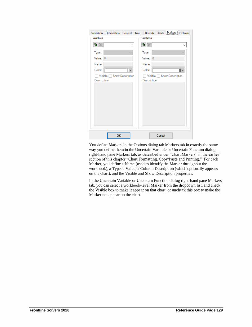
Frontline Solvers 2020 Reference Guide Page 129
You define Markers in the Options dialog tab Markers tab in exactly the same
way you define them in the Uncertain Variable or Uncertain Function dialog
right-hand pane Markers tab, as described under “Chart Markers” in the earlier
section of this chapter “Chart Formatting, Copy/Paste and Printing.” For each
Marker, you define a Name (used to identify the Marker throughout the
workbook), a Type, a Value, a Color, a Description (which optionally appears
on the chart), and the Visible and Show Description properties.
In the Uncertain Variable or Uncertain Function dialog right-hand pane Markers
tab, you can select a workbook-level Marker from the dropdown list, and check
the Visible box to make it appear on that chart, or uncheck this box to make the Marker not appear on the chart.

Frontline Solvers 2020 Reference Guide Page 130
Problem Tab
The Problem tab, shown below, displays certain statistics about the size of your
simulation model, and size limits supported by your Analytic Solver license.
Your license may allow a limited or unlimited number of uncertain variables,
uncertain functions, correlations among variables, Monte Carlo trials per
simulation, or simulations per run. These are shown in the Problem tab.
You can define more uncertain variables, uncertain functions, and correlations
than the maximums shown in the Problem tab, and you can set the Trials per
Simulation and Simulations to Run options to higher values than the maximums.
You can save workbooks with these settings. But when you attempt to run a
simulation, an error message will appear if you have exceeded one or more of
the maximums.
Contact Frontline Systems at [email protected] or (775) 831-0300 if you’d like
to upgrade your license to handle more uncertain variables, uncertain functions,
correlations, trials or simulations. It’s easy to upgrade – you simply enter a new
license code that Frontline will provide to you, as explained in the next section.
You can obtain a Risk Solver license that sets each maximum to “Unlimited,” as shown on the next page; but please bear in mind that, if you create a sufficiently
large model, you will encounter other practical limits such as the amount of
memory or time required to run simulations, or maximum size limits supported
by Microsoft Excel.
Controlling Use of Multiple Processor Cores Analytic Solver Desktop uses Windows facilities to create multiple “threads” of
execution that can be run on different processor cores. If you have other
compute-intensive applications running at the same time as Analytic Solver, you
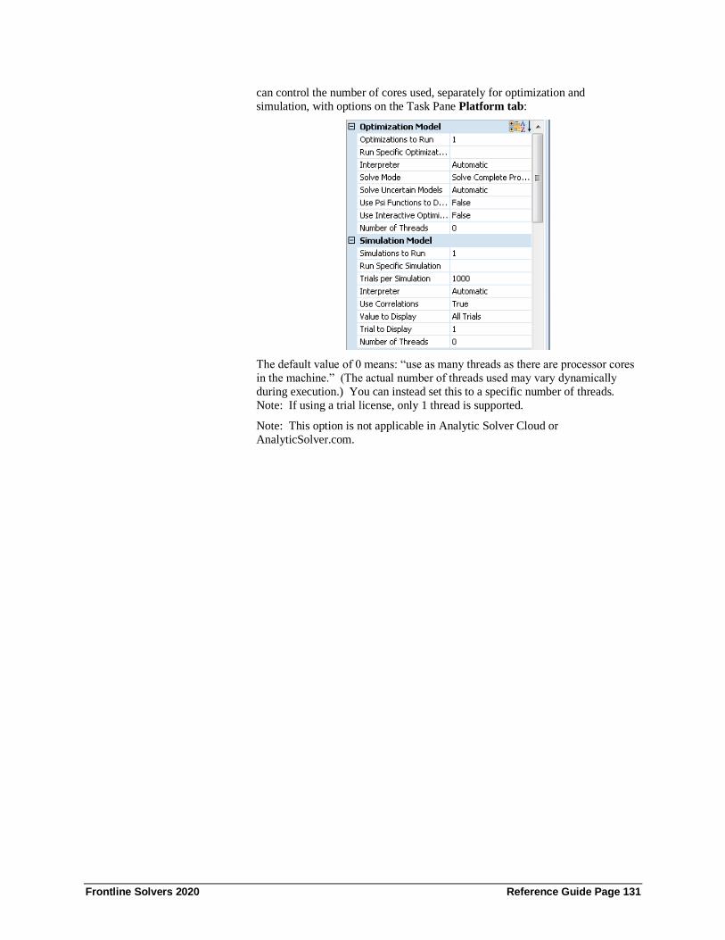
Frontline Solvers 2020 Reference Guide Page 131
can control the number of cores used, separately for optimization and
simulation, with options on the Task Pane Platform tab:
The default value of 0 means: “use as many threads as there are processor cores
in the machine.” (The actual number of threads used may vary dynamically
during execution.) You can instead set this to a specific number of threads.
Note: If using a trial license, only 1 thread is supported.
Note: This option is not applicable in Analytic Solver Cloud or
AnalyticSolver.com.
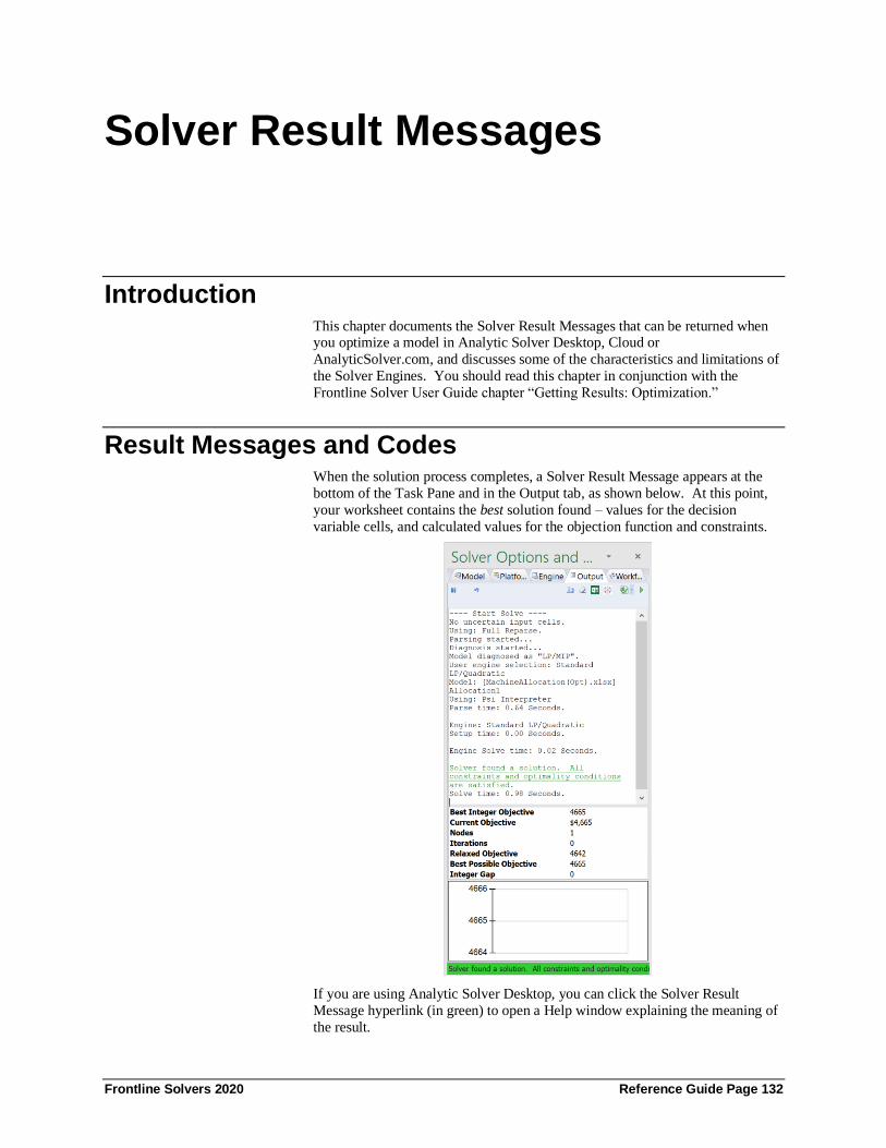
Frontline Solvers 2020 Reference Guide Page 132
Solver Result Messages
Introduction This chapter documents the Solver Result Messages that can be returned when you optimize a model in Analytic Solver Desktop, Cloud or
AnalyticSolver.com, and discusses some of the characteristics and limitations of
the Solver Engines. You should read this chapter in conjunction with the
Frontline Solver User Guide chapter “Getting Results: Optimization.”
Result Messages and Codes When the solution process completes, a Solver Result Message appears at the
bottom of the Task Pane and in the Output tab, as shown below. At this point,
your worksheet contains the best solution found – values for the decision
variable cells, and calculated values for the objection function and constraints.
If you are using Analytic Solver Desktop, you can click the Solver Result
Message hyperlink (in green) to open a Help window explaining the meaning of
the result.

Frontline Solvers 2020 Reference Guide Page 133
Each Solver Result Message has a corresponding integer result code, as
documented in this chapter. If you are controlling the Solver via a VBA
program and you’ve called the Problem.Solver.Optimize method, the Solver
object OptimizeStatus property holds this result code. If you’ve called the
legacy SolverSolve function, this function will return the integer result code.
Standard Solver Result Messages
The standard Solver included with Microsoft Excel can return the result codes
and messages numbered 0 through 13 (message -1 is returned only for Frontline
Systems product licensing problems). Analytic Solver returns the same integer
result codes and displays the same Solver Result Messages described in this
section, for all the conditions it shares with the standard Solver. But the
meanings of these messages have been generalized for the LP/Quadratic Solver,
SOCP Barrier Solver, nonlinear GRG Solver, Interval Global Solver, and
Evolutionary Solver, and the conditions they may return. Please see the
explanations of each message, especially for return code 0, “Solver found a
solution.”
Note the engines bundeled within the Analytic Solver family of products and the
Excel solver.
Analytic Solver Products
Excel Solver
GRG Nonlinear Engine GRG Nonlinear
Standard LP/Quadratic Engine Simplex LP
Standard Evolutionary Engine Evolutionary
Standard Interval Global Engine
Standard SOCP Barrier Engine
Large Scale Frontline Engines
Plug-in Solver engines return the same codes and display the same messages as
the built-in Solver engines whenever possible, but they can also return custom
result codes (starting with 1000) and display custom messages, as described in
their individual documentation. The Interval Global Solver can return three of
these custom result codes and messages, described at the end of this section.
-1. A licensing problem was detected, or your trial license has expired.
This message appears if Analytic Solver cannot find its licensing information, if
the licensing information is invalid, or if you have a time-limited evaluation
license that has expired. Click the Help button for further information about the
licensing problem. Please call Frontline Systems at (775) 831-0300, or send
email to us at [email protected] for further assistance.
0. Solver found a solution. All constraints and optimality conditions are satisfied.
This means that the Solver has found the optimal or “best” solution under the
circumstances. The exact meaning depends on whether you are solving a linear
or quadratic, smooth nonlinear, global optimization, or integer programming
problem, as outlined below. Solvers for non-smooth problems rarely if ever
display this message, because they have no way of testing the solution for true
optimality.
Frontline Solvers 2020 Reference Guide Page 134
If you are solving a linear programming problem or a convex quadratic
programming problem with the LP/Quadratic Solver, the Solver has found the
globally optimal solution: There is no other solution satisfying the constraints
that has a better value for the objective. It is possible that there are other
solutions with the same objective value, but all such solutions are linear combinations of the current decision variable values.
If you are solving a linear (LP), convex quadratic (QP) or quadratically
constrained (QCP), or second order cone programming (SOCP) problem with
the SOCP Barrier Solver, the Solver has found the globally optimal solution:
There is no other solution satisfying the constraints that has a better value for the
objective. It’s possible that there are other solutions with the same objective
value, but all such solutions are linear combinations of the current decision
variable values.
If you are solving a smooth nonlinear optimization problem with no integer
constraints, the GRG Solver has found a locally optimal solution: There is no
other set of values for the decision variables close to the current values and satisfying the constraints that yields a better value for the objective. In general,
there may be other sets of values for the variables, far away from the current
values, which yield better values for the objective and still satisfy the
constraints.
If you are using the Interval Global Solver (within the Analytic Solver products)
for global optimization of a smooth nonlinear problem with no integer
constraints, this means that the Solver has found the globally optimal solution:
There is no other solution satisfying the constraints that has a better value for the
objective. But this is subject to limitations due to the finite precision of
computer arithmetic – discussed below in “Limitations on Global Optimization”
– that can, in rare cases, cause the Solver to “miss” a feasible solution with an even better objective value.
If you are solving a mixed-integer programming problem (any problem with
integer constraints), this message means that the Branch & Bound method has
found a solution satisfying the constraints (including the integer constraints)
with the “best possible” objective value (but see the next paragraph). If the
problem is linear or quadratic, the true integer optimal solution has been found.
If the problem is smooth nonlinear, the Branch & Bound process has found the
best of the locally optimal solutions found for subproblems by the nonlinear
Solver.
In the standard Microsoft Excel Solver, this message also appears for mixed-integer problems where the Solver stopped because the solution was within the
range of the true integer optimal solution allowed by the Tolerance value in the
Solver Options dialog (5% by default). When the Branch & Bound process
stops due to a nonzero Tolerance without “proving optimality,” the message
“Solver found an integer solution within tolerance. All constraints are satisfied”
(result code 14) is displayed to distinguish this condition (see below).
1. Solver has converged to the current solution. All constraints are satisfied.
This means that Solver has found a series of “best” solutions that satisfy the constraints, and that have very similar objective function values; however, no
single solution strictly satisfies the Solver’s test for optimality. The exact
meaning depends on whether you are solving a smooth nonlinear problem with
the GRG Solver or the Interval Global Solver, or a non-smooth problem with the
Evolutionary Solver.
When the GRG Solver or the Interval Global Solver is being used, this message
means that the objective function value is changing very slowly as the Solver

Frontline Solvers 2020 Reference Guide Page 135
progresses from point to point. More precisely, the Solver stops if the absolute
value of the relative (i.e. percentage) change in the objective function, in the last
few iterations, is less than the Convergence tolerance on the Task Pane Engine
tab. A poorly scaled model is more likely to trigger this stopping condition,
even if Use Automatic Scaling is set to True on the Task Pane Engine tab. If you are sure that your model is well scaled, you should consider why it is that
the objective function is changing so slowly. For more information, see the
discussion of “GRG Solver Stopping Conditions” below.
When the Evolutionary Solver is being used, this message means that the
“fitness” of members of the current population of candidate solutions is
changing very slowly. More precisely, the Evolutionary Solver stops if 99% or
more of the members of the population have “fitness” values whose relative (i.e.
percentage) difference is less than the Convergence tolerance on the Task Pane
Engine tab. The “fitness” values incorporate both the objective function and a
penalty for infeasibility, but since the Solver has found some feasible solutions,
this test is heavily weighted towards the objective function values. If you believe that the Solver is stopping prematurely when this test is satisfied, you
can make the Convergence tolerance smaller, but you may also want to increase
the Mutation Rate and/or the Population Size, in order to increase the diversity
of the population of trial solutions. For more information, see the discussion of
“Evolutionary Solver Stopping Conditions” below.
2. Solver cannot improve the current solution. All constraints are satisfied.
This means that the Solver has found solutions that satisfy the constraints, but it
has been unable to further improve the objective, even though the tests for optimality (“Solver found a solution”) and convergence (“Solver converged to
the current solution”) have not yet been satisfied. The exact meaning depends
on whether you are solving a smooth nonlinear problem with the GRG Solver, a
global optimization problem with the Interval Global Solver, or a non-smooth
problem with the Evolutionary Solver.
When the GRG Solver is being used, this message occurs very rarely. It means
that the model is degenerate and the Solver is probably cycling. One possibility
worth checking is that some of your constraints are redundant, and should be
removed. For more information, see the discussion of “GRG Solver Stopping
Conditions” below.
When the Interval Global Solver is being used, this message is more common. It means that the Solver has not found an “improved global solution” (a feasible
solution with an objective value better than the currently best known solution),
in the amount of time specified for the Max Time without Improvement option
Task Pane Engine tab. The reported solution is the best one found so far, but the
search space has not been fully explored. For more information, see the
discussion of “Interval Global Solver Stopping Conditions” below. If you
receive this message, and you are willing to spend more solution time to have a
better chance of “proving” global optimality, increase the value of the Max
Time without Improvement option.
When the Evolutionary Solver is being used, this message is much more
common. It means that the Solver has been unable to find a new, better member of the population whose “fitness” represents a relative (percentage)
improvement over the current best member’s fitness of more than the Tolerance
value on the Limit Options dialog tab, in the amount of time specified by the
Max Time without Improvement option in the same dialog. Since the
Evolutionary Solver has no way of testing for optimality, it will normally stop
with either “Solver converged to the current solution” or “Solver cannot
improve the current solution” if you let it run for long enough. If you believe

Frontline Solvers 2020 Reference Guide Page 136
that this message is appearing prematurely, you can either make the Tolerance
value smaller (or even zero) or increase the amount of time allowed by the Max
Time without Improvement option. For more information, see the discussion of
“Evolutionary Solver Stopping Conditions” below.
3. Stop chosen when the maximum iteration limit was reached.
This message appears when (i) the Solver has completed the maximum number
of iterations, or trial solutions, allowed for the Iterations option in the Task Pane
Engine tab and (ii) you clicked on the Stop button when the Solver displayed the
Show Trial Solution dialog. You may increase the value in the Iterations box, or
click on the Continue button instead of the Stop button in the Show Trial
Solution dialog. But you should also consider whether re-scaling your model or
adding constraints might reduce the total number of iterations required.
If you are solving a mixed-integer programming problem (any problem with integer constraints), this message is relatively unlikely to appear. The
Evolutionary Solver uses the Max Subproblems and Max Feasible Solutions
options on the Limit Options dialog tab, and the Branch & Bound method
(employed by the other Solver engines on problems with integer constraints)
uses the Max Subproblems and Max Integer Solutions options on the Integer
Options dialog tab, to control the overall solution process. The count of
iterations against which the Iteration limit is compared is reset on each new
subproblem, so this limit usually is not reached.
If you are using Stochastic Decomposition to solve for a stochastic linear model,
this status will be returned if the algorithm performs over 5,000 iterations.
4. The objective (Set Cell) values do not converge.
This message appears when the Solver is able to increase (if you are trying to
Maximize) or decrease (for Minimize) without limit the value calculated by the
objective or Set Cell, while still satisfying the constraints. Remember that, if
you’ve selected Minimize, the objective may take on negative values without
limit unless this is prevented by the constraints or bounds on the variables. Set
the Assume Non-Negative option to True on the Task Pane Engine tab to
impose >= 0 bounds on all variables.
If the objective is a linear function of the decision variables, it can always be
increased or decreased without limit (picture it as a straight line), so the Solver
will seek the extreme value that still satisfies the constraints. If the objective is a
nonlinear function of the variables, it may have a “natural” maximum or
minimum (for example, =A1*A1 has a minimum at zero), or no such limit (for
example, =LOG(A1) increases without limit).
If you receive this message, you may have forgotten a constraint, or failed to
anticipate values for the variables that allow the objective to increase or decrease
without limit. The final values for the variable cells, the constraint left hand
sides and the objective should provide a strong clue about what happened.
The Evolutionary Solver never displays this message, because it has no way of systematically increasing (or decreasing) the objective function, which may be
non-smooth. If you have forgotten a constraint, the Evolutionary Solver may
find solutions with very large (or small) values for the objective – thereby
making you aware of the omission – but this is not guaranteed.
5. Solver could not find a feasible solution.
This message appears when the Solver could not find any combination of values
for the decision variables that allows all of the constraints to be satisfied
simultaneously. If you are using the LP/Quadratic Solver or the SOCP Barrier

Frontline Solvers 2020 Reference Guide Page 137
Solver, and the model is well scaled, the Solver has determined for certain that
there is no feasible solution.
If you are using the nonlinear GRG Solver, the GRG method (which always
starts from the initial values of the variables) was unable to find a feasible
solution; but there could be a feasible solution far away from these initial values, which the Solver might find if you run it with different initial values for the
variables.
If you are using the Interval Global Solver, this message means that the Solver
could find no feasible solutions after a systematic exploration of the search
space. The Interval Global Solver is designed to “prove feasibility” as well as
global optimality, and there is very likely no feasible solution; but this is subject
to limitations due to the finite precision of computer arithmetic – discussed
below in “Limitations on Global Optimization” – that can, in rare cases, cause
the Solver to “miss” a solution.
If you are using the Evolutionary Solver, the evolutionary algorithm was unable to find a feasible solution; it might succeed in finding one if you run it with
different initial values for the variables and/or increase the Precision value on
the Task Pane Engine tab (which reduces the infeasibility penalty, thereby
allowing the evolutionary algorithm to explore more “nearly feasible” points).
If you are solving a problem with chance constraints using simulation
optimization, this message means that the Solver could find no solution that
satisfies these constraints to the chance measures (such as 95%) that you
specified. If you ‘relax’ the chance measures (to say 90%) and solve again, it’s
possible that a feasible solution will be found. For robust optimization, see
result codes 26 through 29.
In any case, you should first look for conflicting constraints, i.e. conditions that cannot be satisfied simultaneously. Most often this is due to choosing the wrong
relation (e.g. <= instead of >=) on an otherwise appropriate constraint. The
easiest way to do this is to select the Feasibility Report, shown in the Reports list
box when this message appears, and click OK. (This report can take time for the
LP/Quadratic Solver or SOCP Barrier Solver, more time for the GRG Solver,
and much more time for the Interval Global Solver; it is not available for the
Evolutionary Solver.) For an example of using the Feasibility Report to
diagnose an infeasible solution, see “The Feasibility Report” in the chapter
“Solver Reports.”
6. Solver stopped at user’s request.
This message appears only if you press ESC or the Pause icon on the Output tab
of the Solver Task Pane to display the Show Trial Solution dialog, and then
click on the Stop button. If you are controlling the Solver from a VBA program,
remember that the user may press ESC while your VBA program is running.
You can write VBA code to disable the ESC key, or – better – define a VBA
function that the Solver will call instead of displaying the Show Trial Solution
dialog (an Evaluator in the object-oriented API, or a ShowRef function
argument in the “traditional” SolverSolve function.). Be sure to test for this
OptimizeStatus or integer result (6) in your VBA code, and take action appropriate for your model.
7. The linearity conditions required by this Solver engine are not satisfied.
In the standard Excel Solver, this message is worded “The conditions for
Assume Linear Model are not satisfied,” and it can appear only when the
Assume Linear Model box in the Solver Options dialog is checked.

Frontline Solvers 2020 Reference Guide Page 138
In Analytic Solver Comprehensive, Analytic Solver Optimization, Analytic
Solver Upgrade or Analytic Solver Basic, this message appears if you’ve
selected the LP/Quadratic Solver and the Solver’s tests determine that the
constraints are not linear functions of the variables or the objective is not a linear
or convex quadratic function of the variables; or if you’ve selected the SOCP Barrier Solver and the Solver’s tests determine that the constraints or the
objective are not linear or convex quadratic functions of the variables. To
understand exactly what is meant by a linear or quadratic function, read the
section “Quadratic Functions” in the chapter “Mastering Conventional
Optimization Concepts.”
Field-installable Solver engines can also display this message. If you’ve
selected the Large-Scale LP/QP Solver or the XPRESS Solver Engine, this
message appears if the constraints are not linear functions of the variables or the
objective is not a linear or convex quadratic function of the variables. If you’ve
selected the MOSEK Solver Engine (Standard Edition), this message appears if
the constraints or the objective are not linear or convex quadratic functions of the variables.
If you receive this message, examine the formulas for the objective and
constraints for nonlinear or non-smooth functions or operators applied to the
decision variables. Simply follow the steps in “Transformation Options” in the
chapter “Platform Option Reference” to pinpoint the exact cell formulas that
aren’t linear. If you have Analytic Solver Upgrade and you've reach the limits
of your license, select and examine the Structure Report to determine which
functions or variables in your model are not linear; see “The Structure Report”
in the chapter “Solver Reports.”
8. The problem is too large for Solver to handle.
This message – or the more specific message Too many adjustable cells, Too
many constraints, or Too many integer adjustable cells – appears when the
Solver determines that your model is too large for the Solver engine that is
selected (in the Solver engine dropdown list) at the time you click Solve. You’ll
have to select – or possibly install – another Solver engine appropriate for your
problem, or else reduce the number of variables, constraints, or integer variables
to proceed.
You can check the size (the number of variables, constraints, bounds, and
integers) of the problem you have defined, and compare it to the size limits of the Solver engine you are using, by scrolling down to the bottom of the Task
Pane Engine tab. The problem size is also displayed in the Solver Model dialog.
9. Solver encountered an error value in a target or constraint cell.
This message appears when the Solver recalculates your worksheet using a new
set of values for the decision variables (Changing Cells), and discovers an error
value such as #VALUE!, #NUM!, #DIV/0! or #NAME? in the cell calculating
the objective (Set Cell) or one of the constraints. Inspecting the worksheet for
error values like these will usually indicate the source of the problem. If you’ve entered formulas for the right hand sides of certain constraints, the error might
have occurred in one of these formulas rather than in a cell on the worksheet.
For this and other reasons, it’s better to use only constants and cell references on
the right hand sides of constraints.
If you see #VALUE!, #N/A or #NAME?, look for names or cell references to
rows or columns that you have deleted. If you see #NUM! or #DIV/0!, look for
unanticipated values of the decision variables which lead to arguments outside
the domains of your functions – such as a negative value supplied to SQRT. You
Frontline Solvers 2020 Reference Guide Page 139
can often add constraints to avoid such domain errors; if you have trouble with a
constraint such as $A$1 >= 0, try a constraint such as $A$1 >= 0.0001 instead.
In the Analytic Solver products, when the Polymorphic Spreadsheet Interpreter
is used (Solve With = PSI Interpreter), a more specific message usually appears
instead of “Solver encountered an error value in a (nonspecific) target or constraint cell.” At a minimum, the message will say “Excel error value
returned at cell address,” where address (e.g. Sheet1!$A$1) tells you exactly
where the error was encountered. Other messages may tell you more about the
error. The general form of the message is:
Error condition at cell address. Edit your formulas, or use Excel Interpreter
in the Solver Model dialog. Error condition is one of the following:
Floating point overflow Invalid token
Runtime stack overflow Decision variable with formula
Runtime stack empty Decision variable defined more than once
String overflow Missing Diagnostic/Memory evaluation
Division by zero Unknown function
Unfeasible argument Unsupported Excel function
Type mismatch Excel error value returned
Invalid operation Non-smooth special function
See also result code 21, “Solver encountered an error computing derivatives,”
and result code 12, with messages that can appear when the Interpreter first
analyzes the formulas in your model (when you click the Check Model or Solve
button).
“Floating point overflow” indicates that the computed value is too large to
represent with computer arithmetic; “String overflow” indicates that a string is
too long to be stored in a cell. “Division by zero” would yield #DIV/0! on the
worksheet, and “Unfeasible argument” means that an argument is outside the
domain of a function, such as =SQRT(A1) where A1 is negative.
“Unknown function” appears for functions whose names are not recognized by
the Interpreter, such as user-written functions in VBA. “Unsupported Excel
function” appears for the few functions that the Interpreter recognizes but does
not support. The PSI Interpreter does not support the following functions:
Call(), Cell(), CubeX(), EuroConvert(), GetPivotData(), HyperLink(), Info(),
RegisterID(), and SqlRequest().
The Evolutionary Solver and the field-installable OptQuest Solver rarely, if
ever, display this message – since they maintain a population of candidate
solutions and can generate more candidates without relying on derivatives, they
can simply discard trial solutions that result in error values in the objective or
the constraints. If you have a model that frequently yields error values for trial
solutions generated by the Solver, and you are unable to correct or avoid these
error values by altering your formulas or by imposing additional constraints, you
can still use the Evolutionary Solver or OptQuest Solver to find (or make
progress towards) a “good” solution.
10. Stop chosen when the maximum time limit was reached.
This message appears when (i) the Solver has run for the maximum time
(number of seconds) allowed in the Max Time field on the Engine tab of the
Solver Task Pane and (ii) you clicked on the Stop button when the Solver
displayed the Show Trial Solution dialog. You may increase the value in the
Max Time box or click on the Continue button instead of the Stop button in the
Show Trial Solution dialog. But you should also consider whether re-scaling
your model or adding constraints might reduce the total solution time required.

Frontline Solvers 2020 Reference Guide Page 140
11. There is not enough memory available to solve the problem.
This message appears when the Solver could not allocate the memory it needs to solve the problem. However, since Microsoft Windows supports a “virtual
memory” much larger than your available RAM by swapping data to your hard
disk, before you see this message you are likely to notice that solution times
have greatly slowed down, and the hard disk activity light in your PC is
flickering during the solution process, or even when “Analyzing Solver Model,”
“Diagnosing Problem Function” or “Setting Up Problem” appears on the Excel
status bar.
The Polymorphic Spreadsheet Interpreter in Analytic Solver can use a
considerable amount of memory, when you solve a problem by clicking the
Optimize icon on the Ribbon or the Solve icon on the Solver Task Pane, and
when you click Optimize – Analyze Original Model on the Ribbon. You can progressively reduce the memory used by the Interpreter by taking the following
actions in order, using the Solver Model dialog:
1. Check the Sparse box in the Advanced options group.
2. Set the Check For option to Gradients.
3. Set the Solve With option to Excel Interpreter.
When Solve With = Excel Interpreter, the PSI Interpreter is not used and does
not use any memory; any further problems are due to memory demands of the
Solver engines, Microsoft Excel and Windows. You can save some memory by
closing any Windows applications other than Excel, closing programs that run in
the System Tray, and closing any Excel workbooks not needed to solve the problem.
12. Another Excel instance is using SOLVER32.DLL. Try again later.
This message appeared in early versions of the standard Excel Solver; it does
not occur in modern versions of Microsoft Excel and Windows. In the Analytic
Solver products, result code 12 is associated with the message “Error condition
at cell address. Edit your formulas, or use Excel Interpreter in the Solver Model
dialog,” which is explained in the next section.
13. Error in model. Please verify that all cells and constraints are valid.
This message means that the internal “model” (information about the variable
cells, objective, constraints, Solver options, etc.) is not in a valid form. An
“empty” or incomplete Solver model, perhaps one with no objective and no
constraints other than bounds on the variables, can cause this message to appear.
You might also receive this message if you’ve modified the values of certain
hidden defined names used by the Solver, either interactively or in a VBA
program. To guard against this possibility, you should avoid using any defined
names beginning with “solver” in your own application.
Analytic Solver Result Messages
Analytic Solver may return the result codes and display the messages in the
previous section, as well as the result codes and messages explained below.
These result codes and messages are related to capabilities of Analytic Solver:
the Polymorphic Spreadsheet Interpreter, advanced methods for mixed-integer
problems and global optimization problems, new types of constraints such as
alldifferent and conic, and optimization of models that involve uncertainty.

Frontline Solvers 2020 Reference Guide Page 141
12. Error condition at cell address. Edit your formulas, or use Excel Interpreter in the Solver Model dialog.
This message appears when the Polymorphic Spreadsheet Interpreter first
analyzes the formulas in your model after you click the Solve button or the
Check Model button in the Solver Model dialog. Address is the worksheet
address of the cell (in Sheet1!$A$1 form) where the error was encountered, and
Error condition is one of the following:
OLE error Missing (
Invalid token Missing )
Unexpected end of formula Wrong number of parameters
Invalid array Type mismatch
Invalid number Code segment overflow
Invalid fraction Expression too long
Invalid exponent Symbol table full
Too many digits Circular reference
Real constant out of range External name
Integer constant out of range Multi-area not supported
Invalid expression Non-smooth function
Undefined identifier Unknown function
Range failure Loss of significance
Many of these messages will never appear as long as you entered your formulas
in the normal way through Microsoft Excel, because Excel “validates” your
formulas and displays its own error messages as soon as you complete formula
entry. Some of the messages you may encounter are described in the following paragraphs.
Undefined identifier appears if you’ve used a name or identifier (instead of a
cell reference such as A1) in a formula, and that name was not defined using the
Insert Name Define… or Insert Name Create… commands in Excel, this
message will appear. The “labels in formulas” feature was dropped in Excel
2007, and the Interpreter does not support this use of labels in formulas. You
should define these labels with the Insert Name Define… or Insert Name
Create… commands, or else set Solve With = Excel Interpreter to avoid using
the PSI Interpreter.
Circular reference appears if Excel has already warned you about a circular reference in your formulas, and it can also appear if you’ve used formulas in a
“potentially circular” way. (For example, if cells A1:A2 contain {=1+B1:B4}
and cells B3:B4 contain {=1+A1:A4}, Excel doesn’t consider this a circular
reference, but the PSI Interpreter does.) If you must use circular references in
your model, in the Platform tab of the Task Pane, change the Interpreter option
from “Automatic” to “Excel Interpreter” so you avoid using the PSI Interpreter.
External name appears if your formulas use references to cells in other
workbooks (not just other worksheets), and the Interpreter is unable to open
those workbooks. You should ensure that the external workbooks are in the
same folder as the Solver workbook, or for better performance, move or copy
the worksheets you need into the workbook containing the Solver model.
Multi-area not supported or Missing ) appears if your formulas or defined
names use multiple selections such as (A1:A5,C1:H1). While the Interpreter
does accept argument lists consisting of single selections, such as
=SUM(A1:A5,C1:H1), it does not accept multiple selections for defined names,
or for single arguments such as =SUMSQ((A1:A5,C1:H1), (B1:B5,C2:H2)). If
you must use such multiple selections, you’ll have to set Solve With = Excel
Interpreter.

Frontline Solvers 2020 Reference Guide Page 142
Note: As mentioned above, in the standard Excel Solver, result code 12 was
associated with the message “Another Excel instance is using SOLVER32.DLL.
Try again later,” which does not occur in modern versions of Excel and
Window.
13. Error in model. Please verify that all cells and constraints are valid.
As above, means that the internal “model” (information about the variable cells,
objective, constraints, Solver options, etc.) is not in a valid form. An “empty” or
incomplete Solver model, perhaps one with no objective and no constraints other
than bounds on the variables, can cause this message to appear. You might also
receive this message if you’ve modified the values of certain hidden defined
names used by the Solver, either interactively or in a VBA program. To guard
against this possibility, you should avoid using any defined names beginning
with “solver” in your own application.
14. Solver found an integer solution within tolerance. All constraints are satisfied.
If you are solving a mixed-integer programming problem (any problem with
integer constraints) using Analytic Solver or a subset product (Analytic Solver
Optimization, Analytic Solver Upgrade or Analytic Solver Basic) with a non-
zero value for the integer Tolerance setting in the Integer section of the Task
Pane Engine tab, the Branch & Bound method has found a solution satisfying
the constraints (including the integer constraints) where the relative difference of
this solution’s objective value from the true optimal objective value does not exceed the integer Tolerance setting. (For more information, see “Integer
Section of the Engine Tab Options” in the chapter “Solver Engine Option
Reference.”) This may actually be the true integer optimal solution; however,
the Branch & Bound method did not take the extra time to search all possible
remaining subproblems to “prove optimality” for this solution. If all
subproblems were explored (which can happen even with a non-zero Tolerance
in some cases), Analytic Solver will produce the message “Solver found a
solution. All constraints are satisfied” (result code 0, shown earlier in this
section).
15. Stop chosen when the maximum number of feasible [integer] solutions was reached.
If you are using the Evolutionary Solver, this message appears when (i) the
Solver has found the maximum number of feasible solutions (values for the
variables that satisfy all constraints) allowed by the Max Feasible Sols options
setting on the Engine tab of the Solver Task Pane and (ii) you clicked on the
Stop button when the Solver displayed the Show Trial Solution dialog. You may
increase the value in the Max Feasible Sols box, or click on the Continue button
instead of the Stop button in the Show Trial Solution dialog to continue the
solution process.
If you are using one of the other Solver engines on a problem with integer con-straints, this message appears when (i) the Solver has found the maximum
number of integer solutions (values for the variables that satisfy all constraints,
including the integer constraints) allowed by the Max Integer Sols option setting
on the Engine tab of the Solver Task Pane and (ii) you clicked on the Stop
button when the Solver displayed the Show Trial Solution dialog. You may
increase the value for the Max Integer Sols option, or click on the Continue
button instead of the Stop button in the Show Trial Solution dialog. But you
should also consider whether the problem is formulated correctly, and whether
you can add constraints to “tighten” the formulation. If you are using the
LP/Quadratic Solver in Analytic Solver Comprehensive or Analytic Solver
Optimization, try activating more Cuts and Heuristics in the Integer section of
the Task Pane Engine tab.

Frontline Solvers 2020 Reference Guide Page 143
16. Stop chosen when the max number of feasible [integer] subproblems was reached.
If you are using the Evolutionary Solver, this message appears when (i) the Solver has explored the maximum number of subproblems allowed in the Max
Subproblems option field on the Engine tab of the Solver Task Pane and (ii) you
clicked the Stop button when the Solver displayed the Show Trial Solution
dialog. You may increase the value for the Max Subproblems option, or click on
the Continue button instead of the Stop button in the Show Trial Solution dialog
to continue the solution process.
If you are using one of the other Solver engines on a problem with integer con-
straints, this message appears when (i) the Solver has explored the maximum
number of integer subproblems (each one is a “regular” Solver problem with
additional bounds on the variables) allowed in the Max Subproblems option
field on the Engine tab of the Solver Task Pane and (ii) you clicked on the Stop button when the Solver displayed the Show Trial Solution dialog. You may
increase the value for Max Subproblems, or click on the Continue button instead
of the Stop button in the Show Trial Solution dialog. But you should also
consider whether the problem is formulated correctly, and whether you can add
constraints to “tighten” the formulation. If you are using the LP/Quadratic
Solver in Analytic Solver Comprehensive or Analytic Solver Optimization, try
activating more Cuts and Heuristics in the Integer section on the Task Pane
Engine tab.
17. Solver converged in probability to a global solution.
If you are using the multistart methods for global optimization, with either the
nonlinear GRG Solver, or a field-installable nonlinear Solver engine, this
message appears when the multistart method’s Bayesian test has determined that
all of the locally optimal solutions have probably been found; the solution
displayed on the worksheet is the best of these locally optimal solutions, and is
probably the globally optimal solution to the problem.
The Bayesian test initially assumes that the number of locally optimal solutions
to be found is equally likely to be 1, 2, 3, … etc. up to infinity, and that the
relative sizes of the regions containing each locally optimal solution follow a
uniform distribution. After each run of the nonlinear GRG Solver, or field-installable Solver engine, an updated estimate of the most probable total number
of locally optimal solutions is computed, based on the number of subproblems
solved and the number of locally optimal solutions found so far. When the
number of locally optimal solutions actually found so far is within one unit of
the most probable total number of locally optimal solutions, the multistart
method stops and displays this message.
18. All variables must have both upper and lower bounds.
If you are using the Interval Global Solver or the OptQuest Solver, this message appears if you have not defined lower and upper bounds on all of the decision
variables in the problem. If you are using the Evolutionary Solver or the
multistart methods for global optimization, and you have checked the box
“Require Bounds on Variables” on the Engine tab of the Solver Task Pane (it is
set to True by default), this message will also appear. You should add the
missing bounds and try again. Lower bounds of zero can be applied to all
variables by setting the Assume Non-Negative option to True on the Engine tab
in the Solver Task Pane or by entering “0” for the Decision Vars Lower option
on the Platform tab of the Solver Task Pane. Non-zero upper or lower bounds
can be added as constraints in the Model tab of the Solver Task Pane or by
entering a value for Decision Vars Upper or Decision Vars Lower on the
Platform tab in the Solver Task Pane. You must define bounds on all variables

Frontline Solvers 2020 Reference Guide Page 144
in order to use the Interval Global Solver or the OptQuest Solver. For the
Evolutionary Solver or the multistart methods, such bounds are not absolutely
required (you can uncheck the box “Require Bounds on Variables”), but they are
a practical necessity if you want the Solver to find good solutions in a
reasonable amount of time.
19. Variable bounds conflict in binary or alldifferent constraint.
This message appears if you have both a binary or alldifferent constraint on a
decision variable and a <= or >= constraint on the same variable (that is
inconsistent with the binary or alldifferent specification), or if two or more of
the same decision variables appear in more than one alldifferent constraint.
Binary integer variables always have a lower bound of 0 and an upper bound of
1; variables in an alldifferent group always have a lower bound of 1 and an
upper bound of N, where N is the number of variables in the group. You should check that the binary or alldifferent constraint is correct, and ensure that
alldifferent constraints apply to non-overlapping groups of variables. If a <= or
>= constraint causes the conflict, remove it if possible and try to solve again.
20. Lower and upper bounds on variables allow no feasible solution.
This message appears if you’ve defined lower and upper bounds on a decision
variable, where the lower bound is greater than the upper bound. This
(obviously) means there can be no feasible solution, but most Solver engines
will detect this condition before even starting the solution process, and display this message instead of “Solver could not find a feasible solution” to help you
more quickly identify the source of the problem. If you have defined your
bounds and other constraints in uniform blocks, the lower and upper bounds on a
given range of cells will appear consecutively in the Solver Parameters dialog
outlined list (where they are grouped and sorted), making it easy to spot the
inconsistent bounds.
21. Solver encountered an error computing derivatives. Consult Help on Derivatives, or use Excel Interpreter in the Solver Model dialog.
This message appears when the Polymorphic Spreadsheet Interpreter in Analytic
Solver is being used (Solve With = PSI Interpreter), and the Interpreter
encounters an error when computing derivatives via automatic differentiation.
The most common cause of this message is a non-smooth function in your
objective or constraints, for which the derivative is undefined. But in general,
automatic differentiation is somewhat more strict than finite differencing: As a
simple example, =SQRT(A1) evaluated at A1=0 will yield this error message
when the Solver is using automatic differentiation (since the derivative of the
SQRT function is algebraically undefined at zero), but it won’t yield an error
when Solve With = Excel Interpreter and the Solver is using finite differencing.
If you receive this message, create a Structure Report to pinpoint the exact cell
formulas that are non-smooth, and confirm that the “Nonsmooth Model
Transformation” option on the Task Pane Platform tab is set to “Automatic” to
eliminate the non-smooth functions automatically. If you can’t modify your
formulas to eliminate the non-smooth functions, your options are to (i) use a
Solver engine, such as the Evolutionary Solver or the OptQuest Solver, that
doesn’t require derivatives, or (ii) set Solve With = Excel Interpreter and solve
the problem using finite differencing.
22. Variable appears in more than one cone constraint.
This message appears when you click Solve if the same decision variable
appears in more than one cone constraint. You can define as many cone
Frontline Solvers 2020 Reference Guide Page 145
constraints as you want, but each one must constrain a different group of
decision variables.
If you receive this message, examine the constraints listed under “Conic” in the
Task Pane Model tab to find the variable cell(s) that appear in more than one
cone constraint. You’ll have to modify the problem to eliminate this overlap.
23. Formula depends on uncertainties, must be summarized or transformed. Learn more using the Solver Model dialog Diagnosis tab.
You may see this message when you are first starting to build optimization
models that include uncertainty – consider it part of the “learning experience.”
You’ll be defining constraints or an objective, computed by formulas that depend on uncertain parameters: Each such formula represents an array of
sample values, one for each realization of the uncertainties. For your model to
be well-defined, the objective or constraint must either be summarized to a
single value (such as a mean or percentile value) or transformed into a set of
single-valued constraints (through an automatic transformation in the Solver
Model dialog).
To correct the problem, you can (i) use the Task Pane Model tab to define the
constraint as a chance constraint or the objective as an expected value or risk
measure objective, or (ii) edit the formula so that its ‘top level’ value is
computed by a PSI Statistics function such as PsiMean() or PsiPercentile(). It’s
important to understand why you need to summarize or transform a formula that depends on uncertainties: To learn more, read the chapter “Mastering Stochastic
Optimization Concept” in the Analytic Solver User Guide.
24. Excel Interpreter can only handle normal objective and constraints.
This message appears when you click Solve if you’ve used the Solver
Parameters dialog to define a chance constraint or an expected value or risk
measure objective, but you’ve selected the Excel Interpreter on the Options tab
of the Solver Model dialog. The PSI Interpreter can handle these types of
constraints or objectives, without using PSI Statistics functions on the
worksheet. But the Excel Interpreter cannot do this; you must use PSI Statistics functions to summarize the array of sample values represented by the objective
and each constraint that depends on uncertainty. For example, you can compute
a VaR-type chance constraint with a PsiPercentile() function. If you are using
Analytic Solver Upgrade, the Excel Interpreter is your only option, so you must
use PSI Statistics functions on the worksheet.
25. Simulation optimization doesn't handle models with recourse decisions.
This message appears when you click Solve if you’ve defined a recourse
decision variable, but you’ve set “Solve Uncertain Models” to “Simulation Optimization” on the Platform tab on the Solver Task Pane. Simulation
optimization, as defined in the academic literature and as implemented by
Analytic Solver doesn’t support the concept of recourse decision variables.
However, Analytic Solver enables you to solve problems using stochastic
programming and robust optimization methods, both of which do support
recourse decision variables. To learn more, read the chapter “Mastering
Stochastic Optimization Concepts” in the Analytic Solver User Guide.
26. Solver could not find a feasible solution to the robust chance constrained problem.
This message may appear when you solve a model with uncertainty and chance
constraints using robust optimization. When you do this, the Solver transforms
your original model with uncertainty into a robust counterpart model that is a
conventional optimization problem without uncertainty.

Frontline Solvers 2020 Reference Guide Page 146
This message means that the Solver could not find a feasible solution to the
robust counterpart problem. It does not necessarily mean that there is no
feasible solution to the original problem; the robust counterpart is an
approximation to the problem defined by your chance constraints that may yield
conservative solutions which over-satisfy the chance constraints.
When this message appears, there may be an option to “Auto Adjust Chance
Constraints” – a small white button containing a green arrow, as shown below
for result code 27. Your simplest course of action is to select this option and
click OK. The Solver will then re-solve the problem, automatically adjusting
the sizes of robust optimization uncertainty sets created for the chance
constraints, in an effort to find a feasible solution.
If you don’t see the option “Auto Adjust Chance Constraints,” this normally
means that the automatic improvement algorithm has already been tried
(possibly because the “Auto Adjust Chance” option is set in the Task Pane), and
this algorithm was unable to find a feasible solution. In this case, you should
proceed as described for result code 5, “Solver could not find a feasible solution:” Look for conflicting constraints, i.e. conditions that cannot be
satisfied simultaneously, perhaps due to choosing the wrong relation (e.g. <=
instead of >=) on an otherwise appropriate constraint.
27. Solver found a conservative solution to the robust chance constrained problem. All constraints are satisfied.
This message may appear when you solve a model with uncertainty and chance
constraints using robust optimization. When you do this, the Solver transforms
your original model with uncertainty into a robust counterpart model that is a
conventional optimization model without uncertainty.
The message means that the Solver found an optimal solution to the robust
counterpart model, but when this solution was tested against your original
model (using Monte Carlo simulation to test satisfaction of the chance
constraints), the solution over-satisfied the chance constraints; this normally
means that the solution is ‘conservative’ and the objective function value can be
further improved.
When this message appears, there may be an option to “Auto Adjust Chance Constraints” – a small white button containing a green arrow, as shown below.
Your simplest course of action is to select this option and click OK. The Solver
will then re-solve the problem, automatically adjusting the sizes of robust
optimization uncertainty sets created for the chance constraints, in an effort to
improve the solution.
If you don’t see the option “Auto Adjust Chance Constraints,” this normally
means that the automatic improvement algorithm has already been tried
(possibly because the “Auto Adjust Chance” option is set in the Task Pane.
An alternative course of action is to manually adjust the Chance measures of
selected chance constraints, and re-solve the problem. The automatic improvement algorithm uses general-purpose methods to find an improved
solution; you may be able to do better by adjusting Chance measures based on
your knowledge of the problem.
28. Solver has converged to the current solution of the robust chance constrained problem. All constraints are satisfied.
This message may appear when you solve a model with uncertainty and chance constraints using robust optimization, and you’ve checked the box “Auto Adjust
Chance” in the Solver Model dialog Stochastic tab, or you’ve previously viewed

Frontline Solvers 2020 Reference Guide Page 147
the Solver Results dialog and selected the “Auto Adjust Chance Constraints”
option. It means that the Solver has found the best ‘improved solution’ it can;
the normal constraints are satisfied, and the chance constraints are satisfied to
the Chance level that you specified in the Solver Parameters dialog.
This is usually a very good solution, but it does not rule out the possibility that you may be able to find an even better solution by manually adjusting Chance
measures based on your knowledge of the problem, and re-solving.
29. Solver cannot improve the current solution of the robust chance constrained problem. All constraints are satisfied.
This message may appear when you solve a model with uncertainty and chance constraints using robust optimization, and you’ve checked the box “Auto Adjust
Chance” in the Solver Model dialog Platform tab, or you’ve previously viewed
the Solver Results dialog and selected the “Auto Adjust Chance Constraints”
option. It means that the Solver could not find an improved solution that
satisfies all of the chance constraints to the Chance level that you specified in
the Solver Parameters dialog. Typically in this case, some of the chance
constraints will be satisfied to the level you specified, or even over-satisfied, but
others will be under-satisfied.
You may find that the solution is acceptable, but if the chance constraints must
be satisfied to the level you specified, further work will be required. You may be
able to find an improved solution by manually adjusting Chance measures based on your knowledge of the problem, and re-solving.
30. Stochastic Decomposition cannot be used because the objective depends on uncertain variables.
This result may be returned when you solve a model with uncertainty when
Solve Uncertain Models is set to Stochastic Decomposition on the Platform Tab
Task Pane. This status means that Solver has been given a model that includes uncertainty (an uncertain variable) in the objective function. The Stochastic
Decomposition algorithm does not support uncertain variable coefficients in the
objective function. If your model contains uncertain coefficients in the objective
function, you must set Solve Uncertain Models (on the Platform Tab Task Pane)
to either: Stochastic Transformation, Simulation Optimization or Automatic. If
set to Automatic, Solver will choose the best method of robust optimization to
solve your model.
31. Stochastic Decomposition cannot be used because some recourse variable coefficients depend on uncertain variables.
This result may be returned when you solve a model with uncertainty using the
Stochastic Decomposition algorithm. This status means that Solver has been
given a model that includes an uncertain coefficient for a recourse variable. The
Stochastic Decomposition algorithm does not support uncertain variables as
coefficients for recourse variables in either the objective or in a constraint. If
your model contains uncertain coefficients for the recourse variables, you must
set Solve Uncertain Models (on the Platform Tab Task Pane) to
either: Stochastic Transformation, Simulation Optimization or Automatic. If set to Automatic, Solver will choose the best method of robust optimization to solve
your model.
32. Stochastic Decomposition can only be used on models with recourse variables.
This result may be returned when you solve a model with uncertainty using the
Stochastic Decomposition algorithm. This status means no recourse variables
are present in the model. The Stochastic Decomposition algorithm requires the

Frontline Solvers 2020 Reference Guide Page 148
presence of recourse variables in the model. If your model does not meet this
requirement, you must set Solve Uncertain Models (on the Platform Tab Task
Pane) to either: Stochastic Transformation, Simulation Optimization or
Automatic. If set to Automatic, Solver will choose the best method of robust
optimization to solve your model.
33. Uncertain constraints must contain recourse variables in Stochastic Decomposition.
This result may be returned when you solve a model with uncertainty using the
Stochastic Decomposition algorithm. The Stochastic Decomposition algorithm
requires the presence of recourse variables in any constraint that contains
uncertainty. If your model does not meet this requirement, you must set Solve
Uncertain Models (on the Platform Tab Task Pane) to either: Stochastic
Transformation, Simulation Optimization or Automatic. If set to Automatic,
Solver will choose the best method of robust optimization to solve your model.
34. Stochastic Decomposition requires at least one constraint without uncertainties.
This result may be returned when you solve a model with uncertainty using the
Stochastic Decomposition algorithm. The Stochastic Decomposition algorithm
requires at least one “normal” constraint. If your model does not meet this
requirement, the SDK will stop with this status. Adding a simple constraint
where at least two of your decision variables must be greater than some
constant, say 0, will satisfy this requirement.
999. Unexpected error. Please contact Technical Support.
This status signifies that an unexpected exception has occurred within Solver. If
this status is returned, please contact our technical support team at
Interval Global Solver Result Messages
The Interval Global Solver can return many of the standard result codes and
Solver Result Messages described above, but it can also return one of three
custom result codes and messages, as described below.
1000. Interval Solver requires PSI Interpreter and strictly smooth functions.
This message appears if you select the Interval Global Solver engine and solve,
and the Interpreter option is set to Excel Interpreter on the Task Pane Platform
tab or if your model contains any non-smooth functions. The Interval Global
Solver considers the ‘special’ functions ABS, IF, MAX, MIN or SIGN non-
smooth. If you receive this message, create a Structure Report to pinpoint the
exact cell formulas that are non-smooth; you must modify these formulas to use
the Interval Global Solver.
1001. Function cannot be evaluated for given real or interval arguments.
This message may appear (instead of “Solver encountered an error value…”) if
the Interval Global Solver encounters an arithmetic operation or function that it
cannot evaluate for the current values of the decision variables. Recall that the
Interval Global Solver evaluates Excel formulas over intervals such as [1, 2] as
well as real numbers. In the course of seeking a solution, the Solver may have
to evaluate a formula that (for example) involves division by an interval
containing zero, or the square root of an interval containing negative values,
which yield errors. If you receive this message, try adding constraints, or adjusting the right hand sides of existing constraints to eliminate the problem.
For example, if you have trouble with a constraint such as $A$1 >= 0, try a
constraint such as $A$1 >= 0.0001 instead.
Frontline Solvers 2020 Reference Guide Page 149
1002. Solution found, but not proven globally optimal.
This message indicates that the Interval Global Solver has systematically explored the solution space and has found a solution that is very probably the
global optimum, but it has not been able to “prove global optimality.” Most
often, this means that there is more than a tiny difference between this solution’s
objective value and the best bound on the global optimum’s objective value that
the Solver has been able to find. For more information, see the discussion of
“Interval Global Solver Stopping Conditions” in the section “Limitations on
Global Optimization.”
Problems with Poorly Scaled Models A poorly scaled model is one that computes values of the objective, constraints,
or intermediate results that differ by several orders of magnitude. A classic
example is a financial model that computes a dollar amount in millions or
billions and a return or risk measure in fractions of a percent. Because of the finite precision of computer arithmetic, when these values of very different
magnitudes (or others derived from them) are added, subtracted, or compared –
in the user’s model or in the Solver’s own calculations – the result will be
accurate to only a few significant digits. After many such steps, the Solver may
detect or suffer from “numerical instability.”
The effects of poor scaling in a large, complex optimization model can be
among the most difficult problems to identify and resolve. It can cause Solver
engines to return messages such as “Solver could not find a feasible solution,”
“Solver could not improve the current solution,” or even “The linearity
conditions required by this Solver engine are not satisfied,” with results that are
suboptimal or otherwise very different from your expectations. The effects may not be apparent to you, given the initial values of the variables, but when the
Solver explores Trial Solutions with very large or small values for the variables,
the effects will be greatly magnified.
Dealing with Poor Scaling
Most Solver engines include a Use Automatic Scaling option. When this option
is selected, the Solver rescales the values of the objective and constraint
functions internally in order to minimize the effects of poor scaling. But this
can only help with the Solver’s own calculations – it cannot help with poorly
scaled results that arise in the middle of your Excel formulas.
The best way to avoid scaling problems is to carefully choose the “units” implicitly used in your model so that all computed results are within a few
orders of magnitude of each other. For example, if you express dollar amounts
in units of (say) millions, the actual numbers computed on your worksheet may
range from perhaps 1 to 1,000.
With Analytic Solver, you can check your model for scaling problems that arise
in the middle of your Excel formulas by selecting the Scaling Report when it is
available on the Ribbon, and examining the results of this report, as described in
the chapter “Solver Reports.” This report is available only when certain Solver
Result Messages appear and a scaling problem is found.
Frontline Solvers 2020 Reference Guide Page 150
The Tolerance Option and Integer Constraints Users who solve problems with integer constraints using the standard Excel
Solver occasionally report that “Solver claims it found an optimal solution, but I
manually found an even better solution.” What happens in such cases is that the
Solver stops with the message “Solver found a solution” because it found a
solution within the range of the true integer optimal solution allowed by the
Tolerance option in the Task Pane Engine tab. In similar cases, Analytic Solver
displays a message “Solver found an integer solution within tolerance,” to avoid
confusion.
When you solve a mixed-integer programming problem (any problem with
integer constraints) using the LP/Quadratic, SOCP Barrier, GRG or Interval Global Solver, all of which employ the Branch & Bound method, the solution
process is governed by the integer Tolerance option on the Solver Options or
Integer Options dialog tab. Since the default setting of the Tolerance option is
0.05, the Solver stops when it has found a solution satisfying the integer
constraints whose objective is within 5% of the true integer optimal solution.
Therefore, you may know of or be able to discover an integer solution that is
better than the one found by the Solver.
The reason that the default setting of the integer Tolerance option is 0.05 is that
the solution process for integer problems – which can take a great deal of time in
any case – often finds a near-optimal solution (sometimes the optimal solution)
relatively quickly, and then spends far more time exhaustively checking other possibilities to find (or verify that it has found) the very best integer solution.
The integer Tolerance default setting is a compromise value that often saves a
great deal of time, and still ensures that a solution found by the Solver is within
5% of the true optimal solution.
To ensure that the Solver finds the true integer optimal solution – possibly at the
expense of far more solution time – set the integer Tolerance option to zero. In
Analytic Solver, look for the Tolerance option on the Task Pane Engine tab.
Limitations on Smooth Nonlinear Optimization As discussed in the chapter “Examples: Conventional Optimization” in the
Analytic Solver User Guide, nonlinear problems are intrinsically more difficult
to solve than linear problems, and there are fewer guarantees about what the Solver can do. If your smooth nonlinear problem is convex, the Solver will
normally find the globally optimal solution (subject to issues of poor scaling and
the finite precision of computer arithmetic). But if your problem is non-convex,
the Solver will normally find only a locally optimal solution, close to the starting
values of the decision variables, when you click Solve.
With Analytic Solver, you can easily check whether your model is convex or
non-convex when you click Optimize – Analyze Original Problem. The result
of the convexity test may be conclusive (the Solver has proven that the model is
convex or non-convex) or inconclusive (the Solver was unable to prove either
condition). If the test is inconclusive, you are best advised to assume that your
model is non-convex, unless you can prove through your own mathematical analysis that it is convex.
When dealing with a non-convex problem, it is a good idea to run the Solver
starting from several different sets of initial values for the decision variables.
Since the Solver follows a path from the starting values (guided by the direction
and curvature of the objective function and constraints) to the final solution

Frontline Solvers 2020 Reference Guide Page 151
values, it will normally stop at a peak or valley closest to the starting values you
supply. By starting from more than one point – ideally chosen based on your
own knowledge of the problem – you can increase the chances that you have
found the best possible “optimal solution.” An easy way to do this is to check
the Global Optimization options for your chosen Solver Engine, and use the multistart method to automatically run the Solver from multiple starting points.
Note that, when the GRG Nonlinear Solver is selected in the dropdown list in
the Task Pane (and Automatic Engine Selection is not used), the Generalized
Reduced Gradient algorithm is used to solve the problem – even if it is actually
a linear model that could be solved by the (faster and more reliable) Simplex or
Barrier method. The GRG method will usually find the optimal solution to a
linear problem, but occasionally you will receive a Solver Result Message
indicating some uncertainty about the status of the solution – especially if the
model is poorly scaled, as discussed above. So you should always ensure that
you have selected the right Solver engine for your problem.
GRG Solver Stopping Conditions
It is helpful to understand what the nonlinear GRG Solver can and cannot do,
and what each of the possible Solver Result Messages means for this Solver
engine. At best, the GRG Solver alone – like virtually all “classical” nonlinear
optimization algorithms – can find a locally optimal solution to a reasonably
well-scaled, non-convex model. At times, the Solver will stop before finding a
locally optimal solution, when it is making very slow progress (the objective
function is changing very little from one trial solution to another) or for other
reasons.
Locally Versus Globally Optimal Solutions
When the first message (“Solver found a solution”) appears, it means that the
GRG Solver has found a locally optimal solution – there is no other set of values
for the decision variables close to the current values that yields a better value for
the objective function. Figuratively, this means that the Solver has found a
“peak” (if maximizing) or “valley” (if minimizing) – but if the model is non-
convex, there may be other taller peaks or deeper valleys far away from the
current solution. Mathematically, this message means that the Karush - Kuhn -
Tucker (KKT) conditions for local optimality have been satisfied (to within a certain tolerance, related to the Precision setting on the Task Pane Engine tab).
When Solver has Converged to the Current Solution
When the GRG Solver’s second stopping condition is satisfied (before the KKT
conditions are satisfied), the second message (“Solver has converged to the
current solution”) appears. This means that the objective function value is
changing very slowly for the last few iterations or trial solutions. More
precisely, the GRG Solver stops if the absolute value of the relative change in the objective function is less than the value for the Convergence option on the
Task Pane Engine tab for the last 5 iterations. While the default value of 1E-4
(0.0001) is suitable for most problems, it may be too large for some models,
causing the GRG Solver to stop prematurely when this test is satisfied, instead
of continuing for more iterations until the KKT conditions are satisfied.
A poorly scaled model is more likely to trigger this stopping condition, even if
the Use Automatic Scaling option is set to True on the Task Pane Engine tab.
So it pays to design your model to be reasonably well scaled in the first place:
The typical values of the objective and constraints should not differ from each
Frontline Solvers 2020 Reference Guide Page 152
other, or from the decision variable values, by more than three or four orders of
magnitude.
If you are getting this message when you are seeking a locally optimal solution,
you can change the setting for the Convergence option to a smaller value such as
1E-5 or 1E-6; but you should also consider why it is that the objective function is changing so slowly. Perhaps you can add constraints or use different starting
values for the variables, so that the Solver does not get “trapped” in a region of
slow improvement.
When Solver Cannot Improve the Current Solution
The third stopping condition, which yields the message “Solver cannot improve
the current solution,” occurs only rarely. It means that the model is degenerate and the Solver is probably cycling. The issues involved are beyond the level of
this Reference Guide, as well as most of the books recommended in the
Introduction. One possibility worth checking is that some of your constraints
are redundant, and should be removed. If this suggestion doesn’t help and you
cannot reformulate the problem, try using the Interval Global Solver or the
Evolutionary Solver. To go further with the nonlinear Solver, you may need
specialized consulting assistance.
GRG Solver with Multistart Methods
The multistart methods for global optimization included in Analytic Solver can
overcome some of the limitations of the GRG Solver alone, but they are not a
panacea. The multistart methods will automatically run the GRG Solver (or a field-installable nonlinear Solver engine) from a number of starting points and
will display the best of several locally optimal solutions found, as the probable
globally optimal solution. Because the starting points are selected at random
and then “clustered” together, they will provide a reasonable degree of
“coverage” of the space enclosed by the bounds on the variables. The tighter
the variable bounds you specify and the longer the Solver runs, the better the
coverage.
However, the performance of the multistart methods is generally limited by the
performance of the GRG Solver on the subproblems. If the GRG Solver stops
prematurely due to slow convergence, or fails to find a feasible point on a given
run, the multistart method can improve upon this only by finding another starting point from which the GRG Solver can find a feasible solution, or a
better locally optimal solution, by following a different path into the same
region.
If the GRG Solver reaches the same locally optimal solution on many different
runs initiated by the multistart method, this will tend to decrease the Bayesian
estimate of the number of locally optimal solutions in the problem, causing the
multistart method to stop relatively quickly. In many cases this indicates that
the globally optimal solution has been found – but you should always inspect
and think about the solution, and consider whether you should run the GRG
Solver manually from starting points selected based on your knowledge of the
problem.
GRG Solver and Integer Constraints
Like the multistart methods, the performance of the Branch & Bound method on
nonlinear problems with integer constraints is limited by the performance of the
GRG Solver on the subproblems. If the GRG Solver stops prematurely due to

Frontline Solvers 2020 Reference Guide Page 153
slow convergence, or fails to find a feasible point on a given run, this may
prevent the Branch & Bound method from finding the true integer optimal
solution. In most cases, the combination of the Branch & Bound method and the
GRG Solver will at least yield a relatively good integer solution. However, if
you are unable to find a sufficiently good solution with this combination of methods, consider using one of the field-installable nonlinear Solver engines for
Analytic Solver Comprehensive or Analytic Solver Optimization.
Limitations on Global Optimization With Analytic Solver, you have several choices available for solving global
optimization problems: You can use the nonlinear GRG Solver (or a field-
installable nonlinear Solver engine) with multistart methods; you can use the
Interval Global Solver; or you can use the Evolutionary Solver or OptQuest
Solver to seek global solutions to smooth nonlinear problems, though they are
designed primarily for non-smooth problems.
Which choice should you use? Perhaps the best answer is “try them all, and use
the one that performs best on your model.” But you may favor the Interval Global Solver if it’s important to you to find the true global optimum – not just a
“better” local optimum, or a “good” solution that’s better than what you’re using
now. For example, if you’re seeking the minimum energy configuration of
atoms in a molecule, you’ll want the true global optimum because in nature, the
molecule will be in that configuration most of the time. The Interval Global
Solver may take longer to run, but it has a better chance than other methods of
finding the true global optimum, and it is the only Solver engine that can
“prove” that it has found the global optimum.
This section describes the characteristics and limitations of global optimization
with the Interval Global Solver. For more information on the multistart
methods, see “GRG Solver with Multistart Methods” in the previous section, “Limitations on Smooth Nonlinear Optimization.” For more information on the
Evolutionary Solver, see the following section, “Limitations on Non-Smooth
Optimization.”
Rounding and Possible Loss of Solutions
The Interval Global Solver uses deterministic methods to search for the global
optimum, whereas the Evolutionary Solver and the multistart methods for global
optimization use nondeterministic methods, which involve an element of
random chance. Given time, the Interval Global Solver will find a “proven”
global optimum, and it will find all real solutions to a system of nonlinear
equations (subject to the limitations described here). The Evolutionary Solver
and multistart methods have no way to “prove” that the global optimum has been found.
But in rare cases, when its advanced options are used, the Interval Global Solver
can “lose track of” potential solutions that might prove to be the global
optimum, fail to find a feasible solution, or “lose” real solutions of a system of
nonlinear equations, because of roundoff errors that can arise from the use of
finite precision computer arithmetic. This is more likely to occur for solution(s)
found at or very close to the boundaries of constraints.
The Interval Global Solver uses the Polymorphic Spreadsheet Interpreter’s
interval arithmetic methods, which use “directed rounding” of floating point
arithmetic operations at the machine level, to eliminate the possibility of
Frontline Solvers 2020 Reference Guide Page 154
roundoff error. If you use only the “Classic Interval” option in the Methods
option group on the Task Pane Engine tab, you can be confident that the Interval
Global Solver will (eventually, given enough time) find a “proven” global
optimum. But in its advanced methods, the Interval Global Solver uses both
interval arithmetic and ordinary real arithmetic, for the sake of performance; it avoids using directed rounding for all arithmetic operations, even those
involving ordinary real numbers (which would have to be enclosed in narrow
intervals), and it seeks to avoid spending a great deal of time processing large
numbers of very small “boxes” to rigorously verify that they don’t contain
possible solutions.
The ideal of finding globally optimal solutions with rigorous guarantees is no
doubt achievable for problems of low dimension (with a small number of
variables). But it has been shown that the simplest possible global optimization
problem – a quadratic programming problem in the general case (where the
objective is non-convex, and there may be many locally optimal points at
constraint boundaries) – is NP-hard, meaning that the solution time is very likely to grow exponentially with the number of decision variables.
The Interval Global Solver trades off rigorous guarantees of finding the globally
optimal solution in favor of fast solution times on realistic size problems. And
its methods, while not rigorous, are very effective at finding the true global
optimum. In fact, Frontline Systems has not yet seen or constructed an example
problem where the Interval Global Solver actually “loses” a solution that turns
out to be the global optimum. As a practical matter, you are likely to receive a
Solver Result Message such as “Solution found, but not proven globally
optimal” or “Solver cannot improve the current solution” in situations where, for
various reasons, the Solver has not been able to verify that it has found the true
global optimum.
Interval Global Solver Stopping Conditions
It is helpful to understand what the Interval Global Solver can and cannot do,
and what each of the possible Solver Result Messages means for this Solver
engine. At best, the Interval Global Solver will find a “proven” globally optimal
solution to a reasonably well-scaled smooth nonlinear optimization problem – in
a reasonable amount of time. But at times, the Solver will be unable to “prove”
that the solution is globally optimal, unable to improve the current solution in a
reasonable amount of time, or unable to find a feasible solution. And the words
“proven” and “prove” are in quotes because they are subject to limitations due to
roundoff error, as discussed above under “Rounding and Possible Loss of
Solutions.”
When Solver Cannot Find a Feasible Solution
When the Interval Global Solver reports that “Solver could not find a feasible
solution,” and you have allowed the Solver to run without interruption until this
message appears, it is very likely – though not 100% certain – that no feasible
solution exists. The Interval Global Solver is designed to “prove feasibility” as
well as global optimality, but this is subject to limitations due to roundoff error.
When Solver Cannot Improve the Current Solution
When the Interval Global Solver reports that “Solver cannot improve the current
solution,” it means that the Solver has not found an “improved global solution”
(a feasible solution with an objective value better than the currently best known
solution), in the amount of time specified by the Max Time without

Frontline Solvers 2020 Reference Guide Page 155
Improvement option on the Task Pane Engine tab. The reported solution is the
best one found so far, but the search space has not been fully explored. If you
receive this message, and you are willing to spend more solution time to have a
better chance of “proving” global optimality, increase the value of the Max
Time without Improvement option.
When Solver Cannot Prove Global Optimality
The Interval Global Solver processes a list of “boxes” that consist of bounded
intervals for each decision variable, progressively subdividing and “shrinking”
them, and improving a known bound on the globally optimal objective function
value. Eventually, the boxes that remain each enclose a locally optimal solution,
and the best of these is chosen as the globally optimal solution. The Interval Global Solver returns “Solver found a solution” (result code 0) when it
determines that, in the box enclosing the best solution, (i) the bounded intervals
for each decision variable are smaller than the Accuracy value, and (ii) the
objective value in this box differs from the best known bound on the globally
optimal objective by no more than the Accuracy value. When the Interval
Solver finishes processing the list of boxes, but the above two conditions are not
met, it returns the message “Solution found, but not proven globally optimal.”
Interval Global Solver and Integer Constraints
As with the nonlinear GRG Solver, the performance of the Branch & Bound
method on nonlinear global optimization problems with integer constraints is
limited by the performance of the Interval Global Solver on the subproblems. If the Interval Global Solver should fail to find the globally optimal solution, or
fail to find a feasible point when one exists on a given run, this may prevent the
Branch & Bound method from finding the true integer optimal solution. Since a
single global optimization run can take a great deal of time, and the Branch &
Bound process may require thousands of such runs, the Interval Global Solver
makes further tradeoffs in favor of fast solutions rather than guarantees of
finding the global optimum on each run, when it is solving a problem with
integer constraints. In most cases, however, the combination of the Branch &
Bound method and the Interval Global Solver will at least yield a relatively good
integer solution.
Limitations on Non-Smooth Optimization As discussed in the chapter “Mastering Conventional Optimization Concepts” in the Analytic Solver User Guide, non-smooth problems – where the objective
and/or constraints are computed with discontinuous or non-smooth Excel
functions – are the most difficult types of optimization problems to solve. There
are few, if any, guarantees about what the Solver (or any optimization method)
can do with these problems.
The most common discontinuous function in Excel is the IF function where the
conditional test is dependent on the decision variables. Other common
discontinuous functions are CHOOSE, the LOOKUP functions, and COUNT.
Common non-smooth functions in Excel are ABS, MIN and MAX, INT and
ROUND, and CEILING and FLOOR. Functions such as SUMIF and the
database functions are discontinuous if the criterion or conditional argument depends on the decision variables.
If your optimization problem contains discontinuous or non-smooth functions,
your simplest course of action is to use the Evolutionary Solver to find a “good”

Frontline Solvers 2020 Reference Guide Page 156
solution. You should read the section “Evolutionary Solver Stopping
Conditions” below and the discussion earlier in this chapter of specific Solver
Result Messages, to ensure that you understand what the various messages say
about your model. You can try using the nonlinear GRG Solver on problems of
this type, but you should be aware of the effects of non-smooth functions on these Solver engines, which are summarized below.
You can use discontinuous functions such as IF and CHOOSE in calculations on
the worksheet that are not dependent on the decision variables, and are therefore
constant in the optimization problem. But any discontinuous functions that do
depend on the variables make the overall Solver model non-smooth. Users
sometimes fail to realize that certain functions, such as ABS and ROUND, are
non-smooth. For more information on this subject, read the section
“Discontinuous and Non-Smooth Functions” in the Analytic Solver User Guide
chapter “Mastering Conventional Optimization Concepts.”
Effect on the GRG and LP/Quadratic Solvers
A smooth nonlinear solver, such as the GRG Solvers, relies on derivative or gradient information to guide it towards a feasible and optimal solution. Since it
is unable to compute the gradient of a function at points where the function is
discontinuous, or to compute curvature information at points where the function
is non-smooth, it cannot guarantee that any solution it finds to such a problem is
truly optimal. In practice, the GRG Solver can sometimes deal with
discontinuous or non-smooth functions that are “incidental” to the problem, but
as a general statement, this Solver engine requires smooth nonlinear functions
for the objective and constraints.
If you are using Analytic Solver, with default settings, the Interpreter will
compute derivatives of the problem functions using automatic differentiation. If
you try to solve a problem with non-smooth or discontinuous functions (other than the ‘special functions’ ABS, IF, MAX, MIN or SIGN) using the GRG
Solver, you’ll likely receive the message “Solver encountered an error
computing derivatives.” You can set the Interpreter option on the Task Pane
Platform tab to Excel Interpreter and solve your model – but only with the
caveats noted above. Analytic Solver Upgrade always uses the Excel
Interpreter, so these caveats apply whenever you try to solve a non-smooth
problem.
If you try to solve a problem with non-smooth or discontinuous functions with
the LP/Quadratic Solver (using the Excel Interpreter option), it is possible –
though very unlikely – that the linearity test performed by the Solver will not
detect the discontinuities and will proceed to try to solve the problem. (This probably means that the functions are linear over the range considered by the
linearity test – but there are no guarantees at all that the solution found is
optimal!)
Evolutionary Solver Stopping Conditions
It is helpful to understand what the Evolutionary Solver can and cannot do, and
what each of the possible Solver Result Messages means for this Solver engine.
At best, the Evolutionary Solver – like other genetic or evolutionary algorithms
– will be able to find a good solution to a reasonably well-scaled model.
Because the Evolutionary Solver does not rely on derivative or gradient
information, it cannot determine whether a given solution is optimal – so it
never really knows when to stop. Instead, the Evolutionary Solver stops and returns a solution either when certain heuristic rules (discussed below) indicate
Frontline Solvers 2020 Reference Guide Page 157
that further progress is unlikely, or else when it exceeds a limit on computing
time or effort that you’ve set.
“Good” Versus Optimal Solutions
The Evolutionary Solver makes almost no assumptions about the mathematical
properties (such as continuity, smoothness or convexity) of the objective and the
constraints. Because of this, it actually has no concept of an “optimal solution,”
or any way to test whether a solution is optimal. The Evolutionary Solver
knows only that a solution is “better” in comparison to other solutions found
earlier. It may sometimes find the true optimal solution, on models with a
limited number of variables and constraints; on such models, the heuristic
stopping rules discussed below may cause the Solver to stop at an appropriate time and report this solution. But the Evolutionary Solver will not be able to tell
you that this solution is optimal.
When you use the Evolutionary Solver, you may find – like other users of
genetic and evolutionary algorithms – that you spend a lot of time running and
re-running the Solver, trying to find better solutions. This is an inescapable
consequence of using a Solver engine that makes few or no assumptions about
the nature of the problem functions. You can never be sure whether you’ve
found the best solution, or what the payoff might be of running the evolutionary
algorithm for a longer time. When the Evolutionary Solver stops, you may very
well find that, if you keep the resulting solution and restart the Evolutionary
Solver, it will find an even better solution. You may also find that starting the GRG Solver from the point where the Evolutionary Solver stops will yield a
better (sometimes much better) solution.
When Solver has Converged to the Current Solution
This message means that the “fitness” of members of the current population of
trial solutions is changing very slowly. More precisely, the Evolutionary Solver
stops if 99% or more of the members of the population have “fitness” values
whose relative (i.e. percentage) difference is less than the Convergence tolerance on the Task Pane Engine tab. This condition may mean that the Solver has
found a globally optimal solution – if so, new members of the population (that
replace other, less fit members) will tend to “crowd around” this solution.
However, it may also mean that the population has lost diversity – a common
problem in genetic and evolutionary algorithms – and hence the evolutionary
algorithm is unable to generate new and better solutions through mutation or
crossover of current population members. In this latter case, it may help to
interrupt the Solver with the ESC key and click the Restart button (which
replaces the worst half of the population with newly sampled points), or to run
the Evolutionary Solver again with a larger Population Size and/or an increased
Mutation Rate, which increases the chances of a diverse population.
When Solver Cannot Improve the Current Solution
This message means that the Solver has been unable to find a new, better
member of the population whose “fitness” represents a relative (percentage)
improvement over the current best member’s fitness of more than the Tolerance
value on the Limits group on the Task Pane Engine tab, in the amount of time
specified by the Max Time without Improvement option in the option group. Under this heuristic stopping rule, the Evolutionary Solver will continue
searching for better solutions as long as it is making the degree of progress that
you have indicated via the Tolerance value; if it is unable to make that much

Frontline Solvers 2020 Reference Guide Page 158
progress in the time you’ve specified, the Solver will stop and report the best
solution found.
Evaluating a Solution Found by the Evolutionary Solver
Once you have a solution from the Evolutionary Solver, what can you do with
it? Here are some ideas:
1. Keep the resulting solution, restart the Evolutionary Solver from that
solution, and see if it is able to find an even better solution in a reasonable
length of time.
2. Tighten the Convergence and Tolerance values, increase the Max
Subproblems and Max Feasible Sols values, and restart the Evolutionary Solver. This will take more time, but will allow the Solver to explore more
possibilities.
3. Increase the Population Size and/or the Mutation Rate, and restart the
Evolutionary Solver. This will also take more time, but will tend to
increase the diversity of the population and the portion of the search space
that is explored.
4. Keep the resulting solution, switch to the GRG Solver and start it from that
solution, and see if it finds the same or a better solution. If the GRG Solver
displays the message “Solver found a solution,” you may have found at
least a locally optimal point (but remember that this test depends on
smoothness of the problem functions).
5. Select and examine the Population Report. If the Best Values are similar
from run to run of the Evolutionary Solver, and if the Standard Deviations
are small, this may be reason for confidence that your solution is close to
the global optimum. Since optimization tends to drive the variable values to
extremes, if the solution is feasible and the Best Values are close to the
Maximum or Minimum Values listed in the Population Report, this may
indicate that you have found an optimal solution.
As you work with the Evolutionary Solver, you will appreciate its ability to find
“good” solutions to previously intractable optimization problems, but you will
also come to appreciate its limitations. The Evolutionary Solver allows you to spend less time analyzing the mathematical properties of your model, and still
obtain “good” solutions – but as we suggested in the Introduction, it is not a
panacea.
If your problem is large, or if the payoff from a true optimal solution is
significant, you may want to invest more effort to formulate a model that
satisfies the requirements of a smooth nonlinear optimization problem, or even
an integer linear problem. The chapter “Building Large-Scale Models” in the
Analytic Solver User Guide describes many techniques you can use to replace
non-smooth functions with smooth nonlinear or integer linear expressions. With
enough work, you may be able to obtain a significantly better solution with the
other Solver engines, and to know with some certainty whether or not you have found the optimal solution.

Frontline Solvers 2020 Reference Guide Page 159
Platform Option Reference
This chapter describes the options available on the Task Pane Platform tab. It
also briefly describes how these options may be examined or set using VBA
when using Analytic Solver Desktop, or in another programing language using
Frontline’s Solver Platform SDK.
Note: It is not possible to call Analytic Solver Cloud or AnalyticSolver.com via
VBA.
In Analytic Solver, options may be examined or set interactively via the Task
Pane Platform tab as described in this chapter, or, if using Analytic Solver
Desktop, programmatically using either the new object-oriented API described
below and in the chapter “VBA Object Model Reference,” or the traditional
VBA functions described in the later chapter “Traditional VBA Function
Reference.”
In Solver Platform SDK, options may be examined or set via its object-oriented
API, just like Analytic Solver’s API, or via the SDK procedural API. The
object-oriented API is described below; the SDK procedural API is described in
the SDK API Reference Guide. The string names of most options are the same
for both Analytic Solver and the SDK, and are shown for each option below.
Setting Options Programmatically In Analytic Solver Desktop, you can examine or set Platform options in VBA
using the object-oriented API described in this section. In the Solver Platform
SDK, you can examine or set these options, in a variety of programming
languages, using the same object-oriented API. In both cases, all option values
are of type double, though for some options only integer values, or values 0 and
1 are used.
Object-Oriented API
In the object-oriented API, each Platform option or parameter is represented by
a ModelParam object instance. This object has properties Name, Value,
Default (the initial or default value), MinValue, and MaxValue (the minimum and maximum allowed values). All the options or parameters for a Solver
engine belong to a collection, which is a ModelParamCollection object.
In VBA, we must first create an instance of the Problem class
Dim myProb as ASP.Problem
Next we must initialize either the worksheet (if setting only optimization
options) or the workbook (if setting simulation options for running simulation or
simulation/optimization models).
‘for optimization options
myProb.Init ActiveSheet

Frontline Solvers 2020 Reference Guide Page 160
‘for simulation options
myProb.Init ActiveWorkbook
To access an option or parameter, you start with a reference to the Model object,
say myProb.Model. The Model object’s Params property refers to the
ModelParamCollection. As with all collections, you can access an individual
ModelParam in the collection by name or by index. For example, to refer to the
option that selects either the PSI Interpreter or the Excel Interpreter, you’d write
myProb.Model.Params("Interpreter").
Once you have a reference to the ModelParam object, you can get or set its
properties using simple assignment statements. For example, you can set
Analytic Solver to use the Excel Interpreter by writing:
VBA: myProb.Model.Params("Interpreter").Value = 2
To get the current Interpreter option setting, put the property reference on the
right hand side of an assignment statement (declaring Dim Inter As Double):
VBA: Inter = myProb.Model.Params("Interpreter").Value
In Solver Platform SDK, the same kinds of assignment statements can be used,
with just slight differences due to the syntax of various programming languages:
VB6: myProb.Model.Params("Interpreter").Value = 2
VB.NET: myProb.Model.Params("Interpreter").Value = 2
C++: myProb.Model.Params(L" Interpreter").Value = 2;
C#: myProb.Model.Params("Interpreter").Value = 2;
Matlab: myProb.Model.Params(Interprete).Value = 2;
Java: myProb.Engine().Params().Item("Interpreter").Value(2);
(Since Java currently lacks properties, the syntax used by the Solver Platform
SDK is different.) To get the current Interpreter option value, put the property
reference on the right hand side of an assignment statement, for example in C#:
double Inter =
myProb.Model.Params("Interpreter").Value;
You can access all of the Platform options and parameters by indexing the
ModelParamCollection. For example, myProb.Model.Params(0) refers to the
first parameter in the collection. In all the object-oriented languages, you can
write a for-loop to index through all of the parameters like the following
example in VBA, VB6 or VB.NET:
For i = 0 to myProb.Model.Params.Count - 1
MsgBox myProb.Model.Params(i).Name & " = " &
myProb.Model.Params(i).Value
Next i
In VBA, VB6, VB.NET, and C#, you can also iterate through a collection using
a “for each” loop:
Dim myParam as ModelParam
For Each myParam in myProb.Model.Params
MsgBox myParam.Name & " = " & myParam.Value
Next

Frontline Solvers 2020 Reference Guide Page 161
Platform Solver Options The Platform tab in the Analytic Solver Desktop Task Pane contains multiple
sections: Optimization, Simulation, Decision Tree, Diagnosis, Transformation,
Default Bounds, Advanced and General.
The Platform tab in Analytic Solver Cloud contains the sections: Optimization,
Simulation, Decision Tree, Diagnosis, Transformation, and Default Bounds.
The Platform tab in AnalyticSolver.com contains the sections: Optimization,
Simulation, Decision Tree, Transformation, and Default Bounds.
Each option within each section is described below. Note that you can access
these same options by selecting the Platform tab and clicking on the Options button on the ribbon.
Optimization Model
Below are screen shots of the Optimization Model section located on the
Platform Tab in the Desktop and Cloud Task Pane.
If using Analytic Solver Desktop, in order to set these options or properties in
VBA, you must first create an instance of the Problem class and initialize the
Excel Worksheet (by name or by using “ActiveSheet”), for example:
Dim myProb as New ASP.Problem
myProb.Init ActiveSheet
Analytic Solver Desktop
Analytic Solver Cloud / AnalyticSolver.com

Frontline Solvers 2020 Reference Guide Page 162
Optimizations to Run
VBA / SDK: Property: myProb.Solver.NumOptimizations = integer_value, 0 <
integer_value
Use this property to set the number of optimizations to run when you click the
Optimize button on the Ribbon, or the green arrow (“Solve”) in the Task Pane.
This is useful only if you’ve defined one or more optimization parameters, using the Parameters Optimization choice on the Ribbon.
You can use these features to run multiple, parameterized optimizations. For
example, in a portfolio optimization model, you could define an optimization
parameter in a cell, to be varied from (say) 8% to 14%, and select this cell as the
right hand side of a “return threshold” constraint in your model. If you set the
Optimizations to Run value to 7, Analytic Solver would solve 7 portfolio
optimization problems: the first one would have a return threshold of 8%, the
second would have a return threshold of 9%, and so on through the 7th problem
with a return threshold of 14%. You could then use the Reports and Charts
buttons on the Ribbon to examine results across all 7 optimization problems.
Run Specific Optimization
VBA / SDK: Property: myProb.Solver.OptimizationIndex = integer_value, 0 <
integer_value <= Optimizations to Run
The specific optimization the Solver will perform, if multiple optimizations are
defined. PsiOptParam parameters will be set for this index.
Optimization Interpreter
VBA / SDK: Parameter Name "OptInterpreter", 0 (Automatic), 1 (Psi
Interpreter), or 2 (Excel Interpreter)
Use this option to select the Interpreter to be used for Optimization problems, to
compute normal values, function gradients and other quantities from the
formulas in your model.
Choose Psi Interpreter to use Analytic Solver’s Polymorphic Spreadsheet
Interpreter, Excel Interpreter to use standard Excel recalculation, or
Automatic (the default choice) to allow Analytic Solver to choose the
Interpreter automatically.
No matter what you choose here, after an optimization (or simulation) run is
finished, your spreadsheet formulas are always recalculated by Excel; only the
values of PSI function calls are determined by Analytic Solver. Whenever
you’re in Excel Ready model, you are using the normal Excel Interpreter.
During the time when an optimization is being run, the PSI Interpreter is
normally much faster than the Excel Interpreter, and it can compute more accurate function gradients than the Excel Interpreter. The PSI Interpreter is
more ‘strict’ than the Excel Interpreter, so you may see an error message in the
Task Pane Output tab if your model uses certain (unusual) Excel formulas that
the PSI Interpreter won’t accept.
This option not included in Analytic Solver Cloud or AnalyticSolver.com as
both products always use Analytic Solver's Polymorphic Spreadsheet
Interpreter.

Frontline Solvers 2020 Reference Guide Page 163
Solve Mode
VBA / SDK: Parameter Name "SolveMode", 0 (Solve Complete Model), 1
(Analyze Without Solving), 2 (Solve Without Integer Constraints) or 3 (Solve
for Recourse Variables)
Use this option to determine what action will be taken when you click the
Optimize button on the Ribbon, or the green arrow (“Solve”) in the Task Pane.
Select from Solve Complete Problem, Analyze without Solving, Solve
without Integer Constraints, or Solve for Recourse Variables. It’s
meaningful to Solve with Integer Constraints only if you have integer
constraints in your model. Similarly, it’s meaningful to Solve for Recourse
variables only if you have recourse decision variables in an optimization model
with uncertainty.
Solve Uncertain Models
VBA / SDK: Parameter Name "SolveUncertain", 0 (Automatic), 1 (Simulation
Optimization), 2 (Stochastic Transformation) or 3 (Stochastic Decomposition)
Use this option to determine how an optimization model with uncertainty will be solved when you click the Optimize button on the Ribbon, or the green arrow
(“Solve”) in the Task Pane. Your optimization includes uncertainty if the
formula for the objective, or any constraint, depends (directly or indirectly) on
an uncertain variable cell, where you’ve entered a PSI distribution function
(such as PsiNormal).
Select from Simulation Optimization, Stochastic Transformation, Stochastic
Decomposition (Analytic Solver Desktop only), or Automatic. Automatic (the
default choice) allows Analytic Solver to choose the solution method
automatically.
Simulation Optimization is the most general method (it can handle nonlinear and
non-smooth models), but is also the slowest and least reliable. Stochastic Transformation works only with linear models that include uncertainty; it uses
either stochastic programming or robust optimization methods to solve the
problem (see the Transformation options for further information). Stochastic
Decompostion (supported only in Analytic Solver Desktop) can be used when
the model contains uncertainty and recourse variables, but this method does not
support chance constraints or uncertainty in the objective.
Use Psi Functions to Define Model on Worksheet
VBA / SDK: Parameter Name "PsiOptimizationFunctions", 0 (False) or 1 (True)
Set this option to True if you want to use optimization-specific PSI functions to
define the objective, variables or constraints of your model. These are functions
such as PsiVar() to define decision variables, PsiCon() to define constraints, and PsiObj() to define the objective. Please see the section, Using Psi Optimization
Functions, later in this guide, for a complete description of each Psi function.
This option not applicable in Analytic Solver Cloud or AnalyticSolver.com.
Use Interactive Optimization
VBA / SDK: Parameter Name "InteractiveOptimization", 0 (False) or 1 (True)
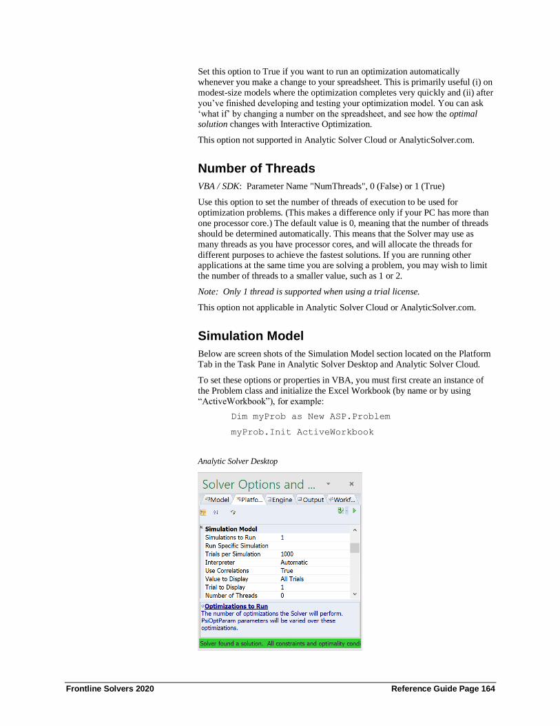
Frontline Solvers 2020 Reference Guide Page 164
Set this option to True if you want to run an optimization automatically
whenever you make a change to your spreadsheet. This is primarily useful (i) on
modest-size models where the optimization completes very quickly and (ii) after
you’ve finished developing and testing your optimization model. You can ask
‘what if’ by changing a number on the spreadsheet, and see how the optimal solution changes with Interactive Optimization.
This option not supported in Analytic Solver Cloud or AnalyticSolver.com.
Number of Threads
VBA / SDK: Parameter Name "NumThreads", 0 (False) or 1 (True)
Use this option to set the number of threads of execution to be used for
optimization problems. (This makes a difference only if your PC has more than
one processor core.) The default value is 0, meaning that the number of threads
should be determined automatically. This means that the Solver may use as
many threads as you have processor cores, and will allocate the threads for
different purposes to achieve the fastest solutions. If you are running other applications at the same time you are solving a problem, you may wish to limit
the number of threads to a smaller value, such as 1 or 2.
Note: Only 1 thread is supported when using a trial license.
This option not applicable in Analytic Solver Cloud or AnalyticSolver.com.
Simulation Model
Below are screen shots of the Simulation Model section located on the Platform
Tab in the Task Pane in Analytic Solver Desktop and Analytic Solver Cloud.
To set these options or properties in VBA, you must first create an instance of
the Problem class and initialize the Excel Workbook (by name or by using
“ActiveWorkbook”), for example:
Dim myProb as New ASP.Problem
myProb.Init ActiveWorkbook
Analytic Solver Desktop

Frontline Solvers 2020 Reference Guide Page 165
Analytic Solver Cloud / Analytic Solver Desktop
Simulations to Run
VBA / SDK: Property: myProb.Solver.NumSimulations = integer_value, 0 <
integer_value
Use this property to set the number of simulations to run when you click the
Simulate button on the Ribbon, or the green arrow in the Task Pane. This is
useful only if you’ve defined one or more simulation parameters, using the
Parameters Simulation choice on the Ribbon.
You can use these features to run multiple, parameterized simulations. For
example, in an airline yield management model where the number of “no-shows” for a departing flight depends on the number of tickets sold, you could
define a cell for the number of tickets sold as a simulation parameter, varied
from (say) 100 to 150. If you set the Simulations to Run value to 51, Analytic
Solver would run 51 simulations: the first would use 100 tickets sold, the second
would use 101 tickets sold, and so on through the 51st problem with 150 tickets
sold. You could then use the Reports and Charts buttons on the Ribbon to
examine results across all 51 simulations.
Run Specific Simulation
VBA / SDK: Property: myProb.Solver.SimulationIndex = integer_value, 0 <
integer_value <= Simulations to Run
The specific simulation Solver will perform if multiple simulations are defined.
PsiSimParam parameters will be set for this index
Trials per Simulation
VBA / SDK: Property: myProb.Solver.NumTrials = integer_value, 0 <
integer_value
Use this property to set the number of Monte Carlo trials to run in each
simulation. The default value is 1,000 trials, which is enough for a good
statistical sample in most models. But applications such as estimating the value
of options and other derivatives may need a higher number of trials.
Simulation Interpreter
VBA / SDK: Parameter Name “Interpreter”, 0 (Automatic), 1 (Psi Interpreter) or
2 (Excel Interpreter)
Use this option to select the Interpreter to be used for Simulation problems, to
compute Monte Carlo trial values from the formulas in your model.
Choose Psi Interpreter to use Analytic Solver’s Polymorphic Spreadsheet
Interpreter, Excel Interpreter to use standard Excel recalculation, or

Frontline Solvers 2020 Reference Guide Page 166
Automatic (the default choice) to allow Analytic Solver to choose the
Interpreter automatically.
No matter what you choose here, after a simulation (or optimization) run is
finished, your spreadsheet formulas are always recalculated by Excel; only the
values of PSI function calls are determined by Analytic Solver. Whenever you’re in Excel Ready model, you are using the normal Excel Interpreter.
During the time when a simulation is being run, the PSI Interpreter is normally
much faster than the Excel Interpreter. The PSI Interpreter is more ‘strict’ than
the Excel Interpreter, so you may see an error message in the Task Pane Output
tab if your model uses certain (unusual) Excel formulas that the PSI Interpreter
won’t accept.
This option is not applicable in Analytic Solver Cloud/AnalyticSolver.com as
Analytic Solver's Polymorphic Spreadsheet Interpreter is always used in these
products.
Use Correlations
VBA / SDK: Parameter Name "UseCorrelations", 0 (False) or 1 (True)
This option determines whether correlations among uncertain variables that you
define (using the Correlations button on the Ribbon) will be used when
computing the random samples drawn for your uncertain variables in Monte
Carlo trials. The default value is True, meaning that correlations will be
respected. You would set this to False only if you wanted to see how your
simulation results would change if the uncertain variables were all independent
and not correlated.
Value to Display
VBA / SDK: Parameter Name "ValuetoDisplay", 0 (All Trials), 1 (Normal Trials), 2 (Error Trials), 3 (Sample Mean) or 4 (Base Case)
Use this option in Analytic Solver Desktop to determine what values for
uncertain variables are returned by PSI distribution function calls (such as
=PsiNormal(1,2)) in your model, and hence what values are displayed on your
spreadsheet. Select from All Trials, Normal Trials, Error Trials, Sample
Mean, and Base Case:
• All Trials means that individual values from both normal trials and
error trials will be displayed. The specific trial values to be displayed
are determined by the Trial Number that appears in the Tools section of
the Analytic Solver Ribbon. You can use the left arrow and right arrow
to change the trial number.
• Normal Trials means that only individual values from normal trials
(where no simulation output or uncertain function had an Excel error
value) will be displayed; error trials will be skipped when you use the
left arrow and right arrow to change the trial number.
• Error Trials means that only individual values from error trials (where
at least one uncertain function had an Excel error value) will be
displayed; normal trials will be skipped when you use the left arrow
and right arrow to change the trial number.

Frontline Solvers 2020 Reference Guide Page 167
• Sample Mean means that each PSI distribution function will return its
sample mean value across all of the normal trials; regardless of the
Trial Number setting.
• Base Case means that each PSI distribution function will return its base
case value (specified in the Base Case field of the Uncertain Variable dialog, and stored via the PsiBaseCase() function), regardless of the
Trial Number setting. If a PSI distribution function doesn’t have a Base
Case value, it will return its sample mean value.
You can also set this option by clicking the small down-arrow next to the Trial
Number on the Ribbon, and choosing one of the above options from the
dropdown list.
This functionality is not supported in Analytic Solver Cloud or
AnalyticSolver.com.
Trial to Display
VBA / SDK: Property: myProb.Solver.SimulationIndex = integer_value", 0 < integer_value <= Number of Trials
Use this property in Analytic Solver Desktop to choose the Monte Carlo trial
number whose individual values should be displayed on your spreadsheet in
Excel Ready mode. The Trial Number appears in the Tools section of the
Analytic Solver Ribbon; you can also use the left arrow and right arrow on the
Ribbon to change the trial number. If you have the Value to Display option set
to Sample Mean or Base Case, this option is ignored.
In Analytic Solver Cloud, this option has been moved to the Tools tab on the
Solver task pane. You can either type the value directly or use the spinners to
increase or decrease the value in the field.
Number of Threads
VBA / SDK: Parameter Name "SimNumThreads", 0 (False) or 1 (True)
Use this option to set the number of threads of execution to be used in the Monte
Carlo simulation process. (This makes a difference only if your PC has more
than one processor core.) The default value is 0, meaning that the number of
threads should be determined automatically. This means that the Solver may use
as many threads as you have processor cores, and will allocate the threads for
different purposes to achieve the fastest solutions. If you are running other
applications at the same time you are solving a problem, you may wish to limit
the number of threads to a smaller value, such as 1 or 2.
This option is not applicable in Analytic Solver Cloud or AnalyticSolver.com.
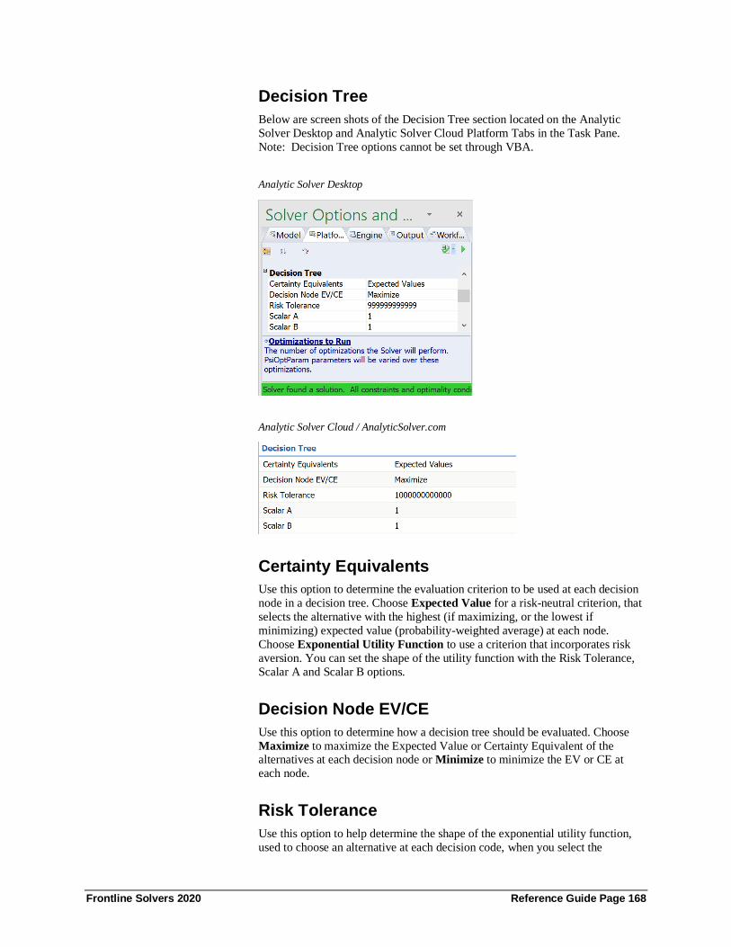
Frontline Solvers 2020 Reference Guide Page 168
Decision Tree
Below are screen shots of the Decision Tree section located on the Analytic
Solver Desktop and Analytic Solver Cloud Platform Tabs in the Task Pane.
Note: Decision Tree options cannot be set through VBA.
Analytic Solver Desktop
Analytic Solver Cloud / AnalyticSolver.com
Certainty Equivalents
Use this option to determine the evaluation criterion to be used at each decision
node in a decision tree. Choose Expected Value for a risk-neutral criterion, that
selects the alternative with the highest (if maximizing, or the lowest if
minimizing) expected value (probability-weighted average) at each node.
Choose Exponential Utility Function to use a criterion that incorporates risk
aversion. You can set the shape of the utility function with the Risk Tolerance,
Scalar A and Scalar B options.
Decision Node EV/CE
Use this option to determine how a decision tree should be evaluated. Choose
Maximize to maximize the Expected Value or Certainty Equivalent of the alternatives at each decision node or Minimize to minimize the EV or CE at
each node.
Risk Tolerance
Use this option to help determine the shape of the exponential utility function,
used to choose an alternative at each decision code, when you select the

Frontline Solvers 2020 Reference Guide Page 169
Certainty Equivalents option Exponential Utility Function. The exponential
utility function takes the form U = A – B*EXP(x/RT) where x is the value of the
alternative, RT is the Risk Tolerance you set with this option, and A and B are
parameters you set with the Scalar A and Scalar B options.
Scalar A
Use this option to help determine the shape of the exponential utility function,
used to choose an alternative at each decision code, when you select the
Certainty Equivalents option Exponential Utility Function. The exponential
utility function takes the form U = A – B*EXP(x/RT) where x is the value of the
alternative, RT is the Risk Tolerance option, A is the value you set with this
option, and B is the Scalar B option.
Scalar B
Use this option to help determine the shape of the exponential utility function,
used to choose an alternative at each decision code, when you select the
Certainty Equivalents option Exponential Utility Function. The exponential
utility function takes the form U = A – B*EXP(x/RT) where x is the value of the alternative, RT is the Risk Tolerance option, A is the value you set with this
option, and B is the Scalar B option.
Diagnosis
Below are screen shots of the Diagnosis section located on the Desktop and
Cloud Platform Tabs in the Task Pane. This section is not included in
AnalyticSolver.com.
Analytic Solver Desktop
Analytic Solver Cloud
Intended Model Type
VBA / SDK: Parameter Name "DesiredModel", 1 (Linear), 2 (Quadratic), or 3
(Nonlinear)

Frontline Solvers 2020 Reference Guide Page 170
Use this option to choose the exceptions that should be included in the Structure
report after analyzing a model. Select from Linear for a linear programming
problem, Quadratic for a quadratic programming problem, or Nonlinear for a
smooth nonlinear optimization problem.
You select the type of model you intended to create here; the Structure report will then highlight formulas in your objective or constraints that do not satisfy
the requirements for this model type. For example, if you select Linear and then
choose Reports Optimization Structure Report, the report will highlight formulas
(if any) that create a nonlinear or non-smooth dependence on the decision
variables.
Intended Use of Uncertainty
VBA / SDK: Parameter Name "UseOfUncertainty", 2 (No Uncertainties), 3
(With Recourse Vars), 4 (In Chance Constraints) or 5 (In Psi Stat Functions)
Use this option to choose the exceptions that should be included in the
Uncertainty Report after analyzing a model. Select from No Uncertainties if you intended that your model should not depend on any uncertain variables,,
With Recourse Vars if you meant to use uncertainty only in constraints that
depend on recourse decision variables, In Chance Constraints if you meant to
use uncertainty only in chance constraints, or In Psi Stat Functions if you
intended to use uncertainty in several ways, but always summarized through PSI
Statistics functions.
You select your intended use of uncertainty here; the Uncertainty Report will
then highlight formulas in your objective or constraints that do not satisfy the
requirements for this use of uncertainty. For example, if you want to create a
stochastic linear programming model with recourse, but without chance
constraints, you would choose With Recourse Vars.
If you are using simulation optimization, and you see the Solver Result message
“Formula depends on uncertainties, must be summarized or transformed”, you
can select In Psi Stat Functions here, then select Reports Optimization
Uncertainty Report to identify the formulas in your model that depend on
uncertainty and are not summarized through PSI Statistics functions such as
PsiMean().
Transformation
Below are screen shots of the Transformation section located on the Desktop
and Cloud Platform Tab in the Task Pane.
To set these options or properties in VBA, you must first create an instance of the Problem class and initialize the Excel Worksheet (by name or by using
“ActiveSheet”), for example:
Dim myProb as New ASP.Problem
myProb.Init ActiveSheet
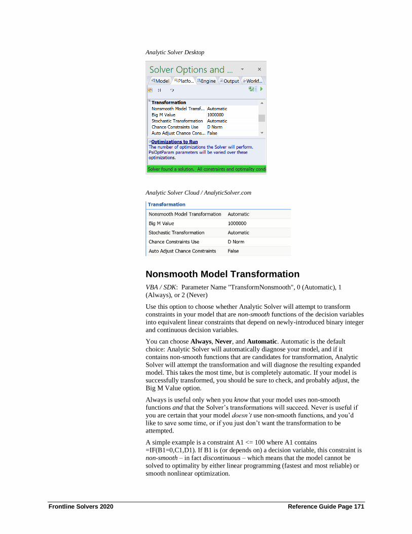
Frontline Solvers 2020 Reference Guide Page 171
Analytic Solver Desktop
Analytic Solver Cloud / AnalyticSolver.com
Nonsmooth Model Transformation
VBA / SDK: Parameter Name "TransformNonsmooth", 0 (Automatic), 1
(Always), or 2 (Never)
Use this option to choose whether Analytic Solver will attempt to transform
constraints in your model that are non-smooth functions of the decision variables
into equivalent linear constraints that depend on newly-introduced binary integer
and continuous decision variables.
You can choose Always, Never, and Automatic. Automatic is the default
choice: Analytic Solver will automatically diagnose your model, and if it
contains non-smooth functions that are candidates for transformation, Analytic
Solver will attempt the transformation and will diagnose the resulting expanded
model. This takes the most time, but is completely automatic. If your model is
successfully transformed, you should be sure to check, and probably adjust, the
Big M Value option.
Always is useful only when you know that your model uses non-smooth
functions and that the Solver’s transformations will succeed. Never is useful if
you are certain that your model doesn’t use non-smooth functions, and you’d
like to save some time, or if you just don’t want the transformation to be attempted.
A simple example is a constraint A1 <= 100 where A1 contains
=IF(B1=0,C1,D1). If B1 is (or depends on) a decision variable, this constraint is
non-smooth – in fact discontinuous – which means that the model cannot be
solved to optimality by either linear programming (fastest and most reliable) or
smooth nonlinear optimization.

Frontline Solvers 2020 Reference Guide Page 172
Assuming for simplicity that B1 is a decision variable that is non-negative, this
constraint can be transformed by introducing a new binary integer variable Y1,
and a new constraint B1 <= BigM * Y1, where BigM is a constant larger than
any possible value for B1 (you can set this value with the Big M Value option).
The IF function in A1 is replaced with =D1*Y1+C1*(1-Y1). Now when Y1=0, B1 is forced to be = 0, and A1=C1; when Y1=1, B1 can have any positive value,
and A1=D1. The non-smooth IF function is transformed into a set of linear
functions, so a faster and more reliable linear programming Solver can
potentially be used – but the overall size of the model is increased.
Analytic Solver can perform much more complex transformations automatically,
for constraints involving the Excel functions IF, AND, OR, NOT, MIN, MAX,
and the relational operators <=, = and >=. Such transformations can result in a
significantly larger model, but if the resulting model is entirely linear, this can
be more than offset by the faster speed and reliability of a linear programming
Solver.
Big M Value
VBA / SDK: Parameter Name "BigM", 0 <= integer value <= 1E+6
Use this option to set a “Big M” constant value to be used in newly generated
constraints that result from a Nonsmooth Model Transformation. The default
value is 1E6 or 1 million – but if you are using Analytic Solver’s transformation features, you should ensure that this value is correct for your model: It must be
bigger than any numeric value that may appear in your intermediate calculations
(for example, bigger than any value a in an expression IF(a>=b,…)) but it
should not be excessively large.
If your value for the Big M option is smaller than the largest value that occurs in
your intermediate calculations, the generated constraints will not have the
desired effect, and your solution will not be valid for your original problem. If
your Big M value is too large, the transformed model will be poorly scaled, and
the Solver will likely encounter problems with numerical stability as it performs
computations with your too-large values. So it pays to investigate the results
computed by your what-if spreadsheet model, and set the Big M option
appropriately.
Stochastic Transformation
VBA / SDK: Parameter Name "StochasticTransformation", 0 (Automatic), 1 (Deterministic), or 2 (Robust Counterpart)
This option has an effect only if the Solve Uncertain Models option is set to
Stochastic Transformation. You can choose Deterministic Equivalent, Robust
Counterpart, or Automatic. This transformation can succeed only if your
objective and constraints are linear functions of the decision variables (they can
also depend on uncertain variables).
Use this option to determine whether Analytic Solver will attempt to transform
your optimization model with uncertainty into a conventional optimization
model without uncertainty: either the Deterministic Equivalent model (as used in
stochastic linear programming), or a Robust Counterpart model (as used in
robust optimization).

Frontline Solvers 2020 Reference Guide Page 173
Automatic, the default choice, will use the transformation to Deterministic
Equivalent form if your model includes recourse decisions and no chance
constraints; otherwise it will use the transformation to Robust Counterpart form.
In both cases, the result of a successful transformation is a conventional linear
programming model, but with considerably more decision variables and constraints than the original model. Generally, the Robust Counterpart model is
much smaller than the Deterministic Equivalent model, but the solution of this
model may be only an approximate (and conservative) solution of the original
problem.
Chance Constraints Use
VBA / SDK: Parameter Name "ChanceConstraintNorm", 1 (L1 Norm), 2 (L2
Norm), 3 (L-Inf Norm) or 4 (D Norm)
This option has an effect only if the Solve Uncertain Models option is set to
Stochastic Transformation, and the Stochastic Transformation option is set to
either Robust Counterpart or Automatic (and the Automatic method selects the Robust Counterpart form). It determines the norm (distance measure) used to
constrain the size of uncertainty sets in the Robust Counterpart model.
Select from the L1 Norm, L2 Norm, L-Inf Norm, or D Norm (the default).
The D norm is equivalent to the intersection of the L1 norm and L-Inf (infinity)
norm. If you choose the L2 norm, the Robust Counterpart model will be a SOCP
(second order cone programming) model, which requires an SOCP or smooth
nonlinear solver (such as the SOCP Barrier Solver or GRG Nonlinear Solver). If
you choose the L1, L-Inf or D norm, the Robust Counterpart model will be an
LP (linear programming) model that can be solved efficiently with an LP, QP, or
SOCP Solver.
Auto Adjust Chance Constraints
VBA / SDK: Parameter Name "ChanceAutoAdjust", 1 (True) or 0 (False)
This option has an effect only if your model includes chance constraints, the
Solve Uncertain Models option is set to Stochastic Transformation, and the
Stochastic Transformation option is set to either Robust Counterpart or
Automatic (and the Automatic method selects the Robust Counterpart form).
Set this option to True if you want Analytic Solver to automatically re-solve the
Robust Counterpart model while adjusting the size of uncertainty sets created
for chance constraints, in an effort to find a better (less conservative) solution.
This can take significantly more time for a large model. If this option is set to
False (the default), Analytic Solver will not automatically re-solve the RC model, but it will offer you the option to re-solve once the initial solution is
found, by pressing a newly-available button at the top of the Task Pane Output
tab.
Default Bounds
Below are screen shots of the Default Bounds section located on the Platform
Tab in the Task Pane of Analytic Solver Desktop and Analtyic Solver Cloud.
To set Decision Vars Upper and Lower, you must first create an instance of the
Problem class and initialize the Excel Worksheet (by name or by using
“ActiveSheet”).
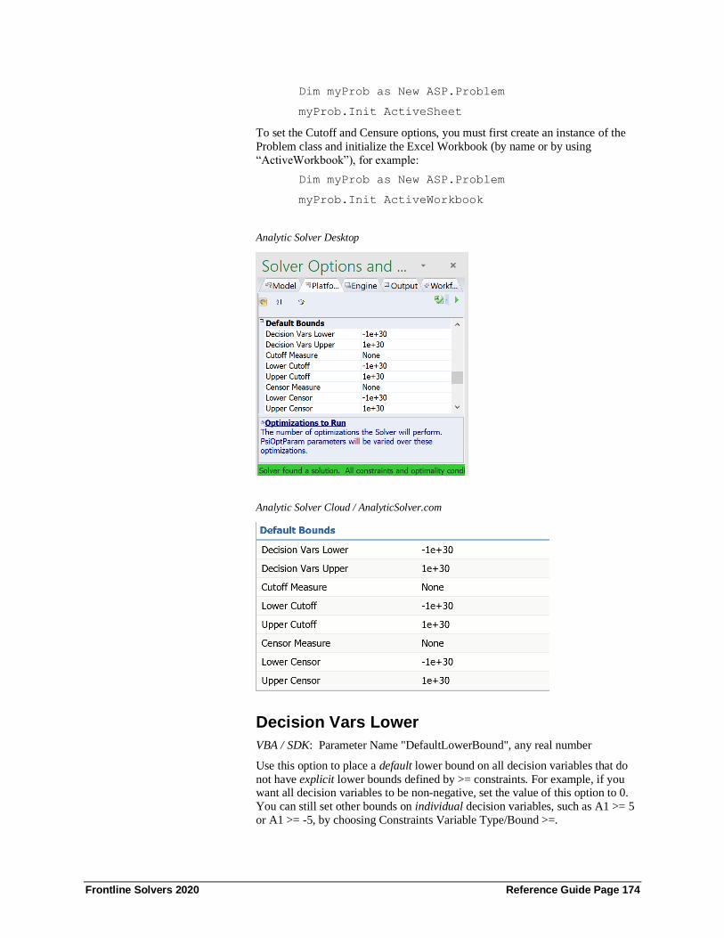
Frontline Solvers 2020 Reference Guide Page 174
Dim myProb as New ASP.Problem
myProb.Init ActiveSheet
To set the Cutoff and Censure options, you must first create an instance of the
Problem class and initialize the Excel Workbook (by name or by using
“ActiveWorkbook”), for example:
Dim myProb as New ASP.Problem
myProb.Init ActiveWorkbook
Analytic Solver Desktop
Analytic Solver Cloud / AnalyticSolver.com
Decision Vars Lower
VBA / SDK: Parameter Name "DefaultLowerBound", any real number
Use this option to place a default lower bound on all decision variables that do
not have explicit lower bounds defined by >= constraints. For example, if you want all decision variables to be non-negative, set the value of this option to 0.
You can still set other bounds on individual decision variables, such as A1 >= 5
or A1 >= -5, by choosing Constraints Variable Type/Bound >=.

Frontline Solvers 2020 Reference Guide Page 175
Decision Vars Upper
VBA / SDK: Parameter Name "DefaultUpperBound", any real number
Use this option to place a default upper bound on all decision variables that do
not have explicit upper bounds defined by <= constraints. This is very useful
when you are solving with the Multistart option or with the Evolutionary Solver.
For example, set the value of this option to 100 if you want all decision variables to have that upper bound. You can still set other bounds on individual decision
variables, such as A1 <= 90 or A1 <= 110, by choosing Constraints Variable
Type/Bound <=.
Cutoff Measure
VBA / SDK: Parameter Name "CutoffType", 0 (None), 1 (Percentile), or 2
(Standard Deviation)
Use this option only if you want to set global default bounds on the probability
distributions of all uncertain variables. This option specifies the “units of
measure” for the values you enter in the Lower Cutoff and Upper Cutoff
options. Choose None (the default) if you don’t want to set these global bounds.
If you choose Percentile, then the Lower Cutoff and Upper Cutoff values must
be between 0.01 and 0.99, and they specify percentiles of each uncertain
variable’s probability distribution. If you choose Std Deviation, then the Lower
Cutoff and Upper Cutoff can be any positive or negative value, and they specify
the number of standard deviations away from the mean for each uncertain
variable.
Note: If set, the optional type argument of PsiTruncate() will override this
option. See the definition for PsiTruncate for more information.
Analytic Solver supports both Cutoff bounds and Censor bounds. When you use
Cutoff bounds, random samples from the distribution are effectively rescaled to
lie within the lower and upper bounds. When you use Censor bounds, random samples from the distribution that lie above the upper bound are set equal to the
upper bound, and samples that lie below the lower bound are set equal to the
lower bound; this causes a “buildup of probability mass” at the bounds – which
is appropriate in some situations, but not in others.
Lower Cutoff
VBA / SDK: Parameter Name "LowerCutoff", Percentiles must be between .01
and .99, Standard Deviation measures can be any real number
Use this option only if you want to set a “Cutoff” type lower bound on the
probability distributions of all uncertain variables. The value you enter for this
option is expressed in either percentiles or standard deviations, depending on the setting of the Cutoff Measure option. Percentile measures must lie between 0.01
and 0.99, Std Deviation measures can be any value.
• This property accepts an "empty" argument. If not provided, the
default of -1E+30 will be used.
• A third optional argument, type, was added in V2019. If a 1 is passed
(default), the bounds will be interpreted as numbers. If a 2 is passed,
the bounds will be interpreted as standard deviations. If a 3 is passed,
the bounds will be interpred as percentiles which must be between 0
and 1.

Frontline Solvers 2020 Reference Guide Page 176
Upper Cutoff
VBA / SDK: Parameter Name "UpperCutoff", Percentiles must be between .01
and .99, Standard Deviation measures can be any real number
Use this option only if you want to set a “Cutoff” type upper bound on the
probability distributions of all uncertain variables. The value you enter for this
option is expressed in either percentiles or standard deviations, depending on the
setting of the Cutoff Measure option. Percentile measures must lie between 0.01
and 0.99, Std Deviation measures can be any value.
• This property accepts an "empty" argument. If not provided, the
default of 1E+30 will be used.
• A third optional argument, type, was added in V2019. If a 1 is passed
(default), the bounds will be interpreted as numbers. If a 2 is passed,
the bounds will be interpreted as standard deviations. If a 3 is passed,
the bounds will be interpred as percentiles which must be between 0 and 1.
Censure Measure
VBA / SDK: Parameter Name "CensureType", 0 (None), 1 (Percentile), or 2
(Standard Deviation)
Use this option only if you want to set global default bounds on the probability
distributions of all uncertain variables. This option specifies the “units of
measure” for the values you enter in the Lower Censor and Upper Censor
options. Choose None (the default) if you don’t want to set these global bounds.
If you choose Percentile, then the Lower Censor and Upper Censor values must
be between 0.01 and 0.99, and they specify percentiles of each uncertain variable’s probability distribution. If you choose Std Deviation, then the Lower
Censor and Upper Censor can be any positive or negative value, and they
specify the number of standard deviations away from the mean for each
uncertain variable.
Note: If set, the optional type argument of PsiCensure() will override this
option. See the definition for PsiCensure for more information.
Analytic Solver supports both Cutoff bounds and Censor bounds. When you use
Cutoff bounds, random samples from the distribution are effectively rescaled to
lie within the lower and upper bounds. When you use Censor bounds, random
samples from the distribution that lie above the upper bound are set equal to the upper bound, and samples that lie below the lower bound are set equal to the
lower bound; this causes a “buildup of probability mass” at the bounds – which
is appropriate in some situations, but not in others.
Lower Censure
VBA / SDK: Parameter Name "LowerCensure", Percentiles must be between .01
and .99, Standard Deviation measures can be any real number
Use this option only if you want to set a “Censor” type lower bound on the
probability distributions of all uncertain variables. The value you enter for this
option is expressed in either percentiles or standard deviations, depending on the
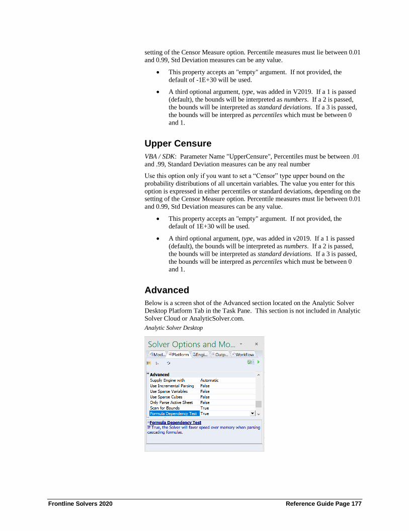
Frontline Solvers 2020 Reference Guide Page 177
setting of the Censor Measure option. Percentile measures must lie between 0.01
and 0.99, Std Deviation measures can be any value.
• This property accepts an "empty" argument. If not provided, the
default of -1E+30 will be used.
• A third optional argument, type, was added in V2019. If a 1 is passed
(default), the bounds will be interpreted as numbers. If a 2 is passed,
the bounds will be interpreted as standard deviations. If a 3 is passed,
the bounds will be interpred as percentiles which must be between 0
and 1.
Upper Censure
VBA / SDK: Parameter Name "UpperCensure", Percentiles must be between .01
and .99, Standard Deviation measures can be any real number
Use this option only if you want to set a “Censor” type upper bound on the
probability distributions of all uncertain variables. The value you enter for this
option is expressed in either percentiles or standard deviations, depending on the setting of the Censor Measure option. Percentile measures must lie between 0.01
and 0.99, Std Deviation measures can be any value.
• This property accepts an "empty" argument. If not provided, the
default of 1E+30 will be used.
• A third optional argument, type, was added in v2019. If a 1 is passed
(default), the bounds will be interpreted as numbers. If a 2 is passed,
the bounds will be interpreted as standard deviations. If a 3 is passed,
the bounds will be interpred as percentiles which must be between 0
and 1.
Advanced
Below is a screen shot of the Advanced section located on the Analytic Solver
Desktop Platform Tab in the Task Pane. This section is not included in Analytic
Solver Cloud or AnalyticSolver.com.
Analytic Solver Desktop

Frontline Solvers 2020 Reference Guide Page 178
Supply Engine with
VBA / SDK: Parameter Name "CheckFor", 1 (Gradients), 2 (Structure), 3
(Convexity), 4 (Automatic)
This option has an effect only if the Optimization Interpreter option is set to Psi
Interpreter. Use this option to specify what kind (and how much) analysis of
your model you want Analytic Solver to perform when you click the Optimize button or the green-arrow Solve button to solve your model.
If you use Automatic (the default choice), Analytic Solver asks the Solver
Engine (chosen either automatically or by your selection on the Engine tab)
what kind of model analysis it can use, and performs that analysis before starting
the Solver Engine. This is usually the best choice, since it means that Solver
Engines that can exploit model structure information will have that information.
But since most Solver Engines can run without structure information, you may
occasionally want to set this option.
The Gradients option has the smallest computational cost: It means that Solver
Engines will benefit from fast, accurate gradients computed via automatic
differentiation, but they will not have model structure, dependency, or convexity information (for example, which variables or functions in the model are linear).
The Structure option includes the Gradients option, plus it performs a structure
and dependency analysis and makes this information available to the Solver
Engine. The Convexity option includes the Gradients and Structure options,
plus it performs an analysis of the convexity of the objective and constraints; it
requires the greatest amount of computation.
Use Incremental Parsing
VBA / SDK: Parameter Name "IncrementalParsing", 0 (False) or 1 (True)
This option has an effect only if the Optimization Interpreter option (for
optimization models) or the Simulation Interpreter (for simulation models) is set to Psi Interpreter. You can use this option to improve performance if you are
making small changes to a large Excel model and then re-solving the model.
To perform its work, the Polymorphic Spreadsheet Interpreter must scan and
parse (analyze) your Excel formulas. This can take considerable time for a large
model. If this option is set to False, the PSI Interpreter will re-reparse the entire
model each time you Solve; this will take more time. If this option is set to True,
the PSI Interpreter will save and re-use the parsed form of the model; as you
make changes to individual cell values or formulas, it will read and parse just
the changes, adding them to the parsed form of the model; this will take more
memory on an ongoing basis.
Use Sparse Variables
VBA / SDK: Parameter Name "Sparse", 0 (False) or 1 (True)
This option has an effect only if the Optimization Interpreter option is set to Psi
Interpreter. Use this option to determine whether the PSI Interpreter should
operate in (its own) Sparse mode or Dense mode. The default setting is False,
meaning that the Interpreter operates in its Dense mode.
If you set this option to True, the PSI Interpreter will use its own Sparse mode,
which can save memory when your optimization model is sparse, but possibly at
the expense of extra time, since a Structure analysis is always performed when

Frontline Solvers 2020 Reference Guide Page 179
analyzing or solving (regardless of the setting of the Supply Engine with
option).
To check the sparsity of your model, click the Analyze button in the Task Pane
Model tab, then check the Sparsity option at the very bottom of the Model tab,
which reports the percentage of nonzeroes (from 0 to 100) in your model. A low number means that your model is very sparse.
Use Sparse Cubes
VBA / SDK: Parameter Name "SparseCubes", 0 (False) or 1 (True)
This option has an effect only if the Interpreter (in the Optimization or
Simulation sections on the Platfom tab on the Solver Task Pane) option is set to Psi Interpreter. Use this option to determine whether the PSI Interpreter should
calculate a cube defined by PsiCube() or PsiTableCube() using Sparse mode or
Dense mode.
Most large cubes are sparse in nature. While they may contain thousands of
elements, in practice, not all combinations of dimension elements are
possible. Hence, not all will define a model function during the Psi Interpreter's
evaluation of the problem. This means that most cubes will provoke output
results as sparse cubes (with missing constraints). Such sparsity in a cube, also
known as structural sparsity, can be exploited to save memory and gain speed.
A sparse cube is defined by missing values in cells for PsiCube() and by missing
records for PsiTableCube(). If this option is equal to False and you have defined a cube using PsiCube() or PsiTableCube(), elements missing from the
cube will be considered equal to 0. If you set this option to True, you have
defined a cube using PsiCube() with missing values or PsiTableCube() with
missing records, and the percentage of elements missing or empty is more than
30% of the total possible cube elements, those missing elements or records will
not be included in the model.
For an example of how to use a sparse cube see the Dimensional Modeling
chapter in the Analytic Solver User Guide.
Only Parse Active Sheet
VBA / SDK: Parameter Name "ActiveOnly", 0 (False) or 1 (True)
This option has an effect only if the Optimization Interpreter option is set to Psi
Interpreter. Use this option to determine whether the PSI Interpreter should
scan and parse only the active worksheet, or the entire workbook (and possibly
other workbooks) when analyzing and solving models. The default setting is
False, meaning that all worksheets and workbooks should be scanned.
If you have a large workbook that contains many worksheets and cell formulas
that don’t participate in the Solver model, setting this option to True can save a
good deal of time; however cells on other worksheets or in other workbooks that
are referenced in formulas making up the Solver model will be treated as
constant – even if they actually contain formulas that refer back to decision
variable cells on the active worksheet.
Scan for Bounds
VBA / SDK: Parameter Name "ScanforBounds", 0 (False) or 1 (True)

Frontline Solvers 2020 Reference Guide Page 180
Use this option to determine whether Analytic Solver should spend time
scanning the model in order to properly classify certain constraints that you
enter as either general constraints or bounds on decision variables. The default
setting is True, which enables scanning for bounds.
In the Task Pane Model tab, constraints such as $A$1 >= 0 (with a constant right hand side) will appear in the ‘Bounds’ outline group when A1 is a decision
variable, or in the ‘Normal’ group when A1 contains a formula and is not a
decision variable. But constraints such as $A$1 >= $B$1 require more analysis:
If A1 is a decision variable and B1 contains a constant, this is a simple variable
bound; but if B1 contains a formula that depends on some other decision
variable; then this is a general constraint.
In a large model, a formula in B1 may depend on hundreds or thousands of other
cells, and there may be hundreds or thousands of constraints such as $A$1 >=
$B$1. When the Scan for Bounds option is set to True, Analytic Solver will
spend time “in the background” tracing down these formulas, to determine
whether constraints of this form are general constraints or bounds on the variables. (You may notice that constraints such as $A$1 >= $B$1 will move
from the Normal outline group to the Bounds group while you are doing other
work.) When this option is set to False, this work is not performed, and some
variable bounds my remain in the Normal group.
The setting of this option has no effect on actually solving the model: In that
case the PSI Interpreter and Solver Engine will determine for certain whether
each constraint is a general constraint or a variable bound. It only affects the
display of the constraints in the Task Pane Model tab.
Formula Dependency Test
Use this option to determine whether a Formula Dependency Test should be applied to your model. Setting this option to "False" will restrict Solver from
applying the test which can be especially helpful in models containing cascading
constraints, or constraints that depend on previously defined constraints, where
Solver is returning "There is not enough memory available to solve the problem
at cell $X$X."
Analytic Solver automatically detects cascading constraints using a formula
dependency test. When such constraints are detected in a model, Analytic Solver
automatically switches from Reverse mode of evaluation to Forward mode, in
order to reduce the amount of time Solver spends parsing the model. Since
Forward evaluation mode requires much more memory than Reverse evaluation
mode, Analytic Solver could stop and return the result, "There is not enough memory available to solve the problem at cell $X$X", when Forward evaluation
mode is used.
If your model contains cascading constraints and Solver is returning this "out of
memory" result, set this option to False to use the Reverse mode of evaluation.
Analytic Solver will most likely spend more time parsing your model but should
not return an "out of memory" error.
General
Below is a screen shot of the General section located on the Analytic Solver
Desktop Platform Tab in the Task Pane. The options within this section are not
included in Analytic Solver Cloud or AnalyticSolver.com.

Frontline Solvers 2020 Reference Guide Page 181
Analytic Solver Desktop
Log Level
VBA / SDK: Parameter Name "LogLevel", -1 (None), 0 (Minimal), 1 (Normal)
or 2 (Verbose)
Use this option to determine how much information is displayed in the Task Pane Output tab solution log area, by Analytic Solver and the selected Solver
Engine. You can select from Minimal, Normal (the default) or Verbose.
The specific kind and amount of information displayed for Minimal, Normal or
Verbose depends on the Solver Engine used to solve the problem. Typically,
Verbose generates much more output in the solution log, such as results from a
presolve step and/or from each major iteration, or subproblem for mixed-integer
problems.
Wrap Text in Output Pane
VBA / SDK: Parameter Name "WrapText", 0 (False), or 1 (True)
Use this option to control whether messages in the Output Pane “wrap” onto additional lines.
If this option is set to True, messages that exceed the width of the Pane will be
split (at word boundaries) onto two or more lines. This is most convenient for
viewing Solver Result messages and similar information.
If this option is set to False, messages will appear on a single line. This can be
useful if you’ve set the Log Level to Verbose and you’re viewing an iteration
log or similar information. You can use the scroll bar at the bottom of the Output
Pane to see the entire message, or you can resize the whole Task Pane to display
more information at once.
Solver Parameters Dialog
VBA / SDK: Parameter Name "DlgStyle", 0 (Automatic), 1 (Old Excel Style) or
2 (New Excel Style)
Use this option to control whether messages in the Output Pane “wrap” onto
additional lines.

Frontline Solvers 2020 Reference Guide Page 182
If this option is set to True, messages that exceed the width of the Pane will be
split (at word boundaries) onto two or more lines. This is most convenient for
viewing Solver Result messages and similar information.
If this option is set to False, messages will appear on a single line. This can be
useful if you’ve set the Log Level to Verbose and you’re viewing an iteration log or similar information. You can use the scroll bar at the bottom of the Output
Pane to see the entire message, or you can resize the whole Task Pane to display
more information at once.
Operating Mode
VBA / SDK: Parameter Name "OperatingMode", 0 (Expert Mode), or 1 (Auto-
Help Mode) or 2 (Guided Mode)
The Operating Mode determines how much Analytic Solver will try to help the
user with dialogs and Help text, when using the software and designing your
model:
• Guided Mode prompts you step-by-step when solving, with dialogs.
• Auto-Help Mode, the default, shows dialogs or Help only when there’s a
problem or error condition.
• Expert Mode provides only messages in the Task Pane Output tab. (This
mode not supported when using a trial license.)
Support Mode
VBA / SDK: Parameter Name "SupportMode", 0 (Basic Support), or 1 (Standard
Support) or 2 (Active Support)
The Support Mode determines how much Analytic Solver will try to help you by
connecting automatically to Frontline Systems’ Technical Support.
• Active Support automatically reports events, errors and problems to
Frontline Support, receives and displays messages to you from Support, and
allows you to start a Live Chat with Support while working in Excel.
• Standard Support automatically reports events, errors and problems
anonymously to Frontline Support, but does not provide a means to receive
messages or start a Live Chat with Support.
• Basic Support provides no automatic connection to Frontline Support.
Users will be required to contact Frontline Systems via email, website, or
phone if help is needed. (This mode not supported when using a trial
license.)
Autoselect Plug-in Solvers
VBA / SDK: Parameter Name "EngAuto", 0 (False), or 1 (True)
This option is only available when one or more of the Solver field installable
engines is installed. When this option is set to True, Analytic Solver will
prioritize the selection of one of the external engines (such as Gurobi, Knitro,
Large Scale GRG, Large Scale SQP, Large Scale LP, Mosek, or OptQuest
Solver) over the five built in Solver Engines: Standard GRG Nonlinear Engine,
Standard LP/Quadratic Engine, Standard Evolutionary Engine, Standard Interval
Global Solver Engine, or Standard SOCP Barrier Engine.
Frontline Solvers 2020 Reference Guide Page 183
Solver Engine Option Reference
This chapter describes the options available on the Task Pane Engine tab, for
each of the bundled Solver engines in Analytic Solver Desktop, Analytic Solver
Cloud and AnalyticSolver.com. It also briefly describes how these options may
be examined or set using Analytic Solver Desktop and VBA, or in another
programing language using Frontline’s Solver Platform SDK.
In Analytic Solver Desktop, options may be examined or set interactively via the
Task Pane Engine tab as described in this chapter, or programmatically using either the new object-oriented API described below and in the chapter “VBA
Object Model Reference,” or the traditional VBA functions described in the
later chapter “Traditional VBA Function Reference.”
In Solver SDK Platform and Solver SDK Pro, options may be examined or set
via its object-oriented API, just like Analytic Solver’s API, or via the SDK
procedural API. The object-oriented API is described below; the SDK
procedural API is described in the SDK API Reference Guide. The string names
of most options are the same for both products and are shown for each option
below.
Bear in mind that the options that control numerical tolerances and solution strategies are pre-set to the choices that are most appropriate for the majority of
problems; you should change these settings only when necessary, after carefully
reading this chapter. The options you will use most often are common to all the
Solver products, and control features like the display of iteration results, or the
upper limits on solution time or Solver iterations.
Setting Options Programmatically In Analytic Solver Desktop, you can examine or set Solver Engine options in
VBA using the object-oriented API described in this section. In Solver SDK
Platform and Solver SDK Pro, you can examine or set Solver Engine options, in
a variety of programming languages, using the same object-oriented API. In
both cases, all option values are of type double, though for some options only integer values, or values 0 and 1 are used.
Object-Oriented API
In the object-oriented API, each Solver engine option or parameter is
represented by an EngineParam object instance. This object has properties
Name, Value, Default (the initial or default value), MinValue, and MaxValue
(the minimum and maximum allowed values). All the options or parameters for
a Solver engine belong to a collection, which is an EngineParamCollection
object.
To access an option or parameter, you start with a reference to the Solver engine
object, say myEngine or myProb.Engine. The engine object’s Params property

Frontline Solvers 2020 Reference Guide Page 184
refers to the EngineParamCollection object. As with all collections, you can
access an individual EngineParam in the collection by name or by index. For
example, to refer to the Max Time limit for the problem’s currently selected
Solver engine, you’d write myProb.Engine.Params("MaxTime").
Once you have a reference to the EngineParam object (as above), you can get or set its properties using simple assignment statements. For example, you can set
the Max Time limit for the currently selected Solver engine to 1000 seconds by
writing:
VBA: myProb.Engine.Params("MaxTime").Value = 1000
To get the current Max Time parameter value, put the property reference on the right hand side of an assignment statement (declaring Dim maxTime As
Double):
VBA: maxTime = myProb.Engine.Params("MaxTime").Value
In the Solver Platform SDK, the same kinds of assignment statements can be used, with just slight differences due to the syntax of various programming
languages:
VB6: myProb.Engine.Params("MaxTime").Value = 1000
VB.NET: myProb.Engine.Params("MaxTime").Value = 1000
C++: myProb.Engine.Params(L"MaxTime").Value = 1000;
C#: myProb.Engine.Params("MaxTime").Value = 1000;
Matlab: myProb.Engine.Params('MaxTime').Value = 1000;
Java: myProb.Engine().Params().Item("MaxTime").Value(1000);
(Since Java currently lacks properties, the syntax used by the Solver Platform
SDK is different.) To get the current Max Time parameter value, put the
property reference on the right hand side of an assignment statement, for
example in C#:
double maxTime =
myProb.Engine.Params("MaxTime").Value;
You can access all of the options and parameters supported by a Solver engine
by indexing its EngineParamCollection. For example,
myProb.Engine.Params(0) refers to the first parameter in the collection. In all
the object-oriented languages, you can write a for-loop to index through all of
the parameters like the following example in VBA, VB6 or VB.NET:
For i = 0 to myProb.Engine.Params.Count - 1
MsgBox myProb.Engine.Params(i).Name & " = " &
myProb.Engine.Params(i).Value
Next i
In VBA, VB6, VB.NET, and C#, you can also iterate through a collection using
a “for each” loop:
Dim myParam as EngineParam
For Each myParam in myProb.Engine.Params
MsgBox myParam.Name & " = " & myParam.Value
Next

Frontline Solvers 2020 Reference Guide Page 185
The Basic Microsoft Excel Solver There is just one Solver Options dialog displayed by the standard Microsoft
Excel Solver, containing options for the included Solver engines. Note, for
Excel 2010 an Evolutionary Solver engine was added to the basic Excel Solver.
This dialog box is depicted below, as it appears in Excel 2016. All of the
options in this dialog are also present on the Engine tab in Analytic Solver.
Note: The linear engine included in the Excel Solver is the LP Simplex Engine.
Common Solver Options On the next page are screen shots of the Engine Tab in the Analtyic Solver
Desktop and Analytic Solver Cloud Task Panes. We’ll walk through the
common options and then the options specific to each engine.

Frontline Solvers 2020 Reference Guide Page 186
Analytic Solver Desktop Analytic Solver Cloud / AnalyticSolver.com
Max Time and Iterations
VBA / SDK: Parameter
Names "MaxTime", "Iterations", integer value > 0
The value for the Max Time option determines the maximum time in seconds that the Solver will run before it stops, including problem setup time and time to
find the optimal solution. For problems with integer constraints, this is the total
time taken to solve all subproblems explored by the Branch & Bound method.
Leaving this option blank, the default, results in an unlimited max time setting.
The value for the Iterations option determines the maximum number of
iterations (“pivots” for the Simplex Solver in Excel Solver or major iterations
for the GRG Solver) that the Solver may perform on one problem. A new “Trial
Solution” is generated on each iteration; the most recent Trial Solution is
reported on the Excel status bar. For problems with integer constraints, the
Iterations setting determines the maximum number of iterations for any one
subproblem. Leaving this option blank, the default, results in an unlimited iterations setting.

Frontline Solvers 2020 Reference Guide Page 187
Bear in mind that if the maximum time or maximum number of iterations is
exceeded, the Solver will stop and display a dialog like the one shown below:
You will have the option to stop at that point or to continue the solution process.
If you click on the Continue button, the time or iteration limit is removed, and
you will not be prompted again.
If you ever want to Stop Solve before it has found a solution, you can simply
press either the ESC key on your keyboard or (if using Analytic Solver Desktop or Cloud) the pause button on the Analytic Solver Model task pane while the
Solver is running. If your model is large enough to take some time to
recalculate even once, you should hold down the ESC key for a second or two.
After a momentary delay, the dialog box shown below will appear, and you will
have the option to stop at that point or continue or restart the solution process.
Precision
VBA / SDK: Parameter Name "Precision", 0 < value < 1
The number entered here determines how closely the calculated values of the
constraint left hand sides must match the right hand sides in order for the
constraint to be satisfied. Recall from “Elements of Solver Models” in the
Analytic Solver User Guide chapter “Mastering Conventional Optimization
Concepts,” that a constraint is satisfied if the relation it represents is true within
a small tolerance; the Precision value is that tolerance. With the default setting
of 1.0E-6 (0.000001), a calculated left hand side of -1.0E-7 would satisfy a
constraint such as A1 >= 0.
Precision and Regular Constraints
Use caution in making this number much smaller, since the finite precision of
computer arithmetic virtually ensures that the values calculated by Microsoft
Excel and the Solver will differ from the expected or “true” values by a small
amount. On the other hand, setting the Precision to a much larger value would
cause constraints to be satisfied too easily. If your constraints are not being satisfied because the values you are calculating are very large (say in millions or
billions of dollars), consider adjusting your formulas and data to work in units of
millions, or checking the Use Automatic Scaling box instead of altering the

Frontline Solvers 2020 Reference Guide Page 188
Precision setting. Generally, this setting should be kept in the range from 1.0E-6
(0.000001) to 1.0E-4 (0.0001).
Precision and Integer Constraints
Another use of Precision is determining whether an integer constraint, such as
A1:A5 = integer, A1:A5 = binary or A1:A5 = alldifferent, is satisfied. If the
difference between the decision variable’s value and the closest integer value is
less than the Precision setting, the variable value is treated as an integer.
Tolerance and Convergence
VBA / SDK: Parameter Names "IntTolerance", "Convergence", 0 <= value <= 1
The Tolerance option determines how close a “candidate” integer solution must be to the true integer optimal solution before the Solver stops. This option is
described more fully in a later section focusing on options for integer
programming problems.
The Convergence option controls the stopping conditions used by the GRG
Solver and the Evolutionary Solver that lead to the message “Solver has
converged to the current solution.” It is described more fully in later sections
focusing on options for these Solver engines.
Use Automatic Scaling / Scaling
VBA / SDK: Parameter Name "Scaling", value 1/True or 0/False
When this option is set to True, the Solver will attempt to scale the values of the objective and constraint functions internally in order to minimize the effects of a
poorly scaled model. A poorly scaled model is one that computes values of the
objective, constraints, or intermediate results that differ by several orders of
magnitude. Poorly scaled models may cause difficulty for both linear and
nonlinear solution algorithms, due to the effects of finite precision computer
arithmetic. For more information, see “Problems with Poorly Scaled Models” in
the chapter “Solver Result Messages,” and “The Scaling Report” in the chapter
“Solver Reports.”
If your model is nonlinear and you set Use Automatic Scaling/Scaling to True,
make sure that the initial values for the decision variables are “reasonable,” i.e.
of roughly the same magnitudes that you expect for those variables at the optimal solution. The effectiveness of the Automatic Scaling option depends on
how well these starting values reflect the values encountered during the solution
process.
Assume Non-Negative / AssumeNonNeg
VBA: Parameter Name "AssumeNonneg", value 1/True or 0/False
SDK: Use Variable object NonNegative method or SolverVarNonNegative
function
When this option is set to True, any decision variables that are not given explicit
lower bounds via >=, binary, or alldifferent constraints in the Constraints list
box of the Solver Parameters dialog will be given a lower bound of zero when
the problem is solved. This option has no effect for decision variables that do have explicit >= constraints, even if those constraints allow the variables to
assume negative values.

Frontline Solvers 2020 Reference Guide Page 189
Show Iteration
VBA: Parameter Name "StepThru", value 1/True or 0/False
SDK: Define an Evaluator for Eval_Type_Iteration
When this option is set to True in Analytic Solver Desktop, a dialog like the one
on the next page will appear on every iteration during the solution process:
This is the same dialog that appears when you press ESC at any time during the
solution process, but when the Show Iteration Results box is checked it appears
automatically on every iteration. When this dialog appears, the best values so far for the decision variables appear on the worksheet, which is recalculated to
show the values of the objective function and the constraints. You may click the
Continue button to go on with the solution process, the Stop button to stop
immediately, or the Restart button to restart (and then continue) the solution
process. You may also click on the Save Scenario... button to save the current
decision variable values in a named scenario, which may be displayed later with
the Microsoft Excel Scenario Manager. For more information on this dialog and
the effect of the Restart button, see the section “During the Solution Process” in
the chapter “Solver Results Messages.”
Bypass Solver Reports / Bypass Reports
VBA: Parameter Name "BypassReports", value 1/True or 0/False SDK: Not Applicable
This option is a “Common Solver Option” and appears in the Engine Tab of the
Task Pane shown below for the LP/Quadratic Solver, SOCP Barrier Solver,
GRG Nonlinear Solver, Interval Global Solver, and Evolutionary Solver. If
using Analytic Solver, you can use it to save time during the solution process if
you do not need the reports for the current solution run. The reports are selected
from the Solver Results dialog at the end of the solution process; unless this box
is checked, the Solver always performs extra computations to prepare for the
possibility that you will select one or more reports from the Solver Results
dialog. When this box is checked, the extra computations are skipped and the
Reports – Optimization list will not contain any reports.
Even though report generation in Analytic Solver Desktop is very fast, the
Bypass Solver Reports option can make a real difference in your total solution
time, especially when you are solving larger models. It is also supported by
many optional plug-in Solver engines that can solve problems with millions of
variables and constraints. It is not unusual for the extra report-related
computations to take as much time as the entire solution process, especially if
you have taken other steps (such as using the functions recognized for fast
problem setup) to ensure the best possible solution times.
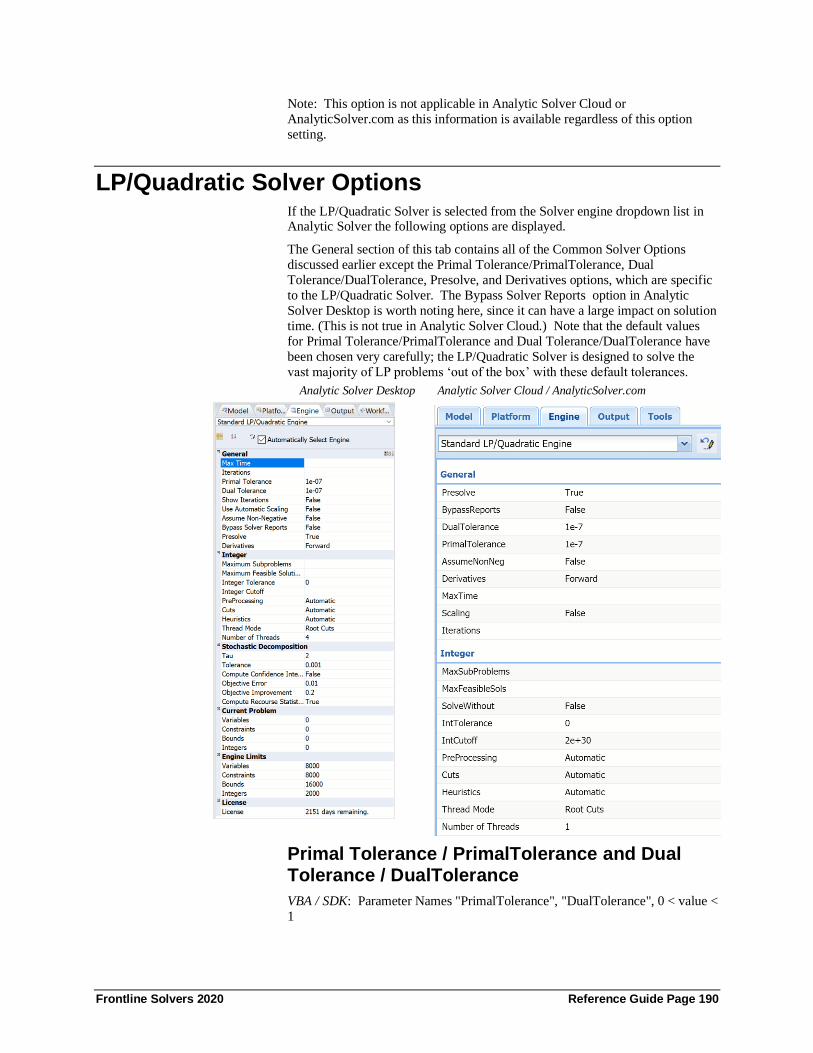
Frontline Solvers 2020 Reference Guide Page 190
Note: This option is not applicable in Analytic Solver Cloud or
AnalyticSolver.com as this information is available regardless of this option
setting.
LP/Quadratic Solver Options If the LP/Quadratic Solver is selected from the Solver engine dropdown list in Analytic Solver the following options are displayed.
The General section of this tab contains all of the Common Solver Options
discussed earlier except the Primal Tolerance/PrimalTolerance, Dual
Tolerance/DualTolerance, Presolve, and Derivatives options, which are specific
to the LP/Quadratic Solver. The Bypass Solver Reports option in Analytic
Solver Desktop is worth noting here, since it can have a large impact on solution
time. (This is not true in Analytic Solver Cloud.) Note that the default values
for Primal Tolerance/PrimalTolerance and Dual Tolerance/DualTolerance have
been chosen very carefully; the LP/Quadratic Solver is designed to solve the
vast majority of LP problems ‘out of the box’ with these default tolerances.
Analytic Solver Desktop Analytic Solver Cloud / AnalyticSolver.com
Primal Tolerance / PrimalTolerance and Dual Tolerance / DualTolerance
VBA / SDK: Parameter Names "PrimalTolerance", "DualTolerance", 0 < value <
1

Frontline Solvers 2020 Reference Guide Page 191
The Primal Tolerance is the maximum amount by which the primal constraints
can be violated and still be considered feasible. The Dual Tolerance is the
maximum amount by which the dual constraints can be violated and still be
considered feasible. The default values of 1.0E-7 for both tolerances are
suitable for most problems.
Presolve
VBA / SDK: Parameter Name "Presolve", value 1/True or 0/False
When this option set to True (which is the default setting), the LP/Quadratic
Solver performs a Presolve step before applying the Primal or Dual Simplex
method. Presolving often reduces the size of an LP problem by detecting
singleton rows and columns, removing fixed variables and redundant
constraints, and tightening bounds.
Derivatives for the Quadratic Solver
When a quadratic programming (QP) problem – one with a quadratic objective
and all linear constraints – is solved with the LP/Quadratic Solver, the quadratic Solver extension requires first or second partial derivatives of the objective
function at various points. In Analytic Solver, these derivatives may be
computed via automatic differentiation or via finite differencing.
When you are using the Interpreter (Interpreter = Automatic or PSI Interpreter
in Analytic Solver Desktop), automatic differentiation is used, exact derivative
values are computed, and the setting of the Derivatives choice is ignored. In
Analytic Solver Desktop, when Solve With = Excel Interpreter, the method used
for finite differencing is determined by the setting of the Derivatives choice.
Forward differencing uses the point from the previous iteration – where the
problem function values are already known – in conjunction with the current
point. Central differencing relies only on the current point and perturbs the decision variables in opposite directions from that point. For QP problems, the
Central differencing choice yields essentially exact (rather than approximate)
derivative values, which can improve solution accuracy and reduce the total
number of iterations; however the initial computation of derivatives may take up
to twice as long as with Forward differencing. (Bear in mind that automatic
differentiation is much faster than either Forward or Central differencing.)
Note: Since the Psi Interpreter is always used in Analytic Solver Cloud and
AnalyticSolver.com, automatic differentiation is always used, exact derivative
values are computed and the setting of the Derivatives choice is ignored.
Options for Mixed-Integer Problems
Below the General section is an Integer section in the LP/Quadratic Solver
Options Engine tab which displays an extensive set of options for mixed-integer
linear programming problems. These options control the Branch and Cut
method for mixed-integer problems.
Max Subproblems/ MaxSubProblems
VBA / SDK: Parameter Name "MaxSubProblems", integer value > 0
The value for the Max Subproblems option places a limit on the number of
subproblems that may be explored by the Branch & Bound algorithm before the
Solver pauses and asks you whether to continue or stop the solution process.

Frontline Solvers 2020 Reference Guide Page 192
Each subproblem is a “regular” Solver problem with additional bounds on the
variables.
In a problem with integer constraints, this limit should be used in preference to
the Iterations limit; the Iterations limit should be set high enough for each of the
individual subproblems solved during the Branch & Bound process. For problems with many integer constraints, you may need to increase this limit
from its default value; any integer value up to 2,147,483,647 may be used.
Max Feasible (Integer) Solutions / MaxFeasibleSols
VBA / SDK: Parameter Name "MaxIntegerSols", integer value > 0
The value for the Max Feasible Sols option places a limit on the number of
feasible integer solutions found by the Branch & Bound algorithm before the
Solver pauses and asks you whether to continue or stop the solution process.
Each feasible integer solution satisfies all of the constraints, including the
integer constraints; the Solver retains the integer solution with the best objective
value so far, called the “incumbent.”
It is entirely possible that, in the process of exploring various subproblems with different bounds on the variables, the Branch & Bound algorithm may find the
same feasible integer solution (set of values for the decision variables) more
than once; the Max Feasible Solutions limit applies to the total number of
integer solutions found, not the number of “distinct” integer solutions.
Integer Tolerance / IntTolerance
VBA / SDK: Parameter Name "IntTolerance", 0 <= value <= 1
When you solve an integer programming problem, it often happens that the
Branch & Bound method will find a good solution fairly quickly but will require
a great deal of computing time to find (or verify that it has found) the optimal
integer solution. The Integer Tolerance setting may be used to tell the Solver to stop if the best solution it has found so far is “close enough.”
The Branch & Bound process starts by finding the optimal solution without
considering the integer constraints (this is called the relaxation of the integer
programming problem). The objective value of the relaxation forms the initial
“best bound” on the objective of the optimal integer solution, which can be no
better than this. During the optimization process, the Branch & Bound method
finds “candidate” integer solutions, and it keeps the best solution so far as the
“incumbent.” By eliminating alternatives as its proceeds, the B&B method also
tightens the “best bound” on how good the integer solution can be.
Each time the Solver finds a new incumbent – an improved all-integer solution –
it computes the maximum percentage difference between the objective of this solution and the current best bound on the objective:
Objective of incumbent - Objective of best bound
------------------------------------------------
Objective of best bound
If the absolute value of this maximum percentage difference is equal to or less
than the Integer Tolerance, the Solver will stop and report the current integer
solution as the optimal result, with the message “Solver found an integer
solution within tolerance.” If you set the Integer Tolerance to zero, the Solver
will “prove optimality” by continuing to search until all alternatives have been
Frontline Solvers 2020 Reference Guide Page 193
explored and the optimal integer solution has been found. This may take a great
deal of computing time.
Integer Cutoff / IntCutoff
VBA / SDK: Parameter Name "IntCutoff", -1E30 < value < +1E30
This option provides another way to save time in the solution of mixed-integer
programming problems. If you know the objective value of a feasible integer
solution to your problem – possibly from a previous run of the same or a very
similar problem – you can enter this objective value for the Integer Cutoff
option. This allows the Branch & Bound process to start with an “incumbent”
objective value (as discussed above under Integer Tolerance) and avoid the work
of solving subproblems whose objective can be no better than this value. If you
enter a value here, you must be sure that there is an integer solution with an
objective value at least this good: A value that is too large (for maximization
problems) or too small (for minimization) may cause the Solver to skip solving
the subproblem that would yield the optimal integer solution.
Preprocessing
VBA / SDK: Parameter Name "PreProcessing", 1 = Automatic, 2 = None, 3 =
Aggressive
Use this option to determine the extent of Preprocessing and Probing strategies
used by the LP/Quadratic Solver on LP/MIP (linear mixed-integer) problems.
Select from None, Aggressive, and Automatic (the default). These methods
consider the possible settings of certain integer variables and their implications
for fixing the values of other integer variables, tightening the bounds on
continuous variables, and in some cases, determining that the subproblem is
infeasible (so it is unnecessary to solve it at all). They can also scan the model
for constraints of the form x1 + x2 + … + xn = 1 where all of the variables xi are binary integer variables. Such constraints often arise in practice, and are
sometimes called “special ordered sets.” In any feasible solution, exactly one of
the variables xi must be 1, and all the others must be 0; hence only n possible
permutations of values for the variables (rather than 2n) need be considered.
Cuts & Heuristics
The LP/Quadratic Solver in Analytic Solver supports a wide range of cuts and
heuristics. Cuts and heuristics require more work on each subproblem, but they
can often lead more quickly to integer solutions and greatly reduce the number
of subproblems that must be explored.
Heuristics
VBA / SDK: Parameter Name "Heuristics", 1 = Automatic, 2 = None, 3 =
Aggressive
Use this option to determine the extent of Heuristic strategies used by the
LP/Quadratic Solver on LP/MIP (linear mixed-integer) problems. Select from
None, Aggressive, and Automatic (the default). A heuristic is a strategy that
often – but not always – will find a reasonably good “incumbent” or feasible
integer solution early in the search. Heuristics used by the LP/Quadratic Solver include: Local Tree Search, Rounding Heuristic, Feasibility Pump, Greedy
Cover Heuristic and many others depending on the problem type and the setting
of this parameter.

Frontline Solvers 2020 Reference Guide Page 194
Cuts
VBA / SDK: Parameter Name "Cuts", 1 = Automatic, 2 = None, 3 = Aggressive
Use this option to determine the extent of Cut Generation strategies used by the
LP/Quadratic Solver on LP/MIP (linear mixed-integer) problems. Select from
None, Aggressive, and Automatic (the default). A cut is an automatically
generated linear constraint for the problem, in addition to the constraints that
you specify. This constraint is constructed so that it “cuts off” some portion of
the feasible region of an LP subproblem, without eliminating any possible
integer solutions. Cuts used by the LP/Quadratic Solver include: Knapsack Cuts,
Gomory Cuts, Mixed Integer Rounding Cuts, Clique Cuts, Flow Cover Cuts,
and many others depending on the problem type and the setting of this parameter.
Thread Mode
VBA / SDK: Parameter Name "Thread_Mode"
0 - Use branching, numberThreads at a time (default)
1 - Use deterministic, numberThreads at a time
2 - Use root cuts, numberThreads at a time 8 - Use heuristics, numberThreads at a time
9 - No Threads, use one thread at a time.
Determines how the threads are used when a mixed integer model is being
solved. If N equals the "Number of Threads", the collection of nodes will be
solved using the selected mode, N threads at a time.
Number of Threads
VBA / SDK: Parameter Name "numberThreads", Default value = number of
available system processors; 0 – Turns parallel processing off
The number of parallel threads of execution to be used when solving mixed-
integer problems. Enter an integer from 1 to the Number of available system
processors. The default is the number of system processors. A value of 0 turns
parallel processing off.
Stochastic Decomposition Options
If using Analytic Solver Desktop, the Stochastic Decomposition section will
contain all of the options specific to the Stochastic Decomposition method
utilized in the Standard LP/Quadratic Solver engine. This functionality is
currently not supported in either Analytic Solver Cloud or AnalyticSolver.com.
Stochastic Decomposition can be used to solve linear models with recourse
variables and uncertainty in the constraints only. (Model must contain at least
one constraint that does not include uncertainty.) To run Stochastic
Decomposition, set Solve Uncertain Models to Stochastic Decomposition on the
Task Pane Platform tab as shown in the screenshot below. Typically, Stochastic
Decomposition should only be used if the internal model created when Deterministic Equivalent is selected for Solve Uncertain Models is so large that
the time and memory required to solve the model is impractical.

Frontline Solvers 2020 Reference Guide Page 195
Tau
VBA / SDK: Parameter Name "StochTau", 1 <= integer value
As iterations proceed, the cut which was formed based on the incumbent vector
is periodically re-evaluated. If tau iterations have passed since the last update or
if the value of the incumbent is less than the objective value at a specific
iteration, the incumbent is reformed. This function will solve an additional
subproblem (based upon the incumbent and the most recent observation of
omega) add the dual solution to the data structures, and re-form the incumbent
cut (thus replacing it in the array of cuts).
Tolerance
VBA / SDK: Parameter Name "StochTol", 0 <= value <= 0.001
The tolerance setting is used to determine the stopping condition for the
Stochastic Decomposition method. A larger value will result in the Stochastic
Decomposition methods stopping more quickly, while a smaller value will force
the Stochastic Decomposition methods to run longer.
Compute Confidence Interval
VBA / SDK: Parameter Name "StochCI", 0/False 1/True
If this option is set to true, the stochastic decomposition methods will compute a
95% confidence interval for the objective function.
Objective Error
VBA / SDK: Parameter Name "StochErr", 0 <= value <= 1
If Compute Confidence Interval is set to true, then the confidence interval for
the objective function will be accurate to within this value, with 95%
confidence.
Objective Improvement
VBA / SDK: Parameter Name "StochR", 0 <= value <= 1
This parameter sets the minimum amount of improvement which must be
observed in order to update the incumbent.
Compute Recourse Statistics
VBA / SDK: Parameter Name "StochComp", 0 <= value <= 1

Frontline Solvers 2020 Reference Guide Page 196
If false, recourse variables for each trial will not be computed. Only “normal”
decision variable values will be available after Solver has found a solution. If
true, recourse variables will be computed for each trial which can be viewed by
clicking through each trial on the Trial # Controls in the Tools section on the
Analytic Solver Ribbon.
After Solver has found a solution, a histogram may be obtained over all trials by
double clicking a cell containing a recourse variable or constraint.
SOCP Barrier Solver Options When the SOCP Barrier Solver is selected from the Solver engine dropdown
list, the following options are displayed.
The General section contains all of the Common Solver Options discussed
earlier except the Precision option, plus the Gap Tolerance (GapTolerance), Step
Size Factor (StepSizeFactor), Feasibility Tolerance (FeasibilityTolerance)
options and the Search Direction (SearchDirection) option group, which are
specific to the SOCP Barrier Solver.
Analytic Solver Desktop Analytic Solver Cloud/AnalyticSolver.com
Gap Tolerance / GapTolerance
VBA / SDK: Parameter Name "GapTolerance", 0 < value < 1

Frontline Solvers 2020 Reference Guide Page 197
The SOCP Barrier Solver uses a primal-dual method that computes new
objective values for the primal problem and the dual problem at each iteration.
When the gap or difference between these two objective values is less than the
Gap Tolerance, the SOCP Barrier Solver will stop and declare the current
solution optimal.
Step Size Factor / StepSizeFactor
VBA / SDK: Parameter Name "StepSizeFactor", 0 < value < .99
This parameter is the relative size (between 0 and 1) of the step that the SOCP
Barrier Solver may take towards the constraint boundary at each iteration.
Feasibility Tolerance / FeasiblityTolerance
VBA / SDK: Parameter Name "FeasibilityTolerance", 0 < value < 1
The SOCP Barrier Solver considers a solution feasible if the constraints are
satisfied to within this tolerance.
Search Direction / SearchDirection
VBA / SDK: Parameter Name "SearchDirection", value 1-Power Class, 2-Power Class with Predictor-Corrector, 3-Dual Scaling, 4- Dual Scaling with Predictor-
Corrector
The SOCP Barrier Solver offers four options for computing the search direction
on each iteration.
Power Class
This option uses the power class, which is a subclass of the commutative class
of search directions over symmetric cones with the property that the long-step barrier algorithm using this class has polynomial complexity.
Power Class with Predictor-Corrector
This option uses the power class as described above, plus a predictor-corrector
term.
Dual Scaling
This option uses HKM (Helmberg, Kojima and Monteiro) dual scaling, a
Newton direction found from the linearization of a symmetrized version of the
optimality conditions.
Dual Scaling with Predictor-Corrector
This option uses HKM dual scaling, plus a predictor-corrector term.
Power Index
VBA / SDK: Parameter Name "PowerIndex", integer value >= 0
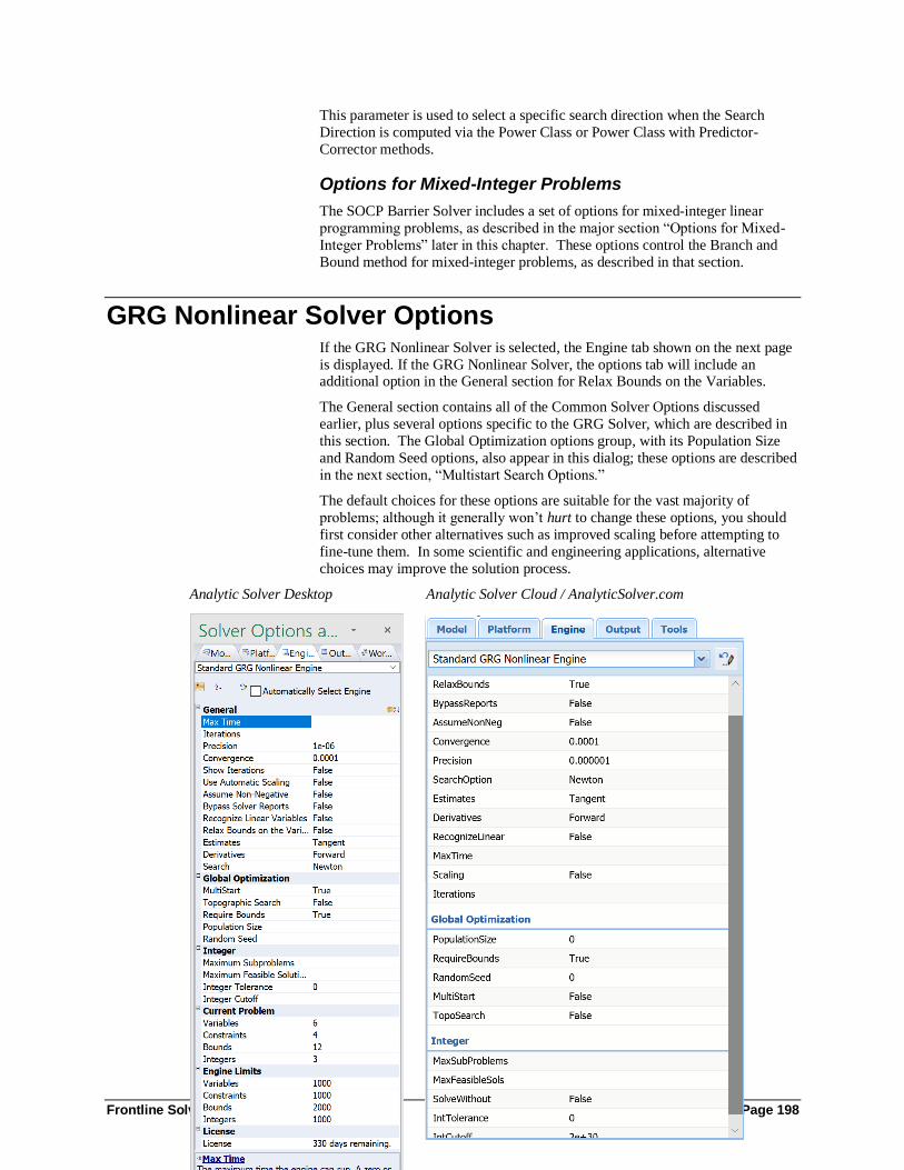
Frontline Solvers 2020 Reference Guide Page 198
This parameter is used to select a specific search direction when the Search
Direction is computed via the Power Class or Power Class with Predictor-
Corrector methods.
Options for Mixed-Integer Problems
The SOCP Barrier Solver includes a set of options for mixed-integer linear
programming problems, as described in the major section “Options for Mixed-
Integer Problems” later in this chapter. These options control the Branch and
Bound method for mixed-integer problems, as described in that section.
GRG Nonlinear Solver Options If the GRG Nonlinear Solver is selected, the Engine tab shown on the next page
is displayed. If the GRG Nonlinear Solver, the options tab will include an additional option in the General section for Relax Bounds on the Variables.
The General section contains all of the Common Solver Options discussed
earlier, plus several options specific to the GRG Solver, which are described in
this section. The Global Optimization options group, with its Population Size
and Random Seed options, also appear in this dialog; these options are described
in the next section, “Multistart Search Options.”
The default choices for these options are suitable for the vast majority of
problems; although it generally won’t hurt to change these options, you should
first consider other alternatives such as improved scaling before attempting to
fine-tune them. In some scientific and engineering applications, alternative
choices may improve the solution process.
Analytic Solver Desktop Analytic Solver Cloud / AnalyticSolver.com
Frontline Solvers 2020 Reference Guide Page 199
Convergence
VBA / SDK: Parameter Name "Convergence", 0 <= value <= 1
As discussed in the chapter “Solver Results Messages,” the GRG Solver will
stop and display the message “Solver has converged to the current solution”
when the objective function value is changing very slowly for the last few iterations or trial solutions. More precisely, the GRG Solver stops if the absolute
value of the relative change in the objective function is less than the value for
the Convergence option for the last 5 iterations. While the default value of 1.0E-
4 (0.0001) is suitable for most problems, it may be too large for some models,
causing the GRG Solver to stop prematurely when this test is satisfied, instead
of continuing for more Trial Solutions until the optimality (KKT) conditions are
satisfied.
If you are getting this message when you are seeking a locally optimal solution,
you can change the setting in the Convergence box to a smaller value such as
1.0E-5 or 1.0E-6; but you should also consider why it is that the objective
function is changing so slowly. Perhaps you can add constraints or use different starting values for the variables, so that the Solver does not get “trapped” in a
region of slow improvement.
Frontline Solvers 2020 Reference Guide Page 200
Recognize Linear Variables / RecognizeLinear
VBA / SDK: Parameter Name "RecognizeLinear", value 1/True or 0/False
If using Analytic Solver Desktiop, setting this option to True activates an
“aggressive” strategy to speed the solution of nonlinear problems that may be
useful when the Polymorphic Spreadsheet Interpreter is not used (Solve With =
Excel Interpreter).
This option is not applicable in Analytic Solver Cloud or AnalyticSolver.com
because the Polymorphic Spreadsheet Interpreter is always turned on.
As explained in the Analytic Solver User Guide chapter “Mastering
Conventional Optimization Concepts,” a Solver problem is nonlinear (and must
be solved with the GRG Solver engines) if the objective or any of the constraints
is a nonlinear function of even one decision variable. But in many such
problems, some of the variables occur linearly in the objective and all of the
constraints. Hence the partial derivatives of the problem functions with respect
to these variables are constant and need not be re-computed on each iteration.
If you set this option to True in Analytic Solver Desktop (and the Interpreter is set to Excel Interpreter), the GRG Solver in Analytic Solver will look for
variables whose partial derivatives are not changing over several iterations, and
then will assume that these variables occur linearly, hence that their partial
derivatives remain constant. At the solution, the partial derivatives are
recomputed and compared to the assumed constant values; if any of these values
has changed, the Solver will display the message “The linearity conditions
required by this Solver engine are not satisfied.” If you receive this message,
you should set the Recognize Linear Variables option to False and re-solve the
problem.
If Interpreter is set to Automatic or Psi Interpreter, the GRG Solver in Analytic
Solver handles partial derivatives via automatic differentiation rather than finite differencing. As a result, when the Psi Interpreter is used, which is the default
and is always in use in Analytic Solver Cloud or AnalyticSolver.com, selecting
this option will not save any time. However, the GRG Solver in Analytic Solver
overcomes this fact because it, along with the optional plug-in Large-Scale SQP
Solver and Knitro Solver engines, are designed to take advantage of information
provided by the Psi Interpreter and will exploit partial linearity in the problem
functions much more effectively than the GRG Solver with the Recognize
Linear Variables option.
Note: This setting is not applicable in Analytic Solver Cloud or
AnalyticSolver.com as the Psi Interpreter is always in use and, as a result, partial
derivatives are calculated using automatic differentiation.
Relax Bounds on Variables / Relax Bounds
VBA / SDK: Parameter Name "RelaxBounds", value 1-True or 0 – False
By default (and unlike the nonlinear GRG Solver bundled with Analytic Solver
Upgrade or Analytic Solver Basic), the GRG Solver within Analytic Solver
Comprehensive, Analytic Solver Optimization, Analytic Solver Cloud and
AnalyticSolver.com ensures that any trial points evaluated during the solution process will not have values that violate the bounds on the variables you specify,
even by a small amount. If your problem functions cannot be evaluated for
values outside the variable bounds, this default behavior will ensure that the
solution process can continue. However, at times this engine can make more
rapid progress along a given search direction by testing trial points with values
slightly outside the bounds on the variables. If you want to permit this to

Frontline Solvers 2020 Reference Guide Page 201
happen, set this parameter to true. If you receive the Solver Result Message
“Solver encountered an error value in a target or constraint cell,” as a first step
you should ensure that this option is set to true.
Derivatives and Other Nonlinear Options
The default values for the Estimates, Derivatives and Search options can be used for most problems. If you’d like to change these options to improve
performance on your model, this section will provide some general background
on how they are used by the GRG Solvers. For more information, consult the
academic papers on the GRG method listed at the end of the Introduction.
On each major iteration, the GRG Solvers require values for the gradients of the
objective and constraints (i.e. the Jacobian matrix). The Derivatives option is
concerned with how these partial derivatives are computed.
The GRG (Generalized Reduced Gradient) solution algorithm proceeds by first
“reducing” the problem to an unconstrained optimization problem, by solving a
set of nonlinear equations for certain variables (the “basic” variables) in terms of others (the “nonbasic” variables). Then a search direction (a vector in n-space,
where n is the number of nonbasic variables) is chosen along which an
improvement in the objective function will be sought. The Search option is
concerned with how this search direction is determined.
Once a search direction is chosen, a one-dimensional “line search” is carried out
along that direction, varying a step size in an effort to improve the reduced
objective. The initial estimates for values of the variables that are being varied
have a significant impact on the effectiveness of the search. The Estimates
option is concerned with how these estimates are obtained.
Estimates
VBA / SDK: Parameter Name "Estimates", value 1-Tangent or 2-Quadratic
This option determines the approach used to obtain initial estimates of the basic
variable values at the outset of each one-dimensional search. The Tangent
choice uses linear extrapolation from the line tangent to the reduced objective
function. The Quadratic choice extrapolates the minimum (or maximum) of a
quadratic fitted to the function at its current point. If the current reduced
objective is well modeled by a quadratic, then the Quadratic option can save time by choosing a better initial point, which requires fewer subsequent steps in
each line search. If you have no special information about the behavior of this
function, the Tangent choice is “slower but surer.” Note: The Quadratic choice
here has no bearing on quadratic programming problems.
Derivatives
VBA / SDK: Parameter Name "Derivatives", value 1-Forward or 2-Central
On each major iteration, the GRG Solver requires values for the gradients of the
objective and constraints (i.e. the Jacobian matrix). In Analytic Solver Desktop,
Analytic Solver Cloud, and AnalyticSolver.com, these derivatives may be
computed via automatic differentiation or via finite differencing. In the Analytic
Solver Upgrade if your model has less than 200 variables, derivatives may be
computed via automatic differentiation or via finite differencing. If your model
has greater than 200 variables, only finite differencing is available.
In Analytic Solver Desktop, Analytic Solver Cloud and AnalyticSolver.com,
when you are using the Psi Interpreter (Solve With = PSI Interpreter), automatic
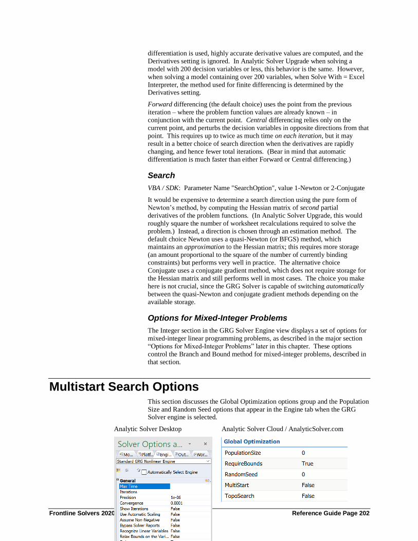
Frontline Solvers 2020 Reference Guide Page 202
differentiation is used, highly accurate derivative values are computed, and the
Derivatives setting is ignored. In Analytic Solver Upgrade when solving a
model with 200 decision variables or less, this behavior is the same. However,
when solving a model containing over 200 variables, when Solve With = Excel
Interpreter, the method used for finite differencing is determined by the Derivatives setting.
Forward differencing (the default choice) uses the point from the previous
iteration – where the problem function values are already known – in
conjunction with the current point. Central differencing relies only on the
current point, and perturbs the decision variables in opposite directions from that
point. This requires up to twice as much time on each iteration, but it may
result in a better choice of search direction when the derivatives are rapidly
changing, and hence fewer total iterations. (Bear in mind that automatic
differentiation is much faster than either Forward or Central differencing.)
Search
VBA / SDK: Parameter Name "SearchOption", value 1-Newton or 2-Conjugate
It would be expensive to determine a search direction using the pure form of
Newton’s method, by computing the Hessian matrix of second partial
derivatives of the problem functions. (In Analytic Solver Upgrade, this would
roughly square the number of worksheet recalculations required to solve the
problem.) Instead, a direction is chosen through an estimation method. The
default choice Newton uses a quasi-Newton (or BFGS) method, which maintains an approximation to the Hessian matrix; this requires more storage
(an amount proportional to the square of the number of currently binding
constraints) but performs very well in practice. The alternative choice
Conjugate uses a conjugate gradient method, which does not require storage for
the Hessian matrix and still performs well in most cases. The choice you make
here is not crucial, since the GRG Solver is capable of switching automatically
between the quasi-Newton and conjugate gradient methods depending on the
available storage.
Options for Mixed-Integer Problems
The Integer section in the GRG Solver Engine view displays a set of options for
mixed-integer linear programming problems, as described in the major section
“Options for Mixed-Integer Problems” later in this chapter. These options
control the Branch and Bound method for mixed-integer problems, described in
that section.
Multistart Search Options This section discusses the Global Optimization options group and the Population
Size and Random Seed options that appear in the Engine tab when the GRG Solver engine is selected.
Analytic Solver Desktop Analytic Solver Cloud / AnalyticSolver.com

Frontline Solvers 2020 Reference Guide Page 203
These options control the multistart methods for global optimization, which will
automatically run the GRG Solver (or certain field-installable Solver engines)
from a number of starting points in order to seek the globally optimal solution. The multistart methods are described under “Global Optimization” in the
Frontline Solver User Guides chapter “Mastering Conventional Optimization
Concepts,” and their behavior and stopping rules are further described under
“GRG Solver with Multistart Methods” in the chapter “Solver Result Messages”
within this Guide.
Multistart Search / Multistart
VBA / SDK: Parameter Name "MultiStart", value 1/True or 0/False
If this option is set to True, the multistart methods are used to seek a globally
optimal solution. If this box is unchecked, the other options described in this
section are ignored. The multistart methods will generate candidate starting
points for the GRG Solver (with randomly selected values between the bounds
you specify for the variables), group them into “clusters” using a method called
multi-level single linkage, and then run the GRG Solver from a representative point in each cluster. This process continues with successively smaller clusters
that are increasingly likely to capture each possible locally optimal solution.
Topographic Search / TopoSearch
VBA / SDK: Parameter Name "TopoSearch", value 1/True or 0/False
If this option (and the Multistart Search box) are set to True, the multistart
methods will make use of a “topographic” search method. This method uses the
objective value computed for the randomly sampled starting points to compute a
“topography” of overall “hills” and “valleys” in the search space, in an effort to
find better clusters and start the GRG Solvers from an improved point (already
in a “hill” or “valley”) in each cluster. Computing the topography takes extra
time, but on some problems this is more than offset by reduced time taken by the
GRG Solver on each subproblem.
Require Bounds on Variables / RequireBounds
VBA / SDK: Parameter Name "RequireBounds", value 1/True or 0/False
This option is set to True by default, but it comes into play only when the
Multistart Search box is checked. The multistart methods generate candidate
starting points for the GRG Solver by randomly sampling values between the
bounds on the variables that you specify. If you do not specify both upper and
lower bounds on each of the decision variables, the multistart methods can still

Frontline Solvers 2020 Reference Guide Page 204
be used, but because the random sample must be drawn from an “infinite” range
of values, this is unlikely to effectively cover the possible starting points (and
therefore have a good chance of finding all of the locally optimal solutions),
unless the GRG Solver is run on a great many subproblems, which will take a
very long time.
The tighter the bounds on the variables that you can specify, the better the
multistart methods are likely to perform. (This is also true of the Evolutionary
Solver.) Hence, this option is checked by default, so that you will be
automatically reminded to include both upper and lower bounds on all of the
variables whenever you select Multistart Search. If both the Multistart Search
and Require Bounds on Variables boxes are checked, but you have not defined
upper and lower bounds on all of the variables, Solver will stop with the result,
“Variable X does not have a finite upper and lower bound.”
When this message appears, you must either add both upper and lower bounds to
each variable by adding constraints in the Task Pane Model tab or by specifying
values for Decision Vars Lower and Decision Vars Upper on the Task Pane Platform tab (or set Assume Non-Negative to True to add lower bounds on the
variables), or else uncheck the Require Bounds on Variables box, then click
Solve again to allow the Solver to proceed with the solution process.
Population Size / PopulationSize
VBA / SDK: Parameter Name "PopulationSize", integer value > 0
The multistart methods generate a number of candidate starting points for the
GRG Solver equal to the value that you enter in this box. This set of starting
points is referred to as a “population,” because it plays a role somewhat similar
to the population of candidate solutions maintained by the Evolutionary Solver.
The minimum population size is 10 points; if you supply a value less than 10 in this box, or leave it blank, the multistart methods use a population size of 10
times the number of decision variables in the problem, but no more than 200.
Random Seed / RandomSeed
VBA / SDK: Parameter Name "RandomSeed", integer value > 0
The multistart methods use a process of random sampling to generate candidate
starting points for the GRG Solver. This process uses a random number
generator that is normally “seeded” using the value of the system clock – so the
random number sequence (and hence the generated candidate starting points)
will be different each time you click Solve. At times, however, you may wish to
ensure that the same candidate starting points are generated on several
successive runs – for example, in order to test different GRG Solver options on each search for a locally optimal solution. To do this, enter an integer value into
this box; this value will then be used to “seed” the random number generator
each time you click Solve.
Interval Global Solver Options When the Interval Global Solver is selected from the Solver engine dropdown
list in the Task Pane the following list of options will be displayed.
The General section contains all of the Common Solver Options discussed
earlier except the Precision option, plus several options specific to the Interval
Global Solver, which are described in this section.

Frontline Solvers 2020 Reference Guide Page 205
The default choices for these options are suitable for most problems, but you
should experiment with the Method options group to see which methods are
fastest on your problem. By default, the Interval Global Solver uses only “first
order” methods; significant speed gains may be achieved via use of the Second
Order and Linear Enclosure methods.
Analytic Solver Desktop Analytic Solver Cloud and AnalyticSolver.com
Accuracy
VBA / SDK: Parameter Name "Accuracy", 0 < value < 1
This option plays a role conceptually similar to the Precision option in the other Solver engines. It is used as a tolerance in the Interval Global Solver to
determine whether a “box” has been reduced in size to approximately a “point
solution,” whether the “distance” between two intervals is sufficiently small, and
– in conjunction with the Resolution option below – whether a proposed solution
to a system of equations should be treated as distinct from all other known
solutions.
Resolution
VBA / SDK: Parameter Name "Resolution", 0 < value < 100
When the Interval Global Solver is seeking all real solutions of a system of
nonlinear equations, the Accuracy and Resolution values are used to distinguish

Frontline Solvers 2020 Reference Guide Page 206
one solution from another. A proposed new solution – a “box” consisting of
intervals enclosing the decision variables – is compared to all other known
solutions. It is considered the same as an existing solution if either the absolute
distance between intervals is less than or equal to the Accuracy value or the
relative distance between intervals (taking into account their magnitudes) is less than or equal to the Resolution value, for all decision variables. If it is not the
same as any existing solution, the new point is accepted as a distinct solution.
Max Time w/o Improvement / MaxTimeNoImp
VBA / SDK: Parameter Name "MaxTimeNoImp", integer value > 0
The value for this option (measured in seconds) is the maximum time that the
Interval Global Solver will spend in its search without finding an “improved
global solution” (a feasible solution with an objective value better than the
currently best known solution). If this time limit is exceeded, the Solver will
stop and display the message “Solver cannot improve the current solution.” For
more information, see “Interval Global Solver Stopping Conditions” in the
chapter “Solver Results Messages.”
Absolute vs. Relative Stop / AbsRelStep
VBA / SDK: Parameter Name "AbsRelStop", value 1/True or 0/False
This option affects the test used to decide whether the globally optimal solution
has been found. As described in “Global Optimization” in the chapter “Solver
Models and Optimization,” the Interval Global Solver uses an Interval Branch &
Bound method that isolates locally optimal solutions and also updates a known
best bound on the globally optimal objective function value. The Solver stops
when it has found a feasible solution whose objective function value is very
close to this best known bound. If the Abs vs. Relative box is checked (the
default), the Solver compares the absolute difference between the objective value and the best bound to the Accuracy value. If this box is unchecked, the
Solver compares the relative difference (dividing by the objective’s magnitude)
to the Accuracy value.
Assume Stationary / AssumeStationary
VBA / SDK: Parameter Name "AssumeStationary", value 1/True or 0/False
This option can be used to speed up the Interval Global Solver in situations
where you know that the globally optimal solution is a “stationary point” and
not a point where a decision variable is equal to its lower or upper bound. The
Solver can save a significant amount of time if it does not have to check for
possible solutions on the “edges of boxes” where a variable equals one of its
bounds. If the Assume Stationary box is checked, the Solver will skip such checks for possible solutions. Of course, this means that if the true global
optimum is at a point where a decision variable equals a bound, the Solver will
probably “miss” this solution and return another point that is not the true global
optimum.
Method Options Group / Method
The Method options group plays a critical role in determining the performance
of the Interval Global Solver. As described in “Global Optimization” in the
chapter “Solver Models and Optimization,” the Interval Branch & Bound

Frontline Solvers 2020 Reference Guide Page 207
algorithm processes a list of “boxes” that consist of bounded intervals for each
decision variable, starting with a single box determined by the bounds that you
specify. On each iteration, it seeks lower and upper bounds for the objective and
the constraints in a given box that will allow it to discard all or a portion of the
box (narrowing the intervals for some of the variables), by proving that the box can contain no feasible solutions, or that it can contain no objective function
values better than a known best bound on the globally optimal objective. Boxes
that cannot be discarded are subdivided into smaller boxes, and the process is
repeated. Eventually, the boxes that remain each enclose a locally optimal
solution, and the best of these is chosen as the globally optimal solution.
To obtain good bounds on function values in a box, the Interval Global Solver
uses a first-order approximation to the problem functions, using interval values
and interval gradients computed by the Interpreter. Two rather different first-
order approximations can be used: The “classic interval” or mean value form
and the linear enclosure form. With each form, different advanced methods can
be used, as discussed below. The “classic interval” form is the default, but it pays to experiment with both forms to see which one performs best on your
model. In addition to these first-order approximations, the Solver always uses
local constraint propagation methods (also known as hull consistency methods)
that narrow intervals at each stage of evaluation of the problem functions.
Classic Interval vs. Linear Enclosure
VBA / SDK: Parameter Name "Method", value 1-Classic Interval or 2-Linear Enclosure
The Classic Interval and Linear Enclosure options form a “radio button group,”
so that only one of these two options is selected. Classic Interval (the default)
uses methods described in the research literature for a number of years; Linear
Enclosure uses recently published methods that are implemented for the first
time, to Frontline Systems’ knowledge, in the Interval Global Solver.
When Classic Interval is selected, the Solver uses the mean value form (based
on the interval gradient) as a first-order approximation of the problem functions.
This form is especially useful in tests that enable the Solver to rapidly “shrink” a
box. With this form, second order methods can be used as described below, but
these are optional since they require evaluation of the interval Hessian.
When Linear Enclosure is selected, the Solver uses the linear enclosure form
as a first-order approximation of the problem functions. The linear enclosure
doesn’t use the interval gradient directly, but it computes similar information to
completely enclose the function within linearized boundaries. This form does
not readily lend itself to the classic interval second order methods, but because it
completely encloses the function, it can be used to enable the Solver to rapidly
discard many boxes.
Second Order
VBA / SDK: Parameter Name "SecondOrder", value 1/True or 0/False
When this box is checked (and Classic Interval is selected – otherwise it is
grayed out), the Interval Global Solver uses a variant of the Interval Newton
method (analogous to Newton’s method for real numbers, but operating over
intervals), employing the Krawczyk operator at its key step, to rapidly find an
interval minimum for the objective and shrink or discard the current box, or to
rapidly determine whether a solution to a system of equations exists in the
current box. Use of the Krawczyk operator requires the interval Hessian, which
is computed by the Interpreter via reverse automatic differentiation.

Frontline Solvers 2020 Reference Guide Page 208
LP Test
VBA / SDK: Parameter Name "LPTest", value 1/True or 0/False
When this box is checked (and Linear Enclosure is selected – otherwise it is
grayed out), the Solver internally creates a series of linear programming
problems, using the linear enclosures of the original problem’s constraints and
the bounds on the current box, and applies Phase I of the Simplex method to this
problem. If the Simplex method finds no feasible solutions, then the original
problem’s constraints also have no feasible solutions in the current box, and this
box or region can be discarded in the overall Interval Branch & Bound
algorithm.
LP Phase II
VBA / SDK: Parameter Name "LPPhaseII", value 1/True or 0/False
When this box is checked (and Linear Enclosure is selected – otherwise it is
grayed out), the Solver proceeds as just described for the LP Test option, but it
also uses Phase II of the Simplex method to seek an improved bound on the
objective function in the current box. If this improved bound is feasible in the
original problem, it is used to update the known best bound on the globally optimal objective in the overall Interval Branch & Bound algorithm.
Evolutionary Solver Options When the Evolutionary Solver is selected from the Solver engine dropdown list
the following options are displayed.
This General section contains all of the Common Solver Options discussed
earlier (the Convergence option has a special meaning for the Evolutionary
Solver, as discussed below), plus several options specific to the Evolutionary
Solver.
Analytic Solver Desktop Analytic Solver Cloud / AnalyticSolver.com

Frontline Solvers 2020 Reference Guide Page 209
As with the other Solver engines, the Max Time option determines the
maximum amount of time the Evolutionary Solver will run before displaying a
dialog box asking whether the user wants to continue. The Iterations option
rarely comes into play, because the Evolutionary Solver always uses the Max
Subproblems and Max Feasible Solutions options on the Limits tab, whether or
not the problem includes integer constraints. (The count of iterations is reset on
each new subproblem, so the Iterations limit normally is not reached.) The
Precision option plays the same role as it does in the other Solver engines –
governing how close a constraint value must be to its bound to be considered
satisfied, and how close to an exact integer value a variable must be to satisfy an integer constraint. It also is used in computing the “penalty” applied to
infeasible solutions that are accepted into the population: A smaller Precision
value increases this penalty.
Convergence
VBA / SDK: Parameter Name "Convergence", 0 <= value <= 1
As discussed in the chapter “Solver Results Messages,” the Evolutionary Solver
will stop and display the message “Solver has converged to the current solution”
if nearly all members of the current population of solutions have very similar
“fitness” values. Since the population may include members representing
infeasible solutions, each “fitness” value is a combination of an objective
function value and a penalty for infeasibility. Since the population is initialized with trial solutions that are largely chosen at random, the comparison begins
after the Solver has found a certain minimum number of improved solutions that
were generated by the evolutionary process. The stopping condition is satisfied
if 99% of the population members all have fitness values that are within the
Convergence tolerance of each other.
If you believe that the message “Solver has converged to the current solution” is
appearing prematurely, you can make the Convergence tolerance smaller, but
you may also want to increase the Mutation Rate and/or the Population Size, in
order to increase the diversity of the population of trial solutions.
Population Size / PopulationSize
VBA / SDK: Parameter Name "PopulationSize", integer value > 0

Frontline Solvers 2020 Reference Guide Page 210
As described in the Analytic Solver User Guide chapter “Mastering
Conventional Optimization Concepts,” the Evolutionary Solver maintains a
population of candidate solutions, rather than a “single best solution” so far,
throughout the solution process. This option sets the number of candidate
solutions in the population. The minimum population size is 10 members; if you supply a value less than 10 for this option, or leave the option blank, the
Evolutionary Solver uses a population size of 10 times the number of decision
variables in the problem, but no more than 200.
The initial population consists of candidate solutions chosen largely at random,
but it always includes at least one instance of the starting values of the variables
(adjusted if necessary to satisfy the bounds on the variables), and it may include
more than one instance of the starting values, especially if the population is large
and the initial values represent a feasible solution.
A larger population size may allow for a more complete exploration of the
“search space” of possible solutions, especially if the mutation rate is high
enough to create diversity in the population. However, experience with genetic and evolutionary algorithms reported in the research literature suggests that a
population need not be very large to be effective – many successful applications
have used a population of 70 to 100 members.
Mutation Rate / MutationRate
VBA / SDK: Parameter Name "MutationRate", 0 <= value <= 1
The Mutation Rate is the probability that some member of the population will be
mutated to create a new trial solution (which becomes a candidate for inclusion
in the population, depending on its fitness) during each “generation” or
subproblem considered by the evolutionary algorithm. In the Evolutionary
Solver, a subproblem consists of a possible mutation step, a crossover step, an optional local search in the vicinity of a newly discovered “best” solution, and a
selection step where a relatively “unfit” member of the population is eliminated.
There are many possible ways to mutate a member of the population, and the
Evolutionary Solver actually employs five different mutation strategies,
including “permutation-preserving” mutation strategies for variables that are
members of an “alldifferent” group. The Mutation Rate is effectively
subdivided between these strategies, so increasing or decreasing the Mutation
Rate affects the probability that each of the strategies will be used during a given
“generation” or subproblem.
Random Seed / RandomSeed
VBA / SDK: Parameter Name "RandomSeed", integer value > 0
The Evolutionary Solver makes extensive use of random sampling, to generate
trial points for the population of candidate solutions, to choose strategies for
mutation and crossover on each “generation,” and for many other purposes.
This process uses a random number generator that is normally “seeded” using
the value of the system clock – so the random number sequence (and hence trial
points and choices made by the Evolutionary Solver) will be different each time
you click Solve. Because of these random choices, the Evolutionary Solver will
normally find at least slightly different (and sometimes very different) solutions
on each run, even if you haven’t changed your model at all. At times, however,
you may wish to ensure that exactly the same trial points are generated, and the
same choices are made on several successive runs. To do this, enter a positive

Frontline Solvers 2020 Reference Guide Page 211
integer value into this box; this value will then be used to “seed” the random
number generator each time you click Solve.
Require Bounds on Variables / RequireBounds
VBA / SDK: Parameter Name "RequireBounds", value 1/True or 0/False
If the option “Require Bounds on Variables” is set to True, and some of the
decision variables do not have upper or lower bounds specified under
Constraints in the Task Pane Model tab (or via the Assume Non-Negative
option) at the time you click Solve, the Solver will stop immediately with the
message “All variables must have both upper and lower bounds” – as illustrated
in the section “Multistart Search Options” earlier in this chapter. If this option is
not set to True, the Solver will not require upper and lower bounds on the
variables, but will attempt to solve the problem without them. Note that this box
is checked by default.
Bounds on the variables are especially important to the performance of the
Evolutionary Solver. For example, the initial population of candidate solutions is created, in part, by selecting values at random from the ranges determined by
each variable’s lower and upper bounds. Bounds on the variables are also used
in the mutation process – where a change is made to a variable value in some
member of the existing population – and in several other ways in the
Evolutionary Solver. If you do not specify lower and upper bounds for all of the
variables in your problem, the Evolutionary Solver can still proceed, but the
almost-infinite range for these variables may significantly slow down the
solution process, and make it much harder to find “good” solutions. Hence, it
pays for you to determine realistic lower and upper bounds for the variables, and
enter them under Constraints in the Task Pane Model tab.
Local Search / LocalSearch
Analytic Solver Comprehensive, Analytic Solver Optimization and Analytic
Solver Basic
VBA / SDK: Parameter Name "LocalSearch", value 1-Randomized Local
Search, 2-Gradient Local Search, 3-SQP with Gradient Sampling, 4-Automatic
Choice
Analytic Solver Upgrade
VBA / SDK: Parameter Name "LocalSearch", value 1-Randomized Local
Search, 2-Gradient Local Search, 3-Deterministic Pattern Search, 4-Automatic
Choice
This option determines the local search strategy employed by the Evolutionary
Solver. As noted under the Mutation rate option, a “generation” or subproblem in the Evolutionary Solver consists of a possible mutation step, a crossover step,
an optional local search in the vicinity of a newly discovered “best” solution,
and a selection step where a relatively “unfit” member of the population is
eliminated. You have a choice of strategies for the local search step. You can
use Automatic Choice (the default), which selects an appropriate local search
strategy automatically based on characteristics of the problem functions.
Randomized Local Search
This local search strategy generates a small number of new trial points in the
vicinity of the just-discovered “best” solution, using a probability distribution
for each variable whose parameters are a function of the best and worst

Frontline Solvers 2020 Reference Guide Page 212
members of the current population. (If the generated points do not satisfy all of
the constraints, a variety of strategies may be employed to transform them into
feasible solutions.) Improved points are accepted into the population.
Gradient Local Search
This local search strategy makes the assumption that the objective function –
even if non-smooth – can be approximated locally by a quadratic model. It uses
a classical quasi-Newton method to seek improved points, starting from the just-
discovered “best” solution and moving in the direction of the gradient of the
objective function. It uses a classical optimality test and a “slow progress” test
to decide when to halt the local search. An improved point, if found, is accepted
into the population.
If using Analytic Solver Comprehensive, Analytic Solver Optimization, Analytic
Solver Basic, Analytic Solver Cloud or AnalyticSolver.com, the third option for
Local Search is SQP with Gradient Sampling.
SQP with Gradient Sampling This local search strategy combines a sequential quadratic programming (SQP)
method with a gradient sampling algorithm to seek improved points; starting
from the just discovered, "best" solution for problems with a possible nonlinear
non-smooth objective function and/or constraints. This strategy requires
the gradients at smooth points enabling this method to effectively handle
problems with finitely many non-smooth points, however it comes with
some extra computational burden. Hence, the best use of the SQP with Gradient
Sampling method is recommended when high quality solutions are required for highly nonlinear non-smooth problems but a fast solution time is not of
significant importance, or when other local search methods fail to find an
optimal solution.
If using Analytic Solver Upgrade, the third option for Local Search is
Deterministic Pattern Search.
Deterministic Pattern Search
This local search strategy uses a “pattern search” method to seek improved
points in the vicinity of the just-discovered “best” solution. The pattern search
method is deterministic – it does not make use of random sampling or choices –
but it also does not rely on gradient information, so it is effective for non-
smooth functions. It uses a “slow progress” test to decide when to halt the local
search. An improved point, if found, is accepted into the population.
Automatic Choice
This option allows the Solver to select the local search strategy automatically.
Solver uses diagnostic information from the Polymorphic Spreadsheet
Interpreter to select a linear Gradient Local Search strategy if the problem has
smooth linear variables, or a nonlinear Gradient Local Search strategy if the
objective function has smooth nonlinear variables. When some or all variables are non-smooth and gradient information is available from the Polymorphic
Spreadsheet Interpreter, the SQP with Gradient Sampling method is chosen. It
also makes limited use of the Randomized Local Search strategy to increase
diversity of the points found by the local search step.

Frontline Solvers 2020 Reference Guide Page 213
Filtered Local Search
Solver applies two tests or “filters” to determine whether to perform a local
search each time a new point generated by the genetic algorithm methods is
accepted into the population. The “merit filter” requires that the objective value
of the new point be better than a certain threshold if it is to be used as a starting
point for a local search; the threshold is based on the best objective value found
so far, but is adjusted dynamically as the Solver proceeds. The “distance filter”
requires that the new point’s distance from any known locally optimal point
(found on a previous local search) be greater than the distance traveled when
that locally optimal point was found.
Thanks to its genetic algorithm methods, improved local search methods, and the distance and merit filters, the Evolutionary Solver performs exceedingly well
on smooth global optimization problems, and on many non-smooth problems as
well.
The local search methods range from relatively “cheap” to “expensive” in terms
of the computing time expended in the local search step; they are listed roughly
in order of the computational effort they require. On some problems, the extra
computational effort will “pay off” in terms of improved solutions, but in other
problems, you will be better off using the “cheap” Randomized Local Search
method, thereby spending relatively more time on the “global search” carried
out by the Evolutionary Solver’s mutation and crossover operations.
In addition to the Local Search options, the Evolutionary Solver employs a set of
methods, corresponding to the four local search methods, to transform infeasible
solutions – generated through mutation and crossover – into feasible solutions in
new regions of the search space. These methods, which also vary from “cheap”
to “expensive,” are selected dynamically (and automatically) via a set of
heuristics. For problems in which a significant number of constraints are
smooth nonlinear or even linear, these methods can be highly effective. Dealing
with constraints is traditionally a weak point of genetic and evolutionary
algorithms, but the hybrid Evolutionary Solver is unusually strong in its ability
to deal with a combination of constraints and non-smooth functions.
If the Evolutionary Solver stops with the message “Solver encountered an
error computing derivatives,” and you are using Analytic Solver Desktop,
you should set Use Sparse Variables to True in the Platform task pane and
Solve again.
Fix Nonsmooth Variables / FixNonSmooth
VBA / SDK: Parameter Name "FixNonSmooth", value 1/True or 0/False
This option determines how non-smooth variable occurrences in the problem
will be handled during the local search step. In Analytic Solver Upgrade, this
option is ignored. If this box is checked, the non-smooth variables are fixed to
their current values (determined by genetic algorithm methods) when a
nonlinear Local Gradient or linear Local Gradient search is performed; only the
smooth and linear variables are allowed to vary. If this box is unchecked, all of the variables are allowed to vary.
Since gradients are undefined for non-smooth variables at certain points, fixing
these variables ensures that gradient values used in the local search process will
be valid. On the other hand, gradients are defined for non-smooth variables at
most points, and the search methods are often able to proceed in spite of some
invalid gradient values, so it often makes sense to vary all of the variables
Frontline Solvers 2020 Reference Guide Page 214
during the search. Hence, this box is unchecked by default; you can experiment
with its setting on your model.
Global Search / GlobalSearch
VBA: Parameter Name "LegacyMode", value - 1/Genetic Algorithm or 0/Scatter
Search
SDK: Parameter Name "GlobalSearch", value - 1/Genetic Algorithm or
0/Scatter Search
If this option is set to Genetic Algorithm, then the Evolutionary Solver will use
methods from the literature on genetic algorithms (its traditional methods) to
solve the model. Otherwise, the Evolutionary Solver will use methods from the
literature on scatter search. On some models, the scatter search algorithm will
result in better answers in less time when compared to the genetic
algorithm. However, for other models, the genetic algorithm may be more
successful. Since the scatter search algorithm tends perform best, by a modest
margin, on the majority of models, it is the default choice. But we suggest you try both algorithms with your model to see which works better for you.
Model Based Search / ModelBasedSearch
VBA / SDK: Parameter Name "ModelBasedSearch", 0-None, 1-CPU Based, 2 –
GPU Based
This option takes effect only when the Global Search option is set to Scatter
Search. When this option is set to “None”, the Scatter Search algorithm is used
without any Model Based Local Search. When this option is set to either “CPU
Based” or “GPU Based”, an internal model of the problem is created (using
radial basis functions) which closely fits the original problem in the search
region. The Evolutionary Solver then uses this internal model to evaluate many
points in parallel (either on the CPU or GPU - depending on the option setting) rather than using Excel or the PSI Interpreter to evaluate each of these points
sequentially. Only the most promising of these points are evaluated against the
actual spreadsheet model. The most promising points from this evaluation are
added to the population of best solutions. This new search method typically
results in better solutions in less time when compared to using only the Scatter
Search algorithm.
Note for Users of Analytic Solver Desktop: Most new computers now contain
GPUs or Graphics Processing Units, either on custom chips (in most laptops) or
plug-in cards. These devices are typically used to quickly build and manipulate
display images for video games and other graphics. However, their ability to
perform floating point arithmetic in parallel can be harnessed for computational purposes. Some GPU cards or chips contain 256, 512 or more special-purpose
processors; in comparison, the computer’s main CPU usually contains just 2 to 4
general-purpose processors If your computer includes a Nvidia or AMD
Radeon graphics card or chip, it would be worth your time to compare the
performance of both the CPU and GPU based approaches. You very well could
find that the GPU based search results in a solution in significantly less time
than the CPU based search.
Feasibility Pump / FeasibilityPump
VBA / SDK: Parameter Name "FeasibilityPump", value 1/True or 0/False
Frontline Solvers 2020 Reference Guide Page 215
The new Feasibility Pump methods for both continuous and integer variables
help the Evolutionary Solver find better solutions, faster than ever.This option
allows the Evolutionary Solver to search for a feasible solution and add it to the
initial population. Feasibility Pump uses a set of fast heuristic and exact methods
that seek a feasible solution, but not necessarily a high quality solution, when finding a feasible solution may be as challenging as finding the optimal
solution.
Limits Section Options
Where the other Solver engines use the Branch & Bound method to solve
problems with integer constraints, subject to limits set in the Integer Options
dialog tab, the Evolutionary Solver handles integer constraints on its own, and is subject to the limits set in this dialog tab. Unlike the other Solver engines, the
Evolutionary Solver always works on a series of subproblems, even if there are
no integer constraints in the model – so these options are always important for
the Evolutionary Solver.
Max Subproblems / MaxSubProblems
VBA / SDK: Parameter Name "MaxSubProblems", integer value > 0
The value for the Max Subproblems option places a limit on the number of
subproblems that may be explored by the evolutionary algorithm before the
Solver pauses and asks you whether to continue, stop or restart the solution
process. In the Evolutionary Solver, a subproblem consists of a possible
mutation step, a crossover step, an optional local search in the vicinity of a newly discovered “best” point, and a selection step where a relatively “unfit”
member of the population is eliminated. During the solution process, the
number of subproblems considered so far is shown on the Excel status bar, along
with the objective of the best feasible solution (if any) found so far. If your
model is moderately large or complex, you may need to increase this limit from
its default value; any value up to 2,147,483,647 may be used.
Max Feasible Solutions / MaxFeasibleSols
VBA / SDK: Parameter Name "MaxIntegerSols", integer value > 0
The value for the Max Feasible Sols option places a limit on the number of
feasible solutions found by the evolutionary algorithm before the Solver pauses and asks you whether to continue, stop or restart the solution process. A feasible
solution is any solution that satisfies all of the constraints, including any integer
constraints. As with the Max Subproblems option, if your model is moderately
large or complex, you may need to increase this limit; any value up to
2,147,483,647 may be used.
Tolerance / IntTolerance
VBA / SDK: Parameter Name "IntTolerance", 0 <= value <= 1
This option works in conjunction with the Max Time without Improvement
option to limit the time the evolutionary algorithm spends without making any
significant progress. If the relative (i.e. percentage) improvement in the best
solution’s “fitness” is less than the Tolerance value for the number of seconds for the Max Time without Improvement option, the Evolutionary Solver stops as
described below. Since the population may include members representing

Frontline Solvers 2020 Reference Guide Page 216
infeasible solutions, the “fitness” value is a combination of an objective function
value and a penalty for infeasibility.
Max Time without Improvement / MaxTimeNoImprove
VBA / SDK: Parameter Name "MaxTimeNoImp", integer value > 0
This option works in conjunction with the Tolerance option to limit the time the evolutionary algorithm spends without making any significant progress. If the
relative (i.e. percentage) improvement in the best solution’s “fitness” is less than
the Tolerance value for the number of seconds in the Max Time without
Improvement option, the Evolutionary Solver stops and displays the Solver
Results dialog. The message is “Solver cannot improve the current solution,”
unless the evolutionary algorithm has discovered no feasible solutions at all, in
which case the message is “Solver could not find a feasible solution.” If you
believe that this stopping condition is being met prematurely, you can either
make the Tolerance value smaller (or even zero), or increase the number of
seconds allowed by the Max Time without Improvement option.
Integer Section of the Engine Tab Options The four options below appear in the Integer section of the GRG Solver engine, Inteval Solver, and SOCP Solver. When you click Engine tab, options for
mixed-integer programming problems are displayed.
Analtyic Solver Desktop Analytic Solver Cloud / AnalyticSolver.com
Max Subproblems / MaxSubProblems
VBA / SDK: Parameter Name "MaxSubProblems", integer value > 0
The value for the Max Subproblems option places a limit on the number of
subproblems that may be explored by the algorithm before the Solver pauses and
asks you whether to continue, stop or restart the solution process. During the solution process, the number of subproblems considered so far is shown on the
Excel status bar, along with the objective of the best feasible solution (if any)
found so far. If your model is moderately large or complex, you may need to
increase this limit from its default value; any value up to 2,147,483,647 may be
used.
Note: A “Restart” button also appears in the dialog box where the Solver asks
you whether you want to continue or stop the solution process; but this button is
meaningful only for the GRG Nonlinear Solver, and it affects only restarting of
the current subproblem. The Branch & Bound algorithm is never restarted, as
this would simply mean discarding the progress that has been made so far.
In a problem with integer constraints, the Max Subproblems limit should be used in preference to the Iterations limit; the Iterations limit should be set high
enough for each of the individual subproblems solved during the Branch &
Bound process. For problems with many integer constraints, you may need to

Frontline Solvers 2020 Reference Guide Page 217
increase this limit from its default value; any integer value up to 2,147,483,647
may be used.
Max Feasible Solutions / MaxFeasibleSols
VBA / SDK: Parameter Name "MaxIntegerSols", integer value > 0
The value for the Max Feasible Sols option places a limit on the number of
feasible solutions found by the evolutionary algorithm before the Solver pauses
and asks you whether to continue, stop or restart the solution process. A feasible
solution is any solution that satisfies all of the constraints, including any integer
constraints. As with the Max Subproblems option, if your model is moderately
large or complex, you may need to increase this limit; any value up to
2,147,483,647 may be used.
Integer Tolerance / IntTolerance
VBA / SDK: Parameter Name "IntTolerance", 0 <= value <= 1
When you solve an integer programming problem, it often happens that the
Branch & Bound method will find a good solution fairly quickly, but will require a great deal of computing time to find (or verify that it has found) the
optimal integer solution. The Integer Tolerance setting may be used to tell the
Solver to stop if the best solution it has found so far is “close enough.”
The Branch & Bound process starts by finding the optimal solution without
considering the integer constraints (this is called the relaxation of the integer
programming problem). The objective value of the relaxation forms the initial
“best bound” on the objective of the optimal integer solution, which can be no
better than this. During the optimization process, the Branch & Bound method
finds “candidate” integer solutions, and it keeps the best solution so far as the
“incumbent.” By eliminating alternatives as its proceeds, the B&B method also
tightens the “best bound” on how good the integer solution can be.
Each time the Solver finds a new incumbent – an improved all-integer solution –
it computes the maximum percentage difference between the objective of this
solution and the current best bound on the objective:
Objective of incumbent - Objective of best bound
------------------------------------------------
Objective of best bound
If the absolute value of this maximum percentage difference is equal to or less
than the Integer Tolerance, the Solver will stop and report the current integer solution as the optimal result, with the message “Solver found an integer
solution within tolerance.” If you set the Integer Tolerance to zero, the Solver
will “prove optimality” by continuing to search until all alternatives have been
explored and the optimal integer solution has been found. This may take a great
deal of computing time.
Integer Cutoff / IntCutoff
VBA / SDK: Parameter Name "IntCutoff", -1E30 < value < +1E30
This option provides another way to save time in the solution of mixed-integer
programming problems. If you know the objective value of a feasible integer
solution to your problem – possibly from a previous run of the same or a very
similar problem – you can enter this objective value for the Integer Cutoff

Frontline Solvers 2020 Reference Guide Page 218
option. This allows the Branch & Bound process to start with an “incumbent”
objective value (as discussed above under Integer Tolerance) and avoid the work
of solving subproblems whose objective can be no better than this value. If you
enter a value here, you must be sure that there is an integer solution with an
objective value at least this good: A value that is too large (for maximization problems) or too small (for minimization) may cause the Solver to skip solving
the subproblem that would yield the optimal integer solution.
The Current Problem and Engine Limits Sections Each engine in Analytic Solver Desktop includes a Problem section which
displays statistics on the size of the current problem and the corresponding
Solver engine size limits, including the number of decision variables, number of
constraints, number of bounds on the variables, and number of integer variables.
These edit controls are “read-only” – the current problem sizes are computed
automatically, and the Solver engine size limits are obtained automatically from
both built-in and field-installable Solver engines.
When the LP/Quadratic Solver is selected from the Solver engine dropdown list the following is displayed. The LP/Quadratic Solver supports linear and
quadratic programming problems of up to 8,000 variables, 8,000 constraints,
16,000 bounds, and 2,000 integer variables.
Loading, Saving and Merging Solver Models On the Analytic Solver Desktop Ribbon there is a dropdown menu for Loading,
Saving, and Merging Models.
Optimization models may only be saved in Classic Format when using Analytic
Solver Cloud and AnalyticSolver.com. Saving the model as an .lp file or using
Psi functions is also not supported in either Analytic Solver Cloud or
AnalyticSolver.com.
Analytic Solver Desktop Analytic Solver Cloud AnalyticSolver.com
The “current” Solver model defined for each worksheet is automatically saved
“behind the scenes” in that worksheet. So it is not necessary to use this feature
to keep track of a single Solver model – the last set of specifications you defined
will be saved automatically when the workbook is saved, and restored when it is
re-opened. But the Load Model... and Save Model... options can be used to save

Frontline Solvers 2020 Reference Guide Page 219
more than one Solver model on the same worksheet, and to merge two models
into one.
Note: A model saved in classic format in Analytic Solver Desktop may not be
loaded in Analytic Solver Cloud, or vice-versa.
Saved Model Formats
The model specifications can be stored as formulas in two formats: The Classic
format, which is upward compatible from the standard Excel Solver, uses certain
built-in Excel functions and array formulas to store the model; it is not intended
for user modification. The Psi Function format, introduced in Version 7.0, uses
add-in functions such as PsiVar(), PsiCon(), PsiObj() and PsiOption() to store
the model; more information can be found in the next chapter “Psi Function
Reference.” Since it is a fully documented format, it may be used to “import”
models that are created manually or with other programs.
Analytic Solver Cloud and AnalyticSolver.com support saving/loading in
Classic format only.
Competitive Products
A third alternative is available for users upgrading to the Analytic Solver
Desktiop products, Analytic Solver Comprehensive, Analytic Solver Optimization or Analytic Solver Basic, from certain competitive software
products: If you click the Load Model button and there’s no model defined for
Analytic Solver in the workbook, but there is a model defined for a recognized
competitive software product, the Solver will list this model and allow you to
select it for loading. When you click OK, the model is loaded and converted – it
becomes the “current” Solver model defined for the active worksheet, for
Analytic Solver.
Saving A Model in LP Format
Starting in Analytic Solver Desktop V2015 the ability to save both linear or
quadratic models in LP or MPS Format was introduced and in Analytic Solver
Desktop V2016-R2, the ability to save linear, quadratic and nonsmooth models
in JSON format was introduced. After you diagnose or solve a model (by
clicking Optimize on the ribbon or the Analyze/Solve icon on the task pane),
click Load/Save -- Save Model in the Tools section on the ribbon, then select
Output File for Format. (If you select this option without solving or analyzing
the model first, you’ll receive an error instructing you to do so first.)

Frontline Solvers 2020 Reference Guide Page 220
Click OK, a Save As dialog will open.
Select the file type and the location for the output file to be saved. Afterwards,
open the file to reveal the Excel model written in LP, MPS, or JSON Format.
LP and MPS formats are available only for LP (linear programming) and QP
(quadratic programming) models with or without integer constraints; they
cannot represent nonlinear, non-smooth, or stochastic optimization models. In
LP format, the objective and each constraint always appears as a sum of decision
variables multiplied by constant coefficients, which are computed when your
model is analyzed. This is based on, but may not "look the same" as your Excel
formulas. For example, if you have a constraint A1 <= 100, X1:X4 are decision
variables, X5 = 0, and your model has formulas:
A1: =2*B1
B1: =SUM(X1:X5)-C1
C1: =4*X1+ 0.5*X3
The constraint A1 <= 100 will appear as:
c0: -6 x1 + 2 x2 + 1 x3 + 2 x4 <= 100
As an example please see below for the output from the Product Mix example
file in lp format.
\ Solver Optimization Model
Maximize
obj : + 75 x1 + 50 x2 + 35 x3
Subject To
c0 : + 1 x1 + 1 x2 <= 450
c1 : + 1 x1 <= 250
c2 : + 2 x1 + 2 x2 + 1 x3 <= 800
c3 : + 1 x1 + 1 x2 <= 450
c4 : + 2 x1 + 1 x2 + 1 x3 <= 600
Bounds
x1 >= 0 x2 >= 0
x3 >= 0
Binary

Frontline Solvers 2020 Reference Guide Page 221
General
End
MPS files are column-oriented and all model components are named. See below for the same Product Mix model, this time saved in MPS format.
NAME Solver Optimization Model
OBJSENSE
MAX
ROWS
L c0
L c1
L c2
L c3
L c4
N obj
COLUMNS
x1 c0 1 c1 1
x1 c2 2 c3 1
x1 c4 2 obj 75
x2 c0 1 c2 2
x2 c3 1 c4 1
x2 obj 50
x3 c2 1 c4 1
x3 obj 35
RHS
RHS1 c0 450 c1 250
RHS1 c2 800 c3 450
RHS1 c4 600
BOUNDS
ENDATA
Files saved with the extension .json are written using the RASON Modeling
Language. Here's the same Product Mix Example, as saved in the .json format.
For more information on this language, see either the Frontline Solvers or
RASON Modeling Language User Guides.
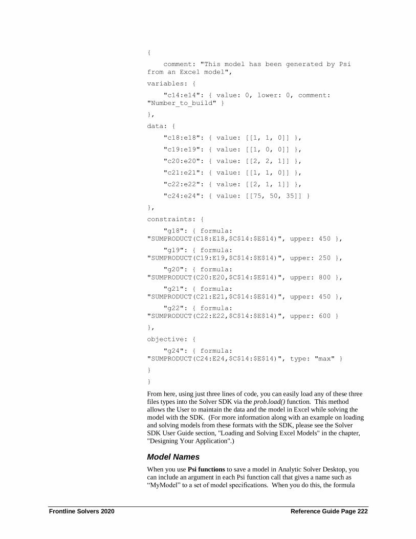
Frontline Solvers 2020 Reference Guide Page 222
{
comment: "This model has been generated by Psi
from an Excel model",
variables: {
"c14:e14": { value: 0, lower: 0, comment:
"Number_to_build" }
},
data: {
"c18:e18": { value: [[1, 1, 0]] },
"c19:e19": { value: [[1, 0, 0]] },
"c20:e20": { value: [[2, 2, 1]] },
"c21:e21": { value: [[1, 1, 0]] },
"c22:e22": { value: [[2, 1, 1]] },
"c24:e24": { value: [[75, 50, 35]] }
},
constraints: {
"g18": { formula:
"SUMPRODUCT(C18:E18,$C$14:$E$14)", upper: 450 },
"g19": { formula:
"SUMPRODUCT(C19:E19,$C$14:$E$14)", upper: 250 },
"g20": { formula:
"SUMPRODUCT(C20:E20,$C$14:$E$14)", upper: 800 },
"g21": { formula:
"SUMPRODUCT(C21:E21,$C$14:$E$14)", upper: 450 },
"g22": { formula:
"SUMPRODUCT(C22:E22,$C$14:$E$14)", upper: 600 }
},
objective: {
"g24": { formula:
"SUMPRODUCT(C24:E24,$C$14:$E$14)", type: "max" }
}
}
From here, using just three lines of code, you can easily load any of these three
files types into the Solver SDK via the prob.load() function. This method
allows the User to maintain the data and the model in Excel while solving the
model with the SDK. (For more information along with an example on loading
and solving models from these formats with the SDK, please see the Solver
SDK User Guide section, "Loading and Solving Excel Models" in the chapter,
"Designing Your Application".)
Model Names
When you use Psi functions to save a model in Analytic Solver Desktop, you
can include an argument in each Psi function call that gives a name such as
“MyModel” to a set of model specifications. When you do this, the formula

Frontline Solvers 2020 Reference Guide Page 223
cells containing Psi functions need not be contiguous on the spreadsheet; they
are associated via the model name. When you click the Load Model button, the
Solver offers you a choice of available models:
The “current” Solver model also has a name, which is the same as the worksheet
name. You can choose any of the named models, or you can choose Select a
range and load a set of Classic format (not Psi function format) specifications
from a contiguous cell range.
Using Multiple Solver Models
It is possible – and often useful – to define more than one Solver model based on
the same worksheet formulas. An example of this is provided in the “Portfolio
of Securities” (Sharpe tab) worksheet in the
StockPortfolioOptimization(Opt).xlsx workbook that is installed along with
Analytic Solver (Help – Examples). This worksheet defines a portfolio
optimization model, where the Solver must determine what percentage of
available funds to invest in four different stocks (A, B, C and D) and Treasury
bills. The worksheet formulas calculate the portfolio rate of return, and the
portfolio risk as measured by the statistical variance of returns. There are two
possible approaches to solving this model: (1) Find the maximum rate of return, subject to an upper limit on the portfolio’s risk, or (2) Find the minimum risk
(variance), subject to a lower limit on the portfolio’s return.
The “current” Solver problem on this worksheet is the one that maximizes
return, subject to a constraint on portfolio risk. But both Solver problems
(“Maximize Return” and “Minimize Risk”) have been set up and their
specifications saved (in Classic format) on the right of this worksheet, starting at
cell T19. If you click on Save/Load Model on the ribbon, select cells T19:T24,
and click OK, you’ll load the specifications for the problem that minimizes risk
subject to a constraint on return.
Merging Solver Models
In the standard Microsoft Excel Solver and earlier versions of the Premium Solver products, loading a model’s specifications through Load Model... causes
any existing specifications for the “current” Solver model to be erased. You are
prompted before this happens with an alert box asking if you want to reset the
previous solver cell selections.
In recent versions of the Analytic Solver and its sub-set products, you have
another choice: You can merge the model specifications being loaded with the
current model specifications. Where the specifications necessarily overlap – as
in the selection of the objective (and the “maximize” or “minimize” setting) and
in the settings of Solver options – the newly loaded specifications take
precedence. But the variable cell selections and the constraint left hand sides,
relations and right hand sides being loaded are merged into the current model. You are prompted to choose between replacing the current model specifications
and merging in the new specifications:

Frontline Solvers 2020 Reference Guide Page 224
Merging model specifications can be quite useful, for it allows you to build and
test smaller, simple Solver models and then combine them into a larger model.
Suppose, for example, that you wanted to create a planning model for a
manufacturing firm that would take into account both the mix of products being
built and the routes along which they were being shipped. You might create two
models on one worksheet, one based on the Product Mix example and the other
based on the Shipping Routes example in SOLVSAMP.XLS, and test them
individually. Then you could combine them with the Merge function, and test
the production-distribution model as a whole.
Frontline Solvers 2020 Reference Guide Page 225
PSI Function Reference
Using PSI Functions This chapter provides summary information on Analytic Solver’s PSI functions that you can use in Excel formulas to create optimization and Monte Carlo
simulation models
You use Psi Optimization functions to define decision variables, constraints,
the objective function, and any engine option.
You use PSI Distribution functions to define the properties of uncertain
variables, either via an analytic probability distribution and its parameters, or via
a pre-generated SIP or SLURP with the PsiSip() and PsiSlurp() functions.
You use PSI Property functions to modify the properties of analytic probability
distributions, by shifting or truncating their domains, or by correlating one
distribution with another.
You use PSI Statistics functions to obtain results of the simulation, such as
statistics, frequency data, or raw trial data, for uncertain functions. You use the
PsiOutput() function to mark cells that calculate values for uncertain functions.
When you run multiple simulations at once, you can use the PsiSimParam()
function to specify a list of values for a cell, one per simulation, where the value
is held constant for all trials in a simulation.
Analytic Solver Comprehensive includes Psi Classification and Psi Prediction
functions to score new classification and prediction data without the need to
click the Score icon on the Data Mining ribbon and also Psi Forecasting
functions to predict new data points in a time series dataset.
Note: When entering Psi functions manually in Analytic Solver Cloud or Data
Mining Cloud apps, the taskpane must be refreshed before running an
optimization, simulation, or parameter analysis report.
Using PSI Optimization Functions
If “Use Psi Functions” is set to true in the Analytic Solver Desktop Task Pane
Platform tab, then Psi Optimization functions can be used to define variables,
constraints, the objective function, set engine options, and monitor or set values
during multiple optimizations or sensitivity analysis. If adding a model to a
worksheet other than the ActiveSheet, “Use Psi Functions” must be set to true
on both the ActiveSheet and the worksheet that will hold the model.
These function are not supported in Analytic Solver Cloud or
AnalyticSolver.com.

Frontline Solvers 2020 Reference Guide Page 226
PsiCalcValue
PsiCalcValue(output_cell_address)
This function defines an observation output for a given formula cell.
PsiCalcValue considers only the observation outputs in a pure workbook
recalculation.
Use this function in conjunction with PsiDecTable() when using a version of
Excel that does not support Dynamic Arrays (V2016 or earlier).
PsiCon
PsiCon(LHS, relation, RHS, active, chance type,
chance measure, comment, model name)
PsiCon adds one or more constraints to the optimization model. LHS is a cell or contiguous range of cells that contain the left hand side(s) of the constraint(s).
Pass the relation, in quotes, of the constraint as the 2nd argument: “<=” (less
than or equal to), “=” (equal to), “>=” (greater than or equal to), “int” (integer),
“bin” (binary), “dif” (alldifferent), “soc” (cone), “src” (rotated cone), or “sem”
(semicontinuous). RHS is a cell or contiguous range of cells that contain the
right hand side(s) of the constraint(s). Passing true for the fourth argument,
active, selects the constraint in the Task Pane Model tab for inclusion in the
active model. Passing false for this argument unchecks the constraint which
removes the constraint from the active model. If this argument is not passed,
then true will be passed by default. Pass integer values for the chance type: 0
(normal), 2 (VaR), 3 (CVaR), or 4 (USet). Pass a value from 0 to 1 for the chance measure. A comment may be added to the constraint (surrounded by
quotes) which will appear under “Comment” in the Variable Property Window.
(To view the Property Window simply highlight the variable or range of
variables in the Task Pane Model tab. The Property Window will appear at the
bottom of the task pane.) You may pass a model or sheet name, in quotes, for
the last argument, model name, to indicate to ASP what model or worksheet the
constraint(s) belong(s).
PsiCurrentOpt
PsiCurrentOpt()
PsiCurrentOpt returns the index (1, 2, 3, etc.) of the current optimization, when
multiple optimizations are being run.
PsiEngine
PsiEngine(engine name, model name)
PsiEngine selects the engine for the optimization model. Pass the name of the
Engine, in quotes, as the first argument, Engine Name: Standard GRG
Nonlinear, Standard LP/QP Quadratic, Standard Evolutionary, Standard Interval
Global, or Standard SOCP Barrier. You may pass a model or sheet name, in
quotes, for the last argument, model name, to indicate to ASP what model or
worksheet the engine selection belongs.
Frontline Solvers 2020 Reference Guide Page 227
PsiInput
PsiInput(cell_or_name)
PsiInput marks a cell as input, which can be used when solving the workbook
using the Solver SDK Platform.
PsiModel
PsiModel(option name, value, model name)
PsiModel sets any Model option, or any option that appears on the Task Pane
Model tab. Pass the name of the option as the first argument, Option Name. Pass the value of the option for Value. You may pass a model or sheet name, in
quotes, for the last argument, model name, to indicate to ASP what model or
worksheet the option setting belongs. Note: Only model options pertaining to
optimization can be set using PsiModel().
PsiObj
PsiObj(objective cell, sense, valueof, chancetype,
chance measure, comment, model name)
PsiObj adds an objective cell to the optimization model. Pass the cell address of
the objective cell as the first argument, Objective Cell. For the Sense argument, pass “min” for a minimization, “max” for a maximization” and “ValueOf” if
using the ValueOf property. If using ValueOf, pass the numerical value as the
next argument, i.e. 1000. Set the type of objective for the ChanceType, Normal,
Expected VaR, CVaR, or USet. If the objective includes uncertainty, set the
Chance Measure in the next argument. Pass integer values for the chance type:
0 (Normal), 1 (Expected), 2 (VaR), 3 (CVaR), or 4 (USet). Pass a value from 0
to 1 for the chance measure. A comment may be added to the objective
(surrounded by quotes) which will appear under “Comment” in the Variable
Property Window. (To view the Property Window simply highlight the variable
or range of variables in the Task Pane Model tab. The Property Window will
appear at the bottom of the task pane.) You may pass a model or sheet name, in
quotes, for the last argument, model name, to indicate to ASP what model or worksheet the objective belongs.
PsiOption
PsiOption(option name, value, model name)
PsiOption sets an option for the optimization engine. Pass the name of the
option as the first argument, Option Name. Pass the value of the option for
Value. You may pass a model or sheet name, in quotes, for the last argument, model name, to indicate to ASP what model or worksheet the option setting
belongs.
PsiOptParam
PsiOptParam(values_or_lower, upper, base_case)
PsiOptParam provides a list of different values that a variable should have in
different optimizations. Pass the lower limit for the parameter or alternatively, a list of values or a cell range, for the Values_or_lower argument and the upper

Frontline Solvers 2020 Reference Guide Page 228
limit for the parameter for the optional Upper argument. The argument,
base_case, will be used when no specific optimization is indicated, i.e. if
running a simulation or sensitivity parameters analysis on a model where
PsiOptParam exists.
Note: In Desktop Analytic Solver, the "current" optimization number is always displayed on the Analytic Solver ribbon, in the Tools section, and the returned
value of PsiOptParam reflects that optimization number. As a result, it is not
possible to "see" the basecase value in action unless another type of parameter
analysis is being run, i.e. a simulation parameter analysis or a sensitivity
parameter analysis.
For a description of this function in use, please see the chapter, Getting Results:
Optimization in the Frontline Solver’s User Guide.
PsiOptStatus
PsiOptStatus()
PsiOptStatus displays the status of optimization as returned by the running
engine. For a complete list of final results returned by the Analytic Solver,
please see the chapter Solver Results Messages.
PsiOptValue
PsiOptValue(cell_or_name, optimization, model)
PsiOptValue returns the specific value for a cell or function of an optimization.
Pass the cell address or defined name of the desired cell for the first argument,
Cell_or_name. Pass the optimization number for the second argument,
Optimization, if multiple optimizations are being run. Pass the Sheet name for
the model argument, when running multiple optimizations on multiple
worksheets (within the same workbook) when the same cell is used for more
than one optimization and the Excel Interpreter is used. (This argument is not
supported when the PSI Interpreter is in use.) For example, if cell Sheet1!A1 is
used in the optimization model in Sheet1 and also the optimization model in Sheet2, =PsiOptValue(Sheet1!A1,2,”Sheet1”) will return the value of cell
Sheet1!A1 for the 2nd optimization on Sheet1. Similarly,
=PsiOptValue(Sheet1!A1, 3, “Sheet2”) will return the value of cell Sheet1!A1
for the 3rd optimization on Sheet2.
PsiSenParam
PsiSenParam(values_or_lower, upper)
PsiSenParam provides a list of different values that a variable should have
during sensitivity analysis. Pass the lower limit for the parameter or
alternatively, a list of values or a cell range, for the Values_or_lower argument
and the upper limit for the parameter for the optional Upper argument. For a
description of this function, please see the chapter, Examples: Parameters and
Sensitivity Analysis.
Frontline Solvers 2020 Reference Guide Page 229
PsiSenValue
PsiSenValue(cell_or_name)
PsiSenValue returns the specific value for a cell or function of a sensitivity
analysis. For a description of this function, please see the chapter, Examples:
Parameters and Sensitivity Analysis.
PsiVar
PsiVar(cell range, type, active, comment, model name)
PsiVar adds one or more cells to the decision variables in the optimization model. The cell range must be a single cell or a range of contiguous cells.
Setting the type argument to “1” will add the cell or cell range as a “normal”
variable while a “2” will add the cell or cell range as a “recourse” variable. If
this argument is not passed, the cell(s) will be added as “normal” variable(s).
Passing true for the third argument, active, selects the cell or cell range in the
Task Pane Model tab for inclusion in the active model. Passing false for this
argument unchecks the cell or cell range in the Task Pane Model tab which
removes the variables from the active model. If this argument is not passed,
then true will be passed by default. A comment may be added to the variable
(surrounded by quotes) which will appear under “Comment” in the Variable
Property Window. (To view the Property Window simply highlight the variable or range of variables in the Task Pane Model tab. The Property Window will
appear at the bottom of the task pane.) You may pass a model or sheet name, in
quotes, for the last argument, model name, to indicate to ASP what model or
worksheet the variable(s) belong(s).
Using PSI Distribution Functions
The PSI Distribution functions are used to define the ‘nature of the uncertainty’
assumed by uncertain variables. They can be broadly classified into four
groups:
• Continuous analytic distributions such as PsiUniform() and PsiNormal()
• Discrete analytic distributions such as PsiBinomial() and PsiGeometric()
• Custom distributions such as PsiCumul() and PsiGeneral()
• Special distributions such as PsiCertified(), PsiSip() and PsiSlurp()
On each trial of a simulation, Risk Solver Engine draws a random sample value
from each PSI Distribution function you use. PsiSip() and PsiSlurp() operate
differently: On each trial, RSE draws the next sequential value listed in the SIP
or SLURP for that uncertain variable. Then Risk Solver uses these sample
values to calculate your model and its uncertain functions
The sample values drawn for PSI Distribution functions other than PsiSip() and
PsiSlurp() depend on the type of distribution function, the parameters of the
distribution (for example, mean and variance for the PsiNormal distribution), and the property functions that you pass as additional arguments to the
distribution function call, which can shift, truncate, or lock the distribution, or
correlate its sample values with samples drawn for other uncertain variables.
To learn more about the analytic probability distributions below, you can consult
standard reference texts on probability, statistics, and Monte Carlo simulation,
such as Simulation Modeling and Analysis, 4th Ed. by Averill Law, Statistical

Frontline Solvers 2020 Reference Guide Page 230
Distributions, 3rd Ed. by Merran Evans, Nicholas Hastings and Brian Peacock,
Univariate Discrete Distributions, 3rd Ed. by Norman Johnson, Adrienne Kemp
and Samuel Kotz, or Continuous Univariate Distributions, Vol. 1 & 2 , 2nd Ed.
by Norman Johnson, Samuel Kotz and N. Balakrishnan.
Using PSI Property Functions
PSI Property functions should be entered only as additional arguments of
analytic and custom PSI Distribution functions. They modify the behavior of
the PSI Distribution function in which they appear.
For example, PsiNormal (0, 1) specifies a Normal distribution with mean 0 and
standard deviation 1: Sample values drawn from this distribution could be any
number from ‘minus infinity’ to ‘plus infinity’ (though sample values near 0 are
more likely to be drawn). If you write PsiNormal (0, 1, PsiTruncate (-10, 10))
the distribution is ‘truncated’ so that sample values always lie within the range
from -10 to +10.
You can specify more than one PSI Property function as an argument to a PSI Distribution function, and they can appear in any order after the required
arguments. For example, PsiBeta (1, 2, PsiTruncate (-10, 10), PsiShift(3),
PsiCorrDepen("MyCorr", 0.5)) specifies a Beta distribution with shape
parameters 1 and 2, truncated to a range from -10 to +10, shifted right by 3, and
correlated with the uncertain variable whose definition contains PsiCorrIndep
("MyCorr"), with rank correlation coefficient 0.5.
Using PSI Statistics Functions
PSI Statistics functions can appear in any cell formula, but their first argument
must be an uncertain function – that is, a cell containing a formula that depends
on (or is itself) a cell containing a PSI Distribution function. For example, cell
A1 might contain =PsiMean (B1), where cell B1 contains =2*C1 and cell C1 contains PsiUniform (0,1).
During a simulation of 1,000 trials, 1,000 random sample values will be drawn
for cell C1 and used to compute cell B1. Hence, you can think of cells C1 and
B1 each ‘containing’ an array of 1,000 values. But cell A1 will contain one
value, which is the average or mean of the 1,000 values computed for cell B1.
When you write =PsiMean (B1), you designate B1 as an uncertain function, i.e.
a cell whose calculated values should be monitored by Risk Solver during a
simulation. If cell B2 contained =3*C1, but no PSI Statistics function depends
(directly or indirectly) on cell B2, Risk Solver will not monitor the values of B2
during a simulation.
You can designate a cell such as B2 as an uncertain function without calculating
a statistic for it by writing =PsiOutput(B2) in some cell of the model or by
simply selecting cell B2 and clicking the Results button on the ribbon. You can
also write the formula in cell B2 as =3*C1+PsiOutput() to cause Risk Solver to
monitor the values of B2 during a simulation.
PSI Statistics functions can include two property functions: PsiTruncate or
PsiTruncateP. If included in the PSI Statistic signature, both properties will
truncate the output trials accordingly, so that the statistic is computed on the
truncated subset of trials. For example,
A1 = PsiNormal(0,1)
B1 = PsiMean(A1,,,,PsiTruncate(-1,1,1))

Frontline Solvers 2020 Reference Guide Page 231
While A1 is simultaneously an input and output function, PsiMean will only
pertain to the output trials. The given trials will be truncated at -1 to the left and
1 on the right. All trials less than -1 and greater than 1 will not participate in the
statistical calculation.
Note: The values returned from a PSI Statistic function will only reflect the range set with a PsiTruncate or a PsiTruncateP property function entered in the
statistics function itself. Simulation results as shown in simulation graphs and
reports will not impact the values returned by the PSI Statistic function.
Accessing Statistics from Different Simulations
Each PSI Statistic function accepts an optional simulation index as its last
argument. If you are performing one simulation at a time (on each change to the spreadsheet, or each VBA call to Problem.Solver.Simulate), you can omit this
argument; its default value is 1, which refers to the first (and only) simulation.
If you are performing multiple simulations at a time, you can use this argument
to select the simulation for which you want the statistic. For example, if you are
performing three simulations as a time, you could write =PsiMean(B1,1) in cell
A1, =PsiMean(B1,2) in cell A2, and =PsiMean(B1,3) in cell A3, to compute
and display the mean value of cell B1 for each of the three simulations.
PsiOutput() and Uncertain Function Objects
If you are programming Analytic Solver in VBA (Analytic Solver Desktop
only), you can use the PsiOutput() function to group uncertain functions in a
contiguous cell range together, so they appear as one Function object in the
VBA object model.
If you don’t use PsiOutput(), each cell that appears as the first argument of a PSI
Statistics function call will appear in the object model as a separate Function
object, a member of the Problem’s Functions collection. For example, if cells
B1:B10 contain formulas that depend on the uncertain variables in your model,
cell A1 contains PsiMean (B1), A2 contains PsiMean (B2), and so on, there will be ten Function objects in the Functions collection, each representing one
uncertain function cell.
It is often convenient to group contiguous uncertain function cells together, so
they appear as one Function object in the Problem’s Functions collection. For
example, you can specify that one Function object myFcn should represent cells
B1:B10 above, then access various statistics for all ten cells by subscripting this
Function object, for example as myFcn.Statistics.Mean(i) for i = 1 to 10.
To do this, you can either add +PsiOutput() to the formula in each cell in the
range B1:B10, or simply highlight cells B1:B10 and click the Results button on
the Ribbon, or you can write a formula =PsiOutput(B1:B10) in a separate cell. Using PsiOutput() in this way overrides the single-cell grouping implied by
other PSI Statistics function calls, and causes the uncertain function cells to be
grouped together in the object model.
Continuous Analytic Distributions
PsiBeta
PsiBeta (1,2,...)

Frontline Solvers 2020 Reference Guide Page 232
PsiBeta (α1,α2) is a flexible distribution for modeling probabilities based on
Bayesian statistics. The Beta distribution can be used as an approximation in the
absence of specific distribution information. Typical uses include modeling time
to complete a task in project networks and Bayesian Statistics.
The Beta distribution can take on a variety of shapes depending on the values of the two parameters α1 and α2. The Beta distribution with α1 = α2 = 1 is the
Uniform (0,1) distribution. The Beta distribution with α1 = 1, α2 = 2 is the Left
Triangular distribution. The beta distribution with α1 = 2, α2 = 1 is the Right
Triangular distribution. A random variable X is defined by PsiBeta (α1,α2) if and
only if 1 – X is defined by Beta (α2,α1).
Parameters
1 2, 0
Range of Function Values
0,1
Probability Density Function
( )( )
( )( )
( )
( ) ( )
21
1
2
11
1 2
1 2
111
1 2
0
1if 0,1
,
0 otherwise
, is the Beta function
, 1
x xx
f x B
B
B t t dt
−−
−
−
−
=
= −
Cumulative Distribution Function
( )( )
( )
( )
( )
1 2
1 2
1 2
1 2
,
,
, is the Incomplete Beta Function
, is the Beta Function
x
x
BF x
B
B
B
=
Mean
1
1 2
+
Variance
( ) ( )1 2
2
1 2 1 2 1
+ + +
Skewness
( )2 1 1 2
1 2 1 2
2 1
2
− + +
+ +

Frontline Solvers 2020 Reference Guide Page 233
Kurtosis
( ) ( ) ( )
( )( )
2
1 2 1 2 1 2 1 2
1 2 1 2 1 2
3 1 2 6
2 3
+ + + + + −
+ + + +
Median
Not applicable
Mode
( ) ( )
( ) ( )
11 2
1 2
1 2
1 2 1 2
1 2 1 2
1 2
1 if 1, 1
2
0 and 1 if 1, 1
0 if 1, 1 or if 1, 1
1 if 1, 1 or if 1, 1
does not uniquely exist if 1
−
+ −
=
=
= =
PsiBetaGen
PsiBetaGen (1,2,a,b,...)
PsiBetaGen (α1,α2,a,b) is a rescaled and relocated Beta distribution, with lower
and upper bounds given respectively by a and b. The shape parameters α1,α2
play the same role as in the PsiBeta function. If X is a Beta random variable
with support in [0,1], then a + (b – a) X is a Beta random variable with support in [a,b].
Alternate Formulation: PsiBetaGenAlt
PsiBetaGenAlt is the PsiBetaGen distribution defined through alternative
arguments. Four parameters are required and all must be chosen from the
following list: percentile1, percentile2, percentile3, percentile4, shape1, shape2,
min or max.
Parameters
1 2, 0
a b
Range of Function Values
,a b
Probability Density Function
( )( ) ( )
( )( )
( )
1 2
1 2
1 1
1
1 2
1 2
,
, is the Beta Function
x a b xf x
B b a
B
− −
+ −
− −=
−

Frontline Solvers 2020 Reference Guide Page 234
Cumulative Distribution Function
( )( )
( )
( )
( )
1 2
1 2
1 2
1 2
,,
,
, is the Incomplete Beta Function
, is the Beta Function
z
x
B x aF x z
B b a
B
B
−= =
−
Mean
( )1
1 2
a b a
+ −
+
Variance
( ) ( )( )
21 2
2
1 2 1 2 1b a
−
+ + +
Skewness
( )2 1 1 2
1 2 1 2
2 1
2
− + +
+ +
Kurtosis
( ) ( ) ( )
( )( )
2
1 2 1 2 1 2 1 2
1 2 1 2 1 2
3 1 2 6
2 3
+ + + + + −
+ + + +
Median
Not applicable
Mode
( )
( ) ( )
( ) ( )
11 2
1 2
1 2
1 2 1 2
1 2 1 2
1 2
1- if 1, 1
2
and if 1, 1
if 1, 1 or if 1, 1
if 1, 1 or if 1, 1
does not uniquely exist if 1
a b a
a b
a
b
−+
+ −
=
=
= =
PsiBetaSubj
PsiBetaSubj (a,c,μ,b,...)
PsiBetaSubj is a flexible distribution like PsiBetaGen, but with parameters you
choose for the minimum (a), most likely (c), mean (µ) and maximum (b) values.
These parameters are used to compute the shape parameters α1,α2 used in the
PsiBeta function.

Frontline Solvers 2020 Reference Guide Page 235
Parameters
( )
( )( )
1 2
2 1
1
if 2
if 2
if c=2
The shape parameters , can be determined using
22
a b
a c b
a bc
a bc
a b
b
a
a ba c
c b a
+
+
+=
−=
−
+ − −
=− −
Range of Function Values
,a b
Probability Density Function
( )( ) ( )
( )( )
( )
1 2
1 2
1 1
1
1 2
1 2
,
, is the Beta Function
x a b xf x
B b a
B
− −
+ −
− −=
−
Cumulative Distribution Function
( )( )
( )
( )
( )
1 2
1 2
1 2
1 2
,,
,
, is the Incomplete Beta Function
, is the Beta Function
z
x
B x aF x z
B b a
B
B
−= =
−
Mean
Variance
( )( )( )3
a b c
a b c
− − −
+ + −

Frontline Solvers 2020 Reference Guide Page 236
Skewness
( ) ( )( )
( )( )
2 3
22
a b c a b c
a b a bc
+ − − + + −
+ − −+ −
Kurtosis
( ) ( ) ( )
( )( )
2
1 2 1 2 1 2 1 2
1 2 1 2 1 2
3 1 2 6
2 3
+ + + + + −
+ + + +
Median
Not applicable
Mode
c
PsiBurr12
PsiBurr12 (loc, scale, shape1, shape2)
PsiBurr12 is a continuous probability distribution for a non-negative random
variable. This distribution uses four parameters: a location parameter, loc, scale
parameter, scale, and shape parameters shape1 and shape2. This distribution is
typically used to model household income.
Parameters
Loc (γ) > 0, scale( β) > 0, shape1(α1) > 0, shape2 (α2) > 0
Function Values
[0, ∞)
Mean
λ + βq1 for α1α2 > 1
Variance
Β2[q2-q12] for α1α2 > 2
Skewness
𝑞3−3𝑞1𝑞2+2𝑞13
(𝑞2− 𝑞12)
32
for α1α2 > 3
Kurtosis
𝑞4−4𝑞1𝑞3+6𝑞12𝑞2−3𝑞1
4
(𝑞2−𝑞12)
2 for α1α2 > 4
Mode
𝛾 + 𝛽 (𝛼1−1
𝛼1𝛼2+1)
1
𝛼2 α2 > 1
𝛾 α2 ≤ 1

Frontline Solvers 2020 Reference Guide Page 237
PsiCauchy
PsiCauchy (loc, λ,...)
PsiCauchy (λ) is a distribution with a central peak, with very heavy tails and no
finite moments; it has no moments such as mean, variance, etc. defined, but its
mode and median are both equal to zero. The ratio of two independent standard
Normal random variables is a Cauchy distribution with parameter λ = 1.
Enter a scale value greater than 0 for the first argument, loc. This value
determines the height or the peak in the distribution.
Alternate Formulation: PsiCauchyAlt
PsiCauchyAlt is the PsiCauchy distribution defined through alternative
arguments. Two percentiles are required.
Parameters
0 , loc > 0
Range of Function Values
( ),−
Probability Density Function
( )( )
2
1
1
f xx
=
+
Cumulative Distribution Function
( )1 1
arctan2
xF x
= +
Mean
Not defined
Variance
Not defined
Skewness
Not defined
Kurtosis
Not defined
Median
0
Mode
0
PsiChiSquare
PsiChiSquare (df,...)

Frontline Solvers 2020 Reference Guide Page 238
PsiChiSquare (df) is a distribution with a finite lower bound of zero, and an
infinite upper bound. It is usually used in statistical significance tests.
The Chi Square distribution is a special case of the Gamma distribution. A Chi
Square random variable with parameter df = 2 is the same as an Exponential
random variable with mean 0.5. As the parameter df approaches infinity, the Chi Square distribution tends to a Normal distribution.
Alternate Formulation: PsiChiSquareAlt
PsiChiSquareAlt is the PsiChiSquare distribution defined through alternative
arguments. One parameter is required which must be chosen from the following
list: percentile or var.
Parameters
0, integerdf
Range of Function Values
)0,
Probability Density Function
( )( )
( )
( )
( )
12 2
2
1
0
1
22
is the Gamma Function,
dfx
df
a t
f x x edf
a
a t e dt
− −
− −
=
=
Cumulative Distribution Function
( )( )
( )( )
( )
,2 2
2
is the Gamma Function,
, is the Incomplete Gamma Function
df x
F xdf
a
a b
=
Mean
df
Variance
2df
Skewness
8df

Frontline Solvers 2020 Reference Guide Page 239
Kurtosis
123
df+
Median
23
df −
Mode
( )2 if 2
0 if 1
df df
df
−
=
PsiDagum
PsiDagum (loc, scale, shape1, shape2)
PsiDagum is a continuous probability distribution for a non-negative random
variable. This distribution uses four parameters: a location parameter, loc (x),
scale parameter, scale (b), and shape parameters scale1(p) and scale2 (a). This
distribution is mostly associated with the study of income distribution and
actuarial statistics.
Parameters
loc (γ), scale( β) > 0, shape1(α1) > 0, shape2 (α2) > 0
Range of Function Values
(0, ∞)
Probability Distribution Function
𝑓(𝑥) = 𝛼1𝛼2
𝛽
𝑧∝1∝2−1
(1+𝑧𝑎1)∝2+1 where z ≡ 𝑥−𝑦
𝛽
Cumulative Distribution Function
F(x) = (1+𝑧−∝1)-α2 where z ≡ 𝑥−𝑦
𝛽
Mean
γ +βq1 for α1 >1
Variance
Β2[q2-q12] for α1 > 2
Skewness
𝑞3−3𝑞1𝑞2+2𝑞13
(𝑞2− 𝑞12)
32
for α2 > 3
Kurtosis
𝑞4−4𝑞1𝑞3+6𝑞12𝑞2−3𝑞1
4
(𝑞2−𝑞12)
2 for α1 > 4
Mode
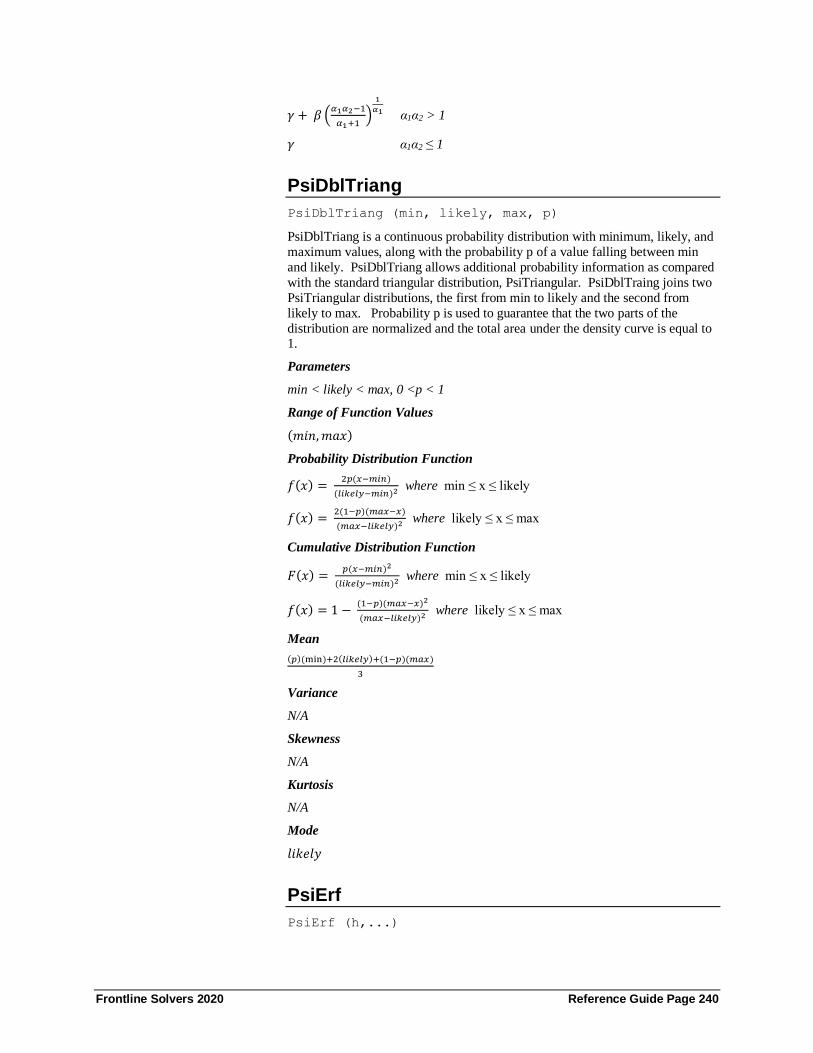
Frontline Solvers 2020 Reference Guide Page 240
𝛾 + 𝛽 (𝛼1𝛼2−1
𝛼1+1)
1
𝛼1 α1α2 > 1
𝛾 α1α2 ≤ 1
PsiDblTriang
PsiDblTriang (min, likely, max, p)
PsiDblTriang is a continuous probability distribution with minimum, likely, and
maximum values, along with the probability p of a value falling between min
and likely. PsiDblTriang allows additional probability information as compared
with the standard triangular distribution, PsiTriangular. PsiDblTraing joins two
PsiTriangular distributions, the first from min to likely and the second from
likely to max. Probability p is used to guarantee that the two parts of the
distribution are normalized and the total area under the density curve is equal to 1.
Parameters
min < likely < max, 0 <p < 1
Range of Function Values
(𝑚𝑖𝑛, 𝑚𝑎𝑥)
Probability Distribution Function
𝑓(𝑥) = 2𝑝(𝑥−𝑚𝑖𝑛)
(𝑙𝑖𝑘𝑒𝑙𝑦−𝑚𝑖𝑛)2 where min ≤ x ≤ likely
𝑓(𝑥) = 2(1−𝑝)(𝑚𝑎𝑥−𝑥)
(𝑚𝑎𝑥−𝑙𝑖𝑘𝑒𝑙𝑦)2 where likely ≤ x ≤ max
Cumulative Distribution Function
𝐹(𝑥) = 𝑝(𝑥−𝑚𝑖𝑛)2
(𝑙𝑖𝑘𝑒𝑙𝑦−𝑚𝑖𝑛)2 where min ≤ x ≤ likely
𝑓(𝑥) = 1 − (1−𝑝)(𝑚𝑎𝑥−𝑥)2
(𝑚𝑎𝑥−𝑙𝑖𝑘𝑒𝑙𝑦)2 where likely ≤ x ≤ max
Mean
(𝑝)(min)+2(𝑙𝑖𝑘𝑒𝑙𝑦)+(1−𝑝)(𝑚𝑎𝑥)
3
Variance
N/A
Skewness
N/A
Kurtosis
N/A
Mode
𝑙𝑖𝑘𝑒𝑙𝑦
PsiErf
PsiErf (h,...)

Frontline Solvers 2020 Reference Guide Page 241
PsiErf is a distribution based on the “error function” ERF(x). Its shape is closely
related to the Normal distribution.
Alternate Formulation: PsiErfAlt
PsiErfAlt is the PsiErf distribution defined through alternative arguments. One parameter is required which must be chosen from the following list: percentile
and var.
Parameters
0h
Range of Function Values
( ),−
Probability Density Function
( ) ( )2
hxhf x e
−=
Cumulative Distribution Function
( ) ( )( )
( )2
0
2
is the Error Function
2v
t
F x hx
v
v e dt
−
=
=
Mean
0
Variance
2
1
2h
Skewness
0
Kurtosis
3
Median
0
Mode
0
PsiErlang
PsiErlang (k,β,...)
PsiErlang (k,β) is a distribution with a finite lower bound, closely related to the
Gamma and Exponential distributions. It has applications in reliability and

Frontline Solvers 2020 Reference Guide Page 242
queuing models. When the parameter k = 1, the Erlang distribution is the same
as an Exponential distribution.
Parameters
, 0
integer
k
k
Range of Function Values
)0,
Probability Density Function
( )( )
( )
1
1 !
xk
k
x ef x
k
−−
=−
Cumulative Distribution Function
( )( )
( )
,
1 !
, is the Incomplete Gamma Function
xk
F xk
x y
=
−
Mean
k
Variance
2k
Skewness
2
k
Kurtosis
63
k+
Median
Not defined
Mode
( )1k −
PsiExponential
PsiExponential (β,...)

Frontline Solvers 2020 Reference Guide Page 243
PsiExponential (β) is a distribution with a finite lower bound and rapidly
decreasing values. It can be used to represent time between random occurrences
in queuing and reliability engineering applications.
The minimum of a set of independent exponential random variables is also an
exponentially distributed random variable.
Alternate Formulation: PsiExponentialAlt
PsiExponentialAlt is the PsiExponential distribution defined through alternative
arguments. One parameter is required which must be chosen from the following
list: percentile or var.
Parameters
0
Range of Function Values
)0,
Probability Density Function
( )1 x
f x e
−
=
Cumulative Distribution Function
( ) 1 if 0
0 otherwise
x
e xF x
− −
=
Mean
Variance
2
Skewness
2
Kurtosis
9
Median
( )ln 2
Mode
0
PsiFatigueLife
PsiFatigueLife (loc, scale, shape)

Frontline Solvers 2020 Reference Guide Page 244
Also known as the Birnbaum-Saunders distribution, the PsiFatigueLife
distribution is used to model failure times, i.e. model crack propagation and the
failure of materials over time.
Parameters
loc, scale (β) > 0, shape (α) > 0
Range of Function Values
(loc, ∞)
Probability Density Function
where z ≡ 𝑥−𝑦
𝛽 and Ф is the cumulative distriobution function of the standard
normal distribution.
Cumulative Distribution Function
where z ≡ 𝑥−𝑦
𝛽 and Ф is the cumulative distriobution function of the standard
normal distribution.
Mean
𝛾 + 𝛽 (1 + 𝛼2
2)
Variance
(𝛼𝛽)2 (1 + 5𝛼2
4)
Skewness
44𝛼3+24𝛼
(5𝛼2 +4)32
Kurtosis
Mode
No Analytic Formula
PsiFDist
PsiFDist (df1, df2)
The PsiFDist distribution is an F distribution with two degrees of freedom, df1
and df2. Typically, this distribution is associated with statistical hypothesis
testing, specifically when determining if two population variances are equal.

Frontline Solvers 2020 Reference Guide Page 245
Parameters
df1 > 0 and integer, df2 > 0 and integer
Range of Function Values
(0, ∞)
Probability Density Function
Cumulative Distribution Function
where β is the Beta function and I is the Regularized Incomplete Beta Function.
Mean
𝑣2
𝑣2−2 for v2 > 2
Variance
2𝑣22(𝑣1+𝑣2−2)
𝑣1(𝑣2−2)2(𝑣2−4) for v2 > 4
Skewness
(2𝑣1+ 𝑣2+2)
(𝑣2−6)√
8(𝑣2−4)
𝑣1(𝑣1+𝑣2−2) for v2 > 6
Kurtosis
3 + 12 [(𝑣2−2)2(𝑣2−4)+𝑣1(𝑣1+ 𝑣2−2)(5𝑣2−22)
𝑣1(𝑣2−6)(𝑣2−8)(𝑣1+ 𝑣2−2)] for v2 > 8
Mode
𝑣2(𝑣1−2)
𝑣1(𝑣2+2) for v1 > 2
0 𝑓𝑜𝑟 𝑣1 ≤ 2
PsiFrechet
PsiFrechet (loc, scale, shape)
The PsiFrechet distribution is used to model extreme events. This distribution is
used commonly in hydrology to model peak annual rainfall and damn overflow.
Parameters
loc (λ) , scale (β) > 0, shape (α) > 0
Range of Function Values
(0, ∞)
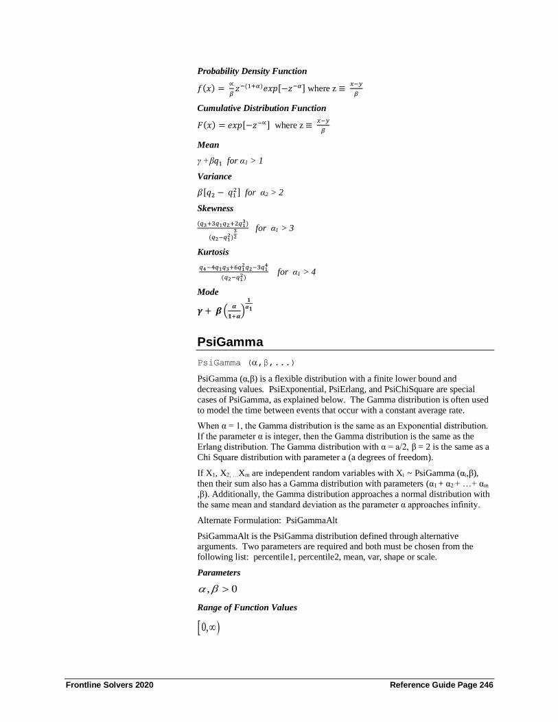
Frontline Solvers 2020 Reference Guide Page 246
Probability Density Function
𝑓(𝑥) = ∝
𝛽𝑧−(1+𝛼)𝑒𝑥𝑝[−𝑧−𝛼] where z ≡
𝑥−𝑦
𝛽
Cumulative Distribution Function
𝐹(𝑥) = 𝑒𝑥𝑝[−𝑧−∝] where z ≡ 𝑥−𝑦
𝛽
Mean
γ +β𝑞1 for α1 > 1
Variance
𝛽[𝑞2 − 𝑞12] for α2 > 2
Skewness
(𝑞3+3𝑞1𝑞2+2𝑞13)
(𝑞2−𝑞12)
32
for α1 > 3
Kurtosis
𝑞4−4𝑞1𝑞3+6𝑞1
2𝑞2−3𝑞14
(𝑞2−𝑞12)
for α1 > 4
Mode
𝜸 + 𝜷 (𝜶
𝟏+𝜶)
𝟏
𝜶𝟏
PsiGamma
PsiGamma (,β,...)
PsiGamma (α,β) is a flexible distribution with a finite lower bound and
decreasing values. PsiExponential, PsiErlang, and PsiChiSquare are special
cases of PsiGamma, as explained below. The Gamma distribution is often used
to model the time between events that occur with a constant average rate.
When α = 1, the Gamma distribution is the same as an Exponential distribution.
If the parameter α is integer, then the Gamma distribution is the same as the
Erlang distribution. The Gamma distribution with α = a/2, β = 2 is the same as a
Chi Square distribution with parameter a (a degrees of freedom).
If X1, X2, …Xm are independent random variables with Xi ~ PsiGamma (αi,β),
then their sum also has a Gamma distribution with parameters (α1 + α2 + …+ αm
,β). Additionally, the Gamma distribution approaches a normal distribution with
the same mean and standard deviation as the parameter α approaches infinity.
Alternate Formulation: PsiGammaAlt
PsiGammaAlt is the PsiGamma distribution defined through alternative arguments. Two parameters are required and both must be chosen from the
following list: percentile1, percentile2, mean, var, shape or scale.
Parameters
, 0
Range of Function Values
)0,

Frontline Solvers 2020 Reference Guide Page 247
Probability Density Function
( ) ( )
( )
1
if 0
0 otherwise
is the Gamma Function
x
x ex
f x
−− −
=
Cumulative Distribution Function
( )( )
( )
( )
,
, is the Incomplete Gamma Function
x
F x
a b
=
Mean
Variance
2
Skewness
2
Kurtosis
63
+
Median
Not defined
Mode
( )1 if 1
0 otherwise
−
PsiHypSecant
PsiHypSecant (loc, scale)
The PsiHypSecant distribution is similar to the normal distribution, but has a
larger kurtosis resulting in a sharper peak.
Alternate Formulation: PsiHypSecantAlt
PsiHypSecantAlt is the PsiHypSecant distribution defined through alternative
arguments. Two parameters are required and both must be used in the following combinations: two different percentiles, percentile and loc or percentile and
scale.

Frontline Solvers 2020 Reference Guide Page 248
Parameters
loc (λ) , scale (β) > 0
Range of Function Values
(-∞, ∞)
Probability Density Function
𝑓(𝑥) = 1
2𝛽𝑠𝑒𝑐ℎ [
𝜋
2𝑧] where z ≡
𝑥−𝑦
𝛽
Cumulative Distribution Function
𝐹(𝑥) =2
𝜋𝑡𝑎𝑛−1 [𝑒
𝜋𝑧
2 ] where z ≡ 𝑥−𝑦
𝛽
Mean
γ
Variance
𝛽2
Skewness
0
Kurtosis
5
Mode
𝜸
PsiInvNormal
PsiInvNormal (μ,λ,...)
PsiInvNormal (µ,λ) is a distribution with a finite lower bound, where it is zero.
The Inverse Normal distribution is used to model Brownian motion and other diffusion processes. As the parameter λ tends to infinity, the Inverse Normal
distribution approaches a Normal distribution.
Alternate Formulation: PsiInvNormalAlt
PsiInvNormalAlt is the PsiInvNormal distribution defined through alternative
arguments. Two parameters are required and both must be chosen from the
following list: two different percentiles, mean, var or scale.
Parameters
, 0
Range of Function Values
( )0,
Probability Density Function
( )
( )2
22
32
x
xf x e
x
− −
=

Frontline Solvers 2020 Reference Guide Page 249
Cumulative Distribution Function
( )
( )
2
1 1
is the Error Function
x xF x e
x x
z
= − + − +
Mean
Variance
3
Skewness
3
Kurtosis
15 3
+
Median
Not defined
Mode
12 2
2
9 31
4 2
+ −
PsiJohnsonSB
PsiJohnsonSB (shape1, shape2, min, max)
The PsiJohnsonSB distribution is a bounded distribution with shape parameters
shape1 and shape2 and boundary parameters min and max.
Parameters
shape1(α1), shape2 (α2) > 0 , max(b) > min (a)
Range of Function Values
[a, 𝑏]
Probability Density Function
𝒇(𝒙) = 𝜶𝟐(𝒃−𝒂)
√𝟐𝝅(𝒙−𝒂)(𝒃−𝒙)× 𝒆
−𝟏
𝟐[𝜶𝟏+𝜶𝟐𝒍𝒏(
𝒙−𝒂
𝒃−𝒙)]
Cumulative Distribution Function
𝐹(𝑥) = Φ [𝛼1+ 𝛼2𝑙𝑛 (𝑥−𝑎
𝑏−𝑥)] where
Φ 𝑖𝑠 𝑡ℎ𝑒 𝑐𝑢𝑚𝑢𝑙𝑎𝑡𝑖𝑣𝑒 𝑑𝑖𝑠𝑡𝑟𝑖𝑏𝑢𝑡𝑖𝑜𝑛 𝑓𝑢𝑛𝑐𝑡𝑖𝑜𝑛 𝑜𝑓 𝑡ℎ𝑒 𝑠𝑡𝑎𝑛𝑑𝑎𝑟𝑑
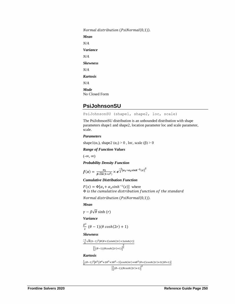
Frontline Solvers 2020 Reference Guide Page 250
𝑁𝑜𝑟𝑚𝑎𝑙 𝑑𝑖𝑠𝑡𝑟𝑖𝑏𝑢𝑡𝑖𝑜𝑛 (𝑃𝑠𝑖𝑁𝑜𝑟𝑚𝑎𝑙(0,1)).
Mean
N/A
Variance
N/A
Skewness
N/A
Kurtosis
N/A
Mode
No Closed Form
PsiJohnsonSU
PsiJohnsonSU (shape1, shape2, loc, scale)
The PsiJohnsonSU distribution is an unbounded distribution with shape
parameters shape1 and shape2, location parameter loc and scale parameter,
scale.
Parameters
shape1(α1), shape2 (α2) > 0 , loc, scale (β) > 0
Range of Function Values
(-∞, ∞)
Probability Density Function
𝒇(𝒙) = 𝜶𝟐
𝜷√𝟐𝝅(𝟏+𝒛𝟐)× 𝒆
−𝟏
𝟐[𝜶𝟏+𝜶𝟐𝒔𝒊𝒏𝒉−𝟐(𝒛)]
𝟐
Cumulative Distribution Function
𝐹(𝑥) = Φ[𝛼1+ 𝛼2𝑠𝑖𝑛ℎ−1(𝑧)] where
Φ 𝑖𝑠 𝑡ℎ𝑒 𝑐𝑢𝑚𝑢𝑙𝑎𝑡𝑖𝑣𝑒 𝑑𝑖𝑠𝑡𝑟𝑖𝑏𝑢𝑡𝑖𝑜𝑛 𝑓𝑢𝑛𝑐𝑡𝑖𝑜𝑛 𝑜𝑓 𝑡ℎ𝑒 𝑠𝑡𝑎𝑛𝑑𝑎𝑟𝑑
𝑁𝑜𝑟𝑚𝑎𝑙 𝑑𝑖𝑠𝑡𝑟𝑖𝑏𝑢𝑡𝑖𝑜𝑛 (𝑃𝑠𝑖𝑁𝑜𝑟𝑚𝑎𝑙(0,1)).
Mean
𝛾 − 𝛽√𝜃 sinh (𝑟)
Variance
𝛽2
2 (𝜃 − 1)(𝜃 𝑐𝑜𝑠ℎ(2𝑟) + 1)
Skewness
−1
4√𝜃(0−1)2[𝜃(𝜃+2)𝑠𝑖𝑛ℎ(3𝑟)+3𝑠𝑖𝑛ℎ(𝑟)]
[1
2(𝜃−1)(𝜃𝑐𝑜𝑠ℎ(2𝑟)+1)]
32
Kurtosis
1
8(𝜃−1)2[𝜃2(𝜃4+2𝜃3+3𝜃2−3)𝑐𝑜𝑠ℎ(4𝑟)+4𝜃2(𝜃+2)𝑐𝑜𝑠ℎ(2𝑟)+3(2𝜃+1)]
[1
2(𝜃−1)(𝜃𝑐𝑜𝑠ℎ(2𝑟)+1)]
2
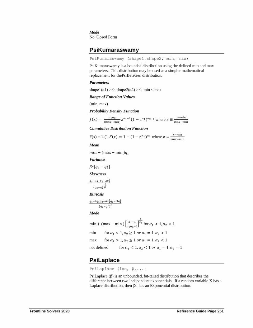
Frontline Solvers 2020 Reference Guide Page 251
Mode
No Closed Form
PsiKumaraswamy
PsiKumaraswamy (shape1,shape2, min, max)
PsiKumaraswamy is a bounded distribution using the defined min and max
parameters. This distribution may be used as a simpler mathematical
replacement for thePsiBetaGen distribution.
Parameters
shape1(α1) > 0, shape2(α2) > 0, min < max
Range of Function Values
(min, max)
Probability Density Function
𝑓(𝑥) = 𝛼1𝛼2
(𝑚𝑎𝑥−𝑚𝑖𝑛)𝑧𝛼1−1(1 − 𝑧𝛼1 )𝛼2−1 where 𝑧 ≡
𝑥−𝑚𝑖𝑛
𝑚𝑎𝑥−𝑚𝑖𝑛
Cumulative Distribution Function
F(x) = 1-(1-𝐹(𝑥) = 1 − (1 − 𝑧∝1)∝2 where 𝑧 ≡𝑥−𝑚𝑖𝑛
𝑚𝑎𝑥−𝑚𝑖𝑛
Mean
𝑚𝑖𝑛 + (max − min )𝑞1
Variance
𝛽2[𝑞2 − 𝑞12]
Skewness
𝑞3−3𝑞1𝑞2+2𝑞13
(𝑞2−𝑞12)
32
Kurtosis
𝑞4−4𝑞1𝑞3+6𝑞12𝑞2− 3𝑞1
4
(𝑞2−𝑞12)
2
Mode
min + (max − min ) [𝛼1−1
𝛼1𝛼2−1]
1
𝛼1 for 𝛼1 > 1, 𝛼2 > 1
min for 𝛼1 < 1, 𝛼2 ≥ 1 𝑜𝑟 𝛼1 = 1, 𝛼2 > 1
max for 𝛼1 > 1, 𝛼2 ≤ 1 𝑜𝑟 𝛼1 = 1, 𝛼2 < 1
not defined for 𝛼1 < 1, 𝛼2 < 1 𝑜𝑟 𝛼1 = 1, 𝛼2 = 1
PsiLaplace
PsiLaplace (loc, β,...)
PsiLaplace (β) is an unbounded, fat-tailed distribution that describes the
difference between two independent exponentials. If a random variable X has a
Laplace distribution, then |X| has an Exponential distribution.

Frontline Solvers 2020 Reference Guide Page 252
Enter a scale value greater than 0 for the first argument, loc. This value
determines the scale or range of the distribution.
Alternate Formulation: PsiLaplaceAlt
PsiLaplaceAlt is the PsiLaplace distribution defined through alternative
arguments. Two parameters are required and both must be chosen from the
following list: two different percentiles or the standard deviation.
Parameters
0 , loc > 0
Range of Function Values
( ),−
Probability Density Function
( )2
x
ef x
−
=
Cumulative Distribution Function
( )
11 if 0
2
1 otherwise
2
x
x
e x
F x
e
−−
=
Mean
0
Variance
22
Skewness
0
Kurtosis
3
Median
0
Mode
0
PsiLevy
PsiLevy (loc,scale)
PsiLevy is a continuous distribution with a location, loc, and a scale parameter,
scale.
Alternate Formulation: PsiLevyAlt
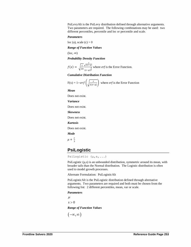
Frontline Solvers 2020 Reference Guide Page 253
PsiLevyAlt is the PsiLevy distribution defined through alternative arguments.
Two parameters are required. The following combinations may be used: two
different percentiles, percentile and loc or percentile and scale.
Parameters
loc (a), scale (c) > 0
Range of Function Values
(loc, ∞)
Probability Density Function
𝑓(𝑥) = √𝑐
2𝜋
𝑒
𝑐2(𝑥−𝜇)
(𝑥−𝜇)32
where erf is the Error Function.
Cumulative Distribution Function
F(x) = 1−𝑒𝑟𝑓 (√𝑐
2(𝑥−𝜇)) where erf is the Error Function
Mean
Does not exist.
Variance
Does not exist.
Skewness
Does not exist.
Kurtosis
Does not exist.
Mode
𝜇 + 𝑐
3
PsiLogistic
PsiLogistic (μ,s,...)
PsiLogistic (µ,s) is an unbounded distribution, symmetric around its mean, with
broader tails than the Normal distribution. The Logistic distribution is often
used to model growth processes.
Alternate Formulation: PsiLogisticAlt
PsiLogisticAlt is the PsiLogistic distribution defined through alternative
arguments. Two parameters are required and both must be chosen from the
following list: 2 different percentiles, mean, var or scale.
Parameters
0s
Range of Function Values
( ),−

Frontline Solvers 2020 Reference Guide Page 254
Probability Density Function
( )
( )
( )2
1
xs
xs
ef x
s e
− −
− −=
+
Cumulative Distribution Function
( ) ( )
1
1x
s
F x
e− −
=
+
Mean
Variance
2 2
3
s
Skewness
0
Kurtosis
6/5
Median
Mode
PsiLogLogistic
PsiLogLogistic (γ,β,,...)
PsiLogLogistic (γ,β,α) is a distribution with a finite lower bound. The natural
log of PsiLogLogistic is a Logistic random variable. The Log-Logistic
distribution can be used to model the time to perform a job or task.
Alternate Formulation: PsiLogLogisticAlt
PsiLogLogisticAlt is the PsiLogLogistic distribution defined through alternative
arguments. Three parameters are required and all must be chosen from the
following list: 3 different parameters, loc, scale or shape.
Parameters
, 0
Range of Function Values
),

Frontline Solvers 2020 Reference Guide Page 255
Probability Density Function
( )
1
2
1
x
f x
x
−
− =
−+
Cumulative Distribution Function
( )1
1
F x
x
=
+ −
Mean
cos
for 1
ec
+
Variance
2 222cos cos
for 2
ec ec
−
Skewness
23
2
32
2
3 6 2 23cosec cos cos cos
for 3
22cos cos
ec ec ec
ec ec
− +
−
Kurtosis
Not defined
Median
Not defined
Mode
1
1 for 1
1
0 otherwise
− + +
PsiLogNormal
PsiLogNormal (μ,σ,...)

Frontline Solvers 2020 Reference Guide Page 256
PsiLogNormal (µ,σ) is a distribution with a finite lower bound and has mean µ
and standard deviation σ. The LogNormal distribution can be used to model
quantities that are products of many small independent variables. The natural
log of PsiLogNormal is a Normal random variable.
Alternate Formulation: PsiLogNormalAlt
PsiLogNormalAlt is the PsiLogNormal distribution defined through alternative
arguments. Two parameters are required and both must be used in the following
combinations: 2 different percentiles, percentile and mean or percentile and
standard deviation.
Parameters
, 0
Range of Function Values
)0,
Probability Density Function
( )
2ln '
'
1
2
'
2 2' '
2 2 2
2
ln 1 , ln
x
ef x
x
− −
=
= + = +
Cumulative Distribution Function
( )
( )
'
'
ln
is the Error Function
xF x
a
−=
Mean
Variance
2
Skewness
3
3
3
+
Kurtosis
6
4 3 2
1 2 1 3 1 3
+ + + + + −
Median
2
2 2
+

Frontline Solvers 2020 Reference Guide Page 257
Mode
( )
4
32 2 2
+
PsiLogNorm2
PsiLogNorm2 (μ,σ,...)
PsiLogNorm2 (µ,σ) is a distribution with a finite lower bound. It can be used to
model quantities that are products of many small independent variables. The
natural log of PsiLogNorm2 is a Normal random variable. In contrast to
PsiLogNormal(), the parameters µ and σ of PsiLogNorm2() are the mean and
standard deviation of the corresponding Normal distribution.
Parameters
0
Range of Function Values
)0,
Probability Density Function
( )
2ln1
2
2
x
ef x
x
− −
=
Cumulative Distribution Function
( )
( )
ln
is the Error Function
xF x
a
− =
Mean
2
2e+
Variance
( )2 221e e +−
Skewness
( )2 2
2 1e e + −
Kurtosis
62 2 24 3 22 3 3e e e + + −
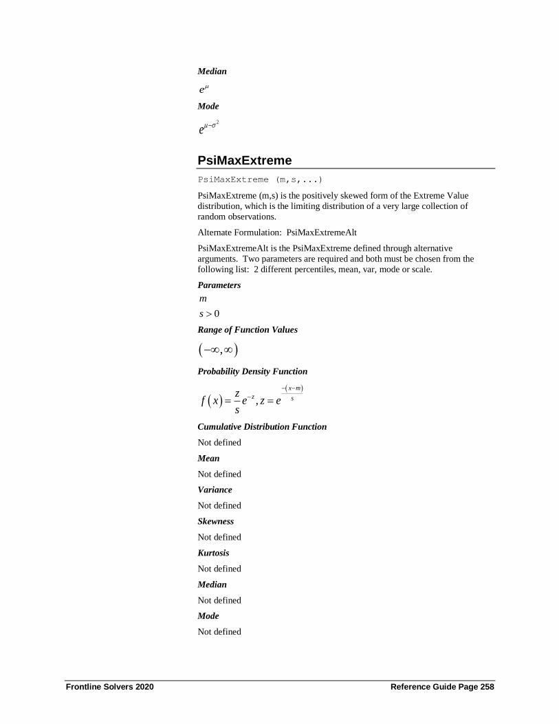
Frontline Solvers 2020 Reference Guide Page 258
Median
e
Mode
2
e −
PsiMaxExtreme
PsiMaxExtreme (m,s,...)
PsiMaxExtreme (m,s) is the positively skewed form of the Extreme Value
distribution, which is the limiting distribution of a very large collection of
random observations.
Alternate Formulation: PsiMaxExtremeAlt
PsiMaxExtremeAlt is the PsiMaxExtreme defined through alternative
arguments. Two parameters are required and both must be chosen from the
following list: 2 different percentiles, mean, var, mode or scale.
Parameters
0
m
s
Range of Function Values
( ),−
Probability Density Function
( )( )
,
x m
z sz
f x e z es
− −
−= =
Cumulative Distribution Function
Not defined
Mean
Not defined
Variance
Not defined
Skewness
Not defined
Kurtosis
Not defined
Median
Not defined
Mode
Not defined

Frontline Solvers 2020 Reference Guide Page 259
PsiMetalog
PsiMetalog(min, max, coefficients)
A general meta-log distribution is defined in models through PsiMetalog(). This
function has as arguments a vector of coefficients (coefficients) and optionally
lower (min) and upper (max) bounds. The metalog distribution family is
designed to be determined from historical data, without requiring a distribution
fitting process. They are computed from a set of historical data pairs {y, x},
where y is a cumulative probability and x is the correspondent percentile. The
coefficients argument is either a range or an array of 2 to 10 numerical elements.
There are 3 optional cases for this distribution:
• Both min and max are missing which results in an unbounded distribution
PsiMetalog(, , {33, 3.7, -2.4, 5.7, 10.1})
• Only min exists which results in a semi-bounded distribution
PsiMetalog(0, , {33, 3.7, -2.4, 5.7, 10.1})
• Both min and max exist which results in a bounded distribution
PsiMetalog(0, 55, {33, 3.7, -2.4, 5.7, 10.1})
Note: An exclusive bounding using only the max argument is not supported.
The min and max arguments are true lower and upper bounds not to be confused
with lower truncate and upper truncate. Optional standard property functions
may be used with this distribution, i.e. PsiTruncate, PsiShift, PsiCorrelate, etc.
The distribution may also be compounded.
Analytic moments are available only for unbounded distributions. Kurtosis is
not computed for more than 5 coefficients.
Parameters
min, max, coefficients
Range of Function Values
( ),−
5-Term Quantile Function (Inverse CDF)
𝑀5 (𝑦) ≔ (𝑎1 + log [𝑦
1−𝑦] 𝑎2 + (
−1
2+ 𝑦) log [
𝑦
1−𝑦] 𝑎3 + (
−1
2+ 𝑦) 𝑎4 + (
−1
2+ 𝑦)
2𝑎5)
See the website, http://metalogdistributions.com/, for more information.
2-Term Metalog Moments
𝑢1,2′ : = 𝑎1 mean (first moment) of 2 term metalog
𝑢2,2 ∶= 1
3𝜋2𝑎2
2 variance (2nd central moment) of 2 term metalog
𝑢3,2 ∶= 0 skewness (3rd central moment) of 2 term metalog
𝑢4,2 ∶= 7
15𝜋4𝑎2
4 kurtosis (4th central moment) of 2 term metalog
See the website, http://metalogdistributions.com/, for more information.
3-Term Metalog Moments
𝑢1,3′ : = 𝑢1,2
′ + 𝑎3
2 mean (first moment) of 3 term metalog
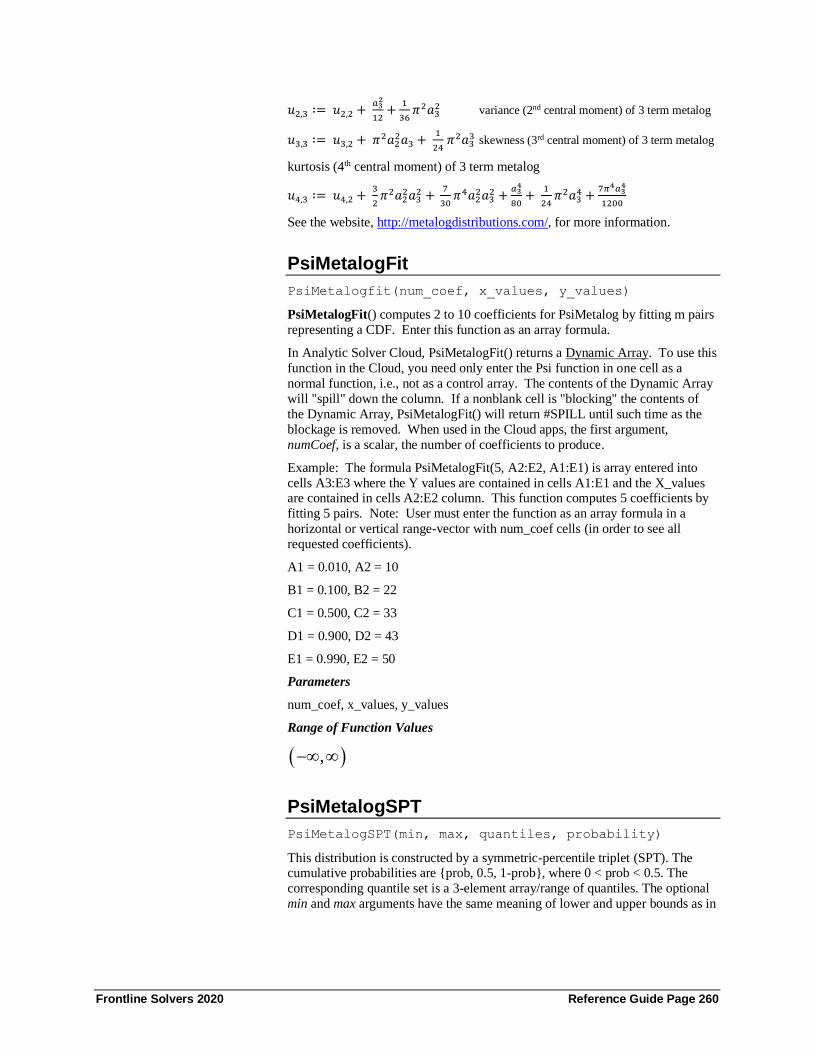
Frontline Solvers 2020 Reference Guide Page 260
𝑢2,3 ∶= 𝑢2,2 + 𝑎3
2
12+
1
36𝜋2𝑎3
2 variance (2nd central moment) of 3 term metalog
𝑢3,3 ∶= 𝑢3,2 + 𝜋2𝑎22𝑎3 +
1
24 𝜋2𝑎3
3 skewness (3rd central moment) of 3 term metalog
kurtosis (4th central moment) of 3 term metalog
𝑢4,3 ∶= 𝑢4,2 + 3
2𝜋2𝑎2
2𝑎32 +
7
30𝜋4𝑎2
2𝑎32 +
𝑎34
80+
1
24𝜋2𝑎3
4 +7𝜋4𝑎3
4
1200
See the website, http://metalogdistributions.com/, for more information.
PsiMetalogFit
PsiMetalogfit(num_coef, x_values, y_values)
PsiMetalogFit() computes 2 to 10 coefficients for PsiMetalog by fitting m pairs
representing a CDF. Enter this function as an array formula.
In Analytic Solver Cloud, PsiMetalogFit() returns a Dynamic Array. To use this
function in the Cloud, you need only enter the Psi function in one cell as a
normal function, i.e., not as a control array. The contents of the Dynamic Array
will "spill" down the column. If a nonblank cell is "blocking" the contents of
the Dynamic Array, PsiMetalogFit() will return #SPILL until such time as the
blockage is removed. When used in the Cloud apps, the first argument,
numCoef, is a scalar, the number of coefficients to produce.
Example: The formula PsiMetalogFit(5, A2:E2, A1:E1) is array entered into
cells A3:E3 where the Y values are contained in cells A1:E1 and the X_values are contained in cells A2:E2 column. This function computes 5 coefficients by
fitting 5 pairs. Note: User must enter the function as an array formula in a
horizontal or vertical range-vector with num_coef cells (in order to see all
requested coefficients).
A1 = 0.010, A2 = 10
B1 = 0.100, B2 = 22
C1 = 0.500, C2 = 33
D1 = 0.900, D2 = 43
E1 = 0.990, E2 = 50
Parameters
num_coef, x_values, y_values
Range of Function Values
( ),−
PsiMetalogSPT
PsiMetalogSPT(min, max, quantiles, probability)
This distribution is constructed by a symmetric-percentile triplet (SPT). The cumulative probabilities are {prob, 0.5, 1-prob}, where 0 < prob < 0.5. The
corresponding quantile set is a 3-element array/range of quantiles. The optional
min and max arguments have the same meaning of lower and upper bounds as in
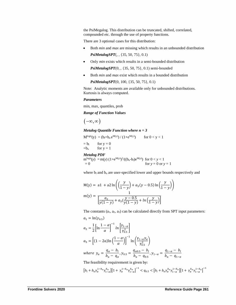
Frontline Solvers 2020 Reference Guide Page 261
the PsiMegalog. This distribution can be truncated, shifted, correlated,
compounded etc. through the use of property functions.
There are 3 optional cases for this distribution:
• Both min and max are missing which results in an unbounded distribution
PsiMetalogSPT(, , {35, 50, 75}, 0.1)
• Only min exists which results in a semi-bounded distribution
PsiMetalogSPT(0, , {35, 50, 75}, 0.1) semi-bounded
• Both min and max exist which results in a bounded distribution
PsiMetalogSPT(0, 100, {35, 50, 75}, 0.1)
Note: Analytic moments are available only for unbounded distributions.
Kurtosis is always computed.
Parameters
min, max, quantiles, prob
Range of Function Values
( ),−
Metalog Quantile Function where n = 3
Mlogit(y) = (bl+bu eM(y)) / (1+eM(y)) for 0 < y < 1
= bl for y = 0
=bu for y = 1
Metalog PDF
mlogit(y) = m(y) (1+eM(y))2/((bu-bl)eM(y)) for 0 < y < 1
= 0 for y = 0 or y = 1
where bl and bu are user-specified lower and upper bounds respectively and
M(y) = a1 + a2 ln ((𝑦
1 − 𝑦) + 𝑎3(𝑦 − 0.5) ln (
𝑦
1 − 𝑦))
m(y) = 1
[𝑎2
𝑦(1 − 𝑦)+ 𝑎3(
𝑦 − 0.5𝑦(1 − 𝑦)
+ 𝑙𝑛 (𝑦
1 − 𝑦)]
The constants (a1, a2, a3) can be calculated directly from SPT input parameters:
𝑎1 = ln(𝛾0.5)
𝑎2 =1
2[ln
1 − 𝛼
𝛼]
−1
𝑙𝑛 [𝛾1−𝛼
𝛾0.52 ]
𝑎3 = [(1 − 2α)ln (1 − 𝛼
𝛼)]
−1
ln (𝛾1−𝛼𝛾𝛼
𝛾0.52 )
𝑤ℎ𝑒𝑟𝑒 𝑦𝛼 = 𝑞𝛼 − 𝑏𝑙
𝑏𝑢 − 𝑞𝛼
, 𝑦0.5 = 𝑞𝛼0.5 − 𝑏𝑙
𝑏𝑢 − 𝑞0.5
, 𝑦1−𝛼 = 𝑞1−𝛼 − 𝑏𝑙
𝑏𝑢 − 𝑞1−𝛼
The feasibility requirement is given by:
[𝑏𝑙 + 𝑏𝑢𝛾𝛼1−𝑘𝛼𝛾1−𝛼
𝑘𝛼 ][1 + 𝛾𝛼1−𝑘𝛼𝛾1−𝛼
𝑘𝛼 ]−1
< 𝑞0.5 < [𝑏𝑙 + 𝑏𝑢𝛾𝛼𝑘𝛼𝛾1−𝛼
1−𝑘𝛼][1 + 𝛾𝛼𝑘𝛼 𝛾1−𝛼
1−𝑘𝛼]−1

Frontline Solvers 2020 Reference Guide Page 262
where 𝑘𝛼 = 1
2[1 − 1.66711 (
1
2− 𝛼)]
See the website, http://metalogdistributions.com/, for more information.
PsiMinExtreme
PsiMinExtreme (m,s,...)
PsiMinExtreme is the negatively skewed form of the Extreme Value
distribution, which is the limiting distribution of a very large collection of
random observations.
Alternate Formulation: PsiMinExtremeAlt
PsiMinExtremeAlt is the PsiMinExtreme distribution defined through alternative arguments. Two parameters are required and both must be chosen
from the following list: 2 different percentiles, mean, var, mode or scale.
Parameters
0
m
s
Range of Function Values
( ),−
Probability Density Function
( )( )
,
x m
z sz
f x e z es
−
−= =
Cumulative Distribution Function
Not defined
Mean
Not defined
Variance
Not defined
Skewness
Not defined
Kurtosis
Not defined
Median
Not defined
Mode
Not defined
PsiMyerson
PsiMyerson (a,b,c,t,...)

Frontline Solvers 2020 Reference Guide Page 263
PsiMyerson (a,b,c,t) is a generalized LogNormal/Normal distribution, specified
using the bottom percentile (a), 50th percentile (b), top percentile (c) and
optional tail percentage parameter (t). This distribution is bounded on the side of
the narrower percentile range; when both the bottom and top percentile ranges
are equal, then this distribution is unbounded.
If the t parameter (tail percentage) is present then the a and c parameters (bottom
and top percentiles) are used to construct a distribution PDF in such a way that
the left and right tails (remaining equal) sum up to the desired t parameter value.
The top percentile is always symmetric to the bottom percentile. For example, if
the bottom percentile equals the 20th percentile, the top percentile will be equal
to the 80th percentile.
The default option for parameter t is 0.50 which means that the left tail and the
right tail each equal 0.25. As a result, parameter a (bottom percentile) is the 25th
percentile and parameter c (top percentile) is the 75th percentile.
This distribution, developed by Dr. Roger Myerson, is used to model random variables when the only information available is the percentile values, and
optionally, a tail percentage parameter indicating the probability of values being
within the specified percentiles. If the specified percentiles are equidistant
(measured by the parameter b’ below), then the Myerson distribution is equiva-
lent to a Normal distribution. When the 50th percentile is equal to the geometric
mean of the top and bottom percentiles, then the Myerson distribution is
equivalent to the LogNormal distribution.
Parameters
( )0,1
If is omitted, it is given a default value of 0.5
a c b
t
t
Range of Function Values
)
( )
( )
,
where,
, if 1
, if 11
, if 11
and,
LB UB
LB UB b
b cLB c UB b
b
b cLB UB c b
b
b cb
c a
= − = =
−= − =
−
−= − = −
−
− =
−
Probability Density Function
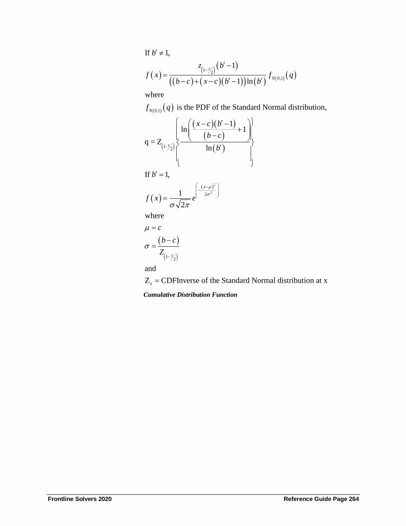
Frontline Solvers 2020 Reference Guide Page 264
( )( )
( )
( ) ( )( )( ) ( ) ( ) ( )
( ) ( )
( )
( )( )( )
( )
( )
( )
( )
( )
2
2
12
0,1
0,1
t1-2
2
12
If 1,
1
1 ln
where
is the PDF of the Standard Normal distribution,
1ln 1
q = Zln
If 1,
1
2
where
a
t
N
N
x
t
b
z b
f x f qb c x c b b
f q
x c b
b c
b
b
f x e
c
b c
Z
−
− −
−
−
= − + − −
− −+ −
=
=
=
−=
x
nd
Z CDFInverse of the Standard Normal distribution at x=
Cumulative Distribution Function
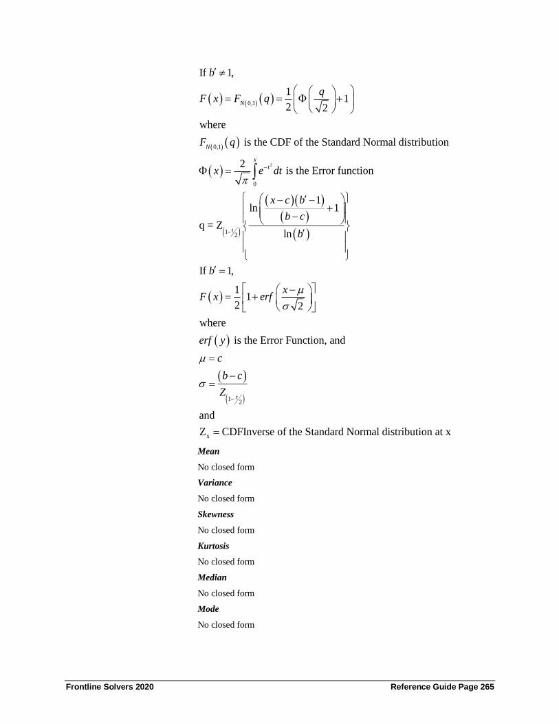
Frontline Solvers 2020 Reference Guide Page 265
( ) ( ) ( )
( ) ( )
( )
( )
( )( )( )
( )
( )
2
0,1
0,1
0
t1-2
If 1,
11
2 2
where
is the CDF of the Standard Normal distribution
2 is the Error function
1ln 1
q = Zln
If 1,
11
2
N
N
x
t
b
qF x F q
F q
x e dt
x c b
b c
b
b
xF x erf
−
= = +
=
− −+ −
=
−= +
( )
( )
( )12
x
2
where
is the Error Function, and
and
Z CDFInverse of the Standard Normal distribution at x
t
erf y
c
b c
Z
−
=
−=
=
Mean
No closed form
Variance
No closed form
Skewness
No closed form
Kurtosis
No closed form
Median
No closed form
Mode
No closed form
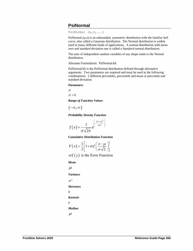
Frontline Solvers 2020 Reference Guide Page 266
PsiNormal
PsiNormal (μ,σ,...)
PsiNormal (µ,σ) is an unbounded, symmetric distribution with the familiar bell
curve, also called a Gaussian distribution. The Normal distribution is widely
used in many different kinds of applications. A normal distribution with mean
zero and standard deviation one is called a Standard normal distribution.
The sum of independent random variables of any shape tends to the Normal
distribution.
Alternate Formulation: PsiNormalAlt
PsiNormalAlt is the PsiNormal distribution defined through alternative
arguments. Two parameters are required and must be used in the following
combinations: 2 different percentiles, percenitile and mean or percentile and standard deviation.
Parameters
0
Range of Function Values
( ),−
Probability Density Function
( )
( )2
221
2
x
f x e
− − =
Cumulative Distribution Function
( )
( )
11
2 2
is the Error Function
xF x erf
erf y
− = +
Mean
Variance
2
Skewness
0
Kurtosis
0
Median

Frontline Solvers 2020 Reference Guide Page 267
Mode
PsiNormalSkew
PsiNormalSkew(a,b,c,...)
PsiNormalSkew (a,b,c) is a generalized Normal distribution with lower bound a,
upper bound b, and skew value c. Lower and upper bound values describe +/-
3rd standard deviation. The skew value c can take on values between (but not
including) -1 and 1. While the Normal distribution is symmetric, the Normal
Skew distribution is skewed either to the left with a positive skew parameter or
to the right with a negative skew parameter.
Both the Myerson distribution (described above) and the PsiNormalSkew
distribution have recently emerged in practice. Both distributions are
generalizations of the Normal distribution but rather than using the mean and standard deviation as arguments, these distributions are calculated using an
upper and lower bound along with either likely and tail arguments (such as with
the Myerson distribution) or a skew argument (such as with the NormalSkew
distribution). When the skew argument is equidistant from the upper and lower
bounds, the NormalSkew distribution equals the Myerson distribution.
In the PsiNormalSkew distribution, the lower and upper bounds are exactly the
same as in the Myerson distribution. The tail argument is missing in the Normal
Skew distribution as it remains at the constant value of 0.002699796146511.
Parameters
a < b
-1< c <1
If c is omitted, it is given a default value of 0. In this case, the PsiNormalSkew
distribution will equal the PsiMyerson distribution.
Range of Function Values
[ , ]
,
, ' 1
( ), ' 1
' 1
( ), ' 1
' 1
'
( 1)( 1)*
2
( " " " " .)
LB UB
where
LB UB if b
b dLB d UB if b
b
b dLB UB d if b
b
where
b db
d a
and
bd a c
The d parameter hereequals the c parameter in the PsiMyerson distribution
= − = =
−= − =
−
−= − = −
−
−=
−
−= + +

Frontline Solvers 2020 Reference Guide Page 268
Probability Density Function
2
(1 )2
(0,1)
N(0,1)
(1 )2
2
' 1,
( ' 1)
( ) ( )(( ) (x d)(b' 1)) ln(b')
where
f (q) is the PDFof theStandard Normaldistribution .
( )( ' 1)ln 1
( )q
ln( ')
' 1,
1( )
2
t
N
t
If b
z b
f x f qb d
x d b
b dZ
b
If b
f x e
−
−
(−)
−
=− + − −
− −+
− =
=
=
(1 )2
( )
( 1)( 1)*
2
( " " " " .)
.
t
where
d
b d
Z
bd a c
The d parameter hereequals the c parameter in the PsiMyerson distribution
and
Z CDFInverseof the Normal distribution at
−
=
− =
−= + +
=
Cumulative Distribution Function

Frontline Solvers 2020 Reference Guide Page 269
( ) ( ) ( )
( ) ( )
( )
( )
( )( )( )
( )
( )
2
0,1
0,1
0
t1-2
If 1,
11
2 2
where
is the CDF of the Standard Normal distribution
2 is the Error function
1ln 1
q = Zln
If 1,
11
2
N
N
x
t
b
qF x F q
F q
x e dt
x d b
b d
b
b
xF x erf
−
= = +
=
− −+ −
=
−= +
( )
( )
( )12
x
2
where
is the Error Function, and
( 1)( 1)*
2
( " " " " .)
and
Z CDFInverse of the Standard Normal distributi
t
erf y
d
b d
Z
bd a c
The d parameter hereequals the c parameter in the PsiMyerson distribution
−
=
−=
−= + +
= on at x
Mean
No closed form
Variance
No closed form
Skewness
No closed form
Kurtosis
No closed form
Median
No closed form

Frontline Solvers 2020 Reference Guide Page 270
Mode
No closed form
PsiPareto
PsiPareto (θ,a,...)
PsiPareto (θ,a) is a distribution with a finite lower bound a, and shape parameter
θ. The Pareto distribution can be used to describe or model wealth distribution,
sizes of particles, etc. It is the exponential of an Exponential random variable.
Alternate Formulation: PsiParetoAlt
PsiParetoAlt is the PsiPareto distribution defined through alternative arguments.
Two parameters are required which must be chosen from the following: 2 different percentiles, shape or scale.
Parameters
, 0a
Range of Function Values
),a
Probability Density Function
( ) 1
af x
x
+
=
Cumulative Distribution Function
( ) 1a
F xx
= −
Mean
for 11
a
−
Variance
( ) ( )
2
2 for 2
1 2
a
− −
Skewness
( )
( )
( )2 1 2 for 3
3
+ −
−
Kurtosis
( )( )( )( )
23 2 3 2 for 4
3 4
− + +
− −

Frontline Solvers 2020 Reference Guide Page 271
Median
1
2a
Mode
a
PsiPareto2
PsiPareto2 (b,q,...)
PsiPareto2 is an alternate form of the Pareto distribution with a finite lower
bound of 0, and a shape parameter q. Like PsiPareto (θ,a), it can be used to
describe or model wealth distribution, sizes of particles, etc. It is the
exponential of an Exponential random variable.
Alternate Formulation: PsiPareto2Alt
PsiPareto2Alt is the PsiPareto2 distribution defined through alternative
arguments. Two parameters are required and both must be chosen from the
following list: 2 different percentiles, scale or shape.
Parameters
, 0b q
Range of Function Values
)0,
Probability Density Function
( )( )
1
q
q
qbf x
x b+
=+
Cumulative Distribution Function
( ) 1
qb
F xx b
= −
+
Mean
for q 11
b
q
−
Variance
( ) ( )
2
2 for q 2
1 2
qb
q q
− −
Skewness
( )
( )
( )2 1 2 for q 3
3
q q
q q
+ −
−

Frontline Solvers 2020 Reference Guide Page 272
Kurtosis
Not defined
Median
1
2 qb
q
Mode
0
PsiPearson5
PsiPearson5 (,β,...)
PsiPearson5 (α,β) is a distribution with a lower bound of 0, and density similar
to that of the LogNormal distribution. The Pearson5 distribution is sometimes
called the Inverse Gamma distribution. It can be used to model time delays
when these can possibly take on unbounded (or very large) values.
Alternate Formulation: PsiPearson5Alt
PsiPearson5Alt is the PsiPearson5 distribution defined through alternative
arguments. Two parameters are required and both must be chosen from the
following list: two different percentiles, shape or scale.
Parameters
, 0
Range of Function Values
)0,
Probability Density Function
( )( )
( )
1 xx ef x
−− +
−=
Cumulative Distribution Function
( )
( ) ( )
11
1 is the Distribution function of a Gamma ,
random variable
G
G
F x Fx
F y
= −
Mean
for 11
−

Frontline Solvers 2020 Reference Guide Page 273
Variance
( ) ( )
2
2 for 2
1 2
− −
Skewness
4 2 for 3
3
−
−
Kurtosis
( )( )
( )( )
3 5 2 for 4
3 4
+ −
− −
Median
Not defined
Mode
1
+
PsiPearson6
PsiPearson6 (1,2,β,...)
PsiPearson6 (α1, α2, β) is a distribution with a lower bound of 0, and a mode just
beyond the lower bound. The Pearson6 distribution is sometimes called the
Beta distribution of the second kind.
If X1 ~ Gamma (α1,β) and X2 ~ Gamma (α2,1) are independent random
variables, then X1/X2 has a Pearson6 distribution. If X is a random variable
with a Pearson6 (α1,α2,1) distribution, then X/(1+X) has a Beta (α1, α2) distribution.
Alternate Formulation: PsiPerson6Alt
PsiPearson6Alt is the PsiPearson6 distribution defined through alternative
arguments. Two parameters are required and both must be chosen from the
following list: 2 different percentiles, shape or scale.
Parameters
1 2, , 0
Range of Function Values
)0,

Frontline Solvers 2020 Reference Guide Page 274
Probability Density Function
( )( )
( ) ( )( )
1
1 2
1
1 2
1 2
, 1
, is the Beta function
x
f x
xB
B
−
+=
+
Cumulative Distribution Function
( )
( ) ( )1 2 is the Distribution function of a Beta ,
random variable
B
B
xF x F
x
F y
=
+
Mean
12
2
for 11
−
Variance
( )
( ) ( )
2
1 1 2 1
22
2 2
for 21 2
−+
− −
Skewness
( )2 1 2
2
1 1 2 2
2 4 2 2 for 3
1 3
− + −
+ − −
Kurtosis
( )
( )( )
( ) ( )( )
( )
2
2 2 1 1 2 2
2
2 2 1 1 2
3 2 2 1 1 5 for 4
3 4 1
− − + + − +
− − + −
Median
Not defined
Mode
( )1
1
2
1 if 1
1
0 otherwise
−
+
PsiPert
PsiPert (a,c,b,...)
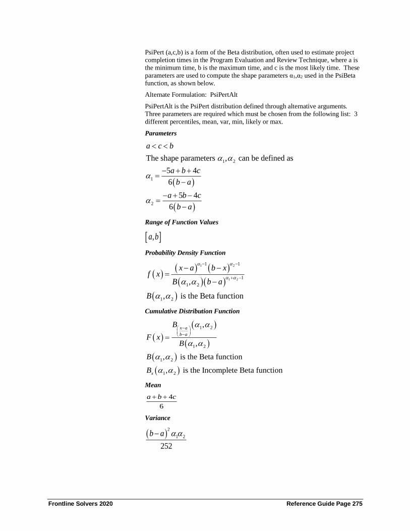
Frontline Solvers 2020 Reference Guide Page 275
PsiPert (a,c,b) is a form of the Beta distribution, often used to estimate project
completion times in the Program Evaluation and Review Technique, where a is
the minimum time, b is the maximum time, and c is the most likely time. These
parameters are used to compute the shape parameters α1,α2 used in the PsiBeta
function, as shown below.
Alternate Formulation: PsiPertAlt
PsiPertAlt is the PsiPert distribution defined through alternative arguments.
Three parameters are required which must be chosen from the following list: 3
different percentiles, mean, var, min, likely or max.
Parameters
( )
( )
1 2
1
2
The shape parameters , can be defined as
5 4
6
5 4
6
a c b
a b c
b a
a b c
b a
− + +=
−
− + −=
−
Range of Function Values
,a b
Probability Density Function
( )( ) ( )
( )( )
( )
1 2
1 2
1 1
1
1 2
1 2
,
, is the Beta function
x a b xf x
B b a
B
− −
+ −
− −=
−
Cumulative Distribution Function
( )
( )
( )
( )
( )
1 2
1 2
1 2
1 2
,
,
, is the Beta function
, is the Incomplete Beta function
x a
b a
x
B
F xB
B
B
−
− =
Mean
4
6
a b c+ +
Variance
( )2
1 2
252
b a −

Frontline Solvers 2020 Reference Guide Page 276
Skewness
( ) 1 2
4 7a b c
b a
+ −
−
Kurtosis
( ) ( ) ( )
( )( )
2
1 2 1 2 1 2 1 2
1 2 1 2 1 2
3 1 2 6
3 2
+ + + + + −
+ + + +
Median
Not defined
Mode
c
PsiRayleigh
PsiRayleigh (β,...)
PsiRayleigh (β) is a distribution with a finite lower bound of 0, a special case of
a Weibull distribution. The Rayleigh distribution can be used to model
component lifetimes.
If X is a random variable with Rayleigh distribution with parameter β = 1, then
X2 has a Chi Square distribution with parameter 2 (two degrees of freedom). If X and Y are independent normally distributed random variables with mean zero
and variance σ2, then (X2+Y2)1/2 has a Rayleigh distribution with parameter σ.
Thus, a Rayleigh distribution may be used to model the length of a two-dimen-
sional vector whose components are independent and normally distributed.
Alternate Formulation: PsiRayleighAlt
PsiRayleighAlt is the PsiRayleigh distribution defined through alternative
arguments. One parameters is required and must be chosen from the following
list: percentile, var or mean.
Parameters
0
Range of Function Values
)0,
Probability Density Function
( )
2
22
2
x
xef x
−
=
Cumulative Distribution Function
( )2
221
x
F x e
− = −

Frontline Solvers 2020 Reference Guide Page 277
Mean
2
Variance
( ) 24
2
−
Skewness
( )
( )3
2
2 3
4
−
−
Kurtosis
( )
2
2
3 32
4
− +
−
Median
( )ln 4
Mode
PsiReciprocal
PsiReciprocal (min, max)
PsiReciprocal is a bounded continuous distribution with min and max
parameters. This distribution is typically used in numerical analysis, Bayesian
statistics and analysis of noise.
Parameters
Min < max
Range of Function Values
[min, 𝑚𝑎𝑥]
Probability Density Function
𝑓(𝑥) =1
𝑥[ln(𝑚𝑎𝑥)−ln(𝑚𝑖𝑛)]
Cumulative Distribution Function
F(x) = ln(𝑥)−ln (𝑚𝑖𝑛)
ln (𝑚𝑎𝑥)−ln(𝑚𝑖𝑛)

Frontline Solvers 2020 Reference Guide Page 278
Mean
𝑞1
Variance
𝑞1 − 𝑞12
Skewness
𝑞3−3𝑞1𝑞2+2𝑞13
(𝑞2 − 𝑞12)
32
Kurtosis
𝑞4−4𝑞1𝑞3+6𝑞12𝑞2−3𝑞1
4
(𝑞2 − 𝑞12)
32
Mode
𝑚𝑖𝑛
PsiStudent
PsiStudent (df,…)
PsiStudent (df) is an unbounded distribution, symmetric about zero, with a shape similar to that of a Standard Normal distribution, and it approaches the Standard
Normal distribution as the degrees of freedom (parameter df) increases. It is
also known as the t-distribution, or Student’s t-distribution.
The Student or t-distribution frequently arises when estimating the mean of a
normally distributed population when the sample size is small. It is also used
when the population variance is unknown, and is estimated from a small sample.
Alternate Formulation: PsiStudentAlt
PsiStudentAlt is the PsiStudent distribution defined through alternative
arguments. One percentile parameter is required.
Parameters
0, integerdf
Range of Function Values
( ),−
Probability Density Function
( )
( )
1
2
2
1
2
2
is the Gamma function
dfdf
dff x
df x dfdf
x
++ =
+

Frontline Solvers 2020 Reference Guide Page 279
Cumulative Distribution Function
( )
( )
2
2
11 ,
2 2
2
, is the Incomplete Beta function
x
x df
a
dfB
F x
B x y
+
+
=
Mean
0 if df > 1
undefined if df = 1
Variance
if 22
dfdf
df
−
Skewness
0 if 3df
Kurtosis
3 6 if 4
- 4
dfdf
df
−
Median
0
Mode
0
PsiTriangGen
PsiTriangGen (ap,m,br,p,r…)
PsiTriangGen (ap,m,br,p,r…) is a Triangular distribution where the lower and
upper bounds are not given as fixed values, but are specified using percentiles.
This distribution is usually used to create rough models in situations where little
or no data is available. The distribution has a most likely value of m, the p
(lower) percentile value is ap, and the r (upper) percentile value is br. Given these values, a PsiTriangGen (ap,m,br,p,r…) distribution corresponds to a
PsiTriangular (a,c,b) distribution with values for the bounds (a and b), and the
most likely value (c) computed as shown below.

Frontline Solvers 2020 Reference Guide Page 280
Parameters
( )
( )
( )
, 0,1
The parameters of the Triangular distribution are defined as
1
1
1
11
1
Here is a solution to the following equation
11
1
1
p r
p r
p
r
p
r
p r
p r
a b
a m b
pa m
qa
p
q
c m
rb m
qb
r
q
q
rm a
pb m m
q
−
=
−
=
−−
−=
−−
−
−− −
− =
− − + −
( )1
11
p
ra
q
−−
−
Range of Function Values
,a b
Probability Density Function
( )
( )
( )( )
( )
( )( )
2 if
2 if
x aa x c
c a b af x
b xc x b
b c b a
−
− −=
− − −
Cumulative Distribution Function
( )
( )
( )( )
( )
( )( )
2
2
if
1 if
x aa x c
c a b aF x
b xc x b
b c b a
−
− −=
−−
− −
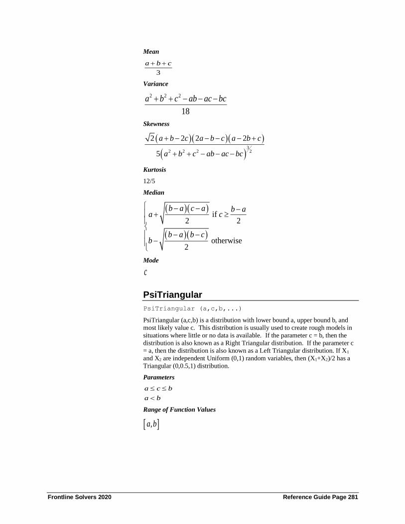
Frontline Solvers 2020 Reference Guide Page 281
Mean
3
a b c+ +
Variance
2 2 2
18
a b c ab ac bc+ + − − −
Skewness
( )( )( )
( )3
2 2 2 2
2 2 2 2
5
a b c a b c a b c
a b c ab ac bc
+ − − − − +
+ + − − −
Kurtosis
12/5
Median
( )( )
( )( )
if 2 2
otherwise2
b a c a b aa c
b a b cb
− − − +
− −−
Mode
c
PsiTriangular
PsiTriangular (a,c,b,...)
PsiTriangular (a,c,b) is a distribution with lower bound a, upper bound b, and
most likely value c. This distribution is usually used to create rough models in
situations where little or no data is available. If the parameter c = b, then the
distribution is also known as a Right Triangular distribution. If the parameter c
= a, then the distribution is also known as a Left Triangular distribution. If X1
and X2 are independent Uniform (0,1) random variables, then (X1+X2)/2 has a
Triangular (0,0.5,1) distribution.
Parameters
a c b
a b
Range of Function Values
,a b

Frontline Solvers 2020 Reference Guide Page 282
Probability Density Function
( )
( )
( )( )
( )
( )( )
2 if
2 if
x aa x c
c a b af x
b xc x b
b c b a
−
− −=
− − −
Cumulative Distribution Function
( )
( )
( )( )
( )
( )( )
2
2
if
1 if
x aa x c
c a b aF x
b xc x b
b c b a
−
− −=
−−
− −
Mean
3
a b c+ +
Variance
2 2 2
18
a b c ab ac bc+ + − − −
Skewness
( )( )( )
( )3
2 2 2 2
2 2 2 2
5
a b c a b c a b c
a b c ab ac bc
+ − − − − +
+ + − − −
Kurtosis
12/5
Median
( )( )
( )( )
if 2 2
otherwise2
b a c a b aa c
b a b cb
− − − +
− −−
Mode
c
PsiUniform
PsiUniform (a,b,...)
PsiUniform (a,b) is a flat, bounded distribution with lower bound a and upper
bound b. It is used to represent a random variable that is equally likely to take

Frontline Solvers 2020 Reference Guide Page 283
on any value between a lower and upper bound. A Uniform (0,1) distribution is
also known as a Standard Uniform distribution, and is used to generate many
other random variables. If X is a random variable with a Standard Uniform
distribution, then a + (b – a)X has a Uniform (a,b) distribution, and (1 – X) has a
Standard Uniform distribution.
Parameters
a b
Range of Function Values
,a b
Probability Density Function
( )1
if
0 otherwise
a x bf x b a
= −
Cumulative Distribution Function
( )
0 if
if
1 if
x a
x aF x a x b
b a
x b
−=
−
Mean
2
a b+
Variance
( )2
12
b a−
Skewness
0
Kurtosis
9/5
Median
2
a b+
Mode
Any value in [a,b]
PsiWeibull
PsiWeibull (,β,...)

Frontline Solvers 2020 Reference Guide Page 284
PsiWeibull (α,β) is a distribution with a finite lower bound of 0. The Weibull
distribution is quite flexible and can be used to model weather patterns, material
strength, processing and delivery times, and in a variety of reliability
engineering applications.
If X is a random variable with Weibull (1,β) distribution, then it also has the Exponential (β) distribution. In fact, a random variable X ~Weibull (α,β) if and
only if Xα ~ Exponential (βα). Also, if X is a random variable with Weibull (2,β)
distribution, then it also has the Rayleigh (β) distribution.
Alternate Formulation: PsiWeibullAlt
PsiWeibullAlt is the PsiBetaGen distribution defined through alternative
arguments. One percentile parameter is required.
Parameters
, 0
Range of Function Values
)0,
Probability Density Function
( )( )1
x
f x x e
−
− −=
Cumulative Distribution Function
( )( )
1x
F x e
−
= −
Mean
( )
1
is the Gamma functionx
Variance
222 1 1
2
−
Skewness
3
2 3
32
2
2
3 3 6 2 1 2 1
2 2 1 1
+ +
−
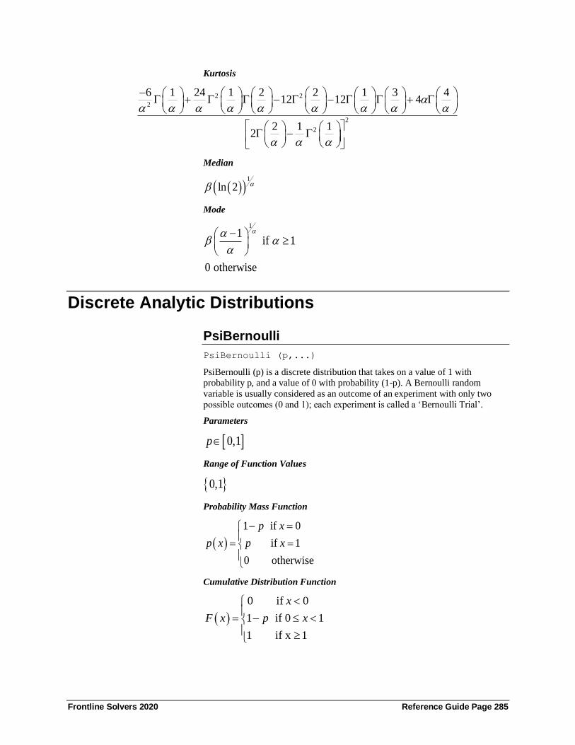
Frontline Solvers 2020 Reference Guide Page 285
Kurtosis
2 2
2
2
2
6 1 24 1 2 2 1 3 412 12 4
2 1 12
− + − − +
−
Median
( )( )1
ln 2
Mode
1
1 if 1
0 otherwise
−
Discrete Analytic Distributions
PsiBernoulli
PsiBernoulli (p,...)
PsiBernoulli (p) is a discrete distribution that takes on a value of 1 with
probability p, and a value of 0 with probability (1-p). A Bernoulli random
variable is usually considered as an outcome of an experiment with only two
possible outcomes (0 and 1); each experiment is called a ‘Bernoulli Trial’.
Parameters
0,1p
Range of Function Values
0,1
Probability Mass Function
( )
1 if 0
if 1
0 otherwise
p x
p x p x
− =
= =
Cumulative Distribution Function
( )
0 if 0
1 if 0 1
1 if x 1
x
F x p x
= −

Frontline Solvers 2020 Reference Guide Page 286
Mean
p
Variance
( )1p p−
Skewness
( )
1 2
1
p
p p
−
−
Kurtosis
( )
26 6 1
1
p p
p p
− +
−
Median
Not defined
Mode
10 if
2
11 if
2
10 and 1 if
2
p
p
p
=
PsiBinomial
PsiBinomial (n,p,...)
PsiBinomial (n,p) is a discrete distribution of the number of successes in n
independent ‘Bernoulli Trials’ (experiments with exactly two possible
outcomes), where p is the success probability in each trial. The Binomial
distribution can be used to model the number of winning trades in a trading
system, or the number of defective items in a batch.
A random variable X is defined by X ~ PsiBinomial (n,p) if and only if n-X ~
PsiBinomial (n,1-p).
The Poisson distribution with parameter λ is a good approximation of the
PsiBinomial (n,p) distribution when n → and 0p → , with np = .
Parameters
0, integer
0,1
n
p
Range of Function Values
0,1, , n

Frontline Solvers 2020 Reference Guide Page 287
Probability Mass Function
( )( )
( )
-1- if 0,1, ,
0 otherwise
where is the binomial coefficient,
!
! !
n xxn
p p x np x x
n
x
n n
x x n x
=
=
−
Cumulative Distribution Function
( ) ( )-
0
0 if 0
1- if 0
1 if
xn ii
i
x
nF x p p x n
i
x n
=
=
Mean
np
Variance
( )1np p−
Skewness
( )
1 2
1
p
np p
−
−
Kurtosis
( )
26 6 1
1
p p
np p
− +
−
Median
one of , 1, 1np np np− +
Mode
( ) ( ) ( )
( )
1 and 1 1 if 1 is integer
1 otherwise
p n p n p n
p n
+ + − +
+
PsiGeometric
PsiGeometric (p,...)
PsiGeometric (p) is a discrete distribution of the number of failures before the first success in a sequence of independent ‘Bernoulli Trials’ (experiments with
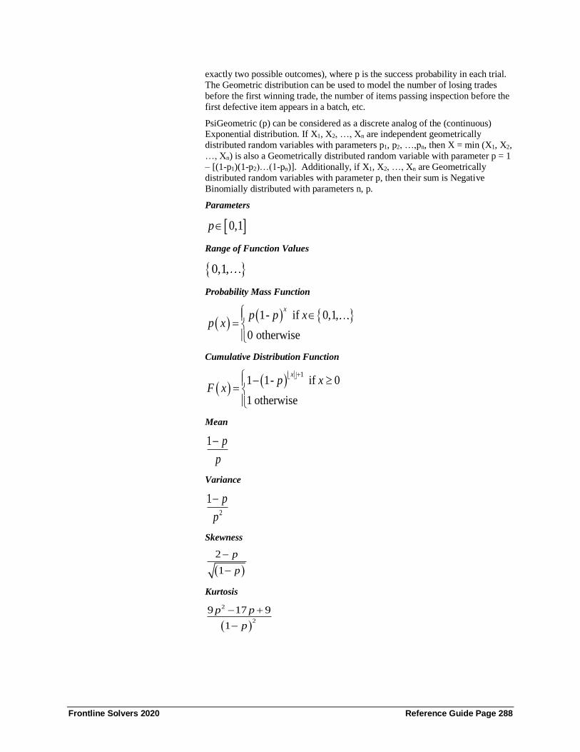
Frontline Solvers 2020 Reference Guide Page 288
exactly two possible outcomes), where p is the success probability in each trial.
The Geometric distribution can be used to model the number of losing trades
before the first winning trade, the number of items passing inspection before the
first defective item appears in a batch, etc.
PsiGeometric (p) can be considered as a discrete analog of the (continuous) Exponential distribution. If X1, X2, …, Xn are independent geometrically
distributed random variables with parameters p1, p2, …,pn, then X = min (X1, X2,
…, Xn) is also a Geometrically distributed random variable with parameter p = 1
– [(1-p1)(1-p2)…(1-pn)]. Additionally, if X1, X2, …, Xn are Geometrically
distributed random variables with parameter p, then their sum is Negative
Binomially distributed with parameters n, p.
Parameters
0,1p
Range of Function Values
0,1,
Probability Mass Function
( )( ) 1- if 0,1,
0 otherwise
xp p x
p x
=
Cumulative Distribution Function
( )( )
11 1- if 0
1 otherwise
xp x
F x
+ − =
Mean
1 p
p
−
Variance
2
1 p
p
−
Skewness
( )
2
1
p
p
−
−
Kurtosis
( )
2
2
9 17 9
1
p p
p
− +
−

Frontline Solvers 2020 Reference Guide Page 289
Median
( )
( )
ln 0.51
ln 1 p−
−
Mode
0
PsiHyperGeo
PsiHyperGeo (n,D,M,...)
PsiHyperGeo (n,D,M) is a discrete distribution of the number of successes in n
successive trials drawn without replacement from a finite population of size M,
when it is known that there are exactly D failures in the population. The
Hypergeometric distribution can be used to model ‘good’ and defective parts in
a manufacturing process.
A Hypergeometric distribution can be approximated by a Binomial distribution
with parameters n, p = D/M, when M is very large as compared to n.
Parameters
0,1,
, 0,1, ,
M
n D M
Range of Function Values
( ) ( ) max 0, , ,min ,n M D D n− +
Probability Mass Function
( )
D M D
x n xp x
M
n
−
− =
Cumulative Distribution Function
( )1
x
i
D M D
i n iF x
M
n
=
−
− =
Mean
nD
M

Frontline Solvers 2020 Reference Guide Page 290
Variance
( )( )( )1
1
D Dn M nM M
M
− −
−
Skewness
( )( ) ( )
( )( )
2 2 1
2
M D M n M
M nD M D M n
− − −
− − −
Kurtosis
( )
( )( )( )
( ) ( )
( )
( )( )2
2
1 1 6 3 66
2 3
M M M M M M n n M n N
n M M M n D M D M
− + − − − ++ −
− − − −
Median
Not defined
Mode
( )( ) ( )( ) ( )( )
( )( )
1 1 1 1 1 1 and 1 if is integral
2 2 2
1 1 otherwise
2
n D n D n D
M M M
n D
M
+ + + + + +−
+ + +
+ +
+
PsiIntUniform
PsiIntUniform (a,b,...)
PsiIntUniform (a,b) is a discrete distribution with equal probability at each
integer value between the lower and upper bounds (a and b). It is used as a
rough estimate of the true distribution when the only information we have is that
the random variable takes integer values between a and b, and each of these
values are equally likely.
Parameters
, integers
a<b
a b
Range of Function Values
, 1, , 1,a a b b+ −
Probability Mass Function
( )1
if , and integer- 1
0 otherwise
a x b xp x b a
= +

Frontline Solvers 2020 Reference Guide Page 291
Cumulative Distribution Function
( )
0 if
1 if
1
1 if
x a
x aF x a x b
b a
x b
− + = − +
Mean
2
a b+
Variance
( )2
1 1
12
b a− + −
Skewness
0
Kurtosis
( ) ( )
2
2
6 1 1
5 1 1
b a
b a
− + +−
− + −
Median
2
a b+
Mode
Net defined
PsiLogarithmic
PsiLogarithmic (p,...)
PsiLogarithmic is a discrete distribution with a lower bound of 1. It is used to
describe the diversity of a sample.
Parameters
( )0,1p
Range of Function Values
1,2,3,
Probability Mass Function
( ) ( )1
if 1ln 1
0 otherwise
xpx
p xp x
−
−=
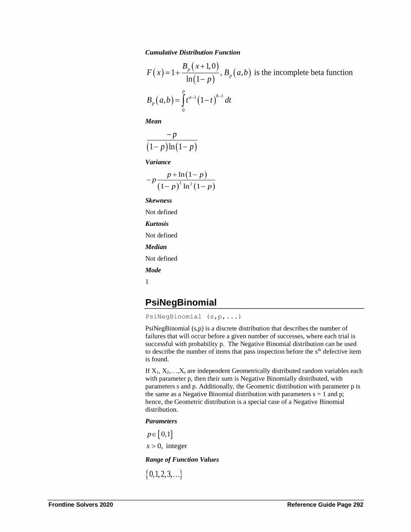
Frontline Solvers 2020 Reference Guide Page 292
Cumulative Distribution Function
( )( )
( )( )
( ) ( )11
0
1,01 , , is the incomplete beta function
ln 1
, 1
p
p
pba
p
B xF x B a b
p
B a b t t dt−−
+= +
−
= −
Mean
( ) ( )1 ln 1
p
p p
−
− −
Variance
( )
( ) ( )2 2
ln 1
1 ln 1
p pp
p p
+ −−
− −
Skewness
Not defined
Kurtosis
Not defined
Median
Not defined
Mode
1
PsiNegBinomial
PsiNegBinomial (s,p,...)
PsiNegBinomial (s,p) is a discrete distribution that describes the number of
failures that will occur before a given number of successes, where each trial is
successful with probability p. The Negative Binomial distribution can be used to describe the number of items that pass inspection before the sth defective item
is found.
If X1, X2,…,Xs are independent Geometrically distributed random variables each
with parameter p, then their sum is Negative Binomially distributed, with
parameters s and p. Additionally, the Geometric distribution with parameter p is
the same as a Negative Binomial distribution with parameters s = 1 and p;
hence, the Geometric distribution is a special case of a Negative Binomial
distribution.
Parameters
0,1
0, integer
p
s
Range of Function Values
0,1,2,3,

Frontline Solvers 2020 Reference Guide Page 293
Probability Mass Function
( )( )
11 if 0,1,
0 otherwise
xss x
p p xp x x
+ − −
=
Cumulative Distribution Function
( )( )
0
11 if 0
0 otherwise
xis
i
s ip p x
F x i
=
− + −
=
Mean
( )1s p
p
−
Variance
( )2
1s p
p
−
Skewness
( )
2
1
p
s p
−
−
Kurtosis
( )
2 6 13
1
p p
s p
− ++
−
Median
Not defined
Mode
( ) ( ) ( )
( )
1 1 1 1 1 1 and 1 if is integer
1 11 otherwise
s p s p s p
p p p
s p
p
− − − − − −+
− −+
PsiPoisson
PsiPoisson (λ,...)
PsiPoisson (λ) is a discrete distribution of the number of events that occur in an
interval of time, when the events occur at a known average rate, and each occurrence is independent of the time of occurrence of the previous event.

Frontline Solvers 2020 Reference Guide Page 294
The Poisson distribution with parameter λ can be approximated by a Normal
distribution with mean λ and variance λ, for large values of λ. If X1, X2,…,Xn
are independent Poisson random variables with parameters λ1, λ2,… λn, then
their sum is also a Poisson random variable with parameter λ1 +λ2+…+λn.
Parameters
>0
Range of Function Values
0,1,
Probability Mass Function
( ) if 0,1,
!
0 otherwise
xex
p x x
−
=
Cumulative Distribution Function
( ) i
0
0 if 0
if 0!
x
i
x
F xe x
i
−
=
=
Mean
Variance
Skewness
1
Kurtosis
13
+
Median
Not applicable
Mode
and 1 if is integer
otherwise
−

Frontline Solvers 2020 Reference Guide Page 295
Custom Distributions
PsiCumul
PsiCumul (a,b, {x1,x2,…,xn}, {p1,p2,…,pn},...)
PsiCumul (a,b, {x1,x2,…,xn},{p1,p2,…,pn},…) is a custom continuous
distribution with lower and upper bounds equal to a and b respectively, and with
user specified values , x1,x2,…,xn and corresponding cumulative probabilities
p1,p2,…,pn.
Parameters
1
1
0 1 0 1
1,2, ,
0 1 1,2, ,
1, 2, , 1
1,2, , 1
Define the boundary parameters as
, , 0, 1
i
i
i i
i i
n n
a b
a x b i n
p i n
p p i n
x x i n
x a x b p p
+
+
+ +
=
=
= −
= −
= = = =
Range of Function Values
,a b
Probability Density Function
( ) 11
1
if i ii i
i i
p pf x x x x
x x
++
+
−=
−
Cumulative Distribution Function
( ) ( )1 1
1
if ii i i i i
i i
x xF x p p p x x x
x x+ +
+
−= + −
−
Mean
Not defined
Variance
Not defined
Skewness
Not defined
Kurtosis
Not defined
Median
Not defined
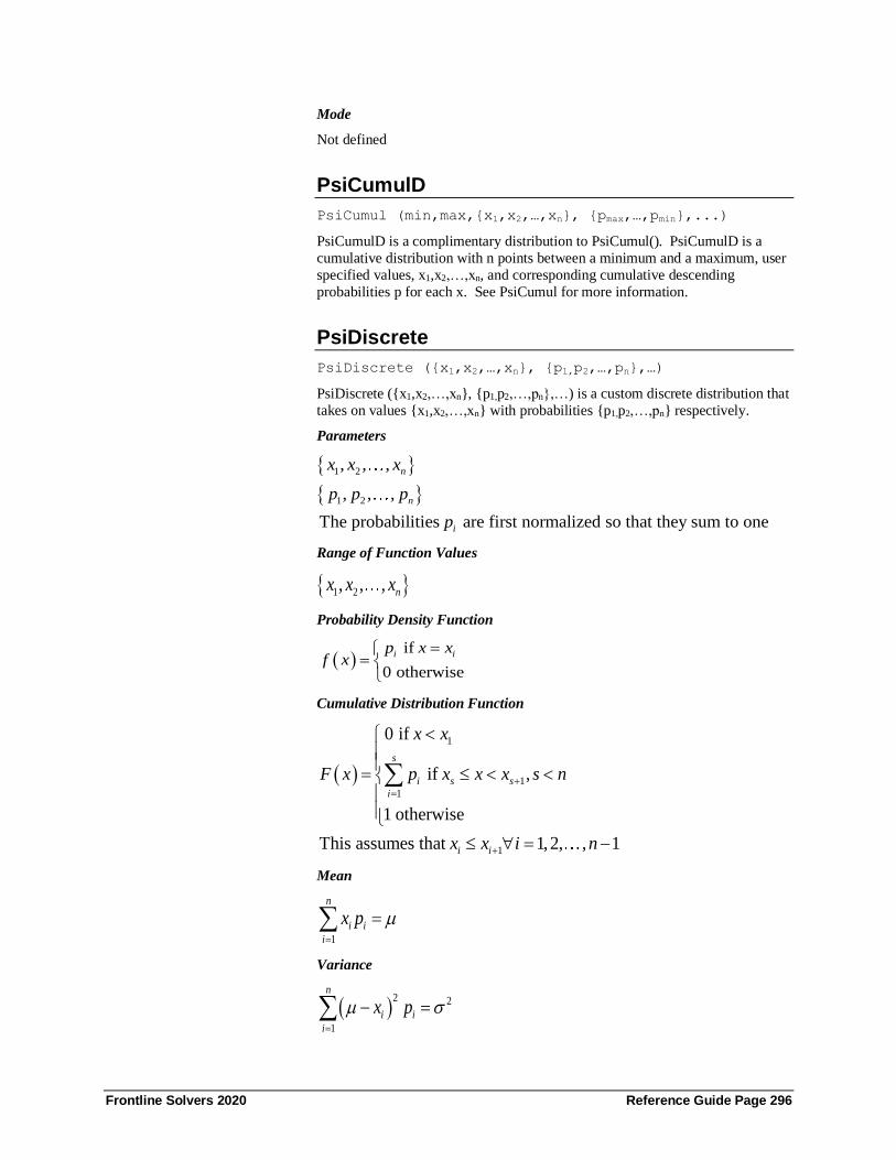
Frontline Solvers 2020 Reference Guide Page 296
Mode
Not defined
PsiCumulD
PsiCumul (min,max,{x1,x2,…,xn}, {pmax,…,pmin},...)
PsiCumulD is a complimentary distribution to PsiCumul(). PsiCumulD is a
cumulative distribution with n points between a minimum and a maximum, user
specified values, x1,x2,…,xn, and corresponding cumulative descending
probabilities p for each x. See PsiCumul for more information.
PsiDiscrete
PsiDiscrete ({x1,x2,…,xn}, {p1,p2,…,pn},…)
PsiDiscrete ({x1,x2,…,xn}, {p1,p2,…,pn},…) is a custom discrete distribution that
takes on values {x1,x2,…,xn} with probabilities {p1,p2,…,pn} respectively.
Parameters
1 2
1 2
, , ,
, , ,
The probabilities are first normalized so that they sum to one
n
n
i
x x x
p p p
p
Range of Function Values
1 2, , , nx x x
Probability Density Function
( ) if
0 otherwise
i ip x xf x
==
Cumulative Distribution Function
( )
1
1
1
1
0 if
if ,
1 otherwise
This assumes that 1,2, , 1
s
i s s
i
i i
x x
F x p x x x s n
x x i n
+
=
+
=
= −
Mean
1
n
i i
i
x p =
=
Variance
( )2 2
1
n
i i
i
x p =
− =

Frontline Solvers 2020 Reference Guide Page 297
Skewness
( )3
1
3
n
i i
i
x p
=
−
Kurtosis
( )4
1
4
n
i i
i
x p
=
−
Median
1
1
where min 1,2, , : 0.5
This assumes that 1,2, , 1
j
s i
i
i i
x s j n p
x x i n
=
+
= =
= −
Mode
( )1,2, ,
argmax ii n
px
=
PsiDisUniform
PsiDisUniform ({x1,x2,…,xn},…)
PsiDisUniform ({x1,x2,…,xn},…) is a custom discrete distribution that takes on
values {x1,x2,…,xn} with equal probability. It is similar to the PsiDiscrete
distribution except that no probabilities are specified – instead all x values are equally likely to occur. (In the equations below, each pi = 1/n.) PsiDisUniform
can be used to resample a set of past observations {x1,x2,…,xn}.
Parameters
1 2, , ,
These values have the corresponding probabilities as
11,2, ,
n
i
x x x
p i nn
= =
Range of Function Values
1 2, , , nx x x
Probability Density Function
( ) if
0 otherwise
i ip x xf x
==
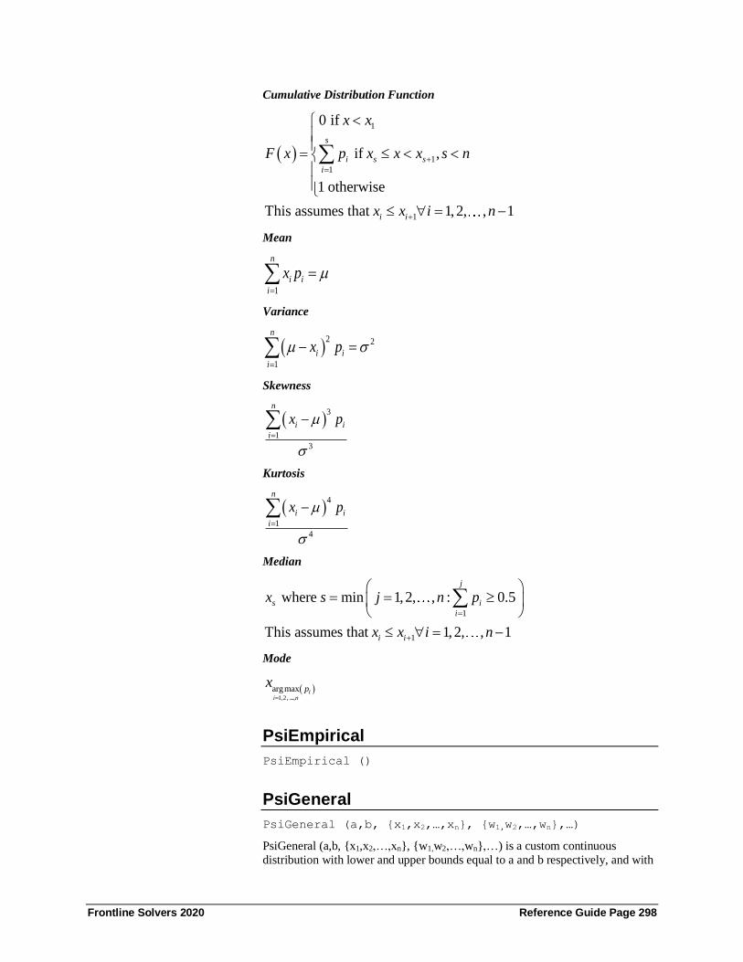
Frontline Solvers 2020 Reference Guide Page 298
Cumulative Distribution Function
( )
1
1
1
1
0 if
if ,
1 otherwise
This assumes that 1,2, , 1
s
i s s
i
i i
x x
F x p x x x s n
x x i n
+
=
+
=
= −
Mean
1
n
i i
i
x p =
=
Variance
( )2 2
1
n
i i
i
x p =
− =
Skewness
( )3
1
3
n
i i
i
x p
=
−
Kurtosis
( )4
1
4
n
i i
i
x p
=
−
Median
1
1
where min 1,2, , : 0.5
This assumes that 1,2, , 1
j
s i
i
i i
x s j n p
x x i n
=
+
= =
= −
Mode
( )1,2, ,
argmax ii n
px
=
PsiEmpirical
PsiEmpirical ()
PsiGeneral
PsiGeneral (a,b, {x1,x2,…,xn}, {w1,w2,…,wn},…)
PsiGeneral (a,b, {x1,x2,…,xn}, {w1,w2,…,wn},…) is a custom continuous
distribution with lower and upper bounds equal to a and b respectively, and with

Frontline Solvers 2020 Reference Guide Page 299
user specified values x1,x2,…,xn and corresponding weights w1,w2,…,wn. This is
similar to a PsiCumul (a,b, {x1,x2,…,xn},{p1,p2,…,pn},…) distribution, where the
probabilities are calculated using the weights as shown below.
Parameters
1
1
1
1,2, ,
1,2, , 1
The cumulative probabilities are defined as
i
i i
ik
i nk
j
j
a b
a x b i n
x x i n
wp
w
+
=
=
=
= −
=
Range of Function Values
,a b
Probability Density Function
( ) 11
1
if i ii i
i i
p pf x x x x
x x
++
+
−=
−
Cumulative Distribution Function
( ) ( )1 1
1
if ii i i i i
i i
x xF x p p p x x x
x x+ +
+
−= + −
−
Mean
Not defined
Variance
Not defined
Skewness
Not defined
Kurtosis
Not defined
Median
Not defined
Mode
Not defined
PsiHistogram
PsiHistogram (a,b,{w1,w2,…,wn},…)
PsiHistogram (a,b,{w1,w2,…,wn},…) is a custom continuous distribution with lower and upper bounds equal to a and b respectively, and with user specified
weights w1,w2,…,wn corresponding to n subintervals of equal size. This is
similar to a PsiCumul (a,b, {x1,x2,…,xn},{p1,p2,…,pn},…) distribution, where the

Frontline Solvers 2020 Reference Guide Page 300
probabilities are calculated using the weights as shown below, and the interval
defined by the bounds a and b is divided into subintervals of equal size as
described below.
Parameters
1 2
1
1
The interval , is divided into subintervals
of equal size , , ,
The cumulative probabilities are defined as
n
i
ik
i nk
j
j
a b
a b n
x x x
b ax a i
n
wp
w=
=
− = +
=
Range of Function Values
,a b
Probability Density Function
( ) 11
1
if i ii i
i i
p pf x x x x
x x
++
+
−=
−
Cumulative Distribution Function
( ) ( )1 1
1
if ii i i i i
i i
x xF x p p p x x x
x x+ +
+
−= + −
−
Mean
Not defined
Variance
Not defined
Skewness
Not defined
Kurtosis
Not defined
Median
Not defined
Mode
Not defined

Frontline Solvers 2020 Reference Guide Page 301
Special Distributions Analytic Solver Desktop offers a number of special PSI Distribution functions
that do not fit readily into the classes of continuous, discrete and custom
distributions described above. For example, PsiCertified() provides easy access
to a named, published Certified Distribution, which could be a continuous,
discrete or custom distribution or a distribution based on a SIP or SLURP.
PsiSip() and PsiSlurp() ensure that Monte Carlo trials are drawn sequentially
from SIP or SLURP data. PsiResample returns a single result while
PsiMVNormal() and PsiMVLogNormal() return array results rather than single-
valued results.
Note: PSI Property functions generally may not be passed as arguments to any of the PSI Distribution functions in this section. The only exception is that
the PsiCertify() function may be passed to PsiSip() or PsiSlurp(), enabling the
SIP or SLURP-based distribution to be named and published as a Certified
Distribution.
Functions PsiMVLogNormal(), PsiMVNormal(), PsiMVResample,
PsiMVShuffle and PsiResample() are included to provide an upgrade path for
users of AnalyCorp’s XLSim software. Note that PsiMVLogNormal() and
PsiMVNormal() require a covariance matrix (not a rank correlation matrix) as
an argument; they cannot be correlated with dissimilar distributions specified via
other PSI Distribution functions.
Note: Certified Distributions and the functions PsiMVLogNormal(), PsiMVNormal(), PsiMVResample, PsiMVShuffle and PsiResample() are not
supported in Analytic Solver Cloud.
PsiCertified
PsiCertified (name,sipname)
PsiCertified creates an uncertain variable that returns trials data for a named,
published Certified Distribution. The name argument is a character string such as “MyDist”. The sipname argument is optional; if used, it is the character
string name of a SIP (column) of a SLURP. A PsiCertified distribution may
return either continuous or discrete sample data, depending on the nature of the
published Certified Distribution. This function is not supported in Analytic
Solver Cloud or AnalyticSolver.com.
PsiFit
PsiFit (data)
PsiFit dynamically fits a probability distribution to sample data, and creates an
uncertain variable linked to the sample data. This dynamically fitted uncertain
variable can then be used in the model as an uncertain input variable. The "data"
argument is an Excel cell range containing the list of sample data.
PsiMVLogNormal
PsiMVLogNormal (µ,∑)
PsiMVLogNormal (µ,∑) is a multivariate distribution that returns a vector of
random variables that are lognormally distributed, with mean values specified
by the vector µ, and covariance values specified by the matrix ∑. This is a
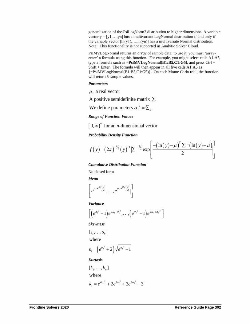
Frontline Solvers 2020 Reference Guide Page 302
generalization of the PsiLogNorm2 distribution to higher dimensions. A variable
vector y = [y1,…,yn] has a multivariate LogNormal distribution if and only if
the variable vector [ln(y1),…,ln(yn)] has a multivariate Normal distribution.
Note: This functionality is not supported in Analytic Solver Cloud.
PsiMVLogNormal returns an array of sample data; to use it, you must ‘array-enter’ a formula using this function. For example, you might select cells A1:A5,
type a formula such as =PsiMVLogNormal(B1:B5,C1:G5), and press Ctrl +
Shift + Enter. The formula will then appear in all five cells A1:A5 as
{=PsiMVLogNormal(B1:B5,C1:G5)}. On each Monte Carlo trial, the function
will return 5 sample values.
Parameters
2
, a real vector
A positive semidefinite matrix
We define parameters i ii
=
Range of Function Values
)0, for an -dimensional vectorn
n
Probability Density Function
( ) ( ) ( )( )( ) ( )( )1
112 2
ln ln2 exp
2
T
n y yf y y
−− − −
− − − =
Cumulative Distribution Function
No closed form
Mean
221
1 2 2, ,n
ne e
+ +
Variance
( ) ( )2 22 2
1 1 1 221 , , 1n n ne e e e ++ − −
Skewness
( )2 2
1
i
[ , , ]
where
s 2 1i i
ns s
e e
= + −
Kurtosis
2 2 2
1
4 3 2
[ , , ]
where
2 3 3i i i
n
i
k k
k e e e
= + + −

Frontline Solvers 2020 Reference Guide Page 303
Median
1 , , ne e
Mode
221 1 , , n ne e
−−
PsiMVNormal
PsiMVNormal (µ,∑)
PsiMVNormal (µ,∑) is a multivariate distribution that returns a vector of
random variables that are normally distributed, with mean values specified by
the vector µ, and covariance values specified by the matrix ∑. This is a
generalization of the PsiNormal distribution to higher dimensions. Note: This functionality is not supported in Analytic Solver Cloud.
PsiMVNormal returns an array of sample data; to use it, you must ‘array-enter’
a formula using this function. For example, you might select cells A1:A5, type
a formula such as =PsiMVNormal(B1:B5,C1:G5), and press Ctrl + Shift +
Enter. The formula will appear in all five cells as {=PsiMVNormal(B1:B5,
C1:G5)}. On each Monte Carlo trial, the function will return 5 sample values.
Note: This function is not supported in Analytic Solver Cloud.
Parameters
2
, a real vector
A positive definite matrix
We define parameters i ii
=
Range of Function Values
( ), for an -dimensional vectorn
n−
Probability Density Function
( ) ( )( ) ( )1
12 22 exp
2
Tn y y
f y
−
− − − − −
=
Cumulative Distribution Function
No closed form
Mean
1, , n
Variance
2 2
1 , , n

Frontline Solvers 2020 Reference Guide Page 304
Skewness
[0] for an -dimensional vectorn n
Kurtosis
[0] for an -dimensional vectorn n
Median
1, , n
Mode
1, , n
PsiResample
PsiResample (data)
PsiResample returns a random sample (with replacement) of the trial values in
the cell range specified by the data argument, i.e. =PsiResample(B1:B1000)
returns a single value randomly selected from the cell range B1:B1000.
PsiMVResample
PsiMVResample (data)
PsiMVResample is a multivariate distribution that returns a vector of sample
data; to use it, you must ‘array-enter’ a formula using this function. The data
argument must be a rectangular Excel range. This function may be array entered
in a single column (or row) of size n where n is the number of rows (or columns)
in the data argument. Note: This functionality is not supported in Analytic
Solver Cloud.
PsiMVResample returns a random sample of the trial values in the cell range
specified by the data argument. If data is a rectangular cell range and the cell
range in which PsiMVResample is array-entered is a single column, then
PsiMVResample returns values from a randomly selected column in data, with
values drawn sequentially from that column, beginning with the first element. Similarly, if data is rectangular and the cell range is a single row,
PsiMVResample returns values from a randomly selected row in data, with
values drawn sequentially from that row, beginning with the first element.
For example, you might select cells A1:A3 ( or cells A1:C1) type a formula such
as =PsiMVResample(D1:F3) and press Ctrl + Shift + Enter. The formula will
then appear in all three cells A1:A3 (or A1:C1) as
{=PsiMVResample(D1:F3)}. On each Monte Carlo trial, cells A1:A3 (or cells
A1:C1) will return a uniformly selected column from the argument.
PsiMVShuffle
PsiMVShuffle (data)
PsiMVShuffle is a multivariate distribution that returns a vector of sample data;
to use it, you must ‘array-enter’ a formula using this function. For example, you

Frontline Solvers 2020 Reference Guide Page 305
might select cells A1:B5, type a formula such as =PsiMVShuffle(C1:D5), and
press Ctrl + Shift + Enter. The formula will then appear in all ten cells A1:B5 as
{=PsiMVShuffle(C1:D5)}. On each Monte Carlo trial, the function will return
10 sample values. Note: This functionality is not supported in Analytic Solver
Cloud.
PsiMVShuffle returns a random permutation of all the trial values in the cell
range specified by the data argument, which should contain at least as many
columns and rows as the cell range in which the function is array-entered.
(Note: This function will still work if the function is array-entered into a cell
range that is smaller or larger than the data cell range.) In the sample drawn on
each Monte Carlo trial, each cell in the data range is selected only once; values
are repeated in a single sample only if they are repeated in data.
PsiSip
PsiSip (sip)
PsiSip returns trials for an uncertain variable from a list or vector of sample
data, called a Stochastic Information Packet (SIP). The sip argument is an Excel
cell range containing the list of sample data. The value returned by PsiSip() on
the ith trial is the ith value in the list.
PsiSlurp
PsiSlurp (slurp,j)
PsiSlurp returns trials for an uncertain variable from a table of correlated sample
data, called a Stochastic Library Unit, Relationships Preserved (SLURP), in the
sequence specified in the table. The slurp argument is a rectangular Excel cell
range containing the SLURP data; the j argument is the index of the desired SIP
(column) of the SLURP, starting from 1. The value returned by PsiSlurp() on
the ith trial is taken from the ith row and the jth column of the table.
PSI Property Functions
PsiBaseCase
PsiBaseCase(value)
Use this property to specify a Base Case value for an Uncertain Variable. This
is the single value that you’d want to have in this input cell if you were not
treating the cell as an Uncertain Variable (i.e. if it did not have a PSI
Distribution function). If there is a number in the cell at the time you define an
Uncertain Variable using the Distributions choice on the Ribbon, that number is
automatically saved as the Base Case value. If you use the Publish button to
“freeze” all Uncertain Variables, the Base case value will replace the PSI
Distribution function in the cell (and the function call will be saved in a cell
comment). When you do this, the Uncertain Variable Formula will be updated
with a call to the PsiBaseCase() property function, passing the value you specify
as the second argument.

Frontline Solvers 2020 Reference Guide Page 306
PsiCertify
PsiCertify (name, default_value, short_description,
full_description, version, author, copyright,
trademark, history)
PsiCertify is used to name, certify and ‘publish’ a PSI Distribution function as a
Certified Distribution. The default_value argument should be a number; all
other arguments should be character strings. Only the name argument is
required; the others are optional. For further information and examples of the use of PsiCertify(), see “Creating and Using Certified Distributions” in the
Frontline Solver User Guide chapter “Mastering Simulation and Risk Analysis
Concepts.”
PsiCensor
PsiCensor ([min], [max], [type])
PsiCensor is used to pile the values of samples from the uncertain variable’s
distribution as follows: if the uncertain variable’s value is less than the Min value, then the sample value will be piled at the Min, if the uncertain variable’s
value is larger than the Max value, then the sample value will be piled at the
Max. This argument results in a “build up” of values around the Min and Max
values in the distribution.
• This property accepts "empty" arguments for the min and max
parameters. If not provided, the default of -1E+30 will be used for min
and the default of 1E+30 will be used for max.
• There is a third optional argument, type, that was added in V2019. If
type = 0 (the default), nothing is passed for the type argument. If type
= 1, the bounds will be interpreted as numbers. If type = 2, the bounds will be interpreted as standard deviations. If type = 3, the bounds will
be interpreted as percentiles which must be between 0 and 1. This
setting overrides the Censure Measure setting on the Platform tab of the
Solver Task Pane.
Example: You can create lower and upper censor bouds of 96 and 104,
respectively, for the PsiNormal distribution given the parameters mean = 100
and standard deviation = 2 in one of three ways:
• When type = 1 (values), use: =PsiNormal(100,2, PsiCensor(95, 105, 1))
• When type =2 (std. dev.), use =PsiNormal(100,2, PsiCensor(-2, 2, 1))
• When type = 3 (percentiles), use =PsiNormal(100,2,PsiCensor(0.03, 0.97,
3))
PsiCollect
PsiCollect ()
PsiCollect is used to specify a subset of the uncertain variables for which sample
data and statistics are collected, for future use. It has no significance in the
current release of Analytic Solver.
PsiCompound
PsiCompund (number_cell, deduction, limit)

Frontline Solvers 2020 Reference Guide Page 307
A compound distribution is made up of a "severity" distribution and a
"frequency" distribution. Assume the following compound distribution,
=PsiBeta(3, 2, PsiCompound(A2)), where A2 = PsiPoisson(100). PsiBeta(3,2)
is referred to as the "severity" distribution. The severity distribution is the
distribution to be added N times. PsiPoisson(100) is referred to as the "frequency" distribution. The frequency distribution determines the size N of
the sum (i.e, how many PsiBeta to sum). N can be a constant but can also be
computed at each trial by drawing from a discrete distribution.
• The number_cell argument passes the number of random trial values
to be summed. Number_cell can be an integer, a cell containing an
integer, a formula evaluating to an integer, or a cell containing a
discrete distribution.
If a fractional value is passed directly or indirectly (by using a formula)
or a continuous distribution is passed to this argument, the result will
be rounded down to the nearest integer.
Note: If a discrete distribution is passed to the number_cell argument,
the frequency distribution must be formulated in such a way that the trial values generated by the distribution must be greater than 1. If not,
trial values < 1 will be set equal to 1.
• The value passed to the deduction argument is subtracted from every
term of the compound sum which results in a shift of the compound
distribution by -N * deduction.
• If a trial value is larger than a specified limit, then the trial value is
reset to the limit.
For a complete example illustrating how to compute a compound distribution,
see the Examples: Simulation and Risk Analysis chapter in the Analytic Solver
User Guide.
PsiCopula
PsiCopula(type, param, [reflection], [instance])
Starting with V2016-R2, Analytic Solver introduces support for Archimedean
(and Eliptical) copulas when inducing correlation amongst uncertain variables.
Archimedean copula correlation is implemented using the conditional
distribution and Laplace-Stieltjes methods.
Type: Analytic Solver supports three types of Archimedean copulas: clayton,
frank, and gumbel. The copula type should be passed in quotes as: "clayton",
"frank", or "gumbel". In this example, "clayton" is passed. The two elliptical
copulas have their own Psi property name: PsiCopulaGauss and
PsiCopulaStudent. See below for their signatures.
Param: The parameter of a copula determines the strength of the correlation. In
this example, a parameter equal to 10 is passed. See the following parameter
restrictions for each Archimedean copula type.
Clayton:
• Bivariate: param >= -1, param ≠ 0.
• Muiltivariate: param > 0
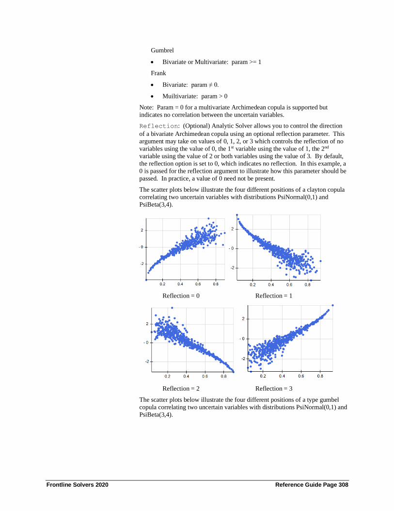
Frontline Solvers 2020 Reference Guide Page 308
Gumbrel
• Bivariate or Multivariate: param >= 1
Frank
• Bivariate: param ≠ 0.
• Muiltivariate: param > 0
Note: Param = 0 for a multivariate Archimedean copula is supported but
indicates no correlation between the uncertain variables.
Reflection: (Optional) Analytic Solver allows you to control the direction
of a bivariate Archimedean copula using an optional reflection parameter. This
argument may take on values of 0, 1, 2, or 3 which controls the reflection of no
variables using the value of 0, the 1st variable using the value of 1, the 2nd
variable using the value of 2 or both variables using the value of 3. By default,
the reflection option is set to 0, which indicates no reflection. In this example, a
0 is passed for the reflection argument to illustrate how this parameter should be
passed. In practice, a value of 0 need not be present.
The scatter plots below illustrate the four different positions of a clayton copula
correlating two uncertain variables with distributions PsiNormal(0,1) and
PsiBeta(3,4).
Reflection = 0 Reflection = 1
Reflection = 2 Reflection = 3
The scatter plots below illustrate the four different positions of a type gumbel
copula correlating two uncertain variables with distributions PsiNormal(0,1) and
PsiBeta(3,4).

Frontline Solvers 2020 Reference Guide Page 309
Reflection = 0 Reflection = 1
Reflection = 2 Reflection = 3
The scatter plots below illustrate the four different positions of a type frank copula correlating two uncertain variables with distributions PsiNormal(0,1) and
PsiBeta(3,4). Note: Since the Frank copula is symmetric, this type of copula
has only one reflection.
Reflection = 0 Reflection = 1
Reflection = 2 Reflection = 3

Frontline Solvers 2020 Reference Guide Page 310
Instance: (Optional) Instance is the string name given to the copula. An
Archimedean copula is explicitly identified by the Instance argument and
implicitly identified by its argument values. When multiple copulas are present
in the same workbook, it is considered "best practice" to use this argument.
Suppose two uncertain variables exist in the same workbook. The PsiCopula
property is used to correlate the two uncertain variables using,
=PsiCopula("clayton", 10, 0). Since the Instance property is missing, the copula
is identified implicitly by its unique set of arguments, in this case ("clayton",
"10"). When not passing the Instance property, the PsiCopula property within
each uncertain variable signature, MUST use the same arguments. Otherwise, the correlation between the uncertain variables will not be invoked.
Note: PsiCopula("clayton", 10) and PsiCopula("clayton", 10, 0) is considered as
the same copula since 0 is the default for the Reflection argument.
To correlate a new group of uncertain variables using a 2nd copula, say
PsiCopula("clayton", 12) or PsiCopula("frank", 10), the Instance argument is
still not required since either copula is identified by its unique parameters of
"clayton" and "12" or "frank" and "10". However, if correlating this same new
group of uncertain variables with a copula using the same arguments of
"clayton" and "10", a unique name must be passed to the Instance argument, for
example, "copula2".
For a complete example of how to use the PsiCopula() property, see the
Modeling Correlation Using Copulas section within the Analytic Solver User
Guide.
Theory
An Archimedean copula, C, is defined as:
C ( u1, u2, …, um ) = φ-1 ( φ ( u1 ) + … + φ ( ud ; θ ) ; θ )
where φ: [0,1] → [0, ∞) is a strict Archimedean copula generator with inverse
𝜑−1 is completely monotonic on [0, ∞). A strictly decreasing function φ:
[0,1]→[0, ∞) that satisfies φ(0) = ∞ and φ(1) = 0. A decreasing function
f(t):[a,b]→(-∞, ∞) is completely monotonic if the following equation is satisfied.
(−1)𝑘 𝑑𝑘
𝑑𝑡𝑘 𝑓(𝑡) ≥ 0, 𝑘 𝜖 ℕ, 𝑡 𝜖(𝑎, 𝑏)
The table below displays the three types of Archimedian copulas, and their
corresponding generators) supported by Analytic Solver.
Copula Type Copula Parameter Generator
Clayton [∑ 𝑢𝑖−𝜃𝑚
𝑖=1 − 𝑚 + 1]-1/θ 𝜃 > 0 θ-1 (u -θ -1)
Frank 1
𝜃𝑙𝑜𝑔 ⌈1 +
∏ [exp (−𝜃𝑢𝑖𝑚𝑖=1 ) − 1]
(exp(−𝜃) − 1]𝑚−1⌉
𝜃𝜖(−∞, ∞)
{0}
𝑓𝑜𝑟 𝑚 = 2 𝑎𝑛𝑑
𝜃 > 0 𝑓𝑜𝑟 𝑚 > 3
-log⌈exp(−𝜃𝑢)−1
exp(−𝜃)−1⌉
Gumbel Exp{−⌈∑ (−𝑙𝑜𝑔𝑢𝑖)𝜃𝑚
𝑖=1 ⌉1
𝜃} θ>1 (− log 𝑢)𝜃
For more information on the theory of Copulas, please see the following
references.
Jackel, Peter., “Monte Carlo Methods in Finance”, John Wiley & Sons Ltd,
2002

Frontline Solvers 2020 Reference Guide Page 311
Nelsen, Roger B., “An Introduction to Copulas”, New York 2006
PsiCopulaGauss
PsiCopulaGauss(sigma, position, [instance])
Sigma: If bivariate, a number between -1 and 1; if multivariate, the Excel cell
range where the correlation matrix is located in the Excel spreadsheet, i.e., if the
copula is multivariate and the correlation matrix is located in cells N2:P4, then pass N2:P4 for this argument.
Position: Specifies the uncertain variable index in the correlation matrix.
For example, the "2" passed in the formula, =PsiBeta(3, 4,
PsiCopulaGauss(N2:P4, 2, "mycop") specifies that the correlation coefficients in
the 2nd column of the correlation matrix in cells N2:P4 will be applied to the
PsiBeta() uncertain variable.
Instance: (Optional) Instance is the string name given to the copula. An
elliptical copula is explicitly identified by the Instance argument and implicitly
identified by the location of the correlation matrix. PsiCopulaGauss() supports
multiple copulas using the same correlation matrix. If passing the same type of
elliptical copula using the same correlation matrix within the same workbook,
this argument must be present. If the workbook contains multiple copulas of
different types, then this argument may be omitted. When multiple copulas are
present in the same workbook, it is considered "best practice" to use this
argument.
Suppose three uncertain variables are present in the same workbook. The three
uncertain variables can be correlated using the PsiCopulaGauss property,
=PsiCopulaGauss(N2:P4, 1, "mycop"). Since the Instance property is present,
the copula is identified explicitly by the name given in the last argument,
"mycop". When not passing the Instance property, the PsiCopulaGauss
property within each uncertain variable signature, MUST use the same
correlation matrix. Otherwise, the correlation between the uncertain variables
will not be invoked.
For a complete example of how to use the PsiCopulaGauss() property, see the
Modeling Correlation Using Copulas section within the Analytic Solver User
Guide.
Theory
If 𝑢𝑗~𝑈(0,1) for j = 1, …, m. where U(0,1) symbolizes the uniform distribution
on the interval [0, 1] and if ∑ is a semidefinite correlation matrix with 𝑚(𝑚 − 1)
2⁄ parameters, then the copula defined by PsiCopulaGauss() can be
written as:
𝑪∑ ( u1, u2, …, um ) = 𝝋∑- ( 𝝋−𝟏 ( u1 ) + … + 𝝋−𝟏 ( um ) )

Frontline Solvers 2020 Reference Guide Page 312
where φ is the distribution function of a standard normal random variable and
𝜑∑ is the m-variate standard normal distribution with mean vector 0 and
covariance matrix ∑.
For more information on the theory of Copulas, please see the following
references.
Jackel, Peter., “Monte Carlo Methods in Finance”, John Wiley & Sons Ltd,
2002
Nelsen, Roger B., “An Introduction to Copulas”, New York 2006
PsiCopulaStudent
PsiCopulaStudent(sigma, position, df, [instance])
Sigma: If bivariate, a number between -1 and 1; if multivariate, the Excel cell
range where the correlation matrix is located in the Excel spreadsheet, i.e., if the
copula is multivariate and the correlation matrix is located in cells N2:P4, then
pass N2:P4 for this argument.
Position: Specifies the uncertain variable index in the correlation matrix.
For example, the "2" passed in the formula, =PsiBeta(3, 4, PsiCopulaStudent(N2:P4, 2, 1, "mycop") specifies that the correlation
coefficients in the 2nd column of the correlation matrix in cells N2:P4 will be
applied to the PsiBeta() uncertain variable.
df: Enter an integer value greater than 1. This parameter specifies the degrees
of freedom for the PsiCopulaStudent function. In this example, 1 degree of freedom is used.
Instance: (Optional) Instance is the string name given to the copula. An
elliptical copula is explicitly identified by the Instance argument and implicitly
identified by the location of the correlation matrix. PsiCopulaStudent() supports
multiple copulas using the same correlation matrix. If passing the same type of elliptical copula using the same correlation matrix within the same workbook,
this argument must be present. If the workbook contains multiple copulas of
different types, then this argument may be omitted. When multiple copulas are
present in the same workbook, it is considered "best practice" to use this
argument.
Suppose three uncertain variables are present in the same workbook. The three
uncertain variables can be correlated using the PsiCopulaStudent property,
=PsiCopulaStudent(N2:P4, 1, 1, "mycop"). Since the Instance property is
present, the copula is identified explicitly by the name given in the last
argument, "mycop". When not passing the Instance property, the
PsiCopulaStudent property within each uncertain variable signature, MUST use the same correlation matrix. Otherwise, the correlation between the uncertain
variables will not be invoked.
Frontline Solvers 2020 Reference Guide Page 313
For a complete example of how to use the PsiCopulaStudent() property, see the
Modeling Correlation Using Copulas section within the Analytic Solver User
Guide.
Theory
If θ = {(v, ∑): v ∈ [(1, ∞), ∑ ∈ ℝ𝑚𝑥𝑚 where 𝑡𝑣 is a univariate t distribution
with v degrees of freedom, then the Student copula implemented with
PsiCopulaStudent() can be written as:
C ( u1, u2, …, um ) = 𝒕𝒗,∑ (𝒕𝒗−𝟏(𝒖𝟏), 𝒕𝒗
−𝟏 (𝒖𝟐), … , 𝒕𝒗−𝟏 (𝒖𝒎))
where 𝑡𝑣,∑ is the multivariate Student's t distribution with correlation matrix ∑
using v degrees of freedom.
For more information on the theory of Copulas, please see the following
references.
Jackel, Peter., “Monte Carlo Methods in Finance”, John Wiley & Sons Ltd,
2002
Nelsen, Roger B., “An Introduction to Copulas”, New York 2006
PsiCorrMatrix
PsiCorrMatrix (matrix cell range, position, instance)
PsiCorrMatrix is used to specify that this uncertain variable is correlated with a
group of other uncertain variables, through a matrix of rank-order correlation
coefficients. The first argument, matrix cell range, is the Excel cell range where
the correlation matrix is located in the Excel spreadsheet. Position specifies the
uncertain variable index in the correlation matrix. Instance is the string name
given to the correlation matrix. For further information and examples, see
“Inducing Correlation Among Uncertain Variables” in the Frontline Solver User
Guide chapter “Mastering Simulation and Risk Analysis Concepts.”
PsiCorrDepen
PsiCorrDepen (corrname,coefficient)
PsiCorrDepen is used to specify that this uncertain variable is correlated with
one other uncertain variable, with the specified rank-order correlation
coefficient. The corrname argument is a text string that must match the
corrname argument of the ‘independent variable,’ a cell containing a PSI
distribution with the PsiCorrIndep() property function call. For further information and examples, see “Inducing Correlation Among Uncertain
Variables” in the Frontline Solver User Guide chapter “Mastering Simulation
and Risk Analysis Concepts.”
PsiCorrIndep
PsiCorrIndep (corrname)
PsiCorrIndep is used to specify that this uncertain variable acts as an independ-ent variable correlated with one other uncertain variable, the dependent variable.
The corrname argument is a text string that must match the corrname argument
of the related PsiCorrDepen() call. For further information and examples, see

Frontline Solvers 2020 Reference Guide Page 314
“Inducing Correlation Among Uncertain Variables” in the chapter Frontline
Solver User Guide chapter “Mastering Simulation and Risk Analysis Concepts.”
PsiLock
PsiLock (value)
PsiLock is used to (temporarily) make an uncertain variable “constant,” so it
returns the specified value for all trials in a simulation, regardless of the
distribution function used.
You can also pass True or False to PsiLock(). If True, the distribution will be
locked to the first generated trial value. If False, no locking will take place.
PsiName
PsiName (name)
PsiName is used to give a string name to an uncertain variable, for future use. It
has no significance in the current release of Analytic Solver.
PsiSeed
PsiSeed (value)
PsiSeed is used to set a random number seed for Monte Carlo samples generated
for this distribution function, that will override any general seed value specified
for the simulation model. It is most often used in an analytic distribution that is
being published as a Certified Distribution. For further information, see
“Creating and Using Certified Distributions” in the Frontline Solver User Guide
chapter “Mastering Simulation and Risk Analysis Concepts.”
PsiShift
PsiShift (shift)
PsiShift is used to shift the domain of this uncertain variable’s distribution by
the specified amount. For further information, see the section “Using PSI
Property Functions” earlier in this chapter.
PsiTruncate
PsiTruncate ([min],[max],[type])
PsiTruncate is used to restrict the values of samples from an uncertain variable
distribution, or a few PSI Statistic functions, to lie within the range from min to
max. Supported PsiStatistics functions are: PsiKurtosis, PsiMax, PsiMean,
PsiMedian, PsiMin, PsiMode, PsiPercentile, PsiPercentileD, PsiRange,
PsiSkewness, PsiStdDev, PsiTarget, PsiTargetD and PsiVariance.
• This property also accepts "empty" arguments for the min and max
parameters. If not provided, the default of -1E+30 will be used for min and the default of 1E+30 will be used for max.
• A third optional argument, type, was added in V2019. If type = 0 (the
default), no value is passed. If type = 1, the bounds will be interpreted
as numbers. If type = 2, the bounds will be interpreted as standard

Frontline Solvers 2020 Reference Guide Page 315
deviations. If type = 3, the bounds will be interpred as percentiles
which must be between 0 and 1. This setting overrides the Cutoff
Measure setting on the Platform tab of the Solver Task Pane.
Example:
You can create lower and upper bounds of 96 and 104, respectively, for the
PsiNormal distribution given the parameters mean = 100 and standard deviation
= 2 in one of three ways:
• When type = 1 (values), use: =PsiNormal(100,2, PsiTruncate(95, 105, 1))
• When type =2 (std. dev.), use =PsiNormal(100,2, PsiTruncate(-2, 2, 2))
• When type = 3 (percentiles), use =PsiNormal(100,2,PsiTruncate(0.03, 0.97,
3))
The same can be done to a supported Psi Statistic function.
If A1 = PsiNormal(0,1)
• When type = 1 (values), use: =PsiMean(A1,,,, PsiTruncate(95, 105, 1))
• When type =2 (std. dev.), use =PsiMean(A1,,,,PsiTruncate(-2, 2, 2))
• When type = 3 (percentiles), use =PsiMean(A1,,,,PsiTruncate(0.03, 0.97,
3))
PsiTruncateP
PsiTruncateP([min],[max])
PsiTruncate is used to restrict the values of samples from an uncertain variable’s
distribution or certain PSI Statistic functions to lie within the range from min to
max measured as percentiles. min <= max and 0 < min, max < 1
Supported PsiStatistics functions are: PsiKurtosis, PsiMax, PsiMean,
PsiMedian, PsiMin, PsiMode, PsiPercentile, PsiPercentileD, PsiRange,
PsiSkewness, PsiStdDev, PsiTarget, PsiTargetD and PsiVariance.
When PsiTruncateP is applied to a distribution or PsiStatistic, Analytic Solver
will restrict samples drawn from the distribution or statistic function to values
within the minimum-maximum range.
This property accepts "empty" arguments for the min and max parameters in
order to restrict values on only 1 side of the distribution. If not provided, no
restriction will be applied.
Example:
Uncertain Function – PsiNormal(0,1,PsiTruncateP(.05, .95))
Psi Statistic Function – PsiMean(A1,,,,PsiTruncateP(.05, .95)) where A1 =
PsiNormal(0,1)
If unsupported parameters are given, function will return #NUM.
PSI Statistics Functions A portion of the statistic functions below may be used in conjunction with
Dimensional Modeling. When used with Dimensional Modeling, two additional
arguments are utilized: struc_format and param_slice. See the chapter
Dimensional Modeling Psi Functions for more information. Psi Statistics
functions that do not support these added parameters are: PsiCorrelation,

Frontline Solvers 2020 Reference Guide Page 316
PsiCount, PsiCurrentSim, PsiCurrentTrial, PsiFrequency, PsiOutput,
PsiSimOutput, PsiSpearmanRho, and all PsiTheo functions.
PsiAbsDev
PsiAbsDev (cell,simulation)
PsiAbsDev returns the average of the absolute deviations of the specified
uncertain function cell’s sample values from their mean. This is also known as
Mean Absolute Deviation (MAD), especially in time series analysis
applications. It is defined as:
( )1
1 n
i
i
MAD X xn
=
= −
Here μ is the mean of the sample values.
PsiBVaR
PsiBVaR (cell,percentile,simulation)
PsiBVaR returns the Value at Risk for the specified uncertain function cell at the
specified ‘confidence level,’ which is better described as a percentile – for
example, 0.95 or 0.99. (The “B” stands for “Basel” or “building block,” and is
used to distinguish this function name from a function named PsiVar().)
In finance applications, the Value at Risk is the maximum loss that can occur at
a given confidence level. In a distribution of returns or profits, losses would lie
at the “left end” of the distribution and would be represented by negative
numbers and smaller percentiles (say 0.01 or 0.05). But it is customary in Value
at Risk analysis to treat losses as positive numbers at the “right end” of the
distribution. Consider a Normal (PsiNormal()) distribution, Analytic Solver
would compute PsiBVaR (cell, percentile) as –PsiPercentile(cell, 1- percentile).
If A1 = PsiNormal(0,1) then PsiBVaR (A1, 0.95) = –PsiPercentile (A1, 0.05).
PsiCITrials
PsiCITrials (cell,confidence level,tolerance,
simulation)
PsiCITrials returns the estimated number of simulation trials needed to ensure
that the specified uncertain function cell’s sample mean value (returned by the
PsiMean() function) lies within the confidence interval specified by confidence
level (for example 0.95 or 0.99) and the half-interval size given by tolerance.
Two optional arguments, simulation and struc_format may also be passed. Pass an integer greater than 0 but less than the entry for Num Simulations in the
Platform tab of the Solver Task Pane. This is the simulation index. Note that
this number of trials is sufficient only to ensure that the single output value
specified by cell lies within the confidence interval. To ensure that N output
cells lie within confidence intervals at level 1 - (e.g. 0.95 = 1 – 0.05), use a
confidence level of / N.

Frontline Solvers 2020 Reference Guide Page 317
PsiCoeffVar
PsiCoeffVar (cell, simulation)
PsiCoeffVar finds the coefficient of variation for the specified uncertain
function. This function is defined as the ratio of the standard deviation to the
mean and is calculated as:
vc
=
This statistic measures the magnitude of the variability in relation to the mean of
the population.
PsiStdErr
PsiStdErr (cell, simulation)
PsiStdErr finds the standard error of the mean of the specified uncertain
function. This function can be defined as the standard deviation of the sample
mean ans is calculated as:
xs
SEn
=
where s is the sample standard deviation and n is the size of the sample.
PsiCorrelation
PsiCorrelation (cell1,cell2,simulation)
PsiCorrelation returns the Pearson product moment correlation coefficient
between the two uncertain variables or functions cell1 and cell2. Correlation is
a measure of linear dependence between two uncertain variables or functions.
The correlation coefficient can take on values between -1 and +1. A correlation
of -1 indicates a perfect negative correlation (the cells move linearly in opposite
directions); a correlation of +1 indicates a perfect positive correlation (the cells
move linearly in the same direction). If the two random variables are independ-
ent, then their correlation coefficient is zero; but if the correlation coefficient is
zero, this does not necessarily mean that the two variables are independent. For more information, see “Dependence and Correlation” in the Frontline Solver
User Guide chapter “Mastering Simulation and Risk Analysis Concepts.”
Pearson’s product moment correlation coefficient between random variables X
and Y is defined as:
( ) ( ) ( ),
cov ,X Y
X Y X Y
E X E X Y E YX Y
− − = =
In Monte Carlo simulation, this value is computed from the sample values x[]
and y[] over n trials as:
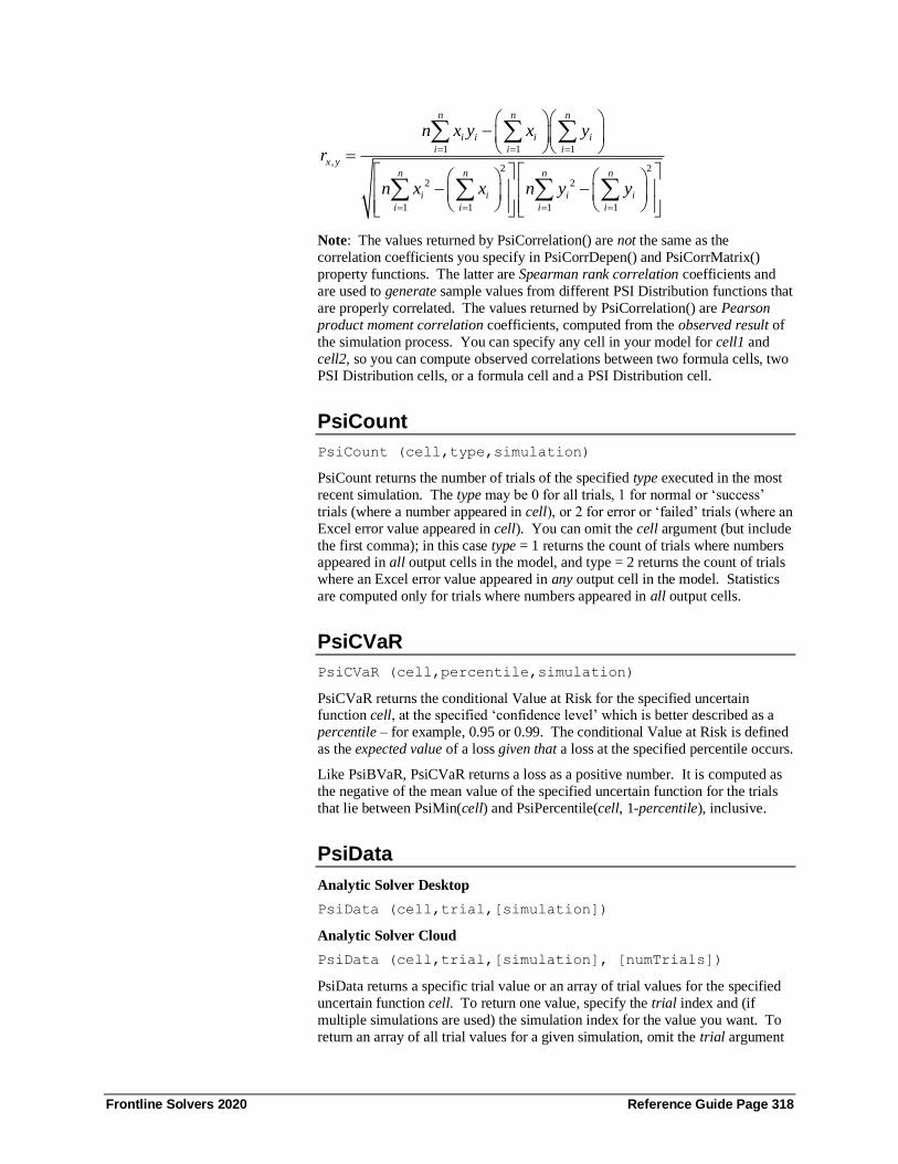
Frontline Solvers 2020 Reference Guide Page 318
1 1 1
,2 2
2 2
1 1 1 1
n n n
i i i i
i i i
x yn n n n
i i i i
i i i i
n x y x y
r
n x x n y y
= = =
= = = =
−
=
− −
Note: The values returned by PsiCorrelation() are not the same as the
correlation coefficients you specify in PsiCorrDepen() and PsiCorrMatrix()
property functions. The latter are Spearman rank correlation coefficients and
are used to generate sample values from different PSI Distribution functions that
are properly correlated. The values returned by PsiCorrelation() are Pearson
product moment correlation coefficients, computed from the observed result of
the simulation process. You can specify any cell in your model for cell1 and
cell2, so you can compute observed correlations between two formula cells, two
PSI Distribution cells, or a formula cell and a PSI Distribution cell.
PsiCount
PsiCount (cell,type,simulation)
PsiCount returns the number of trials of the specified type executed in the most
recent simulation. The type may be 0 for all trials, 1 for normal or ‘success’
trials (where a number appeared in cell), or 2 for error or ‘failed’ trials (where an
Excel error value appeared in cell). You can omit the cell argument (but include
the first comma); in this case type = 1 returns the count of trials where numbers appeared in all output cells in the model, and type = 2 returns the count of trials
where an Excel error value appeared in any output cell in the model. Statistics
are computed only for trials where numbers appeared in all output cells.
PsiCVaR
PsiCVaR (cell,percentile,simulation)
PsiCVaR returns the conditional Value at Risk for the specified uncertain function cell, at the specified ‘confidence level’ which is better described as a
percentile – for example, 0.95 or 0.99. The conditional Value at Risk is defined
as the expected value of a loss given that a loss at the specified percentile occurs.
Like PsiBVaR, PsiCVaR returns a loss as a positive number. It is computed as
the negative of the mean value of the specified uncertain function for the trials
that lie between PsiMin(cell) and PsiPercentile(cell, 1-percentile), inclusive.
PsiData
Analytic Solver Desktop
PsiData (cell,trial,[simulation])
Analytic Solver Cloud
PsiData (cell,trial,[simulation], [numTrials])
PsiData returns a specific trial value or an array of trial values for the specified
uncertain function cell. To return one value, specify the trial index and (if
multiple simulations are used) the simulation index for the value you want. To
return an array of all trial values for a given simulation, omit the trial argument

Frontline Solvers 2020 Reference Guide Page 319
and “array-enter” the PsiData function by selecting a column of cells, typing the
function call, and pressing Ctrl + Shift + Enter. If the number of cells N in the
array-entered result is less than the number of trials in the simulation, only the
first N trials are returned.
In Analytic Solver Cloud, PsiData() returns a Dynamic Array. To use this function in the Cloud, you need only enter the Psi function in one cell as a
normal function, i.e., not as a control array. The contents of the Dynamic Array
will "spill" down the column. If a nonblank cell is "blocking" the contents of
the Dynamic Array, PsiData() will return #SPILL until such time as the
blockage is removed. Use the optional numTrials argument to specify the
number of trials in the Dynamic Array. If not present, all trials will be returned.
PsiExpGain
PsiExpGain (cell,simulation)
PsiExpGain returns the average of all positive data multiplied by 1 -
percentrank of 0 among all data. It is always a positive number.
PsiExpGainRatio
PsiExpGainRatio (cell,simulation)
PsiExpGain returns the expected gain ratio for a specified uncertain function.
This function is calculated as:
PsiExpGainPsiExpGainRatio
PsiExpGain PsiExpLoss=
+
This value ranges between 0 and 1 inclusive.
PsiExpLoss
PsiExpLoss (cell,simulation)
PsiExpLoss returns the average of all negative data multiplied by the
percentrank of 0 among all data. It is always a negative number.
PsiExpLossRatio
PsiExpLossRatio (cell,simulation)
PsiExpLoss returns the expected loss ratio for a specified uncertain function.
This function is calculated as:
PsiExpLossPsiExpLossRatio
PsiExpGain PsiExpLoss=
+
This value ranges between 0 and 1 inclusive.
PsiExpValMargin
PsiExpValMargin (cell,simulation)
PsiExpValMargin is calculated as:

Frontline Solvers 2020 Reference Guide Page 320
PsiExpValMargin = PsiExpGainRatio – PsiExpLossRatio.
This statistic ranges between -1 and 1 inclusive.
PsiFrequency
PsiFrequency (cell,freq_type,bin_bounds,simulation)
PsiFrequency returns an array of frequencies describing the distribution of trial
values for the specified uncertain function cell. Use PsiFrequency to easily draw a histogram chart. You’ll need to “array-enter” this function by selecting a
group of cells, typing the function call, and pressing Ctrl + Shift + Enter.
The freq_type argument affects the contents of each element of the array result:
0 – Each element contains the frequency of trial values falling into the
corresponding bin (like a probability density function)
1 – Each element contains the cumulative frequency of trial values falling into
the corresponding bin plus all lower bins (like a cumulative distribution
function)
2 – Each element contains the cumulative frequency of trial values falling into
the corresponding bin plus all higher bins (like a reverse cumulative distribution function)
In Analytic Solver Desktop, the bin_bounds argument is either an array of values
(e.g. { 5, 10, 15, 20 }) or a cell range containing the upper limit of trial values
that should fall into the corresponding bin. The values should be in strictly
increasing order. As in the Excel FREQUENCY function, the number of
elements in the array result will be one more than the number of values or cells
in the bin bounds argument (or fewer, if the array-entered result occupies fewer
cells); the last element contains the number of trial values larger than the highest
bin bound value.
Alternatively, in Analytic Solver Desktop and only in Analytic Solver Cloud, you can specify an integer number N of bins for the bin bounds argument. In
this case, N equal-size bins are assumed, with bounds sufficient to capture all
trials values from PsiMin (cell) to PsiMax (cell); N values are returned, with the
last one always 1 or 0.
PsiKendallTau
PsiKendallTau(cell1, cell2)
PsiKendallTau returns a non-parametric correlation coefficient (based on the
relative ordering of ranks) between two uncertain variables or functions, cell1
and cell2. This statistic can be used to determine how (if at all) the two
uncertain variables or functions are correlated.
The Kendall Tau rank correlation coefficient measures the ordinal association
between two uncertain variables or functions. It is a measure of rank
correlation. This correlation coefficient is high when observations have a
similar rank between the two variables, and low when observations have a
dissimilar rank between the two variables.

Frontline Solvers 2020 Reference Guide Page 321
PsiKurtosis
PsiKurtosis (cell,simulation)
PsiKurtosis returns the kurtosis for the specified uncertain function cell.
Kurtosis is the 4th moment and measures the peakedness of the distribution of
trial values. It is computed as:
( )( )
( )
4
1
2
2
1
n
i
i
n
i
i
n x
kurtosis X
x
=
=
−
=
−
where μ is the mean of the trial values. A higher kurtosis indicates a distribution
with a sharper peak and heavier tails, and that more of the variability is due to a
small number of extreme outliers or values; a lower kurtosis indicates a
distribution with a rounded peak and that more of the variability is due to many
modest-sized values.
PsiMax
PsiMax (cell,simulation)
PsiMax returns the maximum value attained by the specified uncertain function
cell over all the trials in the simulation.
PsiMean
PsiMean (cell,simulation)
PsiMean returns the mean value for the specified uncertain function cell. The
mean or average value is the 1st moment of the distribution of trials and is
computed as:
1
n
i
i
x
n ==
The mean is frequently used as a measure of central tendency or the “middle” of
an uncertain function; but for skewed distributions, care must be taken in using the mean as a measure of central tendency because the mean is easily distorted
by extreme outlier values.
PsiMeanCI
PsiMeanCI (cell,confidence level,simulation)
PsiMeanCI returns the confidence “half-interval” for the estimated mean value
(returned by the PsiMean() function) for the specified uncertain function cell, at the specified confidence level (for example 0.95 or 0.99). If μ is the value
returned by PsiMean() and δ is the value returned by PsiMeanCI(), the true
mean is estimated to lie within the interval μ - δ to μ + δ.
The confidence level can be interpreted as follows: If we compute a large
number of independent estimates of confidence intervals on the true mean of the
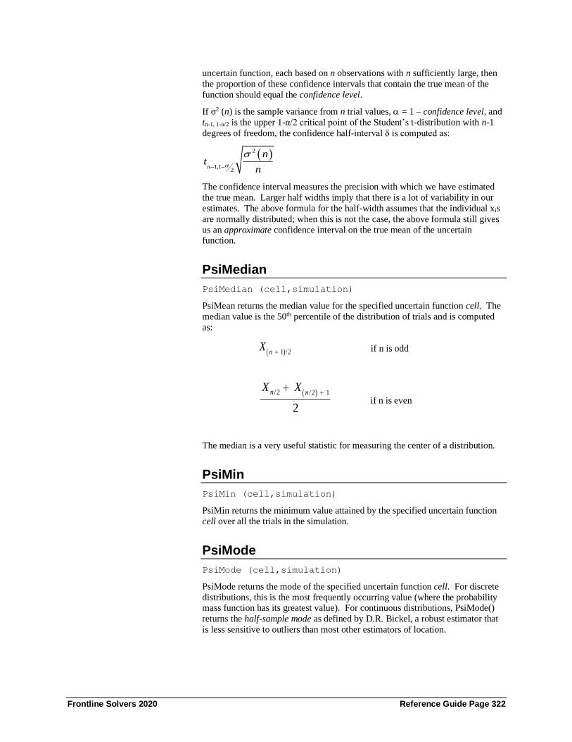
Frontline Solvers 2020 Reference Guide Page 322
uncertain function, each based on n observations with n sufficiently large, then
the proportion of these confidence intervals that contain the true mean of the
function should equal the confidence level.
If σ2 (n) is the sample variance from n trial values, = 1 – confidence level, and
tn-1, 1-α/2 is the upper 1-α/2 critical point of the Student’s t-distribution with n-1
degrees of freedom, the confidence half-interval δ is computed as:
( )2
1,12
n
nt
n
− −
The confidence interval measures the precision with which we have estimated
the true mean. Larger half widths imply that there is a lot of variability in our
estimates. The above formula for the half-width assumes that the individual xis
are normally distributed; when this is not the case, the above formula still gives
us an approximate confidence interval on the true mean of the uncertain function.
PsiMedian
PsiMedian (cell,simulation)
PsiMean returns the median value for the specified uncertain function cell. The
median value is the 50th percentile of the distribution of trials and is computed
as:
( ) 1 /2
nX
+ if n is odd
( )/2 /2 1
2
n nX X
++
if n is even
The median is a very useful statistic for measuring the center of a distribution.
PsiMin
PsiMin (cell,simulation)
PsiMin returns the minimum value attained by the specified uncertain function
cell over all the trials in the simulation.
PsiMode
PsiMode (cell,simulation)
PsiMode returns the mode of the specified uncertain function cell. For discrete
distributions, this is the most frequently occurring value (where the probability mass function has its greatest value). For continuous distributions, PsiMode()
returns the half-sample mode as defined by D.R. Bickel, a robust estimator that
is less sensitive to outliers than most other estimators of location.

Frontline Solvers 2020 Reference Guide Page 323
PsiOutput
PsiOutput() or PsiOutput(cell range)
PsiOutput marks cell as an uncertain function, with a distribution of trial values.
You can either reference the cell as an argument of PsiOutput() – for example PsiOutput (B1) – or you can add PsiOutput() to the computed result – for
example, if the uncertain function formula in cell B1 is =A1+A2*ABS(A3), edit
this formula to read =PsiOutput()+A1+A2*ABC(A3).
PsiOutput() always returns 0, so it will not affect the value of the uncertain
function. Using PsiOutput() is optional – if you reference an uncertain function
cell as the first argument of another PSI Statistics function, that cell is implicitly
marked as an uncertain function.
You can use a formula such as =PsiOutput (B1:B10) to group contiguous
uncertain function cells together in Analytic Solver’s VBA object model, so they
appear as one Function object in the Problem’s Functions collection. For further
information, see “PsiOutput() and “Uncertain Function Objects” in the section “Using PSI Functions” earlier in this chapter.
In V2019, PsiOutput was extended to use a named output signature which may
be referenced in a PsiStatistics function. To use,
1. Enter an uncertain variable in a blank cell.
A1 = PsiNormal(0,1)
2. In a 2nd cell, pass the cell address of the uncertain variable and append "+
PsiOutput("AnyString")", then press Enter. ("AnyString" is the name given
to the output from the uncertain variable.)
A2 = A1 + PsiOutput("Test")
3. Enter any PsiStatistics function, i.e. PsiMean(), in a blank cell and instead
of passing a cell address, pass the name given to PsiOutput.
A3 = PsiMean("Test")
PsiPercentile/PsiPtoX
PsiPercentile (cell,percentile,simulation)
PsiPtoX (cell,percentile,simulation)
PsiPercentile/PsiPtoX return a percentile (.01-.99) value for the specified
uncertain function cell: This means that m (or m%) of the simulation trials have values less than the returned value, where m is the percentile.
PsiPercentileD/PsiQtoX
PsiPercentileD (cell,percentile,simulation)
PsiQtoX (cell,percentile,simulation)
PsiPercentileD/PsiQtoX returns a descending percentile (.01-.99) value for the
specified uncertain function cell: This means that m (or m%) of the simulation
trials have values less than the returned value, where m is the percentile.

Frontline Solvers 2020 Reference Guide Page 324
PsiRange
PsiRange (cell,simulation)
PsiRange returns the range of the specified uncertain function cell. The range is
the difference between the maximum and minimum values attained in the
distribution of trial values.
PsiSemiDev
PsiSemiDev (cell,q,target,simulation)
PsiSemiDev returns the semideviation for the specified uncertain function cell, relative to the target if specified. If the target is omitted, the mean value is
used. This is a one-sided measure of dispersion of values of the uncertain
function. The semideviation is the square root of the semivariance, described
directly below. If a q argument different from 2 is specified, PsiSemiDev()
returns the qth root of the lower partial moment at power q of the uncertain
function.
PsiSemiVar
PsiSemiVar (cell,q,target,simulation)
PsiSemiVar returns the semivariance for the specified uncertain function cell, if
the argument q is omitted, or the ‘lower partial moment’ for the function, if an
argument q different from 2 is specified. The semivariance is computed relative
to the target if specified, or relative to the mean value if target is omitted. This
is a measure of the dispersion of values of an uncertain function, but unlike the
variance which measures (or penalizes) both positive and negative deviations
from the target, the semivariance or lower partial moment is only concerned
with one-sided deviations from the target. It is usually used in finance and
insurance applications, when we are only concerned with downside risks (or loss
in portfolio value). The semivariance is computed by summing only the downside differences from the target of all the trials, raised to the given power q,
divided by the number of trials:
( )
( ) ( )1
1
max ,0
target value
nq
i
i
t xn
x x
t
+=
+
−
=
=
All trials – not just the trials with downside deviations – are included in n.
Again if q is different from 2, the result is called the ‘lower partial moment.
PsiSimData
Analytic Solver Desktop
PsiSimData (cell,trial,[simulation])
Analytic Solver Cloud
PsiSimData (cell,trial,[simulation], [numTrials])

Frontline Solvers 2020 Reference Guide Page 325
PsiSimData behaves the same as PsiData returning a specific trial value or an
array of trial values for the specified uncertain function cell. To return one
value, specify the trial index and (if multiple simulations are used) the
simulation index for the value you want. To return an array of all trial values for
a given simulation, omit the trial argument and “array-enter” the PsiSimData function by selecting a group of cells, typing the function call, and pressing Ctrl
+ Shift + Enter. If the number of cells N in the array-entered result is less than
the number of trials in the simulation, only the first N trials are returned.
In Analytic Solver Cloud, PsiSimData() returns a Dynamic Array. To use this
function in the Cloud, you need only enter the Psi function in one cell as a
normal function, i.e., not as a control array. The contents of the Dynamic Array
will "spill" down the column. If a nonblank cell is "blocking" the contents of
the Dynamic Array, PsiSimData() will return #SPILL until such time as the
blockage is removed. Use the optional numTrials argument to specify the
number of trials in the Dynamic Array. If not present, all trials will be returned.
PsiSimOutput
PsiSimOutput() or PsiSimOutput(cell range)
PsiSimOutput behaves exactly the same as PsiOutput where it marks cell as an
uncertain function, with a distribution of trial values. You can either reference
the cell as an argument of PsiSimOutput() – for example PsiSimOutput (B1) –
or you can add PsiSimOutput() to the computed result – for example, if the
uncertain function formula in cell B1 is =A1+A2*ABS(A3), edit this formula to
read =PsiSimOutput()+A1+A2*ABC(A3).
PsiSimOutput() always returns 0, so it will not affect the value of the uncertain function. Using PsiSimOutput() is optional – if you reference an uncertain
function cell as the first argument of another PSI Statistics function, that cell is
implicitly marked as an uncertain function.
You can use a formula such as =PsiSimOutput (B1:B10) to group contiguous
uncertain function cells together in Analytic Solver’s VBA object model, so they
appear as one Function object in the Problem’s Functions collection. For further
information, see “PsiOutput() and “Uncertain Function Objects” in the section
“Using PSI Functions” earlier in this chapter.
PsiSkewness
PsiSkewness (cell,simulation)
PsiSkewness returns the skewness for the specified uncertain function cell.
Skewness is the 3rd moment of an uncertain function, and describes the
asymmetry of its distribution. Skewness can be either positive or negative:
Positive skewness implies that the distribution is right skewed (longer right
tails), and negative skewness implies that the distribution is left skewed (longer
left tails). Skewness is computed as:
( )( )
( )
3
1
32
2
1
n
i
i
n
i
i
n x
skewness X
x
=
=
−
=
−
where μ is the mean of the trial values.
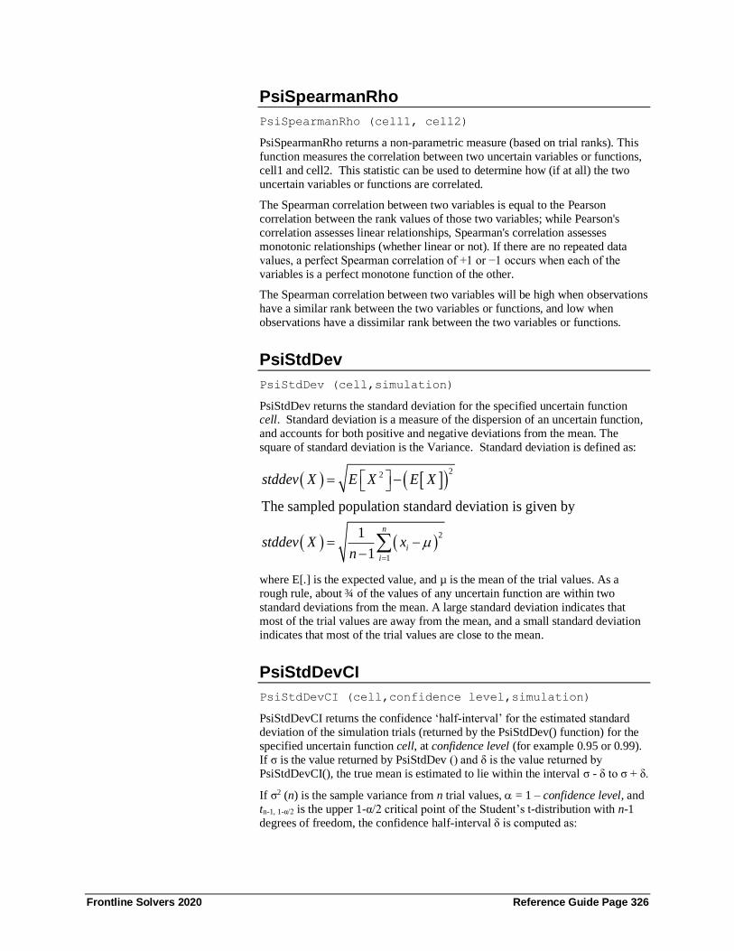
Frontline Solvers 2020 Reference Guide Page 326
PsiSpearmanRho
PsiSpearmanRho (cell1, cell2)
PsiSpearmanRho returns a non-parametric measure (based on trial ranks). This
function measures the correlation between two uncertain variables or functions,
cell1 and cell2. This statistic can be used to determine how (if at all) the two
uncertain variables or functions are correlated.
The Spearman correlation between two variables is equal to the Pearson
correlation between the rank values of those two variables; while Pearson's
correlation assesses linear relationships, Spearman's correlation assesses
monotonic relationships (whether linear or not). If there are no repeated data
values, a perfect Spearman correlation of +1 or −1 occurs when each of the
variables is a perfect monotone function of the other.
The Spearman correlation between two variables will be high when observations
have a similar rank between the two variables or functions, and low when
observations have a dissimilar rank between the two variables or functions.
PsiStdDev
PsiStdDev (cell,simulation)
PsiStdDev returns the standard deviation for the specified uncertain function cell. Standard deviation is a measure of the dispersion of an uncertain function,
and accounts for both positive and negative deviations from the mean. The
square of standard deviation is the Variance. Standard deviation is defined as:
( ) ( )
( ) ( )
22
2
1
The sampled population standard deviation is given by
1
1
n
i
i
stddev X E X E X
stddev X xn
=
= −
= −−
where E[.] is the expected value, and µ is the mean of the trial values. As a
rough rule, about ¾ of the values of any uncertain function are within two
standard deviations from the mean. A large standard deviation indicates that
most of the trial values are away from the mean, and a small standard deviation
indicates that most of the trial values are close to the mean.
PsiStdDevCI
PsiStdDevCI (cell,confidence level,simulation)
PsiStdDevCI returns the confidence ‘half-interval’ for the estimated standard
deviation of the simulation trials (returned by the PsiStdDev() function) for the
specified uncertain function cell, at confidence level (for example 0.95 or 0.99).
If σ is the value returned by PsiStdDev () and δ is the value returned by
PsiStdDevCI(), the true mean is estimated to lie within the interval σ - δ to σ + δ.
If σ2 (n) is the sample variance from n trial values, = 1 – confidence level, and
tn-1, 1-α/2 is the upper 1-α/2 critical point of the Student’s t-distribution with n-1
degrees of freedom, the confidence half-interval δ is computed as:

Frontline Solvers 2020 Reference Guide Page 327
( )( )1,1
2
1
4 1n
kt n
n
− −
−
−
See also the description of the PsiMeanCI() function.
PsiTarget
PsiTarget (cell,target value,simulation)
PsiTarget returns the cumulative frequency of the target value in the distribution
of trial values for the specified uncertain function cell. This function returns the proportion of simulated values for cell that are less than or equal to target value.
PsiTargetD
PsiTargetD (cell_or_name,target value,simulation)
PsiTargetD returns the descending cumulative probability of the target value in
the distribution of trial values for the specified uncertain function cell. This
function returns the proportion of simulated values for cell_or_name that are less than or equal to target value.
A Note on PsiTheo Functions Psi statistics functions that return a statistic on a simulation input distribution, or
uncertain variable, begin with PsiTheo. If a PsiTheoXXX function is applied to
an output function, the error #N/A will be returned. In addition, if the requested
statistic is impossible for the targeted distribution, the statistical function will
return #N/A. PsiTheoXXX functions compute the moment only when
distribution parameters are not dependent on other distributions or decision
variables in order to guarantee that the moment is constant throughout solving.
PsiTheoXXX functions were designed to aid in the visualization of results and
for comparison of the exact analytic moment with the trial statistics.
PsiTheoKurtosis
PsiTheoKurtosis (cell_or_name)
Returns the analytic kurtosis (4th moment) value for the specified distribution.
Example: If A1 =PsiNormal(0,1) then
=PsiTheoKurtosis(A1) returns the kurtosis of the PsiNormal(0,1) function.
PsiTheoMax
PsiTheoMax(cell_or_name)
Returns the maximum value of the specified distribution.
Example: If A1 =PsiNormal(0,1) then
=PsiTheoMax(A1) returns the maximum value for the PsiNormal(0,1)
distribution.

Frontline Solvers 2020 Reference Guide Page 328
PsiTheoMean
PsiTheoMean(cell_or_name)
Returns the mean of the specified distribution.
Example: If A1 =PsiNormal(0,1) then
=PsiTheoMean(A1) returns the mean for the PsiNormal(0,1) distribution.
PsiTheoMedian
PsiTheoMedian(cell_or_name)
Returns the median of the specified distribution.
Example: If A1 =PsiNormal(0,1) then
=PsiTheoMedian(A1) returns the median for the PsiNormal(0,1) distribution.
PsiTheoMin
PsiTheoMin(cell_or_name)
Returns the minimum value of the specified distribution.
Example: If A1 =PsiNormal(0,1) then
=PsiTheoMax(A1) returns the minimum value for the PsiNormal(0,1)
distribution.
PsiTheoMode
PsiTheoMode(cell_or_name)
Returns the analytical mode of the specified distribution.
Example: If A1 =PsiNormal(0,1) then
=PsiTheoMax(A1) returns the mode for the PsiNormal(0,1) distribution.
PsiTheoPercentile/PsiTheoPtoX
PsiTheoPercentile(cell_or_name, percentile)
PsiTheoPtoX(cell_or_name, percentile)
PsiTheoPercentile and PsiTheoPtoX are alternate names for the same function. Both functions return the analytic percentile (CDFInv) value for the distribution
specified in the cell_or_name argument. Enter the desired percentile (in
decimal form) for the percentile argument, i.e. .01, .30, or .98. The
percentile value must be between 0 and 1.
Example: If A1 =PsiNormal(0,1) then
=PsiTheoPercentile(A1, .50) or PsiTheoPtoX(A1, .50) return the 50th percentile
for the PsiNormal(0,1) distribution.
PsiTheoPercentileD/PsiTheoQtoX
PsiTheoPercentileD(cell_or_name, percentile)

Frontline Solvers 2020 Reference Guide Page 329
PsiTheoQtoX(cell_or_name, percentile)
PsiTheoPercentileD and PsiTheoQtoX are alternate names for the same
function. Both return the percentile (CDFInv descending) value for the
distribution specified in the cell_or_name argument. Enter the desired
percentile (in decimal form) for the percentile argument, i.e. .01, .30, or
.98. The percentile value must be between 0 and 1.
Example: If A1 =PsiNormal(0,1) then
=PsiTheoPercentileD(A1, .50) and =PsiTheoQtoX(A1, .50) return the 50th
percentile (CDFInv descending) value for the PsiNormal(0,1) distribution.
PsiTheoRange
PsiTheoRange(cell_or_name)
Returns the range information for the specified distribution.
Example: If A1 =PsiNormal(0,1) then
=PsiTheoRange(A1) returns the range information for the PsiNormal(0,1)
distribution.
PsiTheoSkewness
PsiTheoSkewness(cell_or_name)
Returns the skewness of the specified distribution.
Example: If A1 =PsiNormal(0,1) then
=PsiTheoSkewness(A1) returns the skewness of the PsiNormal(0,1) distribution.
PsiTheoStdDev
PsiTheoStdDev(cell_or_name)
Returns the standard deviation of the specified distribution.
Example: If A1 =PsiNormal(0,1) then
=PsiTheoStdDev(A1) returns the standard deviation of the PsiNormal(0,1)
distribution.
PsiTheoTarget/PsiTheoXtoP
PsiTheoTarget(cell_or_name, target)
PsiTheoXtoP(cell_or_name, target)
Returns the cumulative probability for target for the specified distribution.
The cumulative probability returned is the probability of a value less than or
equal to target occurring. (PsiTheoTarget and PsiTheoXtoP are alternative
names for the same function.)
Example: If A1 =PsiNormal(0,1) then
=PsiTheoTarget(A1, 2) and PsiTheoXtoP(A1, 2) returns the cumulative
probability of the target value, 2, of the PsiNormal(0,1) distribution.
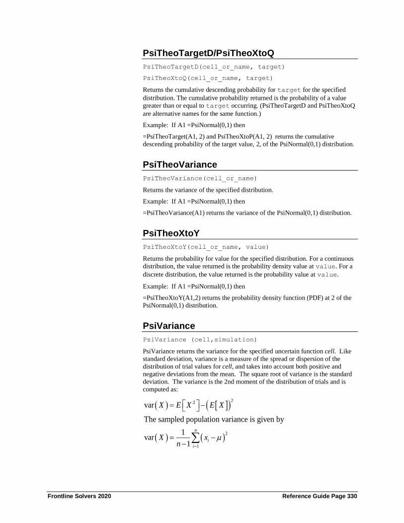
Frontline Solvers 2020 Reference Guide Page 330
PsiTheoTargetD/PsiTheoXtoQ
PsiTheoTargetD(cell_or_name, target)
PsiTheoXtoQ(cell_or_name, target)
Returns the cumulative descending probability for target for the specified
distribution. The cumulative probability returned is the probability of a value
greater than or equal to target occurring. (PsiTheoTargetD and PsiTheoXtoQ
are alternative names for the same function.)
Example: If A1 =PsiNormal(0,1) then
=PsiTheoTarget(A1, 2) and PsiTheoXtoP(A1, 2) returns the cumulative
descending probability of the target value, 2, of the PsiNormal(0,1) distribution.
PsiTheoVariance
PsiTheoVariance(cell_or_name)
Returns the variance of the specified distribution.
Example: If A1 =PsiNormal(0,1) then
=PsiTheoVariance(A1) returns the variance of the PsiNormal(0,1) distribution.
PsiTheoXtoY
PsiTheoXtoY(cell_or_name, value)
Returns the probability for value for the specified distribution. For a continuous
distribution, the value returned is the probability density value at value. For a
discrete distribution, the value returned is the probability value at value.
Example: If A1 =PsiNormal(0,1) then
=PsiTheoXtoY(A1,2) returns the probability density function (PDF) at 2 of the
PsiNormal(0,1) distribution.
PsiVariance
PsiVariance (cell,simulation)
PsiVariance returns the variance for the specified uncertain function cell. Like
standard deviation, variance is a measure of the spread or dispersion of the
distribution of trial values for cell, and takes into account both positive and
negative deviations from the mean. The square root of variance is the standard
deviation. The variance is the 2nd moment of the distribution of trials and is
computed as:
( ) ( )
( ) ( )
22
2
1
var
The sampled population variance is given by
1var
1
n
i
i
X E X E X
X xn
=
= −
= −−

Frontline Solvers 2020 Reference Guide Page 331
Psi Six Sigma Functions
PsiSigmaCP
PsiSigmaCP (cell,lower_limit,upper_limit,simulation)
A Six Sigma index, PsiSigmaCP predicts what the process is capable of
producing if the process mean is centered between the lower and upper limits.
This index assumes the process output is normally distributed.
ˆ6p
UpperSpecificationLimit LowerSpecificationLimitC
−=
where is the estimated standard deviation of the process.
PsiSigmaCPK
PsiSigmaCPK (cell,lower_limit,upper_limit,simulation)
A Six Sigma index, PsiSigmaCPK predicts what the process is capable of
producing if the process mean is not centered between the lower and upper
limits. This index assumes the process output is normally distributed and will be negative if the process mean falls outside of the lower and upper specification
limits.
ˆ ˆ( , )
ˆ3pk
MIN UpperSpecificationLimit LowerSpecificationLimitC
− −=
where is the process mean and is the standard deviation of the
process.
PsiSigmaCPKLower
PsiSigmaCPKLower(cell,lower_limit,simulation)
A Six Sigma index, PsiSigmaCPKLower calculates the one-sided Process
Capability Index based on the lower specification limit. This index assumes the process output is normally distributed.
, lower
ˆ
ˆ3p
LowerSpecificationLimitC
−=
where is the process mean and is the standard deviation of the process.
PsiSigmaCPKUpper
PsiSigmaCPKUpper(cell,upper_limit,simulation)
A Six Sigma index, PsiSigmaCPKUpper calculates the one-sided Process
Capability Index based on the upper specification limit. This index assumes the
process output is normally distributed.
,
ˆ
ˆ3p upper
UpperSpecificationLimitC
−=
where is the process mean and is the standard deviation of the process.

Frontline Solvers 2020 Reference Guide Page 332
PsiSigmaCPM
PsiSigmaCPM(cell,lower_limit,upper_limit,target,
simulation)
A Six Sigma index, PsiSigmaCPM calculates the capability of the process
around a target value. This index is referred to as the Taguchi Capability Index. This index assumes the process output is normally distributed and is always
positive.
2
ˆ
ˆ1 ( )
ˆ
pm
pCC
T
=−
+
where ˆ
pC is the process capability (PsiSigmaCP), is the process mean,
is the standard deviation of the process and T is the target process mean.
PsiSigmaDefectPPM
PsiSigmaDefectPPM(cell,lower_limit,upper_limit,simula
tion)
A Six Sigma index, PsiSigmaDefectPPM calculates the Defective Parts per Million.
1
1
ˆ( ( )
ˆ
ˆ1 ( ))*1000000
ˆ
LowerSpecificationLimitDPMO
UpperSpecificationLimit
−
−
−= +
−−
where is the process mean, is the standard deviation of the process and
1 − is the standard normal inverse cumulative distribution function.
PsiSigmaDefectShiftPPM
PsiSigmaDefectShiftPPM(cell,lower_limit,upper_limit,
shift, simulation)
A Six Sigma index, PsiSigmaDefectShiftPPM calculates the Defective Parts per Million with an added shift.
1
1
ˆ( ( Shift)
ˆ
ˆ1 ( Shift))*1000000
ˆ
ShiftLowerSpecificationLimit
DPMO
UpperSpecificationLimit
−
−
−= − +
−− −
where is the process mean, is the standard deviation of the process and
1 − is the standard normal inverse cumulative distribution function.

Frontline Solvers 2020 Reference Guide Page 333
PsiSigmaDefectShiftPPMLower
PsiSigmaDefectShiftPPMLower(cell,lower_limit,shift,
simulation)
A Six Sigma index, PsiSigmaDefectShiftPPMLower calculates the Defective
Parts per Million, with a shift, below the lower specification limit.
1, ( ( Shift)*1000000
ˆshift lower
LowerSpecificationLimitDPMO
−= −
where is the standard deviation of the process and 1 −
is the standard
normal inverse cumulative distribution function.
PsiSigmaDefectShiftPPMUpper
PsiSigmaDefectShiftPPMUpper(cell,upper_limit,shift,
simulation)
A Six Sigma index, PsiSigmaDefectShiftPPMUpper calculates the Defective
Parts per Million, with a shift, above the lower specification limit.
1, upper ( ( Shift)*1000000
ˆshift
UpperSpecificationLimitDPMO
−= −
where is the standard deviation of the process and 1 −
is the standard
normal inverse cumulative distribution function.
.
PsiSigmaK
PsiSigmaK(cell,lower_limit,upper_limit,simulation)
A Six Sigma index, PsiSigmaK calculates the Measure of Process Center and is
defined as:
ˆ ˆ2* ( , )1
MIN UpperSpecificationLimit LowerSpecificationLimit
UpperSpecificationLimit LowerSpecificationLimit
− −−
−
where is the process mean.
PsiSigmaLowerBound
PsiSigmaLowerBound(cell,number_stdev,simulation)
A Six Sigma index, PsiSigmaLowerBound calculates the Lower Bound as a
specific number of standard deviations below the mean and is defined as:
ˆ ˆ *#StandardDeviations −

Frontline Solvers 2020 Reference Guide Page 334
where is the process mean and is the standard deviation of the process.
PsiSigmaProbDefectShift
PsiSigmaProbDefectShift(cell,lower_limit,
upper_limit,shift,simulation)
A Six Sigma index, PsiSigmaProbDefectShift calculates the Probability of
Defect, with a shift, outside of the upper and lower limits. This statistic is
defined as:
1
1
ˆLowerSpecificationLimit( )
ˆ
ˆ1 ( )
ˆ
Shift
UpperSpecificationLimitShift
−
−
−− +
−− −
where is the process mean , is the standard deviation of the process and
1 − is the standard normal inverse cumulative distribution function.
PsiSigmaProbDefectShiftLower
PsiSigmaProbDefectShiftLower(cell,lower_limit,
shift,simulation)
A Six Sigma index, PsiSigmaProbDefectShiftLower calculates the Probability
of Defect, with a shift, outside of the lower limit. This statistic is defined as:
1 ˆLowerSpecificationLimit( )
ˆShift
− −−
where is the process mean , is the standard deviation of the process and
1 − is the standard normal inverse cumulative distribution function.
PsiSigmaProbDefectShiftUpper
PsiSigmaProbDefectShiftUpper(cell,upper_limit,
shift,simulation)
A Six Sigma index, PsiSigmaProbDefectShiftUpper calculates the Probability of
Defect, with a shift, outside of the upper limit. This statistic is defined as:
1 ˆUpperSpecificationLimit1 ( )
ˆShift
− −− −
where is the process mean , is the standard deviation of the process and
1 − is the standard normal inverse cumulative distribution function.
PsiSigmaSigmaLevel
PsiSigmaSigmaLevel(cell,lower_limit,upper_limit,
shift,simulation)
A Six Sigma index, PsiSigmaSigmaLevel calculates the Process Sigma Level
with a shift. This statistic is defined as:

Frontline Solvers 2020 Reference Guide Page 335
1
1
ˆLowerSpecificationLimit( ( )
ˆ
ˆ1 ( ))
ˆ
Shift
UpperSpecificationLimitShift
−
−
−− − +
−− −
where is the process mean , is the standard deviation of the process is
the standard normal cumulative distribution function, and 1 −
is the standard
normal inverse cumulative distribution function.
PsiSigmaUpperBound
PsiSigmaUpperBound(cell,number_stdev,simulation)
A Six Sigma index, PsiSigmaUpperBound calculates the Upper Bound as a
specific number of standard deviations above the mean and is defined as:
ˆ ˆ *#StandardDeviations −
where is the process mean and is the standard deviation of the process.
PsiSigmaYield
PsiSigmaYield(cell,lower_limit,upper_limit,shift,
simulation)
A Six Sigma index, PsiSigmaYield calculates the Six Sigma Yield with a shift, or the fraction of the process that is free of defects. This statistic is defined as:
1
1
ˆ( )
ˆ
ˆ( )
ˆ
UpperSpecificationLimitShift
LowerSpecificationLimitShift
−
−
−− −
−−
where is the process mean, is the standard deviation of the process and
1 − is the standard normal inverse cumulative distribution function.
PsiSigmaZLower
PsiSigmaZLower(cell,lower_limit,simulation)
A Six Sigma index, PsiSigmaZLower calculates the number of standard
deviations of the process that the lower limit is below the mean of the process.
This statistic is defined as:
ˆ
ˆ
LowerSpecificationLimit
−

Frontline Solvers 2020 Reference Guide Page 336
where is the process mean and is the standard deviation of the process.
PsiSigmaZMin
PsiSigmaZMin(cell,lower_limit,upper_limit,simulation)
A Six Sigma index, PsiSigmaZLower calculates the minimum of
PsiSigmaZLower and PsiSigmaZUpper. This statistic is defined as:
ˆ ˆ( , )
ˆ
MIN LowerSpecificationLimit UpperSpecificationLimit
− −
where is the process mean and is the standard deviation of the process.
PsiSigmaZUpper
PsiSigmaZUpper(cell,upper_limit,simulation)
A Six Sigma index, PsiSigmaZUpper calculates the number of standard
deviations of the process that the upper limit is above the mean of the process.
This statistic is defined as:
ˆ
ˆ
UpperSpecificationLimit
−
where is the process mean and is the standard deviation of the process.
Functions for Multiple Simulations You can specify that multiple simulations should be performed whenever the spreadsheet changes, or whenever you call Problem.Solver.Simulate in VBA
(Analytic Solver Desktop only). If you want to run n (say 5) simulations, simply
enter n for the “Number of Simulations to Run” in the Task Pane Model. In
your VBA code, you can set the property Problem.Solver.NumSimulations = n.
You could then use PsiSimParam() with an argument list of n values, to vary a
parameter in each simulation in the run.
PsiCurrentTrial
PsiCurrentTrial ()
PsiCurrentTrial returns the index (1, 2, 3, etc.) of the current trial during a
simulation run.
PsiCurrentSim
PsiCurrentSim ()
PsiCurrentSim returns the index (1, 2, 3, etc.) of the current simulation, when
you’ve asked for more than one simulation to be run.
Frontline Solvers 2020 Reference Guide Page 337
PsiSimParam
PsiSimParam (values)
PsiSimParam accepts a list of different values that a variable should have in
different simulations, where the value is the same for all trials in one simulation.
Values is either a cell range, such as PsiSimParam(A1:A3), or an array of
numbers, such as PsiSimParam({6.0, 7.5, 9.0}). In the 1st case, PsiSimParam
will return the value in cell A1 for all trials of the first simulation, the value in
cell A2 for all trials of the second simulation and the value in cell A3 for all
trials in the third simulation. In the 2nd case, PsiSimParam will return 6.0 for all
trials of the first simulation, 7.5 for all trials of the second simulation, and 9.0
for all trials of the third simulation. In the 3rd case, PsiSimParam will return the
value in the values argument for the first simulation, the middle value between
the values and upper arguments for the 2nd simulation, and the value in the upper argument for the 3rd simulation. If a value is entered for base_case, this
value will be used when this input cell is not being treated as an uncertain
variable, for example, if multiple optimizations are being run, during Parameter
Analysis, etc.
Functions for Classification, Prediction & Forecasting Analytic Solver Data Mining and the Data Mining Cloud app include the ability
to score data using prediction, classification, forecasting, and transformation
methods without the need to click the Score icon on the Data Mining ribbon. In
addition, Analytic Solver allows users to perform a time series simulation,
where future points in a time series are forecast on each Monte Carlo trial, using
a model created via ARIMA or one of our smoothing methods (Exponential,
Double Exponential, Moving Average, or Holt Winters). (A time series simulation model, created with Analytic Solver Data Mining, can be distributed
to users of Analytic Solver without the need for an additional Analytic Solver
Data Mining license.) PsiForecast(), PsiPosteriors(), PsiPredict(), and
PsiTransform are described below.
Note: In Analytic Solver Cloud and in versions of desktop Excel that support
Dyanamic Arrays, the Psi Data Mining functions return Dynamic Arrays. To
use this function in the Cloud, you need only enter the Psi function in one cell as
a normal function, i.e., not as a control array. The contents of the Dynamic
Array will "spill" down the column. If a nonblank cell is "blocking" the
contents of the Dynamic Array, the Psi Data Mining function will return #SPILL
until such time as the blockage is removed. Use the optional numForecasts argument to specify the number of forecasts in the Dynamic Array. If not
present, one forecast will be returned.
For more information on performing a time series forecast, please see the
Analytic Solver User Guide section, “Time Series Simulation" in the chapter,
“Getting Results: Simulation.” See the Analytic Solver Data Mining User
Guide for an example on how to use the PsiPredict(), PsiPosteriors() and
PsiTransform() functions.
PsiForecast()
PsiForecast(Model, Input_Data, [Simulate],
Num_Forecasts, [Header])

Frontline Solvers 2020 Reference Guide Page 338
Computes the forecasts for Input_Data using a Time Series model stored in
PMML format.
Model: Range containing the stored Times Series model in PMML format.
Input_Data: Range containing the new Time Series data for computing the
forecasts. Range must contain a header with the time series name and a
sufficient number of records for the forecasting with a given model.
Simulate: If True, the forecasts are adjusted with random normally
distributed errors. If False or omitted, the forecasts will be deterministic.
Num_Forecasts: Enter the desired number of forecasts.
Header: If True, a heading will be inserted above the returned forecasts.
Note: In Analytic Solver Cloud and in newer versions of desktop Excel,
PsiForecast() returns a Dynamic Array (see Note in section heading, above).
The contents of the Dynamic Array will "spill" down the column. If a nonblank
cell is "blocking" the contents of the Dynamic Array, PsiForecast() will return #SPILL until such time as the blockage is removed.
Output: A single column containing the header and forecasts for input time
series. The number of produced forecasts is determined by the number of
selected cells in the array-formula entry.
Supported Models:
• Arima
• Exponential Smoothing
• Double Exponential Smoothing
• Holt Winters Smoothing
Previous related Psi Scoring functions: PsiForecastARIMA, PsiForecastExp,
PsiForecastDoubleExp, PsiForecastMovingAvg, PsiForecastHoltWinters
Each forecasting method requires a minimum number of initial points. See the
chart below for each forecasting method's requirements.
Forecasting
Algorithm
Stored Model Sheet Minimum # of
Initial Points when
Simulate = False
Minimum # of
Initial Points when
Simulate = True
Non- Seasonal ARIMA ARIMA_Stored Max(p + d, q) Max(p + d, q)
Seasonal ARIMA ARIMA_Stored Max((p + d + s *(P
+ D), (q + s * Q)
1 + Max((p + d + s
*(P + D), (q + s *
Q)**
Exponential Smoothing Expo_Stored 1 1
Double Exponential Smoothing
DoubleExpo_Stored 1 1
Moving Average
Smoothing
MovingAvg_Stored # of Intervals # of Intervals
Holt Winters
Smoothing
MulHoltWinters_Stored
AddHoltWinters_Stored
NoTrendHoltWinters_Stored
2 * #Periods 2 * #Periods

Frontline Solvers 2020 Reference Guide Page 339
**Adding a number of data points equal to the Number of Periods (as shown on
the Time Series – ARIMA dialog) to the Minimum # of Initial Points when
Simulate = True is recommended when calling PsiForecast() with Simulate =
True.
PsiPosteriors()
PsiPosteriors(Model, Input_Data, [Header])
Computes the posterior probabilities for Input_Data using a Classification
model stored in PMML format.
Model: Range containing the stored Classification model in PMML format.
Input_Data: Range containing the new data for computing posterior
probabilities. Range must contain a header with column names and at least one
row of data containing the exact same features (or columns) as the data used to
create the model.
Header: If True, a heading will be inserted above the returned results.
In Analytic Solver Cloud and in new versions of desktop Excel, PsiPosterior()
returns a Dynamic Array (see Note in section heading, above). To use this
function as a dynamic array, you need only enter the Psi function in one cell as a
normal function, i.e., not as a control array. The contents of the Dynamic Array
will "spill" down the column. If a nonblank cell is "blocking" the contents of
the Dynamic Array, PsiForecast() will return #SPILL until such time as the
blockage is removed.
Output: Multiple columns containing a header with class labels and estimated
posterior probabilities for each class label for all records in Input_Data.
Supported Models:
• Classification:
o Linear Discriminant Analysis
o Logistic Regression
o K-Nearest Neighbors o Classification Tree
o Naïve Bayes
o Neural Network
o Random Trees
o Bagging (with any supported weak learner)
o Boosting (with any supported weak learner)
Previous related Psi Scoring functions: N/A
Classification Algorithm Stored Model Sheet
Linear Discriminant Analysis Classification DA_Stored
Logistic Regression Classification LogReg_Stored
k-Nearest Neighbors Classification KNNC_Stored
Classification Trees CT_Stored
Naïve Bayes Classification NB_Stored
Neural Networks Classification NNC_Stored

Frontline Solvers 2020 Reference Guide Page 340
Ensemble Methods for Classification CBoosting_Stored
CBagging_Stored
CRandTrees_Stored
PsiPredict()
PsiPredict(Model, Input_Data, [Header]))
Predicts the response, target, output or dependent variable for Input_Data
whether it is continuous (Regression) or categorical (Classification) when the
model is stored in PMML format. In addition, this function also computes the
fitted values for a Time Series model when the model is stored in PMML
format. Note: If using a version of Excel that does not support Dynamic
Arrays, this formula must be ented as an array.
Model: Range containing the stored Classification, Regression or TimeSeries
model in PMML format.
Input_Data: Range containing the new data for computing predictions.
Range must contain a header row with column names and at least one row of
data containing the exact same features (or columns) as the data used to create
the model.
Header: If True, a heading will be inserted above the returned results.
In Analytic Solver Cloud or in newer versions of desktop Excel, PsiPredict()
returns a Dynamic Array (see Note in section heading, above) To use this
function as a dynamic array, you need only enter the Psi function in one cell as a normal function, i.e., not as a control array. The contents of the Dynamic Array
will "spill" down the column. If a nonblank cell is "blocking" the contents of
the Dynamic Array, PsiForecast() will return #SPILL until such time as the
blockage is removed.
Output: A single column containing the header and predicted/fitted values for
each record in Input_Data.
To know if the result of the prediction is continuous or categorical, you must
know what kind of model you are passing as an argument to the scoring function
– if you previously fitted the classification model and are now predicting the
new feature vectors, you should expect to get the compatible categorical
response. On the other hand, you should expect the continuous response from
the new data prediction when using a fitted regression model. In V201, the user
had to know the exact type model, such as MLR or LDA, to know what kind of
output will be produced, whereas now, it’s sufficient to know whether you’re
pointing to classification or regression model in order to determine the type of
the response. Note: If the user intends to use an “unknown” model for scoring,
the stored worksheets contain the complete information about the model including several clear indications of the model type and data dictionaries with
the types of the features/response.
As a bonus, not available with old Psi functions, PsiPredict() can compute the
fitted values for the new time series based on the provided TS model. Unlike
future-looking forecasting, provided by PsiForecast(), PsiPredict() computes a
model prediction for each observation in the provided new time series. It is
analogous to classifying/regressing the new feature vectors based on the fitted
model in supervised learning, only that when applied to a time series, the
univariate TS vector, provided on input, provides the material for prediction.
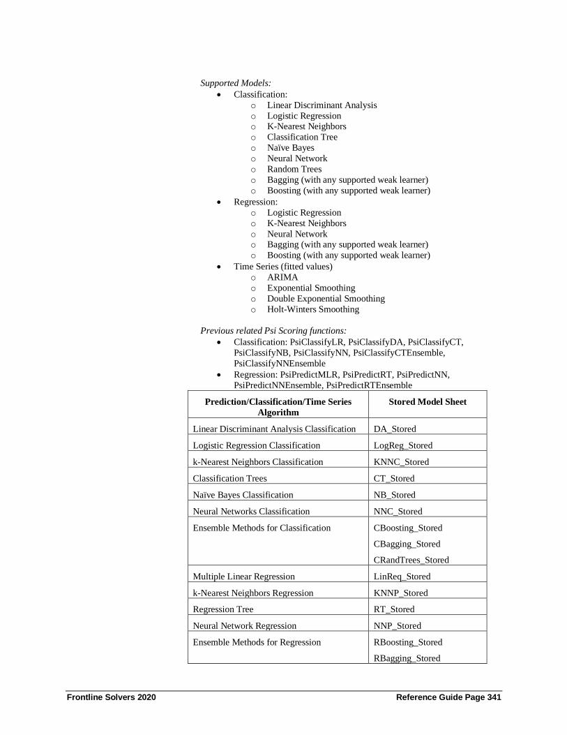
Frontline Solvers 2020 Reference Guide Page 341
Supported Models:
• Classification:
o Linear Discriminant Analysis
o Logistic Regression o K-Nearest Neighbors
o Classification Tree
o Naïve Bayes
o Neural Network
o Random Trees
o Bagging (with any supported weak learner)
o Boosting (with any supported weak learner)
• Regression:
o Logistic Regression
o K-Nearest Neighbors
o Neural Network o Bagging (with any supported weak learner)
o Boosting (with any supported weak learner)
• Time Series (fitted values)
o ARIMA
o Exponential Smoothing
o Double Exponential Smoothing
o Holt-Winters Smoothing
Previous related Psi Scoring functions:
• Classification: PsiClassifyLR, PsiClassifyDA, PsiClassifyCT,
PsiClassifyNB, PsiClassifyNN, PsiClassifyCTEnsemble,
PsiClassifyNNEnsemble
• Regression: PsiPredictMLR, PsiPredictRT, PsiPredictNN,
PsiPredictNNEnsemble, PsiPredictRTEnsemble
Prediction/Classification/Time Series
Algorithm
Stored Model Sheet
Linear Discriminant Analysis Classification DA_Stored
Logistic Regression Classification LogReg_Stored
k-Nearest Neighbors Classification KNNC_Stored
Classification Trees CT_Stored
Naïve Bayes Classification NB_Stored
Neural Networks Classification NNC_Stored
Ensemble Methods for Classification CBoosting_Stored
CBagging_Stored
CRandTrees_Stored
Multiple Linear Regression LinReq_Stored
k-Nearest Neighbors Regression KNNP_Stored
Regression Tree RT_Stored
Neural Network Regression NNP_Stored
Ensemble Methods for Regression RBoosting_Stored
RBagging_Stored

Frontline Solvers 2020 Reference Guide Page 342
RRandTrees_Stored
ARIMA ARIMA_Stored
Exponential Smoothing Expo_Stored
Double Exponential Smoothing DoubleExpo_Stored
Moving Average Smoothing MovingAvg_Stored
Holt Winters Smoothing MultHoltWinters_Stored
AddHoltWinters_Stored
NoTrendHoltWinters_Stored
PsiTransform()
PsiTransform(Model, Input_Data, [Header])
Transforms the Input_Data using a Transformation model stored in PMML
format.
Model: Range containing the stored Transformation model in PMML format.
Input_Data: Range containing the new data for transformation. Range must
contain a header with column names and at least one row of data containing the
exact same features (or columns) as the data used to create the model.
Header: If True, a heading is inserted above the returned results.
In Analytic Solver Cloud or in new versions of desktop Excel, PsiTransform()
returns a Dynamic Array (see Note in section heading, above). To use this
function as a dynamic array, you need only enter the Psi function in one cell as a
normal function, i.e., not as a control array. The contents of the Dynamic Array
will "spill" down the column. If a nonblank cell is "blocking" the contents of
the Dynamic Array, PsiForecast() will return #SPILL until such time as the
blockage is removed. Use the optional numForecasts argument to specify the number of forecasts in the Dynamic Array. If not present, one forecast will be
returned.
Output: One or multiple columns containing a header and transformed data.
Supported Models:
• Transformation:
o Rescaling
• Text Mining
o TF-IDF Vectorization (input data – text variable with the
corpus of documents) o LSA Concept Extraction (input data – term-document matrix,
where columns represent terms and rows represent documents)
Previous related Psi Scoring functions: N/A
Algorithm Stored Model Sheet
Rescaling Rescaling_Stored
Text Mining TFIDF_Stored
LSA_Stored
Frontline Solvers 2020 Reference Guide Page 343
About Microsoft Excel 2016 Functions Microsoft Excel Desktop and Excel for the Web (formerly Excel Online)
contains forecast functions which may be used to predict future points in a time
series dataset:
• FORECAST.ETS
• FORECAST.ETS.SEASONALITY
• FORECAST.LINEAR
• FORECAST.ETS.CONFINT
• FORECAST.ETS.STAT
These functions compute forecasts using exponential smoothing, similar to the
PsiForecastExp, PsiForecastDoubleExp and PsiForecastHoltWinters functions
above, but they use different argument lists and differ in other specific details.
(The Psi ARIMA functions use a different forecasting method.)
Analytic Solver (starting with V2018) includes support for these functions, so
you can use them in your models, with one caveat: If you use such a forecast
function in an optimization model where the arguments depend on the decision variables, or in a simulation model where the arguments depend on uncertain
variables, you may see slightly different calculated forecast values depending on
whether the Psi Interpreter or Excel Interpreter is selected in the Task Pane
Platform tab. When the Psi Interpreter is used, a slightly different (but arguably
better) methodology is used to compute these forecast functions. When the
Excel Interpreter is selected, Microsoft Excel is used to calculate the worksheet
and thus Excel's methodology will be used.
Using PsiForecastETS() and PsiForecastLinear()
Users of Analytic Solver can use PsiForecastETS() and PsiForecastLinear() to
forecast future points in a time series dataset. These two functions were
introduced to coincide with the new Excel 2016 Forecast functions: Forecast.Linear and Forecast.ETS.
PsiForecastLinear() predicts a future value or values for a time series dataset
(containing known or historical data) using linear regression. PsiForecastETS()
uses exponential smoothing to predict a future value or values in a time series
dataset with the option to either detect seasonality in the dataset automatically or
pass a seasonality period. Passing False as the last argument to either function
will result in a static forecast. If True is passed for this argument, a random
error will be included in the forecasted points. For more information on
performing a time series forecast using these two functions, please see the
Analytic Solver User Guide section, “Excel 2016 Forecast Functions" in the
chapter, “Getting Results: Simulation.”
PsiForecastETS()
PsiForecastETS(target_date, values, timeline, [,
seasonality][, data_completion][, aggregation][,
simulate])
target_date: A data point for which you want the predicted value. A data
point may be date/time or numeric. If a target date is given that appears before
the start of the timeline in the dataset, PsiForecastETS will return #NUM (i.e. if, in this example, 1940 is passed for X)

Frontline Solvers 2020 Reference Guide Page 344
values: An Excel range containing the historical values in the given dataset.
timeline: An Excel range containing the time variables in the given dataset.
Both functions require the historical data to be structured using a constant
interval between data points. For example, The Airpass example dataset (Help –
Example Models – Forecasting/Data Mining Examples) presents monthly passenger data, therefore the forecast must also predict the number of passengers
by month.
seasonality: (Optional) This argument indicates the length of the seasonal
pattern. The following values are accepted as valid inputs. All other values will
return a #NUM error.
0: Signifies no seasonality exists in the data. The result is a linear
prediction.
1: (Default Value) Triggers Solver to detect seasonality within the data
automatically.
1 < N < 8,760: Positive integer values greater than 1 but less will be used
as the seasonality period.
data_completion: (Optional) This argument specifies how to handle
missing values. The default value of 1 replaces missing values by interpolation.
If 0 is passed, missing values will be replaced by 0's.
aggregation: (Optional) PsiForecastETS can aggregate multiple points
with the same time stamp. Pass an integer value from 0 to 6 to indicate which
method should be used.
0: (Default) Average
1: SUM
2: COUNT
3: COUNTA
4: MIN
5: MAX
6: MEDIAN
simulate: (Optional) Pass True or False for the third argument. Passing
False (the default) will result in a static forecast that will only update if a cell
passed in the 2nd argument is changed. If True is passed for this argument, a random error will be included in the forecasted points.
PsiForecastLinear()
PsiForecastLinear(X, known_ys, known_xs[, simulate])
X: The target date. A data point for which you want the predicted value. A data
point may be date/time or numeric.
known_ys: An Excel range containing the independent variables in the given
dataset.
known_xs: An Excel range containing the time variables in the given dataset.
simulate: (Optional) Pass True or False for the third argument. Passing False
(the default) will result in a static forecast that will only update if a cell passed in

Frontline Solvers 2020 Reference Guide Page 345
the known_ys argument is changed. If True is passed for this argument, a
random error will be included in the forecasted points.

Frontline Solvers 2020 Reference Guide Page 346
Solver Add-in Math Functions
Introduction Analytic Solver Desktop defines seven special Excel functions: DOTPRODUCT, QUADPRODUCT, MSOLVE, MTRACE, MNORM,
MEIGENVEC, and MEIGENVAL. These functions behave just like Excel
built-in functions: You can use them in formulas in any spreadsheet (not only in
Solver models). When you use the Insert Function… menu option, these
functions will appear in the “Select a Function” or “Paste Function” list
(classified as Math & Trig functions), and you’ll be prompted with named edit
fields for their arguments. All seven functions are recognized by the PSI
Interpreter.
Note: These functions are currently not supported in Analytic Solver Cloud or
AnalyticSolver.com.
DOTPRODUCT and QUADPRODUCT are recognized for purposes of fast problem setup as described in the Analytic Solver User Guide chapter, “Building
Large-Scale Models.”
All functions can either be manually entered by typing the function and
arguments into an Excel cell, or by using the Insert Function icon on the
Formulas ribbon and selecting Math and Trig.

Frontline Solvers 2020 Reference Guide Page 347
Note: Excel range information may be entered using the syntax {1, 2; 3, 4} for a
2 by 2 matrix or A1:B2 where the Excel cells contain the values (see picture
below).
Functions
MSOLVE
MSOLVE(M, b) returns the solution of M x = b efficiently without matrix
inversion. Matrix M must be a square matrix (m x m). Vector b and vector x must be of size m x 1.
In the screenshot below, the M matrix is contained in the range A1:C3 (3 rows x
3 columns), the b matrix is contained in the range E1:E3 (3 rows x 1 column)
and the x matrix (3 rows x 1 column) has been entered as an array formula in the
cell range G1:G3.
This function is currently not supported in Analytic Solver Cloud or
AnalyticSolver.com.
MTRACE
MTRACE(squared_array) returns the sum of the diagonal elements of a squared
matrix (m x m) entered as a range or array.
In the screenshot below, the squared matrix is contained in the cell range A1:C3
and the MTRACE() function is in cell E1.
This function is currently not supported in Analytic Solver Cloud or
AnalyticSolver.com.

Frontline Solvers 2020 Reference Guide Page 348
MNORM
MNORM(array, norm) returns the norm of a matrix entered as an array or Excel
range. Pass norm = 1 for ||a||1 (the maximal column sum), norm = 2 for
Euclid/Frobenius (||a||2 =
2
1 1
( )n n
ij
i j
a= =
), or norm = 3 for ||a||∞ (the maximal
row sum).
Consider the matrix in the screenshot below contained in cells A1:C3. ||a||1 is
being calculated in cell E1, ||a||2 is being calculated in cell E2 and ||a||∞ is being
calculated in cell E3.
This function is currently not supported in Analytic Solver Cloud or
AnalyticSolver.com.
MEIGENVEC
MEIGENVEC(squared_matrix) returns the eigenvectors for a squared matrix
entered as a range or array.
In the screenshot below, the squared matrix is contained in the cell range A1:C3.
Cells E1:G3 contain the MEIGENVEC function entered as an array. If
squared_matrix is of size m x m, and =MEIGENVEC(squared_matrix) is
entered in array form in an m x 1 cell orientation, the first eigenvector will be
returned. If squared_matrix is of size m x m and
=MEIGENVEC(squared_matrix) is entered in array form in an m x 2 cell
orientation, the first and second eigenvectors will be returned, etc. For example,
in the screenshot below squared_matrix is of size 3 x 3 and contained in the range A1:C3, =EIGENVEC(A1:C3) entered in array form in cells E1:E3 will
return the first eigenvector, =EIGENVEC(A1:C3) entered in array form in cells
F1:F3 will return the second eigenvector and =EIGENVEC(A1:C3) entered in
array form in cells E1:G3 will return all three eigenvectors.
This function is currently not supported in Analytic Solver Cloud or
AnalyticSolver.com.
MEIGENVAL
MEIGENVAL(squared_matrix) returns the eigenvalues of a squared matrix
entered as a range or array. Note: While MSOLVE() returns a typical vertical
range, MEIGENVAL() returns a horizontal range. This is done intentionally, so
the user may compute the eigenvectors underneath the eigenvalues. If values
are complex numbers they are printed as strings.
In the screenshot below, the squared matrix is contained in the cell range A1:C3.
Cells E1:G1 contain the eigenvalues.
This function is currently not supported in Analytic Solver Cloud or
AnalyticSolver.com.
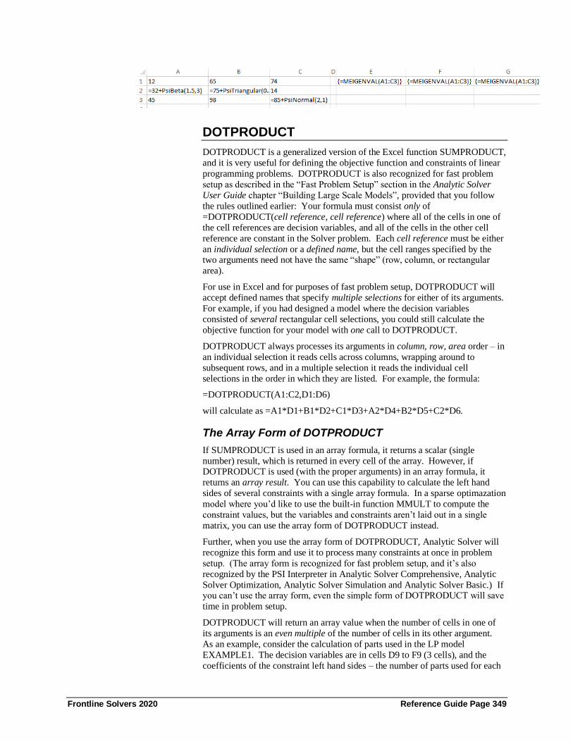
Frontline Solvers 2020 Reference Guide Page 349
DOTPRODUCT
DOTPRODUCT is a generalized version of the Excel function SUMPRODUCT,
and it is very useful for defining the objective function and constraints of linear
programming problems. DOTPRODUCT is also recognized for fast problem
setup as described in the “Fast Problem Setup” section in the Analytic Solver
User Guide chapter “Building Large Scale Models”, provided that you follow
the rules outlined earlier: Your formula must consist only of
=DOTPRODUCT(cell reference, cell reference) where all of the cells in one of
the cell references are decision variables, and all of the cells in the other cell
reference are constant in the Solver problem. Each cell reference must be either
an individual selection or a defined name, but the cell ranges specified by the two arguments need not have the same “shape” (row, column, or rectangular
area).
For use in Excel and for purposes of fast problem setup, DOTPRODUCT will
accept defined names that specify multiple selections for either of its arguments.
For example, if you had designed a model where the decision variables
consisted of several rectangular cell selections, you could still calculate the
objective function for your model with one call to DOTPRODUCT.
DOTPRODUCT always processes its arguments in column, row, area order – in
an individual selection it reads cells across columns, wrapping around to
subsequent rows, and in a multiple selection it reads the individual cell
selections in the order in which they are listed. For example, the formula:
=DOTPRODUCT(A1:C2,D1:D6)
will calculate as =A1*D1+B1*D2+C1*D3+A2*D4+B2*D5+C2*D6.
The Array Form of DOTPRODUCT
If SUMPRODUCT is used in an array formula, it returns a scalar (single
number) result, which is returned in every cell of the array. However, if DOTPRODUCT is used (with the proper arguments) in an array formula, it
returns an array result. You can use this capability to calculate the left hand
sides of several constraints with a single array formula. In a sparse optimazation
model where you’d like to use the built-in function MMULT to compute the
constraint values, but the variables and constraints aren’t laid out in a single
matrix, you can use the array form of DOTPRODUCT instead.
Further, when you use the array form of DOTPRODUCT, Analytic Solver will
recognize this form and use it to process many constraints at once in problem
setup. (The array form is recognized for fast problem setup, and it’s also
recognized by the PSI Interpreter in Analytic Solver Comprehensive, Analytic
Solver Optimization, Analytic Solver Simulation and Analytic Solver Basic.) If you can’t use the array form, even the simple form of DOTPRODUCT will save
time in problem setup.
DOTPRODUCT will return an array value when the number of cells in one of
its arguments is an even multiple of the number of cells in its other argument.
As an example, consider the calculation of parts used in the LP model
EXAMPLE1. The decision variables are in cells D9 to F9 (3 cells), and the
coefficients of the constraint left hand sides – the number of parts used for each

Frontline Solvers 2020 Reference Guide Page 350
product – are in cells D11 to F15 (15= 3*5 cells). We want to calculate the left
hand sides of the constraints in cells C11 to C15. To do this, we would first
select the group of five cells C11:C15 with the mouse. Then we would type:
=DOTPRODUCT(D9:F9,D11:F15)
completing the entry with CTRL+SHIFT+ENTER instead of just ENTER. The
formula will display as {=DOTPRODUCT(D9:F9,D11:F15)} – the braces are
added by Microsoft Excel when the formula is array-entered. With the cell
values shown in EXAMPLE1 prior to solution (e.g. 100 for each of the decision
variables), this array formula will calculate 200 in C11, 100 in C12, 500 in C13,
200 in C14 and 400 in C15. Hence, it will compute the same set of values as the
array expression shown earlier: {=MMULT(_A, TRANSPOSE(_X))}.
Whether it is used in the simple form or the array form, DOTPRODUCT always
processes its arguments in column, row, area order. In the array form, when the
cells in the “shorter” argument have all been processed and cells remain to be
processed in the “longer” argument, DOTPRODUCT “wraps around” to the beginning of the “shorter” argument. In the example above, cell C11 calculates
the value =D9*D11+E9*E11+F9*F11; cell C12 computes
=D9*D12+E9*E12+F9*F12; and so on. Keep this rule in mind when you use
the array form of DOTPRODUCT, and keep your spreadsheet layouts as simple
as possible!
QUADPRODUCT
The QUADPRODUCT function can be used to define the objective for
quadratic programming problems in a single function call, as required for fast
problem setup.
The QUADPRODUCT function is designed to supply coefficients for each
single variable and each pair of variables, in a manner similar to
SUMPRODUCT and DOTPRODUCT.
You supply the arguments of QUADPRODUCT as shown below:
=QUADPRODUCT(variable cells, single coefficients, pair coefficients)
The first argument must consist entirely of decision variable cells. The second
and third arguments must consist entirely of cells whose values are constant in
the optimization problem; if these cells contain formulas, those formulas must
not refer to any of the decision variables. The second argument supplies the
coefficients to be multiplied by each single variable in the first argument, using
an element-by-element correspondence. The third argument supplies the
coefficients to be multiplied by each pair of variables drawn from the first
argument. Hence, if there are n cells in the first argument, there must be n2 cells
in the third argument. If the variables are represented by x1,x2,...,xn, the single
coefficients by a1,a2,...,an, and the pair coefficients by c1,c2,...,cN where N = n2,
QUADPRODUCT computes the function:
n n n
cn(i-1)+j xi xj + aj xj i=1 j=1 j=1
The pairs are enumerated starting with the first cell paired with itself, then the
first cell paired with the second cell, and so on. For example, if the first argument consisted of the cells A1:A3, there should be nine cells in the third
argument, and the values in those cells will be multiplied by the following pairs
in order: A1*A1, A1*A2, A1*A3, A2*A1, A2*A2, A2*A3, A3*A1, A3*A2,
and A3*A3. The value returned by QUADPRODUCT is the sum of all of the

Frontline Solvers 2020 Reference Guide Page 351
coefficients multiplied by their corresponding single variables or pairs of
variables.
Multiple selections can be used for each argument of QUADPRODUCT, subject
to the same considerations outlined above for DOTPRODUCT: You can use the
general syntax for multiple selections in Microsoft Excel, but defined names are needed for purposes of fast problem setup, and multiple selections are not
accepted by the PSI Interpreter.
Frontline Solvers 2020 Reference Guide Page 352
Dimensional Modeling Psi Functions
Introduction This chapter provides function information on Analytic Solver Desktop’s PSI
functions for the Dimensional Modeling feature. The primary goal of
Dimensional Modeling is in the creation of structured, easily readable, compact
Excel models. The second goal of Dimensional Modeling is to extend the
capabilities of Analytic Solver's current Optimization/Simulation/Sensitivity
parameters. For more information on how to use this feature, please see the
Dimensional Modeling chapter in the Analytic Solver User Guide.
This functions are currently not supported in Analytic Solver Cloud or
AnalyticSolver.com.
Psi Cube Functions
PsiCube
PsiCube() creates a multi-dimensional array which holds the dimensional data in
the form of a data range. This data range is structured along the dimension elements of the included set of dimensions.
A sparse cube can be defined by missing values in cells for PsiCube(). If Use
Sparse Cubes = False, on the Platform tab of the Solver Task Pane, and you
have defined a cube using PsiCube() with missing valus, these values will be
considered equal to 0. If Use Sparse Cubes = True, you have defined a cube
using PsiCube() with missing values, and the percentage of elements missing or
empty is more than 30% of the total possible cube elements, those missing
elements will not be included in the model.
The maximum number of elements in a cube created by PsiCube or by formula
evaluation is 1,000,000.
To create a Cube, click Model – Cubes to open the Cube menu.

Frontline Solvers 2020 Reference Guide Page 353
If using an Excel Pivot Table, select From Pivot Table, otherwise select From
Cell Range. (For more information on creating a Cube from within an Excel
Pivot Table, please see below.)
If From Cell Range is selected, the following dialog appears.
Range: Enter an Excel range that contains a fact table or data table.
Dimension(s): Click the down arrow to select the desired Dimension. If
multiple dimensions are to be included in the Cube, click the “+” button, then select the desired Dimension from the next Dimension(s) field.
Take care to enter the dimensions in the correct order. In our Structural example
above, we have the following table.
When entering the dimensions, the first dimension should be the “most rapidly
changing” dimension. Starting from cell B2 (the start of the fact table) and
reading from left to right, the 1st element of the cube will be 1 (Chassis & LCD
TV), the 2nd element of the cube will be 1 (Chassis & Stereo), the 3rd element of
the cube will be 0 (Chassis & Speakers). The 4th element of the cube will be 1
(Screen & LCD TV), the 5th element of the cube will be 0 (Screen & Stereo)
and the 6th element of the cube will be 0 (Screen & Speakers). Between Products and Parts, which dimension is changing more frequently as we read

Frontline Solvers 2020 Reference Guide Page 354
from left to right? Correct! Products is changing more frequently which means
this dimension should come first in the PsiCube() formula.
Location: Select a blank cell on the spreadsheet where the dimension will
reside.
Function Signatures
The signature provided for this function is:
=PsiCube(range_with_values, dim1, [dim2], [dim3], …)
This function creates a cube along the listed dimensions in the data range,
range_with_values. Dim1 is the most rapidly changing dimension in the listed
dimension set when interpreting the data range. (Dimensions should be entered
in order from most rapidly changing to least rapidly changing.)
range_with_values: The data range is simply a range of cells on the Excel
worksheet containing data relevant to the problem, i.e. the number of parts
needed to manufacture a product.
dim1, [dim2], [dim3],….: At least one dimension is required (dim1) and up to 7
more optional dimensions ([dim2], [dim3], …) are used in cube creation. The product of dimension lengths must be equal to the number of values in
range_with_values (the data range). Dimensions can be all structural, all
parametric, or mixed.
Examples
=PsiCube($C$14:$E$14, "Products") where cells C14:E14 contain data for the
Products dimension.
=PsiCube(C18:E22, "Products", "Parts") where cells C18:E22 contain data for
both the Products and Parts dimension.
After a Cube is created, the name and address of the dimension will appear
under Dimensions in the Solver Task Pane.
Address: Displays the cell address where the Structural dimension resides (read
– only).
Formula: Displays the formula in the Address cell (read – only).
Name: Displays the name of the Structural dimension (read – only).
Dimensions: Displays the Dimensions included in the Cube.
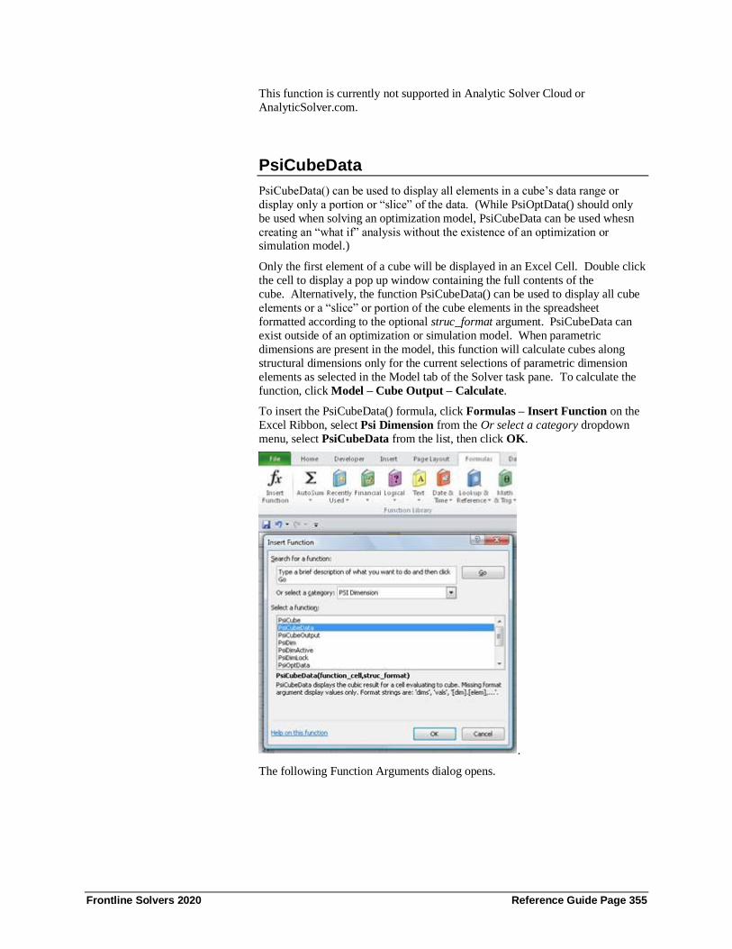
Frontline Solvers 2020 Reference Guide Page 355
This function is currently not supported in Analytic Solver Cloud or
AnalyticSolver.com.
PsiCubeData
PsiCubeData() can be used to display all elements in a cube’s data range or
display only a portion or “slice” of the data. (While PsiOptData() should only
be used when solving an optimization model, PsiCubeData can be used whesn
creating an “what if” analysis without the existence of an optimization or simulation model.)
Only the first element of a cube will be displayed in an Excel Cell. Double click
the cell to display a pop up window containing the full contents of the
cube. Alternatively, the function PsiCubeData() can be used to display all cube
elements or a “slice” or portion of the cube elements in the spreadsheet
formatted according to the optional struc_format argument. PsiCubeData can
exist outside of an optimization or simulation model. When parametric
dimensions are present in the model, this function will calculate cubes along
structural dimensions only for the current selections of parametric dimension
elements as selected in the Model tab of the Solver task pane. To calculate the
function, click Model – Cube Output – Calculate.
To insert the PsiCubeData() formula, click Formulas – Insert Function on the
Excel Ribbon, select Psi Dimension from the Or select a category dropdown
menu, select PsiCubeData from the list, then click OK.
.
The following Function Arguments dialog opens.

Frontline Solvers 2020 Reference Guide Page 356
Function_cell: Enter an existing cube here. (PsiCubeData() can be used with
any cube.)
Struc_format: An optional argument entered as a string. If omitted, all cube
values are printed in a single vector.
If PsiCubeData is entered as an array (with size equal to the number of
dimensions in the Function_cell cube) and struc_format = “dims”,
PsiCubeData() prints all dimensions in the cube with their lengths.
Once the size of the cube is obtained or if the cube dimensions are already
known, enter this function as an array (with size equal to the number of
dimensions by number of cube elements in the Function_cell cube) while
passing struc_format = “vals” to print all cube elements in the form of a
relational or pivot table. In addition, this argument can also be used to selectively print only a portion of a cube’s elements or a “slice” of the data
table. (See below for an example.)
Function Signatures
The signature provided for this function is:
=PsiCubeData(output_cell, [struc_format])
output_cell (required): An existing cube on the spreadsheet. (PsiCubeData()
can be used with any cube.)
struc_format (optional): An optional argument entered as a string. If omitted, all
cube values are printed in a single vector.
If PsiCubeData is entered as an array (with size equal to the number of
dimensions in the Function_cell cube) and struc_format = “dims”,
PsiCubeData() prints all dimensions in the cube with their lengths.
Once the size of the cube is obtained or if the cube dimensions are already
known, enter this function as an array (with size equal to the number of
dimensions by number of cube elements in the Function_cell cube) while passing struc_format = “vals” to print all cube elements in the form of a
relational or pivot table. In addition, this argument can also be used to
selectively print only a portion of a cube’s elements or a “slice” of the data
table. (See below for an example.)
Examples
=PsiCubeData(A1, ”dims”) – When entered as an array with size equal to the number of dimensions included in the A1 cube, the dimension name and number
of elements will be returned.

Frontline Solvers 2020 Reference Guide Page 357
=PsiCubeData(A1, “vals”) – When entered as an array (with size equal to the
number of dimensions by the number cube elements included in the A1 cube),
the values of the fact table will be displayed along with the dimension elements
in the form of a relational or pivot table.
=PsiCubeData(A1, ”[Parts].[Chassis], [Products].[TV]”) - When entered as an array of size 3, only the slice of the data range pertaining to the number of
chassis used when manufacturing a TV will be printed.
Cells containing PsiCubeData() will appear under Results in the Model tab of
the Solver task pane.
Address: Displays the cell address range where PsiCubeData is located (read –
only).
Formula: Displays the array formula located in the Address range (read – only).
This function is currently not supported in Analytic Solver Cloud or
AnalyticSolver.com.
PsiCubeOutput
Use this function to designate that cell as a cubic output. To calculate this
output cell, click Model – Cube Result – Calculate or set Dimensional
Calculation to “Automatic” on the Platform tab on the Solver task pane.
To specify a target cell as a Output function, click Model – Cube Result –
Output to append PsiCubeOutput() to the existing cell formula.
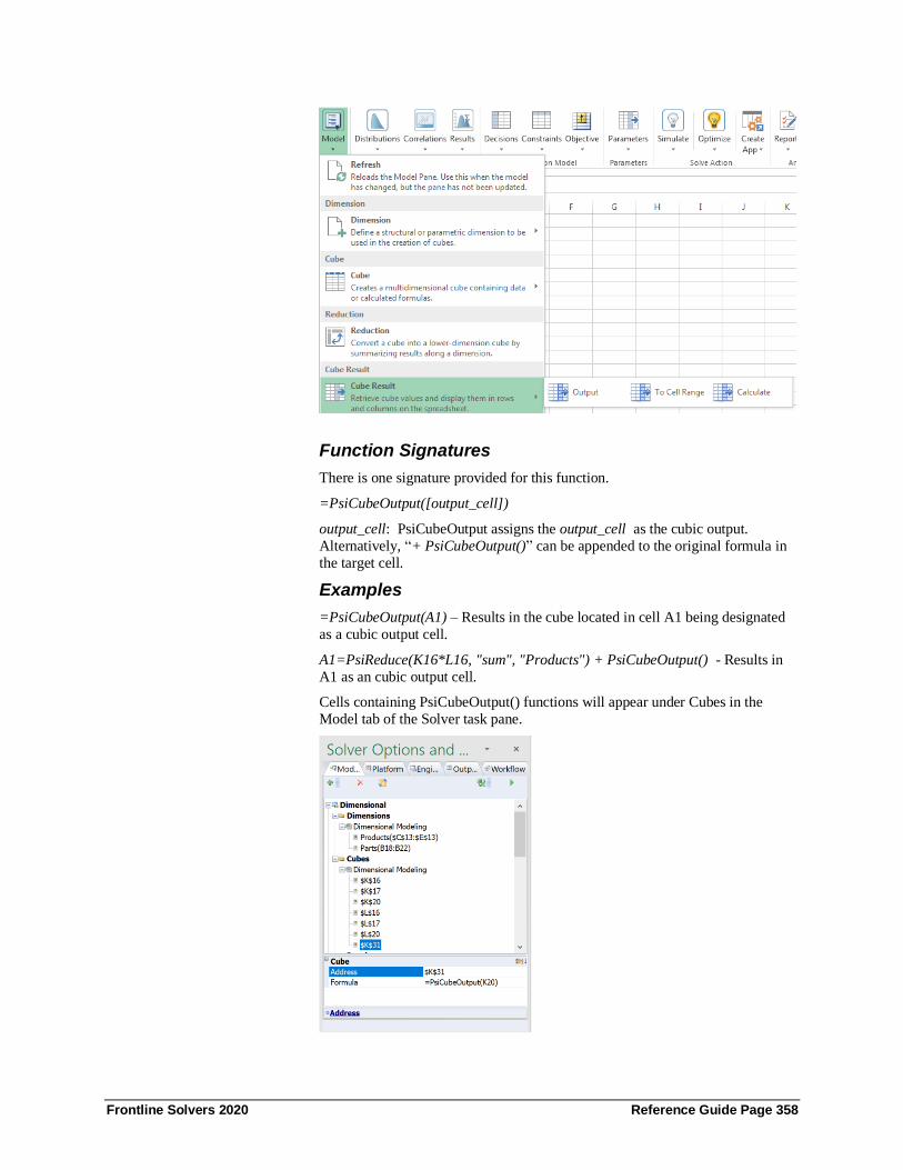
Frontline Solvers 2020 Reference Guide Page 358
Function Signatures
There is one signature provided for this function.
=PsiCubeOutput([output_cell])
output_cell: PsiCubeOutput assigns the output_cell as the cubic output.
Alternatively, “+ PsiCubeOutput()” can be appended to the original formula in
the target cell.
Examples
=PsiCubeOutput(A1) – Results in the cube located in cell A1 being designated
as a cubic output cell.
A1=PsiReduce(K16*L16, "sum", "Products") + PsiCubeOutput() - Results in
A1 as an cubic output cell.
Cells containing PsiCubeOutput() functions will appear under Cubes in the
Model tab of the Solver task pane.
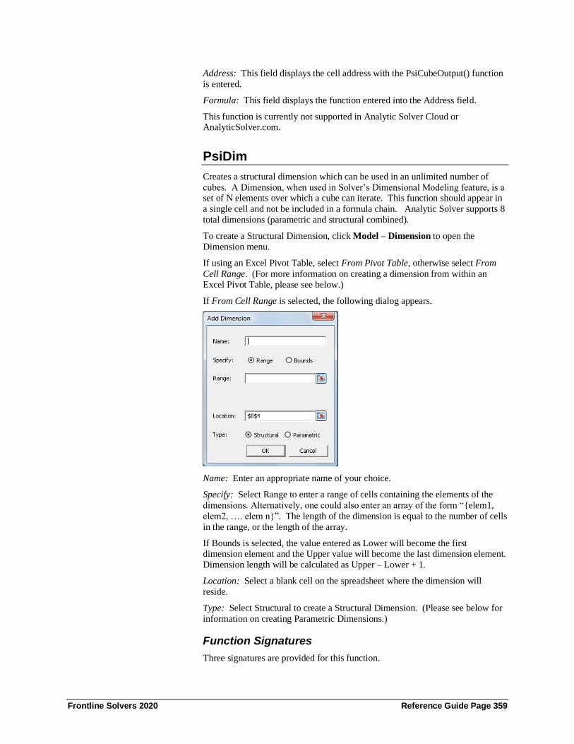
Frontline Solvers 2020 Reference Guide Page 359
Address: This field displays the cell address with the PsiCubeOutput() function
is entered.
Formula: This field displays the function entered into the Address field.
This function is currently not supported in Analytic Solver Cloud or AnalyticSolver.com.
PsiDim
Creates a structural dimension which can be used in an unlimited number of
cubes. A Dimension, when used in Solver’s Dimensional Modeling feature, is a set of N elements over which a cube can iterate. This function should appear in
a single cell and not be included in a formula chain. Analytic Solver supports 8
total dimensions (parametric and structural combined).
To create a Structural Dimension, click Model – Dimension to open the
Dimension menu.
If using an Excel Pivot Table, select From Pivot Table, otherwise select From
Cell Range. (For more information on creating a dimension from within an
Excel Pivot Table, please see below.)
If From Cell Range is selected, the following dialog appears.
Name: Enter an appropriate name of your choice.
Specify: Select Range to enter a range of cells containing the elements of the
dimensions. Alternatively, one could also enter an array of the form “{elem1,
elem2, …. elem n}”. The length of the dimension is equal to the number of cells
in the range, or the length of the array.
If Bounds is selected, the value entered as Lower will become the first dimension element and the Upper value will become the last dimension element.
Dimension length will be calculated as Upper – Lower + 1.
Location: Select a blank cell on the spreadsheet where the dimension will
reside.
Type: Select Structural to create a Structural Dimension. (Please see below for
information on creating Parametric Dimensions.)
Function Signatures
Three signatures are provided for this function.

Frontline Solvers 2020 Reference Guide Page 360
=PsiDim(name, range_or_array)
=PsiDim(name, from_num, to_num)
=PsiDim(name, length)
name: A unique string value assigned to identify the dimension.
range_or_array: Enter a range of cells containing the elements of the
dimensions. Alternatively, one could also enter an array of the form “{elem1,
elem2, …. elem n}”. The length of the dimension is equal to the number of cells
in the range, or the length of the array.
From_num is an integer value which will become the first dimensional element.
To_num is an integer value which will become the last dimensional element.
Dimension length will be calculated as to_num – from_num + 1.
The length argument is an integer value defining the number of elements in the
dimension. Elements will not be assigned names, rather each element will be assigned a value of 1, 2, 3, ….N.
Examples
=PsiDim(“cities”, A1:A3) where A1 = NY, A2 = LA, and A3 = SF - Results in
a Structural dimension named “cities” containing three elements: NY, LA, and
SF.
=PsiDim(“cities”, {“NY”, “LA”, “SF”}) – Results in a Structural dimension named “cities” containing three elements: NY, LA, and SF.
=PsiDim(“countdown”, 60, 0) – Results in a Structural dimension named
“countdown” that contains 61 elements: 60, 59, 58, …, 2, 1, 0.
=PsiDim(“index”, 10) – Results in a Structural dimension named “index” with
10 elements: 1, 2, 3, …, 8, 9, 10.
After a Structural dimension is created, the name and address of the dimension
will appear under Dimensions in the Solver Task Pane.
Address: Displays the cell address where the Structural dimension resides (read
– only).
Formula: Displays the formula in the Address cell (read – only).
Name: Displays the name of the Structural dimension (read – only).
Current Value: Controls the values displayed in the cell containing the cube.
Type: Displays the type of dimension, Structural or Parametric.
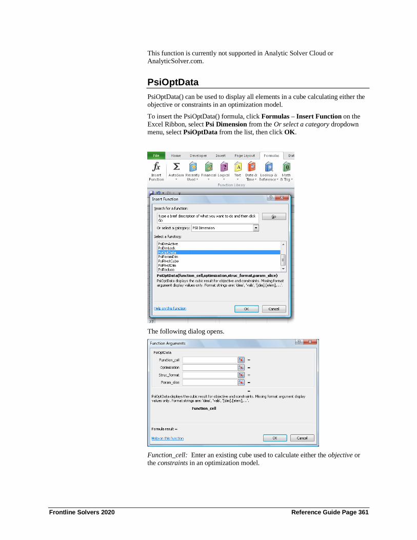
Frontline Solvers 2020 Reference Guide Page 361
This function is currently not supported in Analytic Solver Cloud or
AnalyticSolver.com.
PsiOptData
PsiOptData() can be used to display all elements in a cube calculating either the
objective or constraints in an optimization model.
To insert the PsiOptData() formula, click Formulas – Insert Function on the
Excel Ribbon, select Psi Dimension from the Or select a category dropdown
menu, select PsiOptData from the list, then click OK.
The following dialog opens.
Function_cell: Enter an existing cube used to calculate either the objective or
the constraints in an optimization model.

Frontline Solvers 2020 Reference Guide Page 362
Optimization: This argument is optional. This argument specifies the
optimization number to which the function will be applied. If omitted, the
optimization selected in the Ribbon will be used.
Struc_format: An optional argument entered as a string. If omitted, all cube
values are printed in a single vector.
If PsiCubeData is entered as an array (with size equal to the number of
dimensions in the Function_cell cube) and struc_format = “dims”,
PsiCubeData() prints all dimensions in the cube with their lengths.
Once the size of the cube is obtained or if the cube dimensions are already
known, enter this function as an array (with size equal to the number of
dimensions by number of cube elements in the Function_cell cube) while
passing struc_format = “vals” to print all cube elements in the form of a
relational or pivot table. In addition, this argument can also be used to
selectively print only a portion of a cube’s elements or a “slice” of the data
table. (See below for an example.)
To use this argument to return the value of a specific element in a 1-dimensional
cube containing a structural dimension, use the form:
“[StructuralDimisension1].[Element1]”.
To use this argument to return the value of a 2-dimensional cube (containing
structural dimensions), use the form:
“[StructuralDimension1].[Element],[StructuralDimension2].[Element]”.
To use this argument to return the value of an N-dimensional cube (containing
structural dimensions), use the form:
“[StructuralDimension1].[Element],[StructuralDimension2].[Element],…,[Stru
cturalDimensionN].[Element]”.
Param_slice: The param_slice argument is an optional string argument
specifying the desired element “slice” for the parametric dimensions. If omitted
the element selected for the Dimension’s Current Value in the Solver Task Pane
will be used.
To use this argument to return the value of a specific element in a cube with 1-
dimensional cube containing a parametrc dimension, use the form:
“[ParametricDimisension1].[Element1]”.
To use this argument to return the value of a 2-dimensional cube (containing
parametrc dimensions), use the form:
“[ParametricDimension1].[Element],[ParametricDimension2].[Element]”.
To use this argument to return the value of an N-dimensional cube (containing
parametric dimensions), use the form:
“[ParametricDimension1].[Element],[ParametricDimension2].[Element],…,[P
arametricDimensionN].[Element]”.
Function Signatures
When a cube evaluation results in a given optimization output_cell, (e.g. a constraint or objective definition cell) is a cube, Excel may display at most one
element of that cube. If we enter PsiOptData as an array formula, we can see all
or selected elements of the cube result formatted according to the optional
struc_format string.
There is one signature provided for this function.
=PsiOptData(output_cell, [optimization], [struc_format], [param_slice])

Frontline Solvers 2020 Reference Guide Page 363
output_cell: (required) Enter an existing cube used to calculate either the
objective or the constraints in an optimization model.
Optimization: (optional) An optional argument specifying the current
optimization related to PsiOptParam() functions. If omitted the one selected in
the Ribbon will be assumed.
Struc_format: An optional argument entered as a string. If omitted, all cube
values are printed in a single vector.
If PsiCubeData is entered as an array (with size equal to the number of
dimensions in the Function_cell cube) and struc_format = “dims”,
PsiCubeData() prints all dimensions in the cube with their lengths.
Once the size of the cube is obtained or if the cube dimensions are already
known, enter this function as an array (with size equal to the number of
dimensions by number of cube elements in the Function_cell cube) while
passing struc_format = “vals” to print all cube elements in the form of a
relational or pivot table. In addition, this argument can also be used to selectively print only a portion of a cube’s elements or a “slice” of the data
table. (See below for an example.)
To use this argument to return the value of a specific element in a 1-dimensional
cube containing a structural dimension, use the form:
“[StructuralDimisension1].[Element1]”.
To use this argument to return the value of a 2-dimensional cube (containing
structural dimensions), use the form:
“[StructuralDimension1].[Element],[StructuralDimension2].[Element]”.
To use this argument to return the value of an N-dimensional cube (containing
structural dimensions), use the form: “[StructuralDimension1].[Element],[StructuralDimension2].[Element],…,[Stru
cturalDimensionN].[Element]”.
Param_slice: The param_slice argument is an optional string argument
specifying the desired element “slice” for the parametric dimensions. If omitted
the element selected for the Dimension’s Current Value in the Solver Task Pane
will be used.
To use this argument to return the value of a specific element in a cube with 1-
dimensional cube containing a parametrc dimension, use the form:
“[ParametricDimisension1].[Element1]”.
To use this argument to return the value of a 2-dimensional cube (containing parametrc dimensions), use the form:
“[ParametricDimension1].[Element],[ParametricDimension2].[Element]”.
To use this argument to return the value of an N-dimensional cube (containing
parametric dimensions), use the form:
“[ParametricDimension1].[Element],[ParametricDimension2].[Element],…,[P
arametricDimensionN].[Element]”.
Examples
=PsiOptData(A1, 1, ”dims”) – When entered as an array (with size equal to the
number of dimensions included in the cube located in cell A1) for the 1st
optimization, the dimension name and number of elements will be returned.
=PsiOptData(A1, 2, “vals”) – When entered as an array (with size equal to the
number of dimensions by number of elements included in the cube in A1), the
values of the fact table for the 2nd optimization will be displayed along with the
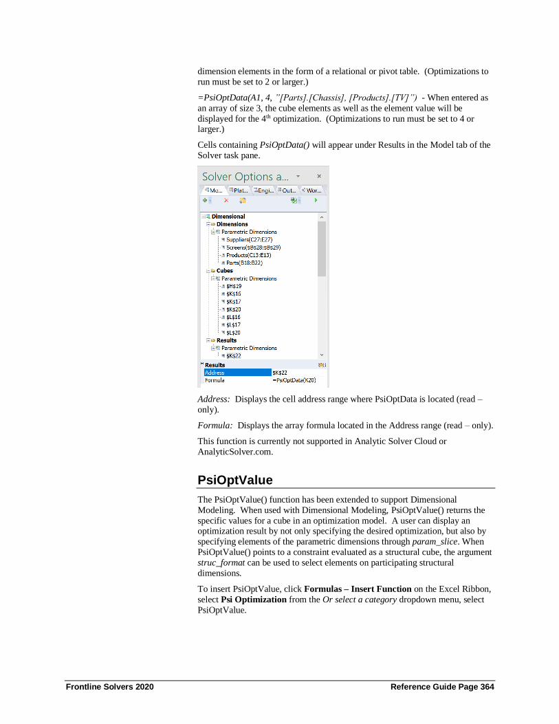
Frontline Solvers 2020 Reference Guide Page 364
dimension elements in the form of a relational or pivot table. (Optimizations to
run must be set to 2 or larger.)
=PsiOptData(A1, 4, ”[Parts].[Chassis], [Products].[TV]”) - When entered as
an array of size 3, the cube elements as well as the element value will be
displayed for the 4th optimization. (Optimizations to run must be set to 4 or larger.)
Cells containing PsiOptData() will appear under Results in the Model tab of the
Solver task pane.
Address: Displays the cell address range where PsiOptData is located (read –
only).
Formula: Displays the array formula located in the Address range (read – only).
This function is currently not supported in Analytic Solver Cloud or
AnalyticSolver.com.
PsiOptValue
The PsiOptValue() function has been extended to support Dimensional
Modeling. When used with Dimensional Modeling, PsiOptValue() returns the
specific values for a cube in an optimization model. A user can display an optimization result by not only specifying the desired optimization, but also by
specifying elements of the parametric dimensions through param_slice. When
PsiOptValue() points to a constraint evaluated as a structural cube, the argument
struc_format can be used to select elements on participating structural
dimensions.
To insert PsiOptValue, click Formulas – Insert Function on the Excel Ribbon,
select Psi Optimization from the Or select a category dropdown menu, select
PsiOptValue.

Frontline Solvers 2020 Reference Guide Page 365
The following dialog appears.
Cell_or_name: Enter an existing cube.
Optimization: This optional argument specifies the simulation number to which
the function will be applied. If omitted, the optimization selected in the Ribbon
will be used.
Model: This argument is not supported in Dimensional Modeling. Leave this
argument blank.
Struc_format: A string argument specifying the desired element selected along
the structural dimension to be monitored. If omitted, the element selected for
the Dimension’s Current Value in the Solver task pane will be used.
To use this argument to return the value of a specific element in a structural
cube, use the form: “[StructuralDimisension1].[Element1]”.

Frontline Solvers 2020 Reference Guide Page 366
To use this argument to return the value of a 2-dimensional cube (containing
structural dimensions), use the form:
“[StructuralDimension1].[Element],[StructuralDimension2].[Element]”.
To use this argument to return the value of a N-dimensional cube (containing
structural dimensions), use the form: “[StructuralDimension1].[Element],[StructuralDimension2].[Element],…,[Stru
cturalDimensionN].[Element]”.
Param_slice: The param_slice argument is an optional string argument
specifying the desired element “slice” for the parametric cube to be monitored.
If omitted the element selected for the Dimension’s Current Value in the Solver
Model task pane will be used.
To use this argument to return the value of a specific element in a 1-dimension
cube containing a parametric dimension use the form:
“[StructuralDimisension1].[Element1]”.
To use this argument to return the value of a 2-dimensional cube (containing parametric dimensions), use the form:
“[StructuralDimension1].[Element],[StructuralDimension2].[Element]”.
To use this argument to return the value of a N-dimensional cube (containing
parametric dimensions), use the form:
“[StructuralDimension1].[Element],[StructuralDimension2].[Element],…,[Stru
cturalDimensionN].[Element]”.
Function Signatures
One signature is provided for this function.
=PsiOptValue(output_cell, [optimization],[model], [struc_format],
[param_slice])
Output_cell: (required) An output cell that evaluates to a cube, e.g. a constraint,
objective, or intermediate cell
optimization: (optional) Specifies the current optimization related to the
PsiOptParam() function. If omitted, the optimization selected in the Ribbon will
be used.
model : (optional) This argument is not supported in Dimensional Modeling.
Leave this argument blank.
struc_format: (optional) A string argument specifying the desired element
selected along the structural dimension to be monitored. If omitted, the
element selected for the Dimension’s Current Value in the Solver task pane will
be used.
To use this argument to return the value of a specific element in a 1-dimensional
cube containing a structural dimension, use the form:
“[StructuralDimisension1].[Element1]”.
To use this argument to return the value of a 2-dimensional cube (containing structural dimensions), use the form:
“[StructuralDimension1].[Element],[StructuralDimension2].[Element]”.
To use this argument to return the value of a N-dimensional cube (containing
structural dimensions), use the form:
“[StructuralDimension1].[Element],[StructuralDimension2].[Element],…,[Stru
cturalDimensionN].[Element]”.

Frontline Solvers 2020 Reference Guide Page 367
param_slice: (optional) An optional string argument specifying the desired
element “slice” along the parametric dimensions to be monitored. Detailed
usage of this argument is the same as the identical one in the PsiOptData().
To use this argument to return the value of a specific element in a 1-dimension
cube containing a parametric dimension use the form: “[StructuralDimisension1].[Element1]”.
To use this argument to return the value of a 2-dimensional cube (containing
parametric dimensions), use the form:
“[StructuralDimension1].[Element],[StructuralDimension2].[Element]”.
To use this argument to return the value of a N-dimensional cube (containing
parametric dimensions), use the form:
“[StructuralDimension1].[Element],[StructuralDimension2].[Element],…,[Stru
cturalDimensionN].[Element]”.
Examples
=PsiOptValue(K21, 2, ””, "[Parts].[Speaker]")– Results in the value of K21 (a
cube comprised of 1 structural dimension) in the 2nd optimization, when Speaker
is selected for the Parts dimension.
=PsiOptValue(L17, 3, ””, "[Products].[TVs], [Parts].[Electronics]") – Results
in the value of L17 (a cube comprised of 2 structural dimensions) in the 3rd
optimization, where the element TVs is selected for the Products dimension and
the element Electronics is selected for the Parts dimension.
Cells containing PsiOptValue functions will appear under Results in the Model
tab of the Solver task pane. Expand the range K31:L31 to display the following.
Address: Displays the cell address range where the PsiOptValue function is
located (read – only).
Formula: Displays the array formula located in the Address range (read – only).

Frontline Solvers 2020 Reference Guide Page 368
Monitor Value: Displays “True” since PsiOptValue by definition creates a
monitored value (read – only).
This function is currently not supported in Analytic Solver Cloud or
AnalyticSolver.com.
PsiParamDim
Creates a Parametric dimension which can be used in an unlimited number of
cubes. When a Parametric dimension is included in a cube, the Psi Interpreter
will treat all data as parametric values. This function should appear in a single cell and not be included in a formula chain. Analytic Solver supports 8 total
dimensions (parametric and structural combined).
To create a Parametric Dimension, click Model – Dimension to open the
Dimension menu.
If using an Excel Pivot Table, select From Pivot Table, otherwise select From
Cell Range. (For more information on creating a dimension from within an
Excel Pivot Table, please see below.)
If From Cell Range is selected, the following dialog appears.
Name: Enter an appropriate name of your choice.
Specify: Select Range to enter a range of cells containing names for dimension
elements or Bounds to enter lower and upper integer values. If Bounds is
selected, the value entered as Lower will become the first dimension element
and the Upper value will become the last dimension element. Dimension length
will be calculated as Upper – Lower + 1.
Location: Select a blank cell on the spreadsheet where the dimension will
reside.

Frontline Solvers 2020 Reference Guide Page 369
Type: Select Parametric to create a Parametric Dimension. (Please see above
for information on creating Structural Dimensions.)
Function Signatures
Three signatures are provided for this function.
=PsiParamDim(name, range_or_array)
=PsiParamDim(name, from_num, to_num)
=PsiParamDim(name, length)
name: A unique string value assigned to identify the dimension.
range_or_array: Range of cells containing the elements of the dimensions. Alternatively, one could also enter an array of the form “{elem1, elem2, ….
elem n}”. The length of the dimension is equal to the number of cells in the
range, or the length of the array.
From_num: Integer value which will become the first dimensional element.
To_num: Integer value which will become the last dimensional element.
Dimension length will be calculated as to_num – from_num + 1.
Length: Argument is an integer value defining the number of elements in the
dimension. Elements will not be assigned names, rather each element will be
assigned a value of 1, 2, 3, ….N.
Examples
=PsiParamDim(“cities”, A1:A3) where A1 = NY, A2 = LA, and A3 = SF -
Results in a Parametric dimension named “cities” containing three elements:
NY, LA, and SF.
=PsiParamDim(“cities”, {“NY”, “LA”, “SF”}) – Results in a Parametric
dimension named “cities” containing three elements: NY, LA, and SF.
=PsiParamDim(“countdown”, 60, 0) – Results in a Parametric dimension
named “countdown” that contains 60 elements: 60, 59, 58, …, 2, 1, 0.
=PsiParamDim(“index”, 10) – Results in a Parametric dimension named
“index” with 10 elements: 1, 2, 3, …, 8, 9, 10.
After a Parametric dimension is created, the name and address of the dimension
will appear under Dimensions in the Solver Task Pane.
Address: Displays the cell address where the Parametric dimension resides
(read – only).

Frontline Solvers 2020 Reference Guide Page 370
Formula: Displays the formula in the Address cell (read – only).
Name: Displays the name of the Structural dimension (read – only).
Current Value: Controls the values displayed in the cell containing the cube.
Locked: Setting Locked to True, will result in the dimension being “locked” or “frozen” to the Current Value element.
Type: Displays the type of dimension, Structural or Parametric.
Active in Optimization: If False, dimension will be ignored in the next
optimization.
Active in Simulation: If False, dimension will be ignored in the next simulation.
Active in Sensitivity Analysis: If False, dimension will be ignored in the next
sensitivity analysis.
PsiDimActive() Signatures
The PsiDimActive() function is a property function passed to PsiParamDim().
=PsiParamDim(name, range_or_array, [PsiDimActive(opt, sim, sen])
=PsiParamDim(name, from_num, to_num, [PsiDimActive(opt, sim, sen])
=PsiParamDim(name, length, [PsiDimActive(opt, sim, sen])
The opt argument can be set to True or False. If False, dimension will not
appear in the next optimization
The sim argument can be set to True or False. If False, dimension will not
appear in the next simulation.
The sen argument can be set to True or False. If False, dimension will not
appear in the next sensitivity analysis.
Example
=PsiParamDim(“cities”, A1:A3, PsiDimActive(true, false, false)) - Results in a
Parametric dimension named “cities” containing three elements: NY, LA, and
SF. This dimension will only be available for optimization models.
PsiDimLock() Signature
The PsiDimLock() function is a property function passed to PsiParamDim().
=PsiParamDim(name, range_or_array, [PsiDimLock(elem_or_index)])
The elem_or_index argument should be either the name of the locked element or
its 1-based index.
Example
=PsiParamDim(“cities”, A1:A3, PsiDimLock(“LA”)) - Results in a Parametric
dimension named “cities” containing three elements: NY, LA, and SF. This dimension will be locked to the “LA” dimension element.
This function is currently not supported in Analytic Solver Cloud or
AnalyticSolver.com.

Frontline Solvers 2020 Reference Guide Page 371
PsiPivotCube
The function creates a cube from a pivot table. A dimension in a pivot table
should be defined explicitly by PsiPivotDim. Since values in pivot tables are not
evaluable, pivot cubes are not transparent to any inputs (variables, distributions
etc.). Hence, values in pivot table must not be dependent on inputs, rather they
must be constants.
To create a Cube from a Pivot Table, click Model – Cubes to open the Cube
menu.
Select From Pivot Table, the following dialog appears.
Pivot Tables: Click the down arrow to select an existing pivot table from the
menu.
Location: Select a blank cell on the spreadsheet where the dimension will
reside.
Function Signatures
One signature is provided for this function.
=PsiPivotCube(cell_within_pivot)
cell_within_pivot: (required) A cell reference within the range of a pivot table
definition. This argument is used by Analytic Solver to identify the appropriate
pivot table.
Examples
=PsiPivotCube($A$3:$E$17) -- Results in a cube created from data within the
Pivot table residing in cells A3:E17.
After a Cube is created, the name and address of the dimension will appear
under Dimensions in the Solver Task Pane.

Frontline Solvers 2020 Reference Guide Page 372
Address: Displays the cell address where the cube is located (read – only).
Formula: Displays the formula in the Address cell (read – only).
This function is currently not supported in Analytic Solver Cloud or
AnalyticSolver.com.
PsiPivotDim
This function extracts a dimension from an existing pivot table, making it either
structural or parametric. To construct a cube from a pivot table you must
explicitly define all table fields as dimensions through PsiPivotDim() first.
To create a Parametric Dimension, click Model – Dimension to open the
Dimension menu.
Select From Pivot Table. The following dialog appears.
Pivot Tables: Click the down array to select the desired Pivot Table from the
drop-down menu.

Frontline Solvers 2020 Reference Guide Page 373
Dimension: Click the down arrow to select the desired Pivot Table field. A
dimension will be created from the selected field.
Type: Select Structural to create a Structural Dimension or Parametric to create
a Parametric Dimension.
Location: Select a blank cell on the spreadsheet where the dimension will
reside.
Function Signatures
There is one signature provided for this function.
=PsiPivotDim(cell_within_pivot, dim_name, [dim_type],…)
cell_within_pivot: (required) A cell reference within the range of a pivot table definition.
dim_name:(required) A string containing the name of the extracted pivot table
field as a dimension. This argument is used by Analytic Solver to create a
dimension with that name.
dim_type: (optional) Pass False for this argument if creating a Structural
Dimension or True if creating a Parametric Dimension. If this argument is
omitted, a Structural Dimension will be created.
If a Parametric Dimension is created, two additional arguments can be used,
PsiDimLock() and/or PsiDimActive(). See below for explanation of these two
functions.
Examples
=PsiPivotDim($A$1, "Product", TRUE) - Results in a Parametric dimension
created from the “Products” field from within the Pivot Table contained in cell
A1.
=PsiPivotDim($A$7, "Product", FALSE) or =PsiPivotDim($A$7, "Product") – Results in a Structural dimension created from the “Product” field from the
Pivot Table located in cell A7.
=PsiPivotDim($A$7, "Product", TRUE, PsiDimLock("dyn tool")) – Results in a
Parametric dimension created from the “Product” field from the Pivot Table
located in cell A7 locked to the dyn tool dimension element. (For more
information on PsiDimLock, see below.)
=PsiPivotDim($A$7, "Product", TRUE, PsiDimLock("dyn tool"),
PsiDimActive(FALSE, TRUE, TRUE)) – Results in a Parametric dimension
created from the “Product” field from the Pivot Table located in cell A7 locked
to the dyn tool dimension element and active in simulation and sensitivity
analysis. This dimension will not be active in optimization. (For more information on PsiDimLock() or PsiDimActive(), see below.)
After a Parametric dimension is created, the name and address of the dimension
will appear under Dimensions in the Solver Task Pane.

Frontline Solvers 2020 Reference Guide Page 374
Formula: Displays the formula in the Address cell (read – only).
Name: Displays the name of the parametric dimension (read – only).
Current Value: Controls the values displayed in the cell containing the cube.
Locked: Setting Locked to True, will result in the dimension being “locked” or
“frozen” to the Current Value element.
Type: Displays the type of dimension, Structural or Parametric.
Active in Optimization: If False, dimension will be ignored in the next
optimization.
Active in Simulation: If False, dimension will be ignored in the next simulation.
Active in Sensitivity Analysis: If False, dimension will be ignored in the next sensitivity analysis.
PsiDimActive() Signatures
The PsiDimActive() function is a property function passed to PsiPivotDim().
=PsiParamDim(name, range_or_array, [PsiDimActive(opt, sim, sen])
=PsiParamDim(name, from_num, to_num, [PsiDimActive(opt, sim, sen])
=PsiParamDim(name, length, [PsiDimActive(opt, sim, sen])
The opt argument can be set to True or False. If False, dimension will not
appear in the next optimization
The sim argument can be set to True or False. If False, dimension will not
appear in the next simulation.
The sen argument can be set to True or False. If False, dimension will not
appear in the next sensitivity analysis.
Example
=PsiParamDim(“cities”, A1:A3, PsiDimActive(true, false, false)) - Results in a
Parametric dimension named “cities” containing three elements: NY, LA, and
SF. This dimension will only be available for optimization models.
PsiDimLock() Signature
The PsiDimLock() function is a property function passed to PsiPivotDim().
=PsiParamDim(name, range_or_array, [PsiDimLock(elem_or_index])
The elem_or_index argument should be either the name of the locked element or
its 1-based index.
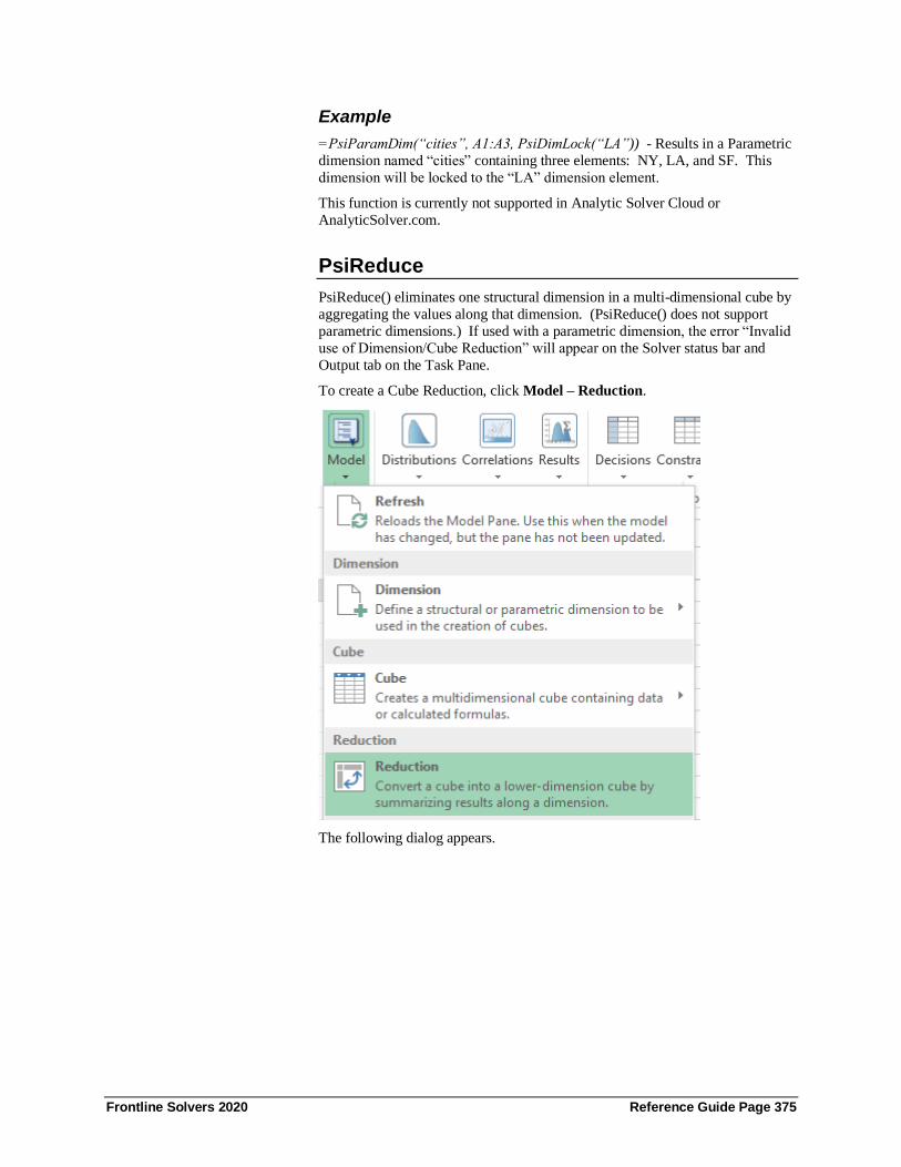
Frontline Solvers 2020 Reference Guide Page 375
Example
=PsiParamDim(“cities”, A1:A3, PsiDimLock(“LA”)) - Results in a Parametric
dimension named “cities” containing three elements: NY, LA, and SF. This
dimension will be locked to the “LA” dimension element.
This function is currently not supported in Analytic Solver Cloud or
AnalyticSolver.com.
PsiReduce
PsiReduce() eliminates one structural dimension in a multi-dimensional cube by
aggregating the values along that dimension. (PsiReduce() does not support
parametric dimensions.) If used with a parametric dimension, the error “Invalid
use of Dimension/Cube Reduction” will appear on the Solver status bar and
Output tab on the Task Pane.
To create a Cube Reduction, click Model – Reduction.
The following dialog appears.
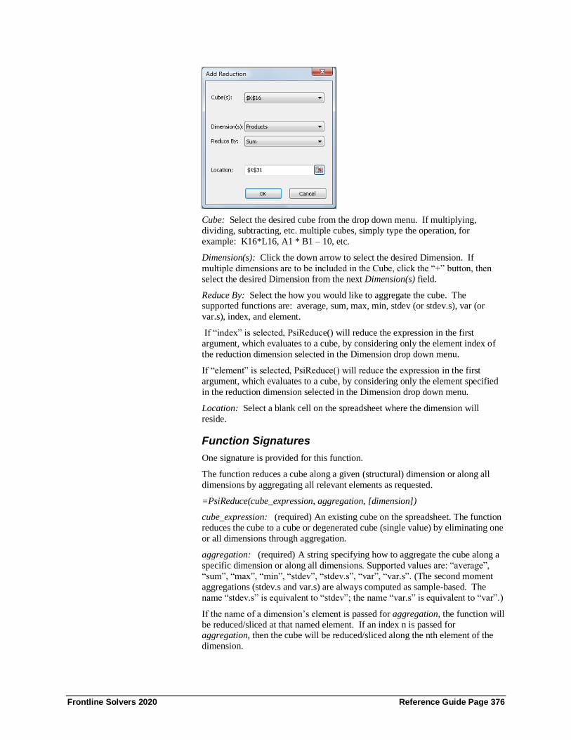
Frontline Solvers 2020 Reference Guide Page 376
Cube: Select the desired cube from the drop down menu. If multiplying,
dividing, subtracting, etc. multiple cubes, simply type the operation, for
example: K16*L16, A1 * B1 – 10, etc.
Dimension(s): Click the down arrow to select the desired Dimension. If
multiple dimensions are to be included in the Cube, click the “+” button, then
select the desired Dimension from the next Dimension(s) field.
Reduce By: Select the how you would like to aggregate the cube. The supported functions are: average, sum, max, min, stdev (or stdev.s), var (or
var.s), index, and element.
If “index” is selected, PsiReduce() will reduce the expression in the first
argument, which evaluates to a cube, by considering only the element index of
the reduction dimension selected in the Dimension drop down menu.
If “element” is selected, PsiReduce() will reduce the expression in the first
argument, which evaluates to a cube, by considering only the element specified
in the reduction dimension selected in the Dimension drop down menu.
Location: Select a blank cell on the spreadsheet where the dimension will
reside.
Function Signatures
One signature is provided for this function.
The function reduces a cube along a given (structural) dimension or along all
dimensions by aggregating all relevant elements as requested.
=PsiReduce(cube_expression, aggregation, [dimension])
cube_expression: (required) An existing cube on the spreadsheet. The function
reduces the cube to a cube or degenerated cube (single value) by eliminating one
or all dimensions through aggregation.
aggregation: (required) A string specifying how to aggregate the cube along a
specific dimension or along all dimensions. Supported values are: “average”,
“sum”, “max”, “min”, “stdev”, “stdev.s”, “var”, “var.s”. (The second moment
aggregations (stdev.s and var.s) are always computed as sample-based. The
name “stdev.s” is equivalent to “stdev”; the name “var.s” is equivalent to “var”.)
If the name of a dimension’s element is passed for aggregation, the function will
be reduced/sliced at that named element. If an index n is passed for aggregation, then the cube will be reduced/sliced along the nth element of the
dimension.

Frontline Solvers 2020 Reference Guide Page 377
Dimension: (optional) The name of the dimension along which the reduction
by aggregation of the cube is requested. If omitted, the cube will be aggregated
along all structural dimensions.
Examples
=PsiReduce(A1,”sum”, "state") - Results in the sum of the values in the A1
cube along the state dimension.
=PsiReduce(A2, “average”) – Results in the average of all values in the fact
table for the cube located in cell A2.
=PsiReduce(A3, “San Francisco”, “City”) – Reduces the cube in cell A3 by
considering only the San Francisco element of the reduction dimension City.
=PsiReduce(A4, 2, “City”) – Reduces the cube in cell A4 by considering only
the 2nd element of the reduction dimension City.
The result of PsiReduce() is another cube. If the cell containing =PsiReduce() is
selected in the Model tab of the Solver task pane, the name and address of the
dimension will appear under Cubes in the Solver Task Pane.
Address: Displays the cell address where the PsiReduce() occurs (read – only).
Formula: Displays the formula in the Address cell (read – only).
Values: Displays the cube being reduced or the first argument of PsiReduce().
This function is currently not supported in Analytic Solver Cloud or AnalyticSolver.com.
PsiTableCube
PsiTableCube() defines a cube over a sparse table representation with an arbitrary order of records.
A sparse cube is defined by missing records for PsiTableCube(). If Use Sparse
Cubes = False, on the Platform tab of the Solver Task Pane, and you have
defined a cube using PsiTableCube(), elements missing from the cube will be
considered equal to 0. If Use Sparse Cubes = True, you have defined a cube
using PsiTableCube() with missing records, and the percentage of elements
missing or empty is more than 30% of the total possible cube elements, those
missing elements or records will not be included in the model.

Frontline Solvers 2020 Reference Guide Page 378
As with PsiCube, the maximum number of elements in a cube created by
PsiTableCube or by formula evaluation is 1,000,000. The maximum number of
index columns or dimensions is 8.
To create a sparse cube using PsiTableCube(), click Formula on the Excel
Ribbon, select Psi Dimension as the category, then select PsiTableCube from the list of PSI Cube functions, then click OK.
The Function Arguments dialog opens. Here is where you will enter the
dimension names as well as the values for the table.
Table_description: Enter an Excel range containing the table headings. These
headings may be entered in an arbitrary order. You may enter a maximum of
eight descriptive (or index) columns.
Table_values: Enter an Excel range containing the table values. Only one value
column is supported.
In our Structural example above, we have the following table,

Frontline Solvers 2020 Reference Guide Page 379
which can be rewritten as:
Using this example, our arguments for PsiCubeTable() would be:
Table_description: M8:N19
Table_values: O8:O19
Function Signatures
The signature provided for this function is:
=PsiTableCube(table_description, table_values)
PsiTableCube() defines a cube over a sparse table representation with an
arbitrary order of records. The missing combinations are assumed to have values equal to 0.
table_description: Enter a range of cells containing string values that describe
the numeric value column, i.e. the part and product names in the “Parts” and
“Products” columns.
range_with_values: The is a range of cells on the Excel worksheet containing
numeric values, i.e. the values listed in the “Qty” column.
Examples
= PsiTableCube(M8:N19, O8:O19) where cells M8:N19 are cells containing
string names such as "Products" and "Parts" and cells O8:O19 contain numeric
values.
This function is currently not supported in Analytic Solver Cloud or
AnalyticSolver.com.
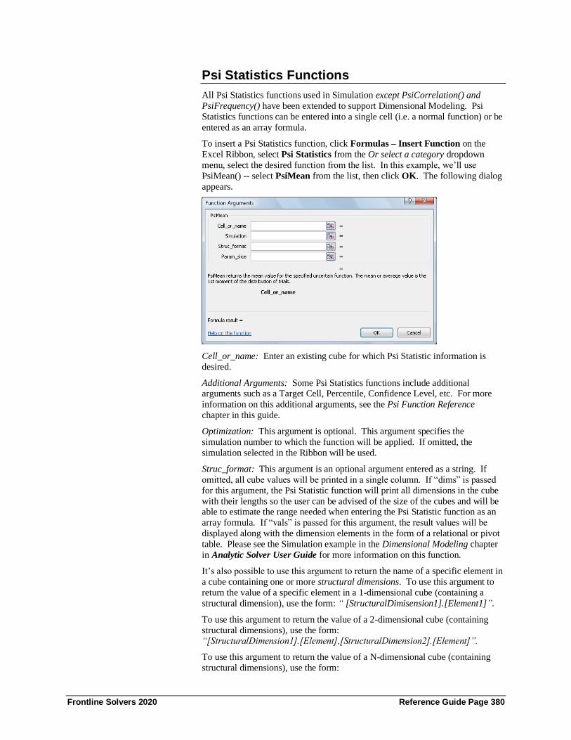
Frontline Solvers 2020 Reference Guide Page 380
Psi Statistics Functions
All Psi Statistics functions used in Simulation except PsiCorrelation() and
PsiFrequency() have been extended to support Dimensional Modeling. Psi
Statistics functions can be entered into a single cell (i.e. a normal function) or be
entered as an array formula.
To insert a Psi Statistics function, click Formulas – Insert Function on the
Excel Ribbon, select Psi Statistics from the Or select a category dropdown
menu, select the desired function from the list. In this example, we’ll use
PsiMean() -- select PsiMean from the list, then click OK. The following dialog
appears.
Cell_or_name: Enter an existing cube for which Psi Statistic information is
desired.
Additional Arguments: Some Psi Statistics functions include additional arguments such as a Target Cell, Percentile, Confidence Level, etc. For more
information on this additional arguments, see the Psi Function Reference
chapter in this guide.
Optimization: This argument is optional. This argument specifies the
simulation number to which the function will be applied. If omitted, the
simulation selected in the Ribbon will be used.
Struc_format: This argument is an optional argument entered as a string. If
omitted, all cube values will be printed in a single column. If “dims” is passed
for this argument, the Psi Statistic function will print all dimensions in the cube
with their lengths so the user can be advised of the size of the cubes and will be able to estimate the range needed when entering the Psi Statistic function as an
array formula. If “vals” is passed for this argument, the result values will be
displayed along with the dimension elements in the form of a relational or pivot
table. Please see the Simulation example in the Dimensional Modeling chapter
in Analytic Solver User Guide for more information on this function.
It’s also possible to use this argument to return the name of a specific element in
a cube containing one or more structural dimensions. To use this argument to
return the value of a specific element in a 1-dimensional cube (containing a
structural dimension), use the form: “ [StructuralDimisension1].[Element1]”.
To use this argument to return the value of a 2-dimensional cube (containing
structural dimensions), use the form: “[StructuralDimension1].[Element],[StructuralDimension2].[Element]”.
To use this argument to return the value of a N-dimensional cube (containing
structural dimensions), use the form:

Frontline Solvers 2020 Reference Guide Page 381
“[StructuralDimension1].[Element],[StructuralDimension2].[Element],…,[Stru
cturalDimensionN].[Element]”.
Param_slice: The param_slice argument is an optional string argument
specifying the desired element “slice” for the parametric dimensions. If omitted
the elements selected in the pane will be used.
It’s also possible to use this argument to return the value of a specific element in
a cube containing one or more parametric dimensions.
To use this argument to return the value of a specific element in a 1-dimensional
cube (containing a parametric dimension), use the form:
“[ParametricDimisension1].[Element1]”.
To use this argument to return the value of a 2-dimensional cube (containing
parametric dimensions), use the form:
“[ParametricDimension1].[Element],[ParametricDimension2].[Element]”.
To use this argument to return the value of a N-dimensional cube (containing parametric dimensions), use the form:
“[ParametricDimension1].[Element],[ParametricDimension2].[Element],…,[P
arametricDimensionN].[Element]”.
Function Signatures
One signature is provided for this function.
=PsiXxx(output_cell, [simulation], [struc_format], [param_slice]) where Xxx is any Psi statistics function except PsiCorrelation and PsiFrequency.
output_cell: (required) A cell reference containing an uncertain function.
Simulation: (optional) An argument specifying the simulation number related
to PsiSimParam() to which the function will be applied. If omitted, the
simulation selected in the Ribbon will be used.
struc_format: (optional) An optional argument entered as a string. If omitted, all
cube values are printed in a single vector.
If PsiCubeData is entered as an array (with size equal to the number of
dimensions in the Function_cell cube) and struc_format = “dims”,
PsiCubeData() prints all dimensions in the cube with their lengths.
Once the size of the cube is obtained or if the cube dimensions are already
known, enter this function as an array (with size equal to the number of
dimensions by number of cube elements in the Function_cell cube) while
passing struc_format = “vals” to print all cube elements in the form of a
relational or pivot table. In addition, this argument can also be used to
selectively print only a portion of a cube’s elements or a “slice” of the data
table. (See below for an example.)
param_slice: Argument specifying the desired element “slice” for parametric
dimensions. If omitted, the elements selected for the Dimension’s Current
Value in the Solver Task Pane will be used.
To use this argument to return the value of a specific element in a 1-dimensional
cube (containing a parametric dimension), use the form:
“[ParametricDimisension1].[Element1]”.
To use this argument to return the value of a 2-dimensional cube (containing
parametric dimensions), use the form:
“[ParametricDimension1].[Element],[ParametricDimension2].[Element]”.

Frontline Solvers 2020 Reference Guide Page 382
To use this argument to return the value of a N-dimensional cube (containing
parametric dimensions), use the form:
“[ParametricDimension1].[Element],[ParametricDimension2].[Element],…,[P
arametricDimensionN].[Element]”.
Examples
=PsiMean(A1, 1, ”dims”) – When entered as an array with size equal to the
number of dimensions included in the A1 cube for the 1st optimization, the
dimension name and number of elements will be returned.
=PsiMean(A1, 2, “vals”) – When entered as an array with size equal to the
number of dimensions included in the A1 cube, the values of the fact table for
the 2nd optimization will be displayed along with the dimension elements in the form of a relational or pivot table. (Simulations to run must be set to 2 or larger
in the Platform tab of the Solver task pane.)
=PsiMean(A1, 4, ”[Parts].[Chassis], [Products].[TV]”) - When entered as an
array of size 3, the cube elements as well as the element value will be displayed
for the 4th optimization. (Simulations to run must be set to 4 or larger in the
Platform tab of the Solver task pane.)
Cells containing Psi Statistics functions will appear under Simulation Statistic
Functions in the Model tab of the Solver task pane. Expand the range H6:I9 to
display the following.
Address: Displays the cell address range where the Psi Statistic is located (read
– only).
Formula: Displays the array formula located in the Address range (read – only).
Select the F8 cube (under F9) to display the following statistics.

Frontline Solvers 2020 Reference Guide Page 383
Address: Displays the cell address range where the Cube referenced in the
PsiStatistic located in cells F9 is located (read – only).
Formula: Displays the formula for the cube located in cell F8 (read – only).
Statistics: Simulation results for the first element in the cube located in cell F8.
For a description of the statistic, click the name of the statistic at the bottom of
the task pane.

Frontline Solvers 2020 Reference Guide Page 384
This function is currently not supported in Analytic Solver Cloud or
AnalyticSolver.com.
RASON Conversion Functions
PsiDataSrc
PsiDataSrc (“src_name”, {val_col_names }, (data),
[idx1_name], [idx1_elements], [idx2_name],
[idx2_elem])
When creating a custom visual in Power BI or Tableau, use PsiDataSrc() to
specify the parameters in the Excel model that you would like to be able to edit
or chart in Power BI.
src_name: Required - This argument names the text file that is translated to the
RASON datasource name. (This argument must be surrounded by quotes.)
val_col_names: Required - An array of strings (or a single string). Each string
is translated to the name of a RASON data element, to which a value column of
the datasource will be bound.
Data: Required - A (potentially multi-area) cell reference in the XLL version.
(This argument is limited to a single-area cell reference in Analytic Solver Cloud.) Each area (cell range) corresponds to one string name in
val_col_names. The size and shape of each cell range provides dimension
information (but not values) for the corresponding RASON data element.
Normally, the Excel model's formulas will also reference cells within these
ranges, so the RASON models' formulas will reference the corresponding
RASON data elements.
idx1_name, idx1_elem, idx2_name, idx2_elem – Idx1_name and idx2_name
are strings and are translated to names of the datasource index columns.
Idx1_elem and idx2_elem are cell references where the cells contain the index
elements. At least one index must be present and at most two.
idx1_name: Required - Enter the name of the 1st index set for the data specified
in the Data argument. The first index set should always be the index set that
describes the row elements. (This argument must be surrounded by quotes.)
idx1_elem: Required - Enter the Excel range containing the data (or elements)
for the 1st index set.
Idx2_name: Optional - Enter the name of the 2nd index set, if present, for the iata
specified in the Data argument. The second index set should always be the
index set that describes the column elements. (This argument must be
surrounded by quotes.)
idx2_elem: Optional - Enter the Excel range containing the data (or elements) for the 2nd index set, if present.
PsiModelSrc
PsiModelSrc (“src_name”, “data_name”)
PsiModelSrc() defines a data source for the constant range data_name used in
the converted RASON model. This function never takes part in model
evaluation. Content is saved in xml model format.

Frontline Solvers 2020 Reference Guide Page 385
src_name – Required: A string that is translated to the RASON datasource
name. (This argument must be surrounded by double quotes.)
data_name – Required: A string that is translated to the name of the RASON
data element, to which the full results of reading the datasource will be bound.
This string must be a defined name in the Excel workbook pointing to a model saved in PMML format. (This argument must be surrounded by double quotes.)
Examples
=PsiModelSrc("pmml_src","pmml_model")
where "pmml_model" is an Excel defined name pointing to the range,
LinReg_Stored!B12:B44. (LinReg_Stored is the name of the worksheet, created
by Analytic Solver Data Mining, containing the Linear Regression PMML
model.)
Psi Decision Table Functions The following functions relate to the use of Decision Tables. PsiCalcValue()
must be used to display the results from a decision table in Excel versions that do not support Dynamic Arrays. PsiDecTable() creates a Decision Table and
PsiJoin() combines to arrays with headers according to a clause argument. See
the Frontline Solvers User Guide for a complete discussion of decision tables
and a walk through of several examples where all three functions are in use.
PsiDecTable
PsiDecTable(data, [output], [ret_header], inputs)
This function defines a decision table over the constant range data and the
specified inputs.
data – This is the cell address of the decision table in the Excel worksheet.
output (Optional) – Use this argument to return a result for a specific input
variable(s).
ret_header (Optional) – Enter TRUE to insert a header at the beginning of each
column of results. Otherwise, enter FALSE or leave blank.
input – Analytic Solver supports anywhere from 1 to 253 input variables in the
decision table.
Example:
=PsiDecTable(G7:K16, "holidays", TRUE, age, service)
• G7:K16 is the location of the decision table on the Excel worksheet,
• "holidays" is passed for output to ensure that the returned results only
include the specified output
• TRUE is passed for ret_header to add a header to the result.
• age and service are the two input variables.
=PsiDecTable(G7:K16, {"holidays", "rule"}, , age, service) where
• G7:K16 is the location of the decision table on the Excel worksheet,
• "holidays" and "rule" are passed for output to ensure that the returned
results only include these two outputs,
Frontline Solvers 2020 Reference Guide Page 386
• an empty argument is passed for ret_header (this is the same as passing
FALSE),
• age and service are the two input variables.
=PsiDecTable(G7:K16, , , age, service) where
• G7:K16 is the location of the decision table on the Excel worksheet,
• An empty argument is passed for output; the entire result collection will
be returned.
• An empty argument is passed for ret_header; results will not include
headings.
• age and service are the two input variables.
For more information on this Psi function, see the Examples: Decision Table
chapter within the Analytic Solver User Guide.
PsiCalcValue
PsiCalcValue(Output_cell)
This function was created to display the result collection for a decision table in
versions of Excel that do not support dynamic arrays.
This function, when entered as an array, defines an observation output for a
given formula cell. Analytic Solver will only consider the observation outputs
in a pure workbook recalculation.
See the example model DT Structure.xlsx (Help – Example Models) to see this
function in use and the Examples: Decision Tables chapter in the Analytic
Solver User Guide for a complete discussion.
PsiJoin
PsiJoin(Table1, Table2, "Clause")
This function joins two arrays, with headers, according to the clause argument.
Currently, on the inner join option is supported.
Table1 – Enter the cell address of the first decision table.
Table2 – Enter the cell address of the second decision table.
Clause – Specifies how the two arrays, or decision tables, are to be joined, i.e.
which columns are to be matched. This argument must be surrounded by quotes.
Example:
= PsiJoin('Loan Types'!J13:L15, A2:I8, "loanType = loanType, confType =
confType, downPct >= 'minDown %'")
Where Table1 = 'Loan Types'!J13:L15, Table2 = A2:I8, and Clause = "loanType
= loanType, confType = confType, downPct >= 'minDown %'"
Note: loanType, confType, and downPct are three common features to both
tables.
For more information on this Psi function, see the Examples: Decision Table
chapter within the Analytic Solver User Guide.

Frontline Solvers 2020 Reference Guide Page 387
Frontline Solvers 2020 Reference Guide Page 388
Solver Reports
Introduction This chapter will help you use the information in the Solver Reports, which can be produced when the Solver finds a solution – or when it fails to find a
solution, and instead reports that the linearity conditions are not satisfied, or that
your model is infeasible. We’ll explain how to interpret the values in the
Sensitivity and Limits Reports, available in the standard Excel Solver and the
Analytic Solver products, and how to use the diagnostic Scaling, Structure and
Feasibility Reports and the specialized Structure, Solutions and Population
Reports, which are unique to the Analytic Solver products. To illustrate the
reports, we’ll use the example file, StandardExamples.xlsx. All files can be
opened and examined by clicking Help – Examples on the Analytic Solver
ribbon, then clicking Optimization. For the Solutions Report, we’ll use other
examples including a historically interesting nonlinear equation.
Report Types
Structure and Transformation Reports
In addition to the eight types of reports described in this chapter, Analytic Solver
offers two additional reports that are produced by the Polymorphic Spreadsheet
Interpreter - the Structure and Transformation reports. The Structure Report
analyzes in depth the linear, quadratic, smooth nonlinear, and non-smooth
variables and functions in your model, and helps you find and fix “exceptional”
formulas if you’re having difficulty building a linear or quadratic programming
model. The Transformation Report documents how the Polymorphic
Spreadsheet Interpreter has automatically transformed your model, replacing
non-smooth functions such as IF, MIN, MAX, ABS, AND, OR, and NOT with
equivalent expressions using new variables and linear constraints.
Answer, Sensitivity and Limits Reports
The Answer, Sensitivity and Limits Reports are available when the Solver finds an optimal solution for your model; they give you additional information about
the solution and its range of applicability.
Note: The Limits Report is not currently supported in Analytic Solver Cloud or
AnalyticSolver.com.
All three reports can be useful, but we recommend that you focus on the
Sensitivity Report. When properly interpreted, this report will tell you a great
deal about your model and its optimal solution, which you could not easily
determine by simply inspecting the final solution values on the worksheet. Using
the Sensitivity Report, you can determine what would happen if you changed
your model in various ways and re-ran the Solver, without your having to
actually carry out these steps.

Frontline Solvers 2020 Reference Guide Page 389
In Excel VBA (when using Analytic Solver Desktop), you can use the object-
oriented API to access the information in the Answer and Sensitivity Reports via
the properties InitialValue, FinalValue, DualValue, DualUpper, and DualLower
of the Variable and Function objects. (Note: These objects and properties can also be used in the Solver Platform SDK, outside of Excel.) See the chapter
“VBA Object Model Reference” for further information.
Scaling Report
The Scaling Report helps you find and fix poorly scaled formulas in your model.
It appears as a choice when Reports – Optimization is selected when you get a
result – such as “Solver could not find a feasible solution,” “Solver could not
improve the current solution,” or “The linearity conditions required by this
Solver engine are not satisfied” – that generally indicate other conditions, but
may be due to a poorly scaled model. If you are puzzled by a result, and you see
that the Scaling Report is available, we highly recommend that you select it,
click OK, and then examine the report contents. This takes only a moment, and
it may save you hours of time if it reveals a scaling problem. See “The Scaling
Report” below for a realistic example, using the Markowitz Portfolio Optimization model in the example workbook, StandardExamples.xlsx.
Structure and Feasibility Reports
The Structure and Feasibility Reports help you diagnose problems in your
models.
With the Structure Report, you can pinpoint and, if desired, eliminate nonlinear
functions from your model, so that it can be solved with a faster and more
reliable linear Solver. Using the object-oriented API (when using Analytic
Solver Desktop), you can access the information in this report by calling the
Model object DependTest method
With the Feasibility Report, you can pinpoint the constraints that interact to
make your model infeasible, and correct them as needed. Using the object-oriented API (when using Analytic Solver Desktop), you can access the
information in the Feasibility Report via the BoundIndex, BoundStatus,
ConstraintIndex and ConstraintStatus properties of the OptIIS object, which is a
member of each Variable and Function object.
Solutions Report
Where the Answer Report gives you detailed information about the single
“bestsolution” that appears on the worksheet when the Solver has finished, the
Solutions Report gives you objective function and decision variable values for a
number of alternative solutions, found during the optimization process. For
mixed integer problems, the report shows each “incumbent‟ or feasible integer
solution found by the Branch & Bound method. For global optimization
problems solved with the GRG, LSSQP, and Knitro Solver engines, the report shows each locally optimal solution found by the Multistart method. For the
Evolutionary and OptQuest Solvers, the report shows members of the final
population of solutions. Using the object-oriented API, when using Analytic
Solver Desktop, (after calling the Solver object Optimize method), you can
access the information in the Solutions Report by setting the Solver object
SolutionIndex property to a value between 1 and the NumSolutions property
value, then accessing the Value properties of the Variable and Function objects.
The Solutions Report has a special meaning for the Interval Global Solver. It is
available for problems with no objective function to be maximized or

Frontline Solvers 2020 Reference Guide Page 390
minimized, and with all equality constraints (a system of equations) or all
inequality constraints (a system of inequalities). For a system of nonlinear
equations, the Answer Report shows only a single solution, but the Solutions
Report shows you all real solutions. For a system of inequalities, the Answer
Report again shows you only a single feasible point, but the Solutions Report shows you an “inner solution” – a region or set of points where all of the
constraints are satisfied.
Population Report
The Population Report is supported by the Evolutionary Solver; it gives you
summary statistical information about the entire population of candidate
solutions maintained by the Evolutionary Solver at the time the solution process
was terminated. It can give you further insight into the quality of solutions found
by the Evolutionary Solver. All of the reports are Microsoft Excel worksheets,
with grid lines and row and column headings turned off. You can turn the grid
lines and headings back on, if you wish, by clicking the Microsoft button,
clicking Options – Advanced and selecting Show Gridlines in the Display
Options for the Worksheet section. In the Analytic Solver Products, you can
request outlined reports, which are worksheets where certain rows are grouped together in an outline structure that you can expand or collapse as you wish.
Because the reports are worksheets, you can copy and edit the report
information, perform calculations on the numbers in the reports, or create graphs
directly from the report data. This makes the Analytic Solver’s reports
considerably more useful than those produced by standalone optimization
software packages.
Selecting the Reports
When Reports – Optimization is selected, you’ll be able to select one of the
reports shown. Simply click on the report name to select the report you want.
To produce multiple reports, simply re-click Reports – Optimization to select
the next desired report. The reports are Microsoft Excel worksheets that are
inserted in the current workbook, just before the sheet containing the Solver model. After the reports are produced, the Solver will return to worksheet
Ready Mode.
If you set “Bypass Solver Reports” to True in the Engine tab on the Solver Task
Pane, Reports -- Optimization will not contain any reports.
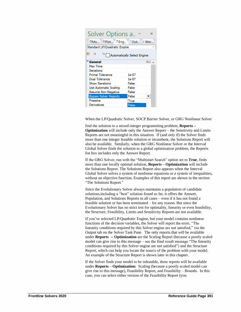
Frontline Solvers 2020 Reference Guide Page 391
When the LP/Quadratic Solver, SOCP Barrier Solver, or GRG Nonlinear Solver
find the solution to a mixed-integer programming problem, Reports –
Optimization will include only the Answer Report – the Sensitivity and Limits
Reports are not meaningful in this situation. If (and only if) the Solver finds
more than one integer feasible solution or incumbent, the Solutions Report will
also be available. Similarly, when the GRG Nonlinear Solver or the Interval
Global Solver finds the solution to a global optimization problem, the Reports
list box includes only the Answer Report.
If the GRG Solver, run with the “Multistart Search” option set to True, finds
more than one locally optimal solution, Reports – Optimization will include
the Solutions Report. The Solutions Report also appears when the Interval
Global Solver solves a system of nonlinear equations or a system of inequalities,
without an objective function. Examples of this report are shown in the section
“The Solutions Report.”
Since the Evolutionary Solver always maintains a population of candidate
solutions,including a “best” solution found so far, it offers the Answer,
Population, and Solutions Reports in all cases – even if it has not found a
feasible solution or has been terminated – for any reason. But since the
Evolutionary Solver has no strict test for optimality, linearity or even feasibility, the Structure, Feasibility, Limits and Sensitivity Reports are not available.
If you’ve selected LP/Quadratic Engine, but your model contains nonlinear
functions of the decision variables, the Solver will report the error, “The
linearity conditions required by this Solver engine are not satisfied,” via the
Output tab on the Solver Task Pane. The only reports that will be available
under Reports -- Optimization are the Scaling Report (because a poorly scaled
model can give rise to this message – see the final result message “The linearity
conditions required by this Solver engine are not satisfied”) and the Structure
Report, which can help you locate the source of the problem with your model.
An example of the Structure Report is shown later in this chapter.
If the Solver finds your model to be infeasible, three reports will be available
under Reports – Optimization: Scaling (because a poorly scaled model can
give rise to this message), Feasibility Report, and Feasibility – Bounds. In this
case, you can select either version of the Feasibility Report (you
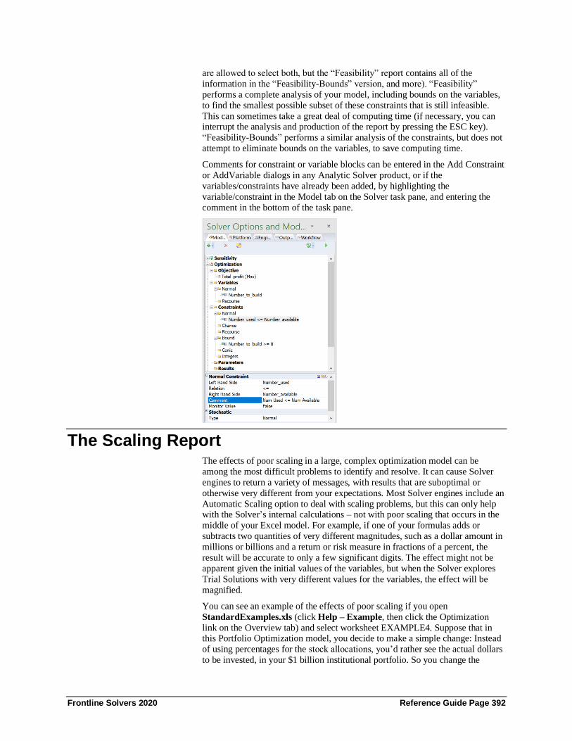
Frontline Solvers 2020 Reference Guide Page 392
are allowed to select both, but the “Feasibility” report contains all of the
information in the “Feasibility-Bounds” version, and more). “Feasibility”
performs a complete analysis of your model, including bounds on the variables,
to find the smallest possible subset of these constraints that is still infeasible.
This can sometimes take a great deal of computing time (if necessary, you can interrupt the analysis and production of the report by pressing the ESC key).
“Feasibility-Bounds” performs a similar analysis of the constraints, but does not
attempt to eliminate bounds on the variables, to save computing time.
Comments for constraint or variable blocks can be entered in the Add Constraint
or AddVariable dialogs in any Analytic Solver product, or if the
variables/constraints have already been added, by highlighting the
variable/constraint in the Model tab on the Solver task pane, and entering the
comment in the bottom of the task pane.
The Scaling Report The effects of poor scaling in a large, complex optimization model can be
among the most difficult problems to identify and resolve. It can cause Solver
engines to return a variety of messages, with results that are suboptimal or
otherwise very different from your expectations. Most Solver engines include an
Automatic Scaling option to deal with scaling problems, but this can only help with the Solver’s internal calculations – not with poor scaling that occurs in the
middle of your Excel model. For example, if one of your formulas adds or
subtracts two quantities of very different magnitudes, such as a dollar amount in
millions or billions and a return or risk measure in fractions of a percent, the
result will be accurate to only a few significant digits. The effect might not be
apparent given the initial values of the variables, but when the Solver explores
Trial Solutions with very different values for the variables, the effect will be
magnified.
You can see an example of the effects of poor scaling if you open
StandardExamples.xls (click Help – Example, then click the Optimization
link on the Overview tab) and select worksheet EXAMPLE4. Suppose that in this Portfolio Optimization model, you decide to make a simple change: Instead
of using percentages for the stock allocations, you’d rather see the actual dollars
to be invested, in your $1 billion institutional portfolio. So you change the

Frontline Solvers 2020 Reference Guide Page 393
constraint TotalPortfolio = 1 (or 100%) to TotalPortfolio = 1000000000.
Simply highlight the constraint, TotalPortfolio = 1 in the Model tab of the Solver
Task Pane, then enter 1E+21 for the Right Hand Side in the bottom of the task
pane, as shown in the screenshot below.
You change the cell formatting to display large numbers instead of percentages,
(CTRL + 1) and you select the Standard GRG Nonlinear Engine (as this engine
is more susceptible to scaling problems when compared to the Standard
LP/Quadratic engine) from the Engine drop down menu on the Engine tab.
When you click Solve, you’re surprised to find that the Solver reports it cannot
find a feasible solution, as shown below.

Frontline Solvers 2020 Reference Guide Page 394
The “solution” found in the Excel spreadsheet is clearly infeasible as the
constraint Total_Portfolio 1E+24 is clearly violated (not met). Since you’re
familiar with the Solver options, you set Use Automatic Scaling to True on the
Engine tab on the Solver task pane and click the Solve icon (green arrow) on the
Output task pane, but you just get a different infeasible result.
In fact – if you continue to click the Solve icon, (say 7 times) Solver will
continue to stop with an infeasible result while the value in cell H9 grows
exponentially. What’s wrong with the Solver? (Past users of the Solver products
have on occasions wrestled with problems just like this.)
Noticing that the Scaling Report is available under Reports - Optimization,
you select this report. The Scaling Report is inserted into your workbook. The
report indicates that there are scaling problems with the formula at the cell with
defined name, Portfolio_Variance (EXAMPLE4!I7). In a very large model, this
cell might be very hard to find by manual inspection. You can click on the
underlined cell reference to jump to cell I17 on the EXAMPLE4 worksheet. You
see that the Variance is a very large number – 1.19E+26. The Scaling Report has drawn your attention to a scaling issue in the formulas that calculate your model
–outside of the Solver’s own calculations.

Frontline Solvers 2020 Reference Guide Page 395
In seeking the optimal solution, the Solver is likely to try extreme values – large
and small – for the variables. This doesn‟t cause problems when the largest
value is 100% or 1 and the smallest is 0, but it does cause problems when the
largest value is greater than a trillion. At this point, calculation of the Portfolio
Variance involves adding a very small value and a very large one (the Stock 5 variance times 1 billion squared) which leads to a loss of accuracy. This loss of
accuracy leads directly to the Solver’s problem in finding a solution.
An Example Model To illustrate the other reports provided by the Analytic Solver products, we’ll
start with the model on worksheet EXAMPLE1 in the workbook
StandardExamples.xls. You can easily load this model by clicking Help –
Examples on the ASP ribbon, then click the Optimization link on the Overview
tab and click the StandardExamples.xlsx link. First, we’ll solve this model in
its original form, using the LP /Quadratic and GRG Solvers, and produce
Answer, Sensitivity and Limits Reports in Analytic Solver Desktop and Answer
and Sensitivity Reports in Analytic Solver Cloud and AnalyticSolver.com.
In brief, the Answer Report summarizes the original and final values of the
decision variables and constraints, with information about which constraints are
“binding” at the solution. The Sensitivity Report provides information about
how the solution would change for small changes in the constraints or the
objective function. And the Limits Report shows you the largest and smallest
value each decision variable can assume while satisfying the constraints, while all other variables are held fixed at their solution values.
Next, we’ll change the available inventory of Chassis at cell B11 to -1. This is
shown in Standard Examples.xlsx on the EXAMPLE2 worksheet. When we
attempt to solve, we receive the message “Solver could not find a feasible
solution,” and we can produce the report shown below in the section “The
Feasibility Report.”
Next, we’ll deliberately introduce a nonlinear function into the model, by
editing the formula at cell C11 to read
=SUMPRODUCT(D11:F11,$D$9:$F$9)^0.9. This is shown in
StandardExamples.xls on the EXAMPLE3 worksheet. When we attempt to
solve this model with the LP/Quadratic Solver, we’ll receive the message “The linearity conditions required by this Solver engine are not satisfied,” and we can
produce the report shown below in “The Structure Report.” Returning to the
unmodified version of EXAMPLE1, we’ll solve the model using the
Evolutionary Solver, waiting until we receive the message “Solver cannot
improve the current solution.” This allows us to produce the report shown below
in “The Population Report.” In V7.0, the Solutions Report was generalized to
report multiple solutions for integer programming problems, global optimization
problems, and non-smooth optimization problems, solved by any of the built-in
or plug-in Solver engines. We’ll illustrate this useful report with additional
examples.
The Solutions Report has a special meaning for the Interval Global Solver, because it can find multiple solutions for systems of equations and systems of
inequalities. To illustrate this, we’ll return to EXAMPLE 1 and make the Set
Cell blank, removing the objective function from this model. What remains is a
set of <= constraints – a system of inequalities (and bounds on the variables).
When we solve this model with the LP/Quadratic and GRG Solvers, we find
only a single feasible solution, which is not very informative. But when we
solve it with the Interval Global Solver, we get an “inner solution” – an entire
region of feasible solutions. To illustrate the Solutions Report for a system of

Frontline Solvers 2020 Reference Guide Page 396
equations, we’ll introduce a simple but historically interesting nonlinear
equation mentioned in the Introduction.
The Answer Report The Answer Report, which is available whenever a solution has been found,
provides basic information about the decision variables and constraints in the
model. It also gives you a quick way to determine which constraints are
“binding” or satisfied with equality at the solution, and which constraints have
slack. The Answer Report includes the message that appears in the Output tab of
the Solver Task Pane, the name of the Solver engine used to solve the problem,
and statistics such as the time, iterations and subproblems required to solve the
problem. An example Answer Report for the worksheet model EXAMPLE1 (when there are no upper bounds on the decision variables) is shown below.
First shown are the objective function and decision variables, with their original value and final values as well as the variable type. Next are the constraints, with
their final cell values; a formula representing the constraint; a “status” column
showing whether the constraint was binding or non-binding at the solution; and
the slack value – the difference between the final value and the lower or upper
bound imposed by that constraint.
A binding constraint, which is satisfied with equality, will always have a slack
of zero. This example shows the effect of automatic outlining of the Solver
reports, which you can turn on by clicking Reports – Optimization – Reports
are not outlined. The outline groups correspond directly to the blocks of
variables and constraints you entered in the Solver Parameters dialog – one
group per row in the Constraints or Variables list box. Comments entered in the Add Constraint and Add Variable dialogs for each block appear in the Answer
Report; they are visible whether the outline is expanded or collapsed.
When creating a report, the Solver constructs the entries in the Name column by
searching for the first text cell to the left and the first text cell above each

Frontline Solvers 2020 Reference Guide Page 397
variable (changing) cell and each constraint cell. If you lay out your Solver
model in tabular form, with text labels in the leftmost column and topmost row,
these entries will be most useful – as in the example above. Also note that the
formatting for the Original Value, Final Value and Cell Value is “inherited”
from the formatting of the corresponding cell in the Solver model.
The Sensitivity Report The Sensitivity Report provides classical sensitivity analysis information for
both linear and nonlinear programming problems, including dual values (in both
cases) and range information (for linear problems only). The dual values for
(nonbasic) variables are called Reduced Costs in the case of linear programming
problems, and Reduced Gradients for nonlinear problems. The dual values for binding constraints are called Shadow Prices for linear programming problems,
and Lagrange Multipliers for nonlinear problems. Constraints which are simple
upper and lower bounds on the variables, that you enter in the Constraints list
box of the Solver Parameters dialog, are handled specially (for efficiency
reasons) by both the linear and nonlinear Solver algorithms, and will not appear
in the Constraints section of the Sensitivity report. When an upper or lower
bound on a variable is binding at the solution, a nonzero Reduced Cost or
Reduced Gradient for that variable will appear in the “Adjustable Cells” section
of the report; this is normally the same as a Lagrange Multiplier or Shadow
Price for the upper or lower bound.
Note: The formatting of cells in the Sensitivity Report can make a significant difference in how the Reduced Gradient, Lagrange Multiplier, Reduced Cost and
Shadow Prices are displayed. Bear this in mind when designing your model and
when reading the report. Since the report is a worksheet, you can always change
the cell formatting with the Format menu.
An example of a Sensitivity Report generated for EXAMPLE1 when the
Solverengine is the Standard LP/Quadratic solver (and there are no upper
bounds on the variables) is shown below.
Interpreting Reduced Costs and Shadow Prices
Reduced Costs are the most basic form of sensitivity analysis information. The
reduced cost for a variable is nonzero only when the variable’s value is equal to
its upper or lower bound at the optimal solution. This is called a nonbasic
variable, and its value was driven to the bound during the optimization process.

Frontline Solvers 2020 Reference Guide Page 398
Moving the variable’s value away from the bound (or tightening the bound) will
worsen the objective function’s value; conversely, “loosening” the bound will
improve the objective. The reduced cost measures the increase in the objective
function’s value per unit increase in the variable’s value. In the example
Sensitivity Report above, the dual value for producing speakers is -2.5, meaning that if we were to build one speaker (and therefore less of something else), our
total profit would decrease by $2.50.
The Shadow Price for a constraint is nonzero only when the constraint is equal
to its bound. This is called a binding constraint, and its value was driven to the
bound during the optimization process. Moving the constraint left hand side’s
value away from the bound will worsen the objective function’s value;
conversely, “loosening” the bound will improve the objective. The Shadow Price
measures the increase in the objective function’s value per unit increase in the
constraint’s bound. In the example report above, increasing the number of
electronics units from 600 to 601 will allow the Solver to increase total profit by
$25.
In the case of linear problems, the Shadow Price remains constant over the range
of Allowable Increases and Decreases in the variables’ objective coefficients
and the constraints’ right hand sides, respectively. For example, for each
decision variable, the report shows its coefficient in the objective function, and
the amount by which this coefficient could be increased or decreased without
changing the dual value. In the example below, we’d still build 200 TVs even if
the profitability of TVs decreased up to $5 per unit. Beyond that point, or if the
unit profit of speakers increased by more than $2.50, we’d start building
speakers. For each constraint, the report shows the constraint right hand side,
and the amount by which the RHS could be increased or decreased without
changing the dual value.
In this example, we could use up to 50 more electronics units, which we’d use to
build more TVs instead of stereos, increasing our profits by $25 per unit.
Beyond 650 units, we would switch to building speakers at an incremental profit
of $20 per unit (a new dual value). A value of 1E + 30 in these reports represents
“infinity” In the example above, we wouldn’t build any speakers regardless of
how much the profit per speaker decreased.
Now, select the Standard GRG Nonlinear engine from the Engine tab on the
Solver Task Pane.
Then click the Solve icon (green arrow) on the Output tab. After the GRG
Nonlinear engine stops with the solution, “Solver found a solution,” click Reports – Optimization – Sensitivity to create a new Sensitivity Report.

Frontline Solvers 2020 Reference Guide Page 399
Interpreting Reduced Gradients and Lagrange Multipliers
The main differences between this report (created by the nonlinear GRG engine)
and the report above is that the Reduced Costs and Shadow Prices are referred to
as Reduced Gradients and Lagrange Multipliers, respectively and the Allowable
Increase and Allowable Decrease columns are not present on this report. This is
because Lagrange Multipliers are valid only at the single point of the optimal
solution – if there is any curvature involved, the LaGrange Multipliers begin to
change (along with the constraint gradients) as soon as you move away from the
optimal solution. However, if you compare the Reduced Gradients (for the
Variables) against the Reduced Costs on the report above, you’ll notice they are
identical. This is also true when comparing the LaGrange Multipliers (for the
constraints) against the Shadow Prices. Note: If you were to solve a quadratic
problem (which is a type of nonlinear problem) with the LP/Quadratic engine, the report would look the same.
The Limits Report The Limits Report, currently supported only in the Microsoft Excel Solver, was
designed by Microsoft to provide a specialized kind of “sensitivity analysis”
information. It is created by re-running the Solver model with each decision
variable (or Changing Cell) in turn as the objective (both maximizing and minimizing), and all other variables held fixed. Hence, it shows a “lower limit”
for each variable, which is the smallest value that a variable can take while
satisfying the constraints and holding all of the other variables constant, and an
“upper limit,” which is the largest value the variable can take under these

Frontline Solvers 2020 Reference Guide Page 400
circumstances. An example of the Limits Report for EXAMPLE1 is shown
below.
The Feasibility Report The purpose of the Feasibility Report is to help you isolate the source of
infeasibilities in your model. Most often, an infeasible result simply means that
you’ve made a mistake in formulating your model, such as specifying a <=
relation when you meant to use >=. However, if your model contains hundreds
or thousands of constraints, it can be quite challenging to locate an error of this
type. By isolating the infeasibility to a small subset of the constraints, the
Feasibility Report can show you where to look, and hence save you a good deal
of time. To produce the Feasibility Report, the Solver may test many different variations of your model, each one with different combinations of your original
constraints. This process ultimately leads to a so-called “Irreducibly Infeasible
System ” (IIS) of constraints and variable bounds which, taken together, make
the problem infeasible, but with the property that if any one of the constraints or
bounds is removed from the IIS, the problem becomes feasible.
In a model with many constraints that “interact” with each other in complex
ways, there may be many possible subsets of the constraints and bounds that
constitute an IIS. Often, some of these subsets have many fewer constraints than
others. The Solver attempts to find an IIS containing as few constraints as
possible, trying first to eliminate “formula” constraints and then to eliminate
simple variable bounds – since it is usually easier to understand the effects of variable bounds on the infeasibility of the resulting IIS.
If we attempt to solve EXAMPLE2 in the StandardExamples.xls workbook –
which is identical to EXAMPLE1 except that cell B11 (the right hand side of the
constraint C11 <= B11) is set to -1 – we receive the message “Solver could not
find a feasible solution.” At this point, we know only that the problem is
somewhere in the set of five constraints (C11:C15 <= B11:B15) and three
bounds on the variables. To pinpoint the problem, we click Reports –
Optimization and select Feasibility from the Reports list, producing a report
like the one shown below.
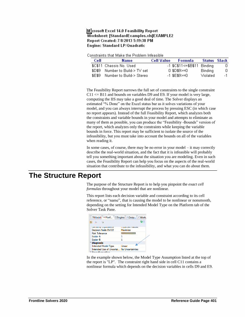
Frontline Solvers 2020 Reference Guide Page 401
The Feasibility Report narrows the full set of constraints to the single constraint C11 <= B11 and bounds on variables D9 and E9. If your model is very large,
computing the IIS may take a good deal of time. The Solver displays an
estimated “% Done” on the Excel status bar as it solves variations of your
model, and you can always interrupt the process by pressing ESC (in which case
no report appears). Instead of the full Feasibility Report, which analyzes both
the constraints and variable bounds in your model and attempts to eliminate as
many of them as possible, you can produce the “Feasibility -Bounds” version of
the report, which analyzes only the constraints while keeping the variable
bounds in force. This report may be sufficient to isolate the source of the
infeasibility, but you must take into account the bounds on all of the variables
when reading it.
In some cases, of course, there may be no error in your model – it may correctly
describe the real-world situation, and the fact that it is infeasible will probably
tell you something important about the situation you are modeling. Even in such
cases, the Feasibility Report can help you focus on the aspects of the real-world
situation that contribute to the infeasibility, and what you can do about them.
The Structure Report The purpose of the Structure Report is to help you pinpoint the exact cell formulas throughout your model that are nonlinear.
This report lists each decision variable and constraint according to its cell
reference, or “name”, that is causing the model to be nonlinear or nonsmooth,
depending on the setting for Intended Model Type on the Platform tab of the
Solver Task Pane.
In the example shown below, the Model Type Assumption listed at the top of the report is "LP". The constraint right hand side in cell C11 contains a
nonlinear formula which depends on the decision variables in cells D9 and E9.

Frontline Solvers 2020 Reference Guide Page 402
If we were to attempt to solve EXAMPLE3 in the StandardExamples.xls
workbook – which is identical to EXAMPLE1 except that the formula at cell
C11is edited to read =SUMPRODUCT(D11:F11,$D$9:$F$9)^0.9, a nonlinear
expression – we receive the message “The linearity conditions required by this Solver engine are not satisfied.” To pinpoint the problem, we click Reports –
Optimization and select Structure from the Reports list, producing a report like
the one shown below.
Variables D9 and E9 are shown as occurring nonlinearly in the model, and the
constraint at cell C11 (the formula that was edited) is a nonlinear function of the
variables. Although the formula at C11 refers to all three variable cells D9:F9,
the coefficient of F9 in this formula (at cell F11) is 0 – hence cell F9 does not
participate in this function, and only cells D9 and E9 are shown as occurring
nonlinearly in the model.
With this information, it is easy to pinpoint the formula at C11 as the source of
the nonlinearity. In real-world models, where a constraint such as C11 may
depend on many other cell formulas, your next step will be to locate the specific
formulas that are nonlinear, determine whether they are correct for your problem, and decide whether they can be rewritten as linear functions, or
whether there is an alternative, linear formulation of your problem (see the
chapter “Building Large-Scale Models” in the Analytic Solver User Guide for
ideas
The Population Report The Population Report gives you summary information about the entire population of candidate solutions maintained by the Evolutionary Solver at the
end of the solution process. The Population Report can give you insight into the
performance of the Evolutionary Solver as well as the characteristics of your
model, and help you decide whether additional runs of the Evolutionary Solver
are likely to yield even better solutions.
For each variable and constraint, the Population Report shows the best value
found by the Evolutionary Solver, and the mean (average) value, standard
deviation, maximum value, and minimum value of that variable or constraint
across the entire population of candidate solutions at the end of the solution
process. These values will give you an idea of the diversity of solutions
represented by the population.
If we run the Evolutionary Solver on EXAMPLE1 with upper bounds of 200 on
the variables, Solver stops with the result, “Solver cannot improve the current
solution” with a solution of D9 = E9 = 200 and F9 = 0 (the same as the linear
programming optimal solution). Clicking this result message on the Output tab
opens a Help window with the explanation of this result.
When the Evolutionary Solver is being used, this message is much
more common. It means that the Solver has been unable to find a new,

Frontline Solvers 2020 Reference Guide Page 403
better member of the population whose “fitness” represents a relative
(percentage) improvement over the current best member’s fitness of
more than the Tolerance option in the Task Pane Engine tab, in the
amount of time specified by the Max Time without Improvement
option on the same tab. Since the Evolutionary Solver has no way of testing for optimality, it will normally stop with either “Solver
converged to the current solution” or “Solver cannot improve the
current solution” if you let it run for long enough. If you believe that
this message is appearing prematurely, you can either make the
Tolerance value smaller (or even zero), or increase the amount of time
allowed by the Max Time without Improvement option.
Since this is the optimal solution, as found by the Standard LP/Quadratic engine,
there is no need to rerun this model. Click: Reports – Optimization –
Population to produce a Population Report like the one below.
You can see that the Best Values of the variables are identical to the Mean
Values across the whole population. In addition, the Best Values are either
identical or very close to both the Maximum and Minimum Values of the
population. Since the solution is feasible, and since the optimization process tends to drive variable values to extremes, this may indicate that we have found
a globally optimal solution (which is true in this case).
The Standard Deviations are relatively small, but this is not too surprising since
points in the population have not yet converged to the point where we would
receive “Solver has converged to the current solution.”
How you interpret the Population Report depends in part on your knowledge of
the problem, and past experience solving it with the Evolutionary Solver or with
other Solver engines. For example, if the Best Values are similar from run to
run, and if the Standard Deviations are small, this may be reason for confidence
that your solution is close to the global optimum. However, if the Best Values
vary from run to run, small Standard Deviations might indicate a lack of diversity in the population, suggesting that you should increase the Mutation
Rate and run the Solver again.

Frontline Solvers 2020 Reference Guide Page 404
The Solutions Report W here the Answer Report gives you detailed information about the single “best
solution” that appears on the worksheet when the Solver Results dialog is
displayed, the Solutions Report gives you objective function and decision
variable values for a number of alternative solutions, found during the
optimization process.
Integer Programming Problems
For mixed-integer problems, the report shows each incumbent or feasible integer
solution found by the Branch & Bound method during the solution process.
Below is an example of the Solutions Report for the Blending 2 example model
included in the example workbook, Blending(Opt).xlsx. (To open click Help –
Examples, then click the Blending(Opt).xlsx hyperlink on the Optimization tab
within the workbook, Frontline Example Models Overview.xlsx.) This problem was solved by the LP/Quadratic Solver with the Integer Tolerance set to 0.0 and
all Cuts & Heuristics disabled. (On this problem, with Cuts & Heuristics enabled
(set Preprocessing, Cuts, and Heuristics to “None” on the Engine tab), the
Solver quickly finds the true integer optimal solution as the third incumbent; the
Solutions Report is available only when multiple incumbents are found.) As
shown below, three incumbents were found.

Frontline Solvers 2020 Reference Guide Page 405
Global Optimization Problems
For global optimization problems, the report shows each locally optimal solution
found by the Multistart method. On the next page is an example of the Solutions
Report for a simple two-variable global optimization problem Branin.xls, solved
by the GRG Nonlinear Solver with the Multistart Search option selected. This
file can be opened by clicking Help – Examples and selecting Branin(Opt).xlsx from the Optimization tab.
In this problem, the “Branin function” must be minimized for variables x and y,
subject to bounds -5 <= x, y <= 10. (Additional bounds of -100 and 100 were
added as the Multistart Methods perform best when all variables have both
upper and lower bounds.) There are three distinct locally optimal solutions with
objective values, 4.11227 (worse), 2.79118 (better) and 0.397887 (best and
globally optimal). The Solver was started at the point x = -2.5, y = 10, which is
close to the second of the three locally optimal solutions. The Multistart Search
process runs the Solver from representative starting points in “clusters” of
randomly selected points; on this run, it first found a solution close to the worst
locally optimal point, then found a solution at the best and globally optimal point.
Non-Smooth Optimization Problems
For arbitrary non-smooth optimization problems, the report shows members of
the Solver’s final population of solutions. Below is an example of the Solutions
Report for the global optimization problem Branin.xlsx, solved by the
Evolutionary Solver.
Again the Solver was started at the point x = -2.5, y = 10, and it was given a
limit of only 200 subproblems. Unlike the Solutions Report for gradient-based
nonlinear optimizers like the GRG Nonlinear Solver, the final population of
solutions is not likely to include many distinct locally optimal points. The best
solutions in the Evolutionary Solver’s final population are all in the
neighborhood of the globally optimal solution, which is x = 3.14159, y =
2.2750. But since the Evolutionary Solver doesn’t require gradient information
or test for local optimality, it is unlikely to find the globally optimal solution with very high accuracy for a smooth nonlinear problem like Branin(Opt).xlsx.

Frontline Solvers 2020 Reference Guide Page 406
Solutions for Systems of Inequalities
The Solutions Report has a special meaning for the Interval Global Solver. It is
available for problems with no objective function to be maximized or
minimized, and with all equality constraints (a system of equations) or all
inequality constraints (a system of inequalities). For a system of equations, the
report is available only if the number of variables and the number of constraints
are equal. If we remove the objective function from the model (by highlighting the objective on the Model tab in the Task Pane and clicking the red X) what
remains is a set of <= constraints – a system of inequalities (and bounds on the
variables). When there is no objective, the Solver will simply find a solution that
satisfies the constraints.
If we solve EXAMPLE1with a blank Set Cell using the LP/Quadratic Solver, we
get a solution where all three variables D9, E9 and F9 are 0. This is certainly a
feasible solution, but it’s not very informative. If we solve the model with the
GRG Solver, we get a solution where all three variables are 100 (equal to the
starting values of the variables). This too is a feasible solution, but it’s also not
very informative. Can we learn something more about the range of feasible
solutions?
If we solve the model with the Interval Global Solver, we get a solution where
all three variables are 75. If we select the Solutions Report from the Solver
Results dialog and click OK, a report like the one below will appear.
The report tells us that the problem has an infinite number of solutions, and it
gives us an “inner solution” – a set of ranges or intervals for each decision
variable, such that all points within these ranges satisfy the system of
inequalities. An inner solution is always a “box” with a dimension for each
decision variable (in general, the ranges for each variable may be different), and
this box lies entirely within the feasible region. It does not usually enclose all of
the feasible points – which can form an arbitrary multidimensional “shape” – and it is also not unique (there can be many possible inner solutions). But it will
give you a much better idea of the range of feasible solutions than you can get
from the Answer Report.
Solutions for Systems of Equations
The Solutions Report for a system of equations can be considerably more
valuable than the Answer Report or the Solutions Report for a system of
inequalities. It relies on the unique ability of the Interval Global Solver to find
all real solutions of a system of nonlinear equations.

Frontline Solvers 2020 Reference Guide Page 407
We can illustrate the Solutions Report for a system of equations with the
simplest case of a single equation – drawn from the 1983 textbook Numerical
Methods for Unconstrained Optimization and Nonlinear Equations, by Jack E.
Dennis and Robert B. Schnabel. This classic (and still popular) textbook – a key
learning resource for the designers of the Microsoft Excel Solver at Frontline Systems in 1990 – describes the capabilities and limitations of methods for
nonlinear optimization and solution of nonlinear equations, using an example in
Section 2.1, titled “What Is Not Possible:”
“Consider the problem of finding the real roots of each of the following
nonlinear equations in one unknown:
f1(x) = x4 – 12x3 +47x2 – 60x,
f2(x) = x4 – 12x3 +47x2 – 60x + 24,
f3(x) = x4 – 12x3 +47x2 – 60x + 24.1.
It would be wonderful if we had a general-purpose computer routine that would tell us: “The roots of f1(x) are x = 0, 3, 4, and 5; the real roots of f2(x)
are x =1 and x ≈ 0.888; f3(x) has no real roots.” It is unlikely that there will
ever be such a routine. In general, the questions of existence and uniqueness
… are beyond the capabilities one can expect of algorithms that solve
nonlinear problems.”
Note that f1(x), f2(x) and f3(x) differ only in the constant term – 0, 24 and 24.1.
Let’s try to solve these equations (for zero roots) in Microsoft Excel. Starting
with a blank worksheet, enter 0 in cell A1 for x, 0 in cell A2 for the constant
term, and in cell A3 enter the equation as =A1^4 - 12*A1^3 + 47*A1^2 - 60*A1
+ A2. In the Model tab on the Solver Task Pane, enter A1as a Variable, and
enter A3 as the Objective with Value Of 0, or else leave the Set Cell blank and enter A3 = 0 in the Constraints list box. Since the Interval Global Solver
requires bounds on the variables, also add constraints A1 <= 100 and A1 >= -
100. Using A2 = 0 initially, we are solving f1(x).
If you select the Interval Global Solver, click the Solve icon (green arrow) on
the Model tab, and select the Solutions Report under Reports -- Optimization,
a report like the one below will appear.
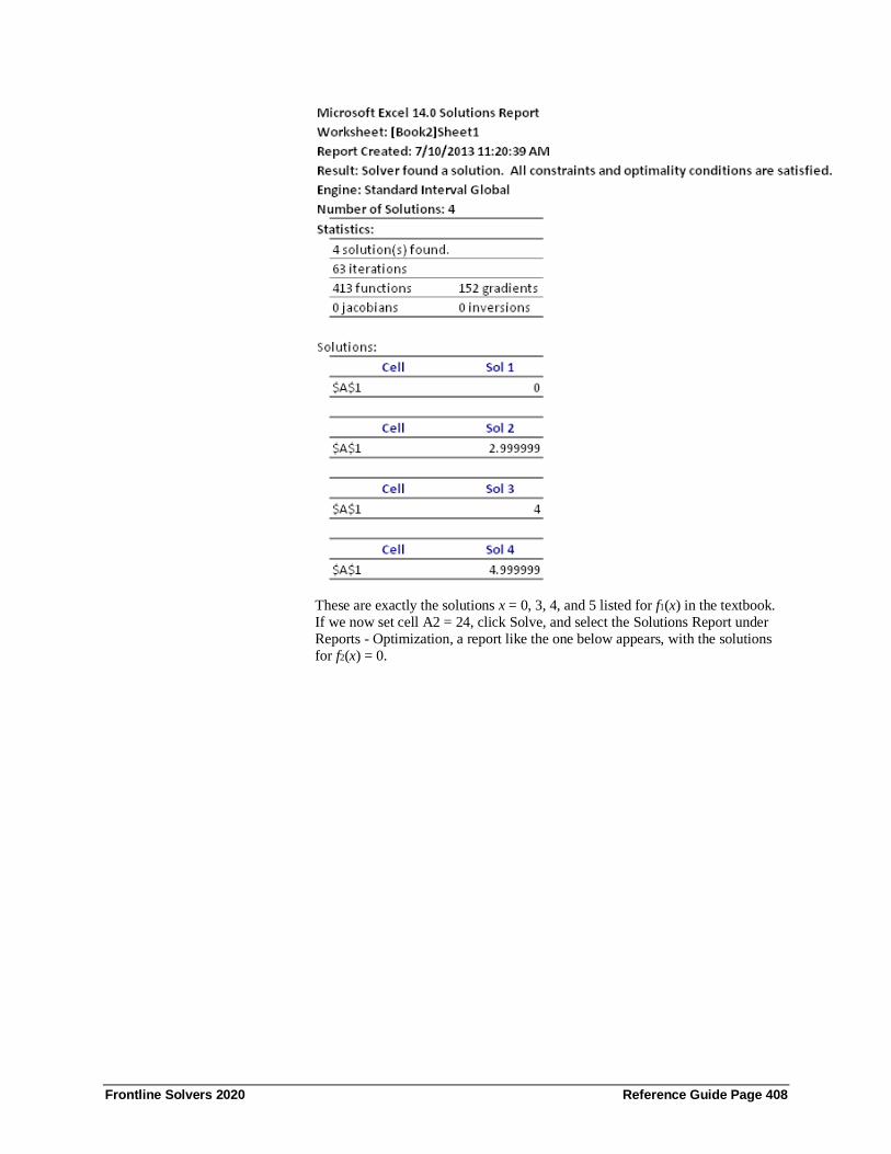
Frontline Solvers 2020 Reference Guide Page 408
These are exactly the solutions x = 0, 3, 4, and 5 listed for f1(x) in the textbook.
If we now set cell A2 = 24, click Solve, and select the Solutions Report under
Reports - Optimization, a report like the one below appears, with the solutions
for f2(x) = 0.

Frontline Solvers 2020 Reference Guide Page 409
Again, these are exactly the solutions x =1 and x ≈ 0.888 listed in the textbook.
If we set A2 = 24.1 and click Solve, the Solver Results dialog appears with
“Solver could not find a feasible solution.”
As this example illustrates, the Interval Global Solver is “ a general-purpose
computer routine” that will tell us: “The roots of f1(x) are x = 0, 3, 4, and 5; the
real roots of f2(x) are x =1 and x ≈ 0.888; f3(x) has no real roots.” And this
capability is not limited to polynomial functions – it is effective for all
continuously differentiable functions.

Frontline Solvers 2020 Reference Guide Page 410
Dennis and Schnabel’s pessimistic prediction that “It is unlikely that there will
ever be such a routine” was probably correct for classical nonlinear optimization
methods that evaluate functions only over real numbers. But the ability of the
Analytic Solver to evaluate Excel formulas over intervals, combined with
interval methods for global optimization, has made such a routine not only possible, but easy to use.

Frontline Solvers 2020 Reference Guide Page 411
VBA Object Model Reference
Introduction This chapter explains how to use the Object-Oriented API in Analytic Solver Desktop to create, modify and solve optimization and simulation models under
the control of your custom application written in VBA.
Note: Calling the VBA Objective Model is not supported in Analytic Solver
Cloud and AnalyticSolver.com.
In the simplest case, you can use a few standard lines of VBA code to run an
optimization or simulation, as described below. But you can do much more in
VBA, to create custom applications that use optimization or simulation.
You can define a Problem and instantiate it from the spreadsheet with two lines
of code, then access the elements of your model via Variable and Function
objects. You can perform optimizations or simulations, access the values of decision variables, constraints and the objective, access trial data and summary
statistics for uncertain variables and functions, and present them the way you
want to your end user. All the power of the Excel object model is available,
including database access, charts and graphs, and custom dialogs and controls.
Analytic Solver’s VBA object model closely resembles the object-oriented API
of Frontline’s Solver SDK Platform or Solver SDK Pro – which can run on a
PC or server without Excel, solve an optimization or simulation model in an
Excel workbook (only Solver SDK Platform), or solve a model that is defined
entirely in programming language code (either Solver SDK Platform). This
makes it very easy to move an application from Excel to a custom program
written in C/C++, Visual Basic, VB.NET, Java or MATLAB.
Adding a Reference in the VBA Editor
To use the new object-oriented API in VBA, you must first add a reference to
the type library for the Analytic Solver COM server. To do this:
1. Press Alt-F11 to open the VBA Editor.
2. Select menu choice Tools References.
3. Scroll down until you find Analytic Solver 2018 Type Library.
4. Check the box next to this entry, and click OK to close the dialog.
5. Use File Save to save your workbook.
Note that this is a different reference from Solver, which is the reference you
add in order to use the “traditional” VBA functions.
You need this reference if your VBA code uses the Event Listener as described
in the next section, or uses other elements of the Analytic Solver VBA object
model, described in later sections of this chapter (or both).

Frontline Solvers 2020 Reference Guide Page 412
Analytic Solver Object Model
Analytic Solver makes available a hierarchy of objects for describing Monte
Carlo simulation problems, pictured below. This object model is a simplified
subset of the object hierarchy offered by Frontline’s Solver SDK Platform
product, which is used to build custom applications in C/C++, Visual Basic,
VB.NET, Java or MATLAB. Note that the same objects are used for both
optimization and simulation problems.
The Problem object represents the whole problem, and the Model object
represents the internal structure of the model, which in Analytic Solver is
defined by your formulas on the spreadsheet.
The Solver object represents either the optimization process or the simulation
process – you call its Optimize method to perform an optimization, or its
Simulate method to perform a Monte Carlo simulation.
The Engine object represents a Solver Engine for optimization, or Risk Solver
Engine for simulation – it has a collection of EngineParam objects you can set to
control how it performs an optimization or simulation.
A Variable object represents a range of one or more contiguous cells that
contains either decision variables or uncertain variables; a Function object
represents a range of cells that contains the objective, constraints, or uncertain
functions.
A Parameter object represents a cell that is automatically varied when you
perform multiple optimizations, multiple simulations, or sensitivity analysis.
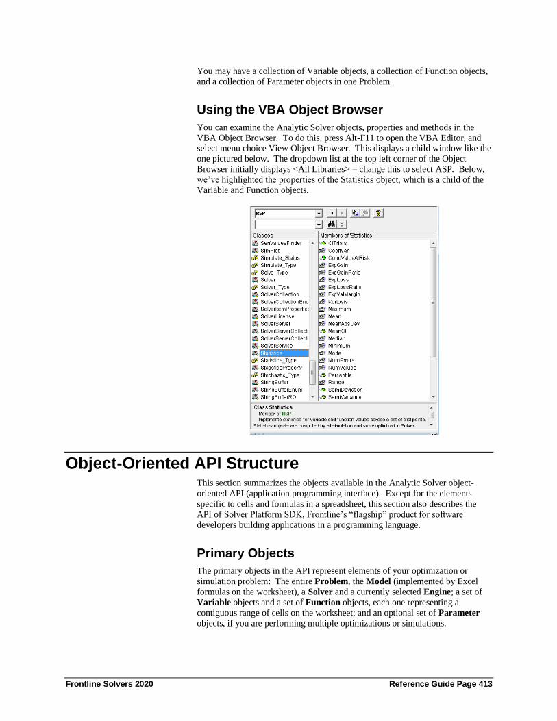
Frontline Solvers 2020 Reference Guide Page 413
You may have a collection of Variable objects, a collection of Function objects,
and a collection of Parameter objects in one Problem.
Using the VBA Object Browser
You can examine the Analytic Solver objects, properties and methods in the
VBA Object Browser. To do this, press Alt-F11 to open the VBA Editor, and select menu choice View Object Browser. This displays a child window like the
one pictured below. The dropdown list at the top left corner of the Object
Browser initially displays <All Libraries> – change this to select ASP. Below,
we’ve highlighted the properties of the Statistics object, which is a child of the
Variable and Function objects.
Object-Oriented API Structure This section summarizes the objects available in the Analytic Solver object-
oriented API (application programming interface). Except for the elements
specific to cells and formulas in a spreadsheet, this section also describes the
API of Solver Platform SDK, Frontline’s “flagship” product for software
developers building applications in a programming language.
Primary Objects
The primary objects in the API represent elements of your optimization or
simulation problem: The entire Problem, the Model (implemented by Excel
formulas on the worksheet), a Solver and a currently selected Engine; a set of
Variable objects and a set of Function objects, each one representing a
contiguous range of cells on the worksheet; and an optional set of Parameter
objects, if you are performing multiple optimizations or simulations.

Frontline Solvers 2020 Reference Guide Page 414
Class
Name Description
Problem Represents an entire Problem.
Solver Represents either simulation or optimization.
Engine Represents a built-in or plug-in Solver Engine for optimization, or
Risk Solver Engine for simulation.
Evaluator Represents user-written code to be called by an Engine when
various events occur during the solution of a Problem.
Model Defines how the user’s model can be evaluated.
Variable Represents a vector of variables, all of the same type.
Function Represents a vector of functions, all of the same type.
Parameter Represents a parameter that will be varied when performing
multiple optimizations, simulations, or worksheet evaluations.
A Problem object has members that represent collections of Solvers, Engines,
Evaluators, Variables, Functions and Parameters. You can subscript the name of a collection to access a specific object – for example one Engine or one Variable
object – using either its (integer) ordinal position in the collection, or its name.
For example:
MsgBox myProb.Engines(i).Name
MsgBox myProb.Variables("D9:F9").Value(i)
MsgBox myProb.Functions("Total Profit").Value(0)
In both Analytic Solver and Solver Platform SDK, you can easily write code that
steps through all of the objects in a collection. For example:
For i = 0 To myProb.Variables.Count - 1
MsgBox myProb.Variables(i).Name
Next i
In VBA, you can also iterate through a collection using a “for each” loop:
Dim myVar As Variable
For Each myVar In myProb.Variables
MsgBox myVar.Name
Next
Since a Variable object represents a contiguous range of uncertain variable cells
on the worksheet, its properties (for example FinalValue) represent arrays of
numbers. Again you can subscript these properties in your VBA code. For example:
For i = 0 To prob.Variables.Count – 1
For j = 0 To prob.Variables(i).Size - 1
MsgBox prob.Variables(i).FinalValue(j)
Next j
Next i

Frontline Solvers 2020 Reference Guide Page 415
Secondary Objects
The secondary objects in the API allow you to work with sets of numbers that
are associated with the Model, an Engine, a Variable or Function, or
optimization or simulation results. The ModelParam and EngineParam
objects each represent one parameter for the modeling system (PSI Interpreter)
or a Solver Engine, respectively. The Statistics object groups together, for
convenient access, statistics computed for both Variables and Functions during a simulation; it is also used by certain Solver Engines for optimization. The
Distribution object represents a probability distribution, and includes methods
to fit a distribution to sample data. The OptIIS object holds the results of an
optimization model infeasibility analysis.
The DoubleMatrix and DependMatrix objects represent sparse matrices – they
can be created in your code with a Dim statement to hold a large matrix of
numbers or dependency information, respectively. A matrix object could be
dimensioned as (say) 1 million rows by 1 million columns, but would reserve
memory only for its nonzero elements; you can use this object much like a two-
dimensional array in assignments statements in your code.
Class Name Description
ModelParam Represents a single Model (PSI Interpreter) parameter.
EngineParam Represents a single Engine parameter.
EngineLimit Represents the problem size limits for an Engine.
EngineStat Represents statistics from the last run of an Engine.
OptIIS Represents an Irreducibly Infeasible Subset of the constraints
and variable bounds in an optimization problem.
Statistics Represents statistics for variable and function values across the
trials of a simulation, or population of final solutions.
Distribution Represents a probability distribution for an uncertain variable,
or a fitted distribution for an uncertain function.
DoubleMatrix Represents a matrix of double values, of dimension m (rows) by
n (columns).
DependMatrix Represents a matrix of integers of values drawn from the
Depend_Type enum.
Primary Objects This section describes the primary objects available in Analytic Solver’s object-
oriented API, and their properties and methods. As noted above, these objects
represent the main elements of your optimization or simulation problem.

Frontline Solvers 2020 Reference Guide Page 416
Problem Object
The Problem object is created to represent an optimization or simulation
problem, with a VBA statement such as:
Dim prob As New Problem
Problem Methods
You can use the Init method to instantiate the Problem from a named model or
worksheet – this will create all of the Variable and Function objects for the
problem defined in that model or worksheet. (If you don’t use Init, the Problem
is instantiated from the active worksheet.) You can use the Load method to
load a set of problem specifications, or the Save method to save problem
specifications on the worksheet.
Problem.Init Worksheet (optimization)
Problem.Init Workbook (simulation)
Problem.Load RangeOrModel, Format
Problem.Save Range, Format
Worksheet is an Excel Worksheet object – an optimization model is based on a
worksheet, though it can include variables and functions from several
worksheets. You can call the following line of code to specify a specific
worksheet.
Problem.Init Worksheets(“WorksheetName”)
Or this line of code to specify the active worksheet.
Problem.Init ActiveSheet
Workbook is an Excel Workbook object – a simulation model includes all of the
uncertain variables and functions in a workbook. You can call the following line
of code to specify the active workbook.
Problem.Init ActiveWorkbook
Or this line of code to specify a specific workbook.
Problem.Init Workbooks(“WorkbookName”)
The Load and Save methods are used to load or save model specifications in a cell range. Range is an Excel range object, and RangeOrModel may be either an
Excel Range object or a text string model name. Format is one of the symbolic
constants File_Format_XLStd (a format compatible with the standard Excel
Solver) or File_Format_XLPSI (a format consisting of PSI function calls).
Problem Properties
Property Name Property
Type
Description
Name string Name of the workbook defining the
problem.
ProblemType Problem_Type
Problem type (linear, nonlinear, etc.,
simulation, or simulation
w/correlations)

Frontline Solvers 2020 Reference Guide Page 417
ProblemConvex Convex_Type Indicates whether problem is convex.
ProblemStochastic Stochastic
_Type
Indicates whether problem is
stochastic (depends on uncertainty).
ObjectiveIndex integer Index of the current objective
function; currently always 0.
Solver Solver Current Solver – either optimization
or simulation.
Engine Engine Current Engine for optimization, or
Risk Solver Engine for simulation.
Model Model Current Model.
VarDecision Variable Current (conventional or first-stage)
decision variable block.
VarRecourse Variable Current recourse decision variable
block, if recourse decisions are used.
FcnConstraint Function Current (normal or ‘hard’) constraint
function block.
FcnObjective Function Current objective function block.
FcnSoftConst Function Current chance (or ‘soft’) constraint
function block, if these are used.
VarUncertain Variable Current uncertain variable block.
FcnUncertain Function Current uncertain function block.
TrialPeriod integer
For a trial license, the number of days
remaining in the trial period. 32767
indicates a permanent license.
Collection Name Object Type Description
Solvers Solver Two members, for optimization and
simulation.
Engines Engine
Six members – built-in Solver Engines
for optimization, plus Risk Solver
Engine for simulation.
Evaluators Evaluator User-defined Evaluators – initially
none.
Variables Variable Ranges of contiguous variable cells.
Functions Function Ranges of contiguous function cells.
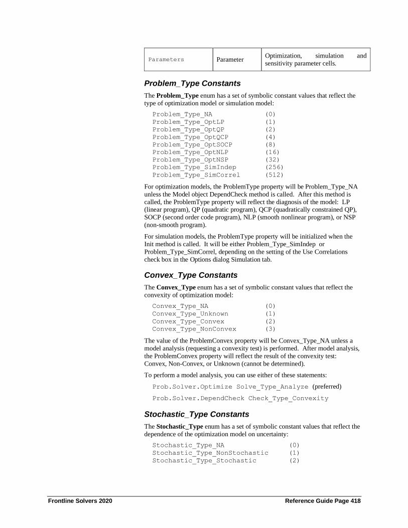
Frontline Solvers 2020 Reference Guide Page 418
Parameters Parameter Optimization, simulation and
sensitivity parameter cells.
Problem_Type Constants
The Problem_Type enum has a set of symbolic constant values that reflect the
type of optimization model or simulation model:
Problem_Type_NA (0)
Problem_Type_OptLP (1)
Problem_Type_OptQP (2)
Problem_Type_OptQCP (4)
Problem_Type_OptSOCP (8)
Problem_Type_OptNLP (16)
Problem_Type_OptNSP (32)
Problem_Type_SimIndep (256)
Problem_Type_SimCorrel (512)
For optimization models, the ProblemType property will be Problem_Type_NA
unless the Model object DependCheck method is called. After this method is
called, the ProblemType property will reflect the diagnosis of the model: LP (linear program), QP (quadratic program), QCP (quadratically constrained QP),
SOCP (second order code program), NLP (smooth nonlinear program), or NSP
(non-smooth program).
For simulation models, the ProblemType property will be initialized when the
Init method is called. It will be either Problem_Type_SimIndep or
Problem_Type_SimCorrel, depending on the setting of the Use Correlations
check box in the Options dialog Simulation tab.
Convex_Type Constants
The Convex_Type enum has a set of symbolic constant values that reflect the
convexity of optimization model:
Convex_Type_NA (0)
Convex_Type_Unknown (1)
Convex_Type_Convex (2)
Convex_Type_NonConvex (3)
The value of the ProblemConvex property will be Convex_Type_NA unless a
model analysis (requesting a convexity test) is performed. After model analysis,
the ProblemConvex property will reflect the result of the convexity test:
Convex, Non-Convex, or Unknown (cannot be determined).
To perform a model analysis, you can use either of these statements:
Prob.Solver.Optimize Solve_Type_Analyze (preferred)
Prob.Solver.DependCheck Check_Type_Convexity
Stochastic_Type Constants
The Stochastic_Type enum has a set of symbolic constant values that reflect the
dependence of the optimization model on uncertainty:
Stochastic_Type_NA (0)
Stochastic_Type_NonStochastic (1)
Stochastic_Type_Stochastic (2)

Frontline Solvers 2020 Reference Guide Page 419
The value of the ProblemStochastic property will be Stochastic_Type_NA
unless a model analysis (requesting a structure or convexity test) is performed.
After this method is called, the ProblemStochastic property will reflect the
dependence of the model on uncertain parameters: Stochastic or Non-Stochastic.
Solver Object
The Solver object represents either the optimization process or the simulation
process. For optimization models, you call its method Optimize to solve the
problem, and access its property OptimizeStatus to check the final status (e.g.
optimal, infeasible, unbounded) of the optimization. For simulation models, you
call its method Simulate to solve the problem, and access its property
SimulateStatus to check the final status of the simulation.
There is only one instance of the Solver object in a problem; this is created
automatically when you create a Problem, and is accessible via a reference such
as myProb.Solver.
Solver Methods
The Optimize method runs the currently selected Solver engine to solve the
problem for the current Model, Variables and Functions. The RestoreVariables
method may be called after an optimization to reset the decision variable cells to
their values before the optimization was started. The IISFind method may be
called if the OptimizeStatus property indicates that no feasible solution was
found – it finds an Irreducibly Infeasible Subset (IIS) of the constraints. The
Report method produces a Solver report, in the form of an Excel worksheet inserted into the active workbook.
Solver.Optimize
Solver.RestoreVariables
Solver.IISFind
Solver.Report ReportName
ReportName is one of the following text strings: "Scaling", "Answer",
"Sensitivity", "Limits", "Feasibility", "Structure", "Population", "Solutions".
The Simulate method runs the currently selected Solver engine to perform a
Monte Carlo simulation for the current Model, Variables and Functions. The
TrialStep method steps through, and displays on the Excel worksheet, trials from the most recent simulation. Stepsize is a positive or negative integer
specifying the number of trials to step forward (positive) or back (negative).
Trialtype is 0 to step through all trials, 1 for normal trials (those with no error
values), or 2 for error trials (those where some uncertain function returned an
error value).
Solver.Simulate
Solver.TrialStep stepsize, trialtype
Accessing Multiple Solutions
For global optimization and mixed-integer programming problems, most Solver
engines find multiple solutions. The best of these solutions is returned via the
FinalValue property of the Variable and Function objects associated with the
problem. But you can access any of the solutions from your VBA code. To do this, set the Solver object SolutionIndex property to an integer from 0 to the

Frontline Solvers 2020 Reference Guide Page 420
value of the NumSolutions property – 1; then access the FinalValue property of
the Variable and Function objects associated with the problem. For example:
For i = 0 To myProb.Solver.NumSolutions - 1
myProb.Solver.SolutionIndex = i
MsgBox myProb.FcnObjective.FinalValue(0)
Next i
Solver Properties
Property Name Property Type Description
SolverType Solver_Type
Type of solution to find:
Solver_Type_Maximize,
Solver_Type_Minimize, or
Solver_Type_FindFeas for optimization models, or
Solver_Type_Simulate for
simulation models.
Problem Problem Problem associated with this
Solver.
Index integer Index in the Solver
Collection; always 0.
OptimizeStatus Optimize_Status
Status after optimization, for
current SolutionIndex and
OptimizationIndex. See
below for possible values.
OptIIS OptIIS
Retrieves the Irreducibly
Infeasible Subset found by
IISFind.
NumSolutions integer Number of different
solutions available.
SolutionIndex integer
Index of the current solution;
used to access multiple
solutions.
NumOptimizations integer Number of different
optimizations to perform.
OptimizationIndex integer
Index of the current optimization; used to access
multiple optimizations.
SimulateStatus Simulate_Status
Status after simulation, for
current SimulationIndex;
see below for possible
values.

Frontline Solvers 2020 Reference Guide Page 421
NumTrials integer
Number of trials to perform
in each simulation. Also
used in Robust Counterpart
or Determ Equivalent
transformation.
NumSimulations integer Number of different
simulations to perform.
SimulationIndex integer
Index of the current
simulation; used to access
multiple simulations.
TrialIndex integer
Index of the trial to display
on the worksheet. If 0,
uncertain variables display
their sample mean values.
TrialDisplay Display_Type
Display_Type_BaseCase,
Disply_Type_Mean,
Display_Type_AllTrial,
Display_Type_NormalTrial,
Display_Type_ErrorTrial
Optimize_Status Constants
The Optimize_Status enum has a set of symbolic constant values that reflect the results of performing an optimization:
Optimize_Status_Api_Err
Optimize_Status_Bad_Dataset
Optimize_Status_Bbmips_Limit
Optimize_Status_Bbnode_Limit
Optimize_Status_Bounds_Conflict
Optimize_Status_Bounds_Inconsist
Optimize_Status_Bounds_Missing
Optimize_Status_Cone_Overlap
Optimize_Status_Converged
Optimize_Status_Derivative_Err
Optimize_Status_Exception
Optimize_Status_Float_Err
Optimize_Status_Incumb_Cand
Optimize_Status_Interpret_Err
Optimize_Status_Invalid
Optimize_Status_Iterate_Limit
Optimize_Status_Lic_Problem
Optimize_Status_Linear_Invalid
Optimize_Status_Memory_Dearth
Optimize_Status_No_Remedies
Optimize_Status_Optimal
Optimize_Status_Probable
Optimize_Status_Time_Out
Optimize_Status_Unbounded
Optimize_Status_Unfeasible
Optimize_Status_User_Abort
Frontline Solvers 2020 Reference Guide Page 422
For more information about these result codes, see the chapter “Solver Results
Messages.”
Accessing Different Optimizations
You can perform multiple optimizations at once, under the control of your VBA
code when you call prob.Solver.Optimize. You can access the final objective
and variable values and dual values for any of these optimizations in your VBA
code. To do this, set the Solver object OptimizationIndex property to an integer
from 0 to the value of the Problem object NumOptimizations property – 1; then
access the members of each Variable and Function object associated with the
problem.
Simulate_Status Constants
The Simulate_Status enum has a set of symbolic constant values that reflect the
results of performing a simulation:
Simulate_Status_Complete
Simulate_Status_User_Abort
Simulate_Status_Lic_Problem
Simulate_Status_Memory_Dearth
Simulate_Status_Interpret_Err
The normal status after a simulation completes is Simulate_Status_Complete.
Simulate_Status_User_Abort indicates that you pressed the ESC key in
interactive mode to abort a simulation, or that your Evaluator in VBA returned
the symbolic value Engine_Action_Stop. Simulate_Interpret_Err indicates that the PSI Interpreter found an unsupported Excel function or other error when
analyzing the formulas in your model. Simulate_Memory_Dearth indicates
that insufficient memory was available to perform the simulation.
Simulate_Status_Lic_Problem indicates a problem with your license to run
Risk Solver – it may be expired or invalid for this computer; please call
Frontline Systems at 775-831-0300 or email [email protected] for assistance.
Accessing Different Simulations
You can also perform multiple simulations at once, either via Interactive
Simulation or under the control of your VBA code when you call
prob.Solver.Simulate. You can access the statistics and trials for any of these
simulations in your VBA code. To do this, set the Solver object
SimulationIndex property to an integer from 0 to the value of the Problem object
NumSimulations property – 1; then access the members of the embedded
Statistics object, or the AllTrials property of each Variable and Function object
associated with the problem.
Engine Object
An Engine object represents a single Solver engine for optimization, such as the
LP/Quadratic Solver or the GRG Nonlinear Solver, or it represents Risk Solver
Engine for simulation.
A collection of Engine objects, one for each installed (built-in or plug-in) Solver
engine, is created automatically when you create a Problem, and is accessible
via a reference such as myProb.Engines. You can subscript the Engines
collection, either by an integer index or by a text string name, to access a
specific Engine.

Frontline Solvers 2020 Reference Guide Page 423
The Problem’s Engine property refers to the currently selected Solver engine.
When the Solver.Optimize method is called, this engine will be run. To select a
different Solver engine, you can either assign a new reference to the Engine
property, for example myProb.Engine = myProb.Engines("Standard
LP/Quadratic"), or you can call the chosen Solver Engine object’s MakeCurrent method. When the Solver.Simulate method is called, Risk
Solver Engine is always run.
Engine Methods
The MakeCurrent method causes this Solver engine to become the currently
selected Engine; after calling this method, myProb.Engine will refer to this
Solver engine, and myProb.Solver.Optimize will run this Solver engine. The ParamReset method resets all of the Solver engine parameters (EngineParam
objects) in this Engine’s Params collection to their default values.
Engine.MakeCurrent
Engine.ParamReset
Engine Properties
Property Name Property
Type
Description
Problem Problem Problem associated with this Engine.
ProblemType Problem_Type Type of problem solved by this Engine.
Name string Name of this Solver engine.
FileSpec string
Filename/path of this Engine’s dynamic
link library. For built-in Engines, returns
an empty string and for external engines
it returns the name of the DLL.
Params EngineParam
Collection
The collection of all parameters for this
Solver engine.
Limit EngineLimit
array
Engine size limits; indexed by Problem
Type.
Index integer Index in the EngineCollection of
this Engine object.
Stat EngineStat Engine statistics from the last Optimize
method call using this Solver engine.
Constant Name Description
LPQPName Name of the built-in LP/QP Solver engine.
LPName Name of the built-in LP Simplex Solver engine. (Not
present in V2018.)
SOCPName Name of the built-in SOCP Barrier Solver engine.

Frontline Solvers 2020 Reference Guide Page 424
GRGName Name of the built-in GRG Nonlinear Solver engine.
EVOName Name of the built-in Evolutionary Solver engine.
INTName Name of the built-in Interval Global Solver engine.
Evaluator Object
An Evaluator object represents a “callback function” you have written in VBA,
that Analytic Solver will call at certain times during the optimization or
simulation process. No Evaluators are required, but you may find it useful to
create one or more Evaluators to monitor or report progress – or even stop
Solver, especially if the optimization or simulation takes a long time.
Using an Evaluator to Check the Progress of an
Optimization or Simulation An evaluator can be used to obtain control from Solver during, before, or after
an optimization or simulation to check the progress of the solution process, to
display a message, etc. For an optimization, there are four such evaluators
available of type: Eval_Type_Iteration, Eval_Type_NewSolution,
Eval_Type_Optimization, and Eval_Type_Subproblem. For a simulation, there are three such evaluators available of type: Eval_Type_Sample,
Eval_Type_Simulation, and Eval_Type_Trial. Please see the table below for an
explanation of each. Progress information evaluators are always optional.
Optimization/Simulation Progress Information
Evaluators
Eval_Type_Iteration Optimization Called on each optimization
iteration. Can be used to track
the progress (check the objective
function, number of iterations,
etc.) of the optimization.
Eval_Type_NewSolution Optimization Called each time a new solution
is found to a mixed-integer
problem (MIP), or nonlinear/nonsmooth
optimization model.
Eval_Type_Optimization Optimization Called at the beginning of each
new optimization, when
NumOptimizations > 1
Eval_Type_Sample Simulation Called once, after
Problem.Solver.Simulate, prior
to starting the first (or only)
simulation.
Eval_Type_Simulation Simulation Called at the end of each
simulation - more than once if
you set the Problem.Solver.NumSimulations
property to a value > 1.
Eval_Type_Trial** Simulation Called at the end of each
simulation trial, on each
simulation.

Frontline Solvers 2020 Reference Guide Page 425
**Because the PSI Interpreter performs “vectorized evaluation” of Monte Carlo
trials, it is possible that many or even all of the trials of a simulation may have
been completed by the time that an Evaluator of type Eval_Type_Trial is called.
However, this Evaluator will still receive a number of calls equal to the number
of trials you’ve specified.
The evaluator of type Eval_Type_Iteration is the most commonly used of these
"Progress Information" optimization evaluators. As such, we will use this
evaluator in our example below. Note: Each of the evaluators above can be
created with the same steps as shown below. Simply substitute
Eval_Type_Iteration when creating the evaluator with Eval_Type_X where X is
NewSolution, OptBegin, OptEnd, Optimization, Sample, Simulation, or Trial.
First we create the evaluator in the main body of our code in a “standard” VBA
module. In this example, the name of our evaluator of type Eval_Type_Iteration
is MonitorProgress. As mentioned above, this type of evaluator is called at
every iteration of an optimization and can be used to obtain control during the
solution process in order to display a message, check for a user abort action, etc.
Sub testnewapi()
'***create a new problem***
Dim prob As New RSP.Problem
prob.Init ActiveSheet
'***Get data and set up an optimization problem***
...
'***Pass the number of variables, constraints, pass
constraint upper and lower bounds, variable upper and
lower bounds, etc. ***
VBA requires an evaluator to reside in a Class module. Therefore, you must
first insert a class module into your VBA project. To do so, click Insert – Class
Module on the VBA menu. A class module is inserted into your project. Click
back to the “standard” module.
The next three lines of code create the MonitorProgress evaluator of type Eval_Type_Iteration . The first line of code (Set x.MonitorProgress = New
RSP.Evaluator) creates the MonitorProgress evaluator. The second line of code
(Dim x as New Class1) creates an instance of the class, x, in the Class1 module.
Note: If you have renamed your class module from the standard name given by
VBA, for example Class1, to something like “SolverClass”, then the line of code
would change to Dim x as New SolverClass.
The third line of code (prob.Evaluators.Item(Eval_Type_Iteration) =
x.MonitorProgress) assigns the evaluator type (Eval_Type_Iteration) to the
MonitorProgress evaluator.
'***setup evaluators***
Set x.MonitorProgress = New RSP.Evaluator
Dim x As New Class1
prob.Evaluators.Item(Eval_Type_Iteration) =
x.MonitorProgress
…
'Minimize and solve.

Frontline Solvers 2020 Reference Guide Page 426
prob.Solver.SolverType = Solver_Type_Minimize
prob.Solver.optimize Solve_Type_Solve
End Sub
Click the Class1 module and enter the example code below. This code is an
example of an evaluator of type Eval_Type_Iteration which writes the iteration
number and the current objective function value to a message box. This will
allow the User to keep watch as the Solver progresses to a solution
Public WithEvents MonitorProgress As RSP.Evaluator
Public Function MonitorProgress_Evaluate(ByVal
Evaluator As RSP.IEvaluator) As RSP.Engine_Action
MsgBox "Objective = " &
Evaluator.Problem.FcnObjective.Value & "
Iterations = " &
Evaluator.Problem.Engine.Stat.Iterations
MonitorProgress_Evaluate =
Engine_Action_Continue
End Function
Note: If, for any reason, you want Analytic Solver to stop optimizing the model,
then you should return Engine_Action_Stop inside of a progress evaluator, not
inside an evaluator of type Function, Jacobian or Hessian.
Action Evaluator
An eighth type of evaluator is available in Analytic Solver to gain control of
Solver whenever a new “Trial Solution” value is found (if Show Iterations is
set to True on the Engine tab on the Solver Task Pane) or a limit on the solution
process is exceeded. This type of evaluator is the Eval_Type_Custom evaluator.
This evaluator takes the place of the 2nd function of the “old” API call
SolverSolve, and will be called in place of displaying the Show Trial Solution dialog box.
In the example evaluator below, Solver is stopped after 60 seconds (60,000
milliseconds) of solving time has passed. One could replace Milliseconds
(Evaluator.Problem.Engine.Stat.Milliseconds) with any other engine statistic
such as iterations (Evaluator.Problem.Engine.Stat.Iterations), subproblems
(Evaluator.Problem.Engine.Stat.Subproblems), feasible solutions
(Evaluator.Problem.Engine.Stat.LocalSolutions), etc. In addition, if Show
Iterations is set to True on the Engine tab of the Solver Task Pane, this evaluator
will be called on each iteration.
Private Function CustomCallback_Evaluate(ByVal
Evaluator As RSP.IEvaluator) As RSP.Engine_Action
'***If 60,000 milliseconds or more have passed, stop
Solver, otherwise continue solving***
If Evaluator.Problem.Engine.Stat.Milliseconds > 60000
Then
CustomCallback_Evaluate = Engine_Action_Stop
Else
CustomCallback_Evaluate = Engine_Action_Continue
End If

Frontline Solvers 2020 Reference Guide Page 427
End Function
Evaluator Properties
Property Name Property Type Description
EvalType Eval_Type
Specifies when to call this
Evaluator: for optimization
models, Eval_Type_Iteration,
Eval_Type_Subproblem,
Eval_Type_Optimization or
Eval_Type_NewSolution; for
simulation, Eval_Type_Sample,
Eval_Type_Trial, or
Eval_Type_Simulation.
Problem Problem Problem associated with this
Evaluator.
RefUser Variant
Any user data that you wish to
make available to the Evaluator
when it is called.
Model Object
The Model object represents your model, as defined by formulas on an Excel
worksheet. There is one instance of the Model object in a problem; it is created
automatically when you create a Problem, and is accessible via a reference such
as myProb.Model. (Information about your model can be obtained by analyzing
cell formulas containing PSI functions, accessed through the Excel VBA object
model.) The other Model properties are initialized, but are “read-only” – to
modify the model, you must modify the Excel formulas in your workbook.
Model Methods
For optimization models, the DependCheck method performs a dependency
analysis of your model – much like pressing the Check Model button in the
Solver Model dialog. After this method is called, access the Problem object
ProblemType property and the Model object AllGradDepend property for
dependency information about the current model.
Model.DependCheck Transformed, CheckFor
Transformed is either 0 (Automatic), 1 (Always), or 2 (Never); see “Transformation Options” in the chapter “Platform Option Reference” for more
information. CheckFor is 1 to check for the ability to compute Gradients, 2 to
check the model Structure, or 3 to check the model’s (Structure and)
Convexity.
Model.Report ReportName
A call to this method must follow a call to Model.DependCheck, or it has no
effect. ReportName is “Structure”, “Uncertainty” or “Linearization”.

Frontline Solvers 2020 Reference Guide Page 428
Model Properties
Property Name Property
Type
Description
Problem Problem Problem associated with this Model.
Params ModelParam
Collection
The collection of all parameters for the
PSI Interpreter, used when it analyzes
the model.
NumVariables integer array
Index by Variable_Type_Decision to
get the total number of decision
variables; index by Variable_Type_Uncertain to get the
total number of uncertain variables.
NumFunctions integer array
Index by Function_Type_Constraint to
get the total number of constraint
functions; index by
Function_Type_Uncertain to get the
total number of uncertain functions.
AllLinear DoubleMatrix
For linear models, the matrix of
(constant) LP coefficient values – rows
represent constraints, columns
represent variables.
AllGradValue DoubleMatrix
For nonlinear models, the Jacobian
matrix of gradient (partial derivative)
values at the current point – rows
represent constraints, columns
represent variables.
AllGradDepend DependMatrix
The dependency matrix – rows
represent constraints, columns
represent variables, values are from the
Depend_Type enum.
NumAllGrad integer
Gets the number of elements
(nonzeroes) in the matrix associated
with variable and function type.
IsCertified Boolean
True if the model is Certified – see
discussion in “Mastering simulation
and Risk Analysis Concepts.”
IsCoherent Boolean
True if the model is Coherent – see
discussion in “Mastering Simulation
and Risk Analysis Concepts.”
NumCorrelations integer
The number of nonzero correlations defined between uncertain variables in
the model.

Frontline Solvers 2020 Reference Guide Page 429
VarDistribution Distribution
array
Each Distribution object describes the
properties of one uncertain variable;
not used in Risk Solver V8.0 and later.
FcnDistribution Distribution
array
Each Distribution object describes the properties of one uncertain function;
not used in Risk Solver V8.0 and later.
DistCorrelations DoubleMatrix
The matrix of correlation coefficients
for all uncertain variables in the model;
contains all PsiCorrMatrix() matrices.
Depend_Type Constants
The Depend_Type enum has a set of symbolic constant values that reflect the
nature of the dependence between a specific function and decision variable in
the AllGradDepend matrix:
Depend_Type_None
Depend_Type_Linear
Depend_Type_Quadratic
Depend_Type_Smooth
Depend_Type_NonSmooth
If a function does not depend at all on a specific variable, the matrix entry for
that function (row) and variable (column) will be Depend_Type_None.
The Model’s ‘Flat Address Space’
In Analytic Solver the Model object is “opaque” – you cannot use several of its
properties. But future releases may make some or all of these properties
available, at least on a ‘read-only’ basis. Since the Model object describes all
variables and functions in the model, whereas Variable and Function objects
describe a single cell range or individual cell, you may want to determine the
correspondence or mapping of individual variable or function cells to positions
in certain Model property arrays.
A good example of this is the Model object DistCorrelations property, which
returns a DoubleMatrix object (described below in the section “Secondary
Objects”) that holds the rank correlation coefficients for each pair of uncertain
variables. This square matrix has as many columns and rows as the total number of uncertain variables in the model. If you have not defined any
correlations between uncertain variables, all entries in this matrix will be zero.
Each uncertain variable is represented in the object model by a Variable object,
which has a Position property that gives the position of this variable in the
Model’s ‘flat address space’ (which includes all uncertain variables), and hence
its index in the DistCorrelations matrix. If the Variable object represents several
uncertain variables (in a contiguous cell range), the Position property gives the
position of the first variable in the range; the other variables follow sequentially
in the ‘flat address space,’ and hence in the matrix.
For example, if Problem myProb has a Variables collection with Variables(0).Name = “Sheet1!A1” and Variables(1).Name = “Sheet1!B1:B3”,
then you could display the correlation coefficient between A1 and B2 (in a
future release, where this object is no longer “opaque”) with the VBA code:
Dim i As Long, j As Long
i = myProb.Variables(0).Position

Frontline Solvers 2020 Reference Guide Page 430
j = myProb.Variables(1).Position + 1
MsgBox myProb.Model.DistCorrelations(i,j)
The DistCorrelations matrix contains a correlation coefficient for every possible
pair of uncertain variables in your model. Since you may have no correlation
defined between many pairs of variables, this matrix may be quite sparse, with
many zero elements. A DoubleMatrix object efficiently stores a sparse matrix.
In your worksheet model, you define correlations using the PSI Property
functions PsiCorrDepend(), PsiCorrIndep() and PsiCorrMatrix().
PsiCorrDepen() specifies a single correlation coefficient between two PSI
Distribution cells, say A1 and B1; if cell A1 appears at position i and cell B1
appears at position j in the correlation matrix, the coefficient passed as the second argument of PsiCorrDepen() would appear in the matrix as
Model.DistCorrelations(i,j). Because the correlation matrix must be symmetric,
Model.DistCorrelations(j,i) will have the same value.
If you have several uncertain variables that are correlated as a group, you can
specify this with the property function PsiCorrMatrix(). Its first argument is a
cell range whose rows and columns form a small correlation matrix, covering
only the variables in the group. The correlation coefficients from this cell range
will appear at various positions in the Model.DistCorrelations matrix, depending
on the positions of the various PSI Distribution cells belonging to the group in
the overall matrix for the problem.
Variable Object
A Variable object can represent either a set of decision variables, or a set of
uncertain variables. Each Variable object has a VariableType property, with
symbolic values drawn from the Variable_Type enum (see below).
When you create a Problem, a collection of Variable objects – one for each
block of contiguous decision variable cells and uncertain variable cells on the
Excel worksheet – is created automatically, and is accessible via a reference
such as myProb.Variables. You can subscript the Variables collection, either
by an integer index or by a text string such as “Sheet1!$A$1” or “Sheet1!Name
to access a specific Variable object.
The Variable objects that are created automatically for a new Problem, based on the Excel worksheet, have properties that are ‘read only’: You can get, but you
cannot set the Name, Value, LowerBound, UpperBound, IntegerType, etc.
You can create a new Variable object (with a line of code such as Dim myVar
as New Variable), call myVar.Init to associate it with a cell range on the
worksheet, set the other properties of this Variable, then add this new Variable
to the Variables collection of the Problem (with code such as
myProb.Variables.Add myVar).
An example of this for decision variables is shown in “CuttingStock.xls:
Multiple Problems and Dynamically Generated Variables.” An example for
uncertain variables is shown in “Creating Uncertain Variables and SLURPs in VBA.” After you do this, the cell range for the new Variable will be available in
the Solver Parameters dialog Variable list box, and it will be saved as part of the
model when the workbook is saved. Immediately after you add the object to the
Variables collection, you’ll find that its properties are now ‘read only’.
Frontline Solvers 2020 Reference Guide Page 431
VarDecision and VarUncertain Properties
The Problem’s VarDecision property initially refers to the first Variable object
in the collection (i.e. the first block of variables in the Variables list box in the
Solver Parameters dialog). To select a different Variable, you can either assign
a new reference to the VarDecision property, for example myProb.VarDecision
= myProb.Variables("$A$1:$A$10"), or you can call the chosen Variable
object’s MakeCurrent method.
The Problem’s VarUncertain property initially refers to the first Variable object
in the collection. To select a different Variable, you can either assign a new
reference to the VarUncertain property, with VBA code such as
myProb.VarUncertain = myProb.Variables("Sheet1!$A$1:$A$5"), or you can call the chosen Variable object’s MakeCurrent method.
Variable_Type Constants
The Variable_Type enum has a set of symbolic constant values that reflect the
type of variable(s) being defined:
Variable_Type_All
Variable_Type_Decision
Variable_Type_Recourse
Variable_Type_Uncertain
Variable_Type_All may be used to index all types of variables at once.
Variable Methods
The Init method causes this Variable object to be associated with a cell range on
the worksheet. Range is an Excel range object. The MakeCurrent method
makes this Variable object the ‘currently selected’ block of variables; after calling this method, myProb.VarDecision will refer to this Variable object.
The NonNegative method, applicable only to (normal or recourse) decision
variables, provides a quick way to specify that all variables in the block are
nonnegative (LowerBound of 0).
The GetFrequency and GetCorrelation methods, applicable only to uncertain
variables, return summary information about sample values, as explained below.
Variable.Init Range
Variable.MakeCurrent
Variable.NonNegative
Variable.GetFrequency
Variable.GetCorrelation
GetFrequency Method
The GetFrequency method returns, for the values sampled during a simulation
for this set of uncertain variables, an array of frequencies with which the values
fall within certain ‘bins’ that you specify. It plays the same role as the
PsiFrequency() function, described in the chapter “PSI Function Reference.”
Variable.GetFrequency FreqType, BinBounds
FreqType affects the contents of each element of the array result:
0 – Each element contains the frequency of trial values falling into the
corresponding bin (like a probability density function)

Frontline Solvers 2020 Reference Guide Page 432
1 – Each element contains the cumulative frequency of trial values falling into
the corresponding bin plus all lower bins (like a cumulative distribution
function)
2 – Each element contains the cumulative frequency of trial values falling into
the corresponding bin plus all higher bins (like a reverse cumulative distribution function)
BinBounds is an array containing the upper limit of trial values that should fall
into the corresponding bin. The values should be in strictly increasing order.
The number of elements in the array result will be one more than the number of
values or cells in this argument; the last element contains the number of trial
values larger than the highest BinBounds value.
GetCorrelation Method
The GetCorrelation method returns product moment correlation coefficients,
computed during the simulation, for this set of uncertain variables with one
other uncertain variable that you specify.
Variable.GetCorrelation VarIndex
VarIndex is the integer position of another uncertain variable in the Model’s ‘flat
address space’ (which includes all uncertain variables); see the Model object
discussion “Using the Correlation Matrix” for details on the flat address space.
Note: The values returned by the GetCorrelation method are not the same as
the correlation coefficients you specify in the Model’s DistCorrelations matrix.
Numbers in this matrix – obtained from the PsiCorrDepen() and PsiCorrMatrix()
property functions used in your worksheet model – are Spearman rank
correlation coefficients and are used to generate sample values from different PSI Distribution functions that are properly correlated. Like the PsiCorrelation()
function, the GetCorrelation method computes Pearson product moment
correlation coefficients, computed from the observed results of the simulation
process.
Variable Properties
Property Name Property Type Description
Problem Problem Problem associated with this Variable.
VariableType Variable_Type Type of the Variable – normal, recourse, or
uncertain.
Name string
Name of the Variable – either a cell range
such as “$A$1:$A$10” or a defined name
appearing on the worksheet.
Size integer Number of elements in this Variable
(vector of decision / uncertain variables).
Index integer Index of this Variable object in the
Variables Collection.
Position integer Starting position of this vector of variables
in the Model flat address space.

Frontline Solvers 2020 Reference Guide Page 433
Enabled Boolean
True if this variable block is enabled (box
is checked in the outlined list in the Task
Pane Model tab).
Comment string Character string entered in the Comment
field for this block of variables.
PSICell string Address of cell with a PSI Optimization
function call for this Variable (if used).
Value double Current values of the vector of variables.
Statistics Statistics
Statistics for this vector of variables; set
for uncertain variables at the end of each
simulation, or set for decision variables at
the end of an optimization (only) when the
Evolutionary Solver or the OptQuest
Solver is selected.
Percentiles DoubleMatrix
One row of 99 columns for each uncertain
variable in this object, holding percentile
values (1st to 99th percentile).
AllTrials DoubleMatrix
One row of Solver.NumTrials columns for
each uncertain variable in this object,
holding trial values used in the simulation.
LowerBound double
Lower bounds on the vector of variables.
Currently, lower bounds must be the same
for all variables in one Variable object.
UpperBound double
Upper bounds on the vector of variables.
Currently, upper bounds must be the same
for all variables in one Variable object.
IntegerType Integer_Type Indicates whether this vector of variables
is continuous, integer, or binary integer.
GroupIndex integer
Index of the alldifferent group to which the
variables belong; 0 if these variables are
not part of any alldifferent group.
ConeType Cone_Type Indicates whether this vector of variables
belongs to a cone, and the type of cone.
ConeIndex integer
Index of the cone to which the variables
belong; 0 if these variables do not belong
to any cone.
InitialValue double Initial values of the vector of variables.
FinalValue double Final values of the vector of variables
(after an optimization).

Frontline Solvers 2020 Reference Guide Page 434
DualValue double Dual values of the vector of variables (after
an optimization).
DualLower double
Lower bounds of the ranges of the
objective coefficients for which the dual
values are valid (after an optimization).
DualUpper double
Upper bounds of the ranges of the
objective coefficients for which the dual
values are valid (after an optimization).
Using the Statistics Object
Each Variable object has an embedded Statistics object that holds statistics about the sample values drawn for this variable during the simulation process.
You can access these statistics with VBA code such as
myVar.Statistics.Mean(0).
Since a Variable object can represent one or several uncertain variables (or
decision variables), the statistics properties always return arrays, and should be
subscripted as shown. For example, if myProb.VarUncertain.Name =
“Sheet1!A1:A10”, you can display the mean and variance for each of these
uncertain variables with the following code:
For i = 0 To myProb.VarUncertain.Size - 1
MsgBox myProb.VarUncertain.Statistics.Mean(i)
MsgBox myProb.VarUncertain.Statistics.Variance(i)
Next i
The Statistics object provides a wide range of statistics and risk measures; for
more information, see the “Statistics Object” below in the section “Secondary
Objects.” Some statistics take arguments and are methods rather than
properties.
Function Object
A Function object can represent the objective function or a block of constraints
in an optimization model, or a set of uncertain functions in a simulation or
stochastic optimization model. Each Function object has a FunctionType
property, with symbolic values drawn from the Function_Type enum (see
below).
When you create a Problem, a collection of Function objects – one for the objective, and one for each block of contiguous constraint cells or uncertain
function cells on the Excel worksheet – is created automatically, and is
accessible via a reference such as myProb.Functions. You can subscript the
Functions collection, either by an integer index or by a text string such as
“Sheet1!$A$1:$A$10”, to access a specific Function object.
The Function objects that are created automatically for a new Problem, based on
the Excel worksheet, have properties that are ‘read only’: You can get, but you
cannot set the Name, Value, Position, etc. of each Function.
You can create a new Function object (with a line of code such as Dim myFunc
as New RSP.Function), call myFunc.Init to associate it with a cell range on the worksheet, set the other properties of this Function, then add this new Function
to the Functions collection of the Problem (with code such as
myProb.Functions.Add myFunc). After you do this, the cell range for the new
Frontline Solvers 2020 Reference Guide Page 435
Function will be available in the Solver Parameters dialog Constraint list box,
and it will be saved as part of the model when the workbook is saved.
Immediately after you add the object to the Functions collection, you’ll find that
its properties are now ‘read only’.
FcnObjective, FcnConstraint and FcnUncertain Properties
The Problem’s FcnObjective property refers to the objective cell, and its FcnConstraint property initially refers to the first constraint Function object in
the collection (i.e. the first block of constraints listed in the Task Pane Model
tab). To select a different Function, you can either assign a new reference to the
FcnConstraint property, for example myProb.FcnConstraint =
myProb.Functions("$A$1:$A$10"), or you can call the chosen Function object’s
MakeCurrent method.
The Problem’s FcnUncertain property initially refers to the first block of
uncertain functions listed in the Task Pane Model tab. To select a different
Function, you can either assign a new reference to the FcnUncertain property,
with VBA code such as myProb.FcnUncertain =
myProb.Functions("Sheet1!$A$1:$A$5"), or you can call the chosen Function object’s MakeCurrent method.
Function_Type Constants
The Function_Type enum has a set of symbolic constant values that reflects the
type of functions defined by this block.
Function_Type_All
Function_Type_Objective
Function_Type_Constraint
Function_Type_Chance
Function_Type_Uncertain
Function_Type_All may be used to index all types of functions at once. Function_Type_Constraint is a block of normal constraints; Function_Type_
Chance is a block of ‘soft’ or chance constraints.
Chance_Type Constants
The Chance_Type enum has a set of symbolic constant values that reflects the
type of chance constraint defined by this block.
Chance_Type_None
Chance_Type_ExpVal
Chance_Type_VaR
Chance_Type_CVaR
Chance_Type_USet
Normal (non-chance) constraints will have the value Chance_Type_None.
Chance_Type_ExpValue is used only for the objective function, and reflects an
expected value type objective.
Function Methods
The Init method causes this Function object to be associated with a cell range on
the worksheet. The MakeCurrent method makes this Function object the ‘currently selected’ block of functions of the associated type. The NonNegative
method provides a quick way to specify that all constraints in the block have a
LowerBound of 0. The Relation method lets you specify a relation – <=, =, or

Frontline Solvers 2020 Reference Guide Page 436
>= – and a right hand side value to be applied to all elements of a block of
constraints.
Function.Init Range
Function.MakeCurrent
Function.NonNegative
Function.Relation Rel, RHS
Range is an Excel range object. Rel is one of the symbolic constants
Cons_Rel_EQ (=), Cons_Rel_GE (>=) or Cons_Rel_LE (<=). Currently RHS
must be a single numeric value, or an array in which all the numeric values are
the same.
GetFrequency Method
The GetFrequency method applies only to uncertain functions. It returns, for
the values computed during a simulation for this set of functions, an array of
frequencies with which the values fall within certain ‘bins’ that you specify. It
plays the same role as the PsiFrequency() function, described in the chapter “PSI
Function Reference.”
Function.GetFrequency FreqType, BinBounds
FreqType affects the contents of each element of the array result:
0 – Each element contains the frequency of trial values falling into the
corresponding bin (like a probability density function)
1 – Each element contains the cumulative frequency of trial values falling into
the corresponding bin plus all lower bins (like a cumulative distribution
function)
2 – Each element contains the cumulative frequency of trial values falling into
the corresponding bin plus all higher bins (like a reverse cumulative
distribution function)
BinBounds is an array containing the upper limit of trial values that should fall
into the corresponding bin. The values should be in strictly increasing order.
The number of elements in the array result will be one more than the number of
values or cells in this argument; the last element contains the number of trial
values larger than the highest BinBounds value.
GetCorrelation Method
The GetCorrelation method applies only to uncertain functions. It returns
Pearson product moment correlation coefficients, computed during the
simulation, for this set of uncertain functions with one other uncertain function
that you specify.
Function.GetCorrelation FcnIndex
FcnIndex is the integer position of another uncertain function in the Model’s
‘flat address space’ (which includes all uncertain functions). To determine the
index, locate the Function object whose Name property includes the cell for this
other uncertain function; its Position property gives the position of this function
in the ‘‘flat address space.’ If this Function object represents more than one
uncertain function (in a contiguous cell range), the Position property gives the position of the first function in the range, and the other functions follow
sequentially in the ‘flat address space.’
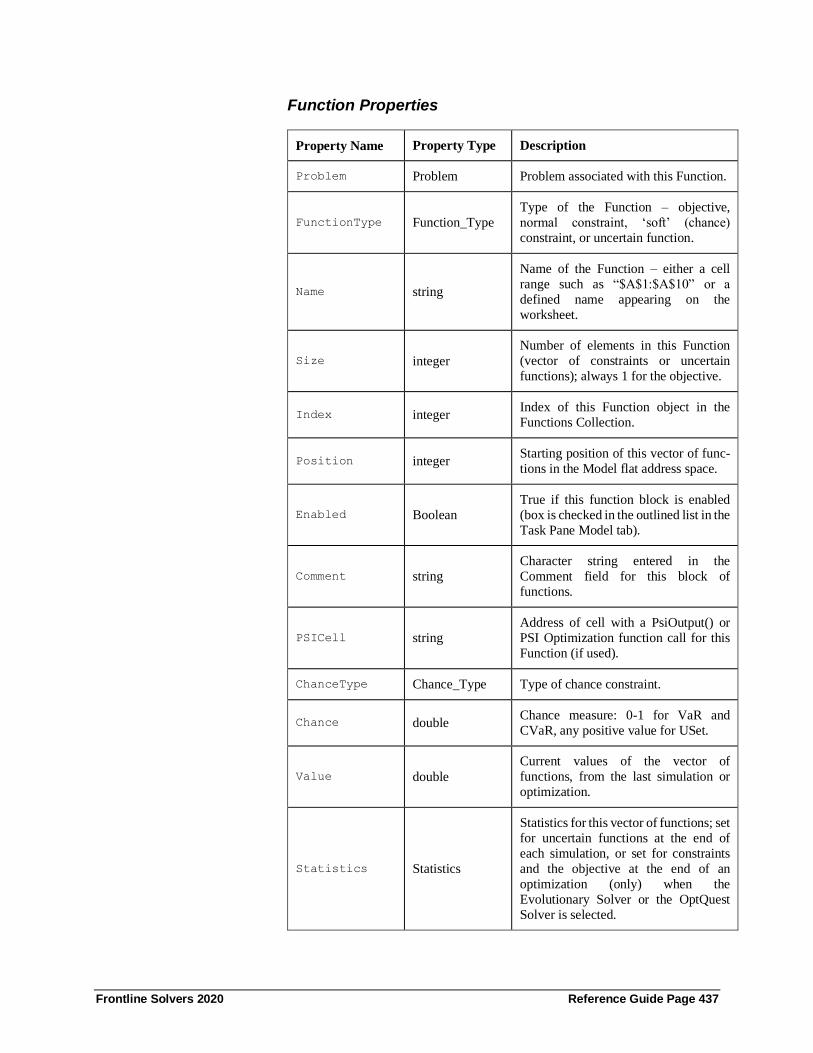
Frontline Solvers 2020 Reference Guide Page 437
Function Properties
Property Name Property Type Description
Problem Problem Problem associated with this Function.
FunctionType Function_Type
Type of the Function – objective,
normal constraint, ‘soft’ (chance)
constraint, or uncertain function.
Name string
Name of the Function – either a cell
range such as “$A$1:$A$10” or a
defined name appearing on the
worksheet.
Size integer
Number of elements in this Function
(vector of constraints or uncertain
functions); always 1 for the objective.
Index integer Index of this Function object in the
Functions Collection.
Position integer Starting position of this vector of func-
tions in the Model flat address space.
Enabled Boolean
True if this function block is enabled
(box is checked in the outlined list in the
Task Pane Model tab).
Comment string
Character string entered in the
Comment field for this block of
functions.
PSICell string
Address of cell with a PsiOutput() or
PSI Optimization function call for this
Function (if used).
ChanceType Chance_Type Type of chance constraint.
Chance double Chance measure: 0-1 for VaR and
CVaR, any positive value for USet.
Value double
Current values of the vector of
functions, from the last simulation or
optimization.
Statistics Statistics
Statistics for this vector of functions; set
for uncertain functions at the end of
each simulation, or set for constraints
and the objective at the end of an
optimization (only) when the
Evolutionary Solver or the OptQuest
Solver is selected.
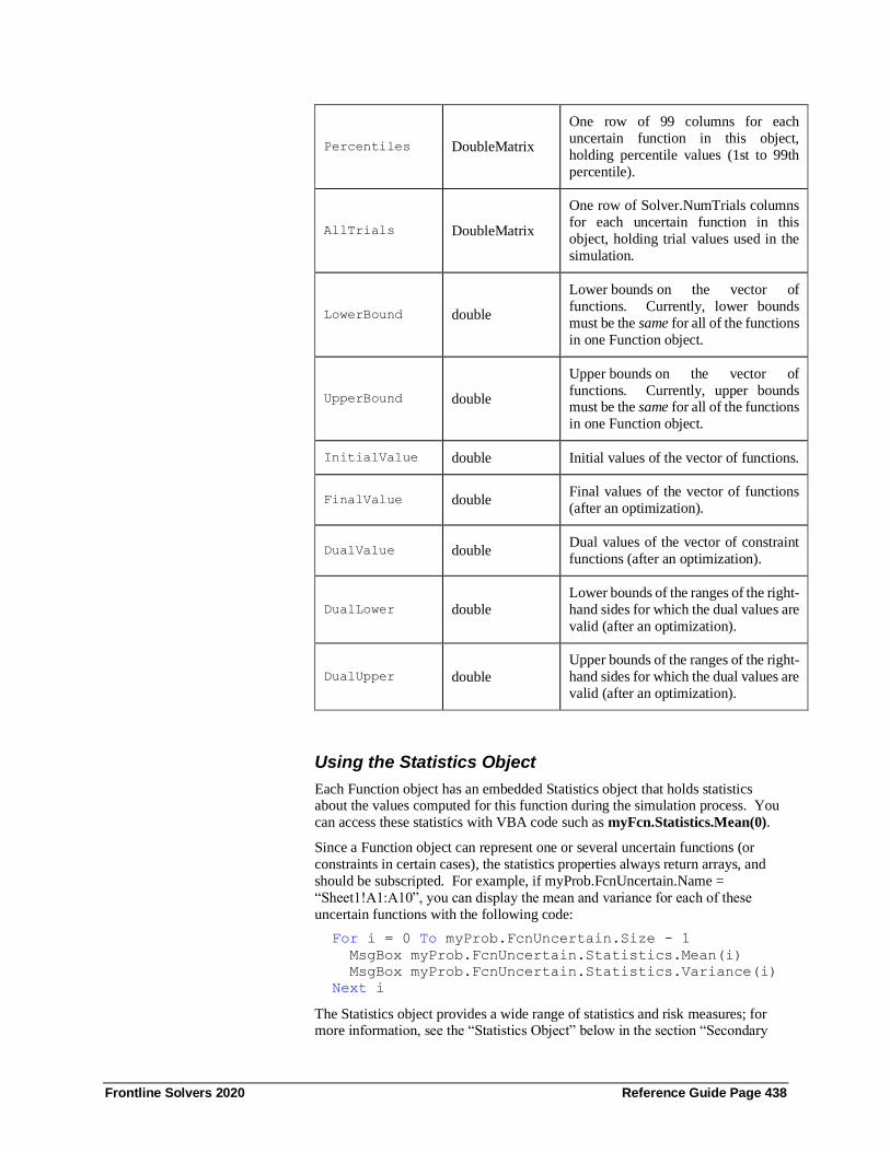
Frontline Solvers 2020 Reference Guide Page 438
Percentiles DoubleMatrix
One row of 99 columns for each
uncertain function in this object,
holding percentile values (1st to 99th
percentile).
AllTrials DoubleMatrix
One row of Solver.NumTrials columns
for each uncertain function in this
object, holding trial values used in the
simulation.
LowerBound double
Lower bounds on the vector of
functions. Currently, lower bounds
must be the same for all of the functions
in one Function object.
UpperBound double
Upper bounds on the vector of
functions. Currently, upper bounds must be the same for all of the functions
in one Function object.
InitialValue double Initial values of the vector of functions.
FinalValue double Final values of the vector of functions
(after an optimization).
DualValue double Dual values of the vector of constraint
functions (after an optimization).
DualLower double
Lower bounds of the ranges of the right-
hand sides for which the dual values are
valid (after an optimization).
DualUpper double
Upper bounds of the ranges of the right-
hand sides for which the dual values are
valid (after an optimization).
Using the Statistics Object
Each Function object has an embedded Statistics object that holds statistics about the values computed for this function during the simulation process. You
can access these statistics with VBA code such as myFcn.Statistics.Mean(0).
Since a Function object can represent one or several uncertain functions (or
constraints in certain cases), the statistics properties always return arrays, and
should be subscripted. For example, if myProb.FcnUncertain.Name =
“Sheet1!A1:A10”, you can display the mean and variance for each of these
uncertain functions with the following code:
For i = 0 To myProb.FcnUncertain.Size - 1
MsgBox myProb.FcnUncertain.Statistics.Mean(i)
MsgBox myProb.FcnUncertain.Statistics.Variance(i)
Next i
The Statistics object provides a wide range of statistics and risk measures; for more information, see the “Statistics Object” below in the section “Secondary
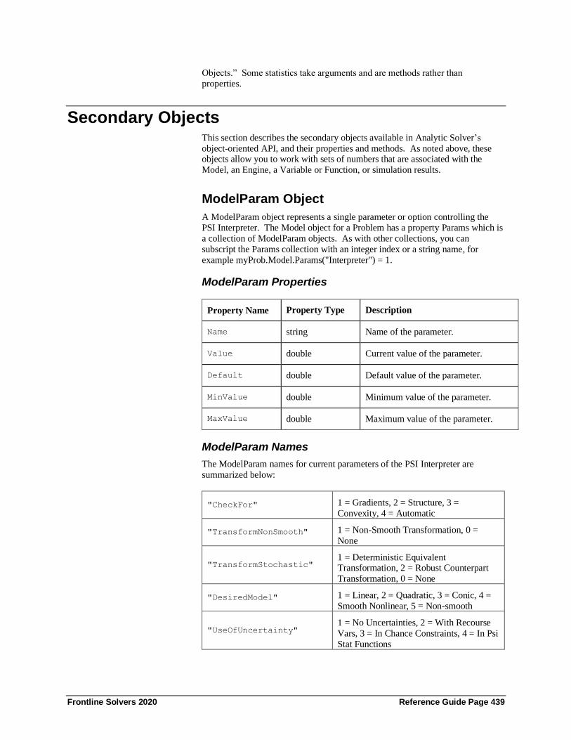
Frontline Solvers 2020 Reference Guide Page 439
Objects.” Some statistics take arguments and are methods rather than
properties.
Secondary Objects This section describes the secondary objects available in Analytic Solver’s
object-oriented API, and their properties and methods. As noted above, these objects allow you to work with sets of numbers that are associated with the
Model, an Engine, a Variable or Function, or simulation results.
ModelParam Object
A ModelParam object represents a single parameter or option controlling the
PSI Interpreter. The Model object for a Problem has a property Params which is
a collection of ModelParam objects. As with other collections, you can
subscript the Params collection with an integer index or a string name, for
example myProb.Model.Params("Interpreter") = 1.
ModelParam Properties
Property Name Property Type Description
Name string Name of the parameter.
Value double Current value of the parameter.
Default double Default value of the parameter.
MinValue double Minimum value of the parameter.
MaxValue double Maximum value of the parameter.
ModelParam Names
The ModelParam names for current parameters of the PSI Interpreter are
summarized below:
"CheckFor" 1 = Gradients, 2 = Structure, 3 =
Convexity, 4 = Automatic
"TransformNonSmooth" 1 = Non-Smooth Transformation, 0 =
None
"TransformStochastic" 1 = Deterministic Equivalent Transformation, 2 = Robust Counterpart
Transformation, 0 = None
"DesiredModel" 1 = Linear, 2 = Quadratic, 3 = Conic, 4 =
Smooth Nonlinear, 5 = Non-smooth
"UseOfUncertainty" 1 = No Uncertainties, 2 = With Recourse
Vars, 3 = In Chance Constraints, 4 = In Psi
Stat Functions

Frontline Solvers 2020 Reference Guide Page 440
"ChanceConstraintNorm" 1 = L1 Norm, 2 = L2 Norm, 3 = L-Inf
Norm, 4 = D-Norm
"ChanceAutoAdjust" 1 = Auto Adjust Chance Constraints, 0 =
Don’t
"RandomSeed" Random number seed, 0 = use system
clock
"SamplingMethod" 1 = Monte Carlo, 2 = Latin Hypercube, 3 = Sobol RMQC
"SolveWith" or "Interpreter"
1 = Use PSI Interpreter, 2 = Use Excel
Interpreter
"SimulationOptimization" 1 = Use Simulation Optimization, 0 =
Don’t
"PsiOptimizationFunctions" 1 = Use PSI Optimization Functions, 0 =
Don’t
"InteractiveOptimization" 1 = Use Interactive Optimization, 0 =
Don’t
"Engines" 1 = All, 2 = Valid, 3 = Good, 4 = Best
"ReqSmooth" 1 = Treat ABS, IF, MAX, MIN, SIGN as
non-smooth, 0 = Treat as smooth
"Sparse" 1 = PSI Interpreter runs in Sparse mode, 0
= Dense mode
"ActiveOnly" 1 = PSI Interpreter analyzes active worksheet only, 0 = analyzes referenced
cells throughout workbook
The “SimulationOptimization” and “ChanceAutoAdjust” parameters are
effective only when your code calls the Solver.Optimize method. The
“DesiredModel”, “UseOfUncertainty”, and “Engines” parameters are effective
only when your code calls the Model.DependCheck method. Other parameters
affect any use of the PSI Interpreter.
EngineParam Object
An EngineParam object represents a single parameter or option controlling the
behavior of a Solver engine. Each Engine object has a property Params which is
a collection of EngineParam objects. As with other collections, you can
subscript the Params collection with an integer index or a string name. For example, you can write myProb.Engine.Params("MaxTime") = 600 to set the
maximum optimization or simulation time to 10 minutes (600 seconds).
EngineParam Properties
Property Name Property Type Description
Name string Name of the parameter.
Value double Current value of the parameter.

Frontline Solvers 2020 Reference Guide Page 441
Default double Default value of the parameter.
MinValue double Minimum value of the parameter.
MaxValue double Maximum value of the parameter.
EngineParam Names
The EngineParam names for current parameters of Risk Solver Engine, the
standard engine for simulation, are summarized below:
"MaxTime" Maximum time (sec) allowed for the
simulation.
"SamplingMethod" The sampling method: 1 = standard Monte
Carlo (default), 2 = Latin Hypercube, 3 =
Sobol numbers.
"RandomGenerator"
Random number generator: 0 for Park-Miller with safeguards, 1 for CMRG generator
(default), 2 for WELL generator, 3 for
Mersenne Twister.
"RandomStreams"
1 = Generate independent streams of random
numbers for each distribution function. 0
(default) = Use a single stream for all
distribution functions
"RandomSeed" Nonzero value sets the random number seed.
0 (default) means that the seed will be
different on every simulation run.
"UseCorrelation"
1 (default) enables rank order correlation for
distribution functions. 0 disables correlation,
causing the PsiCorrDepen, PsiCorrIndep, and PsiCorrMatrix property functions to be
ignored.
To find EngineParam names for the parameters of different Solver engines for
optimization, consult the “Solver Options” chapters in this Guide (for built-in
Engines) and the Frontline Solver Engines Guide (for plug-in Engines).
EngineLimit Object
An EngineLimit object holds limits on the maximum size or complexity of
problems handled by a Solver engine. These limits are ‘read only’ – you can
access them in your VBA code, which can be useful if your code is written to
work with a variety of Solver engines. Each Engine object contains an
EngineLimit object; the currently selected Solver engine’s limits may be referenced as myProb.Engine.EngineLimit.
EngineLimit Properties
Property Name Property Type Description
IterationLimit integer Maximum number of iterations.
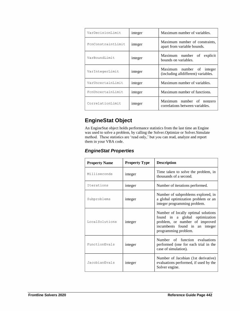
Frontline Solvers 2020 Reference Guide Page 442
VarDecisionLimit integer Maximum number of variables.
FcnConstraintLimit integer Maximum number of constraints,
apart from variable bounds.
VarBoundLimit integer Maximum number of explicit
bounds on variables.
VarIntegerLimit integer Maximum number of integer
(including alldifferent) variables.
VarUncertainLimit integer Maximum number of variables.
FcnUncertainLimit integer Maximum number of functions.
CorrelationLimit integer Maximum number of nonzero
correlations between variables.
EngineStat Object
An EngineStat object holds performance statistics from the last time an Engine was used to solve a problem, by calling the Solver.Optimize or Solver.Simulate
method. These statistics are ‘read only,’ but you can read, analyze and report
them in your VBA code.
EngineStat Properties
Property Name Property Type Description
Milliseconds integer Time taken to solve the problem, in
thousands of a second.
Iterations integer Number of iterations performed.
Subproblems integer
Number of subproblems explored, in
a global optimization problem or an
integer programming problem.
LocalSolutions integer
Number of locally optimal solutions
found in a global optimization
problem, or number of improved
incumbents found in an integer
programming problem.
FunctionEvals integer
Number of function evaluations
performed (one for each trial in the
case of simulation).
JacobianEvals integer
Number of Jacobian (1st derivative)
evaluations performed, if used by the
Solver engine.

Frontline Solvers 2020 Reference Guide Page 443
HessianEvals integer
Number of Hessian (2nd derivative)
evaluations performed, if used by the
Solver engine.
OptIIS Object
An OptIIS object holds information about an Irreducibly Infeasible Subset (IIS) of the constraints, which is found when you call the Solver.FindIIS method.
You can use myProb.Solver.OptIIS to access the OptIIS information for a
problem.
The FindIIS method may be called for a problem when the result of calling the
Optimize method is an ‘infeasible’ OptimizeStatus. An IIS is a subset of the
constraints such that a problem consisting of just these constraints is still
infeasible, but if any one of the constraints in the IIS is dropped, the problem
becomes feasible. Examining the IIS may help you determine why a problem is
infeasible.
OptIIS Properties
Property Name Property
Type
Description
NumBounds integer Number of variable bounds in the IIS.
NumConstraints integer Number of constraints in the IIS.
BoundIndex integer
array
Array of indices of variables (in the Model’s flat address space) whose bounds
are included in the IIS.
BoundStatus IIS_Status
array
Array of status values for variable bounds,
corresponding to indices in the
BoundIndex array.
ConstraintIndex integer
array
Array of indices of constraints (in the
Model’s flat address space) that are
included in the IIS.
ConstraintStatus IIS_Status
array
Array of status values for constraints,
corresponding to indices in the
ConstraintIndex array.
The IIS_Status values can be any of the symbolic names
IIS_Status_LowerBound, IIS_Status_UpperBound, or IIS_Status_Fixed.
Statistics Object
A Statistics object holds statistics summarizing the values computed for all the
trials in a simulation, or for decision variables and constraints across a popula-
tion of final solutions in an optimization. Each Variable object and Function
object contains one Statistics object, holding statistics for that vector of variables
or functions. The Statistics properties for uncertain variables and functions are
always available after a simulation is performed. Statistics for decision

Frontline Solvers 2020 Reference Guide Page 444
variables and constraints are set after an optimization, but only when the
Evolutionary Solver or the OptQuest Solver is used.
Statistics Properties
Property Name Property Type Description
NumValues integer Number of data values (one for each
trial) summarized by these statistics.
NumErrors integer Number of error values among the data
values, ignored in computing statistics.
Minimum double array Minimum value (see PsiMin function).
Maximum double array Maximum value (see PsiMax function).
Mode double array Mode (see PsiMode function).
Mean double array Mean value (see PsiMean function).
Variance double array Variance (see PsiVariance function).
StdDev double array Standard deviation (see PsiStdDev
function).
Skewness double array Skewness (see PsiSkewness function).
Kurtosis double array Kurtosis (see PsiKurtosis function).
MeanAbsDev double array Mean absolute deviation (see
PsiAbsDev function).
Statistics Methods
Property Name Property Type Description
SemiVariance double array SemiVariance or Lower Partial Moment
(see PsiSemiVar function).
SemiDeviation double array SemiDeviation or qth root of LPM (see
PsiSemiDev function).
ValueAtRisk double array Value at Risk (see PsiBVar function).
CondValueAtRisk double array Conditional Value at Risk (see PsiCVar
function).
Target double array Cumulative frequency of specified target
value (see PsiTarget function)
MeanCI double array Confidence interval of the mean value
(see PsiMeanCI function).

Frontline Solvers 2020 Reference Guide Page 445
StdDevCI double array Confidence interval of the standard
deviation (see PsiStdDevCI function).
CITrials double array
Trials required to achieve a specified
confidence interval (see PsiCITrials
function).
DoubleMatrix Object
A DoubleMatrix object is a flexible and powerful tool for working with large,
sparse matrices of numbers. It automatically allocates and manages memory
only for the nonzero elements of the matrix. So, if you create a matrix with one
million rows and one million columns, it will take very little memory initially.
You can then assign nonzero elements to the matrix by writing assignment
statements, treating the DoubleMatrix object much like an ordinary two-
dimensional array.
DoubleMatrix Methods
The Create method creates a structure for a new matrix of the specified size, but
does not initialize any of its elements. The InitDense method creates a new
matrix whose storage is optimized for the situation where most elements are
non-zero – i.e. the matrix is dense. The InitSparse method creates a new matrix
whose storage is optimized for the situation where most elements are zero – i.e.
the matrix is sparse. In both cases, the matrix is initialized with values from the
Elements array, taking these elements in the ArrayOrder order (initially in
“column major” order). Method Clear removes all non-zeros from the matrix, but preserves its size; method Destroy removes all non-zeros and also sets the
number of rows and columns to zero.
Methods NZBgn and NZEnd should be called, to save time, if you wish to
assign a large number of non-zeros to the matrix at one time, without accessing
or using these values until all of them have been assigned. First call NZBgn,
then perform the assignments, then call NZEnd. If you need to ‘undo’ the effect
of NZBgn, call NZCancel instead of NZEnd – in this case, all of the
assignments since NZBgn was called will have no effect.
The MakePSD method can be used on a non-positive semidefinite (PSD) matrix
to transform the matrix into a positive semidefinite matrix that is “close to” to original matrix. This is most often used for correlation matrices in simulation,
but may also be used in certain optimization problems. The Weights argument is
optional; if it is specified, the elements of the transformed matrix with the
largest weights in the corresponding positions of the Weights matrix will be a
close as possible to the original matrix elements, and the elements with the
smallest weights will experience the greatest change in the transformed matrix.
DoubleMatrix.Create Rows, Columns
DoubleMatrix.InitDense Rows, Columns, Elements
DoubleMatrix.InitSparse Rows, Columns, Elements
DoubleMatrix.Clear
DoubleMatrix.Destroy
DoubleMatrix.NZBgn
DoubleMatrix.NZEnd
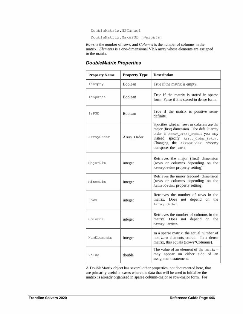
Frontline Solvers 2020 Reference Guide Page 446
DoubleMatrix.NZCancel
DoubleMatrix.MakePSD [Weights]
Rows is the number of rows, and Columns is the number of columns in the
matrix. Elements is a one-dimensional VBA array whose elements are assigned
to the matrix.
DoubleMatrix Properties
Property Name Property Type Description
IsEmpty Boolean True if the matrix is empty.
IsSparse Boolean True if the matrix is stored in sparse
form; False if it is stored in dense form.
IsPSD Boolean True if the matrix is positive semi-
definite.
ArrayOrder Array_Order
Specifies whether rows or columns are the
major (first) dimension. The default array
order is Array_Order_ByCol; you may
instead specify Array_Order_ByRow.
Changing the ArrayOrder property
transposes the matrix.
MajorDim integer
Retrieves the major (first) dimension
(rows or columns depending on the
ArrayOrder property setting).
MinorDim integer
Retrieves the minor (second) dimension
(rows or columns depending on the
ArrayOrder property setting).
Rows integer
Retrieves the number of rows in the
matrix. Does not depend on the
Array_Order.
Columns integer
Retrieves the number of columns in the matrix. Does not depend on the
Array_Order.
NumElements integer
In a sparse matrix, the actual number of
non-zero elements stored. In a dense
matrix, this equals (Rows*Columns).
Value double
The value of an element of the matrix –
may appear on either side of an
assignment statement.
A DoubleMatrix object has several other properties, not documented here, that
are primarily useful in cases where the data that will be used to initialize the
matrix is already organized in sparse column-major or row-major form. For

Frontline Solvers 2020 Reference Guide Page 447
more information, consult the VBA Object Browser or the Solver Platform SDK
documentation, or contact Frontline Systems at [email protected].
DependMatrix Object
A DependMatrix object is used to hold information about dependencies of
problem functions (objective and constraints) on decision variables. In the matrix, rows represent constraints or the objective, and columns represent
variables.
The value of the Model object AllGradDepend property is a DependMatrix.
This matrix is initialized (only) when you call the Model object DependCheck
method. An element of the matrix at position (i, j) has a value from the
Depend_Type enum, that tells you whether constraint i depends in a linear,
quadratic, smooth nonlinear, or nonsmooth way on variable j, or does not
depend on variable j at all.
Depend_Type Constants
The Depend_Type enum has a set of symbolic constant values that reflect the
nature of the dependence between a specific function and decision variable:
Depend_Type_None
Depend_Type_Linear
Depend_Type_Quadratic
Depend_Type_Smooth
Depend_Type_NonSmooth
If a function does not depend at all on a specific variable, the matrix entry for
that function (row) and variable (column) will be Depend_Type_None.
DependMatrix Methods
A DependMatrix is created for you as the value of the Model object
AllGradDepend property; you can simply access its elements by subscripting,
for example by writing myProb.Model.AllGradDepend( i, j). Should you need
to create such a matrix, however, you can use the same methods documented
above for a DoubleMatrix: Create, InitDense, InitSparse, Clear, Destroy,
NZBgn, NZEnd and NZCancel.
DependMatrix Properties
A DependMatrix has the same properties as a DoubleMatrix, as documented
above: IsEmpty, IsSparse, ArrayOrder, MajorDim, MinorDim, Rows,
Columns, NumElements and Value. Only the Value property is different:
Where this property is of type double for a DoubleMatrix, it is of type
Depend_Type for a DependMatrix.
A DependMatrix object has several other properties, not documented here, that
are primarily useful in cases where the data that will be used to initialize the matrix is already organized in sparse column-major or row-major form. For
more information, consult the VBA Object Browser or the Solver Platform SDK
documentation, or contact Frontline Systems at [email protected].
Distribution Object
A Distribution object is a flexible tool for working with analytic probability
distributions. The Model object contains two properties, VarDistribution and

Frontline Solvers 2020 Reference Guide Page 448
FcnDistribution (reserved for future use), that represent arrays of Distribution
objects, one for each uncertain variable and uncertain function in the model
respectively.
If you initialize a Distribution object with a type (Uniform, Normal, Beta, etc.)
and parameters, you can generate sample points drawn from the distribution. Conversely, if you supply a set of sample points, you can automatically fit a
distribution type and parameters to the sample data.
Distribution Methods
In Risk Solver V8.0, the Model object is “opaque” – the VarDistribution and
FcnDistribution properties are not initialized. In future versions, they may
return arrays of Distribution objects that are pre-initialized with types and parameters drawn from your PSI Distribution functions on the worksheet.
When you create a Distribution object of your own with Dim myDist As New
RSP.Distribution, you can initialize it using the methods listed below. The Init
method accepts a string argument containing a PSI Distribution function call
such as “PsiNormal(0,1)” just as you might type it into a worksheet cell –
including PSI Property functions. Alternatively, you can set the Distribution
Type, Params, and ControlParams properties directly, you wish.
The InitSample method accepts an array of sample values; if there are several
occurrences of many of the sample values, you can include each value just once
in the Sample argument, and supply the Occurs argument, an array of counts of occurrences of each sample value.
Distribution.Init PsiFuncString
Distribution.InitSample Sample [,Occurs]
Once you’ve called the InitSample method, you can fit an analytic distribution
to the data. If you know the type of distribution (Uniform, Normal, Beta, etc.),
call the Fit method and supply the type, a desired significance level, and an optional True/False value to indicate whether RSE can shift the center of
candidate distributions to better fit the data. If you don’t know the type of
distribution, you can call the AutoFit method and supply a True/False value to
indicate whether the sample data is continuous or discrete, a desired significance
level, and an optional True/False value to indicate whether to test only
distributions matching the type of data (continuous or discrete), or all available
distributions.
Distribution.Fit Type, SigLevel, Shift
Distribution.AutoFit Continuous, SigLevel [,FitAll]
Only the following analytic distributions can be selected by the Fit and AutoFit
methods: PsiBeta, PsiExponential, PsiGamma, PsiLogNormal, PsiNormal,
PsiUniform, and PsiWeibull for continuous distributions, and PsiBernoulli,
PsiBinomial, PsiGeometric, PsiIntUniform, PsiNegBinomial, and PsiPoisson for
discrete distributions.
Once a Distribution object is initialized with either the Init method or the
InitSample and Fit or AutoFit methods, you can generate sample values for the probability density function (PDF; probability mass function or PMF for discrete
distributions), the cumulative distribution function (CDF), or the inverse of the
cumulative distribution function. When you call the PDF or CDF methods, you
supply a sample (X-axis) value, and the method returns a probability (Y-axis)
value. When you call the CDFInv method, you supply a probability (Y-axis)
value, and the method returns a sample (X-axis) value.

Frontline Solvers 2020 Reference Guide Page 449
Distribution.PDF X
Distribution.CDF X
Distribution.CDFInv F
Distribution Properties
Property Name Property Type Description
Problem Problem Problem associated with this
Distribution (if any).
DistType Dist_Type Specifies the type of distribution
(see Dist_Type enum below).
Name string Name of the distribution.
NumParams integer Number of parameters allowed for
this distribution type.
NumControlParams integer Number of control parameters
(shift, truncate, etc.) allowed.
Params double array Parameter values.
ControlParams double array Control parameter values.
Mean double Analytic mean of distribution.
Variance double Analytic variance of distribution.
Skewness double Analytic skewness of distribution.
Kurtosis double Analytic kurtosis of distribution.
Mode double Analytic mode of distribution.
Median double Analytic median of distribution.
Size integer Number of elements in Sample
property array.
Sample double array Supplied sample data values.
IndepTest double
Result of independence test on
supplied Sample data – smaller
value means more independent.
FitStatistic double
Statistic indicating goodness of fit
for Fit and AutoFit methods:
AIC/BIC and Chi-Squared for
discrete and AIC/BIC, Chi-Sqaure
and Kolmogorov-Smirnof for
continuous distributions.

Frontline Solvers 2020 Reference Guide Page 450
FitTest double
Fitting statistic independent of
sample size. Generally FitSuccess
= True if FitTest < FitLimit.
FitLimit double Goodness of fit test critical value.
SigLevel double
Fitting significance level, usually
a number between 0.9 and 0.99
(often referred to as 1 - ).
FitSuccess Boolean True if distribution fit succeeded.
Note that the Distribution object analytic moment properties (Mean, Variance,
etc.) are not the same as the computed estimates of these moments returned by
the Variable and Function Statistics objects. The Distribution object properties
are computed from the parameters of each distribution type – the formulas used
are shown under each PSI Distribution function in the chapter “PSI Function
Reference.” The Statistics object properties are estimates computed from the
sample values of each trial during a simulation – the formulas used are shown
under each PSI Statistics function, also in the chapter “PSI Function Reference.”

Frontline Solvers 2020 Reference Guide Page 451
Traditional VBA Function Reference
Controlling the Solver’s Operation This chapter explains how to control the Solver using “traditional” VBA
functions, which are upward compatible from the VBA functions supported by
the standard Excel Solver. Analytic Solver also supports a new object-oriented
API that is high-level, easy to use, and compatible with the object-oriented API
offered by Frontline’s Risk Solver for Monte Carlo simulation, and the Solver
SDK Platform and Solver SDK Pro, used to build custom applications of
optimization and simulation using C++, C#, VB.NET, Java, MATLAB and
other languages.
Note: Calling your model using the Traditional VBA functions is not supported in Analytic Solver Cloud and AnalyticSolver.com.
Using traditional VBA functions, you can display or completely hide the Solver
dialog boxes, create or modify the choices of objective, variables and
constraints, check whether an optimal solution was found, and produce reports.
If you need to work with solution values or use report results in your VBA code,
create and solve multiple optimization problems, or ‘port’ your code to run as a
standalone application, you may find that the object-oriented API is a better
choice. Further, the new functionality in Analytic Solver can be controlled only
through the object-oriented API, not with traditional VBA functions.
Running Predefined Solver Models
Controlling the Solver can be as simple as adding one line to your VBA code!
Each worksheet in a workbook may have a Solver problem defined, which is
saved automatically with the workbook. You can create this Solver model
interactively if you wish. If you distribute such a workbook, with a worksheet
containing a Solver model and a VBA module, you can simply add a reference
to the Solver add-in, activate the worksheet, and add one line to call the function
SolverSolve in VBA.
Using the Macro Recorder
If you want to set up a Solver model “from scratch” programmatically, one easy
way to see how to use the object-oriented API is to turn on the Excel Macro
Recorder (click Record Macro on the Developer tab in Excel 2010 and later), and then set up a Solver model interactively. Microsoft Excel will record a
macro in VBA that calls the object-oriented API to mimic the actions you
perform. You can then edit and customize this macro, and incorporate it into
your application.

Frontline Solvers 2020 Reference Guide Page 452
Note: You must use the classic Solver dialog to record a macro, rather than the
Solver Task Pane. To open, click Add-ins – Premium Solver. By default, the
Excel Macro Recorder will record calls to the object-oriented API.
Using Microsoft Excel Help
You can learn about the standard Solver functions in Excel’s online Help. In Excel 2016, 2013, and 2010, open the Visual Basic Editor (Alt-F11), select Help
- Microsoft Visual Basic Help, click on the Search field, and type ‘Solver’ to
display an list of the Solver functions.
Referencing Functions in Visual Basic
To use the VBA functions, your Visual Basic module must include a reference
to the Solver add-in (Solver.xla). Press Alt-F11 to open the Visual Basic Editor,
choose Tools References... and make sure that the box next to Solver is
checked.
You can confirm that you are using the desired version of the add-in by
highlighting the word Solver in the list under Tools References… and noting the file location. The path to Analytic Solver’s Solver.xla is normally C:\Program
Files\Frontline Systems\Analytic Solver\Bin or C:\Program Files (x86)\Frontline
Systems\Analytic Solver\Bin if using 32-bit Excel with a 64-bit operating
system. Note that this is different from a reference to the Analytic Solver
V2018 type library, for example, which you add when you use the new object-
oriented API in VBA.
Note: If running a field – installable engine such as Gurobi Solver, Xpress
Solver, OptQuest Solver, etc., you must also set a reference to that engine. In
order for the engine reference to appear in VBA – Tools – References, you must
first open the Premium Solver classic dialog (Addins – Premium Solver), select
the engine in the engine drop – down menu, then click Options – OK – Close. For more information, please see the Frontline Solvers Engine User Guide.
Calling the Excel Solver in Visual Basic
If you have the standard Excel Solver installed and you want to use it to solve a
model by calling the Solver through VBA, you must set the correct Solver
reference. You can confirm that you are using the desired version of the add-in
by highlighting the word Solver in the list under Tools References… and noting the file location. For example, the path to the Standard Excel Solver in Excel
2016 is: C:\Program Files\Microsoft Office 16\Root\Office 16\
Library\Solver\Solver.xlam
Checking Function Return Values
The Solver functions generally return integer values, which you should check in
your VBA code. The normal return value is 0, indicating that the function
succeeded. Other possible return values are given in the descriptions of the
individual functions. If the arguments you supply are invalid, an error condition
can be raised, which you would have to handle via an On Error VBA statement.
Of particular interest is the return value of the SolverSolve function, which
describes the result of the actual optimization step. The return value can range from -1 to 21 in the Analytic Solver products, with additional values starting at
1000 for the Interval Global Solver and field-installable Solver engines. These
integer values are summarized in the description of the SolverSolve function

Frontline Solvers 2020 Reference Guide Page 453
below, but for a comprehensive discussion, see the chapter “Solver Results
Messages,” starting with the subsection “Standard Solver Result Messages.”
One group of functions can return a variety of numeric, logical, string or array
values, depending on the arguments you supply. These functions (SolverGet,
SolverOkGet, etc.) may be used to “read” the settings of the current Solver model, on the active sheet or any other worksheet whose name you supply.
Standard, Model and Premium Macro Functions
The following sections describe each of the VBA function calls supported by the
Analytic Solver products. These functions are a compatible superset of the
function calls available in the standard Excel Solver.
The functions are listed alphabetically in three groups. The first group consists
of functions available in both the standard Excel Solver and the Analytic Solver
products. The second and third groups, Premium VBA Functions and Solver
Model VBA Functions, consists of functions that are available only in the
Analytic Solver products. If you want to write VBA code that will work with both the standard Solver and Analytic Solver, you should limit yourself to
functions in the first group, and consult the notes on each function call to deter-
mine which arguments are supported by the standard Solver.
Standard VBA Functions The VBA functions in this section are available in both the standard Excel
Solver and Analytic Solver and subset products. Some of these functions have
extra arguments that are supported only in Analytic Solver and subset products,
as noted in each function description.
SolverAdd (Form 1)
Equivalent to choosing Premium Solver... from the Addins or Tools menu and
pressing the Add button in the classic Solver Parameters dialog box or clicking
Constraints – Normal Constraints on the Analytic Solver ribbon. Adds a
constraint to the current problem.
VBA Syntax
SolverAdd (CellRef:=, Relation:=, FormulaText:=, Comment:=, Report:=)
CellRef is a reference to a cell or a range of cells and forms the left hand side of
the constraint. In standard Excel Solver and Analytic Solver Upgrade, all cells
must be on the active worksheet; in Analytic Solver Comprehensive, Analytic
Solver Optimization or Analytic Solver Basic they may be on any sheet.
Relation specifies the arithmetic relationship between the left and right hand
sides, or whether CellRef must have an integer value at the solution.
Relation Relationship
1 <=
2 =
3 >=
4 int (CellRef is an integer variable)
5 bin (CellRef is a binary integer variable)
6 dif (CellRef is an alldifferent group)
7 soc (CellRef belongs to a second order cone)
8 src (CellRef belongs to a rotated second order cone)

Frontline Solvers 2020 Reference Guide Page 454
9 sem (CellRef is a semi-continuous variable)
FormulaText is the right hand side of the constraint and will often be a single
number, but it may be a formula (as text) or a reference to a range of cells.
Comment is a string corresponding to the Comment field in the Add Constraint dialog, only in the Analytic Solver and subset products.
Report is no longer used, but is included for compatibility with previous
versions of Premium Solver products.
The standard Excel Solver supports only Relation values 1 to 5. If Relation is 4
to 9, FormulaText is ignored, and CellRef must be a subset of the decision
variable cells.
If FormulaText is a reference to a range of several cells, the number of cells in
the range must match the number of cells in CellRef, although the shape of the
areas need not be the same. For example, CellRef could be a row and
FormulaText could refer to a column, as long as the number of cells is the same.
Remarks
The SolverAdd, SolverChange and SolverDelete functions correspond to the
Add, Change, and Delete buttons in the classic Solver Parameters dialox box
(Addins – Premium Solver). You use these functions to define constraints. For
many macro applications, however, you may find it more convenient to load the
problem in a single step using the SolverLoad call.
Each constraint is uniquely identified by the combination of the cell reference on
the left and the relationship (<=, =, >=, int, bin, dif, soc, src or sem) between its
left and right sides. This takes the place of selecting the constraint in the Solver Parameters dialog box. You can manipulate constraints with SolverChange and
SolverDelete.
SolverAdd (Form 2)
Equivalent to choosing Premium Solver... from the Addins or Tools menu,
pressing the Variables button, and then pressing the Add button in the Solver
Parameters dialog box or clicking Decisions – Normal on the Analytic Solver
ribbon. Adds a set of decision variable cells to the current problem. This form
is supported only by the Analytic Solver and subset products.
VBA Syntax
SolverAdd (CellRef:=, Comment:=, Report:=)
CellRef is a reference to a cell or a range of cells and forms a set of decision
variables. In Analytic Solver Upgrade, the cells must be on the active
worksheet; in Analytic Solver Comprehensive, Analytic Solver Optimization or
Analytic Solver Basic, they may be on any sheet.
Comment is a string corresponding to the Comment field in the Add Variable
Cells dialog, only in the Analytic Solver and subset products.
Report is no longer used, but is included for compatibility with previous
versions of the Premium Solver products.
Remarks
The SolverAdd, SolverChange and SolverDelete functions correspond to the
Add, Change, and Delete buttons in the classic Solver Parameters dialog box
(Addins – Premium Solver). In this form, you can use these functions to add or

Frontline Solvers 2020 Reference Guide Page 455
change sets of decision variables. For many macro applications, however, you
may find it more convenient to load the problem in a single step using the
SolverLoad function.
Note that the SolverOk ByChange:= argument defines the first entry in the
Variable Cells list box in the classic Solver Parameters dialog or the first entry under Variables on the Task Pane Model tab. Use SolverAdd to define
additional entries in the Variables Cells list box or Task Pane Model tab. Do not
call SolverOk with a different ByChange:= argument after you have defined
more than one set of variable cells.
SolverChange (Form 1)
Equivalent to choosing Premium Solver... from the Addins or Tools menu and
pressing the Change button in the classic Solver Parameters dialog box or
highlighting the constraint in the Task Pane Model tab then changing the value
for the constraint right hand side. Changes the right hand side of an existing
constraint.
VBA Syntax
SolverChange (CellRef:=, Relation:=, FormulaText:=, Comment:=,
Report:=)
For an explanation of the arguments and selection of constraints, see
SolverAdd. In the standard Excel Solver or Analytic Solver Upgrade, the
CellRef cells must all be on the active worksheet; in Analytic Solver
Comprehensive, Analytic Solver Optimization or Analytic Solver Basic, they
may be on any sheet.
Remarks
If the combination of CellRef and Relation does not match any existing constraint, the function returns the value 4 and no action is taken.
To change the CellRef or Relation of an existing constraint, use SolverDelete to
delete the old constraint, then use SolverAdd to add the constraint in the form
you want.
SolverChange (Form 2)
Equivalent to choosing Premium Solver... from the Tools or Addins menu,
pressing the Variables button, and then pressing the Change button in the Solver
Parameters dialog box or highlighting the variable entry in the Task Pane Model
tab and changing the cell reference. Changes a set of decision variable cells.
This form is supported only by the Analytic Solver and subset products.
VBA Syntax
SolverChange (CellRef:=, Relation:=, Comment:=, Report:=)
CellRef is a reference to a cell or a range of cells, currently defined in the
Variable Cells list box as a set of decision variable cells.
Relation is a reference to a different cell or range of cells, which will replace
CellRef as a new set of variable cells. In the standard Excel Solver or Analytic
Solver Upgrade, the CellRef cells must all be on the active worksheet; in
Analytic Solver Comprehensive, Analytic Solver Optimization or Analytic
Solver Basic, they may be on any sheet.

Frontline Solvers 2020 Reference Guide Page 456
Comment is a string corresponding to the Comment field in the Change
Variable Cells dialog, only in the Analytic Solver and subset products.
Report is no longer used, but is included for compatibility with previous
versions of the Premium Solver products.
Remarks
If CellRef does not match any existing set of variable cells, the function returns
the value 1 and no action is taken.
SolverDelete (Form 1)
Equivalent to choosing Premium Solver... from the Tools or Addins menu and
pressing the Delete button in the Solver Parameters dialog box or selecting a
constraint entry in the Task Pane Model tab and clicking . Deletes an
existing constraint.
VBA Syntax
SolverDelete (CellRef:=, Relation:=, FormulaText:=)
For an explanation of the arguments and selection of constraints, see
SolverAdd. The FormulaText argument is optional, but if present, it is used to
confirm that the correct constraint block is being deleted.
Remarks
If the combination of CellRef and Relation does not match any existing
constraint, the function returns the value 4 and no action is taken. If the
constraint is found, it is deleted, and the function returns the value 0.
SolverDelete (Form 2)
Equivalent to choosing Premium Solver... from the Tools or Addins menu and
then pressing the Delete button in the Solver Parameters dialog box or selecting
a variable entry in the Task Pane Model tab and clicking . Deletes an
existing set of variable cells. This form is supported only by Analytic Solver
and subset products.
VBA Syntax
SolverDelete (CellRef:=)
CellRef is a reference to a cell or a range of cells, currently defined in the
Variable Cells list box as decision variable cells. In the standard Excel Solver or
Analytic Solver Upgrade, the CellRef cells must all be on the active worksheet;
in Analytic Solver Comprehensive, Analytic Solver Optimization or Analytic
Solver Basic, they may be on any sheet.
Remarks
If CellRef does not match any existing set of variable cells, the function returns
the value 1 and no action is taken. If the variable cells are found, they are
deleted, and the function returns the value 0.
SolverFinish
Equivalent to selecting options and clicking OK in the Solver Results dialog that
appears when the solution process is finished. The dialog box will not be
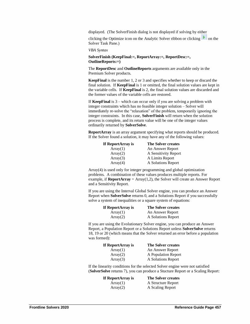
Frontline Solvers 2020 Reference Guide Page 457
displayed. (The SolverFinish dialog is not displayed if solving by either
clicking the Optimize icon on the Analytic Solver ribbon or clicking on the
Solver Task Pane.)
VBA Syntax
SolverFinish (KeepFinal:=, ReportArray:=, ReportDesc:=,
OutlineReports:=)
The ReportDesc and OutlineReports arguments are available only in the
Premium Solver products.
KeepFinal is the number 1, 2 or 3 and specifies whether to keep or discard the
final solution. If KeepFinal is 1 or omitted, the final solution values are kept in
the variable cells. If KeepFinal is 2, the final solution values are discarded and
the former values of the variable cells are restored.
If KeepFinal is 3 – which can occur only if you are solving a problem with
integer constraints which has no feasible integer solution – Solver will
immediately re-solve the “relaxation” of the problem, temporarily ignoring the
integer constraints. In this case, SolverFinish will return when the solution
process is complete, and its return value will be one of the integer values ordinarily returned by SolverSolve.
ReportArray is an array argument specifying what reports should be produced.
If the Solver found a solution, it may have any of the following values:
If ReportArray is The Solver creates
Array(1) An Answer Report
Array(2) A Sensitivity Report
Array(3) A Limits Report
Array(4) A Solutions Report
Array(4) is used only for integer programming and global optimization
problems. A combination of these values produces multiple reports. For example, if ReportArray = Array(1,2), the Solver will create an Answer Report
and a Sensitivity Report.
If you are using the Interval Global Solver engine, you can produce an Answer
Report when SolverSolve returns 0, and a Solutions Report if you successfully
solve a system of inequalities or a square system of equations:
If ReportArray is The Solver creates
Array(1) An Answer Report
Array(2) A Solutions Report
If you are using the Evolutionary Solver engine, you can produce an Answer
Report, a Population Report or a Solutions Report unless SolverSolve returns 18, 19 or 20 (which means that the Solver returned an error before a population
was formed):
If ReportArray is The Solver creates
Array(1) An Answer Report
Array(2) A Population Report
Array(3) A Solutions Report
If the linearity conditions for the selected Solver engine were not satisfied
(SolverSolve returns 7), you can produce a Stucture Report or a Scaling Report:
If ReportArray is The Solver creates
Array(1) A Structure Report Array(2) A Scaling Report

Frontline Solvers 2020 Reference Guide Page 458
If the Solver could not find a feasible solution (SolverSolve returns 5), you can
produce either version of the Feasibility Report, or a Scaling Report:
If ReportArray is The Solver creates
Array(1) A Feasibility Report
Array(2) A Feasibility-Bounds Report Array(3) A Scaling Report
If you are using Analytic Solver Comprehensive or Analytic Solver
Optimization and a field-installable Solver engine, it may produce some or all of
the reports mentioned above and/or its own custom reports. To determine what
you should use for the ReportArray argument, solve a problem interactively
with this Solver engine, and examine the Reports list box in the Solver Results
dialog. Then use the ordinal position of the report you want:
If ReportArray is The Solver creates
Array(1) The first report listed
Array(2) The second report listed (and so on)
ReportDesc is an array of character strings that allows you to select reports by
their names, rather than their ordinal positions in the Reports list. For example,
you can select an Answer Report with Array (“Answer”), or both the Answer
Report and the Sensitivity Report with Array (“Answer”, “Sensitivity”). The
possible strings are:
“Answer” Answer Report
“Sensitivity” Sensitivity Report
“Limits” Limits Report
“Solutions” Solutions Report
“Population” Population Report
“Structure” Structure Report “Feasibility” Feasibility Report (full version)
“Feasibility-Bounds” Feasibility Report (w/o bounds)
“Scaling” Scaling Report
The report names you can include in the array depend on the currently selected
Solver engine and the integer value returned by SolverSolve, as described
above.
OutlineReports is a logical value corresponding to the Outline Reports check
box. If TRUE, any reports you select will be produced in outlined format, and
comments (if any) associated with each block of variables and constraints will
be included in the report; if it is FALSE, the reports will be produced in “regular” format.
SolverFinishDialog
Equivalent to selecting options in the Solver Results dialog that appears when the solution process is finished. The dialog box will be displayed, and the user
will be able to change the options that you initially specify. (This dialog is not
displayed if solving by either clicking the Optimize icon on the Analytic Solver
ribbon or clicking on the Solver Task Pane.)
VBA Syntax
SolverFinishDialog (KeepFinal:=, ReportArray:=, ReportDesc:=,
OutlineReports:=)
For an explanation of the arguments of this function, see SolverFinish.

Frontline Solvers 2020 Reference Guide Page 459
SolverGet
Returns information about the current Solver problem. The settings are
specified in the classic Solver Parameters dialog, on the General tab for Solver
options, on the Platform tab in the Solver Task Pane, or with the other Solver
functions described in this chapter. Values of the TypeNum:= argument from 1
to 18 are supported by the standard Excel Solver.
SolverGet is provided for compatibility with the standard Excel Solver and
earlier versions of the Premium Solver products. For programmatic control of
new features and options included in Version 5.0 or later of the Premium Solver products, see the dialog-specific “Get” functions in the sections “Solver Model
VBA Functions” and “Premium VBA Functions.”
VBA Syntax
SolverGet (TypeNum:=, SheetName:=)
TypeNum is a number specifying the type of information you want. The
following settings are specified in the Solver Parameters dialog box or the Task
Pane Model tab.
TypeNum Returns
1 The reference in the Set Cell box or the #N/A error value if
Solver has not been used on the active document
2 A number corresponding to the Equal To option:
1 = Max
2 = Min
3 = Value Of
3 The value in the Value Of box or in the Task Pane Model tab
4 The reference in the Changing Cells box or under Variables in
the Task Pane Model tab (in the Analytic Solvers, only the first
entry in the Variables list box)
5 The number of entries in the Constraints list box or under
Constraints in the Task Pane Model tab
6 An array of the left hand sides of the constraints as text
7 An array of numbers corresponding to the relations
between the left and right hand sides of the constraints:
1 = <=
2 = =
3 = >=
4 = int
5 = bin
6 = dif
7 = soc
8 = src
9 = sem
8 An array of the right hand sides of the constraints as text
The following settings are specified on the General tab for Solver options or on
the Task Pane Engine tab:
TypeNum Returns
9 The Max Time value (as a number in seconds)
10 The Iterations value (max number of iterations)
11 The Precision value (as a decimal number)

Frontline Solvers 2020 Reference Guide Page 460
12 The integer Tolerance value (as a decimal number)
13 In the standard Solver: TRUE if the Assume Linear Model
check box is selected; FALSE otherwise. In the Analytic
Solvers: TRUE if the linear Simplex (only in Excel Solver) or
LP/Quadratic Solver is selected; FALSE if any other Solver is
selected
14 TRUE if the Show Iteration Result check box is selected in
Solver Parameters or set to True in the Task Pane Engine tab;
FALSE otherwise,
15 TRUE if the Use Automatic Scaling check box is selected in
Solver Parameters or set to True in the Task Pane Engine tab;
FALSE otherwise
16 A number corresponding to the type of Estimates:
1 = Tangent
2 = Quadratic
17 A number corresponding to the type of Derivatives:
1 = Forward
2 = Central
18 A number corresponding to the type of Search:
1 = Newton
2 = Conjugate
The following settings are supported by Analytic Solver and subset products:
TypeNum Returns
19 The Convergence value (as a decimal number) in the
nonlinear GRG Solver
20 TRUE if the Assume Non-Negative check box is selected in
Solver Parameters or set to True in the Task Pane Engine
tab; FALSE otherwise
21 The Integer Cutoff value (as a decimal number)
22 TRUE if the Bypass Solver Reports check box is selected
in Solver Parameters or set to True in the Task Pane
Engine tab; FALSE otherwise
23 An array of the entries in the Variables list box or in
the Task Pane Model tab as text
24 A number corresponding to the Solver engine dropdown list
for the currently selected Solver engine:
1 = Nonlinear GRG Solver
2 = Simplex LP or LP/Quadratic Solver
3 = Evolutionary Solver
4 = Interval Global Solver
5 = SOCP Barrier Solver
In the Analytic Solver Comprehensive and Analytic Solver
Optimization, other values may be returned for field-
installable Solver engines
25 The Pivot Tolerance (as a decimal number) in the
Linear Simplex Solver (For backwards compatibility only)
26 The Reduced Cost Tolerance (as a decimal number) in the
Linear Simplex Solver (For backwards compatibility only)
27 The Coefficient Tolerance (as a decimal number) in the
Large-Scale LP Solver. This option is no longer used.
28 The Solution Tolerance (as a decimal number) in the
Large-Scale LP Solver. This option is no longer used.

Frontline Solvers 2020 Reference Guide Page 461
29 TRUE if the Estimates option in the GRG Solver is set to
Tangent; FALSE if the Estimates option is set to
Quadratic
30 This function is included for backward compatibility
only; a number corresponding to the type of Scaling in
the
Large-Scale LP Solver:
1 = None
2 = Row Only
3 = Row & Col
SheetName is the name of a worksheet that contains the Solver problem for
which you want information. If SheetName is omitted, it is assumed to be the
active sheet.
SolverLoad
Equivalent to choosing Premium Solver... from the Tools menu, choosing the
Options button from the Solver Parameters dialog box, and choosing the Load
Model... button on the General tab or clicking the Save/Load button on the Analytic Solver ribbon. Loads Solver model specifications that you have previ-
ously saved on the worksheet. The Format and ModelName arguments are
supported only in Version 7.0 or later of the Premium Solver products.
VBA Syntax
SolverLoad (LoadArea:=, Merge:=, Format:=, ModelName:=)
LoadArea is a reference to a range of cells from which you want to load a
complete model specification. In Solver versions prior to V7.0, LoadArea must be a reference on the active worksheet; in Version 7.0 or later it can be on any
worksheet.
Merge is a logical value corresponding to either the Merge button or the
Replace button in the dialog that appears after you select the LoadArea
reference and click OK. If it is TRUE, the variable cell selections and
constraints from the LoadArea are merged with the currently defined variables
and constraints. If FALSE, the current model specifications and options are
erased (equivalent to a call to the SolverReset function) before the new
specifications are loaded.
Format corresponds to the Format dropdown list in the Load Model dialog: 1
for “Classic” format and 2 for “PSI Function” format.
In “Classic” format, the first cell in LoadArea contains a formula for the Set
Cell edit box; the second cell contains a formula for the variable cells;
subsequent cells contain additional variable selections and constraints in the
form of logical formulas. The final cells optionally contain an array of Solver
option values.
In “PSI Function” format, the cells contain calls to functions such as PsiVar(),
PsiCon(), PsiObj() and PsiOption(). For details on these functions, see “Using
Psi Optimization Functions” in the chapter “Psi Function Reference.”
ModelName is used only when Format = 2, it overrides the LoadArea
argument and specifies either the name of a worksheet containing the model to be loaded, or the name of a model previously saved in PSI function format.
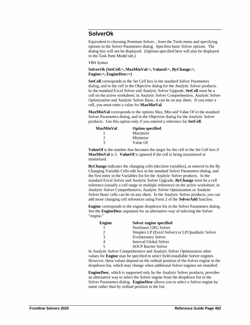
Frontline Solvers 2020 Reference Guide Page 462
SolverOk
Equivalent to choosing Premium Solver... from the Tools menu and specifying
options in the Solver Parameters dialog. Specifies basic Solver options. The
dialog box will not be displayed. (Options specified here will also be displayed
in the Task Pane Model tab.)
VBA Syntax
SolverOk (SetCell:=, MaxMinVal:=, Valueof:=, ByChange:=,
Engine:=, EngineDesc:=)
SetCell corresponds to the Set Cell box in the standard Solver Parameters
dialog, and to the cell in the Objective dialog for the Analytic Solver products.
In the standard Excel Solver and Analytic Solver Upgrade, SetCell must be a
cell on the active worksheet; in Analytic Solver Comprehensive, Analytic Solver
Optimization and Analytic Solver Basic, it can be on any sheet. If you enter a
cell, you must enter a value for MaxMinVal.
MaxMinVal corresponds to the options Max, Min and Value Of in the standard
Solver Parameters dialog, and in the Objective dialog for the Analytic Solver
products. Use this option only if you entered a reference for SetCell.
MaxMinVal Option specified
1 Maximize
2 Minimize
3 Value Of
ValueOf is the number that becomes the target for the cell in the Set Cell box if
MaxMinVal is 3. ValueOf is ignored if the cell is being maximized or
minimized.
ByChange indicates the changing cells (decision variables), as entered in the By
Changing Variable Cells edit box in the standard Solver Parameters dialog, and
the first entry in the Variables list for the Analytic Solver products. In the standard Excel Solver and Analytic Solver Upgrade, ByChange must be a cell
reference (usually a cell range or multiple reference) on the active worksheet; in
Analytic Solver Comprehensive, Analytic Solver Optimization or Analytic
Solver Basic cells can be on any sheet. In the Analytic Solver products, you can
add more changing cell references using Form 2 of the SolverAdd function.
Engine corresponds to the engine dropdown list in the Solver Parameters dialog.
See the EngineDesc argument for an alternative way of selecting the Solver
“engine.”
Engine Solver engine specified
1 Nonlinear GRG Solver 2 Simplex LP (Excel Solver) or LP/Quadratic Solver
3 Evolutionary Solver
4 Interval Global Solver
5 SOCP Barrier Solver
In Analytic Solver Comprehensive and Analytic Solver Optimization other
values for Engine may be specified to select field-installable Solver engines.
However, these values depend on the ordinal position of the Solver engine in the
dropdown list, which may change when additional Solver engines are installed.
EngineDesc, which is supported only by the Analytic Solver products, provides
an alternative way to select the Solver engine from the dropdown list in the
Solver Parameters dialog. EngineDesc allows you to select a Solver engine by name rather than by ordinal position in the list:

Frontline Solvers 2020 Reference Guide Page 463
EngineDesc Solver engine specified
“Standard GRG Nonlinear” Nonlinear GRG Solver
“Standard LP/Quadratic” LP/Quadratic Solver
“Standard Evolutionary” Evolutionary Solver
“Standard Interval Global” Interval Global Solver “Standard SOCP Barrier” SOCP Barrier Solver
“Gurobi Solver” Gurobi Solver
“Knitro Solver” Knitro Solver
“Large-Scale GRG Solver” Large-Scale GRG Solver
“Large-Scale LP Solver” Large-Scale LP Solver
“Large-Scale SQP Solver” Large-Scale SQP Solver
“MOSEK Solver Engine” MOSEK Solver Engine
“OptQuest Solver” OptQuest Solver
“XPRESS Solver Engine” XPRESS Solver Engine
SolverOkDialog
Equivalent to choosing Premium Solver... from the Tools menu and specifying
options in the Solver Parameters dialog. The Solver Parameters dialog box will
be displayed, and the user will be able to change the options you initially
specify.
VBA Syntax
SolverOkDialog (SetCell:=, MaxMinVal:=, Valueof:=, ByChange:=,
Engine:=, EngineDesc:=)
For an explanation of the arguments of this function, see SolverOk.
SolverOptions
Equivalent to choosing Premium Solver... from the Tools menu, then choosing
the Options button in the Solver Parameters dialog box or clicking the Task
Pane Engine tab. Specifies Solver algorithmic options. Arguments supported
by the standard Excel Solver include MaxTime, Iterations, Precision,
AssumeLinear, StepThru, Estimates, Derivatives, SearchOption, IntTolerance, Scaling, Convergence and AssumeNonNeg.
SolverOptions is provided for compatibility with the standard Excel Solver and
early versions of the Premium Solver products. For programmatic control of
new features and options included in the Premium Solver products, see the
functions in the sections “Solver Model VBA Functions” and “Premium VBA
Functions.”
VBA Syntax
SolverOptions (MaxTime:=, Iterations:=, Precision:=, AssumeLinear:=,
StepThru:=, Estimates:=, Derivatives:=, SearchOption:=, IntTolerance:=,
Scaling:=, Convergence:=, AssumeNonNeg:=, IntCutoff:=, BypassReports:=,
PivotTol:=, ReducedTol:=, CoeffTol:=, SolutionTol:=, Crash:=,
ScalingOption:=)
The arguments correspond to the options in the Solver Options dialog box. If an
argument is omitted, the Solver maintains the current setting for that option. If
any of the arguments are of the wrong type, the function returns the #N/A error
value. If all arguments are of the correct type, but an argument has an invalid
value, the function returns a positive integer corresponding to its position. A
zero return value indicates that all options were accepted.
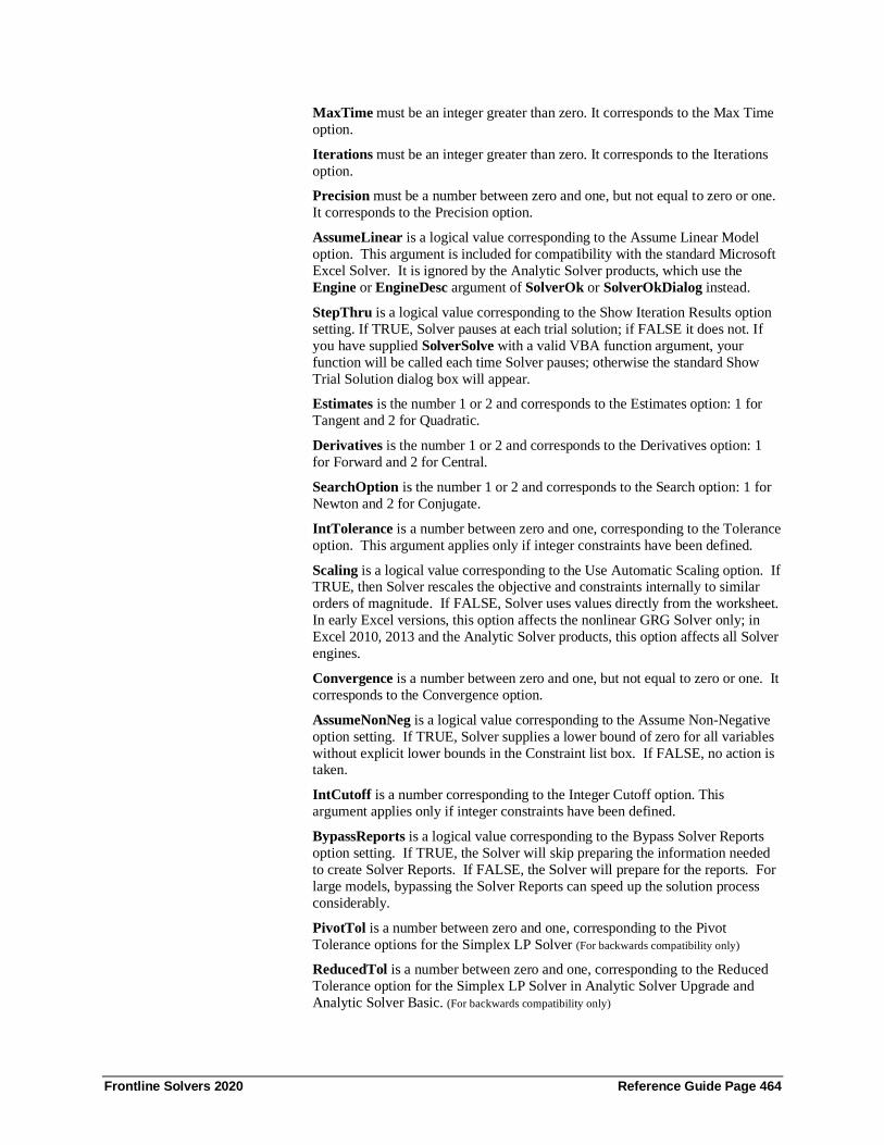
Frontline Solvers 2020 Reference Guide Page 464
MaxTime must be an integer greater than zero. It corresponds to the Max Time
option.
Iterations must be an integer greater than zero. It corresponds to the Iterations
option.
Precision must be a number between zero and one, but not equal to zero or one.
It corresponds to the Precision option.
AssumeLinear is a logical value corresponding to the Assume Linear Model
option. This argument is included for compatibility with the standard Microsoft
Excel Solver. It is ignored by the Analytic Solver products, which use the
Engine or EngineDesc argument of SolverOk or SolverOkDialog instead.
StepThru is a logical value corresponding to the Show Iteration Results option
setting. If TRUE, Solver pauses at each trial solution; if FALSE it does not. If
you have supplied SolverSolve with a valid VBA function argument, your
function will be called each time Solver pauses; otherwise the standard Show
Trial Solution dialog box will appear.
Estimates is the number 1 or 2 and corresponds to the Estimates option: 1 for
Tangent and 2 for Quadratic.
Derivatives is the number 1 or 2 and corresponds to the Derivatives option: 1
for Forward and 2 for Central.
SearchOption is the number 1 or 2 and corresponds to the Search option: 1 for
Newton and 2 for Conjugate.
IntTolerance is a number between zero and one, corresponding to the Tolerance
option. This argument applies only if integer constraints have been defined.
Scaling is a logical value corresponding to the Use Automatic Scaling option. If TRUE, then Solver rescales the objective and constraints internally to similar
orders of magnitude. If FALSE, Solver uses values directly from the worksheet.
In early Excel versions, this option affects the nonlinear GRG Solver only; in
Excel 2010, 2013 and the Analytic Solver products, this option affects all Solver
engines.
Convergence is a number between zero and one, but not equal to zero or one. It
corresponds to the Convergence option.
AssumeNonNeg is a logical value corresponding to the Assume Non-Negative
option setting. If TRUE, Solver supplies a lower bound of zero for all variables
without explicit lower bounds in the Constraint list box. If FALSE, no action is taken.
IntCutoff is a number corresponding to the Integer Cutoff option. This
argument applies only if integer constraints have been defined.
BypassReports is a logical value corresponding to the Bypass Solver Reports
option setting. If TRUE, the Solver will skip preparing the information needed
to create Solver Reports. If FALSE, the Solver will prepare for the reports. For
large models, bypassing the Solver Reports can speed up the solution process
considerably.
PivotTol is a number between zero and one, corresponding to the Pivot
Tolerance options for the Simplex LP Solver (For backwards compatibility only)
ReducedTol is a number between zero and one, corresponding to the Reduced
Tolerance option for the Simplex LP Solver in Analytic Solver Upgrade and
Analytic Solver Basic. (For backwards compatibility only)

Frontline Solvers 2020 Reference Guide Page 465
CoeffTol is no longer used, but is included for compatibility with previous
versions of the Premium Solver products.
SolutionTol is no longer used, but is included for compatibility with previous
versions of the Premium Solver products.
Crash is no longer used, but is included for compatibility with previous versions
of the Premium Solver products.
ScalingOption is no longer used, but is included for compatibility with previous
versions of the Premium Solver products.
SolverReset
Equivalent to choosing Premium Solver... from the Tools menu and choosing
the Reset All button in the Solver Parameters dialog box or clicking Reset All on
the Analytic Solver ribbon. Erases all cell selections and constraints from the
Solver Parameters dialog box, and restores all the settings on the Solver Options,
Limit Options and Integer Options dialog tab or the Task Pane Model, Platform
and Engine tabs to their defaults. The SolverReset function may be
automatically performed when you call SolverLoad.
VBA Syntax
SolverReset
SolverSave
Equivalent to choosing Premium Solver... from the Tools menu, choosing the
Options button from the Solver Parameters dialog box, and choosing the Save
Model... button in the Solver Options dialog box or clicking the Load/Save icon
on the Analytic Solver ribbon. Saves the model specifications on the worksheet.
The Format and ModelName arguments are supported only in Version 7.0 or
later of the Premium Solver products.
VBA Syntax
SolverSave (SaveArea:=, Format:=, ModelName:=)
SaveArea is a reference to a range of cells or to the topmost cell in a column of
cells where you want to save the current model’s specifications. In Solver
versions prior to V7.0, SaveArea must be a reference on the active worksheet;
in Version 7.0 or later it can be on any worksheet
Format corresponds to the Format dropdown list in the Load Model dialog: 1
for “Classic” format and 2 for “PSI Function” format.
In “Classic” format, the first cell in SaveArea contains a formula for the Set
Cell edit box; the second cell contains a formula for the changing cells; subsequent cells contain additional variable selections and constraints in the
form of logical formulas. The final cells optionally contain an array of Solver
option values.
In “PSI Function” format, the cells contain calls to functions such as PsiVar(),
PsiCon(), PsiObj() and PsiOption(). For details on these functions, see
“Defining Your Model with PSI Functions” in the chapter “Building Solver
Models.”
ModelName is used only when Format = 2, and specifies a text name for the
model. This name is saved as the last argument of each PSI Function call in the
saved model specifications.

Frontline Solvers 2020 Reference Guide Page 466
Remarks
If you specify only one cell for SaveArea, the area is extended downwards for
as many cells as are required to hold the model specifications.
If you specify more than one cell and the area is too small for the problem, the model specifications will not be saved, and the function will return the value 2.
SolverSolve
Equivalent to choosing Premium Solver... from the Tools menu and choosing the Solve button in the Solver Parameters dialog box or clicking the Optimize
icon on the Analytic Solver ribbon. If successful, returns an integer value
indicating the condition that caused the Solver to stop, as described below.
VBA Syntax
SolverSolve (UserFinish:=, ShowRef:=)
UserFinish is a logical value specifying whether to show the standard Solver
Results dialog box.
If UserFinish is TRUE, SolverSolve returns its integer value without displaying
anything. Your VBA code should decide what action to take (for example, by
examining the return value or presenting its own dialog box); it must call
SolverFinish in any case to return the worksheet to its proper state.
If UserFinish is FALSE or omitted, Solver displays the standard Solver Results
dialog box, allowing the user to keep or discard the final solution values, and
optionally produce reports.
ShowRef is a VBA function to be called in place of displaying the Show Trial
Solution dialog box. It is used when you want to gain control whenever Solver
finds a new “Trial Solution” value, the user presses the ESC key, or a limit on the solution process is exceeded. Here is an example of defining and using the
argument ShowRef:
Sub Test
answer = SolverSolve(True, ″ShowTrial″)
End Sub
Function ShowTrial(Reason As Integer)
Msgbox Reason
ShowTrial = 0
End Function
The argument Reason, which must be present, is an integer value from 1 to 5:
1. Function called (on every iteration) because the Show Iteration
Results box in the Solver Options dialog was checked, or function
called because the user pressed ESC to interrupt the Solver.
2. Function called because the Max Time limit in the Solver Options
dialog was exceeded.
3. Function called because the Max Iterations limit in the Solver
Options dialog was exceeded.
4. Function called because the Max Subproblems limit on the Integer Options or Limit Options dialog tab was exceeded (Analytic
Solver products only).

Frontline Solvers 2020 Reference Guide Page 467
5. Function called because the Max Integer Sols limit on the Integer
Options dialog tab or the Max Feasible Sols limit on the Limit
Options dialog tab was exceeded (Analytic Solver products only).
The function must return 0 if the Solver should stop (same as the Stop button in
the Show Trial Solution dialog), 1 if it should continue running (same as the Continue button), or 2 if it should restart the solution process (same as the
Restart button). Note: In the standard Excel Solver and the Premium Solver
prior to V5.0, the function should return FALSE instead of 0 to stop, or TRUE
instead of 1 to continue running; the restart alternative is not available.
Your VBA function can inspect the current solution values on the worksheet, or
take other actions such as saving or charting the intermediate values. However,
it should not alter the values in the variable cells, or alter the formulas in the
objective and constraint cells, as this could adversely affect the solution process.
In Analytic Solver Comprehensive, Analytic Solver Optimization or Analytic
Solver Basic, if the PSI Interpreter is used, the worksheet is not updated with new variable values until the end of the solution process; you cannot use the
traditional VBA functions to inspect variable values on each Trial Solution, but
you can use the object-oriented API to do this. See “Evaluators Called During
the Solution Process” in the chapter “Using the Object-Oriented API” for
details.
Remarks
If a Solver problem has not been completely defined, SolverSolve returns the
#N/A error value. Otherwise the Solver engine is started, and the problem
specifications are passed to it. When the solution process is complete,
SolverSolve returns an integer value indicating the stopping condition. The
standard Excel Solver returns values from 0 to 13; the Analytic Solver products return values from –1 to 21. When the Interval Global Solver or field-installable
Solver engines are used, Analytic Solver may return engine-specific values for
custom stopping conditions, starting at 1000.
Value Stopping Condition
-1 A licensing problem was detected, or your trial license
has expired.
0 Solver found a solution. All constraints and optimality
conditions are satisfied.
1 Solver has converged to the current solution. All constraints
are satisfied.
2 Solver cannot improve the current solution. All constraints are
satisfied.
3 Stop chosen when the maximum iteration limit was reached.
4 The Set Cell values do not converge.
5 Solver could not find a feasible solution.
6 Solver stopped at user’s request.
7 The linearity conditions required by this Solver engine are
not satisfied.
8 The problem is too large for Solver to handle.
9 Solver encountered an error value in a target or constraint
cell.

Frontline Solvers 2020 Reference Guide Page 468
10 Stop chosen when the maximum time limit was reached.
11 There is not enough memory available to solve the problem.
12 Error condition at cell address (Analytic Solver only).
13 Error in model. Please verify that all cells and constraints
are valid.
14 Solver found an integer solution within tolerance. All
constraints are satisfied.
15 Stop chosen when the maximum number of feasible [integer]
solutions was reached.
16 Stop chosen when the maximum number of feasible [integer]
subproblems was reached.
17 Solver converged in probability to a global solution.
18 All variables must have both upper and lower bounds.
19 Variable bounds conflict in binary or alldifferent constraint.
20 Lower and upper bounds on variables allow no feasible solution.
21 Solver encountered an error computing derivatives (Analytic
Solver only).
1000 Interval Global Solver requires Solve With Automatic and strictly
smooth functions (Analytic Solver only).
1001 Function cannot be evaluated for given real or interval
arguments (Analytic Solver only).
1002 Solution found, but not proven globally optimal (Analytic Solver
only).
Solver Model VBA Functions The VBA functions in this section are available only in Analytic Solver. You
can use these functions to programmatically use the Polymorphic Spreadsheet
Interpreter to check your model for Gradients, Structure and Convexity, obtain
model statistics, produce the Structure Report and Transformation Report,
determine whether and how the Interpreter will be used when you call
SolverSolve, and control the Interpreter’s advanced options.
SolverModel
Equivalent to choosing Premium Solver... from the Tools menu, choosing the
Model button in the Solver Parameters dialog, setting options in the Solver
Model dialog, and clicking Close or setting the individual options on the Task
Pane Platform tab. Specifies options for the Polymorphic Spreadsheet
Interpreter.
VBA Syntax
SolverModel (Interpreter:=, CheckFor:=, SolveTransformed:=,
ShowTransformations:=, ShowExceptions:=, DesiredModel:=,
Interactive:=, UsePsiFunctions:=, Engines:=, ReqSmooth:=, FastSetup:=,
Sparse:=, ActiveOnly:=)
The arguments correspond to the options in the Solver Model dialog box. The
Check For option appears on all four tabs of this dialog; the Interpreter option

Frontline Solvers 2020 Reference Guide Page 469
appears on the Options tab; the Solve Transformed Problem option appears on
the Model tab; the Desired Model option appears on the Diagnosis tab; and the
remaining options appear on the Options tab.
In the Task Pane Platform tab, the CheckFor options is labeled as Supply Engine
With and appears in the Advanced section, Interpreter appears in the both the Optimization and Simulation sections, Solver Transformed is labled as
Nonsmooth Model Transformation and appears in the Transformation section,
Show Transformations has been removed and is no longer used, Show
Exceptions has been removed and is no longer used, Desired Model has been
renamed to Intended Model Type and appears in the Diagnosis section,
Interactive and Use PsiFunctions appear in the Optimization section,
ReqSmooth (labeled as Use Internal Sparse Representation) and ActiveOnly
(labeled asOnly Parse Active Sheet) both appear in the Advanced section.
If an argument is omitted, the Solver maintains the current setting for that
option. If any of the arguments are of the wrong type, the function returns the
#N/A error value. If all arguments are of the correct type, but an argument has an invalid value, the function returns a positive integer corresponding to its
position. A zero return value indicates that all options were accepted.
Interpreter is a number corresponding to the option selected in the Solve With
option group on the Original tab or the option setting for Interpreter on the Task
Pane Model tab:
Interpreter Action on SolverSolve
1 Use PSI Interpreter
2 Use Excel Interpreter
Note: On the Model Task Pane, this option includes an alternative Automatic setting, see the chapter Platform Option Reference for more information.
CheckFor is a number corresponding to the option selected in the Check For
option group or for the Supply Engine with option on the Task Pane Platform
tab:
CheckFor Option Selected
1 Gradients
2 Structure
3 Convexity
4 Automatic
SolveTransformed is a logical value corresponding to the Solve Transformed Problem check box on the Transformed tab. If TRUE, the Solver solves the
Transformed problem when the SolverSolve function is called. If FALSE, the
Solver solves the Original problem when the SolverSolve function is called.
ShowTransformations This function is included for backward compatibility
only; a logical value corresponding to the Show Transformations check box on
the Transformed tab. If TRUE, the Solver produces a Transformation Report
when the SolverModelCheck function is called. If FALSE, the report is not
produced.
ShowExceptions This function is included for backward compatibility only; a
logical value corresponding to the Show Exceptions to Desired Model check
box on the Options tab. If TRUE, the Solver produces a Structure Report when the SolverModelCheck function is called. If FALSE, the report is not produced.
DesiredModel is a number corresponding to the option selected in the Desired
Model option group.
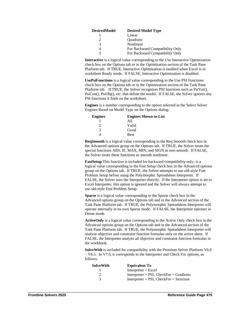
Frontline Solvers 2020 Reference Guide Page 470
DesiredModel Desired Model Type
1 Linear
2 Quadratic
3 Nonlinear
4 For Backward Compatibility Only 5 For Backward Compatibility Only
Interactive is a logical value corresponding to the Use Interactive Optimization
check box on the Options tab or in the Optimization section of the Task Pane
Platform tab. If TRUE, Interactive Optimization is enabled when Excel is in
worksheet Ready mode. If FALSE, Interactive Optimization is disabled.
UsePsiFunctions is a logical value corresponding to the Use PSI Functions
check box on the Options tab or in the Optimization section of the Task Pane
Platform tab . If TRUE, the Solver recognizes PSI functions such as PsiVar(),
PsiCon(), PsiObj(), etc. that define the model. If FALSE, the Solver ignores any
PSI functions it finds on the worksheet.
Engines is a number corresponding to the option selected in the Select Solver
Engines Based on Model Type on the Options dialog:
Engines Engines Shown in List
1 All
2 Valid
3 Good
4 Best
ReqSmooth is a logical value corresponding to the Req Smooth check box in
the Advanced options group on the Options tab. If TRUE, the Solver treats the
special functions ABS, IF, MAX, MIN, and SIGN as non-smooth. If FALSE,
the Solver treats these functions as smooth nonlinear.
FastSetup This function is included for backward compatibility only; is a
logical value corresponding to the Fast Setup check box in the Advanced options
group on the Options tab. If TRUE, the Solver attempts to use old-style Fast
Problem Setup before using the Polymorphic Spreadsheet Interpreter. If
FALSE, the Solver uses the Interpreter directly. If the Interpreter option is set to
Excel Interpreter, this option is ignored and the Solver will always attempt to
use old-style Fast Problem Setup.
Sparse is a logical value corresponding to the Sparse check box in the
Advanced options group on the Options tab and in the Advanced section of the
Task Pane Platform tab. If TRUE, the Polymorphic Spreadsheet Interpreter will operate internally in its own Sparse mode. If FALSE, the Interpreter operates in
Dense mode.
ActiveOnly is a logical value corresponding to the Active Only check box in the
Advanced options group on the Options tab and in the Advanced section of the
Task Pane Platform tab. If TRUE, the Polymorphic Spreadsheet Interpreter will
analyze objective and constraint function formulas only on the active sheet. If
FALSE, the Interpreter analyze all objective and constraint function formulas in
the workbook.
SolveWith is included for compatibility with the Premium Solver Platform V6.0
– V6.5. In V7.0, it corresponds to the Interpreter and Check For options, as
follows:
SolveWith Equivalent To
1 Interpreter = Excel
2 Interpreter = PSI, CheckFor = Gradients
3 Interpreter = PSI, CheckFor = Structure

Frontline Solvers 2020 Reference Guide Page 471
4 Interpreter = PSI, CheckFor = Convexity
5 Interpreter = PSI, CheckFor = Automatic
SolverModelCheck
Equivalent to choosing Premium Solver... from the Tools menu, choosing the
Model button in the Solver Parameters dialog box, and clicking the Check
Model button in the Solver Model dialog or clicking the down arrow on the
Optimize icon and selecting Analyze Original Model or Analyze Transformed
Model. The type of analysis performed is determined by the current setting of the SolverModel CheckFor argument.
VBA Syntax
SolverModelCheck (Transformed:=)
Transformed is a logical value that corresponds to the tab (Original or
Transformed) active when the Check Model button is pressed. If TRUE, the
Polymorphic Spreadsheet Interpreter checks the Transformed model. If FALSE,
the Interpreter checks the Original model.
SolverModelGet
Returns Solver Model option settings for the current Solver problem on the
specified sheet. These settings are entered in the Solver Model dialog. The available settings include the “read-only” edit boxes on the Model tab of the
Solver Model dialog; these values are valid only after you call
SolverModelCheck (FALSE) and SolverModelCheck (TRUE) respectively.
SolverModelGet(28) will return the type of model (Original or Transformed) as
determined by the most recent call to SolverModelCheck.
VBA Syntax
SolverModelGet (TypeNum:=, SheetName:=)
TypeNum is a number specifying the type of information you want. The
following settings are specified in the Solver Model dialog box.
TypeNum Returns
1 The All Variables value on the Original tab
2 The Smooth Variables value on the Original tab
3 The Quadratic Variables value on the Original tab
4 The Linear Variables value on the Original tab
5 The Bounds value on the Original tab
6 The Integers value on the Original tab
7 The All Functions value on the Original tab
8 The Smooth Functions value on the Original tab
9 The Quadratic Functions value on the Original tab
10 The Linear Functions value on the Original tab
11 The All NonZeroes value on the Original tab
12 The Smooth NonZeroes value on the Original tab

Frontline Solvers 2020 Reference Guide Page 472
13 The Quadratic NonZeroes value on the Original tab
14 The Linear NonZeroes value on the Original tab
15 The Sparsity % value on the Original tab
16 The Total Cells value on the Original tab
17 A number corresponding to the Check For option: 1 for
Gradients, 2 for Structure, or 3 for Convexity
18 TRUE if the Solve Transformed Problem check box is
selected; FALSE otherwise
19 This function is included for backward compatibility
only; TRUE if the Show Transformations check box is
selected; FALSE otherwise
20 A number corresponding to the Desired Model option: 1 for
Linear, 2 for Quadratic, 3 for Nonlinear, 4 included for
backward compatibility only, or 4 included for backward
compatibility only
21 A number corresponding to the V6 Solve With option: 1 for No
Action (Excel Interpreter), 2 for Gradients, 3 for Structure,
4 for Convexity, or 5 for Automatic
22 A number corresponding to the Engines option: 1 for All,
2 for Valid, 3 for Good, or 4 for Best
23 TRUE if the Req Smooth option is set True or selected;
FALSE otherwise
24 TRUE if the Fast Setup option is selected or set to True;
FALSE otherwise
25 TRUE if the Sparse option is selected or set to True;
FALSE otherwise
26 TRUE if the Active Only option is selected or set to
True; FALSE otherwise
27 This function is included for backward compatibility
only; TRUE if the Show Exceptions to Desired Model check box is selected; FALSE otherwise
28 A string corresponding to the type of model: "LP", "QP",
"QCP", "NLP", "NSP", or "Unknown". "LP", "QP", "QCP", or
"NLP" may be followed by a space and "Convex" or
"NonCvx".
29 TRUE if the Interactive Optimization option is selected
or set to True; FALSE otherwise
30 TRUE if the Use PSI Functions option is selected or set
to True; FALSE otherwise
31 The All Variables value on the Model tab or on the Task
Pane Model tab
32 The Smooth Variables value on the Model tab or on the
Task Pane Model tab
33 Included for backward compatibility only; The Quadratic
Variables value on the Original
34 The Linear Variables value on the Model tab or on the
Task Pane Model tab
35 The Bounds value on the Model tab or on the Task Pane
Model tab

Frontline Solvers 2020 Reference Guide Page 473
36 The Integers value on the Model tab or on the Task Pane
Model tab
37 The All Functions value on the Model tab or on the Task
Pane Model tab
38 The Smooth Functions value on the Model tab or on the
Task Pane Model tab
39 Included for backward compatibility only; The Quadratic
Functions value on the Original tab
40 The Linear Functions value on the Model tab or on the
Task Pane Model tab
41 Included for backward compatibility only; The All
NonZeroes value on the Model tab or on the Task Pane
Model tab
42 Included for backward compatibility only; The Smooth
NonZeroes value on the Original tab
43 Included for backward compatibility only; The Quadratic
NonZeroes value on the Original tab
44 Included for backward compatibility only; The Linear
NonZeroes value on the Original tab
45 The Sparsity % value on the Model tab or on the Task Pane
Model tab
46 Included for backward compatibility only; The Total Cells
value on the Original tab
SolverDependents
This function is included for backward compatibility only; use the SolverModel-Check function in new applications. Equivalent to choosing Premium Solver...
from the Tools menu, choosing the Model button in the Solver Parameters
dialog box, selecting the Structure option in the Check For option group, and
clicking the Check Model button in the Solver Model dialog.
VBA Syntax
SolverDependents
SolverFormulas
This function is included for backward compatibility only; use the SolverModel-
Check function in new applications. Equivalent to choosing Premium Solver...
from the Tools menu, choosing the Model button in the Solver Parameters
dialog box, selecting the Gradients option in the Check For option group, and clicking the Check Model button in the Solver Model dialog.
VBA Syntax
SolverFormulas
Premium VBA Functions The VBA functions in this section were first introduced in Version 3.0 of the
Premium Solver products, and expanded in later versions. To control most of
the new features and options in the Analytic Solver products, you’ll need to use

Frontline Solvers 2020 Reference Guide Page 474
these functions – notably, the SolverEVOptions, SolverIGOptions,
SolverLimOptions and SolverIntOptions functions. (Or, in Version 7.0 and
later, you can use the new object-oriented API to control these features and
options; see the Analytic Solver User Guide chapter, “Automating Optimization
in VBA” for help.) If you want to write VBA code that can be used with both the standard Solver and the Premium or Analytic Solver products, you should
use only functions in the section “Standard VBA Functions.”
SolverEVGet
Returns Evolutionary Solver option settings for the current Solver problem on
the specified sheet. These settings are entered on the General tab for Solver
options or on the Task Pane Engine tab when the Evolutionary Solver is
selected in the Solver Engine dropdown list.
Several additional options can only be set when using the Obect – Oriented API,
see the Analytic Solver User Guide chapter, “Automating Optimation in VBA”
and the “Solver Engine Option Reference” chapter in this guide for more
information.
VBA Syntax
SolverEVGet (TypeNum:=, SheetName:=)
TypeNum is a number specifying the type of information you want. The
following settings are specified in the Evolutionary Solver Options dialog box.
TypeNum Returns
1 The Max Time value (as a number in seconds)
2 The Iterations value (max number of iterations)
3 The Precision value (as a decimal number)
4 The Convergence value (as a decimal number)
5 The Population Size value (as a decimal number)
6 The Mutation Rate value (as a decimal number)
7 TRUE if the Require Bounds on Variables option is
selected or set to True; FALSE otherwise
8 TRUE if the Show Iteration Result option is selected or
set to True; FALSE otherwise
9 TRUE if the Use Automatic Scaling option is selected or set to
True; FALSE otherwise
10 TRUE if the Assume Non-Negative option is selected or set to
True; FALSE otherwise
11 TRUE if the Bypass Solver Reports option is selected or set to
True; FALSE otherwise
12 The Random Seed value (as a decimal number)
13 A number corresponding to the Local Search option: 1 for
Randomized Local Search, 2 for Gradient Local, 3* for SQP with
Gradient Strategy, or 4 for Automatic Choice.
14 TRUE if the Fix Nonsmooth Variables check box is selected;
FALSE otherwise
*If using Analytic Solver Upgrade, 3 = Deterministic Pattern Search.
Frontline Solvers 2020 Reference Guide Page 475
SheetName is the name of a worksheet that contains the Solver problem for
which you want information. If SheetName is omitted, it is assumed to be the
active sheet.
SolverEVOptions
Equivalent to choosing Premium Solver... from the Tools menu and then
choosing the Options button in the Solver Parameters dialog box when the
Evolutionary Solver is selected in the Solver Engine dropdown list. Specifies
options for the Evolutionary Solver.
VBA Syntax
SolverEVOptions (MaxTime:=, Iterations:=, Precision:=, Convergence:=,
PopulationSize:=, MutationRate:=, RandomSeed:=, RequireBounds:=,
StepThru:=, Scaling:=, AssumeNonNeg:=, BypassReports:=, LocalSearch:=
FixNonSmooth:=)
The arguments correspond to the options in the Solver Options dialog box. If an
argument is omitted, the Solver maintains the current setting for that option. If any of the arguments are of the wrong type, the function returns the #N/A error
value. If all arguments are of the correct type, but an argument has an invalid
value, the function returns a positive integer corresponding to its position. A
zero return value indicates that all options were accepted.
MaxTime must be an integer greater than zero. It corresponds to the Max Time
option.
Iterations must be an integer greater than zero. It corresponds to the Iterations
option.
Precision must be a number between zero and one, but not equal to zero or one.
It corresponds to the Precision option.
Convergence is a number between zero and one, but not equal to zero or one. It
corresponds to the Convergence option.
PopulationSize must be an integer greater than or equal to zero. It corresponds
to the Population Size option.
MutationRate must be a number between zero and one, but not equal to zero or
one. It corresponds to the Mutation Rate option.
RandomSeed must be an integer greater than zero. It corresponds to the
Random Seed option.
RequireBounds is a logical value corresponding to the Require Bounds on Variables option. If TRUE, the Evolutionary Solver will return immediately
from a call to the SolverSolve function with a value of 18 if any of the variables
do not have both lower and upper bounds defined. If FALSE, the Evolutionary
Solver will attempt to solve the problem without bounds on all of the variables.
StepThru is a logical value corresponding to the Show Iteration Results option.
If TRUE, Solver pauses at each trial solution; if FALSE it does not. If you have
supplied SolverSolve with a valid VBA function, your function will be called
each time Solver pauses; otherwise the standard Show Trial Solution dialog box
will appear.
Scaling is a logical value corresponding to the Use Automatic Scaling option. If
TRUE, then Solver rescales the objective and constraints internally to similar orders of magnitude. If FALSE, Solver uses values directly from the worksheet.

Frontline Solvers 2020 Reference Guide Page 476
AssumeNonNeg is a logical value corresponding to the Assume Non-Negative
option. If TRUE, Solver supplies a lower bound of zero for all variables without
explicit lower bounds in the Constraint list box. If FALSE, no action is taken.
BypassReports is a logical value corresponding to the Bypass Solver Reports
option. If TRUE, the Solver will skip preparing the information needed to create Solver Reports. If FALSE, the Solver will prepare for the reports. For
large models, bypassing the Solver Reports can speed up the solution
considerably.
LocalSearch is a number corresponding to the option selected in the Local
Search option group:
LocalSearch Local Search Strategy
1 Randomized Local Search
2 Gradient Local Search
3 SQP with Gradient Sampling*
4 Automatic Choice
*If using Analytic Solver Upgrade, 3 = Deterministic Pattern Search.
In the Premium Solver Platform V5.5 and later, a value of 4 selects the
Automatic Choice option; this allows the Solver to choose a local search method
automatically – Randomized Local Search, Gradient Local Search, or Linear Local Gradient Search, depending on the characteristics of the problem.
FixNonSmooth is a logical value corresponding to the Fix Nonsmooth
Variables option. If TRUE, the Solver will fix the non-smooth variables to their
current values during each local search, and allow only smooth and linear
variables to be varied. If FALSE, the Solver will allow all of the variables to be
varied.
SolverGRGGet
Returns GRG Solver option settings for the current Solver problem on the
specified sheet. These settings are entered on the General tab for Solver options
or on the Task Pane Engine tab when the GRG Solver is selected in the Solver
Engine dropdown list.
VBA Syntax
SolverGRGGet (TypeNum:=, SheetName:=)
TypeNum is a number specifying the type of information you want. The
following settings are specified on the General tab in the GRG Solver Options
dialog box.
TypeNum Returns
1 The Max Time value (as a number in seconds)
2 The Iterations value (max number of iterations)
3 The Precision value (as a decimal number)
4 The Convergence value (as a decimal number)
5 TRUE if the Show Iteration Result option is selected or
set to True; FALSE otherwise
6 TRUE if the Use Automatic Scaling option is selected or set to
True; FALSE otherwise

Frontline Solvers 2020 Reference Guide Page 477
7 TRUE if the Assume Non-Negative option is selected or set to
True; FALSE otherwise
8 TRUE if the Bypass Solver Reports option is selected or set to
True; FALSE otherwise
9 TRUE if the Recognize Linear Variables option is selected or set
to True; FALSE otherwise
10 A number corresponding to the type of Estimates:
1 = Tangent
2 = Quadratic
11 A number corresponding to the type of Derivatives:
1 = Forward
2 = Central
12 A number corresponding to the type of Search:
1 = Newton
2 = Conjugate
13 The Population Size value (as a decimal number)
14 The Random Seed value (as a decimal number)
15 TRUE if the Multistart Search option is selected or set to True;
FALSE otherwise
16 TRUE if the Topographic Search option is selected or set to
True; FALSE otherwise
17 TRUE if Require Bounds on Variables option is selected or set to
True; FALSE otherwise
SheetName is the name of a worksheet that contains the Solver problem for
which you want information. If SheetName is omitted, it is assumed to be the
active sheet.
SolverGRGOptions
Equivalent to choosing Premium Solver... from the Tools menu and then
choosing the Options button in the Solver Parameters dialog box or selecting the
Task Pane Engine tab when the GRG Nonlinear Solver is selected in the Solver
Engines dropdown list. Specifies options for the GRG Solver.
VBA Syntax
SolverGRGOptions (MaxTime:=, Iterations:=, Precision:=, Convergence:=,
PopulationSize:=, RandomSeed:=, StepThru:=, Scaling:=,
,AssumeNonNeg:=, BypassReports:=, RecognizeLinear:=, MultiStart:=,
TopoSearch:=, RequireBounds:=, Estimates:=, Derivatives:=,
SearchOption:=)
The arguments correspond to the options in the Solver Options dialog box. If an
argument is omitted, the Solver maintains the current setting for that option. If
any of the arguments are of the wrong type, the function returns the #N/A error
value. If all arguments are of the correct type, but an argument has an invalid
value, the function returns a positive integer corresponding to its position. A
zero return value indicates that all options were accepted.
MaxTime must be an integer greater than zero. It corresponds to the Max Time
option.
Iterations must be an integer greater than zero. It corresponds to the Iterations
option.

Frontline Solvers 2020 Reference Guide Page 478
Precision must be a number between zero and one, but not equal to zero or one.
It corresponds to the Precision option.
Convergence is a number between zero and one, but not equal to zero or one. It
corresponds to the Convergence option.
PopulationSize must be an integer greater than or equal to zero. It corresponds
to the Population Size option.
RandomSeed must be an integer greater than zero. It corresponds to the
Random Seed option.
StepThru is a logical value corresponding to the Show Iteration Results option.
If TRUE, Solver pauses at each trial solution; if FALSE it does not. If you have
supplied SolverSolve with a valid VBA function, your function will be called
each time Solver pauses; otherwise the standard Show Trial Solution dialog box
will appear.
Scaling is a logical value corresponding to the Use Automatic Scaling option. If TRUE, then Solver rescales the objective and constraints internally to similar
orders of magnitude. If FALSE, Solver uses values directly from the worksheet.
AssumeNonNeg is a logical value corresponding to the Assume Non-Negative
option. If TRUE, Solver supplies a lower bound of zero for all variables without
explicit lower bounds in the Constraint list box. If FALSE, no action is taken.
BypassReports is a logical value corresponding to the Bypass Solver Reports
option. If TRUE, the Solver will skip preparing the information needed to
create Solver Reports. If FALSE, the Solver will prepare for the reports. For
large models, bypassing the Solver Reports can speed up the solution
considerably.
RecognizeLinear is a logical value corresponding to the Recognize Linear
Variables option. If TRUE, the Solver will recognize variables whose partial
derivatives are not changing during the solution process, and assume that they
occur linearly in the problem. If FALSE, the Solver will not make any
assumptions about such variables. See the chapter “Solver Engine Option
Reference” for a further discussion of this option.
MultiStart is a logical value corresponding to the Multistart Search option. If
TRUE, the Solver will use Multistart Search, in conjunction with the GRG
Solver, to seek a globally optimal solution. If FALSE, the GRG Solver alone
will be used to search for a locally optimal solution.
TopoSearch is a logical value corresponding to the Topographic Search option. If TRUE, and if Multistart Search is selected, the Solver will construct a
topography from the randomly sampled initial points, and use it to guide the
search process.
RequireBounds is a logical value corresponding to the Require Bounds on
Variables option. If TRUE, the Solver will return immediately from a call to the
SolverSolve function with a value of 18 if any of the variables do not have both
lower and upper bounds defined. If FALSE, then Multistart Search (if selected)
will attempt to find a globally optimal solution without bounds on all of the
variables.
Estimates is the number 1 or 2 and corresponds to the Estimates option: 1 for Tangent and 2 for Quadratic.
Derivatives is the number 1 or 2 and corresponds to the Derivatives option: 1
for Forward and 2 for Central.
Frontline Solvers 2020 Reference Guide Page 479
SearchOption is the number 1 or 2 and corresponds to the Search option: 1 for
Newton and 2 for Conjugate.
SolverIGGet
Returns Interval Global Solver option settings for the current Solver problem on
the specified sheet. These settings are entered on the General tab for Solver
options or on the Task Pane Engine tab when the Interval Global Solver is
selected in the Solver Engine dropdown list.
VBA Syntax
SolverIGGet (TypeNum:=, SheetName:=)
TypeNum is a number specifying the type of information you want. The
following settings are specified on the General tab in the Interval Global Solver
Options dialog box and on the Task Pane Model tab when the Interval Global
Solver is selected in the Solver Engine dropdown list.
TypeNum Returns
1 The Max Time value (as a number in seconds)
2 The Iterations value (max number of iterations)
3 The Accuracy value (as a decimal number)
4 The Resolution value (as a decimal number)
5 The Max Time w/o Improvement value (as a decimal number)
6 TRUE if the Show Iteration Result check box is selected;
FALSE otherwise
7 TRUE if the Assume Non-Negative check box is selected;
FALSE otherwise
8 TRUE if the Bypass Solver Reports option is selected or set to
TRUE; otherwise
9 TRUE if the Abs vs. Relative Stop option is selected or set to
TRUE; FALSE otherwise
10 TRUE if the Assume Stationary option is selected or set to TRUE;
FALSE otherwise
11 A number corresponding to the type of Method:
1 = Classic Interval
2 = Linear Enclosure
12 TRUE if the Second Order option is selected or set to TRUE;
FALSE otherwise
13 TRUE if the LP Test option is selected or set to TRUE heck box
is selected; FALSE otherwise
14 TRUE if the LP Phase II option is selected or set to TRUE; FALSE
otherwise
SolverIGOptions
Equivalent to choosing Premium Solver... from the Tools menu and then
choosing the Options button in the Solver Parameters dialog box or clicking
Task Pane Engine tab when the Interval Global Solver is selected in the Solver
Engines dropdown list. Specifies options for the Interval Global Solver.
Frontline Solvers 2020 Reference Guide Page 480
VBA Syntax
SolverIGOptions (MaxTime:=, Iterations:=, Accuracy:=, Resolution:=,
MaxTimeNoImp:=, StepThru:=, AssumeNonNeg:=, BypassReports:=,
AbsRelStop:=, AssumeStationary:=, Method:=, SecondOrder:=, LPTest:=,
LPPhaseII:=)
The arguments correspond to the options in the Solver Options dialog box. If an
argument is omitted, the Solver maintains the current setting for that option. If
any of the arguments are of the wrong type, the function returns the #N/A error
value. If all arguments are of the correct type, but an argument has an invalid
value, the function returns a positive integer corresponding to its position. A
zero return value indicates that all options were accepted.
MaxTime must be an integer greater than zero. It corresponds to the Max Time
option.
Iterations must be an integer greater than zero. It corresponds to the Iterations
option.
Accuracy must be a number between zero and one, but not equal to zero or one.
It corresponds to the Accuracy option.
Resolution is a number greater than zero. It corresponds to the Resolution
option.
MaxTimeNoImp is a number corresponding to the Max Time w/o Improvement
option. This argument determines when the Interval Global Solver will stop with
the message “Solver cannot improve the current solution.”
StepThru is a logical value corresponding to the Show Iteration Results option. If TRUE, Solver pauses at each trial solution; if FALSE it does not. If you have
supplied SolverSolve with a valid VBA function, your function will be called
each time Solver pauses; otherwise the standard Show Trial Solution dialog box
will appear.
AssumeNonNeg is a logical value corresponding to the Assume Non-Negative
option. If TRUE, Solver supplies a lower bound of zero for all variables without
explicit lower bounds in the Constraint list box. If FALSE, no action is taken.
BypassReports is a logical value corresponding to the Bypass Solver Reports
option. If TRUE, the Solver will skip preparing the information needed to
create Solver Reports. If FALSE, the Solver will prepare for the reports. For large models, bypassing the Solver Reports can speed up the solution
considerably.
AbsRelStop is a logical value corresponding to the Abs vs. Relative Stop
option. If TRUE, the Solver will use the absolute difference when comparing
the current solution’s objective to the best bound. If FALSE, the Solver will use
the relative difference when making the comparison.
AssumeStationary is a logical value corresponding to the Assume Stationary
option. If TRUE, the Solver will assume that the optimal solution is a stationary
point and is not at a decision variable bound. If FALSE, the Solver will search
for optimal solutions at all points, including those where variables are at their
bounds.
Method is the number 1 or 2 and corresponds to the Method option: 1 for
Classic Interval and 2 for Linear Enclosure.
SecondOrder is a logical value corresponding to the Second Order option. This
option is used only if the Method option is 1. If TRUE, the Solver will use
Frontline Solvers 2020 Reference Guide Page 481
second order (Interval Newton) methods. If FALSE, the Solver will use only
first order methods.
LPTest is a logical value corresponding to the LP Test option. This option is
used only if the Method option is 2. If TRUE, the Solver will use a Simplex
method Phase I test to eliminate boxes that contain no feasible solutions. If FALSE, the Solver will not use this test.
LPPhaseII is a logical value corresponding to the LP Phase II option. If TRUE,
the Solver will use a Simplex method Phase II procedure to seek an improved
bound on the objective in a box. If FALSE, the Solver will not use this
procedure.
SolverIntGet
Returns integer (Branch & Bound) option settings for the current Solver
problem on the specified sheet. These settings are entered on the Integer dialog
tab or on the Task Pane Engine tab for any of the Solver engines.
VBA Syntax
SolverIntGet (TypeNum:=, SheetName:=)
TypeNum is a number specifying the type of information you want. The
following settings are specified on the Integer dialog tab box.
TypeNum Returns
1 The Max Subproblems value (as a decimal number)
2 The Max Feasible Sols value (as a decimal number)
3 The (Integer) Tolerance value (as a decimal number)
4 The Integer Cutoff value (as a decimal number)
5 TRUE if the Solve Without Integer Constraints option is
selected or set to True; FALSE otherwise
6 TRUE if the Use Dual Simplex for Subproblems option is
selected or set to True in the Standard LP Simplex
Engine; FALSE otherwise. (For backwards compatibility
only)
7 TRUE if the Probing / Feasibility option is
selected or set to True in the Standard LP Simplex Engine;
FALSE otherwise (For backwards compatibility only)
8 TRUE if the Bounds Improvement option is selected or set
to True in the Standard LP Simplex Engine; FALSE
otherwise (For backwards compatibility only)
9 TRUE if the Optimality Fixing option is selected or set
to True in the Standard LP Simplex Engine; FALSE
otherwise. (For backwards compatibility only)
10 TRUE if the Variable Reordering option is selected or set
to True; FALSE otherwise. This option is no longer used.
11 TRUE if the Primal Heuristic option is selected or set to
True; FALSE otherwise. This option is no longer used.
12 The Max Gomory Cuts value (as a decimal number) in the
Standard LP Simplex Engine. (For backwards compatibility
only)
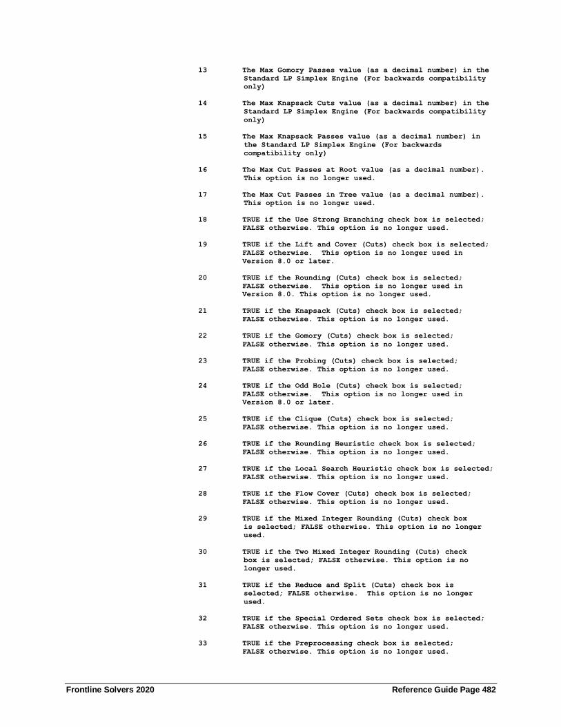
Frontline Solvers 2020 Reference Guide Page 482
13 The Max Gomory Passes value (as a decimal number) in the
Standard LP Simplex Engine (For backwards compatibility
only)
14 The Max Knapsack Cuts value (as a decimal number) in the
Standard LP Simplex Engine (For backwards compatibility
only)
15 The Max Knapsack Passes value (as a decimal number) in
the Standard LP Simplex Engine (For backwards
compatibility only)
16 The Max Cut Passes at Root value (as a decimal number).
This option is no longer used.
17 The Max Cut Passes in Tree value (as a decimal number).
This option is no longer used.
18 TRUE if the Use Strong Branching check box is selected;
FALSE otherwise. This option is no longer used.
19 TRUE if the Lift and Cover (Cuts) check box is selected;
FALSE otherwise. This option is no longer used in
Version 8.0 or later.
20 TRUE if the Rounding (Cuts) check box is selected;
FALSE otherwise. This option is no longer used in
Version 8.0. This option is no longer used.
21 TRUE if the Knapsack (Cuts) check box is selected;
FALSE otherwise. This option is no longer used.
22 TRUE if the Gomory (Cuts) check box is selected;
FALSE otherwise. This option is no longer used.
23 TRUE if the Probing (Cuts) check box is selected;
FALSE otherwise. This option is no longer used.
24 TRUE if the Odd Hole (Cuts) check box is selected;
FALSE otherwise. This option is no longer used in
Version 8.0 or later.
25 TRUE if the Clique (Cuts) check box is selected;
FALSE otherwise. This option is no longer used.
26 TRUE if the Rounding Heuristic check box is selected;
FALSE otherwise. This option is no longer used.
27 TRUE if the Local Search Heuristic check box is selected;
FALSE otherwise. This option is no longer used.
28 TRUE if the Flow Cover (Cuts) check box is selected;
FALSE otherwise. This option is no longer used.
29 TRUE if the Mixed Integer Rounding (Cuts) check box
is selected; FALSE otherwise. This option is no longer
used.
30 TRUE if the Two Mixed Integer Rounding (Cuts) check
box is selected; FALSE otherwise. This option is no
longer used.
31 TRUE if the Reduce and Split (Cuts) check box is
selected; FALSE otherwise. This option is no longer
used.
32 TRUE if the Special Ordered Sets check box is selected;
FALSE otherwise. This option is no longer used.
33 TRUE if the Preprocessing check box is selected;
FALSE otherwise. This option is no longer used.

Frontline Solvers 2020 Reference Guide Page 483
34 TRUE if the Feasibility Pump (Heuristic) box is selected;
0 FALSE otherwise. This option is no longer used.
35 TRUE if the Greedy Cover Heuristic check box is selected;
FALSE otherwise. This option is no longer used.
36 TRUE if the Local Tree check box is selected;
FALSE otherwise. This option is no longer used.
Return values 10, 11, 16 through18, and 21 through 36 are no longer supported
and are included only to avoid breaking macros written for older versions of
Premium Solver. Of the supported values for TypeNum, 6 through 9 and 12
through 15 are included for backward compatibility. To set integer options for
the LP/Quadratic Solver Engine use the object – oriented API as described in the
Analytic Solver User Guide chapter, “Automating Optimation in VBA” and the
chapter, “Solver Engine Option Reference” in this guide. SheetName is the
name of a worksheet that contains the Solver problem for which you want
information. If SheetName is omitted, it is assumed to be the active sheet.
SolverIntOptions
The first five options apply to the LP/Quadratic Solver. The next 10 options are
specific to the LP Simplex Solver which is no longer included in Analytic
Solver. To set additional integer options for the LP/Quadratic Solver, you must use the object – oriented API. See the Analytic Solver User Guide chapter,
“Automating Optimization in VBA” and the “Solver Engine Option Reference”
chapter in this guide for help.
Equivalent to choosing Premium Solver... from the Tools menu, choosing the
Options button in the Solver Parameters dialog box, and then choosing the
Integer tab. Options are also included on the Task Pane Engine tab. Specifies
options for the integer (Branch & Bound) Solver.
VBA Syntax
SolverIntOptions (MaxSubproblems:=, MaxIntegerSols:=, IntTolerance:=,
IntCutoff:=, SolveWithout:=, UseDual:=, ProbingFeasibility:=,
BoundsImprovement:=, OptimalityFixing:=, VariableReordering:=,
UsePrimalHeuristic:=, MaxGomoryCuts:=, GomoryPasses:=,
MaxKnapsackCuts:=, KnapsackPasses:=; MaxRootCutPasses:=,
MaxTreeCutPasses:=, StrongBranching:=, LiftAndCoverCuts:=,
RoundingCuts:=, KnapsackCuts:=, GomoryCuts:=, ProbingCuts:=,
OddHoleCuts:=, CliqueCuts:=, RoundingHeur:=, LocalHeur:=,
FlowCoverCuts:=, MirCuts:=, TwoMirCuts:=, RedSplitCuts:=, SOSCuts:=,
PreProcess:=, FeasibilityPump:=, GreedyCover:=, LocalTree:=)
If an argument is omitted, the Solver maintains the current setting for that
option. If any of the arguments are of the wrong type, the function returns the
#N/A error value. If all arguments are of the correct type, but an argument has
an invalid value, the function returns a positive integer corresponding to its
position. A zero return value indicates that all options were accepted.
MaxSubproblems must be an integer greater than zero. It corresponds to the
Max Subproblems option.
MaxIntegerSols must be an integer greater than zero. It corresponds to the Max
Integer Sols (Solutions) options.
IntTolerance is a number between zero and one, corresponding to the Tolerance option.
Frontline Solvers 2020 Reference Guide Page 484
IntCutoff is a number (any value is possible) corresponding to the Integer
Cutoff option.
SolveWithout is a logical value corresponding to the Solve Without Integer
Constraints option included in the Solve dropdown menu on the Solver
Parameters dialog or in the Optimize drop down menu on the Analytic Solver ribbon. If TRUE, the Solver ignores any integer constraints and solves the
“relaxation” of the mixed-integer programming problem. If FALSE, the Solver
uses the integer constraints in solving the problem.
UseDual is a logical value corresponding to the Use Dual Simplex for
Subproblems option in the LP Simplex Engine. If TRUE, the Solver uses the
Dual Simplex method, starting from an advanced basis, to solve the
subproblems generated by the Branch & Bound method. If FALSE, the Solver
uses the Primal Simplex method to solve the subproblems. This option is no
longer used.
ProbingFeasibility is a logical value corresponding to the Probing / Feasibility option in the LP Simplex Engine. If TRUE, the Solver attempts to derive
settings for binary integer variables, and implications for feasibility of the
subproblem, from the subproblem’s bounds on binary integer variables. If
FALSE, the Solver does not employ these strategies. This option is no longer
used.
BoundsImprovement is a logical value corresponding to the Bounds
Improvement option in the LP Simplex Engine. If TRUE, the Solver attempts to
tighten the bounds of non-binary integer variables, based on the initial or
derived settings of binary integer variables in the subproblem. If FALSE, the
Solver does not employ this strategy.
OptimalityFixing is a logical value corresponding to the Optimality Fixing option in the LP Simplex Engine. If TRUE, the Solver attempts to fix the values
of binary integer variables based on their coefficients in the objective function
and constraints, and on the initial or derived settings of other binary integer
variables. If FALSE, the Solver does not employ this strategy. This option is no
longer used.
VariableReordering is a logical value corresponding to the Variable
Reordering check box. In Version 5 and later of the Premium and Analytic
Solver products, this option is no longer used and its value is ignored.
UsePrimalHeuristic is a logical value corresponding to the Primal Heuristic
check box. If TRUE, the Solver uses heuristic methods to attempt to discover an integer feasible solution at the beginning of the Branch & Bound process. If
FALSE, the Solver does not employ this strategy. This option is no longer used
and its value is ignored.
MaxGomoryCuts must be an integer greater than or equal to zero. It
corresponds to the Max Gomory Cuts option in the LP Simplex Engine. This
option is no longer used.
GomoryPasses must be an integer greater than or equal to zero. It corresponds
to the Max Gomory Passes option in the LP Simplex Engine. This option is no
longer used.
MaxKnapsackCuts must be an integer greater than or equal to zero. It corresponds to the Max Knapsack Cuts option in the LP Simplex Engine. This
option is no longer used.
Frontline Solvers 2020 Reference Guide Page 485
KnapsackPasses must be an integer greater than or equal to zero. It
corresponds to the Max Knapsack Passes option in the LP Simplex Engine. This
option is no longer used.
MaxRootCutPasses must be an integer greater than or equal to zero. It
corresponds to the Max Root Cut Passes edit box. This option is no longer used and its value is ignored.
MaxTreeCutPasses must be an integer greater than or equal to zero. It
corresponds to the Max Tree Cut Passes edit box. This option is no longer used
and its value is ignored.
StrongBranching is a logical value corresponding to the Use Strong Branching
check box. If TRUE, Strong Branching takes a few steps towards a solution for
a number of different candidate integer variables, and selects the one showing
the most rapid improvement in the objective as the actual variable for branching.
If FALSE, no action is taken. This option is no longer used and its value is
ignored.
LiftAndCoverCuts is a logical value corresponding to the Lift and Cover check
box. If TRUE, Lift and Cover cuts are generated. If FALSE, no cuts of this
type are generated. In Version 8.0 and later, this option is no longer used and its
value is ignored.
RoundingCuts is a logical value corresponding to the Lift and Cover check
box. If TRUE, Rounding cuts are generated. If FALSE, no cuts of this type are
generated. In Version 8.0 and later, this option is no longer used and its value is
ignored.
KnapsackCuts is a logical value corresponding to the Knapsack check box. If
TRUE, Knapsack cuts are generated. If FALSE, no cuts of this type are generated. This option is no longer used and its value is ignored.
GomoryCuts is a logical value corresponding to the Gomory check box. If
TRUE, Gomory cuts are generated. If FALSE, no cuts of this type are
generated. This option is no longer used and its value is ignored.
ProbingCuts is a logical value corresponding to the Probing check box. If
TRUE, Probing cuts are generated. If FALSE, no cuts of this type are
generated. This option is no longer used and its value is ignored.
OddHoleCuts is a logical value corresponding to the Odd Hole check box. If
TRUE, Odd Hole cuts are generated. If FALSE, no cuts of this type are
generated. In Version 8.0 and later, this option is no longer used and its value is ignored.
CliqueCuts is a logical value corresponding to the Clique check box. If TRUE,
Clique cuts are generated. If FALSE, no cuts of this type are generated. This
option is no longer used and its value is ignored.
RoundingHeur is a logical value corresponding to the Rounding Heuristic
check box. If TRUE, the Rounding Heuristic is used. If FALSE, no action is
taken. This option is no longer used and its value is ignored.
LocalHeur is a logical value corresponding to the Local Search Heuristic check
box. If TRUE, the Local Search Heuristic is used. If FALSE, no action is
taken. This option is no longer used and its value is ignored.
FlowCoverCuts is a logical value corresponding to the Flow Cover check box.
If TRUE, Flow Cover cuts are generated. If FALSE, no cuts of this type are
generated. This option is no longer used and its value is ignored.

Frontline Solvers 2020 Reference Guide Page 486
MirCuts is a logical value corresponding to the Mixed Integer Rounding check
box. If TRUE, Mixed Integer Rounding cuts are generated. If FALSE, no cuts
of this type are generated. This option is no longer used and its value is ignored.
TwoMirCuts is a logical value corresponding to the Two Mixed Integer
Rounding check box. If TRUE, Two Mixed Integer Rounding cuts are generated. If FALSE, no cuts of this type are generated. This option is no
longer used and its value is ignored.
RedSplitCuts is a logical value corresponding to the Reduce and Split check
box. If TRUE, Reduce and Split cuts (variants of Gomory cuts) will be
generated. This option is no longer used and its value is ignored.
SOSCuts is a logical value corresponding to the Special Ordered Sets check
box. If TRUE, cuts for Special Ordered Sets will be generated. This option is
no longer used and its value is ignored.
PreProcess is a logical value corresponding to the Preprocessing check box. If
TRUE, Preprocessing will be performed. If FALSE, no Preprocessing will be done. This option is no longer used and its value is ignored.
FeasibilityPump is a logical value corresponding to the Feasibility Pump check
box. If TRUE, the Feasibility Pump Heuristic is used. If FALSE, no action is
taken. This option is no longer used and its value is ignored.
GreedyCover is a logical value corresponding to the Greedy Cover Heuristic
check box. If TRUE, the Greedy Cover Heuristic is used. If FALSE, no action
is taken. This option is no longer used and its value is ignored.
LocalTree is a logical value corresponding to the Local Tree check box. If
TRUE, the Local Tree algorithm is used to search for further solutions. If
FALSE, no action is taken. This option is no longer used and its value is ignored.
SolverLimGet
Returns Limit Option settings for the Evolutionary Solver problem (if any) defined on the specified sheet. These settings are entered on the Limits tab in
the Solver Options dialog for the Evolutionary Solver or in the Limits section on
the Task Pane Engine tab when the Evolutionay Engine is selected in the Solver
Engine dropdown menu.
VBA Syntax
SolverLimGet (TypeNum:=, SheetName:=)
TypeNum is a number specifying the type of information you want. The following settings are specified on the Limits tab.
TypeNum Returns
1 The Max Subproblems value (as a decimal number)
2 The Max Feasible Sols value (as a decimal number)
3 The Tolerance value (as a decimal number)
4 The Max Time w/o Improvement value (as a decimal number)
5 Set to TRUE to solve the relaxation of a mixed integer
model; equivalent to choosing Solve without Integer
Constraints on the Solve dropdown menu on the Solver
Parameters dialog or Optimize icon on the Analytic Solver
ribbon.

Frontline Solvers 2020 Reference Guide Page 487
SheetName is the name of a worksheet that contains the Solver problem for
which you want information. If SheetName is omitted, it is assumed to be the
active sheet.
SolverLimOptions
Equivalent to choosing Premium Solver... from the Tools menu, choosing the
Options button in the Solver Parameters dialog box when the Evolutionary
Solver is selected in the Solver Engine dropdown list, then choosing the Limits
tab. Options also appear in the Limits section on the Task Pane Engine tab when the Evolutiony Solver is selected in the Solver Engines dropdown menu.
Specifies Limit Options for the Evolutionary Solver.
VBA Syntax
SolverLimOptions (MaxSubproblems:=, MaxFeasibleSols:=, Tolerance:=,
MaxTimeNoImp:=, SolveWithout:=)
The arguments correspond to the options on the Limits tab. If an argument is
omitted, the Solver maintains the current setting for that option. If any of the arguments are of the wrong type, the function returns the #N/A error value. If
all arguments are of the correct type, but an argument has an invalid value, the
function returns a positive integer corresponding to its position. A zero return
value indicates that all options were accepted.
MaxSubproblems must be an integer greater than zero. It corresponds to the
Max Subproblems option.
MaxFeasibleSols must be an integer greater than zero. It corresponds to the
Max Feasible Sols (Solutions) option.
Tolerance is a number between zero and one, corresponding to the Tolerance
option. This argument works in conjunction with the MaxTimeNoImp argument below.
MaxTimeNoImp is a number corresponding to the Max Time w/o Improvement
option. This argument works in conjunction with the Tolerance argument above
to determine when the Evolutionary Solver will stop with the message “Solver
cannot improve the current solution.”
SolveWithout is a logical value corresponding to the Solve Without Integer
Constraints option included in the Solve dropdown menu on the Solver
Parameters dialog or in the Optimize drop down menu on the Analytic Solver
ribbon. If TRUE, the Evolutionary Solver ignores any integer constraints and
solves the “relaxation” of the problem. If FALSE, the Solver uses the integer
constraints in solving the problem.
SolverLPGet
Returns Simplex LP or LP/Quadratic Solver option settings for the current
Solver problem on the specified sheet. These settings are entered on the General tab in the Solver Options dialog when the LP/Quadratic Solver is selected in the
Solver Engine dropdown list or on the Task Pane Engine tab when the
LP/Quadratic Solver is selected in the Solver Engine dropdown list.
The arguments correspond to the options in the Solver Options dialog box. The
PivotTol and ReducedTol options are available only for the Simplex LP Solver
which are included only for backward compatibility as this engine is no longer
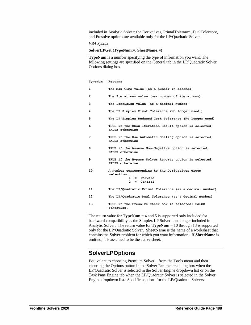
Frontline Solvers 2020 Reference Guide Page 488
included in Analytic Solver; the Derivatives, PrimalTolerance, DualTolerance,
and Presolve options are available only for the LP/Quadratic Solver.
VBA Syntax
SolverLPGet (TypeNum:=, SheetName:=)
TypeNum is a number specifying the type of information you want. The
following settings are specified on the General tab in the LP/Quadratic Solver
Options dialog box.
TypeNum Returns
1 The Max Time value (as a number in seconds)
2 The Iterations value (max number of iterations)
3 The Precision value (as a decimal number)
4 The LP Simplex Pivot Tolerance (No longer used.)
5 The LP Simplex Reduced Cost Tolerance (No longer used)
6 TRUE if the Show Iteration Result option is selected;
FALSE otherwise
7 TRUE if the Use Automatic Scaling option is selected;
FALSE otherwise
8 TRUE if the Assume Non-Negative option is selected;
FALSE otherwise
9 TRUE if the Bypass Solver Reports option is selected;
FALSE otherwise.
10 A number corresponding to the Derivatives group
selection:
1 = Forward
2 = Central
11 The LP/Quadratic Primal Tolerance (as a decimal number)
12 The LP/Quadratic Dual Tolerance (as a decimal number)
13 TRUE if the Presolve check box is selected; FALSE
otherwise.
The return value for TypeNum = 4 and 5 is supported only included for
backward compatibility as the Simplex LP Solver is no longer included in
Analytic Solver. The return value for TypeNum = 10 through 13 is supported
only for the LP/Quadratic Solver. SheetName is the name of a worksheet that
contains the Solver problem for which you want information. If SheetName is
omitted, it is assumed to be the active sheet.
SolverLPOptions
Equivalent to choosing Premium Solver... from the Tools menu and then
choosing the Options button in the Solver Parameters dialog box when the LP/Quadratic Solver is selected in the Solver Engine dropdown list or on the
Task Pane Engine tab when the LP/Quadratic Solver is selected in the Solver
Engine dropdown list. Specifies options for the LP/Quadratic Solvers.
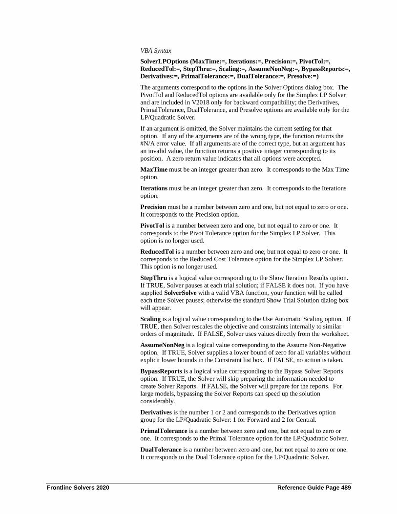
Frontline Solvers 2020 Reference Guide Page 489
VBA Syntax
SolverLPOptions (MaxTime:=, Iterations:=, Precision:=, PivotTol:=,
ReducedTol:=, StepThru:=, Scaling:=, AssumeNonNeg:=, BypassReports:=,
Derivatives:=, PrimalTolerance:=, DualTolerance:=, Presolve:=)
The arguments correspond to the options in the Solver Options dialog box. The
PivotTol and ReducedTol options are available only for the Simplex LP Solver
and are included in V2018 only for backward compatibility; the Derivatives,
PrimalTolerance, DualTolerance, and Presolve options are available only for the
LP/Quadratic Solver.
If an argument is omitted, the Solver maintains the current setting for that
option. If any of the arguments are of the wrong type, the function returns the
#N/A error value. If all arguments are of the correct type, but an argument has
an invalid value, the function returns a positive integer corresponding to its
position. A zero return value indicates that all options were accepted.
MaxTime must be an integer greater than zero. It corresponds to the Max Time
option.
Iterations must be an integer greater than zero. It corresponds to the Iterations
option.
Precision must be a number between zero and one, but not equal to zero or one.
It corresponds to the Precision option.
PivotTol is a number between zero and one, but not equal to zero or one. It
corresponds to the Pivot Tolerance option for the Simplex LP Solver. This
option is no longer used.
ReducedTol is a number between zero and one, but not equal to zero or one. It
corresponds to the Reduced Cost Tolerance option for the Simplex LP Solver.
This option is no longer used.
StepThru is a logical value corresponding to the Show Iteration Results option.
If TRUE, Solver pauses at each trial solution; if FALSE it does not. If you have
supplied SolverSolve with a valid VBA function, your function will be called
each time Solver pauses; otherwise the standard Show Trial Solution dialog box
will appear.
Scaling is a logical value corresponding to the Use Automatic Scaling option. If
TRUE, then Solver rescales the objective and constraints internally to similar orders of magnitude. If FALSE, Solver uses values directly from the worksheet.
AssumeNonNeg is a logical value corresponding to the Assume Non-Negative
option. If TRUE, Solver supplies a lower bound of zero for all variables without
explicit lower bounds in the Constraint list box. If FALSE, no action is taken.
BypassReports is a logical value corresponding to the Bypass Solver Reports
option. If TRUE, the Solver will skip preparing the information needed to
create Solver Reports. If FALSE, the Solver will prepare for the reports. For
large models, bypassing the Solver Reports can speed up the solution
considerably.
Derivatives is the number 1 or 2 and corresponds to the Derivatives option group for the LP/Quadratic Solver: 1 for Forward and 2 for Central.
PrimalTolerance is a number between zero and one, but not equal to zero or
one. It corresponds to the Primal Tolerance option for the LP/Quadratic Solver.
DualTolerance is a number between zero and one, but not equal to zero or one.
It corresponds to the Dual Tolerance option for the LP/Quadratic Solver.

Frontline Solvers 2020 Reference Guide Page 490
Presolve is a logical value corresponding to the Presolve option. If TRUE, the
Solver performs a presolve step before starting the Simplex method that detects
singleton rows and columns, removes fixed variables and redundant constraints,
and tightens bounds. If FALSE, no action is taken. This option is no longer
used.
SolverOkGet
Returns variable, constraint and objective selections and settings for the current
Solver problem on the specified sheet. These settings are entered in the standard Solver Parameters dialog, and its Add and Change dialogs.
VBA Syntax
SolverOkGet (TypeNum:=, SheetName:=)
TypeNum is a number specifying the type of information you want:
TypeNum Returns
1 The reference in the Set Cell box or the #N/A error value if
Solver has not been used on the active document
2 A number corresponding to the Objective Sense option
1 = Max
2 = Min
3 = Value Of
3 The value in the Value Of box
4 The reference in the Changing Cells box or under Variables in
the Task Pane Model tab (in the Analytic Solvers, only the first
entry in the Variables list box)
5 The number of entries in the Constraints list box
6 An array of the left hand sides of the constraints as text
7 An array of numbers corresponding to the relations
between the left and right hand sides of the constraints:
1 = <=
2 = =
3 = >=
4 = int
5 = bin
6 = dif
7 = soc
8 = src
9 = sem
8 An array of the right hand sides of the constraints as text
9 An array of the entries in the Variables list box or under
Variables in the Task Pane Model tab as text
10 A number corresponding to the Solver engine dropdown list
for the currently selected Solver engine:
1 = Nonlinear GRG Solver
2 = LP/Quadratic Solver
3 = Evolutionary Solver
4 = Interval Global Solver
5 = SOCP Barrier Solver
In Analytic Solver other values may be returned
for field-installable Solver engines
11 A string identifying the currently selected Solver engine:
"Standard GRG Nonlinear" = Nonlinear GRG Solver
"Standard LP/Quadratic" = LP/Quadratic Solver
"Standard Evolutionary" = Evolutionary Solver

Frontline Solvers 2020 Reference Guide Page 491
"Standard Interval Global" = Interval Global Solver
"Standard SOCP Barrier" = SOCP Barrier Solver
"Gurobi Solver" = Gurobi Solver
"Knitro Solver" = KnitroF Solver
"Large-Scale GRG Solver" = Large-Scale GRG Solver
"Large-Scale LP Solver" = Large-Scale LP Solver
"Large-Scale SQP Solver" = Large-Scale SQP Solver
"MOSEK Solver Engine" = MOSEK Solver Engine
"OptQuest Solver" = OptQuest Solver
"XPRESS Solver Engine" = XPRESS Solver Engine
12 An array of strings corresponding to the comments associated
with each block of constraints
13 An array of logical values corresponding to the Report check
box associated with each block of constraints (TRUE if the
box is checked, FALSE otherwise); no longer used in V8.0
14 An array of strings corresponding to the comments associated
with each block of variables
15 An array of logical values corresponding to the Report check
box associated with each block of variables (TRUE if the
box is checked, FALSE otherwise); no longer used in V8.0
SheetName is the name of a worksheet that contains the Solver problem for
which you want information. If SheetName is omitted, it is assumed to be the
active sheet.
SolverSizeGet
Returns statistics about the size of the currently defined Solver problem, and the
problem size limits supported by the currently selected Solver engine. The
following settings are “read-only” and appear on the Task Pane Engine tab or on
the Problem tab on the Analytic Solver Options dialog (click the Options icon
on the Analytic Solver ribbon).
VBA Syntax
SolverSizeGet (TypeNum:=, SheetName:=)
TypeNum is a number specifying the type of information you want:
TypeNum Returns
1 The number of decision variables in the current problem
2 The number of constraints in the current problem
3 The number of variable bounds in the current problem
4 The number of integer variables in the current problem
5 The maximum number of decision variables supported by the
currently selected Solver engine
6 The maximum number of constraints supported by the
currently selected Solver engine
7 The maximum number of variable bounds supported by the
currently selected Solver engine
8 The maximum number of integer variables supported by the
currently selected Solver engine
SheetName is the name of a worksheet that contains the Solver problem for
which you want information. If SheetName is omitted, it is assumed to be the
active sheet.

Frontline Solvers 2020 Reference Guide Page 492
RASON Error Codes
Introduction This chapter documents the RASON Error messages that can be returned when you optimize a model, run a simulation or perform a data mining function using
Rason Server.
Error Messages
General JSON Error Indicates that an unexpected internal errors has occurred.
Missing model file or string Indicates that an internal error has occurred by can appear
when a user attempts to solve an empty model string.
Model type (Simulation, optimization,
data mining) mismatch
Indicates that the User has used the wrong RASON end
point to solve the current model. For example, clicking
Simulate in the RASON IDE rather than Solve when
solving an optimization model, or calling Get
rason.net/api/model/id/optimize when
running a simulation model.
Improper engine selected for the
particular model
Indicates that an appropriate engine has not been selected to
solve the model.
Invalid Json token Not in use in RASON 2.0 and later versions.
Unrecognized Json identifier Indicates that a name of a section or a property has been
used which is not part of the RASON syntax. For example,
if a user misspells a section heading such as
“modelSetings” or a non-existent property name is passed.
Invalid Json data type Indicates that the user has entered a different type than
expected. For example, if a number is required, but a string
is passed, or if an array is required, but a scaler has been
passed. This error message may also be returned when an
Excel type not presented in RASON is attempted in
conversion (for example, Excel errors #N/A, #NUM, etc.).
Missing name definition in Json object All objects must be named. If the “name” property is missing, this error will appear.
When using the syntax:
Variables:{
x:{value:0}
}

Frontline Solvers 2020 Reference Guide Page 493
the variable is implicitly named “x”.
However, when using the syntax below, you must specify
the name of the object by using the name property.
Variables:[
{ name: “x”, value: 0}
]
Expecting ':' Missing “:”
Expecting '{' or '['
Missing an expected opening bracket
Expecting '}' or ']' Missing an expected closing bracket
Incompatible Json assignment When a property or object with the ‘:’ operator. Examples
may include, the dimensions of the right hand side of an
optimization constraint not matching the dimensions of the
left hand side of the constraint.
Duplicated Json assignment Indicates that an object has been defined twice.
Incorrect Json array dimensions Indicates that the definition of dimensions: [r,c] is not
correct. Note: Although [r][c] is correct C++ syntax, it is
not correct RASON syntax.
Incorrect Json data array Indicates a mistake in any array definition through the []
operator, for example, [ 1, 2 ]].
Incorrect assignment to a Json ‘type’
identifier
Indicates that “type:” property has been assigned an invalid
value. For example, “type: “bynari”” rather than “type:
binary”” when applied to a decision variable or passing
“type: “maximum”” to a variable or constraint instead of
the objective function.
Missing Json Variable Definition Indicates that in a conic constraint definition, an identifier
has been used, which is not a decision variable.
Index [] misused or out of range Indicates that the application of the range operator [] to an
array is invalid. For example, x[6] while x has length 5.
Incompatible model block definition Could indicate that a two sided constraint has been passed.
For example, a constraint block with a lower bound of 1 and an upper bound of 10.
Invalid binding source definition Indicates an error in a data source definition or the related
index sets. If using PsiDataSrc() fumction in an Excel
model, confirm that there are no trailing or leading spaces
in any of the argument definitions in either the excel cells
or the function definition.
Formulas not allowed in this definition Indicates that a formula has been entered for an object that
should not have a formula, for example, a decision variable
object.
Invalid parameter definition Indicates that PsiOptParam() or PsiSimParam() has been
misspelled or entered improperly
Inconsistent Table Indicates that an invalid table definition has been used in
the functions SELECT or PIVOT; the index operator [] has
been applied to the identifier, which is an invalid table; or
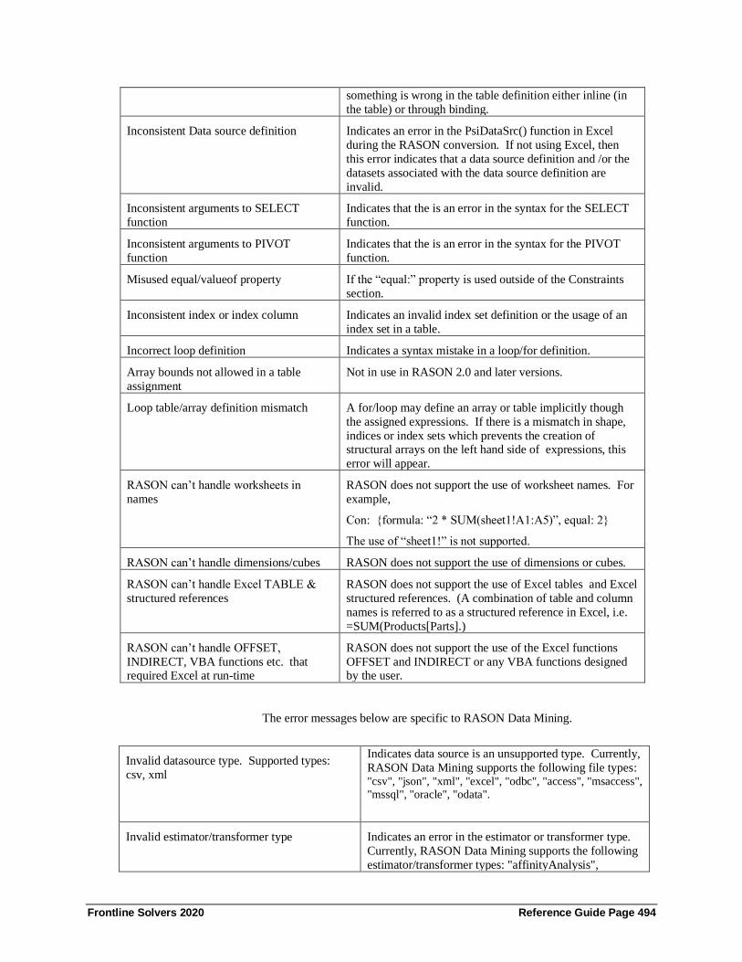
Frontline Solvers 2020 Reference Guide Page 494
something is wrong in the table definition either inline (in
the table) or through binding.
Inconsistent Data source definition Indicates an error in the PsiDataSrc() function in Excel
during the RASON conversion. If not using Excel, then
this error indicates that a data source definition and /or the
datasets associated with the data source definition are
invalid.
Inconsistent arguments to SELECT
function
Indicates that the is an error in the syntax for the SELECT
function.
Inconsistent arguments to PIVOT
function
Indicates that the is an error in the syntax for the PIVOT
function.
Misused equal/valueof property If the “equal:” property is used outside of the Constraints
section.
Inconsistent index or index column Indicates an invalid index set definition or the usage of an
index set in a table.
Incorrect loop definition Indicates a syntax mistake in a loop/for definition.
Array bounds not allowed in a table
assignment
Not in use in RASON 2.0 and later versions.
Loop table/array definition mismatch A for/loop may define an array or table implicitly though
the assigned expressions. If there is a mismatch in shape,
indices or index sets which prevents the creation of structural arrays on the left hand side of expressions, this
error will appear.
RASON can’t handle worksheets in
names
RASON does not support the use of worksheet names. For
example,
Con: {formula: “2 * SUM(sheet1!A1:A5)”, equal: 2}
The use of “sheet1!” is not supported.
RASON can’t handle dimensions/cubes RASON does not support the use of dimensions or cubes.
RASON can’t handle Excel TABLE &
structured references
RASON does not support the use of Excel tables and Excel
structured references. (A combination of table and column
names is referred to as a structured reference in Excel, i.e.
=SUM(Products[Parts].)
RASON can’t handle OFFSET,
INDIRECT, VBA functions etc. that required Excel at run-time
RASON does not support the use of the Excel functions
OFFSET and INDIRECT or any VBA functions designed by the user.
The error messages below are specific to RASON Data Mining.
Invalid datasource type. Supported types:
csv, xml
Indicates data source is an unsupported type. Currently,
RASON Data Mining supports the following file types: "csv", "json", "xml", "excel", "odbc", "access", "msaccess", "mssql", "oracle", "odata".
Invalid estimator/transformer type Indicates an error in the estimator or transformer type.
Currently, RASON Data Mining supports the following
estimator/transformer types: "affinityAnalysis",
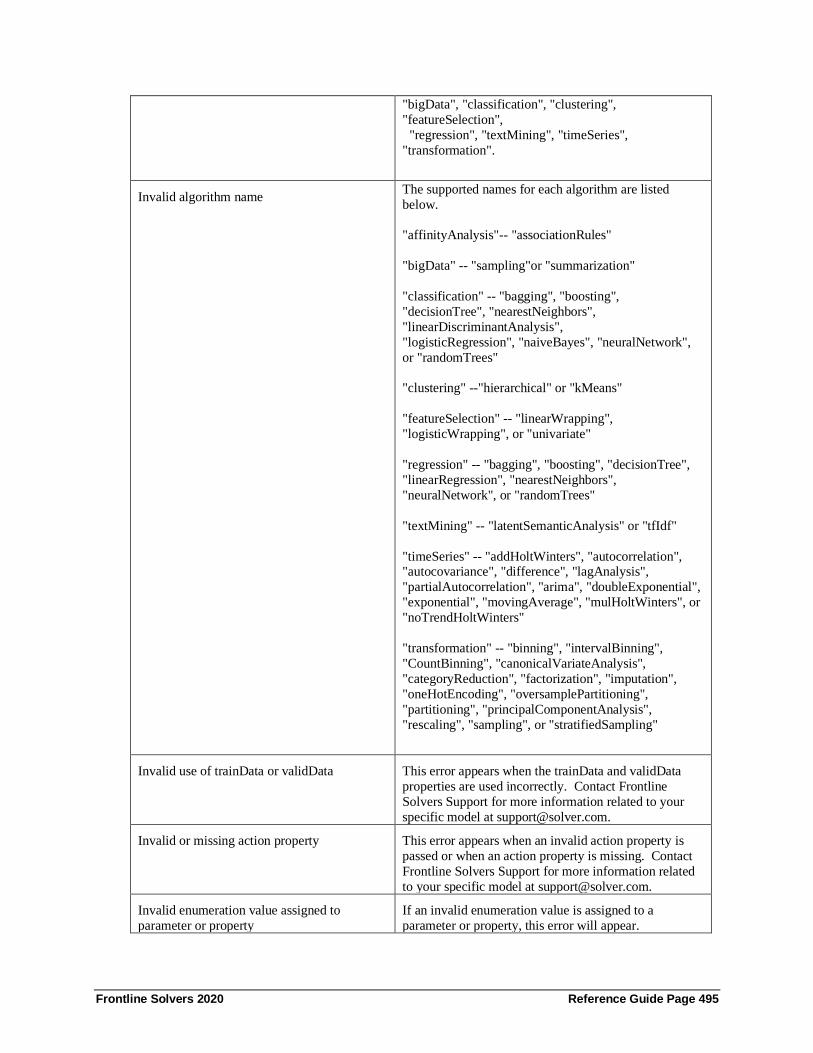
Frontline Solvers 2020 Reference Guide Page 495
"bigData", "classification", "clustering",
"featureSelection",
"regression", "textMining", "timeSeries",
"transformation".
Invalid algorithm name The supported names for each algorithm are listed
below.
"affinityAnalysis"-- "associationRules"
"bigData" -- "sampling"or "summarization"
"classification" -- "bagging", "boosting",
"decisionTree", "nearestNeighbors",
"linearDiscriminantAnalysis",
"logisticRegression", "naiveBayes", "neuralNetwork",
or "randomTrees"
"clustering" --"hierarchical" or "kMeans"
"featureSelection" -- "linearWrapping",
"logisticWrapping", or "univariate"
"regression" -- "bagging", "boosting", "decisionTree",
"linearRegression", "nearestNeighbors",
"neuralNetwork", or "randomTrees"
"textMining" -- "latentSemanticAnalysis" or "tfIdf"
"timeSeries" -- "addHoltWinters", "autocorrelation", "autocovariance", "difference", "lagAnalysis",
"partialAutocorrelation", "arima", "doubleExponential",
"exponential", "movingAverage", "mulHoltWinters", or
"noTrendHoltWinters"
"transformation" -- "binning", "intervalBinning",
"CountBinning", "canonicalVariateAnalysis",
"categoryReduction", "factorization", "imputation",
"oneHotEncoding", "oversamplePartitioning",
"partitioning", "principalComponentAnalysis",
"rescaling", "sampling", or "stratifiedSampling"
Invalid use of trainData or validData This error appears when the trainData and validData
properties are used incorrectly. Contact Frontline
Solvers Support for more information related to your
specific model at [email protected].
Invalid or missing action property This error appears when an invalid action property is
passed or when an action property is missing. Contact
Frontline Solvers Support for more information related
to your specific model at [email protected].
Invalid enumeration value assigned to
parameter or property
If an invalid enumeration value is assigned to a
parameter or property, this error will appear.

Frontline Solvers 2020 Reference Guide Page 496
The following properties/parameters accept only the
values in their sets. If a user enters something different,
this error message appears.
"aggregationType" has values { "avg", "max", "min",
"stddev", "sum" }
"binningTypeFeatures" and "binningTypeTarget” have
values { "equal_count", "equal_interval", "none" }
"dataForErrorComputation" has values { "only_train",
"only_valid", "train_and_valid" }
"dataFormat" has values { "csv", "parquet" }
"dissimilarity" has values { "euclidean", "jaccard",
"matching" }
"hiddenLayerActivation" and “outputLayerActivation"
have values { "logistic_sigmoid", "softmax", "tanh" }
"imputationStrategy" has values { "delete_record",
"mean", "median", "mode", "value" }
"inputDataType" has values { "distance_matrix",
"raw_data" }
"learningOrder" has values { "original", "random" }
"linkage" has values { "centroid", "complete_linkage",
"group_average", "mcquitty", "median",
"single_linkage", "ward" }
"matrixMethod" has values { "correlation", "covariance"
}
"metric" has values { "chi2", "cramersv", "fisher",
"ftest", "gainratio", "gini", "kendall", "mutualinfo",
"pearson", "spearman", "welch" }
"normType" has values { "l1", "l2" }
"partitionMethod" has values { "manual", "random",
"sequential" }
"priorProbMethod" has values { "empirical", "manual",
"uniform" }
"prunedTreeType" has values { "full_grown",
"best_pruned", "min_error", "manual" }
"samplingType" has values { "approximate", "exact" }
"sortOrder" has values { "descending", "ascending" }

Frontline Solvers 2020 Reference Guide Page 497
"stratificationMethod" has values { "equal_size",
"proportional" }
"technique" has values { "adjusted_normalization",
"normalization", "standardization",
"unit_normalization" }
"weightingScheme" has values { "equal",
"inverse_distance" }
"weightingSchemeDocument" has values { "binary",
"entropy", "gf_idf", "inverse", "normal", "prob_idf" }
"weightingSchemeNormalization" has values {
"cosine", "none" }
"weightingSchemeTerm" has values { "augnorm",
"boolean", "logarithmic", "raw_frequency" }
Invalid use of selectedCols or excludedCols This error appears when the selectedCols and
excludedCols properties are used incorrectly. Contact
Frontline Solvers Support for more information related
to your specific model at [email protected].

Frontline Solvers 2020 Reference Guide Page 498
Appendix: Differences between Analytic Solver Desktop and Analytic Solver Cloud
Introduction The overwhelming majority of features in Analytic Solver Desktop are also
included in Analytic Solver Cloud. However, there are a few variations between
the two products. This Appendix lists the key differences between the two.
These differences are also noted where applicable within the Analytic Solver
User and Reference Guides.
Differences
General
• In Analytic Solver Cloud, worksheets must be saved in the .xlsx format
(which was “new” back in 2007). If you have a workbook in .xls format,
open it, choose "Save As" in .xlsx format, then close and re-open it – your
model will then be recognized by Analytic Solver Cloud.
• Analytic Solver Cloud currently requires that variable, constraint, and the
objective cells be defined on a single worksheet. Analytic Solver Desktop
supports models defined on one worksheet, but with variable, constraint,
and/or the objective cells on other worksheets.
• The Solver Task Pane must be opened before an optimization or simulation
model can be solved.
• To create a Tableau extension or a Power BI custom visual, simply solve your optimization or simulation model then click Create App –
Tableau/Power BI on the Analytic Solver Cloud ribbon. (Neither the
Tableau nor Power BI icon is present on the Output tab, of the Solver task
pane, in the Cloud app.)
• The Workflow tab is not included in the Solver task pane of the Analytic
Solver Cloud app. The Model, Platform and Output tabs are not included in
the Data Mining Cloud task pane.
• The Publish icon is not applicable in Analytic Solver Cloud and therefore
does not appear on the Ribbon.

Frontline Solvers 2020 Reference Guide Page 499
• Calling Analytic Solver Cloud through a programming language such as
VBA is not supported.
• The Platform tab for Analytic Solver Cloud does not include options listed
under Advanced Options or General in Analytic Solver Desktop. These
options are not applicable to Analytic Solver Cloud.
• The following functions are not supported in Analytic Solver Cloud:
MSOLVE, MTRACE, MNORM, MEIGENVEC, and MEIGENVAL.
• The Analytic Solver Parameters tab, accessed by clicking Addins –
Premium Solver in Desktop Excel, is not supported in Analytic Solver
Cloud.
• SolverServer, which allows you to solve your optimization or simulation
model on a corporate server, is currently not supported.
• A welcome screen will not appear upon logging in to the Cloud app.
• Neither the Data Mining nor Solver apps support formulas in a call to any
Psi function. For example, the formula = PsiTarget(A1, A2 * A3) is not
supported.
• Information related to Decision Trees does not appear on the Model tab of
the Solver Task Pane. Rather, users must open the Decision Tree dialog by
clicking the Decision Tree icon on the Ribbon when creating new trees or
editing existing trees.
• Dynamic Arrays are supported in both Cloud apps.
• When entering Psi functions manually (i.e. simply typing the function into
an Excel cell) in Analytic Solver Cloud or Data Mining Cloud apps, the
taskpane must be refreshed before performing an optimization, simulation,
data mining task or parameter analysis report.
Dimensional Cubes
• Multi-dimensional cubes are not currently supported in Analytic Solver
Cloud. The Model button on the Ribbon still opens the Solver Task Pane,
but the additional dropdown menu choices for dimensional modeling are
not yet available.
Simulation
Several minor simulation features are not currently supported in Analytic
Solver Cloud . These include:
• Interactive Simulation is not supported in Analytic Solver Cloud, but
multiple parameterized simulations are supported. To run a simulation,
press the green arrow in the Solver Task Pane, or click the Simulate button
on the Ribbon. If you’ve specified a number of Simulations to Run (in the Platform tab of the Solver Task Pane), all the simulations will be run at one
time.

Frontline Solvers 2020 Reference Guide Page 500
• Opening the Uncertain Variable dialog by double clicking a cell containing
an uncertain variable is not supported in the Cloud app. Double-click an
Uncertain Variable cell in the Model tab of the Solver task pane to display
the Uncertain Variable dialog. This dialog displays a chart of the
distribution and allows you to change the distribution type and parameters, fit a distribution to your data, and view statistics and percentiles. You can
also open this dialog by selecting the uncertain variable cell and clicking
Distributions – Pick a Distribution from the Analytic Solver Cloud ribbon.
• Opening the Uncertain Function dialog by double clicking a cell containing
an uncertain function is not supported in the Cloud app. Double-click an
Uncertain Function cell in the Model tab of the Solver task pane to display
the Uncertain Variable dialog. This dialog which displays a chart of
simulation results and sensitivity analysis, and allows you to adjust bounds,
fit an analytic distribution to the results, and view statistics and percentiles.
• Analytic Solver Cloud supports all the same functionality related to correlations as Analytic Solver Desktop, but it is imperative that the Solver
Task Pane is opened before the Correlations Matrices or Correlations
Fitting dialogs are opened (Correlations – Matrices).
Each time the Save button is clicked on the Correlations dialog, the matrix
is checked for consistency (positive semi-definite). If the matrix is not
consistent, you will be asked if you would like Analytic Solver to modify
the matrix. Click yes, to accept Analytic Solver's modifications. Click No
to save the matrix without any modifications. Click Cancel to go back to
the matrix.
Only Gaussian Copulas are supported in the Correlation Dailog. However,
all copulas are supported for Correlation Fitting.
• Printing or copying to the clipboard from the Distributions dialog.
• Switching to 3-D view or rotating the Uncertain Variable or Uncertain
Function charts.
• Neither Markers nor Axis Options menus, in the Uncertain Variable dialog,
are supported.
• Conditional Mean is not supported for the Sensitivity Chart on the
Uncertain Function dialog.
• Multiple Variables menu does not appear on the Scatter Plots tab in the
Uncertain Function dialog.
• Clustering information is not available for uncertain functions.
• Fit icon does not appear on the Uncertain Function dialog. To Fit a
distribution, simply use the Fit option on the Tools menu.
• Compound distributions are not supported.
• The Uncertain Variable Title Bar does not appear in Analytic Solver Cloud.
As a result, the following buttons are not available in Analytic Solver
Cloud: Overlay of Variables, Save, Print, Copy, and Uncertain Function
(where applicable).
• The Uncertain Function Title Bar does not appear in Analytic Solver Cloud.
As a result, the following buttons are not available in the Cloud app:
Overlay of Uncertain Functions, Save, Print, Copy and Uncertain Variable

Frontline Solvers 2020 Reference Guide Page 501
(where applicable), Fit a Distribution, Export to Power BI or Export to
Tableau.
• Help hyperlinks in the uncertain variable or uncertain function dialogs are
not supported.
• The ability to fit a distribution through the uncertain variable dialog is not
supported in the Cloud app. To fit a distribution, simply highlight your
historical data and click Tools – Fit.
• The option Run Sample Independence Test always enabled when fitting a
distribution in Analytic Solver Cloud. In Analytic Solver Desktop, it is
possible to turn this option off.
• In Analytic Solver Desktop, when an uncertain variable is not part of the
simulation (i.e. no uncertain function depends on it), the analytic mean is
displayed in the cell. In Analytic Solver Cloud, a random value will be
displayed.
• All three arguments must be present for the PsiMetalog and PsiMetalogSPT
distributions. In Desktop Analytic Solver, the first two arguments are
optional. These arguments are not optional in Analytic Solver Cloud.
• Popup charts for uncertain variables are not supported.
• In Analytic Solver Cloud, the Trial to Display option is not present on the
Platform tab of the task pane or on the Ribbon.
• When a simulation is performed on a model containing more than one
output function, only output functions will be displayed on the multiple
output function dialog, the dialog that appears after a simulation.
• The 95th and 5th percentile marker values may not be edited in the
uncertain variable dialog. Starting in V2020, these markers may be moved.
It is not yet possible to edit the Axis options or to add Markers to the
distribution in the App.
• PsiForecast() is not recognized as an uncertain function in the Cloud apps.
If the simulation argument is set to "True", the Analytic Solver App will
generate a single random point around the actual forecast according to the
forecast and its standard deviation.
Optimization
There are also several small differences when it comes to performing an
optimization in Analytic Solver Cloud.
• The Constraint Wizard is not yet supported in Analytic Solver Cloud.
• Since cloud add-ins cannot have “cascading submenus”, the Min and Max
choices for Objective have been combined in the Add/Change Objective
dialog, and the Normal, Chance and Variable Type options have been
combined in the Add Constraint dialog.
• Stochastic Decomposition for optimization of models with uncertainly is
not yet available (but coming soon) in Analytic Solver Cloud.

Frontline Solvers 2020 Reference Guide Page 502
• Optimization models may only be saved in Classic Format when using
Analytic Solver Cloud. Saving the model as an .lp file or using Psi
functions is not supported.
• Engine size limits are not posted on the ending tab.
• PsiOptimization functions are not supported.
• The Structure report generated by Analytic Solver Cloud does not include
the Name or Cell Value columns.
• The Auto Adjust icon does not appear on the task pane.
• Although loading/saving an optimization model is supported in both
Analytic Solver Desktop and Analytic Solver Cloud, a model saved using
Classic Format in Analytic Solver Desktop may not be loaded in Analytic
Solver Cloud and vice-versa.
• Optimization option names are slightly different in the Cloud Addin. See
their COM addin equivalent in the chart below.
Analytic Solver Desktop Option Analytic Solver Cloud Option
Assume Non-Negative AssumeNonNeg
Bypass Solver Reports Bypass Reports
Max Time MaxTime
Maximum Subproblems MaxSubProblems
Maximum Feasible Solutions MaxFeasibleSols
Use Automatic Scaling Scaling
N/A SolveWithout
Integer Tolerance IntTolerance
Integer Cutoff IntCutoff
Show Iterations N/A
Dual Tolerance DualTolerance
Primal Tolerance PrimalTolerance
Gap Tolerance GapTolerance
Step Size Factor StepSizeFactor
Feasibility Tolerance FeasibilityTolerance
Search Direction SearchDirection
Recognize Linear Variables RecognizeLinear
Relax Bounds on Variables RelaxBounds
Multistart Search Multistart
Topographic Search TopoSearch
Require Bounds on Variables RequireBounds
Population Size PopulationSize

Frontline Solvers 2020 Reference Guide Page 503
Random Seed RandomSeed
Max Time w/o Improvement MaxTimeNoImp
Absolute vs. Relative Stop AbsRelStep
Assume Stationary AssumeStationary
Method Options Group Method
Population Size PopulationSize
Mutation Rate MutationRate
Random Seed RandomSeed
Require Bounds on Variables RequireBounds
Local Search LocalSearch
Fix Nonsmooth Variables FixNonSmooth
Global Search GlobalSearch
Model Based Search ModelBasedSearch
Feasibility Pump FeasibilityPump
• Turn on Guided Mode under Help – Operating Mode, rather than from the
Platform tab on the task pane.
• Model variables, constraints, and objective are not editable in the in the
bottom portion of the Model task pane.
Parameters
When Sensitivity, Optimization or Simulation menu choices are selected
under Parameters in the App, the appropriate formula is inserted into the selected cell with default lower and upper bounds. (In Desktop Analytic
Solver a dialog opens.)
Create App for Rason
In Analytic Solver Cloud, you can convert your Excel model to a RASON
model with a “destination” of either Rason.com or a newly-created Web
page, but not a “destination” of the desktop RASON IDE. You can use
Create App – Tableau and Create App – Power BI in Analytic Solver
Cloud.

Frontline Solvers 2020 Reference Guide Page 504
Tools
Additional items are not supported in Analytic Solver Cloud including:
• Run Sampled Independence Test under Fit
• Uploading or downloading certified distributions. Certified Distributions
are not supported in Analytic Solver Cloud.


![Frontline [49] MECH - College of Engineering](https://static.fdokumen.com/doc/165x107/6328a921cedd78c2b50e29e2/frontline-49-mech-college-of-engineering.jpg)