International Journal of InnovativeComputing, Information and Control ICIC International c©2010 ISSN 1349-4198Volume 6, Number 4, May 2010 pp. 1–10

ON CONSTANT REFERENCE TRACKING PROBLEM FOR FASTLINEAR CONSTRAINED SYSTEMS

Farhad Bayat1 and Ali A. Jalali2

1,2, Department of Electrical EngineeringIran University of Science & Technology

Narmak, 1684613114, Tehran, Iranfbayat@iust.ac.ir

Received February 2010; revised –

Abstract. This paper addresses the constant reference tracking problem of linear con-strained systems with fast dynamics. Constraints satisfaction and tracking goals areguaranteed by introducing an augmented servo architecture resulting in an analyticalclosed-form solution. The proposed architecture has been combined with explicit modelpredictive control (eMPC) method to achieve optimal tracking, constraints satisfactionand piecewise closed form solution simultaneously. The proposed architecture is intuitiveand gives a direct insight into the physical system and closed loop feedback properties, andtherefore makes it easy to tune and select design parameters in practice. Furthermore,the piecewise closed form solution leads to a computationally efficient controller whichenables it to be applicable for fast dynamic systems. The constant reference signal as-sumption reduces the complexity of the explicit MPC solution considerably. However, it isshown that the present method can be easily applied to applications with finite predefinedset-points. Furthermore, in order to cope with non-predefined set-point applications, aconvex combination based interpolation is suggested and guaranteed to be feasible undersome mild assumptions.Keywords: Tracking, Constrained systems, Model predictive control, Servo-systems.

1. Introduction. Tracking problems come into view in several control applications suchas motion control, robotics, chemical industry and etc. A control system in which thereference signal has to be followed by the system output is called servo-system. Theservo-mechanism and tracking problem are widely studied in literatures from differentpoint of view [1]-[8]. The wide variety of physical systems can be described or fairlyapproximated by linear models and in this regard there are rich and solid theoreticalfoundations supported by numerous experiments. Consequently the tracking problem oflinear systems can be seen as an almost mature and well established topic with severalreported applications. Several methods such as classic LQG/LTR [9], adaptive control[2], robust [1, 7, 31], fuzzy [10, 8] and also model predictive control [11] have been used byresearchers to solve the unconstrained output tracking problem. This is while to the bestof authors’ knowledge the tracking problem of constrained systems with direct constraintshandling during the design procedure has not completely been developed yet. Althoughsome remarkable researches have been reported in the recent years [3, 14] and [30]. Asreported in [3], among the existing results dealing with the tracking problem in presenceof constraints, a remarkable approach is the so-called command governors method [12].This technique is based on the addition of a nonlinear low-pass filter of the reference toguarantee the admissible evolution of the system to the reference. This can be seen asadding an artificial reference (the output of the filter) which is computed at each samplingtime to ensure the admissible evolution of the system, converging on the desired reference.

1

2 FARHAD BAYAT AND ALI A. JALALI

In [13] it is proved that any control invariant set for the constrained system is a trackingdomain of attraction and an interpolation-based control law is proposed. More recentlya predictive control technique for tracking piecewise constant target has been proposedin [3] where the asymptotic stability of any admissible equilibrium point is achieved byadding an artificial steady state and input as decision variables and adding an offset costfunction to the functional. The closed-loop performance of this controller is studied inanother paper by authors and it is demonstrated that the offset cost function plays animportant role in the performance of the model predictive control for tracking [14]. Sincein most of practical applications there are some constraints on either states or actuators,it is important to develop an structure that guarantees direct handling of constraints aswell as other control objectives. This end is considered in this paper by using the explicitmodel predictive control (eMPC) method to achieve an integrated architecture which isoptimal and constraints are guaranteed to be satisfied.Unfortunately, the traditional model predictive control suffers some sever drawbacks thatprevent a broad use of this method in practice. These obstacles can be summarized in twoparts [16], (i) computational complexity connected with the online optimization problem,and (ii) the question of the control system robustness to deviations between actual pro-cess and its model used for prediction. This paper deals with the first problem. Unlikesome existing works that have investigated (i) from numerical point of view (see [24] andreferences therein), this paper substantially aims to overcome the online computationalcomplexity by utilizing multi-parametric programming (mpp) approach for MPC appli-cation [17]-[19]. The mpp enables the MPC to be used in very high-speed embeddedapplications [25]. In this regard, the main contributions of this paper can be summa-rized as follows. At first, an augmented architecture is proposed which is able to directlyhandle the constraints as well as tracking objectives. Instead of pure mathematical for-mulation and working with the optimization problem arising in the MPC formulation, inwhat follows an intuitive architecture is established which gives a direct insight into thephysical system and closed loop feedback operation. In the second place, it is shown thatthe proposed architecture can be formulated as a quadratic programming (QP) problemparameterized in the current state which can be adapted and solved explicitly using theeMPC formulation. Practically the main advantages of this explicit solution can be seenas follows. First, it removes the online optimization and associated difficulties such asinfeasibility and numerical instability. Secondly, the explicit solution provides a greatinsight into the closed loop system behavior, e.g. where the saturation may occur or thecontroller is idle.

2. Problem Description. Consider the discrete-time linear time invariant system:

x (k + 1) = A x (k) + B u (k)

y (k) = C x (k) (1)

where x (k) ∈ Rn, u (k) ∈ Rm and y (k) ∈ Rm are the current state, input and output ofthe system respectively. Also it is assumed that the pair (A, B) is controllable and thesystem (1) is subject to the following constraints:

x (k) ∈ X ⊂ Rn, u (k) ∈ U ⊂ Rm (2)

where X and U are compact polyhedra sets containing the origin in their interiors. Theobjective is to design a suitable controller u(k) which is able to steer the system outputy(k) to any admissible command signal r(k) while no constraint is violated.

SHORT RUNNING TITLE 3

2.1. Augmented servo architecture. The control objectives of the predefined problemare threefold. First, stabilizing the system, secondly, achieving to the offset-free tracking,and finally, handling the constraints. Corresponding to each objective an independentportion is considered in the control signal:

u (k) = ustab (k) + utrack (k) + uconstraint (k) (3)

where ustab(k) = −K1x(k) acts similar to the standard state feedback. In order toachieve the offset-free tracking goal, it is generally required that the feedback structurehas an integration property in the closed loop. Thus considering the output tracking errore(k) = r(k)− y(k), a new variable is introduced by integrating the error signal:

S (k) = S (k − 1) + e (k) (4)

Then utrack(k) = K2S(k) is used for the purpose of eliminating the tracking error.Finally, uconstraint(k) = uc(k) is properly designed to prevent the constraints violation.Three parameters K1, K2 and uc are free designing parameters.

2.2. Servo Controller design. In this section we introduce the synthesis procedure ofthe augmented servo-system to be integrated with eMPC approach in the next section.Let consider the system (1) together with the constraints (2) and the proposed controller(3). Then the successor of (3) is obtained as follows:

u (k + 1) = −K1x (k + 1) + K2S (k + 1) + uc (k + 1)

= (K1 −K1A−K2CA) x (k) + (Im −K1B −K2CB) uk+

K2r (k + 1) + ∆uc (k + 1) (5)

where K2S(k + 1) = K2S(k) + K2e(k + 1), K2S (k) = u (k) + K1x (k) − uc (k) and∆uc (k + 1) = uc (k + 1)−uc (k). Then one can obtain the extended state space equationby combining (1) and (5):[

x(k + 1)u(k + 1)

]=

[A BΓ1 Γ2

] [x(k)u(k)

]+

[0n×m

K2

]r(k + 1) +

[0n×1

∆uc(k + 1)

]y(k) = [C 0m×1]

[x(k)u(k)

](6)

where Γ1 = K1 −K1A−K2CA and Γ2 = Im −K1B −K2CB. Suppose that the con-troller parameters are suitably designed such that the system is stable. Consequently,the vectors x(k), u(k) and S(k) approach the constant vector values x∞, u∞ and S∞,respectively. Considering the constant reference signal r(k) = r, then the stationary formof (6) can be written as:[

x∞u∞

]=

[A BΓ1 Γ2

] [x∞u∞

]+

[0n×m

K2r

]+

[0n×1

∆uc(∞)

](7)

Definition 2.1. (Feasible Set Xf ) The feasible set Xf ⊂ Rn is defined as the set of allstates x ∈ Rn for which the constrained problem defined by (1) and (2) is feasible, i.e.

Xf = x ∈ Rn |∃u (x (k)) ∈ U, x (k) ∈ X (8)

Definition 2.2. (Maximal LQR Invariant Set Ω∞) [34] For an LTI system (1) subject tothe LQR control input u(k) = −Kx(k), the set Ω∞ ⊆ Rn denotes the maximum invariantset of states which satisfy the constraints in (2) for all time, i.e.,

Ω∞ =

x0 ∈ Rn | x (k) ∈ X, u (k) ∈ U,

(A−BK) x (k) ∈ X, ∀k ≥ 0

(9)

4 FARHAD BAYAT AND ALI A. JALALI

Remark 2.1. in the case where the system is unconstrained and the pair (A, B) is con-trollable, then uc (k) = 0, ∀ k = 1, 2, ... and it is always possible to find K1 and K2

(e.g. using LQR method) to achieve control objectives (i.e. stability and tracking). Inthe constrained case it might be impossible to find such a control law. This fact refers tothe so-called feasibility problem (see definition 1 where Xf = Ø or x0 /∈ Xf ). This issuehas been widely investigated in the literatures (see e.g. [26]). Throughout this paper it isassumed that the problem is feasible.

Remark 2.2. In [27] it is shown that the maximal LQR invariant set Ω∞ is a positiveinvariant set containing an open neighborhood of the origin.

Corollary 2.1. Considering the Remarks 2.1 and 2.2, if the system (6) is stabilized bysuitable selection of the design parameters, then ∆uc (k) = 0 for all x (k) ∈ Ω∞. As aresult, since x∞ ∈ Ω∞ then ∆uc (∞) = 0.

Subtracting (7) from (6) and after some manipulations the desired augmented systemequations can be written as:

ξ (k + 1) = G ξ (k) + H v (k) (10)

where

ξ (k) =

[x(k)− x∞u(k)− u∞

]G =

[A B0 0

], H =

[0n×m

Im

],

v (k) = [Γ1 Γ2] ξ (k) + ∆uc (k + 1) (11)

Theorem 2.1. Consider the linear time invariant system (1) together with the constraint(2) and a constant command signal (r). If the control law in (3) is chosen and if Xf 6= Ø(see Def. 2.1), then (y∞ − r) → 0 and the followings are held:

(i) x∞ = (In − A)−1 B[C (In − A)−1 B

]−1r,

(ii) u∞ =[C (In − A)−1 B

]−1r (12)

Proof. Having the Corollary 2.1 in mind and after some manipulation, equation (7) canbe rewritten as: [

I 0

K I

] [I − A −BK2C 0

] [x∞u∞

]=

[0n×m

K2r

](13)

where, K = −K1 −K2C. Then using the matrix inversion lemma one can obtain:

[x∞u∞

]=

[Λ− ΛBΣK2CΛ ΛBΣ−ΣK2CΛ Σ

] [I 0

−K I

] [0n×m

K2r

](14)

where, Σ =(K2C (I − A)−1 B

)−1and Λ = (I − A)−1. Doing some simplifications and

matrix manipulations yield:[x∞u∞

]=

[(In − A)−1B[C(In − A)−1B]−1r

(C(In − A)−1B)−1r

](15)

It is clear that the above equations are obtained provided that all inverses exist. Finally,it is easy to see that y∞ = Cx∞ = r.

SHORT RUNNING TITLE 5

Theorem 2.1 guaranties the asymptotic property of tracking for a constant referencesignal and when the corresponding system is feasible, i.e. there exist the design parameters(K1, K2 and uc) for which the system (10) is stable and all constraints are satisfied. Inthe next section by utilizing the explicit MPC method, the parameters (K1, K2 and uc)are calculated in a way that the stability and constraints satisfaction are guaranteed tobe satisfied simultaneously.

3. Controller Design Using Explicit MPC. In this section we first outline the ex-plicit MPC method and its characteristics. Then it is shown that combining this methodwith the controller presented in the previous section enables us to handle stability andconstraints satisfaction simultaneously. In the standard MPC an open loop control prob-lem is solved by an on-line optimization parameterized by the current state of the system.This finite-time constrained optimal control problem is formulated as:

J∗N (x0) = minU

N−1∑k=0

(xT

k Qxk + uTk Ruk

)+ xT

NQfxN

s.t. x ∈ X ⊆ <n, ∀k ∈ 1, 2, ..., Nu ∈ U ⊆ <m, ∀k ∈ 0, ..., N − 1xk+1 = Axk + Buk, x (0) = x0,

Q = QT 0, Qf = QTf 0, R = RT 0 (16)

where, U =[u′0, ..., u

′N−1

]′is the optimization variable, N denotes the prediction horizon

and Q, R and Qf are constant matrices of suitable dimensions (see [17] for details). Thiscontroller maps the state vector to the input vector of the system implicitly. Althoughmany efficient optimization softwares such as QP/LP solvers have been developed tosolve these optimization problems on-line, yet the complexity can be prohibitive for fastsystems or applications with limited computational resources. A remedy for this problemis developed recently based on the multi-parametric programming (mp-QP) tool [28].This mathematical tool enables us to solve the optimization problem off-line when it isapplied to the standard MPC, so-called explicit model predictive control (eMPC). Thisexplicit solution to the MPC is a piecewise affine (PWA) function defined over polyhedralpartitions (Pr) of the feasible set on the state space. So, when the corresponding region ofthe current state is known, the control calculation is nothing but a simple PWA functionevaluation. The mp-QP is solved by applying the first order Karush-Kuhn-Tucker (KKT)

conditions (see [29] for details). By substituting x (k) = Akx0 +∑k−1

j=0 AjBuk−1−j the

optimization problem (16) can be reformulated as:

J∗N (x) = minU

xTYx + xTFU + 1

2UTHU

s.t. GU 6 W + Ex

x ∈ X ⊆ <n, U ∈ U ⊆ <s (17)

where, H = HT ∈ Rs×s, s = mN , G ∈ Rq×s and E ∈ Rq×n are constant matrices, Wis a constant vector of dimension p, X and U are compact and convex polyhedral sets ofdimensions n and s, respectively. Also q denotes the number of constraints. Transformingthe QP problem (17) into the standard multi-parametric programming problem is easy,once the following linear transformation is considered [17]:

z , U + H−1FT x (18)

6 FARHAD BAYAT AND ALI A. JALALI

The QP in (17) is then reformulated as the following standard mp-QP problem:

V ∗z (x) = min

z

12zTHz

s.t. Gz 6 W + Sx (19)

where S , E + GH−1FT and V ∗z (x) = J∗N (x)− 0.5 xT

(2Y − FH−1FT

)x. Solution to

the above optimization problem has been addressed in [17, 18].

Theorem 3.1. [18], consider the optimization problem (19) with H 0. Let X ⊆ Rn bea polyhedron. Then the solution z∗ (x) and the Lagrange multiplier λ∗ (x) of the mp-QPproblem are piecewise affine functions of the parameter x, and z∗ (x) is continuous.

Theorem 3.2. [17], Consider the finite time constrained problem (16). Then the set offeasible parameters Xf is convex, the optimizer U∗ : Xf → Rs is continuous and PWAfunction of the current state x, and

u∗ (x0) = F r1 x (0) + F r

2 , if x (0) ∈ Pr,

Pr = x ∈ Rn|Hrx 6 Kr, r ∈ 1, 2, ..., Np ,

Xf =∪NP

r=1Pr

(20)

where u∗(x0) = [Im 0m×(s−m)]U∗ denotes the first m components of the optimizer U∗.

Corollary 3.1. [32], Let χNr = i ∈ 1, ..., p |x ∈ Pr, GiU

∗ (x)−Wi − Eix = 0 denotesthe index set of active constraints in (17) subject to the polyhedral region Pr. Then thefeedback gains and the polyhedron Pr in which the solution remains optimal are given as:

F r1 = H−1GT

χNr

(GχN

rH−1GT

χNr

)−1

SχNr−H−1FT ,

F r2 = H−1GT

χNr

(GχN

rH−1GT

χNr

)−1

WχNr

(21)

and

Hr =

[Ψ1 − SΨ−1

2 SχNr

], Kr =

[W −GF r

2

−Ψ−12 WχN

r

](22)

where, Ψ1 = G(F r

1 + H−1FT), Ψ2 = (GχN

rH−1GT

χNr) and matrices GχN

r, WχN

rand SχN

r

are formed by extracting the rows indexed by χNr from G,W and S, respectively.

Combining the results in this section with the proposed architecture in the previoussection leads to a piecewise closed form solution of the design parameters. The resultsare summarized in the following theorem.

Theorem 3.3. Consider the LTI system (1) together with the constraints (2) and constantreference signal r. If the control law (3) is chosen and the closed loop system is feasible bymeans of (8), then the parameters K1, K2 and uc which guarantee the tracking objectiveand constraints satisfaction are given as:

uc (k) = uc (k − 1) + F r2 (k − 1)[

K1 K2

]=

[[0 Im

]− F r

1

] [A− In B

CA CB

]−1

(23)

where F r1 and F r

2 are given in (21).

Proof. It was shown that regulating the augmented system described in (10) and (11)guarantees tracking property of the original system. Moreover, it was demonstrated that

SHORT RUNNING TITLE 7

Figure 1. Closed loop architecture of the augmented servo system.

the eMPC provides an optimal closed form solution to the control problem and guar-antees the constraints satisfaction. Adapting the regulation problem of the augmentedconstrained system (10) and (11) with the mp-QP problem leads to:

v (k) = F r1 ξ (k) + F r

2 , if ξ (k) ∈ Pr, (24)

Comparing (11) and (24) leads to:[Γ1 Γ2

]= F r

1 (k)

∆uc (k + 1) = F r2 (k) (25)

Extracting parameters K1 and K2 yields[K1 K2

] [A− In B

CA CB

]+

[0 Im

]= F r

1 (k)

uc (k) = uc (k − 1) + F r2 (k − 1) (26)

It is straightforward to obtain the expected results of the Theorem 3.3 using (26).

Figure 1 illustrates the architecture of the discussed augmented servo system.

Remark 3.1. Note that the non-constant reference tracking can also be taken into accountby adding the reference signal as an extra parameter in the eMPC design procedure [17],but this may increase the complexity of the resulting controller extensively. That is why inthis paper it is assumed that the reference signal is asymptotically constant. However, as aremedy to this assumption, it is emphasized that the eMPC controller can be calculated fordifferent reference signals independently and then by using an appropriate interpolationmethod the control signal is calculated for any feasible reference signal within the range ofpredefined reference signals. The following theorem characterizes this idea.

Theorem 3.4. Consider the system (1) subject to the constraints (2) and the optimiza-tion problem (17). If U∗

1 and U∗2 are two feasible optimal solutions corresponding to the

reference signals r1 and r2, then any convex combination based interpolation of U∗1 and

U∗2 guarantees the constraints satisfaction (feasibility) of the optimization problem (17).

8 FARHAD BAYAT AND ALI A. JALALI

Proof. By definition, the constraint GU ≤ W + Ex in the convex optimization problem(17) defines a convex set. Let α ∈ [0, 1] be an arbitrary real number, and define Uα ,αU∗

1 +(1−α)U∗2 as a convex combination based interpolation of U∗

1 and U∗2 . By assumption,

U∗1 and U∗

2 are feasible optimal solutions, and thus GU∗1 ≤ W +Ex and GU∗

2 ≤ W +Ex,∀x ∈ Xf . Since α > 0 and (1− α) > 0, then two inequalities can be linearly combined toobtain G(αU∗

1 +(1−α)U∗2 ) ≤ α(W+Ex)+(1−α)(W+Ex) or equivalently GUα ≤ W+Ex,

and therefor Uα is feasible.

Remark 3.2. According to the Remark 3.1 and Theorem 3.4, the proposed architecturecan be efficiently used when the corresponding system is subject to the finite number ofpredefined set-points. Otherwise, one can use the result in Theorem 3.4 by gridding thereference signal domain and interpolating within the grids.

4. Simulation Results.

4.1. Example 1. Consider the following discrete-time system:

x (k + 1) =

0 1 00 0 1

−0.1 −0.05 1

x(k) +

001

u(k)

y(k) =[

1 2 0]x(k) (27)

where the sampling time is Ts = 0.01 sec and the system (27) is subject to the followingconstraints:

‖u(k)‖∞ ≤ 1, ‖x(k)‖∞ ≤ 5 (28)

Using (10) and (11) the augmented system can be obtained as

ξ (k + 1) =

0 1 0 00 0 1 0

−0.1 −0.05 1 10 0 0 0

ξ(k) +

0001

v(k) (29)

In this simulation three constant reference signals r1 = −5, r2 = 0 and r3 = 5 areassumed and explicit controllers are calculated for each case, i.e. Ctrl−5, Ctrl0 and Ctrl5.The constraints corresponding to the augmented system can be obtained for each case byusing (11),(12) and (28). For example for r = 5 one can obtain

−

6.6676.6676.6671.250

6 ξ (k) 6

3.333.333.330.75

(30)

This single extended constraint guarantees the constraints satisfaction of the originalsystem. In order to apply the eMPC method another constraint ‖v(k)‖∞ ≤ 1 is alsoassumed. Applying the proposed approach to the augmented constrained system (29)-(30) leads to explicit solution of the controller parameters as characterized in Theorem3.3. The explicit solution is defined over polyhedral regions in the state space in whichthe control signal is a piecewise affine function of the current state (x) and each region hasown controller gains F r

1 , F r2 . In Fig.2 the polyhedral regions of the augmented system for

r = 5 and ξ4 = 0 are shown. The parameters which have been used to solve the eMPC

SHORT RUNNING TITLE 9

Figure 2. Polyhedral partitions of the augmented system cut throughξ4 = 0 for r = 5 (Example 1).

problems for r = ±5 and 0 are N = 5, R = 1, Q = diag1, 1, 1, 1 and Qf is obtainedfrom the following Riccati equation [17],[20]:

Qf = (A + BKLQ)′Qf (A + BKLQ) + K ′LQRKLQ + Q

KLQ = −(R + B′QfB)−1B′QfA (31)

Finally, corresponding to a constant reference signal and according to the result in The-orem 3.4, a convex combination of the controllers are used to apply to the system. To illus-trate how this idea works in practice, consider the initial point ξ (0) = [−4 − 4 − 4 0]T

and let the reference signal be r = 3. Since r2 = 0 ≤ r = 3 ≤ r3 = 5 so the interpolationprocedure takes the output of the controllers Ctrl0 and Ctrl5, and combines them con-vexly with weights α = 2

5and (1 − α) = 3

5, respectively (note that this procedure is not

unique and generally any convex combination which satisfies the conditions of Theorem3.4 can be also used). The point ξ(0) is associated to the regions CR3 and CR4 of Ctrl0and Ctrl5 respectively. The procedure which discovers the region in which the currentstate resides is called point location problem and several algorithms have been proposedto deal with this problem efficiently (see [33] and references therein). The control signalscorresponding to CR3 and CR4 are v3 = [0 0 0 0]ξ(k) + 1 and v4 = [0 0 0 0]ξ(k) + 0.75.So the final control value is obtained by interpolation

v (k) =[

0 0 0 0]ξ (k) + 0.85

= F1ξ (k) + F2 (32)

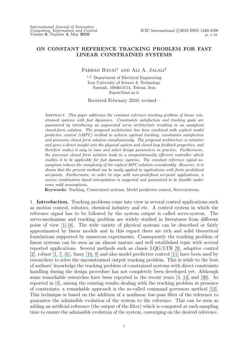
Then the controller parameters can be calculated using (23), i.e. K2 = 0.05, K1 =[−0.1, −0.1, 1] and uc = 0.85. This procedure is repeated in each sampling time and it isobvious that this procedure is more efficient than solving the online optimization problem(16) repetitively. The closed loop response of the system and the input control signal aredepicted in Fig.3 for different command signals. According to the result it can be seenthat the offset free tracking is achieved even when the reference signal is different fromr = ±5 and r = 0. Also it can be seen that the required input constraint ||u(k)||∞ ≤ 1 isfulfilled during the simulation as it was already guaranteed in the Theorem 3.4.

4.2. Example 2. Consider the following system which was studied by [35].

G(s) = 1100s+1

[40 −5−30 40

](33)

10 FARHAD BAYAT AND ALI A. JALALI

Figure 3. Output time trajectory and associated input control signal ofclosed loop system (Example 1).

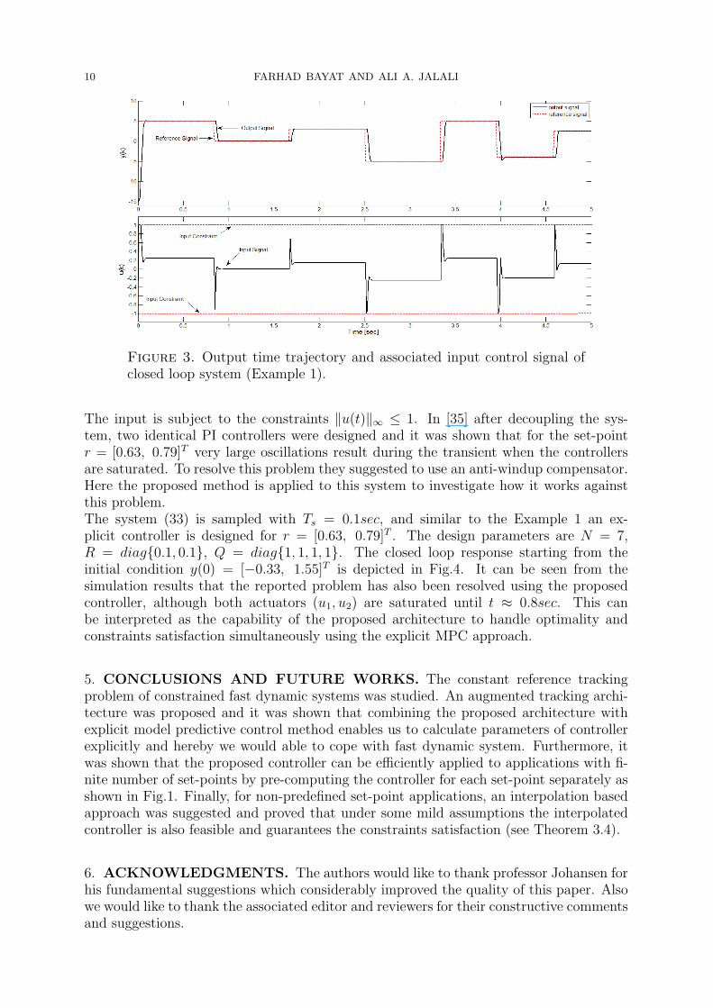
The input is subject to the constraints ‖u(t)‖∞ ≤ 1. In [35] after decoupling the sys-tem, two identical PI controllers were designed and it was shown that for the set-pointr = [0.63, 0.79]T very large oscillations result during the transient when the controllersare saturated. To resolve this problem they suggested to use an anti-windup compensator.Here the proposed method is applied to this system to investigate how it works againstthis problem.The system (33) is sampled with Ts = 0.1sec, and similar to the Example 1 an ex-plicit controller is designed for r = [0.63, 0.79]T . The design parameters are N = 7,R = diag0.1, 0.1, Q = diag1, 1, 1, 1. The closed loop response starting from theinitial condition y(0) = [−0.33, 1.55]T is depicted in Fig.4. It can be seen from thesimulation results that the reported problem has also been resolved using the proposedcontroller, although both actuators (u1, u2) are saturated until t ≈ 0.8sec. This canbe interpreted as the capability of the proposed architecture to handle optimality andconstraints satisfaction simultaneously using the explicit MPC approach.

5. CONCLUSIONS AND FUTURE WORKS. The constant reference trackingproblem of constrained fast dynamic systems was studied. An augmented tracking archi-tecture was proposed and it was shown that combining the proposed architecture withexplicit model predictive control method enables us to calculate parameters of controllerexplicitly and hereby we would able to cope with fast dynamic system. Furthermore, itwas shown that the proposed controller can be efficiently applied to applications with fi-nite number of set-points by pre-computing the controller for each set-point separately asshown in Fig.1. Finally, for non-predefined set-point applications, an interpolation basedapproach was suggested and proved that under some mild assumptions the interpolatedcontroller is also feasible and guarantees the constraints satisfaction (see Theorem 3.4).

6. ACKNOWLEDGMENTS. The authors would like to thank professor Johansen forhis fundamental suggestions which considerably improved the quality of this paper. Alsowe would like to thank the associated editor and reviewers for their constructive commentsand suggestions.

SHORT RUNNING TITLE 11

Figure 4. Closed loop response for Example 2.

REFERENCES

[1] T. Umeno and Y. Hori, Design of Robust Servo systems Based on the Parameterization of TwoDegrees of Freedom Control Systems, Trans. IEE Japan, vol. 109-D, no. 11, pp. 825-832, 1989.

[2] P. Qin, Y. Lin and M. Che, Improvement of Tracking Performance in Model-Free Adaptive ControllerBased on Multi-innovation and Particle Swarm Optimization, International Journal of InnovativeComputing, Information and Control (ICIC), vol. 5(5), 2009. pp. 1367-1377.

[3] D. Limon, I. Alvarado, T. Alamo, E.F. Camacho (2008), MPC for tracking piecewise constantreferences for constrained linear systems, Automatica, 44 (2008) 2382-2387.

[4] A. Leva and L. Bascetta, On the design of the feed forward compensator in two-degree-of-freedomcontrollers, Mechatronics, 2006, 533-546.

[5] W.H. Hughes and C.D. Johnson, A new digital servo-tracking control theory using subspace stabi-lization techniques, System Theory, Proc. of the 29th Southeastern Symposium on, 1997, 17-22.

[6] K.Ohishi, K.Kudo, K.Arai and H.Tokumaru, ”Robust High Speed Tracking Servo System for OpticalDisk System”, Proc. of IEEE 6th Inter. Workshop on Adv. Motion Cont., pp.92-97, 2000.

[7] K.Ohishi, K.Kudo, Y.Hayakawa, K.Arai, D.Koide and H.Tokumaru, ”Robust Feedforward TrackingServo System for Optical Disk Recording System”, Proc. of IECON, vol. 3, pp.1710-1715, 2001.

[8] S. Bououden, S. Filali and K. Kemih, Adaptive Fuzzy Tracking Control for unknown NonlinearSystems, International Journal of Innovative Computing, Information and Control (ICIC), vol. 6(2),2010. pp. 541-549.

[9] S. Weerasooriya and D.T. Phan, Discrete-Time LQG/LTR Design and Modeling of a Disk DriveActuator Tracking Servo System, IEEE Trans. on Indust. Electronics, vol. 42(3), 1995, pp. 240-247.

[10] P. Guillemin, Fuzzy Logic Applied to Motor Control, IEEE Trans. on Industrial Applications, vol.32(1), 1996, pp. 51-56.

[11] M. M’Saad and G. Sanche, Multivariable generalized predictive adaptive control with a suitabletracking capability, Journal of Process Control, vol. 4(1), pp. 45-52, 1994.

[12] A. Bemporad, A. Casavola, and E. Mosca, Nonlinear control of constrained linear systems via pre-dictive reference management. IEEE Transactions on Automatic Control, 1997, 42, 340-349.

[13] F. Blanchini and S. Miani, Any domain of attraction for a linear constrained system is a trackingdomain of attraction, SIAM Journal on Control and Optimization, 2000, 38, 971-994.

[14] A. Ferramosca, D. Limon, I. Alvarado, T. Alamo, E.F. Camacho, MPC for tracking with optimalclosed-loop performance, Automatica, 45 (2009) 1975-1978.

[15] M. Vasak. Time Optimal Control of Piecewise Affine Systems, PhD thesis. University of Zagreb,13th July, 2007.

[16] D. Q. Mayne, J. B. Rawlings, C. V. Rao, and P. O. M. Scokaert, ”Constrained Model PredictiveControl: Stability and Optimality”, Automatica, 36(6):789-814, 2000.

12 FARHAD BAYAT AND ALI A. JALALI

[17] A. Bemporad, M. Morari, V. Dua and E. Pistikopoulos, The explicit linear quadratic regulator forconstrained systems. Automatica, 2002, 38 (1), 3-20.

[18] P. Tondel, T.A. Johansen, A. Bemporad, ”An algorithm for multi-parametric quadratic programmingand explicit MPC solutions”, Automatica, 39 (2003) 489-497.

[19] T.A. Johansen, Approximate explicit receding horizon control of constrained nonlinear systems.Automatica, 2004, 40, 293-300.

[20] V. Dragan and T. Morozan, Discrete-Time Riccati Type Equations and The Tracking Problem, ICICExpress Letters, vol. 2 (2), 2008, pp. 109-116.

[21] I. Rauov, M. Kvasnica, L. Cirka, M. Fikar, Real-Time Model Predictive Control of a LaboratoryLiquid Tanks System, 17th International Conference on Process Control, Slovakia 2009.

[22] S. J. Wright. Applying new optimization algorithms to model predictive control. Chemical ProcessControl-V, AIChE Symposium Series, 93(316):147-155, 1997.

[23] C. V. Rao, S. J. Wright, and J. B. Rawlings. Application of interior point methods to model predictivecontrol. Journal of optimization theory and applications, 99(3): 723-757, Nov. 2004.

[24] Y. Wang and S. Boyd, Fast Model Predictive Control Using Online Optimization, IEEE Transactionson Control Systems Technology, 18(2):267-278, March 2010.

[25] T. A. Johansen1, W. Jackson, R. Schrieber, P. Tndel, Hardware Architecture Design for ExplicitModel Predictive Control, In American Control Conference, Minneapolis, 2006.

[26] J. Rossiter, B. Kouvaritakis and J. Gossner, Guaranteeing feasibility in constrained stable generalizedpredictive control, IEE Proceedings Control Theory & Applications, 1996, 143, 463-469.

[27] M. Sznaier and M.J. Damborg, Suboptimal control of linear systems with state and control inequalityconstraints. In Proc. 26th IEEE Conf. on Decision and Control, volume 1, pages 761-762, LosAngeles, CA, December 1987.

[28] U. Maeder, R. Cagienard, and M. Morari, Explicit Model Predictive Control, Lecture Notes inControl and Information Sciences, 346, Springer, 2007.

[29] A.V. Fiacco, Introduction to sensitivity and stability analysis in nonlinear programming. AcademicPress, London, U.K., 1983

[30] U. Maeder, F. Borrelli, M. Morari, Linear offset-free Model Predictive Control, Automatica, 45 (2009)2214-2222.

[31] T. Lin, M. Kuo and Ch. Hsu, Robust Adaptive Tracking Control of Multivariable Systems Based onInterval Type-2 Fuzzy Approach, International Journal of Innovative Computing, Information andControl (ICIC), vol. 6(3A), 2010, pp. 941-961.

[32] P. Grieder and M. Morari, Complexity reduction of receding horizon control. In Proc. 42th IEEEConf. on Decision and Control, Maui, Hawaii, USA, pp. 3179-3184, 2003.

[33] F. Bayat, T.A. Johansen, A.A. Jalali, Managing time-storage complexity in point location problem:Application to Explicit Model Predictive Control, IEEE 18th Mediterranean Conference on Controland Automation, Marrakech, Morocco, pp. 610-615, 2010.

[34] E.G. Gilbert and K.T. Tan, Linear Systems with State and Control Constraints : The Theory andApplication of Maximal Output Admissible Sets, IEEE Trans. AC, 36, 1008-1020, 1991.

[35] E.F. Muldera, M.V. Kothare and M. Morari, ”Multivariable anti-windup controller synthesis usinglinear matrix inequalities”, Automatica, vol. 37(9), 2001, 1407-141.