R

RF

a

ARRAA

KBLLT

1

rrtl

mltepdm

(2i

t3T

h0

Behavioural Processes 113 (2015) 132–142

Contents lists available at ScienceDirect

Behavioural Processes

jo ur nal home p ag e: www.elsev ier .com/ locate /behavproc

educing bias and analyzing variability in the time-left procedure

. Emmanuel Trujano ∗, Vladimir Ordunaacultad de Psicología, Universidad Nacional Autónoma de México, Mexico City 04510, Mexico

r t i c l e i n f o

rticle history:eceived 22 October 2014eceived in revised form 29 January 2015ccepted 1 February 2015vailable online 3 February 2015

eywords:iasinear timingogarithmic timing

a b s t r a c t

The time-left procedure was designed to evaluate the psychophysical function for time. Although previ-ous results indicated a linear relationship, it is not clear what role the observed bias toward the time-leftoption plays in this procedure and there are no reports of how variability changes with predicted indiffer-ence. The purposes of this experiment were to reduce bias experimentally, and to contrast the differencelimen (a measure of variability around indifference) with predictions from scalar expectancy theory (lin-ear timing) and behavioral economic model (logarithmic timing). A control group of 6 rats performed theoriginal time-left procedure with C = 60 s and S = 5, 10,. . ., 50, 55 s, whereas a no-bias group of 6 rats per-formed the same conditions in a modified time-left procedure in which only a single response per choicetrial was allowed. Results showed that bias was reduced for the no-bias group, observed indifference grew

ime-left linearly with predicted indifference for both groups, and difference limen and Weber ratios decreased asexpected indifference increased for the control group, which is consistent with linear timing, whereasfor the no-bias group they remained constant, consistent with logarithmic timing. Therefore, the time-left procedure generates results consistent with logarithmic perceived time once bias is experimentallyreduced.

© 2015 Elsevier B.V. All rights reserved.

. Introduction

Models of timing base their predictions on the form of theelationship between physical time and perceived time. For thiseason, much effort has been devoted to determine the form ofhat function. Two of the proposed mathematical functions are theogarithmic and the linear forms.

Scalar expectancy theory (SET, Gibbon, 1977), which is one of theost influential models of timing, postulate that time perception is

inear, so the standard deviation of perceived time grows propor-ionally with the mean. Other models of timing (such as behavioralconomic model – BEM, Jozefowiez et al., 2009) assume that timeerception is logarithmic with respect to physical time, so the stan-ard deviation of perceived time remains constant even though theean perceived time grows.

There is empirical evidence supporting both the logarithmic

Roberts, 2006; Yi, 2009) and the linear functions (Matthews et al.,011; Wearden and Jones, 2007). The most cited result support-

ng the linear form of time perception (abbreviated as linear

∗ Corresponding author at: Laboratorio de Comportamiento y Adaptación, Facul-ad de Psicología, Universidad Nacional Autónoma de México, Avenida Universidad004, col. Copilco-Universidad, Coyoacán, Mexico City 04510, Mexico.el.: +52 55 5622 2281.

E-mail address: Rmanute@gmail.com (R.E. Trujano).

ttp://dx.doi.org/10.1016/j.beproc.2015.02.001376-6357/© 2015 Elsevier B.V. All rights reserved.

hypothesis from now on) comes from the time-left procedure(Gibbon and Church, 1981); in this procedure, a subject is trained ona fixed interval (FI) schedule (e.g. 60 s) at one response lever – calledthe comparison option or option C−, and on another FI (e.g. 30 s) atanother lever – called the standard option or option S−. Once thesubject has learned these schedules, choice trials are introduced;in these trials, the organism has to choose between options C andS; option C is presented when the trial begins, whereas option Sappears T seconds (an independent variable) after option C started.For option C, reinforcement is available after C − T seconds whenoption S appears-; on the other hand, time at option S starts to runT seconds after trial begins, so reinforcement is available after Sseconds when it appears. Following the example with C = 60 s andS = 30 s, reinforcement at option C would be available after 60 – Tseconds when option S appears, whereas at option S reinforcementwould be available 30 s later.

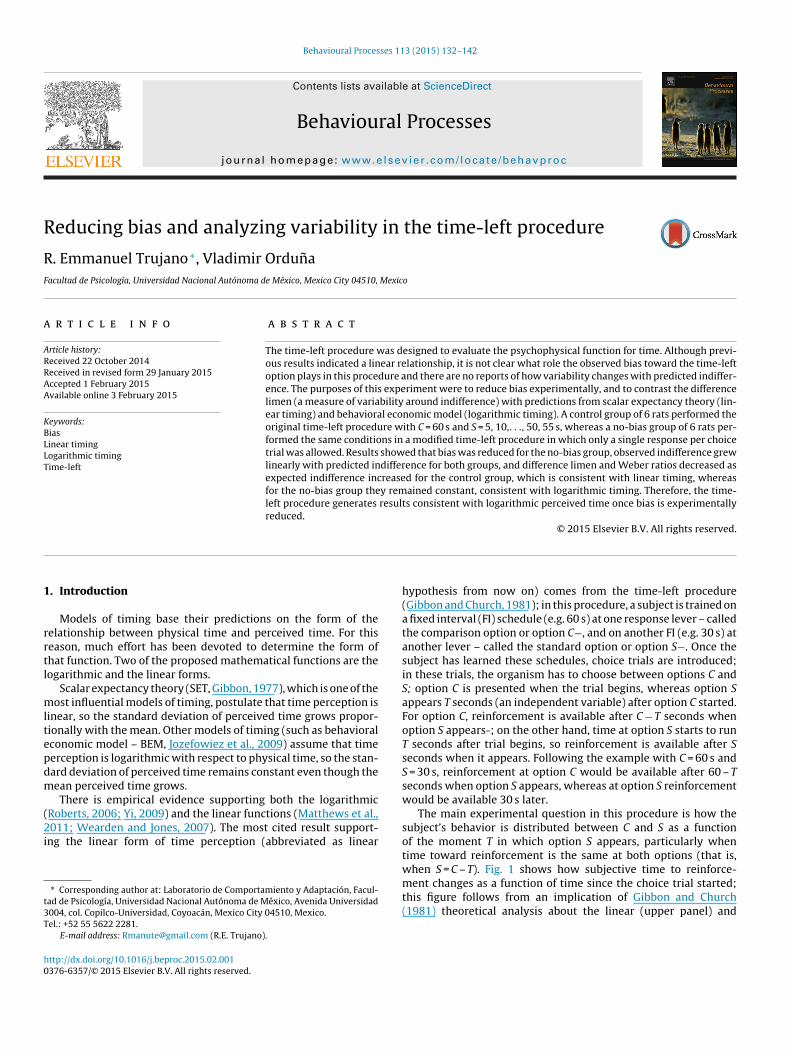
The main experimental question in this procedure is how thesubject’s behavior is distributed between C and S as a functionof the moment T in which option S appears, particularly whentime toward reinforcement is the same at both options (that is,when S = C – T). Fig. 1 shows how subjective time to reinforce-ment changes as a function of time since the choice trial started;

this figure follows from an implication of Gibbon and Church(1981) theoretical analysis about the linear (upper panel) and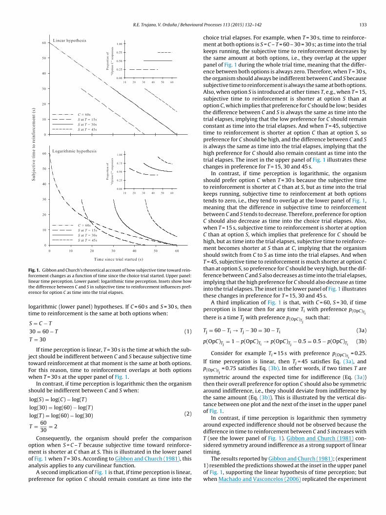

R.E. Trujano, V. Orduna / Behavioural

Fig. 1. Gibbon and Church’s theoretical account of how subjective time toward rein-forcement changes as a function of time since the choice trial started. Upper panel:lte

lt

jtFw

s

omoa

p

inear time perception. Lower panel: logarithmic time perception. Insets show howhe difference between C and S in subjective time to reinforcement influences pref-rence for option C as time into the trial elapses.

ogarithmic (lower panel) hypotheses. If C = 60 s and S = 30 s, thenime to reinforcement is the same at both options when:

S = C − T

30 = 60 − T

T = 30

(1)

If time perception is linear, T = 30 s is the time at which the sub-ect should be indifferent between C and S because subjective timeoward reinforcement at that moment is the same at both options.or this reason, time to reinforcement overlaps at both optionshen T = 30 s at the upper panel of Fig. 1.

In contrast, if time perception is logarithmic then the organismhould be indifferent between C and S when:

log(S) = log(C) − log(T)

log(30) = log(60) − log(T)

log(T) = log(60) − log(30)

T = 6030

= 2

(2)

Consequently, the organism should prefer the comparisonption when S = C – T because subjective time toward reinforce-ent is shorter at C than at S. This is illustrated in the lower panel

f Fig. 1 when T = 30 s. According to Gibbon and Church (1981), thisnalysis applies to any curvilinear function.

A second implication of Fig. 1 is that, if time perception is linear,reference for option C should remain constant as time into the

Processes 113 (2015) 132–142 133

choice trial elapses. For example, when T = 30 s, time to reinforce-ment at both options is S = C – T = 60 – 30 = 30 s; as time into the trialkeeps running, the subjective time to reinforcement decreases bythe same amount at both options, i.e., they overlap at the upperpanel of Fig. 1 during the whole trial time, meaning that the differ-ence between both options is always zero. Therefore, when T = 30 s,the organism should always be indifferent between C and S becausesubjective time to reinforcement is always the same at both options.Also, when option S is introduced at other times T, e.g., when T = 15,subjective time to reinforcement is shorter at option S than atoption C, which implies that preference for C should be low; besidesthe difference between C and S is always the same as time into thetrial elapses, implying that the low preference for C should remainconstant as time into the trial elapses. And when T = 45, subjectivetime to reinforcement is shorter at option C than at option S, sopreference for C should be high, and the difference between C and Sis always the same as time into the trial elapses, implying that thehigh preference for C should also remain constant as time into thetrial elapses. The inset in the upper panel of Fig. 1 illustrates thesechanges in preference for T = 15, 30 and 45 s.

In contrast, if time perception is logarithmic, the organismshould prefer option C when T = 30 s because the subjective timeto reinforcement is shorter at C than at S, but as time into the trialkeeps running, subjective time to reinforcement at both optionstends to zero, i.e., they tend to overlap at the lower panel of Fig. 1,meaning that the difference in subjective time to reinforcementbetween C and S tends to decrease. Therefore, preference for optionC should also decrease as time into the choice trial elapses. Also,when T = 15 s, subjective time to reinforcement is shorter at optionC than at option S, which implies that preference for C should behigh, but as time into the trial elapses, subjective time to reinforce-ment becomes shorter at S than at C, implying that the organismshould switch from C to S as time into the trial elapses. And whenT = 45, subjective time to reinforcement is much shorter at option Cthan at option S, so preference for C should be very high, but the dif-ference between C and S also decreases as time into the trial elapses,implying that the high preference for C should also decrease as timeinto the trial elapses. The inset in the lower panel of Fig. 1 illustratesthese changes in preference for T = 15, 30 and 45 s.

A third implication of Fig. 1 is that, with C = 60, S = 30, if timeperception is linear then for any time Ti with preference p(OpC)Tithere is a time Tj with preference p(OpC)Tj

such that:

Tj = 60 − Ti → Tj − 30 = 30 − Ti (3a)

p(OpC)Tj= 1 − p(OpC)Ti

→ p(OpC)Tj− 0.5 = 0.5 − p(OpC)Ti

(3b)

Consider for example Ti = 15 s with preference p(OpC)Ti= 0.25.

If time perception is linear, then Tj = 45 satisfies Eq. (3a), andp(OpC)Tj

= 0.75 satisfies Eq. (3b). In other words, if two times T are

symmetric around the expected time for indifference (Eq. (3a))then their overall preference for option C should also be symmetricaround indifference, i.e., they should deviate from indifference bythe same amount (Eq. (3b)). This is illustrated by the vertical dis-tance between one plot and the next of the inset in the upper panelof Fig. 1.

In contrast, if time perception is logarithmic then symmetryaround expected indifference should not be observed because thedifference in time to reinforcement between C and S increases withT (see the lower panel of Fig. 1). Gibbon and Church (1981) con-sidered symmetry around indifference as a strong support of lineartiming.

The results reported by Gibbon and Church (1981); (experiment1) resembled the predictions showed at the inset in the upper panelof Fig. 1, supporting the linear hypothesis of time perception; butwhen Machado and Vasconcelos (2006) replicated the experiment

134 R.E. Trujano, V. Orduna / Behavioural Processes 113 (2015) 132–142

F functB ; for Bp eber

wacweS1sB(Sw

taae(

Jtbb

ig. 2. Top panels: preference for the comparison option (assuming no bias) as aEM (right) for C = 60 s and, from left to right, S = 55, 50,. . ., 10, 5 (for SET: � = 0.16sychometric functions predicted by SET and BEM. Bottom right panel: expected W

ith pigeons, they found results similar to the predictions showedt the inset in the lower panel of Fig. 1, suggesting that time per-eption is logarithmic instead. Other studies have reported that,hen time toward reinforcement is the same at both options, pref-

rence for C is higher than for S (Al-Ruwaitea et al., 1997; Cerutti andtaddon, 2004; experiment 1; Gibbon, 1986; Gibbon et al., 1988,984; Preston, 1994; Vieira de Castro and Machado, 2010), whicheem to support a logarithmic transformation of time. However,runner et al. (1994) baseline results, and Meijering and van Rijn2009) results, showed that preference for C is slightly less than for

when S = C – T, which is not compatible neither with the linear norith the logarithmic hypothesis.

Nevertheless, Gibbon postulated that preference for C whenime toward reinforcement is the same at both options could beccurately described by the linear form of time perception as long as

bias parameter B is introduced (Gibbon and Church, 1981; Gibbon

t al., 1984). In fact, Gibbon and Fairhurst (1994) and Brunner et al.1994) found that this bias can be experimentally manipulated.1

1 The nature of the bias remains unclear, but Cerutti and Staddon (2004); see alsoozefowiez and Machado (2013) have suggested that due to a hyperbolic value func-ion the conditioned reinforcement value of option C is lower than that of option Sefore the expected point of indifference, higher after indifference and the differenceetween them becomes increasingly large after indifference.

ion of the moment the standard option is introduced according to SET (left) andEM: � = 0.3). Bottom left panel: changes in the difference limen derived from the

ratios according to SET and BEM as a function of expected indifference points.

Al-Ruwaitea et al. (1999), Cordes et al.(2007) and Wearden(2002) implemented a procedure where subjects were not allowedto alternate between C and S because only a single response couldbe emitted at the moment the standard option appeared. Theyfound results consistent with Gibbon and Church (1981) theoreti-cal analysis: organisms approached indifference very closely whenS = C – T, suggesting that bias could be experimentally reduced.Preston (1994) argued that the measure or preference is an impor-tant variable to take into account in the analysis of bias; he suggeststhat when preference is measured as the proportion of comparisonoption responses as a function of elapsing time in the trial, biaswill be observed, but if preference is measured as the proportion ofentries into the comparison option as a function of the moment thestandard option appears (as a function of T), bias will be reducedand preference will approach indifference when S = C – T. Prestonalso proposed a statistical correction as another way for reducingbias. The results reported by Preston (experiment 1) agree withthese ideas (see his Figs. 3 and 5). Together with the results of Al-Ruwaitea et al. (1999), Cordes et al. (2007), and Wearden (2002),Preston’s analyses suggest that if response bias is eliminated or sta-tistically corrected, then the results from the time-left experimentagree on Gibbon and Church (1981) proposal of a linear form of

time perception.

As can be seen in the above discussion, the prototypicalprocedure to study the form of time perception has generated

ioural

iwfpC

tsapmf

iephcTeiatfma(at

p

w

z

�o�adp

efdtfctmfcscpa

ratfst

a

R.E. Trujano, V. Orduna / Behav

nconclusive results. The first purpose of this experiment was to testhether bias can be experimentally reduced by comparing results

rom the original time-left with those from a modified time-leftrocedure resembling those employed by Al-Ruwaitea et al. (1999),ordes et al. (2007), and Wearden (2002).

The second purpose of this experiment was to test symme-ry; we accomplished this by including more times T at which thetandard option could appear so that there are more data pointsvailable to test symmetry statistically. Being more iterative, thisrocedural aspect allows the opportunity to analyze symmetryore deeply at various moments, ruling out any artifact resultant

rom performing curve fitting to a very limited set of data.The third purpose of our experiment was to test how variability

n perceived time is related to its mean. Gibbon (1977) providedvidence that the standard deviation of perceived time grows pro-ortionally with its mean, which is consistent with the linearypothesis. However, Yi (2009) showed that variability around per-eived time is constant, consistent with the logarithmic hypothesis.o our knowledge, this test has not been performed in any time-leftxperiment. In our experiment, we arranged different conditionsn which the comparison option was always 60 s but the standardlternative was manipulated (5, 10,. . ., 50, 55 s in different condi-ions). The top panels of Fig. 2 shows the expected psychometricunctions for these conditions (assuming no bias) according to a

odel that assumes linear time perception such as SET (left panel)nd another that assumes logarithmic time perception such as BEMright panel). The curves predicted by SET were drawn with Eq. 8and 8b from Gibbon and Church (1981): preference for option Cakes the form

(OpC) = �[z(T)], (4a)

here

(T) = T − C + bS

�√C2 + b2S2

(4b),

is the cumulative unit normal function, b represents bias towardption C (curves were drawn assuming no bias, i.e., b = 1.0) and

is the sensitivity of the system. The curves predicted by BEMre cumulative normal functions with mean � = ln(C – S), and stan-ard deviation � = 0.3 (Jozefowiez et al., 2009), which representredicted indifference and sensitivity of the system, respectively.

Consider first the leftmost psychometric functions of both pan-ls in which S = 55 s: the slope is steeper for logarithmic timing thanor linear timing, which implies that the difference limen (half theifference between time when preference for option C is 0.75 andime when preference for option C is 0.25) is bigger for linear thanor logarithmic timing. Conversely, when S = 5 s the slope of the psy-hometric function is steeper for linear timing than for logarithmiciming, implying that the difference limen is bigger for logarith-

ic than for linear timing. Besides, the slopes of the psychometricunctions increase with the indifference points for linear time per-eption so that the difference limen should decrease, whereas thelopes decrease as indifference increases for logarithmic time per-eption so the difference limen should increase. The bottom leftanel of Fig. 2 summarizes these changes in the difference limen as

function of the expected indifference points for both models.The bottom right panel of Fig. 2 shows the predicted Weber

atios (the difference limen divided by the indifference point)ccording to linear and logarithmic time perception: since lineariming predicts a decreasing trend for the difference limen as indif-erence points increase, the Weber ratio has a similar trend; but

ince logarithmic timing predicts that both measures increase, thenhe Weber ratio remains constant.

Since the linear and logarithmic hypotheses make differentssumptions about how variability in perceived time changes, a

Processes 113 (2015) 132–142 135

test of variability can provide additional information about timeperception in the time-left experiment.

2. Method

2.1. Subjects

Twelve experimentally naive male rats (Rattus Norvegicus) fromthe Wistar strain took part in the experiment. They were individ-ually homed in translucent plastic cages, and maintained at 85% oftheir free feeding weight with free access to water in their homecages. They were 113 days old at the beginning of the experiment.Every rat was randomly assigned to one out of two groups: controlgroup (n = 6) and no-bias group (n = 6).

2.2. Apparatus

Eight operant conditioning chambers (MED Associates, Inc.,Model ENV 008 VP) served as the experimental spaces. Each oper-ant chamber measured 30.5 cm (long) × 24.1 cm (wide) × 21.0 cm(tall), and was enclosed in a sound attenuating cubicle (MED Asso-ciates, Inc., Model ENV-022M). The floor was a stainless steelgrid comprised of nineteen 0.5 cm diameter bars (MED Associates,Inc., Model ENV-005). Each chamber had two retractable responselevers (MED Associates, Inc., Model ENV 112CM) located 2.1 cmabove the floor, in the front wall. Each lever was 4.8 cm wide. Thevisual stimuli used were the center white lights from triple stimu-lus displays situated 1.5 cm above each lever; each triple stimulusdisplay consisted on a bar of acrylic mounted on an aluminum barwith three apertures of 1 cm of diameter and separated by 0.6 cmand it could project (from left to right) red, white or blue light viaultrabrilliant LEDs. A 5.1 cm × 5.1 cm pellet receptacle (MED Asso-ciates, Inc., Model ENV-200R2M) was located in the center of thefront wall, 2.5 cm above the floor, and received, according to theschedule, 45 mg Noyes precision food pellets (Bio-Serv, ProductF0021) from a circular modular pellet dispenser (MED Associates,Inc., Model ENV-203M). Presentation of stimuli and collection ofdata were controlled by personal computers using the Medstateprogramming language (Med-PC-IV, MED Associates, Inc.).

2.3. Procedure

2.3.1. TrainingAll subjects were trained on two fixed interval (FI) schedules:

one of the levers was associated to a FI 60 s (named as the compari-son option C) and the other was associated to a FI 30 s (named as thestandard option S). A training trial for the control group consistedon the following sequence of events: when the trial began, thelever was inserted, its corresponding light turned on, and the firstresponse after the target time elapsed retracted the lever, turnedoff its light and delivered the reinforcer. Three seconds later, a 60 sintertrial interval (ITI) began, during which all lights of the chamberturned off. After the ITI ended, a new trial began.

For the no-bias group, trials involved the following sequence ofevents: for option C, its light turned on and T seconds later its leverwas inserted and the clock was paused; the first response resumedthe clock since the second it was paused, so that reinforcementwas available 60 – T seconds after the first response. For option S,the light from option C turned on, and T seconds later it turned off,the light from option S turned on, its lever was inserted and theclock was paused; the first response initiated the target time and

the reinforcer was available 30 s later. In both types of trials, thefirst response after the target time delivered the reinforcer. Threeseconds later, a 60 s ITI began, during which all lights of the chamberwere turned off, and a new trial began after the ITI ended. For both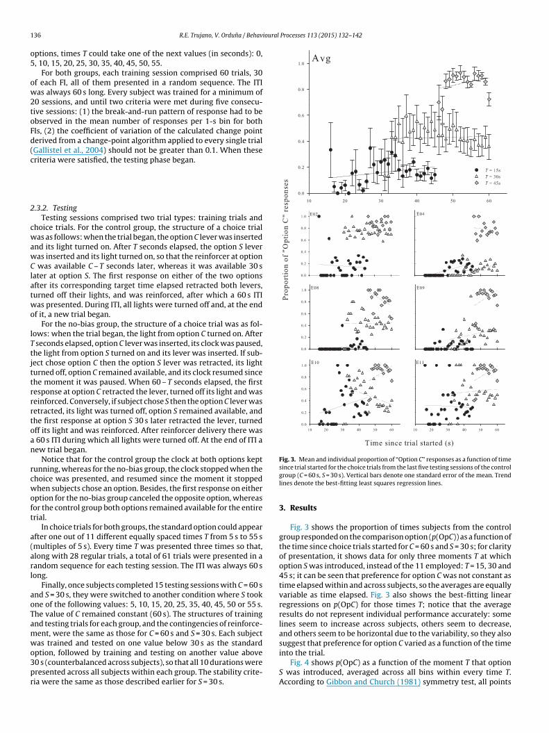

1 ioural Processes 113 (2015) 132–142

o5

ow2toFd(c

2

cwawClatwo

lTtjttrrrtoan

rcwoft

a(arl

aoTamwo3pr

Fig. 3. Mean and individual proportion of “Option C” responses as a function of time

36 R.E. Trujano, V. Orduna / Behav

ptions, times T could take one of the next values (in seconds): 0,, 10, 15, 20, 25, 30, 35, 40, 45, 50, 55.

For both groups, each training session comprised 60 trials, 30f each FI, all of them presented in a random sequence. The ITIas always 60 s long. Every subject was trained for a minimum of

0 sessions, and until two criteria were met during five consecu-ive sessions: (1) the break-and-run pattern of response had to bebserved in the mean number of responses per 1-s bin for bothIs, (2) the coefficient of variation of the calculated change pointerived from a change-point algorithm applied to every single trialGallistel et al., 2004) should not be greater than 0.1. When theseriteria were satisfied, the testing phase began.

.3.2. TestingTesting sessions comprised two trial types: training trials and

hoice trials. For the control group, the structure of a choice trialas as follows: when the trial began, the option C lever was inserted

nd its light turned on. After T seconds elapsed, the option S leveras inserted and its light turned on, so that the reinforcer at option

was available C – T seconds later, whereas it was available 30 sater at option S. The first response on either of the two optionsfter its corresponding target time elapsed retracted both levers,urned off their lights, and was reinforced, after which a 60 s ITIas presented. During ITI, all lights were turned off and, at the end

f it, a new trial began.For the no-bias group, the structure of a choice trial was as fol-

ows: when the trial began, the light from option C turned on. After seconds elapsed, option C lever was inserted, its clock was paused,he light from option S turned on and its lever was inserted. If sub-ect chose option C then the option S lever was retracted, its lighturned off, option C remained available, and its clock resumed sincehe moment it was paused. When 60 – T seconds elapsed, the firstesponse at option C retracted the lever, turned off its light and waseinforced. Conversely, if subject chose S then the option C lever wasetracted, its light was turned off, option S remained available, andhe first response at option S 30 s later retracted the lever, turnedff its light and was reinforced. After reinforcer delivery there was

60 s ITI during which all lights were turned off. At the end of ITI aew trial began.

Notice that for the control group the clock at both options keptunning, whereas for the no-bias group, the clock stopped when thehoice was presented, and resumed since the moment it stoppedhen subjects chose an option. Besides, the first response on either

ption for the no-bias group canceled the opposite option, whereasor the control group both options remained available for the entirerial.

In choice trials for both groups, the standard option could appearfter one out of 11 different equally spaced times T from 5 s to 55 smultiples of 5 s). Every time T was presented three times so that,long with 28 regular trials, a total of 61 trials were presented in aandom sequence for each testing session. The ITI was always 60 song.

Finally, once subjects completed 15 testing sessions with C = 60 snd S = 30 s, they were switched to another condition where S tookne of the following values: 5, 10, 15, 20, 25, 35, 40, 45, 50 or 55 s.he value of C remained constant (60 s). The structures of trainingnd testing trials for each group, and the contingencies of reinforce-ent, were the same as those for C = 60 s and S = 30 s. Each subjectas trained and tested on one value below 30 s as the standard

ption, followed by training and testing on another value above0 s (counterbalanced across subjects), so that all 10 durations wereresented across all subjects within each group. The stability crite-ia were the same as those described earlier for S = 30 s.

since trial started for the choice trials from the last five testing sessions of the controlgroup (C = 60 s, S = 30 s). Vertical bars denote one standard error of the mean. Trendlines denote the best-fitting least squares regression lines.

3. Results

Fig. 3 shows the proportion of times subjects from the controlgroup responded on the comparison option (p(OpC)) as a function ofthe time since choice trials started for C = 60 s and S = 30 s; for clarityof presentation, it shows data for only three moments T at whichoption S was introduced, instead of the 11 employed: T = 15, 30 and45 s; it can be seen that preference for option C was not constant astime elapsed within and across subjects, so the averages are equallyvariable as time elapsed. Fig. 3 also shows the best-fitting linearregressions on p(OpC) for those times T; notice that the averageresults do not represent individual performance accurately: somelines seem to increase across subjects, others seem to decrease,and others seem to be horizontal due to the variability, so they alsosuggest that preference for option C varied as a function of the time

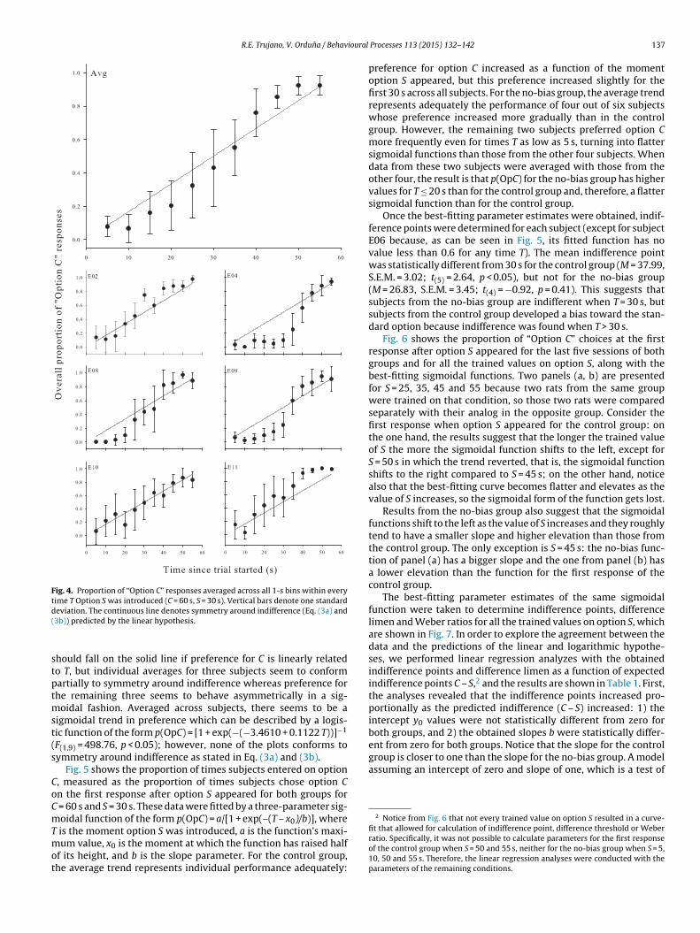
into the trial.

Fig. 4 shows p(OpC) as a function of the moment T that optionS was introduced, averaged across all bins within every time T.According to Gibbon and Church (1981) symmetry test, all points

R.E. Trujano, V. Orduna / Behavioural

Fig. 4. Proportion of “Option C” responses averaged across all 1-s bins within everytime T Option S was introduced (C = 60 s, S = 30 s). Vertical bars denote one standardd(

stptmst(s

CoCmTmot

ent from zero for both groups. Notice that the slope for the controlgroup is closer to one than the slope for the no-bias group. A modelassuming an intercept of zero and slope of one, which is a test of

2 Notice from Fig. 6 that not every trained value on option S resulted in a curve-fit that allowed for calculation of indifference point, difference threshold or Weber

eviation. The continuous line denotes symmetry around indifference (Eq. (3a) and3b)) predicted by the linear hypothesis.

hould fall on the solid line if preference for C is linearly relatedo T, but individual averages for three subjects seem to conformartially to symmetry around indifference whereas preference forhe remaining three seems to behave asymmetrically in a sig-

oidal fashion. Averaged across subjects, there seems to be aigmoidal trend in preference which can be described by a logis-ic function of the form p(OpC) = [1 + exp(−(−3.4610 + 0.1122 T))]−1

F(1,9) = 498.76, p < 0.05); however, none of the plots conforms toymmetry around indifference as stated in Eq. (3a) and (3b).

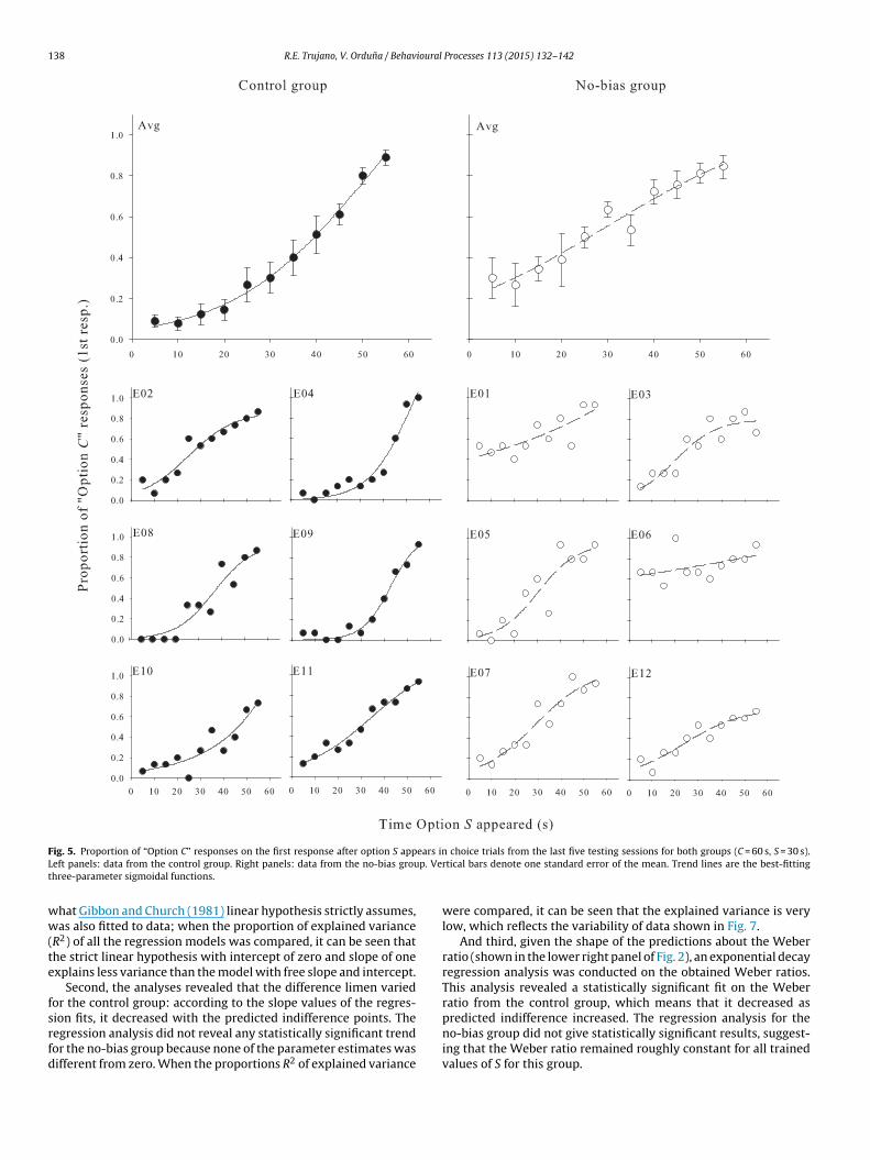
Fig. 5 shows the proportion of times subjects entered on option, measured as the proportion of times subjects chose option Cn the first response after option S appeared for both groups for

= 60 s and S = 30 s. These data were fitted by a three-parameter sig-oidal function of the form p(OpC) = a/[1 + exp(–(T – x0)/b)], where

is the moment option S was introduced, a is the function’s maxi-

um value, x0 is the moment at which the function has raised half

f its height, and b is the slope parameter. For the control group,he average trend represents individual performance adequately:

Processes 113 (2015) 132–142 137

preference for option C increased as a function of the momentoption S appeared, but this preference increased slightly for thefirst 30 s across all subjects. For the no-bias group, the average trendrepresents adequately the performance of four out of six subjectswhose preference increased more gradually than in the controlgroup. However, the remaining two subjects preferred option Cmore frequently even for times T as low as 5 s, turning into flattersigmoidal functions than those from the other four subjects. Whendata from these two subjects were averaged with those from theother four, the result is that p(OpC) for the no-bias group has highervalues for T ≤ 20 s than for the control group and, therefore, a flattersigmoidal function than for the control group.

Once the best-fitting parameter estimates were obtained, indif-ference points were determined for each subject (except for subjectE06 because, as can be seen in Fig. 5, its fitted function has novalue less than 0.6 for any time T). The mean indifference pointwas statistically different from 30 s for the control group (M = 37.99,S.E.M. = 3.02; t(5) = 2.64, p < 0.05), but not for the no-bias group(M = 26.83, S.E.M. = 3.45; t(4) = −0.92, p = 0.41). This suggests thatsubjects from the no-bias group are indifferent when T = 30 s, butsubjects from the control group developed a bias toward the stan-dard option because indifference was found when T > 30 s.

Fig. 6 shows the proportion of “Option C” choices at the firstresponse after option S appeared for the last five sessions of bothgroups and for all the trained values on option S, along with thebest-fitting sigmoidal functions. Two panels (a, b) are presentedfor S = 25, 35, 45 and 55 because two rats from the same groupwere trained on that condition, so those two rats were comparedseparately with their analog in the opposite group. Consider thefirst response when option S appeared for the control group: onthe one hand, the results suggest that the longer the trained valueof S the more the sigmoidal function shifts to the left, except forS = 50 s in which the trend reverted, that is, the sigmoidal functionshifts to the right compared to S = 45 s; on the other hand, noticealso that the best-fitting curve becomes flatter and elevates as thevalue of S increases, so the sigmoidal form of the function gets lost.

Results from the no-bias group also suggest that the sigmoidalfunctions shift to the left as the value of S increases and they roughlytend to have a smaller slope and higher elevation than those fromthe control group. The only exception is S = 45 s: the no-bias func-tion of panel (a) has a bigger slope and the one from panel (b) hasa lower elevation than the function for the first response of thecontrol group.

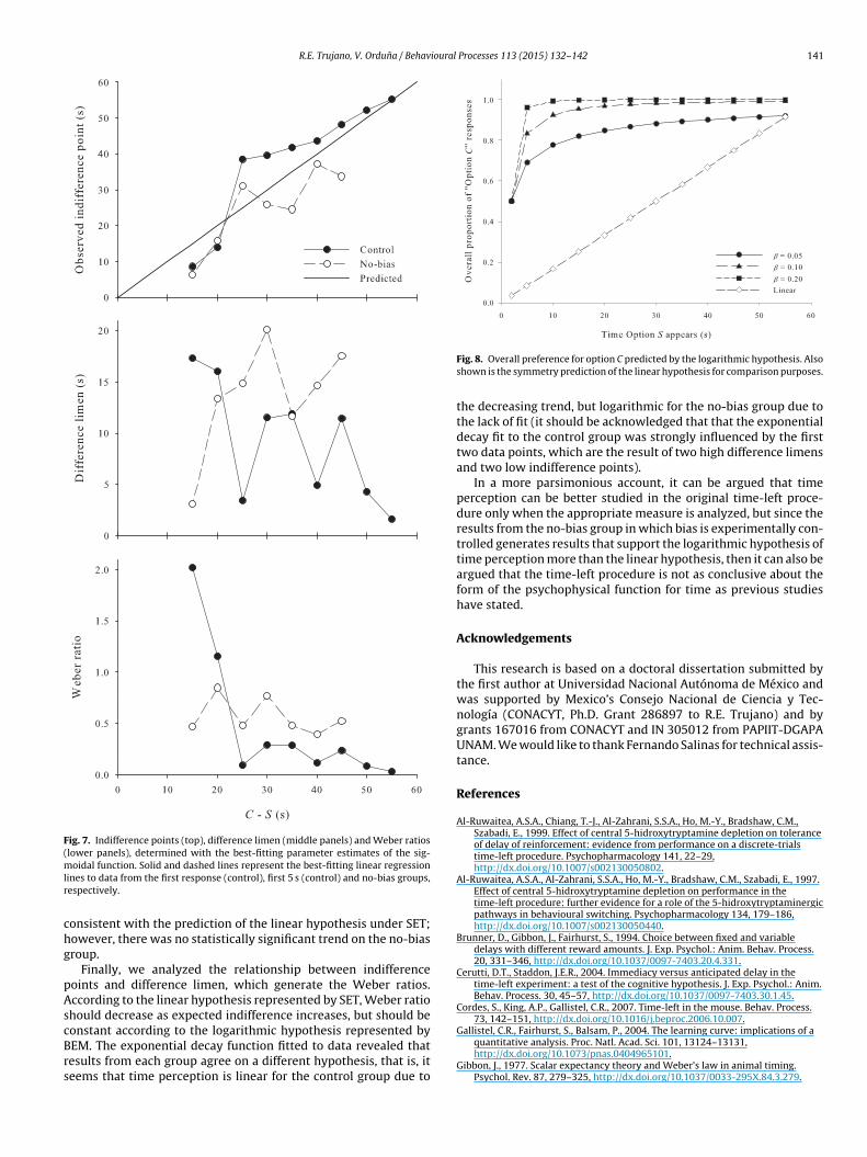
The best-fitting parameter estimates of the same sigmoidalfunction were taken to determine indifference points, differencelimen and Weber ratios for all the trained values on option S, whichare shown in Fig. 7. In order to explore the agreement between thedata and the predictions of the linear and logarithmic hypothe-ses, we performed linear regression analyzes with the obtainedindifference points and difference limen as a function of expectedindifference points C – S,2 and the results are shown in Table 1. First,the analyses revealed that the indifference points increased pro-portionally as the predicted indifference (C – S) increased: 1) theintercept y0 values were not statistically different from zero forboth groups, and 2) the obtained slopes b were statistically differ-

ratio. Specifically, it was not possible to calculate parameters for the first responseof the control group when S = 50 and 55 s, neither for the no-bias group when S = 5,10, 50 and 55 s. Therefore, the linear regression analyses were conducted with theparameters of the remaining conditions.

138 R.E. Trujano, V. Orduna / Behavioural Processes 113 (2015) 132–142

F ears inL p. Vet

ww(te

fsrfd

ig. 5. Proportion of “Option C” responses on the first response after option S appeft panels: data from the control group. Right panels: data from the no-bias grouhree-parameter sigmoidal functions.

hat Gibbon and Church (1981) linear hypothesis strictly assumes,as also fitted to data; when the proportion of explained variance

R2) of all the regression models was compared, it can be seen thathe strict linear hypothesis with intercept of zero and slope of onexplains less variance than the model with free slope and intercept.

Second, the analyses revealed that the difference limen variedor the control group: according to the slope values of the regres-ion fits, it decreased with the predicted indifference points. The

egression analysis did not reveal any statistically significant trendor the no-bias group because none of the parameter estimates wasifferent from zero. When the proportions R2 of explained variance

choice trials from the last five testing sessions for both groups (C = 60 s, S = 30 s).rtical bars denote one standard error of the mean. Trend lines are the best-fitting

were compared, it can be seen that the explained variance is verylow, which reflects the variability of data shown in Fig. 7.

And third, given the shape of the predictions about the Weberratio (shown in the lower right panel of Fig. 2), an exponential decayregression analysis was conducted on the obtained Weber ratios.This analysis revealed a statistically significant fit on the Weberratio from the control group, which means that it decreased aspredicted indifference increased. The regression analysis for the

no-bias group did not give statistically significant results, suggest-ing that the Weber ratio remained roughly constant for all trainedvalues of S for this group.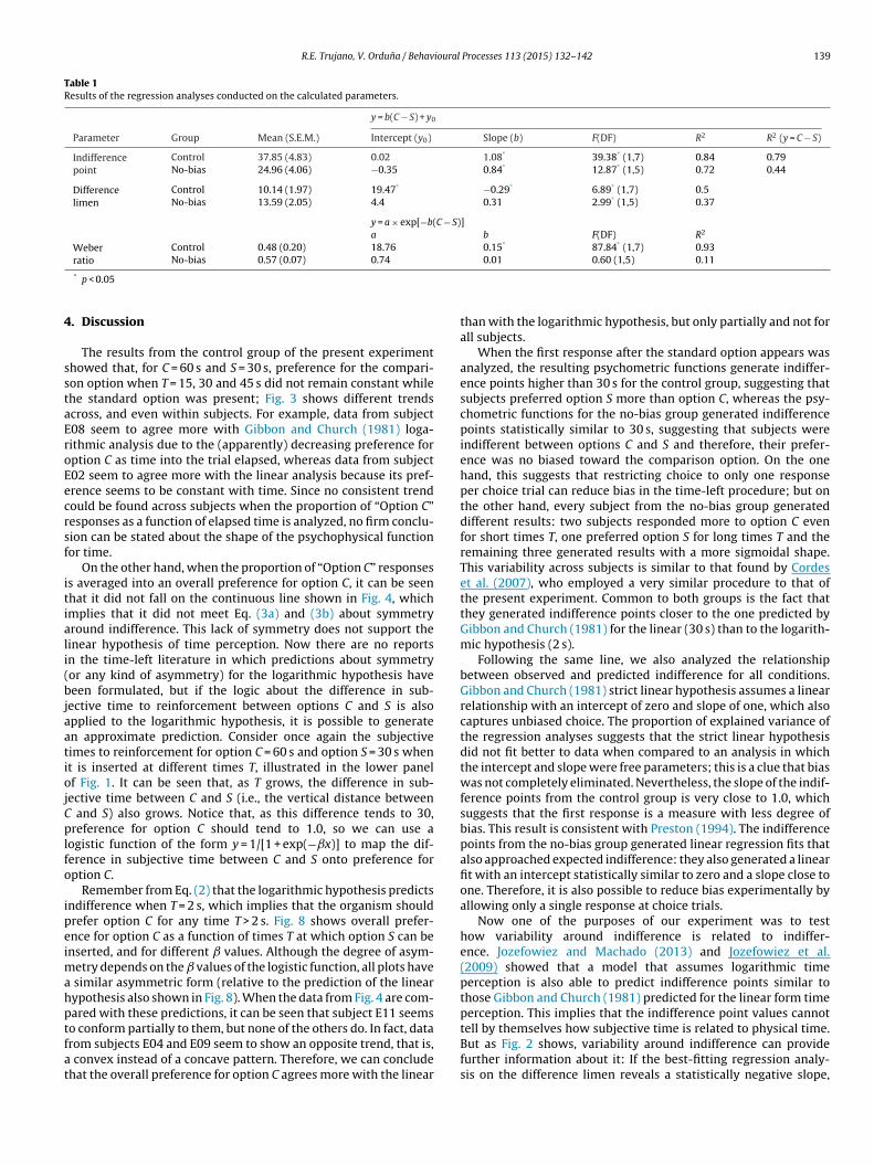

R.E. Trujano, V. Orduna / Behavioural Processes 113 (2015) 132–142 139

Table 1Results of the regression analyses conducted on the calculated parameters.

y = b(C − S) + y0

Parameter Group Mean (S.E.M.) Intercept (y0) Slope (b) F(DF) R2 R2 (y = C − S)

Indifferencepoint

Control 37.85 (4.83) 0.02 1.08* 39.38* (1,7) 0.84 0.79No-bias 24.96 (4.06) −0.35 0.84* 12.87* (1,5) 0.72 0.44

Differencelimen

Control 10.14 (1.97) 19.47* −0.29* 6.89* (1,7) 0.5No-bias 13.59 (2.05) 4.4 0.31 2.99* (1,5) 0.37

y = a × exp[−b(C − S)]a b F(DF) R2

Weber Control 0.48 (0.20) 18.76 0.15* 87.84* (1,7) 0.93

4

sstaEroEecrsf

itiali(bjaatiojCplfo

ipeimahptfat

ratio No-bias 0.57 (0.07) 0.74

* p < 0.05

. Discussion

The results from the control group of the present experimenthowed that, for C = 60 s and S = 30 s, preference for the compari-on option when T = 15, 30 and 45 s did not remain constant whilehe standard option was present; Fig. 3 shows different trendscross, and even within subjects. For example, data from subject08 seem to agree more with Gibbon and Church (1981) loga-ithmic analysis due to the (apparently) decreasing preference forption C as time into the trial elapsed, whereas data from subject02 seem to agree more with the linear analysis because its pref-rence seems to be constant with time. Since no consistent trendould be found across subjects when the proportion of “Option C”esponses as a function of elapsed time is analyzed, no firm conclu-ion can be stated about the shape of the psychophysical functionor time.

On the other hand, when the proportion of “Option C” responsess averaged into an overall preference for option C, it can be seenhat it did not fall on the continuous line shown in Fig. 4, whichmplies that it did not meet Eq. (3a) and (3b) about symmetryround indifference. This lack of symmetry does not support theinear hypothesis of time perception. Now there are no reportsn the time-left literature in which predictions about symmetryor any kind of asymmetry) for the logarithmic hypothesis haveeen formulated, but if the logic about the difference in sub-

ective time to reinforcement between options C and S is alsopplied to the logarithmic hypothesis, it is possible to generaten approximate prediction. Consider once again the subjectiveimes to reinforcement for option C = 60 s and option S = 30 s whent is inserted at different times T, illustrated in the lower panelf Fig. 1. It can be seen that, as T grows, the difference in sub-

ective time between C and S (i.e., the vertical distance between and S) also grows. Notice that, as this difference tends to 30,reference for option C should tend to 1.0, so we can use a

ogistic function of the form y = 1/[1 + exp(−ˇx)] to map the dif-erence in subjective time between C and S onto preference forption C.

Remember from Eq. (2) that the logarithmic hypothesis predictsndifference when T = 2 s, which implies that the organism shouldrefer option C for any time T > 2 s. Fig. 8 shows overall prefer-nce for option C as a function of times T at which option S can benserted, and for different values. Although the degree of asym-

etry depends on the values of the logistic function, all plots have similar asymmetric form (relative to the prediction of the linearypothesis also shown in Fig. 8). When the data from Fig. 4 are com-ared with these predictions, it can be seen that subject E11 seems

o conform partially to them, but none of the others do. In fact, datarom subjects E04 and E09 seem to show an opposite trend, that is,

convex instead of a concave pattern. Therefore, we can concludehat the overall preference for option C agrees more with the linear

0.01 0.60 (1,5) 0.11

than with the logarithmic hypothesis, but only partially and not forall subjects.

When the first response after the standard option appears wasanalyzed, the resulting psychometric functions generate indiffer-ence points higher than 30 s for the control group, suggesting thatsubjects preferred option S more than option C, whereas the psy-chometric functions for the no-bias group generated indifferencepoints statistically similar to 30 s, suggesting that subjects wereindifferent between options C and S and therefore, their prefer-ence was no biased toward the comparison option. On the onehand, this suggests that restricting choice to only one responseper choice trial can reduce bias in the time-left procedure; but onthe other hand, every subject from the no-bias group generateddifferent results: two subjects responded more to option C evenfor short times T, one preferred option S for long times T and theremaining three generated results with a more sigmoidal shape.This variability across subjects is similar to that found by Cordeset al. (2007), who employed a very similar procedure to that ofthe present experiment. Common to both groups is the fact thatthey generated indifference points closer to the one predicted byGibbon and Church (1981) for the linear (30 s) than to the logarith-mic hypothesis (2 s).

Following the same line, we also analyzed the relationshipbetween observed and predicted indifference for all conditions.Gibbon and Church (1981) strict linear hypothesis assumes a linearrelationship with an intercept of zero and slope of one, which alsocaptures unbiased choice. The proportion of explained variance ofthe regression analyses suggests that the strict linear hypothesisdid not fit better to data when compared to an analysis in whichthe intercept and slope were free parameters; this is a clue that biaswas not completely eliminated. Nevertheless, the slope of the indif-ference points from the control group is very close to 1.0, whichsuggests that the first response is a measure with less degree ofbias. This result is consistent with Preston (1994). The indifferencepoints from the no-bias group generated linear regression fits thatalso approached expected indifference: they also generated a linearfit with an intercept statistically similar to zero and a slope close toone. Therefore, it is also possible to reduce bias experimentally byallowing only a single response at choice trials.

Now one of the purposes of our experiment was to testhow variability around indifference is related to indiffer-ence. Jozefowiez and Machado (2013) and Jozefowiez et al.(2009) showed that a model that assumes logarithmic timeperception is also able to predict indifference points similar tothose Gibbon and Church (1981) predicted for the linear form timeperception. This implies that the indifference point values cannot

tell by themselves how subjective time is related to physical time.But as Fig. 2 shows, variability around indifference can providefurther information about it: If the best-fitting regression analy-sis on the difference limen reveals a statistically negative slope,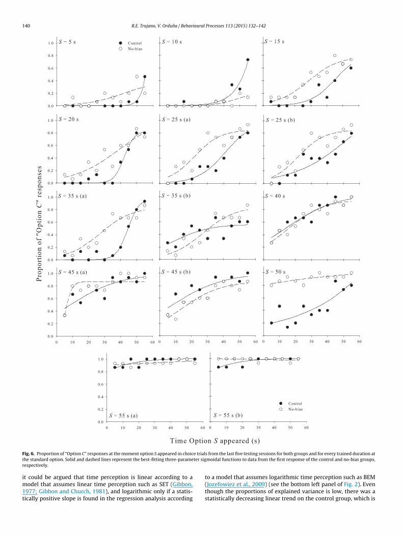

140 R.E. Trujano, V. Orduna / Behavioural Processes 113 (2015) 132–142

F e trialt ter sigr

im1t

ig. 6. Proportion of “Option C” responses at the moment option S appeared in choiche standard option. Solid and dashed lines represent the best-fitting three-parameespectively.

t could be argued that time perception is linear according to aodel that assumes linear time perception such as SET (Gibbon,

977; Gibbon and Church, 1981), and logarithmic only if a statis-ically positive slope is found in the regression analysis according

s from the last five testing sessions for both groups and for every trained duration atmoidal functions to data from the first response of the control and no-bias groups,

to a model that assumes logarithmic time perception such as BEM(Jozefowiez et al., 2009) (see the bottom left panel of Fig. 2). Eventhough the proportions of explained variance is low, there was astatistically decreasing linear trend on the control group, which is

R.E. Trujano, V. Orduna / Behavioural Processes 113 (2015) 132–142 141

Fig. 7. Indifference points (top), difference limen (middle panels) and Weber ratios(lower panels), determined with the best-fitting parameter estimates of the sig-mlr

chg

pAscBrs

oidal function. Solid and dashed lines represent the best-fitting linear regressionines to data from the first response (control), first 5 s (control) and no-bias groups,espectively.

onsistent with the prediction of the linear hypothesis under SET;owever, there was no statistically significant trend on the no-biasroup.

Finally, we analyzed the relationship between indifferenceoints and difference limen, which generate the Weber ratios.ccording to the linear hypothesis represented by SET, Weber ratiohould decrease as expected indifference increases, but should be

onstant according to the logarithmic hypothesis represented byEM. The exponential decay function fitted to data revealed thatesults from each group agree on a different hypothesis, that is, iteems that time perception is linear for the control group due to

Fig. 8. Overall preference for option C predicted by the logarithmic hypothesis. Alsoshown is the symmetry prediction of the linear hypothesis for comparison purposes.

the decreasing trend, but logarithmic for the no-bias group due tothe lack of fit (it should be acknowledged that that the exponentialdecay fit to the control group was strongly influenced by the firsttwo data points, which are the result of two high difference limensand two low indifference points).

In a more parsimonious account, it can be argued that timeperception can be better studied in the original time-left proce-dure only when the appropriate measure is analyzed, but since theresults from the no-bias group in which bias is experimentally con-trolled generates results that support the logarithmic hypothesis oftime perception more than the linear hypothesis, then it can also beargued that the time-left procedure is not as conclusive about theform of the psychophysical function for time as previous studieshave stated.

Acknowledgements

This research is based on a doctoral dissertation submitted bythe first author at Universidad Nacional Autónoma de México andwas supported by Mexico’s Consejo Nacional de Ciencia y Tec-nología (CONACYT, Ph.D. Grant 286897 to R.E. Trujano) and bygrants 167016 from CONACYT and IN 305012 from PAPIIT-DGAPAUNAM. We would like to thank Fernando Salinas for technical assis-tance.

References

Al-Ruwaitea, A.S.A., Chiang, T.-J., Al-Zahrani, S.S.A., Ho, M.-Y., Bradshaw, C.M.,Szabadi, E., 1999. Effect of central 5-hidroxytryptamine depletion on toleranceof delay of reinforcement: evidence from performance on a discrete-trialstime-left procedure. Psychopharmacology 141, 22–29,http://dx.doi.org/10.1007/s002130050802.

Al-Ruwaitea, A.S.A., Al-Zahrani, S.S.A., Ho, M.-Y., Bradshaw, C.M., Szabadi, E., 1997.Effect of central 5-hidroxytryptamine depletion on performance in thetime-left procedure: further evidence for a role of the 5-hidroxytryptaminergicpathways in behavioural switching. Psychopharmacology 134, 179–186,http://dx.doi.org/10.1007/s002130050440.

Brunner, D., Gibbon, J., Fairhurst, S., 1994. Choice between fixed and variabledelays with different reward amounts. J. Exp. Psychol.: Anim. Behav. Process.20, 331–346, http://dx.doi.org/10.1037/0097-7403.20.4.331.

Cerutti, D.T., Staddon, J.E.R., 2004. Immediacy versus anticipated delay in thetime-left experiment: a test of the cognitive hypothesis. J. Exp. Psychol.: Anim.Behav. Process. 30, 45–57, http://dx.doi.org/10.1037/0097-7403.30.1.45.

Cordes, S., King, A.P., Gallistel, C.R., 2007. Time-left in the mouse. Behav. Process.73, 142–151, http://dx.doi.org/10.1016/j.beproc.2006.10.007.

Gallistel, C.R., Fairhurst, S., Balsam, P., 2004. The learning curve: implications of aquantitative analysis. Proc. Natl. Acad. Sci. 101, 13124–13131,http://dx.doi.org/10.1073/pnas.0404965101.

Gibbon, J., 1977. Scalar expectancy theory and Weber’s law in animal timing.Psychol. Rev. 87, 279–325, http://dx.doi.org/10.1037/0033-295X.84.3.279.

1 ioural

G

G

G

G

G

J

J

M

42 R.E. Trujano, V. Orduna / Behav

ibbon, J., 1986. The structure of subjective time: how time flies. In: Bower, G.H.(Ed.), The Psychology of Learning and Motivation: Advances in Research andTheory, vol. 20. Academic Press, San Diego, California,pp. 105–135.

ibbon, J., Church, R.M., 1981. Time-left: linear versus logarithmic subjective time.J. Exp. Psychol.: Anim. Behav. Process. 7, 87–108,http://dx.doi.org/10.1037/0097-7403.7.2.87.

ibbon, J., Church, R.M., Fairhurst, S., Kacelnik, A., 1988. Scalar expectancy theoryand choice between delayed rewards. Psychol. Rev. 95, 102–114,http://dx.doi.org/10.1037/0033-295X.95.1.102.

ibbon, J., Church, R.M., Meck, W.H., 1984. Scalar timing in memory. In: Gibbon, J.,Allan, L. (Eds.), Timing and Time Perception. New York Academy of Science,New York, pp. 52–77, http://dx.doi.org/10.1111/j.1749-6632.1984.tb23417.x.

ibbon, J., Fairhurst, S., 1994. Ratio versus difference comparators in choice. J. Exp.Anal. Behav. 62, 409–434, http://dx.doi.org/10.1901/jeab.1994.62-409.

ozefowiez, J., Machado, A., 2013. On the content of learning in interval timing:representations or associations? Behav. Process. 95, 8–17,http://dx.doi.org/10.1016/j.beproc.2013.02.011.

ozefowiez, J., Staddon, J.E.R., Cerutti, D.T., 2009. The behavioral economics of

choice and interval timing. Psychol. Rev. 116, 519–539,http://dx.doi.org/10.1037/a0016171.

achado, A., Vasconcelos, M., 2006. Acquisition versus steady state in the time-leftexperiment. Behav. Process. 71, 172–187,http://dx.doi.org/10.1016/j.beproc.2005.11.004.

Processes 113 (2015) 132–142

Matthews, W.J., Stewart, N., Wearden, J.H., 2011. Stimulus intensity and theperception of duration. J. Exp. Psychol.: Hum. Percept. Perform. 37, 303–313,http://dx.doi.org/10.1037/a0019961.

Meijering, B., van Rijn, H., 2009. Experimental and computational analyses ofstrategy using the time-left task. In: Taatgen, N.A., van Rijn, H. (Eds.),Proceedings of the 31st Annual Meeting of the Cognitive Science Society.Cognitive Science Society Austin, TX, pp. 1615–1620.

Preston, R.A., 1994. Choice in the time-left procedure and in concurrent chainswith a time-left terminal link. J. Exp. Anal. Behav. 61, 349–373,http://dx.doi.org/10.1901/jeab.1994.61-349.

Roberts, W.A., 2006. Evidence that pigeons represent both time and number on alogarithmic scale. Behav. Process. 72, 207–214,http://dx.doi.org/10.1016/j.beproc.2006.03.002.

Vieira de Castro, A.C., Machado, A., 2010. Prospective timing in pigeons: isolatingtemporal perception in the time-left procedure. Behav. Process. 84, 490–499,http://dx.doi.org/10.1016/j.beproc.2010.02.011.

Wearden, J.H., 2002. Traveling in time: a time-left analogue for humans. J. Exp.Psychol.: Anim. Behav. Process. 28, 200–208,http://dx.doi.org/10.1037/0097-7403.28.2.200.

Wearden, J.H., Jones, L.A., 2007. Is the growth of subjective time in humans a linearor nonlinear function of real time? Q. J. Exp. Psychol. 60, 1289–1302,http://dx.doi.org/10.1080/17470210600971576.

Yi, L., 2009. Do rats represent time logarithmically or linearly? Behav. Process. 81,274–279, http://dx.doi.org/10.1016/j.beproc.2008.10.004.