Acce

pted

Man

uscr

ipt N

ot C

opye

dite

d

Reduced-Order Modeling of Torque on aVertical-Axis Wind Turbine at Varying Tip Speed

Ratios

Muhammad Saifullah Khalid, Tariq Rabbani, Imran Akhtar∗,Naveed Durrani†, and M. Salman Siddiqui

Department of Mechanical EngineeringNUST College of Electrical & Mechanical Engineering

National University of Sciences & TechnologyIslamabad, 44000 Pakistan

Email: imran.akhtar@ceme.nust.edu.pk

ABSTRACTVertical-axis wind turbine (VAWT) has received significantattention due to its application in urban environment.

Torque produced by VAWT determines its efficiency and power output. In this paper, we develop a reduced-ordermodel of torque VAWT at different tip speed ratios (TSR). We numerically simulate both two- and three-dimensionalflows past a three-bladed Darrieus H-type VAWT and compute overall torque acting on the turbine. We then performhigher-order spectral analysis to identify dominant frequencies and nonlinear couplings. We propose a reduced-order model of torque in the form of modified van der Pol equation with additional quadratic term to allow foreven harmonics in addition to odd harmonics present in the system. Using, a perturbation approach of methodof multiple scales, we solve the proposed model and compute the coefficients at different TSR. The model not onlypredicts torque accurately in time domain but also in spectral domain. These reduced-order models provide anaccurate and computationally efficient means to predict overall performance and output of the turbine with varyingfree-stream conditions even in predictive setting.

1 IntroductionDue to growing environmental pollution, rising energy demand and depleting fossil fuel resources, the focus on renew-

able energy has increased significantly and wind power becomes the world’s fastest growing energy resource [1]. SandiaNational Laboratories started work on MegaWatt (MW) Vertical-Axis Wind Turbine (VAWT) in the 1970’s and concluded inthe 1990’s. However, they later switched to Horizontal-Axis Wind Turbine (HAWT) due to various limitations of the largescale VAWT, both H-type and Darrieus type. Contrary to HAWT, till date no vertical axis off-shore or urban wind farmexists for large scale power generation typically in MW [2].Multiple reasons include starting torque, structural constraints,location of gearing boxes and power storage devices, etc. Due to space limitations in an urban environment and success ofsmall scale VAWT, these turbines can offer a viable opportunity to meet electricity demand through harnessing wind energysource, especially in urban/roof top applications. In thissetting, VAWT has number of promising features over HAWT, suchas small tower sway, no yaw mechanism, simple overall formation, small height from ground, low blade operation space,less noise produced, minimum obstruction for birds, and areomni-directional.

Various authors have extensively studied merits and demerits of diverse configurations of VAWT with different designtechniques. Bhutta et al. [3] presented a thorough review ofvarious configuration and design techniques of VAWT. Re-search on VAWT mainly focuses on different configurations, design techniques and optimization, flow field visualizationand analysis, vibration and fatigue of blades and structural components. Nonlinear analysis and fluid-structure interactionstill remains a challenging task for computing aerodynamicperformance and design optimization. Experimental setup may

∗Corresponding Author. Also Adjunct Research Member, Interdisciplinary Center for Applied Mathematics, Virginia Tech,Blacksburg, VA 24061,USA. Email: akhtar@vt.edu

†Adjunct Faculty, Institute of Space Technology, Islamabad,Pakistan

Journal of Computational and Nonlinear Dynamics. Received February 24, 2014;Accepted manuscript posted July 24, 2014. doi:10.1115/1.4028064Copyright (c) 2014 by ASME

Downloaded From: http://asmedigitalcollection.asme.org/ on 08/10/2014 Terms of Use: http://asme.org/terms

Acce

pted

Man

uscr

ipt N

ot C

opye

dite

d

not be a viable solution due to cost constraints. Therefore,computational fluid dynamics (CFD) is often employed to predictthe performance coefficients [4–7]. However, CFD analysis of flows field would require smart grid generation algorithm,efficient solver capable of simulating the flow, computationof a numbers of variables with sufficient accuracy in both spaceand time and interpretation of data generated from simulation.

Reduced-order models provide an alternate to high-fidelitysimulations. The real strength of reduced-order models liesin its predictive settings. Reduced-order models can be classified into two categories; phenomenological and direct modelreduction. In a phenomenological type model, the parameterof interest in a physical system is modeled through an ordinary-differential equation capable of modeling its behavior. One such example is self-excited oscillators which can model awiderange of physical systems ranging from heart beat phenomenon to an RLC circuit to vortex-induced vibrations.

A direct approach, on the other hand, requires computation of reduced-basis for model reduction. One such approachrequires finding coherent structures in the flow to develop a reduced-order model [8]. Proper-orthogonal decomposition(POD) based reduced-order model is a classical example in this category [9]. It forms reduced-order basis functions fromthe flow snapshotscapturing optimal energy of a dynamical system. The governing equations, such as the Navier-Stokesequations, are projected onto these reduced basis to form a reduced-order model thereby reducing the system from millionsof degrees of freedom to order of ten. These models have been successfully employed for modeling aerodynamic forceson the structure [10], flow control [11, 12], sensitivity analysis [13, 14], design and optimization [15], turbulence closuremodeling [16,17], and tubulence/inflow disturbance [18,19].

Using the phenomenon based approach, self-excited oscillators have been used to model aerodynamic forces on a bluffbody. Nayfeh et al. [20] proposed a van der Pol oscillator model for the steady-state lift force coefficient on a circularcylinder over a range of Reynolds numbers using first-order solution with method of multiple scales [21,22]. They performednumerical simulations of the flow past a circular cylinder. Using the data obtained from spectral analysis of time historiesof lift and drag coefficients, they computed the coefficientsin the van der Pol equation. They also related the drag forcecoefficient with lift using a quadratic function. The results of this model compared well with the obtained CFD data. They,later, extended their work to model the transient response of the lift coefficient [23]. Qin [24] used a forced van der Polequation to represent the lift on a transversely oscillating cylinder, and a parametrically excited van der Pol equation tomodel the lift coefficient on an inline oscillating cylinder. Different excitation cases were used to identify the parameters inthe governing equations.

Marzouk et al. [25] proposed a van der Pol-Duffing equation tomodel the lift and drag coefficients. They also matchedthe phase of the aerodynamic response for two-dimensional flow over a stationary circular cylinder. Akhtar et al. [26]extended the van der Pol-Duffing equation to model the lift and drag coefficients over elliptic cylinders. Janajreh et al.[27]presented an analytical model for the prediction of the lifton a rotationally oscillating cylinder in the lock-in regime bya forced van der pol equation. Parameters were determined from a numerical simulation of the flow field. Models werevalidated both in time as well as spectral domain.

Most of the research cited here develops a reduced-order model for the aerodynamics of a stationary bluff body. Inthis study, we develop a reduced-order model for the overalltorque produced by a VAWT. Torque (τ) produced due to theaerodynamic forces (lift and drag) is an important performance parameter to determine the efficiency of a turbine. Torqueproduced by a single blade is referred to as a torque ripple and summation of torque ripple produced by each blade determinesthe overall torque. One important nondimensional parameter in VAWT design is its tip speed ratio (TSR). It is defined asTSR= Rω

Vw, whereω is the angular velocity,R is the radius, andVw is the wind velocity (freestream velocity). Reynolds

number is usually computed using relative velocity. Due to the changing relative velocity, local Reynolds number at theblades changes during the rotation. Another important parameter for the wind turbine is the performance coefficient (CP)which is a measure of turbine efficiency. It signifies how efficient a turbine is in extracting the power available in the wind.It is defined as ratio of power extracted by the turbine (Pt ) to the power available in the wind (Pw). Power of turbine isPt = τω× n and power available isPw = 1

2AsVw3, wheren is the number of blades andAs is the swept area of the rotor.

According to the Betz limit [28], no turbine practically canhave the value of performance coefficient more than 59.7%.The objective here is to develop a quick computational tool in the form of a reduced-order model to determine overall

torque as a function of free-stream wind velocity and angular velocity. These parameters, incoming wind and turbine angularvelocity, are included in the definition of TSR and are, therefore, computed for various TSR values. We see variation in thecoefficients of reduced-order model for different cases, however, we observe a similar trend with varying TSR. Thus, thework performed here is a step towards developing aready-reckonerfor computing the overall torque/performance of VAWTand can be a promising option for urban environment and roof top applications.

It is important to emphasize that the scope of this research is to develop a reduced-order model from numerical data.CFD results serve as the starting point of this study. Although it appears to be reproduction of CFD data yet it is a one-timeeffort. Once a reduced-order model is developed, it provides a database for the parameters involved and it will be mucheasier for the user to employ this model. These reduced-order models are stronger solutions than the empirical formulationsas these models give physical insight of the phenomenon involved, such as important frequencies and their interaction.

In order to develop a reduced-order model for the design loads, instantaneous pressure force and skin friction force dis-tribution over the complete VAWT platform and blades would berequired through CFD. Marzouk [29] presented a new ap-

Journal of Computational and Nonlinear Dynamics. Received February 24, 2014;Accepted manuscript posted July 24, 2014. doi:10.1115/1.4028064Copyright (c) 2014 by ASME

Downloaded From: http://asmedigitalcollection.asme.org/ on 08/10/2014 Terms of Use: http://asme.org/terms

Acce

pted

Man

uscr

ipt N

ot C

opye

dite

d

proach for computing hydrodynamic force rather than its perpendicular or parallel projections on a circular cylinder throughtwo coupled ordinary differential equations. This model approximates time histories of the resultant force and its directionon a circular cylinder effectively.

The manuscript is organized as follows: Section 2 briefly describes the numerical methodology. In Section 3, we performhigher-order spectral analysis of the overall torque of theturbine obtained from CFD to identify dominant frequenciesandnonlinear interaction. We present a reduced-order model and apply method of multiple scales and derive the expressionsforthe coefficients. In Section 4, we compute these coefficientsand compare the overall torque obtained from the reduced-ordermodel with that obtained from CFD simulations.

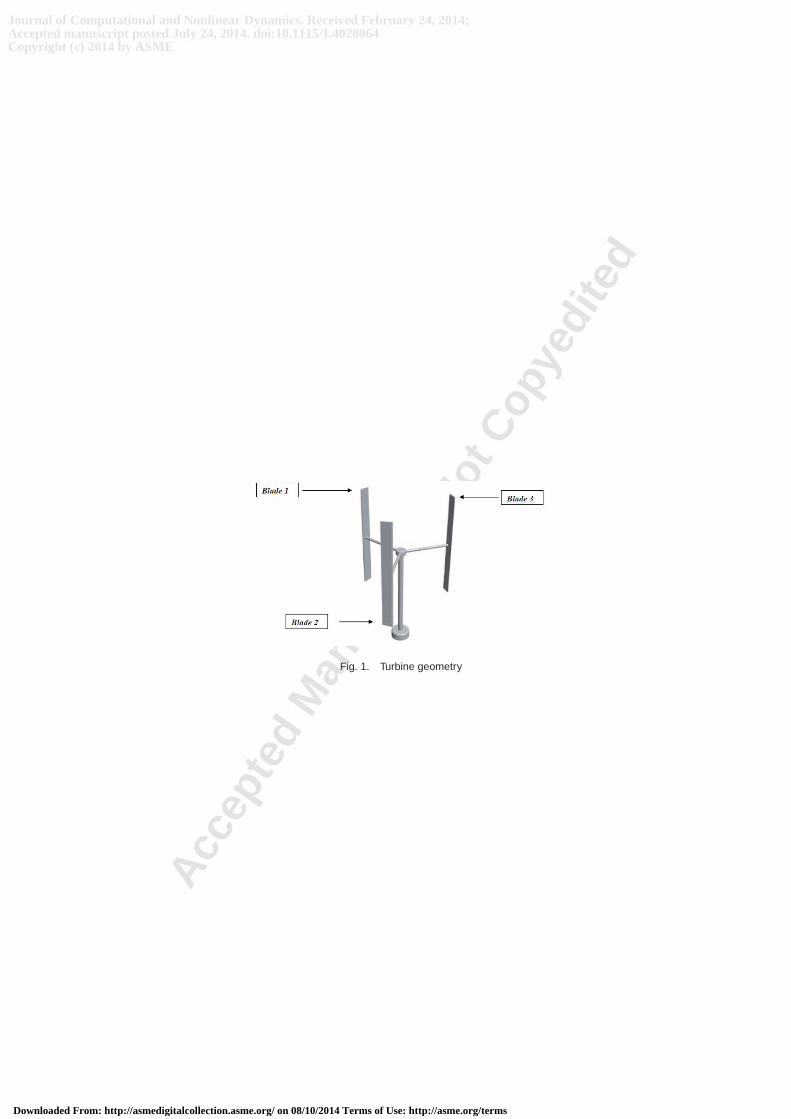
2 Numerical Methology and ResultsThe type of wind turbine in the present study is a Darrieus-type H-VAWT as shown in Fig. 1. The turbine is a lift-based

type with symmetric airfoils modeled as blades of the turbine. The turbine has a diameter (D) of 2.5 m and a chord length(c) of 0.2 m. The blade length is equal to the diameter of turbinemaking its aspect ratio equal to 12.5. This aspect ratio isconsidered an optimum value for the VAWT in urban roof top application [30].

Airfoil selection is critical for optimum performance of the wind turbine as it is solely responsible for the extractionofpower out of the wind. Usually NACA 4-digit series is used forDarrieus type VAWT. However, researchers have also usedNACA-0012, NACA-0015, and NACA-0018 airfoils as the bladesof the wind turbine. In a recent study, Durrani et al. [31]showed that employing NACA-0022 as blades in the VAWT providemaximum magnitude of performance coefficient. Basedon this study, we have employed NACA-0022 as the baseline airfoil for the present research. Here we perform numericalsimulations of three configurations of the VAWT at different TSR as tabulated in Tab. 1.

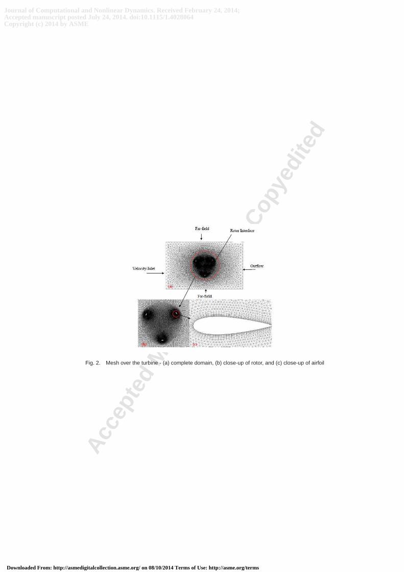
Case I contains a planar section of three airfoils, 120◦ apart, acting as turbine blades. Case II is a three dimensional caseformed by extruding a two-dimensional airfoil to a finite unit length while Case III is a complete turbine design along withstruts and hub. The domain size is selected as 50c×30c. We employ ANSYS Fluent [32] to perform numerical simulations.The choice of this domain size is motivated by the work of Hamada et al. [33] in which they demonstrated that the employeddomain size does not affect the flow behavior of rotating turbine. The mesh size comprising 78319, 446147, and 2054456number of cells is employed for Case I, Case II, and Case III, respectively. Figure 2 shows a two-dimensional grid andclose-up views of the rotor and an airfoil. For three-dimensional cases, perspective views are shown in Fig. 3.

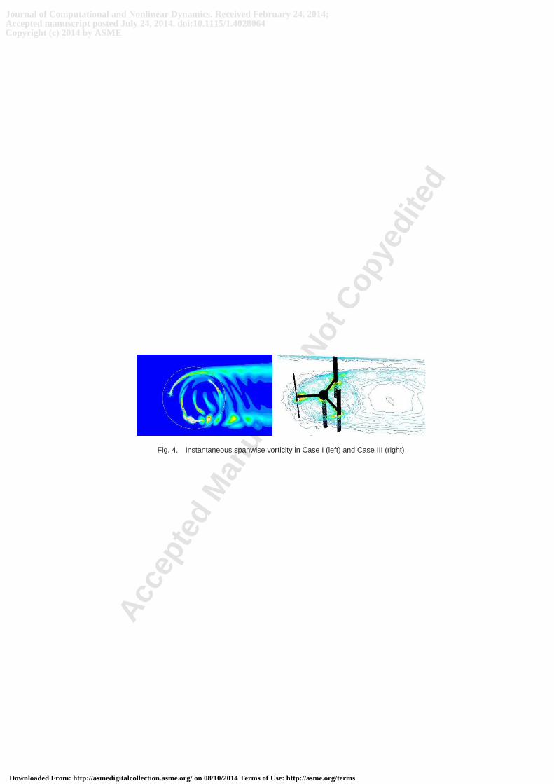
We perform numerical simulations at different TSR ranging from 2.5 to 4.5 with an increment of 0.5. We employ second-order upwind spatial discretization scheme andk− ε Realizable turbulence model. Since the overall torque determines theefficiency of the VAWT, we record its time history at differentTSR. The results obtained from numerical simulations showsimilar trends as obtained in [5]. Figure 4 plots the instantaneous spanwise vorticity for Case I and Case III. With constantwind velocity (Vw = 12m/s) and radius (R= 1.25m), angular velocity (ω) is controlled through TSR. In other words, TSR is anondimensional representation of turbine rotational frequency withωs = 2π fs. Thus, TSR = 2.5 corresponds to a frequencyof 3.82 for a torque ripple produced by a single blade. For a three-bladed turbinefs ≈ 11.4 which is the fundamentalfrequency of the overall torque and can be observed in the wake of turbine rotor as vortex shedding (see Fig. 4). It is for thisreason, we use a subscripts with the angular velocity and frequency of the turbine. Notethat the unit of angular velocity inthis paper is rad/s and that of frequency is Hz. Vorticity magnitude is higher in Case I as compared to Case II and Case III dueto the absence of third-dimensionality effects resulting in higher magnitudes of torque. Details of validation and verificationof the numerical methodology can be found in [7].

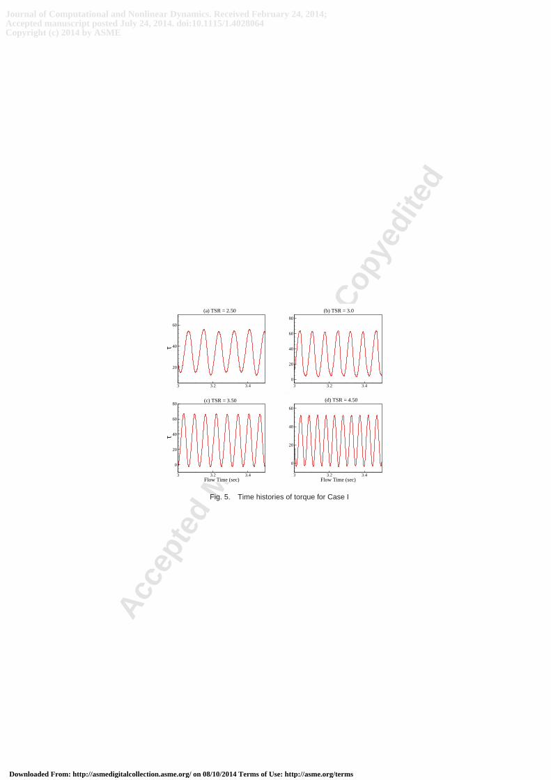
Figure 5 shows temporal histories of oscillating torque component at TSR magnitudes of 2.5, 3.5, 4.0, and 4.5 for CaseI. For TSR = 2.5, we see asymmetry in the quasi-periodic temporal history. This trend of quasi-periodicity reduces with anincrease in TSR along with increase in frequency of the system as observed in this figure.

Significant differences are observed between two- and three-dimensional simulations, especially at high TSR. Clearly,Case I does not take into account the third-dimensionality effects. This difference is attributed to central hub, tip vortices,additional profile drag due to support arms (struts and hub),and effect of spanwise flow leading to performance reduc-tion. Siddiqui et al. [34] performed detailed numerical experiments to quantify the effects of the VAWT geometry on itsperformance.

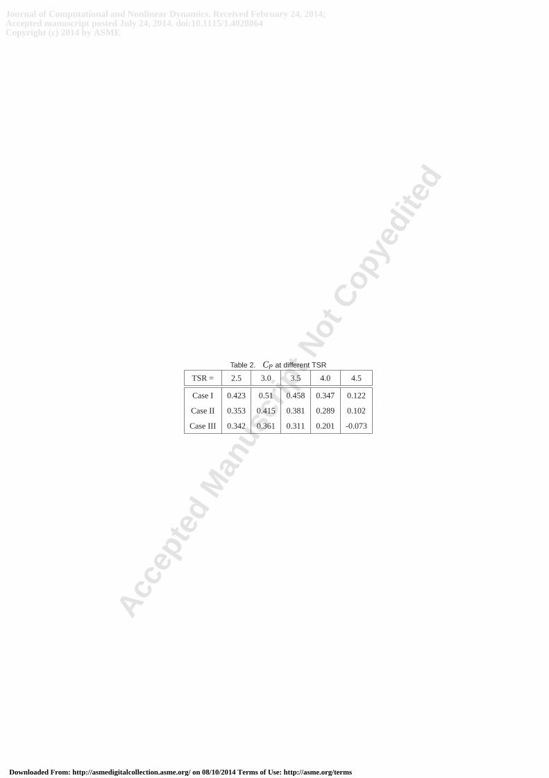
The performance coefficients for the three configurations asa function of TSR are presented in Table 2 to evaluate theoverall accuracy of results. We observe that for all configurations, maximumCP is achieved at TSR = 3 while the minimumoccurs at TSR = 4.5. In comparison, the performance of the full turbine in Case III experiences a drop of approximately 40%as compared to that of Case I.

3 Reduced-Order ModelingWe determine the dominant frequencies in the torque and identify the nonlinear interaction. Subsequently, the informa-

tion is used to determine the terms in the reduced-order model. We then apply method of multiple scales to determine theanalytical solution of the model and find the expression for the coefficients present in the model.

Journal of Computational and Nonlinear Dynamics. Received February 24, 2014;Accepted manuscript posted July 24, 2014. doi:10.1115/1.4028064Copyright (c) 2014 by ASME

Downloaded From: http://asmedigitalcollection.asme.org/ on 08/10/2014 Terms of Use: http://asme.org/terms

Acce

pted

Man

uscr

ipt N

ot C

opye

dite

d

3.1 Identification of Nonlinear TermsTo model the overall torque of the VAWT, we decompose the torque (τ) into its time-averaged component (τ) and

oscillating component (τ) as follows:

τ = τ+ τ (1)

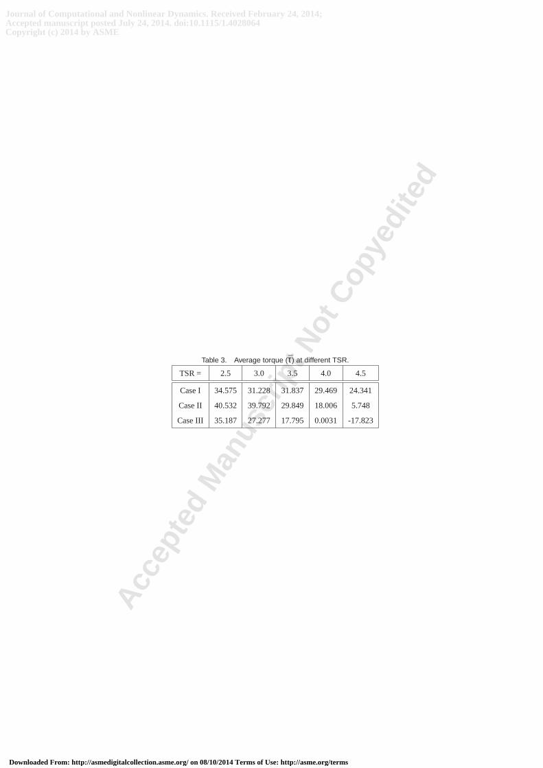
The time-averaged component for all configurations is tabulated in Tab. 3.We observe that negative average torque occurs at high TSR values for the actual turbine design in Case III. It is because

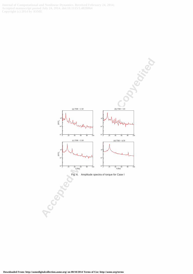
for high solidity values, such as in our case, the blockage effect or effect of wake gets more pronounced. It means that theturbine blades due to their high relative speeds will quickly reach the wake/disturbed flow region of the leading blade andwill decrease the useful torque during peak cycle. Hence, after a certain threshold TSR, the VAWT will retard to a lowerTSR value due to net negative average torque. On the other hand, two-dimensional simulations, as in Case I, do not considerwind-tip effects, drag due to struts and hub, etc. Therefore, Case I shows high magnitudes of average torque at high TSR.To gain insight, spectral analysis of the time history is performed. Figure 6 indicates the presence of fundamental frequencycorresponding to the rotation of the VAWT along with its even and odd harmonics in theτ-spectrum at different TSR values.Presence of both the even and odd harmonics inτ-spectrum indicates the effect of quadratic as well as cubicnonlinearity.Subharmonics and superharmonics of fundamental frequencystart disappearing when TSR is increased. It might be due toreduction of interaction between the vortices produced by three blades in different oscillation cycles.

We also perform higher-order spectral analysis to determine the coupling of frequency components to identify quadraticand cubic interaction. Auto-bispectrum and auto-trispectrum indicate quadratic and cubic coupling levels between frequencycomponents in the signal, respectively.

Auto-bispectrum is used to find the quadratic phase couplingamong different frequencies in the signal. It is defined as

Bxx = limT→∞

1T

E[XT( f1+ f2)X⋆

T( f1)X⋆

T( f2)] (2)

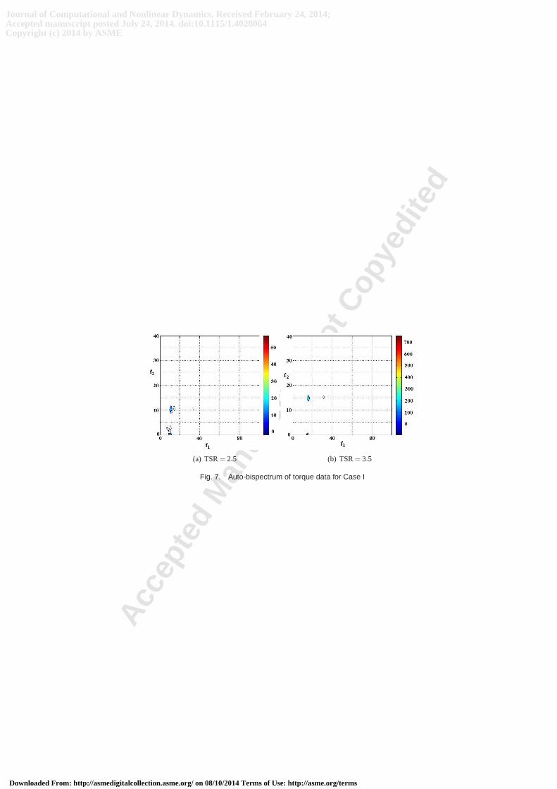
Figure 7 presents auto-bispectrum for TSR of 2.5 and 3.5 in the first quadrant. For more details related to symmetry propertiesof auto-bispectrum, readers are referred to [35]. High magnitude levels indicate strong quadratic coupling between thefrequenciesfs+ fs → 2 fs while lower magnitudes are observed due to 3fs− fs → 2 fs. For TSR = 2.5 and TSR = 3.5, thefundamental frequencies arefs = 11.4 and fs = 16.1, respectively. At low TSR, we also observe very low level ofcouplingdue to relatively larger flow interaction with the turbine blades, however, the coupling at those frequencies diminishes asTSR increases.

Auto-trispectrum shows the cubic phase coupling between various frequencies in the signal. Mathematically, it is definedas;

Txxx= limT→∞

1T

E[XT( f1+ f2+ f3)X⋆

T( f1)X⋆

T( f2)X⋆

T( f3)] (3)

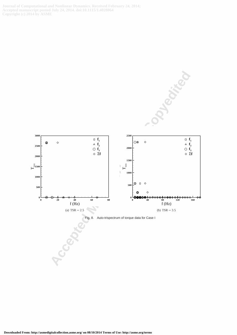
To visualize the auto-trispectrum, methodology presentedin [36] is adopted. It helps in detecting the coupling levelsclearly. In Fig. 8a, highest magnitude levels are present atthe frequency combination of (6.63,6.63,6.63) at TSR = 2.5.Thesefrequencies interact cubically and produce another component at 19.9. Trispectrum magnitudes for rest of the interactionsbetween different harmonics are very low. Similarly, stronger interaction of three triples can be observed at TSR=3.5 asshown in Fig. 8b. The frequencies 6.63, 13.26 and 13.26 are the strongest cubically coupled components in the aerodynamictorque of wind turbine at this TSR. We observe a new frequencycomponent produced through their additive interaction at33.15. Next, a frequency component at 26.52 appears due to cubic coupling of (6.63,6.63,13.26). Third triplet is found atcombination of (13.26,13.26,13.26) due to which frequencycomponent of 39.78 appears in the torque spectrum. All otherinteractions can be neglected due to very small magnitude levels.

3.2 The ModelDue to the presence of both quadratic and cubic nonlinearities in theτ-spectrum, we add a quadratic term to the van der

Pol equation to model the oscillating part of torque as follows:

τ+ω2τ = µτ− γττ−ατ2τ (4)

where the coefficients (µ,α,γ,ω) are positive real numbers. Quadratic term can be modeled asτ2, τ2, or ττ. Presence ofττ-term in the Eqn.( 4) indicates phase of aboutπ

2 between fundamental and first even harmonic. The angular frequencyω

Journal of Computational and Nonlinear Dynamics. Received February 24, 2014;Accepted manuscript posted July 24, 2014. doi:10.1115/1.4028064Copyright (c) 2014 by ASME

Downloaded From: http://asmedigitalcollection.asme.org/ on 08/10/2014 Terms of Use: http://asme.org/terms

Acce

pted

Man

uscr

ipt N

ot C

opye

dite

d

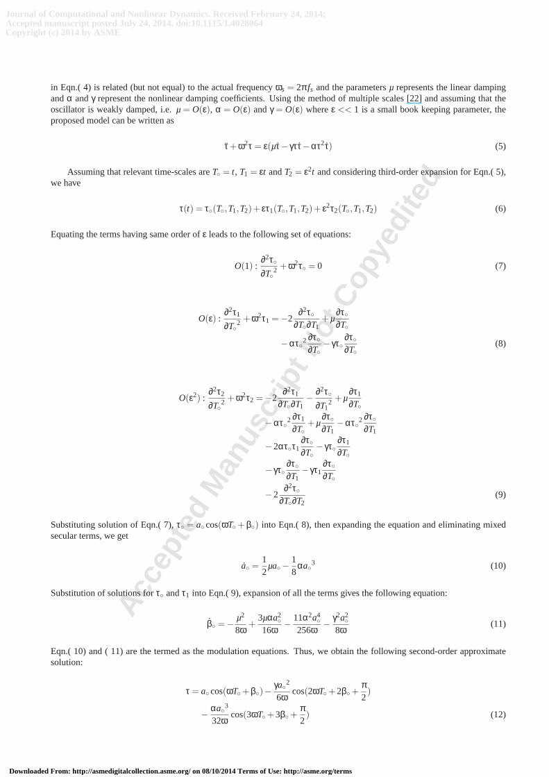
in Eqn.( 4) is related (but not equal) to the actual frequencyωs = 2π fs and the parametersµ represents the linear dampingandα andγ represent the nonlinear damping coefficients. Using the method of multiple scales [22] and assuming that theoscillator is weakly damped, i.e.µ= O(ε), α = O(ε) andγ = O(ε) whereε << 1 is a small book keeping parameter, theproposed model can be written as

τ+ω2τ = ε(µτ− γττ−ατ2τ) (5)

Assuming that relevant time-scales areT◦ = t, T1 = εt andT2 = ε2t and considering third-order expansion for Eqn.( 5),we have

τ(t) = τ◦(T◦,T1,T2)+ ετ1(T◦,T1,T2)+ ε2τ2(T◦,T1,T2) (6)

Equating the terms having same order ofε leads to the following set of equations:

O(1) :∂2τ◦∂T◦

2 +ω2τ◦ = 0 (7)

O(ε) :∂2τ1

∂T◦2 +ω2τ1 =−2

∂2τ◦∂T◦∂T1

+µ∂τ◦∂T◦

−ατ◦2 ∂τ◦∂T◦

− γτ◦∂τ◦∂T◦

(8)

O(ε2) :∂2τ2

∂T◦2 +ω2τ2 =−2

∂2τ1

∂T◦∂T1−

∂2τ◦∂T1

2 +µ∂τ1

∂T◦

−ατ◦2 ∂τ1

∂T◦+µ

∂τ◦∂T1

−ατ◦2 ∂τ◦∂T1

−2ατ◦τ1∂τ◦∂T◦

− γτ◦∂τ1

∂T◦

− γτ◦∂τ◦∂T1

− γτ1∂τ◦∂T◦

−2∂2τ◦

∂T◦∂T2(9)

Substituting solution of Eqn.( 7),τ◦ = a◦ cos(ωT◦+β◦) into Eqn.( 8), then expanding the equation and eliminating mixedsecular terms, we get

a◦ =12

µa◦−18

αa◦3 (10)

Substitution of solutions forτ◦ andτ1 into Eqn.( 9), expansion of all the terms gives the followingequation:

β◦ =−µ2

8ω+

3µαa2◦

16ω−

11α2a4◦

256ω−

γ2a2◦

8ω(11)

Eqn.( 10) and ( 11) are the termed as the modulation equations. Thus, we obtain the following second-order approximatesolution:

τ = a◦ cos(ωT◦+β◦)−γa◦2

6ωcos(2ωT◦+2β◦+

π2)

−αa◦3

32ωcos(3ωT◦+3β◦+

π2) (12)

Journal of Computational and Nonlinear Dynamics. Received February 24, 2014;Accepted manuscript posted July 24, 2014. doi:10.1115/1.4028064Copyright (c) 2014 by ASME

Downloaded From: http://asmedigitalcollection.asme.org/ on 08/10/2014 Terms of Use: http://asme.org/terms

Acce

pted

Man

uscr

ipt N

ot C

opye

dite

d

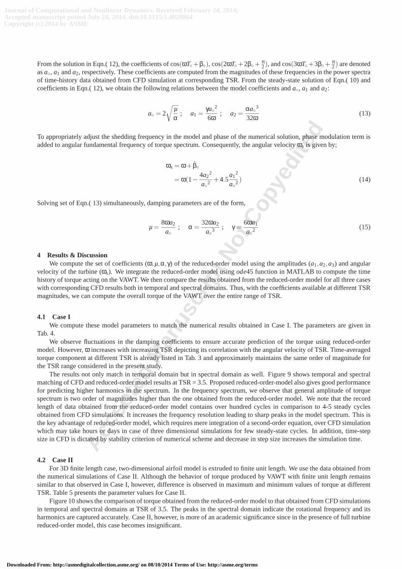
From the solution in Eqn.( 12), the coefficients of cos(ωT◦+β◦), cos(2ωT◦+2β◦+π2), and cos(3ωT◦+3β◦+

π2) are denoted

asa◦, a1 anda2, respectively. These coefficients are computed from the magnitudes of these frequencies in the power spectraof time-history data obtained from CFD simulation at corresponding TSR. From the steady-state solution of Eqn.( 10) andcoefficients in Eqn.( 12), we obtain the following relationsbetween the model coefficients anda◦, a1 anda2:

a◦ = 2

√

µα

; a1 =γa◦2

6ω; a2 =

αa◦3

32ω(13)

To appropriately adjust the shedding frequency in the modeland phase of the numerical solution, phase modulation term isadded to angular fundamental frequency of torque spectrum.Consequently, the angular velocityωs is given by;

ωs = ω+ β◦

= ω(1−4a2

2

a◦2 +4.5a1

2

a◦2 ) (14)

Solving set of Eqn.( 13) simultaneously, damping parameters are of the form,

µ=8ωa2

a◦; α =

32ωa2

a◦3 ; γ =6ωa1

a◦2 (15)

4 Results & DiscussionWe compute the set of coefficients (ω,µ,α,γ) of the reduced-order model using the amplitudes (a1,a2,a3) and angular

velocity of the turbine (ωs). We integrate the reduced-order model usingode45 function in MATLAB to compute the timehistory of torque acting on the VAWT. We then compare the results obtained from the reduced-order model for all three caseswith corresponding CFD results both in temporal and spectral domains. Thus, with the coefficients available at different TSRmagnitudes, we can compute the overall torque of the VAWT overthe entire range of TSR.

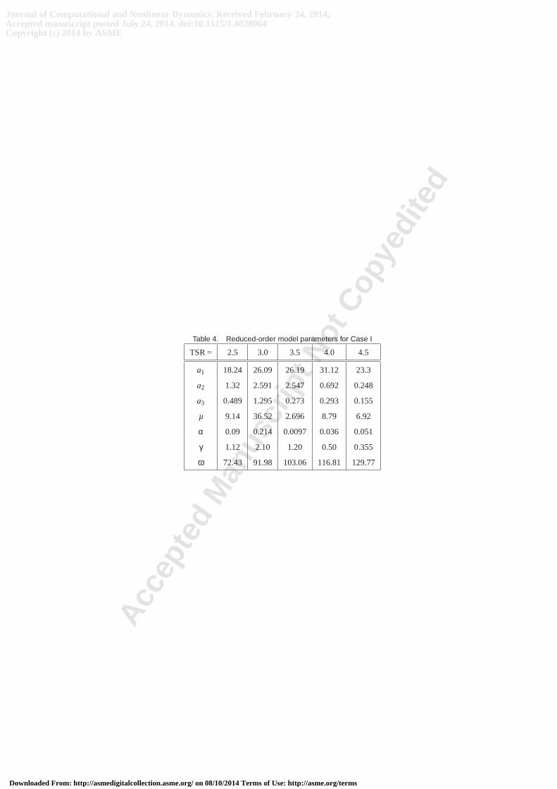
4.1 Case IWe compute these model parameters to match the numerical results obtained in Case I. The parameters are given in

Tab. 4.We observe fluctuations in the damping coefficients to ensureaccurate prediction of the torque using reduced-order

model. However,ω increases with increasing TSR depicting its correlation with the angular velocity of TSR. Time-averagedtorque component at different TSR is already listed in Tab. 3and approximately maintains the same order of magnitude forthe TSR range considered in the present study.

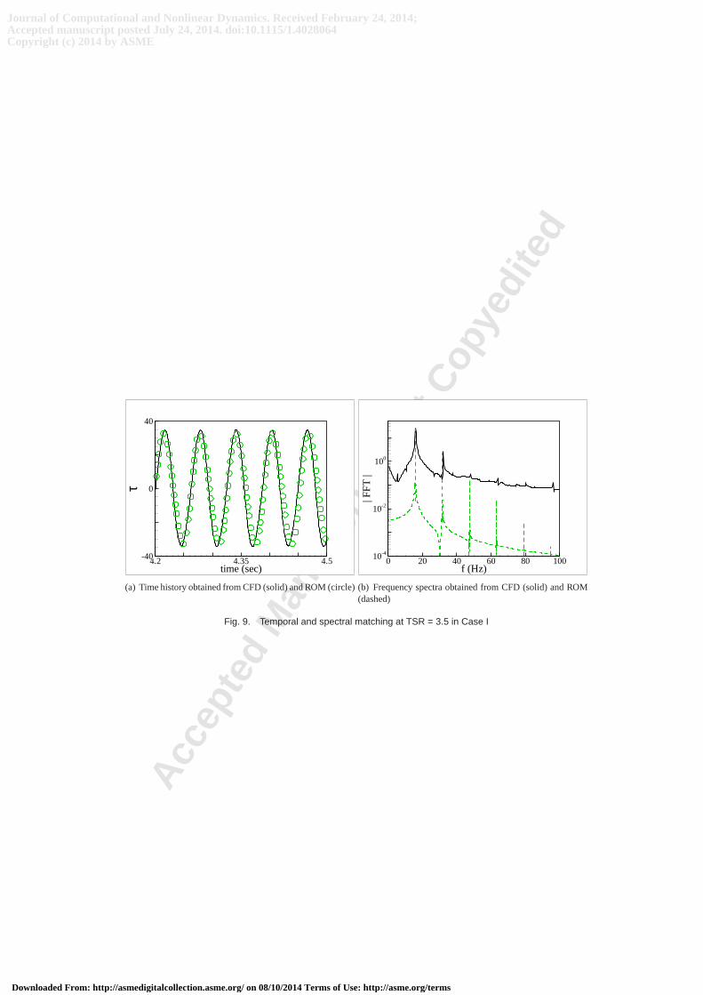
The results not only match in temporal domain but in spectraldomain as well. Figure 9 shows temporal and spectralmatching of CFD and reduced-order model results at TSR = 3.5.Proposed reduced-order-model also gives good performancefor predicting higher harmonics in the spectrum. In the frequency spectrum, we observe that general amplitude of torquespectrum is two order of magnitudes higher than the one obtained from the reduced-order model. We note that the recordlength of data obtained from the reduced-order model contains over hundred cycles in comparison to 4-5 steady cyclesobtained from CFD simulations. It increases the frequency resolution leading to sharp peaks in the model spectrum. Thisisthe key advantage of reduced-order model, which requires mere integration of a second-order equation, over CFD simulationwhich may take hours or days in case of three dimensional simulations for few steady-state cycles. In addition, time-stepsize in CFD is dictated by stability criterion of numerical scheme and decrease in step size increases the simulation time.

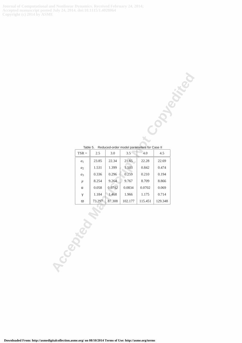
4.2 Case IIFor 3D finite length case, two-dimensional airfoil model is extruded to finite unit length. We use the data obtained from

the numerical simulations of Case II. Although the behaviorof torque produced by VAWT with finite unit length remainssimilar to that observed in Case I, however, difference is observed in maximum and minimum values of torque at differentTSR. Table 5 presents the parameter values for Case II.

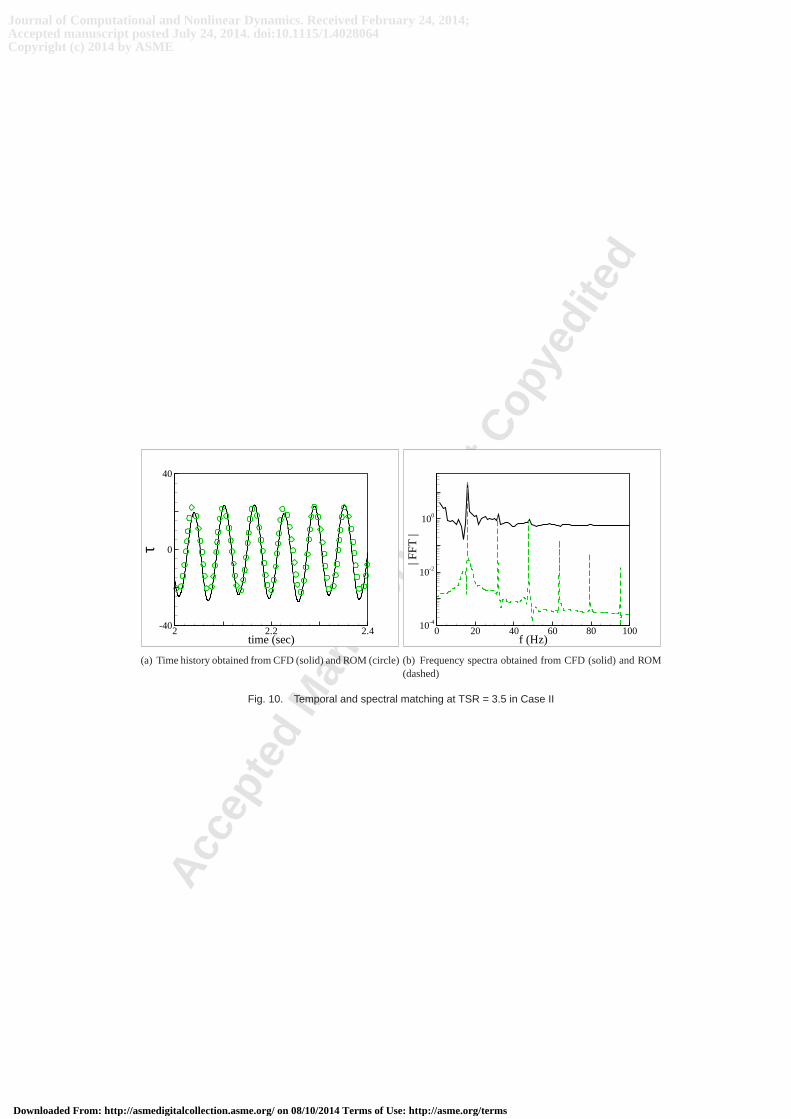
Figure 10 shows the comparison of torque obtained from the reduced-order model to that obtained from CFD simulationsin temporal and spectral domains at TSR of 3.5. The peaks in the spectral domain indicate the rotational frequency and itsharmonics are captured accurately. Case II, however, is more of an academic significance since in the presence of full turbinereduced-order model, this case becomes insignificant.

Journal of Computational and Nonlinear Dynamics. Received February 24, 2014;Accepted manuscript posted July 24, 2014. doi:10.1115/1.4028064Copyright (c) 2014 by ASME

Downloaded From: http://asmedigitalcollection.asme.org/ on 08/10/2014 Terms of Use: http://asme.org/terms

Acce

pted

Man

uscr

ipt N

ot C

opye

dite

d

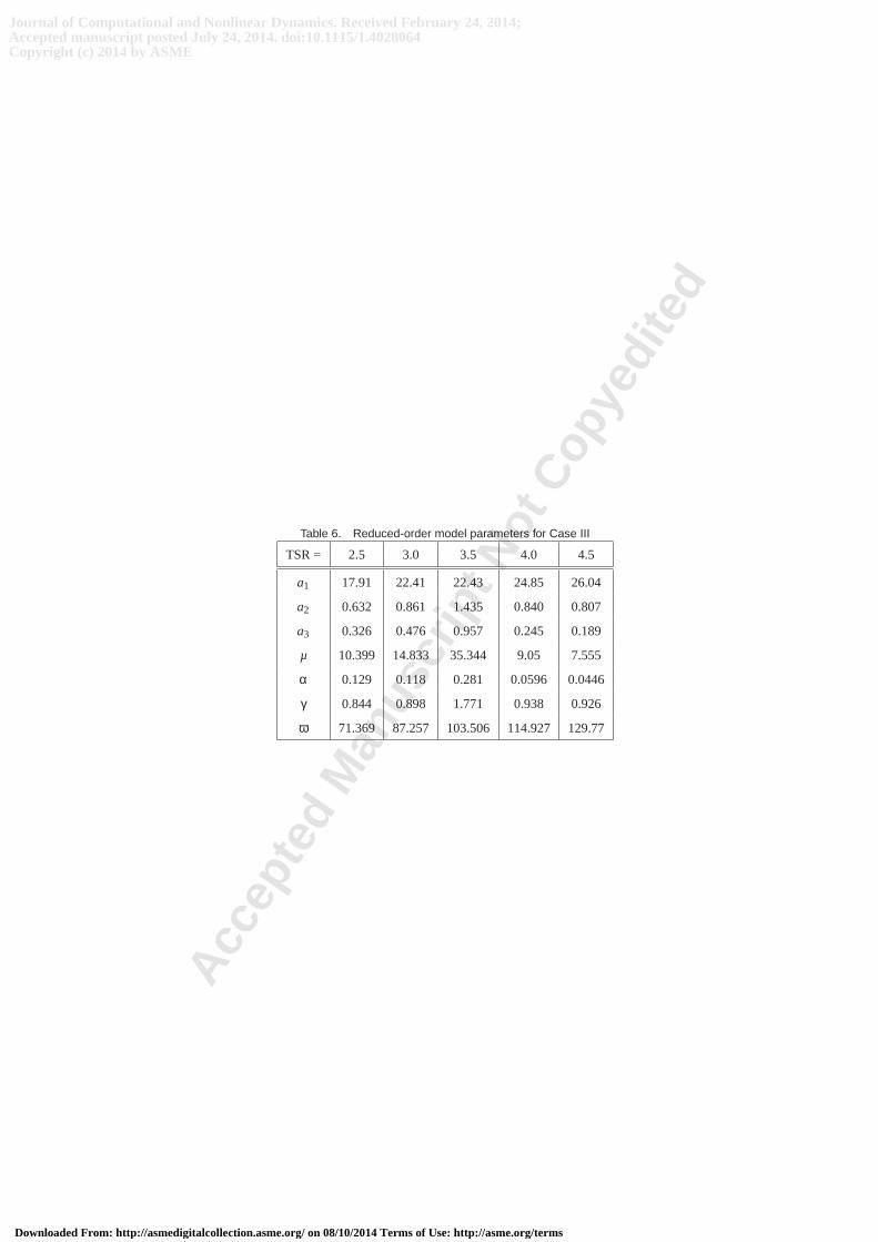
4.3 Case IIIFor a complete turbine, struts and hub are added to the three-dimensional model of finite unit length. Numerical simu-

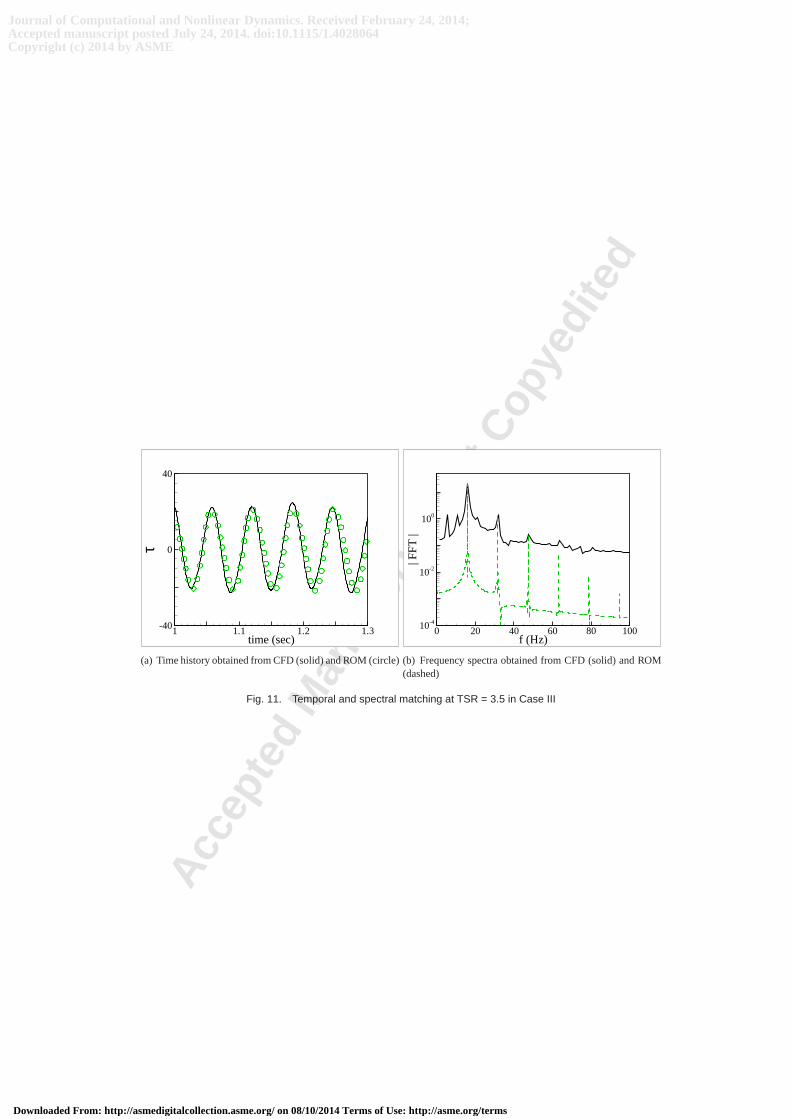
lations at various TSR provide the torque data for computingthe model parameter shown in Tab. 6.We compare the time history and its frequency spectrum at TSRof 3.5 as shown in Fig. 10. The torque obtained from

the reduced-order model compares well with the results obtained from the CFD. Overall, we observe that the amplitude oftorque is reduced in comparison to Case I and Case II attributed to the additional turbine components in Case III.

4.4 DiscussionReduced-order models show a promising application in computing the torque and ultimately performance coefficient

of VAWT at different TSR values. The key advantage of these models can be realized from the fact that a typical three-dimensional simulation of a complete turbine is computationally expensive and may take days to complete while actualexperiments may not be cost effective. A number of significant differences are observed between Case I and Case III.Although, torque generation is qualitatively similar between the two cases, the average torque in Case III is lower thanthatin Case I.

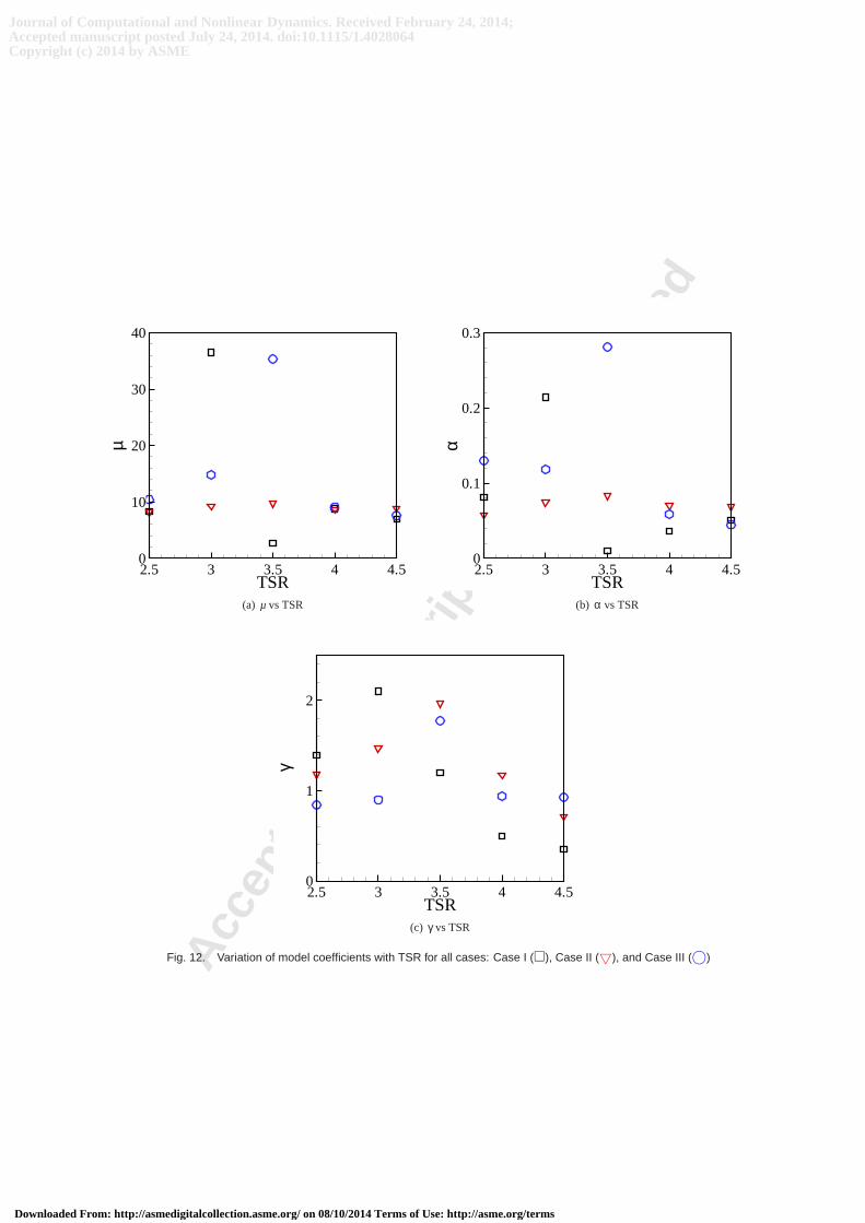
The coefficients in the reduced-order model ensure that the model not only captures the temporal domain accurately butalso dominant frequencies in the spectral domain. We observe a trend in the variation of model coefficients (µ,α,γ) plotted inFig. 12 against TSR. Linear damping (µ) is destabilizing and the system response tends to grow while the nonlinear damping(α) is stabilizing as a result of which small motions tends to increase and large motion decays resulting in a stable limit-cycle solution. Supporting the argument, we observe that increase in the destabilizing factorµ also adjusts the stabilizingcoefficientα accordingly and proportionally increasing itself to matchthe torque obtained from the CFD data. In Case I,maximum value ofµ is 36.52 at TSR 3 and correspondingα is 0.214, which is also maximum relative to its magnitude atother TSR values. In Case II, the maximum value ofµ at TSR 3.5 is 9.77 with the maximum value ofα equal to 0.0834.Similarly, in Case III,µ has the maximum value of 35.34 at TSR 3.5 and accordinglyα adjusts itself with maximum valueof 0.281.

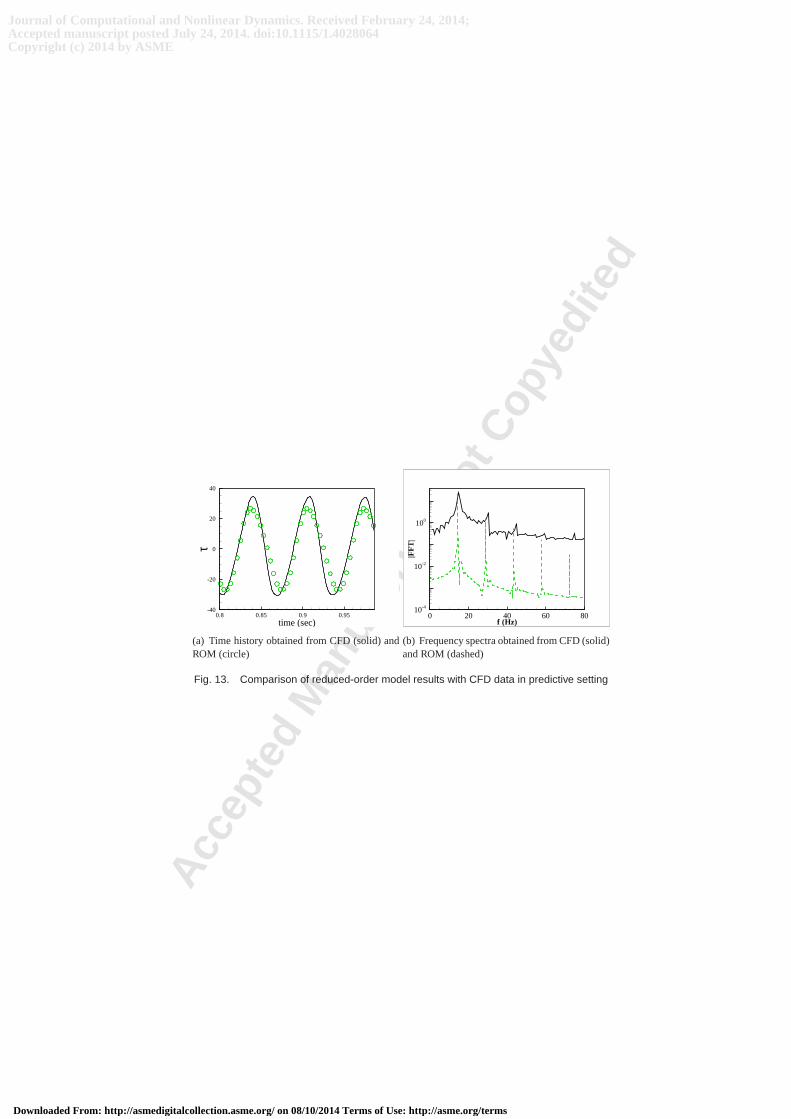
Next, we test the reduced-order model in predictive settingat TSR = 3.25 for Case I. We also perform CFD at this TSR toevaluate the performance of reduced-order model. We compute the model coefficients (µ,α,γ) from Tab. 4 using cubic splineinterpolation. Average torque is also interpolated from the data in Tab. 3. The average torques obtained through interpolationand CFD simulation are 31.53 and 31.47, respectively. We then integrate the model and compute the torque. We compare thetime history and frequency spectrum obtained from the reduced-order model with the data obtained from CFD simulation atTSR = 3.25. Figure 13 shows that the reduced-order model performs well in predictive setting given the fact that variation ofmodel coefficients at TSR = 3.25 is high. We observe that the peak values show a difference of around 15%. The dominantfrequency obtained from reduced-order model data is 14.63 as compared to 14.89 obtained from CFD data indicating 1.75%variation. The difference can be further reduced if the dataset is enhanced in the region of maximum variation in modelcoefficients. The results can be further used to determine the efficiency and power output of the turbine. The tabulated dataof torque at different TSR can be employed for design purposes, especially for urban roof-top applications. In other words,variation in the wind velocity in urban environment can be interpreted into TSR value and the reduced-order model can beemployed to predict torque and output power efficiently.

5 ConclusionsWe performed two- and three-dimensional numerical simulations of a three-bladed VAWT. We recorded the torque data

for two dimensional, three dimensional finite length blades, and complete turbine with struts and hub assembly. We applyspectral analysis to determine the dominant frequencies and nonlinear interaction to identify quadratic and cubic couplings.We proposed a modified van der Pol equation with quadratic term to model the overall torque of the VAWT. The coefficients inthe model varied with changing TSR for different configurations. We applied method of multiple scales to find the analyticalsolution and determined the relations of these coefficients. Using spectral amplitudes, we computed these coefficients. Wethen integrated the model to compute the torque which compared well the with CFD data both in temporal and spectraldomains. This study signifies the importance of reduced-order models in practical engineering applications.

References[1] Ponta, F. L., Seminara, J. J., and Otero, A. D., 2007. “On the aerodynamics of variable-geometry oval-trajectory

darrieus wind turbines”.Renewable energy,32(1), pp. 35–56.[2] Sutherland, H. J., Berg, D. E., and Ashwill, T. D., 2012. “A retrospective of vawt technology”.Sandia Report,

SAND2012-0304.[3] Bhutta, M. M. A., Hayat, N., Farooq, A. U., Ali, Z., Jamil,S. R., and Hussain, Z., 2012. “Vertical axis wind turbine–a

Journal of Computational and Nonlinear Dynamics. Received February 24, 2014;Accepted manuscript posted July 24, 2014. doi:10.1115/1.4028064Copyright (c) 2014 by ASME

Downloaded From: http://asmedigitalcollection.asme.org/ on 08/10/2014 Terms of Use: http://asme.org/terms

Acce

pted

Man

uscr

ipt N

ot C

opye

dite

d

review of various configurations and design techniques”.Renewable and Sustainable Energy Reviews,16(4), pp. 1926–1939.

[4] Debnath, B. K., A. Biswas, A., and Gupta, R., 2009. “Computational fluid dynamics analysis of a combined three-bucket savonius and three-bladed darrieus rotor at variousoverlap conditions”.Journal of Renewable and SustainableEnergy,1(3), p. 033110.

[5] Howell, R., Qin, N., Edwards, J., and Durrani, N., 2010. “Wind tunnel and numerical study of a small vertical axiswind turbine”. Renewable Energy,35(2), pp. 412–422.

[6] Mohamed, M., Janiga, G., Pap, E., and Thevenin, D., 2011. “Optimal blade shape of a modified savoniusturbine usingan obstacle shielding the returning blade”.Energy Conversion and Management,52(1), pp. 236–242.

[7] Siddiqui, M. S., Durrani, N., and Akhtar, I., 2013. “Numerical study to quantify the effects of struts and central hubon the performance of a three dimensional vertical axis windturbine using sliding mesh”. In ASME 2013 PowerConference, American Society of Mechanical Engineers, pp.V002T09A020–V002T09A020.

[8] Sirovich, L., 1987. “Turbulence and the dynamics of coherent structures. i-coherent structures. ii-symmetries andtransformations. iii-dynamics and scaling”.Quarterly of applied mathematics,45, pp. 561–571.

[9] Deane, A. E., and Mavriplis, C., 1994. “Low-dimensionaldescription of the dynamics in separated flow past thickairfoils”. AIAA journal,32(6), pp. 1222–1227.

[10] Akhtar, I., Nayfeh, A. H., and Ribbens, C. J., 2009. “On the stability and extension of reduced-order Galerkin modelsin incompressible flows”.Theoretical and Computational Fluid Dynamics,23(3), pp. 213–237.

[11] Graham, W. R., Peraire, J., and Tang, K. Y., 1999. “Optimal control of vortex shedding using low-order models. partiopen-loop model development”.International Journal for Numerical Methods in Engineering, 44(7), pp. 945–972.

[12] Akhtar, I., and Nayfeh, A. H., 2010. “Model based control of laminar wake using fluidic actuation”.Journal ofComputational and Nonlinear Dynamics,5(4), p. 041015.

[13] Hay, A., Borggaard, J., Akhtar, I., and Pelletier, D., 2010. “Reduced-order models for parameter dependent geometriesbased on shape sensitivity analysis”.Journal of Computational Physics,229(4), pp. 1327–1352.

[14] Akhtar, I., Borggaard, J., and Hay, A., 2010. “Shape sensitivity analysis in flow models using a finite-differenceapproach”.Mathematical Problems in Engineering,2010, pp. 1–22.

[15] Yue, Y., and Meerbergen, K., 2012. “Using krylov-pade model order reduction for accelerating design optimizationof structures and vibrations in the frequency domain”.International Journal for Numerical Methods in Engineering,90(10), pp. 1207–1232.

[16] Wang, Z., Akhtar, I., Borggaard, J., and Iliescu, T., 2011. “Two-level discretizations of nonlinear closure models forproper orthogonal decomposition”.Journal of Computational Physics,230(1), pp. 126–146.

[17] Wang, Z., Akhtar, I., Borggaard, J., and Iliescu, T., 2012. “Proper orthogonal decomposition closure models forturbulent flows: a numerical comparison”.Computer Methods in Applied Mechanics and Engineering,237, pp. 10–26.

[18] Hay, A., Akhtar, I., and Borggaard, J., 2012. “On the useof sensitivity analysis in model reduction to predict flows forvarying inflow conditions”.International Journal for Numerical Methods in Fluids,68(1), pp. 122–134.

[19] Ghommem, M., Akhtar, I., and Hajj, M. R., 2013. “A low–dimensional tool for predicting force decomposition coef-ficients for varying inflow conditions”.Progress in Computational Fluid Dynamics, an International Journal, 13(6),pp. 368–381.

[20] Nayfeh, A. H., Owis, F., and Hajj, M. R., 2003. “A model for the coupled lift and drag on a circular cylinder”. InASME 2003 International Design Engineering Technical Conferences and Computers and Information in EngineeringConference, American Society of Mechanical Engineers, pp.1289–1296.

[21] Nayfeh, A. H., and Mook, D. T., 2008.Nonlinear oscillations. John Wiley & Sons.[22] Nayfeh, A. H., 2011.Introduction to perturbation techniques. John Wiley & Sons.[23] Nayfeh, A. H., Marzouk, O. A., Arafat, H. N., and Akhtar,I., 2005. “Modeling the transient and steady-state flow over

a stationary cylinder”. In ASME 2005 International Design Engineering Technical Conferences and Computers andInformation in Engineering Conference, American Society of Mechanical Engineers, pp. 1513–1523.

[24] Qin, L., 2004. “Development of reduced-order models for lift and drag on oscillating cylinders with higher-orderspectral moments”. PhD thesis, Virginia Polytechnic Institute and State University.

[25] Marzouk, O., Nayfeh, A. H., Akhtar, I., and Arafat, H. N., 2007. “Modeling steady-state and transient forces on acylinder”. Journal of Vibration and Control,13(7), pp. 1065–1091.

[26] Akhtar, I., Marzouk, O. A., and Nayfeh, A. H., 2009. “A van der Pol–Duffing oscillator model of hydrodynamic forceson canonical structures”.Journal of Computational and Nonlinear Dynamics,4(4), p. 041006.

[27] Janajreh, I., and Hajj, M., 2008. “An analytical model for the lift on a rotationally oscillating cylinder”. In BBAAVIInternational Colloquium on Bluff Bodies Aerodynamics & Applications, July, pp. 20–24.

[28] Blackwell, B., 1974. Vertical-axis wind turbine: how it works. Tech. rep., Sandia Labs., Albuquerque, N. Mex.(USA).[29] Marzouk, O. A., 2010. “A nonlinear ode system for the unsteady hydrodynamic force–a new approach”.International

Journal of Engineering and Mathematical Sciences,6(2), pp. 111–125.[30] Claessens, M. C., 2006. “The design and testing of airfoils for application in small vertical axis wind turbines”.Master

Journal of Computational and Nonlinear Dynamics. Received February 24, 2014;Accepted manuscript posted July 24, 2014. doi:10.1115/1.4028064Copyright (c) 2014 by ASME

Downloaded From: http://asmedigitalcollection.asme.org/ on 08/10/2014 Terms of Use: http://asme.org/terms

Acce

pted

Man

uscr

ipt N

ot C

opye

dite

d

of Science Thesis.[31] Durrani, N., Hameed, H., Rahman, H., and Chaudhry, S. R., 2011. “A detailed aerodynamic design and analysis of

a 2d vertical axis wind turbine using sliding mesh in cfd”. In49th AIAA Aerospaces Sciences Meeting and Exhibit,Orlando, Florida, USA.

[32] Fluent, A., 2009. “Ansys fluent 12.0 users guide”.Ansys Inc.[33] Hamada, K., Smith, T., Durrani, N., Qin, N., and Howell,R., 2008. “Unsteady flow simulation and dynamic stall

around vertical axis wind turbine blades”. In 46th AIAA Aerospaces Sciences Meeting and Exhibit, Reno, Nevada.[34] Siddiqui, M. S., Durrani, N., and Akhtar, I., 2014. “Quantification of the effects of geometric approximations on the

performance of a vertical axis wind turbine”.Renewable Energy, under review.[35] Hajj, M. R., Miksad, R. W., and Powers, E. J., 1997. “Perspective: Measurements and analyses of nonlinear wave

interactions with higher-order spectral moments”.Journal of Fluids Engineering,119(1), pp. 3–13.[36] Chabalko, C. C., 2007. “Identification of transient nonlinear aeroelastic phenomena”. PhD thesis, Virginia Polytechnic

Institute and State University.

Journal of Computational and Nonlinear Dynamics. Received February 24, 2014;Accepted manuscript posted July 24, 2014. doi:10.1115/1.4028064Copyright (c) 2014 by ASME

Downloaded From: http://asmedigitalcollection.asme.org/ on 08/10/2014 Terms of Use: http://asme.org/terms

Acce

pted

Man

uscr

ipt N

ot C

opye

dite

d

List of Table Captions

Table 1: Different Configurations of VAWTTable 2:CP at different TSRTable 3: Average torque (τ) at different TSRTable 4: Reduced-order model parameters for Case ITable 5: Reduced-order model parameters for Case IITable 6: Reduced-order model parameters for Case III

Journal of Computational and Nonlinear Dynamics. Received February 24, 2014;Accepted manuscript posted July 24, 2014. doi:10.1115/1.4028064Copyright (c) 2014 by ASME

Downloaded From: http://asmedigitalcollection.asme.org/ on 08/10/2014 Terms of Use: http://asme.org/terms

Acce

pted

Man

uscr

ipt N

ot C

opye

dite

d

List of Figure Captions

Fig. 1: Turbine geometryFig. 2: Mesh over the turbine - (a) complete domain, (b) close-up of rotor, and (c) close-up of airfoilFig. 3: Mesh over the turbine for Case II (left) and Case III (right)Fig. 4: Instantaneous spanwise vorticity in Case I (left) and Case III (right)Fig. 5: Time histories of torque for Case IFig. 6: Amplitude spectra of torque for Case IFig. 7: Auto-bispectrum of torque data for Case IFig. 8: Auto-trispectrum of torque data for Case IFig. 9: Temporal and spectral matching at TSR = 3.5 in Case IFig. 10: Temporal and spectral matching at TSR = 3.5 in Case IIFig. 11: Temporal and spectral matching at TSR = 3.5 in Case IIIFig. 12: Variation of model coefficients with TSR for all cases: Case I (�), Case II (▽), and Case III (©)Fig. 13: Comparison of reduced-order model results with CFDdata in predictive setting

Journal of Computational and Nonlinear Dynamics. Received February 24, 2014;Accepted manuscript posted July 24, 2014. doi:10.1115/1.4028064Copyright (c) 2014 by ASME

Downloaded From: http://asmedigitalcollection.asme.org/ on 08/10/2014 Terms of Use: http://asme.org/terms

Acce

pted

Man

uscr

ipt N

ot C

opye

dite

d

Table 1. Different Configurations of VAWT

Case Configuration Comments

I 2-D model Planar section of airfoils

II 3-D model Finite length of blade

III Full turbine model Includes struts and hub

Journal of Computational and Nonlinear Dynamics. Received February 24, 2014;Accepted manuscript posted July 24, 2014. doi:10.1115/1.4028064Copyright (c) 2014 by ASME

Downloaded From: http://asmedigitalcollection.asme.org/ on 08/10/2014 Terms of Use: http://asme.org/terms

Acce

pted

Man

uscr

ipt N

ot C

opye

dite

d

Table 2. CP at different TSR

TSR = 2.5 3.0 3.5 4.0 4.5

Case I 0.423 0.51 0.458 0.347 0.122

Case II 0.353 0.415 0.381 0.289 0.102

Case III 0.342 0.361 0.311 0.201 -0.073

Journal of Computational and Nonlinear Dynamics. Received February 24, 2014;Accepted manuscript posted July 24, 2014. doi:10.1115/1.4028064Copyright (c) 2014 by ASME

Downloaded From: http://asmedigitalcollection.asme.org/ on 08/10/2014 Terms of Use: http://asme.org/terms

Acce

pted

Man

uscr

ipt N

ot C

opye

dite

d

Table 3. Average torque (τ) at different TSR.

TSR = 2.5 3.0 3.5 4.0 4.5

Case I 34.575 31.228 31.837 29.469 24.341

Case II 40.532 39.792 29.849 18.006 5.748

Case III 35.187 27.277 17.795 0.0031 -17.823

Journal of Computational and Nonlinear Dynamics. Received February 24, 2014;Accepted manuscript posted July 24, 2014. doi:10.1115/1.4028064Copyright (c) 2014 by ASME

Downloaded From: http://asmedigitalcollection.asme.org/ on 08/10/2014 Terms of Use: http://asme.org/terms

Acce

pted

Man

uscr

ipt N

ot C

opye

dite

d

Table 4. Reduced-order model parameters for Case I

TSR = 2.5 3.0 3.5 4.0 4.5

a1 18.24 26.09 26.19 31.12 23.3

a2 1.32 2.591 2.547 0.692 0.248

a3 0.489 1.295 0.273 0.293 0.155

µ 9.14 36.52 2.696 8.79 6.92

α 0.09 0.214 0.0097 0.036 0.051

γ 1.12 2.10 1.20 0.50 0.355

ω 72.43 91.98 103.06 116.81 129.77

Journal of Computational and Nonlinear Dynamics. Received February 24, 2014;Accepted manuscript posted July 24, 2014. doi:10.1115/1.4028064Copyright (c) 2014 by ASME

Downloaded From: http://asmedigitalcollection.asme.org/ on 08/10/2014 Terms of Use: http://asme.org/terms

Acce

pted

Man

uscr

ipt N

ot C

opye

dite

d

Table 5. Reduced-order model parameters for Case II

TSR = 2.5 3.0 3.5 4.0 4.5

a1 23.85 22.34 21.65 22.28 22.69

a2 1.531 1.399 1.503 0.842 0.474

a3 0.336 0.296 0.259 0.210 0.194

µ 8.254 9.264 9.767 8.709 8.866

α 0.058 0.0742 0.0834 0.0702 0.069

γ 1.184 1.468 1.966 1.175 0.714

ω 73.297 87.308 102.177 115.451 129.348

Journal of Computational and Nonlinear Dynamics. Received February 24, 2014;Accepted manuscript posted July 24, 2014. doi:10.1115/1.4028064Copyright (c) 2014 by ASME

Downloaded From: http://asmedigitalcollection.asme.org/ on 08/10/2014 Terms of Use: http://asme.org/terms

Acce

pted

Man

uscr

ipt N

ot C

opye

dite

d

Table 6. Reduced-order model parameters for Case III

TSR = 2.5 3.0 3.5 4.0 4.5

a1 17.91 22.41 22.43 24.85 26.04

a2 0.632 0.861 1.435 0.840 0.807

a3 0.326 0.476 0.957 0.245 0.189

µ 10.399 14.833 35.344 9.05 7.555

α 0.129 0.118 0.281 0.0596 0.0446

γ 0.844 0.898 1.771 0.938 0.926

ω 71.369 87.257 103.506 114.927 129.77

Journal of Computational and Nonlinear Dynamics. Received February 24, 2014;Accepted manuscript posted July 24, 2014. doi:10.1115/1.4028064Copyright (c) 2014 by ASME

Downloaded From: http://asmedigitalcollection.asme.org/ on 08/10/2014 Terms of Use: http://asme.org/terms

Acce

pted

Man

uscr

ipt N

ot C

opye

dite

dFig. 1. Turbine geometry

Journal of Computational and Nonlinear Dynamics. Received February 24, 2014;Accepted manuscript posted July 24, 2014. doi:10.1115/1.4028064Copyright (c) 2014 by ASME

Downloaded From: http://asmedigitalcollection.asme.org/ on 08/10/2014 Terms of Use: http://asme.org/terms

Acce

pted

Man

uscr

ipt N

ot C

opye

dite

d

Fig. 2. Mesh over the turbine - (a) complete domain, (b) close-up of rotor, and (c) close-up of airfoil

Journal of Computational and Nonlinear Dynamics. Received February 24, 2014;Accepted manuscript posted July 24, 2014. doi:10.1115/1.4028064Copyright (c) 2014 by ASME

Downloaded From: http://asmedigitalcollection.asme.org/ on 08/10/2014 Terms of Use: http://asme.org/terms

Acce

pted

Man

uscr

ipt N

ot C

opye

dite

dFig. 3. Mesh over the turbine for Case II (left) and Case III (right)

Journal of Computational and Nonlinear Dynamics. Received February 24, 2014;Accepted manuscript posted July 24, 2014. doi:10.1115/1.4028064Copyright (c) 2014 by ASME

Downloaded From: http://asmedigitalcollection.asme.org/ on 08/10/2014 Terms of Use: http://asme.org/terms

Acce

pted

Man

uscr

ipt N

ot C

opye

dite

dFig. 4. Instantaneous spanwise vorticity in Case I (left) and Case III (right)

Journal of Computational and Nonlinear Dynamics. Received February 24, 2014;Accepted manuscript posted July 24, 2014. doi:10.1115/1.4028064Copyright (c) 2014 by ASME

Downloaded From: http://asmedigitalcollection.asme.org/ on 08/10/2014 Terms of Use: http://asme.org/terms

Acce

pted

Man

uscr

ipt N

ot C

opye

dite

d

3 3.2 3.4

0

20

40

60

80

(b) TSR = 3.0

Flow Time (sec)

τ

3 3.2 3.4

0

20

40

60

80(c) TSR = 3.50

Flow Time (sec)3 3.2 3.4

0

20

40

60

(d) TSR = 4.50

τ

3 3.2 3.4

20

40

60

(a) TSR = 2.50

Fig. 5. Time histories of torque for Case I

Journal of Computational and Nonlinear Dynamics. Received February 24, 2014;Accepted manuscript posted July 24, 2014. doi:10.1115/1.4028064Copyright (c) 2014 by ASME

Downloaded From: http://asmedigitalcollection.asme.org/ on 08/10/2014 Terms of Use: http://asme.org/terms

Acce

pted

Man

uscr

ipt N

ot C

opye

dite

d

f (Hz)0 20 40 60 80 10010-4

10-2

100

(d) TSR = 4.50

f (Hz)

|FF

T| τ

0 20 40 60 80 10010-4

10-2

100

(c) TSR = 3.50

|FF

T| τ

0 20 40 60 80 10010-4

10-2

100

(a) TSR = 2.50

0 20 40 60 80 10010-4

10-2

100

(b) TSR = 3.0

Fig. 6. Amplitude spectra of torque for Case I

Journal of Computational and Nonlinear Dynamics. Received February 24, 2014;Accepted manuscript posted July 24, 2014. doi:10.1115/1.4028064Copyright (c) 2014 by ASME

Downloaded From: http://asmedigitalcollection.asme.org/ on 08/10/2014 Terms of Use: http://asme.org/terms

Acce

pted

Man

uscr

ipt N

ot C

opye

dite

d(a) TSR= 2.5 (b) TSR= 3.5

Fig. 7. Auto-bispectrum of torque data for Case I

Journal of Computational and Nonlinear Dynamics. Received February 24, 2014;Accepted manuscript posted July 24, 2014. doi:10.1115/1.4028064Copyright (c) 2014 by ASME

Downloaded From: http://asmedigitalcollection.asme.org/ on 08/10/2014 Terms of Use: http://asme.org/terms

Acce

pted

Man

uscr

ipt N

ot C

opye

dite

df (Hz)

Txx

x

0 20 40 60 800

500

1000

1500

2000

2500

3000

Σf

f1

f2

f3

(a) TSR= 2.5

f (Hz)

Txx

x

0 40 80 120 1600

500

1000

1500

2000

2500

Σf

f1

f2

f3

(b) TSR= 3.5

Fig. 8. Auto-trispectrum of torque data for Case I

Journal of Computational and Nonlinear Dynamics. Received February 24, 2014;Accepted manuscript posted July 24, 2014. doi:10.1115/1.4028064Copyright (c) 2014 by ASME

Downloaded From: http://asmedigitalcollection.asme.org/ on 08/10/2014 Terms of Use: http://asme.org/terms

Acce

pted

Man

uscr

ipt N

ot C

opye

dite

dtime (sec)

τ

4.2 4.35 4.5-40

0

40

(a) Time history obtained from CFD (solid) and ROM (circle)

f (Hz)

|FF

T|

0 20 40 60 80 10010-4

10-2

100

(b) Frequency spectra obtained from CFD (solid) and ROM(dashed)

Fig. 9. Temporal and spectral matching at TSR = 3.5 in Case I

Journal of Computational and Nonlinear Dynamics. Received February 24, 2014;Accepted manuscript posted July 24, 2014. doi:10.1115/1.4028064Copyright (c) 2014 by ASME

Downloaded From: http://asmedigitalcollection.asme.org/ on 08/10/2014 Terms of Use: http://asme.org/terms

Acce

pted

Man

uscr

ipt N

ot C

opye

dite

dtime (sec)

τ

2 2.2 2.4-40

0

40

(a) Time history obtained from CFD (solid) and ROM (circle)

f (Hz)

|FF

T|

0 20 40 60 80 10010-4

10-2

100

(b) Frequency spectra obtained from CFD (solid) and ROM(dashed)

Fig. 10. Temporal and spectral matching at TSR = 3.5 in Case II

Journal of Computational and Nonlinear Dynamics. Received February 24, 2014;Accepted manuscript posted July 24, 2014. doi:10.1115/1.4028064Copyright (c) 2014 by ASME

Downloaded From: http://asmedigitalcollection.asme.org/ on 08/10/2014 Terms of Use: http://asme.org/terms

Acce

pted

Man

uscr

ipt N

ot C

opye

dite

dtime (sec)

τ

1 1.1 1.2 1.3-40

0

40

(a) Time history obtained from CFD (solid) and ROM (circle)

f (Hz)

|FF

T|

0 20 40 60 80 10010-4

10-2

100

(b) Frequency spectra obtained from CFD (solid) and ROM(dashed)

Fig. 11. Temporal and spectral matching at TSR = 3.5 in Case III

Journal of Computational and Nonlinear Dynamics. Received February 24, 2014;Accepted manuscript posted July 24, 2014. doi:10.1115/1.4028064Copyright (c) 2014 by ASME

Downloaded From: http://asmedigitalcollection.asme.org/ on 08/10/2014 Terms of Use: http://asme.org/terms

Acce

pted

Man

uscr

ipt N

ot C

opye

dite

d

TSR

µ

2.5 3 3.5 4 4.50

10

20

30

40

(a) µ vs TSR

TSR

α

2.5 3 3.5 4 4.50

0.1

0.2

0.3

(b) α vs TSR

TSR

γ

2.5 3 3.5 4 4.50

1

2

(c) γ vs TSR

Fig. 12. Variation of model coefficients with TSR for all cases: Case I (�), Case II (▽), and Case III (©)

Journal of Computational and Nonlinear Dynamics. Received February 24, 2014;Accepted manuscript posted July 24, 2014. doi:10.1115/1.4028064Copyright (c) 2014 by ASME

Downloaded From: http://asmedigitalcollection.asme.org/ on 08/10/2014 Terms of Use: http://asme.org/terms

Acce

pted

Man

uscr

ipt N

ot C

opye

dite

dtime (sec)

τ

0.8 0.85 0.9 0.95-40

-20

0

20

40

(a) Time history obtained from CFD (solid) andROM (circle)

f (Hz)

|FF

T|

0 20 40 60 8010-4

10-2

100

(b) Frequency spectra obtained from CFD (solid)and ROM (dashed)

Fig. 13. Comparison of reduced-order model results with CFD data in predictive setting

Journal of Computational and Nonlinear Dynamics. Received February 24, 2014;Accepted manuscript posted July 24, 2014. doi:10.1115/1.4028064Copyright (c) 2014 by ASME

Downloaded From: http://asmedigitalcollection.asme.org/ on 08/10/2014 Terms of Use: http://asme.org/terms