
reduced order modeling of heat exchangers using - CORE
124
REDUCED ORDER MODELING OF HEAT EXCHANGERS USING HIGH ORDER FINITE CONTROL VOLUME MODELS A Record of Study by ABHISHEK GUPTA Submitted to the Office of Graduate Studies of Texas A&M University in partial fulfillment of the requirements for the degree of MASTERS OF SCIENCE December 2007 Major Subject: Mechanical Engineering
-
Upload
khangminh22 -
Category
Documents
-
view
2 -
download
0
Transcript of reduced order modeling of heat exchangers using - CORE

REDUCED ORDER MODELING OF HEAT EXCHANGERS USING
HIGH ORDER FINITE CONTROL VOLUME MODELS
A Record of Study
by
ABHISHEK GUPTA
Submitted to the Office of Graduate Studies of Texas A&M University
in partial fulfillment of the requirements for the degree of
MASTERS OF SCIENCE
December 2007
Major Subject: Mechanical Engineering

REDUCED ORDER MODELING OF HEAT EXCHANGERS USING
HIGH ORDER FINITE CONTROL VOLUME MODELS
A Record of Study
by
ABHISHEK GUPTA
Submitted to the Office of Graduate Studies of Texas A&M University
in partial fulfillment of the requirements for the degree of
MASTERS OF SCIENCE
Approved by:
Chair of Committee, Dr. Bryan P. Rasmussen
Committee Members, Dr. Won-jong Kim Dr. Theofanis Strouboulis Head of Department, Dr. S.C. Lau
December 2007
Major Subject: Mechanical Engineering

iii
ABSTRACT
Reduced Order Modeling of Heat Exchangers Using
High Order Finite Control Volume Models. (December 2007)
Abhishek Gupta, B.Tech., Amity School of Engineering & Technology, New Delhi
Chair of Advisory Committee: Dr. Bryan P. Rasmussen
A distributed parameter approach for dynamic modeling of heat
exchangers and using it to obtain low order models have been presented in this report.
The finite control volume (FCV) approach accurately captures the distributed nature of
the system parameters but the models obtained are complex and have a high order. This
report presents a FCV approach to multi-phase flow heat exchanger dynamics as a set of
Ordinary Differential Equations (ODEs), rather than a set of Differential-Algebraic-
Equations (DAEs) that are typically used in this paradigm. It also presents an approach
to apply model reduction techniques to FCV models to obtain low order models. A key
advantage of these approaches is retention of the physical nature of the system states
which are lost when using standard model reduction procedures. The low order models
obtained are control oriented and can be utilized for analysis and improvement of the
efficiency of heating, ventilation and air-conditioning devices.

iv
In the loving memory of my mother
v
ACKNOWLEDGEMENTS
I would like to thank my committee chair, Dr. Bryan P. Rasmussen, and my
committee members, Dr. Kim and Dr. Strouboulis for their guidance and support
throughout the course of this research. Thanks to Matt Elliott for providing with the
necessary experimental data and being a wonderful mentor. Thanks to all my colleagues
at Thermo-Fluids Control Laboratory for collaborative research and holding enlightening
conversations. I am also grateful to everybody who directly or indirectly helped me
during the course of this research. Thanks to Dr. Rasmussen for providing much needed
insight, encouragement, support and understanding. This research would not have been
possible without his counsel and direction. Last but not the least, I would like to thank
my parents for their love, support and understanding.

vi
NOMENCLATURE
FCV Finite Control Volume
MB Moving Boundary
n Number of Control Regions
P Pressure
T Temperature
V Volume
h Enthalpy
m Mass of fluid
u Internal Energy
ρ Density
A Area
α Heat Transfer Coefficient
S Slip
C Specific Heat
Subscripts
o Outer
i Inner
k thk control volume

vii
out Outlet
in Inlet
e Evaporator
c Condenser
r Refrigerant
w Wall
a, air Secondary Fluid (Air/Water)
f Liquid
g Vapor
cs Cross-sectional
total Total
viii
TABLE OF CONTENTS
Page
ABSTRACT ..................................................................................................................... iii
ACKNOWLEDGEMENTS ............................................................................................... v
NOMENCLATURE .......................................................................................................... vi
TABLE OF CONTENTS ............................................................................................... viii
LIST OF FIGURES ............................................................................................................ x
LIST OF TABLES ......................................................................................................... xiii
INTRODUCTION .............................................................................................................. 1
1.1 Vapor Compression System .................................................................................. 2
1.2 Literature Review .................................................................................................. 6
1.3 Organization of Report .......................................................................................... 9
DYNAMIC MODELING ................................................................................................ 10
2.1 Modeling Assumptions ....................................................................................... 10
2.2 Moving Boundary Model .................................................................................... 11
2.3 Finite Control Volume Evaporator Model .......................................................... 16
2.4 Finite Control Volume Condenser Model ........................................................... 28
MODEL LINEARIZATION ............................................................................................ 30
3.1 General Linearization Procedure......................................................................... 31
3.2 FCV Evaporator/Condenser Model (using average properties) .......................... 33
3.3 FCV Evaporator/Condenser Model (using properties at outlet) ......................... 42
ix
EXPERIMENTAL SETUP .............................................................................................. 52
4.1 Test Facility ......................................................................................................... 52
SIMULATION SOFTWARE: THERMOSYS ACADEMIC ...................................... 65
5.1 Introduction to Thermosys Academic ................................................................. 65
5.2 Thermosys under New Setup .............................................................................. 66
5.3 Software Usage ................................................................................................... 76
5.4 Simulink Model Limitations ............................................................................... 82
5.5 Future Additions ................................................................................................. 83
MODEL VALIDATION .................................................................................................. 84
6.1 Validation Procedure ........................................................................................... 84
6.2 Simulated and Experimental Results .................................................................. 90
REDUCED ORDER MODELING .................................................................................. 96
7.1 Numerical Model Reduction ............................................................................... 96
7.2 Procedure for Obtaining Reduced Order Models................................................ 98
CONCLUSIONS AND FUTURE WORK .................................................................... 106
8.1 Summary of Results .......................................................................................... 106
8.2 Future Work ...................................................................................................... 106
REFERENCES ............................................................................................................... 108

x
LIST OF FIGURES
Page Figure 1.1: Simple Vapor Compression Cycle System ...................................................... 3
Figure 1.2: Simple Vapor Compression Cycle System ...................................................... 4
Figure 1.3: Simple Variation in Geometry of Heat Exchanger .......................................... 4
Figure 1.4: Plot of Heat Transfer Coefficient for Evaporating/Condensing Flows ........... 5
Figure 2.1: MB Evaporator Model Diagram .................................................................... 11
Figure 2.2: FCV Evaporator Model Diagram .................................................................. 16
Figure 2.3: FCV Condenser Model Diagram ................................................................... 28
Figure 4.1: Experimental System Schematic for the Primary Loop ................................ 53
Figure 4.2: Experimental System Schematic for the Secondary Loop ............................ 54
Figure 4.3: Compressor .................................................................................................... 55
Figure 4.4: Condenser ...................................................................................................... 56
Figure 4.5: Receiver ......................................................................................................... 56
Figure 4.6: Filter Dryer .................................................................................................... 57
Figure 4.7: Electronic Expansion Valve .......................................................................... 58
Figure 4.8: Evaporators .................................................................................................... 58
Figure 4.9: Complete Experimental Setup ....................................................................... 61
Figure 4.10: Pressure Gauge ............................................................................................ 63
Figure 4.11: Thermocouple .............................................................................................. 63
Figure 4.12: Mass Flow Sensor for Refrigerant ............................................................... 64

xi
Figure 4.13: Mass Flow Sensor for Secondary Fluid (water) .......................................... 64
Figure 5.1: Simulink Library Browser ............................................................................. 68
Figure 5.2: Basic dynamic model layout for Thermosys Academic ................................ 69
Figure 5.3: Initial Conditions Subsystem ......................................................................... 70
Figure 5.4: The Enabled Subsystem used to calculate the initial conditions ................... 71
Figure 5.5: Stop Function for To Workspace Block ........................................................ 73
Figure 5.6: GUI for Dynamic/Static Block ...................................................................... 78
Figure 5.7: Sample Interpolation Table: Temperature as a Function of Pressure and
Enthalpy for R134a .......................................................................................................... 82
Figure 5.8: Sample Interpolation Table: Specific Heat as a Function of Pressure and
Temperature for R134a .................................................................................................... 83
Figure 6. 1: Model Validation: Compressor RPM ........................................................... 93
Figure 6. 2: Model Validation: Evaporator Pressure ........................................................ 93
Figure 6.3: Model Validation: Evaporator Superheat ...................................................... 94
Figure 6.4: Model Validation: Evaporator Water Outlet temperature ............................. 94
Figure 6.5: Valve Opening ............................................................................................... 95
Figure 6.6: Evaporator Pressure ....................................................................................... 95
Figure 7.1: Variation of 11A with Superheat and Pressure ............................................ 101
Figure 7.2: Variation of 12A with Superheat and Pressure ............................................ 102
Figure 7.3: Variation of 13A with Superheat and Pressure ............................................ 102
Figure 7.4: Variation of 31A with Superheat and Pressure ............................................ 103

xii
Figure 7.5: Variation of 32A with Superheat and Pressure ............................................ 103
Figure 7.6: Variation of 33A with Superheat and Pressure ............................................ 104
Figure 7.7: Bode Plot: Pressure ...................................................................................... 104
Figure 7.8: Bode Plot: Superheat ................................................................................... 105

xiii
LIST OF TABLES
Page
Table 4.1 Experimental System Parameters ..................................................................... 60
Table 5.1: Component Naming Structure ........................................................................ 73
Table 6.1 Experimental System Parameters ..................................................................... 91

1
Chapter 1
INTRODUCTION
A distributed parameter approach for dynamic modeling of heat exchangers and
using it to obtain low order models have been presented in this report. The presented
approach also ensures that the physical nature of the states of the low order system is
also retained. The low order models obtained are control oriented and can be utilized for
analysis and improvement of the efficiency of heating, ventilation and air-conditioning
devices.
The total world consumption of marketed energy is projected to increase by 57
percent from 2004 to 2030. The non-renewable share of total world energy use was
about 93 percent in 2004 [1]. Besides, combustion of fossil fuels produces CO2 which is
by far the largest contributor to global warming. The Inter-governmental Panel on
Climate Change (IPCC) indicates the need for an immediate 50-70% reduction in global
CO2 emissions in order to stabilize global CO2 concentrations at the 1990 level by 2100
[2]. With the oil prices soaring to a record high of over $90 per barrel [3] and an
impending need to reduce the consumption of fossil fuels, improving the efficiency of
heating, ventilation and air-conditioning devices is a basal requirement. Availability of
control-oriented dynamic models is essential to enable prediction, analysis, and control
design for these complex energy systems.
2
Two modeling paradigms have been shown to be effective in modeling the
dynamics of multi-phase heat exchangers. The more complex finite control volume
(FCV) approach accurately captures the distributed nature of the system parameters;
while the simpler moving boundary (MB) lumped parameter approach uses effective
parameter values to create a more control-oriented model. This report presents a FCV
approach to multi-phase flow heat exchanger dynamics as a set of Ordinary Differential
Equations (ODEs), rather than a set of Differential-Algebraic-Equations (DAEs) that are
typically used in this paradigm. It also presents an approach to apply model reduction
techniques to FCV models to extract an optimal choice of effective parameters for use in
the simpler control oriented models. A key advantage of these approaches is retention of
the physical nature of the system states which are lost when using standard model
reduction procedures.
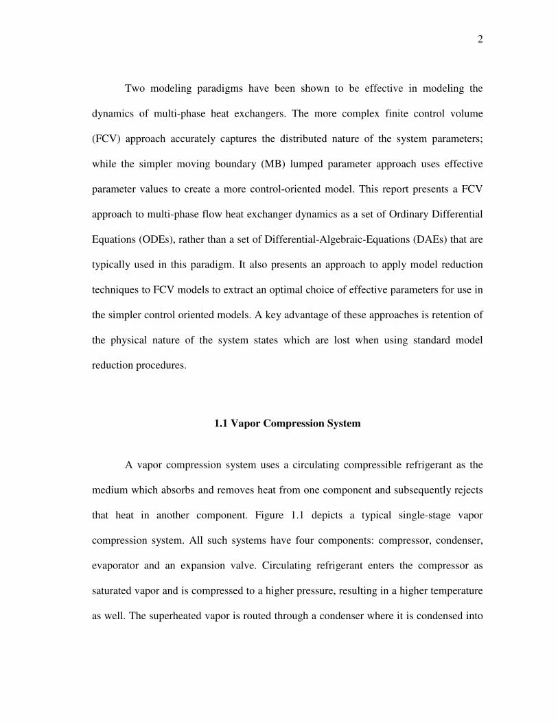
1.1 Vapor Compression System
A vapor compression system uses a circulating compressible refrigerant as the
medium which absorbs and removes heat from one component and subsequently rejects
that heat in another component. Figure 1.1 depicts a typical single-stage vapor
compression system. All such systems have four components: compressor, condenser,
evaporator and an expansion valve. Circulating refrigerant enters the compressor as
saturated vapor and is compressed to a higher pressure, resulting in a higher temperature
as well. The superheated vapor is routed through a condenser where it is condensed into

3
a liquid by flowing through tubes with secondary fluid (such as air or water) flowing
across them. The heat rejected by the circulating refrigerant is carried away by the
secondary fluid in the condenser. Then the saturated liquid is passed through an
expansion valve. At the exit of the valve, the refrigerant is usually two-phase and at a
lower pressure. Next, the two-phase refrigerant is routed through an evaporator where it
is converted into superheated vapor by flowing through tubes with secondary fluid
flowing across them. Thus, heat is absorbed by the circulating refrigerant from the
secondary fluid in the evaporator. The superheated refrigerant is routed back into the
compressor thus, completing the vapor compression cycle. The vapor compression cycle
described in this section is represented on ph-diagram in Figure 1.2. To model a vapor
compression system, a few standard assumptions are made. First, the compression of the
fluid is assumed to be adiabatic. Second, isobaric conditions in the condenser and
evaporator are assumed. Third, expansion through the valve is assumed to be isenthalpic.
Figure 1.1: Simple Vapor Compression Cycle System

4
Figure 1.2: Simple Vapor Compression Cycle System
Modern heat exchangers employ a variety of techniques to maximize heat
transfer. In particular, the heat exchanger may use multiple fluid paths, which may
branch into additional paths as the fluid evaporates to accommodate the increasing
volume of fluid. Even the simplest variation in geometry (such as shown in Figure 1.3)
will affect several key physical parameters such as surface areas and fluid flow cross-
sectional areas.
inh
1,outh
2,outh
Figure 1.3: Simple Variation in Geometry of Heat Exchanger
5
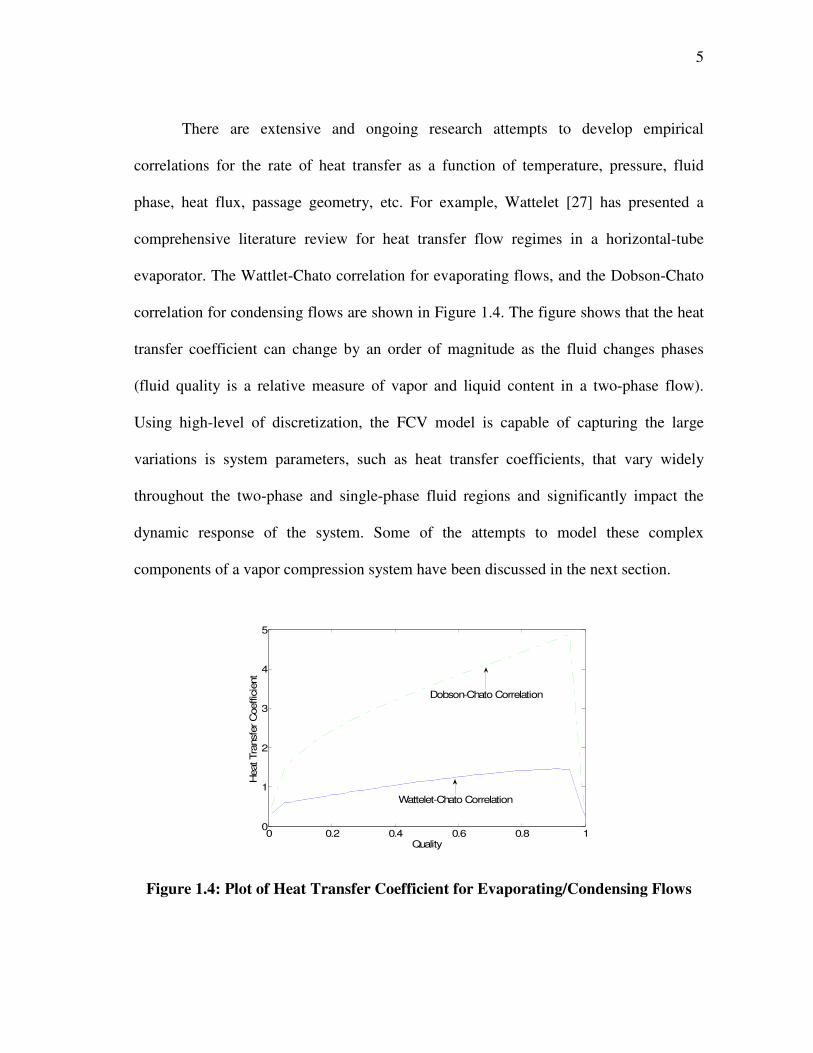
There are extensive and ongoing research attempts to develop empirical
correlations for the rate of heat transfer as a function of temperature, pressure, fluid
phase, heat flux, passage geometry, etc. For example, Wattelet [27] has presented a
comprehensive literature review for heat transfer flow regimes in a horizontal-tube
evaporator. The Wattlet-Chato correlation for evaporating flows, and the Dobson-Chato
correlation for condensing flows are shown in Figure 1.4. The figure shows that the heat
transfer coefficient can change by an order of magnitude as the fluid changes phases
(fluid quality is a relative measure of vapor and liquid content in a two-phase flow).
Using high-level of discretization, the FCV model is capable of capturing the large
variations is system parameters, such as heat transfer coefficients, that vary widely
throughout the two-phase and single-phase fluid regions and significantly impact the
dynamic response of the system. Some of the attempts to model these complex
components of a vapor compression system have been discussed in the next section.
0 0.2 0.4 0.6 0.8 10
1
2
3
4
5
Quality
Heat Tra
nsfe
r C
oeffic
ient
Dobson-Chato Correlation
Wattelet-Chato Correlation
Figure 1.4: Plot of Heat Transfer Coefficient for Evaporating/Condensing Flows

6
1.2 Literature Review
Several authors have made significant contributions to this field of research. In
1955, Paynter [20] presented a model based on transfer function of a heat exchanger to
predict the transient response of parallel-flow and counter-flow heat exchangers. To
estimate the transient response, he suggested design parameters to be considered and
compared his models with experimental data.
Gruhle and Isermann [13] suggested the distributed parameter approach for
modeling of heat exchangers in 1984. The distributed parameter process was
approximated by several lumped parameter models. MacArthur and Grald [16] utilized
distributed parameter approach for predicting the performance of a cyclic heat pump and
compared their results with experimental data. Later in 1992, they presented a moving
boundary approach to model heat exchangers [12].
In 1996, He [14,15] utilized lumped parameter approach to describe the
dynamics of vapor compression cycle. Later in 1997, Willatzen [28] used the moving
boundary approach for dynamic simulation of heat exchangers. In 1997, Narayanan et al.
[18] presented a lumped parameter formulation of a vertical evaporator. They also
accounted for pressure drop and axial variation of heat flux in their model.
Mithraratne et al. [17] presented a distributed parameter model of simulating the
dynamics of an evaporator controlled by a thermostatic expansion valve (TEV) in a
vapor compression refrigeration system in 1998. They also included the axial conduction

7
of heat in the pipe wall as it affects the TEV. In 1998, Tummescheit and Eborn [26]
presented the lumped parameter as well as distributed parameter models as a
commercially available software package known as Modelica. Bendapudi [8]
compared and validated the moving boundary as well as finite control volume
approaches. He also provided a literature review of notable prior efforts in this field of
research [7].
Many authors have contributed in developing low order models as well as high
order discretized models for modeling of heat exchangers. The low order models require
significant amount of tuning of the parameters for effective prediction of transients. The
high order models resulting from using the distributed parameter approach are not
suitable for controller design. Low order models obtained by applying standard model
reduction techniques to the higher order models, lose the significance of the system
states. The effort detailed in this report utilizes the high order models to characterize the
heat exchanger and use it to determine low order models with system states having
physical significance.
Most of the modeling approaches used by the authors above apply the
assumption of mean void fraction to characterize the two-phase region in the heat
exchangers. The void fraction model has been discussed in the next section.
8
1.2.1 Void Fraction
Void fraction is defined as the ratio of vapor volume to total volume in a two-
phase fluid flow. It has long been used to describe certain characteristics of two-phase
flows. Many experimental correlations have been proposed for predicting void fraction
for various conditions and fluids. Rice [24] has presented the well known void fraction
correlations in his reviews for ASHRAE. The void fraction is generally represented as
function of mass quality, x and combinations of various types of property indices
(which remain constant for a given average evaporator or condenser saturation
temperature). Quality of a two-phase fluid is defined as the ratio of vapor mass to total
mass of the fluid. Rice has categorized the correlations into four divisions:
Homogeneous, Slip Ratio, Lockhart-Martinelli, and Mass Flux Dependent. The former
two types are relatively much simpler than the latter two. In a two-phase flow, slip ratio
is defined as the ratio of vapor velocity to liquid velocity. The slip ratio correlation
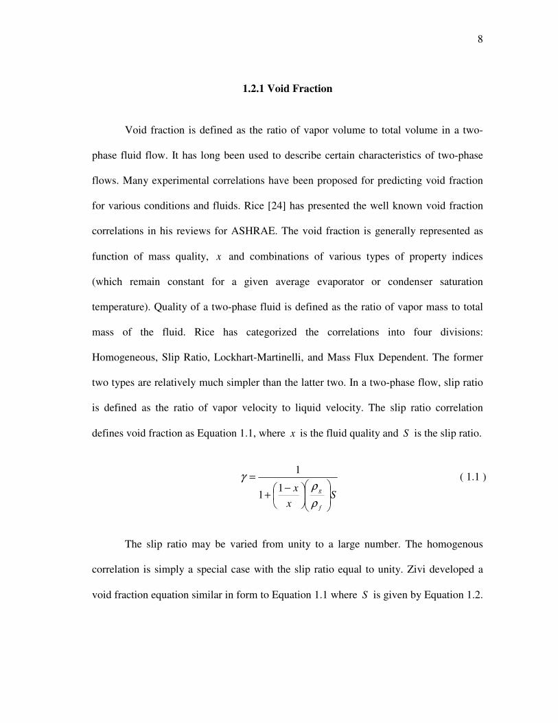
defines void fraction as Equation 1.1, where x is the fluid quality and S is the slip ratio.
Sx
x
f
g
−+
=
ρ
ργ
11
1 ( 1.1 )
The slip ratio may be varied from unity to a large number. The homogenous
correlation is simply a special case with the slip ratio equal to unity. Zivi developed a
void fraction equation similar in form to Equation 1.1 where S is given by Equation 1.2.
9
For the purpose of this research, slip ratio is assumed to be a number between unity and
S obtained by Equation 1.2.
3/1−
=
f
gS
ρ
ρ ( 1.2 )
1.3 Organization of Report
The remainder of this report is organized as follows. Chapter 2 describes the
modeling procedure for each of the evaporator and condenser models using MB and
FCV approach. Chapter 3 describes the procedure for obtaining linearized models of the
heat exchangers. Chapter 4 details the experimental setup and explains the experiments
conducted. Chapter 5 presents the simulation environment developed for simulation,
model validation, and controller design. Model validation results are given in Chapter 6.
Chapter 7 presents the general approach used to derive reduced order models using the
higher order FCV models. Conclusions and suggestions for future work are given in
Chapter 8.
10
CHAPTER 2
DYNAMIC MODELING
This chapter discusses the modeling of heat exchangers (including evaporator
and condenser). Modeling of two phase fluid flow to capture the detailed dynamics is not
only difficult and mathematically complex but it requires a considerable amount of time
and effort to complete the task. Several methods to model two-phase fluid flow have
been reviewed by D.A. Drew for Annual Review of Fluid Mechanics [10]. Fluid flow
through an evaporator or a condenser involves one or more transition of fluid phase from
vapor to single-phase and vice versa. The modeling of heat exchangers begins with
governing equations. Some basic assumptions have been postulated without significantly
compromising the physics of interest.
2.1 Modeling Assumptions
Several assumptions are made to approximate and simplify the subsequent
development of the model. These assumptions have been commonly used in the past
efforts as well. Firstly, the heat exchanger is assumed to be a long, thin and horizontal
tube such that the refrigerant flow inside it can be modeled as a one-dimensional fluid
flow. The refrigerant flow inside the tube is truly three-dimensional because of
turbulence. The major impact of turbulence affects convective heat transfer coefficient
from the refrigerant to the tube. The use of an appropriate heat transfer coefficient
11
correlation should be able to capture the effects of turbulence and the refrigerant can be
safely assumed to have a one-dimensional flow.
Secondly, the pressure drop along the length of the heat exchanger due to change
in momentum of refrigerant or due to viscous friction is assumed to be negligible. Thus,
the refrigerant pressure along the heat exchanger tube is uniform. This eliminates the
need for the equation for conservation of momentum.
The third assumption is that the axial conduction of heat in the refrigerant as well
as the tube material is much less as compared to the heat transfer between refrigerant and
tube material on one side and tube material and secondary fluid on the other side. Lastly,
the cross-sectional area of the flow-stream within each control region is assumed to be
constant.
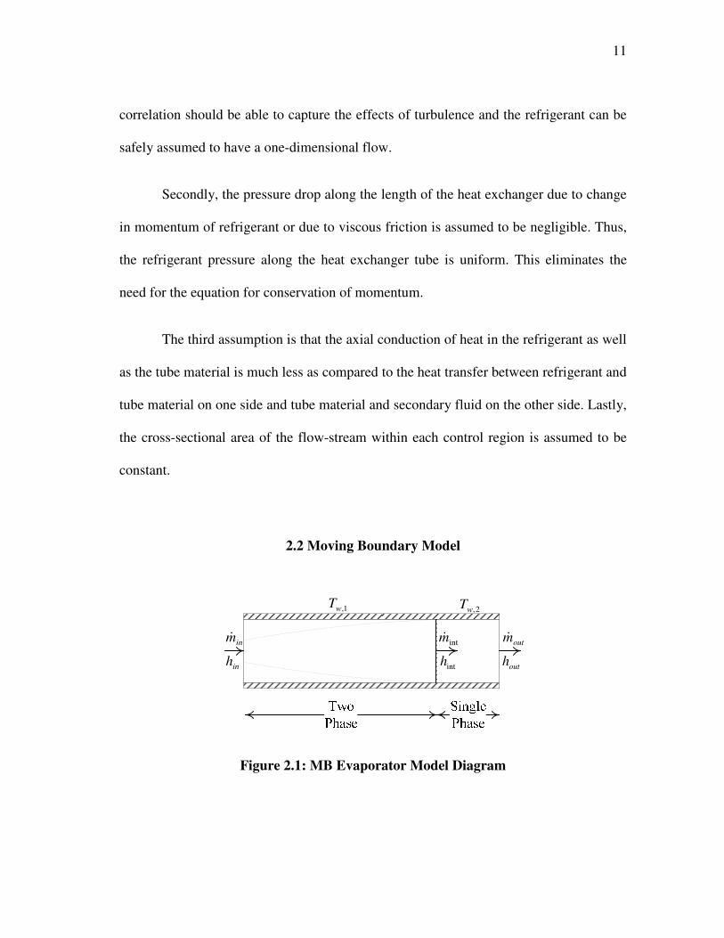
2.2 Moving Boundary Model
1,wT
outhinh inth
2,wT
outm&inm& intm&
Figure 2.1: MB Evaporator Model Diagram

12
The moving boundary (MB) approach to multi-phase heat exchanger modeling
relies on several fundamental assumptions as described in the previous section. Despite
the complexity of typical heat exchanger geometries, the MB approach assumes the heat
exchanger can be modeled as one-dimensional fluid flow through a horizontal tube, with
equivalent mass, surface areas, length, and volume as shown in Figure 2.1. The standard
derivation procedure requires the integration of the governing PDEs given in Equations
2.1-2.3 along the length of the heat exchanger to remove spatial dependence. The
integration rule given in Equation 2.4, commonly known as Leibniz’s equation, is used
to handle the time-varying boundary between the fluid regions. This approach can be
tedious and require a significant amount of algebraic manipulation. With some minor
differences many authors use some form of this approach to model an evaporator in a
sub-critical cycle [8,12,14,26]. In this case, the fluid is assumed to enter as a two-phase
mixture, and leave as a superheated vapor, and thus the model is divided into two
regions. The model assumes a time-invariant mean void fraction in the two-phase region.
0=∂
∂+
∂
∂
z
m
t
A &ρ ( 2.1 )
( ) ( ) ( )rwii TTp
z
hm
t
APAh−=
∂
∂+
∂
−∂α
ρ & ( 2.2 )
( ) ( ) ( )waoowriiw
wp TTpTTpt
TAC −+−=
∂
∂ααρ ( 2.3 )

13
( )( )
( )( )
( )
( )
( )( ) ( )( ) ( )( ) ( )( )dt
tzdttzf
dt
tzdttzf
dztzfdt
ddz
t
tzf tz
tz
tz
tz
11
22 ,,
,, 2
1
2
1
+−
=
∂
∂∫∫
( 2.4 )
The conservation of refrigerant mass as applied to the two-phase and superheat
regions is given in Equations 2.5 and 2.6. Similarly the conservation of refrigerant
energy is shown in Equations 2.7 and 2.8, and the conservation of heat exchanger wall
energy is shown in Equations 2.9 and 2.10.
( ) ( ) ( )
0int1
11
11
=−+
−+
−
−+
+−
inmmL
csA
fg
Lcs
Agfe
PLcs
A
edP
gd
edP
fd
&&&
&&
γρρ
γρργρ
γρ
( 2.5 )
( ) 0
2
1
2
1
int12
2
2
22
2
22
2
=−+−+
∂
∂+
∂
∂+
∂
∂
mmLA
hALh
PALdP
dh
hP
outg
out
P
e
e
g
Pheee
&&&
&&
ρρ
ρρρ
( 2.6 )
( )( )
( )( )
( ) ( )( )
( )111
intint
11
1
1
11
rw
Total
iiinin
csggffcsffgg
ecs
e
gg
e
ff
TTL
LAhmhm
LAhhLAhh
PLAdP
hd
dP
hd
−
=−+
−−+−+
−+−
α
γρργρρ
γρ
γρ
&&
&&
&
( 2.7 )
14
( )
( )222
intint
122222
2
2
222
2
22
2
1
12
1
2
1
2
rw
Total
iioutout
csggoutcs
P
ecs
e
g
Pe
g
he
TTL
LAhmhm
LAhhhLAhh
PLAdP
dhh
hdP
dh
P
e
e
−
=−+
−+
+
∂
∂+
−
+
∂
∂
+
∂
∂
α
ρρρρ
ρρρ
&&
&&
&
( 2.8 )
( ) ( ) ( )waoowriiwwp TTATTATVC −+−= ααρ 1& ( 2.9 )
( ) ( ) ( )waoowriiww
wwp TTATTALL
TTTVC −+−=
−− ααρ 1
2
122
&& ( 2.10 )
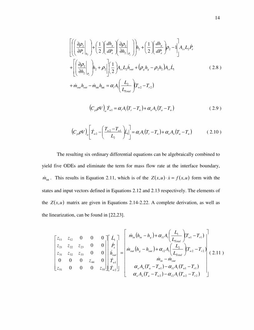
The resulting six ordinary differential equations can be algebraically combined to
yield five ODEs and eliminate the term for mass flow rate at the interface boundary,
intm& . This results in Equation 2.11, which is of the ( ) ( )uxfxuxZ ,, =⋅ & form with the
states and input vectors defined in Equations 2.12 and 2.13 respectively. The elements of
the ( )uxZ , matrix are given in Equations 2.14-2.22. A complete derivation, as well as
the linearization, can be found in [22,23].
( ) ( )
( ) ( )
( ) ( )
( ) ( )
−−−
−−−
−
−
+−
−
+−
=
2222
1111
222
2
111
1
2
1
1
5551
44
333231
232221
1211
000
0000
00
00
000
rwiiwaoo
rwiiwaoo
outin
rw
Total
iioutgout
rw
Total
iiginin
w
w
out
e
TTATTA
TTATTA
mm
TTL
LAhhm
TTL
LAhhm
T
T
h
P
L
zz
z
zzz
zzz
zz
αα
αα
α
α
&&
&
&
&
&
&
&
&
( 2.11 )
15
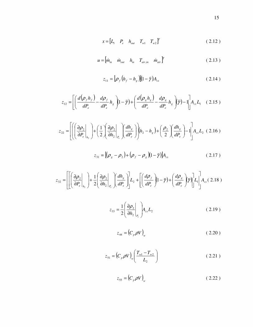
[ ]Twwoute TThPLx 211= ( 2.12 )
[ ]Tairinairinoutin mThmmu &&&,= ( 2.13 )
( )[ ]( ) csgff Ahhz γρ −−= 111 ( 2.14 )
( )
( )( )
( ) 112 11 LAhdP
d
dP
hdh
dP
d
dP
hdz csg
e
g
e
gg
g
e
f
e
ff
−
−+−
−= γ
ρργ
ρρ ( 2.15 )
( ) 22
2
2
2222 1
22
1
2
LAdP
dhhh
dP
dh
hPz cs
e
g
g
e
g
Phee
−
+−
∂
∂
+
∂
∂=
ρρρ ( 2.16 )
( ) ( )( )[ ] csgfg Az γρρρρ −−+−= 1231 ( 2.17 )
( ) ( )cs
e
g
e
f
e
g
Phe
ALdP
d
dP
dL
dP
dh
hPz
e
+−
+
∂
∂+
∂
∂= 12
2
2232 1
2
1
2
γρ
γρρρ
( 2.18 )
2
2
233
2
1LA
hz cs
Pe
∂
∂=
ρ ( 2.19 )
( )wp VCz ρ=44 ( 2.20 )
( )
−=
2
2151
L
TTVCz ww
wp ρ ( 2.21 )
( )wp VCz ρ=55 ( 2.22 )

16
2.3 Finite Control Volume Evaporator Model
For developing the finite control volume (FCV) approach, we begin with
discretizing the evaporator model into n control volumes. Depending on the geometry
of the heat exchanger, the thk control region will have an internal surface area, kiA , ,
external surface area, koA , , and volume of the control region, keV , . The governing
ordinary differential equations are obtained by applying the basic assumptions enlisted in
the previous section to the fundamental conservation equations for each control region.
Lumped parameters are associated with each control region. Although the resulting
equations use lumped parameters for each assumed control region, by increasing the
number of control volumes (i.e. increasing the level of discretization), the model
approximates the distributed parametric nature of a real heat exchanger (Figure 2.2).
kwT ,1,wTnwT ,
1,em&
1,eh1h 1−kh
kem ,&
keh ,
nem ,&
neh ,kh 1−nh outhinh
outm&inm&
Figure 2.2: FCV Evaporator Model Diagram
If the fluid entering the evaporator is two-phase and the fluid exiting the
evaporator is single-phase, the evaporator broadly consists of two regions: two-phase
region and a superheated region. For modeling purpose, it has been assumed that the

17
fluid gradually transitions from two-phase to single-phase fluid inside the heat exchanger
(shown in Figure 2.2). The outlet enthalpy of the fluid in a control region determines the
state of the fluid in that region. If the outlet enthalpy of the fluid in a region is less than
or equal to the vapor saturation enthalpy (at the evaporator pressure), the state of the
fluid in that region is two-phase. If the outlet enthalpy of the fluid in a region is greater
than the vapor saturation enthalpy, the state of the fluid in that region is single-phase.
The control region in which the final transition of fluid from two-phase to single-phase
occurs has been termed by the author as the ‘transition region’. The state of the fluid in
the transition region is assumed to be single-phase. In an evaporator shown in Figure 2.2,
if the transition line is closer to the left boundary of the transition region, the better is our
assumption of guessing the state of the fluid in that region. The modeling error due to the
assumption of the state of fluid in the transition region can be minimized by increasing
the number of control volumes. In the Figure 2.2, 1−kh , 1−km& and kh , km& are the
enthalpy and mass flow rate of the refrigerant at the inlet and outlet of the thk control
region. inh , inm& and outh , outm& are the enthalpy and mass flow rate of the refrigerant at
the inlet and outlet of the heat exchanger. kem ,& gives the rate of change of refrigerant
mass in the thk control region and keh , is assumed to be the average enthalpy in the th
k
control region of the heat exchanger. The conservation equations for refrigerant energy,
mass and tube-wall energy are considered for obtaining the governing ordinary
differential equations.
18
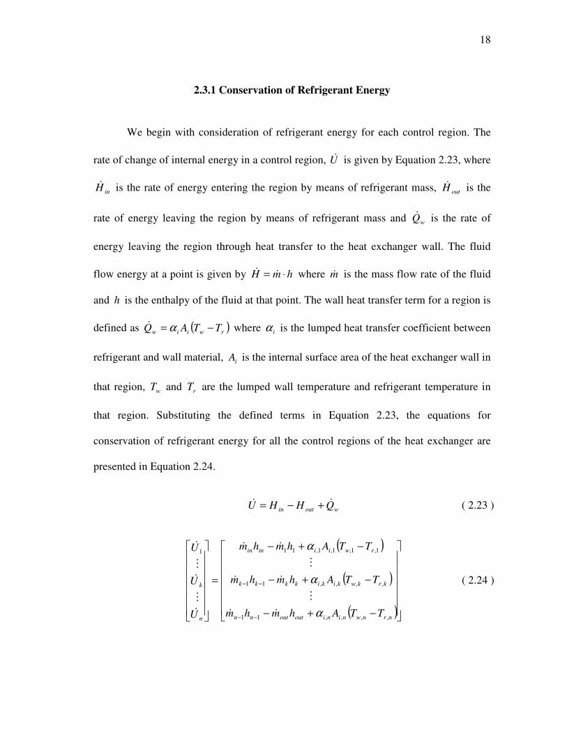
2.3.1 Conservation of Refrigerant Energy
We begin with consideration of refrigerant energy for each control region. The
rate of change of internal energy in a control region, U& is given by Equation 2.23, where
inH& is the rate of energy entering the region by means of refrigerant mass, outH& is the
rate of energy leaving the region by means of refrigerant mass and wQ& is the rate of
energy leaving the region through heat transfer to the heat exchanger wall. The fluid
flow energy at a point is given by hmH ⋅= && where m& is the mass flow rate of the fluid
and h is the enthalpy of the fluid at that point. The wall heat transfer term for a region is
defined as ( )rwiiw TTAQ −= α& where iα is the lumped heat transfer coefficient between
refrigerant and wall material, iA is the internal surface area of the heat exchanger wall in
that region, wT and rT are the lumped wall temperature and refrigerant temperature in
that region. Substituting the defined terms in Equation 2.23, the equations for
conservation of refrigerant energy for all the control regions of the heat exchanger are
presented in Equation 2.24.
woutin QHHU && +−= ( 2.23 )
( )
( )
( )
−+−
−+−
−+−
=
−−
−−
nrnwninioutoutnn
krkwkikikkkk
rwiiinin
n
k
TTAhmhm
TTAhmhm
TTAhmhm
U
U
U
,,,,11
,,,,11
1,1,1,1,111
α
α
α
&&
M
&&
M
&&
&
M
&
M
&
( 2.24 )

19
2.3.2 Conservation of Refrigerant Mass
The conservation of refrigerant mass in each control volume is given by Equation
2.25, which is equal to the difference of the refrigerant mass entering and leaving that
control volume. All the equations in Equation 2.25 can be combined together by adding
them and are presented in Equation 2.26 where em& gives the rate of change of total
refrigerant mass in the heat exchanger.
−
−
−
=
−
−
outn
kk
in
ne
ke
e
mm
mm
mm
m
m
m
&&
M
&&
M
&&
&
M
&
M
&
1
1
1
,
,
1,
( 2.25 )
outine mmm &&& −= ( 2.26 )
2.3.3 Conservation of Tube Wall Energy
The conservation of wall energy in a control region is given in Equation 2.27
where wE& is the rate of change of total energy of the heat exchanger wall in the control
region considered and aQ& is the rate of energy entering the heat exchanger wall through
heat transfer from the external fluid. Substituting the defined terms in Equation 2.27, the
equations for conservation of tube wall energy for all the control regions of the heat
exchanger are presented in Equation 2.28.

20
waw QQE &&& −= ( 2.27 )
( ) ( )
( ) ( )
( ) ( )
−−−
−−−
−−−
=
nrnwnininwnanono
krkwkikikwkakoko
rwiiwaoo
nw
kw
w
TTATTA
TTATTA
TTATTA
E
E
E
,,,,,,,,
,,,,,,,,
1,1,1,1,1,1,1,1,
,
,
1,
αα
αα
αα
M
M
&
M
&
M
&
( 2.28 )
2.3.4 Governing Differential Equations
The combined results presented in Equations 2.24, 2.26 and 2.28 are given in
Equation 2.29. Defining internal energy in terms of refrigerant mass and average specific
internal energy kekeke umU ,,, ⋅= , the time derivative of this term can be expanded as in
Equation 2.30 for the thk control region. Defining refrigerant mass in terms of average
density, ke,ρ and internal volume keV , as kekeke Vm ,,, ρ⋅= , yields Equation 2.31 for the
thk control region. Since density and internal energy can be given as functions of
pressure, eP , and enthalpy, ke,h , of the region being considered, the time derivative of
these variables can be written in terms of the desired state (Equation 2.32). Simplifying
this expression and substituting the formal definition of enthalpy ke
e
keke
Puh
,
,,ρ
+= , and
its partial derivatives of
keke he
ke
ke
e
kehe
ke
P
P
P
u
,,
,
2
,,
, 1
∂
∂+
−=
∂
∂ ρ
ρρ and
ee Pke
ke
ke
e
Pke
ke
h
P
h
u
,
,
2
,,
, 1∂
∂+=
∂
∂ ρ
ρ
results in Equations 2.33, 2.34 and 2.35. Likewise, expanding the time derivative of
21
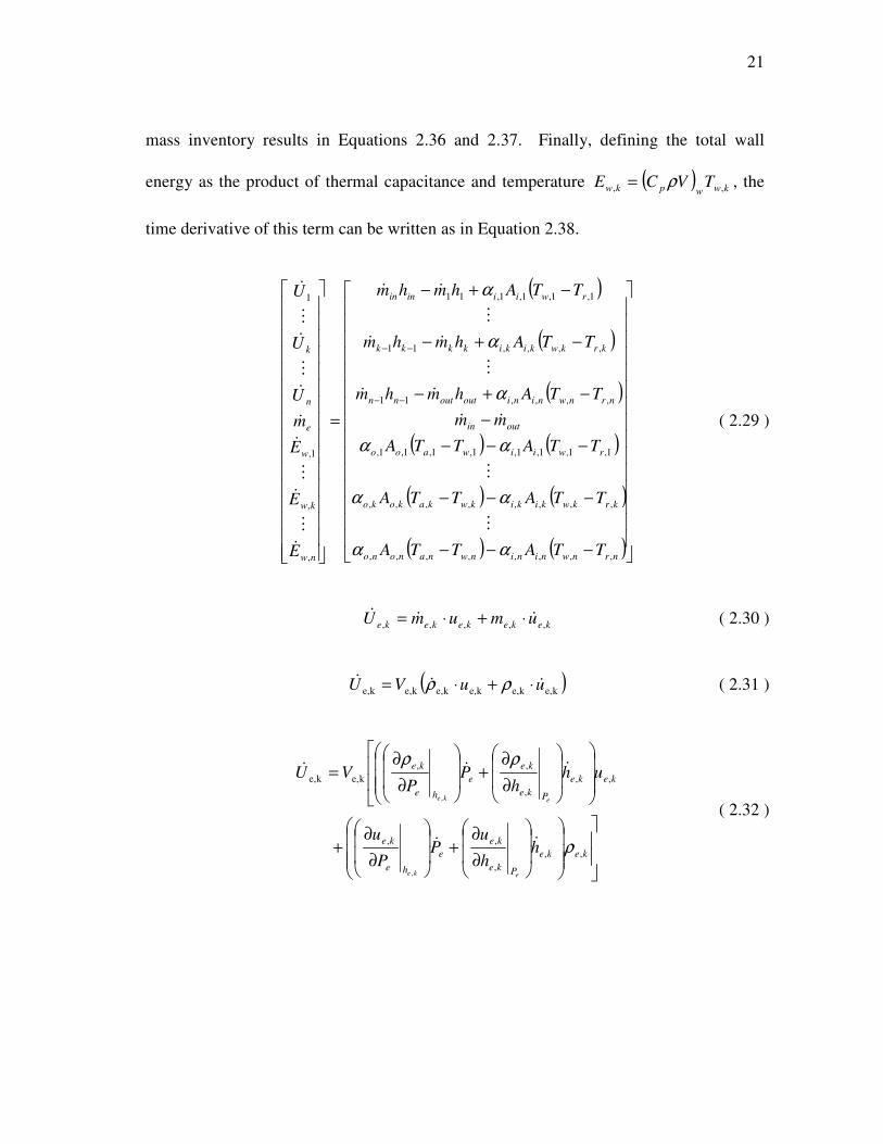
mass inventory results in Equations 2.36 and 2.37. Finally, defining the total wall
energy as the product of thermal capacitance and temperature ( )kwwpkw TVCE ,, ρ= , the
time derivative of this term can be written as in Equation 2.38.
( )
( )
( )
( ) ( )
( ) ( )
( ) ( )
−−−
−−−
−−−
−
−+−
−+−
−+−
=
−−
−−
nrnwnininwnanono
krkwkikikwkakoko
rwiiwaoo
outin
nrnwninioutoutnn
krkwkikikkkk
rwiiinin
nw
kw
w
e
n
k
TTATTA
TTATTA
TTATTA
mm
TTAhmhm
TTAhmhm
TTAhmhm
E
E
E
m
U
U
U
,,,,,,,,
,,,,,,,,
1,1,1,1,1,1,1,1,
,,,,11
,,,,11
1,1,1,1,11
,
,
1,
1
αα
αα
αα
α
α
α
M
M
&&
&&
M
&&
M
&&
&
M
&
M
&
&
&
M
&
M
&
( 2.29 )
kekekekeke umumU ,,,,,&&& ⋅+⋅= ( 2.30 )
( )ke,ke,ke,ke,ke,ke, uuVU &&& ⋅+⋅= ρρ ( 2.31 )
∂
∂+
∂
∂+
∂
∂+
∂
∂=
keke
Pke
ke
e
he
ke
keke
Pke
ke
e
he
ke
hh
uP
P
u
uhh
PP
VU
eke
eke
,,
,
,,
,,
,
,,
ke,ke,
,
,
ρ
ρρ
&&
&&&
( 2.32 )

22
keke
Pke
ke
ke
Pke
ke
ke
eke
he
ke
ke
he
ke
keke
hh
uu
hV
PP
uu
PVU
ee
keke
,,
,
,
,
,
,
,
,
,
,
,
,,
,,
&
&&
∂
∂+
∂
∂+
∂
∂+
∂
∂=
ρρ
ρρ
( 2.33 )
keke
ke
e
ke
Pke
ke
ke
e
ke
e
ke
he
ke
keke
hP
uh
V
PP
uP
VU
e
ke
,,
,
,
,
,
,
,
,
,
,, 1
,
&
&&
+
+
∂
∂+
−
+
∂
∂=
ρρ
ρ
ρ
ρ
( 2.34 )
kekeke
Pke
ke
keeke
he
ke
keke hhh
VPhP
VU
eke
,,,
,
,
,,
,
,, 1
,
&&&
+
∂
∂+
−
∂
∂= ρ
ρρ ( 2.35 )
kekeke Vm ,,, ⋅= ρ&& ( 2.36 )
keke
Pke
ke
e
he
ke
ke Vhh
PP
m
eke
,,
,
,,
,
,
∂
∂+
∂
∂= &&&
ρρ ( 2.37 )
( )kwwpkw TVCE ,,
&& ρ= ( 2.38 )
Equations 2.35, 2.37 and 2.38 can be extended for all the control regions of the
heat exchanger to represent the refrigerant energy, refrigerant mass and tube wall energy
respectively. The resulting equations along with Equation 2.25 and 2.29 can be
combined and simplified into ( )12 +n nonlinear differential equations and reorganized

23
into a matrix form given by Equation 2.39 where x is the state vector. The state vector
x , input vector u and the output vector y are given in Equations 2.40, 2.41 and 2.42
respectively. The elements of matrices ( )uxZ , and ( )uxf , are given in Equations 2.43
through 2.59.
( ) ( )uxfxuxZ ,, =⋅ & ( 2.39 )
[ ]T
nwkwwnekeee TTThhhPx ,,1,,,1, KKKK= ( 2.40 )
[ ]Tairinainoutin mThmmu &&&
,= ( 2.41 )
[ ]T
nekeeoutroutanwkwwoute mmmTTTTThPy ,,1,,,,,1, LLLL= ( 2.42 )
)12()12(33
2221
1211
00
0
0
),(
++
=
nXnZ
ZZ
ZZ
uxZ ( 2.43 )
111
11
1
11
11
nX
n
k
Z
Z
Z
Z
=
M
M
( 2.44 )
( ) 1,11,
1,
1,
1
11
1,
ee
he
e
e VhhP
VZ
e
−−∂
∂=
ρ ( 2.45 )
24
( )
( )
∂
∂++
∂
∂−+
−−∂
∂=
−
−
−
1,1,
,
1,
1,
1,
1,,
,,
,
,11
kee
ke
he
ke
ke
he
e
ekke
kekke
he
ke
ke
k
PV
PVhh
VhhP
VZ
ρρ
ρ
L
( 2.46 )
( )
( )
∂
∂++
∂
∂−+
−−∂
∂=
−
−
−
1,1,
,
1,
1,
1,
1,,
,,
,
,11
nee
ne
he
ne
ne
he
e
eoutne
neoutne
he
ne
ne
n
PV
PVhh
VhhP
VZ
ρρ
ρ
L
( 2.47 )
nXn
nnnnn
kkkkk
ZZZ
ZZZ
Z
Z
=
−
−
12
)1(
12
1
12
12
)1(
12
1
12
11
12
12 0
000
L
MOOM
L
MM
L
( 2.48 )
( ) 1,1,11,
1,
1,
11
12
1,
eee
he
e
e VhhP
VZ
e
ρρ
+−∂
∂= ( 2.49 )
( )ePe
e
ekk
k
hVhhZ
1,
1,
1,1
1
12∂
∂−= −
ρ ( 2.50 )
( )ePke
ke
kekk
kk
hVhhZ
1,
1,
1,1
)1(
12
−
−−−
−
∂
∂−=
ρ ( 2.51 )
( )keke
Pke
ke
kekke
kkV
hVhhZ
e
,,
,
,
,,12 ρρ
+∂
∂−= ( 2.52 )

25
( )ePe
e
enn
n
hVhhZ
1,
1,
1,1
1
12∂
∂−= −
ρ ( 2.53 )
( )ePne
ne
nenn
nn
hVhhZ
1,
1,
1,1
)1(
12
−
−−−
−
∂
∂−=
ρ ( 2.54 )
( )nene
Pne
ne
nenne
nnV
hVhhZ
e
,,
,
,
,,12 ρρ
+∂
∂−= ( 2.55 )
11
,
,
1,
1,21
,1, Xhe
ne
ne
he
e
e
nee
PV
PVZ
∂
∂++
∂
∂=
ρρL ( 2.56 )
XnPne
ne
ne
Pe
e
e
ee
hV
hVZ
1,
,
,
1,
1,
1,22
∂
∂
∂
∂=
ρρL ( 2.57 )
( ) ( )[ ]{ }nwpwp VCVCdiagZ
,1,33 ρρ L= ( 2.58 )
( ) ( )
( ) ( )
( ) ( )
( ) ( )
( ) ( )
( ) ( )1)12(,,,,,,,
,,,,,,,
1,1,1,1,1,1,1,
,,,,1
,,,,1
1,1,1,1,1
),(
Xnnwnanoonwnrnini
kwkakookwkrkiki
waoowrii
outin
nrnwninioutnin
krkwkikikkin
rwiiinin
TTATTA
TTATTA
TTATTA
mm
TTAhhm
TTAhhm
TTAhhm
uxf
+
−
−
−+−
−+−
−+−
−
−+−
−+−
−+−
=
αα
αα
αα
α
α
α
M
M
&&
&
M
&
M
&
( 2.59 )

26
As discussed in Chapter 1, void fraction is the ratio of vapor volume to the total
volume in the region being considered. It is used to describe characteristics of two-
phase flow. The void fraction of thk control region is given by Equation 2.60 where kx
is the quality (ratio of vapor mass to total mass of the refrigerant) of the region and S is
the slip ratio (ratio of vapor velocity to liquid velocity). gρ and fρ are the saturated
vapor density and saturated liquid density of the fluid at the evaporator pressure
respectively. Thus, void fraction is a function of quality and pressure, say ( )ek Pxf ,1 .
Quality of the fluid in the thk control region is given by Equation 2.61 which is a
function of average enthalpy, keh , and evaporator pressure, eP . gh and fh are the
saturated vapor enthalpy and saturated liquid enthalpy of the fluid at the evaporator
pressure respectively. It can be assumed that ( )ekek Phfx ,,2= . Now, the density of the
thk control region is given by Equation 2.62 and can be assumed as a function of void
fraction and evaporator pressure as ( )ekke Pf ,3, γρ = . The partial derivative of density
with respect to evaporator pressure and with respect to average enthalpy is given in
Equations 2.63 and 2.64 respectively. Other derivatives required for calculating
Equations 2.63 and 2.64 are given in Equations 2.65 through 2.72.
( )
( )ek
kgkf
kf
k PxfSxx
x,
11=
−+=
ρρ
ργ ( 2.60 )
( )eke
fg
fke
k Phfhh
hhx ,,2
,=
−
−= ( 2.61 )

27
( ) ( )ekkgkfke Pf ,1 3, γγργρρ =−+= ( 2.62 )
e
k
kee
ke
P
f
P
f
P ∂
∂
∂
∂+
∂
∂=
∂
∂ γ
γ
ρ33,
( 2.63 )
ke
k
kke
ke
h
f
h ,
3
,
,
∂
∂
∂
∂=
∂
∂ γ
γ
ρ ( 2.64 )
−=
∂
∂
e
f
e
g
k
e dP
d
dP
d
P
f ρργ3 ( 2.65 )
( )fg
k
fρρ
γ−=
∂
∂ 3 ( 2.66 )
e
k
kee
k
P
x
x
f
P
f
P ∂
∂
∂
∂+
∂
∂=
∂
∂ 11γ ( 2.67 )
ke
k
kke
k
h
x
x
f
h ,
1
, ∂
∂
∂
∂=
∂
∂γ ( 2.68 )
( )( ) ( )
( )( )2
1
1
11
Sxx
SxP
xP
xP
xSxx
P
f
kgkf
k
e
g
k
e
f
kf
e
f
kkgkf
e −+
−
∂
∂+
∂
∂−
∂
∂−+
=∂
∂
ρρ
ρρρ
ρρρ
( 2.69 )
( )( ) ( )
( )( )2
1
1
1
Sxx
SxSxx
x
f
kgkf
gfkffkgkf
k −+
−−−+=
∂
∂
ρρ
ρρρρρρ ( 2.70 )
( )
( )( )
−
−−+
−
−=
∂
∂
e
g
e
f
fg
fke
e
f
fge
k
dP
dh
dP
dh
hhhh
dP
dh
hhP
x2,
11 ( 2.71 )

28
fgke
k
hhh
x
−=
∂
∂ 1
,
( 2.72 )
As mentioned earlier, the state of the fluid in a control region can be determined
on the basis of the outlet enthalpy of that region. If the fluid is in two-phase, we calculate
the partial derivative of density with respect to evaporator pressure and enthalpy given in
Equations 2.63 and 2.64 respectively. If the fluid is in single-phase, we can use the
property tables to determine the partial derivative of density with respect to evaporator
pressure and enthalpy.
2.4 Finite Control Volume Condenser Model
inh
inm&
outh
outm&1,em&
1,eh1h 1−kh
kem ,&
keh , kh 1−nh
Two
Phase
Single Phase
Liquid
Single Phase
Vapor
nem ,&
neh ,
1,wT kwT , nwT ,
Figure 2.3: FCV Condenser Model Diagram
Usually, the fluid entering the condenser is single-phase super-heated vapor and
the fluid exiting the condenser is single-phase super-cooled liquid as shown in Figure
2.3. Thus, the condenser broadly consists of three regions: superheated region, two-
phase region and a super-cooled region. For developing the finite control volume (FCV)

29
approach, we begin with discretizing the condenser model into n control volumes. As
mentioned earlier, the outlet enthalpy of the fluid in a control region determines the state
of the fluid in that region. If the outlet enthalpy of the fluid in a region is greater than the
vapor saturation enthalpy (at the condenser pressure), the state of the fluid in that region
is single-phase superheated vapor. If the outlet enthalpy of the fluid in a region is less
than or equal to the vapor saturation enthalpy and greater than or equal to the liquid
saturation enthalpy, the state of the fluid in that region is two-phase. If the outlet
enthalpy of the fluid in a region is less than the liquid saturation enthalpy (at the
condenser pressure), the state of the fluid in that region is single-phase super-cooled
liquid. The governing equations for the condenser model are the same as those for the
evaporator model as described in Section 2.3. Equation 2.39 gives the ( )12 +n nonlinear
differential equations for the condenser model where x is the state vector. The partial
derivatives of density required are calculated using Equations 2.63 and 2.64 if the state
of the fluid is two-phase. Property tables are used to determine the partial derivatives of
density if the state of the refrigerant is singe phase.

30
CHAPTER 3
MODEL LINEARIZATION
The finite control volume model developed for the heat exchangers in the
previous chapter is highly nonlinear. For analysis and model reduction purposes, a linear
model is required. Also, for parameter tuning purposes, we need to selectively reduce the
FCV model for comparison with models developed using moving boundary approach.
This chapter outlines the procedure for obtaining linearized models from the nonlinear
models. Two different linearized models have been discussed in this chapter. For
obtaining the first model, it has been assumed that the average enthalpy of the refrigerant
in a control region is the mean of the enthalpy of the refrigerant at the inlet and outlet of
the region. The prediction of system dynamics using this model is not accurate. The
transients in the models maybe induced due to several reasons like a change in
compressor speed and so on. The average enthalpy of each control region is dependent
on the inlet and outlet enthalpies of that region. Also, the outlet enthalpy of one control
region is the inlet enthalpy of the subsequent control region. Thus, there is a strict
mathematical relationship between the average enthalpies of all the control regions. So,
even the slightest change in the input enthalpy of the system propagates through all the
control regions in a single time step, which may not be the reality. The second model
assumes that the average enthalpy of the refrigerant in a control region is the enthalpy of
the refrigerant at the outlet of that region.

31
The first section of this chapter outlines the general linearization procedure. The
next two sections describe the linearization of the FCV models derived in Chapter 2. The
models have been linearized using the mean of inlet and outlet enthalpies as average
enthalpy of a control region as well as assuming the average enthalpy of a control region
as the outlet enthalpy of that region.
3.1 General Linearization Procedure
This procedure follows a standard linearization procedure, where the partial
derivatives of the nonlinear functions with respect to the states and inputs are calculated
neglecting the 2nd and higher order terms [19]. The FCV heat exchanger models have a
unique form as given in Equation 3.1.
( ) ( )uxfxuxZ ,, =⋅ & ( 3.1 )
( ) ( )( )uxh
uxfuxZx
,
,,1
=
=−&
( 3.2 )
Using the assumption xxx o δ+= , a local linearization of this, neglecting higher
order terms, would be Equation 3.3, and with the substitution oxxx −=δ , becomes
Equation 3.4.
uu
hx
x
hx
uxux
δδδ
∂
∂+
∂
∂=
0000 ,,
& ( 3.3 )

32
( ) ( )o
ux
o
ux
uuu
hxx
x
hx −
∂
∂+−
∂
∂=
0000 ,,
& ( 3.4 )
Expanding the first term of Equation 3.4, results in Equation 3.5. Likewise,
expanding the second term results in Equation 3.6. This is of the familiar form
BuAxx +=& (Equation 3.7). This form will be denoted as Equation 3.8, or in the
standard form as Equation 3.9 using the substitutions in Equation 3.10.
[ ] [ ] [ ]
[ ]
∂
∂=
∂
∂−
∂
∂=
∂
∂
−
−
−−
00
00
00
00
00
00
00
00
,
1
,
0
,
1
,
2
,,
1
,,
uxux
uxux
uxux
uxux
x
fZ
fx
ZZ
x
fZ
x
h
321 ( 3.5 )
[ ]
∂
∂=
∂
∂ −
00
00
00 ,
1
,, ux
uxux u
fZ
u
h ( 3.6 )
[ ] ( ) [ ] ( )o
F
uxuxo
F
uxux
uuu
fZxx
x
fZx
ux
−
∂
∂+−
∂
∂=
−−
4342143421
&00
00
00
00,
1
,,
1
, ( 3.7 )
uFZxFZx ux δδ 11 −− +=& ( 3.8 )
uBxAx δδ +=& ( 3.9 )
u
x
FZB
FZA
1
1
−
−
=
= ( 3.10 )
33
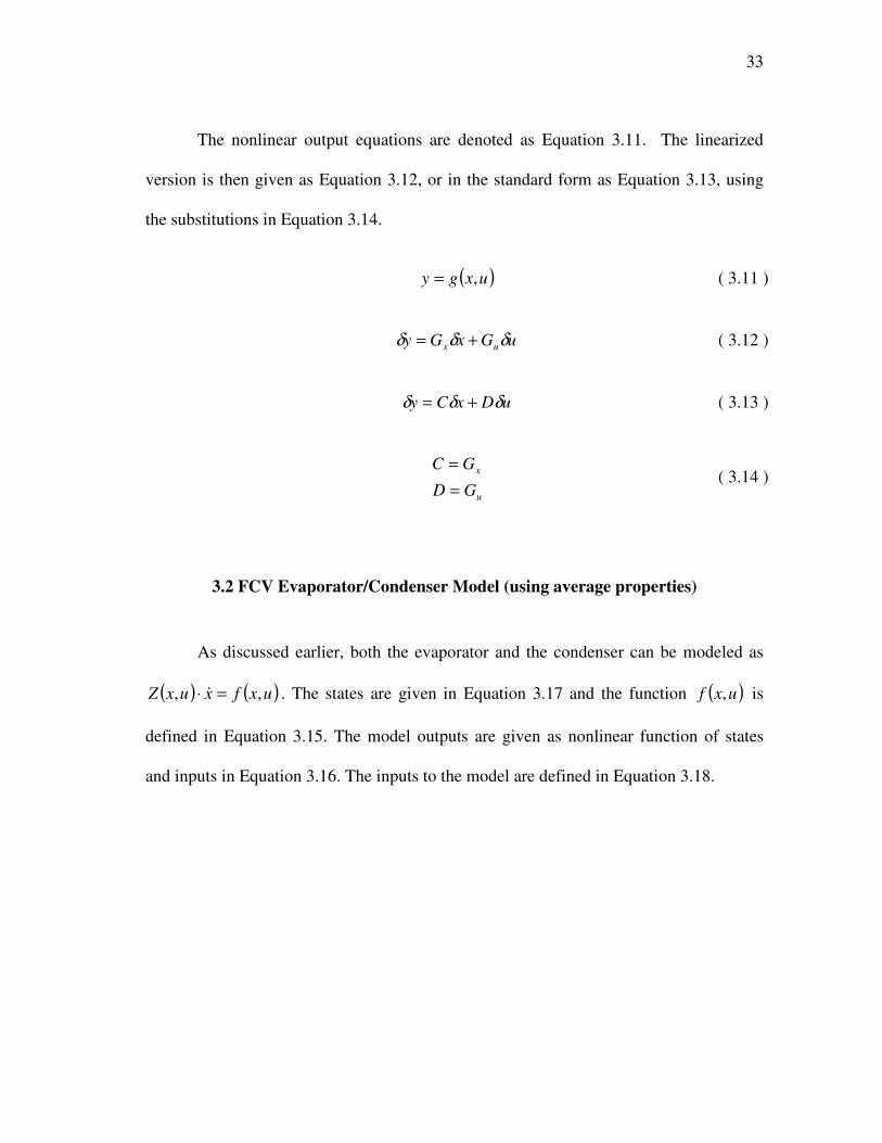
The nonlinear output equations are denoted as Equation 3.11. The linearized
version is then given as Equation 3.12, or in the standard form as Equation 3.13, using
the substitutions in Equation 3.14.
( )uxgy ,= ( 3.11 )
uGxGy ux δδδ += ( 3.12 )
uDxCy δδδ += ( 3.13 )
u
x
GD
GC
=
= ( 3.14 )
3.2 FCV Evaporator/Condenser Model (using average properties)
As discussed earlier, both the evaporator and the condenser can be modeled as
( ) ( )uxfxuxZ ,, =⋅ & . The states are given in Equation 3.17 and the function ( )uxf , is
defined in Equation 3.15. The model outputs are given as nonlinear function of states
and inputs in Equation 3.16. The inputs to the model are defined in Equation 3.18.

34
( ) ( )
( ) ( )
( ) ( )
( ) ( )
( ) ( )
( ) ( )
−+−
−+−
−+−
−
−+−
−+−
−+−
=
−
−
nwnanoonwnrnini
kwkakookwkrkiki
waoowrii
outin
nrnwninioutnin
krkwkikikkin
rwiiinin
TTATTA
TTATTA
TTATTA
mm
TTAhhm
TTAhhm
TTAhhm
uxf
,,,,,,,
,,,,,,,
1,1,1,1,1,1,1,
,,,,1
,,,,1
1,1,1,1,1
),(
αα
αα
αα
α
α
α
M
M
&&
&
M
&
M
&
( 3.15 )
( )
( )
( )( )
( ){ }
( )
⋅
⋅
⋅
+−
−+
−++
−++−
=
==
∑=
−
−
−
nene
keke
ee
oute
ina
n
k
inakao
nw
kw
w
in
n
e
n
ke
kn
nene
e
ne
ke
e
outr
outa
nw
kw
w
out
e
V
V
V
hPT
TTTn
T
T
T
hh
hhh
P
m
m
m
T
T
T
T
T
h
P
uxgy
,,
,,
1,1,
,
1
,,
,
,
1,
1,
1
,1,,
,
,
1,
,
,
,
,
1,
,
1
11
12
,
ρ
ρ
ρ
M
M
M
M
L
L
M
M
M
M
( 3.16 )
[ ]T
nwkwwnekeee TTThhhPx ,,1,,,1, KKKK= ( 3.17 )
[ ]Tairinainoutin mThmmu &&&
,= ( 3.18 )

35
The energy balance for the secondary fluid given a heat exchanger with n
regions is given in Equation 3.19 where kaoT , is the outlet temperature of secondary fluid
in the thk control region. The average temperature of secondary fluid is assumed as a
weighted average of inlet temperature and outlet temperature of the secondary fluid in
the region being considered given in Equation 3.20. µ is the coefficient between 0 and 1
used for calculating the weighted average of temperature. Solving for the average
temperature of secondary fluid, kaT , in the thk control region is given by Equation 3.21.
It can also be deduced that the overall outlet temperature of secondary fluid, outaT , is
related with the outlet temperature of secondary fluid of each control region by Equation
3.22. Thus, the overall outlet temperature of secondary fluid can be calculated as given
in Equation 3.23.
)()( ,,,,,,, kwkakokokaoinaairpair TTATTCm −=− α& ( 3.19 )
kaoinaka TTT ,,, )1( µµ −+= ( 3.20 )
11
1
1
,,
,
,
,,
,,
,
+
−
+
−=
koko
airpair
kw
koko
airpairina
ka
A
Cm
TA
CmT
T
αµ
αµ
&
&
( 3.21 )
( )∑=
−=−n
k
inakaoairp
air
inaoutaairpair TTCn
mTTCm
1
,,,,,, )(&
& ( 3.22 )

36
( )∑=
=n
k
kaoouta Tn
T1
,
1, ( 3.23 )
For linearization, the partial derivatives of average temperature of secondary
fluid are required. The partial derivatives of average temperature for the thk control
region are given in Equations 3.24 – 3.26. The secondary fluid side heat transfer
coefficient is a function of mass flow rate of secondary fluid. Thus, the partial derivative
of heat transfer coefficient can be calculated by calculating the slope of the heat transfer
correlation at the initial equilibrium point.
)(1)1(
11
1
1,,
,
,,,
,
2
,,
,
,
kwina
air
ko
ko
air
koko
airp
koko
airpairair
kaTT
m
m
A
C
A
Cmm
T−
∂
∂−
−
+
−
=∂
∂
&
&
&&
α
ααµ
αµ
( 3.24 )
))1(( ,,,
,
,
,
kokoairpair
airpair
ina
ka
ACm
Cm
T
T
αµ−+=
∂
∂
&
& ( 3.25 )
))1((
)1(
,,,
,,
,
,
kokoairpair
koko
kw
ka
ACm
A
T
T
αµ
αµ
−+
−=
∂
∂
& ( 3.26 )
The correlations mentioned in Equations 3.27 – 3.28 are also used. The
refrigerant side heat transfer coefficient is a function of mass flow rate of refrigerant
mass, heat exchanger pressure and enthalpy of the refrigerant. Thus, the partial
derivatives of heat transfer coefficient can be calculated by calculating the slope of the
heat transfer correlation at the initial equilibrium point.
37
( ) ( )( ) ( )in
j
e
j
ke
kj
jejej hhhhhh 1112 1,
1
,1,, −+−++−++−=−−
− LL ( 3.27 )
( ) ( )( ) ( )in
j
e
j
ke
kj
jejejj hhhhhhh 2111421
1,
2
,
1
1,,1
−−−−
−− −+−++−+++−=− LL ( 3.28 )
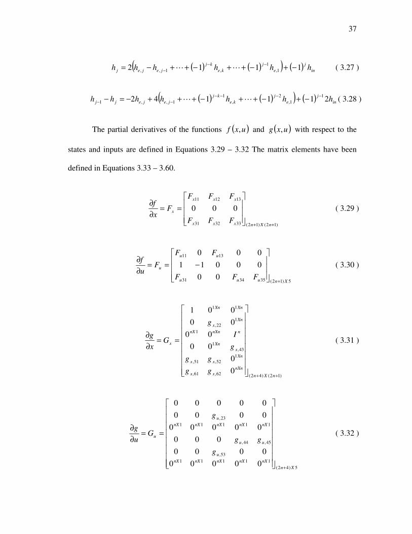
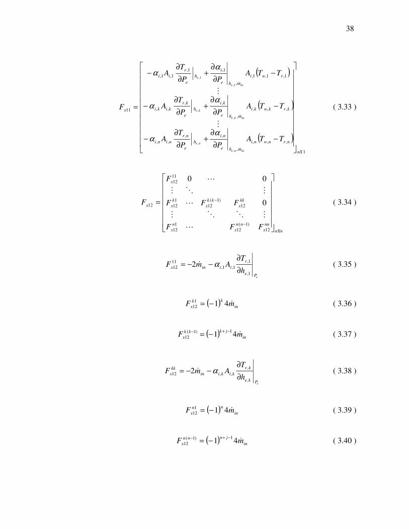
The partial derivatives of the functions ( )uxf , and ( )uxg , with respect to the
states and inputs are defined in Equations 3.29 – 3.32 The matrix elements have been
defined in Equations 3.33 – 3.60.
)12()12(333231
131211
000
++
==∂
∂
nXnxxx
xxx
x
FFF
FFF
Fx
f ( 3.29 )
5)12(353431
1311
00
00011
000
Xnuuu
uu
u
FFF
FF
Fu
f
+
−==∂
∂ ( 3.30 )
)12()42(62,61,
1
52,51,
43,
1
1
1
22,
11
0
0
00
00
00
001
++
==∂
∂
nXn
nXn
xx
Xn
xx
x
Xn
nnXnnX
Xn
x
XnXn
x
gg
gg
g
I
g
Gx
g ( 3.31 )
5)42(
11111
53,
45,44,
11111
23,
00000
0000
000
00000
0000
00000
Xn
nXnXnXnXnX
u
uu
nXnXnXnXnX
u
u
g
gg
g
Gu
g
+
==∂
∂ ( 3.32 )
38
( )
( )
( )1
,,,
,
,,
,,
,,,
,
,,
,,
1,1,1,
,
1,1,
1,1,
11
,
,
,
,
1,
1,
nX
nrnwni
mhe
ni
h
e
nr
nini
krkwki
mhe
ki
h
e
kr
kiki
rwi
mhe
i
h
e
r
ii
x
TTAPP
TA
TTAPP
TA
TTAPP
TA
F
inne
ne
inke
ke
ine
e
−∂
∂+
∂
∂−
−∂
∂+
∂
∂−
−∂
∂+
∂
∂−
=
&
&
&
M
M
αα
αα
αα
( 3.33 )
nXn
nn
x
nn
x
n
x
kk
x
kk
x
k
x
x
x
FFF
FFF
F
F
=
−
−
12
)1(
12
1
12
12
)1(
12
1
12
11
12
12 0
00
L
MOOM
L
MOM
L
( 3.34 )
ePe
r
iiinxh
TAmF
1,
1,
1,1,
11
12 2∂
∂−−= α& ( 3.35 )
( )in
kk
x mF &411
12 −= ( 3.36 )
( )in
jkkk
x mF &411)1(
12
−+− −= ( 3.37 )
ePke
kr
kikiin
kk
xh
TAmF
,
,
,,12 2∂
∂−−= α& ( 3.38 )
( )in
nn
x mF &411
12 −= ( 3.39 )
( )in
jnnn
x mF &411)1(
12
−+− −= ( 3.40 )

39
ePne
nr
niniin
nn
xh
TAmF
,
,
,,12 2∂
∂−−= α& ( 3.41 )
[ ]{ }ninikikiiix AAAdiagF ,,,,1,1,13 ααα KK= ( 3.42 )
( )
( )
( )1
,,,
,
,,
,,
,,,
,
,,
,,
1,1,1,
,
1,1,
1,1,
31
,,
,,
1,1,
nX
nwnrni
mhe
ni
he
nr
nini
kwkrki
mhe
ki
he
kr
kiki
wri
mhe
i
he
r
ii
x
TTAPP
TA
TTAPP
TA
TTAPP
TA
F
innene
inkeke
inee
−∂
∂+
∂
∂
−∂
∂+
∂
∂
−∂
∂+
∂
∂
=
&
&
&
M
M
αα
αα
αα
( 3.43 )
( )
( )
( )
−∂
∂−
∂
∂
−∂
∂−
∂
∂
−∂
∂−
∂
∂
=
nwnrni
mPne
ni
Pne
nr
nini
kwkrki
mPke
ki
Pke
kr
kiki
wri
mPe
i
Pe
r
ii
x
TTAhh
TA
TTAhh
TA
TTAhh
TA
diagF
inee
inee
inee
,,,
,,
,
,
,
,,
,,,
,,
,
,
,
,,
1,1,1,
,1,
1,
1,
1,
1,1,
32
&
&
&
M
M
αα
αα
αα
( 3.44 )
−
∂
∂+−
−
∂
∂+−
−
∂
∂+−
=
1
1
1
,
,
,,,,
,
,
,,,,
1,
1,
1,1,1,1,
33
nw
na
nononini
kw
ka
kokokiki
w
a
ooii
x
T
TAA
T
TAA
T
TAA
diagF
αα
αα
αα
M
M
( 3.45 )

40
( )
( )
( )1
,,,
,
,
1
,,,
,
,
1
1,1,1,
,
1,
1
11
,
,
1,
nX
nrnwni
hPin
ni
outn
krkwki
hPin
ki
kk
rwi
hPin
i
in
u
TTAm
hh
TTAm
hh
TTAm
hh
F
nee
kee
ee
−∂
∂+−
−∂
∂+−
−∂
∂+−
=
−
−
&
M
&
M
&
α
α
α
( 3.46 )
1
)1(
)1(
13
2)1(
2)1(
2
nXin
n
in
k
in
u
m
m
m
F
−
−=
−
−
&
M
&
M
&
( 3.47 )
( )
( )
( )1
,,,
,
,
,,,
,
,
1,1,1,
,
1,
31
,
,
1,
nX
nwnrni
hPin
ni
kwkrki
hPin
ki
wri
hPin
i
u
TTAm
TTAm
TTAm
F
nee
kee
ee
−∂
∂
−∂
∂
−∂
∂
=
&
M
&
M
&
α
α
α
( 3.48 )
1,
,
,,
,
,
,,
,
1,
1,1,
34
nXina
na
nono
ina
ka
koko
ina
a
oo
u
T
TA
T
TA
T
TA
F
∂
∂
∂
∂
∂
∂
=
α
α
α
M
M
( 3.49 )
41
1
,
,,,,,
,
,
,,,,,
,
1,
1,1,1,1,1,
1,
35
)(
)(
)(
nXair
na
nononwnano
air
no
air
ka
kokokwkako
air
ko
air
a
oowao
air
o
u
m
TATTA
m
m
TATTA
m
m
TATTA
m
F
∂
∂+−
∂
∂
∂
∂+−
∂
∂
∂
∂+−
∂
∂
=
&&
M
&&
M
&&
αα
αα
αα
( 3.50 )
( ) ( )[ ]Xn
knn
xg 1
1
22, 222121 −−−=−−
LL ( 3.51 )
( ) ( ) ( )
Xnnw
na
kw
ka
w
a
xT
T
nT
T
nT
T
ng
1,
,
,
,
1,
1,
43,1
1
1
1
1
1
∂
∂
−∂
∂
−∂
∂
−=
µµµLL ( 3.52 )
outhe
outr
xP
Tg
∂
∂=
,
51, ( 3.53 )
( ) ( )Xn
Pout
outr
Pout
outrkn
Pout
outrn
x
eee
h
T
h
T
h
Tg
1
,,,1
52, 22121
∂
∂
∂
∂−
∂
∂−=
−−LL ( 3.54 )
1
,
,
,
,
1,
1,
61,
,
,
1,
nXhe
ne
ne
he
ke
ke
he
e
e
x
ne
ke
e
PV
PV
PV
g
∂
∂
∂
∂
∂
∂
=
ρ
ρ
ρ
M
M
( 3.55 )

42
∂
∂
∂
∂
∂
∂=
eee Pne
ne
ne
Pke
ke
ke
Pe
e
exh
Vh
Vh
Vdiagg,
,
,
,
,
,
1,
1,
1,62,
ρρρLL ( 3.56 )
n
ug )1(23, −= ( 3.57 )
( ) ( )
11
1
1
1
,
,
,
,
,
1,
44, +−
−
∂
∂++
∂
∂++
∂
∂
−=
µµ ina
na
ina
ka
ina
a
uT
T
T
T
T
T
ng KK ( 3.58 )
( )
∂
∂++
∂
∂++
∂
∂
−=
air
na
air
ka
air
a
um
T
m
T
m
T
ng
&K
&K
&
,,1,
45,1
1
µ ( 3.59 )
ePout
outrn
uh
Tg
∂
∂−=
,
53, )1( ( 3.60 )
This model is not capable of capturing the system outputs due to induced
transients such as a change in the valve opening or a change in the compressor speed.
Even the slightest change in the input enthalpy instantaneously affects the output
enthalpy of the refrigerant as they are tightly coupled together due to a strict
mathematical relationship. The inlet and outlet enthalpies of the system are related
through the average enthalpies of all the control regions as given by Equation 3.27.
3.3 FCV Evaporator/Condenser Model (using properties at outlet)
As discussed earlier, both the evaporator and the condenser can be modeled as
( ) ( )uxfxuxZ ,, =⋅ & . The states are given in Equation 3.63 and the function ( )uxf , is

43
defined in Equation 3.61. The model outputs are given as nonlinear function of states
and inputs in Equation 3.62. The inputs to the model are defined in Equation 3.64.
( ) ( )
( ) ( )
( ) ( )
( ) ( )
( ) ( )
( ) ( )
−+−
−+−
−+−
−
−+−
−+−
−+−
=
−
−
nwnanoonwnrnini
kwkakookwkrkiki
waoowrii
outin
nrnwninioutnin
krkwkikikkin
rwiiinin
TTATTA
TTATTA
TTATTA
mm
TTAhhm
TTAhhm
TTAhhm
uxf
,,,,,,,
,,,,,,,
1,1,1,1,1,1,1,
,,,,1
,,,,1
1,1,1,1,1
),(
αα
αα
αα
α
α
α
M
M
&&
&
M
&
M
&
( 3.61 )
( )( ){ }
( )
⋅
⋅
⋅
+−=
==∑
=
nene
keke
ee
oute
ina
n
k
inakao
nw
kw
w
ne
e
ne
ke
e
outr
outa
nw
kw
w
out
e
V
V
V
hPT
TTTn
T
T
T
h
P
m
m
m
T
T
T
T
T
h
P
uxgy
,,
,,
1,1,
,
1
,,
,
,
1,
,
,
,
1,
,
,
,
,
1,
,
1,
ρ
ρ
ρ
M
M
M
M
M
M
M
M
( 3.62 )
[ ]T
nwkwwnekeee TTThhhPx ,,1,,,1, KKKK= ( 3.63 )

44
[ ]Tairinainoutin mThmmu &&&
,= ( 3.64 )
The energy balance for the secondary fluid given a heat exchanger with n
regions is given in Equation 3.65 where kaoT , is the outlet temperature of secondary fluid
in the thk control region. The average temperature of secondary fluid is assumed as a
weighted average of inlet temperature and outlet temperature of the secondary fluid in
the region being considered given in Equation 3.66. µ is the coefficient between 0 and 1
used for calculating the weighted average of temperature. Solving for the average
temperature of secondary fluid, kaT , in the thk control region is given by Equation 3.67.
It can also be deduced that the overall outlet temperature of secondary fluid, outaT , is
related with the outlet temperature of secondary fluid of each control region by Equation
3.68. Thus, the overall outlet temperature of secondary fluid can be calculated as given
in Equation 3.69.
)()( ,,,,,,, kwkakokokaoinaairpair TTATTCm −=− α& ( 3.65 )
kaoinaka TTT ,,, )1( µµ −+= ( 3.66 )
11
1
1
,,
,
,
,,
,,
,
+
−
+
−=
koko
airpair
kw
koko
airpairina
ka
A
Cm
TA
CmT
T
αµ
αµ
&
&
( 3.67 )

45
( )∑=
−=−n
k
inakaoairp
air
inaoutaairpair TTCn
mTTCm
1
,,,,,, )(&
& ( 3.68 )
( )∑=
=n
k
kaoouta Tn
T1
,
1, ( 3.69 )
For linearization, the partial derivatives of average temperature of secondary
fluid are required. The partial derivatives of average temperature for the thk control
region are given in Equations 3.70 – 3.72. The secondary fluid side heat transfer
coefficient is a function of mass flow rate of secondary fluid. Thus, the partial derivative
of heat transfer coefficient can be calculated by calculating the slope of the heat transfer
correlation at the initial equilibrium point.
)(1)1(
11
1
1,,
,
,,,
,
2
,,
,
,
kwina
air
ko
ko
air
koko
airp
koko
airpairair
kaTT
m
m
A
C
A
Cmm
T−
∂
∂−
−
+
−
=∂
∂
&
&
&&
α
ααµ
αµ
( 3.70 )
))1(( ,,,
,
,
,
kokoairpair
airpair
ina
ka
ACm
Cm
T
T
αµ−+=
∂
∂
&
& ( 3.71 )
))1((
)1(
,,,
,,
,
,
kokoairpair
koko
kw
ka
ACm
A
T
T
αµ
αµ
−+
−=
∂
∂
& ( 3.72 )
The refrigerant side heat transfer coefficient is a function of mass flow rate of
refrigerant mass, heat exchanger pressure and enthalpy of the refrigerant. Thus, the
partial derivatives of heat transfer coefficient can be calculated by calculating the slope
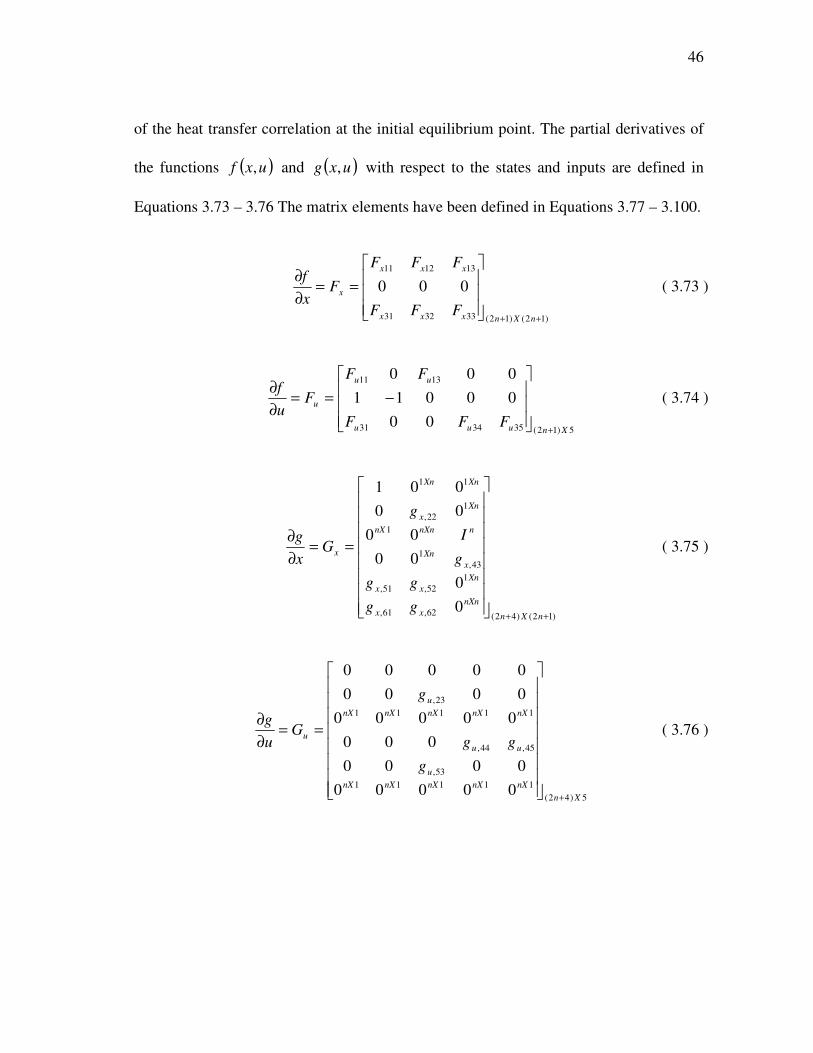
46
of the heat transfer correlation at the initial equilibrium point. The partial derivatives of
the functions ( )uxf , and ( )uxg , with respect to the states and inputs are defined in
Equations 3.73 – 3.76 The matrix elements have been defined in Equations 3.77 – 3.100.
)12()12(333231
131211
000
++
==∂
∂
nXnxxx
xxx
x
FFF
FFF
Fx
f ( 3.73 )
5)12(353431
1311
00
00011
000
Xnuuu
uu
u
FFF
FF
Fu
f
+
−==∂
∂ ( 3.74 )
)12()42(62,61,
1
52,51,
43,
1
1
1
22,
11
0
0
00
00
00
001
++
==∂
∂
nXn
nXn
xx
Xn
xx
x
Xn
nnXnnX
Xn
x
XnXn
x
gg
gg
g
I
g
Gx
g ( 3.75 )
5)42(
11111
53,
45,44,
11111
23,
00000
0000
000
00000
0000
00000
Xn
nXnXnXnXnX
u
uu
nXnXnXnXnX
u
u
g
gg
g
Gu
g
+
==∂
∂ ( 3.76 )

47
( )
( )
( )1
,,,
,
,,
,,
,,,
,
,,
,,
1,1,1,
,
1,1,
1,1,
11
,
,
,
,
1,
1,
nX
nrnwni
mhe
ni
h
e
nr
nini
krkwki
mhe
ki
h
e
kr
kiki
rwi
mhe
i
h
e
r
ii
x
TTAPP
TA
TTAPP
TA
TTAPP
TA
F
inne
ne
inke
ke
ine
e
−∂
∂+
∂
∂−
−∂
∂+
∂
∂−
−∂
∂+
∂
∂−
=
&
&
&
M
M
αα
αα
αα
( 3.77 )
nXn
nn
x
nn
x
kk
x
kk
x
x
x
FF
FF
F
F
=
−
−
12
)1(
12
12
)1(
12
11
12
12
00
0000
000
L
MOO
L
MOO
LL
( 3.78 )
( )1,1,1,
,1,
1,
1,
1,
1,1,
11
12 wri
mPe
i
Pe
r
iiinx TTAhh
TAmF
inee
−∂
∂−
∂
∂−−=
&
&α
α ( 3.79 )
in
kk
x mF &=− )1(
12 ( 3.80 )
( )kwkrki
mPke
ki
Pke
kr
kikiin
kk
x TTAhh
TAmF
inee
,,,
,,
,
,
,
,,12 −∂
∂−
∂
∂−−=
&
&α
α ( 3.81 )
in
nn
x mF &=− )1(
12 ( 3.82 )
( )nwnrni
mPne
ni
Pne
nr
niniin
nn
x TTAhh
TAmF
inee
,,,
,,
,
,
,
,,12 −∂
∂−
∂
∂−−=
&
&α
α ( 3.83 )
[ ]{ }ninikikiiix AAAdiagF ,,,,1,1,13 ααα KK= ( 3.84 )

48
( )
( )
( )1
,,,
,
,,
,,
,,,
,
,,
,,
1,1,1,
,
1,1,
1,1,
31
,,
,,
1,1,
nX
nwnrni
mhe
ni
he
nr
nini
kwkrki
mhe
ki
he
kr
kiki
wri
mhe
i
he
r
ii
x
TTAPP
TA
TTAPP
TA
TTAPP
TA
F
innene
inkeke
inee
−∂
∂+
∂
∂
−∂
∂+
∂
∂
−∂
∂+
∂
∂
=
&
&
&
M
M
αα
αα
αα
( 3.85 )
( )
( )
( )
−∂
∂−
∂
∂
−∂
∂−
∂
∂
−∂
∂−
∂
∂
=
nwnrni
mPne
ni
Pne
nr
nini
kwkrki
mPke
ki
Pke
kr
kiki
wri
mPe
i
Pe
r
ii
x
TTAhh
TA
TTAhh
TA
TTAhh
TA
diagF
inee
inee
inee
,,,
,,
,
,
,
,,
,,,
,,
,
,
,
,,
1,1,1,
,1,
1,
1,
1,
1,1,
32
&
&
&
M
M
αα
αα
αα
( 3.86 )
−
∂
∂+−
−
∂
∂+−
−
∂
∂+−
=
1
1
1
,
,
,,,,
,
,
,,,,
1,
1,
1,1,1,1,
33
nw
na
nononini
kw
ka
kokokiki
w
a
ooii
x
T
TAA
T
TAA
T
TAA
diagF
αα
αα
αα
M
M
( 3.87 )
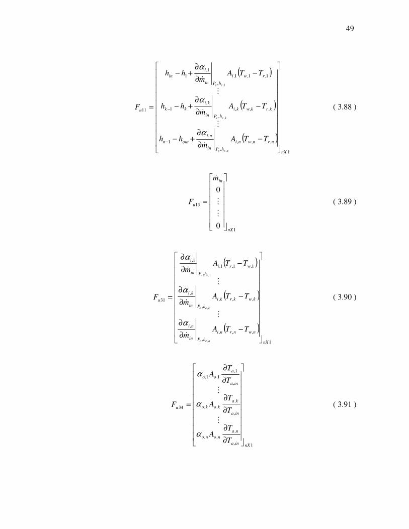
49
( )
( )
( )1
,,,
,
,
1
,,,
,
,
1
1,1,1,
,
1,
1
11
,
,
1,
nX
nrnwni
hPin
ni
outn
krkwki
hPin
ki
kk
rwi
hPin
i
in
u
TTAm
hh
TTAm
hh
TTAm
hh
F
nee
kee
ee
−∂
∂+−
−∂
∂+−
−∂
∂+−
=
−
−
&
M
&
M
&
α
α
α
( 3.88 )
1
13
0
0
nX
in
u
m
F
=
M
M
&
( 3.89 )
( )
( )
( )1
,,,
,
,
,,,
,
,
1,1,1,
,
1,
31
,
,
1,
nX
nwnrni
hPin
ni
kwkrki
hPin
ki
wri
hPin
i
u
TTAm
TTAm
TTAm
F
nee
kee
ee
−∂
∂
−∂
∂
−∂
∂
=
&
M
&
M
&
α
α
α
( 3.90 )
1,
,
,,
,
,
,,
,
1,
1,1,
34
nXina
na
nono
ina
ka
koko
ina
a
oo
u
T
TA
T
TA
T
TA
F
∂
∂
∂
∂
∂
∂
=
α
α
α
M
M
( 3.91 )
50
1
,
,,,,,
,
,
,,,,,
,
1,
1,1,1,1,1,
1,
35
)(
)(
)(
nXair
na
nononwnano
air
no
air
ka
kokokwkako
air
ko
air
a
oowao
air
o
u
m
TATTA
m
m
TATTA
m
m
TATTA
m
F
∂
∂+−
∂
∂
∂
∂+−
∂
∂
∂
∂+−
∂
∂
=
&&
M
&&
M
&&
αα
αα
αα
( 3.92 )
[ ]Xnxg 122, 100 L= ( 3.93 )
( ) ( ) ( )
Xnnw
na
kw
ka
w
a
xT
T
nT
T
nT
T
ng
1,
,
,
,
1,
1,
43,1
1
1
1
1
1
∂
∂
−∂
∂
−∂
∂
−=
µµµLL ( 3.94 )
outhe
outr
xP
Tg
∂
∂=
,
51, ( 3.95 )
XnPout
outr
x
e
h
Tg
1
,
52, 00
∂
∂= L ( 3.96 )
1
,
,
,
,
1,
1,
61,
,
,
1,
nXhe
ne
ne
he
ke
ke
he
e
e
x
ne
ke
e
PV
PV
PV
g
∂
∂
∂
∂
∂
∂
=
ρ
ρ
ρ
M
M
( 3.97 )

51
∂
∂
∂
∂
∂
∂=
eee Pne
ne
ne
Pke
ke
ke
Pe
e
exh
Vh
Vh
Vdiagg,
,
,
,
,
,
1,
1,
1,62,
ρρρLL ( 3.98 )
( ) ( )
11
1
1
1
,
,
,
,
,
1,
44, +−
−
∂
∂++
∂
∂++
∂
∂
−=
µµ ina
na
ina
ka
ina
a
uT
T
T
T
T
T
ng KK ( 3.99 )
( )
∂
∂++
∂
∂++
∂
∂
−=
air
na
air
ka
air
a
um
T
m
T
m
T
ng
&K
&K
&,,1,
45,1
1
µ ( 3.100 )

52
CHAPTER 4
EXPERIMENTAL SETUP
This chapter discusses the experimental equipment and the testing procedure for
generating and acquiring the data. The results are used for validating the nonlinear as
well as linearized models discussed in Chapters 2 and 3. The validation procedure has
been addressed in Chapter 6.
4.1 Test Facility
4.1.1 System Description
The test facility is located at the Thermo-Fluids Control Laboratory at Texas
A&M University at College Station, TX. The experimental system has been designed to
emulate heat exchange in a vapor compression cycle. The system components have been
fabricated to drive R134a (1,1,1,2 - Tetrafluoroethane) as the refrigerant and water as the
secondary fluid. Diagrams of the experimental system for the primary loop and the
secondary loop have been depicted in Figure 4.1 and Figure 4.2 respectively.

53
Evaporator #1
Condenser A1. Compressor
F
S4. R134a Mass Flow (E1)
Filter/Dryer
A2. EEV #1
P
S5. PERO1
Receiver
T
T2-CRO
T
T4-ERO-1
T
T3-ERI-1
T
T1-CRI
P
S11. PERO2
T
T6-ERO-2
T
T5-ERI-2
P
S3. PCRO
Evaporator #2
F
S9. R134a Mass Flow (E2)A3. EEV #2
A4. SDR
Figure 4.1: Experimental System Schematic for the Primary Loop

54
Evaporator #1Condenser
Pump #1
Water Supply Tank
T
T10-EWO-1
T
T12-EWO-2
A5. E1 Water
Flow Control
A6. E2 Water
Flow Control
Pump #2
MWV5—E1 FEED MWV6—E2 FEED
S10. Water Flow,
Evap 2
Evaporator #2
Water Mixing Tank
T
T8-CWO
T
T9-EWI-1
T
T11-EWI-2
MWV7—COND
SHUTOFF
MWV8—E1
SHUTOFFMWV9—E2
SHUTOFF
MWV10—COND
AIR BLEED
MWV11—E1
AIR BLEED
MWV12—E2
AIR BLEED
MWV1—DRAIN
MWV4—COND.
FEED
T
T7-CWI
Figure 4.2: Experimental System Schematic for the Secondary Loop

55
In Figure 4.1, beginning at the compressor (Figure 4.3), the pressurized fluid
(typically vapor) flows into the condenser. The condenser consists of a copper tube
coiled around a plastic core such that water can flow between the coil and the core. It has
been enclosed in a PVC pipe with openings for inlet and outlet of water as shown in
Figure 4.4. The refrigerant rejects heat to water inside the condenser. The condensed
fluid flows into the receiver shown in Figure 4.5. The receiver consists of a pressure
vessel such that only liquid refrigerant is withdrawn from it. The fluid is then made to
pass through a filter dryer shown in Figure 4.6 to make sure there are no remaining
vapors. To ensure proper functioning of the expansion valve only liquid refrigerant
should enter the valve. Trapped vapor in the valve opening will reduce the true area
available for fluid flow.
Figure 4.3: Compressor

56
Figure 4.4: Condenser
Figure 4.5: Receiver
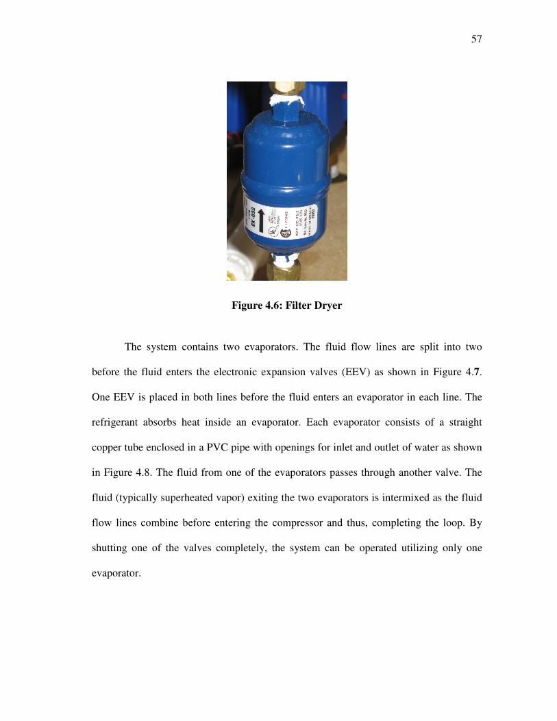
57
Figure 4.6: Filter Dryer
The system contains two evaporators. The fluid flow lines are split into two
before the fluid enters the electronic expansion valves (EEV) as shown in Figure 4.7.
One EEV is placed in both lines before the fluid enters an evaporator in each line. The
refrigerant absorbs heat inside an evaporator. Each evaporator consists of a straight
copper tube enclosed in a PVC pipe with openings for inlet and outlet of water as shown
in Figure 4.8. The fluid from one of the evaporators passes through another valve. The
fluid (typically superheated vapor) exiting the two evaporators is intermixed as the fluid
flow lines combine before entering the compressor and thus, completing the loop. By
shutting one of the valves completely, the system can be operated utilizing only one
evaporator.
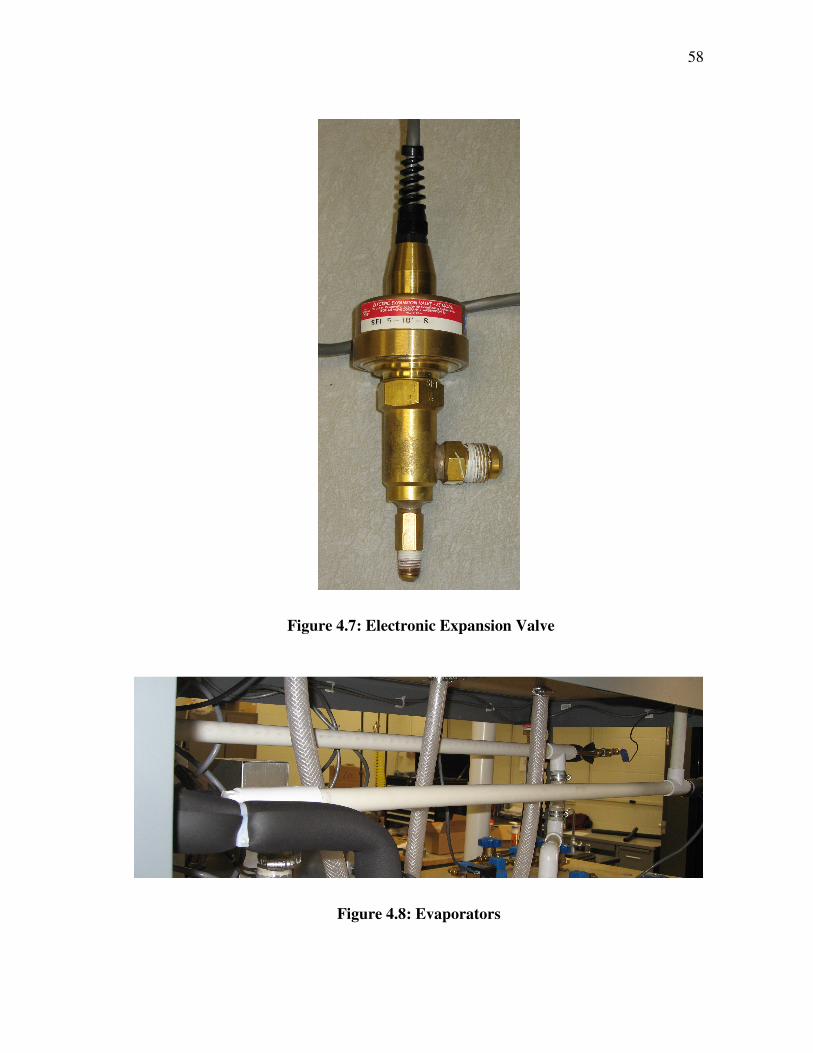
58
Figure 4.7: Electronic Expansion Valve
Figure 4.8: Evaporators
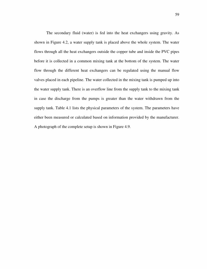
59
The secondary fluid (water) is fed into the heat exchangers using gravity. As
shown in Figure 4.2, a water supply tank is placed above the whole system. The water
flows through all the heat exchangers outside the copper tube and inside the PVC pipes
before it is collected in a common mixing tank at the bottom of the system. The water
flow through the different heat exchangers can be regulated using the manual flow
valves placed in each pipeline. The water collected in the mixing tank is pumped up into
the water supply tank. There is an overflow line from the supply tank to the mixing tank
in case the discharge from the pumps is greater than the water withdrawn from the
supply tank. Table 4.1 lists the physical parameters of the system. The parameters have
either been measured or calculated based on information provided by the manufacturer.
A photograph of the complete setup is shown in Figure 4.9.
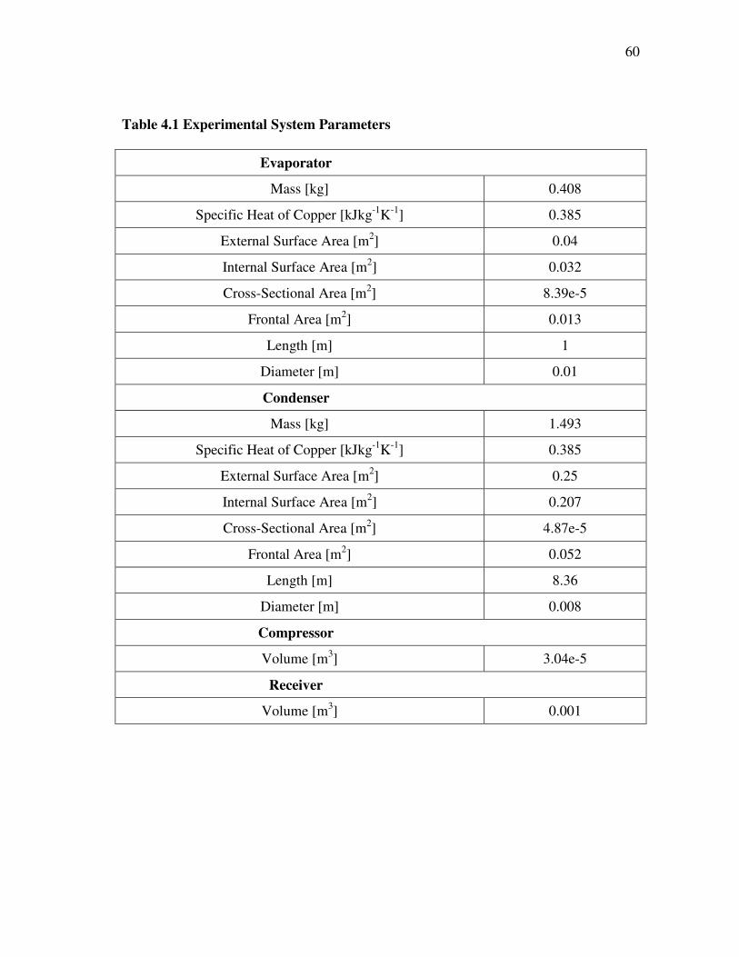
60
Table 4.1 Experimental System Parameters
Evaporator
Mass [kg] 0.408
Specific Heat of Copper [kJkg-1K-1] 0.385
External Surface Area [m2] 0.04
Internal Surface Area [m2] 0.032
Cross-Sectional Area [m2] 8.39e-5
Frontal Area [m2] 0.013
Length [m] 1
Diameter [m] 0.01
Condenser
Mass [kg] 1.493
Specific Heat of Copper [kJkg-1K-1] 0.385
External Surface Area [m2] 0.25
Internal Surface Area [m2] 0.207
Cross-Sectional Area [m2] 4.87e-5
Frontal Area [m2] 0.052
Length [m] 8.36
Diameter [m] 0.008
Compressor
Volume [m3] 3.04e-5
Receiver
Volume [m3] 0.001
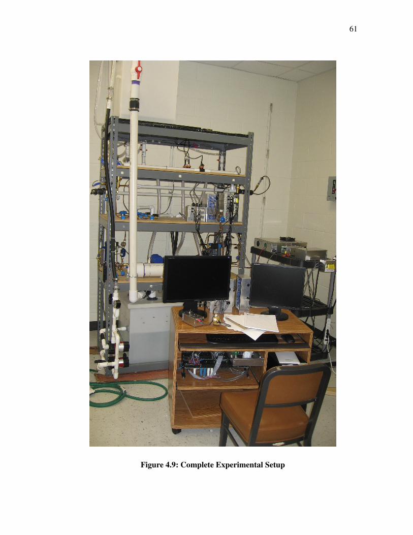
61
Figure 4.9: Complete Experimental Setup
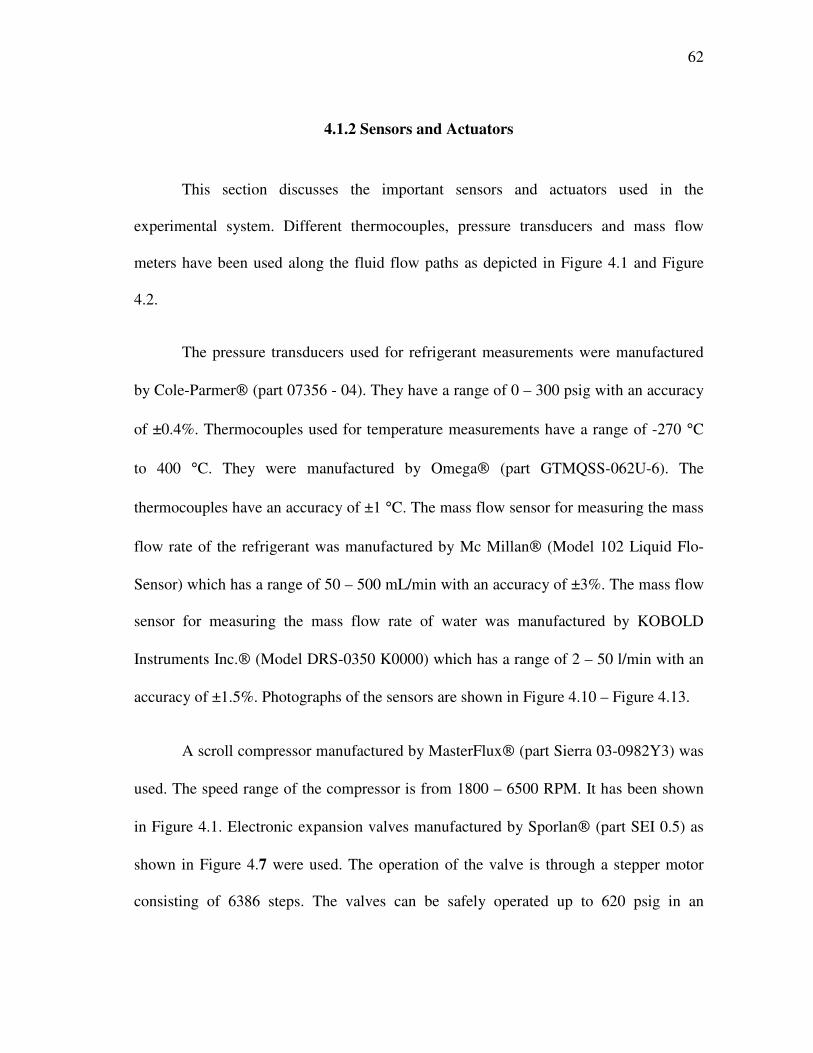
62
4.1.2 Sensors and Actuators
This section discusses the important sensors and actuators used in the
experimental system. Different thermocouples, pressure transducers and mass flow
meters have been used along the fluid flow paths as depicted in Figure 4.1 and Figure
4.2.
The pressure transducers used for refrigerant measurements were manufactured
by Cole-Parmer (part 07356 - 04). They have a range of 0 – 300 psig with an accuracy
of ±0.4%. Thermocouples used for temperature measurements have a range of -270 °C
to 400 °C. They were manufactured by Omega (part GTMQSS-062U-6). The
thermocouples have an accuracy of ±1 °C. The mass flow sensor for measuring the mass
flow rate of the refrigerant was manufactured by Mc Millan (Model 102 Liquid Flo-
Sensor) which has a range of 50 – 500 mL/min with an accuracy of ±3%. The mass flow
sensor for measuring the mass flow rate of water was manufactured by KOBOLD
Instruments Inc. (Model DRS-0350 K0000) which has a range of 2 – 50 l/min with an
accuracy of ±1.5%. Photographs of the sensors are shown in Figure 4.10 – Figure 4.13.
A scroll compressor manufactured by MasterFlux (part Sierra 03-0982Y3) was
used. The speed range of the compressor is from 1800 – 6500 RPM. It has been shown
in Figure 4.1. Electronic expansion valves manufactured by Sporlan (part SEI 0.5) as
shown in Figure 4.7 were used. The operation of the valve is through a stepper motor
consisting of 6386 steps. The valves can be safely operated up to 620 psig in an

63
operating temperature range between -45 °C to 60 °C. The flow rate of water flowing in
the system could also be regulated using flow control valve Erie (part AP23A000) but
it was kept constant during the experiments.
Figure 4.10: Pressure Gauge
Figure 4.11: Thermocouple
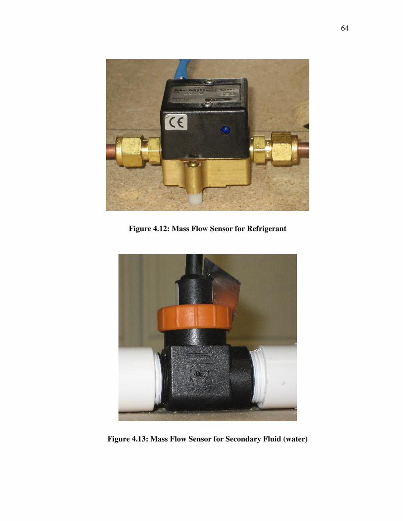
64
Figure 4.12: Mass Flow Sensor for Refrigerant
Figure 4.13: Mass Flow Sensor for Secondary Fluid (water)

65
Chapter 5
SIMULATION SOFTWARE: THERMOSYS ACADEMIC
This chapter describes a set of simulation tools developed for the purposes of
model validation, analysis, and controller design. This library was developed for use
with MatLab and its associated simulation program Simulink. At the time of
publication of this document, this software was entitled “Thermosys Academic”.
5.1 Introduction to Thermosys Academic
Creation of Thermosys Academic was initiated to provide a graphic drag-and-
drop interface for the user to utilize the mathematical modeling of vapor compression
components. The user can utilize the toolbox to predict the steady state as well as
dynamic behavior of a real complex system. The user is required to connect the inputs
and outputs to each component appropriately to represent the system. The toolbox also
provides a platform to validate new models as it can be used to compare the simulated
outputs with experimental data. The first version of this software was called Thermosys
Toolbox. Further details regarding the first version of the toolbox can be found in
[5,22,23].
Thermosys Academic has been designed with an open architecture where a user
can customize the existing components according to his preferences or add new ones.
The framework of the software has been designed in MatLab while Simulink is used to

66
solve the dynamics associated with the models. A basic skeleton of the static and
dynamic models has been created in Simulink. The models can be appropriately
renamed, using the Graphical User Interface (GUI), to provide the functioning of the
required component. The names of the components available in the Thermosys library
conform to a pre-defined naming convention, as discussed in subsequent sections.
5.2 Thermosys under New Setup
Due to some fundamental problems that were associated with the original design
of the Thermosys toolbox, it was decided to shift to the new Thermosys™ Academic. By
using the Thermosys under the new setup, it is much easier to customize the existing
models available in the Thermosys library as well as add new models to the library. The
basic structure of the Thermosys components has been described in this section.
5.2.1 Thermosys Academic Simulink Blocks
Several tools required to simulate the proper functioning of a vapor compression
system are available in the Thermosys library. The tools can be accessed using the
Simulink Library browser under Thermosys as shown in Figure 5.1. The tools are
organized into two directories: Components and Fluid Properties. Three types of
components are available in Thermosys: Dynamic model, Static model and Static model
with transport delay. Any of these components can be dragged in a Simulink model to

67
simulate the functioning of the appropriate component. These are generic blocks and can
morph into the appropriate component as chosen by the user, to simulate the real
component. The models of different components are categorized into one of the three
types based on its nature. All the variations of evaporator, condenser and compressor
models are dynamics models, for example evaporator with receiver model. The
expansion valve is a static model while all the pipe models are static models with
transport delay. The user needs to rename the appropriate generic blocks into component
models which are required. An exhaustive list of available components can be found at
[4]. The next section discusses the dynamic model block. The other two static model
blocks are used in the same manner as the dynamic model block.

68
Figure 5.1: Simulink Library Browser

69
5.2.1.1 Dynamic Model Block
Figure 5.2: Basic dynamic model layout for Thermosys Academic
As mentioned previously, the dynamic model block in the Thermosys Academic
library is utilized for simulating a dynamic component such as an evaporator, condenser
etc. The user is required to specify the Base Function Name and the Component Number
for the dynamic model block using a GUI which has been discussed in subsequent
sections. To access the Simulink block diagram of the dynamic model block the user can
right click on the block and select the Look Under Mask option. This will open up the
Simulink diagram shown in Figure 5.2. The primary dynamic model function to simulate
the component is placed in the function block titled Model by the GUI. The Base
Function Name followed by the Component Number is used to rename the To

70
Workspace block (outlined in green in Figure 5.2). The Component Number field is
written in the block titled Num (outlined in blue in Figure 5.2). Another function
(following the predefined naming structure discussed in the following section) is called
to set the input and output dimensions of the demux block (outlined in red in Figure 5.2).
Figure 5.3: Initial Conditions Subsystem
At the start of the simulation, the initial conditions to the integrator block are
provided by the Initial Conditions subsystem as shown in Figure 5.2. Double clicking on
this Initial Conditions subsystem, opens up the Simulink diagram shown in Figure 5.3.
This subsystem is enabled only at the first time step of the simulation. Double clicking
the Enabled Subsystem block in Figure 5.3, opens up the Simulink diagram depicted in
Figure 5.4. The GUI writes an appropriate function name to the X0 block in Figure 5.4
using the Base Function Name provided by the user. This function name also follows the
predefined naming structure. This function outputs the initial conditions for the
component which had been created before the start of the simulation using the Initial
Conditions Creator for the component.

71
Figure 5.4: The Enabled Subsystem used to calculate the initial conditions
5.2.3 Component Naming Convention
For each of the dynamic components available in Thermosys Academic, there are
five associated m-files (MatLab function files) with that component. The predefined
naming structure for each associated m-file is shown in Table 5.1. An example for an
evaporator (Base Function Name: Evap) is also shown. The first m-file is the primary
model file which is required to simulate the dynamics associated with the component. It
is called at each time step during the simulation and is placed in the function block titled
Model in Figure 5.2. The second m-file is required to set up the inputs and outputs of the
demux block shown in Figure 5.2. It is called by the GUI each time the dynamic model
is renamed. The third m-file is called only at the first time step of the simulation. It is
placed in the XO block in Figure 5.4. It provides the initial conditions to the integrator
block shown in Figure 5.2 through the Enable Subsystem block shown in Figure 5.3. The
fourth file is called at the end of the simulation and is known as the Record Function.

72
The simulation may come to an end or may be terminated by the user. At the stop of the
simulation, the Stop Function associated with the To Workspace block shown in Figure
5.2 is invoked which in turn invokes the Record function associated with the component.
The Stop Function can be accessed by right clicking the To Workspace block, selecting
Block Properties and then selecting Callbacks tab. It has been shown in Figure 5.5. The
Record function for a component reorganizes the individual outputs from that
component and stores them in a structure called Simulated_Outputs. Within this
structure the outputs from all the different components are organized under their own
formatted name ([component][component_number]). The last m-file is known as the
Initial Conditions Creator (or IC Creator). It is run before the start of the simulation after
the global structures have been created. Global structures are discussed in the next
section. The IC Creator helps create the initial conditions for the component using the
operating conditions and physical parameters specified by the user in the global
structures. It contains different solution methods to create the initial conditions for the
component. If no solution method is specified by the user, the first method will be used
as default. Description of the available solution methods for creating the initial
conditions for the component can be read by typing help [component]IC_Creator on the
MatLab command prompt. All the files are required for the functioning of the
component in the Thermosys toolbox. For static components, all the files except
[component]IC.m are required.
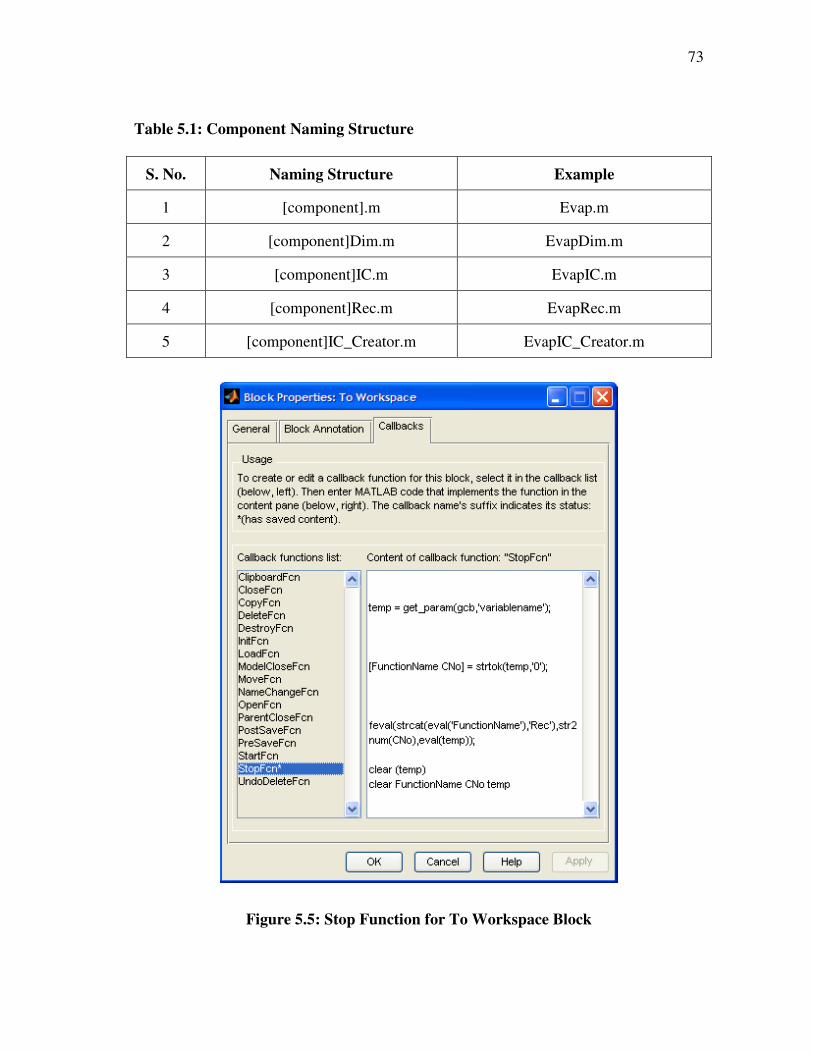
73
Table 5.1: Component Naming Structure
S. No. Naming Structure Example
1 [component].m Evap.m
2 [component]Dim.m EvapDim.m
3 [component]IC.m EvapIC.m
4 [component]Rec.m EvapRec.m
5 [component]IC_Creator.m EvapIC_Creator.m
Figure 5.5: Stop Function for To Workspace Block
74
5.2.4 Global Structures
Thermosys Academic uses global parameter structures to perform a variety of
tasks in the modeling process. These structures are accessed by the various MatLab
function blocks via the associated m-file. The two basic structures that the user must
load manually into the MatLab workspace are named Physical_Parameters and
Operating_Conditions. These two structures provide the component models with the
necessary heat exchanger geometry and initial simulation operating conditions required
to calculate the initial conditions. The global parameter structures need to be created
using the naming convention where the Base Function Name concatenated with the
Component Number is the primary subheading in the global parameter structure.
A third structure, named Initial_Conditions, is created by invoking the
[component]IC_Creator m-file mentioned earlier. The IC Creator for each component is
required to be run prior to the start of the simulation. A fourth structure called
Simulated_Outputs, is created automatically at the stop of the simulation.
Simulated_Outputs contains the outputs generated by all the individual components at
each time step.
5.2.5 Fluid Property Tables
Fluid properties are calculated using tables or subroutines. The tables use
interpolation based on predefined tables, whereas the subroutines iteratively solve

75
empirical equations of state for the selected fluid. The Thermosys Toolbox currently
contains thermo-physical properties and data for five different refrigerants: R134a, R744
(CO2), R22, R404a and R410a.
1-D and 2-D look-up tables were generated in EES (Engineering Equation
Solver) and saved as comma-delimited files (csv). A MatLab m-file loads the comma-
delimited files and stores the data in matrix form. Partial derivatives of thermodynamic
functions are also evaluated and stored as matrices. The tables can be used to calculate
thermodynamic properties by using the interpolation routines included with
MatLab/Simulink®. The Thermosys Toolbox contains pre-programmed Simulink 1-D
and 2-D interpolation blocks for fluid property calculation. These are independent of the
type of fluid. The properties of the fluid loaded in the MatLab workspace are used.
5.2.6 Heat Transfer Correlations
The heat exchanger components use correlations to calculate the necessary heat
transfer coefficients. However, because of the unlimited number and variety of such
correlations, it is impossible to include even a fraction of those desired. Some of the
more important correlations have been included in Thermosys Academic as subroutines.
Other options have also been included such as to specify a constant value, a user-defined
correlation, or to calculate the value from entered data. Under the new setup, the
subroutines are called at each time step and the heat transfer coefficient values are
updated.

76
5.3 Software Usage
5.3.1 Customization of Existing Components
This section describes how the existing components available in Thermosys
Academic can be put to use to simulate a vapor compression cycle. First, the skeletal
structure of the system that needs to be simulated is created. During the simulation,
Simulink calls the appropriate functions for simulating the dynamics of the individual
components in the system. Prior to the start of the simulation, standard global parameter
structures need to be created as mentioned in prior sections. MatLab reads the data from
the global structures during the simulation. Three global structures are required. The first
structure has been called Physical_Parameters. The physical parameters related to the
individual components are specified in this structure. Operating conditions for the
system are defined in Operating_Conditions structure. A third structure, called the
Initial_Conditions, specifying the initial conditions of the system is also required. The
initial conditions of the system can either be specified directly in the Initial Conditions
structure or can be created using the initial conditions creator available in the Thermosys
library for each component used in the system. It is recommended that the user use the
available subroutines to setup the initial conditions structure.
Double clicking a component brings up the GUI shown in Figure 5.6, associated
with that component. The user is required to specify the standard name of the component
in the field titled Base Function Name. In the field titled Component Number, the user is
77
required to put in the component number in which its corresponding parameters are
stored in the global structures. Then, the user needs to press the button titled Apply. This
will show the parameters of that component stored in the global parameter structures in
the corresponding fields on the GUI. Then the user presses the button titled “OK” to
save the changes in the model. This process is repeated one by one for all the
components. Once this initial process to setup the simulation has been completed, the
user specifies configuration parameters for the simulation in Simulink and starts the
simulation. As soon as the simulation completes, or is terminated, the outputs of all the
individual components are automatically stored in the MatLab workspace in a structure
titled Simulated_Outputs. The outputs are available for the user to access, analyze and/or
save them, if required.

78
Figure 5.6: GUI for Dynamic/Static Block
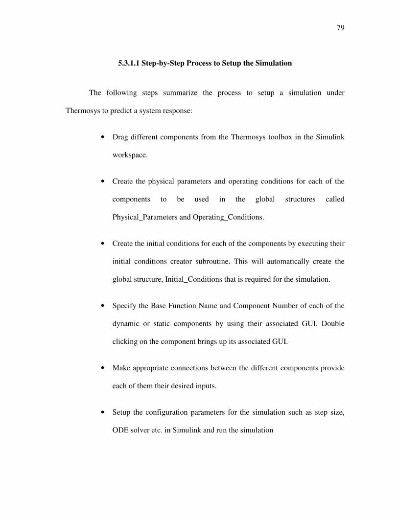
79
5.3.1.1 Step-by-Step Process to Setup the Simulation
The following steps summarize the process to setup a simulation under
Thermosys to predict a system response:
• Drag different components from the Thermosys toolbox in the Simulink
workspace.
• Create the physical parameters and operating conditions for each of the
components to be used in the global structures called
Physical_Parameters and Operating_Conditions.
• Create the initial conditions for each of the components by executing their
initial conditions creator subroutine. This will automatically create the
global structure, Initial_Conditions that is required for the simulation.
• Specify the Base Function Name and Component Number of each of the
dynamic or static components by using their associated GUI. Double
clicking on the component brings up its associated GUI.
• Make appropriate connections between the different components provide
each of them their desired inputs.
• Setup the configuration parameters for the simulation such as step size,
ODE solver etc. in Simulink and run the simulation

80
• Access/analyze and save the generated outputs using the structure
Simulated_Outputs from the MatLab workspace. This structure is
automatically created after the simulation is terminated or it reaches the
end.
5.3.2 Adding New Components to Thermosys Academic
This section is of use for advanced users of Thermosys Academic who would be
interested in enhancing the capabilities of the software by adding new dynamic or static
components to the Thermosys library. The user needs to create four or five m-files
(shown in Table 5.1) depending on whether the component is a static or a dynamic
model. The user needs to use a Base Function Name which does not exist in the
Thermosys library. The user needs to create all the five m-files described earlier as per
the predefined naming convention. The files can be created using the m-files of any of
the existing components as a benchmark. If a static model is being created, it is not
required to create the [component]IC.m file.
5.3.1.1 Step-by-Step Process to Add a New Component
The following steps summarize the process to add a new component to
Thermosys Academic:
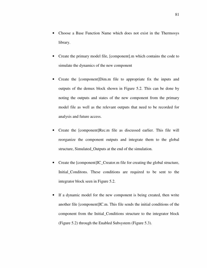
81
• Choose a Base Function Name which does not exist in the Thermosys
library.
• Create the primary model file, [component].m which contains the code to
simulate the dynamics of the new component
• Create the [component]Dim.m file to appropriate fix the inputs and
outputs of the demux block shown in Figure 5.2. This can be done by
noting the outputs and states of the new component from the primary
model file as well as the relevant outputs that need to be recorded for
analysis and future access.
• Create the [component]Rec.m file as discussed earlier. This file will
reorganize the component outputs and integrate them to the global
structure, Simulated_Outputs at the end of the simulation.
• Create the [component]IC_Creator.m file for creating the global structure,
Initial_Conditons. These conditions are required to be sent to the
integrator block seen in Figure 5.2.
• If a dynamic model for the new component is being created, then write
another file [component]IC.m. This file sends the initial conditions of the
component from the Initial_Conditions structure to the integrator block
(Figure 5.2) through the Enabled Subsystem (Figure 5.3).

82
5.4 Simulink Model Limitations
The primary method for fluid property calculation has limitations. First, the
calculated result is only as accurate as the mesh used to create the interpolation table
(Figure 5.7). Second, when evaluating properties near the critical point, incorrect results
are more likely. A good example of this can be seen when plotting specific heat near the
critical point (Figure 5.8). There is a sudden drop in the specific heat as there is a change
in the state of the fluid. This increases the gradient of specific heat to infinity near the
critical point.
-2000
200400
600
0
1000
2000
3000
4000-100
0
100
200
300
400
Enthalpy (kJ/kg)Pressure (kPa)
Tem
per
ature
(C
)
Figure 5.7: Sample Interpolation Table: Temperature as a Function of Pressure
and Enthalpy for R134a

83
-500
50100
150
0
1000
2000
3000
40000.5
1
1.5
2
2.5
3
Temperature (C)Pressure (kPa)
Spec
ific
Hea
t (k
J/k
g/C
Figure 5.8: Sample Interpolation Table: Specific Heat as a Function of Pressure
and Temperature for R134a
5.5 Future Additions
Efforts to improve the library are continuous. Planned additions to the library
include addition of FCV models of heat exchangers with pressure drop, separation of
liquid side and vapor side property tables to prevent inaccurate calculations near the
critical point as well as greater variety of component models.
84
CHAPTER 6
MODEL VALIDATION
While it is never possible to verify that a theory is true however many
observations appear to confirm it, it is possible to falsify a theory if just one observation
contradicts it. This means that scientific theories are testable though not provable and so
the demarcation criterion is whether or not the theory is falsifiable [21]. To test that the
modeling approach outlined in this report appropriately predicts the dynamic behavior of
vapor compression cycles, simulation results were compared with experimental data
obtained. A detailed description of the model validation approach is given in [22,23].
Relevant information from these publications is replicated with permission in this
section for convenience.
The model validation procedure includes the verification of both the prediction of
steady state data as well as the ability of the model to capture the transients of the
system. The first section outlines the general validation procedure, and includes a
description of the various parameters used in the simulation. The next section presents
the comparisons between simulated and experimental data followed by observations.
6.1 Validation Procedure
The parameters for each of the individual components are grouped in three
categories: measurable, empirical, and tunable. The measurable parameters are physical

85
characteristics of the component such as lengths, masses, diameters, etc. For each of the
component, these were measured or calculated based on data provided by the
manufacturer. The empirical parameters are efficiencies or other empirically determined
relationships. Usually, the tunable parameters cannot be measured easily, but are known
to be within a certain range of values and are assumed to follow commonly accepted
parameter correlations.
Thus, the first step of model verification will be determining the measurable and
empirical parameters. Then the tunable parameters are adjusted within reasonable
bounds so that the simulated dynamics approximate the experimentally recorded
dynamics.
6.1.1 Physical Parameters
6.1.1.1 Evaporator and Condenser
Hydraulic Diameter – For different types of heat exchangers (plate, tube, micro-
channel, etc.) this value is calculated differently. Suggestions for calculating this value
for the different types of heat exchangers are available in the literature, and are heat
exchanger dependent. The diameter for the different heat exchangers used in the
experimental system was measured.

86
Fluid Flow Length – This value is defined as the length that the fluid travels from
the entrance to the exit of the heat exchanger. All possible fluid flow paths are assumed
to have the same length. Many heat exchangers use a series of tubes or plates arranged in
a serpentine manner for fluid flow. Often these tubes or plates will join at a “header” and
the fluid is redistributed before entering the next “pass” or series of or tubes or plates.
The fluid flow length of the heat exchangers used in the experimental system was
measured.
Cross-sectional Area – This value can be calculated using the hydraulic diameter.
For most heat exchangers the cross-sectional area is not constant. The number of tubes
or plates per pass generally increases as the fluid evaporates or decreases as the fluid
condensates, thus changing the cross-sectional area. For the purposes of modeling, a
constant cross-sectional area in a control region is assumed. If the cross-sectional area is
calculated from the hydraulic diameter, then it does not take into account headers,
distributors, etc.
Internal Volume – This value can either be calculated as the product of cross-
sectional area and fluid flow length or be measured experimentally. The former does not
account for headers, entrance pipes, etc. and is considered to be the lower bound. The
latter includes all these “extra” volumes and is considered to be the upper bound. Thus
this parameter can be tuned within these bounds.
Internal Surface Area – This parameter is calculated from the hydraulic diameter
of the heat exchanger.
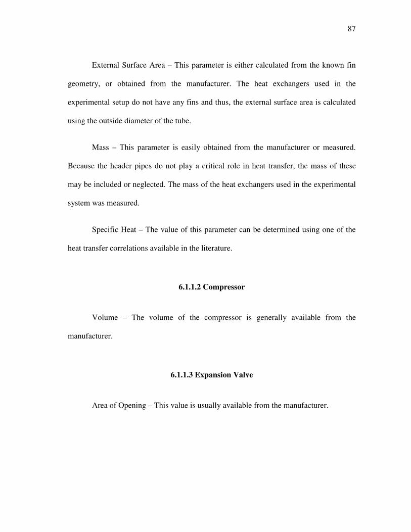
87
External Surface Area – This parameter is either calculated from the known fin
geometry, or obtained from the manufacturer. The heat exchangers used in the
experimental setup do not have any fins and thus, the external surface area is calculated
using the outside diameter of the tube.
Mass – This parameter is easily obtained from the manufacturer or measured.
Because the header pipes do not play a critical role in heat transfer, the mass of these
may be included or neglected. The mass of the heat exchangers used in the experimental
system was measured.
Specific Heat – The value of this parameter can be determined using one of the
heat transfer correlations available in the literature.
6.1.1.2 Compressor
Volume – The volume of the compressor is generally available from the
manufacturer.
6.1.1.3 Expansion Valve
Area of Opening – This value is usually available from the manufacturer.

88
6.1.1.4 Receiver
Volume – This value is usually available from the manufacturer.
6.1.2 Empirical Parameters
6.1.2.1 Evaporator and Condenser
Mean Void Fraction – Many correlations are available as outlined in Chapter 1.
For these simulations, a general slip ratio correlation is assumed.
6.1.2.2 Compressor
Isentropic Efficiency – This value can be estimated using experimental steady
state data, or obtained from the manufacturer.
Volumetric Efficiency – This value can be estimated using experimental steady
state data, or obtained from the manufacturer.
Rate Limit – Actual compressors are rate-limited in their ability to change speed.
This value can be measured from data.

89
6.1.2.3 Expansion Valve
Control Input Relationship – The control input is related to the valve opening
assuming a linear relationship. The empirical parameters for this equation can be
determined using experimental data.
Discharge Coefficient – This value can be estimated using experimental steady
state data, or obtained from the manufacturer.
Rate Limit – Actual expansion valves are rate-limited in their ability to change
the valve opening. This value can be measured from data.
6.1.3 Tunable Parameters
6.1.3.1 Evaporator
Void Fraction Slip Ratio – Slip ratio is defined as the ratio of the velocities of the
vapor and liquid phases in a two-phase flow. The generally accepted bounds on this
parameter are given by the homogeneous correlation and the Zivi correlation. The
homogeneous correlation assumes a slip ratio of unity, 1=S , and the Zivi correlation
gives the slip ratio as ( ) 3/1
gf ρρ . Thus, the slip ratio can be varied between these
bounds.

90
Heat Transfer Coefficients – These values are estimated along the course of the
simulation using an empirical correlation chosen by the user. For these simulations, the
Gnielinski correlation [11] and Wattlet correlation [27] were used for single-phase and
two-phase heat transfer coefficients on refrigerant side respectively. The Colburn Factor
correlation was used for heat transfer coefficient on the secondary fluid side.
6.2 Simulated and Experimental Results
The final choice of parameters used for simulation for model validation is given
in Table 6.1. The initial value of cross-sectional area was estimated based on hydraulic
diameter. Due to a faster transient response of pressure, it was concluded that the
effective volume of the control regions was underestimated. The upper bound of
effective volume of the heat exchanger was calculated as the sum of the volume of the
heat exchanger and the volume of entrance and exit pipes. The chosen effective cross-
sectional area is a value within these bounds. The value of slip ratio was chosen
according to the Zivi correlation. The empirical relationships of mass flow through the
compressor and the valve were developed using steady state data. The two-phase flow
heat transfer coefficient was estimated at each time step using the Wattlet correlation
while that for single-phase flow was estimated using Gnielinski correlation. The Colburn
Factor correlation was used for heat transfer coefficient on the secondary fluid side.
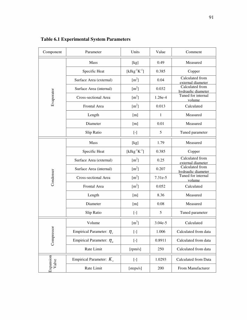
91
Table 6.1 Experimental System Parameters
Component Parameter Units Value Comment
Ev
apo
rato
r
Mass [kg] 0.49 Measured
Specific Heat [kJkg-1K-1] 0.385 Copper
Surface Area (external) [m2] 0.04 Calculated from
external diameter
Surface Area (internal) [m2] 0.032 Calculated from
hydraulic diameter
Cross-sectional Area [m2] 1.26e-4 Tuned for internal
volume
Frontal Area [m2] 0.013 Calculated
Length [m] 1 Measured
Diameter [m] 0.01 Measured
Slip Ratio [-] 5 Tuned parameter
Co
nd
ense
r
Mass [kg] 1.79 Measured
Specific Heat [kJkg-1K-1] 0.385 Copper
Surface Area (external) [m2] 0.25 Calculated from
external diameter
Surface Area (internal) [m2] 0.207 Calculated from
hydraulic diameter
Cross-sectional Area [m2] 7.31e-5 Tuned for internal
volume
Frontal Area [m2] 0.052 Calculated
Length [m] 8.36 Measured
Diameter [m] 0.08 Measured
Slip Ratio [-] 5 Tuned parameter
Co
mp
ress
or
Volume [m3] 3.04e-5 Calculated
Empirical Parameter: vη [-] 1.006 Calculated from data
Empirical Parameter: aη [-] 0.8911 Calculated from data
Rate Limit [rpm/s] 250 Calculated from data
Ex
pan
sio
n
Val
ve Empirical Parameter: vK [-] 1.0293 Calculated from Data
Rate Limit [steps/s] 200 From Manufacturer

92
For model validation, data is collected for transients induced in the system at
steady state due to change in compressor speed. Both the nonlinear as well as linearized
models are compared with experimental data. The outputs of interest evaporator
pressure, evaporator superheat and evaporator water exit temperature are compared.
Figure 6. 1 – Figure 6.4 show model outputs for changes in compressor speed.
For all the model outputs, there is a general agreement, but also notable discrepancies.
For evaporator pressure, the model agrees in the speed of the response but there is a
slight aberration in the steady state gain. For evaporator superheat, the general shape of
the transient is correct, but the speed of the response and steady state magnitudes are
incorrect. The fluid property calculation has limitations which is one of the reasons for
inaccurate prediction of steady state magnitude. The evaporator water exit temperature
appears to match well with data.
The FCV model was also examined for dependency on the selected number of
regions. As expected, the predicted transients increased in accuracy for increasing levels
of discretization, with the simulation results virtually indistinguishable at higher
discretization levels. Figure 6.6 shows the response of the evaporator pressure of a
simple straight tube evaporator for a step change in expansion valve opening (Figure
6.5), for FCV models with 2, 8, 12 and 15 control volumes. While relatively few regions
were required for this deliberately simple geometry, higher levels of discretization would
be appropriate for more realistic heat exchanger configurations.

93
0 50 100 150 200 250 300 350 400 4503300
3400
3500
3600
3700
3800
3900
4000
4100
4200
Time (sec)
Co
mp
ress
or
RP
M
Figure 6. 1: Model Validation: Compressor RPM
0 50 100 150 200 250 300 350 400 450216
218
220
222
224
226
228
230
232
234
236
Time (sec)
Evap
ora
tor
Pre
ssure
(k
Pa)
Data
Linear FCV Evaporator
Nonlinear FCV Evaporator
Figure 6. 2: Model Validation: Evaporator Pressure

94
0 50 100 150 200 250 300 350 400 4504
5
6
7
8
9
10
Time (sec)
Ev
apora
tor
Sup
erh
eat
(C)
Data
Linear FCV Evaporator
Nonlinear FCV Evaporator
Figure 6.3: Model Validation: Evaporator Superheat
0 50 100 150 200 250 300 350 400 45025
25.05
25.1
25.15
25.2
25.25
25.3
25.35
25.4
25.45
25.5
Time (sec)
Ev
apo
rato
r O
utl
et W
ater
Tem
per
ature
(C
)
Data
Linear FCV Evaporator
Nonlinear FCV Evaporator
Figure 6.4: Model Validation: Evaporator Water Outlet temperature
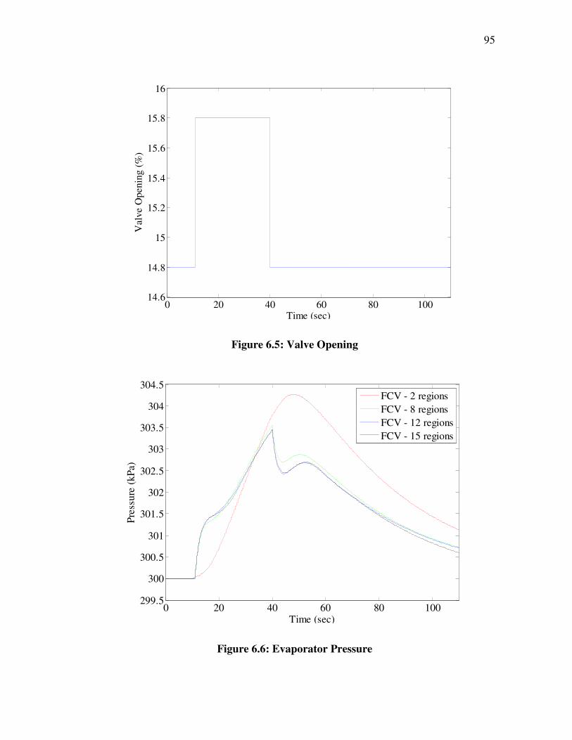
95
0 20 40 60 80 10014.6
14.8
15
15.2
15.4
15.6
15.8
16
Time (sec)
Val
ve
Op
enin
g (
%)
Figure 6.5: Valve Opening
0 20 40 60 80 100299.5
300
300.5
301
301.5
302
302.5
303
303.5
304
304.5
Time (sec)
Pre
ssu
re (
kP
a)
FCV - 2 regions
FCV - 8 regions
FCV - 12 regions
FCV - 15 regions
Figure 6.6: Evaporator Pressure

96
Chapter 7
REDUCED ORDER MODELING
The order of the FCV models depends upon the discretization of the heat
exchanger. The order of the model is ( )12 +n where n is the number of control volume
regions. The model will better capture the transients with greater number of control
volume regions. But, increasing the control regions will also add to the complexity of the
models. The linearized FCV models presented in Chapter 3 can be easily numerically
reduced by applying any of the well known model reduction techniques. The reduced
models thus obtained lose the significance of the states of the system. This chapter
discusses model reduction techniques using balanced truncation and balanced
residualization. Next, a method to numerically reduce the FCV models to obtain low
order models is presented such that the physical significance of the states is retained.
7.1 Numerical Model Reduction
Several model reduction techniques are available in text and literature [6,25].
Antoulas et al. [6] have provided with an excellent survey of model reduction techniques
for large scale systems. Let us assume that a state space system is defined by Equation
7.1. where x , y and u are a vector of states, outputs and inputs and A , B , C and D
are matrices. Suppose some of the states of the system are insignificant as compared to
others and the system needs to be reduced such that those states are not represented. The
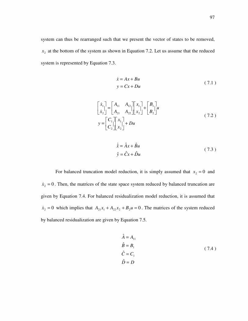
97
system can thus be rearranged such that we present the vector of states to be removed,
2x at the bottom of the system as shown in Equation 7.2. Let us assume that the reduced
system is represented by Equation 7.3.
DuCxy
BuAxx
+=
+=& ( 7.1 )
Dux
x
C
Cy
uB
B
x
x
AA
AA
x
x
+
=
+
=
2
1
2
1
2
1
2
1
2221
1211
2
1
&
&
( 7.2 )
uDxCy
uBxAx
ˆˆˆ
ˆˆˆ
+=
+=& ( 7.3 )
For balanced truncation model reduction, it is simply assumed that 02 =x and
02 =x& . Then, the matrices of the state space system reduced by balanced truncation are
given by Equation 7.4. For balanced residualization model reduction, it is assumed that
02 =x& which implies that 02222121 =++ uBxAxA . The matrices of the system reduced
by balanced residualization are given by Equation 7.5.
DD
CC
BB
AA
=
=
=
=
ˆ
ˆ
ˆ
ˆ
1
1
11
( 7.4 )
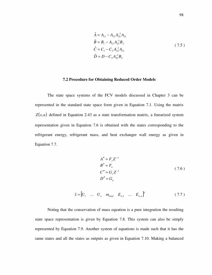
98
2
1
222
21
1
2221
2
1
22121
21
1
221211
ˆ
ˆ
ˆ
ˆ
BACDD
AACCC
BAABB
AAAAA
−
−
−
−
−=
−=
−=
−=
( 7.5 )
7.2 Procedure for Obtaining Reduced Order Models
The state space systems of the FCV models discussed in Chapter 3 can be
represented in the standard state space form given in Equation 7.1. Using the matrix
( )uxZ , defined in Equation 2.43 as a state transformation matrix, a linearized system
representation given in Equation 7.6 is obtained with the states corresponding to the
refrigerant energy, refrigerant mass, and heat exchanger wall energy as given in
Equation 7.7.
u
x
u
x
GD
ZGC
FB
ZFA
=′′
=′′
=′′
=′′
−
−
1
1
( 7.6 )
[ ]Tnwwtotaln EEmUUx ,1,1 KK= ( 7.7 )
Noting that the conservation of mass equation is a pure integration the resulting
state space representation is given by Equation 7.8. This system can also be simply
represented by Equation 7.9. Another system of equations is made such that it has the
same states and all the states as outputs as given in Equation 7.10. Making a balanced

99
realization of this system and using balance truncation, we can obtain a numerically
reduced 3rd order system represented by Equation 7.11.
[ ] [ ]uD
E
m
U
CCCy
u
B
B
B
E
m
U
AAA
AAA
E
m
U
w
totalEmUo
E
m
U
w
total
EEEmEU
UEUmUU
w
total
+
=
+
=
000&&
&
( 7.8 )
uDxCy
uBxAx
ooo
oo
+=
+=& ( 7.9 )
[ ]xIy
uBxAx
o
oo
=
+=~
& ( 7.10 )
rro
rrrr
xCy
uBxAx
=
+=~&
( 7.11 )
Then, a transformation matrix T (given in Equation 7.13) is defined to obtain
average states for refrigerant energy and heat exchanger wall energy. The average states
are given in Equation 7.12. We will obtain the reduced order system in terms of the
average states. Using Equations 7.10 – 7.12, we can calculate avgx as given in Equation
7.14. Assuming rTCP = , and applying similarity transformation to Equation 7.11 and
using Equations 7.9 – 7.11, we can obtain the system given in Equation 7.15. This is a
reduced order linear system having [ ]Tavgwtotalavg EmU , as states and the original

100
outputs as the outputs of the system. Alternatively, the system can also be represented as
given in Equation 7.16. This is a 3rd order system having states which have a physical
significance. Again, since the conservation of mass is a pure integration, the matrix rA
can be represented as given in Equation 7.17.
xT
E
m
U
x
avgw
total
avg
avg =
=
,
( 7.12 )
=XnXn
XnXn
XnXn
T11
11
11
100
010
001
( 7.13 )
rravg xTCx = ( 7.14 )
( ) ( )
( ) uDxPCCy
uPBxPPAx
oavgroo
ravgravg
+=
+=
−
−
1
1& ( 7.15 )
uD
E
m
U
Cy
uB
E
m
U
Ax
r
avgw
total
avg
ro
r
avgw
total
avg
ravg
ˆˆ
ˆˆ
,
,
+
=
+
=&
( 7.16 )
=
333231
131211
000ˆ
AAA
AAA
Ar ( 7.17 )
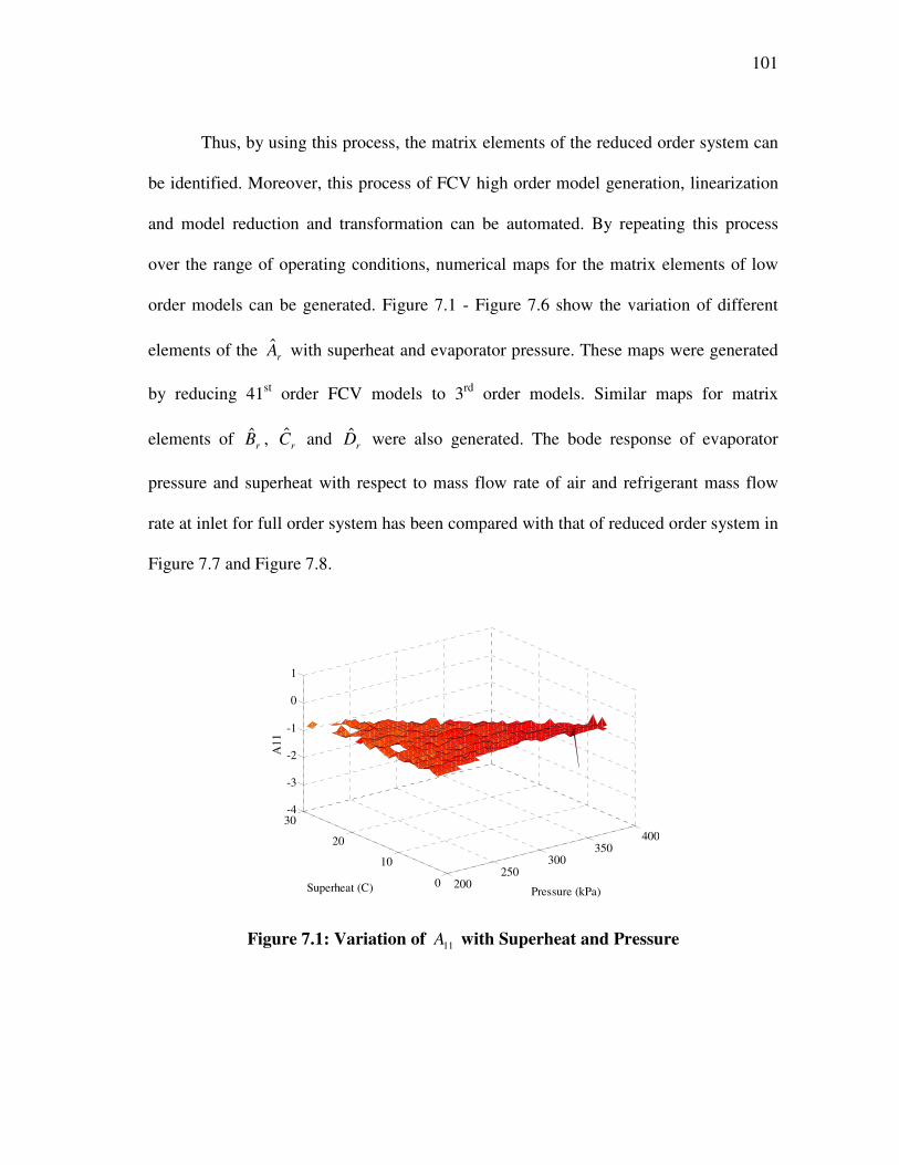
101
Thus, by using this process, the matrix elements of the reduced order system can
be identified. Moreover, this process of FCV high order model generation, linearization
and model reduction and transformation can be automated. By repeating this process
over the range of operating conditions, numerical maps for the matrix elements of low
order models can be generated. Figure 7.1 - Figure 7.6 show the variation of different
elements of the rA with superheat and evaporator pressure. These maps were generated
by reducing 41st order FCV models to 3rd order models. Similar maps for matrix
elements of rB , rC and rD were also generated. The bode response of evaporator
pressure and superheat with respect to mass flow rate of air and refrigerant mass flow
rate at inlet for full order system has been compared with that of reduced order system in
Figure 7.7 and Figure 7.8.
200250
300350
400
0
10
20
30-4
-3
-2
-1
0
1
Pressure (kPa)Superheat (C)
A1
1
Figure 7.1: Variation of 11A with Superheat and Pressure

102
200250
300350
400
0
10
20
30-20
-15
-10
-5
0
5
Pressure (kPa)Superheat (C)
A12
Figure 7.2: Variation of 12A with Superheat and Pressure
200250
300350
400
0
10
20
30-0.2
0
0.2
0.4
0.6
0.8
Pressure (kPa)Superheat (C)
A13
Figure 7.3: Variation of 13A with Superheat and Pressure

103
200250
300350
400
0
10
20
30-10
-5
0
5
Pressure (kPa)Superheat (C)
A31
Figure 7.4: Variation of 31A with Superheat and Pressure
200250
300350
400
0
10
20
30-40
-20
0
20
40
Pressure (kPa)Superheat (C)
A3
2
Figure 7.5: Variation of 32A with Superheat and Pressure

104
200250
300350
400
0
10
20
30-2
-1
0
1
2
Pressure (kPa)Superheat (C)
A3
3
Figure 7.6: Variation of 33A with Superheat and Pressure
Figure 7.7: Bode Plot: Pressure

105
Figure 7.8: Bode Plot: Superheat

106
Chapter 8
CONCLUSIONS AND FUTURE WORK
8.1 Summary of Results
This research makes several key contributions to the study of vapor compression
system dynamics. First, the existing lumped parameter moving boundary approach has
been presented, which provides a simple method to obtain low order models. Second, a
finite control volume approach is presented, avoiding the standard system of DAEs, and
creating a set of nonlinear ODEs. This framework allows inclusion of parametric details
omitted by the simpler models. Third, the resulting models are validated against
experimental data. Finally, an approach to model reduction procedure to obtain low
order models using the high order FCV models has been introduced. The reduced order
models are obtained such that the physical significance of the system states is retained.
The approach is extended to create numerical maps for the matrix elements of the
reduced order models.
8.2 Future Work
This research has many aspects that have yet to be explored. The modeling
approach presented in this report has been validated against limited data. The approach

107
should be validated against data collected for other disturbances such as those due to
change in valve opening, change in temperature of secondary fluid etc.
It has been suggested that the parameter tuning approach can be extended to
create numerical maps for reduced order models using the higher order FCV models.
Such maps should be created for the entire range of operating conditions of a simple heat
exchanger and their efficacy should be validated against experimental data.
It has been mentioned in Chapter 5 that the fluid property tables have
discontinuities near the critical point as the fluid changes state. The calculation of fluid
properties can be improved by separating the property tables for different states of the
fluid.
Also, this approach has been validated for simple vapor compression cycle
consisting of a single compressor, condenser, valve and evaporator. It can be easily
extended to more complex multi-component vapor compression systems containing
more than one evaporator, condenser etc.

108
REFERENCES
[1] “Energy Information Administration: International Energy Outlook 2007,”
http://www.eia.doe.gov/oiaf/ieo/world.html, 2007
[2] “Environmental Indicators: Climate Change,”
http://unstats.un.org/unsd/environment/air_co2_emissions.htm, 2007
[3] “Oil falls after striking record $90 a barrel,”
http://www.reuters.com/article/hotStocksNews/idUSSP10407020071019,
2007
[4] “Thermosys,” http://www1.mengr.tamu.edu/TFCL/thermosys.htm, 2007
[5] “Thermosys,” http://mr-roboto.me.uiuc.edu/thermosys/index.htm, 2007
[6] Antoulas, A.C., Sorensen, D.C. and Gugercin S., “A survey of model reduction
methods for large-scale systems,” Contemporary Mathematics, vol. 280,
pp. 193-219, 2001
[7] Bendapudi, S. and Braun, J. E., “A Review of Literature on Dynamic Models of
Vapor Compression Equipment,” ASHRAE Report #4036-5, May 2002
[8] Bendapudi, S., “Development and Evaluation of Modeling Approaches for
Transients in Centrifugal Chillers,” Thesis, Purdue University, Aug 2004
[9] Chen, Chi-Tsong, “Linear System Theory and Design,” New York: Oxford
University Press, 1999
[10] Drew, D.A., “Mathematical Modeling of Two-Phase Flow,” Annual Review of
Fluid Mechanics, vol. 15, pp. 261-291, 1983
109
[11] Gnielinski, V., “New Equations for Heat and Mass Transfer in Turbulent Pipe
and Channel Flow,” International Chemical Engineering, vol. 16, pp.
359-368, 1976
[12] Grald, E. W. and MacArthur, J. W., “A Moving boundary Formulation for
Modeling Time-Dependent Two-Phase Flows,” International Journal of
Heat & Fluid Flow, vol. 13, no. 3, pp. 266-272, Sep 1992
[13] Gruhle, W.–D. and Isermann, R., “Modeling and Control of a Refrigerant
Evaporator,” Journal of Dynamic Systems, Measurement and control-
Transactions of the ASME, vol. 107, no. 4, pp. 235-240, Dec 1985
[14] He, X.-D., Liu, S., and Asada, H. H., “Modeling of Vapor Compression Cycles
for Multivariable Feedback Control of HVAC Systems,” Journal of
Dynamic Systems Measurement & Control-Transactions of the ASME,
vol. 119, no. 2, pp. 183-191, Jun, 1997
[15] He, X.-D., “Dynamic Modeling and Multivariable Control of Vapor
Compression Cycles in Air Conditioning Systems,” Thesis,
Massachusetts Institute of Technology, Feb 1996
[16] MacArthur, J. W. and Grald, E. W., “Prediction of Cyclic Heat Pump
Performance with a Fully Distributed Model and a Comparison with
Experimental Data,” ASHRAE Transactions, vol. 93, no. 2, pp. 1159-
1178, Jun 1987
[17] Mithraratne, P., Wijeysundera, N.E., and Bong, T.Y., “Dynamic Simulation of a
Thermostatically Controlled Counter-Flow Evaporator,” International
Journal of Refrigeration, vol. 23, no. 3, pp. 174-189, 2000
[18] Narayanan, S., Srinivas, B., Pushpavanam, S., Bhallamudi, S. Murty, “Non-linear
Dynamics of a Two-Phase Flow System in an Evaporator: The Effects of
110
(i) A Time Varying Pressure Drop (ii) An Axially Varying Heat Flux,”
Nuclear Engineering and Design, vol. 178, pp. 279-294, 1997
[19] Ogata, Katsuhiko, “Modern Control Engineering,” Upper Saddle River, New
Jersey: Pearson Education, Inc., 2002
[20] Paynter, Henry M. and Takahashi, Yashundo, “ A New Method of Evaluating
Dynamic Response of Counter-Flow and Parallel-Flow Heat
Exchangers,” ASME Diamond Jubilee Semi-annual Meeting, Boston,
MA, Jun 1955
[21] Popper, K., “Conjectures and Refutations: The Growth of Scientific Knowledge,”
New York: Harper Torchbooks, 1963
[22] Rasmussen, Bryan P., “Control-Oriented Modeling of Transcritical Vapor
Compression Systems,” Thesis, University of Illinois at Urbana-
Champaign, 2002
[23] Rasmussen, Bryan P., “Dynamic Modeling and Advanced Control of Air
Conditioning and Refrigeration Systems,” Thesis, University of Illinois at
Urbana-Champaign, 2005
[24] Rice, C. K., “Effect of Void Fraction Correlation and Heat Flux Assumption on
Refrigerant Charge Inventory Predictions,” ASHRAE Transactions, vol.
93, no. 1, pp. 341-367, 1987
[25] Skogestad, Sigurd and Postlethwaite, Ian, “Multivariable Feedback Control:
Analysis and Design,” Hoboken, NJ: John Wiley, 2005
[26] Tummescheit, Hubertus and Eborn, Jonas, “Design of a Thermo-Hydraulic
Model Library in Modelica,” European Simulation Multiconference,
Manchester, UK, 1998

111
[27] Wattelet, J.P. et al., “Heat transfer flow regimes of refrigerants in a horizontal -
tube evaporator,” ACRC TR-55, University of Illinois at Urbana-
Champaign, 1994
[28] Willatzen, M., Pettit, N. B. O. L., and Ploug-Sorensen, L., “A General Dynamic
Simulation Model for Evaporators and Condensers in Refrigeration. Part
I: Moving Boundary Formulation of Two-Phase Flows with Heat
Exchange,” International Journal of Refrigeration, vol. 21, no. 5, pp.
398-403, Aug, 1998