IOP PUBLISHING MEASUREMENT SCIENCE AND TECHNOLOGY

Meas. Sci. Technol. 18 (2007) 1947–1957 doi:10.1088/0957-0233/18/7/022

Real-time fatigue life estimation inmechanical structures*Shalabh Gupta and Asok Ray

Mechanical Engineering Department, The Pennsylvania State University, University Park,PA 16802, USA

E-mail: szg107@psu.edu and axr2@psu.edu

Received 10 November 2006, in final form 14 March 2007Published 15 May 2007Online at stacks.iop.org/MST/18/1947

AbstractThe paper addresses the issue of online diagnosis and prognosis of emergingfaults in human-engineered complex systems. Specifically, the paper reportsa dynamic data-driven analytical tool for early detection of incipient faultsand real-time estimation of remaining useful fatigue life in polycrystallinealloys. The algorithms for fatigue life estimation rely on time series dataanalysis of ultrasonic signals and are built upon the principles of symbolicdynamics, information theory and statistical pattern recognition. Theproposed method is experimentally validated by using 7075-T6 aluminiumalloy specimens on a special-purpose fatigue test apparatus that is equippedwith ultrasonic flaw detectors and an optical travelling microscope. Thereal-time information, derived by the proposed method, is useful formitigation of widespread fatigue damage and is potentially applicable to lifeextending and resilient control of mechanical structures.

Keywords: symbolic time series analysis, anomaly detection, fatiguedamage, ultrasonic sensing

(Some figures in this article are in colour only in the electronic version)

1. Introduction

Recent developments and maturity of scientific theories havedemonstrated that information-based detection, diagnosis andprognosis of failures is essential for online estimation ofstructural damage and quantification of structural integrityfor maintenance of safe and reliable operation of human-engineered complex systems. This paper addresses the issuesof early diagnosis and prognosis for advanced warning ofincipient and gradually emerging faults in complex dynamicalsystems. Fatigue damage is one of the most commonlyencountered sources of structural degradation and couldpotentially cause catastrophic failures in mechanical systems[1].

The current state-of-the-art in fatigue life estimation islargely based on model-based analysis; however, no existingfatigue damage model, solely based on the fundamentalprinciples of physics, can adequately capture the dynamical

* This work has been supported in part by the US Army Research Laboratoryand the US Army Research Office (ARO) under grant no. DAAD19-01-1-0646.

behaviour of fatigue damage at the grain level [2]. Ingeneral, model-based approaches are critically dependent oninitial defects in the material microstructure, which mayrandomly form crack nucleation sites and are difficult to model[1, 3]. Small deviations in initial conditions and criticalparameters may produce large bifurcations in the expecteddynamical behaviour of fatigue damage [4]. In addition,fluctuations in usage patterns (e.g., random overloads) andenvironmental conditions (e.g., temperature and humidity)may adversely affect the service life of mechanical systems.From this perspective, a data-driven statistical method ispresented for online estimation of remaining useful fatiguelife in mechanical structures as augmentation of the authors’earlier work [5] that addressed early detection of incipientfatigue damage in polycrystalline alloys.

The random distribution of micro-structural flaws inidentically manufactured components can produce a wideuncertainty in the crack initiation phase [1]. For example,inclusions, casting defects and machining marks possiblyoriginated during fabrication may cause stress augmentation atcertain locations. These unavoidable surface and sub-surface

0957-0233/07/071947+11$30.00 © 2007 IOP Publishing Ltd Printed in the UK 1947

S Gupta and A Ray

defects constitute integral parts of the material microstructureof the operating machinery. As such, evolution of fatiguedamage is described as a stochastic phenomenon [1, 3] anda stochastic measure of fatigue crack growth has also beenproposed in the literature [6, 7]. This stochastic natureof fatigue damage emphasizes the need for online updatingof information using sensing devices that are sensitive tosmall microstructural changes and are capable of issuingearly warnings during fatigue damage evolution [8]. Assuch, the above discussions evince that time series analysisof sensor data is essential for real-time monitoring of fatiguein mechanical structures [9].

Impedance of the ultrasonic signals has been shown tobe very sensitive to small microstructural changes occurringduring the early stages of fatigue damage [10–13]. Assuch, ultrasonic sensing has been adopted to monitor theevolution of fatigue damage in ductile aluminium alloy 7075-T6 test specimens. The paper presents the application ofthe symbolic time series analysis (STSA) method [14, 15]to the ultrasonic signals for real-time detection of fatiguedamage and estimation of the remaining useful fatigue life.STSA for anomaly detection is an information-theoreticpattern identification tool that is built upon a fixed-structure,fixed-order Markov chain [15]. Recent literature [16, 17]has reported experimental validation of STSA-based patternidentification by comparison with other existing techniquessuch as principal component analysis (PCA) and artificialneural networks (ANN); STSA has been shown to yieldsuperior performance in terms of early detection of anomalies,robustness to noise, and real-time execution in differentapplications such as electronic circuits, mechanical vibrationsystems and fatigue damage in polycrystalline alloys.

This paper addresses the issues of fatigue damagemonitoring and remaining life estimation as the following tworelated problems:

(1) The forward (analysis) problem of anomaly detection andassimilation of the respective statistical information.

(2) The inverse (synthesis) problem of anomaly identification(e.g., determination of ranges of anomalous parameters).

As a partial solution to the forward problem, recentliterature has reported successful application of the STSAmethod [15] to early detection of fatigue damage [5, 17].The procedure is experimentally validated by using 7075-T6aluminium alloy specimens on a special-purpose fatigue testapparatus that is equipped with ultrasonic flaw detectors andan optical travelling microscope [18]. This paper addressesboth the forward and inverse problems as augmentation ofthe reported work on part of the forward problem (i.e.,early detection of fatigue damage [5]). The underlyingstatistical concepts and the theory of fatigue life estimationare experimentally validated.

The paper is organized in six sections, including thepresent section. Section 2 reviews the underlying concepts andessential features of symbolic time series analysis for anomalydetection [15, 19]. Section 3 formulates the anomaly detectionproblem. Section 4 describes the experimental apparatus onwhich the anomaly detection method is validated in real time.Section 5 presents the pertinent results of both the forwardproblem and the inverse problem. The paper is concluded insection 6 along with recommendations for future research.

2. Review of STSA-based anomaly detection

This section presents the underlying concepts and essentialfeatures of STSA [14] for anomaly detection in complexdynamical systems [15]. While the details are reported inprevious publications [15, 19], the key features of STSA arebriefly summarized here for clarity and completeness of thispaper.

In the STSA procedure, a data sequence is convertedto a symbol sequence by partitioning a compact region ofthe phase space of the dynamical system, over which thetrajectory evolves, into finitely many discrete blocks. Eachblock is labelled as a symbol, where the symbol set � iscalled the alphabet that consists of |�| different symbols.(Note: |�| � 2.) As the system evolves in time, it travelsthrough or touches various blocks in its phase space and thecorresponding symbol σ ∈ � is assigned to it, thus convertingthe data sequence into a symbol sequence.

2.1. The two-time scale modelling

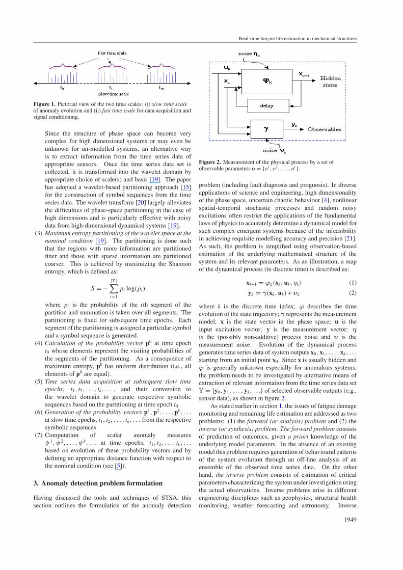
The sampling frequency and data acquisition process isrequired to be faster than the time period of damage evolution.Therefore, fatigue damage monitoring is formulated as a two-time-scale problem: the fast time scale is related to theresponse time of machinery operation. Over the span ofa given time series data sequence, the structural dynamicbehaviour of the system is assumed to remain invariant, i.e.,the process has stationary dynamics at the fast time scale.In other words, the variations in the internal dynamics ofthe system are assumed to be negligible on the fast timescale. The slow time scale is related to the time span overwhich the process may exhibit non-stationary dynamics. Anobservable non-stationary behaviour can be associated withanomalies evolving at the slow time scale. In general, a longtime span in the fast time scale is a tiny (i.e., several ordersof magnitude smaller) interval in the slow time scale. Forexample, evolution of fatigue damage in structural materials(causing a detectable change in the dynamics of the system)occurs on the slow time scale (possibly in the order of monthsor years); the fatigue damage behaviour is essentially invarianton the fast time scale (approximately in the order of seconds orminutes). Nevertheless, the notion of fast and slow time scalesis dependent on the specific application, loading conditionsand operating environment. As such, with the perspective offatigue monitoring, sensor data acquisition is done on the fasttime scale at different slow time epochs separated by regularintervals. Thereby, anomaly detection is done over the slowtime scale from the information generated by the STSA of thedata collected at different slow time epochs. A pictorial viewof the two time scales is presented in figure 1.

The key concepts of STSA-based anomaly detectionprocedure are summarized below.

(1) Time series data acquisition from appropriate sensor(s)at time epoch t0, i.e., the nominal condition, at which thesystem is assumed to be in the healthy state.

(2) Generation of wavelet transform coefficients, obtainedwith an appropriate choice of the wavelet basis [20]. Acrucial step in symbolic time series analysis is partitioningof the phase space for symbol sequence generation [14].

1948

Real-time fatigue life estimation in mechanical structures

Figure 1. Pictorial view of the two time scales: (i) slow time scaleof anomaly evolution and (ii) fast time scale for data acquisition andsignal conditioning.

Since the structure of phase space can become verycomplex for high dimensional systems or may even beunknown for un-modelled systems, an alternative wayis to extract information from the time series data ofappropriate sensors. Once the time series data set iscollected, it is transformed into the wavelet domain byappropriate choice of scale(s) and basis [19]. The paperhas adopted a wavelet-based partitioning approach [15]for the construction of symbol sequences from the timeseries data. The wavelet transform [20] largely alleviatesthe difficulties of phase-space partitioning in the case ofhigh dimensions and is particularly effective with noisydata from high-dimensional dynamical systems [19].

(3) Maximum entropy partitioning of the wavelet space at thenominal condition [19]. The partitioning is done suchthat the regions with more information are partitionedfiner and those with sparse information are partitionedcoarser. This is achieved by maximizing the Shannonentropy, which is defined as:

S = −|�|∑i=1

pi log(pi)

where pi is the probability of the ith segment of thepartition and summation is taken over all segments. Thepartitioning is fixed for subsequent time epochs. Eachsegment of the partitioning is assigned a particular symboland a symbol sequence is generated.

(4) Calculation of the probability vector p0 at time epocht0 whose elements represent the visiting probabilities ofthe segments of the partitioning. As a consequence ofmaximum entropy, p0 has uniform distribution (i.e., allelements of p0 are equal).

(5) Time series data acquisition at subsequent slow timeepochs, t1, t2, . . . , tk, . . . , and their conversion tothe wavelet domain to generate respective symbolicsequences based on the partitioning at time epoch t0.

(6) Generation of the probability vectors p1, p2, . . . , pk, . . .

at slow time epochs, t1, t2, . . . , tk, . . . from the respectivesymbolic sequences

(7) Computation of scalar anomaly measuresψ1, ψ2, . . . , ψk, . . . at time epochs, t1, t2, . . . , tk, . . .

based on evolution of these probability vectors and bydefining an appropriate distance function with respect tothe nominal condition (see [5]).

3. Anomaly detection problem formulation

Having discussed the tools and techniques of STSA, thissection outlines the formulation of the anomaly detection

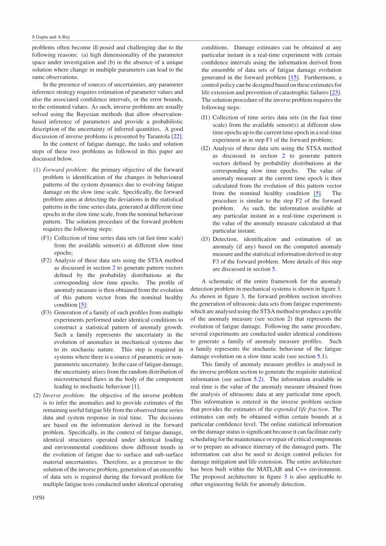
Figure 2. Measurement of the physical process by a set ofobservable parameters o = {o1, o2, . . . , or}.

problem (including fault diagnosis and prognosis). In diverseapplications of science and engineering, high dimensionalityof the phase space, uncertain chaotic behaviour [4], nonlinearspatial-temporal stochastic processes and random noisyexcitations often restrict the applications of the fundamentallaws of physics to accurately determine a dynamical model forsuch complex emergent systems because of the infeasibilityin achieving requisite modelling accuracy and precision [21].As such, the problem is simplified using observation-basedestimation of the underlying mathematical structure of thesystem and its relevant parameters. As an illustration, a mapof the dynamical process (in discrete time) is described as:

xk+1 = ϕk(xk, uk, ηk) (1)

yk = γ(xk, uk) + υk (2)

where k is the discrete time index; ϕ describes the timeevolution of the state trajectory; γ represents the measurementmodel; x is the state vector in the phase space; u is theinput excitation vector; y is the measurement vector; ηis the (possibly non-additive) process noise and υ is themeasurement noise. Evolution of the dynamical processgenerates time series data of system outputs x0, x1, . . . , xk, . . .

starting from an initial point x0. Since x is usually hidden andϕ is generally unknown especially for anomalous systems,the problem needs to be investigated by alternative means ofextraction of relevant information from the time series data setY = {y0, y1, . . . , yk, . . .} of selected observable outputs (e.g.,sensor data), as shown in figure 2.

As stated earlier in section 1, the issues of fatigue damagemonitoring and remaining life estimation are addressed as twoproblems: (1) the forward (or analysis) problem and (2) theinverse (or synthesis) problem. The forward problem consistsof prediction of outcomes, given a priori knowledge of theunderlying model parameters. In the absence of an existingmodel this problem requires generation of behavioural patternsof the system evolution through an off-line analysis of anensemble of the observed time series data. On the otherhand, the inverse problem consists of estimation of criticalparameters characterizing the system under investigation usingthe actual observations. Inverse problems arise in differentengineering disciplines such as geophysics, structural healthmonitoring, weather forecasting and astronomy. Inverse

1949

S Gupta and A Ray

problems often become ill-posed and challenging due to thefollowing reasons: (a) high dimensionality of the parameterspace under investigation and (b) in the absence of a uniquesolution where change in multiple parameters can lead to thesame observations.

In the presence of sources of uncertainties, any parameterinference strategy requires estimation of parameter values andalso the associated confidence intervals, or the error bounds,to the estimated values. As such, inverse problems are usuallysolved using the Bayesian methods that allow observation-based inference of parameters and provide a probabilisticdescription of the uncertainty of inferred quantities. A gooddiscussion of inverse problems is presented by Tarantola [22].

In the context of fatigue damage, the tasks and solutionsteps of these two problems as followed in this paper arediscussed below.

(1) Forward problem: the primary objective of the forwardproblem is identification of the changes in behaviouralpatterns of the system dynamics due to evolving fatiguedamage on the slow time scale. Specifically, the forwardproblem aims at detecting the deviations in the statisticalpatterns in the time series data, generated at different timeepochs in the slow time scale, from the nominal behaviourpattern. The solution procedure of the forward problemrequires the following steps:

(F1) Collection of time series data sets (at fast time scale)from the available sensor(s) at different slow timeepochs;

(F2) Analysis of these data sets using the STSA methodas discussed in section 2 to generate pattern vectorsdefined by the probability distributions at thecorresponding slow time epochs. The profile ofanomaly measure is then obtained from the evolutionof this pattern vector from the nominal healthycondition [5];

(F3) Generation of a family of such profiles from multipleexperiments performed under identical conditions toconstruct a statistical pattern of anomaly growth.Such a family represents the uncertainty in theevolution of anomalies in mechanical systems dueto its stochastic nature. This step is required insystems where there is a source of parametric or non-parametric uncertainty. In the case of fatigue damage,the uncertainty arises from the random distribution ofmicrostructural flaws in the body of the componentleading to stochastic behaviour [1].

(2) Inverse problem: the objective of the inverse problemis to infer the anomalies and to provide estimates of theremaining useful fatigue life from the observed time seriesdata and system response in real time. The decisionsare based on the information derived in the forwardproblem. Specifically, in the context of fatigue damage,identical structures operated under identical loadingand environmental conditions show different trends inthe evolution of fatigue due to surface and sub-surfacematerial uncertainties. Therefore, as a precursor to thesolution of the inverse problem, generation of an ensembleof data sets is required during the forward problem formultiple fatigue tests conducted under identical operating

conditions. Damage estimates can be obtained at anyparticular instant in a real-time experiment with certainconfidence intervals using the information derived fromthe ensemble of data sets of fatigue damage evolutiongenerated in the forward problem [15]. Furthermore, acontrol policy can be designed based on these estimates forlife extension and prevention of catastrophic failures [23].The solution procedure of the inverse problem requires thefollowing steps:

(I1) Collection of time series data sets (in the fast timescale) from the available sensor(s) at different slowtime epochs up to the current time epoch in a real-timeexperiment as in step F1 of the forward problem;

(I2) Analysis of these data sets using the STSA methodas discussed in section 2 to generate patternvectors defined by probability distributions at thecorresponding slow time epochs. The value ofanomaly measure at the current time epoch is thencalculated from the evolution of this pattern vectorfrom the nominal healthy condition [5]. Theprocedure is similar to the step F2 of the forwardproblem. As such, the information available atany particular instant in a real-time experiment isthe value of the anomaly measure calculated at thatparticular instant;

(I3) Detection, identification and estimation of ananomaly (if any) based on the computed anomalymeasure and the statistical information derived in stepF3 of the forward problem. More details of this stepare discussed in section 5.

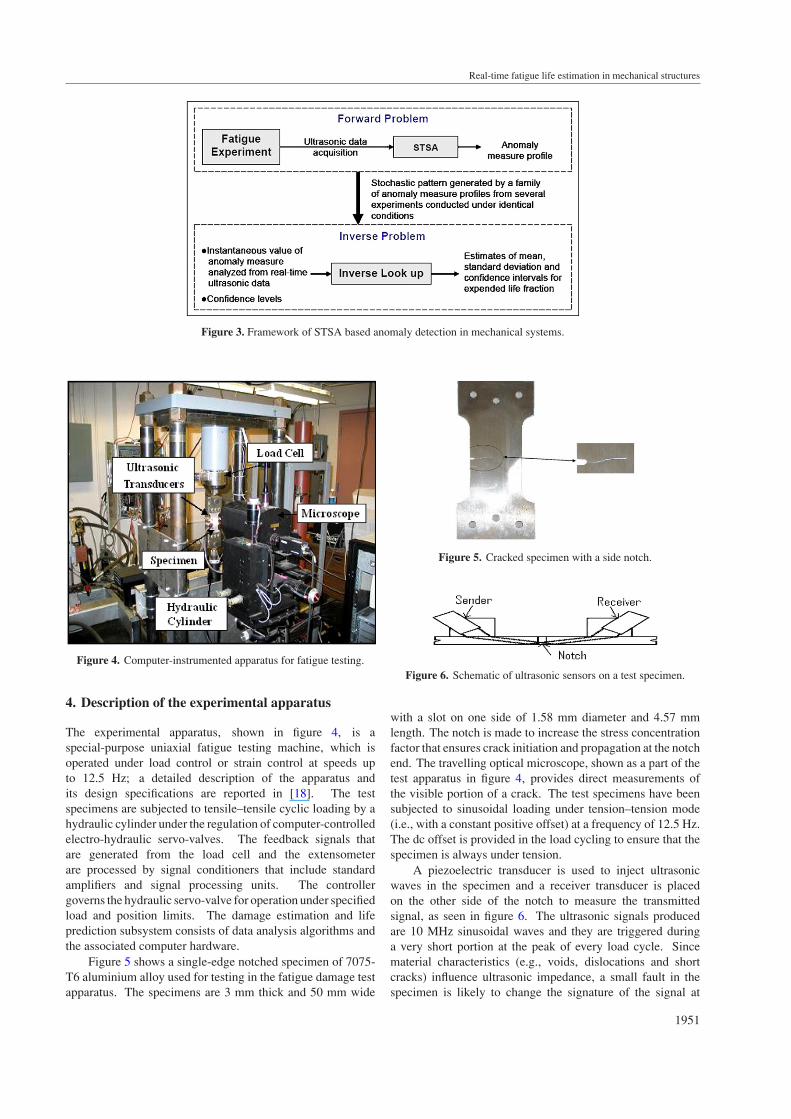
A schematic of the entire framework for the anomalydetection problem in mechanical systems is shown in figure 3.As shown in figure 3, the forward problem section involvesthe generation of ultrasonic data sets from fatigue experimentswhich are analysed using the STSA method to produce a profileof the anomaly measure (see section 2) that represents theevolution of fatigue damage. Following the same procedure,several experiments are conducted under identical conditionsto generate a family of anomaly measure profiles. Sucha family represents the stochastic behaviour of the fatiguedamage evolution on a slow time scale (see section 5.1).

This family of anomaly measure profiles is analysed inthe inverse problem section to generate the requisite statisticalinformation (see section 5.2). The information available inreal time is the value of the anomaly measure obtained fromthe analysis of ultrasonic data at any particular time epoch.This information is entered in the inverse problem sectionthat provides the estimates of the expended life fraction. Theestimates can only be obtained within certain bounds at aparticular confidence level. The online statistical informationon the damage status is significant because it can facilitate earlyscheduling for the maintenance or repair of critical componentsor to prepare an advance itinerary of the damaged parts. Theinformation can also be used to design control policies fordamage mitigation and life extension. The entire architecturehas been built within the MATLAB and C++ environment.The proposed architecture in figure 3 is also applicable toother engineering fields for anomaly detection.

1950

Real-time fatigue life estimation in mechanical structures

Figure 3. Framework of STSA based anomaly detection in mechanical systems.

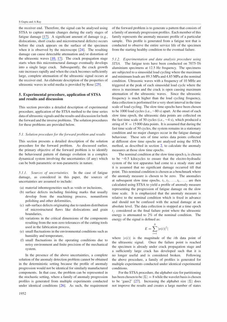
Figure 4. Computer-instrumented apparatus for fatigue testing.

4. Description of the experimental apparatus

The experimental apparatus, shown in figure 4, is aspecial-purpose uniaxial fatigue testing machine, which isoperated under load control or strain control at speeds upto 12.5 Hz; a detailed description of the apparatus andits design specifications are reported in [18]. The testspecimens are subjected to tensile–tensile cyclic loading by ahydraulic cylinder under the regulation of computer-controlledelectro-hydraulic servo-valves. The feedback signals thatare generated from the load cell and the extensometerare processed by signal conditioners that include standardamplifiers and signal processing units. The controllergoverns the hydraulic servo-valve for operation under specifiedload and position limits. The damage estimation and lifeprediction subsystem consists of data analysis algorithms andthe associated computer hardware.

Figure 5 shows a single-edge notched specimen of 7075-T6 aluminium alloy used for testing in the fatigue damage testapparatus. The specimens are 3 mm thick and 50 mm wide

Figure 5. Cracked specimen with a side notch.

Figure 6. Schematic of ultrasonic sensors on a test specimen.

with a slot on one side of 1.58 mm diameter and 4.57 mmlength. The notch is made to increase the stress concentrationfactor that ensures crack initiation and propagation at the notchend. The travelling optical microscope, shown as a part of thetest apparatus in figure 4, provides direct measurements ofthe visible portion of a crack. The test specimens have beensubjected to sinusoidal loading under tension–tension mode(i.e., with a constant positive offset) at a frequency of 12.5 Hz.The dc offset is provided in the load cycling to ensure that thespecimen is always under tension.

A piezoelectric transducer is used to inject ultrasonicwaves in the specimen and a receiver transducer is placedon the other side of the notch to measure the transmittedsignal, as seen in figure 6. The ultrasonic signals producedare 10 MHz sinusoidal waves and they are triggered duringa very short portion at the peak of every load cycle. Sincematerial characteristics (e.g., voids, dislocations and shortcracks) influence ultrasonic impedance, a small fault in thespecimen is likely to change the signature of the signal at

1951

S Gupta and A Ray

the receiver end. Therefore, the signal can be analysed usingSTSA to capture minute changes during the early stages offatigue damage [17]. A significant amount of damage (e.g.,dislocations, short cracks and microstructural defects) occursbefore the crack appears on the surface of the specimenwhen it is observed by the microscope [24]. The resultingdamage can cause detectable attenuation and/or distortion ofthe ultrasonic waves [10, 17]. The crack propagation stagestarts when this microstructural damage eventually developsinto a single large crack. Subsequently, the crack growthrate increases rapidly and when the crack becomes sufficientlylarge, complete attenuation of the ultrasonic signal occurs atthe receiver end. An elaborate description of the properties ofultrasonic waves in solid media is provided by Rose [25].

5. Experimental procedure, application of STSAand results and discussion

This section provides a detailed description of experimentalprocedure, application of the STSA method to the time seriesdata of ultrasonic signals and the results and discussion for boththe forward and the inverse problems. The solution proceduresfor these problems are provided below.

5.1. Solution procedure for the forward problem and results

This section presents a detailed description of the solutionprocedure for the forward problem. As discussed earlier,the primary objective of the forward problem is to identifythe behavioural pattern of damage evolution in a complexdynamical system involving the uncertainties (if any) whichcan be both parametric or non-parametric in nature.

5.1.1. Sources of uncertainties. In the case of fatiguedamage, as considered in this paper, the sources ofuncertainties are assumed to include:

(a) material inhomogeneities such as voids or inclusions,(b) surface defects including finishing marks that usually

develop from the machining process, nonuniformpolishing and other deformities,

(c) sub-surface defects originating due to random distributionof microstructural flaws like dislocations and grainboundaries,

(d) variations in the critical dimensions of the componentsresulting from the non-zero tolerances of the cutting toolsused in the fabrication process,

(e) small fluctuations in the environmental conditions such ashumidity and temperature,

(f) small fluctuations in the operating conditions due tonoisy environment and finite precision of the mechanicalsystem.

In the presence of the above uncertainties, a completesolution of the anomaly detection problem cannot be obtainedin the deterministic setting because the profile of anomalyprogression would not be identical for similarly manufacturedcomponents. In that case, the problem can be represented inthe stochastic setting, where a family of anomaly progressionprofiles is generated from multiple experiments conductedunder identical conditions [26]. As such, the requirement

of the forward problem is to generate a pattern that consists ofa family of anomaly progression profiles. Each member of thisfamily represents the anomaly measure profile of a particularsample. This profile is generated from a fatigue test that isconducted to observe the entire service life of the specimenfrom the starting healthy condition to the eventual failure.

5.1.2. Experimentation and data analysis procedure usingSTSA. The fatigue tests have been conducted on 7075-T6aluminium specimens at 12.5 Hz frequency. The specimensare subjected to a sinusoidal load cycling where the maximumand minimum loads are 89.3 MPa and 4.85 MPa at the nominalcondition. Ultrasonic waves with a frequency of 10 MHz aretriggered at the peak of each sinusoidal load cycle where thestress is maximum and the crack is open causing maximumattenuation of the ultrasonic waves. Since the ultrasonicfrequency is much higher than the load cycling frequency,data collection is performed for a very short interval in the timescale of load cycling. The slow time epochs have been chosento be 1000 load cycles (i.e., ∼80 s) apart. At the onset of eachslow time epoch, the ultrasonic data points are collected onthe fast time scale of 50 cycles (i.e., ∼4 s), which produced astring of N = 15 000 data points. It is assumed that during thefast time scale of 50 cycles, the system remains in a stationarycondition and no major changes occur in the fatigue damagebehaviour. These sets of time series data points collectedat different slow time epochs are analysed using the STSAmethod, as described in section 2, to calculate the anomalymeasures at those slow time epochs.

The nominal condition at the slow time epoch t0 is chosento be ∼0.5 kilocycles to ensure that the electro-hydraulicsystem of the test apparatus had come to a steady state andit is assumed that no significant damage occurred till thatpoint. This nominal condition is chosen as a benchmark wherethe anomaly measure is chosen to be zero. The anomaliesat subsequent slow time epochs, t1, t2, . . . , tk, . . . , are thencalculated using STSA to yield a profile of anomaly measurerepresenting the progression of fatigue damage on the slowtime scale. It is emphasized that the anomaly measure isrelative to the nominal condition which is fixed in advanceand should not be confused with the actual damage at anabsolute level. The data collection is stopped at a time epochtf considered as the final failure point where the ultrasonicenergy is attenuated to 2% of the nominal condition. Theenergy of the signal is defined as:

E =N∑

i=1

|s(i)|2|

where |s(i)| is the magnitude of the ith data point ofthe ultrasonic signal. Once the failure point is reachedthe specimen is already under crack propagation stage anda sufficiently large crack has developed such that it isno longer useful and is considered broken. Followingthe above procedure, a family of profiles is generated formultiple experiments conducted under identical experimentalconditions.

For the STSA procedure, the alphabet size for partitioninghas been chosen to be |�| = 8 while the wavelet basis is chosento be ‘gaus2’ [27]. Increasing the alphabet size |�| doesnot improve the results and creates a large number of states

1952

Real-time fatigue life estimation in mechanical structures

0 0.2 0.4 0.6 0.8 10

0.1

0.2

0.3

0.4

0.5

0.6

Expended life fraction

An

om

aly

Mea

sure

Family of fatigue damage profiles generated by 40 samples under identical loading conditions

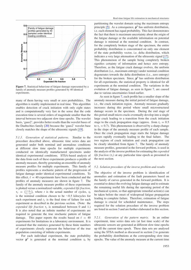
Figure 7. Statistical behaviour of fatigue damage represented by afamily of anomaly measure profiles generated by 40 identicalexperiments.

many of them having very small or zero probabilities. Thealgorithm is readily implemented in real time. This algorithmenables detection of crack initiation with only eight statesand is computationally very fast in the sense that the codeexecution time is several orders of magnitude smaller than theinterval between two adjacent slow time epochs. The waveletbasis, ‘gaus2’, provides better results than the wavelet bases ofthe Daubechies family [20] because the ‘gaus2’ wavelet baseclosely matches the shape of the ultrasonic signals [19].

5.1.3. Generation of statistical patterns. Similar to theprocedure described above, ultrasonic time series data aregenerated under both nominal and anomalous conditionsat different slow time epochs for multiple experimentsconducted on identically manufactured specimens underidentical experimental conditions. STSA-based analysis ofthe data from each of these experiments produces a profile ofanomaly measure, thereby generating an ensemble of anomalymeasure profiles for multiple experiments. This family ofprofiles represents a stochastic pattern of the progression offatigue damage under identical experimental conditions. Tothis effect, � = 40 experiments have been conducted and theprofiles of anomaly measures are shown in figure 7. Thefamily of the anomaly measure profiles of these experimentsis plotted versus a normalized variable, expended life fraction,τe = (

t−t0tf −t0

), where t is the actual number of cycles, t0

is the nominal condition chosen to be ∼0.5 kilocycles foreach experiment and tf is the final time of failure for eachexperiment as described in the previous section. (Note: theexpended life fraction τe is normalized between 0 and 1.)It is also noted that an infinite number of experiments arerequired to generate the true stochastic pattern of fatiguedamage. This paper reports the results based on � = 40experiments for limitations in a laboratory environment. It isassumed that the statistics generated by these finite numbersof experiments closely represent the behaviour of the truepopulation consisting of infinite experiments.

For each individual experiment, the state probabilityvector p0 is generated at the nominal condition t0 by

partitioning the wavelet domain using the maximum entropyprinciple [5]. As a consequence, p0 has uniform distribution,i.e. each element has equal probability. This fact demonstratesthe fact that there is maximum uncertainty about the origin ofthe fatigue damage or the available information on potentialdamage is minimal at the nominal condition. In contrast,for the completely broken stage of the specimen, the entireprobability distribution is concentrated on only one elementof the state probability vector, i.e. delta distribution, whichindicates a very large attenuation of the ultrasonic signal [17].This phenomenon of the sample being completely brokensignifies certainty of information and hence zero entropy.Therefore, as the fatigue crack damage evolves, the uniformdistribution (i.e., maximum entropy) under nominal conditiondegenerates towards the delta distribution (i.e., zero entropy)for the broken specimen. Since, p0 has uniform distributionfor all experiments, the statistical property is identical for allexperiments at the nominal condition. The variations in theevolution of fatigue damage, as seen in figure 7, are causeddue to various uncertainties listed earlier.

As seen in figure 7, each profile has a smaller slope of theanomaly measure during the initial period of fatigue damage,i.e., the crack initiation region. Anomaly measure graduallyincreases during this period where small microstructuraldamage occurs in the specimen. During the end stage ofthis period small micro cracks eventually develop into a singlelarge crack leading to a transition from the crack initiationstage to the crack propagation stage (approx. from τe = 0.5to τe = 0.7). This phenomenon is observed by a sharp changein the slope of the anomaly measure profile of each sample.Once the crack propagation stage starts the fatigue damageoccurs rapidly eventually leading to the final failure. Thetwo regions of crack initiation and crack propagation canbe clearly identified from figure 7. The family of anomalymeasure profiles, generated in the forward problem, is used inthe analysis of the inverse problem for estimating the expendedlife fraction (τe) at any particular time epoch as presented inthe next section.

5.2. Solution procedure of the inverse problem and results

The objective of the inverse problem is identification ofanomalies and estimation of the fault parameters based onthe family of curves generated in the forward problem. It isessential to detect the evolving fatigue damage and to estimatethe remaining useful life during the operating period of themechanical system, so that appropriate remedial action(s) canbe taken before the onset of widespread fatigue propagationleading to complete failure. Therefore, estimation of fatiguedamage is crucial for scheduled maintenance. The stepsrequired for the solution procedure of the inverse problemare listed in section 3 and are further elaborated in this section.

5.2.1. Generation of the pattern matrix. In an onlineexperiment, time series data sets (at fast time scale) of theultrasonic sensors are generated at different slow time epochsup till the current time epoch. These data sets are analysedusing the STSA method as discussed in section 2 to generatethe probability distributions at the corresponding slow timeepochs. The value of the anomaly measure at the current time

1953

S Gupta and A Ray

0 0.1 0.2 0.30

0.2

0.4

0.6

0.8

Expended life fraction (a)

(b)

(c)(d )

Pro

bab

ility

0.6 0.7 0.80

0.05

0.1

0.15

0.2

0.25

Expended life fraction

Pro

bab

ility

0.7 0.8 0.90

0.05

0.1

0.15

0.2

0.25

0.3

Expended life fraction

Pro

bab

ility

0.65 0.7 0.75 0.8 0.850

0.05

0.1

0.15

0.2

0.25

Expended life fraction

Pro

bab

ility

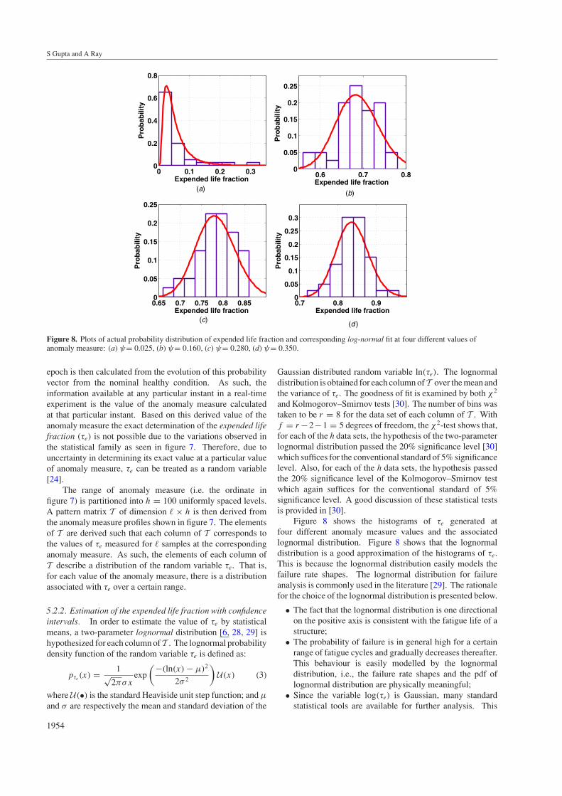
Figure 8. Plots of actual probability distribution of expended life fraction and corresponding log-normal fit at four different values ofanomaly measure: (a) ψ= 0.025, (b) ψ= 0.160, (c) ψ= 0.280, (d) ψ= 0.350.

epoch is then calculated from the evolution of this probabilityvector from the nominal healthy condition. As such, theinformation available at any particular instant in a real-timeexperiment is the value of the anomaly measure calculatedat that particular instant. Based on this derived value of theanomaly measure the exact determination of the expended lifefraction (τe) is not possible due to the variations observed inthe statistical family as seen in figure 7. Therefore, due touncertainty in determining its exact value at a particular valueof anomaly measure, τe can be treated as a random variable[24].

The range of anomaly measure (i.e. the ordinate infigure 7) is partitioned into h = 100 uniformly spaced levels.A pattern matrix T of dimension � × h is then derived fromthe anomaly measure profiles shown in figure 7. The elementsof T are derived such that each column of T corresponds tothe values of τe measured for � samples at the correspondinganomaly measure. As such, the elements of each column ofT describe a distribution of the random variable τe. That is,for each value of the anomaly measure, there is a distributionassociated with τe over a certain range.

5.2.2. Estimation of the expended life fraction with confidenceintervals. In order to estimate the value of τe by statisticalmeans, a two-parameter lognormal distribution [6, 28, 29] ishypothesized for each column ofT . The lognormal probabilitydensity function of the random variable τe is defined as:

pτe(x) = 1√

2πσxexp

(−(ln(x) − µ)2

2σ 2

)U(x) (3)

where U(•) is the standard Heaviside unit step function; and µ

and σ are respectively the mean and standard deviation of the

Gaussian distributed random variable ln(τe). The lognormaldistribution is obtained for each column ofT over the mean andthe variance of τe. The goodness of fit is examined by both χ2

and Kolmogorov–Smirnov tests [30]. The number of bins wastaken to be r = 8 for the data set of each column of T . Withf = r −2−1 = 5 degrees of freedom, the χ2-test shows that,for each of the h data sets, the hypothesis of the two-parameterlognormal distribution passed the 20% significance level [30]which suffices for the conventional standard of 5% significancelevel. Also, for each of the h data sets, the hypothesis passedthe 20% significance level of the Kolmogorov–Smirnov testwhich again suffices for the conventional standard of 5%significance level. A good discussion of these statistical testsis provided in [30].

Figure 8 shows the histograms of τe generated atfour different anomaly measure values and the associatedlognormal distribution. Figure 8 shows that the lognormaldistribution is a good approximation of the histograms of τe.This is because the lognormal distribution easily models thefailure rate shapes. The lognormal distribution for failureanalysis is commonly used in the literature [29]. The rationalefor the choice of the lognormal distribution is presented below.

• The fact that the lognormal distribution is one directionalon the positive axis is consistent with the fatigue life of astructure;

• The probability of failure is in general high for a certainrange of fatigue cycles and gradually decreases thereafter.This behaviour is easily modelled by the lognormaldistribution, i.e., the failure rate shapes and the pdf oflognormal distribution are physically meaningful;

• Since the variable log(τe) is Gaussian, many standardstatistical tools are available for further analysis. This

1954

Real-time fatigue life estimation in mechanical structures

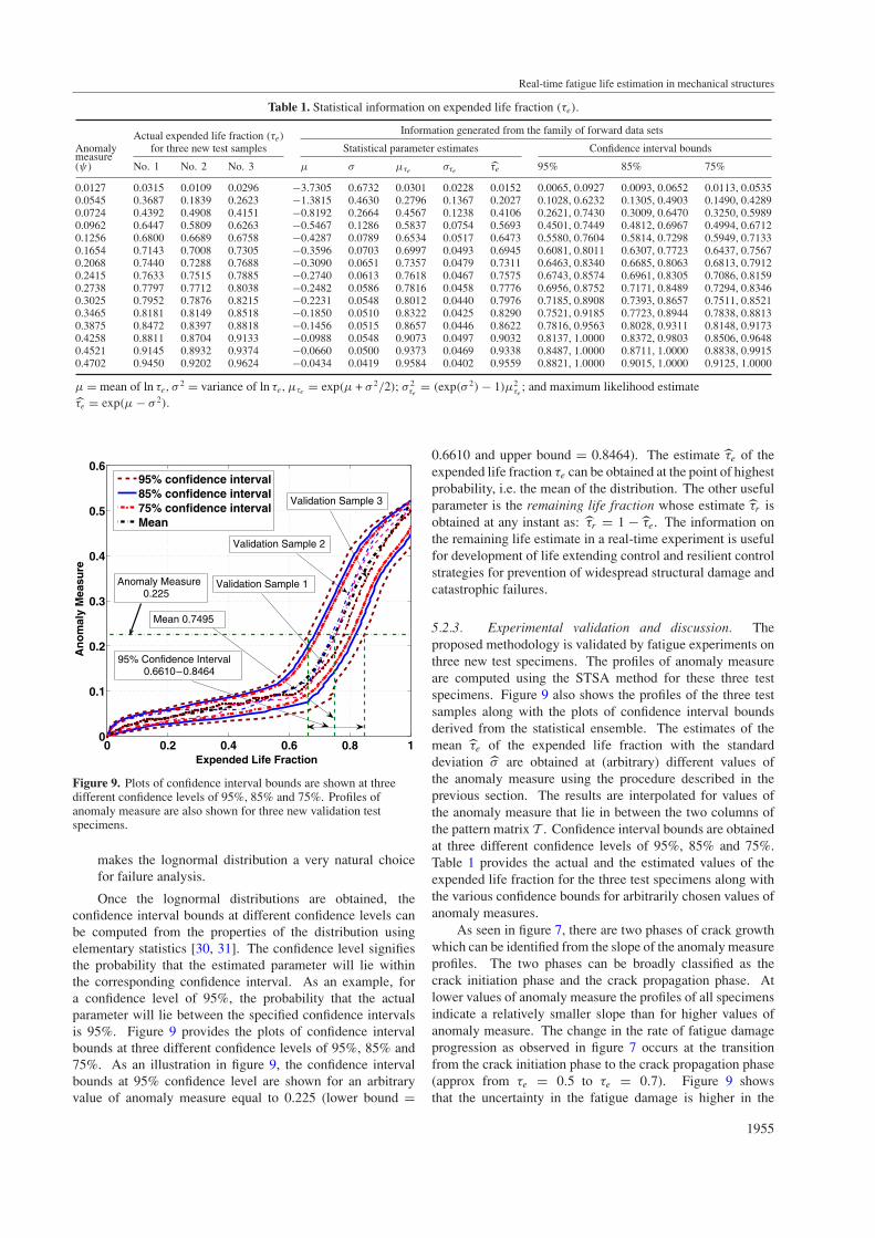
Table 1. Statistical information on expended life fraction (τe).

Information generated from the family of forward data setsActual expended life fraction (τe)

Anomaly for three new test samples Statistical parameter estimates Confidence interval boundsmeasure(ψ) No. 1 No. 2 No. 3 µ σ µτe στe τ̂e 95% 85% 75%

0.0127 0.0315 0.0109 0.0296 −3.7305 0.6732 0.0301 0.0228 0.0152 0.0065, 0.0927 0.0093, 0.0652 0.0113, 0.05350.0545 0.3687 0.1839 0.2623 −1.3815 0.4630 0.2796 0.1367 0.2027 0.1028, 0.6232 0.1305, 0.4903 0.1490, 0.42890.0724 0.4392 0.4908 0.4151 −0.8192 0.2664 0.4567 0.1238 0.4106 0.2621, 0.7430 0.3009, 0.6470 0.3250, 0.59890.0962 0.6447 0.5809 0.6263 −0.5467 0.1286 0.5837 0.0754 0.5693 0.4501, 0.7449 0.4812, 0.6967 0.4994, 0.67120.1256 0.6800 0.6689 0.6758 −0.4287 0.0789 0.6534 0.0517 0.6473 0.5580, 0.7604 0.5814, 0.7298 0.5949, 0.71330.1654 0.7143 0.7008 0.7305 −0.3596 0.0703 0.6997 0.0493 0.6945 0.6081, 0.8011 0.6307, 0.7723 0.6437, 0.75670.2068 0.7440 0.7288 0.7688 −0.3090 0.0651 0.7357 0.0479 0.7311 0.6463, 0.8340 0.6685, 0.8063 0.6813, 0.79120.2415 0.7633 0.7515 0.7885 −0.2740 0.0613 0.7618 0.0467 0.7575 0.6743, 0.8574 0.6961, 0.8305 0.7086, 0.81590.2738 0.7797 0.7712 0.8038 −0.2482 0.0586 0.7816 0.0458 0.7776 0.6956, 0.8752 0.7171, 0.8489 0.7294, 0.83460.3025 0.7952 0.7876 0.8215 −0.2231 0.0548 0.8012 0.0440 0.7976 0.7185, 0.8908 0.7393, 0.8657 0.7511, 0.85210.3465 0.8181 0.8149 0.8518 −0.1850 0.0510 0.8322 0.0425 0.8290 0.7521, 0.9185 0.7723, 0.8944 0.7838, 0.88130.3875 0.8472 0.8397 0.8818 −0.1456 0.0515 0.8657 0.0446 0.8622 0.7816, 0.9563 0.8028, 0.9311 0.8148, 0.91730.4258 0.8811 0.8704 0.9133 −0.0988 0.0548 0.9073 0.0497 0.9032 0.8137, 1.0000 0.8372, 0.9803 0.8506, 0.96480.4521 0.9145 0.8932 0.9374 −0.0660 0.0500 0.9373 0.0469 0.9338 0.8487, 1.0000 0.8711, 1.0000 0.8838, 0.99150.4702 0.9450 0.9202 0.9624 −0.0434 0.0419 0.9584 0.0402 0.9559 0.8821, 1.0000 0.9015, 1.0000 0.9125, 1.0000

µ = mean of ln τe, σ2 = variance of ln τe, µτe

= exp(µ + σ 2/2); σ 2τe

= (exp(σ 2) − 1)µ2τe

; and maximum likelihood estimateτ̂e = exp(µ − σ 2).

0 0.2 0.4 0.6 0.8 10

0.1

0.2

0.3

0.4

0.5

0.6

Expended Life Fraction

An

om

aly

Mea

sure

95% confidence interval85% confidence interval75% confidence intervalMean

Anomaly Measure 0.225

Mean 0.7495

95% Confidence Interval 0.6610–0.8464

Validation Sample 1

Validation Sample 2

Validation Sample 3

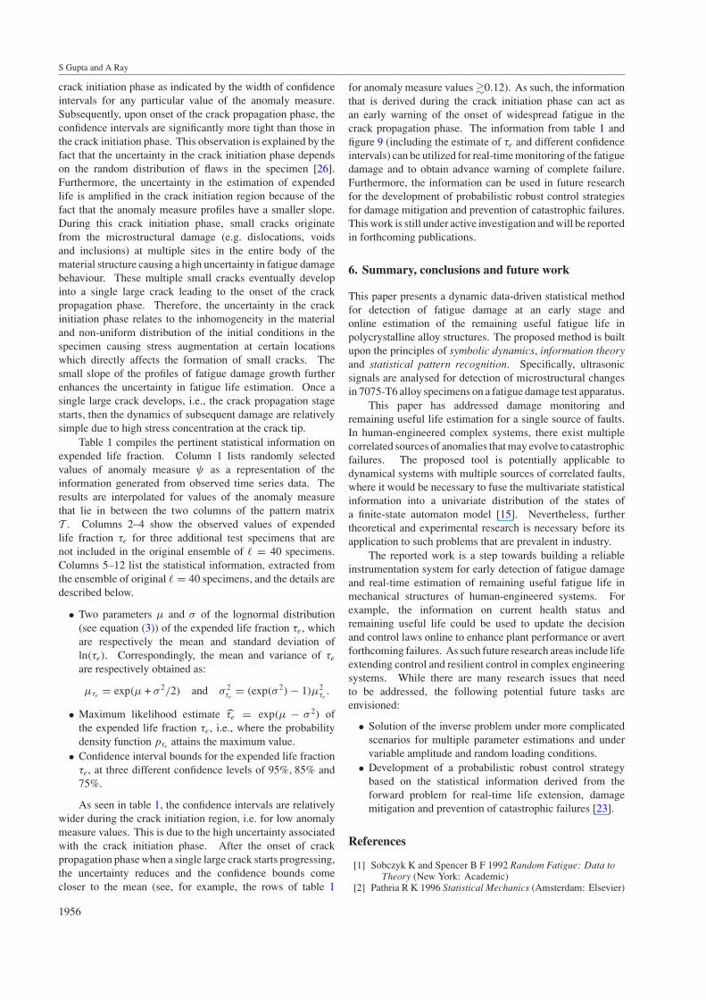
Figure 9. Plots of confidence interval bounds are shown at threedifferent confidence levels of 95%, 85% and 75%. Profiles ofanomaly measure are also shown for three new validation testspecimens.

makes the lognormal distribution a very natural choicefor failure analysis.

Once the lognormal distributions are obtained, theconfidence interval bounds at different confidence levels canbe computed from the properties of the distribution usingelementary statistics [30, 31]. The confidence level signifiesthe probability that the estimated parameter will lie withinthe corresponding confidence interval. As an example, fora confidence level of 95%, the probability that the actualparameter will lie between the specified confidence intervalsis 95%. Figure 9 provides the plots of confidence intervalbounds at three different confidence levels of 95%, 85% and75%. As an illustration in figure 9, the confidence intervalbounds at 95% confidence level are shown for an arbitraryvalue of anomaly measure equal to 0.225 (lower bound =

0.6610 and upper bound = 0.8464). The estimate τ̂e of theexpended life fraction τe can be obtained at the point of highestprobability, i.e. the mean of the distribution. The other usefulparameter is the remaining life fraction whose estimate τ̂r isobtained at any instant as: τ̂r = 1 − τ̂e. The information onthe remaining life estimate in a real-time experiment is usefulfor development of life extending control and resilient controlstrategies for prevention of widespread structural damage andcatastrophic failures.

5.2.3. Experimental validation and discussion. Theproposed methodology is validated by fatigue experiments onthree new test specimens. The profiles of anomaly measureare computed using the STSA method for these three testspecimens. Figure 9 also shows the profiles of the three testsamples along with the plots of confidence interval boundsderived from the statistical ensemble. The estimates of themean τ̂e of the expended life fraction with the standarddeviation σ̂ are obtained at (arbitrary) different values ofthe anomaly measure using the procedure described in theprevious section. The results are interpolated for values ofthe anomaly measure that lie in between the two columns ofthe pattern matrix T . Confidence interval bounds are obtainedat three different confidence levels of 95%, 85% and 75%.Table 1 provides the actual and the estimated values of theexpended life fraction for the three test specimens along withthe various confidence bounds for arbitrarily chosen values ofanomaly measures.

As seen in figure 7, there are two phases of crack growthwhich can be identified from the slope of the anomaly measureprofiles. The two phases can be broadly classified as thecrack initiation phase and the crack propagation phase. Atlower values of anomaly measure the profiles of all specimensindicate a relatively smaller slope than for higher values ofanomaly measure. The change in the rate of fatigue damageprogression as observed in figure 7 occurs at the transitionfrom the crack initiation phase to the crack propagation phase(approx from τe = 0.5 to τe = 0.7). Figure 9 showsthat the uncertainty in the fatigue damage is higher in the

1955

S Gupta and A Ray

crack initiation phase as indicated by the width of confidenceintervals for any particular value of the anomaly measure.Subsequently, upon onset of the crack propagation phase, theconfidence intervals are significantly more tight than those inthe crack initiation phase. This observation is explained by thefact that the uncertainty in the crack initiation phase dependson the random distribution of flaws in the specimen [26].Furthermore, the uncertainty in the estimation of expendedlife is amplified in the crack initiation region because of thefact that the anomaly measure profiles have a smaller slope.During this crack initiation phase, small cracks originatefrom the microstructural damage (e.g. dislocations, voidsand inclusions) at multiple sites in the entire body of thematerial structure causing a high uncertainty in fatigue damagebehaviour. These multiple small cracks eventually developinto a single large crack leading to the onset of the crackpropagation phase. Therefore, the uncertainty in the crackinitiation phase relates to the inhomogeneity in the materialand non-uniform distribution of the initial conditions in thespecimen causing stress augmentation at certain locationswhich directly affects the formation of small cracks. Thesmall slope of the profiles of fatigue damage growth furtherenhances the uncertainty in fatigue life estimation. Once asingle large crack develops, i.e., the crack propagation stagestarts, then the dynamics of subsequent damage are relativelysimple due to high stress concentration at the crack tip.

Table 1 compiles the pertinent statistical information onexpended life fraction. Column 1 lists randomly selectedvalues of anomaly measure ψ as a representation of theinformation generated from observed time series data. Theresults are interpolated for values of the anomaly measurethat lie in between the two columns of the pattern matrixT . Columns 2–4 show the observed values of expendedlife fraction τe for three additional test specimens that arenot included in the original ensemble of � = 40 specimens.Columns 5–12 list the statistical information, extracted fromthe ensemble of original � = 40 specimens, and the details aredescribed below.

• Two parameters µ and σ of the lognormal distribution(see equation (3)) of the expended life fraction τe, whichare respectively the mean and standard deviation ofln(τe). Correspondingly, the mean and variance of τe

are respectively obtained as:

µτe= exp(µ + σ 2/2) and σ 2

τe= (exp(σ 2) − 1)µ2

τe.

• Maximum likelihood estimate τ̂e = exp(µ − σ 2) ofthe expended life fraction τe, i.e., where the probabilitydensity function pτe

attains the maximum value.• Confidence interval bounds for the expended life fraction

τe, at three different confidence levels of 95%, 85% and75%.

As seen in table 1, the confidence intervals are relativelywider during the crack initiation region, i.e. for low anomalymeasure values. This is due to the high uncertainty associatedwith the crack initiation phase. After the onset of crackpropagation phase when a single large crack starts progressing,the uncertainty reduces and the confidence bounds comecloser to the mean (see, for example, the rows of table 1

for anomaly measure values �0.12). As such, the informationthat is derived during the crack initiation phase can act asan early warning of the onset of widespread fatigue in thecrack propagation phase. The information from table 1 andfigure 9 (including the estimate of τe and different confidenceintervals) can be utilized for real-time monitoring of the fatiguedamage and to obtain advance warning of complete failure.Furthermore, the information can be used in future researchfor the development of probabilistic robust control strategiesfor damage mitigation and prevention of catastrophic failures.This work is still under active investigation and will be reportedin forthcoming publications.

6. Summary, conclusions and future work

This paper presents a dynamic data-driven statistical methodfor detection of fatigue damage at an early stage andonline estimation of the remaining useful fatigue life inpolycrystalline alloy structures. The proposed method is builtupon the principles of symbolic dynamics, information theoryand statistical pattern recognition. Specifically, ultrasonicsignals are analysed for detection of microstructural changesin 7075-T6 alloy specimens on a fatigue damage test apparatus.

This paper has addressed damage monitoring andremaining useful life estimation for a single source of faults.In human-engineered complex systems, there exist multiplecorrelated sources of anomalies that may evolve to catastrophicfailures. The proposed tool is potentially applicable todynamical systems with multiple sources of correlated faults,where it would be necessary to fuse the multivariate statisticalinformation into a univariate distribution of the states ofa finite-state automaton model [15]. Nevertheless, furthertheoretical and experimental research is necessary before itsapplication to such problems that are prevalent in industry.

The reported work is a step towards building a reliableinstrumentation system for early detection of fatigue damageand real-time estimation of remaining useful fatigue life inmechanical structures of human-engineered systems. Forexample, the information on current health status andremaining useful life could be used to update the decisionand control laws online to enhance plant performance or avertforthcoming failures. As such future research areas include lifeextending control and resilient control in complex engineeringsystems. While there are many research issues that needto be addressed, the following potential future tasks areenvisioned:

• Solution of the inverse problem under more complicatedscenarios for multiple parameter estimations and undervariable amplitude and random loading conditions.

• Development of a probabilistic robust control strategybased on the statistical information derived from theforward problem for real-time life extension, damagemitigation and prevention of catastrophic failures [23].

References

[1] Sobczyk K and Spencer B F 1992 Random Fatigue: Data toTheory (New York: Academic)

[2] Pathria R K 1996 Statistical Mechanics (Amsterdam: Elsevier)

1956

Real-time fatigue life estimation in mechanical structures

[3] Ozekici S 1996 Reliability and Maintenance of ComplexSystems (NATO Advanced Science Institutes (ASI) Series FComputer and Systems Sciences vol 154) (Dordrecht:Kluwer)

[4] Ott E 1993 Chaos in Dynamical Systems (Cambridge:Cambridge University Press)

[5] Gupta S, Ray A and Keller E 2006 Symbolic time seriesanalysis of ultrasonic signals for fatigue damage monitoringin polycrystalline alloys Meas. Sci. Technol. 17 1963–73

[6] Ray A 2004 Stochastic measure of fatigue crack damage forhealth monitoring of ductile alloy structures Struct. HealthMonit. 3 245–63

[7] Scafetta N, Ray A and West B 2006 Correlation regimes influctuations of fatigue crack growth Physica A 59 1–23

[8] Keller E and Ray A 2003 Real time health monitoring ofmechanical structures Struct. Health Monit. 2 191–203

[9] Abarbanel H 1996 The Analysis of Observed Chaotic Data(New York: Springer)

[10] Rokhlin S and Kim J-Y 2003 In situ ultrasonic monitoring ofsurface fatigue crack initiation and growth from surfacecavity Int. J. Fatigue 25 41–9

[11] Kenderian S, Berndt T, Green R and Djordjevic B 2003Ultrasonic monitoring of dislocations during fatigue ofpearlitic rail steel Mater. Sci. Eng. 348 90–9

[12] Anson L, Chivers R and Puttick K 1995 On the feasibility ofdetecting pre-cracking fatigue damage in metal matrixcomposites by ultrasonic techniques Compos. Sci.Technol. 55 63–73

[13] Vanlanduit S, Guillaume P and Linden G 2003 Onlinemonitoring of fatigue cracks using ultrasonic surface wavesNDT&E Int. 36 601–7

[14] Daw C, Finney C and Tracy E 2003 A review of symbolicanalysis of experimental data Rev. Sci. Instrum. 74 915–30

[15] Ray A 2004 Symbolic dynamic analysis of complex systemsfor anomaly detection Signal Process. 84 1115–30

[16] Chin S, Ray A and Rajagopalan V 2005 Symbolic time seriesanalysis for anomaly detection: a comparative evaluationSignal Process 85 1859–68

[17] Gupta S, Ray A and Keller E 2007 Symbolic time seriesanalysis of ultrasonic data for early detection of fatiguedamage Mech. Syst. Signal Process. 21 866–84

[18] Keller E E 2001 Real time sensing of fatigue crack damage forinformation-based decision and control PhD ThesisDepartment of Mechanical Engineering, Pennsylvania StateUniversity, State College, PA

[19] Rajagopalan V and Ray A 2006 Symbolic time seriesanalysis via wavelet-based partitioning Signal Process.86 3309–20

[20] Mallat S 1998 A Wavelet Tour of Signal Processing 2/e(New York: Academic)

[21] Badii R and Politi A 1997 Complexity Hierarchical Structuresand Scaling in Physics (Cambridge: Cambridge UniversityPress)

[22] Tarantola A 2005 Inverse Problem Theory (Philadelphia, PA:Society for Industrial and Applied Mathematics)

[23] Khatkhate A, Gupta S, Ray A and Keller E 2006 Lifeextending control of mechanical structures using symbolictime series analysis American Control Conf. (Minnesota,USA)

[24] Suresh S 1998 Fatigue of Materials (Cambridge: CambridgeUniversity Press)

[25] Rose J 2004 Ultrasonic Waves in Solid Media (Cambridge:Cambridge University Press)

[26] Klesnil M and Lukas P 1991 Fatigue of Metallic Materials(Material Science Monographs vol 71) (Amsterdam:Elsevier)

[27] Mathworks Inc. 2006 MATLAB Wavelet Toolbox[28] Bogdanoff J and Kozin F 1985 Probabilistic Models of

Cumulative Damage (New York: Wiley)[29] http://www.itl.nist.gov/div898/handbook/eda/section3/

eda3669.htm, NIST/SEMATECH e-Handbook of StatisticalMethods

[30] Brunk H 1995 An Introduction to Mathematical Statistics3rd edn (Lexington, MA: Xerox)

[31] Snedecor G W and Cochran W G 1989 Statistical Methods8th edn (Ames, IA: Iowa State University Press)

1957