A Multiscale Study on Fatigue Mechanism and Life Estimation ...
257
A Multiscale Study on Fatigue Mechanism and Life Estimation on Welded Joints of Orthotropic Steel Decks Benjin Wang Promotors: Prof. H. De Backer, PhD, Prof. A. Chen, PhD Doctoral thesis submitted in order to obtain the academic degrees of Doctor of Civil Engineering (Ghent University) and Doctor of Engineering (Tongji University) Department of Civil Engineering Head of Department: Prof. P. Troch, PhD Faculty of Engineering and Architecture Department of Bridge Engineering Head of Department: Prof. L. Sun, PhD College of Civil Engineering Academic year 2016 - 2017
-
Upload
khangminh22 -
Category
Documents
-
view
0 -
download
0
Transcript of A Multiscale Study on Fatigue Mechanism and Life Estimation ...
A Multiscale Study on Fatigue Mechanism and Life Estimation on Welded Joints of Orthotropic Steel Decks Benjin Wang
Promotors: Prof. H. De Backer, PhD, Prof. A. Chen, PhD
Doctoral thesis submitted in order to obtain the academic degrees of Doctor of Civil Engineering (Ghent University) and
Doctor of Engineering (Tongji University)
Department of Civil Engineering Head of Department: Prof. P. Troch, PhD Faculty of Engineering and Architecture
Department of Bridge Engineering
Head of Department: Prof. L. Sun, PhD College of Civil Engineering
Academic year 2016 - 2017

ISBN 978-94-6355-034-5 NUR 956 Wettelijk depot: D/2017/10.500/69
Examination board: Chair:
Prof. Lewei Tong Tongji University
Co-chair:
Prof. Luc Taerwe Ghent University
Supervisors:
Prof. Airong Chen Tongji University
Prof. Hans De Backer Ghent University
Faculty reading committee:
Prof. Pengfei He Tongji University
Prof. Guoqiang Li Tongji University
Prof. Bohumil Culek University of Pardubice
Prof. Wim De Waele Ghent University
Other members:
Dr. Ken Schotte (secretary) Ghent University
Tongji University
College of Civil Engineering
Department of Bridge Engineering
Siping Road 1239
200092 Shanghai
China
Tel.: +86 021 6598 1871
Fax.: +86 021 6598 4211
Ghent University
Faculty of Engineering and Architecture
Department of Civil Engineering
Technologiepark 904
9052 Zwijnaarde
Belgium
Tel.: +32 9 264 54 89
Fax.: +32 9 264 58 37


I
PREFACE
This thesis gives a conclusion to my five-year Ph.D. study, which seems to be
a long journey with complex feelings and emotions in my life. It is a journey
consists of successes and failures, bitterness and happiness, self-doubts and
insistence, all of which grinded me physically and mentally on both academic and
living aspects, and finally lead me here. Even not as perfect in every aspect, I am
still grateful for the endeavors I contributed and some fortunes I got, that makes
me stick to the plan, never lose my faith during these years, and finally complete
the journey. It will be a treasure that I can always rediscover the value and a
memory that I can always recall, with expectations to explore more of myself.
Hence, for the guidance to me on this journey, I will firstly express my
gratitude to my supervisors, Prof. Airong Chen and Assoc. Prof. Dalei Wang in
Tongji University, and Prof. Hans De Backer in Ghent University. Thanks to your
trusts, encouragements, and most importantly, the exceptional patience for me.
Your valuable insights also enlightened me on many aspects, and deserves my most
sincere thanks.
Heartfelt gratitude to my parents, my wife, and my son, who had provided the
most unselfish supports during these years, and helped me to find the willpower on
getting over all difficulties. I apologize for my absence when studying aboard, but
I do felt your unconditional love more strongly during that period, and it provided
me extra encouragements to finish the research. I truly wish to land my every step
with you in the future.
I would like to address my thanks to Dr. Wim Nagy, my colleague in Ghent
University, for the work you did on the fatigue test and the discussions we had, and
to Dr. Xiaoyi Zhou, my former colleague in Tongji University, for the suggestions
and helps you provides and for the collaborations we had. I am also quite grateful
to Prof. Bohumil Culek and Prof. Eva Schmidova in University of Pardubice,
Czech Republic, for their academic and technical guidance for the fatigue test.
Sincere thanks to Prof. Philippe Van Bogaert, Prof. Peter Troch, Prof. Luc
Taerwe, Prof. Pengfei He, Assoc. Prof. Rujin Ma, Assoc. Prof. Xin Ruan, Dr. Xu
Jiang, Dr. Kai Wu, Dr. Zichao Pan, Dr. Xi Tu, for showing me the academic
elegance and the scientific standards of excellence. All the recommendations you
provided, no matter intentionally or unintentionally, has directed me on the way of
my research work, and will always benefit me in the future career.

II
I also want to thank all colleagues I have been worked with, i.e. colleagues in
the research group of Bridge Design Method and Process, Tongji University, and
the research group of Road Bridge and Tunnel, Ghent University, for all the
supports, helps, and friendships.
Wish you all the best!
Benjin Wang
August, 2017
III
SUMMARY
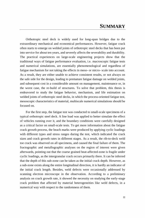
Orthotropic steel deck is widely used for long-span bridges due to the
extraordinary mechanical and economical performances. However, fatigue crack
often starts to emerge on welded joints of orthotropic steel decks that has been put
into service for about ten years, and severely affects the severability and durability.
The practical experiences on large-scale engineering projects show that the
traditional ways of fatigue performance evaluation, i.e. macroscopic fatigue tests
and numerical simulations, are essentially phenomenological and regardless of
fatigue mechanism for not taking the effects in meso- or micro- scale into account.
As a result, they are either unable to achieve consistent results, or not always on
the safe side for the design, leading to premature fatigue damage on welded joints,
and subsequent cost in a considerable amount on management, maintenance or, in
the worst case, the re-build of structures. To solve that problem, this thesis is
endeavored to study the fatigue behavior, mechanism, and life estimation on
welded joints of orthotropic steel decks, in which the process-oriented fatigue test,
mesoscopic characteristics of material, multiscale numerical simulations should be
focused on.
For the first step, the fatigue test was conducted to small-scale specimens of a
typical orthotropic steel deck. A line load was applied to better simulate the effect
of vehicles running over it, and the boundary conditions were carefully designed
as a critical factor on small-scale tests. To get more information about the fatigue
crack growth process, the beach marks were produced by applying cyclic loadings
with different types and stress ranges during the test, which indicated the crack
sizes and crack growth rates in different stages. As a result, the rib-to-deck weld
toe crack was observed on all specimens, and caused the final failure of them. The
fractographic and metallographic analyses on the region of interest were given
afterwards, pointing out that the coarse grained heat-affected-zone is fragile under
cyclic loadings, as the intergranular crack occurs primarily there. It can be inferred
that the depth of this sub-zone can be taken as the initial crack depth. However, as
a sub-zone exists along the entire longitudinal direction, it is hardly an indicator of
the initial crack length. Besides, weld defects were occasionally addressed by
scanning electron microscope in the observation. According to a preliminary
analysis on crack growth rate, it showed the necessity on studying the early-stage
crack problem that affected by material heterogeneities like weld defects, in a
numerical way with respect to the randomness of them.

IV
Consequently, a program of extended finite element method was developed
using MATLAB, with consideration of random weld defects. Additionally, to be
feasible on the representative volume elements extracted from rib-to-deck welded
joints, a level-set function was built for easily modelling the weld toe flank angles.
As the geometries are independent to meshes, the program enables to build models
that are free for re-mesh, providing great benefits to the evaluation of random weld
defects when solving a big number of cases. With this program, a homogenization
method was proposed based on the concept of equivalent crack growth length.
Numerical examples showed its applicability on early-stage cracks, as the
relatively small crack growth rate in that stage will only lead to tiny errors. Then
the main factors that affect crack growth were addressed by parametric analyses.
The results of this homogenization method showed large standard deviations of the
effects from weld defects, which could be important for structures in a much larger
scale. However, given the lack of knowledge on the sizes, numbers and spatial
distributions of weld defects, it is only possible to conduct the homogenization with
some reasonable assumptions.
Afterwards, the multiscale study was carried out in correspondence with the
fatigue test, using the numerical tools achieved before. Two different multiscale
methods were built with respect to the detailed fatigue crack growth process. The
comparison of them implied that the non-concurrent multiscale method, with a full
independent mesoscopic model, is of great efficiency without losing accuracy, and
thus is applied to reproduce the crack growth process in the test. Accordingly,
different stages in crack growth were addressed, and the material constants in the
stable crack growth stage, were achieved by data fitting. The values conformed
with the ones provided in standards and specifications for crack grows in Paris
region, and thus can obtain results with acceptable accuracy. However, the material
constants in Stage I, which is for relatively low stress intensity factors, was not
clear enough as the fatigue test cannot provide more information on the crack
growth rates in this stage.
Finally, the multiscale method was introduced into case studies on three
projects, including the Millau Viaduct in southeast France, the KW5 Bridge on
Albert Canal, Belgium, and the Runyang Yangtze River Bridge in China. The three
case studies estimated the fatigue life based on traffic flows that are: i) measured
in Europe in a short term; ii) recommended by Eurocode; iii) measured in China in
a long term, thus presented the extensive feasibility of this multiscale method.
Specifically, the fatigue life was calculated by two parts, i.e. the macro crack
initiation life and macro crack growth life. The former one was given in a
probabilistic way for the sake of the randomness induced by the initial crack depth

V
and other weld defects, as investigated in the above works. Whilst the latter one
was provided in a deterministic way as the influence factors were of less scatter or
not so critical then. The results suggested that the traffic flow on the Millau Viaduct
was much lighter or easier than that on the Runyang Yangtze River Bridge. Hence,
the fatigue problem will not be a concern for Millau Viaduct in decades. In contrast,
the Runyang Yangtze River Bridge may suffer from fatigue damage in less than
ten years. In addition, the case study on KW5 Bridge implied that the traffic load
recommended by Eurocode was not a proper option when using fracture mechanics
to evaluate the fatigue performance. The main reason is that the traffic volume
consists of heavy vehicles only, and thus is quite large and design-oriented. Hence,
the fatigue life obtained for KW5 Bridge was too short and unrealistic. To sum up,
the study showed its feasibility by applying on the actual projects under various
conditions, and the life estimation results are of acceptable accuracy when traffic
flow is measured in a relatively long term. The obtained results are in a probabilistic
form, and will provide valuable information to making maintenance strategies for
bridges, such as the schedule of the visual inspections and further retrofitting works.

VI
VII
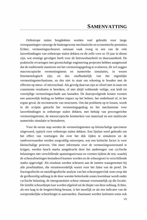
SAMENVATTING
Orthotrope stalen brugdekken worden veel gebruikt voor lange
overspanningen vanwege de buitengewone mechanische en economische prestaties.
Echter, vermoeiingsscheuren ontstaan vaak vroeg in een van de vele
lasverbindingen van orthotrope stalen dekken en dit zelfs voor ze 10 jaar in dienst
zijn, wat ernstige gevolgen heeft voor de betrouwbaarheid en duurzaamheid. De
praktische ervaringen met grootschalige engineering projecten hebben aangetoond
dat de traditionele manieren om het vermoeiingsgedrag te evalueren, dit wil zeggen
macroscopische vermoeiingstests en numerieke simulaties, in wezen
fenomenologisch zijn, en dus onafhankelijk van het eigenlijke
vermoeiingsmechanisme, en dus niet in staat om rekening te houden met de
effecten op meso- of microschaal. Als gevolg daarvan zijn ze ofwel niet in staat om
consistente resultaten te bereiken, of niet altijd voldoende veilige, wat leidt tot
voortijdige vermoeiingsschade aan lasnaden. De daaropvolgende kosten vormen
een aanzienlijk bedrag en hebben impact op het beheer, het onderhoud of, in het
ergste geval, de reconstructie van structuren. Om dat probleem op te lossen, wordt
in dit scriptie getracht het vermoeiingsgedrag en het mechanisme voor
lasverbindingen in orthotrope stalen dekken, met behulp van procesgerichte
vermoeiingstesten, de mesoscopische kenmerken van materiaal en een multiscale
numerieke simulatie te bestuderen.
Voor de eerste stap werden de vermoeiingstesten op kleinschalige specimens
uitgevoerd, typisch voor orthotrope stalen dekken. Een lijnlast werd gebruikt om
het effect van voertuigen die over het dek rijden te simuleren en de
randvoorwaarden werden zorgvuldig ontworpen, wat een kritische factor is voor
kleinschalige proeven. Om meer informatie over de vermoeiingsweerstand te
krijgen, werden beach marks aangebracht door het aanbrengen van cyclische
belastingen met verschillende spanningsniveaus en vormen tijdens de test, waarbij
de scheurafmetingen bestudeerd kunnen worden en de scheurgroei in verschillende
stadia opgevolgd. Als resultaat werden scheuren aan de lasteen waargenomen bij
alle proefstukken, die verantwoordelijk waren voor het falen van de proef. De
fractografische en metallografische analyse van het scheuroppervlak wees erop dat
de grofkorrelig sublaag in de door warmte beïnvloede zones kwetsbaar wordt onder
cyclische belasting, de intergranulaire scheur ontstaat voornamelijk op die locatie.
De initiële scheurdiepte kan worden afgeleid uit de diepte van deze sublaag. Echter,
als een laag in de lengterichting bestaat, is het moeilijk ze als een indicator van de
oorspronkelijke scheurlengte te aanvaarden. Daarnaast werden lasfouten soms ook
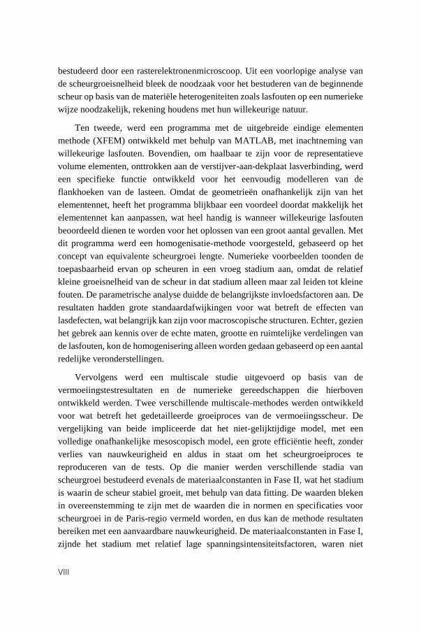
VIII
bestudeerd door een rasterelektronenmicroscoop. Uit een voorlopige analyse van
de scheurgroeisnelheid bleek de noodzaak voor het bestuderen van de beginnende
scheur op basis van de materiële heterogeniteiten zoals lasfouten op een numerieke
wijze noodzakelijk, rekening houdens met hun willekeurige natuur.
Ten tweede, werd een programma met de uitgebreide eindige elementen
methode (XFEM) ontwikkeld met behulp van MATLAB, met inachtneming van
willekeurige lasfouten. Bovendien, om haalbaar te zijn voor de representatieve
volume elementen, onttrokken aan de verstijver-aan-dekplaat lasverbinding, werd
een specifieke functie ontwikkeld voor het eenvoudig modelleren van de
flankhoeken van de lasteen. Omdat de geometrieën onafhankelijk zijn van het
elementennet, heeft het programma blijkbaar een voordeel doordat makkelijk het
elementennet kan aanpassen, wat heel handig is wanneer willekeurige lasfouten
beoordeeld dienen te worden voor het oplossen van een groot aantal gevallen. Met
dit programma werd een homogenisatie-methode voorgesteld, gebaseerd op het
concept van equivalente scheurgroei lengte. Numerieke voorbeelden toonden de
toepasbaarheid ervan op scheuren in een vroeg stadium aan, omdat de relatief
kleine groeisnelheid van de scheur in dat stadium alleen maar zal leiden tot kleine
fouten. De parametrische analyse duidde de belangrijkste invloedsfactoren aan. De
resultaten hadden grote standaardafwijkingen voor wat betreft de effecten van
lasdefecten, wat belangrijk kan zijn voor macroscopische structuren. Echter, gezien
het gebrek aan kennis over de echte maten, grootte en ruimtelijke verdelingen van
de lasfouten, kon de homogenisering alleen worden gedaan gebaseerd op een aantal
redelijke veronderstellingen.
Vervolgens werd een multiscale studie uitgevoerd op basis van de
vermoeiingstestresultaten en de numerieke gereedschappen die hierboven
ontwikkeld werden. Twee verschillende multiscale-methodes werden ontwikkeld
voor wat betreft het gedetailleerde groeiproces van de vermoeiingsscheur. De
vergelijking van beide impliceerde dat het niet-gelijktijdige model, met een
volledige onafhankelijke mesoscopisch model, een grote efficiëntie heeft, zonder
verlies van nauwkeurigheid en aldus in staat om het scheurgroeiproces te
reproduceren van de tests. Op die manier werden verschillende stadia van
scheurgroei bestudeerd evenals de materiaalconstanten in Fase II, wat het stadium
is waarin de scheur stabiel groeit, met behulp van data fitting. De waarden bleken
in overeenstemming te zijn met de waarden die in normen en specificaties voor
scheurgroei in de Paris-regio vermeld worden, en dus kan de methode resultaten
bereiken met een aanvaardbare nauwkeurigheid. De materiaalconstanten in Fase I,
zijnde het stadium met relatief lage spanningsintensiteitsfactoren, waren niet

IX
duidelijk genoeg in de vermoeiingstest aangezien die geen informatie geven over
de scheurgroeisnelheden in dit stadium.
Ten slotte werd de multiscale methode geïntroduceerd in case studies voor drie
projecten: het viaduct van Millau in het zuidoosten van Frankrijk, de KW5 Brug
over het Albertkanaal in Antwerpen, België, en de Runyangbrug over de Yangtze
in China. De drie casestudies hebben het vermoeidheidsleven geschat op basis van
de verkeersstromen die zijn: i) in korte tijd in Europa gemeten; ii) aanbevolen door
Eurocode; iii) op lange termijn in China gemeten, dus de uitgebreide haalbaarheid
van deze multiscale methode voorgesteld. De vermoeiingslevensduur werd
berekend in twee delen, d.w.z. de macro scheurinitiatie levensduur en de macro
scheurgroei levensduur. Eerstgenoemde werd bestudeerd op een probabilistische
wijze omwille van de willekeur geïnduceerd door de initiële scheur diepte en de
andere lasfouten, zoals onderzocht in de bovengenoemde studie. De
laatstgenoemde werd bestudeerd op een deterministische wijze aangezien de
invloedsfactoren veel minder willekeurig zijn. De resultaten suggereerden dat de
doorstroming van het verkeer op het viaduct van Millau veel lichter en makkelijker
was dan die op het Runyangbrug. Daarom zal het vermoeiingsprobleem niet
voorkomen voor het Viaduct van Millau in de eerste tientallen jaren, terwijl de
Runyangbrug daarentegen last kan hebben van vermoeiing in minder dan tien jaar.
Daarnaast bleek de verkeersbelasting aanbevolen door de Eurocode geen goede
optie wanneer breukmechanica toegepast wordt om de vermoeiingsprestaties te
evalueren, omwille van het gebruik van grote en ontwerp-georiënteerde
verkeersvolumes. Vandaar dat de levensduur verkregen voor de KW5 brug te kort
en onrealistisch bleek. Kortom, de studie toonde de haalbaarheid voor het toepassen
op concrete projecten aan, en de resultaten van de levensbeschatting zijn van
aanvaardbare nauwkeurigheid wanneer de verkeersstroom op een relatief lange
termijn wordt gemeten. De verkregen resultaten zijn in een probabilistische vorm,
en zullen waardevolle informatie verstrekken om onderhoudsstrategieën voor
bruggen te maken, zoals het schema van de visuele inspecties en
aanpassingswerken uit te voeren.

X

XI
NOMENCLATURE
a crack length
a0 initial crack length
ac homogenization coefficient of Paris constant
ad crack length that can be detected, i.e. initial length of a marco-crack
aI enriched degrees of freedom
B(x) crack-tip enrichment function
C Paris constant
C0 original value of Paris constant
Ceff effective Paris constant
Ck cycle count
da/dN crack growth rate
Dt damage induced by test truck
Dy damage per year
EI elastic modulus of inclusions
EM elastic modulus of matrix
ES elastic modulus of steel
F shape factor for calculating K
Fb shape factor for bending stress
H(x) Heaviside enrichment function
K stress intensity factor
KI Mode-I stress intensity factor
KII Mode-II stress intensity factor
∆Keff effective stress intensity factor range
∆Kth threshold value of stress intensity factor range
𝛥𝐾̅̅ ̅̅ representative SIF range between two beach marks
Ld data length of the wheel loads in days
m Paris exponent
nI number of inclusions
nP number of pores
nd number of defects
Nbase regular fatigue cycle numbers in the test
Nbeachmark beach mark cycle numbers in the test
Nd fatigue life in days
Ny fatigue life in years
NI(x) shape function in the traditional FEM
Pbase regular fatigue cycle loading range in the test
Pbeachmark minimum beach mark cycle loading in the test
Pmax maximum regular fatigue cycle loading in the test
Pmin minimum regular fatigue cycle loading in the test
Pj possibility for each location
Pl percentage of different types of lorries
PM Poisson’s ratio of matrix
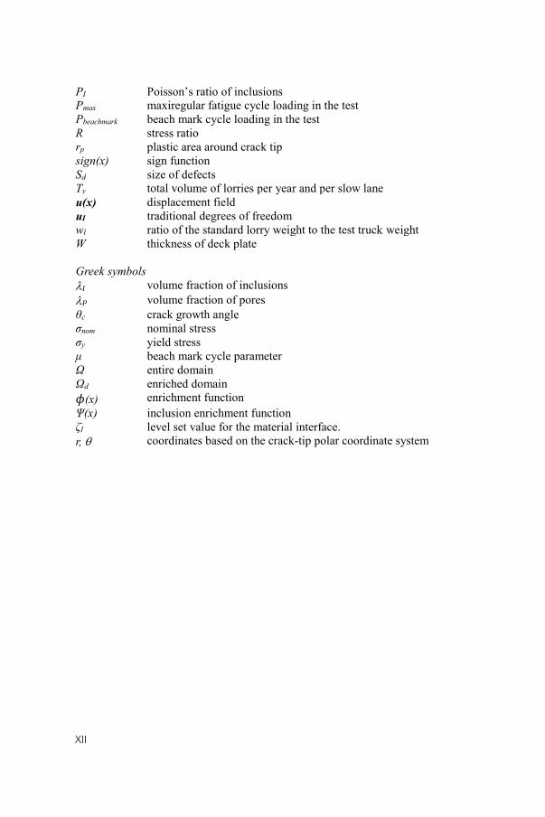
XII
PI Poisson’s ratio of inclusions
Pmax maxiregular fatigue cycle loading in the test
Pbeachmark beach mark cycle loading in the test
R stress ratio
rp plastic area around crack tip
sign(x) sign function
Sd size of defects
Ty total volume of lorries per year and per slow lane
u(x) displacement field
uI traditional degrees of freedom
wl ratio of the standard lorry weight to the test truck weight
W thickness of deck plate
Greek symbols
I volume fraction of inclusions
P volume fraction of pores
θc crack growth angle
σnom nominal stress
σy yield stress
μ beach mark cycle parameter
Ω entire domain
Ωd enriched domain
𝜙(x) enrichment function
Ψ(x) inclusion enrichment function
ζI level set value for the material interface.
r, coordinates based on the crack-tip polar coordinate system
XIII
ABBREVIATIONS
CV coefficient of variance
CGR crack growth rate
DOF degree of freedom
EDS energy dispersive spectroscopy
FEM finite element method
HAZ heat-affected-zone
LEFM linear elastic fracture mechanics
MCGL macro-crack growth life
MCIL macro-crack initiation life
NDT non-destructive test
OSD orthotropic steel deck
PM parental material
PUM partition of unity method
RVE representative volume element
SD standard deviation
SEM scanning electron microscope
SIF stress intensity factor
WM welding material
XFEM extended finite element method

XIV
XV
CONTENTS
Preface ......................................................................................................... I
Summary .................................................................................................. III
Samenvatting ........................................................................................... VII
Nomenclature ........................................................................................... XI
Abbreviations ........................................................................................ XIII
Contents .................................................................................................. XV
List of figures ........................................................................................ XXI
List of tables ....................................................................................... XXIX
CHAPTER 1 ............................................................................................... 1
1.1. General introduction ............................................................ 2
1.2. Literature review.................................................................. 4
1.2.1. Fatigue design method ................................................. 4
1.2.1.1. Fatigue design theories ............................................. 4
1.2.1.2. Vehicle loads ............................................................. 5
1.2.2. Fatigue-prone details on orthotropic steel decks .......... 7
1.2.2.1. Rib-to-deck welded joints ....................................... 10
1.2.2.2. Rib-to-diaphragm welded joints ............................. 11
1.2.2.3. Longitudinal ribs joints ........................................... 13
1.2.3. Weld fatigue ............................................................... 14
1.2.3.1. Fatigue strength classification and evaluation ........ 14
1.2.3.2. Weld defects ............................................................ 17
1.2.3.3. Heat-Affected Zone ................................................ 19
1.2.3.4. Residual stresses ..................................................... 20
1.2.4. Fatigue behavior and prediction ................................. 22
1.2.4.1. Typical stages of fatigue behavior .......................... 22
1.2.4.2. Paris law ................................................................. 23
1.2.4.3. Short crack propagation .......................................... 25
1.3. Problems and Objectives ................................................... 26
CHAPTER 2 ............................................................................................. 29
XVI
2.1. Introduction ....................................................................... 30
2.2. Test scheme ....................................................................... 31
2.2.1. Test specimens and boundary conditions ................... 32
2.2.2. Manufacturing specimens .......................................... 33
2.2.3. Data collection ........................................................... 34
2.3. Fatigue test ......................................................................... 36
2.3.1. Test setups .................................................................. 36
2.3.2. Loads .......................................................................... 38
2.3.3. Test results and discussions ....................................... 40
2.3.3.1. Crack locations ....................................................... 40
2.3.3.2. Beach marks ........................................................... 43
2.4. Fractographic and metallographic analyses ....................... 46
2.4.1. Equipment and Procedures......................................... 46
2.4.2. Fractographic analyses ............................................... 48
2.4.2.1. Crack initiation ....................................................... 48
2.4.2.2. Crack growth .......................................................... 49
2.4.2.3. Fatigue striations ..................................................... 51
2.4.3. Metallographic analyses ............................................. 52
2.4.3.1. Parental material ..................................................... 52
2.4.3.2. Weld root ................................................................ 52
2.4.3.3. Weld toe .................................................................. 55
2.4.3.4. Cross section of fracture ......................................... 58
2.4.4. Hardness test .............................................................. 60
2.4.5. Preliminary analysis on crack growth rate ................. 61
CHAPTER 3 ............................................................................................. 65
3.1. Introduction ....................................................................... 66
3.2. Level set method ................................................................ 68
3.2.1. Level set function for crack ....................................... 68
3.2.2. Level set function for pores and inclusions................ 69
3.2.3. Level set function for weld geometry ........................ 69
XVII
3.3. XFEM basics ..................................................................... 70
3.3.1. Governing equation .................................................... 70
3.3.2. Enrichment functions ................................................. 72
3.3.3. Subdomains for numerical integration ....................... 73
3.3.4. Calculation of stress intensity factor .......................... 74
3.4. Crack growth model .......................................................... 75
3.4.1. Linear-elastic fracture mechanics .............................. 75
3.4.2. Crack growth rate ....................................................... 78
3.4.3. Mixed-mode crack growth ......................................... 79
CHAPTER 4 ............................................................................................. 81
4.1. Introduction ....................................................................... 82
4.2. Generation of RVEs ........................................................... 83
4.2.1. Random defects .......................................................... 83
4.2.2. RVEs for OSDs .......................................................... 85
4.3. Homogenization method .................................................... 86
4.3.1. Basics ......................................................................... 86
4.3.2. Numerical examples ................................................... 88
4.3.3. Parametric analyses .................................................... 95
4.3.3.1. Volume fractions ..................................................... 95
4.3.3.2. Material properties and boundary conditions ......... 96
4.3.3.3. Weld geometry ...................................................... 100
4.4. Results and discussions ................................................... 101
CHAPTER 5 ........................................................................................... 105
5.1. Introduction ..................................................................... 106
5.2. Analyses on beach marks ................................................ 106
5.2.1. Visual identification ................................................. 107
5.2.2. Determination of crack dimensions ......................... 110

XVIII
5.3. Numerical model of fatigue test ...................................... 112
5.3.1. Macroscopic model .................................................. 112
5.3.2. A sub-model based multiscale method .................... 115
5.3.3. A non-concurrent multiscale method ....................... 119
5.4. Crack growth in the fatigue test ....................................... 124
5.4.1. Analyses based on beach marks ............................... 124
5.4.2. Material constants estimation................................... 130
5.5. Discussions ...................................................................... 133
5.5.1. Crack growth simulation .......................................... 133
5.5.2. Early-stage cracks .................................................... 135
5.5.3. Influence of weld defects ......................................... 138
CHAPTER 6 ........................................................................................... 141
6.1. Introduction ..................................................................... 142
6.2. Methodology .................................................................... 142
6.3. A case study based on the traffic flow in Europe ............ 146
6.3.1. Traffic flow .............................................................. 146
6.3.2. Numerical models .................................................... 148
6.3.3. Stress intensity factors ............................................. 150
6.3.4. Calculation of fatigue life ........................................ 153
6.4. A case study based on Eurocode ..................................... 159
6.4.1. On-site test ............................................................... 159
6.4.2. Stress intensity factors ............................................. 160
6.4.3. Calculation of fatigue life ........................................ 162
6.4.4. Discussions .............................................................. 171
6.5. A case study based on the traffic flow in China .............. 173
6.5.1. Traffic flow .............................................................. 174
XIX
6.5.2. Stress range history .................................................. 177
6.5.3. Calculation of fatigue life ........................................ 178
6.5.4. Discussions .............................................................. 185
CHAPTER 7 ........................................................................................... 187
7.1. Conclusions ..................................................................... 188
7.2. The outcome regarding the objectives ............................. 190
7.3. Future researches ............................................................. 191
7.3.1. Residual stress acquisition ....................................... 192
7.3.2. Fatigue behavior in Stage I ...................................... 192
7.3.3. Retrofitting work on cracked components of OSDs 193
7.3.4. Other types of cracks on OSDs ................................ 193
7.3.5. Novel fatigue design methods for OSDs .................. 193
Appendix A ............................................................................................ 195
Appendix B............................................................................................. 199
Bibliography ........................................................................................... 203

XX
XXI
LIST OF FIGURES
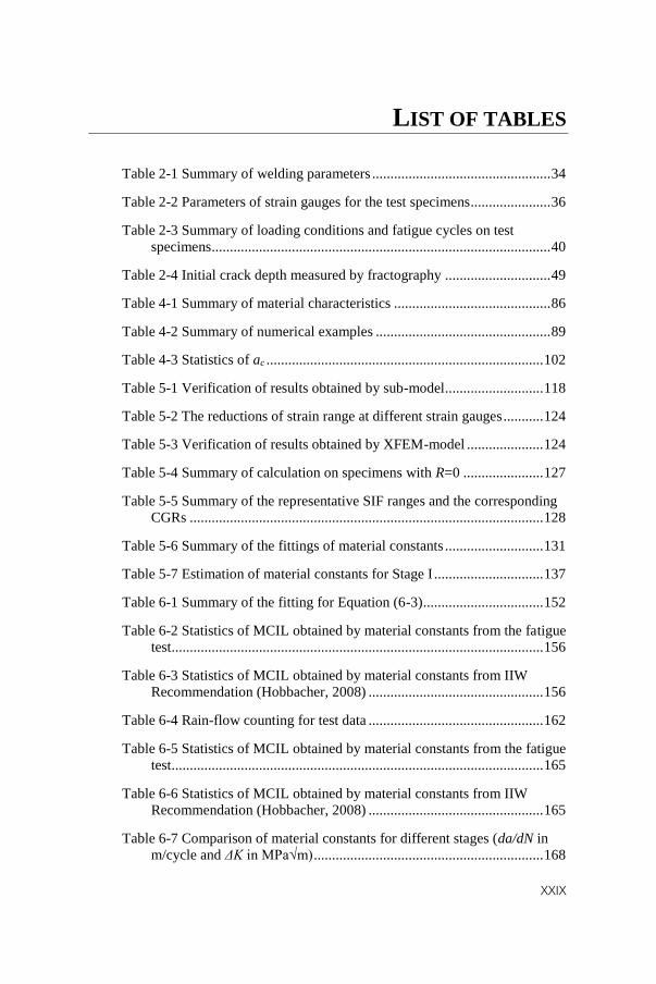
Fig. 1-1 Number of bridges with orthotropic decks identified in each
country (Kolstein, 2007) ........................................................................ 2
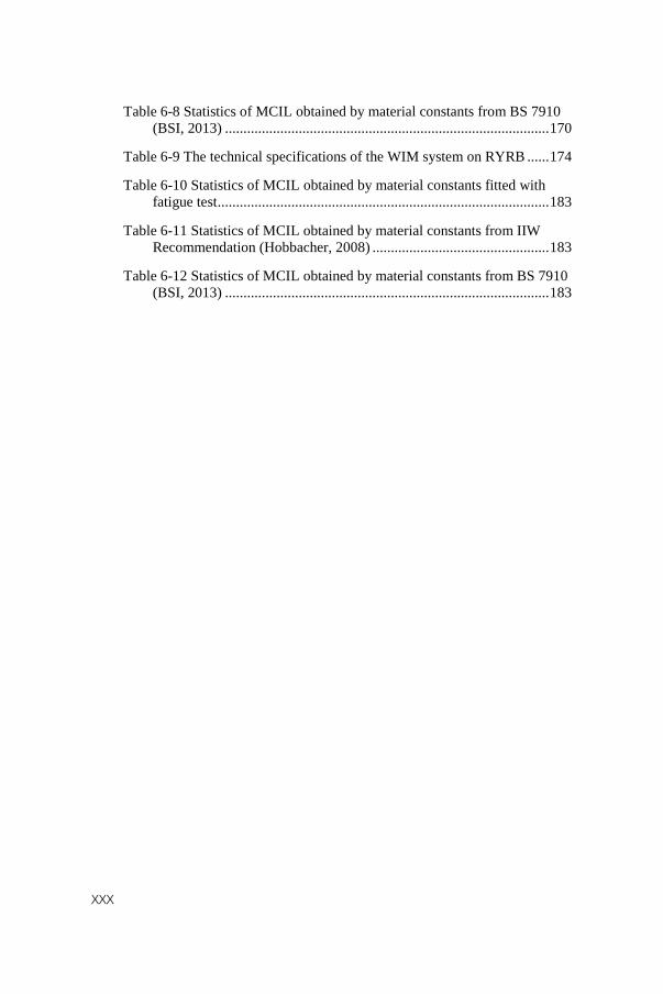
Fig. 1-2 Bridge spans of bridges with OSDs (Kolstein, 2007) ...................... 3
Fig. 1-3 Standard vehicle for fatigue design in BS 5400 ............................... 6
Fig. 1-4 T-loading in Japanese Bridge Fatigue Design Recommendation ..... 6
Fig. 1-5 Design truck and the refined loading pattern for OSDs in AASHTO
............................................................................................................... 6
Fig. 1-6 Frequency distribution of transverse location of central line of
vehicle .................................................................................................... 7
Fig. 1-7 Rib-to-deck weld fracture in Severn Bridge (Wolchuk, 1990)......... 8
Fig. 1-8 Fatigue cracks on Humen Bridge ..................................................... 9
Fig. 1-9 Four typical cracks on OSD on Hanshin Highway Bridges ............. 9
Fig. 1-10 The though-crack in the Second Van Brienenoord Bridge
(Maljaars et al., 2012) .......................................................................... 11
Fig. 1-11 Different types of crack on rib-to-deck welded joints .................. 11
Fig. 1-12 Cut-out shapes in different specifications .................................... 12
Fig. 1-13 Typical crack at RDDP welded joint (Kolstein, 2007) ................. 13
Fig. 1-14 RDDP cracks on Jiangyin Yangtze Bridge, China ....................... 13
Fig. 1-15 Three stages of RDDP crack growth (Zhou, 2010) ...................... 13
Fig. 1-16 The high strength bolt connection of longitudinal ribs (Feng,
2009) .................................................................................................... 14
Fig. 1-17 Different categories of fatigue strength (Gurney, 1979) .............. 16
Fig. 1-18 The fictitious notches in Effective Notch Stress Method
(Hobbacher, 2008) ............................................................................... 16
Fig. 1-19 The effect of weld toe flank angle and weld toe radius
(Gurney,1979) ...................................................................................... 17
Fig. 1-20 Typical weld defects on fracture surfaces (Miki et al., 2001) ...... 18
Fig. 1-21 Length scales of the life cycle of a component subjected to cyclic
loading (Zerbst et al., 2012) ................................................................. 18
XXII
Fig. 1-22 The grain size of parent metal (PM), HAZ of submerged-arc
welding (SAW), and HAZ of laser hybrid welding (Hybrid) (Remes et
al., 2012) .............................................................................................. 19
Fig. 1-23 Microstructures in sections of different distances of HAZ
(Ramazani et al., 2013) ........................................................................ 20
Fig. 1-24 Hardness of a typical butt welded joint (Hertelé et al., 2014) ...... 20
Fig. 1-25 Schematic welding residual stress distributions in a butt joint
(Zerbst et al., 2014) .............................................................................. 21
Fig. 1-26 Fatigue behavior of a thin plate under cyclic tensile stress (Lee,
2005) .................................................................................................... 23
Fig. 1-27 The crack growth rate for A533 steel (R=0.1) (Wang & Chen,
2009) .................................................................................................... 25
Fig. 1-28 Different fatigue thresholds d and ath (Miller, 1993) .................... 26
Fig. 1-29 A brief flowchart of this study ..................................................... 28
Fig. 2-1 Fatigue test schemes (unit: mm) ..................................................... 30
Fig. 2-2 Laboratory of the Educational and Research Center in Transport,
University of Pardubice, Czech Republic (photo by Wim Nagy) ........ 31
Fig. 2-3 Full-scale reference model of an OSD ........................................... 32
Fig. 2-4 Test specimens and boundary conditions ....................................... 33
Fig. 2-5 Load parameters in a beach marks signal (Schepens and Laseure,
2015) .................................................................................................... 35
Fig. 2-6 Strain gauge locations at the stiffener-to-deck plate test specimen 35
Fig. 2-7 The supporting triangular-shaped body .......................................... 37
Fig. 2-8 Supports of the specimens .............................................................. 37
Fig. 2-9 Loading system of the test .............................................................. 38
Fig. 2-10 An example of quasi-static loading (R=0) ................................... 38
Fig. 2-11 An example of fatigue loading ..................................................... 39
Fig. 2-12 An example of quasi-triangular beach mark loading.................... 39
Fig. 2-13 Weld toe crack through the deck plate (Specimen 9) ................... 41
Fig. 2-14 Sketches of simplified local models ............................................. 42
Fig. 2-15 Scheme of root crack study for small-scale specimens ................ 42
XXIII
Fig. 2-16 Wide beach marks on Specimen X............................................... 43
Fig. 2-17 Beach marks on Specimen VII ..................................................... 44
Fig. 2-18 Beach marks on Specimen 10 ...................................................... 44
Fig. 2-19 Crack growth process on test specimens ...................................... 46
Fig. 2-20 Equipment used for analyzing the test specimens. ....................... 47
Fig. 2-21 Different fracture behavior (Specimen VI) .................................. 48
Fig. 2-22 Intergranular decohesion on fracture surface ............................... 49
Fig. 2-23 The incremental secondary cracks with the main crack growth
(Specimen 9) ........................................................................................ 50
Fig. 2-24 Occasional voids/inclusions on the fracture surface (Specimen
VII) ...................................................................................................... 51
Fig. 2-25 The diversity in measuring the striation width (Specimen VII,
Zone 5) ................................................................................................. 51
Fig. 2-26 Microstructures in parental material............................................. 52
Fig. 2-27 Weld defects on weld root ............................................................ 53
Fig. 2-28 The vicinity of weld root (mag. 64x) ........................................... 54
Fig. 2-29 The coarse grained HAZ near the slag (mag. 250x) ..................... 54
Fig. 2-30 The normalized zone near the parental material (mag. 250x) ...... 55
Fig. 2-31 The vicinity of weld toe (mag. 64x) ............................................. 56
Fig. 2-32 Columnar in welding material (mag. 250x) ................................. 56
Fig. 2-33 Partially austenite zone (mag. 250x) ............................................ 56
Fig. 2-34 Microstructure of fusion zone and coarse grained HAZ .............. 58
Fig. 2-35 Microstructure of welding material (mag. 1000x) ....................... 58
Fig. 2-36 Metallography on the cross section of the fractured sample ........ 59
Fig. 2-37 The intra-granular fracture in the normalized zone (Specimen IV)
............................................................................................................. 59
Fig. 2-38 Initial crack depth measure based on coarse grained HAZ .......... 60
Fig. 2-39 The hardness test on the line perpendicular to the weld interface 61
Fig. 2-40 The hardness test on the possible crack path ................................ 61
XXIV
Fig. 2-41 Preliminary graph for crack growth rate ...................................... 63
Fig. 2-42 Different stages of crack growth on a) Al 2024-T3 and b) Al 7075-
T6 (Bogdanov, 2014) ........................................................................... 64
Fig. 3-1 General structure of the XFEM program ....................................... 67
Fig. 3-2 Level set function for crack ............................................................ 68
Fig. 3-3 level set functions ........................................................................... 69
Fig. 3-4 Subdomain for different types of elements .................................... 73
Fig. 3-5 Crack opening modes (Gross and Seelig, 2011) ............................ 75
Fig. 3-6 Crack tip polar coordinate system .................................................. 76
Fig. 3-7 Small-scale yielding verification .................................................... 78
Fig. 4-1 Typical weld defects in a) butt weld and b) fillet weld (Milella,
2012) .................................................................................................... 82
Fig. 4-2 The flowchart of generating random defects .................................. 84
Fig. 4-3 RVE in the rib-to-deck welded joint of OSD ................................. 85
Fig. 4-4 Generated RVEs with randomly distributed inclusions & pores, I
= P =0.05 ........................................................................................... 85
Fig. 4-5 Flowchart of the homogenization process ...................................... 88
Fig. 4-6 Numerical Example 1 ..................................................................... 90
Fig. 4-7 Numerical Example 2 ..................................................................... 91
Fig. 4-8 Numerical Example 3 ..................................................................... 92
Fig. 4-9 Numerical Example 4 ..................................................................... 93
Fig. 4-10 Numerical Example 5 ................................................................... 94
Fig. 4-11 The convergence of mean and CV of ac with respect to volume
fraction of inclusions I ....................................................................... 95
Fig. 4-12 The convergence of mean and CV of ac with respect to volume
fraction of pores P .............................................................................. 95
Fig. 4-13 Variation of homogenization coefficient ac with normalized elastic
modulus of matrix ................................................................................ 96
Fig. 4-14 Variation of homogenization coefficient ac with tension σ .......... 96

XXV
Fig. 4-15 Variation of homogenization coefficient ac with normalized Paris
constant ................................................................................................ 97
Fig. 4-16 Variation of homogenization coefficient ac with normalized elastic
modulus of inclusions .......................................................................... 97
Fig. 4-17 Parametric analysis of ac with respect to number of pores ........... 98
Fig. 4-18 Parametric analysis of ac with respect to number of inclusions ... 98
Fig. 4-19 Parametric analysis of ac with respect to pore sizes and locations
............................................................................................................. 99
Fig. 4-20 Parametric analysis of ac with respect to inclusion sizes and
locations ............................................................................................. 100
Fig. 4-21 Comparison of ac in RVEs with/without flank angle (unit:
MPa√m) ............................................................................................. 100
Fig. 4-22 Distribution of homogenization coefficient ac for different a0 ... 102
Fig. 5-1 Fracture surfaces and beach marks on test specimens .................. 108
Fig. 5-2 Beach mark measurement by microscope (Specimen 10) ............ 109
Fig. 5-3 Ideal shape of the crack with consideration of merging of initial
cracks ................................................................................................. 110
Fig. 5-4 The equivalent semi-elliptical crack on Specimen VII ................ 110
Fig. 5-5 The curve fitting on the crack area varies with the depth ............. 112
Fig. 5-6 Macroscopic model in SAMCEF ................................................. 113
Fig. 5-7 Load distribution on deck plate .................................................... 115
Fig. 5-8 The mesh refinement around a crack of 2mm depth in the XFEM
domain ............................................................................................... 115
Fig. 5-9 The Sub-model based multiscale method ..................................... 117
Fig. 5-10 Stress field on a weld toe (corresponding to the bold part in Fig.
5-9) .................................................................................................... 118
Fig. 5-11 The scheme of XFEM model ..................................................... 120
Fig. 5-12 Stress intensity factors under bending stress of 100 MPa .......... 120
Fig. 5-13 Validation of XFEM model........................................................ 121
Fig. 5-14 Time history of strain measured for Specimen 10 ...................... 123
Fig. 5-15 The shape factor F ...................................................................... 126
XXVI
Fig. 5-16 Crack growth rate for specimens with R=0 ................................ 129
Fig. 5-17 Typical CGR curves and different stages ................................... 130
Fig. 5-18 Curve fitting to estimate the material constants ......................... 132
Fig. 5-19 Crack growth simulation of an initial crack with 0.2 mm in depth
........................................................................................................... 134
Fig. 5-20 Crack growth simulation of an initial crack with 2 mm in depth
........................................................................................................... 135
Fig. 5-21 The homogenization coefficient ac for Stage I cracks ................ 138
Fig. 5-22 The CGR for Stage I cracks affected by weld defects ................ 139
Fig. 6-1 The flowchart for estimating macro-crack initiation life .............. 145
Fig. 6-2 The orthotropic steel deck of Millau Viaduct (Zhou et al., 2015) 146
Fig. 6-3 Typical time history of stress ....................................................... 148
Fig. 6-4 The detailed geometry at the welded joint ................................... 148
Fig. 6-5 Coarse model and sub-model of the Millau Viaduct .................... 149
Fig. 6-6 The influence surfaces of the transverse stress at 8 mm to the
welded joint ....................................................................................... 150
Fig. 6-7 Stress intensity factors obtained by XFEM model ....................... 151
Fig. 6-8 Shape factors for Millau Viaduct calculated by data fitting ......... 152
Fig. 6-9 Distribution of macro crack initiation life Nd for determined a0,
with C0=2.571×10⁻¹¹, m=2.603, according to the fatigue test ............ 154
Fig. 6-10 Distribution of macro crack initiation life Nd for random a0, with
C0=2.571×10⁻¹¹, m=2.603, according to the fatigue test .................... 155
Fig. 6-11 Distribution of macro crack initiation life Nd for determined a0,
with C0=1.65×10⁻¹¹, m=3, according to (Hobbacher, 2008) .............. 155
Fig. 6-12 Distribution of macro crack initiation life Nd for random a0, with
C0=1.65×10⁻¹¹, m=3, according to (Hobbacher, 2008) ...................... 156
Fig. 6-13 Macro-crack growth life from 0.5 mm to 7 mm ......................... 157
Fig. 6-14 Fatigue life for initial crack depth ranging from 0.2 mm to 0.4 mm
........................................................................................................... 157
Fig. 6-15 KW5 Bridge over the Albert Channel, Belgium (photo from De
Backer et al., 2008) ............................................................................ 159
XXVII
Fig. 6-16 Strain gauges at the weld toe (De Backer et al., 2007) ............... 160
Fig. 6-17 Test scheme and the assumed possibility of transverse locations
........................................................................................................... 160
Fig. 6-18 Measured strain on Location 1 ................................................... 161
Fig. 6-19 Measured strain on Location 2 ................................................... 161
Fig. 6-20 Measured strain on Location 3 ................................................... 161
Fig. 6-21 Measured strain on Location 4 ................................................... 161
Fig. 6-22 Measured strain on Location 5 ................................................... 161
Fig. 6-23 Distribution of macro crack initiation life Ny for determined a0,
with C0=2.571×10⁻¹¹, m=2.603, according to the fatigue test ............ 163
Fig. 6-24 Distribution of macro crack initiation life Ny for random a0, with
C0=2.571×10⁻¹¹, m=2.603, according to the fatigue test .................... 164
Fig. 6-25 Distribution of macro crack initiation life Ny for determined a0,
with C0=1.65×10⁻¹¹, m=3, according to (Hobbacher, 2008) .............. 164
Fig. 6-26 Distribution of macro crack initiation life Ny for random a0, with
C0=1.65×10⁻¹¹, m=3, according to (Hobbacher, 2008) ...................... 165
Fig. 6-27 Macro-crack growth life from 0.5 mm to 7.5 mm ...................... 166
Fig. 6-28 Fatigue life for initial crack depth ranging from 0.2 mm to 0.4 mm
........................................................................................................... 166
Fig. 6-29 Comparison of a) simple Paris law and b) two-stage crack growth
relationship (BS 7910) ....................................................................... 168
Fig. 6-30 Distribution of macro crack initiation life Ny for determined a0,
according to BS 7910 (BSI, 2013) ..................................................... 169
Fig. 6-31 Distribution of macro crack initiation life Ny for random a0,
according to BS 7910 (BSI, 2013) ..................................................... 169
Fig. 6-32 Macro-crack growth life from 0.5 mm to 7.5 mm according to BS
7910 ................................................................................................... 170
Fig. 6-33 Fatigue life for initial crack depth ranging from 0.2 mm to 0.4
mm, according to BS 7910 ................................................................ 171
Fig. 6-34 The Runyang Yangtze River Bridge in Jiangsu, China .............. 173
Fig. 6-35 The vehicle number on RYRB measured by WIM system in the
year of 2016 ....................................................................................... 175
XXVIII
Fig. 6-36 The vehicle number distribution on different lanes on RYRB ... 175
Fig. 6-37 The number of vehicles with more than 3 axles on RYRB ........ 176
Fig. 6-38 The accumulative total weight on each lane of RYRB .............. 176
Fig. 6-39 Comparison of the stress ranges induce by single and double tire
with the axle weight of 10 tons .......................................................... 178
Fig. 6-40 The fatigue lives for different lanes by assuming a0=0.3 mm ... 179
Fig. 6-41 Distribution of macro crack initiation life Ny for determined a0,
with C0=2.70×10⁻¹¹, m=2.603, according to the fatigue test .............. 180
Fig. 6-42 Distribution of macro crack initiation life Ny for random a0, with
C0=2.70×10⁻¹¹, m=2.603, according to the fatigue test ...................... 180
Fig. 6-43 Distribution of macro crack initiation life Ny for determined a0,
with C0=1.65×10⁻¹¹, m=3, according to (Hobbacher, 2008) .............. 181
Fig. 6-44 Distribution of macro crack initiation life Ny for random a0, with
C0=1.65×10⁻¹¹, m=3, according to (Hobbacher, 2008) ...................... 181
Fig. 6-45 Distribution of macro crack initiation life Ny for determined a0,
with two-stage model in BS7910 (BSI, 2013) ................................... 182
Fig. 6-46 Distribution of macro crack initiation life Ny for random a0, with
two-stage model in BS7910 (BSI, 2013) ........................................... 182
Fig. 6-47 Macro-crack growth life from 0.5 mm to 7 mm ......................... 184
Fig. 6-48 Fatigue life for initial crack depth ranging from 0.2 mm to 0.4 mm
........................................................................................................... 184
Fig. A-1 The micro-chemical energy analyses on Inclusion I ................... 196
Fig. A-2 The micro-chemical energy analyses on Inclusion II .................. 197
Fig. B-1 Geometrical parameters that affect the SIF of weld toe crack
(Bowness and Lee, 2000)................................................................... 199
XXIX
LIST OF TABLES
Table 2-1 Summary of welding parameters ................................................. 34
Table 2-2 Parameters of strain gauges for the test specimens...................... 36
Table 2-3 Summary of loading conditions and fatigue cycles on test
specimens ............................................................................................. 40
Table 2-4 Initial crack depth measured by fractography ............................. 49
Table 4-1 Summary of material characteristics ........................................... 86
Table 4-2 Summary of numerical examples ................................................ 89
Table 4-3 Statistics of ac ............................................................................ 102
Table 5-1 Verification of results obtained by sub-model ........................... 118
Table 5-2 The reductions of strain range at different strain gauges ........... 124
Table 5-3 Verification of results obtained by XFEM-model ..................... 124
Table 5-4 Summary of calculation on specimens with R=0 ...................... 127
Table 5-5 Summary of the representative SIF ranges and the corresponding
CGRs ................................................................................................. 128
Table 5-6 Summary of the fittings of material constants ........................... 131
Table 5-7 Estimation of material constants for Stage I .............................. 137
Table 6-1 Summary of the fitting for Equation (6-3) ................................. 152
Table 6-2 Statistics of MCIL obtained by material constants from the fatigue
test ...................................................................................................... 156
Table 6-3 Statistics of MCIL obtained by material constants from IIW
Recommendation (Hobbacher, 2008) ................................................ 156
Table 6-4 Rain-flow counting for test data ................................................ 162
Table 6-5 Statistics of MCIL obtained by material constants from the fatigue
test ...................................................................................................... 165
Table 6-6 Statistics of MCIL obtained by material constants from IIW
Recommendation (Hobbacher, 2008) ................................................ 165
Table 6-7 Comparison of material constants for different stages (da/dN in
m/cycle and ΔK in MPa√m) ............................................................... 168
XXX
Table 6-8 Statistics of MCIL obtained by material constants from BS 7910
(BSI, 2013) ........................................................................................ 170
Table 6-9 The technical specifications of the WIM system on RYRB ...... 174
Table 6-10 Statistics of MCIL obtained by material constants fitted with
fatigue test .......................................................................................... 183
Table 6-11 Statistics of MCIL obtained by material constants from IIW
Recommendation (Hobbacher, 2008) ................................................ 183
Table 6-12 Statistics of MCIL obtained by material constants from BS 7910
(BSI, 2013) ........................................................................................ 183

CHAPTER 1
INTRODUCTION
________________________________
CHAPTER 1
2
1.1. General introduction
The orthotropic steel deck (OSD) is a frequently-used structure type for
constructing bridges. This kind of structure was firstly built in 1950s, originated
from the stiffened steel plates used in deck in shipbuilding. Benefitted by the
development of high-strength steel and weld technologies, it became a very
common structure type in bridge constructions, as it can save up to 50% steel
consuming compared to pre-war bridges (Kolstein, 2007). Fig. 1-1 and Fig. 1-2
presented the bridges with OSDs with respect to countries and spans, respectively.
Accordingly, OSD had a lot of applications on small-span bridges. However, even
not obvious on the figures, OSD is certainly the favorite design for large-span
bridges world-widely, for example, the Second Bosphorus Bridge in Turkey, the
Great Belt Bridge in Denmark, the Millau Viaduct in France, etc. As the
infrastructures developed rapidly in recent decades in China, a lot of large-span
bridges with OSDs emerged, such as the ones crossing big rivers including
Runyang Yangtze River Bridge, Sutong Yangtze River Bridge, Taizhou Yangtze
River Bridge, Shanghai Yangtze River Tunnel and Bridge etc., and the ones
crossing sea including Hangzhou Bay Bridge, Qingdao Bay Bridge, etc.
Fig. 1-1 Number of bridges with orthotropic decks identified in each country
(Kolstein, 2007)
INTRODUCTION
3
Fig. 1-2 Bridge spans of bridges with OSDs (Kolstein, 2007)
As the large-span bridges are always located at vital positions for the entire
transportation systems, the durability design or life-cycle design is often laid great
importance on. Even so, OSD turns to be a fatigue-prone structure type as
documented all over the world, such as the Severn Bridge in Great Britain, the
Haseltal and Sinntal viaducts in Germany (Wolchuk, 1990), the Second Van
Brienenoord Bridge in Netherland (Maljaars et al. 2012), the Hanshin Expressway
in Japan (Okura et al., 1989), and the Willamsburg Bridge in the United States
(Tsakopoulos and Fisher, 2003), etc. Causes were found from different
perspectives, like the short influence line that lead to high cycle numbers (Nunn
and Cuninghame, 1974), the misalignments in terms of construction (Tong and
Shen, 1998), the severe overloading in terms of management, etc. These studies
could benefit solving fatigue problems in separated aspects, but are still incapable
of fatigue evaluation and life prediction since the fatigue mechanism on OSDs were
not comprehensively considered.
Therefore, due to the inexperience in the stage of manufacture, construction,
and management, the actual fatigue performance of OSDs may not be satisfied,
even though they were designed with fatigue cautions. Given the fast pace of
massive constructions of China, the seeds of fatigue issues on these bridges might
have been sowed in a more severe amount. Some of the recently-exposed fatigue
problems on existing OSDs were undoubtedly premature, and greatly reduced the
serviceability and durability of bridges.
CHAPTER 1
4
1.2. Literature review
1.2.1. Fatigue design method
Ever since the Silver Bridge collapse in 1967 due to the fatigue failure on its
eye bar, fatigue design becomes a necessity for steel bridges. As for OSDs, the
development on fatigue design mainly focuses on two parts: 1) the design theories
based on the fatigue performance of material itself; 2) the vehicle loads on different
type of bridges.
1.2.1.1. Fatigue design theories
a) Infinite life design
The target of infinite life design is to reduce the stress range on fatigue-prone
details to be small enough, thus the components and the whole structure could have
an infinite fatigue life. As regular S-N curves show, the fatigue life may not be
affected by the stress range when it is smaller than the fatigue limit, which leads to
the infinite life. For an infinite life design, the design equation is as follows,
Δ𝜎𝑚𝑎𝑥 ≤ [∆𝜎𝐿] (1-1)
where ∆𝜎𝑚𝑎𝑥 is the maximum stress range, [∆𝜎𝐿] is the fatigue limit.
It is obvious that the infinite life design will be too conservative and thus
sacrifice the economic efficiency. In addition, some studies on fatigue and fracture
for high-strength steels starts to challenge the existence of fatigue limit (Suresh,
1998), which holds that there is no obvious fatigue limit on S-N curves. Sonsino
(2007a) also proposed similar ideas for the cases of jointed components, material
in high temperatures and corrosive environments. The infinite life design is,
therefore, more of a way on designing irreplaceable components in some industries,
but not an option for large-scale civil engineering projects.
b) Safe life design
Safe life design is to provide sufficient ability to resist fatigue failure for the
structure during its design life. It is developed from infinite life design method,
thus they both use nominal stresses as the basic design parameter following S-N
curves. The difference is that the safe life design considers the fatigue resistance
with respect to the stress range. That means the fatigue performance is evaluated
by calculating the damage induced by the stress ranges higher than the fatigue limit.
The damage is usually accumulated linearly according to Miner’s Rule,
𝐷 = ∑𝑛𝑖/𝑁𝑖 (1-2)
INTRODUCTION
5
where D is the damage; ni is the applied stress cycles; Ni is the stress cycles at
failure; the subscript i refers to the corresponding stress ranges. Therefore, the safe
life design is much more economic than infinite life design, which make it the most
common method to design engineering structures such as OSDs.
c) Damage tolerance design
The concept of damage tolerance design was firstly proposed in the aircraft
industry, which attempted to take initial defects and maintenance into account in
the design phase. The design aims to evaluate the residual life by recognizing the
damages in maintenance, thus requires consideration of three factors: the residual
strength, crack growth life, and damage detection. The residual strength analysis is
to determine the allowable damage and to ensure the structure keeps the capability
to resist fracture. The crack growth life provides the time for the current crack
grows to the critical size, according to which the inspection periods could be
determined. Finally, the damage detection guarantees the cracks or other defects
can be detected before they start to jeopardize the structure safety and serviceability.
Combined with the fracture mechanics, damage tolerance design considers the
ability of fracture resistance effectively, and thus is feasible on preventing fracture
of the structure, especially the brittle fracture on key components. Therefore, it is
helpful to use damage tolerance design when the aforementioned three factors are
achievable, as demonstrated by examples in industries like aircraft, marine (Lassen
and Sorensen, 2002) and automotive (Mahadevan and Ni, 2003). However, it is not
yet conducted on OSDs due to the difficulties in fatigue-oriented inspections in
bridge engineering during the whole service life. The main reason could be
attributed to the difference in scale between fatigue cracks and structures, which
requires high precision and a gigantic amount of work for inspection.
1.2.1.2. Vehicle loads
Vehicle loads are the main cause of the stress ranges applied on welded joints
of OSDs. It can vary from the bridge sites, vehicle types, and the traffic volume
increase when looking into long-term effects like fatigue. Therefore, the vehicle
loads defined in standards or codes are often based on the statistical analyses on
domestic transportation status, and may differ with each other.
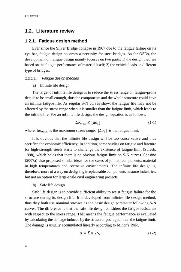
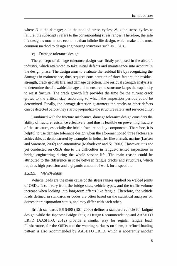
British standards BS 5400 (BSI, 2000) defines a standard vehicle for fatigue
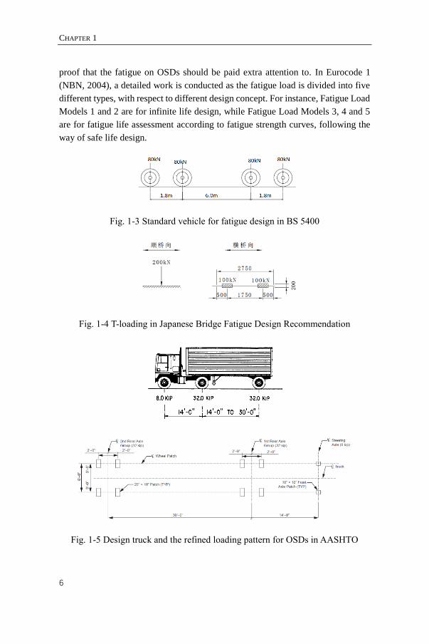
design, while the Japanese Bridge Fatigue Design Recommendation and AASHTO
LRFD (AASHTO, 2012) provide a similar way for regular fatigue load.
Furthermore, for the OSDs and the wearing surfaces on them, a refined loading
pattern is also recommended by AASHTO LRFD, which is apparently another
CHAPTER 1
6
proof that the fatigue on OSDs should be paid extra attention to. In Eurocode 1
(NBN, 2004), a detailed work is conducted as the fatigue load is divided into five
different types, with respect to different design concept. For instance, Fatigue Load
Models 1 and 2 are for infinite life design, while Fatigue Load Models 3, 4 and 5
are for fatigue life assessment according to fatigue strength curves, following the
way of safe life design.
Fig. 1-3 Standard vehicle for fatigue design in BS 5400
Fig. 1-4 T-loading in Japanese Bridge Fatigue Design Recommendation
Fig. 1-5 Design truck and the refined loading pattern for OSDs in AASHTO
INTRODUCTION
7
According to these standards and recommendations, the vehicle types, axial
weights on each lane are significant factors for fatigue performance of OSDs. It
illustrates the necessity to consider the realistic traffic volumes and related
parameters for the specific bridge. Wang et al. (2005) proposed a three-dimensional
nonlinear model based on data from Weigh-In-Motion (WIM) systems to analyze
fatigue damages on steel bridges, with a case study on one specific site on the I-75
in the United States. Ji et al. (2012) generated a random traffic flow model based
on traffic data from the toll system, and analyzed the traffic-induced stresses on the
steel deck of a suspension bridge on the Yangtze River combined with the finite
element model.
Furthermore, the specific wheel location, rather than the vehicle distribution
on different lanes, is quite crucial on this issue, especially for OSDs whose fatigue
is mainly caused by local load effects. Almost all the standards or codes, including
BS 5400 (BSI, 2000), AASHTO LRFD (AASHTO, 2012), Eurocode 1 (NBN,
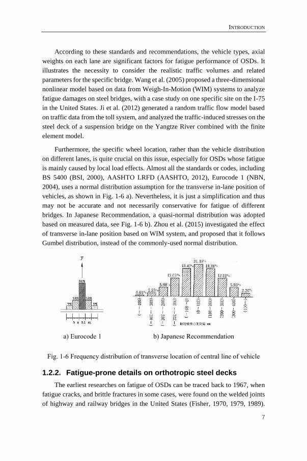
2004), uses a normal distribution assumption for the transverse in-lane position of
vehicles, as shown in Fig. 1-6 a). Nevertheless, it is just a simplification and thus
may not be accurate and not necessarily conservative for fatigue of different
bridges. In Japanese Recommendation, a quasi-normal distribution was adopted
based on measured data, see Fig. 1-6 b). Zhou et al. (2015) investigated the effect
of transverse in-lane position based on WIM system, and proposed that it follows
Gumbel distribution, instead of the commonly-used normal distribution.
a) Eurocode 1
b) Japanese Recommendation
Fig. 1-6 Frequency distribution of transverse location of central line of vehicle
1.2.2. Fatigue-prone details on orthotropic steel decks
The earliest researches on fatigue of OSDs can be traced back to 1967, when
fatigue cracks, and brittle fractures in some cases, were found on the welded joints
of highway and railway bridges in the United States (Fisher, 1970, 1979, 1989).
CHAPTER 1
8
According to the results from on-site investigations and full-scale fatigue tests, it
is believed that the stress range is the most significant factor that affects the fatigue
life. In addition, the fatigue failure behaviors of 22 steel bridges were analyzed,
showing the relationships between fatigue and parameters like crack sizes, weld
geometries and fracture toughness.
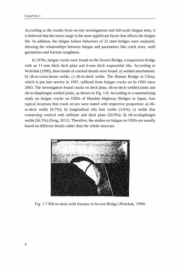
In 1970s, fatigue cracks were found on the Severn Bridge, a suspension bridge
with an 11-mm thick deck plate and 6-mm thick trapezoidal ribs. According to
Wolchuk (1990), three kinds of cracked details were found: a) welded attachments;
b) rib-to-cross-beam welds; c) rib-to-deck welds. The Humen Bridge in China,
which is put into service in 1997, suffered from fatigue cracks on its OSD since
2003. The investigation found cracks on deck plate, rib-to-deck welded joints and
rib-to-diaphragm welded joints, as shown in Fig. 1-8. According to a summarizing
study on fatigue cracks on OSDs of Hanshin Highway Bridges in Japan, four
typical locations that crack occurs were stated with respective proportion: a) rib-
to-deck welds (9.7%); b) longitudinal ribs butt welds (3.6%); c) welds that
connecting vertical web stiffener and deck plate (20.9%); d) rib-to-diaphragm
welds (56.3%) (Zeng, 2011). Therefore, the studies on fatigue on OSDs are usually
based on different details rather than the whole structure.
Fig. 1-7 Rib-to-deck weld fracture in Severn Bridge (Wolchuk, 1990)

INTRODUCTION
9
a) Rib-to-deck weld crack
b) Rib-to-diaphragm weld crack
c) Longitudinal ribs butt weld crack
Fig. 1-8 Fatigue cracks on Humen Bridge
○1 Rib-to-deck welds
○2 Longitudinal ribs butt welds
○3 Vertical stiffener and deck welds
○4 Rib-to-diaphragm welds
Fig. 1-9 Four typical cracks on OSD on Hanshin Highway Bridges
CHAPTER 1
10
1.2.2.1. Rib-to-deck welded joints
Among all types of cracks on OSDs, crack on rib-to-deck welded joints is
regarded as the most harmful one, as it goes through the deck plate and results in
larger deflection and local failure of the pavements. The aforementioned Humen
Bridge was one of the victims of it, and was eventually out of service even after
several retrofitting works. Another instance is the Second Van Brienenoord Bridge
in Netherlands, which was built and put into service in 1990. Fatigue damages
started to bother it after seven years, and led to severe reduction of serviceability
and consequent repairing works of this bridge. The investigation showed that the
typical crack is crack initiated from the rib-to-deck weld root and went through the
deck plate, as shown in Fig. 1-10 (Maljaars et al., 2012).
Wang and Feng (2009) showed that the rib-to-deck welded joints cracked in
the following three ways: a) weld toe crack that goes through the longitudinal rib;
b) weld toe crack that goes through the deck plate; c) weld root crack go through
the weld throat. While according to Zeng (2011), other types of weld root crack
that goes through the deck plate (CR-D-6 and CR-D-8 in Fig. 1-11) were also stated.
De Backer et al. (2007) conducted a strain measurement to investigate the
stress concentration on this detail, achieved results validated by comparison with
that from Finite Element Method (FEM) models. With this measuring system,
different pavements on OSDs were studied afterwards, indicating a possible 20%
to 30% reduction of stresses (De Backer et al., 2008a). They also proposed an
analytical way to calculate the internal forces (De Backer et al., 2008b).
Xiao et al. (2006, 2008) studied different types of cracks around rib-to-deck
welds based on the Kinuura Bridge in Japan. By comparing the experimental results
with the Linear Elastic Fracture Mechanics (LEFM) solutions, it is claimed that the
welded joint will have low fatigue strength if the fusion zone is too small. By using
FEM on OSDs, it was also found that the out-of-plane momentum is the main
reason of the high local stress in this detail, and thus suggested to enlarge the wheel
contact area, or use deck plates with bigger thickness, to improve the fatigue
performance.
Nagy et al. (2015b, 2016) evaluated the fatigue behavior of rib-to-deck welded
joints using LEFM and eXtended finite element method (XFEM), obtained the
crack path at the weld root in a more realistic way. By comparing the crack growth
curves for random and fixed load sequences, it is implied that the load sequence
will not affect the crack length at the final stage.

INTRODUCTION
11
Fig. 1-10 The though-crack in the Second Van Brienenoord Bridge (Maljaars et
al., 2012)
a) Wang and Feng (2009)
b) Zeng (2011)
Fig. 1-11 Different types of crack on rib-to-deck welded joints
As the lack-of-penetration is the main cause of root cracks on this detail, it is
always believed that more penetration to weld root could be effective on preventing
crack initiation from weld root and growth through weld throat. But according to
some recent studies (Ya and Yamada, 2008, Sim and Uang, 2012), specimens with
full penetration are of slightly lower fatigue strength than those with 80%
penetration. Kanimura et al. (2016) investigated the rib-to-deck weld root cracks
with tests on specimens with different weld penetration rates and stress ratios, and
confirmed the benefits of penetration rate slightly lower than 100%, e.g. 80%, on
fatigue strength. In addition, the tensile mean stress, was emphasized for its effect
on root crack initiation.
1.2.2.2. Rib-to-diaphragm welded joints
Rib-to-diaphragm welded joint is a quite, if not the most, fatigue-prone detail
according to the given proportions of detected cracks as mentioned before, i.e.
56.3%.
The common way in early design of OSDs is to weld the longitudinal ribs to
diaphragms directly, without setting up cut-outs on diaphragms, which means the

CHAPTER 1
12
longitudinal ribs were interrupted. This design, as applied by the Severn Bridge,
may result in severe out-of-plane distortion, help crack starting from the bottom of
the longitudinal ribs. Therefore, current fatigue design suggests using cut-outs on
this detail, while the shape of the cut-outs became another issue on fatigue design
afterwards. The widely-used type of cut-outs are in elliptical shape, as suggested
in Japanese recommendation and Eurocode for highway bridges, see Fig. 1-12. For
railway bridges, a novel design, named Haibach cut-out, is recommended by
Eurocode, which can reduce the stress concentration and improve the fatigue
performance on rib-to-diaphragm welded joints.
a) Japanese
Recommendation
b) Eurocode for highway
bridges
c) Eurocode for railway
bridges
Fig. 1-12 Cut-out shapes in different specifications
Nevertheless, the stress concentration induced by the cut-out still exists,
leading to cracks at the bottom weld toe of rib-to-diaphragm welded joints.
Tsakopoulos and Fisher (2003) studied the plan of replacement of the OSD on
Williamsburg Bridge with fatigue tests, and compared to other designs suggested
by AASHTO LRFD. It was proposed that by using thicker diaphragms, the in-plane
stresses can be reduced without increasing out-of-plane stresses. Zhang et al. (2015)
conducted full-scale fatigue tests on this detail, and analyzed it with hot-spot stress
method and notch stress method, concluding that the fatigue performance is still
determined by the out-of-plane distortion of ribs.
Provided that the rib-to-deck welded joints and rib-to-diaphragm welded joints
are both lacking of fatigue resistance, the detail at the intersection of them, as Qian
and Abruzzese (2009) called rib-to-diaphragm-to-deck plate (RDDP), should be
paid extra attention to on fatigue issues. Kolstein (2007) presents a typical example
of cracked RDDP, as given in Fig. 1-13. Another instance of Jiangyin Yangtze
River Bridge is shown in Fig. 1-14. Zhou (2010) summarized the procedure of the
crack propagation at RDDP, divided it into three phases (see Fig. 1-15): i) crack
initiation at RDDP; ii) crack grows perpendicularly, and go through the deck plate;
iii) crack grows longitudinally. It is also suggested that the phase ii and iii may
proceed simultaneously, resulting in dangerous invisible long cracks.
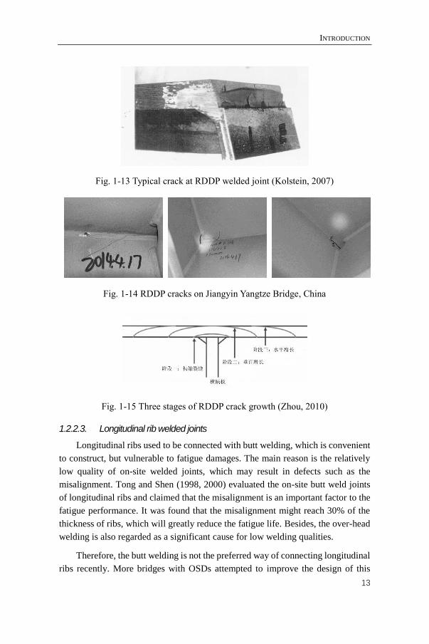
INTRODUCTION
13
Fig. 1-13 Typical crack at RDDP welded joint (Kolstein, 2007)
Fig. 1-14 RDDP cracks on Jiangyin Yangtze Bridge, China
Fig. 1-15 Three stages of RDDP crack growth (Zhou, 2010)
1.2.2.3. Longitudinal rib welded joints
Longitudinal ribs used to be connected with butt welding, which is convenient
to construct, but vulnerable to fatigue damages. The main reason is the relatively
low quality of on-site welded joints, which may result in defects such as the
misalignment. Tong and Shen (1998, 2000) evaluated the on-site butt weld joints
of longitudinal ribs and claimed that the misalignment is an important factor to the
fatigue performance. It was found that the misalignment might reach 30% of the
thickness of ribs, which will greatly reduce the fatigue life. Besides, the over-head
welding is also regarded as a significant cause for low welding qualities.
Therefore, the butt welding is not the preferred way of connecting longitudinal
ribs recently. More bridges with OSDs attempted to improve the design of this
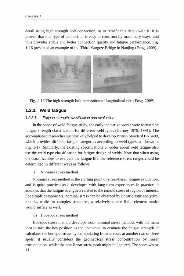
CHAPTER 1
14
detail using high strength bolt connection, or to retrofit this detail with it. It is
proven that this type of connection is easy to construct by machinery ways, and
thus provides stable and better connection quality and fatigue performance. Fig.
1-16 presented an example of the Third Yangtze Bridge in Nanjing (Feng, 2009).
Fig. 1-16 The high strength bolt connection of longitudinal ribs (Feng, 2009)
1.2.3. Weld fatigue
1.2.3.1. Fatigue strength classification and evaluation
In the scope of weld fatigue study, the early indicative works were focused on
fatigue strength classification for different weld types (Gurney 1979, 1991). The
accomplished researches successively helped to develop British Standard BS 5400,
which provides different fatigue categories according to weld types, as shown in
Fig. 1-17. Similarly, the existing specifications or codes about weld fatigue also
use the weld type classification for fatigue design of welds. Note that when using
the classifications to evaluate the fatigue life, the reference stress ranges could be
determined in different ways as follows.
a) Nominal stress method
Nominal stress method is the starting point of stress-based fatigue evaluation,
and is quite practical as it developes with long-term experiences in practice. It
assumes that the fatigue strength is related to the remote stress of region of interest.
For simple components, nominal stress can be obtained by linear elastic analytical
models, while for complex structures, a relatively coarse finite element model
would suffice as well.
b) Hot-spot stress method
Hot-spot stress method develops from nominal stress method, with the main
idea to take the key position as the “hot-spot” to evaluate the fatigue strength. It
calculates the hot-spot stress by extrapolating from stresses at another two or three
spots. It usually considers the geometrical stress concentration by linear
extrapolation, whilst the non-linear stress peak might be ignored. The spots whose
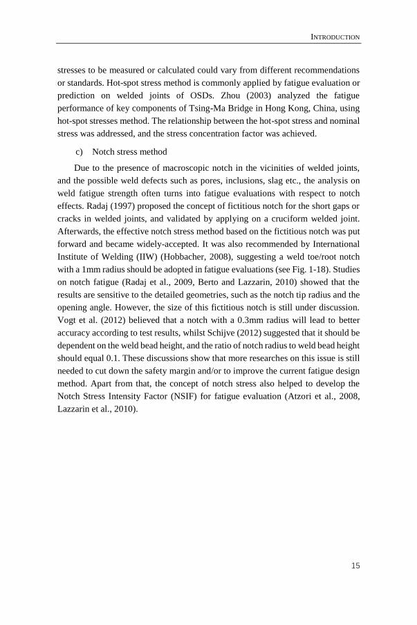
INTRODUCTION
15
stresses to be measured or calculated could vary from different recommendations
or standards. Hot-spot stress method is commonly applied by fatigue evaluation or
prediction on welded joints of OSDs. Zhou (2003) analyzed the fatigue
performance of key components of Tsing-Ma Bridge in Hong Kong, China, using
hot-spot stresses method. The relationship between the hot-spot stress and nominal
stress was addressed, and the stress concentration factor was achieved.
c) Notch stress method
Due to the presence of macroscopic notch in the vicinities of welded joints,
and the possible weld defects such as pores, inclusions, slag etc., the analysis on
weld fatigue strength often turns into fatigue evaluations with respect to notch
effects. Radaj (1997) proposed the concept of fictitious notch for the short gaps or
cracks in welded joints, and validated by applying on a cruciform welded joint.
Afterwards, the effective notch stress method based on the fictitious notch was put
forward and became widely-accepted. It was also recommended by International
Institute of Welding (IIW) (Hobbacher, 2008), suggesting a weld toe/root notch
with a 1mm radius should be adopted in fatigue evaluations (see Fig. 1-18). Studies
on notch fatigue (Radaj et al., 2009, Berto and Lazzarin, 2010) showed that the
results are sensitive to the detailed geometries, such as the notch tip radius and the
opening angle. However, the size of this fictitious notch is still under discussion.
Vogt et al. (2012) believed that a notch with a 0.3mm radius will lead to better
accuracy according to test results, whilst Schijve (2012) suggested that it should be
dependent on the weld bead height, and the ratio of notch radius to weld bead height
should equal 0.1. These discussions show that more researches on this issue is still
needed to cut down the safety margin and/or to improve the current fatigue design
method. Apart from that, the concept of notch stress also helped to develop the
Notch Stress Intensity Factor (NSIF) for fatigue evaluation (Atzori et al., 2008,
Lazzarin et al., 2010).

CHAPTER 1
16
Fig. 1-17 Different categories of fatigue strength (Gurney, 1979)
Fig. 1-18 The fictitious notches in Effective Notch Stress Method (Hobbacher,
2008)
Benefited by the development of computation abilities nowadays, the hot-spot
stress method and notch stress method were applied more and more in realistic
projects. Fricke et al. (2012) studied the fatigue on fillet welds with hot-spot stress
method and effective notch stress method, obtained similar results with both
methods. Aygül et al. (2012, 2013) built the model of OSDs with FEM, and
compared the results to that from full-scale tests. Then the fatigue lives were
calculated by nominal stress method, hot-spot stress method and effective notch
stress method, and the feasibility of the three method on this issue were provided.
Even though the stress-based fatigue evaluation method were proven to be
effective in practice, they were still empirical and required large amount of fatigue
tests for a specific project. As the welding techniques developed and the fatigue
mechanism in welded joints better revealed, the simple way of fatigue strength
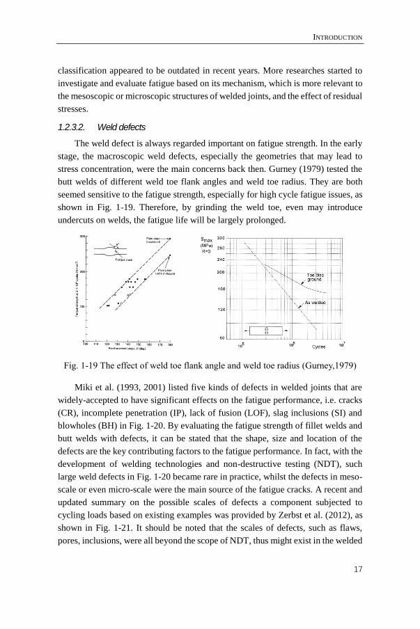
INTRODUCTION
17
classification appeared to be outdated in recent years. More researches started to
investigate and evaluate fatigue based on its mechanism, which is more relevant to
the mesoscopic or microscopic structures of welded joints, and the effect of residual
stresses.
1.2.3.2. Weld defects
The weld defect is always regarded important on fatigue strength. In the early
stage, the macroscopic weld defects, especially the geometries that may lead to
stress concentration, were the main concerns back then. Gurney (1979) tested the
butt welds of different weld toe flank angles and weld toe radius. They are both
seemed sensitive to the fatigue strength, especially for high cycle fatigue issues, as
shown in Fig. 1-19. Therefore, by grinding the weld toe, even may introduce
undercuts on welds, the fatigue life will be largely prolonged.
Fig. 1-19 The effect of weld toe flank angle and weld toe radius (Gurney,1979)
Miki et al. (1993, 2001) listed five kinds of defects in welded joints that are
widely-accepted to have significant effects on the fatigue performance, i.e. cracks
(CR), incomplete penetration (IP), lack of fusion (LOF), slag inclusions (SI) and
blowholes (BH) in Fig. 1-20. By evaluating the fatigue strength of fillet welds and
butt welds with defects, it can be stated that the shape, size and location of the
defects are the key contributing factors to the fatigue performance. In fact, with the
development of welding technologies and non-destructive testing (NDT), such
large weld defects in Fig. 1-20 became rare in practice, whilst the defects in meso-
scale or even micro-scale were the main source of the fatigue cracks. A recent and
updated summary on the possible scales of defects a component subjected to
cycling loads based on existing examples was provided by Zerbst et al. (2012), as
shown in Fig. 1-21. It should be noted that the scales of defects, such as flaws,
pores, inclusions, were all beyond the scope of NDT, thus might exist in the welded

CHAPTER 1
18
joints that do meet to criteria of weld specifications, and affect the fatigue strength
of the structures eventually.
Fig. 1-20 Typical weld defects on fracture surfaces (Miki et al., 2001)
Fig. 1-21 Length scales of the life cycle of a component subjected to cyclic
loading (Zerbst et al., 2012)
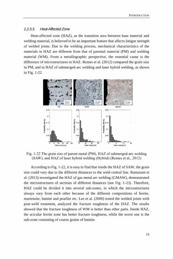
INTRODUCTION
19
1.2.3.3. Heat-Affected Zone
Heat-affected zone (HAZ), as the transition area between base material and
welding material, is believed to be an important feature that affects fatigue strength
of welded joints. Due to the welding process, mechanical characteristics of the
materials in HAZ are different from that of parental material (PM) and welding
material (WM). From a metallographic perspective, the essential cause is the
difference of microstructures in HAZ. Remes et al. (2012) compared the grain size
in PM, and in HAZ of submerged-arc welding and laser hybrid welding, as shown
in Fig. 1-22.
Fig. 1-22 The grain size of parent metal (PM), HAZ of submerged-arc welding
(SAW), and HAZ of laser hybrid welding (Hybrid) (Remes et al., 2012)
According to Fig. 1-22, it is easy to find that inside the HAZ of SAW, the grain
size could vary due to the different distances to the weld central line. Ramazani et
al. (2013) investigated the HAZ of gas metal arc welding (GMAW), demonstrated
the microstructures of sections of different distances (see Fig. 1-23). Therefore,
HAZ could be divided it into several sub-zones, in which the microstructures
always vary from each other because of the different compositions of ferrite,
martensite, bainite and pearlite etc. Lee et al. (2000) tested the welded joints with
post-weld treatment, analyzed the fracture toughness of the HAZ. The results
showed that the fracture toughness of WM is better than other parts. Inside HAZ,
the acicular ferrite zone has better fracture toughness, while the worst one is the
sub-zone consisting of coarse grains of bainite.
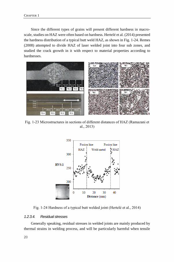
CHAPTER 1
20
Since the different types of grains will present different hardness in macro-
scale, studies on HAZ were often based on hardness. Hertelé et al. (2014) presented
the hardness distribution of a typical butt weld HAZ, as shown in Fig. 1-24. Remes
(2008) attempted to divide HAZ of laser welded joint into four sub zones, and
studied the crack growth in it with respect to material properties according to
hardnesses.
Fig. 1-23 Microstructures in sections of different distances of HAZ (Ramazani et
al., 2013)
Fig. 1-24 Hardness of a typical butt welded joint (Hertelé et al., 2014)
1.2.3.4. Residual stresses
Generally speaking, residual stresses in welded joints are mainly produced by
thermal strains in welding process, and will be particularly harmful when tensile
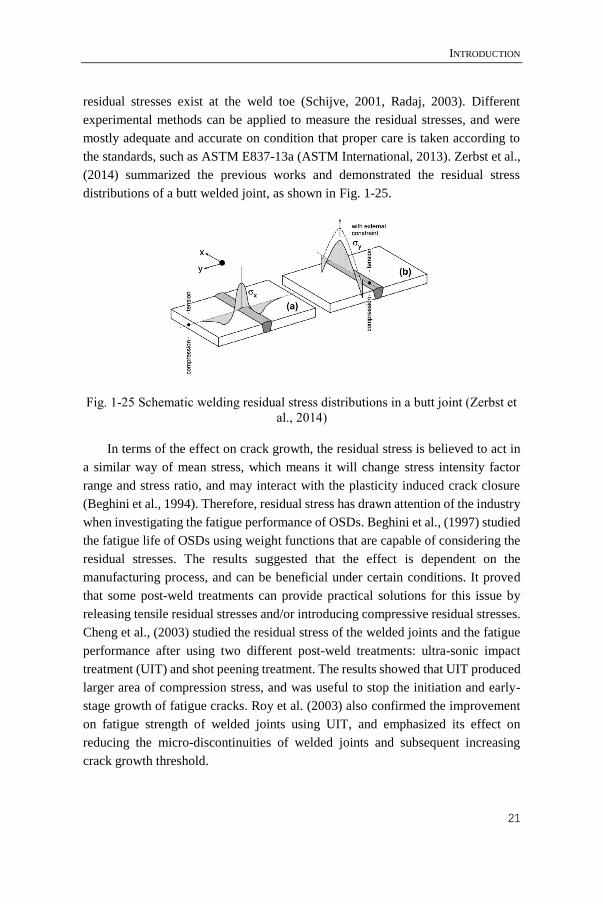
INTRODUCTION
21
residual stresses exist at the weld toe (Schijve, 2001, Radaj, 2003). Different
experimental methods can be applied to measure the residual stresses, and were
mostly adequate and accurate on condition that proper care is taken according to
the standards, such as ASTM E837-13a (ASTM International, 2013). Zerbst et al.,
(2014) summarized the previous works and demonstrated the residual stress
distributions of a butt welded joint, as shown in Fig. 1-25.
Fig. 1-25 Schematic welding residual stress distributions in a butt joint (Zerbst et
al., 2014)
In terms of the effect on crack growth, the residual stress is believed to act in
a similar way of mean stress, which means it will change stress intensity factor
range and stress ratio, and may interact with the plasticity induced crack closure
(Beghini et al., 1994). Therefore, residual stress has drawn attention of the industry
when investigating the fatigue performance of OSDs. Beghini et al., (1997) studied
the fatigue life of OSDs using weight functions that are capable of considering the
residual stresses. The results suggested that the effect is dependent on the
manufacturing process, and can be beneficial under certain conditions. It proved
that some post-weld treatments can provide practical solutions for this issue by
releasing tensile residual stresses and/or introducing compressive residual stresses.
Cheng et al., (2003) studied the residual stress of the welded joints and the fatigue
performance after using two different post-weld treatments: ultra-sonic impact
treatment (UIT) and shot peening treatment. The results showed that UIT produced
larger area of compression stress, and was useful to stop the initiation and early-
stage growth of fatigue cracks. Roy et al. (2003) also confirmed the improvement
on fatigue strength of welded joints using UIT, and emphasized its effect on
reducing the micro-discontinuities of welded joints and subsequent increasing
crack growth threshold.

CHAPTER 1
22
On the other hand, the knowledge about the residual stress distribution of as-
welded joints is equally important, since the majority of existing OSDs did not
employ the post-weld treatments that can release residual stresses in a considerable
way. Nagy et al., (2015a) conducted a hole-drilling measurement on welded joints
of OSD, mainly focused on the weld toe part due to the limitation of possible site
to drill the hole. For the weld root part, Kainuma et al. (2016) measured the residual
stresses using cutting and magnetostriction method. However, given the difficulty
in measuring the residual stresses for welded structure with complex geometries,
especially when a non-destructive way is required, the numerical simulation ways
were developed as an applicable way to predict and evaluate residual stresses.
Based on the measurement mentioned before, Nagy (2017) further calculated the
residual stress distribution around rib-to-deck welded joints by numerical
simulation, and the results were validated by comparing with the test results.
Lindgren (2001a, 2001b, 2001c) summarized the methods on welding simulation,
and established a model incorporating with other methods in engineering. Barsoum
and Barsoum (2009) proposed an FEM way to simulate welding process with
access to prediction of the residual stresses. The prediction was validated by
comparing the crack propagation path calculated by fracture mechanics and that
from fatigue tests.
1.2.4. Fatigue behavior and prediction
Classical fatigue evaluation and prediction were established by stress-life
relationship, i.e. S-N curves, as given in Fig. 1-17. This method only defines the
fatigue failure point for materials, therefore lead to insufficient knowledge on the
fatigue mechanism. Consequently, efforts were made on investigating the progress
of fatigue to reveal the mechanisms.
1.2.4.1. Typical stages of fatigue behavior
The entire fatigue progress is often divided into four stages according to the
different behaviors and mechanisms: i) crack nucleation and initiation; ii) short
crack growth; iii) long crack growth; iv) final fracture (Chen, 2002, Lee, 2005). In
practice, fatigue life spent in Stage i and ii is recognized as crack initiation life, and
that in Stage iii and iv as crack propagation life. In terms of the number of cycles
consumed till final fracture, the fatigue can be divided into high-cycle fatigue and
low-cycle fatigue. In high-cycle fatigue, the elastic deformation is dominant since
the plastic zone around crack tip is quite small, and the crack initiation life occupies
the majority of the whole life, with the proportion about 80% or more according to
some studies (Yang et al. 1997). Whilst in low-cycle fatigue, elastoplastic
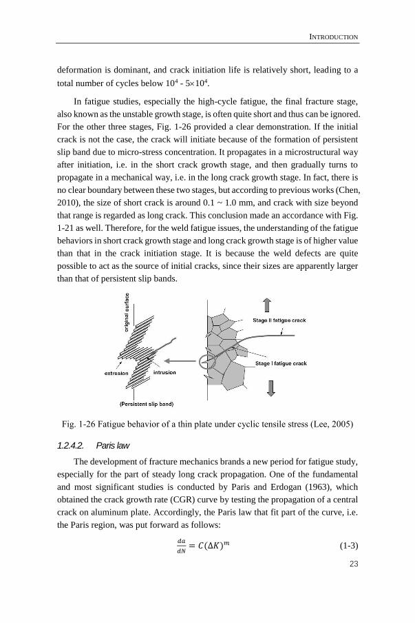
INTRODUCTION
23
deformation is dominant, and crack initiation life is relatively short, leading to a
total number of cycles below 104 - 5104.
In fatigue studies, especially the high-cycle fatigue, the final fracture stage,
also known as the unstable growth stage, is often quite short and thus can be ignored.
For the other three stages, Fig. 1-26 provided a clear demonstration. If the initial
crack is not the case, the crack will initiate because of the formation of persistent
slip band due to micro-stress concentration. It propagates in a microstructural way
after initiation, i.e. in the short crack growth stage, and then gradually turns to
propagate in a mechanical way, i.e. in the long crack growth stage. In fact, there is
no clear boundary between these two stages, but according to previous works (Chen,
2010), the size of short crack is around 0.1 ~ 1.0 mm, and crack with size beyond
that range is regarded as long crack. This conclusion made an accordance with Fig.
1-21 as well. Therefore, for the weld fatigue issues, the understanding of the fatigue
behaviors in short crack growth stage and long crack growth stage is of higher value
than that in the crack initiation stage. It is because the weld defects are quite
possible to act as the source of initial cracks, since their sizes are apparently larger
than that of persistent slip bands.
Fig. 1-26 Fatigue behavior of a thin plate under cyclic tensile stress (Lee, 2005)
1.2.4.2. Paris law
The development of fracture mechanics brands a new period for fatigue study,
especially for the part of steady long crack propagation. One of the fundamental
and most significant studies is conducted by Paris and Erdogan (1963), which
obtained the crack growth rate (CGR) curve by testing the propagation of a central
crack on aluminum plate. Accordingly, the Paris law that fit part of the curve, i.e.
the Paris region, was put forward as follows:
𝑑𝑎
𝑑𝑁= 𝐶(∆𝐾)𝑚 (1-3)
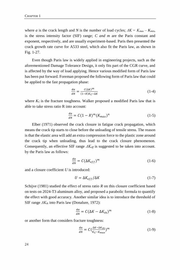
CHAPTER 1
24
where a is the crack length and N is the number of load cycles; ΔK = Kmax – Kmin,
is the stress intensity factor (SIF) range; C and m are the Paris constant and
exponent, respectively, and are usually experiment-based. Paris then presented the
crack growth rate curve for A533 steel, which also fit the Paris law, as shown in
Fig. 1-27.
Even though Paris law is widely applied in engineering projects, such as the
aforementioned Damage Tolerance Design, it only fits part of the CGR curve, and
is affected by the way of load applying. Hence various modified form of Paris law
has been put forward. Foreman proposed the following form of Paris law that could
be applied to the fast propagation phase:
𝑑𝑎
𝑑𝑁=
𝐶(∆𝐾)𝑚
(1−𝑅)𝐾𝐶−∆𝐾 (1-4)
where KC is the fracture toughness. Walker proposed a modified Paris law that is
able to take stress ratio R into account:
𝑑𝑎
𝑑𝑁= 𝐶(1 − 𝑅)𝑚(𝐾𝑚𝑎𝑥)
𝑛 (1-5)
Elber (1971) observed the crack closure in fatigue crack propagation, which
means the crack tip starts to close before the unloading of tensile stress. The reason
is that the elastic area will add an extra compression force to the plastic zone around
the crack tip when unloading, thus lead to the crack closure phenomenon.
Consequently, an effective SIF range ΔKeff is suggested to be taken into account.
by the Paris law as follows:
𝑑𝑎
𝑑𝑁= 𝐶(∆𝐾𝑒𝑓𝑓)
𝑚 (1-6)
and a closure coefficient U is introduced:
𝑈 = ∆𝐾𝑒𝑓𝑓/∆𝐾 (1-7)
Schijve (1981) studied the effect of stress ratio R on this closure coefficient based
on tests on 2024-T3 aluminum alloy, and proposed a parabolic formula to quantify
the effect with good accuracy. Another similar idea is to introduce the threshold of
SIF range ΔKth into Paris law (Donalure, 1972):
𝑑𝑎
𝑑𝑁= 𝐶(∆𝐾 − ∆𝐾𝑡ℎ)
𝑚 (1-8)
or another form that considers fracture toughness:
𝑑𝑎
𝑑𝑁= 𝐶(
∆𝐾−∆𝐾𝑡ℎ
𝐾𝐶−𝐾𝑚𝑎𝑥)𝑚 (1-9)
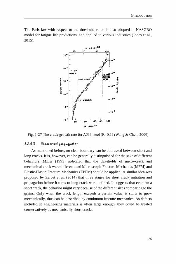
INTRODUCTION
25
The Paris law with respect to the threshold value is also adopted in NASGRO
model for fatigue life predictions, and applied to various industries (Jones et al.,
2015).
Fig. 1-27 The crack growth rate for A533 steel (R=0.1) (Wang & Chen, 2009)
1.2.4.3. Short crack propagation
As mentioned before, no clear boundary can be addressed between short and
long cracks. It is, however, can be generally distinguished for the sake of different
behaviors. Miller (1993) indicated that the thresholds of micro-crack and
mechanical crack were different, and Microscopic Fracture Mechanics (MFM) and
Elastic-Plastic Fracture Mechanics (EPFM) should be applied. A similar idea was
proposed by Zerbst et al. (2014) that three stages for short crack initiation and
propagation before it turns to long crack were defined. It suggests that even for a
short crack, the behavior might vary because of the different sizes comparing to the
grains. Only when the crack length exceeds a certain value, it starts to grow
mechanically, thus can be described by continuum fracture mechanics. As defects
included in engineering materials is often large enough, they could be treated
conservatively as mechanically short cracks.
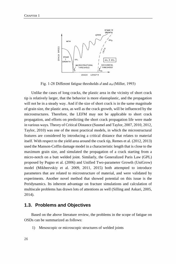
CHAPTER 1
26
Fig. 1-28 Different fatigue thresholds d and ath (Miller, 1993)
Unlike the cases of long cracks, the plastic area in the vicinity of short crack
tip is relatively larger, that the behavior is more elastoplastic, and the propagation
will not be in a steady way. And if the size of short crack is in the same magnitude
of grain size, the plastic area, as well as the crack growth, will be influenced by the
microstructures. Therefore, the LEFM may not be applicable to short crack
propagation, and efforts on predicting the short crack propagation life were made
in various ways. Theory of Critical Distance (Susmel and Taylor, 2007, 2010, 2012,
Taylor, 2010) was one of the most practical models, in which the microstructural
features are considered by introducing a critical distance that relates to material
itself. With respect to the yield area around the crack tip, Remes et al. (2012, 2013)
used the Manson-Coffin damage model in a characteristic length that is close to the
maximum grain size, and simulated the propagation of a crack starting from a
micro-notch on a butt welded joint. Similarly, the Generalized Paris Law (GPL)
proposed by Pugno et al. (2006) and Unified Two-parameter Growth (UniGrow)
model (Mikheevskiy et al. 2009, 2011, 2015) both attempted to introduce
parameters that are related to microstructure of material, and were validated by
experiments. Another novel method that showed potential on this issue is the
Peridynamics. Its inherent advantage on fracture simulations and calculation of
multiscale problems has drawn lots of attentions as well (Silling and Askari, 2005,
2014).
1.3. Problems and Objectives
Based on the above literature review, the problems in the scope of fatigue on
OSDs can be summarized as follows:
1) Mesoscopic or microscopic structures of welded joints
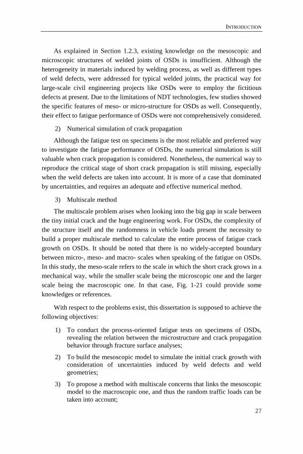
INTRODUCTION
27
As explained in Section 1.2.3, existing knowledge on the mesoscopic and
microscopic structures of welded joints of OSDs is insufficient. Although the
heterogeneity in materials induced by welding process, as well as different types
of weld defects, were addressed for typical welded joints, the practical way for
large-scale civil engineering projects like OSDs were to employ the fictitious
defects at present. Due to the limitations of NDT technologies, few studies showed
the specific features of meso- or micro-structure for OSDs as well. Consequently,
their effect to fatigue performance of OSDs were not comprehensively considered.
2) Numerical simulation of crack propagation
Although the fatigue test on specimens is the most reliable and preferred way
to investigate the fatigue performance of OSDs, the numerical simulation is still
valuable when crack propagation is considered. Nonetheless, the numerical way to
reproduce the critical stage of short crack propagation is still missing, especially
when the weld defects are taken into account. It is more of a case that dominated
by uncertainties, and requires an adequate and effective numerical method.
3) Multiscale method
The multiscale problem arises when looking into the big gap in scale between
the tiny initial crack and the huge engineering work. For OSDs, the complexity of
the structure itself and the randomness in vehicle loads present the necessity to
build a proper multiscale method to calculate the entire process of fatigue crack
growth on OSDs. It should be noted that there is no widely-accepted boundary
between micro-, meso- and macro- scales when speaking of the fatigue on OSDs.
In this study, the meso-scale refers to the scale in which the short crack grows in a
mechanical way, while the smaller scale being the microscopic one and the larger
scale being the macroscopic one. In that case, Fig. 1-21 could provide some
knowledges or references.
With respect to the problems exist, this dissertation is supposed to achieve the
following objectives:
1) To conduct the process-oriented fatigue tests on specimens of OSDs,
revealing the relation between the microstructure and crack propagation
behavior through fracture surface analyses;
2) To build the mesoscopic model to simulate the initial crack growth with
consideration of uncertainties induced by weld defects and weld
geometries;
3) To propose a method with multiscale concerns that links the mesoscopic
model to the macroscopic one, and thus the random traffic loads can be
taken into account;
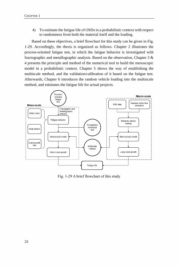
CHAPTER 1
28
4) To estimate the fatigue life of OSDs in a probabilistic context with respect
to randomness from both the material itself and the loading.
Based on these objectives, a brief flowchart for this study can be given in Fig.
1-29. Accordingly, the thesis is organized as follows. Chapter 2 illustrates the
process-oriented fatigue test, in which the fatigue behavior is investigated with
fractographic and metallographic analysis. Based on the observation, Chapter 3 &
4 presents the principle and method of the numerical tool to build the mesoscopic
model in a probabilistic context. Chapter 5 shows the way of establishing the
multiscale method, and the validation/calibration of it based on the fatigue test.
Afterwards, Chapter 6 introduces the random vehicle loading into the multiscale
method, and estimates the fatigue life for actual projects.
Fig. 1-29 A brief flowchart of this study
CHAPTER 2
FATIGUE TESTS AND
MICROSTRUCTURE ANALYSIS
________________________________
This chapter is based on:
Nagy, W., Wang, B., Culek, B., Van Bogaert, Ph., and De Backer, H.,
Experimental fatigue assessment of the stiffener-to-deck plate connection in
orthotropic steel decks. International Journal of Steel Structures (accepted)
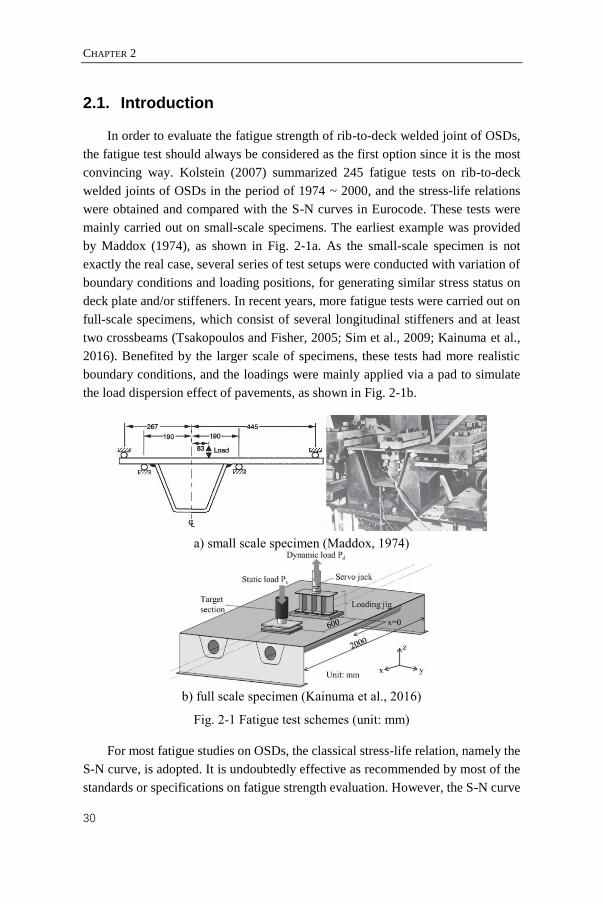
CHAPTER 2
30
2.1. Introduction
In order to evaluate the fatigue strength of rib-to-deck welded joint of OSDs,
the fatigue test should always be considered as the first option since it is the most
convincing way. Kolstein (2007) summarized 245 fatigue tests on rib-to-deck
welded joints of OSDs in the period of 1974 ~ 2000, and the stress-life relations
were obtained and compared with the S-N curves in Eurocode. These tests were
mainly carried out on small-scale specimens. The earliest example was provided
by Maddox (1974), as shown in Fig. 2-1a. As the small-scale specimen is not
exactly the real case, several series of test setups were conducted with variation of
boundary conditions and loading positions, for generating similar stress status on
deck plate and/or stiffeners. In recent years, more fatigue tests were carried out on
full-scale specimens, which consist of several longitudinal stiffeners and at least
two crossbeams (Tsakopoulos and Fisher, 2005; Sim et al., 2009; Kainuma et al.,
2016). Benefited by the larger scale of specimens, these tests had more realistic
boundary conditions, and the loadings were mainly applied via a pad to simulate
the load dispersion effect of pavements, as shown in Fig. 2-1b.
a) small scale specimen (Maddox, 1974)
b) full scale specimen (Kainuma et al., 2016)
Fig. 2-1 Fatigue test schemes (unit: mm)
For most fatigue studies on OSDs, the classical stress-life relation, namely the
S-N curve, is adopted. It is undoubtedly effective as recommended by most of the
standards or specifications on fatigue strength evaluation. However, the S-N curve
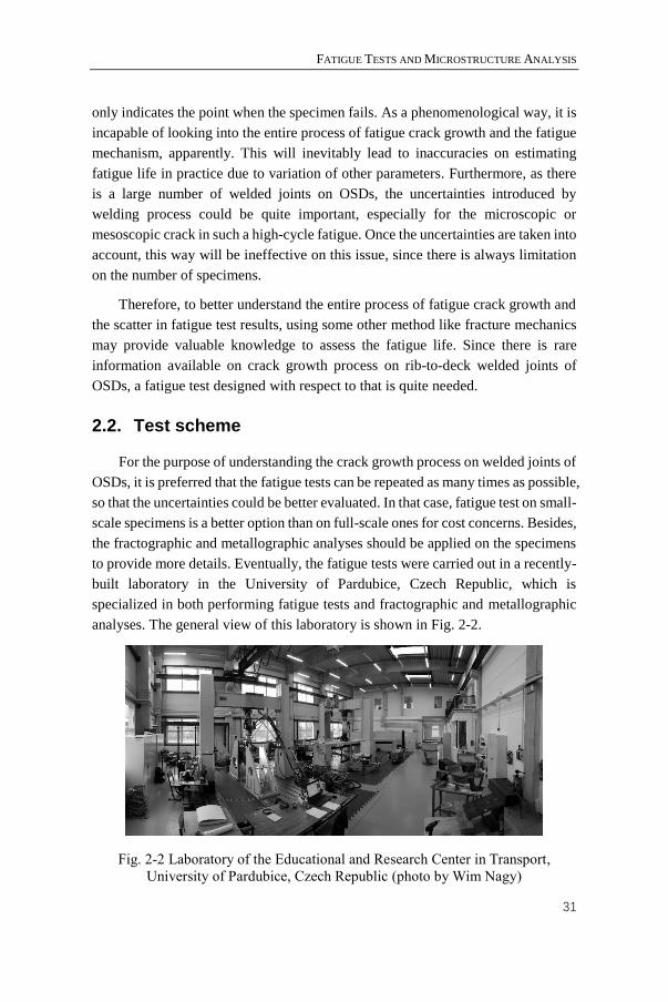
FATIGUE TESTS AND MICROSTRUCTURE ANALYSIS
31
only indicates the point when the specimen fails. As a phenomenological way, it is
incapable of looking into the entire process of fatigue crack growth and the fatigue
mechanism, apparently. This will inevitably lead to inaccuracies on estimating
fatigue life in practice due to variation of other parameters. Furthermore, as there
is a large number of welded joints on OSDs, the uncertainties introduced by
welding process could be quite important, especially for the microscopic or
mesoscopic crack in such a high-cycle fatigue. Once the uncertainties are taken into
account, this way will be ineffective on this issue, since there is always limitation
on the number of specimens.
Therefore, to better understand the entire process of fatigue crack growth and
the scatter in fatigue test results, using some other method like fracture mechanics
may provide valuable knowledge to assess the fatigue life. Since there is rare
information available on crack growth process on rib-to-deck welded joints of
OSDs, a fatigue test designed with respect to that is quite needed.
2.2. Test scheme
For the purpose of understanding the crack growth process on welded joints of
OSDs, it is preferred that the fatigue tests can be repeated as many times as possible,
so that the uncertainties could be better evaluated. In that case, fatigue test on small-
scale specimens is a better option than on full-scale ones for cost concerns. Besides,
the fractographic and metallographic analyses should be applied on the specimens
to provide more details. Eventually, the fatigue tests were carried out in a recently-
built laboratory in the University of Pardubice, Czech Republic, which is
specialized in both performing fatigue tests and fractographic and metallographic
analyses. The general view of this laboratory is shown in Fig. 2-2.
Fig. 2-2 Laboratory of the Educational and Research Center in Transport,
University of Pardubice, Czech Republic (photo by Wim Nagy)
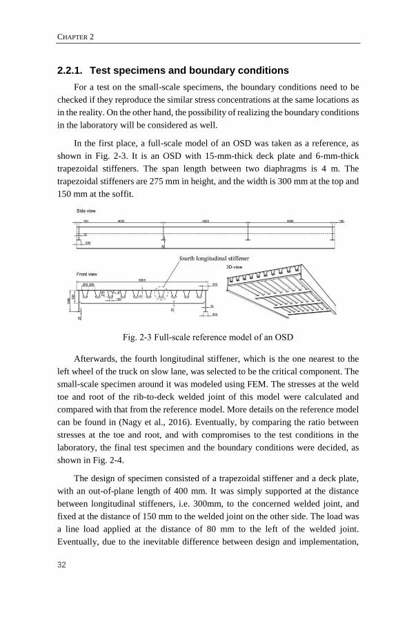
CHAPTER 2
32
2.2.1. Test specimens and boundary conditions
For a test on the small-scale specimens, the boundary conditions need to be
checked if they reproduce the similar stress concentrations at the same locations as
in the reality. On the other hand, the possibility of realizing the boundary conditions
in the laboratory will be considered as well.
In the first place, a full-scale model of an OSD was taken as a reference, as
shown in Fig. 2-3. It is an OSD with 15-mm-thick deck plate and 6-mm-thick
trapezoidal stiffeners. The span length between two diaphragms is 4 m. The
trapezoidal stiffeners are 275 mm in height, and the width is 300 mm at the top and
150 mm at the soffit.
Fig. 2-3 Full-scale reference model of an OSD
Afterwards, the fourth longitudinal stiffener, which is the one nearest to the
left wheel of the truck on slow lane, was selected to be the critical component. The
small-scale specimen around it was modeled using FEM. The stresses at the weld
toe and root of the rib-to-deck welded joint of this model were calculated and
compared with that from the reference model. More details on the reference model
can be found in (Nagy et al., 2016). Eventually, by comparing the ratio between
stresses at the toe and root, and with compromises to the test conditions in the
laboratory, the final test specimen and the boundary conditions were decided, as
shown in Fig. 2-4.
The design of specimen consisted of a trapezoidal stiffener and a deck plate,
with an out-of-plane length of 400 mm. It was simply supported at the distance
between longitudinal stiffeners, i.e. 300mm, to the concerned welded joint, and
fixed at the distance of 150 mm to the welded joint on the other side. The load was
a line load applied at the distance of 80 mm to the left of the welded joint.
Eventually, due to the inevitable difference between design and implementation,

FATIGUE TESTS AND MICROSTRUCTURE ANALYSIS
33
the length of the specimens was actually 370 mm, and the distance between the
loading location and the welded joint was 70 mm.
a) basic scheme (unit: mm)
b) 3D visualization in the laboratory
Fig. 2-4 Test specimens and boundary conditions
2.2.2. Manufacturing specimens
According to the common way of OSD production, the test specimens were
welded by submerged arc welding (SAW) using an electric arc beneath a bed of
granulated flux. To manufacture small-scale specimens with comparable weld
qualities, two 4-meter-long specimens were produced firstly, and then cut into
smaller pieces with equal length for each.
Given that there were two rib-to-deck welded joints on the specimens, the
welding process could be done separately or simultaneously. In both way, tack
welding was applied initially to prevent the thermal deformations from being too

CHAPTER 2
34
large. More details can be found in (Nagy et al., 2017). The welding parameters
were summarized in Table 2-1. It should be noted that wire angle, which is the
angle from the wire to the vertical direction, was designed differently for the two
specimens. Consequently, it produced different weld geometries as shown in the
next section.
Table 2-1 Summary of welding parameters
Welding sequence Separate Simultaneous
Welding machine Semi-automatic Automatic
Description Twin wire Single wire
Current (A) 600 - 700 500 - 600
Wire feed speed (m/min) 0.71 2.0 – 2.5
Voltage (V) 28 – 32 25 – 26
Travel speed (mm/min) 700 – 900 550 – 650
Arc energy (kJ/mm) 1.2 – 1.7 1.3 – 1.8
Distance electrode to work piece (mm) 10 – 20 10 – 20
Wire angle θ 30° 25°
2.2.3. Data collection
As one of the most important concern of this study is the crack growth process,
the fatigue test attempted to generate information about the fatigue fracture as much
as possible. A common way to monitor the fatigue crack growth is the Crack Tip
Opening Displacement (CTOD) (ASTM International, 2015). However, for a
specimen of OSD, it is difficult to make an initial notch or crack, and the complex
geometry of the specimen is not preferred by CTOD measurement as well.
Fortunately, as beach mark is always observed on the fatigue fracture surface
(Witek, 2009), it could provide an alternative method. The only concern is that
according to some of the fatigue tests on OSDs (Ya et al., 2011, Kainuma et al.,
2016), the beach marks obtained were either with limited quantities, or can hardly
be identified visually.
Therefore, it was planned to apply loading sequences designed for this fatigue
test specifically, which can help to produce clear beach marks on the fracture
surface. A way of designing these loading sequences were proposed by Schepens
and Laseure (2015), given as follows,
{
𝑁𝑏𝑒𝑎𝑐ℎ𝑚𝑎𝑟𝑘
𝑁𝑏𝑎𝑠𝑒= 0.5
𝜇 =𝑃𝑚𝑎𝑥 − 𝑃𝑏𝑒𝑎𝑐ℎ𝑚𝑎𝑟𝑘
𝑃𝑚𝑎𝑥− 𝑃𝑚𝑖𝑛= 0.4
(2-1)
where 𝑁𝑏𝑒𝑎𝑐ℎ𝑚𝑎𝑟𝑘, 𝑁𝑏𝑎𝑠𝑒 , 𝑃𝑏𝑒𝑎𝑐ℎ𝑚𝑎𝑟𝑘, 𝑃𝑚𝑎𝑥 and 𝑃𝑚𝑖𝑛 were defined in Fig. 2-5.
The value of 𝜇 is recommended to be 0.4 to keep the variable amplitude effect
from affecting the regular fatigue behavior significantly. However, it does not
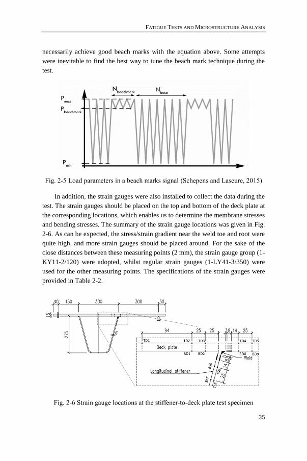
FATIGUE TESTS AND MICROSTRUCTURE ANALYSIS
35
necessarily achieve good beach marks with the equation above. Some attempts
were inevitable to find the best way to tune the beach mark technique during the
test.
Fig. 2-5 Load parameters in a beach marks signal (Schepens and Laseure, 2015)
In addition, the strain gauges were also installed to collect the data during the
test. The strain gauges should be placed on the top and bottom of the deck plate at
the corresponding locations, which enables us to determine the membrane stresses
and bending stresses. The summary of the strain gauge locations was given in Fig.
2-6. As can be expected, the stress/strain gradient near the weld toe and root were
quite high, and more strain gauges should be placed around. For the sake of the
close distances between these measuring points (2 mm), the strain gauge group (1-
KY11-2/120) were adopted, whilst regular strain gauges (1-LY41-3/350) were
used for the other measuring points. The specifications of the strain gauges were
provided in Table 2-2.
Fig. 2-6 Strain gauge locations at the stiffener-to-deck plate test specimen
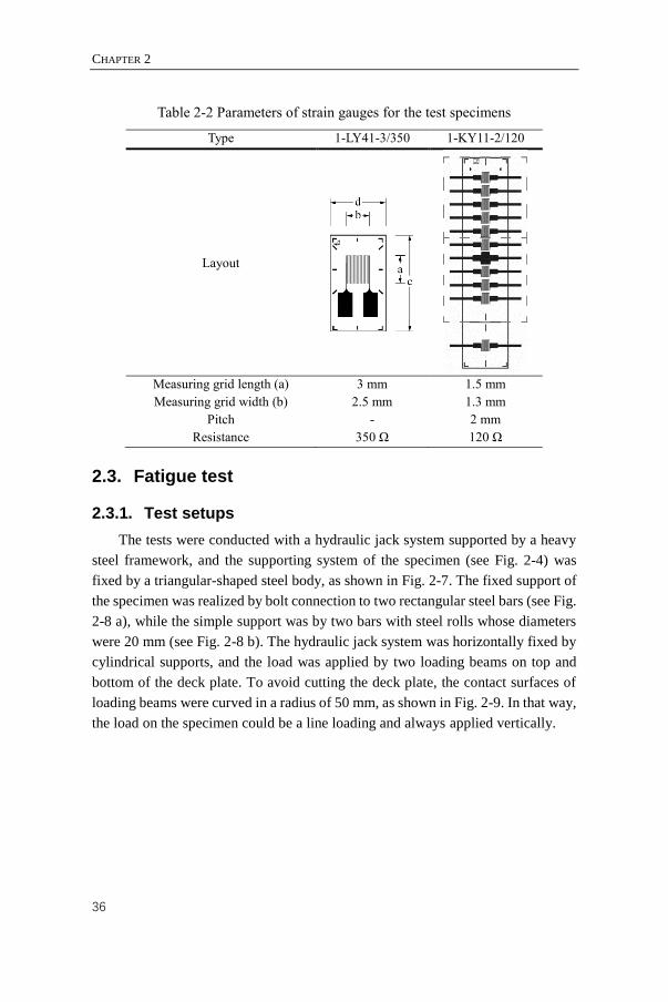
CHAPTER 2
36
Table 2-2 Parameters of strain gauges for the test specimens
Type 1-LY41-3/350 1-KY11-2/120
Layout
Measuring grid length (a) 3 mm 1.5 mm
Measuring grid width (b) 2.5 mm 1.3 mm
Pitch - 2 mm
Resistance 350 Ω 120 Ω
2.3. Fatigue test
2.3.1. Test setups
The tests were conducted with a hydraulic jack system supported by a heavy
steel framework, and the supporting system of the specimen (see Fig. 2-4) was
fixed by a triangular-shaped steel body, as shown in Fig. 2-7. The fixed support of
the specimen was realized by bolt connection to two rectangular steel bars (see Fig.
2-8 a), while the simple support was by two bars with steel rolls whose diameters
were 20 mm (see Fig. 2-8 b). The hydraulic jack system was horizontally fixed by
cylindrical supports, and the load was applied by two loading beams on top and
bottom of the deck plate. To avoid cutting the deck plate, the contact surfaces of
loading beams were curved in a radius of 50 mm, as shown in Fig. 2-9. In that way,
the load on the specimen could be a line loading and always applied vertically.

FATIGUE TESTS AND MICROSTRUCTURE ANALYSIS
37
Fig. 2-7 The supporting triangular-shaped body
a) fixed support
b) roller support
c) full view of the supported specimen
Fig. 2-8 Supports of the specimens
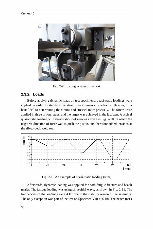
CHAPTER 2
38
Fig. 2-9 Loading system of the test
2.3.2. Loads
Before applying dynamic loads on test specimens, quasi-static loadings were
applied in order to stabilize the strain measurements in advance. Besides, it is
beneficial to determining the strains and stresses more precisely. The forces were
applied in three or four steps, and the target was achieved in the last step. A typical
quasi-static loading with stress ratio R of zero was given in Fig. 2-10, in which the
negative direction of force was to push the piston, and therefore added tensions at
the rib-to-deck weld toe.
Fig. 2-10 An example of quasi-static loading (R=0)
Afterwards, dynamic loading was applied for both fatigue fracture and beach
marks. The fatigue loading was using sinusoidal wave, as shown in Fig. 2-11. The
frequencies of the loadings were 4 Hz due to the stability reason of the assembly.
The only exception was part of the test on Specimen VIII at 6 Hz. The beach mark

FATIGUE TESTS AND MICROSTRUCTURE ANALYSIS
39
loadings, as mentioned before, would have smaller amplitudes, but the normalized
stress ratio between fatigue loading and beach mark loading, μ, was yet to be
optimized. Different values of μ were used, ranging from 0.2 to 0.6. Most of them
were set to be 0.4, as suggested by Schepens and Laseure (2015). However, the
produced beach marks may still be difficult to distinguish by observing the fracture
surface, if the same loading type, i.e. sinusoidal wave, was used for beach marks.
Therefore, a quasi-triangular wave, as a more aggressive type, was applied for
beach mark loadings, while the frequency was kept the same to the fatigue loading,
4 Hz, as shown in Fig. 2-12. When applying beach mark loading, extra cautions on
the stability of specimens should be used as it brought more impact on them.
Fig. 2-11 An example of fatigue loading
Fig. 2-12 An example of quasi-triangular beach mark loading
Eventually, eleven specimens in total were tested, among which nine were
made of simultaneous welding sequence marked with Roman numbers, while the
other two were made of separate welding sequence marked with Arabic numbers.
Table 2-3 showed the summary of the applied loads on test specimens. It can be
seen that most of the cases were carried out with stress ratio R equals 0 or -1. In
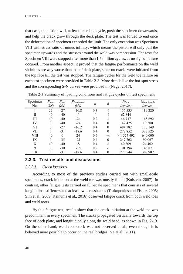
CHAPTER 2
40
that case, the pistion will, at least once in a cycle, push the specimen downwards,
and help the crack grow through the deck plate. The test was forced to end once
the deformation of specimen exceeded the limit. The only exception was Specimen
VIII with stress ratio of minus infinity, which means the piston will only pull the
specimen upwards and the stresses around the weld was compression. The tests for
Specimen VIII were stopped after more than 1.5 million cycles, as no sign of failure
occured. From another aspect, it proved that the fatigue performance on the weld
vicinities are way worse than that of deck plate, since no cracks were initiated from
the top face till the test was stopped. The fatigue cycles for the weld toe failure on
each test specimen were provided in Table 2-3. More details like the hot-spot stress
and the corresponding S-N curves were provided in (Nagy, 2017).
Table 2-3 Summary of loading conditions and fatigue cycles on test specimens
Specimen
No.
Pmax
(kN)
Pmin
(kN)
Pbeachmark
(kN) μ R
Nbase
(cycles)
Nbeachmarks
(cycles)
I 27 -27 -10.8 0.3 -1 156 535 119 220
II 40 -40 / / -1 62 844 /
III 40 -40 -24 0.2 -1 46 737 168 692
IV 0 -40 -24 0.4 0 147 425 19 500
VI 0 -27 -16.2 0.4 0 484 782 178 149
VII 0 -31 -18.6 0.4 0 272 852 337 525
VIII 40 0 24 0.6 -∞ > 1 527 492 640 000
IX 0 -35 -21 0.4 0 247 762 99 067
X 40 -40 -8 0.4 -1 40 809 24 402
9 30 -30 -18 0.2 -1 101 394 148 871
10 0 -31 -18.6 0.4 0 270 544 307 902
2.3.3. Test results and discussions
2.3.3.1. Crack locations
According to most of the previous studies carried out with small-scale
specimens, crack initiation at the weld toe was mostly found (Kolstein, 2007). In
contrast, other fatigue tests carried on full-scale specimens that consists of several
longitudinal stiffeners and at least two crossbeams (Tsakopoulos and Fisher, 2005;
Sim et al., 2009; Kainuma et al., 2016) observed fatigue crack from both weld toes
and weld roots.
By this fatigue test, results show that the crack initiation at the weld toe was
predominant in every specimen. The cracks propagated vertically towards the top
face of deck plate, and longitudinally along the weld bead, as shown in Fig. 2-13.
On the other hand, weld root crack was not observed at all, even though it is
believed more possible to occur on the real bridges (Ya et al., 2011).
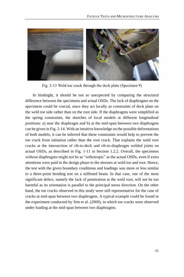
FATIGUE TESTS AND MICROSTRUCTURE ANALYSIS
41
Fig. 2-13 Weld toe crack through the deck plate (Specimen 9)
In hindsight, it should be not so unexpected by comparing the structural
difference between the specimens and actual OSDs. The lack of diaphragms on the
specimens could be crucial, since they act locally as constraints of deck plate on
the weld toe side rather than on the root side. If the diaphragms were simplified as
the spring constraints, the sketches of local models at different longitudinal
positions: a) near the diaphragm and b) at the mid-span between two diaphragms
can be given in Fig. 2-14. With an intuitive knowledge on the possible deformations
of both models, it can be inferred that these constraints would help to prevent the
toe crack from initiation rather than the root crack. That explains the weld root
cracks at the intersection of rib-to-deck and rib-to-diaphragm welded joints on
actual OSDs, as described in Fig. 1-11 in Section 1.2.2. Overall, the specimens
without diaphragms might not be as “orthotropic” as the actual OSDs, even if extra
attentions were paid in the design phase to the stresses at weld toe and root. Hence,
the test with the given boundary conditions and loadings was more or less similar
to a three-point bending test on a stiffened beam. In that case, one of the most
significant defect, namely the lack of penetration at the weld root, will not be too
harmful as its orientation is parallel to the principal stress direction. On the other
hand, the toe cracks observed in this study were still representative for the case of
cracks at mid-span between two diaphragms. A typical example could be found in
the experiment conducted by Sim et al. (2009), in which toe cracks were observed
under loading at the mid-span between two diaphragms.

CHAPTER 2
42
a) near the diaphragm
b) at the mid-span between two
diaphragms
Fig. 2-14 Sketches of simplified local models
Hence, if the study concerns the weld root crack on small-scale specimens, a
different setup of fatigue test is required. Ya et al. (2011) proposed an experimental
way which is similar to a cantilever with geometrical changes of cross-section, see
Fig. 2-15a. Similarly, a test scheme based on this laboratory conditions could be
proposed (Nagy et al., 2017), as shown in Fig. 2-15b. However, it has to be
emphasized that both ways are still different from the realistic OSDs in terms of
load type.
a) Ya et al., 2011
b) Nagy et al., 2017
Fig. 2-15 Scheme of root crack study for small-scale specimens
To summarize, as the weld toe crack was the main reason of fatigue failure on
this test, it should be brought to the forefront in the subsequent fractographic and
metallographic analyses, the numerical calculations and eventually, the realistic
OSDs. The fatigue mechanisms achieved based on weld toe crack may benefit the
analyses on weld root crack as well, but more experimental verification is still
needed.
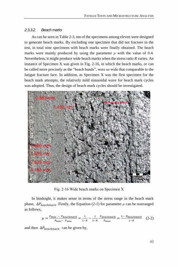
FATIGUE TESTS AND MICROSTRUCTURE ANALYSIS
43
2.3.3.2. Beach marks
As can be seen in Table 2-3, ten of the specimens among eleven were designed
to generate beach marks. By excluding one specimen that did not fracture in the
test, in total nine specimens with beach marks were finally obtained. The beach
marks were mainly produced by using the parameter μ with the value of 0.4.
Nevertheless, it might produce wide beach marks when the stress ratio R varies. An
instance of Specimen X was given in Fig. 2-16, in which the beach marks, or can
be called more precisely as the “beach bands”, were so wide that comparable to the
fatigue fracture face. In addition, as Specimen X was the first specimen for the
beach mark attempts, the relatively mild sinusoidal wave for beach mark cycles
was adopted. Thus, the design of beach mark cycles should be investigated.
Fig. 2-16 Wide beach marks on Specimen X
In hindsight, it makes sense in terms of the stress range in the beach mark
phase, Δ𝑃𝑏𝑒𝑎𝑐ℎ𝑚𝑎𝑟𝑘. Firstly, the Equation (2-1) for parameter μ can be rearranged
as follows,
𝜇 =𝑃𝑚𝑎𝑥 − 𝑃𝑏𝑒𝑎𝑐ℎ𝑚𝑎𝑟𝑘
𝑃𝑚𝑎𝑥− 𝑃𝑚𝑖𝑛=
1
1−𝑅−
1
1−𝑅
𝑃𝑏𝑒𝑎𝑐ℎ𝑚𝑎𝑟𝑘
𝑃𝑚𝑎𝑥=
1− 𝑅𝑏𝑒𝑎𝑐ℎ𝑚𝑎𝑟𝑘
1−𝑅 (2-2)
and then Δ𝑃𝑏𝑒𝑎𝑐ℎ𝑚𝑎𝑟𝑘 can be given by,
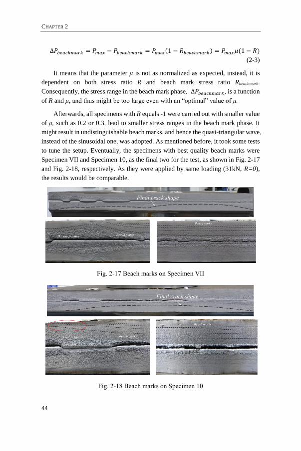
CHAPTER 2
44
Δ𝑃𝑏𝑒𝑎𝑐ℎ𝑚𝑎𝑟𝑘 = 𝑃𝑚𝑎𝑥 − 𝑃𝑏𝑒𝑎𝑐ℎ𝑚𝑎𝑟𝑘 = 𝑃𝑚𝑎𝑥(1 − 𝑅𝑏𝑒𝑎𝑐ℎ𝑚𝑎𝑟𝑘) = 𝑃𝑚𝑎𝑥𝜇(1 − 𝑅)
(2-3)
It means that the parameter μ is not as normalized as expected, instead, it is
dependent on both stress ratio R and beach mark stress ratio Rbeachmark.
Consequently, the stress range in the beach mark phase, Δ𝑃𝑏𝑒𝑎𝑐ℎ𝑚𝑎𝑟𝑘, is a function
of R and μ, and thus might be too large even with an “optimal” value of μ.
Afterwards, all specimens with R equals -1 were carried out with smaller value
of μ, such as 0.2 or 0.3, lead to smaller stress ranges in the beach mark phase. It
might result in undistinguishable beach marks, and hence the quasi-triangular wave,
instead of the sinusoidal one, was adopted. As mentioned before, it took some tests
to tune the setup. Eventually, the specimens with best quality beach marks were
Specimen VII and Specimen 10, as the final two for the test, as shown in Fig. 2-17
and Fig. 2-18, respectively. As they were applied by same loading (31kN, R=0),
the results would be comparable.
Fig. 2-17 Beach marks on Specimen VII
Fig. 2-18 Beach marks on Specimen 10

FATIGUE TESTS AND MICROSTRUCTURE ANALYSIS
45
It is clear that in Specimen VII, there were two main cracks that were
approximately in an elliptical shape, and merged in the middle. They were
longitudinally originated around the quarter points of the whole length. However,
the beach marks on Specimen 10 showed that there was only one main crack
originated at the middle. By checking the beach marks on each specimen, it seems
that the case of two main cracks were the majority. According to the results of
strain gauges, the strain was not distributed uniformly along the longitudinal
direction. The bending of the loading bar resulted in the slightly larger strains
around the quarter positions (Nagy et al., 2017).
Another remarkable thing was the tail of beach marks, which was shown
evidently by the one main crack cases like Specimen 10, as red-circled in Fig. 2-18.
Basically the shape of the crack was semi-elliptical, but the tail of the beach marks
turned out to be extended. This extension was due to the crack merge of the main
crack and small secondary cracks. As the tests applied line loadings in full length,
it is quite possbile to have initial cracks all along the longtudinal direction. The
initial cracks near the tails seemed to form later and grow slower than the main one.
Consequently, they merged with the main crack when it gets close enough,
presented the tail we observed. The form of the initial cracks at the weld toe was
addressed by the fractographic analyses in the next section.
Based on the beach marks of each specimen, a brief crack growth process
could be drawn, as shown in Fig. 2-19. As the beach marks in Specimen X were
too wide, they were measured by both edges, so that the crack growth curve was
almost vertical in some sections. Besides, as the information about the initial crack
was still unknown, the crack growth rate for the entire process could not be
determined. This will be studied by the fractographic and metallographic analyses
in the next section.
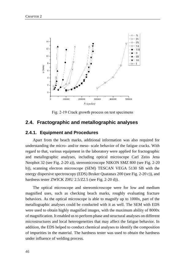
CHAPTER 2
46
Fig. 2-19 Crack growth process on test specimens
2.4. Fractographic and metallographic analyses
2.4.1. Equipment and Procedures
Apart from the beach marks, additional information was also required for
understanding the micro- and/or meso- scale behavior of the fatigue cracks. With
regard to that, various equipment in the laboratory were applied for fractographic
and metallographic analyses, including optical microscope Carl Zeiss Jena
Neophot 32 (see Fig. 2-20 a)), stereomicroscope NIKON SMZ 800 (see Fig. 2-20
b)), scanning electron microscope (SEM) TESCAN VEGA 5130 SB with the
energy dispersive spectroscopy (EDS) Bruker Quatanax 200 (see Fig. 2-20 c)), and
hardness tester ZWICK ZHU 2.5/Z2.5 (see Fig. 2-20 d)).
The optical microscope and stereomicroscope were for low and medium
magnified uses, such as checking beach marks, roughly evaluating fracture
behaviors. As the optical microscope is able to magnify up to 1000x, part of the
metallographic analyses could be conducted with it as well. The SEM with EDS
were used to obtain highly magnified images, with the maximum ability of 8000x
of magnification. It enabled us to perform phase and structural analyses on different
microstructures and local heterogeneities that may affect the fatigue behavior. In
addition, the EDS helped to conduct chemical analyses to identify the composition
of impurities in the material. The hardness tester was used to obtain the hardness
under influence of welding process.
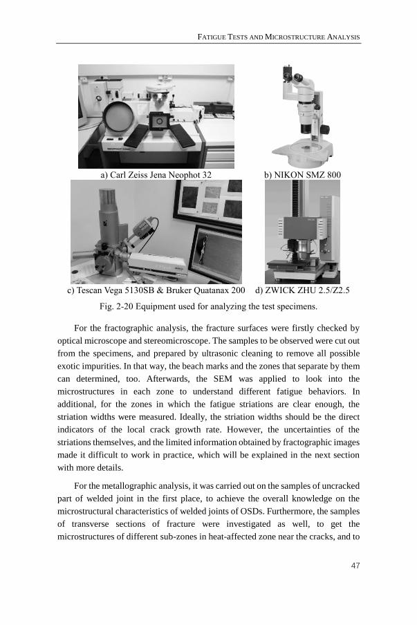
FATIGUE TESTS AND MICROSTRUCTURE ANALYSIS
47
a) Carl Zeiss Jena Neophot 32
b) NIKON SMZ 800
c) Tescan Vega 5130SB & Bruker Quatanax 200
d) ZWICK ZHU 2.5/Z2.5
Fig. 2-20 Equipment used for analyzing the test specimens.
For the fractographic analysis, the fracture surfaces were firstly checked by
optical microscope and stereomicroscope. The samples to be observed were cut out
from the specimens, and prepared by ultrasonic cleaning to remove all possible
exotic impurities. In that way, the beach marks and the zones that separate by them
can determined, too. Afterwards, the SEM was applied to look into the
microstructures in each zone to understand different fatigue behaviors. In
additional, for the zones in which the fatigue striations are clear enough, the
striation widths were measured. Ideally, the striation widths should be the direct
indicators of the local crack growth rate. However, the uncertainties of the
striations themselves, and the limited information obtained by fractographic images
made it difficult to work in practice, which will be explained in the next section
with more details.
For the metallographic analysis, it was carried out on the samples of uncracked
part of welded joint in the first place, to achieve the overall knowledge on the
microstructural characteristics of welded joints of OSDs. Furthermore, the samples
of transverse sections of fracture were investigated as well, to get the
microstructures of different sub-zones in heat-affected zone near the cracks, and to

CHAPTER 2
48
acquire some obvious defects such as the lack-of-penetrations at the weld root. The
samples for both were well polished via physical and chemical methods.
At last, the hardness test was conducted following the instructions from the
metallographic results, which provide the hardness as an indicator of the
mechanical behavior for various zones in welded joints.
2.4.2. Fractographic analyses
2.4.2.1. Crack initiation
The fractography of each specimen was studied based on the zones divided by
beach marks. The crack initiation zone was numbered as Zone 0, then the zone till
the first visible beach mark was Zone 1, and so on. Zone 0 was defined with respect
to the different behavior that lead to a visible boundary, as shown in Fig. 2-21. The
most important phenomenon in this zone, and also maybe for the entire crack
growth life, was the primary intergranular decohesion, which was observed on
fracture samples from all specimens, as shown in Fig. 2-22. A typical example on
Specimen 10 was given by Fig. 2-22 c), in which the areas pointed by arrows are
the place of decohesion, and can be regarded as the cause of crack initiation.
Undoubtedly, the actual cycle number spent before intergranular decohesion
is not exactly zero. It should be related to the applied loading, too. But for a large-
scale structure like OSD, it is believed that the crack initiation life is quite small
(Kolstein, 2007) due to the inevitable weld defects. Consequently, the initial crack
depth for each specimen was obtained by measuring the maximum depth of the
intergranular decohesion. The results are shown in Table 2-4. Accordingly, the
initial crack depth is mainly around 0.3 mm to 0.4 mm. Further information will be
provided by metallographic analysis in the next section.
Fig. 2-21 Different fracture behavior (Specimen VI)
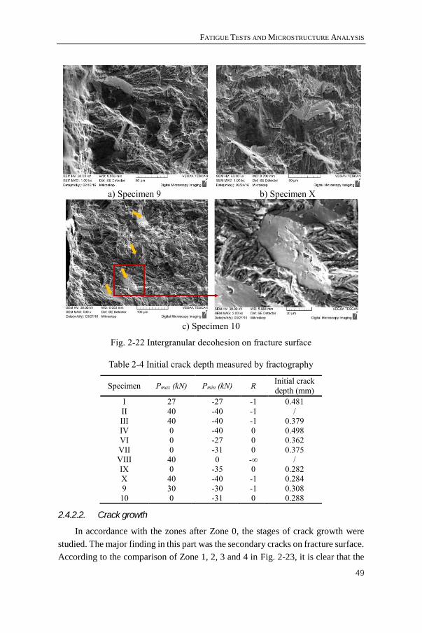
FATIGUE TESTS AND MICROSTRUCTURE ANALYSIS
49
a) Specimen 9
b) Specimen X
c) Specimen 10
Fig. 2-22 Intergranular decohesion on fracture surface
Table 2-4 Initial crack depth measured by fractography
Specimen Pmax (kN) Pmin (kN) R Initial crack
depth (mm)
I 27 -27 -1 0.481
II 40 -40 -1 /
III 40 -40 -1 0.379
IV 0 -40 0 0.498
VI 0 -27 0 0.362
VII 0 -31 0 0.375
VIII 40 0 -∞ /
IX 0 -35 0 0.282
X 40 -40 -1 0.284
9 30 -30 -1 0.308
10 0 -31 0 0.288
2.4.2.2. Crack growth
In accordance with the zones after Zone 0, the stages of crack growth were
studied. The major finding in this part was the secondary cracks on fracture surface.
According to the comparison of Zone 1, 2, 3 and 4 in Fig. 2-23, it is clear that the
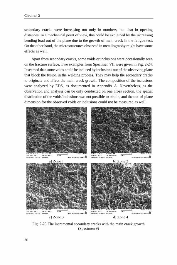
CHAPTER 2
50
secondary cracks were increasing not only in numbers, but also in opening
distances. In a mechanical point of view, this could be explained by the increasing
bending load out of the plane due to the growth of main crack in the fatigue test.
On the other hand, the microstructures observed in metallography might have some
effects as well.
Apart from secondary cracks, some voids or inclusions were occasionally seen
on the fracture surface. Two examples from Specimen VII were given in Fig. 2-24.
It seemed that some voids could be induced by inclusions out of the observing plane
that block the fusion in the welding process. They may help the secondary cracks
to originate and affect the main crack growth. The composition of the inclusions
were analyzed by EDS, as documented in Appendix A. Nevertheless, as the
observation and analysis can be only conducted on one cross section, the spatial
distribution of the voids/inclusions was not possible to obtain, and the out-of-plane
dimension for the observed voids or inclusions could not be measured as well.
a) Zone 1
b) Zone 2
c) Zone 3
d) Zone 4
Fig. 2-23 The incremental secondary cracks with the main crack growth
(Specimen 9)
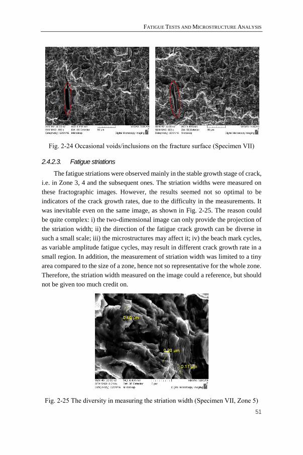
FATIGUE TESTS AND MICROSTRUCTURE ANALYSIS
51
Fig. 2-24 Occasional voids/inclusions on the fracture surface (Specimen VII)
2.4.2.3. Fatigue striations
The fatigue striations were observed mainly in the stable growth stage of crack,
i.e. in Zone 3, 4 and the subsequent ones. The striation widths were measured on
these fractographic images. However, the results seemed not so optimal to be
indicators of the crack growth rates, due to the difficulty in the measurements. It
was inevitable even on the same image, as shown in Fig. 2-25. The reason could
be quite complex: i) the two-dimensional image can only provide the projection of
the striation width; ii) the direction of the fatigue crack growth can be diverse in
such a small scale; iii) the microstructures may affect it; iv) the beach mark cycles,
as variable amplitude fatigue cycles, may result in different crack growth rate in a
small region. In addition, the measurement of striation width was limited to a tiny
area compared to the size of a zone, hence not so representative for the whole zone.
Therefore, the striation width measured on the image could a reference, but should
not be given too much credit on.
Fig. 2-25 The diversity in measuring the striation width (Specimen VII, Zone 5)
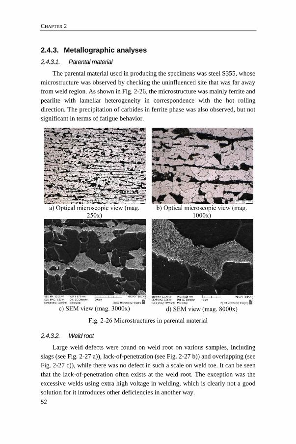
CHAPTER 2
52
2.4.3. Metallographic analyses
2.4.3.1. Parental material
The parental material used in producing the specimens was steel S355, whose
microstructure was observed by checking the uninfluenced site that was far away
from weld region. As shown in Fig. 2-26, the microstructure was mainly ferrite and
pearlite with lamellar heterogeneity in correspondence with the hot rolling
direction. The precipitation of carbides in ferrite phase was also observed, but not
significant in terms of fatigue behavior.
a) Optical microscopic view (mag.
250x)
b) Optical microscopic view (mag.
1000x)
c) SEM view (mag. 3000x)
d) SEM view (mag. 8000x)
Fig. 2-26 Microstructures in parental material
2.4.3.2. Weld root
Large weld defects were found on weld root on various samples, including
slags (see Fig. 2-27 a)), lack-of-penetration (see Fig. 2-27 b)) and overlapping (see
Fig. 2-27 c)), while there was no defect in such a scale on weld toe. It can be seen
that the lack-of-penetration often exists at the weld root. The exception was the
excessive welds using extra high voltage in welding, which is clearly not a good
solution for it introduces other deficiencies in another way.
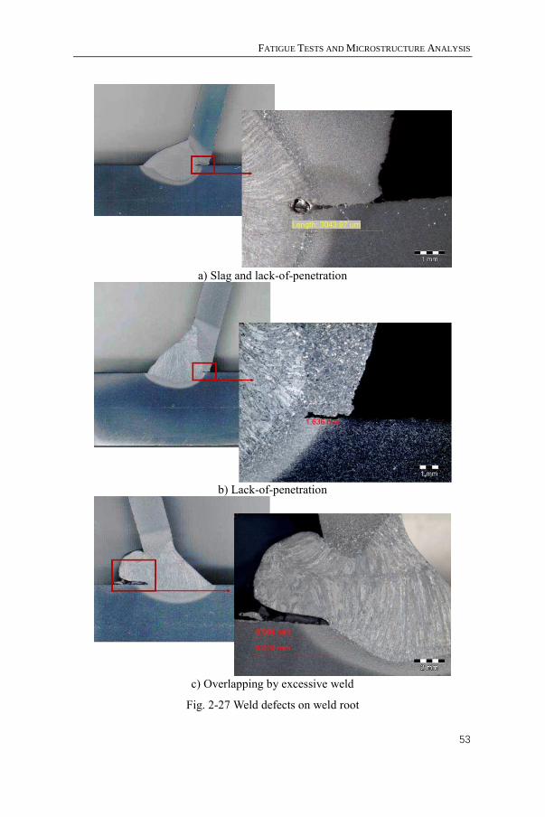
FATIGUE TESTS AND MICROSTRUCTURE ANALYSIS
53
a) Slag and lack-of-penetration
b) Lack-of-penetration
c) Overlapping by excessive weld
Fig. 2-27 Weld defects on weld root
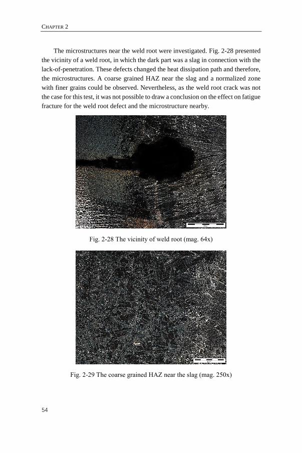
CHAPTER 2
54
The microstructures near the weld root were investigated. Fig. 2-28 presented
the vicinity of a weld root, in which the dark part was a slag in connection with the
lack-of-penetration. These defects changed the heat dissipation path and therefore,
the microstructures. A coarse grained HAZ near the slag and a normalized zone
with finer grains could be observed. Nevertheless, as the weld root crack was not
the case for this test, it was not possible to draw a conclusion on the effect on fatigue
fracture for the weld root defect and the microstructure nearby.
Fig. 2-28 The vicinity of weld root (mag. 64x)
Fig. 2-29 The coarse grained HAZ near the slag (mag. 250x)
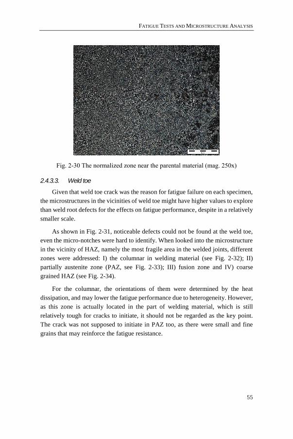
FATIGUE TESTS AND MICROSTRUCTURE ANALYSIS
55
Fig. 2-30 The normalized zone near the parental material (mag. 250x)
2.4.3.3. Weld toe
Given that weld toe crack was the reason for fatigue failure on each specimen,
the microstructures in the vicinities of weld toe might have higher values to explore
than weld root defects for the effects on fatigue performance, despite in a relatively
smaller scale.
As shown in Fig. 2-31, noticeable defects could not be found at the weld toe,
even the micro-notches were hard to identify. When looked into the microstructure
in the vicinity of HAZ, namely the most fragile area in the welded joints, different
zones were addressed: I) the columnar in welding material (see Fig. 2-32); II)
partially austenite zone (PAZ, see Fig. 2-33); III) fusion zone and IV) coarse
grained HAZ (see Fig. 2-34).
For the columnar, the orientations of them were determined by the heat
dissipation, and may lower the fatigue performance due to heterogeneity. However,
as this zone is actually located in the part of welding material, which is still
relatively tough for cracks to initiate, it should not be regarded as the key point.
The crack was not supposed to initiate in PAZ too, as there were small and fine
grains that may reinforce the fatigue resistance.
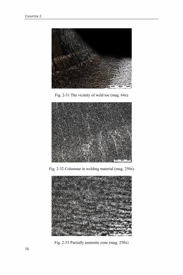
CHAPTER 2
56
Fig. 2-31 The vicinity of weld toe (mag. 64x)
Fig. 2-32 Columnar in welding material (mag. 250x)
Fig. 2-33 Partially austenite zone (mag. 250x)
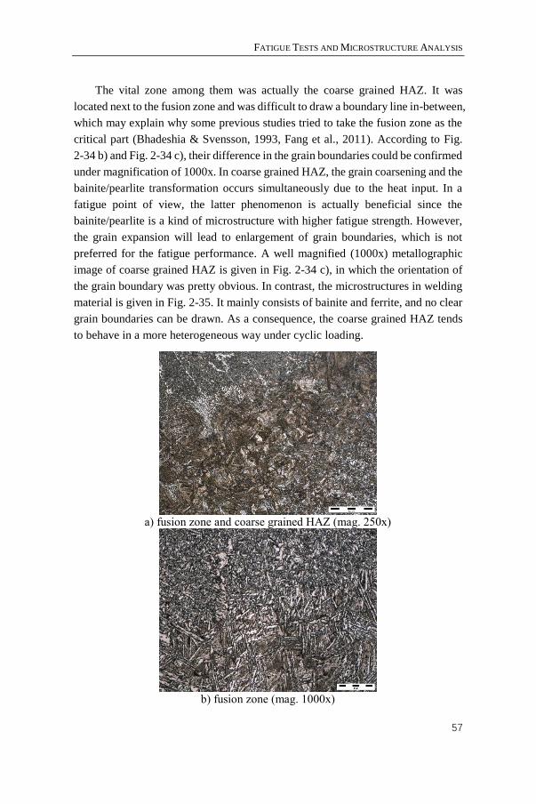
FATIGUE TESTS AND MICROSTRUCTURE ANALYSIS
57
The vital zone among them was actually the coarse grained HAZ. It was
located next to the fusion zone and was difficult to draw a boundary line in-between,
which may explain why some previous studies tried to take the fusion zone as the
critical part (Bhadeshia & Svensson, 1993, Fang et al., 2011). According to Fig.
2-34 b) and Fig. 2-34 c), their difference in the grain boundaries could be confirmed
under magnification of 1000x. In coarse grained HAZ, the grain coarsening and the
bainite/pearlite transformation occurs simultaneously due to the heat input. In a
fatigue point of view, the latter phenomenon is actually beneficial since the
bainite/pearlite is a kind of microstructure with higher fatigue strength. However,
the grain expansion will lead to enlargement of grain boundaries, which is not
preferred for the fatigue performance. A well magnified (1000x) metallographic
image of coarse grained HAZ is given in Fig. 2-34 c), in which the orientation of
the grain boundary was pretty obvious. In contrast, the microstructures in welding
material is given in Fig. 2-35. It mainly consists of bainite and ferrite, and no clear
grain boundaries can be drawn. As a consequence, the coarse grained HAZ tends
to behave in a more heterogeneous way under cyclic loading.
a) fusion zone and coarse grained HAZ (mag. 250x)
b) fusion zone (mag. 1000x)
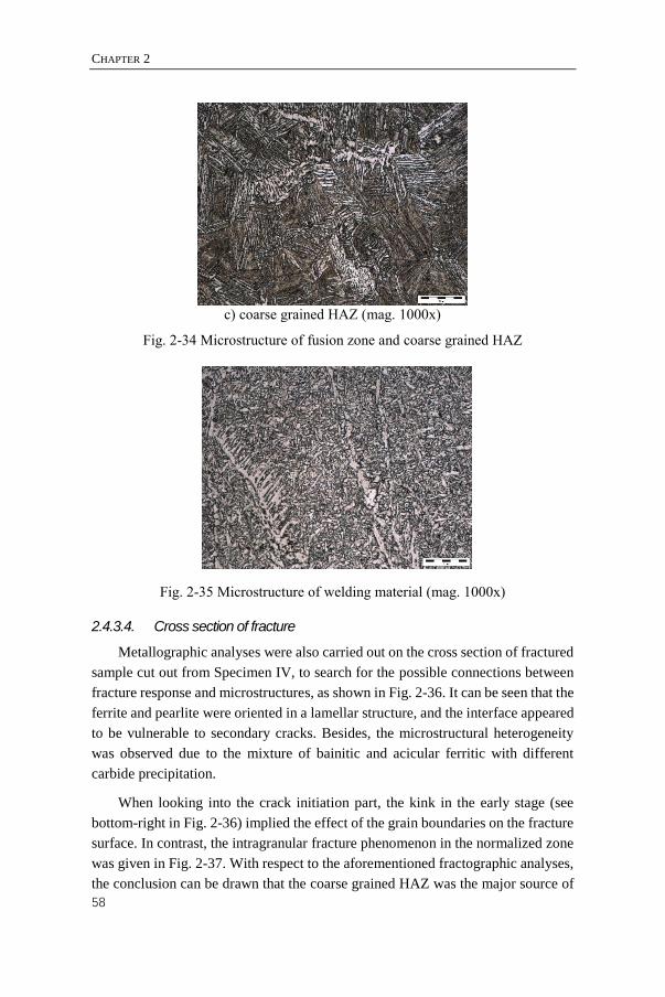
CHAPTER 2
58
c) coarse grained HAZ (mag. 1000x)
Fig. 2-34 Microstructure of fusion zone and coarse grained HAZ
Fig. 2-35 Microstructure of welding material (mag. 1000x)
2.4.3.4. Cross section of fracture
Metallographic analyses were also carried out on the cross section of fractured
sample cut out from Specimen IV, to search for the possible connections between
fracture response and microstructures, as shown in Fig. 2-36. It can be seen that the
ferrite and pearlite were oriented in a lamellar structure, and the interface appeared
to be vulnerable to secondary cracks. Besides, the microstructural heterogeneity
was observed due to the mixture of bainitic and acicular ferritic with different
carbide precipitation.
When looking into the crack initiation part, the kink in the early stage (see
bottom-right in Fig. 2-36) implied the effect of the grain boundaries on the fracture
surface. In contrast, the intragranular fracture phenomenon in the normalized zone
was given in Fig. 2-37. With respect to the aforementioned fractographic analyses,
the conclusion can be drawn that the coarse grained HAZ was the major source of

FATIGUE TESTS AND MICROSTRUCTURE ANALYSIS
59
initial crack, since the crack path did follow the intergranular decohesion in this
zone. A similar fractographic analysis was available in (Schmidova and Hanus,
2011), providing another proof for that statement.
Fig. 2-36 Metallography on the cross section of the fractured sample
Fig. 2-37 The intra-granular fracture in the normalized zone (Specimen IV)
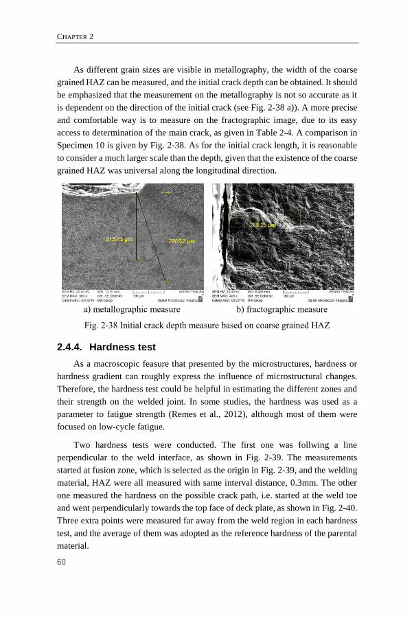
CHAPTER 2
60
As different grain sizes are visible in metallography, the width of the coarse
grained HAZ can be measured, and the initial crack depth can be obtained. It should
be emphasized that the measurement on the metallography is not so accurate as it
is dependent on the direction of the initial crack (see Fig. 2-38 a)). A more precise
and comfortable way is to measure on the fractographic image, due to its easy
access to determination of the main crack, as given in Table 2-4. A comparison in
Specimen 10 is given by Fig. 2-38. As for the initial crack length, it is reasonable
to consider a much larger scale than the depth, given that the existence of the coarse
grained HAZ was universal along the longitudinal direction.
a) metallographic measure
b) fractographic measure
Fig. 2-38 Initial crack depth measure based on coarse grained HAZ
2.4.4. Hardness test
As a macroscopic feasure that presented by the microstructures, hardness or
hardness gradient can roughly express the influence of microstructural changes.
Therefore, the hardness test could be helpful in estimating the different zones and
their strength on the welded joint. In some studies, the hardness was used as a
parameter to fatigue strength (Remes et al., 2012), although most of them were
focused on low-cycle fatigue.
Two hardness tests were conducted. The first one was follwing a line
perpendicular to the weld interface, as shown in Fig. 2-39. The measurements
started at fusion zone, which is selected as the origin in Fig. 2-39, and the welding
material, HAZ were all measured with same interval distance, 0.3mm. The other
one measured the hardness on the possible crack path, i.e. started at the weld toe
and went perpendicularly towards the top face of deck plate, as shown in Fig. 2-40.
Three extra points were measured far away from the weld region in each hardness
test, and the average of them was adopted as the reference hardness of the parental
material.
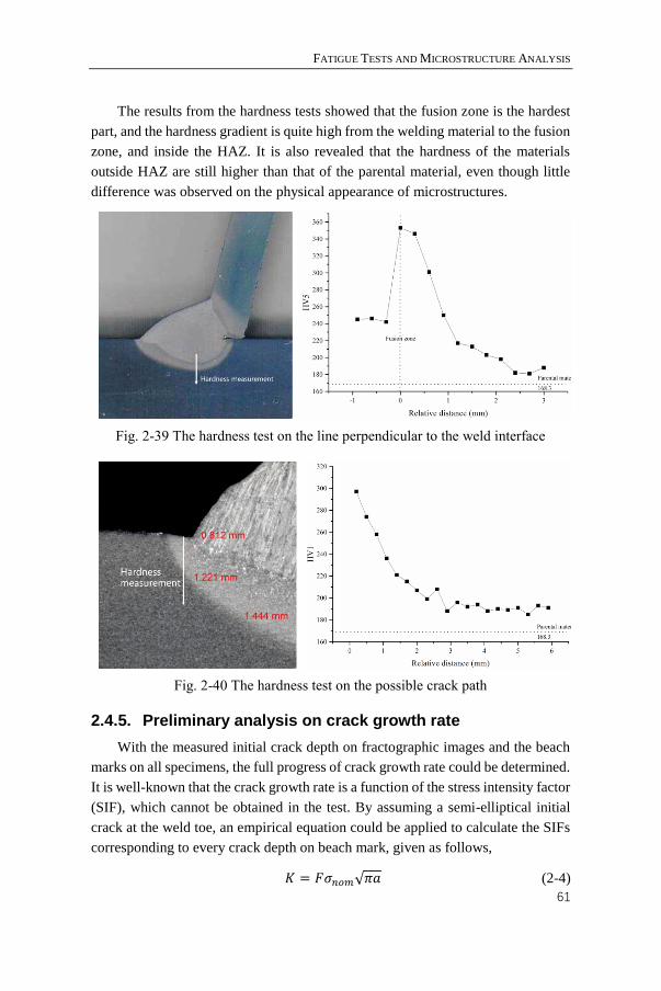
FATIGUE TESTS AND MICROSTRUCTURE ANALYSIS
61
The results from the hardness tests showed that the fusion zone is the hardest
part, and the hardness gradient is quite high from the welding material to the fusion
zone, and inside the HAZ. It is also revealed that the hardness of the materials
outside HAZ are still higher than that of the parental material, even though little
difference was observed on the physical appearance of microstructures.
Fig. 2-39 The hardness test on the line perpendicular to the weld interface
Fig. 2-40 The hardness test on the possible crack path
2.4.5. Preliminary analysis on crack growth rate
With the measured initial crack depth on fractographic images and the beach
marks on all specimens, the full progress of crack growth rate could be determined.
It is well-known that the crack growth rate is a function of the stress intensity factor
(SIF), which cannot be obtained in the test. By assuming a semi-elliptical initial
crack at the weld toe, an empirical equation could be applied to calculate the SIFs
corresponding to every crack depth on beach mark, given as follows,
𝐾 = 𝐹𝜎𝑛𝑜𝑚√𝜋𝑎 (2-4)

CHAPTER 2
62
where 𝜎𝑛𝑜𝑚 is the nominal stress, can be acquired by the strain gauge results; 𝑎
is the crack depth; 𝐹 is the shape factor. In the case of weld toe magnification, 𝐹
is affected by all geometrical parameters such as the crack depth 𝑎, crack half
length c , deck plate thickness T , weld toe flank angle 𝜃 , etc. An equation
proposed by Bowness and Lee (2000) was adopted to calculate the shape factor, 𝐹,
with non-dimensional geometrical parameters. Appendix B presents the detailed
way of the calculation. As it is based on a numerical study on weld toe cracks on
T-butt joints, the results obtained can only be regarded as an approximation to the
test.
As a preliminary analysis, it should be noted that some parameters were
hypothetic. The semi-axis length ratio between a and c was kept to be 0.05 for all
crack depth, since the crack length was believed much larger than the depth as the
previous analyses suggested. The weld toe flank angle was 37 degrees measured in
the weld geometries in Fig. 2-27, although some variations can be seen. The ratio
of attachment width to deck plate thickness was assumed to be 0.8. Consequently,
the crack growth rate curve with respect to the SIFs could be drawn to verify the
Paris law on this issue. To exclude the effect of the stress ratio, only the crack
growth rate curves from cases with R equals zero were presented in Fig. 2-41, in a
logarithmic coordinate system.
In accordance with Paris law, the entire progress of crack growth is generally
described by three stages: I) threshold region; II) Paris region; III) stable tearing
crack growth region (Schijve, 2001). By looking into the curves of the specimens
in Fig. 2-41, two of them with same loading (Specimen VII and Specimen 10) made
good agreements, while other curves showed similar behavior as well, but not as
representative as less beach marks were achieved. It can be seen that in Stage I, the
crack grwoth rate is of larger uncertainties and higher gradient than others.
According to the aforementioned observations, the heterogeneities in
microstructures could be the main reason for the uncertainties in Stage I, which is
logical as the smaller initial cracks are more likely to be affected by microstructures.
One interesting observation is that there exists a slight reduction inside Stage II,
which makes a “pit” on the curve. Thus two sub-stages could be addressed, named
as Stage II-a and Stage II-b hereinafter. The curve for Specimen VI presents
another proof for it, even though the “pit” is not evident due to limited points.
In fact, a similar phenomenon was found by fatigue tests on aluminum alloys,
as shown in Fig. 2-42, in which four stages, (named Stage 1, 2, 3, 4 to be
distinguishable from this test) were determined (Bogdanov, 2014). When
comparing these curves achieved by welded joints and pure materials, it can be
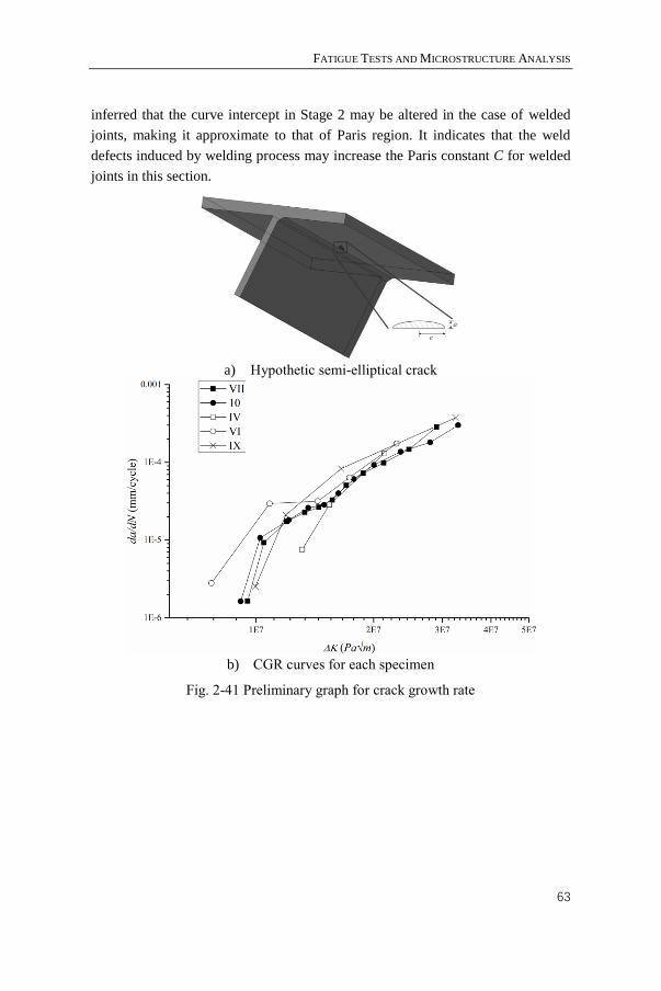
FATIGUE TESTS AND MICROSTRUCTURE ANALYSIS
63
inferred that the curve intercept in Stage 2 may be altered in the case of welded
joints, making it approximate to that of Paris region. It indicates that the weld
defects induced by welding process may increase the Paris constant C for welded
joints in this section.
a) Hypothetic semi-elliptical crack
b) CGR curves for each specimen
Fig. 2-41 Preliminary graph for crack growth rate
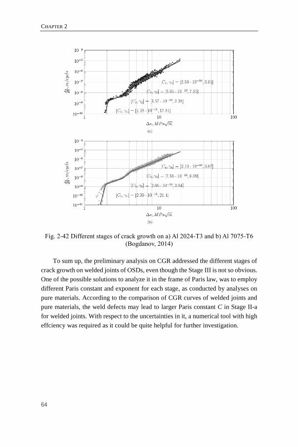
CHAPTER 2
64
Fig. 2-42 Different stages of crack growth on a) Al 2024-T3 and b) Al 7075-T6
(Bogdanov, 2014)
To sum up, the preliminary analysis on CGR addressed the different stages of
crack growth on welded joints of OSDs, even though the Stage III is not so obvious.
One of the possible solutions to analyze it in the frame of Paris law, was to employ
different Paris constant and exponent for each stage, as conducted by analyses on
pure materials. According to the comparison of CGR curves of welded joints and
pure materials, the weld defects may lead to larger Paris constant C in Stage II-a
for welded joints. With respect to the uncertainties in it, a numerical tool with high
effciency was required as it could be quite helpful for further investigation.
CHAPTER 3
CRACK GROWTH BASED ON
EXTENDED FINITED ELEMENT
METHOD
________________________________
This chapter is based on
Wang, B., De Backer, H., and Chen, A. (2016). An XFEM based uncertainty
study on crack growth in welded joints with defects. Theoretical and Applied
Fracture Mechanics, 86, Part B, 125-142.
CHAPTER 3
66
3.1. Introduction
Based on the fatigue test results, it is obvious that the numerical simulation on
fatigue crack on OSDs requires an effective and efficient way to conduct
computations on massive cases with various weld geometries and random weld
defects. Besides, the uncertainties in residual stress distribution may raise the same
demand. Hence the classical FEM is not an option since it is more suitable for one
specific and determined case and thus not efficient enough in both building and
solving steps. In contrast, the extended finite element method (XFEM) is quite
efficient since the geometry is independent to the mesh, which gives it a great
advantage in generating and calculating a large number of models with different
defects inside.
XFEM was firstly proposed by Belytschko et al. (1999, 2001). It originated
from the idea of the Partition of Unity Method (PUM) that any function could be
represented by the summation of a set of local functions. As long as the local
functions are accurate to the real one, the combination of them should approximate
the target function. By introducing this concept into FEM, the displacement field
function could be partitioned into several functions in correspondence with the
different local characteristics.
The computer implementation of XFEM was first proposed by Sukumar et al.
(2003), and then Bordas et al. (2007) presented a general structure for XFEM code.
Traditional FEM software, like ABAQUS, SAMCEF, MORFEO, DYNAFLOW,
etc., started to introduce XFEM modules, though with some limitations. Works
were also conducted on developing specified XFEM program, based on FEM
software using the user defined sub-program like user elements subroutine (UEL)
in ABAQUS (Giner et al., 2009, Shi et al., 2010), or based on general numerical
computing language like MATLAB (Pais, 2011, Yu, 2014).
As XFEM is so powerful and practical on solving discontinuous problems, it
is mainly applied in this study for two parts: i) the mesoscopic models built by an
XFEM program coding with MATLAB; ii) the macroscopic models built in
SAMCEF with its XFEM module. The XFEM program was developed based on
the work by Pais (2011) and Yu (2014). According to the requirements on the issue
of cracked weld joint of OSDs, this program was embedded one module for random
defects, and one for parametric weld toe geometries. The general structure of this
XFEM program is given in Fig. 3-1.
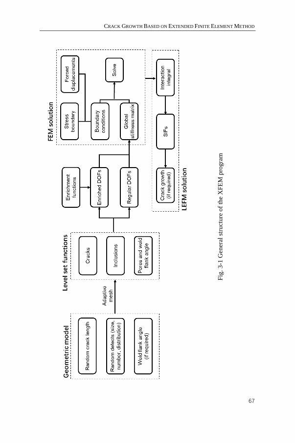
CRACK GROWTH BASED ON EXTENDED FINITE ELEMENT METHOD
67
Fig
. 3
-1 G
ener
al s
tru
ctu
re o
f th
e X
FE
M p
rogra
m
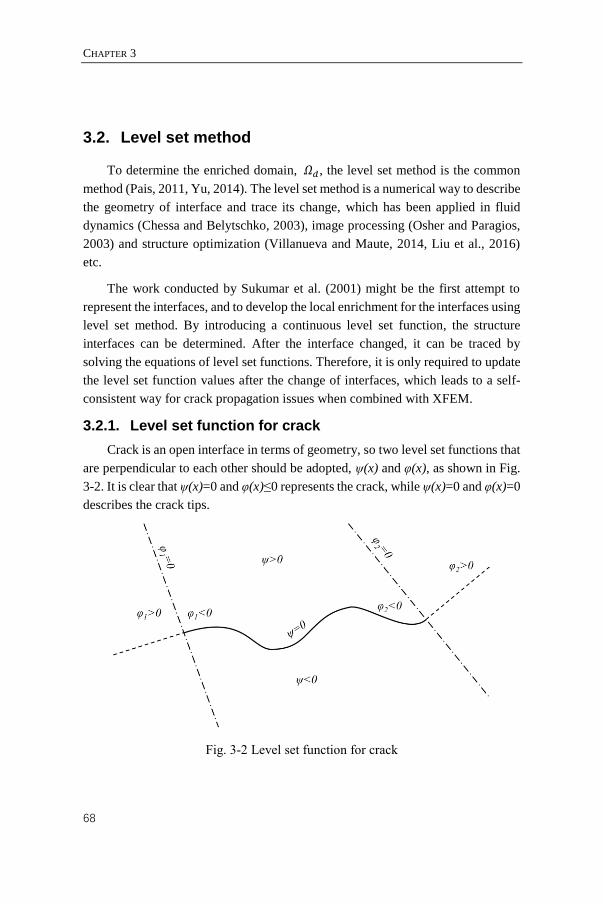
CHAPTER 3
68
3.2. Level set method
To determine the enriched domain, 𝛺𝑑, the level set method is the common
method (Pais, 2011, Yu, 2014). The level set method is a numerical way to describe
the geometry of interface and trace its change, which has been applied in fluid
dynamics (Chessa and Belytschko, 2003), image processing (Osher and Paragios,
2003) and structure optimization (Villanueva and Maute, 2014, Liu et al., 2016)
etc.
The work conducted by Sukumar et al. (2001) might be the first attempt to
represent the interfaces, and to develop the local enrichment for the interfaces using
level set method. By introducing a continuous level set function, the structure
interfaces can be determined. After the interface changed, it can be traced by
solving the equations of level set functions. Therefore, it is only required to update
the level set function values after the change of interfaces, which leads to a self-
consistent way for crack propagation issues when combined with XFEM.
3.2.1. Level set function for crack
Crack is an open interface in terms of geometry, so two level set functions that
are perpendicular to each other should be adopted, ψ(x) and φ(x), as shown in Fig.
3-2. It is clear that ψ(x)=0 and φ(x)≤0 represents the crack, while ψ(x)=0 and φ(x)=0
describes the crack tips.
Fig. 3-2 Level set function for crack

CRACK GROWTH BASED ON EXTENDED FINITE ELEMENT METHOD
69
3.2.2. Level set function for pores and inclusions
Pores and inclusions are regarded as the closed interface in the domain. For
multiple closed interface in a circular shape in the domain, the level set function is
put forward by Sukumar et al. (2001):
φ(𝐗, 0) = min{‖𝑿 − 𝑿𝑐𝑖 ‖ − 𝑟𝑐
𝑖}𝑖 = 1,2,…,𝑛𝑐
(3-1)
where 𝑛𝑐 is the number of circular interfaces, 𝑿𝑐𝑖 is the centre of the ith interface
and 𝑟𝑐𝑖 is the radius. Fig. 3-3a shows the level set function for the ith circular
interface. The level set functions for closed interface with the shape of ellipse and
polygon can be built in the similar way.
a) closed interfaces
b) weld toe geometries
Fig. 3-3 level set functions
3.2.3. Level set function for weld geometry
When looking into the weld geometry, the crucial parameter is the flank angle
in terms of the rib-to-deck weld toe of OSDs. It can be built by simply cutting the
angle out, same as a polygonal void in the model. In that case, the level set function
for a polygonal void given by Sukumar et al. (2001) could be a reference, which is
defined as the projection distance between the point and the interface as follows,
{
φ(𝐗, 0) = ‖𝑿 − 𝑿𝑚𝑖𝑛‖𝑠𝑔𝑛((𝑿 − 𝑿𝑚𝑖𝑛) ∙ 𝒏𝑚𝑖𝑛),
𝑠𝑔𝑛(𝜉) = {1 𝑖𝑓 𝜉 ≥ 0,
−1 𝑖𝑓 𝜉 < 0,‖𝑿 − 𝑿𝑚𝑖𝑛‖ = 𝑚𝑖𝑛‖𝑿 − 𝑿𝑖‖,
(3-2)
where 𝑿𝑚𝑖𝑛 is the orthogonal projection of 𝑿 on the interface; 𝒏𝑚𝑖𝑛 is the
outward normal to the interface at 𝑿𝑚𝑖𝑛.
To define the flank angle α, the definition could be simplified as there are only
two segments that consist the interface. The level set function φ is given in Fig. 3-3

CHAPTER 3
70
b). Line c is the bisector of flank angle α, which divides the model into an upper
part and the lower one. Here the bisector is adopted due to the continuity
requirement for the level set function. Line a and b divide the model into a shadow
part and a regular one. The model is therefore separated into four regions: I, II, III,
and IV. The level set function φ can then be defined by a sign function multiplied
by the distance from the node to Line a or b.
𝜑 = 𝑠𝑖𝑔𝑛(𝑥)𝑑(𝑥) (3-3)
where
𝑠𝑖𝑔𝑛(𝑥) = {1, 𝑅𝑒𝑔𝑖𝑜𝑛 𝐼𝐼, 𝐼𝐼𝐼−1, 𝑅𝑒𝑔𝑖𝑜𝑛 𝐼, 𝐼𝑉
𝑑(𝑥) = {𝑑𝑖𝑠𝑡𝑎𝑛𝑐𝑒 𝑡𝑜 𝐿𝑖𝑛𝑒 𝑎, 𝑅𝑒𝑔𝑖𝑜𝑛 𝐼, 𝐼𝐼 𝑑𝑖𝑠𝑡𝑎𝑛𝑐𝑒 𝑡𝑜 𝐿𝑖𝑛𝑒 𝑏, 𝑅𝑒𝑔𝑖𝑜𝑛 𝐼𝐼𝐼, 𝐼𝑉
It should be noted that the level set functions for all closed sections are using
the same symbol φ, which is for the combination of various discontinuities, and the
same enrichment function is to be applied, i.e.,
𝜑 = min (𝜑𝑖) (3-4)
Therefore, the multiple pores together with the weld toe flank angle could be easily
achieved with the same enrichment function as presented in next section. By
properly setting the position and radius of the pore, it is possible to simulate the
grinded or shot-peened weld toe geometry as well.
3.3. XFEM basics
3.3.1. Governing equation
The function of the displacement field u(x) is approximated by the following
form:
𝒖(𝑥) = ∑ 𝑁𝐼(𝑥)(𝒖𝐼 + ∑ 𝜙(𝑥)𝒂𝐼𝐼𝜖𝛺𝑑𝐼𝜖𝛺 (3-5)
where 𝑁𝐼(𝑥) is the shape function in the traditional FEM, 𝛺 & 𝛺𝑑 are the entire
domain and the enriched domain respectively, 𝒖𝐼 & 𝒂𝐼 are the traditional and
enriched degrees of freedom (DOF), respectively, 𝜙(𝑥) is the enrichment
function of 𝛺𝑑.
Different from regular FEM, the nodal displacement approximation in the
above equation is not correct due to the enriched DOF. Therefore, the shifted
enrichment function Υ𝐼𝐽(𝑥) is put forward (Belytschko et al., 2001) to fix that:
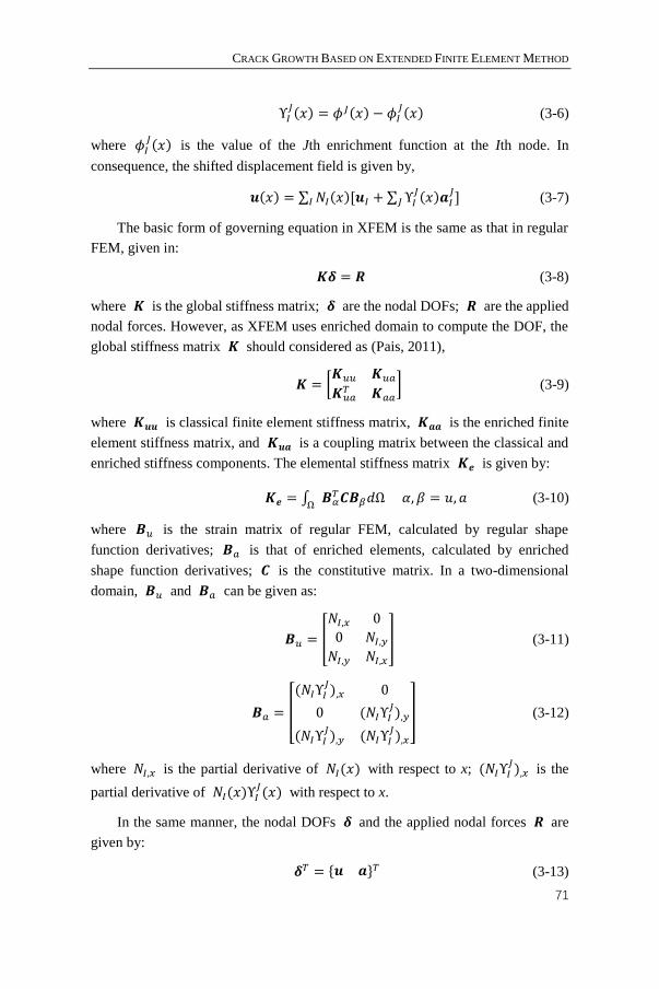
CRACK GROWTH BASED ON EXTENDED FINITE ELEMENT METHOD
71
Υ𝐼𝐽(𝑥) = 𝜙𝐽(𝑥) − 𝜙𝐼
𝐽(𝑥) (3-6)
where 𝜙𝐼𝐽(𝑥) is the value of the Jth enrichment function at the Ith node. In
consequence, the shifted displacement field is given by,
𝒖(𝑥) = ∑ 𝑁𝐼(𝑥)[𝒖𝐼 + ∑ Υ𝐼𝐽(𝑥)𝒂𝐼
𝐽𝐽 ]𝐼 (3-7)
The basic form of governing equation in XFEM is the same as that in regular
FEM, given in:
𝑲𝜹 = 𝑹 (3-8)
where 𝑲 is the global stiffness matrix; 𝜹 are the nodal DOFs; 𝑹 are the applied
nodal forces. However, as XFEM uses enriched domain to compute the DOF, the
global stiffness matrix 𝑲 should considered as (Pais, 2011),
𝑲 = [𝑲𝑢𝑢 𝑲𝑢𝑎
𝑲𝑢𝑎𝑇 𝑲𝑎𝑎
] (3-9)
where 𝑲𝒖𝒖 is classical finite element stiffness matrix, 𝑲𝒂𝒂 is the enriched finite
element stiffness matrix, and 𝑲𝒖𝒂 is a coupling matrix between the classical and
enriched stiffness components. The elemental stiffness matrix 𝑲𝒆 is given by:
𝑲𝒆 = ∫ 𝑩𝛼𝑇𝑪𝑩𝛽𝑑ΩΩ
𝛼, 𝛽 = 𝑢, 𝑎 (3-10)
where 𝑩𝑢 is the strain matrix of regular FEM, calculated by regular shape
function derivatives; 𝑩𝑎 is that of enriched elements, calculated by enriched
shape function derivatives; 𝑪 is the constitutive matrix. In a two-dimensional
domain, 𝑩𝑢 and 𝑩𝑎 can be given as:
𝑩𝑢 = [
𝑁𝐼,𝑥 0
0 𝑁𝐼,𝑦𝑁𝐼,𝑦 𝑁𝐼,𝑥
] (3-11)
𝑩𝑎 = [
(𝑁𝐼Υ𝐼𝐽),𝑥 0
0 (𝑁𝐼Υ𝐼𝐽),𝑦
(𝑁𝐼Υ𝐼𝐽),𝑦 (𝑁𝐼Υ𝐼
𝐽),𝑥
] (3-12)
where 𝑁𝐼,𝑥 is the partial derivative of 𝑁𝐼(𝑥) with respect to x; (𝑁𝐼Υ𝐼𝐽),𝑥 is the
partial derivative of 𝑁𝐼(𝑥)Υ𝐼𝐽(𝑥) with respect to x.
In the same manner, the nodal DOFs 𝜹 and the applied nodal forces 𝑹 are
given by:
𝜹𝑇 = {𝒖 𝒂}𝑇 (3-13)
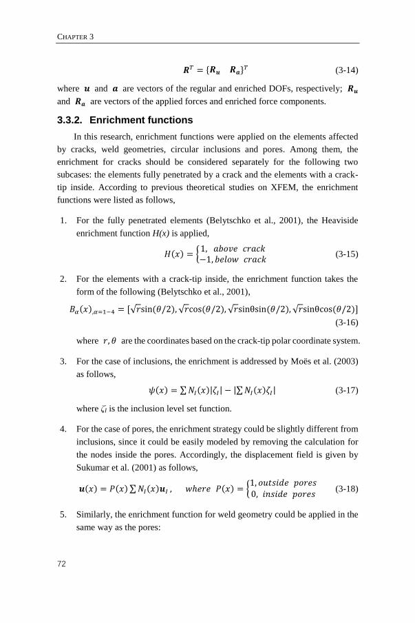
CHAPTER 3
72
𝑹𝑇 = {𝑹𝒖 𝑹𝒂}𝑇 (3-14)
where 𝒖 and 𝒂 are vectors of the regular and enriched DOFs, respectively; 𝑹𝒖
and 𝑹𝒂 are vectors of the applied forces and enriched force components.
3.3.2. Enrichment functions
In this research, enrichment functions were applied on the elements affected
by cracks, weld geometries, circular inclusions and pores. Among them, the
enrichment for cracks should be considered separately for the following two
subcases: the elements fully penetrated by a crack and the elements with a crack-
tip inside. According to previous theoretical studies on XFEM, the enrichment
functions were listed as follows,
1. For the fully penetrated elements (Belytschko et al., 2001), the Heaviside
enrichment function H(x) is applied,
𝐻(𝑥) = {1, 𝑎𝑏𝑜𝑣𝑒 𝑐𝑟𝑎𝑐𝑘−1, 𝑏𝑒𝑙𝑜𝑤 𝑐𝑟𝑎𝑐𝑘
(3-15)
2. For the elements with a crack-tip inside, the enrichment function takes the
form of the following (Belytschko et al., 2001),
𝐵𝛼(𝑥),𝛼=1−4 = [√𝑟sin(𝜃/2), √𝑟cos(𝜃/2), √𝑟sinθsin(𝜃/2), √𝑟sinθcos(𝜃/2)]
(3-16)
where 𝑟, 𝜃 are the coordinates based on the crack-tip polar coordinate system.
3. For the case of inclusions, the enrichment is addressed by Moës et al. (2003)
as follows,
𝜓(𝑥) = ∑𝑁𝐼(𝑥)|휁𝐼| − |∑𝑁𝐼(𝑥)휁𝐼| (3-17)
where ζI is the inclusion level set function.
4. For the case of pores, the enrichment strategy could be slightly different from
inclusions, since it could be easily modeled by removing the calculation for
the nodes inside the pores. Accordingly, the displacement field is given by
Sukumar et al. (2001) as follows,
𝒖(𝑥) = 𝑃(𝑥)∑𝑁𝐼(𝑥)𝒖𝐼 , 𝑤ℎ𝑒𝑟𝑒 𝑃(𝑥) = {1, 𝑜𝑢𝑡𝑠𝑖𝑑𝑒 𝑝𝑜𝑟𝑒𝑠0, 𝑖𝑛𝑠𝑖𝑑𝑒 𝑝𝑜𝑟𝑒𝑠
(3-18)
5. Similarly, the enrichment function for weld geometry could be applied in the
same way as the pores:
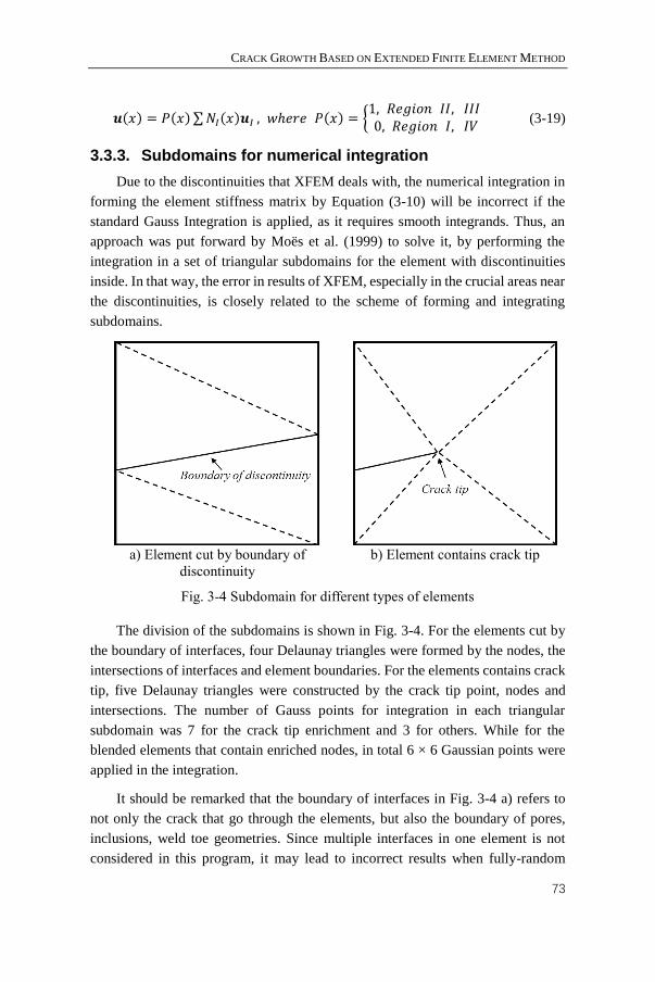
CRACK GROWTH BASED ON EXTENDED FINITE ELEMENT METHOD
73
𝒖(𝑥) = 𝑃(𝑥)∑𝑁𝐼(𝑥)𝒖𝐼 , 𝑤ℎ𝑒𝑟𝑒 𝑃(𝑥) = {1, 𝑅𝑒𝑔𝑖𝑜𝑛 𝐼𝐼, 𝐼𝐼𝐼 0, 𝑅𝑒𝑔𝑖𝑜𝑛 𝐼, 𝐼𝑉
(3-19)
3.3.3. Subdomains for numerical integration
Due to the discontinuities that XFEM deals with, the numerical integration in
forming the element stiffness matrix by Equation (3-10) will be incorrect if the
standard Gauss Integration is applied, as it requires smooth integrands. Thus, an
approach was put forward by Moës et al. (1999) to solve it, by performing the
integration in a set of triangular subdomains for the element with discontinuities
inside. In that way, the error in results of XFEM, especially in the crucial areas near
the discontinuities, is closely related to the scheme of forming and integrating
subdomains.
a) Element cut by boundary of
discontinuity
b) Element contains crack tip
Fig. 3-4 Subdomain for different types of elements
The division of the subdomains is shown in Fig. 3-4. For the elements cut by
the boundary of interfaces, four Delaunay triangles were formed by the nodes, the
intersections of interfaces and element boundaries. For the elements contains crack
tip, five Delaunay triangles were constructed by the crack tip point, nodes and
intersections. The number of Gauss points for integration in each triangular
subdomain was 7 for the crack tip enrichment and 3 for others. While for the
blended elements that contain enriched nodes, in total 6 × 6 Gaussian points were
applied in the integration.
It should be remarked that the boundary of interfaces in Fig. 3-4 a) refers to
not only the crack that go through the elements, but also the boundary of pores,
inclusions, weld toe geometries. Since multiple interfaces in one element is not
considered in this program, it may lead to incorrect results when fully-random
CHAPTER 3
74
defects are generated in the model. To avoid that, it is forbidden in this program
that the pores, inclusions are smaller than the mesh, or getting too close to the
cracks. The XFEM solution for this kind of cases could refer to (Yu, 2014).
3.3.4. Calculation of stress intensity factor
The common way to calculate stress intensity factor (SIF) in XFEM is to use
interaction integrals (Moës et al., 1999). For a two-dimensional problem, the J-
integral of mixed-mode crack is given by,
𝐽 =𝐾𝐼2
𝐸∗+
𝐾𝐼𝐼2
𝐸∗ (3-20)
𝐸∗ = {𝐸 𝑝𝑙𝑎𝑛𝑒 𝑠𝑡𝑟𝑒𝑠𝑠𝐸
1−𝜈2 𝑝𝑙𝑎𝑛𝑒 𝑠𝑡𝑟𝑎𝑖𝑛
(3-21)
where 𝐸 is the Young’s modulus; 𝜈 is the poisson ratio. By assuming the current
state as State 1, and an asymptotic field for Modes I or II as the auxiliary State 2,
the J-integral is given by,
𝐽(1,2) = ∫ [1
2(𝜎𝑖𝑗
(1) + 𝜎𝑖𝑗(2))(휀𝑖𝑗
(1) + 휀𝑖𝑗(2))𝛿1𝑗 − (𝜎𝑖𝑗
(1) + 𝜎𝑖𝑗(2))(𝑢𝑖,1
(1) + 𝑢𝑖,1(2))]𝒏𝒋𝑑ΓΓ
(3-22)
where Γ is the contour around the crack tip, 𝒏 is the normal vector of Γ. By
rearranging terms, it can be rewritten as,
𝐽(1,2) = 𝐽(1) + 𝐽(2) + 𝐼(1,2) (3-23)
where 𝐼(1,2) is the interaction integral,
𝐼(1,2) =2
𝐸∗(𝐾𝐼
(1)𝐾𝐼(2) + 𝐾𝐼𝐼
(1)𝐾𝐼𝐼(2)) (3-24)
Therefore, by setting the auxiliary State 2 to be pure Mode I (𝐾𝐼(2)= 1 and 𝐾𝐼𝐼
(2)=
0) or pure Mode II (𝐾𝐼(2)= 0 and 𝐾𝐼𝐼
(2)= 1), the SIF for State 1 can be given by,
𝐾𝐼(1)=
𝐼(1,𝑀𝑜𝑑𝑒 𝐼)𝐸∗
2 (3-25)
𝐾𝐼𝐼(1)=
𝐼(1,𝑀𝑜𝑑𝑒 𝐼𝐼)𝐸∗
2 (3-26)
The interaction integral in above equations could be solved by converting the
contour integral to the surface integral,
𝐼(1,2) = ∫ [𝜎𝑖𝑗(1)𝑢𝑖,1
(2) + 𝜎𝑖𝑗(2)𝑢𝑖,1
(1) −𝑊(1,2)𝛿1𝑗]𝑞,𝑗𝑑AA (3-27)
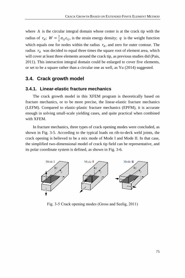
CRACK GROWTH BASED ON EXTENDED FINITE ELEMENT METHOD
75
where A is the circular integral domain whose center is at the crack tip with the
radius of 𝑟𝑑; 𝑊 =1
2𝜎𝑖𝑗휀𝑖𝑗, is the strain energy density; 𝑞 is the weight function
which equals one for nodes within the radius 𝑟𝑑, and zero for outer contour. The
radius 𝑟𝑑 was decided to equal three times the square root of element area, which
will cover at least three elements around the crack tip, as previous studies did (Pais,
2011). This interaction integral domain could be enlarged to cover five elements,
or set to be a square rather than a circular one as well, as Yu (2014) suggested.
3.4. Crack growth model
3.4.1. Linear-elastic fracture mechanics
The crack growth model in this XFEM program is theoretically based on
fracture mechanics, or to be more precise, the linear-elastic fracture mechanics
(LEFM). Compared to elastic-plastic fracture mechanics (EPFM), it is accurate
enough in solving small-scale yielding cases, and quite practical when combined
with XFEM.
In fracture mechanics, three types of crack opening modes were concluded, as
shown in Fig. 3-5. According to the typical loads on rib-to-deck weld joints, the
crack opening is believed to be a mix mode of Mode I and Mode II. In that case,
the simplified two-dimensional model of crack tip field can be representative, and
its polar coordinate system is defined, as shown in Fig. 3-6.
Fig. 3-5 Crack opening modes (Gross and Seelig, 2011)

CHAPTER 3
76
Fig. 3-6 Crack tip polar coordinate system
If the linear elastic part of the cracked body is dominating and the inelastic
zone is so small that can be ignored, the crack tip field can be solved using LEFM,
and the stress and deformation for Mode I crack can be given by,
{
𝜎𝑥𝜎𝑦𝜏𝑥𝑦
} =𝐾𝐼
√2𝜋𝑟cos (
𝜃
2)
{
1 − sin (
𝜃
2) sin (
3𝜃
2)
1 + sin (𝜃
2) sin (
3𝜃
2)
sin (𝜃
2) cos (
3𝜃
2) }
(3-28)
{𝑢𝑣} =
𝐾𝐼
2𝐺√
𝑟
2𝜋(κ − cos 𝜃) {
cos (𝜃
2)
sin (3𝜃
2)} (3-29)
and that for Mode II crack is given by,
{
𝜎𝑥𝜎𝑦𝜏𝑥𝑦
} =𝐾𝐼𝐼
√2𝜋𝑟
{
−sin (
𝜃
2)[2 + cos (
𝜃
2) cos (
3𝜃
2)]
sin (𝜃
2) cos (
𝜃
2) cos (
3𝜃
2)
cos (𝜃
2) [1 − sin (
𝜃
2) sin (
3𝜃
2)] }
(3-30)
{𝑢𝑣} =
𝐾𝐼𝐼
2𝐺√
𝑟
2𝜋{sin (
𝜃
2) (κ + 2 + cos 𝜃)
cos (𝜃
2)(κ − 2 + cos 𝜃)
} (3-31)
where
plane strain: κ = 3 − 4ν, 𝜎𝑧 = 𝜈(𝜎𝑥 + 𝜎𝑦)
plane stress: κ = (3 − ν)/(1 + ν), 𝜎𝑧 = 0
According to the above equations, it is clear that the singular stress will appear
when 𝑟 → 0 , and the singular order is r1/2. The solution for deformation is,
therefore, in correspondence with the enrichment functions in Section 3.3.2. Thus,
the aforementioned crack tip enrichment functions were based on LEFM, and the
CRACK GROWTH BASED ON EXTENDED FINITE ELEMENT METHOD
77
necessity arises to verify if the linear-elastic assumption is available on the issue of
cracked welded joint of OSDs. A criterion proposed by Irwin suggested that when
the cracked body meets the small-scale yielding condition, i.e. the plastic area is
much smaller than the SIF-dominated one, the result obtained by LEFM is accurate
enough (Wang and Chen, 2009). By comparing the plastic area around crack tip
with the crack length, the criterion for plane strain status is given by,
𝑟𝑝/𝑎 ≤ 0.1 (3-32)
𝑟𝑝 =𝐾2
6π𝜎𝑦2 (3-33)
where 𝑟𝑝 is the plastic area around crack tip, 𝑎 is the crack length. 𝜎𝑦 is the
yield strength, 𝐾 is the stress intensity factor.
Even though the accurate SIF for the fatigue crack on OSD is not yet obtained,
an estimation can be provided in a conservative way. Take an instance of a crack
on welded joint under applied remote stress of 100MPa, which is clearly larger than
the stress ranges induced by heavy trucks on OSDs (Wang et al., 2016). The SIF is
calculated according to Stress Intensity Factors Handbook (Murakami and Keer,
1993),
𝐾𝐼 = 𝐹𝜎√𝜋𝑎 (3-34)
where 𝐹 is the shape factor; 𝜎 is the applied remote stress; 𝑊 is the plate width,
i.e. the thickness of the deck plate, 15 mm. In case of bending on a thick plate, 𝐹
can be achieved by the handbook,
𝐹 = [1.122 − 1.40 (𝑎
𝑊) + 7.33 (
𝑎
𝑊)2
− 13.08 (𝑎
𝑊)3
+ 14.0 (𝑎
𝑊)4
] (3-35)
or in case of the semi-elliptical crack at weld toe under bending, 𝐹 can be obtained
according to Bowness and Lee (2000) as in Section 2.4.5,
𝐹 = 𝑓1 (𝑎
𝑇,𝑎
𝑐) + 𝑓2 (
𝑎
𝑇, 𝜃) + 𝑓3 (
𝑎
𝑇, 𝜃,
𝐿
𝑇) (3-36)
The plastic area 𝑟𝑝 with respect to different crack length 𝑎 is shown in Fig.
3-7. It can be seen that until the crack grows to 10 mm in depth, the small-scale
yielding condition is always met. Here the effect of residual stress on the plastic
area was not taken into account. Even so, it is assumed that LEFM is suitable on
this issue, since literatures showed the result will not be so different even when the
elastoplastic behavior is considered (Pais, 2011).

CHAPTER 3
78
Fig. 3-7 Small-scale yielding verification
3.4.2. Crack growth rate
Paris law is the commonly-used model in calculation of fatigue crack growth
rate, which indicates it is related to the stress intensity factor range. The classical
Paris law is expressed in a form as,
𝑑𝑎
𝑑𝑁= 𝐶(∆𝐾)𝑚 (3-37)
where da/dN is the crack growth rate, i.e. the crack growth increment per cycle, C
is the Paris constant, m is Paris exponent, ΔK is the stress intensity factor range.
Though the classical Paris law fits the experimental results quite well for Stage
II cracks (in stable propagation phase, i.e. Paris region), it has some limitations as
a semi-empirical law: i) unable to describe the early or short crack growth rate (near
the threshold region) and unstable crack growth rate; ii) the constants C and m is
regarded as material properties, while the evident factor stress ratio R is ignored;
iii) the effects induced by crack tip plasticity, e.g. crack closure or overload
retardation, cannot be considered. Consequently, several modified forms of Paris
law were put forward, as has been reviewed in Section 1.2.4.2. However, given that
the feasibility of these modified forms is yet to be proved on this issue, the way of
calculating the crack growth in the following is to use the Paris law with material
properties obtained in the fatigue test.
The realistic fatigue loading is another problem for calculating fatigue crack
growth on rib-to-deck welded joints of OSDs with Paris law. For most of the actual
projects like OSDs, the fatigue loading has variable amplitudes, while the constant
CRACK GROWTH BASED ON EXTENDED FINITE ELEMENT METHOD
79
amplitude loading is adopted in fatigue tests such as in Chapter 2 and the
subsequent fatigue category evaluation. As validated by these fatigue tests, the
classical Paris law is more appropriate to be applied in the cases of constant
amplitude loading. Though the modified Paris law provided the access to simulate
the variable amplitude loading with respect to load interactions, the exact process
of the fatigue crack growth is still difficult to obtain due to the computational
feasibility problem caused by the high fatigue cycle number.
In order to analyze the variable amplitude loading induced fatigue, the
damage-based prediction is commonly used. On condition that the influence of load
interactions is negligible, the variable amplitude loading could be counted using
the rainflow algorithm, and then the damage accumulation based on Miner’s rule
can be applied to predict the fatigue life, which is the commonly-used way in actual
projects. For the fatigue crack growth model, the load sequence surely matters as
it defines the plastic zone. Nevertheless, some studies imply that the SIF with
consideration of plasticity caused by variable amplitude loading will have little
difference (Elguedj et al., 2006, 2007).
3.4.3. Mixed-mode crack growth
To simulate the fatigue crack growth based on mode I and mode II SIFs, the
crack growth direction and increment should be addressed. Different theories were
available for both two- and three-dimensional problems. The important works on
two-dimensions are the maximum circumferential stress criterion, minimum strain
energy density criterion, maximum energy release rate criterion, and critical plane
approach, etc. Among them, the maximum circumferential stress criterion is
adopted in this study since it is practical on this issue and friendly to programming
(Moës, 1999).
The maximum circumferential stress criterion is mainly focused on the kink
angle of the crack, 𝜃𝑐. It was proposed by Erdogan and Sih (1963), which suggests
that the crack will grow to the direction perpendicular to maximum circumferential
stress. As the crack tip stress field can be expressed in terms of SIFs, i.e. 𝐾𝐼 and
𝐾𝐼𝐼, the kink angle can be given as follows,
𝜃𝑐 = 2arctan [1
4(𝐾𝐼/𝐾𝐼𝐼 ±√(𝐾𝐼/𝐾𝐼𝐼)
2 + 8)] (3-38)
To achieve the fatigue crack growth increment for each cycle (or cycle block
in a high cycle fatigue), the SIF should be given in a proper way. The early work
on this issue is given by Tanaka (1974). By assuming there is no interaction
between deformations induced by mode I and mode II loading, and the shear yield
stress is one-half of the tension yield stress, an effective SIF, ∆𝐾𝑒𝑓𝑓 , was put
CHAPTER 3
80
forward. ∆𝐾𝑒𝑓𝑓 is a function of 𝐾𝐼 , 𝐾𝐼𝐼 in two-dimensions, and could be
extended to three-dimensions.
∆𝐾𝑒𝑓𝑓 = √∆𝐾𝐼4 + 8∆𝐾𝐼𝐼
44 (3-39)
There are other studies based on different factors, such as the strain energy
density, J-integral, etc., that concerned about mixed-mode crack growth, and were
summarized by (Qian and Fatemi, 1996), providing options to future development
of this program.
CHAPTER 4
XFEM BASED HOMOGENIZATION
METHOD ON WELD DEFECTS
________________________________
This chapter is based on
Wang, B., De Backer, H., and Chen, A. (2016). An XFEM based uncertainty
study on crack growth in welded joints with defects. Theoretical and Applied
Fracture Mechanics, 86, Part B, 125-142.
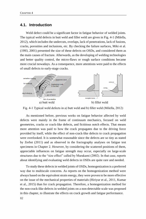
CHAPTER 4
82
4.1. Introduction
Weld defect could be a significant factor in fatigue behavior of welded joints.
The typical weld defects in butt weld and fillet weld are given in Fig. 4-1 (Milella,
2012), which includes the undercuts, overlaps, lack of penetrations, lack of fusions,
cracks, porosities and inclusions, etc. By checking the failure surfaces, Miki et al.
(1993, 2001) presented the size of these defects on OSDs, and considered them as
the main causes of fracture. Afterwards, as the developing of welding technologies
and better quality control, the micro-flaws or rough surface conditions became
more crucial nowadays. As a consequence, more attentions were paid to the effects
of small defects to early-stage cracks.
a) butt weld
b) fillet weld
Fig. 4-1 Typical weld defects in a) butt weld and b) fillet weld (Milella, 2012)
As mentioned before, previous works on fatigue behavior affected by weld
defects were mainly in the frame of continuum mechanics, focused on weld
geometries, cracks or crack-like defects, and fictitious notch effects. That means
more attention was paid to how the crack propagates due to the driving force
provided by itself, while the effect of non-crack-like defects to crack propagation
were overlooked. It is somewhat reasonable since the defects are so tiny as stated
by Zerbst (2011) and as observed in the fractography analyses on fatigue test
specimens in Chapter 2. However, by considering the scattered positions of them,
appreciable influences on fatigue strength may occur, especially on large-scale
structures due to the “size effect” called by Murakami (2002). In that case, reports
about identifying and evaluating weld defects in OSDs are quite rare and needed.
To study these defects in welded joints of OSDs, homogenization is a preferred
way due to multiscale concerns. As reports on the homogenization method were
always based on the equivalent strain energy, they were proven to be more effective
on the issue of the mechanical properties of materials (Hiriyur et al., 2011, Kumar
et al., 2015) than for crack propagation. Therefore, a homogenization method for
the non-crack-like defects in welded joints on a non-detectable scale was proposed
in this chapter, to illustrate the effects on crack growth and fatigue performance.
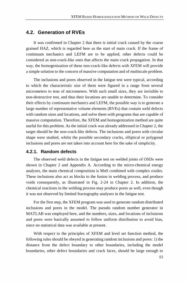
XFEM BASED HOMOGENIZATION METHOD ON WELD DEFECTS
83
4.2. Generation of RVEs
It was confirmed in Chapter 2 that there is initial crack caused by the coarse
grained HAZ, which is regarded here as the start of main crack. If the frame of
continuum mechanics and LEFM are to be applied, other defects could be
considered as non-crack-like ones that affects the main crack propagation. In that
way, the homogenization of these non-crack-like defects with XFEM will provide
a simple solution to the concern of massive computation and of multiscale problem.
The inclusions and pores observed in the fatigue test were typical, according
to which the characteristic size of them were figured in a range from several
micrometers to tens of micrometers. With such small sizes, they are invisible to
non-destructive test, and thus their locations are unable to determine. To consider
their effects by continuum mechanics and LEFM, the possible way is to generate a
large number of representative volume elements (RVEs) that contain weld defects
with random sizes and locations, and solve them with programs that are capable of
massive computation. Therefore, the XFEM and homogenization method are quite
useful for this problem. As the initial crack was already addressed in Chapter 2, the
target should be the non-crack-like defects. The inclusions and pores with circular
shape were studied, whilst the possible secondary cracks, elliptical or polygonal
inclusions and pores are not taken into account here for the sake of simplicity.
4.2.1. Random defects
The observed weld defects in the fatigue test on welded joints of OSDs were
shown in Chapter 2 and Appendix A. According to the micro-chemical energy
analyses, the main chemical composition is MnS combined with complex oxides.
These inclusions also act as blocks to the fusion in welding process, and produce
voids consequently, as illustrated in Fig. 2-24 in Chapter 2. In addition, the
chemical reactions in the welding process may produce pores as well, even though
it was not observed by limited fractography analyses in the fatigue test.
For the first step, the XFEM program was used to generate random distributed
inclusions and pores in the model. The pseudo random number generator in
MATLAB was employed here, and the numbers, sizes, and locations of inclusions
and pores were basically assumed to follow uniform distribution to avoid bias,
since no statistical data was available at present.
With respect to the principles of XFEM and level set function method, the
following rules should be obeyed in generating random inclusions and pores: 1) the
distance from the defect boundary to other boundaries, including the model
boundaries, other defect boundaries and crack faces, should be large enough to
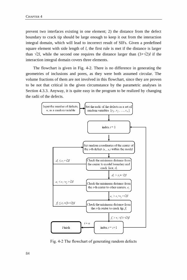
CHAPTER 4
84
prevent two interfaces existing in one element; 2) the distance from the defect
boundary to crack tip should be large enough to keep it out from the interaction
integral domain, which will lead to incorrect result of SIFs. Given a predefined
square element with side length of l, the first rule is met if the distance is larger
than √2l, while the second one requires the distance larger than (3+√2)l if the
interaction integral domain covers three elements.
The flowchart is given in Fig. 4-2. There is no difference in generating the
geometries of inclusions and pores, as they were both assumed circular. The
volume fractions of them are not involved in this flowchart, since they are proven
to be not that critical in the given circumstance by the parametric analyses in
Section 4.3.3. Anyway, it is quite easy in the program to be realized by changing
the radii of the defects.
Fig. 4-2 The flowchart of generating random defects
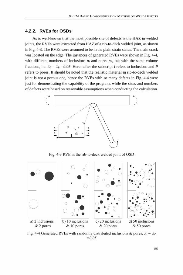
XFEM BASED HOMOGENIZATION METHOD ON WELD DEFECTS
85
4.2.2. RVEs for OSDs
As is well-known that the most possible site of defects is the HAZ in welded
joints, the RVEs were extracted from HAZ of a rib-to-deck welded joint, as shown
in Fig. 4-3. The RVEs were assumed to be in the plain strain status. The main crack
was located on the edge. The instances of generated RVEs were shown in Fig. 4-4,
with different numbers of inclusions nI and pores nP, but with the same volume
fractions, i.e. I = P =0.05. Hereinafter the subscript I refers to inclusions and P
refers to pores. It should be noted that the realistic material in rib-to-deck welded
joint is not a porous one, hence the RVEs with so many defects in Fig. 4-4 were
just for demonstrating the capability of the program, while the sizes and numbers
of defects were based on reasonable assumptions when conducting the calculation.
Fig. 4-3 RVE in the rib-to-deck welded joint of OSD
a) 2 inclusions
& 2 pores
b) 10 inclusions
& 10 pores
c) 20 inclusions
& 20 pores
d) 50 inclusions
& 50 pores
Fig. 4-4 Generated RVEs with randomly distributed inclusions & pores, I = P
=0.05
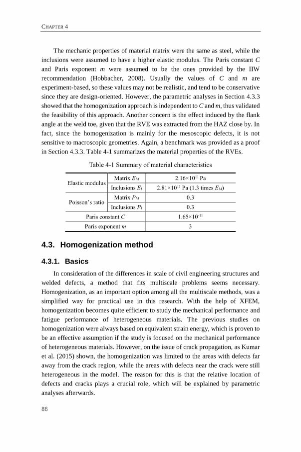
CHAPTER 4
86
The mechanic properties of material matrix were the same as steel, while the
inclusions were assumed to have a higher elastic modulus. The Paris constant C
and Paris exponent m were assumed to be the ones provided by the IIW
recommendation (Hobbacher, 2008). Usually the values of C and m are
experiment-based, so these values may not be realistic, and tend to be conservative
since they are design-oriented. However, the parametric analyses in Section 4.3.3
showed that the homogenization approach is independent to C and m, thus validated
the feasibility of this approach. Another concern is the effect induced by the flank
angle at the weld toe, given that the RVE was extracted from the HAZ close by. In
fact, since the homogenization is mainly for the mesoscopic defects, it is not
sensitive to macroscopic geometries. Again, a benchmark was provided as a proof
in Section 4.3.3. Table 4-1 summarizes the material properties of the RVEs.
Table 4-1 Summary of material characteristics
Elastic modulus Matrix EM 2.16×10¹¹ Pa
Inclusions EI 2.81×10¹¹ Pa (1.3 times EM)
Poisson’s ratio Matrix PM 0.3
Inclusions PI 0.3
Paris constant C 1.65×10⁻¹¹
Paris exponent m 3
4.3. Homogenization method
4.3.1. Basics
In consideration of the differences in scale of civil engineering structures and
welded defects, a method that fits multiscale problems seems necessary.
Homogenization, as an important option among all the multiscale methods, was a
simplified way for practical use in this research. With the help of XFEM,
homogenization becomes quite efficient to study the mechanical performance and
fatigue performance of heterogeneous materials. The previous studies on
homogenization were always based on equivalent strain energy, which is proven to
be an effective assumption if the study is focused on the mechanical performance
of heterogeneous materials. However, on the issue of crack propagation, as Kumar
et al. (2015) shown, the homogenization was limited to the areas with defects far
away from the crack region, while the areas with defects near the crack were still
heterogeneous in the model. The reason for this is that the relative location of
defects and cracks plays a crucial role, which will be explained by parametric
analyses afterwards.
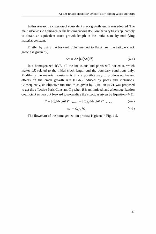
XFEM BASED HOMOGENIZATION METHOD ON WELD DEFECTS
87
In this research, a criterion of equivalent crack growth length was adopted. The
main idea was to homogenize the heterogeneous RVE on the very first step, namely
to obtain an equivalent crack growth length in the initial state by modifying
material constant.
Firstly, by using the forward Euler method to Paris law, the fatigue crack
growth is given by,
∆𝑎 = ∆𝑁[𝐶(∆𝐾)𝑚] (4-1)
In a homogenized RVE, all the inclusions and pores will not exist, which
makes ∆K related to the initial crack length and the boundary conditions only.
Modifying the material constants is thus a possible way to produce equivalent
effects on the crack growth rate (CGR) induced by pores and inclusions.
Consequently, an objective function R, as given by Equation (4-2), was proposed
to get the effective Paris Constant Ceff when R is minimized, and a homogenization
coefficient ac was put forward to normalize the effect, as given by Equation (4-3).
𝑅 = [𝐶0∆𝑁(∆𝐾)𝑚]ℎ𝑒𝑡𝑒𝑟 − [𝐶𝑒𝑓𝑓∆𝑁(∆𝐾)
𝑚]ℎ𝑜𝑚𝑜 (4-2)
𝑎𝑐 = 𝐶𝑒𝑓𝑓/𝐶0 (4-3)
The flowchart of the homogenization process is given in Fig. 4-5.
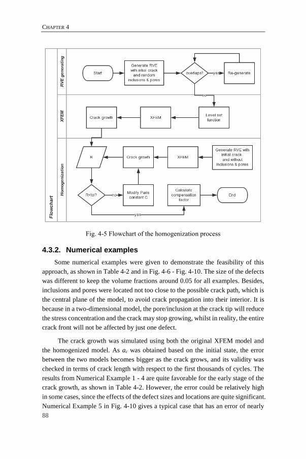
CHAPTER 4
88
Fig. 4-5 Flowchart of the homogenization process
4.3.2. Numerical examples
Some numerical examples were given to demonstrate the feasibility of this
approach, as shown in Table 4-2 and in Fig. 4-6 - Fig. 4-10. The size of the defects
was different to keep the volume fractions around 0.05 for all examples. Besides,
inclusions and pores were located not too close to the possible crack path, which is
the central plane of the model, to avoid crack propagation into their interior. It is
because in a two-dimensional model, the pore/inclusion at the crack tip will reduce
the stress concentration and the crack may stop growing, whilst in reality, the entire
crack front will not be affected by just one defect.
The crack growth was simulated using both the original XFEM model and
the homogenized model. As ac was obtained based on the initial state, the error
between the two models becomes bigger as the crack grows, and its validity was
checked in terms of crack length with respect to the first thousands of cycles. The
results from Numerical Example 1 - 4 are quite favorable for the early stage of the
crack growth, as shown in Table 4-2. However, the error could be relatively high
in some cases, since the effects of the defect sizes and locations are quite significant.
Numerical Example 5 in Fig. 4-10 gives a typical case that has an error of nearly
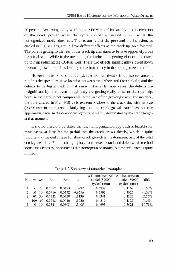
XFEM BASED HOMOGENIZATION METHOD ON WELD DEFECTS
89
20 percent. According to Fig. 4-10 i), the XFEM model has an obvious deceleration
of the crack growth when the cycle number is around 60000, while the
homogenized model does not. The reason is that the pore and the inclusion, as
circled in Fig. 4-10 c), would have different effects as the crack tip goes forward.
The pore is getting to the rear of the crack tip and starts to behave oppositely from
the initial state. While in the meantime, the inclusion is getting closer to the crack
tip to help reducing the CGR as well. These two effects significantly slowed down
the crack growth rate, thus leading to the inaccuracy in the homogenized model.
However, this kind of circumstances is not always troublesome since it
requires the special relative location between the defects and the crack tip, and the
defects to be big enough at that same instance. In most cases, the defects are
insignificant by then, even though they are getting really close to the crack tip,
because their size is not comparable to the size of the growing crack. For instance,
the pore circled in Fig. 4-10 g) is extremely close to the crack tip, with its size
(0.131 mm in diameter) is fairly big, but the crack growth rate does not rise
apparently, because the crack driving force is mainly dominated by the crack length
at that moment.
It should therefore be stated that the homogenization approach is feasible for
most cases, at least for the period that the crack grows slowly, which is quite
important as the early stage for short crack growth is the dominant part of the total
crack growth life. For the changing location between crack and defects, this method
sometimes leads to inaccuracies in a homogenized model, but the influence is quite
limited.
Table 4-2 Summary of numerical examples
No. nI nP I P ac
a in homogenized
model (80000
cycles) (mm)
a in heterogenous
model (80000
cycles) (mm)
diff.
1 5 5 0.0562 0.0473 1.0822 0.4238 0.4167 -1.67%
2 10 10 0.0466 0.0372 0.9596 0.3992 0.3925 -1.68%
3 50 50 0.0522 0.0520 1.1139 0.4341 0.4225 -2.67%
4 100 100 0.0562 0.0610 1.1530 0.4319 0.4329 0.24%
5 10 10 0.0521 0.0603 1.3405 0.4693 0.5621 19.78%
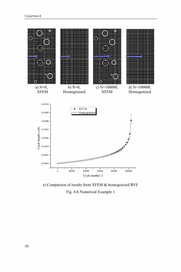
CHAPTER 4
90
a) N=0,
XFEM
b) N=0,
Homogenized
c) N=100000,
XFEM
d) N=100000,
Homogenized
e) Comparison of results from XFEM & homogenized RVE
Fig. 4-6 Numerical Example 1
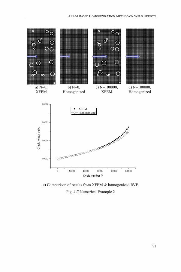
XFEM BASED HOMOGENIZATION METHOD ON WELD DEFECTS
91
a) N=0,
XFEM
b) N=0,
Homogenized
c) N=100000,
XFEM
d) N=100000,
Homogenized
e) Comparison of results from XFEM & homogenized RVE
Fig. 4-7 Numerical Example 2
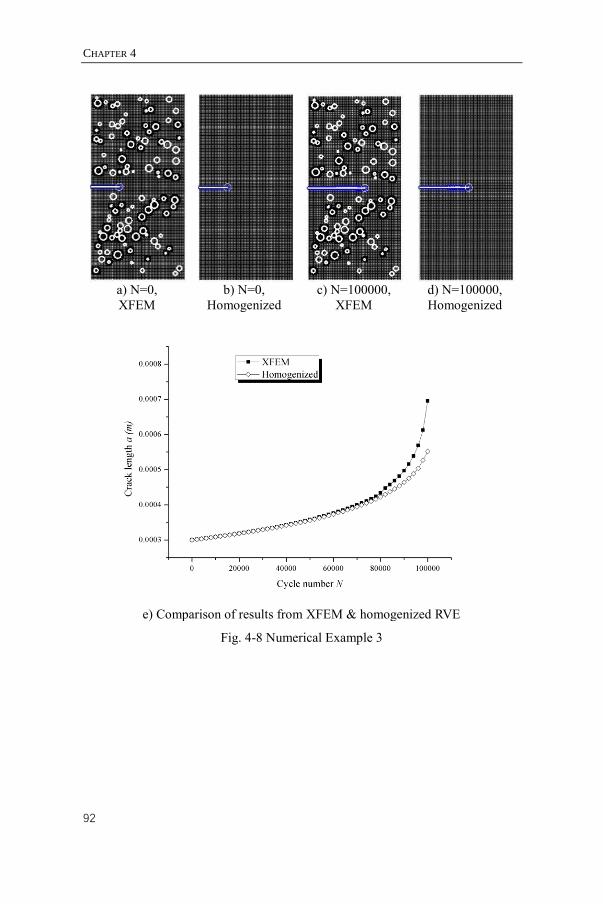
CHAPTER 4
92
a) N=0,
XFEM
b) N=0,
Homogenized
c) N=100000,
XFEM
d) N=100000,
Homogenized
e) Comparison of results from XFEM & homogenized RVE
Fig. 4-8 Numerical Example 3
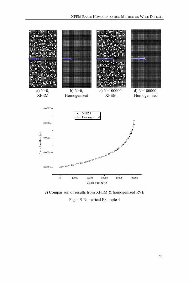
XFEM BASED HOMOGENIZATION METHOD ON WELD DEFECTS
93
a) N=0,
XFEM
b) N=0,
Homogenized
c) N=100000,
XFEM
d) N=100000,
Homogenized
e) Comparison of results from XFEM & homogenized RVE
Fig. 4-9 Numerical Example 4
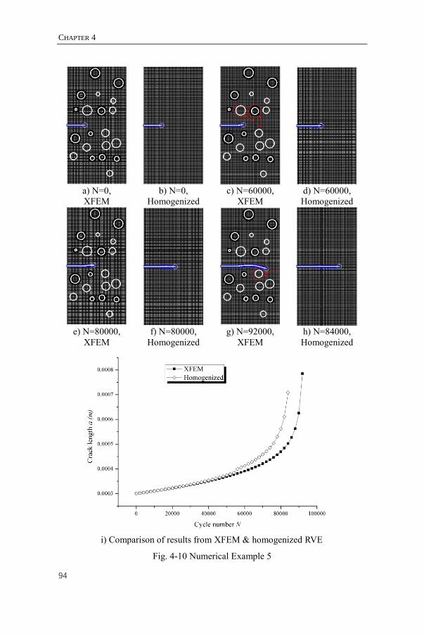
CHAPTER 4
94
a) N=0,
XFEM
b) N=0,
Homogenized
c) N=60000,
XFEM
d) N=60000,
Homogenized
e) N=80000,
XFEM
f) N=80000,
Homogenized
g) N=92000,
XFEM
h) N=84000,
Homogenized
i) Comparison of results from XFEM & homogenized RVE
Fig. 4-10 Numerical Example 5
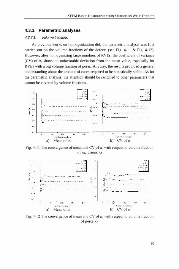
XFEM BASED HOMOGENIZATION METHOD ON WELD DEFECTS
95
4.3.3. Parametric analyses
4.3.3.1. Volume fractions
As previous works on homogenization did, the parametric analysis was first
carried out on the volume fractions of the defects (see Fig. 4-11 & Fig. 4-12).
However, after homogenizing large numbers of RVEs, the coefficient of variance
(CV) of ac shows an unfavorable deviation from the mean value, especially for
RVEs with a big volume fraction of pores. Anyway, the results provided a general
understanding about the amount of cases required to be statistically stable. As for
the parametric analysis, the attention should be switched to other parameters that
cannot be covered by volume fractions.
a) Mean of ac
b) CV of ac
Fig. 4-11 The convergence of mean and CV of ac with respect to volume fraction
of inclusions I
a) Mean of ac
b) CV of ac
Fig. 4-12 The convergence of mean and CV of ac with respect to volume fraction
of pores P
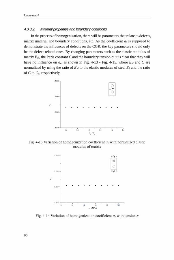
CHAPTER 4
96
4.3.3.2. Material properties and boundary conditions
In the process of homogenization, there will be parameters that relate to defects,
matrix material and boundary conditions, etc. As the coefficient ac is supposed to
demonstrate the influences of defects on the CGR, the key parameters should only
be the defect-related ones. By changing parameters such as the elastic modulus of
matrix EM, the Paris constant C and the boundary tension σ, it is clear that they will
have no influence on ac, as shown in Fig. 4-13 - Fig. 4-15, where EM and C are
normalized by using the ratio of EM to the elastic modulus of steel ES and the ratio
of C to C0, respectively.
Fig. 4-13 Variation of homogenization coefficient ac with normalized elastic
modulus of matrix
Fig. 4-14 Variation of homogenization coefficient ac with tension σ
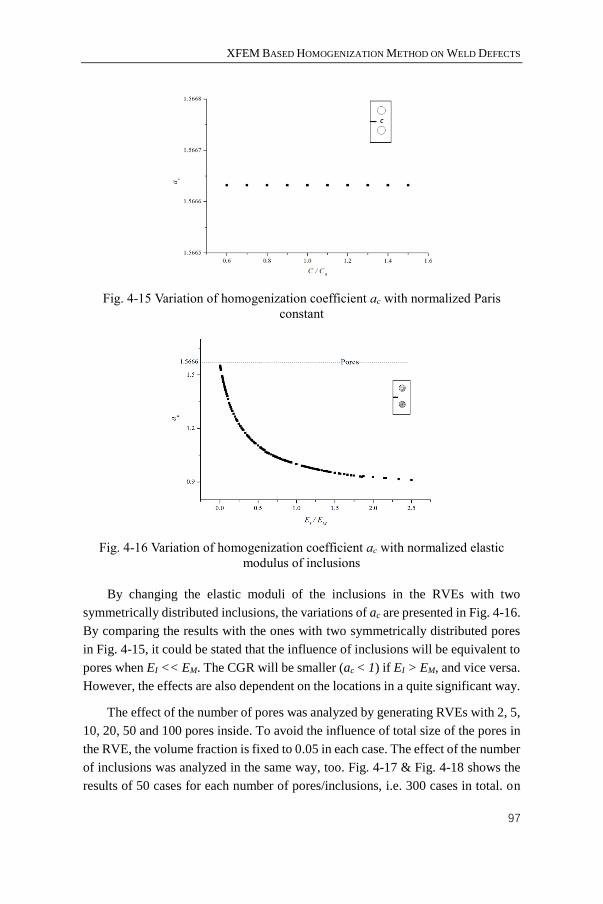
XFEM BASED HOMOGENIZATION METHOD ON WELD DEFECTS
97
Fig. 4-15 Variation of homogenization coefficient ac with normalized Paris
constant
Fig. 4-16 Variation of homogenization coefficient ac with normalized elastic
modulus of inclusions
By changing the elastic moduli of the inclusions in the RVEs with two
symmetrically distributed inclusions, the variations of ac are presented in Fig. 4-16.
By comparing the results with the ones with two symmetrically distributed pores
in Fig. 4-15, it could be stated that the influence of inclusions will be equivalent to
pores when EI << EM. The CGR will be smaller (ac < 1) if EI > EM, and vice versa.
However, the effects are also dependent on the locations in a quite significant way.
The effect of the number of pores was analyzed by generating RVEs with 2, 5,
10, 20, 50 and 100 pores inside. To avoid the influence of total size of the pores in
the RVE, the volume fraction is fixed to 0.05 in each case. The effect of the number
of inclusions was analyzed in the same way, too. Fig. 4-17 & Fig. 4-18 shows the
results of 50 cases for each number of pores/inclusions, i.e. 300 cases in total. on
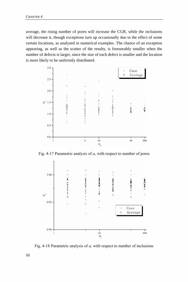
CHAPTER 4
98
average, the rising number of pores will increase the CGR, while the inclusions
will decrease it, though exceptions turn up occasionally due to the effect of some
certain locations, as analyzed in numerical examples. The chance of an exception
appearing, as well as the scatter of the results, is foreseeably smaller when the
number of defects is larger, since the size of each defect is smaller and the location
is more likely to be uniformly distributed.
Fig. 4-17 Parametric analysis of ac with respect to number of pores
Fig. 4-18 Parametric analysis of ac with respect to number of inclusions
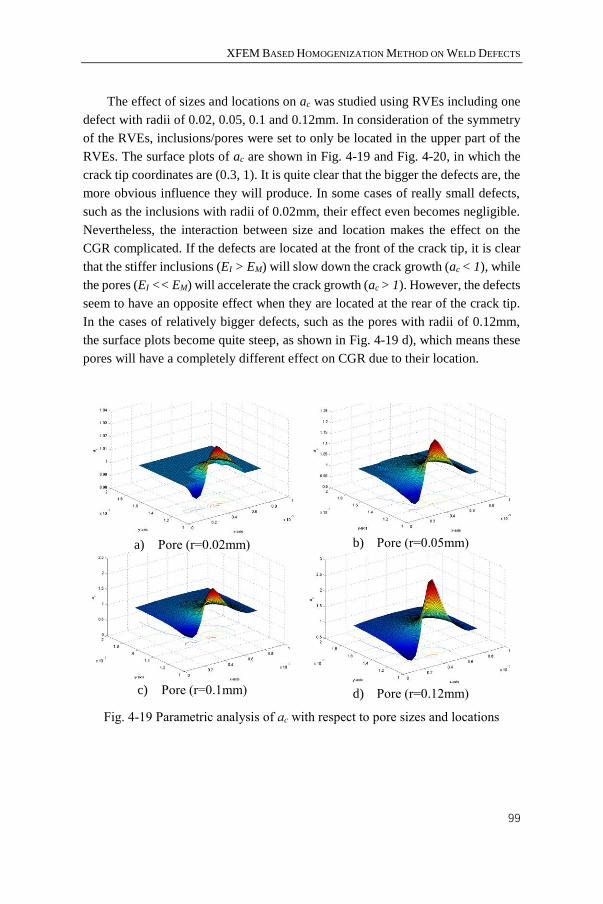
XFEM BASED HOMOGENIZATION METHOD ON WELD DEFECTS
99
The effect of sizes and locations on ac was studied using RVEs including one
defect with radii of 0.02, 0.05, 0.1 and 0.12mm. In consideration of the symmetry
of the RVEs, inclusions/pores were set to only be located in the upper part of the
RVEs. The surface plots of ac are shown in Fig. 4-19 and Fig. 4-20, in which the
crack tip coordinates are (0.3, 1). It is quite clear that the bigger the defects are, the
more obvious influence they will produce. In some cases of really small defects,
such as the inclusions with radii of 0.02mm, their effect even becomes negligible.
Nevertheless, the interaction between size and location makes the effect on the
CGR complicated. If the defects are located at the front of the crack tip, it is clear
that the stiffer inclusions (EI > EM) will slow down the crack growth (ac < 1), while
the pores (EI << EM) will accelerate the crack growth (ac > 1). However, the defects
seem to have an opposite effect when they are located at the rear of the crack tip.
In the cases of relatively bigger defects, such as the pores with radii of 0.12mm,
the surface plots become quite steep, as shown in Fig. 4-19 d), which means these
pores will have a completely different effect on CGR due to their location.
a) Pore (r=0.02mm)
b) Pore (r=0.05mm)
c) Pore (r=0.1mm)
d) Pore (r=0.12mm)
Fig. 4-19 Parametric analysis of ac with respect to pore sizes and locations
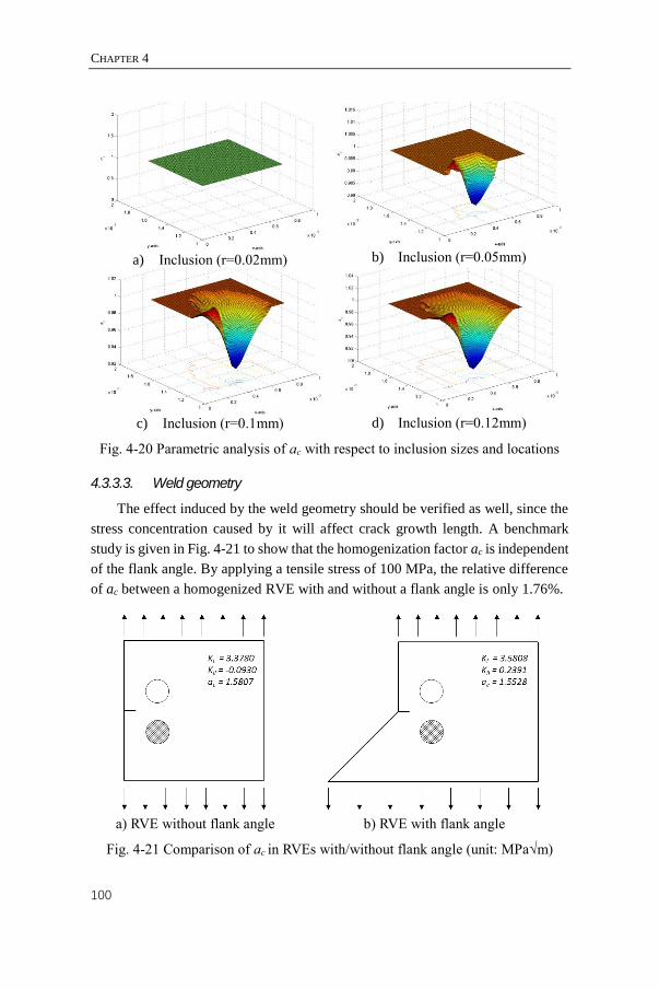
CHAPTER 4
100
a) Inclusion (r=0.02mm)
b) Inclusion (r=0.05mm)
c) Inclusion (r=0.1mm)
d) Inclusion (r=0.12mm)
Fig. 4-20 Parametric analysis of ac with respect to inclusion sizes and locations
4.3.3.3. Weld geometry
The effect induced by the weld geometry should be verified as well, since the
stress concentration caused by it will affect crack growth length. A benchmark
study is given in Fig. 4-21 to show that the homogenization factor ac is independent
of the flank angle. By applying a tensile stress of 100 MPa, the relative difference
of ac between a homogenized RVE with and without a flank angle is only 1.76%.
a) RVE without flank angle
b) RVE with flank angle
Fig. 4-21 Comparison of ac in RVEs with/without flank angle (unit: MPa√m)
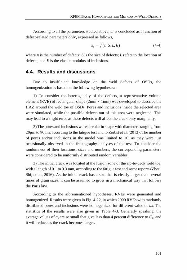
XFEM BASED HOMOGENIZATION METHOD ON WELD DEFECTS
101
According to all the parameters studied above, ac is concluded as a function of
defect-related parameters only, expressed as follows,
𝑎𝑐 = 𝑓(𝑛, 𝑆, 𝐿, 𝐸) (4-4)
where n is the number of defects; S is the size of defects; L refers to the location of
defects; and E is the elastic modulus of inclusions.
4.4. Results and discussions
Due to insufficient knowledge on the weld defects of OSDs, the
homogenization is based on the following hypotheses:
1) To consider the heterogeneity of the defects, a representative volume
element (RVE) of rectangular shape (2mm × 1mm) was developed to describe the
HAZ around the weld toe of OSDs. Pores and inclusions inside the selected area
were simulated, while the possible defects out of this area were neglected. This
may lead to a slight error as these defects will affect the crack only marginally.
2) The pores and inclusions were circular in shape with diameters ranging from
20μm to 90μm, according to the fatigue test and to Zerbst et al. (2012). The number
of pores and/or inclusions in the model was limited to 10, as they were just
occasionally observed in the fractography analyses of the test. To consider the
randomness of their locations, sizes and numbers, the corresponding parameters
were considered to be uniformly distributed random variables.
3) The initial crack was located at the fusion zone of the rib-to-deck weld toe,
with a length of 0.1 to 0.3 mm, according to the fatigue test and some reports (Zhou,
Shi, et al., 2016). As the initial crack has a size that is clearly larger than several
times of grain sizes, it can be assumed to grow in a mechanical way that follows
the Paris law.
According to the aforementioned hypotheses, RVEs were generated and
homogenized. Results were given in Fig. 4-22, in which 2000 RVEs with randomly
distributed pores and inclusions were homogenized for different value of a0. The
statistics of the results were also given in Table 4-3. Generally speaking, the
average values of ac are so small that give less than 4 percent difference to C0, and
it will reduce as the crack becomes larger.

CHAPTER 4
102
a) a0=0.1mm
b) a0=0.2mm
c) a0=0.3mm
d) a0=0.4mm
Fig. 4-22 Distribution of homogenization coefficient ac for different a0
Table 4-3 Statistics of ac
a0 ac
Average Maximum SD CV
0.1 1.0383 1.5834 0.0802 0.0772
0.2 1.0287 1.4370 0.0620 0.0603
0.3 1.0248 1.4395 0.0505 0.0493
0.4 1.0224 1.4363 0.0455 0.0445
Nevertheless, it cannot be addressed that these weld defects are negligible.
With consideration of the weakest part, the standard deviation (SD) and the
coefficient of variation (CV) for ac will play a very important role for large
structures like OSDs with a larger scatter bands of fatigue strength. The SD and
CV for ac is larger when a0 is relatively small, implying better chance to affect the
initial crack growth in an appreciable amount. On the other hand, SD and CV for
ac become smaller with larger crack length, and the average value also showed the
same trend, implying a decrease of the effect of pores and inclusions. If we look
into the different cases for a0, the homogenization coefficient ac in Fig. 4-22 d), i.e.
the case for a0 equals 0.4mm, are more centralized around the value of one, as a
result of increasing dominance on crack-driving force by the crack itself.
XFEM BASED HOMOGENIZATION METHOD ON WELD DEFECTS
103
Therefore, the conclusion can be drawn that the influence of the non-detectable
weld defects could be ignored on condition that the initial crack is large enough.
For the mesoscopic cracks in OSDs, the sizes and locations of the weld defects may
affect the crack, especially in the early stage crack growth. In that case, the
homogenization method can be applied if the analyses are in the frame of
continuum mechanics and LEFM.

CHAPTER 4
104

CHAPTER 5
MULTISCALE STUDY ON CRACK
GROWTH IN WELDED JOINTS OF
ORTHOTROPIC STEEL DECKS
________________________________
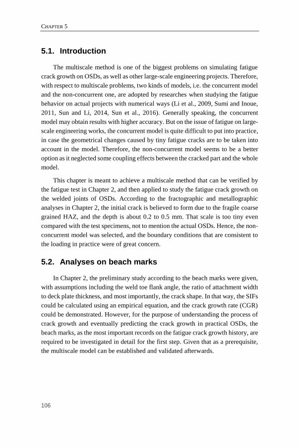
CHAPTER 5
106
5.1. Introduction
The multiscale method is one of the biggest problems on simulating fatigue
crack growth on OSDs, as well as other large-scale engineering projects. Therefore,
with respect to multiscale problems, two kinds of models, i.e. the concurrent model
and the non-concurrent one, are adopted by researches when studying the fatigue
behavior on actual projects with numerical ways (Li et al., 2009, Sumi and Inoue,
2011, Sun and Li, 2014, Sun et al., 2016). Generally speaking, the concurrent
model may obtain results with higher accuracy. But on the issue of fatigue on large-
scale engineering works, the concurrent model is quite difficult to put into practice,
in case the geometrical changes caused by tiny fatigue cracks are to be taken into
account in the model. Therefore, the non-concurrent model seems to be a better
option as it neglected some coupling effects between the cracked part and the whole
model.
This chapter is meant to achieve a multiscale method that can be verified by
the fatigue test in Chapter 2, and then applied to study the fatigue crack growth on
the welded joints of OSDs. According to the fractographic and metallographic
analyses in Chapter 2, the initial crack is believed to form due to the fragile coarse
grained HAZ, and the depth is about 0.2 to 0.5 mm. That scale is too tiny even
compared with the test specimens, not to mention the actual OSDs. Hence, the non-
concurrent model was selected, and the boundary conditions that are consistent to
the loading in practice were of great concern.
5.2. Analyses on beach marks
In Chapter 2, the preliminary study according to the beach marks were given,
with assumptions including the weld toe flank angle, the ratio of attachment width
to deck plate thickness, and most importantly, the crack shape. In that way, the SIFs
could be calculated using an empirical equation, and the crack growth rate (CGR)
could be demonstrated. However, for the purpose of understanding the process of
crack growth and eventually predicting the crack growth in practical OSDs, the
beach marks, as the most important records on the fatigue crack growth history, are
required to be investigated in detail for the first step. Given that as a prerequisite,
the multiscale model can be established and validated afterwards.
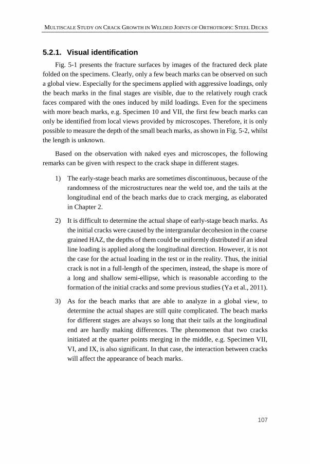
MULTISCALE STUDY ON CRACK GROWTH IN WELDED JOINTS OF ORTHOTROPIC STEEL DECKS
107
5.2.1. Visual identification
Fig. 5-1 presents the fracture surfaces by images of the fractured deck plate
folded on the specimens. Clearly, only a few beach marks can be observed on such
a global view. Especially for the specimens applied with aggressive loadings, only
the beach marks in the final stages are visible, due to the relatively rough crack
faces compared with the ones induced by mild loadings. Even for the specimens
with more beach marks, e.g. Specimen 10 and VII, the first few beach marks can
only be identified from local views provided by microscopes. Therefore, it is only
possible to measure the depth of the small beach marks, as shown in Fig. 5-2, whilst
the length is unknown.
Based on the observation with naked eyes and microscopes, the following
remarks can be given with respect to the crack shape in different stages.
1) The early-stage beach marks are sometimes discontinuous, because of the
randomness of the microstructures near the weld toe, and the tails at the
longitudinal end of the beach marks due to crack merging, as elaborated
in Chapter 2.
2) It is difficult to determine the actual shape of early-stage beach marks. As
the initial cracks were caused by the intergranular decohesion in the coarse
grained HAZ, the depths of them could be uniformly distributed if an ideal
line loading is applied along the longitudinal direction. However, it is not
the case for the actual loading in the test or in the reality. Thus, the initial
crack is not in a full-length of the specimen, instead, the shape is more of
a long and shallow semi-ellipse, which is reasonable according to the
formation of the initial cracks and some previous studies (Ya et al., 2011).
3) As for the beach marks that are able to analyze in a global view, to
determine the actual shapes are still quite complicated. The beach marks
for different stages are always so long that their tails at the longitudinal
end are hardly making differences. The phenomenon that two cracks
initiated at the quarter points merging in the middle, e.g. Specimen VII,
VI, and IX, is also significant. In that case, the interaction between cracks
will affect the appearance of beach marks.

CHAPTER 5
108
Specimen 10
Specimen VII
Specimen IV
Specimen VI
Specimen IX
a) R=0
Specimen 9
Specimen I
Specimen III
Specimen X
b) R= -1
Fig. 5-1 Fracture surfaces and beach marks on test specimens
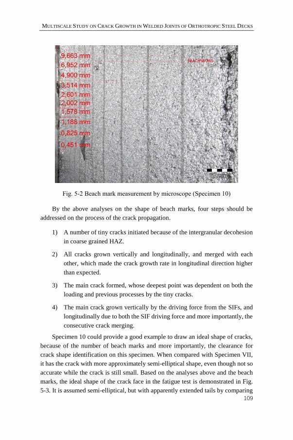
MULTISCALE STUDY ON CRACK GROWTH IN WELDED JOINTS OF ORTHOTROPIC STEEL DECKS
109
Fig. 5-2 Beach mark measurement by microscope (Specimen 10)
By the above analyses on the shape of beach marks, four steps should be
addressed on the process of the crack propagation.
1) A number of tiny cracks initiated because of the intergranular decohesion
in coarse grained HAZ.
2) All cracks grown vertically and longitudinally, and merged with each
other, which made the crack growth rate in longitudinal direction higher
than expected.
3) The main crack formed, whose deepest point was dependent on both the
loading and previous processes by the tiny cracks.
4) The main crack grown vertically by the driving force from the SIFs, and
longitudinally due to both the SIF driving force and more importantly, the
consecutive crack merging.
Specimen 10 could provide a good example to draw an ideal shape of cracks,
because of the number of beach marks and more importantly, the clearance for
crack shape identification on this specimen. When compared with Specimen VII,
it has the crack with more approximately semi-elliptical shape, even though not so
accurate while the crack is still small. Based on the analyses above and the beach
marks, the ideal shape of the crack face in the fatigue test is demonstrated in Fig.
5-3. It is assumed semi-elliptical, but with apparently extended tails by comparing
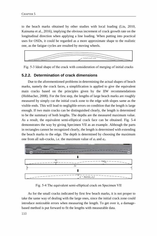
CHAPTER 5
110
to the beach marks obtained by other studies with local loading (Liu, 2010,
Kainuma et al., 2016), implying the obvious increment of crack growth rate on the
longitudinal direction when applying a line loading. When putting into practical
uses for OSDs, it could be regarded as a more approximate shape to the realistic
one, as the fatigue cycles are resulted by moving wheels.
Fig. 5-3 Ideal shape of the crack with consideration of merging of initial cracks
5.2.2. Determination of crack dimensions
Due to the aforementioned problems in determining the actual shapes of beach
marks, namely the crack faces, a simplification is applied to give the equivalent
main cracks based on the principles given by the IIW recommendations
(Hobbacher, 2008). For the first step, the lengths of large beach marks are roughly
measured by simply cut the initial crack zone to the edge with slopes same as the
visible ends. This will lead to negligible errors on condition that the length is large
enough. If two main cracks can be distinguished clearly, the length is determined
to be the summary of both lengths. The depths are the measured maximum value.
As a result, the equivalent semi-elliptical crack face can be obtained. Fig. 5-4
demonstrates the way by giving Specimen VII as an example. Although the parts
in rectangles cannot be recognized clearly, the length is determined with extending
the beach marks to the edge. The depth is determined by choosing the maximum
one from all sub-cracks, i.e. the maximum value of a1 and a2.
Fig. 5-4 The equivalent semi-elliptical crack on Specimen VII
As for the small cracks indicated by first few beach marks, it is not proper to
take the same way of dealing with the large ones, since the initial crack zone could
introduce noticeable errors when measuring the length. To get over it, a damage-
based method is put forward to fit the lengths with measurable data.
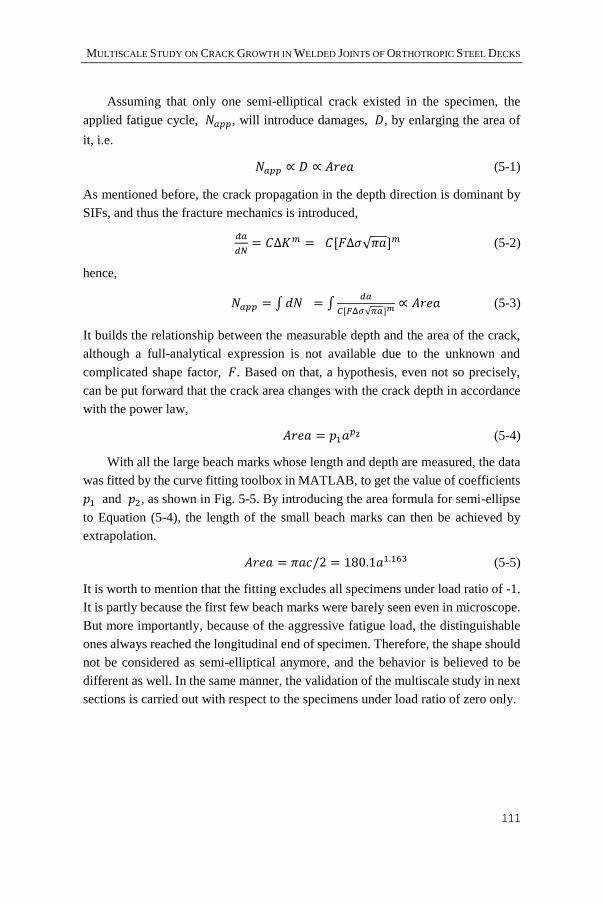
MULTISCALE STUDY ON CRACK GROWTH IN WELDED JOINTS OF ORTHOTROPIC STEEL DECKS
111
Assuming that only one semi-elliptical crack existed in the specimen, the
applied fatigue cycle, 𝑁𝑎𝑝𝑝, will introduce damages, 𝐷, by enlarging the area of
it, i.e.
𝑁𝑎𝑝𝑝 ∝ 𝐷 ∝ 𝐴𝑟𝑒𝑎 (5-1)
As mentioned before, the crack propagation in the depth direction is dominant by
SIFs, and thus the fracture mechanics is introduced,
𝑑𝑎
𝑑𝑁= 𝐶Δ𝐾𝑚 = 𝐶[𝐹Δ𝜎√𝜋𝑎]𝑚 (5-2)
hence,
𝑁𝑎𝑝𝑝 = ∫𝑑𝑁 = ∫𝑑𝑎
𝐶[𝐹Δ𝜎√𝜋𝑎]𝑚∝ 𝐴𝑟𝑒𝑎 (5-3)
It builds the relationship between the measurable depth and the area of the crack,
although a full-analytical expression is not available due to the unknown and
complicated shape factor, 𝐹. Based on that, a hypothesis, even not so precisely,
can be put forward that the crack area changes with the crack depth in accordance
with the power law,
𝐴𝑟𝑒𝑎 = 𝑝1𝑎𝑝2 (5-4)
With all the large beach marks whose length and depth are measured, the data
was fitted by the curve fitting toolbox in MATLAB, to get the value of coefficients
𝑝1 and 𝑝2, as shown in Fig. 5-5. By introducing the area formula for semi-ellipse
to Equation (5-4), the length of the small beach marks can then be achieved by
extrapolation.
𝐴𝑟𝑒𝑎 = 𝜋𝑎𝑐/2 = 180.1𝑎1.163 (5-5)
It is worth to mention that the fitting excludes all specimens under load ratio of -1.
It is partly because the first few beach marks were barely seen even in microscope.
But more importantly, because of the aggressive fatigue load, the distinguishable
ones always reached the longitudinal end of specimen. Therefore, the shape should
not be considered as semi-elliptical anymore, and the behavior is believed to be
different as well. In the same manner, the validation of the multiscale study in next
sections is carried out with respect to the specimens under load ratio of zero only.
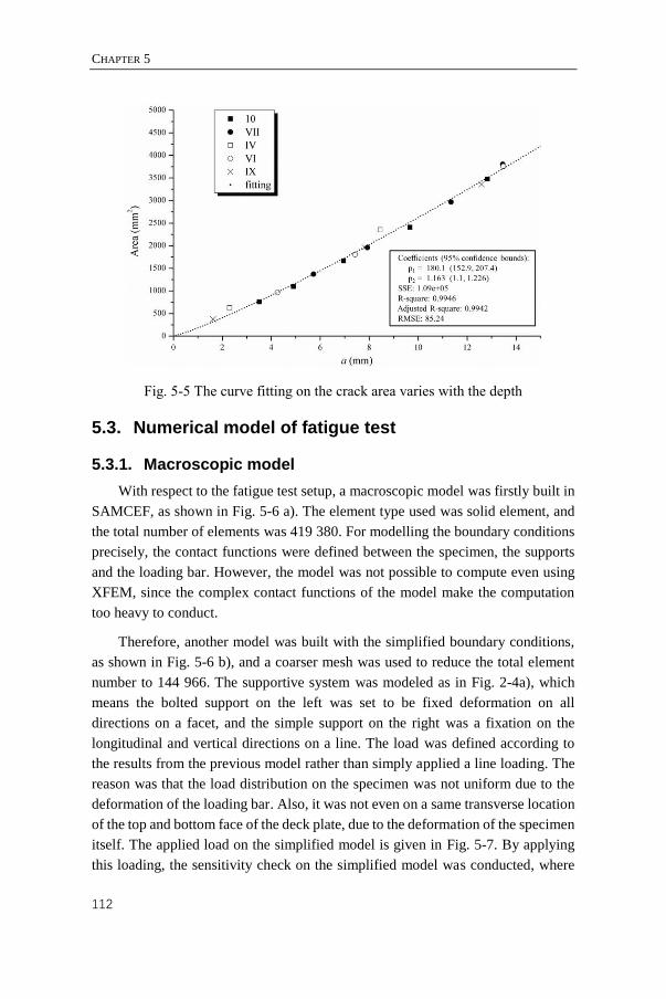
CHAPTER 5
112
Fig. 5-5 The curve fitting on the crack area varies with the depth
5.3. Numerical model of fatigue test
5.3.1. Macroscopic model
With respect to the fatigue test setup, a macroscopic model was firstly built in
SAMCEF, as shown in Fig. 5-6 a). The element type used was solid element, and
the total number of elements was 419 380. For modelling the boundary conditions
precisely, the contact functions were defined between the specimen, the supports
and the loading bar. However, the model was not possible to compute even using
XFEM, since the complex contact functions of the model make the computation
too heavy to conduct.
Therefore, another model was built with the simplified boundary conditions,
as shown in Fig. 5-6 b), and a coarser mesh was used to reduce the total element
number to 144 966. The supportive system was modeled as in Fig. 2-4a), which
means the bolted support on the left was set to be fixed deformation on all
directions on a facet, and the simple support on the right was a fixation on the
longitudinal and vertical directions on a line. The load was defined according to
the results from the previous model rather than simply applied a line loading. The
reason was that the load distribution on the specimen was not uniform due to the
deformation of the loading bar. Also, it was not even on a same transverse location
of the top and bottom face of the deck plate, due to the deformation of the specimen
itself. The applied load on the simplified model is given in Fig. 5-7. By applying
this loading, the sensitivity check on the simplified model was conducted, where
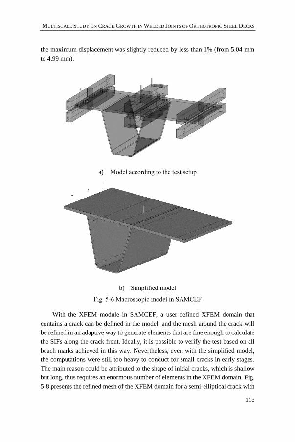
MULTISCALE STUDY ON CRACK GROWTH IN WELDED JOINTS OF ORTHOTROPIC STEEL DECKS
113
the maximum displacement was slightly reduced by less than 1% (from 5.04 mm
to 4.99 mm).
a) Model according to the test setup
b) Simplified model
Fig. 5-6 Macroscopic model in SAMCEF
With the XFEM module in SAMCEF, a user-defined XFEM domain that
contains a crack can be defined in the model, and the mesh around the crack will
be refined in an adaptive way to generate elements that are fine enough to calculate
the SIFs along the crack front. Ideally, it is possible to verify the test based on all
beach marks achieved in this way. Nevertheless, even with the simplified model,
the computations were still too heavy to conduct for small cracks in early stages.
The main reason could be attributed to the shape of initial cracks, which is shallow
but long, thus requires an enormous number of elements in the XFEM domain. Fig.
5-8 presents the refined mesh of the XFEM domain for a semi-elliptical crack with
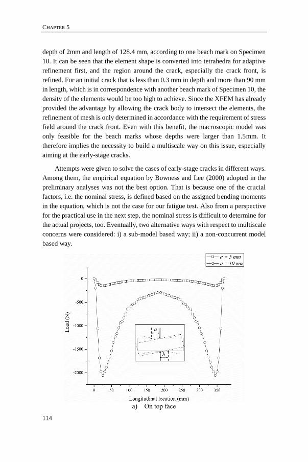
CHAPTER 5
114
depth of 2mm and length of 128.4 mm, according to one beach mark on Specimen
10. It can be seen that the element shape is converted into tetrahedra for adaptive
refinement first, and the region around the crack, especially the crack front, is
refined. For an initial crack that is less than 0.3 mm in depth and more than 90 mm
in length, which is in correspondence with another beach mark of Specimen 10, the
density of the elements would be too high to achieve. Since the XFEM has already
provided the advantage by allowing the crack body to intersect the elements, the
refinement of mesh is only determined in accordance with the requirement of stress
field around the crack front. Even with this benefit, the macroscopic model was
only feasible for the beach marks whose depths were larger than 1.5mm. It
therefore implies the necessity to build a multiscale way on this issue, especially
aiming at the early-stage cracks.
Attempts were given to solve the cases of early-stage cracks in different ways.
Among them, the empirical equation by Bowness and Lee (2000) adopted in the
preliminary analyses was not the best option. That is because one of the crucial
factors, i.e. the nominal stress, is defined based on the assigned bending moments
in the equation, which is not the case for our fatigue test. Also from a perspective
for the practical use in the next step, the nominal stress is difficult to determine for
the actual projects, too. Eventually, two alternative ways with respect to multiscale
concerns were considered: i) a sub-model based way; ii) a non-concurrent model
based way.
a) On top face
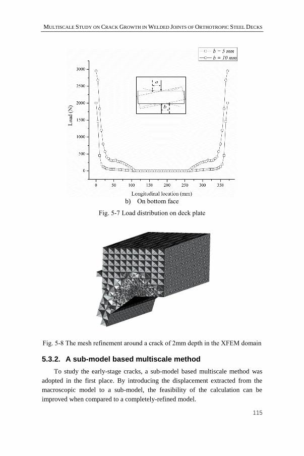
MULTISCALE STUDY ON CRACK GROWTH IN WELDED JOINTS OF ORTHOTROPIC STEEL DECKS
115
b) On bottom face
Fig. 5-7 Load distribution on deck plate
Fig. 5-8 The mesh refinement around a crack of 2mm depth in the XFEM domain
5.3.2. A sub-model based multiscale method
To study the early-stage cracks, a sub-model based multiscale method was
adopted in the first place. By introducing the displacement extracted from the
macroscopic model to a sub-model, the feasibility of the calculation can be
improved when compared to a completely-refined model.
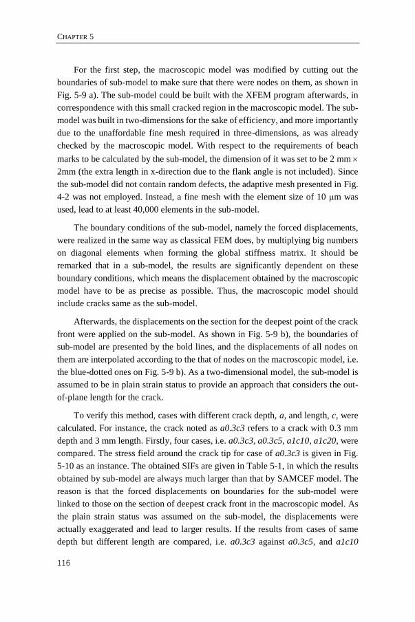
CHAPTER 5
116
For the first step, the macroscopic model was modified by cutting out the
boundaries of sub-model to make sure that there were nodes on them, as shown in
Fig. 5-9 a). The sub-model could be built with the XFEM program afterwards, in
correspondence with this small cracked region in the macroscopic model. The sub-
model was built in two-dimensions for the sake of efficiency, and more importantly
due to the unaffordable fine mesh required in three-dimensions, as was already
checked by the macroscopic model. With respect to the requirements of beach
marks to be calculated by the sub-model, the dimension of it was set to be 2 mm
2mm (the extra length in x-direction due to the flank angle is not included). Since
the sub-model did not contain random defects, the adaptive mesh presented in Fig.
4-2 was not employed. Instead, a fine mesh with the element size of 10 μm was
used, lead to at least 40,000 elements in the sub-model.
The boundary conditions of the sub-model, namely the forced displacements,
were realized in the same way as classical FEM does, by multiplying big numbers
on diagonal elements when forming the global stiffness matrix. It should be
remarked that in a sub-model, the results are significantly dependent on these
boundary conditions, which means the displacement obtained by the macroscopic
model have to be as precise as possible. Thus, the macroscopic model should
include cracks same as the sub-model.
Afterwards, the displacements on the section for the deepest point of the crack
front were applied on the sub-model. As shown in Fig. 5-9 b), the boundaries of
sub-model are presented by the bold lines, and the displacements of all nodes on
them are interpolated according to the that of nodes on the macroscopic model, i.e.
the blue-dotted ones on Fig. 5-9 b). As a two-dimensional model, the sub-model is
assumed to be in plain strain status to provide an approach that considers the out-
of-plane length for the crack.
To verify this method, cases with different crack depth, a, and length, c, were
calculated. For instance, the crack noted as a0.3c3 refers to a crack with 0.3 mm
depth and 3 mm length. Firstly, four cases, i.e. a0.3c3, a0.3c5, a1c10, a1c20, were
compared. The stress field around the crack tip for case of a0.3c3 is given in Fig.
5-10 as an instance. The obtained SIFs are given in Table 5-1, in which the results
obtained by sub-model are always much larger than that by SAMCEF model. The
reason is that the forced displacements on boundaries for the sub-model were
linked to those on the section of deepest crack front in the macroscopic model. As
the plain strain status was assumed on the sub-model, the displacements were
actually exaggerated and lead to larger results. If the results from cases of same
depth but different length are compared, i.e. a0.3c3 against a0.3c5, and a1c10
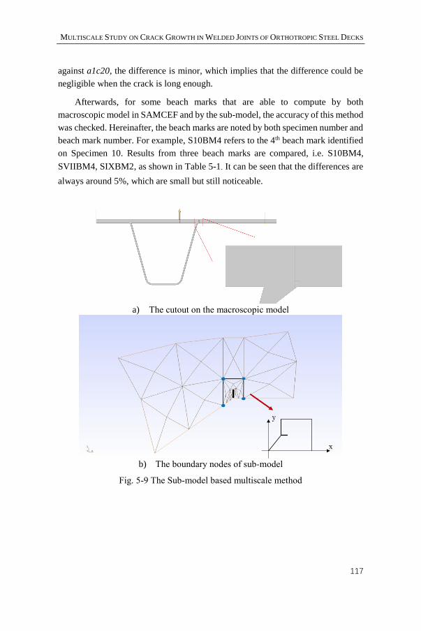
MULTISCALE STUDY ON CRACK GROWTH IN WELDED JOINTS OF ORTHOTROPIC STEEL DECKS
117
against a1c20, the difference is minor, which implies that the difference could be
negligible when the crack is long enough.
Afterwards, for some beach marks that are able to compute by both
macroscopic model in SAMCEF and by the sub-model, the accuracy of this method
was checked. Hereinafter, the beach marks are noted by both specimen number and
beach mark number. For example, S10BM4 refers to the 4th beach mark identified
on Specimen 10. Results from three beach marks are compared, i.e. S10BM4,
SVIIBM4, SIXBM2, as shown in Table 5-1. It can be seen that the differences are
always around 5%, which are small but still noticeable.
a) The cutout on the macroscopic model
b) The boundary nodes of sub-model
Fig. 5-9 The Sub-model based multiscale method
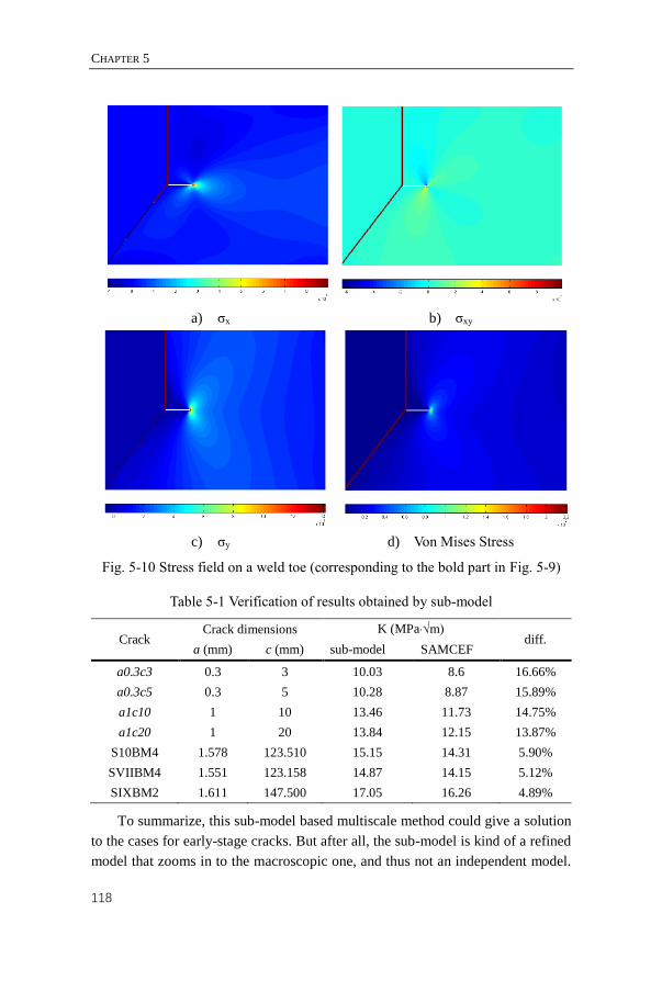
CHAPTER 5
118
a) σx
b) σxy
c) σy
d) Von Mises Stress
Fig. 5-10 Stress field on a weld toe (corresponding to the bold part in Fig. 5-9)
Table 5-1 Verification of results obtained by sub-model
Crack Crack dimensions K (MPa·√m)
diff. a (mm) c (mm) sub-model SAMCEF
a0.3c3 0.3 3 10.03 8.6 16.66%
a0.3c5 0.3 5 10.28 8.87 15.89%
a1c10 1 10 13.46 11.73 14.75%
a1c20 1 20 13.84 12.15 13.87%
S10BM4 1.578 123.510 15.15 14.31 5.90%
SVIIBM4 1.551 123.158 14.87 14.15 5.12%
SIXBM2 1.611 147.500 17.05 16.26 4.89%
To summarize, this sub-model based multiscale method could give a solution
to the cases for early-stage cracks. But after all, the sub-model is kind of a refined
model that zooms in to the macroscopic one, and thus not an independent model.
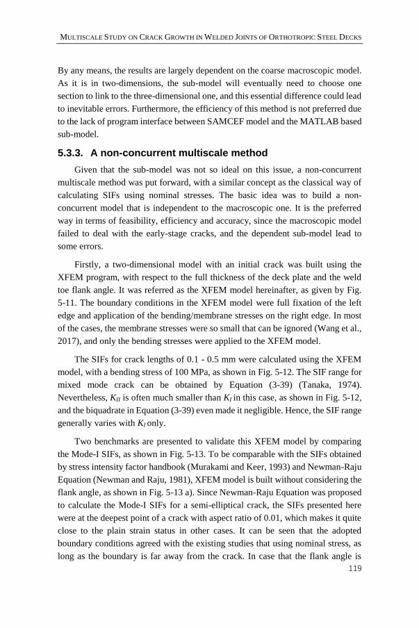
MULTISCALE STUDY ON CRACK GROWTH IN WELDED JOINTS OF ORTHOTROPIC STEEL DECKS
119
By any means, the results are largely dependent on the coarse macroscopic model.
As it is in two-dimensions, the sub-model will eventually need to choose one
section to link to the three-dimensional one, and this essential difference could lead
to inevitable errors. Furthermore, the efficiency of this method is not preferred due
to the lack of program interface between SAMCEF model and the MATLAB based
sub-model.
5.3.3. A non-concurrent multiscale method
Given that the sub-model was not so ideal on this issue, a non-concurrent
multiscale method was put forward, with a similar concept as the classical way of
calculating SIFs using nominal stresses. The basic idea was to build a non-
concurrent model that is independent to the macroscopic one. It is the preferred
way in terms of feasibility, efficiency and accuracy, since the macroscopic model
failed to deal with the early-stage cracks, and the dependent sub-model lead to
some errors.
Firstly, a two-dimensional model with an initial crack was built using the
XFEM program, with respect to the full thickness of the deck plate and the weld
toe flank angle. It was referred as the XFEM model hereinafter, as given by Fig.
5-11. The boundary conditions in the XFEM model were full fixation of the left
edge and application of the bending/membrane stresses on the right edge. In most
of the cases, the membrane stresses were so small that can be ignored (Wang et al.,
2017), and only the bending stresses were applied to the XFEM model.
The SIFs for crack lengths of 0.1 - 0.5 mm were calculated using the XFEM
model, with a bending stress of 100 MPa, as shown in Fig. 5-12. The SIF range for
mixed mode crack can be obtained by Equation (3-39) (Tanaka, 1974).
Nevertheless, KII is often much smaller than KI in this case, as shown in Fig. 5-12,
and the biquadrate in Equation (3-39) even made it negligible. Hence, the SIF range
generally varies with KI only.
Two benchmarks are presented to validate this XFEM model by comparing
the Mode-I SIFs, as shown in Fig. 5-13. To be comparable with the SIFs obtained
by stress intensity factor handbook (Murakami and Keer, 1993) and Newman-Raju
Equation (Newman and Raju, 1981), XFEM model is built without considering the
flank angle, as shown in Fig. 5-13 a). Since Newman-Raju Equation was proposed
to calculate the Mode-I SIFs for a semi-elliptical crack, the SIFs presented here
were at the deepest point of a crack with aspect ratio of 0.01, which makes it quite
close to the plain strain status in other cases. It can be seen that the adopted
boundary conditions agreed with the existing studies that using nominal stress, as
long as the boundary is far away from the crack. In case that the flank angle is
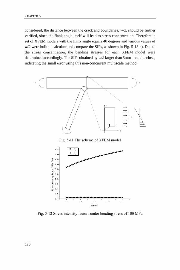
CHAPTER 5
120
considered, the distance between the crack and boundaries, w/2, should be further
verified, since the flank angle itself will lead to stress concentration. Therefore, a
set of XFEM models with the flank angle equals 40 degrees and various values of
w/2 were built to calculate and compare the SIFs, as shown in Fig. 5-13 b). Due to
the stress concentration, the bending stresses for each XFEM model were
determined accordingly. The SIFs obtained by w/2 larger than 5mm are quite close,
indicating the small error using this non-concurrent multiscale method.
Fig. 5-11 The scheme of XFEM model
Fig. 5-12 Stress intensity factors under bending stress of 100 MPa

MULTISCALE STUDY ON CRACK GROWTH IN WELDED JOINTS OF ORTHOTROPIC STEEL DECKS
121
a) without flank angle
b) with flank angle
Fig. 5-13 Validation of XFEM model
Afterwards, this XFEM model was used to calculate the SIFs for beach marks
of early-stage cracks. As the boundary conditions are of great importance in a non-
concurrent multiscale method, the model is valid on condition that the crack is
small enough so that the bending stress ranges keep almost the same value. Hence
the bending stress ranges to be applied should be determined properly. For instance,
the strains measured in the fatigue test of Specimen 10 at different positions are
shown in Fig. 5-14, in which the smaller strain ranges can be easily distinguished

CHAPTER 5
122
as beach mark cycles. Therefore, the strain ranges in different stages can be
compared. A simple and concise way was to compare the average value of the strain
ranges before the i-th beach mark, Δεi, as defined in Fig. 5-14 a). Table 5-2 provides
the strain ranges at different gauges till the 4th beach mark, which refers to the
crack in a depth of 1.578 mm. It can be observed that the reduction of the strain
range is only 2.75% for Strain Gauge BD7 (w/2 = 11 mm) and 3.82% for Strain
Gauge BD6 (w/2 = 9 mm), which are almost negligible. Given that the crack depth
to be calculated by XFEM model was even smaller, the half width of XFEM model,
w/2, was set to be 8 mm. Hence, the size of it is 16 15mm (the extra length due
to the flank angle is not included). As it was much larger than the sub-model, the
element size of 20 μm was adopted for the sake of computing efficiency, leading
to at least 600,000 elements in the XFEM model.
a) Strain gauge BD7 (w/2 = 11 mm)
b) Strain gauge BD6 (w/2 = 9 mm)
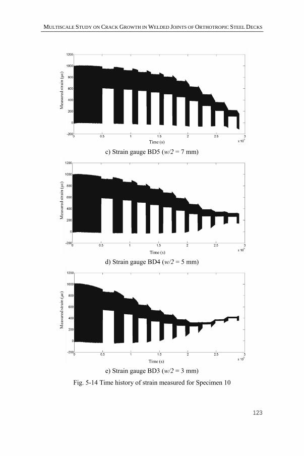
MULTISCALE STUDY ON CRACK GROWTH IN WELDED JOINTS OF ORTHOTROPIC STEEL DECKS
123
c) Strain gauge BD5 (w/2 = 7 mm)
d) Strain gauge BD4 (w/2 = 5 mm)
e) Strain gauge BD3 (w/2 = 3 mm)
Fig. 5-14 Time history of strain measured for Specimen 10
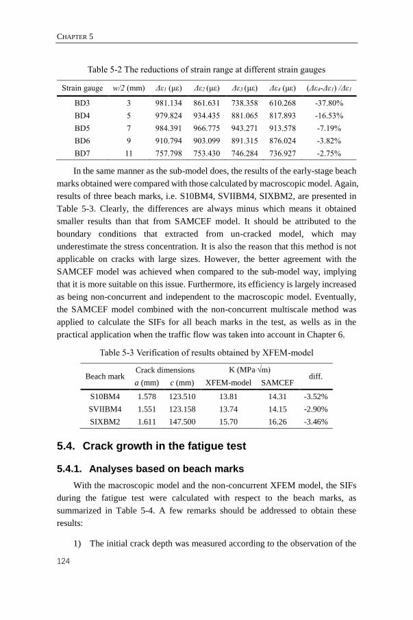
CHAPTER 5
124
Table 5-2 The reductions of strain range at different strain gauges
Strain gauge w/2 (mm) Δε1 (με) Δε2 (με) Δε3 (με) Δε4 (με) (Δε4-Δε1) /Δε1
BD3 3 981.134 861.631 738.358 610.268 -37.80%
BD4 5 979.824 934.435 881.065 817.893 -16.53%
BD5 7 984.391 966.775 943.271 913.578 -7.19%
BD6 9 910.794 903.099 891.315 876.024 -3.82%
BD7 11 757.798 753.430 746.284 736.927 -2.75%
In the same manner as the sub-model does, the results of the early-stage beach
marks obtained were compared with those calculated by macroscopic model. Again,
results of three beach marks, i.e. S10BM4, SVIIBM4, SIXBM2, are presented in
Table 5-3. Clearly, the differences are always minus which means it obtained
smaller results than that from SAMCEF model. It should be attributed to the
boundary conditions that extracted from un-cracked model, which may
underestimate the stress concentration. It is also the reason that this method is not
applicable on cracks with large sizes. However, the better agreement with the
SAMCEF model was achieved when compared to the sub-model way, implying
that it is more suitable on this issue. Furthermore, its efficiency is largely increased
as being non-concurrent and independent to the macroscopic model. Eventually,
the SAMCEF model combined with the non-concurrent multiscale method was
applied to calculate the SIFs for all beach marks in the test, as wells as in the
practical application when the traffic flow was taken into account in Chapter 6.
Table 5-3 Verification of results obtained by XFEM-model
Beach mark Crack dimensions K (MPa·√m)
diff. a (mm) c (mm) XFEM-model SAMCEF
S10BM4 1.578 123.510 13.81 14.31 -3.52%
SVIIBM4 1.551 123.158 13.74 14.15 -2.90%
SIXBM2 1.611 147.500 15.70 16.26 -3.46%
5.4. Crack growth in the fatigue test
5.4.1. Analyses based on beach marks
With the macroscopic model and the non-concurrent XFEM model, the SIFs
during the fatigue test were calculated with respect to the beach marks, as
summarized in Table 5-4. A few remarks should be addressed to obtain these
results:
1) The initial crack depth was measured according to the observation of the
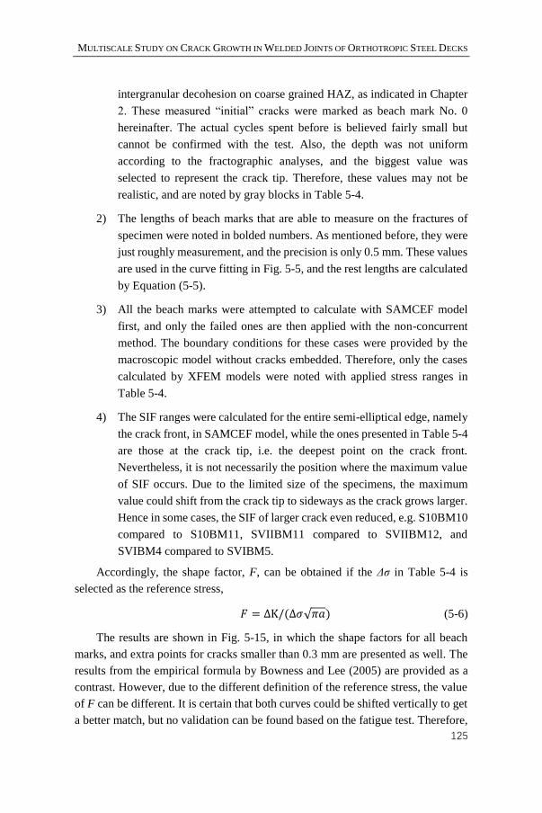
MULTISCALE STUDY ON CRACK GROWTH IN WELDED JOINTS OF ORTHOTROPIC STEEL DECKS
125
intergranular decohesion on coarse grained HAZ, as indicated in Chapter
2. These measured “initial” cracks were marked as beach mark No. 0
hereinafter. The actual cycles spent before is believed fairly small but
cannot be confirmed with the test. Also, the depth was not uniform
according to the fractographic analyses, and the biggest value was
selected to represent the crack tip. Therefore, these values may not be
realistic, and are noted by gray blocks in Table 5-4.
2) The lengths of beach marks that are able to measure on the fractures of
specimen were noted in bolded numbers. As mentioned before, they were
just roughly measurement, and the precision is only 0.5 mm. These values
are used in the curve fitting in Fig. 5-5, and the rest lengths are calculated
by Equation (5-5).
3) All the beach marks were attempted to calculate with SAMCEF model
first, and only the failed ones are then applied with the non-concurrent
method. The boundary conditions for these cases were provided by the
macroscopic model without cracks embedded. Therefore, only the cases
calculated by XFEM models were noted with applied stress ranges in
Table 5-4.
4) The SIF ranges were calculated for the entire semi-elliptical edge, namely
the crack front, in SAMCEF model, while the ones presented in Table 5-4
are those at the crack tip, i.e. the deepest point on the crack front.
Nevertheless, it is not necessarily the position where the maximum value
of SIF occurs. Due to the limited size of the specimens, the maximum
value could shift from the crack tip to sideways as the crack grows larger.
Hence in some cases, the SIF of larger crack even reduced, e.g. S10BM10
compared to S10BM11, SVIIBM11 compared to SVIIBM12, and
SVIBM4 compared to SVIBM5.
Accordingly, the shape factor, F, can be obtained if the Δσ in Table 5-4 is
selected as the reference stress,
𝐹 = ΔK/(Δ𝜎√𝜋𝑎) (5-6)
The results are shown in Fig. 5-15, in which the shape factors for all beach
marks, and extra points for cracks smaller than 0.3 mm are presented as well. The
results from the empirical formula by Bowness and Lee (2005) are provided as a
contrast. However, due to the different definition of the reference stress, the value
of F can be different. It is certain that both curves could be shifted vertically to get
a better match, but no validation can be found based on the fatigue test. Therefore,
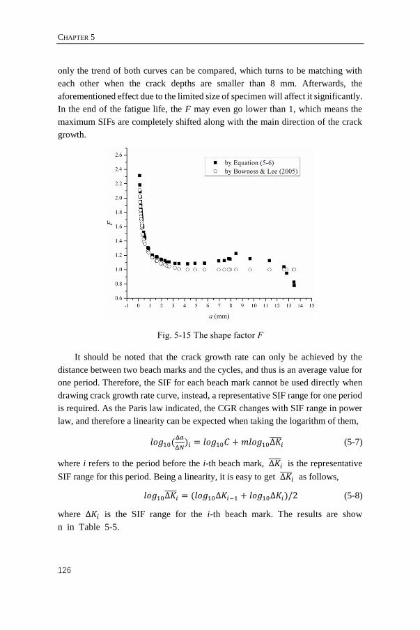
CHAPTER 5
126
only the trend of both curves can be compared, which turns to be matching with
each other when the crack depths are smaller than 8 mm. Afterwards, the
aforementioned effect due to the limited size of specimen will affect it significantly.
In the end of the fatigue life, the F may even go lower than 1, which means the
maximum SIFs are completely shifted along with the main direction of the crack
growth.
Fig. 5-15 The shape factor F
It should be noted that the crack growth rate can only be achieved by the
distance between two beach marks and the cycles, and thus is an average value for
one period. Therefore, the SIF for each beach mark cannot be used directly when
drawing crack growth rate curve, instead, a representative SIF range for one period
is required. As the Paris law indicated, the CGR changes with SIF range in power
law, and therefore a linearity can be expected when taking the logarithm of them,
𝑙𝑜𝑔10(Δ𝑎
Δ𝑁)𝑖 = 𝑙𝑜𝑔10𝐶 + 𝑚𝑙𝑜𝑔10Δ𝐾̅̅ ̅̅ 𝑖 (5-7)
where i refers to the period before the i-th beach mark, Δ𝐾̅̅ ̅̅ 𝑖 is the representative
SIF range for this period. Being a linearity, it is easy to get Δ𝐾̅̅ ̅̅ 𝑖 as follows,
𝑙𝑜𝑔10Δ𝐾̅̅ ̅̅ 𝑖 = (𝑙𝑜𝑔10Δ𝐾𝑖−1 + 𝑙𝑜𝑔10Δ𝐾𝑖)/2 (5-8)
where Δ𝐾𝑖 is the SIF range for the i-th beach mark. The results are show
n in Table 5-5.

MULTISCALE STUDY ON CRACK GROWTH IN WELDED JOINTS OF ORTHOTROPIC STEEL DECKS
127
Table 5-4 Summary of calculation on specimens with R=0
Spec
imen
Beach
mark N
a
(mm) c (mm) a/c
Δσ
(MPa)
ΔK
(MPa·√m)
10
0 0 0.288 93.613 0.003 172.21 8.89
1 100000 0.451 100.699 0.004 172.21 9.87
2 135000 0.825 111.116 0.007 172.21 11.46
3 155000 1.188 117.920 0.010 172.21 12.67
4 170000 1.578 123.505 0.013 \ 14.31
5 185000 2.002 128.390 0.016 \ 15.57
6 200000 2.601 133.987 0.019 \ 17.23
7 215000 3.514 137.500 0.026 \ 19.65
8 230000 4.900 142.500 0.034 \ 23.24
9 245000 6.952 152.500 0.046 \ 28.57
10 260000 9.663 159.000 0.061 \ 34.60
11 270544 12.827 172.500 0.074 \ 32.85
VII
0 0 0.375 97.724 0.004 172.21 9.45
1 100000 0.539 103.678 0.005 172.21 10.30
2 135000 0.863 111.944 0.008 172.21 11.60
3 155000 1.210 118.273 0.010 172.21 12.74
4 170000 1.551 123.158 0.013 \ 14.15
5 185000 1.947 127.808 0.015 \ 15.44
6 200000 2.436 132.567 0.018 \ 16.66
7 215000 3.162 138.324 0.023 \ 18.66
8 230000 4.251 145.159 0.029 \ 21.51
9 245000 5.725 152.500 0.038 \ 25.20
10 260000 7.925 157.500 0.050 \ 31.18
11 272000 11.341 166.500 0.068 \ 36.61
12 272852 13.453 180.000 0.075 \ 29.26
IV
0 0 0.498 102.331 0.005 222.21 13.04
1 50000 0.874 112.166 0.008 222.21 15.03
2 100000 2.299 172.500 0.013 \ 21.29
3 147425 8.447 177.500 0.048 \ 44.37
VI
0 0 0.362 97.173 0.004 149.99 8.17
1 300000 1.199 118.098 0.010 149.99 11.07
2 350000 2.673 134.584 0.020 \ 15.23
3 400000 4.251 145.000 0.029 \ 18.74
4 450000 7.425 155.000 0.048 \ 25.83
5 484782 13.480 177.500 0.076 \ 24.05
IX
0 0 0.282 93.259 0.003 194.43 9.99
1 110000 0.561 104.346 0.005 194.43 11.75
2 160000 1.611 147.500 0.011 \ 16.26
3 235000 7.815 160.000 0.049 \ 35.15
4 247762 12.591 170.000 0.074 \ 40.20

CHAPTER 5
128
Table 5-5 Summary of the representative SIF ranges and the corresponding CGRs
Speci
men i
Δa/ΔN
(m/cycle) Δ𝐾̅̅ ̅̅
(MPa·√m)
Speci
men i
Δa/ΔN
(m/cycle) Δ𝐾̅̅ ̅̅
(MPa·√m)
10
1 1.628E-09 9.37
VII
1 1.641E-09 9.87
2 1.069E-08 10.64 2 9.261E-09 10.93
3 1.815E-08 12.05 3 1.732E-08 12.16
4 2.600E-08 13.23 4 2.273E-08 13.23
5 2.827E-08 14.66 5 2.640E-08 14.56
6 3.993E-08 16.38 6 3.263E-08 16.04
7 6.087E-08 18.40 7 4.840E-08 17.63
8 9.240E-08 21.37 8 7.260E-08 20.04
9 1.368E-07 25.77 9 9.826E-08 23.28
10 1.807E-07 31.44 10 1.467E-07 28.03
11 3.001E-07 33.71 11 2.846E-07 33.78
IV
1 7.525E-09 14.00 12 2.479E-06 32.73
2 2.850E-08 17.89
VI
1 2.789E-09 9.51
3 1.296E-07 30.74 2 2.948E-08 12.98
IX
1 2.540E-09 10.83 3 3.156E-08 16.89
2 2.100E-08 13.58 4 6.348E-08 22.00
3 8.272E-08 25.73 5 1.741E-07 24.92
4 3.742E-07 41.18
Consequently, the relationship between crack growth rate, da/dN, and the SIF
range, ΔK, can be drawn for specimens with load ratio of zero in logarithm
coordinates, as show in Fig. 5-16. Comparing with the preliminary analyses in
Chapter 2, the graph seems to be more converged, especially in the early-stage. It
can be seen that the results for Specimen 10 and VII are in good agreement, as they
were carried out by the same load history. Additionally, results from these two
specimens can be regarded as the references to further analysis and to compare with
others, as they contains the most points among all curves. By contrast, results for
Specimen IV are showing clearly lower CGR than others. It should be attributed to
the fitting for crack shape, where Specimen IV has only two measurable points and
thus the least weight in the fitting. As shown in Fig. 5-5, points for Specimen IV
also seem slightly further away from the fitting curve than other points do.
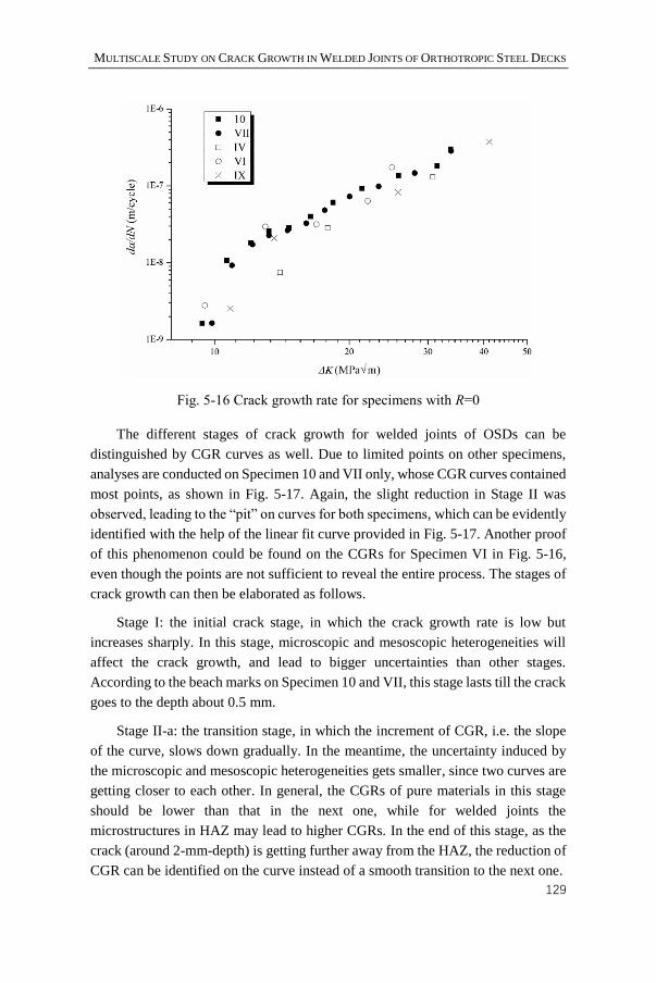
MULTISCALE STUDY ON CRACK GROWTH IN WELDED JOINTS OF ORTHOTROPIC STEEL DECKS
129
Fig. 5-16 Crack growth rate for specimens with R=0
The different stages of crack growth for welded joints of OSDs can be
distinguished by CGR curves as well. Due to limited points on other specimens,
analyses are conducted on Specimen 10 and VII only, whose CGR curves contained
most points, as shown in Fig. 5-17. Again, the slight reduction in Stage II was
observed, leading to the “pit” on curves for both specimens, which can be evidently
identified with the help of the linear fit curve provided in Fig. 5-17. Another proof
of this phenomenon could be found on the CGRs for Specimen VI in Fig. 5-16,
even though the points are not sufficient to reveal the entire process. The stages of
crack growth can then be elaborated as follows.
Stage I: the initial crack stage, in which the crack growth rate is low but
increases sharply. In this stage, microscopic and mesoscopic heterogeneities will
affect the crack growth, and lead to bigger uncertainties than other stages.
According to the beach marks on Specimen 10 and VII, this stage lasts till the crack
goes to the depth about 0.5 mm.
Stage II-a: the transition stage, in which the increment of CGR, i.e. the slope
of the curve, slows down gradually. In the meantime, the uncertainty induced by
the microscopic and mesoscopic heterogeneities gets smaller, since two curves are
getting closer to each other. In general, the CGRs of pure materials in this stage
should be lower than that in the next one, while for welded joints the
microstructures in HAZ may lead to higher CGRs. In the end of this stage, as the
crack (around 2-mm-depth) is getting further away from the HAZ, the reduction of
CGR can be identified on the curve instead of a smooth transition to the next one.
CHAPTER 5
130
Stage II-b: the stable crack propagation stage. It is the stage that the points of
Specimen 10 and VII match with each other perfectly. Therefore, the classical Paris
law can be expected to be applied, and the material constants in Paris law can be
estimated.
Stage III: the unstable crack propagation stage.
Fig. 5-17 Typical CGR curves and different stages
5.4.2. Material constants estimation
As suggested before, in Stage II-b the crack-tip is away from the HAZ and thus
can be assured that crack propagates stably following Paris law during this period.
The material constants in Paris law can be estimated by the results, and applied on
the prediction of actual welded joints of OSDs. However, it is not hard to notice
that the rest points, except the clearly different Stage I, can actually be interpreted
by Paris law as well. In that case, the CGRs for other specimens can be used to
estimate the material constants, although some errors can be introduced due to the
different stages. Hence, two different datasets, i.e. Dataset 1 and Dataset 2, were
adopted in the fitting to estimate the material constants. The former one referred to
the points in Stage II-b for Specimen 10 & VII, while the latter referred to the points
for all specimens by ignoring Stage I. Additionally, as recommended by most of
the literature, such as the IIW recommendation (Hobbacher, 2008), BS 7910 (BSI,
2013), the value of Pairs exponent, m, was set to three with some confidence. To
be comparable, fittings were carried out based on m equals three or the fitted value.
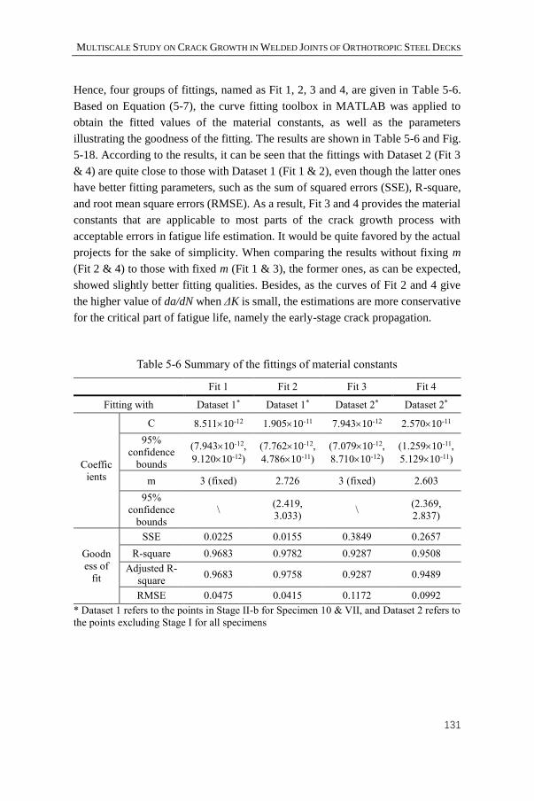
MULTISCALE STUDY ON CRACK GROWTH IN WELDED JOINTS OF ORTHOTROPIC STEEL DECKS
131
Hence, four groups of fittings, named as Fit 1, 2, 3 and 4, are given in Table 5-6.
Based on Equation (5-7), the curve fitting toolbox in MATLAB was applied to
obtain the fitted values of the material constants, as well as the parameters
illustrating the goodness of the fitting. The results are shown in Table 5-6 and Fig.
5-18. According to the results, it can be seen that the fittings with Dataset 2 (Fit 3
& 4) are quite close to those with Dataset 1 (Fit 1 & 2), even though the latter ones
have better fitting parameters, such as the sum of squared errors (SSE), R-square,
and root mean square errors (RMSE). As a result, Fit 3 and 4 provides the material
constants that are applicable to most parts of the crack growth process with
acceptable errors in fatigue life estimation. It would be quite favored by the actual
projects for the sake of simplicity. When comparing the results without fixing m
(Fit 2 & 4) to those with fixed m (Fit 1 & 3), the former ones, as can be expected,
showed slightly better fitting qualities. Besides, as the curves of Fit 2 and 4 give
the higher value of da/dN when ΔK is small, the estimations are more conservative
for the critical part of fatigue life, namely the early-stage crack propagation.
Table 5-6 Summary of the fittings of material constants
Fit 1 Fit 2 Fit 3 Fit 4
Fitting with Dataset 1* Dataset 1* Dataset 2* Dataset 2*
Coeffic
ients
C 8.51110-12 1.90510-11 7.94310-12 2.57010-11
95%
confidence
bounds
(7.94310-12,
9.12010-12)
(7.76210-12,
4.78610-11)
(7.07910-12,
8.71010-12)
(1.25910-11,
5.12910-11)
m 3 (fixed) 2.726 3 (fixed) 2.603
95%
confidence
bounds
\ (2.419,
3.033) \
(2.369,
2.837)
Goodn
ess of
fit
SSE 0.0225 0.0155 0.3849 0.2657
R-square 0.9683 0.9782 0.9287 0.9508
Adjusted R-
square 0.9683 0.9758 0.9287 0.9489
RMSE 0.0475 0.0415 0.1172 0.0992
* Dataset 1 refers to the points in Stage II-b for Specimen 10 & VII, and Dataset 2 refers to
the points excluding Stage I for all specimens
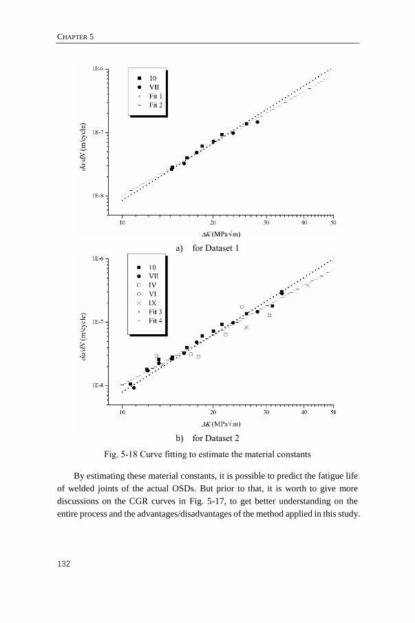
CHAPTER 5
132
a) for Dataset 1
b) for Dataset 2
Fig. 5-18 Curve fitting to estimate the material constants
By estimating these material constants, it is possible to predict the fatigue life
of welded joints of the actual OSDs. But prior to that, it is worth to give more
discussions on the CGR curves in Fig. 5-17, to get better understanding on the
entire process and the advantages/disadvantages of the method applied in this study.

MULTISCALE STUDY ON CRACK GROWTH IN WELDED JOINTS OF ORTHOTROPIC STEEL DECKS
133
5.5. Discussions
5.5.1. Crack growth simulation
Provided by the above study based on the beach marks, it is curious that if the
crack growth can be simulated step by step based on the Paris law. It means to
predict the crack path in a quasi-static way with a given initial crack, which is also
the method adopted by other studies (Pais, 2011; Kumar et al., 2014; Nagy et al.,
2016). In this study, the macroscopic model built in SAMCEF gives the access to
conduct this simulation.
Firstly, a semi-elliptical crack with a depth similar to the measured initial crack
was embedded in the SAMCEF model. With consideration of the limitation of the
computation ability, the crack was 0.2 mm in depth and 6 mm in semi-length, and
the length for each crack growth step was fixed to be 0.2 mm. The loading was
identical to the one applied on Specimen 10 and VII. In each step of computation,
the SIFs on all nodes on the crack front were calculated. The node with the
maximum SIF will grow 0.2 mm forward, while the crack growth length for other
nodes will be determined according to their SIFs. As the length of each crack
growth step being fixed, the crack growth path was not dependent on the material
constants in Paris law, which will only affect the crack growth rate.
Fig. 5-19 a) presents the crack front for 45 steps in the crack growth simulation.
The coordinates are the same as in Fig. 5-6, where the X-axis is the transverse
direction, Y-axis is the longitudinal direction and Z-axis is the vertical direction.
The results show that the ratio of the semi-axis length of the crack is changing
during the growth, and the crack growth length in depth is generally larger than
that in longitudinal direction. After 45 steps, the crack grows to a depth of about
5.5 mm. However, the shape of the crack front cannot meet any beach mark on the
specimens. The main reason is, as mentioned before, the crack will grow
longitudinally not only because of the SIFs, but also by merging with other cracks.
On the other hand, due to the differences in crack shapes, the SIFs cannot be
calculated in a correct way as well. Fig. 5-19 b) presents the comparsion of SIFs at
the crack tip, namely the deepest point, obtained by the crack growth simulation ,
with the same applied loadings as on Specimen 10 and VII. It indicates that the
difference is small for the first few steps, but increases significantly afterwards. In
the case of crack growth simulation, the SIFs even reduce slightly after several
steps. That being said, the maximum value of SIF is not at the crack tip any more
at that moment.
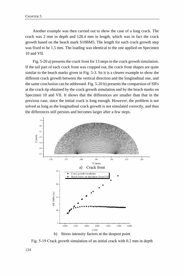
CHAPTER 5
134
Another example was then carried out to show the case of a long crack. The
crack was 2 mm in depth and 128.4 mm in length, which was in fact the crack
growth based on the beach mark S10BM5. The length for each crack growth step
was fixed to be 1.5 mm. The loading was identical to the one applied on Specimen
10 and VII.
Fig. 5-20 a) presents the crack front for 13 steps in the crack growth simulation.
If the tail part of each crack front was cropped out, the crack front shapes are quite
similar to the beach marks given in Fig. 5-3. So it is a clearer example to show the
different crack growth between the vertical direction and the longitudinal one, and
the same conclusion can be addressed. Fig. 5-20 b) presents the comparsion of SIFs
at the crack tip obtained by the crack growth simulation and by the beach marks on
Specimen 10 and VII. It shows that the differences are smaller than that in the
previous case, since the initial crack is long enough. However, the problem is not
solved as long as the longitudinal crack growth is not simulated correctly, and thus
the differences still persists and becomes larger after a few steps.
a) Crack front
b) Stress intensity factors at the deepest point
Fig. 5-19 Crack growth simulation of an initial crack with 0.2 mm in depth

MULTISCALE STUDY ON CRACK GROWTH IN WELDED JOINTS OF ORTHOTROPIC STEEL DECKS
135
a) Crack front
b) Stress intensity factors at the deepest point
Fig. 5-20 Crack growth simulation of an initial crack with 2 mm in depth
To sum up, the simulation on crack growth are not so applicable, since the
driving force of the crack growing longitudinally is also dependent on the
consecutive crack merging. On condition that the initial cracks along the HAZ of
welded joints are not properly determined, the results from the crack growth
simulation cannot be accurate enough. In that case, the best option for now is still
to analyze the crack growth process based on the beach marks, or based on the
fitted equation for crack shapes, e.g. Equation (5-5).
5.5.2. Early-stage cracks
In the early stages, the cracks have different CGRs from Paris law, as well as
the larger randomness in CGR, e.g. Stage I in Fig. 5-16. By looking into the beach
marks and the cycles presented in Table 5-4, the process of early-stage crack
growth is surely of great importance, since the largest part of fatigue life is
consumed in this period.
One similar concept in literatures is the short crack, which is difficult to give
a widely-accepted definition to distinguish from long cracks. Bogdanov (2014)
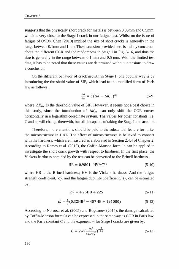
CHAPTER 5
136
suggests that the physically short crack for metals is between 0.05mm and 0.5mm,
which is very close to the Stage I crack in our fatigue test. Whilst on the issue of
fatigue of OSDs, Chen (2010) implied the size of short cracks is generally in the
range between 0.1mm and 1mm. The discussion provided here is mainly concerned
about the different CGR and the randomness in Stage I in Fig. 5-16, and thus the
size is generally in the range between 0.1 mm and 0.5 mm. With the limited test
data, it has to be noted that these values are determined without intensions to draw
a conclusion.
On the different behavior of crack growth in Stage I, one popular way is by
introducing the threshold value of SIF, which lead to the modified form of Paris
law as follows,
𝑑𝑎
𝑑𝑁= 𝐶(Δ𝐾 − Δ𝐾𝑡ℎ)
𝑚 (5-9)
where Δ𝐾𝑡ℎ is the threshold value of SIF. However, it seems not a best choice in
this study, since the introduction of Δ𝐾𝑡ℎ can only shift the CGR curves
horizontally in a logarithm coordinate system. The values for other constants, i.e.
C and m, will change therewith, but still incapable of taking the Stage I into account.
Therefore, more attentions should be paid to the substantial feature for it, i.e.
the microstructure in HAZ. The effect of microstructures is believed to connect
with the hardness, which are measured as elaborated in Section 2.4.4 of Chapter 2.
According to Remes et al. (2012), the Coffin-Manson formula can be applied to
investigate the short crack growth with respect to hardness. In the first place, the
Vickers hardness obtained by the test can be converted to the Brinell hardness,
HB = 0.9801 ∙ HV0.9941 (5-10)
where HB is the Brinell hardness; HV is the Vickers hardness. And the fatigue
strength coefficient, σ𝑓′ , and the fatigue ductility coefficient, ε𝑓
′ , can be estimated
by,
σ𝑓′ = 4.25HB + 225 (5-11)
ε𝑓′ =
1
𝐸(0.32HB2 − 487HB + 191000) (5-12)
Accroding to Noroozi et al. (2005) and Bogdanov (2014), the damage calculated
by Coffin-Manson formula can be expressed in the same way as CGR in Paris law,
and the Paris constant C and the exponent m for Stage I cracks are given by,
𝐶 = 2𝜌∗(𝛹12
4𝜋𝜌∗σ𝑓′ 2)−
1
2𝑏 (5-13)
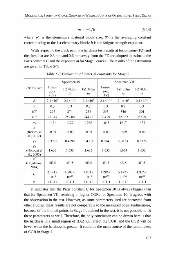
MULTISCALE STUDY ON CRACK GROWTH IN WELDED JOINTS OF ORTHOTROPIC STEEL DECKS
137
𝑚 = −1/𝑏 (5-14)
where 𝜌∗ is the elementary material block size; Ψ1 is the averaging constant
corresponding to the 1st elementary block; b is the fatigue strength exponent.
With respect to the crack path, the hardness test results at fusion zone (FZ) and
the sites that are 0.3 mm and 0.6 mm away from the FZ are adopted to estimate the
Paris constant C and the exponent m for Stage I cracks. The results of the estimation
are given in Table 5-7.
Table 5-7 Estimation of material constants for Stage I
HV test site
Specimen 10 Specimen VII
Fusion
zone
(FZ)
FZ+0.3m
m
FZ+0.6m
m
Fusion
zone
(FZ)
FZ+0.3m
m
FZ+0.6m
m
E 2.1×10⁵ 2.1×10⁵ 2.1×10⁵ 2.1×10⁵ 2.1×10⁵ 2.1×10⁵
ν 0.3 0.3 0.3 0.3 0.3 0.3
HV 297 274 258 353 346 301
HB 281.47 259.80 244.72 334.21 327.62 285.24
'f 1421 1329 1265 1645 1617 1437
b
(Remes, et
al., 2012)
-0.09 -0.09 -0.09 -0.09 -0.09 -0.09
'f 0.3775 0.4099 0.4333 0.3047 0.3133 0.3720
Ψ1
(Noroozi et
al., 2005)
1.633 1.633 1.633 1.633 1.633 1.633
ρ*
(Bogdanov,
2014)
4E-5 4E-5 4E-5 4E-5 4E-5 4E-5
C 2.181×
10-19
4.592×
10-19
7.953×
10-19
4.286×
10-20
5.187×
10-20
1.926×
10-19
m 11.111 11.111 11.111 11.111 11.111 11.111
It indicates that the Paris constant C for Specimen 10 is always bigger than
that for Specimen VII, resulting in higher CGRs for Specimen 10. It agrees with
the observation in the test. However, as some parameters used are borrowed from
other studies, these results are not comparable to the measured ones. Furthermore,
because of the limited points in Stage I obtained in the test, it is not possible to fit
these parameters as well. Therefore, the only conclusion can be drawn here is that
the hardness in a small region of HAZ will affect the CGR, and the CGR will be
lower when the hardness is greater. It could be the main source of the randomness
of CGR in Stage I.
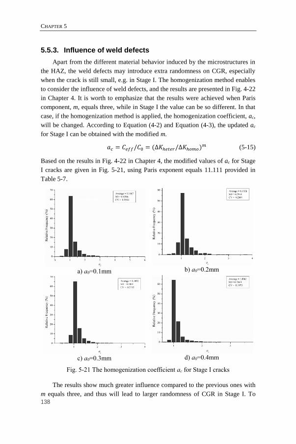
CHAPTER 5
138
5.5.3. Influence of weld defects
Apart from the different material behavior induced by the microstructures in
the HAZ, the weld defects may introduce extra randomness on CGR, especially
when the crack is still small, e.g. in Stage I. The homogenization method enables
to consider the influence of weld defects, and the results are presented in Fig. 4-22
in Chapter 4. It is worth to emphasize that the results were achieved when Paris
component, m, equals three, while in Stage I the value can be so different. In that
case, if the homogenization method is applied, the homogenization coefficient, ac,
will be changed. According to Equation (4-2) and Equation (4-3), the updated ac
for Stage I can be obtained with the modified m.
𝑎𝑐 = 𝐶𝑒𝑓𝑓/𝐶0 = (∆𝐾ℎ𝑒𝑡𝑒𝑟/∆𝐾ℎ𝑜𝑚𝑜)𝑚 (5-15)
Based on the results in Fig. 4-22 in Chapter 4, the modified values of ac for Stage
I cracks are given in Fig. 5-21, using Paris exponent equals 11.111 provided in
Table 5-7.
a) a0=0.1mm
b) a0=0.2mm
c) a0=0.3mm
d) a0=0.4mm
Fig. 5-21 The homogenization coefficient ac for Stage I cracks
The results show much greater influence compared to the previous ones with
m equals three, and thus will lead to larger randomness of CGR in Stage I. To
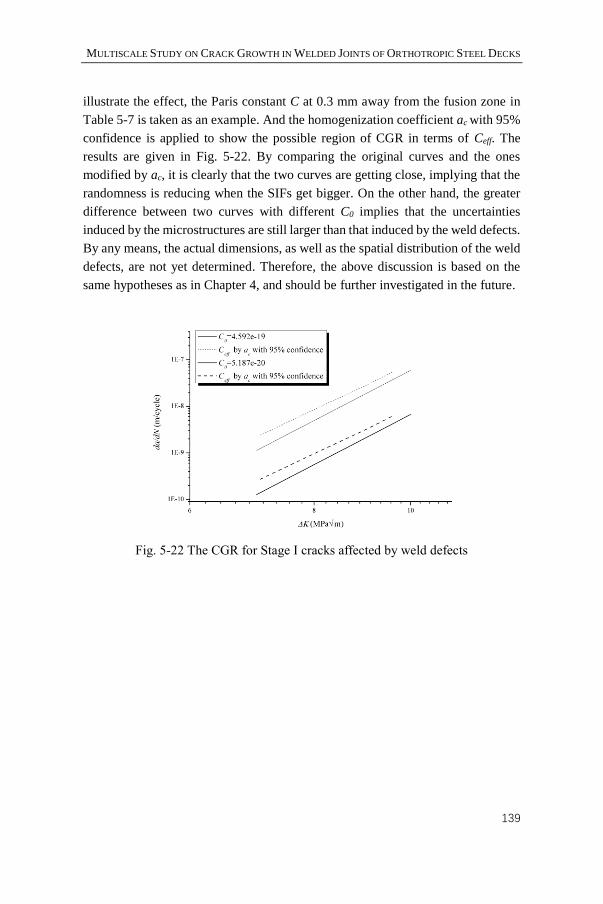
MULTISCALE STUDY ON CRACK GROWTH IN WELDED JOINTS OF ORTHOTROPIC STEEL DECKS
139
illustrate the effect, the Paris constant C at 0.3 mm away from the fusion zone in
Table 5-7 is taken as an example. And the homogenization coefficient ac with 95%
confidence is applied to show the possible region of CGR in terms of Ceff. The
results are given in Fig. 5-22. By comparing the original curves and the ones
modified by ac, it is clearly that the two curves are getting close, implying that the
randomness is reducing when the SIFs get bigger. On the other hand, the greater
difference between two curves with different C0 implies that the uncertainties
induced by the microstructures are still larger than that induced by the weld defects.
By any means, the actual dimensions, as well as the spatial distribution of the weld
defects, are not yet determined. Therefore, the above discussion is based on the
same hypotheses as in Chapter 4, and should be further investigated in the future.
Fig. 5-22 The CGR for Stage I cracks affected by weld defects

CHAPTER 5
140
CHAPTER 6
APPLICATION ON ORTHOTROPIC
STEEL DECKS UNDER RANDOM
TRAFFIC FLOW
________________________________
This chapter is based on:
Wang, B., De Backer, H., and Chen, A. (2016). An XFEM based uncertainty
study on crack growth in welded joints with defects. Theoretical and Applied
Fracture Mechanics, 86, Part B, 125-142.
Wang, B., Zhou, X.Y, De Backer, H., Chen, A, and Schmidt F. (2017). Macro
crack initiation life for orthotropic steel decks considering weld heterogeneity and
random traffic loading. Structure and Infrastructure Engineering. (Accepted)

CHAPTER 6
142
6.1. Introduction
Previous chapters provided the analyses on fatigue crack behavior on rib-to-
deck welded joints of OSDs through experimental and numerical studies on small-
scale specimens. It should be remarked that the loadings on the specimens are
designed and thus determinate, whilst for the actual projects, it will have to
introduce the realistic traffic flow to achieve better prediction on the fatigue lives
of OSDs.
This chapter gives three examples of application of the multiscale method built
in Chapter 5 on actual OSDs, with consideration of the realistic traffic loadings
based on measurements or standards. The first example is based on a traffic flow
measured in a short term in Europe; the second is based on the traffic loadings
recommended by Eurocode; and the third one is based on a long-term traffic flow
measurement in China. These case studies demonstrated the feasibility of the
established method, and the results showed the evident difference of the traffic
loadings from various areas.
6.2. Methodology
As stated in Chapter 5, the behavior of early-stage cracks showed larger
uncertainties and randomness, whilst the behavior for the rest is more stable. In that
case, the study is conducted with respect to two parts, i) the fatigue life for early-
stage crack till it can be detected for the first time, which is called macro-crack
initiation life (MCIL) hereinafter; ii) the rest fatigue life, which is called macro-
crack growth life (MCGL) hereinafter. In the first part, the variation of Paris
constant C induced by the heterogeneity is considered, thus makes a probabilistic
method necessary. In contrast, the second part should be carried out in a
deterministic context, so that it will be easier to combine with the inspections and
maintenance works of bridge. Due to the less scattered CGRs in this stage, the error
in the deterministic study will be fairly small, especially compared to the early
stage where most of the uncertainties exist.
It should be stated at first that, due to insufficient knowledge on the weld
defects of OSDs, the study was based on the following hypotheses:
1) To consider the heterogeneity of the defects, the homogenization was
adopted in the same way as addressed in Section 4.4. It means that the
pores and inclusions were in circular shape with diameters ranging from
20 μm to 90 μm, the number of them was limited to 10, and the
parameters concerning their locations, sizes and numbers were all
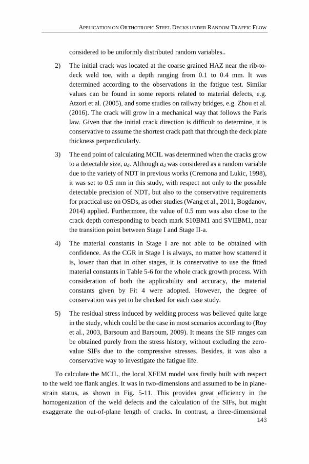
APPLICATION ON ORTHOTROPIC STEEL DECKS UNDER RANDOM TRAFFIC FLOW
143
considered to be uniformly distributed random variables..
2) The initial crack was located at the coarse grained HAZ near the rib-to-
deck weld toe, with a depth ranging from 0.1 to 0.4 mm. It was
determined according to the observations in the fatigue test. Similar
values can be found in some reports related to material defects, e.g.
Atzori et al. (2005), and some studies on railway bridges, e.g. Zhou et al.
(2016). The crack will grow in a mechanical way that follows the Paris
law. Given that the initial crack direction is difficult to determine, it is
conservative to assume the shortest crack path that through the deck plate
thickness perpendicularly.
3) The end point of calculating MCIL was determined when the cracks grow
to a detectable size, ad. Although ad was considered as a random variable
due to the variety of NDT in previous works (Cremona and Lukic, 1998),
it was set to 0.5 mm in this study, with respect not only to the possible
detectable precision of NDT, but also to the conservative requirements
for practical use on OSDs, as other studies (Wang et al., 2011, Bogdanov,
2014) applied. Furthermore, the value of 0.5 mm was also close to the
crack depth corresponding to beach mark S10BM1 and SVIIBM1, near
the transition point between Stage I and Stage II-a.
4) The material constants in Stage I are not able to be obtained with
confidence. As the CGR in Stage I is always, no matter how scattered it
is, lower than that in other stages, it is conservative to use the fitted
material constants in Table 5-6 for the whole crack growth process. With
consideration of both the applicability and accuracy, the material
constants given by Fit 4 were adopted. However, the degree of
conservation was yet to be checked for each case study.
5) The residual stress induced by welding process was believed quite large
in the study, which could be the case in most scenarios according to (Roy
et al., 2003, Barsoum and Barsoum, 2009). It means the SIF ranges can
be obtained purely from the stress history, without excluding the zero-
value SIFs due to the compressive stresses. Besides, it was also a
conservative way to investigate the fatigue life.
To calculate the MCIL, the local XFEM model was firstly built with respect
to the weld toe flank angles. It was in two-dimensions and assumed to be in plane-
strain status, as shown in Fig. 5-11. This provides great efficiency in the
homogenization of the weld defects and the calculation of the SIFs, but might
exaggerate the out-of-plane length of cracks. In contrast, a three-dimensional
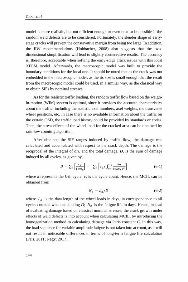
CHAPTER 6
144
model is more realistic, but not efficient enough or even next to impossible if the
random weld defects are to be considered. Fortunately, the slender shape of early-
stage cracks will prevent the conservative margin from being too large. In addition,
the IIW recommendations (Hobbacher, 2008) also suggests that the two-
dimensional simplification will lead to slightly conservative results. The accuracy
is, therefore, acceptable when solving the early-stage crack issues with this local
XFEM model. Afterwards, the macroscopic model was built to provide the
boundary conditions for the local one. It should be noted that as the crack was not
embedded in the macroscopic model, as the its size is small enough that the result
from the macroscopic model could be used, in a similar way, as the classical way
to obtain SIFs by nominal stresses.
As for the realistic traffic loading, the random traffic flow based on the weigh-
in-motion (WIM) system is optimal, since it provides the accurate characteristics
about the traffic, including the statistic axel numbers, axel weights, the transverse
wheel positions, etc. In case there is no available information about the traffic on
the certain OSD, the traffic load history could be provided by standards or codes.
Then, the stress effects of the wheel load for the cracked area can be obtained by
rainflow counting algorithm.
After obtained the SIF ranges induced by traffic flow, the damage was
calculated and accumulated with respect to the crack depth. The damage is the
reciprocal of the integral of dN, and the total damage, D, is the sum of damage
induced by all cycles, as given by,
𝐷 = ∑ [𝑐𝑘
∫𝑑𝑁𝑘]𝑘 = ∑ [𝑐𝑘/ ∫
𝑑𝑎
𝐶(∆𝐾𝑘)𝑚
𝑎𝑑𝑎0
]𝑘 (6-1)
where k represents the k-th cycle; ck is the cycle count. Hence, the MCIL can be
obtained from
𝑁𝑑 = 𝐿𝑑/𝐷 (6-2)
where 𝐿𝑑 is the data length of the wheel loads in days, in correspondence to all
cycles counted when calculating D; 𝑁𝑑 is the fatigue life in days. Hence, instead
of evaluating damage based on classical nominal stresses, the crack growth under
effects of weld defects is into account when calculating MCIL, by introducing the
homogenization method to calculating damage via Paris constant C. In this way,
the load sequence for variable amplitude fatigue is not taken into account, as it will
not result in noticeable differences in terms of long-term fatigue life calculation
(Pais, 2011; Nagy, 2017).

APPLICATION ON ORTHOTROPIC STEEL DECKS UNDER RANDOM TRAFFIC FLOW
145
Fig. 6-1 The flowchart for estimating macro-crack initiation life
To calculate the MCGL, the Equation (6-1) and (6-2) can be applied with the
initial crack depth, a0, being a constant of 0.5 mm, and the randomness of the Paris
constant, C, can be ignored as well. Hence, it will lead to a deterministic result. The
end point of the MCGL is selected to be half thickness of the deck plate, since it is
when the visual detection can surely address the cracks as the paint film damaged
will provide a clear sign at that moment (Ryan et al., 2006). On the other hand, this
end point is determined with respect to the test results in literatures, which suggest
the crack may stop growing then (Kainuma et al., 2016). It can be attributed to that
the crack tip is beyond the possible range that affected by the welding process.
Then the SIF range becomes much smaller as residual stress is faded, which means
the aforementioned Hypothesis (5) is not valid anymore. Nevertheless, it cannot be
justified due to the difficulty in measuring the residual stress in the direction of
deck plate thickness, and the study on residual stress is also not in the scope of this
thesis. Anyway, all the initial/end point and the hypotheses proposed here are given
with compromises from different aspects, and thus are open for discussion.

CHAPTER 6
146
6.3. A case study based on the traffic flow in Europe
A case study was carried out based on the numerical model of the orthotropic
steel deck of Millau Viaduct, which is a well-known multi-span cable-stayed bridge
in the south of France. The view of this bridge and the design of the cross-section
is shown in Fig. 6-2.
a) general view
b) cross-section (unit: mm)
Fig. 6-2 The orthotropic steel deck of Millau Viaduct (Zhou et al., 2015)
6.3.1. Traffic flow
In this study, a set of measured traffic data from the A9 motorway in France is
used. The traffic data was collected by Zhou et al. (2015) using a piezoceramic
weigh-in-motion (WIM) system installed in one direction of the bidirectional 6-
lane motorway near Saint-Jean-de-Vedas (SJDV) in southeast France. As it is only
about 100 km away from the site that Millau Viaduct located, the characteristics of
traffic flow are believed quite representative.

APPLICATION ON ORTHOTROPIC STEEL DECKS UNDER RANDOM TRAFFIC FLOW
147
The WIM system provided not only the axle weights and distances of vehicles
traveling in the slow and fast lanes, but also the vehicle transverse dimensions and
the transverse in-lane positions, which means a more precise position of the vehicle
rather than a distribution by lanes. This is realized by an extra diagonal sensor strip,
which is different from the conventional two parallel sensor strips often used in
ordinary WIM systems. A detailed description of this type of WIM system can be
found in (Jacob et al., 2013). In fact, the distribution of the transverse in-lane
position of vehicles is site-specific. In other words, it depends significantly on the
profile of the lane cross section (Zhou et al., 2015), and maybe the customs of local
drivers and the road surface conditions, too. To evaluate the fatigue performance
or fatigue life of critical joints of existing structures, it is therefore preferred to use
measured distributions of transverse in-lane positions, instead of models
recommended in standards or codes.
The WIM system recorded the traffic data from January 2010 to May 2010,
and a total of 581,011 trucks representing traffic flow for 86 days were selected
from the original data by excluding records that are unreasonable, or in the
weekends and system inactivity. Obviously, in order to obtain a reasonable
evaluation and prediction of the performance of an existing bridge structure,
measured traffic data over a sufficiently long period is recommended, e.g. one year
as suggested by Sivakumar et al. (2011). This kind of long-term data, however, is
not always available due to various facts, such as limited storage for the huge
amounts of data in continuous recording, the available budget for conducting long-
term measurements, etc. Prediction or evaluation of the performance of bridge or
its components with short-term measurements is thus quite common in practice, by
using variance reduction techniques that are able to fully exploit the potential of
short-term data. A common method to analyze the traffic load effect is to use
microscopic traffic simulation to generate long-term traffic loads or load effects
(Chen and Wu, 2011; O'Connor and O'Brien, 2005; Enright and O'Brien, 2013).
Based on the principle of generating traffic flow with the same features, a
Monte-Carlo simulation program was designed in (Zhou, 2013; Zhou et al., 2016b).
By employing the measured traffic data for 86 working days, the traffic data for
900 working days were generated to calculate the fatigue life. More details can be
found in (Wang et al., 2017). Fig. 6-3 showed a typical transverse stress history on
the bottom face of deck plate at 8 mm away from the weld toe. And as there are
always large amount of zero values when no vehicles are running over, the X-axis
in Fig. 6-3 is the reduced time by eliminating the zero-value sections in the traffic
flow simulation.

CHAPTER 6
148
Fig. 6-3 Typical time history of stress
6.3.2. Numerical models
As widely accepted that the fatigue damage of welded joints of OSDs is mainly
due to local effects, the numerical model was built as a partial structure instead of
the whole bridge structure. It focused on a deck segment under the slow lane, as it
is more fatigue-prone due to heavy trucks. The thickness of the deck plate was 14
mm, and that of the trapezoidal stiffener was 6 mm. Due to the lack of design
specification and on-site measurements, the actual weld toe flank angle, α, was not
available. By assuming that the weld will form equal flank angle at toe on deck
plate and on the stiffener, the flank angle was set to be 40 degrees, as shown in Fig.
6-4.
Fig. 6-4 The detailed geometry at the welded joint
The FEM model of this bridge was established in ANSYS 13.0. A coarse
model was built in the first place, which consists of five trapezoidal stiffeners and
two diaphragms. Boundary conditions were applied by fixing the longitudinal

APPLICATION ON ORTHOTROPIC STEEL DECKS UNDER RANDOM TRAFFIC FLOW
149
translation but allowing the rotation around the y-axis for the two diaphragms, and
restraining the vertical deformation on the lateral boundary. This model consisted
of Shell 63 elements, which is a linear-elastic shell element defined in ANSYS, in
a total number of 52156. However, it will not achieve the precise geometry of the
welded joints as a shell model, not to mention the relatively coarse mesh will lead
to insufficient accuracy for the XFEM model in the next step. In that case, a sub-
model of the weld vicinity (see Fig. 6-5) was built by Solid 185 elements, which is
an eight-node solid element defined in ANSYS, and the element number was
181000.
Fig. 6-5 Coarse model and sub-model of the Millau Viaduct
The material properties were the same as steel, i.e. the elastic modulus of
2.11011 Pa, the Poison’s ratio of 0.3, and the density of 7850 kg/m3. By applying
a moving wheel load of 45 kN on an area of 0.45 m by 0.4 m, which was used to
represent the landing area of one tire, along the FEM model in both longitudinal
and transverse directions, influence surfaces for various responses can be obtained.
Fig. 6-6 illustrates the influence surfaces of bending and membrane stresses at the
location of 8 mm to the weld. Accordingly, the bending stresses were always much
higher than the membrane stresses, despite of the different wheel locations.
Afterwards, a two-dimensional XFEM model with an initial crack was built in
the same way as illustrated in Fig. 5-11 in Chapter 5, whose dimensions were
determined according to the geometry of the bridge. Then the SIFs can be
calculated accordingly, as given in the next section.

CHAPTER 6
150
a) Bending stresses
b) Membrane stresses
Fig. 6-6 The influence surfaces of the transverse stress at 8 mm to the welded
joint
6.3.3. Stress intensity factors
The SIFs for crack depths of 0.1 - 0.5 mm, namely in the range of MCIL, were
calculated using the XFEM model. Fig. 6-7 presents the results by applying a
bending stress of 100 MPa, which is almost the same as Fig. 5-12. Again, the results
show that the Mode-I SIFs are much larger than the Mode-II SIFs, and thus are the
dominant part in crack growth. It should be noted that the similarity of the results
presented by Fig. 5-12 and Fig. 6-7 implies that the differences induced by deck
plate thickness are tiny and ignorable when cracks are in such a small size. The
empirical way provides another support to that statement as it suggests the shape
factor is a function of the non-dimensional parameter a/t. However, it will not
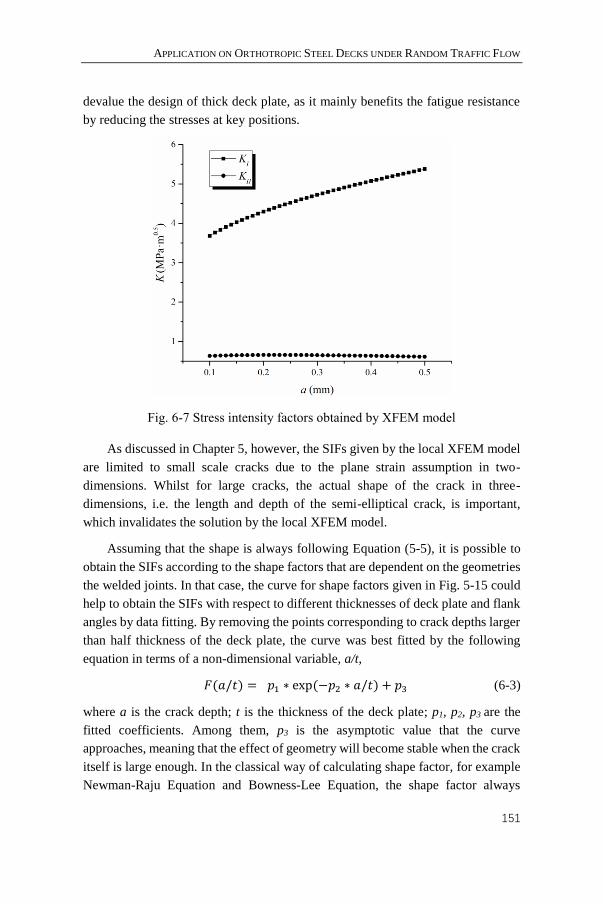
APPLICATION ON ORTHOTROPIC STEEL DECKS UNDER RANDOM TRAFFIC FLOW
151
devalue the design of thick deck plate, as it mainly benefits the fatigue resistance
by reducing the stresses at key positions.
Fig. 6-7 Stress intensity factors obtained by XFEM model
As discussed in Chapter 5, however, the SIFs given by the local XFEM model
are limited to small scale cracks due to the plane strain assumption in two-
dimensions. Whilst for large cracks, the actual shape of the crack in three-
dimensions, i.e. the length and depth of the semi-elliptical crack, is important,
which invalidates the solution by the local XFEM model.
Assuming that the shape is always following Equation (5-5), it is possible to
obtain the SIFs according to the shape factors that are dependent on the geometries
the welded joints. In that case, the curve for shape factors given in Fig. 5-15 could
help to obtain the SIFs with respect to different thicknesses of deck plate and flank
angles by data fitting. By removing the points corresponding to crack depths larger
than half thickness of the deck plate, the curve was best fitted by the following
equation in terms of a non-dimensional variable, a/t,
𝐹(𝑎/𝑡) = 𝑝1 ∗ exp(−𝑝2 ∗ 𝑎/𝑡) + 𝑝3 (6-3)
where a is the crack depth; t is the thickness of the deck plate; p1, p2, p3 are the
fitted coefficients. Among them, p3 is the asymptotic value that the curve
approaches, meaning that the effect of geometry will become stable when the crack
itself is large enough. In the classical way of calculating shape factor, for example
Newman-Raju Equation and Bowness-Lee Equation, the shape factor always

CHAPTER 6
152
following an asymptotic value of one. Similarly, by fitting the results from the
fatigue test, the value of p3 can be considered a constant afterwards. The other two
coefficients, p1 and p2, can always be fitted with the SIFs of early-stage cracks
achieved by XFEM model for various geometries. Table 6-1 and Fig. 6-8 illustrate
the fitting results of the coefficients and the curve of shape factor. It can be seen
that the difference between shape factors given by test specimens and those given
by Millau Viaduct is fairly small.
Table 6-1 Summary of the fitting for Equation (6-3)
Test specimens Millau Viaduct (MV)
Geometrical
parameters
t (mm) 15 14
α (°) 37 40
Coefficients
p1 1.157 1.260
p2 32.75 36.96
p3 1.109 1.109
Goodness of
fit
SSE 1.245E-02 1.759E-03
R-square 0.9952 0.9961
Adjusted R-square 0.9949 0.9959
RMSE 0.0194 0.0078
Fig. 6-8 Shape factors for Millau Viaduct calculated by data fitting
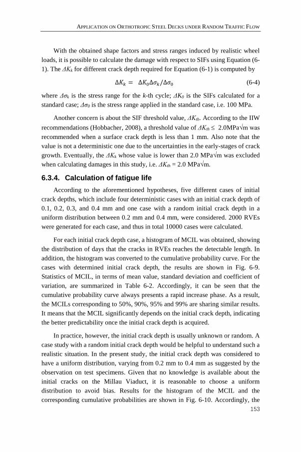
APPLICATION ON ORTHOTROPIC STEEL DECKS UNDER RANDOM TRAFFIC FLOW
153
With the obtained shape factors and stress ranges induced by realistic wheel
loads, it is possible to calculate the damage with respect to SIFs using Equation (6-
1). The ΔKk for different crack depth required for Equation (6-1) is computed by
∆𝐾𝑘 = ∆𝐾0∆𝜎𝑘/∆𝜎0 (6-4)
where Δσk is the stress range for the k-th cycle; ΔK0 is the SIFs calculated for a
standard case; Δσ0 is the stress range applied in the standard case, i.e. 100 MPa.
Another concern is about the SIF threshold value, ΔKth. According to the IIW
recommendations (Hobbacher, 2008), a threshold value of ΔKth 2.0MPa√m was
recommended when a surface crack depth is less than 1 mm. Also note that the
value is not a deterministic one due to the uncertainties in the early-stages of crack
growth. Eventually, the ΔKk whose value is lower than 2.0 MPa√m was excluded
when calculating damages in this study, i.e. ΔKth = 2.0 MPa√m.
6.3.4. Calculation of fatigue life
According to the aforementioned hypotheses, five different cases of initial
crack depths, which include four deterministic cases with an initial crack depth of
0.1, 0.2, 0.3, and 0.4 mm and one case with a random initial crack depth in a
uniform distribution between 0.2 mm and 0.4 mm, were considered. 2000 RVEs
were generated for each case, and thus in total 10000 cases were calculated.
For each initial crack depth case, a histogram of MCIL was obtained, showing
the distribution of days that the cracks in RVEs reaches the detectable length. In
addition, the histogram was converted to the cumulative probability curve. For the
cases with determined initial crack depth, the results are shown in Fig. 6-9.
Statistics of MCIL, in terms of mean value, standard deviation and coefficient of
variation, are summarized in Table 6-2. Accordingly, it can be seen that the
cumulative probability curve always presents a rapid increase phase. As a result,
the MCILs corresponding to 50%, 90%, 95% and 99% are sharing similar results.
It means that the MCIL significantly depends on the initial crack depth, indicating
the better predictability once the initial crack depth is acquired.
In practice, however, the initial crack depth is usually unknown or random. A
case study with a random initial crack depth would be helpful to understand such a
realistic situation. In the present study, the initial crack depth was considered to
have a uniform distribution, varying from 0.2 mm to 0.4 mm as suggested by the
observation on test specimens. Given that no knowledge is available about the
initial cracks on the Millau Viaduct, it is reasonable to choose a uniform
distribution to avoid bias. Results for the histogram of the MCIL and the
corresponding cumulative probabilities are shown in Fig. 6-10. Accordingly, the
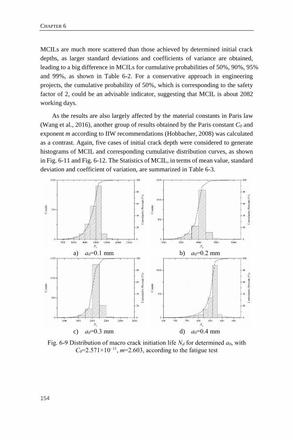
CHAPTER 6
154
MCILs are much more scattered than those achieved by determined initial crack
depths, as larger standard deviations and coefficients of variance are obtained,
leading to a big difference in MCILs for cumulative probabilities of 50%, 90%, 95%
and 99%, as shown in Table 6-2. For a conservative approach in engineering
projects, the cumulative probability of 50%, which is corresponding to the safety
factor of 2, could be an advisable indicator, suggesting that MCIL is about 2082
working days.
As the results are also largely affected by the material constants in Paris law
(Wang et al., 2016), another group of results obtained by the Paris constant C0 and
exponent m according to IIW recommendations (Hobbacher, 2008) was calculated
as a contrast. Again, five cases of initial crack depth were considered to generate
histograms of MCIL and corresponding cumulative distribution curves, as shown
in Fig. 6-11 and Fig. 6-12. The Statistics of MCIL, in terms of mean value, standard
deviation and coefficient of variation, are summarized in Table 6-3.
a) a0=0.1 mm
b) a0=0.2 mm
c) a0=0.3 mm
d) a0=0.4 mm
Fig. 6-9 Distribution of macro crack initiation life Nd for determined a0, with
C0=2.571×10⁻¹¹, m=2.603, according to the fatigue test

APPLICATION ON ORTHOTROPIC STEEL DECKS UNDER RANDOM TRAFFIC FLOW
155
Fig. 6-10 Distribution of macro crack initiation life Nd for random a0, with
C0=2.571×10⁻¹¹, m=2.603, according to the fatigue test
a) a0=0.1 mm
b) a0=0.2 mm
c) a0=0.3 mm
d) a0=0.4 mm
Fig. 6-11 Distribution of macro crack initiation life Nd for determined a0, with
C0=1.65×10⁻¹¹, m=3, according to (Hobbacher, 2008)
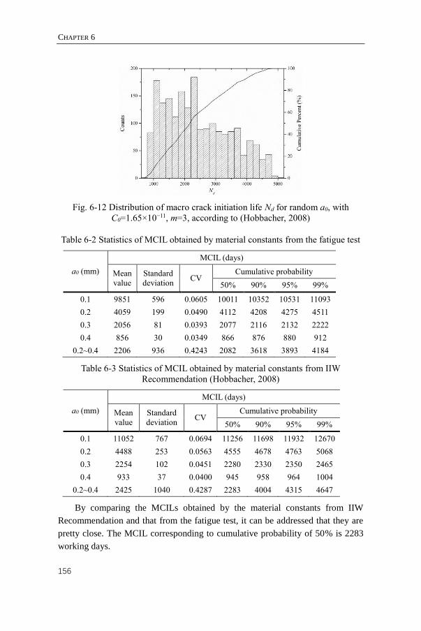
CHAPTER 6
156
Fig. 6-12 Distribution of macro crack initiation life Nd for random a0, with
C0=1.65×10⁻¹¹, m=3, according to (Hobbacher, 2008)
Table 6-2 Statistics of MCIL obtained by material constants from the fatigue test
a0 (mm)
MCIL (days)
Mean
value
Standard
deviation CV
Cumulative probability
50% 90% 95% 99%
0.1 9851 596 0.0605 10011 10352 10531 11093
0.2 4059 199 0.0490 4112 4208 4275 4511
0.3 2056 81 0.0393 2077 2116 2132 2222
0.4 856 30 0.0349 866 876 880 912
0.2~0.4 2206 936 0.4243 2082 3618 3893 4184
Table 6-3 Statistics of MCIL obtained by material constants from IIW
Recommendation (Hobbacher, 2008)
a0 (mm)
MCIL (days)
Mean
value
Standard
deviation CV
Cumulative probability
50% 90% 95% 99%
0.1 11052 767 0.0694 11256 11698 11932 12670
0.2 4488 253 0.0563 4555 4678 4763 5068
0.3 2254 102 0.0451 2280 2330 2350 2465
0.4 933 37 0.0400 945 958 964 1004
0.2~0.4 2425 1040 0.4287 2283 4004 4315 4647
By comparing the MCILs obtained by the material constants from IIW
Recommendation and that from the fatigue test, it can be addressed that they are
pretty close. The MCIL corresponding to cumulative probability of 50% is 2283
working days.
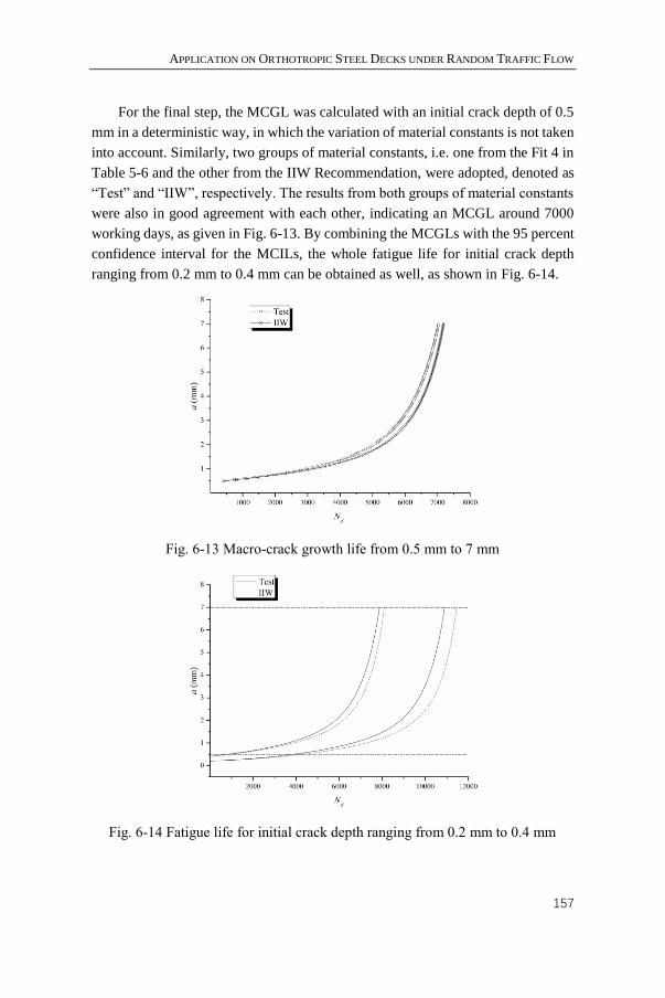
APPLICATION ON ORTHOTROPIC STEEL DECKS UNDER RANDOM TRAFFIC FLOW
157
For the final step, the MCGL was calculated with an initial crack depth of 0.5
mm in a deterministic way, in which the variation of material constants is not taken
into account. Similarly, two groups of material constants, i.e. one from the Fit 4 in
Table 5-6 and the other from the IIW Recommendation, were adopted, denoted as
“Test” and “IIW”, respectively. The results from both groups of material constants
were also in good agreement with each other, indicating an MCGL around 7000
working days, as given in Fig. 6-13. By combining the MCGLs with the 95 percent
confidence interval for the MCILs, the whole fatigue life for initial crack depth
ranging from 0.2 mm to 0.4 mm can be obtained as well, as shown in Fig. 6-14.
Fig. 6-13 Macro-crack growth life from 0.5 mm to 7 mm
Fig. 6-14 Fatigue life for initial crack depth ranging from 0.2 mm to 0.4 mm

CHAPTER 6
158
The results indicate that the MCGL is the main part of whole fatigue life, while
the MCIL takes a small part that accounts one third in maximum. It is not fully
consistent with the fatigue test results, which could be attributed to that the same
material constants C & m were applied in the calculation. In that way, the calculated
CGR is higher in Stage I when compared to the fatigue test results. As the stress
range spectrum caused by traffic flow in this region seems quite moderate, there
should be many cycles assigned to Stage I, and the damage induced by these cycles
will be significantly overestimated in this calculation. Anyway, even in a
conservative scenario that assuming an initial crack depth of 0.4 mm, the Millau
Viaduct will not suffer from fatigue problem in at least 8000 working days, i.e. 32
years. Therefore, the fatigue life of Millau Viaduct could be much larger in the
reality, and will not be the major concern in the maintenance.
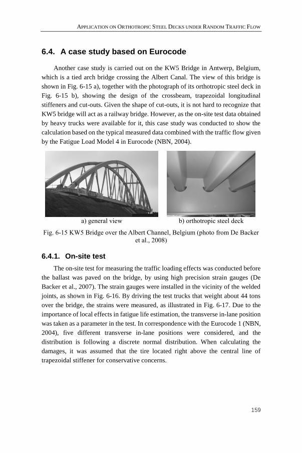
APPLICATION ON ORTHOTROPIC STEEL DECKS UNDER RANDOM TRAFFIC FLOW
159
6.4. A case study based on Eurocode
Another case study is carried out on the KW5 Bridge in Antwerp, Belgium,
which is a tied arch bridge crossing the Albert Canal. The view of this bridge is
shown in Fig. 6-15 a), together with the photograph of its orthotropic steel deck in
Fig. 6-15 b), showing the design of the crossbeam, trapezoidal longitudinal
stiffeners and cut-outs. Given the shape of cut-outs, it is not hard to recognize that
KW5 bridge will act as a railway bridge. However, as the on-site test data obtained
by heavy trucks were available for it, this case study was conducted to show the
calculation based on the typical measured data combined with the traffic flow given
by the Fatigue Load Model 4 in Eurocode (NBN, 2004).
a) general view
b) orthotropic steel deck
Fig. 6-15 KW5 Bridge over the Albert Channel, Belgium (photo from De Backer
et al., 2008)
6.4.1. On-site test
The on-site test for measuring the traffic loading effects was conducted before
the ballast was paved on the bridge, by using high precision strain gauges (De
Backer et al., 2007). The strain gauges were installed in the vicinity of the welded
joints, as shown in Fig. 6-16. By driving the test trucks that weight about 44 tons
over the bridge, the strains were measured, as illustrated in Fig. 6-17. Due to the
importance of local effects in fatigue life estimation, the transverse in-lane position
was taken as a parameter in the test. In correspondence with the Eurocode 1 (NBN,
2004), five different transverse in-lane positions were considered, and the
distribution is following a discrete normal distribution. When calculating the
damages, it was assumed that the tire located right above the central line of
trapezoidal stiffener for conservative concerns.

CHAPTER 6
160
Fig. 6-16 Strain gauges at the weld toe (De Backer et al., 2007)
Fig. 6-17 Test scheme and the assumed possibility of transverse locations
6.4.2. Stress intensity factors
As the design of the OSD of the KW5 Bridge is basically the same as the test
specimen, i.e. 15-mm-thick deck plate and 6-mm-thick stiffeners, the shape factors
are assumed to be the identical as well. Therefore, the Equation (6-3) with the
coefficients given in Table 6-1 can be applied to calculate the shape factors. In that
case, the stress ranges for calculating SIFs should be sufficiently distinct from the
crack site, and the strain gauge that is 11 mm away from the weld toe was selected
in this study.
The test data for each transverse position were shown in Fig. 6-18 ~ Fig. 6-22,
in which the effects of the five axles of the truck could be clearly distinguished.
These strains were measured at the bottom side of the deck plate only, as the data
at the top side are always not available due to the pavement cover. Nevertheless,
according to the influence surface in Fig. 6-6, it can be inferred that the measured
strains can be regarded as the direct indicators of bending stresses. Afterwards, the
rain-flow counting algorithm was applied to obtain the effective load cycles for
each location, as shown in Table 6-4, with the stress amplitudes under 5MPa
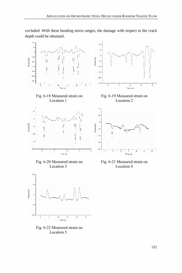
APPLICATION ON ORTHOTROPIC STEEL DECKS UNDER RANDOM TRAFFIC FLOW
161
excluded. With these bending stress ranges, the damage with respect to the crack
depth could be obtained.
Fig. 6-18 Measured strain on
Location 1
Fig. 6-19 Measured strain on
Location 2
Fig. 6-20 Measured strain on
Location 3
Fig. 6-21 Measured strain on
Location 4
Fig. 6-22 Measured strain on
Location 5
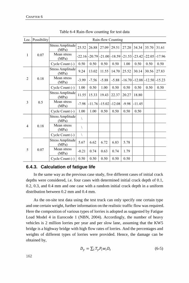
CHAPTER 6
162
Table 6-4 Rain-flow counting for test data
Loc. Possibility Rain-flow Counting
1 0.07
Stress Amplitude
(MPa) 25.52 26.88 27.09 29.51 27.20 34.34 35.70 31.61
Mean stress
(MPa) -22.16 -20.79 -21.00 -18.59 -21.53 -23.42 -22.05 -17.96
Cycle Count (-) 0.50 0.50 0.50 0.50 1.00 0.50 0.50 0.50
2 0.18
Stress Amplitude
(MPa) 9.24 13.02 11.55 14.70 25.52 30.14 30.56 27.83
Mean stress
(MPa) -3.99 -7.56 -5.88 -5.88 -16.70 -12.08 -12.50 -15.23
Cycle Count (-) 1.00 0.50 1.00 0.50 0.50 0.50 0.50 0.50
3 0.5
Stress Amplitude
(MPa) 11.55 15.33 19.43 22.37 20.27 18.80
Mean stress
(MPa) -7.98 -11.76 -15.02 -12.08 -9.98 -11.45
Cycle Count (-) 1.00 1.00 0.50 0.50 0.50 0.50
4 0.18
Stress Amplitude
(MPa) \
Mean stress
(MPa) \
Cycle Count (-) \
5 0.07
Stress Amplitude
(MPa) 5.67 6.62 6.72 6.83 5.78
Mean stress
(MPa) -0.21 0.74 0.63 0.74 1.79
Cycle Count (-) 0.50 0.50 0.50 0.50 0.50
6.4.3. Calculation of fatigue life
In the same way as the previous case study, five different cases of initial crack
depths were considered, i.e. four cases with determined initial crack depth of 0.1,
0.2, 0.3, and 0.4 mm and one case with a random initial crack depth in a uniform
distribution between 0.2 mm and 0.4 mm.
As the on-site test data using the test truck can only specify one certain type
and one certain weight, further information on the realistic traffic flow was required.
Here the composition of various types of lorries is adopted as suggested by Fatigue
Load Model 4 in Eurocode 1 (NBN, 2004). Accordingly, the number of heavy
vehicles is 2 million lorries per year and per slow lane, assuming that the KW5
bridge is a highway bridge with high flow rates of lorries. And the percentages and
weights of different types of lorries were provided. Hence, the damage can be
obtained by,
𝐷𝑦 = ∑ 𝑇𝑦𝑃𝑙𝑤𝑙𝐷𝑡𝑙 (6-5)

APPLICATION ON ORTHOTROPIC STEEL DECKS UNDER RANDOM TRAFFIC FLOW
163
𝑁𝑦 = 1/𝐷𝑦 (6-6)
where Ty refers to the total volume of lorries per year and per slow lane, i.e. 2
million; Pl is the percentage of different types of lorries; Dt is the damage induced
by the test truck; wl is the weight ratio of the lorries in Fatigue Load Model 4 and
the test truck, that is 44 tons.
Fig. 6-23 & Fig. 6-24 gives the MCIL counted by year, which seems extremely
small. The statistics of results are given in Table 6-5. For instance, if the initial
crack depth is 0.3 mm, which is quite close to the measurement in the fatigue test,
for example Specimen 10, VII, VI and IX, the results showed a large probability
that a macro-crack will initiate in only 0.19 years, i.e. less than 3 months. Again,
another group of Paris constant and exponent according to IIW recommendations
(Hobbacher, 2008) was adopted to check if the short fatigue life is resulted by the
effects of material-related constants. The results are shown in Fig. 6-25, Fig. 6-26,
and Table 6-6. Unsurprisingly, the results are quite similar to the ones achieved
according to the fatigue test, same as the previous case study on Millau Viaduct.
a) a0=0.1 mm
b) a0=0.2 mm
c) a0=0.3 mm
d) a0=0.4 mm
Fig. 6-23 Distribution of macro crack initiation life Ny for determined a0, with
C0=2.571×10⁻¹¹, m=2.603, according to the fatigue test
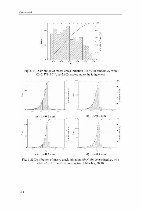
CHAPTER 6
164
Fig. 6-24 Distribution of macro crack initiation life Ny for random a0, with
C0=2.571×10⁻¹¹, m=2.603, according to the fatigue test
a) a0=0.1 mm
b) a0=0.2 mm
c) a0=0.3 mm
d) a0=0.4 mm
Fig. 6-25 Distribution of macro crack initiation life Ny for determined a0, with
C0=1.65×10⁻¹¹, m=3, according to (Hobbacher, 2008)
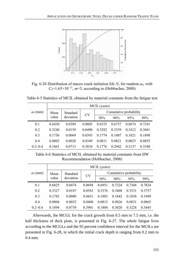
APPLICATION ON ORTHOTROPIC STEEL DECKS UNDER RANDOM TRAFFIC FLOW
165
Fig. 6-26 Distribution of macro crack initiation life Ny for random a0, with
C0=1.65×10⁻¹¹, m=3, according to (Hobbacher, 2008)
Table 6-5 Statistics of MCIL obtained by material constants from the fatigue test
a0 (mm)
MCIL (years)
Mean
value
Standard
deviation CV
Cumulative probability
50% 90% 95% 99%
0.1 0.6430 0.0389 0.0605 0.6535 0.6757 0.6874 0.7241
0.2 0.3240 0.0159 0.0490 0.3282 0.3359 0.3412 0.3601
0.3 0.1756 0.0069 0.0393 0.1774 0.1807 0.1821 0.1898
0.4 0.0802 0.0028 0.0349 0.0811 0.0821 0.0825 0.0855
0.2~0.4 0.1861 0.0713 0.3834 0.1776 0.2942 0.3137 0.3340
Table 6-6 Statistics of MCIL obtained by material constants from IIW
Recommendation (Hobbacher, 2008)
a0 (mm)
MCIL (years)
Mean
value
Standard
deviation CV
Cumulative probability
50% 90% 95% 99%
0.1 0.6825 0.0474 0.0694 0.6951 0.7224 0.7368 0.7824
0.2 0.3327 0.0187 0.0563 0.3376 0.3468 0.3531 0.3757
0.3 0.1782 0.0080 0.0451 0.1803 0.1842 0.1858 0.1949
0.4 0.0804 0.0032 0.0400 0.0815 0.0826 0.0831 0.0865
0.2~0.4 0.1894 0.0739 0.3901 0.1804 0.3020 0.3228 0.3445
Afterwards, the MCGL for the crack growth from 0.5 mm to 7.5 mm, i.e. the
half thickness of deck plate, is presented in Fig. 6-27. The whole fatigue lives
according to the MCGLs and the 95 percent confidence interval for the MCILs are
presented in Fig. 6-28, in which the initial crack depth is ranging from 0.2 mm to
0.4 mm.

CHAPTER 6
166
Both results obtained by the Paris constant C and Paris exponent m from
fatigue test and IIW Recommendation seemed far away from the reality, as the total
fatigue life is as short as 1.5 years. Besides, the MCILs only account for a
proportion of about one fifth in maximum, which is evidently smaller than the case
study on Millau Viaduct. One possible reason is that the current method is
inappropriate to use consistent material constants for the whole fatigue life, which
will lead to larger CGR of Stage I cracks.
Fig. 6-27 Macro-crack growth life from 0.5 mm to 7.5 mm
Fig. 6-28 Fatigue life for initial crack depth ranging from 0.2 mm to 0.4 mm
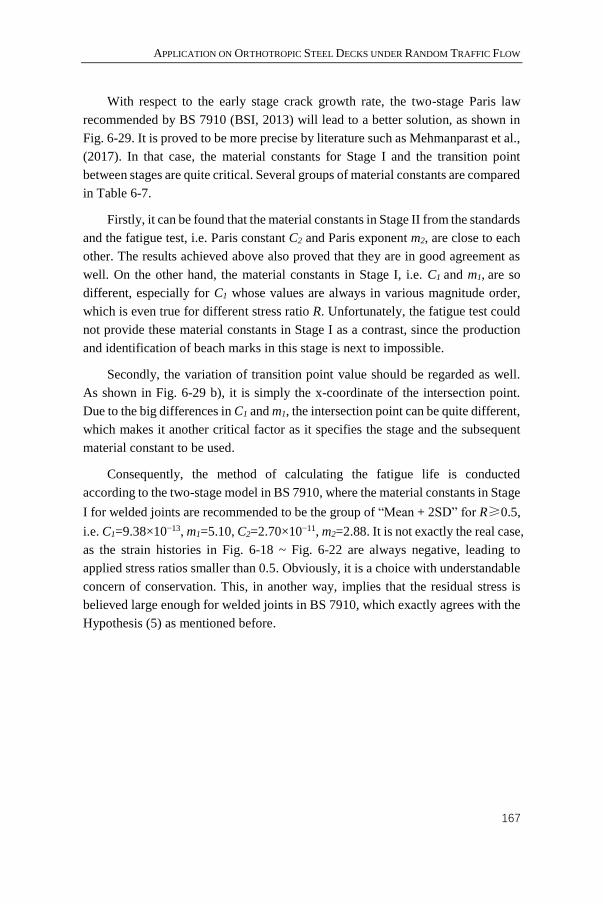
APPLICATION ON ORTHOTROPIC STEEL DECKS UNDER RANDOM TRAFFIC FLOW
167
With respect to the early stage crack growth rate, the two-stage Paris law
recommended by BS 7910 (BSI, 2013) will lead to a better solution, as shown in
Fig. 6-29. It is proved to be more precise by literature such as Mehmanparast et al.,
(2017). In that case, the material constants for Stage I and the transition point
between stages are quite critical. Several groups of material constants are compared
in Table 6-7.
Firstly, it can be found that the material constants in Stage II from the standards
and the fatigue test, i.e. Paris constant C2 and Paris exponent m2, are close to each
other. The results achieved above also proved that they are in good agreement as
well. On the other hand, the material constants in Stage I, i.e. C1 and m1, are so
different, especially for C1 whose values are always in various magnitude order,
which is even true for different stress ratio R. Unfortunately, the fatigue test could
not provide these material constants in Stage I as a contrast, since the production
and identification of beach marks in this stage is next to impossible.
Secondly, the variation of transition point value should be regarded as well.
As shown in Fig. 6-29 b), it is simply the x-coordinate of the intersection point.
Due to the big differences in C1 and m1, the intersection point can be quite different,
which makes it another critical factor as it specifies the stage and the subsequent
material constant to be used.
Consequently, the method of calculating the fatigue life is conducted
according to the two-stage model in BS 7910, where the material constants in Stage
I for welded joints are recommended to be the group of “Mean + 2SD” for R≥0.5,
i.e. C1=9.38×10⁻¹³, m1=5.10, C2=2.70×10⁻¹¹, m2=2.88. It is not exactly the real case,
as the strain histories in Fig. 6-18 ~ Fig. 6-22 are always negative, leading to
applied stress ratios smaller than 0.5. Obviously, it is a choice with understandable
concern of conservation. This, in another way, implies that the residual stress is
believed large enough for welded joints in BS 7910, which exactly agrees with the
Hypothesis (5) as mentioned before.
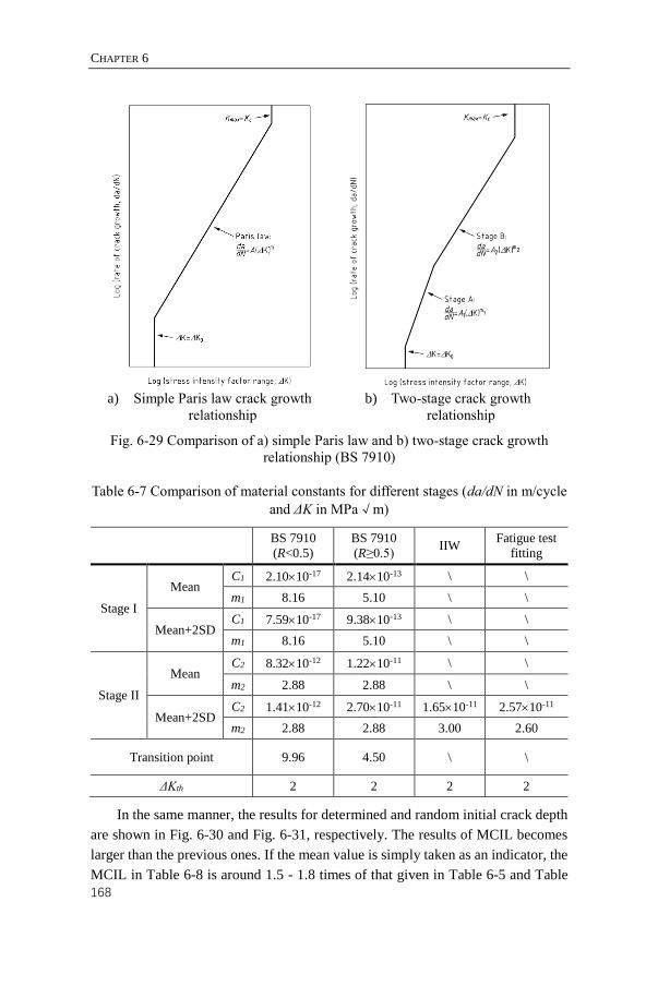
CHAPTER 6
168
a) Simple Paris law crack growth
relationship
b) Two-stage crack growth
relationship
Fig. 6-29 Comparison of a) simple Paris law and b) two-stage crack growth
relationship (BS 7910)
Table 6-7 Comparison of material constants for different stages (da/dN in m/cycle
and ΔK in MPa√m)
BS 7910
(R<0.5)
BS 7910
(R≥0.5) IIW
Fatigue test
fitting
Stage I
Mean C1 2.1010-17 2.1410-13 \ \
m1 8.16 5.10 \ \
Mean+2SD C1 7.5910-17 9.3810-13 \ \
m1 8.16 5.10 \ \
Stage II
Mean C2 8.3210-12 1.2210-11 \ \
m2 2.88 2.88 \ \
Mean+2SD C2 1.4110-12 2.7010-11 1.6510-11 2.5710-11
m2 2.88 2.88 3.00 2.60
Transition point 9.96 4.50 \ \
ΔKth 2 2 2 2
In the same manner, the results for determined and random initial crack depth
are shown in Fig. 6-30 and Fig. 6-31, respectively. The results of MCIL becomes
larger than the previous ones. If the mean value is simply taken as an indicator, the
MCIL in Table 6-8 is around 1.5 - 1.8 times of that given in Table 6-5 and Table
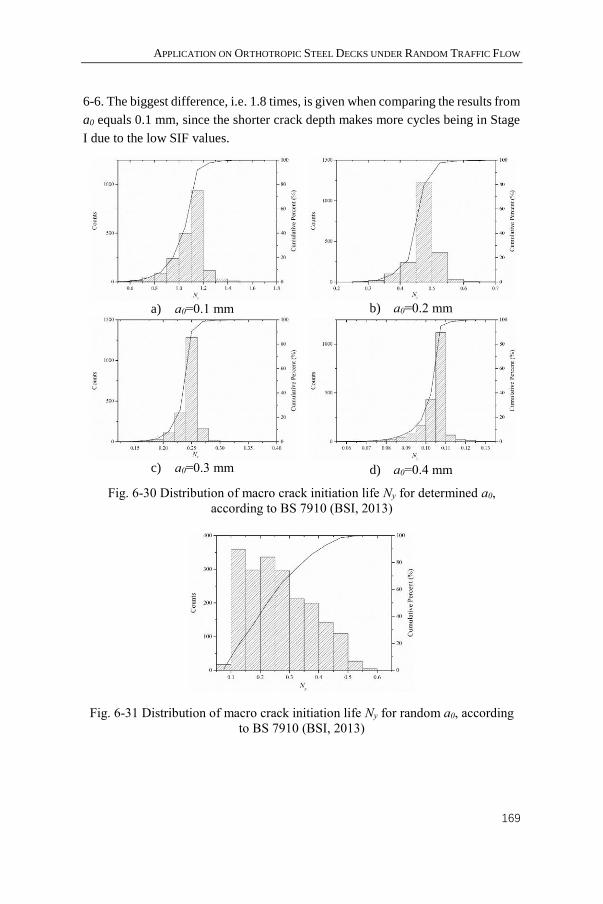
APPLICATION ON ORTHOTROPIC STEEL DECKS UNDER RANDOM TRAFFIC FLOW
169
6-6. The biggest difference, i.e. 1.8 times, is given when comparing the results from
a0 equals 0.1 mm, since the shorter crack depth makes more cycles being in Stage
I due to the low SIF values.
a) a0=0.1 mm
b) a0=0.2 mm
c) a0=0.3 mm
d) a0=0.4 mm
Fig. 6-30 Distribution of macro crack initiation life Ny for determined a0,
according to BS 7910 (BSI, 2013)
Fig. 6-31 Distribution of macro crack initiation life Ny for random a0, according
to BS 7910 (BSI, 2013)

CHAPTER 6
170
Table 6-8 Statistics of MCIL obtained by material constants from BS 7910 (BSI,
2013)
a0 (mm)
MCIL (years)
Mean
value
Standard
deviation CV
Cumulative probability
50% 90% 95% 99%
0.1 1.2644 0.1452 0.1149 1.3006 1.3887 1.4362 1.5904
0.2 0.5569 0.0525 0.0943 0.5700 0.5964 0.6150 0.6834
0.3 0.2865 0.0215 0.0749 0.2919 0.3027 0.3072 0.3331
0.4 0.1212 0.0080 0.0658 0.1238 0.1267 0.1280 0.1372
0.2~0.4 0.3070 0.1288 0.4194 0.2902 0.5019 0.5449 0.5922
Afterwards, the MCGLs are given in Fig. 6-32, and the whole fatigue lives
with respect to initial crack depth of 0.2 ~ 0.4 mm are presented in Fig. 6-33. The
results obtained by BS 7910 are similar to the previous ones. The shortest MCGL
is given by IIW recommendation, and the longest one is provided by the fatigue
test. The one obtained by BS 7910 is in between. Nevertheless, they all lead to a
result that the MCGL is around 1 year, which is still unrealistic. It means the
introduction of Stage I material constants does not matter that much in calculating
MCGL in this case. While speaking of material constants in Stage II, it should be
noted that the values in BS 7910 are even higher than that from the fatigue test and
IIW recommendation.
To sum up, the calculation of fatigue life is certainly improved by applying the
two-stage model. Especially for the part of MCIL, the results seem better to a
certain degree. However, the MCGL is not really affected by it. Eventually, the
whole fatigue life is still not even close to the reality though. With respect to that,
more discussion is provided in the next section.
Fig. 6-32 Macro-crack growth life from 0.5 mm to 7.5 mm according to BS 7910
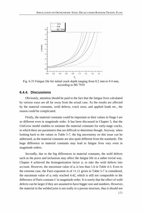
APPLICATION ON ORTHOTROPIC STEEL DECKS UNDER RANDOM TRAFFIC FLOW
171
Fig. 6-33 Fatigue life for initial crack depth ranging from 0.2 mm to 0.4 mm,
according to BS 7910
6.4.4. Discussions
Obviously, attention should be paid to the fact that the fatigue lives calculated
by various ways are all far away from the actual case. As the results are affected
by the material constants, weld defects, crack sizes, and applied loads etc., the
reason could be complicated.
Firstly, the material constants could be important as their values in Stage I are
so different even in magnitude order. It has been discussed in Chapter 5, that the
UniGrow model enables to estimate the material constants for early-stage cracks,
in which there are parameters that are difficult to determine though. Anyway, when
looking back to the values in Table 5-7, the big uncertainty on this issue can be
addressed, as the material constants are also quite different from the standards. The
huge difference in material constants may lead to fatigue lives vary even in
magnitude orders.
Secondly, due to the big differences in material constants, the weld defects
such as the pores and inclusions may affect the fatigue life in a rather trivial way.
Chapter 4 achieved the homogenization factor ac to take the weld defects into
account. However, the maximum value of ac is less than 1.6 in Table 4-3. Even in
the extreme case, the Paris exponent m of 11.11 given in Table 5-7 is considered,
the maximum value of ac only reached 4.42, which is still not comparable to the
difference of Paris constant C in magnitude order. It is surely that the effect of weld
defects can be larger if they are assumed to have bigger size and numbers. However,
the material in the welded joint is not really in a porous structure, thus it should not
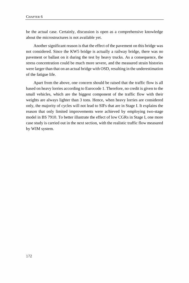
CHAPTER 6
172
be the actual case. Certainly, discussion is open as a comprehensive knowledge
about the microstructures is not available yet.
Another significant reason is that the effect of the pavement on this bridge was
not considered. Since the KW5 bridge is actually a railway bridge, there was no
pavement or ballast on it during the test by heavy trucks. As a consequence, the
stress concentration could be much more severe, and the measured strain histories
were larger than that on an actual bridge with OSD, resulting in the underestimation
of the fatigue life.
Apart from the above, one concern should be raised that the traffic flow is all
based on heavy lorries according to Eurocode 1. Therefore, no credit is given to the
small vehicles, which are the biggest component of the traffic flow with their
weights are always lighter than 3 tons. Hence, when heavy lorries are considered
only, the majority of cycles will not lead to SIFs that are in Stage I. It explains the
reason that only limited improvements were achieved by employing two-stage
model in BS 7910. To better illustrate the effect of low CGRs in Stage I, one more
case study is carried out in the next section, with the realistic traffic flow measured
by WIM system.
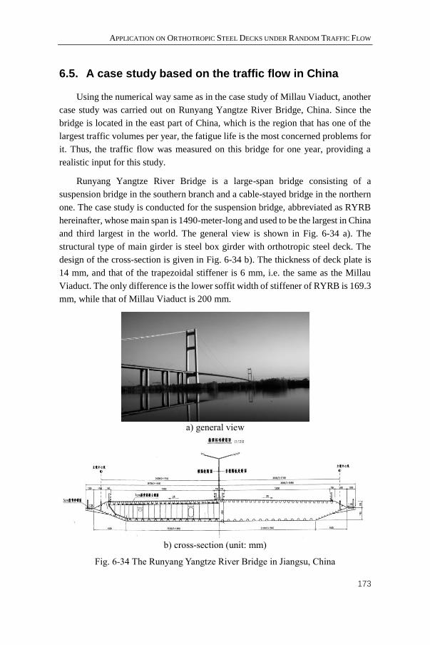
APPLICATION ON ORTHOTROPIC STEEL DECKS UNDER RANDOM TRAFFIC FLOW
173
6.5. A case study based on the traffic flow in China
Using the numerical way same as in the case study of Millau Viaduct, another
case study was carried out on Runyang Yangtze River Bridge, China. Since the
bridge is located in the east part of China, which is the region that has one of the
largest traffic volumes per year, the fatigue life is the most concerned problems for
it. Thus, the traffic flow was measured on this bridge for one year, providing a
realistic input for this study.
Runyang Yangtze River Bridge is a large-span bridge consisting of a
suspension bridge in the southern branch and a cable-stayed bridge in the northern
one. The case study is conducted for the suspension bridge, abbreviated as RYRB
hereinafter, whose main span is 1490-meter-long and used to be the largest in China
and third largest in the world. The general view is shown in Fig. 6-34 a). The
structural type of main girder is steel box girder with orthotropic steel deck. The
design of the cross-section is given in Fig. 6-34 b). The thickness of deck plate is
14 mm, and that of the trapezoidal stiffener is 6 mm, i.e. the same as the Millau
Viaduct. The only difference is the lower soffit width of stiffener of RYRB is 169.3
mm, while that of Millau Viaduct is 200 mm.
a) general view
b) cross-section (unit: mm)
Fig. 6-34 The Runyang Yangtze River Bridge in Jiangsu, China

CHAPTER 6
174
6.5.1. Traffic flow
Different from the first case study using Monte-Carlo simulation based on
short-term data, the traffic flow is measured for a long period on this bridge with a
WIM system. It was installed in both directions, i.e. all 6 lanes of the bridge, and
consisted of two parallel piezoceramic sensors and one induction coil on each lane.
Additionally, the temperature sensor was also included for the calibration of the
temperature strains. Unlike the WIM system on SJDV in the case study of Millau
Viaduct, this one was designed without the diagonal piezoceramic sensor and thus
was not able to measure the exact transverse in-lane position of vehicles.
The final output of this WIM system can provide data about the type, speed,
total length, wheel bases, number of axles, axle weights for each vehicle, as well
as the lane it runs over and the temperature at that moment. The technical
specifications of the WIM system are listed in Table 6-9. One thing worth to
mention is the difficulty in determining the single or double tire for each axle,
which may affect the stress range history due to the different landing area. None of
the measured data could be an accurate indicator. To evaluate it, more discussions
will be provided with respect to the influence surface in the next section.
Since the RYRB has been put into service for more than 11 years, the total
traffic volume per year can be quite stable at present. Therefore, when predicting
the fatigue life in the future, the calculation can be based on the traffic data for a
recent year, which is the year of 2016 in this case. Due to the system maintenance,
the traffic data for the period from June 15 to June 19, and from November 18 to
December 4 are not available, which gives the data for 345 days in total. However,
if the history of the fatigue life is to be traced, this measured traffic flow may be
larger than the actual case in term of total volume, and the fatigue life will be
underestimated.
Table 6-9 The technical specifications of the WIM system on RYRB
Total weight error < 10% Accuracy for vehicle classification
Maximum axle weight > 30t per axle
Measured traffic flow accuracy > 98% Car 95%
Vehicle speed 25 ~ 180 kph Light lorry 95%
Vehicle speed error < 1.5% Medium lorry 98%
Wheel base error < 2% Heavy lorry 99%
Total length error < 7% Coach 95%
Temperature -30 ~ 65℃ Articulated vehicle 99%
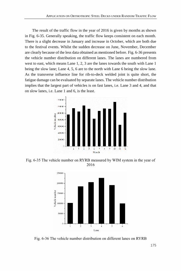
APPLICATION ON ORTHOTROPIC STEEL DECKS UNDER RANDOM TRAFFIC FLOW
175
The result of the traffic flow in the year of 2016 is given by months as shown
in Fig. 6-35. Generally speaking, the traffic flow keeps consistent on each month.
There is a slight decrease in January and increase in October, which are both due
to the festival events. Whilst the sudden decrease on June, November, December
are clearly because of the less data obtained as mentioned before. Fig. 6-36 presents
the vehicle number distribution on different lanes. The lanes are numbered from
west to east, which means Lane 1, 2, 3 are the lanes towards the south with Lane 1
being the slow lane; Lane 4, 5, 6 are to the north with Lane 6 being the slow lane.
As the transverse influence line for rib-to-deck welded joint is quite short, the
fatigue damage can be evaluated by separate lanes. The vehicle number distribution
implies that the largest part of vehicles is on fast lanes, i.e. Lane 3 and 4, and that
on slow lanes, i.e. Lane 1 and 6, is the least.
Fig. 6-35 The vehicle number on RYRB measured by WIM system in the year of
2016
Fig. 6-36 The vehicle number distribution on different lanes on RYRB
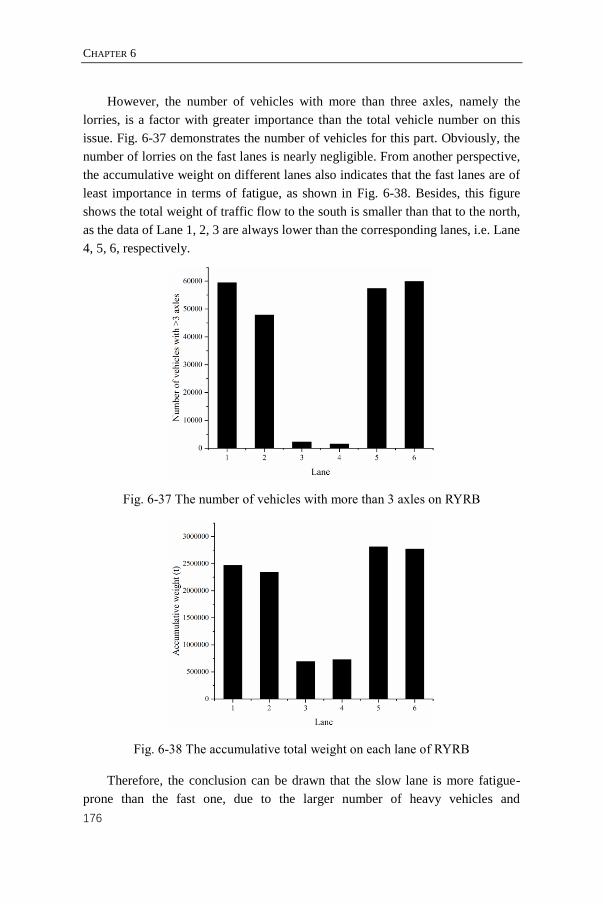
CHAPTER 6
176
However, the number of vehicles with more than three axles, namely the
lorries, is a factor with greater importance than the total vehicle number on this
issue. Fig. 6-37 demonstrates the number of vehicles for this part. Obviously, the
number of lorries on the fast lanes is nearly negligible. From another perspective,
the accumulative weight on different lanes also indicates that the fast lanes are of
least importance in terms of fatigue, as shown in Fig. 6-38. Besides, this figure
shows the total weight of traffic flow to the south is smaller than that to the north,
as the data of Lane 1, 2, 3 are always lower than the corresponding lanes, i.e. Lane
4, 5, 6, respectively.
Fig. 6-37 The number of vehicles with more than 3 axles on RYRB
Fig. 6-38 The accumulative total weight on each lane of RYRB
Therefore, the conclusion can be drawn that the slow lane is more fatigue-
prone than the fast one, due to the larger number of heavy vehicles and
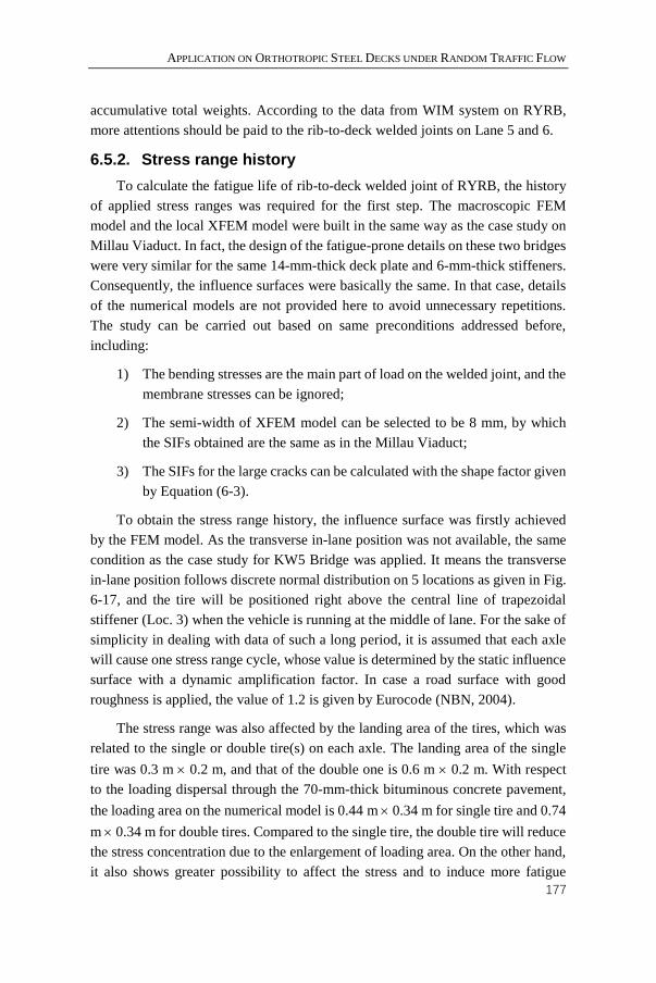
APPLICATION ON ORTHOTROPIC STEEL DECKS UNDER RANDOM TRAFFIC FLOW
177
accumulative total weights. According to the data from WIM system on RYRB,
more attentions should be paid to the rib-to-deck welded joints on Lane 5 and 6.
6.5.2. Stress range history
To calculate the fatigue life of rib-to-deck welded joint of RYRB, the history
of applied stress ranges was required for the first step. The macroscopic FEM
model and the local XFEM model were built in the same way as the case study on
Millau Viaduct. In fact, the design of the fatigue-prone details on these two bridges
were very similar for the same 14-mm-thick deck plate and 6-mm-thick stiffeners.
Consequently, the influence surfaces were basically the same. In that case, details
of the numerical models are not provided here to avoid unnecessary repetitions.
The study can be carried out based on same preconditions addressed before,
including:
1) The bending stresses are the main part of load on the welded joint, and the
membrane stresses can be ignored;
2) The semi-width of XFEM model can be selected to be 8 mm, by which
the SIFs obtained are the same as in the Millau Viaduct;
3) The SIFs for the large cracks can be calculated with the shape factor given
by Equation (6-3).
To obtain the stress range history, the influence surface was firstly achieved
by the FEM model. As the transverse in-lane position was not available, the same
condition as the case study for KW5 Bridge was applied. It means the transverse
in-lane position follows discrete normal distribution on 5 locations as given in Fig.
6-17, and the tire will be positioned right above the central line of trapezoidal
stiffener (Loc. 3) when the vehicle is running at the middle of lane. For the sake of
simplicity in dealing with data of such a long period, it is assumed that each axle
will cause one stress range cycle, whose value is determined by the static influence
surface with a dynamic amplification factor. In case a road surface with good
roughness is applied, the value of 1.2 is given by Eurocode (NBN, 2004).
The stress range was also affected by the landing area of the tires, which was
related to the single or double tire(s) on each axle. The landing area of the single
tire was 0.3 m 0.2 m, and that of the double one is 0.6 m 0.2 m. With respect
to the loading dispersal through the 70-mm-thick bituminous concrete pavement,
the loading area on the numerical model is 0.44 m 0.34 m for single tire and 0.74
m 0.34 m for double tires. Compared to the single tire, the double tire will reduce
the stress concentration due to the enlargement of loading area. On the other hand,
it also shows greater possibility to affect the stress and to induce more fatigue
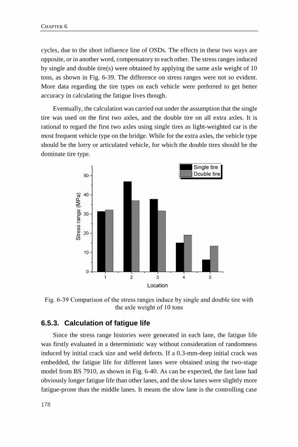
CHAPTER 6
178
cycles, due to the short influence line of OSDs. The effects in these two ways are
opposite, or in another word, compensatory to each other. The stress ranges induced
by single and double tire(s) were obtained by applying the same axle weight of 10
tons, as shown in Fig. 6-39. The difference on stress ranges were not so evident.
More data regarding the tire types on each vehicle were preferred to get better
accuracy in calculating the fatigue lives though.
Eventually, the calculation was carried out under the assumption that the single
tire was used on the first two axles, and the double tire on all extra axles. It is
rational to regard the first two axles using single tires as light-weighted car is the
most frequent vehicle type on the bridge. While for the extra axles, the vehicle type
should be the lorry or articulated vehicle, for which the double tires should be the
dominate tire type.
Fig. 6-39 Comparison of the stress ranges induce by single and double tire with
the axle weight of 10 tons
6.5.3. Calculation of fatigue life
Since the stress range histories were generated in each lane, the fatigue life
was firstly evaluated in a deterministic way without consideration of randomness
induced by initial crack size and weld defects. If a 0.3-mm-deep initial crack was
embedded, the fatigue life for different lanes were obtained using the two-stage
model from BS 7910, as shown in Fig. 6-40. As can be expected, the fast lane had
obviously longer fatigue life than other lanes, and the slow lanes were slightly more
fatigue-prone than the middle lanes. It means the slow lane is the controlling case
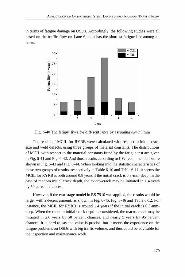
APPLICATION ON ORTHOTROPIC STEEL DECKS UNDER RANDOM TRAFFIC FLOW
179
in terms of fatigue damage on OSDs. Accordingly, the following studies were all
based on the traffic flow on Lane 6, as it has the shortest fatigue life among all
lanes.
Fig. 6-40 The fatigue lives for different lanes by assuming a0=0.3 mm
The results of MCIL for RYRB were calculated with respect to initial crack
size and weld defects, using three groups of material constants. The distributions
of MCIL with respect to the material constants fitted by the fatigue test are given
in Fig. 6-41 and Fig. 6-42. And those results according to IIW recommendation are
shown in Fig. 6-43 and Fig. 6-44. When looking into the statistic characteristics of
these two groups of results, respectively in Table 6-10 and Table 6-11, it seems the
MCIL for RYRB is both around 0.8 years if the initial crack is 0.3-mm-deep. In the
case of random initial crack depth, the macro-crack may be initiated in 1.4 years
by 50 percent chances.
However, if the two-stage model in BS 7910 was applied, the results would be
larger with a decent amount, as shown in Fig. 6-45, Fig. 6-46 and Table 6-12. For
instance, the MCIL for RYRB is around 1.4 years if the initial crack is 0.3-mm-
deep. When the random initial crack depth is considered, the macro-crack may be
initiated in 2.6 years by 50 percent chances, and nearly 5 years by 95 percent
chances. It is hard to say the value is precise, but it meets the experience on the
fatigue problems on OSDs with big traffic volume, and thus could be advisable for
the inspection and maintenance work.
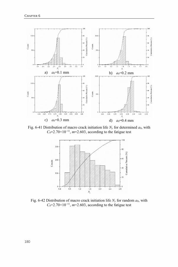
CHAPTER 6
180
a) a0=0.1 mm
b) a0=0.2 mm
c) a0=0.3 mm
d) a0=0.4 mm
Fig. 6-41 Distribution of macro crack initiation life Ny for determined a0, with
C0=2.70×10⁻¹¹, m=2.603, according to the fatigue test
Fig. 6-42 Distribution of macro crack initiation life Ny for random a0, with
C0=2.70×10⁻¹¹, m=2.603, according to the fatigue test
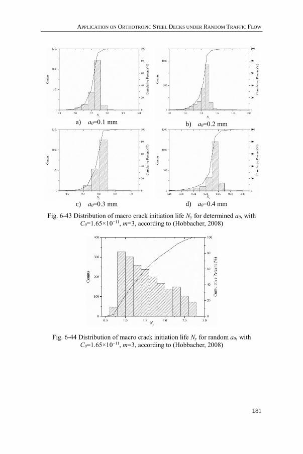
APPLICATION ON ORTHOTROPIC STEEL DECKS UNDER RANDOM TRAFFIC FLOW
181
a) a0=0.1 mm
b) a0=0.2 mm
c) a0=0.3 mm
d) a0=0.4 mm
Fig. 6-43 Distribution of macro crack initiation life Ny for determined a0, with
C0=1.65×10⁻¹¹, m=3, according to (Hobbacher, 2008)
Fig. 6-44 Distribution of macro crack initiation life Ny for random a0, with
C0=1.65×10⁻¹¹, m=3, according to (Hobbacher, 2008)
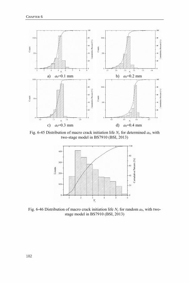
CHAPTER 6
182
a) a0=0.1 mm
b) a0=0.2 mm
c) a0=0.3 mm
d) a0=0.4 mm
Fig. 6-45 Distribution of macro crack initiation life Ny for determined a0, with
two-stage model in BS7910 (BSI, 2013)
Fig. 6-46 Distribution of macro crack initiation life Ny for random a0, with two-
stage model in BS7910 (BSI, 2013)

APPLICATION ON ORTHOTROPIC STEEL DECKS UNDER RANDOM TRAFFIC FLOW
183
Table 6-10 Statistics of MCIL obtained by material constants fitted with fatigue
test
a0 (mm)
MCIL (years)
Mean
value
Standard
deviation CV
Cumulative probability
50% 90% 95% 99%
0.1 2.5011 0.1514 0.0605 2.5418 2.6284 2.6738 2.8167
0.2 1.3918 0.0682 0.0490 1.4100 1.4430 1.4658 1.5468
0.3 0.7812 0.0307 0.0393 0.7892 0.8040 0.8101 0.8443
0.4 0.3455 0.0121 0.0349 0.3494 0.3535 0.3554 0.3682
0.2~0.4 1.4900 0.5109 0.3429 1.4130 2.2524 2.4035 2.5729
Table 6-11 Statistics of MCIL obtained by material constants from IIW
Recommendation (Hobbacher, 2008)
a0 (mm)
MCIL (years)
Mean
value
Standard
deviation CV
Cumulative probability
50% 90% 95% 99%
0.1 2.6412 0.1821 0.0694 2.6726 2.7777 2.8331 3.0083
0.2 1.4414 0.0811 0.0563 1.4628 1.5024 1.5298 1.6276
0.3 0.8018 0.0361 0.0451 0.8111 0.8286 0.8359 0.8768
0.4 0.3520 0.0141 0.0400 0.3566 0.3615 0.3636 0.3788
0.2~0.4 1.5478 0.5429 0.3507 1.4554 2.3638 2.5272 2.7102
Table 6-12 Statistics of MCIL obtained by material constants from BS 7910 (BSI,
2013)
a0 (mm)
MCIL (years)
Mean
value
Standard
deviation CV
Cumulative probability
50% 90% 95% 99%
0.1 5.1192 0.5880 0.1149 5.2657 5.6225 5.8146 6.4391
0.2 2.5927 0.2445 0.0943 2.6537 2.7768 2.8634 3.1818
0.3 1.3694 0.1026 0.0749 1.3949 1.4465 1.4681 1.5921
0.4 0.5782 0.0381 0.0658 0.5904 0.6043 0.6104 0.6544
0.2~0.4 2.8411 1.1335 0.3990 2.6046 4.5619 4.9709 5.4130
In terms of MCGL, the difference between three different models was not so
obvious. According to the results shown in Fig. 6-47, the MCGLs are always in a
range from 4 to 4.5 years. One noticeable change compared to Fig. 6-32 for KW5
Bridge is that the results from BS 7910 is obviously larger than those from the test.
The reason is, when big amounts of light vehicles, such as cars and light lorries,
are taken into account, the CGRs in Stage I are more influential as more cycles will
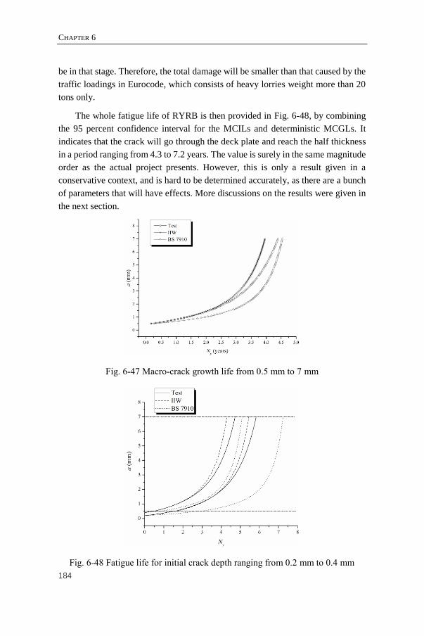
CHAPTER 6
184
be in that stage. Therefore, the total damage will be smaller than that caused by the
traffic loadings in Eurocode, which consists of heavy lorries weight more than 20
tons only.
The whole fatigue life of RYRB is then provided in Fig. 6-48, by combining
the 95 percent confidence interval for the MCILs and deterministic MCGLs. It
indicates that the crack will go through the deck plate and reach the half thickness
in a period ranging from 4.3 to 7.2 years. The value is surely in the same magnitude
order as the actual project presents. However, this is only a result given in a
conservative context, and is hard to be determined accurately, as there are a bunch
of parameters that will have effects. More discussions on the results were given in
the next section.
Fig. 6-47 Macro-crack growth life from 0.5 mm to 7 mm
Fig. 6-48 Fatigue life for initial crack depth ranging from 0.2 mm to 0.4 mm
APPLICATION ON ORTHOTROPIC STEEL DECKS UNDER RANDOM TRAFFIC FLOW
185
6.5.4. Discussions
The parameters, such as the unknown weld defects, the residual stresses, are
certainly important for the results, as discussed before. Apart from that, this case
study was carried out conservatively in other aspects, and the possible sources of
error should be analyzed.
Firstly, only the load dispersal effect of the pavement was taken into account
in the calculation, and the effect on reducing the stresses of weld joints was
neglected. Literatures show a reduction up to 20 to 30 percent of stresses (De
Backer et al., 2008), depending on the type of it. However, this effect is severely
affected by the temperatures and thus hard to quantify.
Secondly, the traffic flow was measured for the year of 2016, which means the
traffic volume has already increased to a certain level. Therefore, the stress range
history was in fact overestimated when applying to the initial crack. However, as
the WIM system was not installed on RYRB for the early years, no data was
available to evaluate the error.
Thirdly, the applied transverse in-lane position was from the Eurocode, which
follows normal distribution and could be unrealistic. The measured transverse in-
lane positions by the WIM system of Millau Viaduct implied that a Gumbel
distribution will be more proper (Wang et al., 2017). Nevertheless, it was also
dependent on the lane layout and the driving custom in the local region, thus the
suggestion on the Eurocode was applied.
Additionally, the results were related to material constants in both Stage I and
II. The material constants in Stage I are quite sensitive factors to the results, since
it not only determines the CGR but also affects the transition point that defines the
stages. Therefore, the material constants are extremely significant when the
realistic traffic load, which consists of big amounts of light vehicles, is considered.
However, their values provided in various sources are surely far away from
consistent. On the other hand, the material constants in Stage II are pretty similar,
and thus is more reliable.
In summary, regarding the various parameters, the precise fatigue life
calculation for OSD requires a thorough knowledge concerning multiple areas.
However, the limit on the experimental or measuring method makes it difficult,
especially for the Stage I crack growth rate, residual stresses and weld defects.

CHAPTER 6
186

CHAPTER 7
CONCLUSIONS AND
FUTURE RESEARCHES
________________________________
CHAPTER 7
188
7.1. Conclusions
On the issue of the common fatigue problems on orthotropic steel decks
(OSDs), the traditional studies are proven to be not reliable, as the fatigue tests fail
to achieve consistent results, and the numerical investigations are not always on the
safe side according to the experiences on actual projects. It could be attributed to
the fact that the parameters in multiple scales are not taken into account, especially
the ones related to the early-stage fatigue cracks. This study is carried out with
respect to multiscale concerns, to propose an efficient and simple method that is
applicable on the actual projects.
In Chapter 1, a general introduction on the issue of fatigue problems on
orthotropic steel decks was provided. The literature related to the fatigue design,
and fatigue-prone details on OSDs were reviewed first, leading the subject to that
related to the weld fatigue under structural loadings, which is a multiscale problem
essentially. Accordingly, a few objectives were put forward for this study.
For the first step, a fatigue test on small scale specimens was conducted, as
elaborated in Chapter 2. The test results suggested that the fatigue crack always
occurs at the rib-to-deck weld toe, and caused final fracture of the specimens. In
order to understand the behavior in the whole process of fatigue crack growth, the
applied loadings were designed to generate beach marks during the test, and the
fractographic and metallographic analyses were carried out after the specimen fails.
A preliminary analysis implied that the heterogeneities of microstructures and weld
defects will affect the crack growth rates (CGRs) in early stages. Therefore, with
respect to the uncertainties in such a meso-scale, a tool with great efficiency for
massive computation was to be developed.
Chapter 3 introduced the brief idea of extended finite element method
(XFEM), which was perfect in dealing with the discontinuity problems. As the
geometries were independent to meshes, the XFEM apparently owns the advantage
of being free for re-mesh, which was quite beneficial when random weld defects
were to be evaluated by solving a big number of representative volume elements
(RVEs). Therefore, an XFEM program was developed using MATLAB, with
which the random defects can be taken into account. Additionally, to be feasible
on the RVEs extracted from rib-to-deck welded joints, a specific level-set function
was established regarding the weld geometries, namely the weld toe flank angles.
Based on the XFEM program, Chapter 4 proposed a homogenization method
on weld defects, with a criteria of equivalent crack growth length. Numerical
examples and parametric analysis were conducted for validation. However, there
CONCLUSIONS AND FUTURE RESEARCHES
189
lacked knowledge on the sizes, numbers and spatial distributions of weld defects,
due to the limitation of detection or identification technologies, even though they
can be occasionally observed by scanning electron microscope (SEM). Therefore,
the homogenization can only be conducted under several assumptions about the
weld defects.
In Chapter 5, multiscale methods were built in a numerical way with respect
to the fatigue test. The identification of the beach marks, namely the crack shapes
and dimensions, was given in the first place. Accordingly, a relation between the
crack face area and the crack depth was proposed to avoid the problem in
calculation because of the longitudinal initial crack merging. Then two multiscale
methods were established and compared, and the crack growth behaviors in
correspondence with the stress intensity factors were analyzed. As a result,
different stages in crack growth can be addressed, among which the Stage I and II
are of main concern on this issue. The achieved material constants in Stage II
seemed to agree with the ones provided in the standards, but those for Stage I is not
clear enough, as the fatigue test cannot provide sufficient information on the CGRs
in this stage.
Chapter 6 further introduced all the methods and knowledges above into the
application on three actual projects, including the Millau Viaduct in southeast
France, the KW5 Bridge on Albert Canal, Belgium, and the Runyang Yangtze
River Bridge, China. In summary of the results, the traffic flow on the bridge will
affect the fatigue lives significantly. Apart from that, the material constants of the
fatigue-prone details are of great importance as well, thus three groups of them are
applied in the calculation, including: a) fitted by the test results given in Chapter 5;
b) from the IIW recommendation; c) from the British standard BS 7910,
abbreviated as Group a, b, and c hereinafter, respectively. Among them, the Group
c was using a two-stage model that pays more attentions to the low CGR in Stage
I, and thus will achieve better results.
In the study on Millau Viaduct, the traffic flow was provided using Monte-
Carlo simulation based on a short-term data from WIM system. The WIM system
was designed with an extra diagonal piezoceramic sensor, thus the precise
transverse in-lane position of tires were measured. With the numerical method
provided in Chapter 5, the fatigue lives were calculated with material constants of
Group a & b. The results were in good agreement with each other, showing the
fatigue life of more than 32 years even in a conservative scenario. It can be
concluded that the fatigue problem is not a major concern for Millau Viaduct, due
to the relatively small traffic volume in that region.
CHAPTER 7
190
As for the study on KW5 Bridge, the traffic flow and transverse in-lane
positions were hypothetic according to Eurocode 1 (NBN, 2004). The fatigue
cycles were calculated based on the on-site test results of strains. However, the
fatigue lives were extremely low when calculated by material constants of Group
a & b. With respect to the low CGR in Stage I, the material constants of Group c
were then introduced. The results were improved to a certain degree, but still far
from acceptable, which could be attributed to the large and design-oriented traffic
volume consists of lorries only.
In that case, the study on Runyang Yangtze River Bridge was carried out, with
a long-term traffic flow data measured by WIM system for one year. When using
the results corresponding to a cumulative probability of 50 % as an indicator, the
MCILs obtained by material constants of Group a & b were less than 1.5 years,
which were still quite small. In contrast, that value obtained by two-stage model of
Group c was 2.6 years. The fatigue life till crack reaching half thickness of the deck
plate was in a range from 5 to 7.2 years, which was in the same order of magnitude
as the actual project presents, even provided in a conservative context. The result
can be advisable on the time to conduct visual inspections and further retrofitting
works.
7.2. The outcome regarding the objectives
To further emphasize the outcome of this study, the following key points are
elaborated in correspondence with the problems and objectives brought up in
Chapter 1.
1) A process-oriented fatigue test on specimens of OSD was designed
and conducted. During the test, beach marks were produced by applying
cyclic loads with different ranges and types, according to which the crack
sizes and crack growth rates in different stages can be addressed. After
the fatigue failure of each specimen, the fractography and metallography
in the region of interest were analyzed. The results pointed out that the
coarse grained HAZ is vulnerable to cyclic loads, as the intergranular
crack occurs primarily there, and thus can be regarded as the initial crack.
2) An XFEM program was developed in order to numerically
investigate the randomness in crack sizes, weld defects of mesoscopic
models, and a homogenization method with a criteria of equivalent
crack growth length was put forward to make it feasible in multiscale
problems. To validate the homogenization method, some numerical
examples are provided, showing that the error is tiny due to the relatively
small crack growth rate of early-stage cracks. The parametric analysis of
the homogenization method presented the main factors of the weld
CONCLUSIONS AND FUTURE RESEARCHES
191
defects on crack growth problems. It can be inferred that the large
standard deviation of the effects from non-detectable weld defects could
be important, since the weakest part is always critical for macroscopic
structures.
3) Two types of multiscale methods were established to link the
macroscopic model and the mesoscopic one. The homogenization
method gives the access to consider weld defects in multiscale problems.
However, the crack itself, especially being a long and shallow one in the
early-stage, is difficult to consider due to the computation ability issue.
Thus, two types of multiscale methods, i.e. a sub-model based one and a
non-concurrent one, were established and applied to calculate the stress
intensity factors of the cracks in the test, and to reproduce the crack
growth process of the test. Both of them were built with a combination of
the XFEM program developed in Chapter 3 and the software SAMCEF
with an XFEM module embedded. The comparison of them confirmed
that the non-concurrent multiscale method is of good accuracy, and most
importantly, has great efficiency in calculating the stress intensity factors,
as it uses a mesoscopic model fully independent to the macroscopic one.
4) Three case studies on actual projects were carried out, obtaining the
fatigue life of OSDs under realistic or standards-specified traffic
loads. The fatigue life was calculated in two parts, i.e. the calculation
of macro crack initiation life (MCIL), and macro crack growth life
(MCGL). The former one was given in a probabilistic way for the sake of
the randomness induced by the initial crack depth and other weld defects.
Whilst the latter one was provided in a deterministic way as the uncertain
influence factors were of less scatter then. The results show that the traffic
flow on the Millau Viaduct is much lighter or easier than that on the
Runyang Yangtze River Bridge. Hence, the fatigue problem will not be a
concern for Millau Viaduct in decades, while in contrast, the Runyang
Yangtze River Bridge may suffer from it in less than ten years. In addition,
according to the short and unrealistic fatigue life obtained for KW5
Bridge, the traffic load recommended by Eurocode is not proper when
using fracture mechanics to evaluate the fatigue performance.
7.3. Future researches
This dissertation provides proposals to study the fatigue problems on OSDs in
a multiscale context. With parameters obtained by the fatigue test, the fatigue lives
of projects under various random traffic loadings are calculated, and validated by
comparing with the ones with standards or specifications. On the other hand, some
hypotheses are addressed as preconditions in building and conducting the method,
and the obtained results should be used with caution, as discussed in the previous
chapters. To better understand the fatigue behavior and predict the fatigue life with
higher accuracy, future works are required for the following aspects.
CHAPTER 7
192
7.3.1. Residual stress acquisition
The residual stress is often taken as a major reason of the fatigue failure, and
the reduction of it is proven quite beneficial to the fatigue performance of structures.
However, as the residual stress itself will not produce a stress range, it mainly
affects the mean stress of fatigue cycles, or in another classical way on fatigue
studies, the stress ratio. A similar concept of effective stress ratio was proposed by
(Barsoum & Barsoum, 2009) to consider the weld residual stress. In case the
fracture mechanics is applied on this issue, the residual stress could affect the SIF
range, as the compressive stresses will lead to zero-value SIFs instead of negative
ones. Hence, the fatigue life of welded joint is surely getting shorter if the tensile
residual stress, as the mean stress, is larger than the stress induced by compressive
applied loads. Another possible solution is to use an effective stress intensity factor
range as a combination of the maximum value and the applied value. It will, of
course, result in a different set of material properties compared to classical Paris
law. By any means, the comprehensive knowledge on residual stresses is required.
Various problems may appear in the residual stress acquisition by experimental or
numerical ways, especially on the spatial distribution. Afterwards, it is possible to
investigate and understand the effect of residual stress on fatigue performance
profoundly.
7.3.2. Fatigue behavior in Stage I
The discussions in previous chapters, especially the ones in Chapter 5 and 6,
indicated the importance of a clear view of fatigue behavior in Stage I. The
homogenization method shows that the weld defects may only take a small part of
the reasons that causes the scattered CGRs in Stage I. However, the realistic sizes,
shapes, and spatial distributions of them are waiting to be determined, which is still
a job with considerable difficulties. On the other hand, the heterogeneous materials
in the welded joints could be a more important factor waiting to be explored.
Literatures have proposed different models to calculate the crack growth on that
issue (Remes et al., 2012, Mikheevskiy et al., 2015), and basically a relevance can
be addressed between the microscopic hardness and the material properties
concerning fatigue performance. The problem is that not all parameters in these
models are measurable, or even next to impossible to determine for macroscopic
structural projects, not to mention that none of these models showed universal
applicability. Therefore, future works should be focused on this part, to propose a
model that is feasible for welded joints of OSDs.
CONCLUSIONS AND FUTURE RESEARCHES
193
7.3.3. Retrofitting work on cracked components of OSDs
The end point in this study is set to be the moment crack reaches half thickness
of deck plate, as it is when the visual inspection can easily address fatigue crack
due to the damage of paint films. Additionally, as the crack tip is already far away
from the HAZ, it can be inferred that the effect of residual stress could be a lot less
than that in the initial state, even though the actual distribution may not be clearly
known. Under that circumstance, the cracked area can be retrofitted and renovated
to keep other types of damages from being introduced, such as corrosion and rust.
If that is not the case, the crack may grow through the deck plate in a much lower
CGR or even stop growing by itself. Hence, one of the future researches is the
retrofitting job to prevent further damages for cracks, including the evaluation of
the necessity to retrofit as well.
7.3.4. Other types of cracks on OSDs
Even though the fatigue crack at weld toe caused the failure on all specimens
in the fatigue test and in other reported tests on small-scale specimens, it is not the
most observed type of crack on actual OSDs. Comparatively, fatigue cracks on the
rib-to-diaphragm welded joints are more common. Most of the cracks, including
the rib-to-deck weld toe crack, belong to the detectable and fixable category, and
are not so harmful to the whole OSD. The only exception is the rib-to-deck weld
root crack, which is dangerous because of the apparent difficulty in inspections.
After it goes through the weld bead or, in the worst case, the deck plate, the fatigue
damage could have caused severe reduction of serviceability. The maintenance cost
can be quite high then. Therefore, future research on predicting the rib-to-deck
weld root crack should be conducted, to provide practical recommendations on
dealing with this type of crack. For that purpose, the experimental study is certainly
preferred, on large-scale specimens, or on well-designed small-scale specimens
with diaphragms as analyzed in Chapter 2.
7.3.5. Novel fatigue design methods for OSDs
After all, the studies on fatigue mechanisms and all influence factors should
be put into practice, and thus gives two requirements to the design methods for
OSDs to fulfill: i) in a probabilistic context and ii) with solutions to multiscale
problems. The former one provides the capability to consider the mesoscopic or
even microscopic characteristics, as they are inevitably with uncertainties, whilst
the latter one ensures the feasibility on the macroscopic structures. Based on the
widely-applied methods nowadays, the design theory for reliability is a suitable
option. In the meantime, a direct probabilistic design theory may provide an
alternative way. From another perspective, a design method with respect to the cost

CHAPTER 7
194
during the whole life-cycle is also valuable on this issue, due to the considerable
amount of it compared to the construction cost. It is quite true for structures like
OSDs specifically, since the fatigue crack is not really devastating to the structural
safety itself, but requires frequent inspections and retrofits for the sake of
serviceability.
APPENDIX A
With the micro-chemical energy analyses using the energy dispersive
spectroscopy (EDS) device of the laboratory, Bruker Quatanax 200, the chemical
composition of inclusions can be achieved. Two inclusions found by both
fractographic and metallographic analysis, noted as Inclusion I and Inclusion II
respectively, were given as an instance here.
Fig. A-1 presents an analysis on Inclusion I by fractograhpy, which seems like
a void or a secondary crack on the image. According to the results, the chemical
composition of it is MnS, indicating that there is an entity of it, and lead to a void
on the fracture face consequently. In contrast, Fig. A-2 gives a clearer instance by
analyzing Inclusion II on metallogrphy. Simiarly with the previous one, the
inclusion is also mainly MnS, while there could be other complex oxides combined
as well.

APPENDIX A
196
Fig. A-1 The micro-chemical energy analyses on Inclusion I
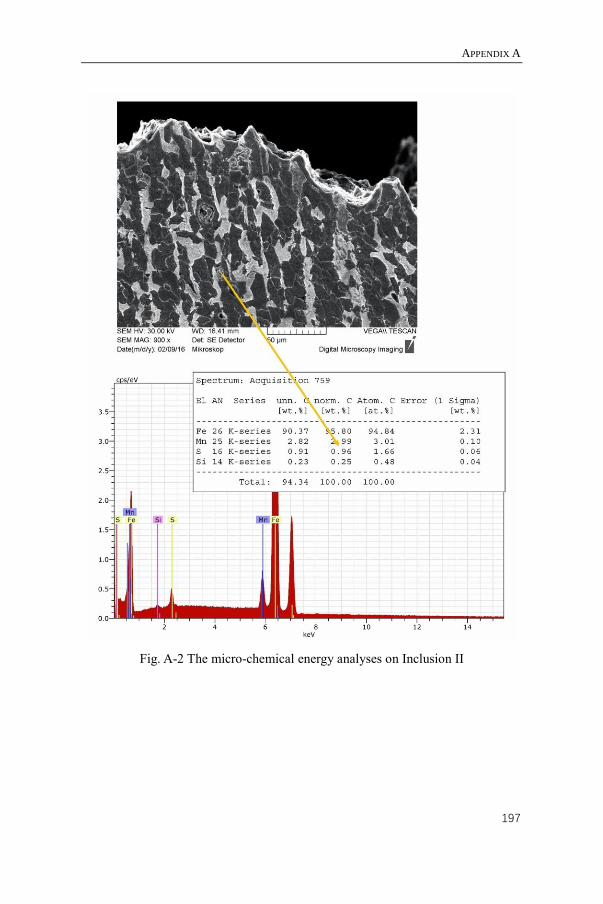
APPENDIX A
197
Fig. A-2 The micro-chemical energy analyses on Inclusion II

APPENDIX A
198

APPENDIX B
To analyze the crack growth rate for the test specimens, a method of
calculating the SIFs is necessary under the frame of fracture mechanics. A widely-
accepted way is to calculate it based on Equation (2-4), in which the shape factor
F is related to complex geometrical parameters. On the issue of a semi-elliptical
cracks on T-butt joint, Bowness and Lee (2000) conducted a parametric study on
the effect of geometry to SIFs, stated that the crack depth a, the crack half length,
c, the deck plate thickness, T, the weld toe flank angle, θ, and the attachment
(including the stiffener and the weld) width on deck plate, L, are the main factors,
as shown in Fig. B-1.
Fig. B-1 Geometrical parameters that affect the SIF of weld toe crack (Bowness
and Lee, 2000)
Accordingly, the empirical equation they put forward to calculate F was
adopted in the preliminary study on the test, as given by
𝐹 = 𝑓1 (𝑎
𝑇,𝑎
𝑐) + 𝑓2 (
𝑎
𝑇, 𝜃) + 𝑓3 (
𝑎
𝑇, 𝜃,
𝐿
𝑇) (B-1)
where f1, f2, f3 are the fitted equations, whose form will differ for the different point
on crack front and for the different loading types. For the case of deepest point on
crack front under bending loading, f1, f2, f3 are given by,
𝑓1 (𝑎
𝑇,𝑎
𝑐) = 0.065916(
𝑎
𝑇)𝐴1+[𝐴2(
𝑎
𝑇)]𝐴3 + 0.52086 exp [(
𝑎
𝑇)−0.10364
] + 𝐴4 (B-2)

APPENDIX B
200
where
𝐴1 = −0.014992 (𝑎
𝑐)2
− 0.021401 (𝑎
𝑐) − 0.23851
𝐴2 = 0.61775 (𝑎
𝑐)−1.0278
𝐴3 = 0.00013242 (𝑎
𝑐) − 1.4744
𝐴4 = −0.28783 (𝑎
𝑐)3
+ 0.58706 (𝑎
𝑐)2
− 0.37198 (𝑎
𝑐) − 0.89887
𝑓2 (𝑎
𝑇, 𝜃) = 𝐴5(1 −
𝑎
𝑇)𝐴6 + 𝐴7(
𝑎
𝑇)𝐴8 (B-3)
where
𝐴5 = 0.11052(𝜃)2 − 0.19007(𝜃) + 0.059156
𝐴6 = −15.124(𝜃)2 + 15.459(𝜃) − 0.0036148
𝐴7 = −0.047620(𝜃)2 + 0.16780(𝜃) − 0.081012
𝐴8 = −17.195 (𝑎
𝑇)2
+ 12.468 (𝑎
𝑇) − 0.51662
𝑓3 (𝑎
𝑇, 𝜃,
𝐿
𝑇) = 𝐴9 (
𝑎
𝑇)𝐴10𝜃
2+𝐴11𝜃+𝐴12+ 𝐴13 (
𝑎
𝑇)𝐴14
+ 𝐴15 (𝑎
𝑇)2
+ 𝐴16 (𝑎
𝑇) + 𝐴17
(B-4)
where
𝐴9 = 0.75722(𝜃)2 − 1.8264(𝜃) + 1.2008
𝐴10 = −0.013885 (𝐿
𝑇)3
− 0.014872 (𝐿
𝑇)2
+ 0.55052 (𝐿
𝑇) − 0.072404
𝐴11 = −0.065232 (𝐿
𝑇)3
+ 0.54052 (𝐿
𝑇)2
− 1.8188 (𝐿
𝑇) − 0.0022170
𝐴12 = −0.034436 (𝐿
𝑇)2
+ 0.28669 (𝐿
𝑇) + 0.36546
𝐴13 = −0.61998(𝜃)2 + 1.4489(𝜃) − 0.90380
𝐴14 = 0.43912(𝜃)2 − 1.3345(𝜃) + 0.57647

APPENDIX B
201
𝐴15 = −0.35848 (𝐿
𝑇)2
+ 1.3975 (𝐿
𝑇) − 1.7535
𝐴16 = 0.31288 (𝐿
𝑇)2
− 1.3599 (𝐿
𝑇) + 1.6611
𝐴17 = −0.0014701 (𝐿
𝑇)2
− 0.0025074 (𝐿
𝑇) − 0.0089846
As for other cases like crack ends (longitudinal tip of crack) and/or under
membrane loading, similar equations were provided, which are not listed here since
they are not the main concern in this study.

APPENDIX B
202
BIBLIOGRAPHY
AASHTO (American Association of State Highway and Transportation of
Officials). (2012). LRFD Bridge Design Specifications. Washington
D.C.
Abbas, S., Alizada, A., & Fries, T.-P. (2010). Model-independent approaches for
the xfem in fracture mechanics. Int J Numer Methods Eng, 1, 0-10.
ASTM International. (2013). ASTM E837-13a: Standard Test Method for
Determining Residual Stresses by the Hole-Drilling Strain-Gage
Method. ASTM International, West Conshohocken, U.S.
ASTM International. (2015). ASTM E647-15e1: Standard Test Method for
Measurement of Fatigue Crack Growth Rates. ASTM international,
West Conshohocken, U.S.
Atzori, B., Lazzarin, P., & Meneghetti, G. (2008). Fatigue strength assessment of
welded joints: From the integration of paris’ law to a synthesis based on
the notch stress intensity factors of the uncracked geometries.
Engineering Fracture Mechanics, 75(3), 364-378.
Atzori, B., Meneghetti, G., & Susmel, L. (2005). Material fatigue properties for
assessing mechanical components weakened by notches and defects.
Fatigue & Fracture of Engineering Materials & Structures, 28(1-2), 83-
97. doi: 10.1111/j.1460-2695.2004.00862.x
Aygül, M., Al-Emrani, M., & Urushadze, S. (2012). Modelling and fatigue life
assessment of orthotropic bridge deck details using fem. International
Journal of Fatigue, 40, 129-142. doi:
http://dx.doi.org/10.1016/j.ijfatigue.2011.12.015
Aygül, M., Bokesjö, M., Heshmati, M., & Al-Emrani, M. (2013). A comparative
study of different fatigue failure assessments of welded bridge details.
International Journal of Fatigue, 49, 62-72. doi:
http://dx.doi.org/10.1016/j.ijfatigue.2012.12.010
Baby, S., Balasubramanian, T., & Pardikar, R. J. (2003). Ultrasonic sizing of
embedded vertical cracks in ferritic steel welds. Theoretical and Applied
Fracture Mechanics, 40(2), 145-151. doi:
http://dx.doi.org/10.1016/S0167-8442(03)00042-9
Barati, E., & Azimi, M. (2016). Use of j-integral for prediction of critical fracture
load in plates with u-notches under mixed mode loading. Theoretical
BIBLIOGRAPHY
204
and Applied Fracture Mechanics, 82, 51-58. doi:
http://dx.doi.org/10.1016/j.tafmec.2015.12.006
Barsoum, Z., & Barsoum, I. (2009). Residual stress effects on fatigue life of
welded structures using lefm. Engineering Failure Analysis, 16(1), 449-
467. doi: http://dx.doi.org/10.1016/j.engfailanal.2008.06.017
Basan, R., Rubeša, D., Franulović, M., & Križan, B. (2010). A novel approach to
the estimation of strain life fatigue parameters. Procedia Engineering,
2(1), 417-426. doi: http://dx.doi.org/10.1016/j.proeng.2010.03.046
Beghini, M., Bertini, L., & Fontanari, V. (1997). Fatigue life evaluation by
weight functions for orthotropic bridge decks. Theoretical and Applied
Fracture Mechanics, 28(1), 41-50.
Beghini, M., Bertini, L., & Vitale, E. (1994). Fatigue crack growth in residual
stress fields: Experimental results and modelling. Fatigue & Fracture of
Engineering Materials & Structures, 17(12), 1433-1444.
Belytschko, T., & Black, T. (1999). Elastic crack growth in finite elements with
minimal remeshing. International Journal for Numerical Methods in
Engineering, 45(5), 601-620.
Belytschko, T., Moës, N., Usui, S., & Parimi, C. (2001). Arbitrary discontinuities
in finite elements. International Journal for Numerical Methods in
Engineering, 50(4), 993-1013.
Beretta, S., & Previtali, B. (2009). Estimate of maximum pore size in keyhole
laser welding of carbon steel. Science and Technology of Welding &
Joining, 14(2), 106-116.
Berto, F., & Lazzarin, P. (2009). A review of the volume-based strain energy
density approach applied to v-notches and welded structures. Theoretical
and Applied Fracture Mechanics, 52(3), 183-194. doi:
http://dx.doi.org/10.1016/j.tafmec.2009.10.001
Berto, F., & Lazzarin, P. (2010). Fictitious notch rounding approach of pointed v-
notch under in-plane shear. Theoretical and Applied Fracture
Mechanics, 53(2), 127-135. doi:
http://dx.doi.org/10.1016/j.tafmec.2010.03.003
Berto, F., Lazzarin, P., & Radaj, D. (2008). Fictitious notch rounding concept
applied to sharp v-notches: Evaluation of the microstructural support
factor for different failure hypotheses. Part i: Basic stress equations.
Engineering Fracture Mechanics, 75(10), 3060-3072. doi:
http://dx.doi.org/10.1016/j.engfracmech.2007.12.011
BIBLIOGRAPHY
205
Berto, F., Lazzarin, P., & Radaj, D. (2009). Fictitious notch rounding concept
applied to sharp v-notches: Evaluation of the microstructural support
factor for different failure hypotheses: Part ii: Microstructural support
analysis. Engineering Fracture Mechanics, 76(9), 1151-1175. doi:
http://dx.doi.org/10.1016/j.engfracmech.2008.01.015
Bhadeshia, H., & Svensson, L. (1993). Modelling the evolution of microstructure
in steel weld metal. Mathematical Modeling of Weld Phenomena, 1,
109-182.
Bogdanov, S. (2014). Fatigue life prediction based on the advanced fatigue crack
growth model and the monte-carlo simulation method. (Doctor),
University of Waterloo
Bordas, S., Nguyen, P. V., Dunant, C., Guidoum, A., & Nguyen-Dang, H. (2007).
An extended finite element library. International Journal for Numerical
Methods in Engineering, 71(6), 703-732. doi: 10.1002/nme.1966
Bowness, D., & Lee, M. M. K. (2000). Prediction of weld toe magnification
factors for semi-elliptical cracks in t–butt joints. International Journal of
Fatigue, 22(5), 369-387. doi: http://dx.doi.org/10.1016/S0142-
1123(00)00012-8
BSI (British Standards Institution). (2000). BS 5400 Steel, Concrete and
Composite Bridges. London.
BSI (British Standards Institution). (2013). BS 7910 Guide to methods for
assessing the acceptability of flaws in metallic structures. London.
Chan, H.-t. T., Ko, J. M., & Li, Z.-X. (2000). Fatigue analysis for steel bridge
deck sections under blocked cycles of traffic loading.
Chan, K. S. (2010). Roles of microstructure in fatigue crack initiation.
International Journal of Fatigue, 32(9), 1428-1447. doi:
http://dx.doi.org/10.1016/j.ijfatigue.2009.10.005
Chen, C.Y. (2002). Fatigue and fracture (in Chinese). Huazhong University of
Science and Technology Press, Wuhan, China.
Chen, S. R. & Wu, J. (2011). Modeling stochastic live load for long-span bridge
based on microscopic traffic flow simulation. Computer & Structures, 89
(9–10), 813–824
Chen, Y. (2013). Study of fatigue performance for detail welding structure of
steel bridge decks under vehicle loading (in Chinese). (Doctor),
Chang’an University, Xi’an, China.
BIBLIOGRAPHY
206
Chen, Z. (2010). Fatigue and reliability analyses of multiload suspension bridges
with washms. (Doctor), The Hong Kong Polytechnic University.
Cheng, X., Fisher, J. W., Prask, H. J., Gnäupel-Herold, T., Yen, B. T., & Roy, S.
(2003). Residual stress modification by post-weld treatment and its
beneficial effect on fatigue strength of welded structures. International
Journal of Fatigue, 25(9), 1259-1269.
Chessa, J., & Belytschko, T. (2003). An enriched finite element method and level
sets for axisymmetric two-phase flow with surface tension. International
Journal for Numerical Methods in Engineering, 58(13), 2041-2064. doi:
10.1002/nme.946
Crémona, C., & Lukić, M. (1998). Probability-based assessment and maintenance
of welded joints damaged by fatigue. Nuclear Engineering and Design,
182(3), 253-266. doi: http://dx.doi.org/10.1016/S0029-5493(97)00295-1
De Backer, H., Amelie Outtier, and Philippe Van Bogaert. (2008a). Alternatives
for bridge surfacings with orthotropic plated deck: A fatigue point of
view. Foundations of Civil and Environmental Engineering, 11(2008).
De Backer, H., Outtier, A., & Van Bogaert, P. (2007). High precision strain gauge
measurements in areas of high stress concentrations of orthotropic plated
bridge decks. Insight-Non-Destructive Testing and Condition
Monitoring, 49(7), 384-389.
De Backer, H., Outtier, A., & Van Bogaert, P. (2008b). Analytical calculation of
internal forces in orthotropic plated bridge decks based on the slope-
deflection method. Journal of Constructional Steel Research, 64(12),
1530-1539. doi: http://dx.doi.org/10.1016/j.jcsr.2008.01.009
El Haddad, M. H., Topper, T. H., & Smith, K. N. (1979). Prediction of non
propagating cracks. Engineering Fracture Mechanics, 11(3), 573-584.
doi: http://dx.doi.org/10.1016/0013-7944(79)90081-X
Elber, W. (1971). The significance of fatigue crack closure Damage tolerance in
aircraft structures: ASTM International.
Elguedj, T., Gravouil, A., & Combescure, A. (2006). Appropriate extended
functions for x-fem simulation of plastic fracture mechanics. Computer
methods in applied mechanics and engineering, 195(7–8), 501-515. doi:
http://dx.doi.org/10.1016/j.cma.2005.02.007
Elguedj, T., Gravouil, A., & Combescure, A. (2007). A mixed augmented
lagrangian-extended finite element method for modelling elastic–plastic
fatigue crack growth with unilateral contact. International Journal for

BIBLIOGRAPHY
207
Numerical Methods in Engineering, 71(13), 1569-1597. doi:
10.1002/nme.2002
Enright, B., & O'Brien, E. J. (2013). Monte carlo simulation of extreme traffic
loading on short and medium span bridges. Structure and Infrastructure
Engineering, 9(12), 1267-1282. doi: 10.1080/15732479.2012.688753
Erdogan, F., & Sih, G. C. (1963). On the crack extension in plates under plane
loading and transverse shear. Journal of Basic Engineering, 85(4), 519-
525. doi: 10.1115/1.3656897
Fang, D., Liu, Y., Chen, Y., & Wang, Q. (2011). Super long life fatigue
performances of welded joints of Q345 bridge steel (in Chinese).
Transactions of the China Welding Institution, 32(08), 77-80.
Feng, Y.C. (2009). Fatigue behavior research of orthotropic steel bridge deck(in
Chinese). (Master), Chang’an University, Xi’an, China.
Fisher, J.W. (1989). The fatigue and fracture of steel bridge (in Chinese): China
Railway Press, Beijing, China.
Fisher, J. W. (1970). Effect of weldments on the fatigue strength of steel beams:
Highway Research Board, National Research Council.
Fisher, J. W., Fisher, T. A., & Kostem, C. N. (1979). Displacement induced
fatigue cracks. Engineering Structures, 1(5), 252-257. doi:
http://dx.doi.org/10.1016/0141-0296(79)90006-3
Fricke, W., von Lilienfeld-Toal, A., & Paetzold, H. (2012). Fatigue strength
investigations of welded details of stiffened plate structures in steel
ships. International Journal of Fatigue, 34(1), 17-26. doi:
http://dx.doi.org/10.1016/j.ijfatigue.2011.01.021
Gabauer, W. (2000). The determination of uncertainties of ramberg-osgood
parameters (from a tensile test).
Giner, E., Sukumar, N., Tarancón, J. E., & Fuenmayor, F. J. (2009). An abaqus
implementation of the extended finite element method. Engineering
Fracture Mechanics, 76(3), 347-368. doi:
http://dx.doi.org/10.1016/j.engfracmech.2008.10.015
Grbovic, A., & Rasuo, B. (2012). Fem based fatigue crack growth predictions for
spar of light aircraft under variable amplitude loading. Engineering
Failure Analysis, 26, 50-64. doi:
http://dx.doi.org/10.1016/j.engfailanal.2012.07.003

BIBLIOGRAPHY
208
Gross, D., & Seelig, T. (2011). Fracture mechanics: With an introduction to
micromechanics: Springer Science & Business Media.
Guo, L. (2005). Structual-state-assessment-oriented finite element modeling of
long span bridge and its applications (in Chinese). (Doctor), Southeast
University, Nanjing, China.
Guo, T., Liu, Z. X., & Zhu, J. S. (2015). Fatigue reliability assessment of
orthotropic steel bridge decks based on probabilistic multi-scale finite
element analysis. Advanced Steel Construction, 11(3), 334-346.
Gurney, T. R. (1979). Fatigue of welded structures: CUP Archive.
Gurney, T. R. (1991). The fatigue strength of transverse fillet welded joints: A
study of the influence of joint geometry: Elsevier.
He, D. D., Li, Z. X., Sheng, H. Q., & Chen, C. (2013). Multi-scale experimental
study on fatigue damage behaviour and its effect on structural nonlinear
response. Fatigue & Fracture of Engineering Materials & Structures,
36(2), 102-114. doi: 10.1111/j.1460-2695.2012.01703.x
Hertelé, S., Gubeljak, N., & De Waele, W. (2014). Advanced characterization of
heterogeneous arc welds using micro tensile tests and a two-stage strain
hardening (‘ugent’) model. International Journal of Pressure Vessels
and Piping, 119, 87-94.
Hertelé, S., O’Dowd, N., Van Minnebruggen, K., Verstraete, M., & De Waele,
W. (2014). Fracture mechanics analysis of heterogeneous welds:
Validation of a weld homogenisation approach. Procedia Materials
Science, 3, 1322-1329.
Hiriyur, B., Waisman, H., & Deodatis, G. (2011). Uncertainty quantification in
homogenization of heterogeneous microstructures modeled by xfem.
International Journal for Numerical Methods in Engineering, 88(3),
257-278.
Hobbacher, A. (2008). IIW recommendations for fatigue design of welded joints
and components, doc. IIW-1823. WRC Bulletin, 520.
Huang, X., Torgeir, M., & Cui, W. (2008). An engineering model of fatigue crack
growth under variable amplitude loading. International Journal of
Fatigue, 30(1), 2-10. doi:
http://dx.doi.org/10.1016/j.ijfatigue.2007.03.004
Jacob, B., Bouteldja, M., & Stanczyk, D. (2013). Installation and experimentation
of ms-wim systems with three strip sensor technologies - early results
BIBLIOGRAPHY
209
International conference on heavy vehicles hvparis 2008 (pp. 163-174):
John Wiley & Sons, Inc.
Ji, B., Chen, D.-h., Ma, L., Jiang, Z.-s., Shi, G.-g., Lv, L., Xu, H.-j., & Zhang, X.
(2012). Research on stress spectrum of steel decks in suspension bridge
considering measured traffic flow. Journal of Performance of
Constructed Facilities, 26(1), 65-75. doi: doi:10.1061/(ASCE)CF.1943-
5509.0000249
Jones, R., Peng, D., Singh Raman, R. K., Huang, P., Tamboli, D., & Matthews,
N. (2015). On the growth of fatigue cracks from material and
manufacturing discontinuities under variable amplitude loading. JOM,
67(6), 1385-1391. doi: 10.1007/s11837-015-1437-1
Judt, P. O., & Ricoeur, A. (2015). Crack growth simulation of multiple cracks
systems applying remote contour interaction integrals. Theoretical and
Applied Fracture Mechanics, 75, 78-88. doi:
http://dx.doi.org/10.1016/j.tafmec.2014.11.001
Kainuma, S., Jeong, Y.-S., Yang, M., & Inokuchi, S. (2016a). Welding residual
stress in roots between deck plate and u-rib in orthotropic steel decks.
Measurement, 92, 475-482.
Kainuma, S., Yang, M., Jeong, Y.-S., Inokuchi, S., Kawabata, A., & Uchida, D.
(2016b). Experiment on fatigue behavior of rib-to-deck weld root in
orthotropic steel decks. Journal of Constructional Steel Research, 119,
113-122. doi: http://dx.doi.org/10.1016/j.jcsr.2015.11.014
Kolstein, M. H. (2007). Fatigue classification of welded joints in orthotropic steel
bridge decks: TU Delft, Delft University of Technology.
Kumar, S., Singh, I. V., & Mishra, B. K. (2014). A multigrid coupled (fe-efg)
approach to simulate fatigue crack growth in heterogeneous materials.
Theoretical and Applied Fracture Mechanics, 72, 121-135. doi:
http://dx.doi.org/10.1016/j.tafmec.2014.03.005
Kumar, S., Singh, I. V., & Mishra, B. K. (2015). A homogenized xfem approach
to simulate fatigue crack growth problems. Computers & Structures,
150, 1-22.
Lassen, T., & Recho, N. (2013). Fatigue life analyses of welded structures:
Flaws: John Wiley & Sons.
Lassen, T., & Sørensen, J. D. (2002). A probabilistic damage tolerance concept
for welded joints part 2: A supplement to the rule based s–n approach.
Marine Structures, 15(6), 615-626. doi:
http://dx.doi.org/10.1016/S0951-8339(02)00021-7
BIBLIOGRAPHY
210
Lassen, T., & Sørensen, J. D. (2002). A probabilistic damage tolerance concept
for welded joints. Part 1: Data base and stochastic modelling. Marine
Structures, 15(6), 599-613. doi: http://dx.doi.org/10.1016/S0951-
8339(02)00020-5
Lautrou, N., Thevenet, D., & Cognard, J. Y. (2009). Fatigue crack initiation life
estimation in a steel welded joint by the use of a two-scale damage
model. Fatigue & Fracture of Engineering Materials & Structures,
32(5), 403-417. doi: 10.1111/j.1460-2695.2009.01344.x
Lazzarin, P., Berto, F., & Zappalorto, M. (2010). Rapid calculations of notch
stress intensity factors based on averaged strain energy density from
coarse meshes: Theoretical bases and applications. International Journal
of Fatigue, 32(10), 1559-1567.
Lee, H., Kim, K., & Kim, C. (2000). Fracture resistance of a steel weld joint
under fatigue loading. Engineering Fracture Mechanics, 66(4), 403-419.
Lee, Y.-L. (2005). Fatigue testing and analysis: Theory and practice (Vol. 13):
Butterworth-Heinemann.
Leitner, M., Gerstbrein, S., Ottersböck, M. J., & Stoschka, M. (2015). Fatigue
strength of hfmi-treated high-strength steel joints under constant and
variable amplitude block loading. Procedia Engineering, 101(0), 251-
258. doi: http://dx.doi.org/10.1016/j.proeng.2015.02.036
Li, Z. X., Chan, T. H. T., & Ko, J. M. (2001). Fatigue damage model for bridge
under traffic loading: Application made to tsing ma bridge. Theoretical
and Applied Fracture Mechanics, 35(1), 81-91. doi:
http://dx.doi.org/10.1016/S0167-8442(00)00051-3
Li, Z. X., Chan, T. H. T., Yu, Y., & Sun, Z. H. (2009). Concurrent multi-scale
modeling of civil infrastructures for analyses on structural
deterioration—part i: Modeling methodology and strategy. Finite
Elements in Analysis and Design, 45(11), 782-794. doi:
http://dx.doi.org/10.1016/j.finel.2009.06.013
Li, Z., Guo, L., & Xu, Y. (2005). Measurement and analysis on fatigue damage of
bridge welded components (in Chinese). Journal of Southeast University
(Natural Science Edition), 35(03), 415-420.
Lindgren, L.-E. (2001a). Finite element modeling and simulation of welding part
1: Increased complexity. Journal of Thermal Stresses, 24(2), 141-192.
doi: 10.1080/01495730150500442
BIBLIOGRAPHY
211
Lindgren, L.-E. (2001b). Finite element modeling and simulation of welding. Part
2: Improved material modeling. Journal of Thermal Stresses, 24(3), 195-
231. doi: 10.1080/014957301300006380
Lindgren, L.-E. (2001c). Finite element modeling and simulation of welding. Part
3: Efficiency and integration. Journal of Thermal Stresses, 24(4), 305-
334. doi: 10.1080/01495730151078117
Liu, P., Luo, Y., & Kang, Z. (2016). Multi-material topology optimization
considering interface behavior via xfem and level set method. Computer
methods in applied mechanics and engineering, 308, 113-133. doi:
http://dx.doi.org/10.1016/j.cma.2016.05.016
Liu, Y.P. (2010). Study on fatigue crack growth behavior in welded steel plates
used for bridges (in Chinese). (Doctor), Huazhong University of Science
and Technology, Wuhan, China.
Maddox, S. J. (1974). The fatigue behaviour of trapezoidal stiffener to deck plate
welds in orthotropic bridge decks: Bridge Design Division, Structures
Department, Transport and Road Research Laboratory.
Maddox, S. J. (1991). Fatigue strength of welded structures: Abington Pub.
Madenci, E., & Oterkus, E. (2014). Peridynamic theory and its applications:
Springer.
Mahadevan, S., & Ni, K. (2003). Damage tolerance reliability analysis of
automotive spot-welded joints. Reliability Engineering & System Safety,
81(1), 9-21. doi: http://dx.doi.org/10.1016/S0951-8320(03)00057-7
Maljaars, J., van Dooren, F., & Kolstein, H. (2012). Fatigue assessment for deck
plates in orthotropic bridge decks. Steel Construction, 5(2), 93-100. doi:
10.1002/stco.201210011
Matsuishi, M., & Endo, T. (1968). Fatigue of metals subjected to varying stress.
Japan Society of Mechanical Engineers, Fukuoka, Japan, 37-40.
Mehmanparast, A., Brennan, F., & Tavares, I. (2017). Fatigue crack growth rates
for offshore wind monopile weldments in air and seawater: Slic inter-
laboratory test results. Materials & Design, 114, 494-504. doi:
http://dx.doi.org/10.1016/j.matdes.2016.10.070
Mikheevskiy, S., Bogdanov, S., & Glinka, G. (2011). Statistical analysis of
fatigue crack growth based on the unigrow model Icaf 2011 structural
integrity: Influence of efficiency and green imperatives (pp. 415-425):
Springer.
BIBLIOGRAPHY
212
Mikheevskiy, S., Bogdanov, S., & Glinka, G. (2015). Analysis of fatigue crack
growth under spectrum loading – the unigrow fatigue crack growth
model. Theoretical and Applied Fracture Mechanics, 79, 25-33. doi:
http://dx.doi.org/10.1016/j.tafmec.2015.06.010
Mikheevskiy, S., & Glinka, G. (2009). Elastic–plastic fatigue crack growth
analysis under variable amplitude loading spectra. International Journal
of Fatigue, 31(11), 1828-1836.
Miki, C., Fahimuddin, F., & Anami, K. (2001). Fatigue performance of butt-
welded joints containing various embedded defects. Doboku Gakkai
Ronbunshu, 2001(668), 29-41. doi: 10.2208/jscej.2001.668_29
Miki, C., Tateishi, K., Fan, H.-d., & Tanaka, M. (1993). Fatigue strengths of
fillet-welded joints containing root discontinuities. International Journal
of Fatigue, 15(2), 133-140. doi: http://dx.doi.org/10.1016/0142-
1123(93)90007-D
Milella, P. P. (2012). Fatigue and corrosion in metals: Springer Science &
Business Media.
Miller, K. J. (1993). The two thresholds of fatigue behaviour. Fatigue & Fracture
of Engineering Materials & Structures, 16(9), 931-939.
Moës, N., Cloirec, M., Cartraud, P., & Remacle, J. F. (2003). A computational
approach to handle complex microstructure geometries. Computer
methods in applied mechanics and engineering, 192(28), 3163-3177.
Moës, N., Dolbow, J., & Belytschko, T. (1999). A finite element method for
crack growth without remeshing. International Journal for Numerical
Methods in Engineering, 46(1), 131-150.
Moreno, B., Martin, A., Lopez-Crespo, P., Zapatero, J., & Dominguez, J. (2015).
On the use of nasgro software to estimate fatigue crack growth under
variable amplitude loading in aluminium alloy 2024-t351. Procedia
Engineering, 101, 302-311. doi:
http://dx.doi.org/10.1016/j.proeng.2015.02.037
Murakami, Y. (2002). Metal fatigue: Effects of small defects and nonmetallic
inclusions: Elsevier.
Murakami, Y., & Keer, L. M. (1993). Stress intensity factors handbook, vol. 3.
Journal of Applied Mechanics, 60, 1063.
Nagy W. (2017). Fatigue Assessment of Orthotropic Steel Decks Based on
Fracture Mechanics. (Doctor), Ghent University, Ghent, Belgium.

BIBLIOGRAPHY
213
Nagy W., Wang B., Culek B., Van Bogaert P., & De Backer, H. (2017).
Experimental fatigue assessment of the stiffener-to-deck plate
connection in orthotropic steel decks. International Journal of Steel
Structures (submitted)
Nagy, W., Schotte, K., Van Bogaert, P., & De Backer, H. (2016). Fatigue strength
application of fracture mechanics to orthotropic steel decks. Advances in
Structural Engineering, 19(11), 1696-1709
Nagy, W., Van Bogaert, P., & De Backer, H. (2015a). Determining residual
stresses in welded connections of orthotropic steel bridge decks with a
hole-drilling technique. Paper presented at the ISEC-08 Implementing
Innovative Ideas in Structural Engineering and Project Management.
Nagy, W., Van Bogaert, P., & De Backer, H. (2015b). Lefm based fatigue design
for welded connections in orthotropic steel bridge decks. Procedia
Engineering, 133, 758-769.
NBN (European Committee for Standardization). (2004). EN 1991-2, Eurocode
1: Actions on structures - part 2: Traffic loads on bridges. Brussels,
Belgium.
Newman, J. C., & Raju, I. S. (1981). An empirical stress-intensity factor equation
for the surface crack. Engineering Fracture Mechanics, 15(1), 185-192.
doi: http://dx.doi.org/10.1016/0013-7944(81)90116-8
Noroozi, A. H., Glinka, G., & Lambert, S. (2005). A two parameter driving force
for fatigue crack growth analysis. International Journal of Fatigue,
27(10–12), 1277-1296. doi:
http://dx.doi.org/10.1016/j.ijfatigue.2005.07.002
Noroozi, A. H., Glinka, G., & Lambert, S. (2007). A study of the stress ratio
effects on fatigue crack growth using the unified two-parameter fatigue
crack growth driving force. International Journal of Fatigue, 29(9–11),
1616-1633. doi: http://dx.doi.org/10.1016/j.ijfatigue.2006.12.008
Noroozi, A. H., Glinka, G., & Lambert, S. (2008). Prediction of fatigue crack
growth under constant amplitude loading and a single overload based on
elasto-plastic crack tip stresses and strains. Engineering Fracture
Mechanics, 75(2), 188-206. doi:
http://dx.doi.org/10.1016/j.engfracmech.2007.03.024
Nunn, D. E., & Cuninghame, J. R. (1974). Stresses under wheel loading on steel
orthotropic decks with trapezoidal stiffeners: Bridge Design Division,
Structures Department, Transport and Road Research Laboratory.
BIBLIOGRAPHY
214
Nykänen, T., Li, X., Björk, T., & Marquis, G. (2005). A parametric fracture
mechanics study of welded joints with toe cracks and lack of
penetration. Engineering Fracture Mechanics, 72(10), 1580-1609. doi:
http://dx.doi.org/10.1016/j.engfracmech.2004.11.004
O'Connor, A. & O'Brien, E. J. (2005). Traffic load modelling and factors
influencing the accuracy of predicted extremes, Canadian Journal of
Civil Engineering, 32 (1), 270–278.
Okura, I., Takigawa, H., & Fukumoto, Y. (1989). Structural parameters
governing fatigue cracking in highway bridges. Doboku Gakkai
Ronbunshu, 1989(410), 253-256. doi: 10.2208/jscej.1989.410_253
Omura, T., Koyama, M., Hamano, Y., Tsuzaki, K., & Noguchi, H. (2017).
Generalized evaluation method for determining transition crack length
for microstructurally small to microstructurally large fatigue crack
growth: Experimental definition, facilitation, and validation.
International Journal of Fatigue, 95, 38-44. doi:
http://dx.doi.org/10.1016/j.ijfatigue.2016.10.010
Osher, S., & Paragios, N. (2003). Geometric level set methods in
imaging,vision,and graphics: Springer-Verlag New York, Inc.
Pais, M. J. (2011). Variable amplitude fatigue analysis using surrogate models
and exact xfem reanalysis. (Doctor), University of Florida, Florida, U.S.
Paris, P., & Erdogan, F. (1963). A critical analysis of crack propagation laws.
Journal of Basic Engineering, 85(4), 528-533. doi: 10.1115/1.3656900
Park, W., & Miki, C. (2008). Fatigue assessment of large-size welded joints based
on the effective notch stress approach. International Journal of Fatigue,
30(9), 1556-1568. doi: http://dx.doi.org/10.1016/j.ijfatigue.2007.11.012
Polák, J. (2003). Cyclic deformation, crack initiation, and low-cycle fatigue.
Comprehensive structural integrity, 4, 1-39.
Pommier, S., Lopez-Crespo, P., & Decreuse, P. Y. (2009). A multi-scale
approach to condense the cyclic elastic-plastic behaviour of the crack tip
region into an extended constitutive model. Fatigue & Fracture of
Engineering Materials & Structures, 32(11), 899-915. doi:
10.1111/j.1460-2695.2009.01392.x
Prabel, B., Combescure, A., Gravouil, A., & Marie, S. (2007). Level set x‐fem
non‐matching meshes: Application to dynamic crack propagation in
elastic–plastic media. International Journal for Numerical Methods in
Engineering, 69(8), 1553-1569.
BIBLIOGRAPHY
215
Pugno, N., Ciavarella, M., Cornetti, P., & Carpinteri, A. (2006). A generalized
paris’ law for fatigue crack growth. Journal of the Mechanics and
Physics of Solids, 54(7), 1333-1349. doi:
http://dx.doi.org/10.1016/j.jmps.2006.01.007
Qian, J., & Fatemi, A. (1996). Mixed mode fatigue crack growth: A literature
survey. Engineering Fracture Mechanics, 55(6), 969-990. doi:
http://dx.doi.org/10.1016/S0013-7944(96)00071-9
Qian, Z., & Abruzzese, D. (2009). Fatigue failure of welded connections at
orthotropic bridges. Frattura ed Integrità Strutturale(9), 105.
Radaj, D. (1996). Review of fatigue strength assessment of nonwelded and
welded structures based on local parameters. International Journal of
Fatigue, 18(3), 153-170. doi: http://dx.doi.org/10.1016/0142-
1123(95)00117-4
Radaj, D. (1997). Fatigue notch factor of gaps in welded joints reconsidered.
Engineering Fracture Mechanics, 57(4), 405-407.
Radaj, D. (2003). Welding residual stresses and distortion: Calculation and
measurement: Elsevier Science & Technology.
Radaj, D., Berto, F., & Lazzarin, P. (2009). Local fatigue strength parameters for
welded joints based on strain energy density with inclusion of small-size
notches. Engineering Fracture Mechanics, 76(8), 1109-1130. doi:
http://dx.doi.org/10.1016/j.engfracmech.2009.01.009
Radaj, D., Sonsino, C. M., & Fricke, W. (2009). Recent developments in local
concepts of fatigue assessment of welded joints. International Journal of
Fatigue, 31(1), 2-11. doi:
http://dx.doi.org/10.1016/j.ijfatigue.2008.05.019
Ramazani, A., Li, Y., Mukherjee, K., Prahl, U., Bleck, W., Abdurakhmanov, A.,
Schleser, M., & Reisgen, U. (2013). Microstructure evolution simulation
in hot rolled dp600 steel during gas metal arc welding. Computational
Materials Science, 68, 107-116.
Remes, H. (2008). Strain-based approach to fatigue strength assessment of laser-
welded joints.
Remes, H. (2013). Strain-based approach to fatigue crack initiation and
propagation in welded steel joints with arbitrary notch shape.
International Journal of Fatigue, 52(0), 114-123. doi:
http://dx.doi.org/10.1016/j.ijfatigue.2013.03.006
BIBLIOGRAPHY
216
Remes, H., Varsta, P., & Romanoff, J. (2012). Continuum approach to fatigue
crack initiation and propagation in welded steel joints. International
Journal of Fatigue, 40(0), 16-26. doi:
http://dx.doi.org/10.1016/j.ijfatigue.2012.01.007
Roy, S., Fisher, J. W., & Yen, B. T. (2003). Fatigue resistance of welded details
enhanced by ultrasonic impact treatment (uit). International Journal of
Fatigue, 25(9), 1239-1247.
Ryan, T. W., Hartle, R., Mann, J. E., & Danovich, L. (2006). Bridge inspector’s
reference manual. Report No. FHWA NHI, 03-001.
Saiprasertkit, K., Hanji, T., & Miki, C. (2012). Fatigue strength assessment of
load-carrying cruciform joints with material mismatching in low- and
high-cycle fatigue regions based on the effective notch concept.
International Journal of Fatigue, 40, 120-128. doi:
http://dx.doi.org/10.1016/j.ijfatigue.2011.12.016
Schepens, I., & Laseure, N. (2015). Fatigue of offshore structures subjected to
variable amplitude loading. (Master), Ghent University, Ghent,
Belgium.
Schijve, J. (1981). Some formulas for the crack opening stress level. Engineering
Fracture Mechanics, 14(3), 461-465.
Schijve, J. (2001). Fatigue of structures and materials: Springer.
Schijve, J. (2012). Fatigue predictions of welded joints and the effective notch
stress concept. International Journal of Fatigue, 45, 31-38. doi:
http://dx.doi.org/10.1016/j.ijfatigue.2012.06.016
Schmidova, E., & Hanus, P. (2011). Effect of welding on the fracture behaviour
of the ferritic corrosion-resistant steel. Materials Engineering.
Shi, J., Chopp, D., Lua, J., Sukumar, N., & Belytschko, T. (2010). Abaqus
implementation of extended finite element method using a level set
representation for three-dimensional fatigue crack growth and life
predictions. Engineering Fracture Mechanics, 77(14), 2840-2863. doi:
http://dx.doi.org/10.1016/j.engfracmech.2010.06.009
Sih, G. C., & Madenci, E. (1985). Prediction of failure in weldments — part ii:
Joint with initial notch and crack. Theoretical and Applied Fracture
Mechanics, 3(1), 31-40. doi: http://dx.doi.org/10.1016/0167-
8442(85)90051-5
Silling, S. A., & Askari, E. (2005). A meshfree method based on the peridynamic
model of solid mechanics. Computers & Structures, 83(17), 1526-1535.
BIBLIOGRAPHY
217
Silling, S. A., & Askari, A. (2014). Peridynamic model for fatigue cracking.
SAND2014-18590. Albuquerque: Sandia National Laboratories.
Sim, H.-B., & Uang, C.-M. (2012). Stress analyses and parametric study on full-
scale fatigue tests of rib-to-deck welded joints in steel orthotropic decks.
Journal of Bridge Engineering, 17(5), 765-773.
Sim, H.-B., Uang, C.-M., & Sikorsky, C. (2009). Effects of fabrication
procedures on fatigue resistance of welded joints in steel orthotropic
decks. Journal of Bridge Engineering, 14(5), 366-373. doi:
doi:10.1061/(ASCE)1084-0702(2009)14:5(366)
Sivakumar, B., Ghosn, M., & Moses, F. (2011). Protocols for collecting and
using traffic data in bridge design (Vol. 683): Transportation Research
Board.
Sonsino C.M. (2007a) Course of SN-curves especially in the high-cycle fatigue
regime with regard to component design and safety. International
Journal of Fatigue, 29(12), 2246 - 2258.
Sonsino, C. M. (2007b). Fatigue testing under variable amplitude loading.
International Journal of Fatigue, 29(6), 1080-1089. doi:
http://dx.doi.org/10.1016/j.ijfatigue.2006.10.011
Sonsino, C. M. (2009). Effect of residual stresses on the fatigue behaviour of
welded joints depending on loading conditions and weld geometry.
International Journal of Fatigue, 31(1), 88-101. doi:
http://dx.doi.org/10.1016/j.ijfatigue.2008.02.015
Stolarska, M., Chopp, D. L., Moës, N., & Belytschko, T. (2001). Modelling crack
growth by level sets in the extended finite element method. International
Journal for Numerical Methods in Engineering, 51(8), 943-960.
Sugioka, K. (2009). Life cycle evaluation of fatigue mitigation for orthotropic
steel bridge decks.
Sukumar, N., Chopp, D. L., Moës, N., & Belytschko, T. (2001). Modeling holes
and inclusions by level sets in the extended finite-element method.
Computer methods in applied mechanics and engineering, 190(46),
6183-6200.
Sukumar, N., & Prévost, J. H. (2003). Modeling quasi-static crack growth with
the extended finite element method part i: Computer implementation.
International Journal of Solids and Structures, 40(26), 7513-7537. doi:
http://dx.doi.org/10.1016/j.ijsolstr.2003.08.002

BIBLIOGRAPHY
218
Sumi, Y., & Inoue, T. (2011). Multi-scale modeling of fatigue crack propagation
applied to random sequence of clustered loading. Marine Structures,
24(2), 117-131. doi: http://dx.doi.org/10.1016/j.marstruc.2011.02.003
Sun, B., & Li, Z. (2014). A multi-scale damage model for fatigue accumulation
due to short cracks nucleation and growth. Engineering Fracture
Mechanics, 127, 280-295. doi:
http://dx.doi.org/10.1016/j.engfracmech.2014.06.014
Sun, B., Xu, Y.-L., & Li, Z. (2016). Multi-scale model for linking collective
behavior of short and long cracks to continuous average fatigue damage.
Engineering Fracture Mechanics, 157, 141-153. doi:
http://dx.doi.org/10.1016/j.engfracmech.2016.02.013
Susmel, L., Sonsino, C. M., & Tovo, R. (2011). Accuracy of the modified wöhler
curve method applied along with the rref = 1 mm concept in estimating
lifetime of welded joints subjected to multiaxial fatigue loading.
International Journal of Fatigue, 33(8), 1075-1091. doi:
http://dx.doi.org/10.1016/j.ijfatigue.2010.09.010
Susmel, L., & Taylor, D. (2007). A novel formulation of the theory of critical
distances to estimate lifetime of notched components in the medium‐
cycle fatigue regime. Fatigue & Fracture of Engineering Materials &
Structures, 30(7), 567-581.
Susmel, L., & Taylor, D. (2010). The theory of critical distances as an alternative
experimental strategy for the determination of k ic and δk th.
Engineering Fracture Mechanics, 77(9), 1492-1501.
Susmel, L., & Taylor, D. (2012). A critical distance/plane method to estimate
finite life of notched components under variable amplitude
uniaxial/multiaxial fatigue loading. International Journal of Fatigue, 38,
7-24. doi: http://dx.doi.org/10.1016/j.ijfatigue.2011.11.015
Susmel, L., Tovo, R., & Lazzarin, P. (2005). The mean stress effect on the high-
cycle fatigue strength from a multiaxial fatigue point of view.
International Journal of Fatigue, 27(8), 928-943. doi:
http://dx.doi.org/10.1016/j.ijfatigue.2004.11.012
Suresh, S. (1998). Fatigue of materials: Cambridge university press.
Tabatabaeipour, M., Hettler, J., Delrue, S., & Van Den Abeele, K. (2016). Non-
destructive ultrasonic examination of root defects in friction stir welded
butt-joints. NDT & E International, 80, 23-34. doi:
http://dx.doi.org/10.1016/j.ndteint.2016.02.007
BIBLIOGRAPHY
219
Tanaka, K. (1974). Fatigue crack propagation from a crack inclined to the cyclic
tensile axis. Engineering Fracture Mechanics, 6(3), 493-507.
Tang, K. K., Li, Z. X., He, D. D., & Zhang, Z. H. (2010). Evolution of plastic
damage in welded joint of steel truss with pre-existing defects.
Theoretical and Applied Fracture Mechanics, 54(2), 117-126. doi:
http://dx.doi.org/10.1016/j.tafmec.2010.10.007
Taylor, D. (2010). The theory of critical distances: A new perspective in fracture
mechanics: Elsevier.
Tebedge, N., Alpsten, G., & Tall, L. (1973). Residual-stress measurement by the
sectioning method. Experimental Mechanics, 13(2), 88-96.
Tong, L., & Shen, Z. (1998). Fatigue behavior of field-butt-welded rib joints in
orthotropic steel bridge decks (in Chinese). Journal of Tongji University,
26(2), 130-133.
Tong, L., & Shen, Z. (2000). Fatigue assessment of orthotropic steel bridge decks
(in Chinese). China Civil Engineering Journal, 33(3), 16-21.
Tovo, R., & Lazzarin, P. (1999). Relationships between local and structural stress
in the evaluation of the weld toe stress distribution. International
Journal of Fatigue, 21(10), 1063-1078. doi:
http://dx.doi.org/10.1016/S0142-1123(99)00089-4
Tsakopoulos, P. A., & Fisher, J. W. (2003). Full-scale fatigue tests of steel
orthotropic decks for the williamsburg bridge. Journal of Bridge
Engineering, 8(5), 323-333.
Villanueva, C. H., & Maute, K. (2014). Density and level set-xfem schemes for
topology optimization of 3-d structures. Computational Mechanics,
54(1), 133-150. doi: 10.1007/s00466-014-1027-z
Vogt, M., Dilger, K., & Kassner, M. (2012). Investigations on different fatigue
design concepts using the example of a welded crossbeam connection
from the underframe of a steel railcar body. International Journal of
Fatigue, 34(1), 47-56. doi:
http://dx.doi.org/10.1016/j.ijfatigue.2011.01.017
Wang, B., De Backer, H., & Chen, A. (2016). An xfem based uncertainty study
on crack growth in welded joints with defects. Theoretical and Applied
Fracture Mechanics, 86, Part B, 125-142. doi:
http://dx.doi.org/10.1016/j.tafmec.2016.06.005
Wang, B., Zhou, X.Y., De Backer, H., Chen, A., & Schmidt, F. (2017). Macro
crack initiation life for orthotropic steel decks considering weld
BIBLIOGRAPHY
220
heterogeneity and random traffic loading. Structure and Infrastructure
Engineering (accepted). doi: 10.1080/15732479.2017.1315733
Wang, C., & Feng, Y. (2009). Review of fatigue research for orthotropic steel
bridge decks (in Chinese). Steel Structures, 24(9), 10-13
Wang, M.C. (1997). Basic principles of the finite element method and numerical
method (in Chinese): Tsinghua University Press, Beijing, China.
Wang, M. Y., Wang, X., & Guo, D. (2003). A level set method for structural
topology optimization. Computer methods in applied mechanics and
engineering, 192(1–2), 227-246. doi: http://dx.doi.org/10.1016/S0045-
7825(02)00559-5
Wang, T.-L., Liu, C., Huang, D., & Shahawy, M. (2005). Truck loading and
fatigue damage analysis for girder bridges based on weigh-in-motion
data. Journal of Bridge Engineering, 10(1), 12-20. doi:
doi:10.1061/(ASCE)1084-0702(2005)10:1(12)
Wang, Y., Li, Z. X., & Li, A. Q. (2011). Fatigue crack growth model for
assessing reliability of box-girders for cable-stayed bridge combining
shms with strain data. Theoretical and Applied Fracture Mechanics,
55(1), 60-67. doi: http://dx.doi.org/10.1016/j.tafmec.2011.01.006
Wang, Z.Q., & Chen, S.H. (2009). Advanced fracture mechanics (in Chinese):
Science Press, Beijing, China.
Wei, P., Wang, M. Y., & Xing, X. (2010). A study on x-fem in continuum
structural optimization using a level set model. Comput. Aided Des.,
42(8), 708-719. doi: 10.1016/j.cad.2009.12.001
Witek, L. (2009). Experimental crack propagation and failure analysis of the first
stage compressor blade subjected to vibration. Engineering Failure
Analysis, 16(7), 2163-2170. doi:
http://dx.doi.org/10.1016/j.engfailanal.2009.02.014
Wolchuk, R. (1990). Lessons from weld cracks in orthotropic decks on three
european bridges. Journal of Structural Engineering, 116(1), 75-84. doi:
10.1061/(ASCE)0733-9445(1990)116:1(75)
Wolf, E. (1970). Fatigue crack closure under cyclic tension. Engineering
Fracture Mechanics, 2(1), 37-45. doi: http://dx.doi.org/10.1016/0013-
7944(70)90028-7
Xiao, Z.-G., Chen, T., & Zhao, X.-L. (2012). Fatigue strength evaluation of
transverse fillet welded joints subjected to bending loads. International
BIBLIOGRAPHY
221
Journal of Fatigue, 38, 57-64. doi:
http://dx.doi.org/10.1016/j.ijfatigue.2011.11.013
Xiao, Z.-G., Yamada, K., Inoue, J., & Yamaguchi, K. (2006). Fatigue cracks in
longitudinal ribs of steel orthotropic deck. International Journal of
Fatigue, 28(4), 409-416.
Xiao, Z.-G., Yamada, K., Ya, S., & Zhao, X.-L. (2008). Stress analyses and
fatigue evaluation of rib-to-deck joints in steel orthotropic decks.
International Journal of Fatigue, 30(8), 1387-1397. doi:
http://dx.doi.org/10.1016/j.ijfatigue.2007.10.008
Ya, S., & Yamada, K. (2008). Fatigue durability evaluation of trough to deck
plate welded joint of orthotropic steel deck. Doboku Gakkai Ronbunshuu
A, 64(3), 603-616. doi: 10.2208/jsceja.64.603
Ya, S., Yamada, K., & Ishikawa, T. (2011). Fatigue evaluation of rib-to-deck
welded joints of orthotropic steel bridge deck. Journal of Bridge
Engineering, 16(4), 492-499. doi: doi:10.1061/(ASCE)BE.1943-
5592.0000181
Yang, X., Li, N., Jin, Z., & Wang, T. (1997). A continuous low cycle fatigue
damage model and its application in engineering materials. International
Journal of Fatigue, 19(10), 687-692.
Yu, T., & Shi, L. (2012). Determination of sharp v-notch stress intensity factors
using the extended finite element method. The Journal of Strain Analysis
for Engineering Design, 47(2), 95-103.
Yu, T.T. (2014). The extended finite element method: Theory, application and
program (in Chinese): Science Press, Beijing, China.
Zerbst, U., Ainsworth, R., Beier, H. T., Pisarski, H., Zhang, Z., Nikbin, K.,
Nitschke-Pagel, T., Münstermann, S., Kucharczyk, P., & Klingbeil, D.
(2014). Review on fracture and crack propagation in weldments–a
fracture mechanics perspective. Engineering Fracture Mechanics, 132,
200-276.
Zerbst, U., Madia, M., & Hellmann, D. (2012). An analytical fracture mechanics
model for estimation of s–n curves of metallic alloys containing large
second phase particles. Engineering Fracture Mechanics, 82(0), 115-
134. doi: http://dx.doi.org/10.1016/j.engfracmech.2011.12.001
Zeng, Z.B. (2011). Classification and reasons of typical fatigue cracks in
orthotropic steel deck (in Chinese). Steel Structures, 26(2), 9-15.
BIBLIOGRAPHY
222
Zhang, Q.-H., Cui, C., Bu, Y.-Z., Liu, Y.-M., & Ye, H.-W. (2015). Fatigue tests
and fatigue assessment approaches for rib-to-diaphragm in steel
orthotropic decks. Journal of Constructional Steel Research, 114, 110-
118. doi: http://dx.doi.org/10.1016/j.jcsr.2015.07.014
Zhang, Y.-H., & Maddox, S. J. (2009). Investigation of fatigue damage to welded
joints under variable amplitude loading spectra. International Journal of
Fatigue, 31(1), 138-152. doi:
http://dx.doi.org/10.1016/j.ijfatigue.2008.04.006
Zhao, Y. X., Wang, J. N., & Gao, Q. (1999). Statistical evolution of small fatigue
crack in 1cr18ni9ti weld metal. Theoretical and Applied Fracture
Mechanics, 32(1), 55-64. doi: http://dx.doi.org/10.1016/S0167-
8442(99)00026-9
Zhao, X.X. (2011). Research on fatigue design parameter and structural details
for orthotropic deck (in Chinese). (Doctor), China Academy of Railway
Sciences, Beijing, China.
Zheng, C. (2013). Research on fatigue reliability evaluation of highway steel
bridges based on fracture mechanics (in Chinese). (Doctor), South
China University of Technology, Guangzhou, China.
Zhou, T.Q. (2003). Hot spot stress analysis of steel bridge components and
numerical simulation of fatigue damage accumulation (in Chinese).
(Doctor), Southeast University, Nanjing, China.
Zhou, Y.B. (2010). Crack study and local fatigue analysis of orthotropic steel
decks on bridges (in Chinese). (Master), Tsinghua University, Beijing,
China.
Zhou, H., Shi, G., Wang, Y., Chen, H., & De Roeck, G. (2016). Fatigue
evaluation of a composite railway bridge based on fracture mechanics
through global–local dynamic analysis. Journal of Constructional Steel
Research, 122, 1-13. doi: http://dx.doi.org/10.1016/j.jcsr.2016.01.014
Zhou, X.-Y., Treacy, M., Schmidt, F., Brühwiler, E., Toutlemonde, F., & Jacob,
B. (2015). Effect on bridge load effects of vehicle transverse in-lane
position: A case study. Journal of Bridge Engineering, 20(12),
04015020. doi: doi:10.1061/(ASCE)BE.1943-5592.0000763
Zhou, X.-Y., Schmidt, F., Toutlemonde, F., & Jacob, B. (2016). A mixture peaks
over threshold approach for predicting extreme bridge traffic load
effects. Probabilistic Engineering Mechanics, 43, 121-131. doi:
http://dx.doi.org/10.1016/j.probengmech.2015.12.004

BIBLIOGRAPHY
223
Zhu, J., & Guo, Y. (2014). Numerical simulation on fatigue crack growth of
orthotropic steel highway bridge deck (in Chinese). Journal of Vibration
and Shock, 33(14), 40-47.
Zhu, S.Z. (2006). Study on fatigue crack growth of 14MnNbq steel and welds(in
Chinese). (Master), Huazhong University of Science and Technology,
Wuhan, China.