CALIBRATION OF FATIGUE TRANSFER FUNCTIONS

FOR MECHANISTIC-EMPIRICAL FLEXIBLE

PAVEMENT DESIGN

Except where reference is made to the work of others, the work described in this thesis is my own or was done in collaboration with my advisory committee. This thesis does not

include proprietary or classified information.

_______________________________________ Angela L. Priest

Certificate of Approval: ______________________________ ______________________________ E. Ray Brown David H. Timm, Chair Professor and Director Assistant Professor National Center for Asphalt Civil Engineering Department Technology ______________________________ ______________________________ Mary Stroup-Gardiner Stephen L. McFarland Associate Professor Dean Civil Engineering Department Graduate School

CALIBRATION OF FATIGUE TRANSFER FUNCTIONS

FOR MECHANISTIC-EMPIRICAL FLEXIBLE

PAVEMENT DESIGN

Angela L. Priest

A Thesis

Submitted to

the Graduate Faculty of

Auburn University

in Partial Fulfillment of the

Requirements for the

Degree of

Masters of Science

Auburn, Alabama December 16, 2005

iii

CALIBRATION OF FATIGUE TRANSFER FUNCTIONS

FOR MECHANISTIC-EMPIRICAL FLEXIBLE

PAVEMENT DESIGN

Angela L. Priest

Permission is granted to Auburn University to make copies of this thesis at its discretion, upon requests of individuals or institutions at their expense. The author reserves all

publication rights.

______________________________ Signature of Author ______________________________ Date of Graduation

iv

THESIS ABSTRACT

CALIBRATION OF FATIGUE TRANSFER FUNCTIONS

FOR MECHANISTIC-EMPIRICAL FLEXIBLE

PAVEMENT DESIGN

Angela L. Priest

Master of Science, December 16, 2005 (B.S., Auburn University, 2004)

146 Typed Pages

Directed by David H. Timm

As agencies continue to adopt mechanistic-empirical (M-E) pavement design, the need

for locally calibrated transfer functions will continue to increase. Transfer functions are

the critical link from mechanical pavement response to field performance. Further, the

models must be applicable to the given field conditions and local materials. To that end,

fatigue transfer functions were developed using data from the 2003 Structural Study at

the National Center for Asphalt Technology (NCAT) Test Track. This included in situ

material properties, performance data, traffic data along with environmental and dynamic

v

response data via embedded instrumentation. Fatigue transfer functions were developed

using exclusively field data. In order to develop the models from the field data, an

extensive testing scheme and parameter characterization process was developed. In

addition, a data acquisition and processing procedure was developed to handle the

dynamic strain data.

From this studying, no comprehensive conclusions could be made regarding the

fatigue performance of the two binders tested: neat PG 67-22 and polymer-modified PG

76-22 because only three test sections showed significant fatigue distress at the time of

this thesis. Of the two complimentary sections that did reach fatigue failure, the PG 67-

22 showed slightly better fatigue performance. Further, the rich bottom test section with

neat binder did not perform as well in fatigue as the other conventional cross sections. In

addition, it was determined that three separate fatigue models were needed to describe the

fatigue performance: a thin, thick and rich bottom model.

vi

ACKNOWLEDGEMENTS

The author would like to acknowledge Dr. David H. Timm for his unwavering

support and motivation in the development of this thesis and other research endeavors.

The author would also like to acknowledge the time and assistance, as well as their

awesome instruction in the classroom, of the advisory committee including Dr. E. Ray

Brown and Dr. Mary Stroup-Gardiner. Further, the contributions of R. Buzz Powell,

Thomas McEwen, Jennifer Still, Immanuel Selvaraj, Nicole Donnee, Tara Liyana, Seckin

Ozkul and Hunter Hodges were imperative to the completion of this work. The author

also wishes to acknowledge the NCAT Application Steering Committee and NCAT Staff

for sharing their experience and offering guidance in this research and other efforts.

Thanks so much for your support.

vii

Style manual or journal used: APA Manual Computer software used: Microsoft Word, Microsoft Excel, DATAQ, DADiSP, MINITAB 14

viii

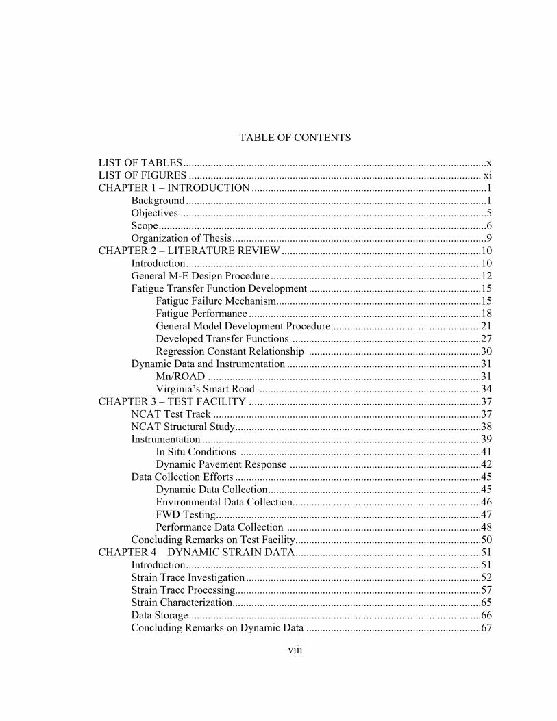
TABLE OF CONTENTS LIST OF TABLES...............................................................................................................x LIST OF FIGURES ........................................................................................................... xi CHAPTER 1 – INTRODUCTION ......................................................................................1 Background..............................................................................................................1 Objectives ................................................................................................................5 Scope........................................................................................................................6 Organization of Thesis.............................................................................................9 CHAPTER 2 – LITERATURE REVIEW .........................................................................10 Introduction............................................................................................................10 General M-E Design Procedure .............................................................................12 Fatigue Transfer Function Development ...............................................................15 Fatigue Failure Mechanism...........................................................................15 Fatigue Performance .....................................................................................18 General Model Development Procedure.......................................................21 Developed Transfer Functions .....................................................................27 Regression Constant Relationship ...............................................................30 Dynamic Data and Instrumentation .......................................................................31 Mn/ROAD ....................................................................................................31 Virginia’s Smart Road .................................................................................34 CHAPTER 3 – TEST FACILITY .....................................................................................37 NCAT Test Track ..................................................................................................37 NCAT Structural Study..........................................................................................38 Instrumentation ......................................................................................................39 In Situ Conditions ........................................................................................41 Dynamic Pavement Response ......................................................................42 Data Collection Efforts ..........................................................................................45 Dynamic Data Collection..............................................................................45 Environmental Data Collection.....................................................................46 FWD Testing.................................................................................................47 Performance Data Collection .......................................................................48 Concluding Remarks on Test Facility....................................................................50 CHAPTER 4 – DYNAMIC STRAIN DATA....................................................................51 Introduction............................................................................................................51 Strain Trace Investigation ......................................................................................52 Strain Trace Processing..........................................................................................57 Strain Characterization...........................................................................................65 Data Storage...........................................................................................................66 Concluding Remarks on Dynamic Data ................................................................67

ix

CHAPTER 5 – METHODOLOGY AND PARAMETER CHARACTERIZATION.......68 Introduction............................................................................................................68 Methodology..........................................................................................................79 Traffic Characterization .........................................................................................71 Weight Data .................................................................................................71 Lateral Distribution of Loads .......................................................................72 Traffic Volume..............................................................................................77 Concluding Remarks on Traffic Characterization ........................................77 HMA Stiffness Characterization............................................................................78 Backcalculated Stiffness Data.......................................................................78 Seasonal Trends ............................................................................................80 Stiffness Prediction Models ..........................................................................81 Concluding Remarks on HMA Characterization..........................................85 Strain Response Characterization ..........................................................................85 General Trends..............................................................................................85 Comparison Between Sections .....................................................................89 Strain Prediction Models...............................................................................93 Concluding Remarks on Strain Characterization..........................................97 Fatigue Performance Characterization...................................................................97 Observed Fatigue Distress ............................................................................97 Crack Mapping............................................................................................100 Data Processing and Characterization ........................................................103 Failure Criteria ............................................................................................107 Concluding Remarks on Methodology and Characterization..............................107 CHAPTER 6 – FATIGUE MODEL DEVELOPMENT .................................................109 Introduction..........................................................................................................109 Methodology........................................................................................................109 Fatigue Model ......................................................................................................111 Thin Model..................................................................................................114 Rich Bottom Model.....................................................................................117 Thick Model................................................................................................119 Concluding Remarks on Model Development.....................................................123 CHAPTER 7 – CONCLUSIONS AND RECOMMENDATIONS.................................124 Conclusions..........................................................................................................124 Recommendations................................................................................................127 REFERENCES ................................................................................................................129

x

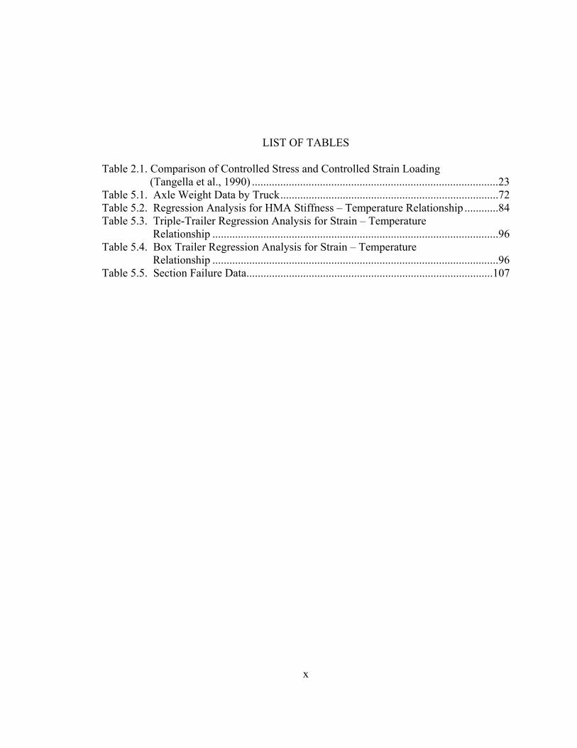
LIST OF TABLES Table 2.1. Comparison of Controlled Stress and Controlled Strain Loading (Tangella et al., 1990) .......................................................................................23 Table 5.1. Axle Weight Data by Truck.............................................................................72 Table 5.2. Regression Analysis for HMA Stiffness – Temperature Relationship ............84 Table 5.3. Triple-Trailer Regression Analysis for Strain – Temperature Relationship .....................................................................................................96 Table 5.4. Box Trailer Regression Analysis for Strain – Temperature Relationship .....................................................................................................96 Table 5.5. Section Failure Data.......................................................................................107

xi

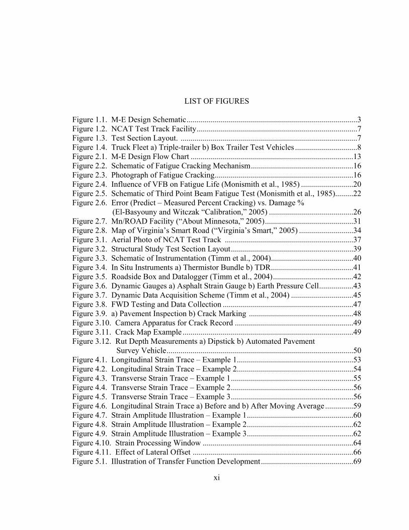
LIST OF FIGURES Figure 1.1. M-E Design Schematic.....................................................................................3 Figure 1.2. NCAT Test Track Facility................................................................................7 Figure 1.3. Test Section Layout. ........................................................................................7 Figure 1.4. Truck Fleet a) Triple-trailer b) Box Trailer Test Vehicles ...............................8 Figure 2.1. M-E Design Flow Chart .................................................................................13 Figure 2.2. Schematic of Fatigue Cracking Mechanism...................................................16 Figure 2.3. Photograph of Fatigue Cracking.....................................................................16 Figure 2.4. Influence of VFB on Fatigue Life (Monismith et al., 1985) ..........................20 Figure 2.5. Schematic of Third Point Beam Fatigue Test (Monismith et al., 1985).........22 Figure 2.6. Error (Predict – Measured Percent Cracking) vs. Damage % (El-Basyouny and Witczak “Calibration,” 2005) ..........................................26 Figure 2.7. Mn/ROAD Facility (“About Minnesota,” 2005)............................................31 Figure 2.8. Map of Virginia’s Smart Road (“Virginia’s Smart,” 2005) ...........................34 Figure 3.1. Aerial Photo of NCAT Test Track ................................................................37 Figure 3.2. Structural Study Test Section Layout.............................................................39 Figure 3.3. Schematic of Instrumentation (Timm et al., 2004).........................................40 Figure 3.4. In Situ Instruments a) Thermistor Bundle b) TDR.........................................41 Figure 3.5. Roadside Box and Datalogger (Timm et al., 2004)........................................42 Figure 3.6. Dynamic Gauges a) Asphalt Strain Gauge b) Earth Pressure Cell.................43 Figure 3.7. Dynamic Data Acquisition Scheme (Timm et al., 2004) ...............................45 Figure 3.8. FWD Testing and Data Collection .................................................................47 Figure 3.9. a) Pavement Inspection b) Crack Marking ....................................................48 Figure 3.10. Camera Apparatus for Crack Record ...........................................................49 Figure 3.11. Crack Map Example .....................................................................................49 Figure 3.12. Rut Depth Measurements a) Dipstick b) Automated Pavement Survey Vehicle.............................................................................................50 Figure 4.1. Longitudinal Strain Trace – Example 1..........................................................53 Figure 4.2. Longitudinal Strain Trace – Example 2..........................................................54 Figure 4.3. Transverse Strain Trace – Example 1.............................................................55 Figure 4.4. Transverse Strain Trace – Example 2.............................................................56 Figure 4.5. Transverse Strain Trace – Example 3.............................................................56 Figure 4.6. Longitudinal Strain Trace a) Before and b) After Moving Average ..............59 Figure 4.7. Strain Amplitude Illustration – Example 1.....................................................60 Figure 4.8. Strain Amplitude Illustration – Example 2.....................................................62 Figure 4.9. Strain Amplitude Illustration – Example 3.....................................................62 Figure 4.10. Strain Processing Window ...........................................................................64 Figure 4.11. Effect of Lateral Offset ................................................................................66 Figure 5.1. Illustration of Transfer Function Development..............................................69

xii

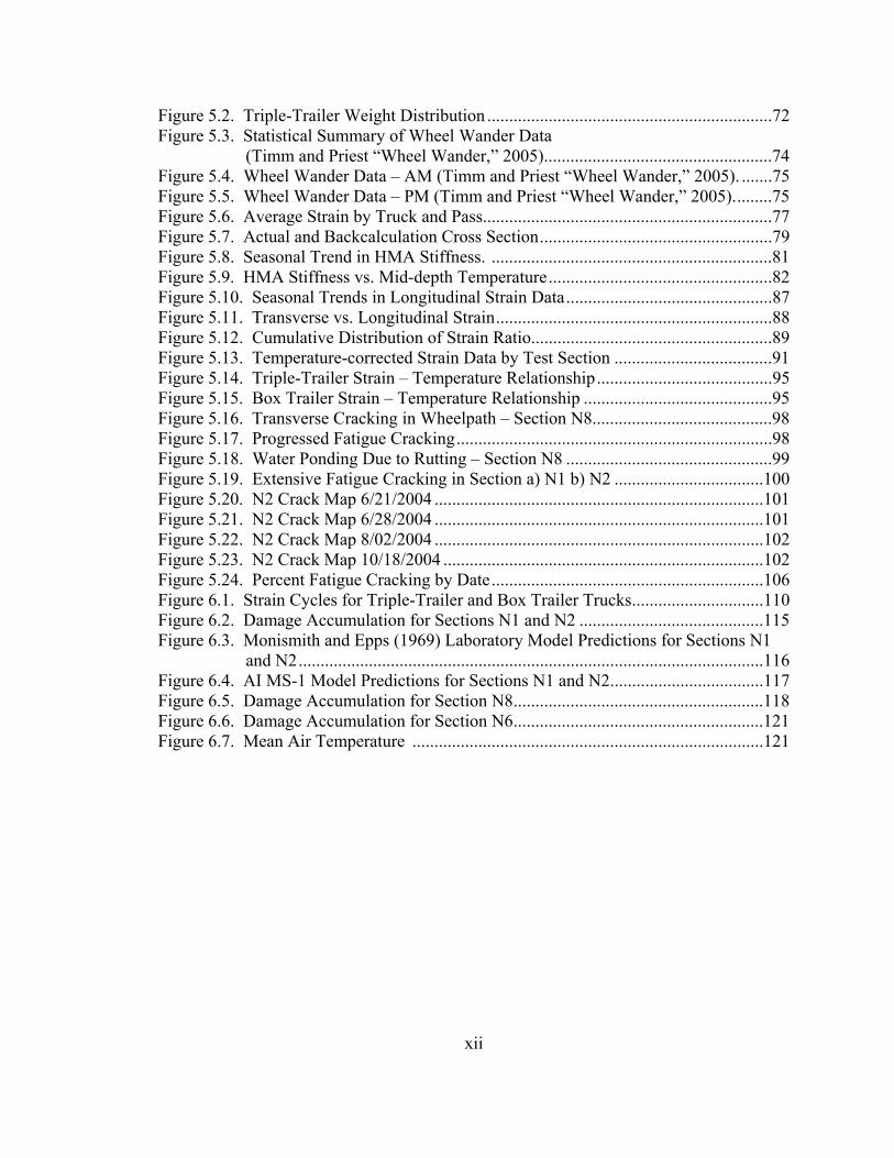
Figure 5.2. Triple-Trailer Weight Distribution .................................................................72 Figure 5.3. Statistical Summary of Wheel Wander Data (Timm and Priest “Wheel Wander,” 2005)....................................................74 Figure 5.4. Wheel Wander Data – AM (Timm and Priest “Wheel Wander,” 2005). .......75 Figure 5.5. Wheel Wander Data – PM (Timm and Priest “Wheel Wander,” 2005).........75 Figure 5.6. Average Strain by Truck and Pass..................................................................77 Figure 5.7. Actual and Backcalculation Cross Section.....................................................79 Figure 5.8. Seasonal Trend in HMA Stiffness. ................................................................81 Figure 5.9. HMA Stiffness vs. Mid-depth Temperature...................................................82 Figure 5.10. Seasonal Trends in Longitudinal Strain Data...............................................87 Figure 5.11. Transverse vs. Longitudinal Strain...............................................................88 Figure 5.12. Cumulative Distribution of Strain Ratio.......................................................89 Figure 5.13. Temperature-corrected Strain Data by Test Section ....................................91 Figure 5.14. Triple-Trailer Strain – Temperature Relationship........................................95 Figure 5.15. Box Trailer Strain – Temperature Relationship ...........................................95 Figure 5.16. Transverse Cracking in Wheelpath – Section N8.........................................98 Figure 5.17. Progressed Fatigue Cracking........................................................................98 Figure 5.18. Water Ponding Due to Rutting – Section N8 ...............................................99 Figure 5.19. Extensive Fatigue Cracking in Section a) N1 b) N2 ..................................100 Figure 5.20. N2 Crack Map 6/21/2004 ...........................................................................101 Figure 5.21. N2 Crack Map 6/28/2004 ...........................................................................101 Figure 5.22. N2 Crack Map 8/02/2004 ...........................................................................102 Figure 5.23. N2 Crack Map 10/18/2004 .........................................................................102 Figure 5.24. Percent Fatigue Cracking by Date..............................................................106 Figure 6.1. Strain Cycles for Triple-Trailer and Box Trailer Trucks..............................110 Figure 6.2. Damage Accumulation for Sections N1 and N2 ..........................................115 Figure 6.3. Monismith and Epps (1969) Laboratory Model Predictions for Sections N1 and N2..........................................................................................................116 Figure 6.4. AI MS-1 Model Predictions for Sections N1 and N2...................................117 Figure 6.5. Damage Accumulation for Section N8.........................................................118 Figure 6.6. Damage Accumulation for Section N6.........................................................121 Figure 6.7. Mean Air Temperature ................................................................................121

1

CHAPTER 1 – INTRODUCTION

Background

Research and development in the structural design of hot mix asphalt (HMA) pavements

over the past fifty years has focused on a shift from empirical design equations to a more

powerful and adaptive design scheme. Mechanistic-empirical (M-E) design has been

developed to utilize the mechanical properties of the pavement structure along with

information on traffic, climate, and observed performance, to more accurately model the

pavement structure and predict its life. Although M-E design still relies on observed

performance and empirical relations, it is a much more robust system that can easily

incorporate new materials, different traffic distributions, and changing conditions.

The M-E design process is more accurately described as an analysis procedure

which is used in an iterative manner. The procedure is used to determine the appropriate

materials and layer thicknesses to provide the structural capacity for the required

performance period. For flexible pavements, this includes considering the main load-

related structural distresses: fatigue cracking and structural rutting.

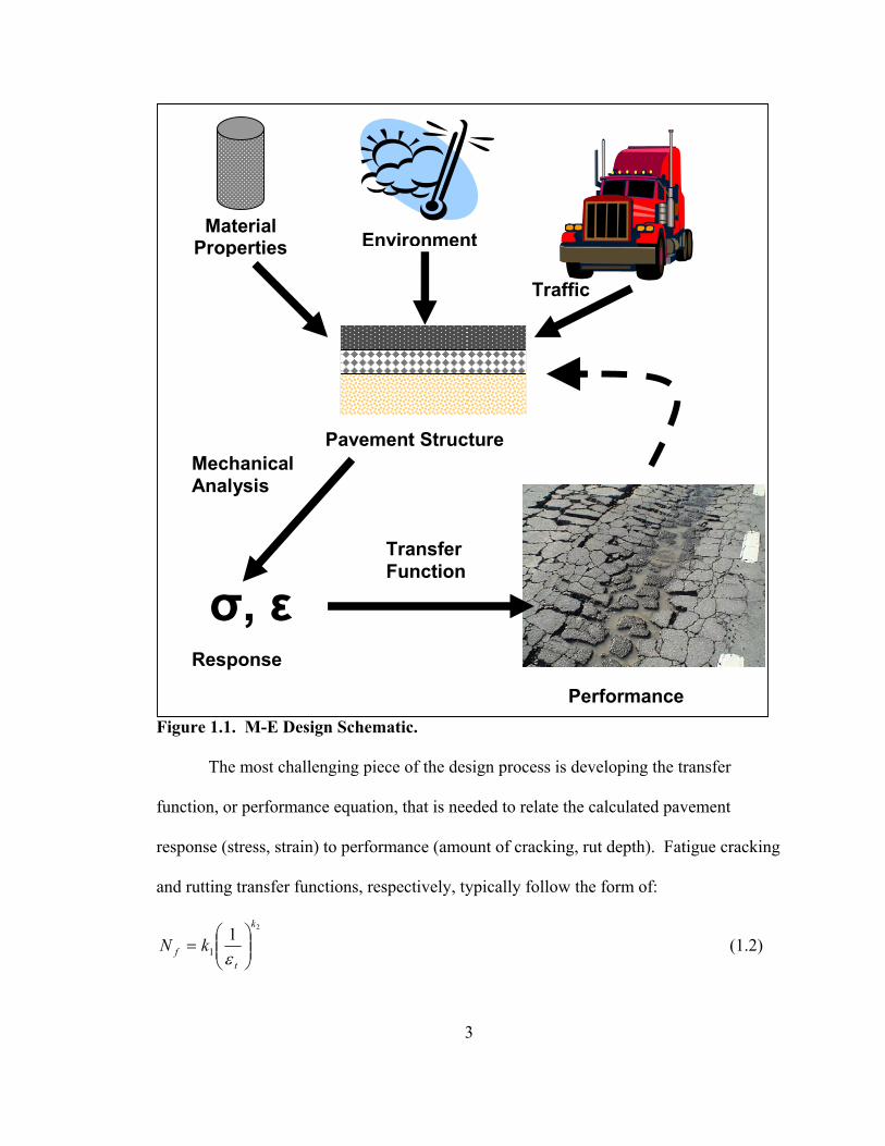
The process, shown conceptually in Figure 1.1, integrates the environmental

conditions and material properties of the HMA and underlying layers into the pavement

structure. The structure is then modeled using a mechanical analysis program, and the

pavement response is calculated given the axle load and tire configuration. The

pavement response is then correlated to performance or cycles to failure, N, through

2

empirically derived transfer functions. The expected traffic or load cycles for the given

design life, n, is then included to calculate a damage factor for that particular condition

(i.e., particular truck load and configuration along with in situ pavement and climatic

conditions). The damage for each condition is typically added together using Miner’s

hypothesis, shown in Equation 1.1, where the failure criteria is reached when the ratio

approaches unity (Miner, 1959).

∑=

=1i i

i

NnD (1.1)

where: ni = Number of load applications at condition, i

Ni = Number of load applications at failure for condition, i

Because the design process is modular, varying degrees of accuracy and

sophistication can be used at each step depending on the needs of the design. For

example, very specific traffic data can be incorporated, or a crude approximation of

equivalent single axle loads (ESAL) can be used. Further, average material property

values (i.e., stiffness, Poisson’s ratio) can be used, or the design can be divided into

seasons with differing properties due to environmental changes and material aging. The

process can also incorporate sophisticated mechanical models like finite element models,

if so desired.

3

Material Properties Environment

Traffic

Pavement Structure Mechanical Analysis

σ, ε Response

Transfer Function

Performance

Figure 1.1. M-E Design Schematic. The most challenging piece of the design process is developing the transfer

function, or performance equation, that is needed to relate the calculated pavement

response (stress, strain) to performance (amount of cracking, rut depth). Fatigue cracking

and rutting transfer functions, respectively, typically follow the form of:

211

k

tf kN

=

ε (1.2)

4

413

k

vr kN

=

ε (1.3)

where: Nf = Number of cycles until fatigue failure

εt = Horizontal tensile strain at the bottom of the HMA layer

Nr = Number of cycles until rutting failure

εv = Vertical compressive strain at the top of the subgrade layer

k1, k2, k3, k4 = Empirical constants

This research focuses on accurately modeling fatigue distress and developing fatigue

transfer functions.

The transfer function is the key to a successful M-E pavement design, and much

effort has been devoted to developing useful transfer functions (e.g., Monismith and

Epps, 1969; Shook et al., 1982; Timm et al. 1999). Transfer functions are somewhat mix

specific and dependant on the climate; therefore, local calibration or development is

required to account for local materials and conditions.

Most fatigue transfer functions are developed using laboratory fatigue tests that

are then calibrated or shifted to match observed field performance. This process

accurately measures the response in the loaded specimen, but is often shifted based on

limited field data. Further, the performance equations developed in the lab are dependant

on the mode of loading, rest periods, and type of apparatus. In fact, some researchers

have argued that there is no accurate way to shift laboratory performance equations to

direct field performance because there are too many discrepancies between the field and

the laboratory (Romero et al., 2000).

5

Other functions have been developed using purely observed field performance

and calculated pavement response (i.e., Timm et al., 1999). This process, too, has its

pitfalls because it relies on the accuracy of the mechanical models. Additionally, the test

sections must be closely monitored over a long period of time. Therefore, engineers

attempt to speed the process with accelerated load facilities. These facilities use loaded

wheels and test strips of varying size to simulate vehicular loading at a controlled and

accelerated rate. Yet, even with loaded wheel devices, there are still differences between

full-scale conditions and the experiment. Consequently, there is a need to develop

transfer equations under representative conditions with accurate response and

performance measurements.

Objectives

Given the above concerns, eight test sections of the National Center for Asphalt

Technology (NCAT) Test Track, a full-scale asphalt pavement testing facility, were

devoted to a structural experiment to investigate the many integral parts of M-E design.

Within the main objectives of the 2003 NCAT Structural Study, the goal of this research

was to develop fatigue performance equations for use in M-E flexible pavement design.

This included the following tasks and objectives:

• Develop a procedure for gathering, processing, and storing dynamic response data

from embedded instrumentation in a useful and concise manner.

• Gather and store environmental data.

• Accurately monitor and quantify field performance.

• Characterize the material properties of the structure including seasonal trends.

6

• Develop a procedure for incorporating the above efforts into the development of a

useful fatigue transfer function that will accurately predict fatigue life to be used

in design and analysis procedures.

• Describe the effect of modified binders and thickness on fatigue performance.

Scope

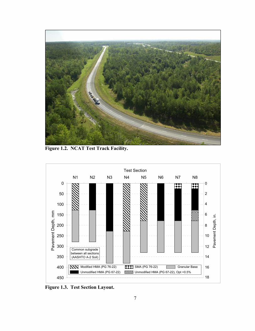
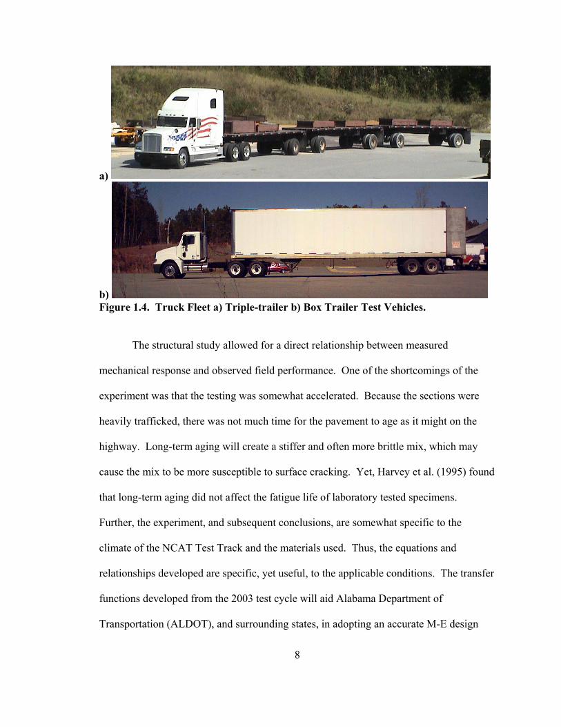
The NCAT Test Track (Figure 1.2), located in Opelika, Alabama, is a 1.7 mile

oval track designed to test asphalt mixtures and structural designs. The 2003 NCAT

Structural Study consisted of eight test sections including three different HMA

thicknesses and different asphalt mixtures and binders, shown in Figure 1.3.

Instrumentation, including strain gauges, earth pressure cells, and thermistors, was

installed in the pavement structure to measure the pavement response and condition

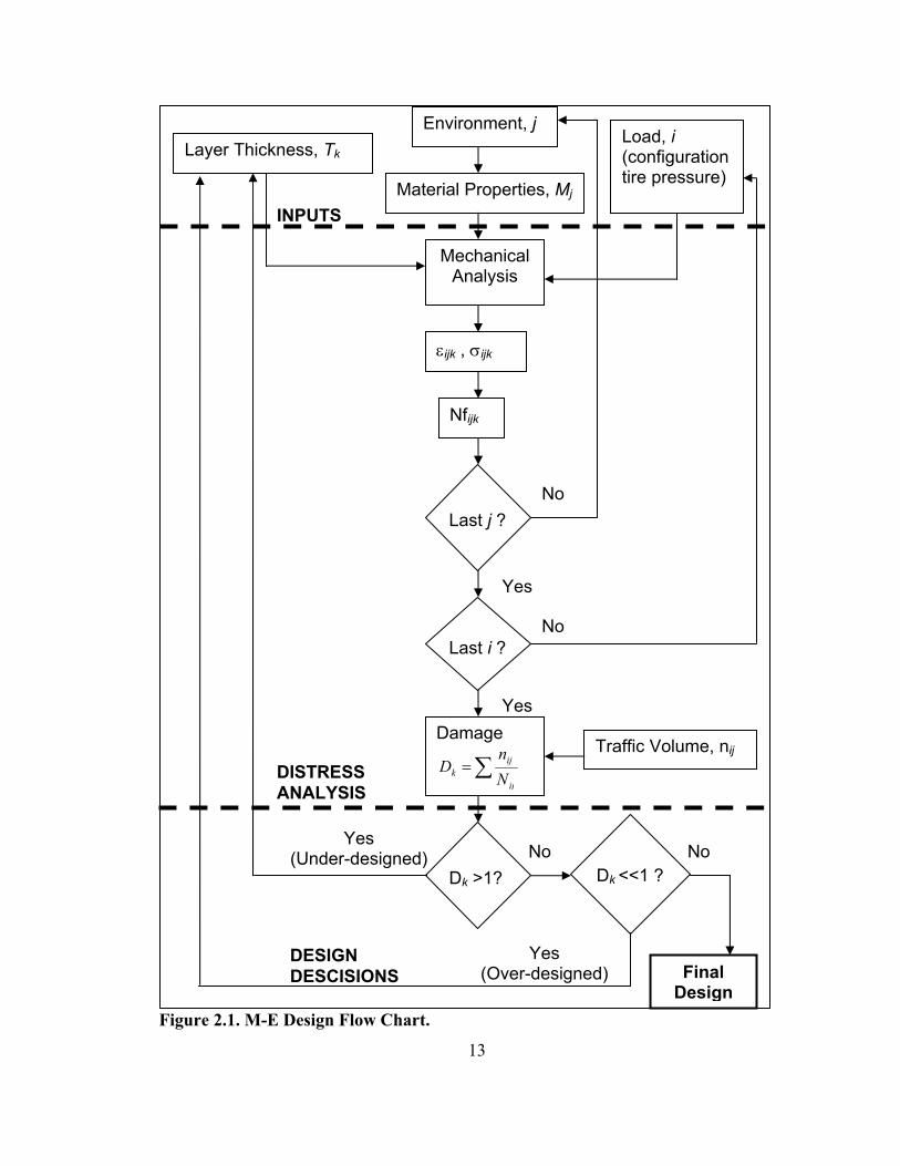
directly. The test sections were trafficked with a fleet of heavily loaded triple-trailers

(gross vehicle weight = 152 kip) and one legally loaded box trailer, both shown in Figure

1.4. In other words, the Test Track was trafficked with real trucks and drivers.

Therefore, similar wheel wander and traffic conditions were applied to the Test Track as

open-access highways.

One million vehicle repetitions (equivalent to approximately 10 million ESAL)

will be applied over the 2-year test cycle which began October 2003. Dynamic response

data and field performance data were collected on a weekly basis, and environmental data

were collected and stored continuously. The test sections were designed to develop

fatigue distress during the testing cycle so that a relationship between damage and

response could be developed.

7

Figure 1.2. NCAT Test Track Facility.

0

50

100

150

200

250

300

350

400

450

N1 N2 N3 N4 N5 N6 N7 N8

Test Section

Pav

emen

t Dep

th, m

m

0

2

4

6

8

10

12

14

18

16

Pav

emen

t Dep

th, i

n.

Modified HMA (PG 76-22)

Unmodified HMA (PG 67-22)

SMA (PG 76-22)

Unmodified HMA (PG 67-22), Opt +0.5%

Granular Base

Common subgradebetween all sections(AASHTO A-2 Soil)

Figure 1.3. Test Section Layout.

8

a)

b) Figure 1.4. Truck Fleet a) Triple-trailer b) Box Trailer Test Vehicles.

The structural study allowed for a direct relationship between measured

mechanical response and observed field performance. One of the shortcomings of the

experiment was that the testing was somewhat accelerated. Because the sections were

heavily trafficked, there was not much time for the pavement to age as it might on the

highway. Long-term aging will create a stiffer and often more brittle mix, which may

cause the mix to be more susceptible to surface cracking. Yet, Harvey et al. (1995) found

that long-term aging did not affect the fatigue life of laboratory tested specimens.

Further, the experiment, and subsequent conclusions, are somewhat specific to the

climate of the NCAT Test Track and the materials used. Thus, the equations and

relationships developed are specific, yet useful, to the applicable conditions. The transfer

functions developed from the 2003 test cycle will aid Alabama Department of

Transportation (ALDOT), and surrounding states, in adopting an accurate M-E design

9

procedure. Further, the process, if not the exact functions, developed at the NCAT Test

Track can be applied to other states and regions that may want to use full-scale

accelerated testing to develop transfer functions.

Organization of Thesis

A literature review is first presented in Chapter 2 in order to explore the development of

fatigue transfer functions and briefly report what other research efforts have discovered.

The literature review also contains a section regarding full-scale pavement testing and

instrumentation.

Chapter 3 provides more detailed information on the NCAT Test Track facility,

2003 Structural Study, pavement instrumentation and testing effort. Following the Test

Facility, Chapter 4 explains the dynamic strain data processing and storage scheme

developed for the 2003 Test Track research cycle. It is important to document how the

strain measurements were obtained for reference to the rest of the work presented here.

Further, detailed information regarding quantifying response from dynamic gauges is not

readily available in the literature.

The methodology used to develop the fatigue transfer functions from data

collected at the Test Track is then presented in Chapter 5. Also in this chapter is the

parameter characterization which includes both the methodology and results.

The final fatigue transfer functions are presented and discussed in Chapter 6. This

includes the developed models and discussion of damage accumulation. Additionally,

the project status at the time of this report is discussed. And lastly, the conclusions and

recommendations are given in the final chapter.

10

CHAPTER 2 – LITERATURE REVIEW

Introduction

Research and development of M-E pavement design has been on-going since the 1960’s.

Much interest and effort has been devoted to improving the design process and

encouraging adaptation by transportation agencies. The movement toward M-E design is

fruitful because of the many benefits over a purely empirical design method. Some of the

advantages include, but are not limited to, the following (Timm et al., 1998; Monismith et

al., 1985):

• Improved traffic characterization through load spectra

• Ability to deal with changing load types

• Enhanced definition of material properties

• Ability to relate material properties to performance

• Accommodate for material aging and environmental changes

• Modular system that allows for enhancement without disrupting the entire process

• Produces a more reliable design

• No longer dependent on the extrapolation of out-dated empirical relationships

Because of the mentioned benefits, many state and federal agencies along with

private organizations have developed M-E pavement design procedures in the U.S. and

abroad. The Asphalt Institute (AI) and Shell International Petroleum Co. have both

developed individual M-E design manuals. Further, other countries have produced full

11

M-E design methods including South Africa (NITRR) and Great Britain through the

University of Nottingham (Monismith, 1992). The American Association of State

Highway and Transportation Officials (AASHTO) is currently working on an M-E design

manual to replace the latest empirically-based design guide, the 1993 AASHTO Design

Guide (AASHTO, 1993). This includes expanding on work done by the National

Cooperative Highway Research Program (NCHRP) Report 1-10B and the AI Thickness

Design Manual MS-1 (1982) to develop the 2002 Design Guide (Eres, 2004). While this

national effort is continuing, many states have developed their own procedures including,

but not limited to, Minnesota, Illinois, Kentucky, and Washington State (Timm et al.,

1999; “Research and Development,” 1982).

The mentioned design guides are similar in their general procedure, but each is

unique in how they manage the inputs, calculate pavement response, and relate response

to performance. Therefore, many of the procedures were investigated and are presented

in this chapter to provide background and relevance to this research, with the main focus

on the development and calibration of fatigue transfer functions.

Additionally, one of the important parts of the NCAT Structural Study was the

embedded instrumentation in the pavement structure. There are many challenges

associated with dynamic pavement instrumentation including installation, construction,

data acquisition, data processing and data organization. Other test facilities that have

used similar instrumentation were examined to provide insight on how to handle the

mentioned challenges. The Minnesota Road Research Project (Mn/ROAD) and

Virginia’s Smart Road are both full-scale pavement test facilities with dynamic

instrumentation; therefore, their operations are explored here.

12

General M-E Design Procedure

The basic approach for M-E design includes computing the pavement response over the

expected range of loads, i, and environmental conditions, j, using transfer functions to

predict performance at each given strain level (set of traffic and environmental

conditions) and summing the damage over the expected design life (Monismith, 1992).

Damage is often totaled using Miner’s hypothesis, where the failure criterion is reached

at a value of 1 (Miner, 1959). This equation was shown previously in Equation 1.1. To

calculate the pavement response, a pavement cross section must first be assumed, k, and

based on the results of the analysis, it can be adjusted to fit the needed conditions. Thus,

the pavement is designed with the required structural capacity for the distress mode

considered (e.g., fatigue cracking). Figure 2.1 is an M-E design flow chart combining

the efforts of others (Timm et al., 1998; Monismith, 1992). It is important to remember

that the M-E design framework should be used in conjunction with engineering judgment

and experience with specific local issues.

13

Figure 2.1. M-E Design Flow Chart.

Layer Thickness, Tk

Material Properties, Mj

Environment, j Load, i (configuration tire pressure)

Mechanical Analysis

εijk , σijk

Nfijk

Last j ?

Last i ?

Yes

Yes

No

No

Damage

∑=ij

ijk N

nD

Traffic Volume, nij

Dk <<1 ? Dk >1?

Yes (Under-designed)

Yes (Over-designed)

No No

Final Design

INPUTS

DISTRESS ANALYSIS

DESIGN DESCISIONS

14

The major components that must be quantified for design are the expected traffic

over the design life including volume, configuration, and load; specific seasonal material

properties for the HMA and unbound pavement layers; a mechanical model to accurately

calculate the pavement response; a transfer function with local calibration for the specific

distress mode; and the distress criteria considered “failure”. Refer to Figure 1.1 for a

conceptual representation.

As explained prior, each part or component of M-E design is somewhat

independent from the entire design process; therefore, each component can have an

individual level of complexity or simplicity according to the desired outcome. Further,

each component can be improved upon as M-E pavement design evolves. For example,

traffic estimates in 18-kip equivalent single axle loads (ESAL) can be used, as was done

with the 1993 AASHTO Design Guide and prior. Yet, converting traffic data to ESAL is

no longer necessary and is often an invalid oversimplification (Ioannides, 1992).

Designers can now take advantage of theoretical models and their ability to calculate

response under any tire configuration, load, and tire pressure (Timm et al., 1998).

Therefore, many M-E procedures utilize load spectra, which describes the modeled traffic

data by axle type, frequency of load magnitude, and tire pressure.

Similar explanations can be made for the other components of M-E design

including material characterization, mechanical models and transfer functions. Fatigue

transfer functions are the focus of this work and will be described in detail below.

15

Fatigue Transfer Function Development

Fatigue Failure Mechanism

Fatigue cracking is one of the major modes of distress in flexible pavements along with

rutting and thermal cracking. It is a significant distress because fatigue cracking

propagates through the entire HMA layer, which then allows water infiltration to the

unbound layers. This causes accelerated surface and structural deterioration, pumping of

the unbound materials and rutting. Pumping may be better known as a rigid pavement

distress, but it is observed in flexible pavements with full-depth cracking, fine unbound

underlying layers and in the presence of water.

The textbook definition of fatigue theory states that fatigue cracking initiates at

the bottom of the flexible layer due to repeated and excessive loading, and it is associated

with the tensile strains at the bottom of the HMA layer (Huang, 1993). Shook et al.

(1982) explain that the M-E structural design process must limit the tensile strain in the

HMA layer in order to control or design against fatigue cracking. Further, the AI MS-1

development manual (“Research and Development,” 1982) refers to ten different M-E

design procedures that use the tensile strain at the bottom of the HMA layer as the critical

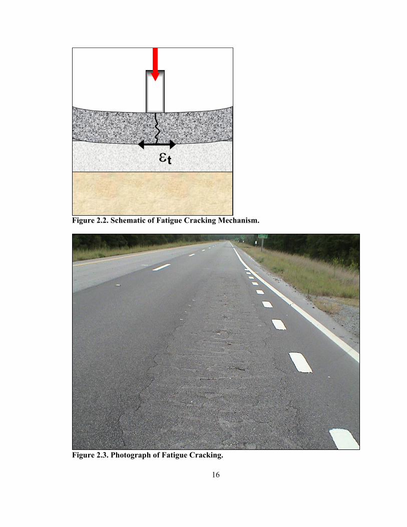
design criteria in regards to fatigue cracking. A schematic of fatigue cracking and the

critical response are shown in Figure 2.2 along with a photograph of extensive fatigue

cracking shown in Figure 2.3. Fatigue cracking is also referred to as alligator cracking

due to its distinctive pattern; the cracking often looks like the back of an alligator (Figure

2.3).

16

εt

Figure 2.2. Schematic of Fatigue Cracking Mechanism.

Figure 2.3. Photograph of Fatigue Cracking.

17

Fatigue distress is defined in the field by measuring the affected pavement area.

This area is then typically expressed as a percentage of the total lane area or the

wheelpath area. Further, there are different levels of severity to further define the

cracking. According to the Strategic Highway Research Program (SHRP) Distress

Identification Manual for the Long-Term Pavement Performance Program (Miller and

Bellinger, 2003), low severity fatigue cracking is individual cracks in the wheelpath with

no signs of pumping. Moderate severity is reached when the cracks become

interconnected, and a high severity rating is given when pumping is evident.

The SHRP distress guide gives a standard on how to measure and categorize

fatigue cracking, but it does not recommend a specific failure criteria. It is important in

fatigue transfer development to determine at what extent of cracking is considered

failure, or in other words, at what point should the damage ratio equal one? It is also

important when using established fatigue transfer functions to know what level of

damage the functions were calibrated to in order to gauge expected performance.

The transfer functions developed from NCHRP 1-10B were calibrated using data

from the American Association of Highway Officials (AASHO) Road Test, conducted in

the late 1950’s, and considered two levels of cracking as failure. The first calibrated

function considered cracking of 10 percent of the wheelpath as failure, and the second

considered greater than 45 percent of the wheelpath. The second failure criterion was

reached using the previous function with a multiplier of 1.38 (Monismith et al., 1985).

The AI transfer functions (an adaptation of NCHRP 1-10B) were also calibrated using

AASHO Road Test data and considered an area greater than 45 percent of the wheelpath

or an equivalent 20 percent of the total lane as failure (Monismith et al., 1985; Shook et

18

al., 1982). The 2002 Design Guide used Long-Term Pavement Performance (LTPP) test

sections to calibrate performance models, and 50 percent cracking of the total lane was

considered failure. It is important to note that the calibration for the 2002 Design Guide

included all severities of fatigue cracking equally without any weight to the higher

severities (El-Basyouny and Witczak “Calibration,” 2005). Additionally, it is important

to explain the LTPP program was set up by SHRP and NCHRP to serve researchers with

a large database of information regarding the construction, properties and performance of

pavement sections across the U.S., with one of the goals to aid in the development of a

new design guide.

Fatigue Performance

Asphalt fatigue research has shown that HMA fatigue life is related to the

horizontal tensile strain following the relationship of Equation 1.2. Further developments

included the HMA mixture stiffness in the fatigue life relationship to account for varying

temperature and loading frequency as given in Equation 2.1 (Tangella et al., 1990):

32 111

kk

tf E

kN

=

ε (2.1)

where: Nf = Number of load cycles until fatigue failure

εt = Applied horizontal tensile strain

E = HMA mixture stiffness

k1, k2, k3 = Regression constants

The HMA stiffness is an important parameter in the fatigue performance, and it must be

considered in conjunction with the expected in situ HMA thickness and failure mode.

19

Consider a relatively flexible mix. It will flex more, causing higher strains, yet it may

more capable of handling the strain due to its flexible nature. Further, a stiffer mix may

show lower fatigue life in the laboratory at a given strain level than a more flexible

counterpart. Yet, in the field, the stiffer structure will have lower strains under traffic

than the flexible mixture; thus, a longer fatigue life (Hajj et al., 2005). Hajj et al. (2005)

explain that mechanistic analysis should be used to understand the interaction between

structure, stiffness, and laboratory testing to determine the balance for the given field and

traffic conditions on a per-project basis.

Some fatigue relationships also include asphalt mixture parameters or mix

volumetrics as another correction factor to the k1 term. Typically, the effect of mix

volumetrics is in the form of (Pell and Cooper, 1975):

)( VB

B

VVVVFB+

= (2.2)

where VB = Percent asphalt volume

VV = Percent air volume

This parameter is also known as voids filled with bitumen (or asphalt) noted as VFB (or

VFA). Previous research showed that minimizing the air voids and maximizing the

amount of asphalt was beneficial to fatigue life. Pell and Cooper (1975) expanded by

showing that the interaction of air and binder volume to produce a high mix density was

the important parameter. They showed that the lower the voids in the mix, VB + VV, the

denser the mix and the better use of the available binder. At high VFB, they noted an

increase in the dynamic stiffness of the mixture, and thus the fatigue performance. It was

then determined that the above relationship captured the effect and interaction of

20

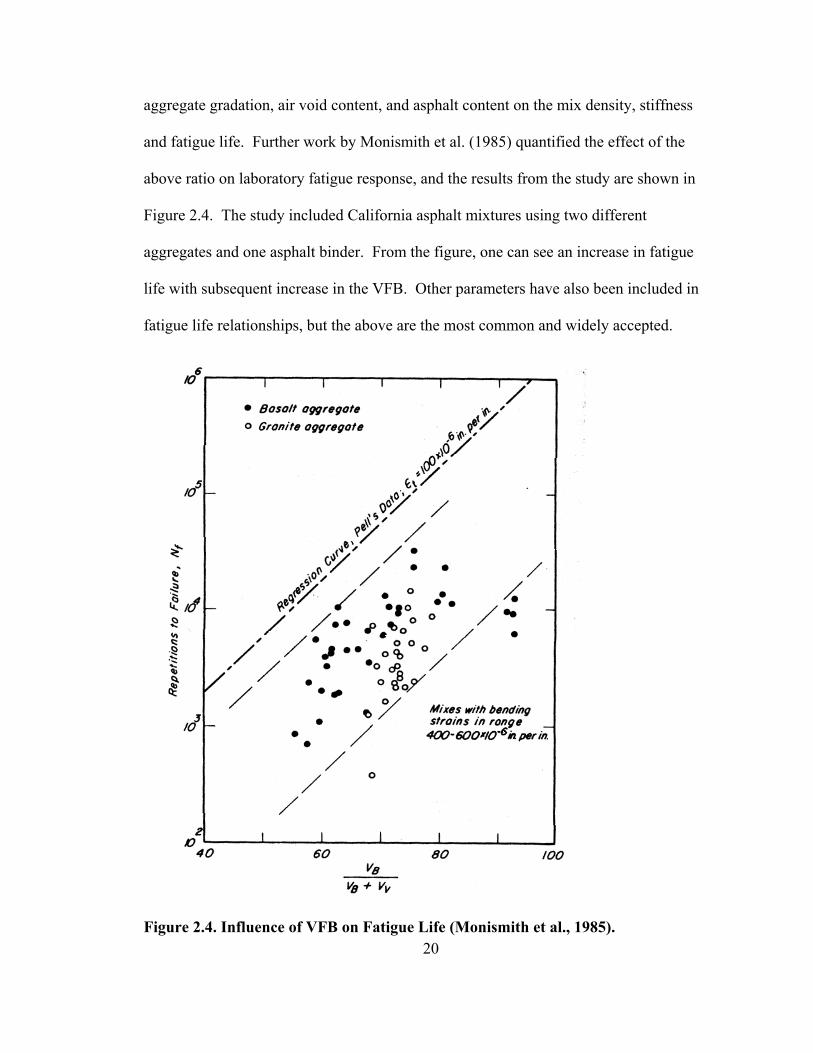
aggregate gradation, air void content, and asphalt content on the mix density, stiffness

and fatigue life. Further work by Monismith et al. (1985) quantified the effect of the

above ratio on laboratory fatigue response, and the results from the study are shown in

Figure 2.4. The study included California asphalt mixtures using two different

aggregates and one asphalt binder. From the figure, one can see an increase in fatigue

life with subsequent increase in the VFB. Other parameters have also been included in

fatigue life relationships, but the above are the most common and widely accepted.

Figure 2.4. Influence of VFB on Fatigue Life (Monismith et al., 1985).

21

General Model Development Procedure

For the most part, fatigue life relationships or performance equations are

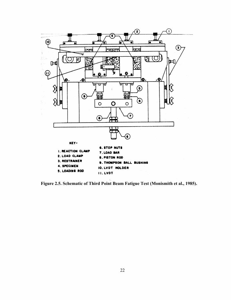
developed in the laboratory using some form of a fatigue testing apparatus. Typically,

HMA samples are cut into beams and subjected to repeated flexural loading either in a

controlled strain or controlled stress mode. The most common apparatus is simple

flexure with third-point loading. A schematic of the test is shown in Figure 2.5. Much

research and debate has been devoted to determining whether controlled stress or

controlled strain is the most appropriate. Most do agree that it depends on the conditions,

mainly thickness, of the in situ pavement. Controlled stress more closely simulates the

mode of loading for thicker HMA layers, while controlled strain is more appropriate for

thin (less than 2 in.) asphalt pavements (El-Basyouny and Witczak “Development,”

2005). Further, Table 2.1 compares controlled stress and controlled strain fatigue loading

and the relative effects of different parameters.

One of the main discrepancies between the two tests is the effect of mixture

stiffness on the fatigue life. For controlled stress testing, stiffer mixes will have a higher

fatigue life, while controlled strain testing will show that stiffer mixes have lower fatigue

life. Because of the discrepancies, the mode of loading should be carefully considered

and reported with beam fatigue results. Further, the observation drives the

recommendation that controlled stress should be used for thicker, more robust pavements,

where high stiffness is beneficial. It should also be noted that controlled stress loading

will result in a more conservative fatigue life than controlled strain loading for identical

mixes (Monismith et al., 1985).

22

Figure 2.5. Schematic of Third Point Beam Fatigue Test (Monismith et al., 1985).

23

Table 2.1. Comparison of Controlled Stress and Controlled Strain Loading (Tangella et al., 1990). Variables Controlled Stress Controlled Strain Thickness of HMA layer

Comparatively thick HMA layers

Thin HMA layers (< 3 in.)

Definition of failure Well-defined failure at specimen fracture

Arbitrarily assigned when the load level has been reduced to some portion of its initial value; for example, to 50 percent of initial

Scatter in test data Less scatter More scatter Required number of specimens

Smaller Larger

Influence of long-term aging

Lead to increased stiffness and presumably increased fatigue life

Lead to reduced fatigue life

Magnitude of fatigue life, N

Generally shorter Generally longer

Effect of mixture variables

More sensitive Less sensitive

Rate of crack propogation

Faster than occurs in situ More representative of in situ conditions

Beneficial effects of rest periods

Greater effect Lesser effect

Either way, laboratory-developed performance equations do not accurately predict

the fatigue life of asphalt pavements in the field (Harvey et al., 1995). There are many

reasons for the difference in laboratory and field performance, and a few are given below

(Tangella et al., 1990):

• In the field, traffic loads are distributed laterally (wheel wander), so the same

point of the pavement is not continually loaded.

• It is possible that in the field the HMA will sustain longer fatigue life after initial

cracking due to support of underlying layers.

24

• Fatigue life relationships are greatly dependent on the type of fatigue test and

mode of loading (i.e. flexural versus diametrical and controlled strain versus

controlled stress) along with testing temperature.

• There are rest periods and the opportunity for healing in the field.

• Field performance is dependent on thickness of the in situ pavement.

Due to the differences in the laboratory and the field, fatigue life relationships

must be calibrated or shifted to observed field performance. This is the empirical part of

M-E design. The calibration process, or developed shift functions, is one of the more

problematic elements of M-E design. The SHRP Project A-003A (Tangella et al., 1990)

warned that “established correlations between laboratory data and field response are

weak, [which] is a major area of concern when attempting to utilize the results of

laboratory investigations to define performance criteria.” The project further reported

that the range of shift factors proposed by a variety of researchers ranged from slightly

over 1 to over 400.

Field calibration is necessary in defining useful transfer functions, but as

mentioned above, the process can be very difficult and often inexact. Many design

manuals, including the AI MS-1 (“Thickness Design,” 1982), calibrated laboratory

derived equations from field performance data from the AASHO Road Test. Therefore,

the calibration and subsequent transfer functions are reliant and restricted by the

conditions of the AASHO Road Test, which are more than likely irrelevant for today’s

conditions. As mentioned earlier, one of the main benefits of M-E design is that

performance predictions will no longer be based on out-dated empirical relationships

presented in the AASHTO Design Guide (1993).

25

The empirical relationships in the AASHTO Design Guide are considered out-

dated because they were developed from the AASHO Road Test. As further background,

the AASHO Road Test was limited to one subgrade soil, one environmental condition,

1950’s vehicles and tires, 1950’s materials and specifications and only a few million

ESAL of traffic (Hallin, 2004). M-E design allows pavement design to move beyond the

limitations of the AASHO Road Test through mechanistic analysis; yet, we are still

willing to then calibrate the response back to AASHO performance data. It seems that

more recent performance data is warranted. Otherwise, M-E design is still limited to

AASHO conditions through the calibration of the distress models. This deficiency is a

major motivator for projects like SHRP’s LTPP project.

As an improvement to earlier efforts, the 2002 Design Guide calibrated the

fatigue transfer function using data from the LTPP database from different pavement

sections all over the U.S. (El-Basyouny and Witczak “Calibration,” 2005). A total of 82

new LTPP sections were included in the analysis, and the 2002 Design Guide Software

was run at a full matrix of assumed shift factors. The set that most closely matched the

performance data was selected to calibrate the model. Another shift factor was then

developed to mathematically shift the thinner asphalt sections (less than 4 in. thick).

Although this particular method may be considered to be applicable over a wider

range of conditions because it was calibrated considering many conditions, one may also

argue that the unspecific calibration deems the functions unsuitable to any one site. From

Figure 2.6, the error between the final 2002 Design Guide distress predictions and the

observed performance reach high levels even with the field calibration. The figure shows

the error in the model in terms of the percent of cracking plotted against the log of the

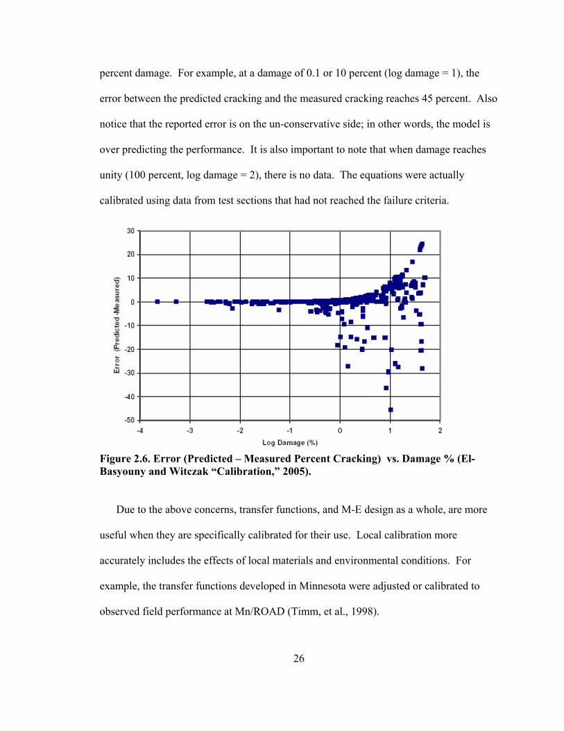
26

percent damage. For example, at a damage of 0.1 or 10 percent (log damage = 1), the

error between the predicted cracking and the measured cracking reaches 45 percent. Also

notice that the reported error is on the un-conservative side; in other words, the model is

over predicting the performance. It is also important to note that when damage reaches

unity (100 percent, log damage = 2), there is no data. The equations were actually

calibrated using data from test sections that had not reached the failure criteria.

Figure 2.6. Error (Predicted – Measured Percent Cracking) vs. Damage % (El-Basyouny and Witczak “Calibration,” 2005).

Due to the above concerns, transfer functions, and M-E design as a whole, are more

useful when they are specifically calibrated for their use. Local calibration more

accurately includes the effects of local materials and environmental conditions. For

example, the transfer functions developed in Minnesota were adjusted or calibrated to

observed field performance at Mn/ROAD (Timm, et al., 1998).

27

Developed Transfer Functions

A sampling of developed transfer functions are presented here to serve as examples and

guidance for this research. Notice that many are very similar in form, with different

coefficients based on their specific use.

Asphalt Institute MS-1

Finn et al. (1977) developed a calibrated fatigue transfer function for NCHRP 1-10B

based on the laboratory equation below developed by Monismith and Epps (1969):

−

−= − 3

*

6 10log854.0

10log291.382.14log EN t

fε (2.3)

where: Nf = Cycles until fatigue failure

εt = Initial tensile strain

E* = Complex modulus of the HMA, psi

Equation 2.3 was calibrated using data from the AASHO Road Test to produce Equation

2.4, considering failure with 45 percent cracking of the wheelpath (20 percent of the total

lane). This particular field calibration only shifted the intercept or multiplier (k1). Notice

the other parameters did not change.

−

−= − 3

*

6 10log854.0

10log291.3086.16log EN t

fε

Or (2.4)

)00432.0(4.18 854.*29.3 −− ∗∗∗= EN tf ε

Equation 2.4 was then adopted by the 9th edition of the AI Thickness Design Manual

MS-1 (“Research and Development,” 1982) and further modified to include a correction

28

factor to account for the volumetrics of the mixture as suggested by Pell and Cooper

(1975). The final MS-1 design equation was:

)00432.0(4.18 854.*29.3 −− ∗∗∗∗= ECN tf ε (2.5)

where: C = 10M

−

+∗= 69.084.4

VB

B

VVVM (2.6)

Shell Pavement Design Manual

Shell International Petroleum Company published an asphalt design manual in 1978 and

included the fatigue transfer function below following a similar pattern of AI MS-1 (Ali

and Tayabji, 1998):

363.2671.50685.0 −− ∗∗= EN tf ε (2.7)

where: εt = Initial tensile strain

E = Stiffness of the HMA, psi

Equation 2.7 was developed from mainly laboratory fatigue data. Further work was done

in 1980, and separate functions were developed for thin (less than 2 in.) and thick (6-8

in.) asphalt pavements, which are presented elsewhere (El-Basyouny and Witczack,

“Development,” 2005).

2002 Design Guide

In the development of the fatigue cracking models for the 2002 Design Guide under

NCHRP 1-37A (Eres, 2004), the researchers considered both the Shell Oil and AI fatigue

29

transfer functions as starting points. It was determined that the AI MS-1 equation was the

most applicable(El-Basyouny and Witczack “Development,” 2005). Equation 2.4 was

basically re-calibrated using LTPP data and including a new correction factor, K, to

account for thinner pavements (less than 4 in.). The final fatigue design equation,

considering failure at 50 percent cracking of the total lane area, is (El-Basyouny and

Witczack “Calibration,” 2005):

281.19492.31100432.0

∗∗∗=

ECKN

tf ε

(2.8)

where:

ache

K∗−+

+=

49.302.111003602.0000398.0

1 (2.9)

hac = Thickness of HMA layer, in.

California Department of Transportation

A large laboratory effort was conducted following the recommendations of SHRP A-

003A by researchers at the University of California, Berkeley to evaluate California

asphalt mixtures for California Department of Transportation. The model derived from

lab data included the mix stiffness, VFB and tensile strain (Harvey et al., 1995).

761.3726.0

053.08

145105875.2 −

−− ∗

∗∗×= t

VFB EeN ε (2.10)

Further, a recommended shift factor was developed to determine design ESAL from

laboratory life. The shift factor developed from the study was (Harvey et al., 1995):

3586.15107639.2 −− ∗×= trShiftFacto ε for εt ≥ 0.000040 (2.11)

30

Minnesota Department of Transportation

The Minnesota Department of Transportation (Mn/DOT) developed a fatigue transfer

function following the Illinois Department of Transportation function developed for

dense-graded asphalt mixtures (Alvarez and Thompson, 1996):

0.36 1105

∗×= −

tfN

ε (2.12)

The final Mn/DOT equation was calibrated using performance data from Mn/ROAD and

is given as (Timm et al., 1999):

206.36 11083.2

∗×= −

tfN

ε (2.13)

Both the Illinois and Minnesota equations followed the simplified form of Equation 1.2.

Regression Constant Relationships

Timm et al. (1999) reported that many studies have observed trends between the

regression coefficients, k1 and k2, of Equation 1.2. These trends, Equations 2.14-16, can

aid in calibration, because if an approximation of k1 is determined, then k2 can be easily

calculated. The relationships can also serve as a check of reasonableness.

12 log252.035.1 kk ∗−= (2.14)

12 log306.0332.1 kk ∗−= (2.15)

12 log213.05.0 kk ∗−= (2.16)

Equation 2.14 was developed by the Federal Highway Administration (Rauhut et al.,

1984), and Equation 2.15 shows a very similar trend developed from research in Norway

31

(Myre, 1990). The final relationship was reported by M-E design research from

Nottingham, England (Cooper and Pell, 1974).

Dynamic Data and Instrumentation

Mn/ROAD

The Minnesota Road Research Project (Mn/ROAD) is a full-scale pavement testing

facility located off of I-94 in Ostego, Minnesota (Figure 2.7). The facility consists of two

main parts: the 3.5 mile mainline that runs parallel to I-94 and carries interstate traffic

and the 2.5 mile low-volume road loop with controlled traffic. At the facility, there are

40 test sections with a wide variety of pavement structures (both flexible and rigid). The

facility promotes cooperative research between Minnesota Department of Transportation

(MnDOT), University of Minnesota and FHWA, as well as other state DOTs (“About

Minnesota,” 2005).

Figure 2.7. Mn/ROAD Facility (“About Minnesota,” 2005).

32

Of most relevance to the NCAT Structural Study, is the embedded

instrumentation at Mn/ROAD. There are approximately 4,500 sensors embedded in the

test sections to monitor both the pavement condition and the dynamic response under

loading (Alvarez and Thompson, 1998). The sensors are connected to 26 roadside boxes,

and there are two main collection systems. Most of the gauges are sampled via an

automated, continuous data acquisition system that is triggered by the passage of a

vehicle which then records a burst of data. The condition gauges are also sampled

automatically based on a routine time schedule. There are also sensors that are collected

manually with an on-site system (Beer et al., 1996).

At Mn/ROAD, there are many types of dynamic response gauges. The three of

most importance to flexible pavements are asphalt strain gauges, linear variable

differential transducers (LVDT) and dynamic soil pressure gauges. As described by

Alvarez and Thompson (1998), the asphalt strain gauges are electrical resistant strain

gauges on an H-shaped bar, and they were installed at the bottom of the asphalt layer in

both the transverse and longitudinal directions. Further, they were installed at the center

of the wheelpath and at 1 ft transverse offsets. The gauges and array are very similar to

what was used for the NCAT Structural Study. The LVDTs consist of an

electromagnetic device and separate core. They were used to measure the vertical

displacement at different depths within the pavement structure. Lastly, soil pressure cells

were used to measure the dynamic vertical pressure due to truck loads. These gauges

consisted of a liquid-filled steel cell with adjacent pressure transducer, also similar to the

gauges used at NCAT.

33

In addition to the response gauges, there are also pavement environmental

condition sensors including thermocouples and time domain reflectometers (TDR). The

TDRs were installed in the soil layers, and measure the in situ moisture content. The

thermocouples are used to measure the temperature profile in the pavement structure

(Alvarez and Thompson, 1998; Beer et al., 1996). At NCAT, TDRs as well as

temperature probes were used.

In 1996, a report was published (Beer et al.) regarding the performance of the

instrumentation at Mn/ROAD, and a few suggestions were given. First, more

redundancy in the asphalt strain gauges was desired due to the loss of gauges during

construction and throughout the testing cycle. It was also noted that nearly twice the

strain gauges orientated in the transverse direction failed as those in the longitudinal

direction. In regards to the moisture content measurements, they recommended

developing specific calibration equations and also reported that the gauges did not work

well when the soil was near saturation. Further recommendations included avoiding

cable splices and long lead wires. Overall, it was reported that the strain gauges and

pressure cells performed satisfactorily.

The automated data acquisition system at Mn/ROAD retrieves and processes the

data and then sends the information to the Mn/DOT Materials Research Engineering

Laboratory where it is checked and stored on an Oracle database (Alvarez and

Thompson, 1998). In this way, the data collection and processing is completely

automated. No further information could be found regarding how strain values were

estimated from the actual dynamic traces.

34

Virginia’s Smart Road

Virginia’s Smart Road is a 5.7 mile limited-access highway that will connect Blacksburg,

Virginia to I-81 upon completion (Figure 2.8). It is a multi-use research facility in

addition to an important transportation corridor for the public. The facility is designed to

accommodate a variety of research efforts including bridge design, Intelligent

Transportation Systems (ITS) development, safety and human factor research, pavement

design, and vehicle dynamic research. Most of the research is a cooperative effort

between the Virginia Department of Transportation (VDOT), FHWA and Virginia

Polytechnic Institute and State University’s Transportation Institute (“Virginia’s Smart

Road Project,” 2005).

Figure 2.8. Map of Virginia’s Smart Road (“Virginia’s Smart,” 2005).

35

The flexible pavement testing at the Smart Road consists of 12 sections, each

approximately 350 ft long, consisting of different materials and all include embedded

response and condition gauges. Again, the important aspect of the project in respect to

this report is the embedded instrumentation and subsequent collection and processing

procedures.

Like Mn/ROAD, the Smart Road instrumentation array consisted of asphalt strain

gauges, pressure cells, TDRs and thermocouples. The data acquisition scheme at Smart

Road consisted of two units; one, to collect the static or condition data, and the other to

collect dynamic data. Both systems were manufactured by IOtech Inc. and required

signal conditioning cards for each gauge (Al-Qadi et al., 2004). The dual acquisition

scheme was also used at NCAT, and will be discussed in Chapter 3.

Three software programs were developed at the Virginia Tech to collect,

organize, and process the dynamic data (Al-Qadi et al., 2004). SmartAcq was developed

to collect the condition data at specified intervals and the dynamic data during the

presence of a vehicle. The dynamic gauges were sampled at 500 Hz per channel, the

temperature probes are collected every 15 minutes and the TDRs were sampled hourly.

The program allowed the user to control the data acquisition systems through a Windows

environment. The collected data were then separated into distinct files by gauge, test

section and date using Smart Organizer software.

The final software program, SmartWave, was developed to display and process

the dynamic strain and pressure data. Al-Qadi et al. (2004) noted that the dynamic traces

were originally viewed individually in a spreadsheet program, but the process was

inefficient due to the large amount of traces and data points per trace. Therefore,

36

researchers at Virginia Tech developed the SmartWave program which allowed for easier

viewing and processing of the dynamic traces (Al-Qadi et al., 2004). The program

allowed the user to see the trace and customize the data processing commands. The

processing consisted of cleaning the signal and collecting the important values from the

trace. After cleaning the signal of electronic noise, the program automatically collected

the extremum [sic] value for each axle of the 6-axle test vehicle. The peak value per axle

could be either compression or tension for the asphalt strain gauges and compression for

the pressure cells. From this process, the collected strain magnitude was the absolute

value from the baseline of the trace to the peak point determined from the SmartWave

algorithm.

After processing, the dynamic response data were stored in an Access database

along with the environmental (condition) data. The data were stored in such a way to

allow for easy retrieval among the two databases. Further, queries were developed to

allow extraction of just maximum response values of replicate tests (Al-Qadi et al.,

2004).

The data acquisition scheme at Virginia’s Smart Road was loosely followed at the

NCAT Structural Study. As explained in the next chapter, proprietary programs and

developed algorithms were used to collect and process the data in a Windows

environment. Also similar to Smart Road, both processes involved some human

interaction.

37

CHAPTER 3 - TEST FACILITY

NCAT Test Track

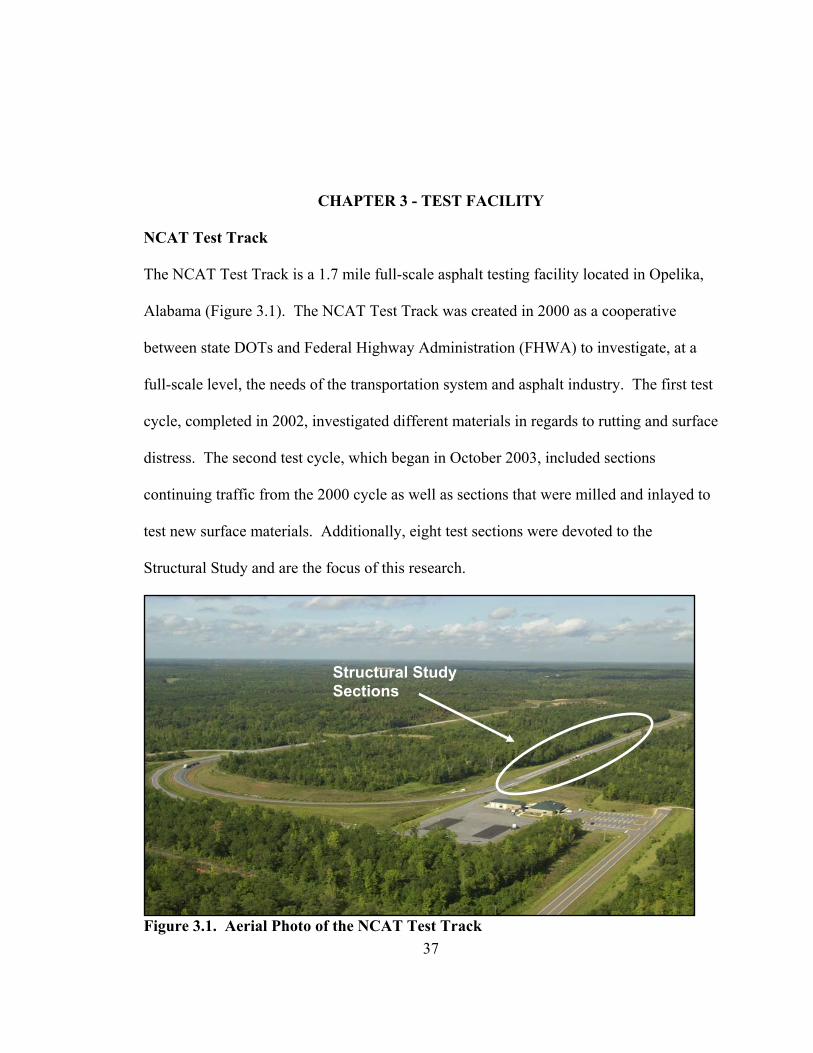
The NCAT Test Track is a 1.7 mile full-scale asphalt testing facility located in Opelika,

Alabama (Figure 3.1). The NCAT Test Track was created in 2000 as a cooperative

between state DOTs and Federal Highway Administration (FHWA) to investigate, at a

full-scale level, the needs of the transportation system and asphalt industry. The first test

cycle, completed in 2002, investigated different materials in regards to rutting and surface

distress. The second test cycle, which began in October 2003, included sections

continuing traffic from the 2000 cycle as well as sections that were milled and inlayed to

test new surface materials. Additionally, eight test sections were devoted to the

Structural Study and are the focus of this research.

Figure 3.1. Aerial Photo of the NCAT Test Track

Structural Study Sections

38

The trucking fleet, consisting of five triple-trailer trucks and a standard class 9 18-

wheeler truck, can apply over 1,000,000 passes (approximately 10 million ESALs) during

a two-year testing cycle. In other words, the NCAT Test Track is loaded with roughly

ten years of traffic volume in two years. In this manner, the testing is somewhat

accelerated, but in all other aspects, the testing is as close to an open-access highway as

possible. Further, the trucks are run at 45 miles per hour and are driven by human

drivers. This testing scheme is both safe and more closely replicates highway traffic.

NCAT Structural Study

The Structural Study, sponsored by ALDOT, Indiana DOT (InDOT) and FHWA,

consisted of eight test sections with three different HMA thicknesses and two different

binder types (PG 67-22 and an SBS modified PG 76-22). All eight sections had an

underlying 6 in. crushed granite granular base over fill material which was constructed

over the existing embankment. Figure 3.2 shows the cross sections of the structural study

sections, N1-N8. Notice that the sections were a full factorial experiment with N7

serving as a duplicate to N6 with an SMA surface, and N8 is a duplicate of N7 with an

asphalt-rich bottom layer.

The sections were designed structurally using the 1993 AASHTO Design Guide

(AASHTO, 1993), and the mix design was performed according to ALDOT

specifications. The sections were designed to show a variety of distresses over the life of

the experiment, and it was intended that at least the 5 and 7 in. sections would exhibit

fairly extensive structural distress in order to correlate performance to field-measured

pavement responses. The thin sections (N1 and N2) were designed for about 1.1 million

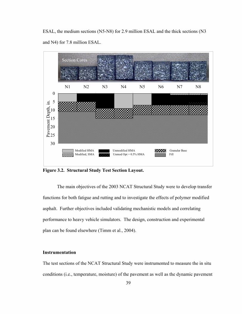
39

ESAL, the medium sections (N5-N8) for 2.9 million ESAL and the thick sections (N3

and N4) for 7.8 million ESAL.

0

5

10

15

20

25

30

N1 N2 N3 N4 N5 N6 N7 N8

Pave

men

t Dep

th, i

n.

Modified HMA Unmodified HMA Granular BaseModified, SMA Unmod Opt + 0.5% HMA Fill

Section Cores

Figure 3.2. Structural Study Test Section Layout.

The main objectives of the 2003 NCAT Structural Study were to develop transfer

functions for both fatigue and rutting and to investigate the effects of polymer modified

asphalt. Further objectives included validating mechanistic models and correlating

performance to heavy vehicle simulators. The design, construction and experimental

plan can be found elsewhere (Timm et al., 2004).

Instrumentation

The test sections of the NCAT Structural Study were instrumented to measure the in situ

conditions (i.e., temperature, moisture) of the pavement as well as the dynamic pavement

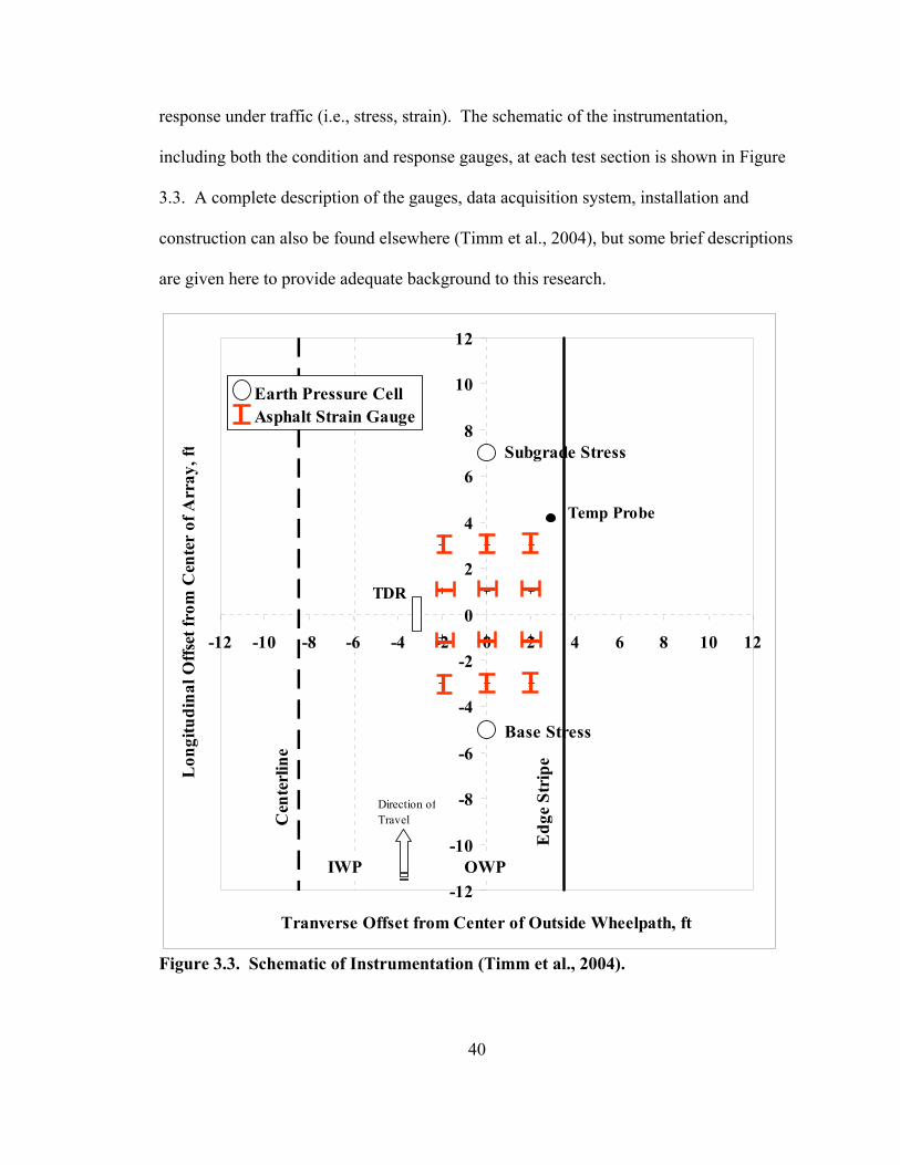
40

response under traffic (i.e., stress, strain). The schematic of the instrumentation,

including both the condition and response gauges, at each test section is shown in Figure

3.3. A complete description of the gauges, data acquisition system, installation and

construction can also be found elsewhere (Timm et al., 2004), but some brief descriptions

are given here to provide adequate background to this research.

-12

-10

-8

-6

-4

-2

0

2

4

6

8

10

12

-12 -10 -8 -6 -4 -2 0 2 4 6 8 10 12

Tranverse Offset from Center of Outside Wheelpath, ft

Lon

gitu

dina

l Offs

et fr

om C

ente

r of

Arr

ay, f

t

Earth Pressure CellAsphalt Strain Gauge

Base Stress

Subgrade Stress

OWPIWP

Cen

terl

ine

Edg

e St

ripe

Direction of Travel

Temp Probe

TDR

Figure 3.3. Schematic of Instrumentation (Timm et al., 2004).

41

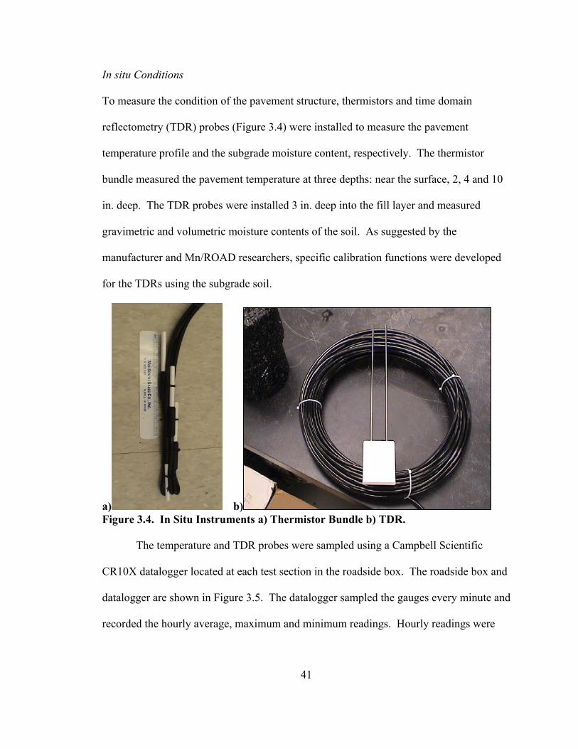
In situ Conditions

To measure the condition of the pavement structure, thermistors and time domain

reflectometry (TDR) probes (Figure 3.4) were installed to measure the pavement

temperature profile and the subgrade moisture content, respectively. The thermistor

bundle measured the pavement temperature at three depths: near the surface, 2, 4 and 10

in. deep. The TDR probes were installed 3 in. deep into the fill layer and measured

gravimetric and volumetric moisture contents of the soil. As suggested by the

manufacturer and Mn/ROAD researchers, specific calibration functions were developed

for the TDRs using the subgrade soil.

a) b) Figure 3.4. In Situ Instruments a) Thermistor Bundle b) TDR. The temperature and TDR probes were sampled using a Campbell Scientific

CR10X datalogger located at each test section in the roadside box. The roadside box and

datalogger are shown in Figure 3.5. The datalogger sampled the gauges every minute and

recorded the hourly average, maximum and minimum readings. Hourly readings were

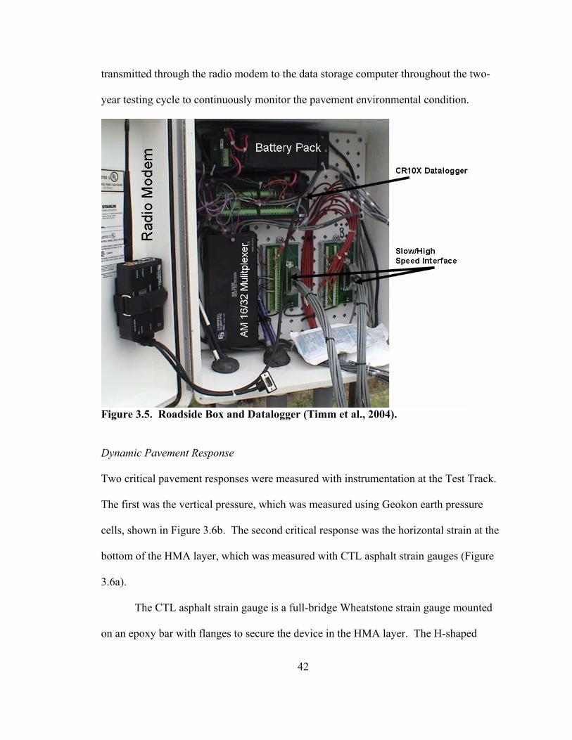
42

transmitted through the radio modem to the data storage computer throughout the two-

year testing cycle to continuously monitor the pavement environmental condition.

Figure 3.5. Roadside Box and Datalogger (Timm et al., 2004).

Dynamic Pavement Response

Two critical pavement responses were measured with instrumentation at the Test Track.

The first was the vertical pressure, which was measured using Geokon earth pressure

cells, shown in Figure 3.6b. The second critical response was the horizontal strain at the

bottom of the HMA layer, which was measured with CTL asphalt strain gauges (Figure

3.6a).

The CTL asphalt strain gauge is a full-bridge Wheatstone strain gauge mounted

on an epoxy bar with flanges to secure the device in the HMA layer. The H-shaped

43

gauges are similar to those used at both Mn/ROAD and Smart Road. The gauges were

installed at the bottom of the HMA layer, and they were orientated in both the

longitudinal (parallel to traffic) and transverse (perpendicular to traffic) directions.

Additionally, the gauges were installed at three different lateral offsets in the wheelpath

to help ensure a direct hit of the truck tire over a gauge. One gauge was installed directly

in the center of the outside wheelpath and one on either side of that gauge at a 2 ft offset.

Also notice from Figure 3.3 that the strain gauge array is repeated. The redundancy is

included to account for the inevitable loss of gauges during construction and subsequent

trafficking, as advised by Mn/ROAD researchers and others (Beers et al., 1996). Further,

if redundant gauges survived, then they provided duplicate data in the analysis.

As mentioned, two Geokon earth pressure cells were installed in each section to

measure the critical vertical stresses involved in rutting analyses. One pressure cell was

installed at the top of the base layer, and the other at the top of the fill layer. Each gauge

was installed in the wheelpath, and no redundant or offset pressure cells were installed

due to their robust design and cost.

a) b) Figure 3.6. Dynamic Gauges a) Asphalt Strain Gauge b) Earth Pressure Cell.

44

The dynamic pavement response gauges required a much higher sampling

frequency than did the in situ condition gauges; therefore, a separate data acquisition

scheme was developed. A portable DATAQ highspeed dynamic data acquisition system

was used to connect to the roadside box through the slow/highspeed interface (Figure 3.5)

and collect dynamic data. The testing setup is shown in Figure 3.7 including the roadside

box and portable DATAQ system. The signal conditioning cards within the acquisition

system are gauge specific and supplied the needed excitation voltage to the gauge and

performed needed amplification to the signal. The data were then streamed, real time, to

the acquisition software on a laptop computer. Because the system was portable, only

one data acquisition system was needed to sample all eight test sections. The highspeed

data acquisition scheme used at the NCAT Test Track was both user-friendly due to its

Windows software environment and economical due to its portable nature.

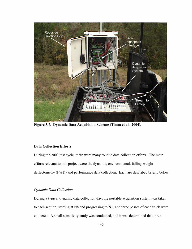
45

Figure 3.7. Dynamic Data Acquisition Scheme (Timm et al., 2004).

Data Collection Efforts

During the 2003 test cycle, there were many routine data collection efforts. The main

efforts relevant to this project were the dynamic, environmental, falling-weight

deflectometry (FWD) and performance data collection. Each are described briefly below.

Dynamic Data Collection

During a typical dynamic data collection day, the portable acquisition system was taken

to each section, starting at N8 and progressing to N1, and three passes of each truck were

collected. A small sensitivity study was conducted, and it was determined that three

Roadside Junction Box

Dynamic Acquisition System

Stream to Laptop

Slow/ highspeed Interface

46

truck passes captured the full variability of the data. This investigation will be explored

further in Chapter 5. It should be noted that initially, dynamic response data were

collected monthly, but once fatigue distresses were noticed in April 2004, the effort was

increased to weekly. It took two hours to collect data from all eight sections, and the

gauges were sampled at a rate of 2,000 Hz per channel in order to capture the full

response of the pavement under truck traffic. To serve as reference, this was the same

sampling frequency as used at Mn/ROAD for dynamic data collection (Mateos and

Snyder, 2002).

Due to the steady traffic at the Test Track and the enormous amount of data that

comprises one truck pass, it was not practical nor necessary to collect dynamic data

continuously. As described later in the Chapter 5, relationships between pavement

temperature and induced strain were developed to quantify the response for each truck

pass of the two-year test cycle.

Environmental Data Collection

The environmental data, including the in situ condition gauges and an on-site weather

station, were sampled continuously throughout the test cycle. As mentioned prior, the in

situ gauges were sampled every minute and hourly summaries were reported and stored

on the data acquisition computer in the laboratory. The data were transmitted wirelessly

from the roadside box to the computer in the on-site lab building, and the wireless

modem can be seen attached to the door of the roadside box in Figure 3.5.

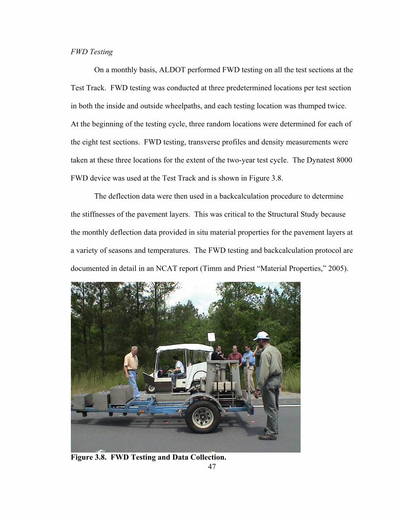
47

FWD Testing

On a monthly basis, ALDOT performed FWD testing on all the test sections at the

Test Track. FWD testing was conducted at three predetermined locations per test section

in both the inside and outside wheelpaths, and each testing location was thumped twice.

At the beginning of the testing cycle, three random locations were determined for each of

the eight test sections. FWD testing, transverse profiles and density measurements were

taken at these three locations for the extent of the two-year test cycle. The Dynatest 8000

FWD device was used at the Test Track and is shown in Figure 3.8.

The deflection data were then used in a backcalculation procedure to determine

the stiffnesses of the pavement layers. This was critical to the Structural Study because

the monthly deflection data provided in situ material properties for the pavement layers at

a variety of seasons and temperatures. The FWD testing and backcalculation protocol are

documented in detail in an NCAT report (Timm and Priest “Material Properties,” 2005).

Figure 3.8. FWD Testing and Data Collection.

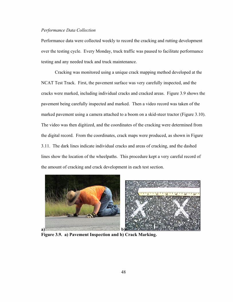
48

Performance Data Collection

Performance data were collected weekly to record the cracking and rutting development

over the testing cycle. Every Monday, truck traffic was paused to facilitate performance

testing and any needed track and truck maintenance.

Cracking was monitored using a unique crack mapping method developed at the

NCAT Test Track. First, the pavement surface was very carefully inspected, and the

cracks were marked, including individual cracks and cracked areas. Figure 3.9 shows the

pavement being carefully inspected and marked. Then a video record was taken of the

marked pavement using a camera attached to a boom on a skid-steer tractor (Figure 3.10).

The video was then digitized, and the coordinates of the cracking were determined from

the digital record. From the coordinates, crack maps were produced, as shown in Figure

3.11. The dark lines indicate individual cracks and areas of cracking, and the dashed

lines show the location of the wheelpaths. This procedure kept a very careful record of

the amount of cracking and crack development in each test section.

a) b) Figure 3.9. a) Pavement Inspection and b) Crack Marking.

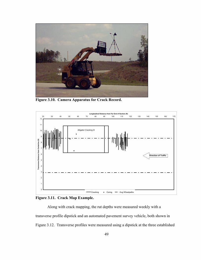
49

Figure 3.10. Camera Apparatus for Crack Record.

0

1

2

3

4

5

6

7

8

9

10

11

1225 35 45 55 65 75 85 95 105 115 125 135 145 155 165 175

Longitudinal Distance from Far End of Section (ft)

Tran

sver

se D

ista

nce

from

Cen

terli

ne (f

t)

Cracking Coring Avg Wheelpaths

Direction of Traffic

Alligator Cracking III

Figure 3.11. Crack Map Example. Along with crack mapping, the rut depths were measured weekly with a

transverse profile dipstick and an automated pavement survey vehicle, both shown in

Figure 3.12. Transverse profiles were measured using a dipstick at the three established

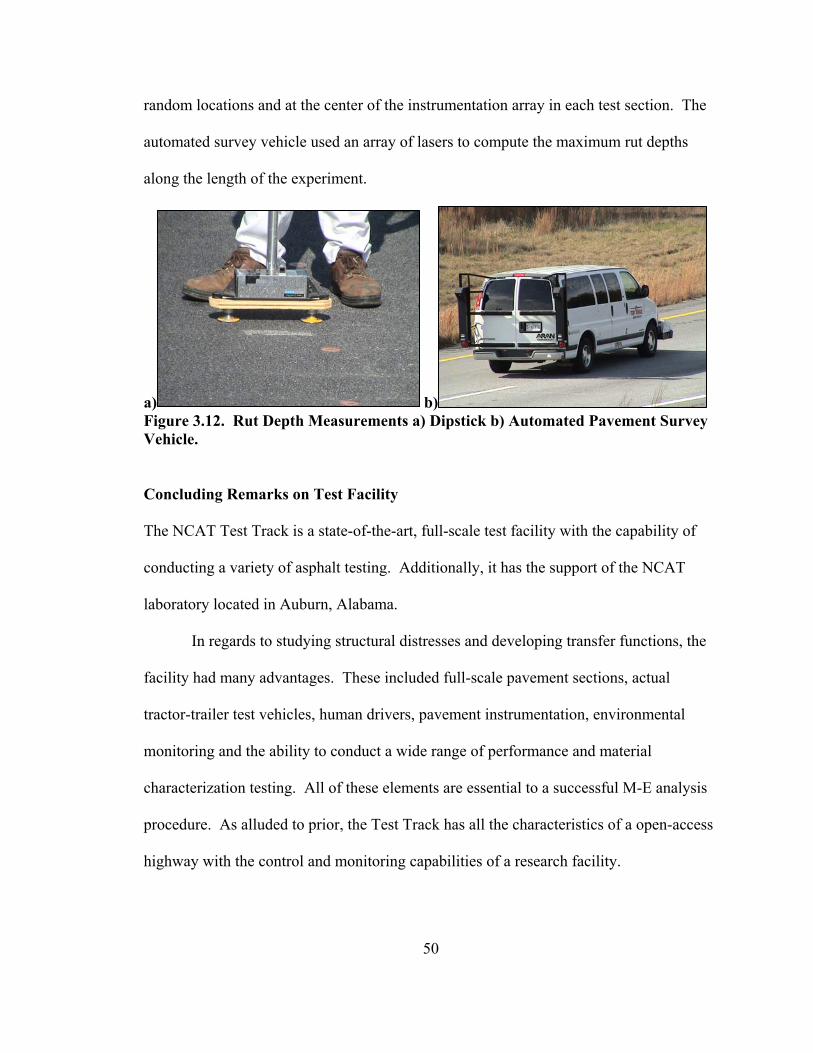
50

random locations and at the center of the instrumentation array in each test section. The

automated survey vehicle used an array of lasers to compute the maximum rut depths

along the length of the experiment.

a) b) Figure 3.12. Rut Depth Measurements a) Dipstick b) Automated Pavement Survey Vehicle. Concluding Remarks on Test Facility

The NCAT Test Track is a state-of-the-art, full-scale test facility with the capability of

conducting a variety of asphalt testing. Additionally, it has the support of the NCAT

laboratory located in Auburn, Alabama.

In regards to studying structural distresses and developing transfer functions, the

facility had many advantages. These included full-scale pavement sections, actual

tractor-trailer test vehicles, human drivers, pavement instrumentation, environmental

monitoring and the ability to conduct a wide range of performance and material

characterization testing. All of these elements are essential to a successful M-E analysis

procedure. As alluded to prior, the Test Track has all the characteristics of a open-access

highway with the control and monitoring capabilities of a research facility.

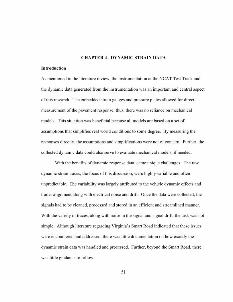
51

CHAPTER 4 - DYNAMIC STRAIN DATA

Introduction

As mentioned in the literature review, the instrumentation at the NCAT Test Track and

the dynamic data generated from the instrumentation was an important and central aspect

of this research. The embedded strain gauges and pressure plates allowed for direct

measurement of the pavement response; thus, there was no reliance on mechanical

models. This situation was beneficial because all models are based on a set of

assumptions that simplifies real world conditions to some degree. By measuring the

responses directly, the assumptions and simplifications were not of concern. Further, the

collected dynamic data could also serve to evaluate mechanical models, if needed.

With the benefits of dynamic response data, came unique challenges. The raw

dynamic strain traces, the focus of this discussion, were highly variable and often

unpredictable. The variability was largely attributed to the vehicle dynamic effects and

trailer alignment along with electrical noise and drift. Once the data were collected, the

signals had to be cleaned, processed and stored in an efficient and streamlined manner.

With the variety of traces, along with noise in the signal and signal drift, the task was not

simple. Although literature regarding Virginia’s Smart Road indicated that these issues

were encountered and addressed, there was little documentation on how exactly the

dynamic strain data was handled and processed. Further, beyond the Smart Road, there

was little guidance to follow.

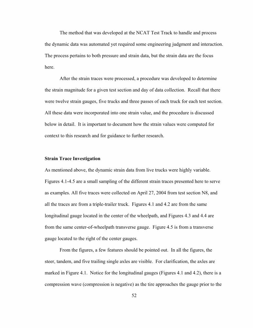
52

The method that was developed at the NCAT Test Track to handle and process

the dynamic data was automated yet required some engineering judgment and interaction.

The process pertains to both pressure and strain data, but the strain data are the focus

here.

After the strain traces were processed, a procedure was developed to determine

the strain magnitude for a given test section and day of data collection. Recall that there

were twelve strain gauges, five trucks and three passes of each truck for each test section.

All these data were incorporated into one strain value, and the procedure is discussed

below in detail. It is important to document how the strain values were computed for

context to this research and for guidance to further research.

Strain Trace Investigation

As mentioned above, the dynamic strain data from live trucks were highly variable.

Figures 4.1-4.5 are a small sampling of the different strain traces presented here to serve

as examples. All five traces were collected on April 27, 2004 from test section N8, and

all the traces are from a triple-trailer truck. Figures 4.1 and 4.2 are from the same

longitudinal gauge located in the center of the wheelpath, and Figures 4.3 and 4.4 are

from the same center-of-wheelpath transverse gauge. Figure 4.5 is from a transverse

gauge located to the right of the center gauges.

From the figures, a few features should be pointed out. In all the figures, the

steer, tandem, and five trailing single axles are visible. For clarification, the axles are

marked in Figure 4.1. Notice for the longitudinal gauges (Figures 4.1 and 4.2), there is a

compression wave (compression is negative) as the tire approaches the gauge prior to the

53

tensile peak. Also notice that there is a full strain reversal between every axle, even

within the tandem axle configuration. In Figure 4.2, the single axles show a diminishing

strain response, even though all five axles weighed approximately the same. After

further investigation, it was determined that the strain changes were in fact due to the

mechanical alignment of the trailers (Timm and Priest “Wheel Wander,” 2005). In other

words, the axles on that particular truck are aligned in such a way that the individual

trailers tend to track toward the center of the lane. In view of that observation, it is

important to note that the gauges were very sensitive to the lateral placement of the tire or

the relative distance between the tire and the gauge.

-150

-100

-50

0

50

100

150

200

0 0.2 0.4 0.6 0.8 1 1.2 1.4 1.6 1.8 2

Time, sec

Hor

izon

tal M

icro

stra

in

Figure 4.1. Longitudinal Strain Trace – Example 1.

Steer Axle

Tandem Axle

Single Axles

54

-150

-100

-50

0

50

100

150

200

250

0 0.2 0.4 0.6 0.8 1 1.2 1.4 1.6 1.8

Time, sec

Hor

izon

tal S

trai

n

Figure 4.2. Longitudinal Strain Trace – Example 2.

As expected, the transverse gauges (Figures 4.3-4.5) did not have the preceding

wave as the truck tire approached due to its perpendicular alignment. Figure 4.3 is an

example of a trace where the tire was slightly off the gauge (to the left or right of it),

pushing it in a compressive response. Figure 4.4 is an example of signal drift within a

single strain trace. Some signals drifted more than others, and the drift complicated

processing because there was not a steady baseline between each axle. The last strain

trace (Figure 4.5) is an example of some of the strange and nearly unexplainable

responses that often show up within a truck pass. Notice the compressive spike

preceding the steer axle and last single axles. Also notice the double hits at the top of the

tandem and first single axles, highlighted by the circles in the figure. The data were

collected from an un-cracked test section under, what can be determined, normal

55

conditions. Therefore, the rather unexplainable characteristics of the given trace are

considered simply byproducts of the sensitive instrumentation and acquisition process.

-200

-150

-100

-50

0

50

0 0.2 0.4 0.6 0.8 1 1.2 1.4 1.6 1.8 2

Time, sec

Hor

izon

tal M

icro

stra

in

Figure 4.3. Transverse Strain Trace – Example 1.

56

-500

-400

-300

-200

-100

0

100

200

300

0 0.2 0.4 0.6 0.8 1 1.2 1.4 1.6 1.8

Time, sec

Hor

izon

tal M

icro

stra

in

Figure 4.4. Transverse Strain Trace – Example 2.

-400

-300

-200

-100

0

100

200

300

0 0.2 0.4 0.6 0.8 1 1.2 1.4 1.6 1.8 2

Time, sec

Hor

izon

tal M

icro

stra

in

Figure 4.5. Transverse Strain Trace – Example 3.

Signal Drift

Compressive Spikes

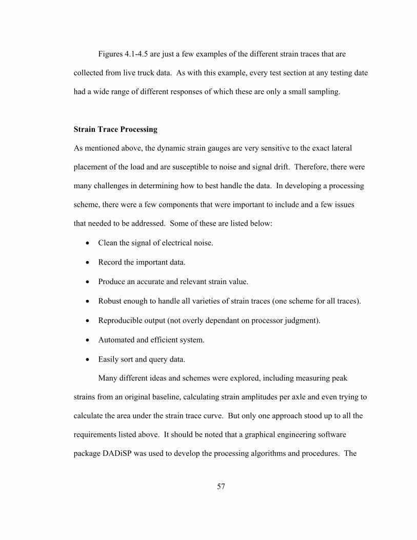
57

Figures 4.1-4.5 are just a few examples of the different strain traces that are

collected from live truck data. As with this example, every test section at any testing date

had a wide range of different responses of which these are only a small sampling.

Strain Trace Processing

As mentioned above, the dynamic strain gauges are very sensitive to the exact lateral

placement of the load and are susceptible to noise and signal drift. Therefore, there were

many challenges in determining how to best handle the data. In developing a processing

scheme, there were a few components that were important to include and a few issues

that needed to be addressed. Some of these are listed below:

• Clean the signal of electrical noise.

• Record the important data.

• Produce an accurate and relevant strain value.

• Robust enough to handle all varieties of strain traces (one scheme for all traces).

• Reproducible output (not overly dependant on processor judgment).

• Automated and efficient system.

• Easily sort and query data.

Many different ideas and schemes were explored, including measuring peak

strains from an original baseline, calculating strain amplitudes per axle and even trying to

calculate the area under the strain trace curve. But only one approach stood up to all the

requirements listed above. It should be noted that a graphical engineering software

package DADiSP was used to develop the processing algorithms and procedures. The

58

steps below are contained in one window worksheet within DADiSP that allowed for a

simplified and organized processing procedure.

First, the signal was cleaned of electrical noise by taking a moving average of 20

points. The moving average smoothed the curve, as shown in Figure 4.6, without losing

the important peaks and valleys. Then the inflection points of the signal were establish

and marked. The processor could adjust certain parameters, including the spread of

points that the program scans and the minimum strain difference between consecutive

inflection points, to manipulate the program in order to mark the relevant points. This

step involved human judgment and interaction. In most cases, the parameters did not

have to be adjusted, but in some cases it was necessary to have the option. For instance,

some traces had erroneous inflection points within one axle hit or along the baseline

which did not need to be marked. As an example, the small humps on the tandem and

first and second single axle on the strain trace showed in Figure 4.5 (circled in the figure)

should not be considered a strain cycle or an important event.

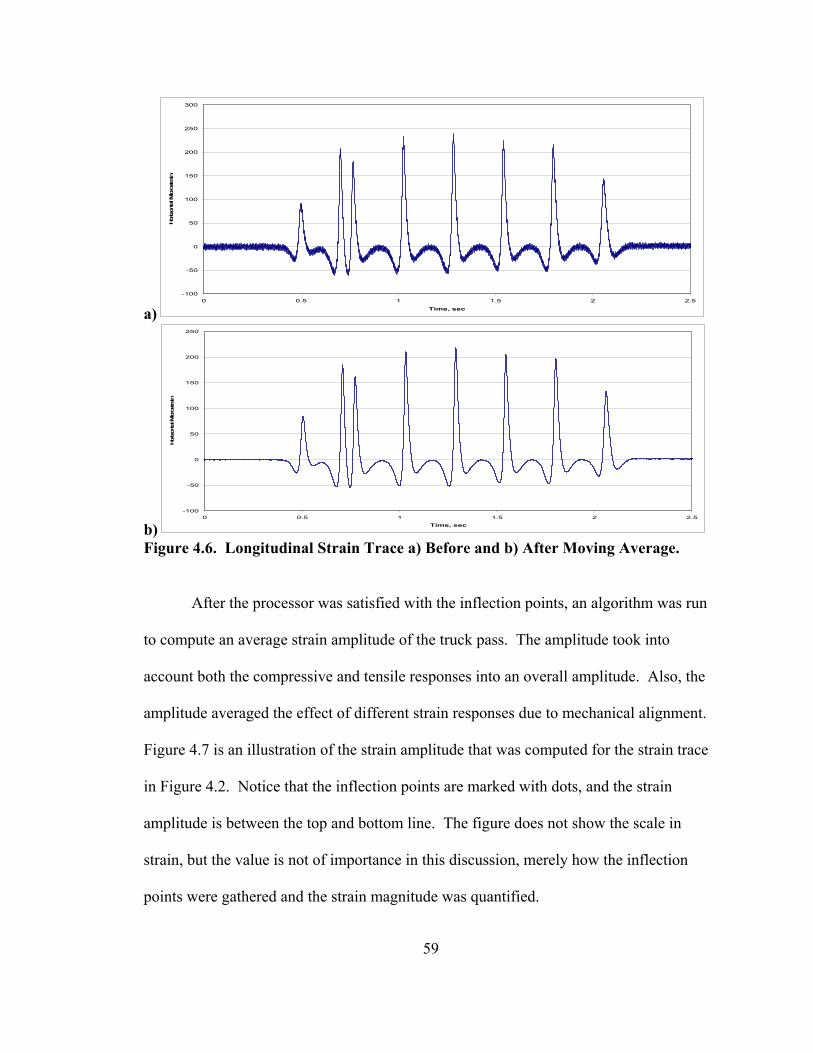
59

a)-100

-50

0

50

100

150

200

250

300

0 0.5 1 1.5 2 2.5

Time, sec

Hor

izon

tal M

icro

stra

in

b)-100

-50

0

50

100

150

200

250

0 0.5 1 1.5 2 2.5

Time, sec

Hor

izon

tal M

icro

strain

Figure 4.6. Longitudinal Strain Trace a) Before and b) After Moving Average.

After the processor was satisfied with the inflection points, an algorithm was run

to compute an average strain amplitude of the truck pass. The amplitude took into

account both the compressive and tensile responses into an overall amplitude. Also, the

amplitude averaged the effect of different strain responses due to mechanical alignment.

Figure 4.7 is an illustration of the strain amplitude that was computed for the strain trace

in Figure 4.2. Notice that the inflection points are marked with dots, and the strain

amplitude is between the top and bottom line. The figure does not show the scale in

strain, but the value is not of importance in this discussion, merely how the inflection

points were gathered and the strain magnitude was quantified.

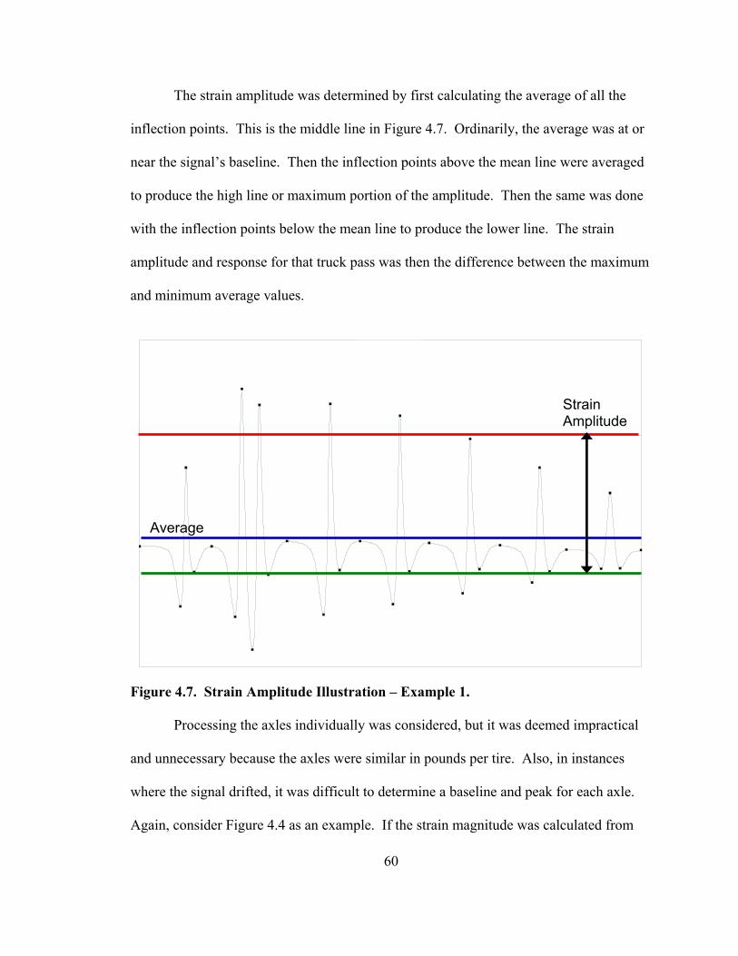
60

The strain amplitude was determined by first calculating the average of all the

inflection points. This is the middle line in Figure 4.7. Ordinarily, the average was at or

near the signal’s baseline. Then the inflection points above the mean line were averaged

to produce the high line or maximum portion of the amplitude. Then the same was done

with the inflection points below the mean line to produce the lower line. The strain

amplitude and response for that truck pass was then the difference between the maximum

and minimum average values.

W5: setplotstyle(1,1)

Figure 4.7. Strain Amplitude Illustration – Example 1.

Processing the axles individually was considered, but it was deemed impractical

and unnecessary because the axles were similar in pounds per tire. Also, in instances

where the signal drifted, it was difficult to determine a baseline and peak for each axle.

Again, consider Figure 4.4 as an example. If the strain magnitude was calculated from

Strain Amplitude

Average

61

the axle peak back to the original baseline, inaccurate numbers would have been

produced. Further, it is difficult to determine a relative baseline and maximum for each

axle of that signal. Figure 4.8 shows the processed strain trace from Figure 4.4 using the

developed procedure. The average amplitude gives an overall measure of the induced

strain response of that truck over eight strain cycles (one for the steer, two for the tandem

and one for each of the singles). As intended, the amplitudes shown in Figures 4.7 and

4.8 are essentially an average of the amplitude of all eight of the individual axles,

considering both the compression and tension response. Further, Figure 4.9 shows the

processed strain trace and subsequent strain amplitude for the rather irregular strain trace

shown in Figure 4.5. From the figure, the processing algorithm does an adequate job of

recording the relevant values and calculating an average strain amplitude for the truck

pass.

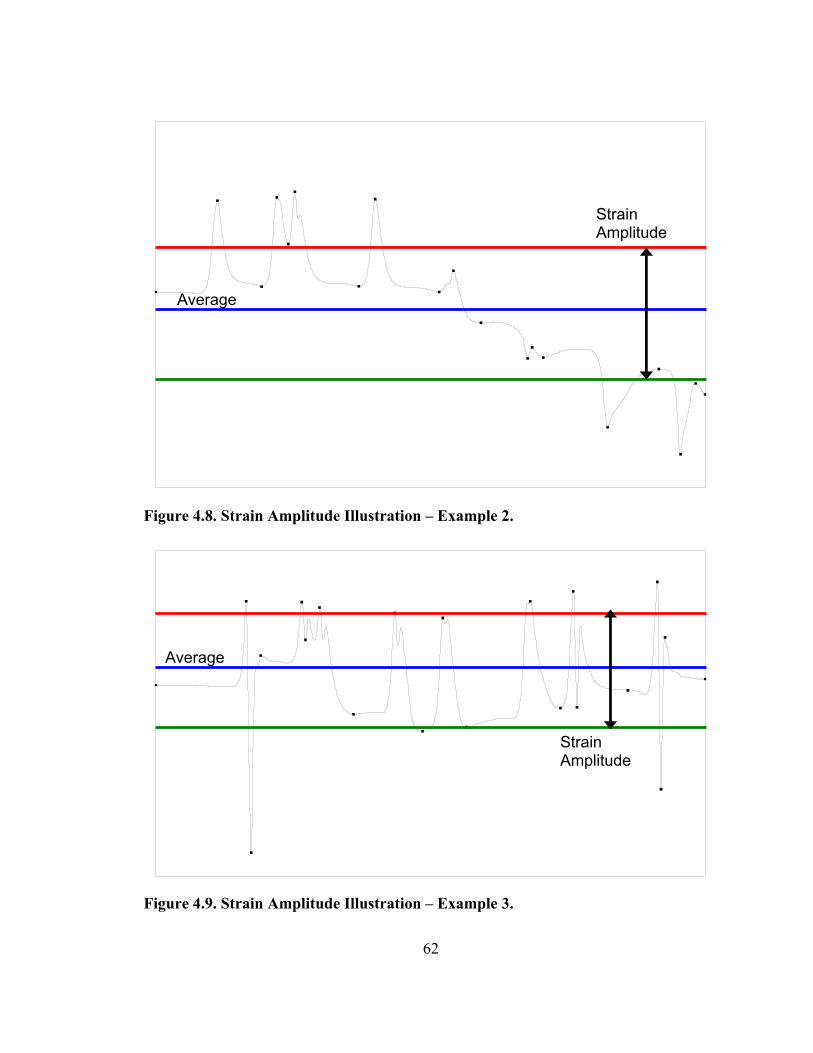
62

W5: setplotstyle(1,1)

Figure 4.8. Strain Amplitude Illustration – Example 2.

W5: setplotstyle(1,1)

Figure 4.9. Strain Amplitude Illustration – Example 3.

Strain Amplitude

Strain Amplitude

Average

Average

63

In the processing window (Figure 4.10), there was a graphical view of the original

trace in the top left and the processed signal in the top right. From the visual information

in the processed window, the processor could then make needed adjustments to the

parameters to mark the significant inflection points in order to produce the most accurate

strain amplitude for the given signal. As mentioned, the adjustments to the algorithm

included the number of points scanned to calculate an inflection point and the minimum

difference between consecutive inflection points.

Once the signal was satisfactory, the processor “recorded” the truck pass. The

program at this point asked for the gauge identification, truck identification and the pass

number to keep the information organized. The recorded data are shown in the bottom

right window which includes the gauge factor (which is unique to each strain gauge),

truck, pass, maximum and minimum inflection point as well as the amplitude in

microstrain.

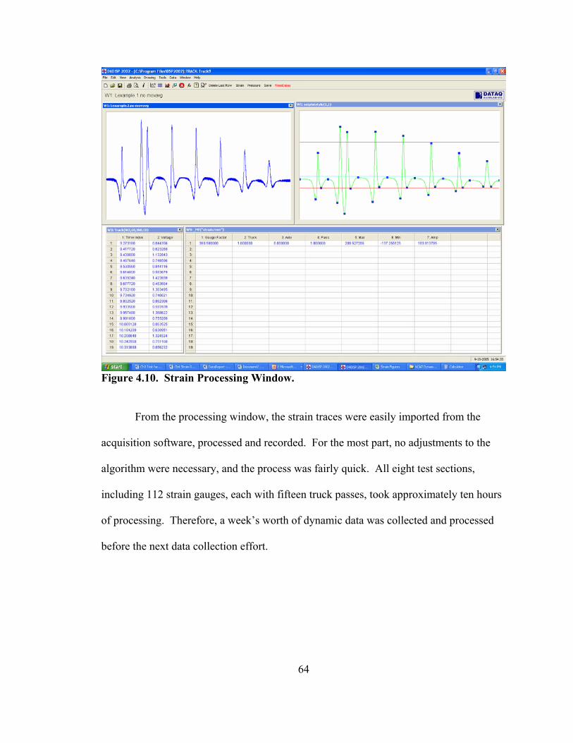
64

Figure 4.10. Strain Processing Window.

From the processing window, the strain traces were easily imported from the

acquisition software, processed and recorded. For the most part, no adjustments to the

algorithm were necessary, and the process was fairly quick. All eight test sections,

including 112 strain gauges, each with fifteen truck passes, took approximately ten hours

of processing. Therefore, a week’s worth of dynamic data was collected and processed

before the next data collection effort.

65

Strain Characterization

All of the truck passes for each strain gauge were collected, processed and stored. But

recall that there were twelve strain gauges per test section; therefore, one truck pass

produced, at most, twelve different strain readings. More precisely, there were six

gauges at each orientation, so each truck pass had at most six readings in both the

longitudinal and transverse orientation.

Depending on where the truck tires actually passed through the gauge array, the

strain values varied. For example, Figure 4.11 shows three longitudinal strain traces from

the same truck pass, one at each lateral offset. From the figure, the truck tire was closest

to the right gauge because it registered the highest strain value, and the left gauge

registered the lowest. It could be argued that the right strain gauge registered the “best

hit” for this particular truck pass. The next truck may have been closer to the center

gauge, causing it to register the highest.

Because the strain reading that most accurately measured the response of the

truck was of interest, the maximum reading of each orientation (transverse and

longitudinal) was considered the strain response for each corresponding truck and pass.

In the case of Figure 4.11, it was the right longitudinal gauge, and for other passes, it may

have been the center or left gauge. If an average was taken of all the longitudinal

amplitudes, then the strain value would be incorrectly reduced. Remember that the

reasoning for an array of gauges, rather than just gauges located directly in the wheelpath,

was to capture the lateral placement of the trucks. With this scheme, it was more likely

that one of the three offsets very closely registered a direct hit of the tire over the gauge,

thus producing the maximum strain value.

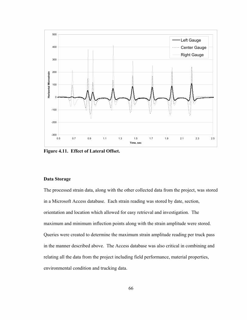
66

-300

-200

-100

0

100

200

300

400

500

0.5 0.7 0.9 1.1 1.3 1.5 1.7 1.9 2.1 2.3 2.5

Time, sec

Hor

izon

tal M

icro

stra

in

Left Gauge

Center Gauge

Right Gauge

Figure 4.11. Effect of Lateral Offset.

Data Storage

The processed strain data, along with the other collected data from the project, was stored

in a Microsoft Access database. Each strain reading was stored by date, section,

orientation and location which allowed for easy retrieval and investigation. The

maximum and minimum inflection points along with the strain amplitude were stored.

Queries were created to determine the maximum strain amplitude reading per truck pass

in the manner described above. The Access database was also critical in combining and

relating all the data from the project including field performance, material properties,

environmental condition and trucking data.

67

Concluding Remarks on Dynamic Data

Processing dynamic pavement response data under live truck traffic is quite a challenge

considering the volume of data collected and the variability in the data. The quirks of the

sensitive instrumentation adds one level of complexity, and the live truck traffic adds

another. These challenges have been noted by other researchers dealing with dynamic

data and truck loading (Al-Qadi et al., 2004).

The processing procedure developed at the NCAT Test Track slowly evolved as

the test cycle progressed. It began in a spreadsheet program retrieving inflection points

by hand and evolved to a more robust and efficient process. As the understanding of the

traces grew, new ways to automate the process were incorporated. The final procedure

still involved a level of human interaction which is both important and necessary. There

are times when judgment is necessary regarding the validity of the gathered data or basic

engineering judgment is needed to determine the relevant characteristics of each dynamic

trace.

It should be noted that the method is not infallible, but it does produce repeatable

and accurate strain values for the vast majority of signals. The results are repeatable in

the sense that the same numbers are generated regardless of the processor. As mentioned,

many improvements to the process have been made throughout this test cycle, and it is

expected that even more will be added in the subsequent testing cycles to make the

process more efficient and flexible to the variety of traces.

68

CHAPTER 5 – METHODOLOGY AND PARAMETER CHARACTERIZATION

Introduction

The fatigue transfer functions developed from the 2003 NCAT Test Track were derived

strictly from field data without laboratory testing or theoretical models. Therefore, the

process was fairly unique and required a massive amount of data collection and synthesis.

From Figure 1.1, the inputs (material properties, environment, traffic and the pavement

structure) for M-E analysis were measured and quantified, in situ, at the Test Track. The

material properties were determined using FWD testing; the environmental data were

collected continuously via temperature probes, TDRs and the weather station; the traffic

was monitored by weight and mileage data; and the layer thicknesses were directly

measured during construction. Further, the pavement response was measured from field

instrumentation (strain gauges and pressure plates) rather than calculated using a

theoretical model. And finally, the pavement performance was monitored and recorded

in the field.

From the above field data collection efforts, the fatigue transfer functions were

developed or calibrated by working Figure 1.1 in both the forward and backward

direction, as shown in Figure 5.1. Simply stated, the transfer functions were calibrated to

most closely relate the pavement response to performance through a transfer function.

The methodology section will further describe how exactly the damage was calculated

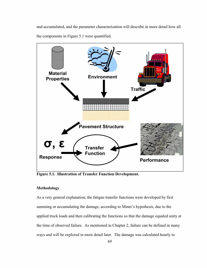
69

and accumulated, and the parameter characterization will describe in more detail how all

the components in Figure 5.1 were quantified.

Figure 5.1. Illustration of Transfer Function Development.

Methodology

As a very general explanation, the fatigue transfer functions were developed by first

summing or accumulating the damage, according to Miner’s hypothesis, due to the

applied truck loads and then calibrating the functions so that the damage equaled unity at

the time of observed failure. As mentioned in Chapter 2, failure can be defined in many

ways and will be explored in more detail later. The damage was calculated hourly to

Material Properties Environment

Traffic

Pavement Structure

σ, ε Response

Transfer Function

Performance

70

account for changes in strain magnitude and HMA stiffness due to daily temperature

fluctuations. The induced strain is dependant on temperature somewhat indirectly though

the stiffness of the HMA layer, which is a function of the temperature of the material.

Recall from Miner’s hypothesis (Equation 1.1) the two variables: the allowable

cycles until failure, Nf, and the applied loads, n. In order to successfully develop transfer

functions, these two parameters had to be calculated over the testing time to accurately

accumulate the damage. A record of the traffic data, or applied cycles, and temperature

data were kept continuously over the test cycle, but the strain data and FWD data were

collected only periodically. As mentioned prior, it was not practical to collect

continuous dynamic or stiffness data for every truck pass or every hour. As a result,

relationships were developed to accurately estimate the stiffness and strain data at a given

condition (temperature). The stiffness – temperature and strain – temperature

relationships, as well as the respective procedures to develop the relationships, are

presented later in this chapter.

In summary, the procedure employed to calibrate fatigue transfer functions in this

study followed these steps:

1. Determine the number of truck passes for the given hour (triple-trailer trucks and

box trailer).

2. Determine the mid-depth temperature of the HMA layer for the given hour from

temperature probe data.

3. Use the strain – temperature relationship to estimate the induced strain due to the

given truck at the given temperature.

71

4. Use the stiffness – temperature relationship to estimate the HMA stiffness at the

given temperature.

5. Determine the time of fatigue failure.

6. Calculate the cycles to failure (Nf) for the given condition.

7. Calculate the incremental damage (Di) for the given traffic cycles (n) and cycles

to failure (Nf).

8. Repeat for each hour and accumulate the damage over the test cycle until the

failure criterion is met.

9. Calculate the regression constants (calibrate the model) so that the total damage

(D) equals 1 at time of failure.

The remaining topics of this chapter will discuss in more detail how the data were

generated and how the relationships were quantified in the steps above. In other words,

each element in Figure 5.1 will be further discussed.

Traffic Characterization

Weight Data

The triple-trailer trucks used at the NCAT Test Track were loaded to accelerate the

testing without venturing too far from legal axle weights (20-kip single axle, 34-kip

tandem axle) The generic load distribution is shown in Figure 5.2, but the exact loads

were monitored and varied slightly from truck to truck. Exact axle weight data are given

in Table 5.1 for the five triple-trailers and the box trailer. Notice that the box trailer was

not loaded as heavily as the triples because it served as the conventional highway vehicle

comparison, in both configuration and load, for trucking and fuel studies. From the

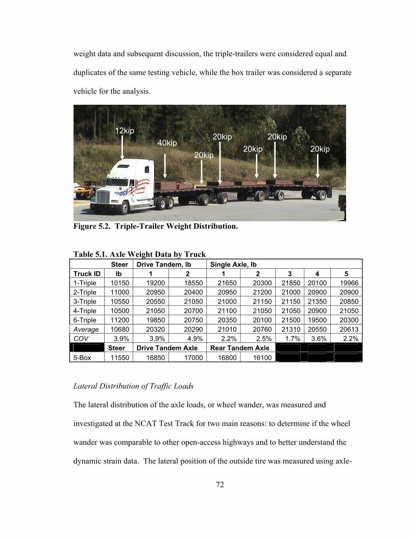
72

weight data and subsequent discussion, the triple-trailers were considered equal and

duplicates of the same testing vehicle, while the box trailer was considered a separate

vehicle for the analysis.

Figure 5.2. Triple-Trailer Weight Distribution.

Table 5.1. Axle Weight Data by Truck Steer Drive Tandem, lb Single Axle, lb

Truck ID lb 1 2 1 2 3 4 5 1-Triple 10150 19200 18550 21650 20300 21850 20100 199662-Triple 11000 20950 20400 20950 21200 21000 20900 209003-Triple 10550 20550 21050 21000 21150 21150 21350 208504-Triple 10500 21050 20700 21100 21050 21050 20900 210506-Triple 11200 19850 20750 20350 20100 21500 19500 20300Average 10680 20320 20290 21010 20760 21310 20550 20613COV 3.9% 3.9% 4.9% 2.2% 2.5% 1.7% 3.6% 2.2% Steer Drive Tandem Axle Rear Tandem Axle 5-Box 11550 16850 17000 16800 16100

Lateral Distribution of Traffic Loads

The lateral distribution of the axle loads, or wheel wander, was measured and

investigated at the NCAT Test Track for two main reasons: to determine if the wheel

wander was comparable to other open-access highways and to better understand the

dynamic strain data. The lateral position of the outside tire was measured using axle-

12kip 40kip

20kip

20kip 20kip 20kip 20kip

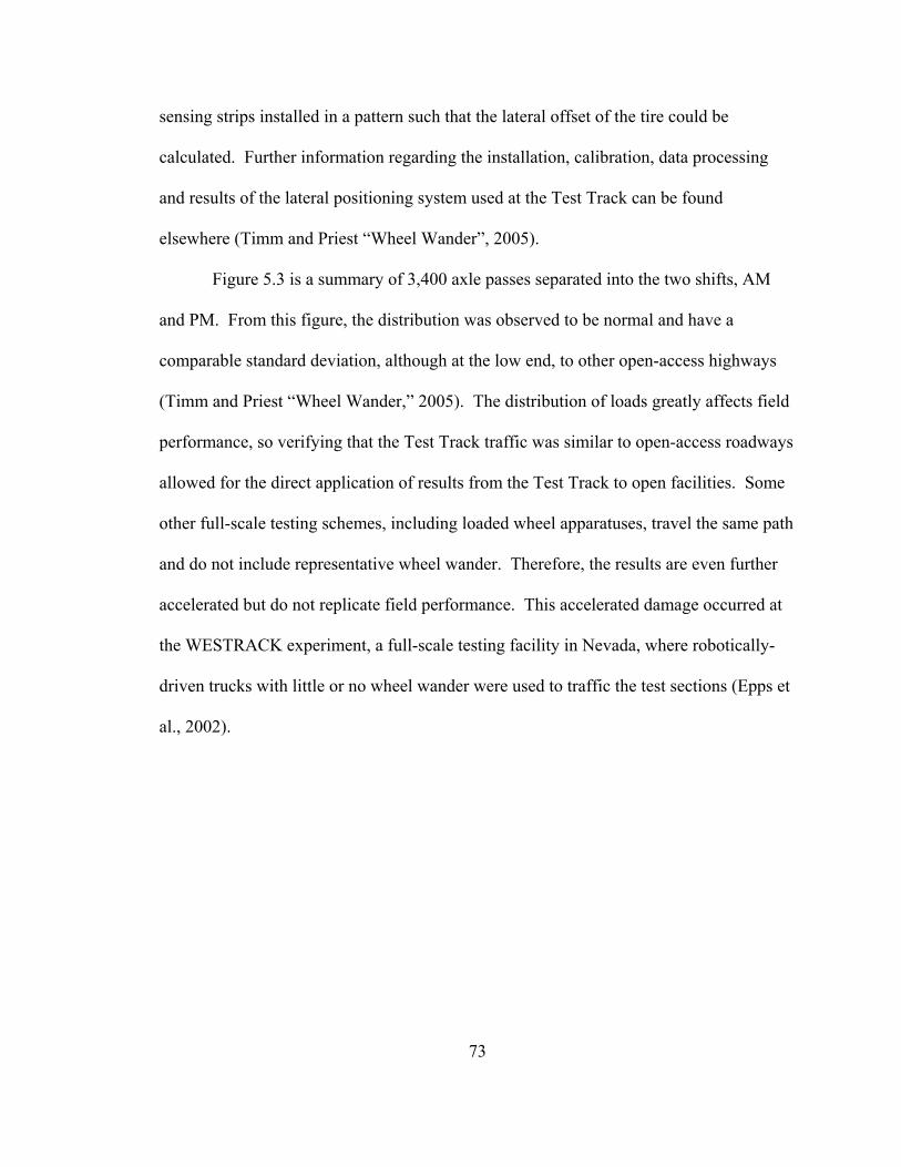
73

sensing strips installed in a pattern such that the lateral offset of the tire could be

calculated. Further information regarding the installation, calibration, data processing

and results of the lateral positioning system used at the Test Track can be found

elsewhere (Timm and Priest “Wheel Wander”, 2005).

Figure 5.3 is a summary of 3,400 axle passes separated into the two shifts, AM

and PM. From this figure, the distribution was observed to be normal and have a

comparable standard deviation, although at the low end, to other open-access highways

(Timm and Priest “Wheel Wander,” 2005). The distribution of loads greatly affects field

performance, so verifying that the Test Track traffic was similar to open-access roadways

allowed for the direct application of results from the Test Track to open facilities. Some

other full-scale testing schemes, including loaded wheel apparatuses, travel the same path

and do not include representative wheel wander. Therefore, the results are even further

accelerated but do not replicate field performance. This accelerated damage occurred at

the WESTRACK experiment, a full-scale testing facility in Nevada, where robotically-

driven trucks with little or no wheel wander were used to traffic the test sections (Epps et

al., 2002).

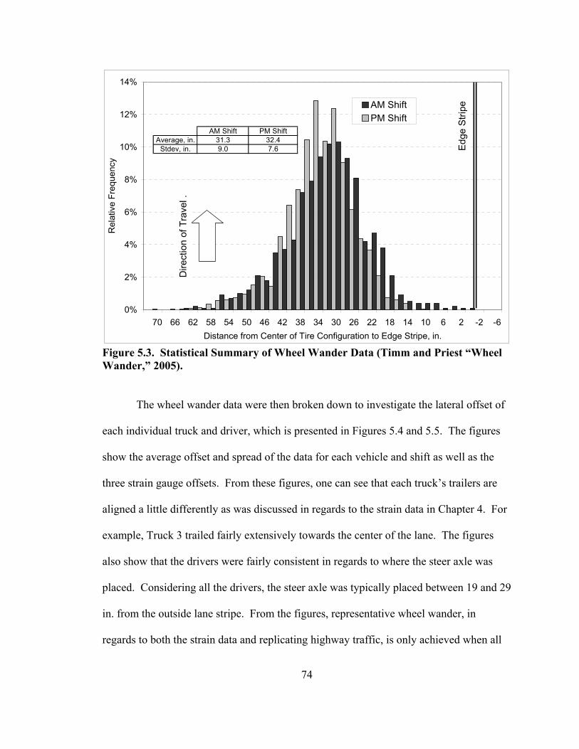
74

0%

2%

4%

6%

8%

10%

12%

14%

-6-22610141822263034384246505458626670Distance from Center of Tire Configuration to Edge Stripe, in.

Rel

ativ

e Fr

eque

ncy

AM ShiftPM Shift

AM Shift PM ShiftAverage, in. 31.3 32.4

Stdev, in. 9.0 7.6 Edg

e S

tripe

Dire

ctio

n of

Tra

vel .

Figure 5.3. Statistical Summary of Wheel Wander Data (Timm and Priest “Wheel Wander,” 2005).

The wheel wander data were then broken down to investigate the lateral offset of

each individual truck and driver, which is presented in Figures 5.4 and 5.5. The figures

show the average offset and spread of the data for each vehicle and shift as well as the

three strain gauge offsets. From these figures, one can see that each truck’s trailers are

aligned a little differently as was discussed in regards to the strain data in Chapter 4. For

example, Truck 3 trailed fairly extensively towards the center of the lane. The figures

also show that the drivers were fairly consistent in regards to where the steer axle was

placed. Considering all the drivers, the steer axle was typically placed between 19 and 29

in. from the outside lane stripe. From the figures, representative wheel wander, in

regards to both the strain data and replicating highway traffic, is only achieved when all

75

the trucks were included together. It is important to note that Truck 6 was added to the

fleet following this investigation, which is why it is not included in Figures 5.4 and 5.5.

0

5

10

15

20

25

30

35

40

45

50

55

60

65

70

1 2 3 4 5 6 7 8 1 2 3 4 5 6 7 8 1 2 3 4 5 6 7 8 1 2 3 4 5 6 7 8 1 2 3 4 5

1 2 3 4 5

Truck, Axle

Offs

et fr

om E

dges

trip

e, in

.

Center Gauges

Right Gauges

Left Gauges

2σ

Figure 5.4. Wheel Wander Data – AM (Timm and Priest “Wheel Wander,” 2005).

0

5

10

15

20

25

30

35

40

45

50

55

60

65

70

1 2 3 4 5 6 7 8 1 2 3 4 5 6 7 8 1 2 3 4 5 6 7 8 1 2 3 4 5 6 7 8 1 2 3 4 5

1 2 3 4 5

Truck, Axle

Offs

et fr

om E

dges

trip

e, in

.

Center Gauges

Right Gauges

Left Gauges

2σ

Figure 5.5. Wheel Wander Data – PM (Timm and Priest “Wheel Wander,” 2005).

76

To further investigate the effect of lateral placement on the collected strain data,

ten consecutive passes of each triple-trailer were collected and analyzed. The strain data,

shown in Figure 5.6, agreed with what was concluded from the wheel wander data. The

individual trucks were fairly consistent by pass, and the range of variability was captured

in about three passes. The figure shows the average strain magnitude over the number of

passes shown on the x-axis. From the figure, no additional information was gathered

with ten passes versus three passes. Additionally, the only way to gather the full range of

strain response from the various sensors in the array was to gather data from all of the

trucks, and thus capture the full lateral wander. Therefore, the testing scheme consisted

of collecting and processing, in the manner described in Chapter 4, three passes of all the

trucks. Then, the maximum strain response for each pass, considering all the triple-

trailers, was determined and averaged together to quantify the strain response for that test

section. Basically, the five different trucks provided the full range of registered strain

response per pass, and then three passes were averaged to account for random variation in

the data.

A similar observation was made regarding the effect of lateral position on the

recorded strain values at Virginia’s Smart Road. Al-Qadi et al. (2004) reports that when

collecting dynamic data, multiple truck passes are collected and processed in attempt to

collect a direct hit of the tire over the gauge. From the multiple passes, the maximum

strain value was considered the direct hit and was stored.

77

0

20

40

60

80

100

120

140

160

180

200

1 2 3 4 5 6 7 8 9 10 11

Number of Passes Included in Average

Ave

rage

Lon

gitu

dina

l Mic

rost

rain

Truck 1

Truck 2

Truck 3

Truck 4

Figure 5.6. Average Strain by Truck and Pass.

Traffic Volume

The trucking operation at the NCAT Test Track consisted of two 7.5 hour shifts, five

days a week. The traffic volume data were recorded based on the mileage per shift and

then converted to laps per hour based on the shift schedule and track length (1.7

mile/lap). Typically, each truck completed 28 laps in an hour. From above, the triple-

trailer laps were combined and considered together, while the box trailer was considered

separately.

Concluding Remarks on Traffic Characterization

The traffic at the NCAT Test Track was highly controlled, and thus the characterization

was fairly straightforward. There were only two vehicle types, and the only difficulty

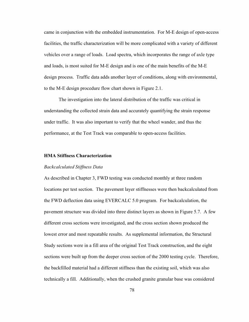
78

came in conjunction with the embedded instrumentation. For M-E design of open-access

facilities, the traffic characterization will be more complicated with a variety of different

vehicles over a range of loads. Load spectra, which incorporates the range of axle type

and loads, is most suited for M-E design and is one of the main benefits of the M-E

design process. Traffic data adds another layer of conditions, along with environmental,

to the M-E design procedure flow chart shown in Figure 2.1.

The investigation into the lateral distribution of the traffic was critical in

understanding the collected strain data and accurately quantifying the strain response

under traffic. It was also important to verify that the wheel wander, and thus the

performance, at the Test Track was comparable to open-access facilities.

HMA Stiffness Characterization

Backcalculated Stiffness Data

As described in Chapter 3, FWD testing was conducted monthly at three random

locations per test section. The pavement layer stiffnesses were then backcalculated from

the FWD deflection data using EVERCALC 5.0 program. For backcalculation, the

pavement structure was divided into three distinct layers as shown in Figure 5.7. A few

different cross sections were investigated, and the cross section shown produced the

lowest error and most repeatable results. As supplemental information, the Structural

Study sections were in a fill area of the original Test Track construction, and the eight

sections were built up from the deeper cross section of the 2000 testing cycle. Therefore,

the backfilled material had a different stiffness than the existing soil, which was also

technically a fill. Additionally, when the crushed granite granular base was considered

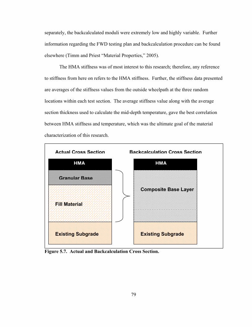
79

separately, the backcalculated moduli were extremely low and highly variable. Further

information regarding the FWD testing plan and backcalculation procedure can be found

elsewhere (Timm and Priest “Material Properties,” 2005).

The HMA stiffness was of most interest to this research; therefore, any reference

to stiffness from here on refers to the HMA stiffness. Further, the stiffness data presented

are averages of the stiffness values from the outside wheelpath at the three random

locations within each test section. The average stiffness value along with the average

section thickness used to calculate the mid-depth temperature, gave the best correlation

between HMA stiffness and temperature, which was the ultimate goal of the material

characterization of this research.

Figure 5.7. Actual and Backcalculation Cross Section.

HMA

Granular Base

Fill Material

Existing Subgrade

HMA

Composite Base Layer

Existing Subgrade

Actual Cross Section Backcalculation Cross Section

80

Seasonal Trends

As noted prior, the HMA stiffness is highly dependant on temperature, which can

be seen in Figure 5.8. The figure shows the seasonal trend in the stiffness data for all

eight test sections. Note that the data have not been corrected to a reference temperature

in order to explore the effect of temperature. As expected, when the temperature

increased in the summer, the pavement softened. Also notice after the summer, sections

N1 and N2 deviated from the general trend of the other test sections. The deviation in

stiffness was due to the extent of cracking in those two sections at that time. The

remaining material analysis disregards any stiffness data after initial cracking was

observed because traditional M-E design does not account for cracking in the pavement

models (“Thickness Design,” 1982; Eres, 2004). Further, the presence of cracks can

cause erroneous deflection data from the FWD.

81

10

100

1000

10000

10/6/2003

11/25/2003

1/14/2004

3/4/2004

4/23/2004

6/12/2004

8/1/2004

9/20/2004

11/9/2004

12/29/2004

2/17/2005

4/8/2005

Date

HM

A S

tiffn

ess,

ksi

N1N2N3N4N5N6N7N8

Figure 5.8. Seasonal Trend in HMA Stiffness.

Stiffness Prediction Models

The effect of temperature on stiffness can be better explored by plotting the stiffness as a

function of temperature rather than date. Figure 5.9 shows the average stiffness as a

function of the mid-depth temperature of the HMA layer. The mid-depth temperature

was calculated from temperature probe data collected during FWD testing, assuming a

linear temperature profile. The mid-depth temperature is often correlated to stiffness and

proved to be the best predictor of stiffness for this study.

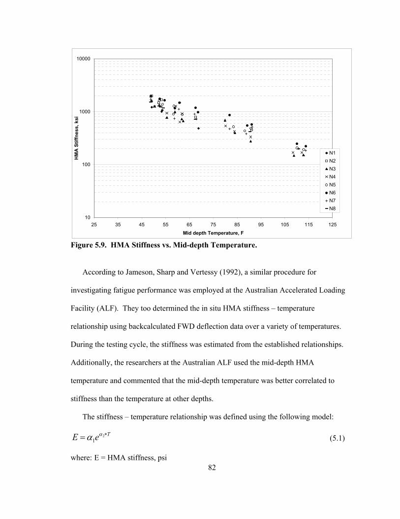
82

10

100

1000

10000

25 35 45 55 65 75 85 95 105 115 125

Mid depth Temperature, F

HM

A S

tiffn

ess,

ksi

N1N2N3N4N5N6N7N8

Figure 5.9. HMA Stiffness vs. Mid-depth Temperature.

According to Jameson, Sharp and Vertessy (1992), a similar procedure for

investigating fatigue performance was employed at the Australian Accelerated Loading

Facility (ALF). They too determined the in situ HMA stiffness – temperature

relationship using backcalculated FWD deflection data over a variety of temperatures.

During the testing cycle, the stiffness was estimated from the established relationships.

Additionally, the researchers at the Australian ALF used the mid-depth HMA

temperature and commented that the mid-depth temperature was better correlated to

stiffness than the temperature at other depths.

The stiffness – temperature relationship was defined using the following model:

TeE ∗= 21

αα (5.1)

where: E = HMA stiffness, psi

83

T = Mid-depth HMA temperature, °F

α1, α2 = Regression constants

A regression analysis was performed for all eight sections, individually, to create accurate

models to predict the in situ stiffness given the temperature, which was collected every

hour. The relationships were established for each section to account for any differences

due to cross section, binder type or construction variability.

The regression constants and R2 value for the eight test sections, as well as a

general equation considering all the data, are given in Table 5.2 following the form of

Equation 5.1. The general model is a good predictor of stiffness, and including other

factors like the HMA thickness and binder type (PG 67-22 unmodified vs. PG 76-22

modified) did not increase the model accuracy. It should be noted that another

investigation of the same data determined that there was no significant evidence that the

two binders produced consistently different mixtures stiffnesses (Timm and Priest

“Material Properties,” 2005). It is also important to point out that there was limited pre-

cracking backcalculated stiffness data for sections N1 and N2 because the first FWD

testing date was December 2003, and the sections showed signs of cracking in April and

June of 2004, respectively. The limited data can also be seen in Figure 5.9 where the data

for N1 and N2 covered a small temperature range. Yet extrapolation was warranted

because the trend was similar to the other sections.

84

Table 5.2. Regression Analysis for HMA Stiffness – Temperature Relationship. Section α1 α2 R2

N1* 11,696,542 -0.0457 0.985 N2* 14,308,573 -0.0414 0.952 N3 8,809,046 -0.0378 0.904 N4 8,030,572 -0.0351 0.915 N5 11,415,436 -0.0386 0.940 N6 8,482,965 -0.0302 0.962 N7 8,067,465 -0.0342 0.917 N8 6,918,499 -0.0321 0.989 All 8,187,876 -0.0340 0.850

Alvarez and Thompson 4,841,000 -0.048

* Limited FWD Data

Research using data from Mn/ROAD found a similar correlation between HMA

temperature and in situ stiffness which followed the model of Equation 5.1. The

regression constants determined by Alvarez and Thompson (1998) are also shown in

Table 5.2 and serve as a check of reasonableness. Although the relationship developed

by Alvarez and Thompson (1998) used the temperature at 1/3 depth, the relationship

follows the same trend and is similar to the relationships developed at the NCAT Test

Track. It is also interesting to note that the binder used at Mn/ROAD was a much softer

binder than that used at the Test Track. A softer 120/150 penetration (roughly PG 52-34)

binder was used, and notice that the intercept value for the temperature – stiffness

relationship was much lower than the equations derived at the NCAT Test Track. The

relationship developed by Alvarez and Thompson (1998) simply serves as a check and

provides confidence in the data.

85

Concluding Remarks on HMA Characterization

From the above analysis, a relationship between mid-depth HMA temperature and in situ

stiffness was developed for each test section. Therefore, the hourly temperature readings

were used as predictors of stiffness over the entire testing cycle. This provided a much

more accurate stiffness number than a seasonal or monthly average. Additionally, the

analysis quantified the effect of temperature on HMA stiffness, which can be used in

other design and research efforts. The study also determined that there was not a

significant difference in the in situ stiffness amongst the two binders, which was not

necessarily expected (Timm and Priest “Material Properties,” 2005).

Strain Response Characterization

General Trends

As with the HMA stiffness data, seasonal trends and damage were observed with the

strain data over time (Figure 5.10). The induced strain is a function of the stiffness of the

mix, which is in turn a function of temperature. As a result, the strain response is

strongly correlated with the temperature of the HMA layer. From Figure 5.10, the strain

values increased during the warmer months and returned to lower values as the fall set in.

Recall from prior discussion that the strain values presented are the average over three

passes of the maximum reading (best hit) for the five triple-trailer trucks. Additionally,

the values presented in Figure 5.10 are from the longitudinal-orientated strain gauges,

exclusively.

Unlike the stiffness data, the strain data are also a function of the thickness of the

HMA layer. The load bearing capacity of the HMA increases with thickness; thus, the

86

induced strains at the bottom of the layer are reduced with thicker HMA sections. The

thickness effect is the central concept behind M-E design: determine the needed layer

thicknesses to control the critical responses, such as horizontal strain at the bottom of the

HMA layer, given the traffic and seasonal data. The thickness effect is especially evident

for the two 5 in. sections, N1 and N2, which have much higher strain levels than the other

sections. It is more difficult to distinguish the other sections from Figure 5.10, but they

will be explored in more detail later. Also notice during the second fall, the strain values

for N8 did not trend back down as the other sections. This was a result of cracking that

was progressing through section N8 beginning in July 2004. By the following fall, the

pavement was fairly damaged and no longer intact; therefore, the recorded strain values

were higher. Also notice that the strain values for N1 and N2 were especially high after

the first spring, when the sections began to show fatigue cracking. Strain data collected

after visible cracking were not included in the fatigue models for the same reasons as the

stiffness data. One, the readings are especially variable and erratic, and two, it is

common practice that fatigue models or transfer functions assume an intact pavement

structure.

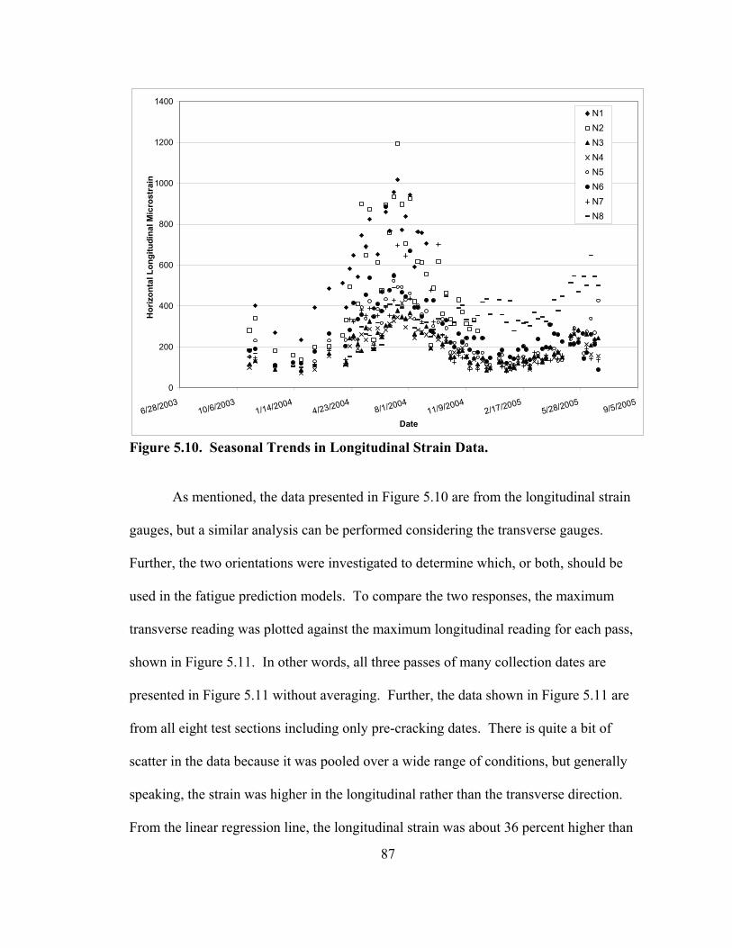
87

0

200

400

600

800

1000

1200

1400

6/28/200310/6/2003

1/14/20044/23/2004

8/1/200411/9/2004

2/17/20055/28/2005

9/5/2005

Date

Hor

izon

tal L

ongi

tudi

nal M

icro

stra

in

N1N2N3N4N5N6N7N8

Figure 5.10. Seasonal Trends in Longitudinal Strain Data.

As mentioned, the data presented in Figure 5.10 are from the longitudinal strain

gauges, but a similar analysis can be performed considering the transverse gauges.

Further, the two orientations were investigated to determine which, or both, should be

used in the fatigue prediction models. To compare the two responses, the maximum

transverse reading was plotted against the maximum longitudinal reading for each pass,

shown in Figure 5.11. In other words, all three passes of many collection dates are

presented in Figure 5.11 without averaging. Further, the data shown in Figure 5.11 are

from all eight test sections including only pre-cracking dates. There is quite a bit of

scatter in the data because it was pooled over a wide range of conditions, but generally

speaking, the strain was higher in the longitudinal rather than the transverse direction.

From the linear regression line, the longitudinal strain was about 36 percent higher than

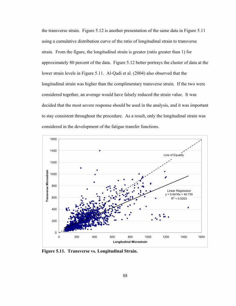
88

the transverse strain. Figure 5.12 is another presentation of the same data in Figure 5.11

using a cumulative distribution curve of the ratio of longitudinal strain to transverse

strain. From the figure, the longitudinal strain is greater (ratio greater than 1) for

approximately 80 percent of the data. Figure 5.12 better portrays the cluster of data at the

lower strain levels in Figure 5.11. Al-Qadi et al. (2004) also observed that the

longitudinal strain was higher than the complimentary transverse strain. If the two were

considered together, an average would have falsely reduced the strain value. It was

decided that the most severe response should be used in the analysis, and it was important

to stay consistent throughout the procedure. As a result, only the longitudinal strain was

considered in the development of the fatigue transfer functions.

Linear Regressiony = 0.6416x + 40.735

R2 = 0.5203

0

200

400

600

800

1000

1200

1400

1600

0 200 400 600 800 1000 1200 1400 1600

Longitudinal Microstrain

Tran

sver

se M

icro

stra

in

Line of Equality

Figure 5.11. Transverse vs. Longitudinal Strain.

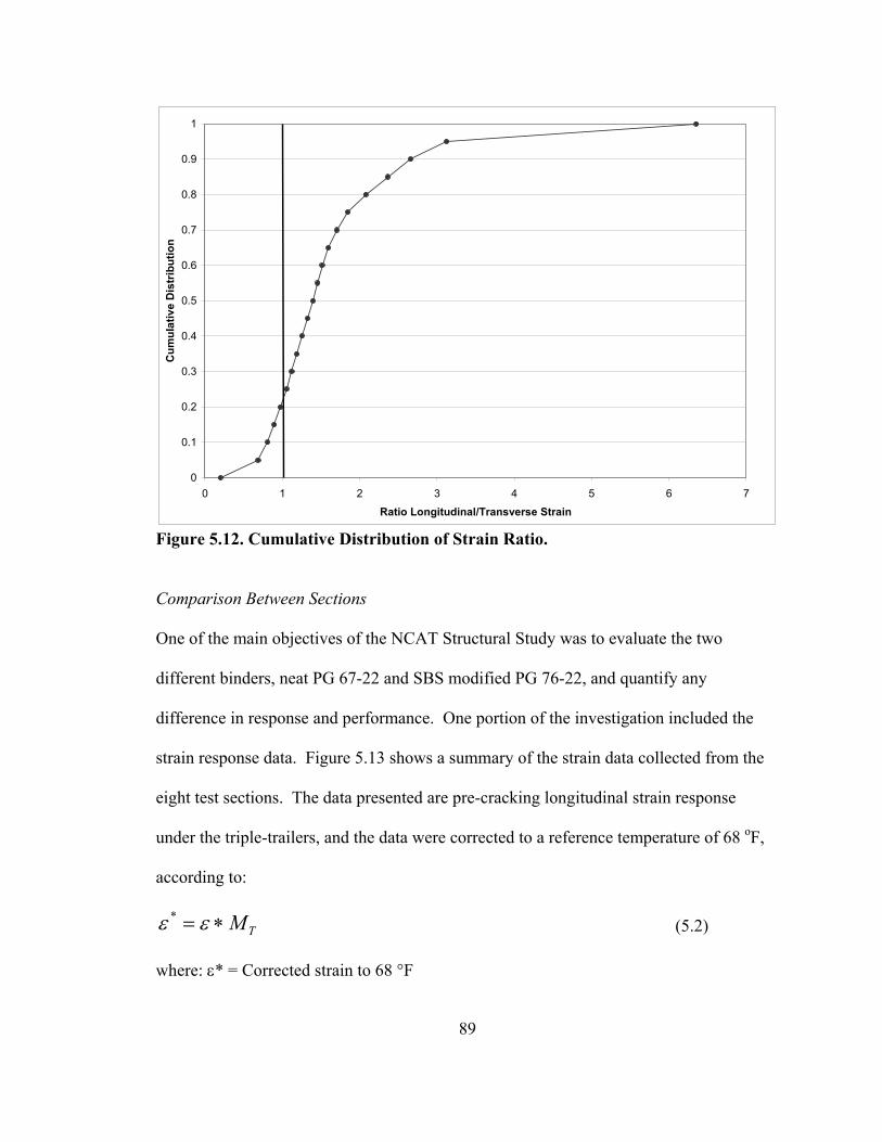
89

0

0.1

0.2

0.3

0.4

0.5

0.6

0.7

0.8

0.9

1

0 1 2 3 4 5 6 7

Ratio Longitudinal/Transverse Strain

Cum

ulat

ive

Dis

trib

utio

n

Figure 5.12. Cumulative Distribution of Strain Ratio.

Comparison Between Sections

One of the main objectives of the NCAT Structural Study was to evaluate the two

different binders, neat PG 67-22 and SBS modified PG 76-22, and quantify any

difference in response and performance. One portion of the investigation included the

strain response data. Figure 5.13 shows a summary of the strain data collected from the

eight test sections. The data presented are pre-cracking longitudinal strain response

under the triple-trailers, and the data were corrected to a reference temperature of 68 oF,

according to:

TM∗= εε * (5.2)

where: ε* = Corrected strain to 68 °F

90

ε = Measure strain at temperature, T

T

TM''68

εε

= (5.3)

ε′68 = Predicted strain at 68 °F

ε′T = Predicted strain at temperature, T

The figure shows the average temperature-corrected strain value along with the standard

deviation. Notice that the variability in the strain data ranged from 20 to 60 microstrain,

with N3 being the least variable. It follows reason that N3 is less variable than the others

because only a few gauges survived construction and the first months of traffic.

Therefore, most of the readings came from the same gauge and the same truck, unlike the

other sections where the maximum reading came from different gauges and trucks. Also

notice from the figure that the three thicknesses are fairly obvious in the strain data. On

average, the thinnest sections (N1, N2) register the highest strains, while the thickest (N3,

N4) show the lowest. Yet, if inspected closely, N2 and N6 along with N3 and N8 have

fairly similar values. Section N8 strain values were more on the order of the 9 in.

sections, yet it showed cracking first among the 7 in. sections. It is not immediately clear

why the strain in section N8 is lower than the other 7 in. sections. Harvey et al. (1995)

investigated the concept of rich bottom asphalt pavement structures in the laboratory and

determined that the stiffness of a mixture with 0.5 percent higher asphalt content and

lower air voids was estimated to increase by 1.15 due to densification. Perhaps, the rich

bottom layer in section N8 was also more dense and thus more stiff than the other base

HMA mixtures. Also, N2 shows lower strains than N1, mostly due to the fact that N2 is

significantly stiffer than N1 (Timm and Priest “Material Properties,” 2005). Further,

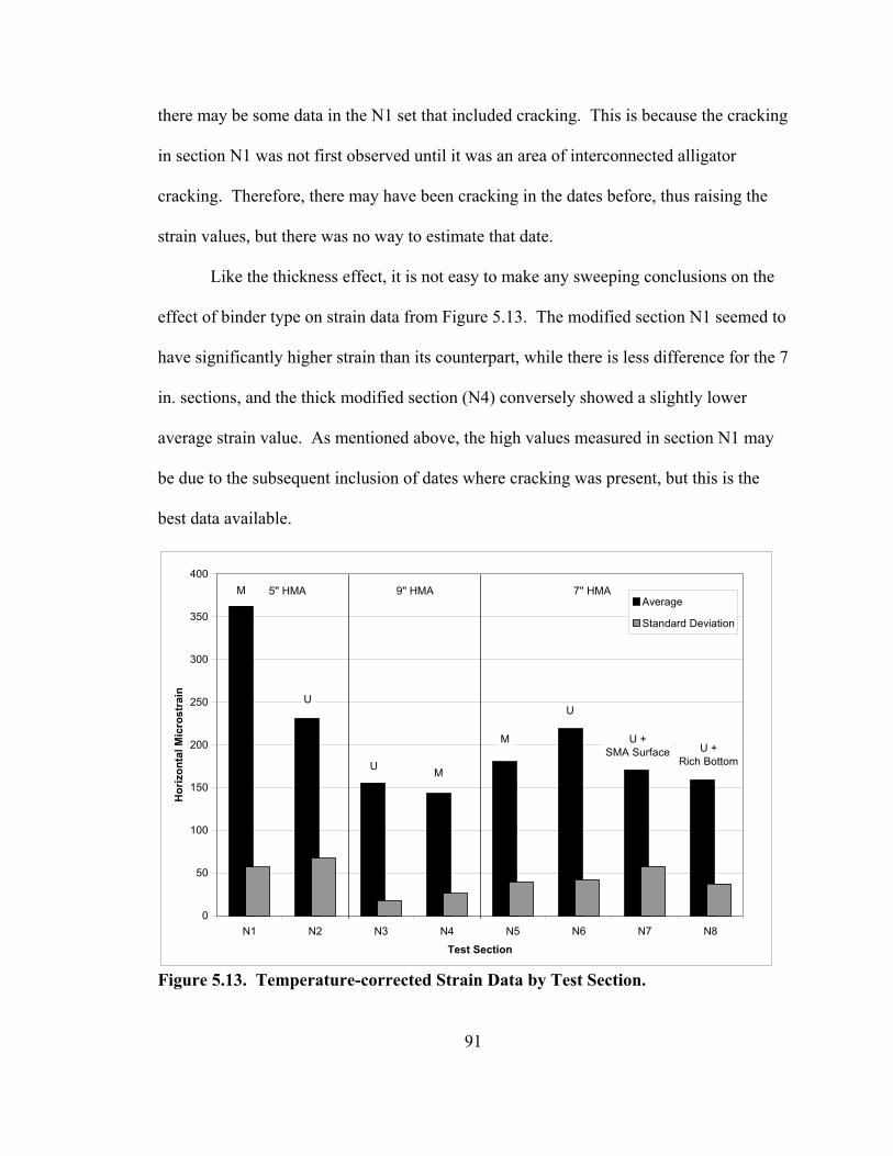
91

there may be some data in the N1 set that included cracking. This is because the cracking

in section N1 was not first observed until it was an area of interconnected alligator

cracking. Therefore, there may have been cracking in the dates before, thus raising the

strain values, but there was no way to estimate that date.

Like the thickness effect, it is not easy to make any sweeping conclusions on the

effect of binder type on strain data from Figure 5.13. The modified section N1 seemed to

have significantly higher strain than its counterpart, while there is less difference for the 7

in. sections, and the thick modified section (N4) conversely showed a slightly lower

average strain value. As mentioned above, the high values measured in section N1 may

be due to the subsequent inclusion of dates where cracking was present, but this is the

best data available.

0

50

100

150

200

250

300

350

400

N1 N2 N3 N4 N5 N6 N7 N8

Test Section

Hor

izon

tal M

icro

stra

in

Average

Standard Deviation

5'' HMA 9'' HMA 7'' HMAM

M

M

U

U

U

U + SMA Surface U +

Rich Bottom

Figure 5.13. Temperature-corrected Strain Data by Test Section.

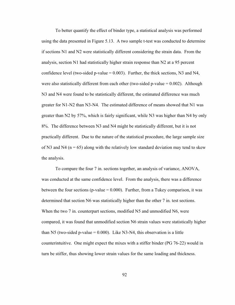
92

To better quantify the effect of binder type, a statistical analysis was performed

using the data presented in Figure 5.13. A two sample t-test was conducted to determine

if sections N1 and N2 were statistically different considering the strain data. From the

analysis, section N1 had statistically higher strain response than N2 at a 95 percent

confidence level (two-sided p-value = 0.003). Further, the thick sections, N3 and N4,

were also statistically different from each other (two-sided p-value = 0.002). Although

N3 and N4 were found to be statistically different, the estimated difference was much

greater for N1-N2 than N3-N4. The estimated difference of means showed that N1 was

greater than N2 by 57%, which is fairly significant, while N3 was higher than N4 by only

8%. The difference between N3 and N4 might be statistically different, but it is not

practically different. Due to the nature of the statistical procedure, the large sample size

of N3 and N4 (n = 65) along with the relatively low standard deviation may tend to skew

the analysis.

To compare the four 7 in. sections together, an analysis of variance, ANOVA,

was conducted at the same confidence level. From the analysis, there was a difference

between the four sections (p-value = 0.000). Further, from a Tukey comparison, it was

determined that section N6 was statistically higher than the other 7 in. test sections.

When the two 7 in. counterpart sections, modified N5 and unmodified N6, were

compared, it was found that unmodified section N6 strain values were statistically higher

than N5 (two-sided p-value = 0.000). Like N3-N4, this observation is a little

counterintuitive. One might expect the mixes with a stiffer binder (PG 76-22) would in

turn be stiffer, thus showing lower strain values for the same loading and thickness.

93

From the analysis, no sweeping conclusions can be made with regards to the

effect of binder grade and modification on strain response. The modified 5 in. section

had higher strain values than the unmodified section, the thickest sections were

practically the same, and the modified 7 in. section had lower strain values than its

modified partner. The above observations in strain data were probably due to

construction and spatial variability rather than an effect of binder type.

On the other hand, the effect of HMA layer thickness is conclusive. An ANOVA

analysis was conducted by pooling the test sections, considering only the three different

HMA thicknesses, and it was determined that all three were statistically different (p-value

< 0.000).

Strain Prediction Models

In a similar manner as the stiffness data, it was not practical to collect dynamic data

continuously (extremely costly in equipment and time). In addition, Figure 5.6 showed

that no new information is gained after approximately three passes. Therefore, it was

important to develop an accurate model to predict the strain magnitude over the entire

two-year testing cycle on a per hour basis. The strain magnitude was a function of the

mid-depth HMA temperature as well as the thickness of the asphalt layer, so individual

regression models were determined for each test section. The individual models

accounted for thickness and other individual peculiarities, and a generic model was

developed from all the test sections which included a thickness term. Additionally, the

strain magnitude was a function of the testing vehicle. The box trailer had to be

considered separately because it was loaded differently, and the box trailer had five axles

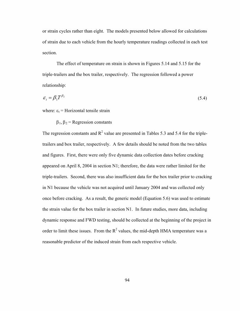
94

or strain cycles rather than eight. The models presented below allowed for calculations

of strain due to each vehicle from the hourly temperature readings collected in each test

section.

The effect of temperature on strain is shown in Figures 5.14 and 5.15 for the

triple-trailers and the box trailer, respectively. The regression followed a power

relationship:

21

ββε Tt = (5.4)

where: εt = Horizontal tensile strain

β1, β2 = Regression constants

The regression constants and R2 value are presented in Tables 5.3 and 5.4 for the triple-

trailers and box trailer, respectively. A few details should be noted from the two tables

and figures. First, there were only five dynamic data collection dates before cracking

appeared on April 8, 2004 in section N1; therefore, the data were rather limited for the

triple-trailers. Second, there was also insufficient data for the box trailer prior to cracking

in N1 because the vehicle was not acquired until January 2004 and was collected only

once before cracking. As a result, the generic model (Equation 5.6) was used to estimate

the strain value for the box trailer in section N1. In future studies, more data, including

dynamic response and FWD testing, should be collected at the beginning of the project in

order to limit these issues. From the R2 values, the mid-depth HMA temperature was a

reasonable predictor of the induced strain from each respective vehicle.

95

0

100

200

300

400

500

600

700

800

900

1000

35 45 55 65 75 85 95 105 115

Mid-depth HMA Temperature, F

Long

itudi

nal H

oriz

onta

l Mic

rost

rain

N1

N2

N3

N4

N5

N6

N7

N8

Figure 5.14. Triple-Trailer Strain – Temperature Relationship.

0

100

200

300

400

500

600

700

800

900

1000

35 45 55 65 75 85 95 105 115

Mid-depth HMA Temperature, F

Long

itudi

nal H

oriz

onta

l Mic

rost

rain

N2

N3

N4

N5

N6

N7

N8

Figure 5.15. Box Trailer Strain – Temperature Relationship.

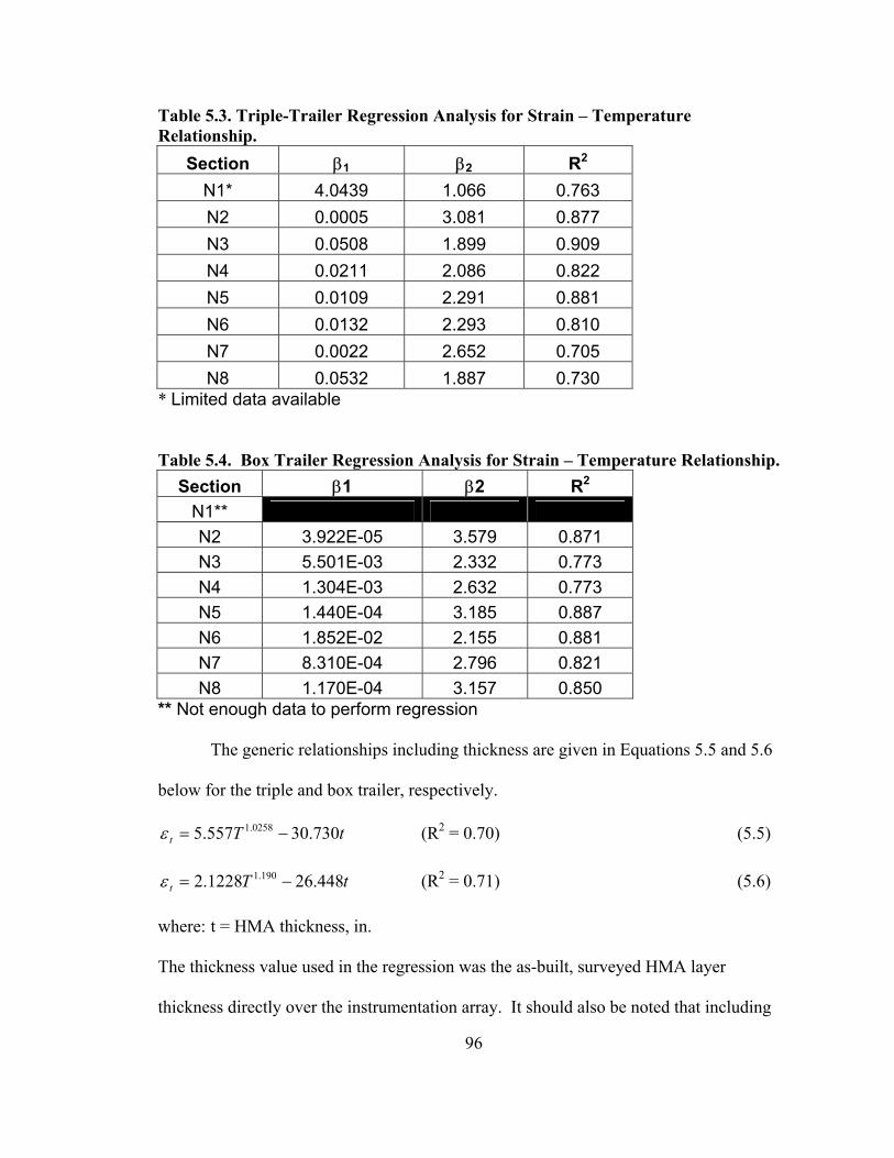
96

Table 5.3. Triple-Trailer Regression Analysis for Strain – Temperature Relationship.

Section β1 β2 R2 N1* 4.0439 1.066 0.763 N2 0.0005 3.081 0.877 N3 0.0508 1.899 0.909 N4 0.0211 2.086 0.822 N5 0.0109 2.291 0.881 N6 0.0132 2.293 0.810 N7 0.0022 2.652 0.705 N8 0.0532 1.887 0.730

* Limited data available Table 5.4. Box Trailer Regression Analysis for Strain – Temperature Relationship.

Section β1 β2 R2 N1** N2 3.922E-05 3.579 0.871 N3 5.501E-03 2.332 0.773 N4 1.304E-03 2.632 0.773 N5 1.440E-04 3.185 0.887 N6 1.852E-02 2.155 0.881 N7 8.310E-04 2.796 0.821 N8 1.170E-04 3.157 0.850

** Not enough data to perform regression The generic relationships including thickness are given in Equations 5.5 and 5.6

below for the triple and box trailer, respectively.

tTt 730.30557.5 0258.1 −=ε (R2 = 0.70) (5.5)

tTt 448.261228.2 190.1 −=ε (R2 = 0.71) (5.6)

where: t = HMA thickness, in.

The thickness value used in the regression was the as-built, surveyed HMA layer

thickness directly over the instrumentation array. It should also be noted that including

97

the binder type in the regression did not significantly improve the model; therefore it was

not included for simplicity.

Concluding Remarks on Strain Characterization

As with the stiffness data, the above analysis was crucial to developing fatigue transfer

functions at the NCAT Test Track. The relationships between strain and temperature

allowed for an accurate calculation of the in situ strain magnitude for each hour of the

testing cycle. In this way, the calculated damage and subsequent fatigue models were

based on field measurements. Additionally, the generic functions developed, as well as

the binder grade and thickness investigation, can aid in future design and analysis

projects for similar HMA mixtures.

Fatigue Performance Characterization

Observed Fatigue Distress

As discussed in Chapter 3, the performance of the test sections was monitored on a

weekly basis including crack mapping and rut depth measurement. Because this thesis

focuses on fatigue transfer functions, the cracking data were of most importance.

At the date of this report, sections N1, N2 and N8 had shown excessive fatigue

failure, and the distress of all three sections progressed in a similar fashion. First, small

transverse cracks appeared in the wheelpath, as shown in Figure 5.16. Then the cracks

progressed to the end of the wheelpath and often arched in the direction of traffic (Figure

5.17). Later, the individual transverse cracks became interconnected into the classical

alligator pattern fatigue cracking, also shown in Figure 5.17. Pumping of the fines from

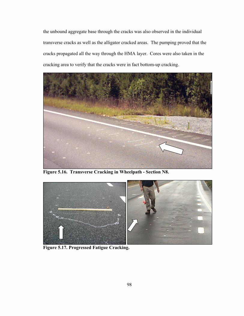
98

the unbound aggregate base through the cracks was also observed in the individual

transverse cracks as well as the alligator cracked areas. The pumping proved that the

cracks propagated all the way through the HMA layer. Cores were also taken in the

cracking area to verify that the cracks were in fact bottom-up cracking.

Figure 5.16. Transverse Cracking in Wheelpath - Section N8.

Figure 5.17. Progressed Fatigue Cracking.

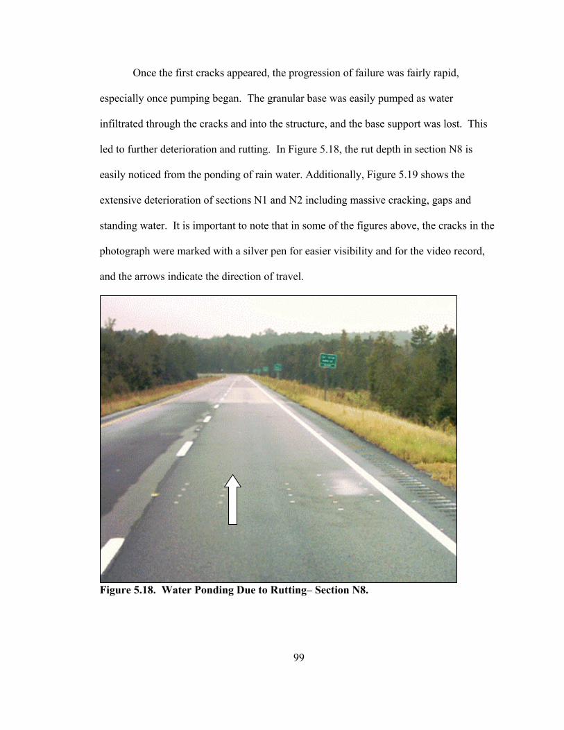
99

Once the first cracks appeared, the progression of failure was fairly rapid,

especially once pumping began. The granular base was easily pumped as water

infiltrated through the cracks and into the structure, and the base support was lost. This

led to further deterioration and rutting. In Figure 5.18, the rut depth in section N8 is

easily noticed from the ponding of rain water. Additionally, Figure 5.19 shows the

extensive deterioration of sections N1 and N2 including massive cracking, gaps and

standing water. It is important to note that in some of the figures above, the cracks in the

photograph were marked with a silver pen for easier visibility and for the video record,

and the arrows indicate the direction of travel.

Figure 5.18. Water Ponding Due to Rutting– Section N8.

100

a) b) Figure 5.19. Extensive Fatigue Cracking in Section a) N1 b) N2. The fatigue cracking of sections N1, N2 and N8 originated in the outside

wheelpath near the gauge array area. Because the sections did not fail prematurely, it

was not likely that the gauges were the cause of the cracking. The sections were fatigued

and reaching the end of life, and the gauge array was an area of discontinuity. It is

probably a more accurate description to conclude that cracking was going to occur in the

section due to fatigue and first appeared in the gauge array because the presence of the

gauges caused an area of weakness within the section. As the distress progressed, the

cracking expanded past the gauge array and also developed in the inside wheelpath.

Crack Mapping

The cracking coordinates determined from the procedure described in Chapter 3

were used to make graphical crack maps in order to keep a visual record of the cracking.

The crack maps were often more useful than even photographs because the format was

consistent. The crack maps provided valuable insight into how the cracks progressed and

at what rate. To serve as an example of the crack maps and the observed fatigue cracking

development at the NCAT Test Track, a series of four crack maps from section N2 are

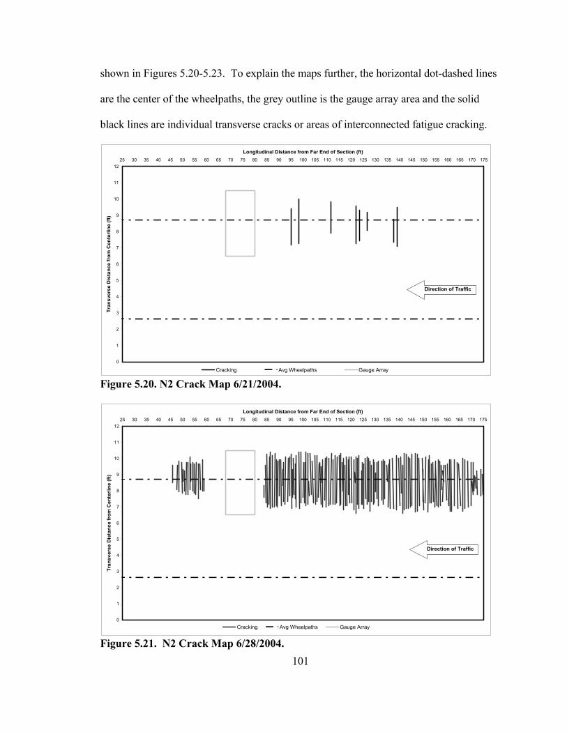
101

shown in Figures 5.20-5.23. To explain the maps further, the horizontal dot-dashed lines

are the center of the wheelpaths, the grey outline is the gauge array area and the solid

black lines are individual transverse cracks or areas of interconnected fatigue cracking.

0

1

2

3

4

5

6

7

8

9

10

11

1225 30 35 40 45 50 55 60 65 70 75 80 85 90 95 100 105 110 115 120 125 130 135 140 145 150 155 160 165 170 175

Longitudinal Distance from Far End of Section (ft)

Tran

sver

se D

ista

nce

from

Cen

terli

ne (f

t)

Cracking Avg Wheelpaths Gauge Array

Direction of Traffic

Figure 5.20. N2 Crack Map 6/21/2004.

0

1

2

3

4

5

6

7

8

9

10

11

1225 30 35 40 45 50 55 60 65 70 75 80 85 90 95 100 105 110 115 120 125 130 135 140 145 150 155 160 165 170 175

Longitudinal Distance from Far End of Section (ft)

Tran

sver

se D

ista

nce

from

Cen

terli

ne (f

t)

Cracking Avg Wheelpaths Gauge Array

Direction of Traffic

Figure 5.21. N2 Crack Map 6/28/2004.

102

0

1

2

3

4

5

6

7

8

9

10

11

1225 30 35 40 45 50 55 60 65 70 75 80 85 90 95 100 105 110 115 120 125 130 135 140 145 150 155 160 165 170 175

Longitudinal Distance from Far End of Section (ft)

Tran

sver

se D

ista

nce

from

Cen

terli

ne (f

t)

Cracking Avg Wheelpaths Gauge Array

Alligator Crack II

Alligator Crack II

Direction of Traffic

Figure 5.22. N2 Crack Map 8/02/2004.

0

1

2

3

4

5

6

7

8

9

10

11

1225 30 35 40 45 50 55 60 65 70 75 80 85 90 95 100 105 110 115 120 125 130 135 140 145 150 155 160 165 170 175

Longitudinal Distance from Far End of Section (ft)

Tran

sver

se D

ista

nce

from

Cen

terli

ne (f

t)

Cracking Avg Wheelpaths Gauge Array

Alligator Cracking

Alligator Cracking

Alligator Cracking

Alligator Cracking

Direction of Traffic

Figure 5.23. N2 Crack Map 10/18/2004.

103

As explained above, once the first cracks appeared after approximately 2.6

million ESAL, the fatigue distress progressed rapidly. From Figures 5.20 and 5.21, one

can see that eight individual cracks progressed to cracking covering nearly the whole

outside wheelpath in one week (or approximately 100,000 ESAL). After a month (Figure

5.22) the individual cracks became interconnected, and within four months (Figure 5.23),

both wheelpaths had full fatigue cracking with pumping.

The figures above are just examples of a few select dates of one test section.

Similar maps were generated from the cracking data for the other test sections to monitor

and record the performance in an easy format.

Data Processing and Characterization

Although the crack maps provided a good graphical representation of the fatigue distress,

there was a need to quantify the amount of cracking with a numerical value in order to

plot the distress data and determine a definitive failure criteria. Recall from Chapter 3

that the cracking video records were digitized and coordinates were obtained from the

video record. The coordinates were used to create the crack maps shown in the section

above and were also used to quantify the amount of cracking in each test section.

The coordinates were processed using a formatted spreadsheet and customized

algorithms. The crack coordinates were imported into the spreadsheet, and the crack map

was displayed. The type of cracking was identified, and then a specific algorithm was

run to measure the amount of cracking given the coordinates. Five categories of cracking

were used to classify the cracks observed at the NCAT Test Track:

1. Transverse cracking – wheelpath

104

2. Transverse cracking – non-wheelpath

3. Longitudinal cracking – wheelpath

4. Longitudinal cracking – non-wheelpath

5. Interconnected fatigue cracking (alligator cracking)

The longitudinal cracking and non-wheelpath transverse cracking observed at the

Test Track were mainly top-down surface cracking rather than fatigue cracking, and they

were found primarily in the other test sections (not part of the Structural Study).

Therfore, they will not be discussed in detail here. The fatigue distresses, wheelpath

transverse and alligator cracking, were quantified as an area following the guidelines of

prior work including the LTPP Distress Manual, AI MS-1 and 2002 Design Guide. It is

important to mention that the LTPP Distress Manual identifies the first stages of fatigue

cracking as longitudinal cracking in the wheelpath, but at the Test Track, the initial stages

of fatigue cracking were transverse cracks. Therefore, they are included as fatigue

cracking in this study.

Individual transverse cracks, like those in Figure 5.20 and 5.21, were measured by

their length, in feet, and then assigned a width of 1 ft to get an area measurement. The

LTPP Distress Manual measures fatigue cracks in affected area, but does not offer precise

recommendations on how to determine an area of an individual crack. Often, there were

many closely-spaced individual cracks, and considering each having a 1 ft width would

have over exaggerated the approximation. Therefore, if two consecutive transverse

cracks were less than 5 ft away from each other, they were considered together, and a

trapezoidal area was calculated from the four coordinates of the two cracks. Basically,

the algorithm went from crack to crack, determined the distance from the current crack to

105

the prior crack, and if the distance was less than 5 ft an area was calculated. If not, the

length was determined and assigned a 1ft width. The total area of transverse cracking

was then determined by adding the individual areas.

For the areas of alligator cracking (e.g., Figures 5.22 and 5.23), the method of

coordinates was used to find that traverse area. The method of coordinates, found in

most introductory surveying textbooks (e.g., Wolf and Brinker, 1994), utilizes the

following equation to find the area of an irregular geometric shape:

( )

−= ∑

=+−

n

iiii xxyA

1112

1 (5.7)

where: A = area of closed traverse

i = point of traverse

n = number of points in traverse

x = x-coordinate

y = y-coordinate

For this analysis, all fatigue cracking, regardless of type or level of severity, was

considered together; therefore the grand total area of fatigue cracking included the

transverse wheelpath and alligator cracking. A similar procedure was used for the

calibration of the 2002 Design Guide using performance data from LTPP sections (El-

Basyouny and Witczak “Calibration,” 2005).

Once the total area of fatigue cracking was determined from the above procedure,

the percentages of cracked area were calculated. The percent of cracking considering the

whole lane (12 ft X 150 ft) was calculated, and the crack progression is shown in Figure

5.24. Another common way to quantify fatigue distress is by percent cracking of the

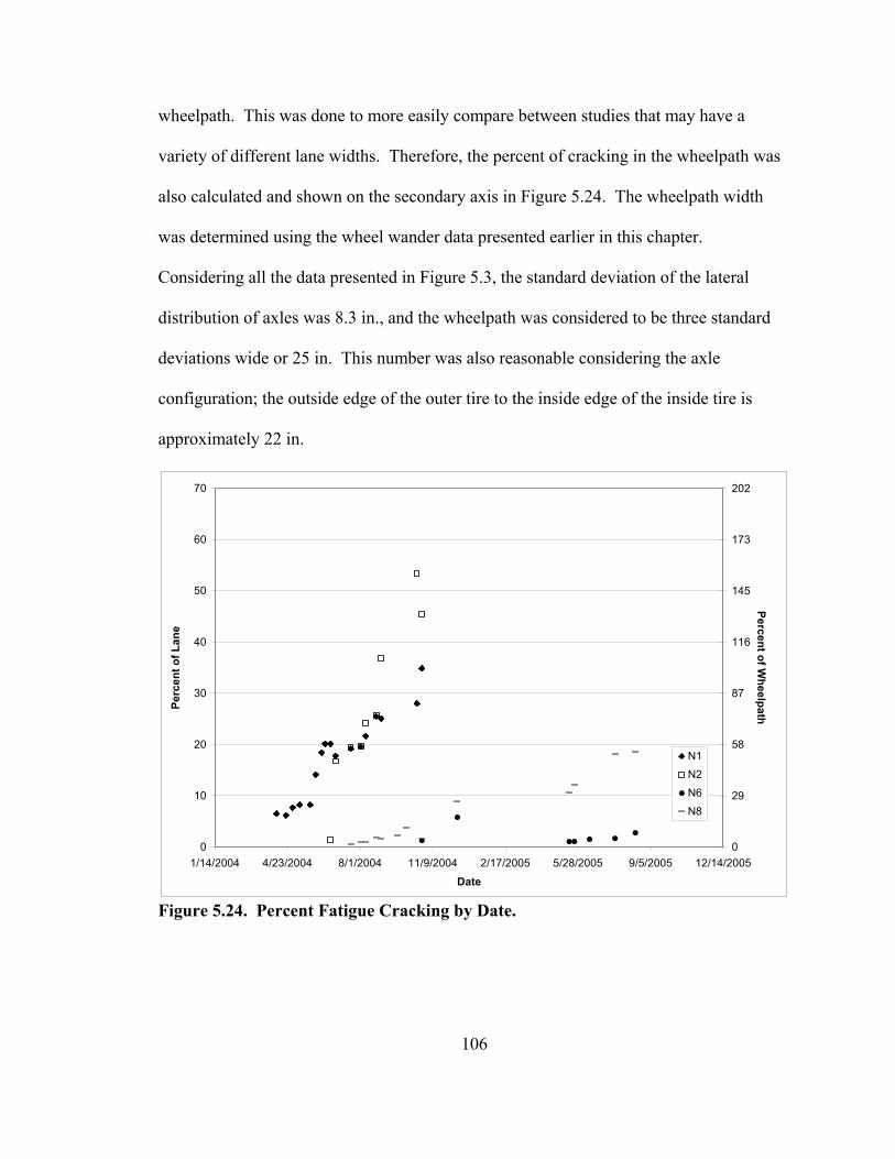
106

wheelpath. This was done to more easily compare between studies that may have a

variety of different lane widths. Therefore, the percent of cracking in the wheelpath was

also calculated and shown on the secondary axis in Figure 5.24. The wheelpath width

was determined using the wheel wander data presented earlier in this chapter.

Considering all the data presented in Figure 5.3, the standard deviation of the lateral

distribution of axles was 8.3 in., and the wheelpath was considered to be three standard

deviations wide or 25 in. This number was also reasonable considering the axle

configuration; the outside edge of the outer tire to the inside edge of the inside tire is

approximately 22 in.

0

10

20

30

40

50

60

70

1/14/2004 4/23/2004 8/1/2004 11/9/2004 2/17/2005 5/28/2005 9/5/2005 12/14/2005

Date

Perc

ent o

f Lan

e

0

29

58

87

116

145

173

202

N1

N2

N6

N8

Percent of Wheelpath

Figure 5.24. Percent Fatigue Cracking by Date.

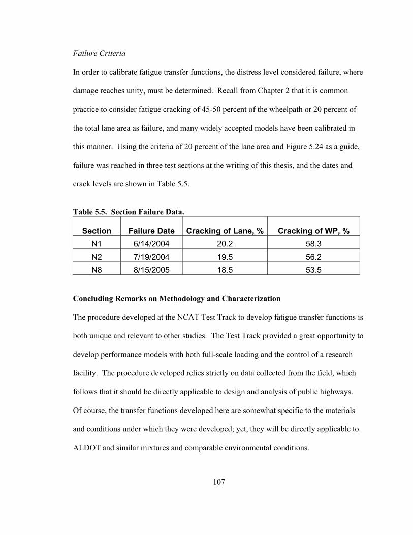
107

Failure Criteria

In order to calibrate fatigue transfer functions, the distress level considered failure, where

damage reaches unity, must be determined. Recall from Chapter 2 that it is common

practice to consider fatigue cracking of 45-50 percent of the wheelpath or 20 percent of

the total lane area as failure, and many widely accepted models have been calibrated in

this manner. Using the criteria of 20 percent of the lane area and Figure 5.24 as a guide,

failure was reached in three test sections at the writing of this thesis, and the dates and

crack levels are shown in Table 5.5.

Table 5.5. Section Failure Data.

Section Failure Date Cracking of Lane, % Cracking of WP, %

N1 6/14/2004 20.2 58.3 N2 7/19/2004 19.5 56.2 N8 8/15/2005 18.5 53.5

Concluding Remarks on Methodology and Characterization

The procedure developed at the NCAT Test Track to develop fatigue transfer functions is

both unique and relevant to other studies. The Test Track provided a great opportunity to

develop performance models with both full-scale loading and the control of a research

facility. The procedure developed relies strictly on data collected from the field, which

follows that it should be directly applicable to design and analysis of public highways.

Of course, the transfer functions developed here are somewhat specific to the materials

and conditions under which they were developed; yet, they will be directly applicable to

ALDOT and similar mixtures and comparable environmental conditions.

108

Further, the methodology as well as the data collection and synthesis procedures

developed in this study should be applicable to other full-scale testing facilities and

further experiments at the NCAT Test Track. The following chapter will show how all of

the pieces described in this chapter come together to develop performance models. One

important recommendation is to collect a fairly extensive amount of data at the beginning

of the experiment before the sections are trafficked.

109

CHAPTER 6 – FATIGUE MODEL DEVELOPMENT

Introduction

At the time of this thesis, three test sections had reached the fatigue cracking failure criteria,

as discussed in the prior chapter. Recall that cracking covering 20 percent of the total lane

area was considered failure. Sections N1 and N2 reached failure in the summer of 2004, and

section N8 reached failure in the summer of 2005. It should be noted that all three sections

survived past their initial design life of 1.1 million ESAL for N1/N2 and 2.9 million ESAL

for section N8.

Final fatigue transfer functions were developed using the data from the three failed

test sections, and preliminary transfer functions were developed for the other sections based

on the traffic and performance data, to date. Revisions will need to be conducted on these

models after the sections deteriorate further.

Methodology

From Chapter 5, the hourly temperature data collected continuously throughout the two-year

test cycle was the critical link between the traffic data and the HMA stiffness and strain data.

For each hourly temperature, the in situ HMA stiffness and strain magnitude were calculated

for each test section and vehicle type. Therefore, each lap of each truck was accounted for

through the relationships established in Chapter 5.

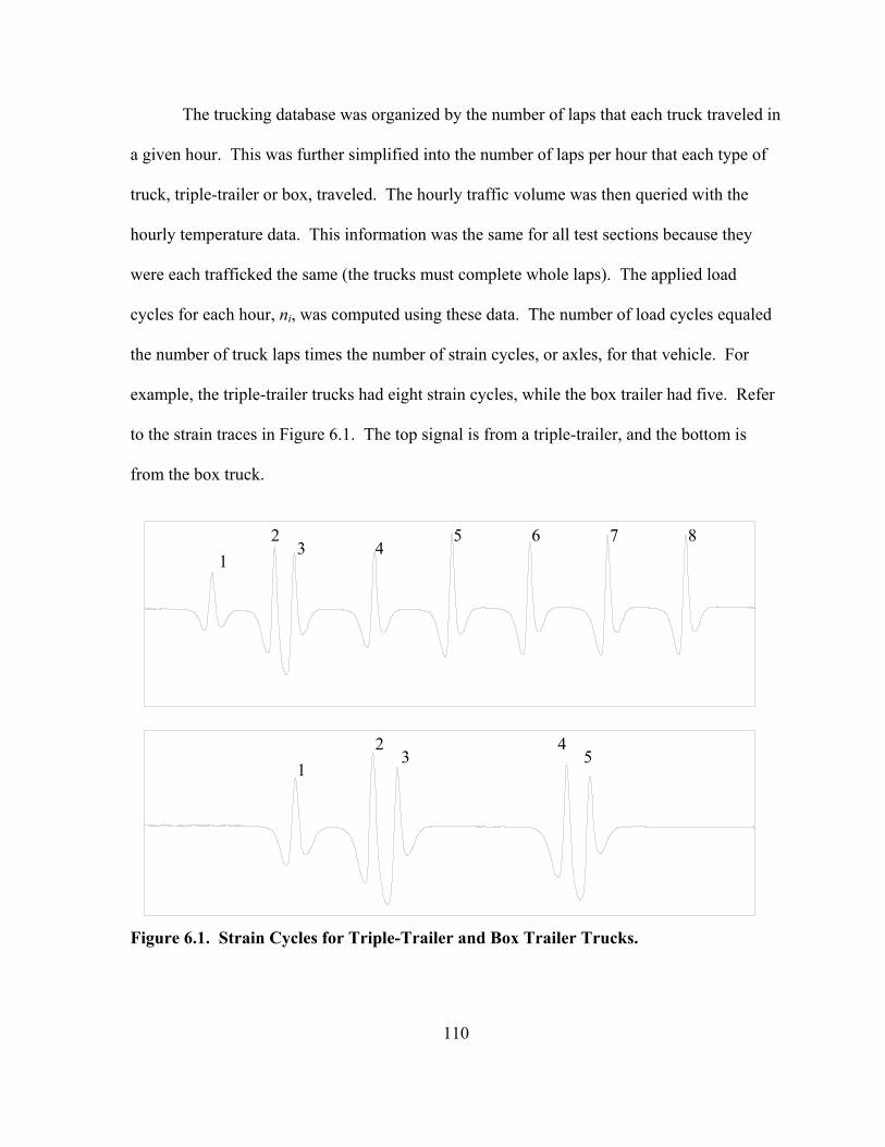
110

The trucking database was organized by the number of laps that each truck traveled in

a given hour. This was further simplified into the number of laps per hour that each type of

truck, triple-trailer or box, traveled. The hourly traffic volume was then queried with the

hourly temperature data. This information was the same for all test sections because they

were each trafficked the same (the trucks must complete whole laps). The applied load

cycles for each hour, ni, was computed using these data. The number of load cycles equaled

the number of truck laps times the number of strain cycles, or axles, for that vehicle. For

example, the triple-trailer trucks had eight strain cycles, while the box trailer had five. Refer

to the strain traces in Figure 6.1. The top signal is from a triple-trailer, and the bottom is

from the box truck.

W2: Box Trailer

W1: Triple-Trailer

Figure 6.1. Strain Cycles for Triple-Trailer and Box Trailer Trucks.

8 76543

2 1

1 2

34

5

111

Then the HMA stiffness and strain amplitude was calculated from the hourly

temperature data, given the test section and vehicle type. With the applied loads, stiffness

and strain values, the cycles to failure, Nfi, was calculated assuming a fatigue transfer

function. From this, the incremental damage, Di, was computed each hour using Miner’s

hypothesis first introduced in Chapter 1 and shown again here:

fi

ii N

nD = (6.1)

where Di = incremental damage for hour i

ni = number of cycles for hour i

Nfi = number of cycles until failure under conditions of hour i

The total damage at any time was then the sum of the incremental damage, as shown in

Equation 1.1.

Using the generated data described above, the fatigue models were then calibrated to

fit the observed performance. The regression coefficients were determined such that the total

damage, D, equaled unity at the determined date of failure. It is important to note that the

effort of this research was to calibrate models previously developed (presented in Chapter 2)

using full-scale field response, material and performance data. The exact models followed

and the calibration results are discussed below.

Fatigue Model

The current state of practice for fatigue transfer functions, including AI MS-1, Shell Oil

Design Guide and the 2002 Design Guide, is in the form of:

112

32 111

kk

tf E

kN

=

ε (6.2)

where: Nf = Number of load cycles until fatigue failure

εt = Applied horizontal tensile strain

E = HMA mixture stiffness

k1, k2, k3 = Regression constants

and may contain a volumetric correction term including the VFB of the mix. As discussed in

Chapter 2, these functions are often developed in the laboratory and then shifted or calibrated

to field performance with correction factors. In the development of the AI MS-1 design

guide, just the constant k1 was adjusted to match field observation (Finn et al., 1977). In the

development of the 2002 Design Guide, all three regression constants were tweaked to better

match LTPP performance data (El-Basyouny and Witczak “Calibration,” 2005).

In a similar manner to the 2002 Design Guide, all three regression constants were

calibrated to fit the data collected at the Test Track for the models presented here. Also

following the 2002 Design Guide and accepted practice, the AI MS-1 equation was used as

the base model and guide to the calibrated functions. The equation was presented in Chapter

2 and is shown here again for easy reference (“Thickness Design,” 1982):

)00432.0(4.18 854.*29.3 −− ∗∗∗∗= ECN tf ε (6.3)

where: C = 10M

−

+∗= 69.084.4

VB

B

VVVM (6.4)

The volumetric term in the AI equation was not used for the models calibrated here.

It was determined that there was not enough variation in the volumetrics of the test sections

113

to make an impact (Timm and Priest “Material Properties,” 2005). All the test sections used

a similar mix design; the only difference among sections (excluding N7 and N8) came from

the binder grade. Further, notice in the above equation that the volumetric correction, C, is

equal to 1 for mixes with air voids of 5 percent and binder volume of 11 percent. The mixes

used at the Test Track were designed with targets very near these values. In fact, for sections

N1 and N2, the average air void content was 6.5 percent, and the average binder volume was

11 percent. Therefore, the term was not considered, and the equation simplified to:

854.029.31*1*0795.0

=

EN

tf ε

(6.5)

The above equation served as the base model that was then calibrated using the field data to

create the final transfer functions.

The two 5 in. sections, N1 and N2, reached their terminal life within the span of the

2003 research cycle as well as one of the 7 in. sections, N8. Recall that section N8 included

the rich bottom layer consisting of 2 in. of HMA with an additional 0.5 percent asphalt

content. It was found that this section behaved differently in fatigue than did sections N1 and

N2. Consequently, one fatigue function could not be developed that explained the

performance of both the 5 in. sections and section N8. Upon further investigation, it was

determined that section N8 performed differently than the other 7 in. and 9 in. test sections,

also. Therefore, three transfer functions are presented here. One function for the 5 in. test

sections was developed, termed the thin model. This model is separate because the data set is

complete. Further, it is widely accepted (El-Basyouny and Witczak “Calibration”, 2005;

Monismith et al., 1985; Tangella et al., 1990) that thin asphalt pavements are subjected to a

different loading mechanism than are thicker pavements. Although sources do not agree with

114

what is considered “thin”, the range is typically less than 2 in. to 5 in. The second transfer

function developed was for section N8 and termed the rich bottom model. And finally, the

third model presented, termed the thick model, was a first attempt at a calibrated model for

the remaining test sections, N3-N7, based on data up to August 2, 2005. The three models

are presented below followed by discussion of the calibration and section performance.

Thin Model

The response, material property and performance data from both sections N1 and N2 were

considered to develop the fatigue transfer function given below in units of strain

(in./in.) and psi:

6529.00312.31*1*4875.0

=

EN

tf ε

(6.6)

Both test sections failed in a very similar manner and within two months of each other.

Section N1 failed prior to section N2, which was expected because the strain values of N1

were statistically higher, and N2 was slightly stiffer than N1. Both of these effects are

quantified in the above equation.

Figure 6.2 shows the accumulation of damage over time for sections N1 and N2.

From the figure, the damage at the terminal date does not exactly equal 1 for the test sections

because it was not possible to develop an equation that will exactly match the performance of

both test sections. Equation 6.6 minimizes the error for both sections and is acceptable to

both. The error either under or over-predicts the failure by only a month.

Notice that the higher strains in section N1 cause the curve to increase steadily from

the beginning of traffic. On the other hand, the accumulation of damage for section N2 does

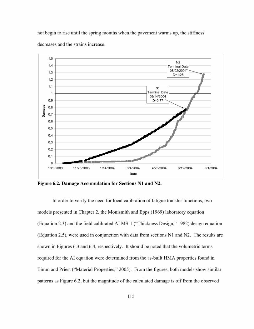
115

not begin to rise until the spring months when the pavement warms up, the stiffness

decreases and the strains increase.

0

0.1

0.2

0.3

0.4

0.5

0.6

0.7

0.8

0.9

1

1.1

1.2

1.3

1.4

1.5

10/6/2003 11/25/2003 1/14/2004 3/4/2004 4/23/2004 6/12/2004 8/1/2004

Date

Dam

age

N2Terminal Date

08/02/2004D=1.28

N1Terminal Date

06/14/2004D=0.77

Figure 6.2. Damage Accumulation for Sections N1 and N2.

In order to verify the need for local calibration of fatigue transfer functions, two

models presented in Chapter 2, the Monismith and Epps (1969) laboratory equation

(Equation 2.3) and the field calibrated AI MS-1 (“Thickness Design,” 1982) design equation

(Equation 2.5), were used in conjunction with data from sections N1 and N2. The results are

shown in Figures 6.3 and 6.4, respectively. It should be noted that the volumetric terms

required for the AI equation were determined from the as-built HMA properties found in

Timm and Priest (“Material Properties,” 2005). From the figures, both models show similar

patterns as Figure 6.2, but the magnitude of the calculated damage is off from the observed

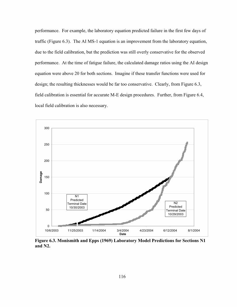
116

performance. For example, the laboratory equation predicted failure in the first few days of

traffic (Figure 6.3). The AI MS-1 equation is an improvement from the laboratory equation,

due to the field calibration, but the prediction was still overly conservative for the observed

performance. At the time of fatigue failure, the calculated damage ratios using the AI design

equation were above 20 for both sections. Imagine if these transfer functions were used for

design; the resulting thicknesses would be far too conservative. Clearly, from Figure 6.3,

field calibration is essential for accurate M-E design procedures. Further, from Figure 6.4,

local field calibration is also necessary.

0

50

100

150

200

250

300

10/6/2003 11/25/2003 1/14/2004 3/4/2004 4/23/2004 6/12/2004 8/1/2004Date

Dam

age

N2Predicted

Terminal Date10/29/2003

N1Predicted

Terminal Date10/30/2003

Figure 6.3. Monismith and Epps (1969) Laboratory Model Predictions for Sections N1 and N2.

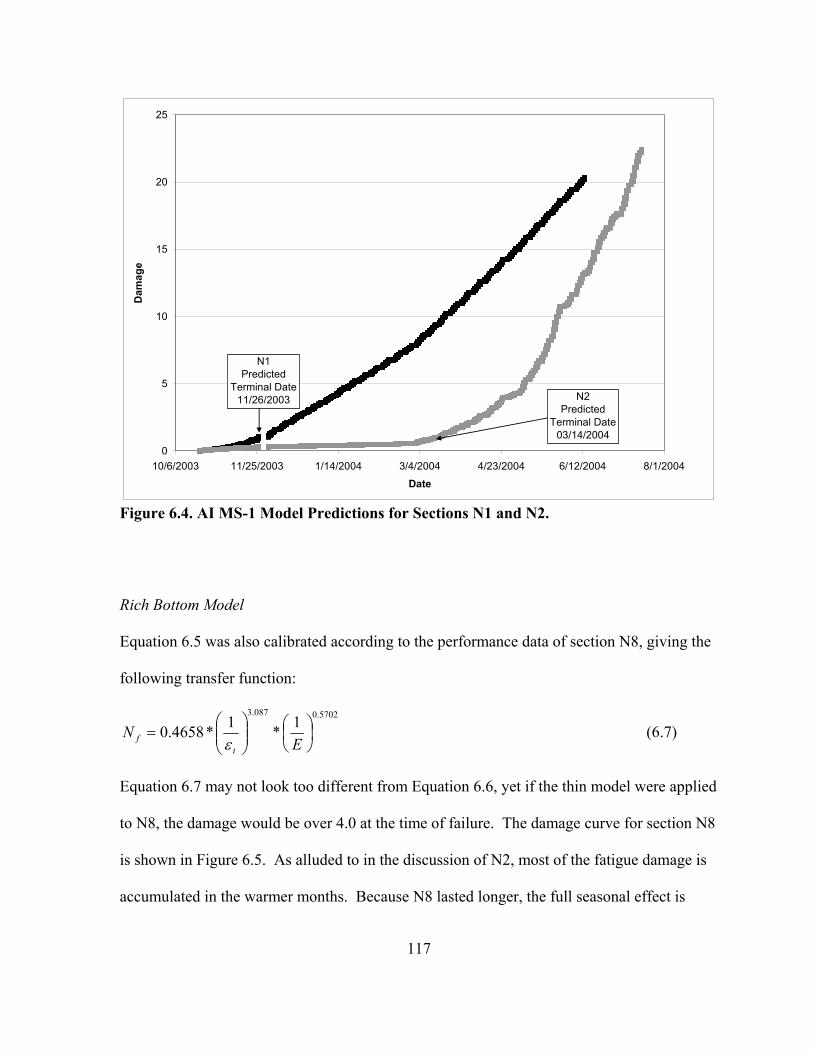
117

0

5

10

15

20

25

10/6/2003 11/25/2003 1/14/2004 3/4/2004 4/23/2004 6/12/2004 8/1/2004

Date

Dam

age

N2Predicted

Terminal Date03/14/2004

N1Predicted

Terminal Date11/26/2003

Figure 6.4. AI MS-1 Model Predictions for Sections N1 and N2.

Rich Bottom Model

Equation 6.5 was also calibrated according to the performance data of section N8, giving the

following transfer function:

5702.0087.31*1*4658.0

=

EN

tf ε

(6.7)

Equation 6.7 may not look too different from Equation 6.6, yet if the thin model were applied

to N8, the damage would be over 4.0 at the time of failure. The damage curve for section N8

is shown in Figure 6.5. As alluded to in the discussion of N2, most of the fatigue damage is

accumulated in the warmer months. Because N8 lasted longer, the full seasonal effect is

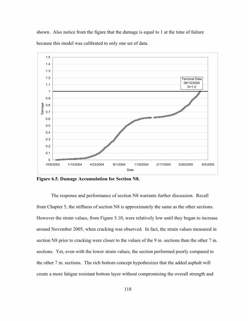
118

shown. Also notice from the figure that the damage is equal to 1 at the time of failure

because this model was calibrated to only one set of data.

0

0.1

0.2

0.3

0.4

0.5

0.6

0.7

0.8

0.9

1

1.1

1.2

1.3

1.4

1.5

10/6/2003 1/14/2004 4/23/2004 8/1/2004 11/9/2004 2/17/2005 5/28/2005 9/5/2005

Date

Dam

age

Terminal Date08/15/2005

D=1.0

Figure 6.5. Damage Accumulation for Section N8.

The response and performance of section N8 warrants further discussion. Recall

from Chapter 5, the stiffness of section N8 is approximately the same as the other sections.

However the strain values, from Figure 5.10, were relatively low until they began to increase

around November 2005, when cracking was observed. In fact, the strain values measured in

section N8 prior to cracking were closer to the values of the 9 in. sections than the other 7 in.

sections. Yet, even with the lower strain values, the section performed poorly compared to

the other 7 in. sections. The rich bottom concept hypothesizes that the added asphalt will

create a more fatigue resistant bottom layer without compromising the overall strength and

119

stability of the structure in regards to rutting. Recall, that a study conducted by Harvey et al.

(1995) investigated the rich bottom concept. They not only predicted an increase in stiffness

of the rich layer, which may be reason for the lower strain values found here, they also

reported an increase in fatigue life by a factor of 2.18. From this experiment, the rich bottom

concept did not hold true considering the performance of N8 versus the control section, N7,

which had only small signs of cracking at the time of this thesis. As a result, further

investigation into the rich bottom concept should be pursued at NCAT and elsewhere, both in

the laboratory and the field, before it is widely accepted as a viable pavement design option.

Thick Model

In order to calibrate a fatigue model using the data from sections N3-N7, a current damage

ratio was assumed. In the calibration of the thin and rich bottom models, the damage was set

equal to 1 at the time of failure. In calibration of the thick model, hourly temperature and

traffic data until August 2, 2005 were used, and a current damage ratio was assigned to each

test section. Section N6 had the highest amounts of cracking and was the only section with

areas of interconnected cracks; therefore, it was assigned a damage of 0.7. Section N5 had a

small amount of cracking in both wheelpaths, and there were some transverse cracks in

section N7; consequently, section N5 and N7 were assigned damage ratio values of 0.4 and

0.5, respectively. The two 9 in. sections (N3 and N4) had no observed cracking prior to

August 2, 2005 and were assigned a value of 0.2. Using the data from the five sections and

the damage assumptions, the general model developed is given below:

4834.0143.31*1*4801.0

=

EN

tf ε

(6.8)

120

The damage accumulation for section N6 is shown in Figure 6.6 to serve as an example. It,

along with the other thick sections, followed the same pattern of section N8 (Figure 6.3). As

further comparison, the average daily air temperatures are shown in Figure 6.7. From the

two figures, the damage accumulation matches well with the temperature data; the warmer

days causing more fatigue damage.

The increase in damage and cracking during the warmer months may contradict some

conventional understanding of cracking damage in flexible pavements. For example,

temperature-induced surface cracking is a major distress in many areas of the U.S., which

occurs during the winter months due to daily temperature fluctuations. This is not the same

mechanism that occurs in bottom-up fatigue cracking. Consider Equation 6.8; the driving

parameter is the tensile strain at the bottom of the HMA layer, which increases in warmer

months due to the decrease in stiffness. The stiffness term included in the equation may

counter-balance this change to some degree, but considering the power coefficients, not to

the same magnitude. In fact, it should be clarified that the stiffness term was originally

included in fatigue models to distinguish between different mixes rather than characterize

seasonal variation of one mix. Additionally, in Alabama, there are no spring thaw issues that

colder climates must consider. During spring thaw, the underlying layers can become

saturated and weakened due to partial thaw conditions. This condition leads to a loss of

support which, in turn, causes high tensile strains at the bottom of the HMA layer. In colder

climates, the effect of spring thaw would have to be considered in the strain data and fatigue

models. For example, temperature alone would not be an accurate predictor of strain during

spring thaw conditions.

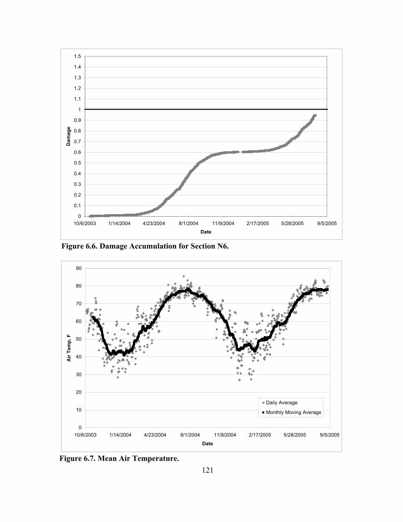
121

0

0.1

0.2

0.3

0.4

0.5

0.6

0.7

0.8

0.9

1

1.1

1.2

1.3

1.4

1.5

10/6/2003 1/14/2004 4/23/2004 8/1/2004 11/9/2004 2/17/2005 5/28/2005 9/5/2005

Date

Dam

age

Figure 6.6. Damage Accumulation for Section N6.

0

10

20

30

40

50

60

70

80

90

10/6/2003 1/14/2004 4/23/2004 8/1/2004 11/9/2004 2/17/2005 5/28/2005 9/5/2005

Date

Air

Tem

p, F

Daily Average

Monthly Moving Average

Figure 6.7. Mean Air Temperature.

122

The increase in damage and cracking during the warmer months may contradict some

conventional understanding of cracking damage in flexible pavements. For example,

temperature-induced surface cracking is a major distress in many areas of the U.S., which

occurs during the winter months due to daily temperature fluctuations. This is not the same

mechanism that occurs in bottom-up fatigue cracking. Consider Equation 6.8; the driving

parameter is the tensile strain at the bottom of the HMA layer, which increases in warmer

months due to the decrease in stiffness. The stiffness term included in the equation may

counter-balance this change to some degree, but considering the power coefficients, not to

the same magnitude. In fact, it should be clarified that the stiffness term was originally

included in fatigue models to distinguish between different mixes rather than characterize

seasonal variation of one mix. Additionally, in Alabama, there are no spring thaw issues that

colder climates must consider. During spring thaw, the underlying layers can become

saturated and weakened due to partial thaw conditions. This condition leads to a loss of

support which, in turn, causes high tensile strains at the bottom of the HMA layer. In colder

climates, the effect of spring thaw would have to be considered in the strain data and fatigue

models. For example, temperature alone would not be an accurate predictor of strain during

spring thaw conditions.

As mentioned prior, the thick fatigue transfer function (Equation 6.8) is based on

assumptions regarding the current state of distress of the test sections. Further improvements

should be made as the test sections are further trafficked and show further distress and

subsequent failure. The plans for the 2006 Test Track testing cycle include leaving these

sections in-place for further traffic and observation. Although the function may be updated,

123

it is predicted that one function can be developed to describe the performance of all five test

sections, including both thicknesses (7 and 9 in.).

Concluding Remarks on Model Development

The fatigue transfer functions presented here were developed to aid ALDOT and other states

in adopting M-E design procedures. The models are applicable to public highway analysis

and design for similar conditions of the NCAT Test Track. The test sections were designed

using ALDOT materials and specifications; therefore, they are directly applicable to the State

of Alabama and other states with similar mixture designs and climatic conditions. Further,

two separate models were presented for thick and thin HMA pavements, avoiding any

necessary shift factors. The rich bottom model was developed using only one test section, so

further investigation is warranted, especially considering the section did not perform as

expected.

124

CHAPTER 7 – CONCLUSIONS AND RECOMMENDATIONS

An accurate fatigue transfer function is the critical link in M-E flexible pavement design.

The model relates the conditions of the pavement structure to the expected performance

or life of the pavement. The conclusions of this research, including the developed

methodology and transfer functions, are presented below. Following the conclusions, a

few recommendations on testing procedure and data collection for future testing cycles

are presented. Further, this component of M-E design is probably the most deficient;

thus, it warrants further attention and improvements. The recommendations based on this

study for additional improvements and research are also given.

Conclusions

Regarding the dynamic instrumentation and test facility, the following conclusions can be

stated:

1. The strain gauge array was sufficient for the experiment. It successfully captured

the wheel wander and maximum strain response along with providing adequate

redundancy to account for gauge loss.

2. The strain quantification used in this research is unique to what others have done

in the past, and it is well suited for the conditions at the Test Track. The

developed strain amplitude algorithm accurately describes an entire vehicle strain

trace and captures the dynamic effects of truck loading.

125

3. Dynamic response data are highly variable and must be investigated thoroughly.

The dynamic data processing procedure developed at NCAT is both interactive

and efficient. Further, it can be adapted to further testing cycles and/or other

facilities.

Below are the conclusions regarding the methodology and parameter characterization

presented in this thesis:

1. It is not necessary to collect and process continuous dynamic response data. The

task would be overwhelming, especially for a project of this size. Stiffness –

temperature and strain – temperature relationships should be established and used

to predict the response for the pavement for the given condition. Further,

dynamic response data should be collected at regular intervals through the test

cycle to monitor the test sections.

2. The five triple-trailer trucks should be considered duplicates of one test vehicle in

regards to the strain characterization. Further, the wheel wander at the NCAT

Test Track is representative of open-access facilities.

3. The maximum registered strain response within the gauge array is considered the

best hit of a tire over the gauge. Further, three passes of each testing vehicle

should be collected to gather the full range of variability.

The conclusions regarding the performance of the test sections and the developed fatigue

models are given below:

1. Both 5 in. sections, N1 and N2, performed over their design life of 1.1 million

ESAL. The first signs of fatigue cracking was observed at 1.6 and 2.5 million

ESAL for section N1 and N2, respectively. Based on the very limited data of

126

these two sections, the unmodified PG 67-22 test section N1 performed slightly

better than its modified counterpart, N2. Although, it can be argued that the two

sections were basically the same in terms of fatigue performance.

2. All of the 7 in test sections outlived their design life of 2.9 million ESAL. Of the

four 7 in. test sections, only N8 had progressive fatigue cracking and reached the

failure criteria by the date of this thesis. The first signs of cracking in N8 were

noticed after approximately 3.4 million ESAL of traffic. Based on the limited test

sections, the rich bottom layer did not produce a more fatigue-resistant structure.

3. No fatigue cracking was observed in the two 9 in. test sections at the time of this

thesis.

4. The fatigue transfer function developed for thin asphalt pavement sections (less

than 5 in.) based on the data of sections N1 and N2 was found to be:

6529.00312.31*1*4875.0

=

EN

tf ε

5. The preliminary fatigue transfer function developed for thicker asphalt pavement

sections based on the data from sections N3-N7 was found to be:

4834.0143.31*1*4801.0

=

EN

tf ε

6. Lastly, the fatigue transfer function developed from the rich bottom section, N8,

is presented below:

5702.0087.31*1*4658.0

=

EN

tf ε

Recall that this function was developed from data from only one test section.

127

Recommendations

Based on this research the following recommendations can be made regarding full-scale

testing, instrumentation and methodology. Further research opportunities are also

explored.

1. The test sections should be designed to ensure failure during the testing cycle. In

addition, if the test sections reach their terminal life, they should be repaired and

maintained. This may involve an overlay or other rehabilitation techniques. In

that way, the maintenance technique can be observed and mechanistically

evaluated.

2. A heavy data collection effort should be performed at the beginning of the testing

cycle prior to any pavement damage. This includes dynamic data collection as

well as FWD testing at a variety of testing temperatures. In this way, accurate

prediction models can be developed on the intact pavement structure.

3. It is recommended that the intact test sections (N3-N7) be left in place for the next

round of testing at the NCAT Test Track for further observation. As the sections

deteriorate, a more accurate thick fatigue model can be developed. Additionally,

the model presented here can be used to predict the life of the remaining test

sections.

4. Further investigation is warranted into the rich bottom layer concept, both in the

laboratory and the field. Further, the rich bottom transfer function developed here

may need further verification because it was based on data from only one test

section.

128

5. The effect of binder type and binder modification on fatigue performance should

be further investigated because the data were limited to one comparison set (N1

and N2). As recommended above, the other sections should be further trafficked

in order to draw more substantial conclusions.

6. Additional cross sections should be tested in later research cycles including

different base and subgrade materials.

129

REFERENCES

AASHTO Guide for Design of Pavement Structures. Washington D.C.: American

Association of State and Highway Transportation Officials, 1993.

About Minnesota Road Research. Minnesota Department of Transportation (MnDOT). 3

October 2005 < http://www.mrr.dot.state.mn.us/research/MnROAD_Project/

mnroadproject.asp>.

Ali, Hesham A. and Shiraz D. Tayabji. “Evaluation of Mechanistic-Empirical

Performance Prediction Models for Flexible Pavements.” Transportation

Research Record No. 1629, Washington, D.C.: Transportation Research Board,

1998, pp.169-80.

Al-Qadi, I. L., A. Loulizi, M. Elseifi and S. Lahouar. "The Virginia Smart Road : The

Impact of Pavement Instrumentation on Understanding Pavement Performance."

The Journal of Association of Asphalt Paving Technologists Vol. 83, 2004, pp.

427-66.

Alvarez, C. and M.R. Thompson. “Mechanistic-Empirical Evaluation of the Mn/Road

Mainline Flexible Pavement Sections,” Project IHR-535, Illinois Cooperative

Highway and Transportation Research Program, University of Illinois, Urbana,

IL, 1998.

130

Beer, Michael G., Greg Johnson and Dave Van Deusen. “Performance of Mn/Road Load

Response and Subsurface Instrumentation,” Staff Paper, Office of Minnesota

Road Research, Mapleweed, MN: Minnesota Department of Transportation, 1996.

Cooper, K.E. and P.S. Pell. “The Efffect of Mix Variables on the Fatigue Strength of

Bituminous Materials,” LR 663, UK: Transport and Road Research Laboratory,

1974.

El-Basyouny, Mohammed and Matthew Witczak. “Development of the Fatigue Cracking

Models for the 2002 Design Guide.” Transportation Research Board 84th Annual

Meeting Compendium of Papers. CD-ROM. Washington, D.C., 2005.

--- “Calibration of the Alligator Fatigue Cracking Model for the 2002 Design Guide.”

Transportation Research Board 84th Annual Meeting Compendium of Papers.

CD-ROM. Washington, D.C., 2005.

Epps, J.A., A. Hand, S. Seeds, T. Schulz, S. Alavi, C. Ashmore, C.L. Monismith, J.A.

Deacon, J.T. Harvey and R. Leahy, “Recommended Performance-Related

Specification for Hot-Mix Asphalt Construction: Results of the Westrack

Project,” NCHRP Report 455, Washington D.C.: Transportation Research Board,

National Research Council, 2002.

Eres Consultants Division. “Guide For Mechanistic-Empirical Pavement Design of New

and Rehabilitated Pavement Structures,” Final Report, NCHRP 1-37A, 2004.

Finn, F., C. Saraf, R. Kulkarni, K. Nair, W. Smith and A. Abdullah. “The Use of Distress

Prediction Subsystems for the Design of Pavement Structures.” Proceedings,

Fourth International Conference Structural Design of Asphalt Pavements, Vol. 1,

University of Michigan, 1997.

131

Hajj, E. Y., P. E. Sebaalay, and D. Weitzel. “Fatigue Characteristics of Superpave and

Hveem Mixtures.” Journal of Transportation Engineering, ASCE , 2005, pp. 302-

10.

Hallin, John. “Implementation of the 2002 Design Guide.” 11 Jan 2004. Report, ERES

Consultants. 13 Oct 2005 < http://www.webs1.uidaho.edu/bayomy/trb/afd60/

TRB2004/Design%20Guide%20workshop/Hallin_Research%20Team%20Imple

mentation%20Ideas.pdf>.

Harvey, John T., John A. Deacon, Bor-Wen Tsai and Carl L. Monismith. “Fatigue

Performance of Asphalt Concrete Mixes and Its Relationship to Asphalt Concrete

Performance in California,” Report No. RTA-65W485-2, Berkeley: California

Department of Transportation, 1995.

Huang, Yang H. Pavement Analysis and Design New Jersey: Prentice Hall,1993.

Ioannides, Anastasios M. “Mechanistic Performance Modeling: A Contradiction of

Terms.” Proceedings, 7th International Conference on Asphalt Pavements, Vol. 2,

Nottingham, England, 1992, pp. 165-79.

Jameson, G.W., K.G. Sharp and N.J. Vertessy. “Full-depth Asphalt Pavement Fatigue

Under Accelerated Loading.” Proceedings, 7th International Conference on

Asphalt Pavements, Vol. 2, Nottingham, England, 1992, pp. 180-200.

Mateos, Angel and Mark B. Snyder. “Validation of Flexible Pavement Structural

Response Models with Data from the Minnesota Road Research Project.”

Transportation Research Record No. 1806, Washington D.C.: Transportation

Research Board, 2002, pp. 19-29.

132

Miller, John S. and William Y. Bellinger. Distress Identification Manual for the Long-

Term Pavement Performance Project. FHWA-RD-03-031, Washington D.C.:

FHWA, 2003.

Miner, Milton A. “Estimation of Fatigue Life with Particular Emphasis on Cumulative

Damage.” Metal Fatigue, edited by Sines and Waisman, McGraw Hill, 1959, pp.

278-89.

Monismith Carl L. “Analytically Based Asphalt Pavement Design and Rehabilitation:

Theory to Practice, 1962-1992.” Transportation Research Record No. 1354,

Washington, D.C.: Transportation Research Board, 1992, pp. 5-26.

Monismith, C.L. and J.A. Epps. “Asphalt Mixture Behavior in Repeated Flexure,”

Transportation and Traffic Engineering, Berkeley, CA: University of California,

1969.

Monismith, C.L., J.A. Epps and F.N. Finn. “Improved Asphalt Mix Design,”

Proceedings, Association of Asphalt Paving Technologists Technical Sessions,

San Antonio, Texas, 1985, pp. 347-406.

Myre, J. “Fatigue of Asphalt Pavements,” Proceedings, Third International Conference

on Bearing Capacity of Roads and Airfields, Norwegian Institute of Technology,

1990.

Pell, P. S. and K. E. Cooper. “The Effect of Testing and Mix Variables on the Fatigue

Performance of Bituminous Materials.” Proceedings, Association of Asphalt

Paving Technologists Vol. 44, 1975, pp. 1-37.

133

Rauhut, J.B., R.L. Lytton and M.I. Darter. “Pavement Damage Functions for Cost

Allocation – Vol. 2 – Descriptions of Detailed Studies,” FHWA-RD-84-019,

Washington D.C.: FHWA, 1984.

Research and Development of The Asphalt Institute’s Thickness Design Manual (MS-1)

Ninth Edition, Research Report No. 82-2, College Park, MD: The Asphalt

Institute, 1982.

Romero, Pedro, Kevin D. Stuart and Walaa Mogawer. “Fatigue Response of Asphalt

Mixtures Tested by the Federal Highway Administration’s Accelerated Loading

Faciltity.” Journal of the Asphalt Paving Technologists Vol. 69, 2000, pp. 212-

35.

Shook, J.F., F.N. Finn, M.W. Witczak, and C.L. Monismith. “Thickness Design of

Asphalt Pavements – The Asphalt Institute Method,” Proceedings, 5th

International Conference on the Structural Design of Asphalt Pavements, Vol.1,

The Netherlands, 1982, pp. 17-44.

Tangella, R., J. Craus, J. A. Deacon, and C. L. Monismith. Summary Report on Fatigue

Response of Asphalt Mixtures. TM-UCB-A-003A-89-3, SHRP Project A-003-A.

University of California, Berkeley: Institute of Transportation Studies, 1990.

Thickness Design, Asphalt Pavements for Highways and Streets. Report MS-1, The

Asphalt Institute, 1982.

Timm, D.H., Bjorn Birgisson and David E. Newcomb. “Development of Mechanistic-

Empirical Design for Minnesota.” Transportation Research Record No. 1629,

Washington, D.C.: Transportation Research Board, 1998, pp. 181-88.

134

Timm, D.H., D.E. Newcomb and B. Birgisson. “Mechanistic-Empirical Flexible

Pavement Thickness Design: The Minnesota Method,” Staff Paper, MN/RC-P99-

10, St. Paul: Minnesota Department of Transportation, 1999.

Timm, D.H. and A.L. Priest. "Material Properties Report," Draft Report, Auburn

University: National Center for Asphalt Technology, 2005.

Timm, D.H. and A.L. Priest. "Wheel Wander at the NCAT Test Track," Report No. 05-

02, Auburn University: National Center for Asphalt Technology, 2005.

Timm, D.H., A.L. Priest and T.V. McEwen. "Design and Instrumentation of the

Structural Pavement Experiment at the NCAT Test Track," Report No. 04-01,

Auburn University: National Center for Asphalt Technology, 2004.

Verstraeten, J., V. Veverka and L. Francken. “Rational and Practical Designs of Asphalt

Pavements to Avoid Cracking and Rutting,” Proceedings, Fifth International

Conference on the Structural Design of Asphalt Pavements, Vol.1, The

Netherlands, 1982, pp. 45-58.

Virginia’s Smart Road Project. Virginia Department of Transportation (VDOT). 3

October 2005 <http://virginiadot.org/projects/constsal-smartrdoverview.asp>.

Wolf, P.R. and R.C. Brinker, Elementary Surveying, Ninth Edition, HarperCollins

College Publishers, New York, 1994.