THE FERMI LARGE AREA TELESCOPE ON ORBIT: EVENT CLASSIFICATION, INSTRUMENT RESPONSE FUNCTIONS, AND...

The Fermi Large Area Telescope On Orbit: Event Classification,

Instrument Response Functions, and Calibration

M. Ackermann1, M. Ajello2, A. Albert3, A. Allafort2, W. B. Atwood4, M. Axelsson5,6,7,

L. Baldini8,9, J. Ballet10, G. Barbiellini11,12, D. Bastieri13,14, K. Bechtol2, R. Bellazzini15,

E. Bissaldi16, R. D. Blandford2, E. D. Bloom2, J. R. Bogart2, E. Bonamente17,18,

A. W. Borgland2, E. Bottacini2, A. Bouvier4, T. J. Brandt19,20, J. Bregeon15,

M. Brigida21,22, P. Bruel23, R. Buehler2, T. H. Burnett24, S. Buson13,14, G. A. Caliandro25,

R. A. Cameron2, P. A. Caraveo26, J. M. Casandjian10, E. Cavazzuti27, C. Cecchi17,18,

O. Celik28,29,30, E. Charles2,31, R.C.G. Chaves10, A. Chekhtman32, C. C. Cheung33,

J. Chiang2, S. Ciprini34,18, R. Claus2, J. Cohen-Tanugi35, J. Conrad36,6,37, R. Corbet28,30,

S. Cutini27, F. D’Ammando17,38,39, D. S. Davis28,30, A. de Angelis40, M. DeKlotz41,

F. de Palma21,22, C. D. Dermer42, S. W. Digel2, E. do Couto e Silva2, P. S. Drell2,

A. Drlica-Wagner2, R. Dubois2, C. Favuzzi21,22, S. J. Fegan23, E. C. Ferrara28,

W. B. Focke2, P. Fortin23, Y. Fukazawa43, S. Funk2, P. Fusco21,22, F. Gargano22,

D. Gasparrini27, N. Gehrels28, B. Giebels23, N. Giglietto21,22, F. Giordano21,22,

M. Giroletti44, T. Glanzman2, G. Godfrey2, I. A. Grenier10, J. E. Grove42, S. Guiriec28,

D. Hadasch25, M. Hayashida2,45, E. Hays28, D. Horan23, X. Hou46, R. E. Hughes3,

M. S. Jackson7,6, T. Jogler2, G. Johannesson47, R. P. Johnson4, T. J. Johnson33,

W. N. Johnson42, T. Kamae2, H. Katagiri48, J. Kataoka49, M. Kerr2, J. Knodlseder19,20,

M. Kuss15, J. Lande2, S. Larsson36,6,5, L. Latronico50, C. Lavalley35,

M. Lemoine-Goumard51,52, F. Longo11,12, F. Loparco21,22, B. Lott51, M. N. Lovellette42,

P. Lubrano17,18, M. N. Mazziotta22, W. McConville28,53, J. E. McEnery28,53, J. Mehault35,

P. F. Michelson2, W. Mitthumsiri2, T. Mizuno54, A. A. Moiseev29,53, C. Monte21,22,

M. E. Monzani2, A. Morselli55, I. V. Moskalenko2, S. Murgia2, M. Naumann-Godo10,

R. Nemmen28, S. Nishino43, J. P. Norris56, E. Nuss35, M. Ohno57, T. Ohsugi54,

A. Okumura2,58, N. Omodei2, M. Orienti44, E. Orlando2, J. F. Ormes59, D. Paneque60,2,

J. H. Panetta2, J. S. Perkins28,30,29,61, M. Pesce-Rollins15, M. Pierbattista10, F. Piron35,

G. Pivato14, T. A. Porter2,2, J. L. Racusin28, S. Raino21,22, R. Rando13,14,62, M. Razzano15,4,

S. Razzaque32, A. Reimer16,2, O. Reimer16,2, T. Reposeur51, L. C. Reyes63, S. Ritz4,

L. S. Rochester2, C. Romoli14, M. Roth24, H. F.-W. Sadrozinski4, D.A. Sanchez64,

P. M. Saz Parkinson4, C. Sbarra13, J. D. Scargle65, C. Sgro15, J. Siegal-Gaskins66,

E. J. Siskind67, G. Spandre15, P. Spinelli21,22, T. E. Stephens28,68, D. J. Suson69,

H. Tajima2,58, H. Takahashi43, T. Tanaka2, J. G. Thayer2, J. B. Thayer2, D. J. Thompson28,

L. Tibaldo13,14, M. Tinivella15, G. Tosti17,18, E. Troja28,70, T. L. Usher2, J. Vandenbroucke2,

B. Van Klaveren2, V. Vasileiou35, G. Vianello2,71, V. Vitale55,72, A. P. Waite2, E. Wallace24,

B. L. Winer3, D. L. Wood73, K. S. Wood42, M. Wood2, Z. Yang36,6, S. Zimmer36,6

arX

iv:1

206.

1896

v2 [

astr

o-ph

.IM

] 2

4 A

ug 2

012

– 2 –

1Deutsches Elektronen Synchrotron DESY, D-15738 Zeuthen, Germany

2W. W. Hansen Experimental Physics Laboratory, Kavli Institute for Particle Astrophysics and Cosmol-

ogy, Department of Physics and SLAC National Accelerator Laboratory, Stanford University, Stanford, CA

94305, USA

3Department of Physics, Center for Cosmology and Astro-Particle Physics, The Ohio State University,

Columbus, OH 43210, USA

4Santa Cruz Institute for Particle Physics, Department of Physics and Department of Astronomy and

Astrophysics, University of California at Santa Cruz, Santa Cruz, CA 95064, USA

5Department of Astronomy, Stockholm University, SE-106 91 Stockholm, Sweden

6The Oskar Klein Centre for Cosmoparticle Physics, AlbaNova, SE-106 91 Stockholm, Sweden

7Department of Physics, Royal Institute of Technology (KTH), AlbaNova, SE-106 91 Stockholm, Sweden

8Universita di Pisa and Istituto Nazionale di Fisica Nucleare, Sezione di Pisa I-56127 Pisa, Italy

9email: [email protected]

10Laboratoire AIM, CEA-IRFU/CNRS/Universite Paris Diderot, Service d’Astrophysique, CEA Saclay,

91191 Gif sur Yvette, France

11Istituto Nazionale di Fisica Nucleare, Sezione di Trieste, I-34127 Trieste, Italy

12Dipartimento di Fisica, Universita di Trieste, I-34127 Trieste, Italy

13Istituto Nazionale di Fisica Nucleare, Sezione di Padova, I-35131 Padova, Italy

14Dipartimento di Fisica e Astronomia ”G. Galilei”, Universita di Padova, I-35131 Padova, Italy

15Istituto Nazionale di Fisica Nucleare, Sezione di Pisa, I-56127 Pisa, Italy

16Institut fur Astro- und Teilchenphysik and Institut fur Theoretische Physik, Leopold-Franzens-

Universitat Innsbruck, A-6020 Innsbruck, Austria

17Istituto Nazionale di Fisica Nucleare, Sezione di Perugia, I-06123 Perugia, Italy

18Dipartimento di Fisica, Universita degli Studi di Perugia, I-06123 Perugia, Italy

19CNRS, IRAP, F-31028 Toulouse cedex 4, France

20GAHEC, Universite de Toulouse, UPS-OMP, IRAP, Toulouse, France

21Dipartimento di Fisica “M. Merlin” dell’Universita e del Politecnico di Bari, I-70126 Bari, Italy

22Istituto Nazionale di Fisica Nucleare, Sezione di Bari, 70126 Bari, Italy

23Laboratoire Leprince-Ringuet, Ecole polytechnique, CNRS/IN2P3, Palaiseau, France

24Department of Physics, University of Washington, Seattle, WA 98195-1560, USA

25Institut de Ciencies de l’Espai (IEEE-CSIC), Campus UAB, 08193 Barcelona, Spain

26INAF-Istituto di Astrofisica Spaziale e Fisica Cosmica, I-20133 Milano, Italy

– 3 –

27Agenzia Spaziale Italiana (ASI) Science Data Center, I-00044 Frascati (Roma), Italy

28NASA Goddard Space Flight Center, Greenbelt, MD 20771, USA

29Center for Research and Exploration in Space Science and Technology (CRESST) and NASA Goddard

Space Flight Center, Greenbelt, MD 20771, USA

30Department of Physics and Center for Space Sciences and Technology, University of Maryland Baltimore

County, Baltimore, MD 21250, USA


32Center for Earth Observing and Space Research, College of Science, George Mason University, Fairfax,

VA 22030, resident at Naval Research Laboratory, Washington, DC 20375, USA

33National Research Council Research Associate, National Academy of Sciences, Washington, DC 20001,

resident at Naval Research Laboratory, Washington, DC 20375, USA

34ASI Science Data Center, I-00044 Frascati (Roma), Italy

35Laboratoire Univers et Particules de Montpellier, Universite Montpellier 2, CNRS/IN2P3, Montpellier,

France

36Department of Physics, Stockholm University, AlbaNova, SE-106 91 Stockholm, Sweden

37Royal Swedish Academy of Sciences Research Fellow, funded by a grant from the K. A. Wallenberg

Foundation

38IASF Palermo, 90146 Palermo, Italy

39INAF-Istituto di Astrofisica Spaziale e Fisica Cosmica, I-00133 Roma, Italy

40Dipartimento di Fisica, Universita di Udine and Istituto Nazionale di Fisica Nucleare, Sezione di Trieste,

Gruppo Collegato di Udine, I-33100 Udine, Italy

41Stellar Solutions Inc., 250 Cambridge Avenue, Suite 204, Palo Alto, CA 94306, USA

42Space Science Division, Naval Research Laboratory, Washington, DC 20375-5352, USA

43Department of Physical Sciences, Hiroshima University, Higashi-Hiroshima, Hiroshima 739-8526, Japan

44INAF Istituto di Radioastronomia, 40129 Bologna, Italy

45Department of Astronomy, Graduate School of Science, Kyoto University, Sakyo-ku, Kyoto 606-8502,

Japan

46Centre d’Etudes Nucleaires de Bordeaux Gradignan, IN2P3/CNRS, Universite Bordeaux 1, BP120, F-

33175 Gradignan Cedex, France

47Science Institute, University of Iceland, IS-107 Reykjavik, Iceland

48College of Science, Ibaraki University, 2-1-1, Bunkyo, Mito 310-8512, Japan

49Research Institute for Science and Engineering, Waseda University, 3-4-1, Okubo, Shinjuku, Tokyo 169-

8555, Japan

– 4 –

50Istituto Nazionale di Fisica Nucleare, Sezione di Torino, I-10125 Torino, Italy

51Universite Bordeaux 1, CNRS/IN2p3, Centre d’Etudes Nucleaires de Bordeaux Gradignan, 33175

Gradignan, France

52Funded by contract ERC-StG-259391 from the European Community

53Department of Physics and Department of Astronomy, University of Maryland, College Park, MD 20742,

USA

54Hiroshima Astrophysical Science Center, Hiroshima University, Higashi-Hiroshima, Hiroshima 739-8526,

Japan

55Istituto Nazionale di Fisica Nucleare, Sezione di Roma “Tor Vergata”, I-00133 Roma, Italy

56Department of Physics, Boise State University, Boise, ID 83725, USA

57Institute of Space and Astronautical Science, JAXA, 3-1-1 Yoshinodai, Chuo-ku, Sagamihara, Kanagawa

252-5210, Japan

58Solar-Terrestrial Environment Laboratory, Nagoya University, Nagoya 464-8601, Japan

59Department of Physics and Astronomy, University of Denver, Denver, CO 80208, USA

60Max-Planck-Institut fur Physik, D-80805 Munchen, Germany

61Harvard-Smithsonian Center for Astrophysics, Cambridge, MA 02138, USA


63Department of Physics, California Polytechnic State University, San Luis Obispo, CA 93401, USA

64Max-Planck-Institut fur Kernphysik, D-69029 Heidelberg, Germany

65Space Sciences Division, NASA Ames Research Center, Moffett Field, CA 94035-1000, USA

66California Institute of Technology, MC 314-6, Pasadena, CA 91125, USA

67NYCB Real-Time Computing Inc., Lattingtown, NY 11560-1025, USA

68Wyle Laboratories, El Segundo, CA 90245-5023, USA

69Department of Chemistry and Physics, Purdue University Calumet, Hammond, IN 46323-2094, USA

70NASA Postdoctoral Program Fellow, USA

71Consorzio Interuniversitario per la Fisica Spaziale (CIFS), I-10133 Torino, Italy

72Dipartimento di Fisica, Universita di Roma “Tor Vergata”, I-00133 Roma, Italy

73Praxis Inc., Alexandria, VA 22303, resident at Naval Research Laboratory, Washington, DC 20375, USA

– 5 –

ABSTRACT

The Fermi Large Area Telescope (Fermi -LAT, hereafter LAT), the primary

instrument on the Fermi Gamma-ray Space Telescope (Fermi) mission, is an

imaging, wide field-of-view, high-energy γ-ray telescope, covering the energy

range from 20 MeV to more than 300 GeV. During the first years of the mission

the LAT team has gained considerable insight into the in-flight performance of

the instrument. Accordingly, we have updated the analysis used to reduce LAT

data for public release as well as the Instrument Response Functions (IRFs), the

description of the instrument performance provided for data analysis. In this

paper we describe the effects that motivated these updates. Furthermore, we

discuss how we originally derived IRFs from Monte Carlo simulations and later

corrected those IRFs for discrepancies observed between flight and simulated

data. We also give details of the validations performed using flight data and

quantify the residual uncertainties in the IRFs. Finally, we describe techniques

the LAT team has developed to propagate those uncertainties into estimates of

the systematic errors on common measurements such as fluxes and spectra of

astrophysical sources.

Subject headings: instrumentation: detectors – instrumentation: miscellaneous –

methods: data analysis – methods: observational – telescopes

– 6 –

Contents

1 INTRODUCTION 11

2 LAT INSTRUMENT, ORBITAL ENVIRONMENT, DATA PROCESS-

ING AND SIMULATIONS 14

2.1 LAT Instrument . . . . . . . . . . . . . . . . . . . . . . . . . . . . . . . . . . 14

2.1.1 Silicon Tracker . . . . . . . . . . . . . . . . . . . . . . . . . . . . . . 15

2.1.2 Electromagnetic Calorimeter . . . . . . . . . . . . . . . . . . . . . . . 19

2.1.3 Anticoincidence Detector . . . . . . . . . . . . . . . . . . . . . . . . . 20

2.1.4 Trigger and Data Acquisition . . . . . . . . . . . . . . . . . . . . . . 21

2.2 Orbital Environment and Event Rates . . . . . . . . . . . . . . . . . . . . . 25

2.3 Observing Strategy and Paths of Sources Across the LAT Field-of-View . . . 26

2.4 Ground-Based Data Processing . . . . . . . . . . . . . . . . . . . . . . . . . 27

2.5 Simulated Data . . . . . . . . . . . . . . . . . . . . . . . . . . . . . . . . . . 30

2.5.1 Ghosts and Overlaid Events . . . . . . . . . . . . . . . . . . . . . . . 30

2.5.2 Specific Source γ-ray Signal Simulation . . . . . . . . . . . . . . . . . 31

2.5.3 Generic γ-ray Signal Simulation . . . . . . . . . . . . . . . . . . . . . 31

2.5.4 Simulation of Particle Backgrounds . . . . . . . . . . . . . . . . . . . 32

3 EVENT TRIGGERING, FILTERING, ANALYSIS AND CLASSIFICA-

TION 35

3.1 Trigger and On-Board Filter . . . . . . . . . . . . . . . . . . . . . . . . . . . 36

3.1.1 Triggering the LAT Readout . . . . . . . . . . . . . . . . . . . . . . . 36

3.1.2 Event Filtering . . . . . . . . . . . . . . . . . . . . . . . . . . . . . . 38

3.2 Reconstruction Algorithms . . . . . . . . . . . . . . . . . . . . . . . . . . . . 39

3.2.1 Calorimeter Reconstruction . . . . . . . . . . . . . . . . . . . . . . . 39

3.2.2 Tracker Reconstruction . . . . . . . . . . . . . . . . . . . . . . . . . . 41

– 7 –

3.2.3 ACD Reconstruction . . . . . . . . . . . . . . . . . . . . . . . . . . . 42

3.3 Event Analysis . . . . . . . . . . . . . . . . . . . . . . . . . . . . . . . . . . 43

3.3.1 Extraction of “Figure-of-Merit” Quantities . . . . . . . . . . . . . . . 43

3.3.2 Event Energy Analysis . . . . . . . . . . . . . . . . . . . . . . . . . . 43

3.3.3 Analysis of the Event Direction . . . . . . . . . . . . . . . . . . . . . 44

3.3.4 Differences in Event Energy and Direction Analyses Between Pass 6

and Pass 7 . . . . . . . . . . . . . . . . . . . . . . . . . . . . . . . . 45

3.3.5 Rejection of Charged Particles in the Field of View . . . . . . . . . . 45

3.3.6 TKR Topology Analysis . . . . . . . . . . . . . . . . . . . . . . . . . 47

3.3.7 CAL Topology Analysis . . . . . . . . . . . . . . . . . . . . . . . . . 48

3.3.8 Event Classification . . . . . . . . . . . . . . . . . . . . . . . . . . . . 48

3.4 Standard Event Classes for γ rays . . . . . . . . . . . . . . . . . . . . . . . . 49

3.4.1 Track-Finding and Fiducial Cuts . . . . . . . . . . . . . . . . . . . . 49

3.4.2 P7TRANSIENT Class Selection . . . . . . . . . . . . . . . . . . . . . . . 50

3.4.3 P7SOURCE Class Selection . . . . . . . . . . . . . . . . . . . . . . . . . 51

3.4.4 P7CLEAN Class Selection . . . . . . . . . . . . . . . . . . . . . . . . . 52

3.4.5 P7ULTRACLEAN Class Selection . . . . . . . . . . . . . . . . . . . . . . 53

3.5 Publicly Released Data . . . . . . . . . . . . . . . . . . . . . . . . . . . . . . 53

3.6 Calibration Sources and Background Subtraction Methods . . . . . . . . . . 54

3.6.1 The Vela Pulsar . . . . . . . . . . . . . . . . . . . . . . . . . . . . . . 56

3.6.2 Bright Active Galactic Nuclei . . . . . . . . . . . . . . . . . . . . . . 57

3.6.3 The Earth Limb . . . . . . . . . . . . . . . . . . . . . . . . . . . . . . 59

3.6.4 The Galactic Ridge . . . . . . . . . . . . . . . . . . . . . . . . . . . . 60

3.6.5 Summary of Astrophysical Calibration Sources . . . . . . . . . . . . . 62

4 BACKGROUND CONTAMINATION 65

– 8 –

4.1 Residual Background Contamination in Monte Carlo Simulations . . . . . . 65

4.2 Estimating and Reducing Residual Background Using Test Samples . . . . . 66

4.3 Estimating Residual Background from Distributions of Control Quantities . 68

4.4 Estimating Irreducible Backgrounds . . . . . . . . . . . . . . . . . . . . . . . 69

4.5 Treatment of Particle Backgrounds . . . . . . . . . . . . . . . . . . . . . . . 72

4.6 Propagating Systematic Uncertainties to High Level Science Analysis . . . . 74

5 EFFECTIVE AREA 77

5.1 Effective Area Studies with Monte Carlo Simulations . . . . . . . . . . . . . 77

5.2 Corrections to the Effective Area Derived from Simulations . . . . . . . . . . 80

5.2.1 Correction for Ghost Events . . . . . . . . . . . . . . . . . . . . . . . 80

5.2.2 Live Time Dependence . . . . . . . . . . . . . . . . . . . . . . . . . . 80

5.2.3 φ Dependence . . . . . . . . . . . . . . . . . . . . . . . . . . . . . . . 82

5.3 Step by Step Performance of Cuts and Filters . . . . . . . . . . . . . . . . . 84

5.3.1 Background Subtraction . . . . . . . . . . . . . . . . . . . . . . . . . 85

5.3.2 Track-Finding and Fiducial Cut Efficiency . . . . . . . . . . . . . . . 85

5.3.3 Trigger Conditions and Trigger Request Efficiency . . . . . . . . . . . 87

5.3.4 On-Board Filter Efficiency . . . . . . . . . . . . . . . . . . . . . . . . 89

5.3.5 P7TRANSIENT Class Efficiency . . . . . . . . . . . . . . . . . . . . . . 90

5.3.6 P7SOURCE,P7CLEAN and P7ULTRACLEAN Class Efficiencies . . . . . . . . 91

5.4 In-Flight Effective Area . . . . . . . . . . . . . . . . . . . . . . . . . . . . . . 91

5.5 Consistency Checks . . . . . . . . . . . . . . . . . . . . . . . . . . . . . . . . 93

5.6 Uncertainties on the Effective Area . . . . . . . . . . . . . . . . . . . . . . . 94

5.6.1 Overall Uncertainty of the Effective Area . . . . . . . . . . . . . . . . 94

5.6.2 Point-to-Point Correlations of the Effective Area . . . . . . . . . . . . 96

5.6.3 Variability Induced by Errors in the Effective Area . . . . . . . . . . 98

– 9 –

5.7 Propagating Uncertainties on the Effective Area to High Level Science Analysis101

5.7.1 Using Custom Made IRFs to Generate an Error Envelope . . . . . . . 101

5.7.2 Using a Bootstrap Method to Generate an Error Envelope . . . . . . 105

5.8 Comparison of Pass 6 and Pass 7 . . . . . . . . . . . . . . . . . . . . . . . 106

6 POINT-SPREAD FUNCTION 108

6.1 Point-Spread Function from Monte Carlo Simulations . . . . . . . . . . . . . 108

6.1.1 Point-Spread Function: Scaling and Fitting . . . . . . . . . . . . . . . 109

6.1.2 Legacy Point-Spread Function Parametrization . . . . . . . . . . . . 112

6.2 Point-Spread Function from On-Orbit Data . . . . . . . . . . . . . . . . . . 113

6.2.1 Angular Containment from Pulsars . . . . . . . . . . . . . . . . . . . 113

6.2.2 Angular Containment from Active Galactic Nuclei . . . . . . . . . . . 113

6.2.3 Point-Spread Function Fitting . . . . . . . . . . . . . . . . . . . . . . 114

6.3 Uncertainties of the Point-Spread Function . . . . . . . . . . . . . . . . . . . 115

6.4 The “Fisheye” Effect . . . . . . . . . . . . . . . . . . . . . . . . . . . . . . . 117

6.5 Propagating Uncertainties of the Point-Spread Function to High Level Science

Analysis . . . . . . . . . . . . . . . . . . . . . . . . . . . . . . . . . . . . . . 120

6.5.1 Using Custom IRFs to Generate an Error Envelope . . . . . . . . . . 121

6.5.2 Effects on Source Extension . . . . . . . . . . . . . . . . . . . . . . . 122

6.5.3 Effects on Variability . . . . . . . . . . . . . . . . . . . . . . . . . . . 124


7 ENERGY DISPERSION 127

7.1 Energy Dispersion and Parametrization from Monte Carlo Simulations . . . 127

7.1.1 Scaling . . . . . . . . . . . . . . . . . . . . . . . . . . . . . . . . . . . 128

7.1.2 Fitting the Scaled Variable . . . . . . . . . . . . . . . . . . . . . . . . 128

7.1.3 Energy Resolution . . . . . . . . . . . . . . . . . . . . . . . . . . . . 129

– 10 –

7.1.4 Correlation Between Energy Dispersion and PSF . . . . . . . . . . . 130

7.2 Spectral Effects Observed with Simulations . . . . . . . . . . . . . . . . . . . 132

7.3 Uncertainties in the Energy Resolution and Scale . . . . . . . . . . . . . . . 134

7.3.1 The Calibration Unit Beam Test Campaign . . . . . . . . . . . . . . 134

7.3.2 Crystal Calibrations with Cosmic-Ray Data . . . . . . . . . . . . . . 135

7.3.3 Absolute Measurement of the Energy Scale Using the Earth’s Geo-

magnetic Cutoff . . . . . . . . . . . . . . . . . . . . . . . . . . . . . . 138

7.3.4 Summary of the Uncertainties in the Energy Resolution and Scale . . 139

7.4 Propagating Systematic Uncertainties of the Energy Resolution and Scale to

High Level Science Analyses . . . . . . . . . . . . . . . . . . . . . . . . . . . 140

7.5 Event Analysis-Induced Spectral Features . . . . . . . . . . . . . . . . . . . 144


8 PERFORMANCE FOR HIGH LEVEL SCIENCE ANALYSIS 148

8.1 Point Source Sensitivity . . . . . . . . . . . . . . . . . . . . . . . . . . . . . 148

8.2 Point Source Localization . . . . . . . . . . . . . . . . . . . . . . . . . . . . 149

8.3 Flux and Spectral Measurements . . . . . . . . . . . . . . . . . . . . . . . . 150

8.4 Variability . . . . . . . . . . . . . . . . . . . . . . . . . . . . . . . . . . . . . 152

9 SUMMARY 156

A SOLAR FLARES AND BAD TIME INTERVALS 160

B LIST OF ACRONYMS AND ABBREVIATIONS 164

C NOTATION 166

– 11 –

1. INTRODUCTION

The Fermi Gamma-ray Space Telescope (Fermi) was launched on 2008 June 11. Com-

missioning of the Fermi Large Area Telescope (LAT) began on 2008 June 24 (Abdo et al.

2009f). On 2008 August 4, the LAT began nominal science operations. Approximately

one year later the LAT data were publicly released via the Fermi Science Support Center

(FSSC)1.

The LAT is a pair-conversion telescope; individual γ rays convert to e+e− pairs, which

are recorded by the instrument. By reconstructing the e+e− pair we can deduce the energy

and direction of the incident γ ray. Accordingly, LAT data analysis is entirely event-based:

we record and analyze each incident particle separately.

In the first three years of LAT observations (from 2008 August 4 to 2011 August 4),

the LAT read out over 1.8× 1011 individual events, of which ∼ 3.4× 1010 were transmitted

to the ground and subsequently analyzed in the LAT data processing pipeline at the LAT

Instrument Science Operations Center (ISOC). Of those, ∼ 1.44× 108 passed detailed γ-ray

selection criteria and entered the LAT public data set.

The LAT team and the FSSC work together to develop, maintain and publicly distribute

a suite of instrument-specific science analysis tools (hereafter ScienceTools2) that can be

used to perform standard astronomical analyses. A critical component of these tools is the

parametrized representations of instrument performance: the instrument response functions

(IRFs). In practice, the LAT team assumes that the IRFs can be factorized into three parts

(the validity of this assumption is studied in § 7.1.4):

1. Effective Area, Aeff(E, v, s), the product of the cross-sectional geometrical collection area,

γ ray conversion probability, and the efficiency of a given event selection (denoted by s) for

a γ ray with energy E and direction v in the LAT frame;

2. Point-spread Function (PSF), P (v ′;E, v, s), the probability density to reconstruct an

incident direction v′ for a γ ray with (E, v) in the event selection s;

3. Energy Dispersion, D(E ′;E, v, s), the probability density to measure an event energy E ′

for a γ ray with (E, v) in the event selection s.

The IRFs described above are designed to be used in a maximum likelihood analysis3 as

1http://fermi.gsfc.nasa.gov/ssc

2http://fermi.gsfc.nasa.gov/ssc/data/analysis/software

3http://fermi.gsfc.nasa.gov/ssc/data/analysis/scitools/likelihood tutorial.html

– 12 –

described in Mattox et al. (1996). Given a distribution of γ rays S(E, p), where p refers

to the celestial directions of the γ rays, we can use the IRFs to predict the distribution of

observed γ rays M(E ′, p′, s):

M(E ′, p ′, s) =

∫ ∫ ∫S(E, p)Aeff(E, v(t; p), s)×

P (v′(t, p ′);E, v(t; p), s)D(E ′;E, v(t; p), s)dEdΩdt. (1)

The integrals are over the time range of interest for the analysis, the solid angle in the LAT

reference frame and the energy range of the LAT.

Note that the IRFs can change markedly across the LAT field-of-view (FoV) . Therefore,

we define the exposure at a given energy for any given energy and direction in the sky E(E, p)

as the integral over the time range of interest of the effective area for that particular direction;

E(E, p, s) =

∫Aeff(E, v(t, p), s)dt. (2)

Another important quantity is the distribution of observing time in the LAT reference frame

of any given direction in the sky (henceforth referred to as the observing profile, and written

tobs), and which is closely related to the exposure:

E(E, p, s) =

∫Aeff(E, v, s)tobs(v; p)dΩ. (3)

The absolute timing performance of the LAT has been described in detail in Abdo et al.

(2009f) and Smith et al. (2008) and will not be discussed in this paper.

To allow users to perform most standard analyses with minimum effort, the LAT team

also provides, via the FSSC, a spatial and spectral model of the Galactic diffuse γ-ray

emission and a spectral template for isotropic γ-ray emission4. In this prescription, con-

tamination of the γ-ray sample from residual charged cosmic rays (CR) is included in the

isotropic spectral template. Although not part of the IRFs, this background contamination

is an important aspect of the instrument performance.

From the instrument design to the high level source analysis, the LAT team has relied

heavily on Monte Carlo (MC) simulations of γ-ray interactions with the LAT to characterize

performance and develop IRFs. The high quality data produced since launch have largely

validated this choice. However, unsurprisingly, the real flight data exhibited unanticipated

4http://fermi.gsfc.nasa.gov/ssc/data/access/lat/BackgroundModels.html

– 13 –

features that required modifications to the IRFs. After years of observations the LAT data set

itself is by far the best source of calibration data available to characterize these modifications.

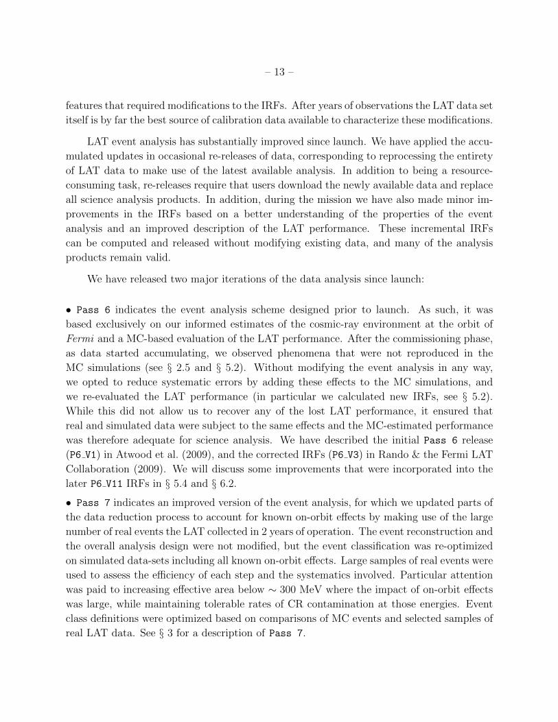
LAT event analysis has substantially improved since launch. We have applied the accu-

mulated updates in occasional re-releases of data, corresponding to reprocessing the entirety

of LAT data to make use of the latest available analysis. In addition to being a resource-

consuming task, re-releases require that users download the newly available data and replace

all science analysis products. In addition, during the mission we have also made minor im-

provements in the IRFs based on a better understanding of the properties of the event

analysis and an improved description of the LAT performance. These incremental IRFs

can be computed and released without modifying existing data, and many of the analysis

products remain valid.

We have released two major iterations of the data analysis since launch:

• Pass 6 indicates the event analysis scheme designed prior to launch. As such, it was

based exclusively on our informed estimates of the cosmic-ray environment at the orbit of

Fermi and a MC-based evaluation of the LAT performance. After the commissioning phase,

as data started accumulating, we observed phenomena that were not reproduced in the

MC simulations (see § 2.5 and § 5.2). Without modifying the event analysis in any way,

we opted to reduce systematic errors by adding these effects to the MC simulations, and

we re-evaluated the LAT performance (in particular we calculated new IRFs, see § 5.2).

While this did not allow us to recover any of the lost LAT performance, it ensured that

real and simulated data were subject to the same effects and the MC-estimated performance

was therefore adequate for science analysis. We have described the initial Pass 6 release

(P6 V1) in Atwood et al. (2009), and the corrected IRFs (P6 V3) in Rando & the Fermi LAT

Collaboration (2009). We will discuss some improvements that were incorporated into the

later P6 V11 IRFs in § 5.4 and § 6.2.

• Pass 7 indicates an improved version of the event analysis, for which we updated parts of

the data reduction process to account for known on-orbit effects by making use of the large

number of real events the LAT collected in 2 years of operation. The event reconstruction and

the overall analysis design were not modified, but the event classification was re-optimized

on simulated data-sets including all known on-orbit effects. Large samples of real events were

used to assess the efficiency of each step and the systematics involved. Particular attention

was paid to increasing effective area below ∼ 300 MeV where the impact of on-orbit effects

was large, while maintaining tolerable rates of CR contamination at those energies. Event

class definitions were optimized based on comparisons of MC events and selected samples of

real LAT data. See § 3 for a description of Pass 7.

– 14 –

All data released prior to 2011 August 1 were based on Pass 6. On 2011 August 1

we released Pass 7 data for the entire mission to date, and since then all data have been

processed only with Pass 7.

This paper has two primary purposes. The first is to describe Pass 7 (§ 3), quanti-

fying the differences with respect to Pass 6 when necessary. The second is to detail our

understanding of the LAT, and toward that end we describe how we have used flight data to

validate the generally excellent fidelity of our simulations of particle interactions in the LAT,

as well as the resulting IRFs and residual charged particle contamination. In particular, we

describe the methods and control data samples we have used to study the residual charged

particle contamination (§ 4), effective area (§ 5), PSF (§ 6), and energy dispersion (§ 7) of

the LAT. Furthermore, we quantify the uncertainties in each case, and discuss how these

uncertainties affect high-level scientific analyses (§ 8).

For convenience, we have included lists of the acronyms and abbreviations (Appendix B)

and notation conventions (Appendix C) used in this paper.

2. LAT INSTRUMENT, ORBITAL ENVIRONMENT, DATA PROCESSING

AND SIMULATIONS

In this paper, we focus primarily on those aspects of the LAT instrument, data, and

analysis algorithms that are most relevant for the understanding and validation of the LAT

performance. Additional discussion of these subjects was provided in a dedicated paper

(Atwood et al. 2009). The calibrations of the LAT subsystems are described in a second

paper (Abdo et al. 2009f).

2.1. LAT Instrument

The LAT consists of three detector subsystems. A tracker/converter (TKR), comprising

18 layers of paired x–y Silicon Strip Detector (SSD) planes with interleaved tungsten foils,

which promote pair conversion and measure the directions of incident particles (Atwood

et al. 2007). A calorimeter (CAL), composed of 8.6 radiation lengths of CsI(Tl) scintillation

crystals stacked in 8 layers, provides energy measurements as well as some imaging capa-

bility (Grove & Johnson 2010). An Anticoincidence Detector (ACD), featuring an array

of plastic scintillator tiles and wavelength-shifting fibers, surrounds the TKR and rejects

CR backgrounds (Moiseev et al. 2007). In addition to these three subsystems a triggering

and data acquisition system selects and records the most likely γ-ray candidate events for

– 15 –

transmission to the ground. Both the CAL and TKR consist of 16 modules (often referred

to as towers) arranged in a 4× 4 grid. Each tower has a footprint of ∼ 37 cm× 37 cm and

is ∼ 85 cm high (from the top of the TKR to the bottom of the CAL). A schematic of the

LAT is shown in Figure 1, and defines the coordinate system used throughout this paper.

Note that the z-axis corresponds to the LAT boresight, and the incidence (θ) and azimuth

(φ) angles are defined with respect to the z- and x- axes respectively.

+x+y

+zv

φ

θ

Fig. 1.— Schematic of the LAT, including the layout of the 16 CAL modules and 12 of the

16 TKR modules (for graphical clarity the ACD is not shown). This figure also defines the

(θ, φ) coordinate system used throughout the paper.

2.1.1. Silicon Tracker

The TKR is the section of the LAT where γ rays ideally convert to e+e− pairs and their

trajectories are measured. A full description of the TKR can be found in Atwood et al.

(2007) and Atwood et al. (2009). Starting from the top (farthest from the CAL), the first

12 paired layers are arranged to immediately follow converter foils, which are composed of

∼ 3% of a radiation length of tungsten. Minimizing the separation of the converter foils from

the following SSD planes, and hence the lever-arm between the conversion point and the first

position measurements, is critical to minimize the effects of multiple scattering. This section

of the TKR is referred to as the thin or front section. The next 4 layers are similar except

that the tungsten converters are ∼ 6 times thicker; these layers are referred to as the thick

or back section. The last two layers have no converter; this is dictated by the TKR trigger,

which requires hits in 3 x–y paired adjacent layers (see § 3.1.1) and is therefore insensitive

to γ rays that convert in the last two layers.

Thus the TKR effectively divides into two distinct instruments with notable differences

– 16 –

TKR front section

TKR back section

CAL

0 3% X×12

0 18% X×4

no W×2

Fig. 2.— Schematic of a LAT tower (including a TKR and a CAL module). The layout of

the tungsten conversion planes in the TKR is illustrated.

in performance, especially with respect to the PSF and background contamination. This

choice was suggested by the need to balance two basic (and somewhat conflicting) require-

ments: simultaneously obtaining good angular resolution and a large conversion probability.

The tungsten foils were designed such that there are approximately the same number of

γ rays (integrated over the instrument FoV) converted in the thin and thick sections. In

addition to these considerations, experience on orbit has also revealed that the aggregate of

the thick layers (∼ 0.8 radiation lengths) limits the amount of back-scattered particles from

the CAL returning into the TKR and ACD in high-energy events (i.e., the CAL backsplash)

and reduces tails of showers in the TKR from events entering the back of the CAL. These

two effects help to decrease the background contamination in front-converting events.

After three years of on-orbit experience with the TKR we can now assess the validity

of our design decisions. The choice of the solid-state TKR technology has resulted in neg-

ligible down time and extremely stable operation, minimizing the necessity for calibrations.

Furthermore, the very high signal-to-noise ratio of the TKR analog readout electronics has

resulted in a single hit efficiency, averaged over the active silicon surface, greater than 99.8%,

with a typical noise occupancy smaller than 10−5 for a single readout channel. (We note for

completeness that the fraction of non-active area presented by the TKR is ∼ 11% at normal

incidence). As discussed below, this has yielded extremely high efficiency for finding tracks

and has been key to providing the information necessary to reject backgrounds.

The efficiency and noise occupancy of the TKR over the first three years of operation are

shown in Figure 3. The variations in the average single strip noise occupancy are dominated

by one or a few noisy strips, which have been disabled at different times during the mission.

The baseline of 4×10−6 is dominated by accidental coincidences between event readouts and

– 17 –

charged particle tracks (see below, and § 2.1.4) and corresponds to an upper limit of ∼ 3

noise hits per event in the full LAT on average. Since these noise hits are distributed across

16 towers and 36 layers per tower, their effect on the event reconstruction is insignificant.

UTC

TK

R h

it ef

ficie

ncy

[%]

99.88

99.89

99.9

99.91

99.92

99.93

99.94

Jan 12009

Jul 1 Jan 12010

Jul 1 Jan 12011

Jul 1

(a)

UTCT

KR

sin

gle-

strip

noi

se o

ccup

ancy

-610

-510

Jan 12009

Jul 1 Jan 12010

Jul 1 Jan 12011

Jul 1

(b)

Fig. 3.— (a) Average TKR hit efficiency and (b) single-strip noise occupancy through the

first three years of the mission. Each data point is the average value for the full LAT over a

week of data taking. The shaded background regions mark the first two years of operation,

corresponding to the data selection used to calibrate the instrument performance.

The TKR readout is digital, i.e., the readout is binary, with a single threshold discrim-

inator for each channel, and no pulse height information is collected at the strip level. The

individual electronic chains connected to each SSD strip consist of a charge-sensitive pream-

plifier followed by a simple CR-RC shaper with a peaking time of ∼ 1.5 µs. Due to the

implementation details, the baseline restoration tends to be current-limited, and the signal

at the output of the shaper is far from the exponential decay characteristic of a linear net-

work, with the discriminated output being high for ∼ 10 µs for Minimum Ionizing Particles

(MIPs) at the nominal ∼ 1/4 MIP threshold setting. As a consequence, the latched TKR

strip signals are typically present for that amount of time after the passage of a MIP. If the

LAT is triggered within this time window, these latent signals will be read out and become

part of the TKR event data. The rate of occurrence of these ghost signals (which may result

in additional tracks when the events are reconstructed) depends directly on the charged par-

ticle background rate. Mitigation against this contamination in the data is discussed below

in § 2.1.4, § 3 and § 5.2.

Each detector subsystem contributes one or more trigger primitive signals that the LAT

trigger system uses to adjudicate whether to read out the LAT detectors (see § 3.1). The

TKR trigger is a coincidence of 3 x–y paired adjacent layers within a single tower (hence a

total of 6 consecutive SSD detector planes). Due primarily to power constraints, the TKR

electronic system does not feature a dedicated fast signal for trigger purposes. Rather, the

– 18 –

logical OR of the discriminated strip signals from each detector plane is used to initiate a

non-retriggerable one-shot pulse of fixed length (typically 32 clock ticks or 1.6 µs), that is

the basic building block of the three-in-a-row trigger primitive (see § 3.1.1). In addition,

the length (or time over threshold) of this layer-OR signal is recorded and included in the

data stream. Since the time over threshold depends on the magnitude of the ionization in

the SSD, which in turn depends on on the characteristics of the ionizing particle, it provides

useful information for the background rejection stage.

The efficiency of the three-in-a-row trigger is > 99%. This is due in part to the redun-

dancy of this trigger for the vast majority of events (i.e., by passing through many layers of

Si, most events have multiple opportunities to form a three-in-a row). The trigger efficiency,

measured in flight using MIP tracks crossing multiple towers, is shown in Figure 4 to be very

stable.

UTC

TK

R tr

igge

r ef

ficie

ncy

[%]

99.75

99.8

99.85

99.9

99.95

100

Jan 12009

Jul 1 Jan 12010

Jul 1 Jan 12011

Jul 1

Fig. 4.— Average efficiency of the TKR three-in-a-row trigger through the first three years

of the mission. Each data point is the average value for the full LAT over a week of data

taking. The shaded background region marks the first two years of operation, corresponding

to the data selection used to calibrate the instrument performance.

Perhaps the most important figure of merit for the TKR is the resulting PSF for re-

constructed γ-ray directions. At low energy the PSF is dominated by multiple scattering,

primarily within the tungsten conversion foils (tungsten accounts for ∼ 67% of the material

in the thin section and ∼ 92% of the material in the thick section). At high energy the com-

bination of the strip pitch of 228 µm, the spacing of the planes and the overall height of the

TKR result in a limiting precision for the average conversion of ∼ 0.1 at normal incidence.

MC simulations predict that the transition to this measurement precision dominated regime

should occur between ∼ 3 GeV and ∼ 20 GeV. We will discuss the PSF in significantly more

detail in § 6.

– 19 –

2.1.2. Electromagnetic Calorimeter

Details of the CAL can be found in Atwood et al. (2009) and Grove & Johnson (2010).

Here, we highlight some key aspects for understanding the LAT performance. The CAL

is a 3D imaging calorimeter. This is achieved by arranging the CsI crystals in each tower

module in 8 layers, each with 12 crystal logs (with dimensions 326 mm×26.7 mm×19.9 mm)

spanning the width of the layer. The logs of alternating layers are rotated by 90 about the

LAT boresight, and aligned with the x and y axes of the LAT coordinate system.

Each log is read out with four photodiodes, two at each end: a large photodiode covering

low energies (< 1 GeV per crystal), and a small photodiode covering high energies (< 70 GeV

per crystal). Each photodiode is connected to a charge-sensitive preamplifier whose output

drives (i) a slow (∼ 3.5 µs peaking time) shaping amplifier for spectroscopy and (ii) a fast

shaping amplifier (∼ 0.5 µs peaking time) for trigger discrimination. In addition, the output

of each slow shaper is connected to two separate track-and-hold stages with different gains

(×1 and ×8).

The outputs of the four track-and-hold stages are multiplexed to a single analog-to-

digital converter. The four gain ranges (two photodiodes× two track-and-hold gains) span an

enormous dynamic range, from < 2 MeV to 70 GeV deposited per crystal, which is necessary

to cover the full energy range of the LAT. A zero-suppression discriminator on each crystal

sparsifies the CAL data by eliminating the signals from all crystals with energies < 2 MeV.

To minimize CAL data volume, each log end reports only a single range, the lowest-gain

unsaturated range (the one-range, best-range readout) for most events. For likely heavy

ions, each log end reports all four ranges (the four-range readout) for calibrating the energy

scale across the different ranges (see § 3.1.1 for details of how the readout mode is selected).

The CAL provides two inputs to the global LAT trigger. At each log end the output

of each fast shaper (for both the large and the small diode) is compared to an adjustable

threshold by a discriminator to form two separate trigger request signals. In the standard

science configuration, the discriminator thresholds are set at 100 MeV and 1 GeV energy

deposition. The 1 GeV threshold is > 90% efficient for incident γ rays above 20 GeV.

For each log with deposited energy, two position coordinates are derived simply from

the geometrical location of the log within the CAL array, while the longitudinal position is

derived from the ratio of signals at opposite ends of the log: the crystal surfaces were treated

to provide monotonically decreasing scintillation light collection with increasing distance

from a photodiode. Thus, the CAL provides a 3D image of the energy deposition for each

event.

Since the CAL is only 8.6 radiation lengths thick at normal incidence, for energies

– 20 –

greater than a few GeV shower leakage becomes the dominant factor limiting the energy

resolution, in particular because event-to-event variations in the early shower development

cause fluctuations in the leakage out the back of the CAL. Indeed, by ∼ 100 GeV about

half of the total energy in showers at normal incidence escapes out the back of the LAT on

average. The intrinsic 3D imaging capability of the CAL is key to mitigating the degradation

of the energy resolution at high energy through an event-by-event 3D fit to the shower

profile. This was demonstrated both in beam tests and in simulations (Baldini et al. 2007;

Ackermann et al. 2010a), achieving better than 10% energy resolution well past 100 GeV.

The imaging capability also plays a critical role in the rejection of hadronic showers (see

§ 3.3.7). Furthermore, for events depositing more than ∼ 1 GeV in the CAL, imaging in

the CAL can be exploited to aid in the TKR reconstruction and in determining the event

direction (see § 3.2).

We have monitored the performance of the CAL continuously over its three years of

operation. We observe a slow (∼ 1% per year) decrease in the scintillation light yield of the

crystals due to radiation damage in low Earth orbit, as we anticipated prior to launch (see

also § 7.3.2). Although we do not yet correct for this decreased light yield, we have derived

calibration constants on a channel-by-channel basis for the mission to date. In 2012 January

we started reprocessing the full data set with these updated calibrations, and in the future

expect to maintain a quarter-yearly cadence of updates to ensure that the calibrated values

do not drift by more than 0.5%.

2.1.3. Anticoincidence Detector

The third LAT subsystem is the ACD, critically important for the identification of

LAT-entering charged cosmic rays. Details of its design can be found in Moiseev et al.

(2007) and Atwood et al. (2009). From the experience of the LAT predecessor, the Energetic

Gamma Ray Experiment Telescope (EGRET), came the realization that a high degree of

segmentation was required in order to minimize self-veto due to hard X-ray back-scattering

(often referred to as backsplash) from showers in the CAL (Esposito et al. 1999).

The ACD consists of 25 scintillating plastic tiles covering the top of the instrument and

16 tiles covering each of the four sides (89 in all). The dimensions of the tiles range between

561 and 2650 cm2 in geometrical surface and between 10 and 12 mm in thickness. By design,

the segmentation of the ACD does not match that of the LAT tower modules, to avoid lining

up gaps between tiles with gaps in the TKR and CAL. The design requirements for the ACD

specified the capability to reject entering charged particles with an efficiency > 99.97%. To

meet the efficiency requirement, careful design of light collection using wavelength-shifting

– 21 –

fibers, and meticulous care in the fabrication to maintain the maximum light yield were

needed. The result was an average light yield of ∼ 23 photo-electrons (p.e.) for a normally-

incident MIP for each of the two redundant readouts for each tile.

The required segmentation inevitably led to less than complete hermeticity, with con-

struction and launch survival considerations setting lower limits on the sizes of the gaps

between tiles. Tiles overlap in one dimension, leaving gaps between tile rows in the other.

The gaps are ∼ 2.5 mm and coverage of these gaps is provided by bundles of scintillating

fibers (called ribbons), read out at each end by a photomultiplier tube (PMT). The light yield

for these ribbons, however, is considerably less than for the tiles: it is typically ∼ 8 p.e./MIP

and varies considerably along the length of a bundle. Therefore, along the gaps the efficiency

for detecting the passage of charged particles is lower. However, the gaps comprise a small

fraction of the total area (< 1%) and accommodating them did not require compromising

the design requirements. In addition to the gaps between ACD tile rows, the corners on the

sides of the ACD have gaps that are not covered by ribbons and must be accounted for in

the reconstruction and event classification (see § 3.4).

As with the TKR and CAL, the ACD provides information used in the hardware trigger

as well as in the full reconstruction of the event. The output of each PMT is connected to

(i) a fast shaping amplifier (with ∼ 400 ns shaping time) for trigger purposes and (ii) two

separate slow electronics chains (with ∼ 4 µs shaping time and different gains) to measure

the signal amplitude. The use of the fast signal in the context of the LAT global trigger

will be discussed in more detail in § 3. Although the main purpose of the ACD is to signal

the passage of charged particles, this subsystem also provides pulse height information. The

two independent slow signals and the accompanying circuitry for automatic range selection

accommodate a large dynamic range, from ∼ 0.1 MIP to hundreds of MIPs.

As for both the TKR and the CAL, the performance of the ACD has been continuously

monitored over the past three years. The stability of the MIP signal is shown in Figure 5 and

in summary shows very little degradation. Note that slight changes in the selection criteria

and spectra of the MIP calibration event sample cause small (< 0.5%) variations in mean

deposited energy per event.

2.1.4. Trigger and Data Acquisition

The LAT hardware trigger collects information from the LAT subsystems and, if certain

conditions are fulfilled, initiates event readout. Because each readout cycle produces a min-

imum of 26.5 µs of dead time (even more if the readout buffers fill dynamically), the trigger

– 22 –

UTC

AC

D M

IP p

eak

posi

tion

[a. u

.]

0.98

0.985

0.99

0.995

1

1.005

1.01

1.015

1.02

Jan 12009

Jul 1 Jan 12010

Jul 1 Jan 12011

Jul 1

Fig. 5.— Relative position of the MIP peak, calibrated for the tile response and corrected

for the incidence angle, through the first three years of the mission. Each data point is the

average value for the 89 ACD tiles over a week of data taking, with the value of the first

point being arbitrarily set to 1. The shaded background region marks the first two years of

operation, corresponding to the data selection used to calibrate the instrument performance.

Data from the first several months of the mission are missing because this quantity had not

yet been included as part of the automated data monitoring and trending.

was designed to be efficient for γ rays while keeping the total trigger rate, which is dominated

by charged CRs, low enough to limit the dead-time fraction to less than about 10% (which

corresponds to a readout rate of about 3.8 kHz). The triggering criteria are programmable

to allow additional, prescaled event streams for continuous instrument monitoring and cal-

ibration during normal operation. We will defer discussion of the actual configuration used

in standard science operations and of the corresponding performance to the more general

discussion of event processing in § 3.1.

To limit the data volume to the available telemetry bandwidth, collected data are passed

to the on-board filter. The on-board filter (see § 3.1.2) consists of a few event selection

algorithms running in parallel, each independently able to accept a given event for inclusion

in the data stream to be downlinked. Buffers on the input to the on-board filter can store

on the order of 100 events awaiting processing. Provided that the on-board filter processes

at least the average incoming data rate no additional dead time will be accrued because

the on-board filter is busy. The processors used for the on-board filter must also build and

compress the events for output, and the time required to make a filter decision varies widely

between events. Therefore, the event rate that the on-board filter can handle depends on the

number of events passing the filter. In broad terms, the processors will saturate for output

rates between 1 kHz and 2.5 kHz, depending on the configuration of the on-board filter. In

practice, the average output rate is about 350 Hz, and the amount of dead time introduced

– 23 –

by the on-board filter is negligible.

Soon after launch, it became apparent that the LAT was recording events that included

an unanticipated background: remnants of electronic signals from particles that traversed

the LAT a few µs before the particle that triggered the event. We refer to these remnants

as ghosts. An example of such an event is shown in Figure 6.

y

z

ray directionγIncoming

rayγGenuine "Ghost" activity

Fig. 6.— Example of a ghost event in the LAT (y–z orthogonal projection). In addition

to an 8.5 GeV back-converting γ-ray candidate (on the right) there is additional activity in

all the three LAT subsystems, with the remnants of a charged-particle track crossing the

ACD, TKR and CAL. The small crosses represent the clusters (i.e., groups of adjacent hit

strips) in the TKR, while the variable-size squares indicate the reconstructed location of the

energy deposition for every hit crystal in the CAL (the side of the square being proportional

to the magnitude of the energy release). The dashed line indicates the γ-ray direction. For

graphical clarity, only the ACD volumes with a signal above the zero suppression level are

displayed.

It is important to re-emphasize a point made in the previous sub-sections: many of

the signals that are passed to the hardware trigger and the on-board filter are generated by

dedicated circuits whose shaping times are significantly shorter than for the circuits that read

out the data from the same sensors for transmission to the ground. Although the signals with

longer shaping times used for the ground event processing measure the energy deposited in

the individual channels far more precisely, they also suffer the adverse consequence of being

– 24 –

more susceptible to ghost particles. Table 1 gives the characteristic times for both the fast

signals (i.e., those used in the trigger) and the slow signals (i.e., those used in the event-level

analysis) for each of the subsystems.

Subsystem Fast signal Slow signal

(trigger) (event data)

ACD 0.4 µs 4 µs

CAL 0.5 µs 3.5 µs

TKR 1.5 µs 10 µs

Table 1: Characteristic readout time windows for LAT subsystems. The TKR subsystem

does not provide a dedicated fast signal for the trigger: the peaking time for the shaped

TKR signal is ∼ 1.5 µs (which is the relevant number for the trigger) but the decay time is

much longer and the average time over threshold for the discriminated output is of the order

of 10 µs for a MIP at normal incidence.

The ghost events have been the largest detrimental effect observed in flight data. They

affect all of the subsystems, significantly complicate the event reconstruction and analysis,

and can cause serious errors in event classification:

• they can leave spurious tracks in the TKR that do not point in the same direction as the

incident γ ray and might not be associated with the correct ACD and CAL information due

to the different time constants of the subsystems;

• they can leave sizable signals in the CAL that can confuse the reconstruction of the

electromagnetic shower, degrading the measurement of the shape and direction of the shower

itself, and that can cause the energy reconstruction to mis-estimate the energy of the incident

γ ray;

• they can leave significant signals in the ACD that can be much larger than ordinary

backsplash from the CAL and that can cause an otherwise reconstructable γ ray to be

classified as a CR.

We will discuss the effects on the LAT effective area in more detail in § 5. In brief:

above ∼ 1 GeV, where the average fractional ghost signal in the CAL is small, the loss of

effective area is of the order of 10% or less. This loss is largely due to the fact that valid γ

rays can be rejected in event reconstruction and classification if ghost energy depositions in

the CAL cause a disagreement between the apparent shower directions in CAL and TKR.

At lower γ-ray energies ghost signals can represent the dominant contribution to the energy

– 25 –

deposition in the instrument, and the corresponding loss of the effective area can exceed 20%.

We also emphasize that, while these figures are averaged over orbital conditions, the fraction

of events that suffer from ghost signals, as well as the quantity of ghost signals present in

the affected events, varies by a factor of 2–3 at different points in the orbit due to variation

in the geomagnetic cutoff and resulting CR rates. Recovering the effective area loss due to

ghost signals is one of the original and main motivations of ongoing improvements to the

reconstruction (Rochester et al. 2010).

Finally, during extremely bright Solar Flares (SFs) the pile-up of several > 10 keV X-

rays within a time interval comparable with the ACD signal shaping time can also cause γ

rays to be classified as CRs (see Appendix A).

2.2. Orbital Environment and Event Rates

Fermi is in a 565-km altitude orbit with an inclination of 25.6. The orbit has a period

of ∼ 96 minutes, and its pole precesses about the celestial pole with a period of ∼ 53.4 days.

At this inclination Fermi spends about 15% of the time inside the South Atlantic Anomaly

(SAA). Science data taking is suspended while Fermi is within the SAA because of the high

flux of trapped particles (for details, see Abdo et al. 2009f).

When Fermi is in standard sky-survey mode the spacecraft rocks north and south about

the orbital plane on alternate orbits. Specifically, the LAT boresight is offset from the

zenith toward either the north or south orbital poles by a characteristic rocking angle. On

2009 September 3 this rocking angle was increased from 35 to 50 in order to lower the

temperature of the spacecraft batteries and thus extend their lifetime. As a result of this

change, the amount of the Earth limb that is subtended by the FoV of the LAT during

survey-mode observations increased substantially. The most noticeable consequence is a

much larger contribution to the LAT data volume from atmospheric γ rays. This will be

discussed more in § 4, and further details about atmospheric γ rays can be found in Abdo

et al. (2009a).

The flux of charged particles passing through the LAT is usually several thousand times

larger than the γ-ray flux. Accordingly, several stages of event selection are needed to purify

the γ-ray content (see § 3.1, § 2.4 and § 3) and some care must be taken to account for

contamination of the γ-ray sample by charged particles that are incorrectly classified as γ

rays (see § 4). Here we distinguish 4 stages of the event classification process:

1. hardware trigger request : the LAT detects some traces of particle interaction and starts

the triggering process (§ 3.1);

– 26 –

2. hardware trigger accept : the event in question generates an acceptable trigger pattern

and is read out and passed to the on-board filter (§ 3.1);

3. on-board filter : the event passes the on-board γ-ray filter criteria (§ 3.1);

4. standard γ-ray selection: the event passes more stringent selection criteria (§ 3.4), such

as P7SOURCE, which is the selection currently being recommended for analysis of individual

point sources, or P6 DIFFUSE, the selection recommended for analysis of point sources in the

Pass 6 iteration of the event selections.

Figure 7 shows an example of both the orbital variations of the charged particle flux,

and how the initially overwhelming CR contamination is made tractable while maintaining

high efficiency for γ rays by several stages of data reduction and analysis. Figure 8 shows how

the charged particle rate varies with spacecraft position. In particular, data taken during

the parts of the orbit with the highest background rates are more difficult to analyze for

two reasons: (i) there are simply more non-γ-ray events that must be rejected, and (ii) the

increased ghost signals complicate the analysis of the γ-ray events (see § 2.5.1).

A model of the particle backgrounds for the region outside the SAA was compiled

before launch as documented in Atwood et al. (2009): above the geomagnetic cutoff rigidity

(∼ 10 GV) the most abundant species is primary galactic CR protons, at lower energies

particle fluxes are dominated by trapped protons and electrons, in addition to the γ rays

due to interaction of CRs with the atmosphere of the Earth. Since launch, the particle model

has been updated to include new measurements, (see, e.g., Ackermann et al. 2010a, for the

electron population).

2.3. Observing Strategy and Paths of Sources Across the LAT Field-of-View

Fermi has spent over 95% of the mission in sky survey mode, with most of the remainder

split between pointed observations and calibrations. Furthermore, in sky survey mode, the

azimuthal orientation of the LAT is constrained by the need to keep the spacecraft solar

panels pointed toward the Sun and the radiators away from the Sun. Specifically, in sky

survey mode Fermi completes one full rotation in φ every orbit.

Therefore, during an orbital precession period the LAT boresight will cross a range

of declinations ±25.6 relative to the rocking angle, while the LAT x-axis will track

the direction toward the Sun. As a result, during the sky survey mode, each point

in the sky traces a complicated path across the LAT FoV, the details of which depend on

the declination and ecliptic latitude. Figure 9 shows examples of these paths for two of

the brightest LAT sources. Furthermore, in sky survey mode operations the path

– 27 –

UTC12:00 18:00 00:00 06:00 12:00

Rat

e [H

z]

-110

1

10

210

310

410Trigger requestTrigger accept

Onboard filter

P7TRANSIENT

P7SOURCE

]°

<100zθ [P7SOURCE

Fig. 7.— Rates at several stages of the data acquisition and reduction process on a typical

day (2011 August 17). Starting from the highest, the curves shown are for the rates: (i) at the

input of the hardware trigger process (trigger request), (ii) at output of the hardware trigger

(trigger accept), (iii) at the output of the on-board filter, (iv) after the loose P7TRANSIENT

γ-ray selection, (v) after the tighter P7SOURCE γ-ray selection, and (vi) the P7SOURCE γ-ray

selection with an additional cut on the zenith angle (θz < 100). See § 3 for more details

about the event selection stages.

that the LAT boresight traces across the sky during any two orbit period is only

slightly different than during the two previous or subsequent orbits.

2.4. Ground-Based Data Processing

Reconstructing the signals in the individual detector channels into a coherent picture

of a particle interaction with the LAT for each of the several hundred events collected every

second is a formidable task. We will defer detailed discussion of the event reconstruction

and classification to § 3; here we describe just the steps to give a sense of the constraints.

1. Digitization: we decompress the data and convert the information about signals in indi-

vidual channels from the schema used in the electronics readout to more physically motivated

schema—such as grouping signals in the ACD by tile, rather than by readout module.

2. Reconstruction: we apply pattern recognition and fitting algorithms commonly used in

high-energy particle physics experiments to reconstruct the event in terms of individual TKR

tracks and energy clusters in the CAL and to associate those objects with signals in the ACD

(see § 3.2).

3. Event analysis : we evaluate quantities that can be used as figures of merit for the event

– 28 –

]°Geographic longitude [-150-100 -50 0 50 100 150

]°G

eogr

aphi

c la

titud

e [

-20

-10

0

10

20

4

6

8

10

12

14

16

Ver

tical

cut

off r

igid

ity [G

V]

(a)


]°G

eogr

aphi

c la

titud

e [

-20

-10

0

10

20

3

4

5

6

7

8

9

10

11

12

Trig

ger

requ

est r

ate

[kH

z]

(b)


]°G

eogr

aphi

c la

titud

e [

-20

-10

0

10

20

0.6

0.7

0.8

0.9

P7S

OU

RC

E r

ate

[Hz]

(c)

Fig. 8.— Orbital background environment as a function of geographic location: (a) vertical

geomagnetic cutoff rigidity; (b) mean rate of events at the input of the hardware trigger

process (trigger requests, see § 3.1.1), which decreases roughly as the square root of the

geomagnetic cutoff rigidity; (c) mean rate of events in P7SOURCE event class (see § 3.4.3)

with the additional cut on the zenith angle (θz < 100). The anti-correlation between the

P7SOURCE event rate and the trigger request rate is the result of the loss of efficiency due

to ghost signals (see § 2.1.4 and § 5.2.2). The black lines and points surrounding the white

area represent the sides and vertices of the SAA polygon as defined for LAT operations. The

LAT does not acquire science data while inside the SAA polygon.

– 29 –

1

10

210

310

°90.0

°78.5

°66.4

°53.1

°36.9

° 0.0°180.0

°22.5

°202.5

°45.0

°225.0

°67.5

°247.5

°90.0

°270.0

°112.5

°292.5

°135.0

°315.0

°157.5

°337.5

Live

time

[s]

(a)

1

10

210

310

°90.0

°78.5

°66.4

°53.1

°36.9

° 0.0°180.0

°22.5

°202.5

°45.0

°225.0

°67.5

°247.5

°90.0

°270.0

°112.5

°292.5

°135.0

°315.0

°157.5

°337.5

Live

time

[s]

(b)

Fig. 9.— Live time maps in instrument coordinates for the Vela pulsar (a) and the Crab

(b). These plots are made in a zenith equal area projection with the LAT boresight at the

center of the image, and the color scale shows the total live time each source was at θz < 85.

Recall that φ = 0 corresponds to the +x axis of the LAT (Fig. 1). These plots cover the

same two-year time range that defines the standard calibration samples (see § 3.6).

from the collections of tracks, clusters and associated ACD information. Once we have ex-

tracted this information we apply multi-variate analysis techniques to extract measurements

of the energy and direction of the event and to construct estimators that the event is in fact

a γ-ray interaction (see § 3.3).

4. Event selection: we apply the selection criteria for the various γ-ray event classes (§ 3.4).

In addition to these procedures, the processing pipeline is responsible for verifying the data

integrity at each step and for producing and making available all the ancillary data products

related to calibration and performance monitoring of the LAT.

On the whole, the LAT data processing pipeline utilizes approximately 130 CPU years

and 300 TB of storage each year.

The ISOC can reprocess data with updated algorithms from any stage in the process.

However, given the quantities of data involved, reprocessing presents challenges both to the

available pool of computing power and storage space. Table 2 gives a rough idea of the

resources used by each stage in the process. Given the available resources, reprocessing from

the Reconstruction step is practical only once a year or less often, and reprocessing from the

Digitization step is feasible only every few years.

– 30 –

Stage CPU Time Disk Usage

[years/year] [TB/year]

Digitization 1.2 26

Reconstruction 85 167

Event analysis 5 10

Event selection 1.3 60

Data monitoring 25 12

Calibration 5 72

Table 2: Various stages of the data processing pipeline. The numbers in the CPU time and

disk usage columns refer to a typical year of data taking.

2.5. Simulated Data

In order to develop the filtering, reconstruction and event selection algorithms described

in § 3 we used a detailed simulation of particle interactions with Fermi written in the

Geant4 (Agostinelli et al. 2003) framework. This simulation includes particle interactions

with a detailed material model of Fermi , as well as simulations of the uncalibrated signals

produced in the various sensors in the three subsystems.

The fact that the simulation is detailed enough to produce uncalibrated signals for each

channel allows the simulations to be truly end-to-end:

1. we maintain fidelity to the analysis of the flight data by processing simulated data with

the same reconstruction and analysis algorithms as the flight data;

2. on a related but slightly different note, we simulate the data as seen by the trigger and

the on-board software, and process the data with a simulation of the hardware trigger and

exactly the same on-board filter algorithms as used on the LAT;

3. we can merge the signals from two events into a single event. As described in § 2.5.1, we

rely on this feature to add an unbiased sample of ghost signals to simulated events.

2.5.1. Ghosts and Overlaid Events

The presence of ghost signals in the LAT data reduced the efficiency of the event se-

lections tuned on simulated data lacking this effect. So we developed a strategy to account

for the ghosts. One of the triggers implemented in the LAT data-acquisition system, the

PERIODIC trigger (see § 3.1.1), provides us with a sample of ghost events: twice per second

– 31 –

the LAT subsystems are read out independent of any other trigger condition. For the CAL

and the ACD, all the channels, even those below threshold, are recorded (this is not possible

for the TKR). Since these triggers occur asynchronously with the particle triggers, the ghost

signals collected are a representative sample of the background present in the LAT.

We merge the signals channel-by-channel from a randomly chosen periodic trigger event

into each simulated event. In more detail, we analyze the signals in each periodic trigger,

converting the instrument signals to physical units; analog-to-digital converter channels in

the ACD and CAL, and time over threshold signals in the TKR, are converted into deposited

energy. Since the intensity and spectrum of cosmic rays seen by the LAT depend on the

position of the Fermi satellite in its orbit, the ghost events are sorted by the value of

McIlwain L (Walt 2005) at the point in the orbit where the event was recorded. Then, during

the simulation process, for each simulated event we randomly select a periodic trigger event

with similar McIlwain L, and add the energy deposits in this “overlay event” to those of the

original simulated event, after which the combined event is digitized and reconstructed in

the usual way.

We have used the improved simulations made with this overlay technique to more ac-

curately evaluate the effective area of the LAT, and to better optimize the event selection

criteria when developing Pass 7. Furthermore, we are studying ways to identify and tag

the ghost signals and remove them from consideration in the event analysis (Rochester et al.

2010).

2.5.2. Specific Source γ-ray Signal Simulation

We have developed interfaces between the software libraries that implement the flux

generation and coordinate transformation used by the ScienceTools and our detailed Geant4-

based detector simulation. This allows us to re-use the same source models that we use with

the ScienceTools within our detailed Geant4-based detector simulation, insuring consistent

treatment of Fermi pointing history and the source modeling. One application for the present

work was simulating atmospheric γ rays above 10 GeV for comparison with our Earth limb

calibration sample (see § 3.6.3).

2.5.3. Generic γ-ray Signal Simulation

In addition to simulating individual sources, we also simulate uniform γ-ray fields that

we can use to explore the instrument response across the entire FoV and energy range of the

– 32 –

LAT. These will henceforth be referred to as allGamma simulations, and they have these

features:

1. the γ rays are generated with an E−1 number spectrum (where E is the γ-ray energy),

i.e., the same number of γ rays are generated in each logarithmic energy bin;

2. the individual γ rays are randomly generated on a sphere with 6 m2 cross sectional area

(i.e., large enough to contain the entire LAT and most of the spacecraft) centered at the

origin of the LAT reference frame, i.e., the center of the TKR/CAL interface plane;

3. the directions of the γ-rays are sampled randomly across 2π of downward-going (in the

LAT reference frame) directions, so as to represent a semi-isotropic incident flux.

For defining the IRFs we simulate 200 million γ rays over the range log10 (E/1 MeV) ∈[1.25, 5.75] and a further 200 million γ rays over the range log10 (E/1 MeV) ∈ [1.25, 2.75].

The net result is to produce a data set that adequately samples the LAT energy band and

FoV and that far exceeds the statistics of any single point source.

2.5.4. Simulation of Particle Backgrounds

In order to develop our event classification algorithms, and to quantify the amount of

residual CR background that remains in each γ-ray event class, we require accurate models

of both the CR background intensities and the interactions of those particles with the LAT.

Accordingly, we use the same Geant4-based detector simulation described in the previous

section to simulate fluxes of CR backgrounds.

There are three components to the CR-induced background in the LAT energy range.

• Primary CRs : Protons, electrons, and heavier nuclei form the bulk of charged CRs. Due

to the shielding by the magnetic field of the Earth, only particles with rigidities above a few

GV (spacecraft position dependent) can reach the LAT orbit. Therefore, the background

from primary CRs is relevant above a few GeV. The LAT event classification provides a

very effective rejection of charged particles, up to an overall suppression factor of 106 for

CR protons (with a prominent contribution from the ACD). However, due to the intense

flux of primary protons, a significant number of misclassified CRs enter even the P7SOURCE,

P7CLEAN, and P7ULTRACLEAN γ-ray classes. Minimum-ionizing primary protons above a few

GeV produce a background around 100–300 MeV in the LAT. However, protons that in-

elastically scatter in the passive material surrounding the ACD (e.g., the micro-meteoroid

shield) without entering the ACD can produce secondary γ rays at lower energies which are

– 33 –

then indistinguishable from cosmic γ rays, and which we refer to as irreducible background

(see also § 4.4).

• Charged secondaries from CR interactions : CRs entering the atmosphere produce a num-

ber of secondaries in interactions with the atmosphere itself. Charged particles produced in

these interactions can spiral back out, constrained by the magnetic field of the Earth, and

eventually re-enter the atmosphere. These particles are predominantly protons, electrons,

and positrons and are an important background below the geomagnetic cutoff rigidity. Due

to the high efficiency of the ACD in rejecting charged particles, the dominant contribution

to this background in the P7CLEAN and P7ULTRACLEAN event classes is positron annihilations

in the passive material around the ACD. The resulting γ rays are again indistinguishable

from cosmic γ rays.

• Neutral secondaries from CR interactions : γ rays and neutrons are also produced in local

CR interactions. Unaffected by the magnetic field, they approach the LAT from the direction

of the Earth with intensities peaking at the Earth limb. Neutrons are easily suppressed by

the event classification scheme and do not contribute significantly to the background. The

γ-ray background is suppressed by pointing away from the Earth and excluding events that

originate from near or below the Earth limb. Due to the long tails of the LAT PSF (see § 6),

however, a small fraction of the events originating from the Earth limb are reconstructed

with directions outside the exclusion regions. Since the Earth limb is extremely bright (Abdo

et al. 2009b), even this small fraction is an important residual background for celestial γ rays.

Since the PSF tails broaden with decreasing energy the main contribution is at energies below

a few hundred MeV (see § 4.5). Similarly, a small fraction of γ rays entering the LAT with

incidence angles greater than 90 are mischaracterized as downward-going (∼ 5% to∼ 0.01%,

depending on the energy, incidence angle, and the event sample). Because the Earth limb is

extremely bright and some part of it is almost always behind the LAT, γ rays from the limb

are the dominant component of “back-entering” background contamination. Furthermore,

since we mis-estimate the directions of these back-entering γ rays by > 90, they are often

reconstructed outside the Earth exclusion region.

Figure 10 shows the average CR-induced particle intensities at the orbit of the LAT

in the model that we use. For comparison the intensity of the extragalactic diffuse γ-ray

emission measured by the LAT (Abdo et al. 2010f) is overlaid to demonstrate the many

orders of background suppression necessary to distinguish it from particle background. The

model was developed prior to launch based on data from satellites in similar orbits and

balloon experiments (Mizuno et al. 2004).

As the particle rates are strongly dependent on location in geomagnetic coordinates, the

details of the orbit model are also important. For tuning the event analysis, or for estimating

– 34 –

Reconstructed energy [MeV]210 310 410 510 610

]-1

sr

-1 s

-2 d

N/d

E [M

eV c

m× 2

E

-510

-410

-310

-210

-110

1

10

210

310

Primary pNuclei (Z > 1)

- + e+Primary e

Secondary p- + e+Secondary e

Neutrons-raysγAtmospheric

EGB intensity

Fig. 10.— Model of the LAT orbital position and particle direction-averaged CR-induced

particle intensities (Mizuno et al. 2004) sampled from a 64 s live time background simulation

run. The intensity of the extragalactic diffuse background emission measured by the LAT

(Abdo et al. 2010f) is shown for comparison. Note that the event energy is reconstructed

under the hypothesis of a downward-going γ ray and in general does not represent the actual

energy for hadrons.

the background rates for typical integration times of months or years, the simulated time

interval must be at least equal to the precession period of the Fermi orbit (53.4 days).

Simulating these high particle rates for such a long time interval is quite impractical, in

terms of both CPU capacity and disk storage requirements. For studies of background

rejection we usually simulate an entire precession period to ensure a proper sampling of the

geomagnetic history, but to limit the particle counts we generate events for only a few seconds

of simulated time every several minutes, e.g., a typical configuration requires event generation

for 4 seconds every 4 minutes of time in orbit. This partial sampling is a compromise between

the limited CPU and disk usage, and the requirement of having good statistics. Considering

the LAT background rejection power, in order to have sizable statistics after even the first

stages of the event analysis are performed, we must start with a simulated background data

set of over 109 CRs.

– 35 –

3. EVENT TRIGGERING, FILTERING, ANALYSIS AND

CLASSIFICATION

In this section we describe the analysis steps that determine which events make it into

our final γ-ray data sample, starting with the triggering and filtering performed by the on-

board data acquisition system (§ 3.1), moving on to the reconstruction of particle interactions

in the event (§ 3.2), the analysis of the event as a whole (§ 3.3) and finally the definition

of the γ-ray classes (§ 3.4). The overall logical structure of this process is illustrated in

Figure 11.

Trigger§ 3.1.1

On-board filter§ 3.1.2

Trigger and filter§ 3.1

CAL recon§ 3.2.1

TKR recon§ 3.2.2

ACD recon§ 3.2.3

Event reconstruction§ 3.2

Merit§ 3.3.1

Energy analysis§ 3.3.2

PSF analysis§ 3.3.3

CPF analysis§ 3.3.5

TKR topology§ 3.3.6

CAL topology§ 3.3.7

Event classification§ 3.3.8

Event-level analysis§ 3.3

Definition of standard photon classes§ 3.4

1Fig. 11.— Logical structure of the analysis steps determining which events are selected for

a given class. The references to section numbers are meant to help the reader navigate the

content of § 3.

The event analysis requires knowledge of the LAT, the physics of particle interactions

within its volumes, and of the particle backgrounds in the Fermi orbit. As described in

§ 2.5, we use large MC samples of γ rays and of CRs to devise the best procedures to extract

estimates of energies and incident directions, and to classify events as either γ rays or charged

particle backgrounds.

Finally, in § 3.5 we describe the publicly available LAT event samples, while in § 3.6

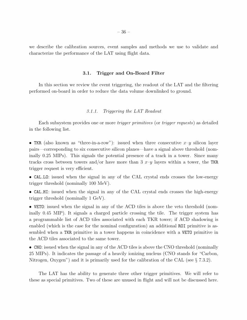
– 36 –

we describe the calibration sources, event samples and methods we use to validate and

characterize the performance of the LAT using flight data.

3.1. Trigger and On-Board Filter

In this section we review the event triggering, the readout of the LAT and the filtering

performed on-board in order to reduce the data volume downlinked to ground.

3.1.1. Triggering the LAT Readout

Each subsystem provides one or more trigger primitives (or trigger requests) as detailed

in the following list.

• TKR (also known as “three-in-a-row”): issued when three consecutive x–y silicon layer

pairs—corresponding to six consecutive silicon planes—have a signal above threshold (nom-

inally 0.25 MIPs). This signals the potential presence of a track in a tower. Since many

tracks cross between towers and/or have more than 3 x–y layers within a tower, the TKR

trigger request is very efficient.

• CAL LO: issued when the signal in any of the CAL crystal ends crosses the low-energy

trigger threshold (nominally 100 MeV).

• CAL HI: issued when the signal in any of the CAL crystal ends crosses the high-energy

trigger threshold (nominally 1 GeV).

• VETO: issued when the signal in any of the ACD tiles is above the veto threshold (nom-

inally 0.45 MIP). It signals a charged particle crossing the tile. The trigger system has

a programmable list of ACD tiles associated with each TKR tower; if ACD shadowing is

enabled (which is the case for the nominal configuration) an additional ROI primitive is as-

sembled when a TKR primitive in a tower happens in coincidence with a VETO primitive in

the ACD tiles associated to the same tower.

• CNO: issued when the signal in any of the ACD tiles is above the CNO threshold (nominally

25 MIPs). It indicates the passage of a heavily ionizing nucleus (CNO stands for “Carbon,

Nitrogen, Oxygen”) and it is primarily used for the calibration of the CAL (see § 7.3.2).

The LAT has the ability to generate three other trigger primitives. We will refer to

these as special primitives. Two of these are unused in flight and will not be discussed here.

– 37 –

The third, the PERIODIC trigger, runs at a nominal frequency of 2 Hz during all science data

taking and is used for diagnostic and calibration purposes.

We emphasize that although the trigger primitives provided by the TKR and the CAL

are tower-based, a trigger initiates a readout of the whole LAT.

Trigger primitives are collected by the Central Trigger Unit. All 256 possible combina-

tions of the eight trigger primitives are mapped into so-called trigger engines. In brief, some

trigger requests are allowed to open a trigger window of fixed duration (nominally 700 ns)

and the set of primitives collected in this time interval is compared to a table of allowed

trigger conditions. In case a trigger condition is satisfied, a global trigger (or trigger accept)

is issued and event acquisition commences. The LAT readout mode (i.e., enabling the CAL

and ACD zero suppression and selecting the CAL one-range or four-range readout) can be

individually set for each trigger engine. In addition, trigger engines are scalable: for each

trigger condition a prescale is specified, corresponding to the number of valid trigger requests

necessary to issue a single global trigger (obviously no prescale is applied to engines intended

for γ-ray collection).

Engine PERIODIC CAL HI CAL LO TKR ROI CNO Prescale Average rate [Hz]

3 1 × × × × × 0 2

4 0 × 1 1 1 1 0 200

5 0 × × × × 1 250 5

6 0 1 × × × 0 0 100

7 0 0 × 1 0 0 0 1500

8 0 0 1 0 0 0 0 400 a

9 0 0 1 1 1 0 0 700

10 0 0 0 1 1 0 50 100

Table 3: Definition of the standard trigger engines: primitives used (1: required, 0: excluded,

×: either), prescale factors and typical rates. In this short-hand representation, engines are

defined with highest precedence first: each combination of trigger primitives is mapped to

the engine corresponding to the first condition it matches. Trigger engines 0, 1 and 2 are

used by the LAT software for bookkeeping and to catch conditions that should not happen

on orbit.

aIn the nominal configuration for science data taking the CAL LO condition is inhibited from opening a trigger

window, and therefore engine 8 is effectively disabled.

– 38 –

The standard trigger engine definitions are listed in Table 3. Trigger engine 7 is partic-

ularly important for γ-ray events: it requires no special primitives, a three-in-a-row signal in

the TKR (TKR), absence of ROI shadowing and CNO from the ACD, and no CAL HI. Engine 6

handles CAL HI events and engine 9 handles events with enough energy deposition in the

CAL to potentially cause ROI shadowing.

Trigger engine 4 is typical for calibration data (e.g., heavy ion collection): it requires no

special primitives, three-in-a-row in the TKR (TKR), a highly ionizing passage in the ACD

(CNO) in close correspondence (ROI) and at least a moderate energy deposition in the CAL

(CAL LO). Engines 5 and 10 process very few γ rays and are used primarily for calibration and

monitoring, so they are prescaled to limit the readout rate and/or to match the downlink

bandwidth allocation.

3.1.2. Event Filtering

As mentioned before, since limited telemetry bandwidth is available for data downlink,

some event filtering is required. The on-board filter allows the coexistence of different filtering

algorithms and in fact, in the nominal science data taking configuration, all the events are

presented to three different filters:

• the gamma filter, designed to accept γ rays (with an output average rate of approximately

350 Hz);

• the hip filter, designed to select heavy ion event candidates, primarily for CAL calibration

(with an output average rate of approximately 10 Hz);

• the diagnostic filter, designed to enrich the downlinked data sample in events useful to

monitor sensor performance and selection biases: specifically ∼ 2 Hz of periodic triggers and

an unbiased sample of all trigger types prescaled by a factor 250 (with an output average

rate of approximately 20 Hz).

The gamma filter consists of a hierarchical sequence of veto tests, with the least CPU-

intensive tests performed first. If an event fails a test, it is marked for rejection and not passed

on for further processing (however, a small subset of events that are marked for rejection

are downlinked through the diagnostic filter). Some of the tests utilize rudimentary, two-

dimensional tracks found by the on-board processing. The gamma filter has several steps

(listed in order of processing):

1. reject events that have patterns of ACD tile hits that are consistent with CRs and do

– 39 –

not have the CAL LO trigger primitive asserted, making it unlikely that the ACD hits were

caused by backsplash;

2. accept all events for which the total energy deposited in the CAL is greater than a

programmable threshold, currently set to 20 GeV;

3. reject events that have ACD hit tile patterns that are spatially associated with the TKR

towers that caused the trigger, provided that the energy deposited in the CAL is less that a

programmable threshold (currently set to 350 MeV);

4. reject events for which a significant energy deposition in the CAL (typically > 100 MeV)

is present but the pattern of hits in the TKR is unlikely to produce any track;

5. reject events for which rudimentary tracks match with individual ACD tiles that were hit,

provided the energy deposited in the CAL is less than some programmable amount (typically

5 GeV);

6. reject events that do not have at least one rudimentary track.

Although it may seem strange to apply the requirement that there be any tracks after cutting

on matches between tracks and the ACD, recall that the on-board filter software is highly

optimized for speed, and terminates processing of each event as soon as it is possible to reach

a decision. Thus the testing for track matches is performed during the track-finding stage,

at the time the tracks are constructed.

3.2. Reconstruction Algorithms

Event reconstruction translates the raw event information from the LAT subsystems

into a high-level event description under the assumption of a γ ray impinging on the LAT

volumes within 90 of the boresight (see Fig. 12 for an illustrative event display).

Here we will briefly summarize the event reconstruction algorithms underlying both

Pass 6 and Pass 7 flavors of the event analysis; a more detailed description is given in

Atwood et al. (2009). We want to stress that Pass 6 and Pass 7 use exactly the same

reconstruction algorithms with the exception of the energy un-biasing (described in § 3.2.1),

which was only applied to Pass 7 data.

3.2.1. Calorimeter Reconstruction

The starting point for the energy evaluation is the measured energy depositions in the

crystals. The centroid of the energy deposition is determined and the principal axes of the

– 40 –

y

z

(a)

ray directionγIncoming

(b)

CAL centroid

CAL axis

(c)

TKR vertex

TKR best tracks (1 and 2)

Fig. 12.— Event display of a simulated 27 GeV γ ray (a) and zoom over the CAL (b)

and TKR (c) portions of the event. The small crosses represent the clusters in the TKR,

while the variable-size squares indicate the reconstructed location and magnitude of the

energy deposition for every hit crystal in the CAL. The dotted line represents the true γ-ray

direction, the solid line is the CAL axis (§ 3.2.1) and the dashed lines are the reconstructed

TKR tracks (§ 3.2.1). The backsplash from the CAL generates tens of hits in the TKR, with

two spurious tracks reconstructed in addition to the two associated with the γ ray (note

that they extrapolate away from the CAL centroid and do not match the CAL direction).

It also generates a few hits in the ACD, which, however, are away from the vertex direction

extrapolation and therefore do not compromise our ability to correctly classify the event as

a γ ray.

– 41 –

shower are evaluated by means of a principal moment analysis. In the Pass 6 and Pass 7

event reconstruction procedure, the energy deposition is treated as a single quantity, with

no attempt to identify contamination from ghost signals. Work to develop an algorithm to

separate the CAL energy deposition into multiple clusters and to disentangle ghost signals

is ongoing (Rochester et al. 2010). The amount of energy deposited in the TKR is evaluated

by treating the tungsten-silicon detector as a sampling calorimeter; this contribution is an

important correction at low energies.

We apply three algorithms to estimate the actual energy of an event: a Parametric

Correction (PC), a fit of the Shower Profile (SP) and a Maximum Likelihood (LH) approach.

The energy assigned to any given event is the energy from one or the other of these algorithms.

The three methods were designed to provide the best performance in different parts of the

energy and incidence angle phase space (in fact, the LH algorithm was only tuned up to

300 GeV, while the SP algorithm does not work well for events below ∼ 1 GeV). Accordingly,

they provide different energy resolutions and their distributions have slightly different biases

(i.e., the most probable values are slightly above or below the true energy) for different

energies and incidence angles; more details can be found in Atwood et al. (2009).

In fact, the only significant change in the Pass 7 event reconstruction relative to Pass 6

is to apply separate corrections for the biases of each energy estimation algorithms. We used

MC simulations to characterize the deviations of the most probable value of the energy

dispersion from the true energy across the entire LAT phase space for the three methods

separately. Such deviations were found to be typically of the order of few percent (with a

maximum value of ∼ 10%) and always significantly smaller than the energy resolution—with

LH displaying a negative bias and PC and SP displaying a positive bias in most of the phase

space.

We generated correction maps (as functions of γ-ray energy and zenith angle) and in

Pass 7 the residual average bias for all the inputs of the final energy assignment (discussed

in § 3.3.2) is less than 1% in the entire LAT phase space.

3.2.2. Tracker Reconstruction

For the TKR we merge and assemble clusters of adjacent hit strips into track candi-

dates by combinatorial analysis. We have developed two methods: for CAL-Seeded Pattern

Recognition (CSPR) the trajectory of the original γ ray is assumed to point at the centroid

of the energy released in the CAL; the Blind Search Pattern Recognition (BSPR) can be

used when there is little or no energy deposit in the CAL sensitive volumes.

– 42 –

Both the CSPR and BSPR algorithms start by considering nearby pairs of TKR clusters

in adjacent layers as candidate tracks (the CSPR algorithm limits the candidate tracks to

those pointing toward the CAL energy centroid). Both algorithms then proceed by using

a Kalman filtering technique (see Kalman 1960; Fruhwirth 1987, for details about Kalman

filtering and its use in particle tracking) which tests the hypotheses that additional TKR

clusters were generated by the same incident particle and should be associated to each

of the candidate tracks, and adds any such clusters to the appropriate candidate tracks.

Furthermore, as each cluster is added to candidate tracks the Kalman filter updates the

estimated direction and associated covariance matrix of those tracks. Both the CSPR and

BSPR algorithms are weighted to consider best candidate track to be the one that is both

pointing toward the CAL centroid and is the longest and straightest. In the CSPR, the

main axis of the CAL energy deposition is also considered, candidate tracks for which the

TKR and CAL estimated directions differ significantly are disfavored starting at ∼ 1 GeV,

and increasingly so at higher energies. At the completion of the CSPR algorithm the best

candidate track is selected and confirmed as a track, and the clusters in it are flagged as

used. We iterate the CSPR algorithm until no further tracks can be assembled from the

unused TKR clusters, then proceed with the BSPR.

If more than one track is found in a given event, we apply a vertexing algorithm that

attempts to compute the most likely common origination point of the two highest quality

(i.e., longest and straightest) tracks, and, more importantly, to use that point as a constraint

in combining the momenta of the two tracks to obtain a better estimate of the direction of

the incoming γ ray.

3.2.3. ACD Reconstruction

The ACD phase of the event reconstruction starts by estimating the energy deposited

in each of the tiles and ribbons. Subsequently, these energy depositions are associated to

each of the tracks found in the TKR. More specifically, each track is projected to the ACD,

and we calculate whether that track intersects each ACD tile or ribbon with non-zero energy

deposition. Furthermore, if the track projection does not actually cross an ACD element

with non-zero energy deposition, we calculate the distance of closest approach between the

track projection and the nearest such ACD element. Finally, we use the distance calculation

and the amount of energy deposited to sort all the possible ACD-TKR associations by how

likely they are to represent a charged particle passing through the ACD and into the TKR.

This ranking is used when considering whether the event should be rejected in later analysis

stages.

– 43 –

3.3. Event Analysis

The first step of the event-level analysis procedure is to extract simpler representations

of the event characteristics from the complex structures assembled during the reconstruction

phase. These high-level quantities are then used for the final assignment of the event energy

and direction (among the outputs of the reconstruction algorithms described in § 3.2) and for

the background rejection. The final product is an event-by-event array of simple quantities

relevant for scientific analysis: energy, direction and estimates of the probability a given

event is a γ ray (Pall).

3.3.1. Extraction of “Figure-of-Merit” Quantities

For each event we reduce the output of the TKR, CAL and ACD reconstruction to a

set of a few hundred figure-of-merit quantities whose analyzing power has been studied and

optimized with MC simulations.

It is important to note that the best track (and to a lesser extent the second best track)

plays a particularly important role in later analyses. Specifically, although we calculate

figure-of-merit variables—such as the agreement between the track direction and the axis of

the CAL shower, or the distance between the track extrapolation and the nearest ACD energy

deposition—for all the tracks in the event, many of the multi-variate analyses described in the

rest of this section consider only those figure-of-merit variables associated with the two best

tracks in the event. Furthermore, the figure-of-merit variables associated with the best track

tend to carry significantly more weight in the multi-variate analysis—which is of primary

importance, as most ghost tracks come from protons and heavy ions and tend to be longer

and straighter than tracks from e+ and e− from a γ-ray conversion.

Early iterations of the event analysis split the events by energy and then applied different

selections in the various energy bands. We found that this approach led to large spectral

features at the bin boundaries. Therefore, we chose instead to scale many of our figure-of-

merit variables with energy so as to remove most of the energy dependence. This allowed us

to have a single set of event selection criteria spanning the entire LAT energy range.

3.3.2. Event Energy Analysis

The second step in the event analysis is selecting one energy estimate among those

available for the event (see § 3.2.1). We apply a classification tree (CT) analysis (Breiman

– 44 –

et al. 1984; Breiman 1996) to select which of the energy reconstruction methods is most

likely to provide the best estimate of the event energy.

Because of the numerous edges and gaps between the logs in the CAL, and because of

the huge energy range and large FoV of the LAT, the quality of the energy reconstruction

can vary significantly from event to event. Therefore, for each event we also apply a second

CT analysis to estimate the probability that the estimated energy is within the nominal core

of the energy dispersion. Specifically we define a scaled energy deviation, as described in

more detail in § 7.1.1, from which most of the energy and angular dependence is factored

(i.e., the energy dispersion in the scaled deviation is largely energy- and angle-independent).

We then train CTs that provide probability estimates this event is less than 2σ (P2σ) or

3σ (P3σ) away from the most probable value of the energy dispersion. Finally, we define a

reconstruction quality estimator PE by combining P2σ and P3σ:

PE =√P2σP3σ. (4)

Large values of PE indicate that the event is likely to be in the core of the energy dispersion,

and so have an accurate energy estimate.

In the Pass 7 analysis we did not use the energy estimates from the LH algorithm:

by construction it is a binned estimator, and energy assignments tended to pile up at the

bin boundaries (see § 7.2 for a more detailed discussion of the effects of removing the LH

algorithm from consideration in the energy assignment). The removal of the LH energies

causes a somewhat degraded energy resolution for those events where it would have been

selected; we compensate for the loss of this energy estimator by requiring a slightly more

stringent cut on the energy reconstruction quality when defining the standard event classes

(e.g., see § 3.4.3).

3.3.3. Analysis of the Event Direction

The third step selects the measured direction of the incoming γ ray from the available

options. Those options are the directions as estimated from (i) the best track (ii) the best

vertex and (iii and iv) the same two options using the centroid of the energy deposition in the

CAL as an additional constraint on the direction of the incident γ ray. Again, we use a CT

analysis to combine the information about the event and determine which of the methods is

most likely to provide the best direction measurement.

As with the energy analysis, the quality of the direction reconstruction can vary signif-

icantly from one event to the next. In this case, we have the additional complication that

γ rays can convert at different heights in the TKR, giving us anywhere between 6 and 36

– 45 –

track position measurements. Therefore we use an additional CT analysis to estimate the

probability Pcore that the reconstructed direction falls within the nominal 68% containment

angle as defined by the simplified analytical model:

C68(E) =

√√√√[c0 ·(

E

100 MeV

)−β]2

+ c21 (5)

(where the values of the coefficients for front- and back-converting events are listed in Ta-

ble 4). The reader will notice the similarity with the functional expression used for the PSF

prescaling described in § 6.1.

Conversion type c0 [] c1 [] β

Front 3.3 0.1 0.78

Back 6.6 0.2 0.78

Table 4: Coefficients of the analytical model for the 68% containment angle for the PSF

from Eqn. (5) used for the multi-variate analysis used to evaluate the quality pCORE of the

direction reconstruction.

3.3.4. Differences in Event Energy and Direction Analyses Between Pass 6 and Pass 7

There is a particular subtlety to the event reconstruction that merits a brief discussion.

Specifically, the different event reconstruction algorithms we use provide a set of choices for

the best energy and direction of each event. The stages of the event-level analysis described

in the previous two subsections select the algorithms that are more likely to provide the

best estimates. Therefore, although the event reconstruction was unchanged except for

the energy un-biasing, changes in the event-level analysis can result in individual events

being assigned slightly different directions and/or energy estimates in Pass 7 with respect

to Pass 6. Figure 13 illustrates such differences for the P7SOURCE events above 100 MeV

that were also included in the P6 DIFFUSE γ-ray class.

3.3.5. Rejection of Charged Particles in the Field of View

The next step of the event analysis starts the process of classifying events as γ rays

or particle backgrounds, specifically identifying events for which evidence clearly indicates

that a charged particle entered the LAT from inside the FoV. We refer to this stage as the

Charged Particle in the Field-of-view (CPF) analysis. To accomplish this we first apply a

– 46 –

Pass 7/EPass 61 - E-0.5 -0.4 -0.3 -0.2 -0.1 0 0.1 0.2 0.3 0.4 0.5

Cou

nts

/ 0.0

04

1

10

210

310

410

510(a)

Pass 7 - Pass 6 angular separation [PSF 68% containment]0 0.5 1 1.5 2 2.5

Cou

nts

/ 0.0

25

1

10

210

310

410

510(b)

Fig. 13.— Event by event differences in the reconstructed energy (a) and direction (b)

between Pass 6 and Pass 7 for a sample of P7SOURCE events above 100 MeV. The two

histograms are based on a week of data, with a zenith angle cut at 100 to remove the

bright Earth limb emission, typically viewed at large angle in LAT coordinates. In order to

factor out the energy dependence of the PSF, the angular separation is measured in units

of nominal 68% containment at the energy of the event. Note that in the vast majority of

the cases the same direction is assigned in Pass 6 and Pass 7. On the other hand, the

systematic offset in energy is due to the energy un-biasing introduced in Pass 7 (§ 3.2.1).

series of filters that classify as background those events for which the best track has hits

all the way to the edge of the TKR and (i) points to an active region of the ACD that has

significant deposited energy, or (ii) points directly to less sensitive areas in the ACD, such

as the corners or gaps between ACD tiles.

After applying these filters we attempt to account for cases where the best reconstructed

track does not represent the incoming particle well. This can happen for a variety of reasons,

for example when the bias of the track finding algorithm toward the longest, straightest track

causes us to incorrectly assign a backsplash particle from the CAL as the best track, or when

the incoming particle passes largely in the gaps between the TKR towers and we incorrectly

select some secondary particle as the best track. We classify as background the events for

which the total energy deposited in the ACD is too large to be accounted for as backsplash

from the CAL. It is important to note that this particular requirement loses the benefit of the

ACD segmentation, so we apply a conservative version to all events, and a tighter version to

events that have a track that passes within an energy dependent distance of significant energy

deposition in the ACD. During extremely bright SFs this total ACD energy requirement can

cause us to misclassify many γ rays as CRs because of energy deposition in the ACD from

SF X-rays (see Appendix A).

– 47 –

All the events that are classified as charged particles at this stage are removed from

further consideration as γ-ray candidates and are passed to separate analyses to identify

various species of charged particles; see, e.g., Abdo et al. (2009e), Ackermann et al. (2010b),

Ackermann et al. (2012c) and Ackermann et al. (2012d).

Finally, we perform another CT analysis to combine all the available information into

an estimate of the probability that the event is from charged particle backgrounds (PCPF).

Although the performance of this selection depends on energy and angle, roughly speaking

more than 95% of the background in the telemetered data is removed by means of these

cuts, and about 10% of the γ-ray sample is lost.

We note in passing that electrons and positrons cause electromagnetic showers that look

extremely similar to γ-ray interactions, and the remaining stages of the event analysis are

based on the topology (e.g., the shape, density and smoothness) of the energy deposition in

the TKR (§ 3.3.6) and CAL (§ 3.3.7), and have very little additional discriminating power

against such backgrounds.

3.3.6. TKR Topology Analysis

In the next stage of the event analysis we use information from the TKR to identify

CR backgrounds that were not identified as such by the CPF analysis. These events are not

immediately removed from the γ-ray analysis but only flagged to allow for removal from the

higher purity event classes. In this part of the analysis we flag events saturating the energy

deposition in the TKR planes with a pattern expected for heavily ionizing particles as well

as events with very high energy deposition in the first hit layers of the TKR, which is a

signature of a particle coming from the CAL that ranges out in the middle of the TKR.

After these two flags are applied, we divide the events among 5 branches for evaluating

their topologies in the TKR: the first one collects events with a vertex solution in the TKR,

the remaining ones separate events with one track and events with many tracks, treating sep-

arately events converting in the thin and thick section of the TKR. This is done because each

of these different topologies has significantly different ratios of γ-ray signal-to-background

contamination, and presents accordingly different difficulty for selecting γ rays. For each

branch we apply a different initial selection to remove many CR background events and

then pass the remaining events to a CT analysis, which estimates the probability (PTKR) the

event comes from γ-ray interactions as opposed to charged particle backgrounds (and more

specifically hadronic charged particle backgrounds).

The variables used in the CT analysis were designed to emphasize differences between the

– 48 –

characteristics of γ-ray conversions and hadronic CRs. This includes distinguishing between

electromagnetic and hadronic showers by counting extra hits near the track, quantifying the

complexity of the event in the TKR and how collimated the overall track structure is, looking

how deep into the fiducial volume the event starts, and requiring that the ionization along

the track is consistent with e± pairs.

3.3.7. CAL Topology Analysis

Next we apply a CAL topology analysis that is similar in design to the TKR topology

analysis. The first part of this analysis consists of few general cuts flagging events coming

from the bottom and sides of the LAT. As with the TKR topology analysis, we then split

the events into five branches depending on the topology; for each branch we apply a cut

and a CT stage. Again, CTs are trained to select γ rays versus hadronic charged particle

backgrounds, and provide an estimate of the probability that the event is a γ ray(PCAL).

The variables used in the CAL topology analysis are not only CAL derived quantities,

but also involve comparisons between what is observed in the CAL and what is seen in the

TKR. Among the important discriminants are how well the track solution points toward

the CAL energy centroid, how well the direction derived from the CAL (via the moments

analysis, see § 3.2.1) agrees with the track direction, the root mean square (RMS) width of

the CAL shower, and the ratio of the highest energy in a single crystal to the total energy

in all crystals.

3.3.8. Event Classification

After the analyses related to the three LAT subsystems, the last stage of our event

analysis applies a final CT analysis utilizing all available information, notably including the

outputs of the CT analyses from previous phases of the event analysis. This second-order

CT analysis is particularly important for defining event classes with high γ-ray purity, as

discussed in § 3.4.

At this point we have a number of specifiers of event reconstruction and classification

quality on an event-by-event basis:

• energy reconstruction quality PE (see § 3.3.2);

• direction reconstruction quality Pcore (see § 3.3.3);

– 49 –

• γ-ray probabilities from the CPF analysis (PCPF, see § 3.3.5) and the TKR (PTKR, see

§ 3.3.6) and CAL (PCAL, see § 3.3.7) topology analysis;

• overall γ-ray probability Pall from the final classification step of the event analysis.

These are the basic ingredients for defining the standard γ-ray classes described in § 3.4.

3.4. Standard Event Classes for γ rays

Making use of the classification quantities described in the preceding subsections we

define event classes optimized for a range of astrophysical source analyses. We note that

these event classes are nested: each succeeding selection is a strict subset of the previous

ones. The relative selection efficiencies for the event classes as well as previous stages of the

event selection process are shown in Figure 14.

Energy [MeV]210 310 410 510

sr]

2A

ccep

tanc

e [m

0

1

2

3

4

5

6

7 Track FoundTrack points into CALPassed On-Board FilterP7TRANSIENT Class

P7SOURCE ClassP7CLEAN ClassP7ULTRACLEAN Class

Fig. 14.— LAT Aeff integrated over the FoV as a function of energy at successive stages of

the event filtering as estimated with simulated data. Since we require a direction and energy

to use a γ ray for science analysis we consider only events with at least one track found and

that pass the fiducial cuts (see § 3.4.1).

3.4.1. Track-Finding and Fiducial Cuts

For the definition of the standard γ-ray classes we confine ourselves to events that have

some chance to be useful for most standard science analysis, namely events for which we

have enough information to reconstruct an energy and a direction. Therefore, we require

that the event has a reconstructed track to allow for a direction estimation. Furthermore,

– 50 –

we require that the track points into the CAL and crosses at least 4 radiation lengths of

material in the CAL and that at least 5 MeV of energy is deposited in the CAL. This second

requirement reduces the fiducial volume of the detector by rejecting off-axis γ rays that pass

near the top of the TKR and miss the CAL. Events with no tracks in the TKR or with less

energy deposited in the CAL are not considered further as candidate γ rays. The remaining

data set (i.e., the events that are passed along as potential candidates for the standard γ-ray

classes) is still composed almost entirely of background events.

We note that these cuts remove from consideration two classes of events that might be

useful for specific, non-standard, analyses. The first class consists of events that deposit all

their energy in the TKR, either because they range out before they reach the CAL or simply

because they miss the CAL entirely. In general the energy resolution is much poorer for these

events, though at low energies (< 100 MeV) the CAL does not improve the energy resolution

significantly. These events have been used effectively in the analysis of both Gamma Ray

Bursts (GRBs) (Pelassa et al. 2010) and SFs (Ackermann et al. 2012a). The second class

consists of events that do not have reconstructed tracks, but have enough information in the

CAL to derive an estimate of the event direction (though without the TKR information the

angular resolution for these events is highly degraded). These events can occur because the

γ ray entered the LAT at a large incidence angle and missed most of the TKR, or simply

because the γ ray passed through the TKR without converting.

3.4.2. P7TRANSIENT Class Selection

For the analysis of brief transient sources (e.g., GRBs) a high purity is not required as

the time selection itself limits the amount of background counts in the ROI. Accordingly, we

define a P7TRANSIENT event class with only a few cuts, with the aim of achieving a residual

background rate of a few Hz while maintaining a large efficiency for γ rays. The list of cuts

is short:

1. the event must pass minimal cuts on the quality estimators PE and Pcore(PE > 0. and

Pcore > 0.);

2. the event energy after all corrections must be greater than 10 MeV;

3. the event energy after all corrections must not amount to more than 5 times the energy

deposited in the CAL;

4. the CPF analysis must not flag the event as a charged particle (PCPF > 0.1);

5. the event must pass a relatively loose cut on Pall(Pall > 0.2).

– 51 –

It is worth noting that although the cuts are optimized somewhat differently in Pass 6:

a similar series of cuts are applied to define the P6 TRANSIENT event class, which is roughly

equivalent to the P7TRANSIENT event class.

3.4.3. P7SOURCE Class Selection

We have several additional considerations when defining the P7SOURCE event class, which

is intended for the analysis of point sources. While the γ rays from a point source are clustered

on the sky near the true source position, residual CR background can be modeled as an

isotropic component and be accounted for in the analysis of the spectrum or position of the

source. Although the exact numbers depend on the details of the PSF and the spectrum of the

source, in general we require a background rate of less than ∼ 1 Hz in the LAT FoV to ensure

that we maintain a high enough signal-to-background ratio so that this has little impact

on source detection and characterization. Furthermore, in contrast to studies of transient

sources, for sources with an integral energy flux above 100 MeV of ∼ 10−11 erg cm−2 s−1

the precision of spectral studies is often limited by systematic uncertainties below 1 GeV

(see § 8.3), increasing the importance of the precision and accuracy of the event energy and

direction reconstruction.

Additionally, we note that for the P7SOURCE event class and both higher-purity event

classes (P7CLEAN and P7ULTRACLEAN) we developed and optimized the cuts using on-orbit

data samples (particularly the clean and dirty samples described in § 3.6.4) as well as MC

simulations. In particular, we performed a comparison of many event quality parameters

and reconstruction variables between the clean and dirty samples to identify characteristics

of the CR background, which is greatly enhanced in the dirty sample, and devised selection

criteria to remove it. Some examples of this procedure are described in more detail in § 4.3.

An important limitation of this technique is obviously that one needs a very low ratio

of residual CR background to γ rays in the clean sample to obtain large contrast between

the clean and dirty samples. It can only be applied to data samples which already have

a γ-ray-to-residual-background ratio that is comparable to 1. Therefore, when optimizing

these selections we only used events that are part of the P7TRANSIENT class (see§ 3.4.1) and

additionally have a high value of Pall estimator introduced in § 3.3.8.

The P7SOURCE event class is defined starting from the P7TRANSIENT event class and

includes tighter cuts on many of the same quantities. Specifically, the P7SOURCE event class

selection requires that:

1. the event must not have been flagged as background based on topological analysis of the

– 52 –

CAL (§ 3.3.6) and TKR (§ 3.3.6) reconstruction, and must pass a tighter cut on PE; the cut

on PE does reject a noticeable number of events, though by definition these events have less

accurate energy estimates on average (PE > 0.1 or PE > 0.3 for events which originally used

the LH energy estimate);

2. the event must pass cuts to reject MIPs based on the event topology in the CAL and the

energy deposited in the TKR;

3. the event must pass a set of cuts on the agreement between the TKR and CAL direction

reconstruction;

4. the event must pass a tighter, energy dependent, cut on Pcore

Pcore > max(0.025, 0.025 + 0.175(3.− log10(E/1MeV));

5. the event must pass a tighter cut on Pall

Pall > max(0.7, 0.996− 1.4× 10−4(max(5.4− log10(E/1MeV), 0)5.3)).

As with the TRANSIENT event classes, it is worth noting that although the cuts are

optimized somewhat differently in Pass 6 a similar series of cuts are applied to define the

P6 DIFFUSE event class, which is roughly equivalent to the P7SOURCE selection.

3.4.4. P7CLEAN Class Selection

For the analysis of diffuse γ-ray emission, we need to reduce the background contami-

nation to a level of about ∼ 0.1 Hz across the LAT FoV, to keep it below the extragalactic

γ-ray background at all energies. For comparison, the total Galactic diffuse contribution is

∼ 1 Hz, depending on where the LAT is pointing, though most of that is localized along the

Galactic plane.

The selection of P7CLEAN class events starts from the P7SOURCE event class and includes

the following additional cuts:

1. the event must pass a series of cuts designed to reject specific backgrounds such as CRs

that passed through the mounting holes in the ACD, or the gaps along the corners of the

ACD, with minimal costs to the γ-ray efficiency (see § 4.2);

2. the event must pass cuts on the topology of the event in the CAL designed to remove

hadronic CRs.

– 53 –

As with the two previous event classes, a similar series of cuts was applied to define the

P6 DATACLEAN event class, which is roughly equivalent to the P7CLEAN event class.

3.4.5. P7ULTRACLEAN Class Selection

For the analysis of extragalactic diffuse γ-ray emission we need to reduce the background

contamination even further below the extragalactic γ-ray background rate to avoid introduc-

ing artificial spectral features. As illustrated in Figure 28 the residual contamination for the

P7ULTRACLEAN class is ∼ 40% lower than that of the P7CLEAN class around 100 MeV (the

residual levels becoming more similar to each other as the energy increases and becoming

the same above 10 GeV).

The selection of P7ULTRACLEAN class events is relatively simple, consisting of a tighter,

energy-dependent cut on Pall:

Pall > 0.996− 0.0394(max(3.26− log10(E/1 MeV), 0)1.78 (Front)

Pall > 0.996− 0.006(max(4.0− log10(E/1 MeV), 0)3.0 (Back).

3.5. Publicly Released Data

At the time of this writing the LAT team has published results and released data

for both the Pass 6 and Pass 7 event analyses, as well as several event classes and the

associated IRFs for each iteration of the event analysis. Furthermore, as our understanding

of the LAT has improved, we have updated the IRFs for particular event classes. Table 5

summarizes these data sets and associated IRFs. This paper will focus in particular on the

performance of the P7SOURCE event class and the validation of the associated P7SOURCE V6

IRFs since this is the data set the LAT team currently recommends for most analyses.

Of the other Pass 7 event classes, P7TRANSIENT is recommended for the analysis of short

(< 1000 s) transient events such as GRBs, P7CLEAN is recommended for analyses requiring

low CR background contamination, such as the study of large-scale diffuse emission, and

P7ULTRACLEAN is recommended when CR background contamination must be minimized,

even at the cost of some loss of effective area, such as when studying the extragalactic

background. Accordingly, all plots, figures and tables will be made with the P7SOURCE event

sample and the P7SOURCE V6 set of IRFs unless stated otherwise.

One other very important point is that the excellent stability of the LAT subsystems (see

– 54 –

§ 2.1) means that changes in the instrument performance over time are not a consideration in

defining the event analyses or IRFs. The small changes in performance at the subsystem level

are easily addressed by calibrations applied during the event reconstruction procedure (Abdo

et al. 2009f). Accordingly, to date the LAT team is able to produce IRFs that are valid for

the entire mission. This in turn simplifies the data analysis task by removing the need to

split the LAT data by time range.

Event Class Pass 7 IRF Set Pass 6 Counterpart Pass 6 IRF Set

P7TRANSIENT P7TRANSIENT V6 P6 TRANSIENT P6 V1 TRANSIENT

P6 V3 TRANSIENT

P7SOURCE P7SOURCE V6a P6 DIFFUSE P6 V1 DIFFUSE

P6 V3 DIFFUSE

P6 V11 DIFFUSE

P7CLEAN P7CLEAN V6a P6 DATACLEAN P6 V3 DATACLEAN

P7ULTRACLEAN P7ULTRACLEAN V6 - -

Table 5: Publicly released event selections and IRFs. Note the slight change in naming

conventions between Pass 6 and Pass 7. The Pass 7 naming convention emphasize the

point that we may release multiple IRFs for the same event class as we improve the IRFs

and background rejection.

aWe have also released P7SOURCE V6MC and P7CLEAN V6MC IRF sets, which feature a MC-based PSF that

includes θ dependence that we have used when we need to minimize the potential of instrument-induced

variability (see § 6).

3.6. Calibration Sources and Background Subtraction Methods

Because of the complexity of the LAT and of the physics simulations of particle inter-

actions we cannot expect the MC to perfectly reproduce the flight data. For this reason we

have developed validation data sets for the IRFs. Although no astrophysical source has per-

fectly known properties, in practice there are several sources for which accurate background

subtraction allows to extract a clean γ-ray sample that we can use to validate the MC predic-

tions. Table 6 summarizes these calibration sources and associated background subtraction

techniques and MC samples. The remainder of the section discusses the particulars of these

samples.

– 55 –

Tab

le6.

Sum

mar

yta

ble

ofca

libra

tion

dat

asa

mple

s.

Vel

aP

uls

ar(§

3.6.

1)A

GN

(§3.

6.2)

Ear

thlim

b(§

3.6.

3)G

alac

tic

ridge

(§3.

6.4)

Mis

sion

Ela

pse

d

Tim

e(M

ET

)

2394

1440

2–30

2486

402

2394

1440

2–30

2486

402

2377

8373

8–23

9102

693,

2443

9583

7–24

4401

823

2394

1440

2–30

2486

402

Ener

gyra

nge

30M

eV–1

0G

eV1–

100

GeV

10–1

00G

eV17

MeV

–300

GeV

Sel

ecti

on15

regi

onof

inte

rest

(RO

I)ar

ound

Vel

a

6R

OI

arou

nd

each

of

the

AG

Na

Zen

ith

cut

Cle

anan

ddir

tyre

-

gion

s(§

3.6.

4)

Zen

ith

cut

θ z<

100

bθ z<

100

105<θ z<

120

θ z<

100

Rock

ing

angl

ecu

tcY

esY

esN

oY

es

Dat

aqual

ity

cutd

Yes

Yes

Yes

Yes

Bkg.

subtr

acti

onP

has

e-ga

ted

Angu

lar

separ

atio

nα

toth

enea

rest

AG

N

Zen

ith

angl

eθ z

Gal

acti

cla

titu

dee

Sig

nal

regi

onφ∈

[0.1

25,0.1

75],

φ∈

[0.5

125,

0.61

25]

α<

0.5

111.

10<θ z<

112.

95

Cle

anre

gion

Bac

kgr

ound

regi

on

φ∈

[0.7,1

]3.

8728

8<α<

410

8.66<θ z<

109.

57 ,

114.

52<θ z<

115.

47

Dir

tyre

gion

MC

sam

ple

θ-w

eigh

ted

allG

amm

aθ-

wei

ghte

dal

lGam

ma

Lim

bflux

model

Non

e

aT

he

crit

eria

use

dto

sele

ctth

eA

GN

sam

ple

are

des

crib

edin§3

.6.2

.

bT

he

zenit

han

gle

cut

for

the

Vel

asa

mple

isap

plied

over

the

enti

re15

RO

I.

cSta

ndar

dro

ckin

gan

gle

sele

ctio

nABS(ROCKANGLE)

<52

ingt

mkt

ime.

dSta

ndar

ddat

aqual

ity

sele

ctio

nDATAQUAL

==

1&&

LATCONFIG

==

1in

gtm

ktim

e.

eIn

the

case

ofth

eG

alac

tic

ridge

we

cannot

subtr

act

bac

kgr

ound

accu

rate

lyen

ough

for

det

aile

dquan

tita

tive

validat

ions;

how

ever

,w

eca

ndis

tingu

ish

bet

wee

nre

gion

sof

hig

her

and

low

erγ

-ray

-to-

CR

rati

os.

– 56 –

3.6.1. The Vela Pulsar

The Vela pulsar (PSR J0835−4510) has the largest integral flux > 100 MeV of any

γ-ray source, and has been well studied in the LAT energy range (Abdo et al. 2009c, 2010h).

Furthermore, the pulsed nature of high-energy γ-ray emission gives us an independent control

on the background. In fact, off-pulse γ-ray emission is almost entirely absent. These factors

combine to make the Vela pulsar an almost ideal calibration source. Unfortunately, the

spectrum of Vela cuts off at ∼ 3 GeV and Vela is nearly undetectable above 30 GeV.

The selection criteria we use to define our Vela calibration samples are listed in Ta-

ble 6. Specific calibration samples used for particular studies may include additional re-

quirements. For example, the “P7TRANSIENT Vela calibration sample” includes all events in

the P7TRANSIENT event class that pass the Vela calibration sample criteria. We used the

TEMPO2 package5 (Hobbs et al. 2006) and a pulsar timing model6 derived from data taken

with the Parkes radio telescope (Abdo et al. 2009c; Weltevrede et al. 2010) to assign a phase

to each γ ray.

Pulse phase0 0.1 0.2 0.3 0.4 0.5 0.6 0.7 0.8 0.9 1

Cou

nts

/ 0.0

125

perio

d

0

20

40

60

80

100

120

140

160

180310×

SignalBackground

Fig. 15.— Phase-folded times for events in the P7TRANSIENT Vela calibration sample, which

includes events between 30 MeV and 10 GeV. The signal and background regions, as defined

in the background subtraction analysis, are highlighted.

We can achieve excellent statistical background subtraction for any distribution (i.e.,

spectrum, spatial distribution, any discriminating variable used in the event classification)

by subtracting the distribution of off-pulse events (defined as phases in the range [0.7, 1.0])

from the distribution of on-peak events (defined as phases in [0.125, 0.175]∪ [0.5125, 0.6125]).

5http://www.atnf.csiro.au/research/pulsar/tempo2/

6http://fermi.gsfc.nasa.gov/ssc/data/access/lat/ephems/

– 57 –

Figure 15 shows the distribution of phases of γ rays in the P7TRANSIENT Vela calibration

sample, including our standard on-peak and off-pulse regions. (Note that the PSF analysis

in § 6.2.1 uses slightly different definitions of on-peak ([0.12, 0.17]∪ [0.52, 0.57]) and off-pulse

[0.8, 1.0] regions; the slight difference in definition causes no significant change in the results).

Admittedly, all bright pulsars are potential candidates; nonetheless for this analysis the

consequent increase in event statistics does not warrant the procedural complication required

to deal with a stacked sample of pulsars (see also § 6.2).

3.6.2. Bright Active Galactic Nuclei

At 1 GeV the 95% containment radius for the P7SOURCE event class is ∼ 1.4 for front-

converting events and ∼ 2.5 for back-converting events (see § 6). Given the density of bright

γ-ray sources in the sky, above this energy the instrument PSF becomes narrow enough that

we can use the angular distance α between a γ ray and the nearest celestial γ-ray source as a

good discriminator for background subtraction, particularly at high Galactic latitudes where

there are fewer sources and the interstellar diffuse emission is less pronounced. Unfortunately,

no single source is bright enough to provide adequate statistics to serve as a good calibrator.

However, by considering γ rays from a sample of bright and/or hard spectrum Active Galactic

Nuclei (AGN) that are isolated from other hard sources we can create a good calibration

sample for energies from 1 GeV to 100 GeV.

Table 7 lists the AGN that we use here, Figure 16 shows their positions, and Figure 17

shows a comparison of their spectral index (Γ) and integral γ-ray flux between 1 GeV and

100 GeV (F35) to other AGN in the second LAT source catalog (2FGL; Nolan et al. 2012).

Note that different but overlapping sets of AGN are used for Aeff-related studies and PSF-

related studies. More information about the source properties can be found in Abdo et al.

(2010a) and Nolan et al. (2012).

The selection criteria we use to define AGN calibration samples are listed in Table 6.

As with the Vela calibration samples, specific calibration samples used for particular studies

may include additional requirements (e.g., the P7TRANSIENT AGN calibration sample).

To use this calibration sample to perform background subtraction we define signal and

background regions in terms of the angular distance α between the γ ray and the closest

AGN. Specifically, we use α < 0.5 for the signal region and the annulus 3.87288 < α < 4

for the background region. These ranges are chosen so that the background region contains

four times the solid angle of the signal region. We adopted the separation between the signal

and background regions in order to minimize signal γ rays from the tails of the PSF leaking

– 58 –

Source l [] b [] 2FGL Used

KUV 00311−1938 94.17 −81.21 J0033.5−1921 PSF

PKS 0118−272 213.58 −83.53 J0120.4−2700 PSF

B3 0133+388 132.43 −22.95 J0136.5+3905 PSF

OC 457 130.79 −14.32 J0136.9+4751 Aeff PSF

PKS 0208−512 276.12 −61.76 J0210.7−5102 Aeff

PKS 0215+015 162.20 −54.41 J0217.9+0143 PSF

S4 0218+35 142.60 −23.49 J0221.0+3555 PSF

3C 66A 140.14 −16.77 J0222.6+4302 Aeff

AO 0235+164 156.78 −39.10 J0238.7+1637 PSF

PKS 0250−225 209.72 −62.10 J0252.7−2218 Aeff

PKS 0301−243 214.64 −60.17 J0303.4−2407 PSF

NGC 1275 150.59 −13.25 J0319.8+4130 PSF

PMN J0334−3725 240.22 −54.36 J0334.3−3728 PSF

PKS 0420−01 195.28 −33.15 J0423.2−0120 PSF

PKS 0426−380 240.70 −43.62 J0428.6−3756 PSF

MG2 J043337+2905 170.52 −12.62 J0433.5+2905 PSF

PKS 0440−00 197.21 −28.44 J0442.7−0017 PSF

PKS 0447−439 248.81 −39.91 J0449.4−4350 Aeff PSF

PKS 0454−234 223.73 −34.90 J0457.0−2325 Aeff PSF

1ES 0502+675 143.80 15.90 J0508.0+6737 PSF

TXS 0506+056 195.40 −19.62 J0509.4+0542 PSF

PKS 0537−441 250.08 −31.09 J0538.8−4405 Aeff PSF

TXS 0628−240 232.68 −15.00 J0630.9−2406 PSF

B3 0650+453 171.20 19.36 J0654.2+4514 Aeff

PKS 0700−661 276.77 −23.78 J0700.3−6611 PSF

MG2 J071354+1934 197.68 13.61 J0714.0+1933 Aeff

B2 0716+33 185.06 19.85 J0719.3+3306 Aeff PSF

S5 0716+71 143.97 28.02 J0721.9+7120 Aeff

PKS 0727−11 227.77 3.13 J0730.2−1141 PSF

PKS 0735+17 201.85 18.06 J0738.0+1742 PSF

PKS 0805−07 229.04 13.16 J0808.2−0750 PSF

S4 0814+42 178.21 33.41 J0818.2+4223 PSF

PKS 0823−223 243.97 8.92 J0825.9−2229 PSF

S4 0917+44 175.70 44.81 J0920.9+4441 PSF

4C +55.17 158.59 47.94 J0957.7+5522 PSF

1H 1013+498 165.53 52.73 J1015.1+4925 Aeff PSF

4C +01.28 251.50 52.77 J1058.4+0133 PSF

TXS 1055+567 149.57 54.42 J1058.6+5628 PSF

Mkn 421 179.82 65.03 J1104.4+3812 Aeff PSF

Ton 599 199.41 78.37 J1159.5+2914 Aeff PSF

W Comae 201.69 83.28 J1221.4+2814 PSF

4C +21.35 255.07 81.66 J1224.9+2122 PSF

PKS 1244−255 301.60 37.08 J1246.7−2546 Aeff PSF

PG 1246+586 123.74 58.77 J1248.2+5820 Aeff PSF

S4 1250+53 122.36 64.08 J1253.1+5302 PSF

3C 279 305.10 57.06 J1256.1−0547 PSF

OP 313 85.59 83.29 J1310.6+3222 Aeff

GB 1310+487 113.32 68.25 J1312.8+4828 PSF

PMN J1344−1723 320.48 43.67 J1344.2−1723 PSF

PKS 1424+240 29.48 68.20 J1427.0+2347 PSF

PKS 1440−389 325.64 18.72 J1443.9−3908 PSF

PKS 1454−354 329.89 20.52 J1457.4−3540 PSF

PKS 1502+106 11.37 54.58 J1504.3+1029 PSF

AP Librae 340.70 27.58 J1517.7−2421 PSF

B2 1520+31 50.18 57.02 J1522.1+3144 Aeff PSF

GB6 J1542+6129 95.38 45.40 J1542.9+6129 PSF

PG 1553+113 21.92 43.95 J1555.7+1111 Aeff PSF

1H 1720+117 34.11 24.47 J1725.0+1151 PSF

B2 1732+38A 64.04 31.02 J1734.3+3858 Aeff

PMN J1802−3940 352.44 −8.42 J1802.6−3940 PSF

PKS 1830−211 12.15 −5.72 J1833.6−2104 Aeff

S4 1849+67 97.50 25.03 J1849.4+6706 Aeff

TXS 1902+556 85.96 20.51 J1903.3+5539 PSF

1H 1914−194 18.24 −14.30 J1917.6−1921 PSF

TXS 1920−211 17.17 −16.26 J1923.5−2105 PSF

1ES 1959+650 98.02 17.67 J2000.0+6509 Aeff PSF

PKS 2005−489 350.37 −32.61 J2009.5−4850 PSF

PKS 2023−07 36.89 −24.39 J2025.6−0736 PSF

PKS 2052−47 352.58 −40.38 J2056.2−4715 PSF

MH 2136−428 358.29 −48.32 J2139.3−4236 PSF

PKS 2155−304 17.74 −52.24 J2158.8−3013 PSF

BL Lacertae 92.60 −10.46 J2202.8+4216 Aeff PSF

PKS 2201+171 75.68 −29.63 J2203.4+1726 PSF

B2 2234+28A 90.12 −25.66 J2236.4+2828 Aeff

3C 454.3 86.12 −38.18 J2253.9+1609 PSF

PKS 2326−502 332.00 −62.30 J2329.2−4956 PSF

Table 7: List of the Active Galactic Nuclei used in the AGN calibration samples for Aeff and

PSF studies.

– 59 –

0

30

60

-30

-60

-60 -12060120180 -180

90

-90

effAPSF

Fig. 16.— Positions of the AGN in the calibration samples, shown in a Hammer-Aitoff

projection in Galactic coordinates. Circles mark the AGN used for Aeff studies and crosses

those used in PSF studies.

Γ1 1.2 1.4 1.6 1.8 2 2.2 2.4 2.6 2.8 3

]-1

s-2

[cm

35F

-1010

-910

-810

-710

effAPSF

Fig. 17.— Integral γ-ray fluxes between 1 GeV and 100 GeV (F35) and spectral indices (Γ)

of the AGN in the calibration samples. Circles mark the AGN used for Aeff studies and

crosses those used in PSF studies. The dots mark all the other sources associated with AGN

in the 2FGL catalog.

into the background region. Figure 18 shows the squares of the angular separations between

γ rays and the nearest bright AGN for all γ rays in the P7TRANSIENT event class in 6 regions

around the 25 AGN listed as the Aeff calibration sample in Table 7, including our definitions

of source and background regions.

3.6.3. The Earth Limb

The Earth’s atmosphere is a very bright γ-ray source. Furthermore, at energies above

a few GeV the γ-ray flux seen by the LAT is dominated by γ rays from the interactions

of primary CR protons with the upper atmosphere. This consideration, together with the

– 60 –

]2°[2α0 2 4 6 8 10 12 14 16

2 °C

ount

s / 0

.2

0

5

10

15

20

25

30

35

40310×

SignalBackground

Fig. 18.— Square of the angular separation between reconstructed γ-ray directions and

the AGN for events in the P7TRANSIENT AGN calibration sample, which includes γ rays in

the energy range 1 GeV to 100 GeV. The signal and background regions, as defined in the

background subtraction analysis, are highlighted.

narrowness of the PSF at energies > 10 GeV, causes the Earth limb to appear as a very

bright and sharp feature, which provides an excellent calibration source. Furthermore, we

have selected data from 200 orbits during which the LAT was pointed near the Earth limb

as the basis of the Earth limb calibration sample. The selection criteria we use to define

the Earth limb calibration samples are listed in Table 6. When using the Earth limb as

a calibration source we generally limit the energy range to energies > 10 GeV, primarily

because at lower energies orbital variations in the geomagnetic field significantly affect the

γ-ray fluxes (however see § 7.5 for a counter-example).

For this calibration source, we define our signal region as 111.1002 < θz < 112.9545

and background regions just above and below the limb: 108.6629 < θz < 109.5725 and

114.5193 < θz < 115.4675. Note that these ranges are defined to give the same solid angle

(0.06π sr) in the signal and background regions.

Figure 19 shows the zenith angle distribution for all γ rays in the P7TRANSIENT event

class for the Earth limb calibration sample.

3.6.4. The Galactic Ridge

At energies above ∼ 30 GeV no single source provides enough γ rays for a good com-

parison between flight data and MC. However, the combination of bright Galactic sources

and Galactic diffuse backgrounds means that there is a very large excess of γ rays coming

– 61 –

]°[zθ107 108 109 110 111 112 113 114 115 116 117

°C

ount

s / 0

.1

210

310

SignalBackground

Fig. 19.— Angle with respect to the zenith for events in the P7TRANSIENT Earth limb calibra-

tion sample, which includes γ rays with energies above 10 GeV. The signal and background

regions, as defined in the background subtraction analysis, are highlighted.

from the Galactic plane relative to high Galactic latitudes.

The intensity of the γ-ray emission at low latitudes in the inner Galaxy is more than

an order of magnitude greater than at high latitudes in the outer Galaxy. In contrast, the

intensity of the CR background is approximately isotropic for observation periods longer

than the 53.4-day orbital precession period.

Unfortunately, since the Galaxy extends over much of the sky, and since the data set

consists of several thousand orbits it is not practical to disentangle the variations of exposure

from the spatial variations in Galactic diffuse emission without relying on detailed modeling

of the Galactic diffuse emission. Accordingly, we use the Galactic ridge primarily when we are

developing our event selections, rather than for precise calibration of the LAT performance.

Specifically, we developed the event classes that require a high γ-ray purity, i.e., the

event classes used in the analysis of celestial point sources and diffuse emission (see § 3.4), in

part by tuning our selection criteria to maximize the contrast between regions in the bright

Galactic plane and at high Galactic latitudes. This helped to mitigate the risk that insuffi-

cient statistics of the MC training sample or limited accuracy of the MC description of the

geometry of the detector and the particle interactions in the LAT limited the discriminating

power and accuracy of the event classification analysis.

The selection criteria we use to define the Galactic ridge calibrations samples are listed

in Table 6. In particular, we use the region (|b| < 1.5 , −40 < l < 50, which was selected

to maximize the total γ-ray flux) to define a clean data sample and the region (|b| > 50,

90 < l < 270) to define a dirty data sample. The ratio of γ rays to CR background in

– 62 –

the clean region is more than an order of magnitude higher than the same ratio in the dirty

region. Figure 20 shows the count maps for the P7SOURCE samples for both regions.

Furthermore, to give a sense of the statistics of these samples at high energies, Figure 21

shows the Galactic latitude distribution for all γ rays in the P7TRANSIENT event class with

energies above 17783 MeV (i.e., log10 (E/1 MeV) > 4.25).

210

310

0

30

60

-30

-60

-60 -12060120180 -180

90

-90

2 °C

ount

s / 0

.25

"Dirty"

"Dirty"

"Clean"

Fig. 20.— Definitions of the clean and dirty regions, showing the counts in both regions

in a Hammer-Aitoff projection. This figure uses the data in the P7SOURCE Galactic ridge

calibration sample.

sin(b)-1 -0.8 -0.6 -0.4 -0.2 0 0.2 0.4 0.6 0.8 1

sr

πC

ount

s / 0

.05

0

5

10

15

20

25

30

35

40

45310×

CleanDirty

Fig. 21.— Sine of Galactic latitude for events above 17783 MeV in the P7TRANSIENT Galactic

ridge calibration sample. The Galactic latitude selections for the clean and dirty regions are

highlighted. Note that the definition of the clean and dirty regions also include selections on

Galactic longitude.

3.6.5. Summary of Astrophysical Calibration Sources

As we will see in the next sections, the IRFs depend heavily on θ (and, to a lesser extent,

on φ). Therefore, any detailed comparison between flight data and MC simulations must

– 63 –

account for the distribution of observing profile, particularly tobs(θ). How best to account

for the observing profile depends on the particulars of the calibration samples.

For any point source, the observing profile is determined by the position of the source,

the rocking angle of the LAT and the amount of time spent in survey mode relative to

pointed observations. Figure 22 shows the observing profile for Vela for the first two years of

the mission. Rather than produce a dedicated large statistics MC sample for Vela, we re-use

our allGamma MC sample, re-weighting the events in that sample so as to match the Vela

observing profile.

)θcos(-1 -0.8 -0.6 -0.4 -0.2 0 0.2 0.4 0.6 0.8 1

sr]

πT

ime

[s /

0.05

0

0

200

400

600

800

1000

1200310×

Total TimeLive Time

< 100zθ < 85zθROI,

Fig. 22.— Vela observing profile: starting from the top, the curves show the accumulated

time as a function of cos θ for the first two years of the mission, the accumulated observing

time (accounting for the dead time when the LAT triggers), the time during which Vela was

less than 100 from the zenith, and the time during which the entire 15 ROI around Vela

was less than 100 from the zenith (or, equivalently, that Vela was less than 85 from the

zenith). The shaded region corresponds to the area outside the LAT FoV.

Similarly, we re-weight the allGamma MC to match the summed observing profiles of

all of the AGN our sample, which is shown in Figure 23. Unfortunately, since AGN are

intrinsically variable, and since the AGN in this sample span a range of fluxes, this re-

weighting technique will not work as well with this sample. On the other hand, by taking a

large set of AGN, we reduce the bias due to the variability of any one particular source. In

broad terms, our re-weighted MC sample reproduced the θ distribution of the AGN sample

to better than 2% (see § 5.5). Finally, we note that since the PSF is narrower above 1 GeV,

and the ROI around each AGN is only 6 we do not apply the ROI-based θz cut when

building the AGN calibration samples.

Since the Earth limb is a spatially extended source, we cannot apply the re-weighting

technique we used for the Vela and AGN samples to account for the observing profile. On

– 64 –

)θcos(-1 -0.8 -0.6 -0.4 -0.2 0 0.2 0.4 0.6 0.8 1

sr]

πT

ime

[s /

0.05

0

0

2

4

6

8

10

12

14

16

18

20

22

24610×

Total TimeLive Time

< 100zθ

Fig. 23.— Sum of the observing profiles for the AGN sample: starting from the top, the

curves show the sum of the accumulated time as a function of cos θ for the first two years of

the mission, the sum of the accumulated live time, and the sum of the accumulated live times

during which each AGN was less than 100 from the zenith. The shaded region corresponds

to the area outside the LAT FoV.

the other hand, since the data set consists of only 200 orbits, and the Earth limb emission is

well understood above 10 GeV we can produce a MC simulation of the Earth limb emission

for those orbits and compare it with the flight data (see § 2.5.2).

Finally, Figure 24 shows the statistics available for each of the samples. This shows that

the calibration sources span most of the LAT energy range, certainly from 30 MeV up to at

least 100 GeV.

Energy [MeV]210 310 410 510

Cou

nts

afte

r ba

ckgr

ound

sub

trac

tion

310

410

510VelaAGN sampleEarth Limb

Fig. 24.— Excess counts in the signal regions as a function of energy for Vela, stacked AGN,

and Earth limb calibration samples for the P7TRANSIENT event class. The horizontal error

bars indicate the energy binning used with the different samples.

– 65 –

4. BACKGROUND CONTAMINATION

In this section we discuss the residual particle backgrounds, methods to estimate the

contamination of LAT γ-ray samples by these backgrounds and how to treat such contami-

nation in high-level analysis. In this context we define particle backgrounds as all events that

are classified as γ rays in a given LAT event class but originate from CRs or the interactions

of CRs in the Earth’s atmosphere. Therefore, the particle backgrounds include both charged

and neutral particles—including secondary γ rays.

The LAT background model is described in detail in § 2.5.4. We focus here on describing

the particle background contamination in the high-purity event classes, i.e., the ones used

for single source, source population and diffuse emission analysis (P7SOURCE and above). We

also focus on average background contamination for long (few months or longer) observation

periods. The CR-induced particle background is extremely variable throughout the orbit

of the LAT; therefore estimates of particle backgrounds for brief transient sources must be

derived from a dedicated analysis of the periods of interest (e.g., as done in Abdo et al.

2009d).

4.1. Residual Background Contamination in Monte Carlo Simulations

We can estimate the residual background in the various event classes by propagating the

LAT background model (see § 2.5.4) through the full Geant4-based LAT detector simulation

chain and applying the event classification analysis on the simulated data (see § 2.2, § 2.4

and § 2.5).

In comparison to the pre-launch particle background model shown in Figure 10 we

have implemented substantial improvements in our model of the primary CR protons and

electrons. The effects of the geomagnetic cutoff on the directional and energy dependence

of the primary CR flux in the pre-launch were based on a dipole approximation of the

geomagnetic field. Currently, we simulate an isotropic flux of CRs, and trace the trajectory

of each particle backward through the geomagnetic magnetic field, eliminating any particles

that intersect the Earth or lower atmosphere. We are using the current version of the

International Geomagnetic Reference Field (IGRF-11), a high order multipole model of the

geomagnetic field (Finlay et al. 2010), and the publicly available trajectory tracing code

described in Smart & Shea (2005). We oversample the primary proton and electron spectrum

at high energies to obtain sufficient statistics up to ∼ 600 GeV in reconstructed energy, and

obtain rate predictions by appropriately deweighting events at the oversampled energies.

A total of 2.2×1012 primary protons and 1.6×108 primary electrons were generated. In

– 66 –

addition, the equivalent of 80 ks (∼ 1 day) of instrument live time of background events from

CR secondaries produced in the Earth atmosphere were simulated according to the spatial

and spectral distributions in the pre-launch LAT particle background model (i.e., with no

trajectory tracing). This intensive simulation effort was used to determine the CR-induced

background between 100 MeV and ∼ 600 GeV in the P7SOURCE, P7CLEAN, and P7ULTRACLEAN

event classes.

However, these simulations still have important shortcomings. For example, the model-

ing of inelastic interactions of alpha particles and heavier ions does not match our observa-

tions (see further discussion in § 4.2, especially Fig. 25 b). The particle background model for

secondaries produced in CR interactions in the atmosphere is derived from measurements

from satellites with different orbits and during different parts of the Solar cycle, and has

been projected to the LAT orbit. Furthermore, due to our required background suppression

factors of up to 106, even small inaccuracies in our simulation of particle interactions with

the LAT can potentially lead to large discrepancies between predicted and actual charged

particle background rates.

As a consequence we take several measures to account for any such shortcomings and

minimize possible discrepancies. First, we compare a region on the sky with a high γ ray

to residual background ratio to a region with a low γ ray to residual background ratio to

isolate those contributions caused by the accumulation of background in the latter data set;

and we compare those contributions to the predictions from the background simulations (see

§ 4.2). Second, we compare several key event parameters between data and simulation for

high-purity γ-ray samples to crosscheck the agreement between data and simulation, and we

slightly adjust the intensities of our CR background model based on a fit of the shapes of

two key event classification variables with signal and background component (see § 4.3).

4.2. Estimating and Reducing Residual Background Using Test Samples

We already described the usage of data samples with different γ-ray-to-background ratios

to define high-purity event classes in § 3.6.4; and we detailed the resulting event classification

cuts in § 3.4.3, § 3.4.4, and § 3.4.5. A key part of the development of the event classes was

using the same clean and dirty samples to search for and eliminate residual background that

is either not simulated with sufficient accuracy or has passed the multi-variate event selection

that was trained on a limited-statistics sample of simulated events.

Two specific examples of such improvements to the event classification are described

in this section. The first is designed to mitigate ACD inefficiencies around the mounting

– 67 –

Distance from tile edge [mm]25 30 35 40 45 50

Cou

nts

/ 1.2

5 m

m

0

10

20

30

40

50

Data)γMC (CR +

MC (CR))γMC (

(a)

ACD tile energy [MeV]1 10 210

Cou

nts

/ 0.0

5 de

cade

1

10

210

310

Data)γMC (CR +

MC (CR))γMC (

(b)

ACD tile energy [MeV]1 10 210

Cou

nts

/ 0.0

5 de

cade

1

10

210

310

Data)γMC (CR +

MC (CR))γMC (

(c)

Fig. 25.— (a) Distribution of minimal distance of the intersection point of the extrapolation

of the best track in the event from the edge of the corresponding ACD tile; (b) distribution

of energy deposited in the ACD tile that intersects the extrapolation of the best track

in the event for a subset of P7TRANSIENT events—with some P7SOURCE cuts applied; (c)

same as (b) but for the P7SOURCE event class. The energy ranges are 30–100 GeV for (a)

and 100–300 GeV for (b) and (c). Only data from high Galactic latitudes |b| > 50 and

longitudes 90 < l < 270, which features a low γ-ray-to-background ratio, are shown (all

the background studies described in this section use ∼ 24 months of data, from August 2008

to end of July 2010). The relative normalizations of the two Monte Carlo components (CR

and γ) are adjusted to fit the data.

holes of the ACD tiles. Figure 25 (a) shows the distribution of the closest distance of the

extrapolation of the best track in the event from the edge of an ACD tile. Only events that

are classified as γ rays in the P7SOURCE class are shown. A peak starting 39 mm from the edge

is clearly visible, corresponding to the closest distance of many mounting holes in the ACD

from the edge of a tile, where charged particles entering the LAT often leave very small or

undetectable signals due to inefficiencies in the ACD response near these mounting holes. A

matching peak is visible in the simulation, showing a good example of the detailed description

of the LAT detector model entering the MC simulation of the LAT. This particular source

of residual background has not been removed by the event classification scheme but can be

easily eliminated. For P7CLEAN and P7UTLTRACLEAN classes we remove all events where the

best track extrapolates to a range between 35 and 45 mm from the closest edge of an ACD

tile that additionally produces a signal in the first TKR layer (see § 3.4.4).

The second example demonstrates the removal of effects from poorly simulated interac-

tions like the inelastic interactions of alpha particles and heavier nuclei. Figure 25 (b) shows

the distribution of the energy deposited in the ACD tile closest to the extrapolation of the

best track in the event onto the ACD plane. The events included pass the P7TRANSIENT

– 68 –

selection and additionally some of the cuts used to define the P7SOURCE class (omitting cuts

that are effective for reducing heavy nuclei contamination). A peak at a few MeV is clearly

visible in both data and simulation corresponding to residual protons traversing the ACD.

The second peak above 10 MeV, corresponding to residual helium, is almost completely miss-

ing in the simulation. Figure 25 (c) shows the same distribution after all selection criteria

for the P7SOURCE class have been applied. The residual helium peak has been removed and

data and simulation show good agreement.

4.3. Estimating Residual Background from Distributions of Control Quantities

There are limitations to the agreement achievable between simulated and experimental

data with methods such as those shown in the previous section. In particular, the primary

and secondary CR fluxes, which are important inputs for our simulation, are uncertainly

known. Furthermore, efficiencies of the trigger and on-board filter might be under- or over-

estimated in the simulation. Therefore we adjust the normalization of the total residual CR

background independently in 15 energy bins between 100 MeV and ∼ 600 GeV to better

describe the counts observed in the calibration data sample with a low γ-ray-to-background

ratio defined in § 3.6.4. The scaling is based on the events in the P7SOURCE class. For

these events, the distributions of two event properties, the Pall estimator (see § 3.3.8) and

the transverse size of the particle shower in the CAL, have different shapes for γ rays and

CRs. The shapes of the distributions are sufficiently distinct for extracting the contribution

of both components by fitting a superposition of simulated γ rays and CRs to the on-orbit

data. Although the difference between the shapes of the distributions for γ rays and CR

background decreases with increasing energy for the Pall estimator, it does increase for the

transverse shower size. Therefore the fit is performed on Pall for energies E ≤ 3 GeV, and on

the transverse shower size for E > 3 GeV. The CR background correction factors obtained

by these fits are then used to adjust the residual background predicted by the simulations.

Figure 26 compares the distribution of the Pall estimator and the transverse shower

size between simulated and experimentally observed events after the normalizations of the

predicted CR background and of the γ-ray simulation have been adjusted. Each plot refers

to a representative energy band in which the fit was performed for the respective variable.

Figure 27 shows the adjustment factors obtained in the fit as a function of energy. An ad-

justment factor of 1 corresponds to the CR background intensity predicted in the simulation.

The adjustment factors vary between 0.7 and 1.6, depending on energy.

We use the predictions of the residual CR background from the MC simulation for the

P7SOURCE, P7CLEAN, and P7ULTRACLEAN event classes multiplied by the adjustment factors

– 69 –

in Figure 27 as our best estimate of the residual background. We use the largest adjustment

factor (1.59) an indicator of the relative uncertainty of our determination of the residual

background. This uncertainty is found to be ∼ 35%, i.e., (1.59− 1.00)/(1.59) = 0.37.

allP0.93 0.94 0.95 0.96 0.97 0.98 0.99 1

Cou

nts

/ 0.0

142

310

410

510

DataMonte CarloMonte Carlo (CR)

)γMonte Carlo (

(a)

Transverse shower size [mm]10 20 30 40 50 60 70 80 90

Cou

nts

/ 2 m

m

1

10

210 DataMonte CarloMonte Carlo (CR)

)γMonte Carlo (

(b)

Fig. 26.— (a) Distribution of the Pall estimator in the energy range 200–400 MeV for γ

rays and residual CRs; (b) distribution of the transverse shower size in the energy range 32–

64 GeV. The ranges are representative of the energy intervals in which the fit was performed

for each of the variables. Only P7SOURCE events from high Galactic latitudes |b| > 50 and

longitudes 90 < |l| < 270, which feature a low γ-ray-to-background ratio (i.e., the “dirty”

calibration sample), are shown. The normalizations of the CR background simulation and

the γ-ray simulation are adjusted to fit the data.

Figure 28 summarizes our best estimate of the differential particle background rates in

the three high-purity event classes for the energy range between 100 MeV and 600 GeV.

Our background model is likely inaccurate below 100 MeV, and therefore the background

contamination cannot be reliably determined by means of Monte Carlo simulations in that

energy range.

4.4. Estimating Irreducible Backgrounds

The term “irreducible” was introduced in § 2.5.4 for CR-induced background with a well-

reconstructed γ ray inside the LAT as its only signature and is therefore indistinguishable

from γ rays of cosmic origin. As the two main classes of irreducible backgrounds we listed

the CR positrons that annihilate outside the detector, and the CR protons that inelastically

scatter in the passive material surrounding the ACD. This irreducible background is mostly

limited to energies below a few GeV due to its production mechanisms. We do not consider

the γ-ray emission from the Earth’s atmosphere as irreducible, as only γ rays with large

– 70 –

Reconstructed energy [MeV]310 410 510

Cor

rect

ion

fact

or

0

0.5

1

1.5

2

2.5

210

Fig. 27.— Correction factors for the CR background simulation as a function of energy,

determined from a fit to the experimental data. The filled band shows the 35% systematic

uncertainty. Note that the energies shown here are based on reconstruction under the hy-

pothesis that the event is a γ ray and most high-energy protons deposit only a small fraction

of their total energy in the LAT.


]-1

sr

-1 C

ount

rat

e [M

eV s

×E

-310

-210

-110

1

Total residual CRsPrimary CR protons

- + e+Primary CR eSecondary CRsEGB

210

(a)


]-1

sr

-1 C

ount

rat

e [M

eV s

×E

-310

-210

-110

1



210

(b)


]-1

sr

-1 C

ount

rat

e [M

eV s

×E

-310

-210

-110

1



210

(c)

Fig. 28.— Best estimates of differential rates of residual particle backgrounds for the

P7SOURCE (a), P7CLEAN (b), and P7ULTRACLEAN (c) event classes. Individual contributions

from primary CR protons, primary CR electrons and the secondaries from CR interactions

are shown; the corresponding count rates for the extragalactic γ-ray background measured

by Fermi (Abdo et al. 2010f) are also overlaid for comparison.

errors in reconstructed directions enter the samples usually chosen for high-level analysis.

The contamination can be reduced by both a stricter selection on event quality to reject

badly reconstructed γ rays and by larger exclusion regions around the Earth.

An estimate of the fraction of irreducible background in the cleanest event class (i.e.,

– 71 –

P7ULTRACLEAN) is informative as it represents a lower limit to the achievable background

rejection. Since the irreducible background cannot be separated from the data we can deduce

its amount only based on available MC information.

To determine the irreducible background from positron annihilations, one can compare

the relative fractions of electrons and positrons surviving at different stages of the event

selection. The secondary CR leptons between 100 MeV and 3 GeV passing the on-board

filter are composed of f−obf ≈ 0.28 of electrons and f+obf ≈ 0.72 of positrons. Technically,

the positron component is the sum of a reducible and an irreducible part; however, at this

stage, the data set is still overwhelmingly dominated by reducible charged CRs, so that the

irreducible contribution is effectively negligible:

f+obf = f+

obf,red + f+obf,irr ≈ f+

obf,red. (6)

The secondary CR leptons passing the P7ULTRACLEAN selection are composed of f−uc ≈ 0.10

of electrons and f+uc = f+

uc,red + f+uc,irr ≈ 0.90 of positrons. Since the reducible electron and

positron components are indistinguishable in the LAT, they scale identically

f+uc,red =

f+obf,redf

−uc

f−obf

≈ f+obff

−uc

f−obf

; (7)

therefore we have:

f+uc,irr = 1− f−uc − f+

uc,red ≈f−obf − f−uc

f−obf

≈ 0.64. (8)

(i.e., ≈ 64% of the secondary leptons in the P7ULTRACLEAN event class are irreducible back-

ground events from positron annihilations).

The amount of irreducible background below 1 GeV from inelastic scatters of protons

can be estimated by evaluating the fraction of the residual simulated CR protons that does

not enter the volume surrounded by the ACD. This is the case for about 95% of the simulated

CR protons passing the P7ULTRACLEAN selection.

For geometric reasons these scatters predominantly occur at the edges of the LAT (about

75% of the residual CR protons, while the remaining 25% scatter in the spacecraft body).

Figure 29 shows the positions of the projected intersections with the top ACD plane for

simulated CR proton events surviving the P7ULTRACLEAN selection with reconstructed ener-

gies below 1 GeV. An enhancement of tracks from the edges of the LAT is clearly visible,

but smeared out due to the finite accuracy of the direction reconstruction. This feature

in fact suggests the possibility to suppress this type of irreducible background by rejecting

events from the edges of the LAT. However, due to the size of the PSF at low energies

tracks intersecting large regions of the LAT surface would have to be vetoed, resulting in an

unacceptable loss of effective area. Therefore, such a veto has not been implemented in any

of the event classes.

– 72 –

x [mm]-1000 -500 0 500 1000

y [m

m]

-1000

-500

0

500

1000

Fig. 29.— Positions of the projected intersections with the top ACD plane for simulated

CR proton events surviving the P7ULTRACLEAN selection. The dashed line marks the edges

of the area covered by the ACD.

4.5. Treatment of Particle Backgrounds

After the event selection, even the purest class will contain residual background from

misclassified CRs. This contribution needs to be accounted for in the modeling used for spec-

tral and spatial analysis of celestial γ-ray sources. In particular, in the maximum likelihood

model fitting framework of the ScienceTools, the misclassified CRs must either be modeled

separately or subsumed into one of the diffuse γ-ray components.

The simplest approach is to add a new source to the model to account for the residual

background due to particle leakage. In most cases, since CR rates are related to geomagnetic

(i.e., Earth) coordinates, for time intervals greater than a few months residual background

events become approximately isotropically distributed in sky coordinates.

The possibility of deriving an effective background template rests mainly on the as-

sumption that the incidence angle dependence of Aeff is the same for CRs and γ rays. In

many cases we also use a simplifying assumption that the CR contamination rates in front-

and back-converting event scale with the relative acceptances. However, as we will discuss

below and in § 4.6, that is not always the case.

The heuristic nature of such a source is evident if one considers how it changes for

different event selections. When we analyze a real γ-ray source using different event class

– 73 –

selections we expect to find the same spectral distribution within the known systematics; on

the other hand, this template depends on the amount of residual background and therefore

on the CR rejection efficiency of the event class, so the templates we derive for the various

event selections are dramatically different. Each event class requires a dedicated background

template.

Under the above assumptions any isotropic γ-ray component (e.g., the contribution of

unresolved extragalactic sources) is not separable from the background leakage by means of a

standard high-level source analysis (likelihood analysis) without additional knowledge (e.g.,

of spectral differences), so the two components are collected into a single term, simply called

the isotropic template7. To derive an isotropic template for a given event selection we perform

a likelihood analysis of the high-latitude (|b| > 30) sky, including all resolved individual

sources and a model of the Galactic interstellar emission8, fitting the spectrum of the isotropic

component. It follows that the derived isotropic template depends on the assumed model

for the Galactic interstellar emission, notably on the inverse-Compton component, which is

smooth and far from negligible even at high Galactic latitudes, since the interstellar radiation

field and CR electrons are broadly distributed about the Galactic plane. Therefore each

Galactic interstellar emission model requires a different isotropic template.

Between ∼ 400 MeV and 10 GeV the assumptions mentioned above are rather good.

In the 2FGL catalog analysis (Nolan et al. 2012) a single isotropic template was used and

no significant systematics were observed above 400 MeV. Outside this energy range the rate

of residual background events in the back section is appreciably greater than for the front

section: the use of a single isotropic template (describing a weighted average of front and back

background contamination) leads to a small hardening of measured spectra of point sources

(Nolan et al. 2012). The effect is maximum for low-significance, soft sources: on average the

spectral indices of power-law spectra are hardened by less than half of the typical uncertainty

in the measured spectral index. It is preferable to derive separate isotropic templates for

front and back and use them in a combined likelihood approach9, if front and back events

are kept separate in the analysis, but the magnitude of this effect does not warrant such a

complication for many analyses.

To derive the true isotropic γ-ray component from the measured isotropic component

it is necessary to separately estimate and subtract the amount of residual background con-

7E.g., iso p7v6source.txt, available at http://fermi.gsfc.nasa.gov/ssc/data/access/lat/BackgroundModels.html

8E.g., gal 2yearp7v6 v0.fits, available at http://fermi.gsfc.nasa.gov/ssc/data/access/lat/BackgroundModels.html

9For example, isotropic iem front v02.txt and isotropic iem back v02.txt, available athttp://fermi.gsfc.nasa.gov/ssc/data/access/lat/BackgroundModels.html.

– 74 –

tamination (see § 4.3).

The strategy to account for the CR background by means of an isotropic template,

however, fails in the case of the γ-ray emission from the Earth limb. Residual background

events in the FoV due to limb emission reconstructed in the tails of the PSF will produce

a distinct pattern on the sky; its shape will depend on the pointing history and the time

and energy ranges under consideration, and will be different for front- and back-converting

events.

A more stringent cut on θz will reduce the contamination at the expense of exposure

in certain regions of the sky. In particular, below 100 MeV exclusion regions to effectively

eliminate the residual background become prohibitively large and significant Earth limb

emission remains in the data sample for the commonly-used zenith angle limit of 100.

For the analysis leading to the 2FGL catalog, γ rays with θz > 100 were rejected. The

remaining Earth limb emission was characterized by a template derived from the residual

emission visible in the 50 MeV to 68 MeV energy band and which extended up to about

400 MeV10 (for details see Nolan et al. 2012). However, this template should not be used for

periods much shorter than two years.

Finally, residual background associated with mischaracterized “back-entering” γ rays

(see § 2.5.3), are another specific background that does not follow the γ ray acceptance. The

probability to accept “back-entering” γ rays into the P7SOURCE event selection is ∼ 1000

times smaller than for “front-entering” γ rays and they are assigned directions roughly 180

away from the true directions. We consider the effect of this background in § 4.6 and find

that treating it as part of the isotropic background does not introduce significant errors into

analyses of point sources.

4.6. Propagating Systematic Uncertainties to High Level Science Analysis

As discussed in the previous section, residual CR background is treated as an isotropic

fictitious γ-ray source in high-level science analysis of astrophysical γ-ray sources. As this

approximation becomes less than perfect, significant systematic uncertainties can arise.

In addition, a slight inconsistency between front and back Aeff (see § 5.5) complicates the

issue further, causing additional uncertainties when deriving separately the isotropic emission

for the two selections. In general, we can quantify the resulting systematic uncertainties by

10Available at http://fermi.gsfc.nasa.gov/ssc/data/access/lat/2yr catalog.

– 75 –

comparing estimates obtained from the front-only selection with the full data set.

The isotropic templates derived for the 2FGL catalog analysis for P7SOURCE V6 events

(and released via the FSSC) can be used for analyses spanning timescales of many months.

On short timescales, especially less than the ∼ 53.4 day precession period of the Fermi

orbit, changes in the distribution of geomagnetic latitudes through which the LAT passes

cause the residual background rates to be strongly dependent on the exact orbital history

of the spacecraft and on the CR spectra at different geomagnetic locations. Analyses based

on short time selections could do better either by using a dedicated estimate of the CR

and isotropic backgrounds, e.g., by using a nearby control region, or take particular care to

assess the impact of a possibly incorrect spectrum and spatial distribution of the background

counts. Often this is done by allowing the isotropic component some freedom in the fitting

procedure; see, for example, § 8.4.

As discussed in § 4.1, § 4.3 and § 4.4 P7CLEAN and P7ULTRACLEAN event classes have much

lower levels of background contamination than P7SOURCE. Accordingly, these samples can be

used to study the dependence of any particular analysis on the level of particle background

contamination in P7SOURCE analysis.

Finally, we have studied the distribution of residual CR backgrounds in the P7SOURCE

event sample bs(E, p) by comparing the observed counts distribution ns(E, p) in that sample

with the predicted distribution ns(E, p), which we obtain by scaling the distribution of the

P7ULTRACLEAN nu(E, p) sample by the ratio of the exposure calculated with the P7SOURCE V6

IRFs Es(E, p) to the exposure calculated with the P7ULTRACLEAN V6 IRFs Eu(E, p). Specifi-

cally,

ns(E, p) =nu(E, p)Es(E, p)Eu(E, p)

bs(E, p) =ns(E, p)− ns(E, p) (9)

We studied the correlation between residual background and exposure as a function

of energy. The detailed results are beyond the scope of this paper, but in general bs is

not strictly proportional to Es. This implies that the effective acceptance for residual CR

backgrounds in the P7SOURCE event sample is not the same as for γ rays.

Although the spatial distribution of the residual CR-background could impact studies

of large-scale diffuse emission, the variation across a typical ∼ 20 ROI used when analyzing

point sources is less that the variation in the exposure (2 to 5%, depending on the energy).

Furthermore, for bright sources with sufficient statistics to make high-precision measure-

ments, the correlation factor between the source parameters and the normalization of the

isotropic component typically has a very small magnitude (< 0.03). Accordingly we neglect

– 76 –

the spatial variations in the CR-background contamination when performing point-source

analyses.

– 77 –

5. EFFECTIVE AREA

In order to correctly evaluate the spectra of astrophysical γ-ray sources we need to know

the effective collecting area of the LAT. In fact, Aeff depends on the geometrical cross section

of the LAT as well as the efficiency for converting and correctly identifying incident γ rays.

Because of the complexity of determining these we use high statistics MC simulations to

evaluate Aeff . We then quantify any discrepancies between simulations and flight data, and

if needed, correct the MC-based Aeff accordingly.

As mentioned in § 1, we express the effective area as a function of the incident γ-ray

energy and direction in the LAT instrument frame. Therefore, the exposure (E) at a given

energy for any point in the sky depends on the effective area and the observing profile (see

Eqn. (3)).

In practice, the observing profile depends on the direction in the sky, and is accurately

known. Therefore, the uncertainties on Aeff(E, θ, φ) are the dominant source of instrument-

related systematic error. Of course, we must also consider the uncertainties on our measure-

ments of the γ ray direction (i.e., the PSF) and the γ ray energy (i.e., the energy dispersion).

However, as we will show in the next three sections, in many cases the uncertainty of Aeff is

more important to the analyses than those of the PSF and the energy dispersion.

In § 5.1 and § 5.2 we will describe how we generate tables of Aeff as a function of energy

and incidence angle (for the front and back sections of the LAT separately), and how we

apply small corrections to those tables to account for variations of Aeff with orbital position

and azimuthal direction of the incoming γ ray. Then in § 5.3 we will describe how we have

validated the MC predictions of the γ-ray selection efficiency for all the stages of the analysis

using calibration samples within the flight data set, while in § 5.4 we will describe corrections

to the Aeff tables motivated by disagreement between the measured and predicted efficiency

in one step of the selection process. Finally, in § 5.5, § 5.6, and § 5.7 we will evaluate

the systematic uncertainties on Aeff and show how we propagate these uncertainties into

estimated systematic errors on measured astrophysical quantities such as fluxes and spectral

indices.

5.1. Effective Area Studies with Monte Carlo Simulations

The starting point of the Aeff evaluation is a dedicated allGamma sample (§ 2.5.3).

Since the γ rays are generated uniformly in log(E) and solid angle, the effective area in any

of the bins in which the parameter space is partitioned can be expressed in terms of the total

number of generated events Ngen and the number of events ni,j,k passing the γ-ray selection

– 78 –

criteria within the specific bin centered at E = Ei, θ = θj and φ = φk:

Aeff(Ei, θj, φk) = (6 m2)

(ni,j,kNgen

)(2π

∆Ωj,k

)(log10Emax − log10Emin

log10Emax,i − log10Emin,i

)(10)

where ∆Ωj,k is the solid angle subtended by the bin j, k in θ and φ, Emin and Emax give

the energy range of the allGamma sample and Emin,i and Emax,i are the boundaries of the

ith energy bin. (See § 2.5.3 for more details about the numerical factors and about the

allGamma simulations in general). In practice, since the effective area is routinely averaged

over φ in scientific analysis, we factor out the φ dependence and rewrite Eqn. (10) as

Aeff(Ei, θj, φk) = (6 m2)

(ni,jNgen

)(2π

∆Ωj

)(log10Emax − log10Emin

log10Emax,i − log10Emin,i

)×R(Ei, θj, φk) (11)

where R(E, θ, φ) is a small (of the order of 10%) correction factor whose average over φ is 1

by construction for any E and θ (see § 5.2.3 for more details). Examples of effective area

tables averaged over φ are shown in Figure 30.

Energy [MeV]210 310 410 510

)θco

s(

0.2

0.3

0.4

0.5

0.6

0.7

0.8

0.9

1 ]2 [m

eff

A

0

0.05

0.1

0.15

0.2

0.25

0.3

0.35

0.4

0.45

0.5

(a) Front

Energy [MeV]210 310 410 510

)θco

s(

0.2

0.3

0.4

0.5

0.6

0.7

0.8

0.9

1 ]2 [m

eff

A

0

0.05

0.1

0.15

0.2

0.25

0.3

0.35

0.4

0.45

0.5

(b) Back

Fig. 30.— Graphical representation of the effective area tables for the P7SOURCE V6 class,

front (a) and back (b) sections of the LAT.

When describing the instrument performance, we more commonly show the effective area

at normal incidence as a function of the energy or the angular dependence of the effective

area for a given energy (usually 10 GeV), as shown in Figure 31.

The integral of the effective area over the solid angle, called the acceptance

A(E) =

∫Aeff(E, θ, φ) dΩ =

∫ π2

0

∫ 2π

0

Aeff(E, θ, φ) sin θ dθ dφ, (12)

is another widely used performance measure and is shown as a function of energy in Figure 32.

– 79 –

Energy [MeV]210 310 410 510

]2 [m

eff

On-

axis

A

0

0.1

0.2

0.3

0.4

0.5

0.6

0.7

0.8

0.9

1

P7SOURCE_V6 TotalP7SOURCE_V6 FrontP7SOURCE_V6 Back

(a)

]° [θ0 10 20 30 40 50 60 70

]2 a

t 10

GeV

[mef

fA

0

0.1

0.2

0.3

0.4

0.5

0.6

0.7

0.8

0.9

1

P7SOURCE_V6 TotalP7SOURCE_V6 FrontP7SOURCE_V6 Back

(b)

Fig. 31.— On-axis effective area as a function of the energy (a) and angular dependence (b)

of the effective area at 10 GeV for the P7SOURCE class.

Energy [MeV]210 310 410 510

sr]

2A

ccep

tanc

e [m

0

0.5

1

1.5

2

2.5 P7SOURCE_V6 TotalP7SOURCE_V6 FrontP7SOURCE_V6 Back

(a)

Energy [MeV]210 310 410 510

sr]

2A

ccep

tanc

e [m

0

0.5

1

1.5

2

2.5

P7TRANSIENT_V6 TotalP7SOURCE_V6 TotalP7CLEAN_V6 Total

(b)

Fig. 32.— Acceptance as a function of energy for the P7SOURCE class (a) and for the other

standard γ-ray classes (b).

Formally, the FoV is defined, at any given energy, as the ratio between the acceptance

and the on-axis effective area:

FoV(E) =A(E)

Aeff(E, θ = 0)(13)

Figure 33 shows that the peak FoV of the LAT for the P7SOURCE event class is of the order

of 2.7 sr between 1 and 10 GeV. At lower energies the FoV decreases with energy, as γ

rays converting in the TKR at large angles pass through comparatively more material and

therefore are less likely to trigger the instrument. A similar (smaller) effect is observed

at very high energy, where, due to backsplash from the CAL, it becomes more difficult to

reconstruct events at large angles. Finally we note that, for geometrical reasons (we require

events in the standard classes to intersect the CAL) the FoV for the back section is typically

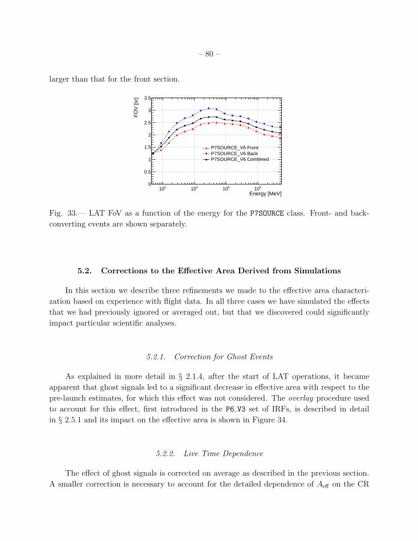
– 80 –

larger than that for the front section.

Energy [MeV]210 310 410 510

FO

V [s

r]

0

0.5

1

1.5

2

2.5

3

3.5

P7SOURCE_V6 FrontP7SOURCE_V6 BackP7SOURCE_V6 Combined

Fig. 33.— LAT FoV as a function of the energy for the P7SOURCE class. Front- and back-

converting events are shown separately.

5.2. Corrections to the Effective Area Derived from Simulations

In this section we describe three refinements we made to the effective area characteri-

zation based on experience with flight data. In all three cases we have simulated the effects

that we had previously ignored or averaged out, but that we discovered could significantly

impact particular scientific analyses.

5.2.1. Correction for Ghost Events

As explained in more detail in § 2.1.4, after the start of LAT operations, it became

apparent that ghost signals led to a significant decrease in effective area with respect to the

pre-launch estimates, for which this effect was not considered. The overlay procedure used

to account for this effect, first introduced in the P6 V3 set of IRFs, is described in detail

in § 2.5.1 and its impact on the effective area is shown in Figure 34.

5.2.2. Live Time Dependence

The effect of ghost signals is corrected on average as described in the previous section.

A smaller correction is necessary to account for the detailed dependence of Aeff on the CR

– 81 –

Energy [MeV]]2

[mef

fO

n-ax

is A

00.10.20.30.40.50.60.70.80.9

1

P6_V1_DIFFUSEP6_V3_DIFFUSE

Energy [MeV]210 310 410 510

Rat

io

0.60.70.80.9

11.1

Fig. 34.— Effective area at normal incidence for the P6 DIFFUSE class, in the pre-launch

version (P6 V1 DIFFUSE, not corrected for ghost effects) and in the updated version includ-

ing a modeling of ghost effects (P6 V3 DIFFUSE). Adapted from Rando & the Fermi LAT

Collaboration (2009).

rates. To account for this we need an estimator for the rate of CRs entering the LAT; the

obvious one is the trigger rate, but technical issues make this choice impractical. A variable

that can be easily obtained from the pointing history files and which is linearly correlated

with trigger rate is the live time fraction Fl, the fraction of the total observing time in which

the LAT is triggerable and not busy reading out a previous event. The average value of Flis ∼ 90% and varies between 82% and 92% over the Fermi orbit.

We bin events from a sample of periodic triggers according to the corresponding live

time fraction and for each bin we produce a dedicated allGamma simulation (§ 2.5.3); for

each of the resulting overlay data sets we derive Aeff . We have found the dependence on

the incidence angle to be small and so we choose to neglect it when studying this effect.

Furthermore, we have found that at a given energy Aeff varies linearly with the live time

fraction. We perform a linear interpolation in each energy bin in accord with

Aeff(E,Fl) = Aeff(E) · (c0(E)Fl + c1(E)) (14)

separately for front and back events.

In Figure 35 we plot c0 and c1 as a function of energy for front-converting events in the

P7SOURCE event class. As shown by the solid lines we use a simple piecewise linear fit to

describe the energy dependence and the fit parameters are stored in the Aeff tables. As we

mentioned, the effective area derived from allGamma simulations that have overlaid periodic

trigger events is effectively corrected for the average effect of this live time dependence, so

we treat this additional correction (which can be positive or negative) as a modulation of

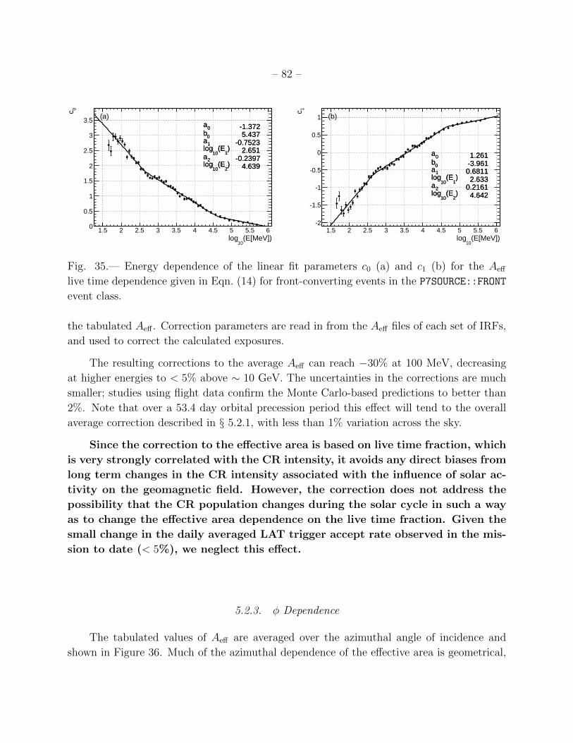
– 82 –

(E[MeV])10

log1.5 2 2.5 3 3.5 4 4.5 5 5.5 6

0c

0

0.5

1

1.5

2

2.5

3

3.5 0a -1.372 0b 5.437 1a -0.7523

) 1

(E10

log 2.651 2a -0.2397

) 2

(E10

log 4.639

0a -1.372 0b 5.437 1a -0.7523

) 1

(E10

log 2.651 2a -0.2397

) 2

(E10

log 4.639

(a)

(E[MeV])10

log1.5 2 2.5 3 3.5 4 4.5 5 5.5 6

1c

-2

-1.5

-1

-0.5

0

0.5

1

0a 1.261 0b -3.961 1a 0.6811

) 1

(E10

log 2.633 2a 0.2161

) 2

(E10

log 4.642

0a 1.261 0b -3.961 1a 0.6811

) 1

(E10

log 2.633 2a 0.2161

) 2

(E10

log 4.642

(b)

Fig. 35.— Energy dependence of the linear fit parameters c0 (a) and c1 (b) for the Aeff

live time dependence given in Eqn. (14) for front-converting events in the P7SOURCE::FRONT

event class.

the tabulated Aeff . Correction parameters are read in from the Aeff files of each set of IRFs,

and used to correct the calculated exposures.

The resulting corrections to the average Aeff can reach −30% at 100 MeV, decreasing

at higher energies to < 5% above ∼ 10 GeV. The uncertainties in the corrections are much

smaller; studies using flight data confirm the Monte Carlo-based predictions to better than

2%. Note that over a 53.4 day orbital precession period this effect will tend to the overall

average correction described in § 5.2.1, with less than 1% variation across the sky.

Since the correction to the effective area is based on live time fraction, which

is very strongly correlated with the CR intensity, it avoids any direct biases from

long term changes in the CR intensity associated with the influence of solar ac-

tivity on the geomagnetic field. However, the correction does not address the

possibility that the CR population changes during the solar cycle in such a way

as to change the effective area dependence on the live time fraction. Given the

small change in the daily averaged LAT trigger accept rate observed in the mis-

sion to date (< 5%), we neglect this effect.

5.2.3. φ Dependence

The tabulated values of Aeff are averaged over the azimuthal angle of incidence and

shown in Figure 36. Much of the azimuthal dependence of the effective area is geometrical,

– 83 –

due to the square shape of the LAT and the alignment of the gaps along the x and y axes.

The RMS variation of the effective area as a function of φ is typically of the

order of 5% and exceeds 10% only at low energies (< 100 MeV) or far off-axis

(θ > 60) where the effective area is small, and at very high energies (> 100 GeV)

where the event rate is small.

-1.5 -1 -0.5 0 0.5 1 1.5

-1.5

-1

-0.5

0

0.5

1

1.5

0

0.1

0.2

0.3

0.4

0.5

0.6

0.7

°90.0

°78.5

°66.4

°53.1

°36.9

° 0.0°180.0

°22.5

°202.5

°45.0

°225.0

°67.5

°247.5

°90.0

°270.0

°112.5

°292.5

°135.0

°315.0

°157.5

°337.5

]2 [m

eff

AFig. 36.— Total effective area at 10 GeV as a function of the incidence angle θ and the

azimuthal angle φ for the P7SOURCE event class. The plot is shown in a zenith equal area

projection with the LAT boresight at the center of the image; the concentric rings correspond

to 0.2 increments in cos(θ).

In order to parametrize the azimuthal dependence of Aeff we fold the azimuthal angle

into the [0, 45] interval and remap it into [0, 1] using the following transformation:

ξ =4

π

∣∣∣(φ modπ

2

)− π

4

∣∣∣ (15)

(the transformation maps 0 to 1, 45 to 0, 90 to 1 and so on). The allGamma events are

binned in energy and θ and in each bin a histogram of ξ is fitted (see Fig. 37 for an example).

Front- and back-converting events are treated separately. The fitting function is:

f(ξ) = 1 + q0ξq1 . (16)

The absolute scale is not important: we normalize the correction to result in an average

multiplicative factor of 1, so that the average Aeff is tabulated. The fitted parameters q0 and

q1 are stored in the Aeff tables.

We note in passing that the default for high-level analyses is to disregard the azimuthal

variations when calculating exposures because they average out when intervals of months

– 84 –

0

q 0.1071

1q 1.141

ξ0 0.1 0.2 0.3 0.4 0.5 0.6 0.7 0.8 0.9 1

Rel

ativ

e ef

fect

ive

area

0.96

0.98

1

1.02

1.04

1.06

1.08

1.1

1.12

0

q 0.1071

1q 1.141

0

q 0.1071

1q 1.141

Fig. 37.— Example of Aeff azimuthal dependence fit. The plot refers to the bin centered

at 7.5 GeV and 30 for the P7SOURCE class, front section—a similar fit is performed in each

(E, θ) bin. The folded azimuthal angle ξ is defined in Eqn. (15) and the fit function in

Eqn. (16). Note that this plots shows Aeff relative to Aeff for ξ = 0.

or longer are considered11. Although the combined θ and φ dependence of the ob-

serving profile averages out only on year-long timescales, the 8-fold symmetry

of the LAT combined with the rotation of the x-axis to track the Sun results

in effective averaging over φ on short time scales. In fact, we have found that

ignoring the φ dependence of the effective area results in only a small variation

of the exposure on 12-hour time scales (< 3% RMS at all energies).

5.3. Step by Step Performance of Cuts and Filters

Before describing the studies we performed to validate our event selections it is worth

recalling that we require background rejection of ∼ 106 while retaining high efficiency for γ

rays. To achieve this we must select events based on many different criteria that are applied in

several stages (see § 2 and § 3), which complicates the task of measuring the overall efficiency.

For validation purposes we specifically examine the agreement of the selection efficiencies (η)

between flight data and MC simulation. Therefore, the most relevant quantity is

R =ηdata

ηmc

, (17)

11Information on how to include the φ dependence of the effective area in exposure calcula-

tions can be found at http://fermi.gsfc.nasa.gov/ssc/data/analysis/scitools/binned likelihood tutorial.html

and http://fermi.gsfc.nasa.gov/ssc/data/analysis/scitools/help/gtltcube.txt.

– 85 –

which is in general a function of direction, energy and conversion point of the incident γ

ray. The approach described in this section can be used both to quantify the systematic

uncertainties in Aeff and possibly to correct the IRFs derived from the MC simulations, in

cases of severe discrepancies with the flight data (e.g., see § 5.4).

5.3.1. Background Subtraction

To measure the efficiency of a cut on flight data, we can perform background subtraction

before and after the cut and compare the excess in the signal region in the two cases. To

the extent that the background subtraction is correct, the cut efficiency is simply the ratio

of the number of background subtracted events before and after the cut we are testing:

η =ns,1 − rnb,1ns,0 − rnb,0

, (18)

where the subscripts s and b indicate the signal and background regions, the subscripts 0

and 1 indicate the samples before and after the cut under test, and r is the ratio of the size

of the background region to the size of the signal region. Note that the sample after the cut

is a subset of the sample before the cut. Therefore, for a reasonable sample size (ns > 10),

the statistical uncertainty of the efficiency is:

δη =

[[(ns,0 − ns,1) + r2(nb,0 − nb,1)]η2 + (ns,1 + r2nb,1)(1− η)2

(ns,0 − rnb,0)2

]1/2

. (19)

An example application of this technique using data from the Vela calibration data set is

shown in Figure 38.

In many cases our cuts have significant overlap—two cuts may reject many of the same

events. In such cases, measuring the efficiency of the second cut after the first cut has

been applied would give a quite different result than measuring the efficiency of the second

cut without the first cut. Therefore, whenever possible, we use the background subtraction

technique described above to evaluate the efficiency of each step of our event selection both

independently of the other steps as well after all the other cuts have been applied.

5.3.2. Track-Finding and Fiducial Cut Efficiency

Although the track-finding and fiducial cuts are applied midway through our event

selection process we choose to discuss them first for two reasons: (i) we require an event

direction to be able to perform a background subtraction on flight data and (ii) we express

– 86 –

Energy [MeV]210 310 410

Cou

nts

/ 0.1

25 e

nerg

y de

cade

310

410

510Signal RegionBackground Region

(a)

Energy [MeV]210 310 410

Cou

nts

/ 0.1

25 e

nerg

y de

cade

310

410

Excess after baseline cutExcess after test cut

(b)

Energy [MeV]210 310 410

Fra

ctio

n of

Eve

nts

0.75

0.8

0.85

0.9

0.95

1Flight DataMonte Carlo

(c)

Energy [MeV]210 310 410

R

0.9

0.92

0.94

0.96

0.98

1

1.02

1.04

1.06

1.08

1.1(d)

Fig. 38.— Measurement of the efficiency of a cut using the background subtraction technique:

(a) count spectra in the signal and background regions for the flight data set—note that the

background counts have been scaled by 1/2 to account for the different phase ranges of the

two regions; (b) excess in the signal region before and after the application of the test cut

for the flight data sets—note that, for both (a) and (b), the corresponding plots for the MC

data sets are not shown; (c) efficiency of the test cut η for the flight and MC data sets; (d)

ratio R of the efficiencies as measured with flight data to the MC predictions. In this case

the baseline sample is the P7SOURCE event selection on the Vela calibration sample and the

cut being tested is the P7CLEAN event selection.

Aeff as a function of E and θ. Therefore, for performance studies we need to apply some

minimum event quality and fiducial cuts before considering events for analysis. The standard

cuts require at least one track found, with at least 5 MeV of energy in the CAL and that

the track extrapolates through at least 4 radiation lengths in the CAL (see § 3.4.1).

Most events that fail these cuts have either poorly reconstructed directions, poorly

reconstructed energies, or both—which makes it difficult to study the performance as a

function of energy and direction. Therefore, we choose to study the efficiency of the track-

– 87 –

finding and fiducial cuts by selecting events that almost fail these cuts in the P7SOURCE

calibration samples. Specifically, we study the fraction of events that are very close to the

cut thresholds and verify that the flight data agree with our MC simulations, see Figure 39.

Energy [MeV]210 310 410 510

Fra

ctio

n of

eve

nts

0

0.2

0.4

0.6

0.8

1

> 6 hits on track > 20 MeVcal AND Eo > 5 XcalL

Fig. 39.— Validation of the track-finding and fiducial cuts. The data points show the fraction

of P7SOURCE events in the Vela (< 10 GeV) and Earth limb (> 10 GeV) calibration samples

that pass the fiducial cuts with some margin: having more than the absolute minimum

number of hits on a track (black points), or having more than 20 MeV of energy deposition

and crossing more than 5 radiation lengths in the CAL (gray points). The curves show the

MC predictions for comparison.

5.3.3. Trigger Conditions and Trigger Request Efficiency

The LAT hardware trigger, trigger configuration and on-board filter are described in

§ 3.1. For our purpose here we first consider the fractions of γ-ray events that have one of the

five physics trigger conditions (TKR, ROI, CAL LO, CAL HI, CNO) asserted. Furthermore, only

two of them (TKR and CAL HI) effectively serve to initiate a trigger request. Of the others,

ROI does not exist without TKR, CAL LO alone does not open the trigger window and from the

point of view of selecting γ-ray events CNO is primarily a veto rather than a trigger. Since

the CAL HI requires at least 1 GeV in a CAL channel, and our fiducial cuts and quality cuts

require at least one track, we are effectively using the TKR condition as the primary trigger

for γ rays up to such energies that the CAL HI is very likely to be asserted.

Using the diagnostic filter events described in § 3.1 we can measure the fractions of

all trigger requests that have individual primitives asserted. However, because of the high

particle background rates this does not really probe the trigger stage of the γ-ray selection

process. On the other hand, for each of the five relevant trigger primitives we measure

– 88 –

this efficiency as a function of energy for the allGamma sample as well as the P7TRANSIENT

selection. For the P7TRANSIENT selection we also measure the fractions of events with each

trigger primitive asserted and compare these to the MC predictions. These are shown in

Figure 40. The only notable discrepancy is that the MC over-predicts the fraction of events

having ROI asserted at very high energies; this is likely related to imperfect simulation of the

backsplash from the CAL, and since the CAL LO and CAL HI are typically asserted for these

events, it does not affect the trigger readout decision (see Table 3).

Energy [MeV]210 310 410 510

Fra

ctio

n of

Eve

nts

0

0.2

0.4

0.6

0.8

1

TKRMultiple TKRCAL_LO

CAL_HIROICNO

(a)

Energy [MeV]210 310 410 510

Fra

ctio

n of

Eve

nts

0

0.2

0.4

0.6

0.8

1

TKRMultiple TKRCAL_LO

CAL_HIROICNO

(b)

Fig. 40.— (a) Fractions of all triggered events with various trigger conditions asserted as a

function of the energy of the simulated event and (b) fraction of all P7TRANSIENT events that

have the same conditions asserted as a function of the reconstructed energy of the event, for

MC simulations (lines) and flight data (points). “Multiple TKR” refers to the events with

more than one three-in-a-row combinations asserted.

• The CAL LO trigger condition requires 100 MeV of energy deposited in any CAL channel.

This condition starts to be asserted for γ rays at ∼ 300 MeV and reaches full efficiency for

events contained within the CAL at ∼ 1 GeV.

• The CAL HI trigger condition requires 1 GeV of energy deposited in any CAL channel.

This condition starts to be asserted for γ rays at ∼ 3 GeV and reaches full efficiency at

∼ 15 GeV.

• The CNO condition requires any ACD tile to have very large signal, consistent with the

passage of a heavy ion. The CNO condition actually serves more to veto than to select an

event for readout, but only becomes active at very high energies (> 100 GeV), where CAL LO

and CAL HI are already active.

• The ROI condition requires any ACD tile in a predefined region of interest associated with

a TKR tower to have a signal above 0.45 MIP. The ROI condition actually serves more to

veto than to select an event for readout and becomes active at a few GeV.

– 89 –

• Since the TKR condition serves as the primary trigger it is very difficult to measure the

efficiency of the condition. However, we can estimate how well the MC simulates this effi-

ciency by studying how well it models cases where the events almost fail the trigger request

conditions. This is possible by calculating the fraction of events with exactly one combi-

nation of three hit layers in a row in the TKR. Most high-energy γ rays have many such

combinations and would have triggered the LAT even if one hit had been lost. However, for

back-converting low-energy events (< 100 MeV) the fraction of single combination events

becomes significant.

Since the fiducial cuts for our standard event selection require that a track is found, and

that the track extrapolates into the CAL, the interplay between the trigger and the standard

event selections is actually quite simple.

• At very low energies, the LAT trigger starts to become efficient at ∼ 10 MeV and follows

the efficiency of the TKR condition, which becomes fully efficient by ∼ 100 MeV.

• At around 1 GeV the CAL LO condition becomes active. By design, this is considerably

lower than the 10 GeV where the ROI starts to be asserted because of backsplash.

• Above ∼ 10 GeV the CAL HI condition becomes active and we no longer rely on the TKR

condition as the primary driver of the trigger.

Furthermore, events that are rejected because ROI is asserted are extremely unlikely to

pass standard event class selections. Taken together, this means that the only part of the

LAT energy band where the trigger has strong influence on Aeff is below ∼ 100 MeV.

5.3.4. On-Board Filter Efficiency

Although the gamma filter has many different cuts (see § 3.1.2), most events that are

rejected by the gamma filter would be either rejected by the fiducial cuts (see § 3.4.1) or

by the P7TRANSIENT event selection. Accordingly, we choose to study the efficiency of the

gamma filter as a whole, and only for those events which pass all the other selection criteria

for the P7TRANSIENT class event sample.

Since we downlink a small fraction of the events that fail the gamma filter (see § 3.1),

we can check that this is indeed the case for this diagnostic sample. However, the large

prescale factor (250) for the diagnostic filter and high level of background rejection in the

P7TRANSIENT selection severely limit our statistics for this study, and we can do little more

– 90 –

Energy [MeV]210 310 410 510

Fra

ctio

n of

Eve

nts

0

0.2

0.4

0.6

0.8

1

1.2

1.4

1.6

1.8

2

Flight dataMonte Carlo

Fig. 41.— Fraction of events passing the P7TRANSIENT selection that also pass the gamma fil-

ter for the diagnostic filter flight data, compared to the MC predictions. Note that point

at 42 GeV is well above the 20 GeV high-energy pass criteria where the gamma filter be-

comes fully efficient, so the low measured value of the efficiency is likely due to a statistical

fluctuation in the subtracted background.

than confirm that the gamma filter is highly efficient for events in the P7TRANSIENT sample

(see Fig. 41).

5.3.5. P7TRANSIENT Class Efficiency

Measuring the efficiency of the selection for the P7TRANSIENT event class is the most

technically challenging part of the Aeff validation for two reasons: (i) at the output of the

gamma filter the background rates are still great enough to overwhelm almost all traces of

γ-ray signals and (ii) the event analysis directs events that are tagged as likely due to CRs

away from the remainder of the γ-ray selection criteria, which means that many of the CT

analyses are never applied, and cannot be used to construct a cleaner sample on which we

can measure the efficiency of any of these cuts independently of the other cuts.

Figure 42(a) shows the efficiency of each part of the P7TRANSIENT selection on events

from the allGamma sample that have passed the gamma filter. As stated above, the high

levels of CR background make it infeasible to use flight data to obtain stringent constraints

on the efficiency of these selection criteria. Therefore, similarly to what we did for the

track-finding and fiducial cuts, we also study the events that almost fail these cuts in the

P7TRANSIENT calibration samples: these comparisons are shown in Figure 42(b).

Because of the difficulty in validating the efficiency of the P7TRANSIENT event selection

– 91 –

criteria, we have chosen to use the consistency checks described in § 5.5 to estimate the

systematic uncertainty in our Aeff representation.

Energy [MeV]210 310 410

Fra

ctio

n of

Eve

nts

0

0.2

0.4

0.6

0.8

1

TRANSIENT Reconstruction Quality (1-3)TRANSIENT Charged Particle Rejection (4)

Cut (5)allTRANSIENT P

Energy [MeV]210 310 410

Fra

ctio

n of

Eve

nts

0

0.2

0.4

0.6

0.8

1

Reconstruction Quality (1-3)Charged Particle Rejection (4)

Cut (5)allP

Fig. 42.— (a) Fractions of events in the allGamma sample passing the gamma filter and

track-finding and fiducial cuts that also pass each part of the P7TRANSIENT (§ 3.4.2) event

selection. (b) Fractions of events in the P7TRANSIENT calibration samples that pass similar

cuts with some margin for MC simulations (lines) and flight data (points). The numbers in

the legends refer to the list of cuts in § 3.4.2.

5.3.6. P7SOURCE,P7CLEAN and P7ULTRACLEAN Class Efficiencies

Although the P7TRANSIENT event class is dominated by residual background across the

entire LAT energy range, the background levels are at least reduced to the point where the

γ-ray signals in the calibration samples described in § 3.6 are clearly detectable. This makes

the validation of the effective area from this point on much easier. We can compare the

efficiency of each cut, as measured on flight data, to the MC prediction with the method

described in § 5.3.1. These comparisons are shown in Figure 43.

5.4. In-Flight Effective Area

We observed that the efficiency for one part of our Pass 6 event selection was sys-

tematically lower near 10 GeV for flight data than for the allGamma we used to evaluate

the effective area, and we attempted to correct the effective area tables to provide more

accurate flux measurements for γ-ray sources. To be more specific, the offending cut is the

Pass 6-equivalent of the P7SOURCE cut on the quality of direction reconstruction described

in § 3.4.3 (item 4 in the numbered list). It is important to note that for Pass 7 we chose

– 92 –

Energy [MeV]210 310 410

Fra

ctio

n of

Eve

nts

0

0.2

0.4

0.6

0.8

1

SOURCE Prefilters (1)SOURCE MIP Rejection (2)SOURCE TKR-CAL Agreement (3)

Cut (4)coreSOURCE P Cut (5)allSOURCE P

Energy [MeV]210 310 410

Fra

ctio

n of

Eve

nts

0

0.2

0.4

0.6

0.8

1

CLEAN MIP Rejection (1)CLEAN Topology Cuts (2)

CutallULTRACLEAN P

Fig. 43.— Fractions of events in the P7TRANSIENT calibration samples that pass each part

of the (a) P7SOURCE event selection (§ 3.4.3) and (b) P7CLEAN (§ 3.4.4) and P7ULTRACLEAN

(§ 3.4.5) event selections for MC simulations (lines) and flight data (points). The numbers

in the legends refer to the list of cuts in § 3.4.3 and § 3.4.4.

instead to make this particular cut less stringent to avoid the need to make such a correction,

so that the in-flight corrections discussed here do not apply to the effective area tables for

the Pass 7 standard γ-ray classes. Furthermore, we traced the discrepancy to limitations

in pre-launch calibration algorithm of CAL light asymmetry that resulted in degraded po-

sition and direction resolution in the CAL: above ∼ 1 GeV consistency between the TKR

and CAL position and direction measurements is a strong indicator of accurate direction

reconstruction.

We measure the ratio of cut efficiency between flight data and MC as a function of

energy and incidence angle (see Figure 44)—as described in § 5.3.1—and we use it to correct

the MC based Aeff . Because most of our calibration sources have limited statistics relative to

the allGamma samples we are forced to use fewer bins when calculating the efficiency ratios.

Furthermore, to avoid inducing sharp spectral features in measurements of γ-ray sources we

smooth the energy and angle dependence of the efficiency ratio. Specifically, we split the

data into two cos(θ) bins: [0.2, 0.7] and [0.7, 1.0]. For values between the bin centers (i.e.,

cos(θ) ∈ [0.45, 0.85]) we perform a linear interpolation in cos(θ). For values outside that

range we use the correction factor from the appropriate cos(θ) bin.

This procedure yields a correction map that we use to convert from the MC Aeff to

our best estimate of the true in-flight Aeff for the P6 V11 DIFFUSE set of IRFs, as shown

in Figure 45. Note that these IRFs should only be used together with the corresponding

– 93 –

Energy [MeV]210 310 410 510

)θco

s(

0.2

0.3

0.4

0.5

0.6

0.7

0.8

0.9

1

Cor

rect

ion

fact

or

0.75

0.8

0.85

0.9

0.95

1

1.05

1.1

1.15

1.2

1.25

(a) Front

Energy [MeV]210 310 410 510

)θco

s(

0.2

0.3

0.4

0.5

0.6

0.7

0.8

0.9

1

Cor

rect

ion

fact

or

0.75

0.8

0.85

0.9

0.95

1

1.05

1.1

1.15

1.2

1.25

(b) Back

Fig. 44.— Ratio of the P6 V11 DIFFUSE to P6 V3 DIFFUSE Aeff for front-converting (a) and

back-converting (b) events. The P6 V11 DIFFUSE Aeff tables have a correction factor relative

to P6 V3 DIFFUSE that is based on the ratio of the efficiencies between flight and simulated

data for the selection cut on the direction reconstruction quality (see item 4 in § 3.4.3).

The underflow bins (white areas) had no Aeff in P6 V3 DIFFUSE. As we did not interpolate

the correction factor along the energy axis, fluctuations in the correction factor lead to the

vertical bands visible in this figure.

rescaled models for Galactic and isotropic diffuse emission provided by the FSSC12.

5.5. Consistency Checks

In this section we will describe several consistency checks we performed to estimate

how well we understand Aeff . Each of these tests consists of splitting a specific γ-ray event

selection into two subsets and comparing the fraction in each of the subsets from the flight

data to the predictions from MC simulations.

As a simple check of our method, we split the event sample into subsets of events

converting on the +x and −x sides of the LAT. As noted in § 5.2 the φ dependence of Aeff is

strongest between directions toward the corners of the LAT relative to directions toward the

sides of the LAT; accordingly, we split the data into events coming from the sides (ξ < 0.5)

or corners (ξ > 0.5), based on Eqn. (15). Finally, we tested the θ dependence of the Aeff by

splitting the data into on-axis (cos θ > 0.7) and off-axis (cos θ < 0.7) subsets. The results of

these tests are shown in Figure 46. In each of these examples, we used the P7SOURCE event

12Specifically, gll iem v02 P6 V11 DIFFUSE.fit and isotropic iem v02 P6 V11 DIFFUSE.txt, available athttp://fermi.gsfc.nasa.gov/ssc/data/access/lat/BackgroundModels.html.

– 94 –

Energy [MeV] s

r]2

Acc

epta

nce

[m0

0.5

1

1.5

2

2.5

P6_V3_DIFFUSEP6_V11_DIFFUSE

Energy [MeV]210 310 410 510

Rat

io

0.60.70.80.9

11.1

Fig. 45.— Comparison of acceptance between P6 V3 DIFFUSE and P6 V11 DIFFUSE IRFs.

The only difference between the IRFs is the application of the corrections to Aeff for

P6 V11 DIFFUSE described in § 5.4.

sample as the starting point.

We also compare the fluxes we measure with different event classes. By doing so we can

check the accuracy of our measured efficiency loss for each of the selection cuts to go from

one event class to the next. Technically we do this by asking what fraction of events in one

event class also remain into an event class with tighter selection. Figure 46 also shows the

results of comparing the P7CLEAN selection to the P7SOURCE selection.

We also compared the fluxes we measure with front-converting events relative to back-

converting events (Fig. 47). Since the primary difference between these two parts of the LAT

is in the distribution of conversion material, this test is especially sensitive to issues with

our Geant4 simulation and probes our modeling of the trigger and track-finding efficiency.

In each case we find that the fraction of events in each subset for the flight data are

consistent with MC predictions to better than 15%. In fact, for most of the cases the

agreement is far better than that, closer to the 2–3% level. The most significant discrepancies

we see are between front-converting and back-converting events (Fig. 47).

5.6. Uncertainties on the Effective Area

5.6.1. Overall Uncertainty of the Effective Area

From the consistency checks described in the previous section we arrive at a rough

overall estimate of the uncertainty of Aeff , which is shown in Figure 48. Note that this

– 95 –

Energy [MeV]210 310 410 510

R

0.8

0.85

0.9

0.95

1

1.05

1.1

1.15

1.2

VelaAGN sampleEarth Limb

(a) x > 0

Energy [MeV]210 310 410 510

R

0.8

0.85

0.9

0.95

1

1.05

1.1

1.15

1.2


> 0.5ξ(b)

Energy [MeV]210 310 410 510

R

0.8

0.85

0.9

0.95

1

1.05

1.1

1.15

1.2


> 0.7θ(c) cos

Energy [MeV]210 310 410 510

R

0.8

0.85

0.9

0.95

1

1.05

1.1

1.15

1.2


(d) P7CLEAN

Fig. 46.— Ratio of the fraction of events as seen in flight data relative to the prediction

from MC simulations: (a) γ rays converting on the +x side of the LAT; (b) γ rays pointing

in 45 ranges of azimuth toward the corners of the LAT (i.e., ξ > 0.5) ; (c) γ rays from near

the LAT boresight, i.e., for which cos θ > 0.7; (d) γ rays passing the P7CLEAN selection.

estimate is assigned simply to account for the largest observed inconsistency, namely the

mismatch between the front-converting and back-converting events. Roughly speaking, for

the P7SOURCE V6 and P7CLEAN V6 event classes these uncertainties may be be quoted as 10%

at 100 MeV, decreasing to 5% at 560 MeV and increasing to 10% at 10 GeV and above. It is

important to note that these uncertainties are statements about overall uncertainty of Aeff

at various energies, and do not include any statement about what types of deviations we

might expect within the stated uncertainty bands, nor about the point-to-point correlations

in any systematic biases of Aeff . Those questions are addressed in the next sections.

– 96 –

Energy [MeV]210 310 410 510

R

0.8

0.85

0.9

0.95

1

1.05

1.1

1.15

1.2


Front-converting

Fig. 47.— Ratio of the fraction of front-converting events as seen in flight data relative to

the prediction from MC simulations:

5.6.2. Point-to-Point Correlations of the Effective Area

Since our selection criteria are generally scaled with energy (see § 3.3.1), we expect any

biases of Aeff to be highly correlated from one energy band to the next. This point is very

important when estimating the size of potential instrumental spectral artifacts.

We have studied the point-to-point correlation of the effective area through the consis-

tency checks described in § 5.5, where it is evident that the deviations from unity are not

independent for neighboring energy bins. In order to quantify this correlation we first scale

the values ri of the data-to-Monte Carlo ratio R in each of the N energy bins (indexed by

i), turning them into normalized deviations

di =(ri −m)√

1(N−1)

∑Ni=1(ri −m)2

, (20)

and m is the arithmetic mean of the ri) and then we construct the metrics

τn =

∑Ni=1+n(di − di−n)2

(N − n). (21)

The quantity in Eqn. (21) is related to a reduced χ2N−n(2x); it is small for highly positively

correlated deviations (in which case the differences between neighboring bins are generally

small), while the expectation value is 2, for all values of n, for normal uncorrelated errors.

Figure 49 shows this metric, for different values of n, calculated on the front vs. back

consistency check shown in Figure 47. (Only the Vela calibration data set is considered

here). The extremely small value of τ1 indicates that neighboring logarithmic energy bins

– 97 –

Energy [MeV]210 310 410 510

eff

Sys

tem

atic

unc

erta

inty

on

A

0.8

0.85

0.9

0.95

1

1.05

1.1

1.15

1.2

effUncertainty on A

< 100 MeV: caution for spectral analysis

Fig. 48.— Systematic uncertainty band on Aeff as a function of energy. The interplay

between the steeply decreasing effective area and the degrading energy resolution below

100 MeV and the resulting impact on spectral analysis will be thoroughly discussed in § 7.

are highly positively correlated (as can be naively inferred from the plot in Fig. 47), while

on the scale of half a decade in energy (n = 4) there is little evidence of a correlation. This

implies that the systematic uncertainties on the effective area are not likely to introduce

significant spectral features over scales much smaller than half a decade in energy (which is

much larger than the LAT energy resolution). The results for all the consistency checks are

summarized in Table 8.

nτ0 0.5 1 1.5 2 2.5 3 3.5 4

Num

ber

of r

ealiz

atio

ns

0

50

100

150

200

250

300

350

= 0

.66

1τ = 0

.94

2τ = 1

.75

4τ

(a)

nτ0 0.5 1 1.5 2 2.5 3 3.5 4

Cum

ulat

ive

prob

abili

ty

-510

-410

-310

-210

-110

1

1τ

2τ

4τ(b)

Fig. 49.— (a) Values of τn (n = 1, 2 and 4) defined in Eqn. (21) for the front/back consistency

check with the Vela data set shown in Figure 47. The parent distribution of τn for random

normal uncorrelated deviations is shown in gray, while the black histogram represents the

values of τn for 10,000 random permutations of the original data points. (Note that in both

cases the distributions are independent of n.) (b) Cumulative probability distribution for

random normal uncorrelated deviations.

– 98 –

Consistency check τ1 P (τ < τ1)

+x vs. −x 1.24 4.9× 10−2

Azimuthal dependence 2.21 0.69

θ dependence 1.05 1.6× 10−2

P7CLEAN selection 0.95 8.4× 10−3

Front vs. back 0.66 5.0× 10−4

Table 8: Summary of the point-to-point correlations for the consistency checks described

in § 5.5. Most of them indicate a strong positive correlation of the systematic biases between

adjacent bins on the effective area (the expectation value for random normal uncorrelated

deviations is τn = 2 for all values of n).

For many analyses, especially those that are limited by statistics, it is enough to con-

sider the overall uncertainty and allow for worst case deviations within the stated uncertainty

bands. However, doing so will result in very conservative systematic error estimates. We will

discuss this in more detail in § 5.7 when we describe techniques to propagate the estimates

of the uncertainty of Aeff to uncertainties on quantities such as fluxes and spectral indices.

Furthermore, we will come back to the issues of point-to-point correlations and the poten-

tial induced spectral features when we discuss the uncertainties associated with the energy

reconstruction in § 7.

5.6.3. Variability Induced by Errors in the Effective Area

As a source moves across the LAT FoV and Aeff changes with the viewing angle, any

errors in the Aeff parametrization as a function of θ potentially could induce artificial vari-

ability. We have searched for such induced variability with Vela. We split the data set into

12 hour periods (indexed by i) and compared the number of γ rays observed (ni) during each

period with the number of γ rays we predict (ni) based on the fraction of the total exposure

for Vela that we integrated during that 12 hour period.

On average, our Vela calibration sample contains 230 (176) on-peak (off-pulse) P7SOURCE

class events in the 100 MeV–10 GeV energy band every 12 hours. Since the off-pulse region

is twice the size of the on-peak region, background subtraction yields an average on-peak

excess of ni = 142 γ rays with an average statistical uncertainty of σi = 16 γ rays in each

time interval.

The exposure calculation requires several inputs:

– 99 –

1. the spacecraft pointing and live time history, which are binned in 30 s intervals;

2. the P7SOURCE V6 Aeff parametrization, which we use when deriving Aeff(E, t), the effective

area for γ rays for Vela for each 30 s interval;

3. the P7SOURCE V6MC PSF (see § 6.1) parametrization, which allows us to calculate the

energy dependent containment C(E, t, 15) within the 15 ROI for each 30 s interval;

4. a parametrization of the spectrum of Vela F (E) so that we may correctly integrate

Aeff(E, t) and C(E, t, 15) over the energy range.

In order to minimize dependence on the modeled flux, we calculate the exposure in-

dependently for 24 energy bins (which we index by j). The exposure in a single time and

energy bin is

Ei,j =

∫ Ei∫ tj

Aeff(E, t)C(E, t, 15)F (E)∫ Ei F (E)dE

dtdE. (22)

We can then express the expected number of γ rays in each time and energy bin (ni,j) as a

fraction of the total number of γ rays in that energy bin (nj),

ni,j =Ei,j

ΣiEi,jnj. (23)

Then we sum ni,j and ni,j across energy bins to find ni and ni.

We have performed this analysis, dividing the first 700 days of the Vela data sample

into 1400 12-hour time intervals and using the phase-averaged flux model

F (E) ∝ E−Γe− EE0 (24)

with Γ = 1.38 and E0 = 1.360 GeV (Abdo et al. 2009c). Figure 50 shows the fractional

variation,ni − nini

(25)

the normalized residuals,ni − niσi

(26)

and the distribution of the normalized residuals for each of the time-intervals. The normal-

ized residuals are very nearly normally distributed. Furthermore, the Fourier transform of the

time-series (Fig. 51) shows only a small peak corresponding to the orbital precession period

and is otherwise consistent with Poisson noise. Note that unlike more complicated analyses

that involve fitting the flux of a point source, this analysis is testing only the accuracy of

the Aeff representation (and to a much lesser extent, the 15 containment of the PSF). We

– 100 –

attribute the peak in the Fourier spectrum to small, incidence angle-dependent

errors in the effective area. As the orbit precesses, the range of incidence angles

sampled, and hence the bias in the calculated exposure, varies slightly.

Although we performed this analysis with 12-hour time intervals, as noted

in § 2.3, the LAT boresight follows very similar paths across the sky during

successive 2-orbit periods. Therefore, the level of instrument-induced variability

observed with 12-hour time intervals is likely to be indicative of the systematic

uncertainties for variability analyses down to 3-hour time scales.

Time [UTC]

n~)

/ n~

(n -

-4

-3

-2

-1

0

1

2

3

4(a)

Time [UTC]Dec 31, 2008 Jan 01, 2010

nσ)

/ n~

(n -

-5

0

5

nσ) / n~(n - -6 -4 -2 0 2 4 6

Num

ber

of 1

2 ho

ur in

terv

als

0

10

20

30

40

50

60

70

80

0.03± = -0.03 µ 0.02± = 1.04 σ

= 42.1 / 54 DOF2χ

(b)

Fig. 50.— Check for variability-induced by errors in the Aeff tables P7SOURCE Vela calibra-

tion sample and the P7SOURCE V6MC IRFs. Panel (a) shows the fractional difference and

normalized residuals between the observed counts in the 100 MeV to 10 GeV band and the

prediction based on the fraction of the total exposure accumulated during each of 1400 12-

hour time intervals. Panel (b) shows the normalized residuals, which are very well fit with a

Gaussian with unit width and zero mean.

Although the estimate used in § 5.6.1 that the systematic uncertainty of Aeff is less

than the disagreement between the extreme cases is quite conservative for long time scale

observations, it is somewhat less conservative for shorter observations. For example, in

observations less than the Fermi orbital precession period of ∼ 53.4 days, a particular

region of the sky might be preferentially observed at incidence angles where the bias of Aeff

is particularly large, or during parts of the orbit in which Fermi is exposed to particularly

high CR background rates and the correction described in § 5.2.2 leaves some residual bias

in the calculated exposure. Finally, we have observed that ignoring the φ dependence of

the effective area (§ 5.2.3) can induce artificial quarter-yearly periodicity in the fluxes from

directions near extremely bright sources, in particular the Vela pulsar.

– 101 –

]-1Frequency [days

-310 -210 -110 1

]σ [ νP

0

1

2

3

4

5

Fig. 51.— The discrete Fourier transform of the n−nσn

time series. The only peak visible above

the noise floor corresponds to the 53-day orbital precession period. Note that the figure is

normalized and the vertical scale is expressed in units of the statistical uncertainty.

5.7. Propagating Uncertainties on the Effective Area to High Level Science

Analysis

As we hinted in the previous section, translating uncertainties on Aeff into systematic

errors on quantities such as fluxes and spectral indices depends on the particular analysis

and requires assumptions about the variation of Aeff within the uncertainty bands.

5.7.1. Using Custom Made IRFs to Generate an Error Envelope

A somewhat brute force approach to this problem is to generate IRFs that represent

worst case scenarios for measuring specific quantities like fluxes or spectral parameters and

use these bracketing IRFs to repeat the analysis and extract the variation in the measured

quantities. Of course, the nature of the variations between the IRFs depends on the quantity

in question.

We address this in a generic way by scaling Aeff by the product of the relative systematic

uncertainty

ε(E) =δAeff(E)

Aeff(E)(27)

and arbitrary bracketing functions B(E) taking values in the [−1, 1] interval. Specifically we

define modified Aeff as

A′eff(E, θ) = Aeff(E, θ) · (1 + ε(E)B(E)) . (28)

– 102 –

The simplest bracketing functions, B(E) = ±1 clearly minimize and maximize Aeff

within the uncertainty band. On the other hand, to maximize the effect on the spectral

index in a power-law fit, we choose a functional form that changes sign at the pivot or

decorrelation energy E0 (i.e., the energy at which the fitted differential flux and spectral

index are uncorrelated):

B(E) = ± tanh

(1

klog(E/E0)

). (29)

The parameter k controls the slope of the transition near E0; in practice we use k = 0.13,

which corresponds to smoothing over twice the LAT energy resolution of ∆E/E ∼ 0.15. The

bracketing IRFs used for effective area studies are listed in Table 9. Figure 52 shows the

Name B(E)

c flux lo +1

c flux hi −1

c index soft + tanh( 1k

log(E/E0))

c index hard − tanh( 1k

log(E/E0))

Table 9: Bracketing Aeff and corresponding energy-dependent scaling functions used to create

them.

bracketing functions for c index soft and c index hard and their effects on the on-axis Aeff .

Energy [MeV]210 310 410 510

eff

Rel

ativ

e A

0.8

0.85

0.9

0.95

1

1.05

1.1

1.15

1.2Base LineIndex Biased SoftIndex Biased Hard

(a)

Energy [MeV]210 310 410 510

sr]

2A

ccep

tanc

e [m

0

0.5

1

1.5

2

2.5

Base LineIndex Biased SoftIndex Biased Hard

(b)

Fig. 52.— Bracketing IRFs for Aeff designed to estimate possible systematic biases of

the measurement of the spectral index. (a) energy dependence of the scaling parameter

ε(E)B(E); (b) acceptance of the resulting scaled Aeff for P7SOURCE. For this example we

used a pivot energy E0 = 1 GeV.

We have studied two sources from the AGN sample to obtain estimates of the effects of

– 103 –

instrumental uncertainties on the measured fluxes and spectral parameters, namely:

• PG 1553+113—associated with 2FGL J1555.7+1111, which has spectral index of 1.66± 0.02,

making it one of the hardest bright AGN;

• B2 1520+31—associated with 2FGL J1522.1+3144, which has a spectral index of 2.37± 0.02

(when fit with a power-law), making it one of the softest bright AGN.

In each case we used the ScienceTools (version v9r25p2) to perform a series of binned max-

imum likelihood fits to a 20 × 20 region centered at the source position over the energy

range 100 MeV–100 GeV. For each individual fit we followed the same procedure:

1. used the γ-ray and time interval selection criteria as for the Vela calibration sample (see

§ 3.6);

2. included all 2FGL sources within 20 in our likelihood model, with the same spectral

parametrizations as were used in the 2FGL catalog;

3. included models of the Galactic diffuse emission (ring 2year P76 v0.fits) and the isotropic

diffuse emission (isotrop 2year P76 source v1.txt) rescaled by the inverse of the function used

to rescale the effective area (so as to ensure the same distribution of expected counts from

these diffuse sources);

4. freed the spectral parameters for all point sources within 8 from the center of the region,

as well as the overall normalizations of both diffuse components.

Following what was done for the 2FGL catalog, we used a simple power-law

dN

dE= N0

(E

E0

)−Γ

(30)

to model the differential flux from PG 1553+113 and a “log-parabola”

dN

dE= N0

(E

E0

)−(α+β ln(E/E0))

(31)

to model that of B2 1520+31. (All of this will be also relevant for the tests with bracketing

PSFs described in § 6.5.1 and with energy dispersion included in the likelihood fit described

in § 7.4).

Table 10 and 11 shows the fits results for PG 1553+113 and B2 1520+31, respectively,

using these Aeff bracketing functions, as well as the integral counts (F25) and energy (S25)

fluxes between 100 MeV and 100 GeV.

– 104 –

Bracketing Aeff N0 Γ F25 S25

[MeV−1 cm−2 s−1] [cm−2 s−1] [MeV cm−2 s−1]

Nominal 2.54× 10−12 1.68 6.91× 10−8 1.19× 10−4

c flux hi 2.75× 10−12 1.67 7.32× 10−8 1.31× 10−4

c flux lo 2.37× 10−12 1.69 6.54× 10−8 1.09× 10−4

c index hard 2.57× 10−12 1.64 6.45× 10−8 1.30× 10−4

c index soft 2.53× 10−12 1.73 7.44× 10−8 1.11× 10−4

Table 10: Fit parameters and integral fluxes obtained using the Aeff bracketing IRFs for

PG 1553+113. Note that the quoted precision is roughly equivalent to the fit uncertainties

and the pivot energy is E0 = 2240 MeV for this source.

Bracketing Aeff N0 α β F25 S25


Nominal 5.23× 10−10 2.24 0.08 4.09× 10−7 1.33× 10−4

c flux hi 5.60× 10−10 2.26 0.07 4.44× 10−7 1.44× 10−4

c flux lo 4.90× 10−10 2.22 0.08 3.79× 10−7 1.24× 10−4

c index hard 5.20× 10−10 2.15 0.10 3.93× 10−7 1.35× 10−4

c index soft 5.27× 10−10 2.33 0.05 4.29× 10−7 1.32× 10−4

Table 11: Fit parameters and integral fluxes obtained using the Aeff bracketing IRFs for

B2 1520+31. Note that the quoted precision is roughly equivalent to the fit uncertainties


– 105 –

The ranges of the fit values indicate propagated uncertainties from the uncertainty in

Aeff (Table 12). It is important to note that the systematic error estimates resulting from this

technique represent conservative estimates within the instrumental uncertainties, rather than

random variations. Furthermore, many of the bracketing IRFs are mutually exclusive, so

when considering relative variations between γ-ray sources it is more appropriate to compare

how the relative values change for each set of bracketing IRFs.

Parameter B2 1520+31 PG 1553+113

(soft) (hard)

δN0/N0 +7.2% −6.3% +8.0% −6.9%

δΓ (δα) +0.09 −0.09 +0.05 −0.05

δβ +0.02 −0.02 -

δF25/F25 +8.5% −7.2% +7.7% −6.6%

δS25/S25 +8.1% −6.9% +10.0% −8.3%

Table 12: Systematic variations arising from uncertainties in the effective area. For the

spectral index (Γ or α) and spectral curvature (β) we give the absolute variation with respect

to the nominal value (e.g., δΓ). For the flux prefactor and the integral fluxes we give the

relative variation with respect to the nominal value (e.g., δN0/N0).

5.7.2. Using a Bootstrap Method to Generate an Error Envelope

Alternatively, given a family of plausible Aeff curves, we can use a weighted bootstrap

approach (see Efron & Tibshirani 1993, for more details) for propagating the systematic

uncertainties on Aeff . The weighed bootstrap approach is closely related to the bracketing

IRFs method described in the previous section and to the methods discussed in Lee et al.

(2011) in the context of the analysis of Chandra X-ray data.

The basic idea is that, for each trial, the event data are bootstrap resampled using a

weighting based on an effective area scaling function that is drawn from a family of plausible

curves. The simplest of such families of Aeff curves (Fig. 53) can be constructed starting

from Eqn. (28) and multiplying the scaling function ε(E)B(E) by a normally distributed

random number ξ with zero mean—which effectively becomes the parameter controlling the

family itself:

A′eff(E, θ, ξ) = Aeff(E, θ) · (1 + ξε(E)B(E)) (32)

We have found the results of the weighted bootstrap with the family of scaling functions

– 106 –

Energy [MeV]210 310 410 510

Sca

ling

func

tion

0.5

0.6

0.7

0.8

0.9

1

1.1

1.2

1.3

1.4

1.5

Fig. 53.— A family of effective area scaling functions obtained for different values of the

normal random variable ξ in Eqn. (32).

defined in Eqn. (32) to be in good agreement with those of the bracketing IRFs approach

described in the previous section. This should not be surprising as the bracketing IRFs

use the ±1σ excursions of the bracketing function and the weighted bootstrap draws from

a Gaussian distribution of function scalings that are also based on that same bracketing

function. The real benefits of the weighted bootstrap arise when one has families of plausible

effective area functions that have more complicated dependencies (e.g., on incidence angle

as well as energy) such that exposures would need to be recalculated to apply the bracketing

method.

5.8. Comparison of Pass 6 and Pass 7

The Pass 7 event classes were designed to meet the same high-level analysis needs as

the Pass 6 classes. Table 5 summarizes the correspondence between the Pass 7 standard

γ-ray classes and their closest Pass 6 equivalents. The corresponding acceptances are shown

in Figure 54.

As discussed in § 3, the main technical improvement in Pass 7 was optimizing the event

selections on simulations that included the ghost signals, and on flight data. The principal

outcome for Pass 7 is a substantial increase of Aeff below ∼ 300 MeV, especially for the

cleaner event classes. At 100 MeV the P7SOURCE V6 and P7CLEAN V6 γ-ray classes feature

an acceptance of ∼ 0.3 m2 sr, to be compared with the ∼ 0.1 m2 sr of the Pass 6 equivalent

(Fig. 54). Pass 7 has opened a window on astronomy with the LAT data below 100 MeV,

though the reader should bear in mind the specific caveats in § 6.5 and § 7.4 when performing

spectral analyses at these energies.

– 107 –

Energy [MeV]210 310 410 510

sr]

2A

ccep

tanc

e [m

0

0.5

1

1.5

2

2.5

P7TRANSIENT_V6 TotalP6_V3_TRANSIENT TotalP7SOURCE_V6 TotalP6_V3_DIFFUSE TotalP7CLEAN_V6 TotalP6_V3_DATACLEAN Total

Fig. 54.— Comparison of the acceptances for the Pass 7 and the Pass 6 standard γ-ray

classes.

Additionally, in Pass 7, the energy dependence of Aeff is smoother. This was accom-

plished in conjunction with obtaining a better overall understanding of the effective area

itself, owing to the extensive use of on-orbit data to verify the fidelity of our MC simulation

at each step of the γ-ray selection process.

– 108 –

6. POINT-SPREAD FUNCTION

As discussed in § 2.1.1, at low energies the PSF is determined by multiple scattering.

For example, the calculated multiple scattering for a normally incident 100 MeV γ ray

converting in the middle of a thin (front) section tungsten foil is ∼ 3.1 (space angle). The

68% containment angle as measured from flight data for 100 MeV γ rays near the LAT

boresight averaged over all towers is ∼ 3.3 and is in agreement with the MC simulations

(see § 6.2). The small difference is due to missing measurements when the trajectories happen

to pass through regions without SSD coverage and the fact that the electron and positron

from a conversion can undergo hard scattering processes such as bremsstrahlung.

If multiple scattering were the only consideration, the PSF should become narrower

as E−1. The measured PSF however improves more slowly with energy, instead falling as

∼ E−0.78 (see § 3.3.3). This slower improvement relative to that expected for pure multiple

scattering is also due to missed measurements and hard scattering processes and is predicted

by the MC calculations.

Above a few GeV the narrowing of the PSF with energy is limited by the finite hit

resolution of the SSDs. The strip pitch of 228 µm and the lever arm for the direction

measurement result in a limiting precision for the average conversion of ∼ 0.1 at normal

incidence. The transition to this measurement precision-dominated regime as predicted by

the MC should occur between ∼ 3 GeV and ∼ 20 GeV. Estimates of the limiting PSF from

flight data however indicate a worse performance above ∼ 3 GeV; the PSF 68% containment

levels off at almost double the calculated value (i.e., ∼ 0.16). This departure is one of

the few instances where the MC results significantly differ from real data (see § 6.2). The

LAT collaboration has identified limitations in the pre-launch calibration algorithms of the

CAL light asymmetry (for more details see Abdo et al. 2009f) as the primary cause of

these discrepancies, and is assessing the improvement of the flight data-derived PSF at high

energies for data which were reprocessed with improved calibration constants13 (see § 3.3.3

for details of how the CAL energy centroid is used in the event direction analysis).

6.1. Point-Spread Function from Monte Carlo Simulations

Equivalently to what we stated in § 1, the PSF is the likelihood to reconstruct a γ ray

with a given angular deviation δv = |v ′ − v |. We write it as P.

13http://fermi.gsfc.nasa.gov/ssc/data/analysis/documentation/Cicerone/Cicerone LAT IRFs/IRF PSF.html

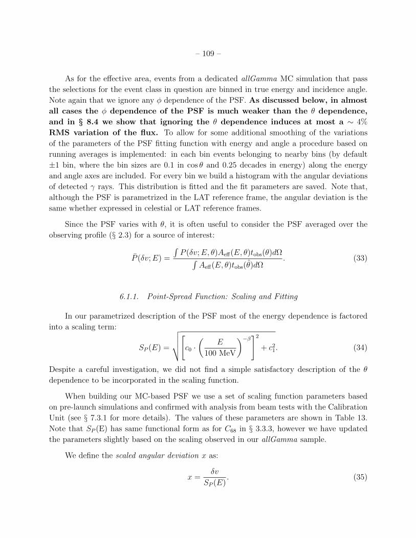
– 109 –

As for the effective area, events from a dedicated allGamma MC simulation that pass

the selections for the event class in question are binned in true energy and incidence angle.

Note again that we ignore any φ dependence of the PSF. As discussed below, in almost

all cases the φ dependence of the PSF is much weaker than the θ dependence,

and in § 8.4 we show that ignoring the θ dependence induces at most a ∼ 4%

RMS variation of the flux. To allow for some additional smoothing of the variations

of the parameters of the PSF fitting function with energy and angle a procedure based on

running averages is implemented: in each bin events belonging to nearby bins (by default

±1 bin, where the bin sizes are 0.1 in cos θ and 0.25 decades in energy) along the energy

and angle axes are included. For every bin we build a histogram with the angular deviations

of detected γ rays. This distribution is fitted and the fit parameters are saved. Note that,

although the PSF is parametrized in the LAT reference frame, the angular deviation is the

same whether expressed in celestial or LAT reference frames.

Since the PSF varies with θ, it is often useful to consider the PSF averaged over the

observing profile (§ 2.3) for a source of interest:

P (δv;E) =

∫P (δv;E, θ)Aeff(E, θ)tobs(θ)dΩ∫

Aeff(E, θ)tobs(θ)dΩ. (33)

6.1.1. Point-Spread Function: Scaling and Fitting

In our parametrized description of the PSF most of the energy dependence is factored

into a scaling term:

SP (E) =

√√√√[c0 ·(

E

100 MeV

)−β]2

+ c21. (34)

Despite a careful investigation, we did not find a simple satisfactory description of the θ

dependence to be incorporated in the scaling function.

When building our MC-based PSF we use a set of scaling function parameters based

on pre-launch simulations and confirmed with analysis from beam tests with the Calibration

Unit (see § 7.3.1 for more details). The values of these parameters are shown in Table 13.

Note that SP (E) has same functional form as for C68 in § 3.3.3, however we have updated

the parameters slightly based on the scaling observed in our allGamma sample.

We define the scaled angular deviation x as:

x =δv

SP (E). (35)

– 110 –

Conversion type c0 [] c1 [] β

Front 3.32 0.022 0.80

Back 5.50 0.074 0.80

Table 13: Parameters of the angular deviation scaling function SP for the PSF parametriza-

tion.

An example of scaled deviation is shown in Figure 55. The effect of the scaling is to make

the profile almost independent of energy, in that the maximum is always close to x = 1 for

all energy bins while the PSF 68% containment varies by almost two orders of magnitude

from 100 MeV to 100 GeV.

Before the fit is performed, each scaled deviation histogram is converted into a proba-

bility density with respect to solid angle. The result is illustrated in Figure 55.

Scaled angular deviation-110 1 10

Cou

nts

/ 0.0

33 d

ecad

e

210

310

410

(a) coreN 0.1989 tailN 0.08639 coreσ 0.5399

tailσ 1.063

coreγ 2.651

tail

γ 2.932

Scaled angular deviation-110 1 10

PS

F e

stim

ate

-610

-510

-410

-310

-210

-110

1 coreN 0.1989

tailN 0.08639 coreσ 0.5399

tailσ 1.063

coreγ 2.651

tail

γ 2.932

(b)

Fig. 55.— (a) Scaled angular deviation histogram and (b) PSF estimate in the range E =

[5.6, 10] GeV and θ = [26, 37] for the P7SOURCE V6 event class, front section.

Note that, although the scaling removes most of the energy dependence, the simulation

indicates significant variation of the PSF with θ. At larger incidence angle the tracks must

cross more material in each TKR plane. At energies below ∼ 1 GeV this degrades the PSF

owing to the increased multiple scattering, while at higher energies (above ∼ 1 GeV) the

additional complication of hard scattering processes in the TKR and additional hits in the

TKR from the nascent electromagnetic shower complicate the track finding and degrade the

PSF. Figure 56 shows how the scaled containment radii evolve with energy and incidence an-

gle. To test the φ dependence of the PSF we have also measured the containment

radii independently for events with ξ > 0.33 and ξ < 0.33, where ξ is the folded

azimuthal angle defined by Eqn. (15). The 68% and 95% containment radii for

the two ξ ranges differ by < 5% for all energies and angles except at high energies

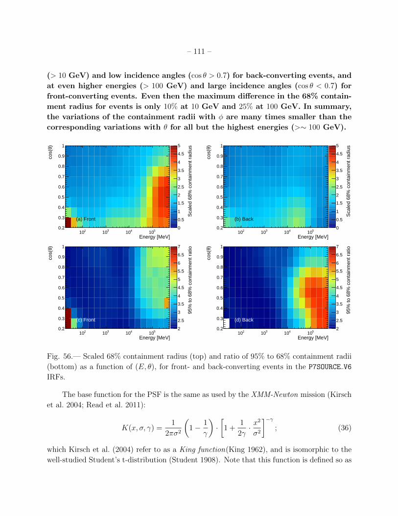
– 111 –

(> 10 GeV) and low incidence angles (cos θ > 0.7) for back-converting events, and

at even higher energies (> 100 GeV) and large incidence angles (cos θ < 0.7) for

front-converting events. Even then the maximum difference in the 68% contain-

ment radius for events is only 10% at 10 GeV and 25% at 100 GeV. In summary,

the variations of the containment radii with φ are many times smaller than the

corresponding variations with θ for all but the highest energies (>∼ 100 GeV).

Energy [MeV]210 310 410 510

)θco

s(

0.2

0.3

0.4

0.5

0.6

0.7

0.8

0.9

1

Sca

led

68%

con

tain

men

t rad

ius

0

0.5

1

1.5

2

2.5

3

3.5

4

4.5

5

(a) Front

Energy [MeV]210 310 410 510

)θco

s(

0.2

0.3

0.4

0.5

0.6

0.7

0.8

0.9

1

Sca

led

68%

con

tain

men

t rad

ius

0

0.5

1

1.5

2

2.5

3

3.5

4

4.5

5

(b) Back

Energy [MeV]210 310 410 510

)θco

s(

0.2

0.3

0.4

0.5

0.6

0.7

0.8

0.9

1

95%

to 6

8% c

onta

inm

ent r

atio

2

2.5

3

3.5

4

4.5

5

5.5

6

6.5

7

(c) Front

Energy [MeV]210 310 410 510

)θco

s(

0.2

0.3

0.4

0.5

0.6

0.7

0.8

0.9

1

95%

to 6

8% c

onta

inm

ent r

atio

2

2.5

3

3.5

4

4.5

5

5.5

6

6.5

7

(d) Back

Fig. 56.— Scaled 68% containment radius (top) and ratio of 95% to 68% containment radii

(bottom) as a function of (E, θ), for front- and back-converting events in the P7SOURCE V6

IRFs.

The base function for the PSF is the same as used by the XMM-Newton mission (Kirsch

et al. 2004; Read et al. 2011):

K(x, σ, γ) =1

2πσ2

(1− 1

γ

)·[1 +

1

2γ· x

2

σ2

]−γ; (36)

which Kirsch et al. (2004) refer to as a King function(King 1962), and is isomorphic to the

well-studied Student’s t-distribution (Student 1908). Note that this function is defined so as

– 112 –

to satisfy the normalization condition:∫ ∞0

K(x, σ, γ) 2πx dx = 1; (37)

the extra 2πx comes from the integral over the solid angle dΩ = sin(x) dxdφ ∼ 2πx dx.

However, at very low energies the PSF widens to the point that the small angle approximation

fails by more than a few percent and K(x) sin(x) must be normalized numerically.

To allow for more accurate descriptions of the tails of the distributions, we use the sum

of two King functions to represent the dependence of the PSF on scaled deviation for a given

incidence angle and energy:

P (x) = fcoreK(x, σcore, γcore) + (1− fcore)K(x, σtail, γtail). (38)

The σ and γ values are stored in tables of PSF parameters as SCORE, STAIL, GCORE and GTAIL

respectively. Because of the arbitrary normalization used in fitting the PSF function, fcore

must be extracted from the NTAIL table parameter, in conjunction with SCORE and STAIL:

fcore =1

1 + NTAIL · STAIL2/SCORE2. (39)

The fitting function has been revised several times since the development of the first

preliminary response functions. The version described here is the one currently being used

and is different from e.g., that used for P6 V3 IRFs. A description of the fit functions used

in the past is given in § 6.1.2.

6.1.2. Legacy Point-Spread Function Parametrization

The first set of publicly released IRFs, P6 V3, used a slightly different PSF parametriza-

tion. Specifically, it allowed for only one σ parameter and fixed the relative normalization

of the two King functions by constraining the two to contribute equally at xb = 2√

5σ. So

for P6 V3 we used

P (x) = fcoreK(x, σ, γcore) + (1− fcore)K(x, σ, γtail), (40)

with

fcore =1

1 +K(xb, σ, γcore)/K(xb, σ, γtail). (41)

– 113 –

6.2. Point-Spread Function from On-Orbit Data

During the first year of the mission we observed that for energies greater than a few

GeV the distributions of γ rays around isolated point sources were systematically wider than

the expectations based on the PSF estimated from the MC simulations. We observed the

same discrepancies for pulsars and blazars. In order to obtain a more accurate description

of the core of the PSF for sources that are observed at a typical range of incidence angles,

starting from the then-current Pass 6 IRFs, we derived the PSF directly from flight data,

by means of a stacking analysis of selected point sources. The details of this analysis are

described in Ackermann, M. et al. (2012, in preparation). Here we summarize the procedure,

the associated uncertainties, and the impact on high-level source analysis.

6.2.1. Angular Containment from Pulsars

In the 1–10 GeV energy range bright pulsars are excellent sources for evaluating the

in-flight PSF: not only they are among the brightest γ ray sources, providing abundant

statistics, the pulsed emission is very stable and the angular distributions of γ rays around

the true positions can be estimated readily by phase selecting γ rays. The Vela pulsar is

the brightest pulsar and an analysis with adequate statistics can be based on Vela alone.

In the remainder of this section we describe the procedure for Vela only; the extension

to an arbitrary number of pulsars is straightforward (see Ackermann, M. et al. 2012, in

preparation).

We use the P7SOURCE Vela calibration sample, which we divided into front- and back-

converting subsamples, and bin the data in 4 energy bins per decade. We then calculate the

pulsar phase for each γ ray. As mentioned in § 3.6.1 we define [0.12, 0.17]∪ [0.52, 0.57] as the

“on” interval and [0.8, 1.0] as “off” (see Fig. 15 for the phase histogram). Next we calculate

the containment angles: the position of Vela is known with a precision that greatly exceeds

the LAT angular resolution and which can be assumed as the true source position. We

make histograms of the angular deviations from Vela for the on-peak and off-pulse intervals

and normalize them for the relative phase ranges. To estimate the PSF from flight data we

measure the containment radii from the difference between the histograms.

6.2.2. Angular Containment from Active Galactic Nuclei

Above ∼ 10 GeV spectral cutoffs of pulsars leave AGN as the only attractive sources for

studying the PSF. In Ackermann, M. et al. (2012, in preparation) we address the potential

– 114 –

contribution from pair halos around AGN and conclude that we see no indication that this

phenomenon is the explanation for the PSF being broader than predicted. Thus, we treat

AGN as point sources. Many γ-ray sources are considered to be only “associated” with AGN,

as opposed to “firmly identified” (see Nolan et al. 2012, for a discussion of the distinction),

because of the limited angular resolution of the LAT. In the present analysis we consider

only sources with high-confidence associations. As for pulsars, the positions of AGN are

known with high precision from other wavelengths, and the angular distances from the true

directions can be calculated. To accumulate enough statistics we stacked several sources and

performed a joint analysis. We selected AGN from among the LAT sources with the highest

significances above 10 GeV outside the Galactic plane. This energy limit is set by the source

density: below a few GeV the LAT PSF is broad enough that nearby sources frequently

overlap.

A significant difference with respect to the pulsar analysis is the necessity of modeling

the background in evaluating the distribution of angular deviations. We assume that after the

stacking of the sky regions far from the Galactic plane the background count distribution can

be assumed to be isotropic. At each energy the background is modeled as a flat distribution

normalized by the amplitude in an annulus centered on the stacked data set. The inner

radius of this annulus was chosen to be significantly larger than the region containing γ rays

from the stacked AGN sample. The uncertainty of the containment radius in each energy

bin was set to the RMS of a large sample of MC realizations for the signal and background

distributions.

6.2.3. Point-Spread Function Fitting

We have developed a procedure (described in detail in Ackermann, M. et al. 2012, in

preparation), to fit our PSF model to the measured containment radii for different energy

ranges. Given the statistical limitations we use a single King function, Eqn. (36). For

the same reason we do not measure the dependence of the PSF on the incidence angle,

i.e., we calculate an acceptance-weighted average over the incidence angle. We first fit the

experimental 68% and 95% containment radii (R68 and R95) with Eqn. (36). Then we extract

a new scaling relation. And finally, we use the fitted (rather that the measured) 68% and

95% containment radii to obtain a new set of PSF parameters for each energy bin. By using

the fitted containment radii, this procedure smooths out the statistical fluctuations across

the energy bins.

The 68% and 95% angular containment radii for the flight-based P7SOURCE V6 PSF are

shown in Figure 57.

– 115 –

Energy [MeV]210 310 410 510

]°C

onta

inm

ent a

ngle

[

-110

1

10

P7SOURCE_V6 Back 95%P7SOURCE_V6 Combined 95%P7SOURCE_V6 Front 95%P7SOURCE_V6 Back 68%P7SOURCE_V6 Combined 68%P7SOURCE_V6 Front 68%

Fig. 57.— 68% and 95% containment angles as a function of energy for the P7SOURCE V6

event class.

6.3. Uncertainties of the Point-Spread Function

The uncertainty of the derived PSF was estimated by comparing the 68% and 95% PSF

containment radii from a set of calibration point sources with the corresponding containment

radii derived from the P7SOURCE V6 PSF (Ackermann, M. et al. 2012, in preparation). The

68% and 95% containment radii measure of the accuracy representation of the PSF in the

core and tail, respectively.

The analysis was performed as a function of energy with 4 energy bins per decade. To

determine the accuracy of the PSF fit as a function of incidence angle, subsamples were also

studied in which γ rays were additionally split into three bins of cos θ ([0.2, 0.5), [0.5, 0.75),

and [0.75, 1.0]).

Figure 58 shows the 68% and 95% containment radii as a function of energy for front-

and back-converting γ rays averaged over incidence angle. The smooth lines show the model

predictions for the MC (P7SOURCE V6MC) and in-flight (P7SOURCE V6) IRFs. At energies

below 3 GeV the containment radii match the MC PSF with fractional residuals no larger

than 10%. Above 3 GeV the MC PSF begins to systematically underestimate the 68%

containment radius by as much as 50% for both front- and back-converting γ rays. As shown

in Figure 58 the P7SOURCE V6 PSF reproduces the flattening of the energy dependence of

the PSF containment at high energies. However owing to the limitations of using a single

King function to parametrize the PSF, this model over-predicts the PSF tails as represented

by the 95% containment radii.

At large incidence angles (cos θ ∈ [0.2, 0.5]) the LAT PSF broadens by approximately

a factor of 1.5. Due to the sky survey observing mode of Fermi and the decreased effec-

– 116 –

Energy [MeV]

]°C

onta

inm

ent a

ngle

[

-210

-110

1

10

(a) Front 68% (full FOV)VelaStacked AGNsIn-flight PSF (P7SOURCE_V6)Monte Carlo PSF (P7SOURCE_V6MC)

Energy [MeV]210 310 410 510

Res

idua

ls

-0.5

0

0.5Energy [MeV]

]°C

onta

inm

ent a

ngle

[

-210

-110

1

10

(b) Front 95% (full FOV)VelaStacked AGNsIn-flight PSF (P7SOURCE_V6)Monte Carlo PSF (P7SOURCE_V6MC)

Energy [MeV]210 310 410 510

Res

idua

ls

-0.5

0

0.5

Energy [MeV]

]°C

onta

inm

ent a

ngle

[

-210

-110

1

10

(c) Back 68% (full FOV)VelaStacked AGNsIn-flight PSF (P7SOURCE_V6)Monte Carlo PSF (P7SOURCE_V6MC)

Energy [MeV]210 310 410 510

Res

idua

ls

-0.5

0

0.5Energy [MeV]

]°C

onta

inm

ent a

ngle

[

-210

-110

1

10

(d) Back 95% (full FOV)VelaStacked AGNsIn-flight PSF (P7SOURCE_V6)Monte Carlo PSF (P7SOURCE_V6MC)

Energy [MeV]210 310 410 510

Res

idua

ls

-0.5

0

0.5

Fig. 58.— 68% and 95% containment radii for γ rays averaged over all incidence angles

(cos θ ∈ [0.2, 1.0]) as a function of energy for front (top) and back (bottom). Data points

with error bars show the measured containment radii derived from the Vela and AGN PSF

calibration data sets. Solid lines show the P7SOURCE V6 model predictions in each energy

bin; dashed lines show the predictions from the MC simulations (P7SOURCE V6MC). Residual

plots indicate the fractional deviation with respect to P7SOURCE V6.

tive area at large incidence angles the fit of the in-flight PSF is dominated by γ rays at

smaller incidence angles (cos θ ∈ [0.5, 1.0]). The variation of the PSF with incidence angle is

most relevant for the analysis of transient phenomena in which the time-scale of interest is

comparable to or shorter than the orbital period of Fermi , such as GRBs and short-period

time-series analyses. As shown in Figure 59, the agreement of in-flight and MC PSF models

with the data appears worse at large incidence angles (cos θ ∈ [0.2, 0.5]) although the limited

statistics limit a rigorous comparison. The in-flight PSF model, which does not incorporate

θ dependence, significantly under-predicts the width of the 68% containment radius for both

front- and back-converting γ rays. The effect of these discrepancies on high-level analysis

will be considered in § 6.5.

– 117 –

Energy [MeV]

]°C

onta

inm

ent a

ngle

[

-210

-110

1

10

(a) Front 68% (off-axis)VelaStacked AGNsIn-flight PSF (P7SOURCE_V6)Monte Carlo PSF (P7SOURCE_V6MC)

Energy [MeV]210 310 410 510

Res

idua

ls

-0.5

0

0.5Energy [MeV]

]°C

onta

inm

ent a

ngle

[

-210

-110

1

10

(b) Front 95% (off-axis)VelaStacked AGNsIn-flight PSF (P7SOURCE_V6)Monte Carlo PSF (P7SOURCE_V6MC)

Energy [MeV]210 310 410 510

Res

idua

ls

-0.5

0

0.5

Energy [MeV]

]°C

onta

inm

ent a

ngle

[

-210

-110

1

10

(c) Back 68% (off-axis)VelaStacked AGNsIn-flight PSF (P7SOURCE_V6)Monte Carlo PSF (P7SOURCE_V6MC)

Energy [MeV]210 310 410 510

Res

idua

ls

-0.5

0

0.5Energy [MeV]

]°C

onta

inm

ent a

ngle

[

-210

-110

1

10

(d) Back 95% (off-axis)VelaStacked AGNsIn-flight PSF (P7SOURCE_V6)Monte Carlo PSF (P7SOURCE_V6MC)

Energy [MeV]210 310 410 510

Res

idua

ls

-0.5

0

0.5

Fig. 59.— 68% and 95% containment radii for off-axis γ rays (cos θ ∈ [0.2, 0.5]) as a function

of energy for front (top) and back (bottom). Data points with error bars show the measured

containment radii derived from the Vela and AGN PSF calibration data sets. Solid lines show

the P7SOURCE V6 model predictions in each energy bin; dashed lines show the predictions

from the MC simulations (P7SOURCE V6MC). Residual plots indicate the fractional deviation

with respect to P7SOURCE V6.

6.4. The “Fisheye” Effect

For sources observed only in a narrow range of incidence angle, particularly near the

edges of the LAT FoV, we must consider an additional complication: particles that scatter

toward the LAT boresight are more likely to trigger the LAT and be reconstructed than

particles that scatter away from the boresight. Furthermore, since the event selections do

not require the separate reconstruction of both tracks from the γ → e+e− conversion and

the reconstruction code will estimate an event direction using a single track if no vertex is

found, for some events we base our direction estimate only on the particle that scattered

more toward the LAT boresight. This effect increases as the energy decreases, since multiple

scattering causes larger deviations.

– 118 –

Over the course of a year the position of the LAT boresight relative to any given direction

in the sky is fairly uniformly distributed in azimuth; however, for shorter periods several

factors can lead to large non-uniformities (see § 2.3). Furthermore, by construction the PSF

is averaged over azimuth. Therefore, for long (> 1 year) integration periods the treatment of

the PSF described in the previous sections is perfectly adequate and the fisheye effect simply

results in a broadening of the PSF which is correctly described by the IRFs. However, for

shorter periods the fisheye effect can result in systematic biases in localization, which should

be accounted for. To do so we consider the polar and azimuthal components of the angular

separation between the true and reconstructed γ-ray directions in the allGamma sample.

Taking v as the true γ-ray direction (in the LAT frame), v ′ as the reconstructed direction,

and z as the LAT boresight we can define the local polar and azimuthal directions:

φ =z × v|z × v| θ =

φ× v|φ× v|

. (42)

Then we calculate the component of the misreconstruction along each:

δφ = sin−1(φ · (v ′ − v )

)δθ = − sin−1

(θ · (v ′ − v )

)(43)

(the extra negative sign in the above equation is applied so that the fisheye effect represents

a bias toward positive values of δθ). It is also worth noting that simply considering the

distributions of differences between the true and reconstructed θ is complicated by the fact

that the amount of solid angle varies with θ.

Figure 60 shows how the mean of δθ varies as a function of energy and incidence angle

for the P7SOURCE event selection. Although the bias can be very large at high incidence

angles and low energies, it is important to recall that (i) the PSF is quite wide in those

cases, and (ii) there is relatively little acceptance in that region. Figure 61 shows the ratio

of the mean to the RMS of δθ for the same energies and angles, and we see that except for

the furthest off-axis events and the lowest energies, the fisheye effect is a small contributor

to the overall width of the PSF when considering persistent γ-ray sources.

We should recall that the P7TRANSIENT event selection does not include as tight con-

straints on the quality of the event reconstruction as the P7SOURCE selection. Accordingly,

the fisheye effect is more pronounced for this event selection, as can be seen in Figures 62 and

63. This is of particular importance for GRBs, for which almost all of the exposure might

be at a single incidence angle. For soft GRBs in the LAT, the bias for the P7TRANSIENT γ

rays near 100 MeV that contribute the most to the localization can be up to 6 at 50 off

axis. Furthermore, since the orientation of the LAT boresight relative to a GRB

might not change significantly during the GRB outburst, these γ rays will tend

– 119 –

Energy [MeV]210 310 410 510

]° [θδm

ean

-210

-110

1

10

° = 63.3θ° = 49.5θ° = 31.8θ

(a) Front

Energy [MeV]210 310 410 510

]° [θδm

ean

-210

-110

1

10

° = 75.5θ° = 63.3θ° = 49.5θ° = 31.8θ

(b) Back

Fig. 60.— Mean of δθ for MC simulated data as a function of energy for several incidence

angles for the P7SOURCE event selection for front-converting (a) and back-converting (b)

events. There are not enough statistics for front-converting events at θ = 75.5 to extract

reliable values.

Energy [MeV]210 310 410 510

θδ /

rms

θδm

ean

-210

-110

1 ° = 63.3θ° = 49.5θ° = 31.8θ

(a) Front

Energy [MeV]210 310 410 510

θδ /

rms

θδm

ean

-210

-110

1 ° = 75.5θ° = 63.3θ° = 49.5θ° = 31.8θ

(b) Back

Fig. 61.— Ratio of the mean to the RMS of δθ for MC simulated data as a function of

energy for several incidence angles for the P7SOURCE event selection for front-converting (a)

and back-converting (b) events. There are not enough statistics for front-converting events

at θ = 75.5 to extract reliable values.

to be biased in the same direction, causing an overall bias in the localization of

the GRB. Therefore, when statistics permit, more robust localizations can be

obtained by using events with energies > 200 MeV, or by using P7SOURCE rather

than P7TRANSIENT class events.

– 120 –

Energy [MeV]210 310 410 510

]° [θδm

ean

-210

-110

1

10

° = 63.3θ° = 49.5θ° = 31.8θ

(a) Front

Energy [MeV]210 310 410 510

]° [θδm

ean

-210

-110

1

10

° = 75.5θ° = 63.3θ° = 49.5θ° = 31.8θ

(b) Back

Fig. 62.— Mean of δθ for MC simulated data as a function of energy for several incidence

angles for the P7TRANSIENT event selection for front-converting (a) and back-converting (b)

events. There are not enough statistics for front-converting events at θ = 75.5 to extract

reliable values.

Energy [MeV]210 310 410 510

θδ /

rms

θδm

ean

-210

-110

1 ° = 63.3θ° = 49.5θ° = 31.8θ

(a) Front

Energy [MeV]210 310 410 510

θδ /

rms

θδm

ean

-210

-110

1 ° = 75.5θ° = 63.3θ° = 49.5θ° = 31.8θ

(b) Back

Fig. 63.— Ratio of the mean to the RMS of δθ for MC simulated data as a function of energy

for several incidence angles for the P7TRANSIENT event selection for front-converting (a) and

back-converting (b) events. There are not enough statistics for front-converting events at

θ = 75.5 to extract reliable values.

6.5. Propagating Uncertainties of the Point-Spread Function to High Level

Science Analysis

Uncertainties in the PSF parametrization lead to an imperfect source model in the high-

level source analysis (likelihood fitting), and therefore to systematic uncertainties in source

spectra (§ 6.5.1), localizations and measurements of source extensions (§ 6.5.2).

An additional source of systematic uncertainty comes from neglecting the θ dependence

– 121 –

of the PSF in the derivation of the parametrization from flight data. In particular, this can

lead to artificial variability as the PSF changes with the varying observing profile.

6.5.1. Using Custom IRFs to Generate an Error Envelope

We can create custom PSFs in a similar manner to that used for the effective area (see

§ 5.7), though with the additional complication that we have to explore variations in the

shape of the PSF as a function of energy and incidence angle. Because the dependence of

the PSF on γ is not intuitive we choose to express the bracketing functions in terms of the

observable quantities R68 and r = R95/R68 rather than in terms of σ and γ. Specifically, in

each bin of energy and incidence angle, we can define the bracketing values R′68 and r′ in

terms of R68 and r:

R′68 = R68(1 + ε68(E)B68(E))

r′ = r(1 + εr(E)Br(E)). (44)

We can then solve for the King function parameters σ′ and γ′ which would correspond to

these values.

We re-analyzed both the B2 1520+31 and the PG 1553+113 ROIs with each of the

PSF bracketing functions listed in Table 14 using the procedure described in § 5.7. Based

on the quality of the fits described in § 6.3, in particular the residuals on the 68% and 95%

containment radii, we have assigned:

ε68(E) = 10%

εr(E) = 50%. (45)

Tables 15 and 16 shows the fits results for PG 1553+113 and B2 1520+31 as well as the

integral counts and energy fluxes between 100 MeV and 100 GeV obtained using these PSF

bracketing functions. The ranges of the fit values indicate propagated uncertainties from the

uncertainty in the PSF (Table 17).

The greater influence of the uncertainty of the PSF on the flux and spectral measure-

ments for the softer source (B2 1520+31) comes about because at lower energies the wider

PSF makes resolving sources more difficult and results in greater correlation with the Galac-

tic and isotropic diffuse components in the likelihood fit, which varied by up to ±4% and

±5% respectively.

– 122 –

Name B68(E) Br(E)

c scalehi t nom +1 0

c scalelo t nom −1 0

c pivothi t nom tanh( 1k

log(E/E0)) 0

c pivotlo t nom − tanh( 1k

log(E/E0)) 0

c nom t scalehi 0 +1

c nom t scalelo 0 −1

c nom t pivothi 0 tanh( 1k

log(E/E0))

c nom t pivotlo 0 − tanh( 1k

log(E/E0))

Table 14: Bracketing PSFs and the energy-dependent scaling functions used to create them.

As in § 5.7 we use k = 0.13, which corresponds to smoothing over ∆E/E ∼ 0.30.

Bracketing PSF N0 Γ F25 S25


Nominal 2.54× 10−12 1.68 6.91× 10−8 1.19× 10−4

c nom t scalelo 2.48× 10−12 1.70 6.94× 10−8 1.13× 10−4

c nom t scalehi 2.54× 10−12 1.66 6.68× 10−8 1.22× 10−4

c nom t pivotlo 2.46× 10−12 1.68 6.67× 10−8 1.15× 10−4

c nom t pivothi 2.58× 10−12 1.68 6.99× 10−8 1.21× 10−4

c scalelo t nom 2.46× 10−12 1.67 6.53× 10−8 1.18× 10−4

c scalehi t nom 2.63× 10−12 1.70 7.32× 10−8 1.21× 10−4

c pivotlo t nom 2.60× 10−12 1.70 7.30× 10−8 1.18× 10−4

c pivothi t nom 2.49× 10−12 1.66 6.50× 10−8 1.21× 10−4

Table 15: Fit parameters and integral fluxes obtained using the PSF bracketing IRFs for

PG 1553+113. Note that the quoted precision is roughly equivalent to the fit uncertainties


6.5.2. Effects on Source Extension

For sufficiently long exposures, the LAT can spatially resolve a number of γ-ray sources.

In the 2FGL catalog, 12 spatially extended LAT sources were identified (Nolan et al. 2012)

using 24 months of LAT data; and several additional extended sources have been recently

resolved from these data by Lande et al. (2012) using special techniques for modeling the

spatial extension. Understanding the possible spatial extension of LAT sources is important

for identifying multiwavelength counterparts, and using a source model with the correct

– 123 –

Bracketing PSF N0 α β F25 S25


Nominal 5.23× 10−10 2.24 0.08 4.09× 10−7 1.33× 10−4

c nom t scalelo 5.34× 10−10 2.31 0.06 4.28× 10−7 1.33× 10−4

c nom t scalehi 5.02× 10−10 2.19 0.09 3.85× 10−7 1.30× 10−4

c nom t pivotlo 5.00× 10−10 2.22 0.09 3.86× 10−7 1.26× 10−4

c nom t pivothi 5.43× 10−10 2.29 0.06 4.34× 10−7 1.38× 10−4

c scalelo t nom 4.87× 10−10 2.21 0.08 3.77× 10−7 1.26× 10−4

c scalehi t nom 5.57× 10−10 2.27 0.07 4.40× 10−7 1.40× 10−4

c pivotlo t nom 5.27× 10−10 2.31 0.06 4.26× 10−7 1.34× 10−4

c pivothi t nom 5.16× 10−10 2.17 0.10 3.91× 10−7 1.32× 10−4

Table 16: Fit parameters and integral fluxes obtained using the PSF bracketing IRFs for

B2 1520+31. Note that the quoted precision is roughly equivalent to the fit uncertainties


Parameter B2 1520+31 PG 1553+113

(soft) (hard)

δN0/N0 +6.6% −6.8% +3.5% −3.4%

δΓ (δα) +0.07 −0.07 +0.02 −0.02

δβ +0.02 −0.02 -

δF25/F25 +7.7% −7.7% +6.0% −5.9%

δS25/S25 +5.4% −5.5% +2.4% −4.9%

Table 17: Systematic variations arising from uncertainties in the PSF. For the spectral index

(Γ or α) and spectral curvature (β) we give the absolute variation with respect to the nominal

value (e.g., δΓ). For the flux prefactor and the integral fluxes we give the relative variations

with respect to the nominal value (e.g., δN0/N0).

spatial extent produces more accurate spectral fits and avoids biases in the model parameters.

In addition to using a correct spatial model, the accuracy of the PSF can also affect

the analyses of extended sources; and using an incorrect PSF will result in biases both in

the fitted model parameters and in the significance of any spatial extension that is found.

For example, flight data indicate that the MC-based PSF in the P7SOURCE V6MC IRFs is too

narrow at energies > 3 GeV (§ 6.2). Fitting the extension of SNR IC 443 (Abdo et al. 2010e)

with a uniform disk for data from the first two years of observations and using the flight-

– 124 –

determined PSF in P7SOURCE V6, we find a best fit disk radius of IC 443 of σ = 0.35±0.01

(Lande et al. 2012). By contrast, fitting these same data, but using the MC-based PSF

in P7SOURCE V6MC, we find a best fit radius of σ = 0.39. This corresponds to a ∼ 10%

systematic bias in the measurement of the extension of IC 443. Since IC 443 is a fairly hard

source, with photon index Γ = 2.2, the bias found for softer sources would be somewhat

smaller.

Use of an imperfect model of the PSF can also affect the assessment of the statistical

significance of the extension of the source. We determine the significance of a measured

source extension using the test statistic

TSext = 2 log(Lext/Lpt), (46)

This is twice the difference in log-likelihood found when fitting the source assuming it is

spatially extended versus assuming it is a point source. The use and validity of this formula

is described in (Lande et al. 2012). For IC 443, using the P7SOURCE V6 IRFs, we find

TSext = 640, corresponding to a formal statistical significance of ∼ 25σ. Performing the

same analysis using P7SOURCE V6MC, we obtain TSext = 1300, corresponding to ∼ 37σ.

6.5.3. Effects on Variability

Neglecting the dependence of the PSF on incidence angle (§ 6.3) may introduce time-

dependent biases of the estimated flux of the source, due to the different distribution of the

source position with respect to the LAT boresight in each time interval. To estimate the

potential size of such biases we consider how great an effect on source fluxes we might see if

we were to naively use the nominal containment radius for aperture photometry analysis (i.e.,

an analysis where we simply count the γ rays within a given aperture radius). Specifically,

we use the MC based PSF to extract the containment radii averaged over the first two years

of the mission R(E) in the direction of the Vela pulsar. Then we split the data into much

shorter time intervals (indexed by i) and compute the fraction of γ rays Ci(E; vela) that fall

within R(E; vela) for each of those shorter intervals:

Ci(E, vela) =

∫ ∫ R(E;vela)

0Aeff(E, θ; vela)tobs,i(θ; vela) sin θdθdr∫Aeff(E, θ)tobs,i(θ; vela) sin θdθ

(47)

Here we consider 68% and 95% containment radii. Figure 64 shows how C68,i(E; vela)

and C95,i(E; vela) vary for each 12-hour time interval over the first 700 days of routine science

operations. If there were no θ dependence to the PSF this figure would show lines at 0.68 and

0.95. However we clearly see that ignoring the θ dependence will cause slight mis-estimates

– 125 –

in the fraction of γ rays falling within the mission-averaged R68 and R95. In fact, the width

of the bands (i.e., the spread of that mis-estimation) indicate the errors in flux we would

expect if we were making a flux estimate based on aperture photometry with aperture cuts at

R. It is worth pointing out explicitly that the C95,i(E) band is significantly narrower, simply

because most of the γ rays are already contained within the R95(E) and the derivative of

the PSF is smaller.

Understanding the effect of the PSF dependence on incidence angle will have on a

full likelihood analysis is much more complicated, as it depends on the other sources in

the likelihood model. However, it is reasonable to take the width of the C68(E) bands as

indicative of the magnitude of the effect when analyzing sources in complex regions where

source proximity is a issue and the width of the C95(E) bands as indicative when analyzing

isolated sources.

Energy [MeV]210 310 410 510

Con

tain

men

t fra

ctio

n

0.5

0.55

0.6

0.65

0.7

0.75

0.8

0.85

0.9

0.95

1

Fra

ctio

n of

eve

nts

(per

ene

rgy

bin)

0

0.05

0.1

0.15

0.2

68%

95%

(a) Front

Energy [MeV]210 310 410 510

Con

tain

men

t fra

ctio

n

0.5

0.55

0.6

0.65

0.7

0.75

0.8

0.85

0.9

0.95

1

Fra

ctio

n of

eve

nts

(per

ene

rgy

bin)

0

0.05

0.1

0.15

0.2

(b) Back

Fig. 64.— Fraction of the PSF contained at the mission averaged 68% and 95% containment

radii in the direction of the Vela pulsar for the P7SOURCE V6MC IRFs as a function of energy for

front-converting (a) and back-converting (b) γ rays for each of 1400 12-hour time intervals.


As a consequence of the issues discussed in § 5.4, Pass 7 event classes have less system-

atic uncertainty for Aeff at the expense of a slightly broader PSF across the entire parameter

space.

In addition Pass 7 standard classes (P7SOURCE and cleaner) feature a PSF derived from

data above 1 GeV; see § 6.2. Below 1 GeV, where the PSF is derived from MC simulations,

the PSF parameters are recalculated in order to ensure a smooth variation of the containment

levels as a function of energy (§ 6.2.3).

– 126 –

Figure 65 compares the 68% containment angles for Pass 6 and Pass 7 classes recom-

mended for routine analyses of γ-ray point sources. While the difference between P6 V3 DIFFUSE

and P7SOURCE V6 is due mostly to the data-derived PSF in the latter, there is also a clear

difference across all energies between the P7SOURCE V6 PSF and in-flight P6 V11 DIFFUSE

PSF.

Energy [MeV]210 310 410 510

]°C

onta

inm

ent a

ngle

[

-110

1

10 P7SOURCE_V6 Back 68%P7SOURCE_V6 Combined 68%P7SOURCE_V6 Front 68%P6_V3_DIFFUSE Back 68%P6_V3_DIFFUSE Combined 68%P6_V3_DIFFUSE Front 68%

(a)

Energy [MeV]210 310 410 510

]°C

onta

inm

ent a

ngle

[-110

1

10 P7SOURCE_V6 Back 68%P7SOURCE_V6 Combined 68%P7SOURCE_V6 Front 68%P6_V11_DIFFUSE Back 68%P6_V11_DIFFUSE Combined 68%P6_V11_DIFFUSE Front 68%

(b)

Fig. 65.— Comparison of the 68% containment radius of the PSF for P7SOURCE V6 with

respect to P6 V3 DIFFUSE (a) and P6 V11 DIFFUSE (b). The P6 V3 DIFFUSE is plotted for

normal incidence; P6 V11 DIFFUSE and P7SOURCE V6 do not include dependence on the in-

cidence angle.

While the difference in the containment radii we described is typically within the PSF

uncertainties this comparison was performed with the incidence angle dependence ignored,

so the tabulated PSF is an average over the FoV weighted by the average exposure over long

timescales. This may be an issue for the analysis of bright sources over short timescales,

when the observation angle distribution in the LAT reference system is significantly different

from the average. Future Pass 7 IRFs may address this by reintroducing the θ dependence.

Current Pass 7 IRFs parametrize the PSF with a simplified version of Eqn. (38) for

which the tail term is omitted as described in § 6.2.3. The less accurate model of the

PSF tails in the Pass 7 classes with on-orbit PSF (to date P7SOURCE V6, P7CLEAN V6 and

P7ULTRACLEAN V6) is probably not an issue for most analyses, but caution is recommended

when comparing the dispersion of γ rays around the true position of bright sources with the

expected distribution derived from the IRFs.

– 127 –

7. ENERGY DISPERSION

The dispersion of measured energies around the true values (i.e., the energy dispersion,

or redistribution function) is generally asymmetric, with the most prominent tail being to-

ward lower energies. This feature, characteristic of thin electromagnetic calorimeters (such

as the LAT CAL, as opposed to full-containment calorimeters) makes the energy redistri-

bution difficult to parametrize. As a matter of fact, since most source spectra are steeply

falling with energy, low-energy tails in the energy dispersion are relatively harmless, while

overestimating the event energy can potentially lead to overestimating the hardness of the

spectrum. In the event selections we specifically make an effort to suppress the high-energy

tails, rejecting events for which we might overcompensate with the energy corrections (see

§ 3.2.1 and § 3.3.2).

While the width and shape of the energy redistribution are well understood, by default

the energy dispersion is not taken into account in the standard likelihood analysis, primarily

due to computational limitations. Furthermore, as we will see in § 7.4, the effect of neglecting

the energy redistribution is usually small enough that it can be ignored. When that is not

the case, it is easy to check the magnitude of the bias induced with dedicated simulations.

If needed, the energy dispersion can be accounted for in the spectral analysis either by

specifically enabling the functionality in the binned likelihood (ScienceTools version 09-26-

00 or later) or by means of unfolding techniques, as we briefly describe in § 7.4.

It is worth stressing that an in-flight validation of the energy response is much more

difficult than the corresponding validations of the effective area and the PSF described in

the previous section, as there is no known astrophysical calibration source that provides a

spectral line at a well defined energy that would play the role that point sources have for

the PSF (see, however, the discussion in § 7.3.3). The energy reconstruction validation will

be described in § 7.3.

7.1. Energy Dispersion and Parametrization from Monte Carlo Simulations

As for Aeff and PSF, in order to derive the energy dispersion events from an allGamma

simulation belonging to a specified event class are binned in true energy E and incidence

angle θ and the distribution of measured energy E ′ is fitted (and the parameters tabulated).

A complex functional form is necessary and attention is required to avoid fit instability and

overly rapid variation of the fit parameters.

– 128 –

7.1.1. Scaling

The success of scaling the PSF distributions (see § 6.1.1) prompted a similar approach

to the histogramming and fitting of the energy deviations. The scaling function SD cur-

rently employed, derived by fitting the 68% containment of the measured fractional energy

distribution (E ′ − E)/E across the entire E–θ plane, is

SD(E, θ) = c0(log10E)2 + c1(cos θ)2 + c2 log10E + c3 cos θ + c4 log10E cos θ + c5. (48)

Front- and back-converting events are treated separately. The parameters used since the

Pass 6 analysis are listed in Table 18. These are included in the IRF files for Pass 6 and

Pass 7 event classes.

c0 c1 c2 c3 c4 c5

Front 0.0210 0.0580 -0.207 -0.213 0.042 0.564

Back 0.0215 0.0507 -0.220 -0.243 0.065 0.584

Table 18: Numerical values of the coefficients defining the energy resolution scaling function

SD in Eqn. (48) for the Pass 6 and Pass 7 event classes.

The scaling function SD allows us to define a scaled energy deviation x for which much

of the energy and angular dependence is already accounted for:

x =(E ′ − E)

SD(E, θ)E(49)

This scaled value is calculated for each simulated event and histogrammed, as shown in

Figure 66. Scaling the distribution achieves two main effects: the width of the core of the

distribution is almost constant for all energies and incidence angles, and the distribution

thus expressed is significantly simpler to parametrize than the un-scaled version.

7.1.2. Fitting the Scaled Variable

The scaled energy deviation, as illustrated by the example in Figure 66, has a well

defined core accompanied by elongated tails. We found we can effectively fit this structure

with several piecewise functions of the form:

R(x, x0, σ, γ) = N exp

(−1

2

∣∣∣∣x− x0

σ

∣∣∣∣γ) (50)

– 129 –

N 0.07687 lσ 0.7168 rσ 0.5806 0x -0.1037 Lσ 0.08331 Rσ 0.05593

Scaled deviation-6 -4 -2 0 2 4 6

Ene

rgy

disp

ersi

on e

stim

ate

-610

-510

-410

-310

-210

-110

1N 0.07687

lσ 0.7168 rσ 0.5806 0x -0.1037 Lσ 0.08331 Rσ 0.05593

L l r R

0x

Fig. 66.— Histogram of the scaled energy deviation, as defined in Eqn. (49), fitted with the

function D(x) in Eqn. (51). The plot refers to the (E, θ) bin centered at 7.5 GeV and 30

for the front section.

Indeed we model the energy dispersion D(x) within each (E, θ) bin as four piecewise func-

tions:

D(x) =

NLR(x, x0, σL, γL) if (x− x0) < −xNlR(x, x0, σl, γl) if (x− x0) ∈ [−x, 0]

NrR(x, x0, σr, γr) if (x− x0) ∈ [0, x]

NRR(x, x0, σR, γR) if (x− x0) > x

(51)

The values of the split point x and of the four exponents γ of the energy dispersion parametriza-

tion in Eqn. (51) are fixed as specified in Table 19. Moreover, the relative normalizations

are set by requiring continuity at x = x0 and |x− x0| = x and therefore the fit is effectively

performed with a total of six free parameters, which are stored in the IRF FITS files: the

overall normalization Nr = Nl (NORM), the centroid position x0 (BIAS), the two core scales

σr (RS1) and σl (LS1) and the two tail scales σR (RS2) and σL (LS2).

x γL γl γr γR

1.5 0.6 1.6 1.6 0.6

Table 19: Numerical values of the split point x and of the four exponents γ in Eqn. (51) that

are fixed when fitting the scaled energy deviations.

7.1.3. Energy Resolution

The energy resolution is a figure of merit which is customarily used to summarize in

a single number the information contained in the energy dispersion parametrization. As

– 130 –

illustrated in Figure 67 we define the energy resolution as the half width of the energy

window containing 34% + 34% (i.e., 68%) of the energy dispersion on both sides of its most

probable value, divided by the most probable value itself. We note that this prescription

gives slightly larger values of energy resolution than using the smallest 68% containment

window.

Energy [MeV]6000 8000 10000 12000 14000

Ene

rgy

disp

ersi

on P

. D. F

.

0

0.1

0.2

0.3

0.4

0.5

0.6

0.7

0.8

0.9-310×

Peak @ 9900 MeV

Full width 68% containment: 1360 MeV

= 6.9%E E∆

Fig. 67.— Energy dispersion at 10 GeV for front-converting P7 SOURCE events 30 off-axis.

The most probable value of the distribution and the 68% containment window are indicated.

Figures 68 and 69 shows the energy resolution for P7SOURCE events as a function of energy

and incidence angle. As mentioned in § 2.1.2 the energy resolution has a broad minimum

between ∼ 1 and ∼ 10 GeV, degrading at lower energies due to the energy deposited in the

TKR and at higher energies due to the leakage of the electromagnetic shower out the sides

and the back of the CAL. Conversely the energy resolution tends to improve as the incidence

angle increases. This is especially true at high energy, where a longer path length in the CAL

implies less shower leakage—though front-converting events more than 55 off-axis tend to

exit the sides of the CAL and have worse energy resolution.

7.1.4. Correlation Between Energy Dispersion and PSF

As stated in § 1, we factorize the IRFs, effectively assuming that the energy and direction

measurements are uncorrelated. We use our allGamma MC sample to test this hypothesis.

We locate each event within the cumulative PSF and measured energy distributions:

PP =

∫ α

0

P (α;E, v)dα

PD =

∫ E′

0

D(E ′;E, v)dE ′ (52)

– 131 –

Energy [MeV]210 310 410 510

)θco

s(

0.2

0.3

0.4

0.5

0.6

0.7

0.8

0.9

1

E/E

δ

0

0.1

0.2

0.3

0.4

0.5

0.6

0.7

(a) Front

Energy [MeV]210 310 410 510

)θco

s(

0.2

0.3

0.4

0.5

0.6

0.7

0.8

0.9

1

E/E

δ

0

0.1

0.2

0.3

0.4

0.5

0.6

0.7

(b) Back

Fig. 68.— Energy resolution (68% containment half-width, as decribed in the text) as a

function of energy and incidence angle for front (a) and back (b) conversions.

Energy [MeV]210 310 410 510

On-

axis

ene

rgy

reso

lutio

n

0

0.05

0.1

0.15

0.2

0.25

0.3

P7SOURCE_V6 FrontP7SOURCE_V6 CombinedP7SOURCE_V6 Back

(a)

]° [θ0 10 20 30 40 50 60 70

Ene

rgy

reso

lutio

n at

10

GeV

0

0.02

0.04

0.06

0.08

0.1

0.12

0.14 P7SOURCE_V6 FrontP7SOURCE_V6 CombinedP7SOURCE_V6 Back

(b)

Fig. 69.— Energy resolution as a function of energy on-axis (a) and incidence angle at

10 GeV (b) for the P7SOURCE V6 event class.

If the IRFs perfectly described the MC sample, both of these distributions should be flat.

Furthermore, if there are no correlations between the energy measurement and the direction

estimate, the two-dimensional combined distribution should also be flat. In practice this is

nearly the case; the correlation coefficient between PP and PD is small (|CP,D| < 0.1) across

most of the energy and incidence angle range, as shown in Figure 70 (a). However, in many

bins of (E, θ), we do observe a small excess of counts with PP ∼ 1 and PD ∼ 0. Those values

correspond to events that are in the tails of the PSF and have a energy estimate that are

significantly lower than the true γ-ray energy. To quantify the magnitude of this effect, we

considered the fraction of highly anti-correlated events fa with PP > 0.98 and PD < 0.02 as

a function of (E, θ). In the absence of correlations, this fraction should be fa ∼ 4 × 10−4.

In fact, for highly off-axis γ rays in some energy ranges this fraction approaches fa ∼ 0.02;

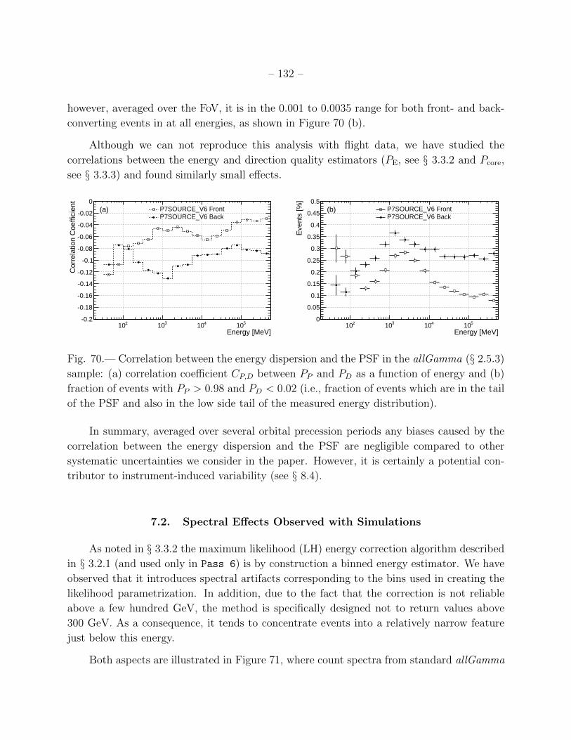
– 132 –

however, averaged over the FoV, it is in the 0.001 to 0.0035 range for both front- and back-

converting events in at all energies, as shown in Figure 70 (b).

Although we can not reproduce this analysis with flight data, we have studied the

correlations between the energy and direction quality estimators (PE, see § 3.3.2 and Pcore,

see § 3.3.3) and found similarly small effects.

Energy [MeV]210 310 410 510

Cor

rela

tion

Coe

ffici

ent

-0.2

-0.18

-0.16

-0.14

-0.12

-0.1

-0.08

-0.06

-0.04

-0.02

0P7SOURCE_V6 FrontP7SOURCE_V6 Back

(a)

Energy [MeV]210 310 410 510

Eve

nts

[%]

0

0.05

0.1

0.15

0.2

0.25

0.3

0.35

0.4

0.45

0.5P7SOURCE_V6 FrontP7SOURCE_V6 Back

(b)

Fig. 70.— Correlation between the energy dispersion and the PSF in the allGamma (§ 2.5.3)

sample: (a) correlation coefficient CP,D between PP and PD as a function of energy and (b)

fraction of events with PP > 0.98 and PD < 0.02 (i.e., fraction of events which are in the tail

of the PSF and also in the low side tail of the measured energy distribution).

In summary, averaged over several orbital precession periods any biases caused by the

correlation between the energy dispersion and the PSF are negligible compared to other

systematic uncertainties we consider in the paper. However, it is certainly a potential con-

tributor to instrument-induced variability (see § 8.4).

7.2. Spectral Effects Observed with Simulations

As noted in § 3.3.2 the maximum likelihood (LH) energy correction algorithm described

in § 3.2.1 (and used only in Pass 6) is by construction a binned energy estimator. We have

observed that it introduces spectral artifacts corresponding to the bins used in creating the

likelihood parametrization. In addition, due to the fact that the correction is not reliable

above a few hundred GeV, the method is specifically designed not to return values above

300 GeV. As a consequence, it tends to concentrate events into a relatively narrow feature

just below this energy.

Both aspects are illustrated in Figure 71, where count spectra from standard allGamma

– 133 –

simulations (§ 2.5.3) are shown for both Pass 6 and Pass 7. While the overall shapes of the

spectra reflect the LAT acceptance for the corresponding event classes (P6 V3 DIFFUSE and

P7 SOURCE V6), a clear sawtooth structure is visible in the Pass 6 count spectrum (with a

typical width comparable with the LAT energy resolution and peak-to-trough amplitude of

the order of ∼ 5%), along with a prominent feature at 300 GeV, above which energies from

the LH estimator cannot be selected

Energy [MeV]210 310 410 510

Cou

nts

/ 0.0

2 de

cade

0

10

20

30

40

50

60310×

Best energyLikelihood energy

(a)

Energy [MeV]210 310 410 510

Cou

nts

/ 0.0

2 de

cade

0

10

20

30

40

50

60310×

(b)

Fig. 71.— Finely binned (50 bins per energy decade) count spectra for events passing

the P6 V3 DIFFUSE (a) and the P7 SOURCE V6 (b) event selections; (a) also shows the LH

energy estimates for the subset of events where they are available (note that the LH energy

estimate is not always available, nor is it always selected when it is available). The final

energy measurement in Pass 6 reflects the artificial sawtooth structures of the underlying

LH energy estimator, which was removed in Pass 7. For both panels the vertical hashing

corresponds to the bin boundaries of the LH energy estimator.

The binning of the count spectra in Figure 71 (50 bins per energy decade) is deliberately

much finer than the instrumental resolution—and therefore much finer than the binning one

would use for a real spectral analysis of Fermi -LAT data. As a matter of fact, the features of

the LH energy estimator have little or no effect in most practical situations. One noticeable

exception is the search for spectral lines, such as might occur from the annihilation or decay

of a massive particle into a two-body final state including γ rays (see Abdo et al. 2010c, for

a more detailed discussion).

As already mentioned, in Pass 7 we chose to remove the LH algorithm from consider-

ation in the energy assignment—see Figure 71 (b).

– 134 –

7.3. Uncertainties in the Energy Resolution and Scale

In this section we will briefly review the systematic uncertainties on the absolute energy

scale and the energy dispersion. The energy measurement is a complex process involving

several different steps (see § 3.2.1 and § 3.3.2). Verification of the process is correspondingly

complex, involving tests with sea-level CR muons, tests at accelerators, and analysis of flight

data.

7.3.1. The Calibration Unit Beam Test Campaign

Since a direct calibration of the LAT with a particle beam was impractical for schedule

and cost reasons, the LAT Collaboration assembled for this purpose a dedicated Calibra-

tion Unit (CU) composed of two complete flight spare towers, one additional CAL module

and five ACD tiles. An intensive beam test campaign was performed on the CU, between

2006 July and November, with the primary goal of validating the MC simulation used to

define the event reconstruction and the background rejection. The CU was exposed to beams

of bremsstrahlung γ rays, protons, electrons, positrons and pions—with energies ranging be-

tween 50 MeV and 280 GeV (Table 20)—produced by the CERN Proton Synchrotron (PS)

and Super Proton Synchrotron (SPS). In addition, the CU was irradiated with 1–1.5 GeV/n12C and 131Xe beams in the Gesellschaft fur Schwerionenforschung (GSI) facility with the

purpose of studying the instrument response to heavy ions.

Particle Line Energy Triggers

γ PS 0–2.5 GeV 12 M

γ (tagged) PS 0.02–1.5 GeV 4 M

e− PS 1–5 GeV 6.4 M

e+ PS 1 GeV 2.5 M

π− PS 5 GeV 0.6 M

p PS 6–10 GeV 0.6 M

e− SPS 10–280 GeV 17.8 M

π− SPS 20 GeV 1.6 M

p SPS 20–100 GeV 0.8 M12C GSI 1–1.5 GeV/n 3 M131Xe GSI 1–1.5 GeV/n 1.5 M

Table 20: Summary of the 2006 Calibration Unit beam test campaign, adapted from Baldini

et al. (2007).

– 135 –

A complete review of the results of the beam test campaign is beyond the scope of this

paper. The reader is referred to Baldini et al. (2007) for a description of the experimental

setup and a review of the main results and to Ackermann et al. (2010b) for additional related

material.

From the standpoint of the energy measurement one of the primary goals of the beam

test campaign was to validate the leakage correction algorithms and, ultimately, the ability

of our MC simulation to reliably predict the energy resolution at high energy. The tests

confirmed that we understand the overall shower development and the energy resolution

to better than 10% up the maximum available electron energy, i.e., 280 GeV (Ackermann

et al. 2010b). As we will see in the next section, this implies that the effect of systematic

uncertainties on the energy resolution itself, when propagated to the high-level spectral

analysis, is essentially irrelevant in the vast majority of practical cases.

The most significant discrepancy was observed in the raw energy deposited in the

calorimeter, as measured values were on average ∼ 9% higher when compared with simula-

tions (with smaller fluctuations around this value, slightly dependent on the particle energy

and incidence angle). The origin of this discrepancy is unknown, and possibly could be at-

tributed to residual environmental effects not properly accounted for, although an imperfect

calibration of the CU cannot be excluded. In § 7.3.3 we will see that we have indications from

flight data that we do understand the absolute energy scale to a precision better than 9%.

7.3.2. Crystal Calibrations with Cosmic-Ray Data

The calibration of the CAL crystals is the starting point of the energy reconstruction

chain and underlies all the subsequent steps (a detailed description of LAT on-orbit calibra-

tions is given in Abdo et al. 2009f). As explained in § 2.1.2, the large dynamic range of the

LAT CAL (2 MeV–70 GeV per crystal) is achieved by means of four independent chains of

electronics per crystal, with different amplifications (or ranges), as summarized in Table 21.

In the most common readout mode (the so called single-range) the highest gain range that

is not saturated is selected as the best estimate and converted into a digital signal that is

eventually used in the event reconstruction.

What is relevant for the discussion here is the on-orbit calibration of the crystal response,

as determined by the crystal light yield and the linearity of the electronics. The lower energy

scales are calibrated using primary protons that do not undergo nuclear interactions in the

LAT, which are selected through a dedicated event analysis. For each crystal the most

probable value of the energy deposition, corrected for the path length, is compared with the

– 136 –

Range Diode Gain Energy range MeV/Bin

lex8 Small High 2 MeV–100 MeV 0.033

lex1 Small Low 2 MeV–1 GeV 0.30

hex8 Large High 30 MeV–7 GeV 2.3

hex1 Large Low 30 MeV–70 GeV 20

Table 21: Readout ranges and energy conversion factors for the CAL crystals, adapted from

Abdo et al. (2009f).

MC prediction and the conversion factor between digital signal and MeV is computed. This

procedure was first tested and validated with sea-level CR muons. The high-energy ranges

are calibrated in the energy range of overlap between lex1 and hex8 using events collected

by a special on-board filter for selecting heavy ions (see Fig. 72), read out in full four-range

mode (i.e., with all four energy ranges read out at each log end). The non-linearity of the

electronics is characterized across the entire energy range using a dedicated internal charge

injection system and is corrected for in the energy measurement.

Pathlength corrected crystal energy [MeV]200 400 600 800 1000 1200 1400 1600

Cou

nts

/ 0.1

83 M

eV

1

10

210

310 B

C

N

O

Ne

Fig. 72.— Distribution of the path length-corrected crystal energy deposition for a sample

of events used to inter-calibrate the low-energy and high-energy CAL energy ranges. The

peaks corresponding to the most abundant Galactic CR species are clearly visible, though

the composition differs somewhat from the Galactic CRs because of secondary production

in the ACD and TKR.

Though we originally intended to use heavy primary nuclei for an independent calibra-

tion of the high-energy ranges, the uncertainty in the scintillation efficiency of heavy nuclei

in the CsI(Tl) crystals relative to electromagnetic showers makes the heavy ion peaks unsuit-

able for an independent cross-check of the absolute scale. The magnitude of the effect was

– 137 –

measured with 600–1600 MeV/nucleon C and Ni beams (Lott et al. 2006), but we are un-

certain how to scale the effect to the typical on-orbit energies (∼ 5 GeV/nucleon or greater)

with our desired accuracy of a few percent.

We have used protons and Galactic CRs from Be to Fe at incidence angles ranging from

on-axis to 60 off axis to demonstrate that the crystal scintillation signal is proportional to

path length for each species—i.e. that the crystal response is piecewise linear over factors of

two in signal. Because the peaks from Be to O are closely spaced and easily resolved, this

method demonstrates that the CAL energy scale is linear over at least the range ∼ 180 MeV

to ∼ 1500 MeV per crystal, so any residual error in absolute energy scale applies equally

over that entire range. Unfortunately it is difficult to bridge the gap between protons at 60

(∼ 22 MeV) and He on axis (∼ 45 MeV), and between He at 60 (∼ 90 MeV) and Be on

axis (∼ 180 MeV), so we cannot demonstrate linearity in this region with this technique. We

are exploring alternative CR event selections and geometries to cover these energy regions.

Nonetheless, the relative variations of the peak positions (for both non interacting protons

and heavier nuclei) can be measured with high accuracy, which effectively allows us to

monitor the time drift of the absolute energy scale and prompt the update of new calibration

constants when necessary. The results in Figure 73 are in good agreement with the pre-

UTC2008 Dec 31 2010 Jan 01 2011 Jan 01

Rel

ativ

e en

ergy

sca

le

0.96

0.965

0.97

0.975

0.98

0.985

0.99

0.995

1

1.005

1.01p0 1.007p1 0.04363 τ 1.916

p0 1.007p1 0.04363 τ 1.916

Fig. 73.— Relative variation of the absolute energy scale, as measured from the position of

the proton peak position, throughout the first three years of the mission.

launch estimates of the crystal light yield attenuation due to radiation damage, which results

predominantly from trapped charged particles in the SAA. A fit with the function

s(t) = (p0 − p1) + p1e− (t−t0)

τ (53)

yields a time constant τ of the order of ∼ 2 years, and predicts an overall shift (∼ p0 − p1)

of the energy scale (which can be corrected for) on the order of 4.5% after 10 years.

– 138 –

7.3.3. Absolute Measurement of the Energy Scale Using the Earth’s Geomagnetic Cutoff

As mentioned at the beginning of this section, there are essentially no astronomical

sources with spectral features that are sharp enough and whose absolute energies are known

to such a level of accuracy that they can be effectively exploited for an on-orbit validation

of the absolute energy scale.

One exception, perhaps unique in the energy range of the LAT, is the narrow 67.5 MeV

pion decay line predicted to originate from interactions of primary CRs with the surface of

the Moon (Moskalenko & Porter 2007). Unfortunately this feature is located at the lower end

of the LAT energy range. While it is not inconceivable that the LAT possibly could provide

the first evidence for the existence of such a line, the limited energy and angular resolution

at these energies, together with the brightness of the limb of the Moon in continuum γ rays,

make the lunar pion line impractical as an absolute energy calibrator.

Energy [MeV]310 410 510

-1C

ount

s M

eV

0

5

10

15

20

25

30

35

40

45

50

L = 1.00-1.14

L = 1.28-1.42

L = 1.56-1.80

Fig. 74.— Examples of simulated CR electron count spectra in bins of McIlwain L for the

Fermi orbit. They are averaged over the FoV and folded with the energy resolution. Effec-

tively these are the templates that the electron count spectra from real data are compared

with in order to measure the absolute energy scale. The peaked shape is the result of the

power-law spectrum of primary electrons being convolved with the screening effect of the

Earth’s magnetic field, which, in each bin of McIlwain L, is effective below a certain cutoff

energy. The relative normalizations reflect the fact that Fermi spends the most live time at

low McIlwain L.

A practical alternative is the geomagnetic rigidity cutoff in the CR electron spectrum.

The LAT is effectively shielded from CRs by the Earth’s magnetic field at a low rigidity.

The convolution of this shielding with the primary power-law spectrum results in a peaked

spectral feature, whose shape and absolute energy can be predicted with good precision by

taking advantage of accurate models of the geomagnetic field that are available (Finlay et al.

– 139 –

2010) and particle tracing computer programs (Smart & Shea 2005). See § 4.1 for additional

details.

Figure 74 shows an example of such predictions in different parts of the Fermi orbit.

The count spectra, averaged over the LAT FoV and folded with the LAT energy resolution,

are shown in linear, rather than logarithmic, scale in order to emphasize the peaked spectral

shape. Comparison of the predicted and measured peak positions is an in-flight measurement

of the systematic bias in the energy scale. Since the magnitude of the Earth’s magnetic field

varies across the Fermi orbit, this approach has the potential to provide a series of calibration

points, specifically between ∼ 6 GeV and ∼ 13 GeV. The fact that this is the energy

range for which the energy resolution of the LAT is best is beneficial for the measurement

itself. Moreover, since both electrons and γ rays generate electromagnetic showers in the

detector, they are effectively indistinguishable from the calorimeter standpoint—so that

energy measurements for one species directly apply to the other.

We have used this approach for an in-flight calibration of the absolute energy scale

using one year of data. The details of the analysis are beyond the scope of this paper and

are discussed in Ackermann et al. (2012c). The main conclusion is that the measured cutoff

energies exceed the predictions by 2.6%± 0.5% (stat)± 2.5% (sys) in the range 6–13 GeV.

7.3.4. Summary of the Uncertainties in the Energy Resolution and Scale

Here we summarize the results related to the systematic uncertainties of energy mea-

surements with the LAT; in the next section we will discuss how these impact the high-level

spectral analysis.

The results from the CU beam test campaign indicated that the energy resolution, as

predicted by our MC simulations, is accurate to within 10% up to the maximum accessible

beam energy (i.e., 280 GeV). As we will see in the next section, this implies that this

particular systematic effect is negligible in most practical situations.

Though we were not able to identify the reason for the ∼ 9% discrepancy in the energy

deposited in the CU calorimeter measured at the beam tests (§ 7.3.1), we do have compelling

indications from the measurement of the CR electron geomagnetic cutoff (§ 7.3.3) that in

fact the systematic error on the absolute energy scale is smaller than that. We stress that

this measurement involves the real LAT, with the real flight calibrations, in its on-orbit

environment. Although the measurement derived from the CR electron cutoff applies only to

a small portion of the LAT energy range, the ∼ 9% effect measured at the beam test affected

essentially the entire range of energy and incidence angle, with a weak dependence on both

– 140 –

(see also the remarks in § 7.3.2 about the additional evidence for the fractional error on the

energy scale being constant over a wide energy range). This evidence is further supported

by the excellent internal consistency of the analysis measuring the electron and positron

spectra separately (Ackermann et al. 2012d). However, it is more difficult to constrain the

energy scale at the low and high ends of the LAT energy range, where the energy resolution

degrades by a factor of ∼ 2. Based on the full body of information currently available we

conclude that that the energy scale for the LAT is correct to +20/ − 50% of the energy

resolution of the LAT at a given energy. This corresponds to an uncertainty of +2/ − 5%

on energy scale over the range 1–100 GeV, and increases to +4/− 10% below 100 MeV and

above 300 GeV.

Finally, the measured energies of the Galactic CR peaks are being monitored to gauge

the time stability of the absolute energy scale, which we can control at the 1% level by

applying calibration constants on a channel-by-channel basis.

7.4. Propagating Systematic Uncertainties of the Energy Resolution and Scale

to High Level Science Analyses

Uncertainties in the energy resolution and scale introduce systematics in spectral anal-

yses, the magnitude of which depends on energy and the spectral shape of the sources under

study. Since these systematic effects are a consequence of event redistribution between energy

bins, effects are also strongly coupled to the energy dependence of Aeff . As the implications

of the systematic uncertainties are so dependent on the analysis, the main purpose of this

section is to illustrate the basic ideas and the tone of the discussion is deliberately general.

The effect of the finite energy resolution is generally negligible for spectral analysis

above ∼ 100 MeV, which as already mentioned is one of the main reasons why it is not

taken into account in the standard likelihood analysis. Even above ∼ 100 GeV, where the

energy resolution is significantly degraded by the leakage of the shower from the CAL, the

effect is negligible compared with other sources of systematics—at least for sources with steep

spectra, like primary CR electrons (Ackermann et al. 2010b). MC studies with simulated

point sources, though, show that the finite resolution can induce a bias in the count spectra

as high as 20–30% at 50 MeV for power-law spectra with Γ ∼ 1.5. The effect is strongly

dependent on the spectral index and is less severe for softer sources, as shown in Figure 75.

A bias in a count spectrum, in general, does not trivially translate into an effect of the

same order of magnitude in the parameter values derived from a spectral analysis. When

fitting a source spectrum with a single power law, for instance, the combination of the

– 141 –

Energy [MeV]210 310 410

Bia

s in

the

coun

t spe

ctra

0.8

1

1.2

1.4

1.6

1.8 = 1.5Γ

= 2.0Γ

= 2.5Γ

= 3.0Γ

Fig. 75.— Bias factor for count spectra induced by not taking into account the finite energy

resolution of the LAT. The plots refer to simulated point sources (with no background) with

power-law spectra, for several different values of the spectral index.

long lever arm of the high-energy data points and the inability of the spectral model to

accommodate any curvature in the count spectrum, results in the energy dispersion having

very little effect on the fit parameters (even though it can produce very significant residuals).

Figure 76 (a) shows that in this setup the bias in the measured spectral index, when fitting

down to 30 MeV, is smaller than 0.03 for any reasonable input spectrum.

Input spectral index1.5 2 2.5 3

Bia

s in

the

fitte

d in

dex

-0.15

-0.1

-0.05

0

0.05

0.1

0.15

w/o edispw edisp

(a) Single power law

Input spectral index1.5 2 2.5 3

Bia

s in

the

fitte

d in

dex

-0.15

-0.1

-0.05

0

0.05

0.1

0.15

w/o edispw edisp

(b) Power law with exponential cutoff

Fig. 76.— Bias in the spectral index returned by a binned likelihood analysis with a minimum

energy of 30 MeV (this setup is taken as a worst case scenario; increasing the minimum energy

for the fit to 100 MeV decreases the bias by a factor of 2 or more). The plots refer to simulated

point sources (with no background) with two different spectral shapes—a single power law

(a) and power-law with an exponential cutoff at 1 GeV (b)— for several different values of

the input index. Enabling the energy dispersion handling in the ScienceTools significantly

reduces the bias in the fit parameters.

– 142 –

The situation can be quite different for other spectral shapes—e.g., a power-law spec-

trum with exponential cutoff, as illustrated in Figure 76 (b). Particularly, the bias introduced

by the energy dispersion reaches in this case ∼ 0.15 for hard spectral indices. The problem

can be studied, for a specific source model, by means of dedicated MC simulations, and

this is strongly recommended, especially for spectral analysis below 100 MeV. Generally

speaking, enabling the energy dispersion handling in the standard binned likelihood analysis

significantly reduces the bias in the fit parameters.

To quantify the magnitude of the bias introduced by ignoring energy dispersion in the

likelihood fit we have re-analyzed both the B2 1520+31 and the PG 1553+113 ROIs with

the energy dispersion treatment enabled using the ScienceTools (version v9r28p0). We list

the changes with respect to the fit results with the energy dispersion ignored in Table 22.

Parameter B2 1520+31 PG 1553+113

(soft) (hard)

δN0/N0 +3.9% +2.2%

δΓ δα −0.04 +0.01

δβ +0.02 -

δF25/F25 +1.4% +3.3%

δS25/S25 +2.0% +1.1%

Table 22: Systematic variations arising from ignoring the effects of energy dispersion when

performing likelihood fitting. For the spectral index (Γ or α) and spectral curvature (β) we

give the absolute variation with respect to the value obtained when ignoring the energy dis-

persion (e.g., δΓ). For the flux prefactor and the integral fluxes we give the relative variation

with respect to the value obtained when ignoring the energy dispersion (e.g., δN0/N0).

MC simulations also show that the effects of systematic uncertainties in the energy

resolution, at the level we understand the energy dispersion of the detector, are essentially

negligible over the entire energy range when studying γ-ray sources that do not have sharp

spectral features—which accounts for the vast majority of cases of practical interest. One

noticeable exception is the search for γ-ray lines, which requires a dedicated analysis when

evaluating limits. But even in that case the systematic uncertainty on the energy resolution

is not a major source of concern: if the actual energy resolution was ∼ 10% broader than

that predicted by the MC the fitted signal counts would be ∼ 10% lower, i.e., not enough to

dramatically decrease the sensitivity to a spectral line.

The effect of systematic uncertainties on the absolute energy scale is also strongly de-

pendent on the energy range of interest. In the ideal case of an energy-independent effective

– 143 –

area, it can be shown that, for a power-law spectrum with index Γ, a relative bias b in the ab-

solute scale translates into a rigid shift of the spectrum itself by the amount ∆F/F = (Γ−1)b

(or ∆S25/S25 = (Γ− 2)b if we consider the integral energy flux). In short, the measurement

of the spectral index is not affected—while the flux obviously is.

As a concrete example, we estimate the effect of systematic uncertainties of the abso-

lute energy scale on the integral fluxes F25 and S25 of PG 1553+113 and B2 1520+31 by

integrating the fitted source spectra and shifting the limits of integration by the uncertain-

ties stated in § 7.3.4. Specifically, we consider the integration ranges 96 MeV–95 GeV and

104 MeV–102 GeV: the resulting uncertainty estimates are reported in Table 23.

Parameter B2 1520+31 PG 1553+113

(soft) (hard)

δF25/F25 +13.4% −4.6% +3.4% −2.5%

δS25/S25 +3.8% −1.4% +1.7% −0.6%

Table 23: Systematic variations of integral fluxes arising from uncertainties in the absolute

energy scale. We give the relative variation with respect to the nominal value (e.g., δF25/F25).

Along the same lines, measured cutoff energies for sources with curved spectra reflect the

bias in the energy scale directly: ∆Ec/Ec = b. These statements are useful rules of thumbs

to estimate the order of magnitude of the effect above ≈ 1 GeV, where the effective area

is not strongly dependent on energy (Fig. 77). In fact, since we have good indications that

we understand the energy scale of the detector at the ∼ 5 % level (see § 7.3.1 and § 7.3.3)

at these energies, the effect of systematic uncertainties in the scale is generally smaller than

other sources of systematics in this energy range, and does not affect the measurement of

the spectral index in the power-law case.

Below a few hundred MeV the systematic uncertainties in the absolute energy scale

should be carefully considered in any analysis due to the unfortunate combination of a

steeply increasing effective area and a worsening of the energy resolution at low energies. As

for the energy dispersion the effect is more pronounced for steep sources. For the typical

case of a spectral index of Γ ≈ 2, a ±5% uncertainty in the energy scale is negligible down

to ∼ 100 MeV but at 50 MeV can easily translate into an additional 10–20% bias in the

count spectrum. Again, the order of magnitude of the effect can be easily assessed on a

case-by-case basis, depending on the spectral shape of the source under study and energy

range of interest.

Spectral unfolding (deconvolution) is an approach for taking into account the energy

dispersion in the spectral fitting. Unfolding is in effect the opposite of the forward folding

– 144 –

Energy [MeV]210 310 410

Bia

s in

the

coun

t spe

ctra

0.8

1

1.2

1.4

1.6

1.8

b = -5.0%

b = 0

b = +5.0%

= 2.0)Γ-5% (±

Fig. 77.— Bias factor on the count spectra induced by systematic uncertainties on the

absolute energy scale for a simulated point source (with no background) with power-law

spectrum with Γ = 2. The parameter b indicates the relative bias in the absolute energy

scale; the case b = 0 corresponds to the line at Γ = 2 in Figure 75.

approach implemented in many popular astronomical data analysis packages (and used in

the standard likelihood point source analysis implemented in the ScienceTools), where the

IRFs are folded with the spectral model and the model parameters are varied until the best

match with the measured count spectrum is found—e.g., this is how XSPEC (Arnaud 1996)

handles the energy dispersion.

Energy unfolding has been used for several analyses of LAT data, mainly to cross-check

the results of the standard likelihood analysis (Abdo et al. 2010g) and especially for the lowest

or highest energies: below ∼ 100 MeV (Abdo et al. 2010b) or above ∼ 100 GeV (Ackermann

et al. 2010b; Abdo et al. 2009e). The Bayesian approach detailed in D’Agostini (1995) is

that typically being used by the LAT Collaboration.

7.5. Event Analysis-Induced Spectral Features

Though we discuss potential event analysis-induced spectral features in the context of

energy reconstruction, we emphasize that the effective area is also germane to this topic.

We conclude that the event analysis and IRFs do not introduce significant artificial spectral

features because bright γ-ray sources are devoid of spectral features—particularly the Earth

limb (§ 3.6.3), which is the single brightest source in the LAT energy range.

Figure 78 shows a count spectrum of P7CLEAN V6 γ rays from the Earth limb based

on the first two years of data. The spectrum is made with ∼ 16 bins per energy decade—

– 145 –

Energy [MeV]210 310 410 510 610

]1.

7 x

Cou

nts

/ bin

[MeV

1.7

E

910

1010

1110

Fig. 78.— Count spectrum of the Earth limb based on the first two years of data, including

P7CLEAN V6 events within three times the acceptance-averaged PSF 68% containment from

the nominal zenith angle of the limb. Since the limb itself is typically observed at large

incidence angle in the instrument frame, events impinging on the LAT more than 65 off-

axis have been removed in order not to overweight the edge of the FoV relative to typical

analyses of celestial sources. The turnover below ∼ 1 GeV is mostly due to the decrease of

the LAT acceptance, rather than to an intrinsic roll-off of the source spectrum.

corresponding to a bin width slightly smaller than the typical LAT energy resolution—and

its smoothness is a good qualitative indicator of the smallness of any possible instrument-

induced spectral feature.

In order to quantify this we compared the counts ni in the i-th energy bin with the

value fi returned by log-parabola fit to the four nearest bins (i.e., two bins on each side).

We can construct two obvious metrics, namely the normalized residuals:

rni =(ni − fi)√

fi(54)

and the fractional residuals

rfi =(ni − fi)

fi. (55)

Figure 79 shows a scatter plot of the two metrics, each point corresponding to an

energy bin in the count spectrum in Figure 78. There are two striking features: (i) a nearly

horizontal branch corresponding to the energy bins below ∼ 1 GeV, where the statistics

are large and the curvature of the count spectrum makes the quadratic fits less accurate

and (ii) a nearly vertical branch, corresponding to the high-energy points, whose relatively

larger fractional deviations (up to ∼ 10%) are just due to statistical fluctuations. We note

for completeness that there are no points farther than 5σ from the fit value above 2 GeV,

– 146 –

]σNormalized residual [-30 -20 -10 0 10 20 30

Fra

ctio

nal r

esid

ual [

%]

-10

-5

0

5

10

Ene

rgy

[MeV

]

210

310

410

510

610

Fig. 79.— Single-point residuals of the count spectrum in Figure 78 with respect to a log-

parabola fit of the four nearest points.

which implies that we do not expect to be able to see artificial spectral features above this

energy in any practical case. At lower energies the high counting statistics of the Earth limb

emission allows placing an upper limit on possible narrow (i.e., less than about twice the

energy resolution) spurious features at the level of a few percent. This method for setting

limits on spurious line features is decreasingly sensitive to broader features, which are more

likely to arise from correlated errors in Aeff (see § 5.6.2).


Though the underlying energy reconstruction algorithms are exactly the same, Pass 7

differs from Pass 6 in (i) the new un-biasing stage described in § 3.2.1 and (ii) the fact that

the LH estimator is no longer used in the event-level analysis for the final energy assignment

(see § 3.3.2).

Figure 80 shows that the energy resolution for the P7SOURCE V6 event class is quite

comparable to that of P6 V3 DIFFUSE over most of the LAT energy range. The most notice-

able difference, namely a slight worsening below 1 GeV (and especially below 100 MeV), is

a small trade-off for the much greater Pass 7 low-energy acceptance. On the other hand

Pass 7 has uniformly better energy resolution than Pass 6 in the energy range above 10

GeV.

– 147 –

Energy [MeV]210 310 410 510

On-

axis

ene

rgy

reso

lutio

n

0

0.05

0.1

0.15

0.2

0.25

0.3

P7SOURCE_V6 FrontP7SOURCE_V6 CombinedP7SOURCE_V6 BackP6_V3_DIFFUSE FrontP6_V3_DIFFUSE CombinedP6_V3_DIFFUSE Back

Fig. 80.— Comparison of the on-axis energy resolutions of the P7SOURCE V6 and

P6 V3 DIFFUSE IRFs.

– 148 –

8. PERFORMANCE FOR HIGH LEVEL SCIENCE ANALYSIS

We report here the high-level science analysis performance of the LAT for the Pass 7

event selections.

8.1. Point Source Sensitivity

A detailed description of the point-source sensitivity of the LAT is given in Abdo et al.

(2010a) and Nolan et al. (2012). In particular, following the procedure described in Abdo

et al. (2010a), a semi-analytical estimate of the LAT sensitivity for point sources can be

calculated for the Pass 7 event analysis. Here we calculate the LAT sensitivity to a point

source for the P7SOURCE V6 IRFs—as described in Abdo et al. (2010a) for P6 V3—under the

following assumptions:

• power-law spectrum with Γ = 2;

• diffuse Galactic emission as described in the 2-year Galactic diffuse model, publicly dis-

tributed as gal 2yearp7v6 v0.fits ;

• diffuse isotropic background as described in the 2-year template, publicly distributed as

iso p7v6source.txt ;

• no confusion with nearby sources;

• exposure calculated for the first 3 years of nominal science operations.

A map of the flux limit is shown in Figure 81. Away from the Galactic plane the

sensitivity is rather uniform. In reality, the presence of bright point sources will affect the

flux limit and a dedicated analysis is recommended to evaluate the limit for any particular

circumstance.

In Figure 82 we show the corresponding differential sensitivity curves. The curves show

the flux limits for narrow energy ranges and illustrate the sensitivity for spectral measure-

ments as a function of energy. We require that in each energy band the source be bright

enough to have 5σ detection and cause at least 10 γ rays to be collected.

Finally, we stress that along the Galactic plane the uncertainties of the Galactic diffuse

emission can affect the detection significance of a source, and structured residuals in the

Galactic diffuse model can be mischaracterized as point sources. Further discussion can be

found in Fermi -LAT point source catalogs and papers about the Galactic diffuse emission

(Abdo et al. 2010a; Nolan et al. 2012; Ackermann et al. 2012b).

– 149 –

-810

]-1

s-2

Flu

x lim

it [c

m

0

30

60

-30

-60

-60 -12060120180 -180

90

-90

(a)

-810-20-1001020

-10

10

]-1

s-2

Flu

x lim

it [c

m

(b)

Fig. 81.— Flux above 100 MeV required for 5σ sensitivity for the P7SOURCE V6 event class

for a point source with power-law spectrum with index Γ = 2. The calculation assumes a

3-year exposure. The entire sky (a) and a zoom on the Galactic center (b) are shown.

Energy (MeV)310 410 510

]-1

s-2

dN/d

E [e

rg c

m2

E

-1210

-1110

-1010

)°, 0°(l, b) = (0)°, 30°(l, b) = (0)°, 90°(l, b) = (0

Fig. 82.— Differential sensitivity for class P7SOURCE V6 for a point source; calculation for

3-year exposure, 4 bins per energy decade. Requirements are 5σ sensitivity and at least 10

counts per bin. The sensitivity is calculated at three locations in the sky: at the Galactic

pole, at an intermediate latitude and on the Galactic plane.

8.2. Point Source Localization

The performance of the LAT for the localization of a point source at the detection

threshold also can be evaluated with a semi-analytical approach. The estimated 2-year

performance (see Nolan et al. 2012) indicates that the 95% localization radius for an isolated

point source detected at 5σ significance at high Galactic latitude ranges from ∼ 0.1 for a

hard spectral index (Γ = 1.5) to ∼ 0.3 for a soft spectral index (Γ = 3.0).

Scaling the source location determinations to more intense background levels is not

straightforward. First of all, localization regions are usually elliptical in shape, as described

in Nolan et al. (2012). Secondarily, as the astrophysical background increases, e.g., in the

Galactic plane, for a given value of the spectral index a higher flux is needed to reach

– 150 –

the detection threshold. As a consequence the size of the localization region, which is more

sensitive to the number of high-energy γ rays than the point source sensitivity, will be smaller

within the Galactic plane. This apparently counter-intuitive result is shown in Figure 83,

where the 95% localization radius for a power-law source is shown as a function of the

spectral index for three different locations. The improvement of the localization radius with

time (Figure 83) is of the order of 10% or less going from a 3-year to a 5-year exposure.

Nolan et al. (2012) compared the positions and error regions of γ-ray sources to the

positions of associated multiwavelength counterparts and empirically corrected the localiza-

tion uncertainties by multiplying the error region by a 1.1 scale factor and adding 0.005 in

quadrature to the 95% error ellipse axes. Although the uncertainties of the Galactic diffuse

emission are significantly larger along the Galactic plane, we did not observe any systematic

increase in the localization offsets with respect to associated multiwavelength counterparts

in the Galactic plane.

Spectral index1.5 2 2.5 3

]°95

% r

adiu

s [

0

0.05

0.1

0.15

0.2

0.25

0.3

)°, 90°(l, b) = (0)°, 30°(l, b) = (0

)°, 0°(l, b) = (0

Fig. 83.— 95% localization radius for class P6SOURCE V6 for a point source at the detection

threshold with power-law spectrum, as a function of the spectral index (3-year exposure

for different locations in the sky). For sources in the Galactic plane detected at a given

significance, the localization performance for those sources which are softer than the Galactic

diffuse background (which consists of spectral components Γ ∈ [2.1, 2.7]) is significantly

degraded with respect to harder sources.

8.3. Flux and Spectral Measurements

The precision to which we can measure the flux and spectral index of any source depends

primarily on the counting statistics, which in turn depends on the flux of the source. However,

since the width of the PSF decreases with energy, high-energy γ rays contribute more to

– 151 –

source detection, so given similar energy fluxes, we can measure harder sources more precisely.

Finally, the flux of the source relative to nearby diffuse backgrounds and other nearby sources

will also limit the precision of the parameter measurements in a likelihood analysis. Figure 84

shows the dependence of the statistical uncertainties of spectral index Γ and the integral

energy flux between 100 MeV and 100 GeV (S25) for the sources in the 2FGL catalog (Nolan

et al. 2012). In both cases the minimum statistical uncertainty decreases as roughly S−0.625 .

]-1 s-2 [MeV cm25S-1210 -1110 -1010 -910

Γ ∆

-310

-210

-110

°|b| < 5°|b| > 5

(a)

]-1 s-2 [MeV cm25S-1210 -1110 -1010 -910

25 /

S25

S∆

-310

-210

-110

°|b| < 5°|b| > 5

(b)

Fig. 84.— Statistical uncertainties on spectral index Γ (a) and integral energy flux above

100 MeV S25 (b) as a function of S25 for all sources in the 2FGL catalog (Nolan et al. 2012).

The dashed lines show a S−0.625 dependence for comparison.

For comparison, we combine the systematic uncertainty estimates based on the bracket-

ing tables for the effective area (§ 5.7), the PSF (§ 6.5), and the effect of ignoring the energy

dispersion (§ 7.4) for the two sources we studied in detail (B2 1520+31 and PG 1553+113).

Since we have not seen any evidence of correlated biases in the different terms of the IRFs

(see, for example § 7.1.4) we simply combine the uncertainties in quadrature, as summarize

in Table 24).

Quantity Aeff PSF Energy Total

Dispersion Scale

δΓPG1553+113 0.05 0.02 0.01 - 0.05

δΓB21520+31 0.09 0.07 0.04 - 0.12δS25

S25 PG1553+11310% 5% 1% 2% 11%

δS25

S25 B21520+318% 6% 2% 4% 11%

Table 24: Rough estimates of the magnitude of the effects of various sources of systematic

errors on the integral energy flux and spectral index of B2 1520+31 and PG 1553+113.

Figure 85 shows the distributions of the statistical uncertainties on Γ and S25 from the

– 152 –

2FGL catalog, along with our estimates of the typical systematic uncertainties for hard and

soft sources based on our analysis of B2 1520+31 and PG 1553+113. For the majority of

sources in the 2FGL catalog the measurement precision is still limited by the statistical

uncertainties, though for the brightest sources the systematic uncertainties dominate. For

both Γ and S25 the transition from statistical limitation to systematic limitation occurs for

S25 ∼ 10−11 erg cm−2 s−1.

Γ ∆-310 -210 -110

Sou

rces

/ 0.

05 d

ecad

e

0

50

100

150

200

250

B2 1520+31(soft)

PG 1553+113 (hard)

(a)

25 / S25 S∆-310 -210 -110

Sou

rces

/ 0.

05 d

ecad

e

0

50

100

150

200

250

B2 1520+31 (soft)

PG 1553+113 (hard)(b)

Fig. 85.— Statistical uncertainties on Γ (a) and S25 (b) for all 2FGL sources. For comparison

the estimated systematic uncertainties for B2 1520+31 and PG 1553+113 are also shown.

We emphasize that the results in this section were derived using bracketing IRFs de-

signed to maximize the variation of the fit results for the particular sources under study.

As such, they represent the systematic uncertainties of measurements on any single source.

Since measurements of different sources share the same IRFs and associated uncertainties,

any relative comparison between measurements is significantly more precise.

Finally, along the Galactic plane the uncertainties of the Galactic diffuse emission can

affect measurements of source parameters and spectral indices. As with the question of how

these uncertainties affect the LAT point source detection sensitivity, detailed discussion is

beyond the scope of this paper, but can be found in Abdo et al. (2010a), Nolan et al. (2012),

and Ackermann et al. (2012b).

8.4. Variability

The LAT’s ability to measure the variability of any given source depends on the char-

acteristics of both the source and the astrophysical backgrounds.

We can use the detection significances of sources in the 2FGL catalog to derive a rough

– 153 –

estimate of the time-scales at which we can probe the variability of those sources. For

detecting variability, the worst-case scenario is a steady source, so we ask how long would be

required on average to detect any source at a particular threshold, assuming steady emission.

Specifically, we can construct a metric τ2σ, the time required to achieve 2σ detection of a

source, assuming steady emission at the average 2FGL level, which can be expressed in terms

of the significance of the source in the 2FGL catalog (σ2FGL) and the amount of data used

to construct the catalog (∼ 730 days):

τ2σ ∼ 4σ−22FGL730 days. (56)

Figure 86 shows this estimator for all 2FGL sources, we emphasize that we are sensitive to

more significant flux changes on timescales shorter than τ2σ.

detectionσDays required for 2-210 -110 1 10 210

Num

ber

of 2

FG

L S

ourc

es

1

10

210

310(a)

]-1 s-2 [MeV cm25S-1210 -1110 -1010 -910 -810

det

ectio

nσ

Day

s re

quire

d fo

r 2

-210

-110

1

10

210 °|b| < 5

°|b| > 5

(b)

Fig. 86.— LAT sensitivity to variability of all 2FGL catalog sources: panel (a) shows the

cumulative distribution of the estimator τ2σ, an estimate of the time needed to detect a

steady source with 2σ significance; panel (b) shows τ2σ as a function of the integral energy

flux between 100 MeV and 100 GeV (S25) for both low- and high- Galactic latitude sources.

In § 5.6.3 and § 6.5.3 we examined how instrumental uncertainties in the Aeff and PSF

can change over time, and could potentially induce artificial variability in the measurement

of point source fluxes.

More specifically, in the case of the Aeff-related variability we showed that the phase-

gated counts excess was extremely stable, with the Fourier transform of δn = n− n showing

only a single small feature consistent with the 53.4-day orbital precession period. However,

since that analysis did not treat the PSF, nor allow for the effect of changing statistics from

differing exposures on the Fourier transform of δn, we could not use it to predict the level

of instrumentally induced variability we might measure in a likelihood-based analysis using

the ScienceTools.

– 154 –

Similarly, our analysis of PSF-related variability estimated how much the containment

as defined by the θ-averaged R68 and R95 might vary over a precession period, but did not

attempt to quantify the effect on a likelihood based analysis using the ScienceTools. In order

to quantify these effects we have studied the Vela and Geminga (Abdo et al. 2010d, PSR

J0633+1746) pulsars in 12-hour time bins with the ScienceTools (version 09-26-02) unbinned

likelihood analysis and the following analysis parameters:

1. we started with the γ-ray and time interval selection criteria as for the Vela calibration

sample (see § 3.6); for the Geminga sample we used the same 15 radius for the ROI;

2. tightened the zenith angle requirement to θz < 95 and used all γ rays with energies

E > 70 MeV;

3. included all 2FGL sources within 20 in our likelihood model, with same spectral parametriza-

tions as were used in the 2FGL catalog;

4. included models of the Galactic diffuse emission (ring 2year P76 v0.fits) and the isotropic

diffuse emission (isotrop 2year P76 source v1.txt);

5. held fixed all of the parameters of the model except for the normalization of the flux of

the pulsar under test and isotropic diffuse emission.

We performed this study with both the P7SOURCE V6 and P7SOURCE V6MC IRFs, and

included the φ dependence of the Aeff in the exposure calculations. In all cases we measured

the pulsars to be almost consistent with having constant fluxes during the first 700 days of

the mission. Specifically, for Geminga P (χ2) = 0.04, while for Vela P (χ2) = 6.3× 10−5, but

adding 2% error in quadrature brought the P (χ2) up to 0.17. Furthermore, no peak was

visible in the Fourier spectra of the fitted fluxes between 12 hours and 700 days. On the other

hand, the fitted normalization for the isotropic diffuse component was not consistent with

constant, and in both cases the Fourier analysis showed a significant peak at the 53.4 day

orbital precession period (see Fig. 87 for results of the Fourier analysis of the Vela flux

and associated isotropic normalization). The variability in the normalization of isotropic

background is caused by the CR background leakage not having the same θ dependence as

the γ-ray effective area, so that exposure calculations used to predict the expected counts

from the isotropic background template suffer slightly different biases during different phases

of the orbital precession period. As we have shown here, this can be handled by leaving the

normalization of the isotropic template free, provided that the source dominates the nearby

isotropic background.

By comparing results obtained on the Vela pulsar with the P7SOURCE V6MC

IRFs (which include the θ dependence of the PSF) to results obtained with the

– 155 –

]-1Frequency [days

-310 -210 -110 1

]σ[ νP

0

0.5

1

1.5

2

2.5

3

3.5

4

4.5 (a)

]-1Frequency [days

-310 -210 -110 1

]σ[ νP

0

2

4

6

8

10 (b)

Fig. 87.— Fourier transforms of the normalized residuals of the Vela integral counts flux

(a) and the isotropic normalization factor (b). Note that the figures are normalized and the

vertical scale is expressed in units of the statistical uncertainty.

P7SOURCE V6 IRFs (which do not), we estimate that ignoring the θ dependence of

the PSF causes a ∼ 4% RMS variation of the flux of Vela when fitted in 12-hour

time intervals. The effect decreases on longer time scales. Since, as stated in

§ 6.1, the PSF depends much more strongly on θ than on φ, we neglect the φ

dependence of the PSF as a potential source of instrument-induced variability.

In summary, when the angular dependence of the IRFs is properly accounted

for, and time variations of the CR-background leakage are absorbed into the nor-

malization of the isotropic component in the likelihood fit, we find the level of

instrument-induced variability to be small (< 5%) for all time scales between 12

hours and 2 years. Since the LAT boresight follows very similar paths across the

sky every two orbits, resulting in similar observing profiles, we believe these sys-

tematic uncertainties are also applicable at the 3-hour time scale. On the other

hand, for observations that do not consist of a complete orbit, and which are

therefore more susceptible to biases in the IRFs at specific incidence angles, the

(∼ 10%) uncertainties in the effective area quoted in § 5.6.1 are more applicable.

Finally, we note that the slow change in the light yield of the CsI logs of the

CAL, and the corresponding change in the energy scale described in § 7.3.2 can

induce slow shifts in observed fluxes by shifting spectra as a function of time.

The effect depends on the spectrum of the source under study, as well as on the

energy band used, and differs for counts fluxes and energy fluxes, as summarized

in Table 23.

– 156 –

9. SUMMARY

Since the beginning of science operations in 2008 August, the Fermi -LAT has opened

a new window on the γ-ray sky, providing the science community with an unrivaled set of

γ-ray data. The LAT data set covers the entire sky over the energy range from ∼ 20 MeV

to greater than 300 GeV every 3 hours.

During these first years of the mission, the LAT Collaboration has studied the on-orbit

performance of the LAT, the character of the flight data from the LAT, and the optimization

of event selections and IRFs for science. This has led to significant improvements in the event

analysis (in particular the Pass 7 version of the event analysis described in § 3.3) and in

the science analysis, and to important clarifications of the systematic uncertainties at each

level of the analysis. In addition, the procedures we designed and developed to perform

these investigations can be reiterated with minimum modifications whenever a new event

reconstruction and classification is adopted.

We have shown that the LAT has performed extremely well: the data are of uniformly

high quality, we have lost less than 0.5% of potential observing time (i.e, when Fermi is

outside the SAA) to unplanned outages and instrumental issues. Furthermore, the LAT

response has been extremely stable: we are able to use a single set of IRFs for the entire

mission to date, with any variations in performance contributing negligibly to systematic

uncertainties (§ 2).

We have also confirmed that the LAT data reduction and analysis tools have performed

very well. The combination of a configurable hardware trigger, an on-board event filter, and

ground based event reconstruction and analysis have allowed us to reduce the CR contam-

ination from 5 - 10 kHz passing through the instrument to ∼ 1 Hz in the P7SOURCE event

sample (and ∼ 0.1 Hz in the P7CLEAN event sample, § 3) while maintaining a peak acceptance

of over 2 m2 sr in the P7SOURCE sample (and > 1.75 m2 sr in the P7CLEAN sample) (§ 5).

We have validated the quality of our MC simulations and found only one significant

discrepancy between the MC simulations and the flight data. Specifically, limitations in the

pre-launch calibration algorithm of the CAL light asymmetry produced calibration constants

that did not match the MC predictions of the spatial resolution performance of the CAL.

However, we have quantified the effects of this discrepancy on the Aeff (§ 5.4) and PSF (§ 6.2)

and are currently assessing the improvement of the PSF for data that were reprocessed with

improved calibration constants.

Pass 7 data have been available for public analysis since 2011 August and provide sub-

stantial improvements over Pass 6, primarily due to greatly increased Aeff below ∼ 300 MeV

(§ 5.8) and improved modeling of the IRFs. Coupled with improved understanding of

– 157 –

the effects of energy dispersion (§ 7) this increase in effective area is opening a

new window for analysis of LAT data for energies below 100 MeV. Table 25 lists

the features of the components included in each of the IRF sets recommended for analysis

with both Pass 6 and Pass 7.

(§ 7)

IRF Set Aeff PSF

P6 V3 TRANSIENT flive, φ Legacy MC

P6 V3 DIFFUSE flive, φ Legacy MC

P6 V3 DATACLEAN flive, φ Legacy MC

P6 V11 DIFFUSE flive, φ,in-flight in-flight

P7TRANSIENT V6 flive, φ in-flight

P7SOURCE V6 flive, φ in-flight

P7CLEAN V6 flive, φ in-flight

P7ULTRACLEAN V6 flive, φ in-flight

P7SOURCE V6MC flive, φ MC

P7CLEAN V6MC flive, φ MC

Table 25: IRF sets recommended for data analysis, and the features included in the various

components. For Aeff , flive and φ refer to the live time fraction and φ dependence, respectively

(§ 5.2.2 and § 5.2.3), and “in-flight” refers to flight-based corrections (§ 5.4). For the PSF

“Legacy MC” refers to an early version of the parametrization fit to allGamma samples

(§ 6.1.2), “in-flight” refers to the flight-based PSF (§ 6.2), and “MC” refers to the more

recent parametrization fit to allGamma samples (§ 6.1.1). Finally, we have used the same

parametrization of the energy dispersion for all of the IRF sets (§ 7.1.2).

In addition to the caveats14 and the documentation15 accompanying the data and the

science analysis software, we provide with this paper a reference document for all currently

known systematic issues. Table 26 provides numerical estimates of the residual uncertainties

and refers to the sections of this paper where we detail procedures to estimate the systematics

uncertainties for many analyses.

Finally, in § 8, we provide details on the science performance we obtain with the Pass 7

event analysis and IRFs. In particular, we provide estimates of the source detection sensi-

tivity threshold (§ 8.1), the source localization performance (§ 8.2), the expected precision

14http://fermi.gsfc.nasa.gov/ssc/data/analysis/LAT caveats.html

15http://fermi.gsfc.nasa.gov/ssc/data/analysis/documentation/

– 158 –

Quantity Aeff PSF Energy

Dispersion Scale

F25 ∼ 8% (§ 5.7) ∼ 8% (§ 6.5) ∼ 3% (§ 7.4) +13%− 5% (§ 7.4)

S25 ∼ 10% (§ 5.7) ∼ 6% (§ 6.5) ∼ 2% (§ 7.4) +4%− 2%(§ 7.4)

Γ ∼ 0.09 (§ 5.7) ∼ 0.07 (§ 6.5) ∼ 0.04 (§ 7.4) -

Variability ∼ 3% (§ 5.6) ∼ 3% (§ 6.5) - -

Localization - ∼ 0.005 (§ 8.2)a - -

Table 26: Rough estimates of the magnitude of the effects of various sources of systematic

errors for commonly-measured γ-ray source properties. We also provide references to the

relevant sections with more details.

aSee Nolan et al. (2012) for a discussion of the systematic uncertainties on source localization.

and accuracy of measurements of fluxes and spectral indices (§ 8.3), and the precision and

accuracy of variability measurements (§ 8.4).

As stated in § 1, the LAT team will continue to make both major improvements and

minor refinements to many aspects of the event reconstruction, analysis and to the associated

IRFs. We will continue to keep the γ-ray astronomy community informed of the state-of-

the-art of our understanding of the LAT and issues relating to analyzing LAT data.

The Fermi LAT Collaboration acknowledges generous ongoing support from a number

of agencies and institutes that have supported both the development and the operation of the

LAT as well as scientific data analysis. These include the National Aeronautics and Space

Administration and the Department of Energy in the United States, the Commissariat a

l’Energie Atomique and the Centre National de la Recherche Scientifique / Institut National

de Physique Nucleaire et de Physique des Particules in France, the Agenzia Spaziale Italiana

and the Istituto Nazionale di Fisica Nucleare in Italy, the Ministry of Education, Culture,

Sports, Science and Technology (MEXT), High Energy Accelerator Research Organization

(KEK) and Japan Aerospace Exploration Agency (JAXA) in Japan, and the K. A. Wallen-

berg Foundation, the Swedish Research Council and the Swedish National Space Board in

Sweden.

Additional support for science analysis during the operations phase is gratefully acknowl-

edged from the Istituto Nazionale di Astrofisica in Italy and the Centre National d’Etudes

Spatiales in France.

The Parkes radio telescope is part of the Australia Telescope, which is funded by the

– 159 –

Commonwealth Government for operation as a National Facility managed by CSIRO. We

thank our colleagues for their assistance with the radio timing observations.

– 160 –

A. SOLAR FLARES AND BAD TIME INTERVALS

With the beginning of the solar activity connected with Cycle 24, in early 2009, it

became clear that Solar Flares (SFs) can cause significant X-ray pile-up in the ACD, clearly

visible in many low-level ACD quantities (see Fig. 88). The on-board ACD veto electronics

(see Table 1) are fast enough that this is not causing any change in the efficiency of the

trigger and/or that of the gamma filter (i.e., there is essentially no loss of γ rays on-board).

However the effects of the pile-up are potentially much more severe at the level of the event

selection on the ground—where the slow signals are used—as the additional activity in the

ACD can cause γ rays to be misclassified as background.

UTC

]-2

X-r

ay fl

ux [W

m

-810

-710

-610

-510

-410 ÅGOES15 0.5-4.0 ÅGOES15 1.0-8.0

(a)

A

B

C

M

X

UTC

Tile

63

occu

panc

y

0

0.2

0.4

0.6

0.8

1

Threshold: 0.22

Candidate BTI(b)

UTC22:30 23:00 23:30

Nor

m. A

CD

mul

tiplic

ity

012345678

Threshold: 1.60

Candidate BTI(c)

Fig. 88.— (a) X-ray flux for the X1.5 solar flare on 2011 March 9 measured by the GOES-15

satellite in the energy bands 0.5–4.0 A (3.1–24.8 keV) and 1.0–8.0 A (1.5–12.4 keV). The

latter is customarily used to classify solar flares based on their X-ray radiance, as indicated

by the letters A, B, C, M, X on the right. The effect on two of the basic ACD quantities

(see text for more details) is clearly visible in panels (b) and (c).

The basic phenomenology is somewhat similar to the ghost-induced loss of efficiency

introduced in § 2.1.4 and discussed in detail throughout the paper, the main difference being

that during the most intense SFs the effect can be large enough to make the LAT essentially

blind to γ rays. From the point of view of the data analysis the most relevant implication

is that there are time intervals in which the standard IRFs do not accurately represent

the detector and therefore the results of the likelihood analysis are potentially unreliable.

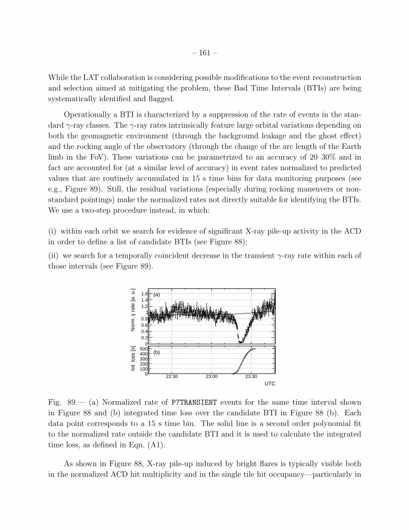
– 161 –

While the LAT collaboration is considering possible modifications to the event reconstruction

and selection aimed at mitigating the problem, these Bad Time Intervals (BTIs) are being

systematically identified and flagged.

Operationally a BTI is characterized by a suppression of the rate of events in the stan-

dard γ-ray classes. The γ-ray rates intrinsically feature large orbital variations depending on

both the geomagnetic environment (through the background leakage and the ghost effect)

and the rocking angle of the observatory (through the change of the arc length of the Earth

limb in the FoV). These variations can be parametrized to an accuracy of 20–30% and in

fact are accounted for (at a similar level of accuracy) in event rates normalized to predicted

values that are routinely accumulated in 15 s time bins for data monitoring purposes (see

e.g., Figure 89). Still, the residual variations (especially during rocking maneuvers or non-

standard pointings) make the normalized rates not directly suitable for identifying the BTIs.

We use a two-step procedure instead, in which:

(i) within each orbit we search for evidence of significant X-ray pile-up activity in the ACD

in order to define a list of candidate BTIs (see Figure 88);

(ii) we search for a temporally coincident decrease in the transient γ-ray rate within each of

those intervals (see Figure 89).

UTC

rat

e [a

. u.]

γN

orm

.

00.20.40.60.8

11.21.41.6 (a)

UTC22:30 23:00 23:30

Int.

loss

[s]

0100200300400500

(b)

Fig. 89.— (a) Normalized rate of P7TRANSIENT events for the same time interval shown

in Figure 88 and (b) integrated time loss over the candidate BTI in Figure 88 (b). Each

data point corresponds to a 15 s time bin. The solid line is a second order polynomial fit

to the normalized rate outside the candidate BTI and it is used to calculate the integrated

time loss, as defined in Eqn. (A1).

As shown in Figure 88, X-ray pile-up induced by bright flares is typically visible both

in the normalized ACD hit multiplicity and in the single tile hit occupancy—particularly in

– 162 –

tile 63, which is the largest tile on the +x side of the observatory (i.e., the side facing the

Sun). Though the correlation with the X-ray radiance measured by GOES is far from perfect

(with a zero-suppression threshold of ∼ 100 keV the ACD is sensitive to somewhat higher

energies than GOES), both quantities are good proxies for the increase in the X-ray flux.

Figure 89 (a) shows the corresponding large suppression of the normalized P7TRANSIENT rate

for the same solar flare. As shown in Figure 89 (b), by fitting this normalized rate outside

the candidate BTI it is also possible to define an integrated time loss Tloss corresponding to

a particular candidate BTI

Tloss =∑BTI

(fi − ri)∆t (A1)

(where fi and ri are the fitted and measured normalized rates in the i-th time bin, respec-

tively, and ∆t is the bin width, i.e., 15 s). Roughly speaking, if Tloss is larger than a few

minutes we will mark the relevant time interval as bad.

All LAT γ-ray data automatically have the DATA QUAL field in the spacecraft pointing

and live time history file (spacecraft file)16 set to 1 by the data processing system and are

immediately exported to the FSSC where they become publicly available. The potential for

BTIs is reviewed only after the fact. This is because such a high percentage of the LAT data

is good and making them publicly available as quickly as possible is a priority.

UTC

Sum

of B

TIs

[min

utes

]

0

100

200

300

400

500

600

2009 Jan 1 2010 Jan 1 2011 Jan 1 2012 Jan 1

Fig. 90.— Time history of the sum of BTIs induced by SFs. The sum of time intervals

marked as BAD as of March 2012 is ∼ 600 minutes (i.e., ∼ 10 hours).

For each flare the entire information available is reviewed manually and if there is a

significant loss of efficiency the corresponding time period is marked as BAD (specifically,

the DATA QUAL field is set to −1) and a new spacecraft file is generated with the appropriate

16 http://fermi.gsfc.nasa.gov/ssc/data/analysis/documentation/Cicerone/Cicerone Data/LAT Data Columns.html#SpacecraftFile

– 163 –

data quality flag in the corresponding 30 second time bins. This new file is then exported

to the FSSC and supersedes the original file. As of 2012 March the sum of time intervals

marked as BAD is ∼ 10 hours (Fig. 90).

– 164 –

B. LIST OF ACRONYMS AND ABBREVIATIONS

2FGL Fermi LAT Second Source Catalog . . . . . . . . . . . . . . . . . . . . . . . . . . . . . . . . . . . § 3.6.2

ACD LAT Anti-Coincidence Detector subsystem . . . . . . . . . . . . . . . . . . . . . . . . . . . . . § 2.1

AGN Active Galactic Nucleus . . . . . . . . . . . . . . . . . . . . . . . . . . . . . . . . . . . . . . . . . . . . . . § 3.6.2

BTI Bad Time Interval . . . . . . . . . . . . . . . . . . . . . . . . . . . . . . . . . . . . . . . . . . . . . . . . . . . . . . . § A

BSPR Blind Search Pattern Recognition . . . . . . . . . . . . . . . . . . . . . . . . . . . . . . . . . . . . . § 3.2.2

CAL LAT imaging Calorimeter subsystem. . . . . . . . . . . . . . . . . . . . . . . . . . . . . . . . . . . .§ 2.1

CNO Carbon, Nitrogen, Oxygen [CR species] . . . . . . . . . . . . . . . . . . . . . . . . . . . . . . . § 3.1.1

CPF Charged Particle in the Field of view analysis . . . . . . . . . . . . . . . . . . . . . . . . . § 3.3.5

CR Cosmic Ray . . . . . . . . . . . . . . . . . . . . . . . . . . . . . . . . . . . . . . . . . . . . . . . . . . . . . . . . . . . . . . § 1

CSPR Calorimeter-Seeded Pattern Recognition . . . . . . . . . . . . . . . . . . . . . . . . . . . . . . § 3.2.2

CT Classification Tree . . . . . . . . . . . . . . . . . . . . . . . . . . . . . . . . . . . . . . . . . . . . . . . . . . . . § 3.3.2

CU LAT Calibration Unit. . . . . . . . . . . . . . . . . . . . . . . . . . . . . . . . . . . . . . . . . . . . . . . . .§ 7.3.1

EGRET Energetic Gamma-Ray Experiment Telescope . . . . . . . . . . . . . . . . . . . . . . . . . § 2.1.3

Fermi Fermi Gamma-ray Space Telescope . . . . . . . . . . . . . . . . . . . . . . . . . . . . . . . . . . . . . . . § 1

FoV Field of view . . . . . . . . . . . . . . . . . . . . . . . . . . . . . . . . . . . . . . . . . . . . . . . . . . . . . . . . . . . . . § 1

FSSC Fermi Science Support Center . . . . . . . . . . . . . . . . . . . . . . . . . . . . . . . . . . . . . . . . . . . .§ 1

GRB Gamma-Ray Burst. . . . . . . . . . . . . . . . . . . . . . . . . . . . . . . . . . . . . . . . . . . . . . . . . . . .§ 3.4.1

GSI Gesellschaft fur SchwerIonenforschung . . . . . . . . . . . . . . . . . . . . . . . . . . . . . . . . § 7.3.1

IRF Instrument Response Function . . . . . . . . . . . . . . . . . . . . . . . . . . . . . . . . . . . . . . . . . . . § 1

ISOC Instrument Science Operations Center . . . . . . . . . . . . . . . . . . . . . . . . . . . . . . . . . . . . § 1

LAT Fermi Large Area Telescope . . . . . . . . . . . . . . . . . . . . . . . . . . . . . . . . . . . . . . . . . . . . . .§ 1

LH Maximum LikeliHood [energy estimation algorithm] . . . . . . . . . . . . . . . . . . .§ 3.2.1

MC Monte Carlo . . . . . . . . . . . . . . . . . . . . . . . . . . . . . . . . . . . . . . . . . . . . . . . . . . . . . . . . . . . . . § 1

MET Mission Elapsed Time . . . . . . . . . . . . . . . . . . . . . . . . . . . . . . . . . . . . . . . . . . . . . . . . . . . . § 6

MIP Minimum Ionizing Particle . . . . . . . . . . . . . . . . . . . . . . . . . . . . . . . . . . . . . . . . . . . .§ 2.1.1

PC Parametric correction [energy estimation algorithm] . . . . . . . . . . . . . . . . . . . § 3.2.1

p.e. photo-electron . . . . . . . . . . . . . . . . . . . . . . . . . . . . . . . . . . . . . . . . . . . . . . . . . . . . . . . . § 2.1.3

PMT PhotoMultiplier Tube . . . . . . . . . . . . . . . . . . . . . . . . . . . . . . . . . . . . . . . . . . . . . . . . .§ 2.1.3

PS CERN Proton Synchrotron . . . . . . . . . . . . . . . . . . . . . . . . . . . . . . . . . . . . . . . . . . . § 7.3.1

PSF Point-Spread Function . . . . . . . . . . . . . . . . . . . . . . . . . . . . . . . . . . . . . . . . . . . . . . . . . . . § 2

ROI Region of Interest . . . . . . . . . . . . . . . . . . . . . . . . . . . . . . . . . . . . . . . . . . . . . . . . . . . . . . . . § 6

SAA South Atlantic Anomaly . . . . . . . . . . . . . . . . . . . . . . . . . . . . . . . . . . . . . . . . . . . . . . . . § 2.2

SF Solar Flare . . . . . . . . . . . . . . . . . . . . . . . . . . . . . . . . . . . . . . . . . . . . . . . . . . . . . . . . . . . § 2.1.4

SP Shower Profile [energy estimation algorithm] . . . . . . . . . . . . . . . . . . . . . . . . . . § 3.2.1

SSD Silicon Strip Detector. . . . . . . . . . . . . . . . . . . . . . . . . . . . . . . . . . . . . . . . . . . . . . . . . . .§ 2.1

SPS CERN Super Proton Synchrotron . . . . . . . . . . . . . . . . . . . . . . . . . . . . . . . . . . . . . § 7.3.1

– 165 –

TKR LAT Tracker/converter subsystem . . . . . . . . . . . . . . . . . . . . . . . . . . . . . . . . . . . . . . § 2.1

– 166 –

C. NOTATION

Aeff Effective area . . . . . . . . . . . . . . . . . . . . . . . . . . . . . . . . . . . . . . . . . . . . . . . . . . . . . . . . . . . . § 1

B, Ba, Bidx Bracketing functions for Aeff . . . . . . . . . . . . . . . . . . . . . . . . . . . . . . . . . . . . . . . . . . § 5.7.1

B, B68, Br Bracketing functions for the PSF . . . . . . . . . . . . . . . . . . . . . . . . . . . . . . . . . . . . . § 6.5.1

b Bias in the energy scale. . . . . . . . . . . . . . . . . . . . . . . . . . . . . . . . . . . . . . . . . . . . . . . . .§ 7.4

b Distribution of CR background events mischaracterized as γ rays . . . . . . . § 4.6

(l, b) Galactic coordinates. . . . . . . . . . . . . . . . . . . . . . . . . . . . . . . . . . . . . . . . . . . . . . . . . . . . . . . . .

C68 68% containment radius of the PSF . . . . . . . . . . . . . . . . . . . . . . . . . . . . . . . . . . . § 3.3.3

Ci Actual containment at a given nominal containment radius. . . . . . . . . . . .§ 6.5.3

ci Generic fitting constants . . . . . . . . . . . . . . . . . . . . . . . . . . . . . . . . . . . . . . . . . . . . . . . . . . . .

D Energy dispersion parametrization. . . . . . . . . . . . . . . . . . . . . . . . . . . . . . . . . . . . . . . .§ 1

di Normalized deviations . . . . . . . . . . . . . . . . . . . . . . . . . . . . . . . . . . . . . . . . . . . . . . . . § 5.6.2

E Energy . . . . . . . . . . . . . . . . . . . . . . . . . . . . . . . . . . . . . . . . . . . . . . . . . . . . . . . . . . . . . . . . . . . § 1

F25 Integral counts flux between 100 MeV and 100 GeV. . . . . . . . . . . . . . . . . . .§ 5.7.1

Fl Live time fraction. . . . . . . . . . . . . . . . . . . . . . . . . . . . . . . . . . . . . . . . . . . . . . . . . . . . .§ 5.2.2

fcore Fraction of counts in the “core” King function for the PSF . . . . . . . . . . . . § 6.1.1

K King function [used to model the PSF] . . . . . . . . . . . . . . . . . . . . . . . . . . . . . . . .§ 6.1.1

k Aeff bracketing smoothing constant . . . . . . . . . . . . . . . . . . . . . . . . . . . . . . . . . . . § 5.7.1

L McIlwain L . . . . . . . . . . . . . . . . . . . . . . . . . . . . . . . . . . . . . . . . . . . . . . . . . . . . . . . . . . . § 2.5.1

Lext Log likelihood for fit as an extended source . . . . . . . . . . . . . . . . . . . . . . . . . . . § 6.5.2

Lpt Log likelihood for fit as an point source . . . . . . . . . . . . . . . . . . . . . . . . . . . . . . . § 6.5.2

M Predicted counts distribution of γ rays. . . . . . . . . . . . . . . . . . . . . . . . . . . . . . . . . . . . § 1

N0 Flux prefactor . . . . . . . . . . . . . . . . . . . . . . . . . . . . . . . . . . . . . . . . . . . . . . . . . . . . . . . . § 5.7.1

Ngen Number of events generated [when making IRFs] . . . . . . . . . . . . . . . . . . . . . . . § 5.1

n Number of observed counts . . . . . . . . . . . . . . . . . . . . . . . . . . . . . . . . . . . . . . . . . . . . . § 5.1

n Expected counts . . . . . . . . . . . . . . . . . . . . . . . . . . . . . . . . . . . . . . . . . . . . . . . . . . . . . . § 5.6.3

P Point-spread function parametrization . . . . . . . . . . . . . . . . . . . . . . . . . . . . . . . . . . . . § 1

P PSF averaged over the observing profile. . . . . . . . . . . . . . . . . . . . . . . . . . . . . . . . .§ 6.1

Pall Combined estimator that the event is a γ ray . . . . . . . . . . . . . . . . . . . . . . . . . § 3.3.8

PCAL Estimator that the event is a γ ray, based on the CAL topology analysis§ 3.3.7

Pcore Estimator of the quality of direction measurement . . . . . . . . . . . . . . . . . . . . § 3.3.3

PCPF Estimator that the event is a γ ray, based on the CPF analysis . . . . . . . .§ 3.3.5

PE Estimate of the quality of energy measurement . . . . . . . . . . . . . . . . . . . . . . . .§ 3.3.2

PTKR Estimator that the event is a γ ray, based on the TKR topology analysis§ 3.3.6

p Incident direction in celestial reference frame . . . . . . . . . . . . . . . . . . . . . . . . . . . . . § 1

R Rando function, used to model the energy dispersion . . . . . . . . . . . . . . . . . . § 7.1.2

R Ratio of efficiency for flight data to MC simulated data . . . . . . . . . . . . . . . . . § 5.3

– 167 –

R68 68% containment radius of the PSF (also R95) . . . . . . . . . . . . . . . . . . . . . . . . § 6.2.3

r Ratio of size of signal region to background region . . . . . . . . . . . . . . . . . . . . § 5.3.1

r Ratio of 95% to 68% containment radii of the PSF . . . . . . . . . . . . . . . . . . . . § 6.5.1

rni Normalized residuals . . . . . . . . . . . . . . . . . . . . . . . . . . . . . . . . . . . . . . . . . . . . . . . . . . . . § 54

rfi Fractional residuals . . . . . . . . . . . . . . . . . . . . . . . . . . . . . . . . . . . . . . . . . . . . . . . . . . . . . § 55

S Source distribution of γ rays. . . . . . . . . . . . . . . . . . . . . . . . . . . . . . . . . . . . . . . . . . . . . . § 1

S25 Integral energy flux between 100 MeV and 100 GeV. . . . . . . . . . . . . . . . . . .§ 5.7.1

SD Energy dispersion scaling function . . . . . . . . . . . . . . . . . . . . . . . . . . . . . . . . . . . . § 7.1.1

SP PSF scaling function . . . . . . . . . . . . . . . . . . . . . . . . . . . . . . . . . . . . . . . . . . . . . . . . . . . . . § 1

s Light yield scaling function. . . . . . . . . . . . . . . . . . . . . . . . . . . . . . . . . . . . . . . . . . . . . .§ 53

TSext Test statistic for source extension . . . . . . . . . . . . . . . . . . . . . . . . . . . . . . . . . . . . . . . § 46

tobs Observing time. . . . . . . . . . . . . . . . . . . . . . . . . . . . . . . . . . . . . . . . . . . . . . . . . . . . . . . . . . .§ 1

v Incident direction in the LAT frame . . . . . . . . . . . . . . . . . . . . . . . . . . . . . . . . . . . . . . § 1

x Scaled angular deviation . . . . . . . . . . . . . . . . . . . . . . . . . . . . . . . . . . . . . . . . . . . . . . § 6.1.1

x Scaled energy redistribution. . . . . . . . . . . . . . . . . . . . . . . . . . . . . . . . . . . . . . . . . . .§ 7.1.1

x Rando function break point . . . . . . . . . . . . . . . . . . . . . . . . . . . . . . . . . . . . . . . . . . . § 7.1.2

α Spectral Index in “log-parabola” model . . . . . . . . . . . . . . . . . . . . . . . . . . . . . . . § 5.7.1

β Spectral curvature parameter in “log-parabola” model . . . . . . . . . . . . . . . . § 5.7.1

β PSF energy scaling index . . . . . . . . . . . . . . . . . . . . . . . . . . . . . . . . . . . . . . . . . . . . . § 6.1.1

Γ Spectral index . . . . . . . . . . . . . . . . . . . . . . . . . . . . . . . . . . . . . . . . . . . . . . . . . . . . . . . . § 5.7.1

γ King function “tail” parameter . . . . . . . . . . . . . . . . . . . . . . . . . . . . . . . . . . . . . . . § 6.1.1

γ Rando function “tail” parameter . . . . . . . . . . . . . . . . . . . . . . . . . . . . . . . . . . . . . . § 7.1.2

ε Relative uncertainty in Aeff . . . . . . . . . . . . . . . . . . . . . . . . . . . . . . . . . . . . . . . . . . . . . .§ 27

ηdata, ηmc Efficiencies for flight data and MC simulated data. . . . . . . . . . . . . . . . . . . . .§ 5.3.1

(θ, φ) Polar angle and azimuth of the incident direction in the LAT frame . . . . . § 2.1

(θz, φz) Zenith angle and Earth azimuth angle . . . . . . . . . . . . . . . . . . . . . . . . . . . . . . . . . . § 2.2

θ, φ Unit vector along local θ,φ directions . . . . . . . . . . . . . . . . . . . . . . . . . . . . . . . . . . . . § 42

ξ Folded φ . . . . . . . . . . . . . . . . . . . . . . . . . . . . . . . . . . . . . . . . . . . . . . . . . . . . . . . . . . . . . .§ 5.2.3

σ King function width parameter . . . . . . . . . . . . . . . . . . . . . . . . . . . . . . . . . . . . . . . § 6.1.1

σ Rando function width parameter . . . . . . . . . . . . . . . . . . . . . . . . . . . . . . . . . . . . . .§ 7.1.2

τn Correlation metric . . . . . . . . . . . . . . . . . . . . . . . . . . . . . . . . . . . . . . . . . . . . . . . . . . . . § 5.6.2

– 168 –

REFERENCES

Abdo, A. A., et al. 2009a, Phys. Rev. D, 80, 122004

—. 2009b, Phys. Rev. D, 80, 122004

—. 2009c, ApJ, 696, 1084

—. 2009d, ApJ, 707, 580

—. 2009e, Physical Review Letters, 102, 181101

—. 2009f, Astroparticle Physics, 32, 193

—. 2010a, ApJS, 188, 405

—. 2010b, ApJ, 708, 1254

—. 2010c, Physical Review Letters, 104, 091302

—. 2010d, ApJ, 720, 272

—. 2010e, ApJ, 712, 459

—. 2010f, Physical Review Letters, 104, 101101

—. 2010g, ApJ, 716, 30

—. 2010h, ApJ, 713, 154

Ackermann, M., et al. 2010a, Phys. Rev. D, 82, 092004

—. 2010b, Phys. Rev. D, 82, 092004

—. 2012a, ApJ, 745, 144

—. 2012b, ApJ, 750, 3

—. 2012c, Astroparticle Physics, 35, 346

—. 2012d, Physical Review Letters, 108, 011103

Ackermann, M., et al. 2012, in preparation

Agostinelli, S., et al. 2003, Nucl. Instrum. Meth., A506, 250

Arnaud, K. A. 1996, ASP Conf. Series, 101, 17

– 169 –

Atwood, W. B., et al. 2007, Astroparticle Physics, 28, 422

—. 2009, ApJ, 697, 1071

Baldini, L., et al. 2007, in American Institute of Physics Conference Series, Vol. 921, The

First GLAST Symposium, ed. S. Ritz, P. Michelson, & C. A. Meegan, 190–204

Breiman, L. 1996, Machine Learning, 24, 123, 10.1007/BF00058655

Breiman, L., Friedman, J., Olshen, R., & Stone, C. 1984, Classification and Regression Trees

(New York: Chapman & Hall), 358

D’Agostini, G. 1995, Nuclear Instruments and Methods in Physics Research Section A:

Accelerators, Spectrometers, Detectors and Associated Equipment, 362, 487

Efron, B., & Tibshirani, R. 1993, An Introduction to the Bootstrap (Boca Raton, FL:

Chapman & Hall/CRC)

Esposito, J. A., et al. 1999, ApJS, 123, 203

Finlay, C. C., et al. 2010, Geophysical Journal International, 183, 1216

Fruhwirth, R. 1987, Nucl.Instrum.Meth., A262, 444

Grove, J. E., & Johnson, N. 2010, Proc. SPIE, 7732

Hobbs, G. B., Edwards, R. T., & Manchester, R. N. 2006, MNRAS, 369, 655

Kalman, R. E. 1960, Transactions of the ASME–Journal of Basic Engineering, 82, 35

King, I. 1962, AJ, 67, 471

Kirsch, M. G. F., et al. 2004, in Society of Photo-Optical Instrumentation Engineers (SPIE)

Conference Series, Vol. 5488, Society of Photo-Optical Instrumentation Engineers

(SPIE) Conference Series, ed. G. Hasinger & M. J. L. Turner, 103–114

Lande, J., et al. 2012, arXiv:1207.0027

Lee, H., et al. 2011, ApJ, 731, 126

Lott, B., et al. 2006, Nuclear Instruments and Methods in Physics Research Section A:

Accelerators, Spectrometers, Detectors and Associated Equipment, 560, 395

Mattox, J. R., et al. 1996, ApJ, 461, 396

– 170 –

Mizuno, T., Kamae, T., Godfrey, G., Handa, T., Thompson, D. J., Lauben, D., Fukazawa,

Y., & Ozaki, M. 2004, ApJ, 614, 1113

Moiseev, A. A., Hartman, R. C., Ormes, J. F., Thompson, D. J., Amato, M. J., Johnson,

T. E., Segal, K. N., & Sheppard, D. A. 2007, Astroparticle Physics, 27, 339

Moskalenko, I. V., & Porter, T. A. 2007, ApJ, 670, 1467

Nolan, P. L., et al. 2012, ApJS, 199, 31

Pelassa, V., Preece, R., Piron, F., Omodei, N., Guiriec, S., Fermi LAT, f. t., & GBM

collaborations. 2010, arXiv:1002.2617

Rando, R., & the Fermi LAT Collaboration. 2009, arXiv:0907.0626

Read, A. M., Rosen, S. R., Saxton, R. D., & Ramirez, J. 2011, A&A, 534, A34

Rochester, L., Usher, T., Johnson, R. P., & Atwood, B. 2010, arXiv:1001.5005

Smart, D. F., & Shea, M. A. 2005, Advances in Space Research, 36, 2012

Smith, D. A., et al. 2008, A&A, 492, 923

Student. 1908, Biometrika, 6, 1

Walt, M. 2005, Introduction to Geomagnetically Trapped Radiation, Cambridge Atmo-

spheric and Space Science Series (Cambridge University Press)

Weltevrede, P., et al. 2010, Publications of the Astronomical Society of Australia, 27, 64

This preprint was prepared with the AAS LATEX macros v5.2.

THE FERMI LARGE AREA TELESCOPE ON ORBIT: EVENT CLASSIFICATION, INSTRUMENT RESPONSE FUNCTIONS, AND...

Documents

Transcript of THE FERMI LARGE AREA TELESCOPE ON ORBIT: EVENT CLASSIFICATION, INSTRUMENT RESPONSE FUNCTIONS, AND...