University of South FloridaScholar Commons

Graduate Theses and Dissertations Graduate School

4-1-2004

Real Time Digital Signal Processing AdaptiveFilters for Correlated Noise Reduction in RingLaser Gyro Inertial SystemsDavid A. DohenyUniversity of South Florida

Follow this and additional works at: https://scholarcommons.usf.edu/etd

Part of the American Studies Commons

This Thesis is brought to you for free and open access by the Graduate School at Scholar Commons. It has been accepted for inclusion in GraduateTheses and Dissertations by an authorized administrator of Scholar Commons. For more information, please contact scholarcommons@usf.edu.

Scholar Commons CitationDoheny, David A., "Real Time Digital Signal Processing Adaptive Filters for Correlated Noise Reduction in Ring Laser Gyro InertialSystems" (2004). Graduate Theses and Dissertations.https://scholarcommons.usf.edu/etd/1015

Real Time Digital Signal Processing

Adaptive Filters for Correlated Noise Reduction in Ring Laser Gyro

Inertial Systems

by

David A. Doheny

A thesis submitted in partial fulfillment of the requirements for the degree of

Master of Science Electrical Engineering Department of Electrical Engineering

College of Engineering University of South Florida

Major Professor: Ravi Sankar, Ph.D. Kenneth A. Buckle, Ph.D.

David Snider, Ph.D.

Date of Approval: April 1, 2004

Keywords: Mean, Recursive, Least, Square, Estimator

© Copyright 2004, David A. Doheny

Dedication

To Terri, Seth and Aaron My life’s inspiration…

Though the road is long and fraught with peril, without a start, there is no finish.…

Acknowledgments It is imperative that government, industry and academia find opportunities for close, prolonged associations to insure scientific exchange of technical ideas and solutions. This work was supported in part by grants from Honeywell International Academic Research Program, The Florida Space Grant Consortium and The Florida Legislature Grant Program for the I-4 High Tech Corridor Initiative. With support and guidance of Dr. Sankar, Professor, Electrical Engineering, University of South Florida, the author presents this thesis, Real Time Digital Signal Processing Adaptive Filters for Correlated Noise Reduction in Ring Laser Gyro Inertial Systems. No work is authored alone. From my first shoe tie to the last stroke of ivory in this writing the encouragement, to ponder, to conjecture, to learn, to formulate and to validate with support from a collage of individuals throughout my life has resulted in this work. There are infinite contributions though the years from family, friends, and colleagues. Thank-you all.

To Dr. Ravi Sankar, a heartfelt thank-you for your patience, scholastic enthusiasm and academic expertise. I am one of many that you have instilled the craving and excitement of science. You will forever be a part of us all! To my countless teachers, professors and mentors you have my sincere appreciation. To my colleagues who listened to my endless ramblings, I extend a hearty thank-you.

i

Table of Contents

List of Tables iii

List of Figures iv

Abstract viii

Chapter One – Introduction 1 1.1 Definition 1 1.2 Applications 1 1.3 Basic Properties 1 1.4 Adaptive Noise Cancellation Algorithms 2 1.5 Description and Organization of Thesis 3 Chapter Two – Adaptive Signal Processing for Ring Laser Gyros 4 2.1 Background 4 2.2 Motivation for Real Time Adaptive Filters in RLG Based Systems 5 2.3 Algorithm Development 5 2.3.1 LMS Algorithm 6 2.3.2 Normalizing LMS Algorithm 10 2.3.3 LMS Full Matrix Algorithm 11 2.3.4 Recursive Least Squares Algorithm 13 2.3.5 Joint Process Gradient Estimator Algorithm 17 2.4 Second System Analysis 20 2.5 Convergence and Stability 20 2.6 Computational Complexity 21 2.7 Covariance Analysis of Algorithm Types 22 2.8 Adaptive Algorithm Summary 27

Chapter Three – Considerations For Hardware Development 29 3.1 Development 29 3.2 A Query of Tool suites 29 3.2.1 Mentor Graphics Monet 30 3.2.2 Synopsys COSSAP 31 3.2.3 Frontier Design Digital Signal Processing Station 32

ii

Chapter Four – Algorithm Implementation 35 4.1 Direction 35 4.2 Algorithm Development Using DSP Station 35 4.3 Tool Independent Development 38 4.4 VHDL and Functional Simulation 38 4.5 ASIC Selection 39 4.6 Synthesis 40 4.7 Place and Route 41 4.8 Worst Case Timing 41 4.9 Post Route Simulation 41 4.10 Test Bench for Simulation and Validation 42 4.11 VHDL Architecture 44 4.12 Scaling 48 4.13 Results and Analysis 48

Chapter Five – Other Considerations 50 5.1 Finite Word Length Effects 50 5.1.1 Overflow 51 5.1.2 Quantization 51 5.2 Evaluation of Overflow and Quantization of LMS Algorithm 51 5.3 Scaling Optimization 54

Chapter Six – Conclusion and Future Research 56 6.1 Conclusion 56 6.2 Future Research 57

References 58 Bibliography 59 Appendices 60 Appendix A: Algorithm Figures 61 Appendix B: MathCAD Scripts 113 Appendix C: Sample Listing of MATLAB Program 130 Appendix D: VHDL Listings 154 Appendix E: Field Programmable Gate Array Pin List and Timing 173

iii

List of Tables

Table 2.1 Effects of µ on Convergence 20 Table 2.2 Trade-offs in Adaptive Filter Algorithms 22 Table 2.3 Statistical Measurements for System #1 and #2 Input Parameters 24 Table 2.4 Statistical Parameter Acronym Definitions I 25 Table 2.5 Statistical Measurements for System #1 26 Table 2.6 Statistical Measurements for System #2 26 Table 2.7 Algorithm Acronym Definitions 27 Table 2.8 Statistical Parameter Acronym Definitions II 27 Table 4.1 Worst Case Analyses Summary 41 Table 4.2 MATLAB Versus VHDL Output 49

iv

List of Figures Figure 2.1 Single Channel Least Mean Square Adaptive Filter 6 Figure 2.2 Full Matrix Least Mean Square Adaptive Filter 12 Figure 2.3 Single Channel Recursive Least Square Adaptive Filter 13 Figure 2.4 Full Matrix Recursive Least Square Adaptive Filter 16 Figure 2.5 Single Channel Joint Process Gradient Estimator 19 Figure 2.6 Full Matrix Joint Process Gradient Estimator 19 Figure 3.1 Monet Algorithm/Architecture Design Environment 31 Figure 3.2 COSSAP Digital Signal Processing (DSP) Design Environment 32 Figure 3.3 Frontier Design Digital Signal Processing Station Platform 33 Figure 4.1 Schematic Representation of Single Channel Real Time LMS Filter 35 Figure 4.2 Operational LMS Input/Output Trace History 36 Figure 4.3 Data Analysis of RLG and LMS Filter Output 37 Figure 4.4 Platform and Test Bench Environment 43 Figure 4.5 Top Level Data Flow/Schematic Diagram of VHDL LMS Algorithm 45 Figure 4.6 LMS State Machine Sequence Diagram 47 Figure 5.1 Finite Word Length Effects 50 Figure A1 PSD of Correlated Gyro Readout Noise 61 Figure A2 Cumulative PSD-Correlated Gyro Readout Noise 61 Figure A3 PSD of Gyro Dither Pick Off 62 Figure A4 Cumulative PSD of Gyro Dither Pick Off 62 Figure A5 LMS Performance Surface 63 Figure A6 Gyro X,Y, Z LMS Learning Curve 63 Figure A7 LMS G1 Gain Values 64 Figure A8 LMS G1 Gains 64 Figure A9 LMS G2 Gain Values 65 Figure A10 LMS G2 Gains 65 Figure A11 LMS G1 Gain Versus G2 Gain Curves 66 Figure A12 Performance Surface Using Actual Gains and MSE X Channel 66 Figure A13 LMS Gains-Vs-MSE 67 Figure A14 LMS G1 Gains Versus Uncorrelated Readout Noise 67 Figure A15 LMS PSD-Stripped Delta Theta Uncorrelated Readout Noise 68 Figure A16 LMS CPSD-Stripped Delta Theta Uncorrelated Readout Noise 68 Figure A17 Full Matrix LMS G1 Gain Values 69 Figure A18 Full Matrix LMS G1 Gains 69 Figure A19 Full Matrix LMS G2 Gain Values 70 Figure A20 Full Matrix LMS G2 Gains 70

v

Figure A21 FMLMS PSD – Stripped Delta Theta Uncorrelated Readout Noise 71 Figure A22 FMLMS CPSD – Stripped Delta Theta Uncorrelated Readout Noise 71 Figure A23 Normalized LMS G1 Gain Values 72 Figure A24 Normalized LMS G1 Gains 72 Figure A25 Normalized LMS G2 Gain Values 73 Figure A26 Normalized LMS G2 Gains 73 Figure A27 NLMS PSD-Stripped Delta Theta Uncorrelated Readout Noise 74 Figure A28 NLMS CPSD-Stripped Delta Theta Uncorrelated Readout Noise 74 Figure A29 RLS W0 Weight Values 75 Figure A30 RLS W0 Weight Values 75 Figure A31 RLS W1 Weight Values 76 Figure A32 RLS W1 Weight Values 76 Figure A33 RLS Main Channel Uncorrelated Delta Theta PSD 77 Figure A34 RLS Main Channel Uncorrelated Delta Theta CPSD 77 Figure A35 Full Matrix RLS W0 Gain Values 78 Figure A36 Full Matrix RLS W0 Gains 78 Figure A37 Full Matrix RLS W1 Gain Values 79 Figure A38 Full Matrix RLS W1 Gains 79 Figure A39 Full Matrix RLS PSD-Stripped Delta Theta Uncorrelated 80 Readout Noise Figure A40 Full Matrix RLS CPSD-Stripped Delta Theta Uncorrelated 80 Readout Noise Figure A41 JPGE Gains 81 Figure A42 JPGE Gamma Values 81 Figure A43 JPGE – PSD Uncorrelated Gyro Readout Noise E(2) 82 Figure A44 JPGE – CPSD Uncorrelated Gyro Readout Noise E(2) 82 Figure A45 JPGE – PSD Uncorrelated Gyro Readout Noise E(3) 83 Figure A46 JPGE – CPSD Uncorrelated Gyro Readout Noise E(3) 83 Figure A47 FMJPGE Gains 84 Figure A48 FMJPGE Gamma Values 84 Figure A49 FMJPGE – PSD Uncorrelated Gyro Readout Noise E(2) 85 Figure A50 FMJPGE – CPSD Uncorrelated Gyro Readout Noise E(2) 85 Figure A51 FMJPGE – PSD Uncorrelated Gyro Readout Noise E(3) 86 Figure A52 FMJPGE – CPSD Uncorrelated Gyro Readout Noise E(3) 86 Figure A53 LMS – Variance Correlated Readout Noise 87 Figure A54 LMS – Variance Dither Pick Off 87 Figure A55 LMS – Covariance Correlated Readout Noise to DPO 88 Figure A56 LMS – Correlation Coefficient Correlated Readout Noise to DPO 88 Figure A57 LMS – Variance Uncorrelated Readout Noise 89 Figure A58 LMS – Covariance Uncorrelated Readout Noise to Dither Pick Off 89 Figure A59 LMS – Correlation Coefficient Uncorrelated Readout Noise to DPO 90 Figure A60 FMLMS – Variance Uncorrelated Readout Noise 90 Figure A61 FMLMS – Covariance Uncorrelated Readout Noise to DPO 91 Figure A62 FMLMS – Correlation Coefficient Un-correlated Readout 91 Figure A63 NLMS – Variance Uncorrelated Readout Noise 92

vi

Figure A64 NLMS – Covariance Uncorrelated Readout Noise to DPO 92 Figure A65 NLMS – Correlation Coefficient Uncorrelated Readout Noise to DPO 93 Figure A66 Main Channel RLS – Variance Uncorrelated Readout Noise to DPO 93 Figure A67 Main Channel RLS – Covariance Uncorrelated Readout to DPO 94 Figure A68 Main Channel RLS – Correlation Coefficient Uncorrelated Gyro 94 Readout Noise to Pick Off Figure A69 Full Matrix RLS – Variance Uncorrelated Readout Noise 95 Figure A70 Full Matrix RLS – Covariance Uncorrelated Readout Noise to DPO 95 Figure A71 FMRLS-Correlation Coefficient Uncorrelated Gyro 96 Readout Noise to DPO Figure A72 JPGE – Variance Uncorrelated Readout Noise 96 Figure A73 JPGE – Covariance Uncorrelated Readout Noise to DPO 97 Figure A74 JPGE-Correlation Coefficient Uncorrelated Readout Noise to DPO 97 Figure A75 FMJPGE – Variance Uncorrelated Readout Noise 98 Figure A76 FMJPGE – Covariance Uncorrelated Readout Noise to DPO 98 Figure A77 FMJPGE – Correlation Coefficient Uncorrelated Readout 99 Noise to DPO Figure A78 Isolated System LMS PSD – Delta Theta-Correlated Readout Noise 99 Figure A79 Isolated System LMS CPSD – Delta Theta-Correlated Readout Noise 100 Figure A80 Isolated System LMS PSD – Delta Dither Pick Off 100 Figure A81 Isolated System LMS CPSD – Delta Dither Pick Off 101 Figure A82 Isolated System LMS G1 Gain Values 101 Figure A83 Isolated System LMS G2 Gains 102 Figure A84 Isolated System LMS G2 Gain Values 102 Figure A85 Isolated System LMS G2 Gains 103 Figure A86 Isolated System LMS PSD – Stripped Delta Theta Uncorrelated 103 Readout Noise Figure A87 Isolated System LMS CPSD – Stripped Delta Theta Uncorrelated 104 Readout Noise Figure A88 Isolated System – Variance Correlated Readout Noise 104 Figure A89 Isolated System – Variance Dither Pick Off 105 Figure A90 Isolated System LMS – Covariance Correlated Readout 105 Noise to DPO Figure A91 Isolated System JPGE – Correlation Coefficient Correlated 106

Readout Noise to DPO Figure A92 Isolated System LMS – Variance Uncorrelated Readout Noise 106 Figure A93 Isolated System LMS – Covariance Uncorrelated 107

Readout Noise to DPO Figure A94 Isolated System LMS – Correlation Coefficient Uncorrelated 107 Readout Noise Figure A95 Isolated System FMLMS G1 Gain Values 108 Figure A96 Isolated System FMLMS G1 Gain Values 108 Figure A97 Isolated System FMLMS G2 Gain Values 109 Figure A98 Isolated System FMLMS G2 Gain Values 109 Figure A99 Isolated System FMLMS PSD – Stripped Delta Theta Uncorrelated 110

vii

Readout Noise Figure A100 Isolated System FMLMS CPSD – Stripped Delta Theta Uncorrelated 110 Readout Noise Figure A101 Isolated System FMLMS – Variance Uncorrelated Readout Noise 111 Figure A102 Isolated System FMLMS – Covariance Uncorrelated Readout Noise 111 to Dither Pick Off Figure A103 Isolated System FMLMS – Correlation Coefficient Uncorrelated 112 Readout Noise To DPO Figure B1 PSD Raw Xgyro 113 Figure B2 CPSD Raw Xgyro 113 Figure B3 PSD Raw Xdpo 114 Figure B4 CPSD Raw Xdpo 114 Figure B5 VHDL LMS Output Xgyro 116 Figure B6 VHDL Adaptive Gain h0 116 Figure B7 VHDL Adaptive Gain h1 116 Figure B8 VHDL PSD Filtered Xgyro 117 Figure B9 VHDL CPSD Filtered Xgyro 117 Figure B10 MATLAB LMS Output Xgyro 118 Figure B11 MATLAB Adaptive Gain h0 118 Figure B12 MATLAB Adaptive Gain h1 118 Figure B13 MATLAB PSD Filtered Xgyro 119 Figure B14 MATLAB CPSD Filtered Xgyro 119 Figure B15 Quadratic Error Surface 127

viii

Real Time Digital Signal Processing Adaptive Filters For Correlated Noise Reduction in Ring Laser Gyro

Inertial Systems

David A. Doheny

ABSTRACT

Existing opportunities in advanced interceptor, satellite guidance and aircraft

navigation technologies, requiring higher signal processing speeds and lower noise

environments, are demanding Ring Laser Gyro (RLG) based Inertial Systems to reduce

initialization and operational data latency as well as correlated noise magnitudes.

Existing signal processing algorithms are often less than optimal when considering these

requirements. Advancements in micro-electronic processes have made Application

Specific Integrated Circuits (ASIC) a fundamental building block for system

implementation when considering higher- level signal processing algorithms.

Research of real time adaptive signal processing algorithms embedded in ASICs

for use in RLG based inertial systems will help to understand the trade-off in finite

register length effects to correlated noise magnitude, organizational complexity,

computational efficiency, rate of convergence, and numerical stability. Adaptive filter

structures selected will directly affect meeting inertial system performance requirements

for data latency, residual noise budgets and real time processing throughput. Research in

ix

this area will help to target specific adaptive noise cancellation algorithms for RLG based

inertial systems in a variety of military and commercial space applications.

Of particular significance is an attempt to identify an algorithm embedded in an ASIC

that will reduce the correlated noise components to the theoretical limit of the RLG

sensor itself. This would support a variety of applications for the low noise space

environments that the RLG based inertial systems are beginning to find promise for such

as advanced military interceptor technology and commercial space satellite navigation,

guidance and control systems.

1

Chapter One

Introduction 1.1 Definition

Adapt. v.t., To make suitable to or fit for a specific use or situation. (Webster's Revised Unabridged Dictionary, © 1996, 1998 MICRA, Inc.)

The root word for adaptive is adapt. Early definitions for the word adapt, listed in a variety of dictionaries, almost exclusively target environmental (physiological, psychological, and sociological) adaptation. As man continues his progress in developing mechanical and electrical technologies, the definition becomes more generic, covering not only the biological but also the tools of his development and use. 1.2 Applications

With the advancement of microelectronics, allowing for the development of extremely small application specific integrated circuits operating at increasingly higher speeds, adaptive signal processing algorithms have become more prevalent in today’s technology. Adaptive Noise Cancellation (ANC) algorithms have been used extensively in audio, medical and communications. Examples are echo cancellers (filters) in telephone equipment, system identification in communications networks, heart component suppression in bio-medical electrocardiograph monitors. Adaptive quantization has found promise in areas of speech signal processing allowing for adaptive dynamic range and quantization levels. Adaptive control algorithms are used widely in digital control systems such as Automatic Gain Control (AGC). Adaptive beam formers are used extensively in radar, sonar and seismology. As we continue to understand the innate environmental adaptation that surrounds us, so too will we adapt our understanding to processes that enhance our everyday lives. 1.3 Basic Properties

The “adapt” definition listed above, does not alone dictate the properties of an adaptive process. An adaptive process can be open or closed. An adaptive process can be self-controlling. In some instances, the process can exhibit artificial intelligence by learning. These processes can be recoverable. They incorporate both linear and non-

2

linear components. They can be time variant and time invariant. In general, adaptive processes allow for a wide variety of attributes to be part of their characteristics.

Fixed design processes assume that the input to output relationships are well defined. The non-adaptive design approach assumes bounded attributes (e.g. gain and phase margins) insuring a transfer function of the input to a known output based on characteristics ideally selected for the application. Germane to the adaptive processes is the ability to self adjust. Adaptive processes allow for a continuous adjustment of the transfer function properties based on some error criteria. As such, adaptive processes differ from fixed design processes in that they are inherently non- linear unless held fixed once the error criteria has been met. As well, adaptive processes operate to optimize, through adjustment, their outputs by controlling to some predefined value.

Systems, linear and non- linear, fixed or adaptive, are classified as open loop or closed loop. If the system takes a component of the output and feeds it back into the system, the system is considered closed loop. Adaptive systems can operate in either open or closed loop mode. There is a subtle difference to the definition of the open loop system for an adaptive process. All adaptive systems require knowledge of specific performance parameters to adapt or adjust. An open loop adaptive system may be a system where the output data is collected and analyzed in an offline process of the adaptive process itself. The results of the analysis are then feedback manually to the selected adjustment criteria so that adaptation to performance requirements will occur. In a closed loop adaptive system, the analysis would be a component of the process and the adjustment to the performance parameters would occur automatically in order to optimize it’s output. 1.4 Adaptive Noise Cancellation Algorithms

While adaptive processes can be applied to a plethora of mechanical and electrical applications. The focus of this writing is cancellation of correlated noise. As such adaptive cancellation algorithms have been researched. Such algorithms include the Least Mean Square (LMS), Recursive Least Square (RLS) and Joint Process Gradient Estimator lattice (JPGE) Algorithms. In each of these, the adaptive processes are closed loop with the adjustments made to minimize the mean squared error criteria.

All of these algorithms can be traced to early work by such mathematicians as Gram, Schmidt, Wiener, Woodrow, and Hopf. Grahm and Schmidt’s development of the normal equations, Wieners and Hopf’s adaptation of the Grahm-Schmidt orthogonalization to estimation theory and Woodrow-Hopfs work toward the development of the LMS algorithm all set a foundation for development of the Normalized LMS, RLS and JPGE.

3

1.5 Description and Organization of Thesis

The thesis main objective was to research, develop and code real time Adaptive Digital Signal Processing, ADSP, Filters for use in Ring Laser Gyro, RLG, based Inertial Systems to reduce correlated noise components. Trade-off in the filters structures, computation complexity, convergence, finite register length effects and effectiveness has been evaluated. Comparison of a Least Mean Square MATLAB model and an Application Specific Integrated Circuit, ASIC, implementation have been evaluated.

Each of the real time adaptive digital signal processing algorithms was developed

for a diagonal and full matrix implementation. The diagonal algorithm implementations focus on reduction of correlated noise in each of the RLGs X, Y and Z channel. These are common art formulations of the classical filter structures. The full matrix implementation extends the common art to eliminate cross-coupled noise from channel to channel. There are also two RLG based systems that the algorithms were executed. One of the systems does not incorporate Mechanical Vibration Isolation, MVI, between the Inertial Sensor Assembly on which the RLGs are mounted and the systems chassis. The other system does incorporate MVIs.

Chapter One provides a definition of adaptation, reviews applications and basic

properties for adaptive filters and outlines the thesis. Chapter Two reviews the basic operation of the RLG based Inertial Systems, the motivation to use and development diagonal and full matrix ADSP algorithms for correlated noise reduction and trade off in performance parameters for the algorithm types. Chapter Three presents considerations when targeting an ADSP for hardware implementation to include a query of tool suites available in today’s technology. Chapter Four outlines the steps taken for algorithm development in targeting an ASIC. Chapter five looks at other considerations, such as dynamic range, overflow and quantization after having successfully implemented the LMS algorithm in an ASIC. Appendix A illustrates the numerous plots of data referenced throughout the writing. Appendix B lists two MathCAD scripts that reflect evaluation of the LMS filter. Appendix C is a sample MATLAB script of the LMS filter. Appendix D is a sample of the top- level test bench and LMS filter in VHDL that was used to target the ASIC. Appendix E contains excerpts from the tool output of the ASIC pin list and static timing analysis.

4

Chapter Two

Adaptive Signal Processing for Ring Laser Gyros

2.1 Background

There are a variety of adaptive signal processing algorithms that have been developed and proven to work for a broad range of applications. In the past, technology has also produced a wide variety of inertial sensing instruments. By far, the most commonly used inertial sensor today is the strap down Ring Laser Gyro (RLG). In order to sense rotational motion in three-dimensional space, a typical inertial system will have three RLGs embedded in it, one for sensing each axis. To extract any usable information from the RLG a variety of analog circuitry, digital circuitry and signal processing support is required.

One physical drawback of the RLG is, at low input rates, the inertial sensor experiences a phenomena known as “lock- in”. Lock- in is the inability of the sensor support electronics to disseminate any rotational rate data from the information bearing output signal of the RLG. To alleviate this physical constraint, the RLG, mounted on a rigid block, is electro-mechanically dithered using a sinusoidal drive signal force and a component of Pseudo Random Noise (PRN), thereby insuring a nearly continuous component of rate into the RLG at all times.

The support electronics of the RLG converts incremental angle (rate) information into digital words. These digital words not only have the induced incremental angle due to the measured base motion, but also contain the incremental angle due to the sinusoidal dither drive as well. The PRN component of the induced noise is filtered in the electromechanical dither oscillators’ control loop. The signal processing of the RLG output words requires the “filtering” or “stripping” of the unwanted sinusoid while passing the true rotational rate information.

Filtering of the information can be accomplished but with the penalty of data latency due to iterative algorithm effects. A more elaborate approach of dither removal, referred to as “dither stripping”, lends itself to real time signal processing. In past dithe r stripping algorithms, the estimate of the incremental angle due to the sinusoidal dither component is determined from a digitized reference sample, referred to as the dither pick off (DPO) of the sinusoidal motion. This digitized information is then sub tracted from the incremental RLG data thereby producing true rate motion with residual correlated

5

noise components. The algorithm model is a batch process that imposes a moderate amount of computational complexity for a real time system. 2.2 Motivation for Real Time Adaptive Filters in RLG Based Systems

To date, a variety of real time adaptive filters such as the LMS, RLS and JPGE have been researched and developed with some success in identifying candidate structure for low noise and low data latency requirements. Specifically, a three channel, two gain (sometimes referred to as weights or coefficients) per channel LMS, RLS and JPGE structures were implemented as a main channel correlated noise canceller. To illustrate trade off in performance, the basic LMS algorithm was then altered to a Normalized LMS adaptive filter. Cross channel coupling of the individual RLG mechanical dithered motion from RLG axis to RLG axis motivated research into a full matrix algorithm structure. The basic LMS, RLS and JPGE structures were expanded from six to eighteen gains for all three channels. These algorithms not only strip the main channel correlated noise from their respective RLGs, but also strip any cross-coupled correlated noise component terms.

Real time data from two candidate RLG based systems was recorded and used for evaluation of the LMS, RLS and JPGE algorithms. The first system showed very little cross coupling from channel to channel of the mechanical dither. Power Spectral Density (PSD) and Cumulative PSDs (CPSD) were generated as a means for an evaluation of the LMS filters’ effectiveness and convergence properties for these algorithms.

Figure A1 in appendix A, shows the superimposed PSD of the correlated information bearing signals, ∆Θx, ∆Θy and ∆Θz for the three RLG channels. Inclusive in each channels’ data are the three components of signal information; the base motion of rotation, the sinusoidal reference signal and the three components of signal information. Figure A2, shows the CPSD of the same information. Note that the sinusoidal dither reference signals at approximately 525 Hz, 575 Hz and 600 Hz have the greatest magnitude of energy associated with them. Figure A3 and A4 are the superimposed PSD and CPSD of the sinusoidal reference signals, X, Y and Z, of the three RLG channels. The sinusoidal energy peaks were validated to be true representations of the digitized “control to” magnitudes of the closed loop electromechanical dither amplitudes for each of the three channels. 2.3 Algorithm Development

There are a variety of adaptive filter algorithms discussed throughout the literature. Development of any adaptive filter algorithm should evaluate the real time implications when considering targeting the algorithm for hardware of software. Trade studies into each of the algorithms organizational and computational complexity were performed. Evaluation of the LMS, RLS and JPGE structures has helped to identify

6

optimal implementations for use in a variety of mechanically dithered Ring Laser Gyro Inertial Systems. 2.3.1 LMS Algorithm

One of the most well known, and often implemented, adaptive filter algorithms is

the Least Mean Square algorithms, or LMS. Its popularity is due, in large part, to its simplicity and ease of computation. The algorithm is based on the gradient decent approach to correlated noise cancellation. As a gradient decent algorithm, the intent of the algorithm is to extract or de-correlate a reference signal from an input signal containing correlated reference signal components.

Fundamental to the LMS algorithm operation, is the requirement that the input signal and the correlated noise source be available. A simplified block diagram of the LMS filter can be seen in Figure 2.1. The change of angle input signal, ∆Θinput, includes components consisting of the desired rotation signal, ∆Θbase, the correlated noise dither pick off reference signal ∆Θref, and the uncorrelated noise signal, Snoise. The operation of the LMS algorithm is to subtract or “strip” the correlated noise reference from the input signal, leaving the desired and uncorrelated noise residual signals.

Figure 2.1 – Single Channel Least Mean Square Adaptive Filter

The LMS algorithms’ purpose is to cancel the component of the reference and any other non-orthogonal signal components that may exist between the reference and the input. Assuming the base motion of the input in Figure 2.1 is static or zero, ∆Θbase = 0, the output of the LMS can be viewed as the uncorrelated error signal, Snoise. The LMS algorithm finds its roots in the Adaptive Linear Combiner, ALC. The ALC algorithm takes the input and the successive samples of the delayed versions of the input, multiplies each by a weight (liberally referred to as a gain or coefficient), linearly combines them and then subtracts the sum from the desired response. The LMS algorithm advances one step further in the process by using its output to adjust the weights adaptively in order to minimize an error criterion.

LMS Algorithm

∆Θinput = ∆Θbase + ∆Θref + Snoise

∆Θref

+

_

∆ΘOutput = ∆Θbase + Snoise

7

The LMS algorithm’s error criterion for determining the effectiveness of the process is the measurement of the Mean Squared Error, MSE, of the output. This can be derived from the basic equations governing the algorithm itself. Equations (2.1) through (2.6) reflect the derivation for the MSE. From this, the MSE is derived to be a quadratic form. Continuing the development in equations (2.7) and (2.8), we arrive at the LMS algorithm weight update equations. From the adaptive linear combiner, the LMS algorithm can be derived. The output of the LMS filter can be calculated as: ∆Θoutput = ∆Θinput - ∆Θestimate (2.1) The estimate can be a calculated for nth order, so the formulation requires the output to be calculated using an expansion of the estimate as: ∆Θoutput = ∆Θinput - ∆Θestimate = ∆Θinput – (WT ∆Θref) (2.2)

Where WT = [w1, w2, w3…. wk]T is a k by 1 vector of weights and ∆Θref = [∆Θref(n), ∆Θref(n-1), ∆Θref(n-2)….] is a 1 x k vector of present and past values of the reference.

Squaring both sides of (2.2) and expanding, we get a quadratic equation of the form:

(∆Θoutput)2 = (∆Θinput)2 + (WT∆Θref ∆ΘrefTW) - (2∆Θinput ∆Θref

TW) (2.3)

If we define the auto correlation, R, of the reference as:

R = E[∆Θref ∆ΘrefT] (2.4)

And the cross correlation of the input and the reference as:

P = E[∆Θinput ∆Θref] (2.5)

We can express the output in terms of the mean square error as:

MSE ∆ ξ = E[∆Θinput ] + WTRW – 2PTW (2.6)

The LMS algorithm operates on the quadratic error performance surface defined in (2.6) above is a gradient decent estimation process. There are two classical processes in which the algorithm chases the minimum of the quadratic performance surface: the Newton and the steepest decent process. The Newton process varies from the steepest gradient decent process in that its weight vector updates are always towards the error minimum and attempts to estimate the minimum in a single step. The steepest gradient decent process weight vector updates are always in the direction of the negative gradient

8

of the error surface and is inherently a multi-step process. Through out this writing, the gradient decent algorithm is discussed. In order for the steepest gradient decent algorithm to converge to a minimum mean square error, the weight vector must continuously be updated. At the minimum mean square error, the weight vector is considered to be at its optimal value. In absence of any noise, the gradient from estimate to estimate at the minimum error would be ideally zero. The gradient, ∇( ξ), of the mean square error can be calculated by taking the partial derivative of the MSE and setting the column vector to zero. ∇(ξ) = [∂ξ/∂W1 ∂ξ/∂W2 ∂ξ/∂W3…]T = 2RW - 2P = 0 (2.7) where R and P are defined by equations (2.4) and (2.5) respectively. This matrix equation illustrates that the time varying weight vector for the Weiner-Hopf solution, which when reduced, is given by: Wopt = R-1P (2.8) Which states that the optimum weight vector, resulting in the lowest possible error, is equal to the cross correlation of the input, ∆Θinput , and the reference input, ∆Θref, divided by the autocorrelation of the reference input, ∆Θref.. In order to insure continued convergence of the mean square error to an operational minimum, the weight vector must be forever updated and the error calculated. The reduction in error is insured by recalculating the weight vector at subsequent iterations with a negative gradient or ξ(W + ∆W) < ξ(W). In equation (2.6) above, the performance index was defined as a quadratic. When taking the partial with respect to the weight vector we get: ∂ξ/∂W = -2 (RW-P) (2.9) If the weights are allowed to become time dependent, the weight updates can be defined as a function of the negative gradient as:

Wn+1 = Wn + µ(-∇(ξ)) (2.10)

Where µ is a constant that controls the step size, and therefore the rate of the gradient search, resulting in an achievable optimum. Remembering that the gradient estimate, ∇(ξ) is equal to the squared error estimate, ∇(ε2) where ε = ∆Θinput – (WT ∆Θref), we get the estimate of the gradient as: ∇(ξ) = ∇(ε2) = [∂εn

2/∂W1 ∂ εn2/∂W2 ∂ εn

2/∂W3…∂ εn2/∂Wk]

=2 εn [∂εn/∂W1 ∂ εn/∂W2 ∂ εn/∂W3…∂ εn/∂Wk] = -2 εn Θrefn (2.11)

9

From this, we can write the steepest decent weight update equation as:

Wn+1 = Wn + µ(-∇(ξ)) = Wn + 2µεn Θrefn (2.12)

Where, n is an integer index of time,Wn+1 is the updated weight (gain or coefficient) vector, Wn is the current weight vector, µ is the convergence factor, εn is the error signal, and Θrefn is the reference input.

Further derivation of the weight update equations reflect that the eigenvalues of the auto correlation matrix, R, represent a set of equations that describes the transient behavior of the iterative process from the initial value of the weights to the optimal solut ion. Using actual recorded data, plotting the MSE against the weight values produces the quadratic performance surface as seen in Figure A5. The convergence of the algorithm follows the performance surface to the MSE minimum where we find the optimal weight values. The algorithm continues to search the minimum with a continuous variation in the weights and MSE value.

The LMS algorithm was developed in MATLAB for the purpose of stripping the sinusoidal electro-mechanical dither reference input frequency components from their respective RLG channels. A matrix implementation of the relative equations listed in (2.1) through (2.12) is generated in MATLAB. The matrix version incorporates all three channels of dither stripping in a concise mathematical format. Another MATLAB script was developed to generate the quadratic performance surface. Reference Figure A5. In the process of generating the quadratic performance surface, the auto correlation matrix was derived and the eigenvalues were obtained. The stability criteria derived in the derivations (and validated in the literature) shows the LMS to be stable for the condition that the geometric ratio, r is: | r | = | 1-2µλ | < 1 (2.13) is valid. Where mu, µ, is the convergence factor and lambda, λ, is the eigenvalue of the autocorrelation matrix R. Reformulating this equation for stability when considering the rate of convergence gives 1/ λmax > µ > 0 (2.14)

From the autocorrelation matrix, the maximum eigenvalue was obtained for each of the three channels. For ease of implementation, a single convergence factor, µ , was used in the algorithm.

In Figure A1 we see the PSD and of the raw gyro data prior to any filtering. The magnitudes of the fundamental dither frequencies at 525 Hz, 575 Hz and 600 Hz are

10

clearly visible. Figure A2 illustrates the CPSD of this PSD plot. Figure A3 and A4 shows the three channels of dither reference PSD and CPSD respectively. Figure A5 show the quadratic performance surface using the channel RLG X data.

Figure A6 shows the learning curves (MSE versus sample) for the three X, Y, and Z RLG channels respectively. As the algorithm converges towards the minimum weights, the filters output reflects a minimum MSE or uncorrelated readout noise. Figure A7 and A9 shows the adaptive weights (gains) for all three channels reflecting their convergence to the optimal values. Figure A8 and A10 show the same gain values separated for ease of viewing. The cross-coupled terms, to be discussed later, are shown to be zero.

Figure A11 shows the convergence of the g1 versus g2 gain values as they approach their optimum values. Figure A12 show a cross cut of the actual performance surface for the RLG X channel, reflecting the interaction of the g1, g2 and mean square error. Figures A13 illustrates the g1 gains versus the mean square error (or uncorrelated readout error) for each of the channels in two-dimensional and three-dimensional respectively.

Figure A15 and A16 respectively shows a plot of the PSD and CPSD of the three RLG channels at the output of the LMS algorithm. These plots reflect the uncorrelated gyro readout noise magnitude (mean square error) under static conditions. Notice the relative magnitude of the data to that of the correlated RLG data plot in Figure A1 and A2. By interpretation of these figures we can see the LMS filter as having “stripped” the correlated readout noise leaving uncorrelated readout noise and residual. Noticeable jumps in the cumulative PSD data at other frequencies reflect folded frequencies from the fundamental and harmonic components in each of the ring laser gyros main channels as well as effects of cross channel coupling. 2.3.2 Normalizing LMS Algorithm

Corrections applied to the gains (often referred to as weights or coefficients) are directly proportional to the digitized dither (reference) input. When the dither variations are large, the basic LMS structure can experience problems with gradient noise amplification. In order to minimize the effects of less than optimal convergence factors and diminish the gradient noise amplification, a Normalized LMS algorithm was developed. This algorithm does not have knowledge of the input correlation matrix. It is not necessary then to estimate a convergence factor. Because of this, the rate of convergence (and the gradient estimate) depends on the norm of the input data. The new weight update equation is shown in equation (2.15). A constant between the value of 0 and 2 is selected as a normalized step size, β. Α small value, δ, is added to the norm in the ratio should the initial input data be very small or zero, thereby insuring convergence.

11

Wn+1 = Wn + µ(-∇(ξ)) = Wn + [β/(|| Θrefn ||2+δ)]εn Θrefn (2.15)

Again, convergence of the order two gains can be seen clearly in figures A23 through A26 for the Normalized LMS. The full matrix g1 gains can be seen on a single graph in figure A23, with an exploded view illustrated in figure A24. Like wise, the full matrix g2 gains can be seen on a single graph in figure A25, with an exploded view illustrated in figure A26. While the problem with noise amplification is diminished, the possibility of the input dither reference signal being sampled consisting near zero can lead to instability in the algorithm. To insure against instability, a small positive value is added to the normalizing factor. As can be seen in the PSD and CPSD figures A27 and A28 respectively, the effectiveness of correlated noise removal parallels that of the standard LMS adaptive filter. Convergence of the NLMS algorithm is slightly longer than that of the LMS. 2.3.3 LMS Full Matrix Algorithm

Early in the development of the LMS algorithm, a particular RLG systems’ data reflected the contents of cross-coupled mechanical dither energy into each of the three main RLG channels. Further development of the LMS algorithm added cross channel stripping terms to remove these components of noise. This is referred to as the Full Matrix, FM, implementation of the LMS Algorithm. A top-level block diagram of this algorithm can be seen in Figure 2.2. As can be seen in the figure, each channel receives its own reference as well as the other two channels reference signals at the LMS input.

12

Figure 2.2 – Full Matrix Least Mean Square Adaptive Filter

The full matrix LMS adaptive filter has an order two update matrix implementation with nine gain values for magnitudes and nine gains for phase. This gives each channel a set of six gains for a total of 18 gains. The off diagonal elements are responsible for the elimination of the correlated cross channel dither noise. Figure A17 and A18 shows full matrix g1 gains in matrix form. As well, Figure A19 and A20 show the full matrix g2 gains in matrix form. Figure A21 and A22 show the PSD and CPSD respectively of the full matrix performance relative to spectral energy in the nyquist range.

The Normalized LMS algorithm was also updated to a full matrix algorithm Figure A23 through Figure A26 are plot of the gains. Figure A27 and A28 are the gyro readout noise PDS and CPSD after noise cancellation.

LMS Algorithm

+ _

LMS Algorithm

+ _

LMS Algorithm

+ _

∆Θxinput = ∆Θxbase + ∆Θxref + ∆Θyref + ∆Θzref + Snoise

∆Θyinput = ∆Θxbase + ∆Θxref + ∆Θyref + ∆Θzref + Snoise

∆Θzinput = ∆Θxbase + ∆Θxref + ∆Θyref + ∆Θzref + Snoise

∆Θxestimate

∆Θyestimate

∆Θzestimate

∆Θxoutput = ∆Θxbase + Snoise

∆Θyoutput = ∆Θybase + Snoise

∆Θzoutput = ∆Θzbase + Snoise

∆Θxref ∆Θyref ∆Θzref

∆Θxref ∆Θyref ∆Θzref

∆Θxref ∆Θyref ∆Θzref

13

As with the basic LMS, a single convergence factor was used to reduce organizational and operational complexity of the filter. Initially the full matrix implementation was performed on a system with data that did not show mechanical coupling. This was done as a reference system to insure converges of the gains and decorrelation of the data. It was hopeful that the relative magnitude of uncorrelated noise would be reduced.

Once implemented, the full matrix LMS algorithm and the normalized LMS algorithms were easily adapted for a main channel (no cross terms) noise canceller. This was accomplished by multiplying the gain (weight) update equation by a 3 x 3 identity matrix with the off diagonal terms zeroed: leaving the diagonal of the matrix responsible for the gain updates for the main channel noise cancellation. 2.3.4 Recursive Least Squares Algorithm

Previous discussions relating to the LMS algorithm have been based on gradient decent convergence to the minimum mean square error. These algorithms require knowledge of the auto correlation of the input and the inputs cross correlation to the output. The mean square error is calculated in the real time adaptive LMS using an estimate of these statistics from the input data. For many applications where convergence time is not critical this approach is sufficient. However, for those applications that require fast convergence, the trade off for rapid convergence becomes excessive mean square error. An alternative algorithm would then require that the criteria for the error measurement not be a function of the statistics of the data, but on the data itself. One such algorithm is the Recursive Least Squares, RLS. A functional block diagram of the RLS can be seen in figure 2.3.

Figure 2.3 – Single Channel Recursive Least Square Adaptive Filter

RLS Algorithm

∆Θinput = ∆Θbase + ∆Θref + Snoise

∆Θref

+

_

∆Θoutput = ∆Θbase + Snoise

14

Derivation of the RLS follows from the minimization of the error at time n based on weighted least squares. The performance index is then calculated as: ξ(n) = ε(n) = ∑ λk-i |e(i)|2, k = 0 to n (2.16)

For this formulation, lambda, λ, is a forgetting factor between the value of 0 and 1 and e(i) is the error for the ith step. The exponential weight of lambda limits the amount of data in the past used for the error estimation and helps the algorithm to better track nonstationarities in the signal. Like the LMS, e(i) is defined as ∆Θoutput = ∆Θinput – ∆Θestimate or ei = di – yi

Like the LMS the derivation proceeds to find the weights that minimize ε(n) by taking the partial derivatives with respect to the weight vector and then setting it to zero. From these equations optimal weight vector can be formulated as Wn=rn/Rn (2.17) Where rn and Rn are the deterministic cross and auto correlation matrices and are given by: r(n) = ∑λn-i∆Θinput(i)∆Θref(i) for i = 0 to n (2.18) and R(n) = ∑λn-i∆Θref∆Θref(i) for i = 0 to n (2.19)

Equation (2.16) is referred to as the deterministic normal equations. Instead of trying to solve the normal equations directly for each value at time instant, (n), the algorithm allows for calculating the weights, the auto correlation matrix and the cross correlation matrix recursively by expressing the current values at the index n in terms of the past values, (n-1). In order to calculate these values recursively and efficiently the matrix inversion lemma (also known as the Woodbury’s Identity) is applied to the auto-correlation matrix. Taking the inverse of the autocorrelation matrix as P(n), defining a recursive gain vector g(n) and information vector z(n), the RLS can be formulated. The equations for this algorithm are listed in (2.20) through (2.24). z(n) = P(n-1) ∆Θref(n) (2.20) g(n)= z(n)/[λ + ∆Θref(n)Tz(n)] (2.21) α(n)=∆Θinput -Wn-1

T∆Θref(n) (2.22) Wn=Wn-1 + α(n)g(n) (2.23) P(n)=1/λ[P(n-1)-g(n)zT(n)] (2.24)

15

Where W(n) is the coefficient (weight) matrix. It should be noted that equation (2.22) describes the filtering operations of the filter. In essence this operation illustrates an excitement of a transversal filter in order to compute the a priori estimation error, α(n). Equation (2.23) describes the tap weight vector update by incrementing the previous value by an amount equivalent to the a priori estimation error, multiplied by the time varying gain vector, g(n). Equations (2.20) and (2.21) allow us to update the gain vector itself leaving equation (2.24) to calculate the inverse correlation matrix.

As with the LMS algorithm, two formulations of the RLS were developed using MATLAB. First, a matrix formulation for main channel cancellation was developed. Once validated, a Full Matrix RLS version was created. Figure 2.4 illustrates a Full Matrix RLS adaptive filter.

16

Figure 2.4 – Full Matrix Recursive Least Square Adaptive Filter

For comparison to the LMS gain convergence, Figure A29 and A31 show all three W0 (g0) and W1 (g1) values on the same plot respectively. For a better illustration, Figure A30 shows the individual W0 gain (coefficient) values with Figure A32 showing the individual W1 gain (coefficient) values. The same data set that was recorded and run through the LMS algorithm was used as the input data for the RLS algorithm. Therefore the PSD and CPSD shown in Figure A1 and A2 are valid for the correlated input data. Figure A33 and A34 show the uncorrelated output from the RLS algorithm.

The Full Matrix RLS resulted in Figures A35 and A37 showing all nine W0 and W1 gain values on the same plots respectively. Figure A36 shows the individual W0 gains values with Figure A38 showing the individual W1 gain values. The same data set that was recorded and run through the LMS algorithm was used as the input data for the RLS algorithm. Therefore the PSD and CPSD shown in Figure A1 and A2 are valid for the correlated input data. Figure A39 and A40 show the uncorrelated output from the RLS algorithm. The plots reflect the convergence to a minimum error with a significant

RLS Algorithm

+

_

RLS Algorithm

+

_

RLS Algorithm

+

_

∆Θxinput = ∆Θxbase + ∆Θxref + ∆Θyref + ∆Θzref + Sxnoise

∆Θyinput = ∆Θybase + ∆Θxref + ∆Θyref + ∆Θzref + Synoise

∆Θzinput = ∆Θzbase + ∆Θxref + ∆Θyref + ∆Θzref + Sznoise

∆Θxestimate

∆Θyestimate

∆Θzestimate

∆Θxoutput = ∆Θxbase + Snoise

∆Θyoutput = ∆Θybase + Snoise

∆Θzoutput = ∆Θzbase + Snoise

∆Θxref ∆Θyref ∆Θzref

∆Θxref ∆Θyref ∆Θzref

∆Θxref ∆Θyref ∆Θzref

17

reduction in real time, relative to the LMS algorithm, with very little degradation in error cancellation. 2.3.5 Joint Process Gradient Estimator Algorithm

To further the study of adaptive processes, another Main channel and Full matrix adaptive process was developed. While computationally more intensive, the Joint Process Gradient Estimator, JPGE, filter was developed in hopes of finding a more effective noise cancellation algorithm. The JPGE employs a recursive lattice structure. Lattice structures have long been known for their ease of implementation when considering digital signal processing. Because subsequent sections of the lattice are identical, implementing them in processing algorithms and Very Large Scale Integrated, VLSI, circuit devices becomes very straightforward. The basic concept behind a JPGE is that it is both a predictor and an estimator, hence the name joint process. Each subsequent lattice section essentially orthogonalizes the components of the reference inputs by prediction. The outputs of the lattice predictor are then incorporated in an adaptive estimation of those correlated components in the desired input.

While the derivation of the computations are beyond the scope of this paper, the JPGE finds its theory in the basics of the Grahm-Schmidt orthogonalization procedures, lattice prediction theory, and adaptive estimation theory. The gradient lattice filters predominant features are overall computational efficiency, very fast convergence, independence of the eigenvalue spread of the input covariance matrix, and modularity of its structure.

Both a Main channel and Full Matrix algorithm was developed in MATLAB. Comparison of the results of the Main channel to Full Matrix implementations is parallel in their effectiveness when considering noise cancellation. The Full Matrix formulation of the JPGE was not as effective on noise cancellation as the previous algorithms developed. Figure 2.5 illustrates a single channel JPGE diagram. A Main Channel algorithm would incorporate three of these diagrams, one for each channel. Figure 2.6 illustrates a Full Matrix Joint Process Gradient Estimator, FMJPGE, lattice with the cross coupling terms (gains) shown.

The basic Joint Process Gradient Estimator algorithm is listed in equations (2.25) through (2.26) below. Remember, while the below equations reflect a single channel, the algorithm was developed in matrix form for both the three channel Main and Full Matrix implementation.

At time n, the quantities γp(n), dp(n) for p = 1,2,…M and gp(n), dp-(n), for p =

0,1,2…M are available, as well as ∆Θinput and ∆Θref.

18

Initialize: e0

+ (n) = ∆Θrefn, ∆Θest(n) = g0(n)e-0(n), e0(n) = ∆Θn – ∆Θest0(n) (2.25)

d-0(n) = λd-

0(n-1) + e-0(n) (2.26)

g0(n+1) = g0(n) + [β/d-0(n)] e0(n) e-

0(n) (2.27) For order = 1,2,…. e+

p = e+p-1(n) - γp(n) e-

p-1(n-1) (2.28) e-

p = e-p-1(n) - γp(n) e+

p-1(n-1) (2.29) dp(n) = λdp(n-1) + e+

p-1(n)2 + e-p-1(n-1)2 (2.30)

γp(n+1) = γp(n) + [β/dp(n)][ e+p(n) e-

p-1(n-1) + e-p(n)e+

p-1(n)] (2.31) ∆Θest(n) = ∆Θestp-1(n) - gp(n)e-

p(n) (2.32) ep(n) = ep-1(n) - gp(n)e-

p(n) (2.33) d-

p(n) = λd-p(n-1) + e-

p-1(n)2 (2.34) d n d n e np p p

− − −= − +( ) ( ) ( )λ 1 2 (2.35) gp(n+1) = gp(n) + [β/d-

p(n)] ep(n) e-p(n) (2.36)

Continue to the next time instant, n n→ + 1

19

Figure 2.5 – Single Channel Joint Process Gradient Estimator (JPGE)

Figure 2.6 – Full Matrix Joint Process Gradient Estimator (JPGE)

+

G1 G2

+ _ + _

+ _ + _

+ _ _

+ +

G2

+ _ + +

∆Θx(n)

∆Θxref(n)

∆Θest_x0(n) ∆Θest_x1(n)

e0(n) e1(n) e2(n)

∆Θest_x2(n)

e-0(n)

e+0(n) γ1x γ2x

e-0(n) e-

2(n)

e+1(n) e+

2(n) Z-1 Z-1

G0xx

+ _

+ _ _

+ _

+

_ _

+ +

G0xy G0xz G1xx G1xy G1xz

_

Y Channel JPGL

Z Channel JPGL

∆Θx(n) ex0(n) ex1(n) ex2(n)

∆Θxref(n)

∆Θest_x0(n) ∆Θest_x1(n) + + ∆Θest_x2

e-x1(n)

e+x1(n)

+ _

+

+

+

G2xx G2xy G2xz

+

e-x2(n)

e+x2(n)

Z-1 Z-1

ey2(n)

∆Θest_y2(n)

ey3(n) ∆Θest_z3(n)

γ1x γ2x e-x0(n)

∆Θy(n)

∆Θxref(n)

e+0(n)

∆Θz(n)

∆Θzref(n)

20

Both main channel and full matrix data was plotted and can be referenced in figures A41 through A46 and A47 through A52 respectively. For a main channel with no cross terms operating, A41 illustrates the convergence of the adaptive weight updates while A42 reflects the predictive coefficients. A43 and A44 reflect PSD and CPSD of the first stage error output values, E(2), while A44 and A45 reflect PSD and CPSD of the second stage errors, E(3). For the Full Matrix JPGE, Figure A47 illustrates the adaptive weights while A48 reflects the prediction coefficients. Full Matrix PSD and CPSD plots for the first and second stage output errors are illustrated in Figures A49, A50, A51 and A52 respectively. 2.4 Second System Analysis

To show the importance of migrating from a main channel to full matrix implementation of the algorithms, a candidate system (#2) with known cross channel dither motion coupling was instrumented and data recorded. Figures A78 through A87 and Figures 92 through 100 reflect the same type of data recorded in previous algorithms. What can be seen is the relative reduction of uncorrelated gyro readout noise from the PSD and CPSD plots between the two algorithm outputs. Statistical data tabulated in this paper reflects a gross improvement in noise reduction. To reduce the amount of data attached, only the LMS algorithm was executed on system #2’s data. 2.5 Convergence and Stability

Trade off in convergence in the algorithms developed to date can be seen in the plots of the gains. For the LMS algorithms the trade off in convergence comes at the cost of a higher standard deviation of the uncorrelated noise. The convergence factor mu, µ, has an effect on the stability of the LMS much like the damping factor in a classic filter. Stability can be measured from one extreme, convergent, to the other extreme, non-convergent, with three incremental granularity measures as listed in Table 2.1 below. In each case the convergence factor is a function of the maximum eigenvalue, which establishes the performance surface slope.

Table 2.1 – Effects of µ on Convergence

Stable(Convergent) 0 < µ < 1/λ Overdamped 0 < µ < 1/2λ Critically Damped 0 = 1/2λ Underdamped 1/2λ < µ <1/λ Unstable(Non-Convergent) µ > 1/λ and µ <0

For applications where the uncorrelated noise values are required to approach the

theoretical limit, an over damped system requiring the slowest convergence times would be selected. For application that require fast convergence migration to the under damped

21

system would be selected with knowledge that the correlated noise values would have a larger standard deviation.

While the LMS algorithm is attractive because of its ease of implementation, the RLS algorithm offers both rapid convergence and low noise. Because the least squares process is minimizing a squared error that depends explicitly on the specific values of the input data and the reference input, the coefficients are optimal at each iteration and therefore the uncorrelated data approaches the optimum almost immediately.

It should be recognized that the convergence analysis of the RLS is based in independence theory and is beyond the scope of this writing. The results of the analysis can be summarized for a clear understanding of the RLS convergence properties. The LMS algorithm requires that the mean value convergence occur for n→ ∞, dictated by its gradient search for the optimum weights (minimum error). The RLS algorithm is convergent in the mean value for the case that the number of transversal filter taps is less than or equal to the number of weights. The mean squared error in the weight vector, and ultimately the sensitivity of the RLS algorithm, is inversely proportional to the smallest eigenvalue. This implies that ill-conditioned least squares problems will undoubtedly lead to unstable convergence problems. The weight vector in the LMS tends to be convergent as an exponential due to the gradient estimation of the least mean squared error. The weight vector in the RLS algorithm decays linearly due to the very nature of the multiple linear regression model as it applies to the transversal filter within the RLS structure.

Deductions can be made by an analysis of the learning curves for the LMS and RLS algorithms. First, convergence of the LMS is explicitly dependent on the eigenvalues of the ensemble-averaged correlation matrix. The RLS algorithm is independent of the eigenvalues of the correlation matrix. As the number of iterations becomes large (infinity in the limit), the LMS algorithm produces an excess mean square error (average mean-square error less the minimum mean square error) as a result of the noise in the gradient search process. The RLS algorithm produces (in theory) zero excess mean squared error because the mean squared error approaches a value equal to the variance of the measurement error. 2.6 Computational Complexity

The algorithms developed in this research were coded using MATLAB: predominantly matrix formulation. While MATLAB is a computationally accurate tool, efficiency in coding comes at the cost of experience with the tool. It became intuitive as this research progressed that matrix formulations of the algorithms, while more concise, was less time efficient than extracted single line computations.

Computational efficiency is realized by examining the operations required for each of the algorithms. The LMS algorithm requires on the order of p (order)

22

multiplications and additions. The RLS algorithm increases its computational complexity by requiring 3(p+1)^2+2(p+1) multiplications with an equal amount of additions. What is gained with this increase in computational complexity is performance in convergence and insensitivity to the eigenvalue spread of the correlation matrix for stationary data.

It should be noted that the RLS tracking is dependent on the exponential weighting factor. The LMS algorithm employed a high pass filter in the gain update equation to insure the gain updates did not track the rate data at the input to the algorithm. The RLS algorithm can adjust the weighting factor to minimize impact to gain updates; thereby minimizing the effects of rate input. Under extreme conditions the weight update equations in the RLS and JPGE may require high pass filters as well.

The JPGE is by far the worst algorithm of choice when considering computational complexity; however, the lattice structure is simple. Another trade is the modular structure of the JPGE allowing for ease of implementation in VLSI and signal processing applications. The convergence or the adaptation of the weights to their optimum supports the use of the JPGE algorithm in applications when rapid response is required. In summary, the table below lists the basic trade-offs of the three algorithms.

Table 2.2 – Trade-offs in Adaptive Filter Algorithms

Algorithm Speed Complexity Stability LMS Slow Simple Stable RLS Fast Complex Stable

Lattice Fast Simple Stable 2.7 Covariance Analysis of Algorithm Types

A good statistical measure of correlated noise cancellation for the different algorithms researched are the variance and covariance of the input data and the output data. A MATLAB script was used to calculate these values. The covariance matrix is defined as follows

= 2

2

y

x

yxryxr

COVxyσσσ

σσσ (2.37)

Where σx

2 is the variance of x, σy2is the variance of y, and rσxσy is the covariance of x

and y. From this the correlation coefficient r can be calculated by

2y

2x

COVxyr

σσ= (2.38)

23

For each of the algorithms, the variance and covariance of the input parameters, output parameters and input to output parameters is calculated using the mean value of a 50-point sliding window. Figure A53 through A77 show a variety of statistical data for each of the algorithm types implemented using system #1 data. Specifically Figure A53 and A54 respectively show the variance of the X, Y and Z correlated gyro readout input, ∆Θinput, and the dither reference (also referred to as the dither pick off) input, ∆Θref. Figure A55 plots the covariance of these two inputs reflecting a higher degree of correlation in the two signals. A good measure of how closely the two signals are correlated is illustrated in Figure A56, showing a value of the correlation coefficient to be nearly one. Table 2.3 tabulates the mean values calculated for each of the statistical parameters for both system #1 and system #2.

To show the effectiveness of the noise cancellation, the variance Vungx, Vungy, Vungz of the uncorrelated gyro readout noise output, ∆Θoutput, was calculated and plotted for each of the algorithm types. To show reduction in correlation, the covariance, CVungpx, CVungpy and CVunpgpz, of each of the algorithms output, ∆Θoutput to the reference input, ∆Θref was calculated.. Again, as a true measure of the correlation between the input reference, ∆Θref, to the uncorrelated output signal, ∆Θoutput, the correlation coefficient, CCunpgx, CCungpy, CCungpyz was calculated and plotted.

Figure A57 is a plot of the three channels of Vungx, Vungy, Vungz for the main channel LMS. From the left of the plot it can be seen that the variance of the data is large prior to the gains converging to their optimal value. As the gains do converge, the variance of the data is reduced to near zero. Figure A58 is a plot of the covariance CVungpx, CVunpgy, CVunpgz, for the main channel LMS. Again it is evident that a high degree of correlation exists between the reference input and LMS output at the start of the algorithm with a decreasing covariance value as the gains converge. The correlation coefficient bares this out as well. Figure A59 reflects a value of the correlation coefficients, CCugpx, CCungpy, CCungpz close to value of one at the start of the algorithm slowly converging to a value about zero once the adaptive weights converge. For each of the other algorithms, the same three plots were generated in the respective order, variance, covariances, and correlation coefficients. Figure A60 through A62 are these same plots for the Full Matrix LMS algorithm. Figures A63 through A65 are plots for these parameters for the full matrix Normalized LMS algorithm. The main channel RLS algorithms’ statistical parameters are illustrated in Figures A66 through A68 with Figures A69 through A71 illustrating the Full Matrix RLS statistical parameters. For the JPGE, the variance of the main channels uncorrelated readout noise and its covariance with the dither reference signal are plotted in Figure A72 and A73 respectively, with the correlation coefficient being plo tted in Figure A74. In each case, the variances, covariance’s, and correlation coefficients converge to their minimum with the adaptive algorithms’ convergence of the gains. The mean value of the 50-point sliding window of the statistical data was tabulated and can be seen in Table 2.4.

24

A second system was used as a candidate for showing a high degree of cross coupling the mechanical dither frequencies. The same data was generated for the second system as that for the first system. To reduce the amount of data generated only the main channel and full matrix LMS algorithm was run on this second system. Figure A78 and A79 show the PSD and CPSD of the correlated gyro readout noise inputs. Figure A80 and A81 show the PSD and CPSD of the dither reference signals. Figure A82 through A85 show the adaptive gains for the main channel LMS. The uncorrelated gyro readout noise PSD and CPSD for System #2 is illustrated in Figure A86 and A87 respectively. Figure A88 through A94 show the statistical data as described in the preceding paragraphs. Table 2.3 and 2.5 list the parameters, the 50-point sliding window mean value and associated reference figure numbers.

In comparison to the main channel LMS data, the same data was generated for the Full Matrix LMS for System #2. For system #2 Figure A95 through A98 show the adaptive gains for the Full Matrix LMS. Figure A99 and A100 show the Full Matrix PSD and CPSD of the uncorrelated gyro readout noise. Figure A101 through A103 show the same type of statistical data for the LMS Algorithm performed on System #2 as was generated for System #1. Table 2.3 shows the variance of the correlated RLG inputs and the dither reference inputs. Also listed is the covariance value of the two inputs relative to one another. The correlation coefficient between the correlated gyro readout noise input and the dither reference input for the X, Y, and Z channels.

Table 2.3 – Statistic Measurement for System #1 and #2 Input Parameters

Statistic Parameter

Reference Figure System

#1

System #1 input Data

Reference Figure System

#2

System #2 input Data

Vcorgx Figure A53 1.267e5 Figure A88 1.940e6 Vcorgy Figure A53 1.033e5 Figure A88 9.466e6 Vcorgz Figure A53 1.066e5 Figure A88 1.298e6

Vpx Figure A54 2.710e6 Figure A89 4.535e7 Vpy Figure A54 2.596e6 Figure A89 4.662e7 Vpz Figure A54 2.467e6 Figure A89 4.557e7

CVcorgpx Figure A55 5.857e5 Figure A90 -7.0143e6 CVcorgpy Figure A55 5.1783e5 Figure A90 6.6208e6 CVcorgpz Figure A55 5.1146e5 Figure A90 7.584e6 CCcorgpx Figure A56 0.9995 Figure A90 -.9958 CCcorgpy Figure A56 0.9996 Figure A90 0.9966 CCcorgpz Figure A56 0.9996 Figure A90 0.9970

25

Table 2.4 – Statistic Parameter Acronym Definitions I

Vcorgx Variance of Correlated Gyro Readout Noise X Channel Vcorgy Variance of Correlated Gyro Readout Noise Y Channel Vcorgz Variance of Correlated Gyro Readout Noise Z Channel Vpx Variance Dither Reference X Channel Vpy Variance Dither Reference Y Channel Vpz Variance Dither Reference Z Channel CVcorgpx Covariance of the X Channel Correlated Gyro Readout Noise to X

Dither Reference CVcorgpy Covariance of the Y Channel Correlated Gyro Readout Noise to Y

Dither Reference CVcorgpz Covariance of the Z Channel Correlated Gyro Readout Noise to Z

Dither Reference CCcorgpx Correlation Coefficient X Channel Correlated Gyro Readout Noise to

X Dither Reference CCcorgpy Correlation Coefficient Y Channel Correlated Gyro Readout Noise to

Y Dither Reference CCcorgpz Correlation Coefficient Z Channel Correlated Gyro Readout Noise to

Z Dither Reference

Comparing table 2.3 with table 2.5 entries, it can be seen that the algorithms are fairly close in their ability to strip the reference inputs. The variances for the uncorrelated gyro readout noise, Vungx, Vungy and Vungz of the two systems track very closely to one another. For System #1 it is difficult to see the benefit of the full matrix implementation for any of the algorithms. For instance, the Vungx parameter actually increases for each of the algorithm types when going from a main channel (-D) to a full matrix (-FM) implementation.

For System #2, it is readily apparent by the data in Table 2.5 that the full matrix implementation reduces the cross-coupled frequency components from channel to channel. In comparison, the uncorrelated gyro readout noise magnitude in the CPSD plots of System #2, Figure A87 and A100, reflect a factor of 4x reduction in noise magnitude. The variance values show a maximum variance variation of almost 7x for the X channel with a minimum of 2x for the Z channel. It is also interesting to note the frequency components in the PSD plots for the uncorrelated gyro readout noise of System #2 when comparing the main channel to full matrix implementations. The initial dither frequencies for System #2 are around 625 Hz for the X channel, 575 Hz for the Y channel and 525 Hz for the Z channel (see figure A78 PSD Plot). After the main channel LMS, a noticeable reduction in these three frequencies is evident (see Figure A86 PDS plot). Notice that the components of dither frequencies that are illustrated in Figure A86 happen to be cross-coupled frequencies. This can be seen because we have the Z channels data

26

reflecting a 625 Hz dither frequency component of X channels dither frequency, validating that there is, in fact, cross coupling of the dither frequencies. Further inspection reveals that not only do we have the cross-coupled dither frequencies but we also have folded harmonics as a function of sampling. When we reference Figure A99 PSD plot we see the cross-coupled dither frequency magnitudes greatly reduced, validating the full matrix algorithm is in fact stripping the cross-coupled dither components.

Table 2.5 – Statistical Measurements for System #1

Statistic Parameter

LMS-D

LMS-FM

NLMS-D

NLMS-FM

RLS-D RLS-FM

JPGE-D JPGE-FM

Vungx .378 .409 .331 .335 .3615 .447 0.365 .413 Vungy .550 .589 .546 .549 .5229 .630 0.527 .539 Vungz .560 .515 .504 .435 .5553 .600 0.537 .480 CVungpx -4.202 -2.916 12.692 12.381 -8.929 -35.328 17.364 -195.40 CVungpy 2.490 0.701 26.54 25.045 -28.26 3.8761 27.760 -106.63 CVungpz 10.792 14.09 19.506 14.383 -18.59 3.8882 56.094 19.833 CCungpx -0.004 -0.002 0.011 0.012 -0.010 -0.295 0.017 -0.184 CCungpy 0.002 -0.001 0.025 0.026 -0.023 0.2958 0.024 0.089 CCungz 0.007 0.008 0.004 0.009 -0.023 0.3.078 0.043 0.016

Table 2.6 – Statistical Measurements for System #2

Statistic Parameter

LMS-D Reference Figure LMS-FM Reference Figure

Vungx 14.5389 Figure A92 2.8472 Figure A101 Vungy 11.8725 Figure A92 2.3216 Figure A101 Vungz 8.6235 Figure A92 3.787 Figure A101 CVungpx -2.426e2 Figure A93 -1.596e2 Figure A102 CVungpy 1.5317e3 Figure A93 1.575e3 Figure A102 CVungpz 4.4234e2 Figure A93 4.651e2 Figure A102 CCungpx -0.0135 Figure A93 -0.0224 Figure A103 CCungpy 0.0766 Figure A93 .1632 Figure A103 CCungpz 0.0354 Figure A93 .0577 Figure A103

27

Table 2.7 – Algorithm Acronym Definitions

LMS-D Least Mean Square Diagonal (Main channel cancellation only) LMS-FM Least Mean Square Full Matrix (Main channel and cross channel

cancellation) NLMS-D Normalized Least Mean Square Diagonal NLMS-FM Normalized Least Mean Square Full Matrix RLS-D Recursive Least Square Diagonal RLS-FM Recursive Least Square Full Matrix JPGE-D Joint Process Gradient Lattice Diagonal JPGE-FM Joint Process Gradient Lattice Full Matrix

Table 2.8 – Statistic Parameter Acronym Definitions II

Vungx Variance of Uncorrelated (Stripped) Gyro Readout noise X channel Vungy Variance of Uncorrelated (Stripped) Gyro Readout noise Y channel Vungz Variance of Uncorrelated (Stripped) Gyro Readout noise Z channel Cvungpx Covariance of Uncorrelated (Stripped) Gyro Readout noise X channel to

Dither Reference X CVungpy Covariance of Uncorrelated (Stripped) Gyro Readout noise Y channel to

Dither Reference Y CVungpy Covariance of Uncorrelated (Stripped) Gyro Readout noise Z channel to

Dither Reference Z Ccungpx Correlation Coefficient of Uncorrelated (Stripped) Gyro Readout noise X

channel to Dither Reference X Ccungpy Correlation Coefficient of Uncorrelated (Stripped) Gyro Readout noise Y

channel to Dither Reference Y Ccungz Correlation Coefficient of Uncorrelated (Stripped) Gyro Readout noise Z

channel to Dither Reference Z 2.8 Adaptive Algorithm Summary

Basic LMS, RLS and JPGE structures have been implemented. Statistical Analysis of the structures reveals that each of the algorithms has advantages and disadvantages. The LMS reflects slow convergence properties but simplicity in design. The RLS algorithm shows fast convergence with complexity in design. The Joint Process Gradient Estimator reveals modularity of design, fast convergence and increase in computational operations. Statistical data reveals trade offs in a main channel to full matrix implementation when considering two system configurations. It is apparent that for some systems the expansion of the algorithm to a full matrix structure does not insure a decrease in uncorrelated gyro readout noise magnitudes. The data illustrates that for those systems where uncorrelated noise magnitudes are influenced by cross-coupled dither components, the full matrix algorithm is warranted. From system to system, the requirements dictating noise levels will ultimately dictate which algorithm should be used.

28

The derivation of main and full matrix real time adaptive filter structures supports

evaluating performance tradeoffs such as convergence rate, effectiveness of correlated noise cancellation, organizational complexity and computational efficiency. Development of real time adaptive filters for use in dithered ring laser gyro based inertial systems will insure an optimal selection of candidate structures for a wide variety of commercial and military applications.

29

Chapter Three

Considerations For Hardware Development 3.1 Development

Once the algorithms were developed, the focus of the effort targets the implementation of a real time adaptive filter algorithm into an Application Specific Integrated Circuit (ASIC) using Very High Scale Integrated Circuit Hardware Description Language (VHDL). Specifically, a candidate structure was selected, industry tool suites were researched and selected, an algorithm was designed, compiled and validated using VHDL, a test bench environment was written in VHDL for use in digital simulation, validation and analysis, platform scripts were written to insure that an automated, systematic and orderly control of data files was in place and preliminary analysis of the algorithm output data was accomplished.

The goal of the effort was to synthesize the behavioral VHDL into structural VHDL (logic gates) targeting Honeywell Inc. Radiation Insensitive Metal Oxide Semiconductor II (RICMOS II) ASIC technology and analyze the effects of finite register lengths on system performance parameters. The effort fell short of this goal. A need to migrate from workstation platform tool types became necessary. This migration was due to tool and license obsolescence. A lot of effort went into understanding the tools initially selected with research directed toward both a bit serial and bit parallel implementation.

Of the algorithms researched and developed, the Least Mean Square (LMS) algorithm was selected for migration to VHDL. Organizational and computational simplicity allows for the LMS algorithm to be easily migrated with little degradation to performance parameters such as convergence, stability, and correlated noise magnitude reduction. The selection of this algorithm will satisfy the evaluation of these performance parameters when considering finite word length effects, limit cycling, and hardware resource implementation limitations. 3.2 A Query of Tool Suites

The Frontier Design Tool DSP Station’s MISTRAL I and MISTRAL II were originally selected as the tool suite for the research effort. Both tools were researched, used and subsequently abandoned. The MISTRAL I tool suite was used early on in the

30

research in hopes of generating a bit serial implementation of the LMS algorithm. Little success was obtained in generating/compiling the Design Flow Language into usable VHDL code for ASIC targets.

The bit parallel implementation tool suite, MISTRAL II, was used later in the research with some success in generating structures requiring programmable read only memory and random access memory devices. These structures may be warranted when considering the migration to a full matrix implementation of any of the adaptive structured researched, however the initial intent was to target a single channel for evaluation.

Both of these tool suites have been phased out by Frontier Design and are now obsolete. Frontier Design has migrated to a new tool suite and no longer supports the DSP Work Station tool suite including the MISTRAL I & II compilers. Initial costs in seat license and learning curve effort made the use of the new tool suite prohibitive. As a result, it was decided to approach the VHDL at a less abstract (component) implementation level and write the VHDL behaviorally, making it independent of the higher level (system) of abstraction code compilers and generators.

This writing reflects all of the work done with the exception of the MISTRAL I & II work outputs. The data structures generated for that effort were consistently generated in real time as a function of tool invocation. Tool and License obsolescence prohibit acquiring any usable output. Early work reflecting the Design Flow Language is presented to reflect work accomplished under the research funding.

Three ASIC targeting Computer Aided Design environments were researched. Mentor Graphic Corporations’ Interactive Architectural Behavioral Design Exploration Monet, Synopsys Corporations’ COSSAP and Frontier Designs’ DSP Station tool suites were traded with the selection of Frontier Designs’ DSP Station for the migration process. While each tool suite provides robust and adequate components for each step in the design process cycle, availability at the time of the Frontier Design Corporations tool suite through Honeywell Inc. Computer Aided Design ultimately dictated its use. The Frontier Design DSP Station tool suite was a third party tool operating under Mentor Graphics Corporations’ Falcon Framework platform. 3.2.1 Mentor Graphics Monet

The first tool suite looked at was Mentor Graphics Corporations’ Monet. This is primarily an interactive architectural exploration tool used to evaluate algorithms at a higher level of abstraction behavioral level. The tool allows for evaluation of an algorithm for design trade-offs in algorithm speed, operational complexity, resource utilization, delay constraints and data flow relationships. Monet allows the designer to quickly assess alternatives at the behavioral level and then automatically generate VHDL Register Transfer Logic (RTL) for synthesis. Algorithms developed can be evaluated

31

with tool outputs such as data flow diagrams, Gantt charts, state diagrams, and data path schematics. Flexibility in the tool allows for VHDL generation anywhere in the process so that simulation, synthesis and analysis can be accomplished using other downstream tools. Figure 3.1 depicts a simplified path when using the Monet tool.

Figure 3.1 – Monet Algorithm/Architecture Design Environment 3.2.2 Synopsys COSSAP

The second tool researched was Synopsys Corporations COSSAP. COSSAP is marketed as a complete system level design environment. It supports a wide range of design levels from systems to logic. It provides a variety of application capabilities for the design, development, test and analysis of digital signal processing algorithms, architectures and implementations. Figure 3.2 shows the COSSAP design environment reflecting a robust front end tool suite for developing DSP algorithms and various levels of abstraction for both hardware and software implementations. The Synopsys computer aided design environment is considered one of the industries premier logic synthesis tool suites when targeting ASIC development.

Develop Algorithm

Architectural Exploration

Evaluate/ Select

Architecture

Generate VHDL Code

RTL Design

Perform RTL

Synthesis

Gate-Level Design

Verification

32

Figure 3.2 – COSSAP Digital Signal Processing (DSP) Design Environment 3.3.3 Frontier Design Digital Signal Processing Station

The third digital signal processing Computer Aided Design tool suite researched was Frontier Designs’ Digital Signal Processing (DSP) Station. Figure 3.3 depicts the DSP Station design environment. This tool suite is specifically designed with DSP algorithm to ASIC implementation migration path in mind. The DSP Station is a third party tool suite operating in conjunction with Mentor Graphics Falcon FrameWork platform. A very robust front-end design environment gives maximum flexibility for algorithm development through schematics, Design Flow Language, DSP C or ANSI-C.

Optimized HDL Code Generation

DSP Building Blocks

DSP Building Blocks

Behavioral Compiler HDL Compiler

Design Compiler

Stream Driven Simulator

DSP Building Blocks

C Compiler

Assembler

Optimized ANSI-C

Code Compiler

H/W & S/W Co-Simulation Programmable

DSP/ µP Embedded Logic

ASIC/FPGA

Algorithmic/Implementation Model Libraries

Filter Design Tools

Interactive Data Visualization Tools

Block Diagram Editor Use Model ReUse

Interactive Simulator Control

Hardware Implementation

Flow

Software Implementation

Flow

33

Post processing and simulation environment exists through the DSP Design Lab for the interim algorithm evaluation with analysis tools being provided through Filter Design Lab for finite word length effects and limit cycling evaluation.

Figure 3.3 – Frontier Design Digital Signal Processing Station Platform

Design Manager -Tools Launch -Data Base Management -Library Management

Design Architect

DSP Design Lab

Behavioral Synthesis -Bit Serial Mistral I -Bit Parallel Mistral II

DSP Blocks Libraries -Base -Logic -Functional -Complex -Adaptive

DSP Blocks Libraries -Base -Logic -Functional -Complex -Adaptive

DSP Blocks Libraries -Base -Logic -Functional -Complex -Adaptive

DSP Blocks Libraries -Base -Logic -Functional -Complex -Adaptive

Schematics Design Flow

Language DSPC ANSI-C

Design Viewpoint -Model Property Editor

Specification -Performance Requirements -Algorithmic Requirements -Design Limitation Requirements

Simulation -DSP SIM

Code Generation -Generate C

Processing Waveform -management & post processing -generation & viewing

Filter Design Lab

Analysis -Constant Optimization -Signal Wordlength -Limit Cycle

Design Compiler -VHDL to Logic Synthesis

ModelSim -Logic Simulator

Editor -Test Bench Development -Test Vector Generation

34

Costs for each of the primary DSP tools, and the platform environments that they operate under, were in the tens of thousands of dollars. Hence, selection of the tool to be used was dictated by availability. Earlier in the research, Honeywell Inc. had updated their contracts with Y2K compliant copies of Frontier Design DSP Station and Mentor Graphics Falcon Frame Work tool suites, thereby making them accessible for development.

35

Chapter Four

Algorithm Implementation 4.1 Direction

Direction to proceed with implementation is always a milestone point in the process. Decisions made at this juncture can have drastic and costly effects in costs and schedule. Cost and availability, support and obsolescence and tool automation and ease of use all effect the migration of the design from algorithm to silicon: as will be seen. 4.2 Algorithm Development Using DSP Station

Using Frontier Designs DSP Station, a three-channel LMS algorithm was developed. The LMS algorithm was implemented in schematic form and then compiled into the Design Flow Language specific to the DSP Station environment. Figure 4 illustrates a single channel LMS schematic. The schematic diagram was replicated for each of the three orthogonal RLG Channels. This replicated the orthogonal or main channel adaptive filter structure implemented in MATLAB. This implementation does not provide for cross channel correlated noise reduction.

Figure 4.1 – Schematic Representation of Single Channel Real Time LMS Filter

As part of the schematic diagram capture process, the LMS component provided with the DSP Station Libraries was updated to initialize internal variables that were

THETA_STRIPPED_X

+ + 2048

normd x offsetx

DPOX

Z-1

dlyd_gyrox

++

+ _

Z-1 THETA

LMS

#TAPS: 2 Beta: 131578947

y

e

s

d

THETA_EST_X

dlyd_dpox

delta_gyrox

delta_dpox

36

causing immediate overflow at the algorithm start. Actual recorded RLG sensor data from a candidate system was used to exercise the inputs to the three channels. Offsets were added as required because of previous processing within the RLG systems. The sampling of the RLG and Dither Reference data within the system is a running integration and requires a delta calculation prior to feed forwarding into the LMS core.

Data taken at the inputs and outputs include: the dither reference inputs, DPOX, DPOY, and DPOZ, the RLG inputs, THETAX, THETAY and THETAZ, the stripped (filtered) RLG information, THETA_STRIPPED_X, THETA_STRIPPED_Y and THETA_STRIPPED_Z, and the first coefficient of a two-coefficient model, Coefficient_h0X, Coefficient_Y, and Coefficient_Z. Reference Figure 4.2.

Subsequently FFTs were taken to show the frequency component magnitudes of the original RLG Data, THETAX_fft, the Dither Reference data, DPOX_fft, and the stripped (filtered) RLG Data, Theta_Stripped_x_fft. The system sampling rate was 16oo Hz. The FFT plots in Figure 6 show an output folded about the nyquist bandwidth 0 to 800 Hz. The tool does not omit the folded data and subsequently the plot includes it. The data above the 800 Hz frequency is a function of the FFT algorithm and not true frequency content.

Figure 4.2 – Operational LMS Input/Output Trace History

DPOX

DPOY

DPOZ

THETAX

THETAY

THETAZ

THETA_STRIPPED_X

THETA_STRIPPED_Y

THETA_STRIPPED_Z

Coefficient_h0X

Coefficient_h0Y

Coefficient_h0Z

1600 Hz Sample

37

Figure 4.3 – Data Analysis of RLG and LMS Filter Output

The development process was to be continued by evaluating the finite register length limit required to meet the dynamic range and quantization levels needed to operate the algorithm efficiently. The DSP Station provided tools for word length and limit cycling analysis. This work was subsequently abandoned due to tool and license obsolescence. The goal was to evaluate the scaling and word length of data parameters at each node in the algorithm and then adjust to optimize the design for migration to VHDL implementation. This would have insured an efficient target of ASIC resource utilization while maintaining performance optimization.

Parallel to the optimization process described above, the design was compiled using the Mistral I Bit Serial Behavioral VHDL Compiler. This process was laborious and was never able to provide efficient conversion from the Design Flow Language (DFL) output to behavioral VHDL. The VHDL generated was unable to be turnkey synthesized to structural VHDL implementing simulatable logic gates using either Mentor Graphics Leonardo Synthesis tool or Synopsys Design Compiler synthesis tools. A VHDL test bench was created with the appropriate Test Vector Generators (TVGs) to exercise the design at the logic level. Data Analysis was then to be executed to insure operational compliance and performance requirements could be met.

Theta_Stripped_X_fft Amplitude_dB

ThetaX_fft Amplitude_dB

Frequency(Hz)

DPOX_fft Amplitude_dB

38

With the continued inability of generating efficient and synthesizable structural VHDL code from the bit serial MISTRAL I tool, the research migrated to the bit parallel MISTRAL II tool. Data structures using programmable read only memory (PROM) and random access memory (RAM) were generated in conjunction with a higher level of abstraction of behavioral VHDL code. These data structures were inherent in the tool suite compilation process with little success in preventing the use of such high levels of abstraction. About this time in the research effort, the tool suite license supporting both MITRAL I and MISTRAL II became obsolete. The other two too suites initially researched, MONET and COSSAP, were not well understood and the licensing for user seats was cost prohibitive making the migration of the research effort in that direction impossible. 4.3 Tool Independent Development

With effort expended on understanding and using these high level compilation

tools, and the costs associated with migrating to another high level tool suite, it was decided to generate the VHDL using lower levels of behavioral abstraction. This would allow the research effort to depend on tools that have been common to the ASIC user community for years and made the VHDL code generated independent of high levels of abstraction compilers and tool suites. 4.4 VHDL and Functional Simulation

Starting nearly from scratch, the LMS algorithm was generated in behavioral VHDL in support of a single channelized approach. With a single channel generated, it is easy to migrate to a three-channel implementation for use in a strictly orthogonal (no cross channel reduction of coupled noise) configuration. The VHDL test bench previously generated was in large part usable but had to be rewritten, in part, to support the lower level behavioral approach. A suitable directory structure was defined and implemented. Platform script files were written in order to provide systematic and orderly control over tool invocation, data reception, data storage and user access. Functional simulation was performed using Mentor Graphics Modelsim at sub functional levels, with migration toward a top- level hierarchical simulation at the top level.

Data analysis was accomplished by porting the output of the LMS VHDL to a PC platform. Data from both the MATLAB algorithm and VHDL algorithm were subsequently read into MathCAD using script files. These script files were used to restructure the data and generate PSD and CPSD graphs.

A self-contained test bench was developed in VHDL consisting of the LMS filter component, data read and write components and clock generation components. The test-bench supports timing and control of clock generation, data input/output and LMS filter execution times.

39

4.5 ASIC Selection Preliminary trade studies were accomplished in deciding the Application Specific

Integrated Circuit, ASIC, device to target for the LMS algorithm. An architecture was selected. Synthesizers were researched. Synthesis of the behavioral VHDL to Structural VHDL was accomplished. Layout of logic in candidate ASIC device was accomplished. Post layout simulation and validation were performed. Worst-case timing analysis was performed. Finite register length effects were evaluated.

The term ASIC has become a generic term for Sea of Gates, Custom Array or Field Programmable Gate Array, FPGA, architectures. Selection criteria for which device used depends on system flow-down requirements in the application intended. For commercial and military non-space products, there is a vast array of ASIC devices available. The availability of devices for space based systems narrows significantly due to the relative costs associated with manufacturing these devices to survive the stringent radiation tolerant environment. Regardless of the system environments, parameters such as size, power, speed, reliability, costs and risks to development schedule are considered in selecting the device.

For both commercial and military product developments, FPGA devices have been the designer’s choice. Re-programmability of these device help to mitigate risks to final product cost and schedule due to multi-pass design cycles. Advancements in micro-circuit design have helped to make the FPGA competitive to the sea of gate and standard cell arrays when considering size, gate count, power, unit device and design and development costs. In recent years larger gate count FPGA devices have entered into the market allowing designers to target final product configuration with these devices. While million gates commercial FPGA devices are now common in the market, availability of higher gate count radiation tolerant FPGAs is still lacking. However, for smaller designs, radiation tolerant FPGAs are now becoming commonplace. Architectures supporting triple module redundancy with embedded voting schemes and advancements in Complimentary Metal Oxide Semiconductor, CMOS, fabricated on silicon on sapphire substrate have helped to push the FPGAs ability to survive in harsh radiation environments.

The target for the LMS VHDL was selected based on availability of tools supporting the advancement of the algorithm from VHDL to logic gates and the ability to migrate the development design to a final product design with minimum impact to cost and time to market cycle. The device selected is the ACTEL RT54SX72S FPGA. The ACTEL RT54SX-S architecture is based on a high voltage twin-well CMOS process using 0.25 micron geometry design rules. It is a metal-to-metal anti- fuse device with a very low on state resistance of <25 ohms and a capacitance of 1.0 femto-farad, providing for very low signal impedance. The device can operate with internal frequencies of 300 MHz allowing for very fast execution of embedded algorithms. It implements a triple

40

module redundancy architecture that makes it suitable for all but strategic level (nuclear) spaced based applications. The 256 pin package allows development in a less costly commercial device and migration to a pin for pin compatible space high-reliability device. The operational voltage selection allows for a +2.5 VDC array core and a +5 VDC I /O ring, minimizing the need for level translation when using other standard +5 VDC CMOS circuits in the design. 4.6 Synthesis

Today’s supporting VHDL computer aided design tool suites offer a wide range of VHDL to logic gate synthesizers. Mentor Graphic Leonardo, Synopsis Design Compiler, and Synplicity Synplify_Pro are used extensively throughout the industry. Trades on which synthesizer to use include cost, availability, ease of use, architecture library support and synthesis execution time. All of the aforementioned synthesizers were evaluated. Each of the synthesizers is available, will support the selected architecture and is comparably easing to use. The original decision was to use Synopsis Design Compiler. Difficulty with routing internal signals to I/O ports forced a change of the synthesis tools to the Synplify Pro synthesizer. Synplicity’s Synplify_Pro is a stand-alone third party tool that has shown exceptional ease of use and speed of synthesis with minimum need for user intervention requiring manual placement and route.

The Synplify_Pro allows for either command script or graphic user interface. For larger, very high-speed designs the user is often required to generate constraint scripts that control the synthesis output. The LMS algorithm operates at a synchronous 16 MHz clock speed with the data path flows operating at 1600 Hz. With these relatively low execution times, constraint scripts were not required so that the graphic user interface was used.

The LMS single channel design was synthesized with no errors. Additions of VHDL buffer registers were required in order to port the gain h0 and h1 values to the chip I/O for evaluation. In a production design, these values would not be required outputs, thereby minimizing sequential logic and I/O usage. Warnings were generated reflecting an optimization and elimination of superfluous logic. The synthesizer reads the Behavior VHDL as input and generates structural VHDL as an output. The structural VHDL is in a logically flattened format necessary for layout place and route tools. The original VHDL was written at a Register Transfer Logic (RTL) level as opposed to a higher level of abstraction so that the designers could control the design implementation. Higher levels of behavioral VHDL coding style leave the structure of the design to the synthesizer, thereby making it more difficult to debug and evaluate. The synthesized structural VHDL is available in hard copy on request.

41

4.7 Place and Route

Targeting the Actel FPGA device warranted use of the Actel suite of place and route tools. Synthesis output is read in by the Actel Designer tool and, via a graphical user interface, allows for placement and routing of the synthesized design. Once placed and routed, the design is then evaluated for post layout functionality. The Actel Designer tool supports timing analysis, I/O pin to signal assignments and back annotation of the routed design.

Timing analysis reflects no violations in meeting setup and hold times. I/O port

to signal assignments were not constrained and the router was allowed to assign signals to pins. In a production design, some constraints for signal to pin assignments would be undertaken in order to facilitate printed wiring board flow and noise coupling considerations. Bus structures would be placed to minimize ground bounce and high frequency signals would be isolated between unused pins as appropriate. For this effort pin placement is not critical. The synthesized schematic of the place and routed design are available in hard copy on request. 4.8 Worst Case Timing

Maximum route time constraints of 62.5 ns (1/16 MHz) were placed on the place and route tool to meet the register to register, input to register, output to register and input to output over worst case temperature, voltage and total dose radiation and manufacturing process variations. Table 4.1 tabulates the worst-case analysis summary. A snapshot of the worst-case path delays is listed in Appendix E.

Table 4.1 – Worst Case Analyses Summary

Parameter Requirement Worst Case

Maximum Clock Speed 16 MHz 17.76 MHz Maximum Input To Register Delay

62.5 ns 35.86 ns

Maximum Register to Output Delay

62.5 ns 10.82 ns

Maximum Input to Output

62.5 ns No paths

4.9 Post Route Simulation

Once timing analysis is performed the place and routed design was then back annotated. The back annotation is output with a standard delay format with actual FPGA device delays embedded, which is used in the same test bench environment that the behavior VHDL was validated in. The test bench validates the post route design for operational compliance and validates the worst-case analysis. The output of the

42

simulations is then transferred to a PC environment where the data can be read by MathCAD scripts for evaluation and comparison to prior MATBLAB algorithm and simulation results.

The VHDL test bench previously generated was in large part usable but had to be updated, in part, to support the structural back annotated simulation. A suitable directory structure was defined and implemented. Platform script files were written in order to provide systematic and orderly control over tool invocation, data reception, data storage and user access.

Data analysis was accomplished by porting the output of the LMS VHDL to a PC platform. Data from both the MATLAB algorithm and VHDL algorithm were subsequently read into MathCAD using script files. These script files were used to restructure the data and generate PSD and CPSD graphs of the post route design. 4.10 Test Bench for Simulation and Validation

A self-contained test bench was developed in VHDL consisting of the LMS filter component, data read and write components and clock generation components. The test-bench supports timing and control of clock generation, data input/output and LMS filter execution times. Figure 4.4 illustrates the platform and test-bench environment designed.

43

Figure 4.4 – Platform and Test Bench Environment

Least Mean Square Lms.vhdl

Clock Generator clk_gen.vhdl

Calculate Delta calc_delta.vhdl

Adder/ Subtractor add_sub.vhdl

Fourty-Eight Bit Multiplier

mutl48.vhdl

Sixteen Bit Register reg_16.vhdl

LMS State Machine lms_sm.vhdl

Sixteen Bit Multiplexer

mux_16.vhdl

Fourty-Eight Bit Multiplexer

mux_48.vhdl

Fourty-Eight Bit Register

reg_48.vhdl

Sampled Ring Laser Gyro Data

Θ(n) File

Sampled Dither Pick

Off Data α(n) File

Automated System Control

Scripts

Digital Simulation: Model Technology

VSIM

16 MHz

Read Data read_data.vhdl Write Data

write_data.vhdl

Θ(n)

α(n)

h1(n)

Stripped Ring Laser

Gyro Data ∆Θs(n),

h0(n), h1(n) Fraction File

Stripped Ring Laser

Gyro Data ∆Θs(n),

h0(n), h1(n) Integer File

Analysis: MathCAD PSD, CPSD

Scripts Personal Computer Windows Based

Raw Data Record: Inertial Measurement

System

Θx, Θy, Θz, αx, αy, αz Personal Computer Windows Based

1600 Hz

h0(n)

∆Θ(n)

Unix Based Workstation

LMS Mean Square Test Bench lms_tb.vhdl

44

4.11 VHDL Architecture

The VHDL was written such that the entire design could be targeted for synthesis without the use of PROM, RAM or Intellectual Property (IP) super cells. The design was formulated taking advantage of the Actel FPGA architecture in mind. The Actel FPGA architecture lends itself to highly multiplexed designs. In order to reduce the arithmetic entity instantiations, the design implements a multiplex data path scheme resulting in a single multiply, a single accumulate and two differencing functions. This approach was taken with the knowledge that the sample period is relatively slow in comparison to the high-speed operation of the ACTEL FPGA. Higher sampling periods may preclude this option.

45

Figure 4.5 – Top Level Data Flow /Schematic Diagram of VHDL LMS Algorithm

X

Reg

En

Delta Reg

En

Reg

En

Reg

En

Reg

En

Delta

Fdelta

g(n)

dpo(n)

gyro_in

ddpo_ddponm1_mux

Reg

En

Reg

En

ddpo(n)

dg(n) 16 16

Fdelta

Mux

ddpo(n-1) Fsamp Fsamp

Fsamp

Fsamp

dgy_h0h1_mux

48 Mux

48

48 Add Reg

En alu_en

Mux

Constant=2*mu

48

Mux

Reg

En h0(n) or h1(n)

h0h1_mux

Mux

Reg

En

Reg

En

en_mu2en_mux

Mux

Reg

En

h0_reg_en

h1_reg_en

en_reg_en

mu2en_reg_en

e(n) or 2*mu*e(n)

e(n)

2*mu*e(n)

h0(n)

h1(n)

hoh1_enmu2en_mux

h0(n) or h1(n) or

e(n) or 2*mu*e(n)

mult_en

alu_rst Rst

LMS Algorithm m=M

X(n)=Σhm(n)y(n -m) m=0 e(n)=X(n) -X(n) h0(n+1)=h0(n)+2*mu*e(n)*y(n) h1(n+1)=h1(n)+2*mu*e(n)*y(n-1)

Mux Fsamp

dpo_in

sum_in_mux

ddpo_mu2_mux

46

The VHDL consists of the top level, lms.vhdl, source code instantiating eight VHDL sub-components: add_sub.vhdl, calc_delta.vhdl, mult_48.vhdl, reg_16.vhdl, reg_48.vhdl, mux_16.vhdl, mux_48.vhdl and lms_sm.vhdl. The lms.vhdl is responsible for mapping the sub-components and sign extension of incoming data. Reference Figure 4.5 for a pseudo block/schematic diagram of the lms.vhdl component and data flow structure. The calc_delta.vhdl code is responsible for taking the delta of the incoming data. Previous work in adaptive filter algorithms reflects that noise reduction techniques using deltas on incoming data gives better random walk performance in Ring Laser Gyro based systems. The reg_16.vhdl and reg_48.vhdl are VHDL representations of sixteen and forty-eight bit registers respectively. Temporary register storage of iterative data variable values is imperative for correct algorithmic operation.

The mux_16.vhdl and mux_48.vhdl are VHDL representations of sixteen bit and

48 bit digital multiplexers respectively. The add_sub.vhdl is a 48 bit signed adder/subtractor. The mult_48_slv.vhdl is a forty-eight bit standard logic vector multiplier implemented using a common “shift and add” multiplication algorithm. The lms_sm.vhdl is the controller for the multiplier, adder/subtractor, multiplexer, register and data path control. The lms_sm.vhdl is implemented as a 32 state sequence machine of which twenty-five states are needed. The control signals illustrated in Figure 4.5 are outputs of the LMS state machine. The lms_sm.vhdl is the controller for the multiplier, adder/subtractor, multiplexer, register and data path control. Figure 4.6 illustrates lms_sm.vhdl state diagram, as it would appear using only the twenty-five states. Top level VHDL code is listed in Appendix D.

47

Figure 4.6 – LMS State Machine State Sequence Diagram

If Reset Active next State = S0

Else RTI Enabled?

State-S0

Register ∆Θ(n)&∆α(n)

State-S1

Add ∆Θ(n) to ALU

State-S2

Multiply h0(n)&∆α(n)

State-S3

Subtract h0(n)&∆α(n) From ALU

State-S5

No Multiply Complete Yet?

State-S4

Multiply h1(n)&∆α(n-1)

State-S6

No Multiply Complete Yet?

State-S7

Subtract h1(n)&∆α(n-1) From

ALU

State-S8

Register ∆Θs(n)

State-S9

Reset ALU

State-S10

No

Add h0(n) to ALU

State-S11

Multiply 2µ∗∆Θs(n)

State-S12

No Multiply Complete Yet?

State-S13

Register 2µ∗∆Θs(n) State-S14

Multiply 2µ∗∆Θs(n)* ∆α(n)

State-S15

No Multiply Complete Yet?

State-S16

Yes

Yes

Yes

Yes

Add 2µ∗∆Θs(n)* ∆α(n) to ALU

State-S17

Register h0(n+1)

State-S18

Reset ALU

State-S19

Add h1(n) to ALU

State-S20

Multiply 2µ∗∆Θs(n)* ∆α(n-1)

State-S21

No Multiply

Complete Yet?

State-S22

Yes

Add 2µ∗∆Θs(n)* ∆α(n-1) to ALU

State-S23

Register h1(n+1)

State-S24

Reset ALU

State-S25

Yes

48

4.12 Scaling

Scaling was selected as <48,28> using a total of forty-eight bits: giving twenty bits of integer and twenty-eight bits of fraction. The use of twenty-eight bits of fraction was required in order to represent the optimal value of the LMS algorithm’s convergence factor, µ. For this application eigenvalue analysis reflected this value in the neighborhood of 7.68 e-9. Twenty eight bits provides for a convergence factor at approximately half the selected value or 1/228 ( 3.73 e-9) although a value closest to the selected value was used. The decision to go with twenty bits of integer was based on providing orders of magnitude scaling above the sixteen bit RLG and reference dither pickoff data being read into the algorithm. 4.13 Results and Analysis

Each VHDL component was individually tested and simulated at the component level to insure accuracy for positive and negative values using a digital simulator and a variety of interim/altered test-benches. Overflow detection is available in both the multiplier and adder/subtractor but is not currently reported or used. Scaling is such that no overflow conditions were detected in simulations to date. For efficiency of logic, the multiplier output was truncated as opposed to rounded.

Once the routed LMS algorithm VHDL was proven to be operational at the digital simulator level, the stripped output, ∆θs(n), and adaptive gains, h0(n) and h1(n), data were converted from bit vector format to integer format. The non-availability of a conversion utility, converting data from bit vector to a scaled integer format, required splitting the data at the implied decimal point and writing two data files in integer format. This allowed the data to be easily ported into a MathCAD Script. The MathCAD script scaled the fractional portion of the data and then combined the integer and fractional data values into a format that is usable for analysis without loosing any accuracy. Appendix A illustrates the MathCAD script. The MathCAD script reads in the raw RLG, dither reference, VHDL output, and MATLAB output data. The raw data, VHDL output and MATLAB output data is plotted. PSDs and CPSDs are calculated and plotted to illustrate the effectiveness of the LMS algorithms.

Initial evaluation of the VHDL algorithm in both pre-route and post route simulations reflects similar results to that seen in the MATLAB algorithm. Pre-route VHDL and post route back annotated FPGA design results were exactly the same. Using similar convergence factors, and consistent window snapshot of the data from the MATLAB algorithm and the VHDL algorithm the results are compared in Table 4.2.

49

Table 4.2 – MATLAB Versus VHDL Outputs

CPSD h0gain h1 gain (CPSD/2)1/2 MATLAB 0.35572 arc-sec2 0.21926 0.00718 0.42173 arc-sec

VHDL 0.34997 arc-sec2 0.21916 0.00705 0.41831 arc-sec FPGA 0.34997 arc-sec2 0.21916 0.00705 0.41831 arc-sec

Percent Deviation 0.81 % 0.04 % 1.81 % 0.81 %

The MATLAB algorithm was used as the more accurate representation of the LMS algorithm performance. The MATLAB uses floating point processing, where as the VHDL is a fixed point processing algorithm. The original MATLAB algorithm used a 2µ value or 15.2 x 10-9, where as the VHDL algorithm used a 2µ value of 14.9011 x 10-9. Variations in the data between the two can be contributed in large part to the 1.9% difference in the 2µ values. The CPSD of the MATLAB algorithms final magnitude is 0.35572 arc-sec2 compared to the VHDL algorithms final magnitude of 0.34997 arc-sec2. Reducing the RMS values to the readout noise peak magnitude gives a MATLAB noise magnitude of 0.42173 arc-secs versus the VHDL noise magnitude of 0.4831 arc-secs. This represents less than a 0.81 percent deviation of the VHDL to the MATLAB. Reference the MATHCAD script for deviation calculation. It is also noted that the adaptive gains between the two models closely track each other with convergence of the gains to their optimal approximately 200 real time (1600 Hz) samples into the filtering process. The higher deviation of the h1 gain is suspected because of the relative magnitudes being processed. Convergence of the adaptive gains can be increased with trade-off in deviation of correlated noise magnitudes.

It should be noted that the 572 Hz incremental rise in the CPSD data reflects a cross coupling of dither energy from an orthogonal gyro within the selected candidate system. The dither reference signal that was fundamental to this algorithms filtering was around 512 Hz. This component of frequency can be seen in the raw data plots in the CPSD plots of the MATHCAD scripts. The CPSD of the filtered data reflects a flattening about the 512 Hz frequency, indicating an effective adaptive filter output.

50

Chapter Five

Other Considerations 5.1 Finite Word-Length Effects

Representation of digital information is, by definition, finite. All digital systems, at the lowest level, represent data in a binary format. Values represented are therefore limited in dynamic range. Both the maximum and the minimum values of the information are constrained. The unwanted and unfavorable effect of digital representations is often referred to as “finite word-length effects”.

Finite word length effects are the study of an approximation to the true value of information. The approximation contributes non- linear behavior to the value represented. A simple model of the non- linear representation can be formulated as: Signal_nonlinear(n) = Signal_linear(n) + error(n).

Figure 5.1 – Finite Word-Length Effects

Finite Word Length Effects

S_nonlinear(n) = S_linear(n) +Error(n)

Overflow (Large Scale approximation effects)

Quantization (Small Scale approximation effects)

Most Significant Bit of Signal Word • Saturation • Zero saturation wrapping • Sign magnitude wrapping

Least Significant Bit of Signal Word • Rounding • Truncation (value truncation) • Zero Truncation (magnitude

truncation)

Correlated (small-scale limit cycles overflow)

Uncorrelated (noise errors)

51

Figure 5.1 illustrates a top-level view of finite word length effects. In general, finite word length effects can be sectioned into overflow and quantization. Overflow is due to a violation in the large-scale approximation when selecting the most significant bit to represent the information. Quantization is due to a violation in small-scale approximations when selecting the least significant bit to represent the information.

Typical techniques for overcoming overflow are saturation, zero saturation

wrapping and sign magnitude wrapping. Typical techniques for overcoming quantization are rounding, truncation, zero truncation. 5.1.1 Overflow

Overflow errors are caused by the result of a mathematical operation result exceeding the maximum allowable dynamic range set by 2n-1. Where n is the number of bits chosen to represent the integer part of the value. If there are n bits available to represent the integer part of the value, and the result of the operation requires n+b bits, then the maximum magnitude of the integer error is 2b-2n. Calculation resulting in overflow often cause cycling between the most positive and most negative values represented by the n bits. This is referred to as large scale overflow oscillations or limit cycling. In most applications, these oscillations can be eliminated by saturation techniques or evaluating the maximum value anticipated and designing the system with ample number of bits to insure against overflow. For addition calculations the number of bits selected to represent the result to guard against overflow would be equal to twice the largest magnitude expected. For multiplication calculations, the number of bits selected to represent the result to guard against overflow would be equal to the square of the largest magnitude expected. 5.1.2 Quantization

Quantization errors are caused by the result of a mathematical operation result being less than the minimum allowable dynamic range set by 1-2-n. Where n is the number of bits chosen to represent the fractional amount of the value. If there are n bits available to represent the fractional part of the value, and the result requires n+b bits, then the error would be 2-n. The quantization can be viewed as either correlated or uncorrelated. Correlated quantization effects are classed as noise. Uncorrelated quantization effects sometimes add signals with an undesired frequency content. This can cause small-scale limit cycle oscillations with a small input or even zero input small-scale limit cycles with zero input into the calculation. 5.2 Evaluation of Overflow and Quantization of LMS Algorithm

In the LMS algorithm there are two sources of quantization error to be considered. The first arises from the use of an A/D converter to convert the digital inputs. And the second from the use of finite word- length arithmetic.

52

The use of an A/D converter for the reference dither pick off signal contributes the error associated with an assumed uniform step size, δ, and quantizing levels at 0, + δ, + 2δ, + ….nδ, where n is the number of bits associated with the A/D conversion output.

The quantizing level can be calculated as (|Fs+|+|Fs-|)/2n, where Fs+ is the positive

full-scale input voltage range and Fs- is the negative full scale input voltage range. Converted values at kT can be represented by kδ-(δ/2) to kδ+(δ/2), where k is a positive or negative integer and kδ is the quantizer output and T is the inverse of the sampling frequency rate. This leads to a converted value at the output within the quantizer uncertainty of δ centered at δ/2. When the dynamic range is not extreme and the number of bits used are sufficient for a reasonable representation of the data, the contribution of the quantization noise is shown to be independent of the input signal with zero mean process. The quantization error, ε, from the analog input to the converted output that is defined in the range between -(δ/2) < ε < +(δ/2) can be shown to be uniformly distributed with a variance determined by the step size, δ. The mean square value, which can be shown to be the variance of the quantization error, is then formulated as:

12

2d22/

2/

122 δ=εε∫

δ

δ− δ=σ=ε (5.1)

The A/D converter used in this application is a 12-bit converter with full scaling

between +10V giving a quantization, δ, value of 20/212= 4.8828125x10-3 Volts/Bit. The variance, σ2, is then calculated to be 1.9868x10-6 Volts/Bit. The root mean square or standard deviation of the error is then:

12/RMS δ=σε = (5.2)

which is equal to (20/212)/121/2 = 1.4095X10-3 Volts/Bit. The nominal amplitude of the reference dither pick off signal is +3Volts. This represents 30 % of the full-scale range of the A/D converter.

The LMS gyro input data is generated from a scaled output of a digitized analog signal. The quantization of this information is 1.1125 arc-sec/pulse and is accumulated over the 1600 Hz sampling period. Like the A/D converter, when the quantization is granular enough and the signal spectrum is sufficiently broad, the distortion produced by the quantizing may be modeled as an additive independent source of white noise with zero mean and variance determined by the mean squared value of the error. For the gyro then, we calculate a variance of 1.11252/12= 103.1380x10-3 and a root mean square or standard deviation of 321.1511x10-3.

53

Finite word length errors associated with the LMS algorithm itself can be attributed to the arithmetic calculations of addition or multiplication. There is only one adder and one multiplier. Assuming that sufficient word- length is selected and no overflow will occur during the calculation process there should be no error associated with the addition, however, there will be error associated with the multiplication. Unlike analog quantization, digital quantization due to round off or truncation may result in a non-zero mean error.

There are two issues that require attention in a discrete finite word length implementation of an adaptive filter: numerical stability and numerical accuracy. Numerical stability is required to insure the filter doesn’t diverge and begin overflowing. Numerical accuracy is a function of the number of bits used for any given calculation. Certainly, the larger the number of bits used, the more accurate the calculations and the closer to an analog representation the discrete version of the adaptive filter converges to.

The referenced dither pick off and the gyro input quantization have already been discussed with variance and standard deviations calculated. The discrete LMS filter has quantized tap weights and a quantized output. The tapped weights and the outputs are both calculated using the same multiply and accumulate section of the VHDL. The multiplier is a generic shift and add algorithm that uses only one adder that successively accumulates the partial products into a register. The partial products are shifted to the right leaving the partial product and the multiplicand in their required relative position for further processing. The adder performs both addition and subtraction. This implementation insures that the add never causes an overflow because the addition and subtraction operations alternate and the two numbers being added or subtracted always have opposite signs. This algorithm makes and efficient implementation for behavior VHDL and ultimately a structural layout.

The multiplier is designed as a 48 by 48 bit multiplication, requiring a 96-bit output. The multiplier is designed to work with a <48,28> input scaling, giving 20 bits of integer and 28 bits of fraction. The output of the multiplier is scaled at <96,56> giving 40 bits of integer and 56 bits of fraction. This result fed forward to the accumulator truncates both the least significant 28 bits of fraction and the 20 most significant bits of integer leaving 20 bits of integer and 28 bits of fractional representation or a scaling of <48,20>. With 20 bits of integer, 1 sign and 19 magnitude bits, a maximum magnitude value of 219 or 524,288 can be represented. With 28 bits of fraction, a minimum value of 1/228 = 3.72529098 x 10-9 can be represented. Calculations through the multiplier include the h0(n) x ∆α(n), h1(n) x ∆α(n-1), 2µ x ∆Θs(n) , 2µ ∆Θs(n) x ∆α(n), 2µ ∆Θs(n) x ∆α(n-1).

For each multiplicative case, the scaling is selected such that numerical stability and numerical accuracy is achieved. The delta alphas, ∆α(n) and delta thetas, ∆Θ(n), results will always be less than the absolute maximum magnitudes of the alphas, α(n), which was 3480 and thetas, Θ(n) which was 26490. The h0 and h1 absolute magnitude

54

maximums have been shown to be 0.24076 and 0.07642 respectively. The absolute magnitude maximum of the mean squared error or ∆Θs(n) (referred to as e(n) or mean(ε2(n)) have been shown to be 778. The convergence factor, µ, for the VHDL algorithm was chosen to be 100 times less or 754.151446570201 x 10-9 than the minimum to insure minimum variance of the stripped gyro data. The 2µ value of the VHDL was selected as 7.450580596924E-9. This value was approximately twice the minimum capable representation given the 48,28 scaling. 5.3 Scaling Optimization

The maximum magnitude of the delta alphas, ∆α(n) and ∆Θ(n) presented to the multiplier are representative of the rate input of the system in a stable test configuration. When considering the requirements on scaling, the system dynamic range must be considered.

The mechanical peak dither rate contribution to the maximum rate induced at the RLG has been shown to be 225 degrees/second. A typical system dynamic rate + noise range is 400 degrees/second. This gives a total input range at the RLG of 625 degrees/second. Given a scale factor of 1.1125 arc-seconds per pulse out of the digitizing electronics and a 1600 Hz sampling period, a maximum value for delta theta, ∆Θ(n), would be approximately 1,406.25.5 pulses/sample period. The theta, Θ(n), pulse accumulation is implemented in a 16-bit roll over counter, therefore the holding register inputs are required to be 16 bits as well. But the ∆Θ(n) values out of the differencing logic in the LMS filter could have been 12 bits.

The dither reference input maximum is based on a 6 volt peak to peak sine wave. In this system there is a -2048 count bias on each data sample. Given the 4.8828125 volts/bit scale factor of the A/D, a maximum value of alpha, α(n), less the bias count, is 1,229. Given a minimum dither frequency of 500 Hz sampled at 1600 Hz, the maximum value of delta alpha, ∆α(n), (less the bias) is 870.

Given the absolute maximum values for each of the parameters discussed in the previous sections, the absolute maximum magnitude values associated with each multiply given the dynamic requirements of the system are: MAX[h0(n) x ∆α(n)] = 0.24076 x 870 = 240.76 MAX[h1(n) x ∆α(n-1)] =0.07624 x 870 = 66.3288 MAX[2µ x ∆Θs(n) ] = 7.450580596924E-9 X 1462.5 = 10.8964741E-6 MAX[2µ ∆Θs(n) x ∆α(n) ] = 7.450580596924E-9 x 1462.5 x 870 = 4.73996624E-3 MAX[2µ ∆Θs(n) x ∆α(n-1)] = 7.450580596924E-9 x 1462.5 x 870 = 4.73996624E-3

55

By calculating the 2µ ∆Θs(n) before multiplying by ∆α(n), we limit the large output associated with a 1462.5 x 870 value reflecting a maximum integer value out of the multiplier to be 910,237.5. This would require a 20-bit integer value.

Given the scaling of <48,20>, a maximum allowable magnitude of the integer would be 219 = 524,288 and the fractional component would be1/228 = 3.725290298x10-9. The maximum inputs to the multiplier would be required to be 12 bits for the gyro and 12 bits for the dither reference. The largest multiplier magnitude output would require 8 bits. We have therefore shown that there is sufficient dynamic range and quantization in the scaling selection to insure numerical stability and accuracy. The system was never exercised over the maximum dynamic range input so the LMS filter was never exercised to its fullest capability reflecting no overflow conditions.

It is obvious to the investigators that the maximum gain values of h0 and h1 are not sufficiently known for the maximum dynamic range of the system nor is it known what the optimum value of the convergence factor, µ, is under these conditions. For a thorough analysis of the multiplier scaling, the a priori data would be required under a maximum dynamic range. But it is sufficient to say that the current scaling would be sufficed.

The variance and standard deviation of the multiplier output is then calculated to be (2-28)2/12 = 6.0047 x 10-12 and 1.07539 x 10-9. These values reflect a very small contribution to the overall LMS algorithm.

The analysis from the Cumulative Power Spectral Density reflects a final noise value difference of less than 1% when comparing the MATLAB model to the routed version of the VHDL MODEL. Based on the calculations under maximum dynamic range of the system, the over all scaling of <48,28> would be adequate. It is also true that the 28 bits of fractional processing could be reduced at the cost of a greater mean square error value at the LMS filter output. Remembering that the convergence factor was selected to be 100 times less than the calculated maximum in order to achieve a smaller mean square error. So a fractional representation of 22 bits could have been used giving an over all scaling of <42,22> or 20 bits of integer and 22 bits of fraction. While the analysis reflects this, a re-write of the VHDL and a test configuration under maximum dynamic range of the system would to prove this fact would be cost and schedule prohibitive.

56

Chapter Six

Conclusion and Future Research 6.1 Conclusion

The research and design effort met its intended goals. Research and development of diagonal and full matrix real time adaptive digital signal processing algorithms were accomplished. To date, a variety of real time adaptive LMS, RLS and JPGE structures have been researched and developed with some success in identifying candidate structure for low noise and low data latency requirements. Trade off in architecture and organizational complexity was evaluated. An understanding into efficiency and reduction in correlated noise was gained. Error criteria versus convergence of the algorithms were explored. Contribution of this parameter to system level performance has been identified.

Tool suite trade studies have made the researcher more sensitive to selection

criteria when considering tool suite maturity and longevity, especially when considering the associated costs and schedule impacts that can occur when having to migrate from one tool suite to another. The VHDL coding and subsequent synthesis, place and route brought a wealth of knowledge to the author when considering the platform system configuration and control, the fundamental design processes needed to be established, and the algorithmic research and development design, validation and verification pre and post layout. Cross tool and platform boundaries were established with success in porting data between a variety of data types and third party tools needed for analysis. Overall, the research was a success.

Synthesis of the VHDL algorithm using the Synplify_Pro synthesis tool was accomplished. Continued analysis with regard to the effects of finite register lengths to convergence, limit cycling, and reduction of correlated noise magnitudes was evaluated. Evaluation of overflow detection and the need for correction was looked at. It is the expressed hopes of the investigators that a VHDL architecture in support of a full matrix LMS implementation for reduction of both fundamental and cross channel noise canceling can be achieved. Possibilities now exist for other adaptive filter algorithms to be researched. The Recursive Least Square algorithm is one such adaptive filter algorithm that exists in block processing configuration using a microprocessor. It may be possible to generate an efficient RLS algorithm in VHDL that will eliminate the need for

57

a microprocessor-based system, thereby reducing both non-recurring and recurring unit product costs. 6.2 Future Research

For every questioned asked, numerous questions are formulated. For every data point acquired and analyzed, additional data is needed to further understand the nature of the subject. Lucky for mankind, there are endless questions and endless answers. This subject is no different.

There is opportunity to reduce the correlated noise components even further. The

power spectral density plots reveal harmonic components of both main channel and cross channel coupling. The opportunity exists to develop higher order filter structures that will reduce the quadratic (second harmonic) and cubic (third harmonic) components for both the diagonal and full matrix implementations. Algorithms could be researched and developed extending the two gain models to nth gain models. Evaluation of frequency components due to beat frequency generation of the fundamental and their harmonics against each other can be researched. Efficient three channel diagonal and full matrix implementations of each of the filter structures can be developed in VHDL for targeting ASICs. Of particular interest would be research of more concise structures using the full breadth of Systems On Chip, SOC, ASICs. Structures including memory and Multiply and Accumulate, MAC, super cells could be evaluated. There will undoubtedly be continued interest and research that comes from these studies: validating that there is no end to the questions and answers in the area of real time adaptive digital signal processing in Ring Laser Gyro based Inertial Systems.

58

References

Bode H.W.,and Shannon, C.E., (1950). A simplified derivation of linear least squares smoothing and prediction theory, Proc. IRE, vol. 38, pp. 417-425, Apr. Haykin, S. (1986). Adaptive Filter Theory, Englewood Cliffs, NJ: Prentice-Hall. Hayes, M.H. (1996). Statistical Digital Signal Processing and Modeling, New York: John Wiley & Sons. Kailath, T. (1974)., A view of three decades of linear filtering theory, IEEE Trans. Inf. Theory, vol. IT-20, pp. 145-181, Mar. Kong, X., and Solo, V. (1995). Adaptive Signal Processing Algorithms: Stability and Performance, Englewood Cliffs, NJ: Prentice-Hall. Orfanidis, S.J. (1988). The Double/Direct RLS Lattice, Proc. Int. Conf. Acoust., Speech, Signal Process., New York. Orfanidis, S. J. (1988). Optimum Signal Processing: An Introduction, NewYork: Macmillian Publishing Company. Openheimer, A.V. and Schafer, R. W. (1975), Digital Signal Processing, Englewood Cliffs, NJ: Prentice-Hall. Widrow, B. et al. (1976), Stationary and Nonstationary Learning Characteristics of the LMS Adaptive Filter, Proc. IEEE, 64, 1151-1162. Kong, X., and Solo, V. (1995). Adaptive Signal Processing Algorithms: Stability and Performance, Englewood Cliffs, NJ: Prentice-Hall. Mitra, S.K. (1998). Digital Signal Processing: A Computer Based Approach, New York: McGraw-Hill. Strang, Gilbert (1993). Introduction to Linear Algebra, Wellesley, MA: Wellesley-Cambridge Press. Weiner, N. (1949). Extrapolation, Interpolation and Smoothing of Stationary Time Series with Engineering Applications, MIT Press: Cambridge, MA.

59

Bibliography

Hayes, M.H. (1996). Statistical Digital Signal Processing and Modeling, New York: John Wiley & Sons. Orfanidis, S. J. (1988). Optimum Signal Processing: An Introduction, NewYork: Macmillian Publishing Company. Stearns, S.D. and Widrow B. (1985). Adaptive Signal Processsing, , Englewood Cliffs, NJ: Prentice-Hall.

60

Appendices

Appendix A: Algorithm Figures

61

GyroX-Red GyroY-Blue GyroZ-green

0 100 200 300 400 500 600 700 8000

2000

4000

6000

8000

10000

12000

14000

16000Figure A1 - PSD of Correlated Gyro Readout Noise

Frequency (HZ)Cor

rela

ted

Gyr

o R

eado

ut N

oise

/Her

tz; A

RC

*SE

C^2

/Her

tz

GyroX-Red GyroY-Blue GyroZ-green

0 100 200 300 400 500 600 700 8000

0.5

1

1.5

2

2.5

3

3.5

4

4.5x 104Figure A2 - Cumulative PSD-Correlated Gyro Readout Noise

Frequency (HZ)

Cor

rela

ted

Gyr

o R

eado

ut N

oise

: AR

C*S

EC

^2/H

ertz

Appendix A: (Continued)

62

GyroX-Red GyroY-Blue GyroZ-green

0 100 200 300 400 500 600 700 8000

0.5

1

1.5

2

2.5

3

3.5x 105 Figure A3-PSD of Gyro Dither Pick Off

Frequency (HZ)

Noi

se R

efer

ence

: A/D

Cou

nt V

alue

/Her

tz

GyroX-Red GyroY-Blue GyroZ-green

0 100 200 300 400 500 600 700 8000

1

2

3

4

5

6

7

8

9

10x 105 Figure A4-Cumulative PSD of Gyro Dither Pick Off

Frequency (HZ)

Noi

se R

efer

ence

: A/D

Cou

nt V

alue

/Her

tz

Appendix A: (Continued)

63

-10-5

05

10

-10

-5

0

5

100

0.5

1

1.5

2

2.5

3

x 108

W0W1

MS

Ex

Figure A5 - LMS Performance Surface

GyroX-Red

0 100 200 300 400 500-500

0

500Figure A6 - Gyro X,Y,Z LMS Learning Curve

GyroY-Green

0 100 200 300 400 500-500

0

500

Unc

orre

late

d R

eado

ut N

oise

: AR

C-S

EC

GyroZ-Blue

0 100 200 300 400 500-500

0

500

Sample

Appendix A: (Continued)

64

GyroX-Red GyroY-Blue GyroZ-green

0 500 1000 1500 2000-0.05

0

0.05

0.1

0.15

0.2

0.25Figure A7-LMS G1 Gain Values

1.6K Hz Samples

Gai

n M

agni

tude

G1xx

0 1000 20000

0.2

0.4

Gai

n M

agni

tude G1xy

0 1000 2000-1

0

1Figure A8-LMS G1 Gains

G1xz

0 1000 2000-1

0

1

G1yx

0 1000 2000-1

0

1

Gai

n M

agni

tude G1yy

0 1000 20000

0.2

0.4G1yz

0 1000 2000-1

0

1

G1zx

0 1000 2000-1

0

1

1.6K Hz Samples

Gai

n M

agni

tude G1zy

0 1000 2000-1

0

1

1.6K Hz Samples

G1zz

0 1000 20000

0.2

1.6K Hz Samples

Appendix A: (Continued)

65

GyroX-Red GyroY-Blue GyroZ-green

0 500 1000 1500 2000-0.07

-0.06

-0.05

-0.04

-0.03

-0.02

-0.01

0

0.01Figure A9-LMS G2 Gain Values

1.6K Hz Samples

Gai

n M

agni

tude

G2xx0 1000 2000

-0.04

-0.02

0

0.02

Gai

n M

agni

tude G2xy

0 1000 2000-1

0

1Figure A10-LMS G2 Gains

G2xz

0 1000 2000-1

0

1

G2yx

0 1000 2000-1

0

1

Gai

n M

agni

tude G2yy

0 1000 2000-0.05

0

0.05G2yz

0 1000 2000-1

0

1

G2zx

0 1000 2000-1

0

1

1.6K Hz Samples

Gai

n M

agni

tude G2zy

0 1000 2000-1

0

1

1.6K Hz Samples

G2zz0 1000 2000

-0.1

0

1.6K Hz Samples

Appendix A: (Continued)

66

GyroX Gain Magnitudes-Red-0.05 0 0.05 0.1 0.15 0.2 0.25

-0.04

-0.02

0

0.02Figure A11-LMS G1 Gain Versus G2 Gain Curves

G1x

G2x

GyroY Gain Magnitudes-Green

-0.05 0 0.05 0.1 0.15 0.2 0.25-0.05

0

0.05

G1y

G2y

GyroZ Gain Magnitudes-Blue0 0.05 0.1 0.15 0.2 0.25

-0.1

0

G1z

G2z

-0.050

0.050.1

0.150.2

-0.04

-0.02

0

0.020

1

2

3

4

5

x 104

g1g2

MS

Ex

Figure A12 - Performance Surface Using Actuals Gains and MSE X Channel

Appendix A: (Continued)

67

GyroX-Red GyroY-Blue GyroZ-Green

-0.10

0.10.2

0.3

-0.1

-0.05

0

0.05-500

0

500

g1g2

MS

EFigure A13-LMS Gains-VS-MSE

Gyro G1X-Red Gyro G2X-Blue

-0.05 0 0.05 0.1 0.15 0.2 0.25-500

0

500Figure A14-LMS G1 Gains Versus Uncorrelated Readout Noise

Gain MagnitudeGyro G1Y-Red Gyro G2Y-Blue

-0.05 0 0.05 0.1 0.15 0.2 0.25-500

0

500

Gain Magnitude

Unc

orre

late

d G

yro

Rea

dout

Noi

se: A

RC

-SE

C

Gyro G1Z-Red Gyro G2Z-Blue

-0.1 -0.05 0 0.05 0.1 0.15 0.2 0.25-500

0

500

Gain Magnitude

Appendix A: (Continued)

68

GyroX-Red GyroY-Blue GyroZ-green

0 100 200 300 400 500 600 700 8000

0.005

0.01

0.015

0.02

0.025Figure A15-LMS PSD-Stripped Delta Theta Uncorrelated Readout Noise

Frequency (HZ)Unc

orre

late

d G

yro

Rea

dout

Noi

se/H

ertz

: AR

C-S

EC

^2/H

ertz

GyroX-Red GyroY-Blue GyroZ-green

0 100 200 300 400 500 600 700 8000

0.05

0.1

0.15

0.2

0.25

0.3

0.35

0.4

0.45Figure A16-LMS CPSD-Stripped Delta Theta Uncorrelated Readout Noise

Frequency (HZ)

Unc

orre

late

d G

yro

Rea

dout

Noi

se: A

RC

-SE

C^2

/Her

tz

Appendix A: (Continued)

69

GyroX-GreenGyroY-Red GyroZ-Black

0 500 1000 1500 2000-0.1

-0.05

0

0.05

0.1

0.15

0.2

0.25Figure A17- Full Matrix LMS G1 Gain Values

1.6K Hz Samples

Gai

n M

agni

tude

G1xx

0 1000 20000

0.2

0.4

Gai

n M

agni

tude G1xy

0 1000 2000-0.05

0

0.05Figure A18-Full Matrix LMS G1 Gains

G1xz

0 1000 2000-0.02

0

0.02

0.04

G1yx

0 1000 2000-0.05

0

0.05

Gai

n M

agni

tude G1yy

0 1000 20000

0.2

0.4

G1yz

0 1000 2000-0.1

0

G1zx

0 1000 2000-0.02

0

0.02

0.04

1.6K Hz Samples

Gai

n M

agni

tude

G1zy

0 1000 2000-0.04

-0.02

0

0.02

1.6K Hz Samples

G1zz

0 1000 20000

0.2

1.6K Hz Samples

Appendix A: (Continued)

70

GyroX-GreenGyroY-Red GyroZ-Black

0 500 1000 1500 2000-0.1

-0.08

-0.06

-0.04

-0.02

0

0.02

0.04

Figure A19-Full Matrix LMS G2 Gain Values

1.6K Hz Samples

Gai

n M

agni

tude

G2xx0 1000 2000

-0.02

-0.01

0

0.01

Gai

n M

agni

tude G2xy

0 1000 2000-0.05

0

0.05Figure A20-Full Matrix LMS G2 Gains

G2xz

0 1000 2000-0.02

0

0.02

G2yx

0 1000 2000-0.1

0

Gai

n M

agni

tude

G2yy

0 1000 2000-0.1

0

G2yz

0 1000 2000-0.04

-0.02

0

0.02

G2zx

0 1000 2000-0.04

-0.02

0

0.02

1.6K Hz Samples

Gai

n M

agni

tude G2zy

0 1000 2000-0.05

0

0.05

1.6K Hz Samples

G2zz0 1000 2000

-0.1

0

1.6K Hz Samples

Appendix A: (Continued)

71

GyroX-Red GyroY-Blue GyroZ-green

0 100 200 300 400 500 600 700 8000

0.005

0.01

0.015

0.02

0.025Figure A21-FMLMS PSD-Stripped Delta Theta Uncorrelated Readout Noise

Frequency (HZ)

Unc

orre

late

d G

yro

Rea

dout

Noi

se: A

RC

-SE

C^2

/Her

tz

GyroX-Red GyroY-Blue GyroZ-green

0 100 200 300 400 500 600 700 8000

0.05

0.1

0.15

0.2

0.25

0.3

0.35

0.4

0.45

0.5Figure A22-FMLMS CPSD-Stripped Delta Theta Uncorrelated Readout Noise

Frequency (HZ)

Unc

orre

late

d G

yro

Rea

dout

Noi

se: A

RC

-SE

C^2

/Her

tz

Appendix A: (Continued)

72

G1X-GreenG1Y-Red G1Z-Black

0 500 1000 1500 2000-0.05

0

0.05

0.1

0.15

0.2

0.25Figure A23-Normalized LMS G1 Gain Values

1.6K Hz Samples

Gai

n M

agni

tude

G1xx

0 1000 20000

0.2

0.4

Gai

n M

agni

tude

G1xy

0 1000 2000-10

-5

0

5x 10

-3Figure A24-Normalized LMS G1 Gains

G1xz0 1000 2000

-5

0

5x 10

-3

G1yx

0 1000 2000-5

0

5

10x 10-3

Gai

n M

agni

tude G1yy

0 1000 20000

0.2

0.4

G1yz

0 1000 2000-0.02

-0.01

0

0.01

G1zx

0 1000 2000-5

0

5

10x 10

-3

1.6K Hz Samples

Gai

n M

agni

tude

G1zy

0 1000 2000-0.02

-0.01

0

0.01

1.6K Hz Samples

G1zz

0 1000 20000

0.2

1.6K Hz Samples

Appendix A: (Continued)

73

G2X-GreenG2Y-Red G2Z-Black

0 500 1000 1500 2000-0.04

-0.035

-0.03

-0.025

-0.02

-0.015

-0.01

-0.005

0

0.005

0.01Figure A25-Normalized LMS G2 Gain Values

1.6K Hz Samples

Gai

n M

agni

tude

G2xx0 1000 2000

-0.02

-0.01

0

0.01

Gai

n M

agni

tude G2xy

0 1000 2000-5

0

5

10x 10-3Figure A26-Normalized LMS G2 Gains

G2xz0 1000 2000

-5

0

5x 10-3

G2yx

0 1000 2000-10

-5

0

5x 10

-3

Gai

n M

agni

tude

G2yy

0 1000 2000-0.04

-0.02

0

0.02G2yz

0 1000 2000-0.01

0

0.01

G2zx

0 1000 2000-5

0

5x 10-3

1.6K Hz Samples

Gai

n M

agni

tude G2zy

0 1000 2000-5

0

5

10x 10-3

1.6K Hz Samples

G2zz0 1000 2000

-0.04

-0.02

0

0.02

1.6K Hz Samples

Appendix A: (Continued)

74

GyroX-Red GyroY-Blue GyroZ-Green

0 100 200 300 400 500 600 700 8000

0.005

0.01

0.015

0.02

0.025Figure A27-NLMS PSD-Stripped Delta Theta Uncorrelated Readout Noise

Frequency (HZ)

Unc

orre

late

d G

yro

Rea

dout

Noi

se/H

ertz

: AR

C-S

EC

^2/H

ertz

GyroX-Red GyroY-Blue GyroZ-Green

0 100 200 300 400 500 600 700 8000

0.05

0.1

0.15

0.2

0.25

0.3

0.35

0.4Figure A28-NLMS CPSD-Stripped Delta Theta Uncorrelated Readout Noise

Frequency (HZ)

Unc

orre

late

d G

yro

Rea

dout

Noi

se: A

RC

-SE

C^2

/Her

tz

Appendix A: (Continued)

75

Wx0-GreenWy0-Blue Wz0-Red

0 5 10 15 20 25 30 35 40 45 500

0.05

0.1

0.15

0.2

0.25Figure A29 - RLS W0 Weight Values

1.6K Hz Samples

Gai

n M

agni

tude

Wx0

0 1000 2000 3000 4000 5000 6000 7000 80000

0.005

0.01Figure A30 - RLS W0 Weight Values

Cou

nts

Am

plitu

de

Wy0

0 1000 2000 3000 4000 5000 6000 7000 80000

0.005

0.01

Cou

nts

Am

plitu

de

Wz0

0 1000 2000 3000 4000 5000 6000 7000 80000

0.1

1.6K Hz Samples

Cou

nts

Am

plitu

de

Appendix A: (Continued)

76

Wx1-GreenWy1-Blue Wz1-Red

0 5 10 15 20 25 30 35 40 45 500

0.02

0.04

0.06

0.08

0.1

0.12Figure A31 - RLS W1 Weight Values

1.6K Hz Samples

Gai

n M

agni

tude

Wx1

0 1000 2000 3000 4000 5000 6000 7000 80000

0.005

0.01Figure A32 - RLS W1 Weight Values

Cou

nts

Am

plitu

de

Wy1

0 1000 2000 3000 4000 5000 6000 7000 80000

0.005

0.01

Cou

nts

Am

plitu

de

Wz1

0 1000 2000 3000 4000 5000 6000 7000 80000

0.1

1.6K Hz Samples

Cou

nts

Am

plitu

de

Appendix A: (Continued)

77

X-GreenY-Blue Z-Red

0 100 200 300 400 500 600 700 8000

0.005

0.01

0.015

0.02

0.025

0.03

0.035Figure A33 - RLS Main Channel Uncorrelated Delta Theta PSD

Frequency (HZ)

AR

C-S

EC

**2/

Her

tz

X-GreenY-Blue Z-Red

0 100 200 300 400 500 600 700 8000

0.05

0.1

0.15

0.2

0.25

0.3

0.35

0.4Figure A34 - RLS Main Channel Uncorrelated Delta Theta CPSD

Frequency (HZ)

AR

C-S

EC

**2/

Her

tz

Appendix A: (Continued)

78

0 100 200 300 400 500-1

-0.8

-0.6

-0.4

-0.2

0

0.2

0.4

0.6

0.8

1Figure A35-Full Matrix RLS-W0 Gain Values

1.6K Hz Samples

Gai

n M

agni

tude

Wxx0

0 500 1000-1

0

1

Wei

ght M

agni

tude

Wxy0

0 500 1000-1

0

1Figure A36-Full Matrix RLS W0 Gains

Wxz0

0 500 1000-1

0

1

Wyx0

0 500 1000-1

0

1

Wei

ght M

agni

tude

Wyy0

0 500 1000-1

0

1Wyz0

0 500 1000-1

0

1

Wzx0

0 500 1000-0.2

0

0.2

1.6K Hz Samples

Wei

ght M

agni

tude

Wzy0

0 500 1000-0.2

0

0.2

1.6K Hz Samples

Wzz0

0 500 1000

0

1.6K Hz Samples

Appendix A: (Continued)

79

0 100 200 300 400 500-1.5

-1

-0.5

0

0.5

1

1.5Figure A37-Full Matrix RLS W1 Gain Values

1.6K Hz Samples

Gai

n M

agni

tude

Wxx1

0 500 1000-1

0

1

Wei

ght M

agni

tude

Wxy1

0 500 1000-1

0

1Figure A38-Full Matrix RLS W1 Gains

Wxz1

0 500 1000-1

0

1

Wyx1

0 500 1000-1

0

1

Wei

ght M

agni

tude

Wyy1

0 500 1000-1

0

1Wyz1

0 500 1000-1

0

1

Wzx1

0 500 1000-0.2

0

0.2

1.6K Hz Samples

Wei

ght M

agni

tude

Wzy1

0 500 1000-0.2

0

0.2

1.6K Hz Samples

Wzz1

0 500 1000

0

1.6K Hz Samples

Appendix A: (Continued)

80

GyroX-Red GyroY-Blue GyroZ-Green

0 100 200 300 400 500 600 700 8000

0.005

0.01

0.015

0.02

0.025Figure A39 - Full Matrix RLS PSD-Stripped Delta Theta Uncorrelated Readout Noise

Frequency (HZ)

Unc

orre

late

d G

yro

Rea

dout

-Noi

se/H

ertz

: AR

C-S

EC

^2/H

ertz

X-red Y-Blue Z-Green

0 100 200 300 400 500 600 700 8000

0.05

0.1

0.15

0.2

0.25

0.3

0.35

0.4Figure A40 - Full Matrix RLS-CPSD Stripped Delta Theta Uncorrelated Readout Noise

Frequency (HZ)

Unc

orre

late

d R

eado

ut N

oise

: AR

C-S

EC

**2/

Her

tz

Appendix A: (Continued)

81

g1x

0 50 1000

0.2

Gai

n M

agni

tude

Figure A41-JPGE Gains

g1y

0 50 1000

0.2

g1z

0 50 1000

0.2

g2x

0 50 1000

0.005

0.01

Gai

n M

agni

tude

g2y

0 50 1000

0.005

0.01g2z

0 50 1000

0.1

g3x

0 50 1000

0.5

1

1.5x 10

-3

1600 Hz Samples

Gai

n M

agni

tude g3y

0 50 100-3

-2

-1

0x 10

-3

1600 Hz Samples

g3z

0 50 1000

0.2

1600 Hz Samples

Gamma2x

0 50 100-1

-0.5

0

Gai

n M

agni

tude

Figure A42 - JPGE Gamma Values

Gamma2y

0 50 100-1

-0.5

0

Gai

n M

agni

tude

Gamma2z

0 50 100-1

-0.5

0

1600 Hz Samples

Gai

n M

agni

tude

Gamma3x

0 50 100-1

-0.5

0

Gamma3y

0 50 100-1

-0.5

0

Gamma3z

0 50 100-1

-0.5

0

0.5

1600 Hz Samples

Appendix A: (Continued)

82

GyroX-GreenGyroY-Blue GyroZ-Red

0 100 200 300 400 500 600 700 8000

0.005

0.01

0.015

0.02

0.025

0.03

0.035

0.04

Frequency (HZ)

Unc

orre

late

d G

yro

Rea

dout

Noi

se:

AR

C-S

EC

**2/

Her

tzFigure A43 - JPGE-PSD Uncorrelated Gyro Readout Noise E(2)

GyroX-GreenGyroY-Blue GyroZ-Red

0 100 200 300 400 500 600 700 8000

0.05

0.1

0.15

0.2

0.25

0.3

0.35

0.4

0.45

Frequency (HZ)

Unc

orre

late

d G

yro

Rea

dout

Noi

se:

AR

C-S

EC

**2/

Her

tz

Figure A44 - JPGE-CPSD Uncorrelated Gyro Readout Noise E(2)

Appendix A: (Continued)

83

GyroX-GreenGyroY-Blue GyroZ-Red

0 100 200 300 400 500 600 700 8000

0.005

0.01

0.015

0.02

0.025

0.03

0.035

0.04

Frequency (HZ)

Unc

orre

late

d G

yro

Rea

dout

Noi

se:

AR

C-S

EC

**2/

Her

tzFigure A45 - JPGE-PSD Uncorrelated Gyro Readout Noise E(3)

GyroX-GreenGyroY-Blue GyroZ-Red

0 100 200 300 400 500 600 700 8000

0.05

0.1

0.15

0.2

0.25

0.3

0.35

0.4

Frequency (HZ)

Unc

orre

late

d G

yro

Rea

dout

Noi

se:

AR

C-S

EC

**2/

Her

tz

Figure A46 - JPGE-CPSD Uncorrelated Gyro Readout Noise E(3)

Appendix A: (Continued)

84

g1x

0 50 1000

0.2

0.4G

ain

Mag

nitu

de

g1y

0 50 1000

0.2

0.4Figure A47-FMJPGE Gains

g1z

0 50 1000

0.2

0.4

g2x

0 50 100

-0.2

0

Gai

n M

agni

tude g2y

0 50 100-0.2

-0.1

0g2z

0 50 100-0.4

-0.2

0

g3x

0 50 1000

0.05

0.1

1600 Hz Samples

Gai

n M

agni

tude

g3y

0 50 1000

0.05

0.1

1600 Hz Samples

g3z

0 50 100-0.1

0

1600 Hz Samples

Gamma2x

0 50 100-0.5

0

0.5

Gai

n M

agni

tude

Figure A48 - FMJPGE Gamma Values

Gamma2y

0 50 100-1

-0.5

0

0.5

Gai

n M

agni

tude

Gamma2z

0 50 100-1

-0.5

0

0.5

1600 Hz Samples

Gai

n M

agni

tude

Gamma3x

0 50 100-1

-0.5

0

0.5

Gamma3y

0 50 100-1

-0.5

0

0.5

Gamma3z

0 50 100-1

-0.5

0

0.5

1600 Hz Samples

Appendix A: (Continued)

85

GyroX-GreenGyroY-Blue GyroZ-Red

0 100 200 300 400 500 600 700 8000

0.05

0.1

0.15

0.2

0.25

Frequency (HZ)

Unc

orre

late

d G

yro

Rea

dout

Noi

se:

AR

C-S

EC

**2/

Her

tzFigure A49-FMJPGE-PSD Uncorrelated Gyro Readout Noise E(2)

GyroX-GreenGyroY-Blue GyroZ-Red

0 100 200 300 400 500 600 700 8000

0.5

1

1.5

Frequency (HZ)

Unc

orre

late

d G

yro

Rea

dout

Noi

se:

AR

C-S

EC

**2/

Her

tz

Figure A50-FMJPGE-CPSD Uncorrelated Gyro Readout Noise E(2)

Appendix A: (Continued)

86

GyroX-GreenGyroY-Blue GyroZ-Red

0 100 200 300 400 500 600 700 8000

0.2

0.4

0.6

0.8

1

1.2

1.4

1.6

1.8

Frequency (HZ)

Unc

orre

late

d G

yro

Rea

dout

Noi

se:

AR

C-S

EC

**2/

Her

tzFigure A51 - FMJPGE-PSD Uncorrelated Gyro Readout Noise E(3)

GyroX-GreenGyroY-Blue GyroZ-Red

0 100 200 300 400 500 600 700 8000

1

2

3

4

5

6

7

8

Frequency (HZ)

Unc

orre

late

d G

yro

Rea

dout

Noi

se:

AR

C-S

EC

**2/

Her

tz

Figure A52 - FMJPGE-CPSD Uncorrelated Gyro Readout Noise E(3)

Appendix A: (Continued)

87

GyroX-Red GyroY-Blue GyroZ-green

0 200 400 600 800 10000.95

1

1.05

1.1

1.15

1.2

1.25

1.3

1.35x 105

50 Point Sliding Window Sample

Var

ianc

e M

agni

tude

Figure A53 - LMS - Variance Correlated Readout Noise

GyroX-Red GyroY-Blue GyroZ-green

0 200 400 600 800 10002.2

2.3

2.4

2.5

2.6

2.7

2.8

2.9x 106

50 Point Sliding Window Sample

Var

ianc

e M

agni

tude

Figure A54 - LMS - Variance Dither Pick Off

Appendix A: (Continued)

88

GyroX-Red GyroY-Blue GyroZ-green

0 200 400 600 800 10004.6

4.8

5

5.2

5.4

5.6

5.8

6

6.2x 105

50 Point Sliding Window Sample

Cov

aria

nce

Mag

nitu

deFigure A55-LMS-Covariance Correlated Readout Noise to DPO

GyroX-Red GyroY-Blue GyroZ-green

0 1000 2000 3000 4000 5000 6000 70000.9995

0.9996

0.9996

0.9996

0.9996

0.9996

0.9997

0.9997

0.9997

0.9997

0.9997

50 Point Sliding Window Sample

Cor

rela

tion

Coe

ffici

ent M

agni

tude

Figure A56-LMS-Correlation Coefficient Correlated Readout Noise to DPO

Appendix A: (Continued)

89

GyroX-Red GyroY-Blue GyroZ-green

0 200 400 600 800 10000

0.5

1

1.5

2

2.5

3

3.5

4

4.5x 104

50 Point Sliding Window Sample

Var

ianc

e M

agni

tude

Figure A57 - LMS Variance Uncorrelated Readout Noise

GyroX-Red GyroY-Blue GyroZ-green

0 200 400 600 800 1000-0.5

0

0.5

1

1.5

2

2.5

3x 105

50 Point Sliding Window Sample

Cov

aria

nce

Mag

nitu

de

Figure A58 - LMS Covariance Uncorrelated Readout Noise to DPO

Appendix A: (Continued)

90

GyroX-Red GyroY-Blue GyroZ-green

0 1000 2000 3000 4000 5000 6000 7000-0.5

0

0.5

1

50 Point Sliding Window Sample

Cor

rela

tion

Coe

ffici

ent M

agni

tude

Figure A59-LMS-Correlation Coefficient Uncorrelated Readout Noise to Pick Off Gyro

GyroX-Red GyroY-Blue GyroZ-green

0 100 200 300 400 500 600 700 800 900 10000

0.5

1

1.5

2

2.5

3

3.5

4

4.5

5x 10

4

50 Point Sliding Window Sample

Var

ianc

e M

agni

tude

Figure A60 - Full Matrix LMS - Variance Uncorrelated Readout Noise

Appendix A: (Continued)

91

GyroX-Red GyroY-Blue GyroZ-green

0 100 200 300 400 500 600 700 800 900 1000-0.5

0

0.5

1

1.5

2

2.5

3

3.5x 10

5

50 Point Sliding Window Sample

Cov

aria

nce

Mag

nitu

deFigure A61-FMLMS-Covariance Uncorrelated Readout Noise to DPO

GyroX-Red GyroY-Blue GyroZ-Green

0 1000 2000 3000 4000 5000 6000 7000-0.5

0

0.5

1

50 Point Sliding Window Sample

Cor

rela

tion

Coe

ffici

ent M

agni

tude

Figure A62-FMLMS-Correlation Coefficient Uncorrelated Readout Noise to DPO

Appendix A: (Continued)

92

GyroX-Red GyroY-Blue GyroZ-green

0 100 200 300 400 500 600 700 800 900 10000

2

4

6

8

10

12x 10

4

50 Point Sliding Window Sample

Var

ianc

e M

agni

tude

Figure A63 - NLMS-Variance Uncorrelated Readout Noise

GyroX-Red GyroY-Blue GyroZ-Green

0 200 400 600 800 10000

1

2

3

4

5

6x 105

50 Point Sliding Window Sample

Cov

aria

nce

Mag

nitu

de

Figure A64 - NLMS - Covariance Uncorrelated Readout Noise to Dither Pick Off

Appendix A: (Continued)

93

GyroX-Red GyroY-Blue GyroZ-Black

0 1000 2000 3000 4000 5000 6000 7000-0.6

-0.4

-0.2

0

0.2

0.4

0.6

0.8

1

50 Point Sliding Window Sample

Cor

rela

tion

Coe

ffici

ent M

agni

tude

Figure A65-NLMS - Correlation Coefficient Uncorrelated Readout Noise to DPO

GyroX-Red GyroY-Blue GyroZ-Green

0 100 200 300 400 500 600 700 800 900 10000

500

1000

1500

2000

2500

3000

3500

4000

50 Point Sliding Window Sample

Var

ianc

e M

agni

tude

Figure A66 - Main Channel RLS-Variance Uncorrelated Readout Noise

Appendix A: (Continued)

94

GyroX-Red GyroY-Blue GyroZ-Green

0 100 200 300 400 500 600 700 800 900 1000-2000

0

2000

4000

6000

8000

10000

12000

14000

16000

18000

50 Point Sliding Window Sample

Cov

aria

nce

Mag

nitu

deFigure A67 - Main Channel RLS-Covariance Uncorrelated Readout Noise to DPO

GyroX-Red GyroY-Blue GyroZ-Green

0 1000 2000 3000 4000 5000 6000 7000-0.6

-0.4

-0.2

0

0.2

0.4

0.6

50 Point Sliding Window Sample

Cor

rela

tion

Coe

ffici

ent M

agni

tude

Figure A68 -Main Channel RLS-Correlation Coefficient Uncorrelated Gyro Readout Noise to DPO

Appendix A: (Continued)

95

GyroX-Red GyroY-Blue GyroZ-Green

0 100 200 300 400 500 600 700 800 900 10000

2

4

6

8

10

12x 10

5

50 Point Sliding Window Sample

Var

ianc

e M

agni

tude

Figure A69 - Full Matrix RLS-Variance Uncorrelated Readout Noise

GyroX-Red GyroY-Blue GyroZ-Green

0 100 200 300 400 500 600 700 800 900 1000-2

-1.5

-1

-0.5

0

0.5

1

1.5

2x 10

5

50 Point Sliding Window Sample

Cov

aria

nce

Mag

nitu

de

Figure A70-Full Matrix RLS-Covariance Uncorrelated Readout Noise to DPO

Appendix A: (Continued)

96

GyroX-Red GyroY-Blue GyroZ-Black

0 1000 2000 3000 4000 5000 6000 7000-1

-0.8

-0.6

-0.4

-0.2

0

0.2

0.4

0.6

0.8

50 Point Sliding Window Sample

Cor

rela

tion

Coe

ffici

ent M

agni

tude

Figure A71-FMRLS-Correlation Coefficient Uncorrelated Gyro Readout Noise to DPO

GyroX-Red GyroY-Blue GyroZ-Green

0 100 200 300 400 500 600 700 800 900 10000

500

1000

1500

2000

2500

3000

3500

4000

50 Point Sliding Window Sample

Var

ianc

e M

agni

tude

Figure A72 - JPGE-Variance Uncorrelated Readout Noise

Appendix A: (Continued)

97

GyroX-Red GyroY-Blue GyroZ-Green

0 100 200 300 400 500 600 700 800 900 1000-5000

0

5000

10000

15000

20000

50 Point Sliding Window Sample

Cov

aria

nce

Mag

nitu

deFigure A73 - JPGE-Covariance Uncorrelated Readout Noise to DPO

GyroX-Red GyroY-Blue GyroZ-Green

0 1000 2000 3000 4000 5000 6000 7000-0.6

-0.4

-0.2

0

0.2

0.4

0.6

50 Point Sliding Window Sample

Cor

rela

tion

Coe

ffici

ent M

agni

tude

Figure A74 - JPGE-Correlation Coefficient Uncorrelated Readout Noise to DPO

Appendix A: (Continued)

98

GyroX-Red GyroY-Blue GyroZ-Green

0 100 200 300 400 500 600 700 800 900 10000

1000

2000

3000

4000

5000

6000

50 Point Sliding Window Sample

Var

ianc

e M

agni

tude

Figure A75 - FMJPGE-Variance Uncorrelated Readout Noise

GyroX-Red GyroY-Blue GyroZ-Green

0 100 200 300 400 500 600 700 800 900 1000-1.5

-1

-0.5

0

0.5

1

1.5x 10

4

50 Point Sliding Window Sample

Cov

aria

nce

Mag

nitu

de

Figure A76 - FMJPGE-Covariance Uncorrelated Readout Noise to DPO

Appendix A: (Continued)

99

GyroX-Red GyroY-Blue GyroZ-Green

0 1000 2000 3000 4000 5000 6000 7000-0.8

-0.6

-0.4

-0.2

0

0.2

0.4

0.6

50 Point Sliding Window Sample

Cor

rela

tion

Coe

ffici

ent M

agni

tude

Figure A77 - FMJPGE-Correlation Coefficient Uncorrelated Readout Noise to DPO

GyroX-Red GyroY-Blue GyroZ-green

0 200 400 600 800 1000 12000

0.5

1

1.5

2

2.5x 10

5Figure A78-Isolated System LMS PSD-Delta Theta-Correlated Readout Noise

Frequency (HZ)

Cor

rela

ted

Gyr

o R

eado

ut N

oise

: AR

C*S

EC

^2/H

ertz

Appendix A: (Continued)

100

GyroX-Red GyroY-Blue GyroZ-green

0 200 400 600 800 1000 12000

1

2

3

4

5

6

7x 10

5Figure A79-Isolated System LMS CPSD-Delta Theta-Correlated Readout Noise

Frequency (HZ)

Cor

rela

ted

Gyr

o R

eado

ut N

oise

: AR

C*S

EC

^2/H

ertz

GyroX-Red GyroY-Blue GyroZ-green

0 200 400 600 800 1000 12000

1

2

3

4

5

6

7

8x 10

6 Figure A80 - Isolated System LMS PSD-Delta Dither Pick Off

Frequency (HZ)

Noi

se R

efer

ence

: A/D

Cou

nt V

alue

/Her

tz

Appendix A: (Continued)

101

GyroX-Red GyroY-Blue GyroZ-green

0 200 400 600 800 1000 12000

0.5

1

1.5

2

2.5x 10

7 Figure A81 - Isolated System LMS CPSD-Delta Dither Pick Off

Frequency (HZ)

Noi

se R

efer

ence

: A/D

Cou

nt V

alue

/Her

tz

0 200 400 600 800 1000 1200 1400 1600 1800 2000-0.15

-0.1

-0.05

0

0.05

0.1

0.15

0.2Figure A82-Isolated System LMS G1 Gain Values

1.6K Hz Samples

Gai

n M

agni

tude

Appendix A: (Continued)

102

g1xx

0 1000 2000

-0.1

0G

ain

Mag

nitu

de g1xy

0 1000 2000-1

0

1Figure A83-Isolated System-LMS G1 Gains

g1xz

0 1000 2000-1

0

1

g1yx

0 1000 2000-1

0

1

Gai

n M

agni

tude

g1yy

0 1000 20000

0.1

0.2g1yz

0 1000 2000-1

0

1

g1zx

0 1000 2000-1

0

1

1.6K Hz Samples

Gai

n M

agni

tude g1zy

0 1000 2000-1

0

1

1.6K Hz Samples

g1zz

0 1000 20000

0.1

0.2

1.6K Hz Samples

0 200 400 600 800 1000 1200 1400 1600 1800 2000-0.02

-0.015

-0.01

-0.005

0

0.005

0.01

0.015

0.02

0.025

0.03Figure A84 Isolated System-LMS G2 Gain Values

1.6K Hz Samples

Gai

n M

agni

tude

Appendix A: (Continued)

103

g2xx

0 1000 2000-0.02

0

0.02

0.04G

ain

Mag

nitu

de g2xy

0 1000 2000-1

0

1Figure A85-Isolated System-LMS G2 Gains

g2xz

0 1000 2000-1

0

1

g2yx

0 1000 2000-1

0

1

Gai

n M

agni

tude g2yy

0 1000 2000-0.02

-0.01

0

0.01g2yz

0 1000 2000-1

0

1

g2zx

0 1000 2000-1

0

1

1.6K Hz Samples

Gai

n M

agni

tude g2zy

0 1000 2000-1

0

1

1.6K Hz Samples

g2zz

0 1000 2000-0.02

-0.01

0

0.01

1.6K Hz Samples

GyroX-Red GyroY-Blue GyroZ-Green

0 200 400 600 800 1000 12000

0.2

0.4

0.6

0.8

1

1.2

1.4

1.6Figure A86 - Isolated System LMS PSD-Stripped Delta Theta Uncorrelated Readout Noise

Frequency (HZ)

Unc

orre

late

d G

yro

Rea

dout

Noi

se/H

ertz

: AR

C-S

EC

^2/H

ertz

Appendix A: (Continued)

104

GyroX-Red GyroY-Blue GyroZ-Green

0 200 400 600 800 1000 12000

1

2

3

4

5

6

7

8

9Figure A87 - Isolated System LMS CPSD-Stripped Delta Theta Uncorrelated Readout Noise

Frequency (HZ)

Unc

orre

late

d G

yro

Rea

dout

Noi

se: A

RC

-SE

C^2

/Her

tz

GyroX-Red GyroY-Blue GyroZ-Green

0 100 200 300 400 500 600 700 800 900 10000.7

0.8

0.9

1

1.1

1.2

1.3

1.4

1.5

1.6

1.7x 10

6

50 Point Sliding Window Sample

Var

ianc

e M

agni

tude

Figure A88 - Isolated System LMS-Variance Correlated Readout Noise

Appendix A: (Continued)

105

GyroX-Red GyroY-Blue GyroZ-Green

0 100 200 300 400 500 600 700 800 900 10003

3.5

4

4.5

5

5.5

6

6.5x 10

7

50 Point Sliding Window Sample

Var

ianc

e M

agni

tude

Figure A89 - Isolated System LMS-Variance Dither Pick Off

GyroX-Red GyroY-Blue GyroZ-Green

0 100 200 300 400 500 600 700 800 900 1000-8

-6

-4

-2

0

2

4

6

8

10x 10

6

50 Point Sliding Window Sample

Cov

aria

nce

Mag

nitu

de

Figure A90 - Isolated System LMS-Covariance Correlated Readout Noise to DPO

Appendix A: (Continued)

106

GyroX-Red GyroY-Blue GyroZ-Green

0 1000 2000 3000 4000 5000 6000 7000-1

-0.8

-0.6

-0.4

-0.2

0

0.2

0.4

0.6

0.8

1

50 Point Sliding Window Sample

Cor

rela

tion

Coe

ffici

ent M

agni

tude

Figure A91 - Isolated System-Correlation Coefficient Correlated Readout Noise to DPO

GyroX-Red GyroY-Blue GyroZ-Green

0 100 200 300 400 500 600 700 800 900 10000

2

4

6

8

10

12x 10

5

50 Point Sliding Window Sample

Var

ianc

e M

agni

tude

Figure A92 - Isolated System LMS-Variance Uncorrelated Readout Noise

Appendix A: (Continued)

107

GyroX-Red GyroY-Blue GyroZ-Green

0 100 200 300 400 500 600 700 800 900 1000-8

-6

-4

-2

0

2

4

6

8x 10

6

50 Point Sliding Window Sample

Cov

aria

nce

Mag

nitu

de

Figure A93 - Isolated System LMS-Covariance Uncorrelated Readout Noise to DPO

GyroX-Red GyroY-Blue GyroZ-Green

0 1000 2000 3000 4000 5000 6000 7000-1

-0.8

-0.6

-0.4

-0.2

0

0.2

0.4

0.6

0.8

1

50 Point Sliding Window Sample

Cor

rela

tion

Coe

ffici

ent M

agni

tude

Figure A94 - Isolated System LMS-Correlation Coefficient Uncorrelated Readout Noise to DPO

Appendix A: (Continued)

108

0 200 400 600 800 1000 1200 1400 1600 1800 2000-0.15

-0.1

-0.05

0

0.05

0.1

0.15

0.2Figure A95-Isolated System FMLMS G1 Gain Values

1.6K Hz Samples

Gai

n M

agni

tude

g1xx

0 1000 2000

-0.1

0

Gai

n M

agni

tude

g1xy

0 1000 2000-10

-5

0

5x 10

-3Figure A96-Isolated System FMLMS G1 Gain Values

g1xz

0 1000 2000-4

-2

0

2x 10

-3

g1yx

0 1000 2000-5

0

5

10x 10-3

Gai

n M

agni

tude

g1yy

0 1000 20000

0.1

0.2g1yz

0 1000 2000-5

0

5

10x 10-3

g1zx

0 1000 2000-2

0

2

4x 10

-3

1.6K Hz Samples

Gai

n M

agni

tude g1zy

0 1000 2000-5

0

5

10x 10

-3

1.6K Hz Samples

g1zz

0 1000 20000

0.1

0.2

1.6K Hz Samples

Appendix A: (Continued)

109

0 200 400 600 800 1000 1200 1400 1600 1800 2000-0.02

-0.01

0

0.01

0.02

0.03

0.04Figure A97 Isolated System-FMLMS G2 Gain Values

1.6K Hz Samples

Gai

n M

agni

tude

g2xx

0 1000 2000-0.02

0

0.02

0.04

Gai

n M

agni

tude

g2xy

0 1000 2000-10

-5

0

5x 10

-3Figure A98-Isolated System FMLMS G2 Gain Values

g2xz

0 1000 2000-5

0

5x 10

-3

g12yx

0 1000 2000-10

-5

0

5x 10-3

Gai

n M

agni

tude g2yy

0 1000 2000-0.02

-0.01

0

0.01

g12yz

0 1000 2000-10

-5

0

5x 10-3

g2zx

0 1000 2000-5

0

5x 10

-3

1.6K Hz Samples

Gai

n M

agni

tude g2zy

0 1000 2000-5

0

5

10x 10

-3

1.6K Hz Samples

g2zz

0 1000 2000-0.02

-0.01

0

0.01

1.6K Hz Samples

Appendix A: (Continued)

110

GyroX-Red GyroY-Blue GyroZ-Green

0 200 400 600 800 1000 12000

0.05

0.1

0.15

0.2

0.25

0.3

0.35

0.4Figure A99 -Isolated System FMLMS PSD-Stripped Delta Theta Uncorrelated Readout Noise

Frequency (HZ)

Unc

orre

late

d G

yro

Rea

dout

Noi

se/H

ertz

: AR

C-S

EC

^2/H

ertz

GyroX-Red GyroY-Blue GyroZ-Green

0 200 400 600 800 1000 12000

0.5

1

1.5

2

2.5

3Figure A100 - Isolated System FMLMS CPSD-Stripped Delta Theta Uncorrelated Readout Noise

Frequency (HZ)

Unc

orre

late

d G

yro

Rea

dout

Noi

se: A

RC

-SE

C^2

/Her

tz

Appendix A: (Continued)

111

GyroX-Red GyroY-Blue GyroZ-Green

0 100 200 300 400 500 600 700 800 900 10000

2

4

6

8

10

12x 10

5

50 Point Sliding Window Sample

Var

ianc

e M

agni

tude

Figure A101 - Isolated System FMLMS-Variance Uncorrelated Readout Noise

GyroX-Red GyroY-Blue GyroZ-Green

0 100 200 300 400 500 600 700 800 900 1000-8

-6

-4

-2

0

2

4

6

8x 10

6

50 Point Sliding Window Sample

Cov

aria

nce

Mag

nitu

de

Figure A102 - Isolated System FMLMS-Covariance Uncorrelated Readout Noise to DPO

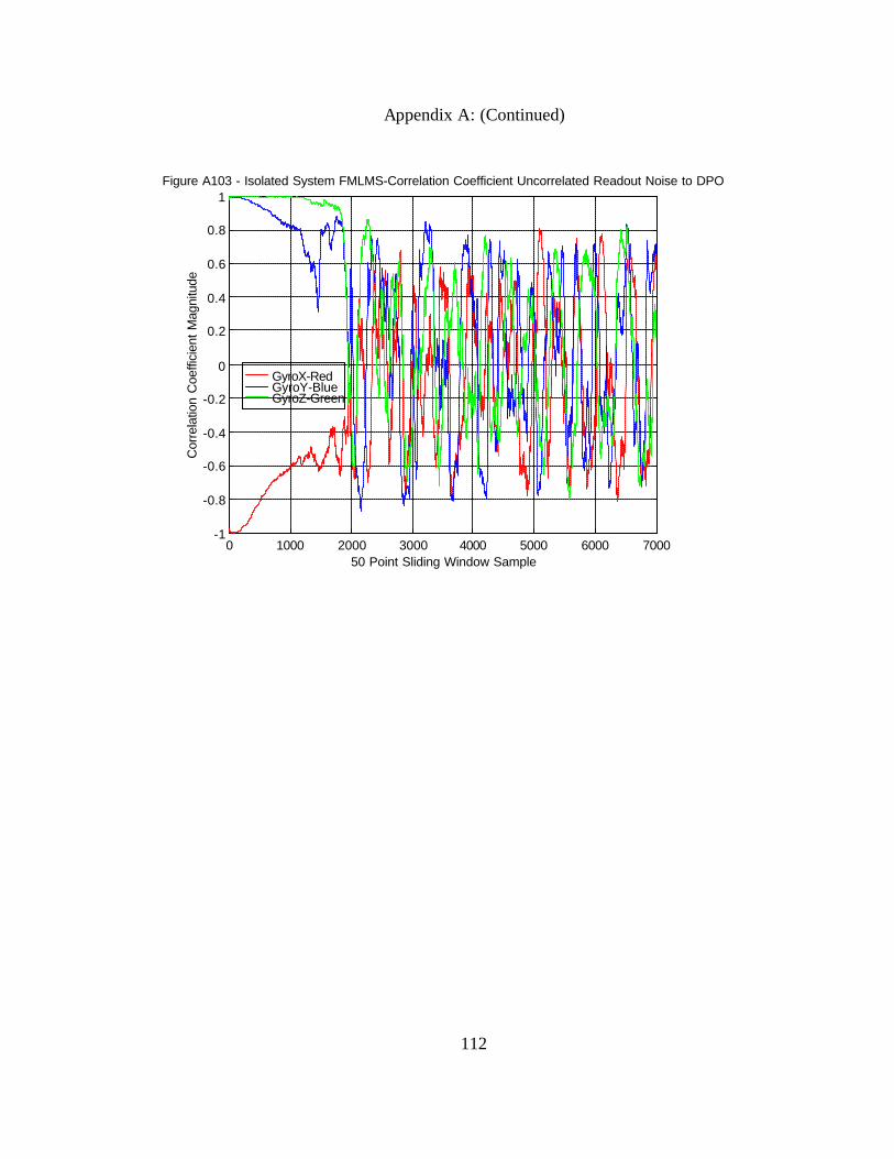
Appendix A: (Continued)

112

GyroX-Red GyroY-Blue GyroZ-Green

0 1000 2000 3000 4000 5000 6000 7000-1

-0.8

-0.6

-0.4

-0.2

0

0.2

0.4

0.6

0.8

1

50 Point Sliding Window Sample

Cor

rela

tion

Coe

ffici

ent M

agni

tude

Figure A103 - Isolated System FMLMS-Correlation Coefficient Uncorrelated Readout Noise to DPO

Appendix B: MathCAD Scripts

113

0 100 200 300 400 500 600 700 800

5 .105

1 .106 Figure B2 - CPSD Raw Xgyro

Frequency

Gyr

o A

ngle

Mag

nitu

de -a

rc*s

ec S

quar

ed

CumSΘssraw j

512Hz

F j

0 100 200 300 400 500 600 700 800

5000

1 .104 Figure B1 - PSD Raw Xgyro

Frequency

Gyr

o A

ngle

Mag

nitu

de-a

rc*s

ec S

quar

ed

SΘssrawj

512Hz

F j

CumSΘssrawj CumSΘssrawj 1− SΘssraw j∆F⋅+:=CumSΘssraw1 0:=

SΘssraw 2FFTΘssraw( )2

→

Fs⋅:=

FFTΘssraw cfft Θssraw( ):=

∆F 2.0000Hz=Fj j 1−( ) ∆F⋅:=∆F1

P ∆T⋅:=j 2 M..:=

M 401.00000=M floorP

2

1+:=∆T1

Fs:=Fs 1600 Hz⋅:=

Θssrawk Θrawk 400+:=k 1 P..:=P 800:=

asecdeg

3600:=µrad 10

6−rad⋅:=i 1 N 2000−( )..:=N 1.00000 10

4×=N rows data( ):=

Θraw data 5⟨ ⟩:=X data 1⟨ ⟩

:=

data READPRN "C:\Documents and Settings\dadoheny\Desktop\MSEE_DATA\plt_hrss1.dat"( ):=

Read In raw RLG, Q, data and plot PSD and CPSD. Remember the RLG contains base motion + dither reference + uncorrelated noise.

MathCAD 2002 Script: plt_lms_2002.mcd

Appendix B: (Continued)

114

0 100 200 300 400 500 600 700 800

5 .105

1 .106 Figure B4 - CPSD Raw Xdpo

Frequency

Dith

er M

agni

tude

- A

/D S

ampl

e Sq

uare

d

CumSαssraw j

512Hz

F j

0 100 200 300 400 500 600 700 800

2 .105

4 .105

Figure B3 - PSD Raw Xdpo

Frequency

Dith

er M

agni

tude

- A

/D S

ampl

e Sq

uare

d

Sαssrawj

512Hz

F j

CumSαssrawj CumSαssrawj 1− Sαssraw j∆F⋅+:=CumSαssraw1 0:=

Sαssraw 2FFTαssraw( )2

→

Fs⋅:=FFTαssraw cfft αssraw( ):=

∆F 2.0000Hz=Fj j 1−( ) ∆F⋅:=∆F1

P ∆T⋅:=j 2 M..:=

M 401.00000=M floorP

2

1+:=∆T1

Fs:=Fs 1600 Hz⋅:=

αssrawi αrawi 400+:=i 1 P..:=

asecdeg

3600:=

µrad 106−

rad⋅:=P 800:=N 3200:=

αraw xdporaw:=

xdporaw READPRN "C:\Documents and Settings\dadoheny\Desktop\MSEE_DATA\xdpo.dat"( ):=

Read In raw Dither Reference data and plot CPSD and PSD.

Appendix B: (Continued)

115

Read in Data processed by VHDL algorithm.

i 1 1600..:=

h0_int READPRN "C:\Documents and Settings\dadoheny\Desktop\MSEE_DATA\h0_int.dat"( ):=

h0_frac READPRN "C:\Documents and Settings\dadoheny\Desktop\MSEE_DATA\h0_frac.dat"( ):=

h0i h0_inti

h0_fraci

228

+:=

h1_int READPRN "C:\Documents and Settings\dadoheny\Desktop\MSEE_DATA\h1_int.dat"( ):=

h1_frac READPRN "C:\Documents and Settings\dadoheny\Desktop\MSEE_DATA\h1_frac.dat"( ):=

h1i h1_inti

h1_fraci

228

+:=

∆Θ_int READPRN "C:\Documents and Settings\dadoheny\Desktop\MSEE_DATA\en_int.dat"( ):=

∆Θ_frac READPRN "C:\Documents and Settings\dadoheny\Desktop\MSEE_DATA\en_frac.dat"( ):=

∆Θi ∆Θ_inti∆Θ_fraci

228

+:=

Appendix B: (Continued)

116

Plot filtered output and adaptive gains from VHDL algorithm, h0, h1.

0 200 400 600 800 1000 1200 1400 1600100

0

100Figure B5 - VHDL LMS Output Xgyro

Real Time Interrupt Sample

Gyr

o M

agni

tude

- ar

c-se

cs

∆Θi

i

0 200 400 600 800 1000 1200 1400 16000.4

0.2

0

0.2

0.4Figure B6 - VHDL Adaptive Gain h0

Real Time Interrupt Sample

Coe

ffic

ient

Mag

nitu

de

.21916

h0i

i

0 200 400 600 800 1000 1200 1400 16000.1

0.05

0

0.05Figure B7 - VHDL Adaptive Gain h1

Real Time Interrupt Sample

Coe

ficie

nt M

agni

tude

0.00705

h1i

i

Appendix B: (Continued)

117

Filtered Frequency is at 512 Hz, 572 Hz Component is cross coupled dither energy from an orthogonally mounted RLG.

0 200 400 600 800

0.2

0.4

Figure B9 - VHDL CPSD Filtered Xgyro

Frequency

Gyr

o M

agni

tude

arc

*sec

Squ

ared

0.34997

CumS∆Θss j

512 572Hz

F j

0 100 200 300 400 500 600 700 800

0.01

0.02

Figure B8- VHDL PSD Filtered Xgyro

Frequency

Gyr

o M

agni

tude

- ar

c*se

c Sq

uare

d

S∆Θss j

512 572Hz

F j

CumS∆Θss j CumS∆Θss j 1− S∆Θss j∆F⋅+:=CumS∆Θss1 0 asec

2⋅:=

S∆Θss 2FFT∆Θss( )2

→

Fs⋅:=FFT∆Θss cfft ∆Θss( ):=

∆F 2.0000Hz=Fj j 1−( ) ∆F⋅:=∆F1

P ∆T⋅:=j 2 M..:=

M 401.00000=M floorP

2

1+:=∆T1

Fs:=Fs 1600 Hz⋅:=

∆Θssi ∆Θi 400+:=i 1 P..:=

asecdeg

3600:=µrad 10

6−rad⋅:=P 800:=N 3200:=

Calculate and plot PSD and CPSD on VHDL algorithm data.

Appendix B: (Continued)

118

Read in LMS Data generated in MATLAB LMS Algorithm.

∆Θmatlab READPRN "C:\Documents and Settings\dadoheny\Desktop\MSEE_DATA\strpgymatlab.dat"( ):=

h0matlab READPRN "C:\Documents and Settings\dadoheny\Desktop\MSEE_DATA\g1matlab.dat"( ):=

h1matlab READPRN "C:\Documents and Settings\dadoheny\Desktop\MSEE_DATA\g2matlab.dat"( ):=

Plot filtered output, ∆Θ, and adaptive gains from VHDL algorithm, h0, h1.

0 100 200 300 400 500 600 700 800100

0

100Figure B10 - MATLAB LMS Output Xgyro

Real Time Interrupt Sample

Gyr

o M

agni

tude

- ar

c*se

c Sq

uare

d

∆Θmatlabi

i

100 200 300 400 500 600 700 8000

0.2

Figure B11 - MATLAB Adaptive Gain h0

Real Time Interrupt Sample

Coe

ffic

ient

Mag

nitu

de

0.21926

h0matlabi

i

0 100 200 300 400 500 600 700 800

0

Figure B12 - MATLAB Adaptive Gain h1

Real Time Interrupt Sample

Coe

ffic

ient

Mag

nitu

de

0.007179

h1matlabi

i

Appendix B: (Continued)

119

0 200 400 600 800

0.2

0.4

Figure B14 -MATLAB CPSD Filtered Xgyro

Frequency

Gyr

o M

agni

tude

- ar

c*se

c Sq

uare

d

0.35572

CumS∆Θssmatlab j

512Hz

F j

0 100 200 300 400 500 600 700 800

0.01

Figure B13 - MATLAB PSD Filtered Xgyro

Frequency

Gyr

o M

agni

tude

- ar

c*se

c Sq

uare

d

S∆Θssmatlabj

512Hz

F j

CumS∆Θssmatlab j CumS∆Θssmatlab j 1− S∆Θssmatlab j∆F⋅+:=

CumS∆Θssmatlab1 0:=

S∆Θssmatlab 2FFT∆Θssmatlab( )2

→

Fs⋅:=

FFT∆Θssmatlab cfft ∆Θssmatlab( ):=

∆F 2.0000Hz=Fj j 1−( ) ∆F⋅:=∆F1

P ∆T⋅:=j 2 M..:=

M 401.00000=M floorP

2

1+:=∆T1

Fs:=Fs 1600 Hz⋅:=

∆Θssmatlabi∆Θmatlabi 400+

:=i 1 P..:=

asecdeg

3600:=µrad 10

6−rad⋅:=P 800:=N 3200:=

Calculate and plot PSD and CPSD on MATLAB algorithm data.

Appendix B: (Continued)

120

%devh1gain 1.81058=

%devh1gainh1matlab h1vhdl−

h1matlab100⋅:=

h1vhdl 0.00705:=h1matlab 0.00718:=

Calculate deviaton of adaptive h1 gain:

%devh0gain 0.04561=

%devh0gainh0matlab h0vhdl−

h0matlab100⋅:=

h0vhdl 0.21916:=h0matlab 0.21926:=

Calculate deviaton of adaptive h0 gain:

%devnoisemag 0.81151=

%devnoisemagNoiseMagmatlab NoiseMagvhdl−

NoiseMagmatlab100⋅:=

NoiseMagvhdl 0.41831=NoiseMagmatlab 0.42173=

NoiseMagvhdlCPSDvhdl

2:=

NoiseMagmatlabCPSDmatlab

2:=

CPSDvhdl 0.34997:=CPSDmatlab 0.35572:=

Calculate deviaton Noise Magnitude:

Determine deviation in Noise Magnitude and Adaptive gains between MATLAB and VHDL algortihms.

Appendix B: (Continued)

121

ν∆Θ mean ∆Θanal( ):= ν∆Θ 0.01046−=

stdev∆Θ stdev ∆Θanal( ):= stdev∆Θ 0.60578=

stdev∆Θunbiased 0.57666=stdev∆Θunbiased stdev ∆Θanal( ) n

n 1−⋅:=

Mean and standard deviation the gain weight values data points post convergence.

n 400:= j 0 n..:= g0j h0j 800+:= g1j h1j 800+:=

νg0 mean g0( ):= νg0 0.21918=

stdevg0 stdev g0( ):= stdevg0 3.60951 105−

×=

stdevg0unbiased stdev g0( )n

n 1−⋅:= stdevg0unbiased 3.61403 10

5−×=

νg1 mean g0( ):= νg1 0.21918=

stdevg1 stdev g1( ):= stdevg1 4.45001 105−

×=

stdevg1unbiased stdev g1( )n

n 1−⋅:= stdevg1unbiased 4.45558 10

5−×=

Analysis of the stripped gyro data.Mean and standard deviation of first set of 400 data points. Reference plot VHDL - Real Time LMS Output - Xgyro.

n 400:= j 0 n..:= ∆Θanalj ∆Θ j:=

ν∆Θ mean ∆Θanal( ):= ν∆Θ 65.21803−=

stdev∆Θ stdev ∆Θanal( ):= stdev∆Θ 1.29438 103

×=

stdev∆Θunbiased stdev ∆Θanal( ) n

n 1−⋅:= stdev∆Θunbiased 1.29600 10

3×=

Mean and standard deviation of second set of 400 data points.

n 400:= j 0 n..:= ∆Θanalj ∆Θ j 400+:=

ν∆Θ mean ∆Θanal( ):=ν∆Θ 0.01101−=

stdev∆Θ stdev ∆Θanal( ):=stdev∆Θ 0.57594=

stdev∆Θunbiased stdev ∆Θanal( ) n

n 1−⋅:= stdev∆Θunbiased 0.57666=

Mean and standard deviation of third set of 400 data points.

n 400:= j 0 n..:= ∆Θanalj ∆Θ j 800+:=

Appendix B: (Continued)

122

corrΘand∆Θunbiased 4.42664 103−

×=corrΘand∆Θunbiased corr Θanal ∆Θanal,( ) n

n 1−⋅:=

corrΘand∆Θ 4.42111 103−

×=corrΘand∆Θ corr Θanal ∆Θanal,( ):=

∆Θanalj ∆Θ j 800+:=Θanalj Θ j 800+:=

j 0 n..:=n 400:=

Correlation Coefficient of the third set of 400 data points.

corrΘand∆Θunbiased 8.72695− 104−

×=corrΘand∆Θunbiased corr Θanal ∆Θanal,( ) n

n 1−⋅:=

corrΘand∆Θ 8.71603− 104−

×=corrΘand∆Θ corr Θanal ∆Θanal,( ):=

∆Θanalj ∆Θ j 400+:=Θanalj Θ j 400+:=

j 0 n..:=n 400:=

Correlation Coefficient of the second set of 400 data points.

corrΘand∆Θunbiased 0.06279=corrΘand∆Θunbiased corr Θanal ∆Θanal,( ) n

n 1−⋅:=

corrΘand∆Θ 0.06271=corrΘand∆Θ corr Θanal ∆Θanal,( ):=

∆Θanalj ∆Θ j:=Θanalj Θ j:=

j 0 n..:=n 400:=

Correlation Coefficient of the first 400 data points.

Appendix B: (Continued)

123

covarΘand∆Θunbiased 0.55970=covarΘand∆Θunbiased cvar Θanal ∆Θanal,( ) n

n 1−⋅:=

covarΘand∆Θ 0.55900=covarΘand∆Θ cvar Θanal ∆Θanal,( ):=

∆Θanalj ∆Θ j 800+:=Θanalj Θ j 800+:=

j 0 n..:=n 400:=

Covariance of the third set of 400 data points.

covarΘand∆Θunbiased 0.10438−=covarΘand∆Θunbiased cvar Θanal ∆Θanal,( ) n

n 1−⋅:=

covarΘand∆Θ 0.10424−=covarΘand∆Θ cvar Θanal ∆Θanal,( ):=

∆Θanalj ∆Θ j 400+:=Θanalj Θ j 400+:=

j 0 n..:=n 400:=

Covariance of the second set of 400 data points.

covarΘand∆Θunbiased 1.69610 104

×=covarΘand∆Θunbiased cvar Θanal ∆Θanal,( ) n

n 1−⋅:=

covarΘand∆Θ 1.69398 104

×=covarΘand∆Θ cvar Θanal ∆Θanal,( ):=

∆Θanalj ∆Θ j:=Θanalj Θ j:=

j 0 n..:=n 400:=

Covariance of the first 400 data points.

Appendix B: (Continued)

124

ν∆Θ mean ∆Θanal( ):= ν∆Θ 0.01046−=

stdev∆Θ stdev ∆Θanal( ):= stdev∆Θ 0.60578=

stdev∆Θunbiased 0.57666=stdev∆Θunbiased stdev ∆Θanal( ) n

n 1−⋅:=

Mean and standard deviation the gain weight values data points post convergence.

j 0 n..:= g0j h0j 800+:= g1j h1j 800+:=n 400:=νg0 mean g0( ):= νg0 0.21918=

stdevg0 stdev g0( ):= stdevg0 3.60951 105−

×=

stdevg0unbiased stdev g0( )n

n 1−⋅:= stdevg0unbiased 3.61403 10

5−×=

νg1 mean g0( ):= νg1 0.21918=

stdevg1 stdev g1( ):= stdevg1 4.45001 105−

×=

stdevg1unbiased stdev g1( )n

n 1−⋅:= stdevg1unbiased 4.45558 10

5−×=

Mean and standard deviation of first set of 400 data points.

n 400:= j 0 n..:= ∆Θanalj ∆Θ j:=

ν∆Θ mean ∆Θanal( ):= ν∆Θ 65.21803−=

stdev∆Θ stdev ∆Θanal( ):= stdev∆Θ 1.29438 103

×=

stdev∆Θunbiased stdev ∆Θanal( ) n

n 1−⋅:= stdev∆Θunbiased 1.29600 10

3×=

Mean and standard deviation of second set of 400 data points.

n 400:= j 0 n..:= ∆Θanalj ∆Θ j 400+:=

ν∆Θ mean ∆Θanal( ):=ν∆Θ 0.01101−=

stdev∆Θ stdev ∆Θanal( ):=stdev∆Θ 0.57594=

stdev∆Θunbiased stdev ∆Θanal( ) n

n 1−⋅:= stdev∆Θunbiased 0.57666=

Mean and standard deviation of third set of 400 data points.

n 400:= j 0 n..:= ∆Θanalj ∆Θ j 800+:=

Appendix B: (Continued)

125

msGX 43384.242661=msGX

i

GXi m Xi⋅ b+( )− 2∑

1

N 1−⋅:=

Find the mean value of the X-axis gyro data:

m 0.003847−=m slope X GX,( ):=

b 25946.755814−=b intercept X GX,( ):=

Determine slope and intercept for detrend of gyro data :

max ∆DPOX→( ) 2429=∆DPOXi DPOXi DPOXi 1−−:=max DPOX

→( ) 3480=

max ∆GX→( ) 526=∆GXi GXi GXi 1−−:=max GX

→( ) 26290=

Determine maximum values of gyro, delta gyro, dither pickoff and delta dither pick off:

DPOX data 8⟨ ⟩:=GX data 5⟨ ⟩

:=X data 1⟨ ⟩:=

Extract X-axis sample number, gyro angle and dither pickoff data:

i 1 N 1−..:=N 10000=N rows data( ):=

Define index:

data READPRN "C:\Documents and Settings\dadoheny\Desktop\MSEE_DATA\plt_hrss1.dat"( ):=

Read Data from Data File: raw Ring Laser Gyro and Dither Pickoff Data

MathCAD 2003 Script: lms_eig_calc.mcd

The following derivation reflects calculations associated with a Least Mean Squarealgorithm. Data captured from an actual Inertial Measurement System is read in and calculation are made.

The script is fairly self documenting and is meant to reflect calculations in pursuitof the minimum mean square error output and maximum convergence factor requiredin targetting the algortihm for a VHDL implementation.

Appendix B: (Continued)

126

f g0 g1,( ) R0 0, g02

⋅ R0 0, g12

⋅+ 2 R0 1,⋅ g0⋅ g1⋅+ 2 P0⋅ g0⋅− 2 P1⋅ g1⋅− msGX+:=

The expected value of the "desired" signal squared, E[d2}, is already representedabove by msGX.

The equation for the mean-squared error (MSE), as a function of the gains is:

MSE=E[d2]+GTRG-2PTG

Expanding this and inserting the above calculations gives:

P200549.444027

80735.006997−

=R927882.20152

398111.409641−

398111.409641−

927882.20152

=

PccGPOX

ccGPOXP

:=RmsDPOX

ccDPOX

ccDPOX

msDPOX

:=

From the above calculations, the inpur correlation matrix, R, and the Cross Correlation matrix, P, can be constructed:

ccGPOXP 80735.006997−=ccGPOXP

i

GXi m Xi⋅ b+( )− DPOXi 1− 2048+( )⋅∑

1

N 1−⋅:=

Find average value of X-axis detrended gyro data versus previous pickoff sample:

ccGPOX 200549.444027=ccGPOX

i

GXi m Xi⋅ b+( )− DPOXi 2048+( )⋅∑

1

N 1−⋅:=

Find the average value of X-axis detrended gyro data versus current pickoff sample:

ccDPOX 398111.409641−=ccDPOX

i

DPOXi 2048+( ) DPOXi 1− 2048+( )⋅∑

1

N 1−⋅:=

Find the acverage value of X-axis pickoff sample k versus sample(k-1) i.e. cross-correlation:

msDPOX 927882.20152=msDPOX

i

DPOXi 2048+( )2∑

1

N 1−⋅:=

Find mean_squared value of X-axis pickoff data:

Appendix B: (Continued)

127

g1g0

Mean_Squared Error

Figure B15 - Quadratic Error Surface

S

SNg1 j− i, f Lg0 i Dg0⋅+ Lg1 j Dg1⋅+,( ):=

Dg11

Ng1Ug1 Lg1−( )⋅:=Dg0

1

Ng0Ug0 Lg0−( )⋅:=

j 0 Ng1..:=i 0 Ng0..:=

Generate an array of mean-squared error values as a function of g0 and g1:

Lg1 0.0001:=Lg0 0.0001:=

Ug1 10:=Ug0 10:=

Define the upper and lower limts for g0 and g1:

Ng1 10:=Ng0 10:=

From this data, a 3-dimensional plot can be constructed. Define the number of divisions in the g0 and g1 directions.

Appendix B: (Continued)

128

MSE_min 0.872778=MSE_min msGX PT G_Opt⋅−:=

G_Opt0.219147

0.007016

=G_Opt R

1−P⋅:=

MSE_min=E[d2] -PT(R-1P)=E[d2] -PT(G_Opt)

Taking advantage of correlation matrix symmetry:

MSE_min=E[d2] +(R-1P)TR(R-1P)-2PT(R-1P)

MSE_min=E[d2] +(G_Opt)TR(G_opt)-2PTG_Opt

Substituting this int Equation (1):

G_Opt=R-1P

Substituting the optimal value of the gains and solving gives:

2RG-2P=0

Alternatively, the minimum mean-square erro may be found by taking the gradient of Equatiion (1) and setting the results equal to zero. The result, in matrix form is:

The two gains calculated above g0_min and g1_min, agree with the are consistant with the independent calculations using the MATLAB algorithms. The MATLAB algorithms calculate a g0_min value of 0.21914928 and a g1_min value of 0.0070046 and a mean-squared error minimum of 0.7508333.

MSE_min 0.8727783=MSE_min f g0_min g1_min,( ):=

Inserting the minimum gain values into Equation (2) gives the minimum mean_squared error:

g1_min 0.0070159=g1_minR0 1, P0⋅ R0 0, P1⋅−

R0 1,( )2R0 0,( )2

−:=

g0_min 0.2191469=g0_minR0 0, R0 1,⋅ P1⋅( ) R0 0,( )2

P0⋅−

R0 0, R0 1, R0 0,−( )⋅ R0 1, R0 0,+( )⋅:=

The minimum mean-square error is found by taking partial deerivatives of Equation (1) first with respect to g0 and then with respect to g1 and setting each equation equal to zero. Soving the system of equations for g0 and g1 gives the pair of gains that yield the minimum of the performance surface:

Appendix B: (Continued)

129

µ_finite_x2 7.450580596924 109−

×=µ_finite_x2 2 µ_finite⋅:=

µ_finite 3.725290298462 109−

×=µ_finite1

228

:=

This reflects a value using a minimum of 28 bits or 1/228, automatically forcing a scalingsufficient to meet the quantization of µ and requiring a 28 bit fractional bit representation.

Bitsµ_max_selected 27.982499=Bitsµ_max_selected

log1

µ_max

100 2⋅

log 2( ):=

µ_vhdl 3.770757232851 109−

×=µ_vhdlµ_max

100 2⋅:=

Twenty-one bits are required to meet the requirement of the µ_max value. However their is a trade off between convergence and the variance of the mean square error. In the VHDL algorithm a suitable selection was made to insure convergence and minimization of the mean square error. Because the algorithm actually uses a 2µ value, a number approximately equal to the µ_max divided by a factor of 100 was used and then divided by two giving:

Bitsµ_max 20.338642=Bitsµ_max

log1

µ_max

log 2( ):=

In order to represent this maximum value to insure convergence, the following calculation reflects the number of bits required to represent this in a finite register implementation based

on 2n=1/µ_max:

µ_max 754.151446570201 109−

×=µ_max1

λ_max:=

It can be shown that the LMS algorithm converges when 0 < m < 1/l_max:

λ_max 1325993.611161=λ_max max eigenvals RT R⋅( )( ):=

Or by taking the maxiimum value of the square root of the eigenvalues or RTR we get the max eigen_value:

λ1325993.611161

529770.791879

=λ eigenvals R( ):=

From this we can calculate the eigenvalues of the correlation matrix and subsequently the optimal convergence factor.

Appendix C: Sample Listing of MATLAB Program

130

The following is a sample listing of the MATLAB program for the LMS program. Similar programs were generated for the Main Channel and Full Matrix LMS, Normalized LMS, RLS and Joint Process Gradient Lattice. %%%%%%%%%%%%%%%%%%%%%%%%%%%%%%%%%%%%%%%%%%% % File name: LMS717d.m % Purpose: Real Time Adaptive Least Mean Square (LMS) Algorithm % Author: David A. Doheny % Description: Three channel LMS algorithm. Supports Diagonal, Main % channel and Cross channel LMS algorithm on input signal % and a reference signal. Identity matrix multiply of gain % update equations allow for zeroing out the cross terms. % % Last Revision Date: January 15, 2004. % %%%%%%%%%%%%%%%%%%%%%%%%%%%%%%%%%%%%%%%%%%% % Clear all previous variables % Close all previous plots % Specify display accuracy clear all; close all; format long; %%%%%%%%%%%%%%%%%%%%%%%%%%%%%%%%%%%%%%%%%%% % Read Data and assign id number % Format is Defined as follows: 11 columns of data % Record #, Line #, Striped X, Striped Y, Striped Z, % Gyro X, Gyro Y, Gyro Z, Pickoff x, Pickoff Y, Pickoff z %%%%%%%%%%%%%%%%%%%%%%%%%%%%%%%%%%%%%%%%%%% fid=fopen('c:\matlab\MSEE\hrss1.dat'); %%%%%%%%%%%%%%%%%%%%%%%%%%%%%%%%%%%%%%%%%%% % set colors for sreen print %set(0,'DefaulttextColor','black'); %set(0,'DefaultaxesXColor','black'); %set(0,'DefaultaxesYColor','black'); %set(0,'DefaultaxesZColor','black'); %set(0,'DefaultFigureColor','white'); %set(0,'DefaultaxesColor','white'); %%%%%%%%%%%%%%%%%%%%%%%%%%%%%%%%%%%%%%%%%%%

Appendix C: (Continued)

131

% Number of records to read % Sampling frequency of data % Number of records to process % Transpose input % Clear a and save PC memory % Extract count index %%%%%%%%%%%%%%%%%%%%%%%%%%%%%%%%%%%%%%%%%%% n2read=8192; fs=1600; n2proc=4096; a=fscanf(fid,'%d',[11,n2read]); b=a'; clear a; count=b(1:n2proc,2); %%%%%%%%%%%%%%%%%%%%%%%%%%%%%%%%%%%%%%%%%%% % initialize mu (scaler) % initialize mu for cubic terms % Identity Matrix for disabling cross terms %%%%%%%%%%%%%%%%%%%%%%%%%%%%%%%%%%%%%%%%%%% mu=7.6e-9; muc=7.6e-23; ident=[1,0,0;0,1,0;0,0,1]; %%%%%%%%%%%%%%%%%%%%%%%%%%%%%%%%%%%%%%%%%%% % extract 3 channels of gyro input data % from gyro input matrix extract x vector % from gyro input matrix extract y vector % from gyro input matrix extract z vector %%%%%%%%%%%%%%%%%%%%%%%%%%%%%%%%%%%%%%%%%%% gy=[b(:,6),b(:,7),b(:,8)]; gyx=gy(:,1); gyy=gy(:,2); gyz=gy(:,3); %%%%%%%%%%%%%%%%%%%%%%%%%%%%%%%%%%%%%%%%%%% % extract 3 channels of pick off reference data % from pick off data matrix extract x vector % from pick off data matrix extract y vector

Appendix C: (Continued)

132

% from pick off data matrix extract z vector %%%%%%%%%%%%%%%%%%%%%%%%%%%%%%%%%%%%%%%%%%% po=[b(:,9)+2048,b(:,10)-2048,b(:,11)-2048]; pox=po(:,1); poy=po(:,2); poz=po(:,3); %%%%%%%%%%%%%%%%%%%%%%%%%%%%%%%%%%%%%%%%%%% % Form delta theta and delta pick off values, [X(n)-X(n-1)], % preferred data to use, elliminates random walk; % dtheta and theta are [n2read x 3] matrix. % Once deltas are formed, extract x, y, and z vectors. %%%%%%%%%%%%%%%%%%%%%%%%%%%%%%%%%%%%%%%%%%% for n=2:n2read; dgy(n,:)=gy(n,:)-gy(n-1,:); dpo(n,:)=po(n,:)-po(n-1,:); dgyx=dgy(:,1); dgyy=dgy(:,2); dgyz=dgy(:,3); dpox=dpo(:,1); dpoy=dpo(:,2); dpoz=dpo(:,3); end; %%%%%%%%%%%%%%%%%%%%%%%%%%%%%%%%%%%%%%%%%%% % For the LMS with Cubic terms, cube each pickoff value. % Then reform into matrix %%%%%%%%%%%%%%%%%%%%%%%%%%%%%%%%%%%%%%%%%%% dpoxcu=dpo(:,1).*dpo(:,1).*dpo(:,1); dpoycu=dpo(:,2).*dpo(:,2).*dpo(:,2); dpozcu=dpo(:,3).*dpo(:,3).*dpo(:,3); dpocub=[dpoxcu, dpoycu, dpozcu]; %%%%%%%%%%%%%%%%%%%%%%%%%%%%%%%%%%%%%%%%%%% % LMS ALGORITHM %%%%%%%%%%%%%%%%%%%%%%%%%%%%%%%%%%%%%%%%%%% % Initialize variables, vectors or matrix to zero

Appendix C: (Continued)

133

% Current weights (gains or coefficients) G1CUR=zeros(3)*1; G2CUR=zeros(3)*2; CUCUR=zeros(3)*3; % Previous weights matrix G1NP1=zeros(3,3); G2NP1=zeros(3,3); CUNP1=zeros(3,3); %%%%%%%%%%%%%%%%%%%%%%%%%%%%%%%%%%%%%%%%%%% % Begin LMS Loop %%%%%%%%%%%%%%%%%%%%%%%%%%%%%%%%%%%%%%%%%%% for n=4:(n2read); % Delta theta estimate calculations % Alias the estimate, x_hapn % Two weights per channel %Linear implementation only dthtd_est=(G1CUR*dpo(n,:)')+(G2CUR*dpo(n-1,:)'); dthtdest(n,:)=dthtd_est'; %Use for no cubic %%%%%%%%%%%%%%%%%%%%%%%%%%%%%%%%%%%%%%%%%%% % % Use for Linear plus a cubic term % % dthtd_est=((G1CUR*dpo(n,:)')-(CUCUR*dpocub(n,:)'))+(G2CUR*dpo(n-1,:)'); % dthtdest(n,:)=dthtd_est'; % % Use for Cubic % Delta theta - delta theta estimate % Alias the error equation, e(n) %%%%%%%%%%%%%%%%%%%%%%%%%%%%%%%%%%%%%%%%%%% dthts_gy=dgy(n,:)-dthtdest(n,:); dthtsgy(n,:)=dthts_gy; % High pass filter on weight update to insure stationary process in weight update % Under rotation, the gains tend to track rates. This insures that they don't dthts_hp=-.25*dthtsgy(n,:)'+0.5*dthtsgy(n-1,:)'-0.25*dthtsgy(n-2,:)';

Appendix C: (Continued)

134

dthtshp(n,:)=dthts_hp'; % Calculation first adaptive weight or [gain] , w(0) [or g(0) or h(0)] % Save current weight update % Convert 3 x3 matrix to 1 X 9 for storage and ease of index when ploting G1NP1=(G1CUR+2.*mu.*dthtshp(n,:)'*dpo(n-1,:)).*ident; % Use when not filtering the gain update equation through hipass % G1NP1=G1CUR+2.*mu.*dthtshp(n,:)'*dpo(n,:); G1CUR=G1NP1; g1(n,:)=reshape(G1CUR,1,9); % Calculation of second adpative weight or [gain], w(0) [or g(0) or h(0)] % Save current weight update % Convert 3 x3 matrix to 1 X 9 for storage and ease of index when ploting G2NP1=(G2CUR+2.*mu.*dthtshp(n,:)'*dpo(n-2,:)).*ident; % Use when not filtering the gain update equation through hipass % G2NP1=G2CUR+2.*mu.*dthtshp(n,:)'*dpo(n-1,:); G2CUR=G2NP1; g2(n,:)=reshape(G2CUR,1,9); %%%%%%%%%%%%%%%%%%%%%%%%%%%%%%%%%%%%%%%%%%% % Uncomment next three lines when us ing linear and cubic model implementation % Cubic gain update equation. only one weight for cubic terms. % CUNP1=CUCUR+2.*muc.*dthtshp(n,:)'*dpocub(n-1,:); % CUCUR=CUNP1; % cub(n,:)=reshape(CUCUR,1,9); %%%%%%%%%%%%%%%%%%%%%%%%%%%%%%%%%%%%%%%%%%% % End LMS Loop %%%%%%%%%%%%%%%%%%%%%%%%%%%%%%%%%%%%%%%%%%% end; %%%%%%%%%%%%%%%%%%%%%%%%%%%%%%%%%%%%%%%%%%% % Extract Stripped delta theta x gyro data % Extract Stripped delta theta x gyro data % Extract Stripped delta theta x gyro data

Appendix C: (Continued)

135

dthtsgyx=dthtsgy(:,1); dthtsgyy=dthtsgy(:,2); dthtsgyz=dthtsgy(:,3); %%%%%%%%%%%%%%%%%%%%%%%%%%%%%%%%%%%%%%%%%%% % If needed save data to MATLAB format data files. % save c:\matlab\dthtsgy.mat dthtsgy % save c:\matlab\g1.mat g1 % save c:\matlab\g2.mat g2 % % Use for generating portable graphs in Post script or windows meta file formats %print -dpsc2 <parameter name> %print -dmeta <parameter name> % %%%%%%%%%%%%%%%%%%%%%%%%%%%%%%%%%%%%%%%%%%% % % Plot Dither Gyro Information % %%%%%%%%%%%%%%%%%%%%%%%%%%%%%%%%%%%%%%%%%%% % Calculate running sums for use in PSD and CPSD % Detrend delta theta gyro data % Generate PSD delta theta gyro data % Generate CPSD delta theta gyro data% %%%%%%%%%%%%%%%%%%%%%%%%%%%%%%%%%%%%%%%%%%% sum(1,:) = dgy(n2proc,:); for I=2:n2proc, sum(I,1) = sum(I-1,1) + dgy(I+n2proc,1); sum(I,2) = sum(I-1,2) + dgy(I+n2proc,2); sum(I,3) = sum(I-1,3) + dgy(I+n2proc,3); end; for I = 1:3, p=polyfit(count,sum(:,I),1); %remove trend in gyro data dsum(:,I)=sum(:,I)-polyval(p,count); Y(:,I) = fft(dsum(:,I),n2proc); Pyy(:,I) = Y(:,I).*conj(Y(:,I))/n2proc/n2proc; CPyy(:,I) = 2*Pyy(:,1); for j = 2:n2proc/2, CPyy(j,I) = CPyy(j-1,I) + 2*Pyy(j,I); end;

Appendix C: (Continued)

136

end; % Prepare for plots % Save plot data f = fs/n2proc*(0:n2proc/2-1); freq = f'; clear f; figure; plot(freq, Pyy(1:n2proc/2,1),'r',freq, Pyy(1:n2proc/2,2),'b',freq, ... Pyy(1:n2proc/2,3),'g'); title('Figure 6 - PSD of Correlated Gyro Readout Noise') xlabel('Frequency (HZ)'); ylabel('Correlated Gyro Readout Noise/Hertz; ARC*SEC^2/Hz') legend('GyroX-Red', 'GyroY-Blue', 'GyroZ-green') grid; print -dmeta Fig6; figure; plot(freq, CPyy(1:n2proc/2,1),'r',freq, CPyy(1:n2proc/2,2),'b',freq, ... CPyy(1:n2proc/2,3),'g'); title('Figure 7 - Cumulative PSD-Correlated Gyro Readout Noise') xlabel('Frequency (HZ)'); ylabel('Correlated Gyro Readout Noise: ARC*SEC^2') legend('GyroX-Red', 'GyroY-Blue', 'GyroZ-green') grid; print -dmeta Fig7; % If needed save cplsd data in ascii format % cpsdlms = [freq CPyy(1:n2proc/2,1) CPyy(1:n2proc/2,2) CPyy(1:n2proc/2,3)]; % save c:\matlab\cpsdlms.dat cpsdlms -ascii; %%%%%%%%%%%%%%%%%%%%%%%%%%%%%%%%%%%%%%%%%%% % % Plot Dither Pick Off Information % %%%%%%%%%%%%%%%%%%%%%%%%%%%%%%%%%%%%%%%%%%% % Calculate running sums for use in PSD and CPSD % Detrend Gyro dither pick off data % Generate PSD Gyro dither pick off data % Generate CPSD Gyro dither pick off data sum(1,:) = dpo(n2proc,:);

Appendix C: (Continued)

137

for I=2:n2proc, sum(I,1) = sum(I-1,1) + dpo(I+n2proc,1); sum(I,2) = sum(I-1,2) + dpo(I+n2proc,2); sum(I,3) = sum(I-1,3) + dpo(I+n2proc,3); end; % Detrend data % Generate PSD Pick Off Data % Generate CPSD Pick Off Data for I = 1:3, p=polyfit(count,sum(:,I),1); dsum(:,I)=sum(:,I)-polyval(p,count); Y(:,I) = fft(dsum(:,I),n2proc); Pyy(:,I) = Y(:,I).*conj(Y(:,I))/n2proc/n2proc; CPyy(:,I) = 2*Pyy(:,1); for j = 2:n2proc/2, CPyy(j,I) = CPyy(j-1,I) + 2*Pyy(j,I); end; end; % Prepare for plots % Save plot data f = fs/n2proc*(0:n2proc/2-1); freq = f'; clear f; figure; plot(freq, Pyy(1:n2proc/2,1), 'r', freq, Pyy(1:n2proc/2,2), 'b', freq, ... Pyy(1:n2proc/2,3), 'g'); title('Figure 8-PSD of Gyro Dither Pick Off') xlabel('FREQUENCY (HZ)'); ylabel('Noise Reference: A/D Count Value/Hz') legend('GyroX-Red', 'GyroY-Blue', 'GyroZ-green') grid; print -dmeta Fig8; % Prepare for plots % Save plot data figure; plot(freq, CPyy(1:n2proc/2,1), 'r', freq, CPyy(1:n2proc/2,2), 'b',freq, ...

Appendix C: (Continued)

138

CPyy(1:n2proc/2,3), 'g'); title('Figure 9-Cumulative PSD of Gyro Dither Pick Off') xlabel('FREQUENCY (HZ)'); ylabel('Noise Reference: A/D Count Value') legend('GyroX-Red', 'GyroY-Blue', 'GyroZ-green') grid; print -dmeta Fig9; %%%%%%%%%%%%%%%%%%%%%%%%%%%%%%%%%%%%%%%%%%% % % Plot learning curves % %%%%%%%%%%%%%%%%%%%%%%%%%%%%%%%%%%%%%%%%%%% figure; subplot(3,1,1), plot(count(1:500), dthtsgyx(1:500), 'red'); title('Figure 11a-LMS Learning Curve') legend('GyroX-Red') grid; subplot(3,1,2), plot(count(1:500), dthtsgyy(1:500), 'green'); title('Figure 11b-LMS Learning Curve') ylabel('Uncorrelated Readout Noise: ARC-SEC^2') legend('GyroY-Green') grid; subplot(3,1,3), plot(count(1:500), dthtsgyz(1:500), 'blue'); title('Figure 11c-LMS Learning Curve') xlabel('Sample'); legend('GyroZ-Blue') grid; print -dmeta Fig11; %%%%%%%%%%%%%%%%%%%%%%%%%%%%%%%%%%%%%%%%%%% %%%% %%%% Plot G1 Gains (Weights or coefficients) all together. %%%% %%%%%%%%%%%%%%%%%%%%%%%%%%%%%%%%%%%%%%%%%%% figure; plot (g1(1:2000,1),'red'), title('Figure 12-LMS G1 Gain Values'), ... xlabel('1.6K Hz Samples'), ylabel('Gain Magnitude') Grid; hold on %plot (g1(1:2000,2),'cyan')

Appendix C: (Continued)

139

%plot (g1(1:2000,3),'black') %plot (g1(1:2000,4),'yellow') plot (g1(1:2000,5),'blue') %plot (g1(1:2000,6),'magenta') %plot (g1(1:2000,7),'black') %plot (g1(1:2000,8),'blue') plot (g1(1:2000,9),'green') hold off legend('GyroX-Red', 'GyroY-Blue', 'GyroZ-green') print -dmeta Fig12 %%%%%%%%%%%%%%%%%%%%%%%%%%%%%%%%%%%%%%%%%%% % % Plot G1 Gains (Weights or coefficients) individually. % %%%%%%%%%%%%%%%%%%%%%%%%%%%%%%%%%%%%%%%%%%% figure; subplot(3,3,1), plot (g1(1:2000,1),'red'), title('Figure 13a-LMS G1xx'), ... ylabel('Gain Magnitude') Grid; subplot(3,3,2), plot (g1(1:2000,2),'blue'), title('Figure 13b-LMS G1xy') Grid; subplot(3,3,3), plot (g1(1:2000,3),'black'), title('Figure 13c-LMS G1xz') Grid; subplot(3,3,4), plot (g1(1:2000,4),'cyan'), title('Figure 13d-LMS G1yx'), ... ylabel('Gain Magnitude') Grid; subplot(3,3,5), plot (g1(1:2000,5),'blue'), title('Figure 13e-LMS G1yy') Grid; subplot(3,3,6), plot (g1(1:2000,6),'magenta'), title('Figure 13f-LMS G1yz') Grid; subplot(3,3,7), plot (g1(1:2000,7),'green'), title('Figure 13g-LMS G1zx'), ... xlabel('1.6K Hz Samples'), ylabel('Gain Magnitude') Grid; subplot(3,3,8), plot (g1(1:2000,8),'blue'), title('Figure 13h-LMS G1zy'), ... xlabel('1.6K Hz Samples') Grid; subplot(3,3,9), plot (g1(1:2000,9),'green'), title('Figure 13i-LMS G1zz'), ... xlabel('1.6K Hz Samples') Grid; print -dmeta Fig13;

Appendix C: (Continued)

140

%%%%%%%%%%%%%%%%%%%%%%%%%%%%%%%%%%%%%%%%%%% %%%% %%%% Plot G2 Gains (Weights or coefficients) all together. %%%% %%%%%%%%%%%%%%%%%%%%%%%%%%%%%%%%%%%%%%%%%%% figure; plot (g2(1:2000,1),'red'), title('Figure 14-LMS G2 Gain Values'), ... xlabel('1.6K Hz Samples'), ylabel('Gain Magnitude') grid; hold on %plot (g2(1:2000,2),'black') %plot (g2(1:2000,3),'yellow') %plot (g2(1:2000,4),'cyan') plot (g2(1:2000,5),'blue') %plot (g2(1:2000,6),'magenta') %plot (g2(1:2000,7),'cyan') %plot (g2(1:2000,8),'black') plot (g2(1:2000,9),'green') hold off legend('GyroX-Red', 'GyroY-Blue', 'GyroZ-green') print -dmeta Fig14; %%%%%%%%%%%%%%%%%%%%%%%%%%%%%%%%%%%%%%%%%%% %%%% %%%% Plot G2 Gains (Weights or coefficients) individually. %%%% %%%%%%%%%%%%%%%%%%%%%%%%%%%%%%%%%%%%%%%%%%% figure; subplot(3,3,1), plot (g2(1:2000,1),'red'), title('Figure 15a-LMS G2xx'), ... ylabel('Gain Magnitude') Grid; subplot(3,3,2), plot (g2(1:2000,2),'yellow'), title('Figure 15b-LMS G2xy') Grid; subplot(3,3,3), plot (g2(1:2000,3),'black'), title('Figure 15c-LMS G2xz') Grid; subplot(3,3,4), plot (g2(1:2000,4),'cyan'), title('Figure 15d-LMS G2yx'), ... ylabel('Gain Magnitude') Grid; subplot(3,3,5), plot (g2(1:2000,5),'blue'), title('Figure 15e-LMS G2yy') Grid;

Appendix C: (Continued)

141

subplot(3,3,6), plot (g2(1:2000,6),'magenta'), title('Figure 15f-LMS G2yz') Grid; subplot(3,3,7), plot (g2(1:2000,7),'black'), title('Figure 15g-LMS G2zx'), ... xlabel('1.6K Hz Samples'), ylabel('Gain Magnitude') Grid; subplot(3,3,8), plot (g2(1:2000,8),'blue'), title('Figure 15h-LMS G2zy'), ... xlabel('1.6K Hz Samples') Grid; subplot(3,3,9), plot (g2(1:2000,9),'green'), title('Figure 15i-LMS G2zz'), ... xlabel('1.6K Hz Samples') Grid; print -dmeta Fig15; %%%%%%%%%%%%%%%%%%%%%%%%%%%%%%%%%%%%%%%%%%% %%%% %%%% Plot Cubic Gains (Weights or coefficients) individually. %%%% %%%%%%%%%%%%%%%%%%%%%%%%%%%%%%%%%%%%%%%%%%% %figure; % %subplot(3,3,1), plot (cub(:,1),'green'), title('Cubxx'), ylabel('Gain Magnitude') %Grid; %subplot(3,3,2), plot (cub(:,2),'blue'), title('Cubxy') %Grid; %subplot(3,3,3), plot (cub(:,3),'black'), title('Cubxz') %Grid; %subplot(3,3,4), plot (cub(:,4),'cyan'), title('Cubyx'), ylabel('Gain Magnitude') %Grid; %subplot(3,3,5), plot (cub(:,5),'red'), title('Cubyy'), %Grid; %subplot(3,3,6), plot (cub(:,6),'magenta'), title('Cubyz') %Grid; %subplot(3,3,7), plot (cub(:,7),'green'), title('Cubzx'), ... xlabel('1.6K Hz Samples'), ylabel('Gain Magnitude') %Grid; %subplot(3,3,8), plot (cub(:,8),'blue'), title('Cubzy'), xlabel('1.6K Hz Samples') %Grid; %subplot(3,3,9), plot (cub(:,9),'black'), title('Cubzz'), xlabel('1.6K Hz Samples') %Grid; %print -dmeta LCUBSUBS;

Appendix C: (Continued)

142

%%%%%%%%%%%%%%%%%%%%%%%%%%%%%%%%%%%%%%%%%%% %%%% %%%% Plot Cubic Gains (Weights or coefficients) all together. %%%% %%%%%%%%%%%%%%%%%%%%%%%%%%%%%%%%%%%%%%%%%%% %figure; %plot (cub(:,1),'green'), title('Cubic Gain Values'), ... xlabel('1.6K Hz Samples'), ylabel('Gain Magnitude') %hold on %plot (cub(:,2),'blue') %plot (cub(:,3),'black') %plot (cub(:,4),'cyan') %plot (cub(:,5),'red') %plot (cub(:,6),'magenta') %plot (cub(:,7),'green') %plot (cub(:,8),'blue') %plot (cub(:,9),'black') %hold off %Grid; %print -dmeta LCBUALL; %%%%%%%%%%%%%%%%%%%%%%%%%%%%%%%%%%%%%%%%%%% % Plot G1 versus G2 % %%%%%%%%%%%%%%%%%%%%%%%%%%%%%%%%%%%%%%%%%%% figure; subplot(3,1,1), plot(g1(1:8192,1), g2(1:8192,1),'red'); title('Figure 16a,b,c-LMS G1 Gain Versus G2 Gain Curves') xlabel('G1x Gain Magnitude'); ylabel('G2x Gain Magnitude') legend('GyroX-Red') grid; subplot(3,1,2), plot(g1(1:8192,5), g2(1:8192,5), 'green'); xlabel('G1y Gain Magnitude'); ylabel('G2y Gain Magnitued') legend('GyroY-Green') grid; subplot(3,1,3), plot(g1(1:8192,9), g2(1:8192,9), 'blue'); xlabel('G1z Gain Magnitude'); ylabel('G2z Gain Magnitude')

Appendix C: (Continued)

143

legend('GyroZ-Blue') grid; print -dmeta Fig16; %%%%%%%%%%%%%%%%%%%%%%%%%%%%%%%%%%%%%%%%%%% % % Plot G1 Gains versus Uncorrelated Gyro Readout Noise % %%%%%%%%%%%%%%%%%%%%%%%%%%%%%%%%%%%%%%%%%%% % figure; subplot(3,1,1), plot(g1(1:8192,1), dthtsgyx(1:8192),'red'); hold on; plot(g2(1:8192,1), dthtsgyx(1:8192),'blue'); hold off; title('Figure 19a,b,c-LMS G1 Gains Versus Uncorrelated Readout Noise') xlabel('G1x & G2x Gain Magnitude'); legend('Gyro G1X-Red', 'Gyro G2X-Blue'); grid; subplot(3,1,2), plot(g1(1:8192,5), dthtsgyy(1:8192), 'red'); hold on; plot(g2(1:8192,5), dthtsgyx(1:8192),'blue'); hold off; xlabel('G1y and G2y Gain Magnitude'); ylabel('Uncorrelated Gyro Readout Noise/Hertz: ARC-SEC^2/Hz') legend('Gyro G1Y-Red', 'Gyro G2Y-Blue'); grid; subplot(3,1,3), plot(g1(1:8192,9), dthtsgyz(1:8192), 'red'); hold on; plot(g2(1:8192,9), dthtsgyx(1:8192),'blue'); hold off; xlabel('G1z and G2z Gain Magnitude'); legend('Gyro G1Z-Red', 'Gyro G2Z-Blue'); grid; print -dmeta Fig19; %%%%%%%%%%%%%%%%%%%%%%%%%%%%%%%%%%%%%%%%%%% % % Plot Uncorrelated (stripped) Gyro Information % %%%%%%%%%%%%%%%%%%%%%%%%%%%%%%%%%%%%%%%%%%%

Appendix C: (Continued)

144

% Extract X,Y and Z Uncorrelted data from matrix into vectors % Calculate running sums for use in PSD and CPSD % Detrend Uncorrelated Gyro data % Generate PSD Uncorrelated Gyro data % Generate CPSD Uncorrelated Gyro data dthtsgyx=dthtsgy(:,1); %extract stripped delta theta x data dthtsgyy=dthtsgy(:,2); %extract stripped delta theta y data dthtsgyz=dthtsgy(:,3); %extract stripped delta theta z data sum(1,:) = dthtsgy(n2proc,:); for I=2:n2proc, sum(I,1) = sum(I-1,1) + dthtsgy(I+n2proc,1); sum(I,2) = sum(I-1,2) + dthtsgy(I+n2proc,2); sum(I,3) = sum(I-1,3) + dthtsgy(I+n2proc,3); end; for I = 1:3, p=polyfit(count,sum(:,I),1); %remove trend in gyro data dsum(:,I)=sum(:,I)-polyval(p,count); Y(:,I) = fft(dsum(:,I),n2proc); Pyy(:,I) = Y(:,I).*conj(Y(:,I))/n2proc/n2proc; CPyy(:,I) = 2*Pyy(:,1); for j = 2:n2proc/2, CPyy(j,I) = CPyy(j-1,I) + 2*Pyy(j,I); end; end; % Prepare for plots % Save plot data f = fs/n2proc*(0:n2proc/2-1); freq = f'; clear f; figure; plot(freq, Pyy(1:n2proc/2,1),'r',freq, Pyy(1:n2proc/2,2),'b',freq, ... Pyy(1:n2proc/2,3),'g'); title('Figure 20-LMS PSD-Stripped Delta Theta Uncorrelated Readout Noise') xlabel('FREQUENCY (HZ)'); ylabel('Uncorrelated Gyro Readout Noise/Hertz: ARC-SEC^2/Hz');

Appendix C: (Continued)

145

legend('GyroX-Red', 'GyroY-Blue', 'GyroZ-green'); grid; print -dmeta Fig20; % Prepare for plots % Save plot data figure; plot(freq, CPyy(1:n2proc/2,1),'r', freq, CPyy(1:n2proc/2,2),'b', freq, ... CPyy(1:n2proc/2,3),'g'); title('Figure 21-LMS CPSD-Stripped Delta Theta Uncorrelated Readout Noise'); xlabel('FREQUENCY (HZ)'); ylabel('Uncorrelated Gyro Readout Noise: ARC-SEC^2'); legend('GyroX-Red', 'GyroY-Blue', 'GyroZ-green'); grid; print -dmeta Fig21; %%%%%%%%%%%%%%%%%%%%%%%%%%%%%%%%%%%%%%%%%%% % % Calculate covariance of 50 point sliding window % Entries are % COV[X,Y]=(1,1)=variance X (1,2)=correlation coefficient*varX*varY % (2,1)=correlation (2,2)=variance of Y % coefficient*varX*varY % %%%%%%%%%%%%%%%%%%%%%%%%%%%%%%%%%%%%%%%%%%% m=50; for n=1:7951; % Covariance Matrix of Correlated Gyro data and Pick Off covxd=cov(dgyx(n:m),dpox(n:m)); covyd=cov(dgyy(n:m),dpoy(n:m)); covzd=cov(dgyz(n:m),dpoz(n:m)); % Covariance Matrix of Uncorrelated Gyro data and Pick Off covsxd=cov(dthtsgyx(n:m),dpox(n:m)); covsyd=cov(dthtsgyy(n:m),dpoy(n:m)); covszd=cov(dthtsgyz(n:m),dpoz(n:m)); % Reformat data from each 2 by 2 matrix to n by 4 Matrix for % ease of plot index recordcovxd(n,:)=reshape(covxd,1,4); recordcovyd(n,:)=reshape(covyd,1,4); recordcovzd(n,:)=reshape(covzd,1,4);

Appendix C: (Continued)

146

% Reformat data from each 2 by 2 matrix to n by 4 Matrix for % ease of plot index recordcovsxd(n,:)=reshape(covsxd,1,4); recordcovsyd(n,:)=reshape(covsyd,1,4); recordcovszd(n,:)=reshape(covszd,1,4); % Calculate Correlation Coeficient of Correlated data % CorCox(n)=covxd(1,2)/sqrt(covxd(1,1)*covxd(2,2)); CorCoy(n)=covyd(1,2)/sqrt(covyd(1,1)*covyd(2,2)); CorCoz(n)=covzd(1,2)/sqrt(covzd(1,1)*covzd(2,2)); % Transpose CorCoefx=CorCox'; CorCoefy=CorCoy'; CorCoefz=CorCoz'; % Calculate Correlation Coeficient of Correlated data % CorCosx(n)=covsxd(1,2)/sqrt(covsxd(1,1)*covsxd(2,2)); CorCosy(n)=covsyd(1,2)/sqrt(covsyd(1,1)*covsyd(2,2)); CorCosz(n)=covszd(1,2)/sqrt(covszd(1,1)*covszd(2,2)); % Transpose CorCoefsx=CorCosx'; CorCoefsy=CorCosy'; CorCoefsz=CorCosz'; % increase index m=m+1; end; %%%%%%%%%%%%%%%%%%%%%%%%%%%%%%%%%%%%%%%%%%% % % Plot Variance of Correlated Gyro Readout Noise % %%%%%%%%%%%%%%%%%%%%%%%%%%%%%%%%%%%%%%%%%%% figure; plot(recordcovxd(1:1000,1), 'red'); hold on; plot(recordcovyd(1:1000,1), 'blue'); plot(recordcovzd(1:1000,1), 'green'); hold off; xlabel('50 Point Sliding Window Sample'); ylabel('Variance Correlated Readout Noise') Title('Figure 58 - LMS - Variance Correlated Readout Noise')

Appendix C: (Continued)

147

legend('GyroX-Red', 'GyroY-Blue', 'GyroZ-green'); grid; print -dmeta Fig58; %%%%%%%%%%%%%%%%%%%%%%%%%%%%%%%%%%%%%%%%%%%% % Plot Variance of Dither Pick OFf % %%%%%%%%%%%%%%%%%%%%%%%%%%%%%%%%%%%%%%%%%%% figure; plot(recordcovxd(1:1000,4),'red'); hold on; plot(recordcovyd(1:1000,4),'blue'); plot(recordcovzd(1:1000,4),'green'); hold off; xlabel('50 Point Sliding Window Sample'); ylabel('Variance Magnitude'); Title('Figure 59 - LMS - Variance Dither Pick Off'); legend('GyroX-Red', 'GyroY-Blue', 'GyroZ-green'); grid; print -dmeta Fig59; %%%%%%%%%%%%%%%%%%%%%%%%%%%%%%%%%%%%%%%%%%% % % Plot Co-variance of Correltaed Gyro Readout noise to Dither Pick OFf % %%%%%%%%%%%%%%%%%%%%%%%%%%%%%%%%%%%%%%%%%%% figure; plot(recordcovxd(1:1000,3),'red'); hold on; plot(recordcovyd(1:1000,3),'blue'); plot(recordcovzd(1:1000,3),'green'); hold off; xlabel('50 Point Sliding Window Sample'); ylabel('Co-Variance Magnitude'); Title('Figure 60 - LMS - CoVariance Correlated Readout Noise to Dither Pick Off') legend('GyroX-Red', 'GyroY-Blue', 'GyroZ-green'); grid; print -dmeta Fig60; %%%%%%%%%%%%%%%%%%%%%%%%%%%%%%%%%%%%%%%%%%%

Appendix C: (Continued)

148

% % Plot Correlation Coefficients % %%%%%%%%%%%%%%%%%%%%%%%%%%%%%%%%%%%%%%%%%%% figure; plot(CorCoefx(1:7000)','red'); hold on; plot(CorCoefy(1:7000)','blue'); plot(CorCoefz(1:7000)','green'); hold off; xlabel('50 Point Sliding Window Sample'); ylabel('Correlation Coefficient Magnitude'); Title... ('Figure 61-LMS-Correlation Coefficient Correlated Readout Noise to Pick Off Gyro'); legend('GyroX-Red', 'GyroY-Blue', 'GyroZ-green'); grid; print -dmeta Fig61; %%%%%%%%%%%%%%%%%%%%%%%%%%%%%%%%%%%%%%%%%%% % % Plot Un-Correlated Gyro Readout Noise to Dither Pick Off % %%%%%%%%%%%%%%%%%%%%%%%%%%%%%%%%%%%%%%%%%%% figure; plot(recordcovsxd(1:1000,1), 'red'); hold on; plot(recordcovsyd(1:1000,1), 'blue'); plot(recordcovszd(1:1000,1), 'green'); hold off; xlabel('50 Point Sliding Window Sample') ylabel('Variance Correlated Readout Noise') Title('Figure 62 - LMS - Variance Un-Correlated Readout Noise') %legend('GyroX-Red', 'GyroY-Blue', 'GyroZ-green') grid; legend('GyroX-Red', 'GyroY-Blue', 'GyroZ-green') print -dmeta Fig62; %%%%%%%%%%%%%%%%%%%%%%%%%%%%%%%%%%%%%%%%%%% % % Plot Variance of Dither Pick Off %

Appendix C: (Continued)

149

%%%%%%%%%%%%%%%%%%%%%%%%%%%%%%%%%%%%%%%%%%% %figure; %plot(recordcovsxd(1:1000,4),'red'); %hold on; %plot(recordcovsyd(1:1000,4),'blue'); %plot(recordcovszd(1:1000,4),'green'); %hold off; %xlabel('50 Point Sliding Window Sample'); %ylabel('Variance Magnitude'); %Title('Figure TBD Variance Dither Pick Off'); %legend('GyroX-Red', 'GyroY-Blue', 'GyroZ-green'); %grid; %%%%%%%%%%%%%%%%%%%%%%%%%%%%%%%%%%%%%%%%%%% % % Plot Co-variance of Un-Correlated Gyro Readout noise to Dither Pick OFf % %%%%%%%%%%%%%%%%%%%%%%%%%%%%%%%%%%%%%%%%%%% figure plot(recordcovsxd(1:1000,3),'red'); Hold on; plot(recordcovsyd(1:1000,3),'blue'); plot(recordcovszd(1:1000,3),'green'); hold off; xlabel('50 Point Sliding Window Sample'); ylabel('Co-Variance Magnitude'); Title... ('Figure 63 - LMS - Co-Variance Un-Correlated Readout Noise to Dither Pick Off'); legend('GyroX-Red', 'GyroY-Blue', 'GyroZ-green'); grid; print -dmeta Fig63; %%%%%%%%%%%%%%%%%%%%%%%%%%%%%%%%%%%%%%%%%%% % % Plot Correlation Coefficients % %%%%%%%%%%%%%%%%%%%%%%%%%%%%%%%%%%%%%%%%%%% figure; plot(CorCoefsx(1:7000)','red'); Hold on;

Appendix C: (Continued)

150

plot(CorCoefsy(1:7000)','blue'); plot(CorCoefsz(1:7000)','green'); hold off; xlabel('50 Point Sliding Window Sample'); ylabel('Correlation Coefficient Magnitude'); Title... ('Figure 64-LMS-Correlation Coefficient Un-Correlated Readout Noise to Pick Off Gyro'); legend('GyroX-Red', 'GyroY-Blue', 'GyroZ-green'); grid; print -dmeta Fig64; % take a 1000 point sample mean of the: %1.) Variance of Correlated Readout noise Vcorgx=mean(recordcovxd(1000:2000,1)) Vcorgy=mean(recordcovyd(1000:2000,1)) Vcorgz=mean(recordcovzd(1000:2000,1)) %2.) Variance Correlated Pickoff Vpx=mean(recordcovxd(1000:2000,4)) Vpy=mean(recordcovyd(1000:2000,4)) Vpz=mean(recordcovzd(1000:2000,4)) %3.) Covariance of Correlated gyro to pick off CVcorgpx=mean(recordcovxd(1000:2000,2)) CVcorgpy=mean(recordcovyd(1000:2000,2)) CVcorgpz=mean(recordcovzd(1000:2000,2)) %4.) Correlation Coeficient Before Stipping CCgpx=mean(CorCoefx(1000:2000)) CCgpy=mean(CorCoefy(1000:2000)) CCgpz=mean(CorCoefz(1000:2000)) %5.) Variance uncorrelated Gyro Readout noise after stripping Vungx=mean(recordcovsxd(1000:2000,1)) Vungy=mean(recordcovsyd(1000:2000,1)) Vungz=mean(recordcovszd(1000:2000,1)) %2.) Variance Uncorrelated Pickoff Vunpx=mean(recordcovxd(1000:2000,4)) Vunpy=mean(recordcovyd(1000:2000,4)) Vunpz=mean(recordcovzd(1000:2000,4)) %6.) Covariance Uncorrelated Gyro Readout noise to picokoff CVungpx=mean(recordcovsxd(1000:2000,2)) CVungpy=mean(recordcovsyd(1000:2000,2)) CVungpz=mean(recordcovszd(1000:2000,2))

Appendix C: (Continued)

151

%7.) Correlation Coeficient after stripping CCungpx=mean(CorCoefsx(1000:2000)) CCungpy=mean(CorCoefsy(1000:2000)) CCungpz=mean(CorCoefsz(1000:2000)) % Size of matrix, vectors and variables % Name Size Bytes Class % CCgpx 1x1 8 double array % Ccgpy 1x1 8 double array % CCgpz 1x1 8 double array % Ccungpz 1x1 8 double array % CCungpx 1x1 8 double array % CCungpy 1x1 8 double array % CPyy 4096x3 98304 double array % CUCUR 3x3 72 double array % CUNP1 3x3 72 double array % CVcorgpx 1x1 8 double array % CVcorgpy 1x1 8 double array % CVcorgpz 1x1 8 double array % CVungpz 1x1 8 double array % CVungpx 1x1 8 double array % CVungpy 1x1 8 double array % CorCoefsx 7951x1 63608 double array % CorCoefsy 7951x1 63608 double array % CorCoefsz 7951x1 63608 double array % CorCoefx 7951x1 63608 double array % CorCoefy 7951x1 63608 double array % CorCoefz 7951x1 63608 double array % CorCosx 1x7951 63608 double array % CorCosy 1x7951 63608 double array % CorCosz 1x7951 63608 double array % CorCox 1x7951 63608 double array % CorCoy 1x7951 63608 double array % CorCoz 1x7951 63608 double array % G1CUR 3x3 72 double array % G1NP1 3x3 72 double array % G2CUR 3x3 72 double array % G2NP1 3x3 72 double array % I 1x1 8 double array % Pyy 4096x3 98304 double array % Vcorgx 1x1 8 double array % Vcorgy 1x1 8 double array

Appendix C: (Continued)

152

% Vcorgz 1x1 8 double array % Vpx 1x1 8 double array % Vpy 1x1 8 double array % Vpz 1x1 8 double array % Vungx 1x1 8 double array % Vungy 1x1 8 double array % Vungz 1x1 8 double array % Vunpx 1x1 8 double array % Vunpy 1x1 8 double array % Vunpz 1x1 8 double array % Y 4096x3 196608 double array (complex) % b 8192x11 720896 double array % count 4096x1 32768 double array % covsxd 2x2 32 double array % covsyd 2x2 32 double array % covszd 2x2 32 double array % covxd 2x2 32 double array % covyd 2x2 32 double array % covzd 2x2 32 double array % dgy 8192x3 196608 double array % dgyx 8192x1 65536 double array % dgyy 8192x1 65536 double array % dgyz 8192x1 65536 double array % dpo 8192x3 196608 double array % dpocub 8192x3 196608 double array % dpox 8192x1 65536 double array % dpoxcu 8192x1 65536 double array % dpoy 8192x1 65536 double array % dpoycu 8192x1 65536 double array % dpoz 8192x1 65536 double array % dpozcu 8192x1 65536 double array % dsum 4096x3 98304 double array % dthtd_est 3x1 24 double array % dthtdest 8192x3 196608 double array % dthts_gy 1x3 24 double array % dthts_hp 3x1 24 double array % dthtsgy 8192x3 196608 double array % dthtsgyx 8192x1 65536 double array % dthtsgyy 8192x1 65536 double array % dthtsgyz 8192x1 65536 double array % dthtshp 8192x3 196608 double array % fid 1x1 8 double array

Appendix C: (Continued)

153

% freq 2048x1 16384 double array % fs 1x1 8 double array % g1 8192x9 589824 double array % g2 8192x9 589824 double array % gy 8192x3 196608 double array % gyx 8192x1 65536 double array % gyy 8192x1 65536 double array % gyz 8192x1 65536 double array % ident 3x3 72 double array % j 1x1 8 double array % m 1x1 8 double array % mu 1x1 8 double array % muc 1x1 8 double array % n 1x1 8 double array % n2proc 1x1 8 double array % n2read 1x1 8 double array % p 1x2 16 double array % po 8192x3 196608 double array % pox 8192x1 65536 double array % poy 8192x1 65536 double array % poz 8192x1 65536 double array % recordcovsxd 7951x4 254432 double array % recordcovsyd 7951x4 254432 double array % recordcovszd 7951x4 254432 double array % recordcovxd 7951x4 254432 double array % recordcovyd 7951x4 254432 double array % recordcovzd 7951x4 254432 double array % sum 4096x3 98304 double array %Grand total is 935584 elements using 7582976 byte

Appendix D: VHDL Listings

154

lms_tb_48.vhdl and Least Mean Square, lms.vhdl code are listed in this appendix. I.) lms_tb_48.vhdl (listed) clk_gen.vhdl(not listed) div2_q0.vhdl(not listed) div2_tc.vhdl(not listed) div5_tc.vhdl(not listed) div8_qotc.vhdl(not listed) clk_ng.vhdl(not listed) lms_read_data.vhdl(not listed) lms_write_data.vhdl(not listed) II.) lms.vhdl (listed) lms_sm.vhdl(not listed) reg_16.vhdl(not listed) reg_48.vhdl(not listed) mux_16.vhdl(not listed) mux_48.vhdl(not listed) calc_delta.vhdl(not listed) add_sub.vhdl(not listed) mult_48_slv.vhdl(not listed)

Appendix D: (Continued)

155

----------------------------------------------------------------------- -- copyright 2004 -- Honeywell, Space and Strategic Systems Operation -- All Rights Reserved ----------------------------------------------------------------------- ----------------------------------------------------------------------- -- File name : lms_tb_48.vhdl -- Title : Least Mean Square Test Tench -- Module : lms_tb -- Purpose : To provide a testbench for the Least Mean Square Algorithm -- A Variety of VHDL Entities comprise the Test Bench. -- In paricular: -- 1.) A Non-Generic Clock Generator -- 2.) A Timing Clock Generator -- 3.) A Read Data File For input -- 4.) A Write Data File For output -- 5.) The LMS Filter ----------------------------------------------------------------------- -- Modification History: -- Date Author Revision Comments -- 01/01/04 David A. Doheny - init/final draft ----------------------------------------------------------------------- LIBRARY ieee; USE ieee.std_logic_1164.ALL; USE ieee.numeric_std.all; LIBRARY work; ENTITY tb_48_ent IS --Empty Entity END tb_48_ent; ARCHITECTURE tb_48_arch OF tb_48_ent IS ----------------------------------------------------------------------- -- List CONSTANTS used in the EPIC TESTBENCH: ----------------------------------------------------------------------- CONSTANT lms_clk_period : time := 31 ns; --32 MHz oscillator

COMPONENT clkgen_ent

Appendix D: (Continued)

156

PORT ( c32mhz : IN std_logic; c16mhz : IN std_logic; reset : IN std_logic; c16mhz_out : OUT std_logic; p1600hz : OUT std_logic ); END COMPONENT; --synopsys translate_off -- for all : clkgen_ent USE entity lms.clkgen_ent(clkgen_arch); -- for all : clkgen_ent USE entity work.clkgen_ent(clkgen_arch); -- synopsys translate_on COMPONENT clock_ng_ent PORT ( control : IN std_logic; clock_period : IN time ; clk_signal : OUT std_logic := '1' ); END COMPONENT; -- synopsys translate_off -- for all: clock_ng_ent USE entity lms.clock_ng_ent(clock_ng_arch); -- for all: clock_ng_ent USE entity work.clock_ng_ent(clock_ng_arch); -- synopsys translate_on COMPONENT lms_read_data_ent generic ( infile1 : string := "/project/lms_dsp/MSEE_DSP/source/input_data/xdpo.dat"; infile2 : string := "/project/lms_dsp/MSEE_DSP/source/input_data/xgyro.dat" ); PORT( c16mhz : IN std_logic; p1600hz : IN std_logic; dpo : OUT std_logic_vector(15 downto 0); gyro : OUT std_logic_vector(15 downto 0) );

Appendix D: (Continued)

157

END COMPONENT; -- synopsys translate_off -- for all: lms_read_data_ent USE entity lms.lms_read_data_ent(lms_read_data_arch); -- for all: lms_read_data_ent USE entity work.lms_read_data_ent(lms_read_data_arch); -- synopsys translate_on COMPONENT lms_write_data_ent generic ( outfile1 : string := "/project/lms_dsp/MSEE_DSP/source/output_data/en_int.dat"; outfile2 : string := "/project/lms_dsp/MSEE_DSP/source/output_data/en_frac.dat"; outfile3 : string := "/project/lms_dsp/MSEE_DSP/source/output_data/h0_int.dat"; outfile4 : string := "/project/lms_dsp/MSEE_DSP/source/output_data/h0_frac.dat"; outfile5 : string := "/project/lms_dsp/MSEE_DSP/source/output_data/h1_int.dat"; outfile6 : string := "/project/lms_dsp/MSEE_DSP/source/output_data/h1_frac.dat" ); PORT( c16mhz : IN std_logic; p1600hz : IN std_logic; en : IN std_logic_vector; h0 : IN std_logic_vector; h1 : IN std_logic_vector ); END COMPONENT; -- synopsys translate_off -- for all: lms_write_data_ent USE entity work.lms_write_data_ent (lms_write_data_arch); -- synopsys translate_on COMPONENT lms_ent PORT ( reset :IN std_logic; clk :IN std_logic; clk_en :IN std_logic; gyro_data :IN std_logic_vector(15 DOWNTO 0); dpo_data :IN std_logic_vector(15 DOWNTO 0);

Appendix D: (Continued)

158

h0 :OUT std_logic_vector(47 downto 0); h1 :OUT std_logic_vector(47 downto 0); en :OUT std_logic_vector(47 downto 0) ); END COMPONENT; -- synopsys translate_off -- for all: lms_ent USE entity lms.lms_ent(lms_arch); -- for all: lms_ent USE entity work.lms_ent(lms_arch); -- synopsys translate_on --------------------------------------------------------------- -- List Signals Used in test bench --------------------------------------------------------------- SIGNAL start : std_logic := '1'; SIGNAL reset : std_logic := '1'; SIGNAL c32mhz : std_logic; SIGNAL c16mhz : std_logic; SIGNAL p1600hz : std_logic; SIGNAL dpo_data : std_logic_vector(15 downto 0):=(others => '0'); SIGNAL gyro_data : std_logic_vector(15 downto 0):=(others => '0'); SIGNAL h0 : std_logic_vector(47 downto 0):= X”000000000003"; SIGNAL h1 : std_logic_vector(47 downto 0):= X”000000000003";; SIGNAL : std_logic_vector(47 downto 0):=(others => '0'); --------------------------------------------------------------- BEGIN -- lms_tb_arch CLK_32M: clock_ng_ent PORT MAP ( Control => start, clock_period => lms_clk_period, clk_signal => c32mhz ); CLKGEN_1: clkgen_ent PORT MAP ( c32mhz => c32mhz,

c16mhz => c16mhz,

Appendix D: (Continued)

159

reset => reset, c16mhz_out => c16mhz, p1600hz => p1600hz ); LMS_READ_DATA1:lms_read_data_ent PORT MAP ( c16mhz => c16mhz, p1600hz => p1600hz, dpo => dpo_data, gyro => gyro_data ); LMS_WRITE_DATA1:lms_write_data_ent PORT MAP ( c16mhz => c16mhz, p1600hz => p1600hz, h0 => h0, h1 => h1, en => en ); LMS_FILTER: lms_ent PORT MAP( reset => reset, clk => c16mhz, clk_en => p1600hz, gyro_data => gyro_data, dpo_data => dpo_data, h0 => h0, h1 => h1, en => en

); --------------------------------------------------------------------- --Miscellaneous Signal Definiton ---------------------------------------------------------------- reset <= '1', ‘0’ after 100 ns; END tb_48_arch;

Appendix D: (Continued)

160

------------------------------------------------------------------------------- -- copyright 2000 -- Honeywell, Space and Strategic Systems Operation -- All Rights Reserved -------------------------------------------------------------------------------- -- File name : lms.vhdl -- Title : Least Mean Square -- Module : lms -- Purpose : Perform a Single Channel Least Mean Square Algorithm -- Design includes: -- 1.) 48 bit adder/subtractor -- 2.) 48 bit multiplier -- 3.) 16 bit registers -- 4.) 48 bit registers -- 5.) Subtractors -- 6.) 2 channel, 16 bit, multiplexers -- 7.) 2 channel, 48 bit, multiplexers -- ------------------------------------------------------------------------------ -- Modification History: -- Date Author Revision Comments -- 01/01/04 David A. Doheny - init/finaldraft ------------------------------------------------------------------------------- LIBRARY ieee; USE ieee.std_logic_1164.all; USe ieee.numeric_std.all; LIBRARY lms; USE lms.add_sub_ent; USE lms.calc_delta_ent; USE lms.mult_48_slv_ent; USE lms.reg_16_ent; USE lms.reg_48_ent; USE lms.mux_16_ent; USE lms.mux_48_ent; USE lms.lms_sm_ent; ENTITY lms_ent IS PORT( Reset :IN std_logic;

Appendix D: (Continued)

161

clk :IN std_logic; clk_en :IN std_logic; dpo_data :IN std_logic_vector(15 downto 0); gyro_data :IN std_logic_vector(15 downto 0); h0 :OUT std_logic_vector(47 downto 0) :=X”000000000003"; h1 :OUT std_logic_vector(47 downto 0) :=X”000000000003"; en :OUT std_logic_vector(47 downto 0) :=X”000000000003"; ); END lms_ent; ---------------------------- -- Start Architecture of lms ---------------------------- ARCHITECTURE lms_arch OF lms_ent IS -------------------------------------------------------- -- Define Components Used in Least Mean Square Algorithm -------------------------------------------------------- COMPONENT calc_delta_ent -- generic (); PORT( reset :IN std_logic; clk :IN std_logic; clk_en :IN std_logic; data :IN std_logic_vector(15 downto 0); delta :OUT std_logic_vector(15 downto 0) ); END COMPONENT; --synopsys translate_off --for all : calc_delta_ent USE entity lms.calc_delta_ent (calc_delta_arch); --for all : calc_delta_ent USE entity work.calc_delta_ent(calc_delta_arch); -- synopsys translate_on COMPONENT add_sub_ent PORT (

reset :IN std_logic; clr_sum :IN std_logic;

clk :IN std_logic;

Appendix D: (Continued)

162

clk_en :IN std_logic; add_sub :IN std_logic; data_in :IN std_logic_vector(47 downto 0);

data_out :OUT std_logic_vector(47 downto 0)

); END COMPONENT; -- synopsys translate_off --for all: add_sub_ent USE entity lms.add_sub_ent(add_sub_arch); --for all: add_sub_ent USE entity work.add_sub_ent(add_sub_arch); -- synopsys translate_on COMPONENT mult_48_slv_ent PORT(

reset :IN std_logic; clk :IN std_logic; load :IN std_logic; data1 :IN std_logic_vector(47 downto 0);

data2 :IN std_logic_vector(47 downto 0); done :OUT std_logic;

prod_out :OUT std_logic_vector(47 downto 0) ); END COMPONENT; -- synopsys translate_off --for all: mult_48_slv_ent USE entity lms.mult_48_slv_ent(mult_48_slv_arch); --for all: mult_48_slv_ent USE entity work.mult_48_slv_ent(mult_48_slv_arch); -- synopsys translate_on COMPONENT lms_sm_ent PORT (

clk : IN std_logic; reset : IN std_logic; clk_en : IN std_logic; mult_done : IN std_logic;

alu_en : OUT std_logic; alu_rst : OUT std_logic; alu_add_sub : OUT std_logic; mult_en : OUT std_logic; dgy_reg_en : OUT std_logic; ddpo_reg_en : OUT std_logic;

Appendix D: (Continued)

163

en_reg_en : OUT std_logic; h0_reg_en : OUT std_logic; h1_reg_en : OUT std_logic; mu2en_reg_en : OUT std_logic; ddpo_ddponm1_mux : OUT std_logic; ddpo_mu2_mux : OUT std_logic; h0_h1_mux : OUT std_logic; gy_h0h1_mux : OUT std_logic; en_mu2en_mux : OUT std_logic; h0h1_enmu2en_mux : OUT std_logic; sum_in_mux : OUT std_logic );

END COMPONENT; --synopsys translate_off --for all: lms_sm_ent USE entity lms.lms_sm_ent(lms_sm_arch); --for all: lms_sm_ent USE entity work.lms_sm_ent(lms_sm_arch); -- synopsys translate_on COMPONENT reg_16_ent PORT (

clk : IN std_logic; clk_en : IN std_logic; reset : IN std_logic; data : IN std_logic_vector(15 downto 0);

reg_q : OUT std_logic_vector(15 downto 0)

); END COMPONENT; -- synopsys translate_off --for all: reg_16_ent USE entity lms.reg_16_ent(reg_16_arch); --for all: reg_16_ent USE entity work.reg_16_ent(reg_16_arch); -- synopsys translate_on COMPONENT reg_48_ent PORT (

clk : IN std_logic; clk_en : IN std_logic; reset : IN std_logic; data : IN std_logic_vector(47 downto 0);

Appendix D: (Continued)

164

reg_q : OUT std_logic_vector(47 downto 0) ); END COMPONENT; -- synopsys translate_off --for all: reg_48_ent USE entity lms.reg_48_ent(reg_48_arch); --for all: reg_48_ent USE entity work.reg_48_ent(reg_48_arch); -- synopsys translate_on COMPONENT mux_16_ent PORT (

sel : IN std_logic; ina : IN std_logic_vector(15 downto 0);

inb : IN std_logic_vector(15 downto 0);

mux_out : OUT std_logic_vector(15 downto 0) );

END COMPONENT; --synopsys translate_off --for all: mux_16_ent USE entity lms.mux_16_ent(mux_16_arch); --for all: mux_16_ent USE entity work.mux_16_ent(mux_16_arch); --synopsys translate_on COMPONENT mux_48_ent PORT ( sel : IN std_logic; ina : IN std_logic_vector(47 downto 0); inb : IN std_logic_vector(47 downto 0); mux_out : OUT std_logic_vector(47 downto 0) ); END COMPONENT; --synopsys translate_off --for all: mux_48_ent USE entity lms.mux_48_ent(mux_48_arch); --for all: mux_48_ent USE entity work.mux_48_ent(mux_48_arch); --synopsys translate_on ------------------------------------------------------------------------------- -- Define Constant, Variables Signals used in Least Mean Square Algorithm

Appendix D: (Continued)

165

------------------------------------------------------------------------------- SIGNAL vcc :std_logic; SIGNAL gnd :std_logic; SIGNAL delta_gyro :std_logic_vector(15 downto 0); SIGNAL delta_dpo :std_logic_vector(15 downto 0); SIGNAL alu_rst :std_logic; SIGNAL alu_en :std_logic; SIGNAL alu_add_sub :std_logic; SIGNAL alu_in_data :std_logic_vector(47 downto 0); SIGNAL alu_cout :std_logic; SIGNAL alu_ovrfl :std_logic; SIGNAL alu_out_data :std_logic_vector(47 downto 0); SIGNAL mult_en :std_logic; SIGNAL mult_done :std_logic; SIGNAL mult_data :std_logic_vector(47 downto 0); SIGNAL dgy_reg_en :std_logic; SIGNAL ddpo_reg_en :std_logic; SIGNAL en_reg_en :std_logic; SIGNAL h0_reg_en :std_logic; SIGNAL h1_reg_en :std_logic; SIGNAL mu2en_reg_en :std_logic; SIGNAL ddpo_ddponm1_mux:std_logic; SIGNAL ddpo_mu2_mux :std_logic; SIGNAL h0_h1_mux :std_logic; SIGNAL gy_h0h1_mux :std_logic; SIGNAL en_mu2en_mux :std_logic; SIGNAL h0h1_enmu2en_mux:std_logic; SIGNAL sum_in_mux :std_logic; SIGNAL dgy_data :std_logic_vector(15 downto 0) :=X"0000"; SIGNAL ddpo_data :std_logic_vector(15 downto 0) :=X"0000"; SIGNAL ddponm1_data :std_logic_vector(15 downto 0) :=X"0000"; SIGNAL ddpo_ddponm1_data:std_logic_vector(15 downto 0) :=X"0000"; SIGNAL gy_h0h1_data :std_logic_vector(47 downto 0) :=X"0000"; SIGNAL h0_data :std_logic_vector(47 downto 0) :=X"000000000003";

Appendix D: (Continued)

166

SIGNAL h1_data :std_logic_vector(47 downto 0) :=X"000000000003"; SIGNAL h0_h1_data :std_logic_vector(47 downto 0) :=X"000000000003"; SIGNAL en_data :std_logic_vector(47 downto 0) :=X"000000000000"; SIGNAL mu2_data :std_logic_vector(47 downto 0) :="000000000004"; SIGNAL ddpo_mu2_data :std_logic_vector(47 downto 0) :="000000000000"; SIGNAL mu2en_data :std_logic_vector(47 downto 0) :="000000000000"; SIGNAL h0h1_data :std_logic_vector(47 downto 0) :="000000000000"; SIGNAL h0h1_enmu2en_data:std_logic_vector(47 downto 0) :="000000000000"; SIGNAL en_mu2en_data :std_logic_vector(47 downto 0) :="000000000000"; SIGNAL ddpo_ddponm1_data_scld :std_logic_vector(47 downto 0) :="000000000000"; SIGNAL dgy_data_scld :std_logic_vector(47 downto 0) :="000000000000"; BEGIN ------------------------------------------------------------------------------- -- Map calc_delta signals for gyro channel -------------------------------------------------------------------------------DELTA_GYRO_CALC1: calc_delta_ent PORT MAP (

reset => reset, clk => clk, clk_en => clk_en, data => gyro_data,

delta => delta_gyro

); ------------------------------------------------------------------------------- -- Map add_offset signals for dither pick off ------------------------------------------------------------------------------- DELTA_DPO_CALC1: calc_delta_ent PORT MAP (

reset => reset, clk => clk, clk_en => clk_en, data => dpo_data,

delta => delta_dpo );

ADD_SUB: add_sub_ent PORT MAP (

reset => reset,

Appendix D: (Continued)

167

clr_sum => alu_rst, clk => clk, clk_en => alu_en, add_sub => alu_add_sub, data_in => alu_in_data,

data_out => alu_out_data );

MULTIPLY_48:mult_48_slv_ent PORT MAP(

reset => reset, clk => clk, load => mult_en, data1 => ddpo_mu2_data, data2 => h0h1_enmu2en_data,

done => mult_done, prod_out => mult_data );

LMS_STATE_MACHINE:lms_sm_ent PORT MAP(

reset => reset, clk => clk, clk_en => clk_en, mult_done => mult_done,

alu_en => alu_en, alu_rst => alu_rst, alu_add_sub => alu_add_sub,

mult_en => mult_en,

dgy_reg_en => dgy_reg_en, ddpo_reg_en => ddpo_reg_en,

en_reg_en => en_reg_en, h0_reg_en => h0_reg_en, h1_reg_en => h1_reg_en, mu2en_reg_en => mu2en_reg_en,

ddpo_ddponm1_mux => ddpo_ddponm1_mux,

Appendix D: (Continued)

168

ddpo_mu2_mux => ddpo_mu2_mux, h0_h1_mux => h0_h1_mux, gy_h0h1_mux => gy_h0h1_mux, en_mu2en_mux => en_mu2en_mux, h0h1_enmu2en_mux => h0h1_enmu2en_mux, sum_in_mux => sum_in_mux );

REG_DELTA_GYRO:reg_16_ent PORT MAP(

reset => reset, clk => clk, clk_en => dgy_reg_en, data => delta_gyro,

reg_q => dgy_data );

REG_DELTA_DPO:reg_16_ent PORT MAP( reset =>reset, clk => clk, clk_en => ddpo_reg_en, data => delta_dpo, reg_q => ddpo_data ); REG_DELTA_DPONM1:reg_16_ent PORT MAP(

reset => reset, clk => clk, clk_en => clk_en, data => ddpo_data,

reg_q => ddponm1_data );

REG_H0:reg_48_ent PORT MAP(

Reset => reset, clk => clk, clk_en => h0_reg_en,

Appendix D: (Continued)

169

data => alu_out_data,

reg_q => h0_data );

REG_H1:reg_48_ent PORT MAP(

reset => reset, clk => clk, clk_en => h1_reg_en, data => alu_out_data,

reg_q => h1_data );

REG_EN:reg_48_ent PORT MAP(

reset => reset, clk => clk, clk_en => en_reg_en, data => alu_out_data,

reg_q => en_data

); REG_MU2EN:reg_48_ent PORT MAP(

reset => reset, clk => clk, clk_en => mu2en_reg_en, data => alu_in_data,

reg_q => mu2en_data );

-------------------------------------------------------------------------- -- Updated to include registered ouputs. Allows the synthesizer to route -- signal busses independently -------------------------------------------------------------------------- REG_H0_OUT:reg_48_ent PORT MAP(

reset => reset, clk => clk,

Appendix D: (Continued)

170

clk_en => vcc, data => h0_data,

reg_q => h0 );

REG_H1_OUT:reg_48_ent PORT MAP(

reset => reset, clk => clk, clk_en => vcc, data => h1_data,

reg_q => h1 ); REG_EN_OUT:reg_48_ent PORT MAP(

reset => reset, clk => clk, clk_en => vcc, data => en_data,

reg_q => en );

-------------------------------------------------------------------------- -- End update -------------------------------------------------------------------------- MUX_DDPO_DDPONM1: mux_16_ent PORT MAP(

Sel => ddpo_ddponm1_mux, Ina => ddpo_data, Inb => ddponm1_data,

mux_out => ddpo_ddponm1_data );

MUX_DDPO_MU2: mux_48_ent PORT MAP(

Sel => ddpo_mu2_mux, ina => ddpo_ddponm1_data_scld, inb => mu2_data,

Appendix D: (Continued)

171

mux_out => ddpo_mu2_data

); MUX_H0_H1: mux_48_ent PORT MAP(

sel => h0_h1_mux, ina => h0_data, inb => h1_data,

mux_out => h0_h1_data );

MUX_GY_H0H1: mux_48_ent PORT MAP(

sel => gy_h0h1_mux, ina => dgy_data_scld, inb => h0_h1_data,

mux_out => gy_h0h1_data );

MUX_EN_MU2EN: mux_48_ent PORT MAP(

sel => en_mu2en_mux, ina => en_data, inb => mu2en_data,

mux_out => en_mu2en_data );

MUX_H0H1_ENMU2EN: mux_48_ent PORT MAP(

sel => h0h1_enmu2en_mux, ina => h0_h1_data, inb => en_mu2en_data,

mux_out => h0h1_enmu2en_data );

MUX_SUM_IN: mux_48_ent PORT MAP(

sel => sum_in_mux,

Appendix D: (Continued)

172

ina => gy_h0h1_data, inb => mult_data,

mux_out => alu_in_data );

--------------------------------------------------------------------------- -- Miscellaneous VHDL --------------------------------------------------------------------------- vcc <= '1'; gnd <= '0'; SIGN_EXTEND_GYRO: PROCESS(dgy_data) BEGIN

IF ( dgy_data(15) = '0') THEN dgy_data_scld(27 downto 0) <= X"0000000"; dgy_data_scld(43 downto 28) <= dgy_data; dgy_data_scld(47 downto 44) <= "0000";

ELSIF (dgy_data(15) = '1') THEN dgy_data_scld(27 downto 0) <= X"0000000"; dgy_data_scld(43 downto 28) <= dgy_data; dgy_data_scld(47 downto 44) <= "1111";

ELSE dgy_data_scld(47 downto 0) <= X"000000000000";

END IF; END PROCESS; SIGN_EXTEND_DPO: PROCESS(ddpo_ddponm1_data) BEGIN

IF (ddpo_ddponm1_data(15) = '0') THEN ddpo_ddponm1_data_scld(27 downto 0) <= X"0000000"; ddpo_ddponm1_data_scld(43 downto 28) <= ddpo_ddponm1_data; ddpo_ddponm1_data_scld(47 downto 44) <= "0000";

ELSIF (ddpo_ddponm1_data(15) = '1') THEN ddpo_ddponm1_data_scld(27 downto 0) <= X"0000000"; ddpo_ddponm1_data_scld(43 downto 28) <= ddpo_ddponm1_data; ddpo_ddponm1_data_scld(47 downto 44) <= "1111";

ELSE ddpo_ddponm1_data_scld(47 downto 0) <= X"000000000000";

END IF; END PROCESS; END lms_arch;

Appendix E: Field Programmable Gate Array Pin List and Timing

173

The following are output tool listings for the FPGA target including: • Pin List By Number • Timing analysis - sample *********************************************************** Pin Report - Date: Tue May 20 12:08:56 2003 Pinchecksum: f3db059b_c28e675c Design Name: lms_042103 Family: 54SXA Die: RT54SX72S Package: 256 CQFP *********************************************************** Number Port Name Function State ------ --------- -------- ----- 1 --- GND RESERVED 2 --- TDI/IO UNASSIGNED 3 --- --- UNASSIGNED 4 --- --- UNASSIGNED 5 --- --- UNASSIGNED 6 dpo_data(0) --- 7 dpo_data(8) --- 8 dpo_data(2) --- 9 dpo_data(1) --- 10 dpo_data(3) ---

.

. 75 gyro_data(14) --- 76 gyro_data(9) --- 77 h0(38) --- 78 en(47) --- 79 h1(36) ---

.

. 233 en(23) --- 234 en(20) --- 235 h0(23) ---

.

.

. 251 --- --- UNASSIGNED 252 --- --- UNASSIGNED 253 --- --- UNASSIGNED 254 --- --- UNASSIGNED 255 --- --- UNASSIGNED 256 --- TCK/IO UNASSIGNED

Appendix E: (Continued)

174

Timer Version 01.01.01 Actel Corporation - Actel Designer Software Release R1-2003 Service Pack 1, Copyright (c) 1989-2003 Date: Tue May 20 07:36:24 2003 Design: lms_ent Family: 54SXA Die: RT54SX72S Package: 256 CQFP Radiation Exposure: 100 KRad Temperature: MIL Voltage: MIL Speed Grade: STD Design State: Post-Layout Timing: Worst Case Path Tracing: Longest Paths Break at Clk/G pins: True Break at Preset/Clr pins: True Break at Data pins of Latchs: True Section Clock Frequency Actual Required ClockName 17.67MHz 16.00MHz CLK End Section Section $Inputs() to $Outputs() --- No Paths found --- End Section Section $Inputs() to $Registers(CLK):$DataPins() Delay(ns) Slack(ns) Pins 35.86 26.64 From: reset To: DELTA_DPO_CALC1/delta_15:D 35.08 27.42 From: reset To: DELTA_DPO_CALC1/delta_14:D To: MULTIPLY_48/regq_26:D End Section Section $Inputs() to $Registers(CLK):$ClockPins() Delay(ns) Slack(ns) Pins 5.89 56.61 From: CLK To: REG_H1_OUT/reg_q_14:CLK 5.63 56.87 From: CLK To: REG_H1_OUT/reg_q_15:CLK End Section

Appendix E: (Continued)

175

Section $Inputs() to $Registers(CLK):$AsyncPins() Delay(ns) Slack(ns) Pins 23.54 N/A From: reset To: REG_H0_OUT/reg_q_33:CLR 23.54 N/A From: reset To: REG_H0_OUT/reg_q_32:CLR reset(R) End Section Section $Registers(CLK):$InputPins() to $Outputs() Delay(ns) Slack(ns) Pins 10.82 51.68 From: REG_EN_OUT/reg_q_8:CLK To: en<8> 10.17 N/A From: REG_EN_OUT/reg_q_8:CLR To: en<8> REG_EN_OUT/reg_q_8:CLK(R) End Section Section $Registers(CLK):$ClockPins() to $Registers(CLK):$InputPins(TmacEX_ASYNCPINS) Delay(ns) Slack(ns) Pins 55.91 6.18 From: LMS_STATE_MACHINE/serio_state_h/serio_state_0Z1Z_0:CLK To: ADD_SUB/accum_val_42:D 55.78 5.92 From: LMS_STATE_MACHINE/serio_state_h/serio_state_0Z1Z_0:CLK To: ADD_SUB/accum_val_43:D End Section Section $Registers(CLK):$ClockPins() to $Registers(CLK):$AsyncPins() --- No Paths found --- End Section Section $Registers(CLK):$AsyncPins() to $Registers(CLK):$InputPins() Delay(ns) Slack(ns) Pins 31.92 N/A From: REG_H0/reg_q_7:CLR To: ADD_SUB/accum_val_42:D 31.80 N/A From: REG_H1/reg_q_14:CLR To: ADD_SUB/accum_val_42:D End Section