University of Pretoria

Department of Economics Working Paper Series

Real Interest Rate Persistence in South Africa: Evidence and Implications Sonali Das CSIR, Pretoria

Rangan Gupta University of Pretoria

Patrick T. Kanda University of Pretoria

Christian K. Tipoy University of Pretoria

Mulatu F. Zerihun University of Pretoria

Working Paper: 2012-04

January 2012

__________________________________________________________

Department of Economics

University of Pretoria

0002, Pretoria

South Africa

Tel: +27 12 420 2413

Real Interest Rate Persistence in South Africa: Evidence andImplications

Sonali Das ∗ Rangan Gupta † Patrick T. Kanda ‡ Christian K. Tipoy §

Mulatu F. Zerihun ¶

January 30, 2012

Abstract

The real interest rate is a very important variable in the transmission of monetary policy.It features in vast majority of financial and macroeconomic models. Though the theoreti-cal importance of the real interest rate has generated a sizable literature that examines itslong-run properties, surprisingly, there does not exist any study that delves into this issue forSouth Africa. Given this, using quarterly data (1960:Q2-2010:Q4) for South Africa, our paperendeavors to analyze the long-run properties of the EPRR by using tests of unit root, coin-tegration, fractional integration and structural breaks. In addition, we also analyze whethermonetary shocks contribute to fluctuations in the real interest rate based on test of structuralbreaks of the rate of inflation, as well as, Bayesian change point analysis. Based on the testsconducted, we conclude that the South African EPPR can be best viewed as a very persistentbut ultimately mean-reverting process. Also, the persistence in the real interest rate can betentatively considered as a monetary phenomenon.

Keywords: Real Interest Rate, Monetary Policy, Persistence, Mean Reversion.JEL Classification: C22, E21, E44, E52, E62, G12.

1 Introduction

Macroeconomic and financial theoretical models, e.g. the consumption-based asset pricing model(Lucas, 1978; Breeden, 1979; Hansen and Singleton, 1982, 1983), neoclassical growth models(Cass, 1965; Koopmans, 1965), central bank policy models (Taylor, 1993) and many monetarytransmission mechanism models include the real interest rate (interest rate less expected or realizedinflation rate) as a key variable. There are two types of real interest rates: the ex ante real interestrate (EARR) and the ex post real rate (EPRR). Economic agents base their decisions on theirexpectations about the inflation level over the decision horizon. As such, the EARR turns out tobe the appropriate gauge for assessing economic decisions. However, given that the EARR cannotbe directly observable, we cannot evaluate its time-series properties.Though the theoretical importance of the real interest rate has generated a sizable literature1 thatexamines its long-run properties, surprisingly, to the best of our knowledge, there does not exist

∗Logistics and Quantitative Methods, CSIR Built Environment, P.O. Box: 395, Pretoria, 0001, South Africa.†Corresponding author, Department of Economics, University of Pretoria, Pretoria 0002, South Africa, phone: +27

(012) 420 3460, Email: Rangan.Gupta@up.ac.za.‡Ph.D. Candidate Department of Economics, University of Pretoria, Pretoria 0002, South Africa.§Ph.D. Candidate Department of Economics, University of Pretoria, Pretoria 0002, South Africa.¶Ph.D. Candidate Department of Economics, University of Pretoria, Pretoria 0002, South Africa.1See Neely and Rapach (2008) for a detailed literature review.

2

any study that delves into this issue for South Africa.2 Against this backdrop, using quarterly data(1960:Q2-2010:Q4) for South Africa, our paper endeavors to analyze the long-run properties ofthe EPRR by using tests of unit root, cointegration, fractional integration and structural breaks. Inaddition, we also analyze whether monetary shocks contribute to fluctuations in the real interestrate based on the Bai and Perron (1998) test of structural breaks of the rate of inflation, as wellas, Bayesian change point analysis proposed by Barry and Hartigan (1993). The remainder ofthe paper is organized as follows: Section 2 discusses the theoretical background on the long-runbehavior of the real interest rate. Section 3 lays out the difference between the EARR and EPRRand presents the results from the unit root, cointegration and fractional integration tests; whileSection 4 analyzes structural breaks in the real interest rate. Section 5 investigates the monetaryexplanation of persistence, and finally Section 6 concludes the paper.

2 Theoretical Background

Consumption-Based Asset Pricing Model

Lucas (1978), Breeden (1979), and Hansen and Singleton (1982, 1983)’s canonical consumptionbased asset pricing model hypothesizes a representative household choosing a real consumptionsequence, {ct}

∞t=0 , to solve the problem:

max∞∑

t=0

βtu(ct),

subject to an intertemporal budget constraint. β is a discount factor and u(ct) represents an instan-taneous utility function. The first-order condition yields the intertemporal Euler equation,

(1) Et{β[u′(ct+1)/u′(ct)](1 + rt)} = 1,

where 1 + rt represents the gross one-period real interest rate with payoff at period t + 1 and Et

is the conditional expectation operator. Many studies often consider the utility function to havethe constant relative risk aversion form, u(ct) = c1−γ

t /(1 − γ) Where γ is the coefficient of relativerisk aversion. Therefore, making use of the assumption of joint log-normality of consumptiongrowth and the real interest rate, the log-linear version of equation (1) can be written as (Hansenand Singleton, 1982, 1983):

(2) κ − γEt[∆log(ct+1)] + Et[log(1 + rt)] = 0,

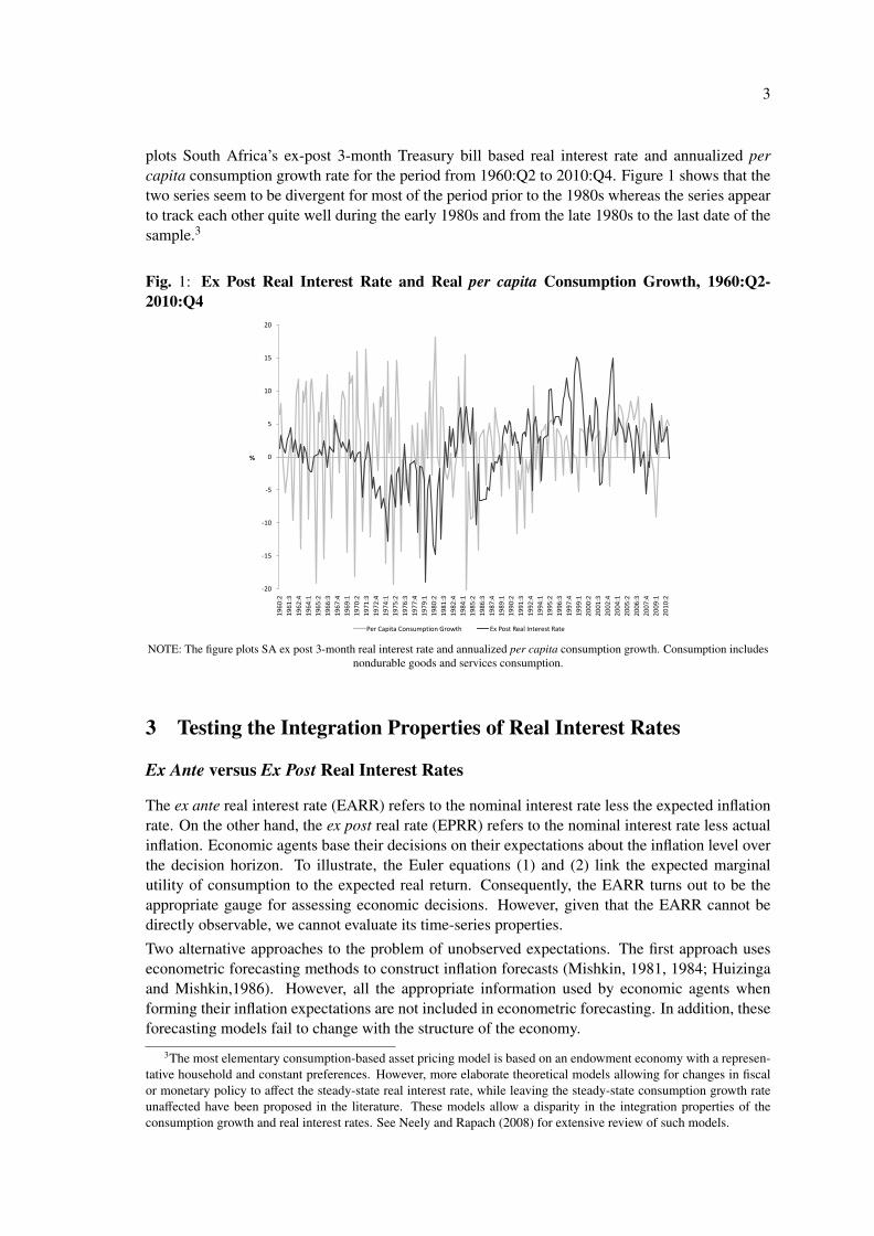
where ∆log(ct+1) = log(ct+1)−log(ct) = log(β)+0.5σ2, and σ2 is the constant conditional varianceof log[β(cl+1/cl)−α(1 + rl)]. Equation (2) relates the conditional expectations of the per capita realconsumption growth rate [∆log(ct+1)] with the (net) real interest rate [log(1 + rt) u rt]. Accordingto Rose (1988), if equation (2) is to hold, then the per capita real consumption growth rate andthe (net) real interest rate series must have the same integration properties. Bearing in mind that[∆log(ct+1)] is nearly without doubt a stationary process, Rose (1988) shows that the real interestrate is non-stationary i.e. rt v I(1) in many industrialized countries. A unit root in the real interestrate together with stationary consumption growth imply that permanent changes in the level ofthe real rate will be unmatched by such changes in consumption growth. Therefore, equation (2)seemingly cannot hold. The problem identified by Rose (1988) is vindicated in Figure 1, which

2Studies that exists for South Africa only deals with the uncovered interest rate parity condition, or in other words,the interest rate behavior of South Africa relative to other developed or emerging economies. See for example Kahnand Farrell (2002), Kryshko (2006), Lacerda et al., (2010) and de Bruyn et al., (2011).

3

plots South Africa’s ex-post 3-month Treasury bill based real interest rate and annualized percapita consumption growth rate for the period from 1960:Q2 to 2010:Q4. Figure 1 shows that thetwo series seem to be divergent for most of the period prior to the 1980s whereas the series appearto track each other quite well during the early 1980s and from the late 1980s to the last date of thesample.3

Fig. 1: Ex Post Real Interest Rate and Real per capita Consumption Growth, 1960:Q2-2010:Q4

-20

-15

-10

-5

0

5

10

15

20

19

60

:2

19

61

:3

19

62

:4

19

64

:1

19

65

:2

19

66

:3

19

67

:4

19

69

:1

19

70

:2

19

71

:3

19

72

:4

19

74

:1

19

75

:2

19

76

:3

19

77

:4

19

79

:1

19

80

:2

19

81

:3

19

82

:4

19

84

:1

19

85

:2

19

86

:3

19

87

:4

19

89

:1

19

90

:2

19

91

:3

19

92

:4

19

94

:1

19

95

:2

19

96

:3

19

97

:4

19

99

:1

20

00

:2

20

01

:3

20

02

:4

20

04

:1

20

05

:2

20

06

:3

20

07

:4

20

09

:1

20

10

:2

%

Per Capita Consumption Growth Ex Post Real Interest Rate

NOTE: The figure plots SA ex post 3-month real interest rate and annualized per capita consumption growth. Consumption includesnondurable goods and services consumption.

3 Testing the Integration Properties of Real Interest Rates

Ex Ante versus Ex Post Real Interest Rates

The ex ante real interest rate (EARR) refers to the nominal interest rate less the expected inflationrate. On the other hand, the ex post real rate (EPRR) refers to the nominal interest rate less actualinflation. Economic agents base their decisions on their expectations about the inflation level overthe decision horizon. To illustrate, the Euler equations (1) and (2) link the expected marginalutility of consumption to the expected real return. Consequently, the EARR turns out to be theappropriate gauge for assessing economic decisions. However, given that the EARR cannot bedirectly observable, we cannot evaluate its time-series properties.Two alternative approaches to the problem of unobserved expectations. The first approach useseconometric forecasting methods to construct inflation forecasts (Mishkin, 1981, 1984; Huizingaand Mishkin,1986). However, all the appropriate information used by economic agents whenforming their inflation expectations are not included in econometric forecasting. In addition, theseforecasting models fail to change with the structure of the economy.

3The most elementary consumption-based asset pricing model is based on an endowment economy with a represen-tative household and constant preferences. However, more elaborate theoretical models allowing for changes in fiscalor monetary policy to affect the steady-state real interest rate, while leaving the steady-state consumption growth rateunaffected have been proposed in the literature. These models allow a disparity in the integration properties of theconsumption growth and real interest rates. See Neely and Rapach (2008) for extensive review of such models.

4

The second approach uses the actual inflation rate as a proxy for inflation expectations. Bydefinition, the actual inflation rate at time t(πt) is the sum of the expected inflation rate and aforecast error term (εt):

(3) πt = Et−1πt + εt.

If expectations are formed rationally, Et−1πt should be an optimal forecast of inflation (Nelson andSchwert, 1977), and εt should therefore be a white noise process. The EARR can approximatelybe expressed as:

(4) reat = it − Etπt+1,

where it is the nominal interest rate. Solving equation (3) for Et(πt+1) and substituting it intoequation (4), we obtain

reat = it − (πt+1 − εt+1)(5)

= it − πt+1 + εt+1 = rept + εt+1,

where rept = it − πt+1 is the EPRR. Equation (5) implies that, under rational expectations, only

a white noise component distinguishes the EPRR from the EARR. Consequently, the EPRR andEARR will have the same long-run (integration) properties. This result holds if the expectationerrors (εt+1) are stationary and does not necessarily requires rational expectations to hold (Pelaez,1995; Andolfatto et al., 2008).The literature usually assesses the integration properties of the EPRR through a decision rule.First, the individual components of the EPRR i.e. it and πt+1 are analyzed. If unit root tests revealthat both it and πt+1 are I(0), then EPRR is stationary. On the other hand, if it and πt+1 havedifferent orders of integration e.g. it v I(1) and πt+1 v I(0), then EPRR must be non-stationary,as a linear combination of an I(0) process and an I(1) process results in an I(1) process. Lastly, ifboth it and πt+1 are I(1), then stationarity of the EPRR is assessed through a cointegration test ofit and πt+1 i.e. testing if the linear combination it − [θ0 + θ1πt+1] is stationary. Two approaches areused in the literature: First, a cointegrating vector of (1,−θ1)

′

= (1,−1)′

is imposed and thereaftera a unit root test of rep

t = it − πt+1 is applied. Such an approach usually has more power to rejectthe null of cointegration when the true cointegrating vector is (1,−1)

′

. Alternatively, the secondapproach involves freely estimating the cointegrating vector between it and πt+1 thereby allowingfor tax effects (Darby, 1975). If it and πt+1 are I(1) processes then EPRR requires θ1 =1 or 1

1−τwith τ being the marginal tax rate on the nominal interest income. Generally, estimates of θ1 inthe range of 1.30 to 1.40 is considered plausible when allowing for tax effects, since this wouldimply amarginal tax rate of 20 to 30 percent. Note that cointegration between it and πt+1 does notnecessarily imply that the EPRR is stationary, one requires θ1 = 1 or 1

τ in addition, since othervalues of θ1 would imply that the equilibrium real interest rate varies with inflation.

Unit Root and Cointegration Tests

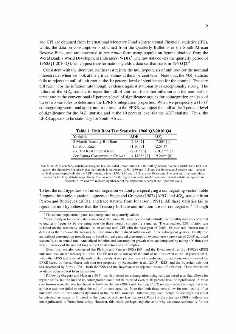
There exist a vast literature on unit root and cointegration tests applied to assessing the time seriesproperties of the real interest rate.4 Table 1 illustrates the unit root tests based on the augmentedDickey and Fuller (1979) [ADF] and the MZα test proposed by Ng and Perron (2001) for theSouth African 3-month Treasury bill rate, the Consumer Price Index (CPI) inflation, the ex postreal interest rate and the per capita consumption growth rate. The MZα statistic is designed to havebetter size and power properties than the ADF test. Note that the data for the Treasury bill rate

4This can be found in Neely and Rapach (2008).

5

and CPI are obtained from International Monetary Fund’s International Financial statistics (IFS),while, the data on consumption is obtained from the Quarterly Bulletins of the South AfricanReserve Bank, and are converted to per capita form using population figures obtained from theWorld Bank’s World Development Indicators (WDI).5 The raw data covers the quarterly period of1960:Q1-2010:Q4, which post transformations yields a data set that starts in 1960:Q2.6

Consistent with the literature, neither test rejects the null hypothesis of unit root for the nominalinterest rate, when we look at the critical values at the 5 percent level. Note that, the MZα statisticfails to reject the null of unit root at the 10 percent level of significance for the nominal Treasurybill rate.7 For the inflation rate though, evidence against stationarity is exceptionally strong. Thefailure of the MZα statistic to reject the null of unit root for either inflation and the nominal in-terest rate at the conventional (5 percent) level of significance argues for cointegration analysis ofthese two variables to determine the EPRR’s integration properties. When we prespecify a (1,-1)′

cointegrating vector and apply unit root tests to the EPRR, we reject the null at the 5 percent levelof significance for the MZα statistic and at the 10 percent level for the ADF statistic. Thus, theEPRR appears to be stationary for South Africa.

Table 1: Unit Root Test Statistics, 1960:Q2-2010:Q4Variable ADF MZα3-Month Treasury Bill Rate -2.48 [1] -7.00* [1]Inflation Rate -1.80 [7] -2.51 [7]Ex Post Real Interest Rate -2.60* [8] -10.27** [7]Per Capita Consumption Growth -4.14*** [7] -9.24** [8]

NOTE: the ADF and MZα statistics correspond to a one-sided (lower-tail) test of the null hypothesis that the variable has a unit rootagainst the alternative hypothesis that the variable is stationary. -2.58, -2.89 and -3.51 are the 10 percent, 5 percent and 1 percentcritical values respectively for the ADF statistic, while, -5.70, -8.10 and -13.80 are the 10 percent, 5 percent and 1 percent critical

values for the MZα statistic respectively. The lag order for the regression model used to compute the test statistic is reported inbrackets. *, ** and *** indicate significance at the 10 percent, 5 percent and 1 percent levels.

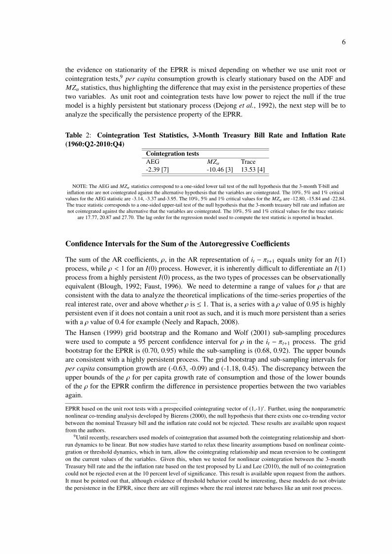
To test the null hypothesis of no cointegration without pre-specifying a cointegrating vector, Table2 reports the single-equation augmented Engle and Granger (1987) [AEG] and MZα statistic fromPerron and Rodriguez (2001), and trace statistic from Johansen (1991). All these statistics fail toreject the null hypothesis that the Treasury bill rate and inflation are not cointegrated.8 Though

5The annual population figures are interpolated to quarterly values.6Specifically as far as the data is concerned, the 3-month Treasury constant maturity rate monthly data are converted

to quarterly frequency by averaging over the three months comprising a quarter. The annualized CPI inflation rateis based on the seasonally adjusted (at an annual rate) CPI with the base year of 2005. Ex post real interest rate isdefined as the three-month Treasury bill rate minus the realized inflation rate in the subsequent quarter. Finally, theannualized consumption growth rate is based on real personal consumption expenditures (base year of 2005) adjustedseasonally at an annual rate. Annualized inflation and consumption growth rates are computed by taking 400 times thefirst differences of the natural logs of the CPI deflator and consumption.

7Given this, we also conducted the Phillips and Perron (1988) [PP] and the Kwiatkowski et al., (1992) [KPSS]unit root tests on the treasury bill rate. The PP test could not reject the null of unit root even at the 10 percent level,while the KPSS test rejected the null of stationarity at one percent level of significance. In addition, we also tested theEPRR based on the nonlinear unit root test proposed by Kapetanios et al., (2003) [KSS] and the Bayesian unit roottest developed by Sims (1988). Both the KSS and the Bayesian tests rejected the null of unit root. These results areavailable upon request from the authors.

8Following Gregory and Hansen (1996), we also tested for cointegration using residual based tests that allows forregime shifts, but the null of no cointegration could not be rejected even at 10 percent level of significance. Similarconclusions were also reached based on both the Bierens (1997) and Breitung (2002) nonparametric cointegration tests,as these tests too failed to reject the null of no cointegration. Note that both these tests allow for nonlinearity of anunknown form in the short-run dynamics of the the two variables. Interestingly, even though no cointegration couldbe detected, estimates of θ1 based on the dynamic ordinary least squares (DOLS) or the Johansen (1991) methods arenot significantly different from unity. However, this result, perhaps, explains as to why we detect stationarity for the

6

the evidence on stationarity of the EPRR is mixed depending on whether we use unit root orcointegration tests,9 per capita consumption growth is clearly stationary based on the ADF andMZα statistics, thus highlighting the difference that may exist in the persistence properties of thesetwo variables. As unit root and cointegration tests have low power to reject the null if the truemodel is a highly persistent but stationary process (Dejong et al., 1992), the next step will be toanalyze the specifically the persistence property of the EPRR.

Table 2: Cointegration Test Statistics, 3-Month Treasury Bill Rate and Inflation Rate(1960:Q2-2010:Q4)

Cointegration testsAEG MZα Trace-2.39 [7] -10.46 [3] 13.53 [4]

NOTE: The AEG and MZα statistics correspond to a one-sided lower tail test of the null hypothesis that the 3-month T-bill andinflation rate are not cointegrated against the alternative hypothesis that the variables are cointegrated. The 10%, 5% and 1% critical

values for the AEG statistic are -3.14, -3.37 and-3.95. The 10%, 5% and 1% critical values for the MZα are -12.80, -15.84 and -22.84.The trace statistic corresponds to a one-sided upper-tail test of the null hypothesis that the 3-month treasury bill rate and inflation arenot cointegrated against the alternative that the variables are cointegrated. The 10%, 5% and 1% critical values for the trace statistic

are 17.77, 20.87 and 27.70. The lag order for the regression model used to compute the test statistic is reported in bracket.

Confidence Intervals for the Sum of the Autoregressive Coefficients

The sum of the AR coefficients, ρ, in the AR representation of it − πt+1 equals unity for an I(1)process, while ρ < 1 for an I(0) process. However, it is inherently difficult to differentiate an I(1)process from a highly persistent I(0) process, as the two types of processes can be observationallyequivalent (Blough, 1992; Faust, 1996). We need to determine a range of values for ρ that areconsistent with the data to analyze the theoretical implications of the time-series properties of thereal interest rate, over and above whether ρ is ≤ 1. That is, a series with a ρ value of 0.95 is highlypersistent even if it does not contain a unit root as such, and it is much more persistent than a serieswith a ρ value of 0.4 for example (Neely and Rapach, 2008).The Hansen (1999) grid bootstrap and the Romano and Wolf (2001) sub-sampling procedureswere used to compute a 95 percent confidence interval for ρ in the it − πt+1 process. The gridbootstrap for the EPRR is (0.70, 0.95) while the sub-sampling is (0.68, 0.92). The upper boundsare consistent with a highly persistent process. The grid bootstrap and sub-sampling intervals forper capita consumption growth are (-0.63, -0.09) and (-1.18, 0.45). The discrepancy between theupper bounds of the ρ for per capita growth rate of consumption and those of the lower boundsof the ρ for the EPRR confirm the difference in persistence properties between the two variablesagain.

EPRR based on the unit root tests with a prespecified cointegrating vector of (1,-1)′. Further, using the nonparametricnonlinear co-trending analysis developed by Bierens (2000), the null hypothesis that there exists one co-trending vectorbetween the nominal Treasury bill and the inflation rate could not be rejected. These results are available upon requestfrom the authors.

9Until recently, researchers used models of cointegration that assumed both the cointegrating relationship and short-run dynamics to be linear. But now studies have started to relax these linearity assumptions based on nonlinear cointe-gration or threshold dynamics, which in turn, allow the cointegrating relationship and mean reversion to be contingenton the current values of the variables. Given this, when we tested for nonlinear cointegration between the 3-monthTreasury bill rate and the the inflation rate based on the test proposed by Li and Lee (2010), the null of no cointegrationcould not be rejected even at the 10 percent level of significance. This result is available upon request from the authors.It must be pointed out that, although evidence of threshold behavior could be interesting, these models do not obviatethe persistence in the EPRR, since there are still regimes where the real interest rate behaves like an unit root process.

7

Testing for Fractional Integration

Unit root and cointegration tests determine whether a process is stationary or non-stationary (i.e.,I(0) or I(1)). The distinction between I(0) and I(1) implicitly restricts the types of allowed dynamicprocesses. As a result, studies such as Granger (1980), Granger and Joyeux (1980) and Hosking(1981) test for fractional integration in the EARR and EPRR. A fractionally integrated series isdenoted by I(d), 0 ≤ d ≤ 1. If d = 0, then the series is I(0) and shocks decay at a geometricrate. If d = 1, then the series is I(1), and shocks have permanent effects. If 0 < d < 1 then theseries is mean-reverting as in the I(0) case. However, shocks vanish at a much slower hyperbolicrate. Such series can be considerably more persistent than a very persistent I(0) series (Neely andRapach, 2008).Testing for fractional integration in this paper is carried out by estimating the d parameter usingthe Shimotsu (2008) semi-parametric two-step feasible exact local Whittle estimator, which allowsfor an unknown mean in the series. The estimate of d for the South African EPRR is found to be0.69 with a 95 percent confidence interval of (0.49, 0.89), suggesting long-memory, but mean-reverting behavior. So we can reject the hypothesis that d = 0 or d = 1.10 The estimate of d forper capita consumption growth is equal to 0.18, with a 95 percent confidence interval of (-0.02,0.38), suggesting that we cannot reject the null hypothesis of d = 0 at conventional significancelevels.11 The fractional integration results further corroborate the difference in persistence betweenthe EPRR and per capita consumption growth.

4 Testing for Regime Switching and Structural Breaks in Real Inter-est Rate

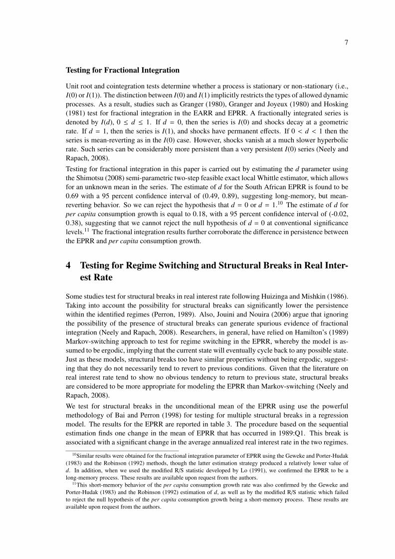
Some studies test for structural breaks in real interest rate following Huizinga and Mishkin (1986).Taking into account the possibility for structural breaks can significantly lower the persistencewithin the identified regimes (Perron, 1989). Also, Jouini and Nouira (2006) argue that ignoringthe possibility of the presence of structural breaks can generate spurious evidence of fractionalintegration (Neely and Rapach, 2008). Researchers, in general, have relied on Hamilton’s (1989)Markov-switching approach to test for regime switching in the EPRR, whereby the model is as-sumed to be ergodic, implying that the current state will eventually cycle back to any possible state.Just as these models, structural breaks too have similar properties without being ergodic, suggest-ing that they do not necessarily tend to revert to previous conditions. Given that the literature onreal interest rate tend to show no obvious tendency to return to previous state, structural breaksare considered to be more appropriate for modeling the EPRR than Markov-switching (Neely andRapach, 2008).We test for structural breaks in the unconditional mean of the EPRR using use the powerfulmethodology of Bai and Perron (1998) for testing for multiple structural breaks in a regressionmodel. The results for the EPRR are reported in table 3. The procedure based on the sequentialestimation finds one change in the mean of EPRR that has occurred in 1989:Q1. This break isassociated with a significant change in the average annualized real interest rate in the two regimes.

10Similar results were obtained for the fractional integration parameter of EPRR using the Geweke and Porter-Hudak(1983) and the Robinson (1992) methods, though the latter estimation strategy produced a relatively lower value ofd. In addition, when we used the modified R/S statistic developed by Lo (1991), we confirmed the EPRR to be along-memory process. These results are available upon request from the authors.

11This short-memory behavior of the per capita consumption growth rate was also confirmed by the Geweke andPorter-Hudak (1983) and the Robinson (1992) estimation of d, as well as by the modified R/S statistic which failedto reject the null hypothesis of the per capita consumption growth being a short-memory process. These results areavailable upon request from the authors.

8

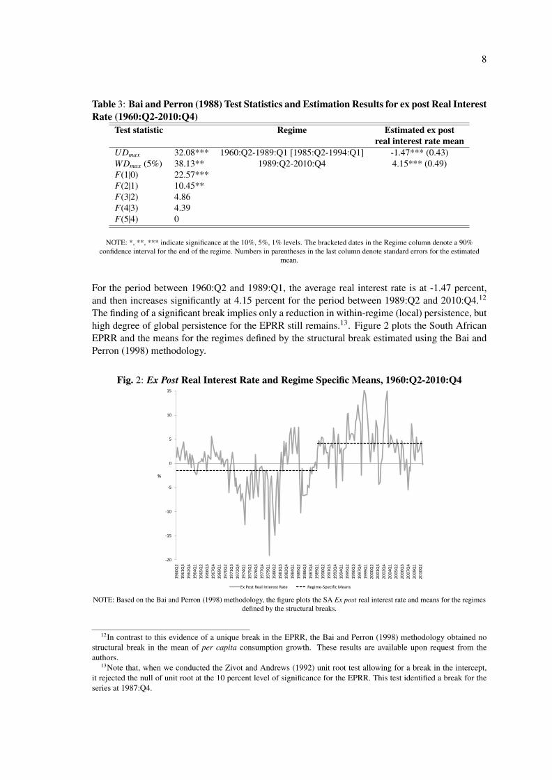
Table 3: Bai and Perron (1988) Test Statistics and Estimation Results for ex post Real InterestRate (1960:Q2-2010:Q4)

Test statistic Regime Estimated ex postreal interest rate mean

UDmax 32.08*** 1960:Q2-1989:Q1 [1985:Q2-1994:Q1] -1.47*** (0.43)WDmax (5%) 38.13** 1989:Q2-2010:Q4 4.15*** (0.49)F(1|0) 22.57***F(2|1) 10.45**F(3|2) 4.86F(4|3) 4.39F(5|4) 0

NOTE: *, **, *** indicate significance at the 10%, 5%, 1% levels. The bracketed dates in the Regime column denote a 90%confidence interval for the end of the regime. Numbers in parentheses in the last column denote standard errors for the estimated

mean.

For the period between 1960:Q2 and 1989:Q1, the average real interest rate is at -1.47 percent,and then increases significantly at 4.15 percent for the period between 1989:Q2 and 2010:Q4.12

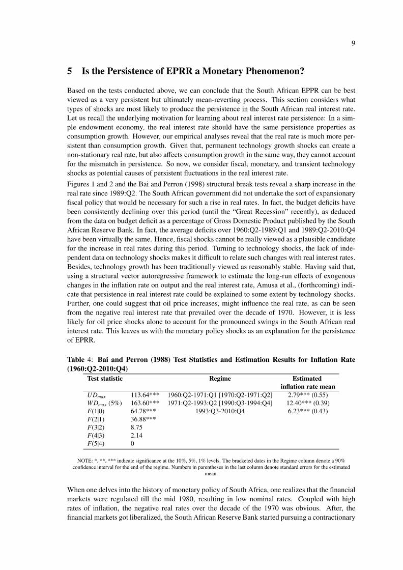
The finding of a significant break implies only a reduction in within-regime (local) persistence, buthigh degree of global persistence for the EPRR still remains.13. Figure 2 plots the South AfricanEPRR and the means for the regimes defined by the structural break estimated using the Bai andPerron (1998) methodology.

Fig. 2: Ex Post Real Interest Rate and Regime Specific Means, 1960:Q2-2010:Q4

-20

-15

-10

-5

0

5

10

15

19

60

Q2

19

61

Q3

19

62

Q4

19

64

Q1

19

65

Q2

19

66

Q3

19

67

Q4

19

69

Q1

19

70

Q2

19

71

Q3

19

72

Q4

19

74

Q1

19

75

Q2

19

76

Q3

19

77

Q4

19

79

Q1

19

80

Q2

19

81

Q3

19

82

Q4

19

84

Q1

19

85

Q2

19

86

Q3

19

87

Q4

19

89

Q1

19

90

Q2

19

91

Q3

19

92

Q4

19

94

Q1

19

95

Q2

19

96

Q3

19

97

Q4

19

99

Q1

20

00

Q2

20

01

Q3

20

02

Q4

20

04

Q1

20

05

Q2

20

06

Q3

20

07

Q4

20

09

Q1

20

10

Q2

%

Ex Post Real Interest Rate Regime-Specific Means

NOTE: Based on the Bai and Perron (1998) methodology, the figure plots the SA Ex post real interest rate and means for the regimesdefined by the structural breaks.

12In contrast to this evidence of a unique break in the EPRR, the Bai and Perron (1998) methodology obtained nostructural break in the mean of per capita consumption growth. These results are available upon request from theauthors.

13Note that, when we conducted the Zivot and Andrews (1992) unit root test allowing for a break in the intercept,it rejected the null of unit root at the 10 percent level of significance for the EPRR. This test identified a break for theseries at 1987:Q4.

9

5 Is the Persistence of EPRR a Monetary Phenomenon?

Based on the tests conducted above, we can conclude that the South African EPPR can be bestviewed as a very persistent but ultimately mean-reverting process. This section considers whattypes of shocks are most likely to produce the persistence in the South African real interest rate.Let us recall the underlying motivation for learning about real interest rate persistence: In a sim-ple endowment economy, the real interest rate should have the same persistence properties asconsumption growth. However, our empirical analyses reveal that the real rate is much more per-sistent than consumption growth. Given that, permanent technology growth shocks can create anon-stationary real rate, but also affects consumption growth in the same way, they cannot accountfor the mismatch in persistence. So now, we consider fiscal, monetary, and transient technologyshocks as potential causes of persistent fluctuations in the real interest rate.Figures 1 and 2 and the Bai and Perron (1998) structural break tests reveal a sharp increase in thereal rate since 1989:Q2. The South African government did not undertake the sort of expansionaryfiscal policy that would be necessary for such a rise in real rates. In fact, the budget deficits havebeen consistently declining over this period (until the “Great Recession” recently), as deducedfrom the data on budget deficit as a percentage of Gross Domestic Product published by the SouthAfrican Reserve Bank. In fact, the average deficits over 1960:Q2-1989:Q1 and 1989:Q2-2010:Q4have been virtually the same. Hence, fiscal shocks cannot be really viewed as a plausible candidatefor the increase in real rates during this period. Turning to technology shocks, the lack of inde-pendent data on technology shocks makes it difficult to relate such changes with real interest rates.Besides, technology growth has been traditionally viewed as reasonably stable. Having said that,using a structural vector autoregressive framework to estimate the long-run effects of exogenouschanges in the inflation rate on output and the real interest rate, Amusa et al., (forthcoming) indi-cate that persistence in real interest rate could be explained to some extent by technology shocks.Further, one could suggest that oil price increases, might influence the real rate, as can be seenfrom the negative real interest rate that prevailed over the decade of 1970. However, it is lesslikely for oil price shocks alone to account for the pronounced swings in the South African realinterest rate. This leaves us with the monetary policy shocks as an explanation for the persistenceof EPRR.

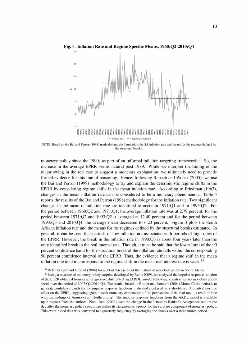
Table 4: Bai and Perron (1988) Test Statistics and Estimation Results for Inflation Rate(1960:Q2-2010:Q4)

Test statistic Regime Estimatedinflation rate mean

UDmax 113.64*** 1960:Q2-1971:Q1 [1970:Q2-1971:Q2] 2.79*** (0.55)WDmax (5%) 163.60*** 1971:Q2-1993:Q2 [1990:Q3-1994:Q4] 12.40*** (0.39)F(1|0) 64.78*** 1993:Q3-2010:Q4 6.23*** (0.43)F(2|1) 36.88***F(3|2) 8.75F(4|3) 2.14F(5|4) 0

NOTE: *, **, *** indicate significance at the 10%, 5%, 1% levels. The bracketed dates in the Regime column denote a 90%confidence interval for the end of the regime. Numbers in parentheses in the last column denote standard errors for the estimated

mean.

When one delves into the history of monetary policy of South Africa, one realizes that the financialmarkets were regulated till the mid 1980, resulting in low nominal rates. Coupled with highrates of inflation, the negative real rates over the decade of the 1970 was obvious. After, thefinancial markets got liberalized, the South African Reserve Bank started pursuing a contractionary

10

Fig. 3: Inflation Rate and Regime Specific Means, 1960:Q2-2010:Q4

-5

0

5

10

15

20

25

19

60

Q2

19

61

Q3

19

62

Q4

19

64

Q1

19

65

Q2

19

66

Q3

19

67

Q4

19

69

Q1

19

70

Q2

19

71

Q3

19

72

Q4

19

74

Q1

19

75

Q2

19

76

Q3

19

77

Q4

19

79

Q1

19

80

Q2

19

81

Q3

19

82

Q4

19

84

Q1

19

85

Q2

19

86

Q3

19

87

Q4

19

89

Q1

19

90

Q2

19

91

Q3

19

92

Q4

19

94

Q1

19

95

Q2

19

96

Q3

19

97

Q4

19

99

Q1

20

00

Q2

20

01

Q3

20

02

Q4

20

04

Q1

20

05

Q2

20

06

Q3

20

07

Q4

20

09

Q1

20

10

Q2

%

Inflation Rate Regime-Specific Means

NOTE: Based on the Bai and Perron (1998) methodology, the figure plots the SA inflation rate and means for the regimes defined bythe structural breaks.

monetary policy since the 1990s as part of an informal inflation targeting framework.14 So, theincrease in the average EPRR seems natural post 1989. While we interpret the timing of themajor swing in the real rate to suggest a monetary explanation, we ultimately need to provideformal evidence for this line of reasoning. Hence, following Rapach and Wohar (2005), we usethe Bai and Perron (1998) methodology to try and explain the deterministic regime shifts in theEPRR by considering regime shifts in the mean inflation rate. According to Friedman (1963),changes in the mean inflation rate can be considered to be a monetary phenomenon. Table 4reports the results of the Bai and Perron (1998) methodology for the inflation rate. Two significantchanges in the mean of inflation rate are identified to occur in 1971:Q1 and in 1993:Q2. Forthe period between 1960:Q2 and 1971:Q1, the average inflation rate was at 2.79 percent; for theperiod between 1971:Q2 and 1993:Q2 it averaged at 12.40 percent and for the period between1993:Q3 and 2010:Q4, the average mean decreased to 6.23 percent. Figure 3 plots the SouthAfrican inflation rate and the means for the regimes defined by the structural breaks estimated. Ingeneral, it can be seen that periods of low inflation are associated with periods of high rates ofthe EPRR. However, the break in the inflation rate in 1990:Q3 is about four years later than theonly identified break in the real interest rate. Though, it must be said that the lower limit of the 90percent confidence band for the structural break of the inflation rate falls within the corresponding90 percent confidence interval of the EPRR. Thus, the evidence that a regime shift in the meaninflation rate tend to correspond to the regime shift in the mean real interest rate is weak.15

14Refer to Ludi and Ground (2006) for a detail discussion of the history of monetary policy in South Africa.15Using a measure of monetary policy surprise developed by Reid (2009), we analyzed the impulse response function

of the EPRR obtained from an autoregressive distributed lag (ARDL) model following a contractionary monetary policyshock over the period of 2002:Q2-2010:Q4. The results, based on Romer and Romer’s (2004) Monte Carlo methods togenerate confidence bands for the impulse response functions, indicated a delayed very short-lived (1 quarter) positiveeffect on the EPRR, suggesting again a weak monetary explanation of the persistence of the real rate – a result in linewith the findings of Amusa et al., (forthcoming). The impulse response functions from the ARDL model is availableupon request from the authors. Note, Reid (2009) used the change in the 3-months Banker’s Acceptance rate on theday after the monetary policy committee makes its statement as a proxy for the surprise component of monetary policy.This event-based data was converted to a quarterly frequency by averaging the shocks over a three month period.

11

Bayesian Change Point Analysis

Given the weak evidence that the EPRR persistence is a monetary phenomenon based on the struc-tural break test, we decided to look into this issue further using a Bayesian change point analysisfor the real rate and the inflation rate. This method allows us to obtain posterior probabilities of achange for each point of the two series, thus, (possibly) allowing us to better relate inflation withthe persistence of the EPRR. In the following paragraphs, we describe the Barry and Hartigan(1993) algorithm for the Bayesian change point methodology.The Barry and Hartigan (1993) algorithm models the series generating process by assuming thatthere is an underlying sequence of parameters partitioned into contiguous blocks of equal param-eter values. The beginning of each block is then a change point, while observations are assumedto be independent in different blocks given the sequence of parameter. Let X1, X2, ...,Xn be inde-pendent observations, with each Xi having a density dependent on θi, i = 1, ..., n. Furthermore,there exists an unknown number of contiguous blocks with partitions ρ = {i0, i1, ..., ib} such that0 = i0 < i1 < ... < in = n and θi = θib when ir−1 < i ≤ ir.In the notation used by Barry and Hartigan (1993), let Xi j denote the sequence of points Xi+1, ..., X j

in time. Let fi j(xi j|θ j) denote the density of xi j when θi+1 = θi+2 = ... = θ j . For constant blocks, atransition distribution is defined as follows: Given θi, θi+1 equals θi with probability 1 − pi or hasdensity f (θi+1|θi) with probability pi. This in essence implies that smaller values of pi will resultin longer θi blocks.Further, the probability of a partition ρ = i0, i1, ..., ib is given by f (ρ) = Kci0iici1i2 ...cib−1ib whereci j are prior cohesion for adjacent blocks i j. In notations, let X1, X2, ...,Xn are assumed to be anindependent for a given sequence of µi, such that Xi v N(µi, σ

2), i = 1, 2, ..., n. A prior cohesionci j following Yao (1984) is introduced as follows:

(6) ci j =

{(1 − p) j−i−1 p, j < n(1 − p) j−i−1 j = n

Also, a block prior is introduced as follows:

(7) fi j(µ j) v N(µ0,σ2

0

j − i)

The priors distribution for each of µ0, σ20, p, w = σ2

(σ20+σ2)

are as follows:

f (µ0) = 1,−∞ ≤ µ0 ≤ ∞

f (σ2) = 1/σ2, 0 ≤ σ2 ≤ ∞

f (p) = 1/p0, 0 ≤ p ≤ p0

f (w) = 1/w0, 0 ≤ w ≤ w0

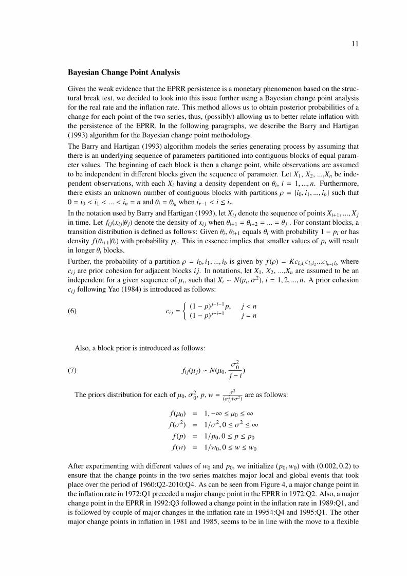
After experimenting with different values of w0 and p0, we initialize (p0,w0) with (0.002, 0.2) toensure that the change points in the two series matches major local and global events that tookplace over the period of 1960:Q2-2010:Q4. As can be seen from Figure 4, a major change point inthe inflation rate in 1972:Q1 preceded a major change point in the EPRR in 1972:Q2. Also, a majorchange point in the EPRR in 1992:Q3 followed a change point in the inflation rate in 1989:Q1, andis followed by couple of major changes in the inflation rate in 19954:Q4 and 1995:Q1. The othermajor change points in inflation in 1981 and 1985, seems to be in line with the move to a flexible

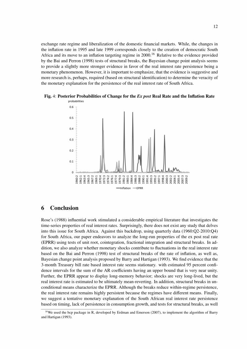
12

exchange rate regime and liberalization of the domestic financial markets. While, the changes inthe inflation rate in 1995 and late 1999 corresponds closely to the creation of democratic SouthAfrica and its move to an inflation targeting regime in 2000.16 Relative to the evidence providedby the Bai and Perron (1998) tests of structural breaks, the Bayesian change point analysis seemsto provide a slightly more stronger evidence in favor of the real interest rate persistence being amonetary phenomenon. However, it is important to emphasize, that the evidence is suggestive andmore research is, perhaps, required (based on structural identification) to determine the veracity ofthe monetary explanation for the persistence of the real interest rate of South Africa.

Fig. 4: Posterior Probabilities of Change for the Ex post Real Rate and the Inflation Rate

0

0.1

0.2

0.3

0.4

0.5

0.6

1960:2

1962:1

1963:4

1965:3

1967:2

1969:1

1970:4

1972:3

1974:2

1976:1

1977:4

1979:3

1981:2

1983:1

1984:4

1986:3

1988:2

1990:1

1991:4

1993:3

1995:2

1997:1

1998:4

2000:3

2002:2

2004:1

2005:4

2007:3

2009:2

probabilities

Inflation EPRR

6 Conclusion

Rose’s (1988) influential work stimulated a considerable empirical literature that investigates thetime-series properties of real interest rates. Surprisingly, there does not exist any study that delvesinto this issue for South Africa. Against this backdrop, using quarterly data (1960:Q2-2010:Q4)for South Africa, our paper endeavors to analyze the long-run properties of the ex post real rate(EPRR) using tests of unit root, cointegration, fractional integration and structural breaks. In ad-dition, we also analyze whether monetary shocks contribute to fluctuations in the real interest ratebased on the Bai and Perron (1998) test of structural breaks of the rate of inflation, as well as,Bayesian change point analysis proposed by Barry and Hartigan (1993). We find evidence that the3-month Treasury bill rate based interest rate seems stationary. with estimated 95 percent confi-dence intervals for the sum of the AR coefficients having an upper bound that is very near unity.Further, the EPRR appear to display long-memory behavior; shocks are very long-lived, but thereal interest rate is estimated to be ultimately mean-reverting. In addition, structural breaks in un-conditional means characterize the EPRR. Although the breaks reduce within-regime persistence,the real interest rate remains highly persistent because the regimes have different means. Finally,we suggest a tentative monetary explanation of the South African real interest rate persistencebased on timing, lack of persistence in consumption growth, and tests for structural breaks, as well

16We used the bcp package in R, developed by Erdman and Emerson (2007), to implement the algorithm of Barryand Hartigan (1993).

13

as, Bayesian change point analysis. In the future, further analysis of the relative importance ofdifferent types of shocks in explaining real interest rate persistence could be of immense help tothis literature.

References

Andolfatto, D., Hendry, S. and Moran, K. ”Are Inflation Expectations Rational?” Journal ofMonetary Economics, 2008, 55(2), pp. 406-22.

Amusa, K., Gupta, R., Karolia, S. and Simo-Kengne, B. D. “The Long-Run Impact of Infla-tion in South Africa.” Journal of Policy Modeling, Forthcoming.

Bai, J. and Perron, P. “Estimating and Testing Linear Models with Multiple StructuralChanges.” Econometrica, 1998, 66(1), pp. 47-78.

Barry, D. and Hartigan J. A. “A Bayesian Analysis for Change Point Problems.” Journal ofthe American Statistical Association, 1993, 88, pp. 309-19.

Bierens, H. J. “Nonparametric Nonlinear Cotrending Analysis, with an Application to Inter-est and Inflation in the United States.” Journal of Business and Economic Statistics, 2000,18(3), pp. 323-37.

Bierens, H. J. “Nonparametric Nonlinear Co-Trending Analysis, with an Application toInterest and Inflation in the U.S.” Journal of Business and Economic Statistics, 2000, 18,pp. 323-37.

Blough, S. R. “The Relationship Between Power and Level for Generic Unit Root Tests inFinite Samples.” Journal of Applied Econometrics, 1992, 7(3), pp. 295-308.

Breeden, D. T. “An Intertemporal Asset Pricing Model with Stochastic Consumption andInvestment Opportunities.” Journal of Financial Economics, 1979, 7(3), pp. 265-96.

Breitung, J. “Nonparametric Tests for Unit Roots and Cointegration.” Journal of Economet-rics, 2002, 108(2), pp. 343-63.

Caporale, T. and Grier, K. B. “Inflation, Presidents, Fed Chairs, and Regime Changes in theU.S. Real Interest Rate.” Journal of Money, Credit, and Banking, 2005, 37(6), pp. 1153-63.

Carlson, J. A. “Short-Term Interest Rates as Predictors of Inflation: Comment.” AmericanEconomic Review, 1977, 67(3), pp. 469-75.

Cass, D. “Optimum Growth in an Aggregate Model of Capital Accumulation.” Review ofEconomic Studies, 1965, 32(3), pp. 233-40.

Crowder, W. J. and Hoffman, D. L. “ The Long-Run Relationship Between Nominal InterstRates and Inflation: The Fisher Equation Revisited.” Journal of Money, Credit, and Banking,1996, 28(1), pp.102-118.

Darby, M. R. “The Financial and Tax Effects of Monetary Policy on Interest Rates.” Eco-nomic Inquiry, 1975, 13(2), pp. 266-76.

de Bruyn, R., Gupta, R. and Stander, L. “Testing the Monetary Model for Exchange RateDetermination in South Africa: Evidence from 101 Years of Data.” University of PretoriaDepartment of Economics Working Paper, 2011, No. 201134.

14

DeJong, D. N., Nankervis, J. C., Savin, N. E. and Whiteman, C. H. “The Power Problems ofUnit Root Tests in Time Series with Autoregressive Errors.” Journal of Econometrics, 1992,53(1-3), pp. 323-43.

Dickey, D. A. and Fuller, W. A. “Distribution of the Estimators for Autoregressive TimeSeries with a Unit Root.” Journal of the American Statistical Association, 1979, 74(366),pp. 427-31.

Engle, R. F. and Granger, C. W. J. “Co-integration and Error Correction: Representation,Estimation, and Testing.” Econometrica, 1987, 55(2), pp. 251-76.

Erdman, C. and Emerson, J. W. “bcp; An R Package for Performing a Bayesian Analysis ofChange Point Problems.” Journal of Statistical Software, 2007, 23(3), pp. 1-13.

Faust, J. “Near Observational Equivalence and Theoretical Size Problems with Unit RootTests.” Econometric Theory, 1996, 12(4), pp. 724-31.

Fisher, I. “The Theory of Interest.” MacMillan: New York, 1930.

Geweke and Porter-Hudak. “The Estimation and Application of Long Memory Time SeriesModels.” Journal of Time Series Analysis, 1983, pp. 221-238.

Granger, C. W. J. “Long Memory Relationships and the Aggregation of Dynamic Models.”Journal of Econometrics, 1980, 14(2), pp. 227-38.

Granger, C. W. J. and Joyeux, R. “An Introduction to Long-Memory Time Series Modelsand Fractional Differencing.” Journal of Time Series Analysis, 1980, 1, pp. 15-39.

Gregory, A. W. and Hansen, B. E. “Residual-based tests for Cointegration in Models withRegime Shifts.” Journal of Econometrics, 1996, 70(1), pp. 99-126.

Hamilton, J. D. “A New Approach to the Economic Analysis of Nonstationary Time Seriesand the Business Cycle.” Econometrica, 1989, 57(2), pp. 357-84.

Hansen, B. E. “The Grid Bootstrap and the Autoregressive Model.” Review of Economicsand Statistics, 1999, 81(4), pp. 594-607.

Hansen, L. P. and Singleton, K. J. “Generalized Instrumental Variables Estimation of Non-linear Rational Expectations Models.” Econometrica, 1982, 50(5), pp. 1269-86.

Hansen, L. P. and Singleton, K. J. “Stochastic Consumption, Risk Aversion, and the Tem-poral Behavior of Asset Returns.” Journal of Political Economy, 1983, 91(2), pp. 249-65.

Hosking, J. R. M. “Fractional Differencing.” Biometrika, 1981, 68(1), pp. 165-76.

Huizinga, J. and Mishkin, F. S. “Monetary Policy Regime Shifts and the Unusual Behaviorof Real Interest Rates.” Carnegie-Rochester Conference Series on Public Policy, 1986, 24,pp. 231-74.

Johansen, S. “Estimation and Hypothesis Testing of Cointegration Vectors in Gaussian Vec-tor Autoregressive Model.” Econometrica, 1991, 59(6), pp. 1551-80.

Jouini, J. and Nouira, L. “Mean-Shifts and Long-Memory in the U.S. Ex Post Real InterestRate.” Universit de la Mditerrane, GREQAM, 2006, Mimeo.

15

Kahn, B. and Farrell, G. “South African real Interest Rates in Comparative Perspective:Theory and Evidence.” South African Reserve Bank Occasional Paper, 2002, No 17.

Kapetanios, G., Shin, Y. and Snell, A. “Testing for a Unit Root in the Non-Linear STARFramework.” Journal of Econometrics, 2003, 112, pp. 359-79.

Koopmans, T. C. “On the Concept of Optimal Economic Growth,” in The Economic Ap-proach to Development Planning. Amsterdam: Elsevier, 1965, pp. 225-300.

Kryshko, M. “Nominal Exchange Rates and Uncovered Interest Parity: Non-Parametric Co-integration Analysis.” University of Pennsylvania Department of Economics, 2006, Mimeo.

Kwiatkowski, D., Phillips, P. C. B., Schmidt, P and Shin, Y. “Testing the Null Hypothesis ofStationarity Against the Alternative of a Unit Root: How Sure Are We That Economic TimeSeries Have a Unit Root?” Journal of Econometrics, 1992, 54(1-3), pp. 159-78.

Lacerda, M., Fedderke, J. W. and Haines, L. M. “Testing for Purchasing Power Parity andUncovered Interest Parity in the Presence of Monetary and Exchange Rate Regime Shifts.”The South African Journal of Economics, 2010, 78(4), pp. 363-382.

Lai, K. S. “Long-Term Persistence in the Real Interest Rate: Evidence of a Fractional UnitRoot.” International Journal of Finance and Economics, 1997, 2(3), pp. 225-35.

Li, J. and Lee, J. “Adl Tests for Threshold Cointegration.” Journal of Time Series Analysis,2010, 31(4), pp. 241-54.

Lucas, R. E. “Asset Prices in an Exchange Economy.” Econometrica, 1978, 46(6), pp. 1429-45.

Ludi, K. and Ground, M. “Investigating the Bank Lending Channel in South Africa: AVAR Approach.” University of Pretoria Department of Economics Working Paper, 2006,No. 200604.

Lo. “Long-term Memory in Stock Market Prices”, Econometrica, 1991, 59, pp. 1279-1313.

Mishkin, F. S. “The Real Rate of Interest : An Empirical Investigation.” Carnegie-RochesterConference Series on public policy, 1981, 15, pp. 151-200.

Mishkin, F. S. “The Real Interest :Rate : A Multi-Country Empirical Study.” CanadianJournal of Economics, 1984, 17(2), pp. 283-311.

Neely C. J. and Rapach D. E. “Real Interest Rate Persistence: Evidence and Implications.”Federal Reserve Bank of St. Louis Review, 2008, 90(6), pp.609-41.

Nelson, C. R. and Schwert, G. W. “Short-Term Interest Rates as Predictors of Inflation: OnTesting the Hypothesis that the Real Interest Rate Is Constant.” American Economic Review,1997, 67(3), pp. 478-86.

Ng, S. and Perron, P. “Lag Length Selection and the Construction of Unit Root Tests withGood Size and Power.” Econometrica, 2001, 69(6), pp. 1519-54.

Pelaez, R. F. “The Fisher Effect: Reprise.” Journal of Macroeconomics, 1995, 17(2), pp.333-46.

Perron, P. “The Great Crash, the Oil Price Shock and the Unit Root Hypothesis.” Economet-rica, 1989, 57(6), pp. 1361-401.

16

Perron, P. and Rodriguez, G. H. “Residual Based Tests for Cointegration with GLS De-trended Data.” Boston University, 2001, Mimeo.

Phillips, P. C. B. and Perron, P. “Testing for a Unit Root in Time Series Regression.”Biometrika, 1988, 75(2), pp. 335-46.

Rapach, D. E. and Wohar, M. E. “Regime Changes in International Real Interest Rates: AreThey a Monetary Phenomenon?” Journal of Money, Credit, and Banking, 2005, 37(5), pp.887-906.

Reid, M. “The Sensitivity of South African Inflation Expectations To Surprises.” SouthAfrican Journal of Economics, 2009, 77(3), pp 414-29.

Robinson, P.M. “Semi-parametric Analysis of Long-memory Time Series.” Annals of Statis-tics, 1992, 22, pp. 515-39.

Romano, J. P. and Wolf, M. 2001.“Subsampling Intervals in Autoregressive Models withLinear Time Trends.” Econometrica, 2001, 69(5), pp. 1283-314.

Romer, C. D. and Romer, D. H. “A New Measure of Monetary Shocks: Derivation andImplications.” American Economic Review, 2004, 94(4), pp. 1055-84.

Rose, A. K. “Is the Real Interest Rate Stable?” Journal of Finance, 1988, 43(5), pp. 1095-112.

Shimotsu, K. “Exact Local Whittle Estimation of Fractional Integration with an UnknownMean and Time Trend.” Queen’s University Working Paper, 2008.

Sims, C. “Bayesian Skeptism on Unit Root Econometrics.” Institute for Empirical Macroe-conomics, 1988, University of Minnesota.

Sun, Y. and Phillips, P. C. B. ” Journal of Applied Econometrics, 2004, 19(7), pp. 869-86.

Taylor, J. B. “Discretion versus Policy Rules in Practice.” Carnegie-Rochester ConferenceSeries on Public Policy, 1993, 39, pp. 195-214.

Yao, Y. “Estimation of a Noisy Discrete-Time Step Function: Bayes and Empirical BayesApproaches.” The Annal of Statistics, 1984, 12(4), pp. 1434-47.

Zivot, E. and Andrews, W. “Further Evidence on the Great Crash, the Oil Price Shock andthe Unit Root Hypothesis.” Journal of Business and Economic Statistics, 1992, 10, pp. 251-70.