Do interest rate options contain information about excess returns

Do Interest Rate Options Contain Information

About Excess Returns? ∗

Caio Almeida† Jeremy J. Graveline‡ Scott Joslin§

First Draft: June 3, 2005Current Draft: January 31, 2008

COMMENTS WELCOME

Abstract

There is strong empirical evidence that long-term interest rates con-tain a time-varying risk premium. Interest rate options may containinformation about this risk premium because their prices are sensitiveto the volatility and market prices of the risk factors that drive interestrates. We use the joint time series of swap rates and interest rate capprices to estimate dynamic term structure models. The risk premiumsthat we estimate using option prices are better able to predict excessreturns for long-term swaps over short-term swaps. Moreover, in con-trast to previous literature, the most succesful models for predictingexcess returns have risk factors with stochastic volatility. We also showthat the models we estimate using option prices match the failure ofthe expectations hypothesis.

∗We thank Chris Armstrong, Snehal Banerjee, David Bolder, Mikhail Chernov, DarrellDuffie, Peter Feldhutter, Rene Garcia, Chris Jones, Yaniv Konchitchki, Peter Reiss, andseminar participants at the American Financia Association meetings in Chicago, the North-ern Finance Association meetings in Vancouver, the University of Waterloo, the Bank ofCanada Fixed Income conference, Barclays Global Investors, and Stanford GSB. We arevery grateful to Ken Singleton for many discussions and comments.

†Graduate School of Economics, Fundacao Getulio Vargas, [email protected]‡Carlson School of Management, University of Minnesota, [email protected]§MIT Sloan School of Management, [email protected]

1

1 Introduction

A bond or swap that is sold before it matures has an uncertain return. Thereis strong empirical evidence that this return is predictable and time-varyingwhich suggests that long-term interest rates contain a time-varying risk pre-mium. Previous papers have estimated this risk premium using the time-seriesand cross-section of interest rates with different maturities.1 In this paper weask whether interest rate option prices can be used to obtain better estimatesof the risk premium in long-term interest rates. Option prices may be usefulfor estimating this risk premium because they are sensitive to the volatilityand market prices of the same risk factors that drive the underlying interestrates.

An arbitrage-free term structure model is an ideal empirical tool for ourpurposes because it describes the dynamics of both interest rate option pricesand their underlying interest rates. Related papers that investigate the riskpremium in long term interest rates use only bonds or swap rates to estimatethe parameters of their term structure models. Instead, we use the joint timeseries of both swap rates and interest rate cap prices with different maturities.Our main finding is that the risk premiums that we estimate using interestrate option prices are better able to predict excess returns for long-term swaps.We further analyze these results and show that options help us to identify theportions of the risk premium that are related to the slope and level of the yieldcurve. We also show that the magnitude of the estimated price of volatilityrisk is reduced when we include options. In short, interest rate option pricescontain valuable information about the risk premium in long-term interestrates.

Previous papers such as Duffee (2002) and Cheridito et al. (2007) have foundthat excess returns to long-term bonds were best captured by term structuremodels with constant factor volatilities. However, Dai and Singleton (2003)note that an obvious short-coming of these models is that they are unable tocapture the time-series variation in interest rate volatility. Moreover, whenfactor volatilities are constant, the market prices of risk are forced to provideall of the variation in risk premia. Therefore, term structure models withmis-specified constant factor volatilities can also contaminate estimates of themarket prices of those risk factors. In this paper we study the same 3-factor

1See Duffee (2002), Dai and Singleton (2002), Duarte (2004), and Cheridito et al. (2006).

2

affine term structure models that were developed by Cheridito et al. (2007)(a generalization of the models developed and studied by Duffee (2002)), butwe use the joint time series of swaps and interest rate cap prices to estimatethe models.2 An important finding in our paper is that, when we use interestrate option prices to estimate the model parameters, the models with 1 or 2stochastic volatility factors successfully capture the variation in interest ratevolatility and are also best at predicting excess returns.

The models with stochastic volatility that we estimate with options alsosatisfy two additional challenges posed by Dai and Singleton (2003): theysuccessfully price interest rate caps and they capture the failure of the expec-tations hypothesis.3 The failure of the expectations hypothesis refers to theempirical property that excess returns to long-term bonds and swaps are neg-atively related to the slope of the yield curve (and increasingly so for longermaturity yields). Dai and Singleton (2002) found that only models with con-stant volatility successfully match the failure of the expectations hypothesis.We show that term structure models with stochastic volatility also match thefailure of the expectations hypothesis when we include options in estimation.Further analysis confirms that interest option prices help us to identify theportions of the risk premium that are related to the slope of the yield curve.

Our empirical analysis deviates from recent research that has focused onunspanned stochastic volatility, or USV, in fixed income markets.4 In termstructure models that exhibit USV, interest rate options have an importanteconomic role because they cannot be replicated using the underlying bonds orswaps. Our objective in this paper is to focus exclusively on the econometricbenefits of using options to estimate the risk premium in long-term interestrates. Therefore our empirical analysis only considers term structure models inwhich options are redundant securities. Our decision to exclude USV modelsfrom our analysis is also supported by recent research that rejects USV modelsin favor of models with complete markets.5

2Researchers have also extensively studied quadratic term structure models (see Ahnet al. (2002), and Leippold and Wu (2002)). However, Cheng and Scaillet (2007) show in arecent paper that affine and quadratic term structure models are equivalent and thereforeour choice to restrict our analysis to affine models is without loss of generality.

3See Fama (1984a), Fama (1984b), Fama and Bliss (1987) and Campbell and Shiller(1991).

4See Collin-Dufresne and Goldstein (2002b), Collin-Dufresne et al. (2008), Andersen andBenzoni (2006), Li and Zhao (2006), and Thompson (2008).

5See Bikbov and Chernov (2005), Joslin (2007), and Kim (2007).

3

Other papers that use interest rate options to estimate dynamic term struc-ture models focus on accurately pricing both options and the underlying inter-est rates. Umantsev (2002) estimates affine models jointly using both swapsand swaptions and analyzes the volatility structure of these markets. Longstaffet al. (2001) and Han (2007) explore the correlation structure in yields thatis required to simultaneously price both caps and swaptions. Bikbov andChernov (2005) use both Eurodollar futures and short-dated option prices toestimate affine term structure models and discriminate between various volatil-ity specifications. Our paper differs from these papers in that we examine theimpact of including options in estimation on a model’s ability to capture thedynamics of interest rates and predict excess returns.

Our paper is also related to empirical papers that examine the joint timeseries of option prices and returns in the underlying equity or foreign exchangemarkets. Chernov and Ghysels (2000), Pan (2002), Jones (2003), and Eraker(2004) analyze S&P 100 or 500 index returns jointly with options on the index.Bakshi et al. (2008) and Graveline (2008) study foreign exchange options andthe underlying currency returns. These papers use option prices to help esti-mate risk premia in the underlying equity or currency returns and our paperhas a similar objective applied to fixed income markets.6

The remainder of the paper is organized as follows. Section 2 describes thedata and estimation procedure we use. Section 3 compares how well the modelswe estimate predict excess returns and Section 4 examines linear projectionsof excess returns on the yield curve. Section 5 concludes. Technical detailsand model fits to swap rates, cap prices, and historical volatilities are providedin appendices.

2 Model and Estimation Strategy

To fix notation, let P Tt be the price at time t of a zero coupon bond that pays

$1 at time T . If the bond is sold before it matures, say at time t + ∆t, thenit has an uncertain return ln

(P T

t+∆t/PTt

)/∆t. A bond that matures at time

t + ∆t provides a certain return −ln(P t+∆t

t

)/∆t, so the excess return on the

6See also Jackwerth (2000), Aıt-Sahalia and Lo (2000), and Aıt-Sahalia et al. (2001) forpapers that compare the risk-neutral distribution of returns implied from option prices tothe objection distribution of returns inferred from time series data.

4

longer dated bond is given by

re,Tt,∆t := ln

(P T

t+∆t/PTt

)/∆t + ln

(P t+∆t

t

)/∆t . (1)

Our objective in this paper is to examine how well different arbitrage-freeaffine term structure models predict this excess return for long-term swaps.

To be specific, we examine 3-factor term structure models in which thepricing kernel follows a diffusion process of the form

dMt = −Mt rt dt − Mt Λ⊤

t dWt , (2a)

where

rt := ρ0 + ρ1 · Xt , (2b)

Λt :=(√

∆ [α + βXt])−1 [(

KP

0 −K0

)+

(KP

1 −K1

)Xt

], (2c)

anddXt =

[KP

0 + KP

1Xt

]dt +

√

∆ [α + βXt] dWt . (2d)

In equation (2), Xt is a 3-dimensional vector of factors, Wt is a 3-dimensionalBrownian motion, and ∆ [·] denotes a square matrix with its vector argumentalong the diagonal. We refer to the drift of the pricing kernel, r, as the shortinterest rate and the volatility, Λ, as the market price of risk.7

In this setting, the dynamics of zero coupon bond prices are given by

dP Tt = P T

t

[rt + σT

t Λt

]dt + P T

t σTt dWt , (3)

where σTt = B (T − t)⊤

√

∆ [α + βXt] and B (·) is the solution to a RiccatiODE.8 From equation (3), the volatility of zero coupon bond prices or yields

7We use an extended affine market price of risk introduced by Cheridito et al. (2007)as a generalization of the essentially affine market price of risk used in Duffee (2002). Themodel specifications are described in more detail in the appendix.

8Duffie and Kan (1996) show that zero coupon bond prices are an exponential affinefunction of the factors,

PTt = eA(T−t)+B(T−t)·Xt , (4)

where B (·) and A (·) solve the Riccati ODEs

d

dτB (τ) = −ρ1 + K⊤

1 B (τ) +1

2β⊤∆[B (τ)]B (τ) , B (0) = 0 , (5a)

d

dτA (τ) = −ρ0 + K⊤

0 B (τ) +1

2α⊤∆[B (τ)]B (τ) , A (0) = 0 . (5b)

5

is determined by the volatility of the risk factors. Also, the instantaneousexpected excess return, or risk premium, is given by

σTt Λt = B (T − t)⊤

√

∆ [α + βXt] Λt , (6)

which depends on both the volatility and market prices of the risk factors.

Previous papers that investigate the risk premium in long-term interest ratesuse only the time series of bonds or swaps with different maturities for esti-mation. Instead, we also use the time series of interest rate cap prices withdifferent maturities. An interest rate cap is a portfolio of options on the 3-month Libor rate that effectively caps the interest rate that is paid on thefloating side of a swap. Since caps are interest rate options, their prices aresensitive to the volatility of the risk factors. Cap prices also depend on themarket prices of risk, which are embedded in the pricing kernel. Therefore weinclude cap prices in estimation because they may contain additional econo-metric information about the risk premium in long-term interest rates.

The price of an N -period cap on 3-month floating interest payments withstrike rate C is

CNt

(C

)=

N∑

n=2

Et

[Mt+0.25n

Mt

0.25(Lt+0.25(n−1) − C

)+

︸︷︷︸

caplet payoff

]

, 9 (7)

where Lt+0.25(n−1) is the 3-month Libor interest rate so that

1 + 0.25Lt+0.25(n−1) = 1/P t+0.25nt+0.25(n−1) . (8)

Duffie et al. (2000) show that cap prices can be computed as a sum of in-verted Fourier transforms in affine term structure models. However, whenthe solutions A and B to the Riccati ODEs in equation (5) are not known inclosed form, direct Fourier inversion can be too computationally expensive foruse in estimation. Instead, we use a more computationally efficient adaptivequadrature method that is based on Joslin (2006).

Our data, obtained from Datastream, consists of Libor rates, swap rates, andat-the-money cap implied volatilities from January 1995 to February 2006. Weuse 3-month Libor and the entire term structure of swap rates to bootstrapzero coupon swap rates at 1-, 2-, 3-, 5-, 7-, and 10-years.10 We also use at-the-money caps with maturities of 1-, 2-, 3-, 4-, 5-, 7-, and 10-years.

10Our bootstrap procedure assumes that forward swap zero rates are constant betweenobservations.

6

Our empirical analysis centers on three different model specifications with 0,1, or 2 of the factors driving the stochastic volatility of interest rates. Follow-ing Dai and Singleton (2000), we use the notation AM (3) to denote a 3-factoraffine term structure model in which M of the factors drive the stochasticvolatility of interest rates.11 We use quasi-maximum likelihood to estimatemodel parameters for A0(3), A1(3), and A2(3) models. The full model spec-ifications and estimation procedure are described in detail in the appendix.We estimate all of the models under the assumption that the model correctlyprices 3-month Libor and the 2- and 10-year zero coupon swap rates exactlyand we assume that the remaining zero coupon swap rates are priced witherror.12 In addition, we estimate another set of parameters for the A1(3) andA2(3) models under the assumption that at-the-money caps with maturities of1-, 2-, 3-, 4-, 5-, 7-, and 10-years are also priced with error. We refer to theseversions of the models that we estimate with option prices as the A1(3)o andA2(3)o models. The parameter estimates are provided in Table 4 in AppendixB.

Sections C and D in the appendix present the cross-sectional price errorsand the fit to historical estimates of conditional volatility. To briefly sum-marize those results, the root mean squared pricing errors for zero couponswap rates with different maturities ranges from 3.8 bps to 10 bps across themodels that we estimate. When we include options in estimation, the fit tozero coupon swap rates does not change much across, but the fit to at-the-money cap prices significantly improves for longer dated caps. For example,the root mean squared relative pricing error for at-the-money 5-year caps is17% in the A1(3) model and is 9.2% in the A1(3)o model. Similarly, the rootmean squared relative pricing error for at-the-money 5-year caps is 13.3% inthe A2(3) model and 9.0% in the A2(3)o model. Unlike prices, conditionalvolatility is not directly observed and therefore it must be estimated. Forestimates of conditional volatility based on historical data we use an expo-nential weighted moving average (EWMA) with a 26-week half-life, and alsoestimate an EGARCH(1,1) for each zero coupon swap rate maturity. Noneof the models match the conditional volatility of short-term interest rates,but the A1(3), A1(3)o, and A2(3)o models capture the conditional volatility of

11Dai and Singleton (2000) provide a canonical representation of AM (3) models.12By assuming that a subset of securities are priced correctly by the model, we can use

these prices to invert for the values of the latent states. See Chen and Scott (1993) for moredetails.

7

long-term interest rates.13

3 Predictability of Excess Returns

In this section we examine how well the risk premiums that we estimate areable to predict excess returns for long-term swaps. Recall that the risk pre-mium, or expected excess return on a τ -maturity bond that is purchased attime t and sold at time t + ∆t is

Et

[re,τt,∆t

]:= Et

[ln

(P t+τ

t+∆t/Pt+τt

)]/∆t − r∆t

t .

In an affine term structure model, this risk premium is given by

Et

[re,τt,∆t

]=

1

∆t

{A (τ − ∆t) + B (τ − ∆t) · Et [Xt+∆t]− [A (τ) + B (τ) · Xt] + A (∆t) + B (∆t) · Xt

}

.14

Figure 1 plots the 1-year expected excess return on a 5-year zero couponbond for each of the models that we estimate. The expected excess returns forthe A1(3)o and A2(3)o models that we estimate using options are very similarto the expected excess return for the A0(3) (the best model for predictingexcess returns when options are not used in estimation). The expected excess

13Thompson (2008) and Jacobs and Karoui (2006) also find that affine term structuremodels match the conditional volatility of long-term interest rates. Bester (2004) arguesthat random field models are better able to fit the volatility patterns yields than are affinemodels.

14Recall from equation (3) that the dynamics of zero coupon prices are given by

dPTt = PT

t [rt + σt Λt] dt + PTt σt dWt ,

where σt = B (T − t)⊤

√

∆[α + βXt]. The volatility weighted by the market prices of risk,σt Λt, is typically referred to as the risk premium. Expressed in logs, the dynamics of zerocoupon bond prices are

d lnPTt =

[

rt + σt Λt −1

2σt σ⊤

t

]

dt + σtdWt ,

which implies that the expected excess return Et

[

re,τt,dt

]

= σt Λt −12σt σT

t contains an addi-

tional convexity adjustment, − 12σt σT

t (which is small in practice).

8

Jul97 Jan00 Jul02 Jan05

0

0.02

0.04

0.06

A0(3)

A1(3)o

A2(3)o

Jul97 Jan00 Jul02 Jan05

0.01

0.02

0.03

0.04

A1(3)

A2(3)

Annual Expected Excess Return – 5-Year Zero Coupon Bond

Annual Expected Excess Return – 5-Year Zero Coupon Bond

Date

Date

Figure 1: Annual Expected Excess Return – 5-Year Zero Coupon BondThis figure plots the 1-year expected excess return on a 5-year zero couponbond for each of the models that we estimate. The top plot shows that ex-pected excess return for the A0(3) model that we estimated without usingoptions, and the A1(3)o and A2(3)o models that we estimated using options.The bottom plot shows the expected excess return for the A1(3) and A2(3)models that we estimated without using options.

9

returns for the A1(3) and A2(3) models are very similar, but different from theircounterparts (the A1(3)o and A2(3)o) models that we estimate using options.

To measure how well the risk premiums that we estimate predict excessreturns, we compute the following statistic

R2 = 1 −mean

[(re,τt,∆t − Et

[re,τt,∆t

])2]

var[re,τt,∆t

] .

We then compare the R2s for each model with the R2s from three versions ofthe regressions of excess returns on forward rates as performed in Cochraneand Piazzesi (2005).15

Table 1 presents the R2 statistics and bootstrapped confidence intervals for1 year excess returns for the period from January 1995 to February 2006 thatwas used to estimate the model. Amongst the three models that we estimatewithout options, the A1(3) model is best at predicting 1 year excess returnsfor zero coupon swaps with maturities up to 5 years. For these maturities,the A2(3) model outperforms the A0(3) model. For maturities beyond 5 years,the A0(3) model is best at predicting 1 year excess returns, followed by theA1(3) model and then the A2(3) model. Table 10 in Appendix F provides thepredictability results for 3 month excess returns with a shorter horizon and

15For different maturities, Cochrane and Piazzesi (2005) run regressions of yields vari-ations on a linear combination of forward rates. For each n-year zero coupon swap rate(n = 2, 3, 4, 5), they regress

re,nt,∆t − r∆t

t = βn0 + βn

1 r1t + βn

2 f2t + βn

3 f3t + βn

4 f4t + βn

5 f5t + εn

t ,

where fτt := τ rτ

t −(τ − 1) rτ−1t is the 1-year forward rate at time t between t+τ−1 and t+τ .

CP5 are the regressions described above, while CP10 are corresponding regressions using oneperiod forward rates for loans between maturities that range up to 10 years. Finally, CP5,10

uses only 5 one year forward rates (which begin in 0,2,4,6, and 8 years) as regressors.

10

A0(3) A1(3) A1(3)o A2(3) A2(3)o CP5 CP10 CP5,10

2 Yr-71.0 -62.6 -68.6 -58.1 -66.4 36.4 45.3 36.1

[-104.2, -42.9] [-92.4, -38.0] [-98.9, -42.3] [-86.4, -33.7] [-98.1, -40.2] [30.8, 43.0] [38.2, 54.4] [28.5, 42.4]

3 Yr-23.4 -16.2 -17.1 -14.9 -11.9 42.5 50.4 40.8

[-46.8, -3.4] [-37.8, 1.6] [-38.2, 1.3] [-36.3, 3.5] [-32.4, 5.7] [36.0, 48.9] [44.0,58.3] [32.5, 47.0]

4 Yr-4.9 -0.7 1.8 -3.4 7.2 47.8 54.6 44.6

[-24.7, 12.1] [-19.3, 14.9] [-16.0, 17.1] [-23.0, 13.6] [-9.7, 21.7] [41.1, 54.0] [47.9, 61.8] [36.0, 51.0]

5 Yr6.2 7.4 12.9 2.1 17.7 51.5 57.5 46.8

[-11.4, 21.5] [-10.6, 22.5] [-3.4, 26.4] [-17.3, 18.7] [2.4, 31.0] [45.1, 57.5] [51.7, 64.1] [37.4, 53.2]

6 Yr13.3 11.5 19.7 4.8 23.7 59.0 47.0

[-3.1, 27.2] [-6.4, 26.7] [4.7, 32.6] [-14.5, 21.2] [9.1, 36.4] [53.1, 65.7] [37.9, 53.6]

7 Yr20.4 14.9 26.3 8.0 29.4 60.0 46.4

[4.8, 33.5] [-3.2, 30.2] [11.8, 38.5] [-10.8, 24.2] [14.7, 41.7] [53.9, 66.8] [37.3, 52.3]

8 Yr23.2 15.5 28.5 8.3 30.9 60.0 45.0

[8.5, 35.7] [-3.1, 30.8] [14.4, 40.6] [-11.3, 24.8] [16.0, 43.2] [54.4, 66.0] [35.4, 50.6]

9 Yr27.0 16.8 31.9 9.8 33.5 59.9 43.5

[12.3, 39.4] [-1.9, 32.0] [17.8, 44.0] [-10.3, 26.7] [19.0, 45.5] [53.9, 66.3] [33.9, 49.3]

10 Yr29.6 17.3 33.9 10.8 35.0 59.8 42.0

[15.4, 41.6] [-0.9, 33.0] [20.5, 45.5] [-9.2, 27.3] [20.8, 47.0] [53.7, 66.2] [32.3, 47.3]

Table 1: Predictability of Excess Returns (R2s in %)This table presents R2s obtained from overlapping weekly projections of oneyear realized zero coupon swap rate returns, for different maturities, on modelimplied returns. Bootstrapped standard errors are presented below in paren-theses and are computed using the method proposed in Wu (1986). CP5 is theprediction from a regression of excess returns on 1-year zero rates and 1-yearforward rates at 1-, 2-, 3-, and 4-years. CP10 is the prediction from a regressionof excess returns on 1-year zero rates and 1-year forward rates at 1-, 2-, 3-,4-, 5-, 6-, 7-, 8-, 9-, and 10-years. CP5,10 uses only 5 forward rates as regres-sors ranging up to 10 years. Regressions are based on overlapping data. TheA0(3), A1(3), and A2(3) models were estimated by inverting 3-month, 2-year,and 10-year swap zeros and measuring 1-, 3-, 5-, and 7-year zeros with error.The A1(3)o and A2(3)o models were estimated with the additional assumptionthat 1-, 2-, 3-, 4-, 5-, 7-, and 10-year at-the-money cap prices were measuredwith error.

11

more independent observations. The results are qualitatively the same as thosefor 1 year excess returns.

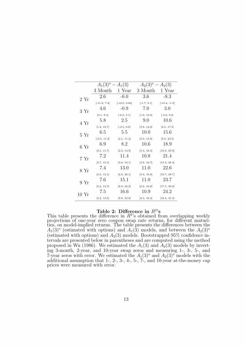
When we include options in estimation, the A1(3)o and A2(3)o models arebetter able to predict 1 year excess returns relative to their A1(3) and A2(3)counterparts and the A0(3) model that we estimated without including options.On average, the R2s across different maturities for the A1(3)o model are largerthan the R2s for the A1(3) model by a factor of 1.9. The improvement is evenlarger for the A2(3) model where the R2s are larger than the those for theA2(3) model by an average factor of 2.8. Table 2 contains the difference inR2’s between the A1(3)o and A1(3) models, and between the A2(3)o and A2(3).The bootstrapped confidence intervals indicate that, when we use options toestimate the models, the improvement is statistically significant.

Comparing across models that we estimate with options, the A2(3)o modelis slightly better than the A1(3)o model at predicting 1 year excess returns.Moreover, the R2s for both models are much closer in magnitude to thoseobtained from the regressions in Cochrane and Piazzesi (2005). The regressionsin Cochrane and Piazzesi (2005) are designed to only match excess returns andso they serve as somewhat of an upper bound for the the level of predictabilityof excess returns.

In short, the risk premiums that we estimate using interest rate cap pricesare better able to predict excess returns for long term swaps. The questionremains, what elements of the risk premium do options help to identify? Inmodels with stochastic volatility, interest rate option prices are sensitive tothe price of volatility risk, which is one element of the risk premium that maydepend on whether options are used in estimation. As a measure of the price ofvolatility risk, we use the difference between the long run risk neutral expectedzero coupon bond volatility and the long run actual expected zero coupon bondvolatility. Figures 2 and 3 plot the actual long run expected volatility and therisk-neutral long run expected volatility of zero coupon swap rates for themodels with stochastic volatility.16 This measure of the price of volatility riskis essentially zero for the A2(3)o model that we estimated with options andsmall but negative for the A1(3)o model that we estimated with options. Whenwe do not include options in estimation, this measure of the price of volatility

16The long run expected volatility of the τ -year zero coupon swap rate is

1

τ

√

B (τ)⊤

∆[

α − β(KP

1

)−1KP

0

]

B (τ) .

12

A1(3)o − A1(3) A2(3)o − A2(3)3 Month 1 Year 3 Month 1 Year

2 Yr2.6 -6.0 3.6 -8.3

[-11.9, 7.4] [-12.0, 0.00] [-1.7, 9.1] [-15.4, -1.5]

3 Yr4.6 -0.9 7.0 3.0

[0.1, 9.4] [-6.5, 5.1] [1.6, 12.8] [-3.0, 9.6]

4 Yr5.8 2.5 9.0 10.6

[1.4, 10.7] [-3.5, 8.6] [3.8, 14.8] [4.5, 17.5]

5 Yr6.5 5.5 10.0 15.6

[-0.5, 11.8] [2.1, 11.2] [5.0, 15.8] [9.5, 22.5]

6 Yr6.9 8.2 10.6 18.9

[2.5, 11.7] [2.2, 14.9] [5.4, 16.4] [12.9, 25.8]

7 Yr7.2 11.4 10.8 21.4

[2.7, 12.3] [5.0, 18.1] [5.8, 16.7] [15.3, 28.4]

8 Yr7.4 13.0 11.0 22.6

[3.0, 12.4] [6.6, 20.1] [5.9, 16.8] [16.7, 29.7]

9 Yr7.6 15.1 11.0 23.7

[3.2, 12.3] [8.8, 22.2] [6.2, 16.6] [17.7, 30.6]

10 Yr7.5 16.6 10.9 24.2

[3.2, 12.2] [9.9, 23.8] [6.3, 16.4] [18.4, 31.3]

Table 2: Difference in R2’sThis table presents the difference in R2’s obtained from overlapping weeklyprojections of one-year zero coupon swap rate returns, for different maturi-ties, on model-implied returns. The table presents the differences between theA1(3)o (estimated with options) and A1(3) models, and between the A2(3)o

(estimated with options) and A2(3) models. Bootstrapped 95% confidence in-tervals are presented below in parentheses and are computed using the methodproposed in Wu (1986). We estimated the A1(3) and A2(3) models by invert-ing 3-month, 2-year, and 10-year swap zeros and measuring 1-, 3-, 5-, and7-year zeros with error. We estimated the A1(3)o and A2(3)o models with theadditional assumption that 1-, 2-, 3-, 4-, 5-, 7-, and 10-year at-the-money capprices were measured with error.

13

risk is more negative in the A1(3) model, and large and positive for the A2(3)model. Therefore, including options affects the price of volatility risk that weestimate. Since the A1(3)o and A2(3)o are best at pricing interest rate capsand predicting excess returns, these models indicate that the price of volatilityrisk is small, and possibly negative.

0 2 4 6 8 104

5

6

7

8

9

10

11

12x 10

−3

ActualRisk Neutral

Expected Volatility – A1(3) Model

Yield Maturity

0 2 4 6 8 104

5

6

7

8

9

10

11

12x 10

−3

ActualRisk Neutral

Expected Volatility – A1(3)o Model

Yield Maturity

Figure 2: Actual and Risk Neutral Expected Volatility - A1(3)These figures show the long run expected volatility of zero coupon yields withmaturities up to 10 years. The plot on the left shows the expected long runvolatility in the A1(3) model that is estimated without using options. The ploton the right shows the expected long run volatility in the A1(3)o model that isestimated using options. The dashed line is the expected volatility under therisk neutral pricing measure. The solid line is the actual expected volatility.

To further compare the structure of expected excess returns across the mod-els that we estimate, we can express them as functions of observable yields(which are, in turn, affine functions of the underlying states in the model)17

The long run risk neutral expected volatility of the τ -year zero coupon swap rate is

1

τ

√

B (τ)⊤

∆[α − β K−1

1 K0

]B (τ) .

17Collin-Dufresne et al. (2006a) provide a compelling argument for using observables(rather than latent states) to present a standardized comparison across term structure mod-els.

14

0 2 4 6 8 10

4

5

6

7

8

9

10

11

12

13

x 10−3

ActualRisk Neutral

Expected Volatility – A2(3) Model

Maturity

0 2 4 6 8 10

4

5

6

7

8

9

10

11

12

13

x 10−3

ActualRisk Neutral

Expected Volatility – A2(3)o Model

Maturity

Figure 3: Actual and Risk Neutral Expected Volatility - A2(3)These figures show the long run expected volatility of zero coupon yields withmaturities up to 10 years. The plot on the left shows the expected long runvolatility in the A2(3) model that is estimated without using options. The ploton the right shows the expected long run volatility in the A2(3)o model that isestimated using options. The dashed line is the expected volatility under therisk neutral pricing measure. The solid line is the actual expected volatility.

In each model that we estimate we can write

Et

[re,τt,∆t

]= CONSTANT + LEVEL× r0.5

t + SLOPE×(r10t − r0.5

t

)

+ CURVATURE×(2 · r2

t − r10t − r0.5

t

).

Table 3 provides the values for CONSTANT, LEVEL, SLOPE, and CURVATURE foreach of the models that we estimate. The value of CURVATURE is virtuallythe same in the A1(3) and A1(3)o models, but the value of LEVEL increasesslightly from 1.2019 to 1.5896 and the value of SLOPE doubles from 1.4992 to2.9757. Similarly, for the A2(3) and A2(3)o models, the value of CURVATURE isvery similar, but the value of LEVEL increases from 0.4109 to 1.5082 and thevalue of SLOPE increases from 0.6602 to 2.8510. Therefore, including optionsin model estimation primarily helps to identify the risk premium (or expectedexcess return) that is associated with the slope of the yield curve. For theA2(3)o model, including options in estimation also helps to identify the riskpremium that is associated with the level of the yield curve. It is interestingto note that the value of SLOPE is very similar in the A0(3), A1(3)o, and A2(3)o

models (2.7523, 2.9757, and 2.8510 respectively) which are the best models for

15

A0(3) A1(3) A1(3)o A2(3) A2(3)o

CONSTANT -0.0721 -0.0531 -0.0943 0.0001 -0.0840LEVEL 1.0793 1.2019 1.5896 0.4109 1.5082SLOPE 2.7523 1.4992 2.9757 0.6602 2.8510

CURVATURE -0.3025 -0.3517 -0.3561 0.4066 0.2898

Table 3: Composition of Expected Excess ReturnThis table provides the values for CONSTANT, LEVEL, SLOPE, and CURVATURE foreach of the models that we estimate, where the 1-year expected excess returnon a 5-year zero coupon bond is

Et

[re,5t,1

]= CONSTANT + LEVEL× r0.5

t + SLOPE×(r10t − r0.5

t

)

+ CURVATURE×(2 · r2

t − r10t − r0.5

t

).

For example, the 1-year expected excess return on a 5-year zero coupon bondin the A1(3)o model is

Et

[re,5t,1

]= −0.0943 + 1.5896 × r0.5

t + 2.9757 ×(r10t − r0.5

t

)

− 0.3561 ×(2 · r2

t − r10t − r0.5

t

),

where r0.5t is the 6-month interest rate, r2

t is the 2-year interest rate, and r10t

is the 10-year interest rate.

predicting excess returns.

Comparing across the A0(3) model and the models that we estimate withoptions, the A0(3) and A1(3)o models differ mainly in the value of LEVEL

(1.0793 verus 1.5896 respectively). The A0(3) and A2(3)o models differ inthe values of both LEVEL (1.0793 verus 1.5082 respectively) and CURVATURE (-0.3025 versus 0.2898 respectively). The A1(3)o and A2(3)o models differ mainlyin the value of CURVATURE (-0.3561 versus 0.2898 respectively).

4 Linear Projection of Yields

Dai and Singleton (2002) present two challenges for dynamic term structuremodels that are related to risk premia in fixed income markets. This sectionexamines whether the models we estimate satisfy these challenges.

16

The first challenge, which Dai and Singleton (2002) refer to as LPY(I), isto match the pattern of violations of the exectations hypothesis documentedin Fama and Bliss (1987) and Campbell and Shiller (1991). These papersperform the following regression

rn−∆tt+∆t − rn

t = Φ0,n + Φ1,n

∆t

n − ∆t

(rnt − r∆t

t

)+ εn

t ,

and find that the regression coefficients, Φ1,n, are increasingly negative forlarger maturities n.

Figure 4 provides the LPY(I) regression results for the models that we es-timate.18,19 In contrast to Dai and Singleton (2002), all of the models aregenerally consistent with the observed slope coefficients. For all of the models,the observed slope coefficients lie within a simulated 95% confidence interval.Figure 5 shows the 95% simulated confidence interval for the A1(3)o model.

Dai and Singleton (2002) refer to the second challenge that they pose asLPY(II). This challenges states that the projection of risk-adjusted changesin zero coupon swap rates onto the slope of the yield curve should recover aregression coefficient of 1. That is, if the risk premium in the model is correct,then the risk premium adjusted regression


t +∆t

n − ∆tEt

[re,nt,∆t

]

︸︷︷︸

PACY nt,∆t

= Φ0,n + Φ1,n

∆t

n − ∆t

(rnt − r∆t

t

)

︸︷︷︸

SLOPEnt

+εnt , (9)

should produce a regression coefficient Φ1,n = 1.

We find that the combination of small sample size and near unit roots in zerocoupon swap rates results in a small, but non-negligible, bias in the regressioncoefficients. The source of this bias is described in Appendix E. Though cum-bersome, the bias can be computed in closed form and will not, in general,be zero. Instead of directly computing the bias, we estimate it by simulat-ing directly from the model and computing the deviation from unity of thesimulated LPY(II) coefficients.

18We compute the linear projections using 3 month changes in swap rates rather than the1 month changes that Dai and Singleton (2002) use. We chose 3 month changes to minimizethe effect from bootstrapping the zero coupon yield curve. The results for 1 month changesare qualitatively similar.

19The mean regression coefficients for each model were generated using 1,000 simulations.

17

1 2 3 4 5 6 7 8 9 10−6

−5

−4

−3

−2

−1

0

1

Maturity (years)

Reg

ress

ion

Coe

ffici

ent

DataA

0(3)

A1(3)

A1(3)o

A2(3)

A2(3)o

Figure 4: Regression Coefficients from Linear Projection on YieldsThis figure shows the regression coefficients of the Campbell-Shiller regressionRn−1

t+1 −Rnt on slope, (Rn

t − rt)/(n− 1). The model values are simulated meanregression coefficients. The A0(3), A1(3), and A2(3) models were estimated byinverting 3-month, 2-year, and 10-year swap zeros and measuring 1-, 3-, 5-, and7-year zeros with error. The A1(3)o and A2(3)o models were estimated withthe additional assumption that 1-, 2-, 3-, 4-, 5-, 7-, and 10-year at-the-moneycap prices were measured with error.

18

1 2 3 4 5 6 7 8 9 10−10

−8

−6

−4

−2

0

2

Maturity (years)

Reg

ress

ion

Coe

ffici

ent

DataMean Simulated95% Confidence Bound

Figure 5: Confidence Interval for Linear Projection on YieldsThis figure shows the sample regression coefficient of the Campbell-Shillerregression Rn−1

t+1 − Rnt on slope, (Rn

t − rt)/(n − 1) for the A1(3)o model. Thedotted line provides the confidence interval computed from simulation. Themodel was estimated by inverting 3-month, 2-year, and 10-year swap zerosand measuring 1-, 3-, 5-, and 7-year zeros and 1-, 2-, 3-, 4-, 5-, 7-, and 10-yearat-the-money cap prices with error.

19

0 1 2 3 4 5 6 7 8 9 10−3

−2.5

−2

−1.5

−1

−0.5

0

0.5

1

1.5

2

Maturity (years)

Reg

ress

ion

Coe

ffici

ent

A0(3)

A1(3)

A1(3)o

A2(3)

A2(3)o

Figure 6: Risk Premium Adjusted Linear Projection on YieldsThis figure shows the regression coefficient from the projection risk premiumadjusted excess returns on the slope, (Rn

t − rt)/(n−1). The A0(3), A1(3), andA2(3) models were estimated by inverting 3-month, 2-year, and 10-year swapzeros and measuring 1-, 3-, 5-, and 7-year zeros with error. The A1(3)o andA2(3)o models were estimated with the additional assumption that 1-, 2-, 3-,4-, 5-, 7-, and 10-year at-the-money cap prices were measured with error.

20

0 1 2 3 4 5 6 7 8 9 10−1

0

1

2

3

4

5

6

7

Maturity (years)

Reg

ress

ion

Coe

ffici

ent

ModelMean Simulated95% Confidence Bound

Figure 7: Confidence Interval for LPY(II)This figure shows the confidence interval for the regression coefficient in theA1(3)o model from the projection risk premium adjusted excess returns on theslope, (Rn

t − rt)/(n− 1). The A1(3)o model is estimated by inverting 3-month,2-year, and 10-year swap zeros and measuring 1-, 3-, 5-, and 7-year zeros and1-, 2-, 3-, 4-, 5-, 7-, and 10-year at-the-money cap prices with error.

21

Figure 6 shows the model LPY(II) regression results adjusted for the bias.The A1(3)o and A2(3)o models that we estimate with options dominate theA0(3), A1(3), and A2(3) models that we estimate without options. Althoughwe do not recover an exact regression coefficient of one, the value is quitenear the center of the simulated confidence intervals for the A0(3), A1(3)o, andA2(3)o models. Figure 7 shows the simulated 95% confidence interval for theA1(3)o model. The stochastic volatility models that we estimated withoutoptions nearly follow the 95% lower confidence bound. In summary, whenwe include options in estimation, the expected excess returns in the A1(3)o

and A2(3)o models match the desired properties of linear projections on yieldsproposed in Dai and Singleton (2003).

5 Conclusion

Interest rate options may contain information about the risk premium in long-term interest rates because their prices are sensitive to the volatility and mar-ket prices of the same risk factors that move interest rates. We use the timeseries of interest rate cap prices and swap rates to estimate 3-factor affine termstructure models. The risk premiums that we estimate using interest rate op-tion prices are better able to predict excess returns for long-term swaps overshort-term swaps. We show that including options reduces our estimate of themagnitude of the price of volatility risk, and helps us to identify the portionof the risk premium that is associated with the slope and level of the yieldcurve. We also find that, with a bias correction, the models with stochasticvolatility that we estimate with options successfully capture the failure of theexpectations hypothesis and match regressions of returns on the slope of theyield curve.

22

A Detailed Model Specifications

We estimate 3-factor affine term structure models. The state vector X followsan diffusion process with affine drift and variance,

dXt =[KP

0 + KP

1Xt

]dt +

√

∆ [α + βXt] dWt .

We have used the notation ∆ [·] to denote a square matrix with its vectorargument along the diagonal. The pricing kernel M also follows a diffusionprocess

dMt = −Mt rt dt − Mt Λ⊤

t dWt .

The drift, r, of the pricing kernel is an affine function of the state vector

rt := ρ0 + ρ1 · Xt ,

The volatility, Λ, of the pricing kernel has an extended affine form

Λt :=(√

∆ [α + βXt])−1 [(

KP

0 −K0

)+

(KP

1 −K1

)Xt

].20

We estimate AM(3) models,21 where M = 0, 1, 2 is the number of factorsin the state vector X that have stochastic volatility. For example, in theA0(3) model, β = 0 so that none of the factors have stochastic volatility.For each model, Dai and Singleton (2000) and Cheridito et al. (2007) identifythe necessary restrictions required to ensure that the stochastic processes areadmissable, the parameters are identified, and the physical and risk neutralmeasures are equivalent. The full specifications of the A0 (3), A1 (3), and A2 (3)are described below.

20We use an extended affine market price of risk introduced by Cheridito et al. (2007) asa generalization of the essentially affine market price of risk used in Duffee (2002).

21These models were introduced in Dai and Singleton (2000).

23

A0 (3) Model Specification

KP

1 =

KP

1,11 0 0KP

1,21 KP

1,22 0KP

1,31 KP

1,32 KP

1,33

, KP

0 =

KP

0,1

KP

0,2

KP

0,3

,

K1 =

K1,11 0 0K1,21 K1,22 0K1,31 K1,32 K1,33

, K0 =

000

,

β =

0 0 00 0 00 0 0

, α =

111

,

ρ1,1 ≥ 0 , ρ1,2 ≥ 0 , ρ1,3 ≥ 0 .


KP

1 =

KP

1,11 0 0KP

1,21 KP

1,22 KP

1,23

KP

1,31 KP

1,32 KP

1,33

, KP

0 =

KP

0,1

KP

0,2

KP

0,3

,

K1 =

K1,11 0 0K1,21 K1,22 K1,23

K1,31 K1,32 K1,33

, K0 =

K0,1

00

,

β =

1 0 0β2,1 0 0β3,1 0 0

, α =

011

,

KP

0,1 ≥1

2, K0,1 ≥

1

2,

β2,1 ≥ 0 , β3,1 ≥ 0 ,

ρ1,2 ≥ 0 , ρ1,3 ≥ 0 .

24


KP

1 =

KP

1,11 KP

1,12 0KP

1,21 KP

1,22 0KP

1,31 KP

1,32 KP

1,33

, KP

0 =

KP

0,1

KP

0,2

KP

0,3

,

K1 =

K1,11 K1,12 0K1,21 K1,22 0K1,31 K1,32 K1,33

, K0 =

K0,1

K0,2

0

,

β =

1 0 00 1 0

β3,1 β3,2 0

, α =

001

,

KP

0,1 ≥1

2, K0,1 ≥

1

2, KP

0,2 ≥1

2, K0,2 ≥

1

2,

β3,1 ≥ 0 , β3,2 ≥ 0 ,

ρ1,3 ≥ 0 .

B Detailed Estimation Procedure

We estimate all the models using quasi-maximum likelihood in a proceduresimilar to Duffee (2002) and Dai and Singleton (2002). Using the instrumentspriced without error and the risk neutral dynamics of Xt, we invert to findthe time series of states {Xt}. Given the states, we then compute the modelimplied prices of the instruments priced without error. Following Dai andSingleton (2002), we assume that the pricing errors are IID normal with meanzero. Finally, using the physical dynamics of the state vector and the QMLapproximation, we compute the likelihood of the inverted states. This givesthe liklelihod of a given set of parameters to be:

likelihood =∏

ℓPQML(Xt|Xt−1) · (Jacobian) · (likelihood of pricing errors).

We use a slighlty different procedure than Duffee (2002) to compute the con-ditional mean and variance of the state variable. For a general affine process,

25

A0(3) A1(3) A1(3)o A2(3) A2(3)o

K1P1,1 -1.4 (0.486) -0.21 (0.339) -0.307 (0.319) -0.244 (0.371) -2.35 (0.649)

K1P1,2 0.448 (0.459) 0 0 1.06 (1.16) 2.94 (0.857)

K1P1,3 -0.108 (0.108) 0 0 0 0

K1P2,1 0.781 (0.497) -1.96 (0.501) -2.23 (0.45) 0.193 (0.157) 0.69 (0.458)

K1P2,2 -0.893 (0.47) -0.962 (0.429) -0.441 (0.3) -1.29 (0.477) -1.06 (0.577)

K1P2,3 0.259 (0.124) -0.58 (1.39) -0.801 (2) 0 0

K1P3,1 -3.27 (0.728) -1.88 (4.98) -4 (9.69) 0.817 (1.8) 2.11 (0.745)

K1P3,2 1.06 (0.652) -0.438 (1.24) -0.341 (1) -3.42 (6.83) -3.61 (0.891)

K1P3,3 -0.46 (0.172) -0.767 (0.51) -2.19 (0.813) -0.511 (0.164) -0.321 (0.143)

K0P1

1.04 (1.98) 1.38 (1.9) 2.28 (2.53) 1.97 (21.7) 1.61 (5.11)

K0P2

-1.31 (1.99) -0.0177 (3.72) 7.38 (4.99) 0.614 (10.2) 0.5 (3.2)

K0P3

-0.184 (2.95) -1.71 (9.05) -1.8 (12.2) 0 0

K1Q1,1

-1.3 (0.043) -0.62 (0.0128) -0.568 (0.0111) -0.0864 (0.0634) -1.29 (0.0669)

K1Q1,2

0 0 0 0.484 (0.377) 1.64 (0.245)

K1Q1,3

0 0 0 0 0

K1Q2,1

-0.0947 (0.0443) -2.06 (0.334) -2.11 (0.336) 0.176 (0.109) 0.0652 (0.0294)

K1Q2,2

-0.0298 (0.0013) -0.939 (0.42) -0.236 (0.354) -1.35 (0.0748) -0.756 (0.0601)

K1Q2,3

0 -0.723 (1.7) -1.21 (2.98) 0 0

K1Q3,1

-4 (0.159) -1.61 (4.27) -2.88 (7) 1.1 (2.31) 2.95 (0.817)

K1Q3,2

1.38 (0.0544) -0.592 (1.52) -0.168 (0.492) -4 (8.12) -3.64 (0.811)

K1Q3,3

-0.681 (0.014) -0.502 (0.413) -1.44 (0.355) -0.653 (0.0117) -0.0819 (0.00106)

K0Q1

0 2.81 (0.682) 3.62 (0.769) 1.67 (3.11) 0.5 (1.76)

K0Q2

0 0 0 1.29 (5.39) 3.42 (1.02)

K0Q3

0 0 0 -1.37 (13.9) -1.23 (2.84)

β1,1 0 1 1 1 1β1,2 0 0.0638 (0.0361) 0.149 (0.0698) 0 0β1,1 0 4.49 (21.3) 5.84 (28.6) 0 (0.0612) 0 (0.0478)β1,1 0 0 0 1 1β1,1 0 0 0 0.74 (3.12) 0.411 (0.253)

ρ0 0.111 (0.00229) 0.0478 (0.0186) 0.0166 (0.0111) -0.0148 (0.0871) 0.0684 (0.0422)

ρ1

10.00241 (2.28e-4) 0.000734 (1.48e-4) 0.000811 (1.24e-4) -8.28e-5 (6.66e-5) -0.000995 (9.91e-5)

ρ1

20.00022 (2.62e-4) 0.00454 (3.22e-4) 0.00309 (3.88e-4) 0.000897 (2.25e-4) 0.00113 (1.59e-4)

ρ1

30.00559 (8.89e-5) 0.000252 (5.55e-4) 0.000487 (0.00121) 0.00191 (0.00395) 0.00236 (6.53e-4)

M 0 1 1 2 2N 3 3 3 3 3mean LLK 41.6 41.7 74.6 41.6 74.7

Table 4: Parameter Estimates.This table presents all parameter values for the different affine term structuremodels we estimate. Standard errors are in parentheses. The A0(3), A1(3), andA2(3) models were estimated by inverting 3-month, 2-year, and 10-year swapzeros and measuring 1-, 3-, 5-, and 7-year zeros with error. The A1(3)o andA2(3)o models were estimated with the additional assumption that 1-, 2-, 3-,4-, 5-, 7-, and 10-year at-the-money cap prices were measured with error. If aparameter is reported as 0 or 1, it is restricted to be so by the identification andexistence conditions in Dai and Singleton (2000) and Cheridito et al. (2006).

26

Xt, with conditional drift K0+K1Xt and conditional variance H0+H1 ·Xt, themean and variance of Xt conditional on X0 satisfy the differential equations

Mt = K0 + K1Mt ,

Vt = K1Vt + VtKt1 + H0 + H1 · Mt ,

If we let f be the (N +N2)-vector (M, vec(V )), then by stacking these coupledODEs we see that f satisfies the ODE

f =

[K1 0∆ IN ⊗ K1 + K1 ⊗ IN

]

f +

[K0

vec(H0)

]

,

where ∆ is an (N2 × N) matrix with ∆i,j = vec(H1,·,·,i)j. Rather than con-sidering separate cases to solve this ODE in closed form, we instead computethe fundamental solution numerically using 4th order Runge-Kutta. From thefundamental solution, it is then easy to compute the solution for arbitraryinitial conditions.

C Fit to Yields and Cap Prices

Table 5 provides the root mean squared pricing errors (in basis points) for zerocoupon swap rates with different maturities. The root mean squared errors are0 for the 3-month, 2-, and 10-year zero coupon swap rates because the latentstate variables are chosen so that the models correctly price these rates. Theroot mean squared pricing errors for other maturities range from about 4 basispoints to about 10 basis points.22 There is very little difference in the cross-sectional fit between the A0(3), A1(3), and A2(3) models that we estimatewithout using options. Similarly, there is also little difference between theA1(3)o and A2(3)o models that we estimate with options. The use of optionsto estimate the A1(3)o and A2(3)o models has only a small effect on the models’fits to the cross-section of zero coupon swap rates with different maturities.Including options improves the fit (relative to models that we estimate withoutusing options) by less than a basis point at the short end of the yield curve(up to 1 year) and worsens the fit by slightly more than a basis point at thelong end of the yield curve (beyond 1 year).

22The cross-sectional pricing errors for all of the models that we estimate are comparablewith the pricing errors reported in recent papers such as Dai and Singleton (2000), Duffee(2002), and Cheridito et al. (2007).

27

A0(3) A1(3) A1(3)o A2(3) A2(3)o

3 Month ∗ ∗ ∗ ∗ ∗6 Month 7.1 7.1 6.8 7.1 6.8

1 Year 9.9 9.9 9.3 10.0 9.32 Year ∗ ∗ ∗ ∗ ∗3 Year 4.1 4.1 4.5 4.1 4.54 Year 5.3 5.2 6.3 5.2 6.25 Year 5.2 5.2 6.7 5.2 6.67 Year 3.8 3.8 5.5 3.8 5.3

10 Year ∗ ∗ ∗ ∗ ∗

Table 5: Pricing Errors in BPS for Swap Implied ZerosThis table shows the root mean square pricing errors in basis points for yieldson swap implied zeros. The A0(3), A1(3), and A2(3) models were estimated byinverting 3-month, 2-year, and 10-year swap zeros and measuring 1-, 3-, 5-, and7-year zeros with error. The A1(3)o and A2(3)o models were estimated withthe additional assumption that 1-, 2-, 3-, 4-, 5-, 7-, and 10-year at-the-moneycap prices were measured with error.

A0(3) A1(3) A1(3)o A2(3) A2(3)o

1 Year 33.6 32.4 36.4 33.3 35.52 Year 19.9 19.0 14.6 16.9 14.43 Year 18.9 18.0 10.9 15.7 10.94 Year 17.3 17.3 9.6 14.2 9.65 Year 16.3 17.0 9.2 13.3 9.07 Year 14.3 16.1 8.6 11.7 8.3

10 Year 13.4 15.8 9.2 11.0 8.9

Table 6: Relative Pricing Errors in % for At-the-Money CapsThis table shows the root mean square relative pricing errors in % for at-the-money caps. The A0(3), A1(3), and A2(3) models were estimated by inverting3-month, 2-year, and 10-year swap zeros and measuring 1-, 3-, 5-, and 7-yearzeros with error. The A1(3)o and A2(3)o models were estimated with theadditional assumption that 1-, 2-, 3-, 4-, 5-, 7-, and 10-year at-the-money capprices were measured with error.

28

Table 6 displays the root mean squared pricing errors in percentage termsfor at-the-money caps with various maturities.23 For all of the models, thepercentage pricing errors are worst for 1-year caps and decline as the maturityof the cap increases.24 Amongst the models that we estimate without includingoptions, the A2(3) model provides the best fit to the cross-section of at-the-money cap prices. The A1(3)o and A2(3)o models have slightly larger relativepricing errors for 1-year caps than their A1(3) and A2(3) counterparts that weestimate without options. However, the relative pricing errors for caps withlonger maturities are considerably lower when we include caps in estimation.For example, the root mean squared relative pricing error for at-the-money 5-year caps is 17% in the A1(3) model and is 9.2% in the A1(3)o model. Similarly,the root mean squared relative pricing error for at-the-money 5-year caps is13.3% in the A2(3) model and 9.0% in the A2(3)o model. The relative pricingerrors for the A2(3)o model are slightly better than those for the A1(3)o.

The pricing errors for caps from the A1(3)o and A2(3)o models that we es-timate with options compare favorably with the pricing errors that have beenreported in previous literature.25 Driessen et al. (2003) estimate a 3-factorGaussian HJM model with cap data and report absolute pricing errors (av-eraged across maturities) of 17.1%. Li and Zhao (2006) estimate a 3-factorquadratic term structure model and find that the root mean squared percent-age pricing error for 5-year at-the-money caps is 10.4%. Jagannathan et al.(2003) estimate a 3-factor CIR model and find that the mean absolute pricingerrors are 36.62 basis points for 5-year caps compared to a mean market price

23Figures 8 and 9 provide 3- and 5-year at-the-money cap prices for the A1(3), A1(3)o,A2(3), and A2(3)o models. Figure 10 plots the time series of prices in the A1(3)o modelfor at-the-money caps with maturities from 1 to 10 years. The time series of cap prices issimilar for the A2(3)o model.

24The root mean squared relative pricing errors for 1-year caps range from 32.4% to 36.4%.The pricing errors for zero coupon swap rates are also largest at 1-year. Dai and Singleton(2002) find that a fourth factor is required to capture the short end of the yield curve. Wechoose to implement more parsimonious 3-factor models because we are primarily interestedin predicting changes in long-term interest rates.

25Previous papers have also used interest rate option prices other than caps to estimatedynamic term structure models. Umantsev (2002) finds that pricing errors for swaptions aresignificantly reduced when he uses swaption prices to estimate affine term structure models.Bikbov and Chernov (2005) use Eurodollar options to estimate term structure models withconstant, stochastic, and unspanned stochastic volatility. They find that only stochasticvolatility models (such as our A1(3)o and A2(3)o models) can reconcile both option pricesand the term structure of interest rates.

29

Jan96 Jan97 Jan98 Jan99 Jan00 Jan01 Jan02 Jan03 Jan04 Jan05 Jan060.008

0.01

0.012

0.014

0.016

0.018

0.02

0.022

0.024

0.026

Pric

es

Date

dataA

1(3)

A1(3)o


0.01

0.012

0.014

0.016

0.018

0.02

0.022

0.024

0.026

Pric

es

Date

dataA

2(3)

A2(3)o

Figure 8: 3-Year At-the-money Cap PricesThe top figure plots the 3-year at-the-money cap prices in the A1(3) model(solid grey line) and the A1(3)o model (dashed line). The actual prices areplotted with a solid black line. The bottom figure plots the 3-year at-the-money cap prices in the A2(3) model (solid grey line) and the A2(3)o model(dashed line). The actual prices are plotted with a solid black line. The A1(3)and A2(3) models were estimated by inverting 3-month, 2-year, and 10-yearswap zeros and measuring 1-, 3-, 5-, and 7-year zeros with error. The A1(3)o

and A2(3)o models were estimated with the additional assumption that 1-, 2-,3-, 4-, 5-, 7-, and 10-year at-the-money cap prices were measured with error.

30


0.02

0.025

0.03

0.035

0.04

0.045

0.05

0.055

Pric

es

Date

dataA

1(3)

A1(3)o


0.02

0.025

0.03

0.035

0.04

0.045

0.05

0.055

Pric

es

Date

dataA

2(3)

A2(3)o

Figure 9: 5-Year At-the-money Cap PricesThe top figure plots the 5-year at-the-money cap prices in the A1(3) model(solid grey line) and the A1(3)o model (dashed line). The actual prices areplotted with a solid black line. The bottom figure plots the 5-year at-the-money cap prices in the A2(3) model (solid grey line) and the A2(3)o model(dashed line). The actual prices are plotted with a solid black line. The A1(3)and A2(3) models were estimated by inverting 3-month, 2-year, and 10-yearswap zeros and measuring 1-, 3-, 5-, and 7-year zeros with error. The A1(3)o

and A2(3)o models were estimated with the additional assumption that 1-, 2-,3-, 4-, 5-, 7-, and 10-year at-the-money cap prices were measured with error.

31

Jan96 Jan97 Jan98 Jan99 Jan00 Jan01 Jan02 Jan03 Jan04 Jan05 Jan060

0.02

0.04

0.06

0.08

0.1

0.12

Pric

es

Date

Figure 10: Cap Prices for A1(3)o modelThis figure plots cap prices for 1-, 2-, 3-, 4-, 5-, 7-, and 10-year at-the-moneycaps. The think lines indicate actual prices. The model prices for the A1(3)o

model are plotted in thicker lines, with longer maturities having higher prices.The A1(3)o model was estimated by inverting 3-month, 2-year, and 10-yearswap zeros. Additionally, the 1-, 3-, 5-, and 7-year zeros and 1-, 2-, 3-, 4-, 5-,7-, and 10-year at-the-money cap prices were measured with error.

32

of 284.84 basis points (the results are similar for caps with other maturities).Longstaff et al. (2001) estimate a 4-factor string market model using swaptionsand find that it overprices caps. They report that the mean percentage valu-ation error for 5-year caps is 5.665% and ranges from a minimum of -2.385%to a maximum of 38.071%. All of these papers report larger pricing errors forshorter-dated caps.

Although not reported here, the A1(3)o and A2(3)o that we estimate withcaps also provide an excellent fit to the prices of at-the-money swaptions.

33

A0(3) A1(3) A1(3)o A2(3) A2(3)o

6 Month 0.0 19.2 28.9 39.1 30.11 Year 0.0 50.8 56.3 58.3 52.92 Year 0.0 75.0 77.0 63.2 66.93 Year 0.0 83.0 81.5 39.0 70.64 Year 0.0 84.4 81.4 15.4 71.95 Year 0.0 84.1 79.3 -2.6 69.37 Year 0.0 84.3 77.4 -21.2 66.4

10 Year 0.0 82.0 75.0 -26.7 61.6

Table 7: Correlation between model and EGARCH volatilityThis table shows the correlation between model-implied one-week volatilitiesand EGARCH(1,1) volatility estimates. The A0(3), A1(3), and A2(3) modelswere estimated by inverting 3-month, 2-year, and 10-year swap zeros and mea-suring 1-, 3-, 5-, and 7-year zeros with error. The A1(3)o and A2(3)o modelswere estimated with the additional assumption that 1-, 2-, 3-, 4-, 5-, 7-, and10-year at-the-money cap prices were measured with error.

D Fit to Volatility

In this section we examine how well the term structure models match the con-ditional volatility of interest rates. Unlike prices, conditional volatility is notdirectly observed and therefore it must be estimated.26 For estimates of con-ditional volatility based on historical data we use an exponential weighted mov-ing average (EWMA) with a 26-week half-life, and also estimate an EGARCH(1,1)for each zero coupon swap rate maturity. Figure 11 plots the conditionalvolatility of zero coupon swap rates from the term structure models againstour estimates of conditional volatility that use historial data. Tables 7 and 8provide the correlation between the conditional volatilty in the pricing modeland the EGARCH and EWMA estimates of conditional volatility respectively.Table 9 provides the average conditional volatilities for the pricing models andthe EGARCH and EWMA estimates.

The volatility of the 6-month zero coupon swap rate is very similar between

26Implied volatilities from cap prices are forward looking and directly observable. How-ever, in the case of models with stochastic volatility, the market prices of risk may causethe implied volatilities from cap prices to differ from the actual conditional volatility.

34


0.4

0.6

0.8

1

1.2

1.4

1.6

1.8

2x 10

−3

Date

Vol

atili

ty o

f 6 M

onth

Yie

ld

A1(3)o

A1(3)

EGARCH(1,1)EWMA


0.4

0.6

0.8

1

1.2

1.4

1.6

1.8

2x 10

−3

DateV

olat

ility

of 6

Mon

th Y

ield

A0(3)

A2(3)o

A2(3)

EGARCH(1,1)EWMA


0.8

1

1.2

1.4

1.6

1.8

2

2.2x 10

−3

Date

Vol

atili

ty o

f 2 Y

ear

Yie

ld

A1(3)o

A1(3)

EGARCH(1,1)EWMA


1

1.2

1.4

1.6

1.8

2x 10

−3

Date

Vol

atili

ty o

f 2 Y

ear

Yie

ld

A0(3)

A2(3)o

A2(3)

EGARCH(1,1)EWMA


0.8

1

1.2

1.4

1.6

1.8

2x 10

−3

Date

Vol

atili

ty o

f 10

Yea

r Y

ield

A1(3)o

A1(3)

EGARCH(1,1)EWMA


1

1.2

1.4

1.6

1.8

2x 10

−3

Date

Vol

atili

ty o

f 10

Yea

r Y

ield

A0(3)

A2(3)o

A2(3)

EGARCH(1,1)EWMA

Figure 11: Realized VolatilityThese figures plot weekly model conditional volatility of (from top to bottom)6-month, 2-year, and 10-year zero coupon swap rates against various estimatesof weekly conditional volatility using historical data. For estimates of condi-tional volatility based on historical data we use an exponential weighted mov-ing average (EWMA) with a 26-week half-life and estimate an EGARCH(1,1)for each maturity. The plots on the left show the conditional volatility inthe A1(3) and A1(3)o models. The plots on the right show the conditionalvolatility in the A0(3), A1(3), and A1(3)o models.

35

A0(3) A1(3) A1(3)o A2(3) A2(3)o

6 Month 0.0 33.2 41.8 35.1 40.31 Year 0.0 55.8 62.7 54.5 63.42 Year 0.0 74.0 76.0 50.1 76.13 Year 0.0 76.7 75.6 29.6 75.64 Year 0.0 77.2 74.1 9.9 74.05 Year 0.0 77.4 73.0 -3.4 72.07 Year 0.0 80.6 74.2 -18.7 71.4

10 Year 0.0 80.7 75.8 -18.9 71.7

Table 8: Correlation between model and EWMA volatilityThis table provides the correlation between model-implied one-week volatilitiesand Exponential Weighted Moving Average volatility estimates. The EWMAestimates were computing using a 26 week half-life. The A0(3), A1(3), andA2(3) models were estimated by inverting 3-month, 2-year, and 10-year swapzeros and measuring 1-, 3-, 5-, and 7-year zeros with error. The A1(3)o andA2(3)o models were estimated with the additional assumption that 1-, 2-, 3-,4-, 5-, 7-, and 10-year at-the-money caps were measured with error.

A0(3) A1(3) A1(3)o A2(3) A2(3)o EGARCH EWMA6 Month 7.3 6.8 6.1 6.6 6.1 6.6 6.5

1 Year 9.8 10.5 11.2 10.1 11.1 9.9 10.32 Year 12.0 13.1 14.8 12.7 14.8 12.6 12.93 Year 12.7 13.6 15.8 13.4 15.9 13.3 13.54 Year 12.8 13.6 16.0 13.5 16.1 13.5 13.75 Year 12.8 13.5 15.9 13.5 16.0 13.7 13.97 Year 12.8 13.2 15.3 13.4 15.4 13.6 13.8

10 Year 12.7 12.8 14.2 13.1 14.2 13.5 13.6

Table 9: Average Conditional VolatilitiesThis table shows the the average conditional one week volatility of swap rates,σt(yt+1), in basis points. Semi-nonparametric estimates of the the averageconditional one week volatility are also provided. The A0(3), A1(3), and A2(3)models were estimated by inverting 3-month, 2-year, and 10-year swap zerosand measuring 1-, 3-, 5-, and 7-year zeros with error. The A1(3)o and A2(3)o

models were estimated with the additional assumption that 1-, 2-, 3-, 4-, 5-,7-, and 10-year at-the-money cap prices were measured with error.

36

the A1(3) and A1(3)o models, and between the A2(3) and A2(3)o models. Thehistorical estimates of the conditional volatility of the 6-month zero couponswap rate jump in 2001 and none of the models track this jump.27 However, allof the pricing models match the average level of the estimates of conditionalvolatility of the 6-month zero coupon swap rate.

For maturities beyond 1 year, the conditional volatility of zero coupon swaprates in the A1(3), A1(3)o, and A2(3)o models are all highly correlated withboth the EGARCH and EWMA estimates of conditional volatility. The cor-relations are highest in the A1(3) model, followed closely by the A1(3)o model,and then the A2(3)o model. The conditional volatility in the A2(3) model ispositively correlated with the estimates of conditional volatility for maturitiesup to 4 years, but negatively correlated for maturities beyond 4 years. TheA1(3) and A2(3) models match the average level of conditional volatility forthe EGARCH and EWMA estimates. The average conditional volatility inthe A1(3)o and A2(3)o models are about 2% higher than the estimates basedon EGARCH and EWMA.

The conditional volatility of all swap rates is constant in the A0(3) modeland therefore it cannot capture any time-series variation. Over our sampleperiod, the average level of conditional volatility in the A0(3) model for zerocoupon swap rates with different maturities is slightly below our estimatesbased on historical data.

In summary, none of the models match the conditional volatility of short-term interest rates, but the A1(3), A1(3)o, and A2(3)o models capture theconditional volatility of long-term interest rates.

27Collin-Dufresne and Goldstein (2002b) find that the volatility of short-term interestrates is not related to the yield curve. Collin-Dufresne et al. (2006b) argue that a four-factor model with unspanned stochastic volatility is required to capture the volatility of theshort end of the yield curve.

37

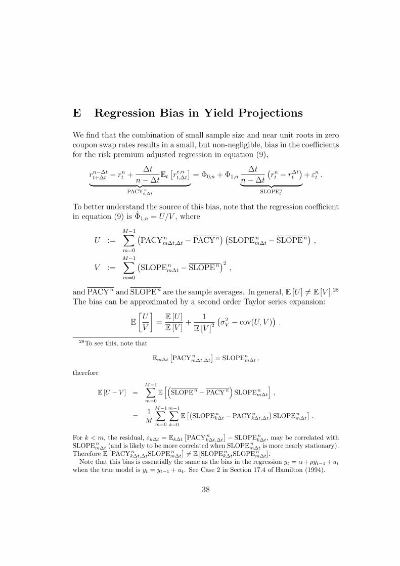
E Regression Bias in Yield Projections

We find that the combination of small sample size and near unit roots in zerocoupon swap rates results in a small, but non-negligible, bias in the coefficientsfor the risk premium adjusted regression in equation (9),


t +∆t

n − ∆tEt

[re,nt,∆t

]

︸︷︷︸

PACY nt,∆t

= Φ0,n + Φ1,n

∆t

n − ∆t

(rnt − r∆t

t

)

︸︷︷︸

SLOPEnt

+ εnt .

To better understand the source of this bias, note that the regression coefficientin equation (9) is Φ1,n = U/V , where

U :=M−1∑

m=0

(PACYn

m∆t,∆t − PACYn) (

SLOPEnm∆t − SLOPEn

),

V :=M−1∑

m=0

(SLOPEn

m∆t − SLOPEn)2

,

and PACYn and SLOPEn are the sample averages. In general, E [U ] 6= E [V ].28

The bias can be approximated by a second order Taylor series expansion:

E

[U

V

]

=E [U ]

E [V ]+

1

E [V ]2(σ2

V − cov(U, V ))

.

28To see this, note that

Em∆t

[PACYn

m∆t,∆t

]= SLOPEn

m∆t ,

therefore

E [U − V ] =

M−1∑

m=0

E

[(

SLOPEn − PACYn)

SLOPEnm∆t

]

,

=1

M

M−1∑

m=0

m−1∑

k=0

E[(

SLOPEnk∆t − PACYn

k∆t,∆t

)SLOPEn

m∆t

].

For k < m, the residual, εk∆t = Ek∆t

[PACYn

k∆t,∆t

]− SLOPEn

k∆t, may be correlated withSLOPEn

m∆t (and is likely to be more correlated when SLOPEnm∆t is more nearly stationary).

Therefore E[PACYn

k∆t,∆tSLOPEnm∆t

]6= E [SLOPEn

k∆tSLOPEnm∆t].

Note that this bias is essentially the same as the bias in the regression yt = α+ρyt−1 +ut

when the true model is yt = yt−1 + ut. See Case 2 in Section 17.4 of Hamilton (1994).

38

Though cumbersome, the bias can be computed in closed form and is not,in general, zero. Instead of directly computing the bias, we estimate it bysimulating directly from the model and computing the deviation from unity ofthe simulated LPY(II) coefficients.

F Additional Tables and Figures

39

A0(3) A1(3) A1(3)o A2(3) A2(3)o

2 Yr0.7 0.9 3.5 -0.2 3.4

(9.4) (9.6) (9.2) (9.4) (9.2)

3 Yr6.5 4.0 8.6 2.7 9.7

(9.1) (9.6) (8.8) (9.4) (8.5)

4 Yr10.2 5.9 11.7 4.0 13.0(8.9) (9.6) (8.5) (9.5) (8.3)

5 Yr12.5 7.0 13.5 4.6 14.6(8.7) (9.4) (8.6) (9.6) (8.2)

6 Yr13.8 7.5 14.4 4.9 15.5(8.6) (9.3) (8.4) (9.4) (8.1)

7 Yr14.9 7.9 15.1 5.2 16.0(8.6) (9.2) (8.2) (9.5) (8.1)

8 Yr15.4 8.0 15.4 5.2 16.2(8.4) (9.2) (8.4) (9.5) (8.1)

9 Yr15.9 8.0 15.6 5.3 16.3(8.4) (9.0) (8.4) (9.6) (8.0)

10 Yr16.1 8.0 15.5 5.3 16.2(8.3) (9.1) (8.3) (9.3) (8.0)

Table 10: Predictability of Excess Returns (R2s)This table presents R2s obtained from overlapping weekly projections of 3month realized zero coupon swap rate returns, for different maturities, onmodel implied returns. Regressions are based on overlapping data. The A0(3),A1(3), and A2(3) models were estimated by inverting 3-month, 2-year, and 10-year swap zeros and measuring 1-, 3-, 5-, and 7-year zeros with error. TheA1(3)o and A2(3)o models were estimated with the additional assumption that1-, 2-, 3-, 4-, 5-, 7-, and 10-year at-the-money cap prices were measured witherror.

40

References

Dong-Hyun Ahn, Robert F. Dittmar, and A. Ronald Gallant. Quadratic termstructure models: Theory and evidence. The Review of Financial Studies,15(1):243–288, Spring 2002.

Yacine Aıt-Sahalia and Andrew W. Lo. Nonparametric risk managementand implied risk aversion. Journal of Econometrics, 94(1-2):9–51, January-February 2000.

Yacine Aıt-Sahalia, Yubo Wang, and Francis Yared. Do option markets cor-rectly price the probabilities of movement of the underlying asset? Journal

of Econometrics, 102(1):67–110, May 2001.

Torben G. Andersen and Luca Benzoni. Do bonds span volatility risk in theu.s. treasury market? a specification test for affine term structure models.Working Paper, 14 December 2006.

Gurdip S. Bakshi, Peter P. Carr, and Liuren Wu. Stochastic risk premiums,stochastic skewness in currency options, and stochastic discount factors ininternational economies. Journal of Financial Economics, 87(1):132–156,January 2008.

C. Alan Bester. Random field and affine models for interest rates: An empiricalcomparison. Working Paper, September 2004.

Ruslan Bikbov and Mikhail Chernov. Term structure and volatility: Lessonsfrom the eurodollar futures and options. Working Paper, 23 November 2005.

John Y. Campbell and Robert J. Shiller. Yield spreads and interest ratemovements: A bird’s eye view. Review of Economic Studies, 58(3):495–514,May 1991.

Ren-Raw Chen and Louis Scott. Maximum likelihood estimation for a multi-factor equilibrium model of the term structure of interest rates. Journal of

Fixed Income, 3:14–31, 1993.

Peng Cheng and Olivier Scaillet. Linear-quadratic jump-diffusion modeling.Mathematical Finance, 17(4):575–598, October 2007.

41

Patrick Cheridito, Damir Filipovic, and Robert L. Kimmel. Market priceof risk specifications for affine models: Theory and evidence. Journal of

Financial Economics, September 2006.

Patrick Cheridito, Damir Filipovic, and Robert L. Kimmel. Market priceof risk specifications for affine models: Theory and evidence. Journal of

Financial Economics, 83(1):123–170, January 2007.

Mikhail Chernov and Eric Ghysels. A study towards a unified approach tothe joint estimation of objective and risk neutral measures for the purposeof options valuation. Journal of Financial Economics, 56(3):407–458, June2000.

John H. Cochrane and Monika Piazzesi. Bond risk premia. American Economic

Review, 95(1):138–160, March 2005.

Pierre Collin-Dufresne and Robert S. Goldstein. Pricing swaptions within anaffine framework. Journal of Derivatives, 10(1):1–18, Fall 2002a.

Pierre Collin-Dufresne and Robert S. Goldstein. Do bonds span the fixedincome markets? theory and evidence for unspanned stochastic volatility.Journal of Finance, 57(4):1685–1730, August 2002b.

Pierre Collin-Dufresne, Robert S. Goldstein, and Christopher S. Jones. Identi-fication of maximal affine term structure models. Working Paper, 6 August2006a.

Pierre Collin-Dufresne, Robert S. Goldstein, and Christopher S. Jones. Caninterest rate volatility be extracted from the cross section of bond yields? aninvestigation of unspanned stochastic volatility. Working Paper, 15 Septem-ber 2006b.

Pierre Collin-Dufresne, Robert S. Goldstein, and Christopher S. Jones. Caninterest rate volatility be extracted from the cross section of bond yields?Working Paper, 29 January 2008.

Qiang Dai and Kenneth J. Singleton. Specification analysis of affine termstructure models. Journal of Finance, 55(5):1943–1978, October 2000.

Qiang Dai and Kenneth J. Singleton. Expectation puzzles, time-varying riskpremia, and affine models of the term structure. Journal of Financial Eco-

nomics, 63(3):415–441, March 2002.

42

Qiang Dai and Kenneth J. Singleton. Term structure dynamics in theory andreality. Review of Financial Studies, 16(3):631–678, Fall 2003.

Joost Driessen, Pieter Klaassen, and Bertrand Melenberg. The performanceof multi-factor term structure models for pricing and hedging caps andswaptions. Journal of Financial and Quantitative Analysis, 38(3):635–672,September 2003.

Jefferson Duarte. Evaluating an alternative risk preference in affine term struc-ture models. Review of Financial Studies, 17(2):379–404, July 2004.

Gregory R. Duffee. Term premia and interest rate forecasts in affine models.Journal of Finance, 57(1):405–443, February 2002.

J. Darrell Duffie and Rui Kan. A yield-factor model of interest rates. Mathe-

matical Finance, 6(4):379–406, October 1996.

J. Darrell Duffie, Jun Pan, and Kenneth Singleton. Transform analysis andasset pricing for affine jump-diffusions. Econometrica, 68(6):1343–1376,November 2000.

Bjørn Eraker. Do stock prices and volatility jump? reconciling evidence fromspot and option prices. Journal of Finance, 59(3):1367–1403, June 2004.

Eugene F. Fama. The information in the term structure. Journal of Financial

Economics, 13(4):509–528, December 1984a.

Eugene F. Fama. Term premiums in bond returns. Journal of Financial

Economics, 13(4):529–546, December 1984b.

Eugene F. Fama and Robert R. Bliss. The information in long-maturity for-ward rates. American Economic Review, 77(4):680–692, September 1987.

Jeremy J. Graveline. Exchange rate volatility and the forward premiumanomaly. Working Paper, 31 January 2008.

James D. Hamilton. Time Series Analysis. Princeton University Press, 1994.

Bin Han. Stochastic volatilities and correlations of bond yields. forthcoming

in the Journal of Finance, 2007.

43

Steve L. Heston. A closed-form solution for options with stochastic volatilitywith applications to bond and currency options. Review of Financial Studies,6(2):327–343, 1993.

Jens Carten Jackwerth. Recovering risk aversion from option prices and real-ized returns. Review of Financial Studies, 13(2):433–451, Summer 2000.

Kris Jacobs and Lotfi Karoui. Affine term structure models, volatility and thesegmentation hypothesis. Working Paper, 15 May 2006.

Ravi Jagannathan, Andrew Kaplin, and Steve Sun. An evaluation of multi-factor cir models using libor, swap rates, and cap and swaption prices. Jour-

nal of Econometrics, 116(1-2):113–146, September-October 2003.

Christopher S. Jones. The dynamics of stochastic volatility: Evidence fromunderlying and options markets. Journal of Econometrics, 116(1-2):181–224, September-October 2003.

Scott Joslin. Pricing and hedging volatility risk in fixed income markets. Work-ing Paper, 2006.

Scott Joslin. Pricing and hedging volatility risk in fixed income markets. Work-ing Paper, 30 September 2007.

Don H. Kim. Spanned stochastic volatility: A reexamination of the relativepricing between bonds and bond options. BIS Working Papers, December2007.

Markus Leippold and Liuren Wu. Asset pricing under the quadratic class. The

Journal of Financial and Quantitative Analysis, 37(2):271–295, June 2002.

Haitao Li and Feng Zhao. Unspanned stochastic volatility: Evidence fromhedging interest rate derivatives. Journal of Finance, 61(1):341–378, Febru-ary 2006.

Francis A. Longstaff, Pedro Santa-Clara, and Eduardo S. Schwartz. The rela-tive valuation of caps and swaptions: Theory and empirical evidence. Jour-

nal of Finance, 56(6):2067–2109, December 2001.

Jun Pan. The jump-risk premia implicit in options: Evidence from an in-tegrated time-series study. Journal of Financial Economics, 63(1):3–50,January 2002.

44

Samuel Brodsky Thompson. Identifying term structure volatility from thelibor-swap curve. Working Paper, December 2004.

Samuel Brodsky Thompson. Identifying term structure volatility from thelibor-swap curve. The Review of Financial Studies, 21(2):819–854, April2008.

Len Umantsev. Econometric Analysis of European Libor-Based Options within

Affine Term-Structure Models. PhD thesis, Stanford University, 2002.

C.F.J. Wu. Jackknife, bootstrap and other resampling methods in regressionanalysis. Annals of Statistics, 14(4):1261–1295, December 1986.

45

Do interest rate options contain information about excess returns

Documents

Transcript of Do interest rate options contain information about excess returns