The University of Adelaide School of Economics

Research Paper No. 2012-03 July 2012

Modelling the Excess Burden of Royalties

Henry Ergas and Jonathan Pincus

1

Abstract

Modelling the excess burden of royalties

Henry Ergas and Jonathan Pincus1

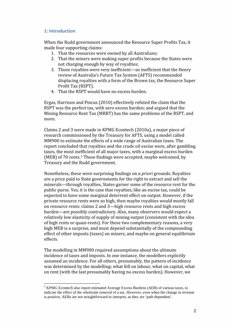
The Australian Treasury contracted KPMG Econtech (2010a) to estimate the efficiencies of Australian taxes, using MM900. The resultant report, endorsed by Treasury, was a major input into the Henry report into Australia’s Future Tax System (AFTS 2010); and into the policy decisions that ensued. KPMG Econtech (2010a) found a marginal excess burden (MEB) of 70%, making royalties the second most inefficient major tax, after gambling taxes. Subsequently, AFTS recommended that royalties be replaced by an excess profits tax. The modelling of royalties presents some puzzles. KPMG Econtech found that the existing import tariffs improved economic welfare. It is surprising, therefore, that the modelling found that royalties severely damaged national efficiency: a tailored export tax is the first best trade policy, and the 2009-10 royalty and the tax regime was arguably a closer substitute than is the existing tariff. Within a partial equilibrium framework that accounts for other taxes and for demand and supply effects, unbelievably high tax rates are required to generate MEB of 70%. The MEB depends crucially on the assumptions about supply, which was modeled by KPMG Econtech using a CES production function that does not seem well suited to an industry using essential but exhaustible resources. Unfortunately, the report is unclear as to how an apportionment was made between a reduction in resource rents, and a reduction in the returns to financial capital in mining: the incidence table for royalties suggests a very low excess burden.

1 Ergas: SMART Facility, University of Wollongong; Pincus: School of Economics, The University of Adelaide (corresponding author). This is a drastic revision of a paper given at Australian Conference of Economists 2012, Melbourne, Victoria, July 8 -12, 2012. Thanks but no blame goes to Mark Harrison, John Freebairn and conference participants.

2

1: Introduction When the Rudd government announced the Resource Super Profits Tax, it made four supporting claims:

1. That the resources were owned by all Australians; 2. That the miners were making super profits because the States were

not charging enough by way of royalties; 3. Those royalties were very inefficient—so inefficient that the Henry

review of Australia’s Future Tax System (AFTS) recommended displacing royalties with a form of the Brown tax, the Resource Super Profit Tax (RSPT).

4. That the RSPT would have no excess burden.

Ergas, Harrison and Pincus (2010) effectively refuted the claim that the RSPT was the perfect tax, with zero excess burden; and argued that the Mining Resource Rent Tax (MRRT) has the same problems of the RSPT, and more. Claims 2 and 3 were made in KPMG Econtech (2010a), a major piece of research commissioned by the Treasury for AFTS, using a model called MM900 to estimate the effects of a wide range of Australian taxes. The report concluded that royalties and the crude oil excise were, after gambling taxes, the most inefficient of all major taxes, with a marginal excess burden (MEB) of 70 cents.2

These findings were accepted, maybe welcomed, by Treasury and the Rudd government.

Nonetheless, these were surprising findings on a priori grounds. Royalties are a price paid to State governments for the right to extract and sell the minerals—through royalties, States garner some of the resource rent for the public purse. Yes, it is the case that royalties, like an excise tax, could be expected to have some marginal deterrent effect on output. However, if the private resource rents were so high, then maybe royalties would mostly fall on resource rents: claims 2 and 3—high resource rents and high excess burden—are possibly contradictory. Also, many observers would expect a relatively low elasticity of supply of mining output (consistent with the idea of high rents or quasi-rents). For these two complementary reasons, a very high MEB is a surprise, and must depend substantially of the compounding effect of other imposts (taxes) on miners, and maybe on general equilibrium effects. The modelling in MM900 required assumptions about the ultimate incidence of taxes and imposts. In one instance, the modellers explicitly assumed an incidence. For all others, presumably, the pattern of incidence was determined by the modelling: what fell on labour, what on capital, what on rent (with the last presumably having no excess burden). However, we

2 KPMG Econtech also report estimated Average Excess Burdens (AEB) of various taxes, to indicate the effect of the wholesale removal of a tax. However, even when the change in revenue is positive, AEBs are not straightforward to interpret, as they are ‘path dependent’.

3

found the incidence tables in the report inscrutable; and their explanation, deficient. For the major minerals, an export demand elasticity of -6 was assumed in MM900. The usual rule has it that the optimal trade tax is the inverse of this elasticity, or 17%. Treasury’s own data suggests that, at that time, miners paid less than 17 per cent tax out of sales; but close enough to allow the possibility that the taxes improved economic welfare (which is what KPMG Econtech concluded about import tariffs). This paper is about modelling the excess burden of royalties. We believe that royalties create an excess burden on the supply side, with some significant offset on the export price side. What we do not believe is that the modelling of royalties by KPMG Econtech for Treasury is sufficiently convincing for it to provide a firm basis for policy. And it is curious that such a dramatic finding did not elicit much critical attention from economists. Temporarily at least, it looked as though the issue would be somewhat moot, because the recently enacted Mineral Resource Rent Tax gives a tax credit for royalty payments. Thus, for any firms with a positive liability under MRRT, there is no excess burden from royalties, since they merely transfer money from the Commonwealth to the States. However, recent falls in minerals prices and rises in production costs and royalty rates have again brought the issue into prominence. Also, the Opposition have indicated that (if elected) they would abolish the MRRT. Section 2 offers ‘back of the envelope’ estimates of the tax burden on mining in 2004-05 (in excise equivalents), and the resultant MEB; and finds a large disparity with that reported in KPMG Econtech (2010a). The next section examines the explanations provided by KPMG Econtech for the very high excess burden of royalties. Section 4 looks at the supply curve of minerals in MM900, and at reasons to expect a relatively low number. The next section discusses the difficulties of interpreting the incidence tables in KPMG Econtech (2010a). Conclusions are in section 6.

2. Back of the envelope This section provides rough estimate of the tax burden on mining for 2004-05. We then use them to calculate MEB in a partial equilibrium model with demand and supply side effects. On the tax side, our estimates of excise-equivalents of company tax, payroll tax, and royalties are respectively 6%, 2% and 5% of the value of output, for a total of 13%. This is less than half the tax load (of 28.9%) required, in partial equilibrium, to generate the 70% MEB for royalties reported in KPMG Econtech (2010a). We make no pretence that our tax estimates are precise; however, to the extent possible, they rely on published ABS and Treasury data and on KPMG Econtech (2010a) for the values of the elasticities of supply and of export-demand.

4

A crucial parameter—company taxation as a proportion of sales—is difficult to discover from public information for the year 2004-05. The ABS first provided data on company income and taxation for mining in Taxation Statistics 2007-08 (Table 8: Company tax), which showed a ratio of net company tax to total income of 5.0%.3 In 2004-05, miners paid company taxes at an average rate of 12.5% of gross operating surplus (GOS) (Treasury data cited in Australian Financial Review, 7 May 2012: 53). If, as has been suggested to us, the ratio of GOS to sales were 50%, then company tax amounted to 6.2% of mining sales. We have taken the rate of 6%. Payrolls accounted for about 40% of mining costs, with the tax levied at about 5%, for an excise equivalent of 2%. Thus, company and payroll taxes were around 8% of sales. For royalties, the Commonwealth Grants Commission provided us an unpublished compilation of data from Government Financial Statistics, showing that the states and territories received $4, 684m in 2007-08. This was 2.2% of mining company income reported for that year by the ABS. Rapidly rising minerals prices had led to a fall in the burden of royalties; and there are timing questions involved, so (in view of other information about ad valorem royalties) we have taken the average royalty rate to be 5%. Thus, these rough estimates give a total tax burden equal to 13% of sales.4

The reader is invited by KPMG Econtech (2010a) to start thinking about excess burdens in partial equilibrium terms—see 3.3: The Incidence of Taxes, and especially Figure 3.2, p. 23; and we will adopt that approach here. Temporarily, assume that all output were exported and that export demand were perfectly elastic. In section 4, we show that the supply elasticity assumed by KPMG Econtech for mining was around 𝜂= 1.75.5 Defining 𝜏 = 𝑡/(1 − 𝑡), the partial equilibrium formula for MEB is 𝜏𝜂/(1 − 𝜏𝜂): see Appendix. To achieve MEB of 70% requires a total tax burden of 19% on sales, when only supply effects operate. With our estimate of a tax rate of 13%, the MEB on the supply side is 35%.6

However, we need to allow for demand side effects. Because such a large share of the relevant minerals is exported, the imposts that fall on mining are close to being export taxes. KPMG Econtech assumed an export demand elasticity of -6; so some of the tax burden would fall on foreigners. A total tax burden of 13% is less than the optimum export tax rate of 17% (where 0.17 = 1/6). Arguably, however, this regime more closely approaches the first best trade tax regime than does the set of existing tariffs: exports with

3 Export prices rose between 2004-05 and 2007-08, which would presumably raise the ratio of tax to income; but there was also the start of an investment boom, which would tend to lower it. Although total income includes more than sales—e.g., interest and dividends received—for mining it is probably a reasonable approximation. 4 In the estimate of 13% equivalent tax rate for 2004-05, royalties comprise 38% of the total burden, close to the 40% from a survey of larger miners for the Minerals Council for 2007-08 through 2009-10: Minerals Council of Australia (2011). 5 MM900 had a number of different mining industries. 6 Sometimes the MEB formula incorrectly uses t instead of 𝜏, which lowers the MEB estimates. For example, with a tax rate of 13%, the MEB on the supply side would fall from 35% to 29%.

5

more elastic demand (in MM900), like agriculture, pay no royalties; import tariffs on final goods and services are far from uniform. Yet KPMG Econtech found that the existing set of tariffs improve economic welfare, whereas royalties substantially worsens it. Due to the elasticity of export demand, our interim result of MEB of 35% is an overestimate for three reasons (see Appendix):

1) The triangle of loss on the supply side is smaller than calculated earlier because the supply price falls less than the full extent of the tax;

2) For any given excess burden on the supply side, the revenue gain is scaled up, compared with the situation in which demand is perfectly elastic;

3) There is an offsetting national gain on the demand side, a rectangle, because foreigners bear some of the tax burden.

Simplifying, we assume that all production is exported. With an export demand elasticity of ε𝜖 = −6, and a supply elasticity ofη𝜂 = 1.75, a tax of t will raise the demand price by the ratio 𝜂/(−𝜖 + 𝜂) or 23% of the tax, and supress the supply price by 77% of the tax. Foreigners would pay 23% of the tax revenue; and this percentage should be subtracted from the MEB calculated with reference to the supply side only (after accounting for effects 1 and 2 above: see Appendix).7

When the demand elasticity is taken into account, the MEB falls from 35% to negative, − 3.6%.

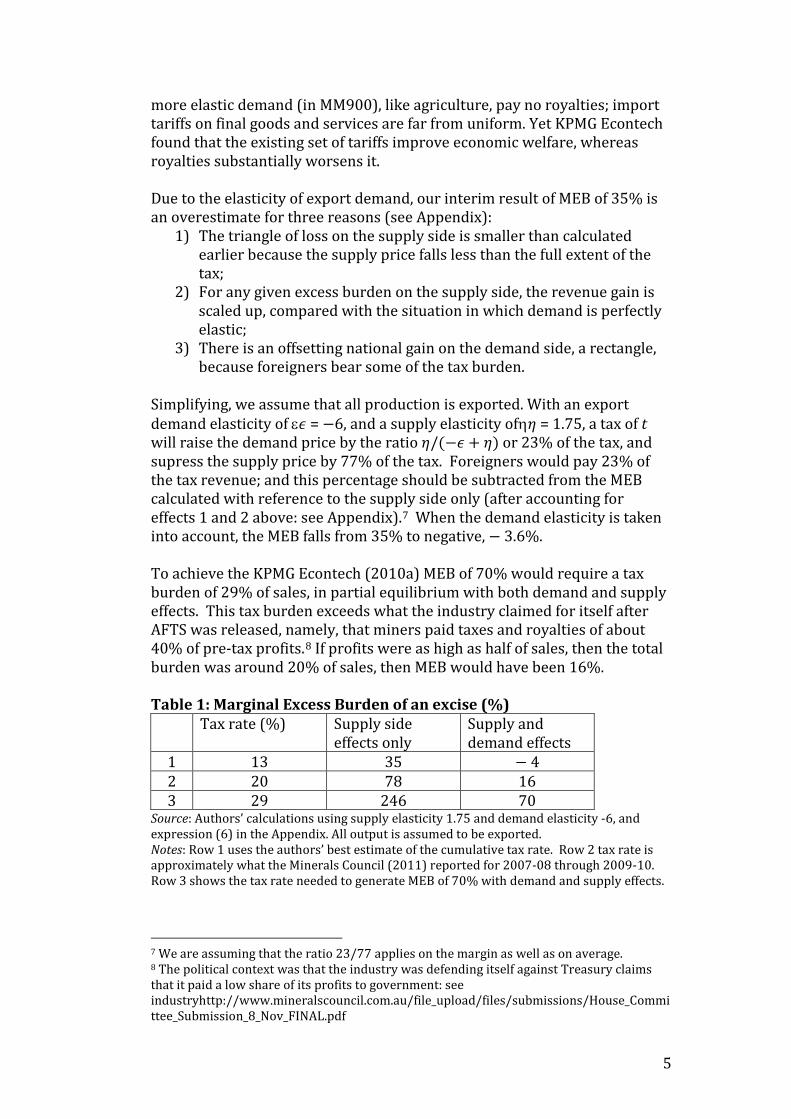
To achieve the KPMG Econtech (2010a) MEB of 70% would require a tax burden of 29% of sales, in partial equilibrium with both demand and supply effects. This tax burden exceeds what the industry claimed for itself after AFTS was released, namely, that miners paid taxes and royalties of about 40% of pre-tax profits.8

If profits were as high as half of sales, then the total burden was around 20% of sales, then MEB would have been 16%.

Table 1: Marginal Excess Burden of an excise (%) Tax rate (%) Supply side

effects only Supply and demand effects

1 13 35 − 4 2 20 78 16 3 29 246 70

Source: Authors’ calculations using supply elasticity 1.75 and demand elasticity -6, and expression (6) in the Appendix. All output is assumed to be exported. Notes: Row 1 uses the authors’ best estimate of the cumulative tax rate. Row 2 tax rate is approximately what the Minerals Council (2011) reported for 2007-08 through 2009-10. Row 3 shows the tax rate needed to generate MEB of 70% with demand and supply effects.

7 We are assuming that the ratio 23/77 applies on the margin as well as on average. 8 The political context was that the industry was defending itself against Treasury claims that it paid a low share of its profits to government: see industryhttp://www.mineralscouncil.com.au/file_upload/files/submissions/House_Committee_Submission_8_Nov_FINAL.pdf

6

Although the BOTE calculations (summarised in Table 1) are rough and ready, they do seem to throw doubt on the estimate of MEB of royalties of 70%. And the gaps are far too large to be bridged by general equilibrium effects.

3. Sources of excess burden As we read KPMG Econtech (2010a), the following describe the market in MM900 for the relevant natural resources:

1. Supply of the resource is a fixed endowment.9

2. Each resource endowment is industry-specific.

3. Each resource is homogenous in quality and cost of extraction. 4. Production was modelled through a representative firm operating

under constant returns to scale; and so there is no heterogeneity amongst producers.

5. The resource earns a resource price or pure rent, determined by the intersection of the demand for the resource and the fixed supply.

The explanation offered in KPMG Econtech (2010a) for the high excess burden of royalties comprises four elements:

1. Royalties are like an excise, in that they depress the price that the producer receives and so causes output to fall along the supply curve. (We discuss the supply curve in section 4.)

2. Royalties, like the company tax, reduces the return to capital, and so capital is displaced when royalties are applied.

3. Miners earn excess profits and so some of the burden falls on rents. The current section concerns points 2 and 3.

4. Miners cannot pass much of the burden of royalties to their customers, who are mainly foreigners. (This does not quite fit the assumptions of MM900, with the effects just discussed.)

In the report (p. 17), the authors pointed out that “The party paying a tax, and so carrying its impact, is sometimes different from the party who actually bears the final burden or incidence of the tax, after economic responses.” When discussing the modelling of production involving natural resources generally, the report stated that

‘Any tax placed on a type of fixed factor will not change the supply of that fixed factor. With the fixed supply of the fixed factor to the market, the rent that users will be

9 Two ways in which royalties impose an excess burden are that some marginal prospects are never, or belatedly or not fully mined, even though such mining would be expected to be profitable without the imposition of royalties; and that royalties discourage some exploration and prospecting of the kind that could lead to the establishment of marginal mines. However, MM900 does not include the activity of prospecting; and only includes as resources those that have been developed. Thus. MM900 neglects a source of excess burden.

7

prepared to pay for the use of the fixed factor will be unaffected by the tax, and will continue to reflect the fixed factor’s marginal productivity. This means that the burden of the tax will be fully borne by the fixed factor owners’ (p. 36)

For the PRRT, the economic incidence is determined by economic theory:

The inclusion of fixed factors is particularly useful for measuring the excess burden of the Petroleum Resource Rent Tax, which is intended to be a tax on the above normal profits of the oil extraction industry’ (p. 36). The PRRT is modelled as a tax on oil and natural gas resources, which are assumed to be in fixed supply. This methodology rests on the assumption that the PRRT is designed so that it taxes only excess profits of petroleum extractors, which they derive from access to a natural resource which is limited in supply. If only these excess profits are taxed, then investment decisions of petroleum extractors will not be distorted (p. 51; emphasis in the original).

(Later, the source of payment was identified as gross operating surplus, GOS: p. 86). Thus, for the PRRT, incidence was assumed to fall entirely on rents.10

In contrast, KPMG Econtech took it to be the case that, because royalties and crude oil excise were legally charged on the basis of output (quantity or value) and paid by the owners, then they must necessarily have an effect on output via the return to capital and labour:

The analysis of resource royalties and crude oil excise is similar to that of the company tax. These taxes are mostly levied on production volumes or values of the mining sector. Resource royalties and crude oil excise have a very high excess burden. KPMG Econtech estimates the marginal excess burden of royalties and crude oil excise to be 70 cents in the dollar and the average excess burden to be 50 cents in the dollar. The very high excess burden for these taxes does not compare favourably to the low excess burden for petroleum resource rent tax. This is because the resource royalties and crude oil excise are based on production volumes or values – which depend on factors that are mobile, capital and labour, as well as on returns to immobile natural resources. Thus, the mobility of capital is again an important factor contributing to the very high excess burden for resource royalties and crude oil excise…(p. 58)

The crucial matter is that royalties are levied on the quantity or value of output, and not on the quantity of the resource input used (which would be hard to monitor.) If royalties were levied on the quantity of input instead of on output, then in a model like MM900, there would be a minimum market-clearing price for access to minerals; and only royalties above the market-clearing rate would impose an excess burden. Similarly, a lump-sum payment for access to the resource would impose no excess burden.11

Therefore, the argument that royalties depress the return to capital seems to us confusing and redundant, once the point is made that royalties raise

10 Interestingly, when Treasurer Swan (2011) introduced the legislation for MRRT, he noted that, because ‘the sources of mining rents are difficult to identify separately in practice, the MRRT aims to strike an appropriate balance between recovering a sufficient return to the community from the profits attributable to the underlying resource rents at the valuation point, and recognising that some mining expertise and capital may also be taxed in a process which has regard to realised profits and their equivalents.’ 11 Alternatively, if there was a fixed coefficient between resource input and the base on which royalties are levied, then the excess burden would again be zero until the royalty rate exceeded the market-clearing rate.

8

the marginal cost curve. Assuming all inputs are substitutes (which is what MM900 did, using the nested CES production function), the rise in the cost curve is sufficient to cause a fall in output, requiring a reduction in all inputs, including capital. It does not seem correct to state that ‘The analysis of resource royalties and crude oil excise is similar to that of the company tax’—royalties are levied on output, whereas company tax is levied on income net of costs and various allowances. The incidence of royalties depends totally on the supply curve (given the levels of non-royalty taxes and charges).

4. Supply curve By assuming a specific supply curve, KPMG Econtech determined the extent to which royalties fell on resource rents. If miners were operating with relatively elastic supply, then there would be a substantial impact on mining output (and GE effects would magnify this impact, large or small, into the excess burden). If, in contrast, the Australian mining industries were operating on a rather inelastic portion of the supply curve, then the impact of royalties would be little on output and much on rents. According to KPMG Econtech (and AFTS and the Rudd government), this industry earned excess profits by way of resource rents even after royalties had been paid.12

Then, when the producer price falls as a result of royalties, much of the initial incidence would be on private resource rents, not on the return to mobile capital; and the excess burden would be small. Implicitly, the shape of the supply curve determines where the incidence falls.

A modelling framework ideally should reflect important elements of the reality of mining: in particular, that the heterogeneity amongst firms in the industry, and within and between deposits, helps give rise to the upward slope of the supply curves for mining output. Moreover, as mining output increases, recourse must be had to less productive or more distant ore bodies and to the higher cost portions of existing ore bodies—and, therefore, the supply curve of mineral output should get steeper as output increases. Such realism would mandate either a constant elasticity of supply less than unity13

, or a supply curve with an elasticity that falls as output increases. This realism is reflected in the phrase from page 58 of the report, about how royalties cause the contraction in output by ‘the more marginally profitable mining operations’. However, heterogeneity was completely assumed away in MM900: instead, supply depends an assumed number (0.75) for the elasticity of substitution among primary factors of production.

MM900 used nested CES production functions, from which the supply elasticity can be recovered. MM900 uses the substitution elasticities shown

12 The report does not make it clear on what it based the judgment that mining was earning excess profits by way of resource rents: was it an examination of mining profits as of 2004-05; or on an estimation of what mining profits would have been if 2004-05 export prices had ruled in 2009-10. The latter would have required the use of a supply curve to construct the counter-factual. 13 A constant elasticity of supply greater than one implies a supply curve that is convex from above.

9

below in Table 2. Apparently, these elasticities applied to all industries, mining as well as non-mining: the ease of substituting land for other fixed factors (including natural resources) was assumed to be the same in manufacturing as in mining.14 For extractive industries, however, no amount of labour and capital, no matter how cheap, can produce more than a tonne of output from less than a tonne of ore, so there seems to be some real limit on substitution at the top (primary factor) level. That comment aside: there are well known problems of estimating such elasticities; and it is recognised that their choice (and the choice of what to nest with what) can make sizeable differences to the results of CGE simulations (Turner, 2012).15

Table 2: Elasticities of substitution Substitution Possibility Elasticity of Substitution Labour – Capital – Fixed factors

0.75

Labour: low skilled – high skilled

1.25

Capital: structures – other capital

0.5

Fixed factors: land – other fixed factors

0.5

Source: KPMG Econtech (2010a), Table C.1 With the nested CES production function of MM900, the supply elasticity is given by the expression 𝜂 = 𝜎(1 − 𝜃𝑓)/𝜃𝑓𝜃𝑣, where σ is the elasticity of primary factor substitution; θf is the share of the fixed factor in value added; and θv is the share of value added in production.16

The value of σ is given above as 0.75. We could not find the values for the cost shares in the report, but it has been suggested to us that 5/12 and 3/5 are reasonable numbers (for the year of the data set), giving a supply elasticity of 1.75. This implies that a (permanent) doubling of export prices would result in Australian mineral annual exports 3.5 times larger, forever. Not everyone regards this as realistic.

As a check, we can compute the ‘general-equilibrium elasticity’ as the ratio of the percentage rise in output to the percentage rise in the producer price following the simulated removal of royalties. The numerator is a 7.5% rise in output (KPMG Econtech 2010a: 134). Unfortunately, although KPMG Econtech estimated the ad valorem equivalents of royalties and the crude oil excise applied in MM900, they report neither them nor their average. In 2009-10, no ad valorem royalties exceeded 6% and many were lower; and

14 It is somewhat ironical that the motivation of Arrow, Chenery, Minhas and Solow for launching the CES production function was to provide a model in which the elasticity of substitution would differ across industries. 15 KPMG Econtech (2010a) did not report any sensitivity analyses. 16 These shares depend on factor prices and unit inputs. The ‘price’ of the natural resource is the royalty payment made by the miner. But when a primary factor—natural resources—is earning a rent, then the rent, although included in value added, is a residual, not a factor price to which the entrepreneurs react.

10

low valued products generally were charged specific duties with, we expect, equivalents lower than 6%. The crude oil excise rates ranged up to 30%. From this and other information, we expect that the average levy was between 10% and 5%, implying a range for the general equilibrium supply elasticity of 0.75 to 1.5.17

The partial equilibrium supply elasticity would be lower than the GE elasticity, when the induced fall in the exchange rate and the fall in world export prices are taken into account.

Some general considerations point to relatively inelastic supply (in general equilibrium). The supply responsiveness of any industry that depends heavily on a specific, immobile, fixed resource must be lower, ceteris paribus, than that of other industries, when we take account of competition for factors of production in relation to the size of the pool.18

Consider, for example, what would occur if the output of one relatively small non-mining industry were made exempt from the GST. The output of this industry would rise, drawing in more labour, land and capital. In MM900, capital is in perfectly elastic supply, but land suitable for commercial purposes is in fixed supply nationally; and nationally, labour is in very inelastic supply. However, as this non-mining industry is a small part of the national economy, and as its assumed tax advantage not huge, it would not expand sufficiently to run into a highly inelastic national supply of labour or land. Unlike a mining industry with ore bodies, this industry can draw a necessary input, land, from other uses in the economy: the supply to the non-mining industry of all three factors is very elastic, and so it is reasonable to infer a relatively high responsiveness of supply, within the range of producer prices that was being contemplated. But for the mining industries, using an industry-specific resource that is in fixed supply, the supply responsiveness must be lower than in otherwise similar industries.

Not only the general consideration offered above, but also casual empiricism gives some support to the possibility of relatively inelastic supply. Over recent years, minerals price have soared remarkably, and remained high for almost a decade, and are widely forecast to remain high (although not quite at the record levels experienced), as Australia enjoyed the best terms of trade possibly ever. Prices in 2009-10 were already 50% higher for minerals than in 2004-05, yet mining output has not increased greatly. MM900 is an avowedly comparative static model, and so lags in supply responses are not included (but see section 2 above). Nonetheless, this recent experience does suggest relatively inelastic supply. Moreover, there is a methodological point to consider: how to model exhaustible mineral resources. MM900 is a comparative static, general equilibrium model, using a database of 2009-10 (albeit modified for the rise in mineral prices since 2004-05 and for the GFC). Each mining industry uses an industry-specific natural resource, assumed to be in inelastic supply 17 This 1.5 is not to be compared with the 1.5 that their Table C.3 confusingly labelled as the ‘export supply’ elasticity of all minerals. 18 If factor supplies were perfectly elastic, so would be the supply of a competitive industry under constant returns to scale.

11

(‘fixed’). The equilibrium is conceptualised as having been achieved after all endogenous adjustments have been made to the ‘shock’ administered to the model, which is in this case the removal of royalties and crude oil excise. It may be tempting to think of such equilibria as persisting in time, if nothing further occurred to disturb them. The modelling framework would support this inference if all productive inputs were reproducible, but not if natural capital were exhaustible. Mining resources are exhaustible in fact; and the model assumes natural resources are in fixed supply. Therefore, unless we assume some costless process by which natural resource stocks are restored, how can we interpret the model as telling us what would happen from now on, into the indefinite future, if the economy were fully adjusted to the removal of royalties and if nothing else occurred to shock the economy in any way? It is not appropriate, as KPMG Econtech claimed (p. 27) that “…the analysis from MM900 will be a long-run analysis,” if we continue to ascribe an equilibrium quality to it. MM900, like all CGE models, shows what would hold after all prices and quantities had adjusted to tax changes (p. 27); but it does not means that an accurate ‘long run’ counterfactual is captured by a model with a database that, in the case of mining and the like, did not reflect ‘long run’ or comparative-static equilibrium. Unless natural resources are inexhaustible, there is nothing other than a transitory equilibrium. In summary: of necessity, KPMG Econtech prejudged the crucial question with respect to royalties: the value of the supply elasticity; but the report did not provide or discuss its value. If the industry were operating on an elastic part of the supply curve before the removal of royalties, then royalties would be expected to have a large excess burden in MM900. But were the industry operating on a relatively inelastic or very inelastic part of the supply curve, then royalties would have had a low excess burden (given the presence of other government imposts on the industry). As indicated in the quotation above (from p. 58), KPMG Econtech explained the large excess burden by pointing out that royalties, like an excise tax, reduce supply (which is a theoretically unobjectionable and realistic claim); but also by postulating a displacement of (financial) capital when royalties depress the return to mining capital. But the displacement of capital assumes, does it not, that the miners were not earning excess profits in the form of resource rents—contrary to what KPMG Econtech asserted. If the miners were earning excess profits as resource rents, why would a fall in the return to mining capital act to drive capital away from the industry? By definition, pure resource rents are returns in excess of what is needed to induce the natural resource into the activity; so, if pure rents fall, then the factor of production that was earning pure rents, and is still earning some pure rents, will not move to another industry. KPMG Econtech (2010a) provided tables of the estimated final incidence of various taxes, to which we now turn.

12

5. Incidence Tables MM900 is a large computable general equilibrium model, with 109 industries and almost 900 separate products; and 19 taxes or levies. It is a comparative static GE model, not a dynamic one—that is, it computes (relative) prices, quantities, revenues and so on, as though the economy had fully adjusted to the ‘shock’ that caused it to deviate from the initial solution; but MM900 does not compute any time paths of adjustment. To estimate incidence and average excess burdens, the model was shocked by setting a levy or tax to zero; the new equilibrium was computed, and compared with the equilibrium in which the levy or tax was imposed. In the simulations for the MEB, the rate of impost was reduced by 5%. MM900 assumed that capital was provided from two sources: domestic savings (assumed proportional to income) and foreign capital, which is in perfectly elastic supply. The labour market clears through flexible wages; and the labour-leisure trade-off means that labour supply has some elasticity, but it is quite small. Foreign balance is maintained through the operations of a flexible exchange rate, the effects of which work through the economy. There is some responsiveness of world prices to variations in some Australian exports; and production for domestic absorption cannot be transformed one-to-one into production for export.19

After the removal or reduction in a tax, a lump sum transfer from the private sector balanced the public sector accounts. (The transfer was from households, who own all Australian assets and labour.) Excess burden was measured as the compensating variation in income necessary to restore the utility of the representative household.

The database is for 2009-10, except that certain unspecified adjustments were made for the rise in the terms of trade since 2004-05; and for the effects of the GFC. Natural resource endowments were assumed in fixed supply; and, because the model uses the ‘representative firm’ and all production functions exhibit constant returns to scale, it is as though each mining firm had its own resource endowment. Importantly, Table 3.1 Identifying Tax Incidence reported that, for the Agent called 'Owners of non-land fixed factors of production e.g. natural resources', the 'Variable indicating tax incidence' is ‘Change in after-tax private income from other economic rents.'20

In the main mining industries, KPMG Econtech (2010a) found excess profits or returns:

The zero profit assumption is a common assumption in economic modelling. However, in reality, excess returns do exist in some industries. These excess returns can arise as a result of factors such as access to a natural resource (such as petroleum or mineral deposits), monopoly power...The following industries are identified as having "excess returns" that, for modelling purposes, are attributed to the fixed factor: Coal; Oil and gas; Iron ore; non-ferrous metals…(pp. 35, 36).

19 This assumption is hard to reconcile with the methodology of comparative statics. 20 In section 2 above, it was suggested that a thoroughgoing comparative static model would conclude that these owners would bear all the incidence of royalties (so long as post-royalty rents did not fall to zero).

13

The report provided a series of tables, 5.1 through 5.30, headed “Incidence of…Taxes”.21

The tables are in terms of changes in total of after-tax private income and in its main elements: labour income, capital income, and rents and transfers abroad. For convenience, KPMG Econtech’s incidence tables for three levies are consolidated into Table 3 with the addition of row 12 for the average excess burdens (AEB, as %), allowing us to calculate its dollar value (row 13). It is important to note that the ‘revenue’ figures for each levy are the general equilibrium changes in government revenue when the levy is imposed, and not the revenue that one would find in the ABS publications on public finances.

Table 3: KPMG Econtech estimates of revenue and income changes for three 'taxes' ($m)

A B C

PRRT Land Taxes Royalties

and crude oil excise

Sources Table 5.1 (p. 51)

Table 5.2 (p. 53)

Table 5.9 (p. 59)

1 Revenue 1398 3229 3381 2 Change in after-tax private income 3 Labour income 0 14 -135 4 Capital income 0 0 252 5 Residential land income 0 -2 19 6 Rural land income 0 -72 -115 7 Urban land income 0 -2706 32 8 Other rent income -1218 -41 -1175 9 Transfers -180 -418 -128

10 Total change in after-tax private income -1398 -3225 -1251

11 Change in total private income -0.2% -0.5% -0.2% 12 Average Excess Burden, AEB 0% 6% 50% 13 Excess burden (revenue, row 1, times

AEB, row 12; $m) 0 -194 -1691 Sources: KPMG Econtech (2010), Tables 5.1, 5.2, 5.9 and A (for row 12); row 13 is our arithmetic.

One would expect to be able to use these incidence tables to understand a question central to this paper: what assumption did KPMG Econtech make, concerning how the imposition (or removal) of royalties and crude oil excise impacted on private resource rent income (before the general equilibrium adjustment). These tables, however, are enigmatic: they leave these readers unsure as to where the huge excess burden of royalties falls. 21 Two tables in the report are numbered Tables 5.1: one on p. 44 (which is a replica of Table A) and the other on p. 51—we are reproducing the contents of the latter.

14

KPMG Econtech’s incidence tables show the incidence or final burdens of the various imposts. The incidence on the private sector can be on the supply side (on nominal incomes) and on the prices of consumption. On the supply side, the burden is by way of changes in factor prices or in the quantities of factors used in the national economy. The nominal wage rate is the numeraire. Changes in prices and, therefore, in real wages alter the purchasing power of income and the utility derived from nominal incomes.22

KPMG Econtech (2010a) provided guidance in interpretation of the incidence tables:

“Changes in capital income and transfers [abroad] are included only for completeness. They reflect specific model assumptions, and do not carry any policy implications…Therefore, the movements in income from capital ownership and transfers will move with income generally. They are not closely linked to the nature of the tax under consideration, and do not have policy implications” (p. 42).

This could be read to suggest that the only variation, of significance to excess burden, is that to labour income.23

In any general equilibrium model, all prices are determined in relative terms, but expressed in nominal terms…In MM900, the average nominal wage has been chosen as numeraire. Although the choice of numeraire does not affect the modelling results, it does need to be taken into account in interpreting nominal price changes. For example, a fall in the real way could come about through either a reduction in the nominal wage or an increase in consumer prices. In MM900, it will always be the latter, because the nominal wage is fixed. Therefore, any price increase reported in the incidence tables can simply be interpreted as a fall in the real wage (p. 43).

Also, the incidence tables are expressed in money terms and, because the nominal wage is numeraire, falls in nominal wage income must be proportional to falls in aggregate employment:

However, presumably there is no need to adjust for price changes, when comparing two nominal amounts and, in particular, when comparing excess burden and changes in wages, both in nominal dollars. Ultimately, we are interested in excess burden, and not incidence per se, and so we have supplemented the incidence tables with information about excess burden (lines 12 and 13 of Table 3). A theoretical point, essential to our argument, is that the incidence of relevance for excess burden cannot be that falling on the rents earned by the fixed factors of land and resources. Taking notice of KPMG Econtech’s comments on the policy-irrelevance of change in capital income, cited earlier, then we would expect excess burden

22 ‘In summary, the incidence of most Australian taxes can be expected to fall on labour. This reflects the common modelling assumptions of perfect competition with constant returns to scale, and that Australia is (almost) a price taker in world trade and capital markets. However, land and resources bear some of the incidence of the tax system, and when taxes are applied directly to them they bear the full incidence’ (KPMG Econtech 2010a, p. 27). 23 In MM900, labour is in imperfectly elastic supply, neither perfectly elastic nor perfectly inelastic, but closer to the latter. Therefore, was well as receiving compensation for the loss of leisure, labour earns ‘rents’. However, it is conventional to ignore this complication.

15

to be equal to the change in labour income. For PRRT, this equality is met: EB is zero and so is the change in after-tax labour income. However, for land taxes, the change in after-tax labour income is a rise of $14m, not the fall of $194m necessary to explain the EB. But for royalties, the gap is tremendous: the fall in labour income is $135m, whereas EB is $1,691m. If excess burden is only reflected in changes in labour incomes, then $1,556m of excess burden is unaccounted for (or $1,808m is missing if, contrary to the advice of KPMG Econtech, labour and capital incomes are taken together). Without this missing excess burden, the AEB of royalties and crude oil excise is not the +50% reported by KPMG Econtech, but +4% (or -3.4%, if we include capital). Earlier, we provided partial equilibrium estimates of the marginal excess burden of royalties (table 1). We made the simplifying assumption that all the relevant output was exported to markets with a demand elasticity of -6; and assumed a supply elasticity of 1.75. When we applied the relevant formula (expression 6 in the Appendix) to our estimate of the cumulative tax burden on mining, the resulting MEB was a small negative, not the 70% reported to Treasury. This was a modest underestimate, in so far as not all the output was exported and so we neglected a ‘triangle’ of loss in consumer surplus.24

On the other hand, it assumes that all imposts on mining were exactly as damaging as an excise on output. On our interpretation, the incidence table for royalties and crude oil excise gives support to the idea that the average excess burden of closer to zero than to 50%.

Unfortunately, the gap between the excess burden of royalties and the change in labour income (or non-rent income) was not noted in the KPMG Econtech report, and so no explanation was offered there. Maybe the explanation, of the gap between the excess burden of royalties and the modest fall in the incomes of non-fixed factors, lies in the methodology of MM900, which treated royalties and excises together. According to the Commonwealth Grants Commission (2011: Box 5-1), royalty payments received by the States in 2009-10, were $2,284m. KPMG Econtech (2010a) made some unspecified adjustments to the mining sector accounts to offset the price rises since 2004-05; maybe these reduced royalties in the database close to the $1,556m (or $1,808m) of ‘missing’ excess burden. This leads us to speculate that the problem for royalties and crude oil excise may arise because, under the system of national accounting used internationally and in Australia, royalties are not a tax, but a price paid 24 In KPMG Econtech (2010a), excess burden is estimated by compensating variation for households, for changes in money incomes and in prices. Therefore, we would expect that the CV reported would include a provision for the rise in prices: ‘For example, a tax may reduce the nominal income from any of the primary factors of production: labour; land; other fixed factors; or capital. Or it may also be transmitted into higher prices, reducing real incomes” (p. 47). For royalties and crude oil excise, the incidence table shows a consumer price rise of 0.5% (and no price rises for PRRT or land taxes). Total final household expenditure in 2009-10 was $190.9b (ABS 52040: 20); 0.5% of that is $960m, which is about half of the missing excess burden. The ‘unexplained’ excess burden is much too large to be caused by rounding errors.

16

for access to minerals for mining and sale. Therefore, royalties are a cost of production; if they were forgiven, then the gross operating surplus of the miners rises; that is, private pre-tax income rises. In contrast, excises are taxes: if the excise were to be removed, then, in the national accounts, private pre-tax income (GOS) does not change in the first instance. However, KPMG Econtech treated royalties and crude oil excise together in the simulation. This could have led KPMG Econtech erroneously to interpret the transfer from the private sector to the public sector of about $2b of royalty income—which decreased private pre-tax incomes, dollar for dollar—as a part of excess burden. If so, then KPMG Econtech counted a transfer of rents as excess burden.

6: Conclusions There is a certain irony in the role of rents here, as there is in the publication by Treasury of the modelling done for it by KPMG Econtech. The AFTS inquiry was headed by Dr Ken Henry, then Secretary of the Commonwealth Treasury, who holds a PhD in economics for a thesis on Housing Policy that was mostly concerned with the taxation of imputed rent. One of the main thrusts of AFTS was to shift the tax burden onto rents, of various kinds. Following the publication of AFTS, Mr Rudd, then Prime Minister, accompanied by the Treasurer and Dr Henry, announced the intention to introduce the Resource Super Profits Tax (RSPT), on two grounds relating to rents. First, although it was recognised that the States do capture rents through royalties, AFTS and the government judged that they did not capture enough. Secondly, Dr Henry and others repeatedly claimed that royalties were very inefficient, and that the RSPT would have no excess burden at all—zero excess burden, even at rates of tax as high as 90%, because it fell solely on rents. Ergas, Harrison and Pincus (2010) refuted this extreme claim about the RSPT and its later replacement, the Minerals Resource Rent Tax (MRRT). These two taxes were introduced to capture more of the rents of miners for the Commonwealth government. Rents were at the centre of the case. Yet the very estimate of the deadweight loss, cited in support of this proposition, was based on the assumption—not the finding—that rents did not bear most of royalties and crude oil excise. KPMG Econtech looked at the data for 2009-10 and found rates of return in excess of ‘normal’. If they had looked at the rate of return for those mines in operation a decade or more earlier—and they made up the vast majority of those operating in 2009-10, they probably would have found very low rates of return after royalties.25

25 We should emphasise the words ‘after royalties’, because GOS is defined net of royalties; royalties are a cost of production, a price paid for rights. However, if royalties had exacted all of the ex ante resource rents, then what KPMG Econtech observed in 2009-10 was the result of the miners having taken a gamble that paid off. That it paid off, surprised many investors as well as senior policy advisers, as Ergas, Harrison and Pincus (2010) briefly recount.

Even in the 2000s, according to Dean Parham (Australia’s Productivity Growth Slump, 2012: Figure 4.1), the internal rate of return to mining never exceeded about 18%, and averaged about 13%.

17

Companies that invested in Australian mines decades ago took huge risks. When the investment began, Japan was the main customer, and Japan’s chief exports were textiles; China was nowhere to be seen in the world market for coal and iron ore. Very few governments, very few investors, very few public servants in Treasuries, and very few economic modelers foresaw the huge rise in Chinese demand, and the huge rise in the prices of these natural resources. To take a spot check of rates of return and find them excessive is to risk confusing pure rents with quasi-rents: see Ergas, Harrison and Pincus (2010). The methodological difficulty in using computable general equilibrium to model industries that can earn large quasi-rents—windfalls, if you like—is that the modeler has to assume that the data on outputs and costs reflect equilibrium; or else, create a simulated dataset. The MM900 factor market description assumes homogeneity in the quality of resources, and in the efficiency of firms. Were additional realism added, by way of heterogeneity, we expect that a model would show that the AEB and MEB of royalties as low if not lower than that of MRRT, when the latter is properly modelled along the lines suggested in Ergas, Harrison and Pincus (2010). We believe that the ex ante excess burdens of royalties, of RSPT and of MRRT—or what KPMG Econtech called the ‘long run’ burdens—are none of them zero. However, we claim that there is, at least, serious doubt about the credibility of the KPMG Econtech claim that the marginal excess burden is 70% (and the average excess burden of royalties is 50%). The means used by government to garner mineral rents include up-front auctions of exploration and mining rights; royalties; and profit taxes. The best choice of the relative reliance on these depends in part on considerations of economic efficiency. Up-front auctions bring revenue certainty to government, and are generally considered to have low excess burdens, but there are concerns about the thinness of the auction market, about seller’s regret and about lack of ‘consumption smoothing’ by governments receiving large lump sum payments from what are essentially assets sales. Royalties, which have been used widely throughout the world and over many centuries, still present some modelling challenges, as we have endeavoured to show. The MMRT is a complicated form of taxation and, due its nature and its novelty, there are no reliable estimates of the revenue stream that it is likely to produce, let alone well considered estimates of its likely excess burden. If their table 5.9 for the incidence is interpreted literally, then KPMG Econtech should have found a negative excess burden for royalties and crude oil excise: it shows a small fall in labour income (and KPMG Econtech wrote that the changes in capital income and transfers—which are also small—should be disregarded). Without a substantial boost from the terms of trade effect, such a finding would be nonsensical: royalties do discourage marginal mining activities, with the emphasis on the word ‘marginal’: with CES production functions and a fixed factor, the (long run) supply curve is

18

nowhere vertical. Nonetheless, given that these industries, according to KPMG Econtech, earned substantial resource rents after they had paid the royalties, an MEB of 70% is surprising; and given the importance of this finding, a more convincing explanation was required than was offered. What is disappointing is the lack of critical discussion of the findings of KPMG Econtech (2010a) regarding royalties, and their acceptance by Treasury. Part of the explanation is that the model and data were not released, and so it was difficult for outsiders to engage in any form of exegesis, let alone a forensic examination. (During Dr Henry’s tenure, Treasury refused to release details of the modelling of major economic policy issues.) Moreover, it should be kept in mind that subsequent to the release of the AFTS report, Dr Henry publicly chided academic economists for not silencing themselves, and for continuing with (adverse) commentary on government policy, once the government had announced its decisions.

19

References (AFTS) Commonwealth of Australia, Department of Treasury (2010), ‘Australia’s Future Tax System. Report to the Treasurer’, December 2009, http://taxreview.treasury.gov.au/content/Content.aspx?doc=html/pubs reports.htm (accessed 29 August 2012) Argy, F., Borland, J., Cobb-Clark, D., Coelli, T., Denniss, R., Fels, A., Freebairn, J., Grafton, Q., Gruen, N., Guest, R., Hamilton, C., Keating, M., Langmore, J., Mangan, J., Menezes, F., O’Donnell, C., Pannell, D., Quiggin, J., Rao, P., Rolfe, J., Smith, B. and Throsby, D. (2010), Statement [in favour of a resource rent tax to replace royalties]. No longer available at johnquiggin.com/2010/05/26/resource-rent-tax-statement/ (ABS) Australian Bureau of Statistics, ‘Taxation Statistics, 2007-08’ (2008) http://www.ato.gov.au/content/00225078.htm Australian Government, Policy Transition Group (2010) Report to the Australian Government. New Resource Taxation Arrangements http://www.futuretax.gov.au/content/Publications/downloads/New Resource Taxation Arrangements Report.pdf (accessed 29 August 2012) Commonwealth Grants Commission (2011), ‘Report on GST Revenue Sharing Relativities — 2011 Update’ http://www.cgc.gov.au/ data/assets/pdf file/0005/21758/2011Update final report.pdf (accessed 17 September 2012) (DEEWR) Commonwealth of Australia, Department of Education, Employment and Workplace Relations (2010) ‘The Resource Super Profits Tax. A Fair Return to the Nation’, http://www.deewr.gov.au/Department/Documents/Files/Announcement%20document.pdf (accessed 29 August 2012). Ergas, Henry, Mark Harrison and Jonathan Pincus (2010), ‘Some economics of mining taxes’, Economic Papers, 29.4: 369-383 (December). Fitzgerald, Barry and Mathew Murphy (2010), ‘KPMG digs deep to placate angry miners’ http://www.brisbanetimes.com.au/business/kpmg-digs-deep-to-placate-angry-miners-20100527-whu4.html (Accessed 29 August 2012) KPMG Econtech (2010a), ‘CGE Analysis of the Current Australian Tax System. Final Report (dated 26 March 2010) http://taxreview.treasury.gov.au/content/html/commissioned_work/ downloads/KPMG_Econtech_Efficiency%20of%20Taxes_Final_Report.pdf

20

(accessed 29 August 2012) KPMG Econtech (2010b), ‘The Treasury: CGE Analysis of Part of the Government’s AFTRS Response’ http://www.kpmg.com.au/Portals/0/KPMGEcontech-Report-CGE-Analysis-of-part-of-Governments-AFTS-Response.pdf (accessed 29 August 2012) Minerals Council of Australia (2011), ‘Submission to the House of Representatives Economics Committee, Mineral Resource Rent Tax Bill 2011 and related bills’ http://www.mineralscouncil.com.au/file upload/files/submissions/House Committee Submission 8 Nov FINAL.pdf (accessed 29 August 2012) Smith, B. (2010), ‘‘‘Charging for Non-renewable Resource Depletion’’ or ‘‘Slimming the Goose: Less Foie Gras but More Golden Eggs?’’’, Paper prepared for the conference: Australia’s Future Tax System: A Post-Henry Review, Sydney, 21–23 June. Swan, Wayne (2011), The Parliament of the Commonwealth of Australia, House of Representatives, Exploratory Memorandum for the Mineral Resources Rent Tax http://www.ato.gov.au/taxprofessionals/content.aspx?doc=/content/00286481.htm) (accessed 29 August 2012) The Australian (2010), ‘Mining Tax ‘‘Not that Hard’’ to Understand – Henry’, The Australian, 22 November. www.theaustralian.com.au/business/news/mining-tax-not-that-hard-to-understand-henry/story-e6frg90f-1225958471865. Treasury, Department of (2010a?), ‘Minerals Resource Rent Tax (MRRT) Headline Statement’, http://archive.treasury.gov.au/documents/2247/PDF/FOI 2247.pdf (accessed 29 August 2012) Treasury, Department of (2010b), Application of RSPT to Fortescue Metals Group, 23 June. Available at: http://au.news.yahoo.com/thewest/a/-/newshome/8143314/secret-documents-reveal-mine-tax-truth/. Turner, Karen , Ian Lange, Patrizio Lecca and Soo Jung Ha, ‘Econometric estimation of nested production functions and testing in a computable general equilibrium analysis of economy-wide rebound effects’, Stirling Economics Discussion Paper 2012-08, May 2012 http://www.stir.ac.uk/management/research/economics/working-papers/

21

Appendix A: MEB of an excise when all output is exported Assumptions (see Figure 1):

1. Linear supply and demand curves, denoted S(Ps) and D(Pd), with slopes 𝜁 (>0) and −𝛿 (< 0).

2. An excise is imposed at rate t. 3. The price without the tax is normalised to one. 4. All output is exported. 5. A marginal rise in the tax rate increases revenue.

Define the (constant) shares of the tax borne by demanders and suppliers as 𝒟 and 𝒮 respectively, where 𝒟 + 𝒮 = 1; 𝒟 = 𝜁

𝜁+𝛿; 𝒮 = 𝛿

𝜁+𝛿.

Q0 and Q1 are the levels of output and exports before and after the tax is imposed. The value of Q0 −Q1 = 𝒮𝑡/𝜁 = 𝒟𝑡/𝛿. At Q1,

• the elasticity of demand is ε𝜖(𝑄1) ≡ −(1 + 𝒟𝑡)/𝛿𝑄1 < 0. (1) • the supply elasticity is 𝜂(𝑄1) ≡ (1 − 𝒮𝑡)/𝜁𝑄1 > 0. (2)

When an excise at rate t is imposed, the revenue, R, is 𝑅 = 𝑡𝑄1 = 𝒟𝑡𝑄1 + 𝒮𝑡𝑄1 (3) The excess burden, EB, consists of the supply-side triangle FEG (a deadweight loss to the economy) and the rectangle GHIJ of revenue paid by foreigners (a gain to the economy), which is the first term on the RHS of (3). It is conventional to define EB so that the triangle is counted as positive. EB = {(1 2)𝒮𝑡(𝑄0⁄ − 𝑄1)} − 𝒟𝑡𝑄1 = (1 2)(𝒮𝑡)2/𝜁⁄ − 𝒟𝑅 (4) The marginal excess burden of t is MEB ≡ 𝑑𝐸𝐵

𝑑𝑅= 𝑑𝐸𝐵 𝑑𝑡⁄

𝑑𝑅 𝑑𝑡⁄ = 𝒮2𝑡/𝜁𝑄1+𝑡/𝜁

− 𝒟 (5) Using the definitions of elasticities (1) and (2), and defining 𝜏𝑠 ≡

𝒮𝑡1−𝒮𝑡

, we have 𝑀𝐸𝐵 = 𝒮𝜏𝑠𝜂

1−𝜏𝑠𝜂− 𝒟 (6)

Notice that if demand were perfectly elastic, so that 𝒮= 1 and 𝒟 = 0, then the MEB simplifies to the usual formula. (An intuitive explanation of the scalar 𝒮 in the first right-hand term of (6) is that for every extra dollar of excess burden on the supply side, the additional revenue is scaled up by the factor 1/ 𝒮, compared with the situation when demand is perfectly elastic.) Also, it

22

seems possible for MEB to become negative as 𝒮 → 0, and foreigners bear increasingly more of the cost of the impost. To evaluate (6), we need to solve for 𝒟 and 𝒮 in terms of (known) elasticities. These do not resolve to a simple expressions, and so we have used the following approximations: 𝒟 ≈ 𝜂

𝜀+𝜂; 𝒮 ≈ 𝜀

𝜀+𝜂. These approximations

understate 𝒟 and overstate 𝒮, and so lead to an overestimate of MEB.

23

Supply

$

Quantity

Export Demand

E

F

Q0 Q1

H

J

K 1 − 𝒮𝑡

1 G

I

1 + 𝒟𝑡

Figure 1: Excess burden of an excise when all output is exported Notes: 1: The slopes of the supply curve and demand curves are 𝜁 > 0 and − 𝛿. 2: Prior to any tax, price = 1 and quantity is Q0. 3: An excise is imposed at rate 𝑡 = 𝒟𝑡 + 𝒮𝑡, where 𝒟 = 𝛿

𝛿+𝜁 and 𝒮 = 𝜁

𝛿+𝜁

4: Under the tax, the supply price is 1 − 𝒮𝑡, and the demand price is 1 + 𝒟𝑡, and the quantity is Q1.

5: Excess burden is 𝐹𝐸𝐺 − 𝐻𝐼𝐽𝐺.