The exchange rate and the term structure of interest rates in Mexico

Journal of Development EconomicsŽ .Vol. 63 2000 135–155

www.elsevier.comrlocatereconbase

The exchange rate and the term structure ofinterest rates in Mexico

Masao Ogaki a, Julio A. Santaella b,)

a Ohio State UniÕersity, USAb ´ ( )Departmento Academico de Economia, Instituto Tecnologico Autonomo de Mexico ITAM , Mexico´ ´ ´ ´

Abstract

Mexico adopted a floating exchange rate regime in December 1994. The Bank ofMexico’s monetary policy gives attention to maintain Aorderly conditions in foreignexchange markets.B The Bank of Mexico relies primarily on the control of the overnightinterest rate in conducting its monetary policy. The question arises whether this extremelyshort-term interest rate is the relevant instrument to achieve exchange rate objectives.Theory suggests that the relationship between the exchange rate and the term structure ofinterest rates can be complicated and counterintuitive when investors are risk averse. In thispaper, we pursue an empirical investigation on the effect of the term structure of interestrates on the exchange rate for Mexico. This information could be useful to understand andmanage the operation of the Mexican floating exchange rate regime. q 2000 ElsevierScience B.V. All rights reserved.

JEL classification: F21; F30Keywords: Interest rates; Term structure; Exchange rate

1. Introduction

The summer of 1997 saw a flurry of developing countries moving towardfloating exchange rate regimes. The most notable episodes were the currencycollapses in Southeast Asia, which forced monetary authorities in these countries

) Corresponding author.Ž .E-mail address: [email protected] J.A. Santaella .

0304-3878r00r$ - see front matter q2000 Elsevier Science B.V. All rights reserved.Ž .PII: S0304-3878 00 00103-6

( )M. Ogaki, J.A. SantaellarJournal of DeÕelopment Economics 63 2000 135–155136

to abandon long-standing currency pegs. More recently, several South Americancountries joined the fray, allowing their currencies to float in 1999.

Floating currencies in the context of capital mobility restore, of course, thepossibility of having a true monetary policy. Perhaps, one of the most widespreadconsensuses across academic and policy-making circles that is likely to guidemonetary policy of the recent floaters is on the solid relationship between interestrates and the exchange rate. Conventional knowledge, based on the Mundell–

Ž .Fleming tradition and Dornbusch’s 1976 contribution, and also in more recentpapers with risk-neutral investors, is that increases in any interest rate wouldappreciate the domestic currency. A corollary of this proposition is that the termstructure of interest rates is irrelevant for the determination of the exchange rate.As this paper will argue, reliance on this conventional wisdom is unwarranted.

For a start, the uncovered interest parity implied by risk neutrality is typicallyŽrejected by the short-horizon data see, e.g., Isard, 1995; Engel, 1996 for recent

. Ž .surveys . As Engel 1996 emphasizes, one form of rejection found in many recentpapers is that regressions of the future depreciation on the current forward

Žpremium which is equal to the short-term interest differential under the covered.interest parity yield negative estimates of the slope coefficient. This is called the

Ž .forward premium anomaly see Backus et al., 1998 for a recent discussion . It isdifficult to find an economic explanation of the forward premium anomaly. For

Ž .example, Mark and Wu 1998 shows that the standard consumption-based capitalasset pricing model is unable to explain the forward premium anomaly.

Ž .Meredith and Chinn 1998 recently found another stylized fact: the forwardpremium anomaly does not exist in long-horizon data. When they regress long-horizon exchange rates onto long-term interest rate differentials for the G-7countries, all the coefficients on interest rate differentials are of the correct sign.There is much indirect empirical evidence that the uncovered interest parity holdsbetter in the long run than in the short run. Cointegration results in Meese and

Ž . Ž .Rogoff 1988 and Edison and Pauls 1993 suggest that long-term interest ratedifferentials are more important than short-term interest rate differentials in the

Ž .long-run determination of the real exchange rates. Baxter 1994 finds that thecorrelation between real exchange rates and real interest differentials is generallypositive at trend and business-cycle frequencies, and is stronger for long-term

Ž .interest differentials. Boughton 1988 finds for the United States, Germany andJapan that the empirical performance of asset market models of exchange rates canbe improved by including information about the term structure of interest rate

Ž . Ž .differentials. Eichenbaum and Evans 1997 and Mark 1995 have found thatsome implications of uncovered interest parity do not hold in the short run, but do

Ž .hold in the long run. Byeon and Ogaki 1999 use cointegration techniques andfind that the short-term interest rate differential and the long-term interest ratedifferential have the opposite effects on the exchange rate.

An economic model can be consistent with these short-run and long-runstylized facts about the forward premium anomaly if short-term domestic and

( )M. Ogaki, J.A. SantaellarJournal of DeÕelopment Economics 63 2000 135–155 137

foreign bonds are complements, but long-term domestic and foreign bonds areŽ .substitutes in the model. Ogaki 1999 constructs such a model by assuming that

the investors are risk averse and have a short investment horizon.1 In this modelwith domestic one-period and two-period bonds, as well as foreign bonds,domestic one-period bonds and foreign bonds are complements even when in-vestors are close to risk neutral. The model predicts a complicated relationshipbetween the exchange rate and the term structure of interest rates.

Ž .The intuition behind this result arises from Ogaki’s 1990 concept of indirectcomplementarity, which relates to the risk structure of interest rates under theassumption of risk aversion. If domestic one-period interest rates unexpectedlyrise, investors with a one-period investment horizon holding domestic two-periodbonds suffer a capital loss. If the domestic currency appreciates as a result of thisincrease, then holders of foreign bonds also suffer a capital loss. Therefore, aslong as an increase in one-period interest rates is associated with an appreciationof the domestic currency, risk-averse agents have an incentive to avoid holdingboth domestic two-period bonds and foreign bonds. Hence, these two assets arelikely to be strong substitutes. Since domestic one-period and two-period bondsare also likely to be strong substitutes, and since a substitute of a substitute is anindirect complement, domestic one-period bonds and foreign bonds must be strongindirect complements.

When the indirect complementarity dominates the direct substitutability be-tween domestic one-period bonds and foreign bonds, the relationship betweenexchange rates and interest rate differentials can be counterintuitive and at oddswith the conventional wisdom. Suppose that the one-period real interest rate in thedomestic country rises relative to foreign real one-period interest rates. If thedomestic two-period real interest rate also rises relative to their foreign counter-parts, then the domestic currency appreciates as predicted by standard models.However, if the domestic two-period real interest rate does not rise, then thedomestic currency depreciates. This is because economic agents substitute awayfrom domestic two-period bonds, and this increases the demand for foreign bonds.In order to achieve equilibrium for foreign bonds, the domestic currency depreci-ates now, which decreases the demand for foreign bonds because the depreciationgives rise to an expectation that the domestic currency will appreciate in thefuture. The intuition for the one-period and two-period interest rates in this modelcan be applied to any short-term and longer-term interest rates as long as theinvestment horizon of the investors is consistent with the term to maturity of theshort-term bond.

1 Ž .McCallum 1994 provides an explanation for evidence against uncovered interest parity based onpolicy reactions. Our explanation is complementary to his because McCallum’s model requires an errorterm that allows the exchange rate to deviate from the level implied by the exact uncovered interest rate

Ž .parity relationship. Alvarez et al. 1999 construct a model of segmented asset markets, which can beconsistent with the forward premium anomaly.


In this paper, we pursue an empirical investigation on the effect of the termstructure of interest rates on the exchange rate for Mexico. A floating exchangerate regime was adopted in Mexico following the collapse of the exchange rateband in December 1994. However, as in many other developing countries,Mexico’s historical experience with the operation of floating regimes has beenbrief. The Bank of Mexico has adopted a monetary policy framework that consistsof targeting base money. The ultimate objective is to control inflation, butattention is also given to maintain Aorderly conditions in foreign exchangemarkets.B In achieving its objectives, the Bank of Mexico relies primarily on thecontrol of day to day liquidity, particularly through the use of targets for theoverdraft balances that commercial banks can have with the Bank of Mexico.When monetary authorities attempt to restore order to the foreign exchangemarket, it is usually done through the management of the banking system’sliquidity, with a view to affect overnight or AfundingB interest rates. The questionarises whether this extremely short-term interest rate is the relevant instrument toachieve foreign exchange market objectives. It is possible, as suggested above,that in this short-term interest rate may have counterintuitive effects on theexchange rate. If this were the case, the Bank of Mexico could, in principle, usetraditional open market operations to affect longer-term interest rates for thispurpose.

An illustrative example of the importance of the relation between the exchangerate and the term structure of interest rates comes from events in Mexico in theaftermath of the Russian crisis of 1998. What used to be a normal-looking yieldcurve before the Russian crisis, became highly inverted at the onset of the crisisjust as the Mexican peso became under strong selling pressure and was depreciat-ing quite rapidly. Thus, at least during this episode, the behavior of the termstructure of interest rates did not conform to the conventional wisdom. Moreover,the consequence of these big shifts in the yield curve was a large capital loss forholders of short-term instruments, especially Mexican banks.

In spite of the importance of the subject, there has been virtually no research onthe relationship between the term structure of interest rates and the exchange rate

Ž .in the case of Mexico. Regarding other related studies, Tapia 1990 finds apositive relationship between the nominal exchange rate and the 3-month interest

Ž .rate differential for the period 1978–1987. Werner 1996 finds evidence in favorof the portfolio balance model with his test for the relevance of relative assetsupplies in explaining the currency risk premium for Mexico.

Unfortunately, long-term bond markets are not well developed in Mexico. Thatforced us to focus on the term structure of money market interest rates in thispaper. We investigate how 1- and 3-month Cetes interest rates affect the exchangerate in Mexico. Assuming that the investment horizon is 1 month, we expect thatthe 3-month interest differential to have the standard effect on the exchange rate: arise in the 3-month Cetes rate tends to appreciate the Mexican peso. If the indirectcomplementarity dominates the direct complementarity, then the 1-month interest


rate differential will have the opposite effect on the exchange rate after controllingfor the 3-month interest rate differential. Our empirical results are consistent withthis view, notwithstanding the focus on such a short horizon. This informationcould be useful to understand and manage the operation of the Mexican floatingexchange rate regime, as well as provide some guidance to other developingcountries.

2. A model of exchange rate and the term structure of interest rates

In this section, we present a partial equilibrium model of exchange rateŽ .determination based on the work of Ogaki 1999 , which motivates our empirical

investigation. The model is a three-asset extension of the two-asset model ofŽ .Driskill and McCafferty 1980 . The demand of foreign bonds is derived endoge-

Žnously from a rational expectations equilibrium for the covariance of the one-.period interest rate and the exchange rate. For simplicity, the price level is

assumed to be constant. Alternatively, all variables can be considered to bemeasured in real terms. Investors are assumed to be identical and live for twoperiods, and the same number of investors is assumed to be born every period. LetB , B , and B denote domestic one-period bonds, domestic two-period bonds1, t 2, t F, t

and foreign bonds, respectively. The one-period and two-period bonds are discountbonds, which will pay one unit of the domestic currency after two periods and oneperiod, respectively. Let q be the price of two-period bonds during period t, r bet t

the domestic on one-period bonds and R be the domestic interest rate ont

two-period bonds interest rate. Then the price on two-period bonds is:

1q s , 1Ž .t 21qRŽ .t

and the rate of return of holding two-period bonds for one period is:

1 1r s yq . 2Ž .2, t tž /q 1qrt tq1

Ž . Ž .From Eqs. 1 and 2 , we obtain21qRŽ .t

r s y1(2 R yr . 3Ž .2, t t tq11qrŽ .tq1

Define the risk premium for two-period bonds, u , to be the difference between2, t

the expected rate of return for two-period bonds and that for one-period bonds:

1u sE r yr s2 R y r qE r , 4� 4Ž . Ž . Ž .2, t t 2, t t t t t tq12

where E is the expectation operator conditional on the information set in period t,t

V . We assume that V includes the current and past values of r , R , r ) and s ,t t t t t t


where r ) is the foreign one-period interest rate and s is the natural log of thet t

exchange rate expressed in terms of the domestic currency.Then the one-period holding rate of return on foreign bonds in terms of the

domestic currency is

r sr ) qs ys . 5Ž .F , t t tq1 t

Let the risk premium for the foreign bonds, u , be defined as the differenceF, t

between the expected return on foreign bonds and the domestic one-period interestrate:

u sr ) qE s ys yr . 6Ž . Ž .F , t t t tq1 t 1

The representative investor in period t maximizes his expected utility defined overnext period’s wealth

E u w 7Ž . Ž .Ž .t t tq1

subject to the budget constraint,

Bd qBd qBd sw 8Ž .1, t 2, t F , t t

where Bd represents the investor’s holding of asset i, the superscript d denotesi ,t

demand, w is the domestic currency value of his assets in the beginning of thet

period t, and w satisfiestq1

w sBd 1qr qBd 1qr qBd 1qr . 9Ž . Ž . Ž . Ž .tq1 1, t t 2, t 2, t F , t F , t

In this partial equilibrium model, the stochastic processes for the interest rates areexogenously given, and the utility function is parameterized. The equilibriumexchange rate satisfies the condition that Bd is equal to B s where B s is theF, t F, t F, t

supply of the foreign bonds to the domestic residents. As is customary elsewhere,the supply of foreign bonds is equal to the cumulative current account balance, andfollows the dynamic equation:

B s sB s qC 10Ž .F , t F , ty1 t

where C is the current account balance in period t. Neglecting interest receivedt

by holders of foreign bonds, C is assumed to satisfyt

C syaqbs qu , 11Ž .t t t

where a and b are positive numbers, and u is the trade shock, which is assumedt

to be white noise with variance s 2.u

Suppose that w is normally distributed conditional on V , and that thetq1 t

utility function is of the CARA class, so that the absolute risk aversion yuYruX isa positive constant z . Then the demand function for foreign bonds and the demandfunction for two-period bonds are

Bd E r ,r , E r scu ycu 12Ž . Ž . Ž .Ž .F , t t F , t t t 2, t F , t 2, t

s 2sdB E r ,r , E r sc u ycfu , 13Ž . Ž . Ž .Ž .2,1 t F , t t t 2, t 2, t F , t2sr


where

1cs 14Ž .2 2zs 1yrŽ .s sr

ssrfsy 15Ž .2sr

22s sE s yE s 16Ž . Ž .½ 5s t tq1 t tq1

22s sE r yE r 17Ž . Ž .½ 5r t tq1 t tq1

s sE s yE s r yE r 18� 4Ž . Ž . Ž .sr t tq1 t tq1 tq1 t tq1

ssrr s . 19Ž .sr 2 2( (s ss r

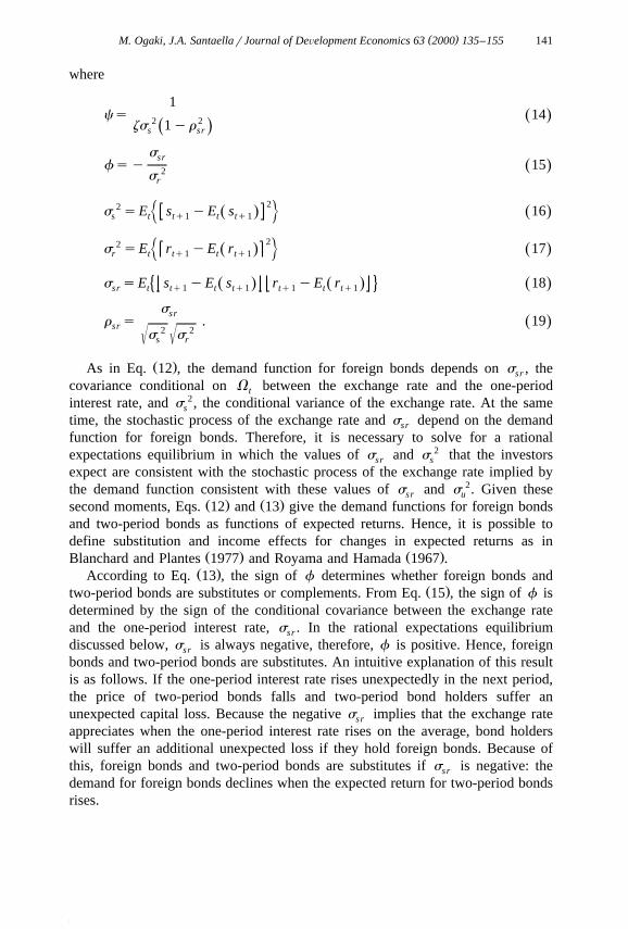
Ž .As in Eq. 12 , the demand function for foreign bonds depends on s , thesr

covariance conditional on V between the exchange rate and the one-periodt

interest rate, and s 2, the conditional variance of the exchange rate. At the sames

time, the stochastic process of the exchange rate and s depend on the demandsr

function for foreign bonds. Therefore, it is necessary to solve for a rationalexpectations equilibrium in which the values of s and s 2 that the investorssr s

expect are consistent with the stochastic process of the exchange rate implied bythe demand function consistent with these values of s and s 2. Given thesesr u

Ž . Ž .second moments, Eqs. 12 and 13 give the demand functions for foreign bondsand two-period bonds as functions of expected returns. Hence, it is possible todefine substitution and income effects for changes in expected returns as in

Ž . Ž .Blanchard and Plantes 1977 and Royama and Hamada 1967 .Ž .According to Eq. 13 , the sign of f determines whether foreign bonds and

Ž .two-period bonds are substitutes or complements. From Eq. 15 , the sign of f isdetermined by the sign of the conditional covariance between the exchange rateand the one-period interest rate, s . In the rational expectations equilibriumsr

discussed below, s is always negative, therefore, f is positive. Hence, foreignsr

bonds and two-period bonds are substitutes. An intuitive explanation of this resultis as follows. If the one-period interest rate rises unexpectedly in the next period,the price of two-period bonds falls and two-period bond holders suffer anunexpected capital loss. Because the negative s implies that the exchange ratesr

appreciates when the one-period interest rate rises on the average, bond holderswill suffer an additional unexpected loss if they hold foreign bonds. Because ofthis, foreign bonds and two-period bonds are substitutes if s is negative: thesr

demand for foreign bonds declines when the expected return for two-period bondsrises.


The stochastic processes of one-period interest rates are assumed to be asfollows:

r smqe qe q´ 20Ž .t t ty1 t

1R smqe q e 21Ž .t t ty12

r ) sm 22Ž .t

where e and ´ are, respectively, the interest rate shock with a duration of twot t

periods and the temporary interest rate shock with a duration of one period, and m

is constant. It is assumed that e and ´ are white noise with variance s 2 and s 2,t t e ´

respectively, and that they are independent of each other and of u .tThe conditional expectation is assumed to coincide with the best linear predic-

tion. It follows that

E r smqe , 23Ž . Ž .t tq1 t

Ž . Ž .and from Eqs. 4 and 21 ,

u sy´ . 24Ž .2, t t

Ž .As shown in Eq. 24 , the assumption employed here is that only the interest rateshock with the two-period duration is transmitted to the two-period interest rate, sothat the risk premium is equal to the temporary interest rate shock.

Define hss 2rs 2, which may be called the measure of substitution between´ e

one-period and two-period bonds. If hs0, then the risk premium for two-periodbonds will always be zero, implying that one-period and two-period bonds areperfect substitutes. The greater is h, the smaller the degree of the substitution.

Solving the equilibrium conditions for the foreign bond market as a differenceŽ .equation system of E s , with respect to t , provides the unique saddle pointt tqt

solution,2

1yls ssy u y l 1ql e qle q l fy1 ´Ž . Ž .t t t ty1 tb

1yly B , 25Ž .F , ty1b

where ssarb is the long-run equilibrium exchange rate, which clears the currentaccount, and

b b 4cls1q y 1q . 26Ž .(

2c 2c b

It is easy to check 0-l-1, ElrEc)0, lim ls0 and lim ls1.c™ 0 c™`

2 Ž .For derivation details, refer to Ogaki 1999 .


Ž . 2Eq. 25 shows that the investors’ expected values of s and s affect thesr s

exchange rate dynamics through l and f. On the other hand, the exchange rateŽ . 2dynamics in Eq. 25 imply certain values of s and s , which need to besr s

consistent with the investors’ expected values in the rational expectations equilib-rium.

Before discussing the solution for the equilibrium, it is worth noting the natureŽ .of Eq. 25 , which will be the basis of our empirical work below. The discrepancy

between the actual and the long-run equilibrium exchange rate is explained by theŽ .trade shock in the first term in brackets , the interest rate shock that is transmitted

Ž .to the two-period interest rate the second term in brackets , the interest rate shockŽ .that is not transmitted to the two-period interest rate the third term in brackets

Ž .and the cumulative current account balance in the fourth term in brackets . Thetrade shock, which tends to give rise to current account surplus, makes thedomestic currency appreciate. Prolonged increases in the one-period interest ratemake the domestic currency appreciate, though the contemporaneous shock e hast

a greater effect than the previous period’s shock e . As the cumulative currentty1

account balance becomes greater, the domestic currency’s appreciation increases:for investors to have incentives to hold more foreign bonds, the domestic currencymust appreciate at present so that investors can anticipate that it will depreciate inthe future.

All of these effects are consistent with the conventional wisdom and go in thestandard directions. The shock that is not transmitted to the two-period interestrate, ´ , however, has a perverse effect if the relative magnitude of the indirectt

complements relationship, f, is greater than 1. This is because the indirectcomplementarity of one-period and foreign bonds will exceed the direct substi-tutability if f)1.

The term f may be obtained by solving for the rational expectation ofcovariance. By equating the conditional covariance of the one-period interest rate

Ž .and the exchange rate implied by Eq. 25 and s used to define f, we obtain ssr sr

in the rational expectations equilibrium:

l 1qlqh 1qh s 2Ž . Ž . es sy -0. 27Ž .sr 1qhqhl

Ž .Therefore, by Eq. 15 ,

l 1qlqhŽ .fs )0. 28Ž .

1qhqhl

In the rational expectations equilibrium, the conditional covariance between theexchange rate and the one-period interest rate, s , is negative. Hence, foreignsr

bonds and two-period bonds are substitutes as explained in the previous section.The measure of the relative magnitude of the indirect complements relationship,f, is positive. The main issue for the purpose of this paper is whether f is greateror less than 1.


Ž .In order to examine the magnitude of f in Eq. 27 , we need to know how l

Ž .depends on the underlying parameters of the model. Ogaki 1999 analyzes thisdependence by solving for the rational expectation of the conditional variance ofthe exchange rate. He shows that there exists a unique rational expectationsequilibrium for the model, and that f is greater than 1 when the investor’s riskaversion parameter, a , and the measure of the degree of substitution betweenone-period and two-period bond, h, are close to zero. Because f can be smallerthan 1 for other parameter configurations, whether or not f is greater than 1 is anempirical question.

3. Data and preliminary considerations

We study the effect of the term structure of interest rates on the exchange ratefor Mexico, using the United States as the foreign country. The data series forMexico are monthly, and cover the period from January 1983 to June 1997. Thenominal 1-month and 3-month interest rates are monthly averages of the weekly

Ž .auctions of the 28-day and 91-day Cetes T-Bills , respectively, and were takenŽ .from Indicadores Economicos Banco de Mexico . The consumer price index is´ ´

used as the price level. The data for United States cover the same period. The1-month and 3-month Euro Market rates are used for the nominal interest rates.The weekly data obtained from the INTLINE data base are converted into monthlydata within AREMOS II. The consumer price index is also used as the price level.The nominal exchange rate data, expressed as the price of the US dollar in termsof the Mexican peso, were also from Indicadores Economicos. The real exchange´rate is calculated as the nominal exchange rate multiplied by the US price leveldivided by the Mexican price level. The data are not seasonally adjusted. Theinflation rate is the first difference of the log of the price level. The real interestrate is the log of one plus the nominal interest rate minus the expected inflationrate, which is estimated as explained below.

For Mexico, the 3-month nominal interest data are missing for August 1986,ŽSeptember 1986, and November 1988 no Cetes were sold in the weekly auctions

. Ž .for these months . A vector autoregression VAR of order five for the inflationrate, the 1-month nominal interest rate, and the 3-month nominal interest rate wasused to assign values to these periods. The VAR was estimated using the data upto July 1986, and the projected values for August 1986 and September 1986 wereassigned to these periods. Then the VAR was re-estimated using the data up toOctober 1988, and the projected value for November 1988 was assigned to thisperiod.

The model is specified in real interest rates, so an estimate of expected inflationŽ ) .was constructed. The 3-month real interest rate differential, r yr , is used to3, t 3, t

capture the effect of the interest rate shock with the longer duration in the model,e . In order to estimate the real interest rates, a VAR of order five for the inflationt


rate, the 1-month nominal interest rate and the 3-month nominal interest rate wasestimated for each country using the whole sample period. Then the three-period-ahead forecast of the inflation rate was calculated form the estimated VAR in eachperiod. The forecast was subtracted from the 3-month nominal interest to calculatethe real interest rate.

We use the normalized one-period interest rate, r to capture the effect of theN, t

temporary interest shock. The normalized one-period interest rate is defined asfollows:

21r s E r yr , 29Ž . Ž .ÝN , t t 1, tqk 3, t3 ks0

where r and r are the 1-month and 3-month nominal interest rates, respec-1, t 3, t

tively. The normalized 1-month interest rate is the negative risk premium for the3-month bonds, just as ´ is the negative risk premium for the two-period bonds int

the model. It captures the movements in 1-month interest rates as a deviation from3-month interest rates. The normalized interest rate is estimated using the one-period- and two-period-ahead forecasts from the estimated VAR for each country.

Ž .Table 1 reports results for Said and Dickey’s 1984 test for a unit root. LetŽ .SD p be Said and Dickey’s test with the order of autoregression equal to p. The

Ž . Ž . Ž .table reports SD 1 , SD 5 and SD 10 for each series. A constant is included forthe regression. The first row reports results for the log real exchange rate, s. Noneof the test statistics is significant at the 5% level. Hence, the null hypothesis thatthe log real exchange rate is unit root nonstationary cannot be rejected. For the

Ž ) . Ž . Ž .3-month real interest rate differential, r yr , SD 1 is significant, but SD 53, t 3, tŽ .and SD 10 are not significant at the 5% level. For the normalized 1-month

Ž ) . Ž . Ž . Ž .interest rate differential, r yr , SD 1 and SD 5 are significant, but SD 10N, t N, t

is not significant at the 5% level. Hence, the results for the interest ratedifferentials depend on the order of the autoregression. Standard economic theorysuggests that these interest rate differentials can hardly be unit root nonstationary.However, these ambiguous test results suggest that there exists a persistentcomponent in each interest rate differential, which might be locally approximatedby unit root nonstationarity.

Table 1Unit root test results

Ž . Ž .SD p is the Said and Dickey’s 1984 test with order of autoregression equal to p.

Ž . Ž . Ž .SD 1 SD 5 SD 10

s y1.877 y1.742 y2.425t)r y r y6.435 y2.786 y2.5593, t 3, t)r y r y6.165 y4.286 y2.530N , t N , t


4. The econometric method

The model in Section 2 abstracts from some features of data, such as nonsta-tionarity of the real exchange rate, so that it can be solved for the rationalexpectations equilibrium. In our empirical analysis, we follow the spirit of the

Ž .reduced form of the model, Eq. 25 , while incorporating important features ofdata. The cointegrating regression we use cannot be viewed as a structuralregression, but should be viewed as a method to find a stylized fact about therelationship between the exchange rate and the term structure of interest rates.While interesting, it is beyond the scope of this paper to derive structuraleconometric models for the exact model in Section 2 in the presence of cointegrat-ing relationships.

The regression we employ is of the form

s smqa r yr ) qb r yr ) qh , 30Ž .Ž . Ž .t 3, t 3,r N , t N , t t

Ž ) .where the 3-month interest rate differential, r yr , is used to capture the3, t 3, t

effect of the interest rate shock with the longer duration in the model, e .3 We uset

the normalized one-period interest rate, r to capture the effect of the temporaryN, t

interest shock.Because the null hypothesis that the real exchange rate is difference stationary

Ž .cannot be rejected, we view Eq. 30 as a cointegrating regression. We applyŽ . Ž . Ž . 4Park’s 1992 Canonical Cointegrating Regression CCR to Eq. 30 . This

procedure allows us to test the null hypothesis of cointegration and the determinis-tic cointegration restriction. According to our model solution, a is negative as inthe standard exchange rate models. However, the sign of b can be positive if theindirect complementarity between the 1-month domestic and foreign bonds domi-nates their direct substitutability.

To understand CCR, consider a cointegrated system

ysX Xgqh 31Ž .t t

D X sn , 32Ž .2 t t

Ž .where X s 1, X , y and X are difference stationary, and h and n aret 2 t t 2 t t t

3 Note that the model in Section 2 suggests an regression of a real exchange rate onto short-term andŽ . Ž .long-term real interest rate differentials. Frankel 1979 and Boughton 1988 regress exchange rates

onto both short-term and long-term interest differentials. Apart from the fact that they do not interprettheir regressions in terms of cointegration, our regressions are different from theirs because they usereal and nominal interest rate differentials. Frankel uses the real short-term interest rate differential andthe nominal long-term interest rate differential. Boughton uses the nominal short-term interest ratedifferential and the real long-term interest rate differential.

4 Ž .Byeon 1996 applies different asymptotically efficient estimation methods for similar cointegrat-ing regressions with G-7 country data, and finds that his results are similar.


Ž .stationary with zero mean. Here, y is a scalar and X is an ny1 =1 randomt t

vector. Let

w s h ,n X . 33Ž . Ž .t 11 t

Ž . Ž X . Ž . ` Ž . ` Ž .Define F i sE w ,w , SsF 0 , GsÝ F i and VsÝ F i . Here,t tyi is0 isy`

V is the long-run covariance matrix of w . Partition V ast

1V V11 12

Vs 34Ž .ž /V V21 22 ny1

and partition G conformably. Define

V sV yV Vy1V 35Ž .11 .2 11 12 22 21

Ž X X .Xand G s G ,G . The CCR procedure assumes that V is definitely positive,2 12 22 22Ž .implying that X is not itself cointegrated see, e.g., Engle and Granger; 1987 .t

Ž . ŽThis assumption assures that 1,yg is the unique cointegrating vector up to a.scale factor .

Ž .The OLS estimator in Eq. 31 is super-consistent in that the estimatorŽ .converges to g at the rate of T sample size even when D X and n are2 t t

correlated. The OLS estimator, however, is not asymptotically efficient.Consider transformations

y) sy qPX w 36Ž .t t y t

X ) sX qPX w ,2 t 2 t x t

) Ž )X.X ) )and X s 1, X . Because w is stationary, y and X are cointegrated witht 2 t t t t

Ž .the same cointegrating vector 1,yg as y and X for any P and P .t t y x

The idea of the CCR is to choose P and P , so that the OLS estimator isy x

asymptotically efficient when y) is regressed on X ). This requirest t

Xy1 y1P sS G gq 0,V V 37Ž .Ž .y 2 12 22

P sSy1G .x 2

In practice, long-run covariance parameters in these formulas are estimated, andthe estimated P and P are used to transform y and X ) . As long as thesey x t t

parameters are estimated consistently, the resultant CCR estimator is asymptoti-cally efficient.

The CCR estimators have asymptotic distributions that can be essentiallyconsidered as normal distributions, so that their standard errors can be interpreted


in the usual way.5 An important property of the CCR procedure is that linearrestrictions can be tested by x 2 tests that are free from nuisance parameters. We

2 Ž .use x tests in a regression with spurious deterministic trends added to Eq. 31 totest for cointegration. For this purpose, the CCR procedure is applied to aregression

q) i ) )y smq c t qg X qh .Ýt i 2 t t

is1

Ž .Let H 0,q denote the standard Wald statistic to test the hypothesis c sc s1 2) Ž. . . sc s0 with the estimate of the variance of h replaced by V see Park,q t 11.2

. Ž . 21990 for details . Then H 0,q converges in distribution to a x random variableq

under the null hypothesis of cointegration, while it diverges under the alternativehypothesis of no cointegration because the trend terms become spuriously signifi-cant.

During the 1983:1–1997:6 period used in our estimations, there have beenŽ .exchange regime changes in Mexico see Santaella and Vela, 1996 . These may

have caused shifts in the long-run relationship between the real exchange rate andthe real interest rate differentials, even though it is theoretically possible for therelationship to be stable over different regimes. For this reason, it is necessary to

Ž .test whether or not there have been structural breaks in the regression in Eq. 30 .Ž .We use Hansen’s 1992 tests for parameter instability for this purpose.

Ž .Hansen’s tests are developed for Phillips and Hansen’s 1990 fully modifiedestimation method, but can be adapted to the CCR method as follows because

6 Ž Ž ..these two methods are very similar. In the regression model Eq. 31 , we nowallow g to be different over two subsamples:

gsg if tFta

gsg if t)tb

where t is the timing of the structural break. We consider two tests developed byŽ .Hansen 1992 for the null hypothesis H : g sg . The null hypothesis is the0 a b

same for both tests, but they differ in the treatment of alternative hypotheses: forthe first test, the timing of the structural break is known, while for the second test,it is unknown.

5 The CCR estimators are asymptotically efficient, but there are other asymptotic efficient estimatorsŽ . Ž .by Phillips and Hansen 1990 . Monte Carlo experiments in Park and Ogaki 1991 show that the CCR

estimators have better small sample properties in terms of the mean square error than Johansen’s MLŽ .estimators. Following Monte Carlo based recommendations by Park and Ogaki 1991 and Han and

Ž .Ogaki 1997 , we used the prewhitening method and report third stage CCR estimates and fourth stageŽ .CCR H p,q test statistics.

6 We thank Joon Park for his helpful advice on adapting the tests.


The first test, denoted by F , is essentially the classical Chow test for a knownt

structural break date of t . Under the null hypothesis of no break, we transform theŽ .data as in Eq. 35 . Define

d s1 if tFtt

d s0 if t)tt

Then apply the OLS to

y) sd X )Xg q 1yd X )

Xg qh ) . 38Ž . Ž .t t t a t t b t

Then F is the standard Wald statistic to test the hypothesis g sg with thet a b

estimate of the variance of h ) replaced by V . Then F has an asymptotict 11.2 t

chi-square distribution with degrees of freedom equal to the number of parametersin g .

For the second test, the timing of the structural break is unknown. The teststatistic, denoted by SupF, is defined by SupFssup F where supremum is takenover the range of 0.15TFtF0.85T , where T is the sample size. Asymptotic

Ž .critical values of this test statistic are tabulated in Hansen 1992 .

5. Empirical results

Our empirical results are consistent with the proposition that the term structureof interest rates matters for the exchange rate in the case of Mexico. The first rowof Table 2 presents cointegrating regression results when the whole sample periodis used. The sign of the point estimate of a is negative and statisticallysignificantly different from zero. A negative a is in the standard direction ofincreases in interest rates leading to exchange rate appreciation as expected fromthe conventional wisdom, and is also consistent with our model in Section 2.However, contrary to the traditional intuition, the point estimate of b is positive

Table 2Canonical cointegrating regression results

ˆ Ž . Ž .Sample period a b H 0,1 H 0,2 SupFˆŽ . Ž . Ž . Ž . Ž . Ž .1 2 3 4 5 6

Ž . Ž . Ž . Ž . Ž .1993:7–97:5 y2.922 0.278 5.427 1.107 0.134 0.714 0.768 0.681 15.881 0.049Ž . Ž . Ž . Ž . Ž .l988:1–97:5 y3.061 0.4420 6.976 1.2860 1.225 0.2680 1.248 0.536 2.112 )0.200

In columns 2 and 3, standard errors are in parentheses. Columns 4 and 5 report x 2 test statistics forstochastic cointegration with one and two degrees of freedom, respectively. P values are in parenthe-ses. Column 6 reports SupF test statistic for a structural break with an unknown timing.


and significantly different from zero. A natural explanation arising from ourtheoretical analysis is that the indirect complementarity dominates the directsubstitutability. The implication of this result is that increases in the 3-monthinterest rate differential will, ceteris paribus, be associated with a depreciatingMexican peso in the long run.

As suggested above, the possibility of structural breaks is an issue in the case ofMexico. Table 2 shows that the SupF test is significant at the 5% level, indicatingthat a structural break is present. The F test statistics were computed for possiblestructural break dates from November 1985 to December 1995. The F statisticst

are below their 5% critical value from November 1985 to July 1986, above their5% critical value from December 1985 to March 1988, and below their 5% criticalvalue from April 1988 to December 1995. The F attains the maximum value oft

15.881 in November 1987, which is above its 1% critical value.The timing of the structure break has a natural explanation. A comprehensive

stabilization plan was implemented in December 1987 in Mexico. Hence, theseparameter instability test results indicate that the stabilization plan changed thecointegrating relationship between the real exchange rate and the term structure ofthe real interest rate differentials.

Because the tests for parameter instability used in this paper assume only onestructural break, cointegrating regressions were applied to the sample period fromJanuary 1988 to May 1997 in order to confirm that there is no additional structuralbreak. The second row of Table 1 presents these cointegrating regression results.7

It is noteworthy that the estimate of a continues to be significantly negative,while the estimated b remains significantly positive, thus maintaining the samequalitative relation of the term structure of interest rates to the exchange ratedespite the structural break.

After the stabilization plan was implemented, several exchange regimes havebeen adopted in Mexico ranging from a fixed exchange rate regime to a floatingregime. The test results for parameter instability, however, indicate that thecointegrating relationship between the real exchange rate and the term structure ofthe real interest rate differentials may have been stable over this period. The SupFtest statistic is not significant at the conventional significance levels. No individualF statistic computed from December 1988 to June 1996 is above its 38% criticalvalue.

With an additional assumption that the normalized real 1-month interest ratedifferential is predetermined with respect to both the real 3-month interest ratedifferential and the real exchange rate, and that the 3-month interest rate differen-tial is predetermined with respect the real exchange rate, one can compute the

7 The long-run covariance parameters for these results used for the third-stage and fourth-stage CCRare taken from the third-stage and fourth-stage CCR reported in the first row of Table 1.


orthogonalized impulse response functions. These assumptions are stringent, but itis often of interest to examine an example of dynamic responses. Under theseassumptions, the orthogonalized impulse response functions are defined with

Žrespect to the disturbances in the structural error correction model see, e.g., Kim.and Ogaki, 1999 .

Imposing the estimates of the cointegrating vector for the sample period of1988:1–1997:5, we estimate the error correction model with OLS for eachequation. This method to estimate the error correction model is the same as Engle

Ž .and Granger 1987 except that the first step estimator for the cointegrating vectorhere is from the asymptotically efficient CCR estimator rather than the inefficientOLS estimator. From the estimated error correction model, the VAR respresenta-tions for the levels of the three variables in the system are computed. Theorthogonalized impulse responses are calculated with the standard method from

Ž .this VAR representation see, e.g., Hamilton, 1994 for the method .The orthogonalized impulse response functions of the real exchange rate to the

real interest rate differential shocks are plotted in Fig. 1. Because the variables canbe locally approximated by unit root nonstationary and are cointegrated, interestrate shocks have permanent effects on the exchange rate, as implied by the

Fig. 1. Mexico: Impulse response of the exchange rate to unit changes in interest rate differentials.


cointegrating vector. The initial impact of a 1% positive shock to the 1-monthinterest rate is a 0.102 increase in the exchange rate, while a 1% positive shock tothe 3-month interest rate is a 0.075% fall in the exchange rate. Thus, the estimatedinitial impact works in the same direction as implied by the cointegrating vectorfor the long-run for each real interest rate differential.

After the impact effects, the dynamics become very complicated. At 1 monthafter the interest rate shock, the response is in the opposite direction from theinitial impact for each interest rate differential. From the second month on, theresponse of the exchange rate to the 3-month interest rate shock reverts to beingnegative, and remains negative as implied by the cointegrating vector. However,the response of the exchange rate to orthogonalized shocks to the 1-month interestrate differential does not revert immediately to the long-run cointegrating relation-ship. From the first month on, the response to the 1-month interest rate shock isnegative for a long time, and it takes 152 months for the response to becomepositive. Thus, a counterintuitive result from these impulse responses, which isnonetheless possible in our model, is that the Mexican peso depreciates in themedium-run when the 1-month interest rate rises in Mexico.

6. Conclusions

Conventional wisdom is that increases in any interest rate would appreciate thedomestic currency, and thus that the term structure of interest rates is irrelevant forthe determination of the exchange rate. This paper has argued that this conven-tional wisdom can be challenged both on theoretical and empirical grounds.

We study the relationship between the term structure of interest rates and theexchange rate for Mexico. Our empirical results suggest that interest rates mayhave counterintuitive effects on the exchange rate, which may arise from thecomplementarity between 1-month domestic bonds and foreign bonds. The cointe-grating regression estimated in this paper indicates that 1-month and 3-monthinterest rate differentials have opposing effects on the exchange rate for Mexico.While increases in the 1-month interest rate differential will, other things equal,affect the exchange rate in the standard appreciation direction, increases in the3-month rate differential tend to depreciate the exchange rate. Therefore, the effectof the 1-month interest rate differential on the exchange rate depends on how the3-month interest rate moves in response to changes in the 1-month interest rate.Imagine for the moment that Bank of Mexico affects liquidity conditions in orderto raise the 1-month interest rate, intending to cause an appreciation of the peso. Ifthe 3-month interest rate rises in response to the rise in the 1-month rate, then thepeso will tend to appreciate as in the standard exchange rate model that assumesrisk neutral investors. However, if the 3-month interest rate does not rise, then thepeso will tend to depreciate.


Because the exchange regime of Mexico has been changing, we performedstructural break tests for parameter instability for the cointegrating regression ofthe real exchange rate onto the 1-month and 3-month real interest rate differentials.Even though the test results indicate breaks in the cointegrating relationshiparound December 1987 when a comprehensive stabilization plan was implementedin Mexico, they indicate that the cointegrating relationship has been stable sincethen despite several exchange regime changes.

The empirical results obtained in this paper could be useful to understand andmanage the operation of the Mexican floating exchange rate regime. They showthat attention must be given to the term structure of interest rates when consideringexchange rate objectives. The fact that the traditional intuition may not work,should also provide a warning to other developing countries that have nowadopted floating exchange rate regimes.

Acknowledgements

We thank Marco Bonomo, Nelson Mark, Miguel Savastano, Nilson Teixeira,and participants of meetings of the Latin American and Caribbean EconomicAssociation and the Inter-American Seminar on Economics for their helpfulcomments. Portions of this paper were written while Santaella was at the ResearchDepartment of the International Monetary Fund and Ogaki was a visiting scholar.They thank the Commodities and Special Issues Division staff for a stimulatingresearch environment. The authors are responsible for the views expressed in thispaper and for all remaining errors.

References

Alvarez, F., Atkeson, A., Kehoe, P., 1999. Volatile Exchange Rates and the Forward PremiumAnomaly: A Segmented Asset Market View, manuscript, Federal Reserve Bank of Minneapolis.

Backus, D., Foresi, S., Telmer, C., 1998. Affine Models of Currency Pricing: Accounting for theForward Premium Anomaly, manuscript, Stern School of Business, New York University.

Baxter, M., 1994. Real exchange rates and real interest differentials: have we missed the business–cyclerelationship? Journal of Monetary Economics 33, 5–37.

Blanchard, O.J., Plantes, M.K., 1977. A note on gross substitutability of financial assets. Econometrica45, 769–771.

Boughton, J., 1988. Exchange rates and the term structure of interest rates. International MonetaryFund Staff Papers 35, 36–62.

Byeon, Y.H., 1996. Empirical Analyses of a Link Between Real Exchange Rates and the TermStructure of Real Interest Rates, PhD dissertation, Ohio State University.

Byeon, Y.H., Ogaki, M., 1999. An Empirical Investigation of Exchange Rates and the Term Structureof Interest Rates, manuscript.


Dornbusch, R., 1976. Expectations and exchange rate dynamics. Journal of Political Economy 84,1161–1176.

Driskill, A.R., McCafferty, S., 1980. Speculation, rational expectations and stability of the foreignexchange market. Journal of International Economics 10, 92–102.

Edison, H.J., Pauls, B.D., 1993. A re-assessment of the relationship between real exchange rates andreal interest rates: 1974–1990. Journal of Monetary Economics 31, 165–187.

Eichenbaum, M., Evans, C., 1997. Some empirical evidence on the effects of shocks to monetaryŽ .policy on exchange rates. Quarterly Journal of Economics 112, 975–1009, February .

Engel, C., 1996. The forward discount anomaly and the risk premium: a survey of recent evidence.Journal of Empirical Finance 3, 123–192.

Engle, R., Granger, C., 1987. Co-integration and error correction: representation, estimation andŽ .testing. Econometrica 55, 251–276, March .

Frankel, J.A., 1979. On the mark: a theory of floating exchange rates based on real interest ratedifferentials. American Economic Review 69, 610–623.

Hamilton, J., 1994. Time Series Analysis. Princeton Univ. Press, Princeton, New Jersey.Han, H., Ogaki, M., 1997. Consumption, income and cointegrating: further analysis. International

Review of Economics and Finance 6, 107–117.Ž .Hansen, B., 1992. Tests for parameter instability in regressions with I 1 Process. Journal of Business

Ž .and Economic Statistics 10, 321–335, July .Isard, P., 1995. Exchange Rate Economics. Cambridge Univ. Press, Cambridge.Kim, J., Ogaki, M., 1999. Structural Error Correction Models: An Application to an Exchange Rate

Model, manuscript.Mark, N., 1995. Exchange rates and fundamentals: evidence on long horizon predictability. American

Ž .Economic Review 85, 201–218, March .Mark, N., Wu, Y., 1998. Rethinking deviations from uncovered interest parity: the role of covariance

risk and noise. Economic Journal 108, 1686–1706.McCallum, B.T., 1994. A reconsideration of the uncovered interest parity relationship. Journal of

Monetary Economics 33, 105–132.Meese, R., Rogoff, K., 1988. Was it real? The exchange rate–interest rate differential relation over the

modern floating-rate period. Journal of Finance 43, 933–948.Meredith, G., Chinn, M.D., 1998. Long-Horizon Uncovered Interest Parity National Bureau of

Economic Research Working Paper 6797.Ogaki, M., 1990. The indirect and direct substitution effects. American Economic Review 80,

1271–1275.Ogaki, M., 1999. A Theory of Exchange Rates and the Term Structure of Interest Rates, manuscript.Park, J.Y., 1990. Testing for unit roots and cointegration by variable addition, in cointegration,

Ž .spurious regressions, and unit roots. In: Fomby, T.B., Rhodes, G.F. Jr. Eds. , Advances inEconometrics vol. 8 JAI, Greenwich, CT.

Park, J.Y., 1992. Canonical cointegrating regressions. Econometrica 60, 119–143.Park, J.Y., Ogaki, M., 1991. Inference in Cointegrated Models Using VAR Prewhitening to Estimate

Short-run Dynamics. Paper no. 281, Rochester Center for Economic Research Working, Universityof Rochester, Rochester, NY.

Ž .Phillips, P.C.B., Hansen, B.E., 1990. Statistical inference in instrumental variable regression with I 1Processes. Review of Economic Studies 57, 99–125.

Royama, S., Hamada, K., 1967. Substitution and complementarity in the choice of risky assets. In:Ž .Hester, D.D., Tobin, J. Eds. , Risk Aversion and Portfolio Choice. John Wiley, New York, NY,

pp. 27–40.Said, E., Dickey, D.A., 1984. Testing for unit roots in autoregressive-moving average models of

Ž .unknown order. Biometrica 71, 599–607, December .Santaella, J.A., Vela, A.E., 1996. The 1987 Mexican Disinflation Program: An Exchange Rate-Based

Stabilization? IMF Working Paper WPr96r24.


Tapia, J., 1990. Diferenciales de tasas de interes y paridad de poder de compra en regımenes´ ´cambiarios flexibles: la experiencia Mexicana 1978.01–1987.02. El Trimestre Economico 57,´

Ž .737–753, July–September .Werner, A., 1996. Mexico’s Currency Risk Premia in 1992–94: A Closer Look at the Interest Rate

Ž .Differentials. IMF Working Paper WPr96r41 April .

The exchange rate and the term structure of interest rates in Mexico

Documents

Transcript of The exchange rate and the term structure of interest rates in Mexico