Low-Frequency Volatility of Yen Interest Rate Swap Market in Relation to Macroeconomic Risk*

Low-Frequency Volatility of YenInterest Rate Swap Market in

Relation to Macroeconomic Riskn

A.S.M. SOHEL AZADw,¼, VICTOR FANG

wAND J. WICKRAMANAYAKE

w

wDepartment of Accounting and Finance, Monash University, Caulfield East, Vic,

Australia and ¼Department of Finance and Banking, University of Chittagong,

Chittagong, Bangladesh

ABSTRACT

Using ‘low-frequency’ volatility extracted from aggregate volatility shocks ininterest rate swap (hereafter, IRS) market, this paper investigates whetherJapanese yen IRS volatility can be explained by macroeconomic risks. Theanalysis suggests that this low-frequency yen IRS volatility has strong andpositive association with most of the macroeconomic risk proxies (e.g.,volatility of consumer price index, industrial production volatility, foreignexchange volatility, slope of the term structure and money supply) with theexception of the unemployment rate, which is negatively related to IRSvolatility. This finding is fairly consistent with the argument that the greaterthe macroeconomic risk the greater is the use of derivative instruments tohedge or speculate. The relationship between the macroeconomic risks and IRSvolatility varies slightly across the different swap maturities but is robust toalternative volatility specifications. This linkage between swap market andmacroeconomy has practical implications since market makers and hedgersuse the swap rate as benchmark for pricing long-term interest rates, corporatebonds and various other securities.

I. INTRODUCTION

Financial markets are said to respond to external forces (even though they mayalso have feedback effects) representing the market or systematic risk. Macro-economic risk1 is considered central to this market risk/volatility. This gives themacroeconomic risk an honoured place in asset pricing literature. Beginning withOfficer (1973), much has been written on the sources of macroeconomic risks that

n We thank an anonymous referee of International Review of Finance for insightful comments andsuggestions, which increased the value of this paper. A special thank to Jose Gonzalo Rangel forsharing his computer program of Spline-GARCH model. The first author is thankful to MRGS(Monash Research Graduate School, Monash University) for financial support toward his doctoralstudy at Monash. All remaining errors are our responsibility.1 The terms macroeconomic risk, uncertainty and volatility will be used interchangeably in this

study.

r 2011 The Authors. International Review of Finance r International Review of Finance Ltd. 2011. Publishedby Blackwell Publishing Ltd., 9600 Garsington Road, Oxford OX4 2DQ, UK and 350 Main Street, Malden, MA02148, USA.

International Review of Finance, 11:3, 2011: pp. 353–390DOI: 10.1111/j.1468-2443.2011.01129.x

drive the asset prices and market volatility to change over time. However, therelationship between the financial market volatility and macroconomic risks hasbeen found weak both in terms of the significance of the relevant macroeconomicrisk proxy as well as the overall explanatory power of the model. The large-scalefailure to provide strong empirical support of the links between macroconomic riskand the volatility of financial market can be partly attributed to misspecificationof the financial market volatility. For example, financial market volatility haslargely been proxied by aggregate volatility shocks only (e.g., Schwert 1989;Hamilton and Lin 1996; Diebold and Yilmaz 2008) with the exception of fewrecent asset pricing literature including those of Engle and Lee (1999), Adrian andRosenberg (2008) and Engle and Rangel (2008). These studies suggest todecompose financial market volatility into two components: (1) high-frequencyor short-term volatility and (2) low-frequency or long-term volatility. They showthat the use of later component indicates stronger relationship betweenmacroeconomic risk and the volatility of financial market. Exploring this empiricalrelationship is doubly essential as far as financial and economic crises areconcerned. It is argued that ‘underestimation of macroeconomic risk’ is one of themajor sources of current global financial and economic crises (Cowen 2009).Considering this, placing due emphasis on the macroeconomic risk is important forthe swap2 being an interest rate sensitive product.

By macroeconomic risk, we mean the uncertainty or volatility associated withmacroeconomic variables (such as, volatility of industrial production, volatility of CPIand volatility of interest rate etc.). It measures the size and magnitude of thesurprises in macroeconomic aggregates over the year. Beber and Brandt (2009)define the term macroeconomic risk as the market participants being unsure aboutthe current state of the economy. They opine that market participants usederivatives to hedge or speculate on macroeconomic risk/uncertainty. Thisargument is based on famous Black (1987)’s hypothesis, which suggests thatmacroeconomic risk/volatility and investment activities are positively correlated.The hypothesis has relevance to swap market as well. That is, there is a high (less)incentive for the hedgers to use swap, if the macroeconomic risk is high (low).

In order to examine how the above argument and/or Black’s hypothesisworks in swap market, we investigate the statistical and economic relationshipbetween macroeconomic risk and the volatility of swap market. There are severalimportant reasons why interest rate swap (IRS) is to be studied. First, as aninterest rate sensitive product, the IRS is expected to have a closer link withmacroeconomic variables than other financial products like stocks. Second, theswap market is highly liquid than the bond markets. Third, since becomingpopular, swap rate has been used by both hedgers and speculators as abenchmark for long-term interest rates, pricing of corporate bonds and variousother securities. For example, Cortes (2006) notes that one can derive the future

2 We will use the terms ‘interest rate swap’ and ‘swaps’ interchangeably in this study. Of the

different kinds of swaps, this study considers only plain vanilla swap, i.e., fixed-for-floating

interest rate swaps.

International Review of Finance

r 2011 The AuthorsInternational Review of Finance r International Review of Finance Ltd. 2011354

path of interest rates from the swap curve. Related to this, Huang et al. (2008)argues that swap curve consists of richer information than the Treasury yieldcurve. Fourth, swap instruments are found to be an effective tool than financialfutures and options in hedging against the interest rate risk for horizons beyond2 or 3 years (Bicksler and Chen 1986). In addition to managing interest rate risk,corporations use the swap to create a synthetic long-term instrument for raisingfunds (McNulty 1990). The use of swap has several other benefits namely,financial arbitrage, tax and regulatory arbitrage, exposure management andcompleting markets (Smith et al. 1986).3 Finally, the significance of IRS can also beseen from its exponential growth in the last decade. It is now the fastest growingand largest derivative market in the world in terms of notional principal. Therecent BIS (2009) survey indicates that the outstanding ‘notional principal’ hasgrown from virtually nothing in early 1990s to US$350 trillion in 2009 (see Figure1). In terms of notional principal, it surpassed derivative markets as well as UStreasury debt. The Derivatives Usage Survey 2009 by ISDA (International Swapsand Derivatives Association, Inc. 2009) indicates that 94% of world’s largestcorporations use swaps and other derivative products to manage their businessand macroeconomic risks. Thus, one of the implied purposes of this study is toexamine the rationale behind the use of swap in managing macroeconomic risk.These attributes of IRS encouraged us to fill the research gap on the relationshipbetween swap market volatility and macroeconomic risk.

This paper makes several contributions. For the first time, we estimate anddecompose aggregate volatility shocks in IRS markets, into high- and low-frequency components to capture both transitory and permanent shocks. One

0

50

100

150

200

250

300

350

400

Jun.

98D

ec.9

8Ju

n.99

Dec

.99

Jun.

00D

ec.0

0Ju

n.01

Dec

.01

Jun.

02D

ec.0

2Ju

n.03

Dec

.03

Jun.

04D

ec.0

4Ju

n.05

Dec

.05

Jun.

06D

ec.0

6Ju

n.07

Dec

.07

Jun.

08D

ec.0

8Ju

n.09

Dec

.09

Trillion Dollar

Figure 1 Notional Amounts Outstanding of Interest Rate Swap

Source: BIS (2009)

3 See Turnbull (1987) for an explanation of those benefits.

Low-Frequency Volatility of Yen Interest Rate Swap Market

r 2011 The AuthorsInternational Review of Finance r International Review of Finance Ltd. 2011 355

important feature of this volatility decomposition is that in contrast to high-frequency component, low-frequency volatility generates a parsimonious volatilityterm structure for different swap maturities. We model this volatility term structureas a function of macroeconomic risks/uncertainties to discover the macroeconomicsources of variation in this volatility term structure. Although finance literatureregularly emphasizes volatility as crucial to pricing financial products, previousliterature has not considered this issue in swap markets. We fill this gap byexploring an empirical link between macroeconomic risk/volatility and the swapmarket volatility. Understanding this linkage has important implications for (i)predicting the volatility term structure of IRS markets in relation to macroeconomicrisks (ii) estimating and resolving future uncertainty in both macroeconomicfundamentals as well as swap markets (iii) specifying whether macroeconomic riskhas greater impact on longer or on shorter maturities of swap and finally (iv)looking at the volatility term structure of the IRS markets, the hedgers can forecastthe macroeconomic fluctuations and fix the swap rates of those maturities whichhave stronger relationship with the macroeconomic risk proxies. Finally, we includethe reverse regression results to illustrate that, as a forward looking instrument, theIRS has predictive power in forecasting the macroeconomic risk.

Our analysis on Japanese swap market covering 3, 5, 7 and 10 years swapmaturities for the period from October 1989 through August 2009 indicatesthat the low-frequency IRS volatilities are significantly associated with most ofthe candidate macroeconomic risk proxies. Some of them (volatility of CPI,volatility of industrial production, volatility of foreign exchange rate, volatilityof interest rate, slope of the term structure and money supply) are found to havepositive influence on the low-frequency IRS volatility for different swapmaturities, while only the unemployment rate is found to have negativeinfluence on the low-frequency IRS volatility. Interestingly, however, consistentwith the argument that volatility measures obtained from derivatives marketsprovide useful information on investors’ perceptions of future economicuncertainty, it seems swap market volatility contains fair amount of informa-tion in predicting macroeconomic risk/uncertainty. Similar findings are alsoreported in other financial markets namely, stocks and bond markets (Schwert1989; Engle et al. 2008).

We subject our empirical findings to a couple of robustness tests. Twoalternative measures of volatility are taken to do this. First, we take the benchmarklong-term volatility obtained from the additive volatility decomposition of Engleand Lee (1999). Second, we take the realized volatility (RV) as it is argued thatunder suitable conditions, realized volatilities are considered as the observedrealizations of volatility (Andersen et al. 2003a). Both these alternative volatilitymeasures, obtained for different swap maturities, are then regressed on themacroeconomic risk proxies mentioned above. The empirical analysis suggests that,compared with these two alternative measures, the low-frequency volatilityprovides a better link between the swap market and macroeconomy. Moreover,the use of low-frequency volatility results in higher adjusted R2 statistics comparedwith the alternative measures.



The remainder of this paper is structured as follows. Section II provides somediscussion on the market volatility and macroeconomic risk. Data, variables andhypotheses are explained in Section III. Section IV describes the methodology,while Section V analyses our empirical findings. Section VI is devoted torobustness check and Section VII concludes.

II. FINANCIAL MARKET VOLATILITY AND MACROECONOMIC RISK

Financial economists to a greater extent agree that financial market volatility ispredictable over time with authenticated information. Finance literatureattributes this volatility predictability to ‘efficient market hypothesis’ (Boller-slev et al. 1992; Jones et al. 1998). Interestingly, however, the sources of thispersistency in volatility remain elusive. This may be due to difficulty inproviding convincing theoretical explanations for the underlying sources of thepersistence in volatility (Andersen and Bollerslev 1997). Roll (1988) argues thatif all the relevant macroeconomic, industry and firm specific information thatdrives the price movement are available and accounted for, then R2 should beclose to 1.0. However, by including all this information Roll (1988) finds thato40% of the (stock) market volatility in US can be explained by macro-economic and other variables. Thus, it remains a mystery as to which variablesor models can account for the unexplained volatility. Researchers haveattributed low R2 to various issues. First, there remain other variables thatmight explain the remaining volatility (Roll 1988). Second, macroeconomic riskplays different roles in different financial markets. Some financial markets, forexample, stock markets, are less affected by macroeconomy than bond markets(McQueen and Roley 1993). Third, and more noteworthy is the inability toprice the macroeconomic risk accurately, which is considered a fundamentalobstacle to testing asset pricing theories (Jones et al. 1998). This third viewimplies that it is important to accurately measure financial market volatility toimprove the performance of the model. In order to accurately measure thevolatility of financial market, Engle and Lee (1999), Adrian and Rosenberg(2008) and Engle and Rangel (2008) suggest to decompose financial marketvolatility into (1) short-term or high-frequency volatility and (2) long-term orlow-frequency volatility.

Adrian and Rosenberg (2008) and Engle and Rangel (2008) relate the long-term component to business cycle risk or macroeconomic risk. In the swapmarket, this can be related to business cycle risk premium. Adrian andRosenberg (2008) relate the short-term component to market skewness risk orfinancial constraint risk. The skewness risk or financial constraint risk isimportant as far as swap pricing is concerned. For example, the credit risk (inthe swap spread) for a company can differ between domestic and overseasmarkets. Nishioka and Baba (2004) show that the CDS (credit default swap)spreads are generally wider than the corporate spreads for the same Japanesecompanies. This difference (in spread) is an indication of market skewness risk,



which if significant, needs to be incorporated in the theoretical models. That is,if the market skewness risk is significant, then the market swap rate should becorrespondingly higher.4

Engle and Rangel (2008) find that R2 is significantly increased (to 55%) whenstock market volatility is proxied by low-frequency component. Christoffersenet al. (2008) among others find that two component volatility modelsoutperform one component or aggregate volatility models. The most distinctivefeature of this two-component volatility model is its ability to model thevolatility term structure (Christoffersen et al. 2008).

In order to understand two-component volatility models, we start with thefamiliar GARCH (1, 1) model, which can be used to extract the aggregate marketvolatility:5

rt � Et�1ðrtÞ ¼ffiffiffiffiffiht

pet ð1Þ

where rt is the price/return of an asset at time t and Et�1(rt) is the expected price/return at t�1. ht is the conditional volatility at time t. Following the abovediscussion, the volatility ht, can be decomposed, in an additive or multiplicativeform, into two components as follows:

ht ¼ gt þ tt ð2Þ

(see, Engle and Lee 1999; Adrian and Rosenberg 2008)

ht ¼ gttt ð3Þ

(see, Engle and Rangel 2008) where gt is the high-frequency volatility related toshort-term or market skewness risk and tt is the low-frequency volatility relatedto long-term or macroeconomic risk. Our focus is on tt, which can be estimated inan additive (equation (2)) or multiplicative form (equation (3)). Even thoughthere is no theoretical explanation on which decomposition is better, empiricalevidence shows that risk tends to affect asset prices multiplicatively rather thanadditively (Codogno et al. 2003). Hence, we put more emphasis on multi-plicative decomposition in our main study. Nonetheless, the additive decom-position is also used for robustness check. For ease of understanding, wedistinguish the tt term as ‘low-frequency’ volatility for multiplicative decom-position and ‘long-term’ volatility for additive decomposition. Such decom-position of market volatility is motivated by the Merton (1973)’s intertemporalcapital asset pricing model (ICAPM) in which state variables of the returngenerating process become state variables of the pricing kernel. With the two-component volatility process, the equilibrium pricing kernel depends on high-frequency volatility, low-frequency volatility as well as the expected return. Weincorporate the above features in modelling the swap market volatility. Table 1shows the findings of prior literature on the relationship between the low-frequency volatility and macroeconomic risk proxies.

4 Unfortunately, the prior literature is very scanty and, due to the space limitation, this paper also

excludes the analysis of the influence of skewness risk on swap pricing.

5 Yen swap rate is found to follow a random walk (Eom et al. 2000).



III. DATA, VARIABLE CONSTRUCTION AND HYPOTHESISDEVELOPMENT

A. Data

Low-frequency volatilities of IRS are estimated from daily closing mid-rates onswap maturities of 3, 5, 7 and 10 years for Japan, the second largest swap marketas an individual country. The analysis is confined to these maturities as theseare more liquid than other maturities. Swap data are collected from DataStream.Monthly data for explanatory variables are collected from different sources.Table 2 provides details of the data sources. The study covers the period fromOctober 1989 to August 2009, giving a total of 5,265 daily observations for eachswap maturity and 239 monthly observations for each macroeconomic variable.The study also considers two-major financial crises (Asian financial crisis andglobal financial crisis) during the sample period.

B. Variable construction and hypothesis development

This section describes both the dependent (swap volatilities) and explanatoryvariables (macroeconomic risk proxies and related policy variables). Since volatilitiesare not directly observed, we need to define a measure of low-frequencyvolatilities to construct our dependent variable. For each swap maturity describedabove, we first estimate the daily low-frequency volatility using the Spline-GARCH model of Engle and Rangel (2008). We then take the average of the dailylow-frequency volatilities for the respective month considering 21 trading days ina month. As noted, for robustness check we also estimate two alternative measuresof low-frequency volatilities: the benchmark long-term volatility from Engle and

Table 1 Relationship between Macroeconomic Risk and Low-Frequency Market Risk

Studies Effect of macroeconomic variables onlow-frequency volatility

GDP IP IRs SY CPI PPI UE Ex

Becker and Clements (2007) 1 �Adrian and Rosenberg (2008) �Diebold and Yilmaz (2008) 1 1

Engle and Rangel (2008) 1 1 1 �Engle et al. (2008) 1/� 1

Nowak et al. (2009) 1/� 1/� 1/�

This table gives a summary of prior literature on the impact of macroeconomic risk on low-frequency volatility.IP, Industrial production; IRs, short-term interest rates; SY, slope of the yield curve; CPI,Consumer Price index; PPI, Producer Price Index; UE, Unemployment rate; Ex, Exchange rates.Most studies in this table use the second moments of the macroeconomic variables with theexception of unemployment rate.



Lee (1999)’s additive volatility decomposition and the RV. Hence, in total we havethree measures of volatilities for different swap maturities.

The choice of our explanatory variables is guided by economic theory and theirimportance and relevance supported by prior literature (on swap markets as wellas on low-frequency volatility). Moreover, to have robust results, we considerthose macroeconomic variables that are available in monthly observations. Forexample, since the gross domestic product (GDP) data are only available at aquarterly frequency and our analysis is monthly, we use industrial productiongrowth as our proxy for the growth rate of GDP. To recall, there is no study thatconsiders macroeconomic risks for analysing the behaviour of swap markets.Therefore, following the existing literature on volatility decomposition and onthose that consider the impact of macroeconomic risks on financial markets, we

Table 2 Explanatory Variables, Proxies and Predicted Signs

Explanatoryvariables

Proxies/transformations Predicted Sign onLow-frequencyIRS Volatility

Source

Volatility ofindustrialproduction

Absolute values of theresiduals from an AR(1) model,obtained from industrialproduction index

1/� Cabinet Office(CAO), Ministryof Finance,Japan

Volatility of CPI Absolute values of the residualsfrom an AR(1) model, obtainedfrom seasonally adjustedconsumer price index

1 CAO, Ministryof Finance,Japan

Volatility ofinterest rate

Absolute values of the residualsfrom an AR(1) model, obtainedfrom Nikkei short-term bondindex yield

1 DataStream

Foreignexchangevolatility

Absolute values of the residualsfrom an AR(1) model, obtainedfrom real effective exchangerate of Japanese yen againstUS dollar

1 CAO, Ministryof Finance,Japan

Slope of theyield curve

Difference between Nikkeilong-term bond index yieldand Nikkei short-term bondindex yield

1/� DataStream

Unemploymentrate

Seasonally adjustedunemployment rate

1/� CAO, Ministryof Finance,Japan

Money supply(M2)

Percent changes from theprevious year in averageamounts outstanding/MoneyStock

1 Bank of Japan

To proxy the volatility of innovations to macroeconomic fundamentals, Schwert (1989) andAdrian and Rosenberg (2008) take the residuals from an AR(3), while Engle and Rangel (2008) takethe residuals from an AR(1). Bansal and Yaron (2004) and Wachter (2006) take the conditionalvolatility from GARCH (1,1). We take residuals from AR(1) model.



take the levels as well as volatilities of macroeconomic variables. Althoughmacroeconomic variables are endogenous in some ultimate sense (Chen et al.1986), careful selection of relevant proxies is regarded as an appropriate approachto reduce estimation bias.

Unfortunately, both the economic theories and prior literature have been silenton the directional (positive or negative) hypothesis between macroeconomic riskproxies and the volatility of financial markets. Hence, the existing literatureattempts largely to provide an empirical relationship between the financial marketsand the macroeconomy (either first or second moments or both). Few studies (e.g.,Catao and Kapur 2004) provide some analysis of theoretical link betweenmacroeconomic risk/volatility and probability of default. They show that volatilityincreases default risk and raises interest rates and, hence a positive associationbetween the volatility of financial markets and macroeconomic risk can be expected.Lettau et al. (2008) explore theoretical and empirical links between secondmoments of macroeconomic factors (e.g., consumption, GDP etc) and stockreturns. They attribute the declining equity premium to a fall in macroeconomic risk,or the volatility of the aggregate economy. Beber and Brandt (2009) argue thatmacroeconomic risk leads to a greater degree of hedging or speculative activities infinancial markets. That is, the greater the macroeconomic risk, the greater is the useof derivatives to gain from hedging or speculating. Genberg and Sulstarova (2008)hypothesize a positive association between macroeconomic risk and bond spreads.All the above studies are somehow linked to Black’s (1987) hypothesis. Accordingto this hypothesis, macroeconomic risk and investment are positively correlated.Based on the above discussion, we expect a positive association between the low-frequency volatility and macroeconomic risk variables.

A rather ambiguous explanation is found with regard to the impact ofvariability of GDP growth rate (proxied by the volatility of industrial production)on the volatility of financial markets. On the one hand, Officer (1973) andDiebold and Yilmaz (2008) find positive relationship between the variability ofGDP growth rate or volatility of industrial production and the second moments ofthe financial markets. They argue that the variability of industrial productionprovides a measure of economic uncertainty and, hence can increase the volatility(of financial markets) instead of reducing it. On the other hand, some studiesincluding Schwert (1989), Hamilton and Lin (1996), Adrian and Rosenberg (2008)and Engle and Rangel (2008) provide support of negative relationship, whichimplies that the variability of GDP growth rate is not necessarily harmful for theeconomy as the growth rate of GDP provides a measure of country’s overalleconomic performance. According to this view, the higher the growth rate thelower the macroeconomic risk and default probability (of swap counterparties).Based on this explanation, low frequency volatility can be inversely associatedwith the variability of GDP growth rate (or the volatility of industrial production).

Our second choice of macroeconomic risk proxies are related to monetary policyshocks. We choose these variables as they were the key policy variablessurrounding the Japanese economic slowdown and frequent recessions followingthe burst of the stock market bubble that occurred in the late 1980s. Since the



so-called ‘lost-decade’ (1990s), Bank of Japan (BOJ), Japanese Ministry of Finance(MOF) and Japanese economists suggested conflicting measures regarding themonetary policies to tackle deflation and avoid frequent recessions. Many arguethat the Japanese Government and BOJ implemented an easy and mistakenmonetary policy (Cargill 2000; Mikitani 2000). It is worth mentioning thatmonetary policy shocks are transmitted to IRS volatility through several channelsincluding Treasury interest rates.6 An increase in money supply decreases theinterest rate, affects the slope of the yield curve and eventually the swap markets. Ifinterest rates increase, market makers’ hedging costs also increase (Brown et al.1994) and thus the low-frequency volatility is also affected. With respect tomonetary policy shocks, two related hypotheses of Urich and Wachtel (1981, 1984)can be discussed. These are (i) ‘policy implications hypothesis’ or ‘anticipatedliquidity effect hypothesis’ and (ii) ‘inflationary expectation hypothesis’.

According to the ‘policy implications hypothesis’ or ‘anticipated liquidity effecthypothesis’, an increase in money supply leads to an increase in the interest ratein anticipation of future tightening of interest rates. While actual monetaryexpansion leads to lower interest rates through a liquidity effect, an unanticipatedgrowth in the money supply leads market participants to expect the central bankto counteract in the future. For example, an increase in money supply is expectedto increase inflation, which in turn, leads the central bank to tighten themonetary policy. As a consequence, the interest rate rises and the swap marketsare affected. ‘Inflationary expectation hypothesis’ suggests that an increase inmoney supply gives rise to expectations of further monetary ease and higherfuture inflation. The hypotheses imply that the rise of inflation leads to increasedIRS activities and hence increase the low-frequency equity volatility. Thus, wepredict that low-frequency IRS volatility is positively associated with monetarypolicy shocks. Earlier, in a stock market study, Engle and Rangel (2008) find thatthe higher inflation causes the low-frequency volatility to increase.

We also take exchange rate volatility as it is an important macroeconomicvariable affecting the international trade of the economy and foreign directinvestment. Moreover, exchange rate volatility is an important factor if swapcounterparties originate from two different countries. A country’s exchange ratecan be affected by different channels including inflation, interest ratesdifferential and foreign exchange carry trade (Andersen et al. 2003b; Simpsonet al. 2005). Suhonen (1998) finds that a part of interest rate volatility istransmitted into exchange rates, which makes currency movements animportant issue in swap pricing. If the exchange rate is highly volatile, thecross-border counterparties demand more payer positions, thereby affecting theswap markets. Related to this, we predict that low-frequency IRS volatility tohave a positive relationship with the exchange rate volatility.

6 Monetary policy regimes are found to be important factors affecting the swap markets. See

Huang and Chen (2007) and Ito (2008) for different impacts of yield curve behaviour and other

factors on the swap spreads under different monetary policy regimes in USA and Japan,

respectively.



The slope of the yield curve (calculated as the difference between long-termand short-term government bond yield) is one of the frequently usedmacroeconomic risk variables to explain the behaviour of IRS market. The slopeindicates expected future interest rate as well as an economic expansion orcontraction. A positive slope is indicative of future interest rate rise, which leadsto more hedging or speculative activities. As a result, the swap market becomesvolatile. The reverse is true for a negative or inverted slope, which implies anexpectation of interest rate fall. The slope is negatively associated with the swapmarket only if we talk about the spread.7 However, when we talk about thevolatility then it can have either positive or negative influence on the (swap)market volatility. A decrease in interest rate causes less demand for hedging,which in turn frustrates the IRS activities and, hence reduces the volatility ofswap. The slope of yield curve also has the implication of liquidity. A tightliquidity relates to a flat or inverse slope of yield-curve. The trading activity isexpected to drop when the liquidity dries up. Hence, IRS volatility may decreasewith less trading. This leads to a positive relationship between the slope of theyield curve and the IRS volatility. If this is the case, then IRS volatility isdominantly driven by liquidity factor more than an expectation of economyexpansion or contraction.8

The development of IRS markets is largely attributed to the volatile interestrates in the 1970s. The volatility of interest rate drives the demand for swapproducts to hedge interest rate risk exposure. A large body of literature findsthat curvature/volatility of short-term interest rate affects the swap market. Wetake this variable to reflect the uncertainty associated with the interest rates.Although mixed results are found,9 the volatility of interest rate is expected tohave positive influence on the volatility of swap markets in the sense that thehigher the volatility of interest rate, the higher is the use of IRS. The curvatureor volatility of short-term interest rate is proxied by the residuals from an AR(1).Nonetheless, a couple of interest rates including 1-week and 1-month GensakiT-bill rates are also considered for robust results.

Our final explanatory variable is the unemployment rate, one of the coremacroeconomic risk proxies that give the overall picture of the economy. Langet al. (1998) use unemployment level as a proxy of business cycle.10 Litzenberger(1992) argues that default risk allocation between swap counterparties varies withthe business cycle. According to this argument, the expansionary phase shouldbe associated with less default, while the recessionary phase should be associatedwith more default cases. Thus, Lang et al. (1998) find that the swap markets (i.e.,spreads) contain pro-cyclical element. This pro-cyclicality indicates that

7 Prior literature largely finds a negative association between the slope of the yield curve and the

swap spread. See Fang and Muljono (2003) and references therein.

8 We thank an anonymous referee for her/his advice to link the slope to liquidity.

9 See Lekkos and Milas (2001) and Fang and Muljono (2003).

10 Studies in stock market take the variability of industrial production as a proxy of business cycle

risk (Adrian and Rosenberg 2008). McQueen and Roley (1993) use both the industrial production

and unemployment to indicate the business conditions.



low-frequency IRS volatility is positively associated with the unemployment rate.But another explanation is that when economy is in recession, there are lesseconomic activities, less investment and less preference for derivative instru-ments. All these phenomena frustrate the IRS activities as there would be lessincentive for the hedgers to have protection against rate rise risk. Research showsthat decline in preferences for liquid fixed-income assets lead to compression ofcredit spreads. Hence, one can expect a negative association between theunemployment rate and low-frequency IRS volatility.

Overall, the economic theories and prior literature imply that themacroeconomic risks and volatility of derivative markets are interdependentand require each other for the economic wellbeing. Based on the abovediscussion, we can generalize our hypothesis that while low-frequency volatilityhas a positive relationship with macroeconomic risk proxies, it may have bothpositive and negative association with the levels of macroeconomic variables.Table 2 provides a summary of the explanatory variables and their relationshipswith the low-frequency volatility of yen IRS markets.

IV. ESTIMATION METHODOLOGY

In this section, we explain the methodologies to estimate and decompose theaggregate IRS volatility into two components namely, high- and low-frequencyvolatility components. We then show how the low-frequency volatility ismodelled as a function of macroeconomic risk proxies as explained above.

A. Estimating and decomposing aggregate IRS volatility

Using the Spline-GARCH model of Engle and Rangel (2008), we first estimateaggregate IRS volatility and then decompose it into high-frequency volatilityand low-frequency volatility components as follows:

Dri;t ¼ffiffiffiffiffiffiffihi;t

qei;t ¼

ffiffiffiffiffiffiffiffiffiffiffiffiffiffiffigi;t � ti;tp

ei;t ; ei;t jFt�1 � Nð0;1Þ ð4Þ

gi;t ¼ ð1� ai � biÞ þ ai

e2i;t�1

ti;t�1

!þ bigi;t�1 ð5Þ

ti;t ¼ go;i exp g1;it þXk

j¼1

oj;iððt � tj�1ÞþÞ2

0@

1A ð6Þ

gi;t ¼ 1� ai � bi �ci

2

� �þ ai

e2i;t�1

ti;t�1

!þ ci

e2i;t�1

ti;t�1

!Iri;t�1

< 0þ bigi;t�1 ð7Þ

where Dri, t(5ri, t�ri, t�1) measures the changes in the swap rates ri, t, formaturities i51, 2, 3, 4 (i.e., 3, 5, 7 and 10 years) on day t. The aggregate



volatility hi, t is decomposed into two components: (i) gi, t and (ii) ti, t, where gi, t

and ti, t characterize the high- and low-frequency volatility components,respectively, on day t for swap maturities i. High-frequency volatility is quicklymean-reverting, while low-frequency volatility is slowly mean-reverting (Adrianand Rosenberg 2008). Despite its persistency, gi, t does not have long-termimpact on hi, t but it is the ti, t to have persistent impact on hi, t. Therefore, forsubsequent analysis, that is, to investigate the relationship between macro-economic risk and swap market volatility, we only consider the low-frequencyvolatility. Ft�1 denotes an extended information set including the history ofswap rates changes up to day t�1. Given the estimates for g5(gog1)0 and oj0 (j51to k) a sequence of ftjgj51

k (where t141 and tk�T, denotes a division of the timehorizon T in k equally spaced intervals) can be estimated. The spline fits a

smooth curve to a sequence of points ttj

n ok

j¼1. These points/values for the low-

frequency/long-term volatility at times ftjgkj¼1 are unobserved and based on the

spline parameters. We estimate the following parameters for the above Spline-GARCH model: a, b, go, g1 and oj (j51 to k). In choosing ‘optimal’ number ofknots k, similar to Engle and Rangel (2008), we use Bayesian InformationCriteria (BIC). k governs the cyclical pattern in ti, t. Large values of k imply morefrequent cycles. The coefficient, fojgmeasures the ‘sharpness’ (i.e., the durationand strength) of each cycle. It is to be noted that the ti, t can be estimated as adirect function of macroeconomic risk.11 Equation (7) is a case of market skewnessrisk to accommodate the leverage effects where bad news (negative shocks)raises the future high-frequency volatility more than good news (positiveshocks). The term Iri;t�1

< 0 in (7) is an indicator function of negative shocks.

Equation (7) is analogous to asymmetric Spline-GARCH in Rangel and Engle(2011). It is to be noted that we do not consider the market skewness risk in thispaper. The log likelihood function for the Spline-GARCH model under theconditional normality assumption and with the sample of size T is thefollowing:

LðyÞ ¼ �0:5Xt

y¼1

T logð2pÞ þ logðti;tgi;tÞ þðri;t � mi;tÞ2

ti;tgi;t

!: ð8Þ

11 Engle and Rangel (2008) do not estimate the knot points as a direct function of macroeconomic

variables in order to give the estimation more flexibility but Engle et al. (2008) estimate the low-

frequency volatility, tt, as a direct function of macroeconomic risk. Engle et al. (2008) estimate the

low-frequency/unconditional volatility as follows: mþPk

k¼1 jkðywt�kÞ. tt is assumed to be fixed

within discrete periods of time such as daily, monthly and quarterly. wt�k is a vector containing

low-frequency macroeconomic information and y is a parameter vector to be estimated. Weights

assigned to wt�k are given by Wk that is based on the mixed data sampling (MIDAS) of Ghysels

et al. (2005, 2007).



B. Low-frequency IRS volatility and macroeconomic risk

Since our objective is to examine whether market volatility in swaps can beexplained by macroeconomic risk/volatility, following Adrian and Rosenberg(2008) and Engle and Rangel (2008), we model low-frequency IRS volatility as afunction of macroeconomic and related policy variables that have relationshipswith the IRS markets.12 The empirical setting is as follows:

Lowvoli;t ¼ ci;0 þ yi;1cpivolþ yi;2ipvolþ yi;3irvolþ yi;4fxvol

þ yi;5slopeþ yi;6unemþ yi;7m2þ mi;t

ð9Þ

where Lowvoli, t, Low-frequency volatility for swap maturities i for period t isobtained by equation (6); cpivol, Volatility of consumer price index; ipvol,Volatility of industrial production; irvol, Volatility of short-term interest rate;fxvol, Volatility of foreign exchange rate; slope, Slope of the term structure;unem, Unemployment rate; m2, Money supply.

Seven macroeconomic risk proxies are considered to explain the low-frequencyvolatility of swap. We expect that a statistically significant relationship wouldexist between those macroeconomic risk proxies and the low-frequency IRSvolatility. Since we take monthly observations for macroeconomic volatility/risk,we need to have a measure of monthly low-frequency IRS volatility. The averagelow-frequency volatility for a month can be computed as the followingsample average:

Lowvoli;t ¼

ffiffiffiffiffiffiffiffiffiffiffiffiffiffiffiffiffiffiffiffiffiffiffiffi1

Ni;t

XNi;t

d¼1

ti;d;t

vuut ð10Þ

where Lowvoli, t stands for low-frequency volatility of swap in month t swap formaturity i (53, 5, 7 and 10). Ni, t is the number of trading days in a month t formaturity i. ti, d, t is the daily low-frequency volatility observed for maturity i, ofswap quote day d at year t. Macroeconomic risk can be proxied by the (absolutevalue of) residuals from an autoregressive (AR) model or conditional volatilityfrom GARCH (1, 1) model. We take the absolute values from an AR(1) modelusing the following regression:

Yt ¼ bYt�1 þ et ð11Þ

where Yt is the relevant macroeconomic variable and jet j is the estimate ofvolatility/risk proxy for macroeconomic variable Yt.

12 High-frequency volatility is less affected by macroeconomic risk factors. This short-term/

asymmetric/noisy component is related to market skewness risk, which is related to tightness of

financial constraints (see Adrian and Rosenberg 2008 for more details). In swap, skewness risk

can be linked to credit risk differentials of a company across the local and overseas markets. Prior

literature has less focused on high-frequency volatility to examine its linkage with macro-

economic risks. Similarly, this paper does not consider the high-frequency or market skewness

risk. That is, the high-frequency volatility is not regressed on the macroeconomic risk proxies.

We thank an anonymous referee to bring this into attention.



V. ESTIMATION RESULTS AND DISCUSSION

We first report the estimation results of the Spline-GARCH for different swapmaturities. For each swap maturity, we use its daily swap rate changes andestimate the Spline-GARCH model of Engle and Rangel (2008). Table 3 reportsthe parameter estimates for 3, 5, 7 and 10 years swaps. a and b indicate theARCH and GARCH effects, respectively, in the Spline-GARCH model. For allswap maturities, the coefficients of the GARCH components (a and b) arestatistically significant and standard in terms of magnitude. g5(gog1)0 and oj

(j51 to k) are the additional parameters that we need to estimate the Spline-GARCH model. As regards knot points, k, which indicate the cyclical effects inthe series, we tried up to 20 knot points using BIC to determine the optimalknots for the Spline-GARCH. Earlier, in the methodology section we mentionedthat large values of k imply more frequent (business) cycles and that thecoefficients, oj, measure the ‘sharpness’ (i.e., the duration and strength) of eachcycle. The analysis shows that 3 and 5 years swaps have minimum BIC at 5-knotpoints, while 7 and 10 years swaps have minimum BIC at 4-knot points. Thecoefficients oj are highly significant for all swap maturities except 3-year swap

Table 3 Estimation Results of Spline-GARCH for Different Swap Maturities

Parameters 3-year swap 5-year swap 7-year swap 10-year swap

a 0.116025nn 0.095355nn 0.079677nn 0.078847nn

(0.005613) (0.005893) (0.005416) (0.005084)b 0.853925nn 0.87309nn 0.894582nn 0.892794nn

(0.006451) (0.007635) (0.007039) (0.006772)go 1.821916nn 2.516014nn 1.997199nn 1.863897nn

(0.11467) (0.171903) (0.15021) (0.154528)g1 �0.00064nn �0.00207nn �0.00156nn �0.00147nn

(0.000211) (0.000235) (0.000204) (0.000219)o1 4.78E-07nn 1.32E-06nn 8.76E-07nn 8.31E-07nn

(1.49E-07) (1.67E-07) (1.11E-07) (1.16E-07)o2 �9.61E-07nn �1.98E-06nn �1.58E-06nn �1.46E-06nn

(2.33E-07) (2.67E-07) (1.65E-07) (1.71E-07)o3 �1.94E-07 4.34E-07n 1.37E-06nn 1.14E-06nn

(1.81E-07) (2.18E-07) (1.19E-07) (1.21E-07)o4 3.03E-06nn 1.53E-06nn �1.27E-06nn �7.55E-07nn

(1.93E-07) (2.11E-07) (2.03E-07) (2.00E-07)o5 �5.46E-06nn �3.21E-06nn

(3.03E-07) (3.06E-07) � �

This table shows the estimation results of Spline-GARCH based on a model with Gaussianinnovation. The model specification is provided in Equations (4) through (6). The sample covers thedaily observations from October 1989 through August 2009. Equation (7) is not used as we arefocusing on low-frequency component only. One can use this specification for estimating marketskewness risk. a and b are the ARCH and GARCH effects, respectively, in the Spline-GARCH model.g5(gog1)0 and oj (j51 to k) are the additional parameters that we need to estimate the Spline-GARCHmodel. oj are the coefficients that measure the duration and strength of business cycles.n and nnSignificance at 5% and 1%, respectively. Standard errors of the estimated coefficients arein parentheses.



for which the coefficient o3 (measuring the significance of knot-3) is statisticallyinsignificant. We attribute the variation in the number of knots to the marketvolatility patterns of the respective swap maturity as well as to their responses tobusiness cycle risks during the sample period. The findings also suggest that 3 and5 years swaps may have closer link with the macroeconomic uncertainty and,hence those two swaps are associated with 1-knot more than 7 and 10 years swaps.Further discussion on the association between macroeconomic risks and volatility ofindividual swap maturity will be presented.

Figures 2–5 provide a visual inspection of two volatility measures: daily high-frequency and low-frequency volatilities, respectively for 3, 5, 7 and 10 yearsswap maturities. The high-frequency component is associated with the short-run conditional volatility and the low-frequency component is associated withthe slow-moving trend that characterizes the unconditional volatility. It isevident that yen swap market volatilities were very high during the 1990s. Atthe start of the 21st century, the volatility had declined and began to reboundsince 2004. Overall, the low-frequency component articulates the facts that thevolatilities of yen swap market are highly related to business cycle fluctuationsthat are determined by the Economic and Social Research Institute (ESRI),Cabinet Office, Government of Japan.

For the subsequent analysis, we need the low-frequency volatilities fordifferent swap maturities. Since our macroeconomic variables are in monthly

0.4

0.8

1.2

1.6

2.0

2.4

1990 1992 1994 1996 1998 2000 2002 2004 2006 2008

HVOL_3LVOL_3

Figure2 High and Low Frequency Volatilities of 3-Year SwapThis figure plots the estimated daily high- and low-frequency volatility components forthe period from October 1989 to August 2009 for 3-year yen interest rate swap. The high-frequency component is estimated using equation (5) and the low-frequency componentis estimated using equation (6). The dotted line indicates the high-frequency component,while the solid line indicates the low-frequency component.



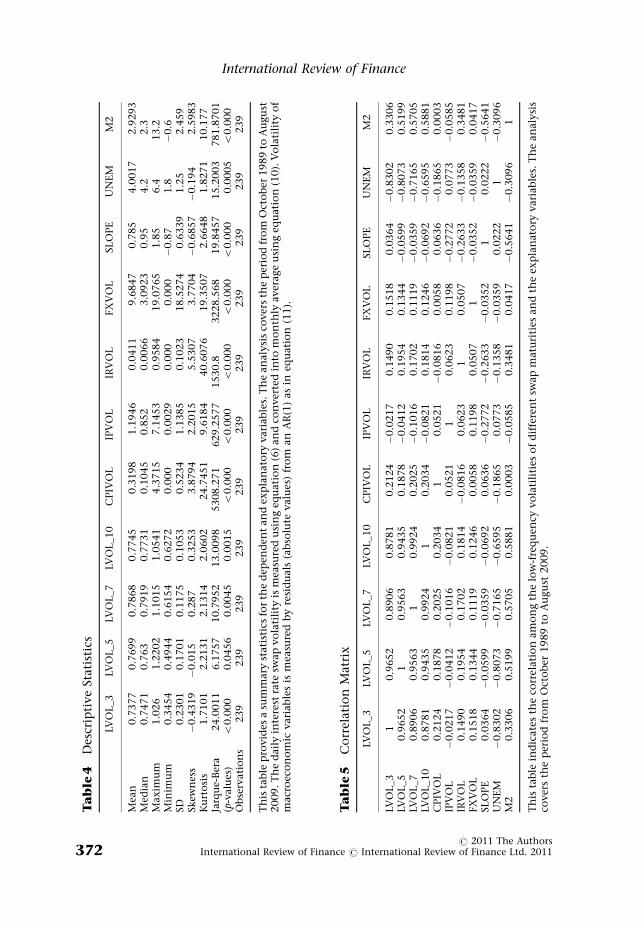
observations, we obtain monthly low-frequency volatilities for each swapmaturity using equation (10). Table 4 shows the summary statistics of low-frequency IRS volatility (monthly average) and of macroeconomic risk proxies.Table 5 indicates the correlation matrix among low-frequency swap volatilityand macroeconomic risk proxies. The correlations among the different swapmaturities are very high. The highest positive correlation among the macro-economic risk is between the money supply and the volatility of interest rate andthe highest negative correlation is between the money supply and the slope ofthe term structure. The correlations between the low-frequency volatilities andthe macroeconomic risk proxies are positive for most variables excludingindustrial production volatility (IPVOL), slope and unemployment rate(UNEM). The stationarity of the variables is confirmed with the AugmentedDickey-Fuller (ADF) unit root test and the test statistics are reported in Table 6.The unit root null is rejected for all the variables.

Table 7 shows the OLS regression results based on equation (9) on the fullsample covering the period from October 1989 through August 2009 as well astwo crisis periods (Asian financial crisis and current global financial crisis).Overall, the model appears to have the best fit for the 5-year swap followed by 3,7 and 10 years swaps. The full sample analysis suggests that IRS volatility isassociated positively with the volatility of inflation (CPIVOL), volatility of

0.2

0.4

0.6

0.8

1.0

1.2

1.4

1.6

1.8

2.0

1990 1992 1994 1996 1998 2000 2002 2004 2006 2008

HVOL_5LVOL_5

Figure3 High and Low Frequency Volatilities of 5-Year SwapThis figure plots the estimated daily high- and low-frequency volatility componentsfor the period from October 1989 to August 2009 for 5-year yen interest rate swap.The high-frequency component is estimated using equation (5) and the low-frequency component is estimated using equation (6). The dotted line indicates thehigh-frequency component, while the solid line indicates the low-frequencycomponent.



industrial production (IPVOL), volatility of foreign exchange rate (FXVOL), slopeof the term structure and money supply and negatively with the unemploymentrate. The relationship varies slightly across different swap maturities. Of the sevenmacroeconomic risk proxies, all the explanatory variables, excluding interest ratevolatility (IRVOL), are found to have significant influences on the low-frequencyvolatility of different swaps. The coefficient of CPI volatility (CPIVOL) isstatistically significant and large in magnitude for all swaps.

The coefficient of IPVOL is positive, significant to all swap maturities butsmall in magnitude. It indicates that an increase in the volatility of industrialproduction increases the low-frequency volatility of swap. Similar results but indifferent financial markets are reported by existing studies (e.g., Officer 1973;Diebold and Yilmaz 2008). Officer (1973) attributes the drop in stock marketvolatility in the 1960s to reduced variability in industrial production. However,in contrast to stock market findings, our results have different implications. Aswe explained before, the variability of GDP or industrial production raises theprobability of default, which in turn increases the default risk and raises theinterest rate. According to this explanation, when macroeconomy is volatile,investors fear that volatility and, thus the volatility of industrial productionincreases the volatility of swap markets instead of reducing it. Even if weexplain the phenomenon from a different point of view, say, the increasedeconomic activity, the volatility of swap market is still expected to respond

0.4

0.6

0.8

1.0

1.2

1.4

1.6

1990 1992 1994 1996 1998 2000 2002 2004 2006 2008

HVOL_7LVOL_7

Figure4 High and Low Frequency Volatilities of 7-Year SwapThis figure plots the estimated daily high- and low-frequency volatility components forthe period from October 1989 to August 2009 for 7-year yen interest rate swap. The high-frequency component is estimated using equation (5) and the low-frequency componentis estimated using equation (6). The dotted line indicates the high-frequency component,while the solid line indicates the low-frequency component.



positively to the volatility of industrial production. An increased economicactivity gives rise to inflation, which induces the central bank to tighten theinterest rate in order to curb the possible impact of inflation. Therefore, a part ofindustrial production (IP) volatility is transmitted to interest rate, which causesmore demand for the swap and hence vibrates the swap markets.

The coefficient of interest rate volatility (IRVOL) is positive for 3 and 5 yearsswaps, negative for 7 and 10 years swaps but statistically insignificant in bothcases. Earlier studies find mixed results (see for instance, In et al. 2003). OnJapanese swap market, Eom et al. (2000) find that curvature (i.e., IRVOL) haspositive and significant influence on the yen swaps spreads. It is well knownthat the rise of swap market is attributed to the volatile interest rate markets inthe early 1970. So, a positive association is empirically appealing for Japan.However, using all relevant proxies for interest rates, we found no significantrelationship between the IRVOL and swap. One reason may be that althoughthe interest rate is an important factor driving the swap market volatility, itssecond moment may not be a key variable in explaining the volatility of yenswap market. It is nonetheless important to mention that the slope of the termstructure is found to be an important variable explaining the behaviour of theswap market. Another reason is that, as Boyd et al. (2005) demonstrate, somemacroeconomic variables (e.g., unemployment and inflation) reflect theinformation about the interest rates.

0.3

0.4

0.5

0.6

0.7

0.8

0.9

1.0

1.1

1.2

1.3

1.4

1990 1992 1994 1996 1998 2000 2002 2004 2006 2008

HVOL_10LVOL_10

Figure 5 High and Low Frequency Volatilities of 10-Year SwapThis figure plots the estimated daily high- and low-frequency volatility components forthe period from October 1989 to August 2009 for 10-year yen interest rate swap. The high-frequency component is estimated using equation (5) and the low-frequency componentis estimated using equation (6). The dotted line indicates the high-frequency component,while the solid line indicates the low-frequency component.



Ta

ble

4D

escr

ipti

ve

Stati

stic

s

LVO

L_3

LVO

L_5

LVO

L_7

LVO

L_1

0C

PIV

OL

IPV

OL

IRV

OL

FX

VO

LSL

OPE

UN

EM

M2

Mea

n0.7

377

0.7

699

0.7

868

0.7

745

0.3

198

1.1

946

0.0

411

9.6

847

0.7

85

4.0

017

2.9

293

Med

ian

0.7

471

0.7

63

0.7

919

0.7

731

0.1

045

0.8

52

0.0

066

3.0

923

0.9

54.2

2.3

Maxim

um

1.0

26

1.2

202

1.1

015

1.0

541

4.3

715

7.1

453

0.9

584

19.0

765

1.8

56.4

13.2

Min

imu

m0.3

454

0.4

944

0.6

154

0.6

272

0.0

00

0.0

029

0.0

00

0.0

00

�0.8

71.8

�0.6

SD0.2

301

0.1

701

0.1

175

0.1

053

0.5

234

1.1

385

0.1

023

18.5

274

0.6

339

1.2

52.4

59

Skew

nes

s�

0.4

319

�0.0

15

0.2

87

0.3

253

3.8

794

2.2

015

5.5

307

3.7

704

�0.6

857

�0.1

94

2.5

983

Ku

rto

sis

1.7

101

2.2

131

2.1

314

2.0

602

24.7

451

9.6

184

40.6

076

19.3

507

2.6

648

1.8

271

10.1

77

Jarq

ue-

Ber

a24.0

011

6.1

757

10.7

952

13.0

098

5308.2

71

629.2

577

1530.8

3228.5

68

19.8

457

15.2

003

781.8

701

(p-v

alu

es)

o0.0

00

0.0

456

0.0

045

0.0

015

o0.0

00

o0.0

00

o0.0

00

o0.0

00

o0.0

00

0.0

005

o0.0

00

Ob

serv

ati

on

s239

239

239

239

239

239

239

239

239

239

239

Th

ista

ble

pro

vid

esa

sum

mary

stati

stic

sfo

rth

ed

epen

den

tan

dex

pla

nato

ryvari

ab

les.

Th

ean

aly

sis

cover

sth

ep

erio

dfr

om

Oct

ob

er1989

toA

ugu

st2009.T

he

dail

yin

tere

stra

tesw

ap

vo

lati

lity

ism

easu

red

usi

ng

equ

ati

on

(6)

an

dco

nver

ted

into

mo

nth

lyaver

age

usi

ng

equ

atio

n(1

0).

Vo

lati

lity

of

mac

roec

on

om

icvari

ab

les

ism

easu

red

by

resi

du

als

(ab

solu

tevalu

es)

fro

man

AR

(1)

as

ineq

uat

ion

(11).

Ta

ble

5C

orr

elati

on

Matr

ix

LVO

L_3

LVO

L_5

LVO

L_7

LVO

L_1

0C

PIV

OL

IPV

OL

IRV

OL

FX

VO

LSL

OPE

UN

EM

M2

LVO

L_3

10.9

652

0.8

906

0.8

781

0.2

124

�0.0

217

0.1

490

0.1

518

0.0

364

�0.8

302

0.3

306

LVO

L_5

0.9

652

10.9

563

0.9

435

0.1

878

�0.0

412

0.1

954

0.1

344

�0.0

599

�0.8

073

0.5

199

LVO

L_7

0.8

906

0.9

563

10.9

924

0.2

025

�0.1

016

0.1

702

0.1

119

�0.0

359

�0.7

165

0.5

705

LVO

L_1

00.8

781

0.9

435

0.9

924

10.2

034

�0.0

821

0.1

814

0.1

246

�0.0

692

�0.6

595

0.5

881

CPIV

OL

0.2

124

0.1

878

0.2

025

0.2

034

10.0

521

�0.0

816

0.0

058

0.0

636

�0.1

865

0.0

003

IPV

OL

�0.0

217

�0.0

412

�0.1

016

�0.0

821

0.0

521

10.0

623

0.1

198

�0.2

772

0.0

773

�0.0

585

IRV

OL

0.1

490

0.1

954

0.1

702

0.1

814

�0.0

816

0.0

623

10.0

507

�0.2

633

�0.1

358

0.3

481

FX

VO

L0.1

518

0.1

344

0.1

119

0.1

246

0.0

058

0.1

198

0.0

507

1�

0.0

352

�0.0

359

0.0

417

SLO

PE

0.0

364

�0.0

599

�0.0

359

�0.0

692

0.0

636

�0.2

772

�0.2

633

�0.0

352

10.0

222

�0.5

641

UN

EM

�0.8

302

�0.8

073

�0.7

165

�0.6

595

�0.1

865

0.0

773

�0.1

358

�0.0

359

0.0

222

1�

0.3

096

M2

0.3

306

0.5

199

0.5

705

0.5

881

0.0

003

�0.0

585

0.3

481

0.0

417

�0.5

641

�0.3

096

1

Th

ista

ble

ind

icate

sth

eco

rrel

atio

nam

on

gth

elo

w-f

req

uen

cyvo

lati

liti

eso

fd

iffe

ren

tsw

ap

matu

riti

esan

dth

eex

pla

nat

ory

vari

ab

les.

Th

ean

aly

sis

cover

sth

ep

erio

dfr

om

Oct

ober

1989

toA

ugu

st2009.



Table 6 Unit Root Tests

3YIRS 5YIRS 7YIRS 10YIRS CPIVOL IPVOL IRVOL FXVOL Slope UNEM M2

ADF teststats

�68.94 �71.47 �73.95 �74.28 �2.63 �8.73 �12.11 �5.84 �5.36 �2.94 �4.68

p-value 0.000 0.000 0.000 0.000 0.09 0.000 0.000 0.000 0.000 0.04 0.000

This table shows the Augmented Dickey-Fuller (ADF) unit test statistics for the swap rate changesand macroeconomic risk proxies. The critical values for the ADF test are �3.4594, �2.8742 and�2.5736 at 1%, 5% and 10%, respectively.

Table 7 Low-Frequency Volatility and Macroeconomic Risk

Whole sample (October 1989–August 2009) Crisis period

3-yearswap

5-yearswap

7-yearswap

10-yearswap

Crisisperiod (I)

CrisisPeriod (II)

Intercept 1.2204 1.0182 0.8674 0.8172 0.9581 0.8630CPIVOL 0.0239nn 0.0141n 0.0176nn 0.0187nnn 0.0021 0.0007

(0.0112) (0.0087) (0.0079) (0.0071) (0.0014) (0.0064)IPVOL 0.0007nnn 0.0005nnn 0.0002nn 0.0002nn 0.0001 0.00001

(0.0002) (0.0001) (0.0001) (0.0001) (0.0001) (o0.0001)IRVOL 0.0483 0.0079 �0.0296 �0.0195 0.0352n 0.0029

(0.0852) (0.0645) (0.0473) (0.0464) (0.0137) (0.0055)FXVOL 0.0014nnn 0.0008nnn 0.0005nn 0.0005nn 0.00001 �0.0001

(0.0004) (0.0002) (0.0002) (0.0002) (o0.0001) (o0.0001)SLOPE 0.0704nn 0.0617nnn 0.0584nnn 0.0498nnn 0.0333nnn �0.0034

(0.0284) (0.0201) (0.0150) (0.0146) (0.0065) (0.0038)UNEM �0.1626nnn �0.1056nnn �0.0577nnn �0.0449nnn �0.0236nnn �0.0313nnn

(0.0125) (0.0087) (0.0064) (0.0059) (0.0063) (0.0023)M2 0.0184nn 0.0306nnn 0.0283nnn 0.0266nnn 0.0019 �0.0016

(0.0072) (0.0058) (0.0047) (0.0046) (0.0017) (0.0071)Adjusted R2 0.7273 0.7677 0.7130 0.6597 0.9805 0.8759F-stat 91.6947nnn 113.3726nnn 85.4517nnn 66.8985nnn 80.1099nnn 26.2044nnn

Results from the following OLS regression model (see equation (9) for details):

Lowvoli;t ¼ ci;0 þ yi;1cpivolþ yi;2ipvolþ yi;3irvolþ yi;4fxvol


where the dependent variable is the low-frequency volatility obtained from using equation (6).Volatility series for CPI (consumer price index), IP (industrial production), IR (interest rate – 90-days TB rate) and foreign exchange rates are obtained from the (absolute value of) residuals ofAR(1) models. Slope5Slope of the yield curve; UNEM5unemployment rate. Standard errors of theestimated coefficients are in parentheses and are corrected for autocorrelation and hetero-scedasticity by using the Newey–West method (lag truncation54). Sample covers the period fromOctober 1989 through August 2009.n,nn and nnnSignificance at 10%, 5% and 1%, respectively. The analysis is done on full sample aswell as on two crisis periods. Crisis Period (I) is for Asian financial crisis (July 1997–June 1998) andCrisis Period (II) is for current global financial crisis (GFC, July 2007–August 2009). For the crisisperiod analysis, only 5-year swap is considered to keep the computation job minimum.



The FXVOL has a positive and statistically significant influence on the low-frequency volatility of all swaps. Suhonen (1998) also finds positive but statisticallyweak relationship between the volatility of foreign exchange and swap spread. Toreiterate, a positive relationship suggests that when the exchange rate is highlyvolatile, the cross-border counterparties demand more payer positions, whichincrease the demand for swaps and affects the swap markets. The result is alsoconsistent with the proposition that the low-frequency component of volatility ishigh when the macroeconomic risk factors are volatile (Engle and Rangel 2008).

Of the other macroeconomic variables, the SLOPE coefficient is found to bepositive and significant throughout all swap maturities for the full sampleanalysis as well as the Asian crisis period but negative and insignificant duringthe GFC crisis. Figure 6 reveals that the SLOPE of the yield curve (i.e., thedifference between long-term and short-term bond yield, from October 1989 toAugust 2009) was positive for the entire sample with the exception of early1990s when the stock price and real estate bubble burst and, since the early2008 when the GFC crisis became more pronounced. Therefore, the result isconsistent with the theory in that a positive (negative) SLOPE implies anexpectation of future interest rates rise (fall), which motivates (frustrates) theIRS activities.13 Of note is that a positive (negative) SLOPE is also an indication

–1.2

–0.8

–0.4

0.0

0.4

0.8

1.2

1.6

2.0

90 91 92 93 94 95 96 97 98 99 00 01 02 03 04 05 06 07 08 09

Figure6 Slope of the Yield CurveThis figure plots the slope of the yield curve over time. It is calculated as the differencebetween long-term and short-term Nikkei bond index yield. The figure covers themonthly data from October 1989 to August 2009.

13 Fang and Muljono (2003) use the SLOPE as proxy for the anticipated future interest rates.



of economic expansion (contraction). It is interesting to observe that eventhough the Japanese economy has triggered 1990s as the ‘lost decade’ and asher economy has experienced several recessions in the last two decades, theSLOPE has been positive for most part of the sample.14 As a result, giventhe decades long low interest rates environment, the positive slope has causedconcerns for some hedgers to hedge their interest rate risk exposure.Nonetheless, as Figures 2–5 suggest, the low-frequency volatility, which wasinitially high during the first 10 years in the sample, gradually declined duringthe last 10 years of the sample.

The positive coefficient of the SLOPE factor can also be linked to theliquidity, which has an influence on the slope of the yield curve. A tightliquidity is related to a flat or inverse slope of yield-curve.15 When the liquiditydries up, the swap trading activity may decrease, which in turn causes the IRSvolatility to fall. Consequently, there can be a positive relationship between theslope of the yield curve and the IRS volatility. We find some support for theliquidity effect in Table 8, which shows the result of causal relationship betweenIRS volatility and macroeconomic risk proxies. The results in Table 8 suggest thatmoney supply (M2) has a strong causal link with IRS volatility both for thewhole sample and the crisis period analyses. These results have an importantimplication with regard to swap markets’ responses to the macroeconomic riskfactors. That is, the IRS volatility may not be dominantly driven by anexpectation of interest rate rise or fall and/or an economic expansion orcontraction but more by liquidity.

The coefficient of money supply (M2) is positive and statistically significantfor all swaps. In an earlier paper on the relationship between macroeconomyand financial markets, Officer (1973) also provides a positive associationbetween the money supply and stock market volatility. The result is alsoconsistent with both the ‘policy implications hypothesis’ or ‘anticipatedliquidity effect hypothesis’ and ‘inflationary expectation hypothesis’. Thesehypotheses imply that an increase in money supply leads to an increase in theinterest rate and inflation in anticipation of future tightening of interest rates.Consequently, the money supply shock is transmitted to IRS through interestrate and/or inflation.

The only variable, unemployment rate (UNEM) is found to have negativeinfluence on the low-frequency volatility of yen swap markets. The coefficientof unemployment rate is highly significant and large in magnitude throughoutall swap maturities. This suggests that swap pricing (and its volatility) is stronglyaffected by the business cycle variable. Unemployment is viewed as newsworthymacroeconomic variable that, according to Boyd et al. (2005), bundles threetypes of primitive information including the future interest rates, the riskpremium and corporate earnings and dividends. A sustained increase in the

14 We also estimated the regressions excluding the periods of negative slope. The coefficient sign

was not changed.

15 Figure 6 shows that the slope of the yield curve seems to be quite flat.



unemployment rate gives an indication of continued economic slowdown orless economic activities. The negative influence of unemployment rate (UNEM),which is taken as a proxy of business cycle risk by Lang et al. (1998), on the swapmarket is related to the fact that with the economic slowdown and lessinvestment activities, the demand for the hedging instruments including IRS isdecreased. Since investment activities decline at times of economic depression/slowdown, the negative influence of unemployment is logical in that theinvestors are less likely to hedge their interest rate risk exposure. If, on the one

Table 8 Pair-wise Granger Causality Tests between Macroeconomic Risksand Low-Vol

Null Hypothesis F-stats (P-values are in Parentheses)

Full sample Crisis Period

3-yearIRS

5-yearIRS

7-yearIRS

10-yearIRS

(I) 3-yearIRS

(II) 3-yearIRS

CPIVOL does not GrangerCause Low-Vol

1.208 0.624 0.629 0.650 0.6616 0.5816(0.300) (0.536) (0.533) (0.522) (0.437) (0.4535)

Low-Vol does not GrangerCause CPIVOL

4.567nnn 3.484nn 4.596nnn 4.832nnn 0.4488 0.0016(0.0113) (0.032) (0.011) (0.008) (0.5197) (0.9686)

IPVOL does not GrangerCause Low-Vol

0.067 0.723 0.656 0.314 0.3849 4.8605nn

(0.9347) (0.486) (0.519) (0.730) (0.5504) (0.0378)Low-Vol does not GrangerCause IPVOL

2.249n 2.017 1.350 0.287 0.0345 1.0722(0.101) (0.135) (0.261) (0.750) (0.8569) (0.3112)

IRVOL does not GrangerCause Low-Vol

1.983 1.458 1.568 1.509 7.7753nn 0.8258(0.139) (0.234) (0.210) (0.223) (0.0211) (0.3729)

Low-Vol does not GrangerCause IRVOL

2.722n 6.666nnn 4.37nnn 4.087nn 0.0047 1.6414(0.067) (0.001) (0.013) (0.018) (0.9468) (0.2129)

FXVOL does not GrangerCause Low-Vol

0.825 0.515 0.373 0.159 4.66328n 3.2107n

(0.439) (0.597) (0.688) (0.852) (0.0591) (0.0863)Low-Vol does not GrangerCause FXVOL

3.251nn 0.961 0.986 1.934 1.4431 0.357(0.040) (0.383) (0.374) (0.146) (0.2603) (0.556)

SLOPE does not GrangerCause Low-Vol

3.669nn 1.639 0.768 0.5639 23.8747nnn 30.301nnn

(0.027) (0.196) (0.465) (0.569) (0.0009) (o0.0001)Low-Vol does not GrangerCause SLOPE

2.260n 6.183nnn 3.936nn 2.012 5.0718n 0.2922(0.106) (0.002) (0.020) (0.136) (0.0508) (0.594)

UNEM does not GrangerCause Low-Vol

9.92nnn 17.27nnn 15.50nnn 17.452nnn 6.8570nn 23.485nnn

(0.0001) (o0.0001) (o0.0001) (o0.0001) (0.0279) (0.0001)Low-Vol does not GrangerCause UNEM

4.57nnn 0.419 0.132 0.101 4.5415n 2.2926(0.011) (0.657) (0.876) (0.903) (0.0619) (0.1436)

M2 does not GrangerCause Low-Vol

4.95nnn 4.095nn 2.650n 1.765 12.1734nnn 4.7525nn

(0.0079) (0.017) (0.072) (0.173) (0.0068) (0.0397)Low-Vol does not GrangerCause M2

0.974 5.968nnn 2.458n 2.530n 0.02042 3.6375n

(0.379) (0.003) (0.087) (0.081) (0.8895) (0.0691)

This table shows the pair-wise Granger causality test results. See Table 2 or equation (9) for detailsof the macroeconomic risk proxies. Sample covers the period from October 1989 through August2009.n, nn and nnnSignificance at 10%, 5% and 1%, respectively. In parentheses are p-values. The analysisis done on full sample as well as on two crisis periods. For the crisis period analysis, only 3-yearswap (3-year IRS) is considered as it is found to have causal link with many macro-risk variablesthan other maturities. Crisis Period (I) is for Asian financial crisis (July 1997–June 1998) and CrisisPeriod (II) is for current global financial crisis (July 2007–August 2009).



hand, Black (1987)’s hypothesis (higher the macroeconomic volatility, higher isthe investment activity) does work, an active economy would be a volatile onein which investors need to hedge and manage the risks. On the other hand, aninactive economy (unemployment or less investment activities) indicates thatinvestors require less protection against rate rise risk. As noted earlier, the lowlevel of macroeconomic volatility/risk causes decline in preferences for fixed-income assets, which frustrate derivative activities (Loeys and Panigirtzoglou2005; Cailleteau and Mali 2007). The reason being that the market riskpremium is low when macroeconomic risk falls. Lettau et al. (2008) provide theevidence that a fall in macroeconomic risk leads to decline in equity premium.Sultan (2006) notes that swap market can contain a risk premium.

The above results are consistent with both the theory and prior empiricalfindings. The model appears to have the best fit for the 5-year swap followedby 3, 7 and 10 years. The analysis for two crisis periods (Asian financial crisisand recent global financial crisis, see column 6 and 7 of Table 7) indicatesa varying degree of relationship between the low-frequency IRS volatilityand macroeconomic risk proxies. Both the sign and level of significance ofthe explanatory variables differ in two crisis periods. It is rather difficult tosketch any theoretically appealing relationship between the swap andmacroeconomy in times of economic crisis. During the Asian financial crisis(from July 1997 to June 1998), the low-frequency volatility of swap is foundto be positively associated with interest rate volatility (IRVOL) and SLOPEbut negatively associated with unemployment rate (UNEM).16 During therecent global financial crisis period (from July 2007 to August 2009), none butthe coefficient of unemployment rate is statistically significant. Therefore, thebusiness cycle risk (unemployment rate) continues to have significant relation-ship with the swap market at both the crisis period analysis and the wholesample analysis.17

The overall results are consistent with the notion that macroeconomic riskleads to a greater degree of hedging or speculative activities in financial markets.Since most of the macroeconomic risk proxies are positively associated (with theexception of unemployment rate) with the volatility of the swap markets, wecan argue that the greater the macroeconomic risk, the greater is the use ofderivatives to gain from hedging or speculating (Beber and Brandt 2009).18

However, in contrast to other macroeconomic risk proxies, an increasein unemployment rate is an indication of economic depression/slowdown,

16 For simplicity, we only considered 5-year swap. Of note is that the model appears to have the best

fit for the 5-year swap followed by other maturities. However, the results do not vary much when

other maturities are considered.

17 We also analysed the relationship excluding the crisis periods from the whole sample. However,

the results are more or less same as those of whole sample analysis and, hence not reported.

18 The results are also robust to the choice of principal components (of the macroeconomic risk

proxies) as independent variables. The principal components are shown in Table 9. Of the three

components, the coefficients of components 1 and 2 are found to be statistically significant and

positive for all swaps. The results can be obtained from the authors on request.



which means less interest rate volatility that causes less concern for hedginginterest rate risk.

We now report the results of pair-wise causal relationship between macro-economic risk proxies and the low-frequency IRS volatility to examine which of thetwo leads the relationship. Of the recent literature, Diebold and Yilmaz (2008) andEngle et al. (2008) study both the correlation and causation between macro-economic volatility/risk and stock market volatility. Testing the causal link isimportant as Chen et al. (1986) and Schwert (1989), among others, argue thatthere is no satisfactory theory that indicates an entirely one way relationshipbetween financial markets and macroeconomy. Rather, there is a lead-lagrelationship between the two. Studying this relationship facilitates investigatingas to whether policy makers implicate the market reactions (feedback effects) intothe subsequent policy decisions. In addition, the notion that financial volatilityhelps predicting macroeconomic volatility or risk is also captured (Schwert 1989).That is, one can ascertain the degree of responses of macroeconomic risk to a changein low-frequency IRS volatility. On the one hand, if the causal link is uni-directional from the macroeconomy to the low-frequency volatility, then weconjecture that macroeconomic risk has a pronounced effect on the low-frequencyvolatility. The practical implication is that the hedgers or speculators of swaps canhedge their interest rate risk exposure or speculate due to the rise of macroeconomicrisk. On the other hand, if the causal link is uni-directional from the low-frequency volatility to the macroeconomy, then as a forward looking instrument,the IRS is deemed to have predictive power to forecast the fluctuations inmacroeconomic risk. This enables the investors to look for protection againstmacroeconomic risk. If a bi-directional causality is found, there exists feedback effectand we conjecture that macroeconomic policy makers regularly monitor andreflect the market reactions.

Table 8 shows the results of pair-wise Granger causality tests conductedbetween macroeconomic risk proxies and the low-frequency IRS volatility.The analysis indicates that excluding unemployment rate, none of themacroeconomic risk proxies have entirely one-way causality to low-frequencyIRS volatility. Rather, the reverse direction appears strong for most ofthe macroeconomic risk proxies. For example, the hypothesis that low-frequencyvolatility (for most of the swap maturities) does not Granger-cause macro-economic risk/volatility is rejected for CPIVOL, IPVOL, IRVOL and FXFOL etc.A bi-directional causality’ or ‘bi-directional feedback’ exists between low-frequency swap volatility and two macroeconomic risk proxies namely, slope andunemployment rate in the case of 3-year swap. For the 5 and 7 years swaps, a bi-directional causality exists only between low-frequency swap volatility andmoney supply. We find none of the macroeconomic risk proxies to have bi-directional relationship with the 10-year swap. Taken together, the lagged swapmarket volatility has predictive power for current macroeconomic risk.

For the crisis period, only 3-year swap is analysed considering three factors.First, the 3-year swap is one of the most liquid markets. Second, it is a key ratein the yield curve and third, as Table 8 indicates, in contrast to other maturities,



3-year swap has better causal relationship with most macro-risk factors. Theanalysis suggests that during the Asian financial crisis period, a bi-directionalcausality is found to exist between low-frequency IRS volatility and twomacroeconomic variables: SLOPE and unemployment rate. For other macro-economic variables like IRVOL, FXVOL and M2, the null hypothesis thatmacroeconomic risk does not Granger cause low-frequency IRS volatility isrejected. That is, IRVOL, FXVOL and M2 lead the relationship during the Asiancrisis period. During the recent global financial crisis period, a bi-directionalcausality exists between low-frequency volatility and money supply. To put itanother way, the feedback effect between the liquidity factor and the tradingactivity in IRS seems to be strong during the recent global financial crisis. Forother macroeconomic variables like, IPVOL, FXVOL, SLOPE and unemploy-ment rate, the reverse causality is found strong indicating that thesemacroeconomic variables lead the relationship. The implication is that, attimes of major economic crises, the forecast of macro-risk variables helppredicting the IRS volatility but not the other way around.

Interestingly, when we use alternative specifications of IRS volatility[alternative specifications include: (i) long-term volatility19 from the additivedecomposition (see equation (13) in Section VI) and (ii) RV (see equation (16) inSection VI)] we find little evidence of causal relationship between macro-economic risks and swap market volatility.20 This result is consistent with thoseof Engle et al. (2008). They find evidence of causal link between macroeconomyand stock market volatility only when they use low-frequency component,which is obtained from the multiplicative decomposition of volatility. Butwhen they use noisy RV, little evidence of causal relationship betweenmacroeconomic risks and stock market volatility is detected. This emphasizesthe importance of using the multiplicative decomposition of financial volatilityover either additive volatility decomposition or noisy RV. Among the otherstudies that have examined the causal link between macroeconomy andfinancial market volatility, only Diebold and Yilmaz (2008) find that causalityruns from the fundamental (macroeconomic) volatility to stock marketvolatility. Further to note, the results in Diebold and Yilmaz (2008) could beoverstated as they used aggregate stock volatility without decomposing it.

On balance, with regard to causal relation between swap market volatilityand macroeconomic risk/volatility, it looks like swap market volatility containsfair amount of information in predicting macroeconomic risk. This implies thatthe market gives the signals of forthcoming uncertainty in the macroeconomy.Therefore, our results are not only consistent with the existing findings instocks and bond markets (Schwert 1989; Engle et al. 2008) but also consistentwith the large scale agreement that volatility measures obtained from

19 It is to be noted that both the low-frequency volatility and long-term volatility proxy the

permanent component of volatility. We use two different terms in order to distinguish between

the models (multiplicative decomposition and additive decomposition) of volatility.

20 The results are not reported to conserve the space but available from authors on request.



derivatives markets provide useful information on investors’ perceptions offuture economic uncertainty/risk (Beber and Brandt 2009; Buraschi et al. 2009).

The reverse causality stimulates a natural question to be answered. Shouldthe swap market be regressor or regressee? It is to be noted that the swap rate isthe market expectation at the beginning of the period or at time t, so the low-frequency volatility of IRS is the volatility of the expectation from t to t11,while the macro-risk variables are the realized values from t to t11. In this sense,the low-frequency volatility should be the predictor of the market risk insteadof being explained by the market risk. Hence, because the reverse causality isstronger, one would expect the macroeconomic variable(s) to be regressed onthe swap market volatility. However, prior literature has largely ignored theimplication of this reverse causality. Since, the reverse causality is stronger formost of the macroeconomic risk proxies, we run the reverse regression where theswap market acts as the channels to forecast the behaviour of the macroeconomicrisks.21 We do this by taking into account individual macro-risk variables as wellas extracting their principal components (three components are identified byusing principal component analysis). These variables are then regressed on low-frequency volatility of 5-year swap as it is found to have the best fit in ourregression (see Table 7). In Table 9, the principal component analysis suggeststhat three factors (IRVOL, SLOPE and M2) belong to component 1, two factors(CPIVOL and UNEM) belong to component 2 and two factors (IPVOL andFXVOL) belong to component 3. All the macroeconomic risk proxies havesignificant weights on the principal components.

The results (shown in Table 10) of reverse regression indicate thatcomponent-1 and component-2 are significantly associated with the low-frequency IRS volatility. The regression results with component-3 and IPVOLexhibit insignificant F-stat, while the coefficient of low-vol as a determinant ofthe SLOPE variable is found to be insignificant and hence not reported. Overall,the results are stimulating for those who are interested to forecast themacroeconomic risk/uncertainty using the volatility forecasts obtained from thederivative markets.22 For brevity, we do not report the results for othermaturities as they are more or less similar to those of 5-year swap.

VI. ROBUSTNESS TO ALTERNATIVE SPECIFICATIONS

A natural question arises as to whether the above empirical findings are robustto alternative specifications of volatility. We start our robustness check with thebenchmark additive specification of Engle and Lee (1999) and then with RV.

21 We thank an anonymous referee for advising us to include this analysis.

22 Owing to the scope of the paper, we have ignored the robustness check (in-sample as well as out-

of-sample forecasts) in relation to the argument that the (swap) market volatility is able to

provide useful information to predict the macroeconomic risk/uncertainty. We have a plan to

accommodate this in future research.



Recall that Engle and Lee (1999)’s component GARCH model has two volatilitycomponents:

(i) short-run/transitory volatility,

gi;t ¼ ðai � biÞgi;t�1 þ aiðe2i;t�1 � hi;t�1Þ ð12Þ

(ii) long-term/permanent volatility,

ti;t ¼ oi þ rti;t�1 þ Wiðe2i;t�1 � hi;t�1Þ ð13Þ

where volatility innovation, (ei, t�12 �hi,t�1), drives both the short-run and long-

term components. To recall, the short-term or transitory volatility (equation(12)) is similar in spirit to that of high-frequency volatility (equation (5)), while

Table 9 Principal Component Analysis

Component

1 2 3

CPIVOL �0.212 0.759 0.281IPVOL 0.076 �0.151 0.837IRVOL 0.654 �0.024 �0.014FXVOL 0.023 0.143 0.518SLOPE �0.764 0.125 �0.337UNEM �0.295 �0.736 0.211M2 0.844 0.227 �0.072

This table shows the rotated component matrix of the macroeconomic risk proxies. Thecomponents are extracted from the principal component analysis (PCA) using the rotationmethod Varimax with Kaiser Normalization. Rotation converged in six iterations. The variables inbold indicate that they are highly correlated with the principal components.

Table 10 Macroeconomic Risk and Low-frequency Volatility (Reverse Regression)

Individual macro-risk variable Principal components

CPIVOL IRVOL FXVOL UNEM M2 PC1 PC2

Intercept �0.1251 �0.0493 �1.5831 8.6012 �2.8563 �1.7101 �3.0447Low-vol 0.5779nnn 0.1175nn 14.6360nn �5.9745nnn 7.5151nnn 2.2213nn 3.9548nnn

(0.2231) (0.0527) (7.4570) (0.4388) (2.4735) (0.9915) (0.3812)AdjustedR2

0.0312 0.0341 0.0139 0.6596 0.2672 0.1392 0.4503

F-stat 8.6671nnn 9.410nnn 4.3589nn462.2781nnn 87.7908nnn 39.4792nnn195.9841nnn

This table shows the reverse regression results where, the dependent variables are the individualmacroeconomic risk proxies and the principal components (PC) as shown in Table 9. Theindependent variable is the low-frequency volatility (Low-vol) of 5-year yen IRS. Standard errors(SE) of the estimated coefficients are in parentheses and are corrected for autocorrelation andheteroscedasticity by using the Newey–West method with lag truncation up to 4. Sample coversthe period from October 1989 to August 2009.nn and nnnSignificance at 5% and 1%, respectively.



the long-term or permanent volatility (equation (13)) is similar in spirit to thatof low-frequency volatility (equation (6)). After obtaining the daily long-termvolatility, ti, t, from Engle and Lee’s (1999) component GARCH model, we takethe average of the daily long-term volatility in month t as follows:

Longvoli;t ¼

ffiffiffiffiffiffiffiffiffiffiffiffiffiffiffiffiffiffiffiffiffiffiffiffi1

Ni;t

XNi;t

d¼1

ti;d;t

vuut ð14Þ

where Longvoli, t stands for average daily long-term volatility of swap formaturity i (53, 5, 7 and 10) at month t. Ni, t is the number of trading days in amonth at year t for maturity i. ti, d, t is the daily long-term volatility observed formaturity i, of swap quote day d at year t. This daily long-term volatility isobtained by using equation (13). Thus, we model the long-term volatility (in amonth), Longvoli, t as a function of same macroeconomic risk proxies, which areused in equation (9). The empirical setting is as follows:

Longvoli;t ¼ ci;0 þ yi;1cpivolþ yi;2ipvolþ yi;3irvolþ yi;4fxvol

þ yi;5slopeþ yi;6unemþ yi;7m2þ mi;t :ð15Þ

Table 11 presents the estimation results of the equation (15) based on long-term volatility from the additive volatility decomposition. The results indicatethat the signs of the macroeconomic risk proxies do not change significantly.However, the relationship between macroeconomic risks and the swap marketbecomes weaker with the choice of long-term volatility from additivedecomposition. The IRS volatility was significantly associated with sixmacroeconomic risk proxies when we used low-frequency volatility frommultiplicative decomposition. But now with the long-term volatility fromadditive decomposition, we find that IRS volatility is associated with, on anaverage, four macroeconomic risk proxies. The adjusted R2 statistics also fallsconsiderably with the longer swap maturities. This suggests that, in contrast tolong-term volatility obtained from Engle and Lee (1999)’s model, the low-frequency volatility of Engle and Rangel (2008) provides a better link betweenthe swap market and macroeconomy.

As regards the sign of the individual coefficient, the analysis (Table 11) showsthat the coefficient of CPI volatility becomes statistically insignificant for allswap maturities (only marginally significant for 5-year swap). Similarly, thecoefficient of FX volatility becomes statistically insignificant for all swaps. Thecoefficient of IP volatility is positive and statistically significant for all swapmaturities but small in magnitude. The coefficients of slope and money supplyare positive, highly significant and moderate in magnitude. The other variables(slope, unemployment rate and money supply) behave almost in similarfashion as in the case of low-frequency volatility specification in equation (9).That is, IRS volatility is associated significantly and positively with slope andmoney supply but negatively with unemployment rate.



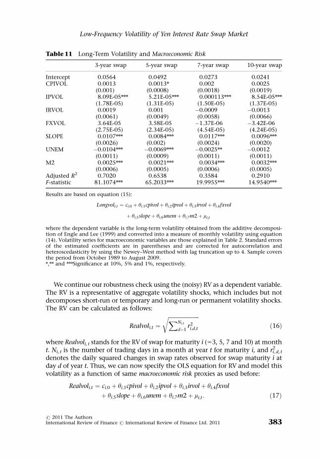
We continue our robustness check using the (noisy) RV as a dependent variable.The RV is a representative of aggregate volatility shocks, which includes but notdecomposes short-run or temporary and long-run or permanent volatility shocks.The RV can be calculated as follows:

Realvoli;t ¼ffiffiffiffiffiffiffiffiffiffiffiffiffiffiffiffiffiffiffiffiffiffiffiXNi;t

d¼1r2i;d;t

rð16Þ

where Realvoli, t stands for the RV of swap for maturity i (53, 5, 7 and 10) at montht. Ni, t is the number of trading days in a month at year t for maturity i, and ri,d, t

2

denotes the daily squared changes in swap rates observed for swap maturity i atday d of year t. Thus, we can now specify the OLS equation for RV and model thisvolatility as a function of same macroeconomic risk proxies as used before:

Realvoli;t ¼ ci;0 þ yi;1cpivolþ yi;2ipvolþ yi;3irvolþ yi;4fxvol

þ yi;5slopeþ yi;6unemþ yi;7m2þ mi;t : ð17Þ

Table 11 Long-Term Volatility and Macroeconomic Risk

3-year swap 5-year swap 7-year swap 10-year swap

Intercept 0.0564 0.0492 0.0273 0.0241CPIVOL 0.0013 0.0013n 0.002 0.0025

(0.001) (0.0008) (0.0018) (0.0019)IPVOL 8.09E-05nnn 5.21E-05nnn 0.000113nnn 8.54E-05nnn

(1.78E-05) (1.31E-05) (1.50E-05) (1.37E-05)IRVOL 0.0019 0.001 �0.0009 �0.0013

(0.0061) (0.0049) (0.0058) (0.0066)FXVOL 3.64E-05 3.58E-05 �1.37E-06 �3.42E-06

(2.75E-05) (2.34E-05) (4.54E-05) (4.24E-05)SLOPE 0.0107nnn 0.0084nnn 0.0117nnn 0.0096nnn

(0.0026) (0.002) (0.0024) (0.0020)UNEM �0.0104nnn �0.0069nnn �0.0025nn �0.0012

(0.0011) (0.0009) (0.0011) (0.0011)M2 0.0025nnn 0.0021nnn 0.0034nnn 0.0032nnn

(0.0006) (0.0005) (0.0006) (0.0005)Adjusted R2 0.7020 0.6538 0.3584 0.2910F-statistic 81.1074nnn 65.2033nnn 19.9955nnn 14.9540nnn

Results are based on equation (15):

Longvoli;t ¼ ci;0 þ yi;1cpivolþ yi;2ipvolþ yi;3irvolþ yi;4fxvol


where the dependent variable is the long-term volatility obtained from the additive decomposi-tion of Engle and Lee (1999) and converted into a measure of monthly volatility using equation(14). Volatility series for macroeconomic variables are those explained in Table 2. Standard errorsof the estimated coefficients are in parentheses and are corrected for autocorrelation andheteroscedasticity by using the Newey–West method with lag truncation up to 4. Sample coversthe period from October 1989 to August 2009.n,nn and nnnSignificance at 10%, 5% and 1%, respectively.



As Table 12 demonstrates, the CPI volatility has a negative but insignificantinfluence on the realized volatilities of 3 and 5 years swap. Recall that, itscoefficient was statistically significant for all swaps in the case of low-frequencyvolatility, and for 5-year swap in the case of long-term volatility. The coefficient ofIP volatility is positive, small in magnitude and statistically significant for allswaps. The coefficient of IR volatility is positive, statistically significant for 3 and 5years swap and moderate in magnitude. The coefficient of FX volatility is negativefor all except 5-year swap but not statistically significant. The slope coefficient ispositive, moderate in magnitude and statistically significant for all swaps. Similarfindings are found in the case of money supply. However, the coefficient ofmoney supply is not as large as IR volatility, slope and unemployment rate. Thecoefficient of unemployment rate is negative for all swaps and statisticallysignificant for all but 10-year swap. Unlike the long-term volatility but similar tolow-frequency specification, the model has the best fit with the 5-year swap (theadjusted R2 statistics is 26.49%) followed by 3, 7 and 10 years swaps.

The robustness check ends with the comparison of adjusted R2 statistics thatare obtained from different specifications of volatility. Table 13 presents the

Table 12 Realized Volatility and Macroeconomic Risk

3-year swap 5-year swap 7-year swap 10-year

Intercept 0.0565 0.0364 0.0095 0.0043CPIVOL 0.0038 0.0042 0.005 0.0049

(0.0067) (0.0063) (0.0061) (0.0057)IPVOL 0.0002nnn 0.0003nnn 0.0002nnn 0.00013nnn

(4.31E-05) (3.76E-05) (3.95E-05) (3.55E-05)IRVOL 0.0232n 0.0308n 0.0207 0.0169

(0.0124) (0.0174) (0.0161) (0.0163)FXVOL �1.51E-05 6.51E-06 �1.00E-05 �1.93E-05

(0.000107) (0.000123) (0.0001) (9.89E-05)SLOPE 0.0195nnn 0.0193nnn 0.0228nnn 0.018nnn

(0.0061) (0.005) (0.0053) (0.0041)UNEM �0.0153nnn �0.0103nnn �0.004n �0.0017

(0.0033) (0.0027) (0.002301) (0.00232)M2 0.00446nnn 0.0057nnn 0.006nnn 0.0059nnn

(0.001863) (0.0016) (0.0012) (0.0011)Adjusted R2 0.2578 0.2649 0.2102 0.1764F-statistic 12.8105nnn 13.2505nnn 10.0493nnn 8.2836nnn

Results from the following OLS regression model (see equation (17)):

Realvoli;t ¼ ci;0 þ yi;1cpivolþ yi;2ipvolþ yi;3cpivol

þ yi;4fxvolþ yi;5slopeþ yi;6unemþ yi;7m2þ mi;t

where the dependent variable is the realized volatility obtained from using equation (16).Volatility series for macroeconomic variables are those explained in Table 2. Standard errors of theestimated coefficients are in parentheses and are corrected for autocorrelation and hetero-scedasticity by using the Newey–West method with lag truncation up to 4. Sample covers theperiod from October 1989 through August 2009.n and nnnSignificance at 10% and 1%, respectively.



adjusted R2 statistics and their averages for four-swap maturities. Using low-frequency (column 2 of Table 13) or long-term volatility (column 3 of Table 13)from two-component GARCH specifications, the highest adjusted R2 statistics isobtained for 5-year swap followed by 3, 7 and 10 years swap rates. Using simpleRV (column 4 of Table 13) the highest R2 statistics is obtained for 3-year swap. Itis obvious that average adjusted R2 statistics is the highest, which is 71.69%, inthe case of low-frequency volatility from multiplicative decomposition of Engleand Rangel (2008). The second highest average adjusted R2 statistics, which is50.13%, is also obtained from two-component GARCH specifications. Thelowest average adjusted R2 statistics, which is 22.73%, is obtained from RV.Thus, the explanatory power of the model, i.e., the average adjusted R2

statistics, falls sharply with the traditional measure of volatility. This, none-theless, signifies the importance of using a better measure of market risk proxyfor the financial markets concerned.

To summarise, our results stimulate new research agenda in the IRS marketsby providing strong empirical support for the relationship between swap marketvolatility and macroeconomic volatilities/risks. First, we estimate the aggregateIRS volatility for four different swap maturities of the yen IRS market and thenextract the persistent component, which gives us a parsimonious volatility termstructure for various swap maturities. Second, we model this volatility termstructure as a function of candidate macroeconomic risk proxies. Third, wedocument that relationship between macroeconomic risks and swap markets arestronger when we use the persistent component (i.e., low-frequency or long-term) of volatility shocks. Finally, the results are fairly consistent throughout allswaps when we use the low-frequency volatility to model the relationship butare inconsistent when we use long-term volatility from additive volatilitydecomposition or RV.

VII. SUMMARY AND CONCLUSIONS

It’s become a widespread belief that financial market volatility changes overtime. Prior literature attributes this time variation in financial market volatility

Table 13 Comparison of Adjusted R-Squared Statistics under Different Models

Swaps Low-frequency volatility Long-term volatility Realized volatility

3-year swap 0.7273 0.7020 0.25785-year swap 0.7677 0.6538 0.26497-year swap 0.7130 0.3584 0.210210-year swap 0.6597 0.2910 0.1764Average 0.7169 0.5013 0.2273

This table provides a comparison of adjusted R2 statistics obtained from different models. Theadjusted R2 statistics for low-frequency volatility is based on equation (9), for long-term volatilityis based on equation (15) and for realized volatility is based on equation (17).



to variation of business cycle and other macroeconomic risk proxies. There arenow enormous sophisticated econometric models to capture this phenomenonin different financial markets. However, only few of the models have beensuccessful to model the sources of time variation in volatility. This is boththeoretically and empirically appealing for the swap market being an interestrate sensitive product. Therefore, this paper raises the issue whether the timevariation in swap market volatility can be linked to macroeconomic risk factors,albeit using a parsimonious volatility term structure namely, ‘low-frequencyvolatility’ extracted from aggregate volatility shocks for different swapmaturities. The analysis indicates a strong association between the two.

Our results are robust to the choice of different alternative measures of volatilityas used in the literature on GARCH modelling. The explanatory power falls sharplywith the use of alternative measures like RV. The study includes some importantfindings especially as far as the relationship between swap market volatility andmacroeconomic risk/volatility is concerned. The analysis suggests that both longerand shorter maturities of swap have strong association with macroeconomic riskproxies. All swaps (3, 5, 7 and 10 years) are found to be significantly related with sixmacroeconomic risk proxies. The relationship does not vary largely across swapmaturities rather it becomes even stronger during the major economic crises.Hence, the use of swap by world’s major corporations to manage macroeconomic riskis economically justifiable. Such empirical evidence encourages theoretical workrelating uncertainty of macroeconomic fundamentals to causes of fluctuations inswap market volatility at long horizons. We also provide some empirical evidenceof reverse regression since our reverse causality was strong between macroeconomicrisk and low-frequency volatility. The results are stimulating for both thetheoretical and empirical studies which may look at the forecasting ability of thelow-frequency volatility to predict macroeconomic risk. The practical implication isthat the hedgers can forecast ahead whether they need to increase (decrease) IRSusage to hedge rate rise risk at times of higher (lower) macroeconomic risk.

A.S.M. Sohel AzadDepartment of Accounting and FinanceMonash UniversityCaulfield East, Victoria 3145, [email protected] or [email protected]

REFERENCES

Adrian, T., and J. Rosenberg (2008), ‘Stock Returns and Volatility: Pricing the Short-Run and Long-Run Components of Market Risk’, Journal of Finance, 63, 2997–3030.

Andersen, T., T. Bollerslev, F. Diebold, and P. Labys (2003a), ‘Modeling and ForecastingRealized Volatility’, Econometrica, 71, 579–625.

Andersen, T. G., and T. Bollerslev (1997), ‘Heterogeneous Information Arrivals andReturn Volatility Dynamics: Uncovering the Long-Run in High Frequency Returns’,Journal of Finance, 52, 975–1005.



mailto:[email protected]

Andersen, T. G., T. Bollerslev, F. X. Diebold, and C. Vega (2003b), ‘Micro Effects ofMacro Announcements: Real-Time Price Discovery in Foreign Exchange’, AmericanEconomic Review, 93, 38–62.

Bansal, R., and A. Yaron (2004), ‘Risks for the Long Run: A Potential Resolution of AssetPricing Puzzles’, Journal of Finance, 59, 1481–509.

Beber, A., and M. W. Brandt (2009), ‘Resolving Macroeconomic Uncertainty in Stockand Bond Markets’, Review of Finance, 13, 1–45.

Becker, R., and A. Clements (2007), Forecasting Stock Market Volatility Conditional onMacroeconomic Conditions. National Centre for Econometric Research (NCER)Working Paper Series, No # 18 (June).

Bicksler, J., and A. H. Chen (1986), ‘An Economic Analysis of Interest Rate Swaps’,Journal of Finance, 41, 645–55.

BIS (2009), OTC Derivatives Market Activity At End-December. Basel, Switzerland: Bankfor International Settlements.

Black, F. (1987), Business Cycles and Equilibrium. Cambridge, MA: Blackwell.Bollerslev, T., R. Y. Chou, and K. F. Kroner (1992), ‘ARCH Modeling in

Finance: A Review of the Theory and Empirical Evidence’, Journal of Econometrics,52, 5–59.

Boyd, J. H., J. Hu, and R. Jagannathan (2005), ‘The Stock Market’s Reaction toUnemployment News: Why Bad News is Usually Good for Stocks’, Journal of Finance,60, 649–72.

Brown, K. C., W. V. Harlow, and D. J. Smith (1994), ‘An Empirical Analysis of InterestRate Swap Spreads’, Journal of fixed income, 3, 61.

Buraschi, A., F. Trojani, and A. Vedolin (2009), ‘When Uncertainty Blows in theOrchard: Comovement and Equilibrium Volatility Risk Premia’, European FinanceAssociation Conference, 19–22 August, Bergen, Norway.

Cailleteau, P., and A. Mali (2007), ‘Why is Credit Risk Priced so Low? A Perspective onGlobal Liquidity’, Moody’s International Policy Perspectives, February, 2007, 1–8.

Cargill, T. F. (2000), What Caused Japan’s Banking Crisis?: Crisis and Change in theJapanese Financial System. Dordrecht: Kluwer Academic Publishers, pp. 37–58.

Catao, L., and S. Kapur (2004), Missing Link: Volatility and the Debt IntoleranceParadox. IMF Working Paper, No. WP/04/51.

Chen, N.-F., R. Roll, and S. A. Ross (1986), ‘Economic Forces and the Stock Market’,Journal of Business, 59, 383–403.

Christoffersen, P., K. Jacobs, C. Ornthanalai, and Y. Wang (2008), ‘Option Valuationwith Long-Run and Short-Run Volatility Components’, Journal of FinancialEconomics, 90, 272–97.

Codogno, L., C. Favero, and A. Missale (2003), ‘Yield Spreads on EMU GovernmentBonds’, Economic Policy, 18, 503–32.

Cortes, F. (2006), Understanding the Term Structure of Swap Spreads. Bank of EnglandQuarterly Bulletin, (Spring).

Cowen, T. (2009), ‘A Simple Theory of the Financial Crisis; or, Why Fischer Black StillMatters’, Financial Analysts Journal, 65, 17–20.

Diebold, F. X., and K. Yilmaz (2008), Macroeconomic Volatility and StockMarket Volatility, Worldwide. National Bureau of Economic Research, WorkingPaper 14269.

Engle, R., and G. Lee (1999), ‘A Permanent and Transitory Component Model of StockReturn Volatility’, in R. Engle and H. White (eds), Cointegration, Causality, andForecasting: A Festschrift in Honor of Clive W.J. Granger. New York: Oxford UniversityPress, pp. 475–97.

Engle, R. F., E. Ghysels, and B. Sohn (2008), ‘On the Economic Sources of Stock MarketVolatility’, Finance Working Papers No. FIN-08-043, Stern School of Business, NewYork University.



Engle, R. F., and J. G. Rangel (2008), ‘The Spline-GARCH Model for Low-FrequencyVolatility and its Global Macroeconomic Causes’, Review of Financial Studies, 21,1187–222.

Eom, Y. H., M. G. Subrahmanyam, and J. Uno (2000), ‘Credit Risk and the Yen InterestRate Swap Market’, Salomon Centre Derivatives Research Working Paper No. S-DRP-01-08, Stern School of Business, New York University.

Fang, V., and R. Muljono (2003), ‘An Empirical Analysis of the Australian Dollar SwapSpreads’, Pacific-Basin Finance Journal, 11, 153–73.

Genberg, H., and A. Sulstarova (2008), ‘Macroeconomic Volatility, Debt Dynamics,and Sovereign Interest Rate Spreads’, Journal of International Money and Finance, 27,26–39.

Ghysels, E., P. Santa-Clara, and R. Valkanov (2005), ‘There is a Risk-Return TradeoffAfter All’, Journal of Financial Economics, 76, 509–48.

Ghysels, E., A. Sinko, and R. Valkanov (2007), ‘MIDAS Regressions: Further Results andNew Directions’, Econometric Reviews, 26, 53–90.

Hamilton, J., and G. Lin (1996), ‘Stockmarket Volatility and the Business Cycle’,Journal of Applied Econometrics, 5, 573–93.

Huang, Y., and C. R. Chen (2007), ‘The Effect of Fed Monetary Policy Regimes on theUS Interest Rate Swap Spreads’, Review of Financial Economics, 16, 375–99.

Huang, Y., S. N. Neftci, and F. Guo (2008), ‘Swap Curve Dynamics Across Markets: Caseof US Dollar versus HK Dollar’, Journal of International Financial Markets, Institutionsand Money, 18, 79–93.

In, F., R. Brown, and V. Fang (2003), ‘Modeling Volatility and Changes in the SwapSpread’, International Review of Financial Analysis, 12, 545–61.

ISDA (International Swaps and Derivatives Association Inc., 2009). 2009 ISDADerivatives Usage Survey. ISDA Research Notes, November 2, 2009, 1–6.

Ito, T. (2008), ‘The Interest Rate Swap Spreads and Monetary Policy in Japan’, 21stAustralasian Finance and Banking Conference, 16–18 December, 2008, Sydney.

Jones, C. M., O. Lamont, and R. L. Lumsdaine (1998), ‘Macroeconomic News and BondMarket Volatility’, Journal of Financial Economics, 47, 315–37.

Lang, L. H. P., R. H. Litzenberger, and A. L. Liu (1998), ‘Determinants of Interest RateSwap Spreads’, Journal of Banking & Finance, 22, 1507–32.

Lekkos, I., and C. Milas (2001), ‘Identifying the Factors that Affect Interest-Rate SwapSpreads: Some Evidence from the United States and the United Kingdom’, Journal ofFutures Markets, 21, 737–68.

Lettau, M., S. C. Ludvigson, and J. A. Wachter (2008), ‘The Declining EquityPremium: What Role Does Macroeconomic Risk Play?’, Review of Financial Studies,21, 1653–87.

Litzenberger, R. H. (1992), ‘Swaps: Plain and Fanciful’, Journal of Finance, 47,831–50.

Loeys, J., and N. Panigirtzoglou (2005), Volatility, Leverage and Returns. Global MarketStrategy, J.P. Morgan Securities Ltd., London, October 19.

McNulty, J. E. (1990), ‘The Pricing of Interest Rate Swaps’, Journal of Financial ServicesResearch, 4, 53–63.

McQueen, G., and V. Roley (1993), ‘Stock Prices, News, and Business Conditions’,Review of Financial Studies, 6, 683–707.

Merton, R. (1973), ‘An Intertemporal Capital Asset Pricing Model’, Econometrica, 41,867–87.

Mikitani, R. (2000), ‘The Nature of Japanese Financial Crisis’, in R. Mikitani and A. S.Posen (eds), Japan’s Financial Crisis and Its Parallels to US Experience. Washington,DC: Institute for International Economics, pp. 27–35.

Nishioka, S., and N. Baba (2004), Credit risk Taking by Japanese Investors. Bank ofJapan Working Paper Series, No. 04-E-7, July.



Nowak, S., J. Andritzky, A. Jobst, and N. Tamirisa (2009), Macroeconomic Funda-mentals, Price Discovery and Volatility Dynamics in Emerging Markets. Interna-tional Monetary Fund, Working Paper # WP/09/147.

Officer, R. F. (1973), ‘The Variability of the Market Factor of the New York StockExchange’, Journal of Business, 46, 434–53.

Rangel, J. G., and R. F. Engle (2011), ‘The Factor-Spline-GARCH Model for High andLow Frequency Correlations’, Working Papers 2009-03, Banco de Mexico.

Roll, R. (1988), ‘R2’, Journal of Finance, 43, 541–66.Schwert, G. W. (1989), ‘Why Does Stock Market Volatility Change Over Time?’, Journal

of Finance, 44, 1115–53.Simpson, M. W., S. Ramchander, and M. Chaudhry (2005), ‘The Impact of

Macroeconomic Surprises on Spot and Forward Foreign Exchange Markets’, Journalof International Money and Finance, 24, 693–718.

Smith, C., C. Smithson, and L. Wakeman (1986), ‘The Evolving Market for Swaps’,Midland Corporate Finance Journal, 3, 20–32.

Suhonen, A. (1998), ‘Determinants of Swap Spreads in a Developing Financial Market:Evidence from Finland’, European Financial Management, 4, 379–99.

Sultan, J. (2006), Modeling Correlation Risk Risk Management. Boston: Academic Press,pp. 273–94.

Turnbull, S. M. (1987), ‘Swaps: A Zero Sum Game?’, Financial Management, 16, 15–21.Urich, T., and P. Wachtel (1981), ‘Market Response to the Weekly Money Supply

Announcements in the 1970s’, Journal of Finance, 36, 1063–72.Urich, T., and P. Wachtel (1984), ‘The Effects of Inflation and Money Supply

Announcements on Interest Rates’, Journal of Finance, 39, 1177–88.Wachter, J. A. (2006), ‘A Consumption-Based Model of the Term Structure of Interest

Rates’, Journal of Financial Economics, 79, 365–99.

APPENDIX A: DERIVATION OF LOW-FREQUENCY VOLATILITY, tT,IN SPLINE-GARCH OF ENGLE AND RANGEL (2008)

Here, we show how the volatility component, tt, in equation (6) tis obtained.The similar explanation is also found in Becker and Clements (2007). The splinemodel of Engle and Rangel (2008) modifies the standard GARCH (1, 1) byintroducing a trend in the volatility process. This trend describes how low-frequency component is associated with slowly varying deterministic condi-tions in the economy or random variables that are highly persistent and moveslowly. Engle and Rangel (2008) approximate this (unobserved) trend non-parametrically using an exponential quadratic spline, which generates asmooth curve describing the low-frequency volatility identified from the data.The exponential functional form guarantees that the low-frequency componentof volatility is non-negative. The unconditional expectation for e2

t can bederived as follows:

Eðe2t Þ ¼ ht ¼ EðgtÞtt ðA:1Þ

Ee2t

tt

� �¼ ht

tt¼ EðgtÞ ðA:2Þ



where gt is a forecast of et2/tt. However, actual realizations of et

2/tt are not equal togt. Hence, we add et

2/tt to both sides of gt in equation (5) to obtain:

gt þe2t

tt¼ ð1� a� bÞ þ a

e2t�1

tt�1

� �þ bgt�1 þ

e2t

ttðA:3Þ

¼ ð1� a� bÞ þ ðaþ bÞ e2t�1

tt�1

� �� b

e2t�1

tt�1� gt�1

� �þ e2

t

ttðA:4Þ

e2t

tt¼ð1� a� bÞ þ ðaþ bÞ e2

t�1

tt�1

� �

� be2t�1

tt�1� gt�1

� �þ e2

t

tt� gt

� � ðA:5Þ

Assuming E(et2/tt�gt)50, we get

Ee2t

tt

� �¼ ð1� a� bÞ þ ðaþ bÞE e2

t�1

tt�1

� �ðA:6Þ

Considering the stationary conditions on the above process it can be seenthat E(et

2/tt)51. This in turn implies that

Eðe2t Þ ¼ ht ¼ EðgtÞtt ¼ tt ðA:7Þ

Thus, the unconditional expectation of gt equals 1 implies that theunconditional/low-frequency volatility depends exclusively on tt term. Engleand Rangel (2008) exploit this result so that the unconditional volatilitycoincides with the low-frequency volatility. They model this low-frequencyvolatility component using an exponential quadratic spline with generates ofpositive smooth curve based exclusively on data evidence. The quadratic spline isspecified as the sum of k truncated quadratic basis functions as in equation (6).



Low-Frequency Volatility of Yen Interest Rate Swap Market in Relation to Macroeconomic Risk*

Documents

Transcript of Low-Frequency Volatility of Yen Interest Rate Swap Market in Relation to Macroeconomic Risk*