Reactive Power Control in AC Power Systems

Power Systems

Reactive Power Control in ACPower Systems

Naser Mahdavi TabatabaeiAli Jafari AghbolaghiNicu BizonFrede Blaabjerg Editors

Fundamentals and Current Issues

Power Systems

More information about this series at http://www.springer.com/series/4622

Naser Mahdavi TabatabaeiAli Jafari Aghbolaghi • Nicu BizonFrede BlaabjergEditors

Reactive Power Controlin AC Power Systems

Fundamentals and Current Issues

123

EditorsNaser Mahdavi TabatabaeiElectrical Engineering DepartmentSeraj Higher Education InstituteTabrizIran

Ali Jafari AghbolaghiZanjan Electric Energy DistributionCompany

ZanjanIran

Nicu BizonFaculty of Electronics, Communication andComputers

University of PiteştiPiteştiRomania

Frede BlaabjergDepartment of Energy TechnologyAalborg UniversityAalborgDenmark

ISSN 1612-1287 ISSN 1860-4676 (electronic)Power SystemsISBN 978-3-319-51117-7 ISBN 978-3-319-51118-4 (eBook)DOI 10.1007/978-3-319-51118-4

Library of Congress Control Number: 2017930608

© Springer International Publishing AG 2017This work is subject to copyright. All rights are reserved by the Publisher, whether the whole or partof the material is concerned, specifically the rights of translation, reprinting, reuse of illustrations,recitation, broadcasting, reproduction on microfilms or in any other physical way, and transmissionor information storage and retrieval, electronic adaptation, computer software, or by similar or dissimilarmethodology now known or hereafter developed.The use of general descriptive names, registered names, trademarks, service marks, etc. in this

publication does not imply, even in the absence of a specific statement, that such names are exempt fromthe relevant protective laws and regulations and therefore free for general use.The publisher, the authors and the editors are safe to assume that the advice and information in thisbook are believed to be true and accurate at the date of publication. Neither the publisher nor theauthors or the editors give a warranty, express or implied, with respect to the material contained herein orfor any errors or omissions that may have been made. The publisher remains neutral with regard to

jurisdictional claims in published maps and institutional affiliations.

Printed on acid-free paper

This Springer imprint is published by Springer NatureThe registered company is Springer International Publishing AG

The registered company address is: Gewerbestrasse 11, 6330 Cham, Switzerland

Dedicated to

all our teachers and colleagues

who enabled us to write this book,

and our family and friends

for supporting us all along

Foreword

Electric power systems will be operated in reliable and efficient situation consid-

ering reactive power control and voltage stability management. Reactive power

margins are related to the voltage stability. The aspects are satisfied by designing

and operating of right voltages limits, maximizing utilization of transmission sys-

tems and minimizing of reactive power flow. Therefore, controlling reactive power

and voltage is one of the major challenges of power system engineering.

Reactive power as the dissipated power is affected by capacitive and inductive

phenomena that they drop voltage and draw current in the form of heat or waste

energy. Reactive power is generated by the capacitors and generators, whereas it is

consumed by the inductors and is essential in the parallel connection circuits as

power factor controlling and power transmission lines.

Reactive power control and voltage stability aspects are effective in reliability of

electric power networks. Voltage instability commonly occurs as a result of reactive

power deficiency. The trends are to reduce reactive power and increase voltage

stability to improve efficiency and operation of power systems. There is a direct

relation between reactive power and voltage behavior which serves the voltage

collapse and rising effects in power systems.

Regulating the reactive power and voltage control should be done according to

flexible and fast controlled devices. Placement and adjustment of reactive power

play important roles in operation of reactive power compensation and voltage

control. Therefore, the operations of reactive power resources in the power systems

such as automatic transformer tap changer, synchronous condenser, capacitor

banks, capacitance of overhead lines and cables, static VAR compensators and

FACTS devices are very significant.

Reactive power control and voltage stability management are considered as

regional challenges to meet, which otherwise can cause the scale of blackouts

increase in the power systems. Theoretical and application issues in these areas help

us to identify problems related to reliability and stability of the power systems and

prevent the system degradation.

vii

The above aspects are illustrated in this book by the editors and authors, in the

following topics: electrical power systems operation and control, reactive power

and voltage stability in power systems, reactive power control in transmission lines,

reactive power compensation and optimal placement, reactive power in renewable

resources, reactive power optimization and software applications, optimal reactive

power dispatch, induction generator operation and analysis, communication net-

works and standards in power systems, power systems SCADA applications, and

geomagnetic storms effects in electric networks.

The book chapters and materials are very efficient in theoretical and application

issues and are highly recommended for studying and considering in educational and

research fields.

November 2016 Academician Arif M. Hashimov

Institute of Physics

Azerbaijan National Academy of Sciences

Baku

Azerbaijan

viii Foreword

Preface

The modern electric power systems are more expanded worldwide and include

more energy resources and critical parts based on the requirements of the

twenty-first century. General parts of electric power systems as generation, trans-

mission and consumption are important to be analyzed and well operated for the

development of industry and life.

The engineers and scientists need applicable and renewable methods for ana-

lyzing and controlling each part of the electric power systems and to overcome

complicated actions which occur in the systems due to their operational and

interconnection behaviors. The objective of the analysis is minimizing the losses

of the networks and increasing the overall efficiency and economic advantages.

The central and distributed generation of electric power networks connect to

more loads, transmission lines, transformers and energy sources together including

nonlinear equipment such as power semiconductor devices. The engineers and

scientists are interested in analyzing the power systems operations to control

and develop the AC/DC networks including high voltage transmission lines and

equipment.

Flexible and fast power flow control and transmission are expected to raise the

network effective operation, power wheeling requirement and transmission capa-

bility as well as voltage stability. Computational intelligence methods are applied to

electric power analysis to facilitate the effective analysis techniques and solve

several power system problems especially in power transmission and voltage

stability.

Reactive Power Control in AC Power Systems: Fundamentals and Current

Issues is a book aimed to highlight the reactive power control and voltage stability

concepts and analysis to provide understanding on how they are affected by dif-

ferent criteria of available generations, transmissions and loads using different

research methods.

A large number of specialists joined as authors of the book chapters to provide

their potentially innovative solutions and research related to reactive power control

and voltage stability, in order to be useful in developing new ways in electric power

analysis, design and operational strategies. Several theoretical researches, case

ix

analysis, and practical implementation processes are put together in this book that

aims to act as research and design guides to help graduates, postgraduates and

researchers in electric power engineering and energy systems.

The book, which presents significant results obtained by leading professionals

from industries, research and academic fields, can be useful to a variety of groups in

specific areas. All works contributed to this book are new, previously unpublished

material or extended version of published papers in the proceedings of international

conferences and transactions on international journals. The book consists of

16 chapters in three parts.

Part I Fundamentals of Reactive Power in AC Power Systems

The six chapters in the first part of this book present the fundamentals of reactive

power in AC power systems considering different operating cases. The topics in this

part include the advanced methods and applications in electric power systems and

networks related to the fields of fundamentals of reactive power in AC power

systems, reactive power role in AC power transmission systems, reactive power

compensation in energy transmission systems with sinusoidal and nonsinusoidal

currents, reactive power importance in wind power plants, and fundamentals and

contemporary issues of reactive power control in AC power systems.

Chapter 1 describes the general overview of electric power systems including

power generation, transmission and distribution systems, linear AC circuits in

steady state conditions, flow of power between generator and customers is studied

by using the active, reactive, apparent and complex power, electric power system

quality, measurement and instrumentation methods of power systems parameters,

and general standards in energy generation, transmission and marketing. The

importance of reactive power in AC power systems and its various interpretations

are also discussed in this chapter.

The basic theory of AC circuits, behavior of two-port linear elements and

analysis methods of AC circuits are given in Chap. 2. The physical interpretation of

electric powers in AC power systems, fundamental problems of reactive power

consumption automated management in power systems, equipment for power factor

correction, designing simple systems for compensating of reactive power for dif-

ferent levels of installation, the overall harmonic distortion of voltage and current,

and qualitative and quantitative aspects related to active and reactive power cir-

culation in AC power systems including several examples and case studies referring

to classical linear AC circuits under sinusoidal and nonsinusoidal conditions are

also the topics of this chapter.

Chapter 3 presents basic principles of power transmission operation, equipment

for reactive power generation, shunt/series compensation, control of reactive power

in power transmission system. The chapter describes the capacitive and inductive

properties of power transmission lines and also reactive power consumption by

transmission lines which increases with the square of current. The chapter states the

x Preface

sources, effects and limitations of the reactive power and flowing in transmission

lines and transformers as well as control of reactive power should satisfy the bus

voltages, system stability and network losses in the power systems.

The definition of reactive power under nonsinusoidal conditions in nonlinear

electric power systems is described in Chap. 4. This chapter discusses and simulates

the reactive power compensation for sinusoidal and nonsinusoidal situations, where

nonlinear circuit voltages and currents contain harmonics and also the control

algorithms of automatic compensators. The main aim of the chapter is based on the

dissipative systems and cyclodissipativity theories for calculation of compensation

elements for reactive power compensation by minimizing line losses. The chapter is

also including the examples and computer simulations to show the mathematical

framework for analyzing and designing of compensators for reactive power com-

pensation in general nonlinear loads.

Chapter 5 deals with the rate of reactive power absorption or injected by the

wind units and also the key role of reactive power generation and consumption in

large-scale wind farms. The chapter describes requirements of reactive power

compensation, voltage stability and also power quality improvement in the electric

grid of wind turbine to reduce the power losses and control of voltage level. The

units of wind turbines of types 1 to 4 are also categorized and discussed in the

chapter considering their construction, generation, converters, reactive power and

voltage control abilities. The coordination related to reactive power adjustment in

the wind turbines is also discussed in this chapter.

The concept of power quality and voltage stability improvement based on the

reactive power control is introduced in Chap. 6. The chapter describes the impact of

reactive power flow in the power system and defines the power components of

electrical equipment that produces or absorbs reactive power. Then the reactive

power control and relations between reactive power and voltage stability are pre-

sented. The chapter also contains reactive power control methods for voltage

stability and presents voltage control management based on case studies.

Part II Compensation and Reactive Power Optimization

in AC Power Systems

The second part of this book tries to highlight in six chapters the concepts of

reactive power optimization and compensation. The topics in this part include

optimal reactive power control for voltage stability improvement, reactive power

compensation, optimal placement of reactive power compensators, reactive power

optimization in classic methods and also using MATLAB and DIgSILENT, and

multi-objective optimal reactive power dispatch.

Chapter 7 is entirely focused on the voltage stability control using three main

techniques of reactive power management, active power re-dispatch, and load

shedding. The chapter discusses about determining the location of VAR sources

Preface xi

and their setting and installation, online and offline reactive power dispatch, and

optimal reactive power flow (ORPF). The reactive power flow and voltage mag-

nitudes of generator buses, shunt capacitors/reactors, output of static reactive power

compensators, transformer tap-settings are considered as the control parameters and

are used for minimizing the active power loss and improving of the voltage profile

in ORPF. This chapter also confers the reactive power dispatch as a nonlinear and

nonconvex problem with equality and inequality constraints.

The reactive power compensators based on advanced industrial applications are

highlighted in Chap. 8. The basic theoretical background of reactive power com-

pensation as well as conventional compensators and improved FACTS are intro-

duced in the chapter. The compensation devices including shunt, series and

shunt-series configurations for transmission lines regarding their characteristics and

also analytical expressions are presented in the chapter. The power flow control,

voltage and current modifications as well as stability issues are also analyzed and

compared for similar compensation devices and emerging technologies.

Chapter 9 provides a framework and versatile approach to develop a

multi-objective reactive power planning (RPP) strategy for coordinated handling of

reactive power from FACTS devices and capacitor banks. This chapter deals with

power system operators for determining the optimal placement of FACTS devices

and capacitor banks should be injected in the network to improve simultaneously

the voltage stability, active power losses and cost of VAR injection. A formulation

and solution method for reactive power planning, and voltage stability based on

cost functions are also presented in the chapter.

Chapter 10 presents the reactive power optimization using artificial optimization

algorithms as well as the formulations and constraints to implement reactive power

optimization. The classic method of reactive power optimization and basic prin-

ciples and problem formulation of reactive power optimization using artificial

intelligent algorithms are discussed in the chapter. In addition, this chapter focuses

on the particle swarm optimization algorithm and pattern search method application

in reactive power optimization including the case studies.

The efficient approach using parallel working of MATLAB and DIgSILENT

software with the intention of reactive power optimization is discussed in Chap. 11.

This chapter presents the toolboxes, functions and flexibility powers of MATLAB

and DIgSILENT in electrical engineering calculation and implementation. Also it

provides the advantages of parallel calculations of MATLAB and DIgSILENT and

relation of two software to carry out the heuristic algorithms as fast, simple and

accurate as possible to optimize reactive power in AC power systems.

In Chap. 12, the reactive power compensation devices are modeled using

deterministic multi-objective optimal reactive power dispatch (DMO-ORPD) and

two-stage stochastic multi-objective optimal reactive power dispatch (SMO-ORPD)

in discrete and continuous studies. They are formulated as mixed integer nonlinear

program (MINLP) problems, and solved by general algebraic modeling system

(GAMS). A case study for evaluation of the performance of different proposed

MO-ORPD models is also shown in the chapter. This chapter presents the

MO-ORPD problem taking into account different operational constraints such as

xii Preface

bus voltage limits, power flow limits of branches, limits of generators voltages,

transformers tap ratios and the amount of available reactive power compensation at

the weak buses.

Part III Challenges, Solutions and Applications in AC Power

Systems

The final part of this book consists of four chapters and considers some applications

and case studies in AC power systems related to the issues of active and reactive

power concepts. The topics in this part include self-excited induction generator,

communications for electric power systems, SCADA applications for electric power

systems and effect of geomagnetic storms on electrical networks.

Chapter 13 discusses about a three-phase self-excited induction generator in an

autonomous power generation mode. The chapter presents generator operating

points and control strategies to maintain the frequency at quasi-constant values and

to use it as power converter such as a simple dimmer to control the reactive power.

The frequency analysis in steady state and transient cases is studied in this chapter

using a single-phase equivalent circuit as well as theoretical and numerical results

are also validated on a laboratory test bench.

Chapter 14 describes communications applied for electric power systems

including communication standards and infrastructure requirements for smart grids.

The chapter presents three primary functions of smart grids to accomplish in real

time requests of both consumers and suppliers based on communications tech-

nologies. The most usual communication systems including fiber optic communi-

cation, digital subscriber line/loop, power line communications, and wireless

technologies for using the power system control for smart grids architecture are

highlighted in the chapter. The case studies related to communication systems of

electric power system are also carried out in this chapter.

The SCADA systems and applications in electric power networks are studied in

Chap. 15. The chapter explains the role and theory of SADA systems, security,

real-time control and data exchange between remote units and central units.

The SCADA systems are also applied for optimization and realization of reactive

power in AC power systems. Some disadvantages of dispatching systems such as

graphical information and interface are explained in the chapter and the rules of

improving them are also carried out. The flexibility designing of the systems for

small and large networks are also explained.

Chapter 16 introduces the effect of geomagnetic fields called as storms on

electric power systems. This chapter discusses about the physical nature of earth’s

magnetic field and its measurements in geomagnetic observatories and shows that

the variation of geomagnetic field affect the operation of various distracting elec-

tronic devices, such as electrical transmission systems. An algorithm for calculating

Preface xiii

induced currents in the power transmission lines and also the violation of stability

of the system considering the illustrative example are also derived in this chapter.

The editors recommend this book as suitable for an audience professional in

electric power systems, as well as researchers and developers in the field of energy

and power engineering. It is anticipated that the readers have sufficient knowledge

in electric power engineering and also advanced mathematical background.

In total, the book includes theoretical background and case studies in reactive

electric power and voltage stability concepts. The editors have made efforts to cover

the essential topics of reactive electric power to balance theoretical and applicative

aspects in the chapters of this book. The book has been written by a team of

researchers from which use the dedicated intensive resources for achieving certain

mental attitudes for interested readers. At the same time, the application and case

studies are intended for real understanding and operation.

Finally, the editors hope that this book will be useful to undergraduate and

graduate students, researchers and engineers, trying to solve reactive electric power

problems using modern technical and intelligent systems based on theoretical

aspects and application case studies.

Tabriz, Iran Naser Mahdavi Tabatabaei

Zanjan, Iran Ali Jafari Aghbolaghi

Piteşti, Romania Nicu Bizon

Aalborg, Denmark Frede Blaabjerg

xiv Preface

Contents

Part I Fundamentals of Reactive Power in AC Power Systems

1 Electrical Power Systems . . . . . . . . . . . . . . . . . . . . . . . . . . . . . . . . . . 3

Horia Andrei, Paul Cristian Andrei, Luminita M. Constantinescu,

Robert Beloiu, Emil Cazacu and Marilena Stanculescu

2 Fundamentals of Reactive Power in AC Power Systems . . . . . . . . . 49

Horia Andrei, Paul Cristian Andrei, Emil Cazacu

and Marilena Stanculescu

3 Reactive Power Role and Its Controllability in AC Power

Transmission Systems . . . . . . . . . . . . . . . . . . . . . . . . . . . . . . . . . . . . . 117

Esmaeil Ebrahimzadeh and Frede Blaabjerg

4 Reactive Power Compensation in Energy Transmission

Systems with Sinusoidal and Nonsinusoidal Currents . . . . . . . . . . . 137

Milan Stork and Daniel Mayer

5 Reactive Power Control in Wind Power Plants. . . . . . . . . . . . . . . . . 191

Reza Effatnejad, Mahdi Akhlaghi, Hamed Aliyari,

Hamed Modir Zareh and Mohammad Effatnejad

6 Reactive Power Control and Voltage Stability

in Power Systems. . . . . . . . . . . . . . . . . . . . . . . . . . . . . . . . . . . . . . . . . 227

Mariana Iorgulescu and Doru Ursu

Part II Compensation and Reactive Power Optimization

in AC Power Systems

7 Optimal Reactive Power Control to Improve Stability

of Voltage in Power Systems . . . . . . . . . . . . . . . . . . . . . . . . . . . . . . . 251

Ali Ghasemi Marzbali, Milad Gheydi, Hossein Samadyar,

Ruhollah Hoseyni Fashami, Mohammad Eslami

and Mohammad Javad Golkar

xv

8 Reactive Power Compensation in AC Power Systems . . . . . . . . . . . 275

Ersan Kabalci

9 Optimal Placement of Reactive Power Compensators

in AC Power Network. . . . . . . . . . . . . . . . . . . . . . . . . . . . . . . . . . . . . 317

Hossein Shayeghi and Yashar Hashemi

10 Reactive Power Optimization in AC Power Systems . . . . . . . . . . . . 345

Ali Jafari Aghbolaghi, Naser Mahdavi Tabatabaei,

Narges Sadat Boushehri and Farid Hojjati Parast

11 Reactive Power Optimization Using MATLAB

and DIgSILENT . . . . . . . . . . . . . . . . . . . . . . . . . . . . . . . . . . . . . . . . . 411

Naser Mahdavi Tabatabaei, Ali Jafari Aghbolaghi,


12 Multi-objective Optimal Reactive Power Dispatch

Considering Uncertainties in the Wind Integrated

Power Systems . . . . . . . . . . . . . . . . . . . . . . . . . . . . . . . . . . . . . . . . . . . 475

Seyed Masoud Mohseni-Bonab, Abbas Rabiee

and Behnam Mohammadi-Ivatloo

Part III Challenges, Solutions and Applications

in AC Power Systems

13 Self-excited Induction Generator in Remote Site. . . . . . . . . . . . . . . . 517

Ezzeddine Touti, Remus Pusca, J. Francois Brudny

and Abdelkader Chaari

14 Communications for Electric Power System . . . . . . . . . . . . . . . . . . . 547

Maaruf Ali and Nicu Bizon

15 SCADA Applications for Electric Power System. . . . . . . . . . . . . . . . 561

Florentina Magda Enescu and Nicu Bizon

16 Effect of Geomagnetic Storms on Electric Networks. . . . . . . . . . . . . 611

Daniel Mayer and Milan Stork

Index . . . . . . . . . . . . . . . . . . . . . . . . . . . . . . . . . . . . . . . . . . . . . . . . . . . . . . 631

xvi Contents

List of Figures

Figure 1.1 Representation of three-phase symmetrical and positive

phase-sequence system: a Time domain, b Cartesian

coordinates . . . . . . . . . . . . . . . . . . . . . . . . . . . . . . . . . . . . . . 7

Figure 1.2 Representation of three-phase symmetrical and negative


coordinates . . . . . . . . . . . . . . . . . . . . . . . . . . . . . . . . . . . . . . 8

Figure 1.3 Representation of three-phase symmetrical and zero


coordinates . . . . . . . . . . . . . . . . . . . . . . . . . . . . . . . . . . . . . . 9

Figure 1.4 Star connection . . . . . . . . . . . . . . . . . . . . . . . . . . . . . . . . . . . 9

Figure 1.5 Delta connection . . . . . . . . . . . . . . . . . . . . . . . . . . . . . . . . . . 11

Figure 1.6 Symmetrical and balanced three-phase system . . . . . . . . . . . 14

Figure 1.7 Equivalent three-phase circuit . . . . . . . . . . . . . . . . . . . . . . . . 15

Figure 1.8 Equivalence delta—star . . . . . . . . . . . . . . . . . . . . . . . . . . . . . 15

Figure 1.9 Single-phase circuit of phase 1 . . . . . . . . . . . . . . . . . . . . . . . 16

Figure 1.10 Decomposition of an unsymmetrical system in three

symmetrical systems . . . . . . . . . . . . . . . . . . . . . . . . . . . . . . . 18

Figure 1.11 Decomposition of the a unsymmetrical system,

b positive, c negative, and d zero-sequences. . . . . . . . . . . . . 19

Figure 1.12 Single phases of a positive, b negative, and

c zero-sequence . . . . . . . . . . . . . . . . . . . . . . . . . . . . . . . . . . . 20

Figure 1.13 Voltage measurement in mono-phase AC circuits . . . . . . . . . 22

Figure 1.14 Phase and line voltage measurements . . . . . . . . . . . . . . . . . . 22

Figure 1.15 Current measurement in mono-phase circuit . . . . . . . . . . . . . 23

Figure 1.16 Current measurement in three-phase circuit. . . . . . . . . . . . . . 23

Figure 1.17 Current measurement for a three-phase balanced circuit . . . . 23

Figure 1.18 Active power measurement in mono-phase circuits . . . . . . . . 24

Figure 1.19 Active power measurement in three-phase circuits with

neutral line load . . . . . . . . . . . . . . . . . . . . . . . . . . . . . . . . . . 24

Figure 1.20 Power measurement in three-phase circuits without

neutral line load . . . . . . . . . . . . . . . . . . . . . . . . . . . . . . . . . . 25

xvii

Figure 1.21 Power measurement in three-phase circuits without

neutral line load using two wattmeters . . . . . . . . . . . . . . . . . 25

Figure 1.22 Power measurement for balanced load and symmetrical

source voltage with natural neutral point. . . . . . . . . . . . . . . . 26

Figure 1.23 Power measurement for balanced load and symmetrical

source voltage with an artificial neutral point . . . . . . . . . . . . 26

Figure 1.24 Exemplification of a voltage dip and a short supply

interruption, classified according to EN 50160;

Un—nominal voltage of the supply system (rms),

UA—amplitude of the supply voltage, U (rms)—the

actual rms value of the supply voltage [3] . . . . . . . . . . . . . . 29

Figure 1.25 a Power Q-meter, b Measurement stand . . . . . . . . . . . . . . . . 32

Figure 1.26 Wiring diagram for U, I, f measurements . . . . . . . . . . . . . . . 33

Figure 1.27 Significance of phase-shifts u and w. . . . . . . . . . . . . . . . . . . 37

Figure 1.28 Fourier series decomposition of a periodic distorted

voltage signal . . . . . . . . . . . . . . . . . . . . . . . . . . . . . . . . . . . . 39

Figure 1.29 Current signals, harmonics and various PQ parameters

measured for a low-voltage industrial load . . . . . . . . . . . . . . 45

Figure 2.1 Signals and values characteristic for a sinusoidal

variation . . . . . . . . . . . . . . . . . . . . . . . . . . . . . . . . . . . . . . . . 51

Figure 2.2 The phase-shift between two sinusoidal signals . . . . . . . . . . 52

Figure 2.3 Complex representation of sinusoidal and complex

signals . . . . . . . . . . . . . . . . . . . . . . . . . . . . . . . . . . . . . . . . . . 53

Figure 2.4 Passive circuit’s elements . . . . . . . . . . . . . . . . . . . . . . . . . . . 54

Figure 2.5 Ideal current ad voltage generators . . . . . . . . . . . . . . . . . . . . 54

Figure 2.6 Passive linear two-port system magnetically not coupled

to the exterior . . . . . . . . . . . . . . . . . . . . . . . . . . . . . . . . . . . . 55

Figure 2.7 Imittances’ triangles . . . . . . . . . . . . . . . . . . . . . . . . . . . . . . . 56

Figure 2.8 Powers’ triangle . . . . . . . . . . . . . . . . . . . . . . . . . . . . . . . . . . 60

Figure 2.9 AC circuit with 6 branches . . . . . . . . . . . . . . . . . . . . . . . . . . 62

Figure 2.10 The equivalent AC circuit . . . . . . . . . . . . . . . . . . . . . . . . . . . 63

Figure 2.11 AC circuit with two energy sources . . . . . . . . . . . . . . . . . . . 65

Figure 2.12 Superposition principle . . . . . . . . . . . . . . . . . . . . . . . . . . . . . 67

Figure 2.13 A simple installation for an AC electric drive . . . . . . . . . . . . 68

Figure 2.14 The electric equipment in the mechanical work-place . . . . . . 70

Figure 2.15 Convention of the directions for defining the power

at terminals . . . . . . . . . . . . . . . . . . . . . . . . . . . . . . . . . . . . . . 74

Figure 2.16 The current and voltage signals of the instantaneous

power . . . . . . . . . . . . . . . . . . . . . . . . . . . . . . . . . . . . . . . . . . 74

Figure 2.17 Power factor variation function of asynchronous

motor’s loading and the reactive power consumption

for small and big power motors function of the

relative power voltage . . . . . . . . . . . . . . . . . . . . . . . . . . . . . . 83

Figure 2.18 Examples for placing the capacitors bank . . . . . . . . . . . . . . . 86

xviii List of Figures

Figure 2.19 Individual compensation for asynchronous motors and

for transformers. . . . . . . . . . . . . . . . . . . . . . . . . . . . . . . . . . . 86

Figure 2.20 Connections possibilities for capacitors bank . . . . . . . . . . . . 88

Figure 2.21 The principle scheme for an automated controlled power

factor in an installation . . . . . . . . . . . . . . . . . . . . . . . . . . . . . 89

Figure 2.22 Connecting the power factor correction system in a

non-sinusoidal state system . . . . . . . . . . . . . . . . . . . . . . . . . . 90

Figure 2.23 Selecting the reactive power compensation possibility

function of installation’s nonlinear receivers’ weight . . . . . . 91

Figure 2.24 Selection of reactive power compensation functions of

installation’s nonlinear loads’ weight . . . . . . . . . . . . . . . . . . 92

Figure 2.25 Connecting the detuned reactors in a D connection

capacitors bank . . . . . . . . . . . . . . . . . . . . . . . . . . . . . . . . . . . 92

Figure 2.26 The energy quality parameters of the industrial consumer

under investigation . . . . . . . . . . . . . . . . . . . . . . . . . . . . . . . . 94

Figure 2.27 The current variation on the consumer’s most loaded

phase taken on a monitor interval . . . . . . . . . . . . . . . . . . . . . 95

Figure 2.28 Representation of an AC circuit branch . . . . . . . . . . . . . . . . 97

Figure 2.29 AC circuit under non-sinusoidal conditions. . . . . . . . . . . . . . 101

Figure 2.30 Resistive-inductive AC circuit. . . . . . . . . . . . . . . . . . . . . . . . 104

Figure 2.31 Three-phase circuit with star connection . . . . . . . . . . . . . . . . 106

Figure 2.32 The “splitter” . . . . . . . . . . . . . . . . . . . . . . . . . . . . . . . . . . . . 108

Figure 2.33 Multisim analysis of power absorbed by, a R01 in DC

regime, b R001 in AC regime, c R00

2 in DC regime . . . . . . . . . . 110

Figure 2.34 AC circuit with CEAPP . . . . . . . . . . . . . . . . . . . . . . . . . . . . 110

Figure 3.1 Transmission line connecting two buses (i, j) presented

by a PI equivalent model . . . . . . . . . . . . . . . . . . . . . . . . . . . 118

Figure 3.2 Parallel compensators for reactive power control,

a Thyristor-Controlled Reactors, b Thyristor-Switched

Reactor, c Thyristor-Switched Capacitor, d Fixed

Capacitor Thyristor-Controlled Reactor,

e Thyristor-Switched Capacitor-Thyristor-Controlled

Reactor . . . . . . . . . . . . . . . . . . . . . . . . . . . . . . . . . . . . . . . . . 124

Figure 3.3 Series compensators for reactive power control,

a Thyristor-Switched Series Capacitor (TSSC),

b Thyristor-Controlled Series Capacitor (TCSC),

c Thyristor-Controlled Series Reactor (TCSR) . . . . . . . . . . . 126

Figure 3.4 STATic synchronous COMpensator (STATCOM) . . . . . . . . 127

Figure 3.5 Static Synchronous Series Compensator (SSSC) . . . . . . . . . . 127

Figure 3.6 Unified Power Flow Controller (UPFC) . . . . . . . . . . . . . . . . 128

Figure 3.7 Interline Power Flow Controller (IPFC) . . . . . . . . . . . . . . . . 128

Figure 3.8 Model of a lossless power transmission system . . . . . . . . . . 129

Figure 3.9 Simplified model of a compensated transmission line by a

shunt-connected capacitor . . . . . . . . . . . . . . . . . . . . . . . . . . . 130

List of Figures xix

Figure 3.10 Shunt compensation based on the power electronic

converters . . . . . . . . . . . . . . . . . . . . . . . . . . . . . . . . . . . . . . . 130

Figure 3.11 V-I characteristic of the shunt compensator . . . . . . . . . . . . . . 131

Figure 3.12 Simplified model of a series compensated

transmission line . . . . . . . . . . . . . . . . . . . . . . . . . . . . . . . . . . 132

Figure 3.13 Series compensation based on the power electronic

converter . . . . . . . . . . . . . . . . . . . . . . . . . . . . . . . . . . . . . . . . 133

Figure 3.14 Voltage control block diagram in dq reference frame . . . . . . 134

Figure 3.15 Voltage control based on phasor estimation by series

compensator, a vector diagram of the voltages

and current during compensation, b block diagram

of the control scheme . . . . . . . . . . . . . . . . . . . . . . . . . . . . . . 134

Figure 4.1 Principle of typical reactive power compensation . . . . . . . . . 145

Figure 4.2 Example of RP compensation for linear RLC load and

nonharmonic source . . . . . . . . . . . . . . . . . . . . . . . . . . . . . . . 146

Figure 4.3 Current iS versus value of compensation capacitor CCO

(Example 4.1) . . . . . . . . . . . . . . . . . . . . . . . . . . . . . . . . . . . . 149

Figure 4.4 Current iS versus value of compensation inductor LC(Example 4.1) . . . . . . . . . . . . . . . . . . . . . . . . . . . . . . . . . . . . 150

Figure 4.5 Example of RP compensation for linear RL load and

nonharmonic source . . . . . . . . . . . . . . . . . . . . . . . . . . . . . . . 151


(Example 4.2) . . . . . . . . . . . . . . . . . . . . . . . . . . . . . . . . . . . . 152

Figure 4.7 Time evolution of voltage (top), current from source

(middle) and effective current from source for

uncompensated (time <0.44) and compensated circuit

(time � 0.44) . . . . . . . . . . . . . . . . . . . . . . . . . . . . . . . . . . . . 153

Figure 4.8 Nonlinear circuit with triac . . . . . . . . . . . . . . . . . . . . . . . . . . 153


for nonlinear circuit (Example 4.3) . . . . . . . . . . . . . . . . . . . . 154

Figure 4.10 Voltage and currents in nonlinear circuit. From top to

bottom: Power source voltage, current through the load,

current through compensation capacitor and current from

source after compensation (Example 4.3) . . . . . . . . . . . . . . . 155

Figure 4.11 Time diagram of voltage and currents in nonlinear

circuit during the automatic compensation. From top

to bottom: Voltage of power source, supply current iS,

effective value of supply current, current through the load.

Compensation start in time t = 0.2. Source voltage is

changed in t = 0.4 to pure sinusoidal. The time slice is

0:20� 0:50h i (Example 4.3) . . . . . . . . . . . . . . . . . . . . . . . . . 156

Figure 4.12 Value of compensation capacitor versus alpha

(Example 4.3) . . . . . . . . . . . . . . . . . . . . . . . . . . . . . . . . . . . . 156

xx List of Figures

Figure 4.13 Three-phase star (Y) network with line resistances

RR, RS, RT, loads ZR, ZS, ZT and neutral wire . . . . . . . . . . . . 157

Figure 4.14 Three-phase resistive load RLR, RLS, RLT

and its equivalent Re . . . . . . . . . . . . . . . . . . . . . . . . . . . . . . . 157

Figure 4.15 Three-phase source with line resistance, transformer

TR (D to Y) and load ZR, ZS, ZT . . . . . . . . . . . . . . . . . . . . . . 157

Figure 4.16 Three-phase network with transformer TR

(D to Y connection), load and compensation . . . . . . . . . . . . 157


(D to Y connection) with unbalanced load . . . . . . . . . . . . . . 161


(D to Y connection) with unbalanced load

and compensation circuit. . . . . . . . . . . . . . . . . . . . . . . . . . . . 162

Figure 4.19 Three-phase equivalent network with unbalanced load

and compensation circuit. Avoid of transformer (Figs. 4.17

and 4.18) was possible by means of Y-load to D-load

transformation . . . . . . . . . . . . . . . . . . . . . . . . . . . . . . . . . . . . 162

Figure 4.20 Three-phase network with load ZL and compensation

parts C1, C2 and L . . . . . . . . . . . . . . . . . . . . . . . . . . . . . . . . 162

Figure 4.21 Three-phase network with load ZL, compensation parts

C1, C2 and L and switch SW which is used for

connection compensation parts . . . . . . . . . . . . . . . . . . . . . . . 165

Figure 4.22 Time evolution of voltages and currents in circuit

according Example 4.4, before compensation. From top

to bottom: Voltage VR, current iR, voltage VS, current iS,

voltage VT, current iT . . . . . . . . . . . . . . . . . . . . . . . . . . . . . . 166


according Example 4.4, after compensation. From top

to bottom: Voltage VR, current iR, voltage VS, current iS,

voltage VT, current iT . . . . . . . . . . . . . . . . . . . . . . . . . . . . . . 166

Figure 4.24 Time evolution of RMS currents in circuit according

Example 4.4, before and after compensation.

Compensation parts are connected in time � 0.44.

From top to bottom: RMS currents iR, iS, iT . . . . . . . . . . . . . 167


according Example 4.5, before compensation.

From top to bottom: Voltage VR, current iR, voltage

VS, current iS, voltage VT, current iT . . . . . . . . . . . . . . . . . . . 169


according Example 4.5, after compensation.

From top to bottom: Voltage VR, current iR, voltage VS,

current iS, voltage VT, current iT . . . . . . . . . . . . . . . . . . . . . . 170

List of Figures xxi

Figure 4.27 Time evolution of RMS currents in circuit according

Example 4.4, before and after compensation.

Compensation parts are connected in time � 0.44. From

top to bottom: RMS currents iR, iS, iT . . . . . . . . . . . . . . . . . . 170

Figure 4.28 Block diagram of the system using frequency changing

compensated T/4 delay algorithm . . . . . . . . . . . . . . . . . . . . . 174

Figure 4.29 Magnitude and phase response of low-pass filter

1st order with cutoff frequency 2 Hz. . . . . . . . . . . . . . . . . . . 174

Figure 4.30 Block diagram of the system using first order low-pass

filter method . . . . . . . . . . . . . . . . . . . . . . . . . . . . . . . . . . . . . 174

Figure 4.31 Half-Wave rectified waveform test. Solid line—test

waveform, dash line—reference waveform . . . . . . . . . . . . . . 176

Figure 4.32 Phase-Fired waveform test. Solid line—test waveform,

dash line—reference waveform . . . . . . . . . . . . . . . . . . . . . . . 177

Figure 4.33 Burst-Fired waveform test. Solid line—test waveform,

dash line—reference waveform. Test waveform is on for

2 cycles and off for 2 cycles . . . . . . . . . . . . . . . . . . . . . . . . . 178

Figure 4.34 Example of non-ideal PF. Zero displacement between

voltage and current fundamental component (top),

but higher harmonic in current (cos(u1) = 0, DF 6¼0).

Zero current harmonic content (bottom), but nonzero

phase shift (cos(u1) 6¼0, DF = 0) . . . . . . . . . . . . . . . . . . . . . . 180

Figure 4.35 Example of passive PFC [70, 71] . . . . . . . . . . . . . . . . . . . . . 180

Figure 4.36 The block diagram of two stage PFC cascade

connection. . . . . . . . . . . . . . . . . . . . . . . . . . . . . . . . . . . . . . . 181

Figure 4.37 Block diagram of the classic PFC circuit [68]. . . . . . . . . . . . 182

Figure 4.38 Discontinuous mode of PFC operation . . . . . . . . . . . . . . . . . 182

Figure 4.39 Inductor current in continuous mode of PFC operation . . . . . 183

Figure 4.40 Energizing the PFC Inductor [85] . . . . . . . . . . . . . . . . . . . . . 183

Figure 4.41 Charging the PFC Bulk Capacitor [85] . . . . . . . . . . . . . . . . . 184

Figure 4.42 Powering the Output [85] . . . . . . . . . . . . . . . . . . . . . . . . . . . 184

Figure 4.43 Energizing the PFC Inductor [85] . . . . . . . . . . . . . . . . . . . . . 184

Figure 4.44 Charging the PFC Bulk Capacitor and Powering

the Output [85] . . . . . . . . . . . . . . . . . . . . . . . . . . . . . . . . . . . 185

Figure 5.1 DFIG structure . . . . . . . . . . . . . . . . . . . . . . . . . . . . . . . . . . . 206

Figure 5.2 DFIG power flow diagram . . . . . . . . . . . . . . . . . . . . . . . . . . 207

Figure 5.3 DFIG wind turbine two part shaft system model . . . . . . . . . 210

Figure 5.4 Wind power plant system in MATLAB software . . . . . . . . . 211

Figure 5.5 RSC controlling circuit . . . . . . . . . . . . . . . . . . . . . . . . . . . . . 213

Figure 5.6 Curve of feature of power absorption . . . . . . . . . . . . . . . . . . 213

Figure 5.7 Curve of output power in lieu of change of wind speed . . . . 214

Figure 5.8 Change of power coefficient in terms of k variable . . . . . . . . 215

Figure 5.9 IEEE standard 30-bus test system . . . . . . . . . . . . . . . . . . . . . 220

Figure 5.10 Curves of the first Pareto front without wind turbine . . . . . . 222

xxii List of Figures

Figure 5.11 Curves of the first Pareto front with wind turbine . . . . . . . . . 223

Figure 6.1 Single phase equivalent circuit . . . . . . . . . . . . . . . . . . . . . . . 231

Figure 6.2 Phasor diagram of drop in voltage on longitudinal

impedance . . . . . . . . . . . . . . . . . . . . . . . . . . . . . . . . . . . . . . . 232

Figure 6.3 Reactive power compensation on consumer bus . . . . . . . . . . 234

Figure 6.4 Reactive power variation versus magnetizing current . . . . . . 235

Figure 6.5 a Star connection of bank-capacitor, b triangle

connection. . . . . . . . . . . . . . . . . . . . . . . . . . . . . . . . . . . . . . . 236

Figure 6.6 STATCOM schematic diagram [16] . . . . . . . . . . . . . . . . . . . 237

Figure 6.7 Electrical network conditioner UPQC [17] . . . . . . . . . . . . . . 238

Figure 6.8 Electrical network to a consumer through two parallel

circuits . . . . . . . . . . . . . . . . . . . . . . . . . . . . . . . . . . . . . . . . . 238

Figure 6.9 Capacitor mounted in cascade on transmissions line . . . . . . . 239

Figure 6.10 Single phase equivalent circuit of compensated electrical

network . . . . . . . . . . . . . . . . . . . . . . . . . . . . . . . . . . . . . . . . . 239

Figure 6.11 The transformer station through which a central debits . . . . . 243

Figure 6.12 ASVR integration in electrical network. . . . . . . . . . . . . . . . . 244

Figure 6.13 Q–V diagram with imposed Q. . . . . . . . . . . . . . . . . . . . . . . . 245

Figure 6.14 Q–V diagram photovoltaic power plant—U preset . . . . . . . . 246

Figure 7.1 Operating expenses curve for one generator . . . . . . . . . . . . . 258

Figure 7.2 Q property of an individual WT appertaining

to G80-2.0 MW . . . . . . . . . . . . . . . . . . . . . . . . . . . . . . . . . . 260

Figure 7.3 Q property of the tested WF comprised of twelve

G80-2.0 MWWTs, with no compensation gear . . . . . . . . . . . 261

Figure 7.4 Flowchart for the possible answer exploration process . . . . . 262

Figure 7.5 The model of the wind farm having 42 nodes . . . . . . . . . . . 266

Figure 7.6 IEEE 118-bus system . . . . . . . . . . . . . . . . . . . . . . . . . . . . . . 267

Figure 7.7 Values of three indices after standardization . . . . . . . . . . . . . 270

Figure 8.1 The power triangle . . . . . . . . . . . . . . . . . . . . . . . . . . . . . . . . 277

Figure 8.2 Pure resistive loaded system, a circuit diagram, b phasor

diagram . . . . . . . . . . . . . . . . . . . . . . . . . . . . . . . . . . . . . . . . . 279

Figure 8.3 Pure inductive loaded system, a circuit diagram, b phasor

diagram . . . . . . . . . . . . . . . . . . . . . . . . . . . . . . . . . . . . . . . . . 279

Figure 8.4 Pure capacitive loaded system, a circuit diagram, b phasor

diagram . . . . . . . . . . . . . . . . . . . . . . . . . . . . . . . . . . . . . . . . . 280

Figure 8.5 PF analyses in an AC system, a circuit diagram, b resistive

load phasor diagram, c inductive load phasor diagram,

d capacitive load phasor diagram . . . . . . . . . . . . . . . . . . . . . 280

Figure 8.6 Symmetrical system with source and receptor sections,

a circuit diagram, b phasor diagram . . . . . . . . . . . . . . . . . . . 281

Figure 8.7 Ideal shunt compensator connection to the symmetrical

system . . . . . . . . . . . . . . . . . . . . . . . . . . . . . . . . . . . . . . . . . . 282

List of Figures xxiii

Figure 8.8 Phasor diagrams of ideal shunt compensator, a reactive

power compensation, b reactive and active power

compensation . . . . . . . . . . . . . . . . . . . . . . . . . . . . . . . . . . . . 282

Figure 8.9 Ideal series compensator connection to the symmetrical

system . . . . . . . . . . . . . . . . . . . . . . . . . . . . . . . . . . . . . . . . . . 283

Figure 8.10 Phasor diagram of ideal series reactive compensator;

a capacitive operation without compensation,

b capacitive operation with compensation, c reactive

operation without compensation, d reactive operation

with compensation . . . . . . . . . . . . . . . . . . . . . . . . . . . . . . . . 284

Figure 8.11 Power transfer characteristics for several

compensation cases . . . . . . . . . . . . . . . . . . . . . . . . . . . . . . . . 285

Figure 8.12 A comprehensive list of FACTS devices . . . . . . . . . . . . . . . 286

Figure 8.13 Operating area of a power flow controller (PFC)

in the power controller plane . . . . . . . . . . . . . . . . . . . . . . . . 290

Figure 8.14 Thyristor switched capacitor, a circuit diagram,

b control characteristic of SVC . . . . . . . . . . . . . . . . . . . . . . . 291

Figure 8.15 Thyristor controlled reactor, a circuit diagram,

b voltage and current waveforms, c equivalent

admittance of a TCR as a function of the switching

angle a . . . . . . . . . . . . . . . . . . . . . . . . . . . . . . . . . . . . . . . . . 293

Figure 8.16 Thyristor controlled series compensator . . . . . . . . . . . . . . . . 294

Figure 8.17 Equivalent resistance of TCSC as a function of the

switching angle a . . . . . . . . . . . . . . . . . . . . . . . . . . . . . . . . . 295

Figure 8.18 VSC topologies used in FACTS, a basic six-pulse

two-level VAR compensator, b basic three-level

VAR compensator. . . . . . . . . . . . . . . . . . . . . . . . . . . . . . . . . 296

Figure 8.19 STATCOM, a circuit diagram of line integration,

b control characteristic of STATCOM . . . . . . . . . . . . . . . . . 297

Figure 8.20 Circuit diagram of two-level 12-pulse STATCOM . . . . . . . . 299

Figure 8.21 Circuit diagram of a quasi two-level 24-pulse

STATCOM . . . . . . . . . . . . . . . . . . . . . . . . . . . . . . . . . . . . . . 300

Figure 8.22 Circuit diagram of a three-level 24-pulse STATCOM . . . . . . 301

Figure 8.23 Circuit diagram of a five-level CHB STATCOM . . . . . . . . . 303

Figure 8.24 Phase voltage generation of a five-level CHB

STATCOM . . . . . . . . . . . . . . . . . . . . . . . . . . . . . . . . . . . . . . 304

Figure 8.25 Static synchronous series compensator (SSSC) . . . . . . . . . . . 305

Figure 8.26 Symmetrical system under series compensating,

a circuit diagram of series compensating capacitor,

b phasor diagram of capacitor, c circuit diagram of SSSC,

d phasor diagram of SSSC . . . . . . . . . . . . . . . . . . . . . . . . . . 306

Figure 8.27 Delivered power P and transmission angle d relation,

a series capacitive compensation, b SSSC . . . . . . . . . . . . . . 307

Figure 8.28 The block diagram of UPFC . . . . . . . . . . . . . . . . . . . . . . . . . 307

xxiv List of Figures

Figure 8.29 The block diagram of DPFC . . . . . . . . . . . . . . . . . . . . . . . . . 309

Figure 8.30 The block diagram of HVDC transmission system . . . . . . . . 310

Figure 8.31 The block diagram of MMC based HVDC system . . . . . . . . 311

Figure 9.1 Schematic diagram of HFC . . . . . . . . . . . . . . . . . . . . . . . . . . 321

Figure 9.2 Injection model for HFC . . . . . . . . . . . . . . . . . . . . . . . . . . . . 323

Figure 9.3 M-FACTS structure with a shunt converter and several

series converter . . . . . . . . . . . . . . . . . . . . . . . . . . . . . . . . . . . 323

Figure 9.4 M-FACTS diagram with a shunt converter and several

series converters . . . . . . . . . . . . . . . . . . . . . . . . . . . . . . . . . . 324

Figure 9.5 Schematic diagram of GUPFC . . . . . . . . . . . . . . . . . . . . . . . 326

Figure 9.6 Voltage source model of GUPFC . . . . . . . . . . . . . . . . . . . . . 326

Figure 9.7 Equivalent current source model GUPFC . . . . . . . . . . . . . . . 327

Figure 9.8 Voltage source model of GUPFC . . . . . . . . . . . . . . . . . . . . . 327

Figure 9.9 Equivalent shunt voltage source pattern . . . . . . . . . . . . . . . . 328

Figure 9.10 Equivalent power injection model of GUPFC . . . . . . . . . . . . 328

Figure 9.11 Linear membership equation . . . . . . . . . . . . . . . . . . . . . . . . . 334

Figure 9.12 Flowchart of the proposed RPP . . . . . . . . . . . . . . . . . . . . . . 335

Figure 9.13 Sub-algorithm of A for design procedure delineated in

Fig. 9.12 . . . . . . . . . . . . . . . . . . . . . . . . . . . . . . . . . . . . . . . . 335

Figure 9.14 Sub-algorithm of B for design procedure delineated in

Fig. 9.12 . . . . . . . . . . . . . . . . . . . . . . . . . . . . . . . . . . . . . . . . 336

Figure 9.15 Simple codification for RPP problem . . . . . . . . . . . . . . . . . . 336

Figure 9.16 IEEE 57-bus system . . . . . . . . . . . . . . . . . . . . . . . . . . . . . . . 337

Figure 9.17 The Pareto archive in two-dimensional and

three-dimensional objective area based on framework 1 . . . . 338





Figure 9.20 Comparison of the performances. . . . . . . . . . . . . . . . . . . . . . 341

Figure 10.1 Three-bus power system . . . . . . . . . . . . . . . . . . . . . . . . . . . . 348

Figure 10.2 The simplified electrical circuit of synchronous

generator . . . . . . . . . . . . . . . . . . . . . . . . . . . . . . . . . . . . . . . . 350

Figure 10.3 The single-phase Thevenin equivalent circuit . . . . . . . . . . . . 351

Figure 10.4 The corresponding phasor diagram to Fig. 10.3,

without compensation . . . . . . . . . . . . . . . . . . . . . . . . . . . . . . 352

Figure 10.5 The corresponding phasor diagram to Fig. 10.3, with

compensation . . . . . . . . . . . . . . . . . . . . . . . . . . . . . . . . . . . . 353

Figure 10.6 General procedure of optimization by heuristic

algorithms . . . . . . . . . . . . . . . . . . . . . . . . . . . . . . . . . . . . . . . 360

Figure 10.7 General reactive power optimization trend using

intelligent algorithms. . . . . . . . . . . . . . . . . . . . . . . . . . . . . . . 361

Figure 10.8 A fish swarm using their collective intelligence . . . . . . . . . . 367

List of Figures xxv

Figure 10.9 The flowchart of reactive power optimization

using PSO . . . . . . . . . . . . . . . . . . . . . . . . . . . . . . . . . . . . . . . 372

Figure 10.10 Flowchart of pattern search optimization algorithm. . . . . . . . 376

Figure 10.11 Graphical show of how pattern search optimization

algorithm works [12]. . . . . . . . . . . . . . . . . . . . . . . . . . . . . . . 377

Figure 10.12 Flowchart of the first strategy using heuristic algorithms

incorporated with direct search method . . . . . . . . . . . . . . . . . 378

Figure 10.13 The flowchart of the second strategy using heuristic

algorithms incorporated with direct search methods . . . . . . . 379

Figure 10.14 Flowchart of particle swarm pattern search

optimization algorithm . . . . . . . . . . . . . . . . . . . . . . . . . . . . . 383

Figure 10.15 Reactive power optimization trend for 6-bus power

system using particle swarm pattern search algorithm . . . . . . 384

Figure 10.16 Voltage stability index for 6-bus power system using

particle swarm pattern search algorithm . . . . . . . . . . . . . . . . 384

Figure 10.17 Voltage deviation for 6-bus power system using particle

swarm pattern search algorithm. . . . . . . . . . . . . . . . . . . . . . . 385


system using genetic pattern search algorithm. . . . . . . . . . . . 386


genetic pattern search algorithm . . . . . . . . . . . . . . . . . . . . . . 387

Figure 10.20 Voltage deviation for 6-bus power system using genetic

pattern search algorithm . . . . . . . . . . . . . . . . . . . . . . . . . . . . 387




particle swarm pattern search algorithm . . . . . . . . . . . . . . . . 389

Figure 10.23 Voltage deviation for 14-bus power system using particle

swarm pattern search algorithm. . . . . . . . . . . . . . . . . . . . . . . 390


system using genetic pattern search algorithm. . . . . . . . . . . . 392


genetic pattern search algorithm . . . . . . . . . . . . . . . . . . . . . . 392

Figure 10.26 Voltage deviation for 14-bus power system using genetic

pattern search algorithm . . . . . . . . . . . . . . . . . . . . . . . . . . . . 393

Figure 10.27 Reactive power optimization trend for 39-bus

New England power system using particle swarm pattern

search algorithm . . . . . . . . . . . . . . . . . . . . . . . . . . . . . . . . . . 395

Figure 10.28 Eigenvalues of 39-bus New England power system

without power system stabilizers after optimization . . . . . . . 395

Figure 10.29 Single-line diagram of IEEE 6-bus standard

power system . . . . . . . . . . . . . . . . . . . . . . . . . . . . . . . . . . . . 400

Figure 10.30 Single-line diagram of IEEE 14-bus standard

power system . . . . . . . . . . . . . . . . . . . . . . . . . . . . . . . . . . . . 401

xxvi List of Figures

Figure 10.31 Single-line diagram of IEEE 39-bus New England

power system [13]. . . . . . . . . . . . . . . . . . . . . . . . . . . . . . . . . 404

Figure 11.1 The flowchart of reactive power optimization using

DIgSILENT and MATLAB . . . . . . . . . . . . . . . . . . . . . . . . . 414

Figure 11.2 DIgSILENT PowerFactory—creating a new project [1] . . . . 415

Figure 11.3 DIgSILENT PowerFactory—assigning a name to the

project [1] . . . . . . . . . . . . . . . . . . . . . . . . . . . . . . . . . . . . . . . 416

Figure 11.4 DIgSILENT PowerFactory—tracing sheet [1] . . . . . . . . . . . . 416

Figure 11.5 DIgSILENT PowerFactory—IEEE 6-bus power grid [1]. . . . 417

Figure 11.6 DIgSILENT PowerFactory—the main page of

synchronous generators [1] . . . . . . . . . . . . . . . . . . . . . . . . . . 417

Figure 11.7 DIgSILENT PowerFactory—the main page of

synchronous generators, “Load Flow” tab [1] . . . . . . . . . . . . 418

Figure 11.8 DIgSILENT PowerFactory—adjusting nominal apparent

power of synchronous generators [1] . . . . . . . . . . . . . . . . . . 418

Figure 11.9 DIgSILENT PowerFactory—adjusting reactive power

limitations of synchronous generators [1] . . . . . . . . . . . . . . . 419

Figure 11.10 DIgSILENT PowerFactory—adjusting voltage magnitudes

of synchronous generators [1] . . . . . . . . . . . . . . . . . . . . . . . . 419

Figure 11.11 DIgSILENT PowerFactory—the main page for

transformers [1]. . . . . . . . . . . . . . . . . . . . . . . . . . . . . . . . . . . 420


transformers, “Basic Data” tab [1] . . . . . . . . . . . . . . . . . . . . 420

Figure 11.13 DIgSILENT PowerFactory—adjusting tap settings of

transformers [1]. . . . . . . . . . . . . . . . . . . . . . . . . . . . . . . . . . . 421


transformers, “Load Flow” tab [1] . . . . . . . . . . . . . . . . . . . . 421

Figure 11.15 DIgSILENT PowerFactory—setting up operational

limitations for synchronous condensers [1] . . . . . . . . . . . . . . 422

Figure 11.16 DIgSILENT PowerFactory—“data manager” [1]. . . . . . . . . . 422

Figure 11.17 DIgSILENT PowerFactory—creating DPL

command [1]. . . . . . . . . . . . . . . . . . . . . . . . . . . . . . . . . . . . . 423

Figure 11.18 DIgSILENT PowerFactory—“DPL command”

window [1] . . . . . . . . . . . . . . . . . . . . . . . . . . . . . . . . . . . . . . 423

Figure 11.19 DIgSILENT PowerFactory—creating general set [1]. . . . . . . 424

Figure 11.20 DIgSILENT PowerFactory—introducing “General Set”

to DPL command [1] . . . . . . . . . . . . . . . . . . . . . . . . . . . . . . 424


to DPL command [1] . . . . . . . . . . . . . . . . . . . . . . . . . . . . . . 425


to DPL command [1] . . . . . . . . . . . . . . . . . . . . . . . . . . . . . . 425

Figure 11.23 DIgSILENT PowerFactory—defining external variables

to the DPL [1] . . . . . . . . . . . . . . . . . . . . . . . . . . . . . . . . . . . 426

List of Figures xxvii

Figure 11.24 DIgSILENT PowerFactory—introducing “Load Flow

Calculation” function to DPL [1] . . . . . . . . . . . . . . . . . . . . . 426

Figure 11.25 DIgSILENT PowerFactory—“Edit Format

for Nodes” [1]. . . . . . . . . . . . . . . . . . . . . . . . . . . . . . . . . . . . 431

Figure 11.26 DIgSILENT PowerFactory—“Edit Format for Nodes”

“Insert Row(s)” [1] . . . . . . . . . . . . . . . . . . . . . . . . . . . . . . . . 431

Figure 11.27 DIgSILENT PowerFactory—“Variable Selection”

window [1] . . . . . . . . . . . . . . . . . . . . . . . . . . . . . . . . . . . . . . 432

Figure 11.28 MATLAB—Pattern Search toolbox [2]. . . . . . . . . . . . . . . . . 443

Figure 11.29 DIgSILENT and MATLAB—running the optimization

procedure [1], [2] . . . . . . . . . . . . . . . . . . . . . . . . . . . . . . . . . 452

Figure 11.30 MATLAB—the figures of results after reactive power

optimization [2]. . . . . . . . . . . . . . . . . . . . . . . . . . . . . . . . . . . 452

Figure 11.31 MATLAB—the results which are represented

in command window [2] . . . . . . . . . . . . . . . . . . . . . . . . . . . . 453

Figure 11.32 DIgSILENT PowerFactory—the power network after

reactive power optimization [1]. . . . . . . . . . . . . . . . . . . . . . . 453

Figure 11.33 DIgSILENT PowerFactory—File Menu ! Examples . . . . . . 454

Figure 11.34 DIgSILENT PowerFactory—Examples ! 39 Bus

System . . . . . . . . . . . . . . . . . . . . . . . . . . . . . . . . . . . . . . . . . 455

Figure 11.35 DIgSILENT PowerFactory—39 Bus System ready

to use . . . . . . . . . . . . . . . . . . . . . . . . . . . . . . . . . . . . . . . . . . 455

Figure 11.36 DIgSILENT PowerFactory—DPL command set . . . . . . . . . . 456

Figure 11.37 DIgSILENT and MATLAB—how to run

the optimization procedure . . . . . . . . . . . . . . . . . . . . . . . . . . 471

Figure 11.38 MATLAB—the result after the optimization . . . . . . . . . . . . . 472

Figure 11.39 DIgSILENT PowerFactory—activating Small Signal

Analysis study case . . . . . . . . . . . . . . . . . . . . . . . . . . . . . . . . 472

Figure 11.40 DIgSILENT PowerFactory—Modal Analysis tool. . . . . . . . . 473

Figure 11.41 DIgSILENT PowerFactory—Eigenvalue Plot . . . . . . . . . . . . 473

Figure 12.1 Uncertainty modeling approaches [34] . . . . . . . . . . . . . . . . . 479

Figure 12.2 The load PDF and load scenarios, a Normal PDF,

b considered scenarios . . . . . . . . . . . . . . . . . . . . . . . . . . . . . 480

Figure 12.3 Rayleigh PDF for wind speed characterization . . . . . . . . . . . 480

Figure 12.4 The power curve of a wind turbine . . . . . . . . . . . . . . . . . . . . 481

Figure 12.5 Illustration of scenario generation procedure . . . . . . . . . . . . . 482

Figure 12.6 One-line diagram of IEEE 30-bus test system . . . . . . . . . . . . 491

Figure 12.7 Illustration of the studied cases . . . . . . . . . . . . . . . . . . . . . . . 492

Figure 12.8 Pareto optimal front for DMO-ORPD without WFs

(Case-I) . . . . . . . . . . . . . . . . . . . . . . . . . . . . . . . . . . . . . . . . . 493

Figure 12.9 Pareto front of DMO-ORPD with WFs (Case-I) . . . . . . . . . . 495

Figure 12.10 Pareto front of SMO-ORPD (Case-I) . . . . . . . . . . . . . . . . . . 497

Figure 12.11 Active power generation in slack bus (bus 1)

in all scenarios (in MW)-(Case-I) . . . . . . . . . . . . . . . . . . . . . 498

xxviii List of Figures

Figure 12.12 Active/reactive power output of wind farm (located at bus

20) in all scenarios (in MW and MVAR) - (Case-I) . . . . . . . 499

Figure 12.13 Switching steps in VAR compensation buses at different

scenarios (Case-I) . . . . . . . . . . . . . . . . . . . . . . . . . . . . . . . . . 499

Figure 12.14 Pareto front of DMO-ORPD without WFs (Case-II) . . . . . . . 500

Figure 12.15 Pareto front of DMO-ORPD with WFs (Case-II) . . . . . . . . . 502

Figure 12.16 Pareto front of SMO-ORPD (Case-II) . . . . . . . . . . . . . . . . . . 504

Figure 12.17 Active power generation in slack bus (bus 1) in all

scenarios (in MW)-(Case-II) . . . . . . . . . . . . . . . . . . . . . . . . . 505

Figure 12.18 Active and reactive power output of wind farm (located

at bus 20) in all scenarios (in MW

and MVAR)—(Case-II). . . . . . . . . . . . . . . . . . . . . . . . . . . . . 506

Figure 12.19 Switching steps in VAR compensation buses

at different scenarios (Case-II). . . . . . . . . . . . . . . . . . . . . . . . 506

Figure 12.20 Comparison of the obtained results of Case-I in different

conditions, aPL and EPL (MW), bVD and EVD (pu) . . . . . . 509

Figure 12.21 Comparison of the obtained results of Case-II in different

conditions, aPL and EPL (MW), bLM and ELmax. . . . . . . . . 509

Figure 13.1 Global diagram configuration of an isolated SEIG . . . . . . . . 519

Figure 13.2 Representation of the machine statoric and rotoric

windings . . . . . . . . . . . . . . . . . . . . . . . . . . . . . . . . . . . . . . . . 520

Figure 13.3 Changing of reference frame . . . . . . . . . . . . . . . . . . . . . . . . . 521

Figure 13.4 Variations of x0 and �vsj j at SEIG startup . . . . . . . . . . . . . . . 524

Figure 13.5 Stator voltage at startup, a simulation result,

b experimental result. . . . . . . . . . . . . . . . . . . . . . . . . . . . . . . 525

Figure 13.6 Single phase equivalent circuit with parallel R–L load . . . . . 526

Figure 13.7 Operating points for R0,C0 and L0 load . . . . . . . . . . . . . . . . 529

Figure 13.8 Impact of L on the operating points positions,

aL = 0.17 H, bL = 0.55 H, cL = 1 H, dL = 100 H. . . . . . . . 531

Figure 13.9 Flowchart of the iterative method of Newton-Raphson . . . . . 532

Figure 13.10 a Decrease in R value at constant C = 87.5 lF, b Increase

in R value at constant C = 87.5 lF . . . . . . . . . . . . . . . . . . . . 534

Figure 13.11 Tilting from R0 = 111 X and C0 = 87.5 lF to (R2 = 86 X,

C2 = 95.5 lF) and (R1 = 132 X, C1 = 83 lF) . . . . . . . . . . . 535

Figure 13.12 Regulating load in parallel with the capacitor CM . . . . . . . . . 536

Figure 13.13 a Dimmer connected to regulating load, b Voltage

and current characteristics: 1st mode. . . . . . . . . . . . . . . . . . . 537

Figure 13.14 a Single-phase dimmer, b current and voltage

waveforms. . . . . . . . . . . . . . . . . . . . . . . . . . . . . . . . . . . . . . . 537

Figure 13.15 Variation of C versus the firing angle w . . . . . . . . . . . . . . . . 540

Figure 13.16 Voltage at the dimmer output versus the w

firing angle . . . . . . . . . . . . . . . . . . . . . . . . . . . . . . . . . . . . . . 541

Figure 13.17 Voltage collapse during sudden load variation,

a simulation result, b experimental result . . . . . . . . . . . . . . . 542

List of Figures xxix

Figure 13.18 Practical startup procedure . . . . . . . . . . . . . . . . . . . . . . . . . . 542

Figure 14.1 The layer view of the smart grid network . . . . . . . . . . . . . . . 548

Figure 14.2 NIST Smart Grid Framework 3.0 [9] . . . . . . . . . . . . . . . . . . 554

Figure 14.3 The Integration of WiMAX for Smart Grid

Applications [11] . . . . . . . . . . . . . . . . . . . . . . . . . . . . . . . . . 556

Figure 14.4 Mesh Networking in Smart Grid Application [12] . . . . . . . . 557

Figure 15.1 Extended SCADA architecture with application

in hydro-energetics . . . . . . . . . . . . . . . . . . . . . . . . . . . . . . . . 564

Figure 15.2 Research extracts from literature . . . . . . . . . . . . . . . . . . . . . . 567

Figure 15.3 SCADA system for hybrid EPS based on RESs . . . . . . . . . . 571

Figure 15.4 Exploiting the RESs for usual home applications . . . . . . . . . 571

Figure 15.5 SCADA hardware . . . . . . . . . . . . . . . . . . . . . . . . . . . . . . . . . 573

Figure 15.6 First generation of SCADA systems . . . . . . . . . . . . . . . . . . . 574

Figure 15.7 Second generation of SCADA systems . . . . . . . . . . . . . . . . 575

Figure 15.8 Third Generation of SCADA systems . . . . . . . . . . . . . . . . . . 575

Figure 15.9 SCADA software architecture . . . . . . . . . . . . . . . . . . . . . . . . 576

Figure 15.10 SCADA systems . . . . . . . . . . . . . . . . . . . . . . . . . . . . . . . . . . 577

Figure 15.11 SCADA energy management system . . . . . . . . . . . . . . . . . . 578

Figure 15.12 Procedure for treating the incidents . . . . . . . . . . . . . . . . . . . . 580

Figure 15.13 Assessment of exposure to risks . . . . . . . . . . . . . . . . . . . . . . 581

Figure 15.14 Architecture of the existing SCADA System . . . . . . . . . . . . 583

Figure 15.15 SCADA system information feeds . . . . . . . . . . . . . . . . . . . . 585

Figure 15.16 Streams and SCADA system architecture for the river

hydro-arrangement . . . . . . . . . . . . . . . . . . . . . . . . . . . . . . . . 586

Figure 15.17 Architecture of the proposed SCADA system . . . . . . . . . . . . 588

Figure 15.18 Streams and SCADA system architecture proposed

for river hydro-arrangement . . . . . . . . . . . . . . . . . . . . . . . . . 589

Figure 15.19 a Screen of citect explorer. b Screen of project editor.

c Screen of graphics builder d Screen of cicode editor.

e Scheme of the CitectSCADA project . . . . . . . . . . . . . . . . . 593

Figure 15.20 Medium-voltage EPS based on RESs represented

in the existing SCADA system . . . . . . . . . . . . . . . . . . . . . . . 595

Figure 15.21 a Concept diagram of the SCADA application. b Window

“New Project”. c Window “Cluster”. d Window “Network

Address”. e Window “Alarm Server”. f Window “Report

Server”. g Window “Trend Server” h Window “I/O

Server”. i Window “Express communications wizard”.

j Imported images. k “Transformer” symbol and window

“Symbol Set Properties”. l “Electrical splitter” symbol

and window “Symbol Set Properties” m “Switch” symbol

and window “Symbol Set Properties”. n Animated

symbols. o Window “Variable Tags”. p Window “Symbol

Set Properties”. qWindow for proposed process. r Graphic

xxx List of Figures

window of the active process. s The sequence of code

in the graphical user interface (GUI) . . . . . . . . . . . . . . . . . . . 597

Figure 15.22 Concept diagram of the application. . . . . . . . . . . . . . . . . . . . 605

Figure 15.23 EPS based on RESs . . . . . . . . . . . . . . . . . . . . . . . . . . . . . . . 605

Figure 16.1 The course of the vertical component of the geomagnetic

field on 22 March 2013, as measured by certified

geomagnetic observatory at Budkov, Czech [10] . . . . . . . . . 612

Figure 16.2 Geomagnetic field undisturbed with the solar wind. . . . . . . . 613

Figure 16.3 Simplified view of the Earth’s interior . . . . . . . . . . . . . . . . . 615

Figure 16.4 Physical structure of the Rikitake dynamo . . . . . . . . . . . . . . 616

Figure 16.5 Vector of the geomagnetic field and its components:

B = iBx + jBy + kBn . . . . . . . . . . . . . . . . . . . . . . . . . . . . . . . 617

Figure 16.6 Magnetosphere deformed with onslaught of the

solar wind . . . . . . . . . . . . . . . . . . . . . . . . . . . . . . . . . . . . . . . 618

Figure 16.7 Polygonal networkN—general model of the

transmission system . . . . . . . . . . . . . . . . . . . . . . . . . . . . . . . 621

Figure 16.8 NetworkN, which is solved . . . . . . . . . . . . . . . . . . . . . . . . . . 623

Figure 16.9 Course of the normal component of the magnetic induction

Bn(t) depending on time (top), derivative of Bn(t) (middle)

and f(t) (bottom) . . . . . . . . . . . . . . . . . . . . . . . . . . . . . . . . . . 624

Figure 16.10 Currents i1 (top) to i8 (bottom) for network

according Fig. 16.8 . . . . . . . . . . . . . . . . . . . . . . . . . . . . . . . . 626

List of Figures xxxi

List of Tables

Table 1.1 Classification of EPS . . . . . . . . . . . . . . . . . . . . . . . . . . . . . . . 6

Table 1.2 Comparison of supply voltage requirements according

to EN 50160 and the EMC standards EN 61000 . . . . . . . . . . 29

Table 1.3 Maximum admissible harmonic voltages and distortion (%),

h—order of harmonic [36, 37] . . . . . . . . . . . . . . . . . . . . . . . . 32

Table 1.4 The parameters values of supply voltage—without load. . . . . 33

Table 1.5 The parameters values of supply voltage—with load

three-phase asynchronous electric motor 240 V/400 V,

6.6A/3.8 A, 1.5 kW, 1405 rpm, 50 Hz. . . . . . . . . . . . . . . . . . 34

Table 2.1 Absorbed active power for different values

of the resistances . . . . . . . . . . . . . . . . . . . . . . . . . . . . . . . . . . 110

Table 3.1 Comparison between reactive power sources for power

system stability enhancement [16] . . . . . . . . . . . . . . . . . . . . . 128

Table 4.1 Error benchmark of different reactive energy calculation

methods . . . . . . . . . . . . . . . . . . . . . . . . . . . . . . . . . . . . . . . . . 172

Table 5.1 Possible states for the doubly fed induction generator . . . . . . 208

Table 5.2 Specifications of the system generator units [22] . . . . . . . . . . 221

Table 5.3 N.R. results . . . . . . . . . . . . . . . . . . . . . . . . . . . . . . . . . . . . . . 221

Table 5.4 Results without wind turbine . . . . . . . . . . . . . . . . . . . . . . . . . 222

Table 5.5 Results with wind turbine . . . . . . . . . . . . . . . . . . . . . . . . . . . . 223

Table 7.1 Properties of wind power . . . . . . . . . . . . . . . . . . . . . . . . . . . . 260

Table 7.2 Voltage and reactive power control alternatives

in wind farms . . . . . . . . . . . . . . . . . . . . . . . . . . . . . . . . . . . . . 261

Table 7.3 Contrasted conclusions of reactive power optimization

in wind farms . . . . . . . . . . . . . . . . . . . . . . . . . . . . . . . . . . . . . 266

Table 7.4 Altered reactive load demand in the IEEE 118-bus

system . . . . . . . . . . . . . . . . . . . . . . . . . . . . . . . . . . . . . . . . . . 267

Table 7.5 Altered generator maximal reactive power output. . . . . . . . . . 268

Table 7.6 Three indices employed for fuzzy grouping algorithm . . . . . . 269

xxxiii

Table 9.1 Location, size and setting of reactive power sources

added to network in frameworks under different solution

methods . . . . . . . . . . . . . . . . . . . . . . . . . . . . . . . . . . . . . . . . . 339

Table 9.2 Frameworks results. . . . . . . . . . . . . . . . . . . . . . . . . . . . . . . . . 340

Table 9.3 Considered cases . . . . . . . . . . . . . . . . . . . . . . . . . . . . . . . . . . 341

Table 10.1 Power flow results after optimization for 6-bus power


Table 10.2 Active power losses for 6-bus power system using particle

swarm pattern search algorithm . . . . . . . . . . . . . . . . . . . . . . . 385

Table 10.3 Voltage deviation and voltage stability data for 6-bus

power system using particle swarm pattern search

algorithm . . . . . . . . . . . . . . . . . . . . . . . . . . . . . . . . . . . . . . . . 386


system using genetic pattern search algorithm . . . . . . . . . . . . 388

Table 10.5 Active power losses data for 6-bus power system using

genetic pattern search algorithm . . . . . . . . . . . . . . . . . . . . . . . 388

Table 10.6 Voltage deviation and voltage stability data for 6-bus power





particle swarm pattern search algorithm . . . . . . . . . . . . . . . . . 391


power system using particle swarm pattern search

algorithm . . . . . . . . . . . . . . . . . . . . . . . . . . . . . . . . . . . . . . . . 391




genetic pattern search algorithm . . . . . . . . . . . . . . . . . . . . . . . 394


power system using genetic pattern search algorithm . . . . . . . 394

Table 10.13 Active power losses data of IEEE 39-bus New England

power system using particle swarm pattern

search algorithm . . . . . . . . . . . . . . . . . . . . . . . . . . . . . . . . . . . 396

Table 10.14 Power flow results after optimization for 39-bus New

England power system using particle swarm pattern search

algorithm . . . . . . . . . . . . . . . . . . . . . . . . . . . . . . . . . . . . . . . . 397

Table 10.15 The tap setting of transformers of IEEE 39-bus New

England power system after optimization . . . . . . . . . . . . . . . . 397

Table 10.16 The data for transmission lines and transformers of IEEE

6-bus standard power system . . . . . . . . . . . . . . . . . . . . . . . . . 398

Table 10.17 The corresponding limitations for control and state variables

of IEEE 6-bus standard power system . . . . . . . . . . . . . . . . . . 400

xxxiv List of Tables

Table 10.18 Initial statues and power flow results for IEEE 6-bus

standard power system . . . . . . . . . . . . . . . . . . . . . . . . . . . . . . 401

Table 10.19 The data for transmission lines and transformers of IEEE

14-bus standard power system . . . . . . . . . . . . . . . . . . . . . . . . 401

Table 10.20 The corresponding limitations to control variables of IEEE

14-bus standard power system . . . . . . . . . . . . . . . . . . . . . . . . 402

Table 10.21 Initial statues and power flow results for IEEE 14-bus

standard power system . . . . . . . . . . . . . . . . . . . . . . . . . . . . . . 403

Table 10.22 Data of lines of IEEE 39-bus New England power system

(100 MVA, 60 Hz) [13] . . . . . . . . . . . . . . . . . . . . . . . . . . . . . 403

Table 10.23 Load demands of IEEE 39-bus New England power system

[13] . . . . . . . . . . . . . . . . . . . . . . . . . . . . . . . . . . . . . . . . . . . . 404

Table 10.24 Generator dispatch of IEEE 39-bus New England power

system [13]. . . . . . . . . . . . . . . . . . . . . . . . . . . . . . . . . . . . . . . 405

Table 10.25 Data of transformers (100 MVA) of IEEE 39-bus New

England power system [13] . . . . . . . . . . . . . . . . . . . . . . . . . . 406

Table 10.26 Data of generators (100 MVA) of IEEE 39-bus New


Table 10.27 Data of AVRs of IEEE 39-bus New England

power system [13] . . . . . . . . . . . . . . . . . . . . . . . . . . . . . . . . . 407

Table 10.28 Initial statues and power flow results for IEEE 39-bus New


Table 12.1 Pareto optimal solutions for DMO-ORPD without WFs

(Case-I) . . . . . . . . . . . . . . . . . . . . . . . . . . . . . . . . . . . . . . . . . 493

Table 12.2 Optimal control variables for the best compromise solution

(Solution#16) in (Case-I) . . . . . . . . . . . . . . . . . . . . . . . . . . . . 494

Table 12.3 Pareto optimal solutions for DMO-ORPD with expected

WFs (Case-I) . . . . . . . . . . . . . . . . . . . . . . . . . . . . . . . . . . . . . 495


(Solution#16) in DMO-ORPD with expected

wind-(Case-I) . . . . . . . . . . . . . . . . . . . . . . . . . . . . . . . . . . . . . 496

Table 12.5 Pareto optimal solutions for SMO-ORPD (Case-I) . . . . . . . . . 497

Table 12.6 Optimal values for here and now control variables at the

best compromise solution (Solution#16) in Case-I . . . . . . . . . 498

Table 12.7 Pareto optimal solutions for DMO-ORPD without WFs

(Case-II) . . . . . . . . . . . . . . . . . . . . . . . . . . . . . . . . . . . . . . . . . 500


(Solution#17) in DMO-ORPD without wind-Case-II . . . . . . . 501

Table 12.9 Pareto optimal solutions for DMO-ORPD with expected

WFs (Case-II). . . . . . . . . . . . . . . . . . . . . . . . . . . . . . . . . . . . . 502


(Solution#17) in Case-II . . . . . . . . . . . . . . . . . . . . . . . . . . . . . 503

Table 12.11 Pareto optimal solutions for SMO-ORPD) (Case-II) . . . . . . . . 504

List of Tables xxxv

Table 12.12 Optimal values for here and now control variables at the

best compromise solution (Solution#16) in Case-II . . . . . . . . 505

Table 12.13 Comparison of the obtained PL and VD in DMO-ORPD

(without WFs), with the published methods . . . . . . . . . . . . . . 507

Table 12.14 Comparison of the obtained PL and LM in DMO-ORPD

(without WFs), with the published methods . . . . . . . . . . . . . . 508

Table 12.15 The data of VAR Compensation devices . . . . . . . . . . . . . . . . 510

Table 13.1 Changes in angular frequency, slip and voltage versus load

at constant power . . . . . . . . . . . . . . . . . . . . . . . . . . . . . . . . . . 533

Table 14.1 Properties of the Communication Systems for the Smart

Grid [3] . . . . . . . . . . . . . . . . . . . . . . . . . . . . . . . . . . . . . . . . . 555

Table 15.1 The evolution of energy systems . . . . . . . . . . . . . . . . . . . . . . 570

Table 15.2 Systems developments in IT and SCADA security. . . . . . . . . 579

xxxvi List of Tables

Part I

Fundamentals of Reactive Power in ACPower Systems

Chapter 1

Electrical Power Systems

Horia Andrei, Paul Cristian Andrei, Luminita M. Constantinescu,

Robert Beloiu, Emil Cazacu and Marilena Stanculescu

Abstract The general description of architecture and classification of power sys-

tems are presented at the beginning of the first chapter. Afterwards the basic

concepts and analysis methods of electrical power systems are given, being

accompanied by many examples of calculation. Also the power flow between the

generators and consumers has been considered. In order to characterize the

parameters of power systems next section of the first chapter is dedicated to

measurement methods of power systems parameters. Electrical energy needed to

power industrial or household electric consumers, like any other product, should

satisfy specific quality requirements. In this respect the power quality aspects and

the standards for power systems parameters are presented. The flow of reactive

power and energy in power systems produces significant effects on the optimal

functioning of suppliers and customers which are connected. Therefore in the last

section of first chapter is defined the importance of reactive power in AC power

systems and on its various understandings. Usually the first chapter is closed with a

large list of bibliographic references.

H. Andrei (&)

Doctoral School of Engineering Sciences, University Valahia of Targoviste,

Targoviste, Dambovita, Romania

e-mail: [email protected]

P.C. Andrei � E. Cazacu � M. Stanculescu

Department of Electrical Engineering, University Politehnica Bucharest,

Bucharest, Romania


E. Cazacu


M. Stanculescu


L.M. Constantinescu � R. BeloiuUniversity of Pitesti, Pitesti, Romania


R. Beloiu


© Springer International Publishing AG 2017

N. Mahdavi Tabatabaei et al. (eds.), Reactive Power Control in AC Power Systems,

Power Systems, DOI 10.1007/978-3-319-51118-4_1

3

1.1 Chapter Overview

First part of this chapter is dedicated to an overview over all the topics presented in

its sections. Power generation, transmission and distribution systems—that can be

usually called electrical power systems—use almost exclusively AC circuits due to

economic and technical advantages they offer. In this respect the second section of

this chapter makes a general description of power systems. Generalities about the

linear AC circuits in steady state conditions when the parameters as currents

through and the voltages across the branches of circuits are sinusoidal are described

in section three. Also the flow of power between generator and customers is studied

by using the active, reactive, apparent and complex power like other important

energetically parameters of AC circuits in sinusoidal state.

In the complex and interconnected power system a large variety of the elec-

tromagnetic field occurrences are present. They influence, in any time and location,

the system parameters particularly his currents and voltages, one of the most

important parameters being the power quality (PQ). Therefore all those who are

interconnected and use the power system like power suppliers, distributors and

customers are interested to preserve the PQ quality in their nominal values or in

other words the electrical power as clean as possible.

Generally speaking the power quality term includes all the parameters which are

defined for power systems. In order to check the PQ state, the parameters of power

systems must be measured as accurately as possible. Herein in Sect. 4 of the chapter

is presented an overview of the most important measurement and instrumentation

methods of power systems parameters. In addition the parameters of PQ must be

compared with a set of nominal (technical reference) values, namely standards.

Particularly each country holds its own PQ standards and PQ instrumentation. On

the other hand the globalization of the energy generation, transmission and market

imposes general standards for common PQ parameters. A review of these inter-

national standards represents another purpose of this chapter which is allocated in

Sect. 5.

The circulation of reactive power in power systems produces significant effects

on the optimal functioning of suppliers and customers which are connected.

Therefore about the importance of reactive power in AC power systems and on its

various understandings refers the last section of the chapter.

This chapter is closed with a specific list of bibliographic references.

1.2 Introduction in Electrical Power Systems

Nowadays electrical power, together with natural resources, is becoming one of the

most technical, economic and political factors. Often the stability and development

of a region of the world depends on the respective countries’ energy systems and

resources among which the electricity plays a key role.

4 H. Andrei et al.

The traditional architecture of Electrical Power Systems (EPS) is based on power

generation, transmission, distribution and usage interconnected subsystems [1, 2].

For the past century the rate of change about energy production, distribution and

customers is significant: on one hand the depletion of natural resources and envi-

ronmental protection measures have led to the use of renewable energy sources

(RES) such as wind turbines (WT), photovoltaic (PV) modules, geo-thermal

(GT) or bio-mass (BM) systems and to the penetration of sophisticated distributed

generation (DG) and Micro and Smart Grids (MG) systems; on the other hand

through the development of industry production is resulted diverse range of much

sensitive industrial and residential equipment [3, 4].

More efficient operation modes of distribution subsystems have been imple-

mented with the increasing of DG penetration rate. Thus the presence of a multitude

of energy sources leads to improving the continuity of power supply to the

industrial and residential consumers. One the other hand there are several technical

and economic issues that can be exceeded by introducing of new operation and

control concepts as MG paradigm. The MG is a complex flexible and system

control system of power flow between the generators and consumers. MG provides

real-time decisions and auxiliary services to networks (relieves congestions, aiding

restoration after faults e.a.). Also MG can provide to customers their thermal and

electric energy needs, enhance the PQ, reduce the pollution and the costs of con-

sumed energy e.a.

Nowadays complex and complicated technical, economic and political processes

of industry and residential consumers development influence the dynamics of EPS

[5–7]:

– globalization means the inter-country or inter-continental networks integration,

energy market and investment combination and technological integration;

– liberalization is associated with the development of regional or inter-regional

energy markets;

– decentralization assumes the development of small and large units power,

together with upgrading and renewal of transmission and distribution networks,

and introducing of DG concept;

– diversification means the increasing of multitude of energy sources (fuels,

renewable energy sources e.a.) and of types of power plants;

– modernization results from the development of old technologies and the

implementation of new and efficient ones.

Considering that EPS have different functions and nominal voltages, respec-

tively various constructive types, there are some criteria for their classification

[8–10]:

– criteria of nominal voltage is important because with its help is determine the

power and distance that can be transmitted, the cost of the transmission line and

its equipment e.a. EPS classification taking into account the nominal voltage is

presenting in Table 1.1.

1 Electrical Power Systems 5

The nominal voltage means the rms value of a line voltage between phases; its

standardized values are recommended by the International Electrotechnical

Commission (CEI). For example the standardization values in kV are: 3; 3.3; 6; 10;

11; 15; 20; 22; 30; 45; 47; 66; 69; 110; 115; 132; 138; 150; 161; 220; 230; 287;

330; 345; 380; 400; 500; 700, and each country can adopt specific several such

values. The LV is used in indoor electrical installations to supply directly the low

voltage customers as well as the small urban and industrial networks, with power up

to tens of kVA. The MV is used in urban and industrial networks for supply

transformers with powers between tens and hundreds of kVA and also can supply

directly medium voltage equipment. Transmission and distribution lines for powers

between tens of MVA and 1–2 hundreds of MVA are carried out with HV.

The VHV is used for transmission lines of powers between hundreds and thousands

of MVA.

– criteria of functions classify EPS in usage (utilization), distribution and trans-

mission networks.

– criteria of topology classify EPS in: (i) radial networks that means each cus-

tomer can be supplied from one side (source) only; (ii) meshed networks that

means each customer can be supplied from two sides; (iii) complex meshed

networks that means each customer can be supplied from of more than the two

sides.

– criteria of adopted power system classify EPS in AC respectively DC. Starting

from historical scientific insights of M. Dolivo-Dobrovolski and N. Tesla now

the widespread EPS system consists in 3 and 2-phases electrical AC networks.

But from struggle between AC and DC transmission systems is possible in the

near future that very high voltage DC systems to win.

1.3 Basic Concepts and Analysis Methods of Electrical

Power Systems

From theoretical point of view EPS are considering as symmetrical three-phase

systems, condition that is ensured through the symmetrization of transmissions and

distribution lines, and transformers. Starting from this ideal assumption the sym-

metrical three-phase transmission and distribution networks, including equipment

and transformers, can be analyzed by using symmetrical components method and

the decomposition in single phase circuits. The equivalent circuits of EPS contain

Table 1.1 Classification of

EPSClass of EPS Nominal voltage

Low voltage (LV) 50–1000 V

Medium voltage (MV) 1–35 kV

High voltage (HV) 35–275 kV

Very high voltage (VHV) >300 kV

6 H. Andrei et al.

non-linear passive elements, as resistances, inductances and capacitances.

Nonlinearity of these elements are neglected in most frequent calculations, con-

sidering that their values change relatively small according to the low and expected

limits of change of the voltage, current or frequency. For this reason the equivalent

circuits of EPS are considered linear and are disposed longitudinal and transversal

as in C, T or P scheme types [11–13].

A three-phase symmetrical and positive phase-sequence system in instantaneous

values is expressed as [14, 15]

vd1ðtÞ ¼ Vffiffiffi

2p

sinðxtþ cÞ


2p

sinðxtþ c� 2p

3Þ


2p

sinðxtþ c� 4p

3Þ ¼ V

ffiffiffi

2p

sinðxtþ cþ 2p

3Þ

ð1:1Þ

respectively by the complex vectors

Vd1 ¼ Vejc ¼ V

Vd2 ¼ Vejðc�2p3Þ ¼ Ve�j2p

3 ¼ a2V

Vd3 ¼ Vejðcþ2p3Þ ¼ Vej

2p3 ¼ aV

ð1:2Þ

where a ¼ ej2p3 ¼ e�j4p

3 ¼ � 12þ j

ffiffi

3p

2is called phase operator. The representation of

instantaneous values (1.1) in time domain and of complex vectors (1.2) in complex

Cartesian coordinates are presented in Fig. 1.1a, b.

Fig. 1.1 Representation of three-phase symmetrical and positive phase-sequence system: a Time

domain, b Cartesian coordinates


A three-phase symmetrical and negative phase-sequence system in instantaneous

values is expressed as

vi1ðtÞ ¼ Vffiffiffi

2p

sinðxtþ cÞ


2p

sinðxtþ cþ 2p

3Þ


2p

sinðxtþ c� 2p

3Þ

ð1:3Þ

respectively by the complex vectors

V i1 ¼ Vejc ¼ V

V i2 ¼ Vejðcþ2p3Þ ¼ Vej

2p3 ¼ aV

V i3 ¼ Vejðc�2p3Þ ¼ Ve�j2p

3 ¼ a2V

ð1:4Þ

which have the representations in time domain and complex Cartesian coordinates

illustrated in Fig. 1.2a, b.

A three-phase symmetrical and zero phase-sequence system in instantaneous

values is expressed as

v01ðtÞ ¼ v02ðtÞ ¼ v03ðtÞ ¼ Vffiffiffi

2p

sinðxtþ cÞ ð1:5Þ

and by the complex vectors

Vo1 ¼ Vo2 ¼ Vo3 ¼ Vejc ¼ V ð1:6Þ

The representation of values (1.5) and (1.6) is shown in Fig. 1.3a, b.

Fig. 1.2 Representation of three-phase symmetrical and negative phase-sequence system: a Time


8 H. Andrei et al.

Practically, two general connections are considered in EPS: star and delta

[16–18].

(i) Star connection. Let us consider an elementary EPS in which the generator

(G) and consumer (load, receptor—R) are arranged into a star connection. The

transmission line (L) links G with R. The star connection illustrated in Fig. 1.4

is defined in that all the phase terminals are connected together to form the

neutral point. The both neutral nodes of the generator “O” and of the receptor

“N” is linked by neutral wire. The electromotive voltages of generators e1, e2,

e3, the voltages across the terminals of generators u1G ; u2G ; u3G , the voltages

between the transmission lines u12, u23, u31, the currents in the transmission

lines i1, i2, i3 and the voltages across the terminals of receptor u1R ; u2R ; u3Rthere are three-phase systems.

For an adequate systematization of knowledge following definitions are useful:

• the triplets e1; u1G ; i1Gð Þ, e2; u2G ; i2Gð Þ and e3; u3G ; i3Gð Þ are called phase

signals of generators;

Fig. 1.3 Representation of three-phase symmetrical and zero phase-sequence system: a Time


Fig. 1.4 Star connection


• the doublets u1R ; i1Rð Þ, u2R ; i2Rð Þ and u3R ; i3Rð Þ are called phase signals of

receptors (consumers);

• the voltages (u12, u23, u31) between of the three line wires are called line

voltages, also the line impedances have not been taken into account;

• the currents (i1, i2, i3) across the line wires are called line currents;

• the impedances Z1, Z2, Z3 are called phase impedances of receptor.

Generally speaking the set signals e1; u1G ; i1G ; u1R ; i1R ; Z1ð Þ makes up phase 1 of

star connection and similar definitions are used for the other two phases. For star

connection the line currents are equal to the phase currents

i1G ¼ i1 ¼ i1R; i2G ¼ i2 ¼ i2R; i3G ¼ i3 ¼ i3R ð1:7Þ

respectively in complex values

I1G ¼ I1 ¼ I1R ; I2G ¼ I2 ¼ I2R ; I3G ¼ I3 ¼ I3R ð1:8Þ

and in rms values Il = Iph.

Also for the neutral wire are defined: i0 or in—the current, uNO or un—the

voltage, and Z0 or ZN—the impedance.

Considering the positive reference directions for line currents from generators to

receptors and for current across the neutral wire from neutral point of the receptors

to that of the generators, then by applying Kirchhoff laws following relations in

complex values are described the star connection

I1 þ I2 þ I3 ¼ I0

U12 ¼ U1R� U2R

U23 ¼ U2R� U3R

U31 ¼ U3R� U1R

U12 þU23 þU31 ¼ 0

U1RþUNO þU10 ¼ 0

U2RþUNO þU20 ¼ 0

U3RþUNO þU30 ¼ 0

ð1:9Þ

Another set of relations express Ohm’s law for receptor phases and for neutral

wire in complex values are expressed as

U1R¼ Z1 � I1

U2R¼ Z2 � I2

U3R¼ Z3 � I3

UNO ¼ Z0 � I0

ð1:10Þ

10 H. Andrei et al.

(ii) Delta connection. Let us consider an elementary EPS in which the generator

and receptor (consumer) are arranged into a delta (mesh) connection

(Fig. 1.5). The transmission line links generator with receptor. Symmetrical

cycling between the pairs of impedances leads so that the start terminal of one

phase impedance is connected to the finish terminal of another are used for

delta connection.

For an adequate systematization of knowledge following definitions are useful:

• the triplets e12; u21G ; i21Gð Þ, e23; u23G ; i23Gð Þ and e31; u31G ; i31Gð Þ are called

phase signals of generators;

• the doublets u12R ; i12Rð Þ, u23R ; i23Rð Þ and u31R ; i31Rð Þ are called phase signals of

receptors (consumers);

• the voltages (u12, u23, u31) between of the three line wires are called line

voltages, also the line impedances have not been taken into account;

• the currents (i1, i2, i3) across the line wires are called line currents;

• the impedances Z12, Z23, Z31 are called phase impedances of receptor.

Generally speaking the set signals e12; u12G ; i12G ; u12R ; i12R ; Z12ð Þ makes up

phase 1 of delta connection and similar definitions are used for the other two

phases. If the line impedances are not considering, for star connection the line

voltages of generators are equal to the line voltage of receptor

u12G ¼ u12R ¼ u12; u23G ¼ u23R ¼ u23; u31G ¼ u31R ¼ u31 ð1:11Þ

and in rms values Vl = Vph.

Based on Kirchhoff’s current law (KCL) the following relations are true

I1 ¼ I12 � I31

I2 ¼ I23 � I12

I3 ¼ I31 � I23

ð1:12Þ

Fig. 1.5 Delta connection


By summing (1.12) results

I1 þ I2 þ I3 ¼ 0 ð1:13Þ

Also applying Ohm’s law on each phase of the receptor are obtained

U12 ¼ Z12 � I12U23 ¼ Z23 � I23U31 ¼ Z31 � I31

ð1:14Þ

A three-phase system is called symmetrical if it is supplied by a symmetrical

voltages system (1.1), (1.3) or (1.5). Otherwise it is considered unsymmetrical. If all

the complex phase impedances of star or delta connection are equal the system is

balanced, otherwise is non-balanced. A symmetrical and balanced system produces

symmetrical lines and phases currents systems. In symmetrical and balanced sys-

tems all neutral points are the same potential and the current across the neutral wire

is null. On the other hand in symmetrical and balanced conditions for star con-

nection the rms value of line voltage isffiffiffi

3p

times the rms value of phase voltage

Vl ¼ffiffiffi

3p

Vph, respectively for delta connection the rms value of line current isffiffiffi

3p

times the rms value of phase current Il ¼ffiffiffi

3p

Iph.

The overall complex powers absorbed by a receptor in star (including the neutral

wire) and delta connections are given by

SR;star

¼ U1RI�1 þU2R

I�2 þU3RI�3 þUNOI

�0 ¼ Z1I

21 þ Z2I

22 þ Z3I

23 þ Z0I

20

¼ PR;star þ jQR;star

ð1:15Þ

respectively

SR;delta

¼ U12RI�12 þU23R

I�23 þU31RI�31 ¼ Z12I

212 þ Z23I

223 þ Z31I

231 þ Z0I

20

¼ PR;delta þ jQR;delta

ð1:16Þ

where the real part represents the overall active absorbed power (PR—dissipated in

the resistors) and the imaginary part represents the overall absorbed reactive power

(QR—dissipated in the inductors minus in the capacitors). When symmetrical and

balanced conditions are verified then for any form of interlinkage (star or delta) the

overall active and reactive absorbed powers are given by

PR ¼ 3VphIph cosu ¼ffiffiffi

3p

VlIl cosu

QR ¼ 3VphIph sinu ¼ffiffiffi

3p

VlIl sinuð1:17Þ

12 H. Andrei et al.

where the angle u is the phase displacement between the voltage and current

phases, or in other word, is the phase angle of the complex phase impedance. Also

the apparent (overall) power for star and delta connections is defined as

SR;star ¼ffiffiffiffiffiffiffiffiffiffiffiffiffiffiffiffiffiffiffiffiffiffiffiffiffiffiffiffiffi

P2R;star þQ2

R;star

q

; SR;delta ¼ffiffiffiffiffiffiffiffiffiffiffiffiffiffiffiffiffiffiffiffiffiffiffiffiffiffiffiffiffiffiffiffi

P2R;delta þQ2

R;delta

q

ð1:18Þ

According to the Eq. (1.17) in symmetrical and balanced conditions for both

connections the following expression is true

SR ¼ 3VphIph ¼ffiffiffi

3p

VlIl ð1:19Þ

The calculation methods of EPS are based on the properties of three-phase

circuits with different types of supplying system’s voltages and on some properties

of various phase connections [19, 20]. Two elementary methods are presented

below.

(a) Calculation of symmetrical and balanced three-phase circuits. In this case we

assume that the voltage generators are symmetrical and know, and also the receptor

is balanced. Symmetrical three-phase circuits consisting of many star or delta

receptors are solved by the use of single-phase circuit, for example of phase 1.

Based on the principles of this elementary method have been developed software

programs for the analysis of three-phase circuits. This method contains following

steps [21, 22]:

(a1) The coupled inductances in phase 1 are replaced with equivalent inductance

−Zm. Based on three-phase symmetrical currents property I1 + I2 + I3 = 0, then the

voltage across the coupled inductance in phase 1 can be expressed as

Um,1 = ZmI2 + ZmI3 = Zm(I2 + I3) = −ZmI1, where the complex mutual impedance

is Zm = �jxM, and M is the mutual inductance which can be considered in aiding

(+) or opposite (−) direction. Analogous equivalences are applied to couple

inductances of other two phases.

(a2) All the delta connections are replaced with equivalent star connections, by

using the relation ZY ¼ ZD=3, where ZY and ZD are the phase impedances of star

respectively delta connections.

(a3) In a symmetrical and balanced three-phase star circuits all neutral points have

the same potential and I1 + I2 + I3 = IN = 0. Therefore all neutral points can be

connected each other through a null resistance wire without modifying the

three-phase circuit voltages and currents. Such the single-phase circuit becomes a

closed-loop.

(a4) The voltages and currents of phase 1 are calculated by using the Kirchhoff’s

laws in single-phase circuit. Finally on determine the other two phases voltages and

currents through the use of phase operator a, according to the type of

phase-sequences of the voltages generator system.

(a5) By using Eqs. (1.17) and (1.19) the overall active, reactive, apparent and

complex absorbed power are calculated.


Example 1.1 Let us consider a symmetrical three-phase generator in star connec-

tion shown in Fig. 1.6. Its positive phase-sequence voltages system are

E1 ¼ 400ffiffiffi

2p

, E2 ¼ 400ffiffiffi

2p

e�j2p3 ;E3 ¼ 400

ffiffiffi

2p

eþ j2p3 supplying through a transmis-

sion line impedance Z1 = 40 + 80j first star connection receptor R1 = 40 X,

XL1 = XC1 = XM1 = 40 X, neutral wire impedance ZON1 = 10(1−j) X, and through

another transmission line impedance r1 = 10 X, the second delta connection

receptor R2 = 90 X, XL2 = 150 X and XM2 = 30 X.

In order to calculate the generator line currents (I11, I21, I31), the phase currents

(I1Y, I2Y, I3Y) and voltages (U1Y, U2Y, U3Y) of star receptor, the phase currents

(I12D, I23D, I31D) and voltages (U12D, U23D, U31D) of delta receptor and the overall

absorbed powers, the above mentioned elementary method is applied:

(a1) The equivalences of coupled inductances of star and delta connections are

presented in Fig. 1.7;

(a2) Replacement of delta connection with equivalent star connection whose neutral

point is N2 is shown in Fig. 1.8. There the values of equivalent impedances are

Z1Y ¼ R1 þ jðXL1 � XM1 � XC1Þ ¼ 40ð1� jÞX

Z2Ye¼ Z2D

3¼ R2 þ jðXL2 � XM2Þ

3¼ 90þ 120j

3¼ 30þ 40jX

Fig. 1.6 Symmetrical and balanced three-phase system

14 H. Andrei et al.

(a3) A null resistance wire is introduced in order to connect all the neutral points O,

N and N1 (dash line in Fig. 1.8);

(a4) The single-phase circuit of phase 1 is shown in Fig. 1.9. By using Kirchhoff’s

laws one obtains

Fig. 1.7 Equivalent three-phase circuit

Fig. 1.8 Equivalence delta—star


I11 ¼E1

Z1 þZ1Y ðr1 þ Z2Ye

ÞZ1Y þ r1 þ Z2Ye

¼ 5e�jp4 A; I1Y ¼ I11 �

re þ Z1Ye

Z1Y þ re þ Z2Ye

¼ 5ffiffiffi

2p

2A

The currents of other two phases of first star receptor are obtained by using the

phase operator

I2Y ¼ I1Ye�j2p

3 ¼ 5ffiffiffi

2p

2e�j7p

6 A; I3Y ¼ I1Yej2p3 ¼ 5

ffiffiffi

2p

2ej

p6 A

From KCL results the line 1 current of the second equivalent star

I 011 ¼ I1Ye ¼ 5ffiffi

2p

2e�jp

2A. Then the other two phase currents are calculated as

I 021 ¼ I2Ye ¼ I 011e�j2p

3 ¼ 5ffiffi

2p

2e�j7p

6 A, I 031 ¼ I3Ye ¼ I 011ej2p3 ¼ 5

ffiffi

2p

2ej

p6A.

If the properties of symmetrical systems are used thus the delta connection

receptor is crossed by the phase currents

I12D ¼ I1Yeffiffiffi

3p

e�jp6 ¼ 5

2

ffiffiffi

6p

e�j2p3 A; I23D ¼ I2Ye

ffiffiffi

3p

e�jp6 ¼ 5

ffiffiffi

6p

2e�j4p

3 A;

I31D ¼ I3Yeffiffiffi

3p

e�jp6 ¼ 5

ffiffiffi

6p

2A

First star receptor has the phase voltages

U1Y ¼ Z1Y I1Y ¼ 200e�jp4V; U2Y ¼ U1Ye

�j2p3 ¼ 200e�j11p

12 V;

U3Y ¼ U1Yej2p3 ¼ 200ej

5p12V

Fig. 1.9 Single-phase circuit of phase 1

16 H. Andrei et al.

and also the phase voltages of delta receptor are given by

U12D ¼ Z1DI12D ¼ 375ffiffiffi

6p

ej �2p3þ arctan4

3ð ÞV; U23D ¼ U12De�j2p

3 ¼ 375ffiffiffi

6p

ej �4p3þ arctan4

3ð ÞV

U31D ¼ U12Dej2p3 ¼ 375

ffiffiffi

6p

ej arctan43ð ÞV

(a5) The overall absorbed active, reactive, apparent and complex powers by

receptors and transmission lines are respectively

Pabs ¼ 3Re Ze½ �I211 þ 3Re Z1y

� �

I21y þ 3reI211 þ 3Re Z2D½ �I212D ¼ 6000 W

Qabs ¼ 3Im Z1½ �I211 þ 3Im Z1y

� �

I21y þ 3Im Z2D½ �I212D ¼ 6000 VAr

Sabs ¼ 3 Zj j1�I211 þ 3 Zj j1y�I21y þ 3re � I 0211 þ 3 Zj j12D�I212D ¼ffiffiffiffiffiffiffiffiffiffiffiffiffiffiffiffiffiffiffiffiffiffi

P2abs þQ2

abs

q

¼ 6000ffiffiffi

2p

VA

Sabs ¼ Pþ jQ ¼ 6000þ 6000j

These powers are received from the generator whose overall complex power is

Sgen ¼ E1I�11 þE2I

�21 þE3I

�31 ¼ 3E1I

�11 ¼ 6000þ 6000j

hence the conservation of active and reactive powers is proved

Pgen ¼ Re Sgen

h i

¼ 6000 W � Pabs; Qgen ¼ Im Sgen

h i

¼ 6000 VAr � Qabs

Due to the losses in transmission lines, the active power transmission efficiency

can be calculated as

g ¼ 3Re½Z1Y �:I21Y þ 3Re½Z2D�:I212DPabs

¼ 0:68

Also the power factor (PF, also k or cosu) of the considered EPS is defined as

k ¼ cosu ¼ P

S¼ 0:706

(b) Calculation of asymmetrical three-phase circuits by using the method of sym-

metrical components. In EPS two kinds of asymmetry transverse and longitudinal

may occur. Transverse asymmetry occurs when an unbalanced receptor is con-

nected to a symmetrical three-phase network. Such an unbalanced load may take

the form of asymmetrical short-circuits as line-to-line, one or two line-to-earth

short-circuits. Longitudinal asymmetry occurs when the phases of a transmission

line contain un-equal impedances (unsymmetrical section of transmission line) or

when an open-circuit occurs in one or two phases. By the elementary method of

symmetrical components an asymmetrical three-phase set of currents or voltages

can be decomposed into three symmetrical systems positive, negative and zero


phase-sequence which are called symmetrical components [23]. Since it is based on

superposition theorem the decomposition can be applied only to linear circuits.

It is demonstrates that any asymmetrical three-phase system V1;V2;V3 can be

explained as the sum of three symmetrical systems: positive, negative and zero

phase-sequences [24, 25], so

V1 ¼ Vo1 þVd1 þV i1



ð1:20Þ

where

Vd1 ¼ Vd ; Vd2 ¼ Vd � e�j2p3 ¼ a2Vd ; Vd1 ¼ Vd � ej

2p3 ¼ aVd ð1:21Þ

V i1 ¼ V i ; V i2 ¼ V i � ej2p3 ¼ a � V i ; V i1 ¼ V i � e�j2p

3 ¼ a2 � V i ð1:22Þ

Vo1 ¼ Vo2 ¼ Vo3 ¼ Vo ð1:23Þ

Taking into account the relations (1.21)–(1.23), the decomposition

(1.21)—shown in Fig. 1.10—can be rewritten in the form

V1 ¼ Vo þVd þV i

V2 ¼ Vo þ a2 � Vd þ a � V i

V3 ¼ Vo þ a � Vd þ a2 � V i

ð1:24Þ

If it is considered know the asymmetrical system V1;V2;V3, then zero ðVoÞ,positive ðVdÞ and negative-sequences ðV iÞ are calculated as

Fig. 1.10 Decomposition of an unsymmetrical system in three symmetrical systems

18 H. Andrei et al.

Vo ¼1

3V1 þV2 þV3ð Þ

Vd ¼1

3V1 þ a � V2 þ a2 � V3

� �

V i ¼1

3V1 þ a2 � V2 þ a � V3

� �

ð1:25Þ

In order to evaluate the state of asymmetry, are defined two dimensionless

parameters: the coefficient of dissymmetry ed ¼ Vi

Vd, and the coefficient of asym-

metry ea ¼ Vo

Vd, where Vo, Vd , Vi are the rms values of zero, positive and

negative-sequences. In real applications a system is considered symmetrical if edand ea have values lower than 0.05.

The calculation of three-phase systems operating under asymmetrical conditions

can be made based on the superposition theorem: are calculated separately each

symmetrical component, and finally these components gather.

Example 1.2 Let us consider a balanced star receptor supplied by an asymmetrical

system of phase voltages U10; U20; U30. The calculation of phase currents

I1; I2; I3 is made by method of symmetrical components. Asymmetrical system

shown in Fig. 1.11a, is decomposed in three symmetrical systems positive

(Fig. 1.11b), negative (Fig. 1.11c) and zero-sequences (Fig. 1.11d).

Since the receiver is balanced, the current through the neutral wire is zero for

positive and negative component, and for zero-sequence component is 3 times the

Fig. 1.11 Decomposition of the a unsymmetrical system, b positive, c negative, and

d zero-sequences


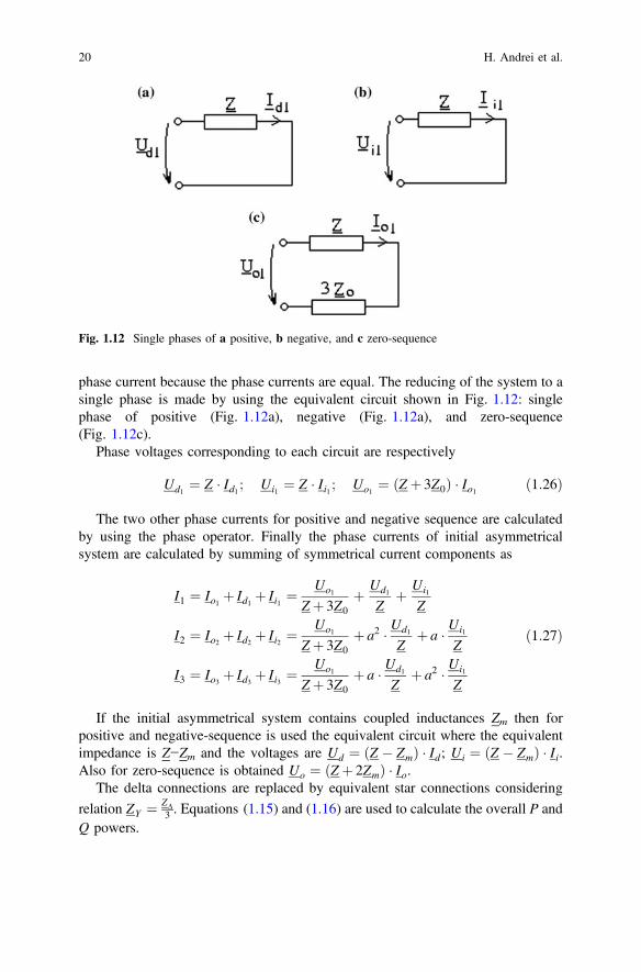
phase current because the phase currents are equal. The reducing of the system to a

single phase is made by using the equivalent circuit shown in Fig. 1.12: single

phase of positive (Fig. 1.12a), negative (Fig. 1.12a), and zero-sequence

(Fig. 1.12c).

Phase voltages corresponding to each circuit are respectively

Ud1¼ Z � Id1 ; Ui1

¼ Z � I i1 ; Uo1¼ Z þ 3Z0ð Þ � Io1 ð1:26Þ

The two other phase currents for positive and negative sequence are calculated

by using the phase operator. Finally the phase currents of initial asymmetrical

system are calculated by summing of symmetrical current components as

I1 ¼ Io1 þ Id1 þ I i1 ¼Uo1

Zþ 3Z0

þ Ud1

Zþ Ui1

Z


Zþ 3Z0

þ a2 � Ud1

Zþ a � Ui1

Z


Zþ 3Z0

þ a � Ud1

Zþ a2 � Ui1

Z

ð1:27Þ

If the initial asymmetrical system contains coupled inductances Zm then for

positive and negative-sequence is used the equivalent circuit where the equivalent

impedance is Z−Zm and the voltages are Ud ¼ Z � Zmð Þ � Id; Ui ¼ Z � Zmð Þ � I i.Also for zero-sequence is obtained Uo ¼ Zþ 2Zmð Þ � Io.

The delta connections are replaced by equivalent star connections considering

relation ZY ¼ ZD

3. Equations (1.15) and (1.16) are used to calculate the overall P and

Q powers.

Fig. 1.12 Single phases of a positive, b negative, and c zero-sequence

20 H. Andrei et al.

In conclusion, the elementary method of symmetrical components comprises the

following steps:

(i) asymmetrical supplied voltage system is decomposed in three symmetrical

components;

(ii) after the equivalence of coupled inductances and of delta-star connections,

are calculated the impedances of positive, negative and zero-sequences;

(iii) symmetrical components of currents system are calculated by using single

phase circuit and phase operator;

(iv) asymmetrical currents of initial system are calculated by adding the sym-

metrical current components.

1.4 State of the Art: Measurement Methods of Power

Systems Parameters

In EPS systems it is important to measure its electrical characteristics [26]. In this

section are described and illustrated measurement methods of voltage, current,

active power and frequency.

Regardless of what parameter is measured, before the actual operation is done

there are some precautions to be considered:

• the level of the measured parameter

• the scale of the measuring apparatus

In order to have a safe measuring operation, the maximum value of the measured

parameter should not be higher than the maximum indication of the measuring

device. If this precaution is not carefully considered, it could lead to permanent

damage of the measuring instrument.

1.4.1 Voltage Measurement

(i) Mono-phase circuits. In mono-phase circuits, the voltage measurement con-

sists in connecting a voltmeter at the terminals of the voltage source [27] as

indicated in Fig. 1.13. Voltmeter V indicates the rms value of the voltage

source.

(ii) Three-phase circuits contain two types of voltages, as are described in

Sect. 1.3: line voltage—that is measured between two lines of the supply

system, and phase voltage—that is measured between one line and the com-

mon point.

In Fig. 1.14 is shown the measurement principle of line and phase voltages.

There voltmeter V1 measures the line voltage between the phases U and V, while


voltmeter V2 measures the phase voltage between the phases U and the common

point.

1.4.2 Current Measurement

The current appears in an electrical circuit when it is closed on a load. If the circuit

is open, so that no load is connected to the source’s terminals, there is no current

flow. The current is measured by connecting an ammeter in series with the load

[28].

(i) Mono-phase circuits. In mono-phase circuits the current in measured by

connecting in series an ammeter with the load. In Fig. 1.15 is indicated the

procedure to measure the rms value of current across the load Z.

(ii) Three-phase circuits. In three-phase circuits the current is measured in the

same way as in mono-phase circuits. The measuring of the current for each

phase of the circuit there will be used three ammeters, one for each circuit

phases. In Fig. 1.16 the ammeters A1, A2 and A3 measure the rms values of

current through the loads Z1, Z2 and Z3, respectively.

If the loads are identical on all the three phases, they constitute a balanced

circuit, it is enough to connect in series only one ammeter on only one phase, as the

other rms values of currents are equals. This situation is displayed in Fig. 1.17.

Fig. 1.13 Voltage

measurement in mono-phase

AC circuits

Fig. 1.14 Phase and line

voltage measurements

22 H. Andrei et al.

1.4.3 Active Power Measurement

(i) Active power measurement in mono-phase circuits can be done with the

wattmeter. The wattmeter has two coils [29]: current and voltage. The voltage

coil of the wattmeter is connected in parallel with the load, while the current

coil is connected in series with the load, as displayed in Fig. 1.18.

(ii) Active power measurement in three-phase circuits is quite similar regardless of

load configuration as far as procedure [30]. This consists in connecting a

wattmeter in the circuit with the current coil in series with the load and with

Fig. 1.15 Current


circuit

Fig. 1.16 Current

measurement in three-phase

circuit

Fig. 1.17 Current

measurement for a

three-phase balanced circuit


the voltage coil in parallel with the load. The three-phase circuits have some

particularities due to load configurations.

If the load has a neutral line, such as star connected loads, then the power can be

measured by using three wattmeters. The voltage coils of the wattmeters are con-

nected between each phase and the neutral point of the load and voltage source [4].

The current coils are connected in series with the load on each phase, as displayed

in Fig. 1.19.

If the load does not have an accessible neutral point or is delta connected, in

order to measure the power using three wattmeters, these are connected such as to

construct an artificial neutral point for them. This situation is indicated in Fig. 1.20.

Thus the active power absorbed by the load can be expressed by

P ¼ P1 þP2 þP3 ð1:28Þ

If a neutral point is created, it is preferred that it has the same potential as one of

the source phase as indicated in Fig. 1.21. In this situation the indication of the third

wattmeter would be zero as its voltage coil would be connected at the same

Fig. 1.18 Active power


circuits

Fig. 1.19 Active power


circuits with neutral line load

24 H. Andrei et al.

potential. Because of this, it is eliminated from the circuit as not being useful. The

measured active power is the sum of the indications of each wattmeter, expressed as

P ¼ P1 þP2 ð1:29Þ

A different situation is the case of balanced loads and symmetrical voltages on

each source phase. In this case it is enough to use one wattmeter as indicated in

Fig. 1.22. In this situation, the total power is determined by multiplying the indi-

cation of the wattmeter by three, as in expressed in Eq. (1.30)

P ¼ 3 � P1 ð1:30Þ

The situation presented in Fig. 1.22 is valid if the load has an accessible neutral

point. In case that the load does not have an accessible neutral point, or is delta

connected, then it is created an artificial neutral point by using two additional

Fig. 1.20 Power


circuits without neutral line

load

Fig. 1.21 Power


circuits without neutral line

load using two wattmeters


resistors as indicated in Fig. 1.23. The values of the additional resistors R1 and R2

are equal to the value of the resistance of the voltage circuit of the wattmeter.

1.5 State of the Art: Standards for Power Systems

Parameters

Electrical energy needed to power industrial or household electric consumers, as all

the products, should satisfy same quality demands. These demands, like good PQ

ensure the electrical equipment is to operate without errors and this is a responsively

of the supplier [17, 31].

On the other hand, an important part of the equipment in use today, in particular

electronic and computer devices generates distortion of the voltage supply in the

installation, because of its non-linear characteristics, i.e. it draws a non-sinusoidal

Fig. 1.22 Power

measurement for balanced

load and symmetrical source

voltage with natural neutral

point

Fig. 1.23 Power

measurement for balanced

load and symmetrical source

voltage with an artificial

neutral point

26 H. Andrei et al.

current with a sinusoidal supply voltage. In this case the PQ is a responsively of the

electricity user.

In consequence, maintaining satisfactory PQ is a joint responsibility for the

supplier and the electricity user.

Standard IEC 60038 distinguishes “two different voltages in electrical networks

and installations” [32]:

– supply voltage, which “is the line-to-line or line-to-neutral voltage at the point

of common coupling (PCC), i.e. main supplying point of installation”;

– utility voltage, which “is the line-to-line or line-to-neutral voltage at the plug or

terminal of the electrical device”.

The main document dealing with demands concerning the supplier’s side is

standard EN 50160 [33] which characterize voltage parameters of electrical energy

in public distribution systems.

According with Standard EN 50160, “the main voltage characteristics of public

distribution systems are”:

Supply voltage—“the root mean square (rms) value of the voltage at a given

moment at the PCC, measured over a given time interval”.

Nominal voltage of the system (Un)—“the voltage by which a system is desig-

nated or identified and to which certain operating characteristics are referred”.

Declared supply voltage (Uc)—“is normally the nominal voltage Un of the

system. If, by agreement between the supplier and the user, a voltage different from

the nominal voltage is applied to the terminal, then this voltage is the declared

supply voltage Uc”.

Normal operating condition—“the condition of meeting load demand, system

switching and clearing faults by automatic system protection in the absence of

exceptional conditions due to external influences or major events”.

Voltage variation—“is an increase or decrease of voltage, due to variation of the

total load of the distribution system or a part of it”.

Flicker—“impression of unsteadiness of visual sensation induced by a light

stimulus, the luminance or spectral distribution of which fluctuates with time”.

Flicker severity—“intensity of flicker annoyance defined by the UIE-IEC flicker

measuring method and evaluated by the following signals”:

– Short term severity (Pst) “measured over a period of ten minutes”;

– Long term severity (Plt) “calculated from a sequence of 12 Pst—values over a

two-hour interval, according to the following expression”:

Plt ¼

ffiffiffiffiffiffiffiffiffiffiffiffiffiffi

X

12

i¼1

P3sti

12

3

v

u

u

t ð1:31Þ

Supply voltage dip—“a sudden reduction of the supply voltage to a value

between 90 and 1% of the declared voltage Uc, followed by a voltage recovery after


a short period of time”. Conventionally, the duration of a voltage dip is between

“10 ms and 1 min”. The depth of a voltage dip is defined as the “difference between

the minimum rms voltage during the voltage dip and the declared voltage”.

Supply interruption—is a condition in which “the voltage at the supply terminals

is lower than 1% of the declared voltage Uc”. A supply interruption is classified as:

– “prearranged in order to allow the execution of scheduled works on the dis-

tribution system, when consumers are informed in advance”;

– “accidental, caused by permanent (a long interruption) or transient (a short

interruption) faults, mostly related to external events, equipment failures or

interference”.

Temporary power frequency over-voltages—“have relatively long duration,

usually of a few power frequency periods”, and originate mainly from switching

operations or faults, e.g. sudden load reduction, or disconnection of short circuits.

Transient over-voltages—“are oscillatory or non-oscillatory, highly damped,

short over-voltages with a duration of a few milliseconds or less, originating from

lightning or some switching operations”, e.g. at switch-off of an inductive current.

Harmonic voltage—“a sinusoidal voltage with a frequency equal to an integer

multiple of the fundamental frequency of the supply voltage”. Harmonic voltages

can be evaluated:

– “individually by their relative amplitude Uh related to the fundamental voltage

U1”, where h is the order of the harmonic;

– “globally, usually by the total harmonic distortion factor THDu”, calculated

using the following expression:

THDu ¼

ffiffiffiffiffiffiffiffiffiffiffiffiffiffiffiffiffiffiffiffiffiffiffiffiffiffiffiffiffiffiffi

X

40

h¼2

ðUhÞ2

,

U1

v

u

u

t ð1:32Þ

Inter-harmonic voltage—“is a sinusoidal voltage with frequency between the

harmonics”, i.e. the frequency is not an integer multiple of the fundamental.

Voltage unbalance—“is a condition where rms value of the phase voltages or the

phase angles between consecutive phases in a three-phase system is not equal”.

Standard EN 50160 gives the main voltage parameters and their permissible

deviation ranges at the customer’s PCC in public low voltage (LV) and medium

voltage (MV) electricity distribution systems, under normal operating conditions

(Fig. 1.24). In this circumstances, LV signify that the phase to phase nominal rms

voltage does not exceed 1000 V and MV signify that the phase-to-phase nominal

rms value is between 1 and 35 kV.

The comparison of the EN 50160 requirements with those of the EMC standards

EN 61000, listed in Table 1.2 show significant differences in various parameters

[33–35].

28 H. Andrei et al.

Fig. 1.24 Exemplification of a voltage dip and a short supply interruption, classified according to

EN 50160; Un—nominal voltage of the supply system (rms), UA—amplitude of the supply

voltage, U (rms)—the actual rms value of the supply voltage [3]

Table 1.2 Comparison of supply voltage requirements according to EN 50160 and the EMC

standards EN 61000

No Parameter Supply voltage

characteristics

according to EN

50160

Low voltage

characteristics according

to EMC standard EN

61000

EN 61000-2-2 Other parts

1 Power

frequency

LV, MV: mean value

of fundamental

measured over 10 s

±1% (49.5–50.5 Hz)

for 99.5% of week

–6%/+4% (47–52 Hz)

for 100% of week

2%

2 Voltage

magnitude

variations

LV, MV: ±10% for

95% of week,

mean 10 min rms

values (Fig. 1.1)

±10% applied for

15 min

3 Rapid voltage

changes

LV: 5% normal

10% infrequently

Plt � 1 for 95%

of week

MV: 4% normal

6% infrequently

Plt � 1 for 95%

of week

3% normal

8% infrequently

Pst < 1.0

Plt < 0.8

3% normal

4% maximum

Pst < 1.0

Plt < 0.65

(EN 61000-3-3)

3% (IEC

61000-2-12)

(continued)


Table 1.2 (continued)

No Parameter Supply voltage

characteristics

according to EN

50160

Low voltage

characteristics according

to EMC standard EN

61000

EN 61000-2-2 Other parts

4 Supply voltage

dips

Majority: duration

<1 s, depth <60%

Locally limited dips

caused by load

switching on:

LV: 10–50%, MV:

10–15% (Fig. 1.1)

urban:

1–4 months

up to 30% for

10 ms

up to 60% for

100 ms

(EN 61000-6-1,

6-2)

up to 60% for

1000 ms

(EN 61000-6-2)

5 Short

interruptions of

supply voltage

LV, MV: (up to

3 min)

few tens—few

hundreds/year

Duration 70% of them

<1 s

95% reduction for

5 s

(EN 61000-6-1,

6-2)

6 Long

interruption of

supply voltage

LV, MV:

(longer than 3 min)

<10–50/year

7 Temporary,

power

frequency

over-voltages

LV: <1.5 kV rms

MV: 1.7 Uc (solid or

impedance earth)

2.0 Uc (unearthed or

resonant earth)

8 Transient

over-voltages

LV: generally <6 kV,

occasionally higher;

rise time: ms—ls.

MV: not defined

±2 kV,

line-to-earth

±1 kV,

line-to-line

1.2/50(8/20)

Tr/Th ls

(EN 61000-6-1,

6-2)

9 Supply voltage

unbalance

LV, MV: up to 2% for

95% of week, mean

10 min rms values,

up to 3% in some

locations

2% 2%

(IEC 61000-2-12)

10 Harmonic

voltage

LV, MV: (Table 1.2) 6%-5th, 5%-7th,

3.5%-11th,

3%-13th,

THD <8%

5% 3rd, 6% 5th,

5% 7th, 1.5% 9th,

3.5% 11th,

3% 13th,

0.3% 15th,

2% 17th

(EN 61000-3-2)

11 Inter-harmonic

voltage

LV, MV: under

consideration

0.2%

30 H. Andrei et al.

Harmonic emissions are subject to various standards and regulations [36, 37]:

– “Compatibility standards for distribution networks”;

– “Emissions standards applying to the equipment causing harmonics”;

– “Recommendations issued by utilities and applicable to installations”.

Currently, a triple system of standards and regulations is in force based on the

documents listed below.

“Standards governing compatibility between distribution networks and prod-

ucts” determine the necessary compatibility between distribution networks and

products:

– The harmonics caused by a device must not disturb the distribution network

beyond certain limits;

– Each device must be capable of operating normally in the presence of distur-

bances up to specific levels;

– Standard IEC 61000-2-2 is applicable for public low-voltage power supply

systems;

– Standard IEC 61000-2-4 is applicable for LV and MV industrial installations.

“Standards governing the quality of distribution networks” contain:

– Standard EN 50160 stipulates the characteristics of electricity supplied by public

distribution networks;

– Standard IEEE 519 presents a joint approach between utilities and customers to

limit the impact of non-linear loads. What is more, utilities encourage preventive

action in view of reducing the deterioration of PQ, temperature rise and the

reduction of power factor. They will be increasingly inclined to charge cus-

tomers for major sources of harmonics.

“Standards governing equipment” contain

– Standard IEC 61000-3-2 for low-voltage equipment with rated current under

16 A;

– Standard IEC 61000-3-12 for low-voltage equipment with rated current higher

than 16 A and lower than 75 A.

Maximum permissible harmonic levels

An estimation of typical harmonic contents often encountered in electrical dis-

tribution networks and the levels that should not be exceeded is presents in

Table 1.3.

Example 1.3 For an assessment of supply voltage, three-phase network,

240 V/400 V are presented the measurement values which was done with PowerQ

Plus MI 2392, a portable multifunction instrument for measurement and analysis of

three-phase power systems shown in Fig. 1.25. The basic measurement time

interval for: voltage, current, harmonics is a 10-cycle time interval. The 10-cycle

measurement is resynchronized on each interval tick according to the IEC

61000-4-30 Class B [38, 39]. Measurement methods are based on the digital


sampling of the input signals, synchronized to the fundamental frequency. Each

input (3 voltages and 3 currents) is simultaneously sampled 1024 times in 10 cycles

(Fig. 1.26).

The supply voltage, which is the line-to-line or line-to-neutral voltage at the PCC

[38] i.e. main supplying point of installation. The measured values of supply

voltage parameters without and with load (a three-phase asynchronous motor) are

presented in Tables 1.4 and 1.5, respectively.

Table 1.3 Maximum admissible harmonic voltages and distortion (%), h—order of harmonic [36,

37]

LV MV HV

Odd harmonics

non-multiples of 3

5 6 5 2

7 5 4 2

11 3.5 3 1.5

13 3 2.5 1.5

17 < h < 49 2:27 17h� 0:27 1:9 17

h� 0:2 1:2 17

h

Odd harmonics

multiples of 3

3 5 4 2

9 1.5 1.2 1

15 0.4 0.3 0.3

21 0.3 0.2 0.2

21 < h < 45 0.2 0.2 0.2

Even harmonics 2 2 1.8 1.4

4 1 1 0.8

6 0.5 0.5 0.4

8 0.5 0.5 0.4

10 <= h <= 50 0:25 10hþ 0:25 0:25 10

hþ 0:22 0:19 10

hþ 0:16

THDu 8 6.5 3

Fig. 1.25 a Power Q-meter, b Measurement stand

32 H. Andrei et al.

Fig. 1.26 Wiring diagram for U, I, f measurements

Table 1.4 The parameters values of supply voltage—without load

4 W L1 L2 L3 Unit of measurement

UL 235.8 235.3 234.4 V

THDu 2.5 2.6 2.3 %

h1 100 100 100 %

h2 0 0 0 %

h3 0.3 0.3 0.2 %

h4 0 0 0 %

h5 2.0 2.1 2.0 %

h6 0 0 0 %

h7 1.2 1.3 1.2 %

h8–h10 0 0 0 %

h11 0.1 0.2 0.1 %

h12 0 0 0 %

h13 0 0.1 0 %

h14–h18 0 0 0 %

h19 0 0 0.1 %

h20–h50 0 0 0 %

IL 0 A

THDi 0 %

f 49.98 Hz


ULL 410.3 407.7 405.7 V

THDu 2.5 2.4 2.3 %

I0 0.5 A

f 49.98 Hz


In concordance with the measured values presented in Tables 1.4 1.5, then:

– voltage magnitude variations: ±10%, means range [216−264 V]/[360–440 V];

– harmonic voltage: 6%-5th, 5%-7th, 3.5%-11th, 3%-13th, THDu <8%;

– frequency mean value of fundamental measured over 10 s,±1% (49.5–50.5 Hz).

Thus the electric parameters of public distribution systems, in PCC and the

utility voltage satisfy the requirements of standards set.

1.6 Importance of Reactive Power

Reactive energy and reactive power represent basic signals which are present in all

alternating voltage installations, due to their nature and specificity, although they do

not produce directly useful effects (light, heat, mechanical work etc.). Most of the

time, the realization of useful effects is not possible without reactive energy con-

sumption, taking into account the magnetization processes that take place in motor

drives iron cores and in electrical transformers. Also, the leakage fluxes corre-

sponding to the electric lines and to the coils determine reactive power consump-

tion. The resistors, used as electrical energy receivers, consume only active energy,

Table 1.5 The parameters values of supply voltage—with load three-phase asynchronous electric

motor 240 V/400 V, 6.6A/3.8 A, 1.5 kW, 1405 rpm, 50 Hz


UL 234.8 234.9 233.5 V

THDu 2.3 2.4 2.3 %

h1 100 100 100 %

h2 0 0 0 %

h3 0.2 0.2 0.2 %

h4 0 0 0 %

h5 1.8 2.0 1.9 %

h6 0 0 0 %

h7 1.2 1.1 1.2 %

h8-h14 0 0 0 %

h15 0.1 0.0 0.0 %

h16-h50 0 0 0 %

IL 2.3 2.4 2.5 A

f 49.98 Hz


ULL 409.3 407.0 404.0 V

THDu 2.3 2.6 2.5 %

I0 0.6 A

f 49.98 Hz

34 H. Andrei et al.

but its transfer through the installations placed upstream reactive determines energy

and reactive power losses.

In general, one can say that, in nowadays electrical systems, the active energy

and active power management take place only in the presence and with a big

consumption of reactive energy and reactive power. From here it results also the

concern that, the problems corresponding to producing and management of reactive

power and reactive energy to be examined simultaneously with those related to

active power and under higher efficiency taking into account their corresponding

specificity. At the same time, one should notice also the signal that expresses the

correlation between the two powers and energies categories that is the power factor

PF, as a main signal for guiding the corresponding problems analysis.

As a general aspect for reactive power and reactive energy management in

electrical installations, one considers as necessary, to underline the essential dif-

ference between the process required to produce active power and active energy

that takes place, in principal, in electric power plants, belonging to the energetic

system and the one corresponding to producing reactive energy and reactive power.

This is due to that active energy production implies primary energy consumption,

which is not the case of the reactive energy, excepting the case for covering some

active energy losses, reduced as signal.

The necessity to have a reactive power flow control arises from the fact that,

practically, in each station, for solving sinusoidal states, the adopted solution is that

of using capacitor banks. These are installed, usually, on LV mains power supply of

the transformer power, where are connected the consumers from all or from a part

of the enterprise. The purpose, with priority, is to obtain an overall power factor, at

least equal to the neutral value (imposed by the electrical energy provider contract),

in the point used for measuring the active and reactive energy consumption of the

electrical installations placed downstream, avoiding the overcompensation situa-

tions. In general, for the energy provided to the consumers, the values obtained for

the overall power are in 0.93 … 0.97 range.

Many factories use also automatic multi-step power factor correction systems

(MSPFC), to maintain constant value for the power factor. This is the situation for

long-term functioning in industrial installations, on the occasion of the current jobs.

One can affirm this solution contributes to a rational management of the reactive

energy and reactive power, representing a priority in the electrical energy sector.

The analysis of this aspect is done, in general, at the enterprises level, because

the electrical energy consumers from this one, and especially the operation, with

very large nominal power range, sometimes due to over-sizes, as well as the cor-

responding low-loaded functioning, have the biggest weight from the general re-

active power consumption, sometimes up to 60–70%.

The transformers from the electroenergetical system take around 20% out from

the reactive power, the rest of the consumption belonging to the other installations.

The solution of placing a capacitor bank in the transformer power substation

under the name of global compensation, presents advantage only for upstream

installations, exterior to the enterprise, respectively for generating, transport and

distribution installations. Using this type of compensation, the advantage


represented by reactive and active power and energy losses, does not appear also for

enterprise’s installations. From this point of view the installations from the enter-

prise do not benefit from the advantage given by reactive power local production.

Taking into account the importance of the contribution, given by reactive power

compensation measures, also to the losses reduction in distribution installation

inside the enterprise, is indicated that, for on-going processes, to examine also the

possibilities to de-centralize the banks in proper installations, that is to use with

more economical compensation types, respectively, the individual or by sector

consumers.

It is necessary to notice that, a special importance for consumers and elec-

troenergetical system reactive power management, the apparition of new types of

receivers, with non-linear electrical characteristics critically influence the reactive

power management. The presence of the harmonic state, in many cases, determines

practically the total revision of the compensation used currently, by exclusively

installing the capacitor banks. This fact is determined by the reciprocal influence of

these two aspects, the reactive power compensation and the harmonic, implying the

application of a unique measure, respectively that of using filters that include also

the existing capacitor banks.

Due to the complexity of the two problems and especially to the necessity and of

the urgency of solving a phenomena assembly, one will examine, as follows, the

most important theoretical and technical-economical specific aspects, that can be

used to establish the on-going processes. In all cases, one should analyze, together,

the two problems, taking into account that practically all modern electrical energy

consumers present a nonlinear characteristic.

1.6.1 Reactive Power Flow Effects Evaluation

Electric devices are designed at a certain apparent power S that is proportional to

the product between the rms values corresponding to the voltage U and to the

current I. The power flow in the electroenergetical system is accompanied, function

of the electric energy consumer structure, by the active power flow P, reactive

power flow Q and distorted power flow D. The only useful one is the active power

flow and its corresponding share from the apparent power necessary is computed

using the power factor PF defined as [40]:

PF ¼ P

S¼ P

ffiffiffiffiffiffiffiffiffiffiffiffiffiffiffiffiffiffiffiffiffiffiffiffiffiffiffi

P2 þQ2 þD2p ð1:33Þ

The weights corresponding to the reactive and distorted powers are estimated

using the reactive factor q and the distorted factor s for the permanent harmonic

state, according to the relationships

36 H. Andrei et al.

q ¼ Q

P¼ tanu; s ¼ D

ffiffiffiffiffiffiffiffiffiffiffiffiffiffiffiffi

P2 þQ2p ¼ tanw ð1:34Þ

where the phasors P, Q, D form a three-orthogonal reference system, and the

phase-shifts u and w have the significance given in Fig. 1.27.

So, one obtains a new expression for the power factor k ¼ cos/ � cosw. If oneconsiders a sinusoidal permanent single-phase circuit, then: D ¼ 0ðw ¼ 0Þ and

k ¼ cosu so the power factor is numerically equal to the cosine of phase-shift angle

between the voltage and the current.

For three-phase equilibrium circuits, linear and sinusoidal voltage powered, the

power factor has exactly the same mathematical expression and significance as for

single-phase circuit case. If the electric circuits are slightly asymmetrical, then the

voltage-current phase-shifts are different from a phase to another u1 6¼ u2 6¼ u3

and the power factor will be:

PF ¼ P1 þP2 þP3ffiffiffiffiffiffiffiffiffiffiffiffiffiffiffiffiffiffiffiffiffiffiffiffiffiffiffiffiffiffiffiffiffiffiffiffiffiffiffiffiffiffiffiffiffiffiffiffiffiffiffiffiffiffiffiffiffiffiffiffiffiffiffiffiffiffiffiffiffi

ðP1 þP2 þP3Þ2 þðQ1 þQ2 þQ3Þ2q ð1:35Þ

where Pj and Qj are the active, respectively the reactive powers corresponding to

each one of the phases (j = 1, 2, 3).

The relationships above define the instantaneous power factor that corresponds

to a certain moment form the consumer’s installation functioning. Because the load

presents fluctuations, the current legislation recommends the determination of the

weighted overall power factor based on the active and reactive energy consumption

Ea, Er from a certain period, in the hypothesis that the receivers behave as a linear

three-phase load, in equilibrium, working in sinusoidal permanent state:

Fig. 1.27 Significance of

phase-shifts u and w


cosu ¼ Eaffiffiffiffiffiffiffiffiffiffiffiffiffiffiffiffi

E2a þE2

r

p ð1:36Þ

Related to the weighted overall power factor, this can be neutral when is being

determined without taking into consideration the reactive power compensation

installations, and general, when one takes into account the powers provided by

these installations. The value of the general weighted overall power factor from

which the reactive energy power consumption is no longer charged, is called

neutral power factor and for the national energetic system is cos�n ¼ 0; 92.For electrical installations inside the consumer: the power factor decreasing

causes, the effects of a reduced power factor, means and methods for power factor

mitigation, a technical-economical computation for placing the reactive power

sources etc.

The irrational and big reactive power consumption, that generates a reduced

power factor, presents a series of disadvantages for the electric installation, among

which we mention [25]: the increase of active power losses in the passive elements

of the installation, the increase of voltages’ losses, installation’ oversize and the its

electric energy diminished transfer capacity.

1.6.2 Harmonic State Indicator—Specific PQ Parameters

Electrical installations that contain non-linear consumers absorb non-sinusoidal

electric current even in the theoretical case of a perfect sinusoidal voltage supply.

The non-sinusoidal electric current flows through the impedances corresponding to

these electrical installations determine non-sinusoidal voltage drops that, super-

posed over the initial sinusoidal voltage signals, determine their distortion (shown

in Fig. 1.28). This determines a supplementary solicitation of the electrical

installations.

According to Fourier theory [3, 7] the periodic distorted signals can be

decomposed in sinusoidal components whose frequencies are integer multiple of

the frequency corresponding to the analyzed signal period. The sinusoidal signal

with reference frequency (that corresponds to the analyzed period signal) is called

fundamental signal, and the sinusoidal signals with frequency integer multiple of

the fundamental frequency are called harmonics.

u ¼ U0 þX

1

k¼1

ffiffiffi

2p

Uk sinðkx1tþ akÞ;

i ¼ I0 þX

1

k¼1

ffiffiffi

2p

Ik sinðkx1tþ bkÞð1:37Þ

38 H. Andrei et al.

where: U0 and I0 represents the DC components of the input voltage and current, Uk

and Ik are the rms values of harmonic voltages, respectively of the harmonic cur-

rents, x1 pulsation corresponding to the fundamental frequency, ak, bk—

phase-shifts corresponding to the harmonic voltages signals, respectively to har-

monic currents signals with respect to a reference axis.

To define the main indicators of harmonic state, we consider, as a reference

periodic signal, the electric wave shape through the load i(t) developed in Fourier

series. The following definitions are valid for any periodic signal [41, 42].

• Harmonic level—is defined as the ratio between the rms value of the harmonic

of rank k and the rms value of the fundamental harmonic (rank 1):

ck½%� ¼ Ik

I1� 100½%� ð1:38Þ

This factor is an important indicator for evaluating the distortion level, its

maximum admitted values is being indicated in the voltage or current signal.

• DC−component of the signal is defined as the integral on a variation signal

period:

Fig. 1.28 Fourier series decomposition of a periodic distorted voltage signal


Ih i ¼ DC ¼ 1

T

Z

T

t0 þT

iðtÞdt ¼ I0 ð1:39Þ

The mean value of a signal different from zero indicates the presence of a DC

component in its spectrum.

• Crest factor−CF—defined as the ratio between the maximum value (amplitude

iM of the periodic non-sinusoidal signal) and its rms value IRMS:

kv ¼ CFi ¼iM

IRMS

ð1:40Þ

• for a pure sine wave, kv = 1.41;

• for periodic “shaped-top” distorted waveform signal kv > 1.41;

• for a periodic “flat-top” distorted waveform signal kv < 1.41.

The voltage signals characterized by a crest factor kvi[ffiffiffi

2p

can present in time

dangerous thermal solicitations.

• Form Factor—is the ratio between the rms value of the signal and the mean

value corresponding to half a period Imed1/2:

kf ¼I

Imed1=2¼ kf ¼

IRMS

1T

R

t0 þ T

t0

iðtÞj jdtð1:41Þ

For the signals met in electrical installations the form factor can take the values:

• for a sinusoidal signal, kf = 1.11;

• for a periodic signal shaper than a sinusoid kf > 1.11;

• for a sinusoid flatter than a periodic signal kf < 1.11.

• Root Mean Square—rms Value:

IRMS ¼

ffiffiffiffiffiffiffiffiffiffiffiffiffiffiffiffiffiffiffiffiffiffiffi

1

T�Z

T

0

i2 � dt

v

u

u

u

t or IRMS ¼ffiffiffiffiffiffiffiffiffiffiffiffiffiffiffiffiffiffiffiffiffiffiffiffiffiffiffiffiffiffiffiffiffi

I20 þ I21 þ I22 þ . . .

q

¼ffiffiffiffiffiffiffiffiffiffiffiffi

X

n

k¼0

I2k

s

ð1:42Þ

40 H. Andrei et al.

Remarks:

• For signals containing harmonics one uses the terminology True rms Value. To

compute it, one should take into also the high-order harmonics (usual up to 50!).

• Not all measuring equipment can correctly measure the rms value of a

non-sinusoidal signal (True rms Value), many of them displaying only the rms

value corresponding to the fundamental (first harmonic)!

• Residual component (Id)—is computed as the rms value of the harmonics cor-

responding to the analyzed signal:

Id ¼ffiffiffiffiffiffiffiffiffiffiffiffiffiffiffiffiffiffi

I2RMS � I21

q

ffiffiffiffiffiffiffiffiffiffiffiffiffiffiffiffiffiffiffiffiffiffiffiffiffiffiffiffiffiffiffiffiffiffi

I20 þ I22 þ I23 þ . . .

q

ð1:43Þ

The distortion residue is a measure if the thermal effect determined by the

distorted signal harmonic components.

• Total Harmonic Distortion−THD—is the ratio between the distortion residue of

the signal and the fundamental rms value:

THDi ¼Id

I1¼

ffiffiffiffiffiffiffiffiffiffiffiffiffiffiffiffiffiffi

I2RMS � I21

p

I1¼


I22 þ I23 þ I23 þ � � �p

I1¼

ffiffiffiffiffiffiffiffiffiffiffi

P

n

k¼2

I2k

s

I1� 100 ½%� ð1:44Þ

The THD is one of the indicators used to evaluate the distortion level, the

maximum admitted values in the electrical network nodes being tabled [43].

• Distortion Factor−DF—is defined as the ratio between the distorted residue of

the signal and the rms value of the signal:

DFi ¼Id

IRMS

¼ffiffiffiffiffiffiffiffiffiffiffiffiffiffiffiffiffiffi

I2RMS � I21

p

IRMS

¼ffiffiffiffiffiffiffiffiffiffiffiffiffiffiffiffiffiffiffiffiffiffiffiffiffiffiffiffiffiffiffiffiffiffi

I22 þ I23 þ I23 þ � � �p

IRMS

¼

ffiffiffiffiffiffiffiffiffiffiffi

P

n

k¼2

I2k

s

IRMS

� 100 ½%� ð1:45Þ

The DF is much closed as value to THD and it is used also as a principal

indicator for appreciating the distortion level.

Remark:

• In literature [44, 45], THD is also denoted by THD-F (distortion related to the

fundamental) and DF can be found denoted by THD-R (distortion related to the

rms value)

• One can easily prove the relationship: I1Irms

¼ 1ffiffiffiffiffiffiffiffiffiffiffiffiffiffiffi

1þ THDi2p


• The derating factor KF of the transformer’s apparent power—is defined (only

for electric current) as follows:

KF ¼

P

n

k¼1

kIkð Þ2

P

n

k¼1

I2k

ð1:46Þ

where Ik is the rms value of the harmonic of rank k of the electric current that flows

through the transformer’s windings. KF (defined only for the current) allows an

evaluation of the supplementary heating of the transformers circulated by distorted

currents that imply derating its installed power [46, 47].

In order to evaluate the energetic indicators of harmonic state, one defines the

following types of powers:

• Single-phase active power P (active power) for harmonic state is:

P ¼ 1

m � T �Z

sþm�T

s

pdt ¼ 1

mT

Z

sþm�T

s

uidt ¼X

1

h¼1

UkIm cosuk W½ � ð1:47Þ

where uk = ak − bk is the phase-shift between the signals corresponding to the

voltage and to the current, in the plan of harmonic of rank k.

• Active energy Wa in harmonic state is:

Wa ¼Z

sþ t

s

P � dt Ws½ � ð1:48Þ

• Single-phase reactive power Q (reactive power) is given by the expression:

Q ¼X

1

k¼1

UkIk sinuk VAr½ � ð1:49Þ

42 H. Andrei et al.

• Single-phase reactive energy Wr in harmonic state is:

Wr ¼Z

sþ t

s

Q � dt VArs½ � ð1:50Þ

• Single-phase apparent power S (apparent power) is defined by the expression:

S ¼ URMSIRMS ¼ffiffiffiffiffiffiffiffiffiffiffiffiffiffiffiffiffiffiffiffiffiffiffiffiffiffiffiffiffiffiffiffiffiffiffiffiffiffiffi

U20 þU2

1 þU22 þ . . .

q

�ffiffiffiffiffiffiffiffiffiffiffiffiffiffiffiffiffiffiffiffiffiffiffiffiffiffiffiffiffiffiffiffiffi

I20 þ I21 þ I22 þ . . .

q

¼ffiffiffiffiffiffiffiffiffiffiffiffiffiffiffi

X

n

k¼0

U2k �

s ffiffiffiffiffiffiffiffiffiffiffiffi

X

n

k¼0

I2k

s ð1:51Þ

• Single-phase apparent energy W is defined by:

W ¼Z

sþ t

s

S � dt VAs½ � ð1:52Þ

• Distorted power—is defined as a complement of active and reactive power

related to the apparent power:

D ¼ffiffiffiffiffiffiffiffiffiffiffiffiffiffiffiffiffiffiffiffiffiffiffiffiffiffiffi

S2 � P2 � Q2p

VAd½ � ð1:53Þ

Remark:

• Most modern measuring equipment designed for measuring electric energy and

electric power can measure instantly each of the 4 defined powers (energies).

• Power Factor−PF—is defined as the ratio between the active power P and the

total apparent power S:


k ¼ PF ¼ P

S¼

P

1

k¼1

UkIk cosuk

URMSIRMS

ð1:54Þ

• Displacement Power Factor−DPF—is defined as the ratio between the active

power P1 and the apparent power S1, corresponding to the fundamental har-

monic (k = 1):

k1 ¼ DPF ¼ P1

S1¼ U1I1 cosu1

U1I1¼ cosu1 ð1:55Þ

Remarks:

• The two definitions for PF and DPF leads to different values displayed sepa-

rately by modern measuring equipment. Moreover, the value of the angle u1 and

its tangent tan u1 are also displayed.

• The equality k ¼ PS¼ cosu ðPF ¼ DPFÞ is valid only for a single-phase circuit

and only in a pure sinusoidal state (ideal case), so the interpretation of the power

factor function of voltage-current phase-shift should be avoided!

• If, it’s necessary, the dimensioning of a capacitor bank for reactive power

compensation can be done only based on power factor cosu1 = DPF and not on

PF!

• One can easily prove the relationship: PF ¼ cosu1ffiffiffiffiffiffiffiffiffiffiffiffiffiffiffi

1þ THDi2p ¼ DPF

ffiffiffiffiffiffiffiffiffiffiffiffiffiffiffi

1þ THDi2p (valid in the

case of negligible voltage distortion THDu < 5%).

Most of the above mentioned parameters are nowadays commonly indicated by

high accuracy measurement devices such PQ analyzers. They are able to perform a

complete Fourier analysis for the three-phase current and voltage signals up to the

50 harmonic. Figure 1.29 illustrates these parameters measured with a Chauvin

Arnoux 8335 device for a low-voltage industrial load.

General solutions for reducing the reactive power consumption are [48–50]:

• adopting, if possible, some technological processes, aggregates and technolog-

ical and functioning schemes, characterized by a high power factor;

• judicious choice of the type and powers for the electric motor drives, for the

transformers, avoiding over-sizing; introducing the synchronous motor instead

of the asynchronous one will be justified from economical point of view con-

sidering the asynchronous motor individually compensated with derivation

capacitors.

44 H. Andrei et al.

The principal means used especially in existing installations are the following:

• power transformers running in parallel, following the minimum reactive losses

graph, when the exploitation conditions allow it;

• exploitation of synchronous motors at the maximum limit of producing reactive

power;

• limiting the unloaded running of asynchronous motors, of special transformers,

if the technological process allows it;

• using Y-D switches for low-voltage asynchronous motors, systematically loaded

under 40% from its nominal load, for a long-term functioning in Y connection;

• replacing asynchronous motors and of the over-sized transformers, based on

technical-economic analysis using the updated total spending method.

The main specialized reactive power sources are synchronous compensators and

derivation capacitors.

Reactive power control has a significant role in role in supporting the power

transmission systems.

Fig. 1.29 Current signals, harmonics and various PQ parameters measured for a low-voltage

industrial load


Reactive power is required to deliver active power through transmission lines at

a certain voltage level. Motors, transformers and other power loads, intrinsically

require reactive power in order to maintain their functionality. Either the lake or the

excess of reactive power may lead to numerous PQ disturbances, which adversely

affect both the loads and the supply network [16].

References

1. J.C. Maxwell, A Treatise on Electricity and Magnetism, 3rd ed. vol. 1 and 2, New York,

Dover Publication, 1954.

2. V. Bellevitch, Classical Network Theory, Holden-Day, 1968.

3. L.O. Chua, Nonlinear Network Theory, New York, McGraw Hill, 1969.

4. P. Penfield Jr, R. Spence, S. Duinker, Tellegen’s Theorem and Electrical Networks, Research

monograph no. 58, Massachusetts, M.I.T. Press, 1970.

5. R.W. Newcomb, Linear Multiport Synthesis, New York, McGraw-Hill, 1966.

6. M. Preda, P. Cristea, Fundamentals of Electrotechnics (in Romanian: Bazele Electrotehnicii),

vol. 2, Bucharest, ed. Didactica si Pedagogica, 1980.

7. C.A. Desoer, E.S. Kuh, Basic Circuit Theory, New York, Mc Graw-Hill, 1969.

8. J.C. Willems, Dissipative and Dynamical Systems, Eur. J. Contr., vol. 13, pp. 134–151, 2007.

9. M. Vasiliu, I.F. Hantila, Electromagnetics, Bucharest, ed. Electra, 1st ed., 2006.

10. C.I. Mocanu, Electromagnetic Field Theory (in Romanian: Teoria Campului Electromagnetic,

Bucharest, ed. Didactica si Pedagogica, 1st ed., 1981.

11. C.I. Mocanu, Electric Circuits Theory (in Romanian: Teoria circuitelor electrice) Bucharest,

ed. Didactica si Pedagogica, 1st ed., 1979.

12. H. Andrei, Modern Electrical Engineering (in Romanian: Inginerie Electrica Moderna), vol. 1,

ed. Bibliotheca, Targoviste, 2010.

13. J. Arrillage, N. Watson, S. Chen, Power System Quality Assessment, John Wiley & Sons,

New York, 2001.

14. L.F. Beites, J.G. Mayordomo, A. Hernandes, R. Asensi, Harmonics, Inter Harmonic,

Unbalances of Arc Furnaces: A New Frequency Domain Approach, IEEE Transactions on

Power Delivery, 16(4), 2001, 661–668.

15. C. Cepisca, H. Andrei, S. Ganatsios, S.D. Grigorescu, Power Quality and Experimental

Determinations of Electrical Arc Furnaces, Proc. 14th IEEE Mediterranean Electrotechnical

Conference, MELECON, vol. 1 and 2, pp. 546–551, Ajaccio France, May 5–7, 2008.

16. A.E. Emmanuel, On the Assessment of Harmonic Pollution, IEEE Transaction on Power

Delivery, vol. 10(3), 1995, 1693–1698.

17. A. Eberhard, Power Quality, InTech, Vienna, 2011.

18. A.E. Emmanuel, Apparent Power Definition for Three-Phase systems, IEEE Transactions on

Power Delivery, 14 (3), 1999, 762–772.

19. J. Zhu, Optimization of Power System Operation, Willey & Sons, 2009.

20. P.S. Filipski, Y. Baghzouz, M.D. Cox, Discussion of Power Definitions Contained in the

IEEE Dictionary, IEEE Transaction on Power Delivery, vol. 9(3), 1994, 1237–1244.

21. E.F. Fuchs, M.A.S. Masoum, Power Quality in Power Systems and Electrical Machines,

Elsevier Academic Press, Amsterdam, 2006.

22. R. Hurst, Power Quality and Grounding Handbook, The Electricity Forum, Toronto, Canada,

1994.

23. V. Katic, Network Harmonic Pollution - A Review and Discussion of International and

National Standards and Recommendations, Proc. of Power Electronic Congress - CIEP,

pp. 145–151, Paris, France, October 24–26, 1994.

46 H. Andrei et al.

24. T.S. Key, J.S. Lai, IEEE and International Harmonic Standard Impact on Power Electronic

Equipment Design, Proc. of International Conference Industrial Electronics, Control and

Instrumentation - IECON, pp. 430–436, London, England, May, 25–27, 1997.

25. C. Sankaran, Power Quality, CRC Press, London, 2008.

26. P. Arpaia, Power Measurement, CRC Press LLC, 2000.

27. B. Gatheridge, How to Measure Electrical Power, EDN Network, 2012.

28. S. Humphrey, H. Papadopoulos, B. Linke, S. Maiyya, A. Vijayaraghavan, R. Schmitt, Power

Measurement for Sustainable High-Performance Manufacturing Processes, Procedia CIRP,

vol. 14, pp. 466–471, 2014.

29. M.A. Lombardi, Fundamentals of Time and Frequency, http://tf.nist.gov/general/pdf/ 1498.

pdf, Accessed July 2015.

30. Oscilloscope, https://en.wikipedia.org/wiki/Oscilloscope.

31. H. Markiewicz, A. Klajn, Power Quality Application Guide, Wroclaw University of

Technology, July 2004.

32. IEC 6038 - International Electrotechnical Commission Standard Voltages, 1999.

33. EN 50160 - European Norm Voltage Characteristics of Electricity Supplied by Public

Distribution Systems, 1999.

34. IEC 61000-4-7, International Electrotechnical Commission.

35. IEC 61000-4-15, International Electrotechnical Commission.

36. F.C. De La Rosa, Harmonics and Power Systems, New York, Taylor & Francis, 2006.

37. Electrical Installation Guide, Schneider Electric, 2015.

38. Technische Anschlussbedingungen (Technical requirements of connection), VDEW.

39. Rozporzadzenie Ministra Gospodarki z dnia 25 wrzesnia 2000, w sprawie szczególowych

warunków przylaczania podmiotów do sieci elektroenergetycznych, obrotu energia elek-

tryczna, swiadczenia uslug przesylowych, ruchusieciowego i eksploatacji sieci oraz

standardów jakosciowych obslugi odbiorców. Dziennik Ustaw Nr 85, poz. 957 (Rules of

detailed conditions of connection of consumers to the electrical power network and quality

requirements in Poland).

40. A.E. Emanuel, Power Definitions and the Physical Mechanism of Power Flow, John Wiley &

Sons, 2011.

41. A. Baggini, Handbook of Power Quality, John Wiley & Sons, 2008.

42. IEEE 100-1996, The IEEE Standard Dictionary of Electrical and Electronics Terms, 6th

Edition, 1996.

43. IEEE-WG, IEEE Working Group on Nonsinusoidal Situations, Practical Definitions for

Powers in Systems with Nonsinusoidal Waveforms and Unbalanced Loads, IEEE

Transactions on Power Delivery, vol. II, no. 1, 1996, 79–101.

44. R.C. Dugan, M.F. McGranaghan, S. Santoso, H.W. Beaty, Electrical Power Systems Quality,

McGraw Hill Professional, 2012.

45. A. Kusko, M. Thomson, Power Quality in Electrical Systems, McGraw Hill Professional,

2007.

46. IEC 61000-4-30, Testing and Measurement Techniques-Power Quality Measurement Method,

1999.

47. IEEE Recommended Practice for Monitoring Electric Power Quality, IEEE 1159, 1995.

48. Romanian Norm for Limitation of Harmonic Pollution and Unbalance in Electrical Networks,

PE 143, 2004.

49. Characteristics of Supplied Voltage in Public Distribution Networks, SREN 50160, October

1998.

50. Power Quality Application Guide, Voltage Disturbance, Standard EN50160, July 2004.


http://tf.nist.gov/general/pdf/

https://en.wikipedia.org/wiki/Oscilloscope

Chapter 2

Fundamentals of Reactive Power in AC

Power Systems

Horia Andrei, Paul Cristian Andrei, Emil Cazacu

and Marilena Stanculescu

Abstract The fundamentals of reactive power in AC power systems are discussed

in the second chapter. The chapter presents basic theory of AC circuits including

two-ports linear elements, basic equations and definition of powers in AC circuits.

The phasor diagrams and power measurement techniques in AC networks are also

presented. The chapter also investigates the effects of reactive power as well as

power factor compensation in consumers. The end part of the chapter is related to

minimum active and reactive absorbed power in linear AC circuits and also

non-sinusoidal conditions. All of the parts include some practical examples and

case studies. The chapter is closed with a large list of bibliographic references.

2.1 Chapter Overview

The chapter opens with an overview. Starting on the Kirchhoff’s laws expressed in

terms of symbolic (complex) form the basic theory of AC circuits is summarized in

first section of chapter two. The impedance and admittance are used in order to

characterize the behavior of two-ports linear elements. Also a review about the

analysis methods of AC circuits is absolutely necessary to emphasize the equations

systems that are commonly used. Then are introduced the definitions and physical

interpretation of powers in AC power systems: the active, reactive and apparent

H. Andrei (&)

Doctoral School of Engineering Sciences, University Valahia of Targoviste, Targoviste,

Dambovita, Romania


P.C. Andrei � E. Cazacu � M. Stanculescu

Department of Electrical Engineering, University Politehnica Bucharest, Bucharest, Romania


E. Cazacu


M. Stanculescu





49

power, the power, reactive and deforming factor, the overall harmonic distortion of

voltage and current, the harmonic level. Several examples put in evidence the

theoretical aspects presented below. General problems about energy and power in

AC power systems is intuitive and lead to a better understanding of the definitions

of these energetic parameters. Accompanied by presentation of some modern

measurement methods of these parameters and calculation examples for studied

cases of power systems, all of them are the subjects exposed in the third section of

this chapter.

The next section has as a main objective the reader’s assimilation of the fun-

damental problems of reactive power consumption automated management in

power systems and of some methods used to limit the negative effects due to a

reduced power factor. On this line, there has been elaborated a selection of the

equipment for power factor correction based on the analysis of the customer’s

electric energy quality. There are also presented the notions needed to design some

simple systems used to compensate the reactive power for different levels of the

installation. Several examples have been studied separately in this section.

The qualitative and quantitative aspects related to the active and reactive power

circulation in AC networks are presented in section four of this chapter. In this way

the recent Principles of Minimum Absorbed Active and Reactive Power (PMARP)

in AC Power Systems are demonstrated and formulated. For AC circuits under

sinusoidal and non-sinusoidal conditions the PMARP proves, on one hand, that the

active power absorbed by all the resistances of the AC power system is minimum

and, on the other hand, that the reactive power absorbed (generated) by all the

resistive-inductive (resistive-capacitive) elements is minimum.

Also one demonstrates that (i) this principle is verified by the currents which

satisfy Kirchhoff current law (KCL) and nodal method (NM), and (ii) the

co-existence (CEAPP) of PMARP and of maximum active power transfer theorem

(MPTT). Several examples presented hereinafter demonstrate the PMARP and

CEAPP for classical linear and reciprocal AC circuits under sinusoidal and

non-sinusoidal signals and prove the originality of the new theoretical concepts

introduced by authors. The second chapter is closed with a specific list of biblio-

graphic references.

2.2 Basic Theory of AC Circuits

2.2.1 Two-Port Linear Elements

(i) Sinusoidal signals—Characterization, symbolic representation

By definition, a sinusoidal signal is that signal whose time variation is described by

an expression of the following form [1–4]

50 H. Andrei et al.

x tð Þ ¼ Xmax sin xtþuð Þ ¼ Xffiffiffi

2p

sin xtþuð Þ ð2:1Þ

In Eq. (2.1) the signals have the following significance:

– Xmax—is the amplitude or the peak value of the sinusoidal signal and it repre-

sents the maximum positive value of x(t) variation during one period.

– X—is the effective (root mean square−rms) value of the sinusoidal signal.

Between amplitude and rms value there is a relationship as it can be deduced

from (2.1), which is the dependence: Xmax ¼ Xffiffiffi

2p

. The rms value X is the value

indicated by the measuring equipment.

– x—angular frequency. For a given signal, between the angular frequency and

its frequency (or period—T) there is the following relationship

x ¼ 2pf ¼ 2p

Tð2:2Þ

– a = xt + u—represents the phase at a given moment in time (t arbitrary). For

t = 0 one obtains the initial phase u of the sinusoidal signal.

To illustrate better the physical significance of these signals we represent

graphically the time variation of a sinusoidal signal in Fig. 2.1.

By definition, the mean value of a periodic signal is given by:

xh i ¼ 1

T

Z

t0 þT

t0

x tð Þdt ¼ 0 ð2:3Þ

Fig. 2.1 Signals and values characteristic for a sinusoidal variation

2 Fundamentals of Reactive Power in AC Power Systems 51

From Eq. (2.3) for a sinusoidal signal its corresponding mean value is zero.

A zero mean value periodic signal is called alternative signal. The rms value of a

signal is the square root of the mean value of the square of its corresponding

variation.

X ¼ffiffiffiffiffiffiffiffi

x2h ip

¼

ffiffiffiffiffiffiffiffiffiffiffiffiffiffiffiffiffiffiffiffiffiffiffiffiffiffiffi

1

T

Z

t0 þT

t0

x2ðtÞdt

v

u

u

u

t ¼ Xmaxffiffiffi

2p ð2:4Þ

For two signals having the same angular frequency x one defines the phase shift

u as being the difference between the phases corresponding to the two sinusoidal

signals—i.e. the difference between their initial phases.

x1ðtÞ ¼ X1

ffiffiffi

2p

sinðxtþu1Þx2ðtÞ ¼ X2

ffiffiffi

2p

sinðxtþu2Þu ¼ ðxtþu1Þ � ðxtþu2Þ ¼ u1 � u2

ð2:5Þ

In Fig. 2.2, is presented the phase-shift between two signals having different

amplitudes and different initial phases.

(ii) Complex representation of sinusoidal signals

For any sinusoidal signal x(t) of an angular frequency x, one can bi-univocally

associate a complex number X called its complex or the complex image of x(t), of

Fig. 2.2 The phase-shift between two sinusoidal signals

52 H. Andrei et al.

modulus equal to its rms value and the argument equal to the initial phase of the

sinusoidal signa

xðtÞ ¼ Xffiffiffi

2p

sinðxtþuÞ , X ¼ Xeju ¼ Xðcosuþ j sinuÞ ð2:6Þ

In Eq. (2.6) one denoted by j ¼ffiffiffiffiffiffiffi

�1p

the complex number of modulus equal to

one and the phase equal to p=2. This analytical representation used for sinusoidal

signals is called complex representation. This representation allows also a repre-

sentation in the complex plan of the sinusoidal signals (Fig. 2.3).

This representation is very useful because it allows the computation of AC

sinusoidal electrical circuits easier and allows also a better interpretation of the

obtained results.

As a consequence, during the first step, the sinusoidal signals will be expressed

using complex numbers. Then, after computation, using in principal the same

equivalence theorems and the same solving methods as in DC, one will came back

to time domain using bi-univocal properties of complex transformation.

(iii) Two-ports linear circuits’ elements

Passive circuit elements

In principal, these circuit’s elements are represented by: resistor, coil, capacitor and

mutually connected coils, each of these elements being characterized by a single

constant parameter: the resistance R, the inductivity L, the capacity C, respectively

the mutual inductance M, that is a parameter apart from the parameters corre-

sponding to the two magnetic coupled coils.

In Fig. 2.4 are presented the analytical equations characterizing each element.

For magnetic coupled coils the sign between the two terms is + if i1 and i2 have the

same direction with respect to the polarized terminals and the sign is − if i1 enters

the polarized terminal and i2 exits the polarized terminal, or vice versa. As it is

shown in the figure for the direction of the currents and for the terminals position

marked in the figure, the sign is positive.

Fig. 2.3 Complex representation of sinusoidal and complex signals


Active circuit elements

These elements are: the ideal voltage generator and the ideal current generator. The

ideal voltage generator is characterized by that no matter what the value of the

current intensity i(t) is, this gives at its terminals a constant voltage u(t) equal to the

value of the voltage generator e(t). The ideal current generator is characterized by

that no matter what the value of the voltage u(t) at its terminals is, this gives to the

circuits a constant current i(t) equal to the value given by the current generator j(t).

The symbols and the functioning equations corresponding to the ideal voltage

generator and to the ideal current generator are presented in Fig. 2.5.

For real voltage and current generators, there is also another component called

inner resistance placed in series with the voltage generator and in parallel with the

current generator.

(iv) Complex imittances

The computation of periodic AC electrical circuits can be done in a systematic way

by using the notions of complex impedance respectively complex admittance named

using the common name of complex imittances.

To do this, one considers a passive linear two-port system, whose constitutive

inductive elements do not present magnetic couplings with the exterior.

The voltage and the current at its terminals have a sinusoidal variation Fig. 2.6.

( ) ( )R Ru t Ri t=( )

( ) LL

di tu t L

dt= 1

( ) ( )c Cu t i t dtC

= ∫

1

1

1 21

2 12

( )

( )

L

L

di diu t L M

dt dt

di diu t L M

dt dt

= ±

= ±

Fig. 2.4 Passive circuit’s elements

u(t) = e(t) i(t) = j(t)

Fig. 2.5 Ideal current ad

voltage generators

54 H. Andrei et al.

The time variation of the voltage and current at two-port system’s terminals:

uðtÞ ¼ Uffiffiffi

2p

sinðxtþuUÞ; U ¼ UejuU ¼ UðcosuU þ j sinuUÞiðtÞ ¼ I

ffiffiffi

2p

sinðxtþuIÞ; I ¼ IejuI ¼ IðcosuI þ j sinuIÞð2:7Þ

By definition one calls the complex impedance corresponding to the two-port

system as being the ratio between the complex images of the voltage at its terminals

and the absorbed current (Ohm’s law)

Z ¼ U

I¼ U

IejðuU�uIÞ ¼ Zeju ¼ Zðcosuþ j sinuÞ ¼ Rþ jX ð2:8Þ

The modulus Z [X] is called the two-port system’s real impedance and its

argument u ¼ uU � uI is called the two-port system’s phase and

R ¼ <e Zf g ¼ Z cosu� two-port system equivalent inner resistance X½ �X ¼ =m Zf g ¼ Z sinu� two-port system equivalent inner reactance X½ �

ð2:9Þ

Obviously one can determine the relationships

Z ¼ U

I¼


R2 þX2p

ð2:10Þ

By definition Y [S] one calls complex admittance of the two-port system the ratio

between the complex images of the current and of the voltage at its terminals:

Y ¼ I

U¼ I

Ue�jðuU�uI Þ ¼ Yeju ¼ Yðcosu� j sinuÞ ¼ G� jB ð2:11Þ

In Eq. (2.11) one identifies G—the equivalent conductance and B—the equiv-

alent susceptance as the real, respectively the changed sign coefficient of the

imaginary part from Y .

Fig. 2.6 Passive linear two-port system magnetically not coupled to the exterior


G ¼ <e Yf g ¼ Y cosu� two-port system equivalent inner conductance S½ �B ¼ =m Yf g ¼ Y sinu� two-port system equivalent inner susceptance S½ �

ð2:12Þ

As for the impedance case, for the admittance we have the relationships

Y ¼ I

U¼


G2 þB2p

;u ¼ arctanB

Gð2:13Þ

We notice that the admittance (real or complex) represents the inverse of the

impedance (real or complex). As a consequence, between the parameters shown

above one can determine a series of relationships

Y ¼ 1

Z

Y ¼ 1

Z

R ¼ G

Y2¼ GZ2

G ¼ R

Z2¼ RY2

X ¼ B

Y2¼ BZ2

B ¼ X

Z2¼ XY2

ð2:14Þ

Taking into account the Eqs. (2.10) and (2.13) we notice that it is possible to

build two right triangles generically called the impedances’ triangle and the

admittances’ triangle (Fig. 2.7).

The linear not-coupled with the exterior two-port system should compulsory

satisfy the condition

u 2 � p

2;

p

2

h i

ð2:15Þ

The condition (2.15) is equivalent to <e Zf g ¼ R� 0. If =m Zf g[ 0 or u[ 0

the regime is inductive. In this case we can equate the whole two-port system either

in series or in parallel (depending on the way in which one works: either in

impedance or in admittance) with a resistor in connection to an inductor.

For series connection For parallel connection

R ¼ <e Zf g

XL ¼ =m Zf g ) L ¼ XL

x

G ¼ <e Yf g

BL ¼ =m Yf g ) L ¼ 1

xBL

ð2:16Þ

22XRZ +=

22 BGY +=ZY 1=

Fig. 2.7 Imittances’ triangles

56 H. Andrei et al.

If =m Zf g\0 or u\0 the regime is capacitive. In this case we can equate the

whole two-port system either in series or in parallel (depending on the way in which

one works: either in impedance or in admittance) with a resistor in connection with

a capacitor.

For series connection For parallel connection

R ¼ <e Zf g

XC ¼ =m Zf g ) C ¼ 1

xXC

G ¼ <e Yf g

BC ¼ =m Yf g ) C ¼ BC

x

ð2:17Þ

2.2.2 Basic Equations: Kirchhoff’s Laws in Complex

Representation [2–5]

For circuits containing resistors, coils, capacitors and ideal sinusoidal electromotive

sources (emfs), the Kirchhoff’s Currents (KCL) and Voltage Laws (KVL) in

instantaneous values are given below

X

lk2njik ¼ 0 ð2:18Þ

X

lk2biðRk � ik þ Lk �

dik

dtþMkh �

dih

dtþ 1

Ck

Z

ikdtÞ ¼X

lk2biek ð2:19Þ

where: j ¼ 1; . . .; n� 1 are the n� 1 nodes of the circuit that can be expressed

using n� 1 independent KCL equations, i ¼ 1; . . .; l� nþ 1 are the b ¼ l� nþ 1

loops of the circuit that can be expressed using l� nþ 1 KVL independent

equations, and k = 1,…, l are the l branches of the circuit, eventually coupled with

other h ¼ 1; . . .; l; h 6¼ k, branches of the circuit.

Using the properties of the symbolic method, the equations in complex form

corresponding to Kirchhoff’s laws are obtained

X

IK2njIk ¼ 0; j ¼ 1; 2; . . .; n� 1 ð2:20Þ

X

IK2bjðRk � Ik þ jxLk � Ik þ jx Mkh � Ih þ

1

jxCk

� IkÞ ¼X

Ik2biEk

with i ¼ 1; 2; . . .; l�nþ 1

ð2:21Þ

The solutions Ik of the complex Eqs. (2.20) and (2.21) are therefore the sinu-

soidal particular solutions of the integral-differential Eqs. (2.18) and (2.19).


The resistive, inductive and capacitive voltages from the left side of Eq. (2.21)

can be written in complex form having a common representation that is Z.I with the

complex impedance defined according to its corresponding branch. Using this

convention, KVL is compactly expressed as follows

X

IK2bjZk � Ik ¼

X

Ik2bjEk ð2:22Þ

So, the statements of the two theorems are:

– KCL in complex form: “the sum of the currents’ complex representations in a

node nj is zero”;

– KVL in complex form: “the sum of the voltages’ complex representations

computed at the terminals of lk branches along a loop bj, is equal to the sum of

the complex representation corresponding to the emf from the branches

belonging to the same loop”.

In this way, the Eqs. (2.20) and (2.21) or (2.22) represent—for a circuit in

sinusoidal state having n nodes and l branches—the complete Kirchhoff indepen-

dent equations system with a number of l = (n–1) + (l–n + 1) equations and with

l unknowns.

There is a formal analogy between AC (sinusoidal state) and DC circuits, both

regarding the DC equations system and the AC circuits’ complex equations sys-

tems, as well as regarding the signals that characterize and describe the DC circuits

functioning and the AC circuits’ complex signals. as the following

DC AC

I , I

U , U

R , Z

E , E

The only difference between the two functioning states (DC and AC), is rep-

resented by circuits with magnetic couplings in sinusoidal state that have no cor-

respondent in DC state. That’s why, the computation, analysis methods and the

theorems established for DC state can be used without any modification for sinu-

soidal state circuits with no magnetic couplings.

The algorithm for AC circuit computation using Kirchhoff’s laws is:

– compute the circuit’s impedances, the complex emfs and the complex current

sources;

– draw the equivalent complex scheme of the circuit using the corresponding

complex;

– express Kirchhoff’s equations in complex form and solve the system (either in

currents unknowns, or in voltages unknowns);

58 H. Andrei et al.

– determine the corresponding instantaneous values form previously computed

complex values.

2.2.3 Definitions of Powers in AC Circuits [1, 6, 7]

To define the powers in sinusoidal periodic regime we consider again the case of

the linear, passive and inductive not-coupled with the exterior two-port system

(Fig. 2.6).

The instantaneous power—p is defined as the received power at each instance of

time at its terminals and is the product between the instantaneous values of the

voltage and current, having the following expression

pðtÞ ¼ uðtÞiðtÞ ¼ UI cosðuU � uIÞ � cosð2xtþuU þuIÞ½ � ð2:23Þ

As one can notice from Eq. (2.23) the instantaneous power contains two terms: a

constant term that characterizes the average power exchange of the two-port system

and an alternative term that has the angular frequency twice as much as the fre-

quency of the applied voltage.

Active power—P is by definition the average function of time of the instantaneous

power

P ¼ ph i ¼ 1

T

Z

t0 þT

t0

pðtÞdt ¼ UI cosðuU � uIÞ ¼ UI cosu ½W� ð2:24Þ

Taking into account the Eq. (2.24), the active power is always positive so it is

received by the passive linear two-port system.

Taking into consideration the relationships stated for the linear two-port system

case, the active power consumed by this one, can be also expressed function of its

resistance, respectively its conductance

P ¼ RI2 ¼ GU2 ð2:25Þ

The active power is consumed by the active elements from a circuit (the resis-

tances) its unit measure being the watt (W).

The reactive power—Q received by the two-port system is defined in a similar

manner as the active power

Q ¼ UI sinu ½VAr� ð2:26Þ

This power changes its sign together with the phase shift u between the voltage

and the current, such that it can be both positive and negative, therefore consumed


and generated by the two-port system. As in the active power case, the reactive

power can be expressed function of reactances or susceptances

Q ¼ XI2 ¼ BU2 ð2:27Þ

The reactive power is “consumed” by the circuit’s reactive elements (coils,

capacitors and magnetic coupled coils), its unit measure being volt-ampere reactive

(VAr).

The apparent power—S is by definition the product between the rms values of

voltage and current

S ¼ UI ½VA� ð2:28Þ

As in the previous cases we can express the apparent power function of the

passive linear two-port system’s imittances as

S ¼ ZI2 ¼ YU2 ð2:29Þ

The apparent power is an indicator upon the circuit’s functioning, being the

maximum of the active power for u ¼ 0, respectively of the reactive power for

u ¼ p=2. Its corresponding unit measure is (VA). Taking into account the defini-

tion procedure of these powers one can also introduce, as for the imittances’ case, a

triangle corresponding to the three powers: active, reactive ad apparent. In Fig. 2.8

there is represented the powers’ triangle as well as the computation relationships for

the active and reactive power, function of apparent power.

A very important signal from an energetic point of view is the power factor (PF)

defined as the ratio between the two-port system’s consumed active power and the

apparent power

PF � cosu � k ¼ P

S2 0 1½ � ð2:30Þ

A synthesis of the powers defined above is the complex power S, defined as the

product between the complex image of the voltage applied to the two-port system

and the complex conjugated complex image of the absorbed current

S ¼ U I� ¼ Seju ¼ Sðcosuþ j sinuÞ ¼ Pþ jQ ð2:31Þ

22 QPS +=

ϕcosSP =

ϕsinSQ =

Fig. 2.8 Powers’ triangle

60 H. Andrei et al.

As one can notice the modulus of the complex power is represented by the

apparent power, its real part can be identified with the active power and the

coefficient of the imaginary part can be identified with the reactive power defined

for the two-port system. Equation (2.28) states these remarks.

Sj j ¼ S

P ¼ <e Sf gQ ¼ =m Sf g

ð2:32Þ

For these reasons, when computing the powers, one proceeds directly to com-

pute the complex power after which one identifies the active and reactive powers by

separating its components.

Reactive circuits elements—energy sources (voltage sources, respectively current

sources) that generate complex power in the circuit. For the voltage sources’ case it

is given by the product between the complex image of the voltage at its terminals

and the complex conjugated image of the supplied current that circulates the source.

For the current source, the complex apparent power is given by the product between

the complex image of the voltage at its terminals and the complex conjugated image

of the source current. For both sources the relationships are taken with the plus sign

if the directions chosen for voltage and the current obeys the generator rule,

otherwise the complex powers present minus sign in front of the above expressions

(Fig. 2.5).

One should emphasize that the direction of the voltage at the current source

terminals should be chosen from the extremity indicated by the arrow at the base.

The total complex power for a circuit consists of a sum between all the complex

powers corresponding to all energy sources (voltage and current) from that circuit;

its real part should be equal to the active power, and its imaginary part should be

equal to the reactive power of the circuit.

S ¼X

n

k¼1

E k I�k þ

X

n

l¼1

UkJ�k ¼ Pþ jQ

P ¼X

n

k¼1

RkI2k

Q ¼X

n

k¼1

xLkI2k �

X

n

k¼1

1

xCk

I2k �X

n

k¼1

X

m

l¼1

2Mk<e I k I�l

� �

ð2:33Þ

If one computes separately the active, respectively the reactive power, the fol-

lowing identities exist P ¼ <e Sf g, Q ¼ =m Sf g, respectively. The power balance

mainly validates the computed currents values of a specific AC circuit.


2.2.4 Examples

Example 2.1 Let us consider the passive circuit from Fig. 2.9. The following

parameters of the circuit elements are known: R3 ¼ 2X, f ¼ 50Hz,

L2 ¼ 40=p mH, L5 ¼ 20=p mH, L6 ¼ 60=pmH, C1 ¼ 5=pmF, C4 ¼ 10=p mF,

uABðtÞ ¼ 128 � sin xtþ p=4ð Þ ½V�.Find:

(1) the instantaneous voltages at the terminals of each passive element from the

given circuit (using the voltage divider rule);

(2) the instantaneous electric currents for each passive element from the given

circuit (using the current divider rule).

We build the equivalent scheme in Fig. 2.10a. The passive elements are char-

acterized by impedances, and the source is characterized by a voltage phasor.

In the equivalent scheme we have

ZC1¼ 1

jx � C1

¼ �2j; ZC4¼ 1

jx � C4

¼ �j; ZL2¼ jx � L2 ¼ 4j

ZL5¼ jx � L5 ¼ 2j; ZL6

¼ jx � L6 ¼ 6j; ZR3¼ R3 ¼ 2

UAB ¼ 128ffiffiffi

2p � ej�p4 ¼ 64

ffiffiffi

2p

� cosp

4

� �

þ j sinp

4

� �h i

¼ 64 � ð1þ jÞ

where x ¼ 2p f ¼ 100p.

(1) Determination of the electric voltages at the circuit’s elements terminals. In

order to use the relationships from the voltage divider rule one should have the

impedances placed in series. Notice that the impedances ZC4and ZL5

are connected

in parallel and the equivalent impedance between these two is: Ze1¼ ZC4

�ZL5

ZC4þ ZL5

. It

results: Ze1¼ �2j. The impedances ZR3

and Ze1are connected in series

(Fig. 2.10b), so the equivalent impedance between these two is: Ze2¼ ZR3

þ Ze1. It

results: Ze2¼ 2� 2j.

Fig. 2.9 AC circuit with 6

branches

62 H. Andrei et al.

Notice the impedances Ze2and ZL2

are connected in parallel (Fig. 2.10c), and the

equivalent impedance between these two is: Ze3¼ Z

e2�Z

L2

Ze2þ Z

L2

. It results:

Ze3¼ 4 � ð1� jÞ.We obtained three impedances in series connection. We can apply the rela-

tionships from the voltage divider rule (Fig. 2.10d).

UC1¼ Z

C1

ZC1þ Ze3

þ ZL6

� UAB

Ue3¼ Z

e3

ZC1

þ Ze3þZ

L6

� UAB

UL6¼ ZL6

ZC1þ Ze3

þ ZL6

� UAB

8

>

>

>

>

<

>

>

>

>

:

Results:

UC1¼ 32 � ð1� jÞ ¼ 32

ffiffiffi

2p

� e�jp4

Ue3¼ 128 ¼ 128 � ej0

UL6¼ 96 � ð�1þ jÞ ¼ 96

ffiffiffi

2p

� ej3p4

8

<

:

Because Ue3is the voltage from the equivalent impedances’ terminals, we’ll

compute the voltages for each realized equivalence. The impedances Ze2and ZL2

are connected in parallel. It results: UL2¼ Ue2

¼ Ue3. UL2

¼ 128 ¼ 128 � ej0.The impedances ZR3

and Ze1are connected in series, so we can use the rela-

tionships corresponding to the voltage divider rule

Fig. 2.10 The equivalent AC circuit


UR3¼ Z

R3

ZR3

þZe1

� Ue2

Ue1¼ Ze1

ZR3þ Ze1

� Ue2

8

<

:

It results:

UR3¼ 64 � ð1þ jÞ ¼ 64

ffiffiffi

2p

� ejp4Ue1

¼ 64 � ð1� jÞ

�

The impedances ZC4and ZL5

are connected in parallel. It results:

Ue1¼ UC4

¼ UL5.

We obtain:

UC4¼ 64 � ð1� jÞ ¼ 64

ffiffiffi

2p

� e�jp4

UL5¼ 64 � ð1� jÞ ¼ 64

ffiffiffi

2p

� e�jp4

(

Therefore, there are determined all the voltages at the terminals corresponding to

each passive element in the complex domain. The instantaneous values of the

voltages determined above are

uC1ðtÞ ¼ 64 � sin xt � p

4

�

½V �; uL2ðtÞ ¼ 128ffiffiffi

2p

� sin xtð Þ ½V �uR3

ðtÞ ¼ 128 � sin xtþ p4

�

½V �; uC4ðtÞ ¼ 128 � sin xt � p

4

�

½V �uL5ðtÞ ¼ 128 � sin xt � p

4

�

½V �; uL6ðtÞ ¼ 192 � sin xtþ 3p4

�

½V �

8

<

:

(1) Determination of the currents across the circuit’s elements. We should deter-

mine the current IAB from the Fig. 2.10,e. Because the impedances ZC1, Ze3

and

ZL6are in series connection the current across them is : IAB ¼ U

AB

ZC1

þZe3þZ

L6

and

it results IAB ¼ IC1¼ Ie3 ¼ IL6 ¼ 16 � ð1þ jÞ. So we have

IC1¼ 16 � ð1þ jÞ ¼ 16

ffiffiffi

2p

� ejp4IL6 ¼ 16 � ð1þ jÞ ¼ 16

ffiffiffi

2p

� ejp4

(

Because the impedances Ze2and ZL2

are connected in parallel, we use the

relationships from the current divider rule to determine the currents IL2 and Ie2

IL2 ¼YL2

YL2

þ Ye2

� IABIe2 ¼

Ye2

YL2

þ Ye2

� IAB

8

<

:

64 H. Andrei et al.

It results

IL2 ¼ 16 � ð1� jÞ ¼ 16ffiffiffi

2p

� e�jp4

Ie2 ¼ 32j

�

The impedances ZR3and Ze1

are connected in series, so it results: Ie1 ¼ IR3¼ Ie2 .

So: IR3¼ 32j ¼ 32 � ejp2. Because the impedances ZC4

and ZL5are connected in

parallel, we determine the currents IL5 and IC4using the relationships from the

current divider rule

IL5 ¼YL5

YL5

þ YC4

� Ie1IC4

¼ YC4

YL5þ YC4

� Ie1

8

<

:

We obtain:

IL5 ¼ �32j ¼ 32 � e�j�p2

IC4¼ 64j ¼ 64 � ej�p2

�

The instantaneous values of the electric currents for each element are

iC1ðtÞ ¼ 32 � sin xtþ p

4

�

½A�; iL2ðtÞ ¼ 32 � sin xt � p4

�

½A�iR3

ðtÞ ¼ 32ffiffiffi

2p

� sin xtþ p2

�

½A�; iC4ðtÞ ¼ 64

ffiffiffi

2p

� sin xtþ p2

�

½A�iL5ðtÞ ¼ 32

ffiffiffi

2p

� sin xt � p2

�

½A�; iL6ðtÞ ¼ 32 � sin xtþ p4

�

½A�

8

<

:

Example 2.2 In the circuit given in Fig. 2.11 we have: R1 ¼ 2X, xL1 ¼ 1xC1

¼3X; xL2 ¼ 2X, 1

xC3¼ 1X, e1ðtÞ ¼ 20 � sin xtþ p

4

�

½V�, j3ðtÞ ¼ 10ffiffiffi

2p

�sin xtþ p

2

�

½A�.

(1) solve the circuit using Kirchhoff’s laws;

(2) solve the circuit using the superposition principle;

(3) power balance.

Fig. 2.11 AC circuit with

two energy sources


The computation of AC circuits is done using the complex representation. In

complex domain, the passive elements are characterized by impedances and the

energy sources by phasors. For the passive circuit elements, the impedances are

computed as follows

ZR1¼ R1 ¼ 2; ZL1

¼ jx � L1 ¼ 3j; ZC1¼ 1

jx � C1

¼ �3j; ZL2¼ jx � L2 ¼ 2j;

ZC3¼ 1

jx � C3

¼ �j

The voltage source is represented in complex domain by the phasor E1 ¼20ffiffi

2p � ejp4 ¼ 10 � ð1þ jÞ and the current source is represented in complex domain by

the phasor J3 ¼ 10ffiffi

2pffiffi

2p � ejp2 ¼ 10j. Grouping all the impedances from a branch in an

equivalent impedance one obtains (Fig. 2.11b), in which: Z1 ¼ ZR1þ ZL1

þ ZC1

¼ 2, Z2 ¼ ZL1¼ 2j and Z3 ¼ ZC1

¼ �j.

(1) Kirchhoff’s equations method

The topological elements are: 2 nodes, 3 branches and 2 loops. KCL and KVL are

expressed as

KCLðAÞ : �I1 þ I2 þ J3 ¼ 0

KVLðb1Þ : Z1 � I1 þ Z2 � I2 ¼ E1

KVLðb2Þ : Z3 � J3 � Z2 � I2 � Uj3¼ 0

8

<

:

We obtain

I1 ¼ 5j

I2 ¼ �5j

Uj3¼ 0

8

<

:

These values are transformed in time domain

i1ðtÞ ¼ 5ffiffiffi

2p

� sin xtþ p

2

� �

½A�

i2ðtÞ ¼ 5ffiffiffi

2p

� sin xt � p

2

� �

½A�

uj3ðtÞ ¼ 0 ½V�

(2) Superposition principle

The initial circuit (in complex domain) contains two ideal energy sources and so

we’ll have to compute two cases

66 H. Andrei et al.

Case 1

In this circuit the ideal voltage source is reduced to its inner resistance, and the ideal

current source is characterized by the phasor J3 (Fig. 2.12, a). We determine the

currents using the relationships from the current divider rule:

I 01 ¼Y1

Y1 þY2� J3 ¼

1Z1

1Z1

þ 1Z2

� J3

I 02 ¼Y2

Y1 þY2� ð�J3Þ ¼

1Z2

1Z1

þ 1Z2

:ð�J3Þ

8

>

<

>

:

We obtain:

I 01 ¼ 5 � ð�1þ jÞI 02 ¼ 5 � ð�1� jÞ

�

To determine the voltage U0j3

we apply KVL for the loop “b” such that:

ðbÞ : Z3 � J3 � Z2 � I 02 � U0j3¼ 0, and results: U0

j3¼ 10j.

Case 2

In this circuit the ideal current source is reduced to its inner resistance) and the ideal

voltage source is characterized by the phasor E1 (Fig. 2.12b). Applying KVL for

the loop “b” such that: ðbÞ : Z1 � I 001 þ Z2 � I 002 ¼ E1. We take into account that

I 001 ¼ I 002 , and results I 001 ¼ I 002 ¼ 5. One notices that U00j3¼ �Z2 � I 002 . We obtain:

U00j3¼ �10j.

The final results are obtained by superposing the results obtained independently

in each of the two cases. Taking into account the directions of the determined

signals for each case compared to the directions from the initial circuit

I1 ¼ I 01 þ I 001I2 ¼ I 02 þ I 002Uj3

¼ U0j3þU00

j3

8

<

:

Fig. 2.12 Superposition principle


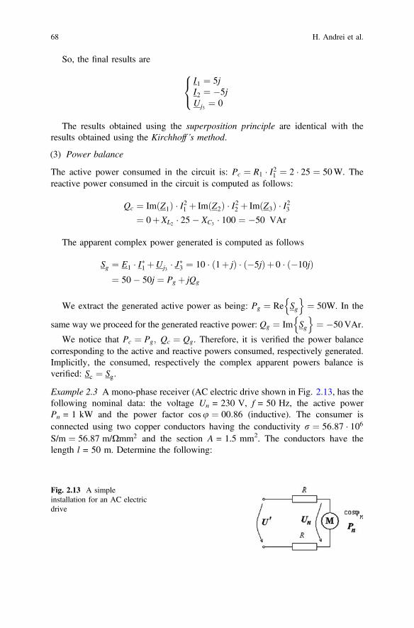
So, the final results are

I1 ¼ 5j

I2 ¼ �5j

Uj3¼ 0

8

<

:

The results obtained using the superposition principle are identical with the

results obtained using the Kirchhoff’s method.

(3) Power balance

The active power consumed in the circuit is: Pc ¼ R1 � I21 ¼ 2 � 25 ¼ 50W. The

reactive power consumed in the circuit is computed as follows:

Qc ¼ Im Z1ð Þ � I21 þ Im Z2ð Þ � I22 þ Im Z3ð Þ � I23¼ 0þXL2 � 25� XC3

� 100 ¼ �50 VAr

The apparent complex power generated is computed as follows

Sg ¼ E1 � I�1 þUj3� J�3 ¼ 10 � ð1þ jÞ � ð�5jÞþ 0 � ð�10jÞ

¼ 50� 50j ¼ Pg þ jQg

We extract the generated active power as being: Pg ¼ Re Sg

n o

¼ 50W. In the

same way we proceed for the generated reactive power: Qg ¼ Im Sg

n o

¼ �50VAr.

We notice that Pc ¼ Pg; Qc ¼ Qg. Therefore, it is verified the power balance

corresponding to the active and reactive powers consumed, respectively generated.

Implicitly, the consumed, respectively the complex apparent powers balance is

verified: Sc ¼ Sg.

Example 2.3 A mono-phase receiver (AC electric drive shown in Fig. 2.13, has the

following nominal data: the voltage Un = 230 V, f = 50 Hz, the active power

Pn = 1 kW and the power factor cosu ¼ 00:86 (inductive). The consumer is

connected using two copper conductors having the conductivity r ¼ 56:87 � 106S/m ¼ 56:87 m/Xmm2 and the section A = 1.5 mm2. The conductors have the

length l = 50 m. Determine the following:

Fig. 2.13 A simple

installation for an AC electric

drive

68 H. Andrei et al.

(1) The current absorbed by the receiver (the corresponding rms and complex

values) under nominal conditions.

(2) The reactive power, Q, the apparent power, S, corresponding to the receiver.

(3) The rms value U0 of a voltage source such that at the consumers’ terminals one

finds its nominal voltage.

(1) From the expression of the active power one can determine the computation

relationship for the absorbed current

In ¼ I ¼ Pn

Un cosu¼ 5:05 A

The complex value of the current (taking into account the inductive character)

can be expressed as follows

I ¼ Ieju ¼ Iðcosu� j sinuÞ ¼ 4:34� 2:57jsinu1 ¼


1� cos2 u1

p

¼ 0:51

(2) The reactive power is

Q ¼ P tanu ¼ P

ffiffiffiffiffiffiffiffiffiffiffiffiffiffiffiffiffiffiffiffi

1� sin2 up

cosu¼ 593:36 VAr

The apparent power

S ¼ffiffiffiffiffiffiffiffiffiffiffiffiffiffiffiffi

P2 þQ2p

¼ P

cosu¼ 1162:79 VA ¼ 1:16 kVA

(3) The rms value U0 of the voltage needed to power the system, such that at the

consumer one has the nominal value, can be determined, using the simplest mode,

from the computed power balance. Therefore

S0 ¼ U0I ¼ffiffiffiffiffiffiffiffiffiffiffiffiffiffiffiffiffiffiffiffiffiffiffiffiffiffiffiffiffiffiffiffiffiffi

Pþ 2RI2ð Þ2 þQ2

q

) U0 ¼


Pþ 2RI2ð Þ2 þQ2

q

I

where

R ¼ l

rA¼ 0:586 X

As a consequence, the rms value of the voltage at the end of the line is

U0 ¼


Pþ 2RI2ð Þ2 þQ2

q

I¼ 235:45 V


Example 2.4 Let us consider a mechanical work-place, where there are mono-phase

electric drives shown in Fig. 2.14, with the specifications given below (nominal

electric power and the power factor (inductive)

P1 ¼ 1 kW, cosu1 ¼ 0:60;U ¼ 220 V

P2 ¼ 4 kW, cosu2 ¼ 0:70;U ¼ 220 V

P3 ¼ 5 kW; cosu3 ¼ 0:76;U ¼ 220 V

P4 ¼ 10 kW; cosu4 ¼ 0:80;U ¼ 220 V

All drives are powered in parallel with a sinusoidal voltage having the rms value

U ¼ 220 V and the frequency 50 Hz.

Find:

(1) The currents absorbed by the receivers and the total current for its corre-

sponding power line (rms and complex values);

(2) The installation total power factor;

(3) The value of the capacitors’ battery that should be placed in parallel with

respect to the drives, such that the power factor of the entire installation to be

cosu0 ¼ 0:92;(4) The rms value of the current absorbed by the installation after introducing the

capacitors’ battery;

(5) The current drop and the losses on the power line after introducing the power

factor compensation system (given in percentage).

Solution:

(1) From the expressions corresponding to the active power and to the power factor

(inductive for all consumers), one can determine the electric currents absorbed by

the drives (in complex and rms value), as well as the reactive power absorbed by

these ones

Fig. 2.14 The electric equipment in the mechanical work-place

70 H. Andrei et al.

I1 ¼P1

U cosu1

¼ 7:57 A; I1 ¼ I1eju1 ¼ I1ðcosu1 � j sinu1Þ ¼ 4:54� 6:06j

sinu1 ¼ffiffiffiffiffiffiffiffiffiffiffiffiffiffiffiffiffiffiffiffiffiffiffi

1� cos2 u1

p

¼ 0:8; Q1 ¼ P1 tanu1 ¼ P1

ffiffiffiffiffiffiffiffiffiffiffiffiffiffiffiffiffiffiffiffiffiffi

1� sin2 u1

p

cosu1

¼ 1:33 kVAr

I2 ¼P2

U cosu2



1� cos2 u2

p

¼ 0:71; Q2 ¼ P2 tanu2 ¼ P2


1� sin2 u2

p

cosu2

¼ 4:08 kVAr

I3 ¼P3

U cosu3



1� cos2 u3

p

¼ 0:64; Q3 ¼ P3 tanu3 ¼ P3


1� sin2 u3

q

cosu3

¼ 4:27 kVAr

I4 ¼P4

U cosu4



1� cos2 u4

p

¼ 0:60; Q4 ¼ P4 tanu4 ¼ P4


1� sin2 u4

p

cosu4

¼ 7:50 kVAr

The value of the total current absorbed by the installation is:

I ¼ I1 þ I2 þ I3 þ I4 ¼ 90:90� 78:13j

with the rms value

I ¼ 119:873 A

An alternative method for determining the value of the rms current absorbed by

the whole installation is used in the power balance formula. Therefore, the rms

value of the total apparent absorbed power can be expressed function of the values

corresponding to the voltage and to the current

S ¼ UI ¼ffiffiffiffiffiffiffiffiffiffiffiffiffiffiffiffi

P2 þQ2p

where

P ¼ P1 þP2 þP3 þP4

Q ¼ Q1 þQ2 þQ3 þQ4

S ¼ffiffiffiffiffiffiffiffiffiffiffiffiffiffiffiffiffiffiffiffiffiffiffiffiffiffiffiffiffiffiffiffiffiffiffiffiffiffiffiffiffiffiffiffiffiffiffi

ð20000Þ2 þð17189:95Þ2q

¼ 26372:23 VA

I ¼ S

U¼ 26372:23

220¼ 119:873A


(2) The installation power factor is

cosu ¼ P

S¼ P


P2 þQ2p ¼ 20000

236372:23¼ 00:758

tanu ¼ Q

P¼ 00:85

(3) The value of the capacitors’ battery necessary for power factor correction at

cosu0 ¼ 0:92 can be determined taking into account that the active power remains

constant after connecting the capacitors. After connecting the capacitors, the

reactive consumed power is

Q0 ¼ P tanu0

where

tanu0 ¼ffiffiffiffiffiffiffiffiffiffiffiffiffiffiffiffiffiffiffiffiffi

1� sin2 u0p

cosu0 ¼ 0:48

On the other hand

Q0 ¼ P tanu0 ¼ P tanuþQC ¼ P tanu� xCU2 ¼ 9:68 kVAr

From where it results

C ¼ Pðtanu� tanu0ÞxU2

¼ 493:48 lF

(4) The new value of the current absorbed by the installation after connecting the

capacitors’ battery can be determined by either applying the KCL or one takes into

account the active power conservation.

– Applying the KCL, it results

I 0 ¼ I1 þ I2 þ I3 þ I4 þ IC

where

IC ¼ jxCU ¼ j34:10

with rms value I 0 ¼ 101:01 A.

72 H. Andrei et al.

– If we take into account the active power conservation

P ¼ UI cosu

respectively,

P ¼ UI 0 cosu0

From where

I 0 ¼ Icosu

cosu0 ¼ 119:8730:758

0:9¼ 101:01 A

(5) The percentage reduction of the current computed on the power line and of the

active power losses can be evaluated as follows:

The current percentage reduction

DI% ¼ I � I 0

I� 100 ¼ 1� I 0

I

�

� 100 ¼ 1� cosu

cosu0

�

� 100 ¼ 15:73 %

The percentage reduction of the active power losses

DP% ¼ DP� DP0

DP� 100

¼ 1� I 0

I

�2 !

� 100 ¼ 1� cosu

cosu0

�2 !

� 100 ¼ 29:10 %

where DP0 ¼ 2Rl I02 and DP ¼ 2Rl I

2, represents the losses on the power line after

and respectively before connecting the capacitors’ battery, where the resistance

corresponding to one power line is denoted by Rl.

2.3 Intuitive Understanding of Powers in AC Power

Systems

2.3.1 Energy and Power in AC Power Systems

Let’s consider a two-port circuits source (generator) and receptor—shown in

Fig. 2.15-having at the terminals the voltage ub and across it the current i. The

instantaneous power defined as in Eq. (2.23) at the two-port terminals of the

generator and receptor is:


pb ¼ ubi ¼ 2UbI sin xtþ bð Þ sin xtþ cð Þ¼ UbI cosu� UbI cos 2xtþ 2b� uð Þ

ub ¼ Ub

ffiffiffi

2p

sin xtþ bð Þ; i ¼ Iffiffiffi

2p

sin xtþ b� uð Þ

This power is a periodic signal having a constant component and a sinusoidal

one, of double frequency (Fig. 2.16).

The energy received (or generated) by a two-port system, in a time s = nT or

much bigger than a period s T, is obtained by multiplying the active power with

the corresponding time. Indeed, for the energy, we obtain the following successive

expressions [2–4, 7]:

Ws ¼Z

s

0

pbdt ¼Z

nT

0

pbdt ¼ n

Z

T

0

pbdt ¼ nTP

¼ sUbI cosu ¼ sReI2 ¼ sGeU

2

ð2:34Þ

Fig. 2.15 Convention of the directions for defining the power at terminals

Fig. 2.16 The current and voltage signals of the instantaneous power

74 H. Andrei et al.

where Re and Ge are the equivalent resistance respectively conductance of the

passive two-port receptor. The active power P received by a passive two-port

receptor is always positive or at least zero (for non-dissipative circuits). The

expression of the instantaneous power shows that even if the circuit is passive, so it

is a receiver (P > 0), there are moments in time when it is negative, so the circuit

gives energy. In those time moments, the energy accumulated in the coils’ magnetic

field or in the capacitors’ electric field is partially returned to the power source.

The apparent power (2.28) of the considered passive two-port receptor can be

expressed also using the equivalent impedance Ze or admittance Ye of passive

two-ports receptor S ¼ UbI ¼ ZeI2 ¼


R2e þX2

e

p

I2 ¼ YeU2b ¼


G2e þB2

e

p

U2b , where

Xe and Be are the equivalent reactance respectively susceptance.

The apparent power does not have the same important energetic significance, as

the active power, but it represents an important computation quantity, because it

represents the maximum possible value of the active power at different not-variable

values of the voltage and current and for variable phase. Because the machine

drives, the electric transformers and the electric pieces of equipment are charac-

terized by maximum admitted limit values of the current (such that the losses

caused by Joule effect in conductors don’t determine excessive heating) and of the

voltage (such that the magnetic circuit doesn’t saturate and the isolation is not

damaged etc.), the apparent power characterizes their functioning limits and is

usually written on the nameplate of the respective device [7, 8].

The power factor (at receivers) defined in (2.30) as a positive and subunitary

ratio between the active power and the apparent power k ¼ PF ¼ P=S, then for

two-ports receptor in sinusoidal state is always k ¼ cosu: In order that a given

apparent power installation to function with a maximum active power, the corre-

sponding power factor should be maximum (or as close as possible to the unit) that

is in sinusoidal state the phase-shift to be as small as possible.

The reactive power Q defined as in (2.26) is for the considered two-port receptor

in sinusoidal state Q ¼ S sinu ¼ UbI sinu ¼ XeI2 ¼ BeU

2b . The reactive power of

the resistive circuit is zero, also the coils consume reactive power, and the capac-

itors generate reactive power.

The reactive power has been introduced based on the definition relationship built

in analogy with the active power expression, parallelism that can be found also in

other relationships. The reactive power does not correspond to an average energy

contribution at the terminals. However it has a practical significance for the fol-

lowing reasons:

– the power factor (2.30) can be written as

k ¼ PF ¼ P

S¼

ffiffiffiffiffiffiffiffiffiffiffiffiffiffiffi

S2 � P2p

S¼

ffiffiffiffiffiffiffiffiffiffiffiffiffiffiffiffiffiffiffiffiffi

1� P

S

�2s

ð2:35Þ

– the last expression emphasizes the fact that power factor improvement is

equivalent to the reactive power (compensation) reduction problem;


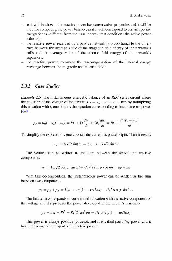
– as it will be shown, the reactive power has conservation properties and it will be

used for computing the power balance, as if it will correspond to certain specific

energy forms (different from the usual energy, that conditions the active power

balance);

– the reactive power received by a passive network is proportional to the differ-

ence between the average value of the magnetic field energy of the network’s

coils and the average value of the electric field energy of the network’s

capacitors.

– the reactive power measures the un-compensation of the internal energy

exchange between the magnetic and electric field.

2.3.2 Case Studies

Example 2.5 The instantaneous energetic balance of an RLC series circuit where

the equation of the voltage of the circuit is u ¼ uR þ uL þ uC. Then by multiplying

this equation with i, one obtains the equation corresponding to instantaneous power

[6–9]

pb ¼ uRiþ uLiþ uCi ¼ Ri2 þ LidiL

dtþCuc

duc

dt¼ Ri2 þ dðwe þwmÞ

dt

To simplify the expressions, one chooses the current as phase origin. Then it results

ub ¼ Ub

ffiffiffi

2p

sin xtþuð Þ; i ¼ Iffiffiffi

2p

sinxt

The voltage can be written as the sum between the active and reactive

components

ub ¼ Ub

ffiffiffi

2p

cosu sinxtþUb

ffiffiffi

2p

sinu cosxt ¼ uR þ uX

With this decomposition, the instantaneous power can be written as the sum

between two components

pb ¼ pR þ pX ¼ UbI cosu 1� cos 2xtð ÞþUbI sinu sin 2xt

The first term corresponds to current multiplication with the active component of

the voltage and it represents the power developed in the circuit’s resistance

pR ¼ uRi ¼ Ri2 ¼ RI22 sin2 xt ¼ UI cosu 1� cos 2xtð Þ

This power is always positive (or zero), and it is called pulsating power and it

has the average value equal to the active power.

76 H. Andrei et al.

The second term

pX ¼ uX i ¼ uL þ uCið Þ ¼ dðwm þweÞdt

¼ pb � pR ¼ UI sinu sin 2xt

is the instantaneous power resulted from multiplying the current with the reactive

component of the voltage and is called harmonic instantaneous power, having zero

average value and the amplitude equal to the reactive power modulus. The har-

monic instantaneous power is equal to the variation speed of the total instantaneous

energy (electric we and magnetic wm) of the circuit.

So, the reactive power (in modulus) is equal to the amplitude of the variation

speed of the energy accumulated by the circuit electromagnetic field.

Another interpretation can be as follows. The reactive power is written in suc-

cessive forms [10–14] as

Q ¼ XeI2 ¼ XC � XLð ÞI2 ¼ LxI2 � I2

Cx¼ 2x LI2 � CU2

C

�

The magnetic energy average value is

~wm ¼ 1

2T

Z

T

0

L i2dt ¼ 1

2L

1

T

Z

T

0

i2dt

8

<

:

9

=

;

¼ 1

2LI2

and the electric energy average value is

we ¼1

2T

Z

T

0

C u2Cdt ¼1

2C

1

T

Z

T

0

u2Cdt

8

<

:

9

=

;

¼ 1

2CU2

C

Finally, we have the relationship

Q ¼ 2x ~wm � ~weð Þ

The reactive power is proportional to the difference between the average mag-

netic energy and average electric energy of the circuit. It results the reactive power

is zero when ~wm � ~we ¼ 0: This relationship corresponds to a zero phase-shift

u = 0 and defines the resonance condition of the circuit.

2.4 Effects of Reactive Power on the Power System

Parameters

The irrational and big reactive power consumption, that generates a reduced power

factor, presents a series of disadvantages for the electric installation, among which

we mention [15]: the increase of active power losses in the passive elements of the


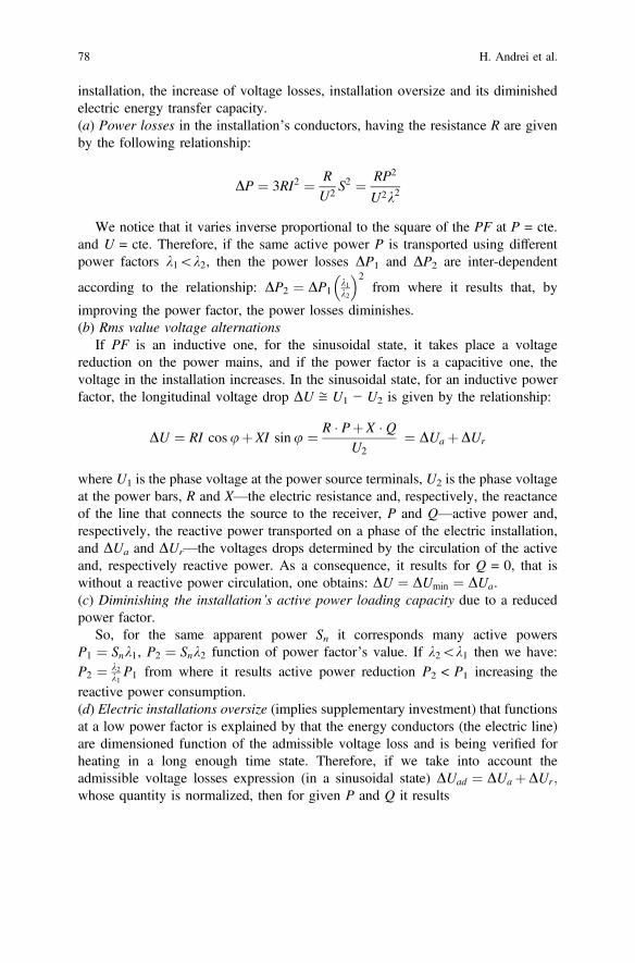
installation, the increase of voltage losses, installation oversize and its diminished

electric energy transfer capacity.

(a) Power losses in the installation’s conductors, having the resistance R are given

by the following relationship:

DP ¼ 3RI2 ¼ R

U2S2 ¼ RP2

U2k2

We notice that it varies inverse proportional to the square of the PF at P = cte.

and U = cte. Therefore, if the same active power P is transported using different

power factors k1\k2, then the power losses DP1 and DP2 are inter-dependent

according to the relationship: DP2 ¼ DP1k1k2

� �2

from where it results that, by

improving the power factor, the power losses diminishes.

(b) Rms value voltage alternations

If PF is an inductive one, for the sinusoidal state, it takes place a voltage

reduction on the power mains, and if the power factor is a capacitive one, the

voltage in the installation increases. In the sinusoidal state, for an inductive power

factor, the longitudinal voltage drop DU ≅ U1 − U2 is given by the relationship:

DU ¼ RI cosuþXI sinu ¼ R � PþX � QU2

¼ DUa þDUr

where U1 is the phase voltage at the power source terminals, U2 is the phase voltage

at the power bars, R and X—the electric resistance and, respectively, the reactance

of the line that connects the source to the receiver, P and Q—active power and,

respectively, the reactive power transported on a phase of the electric installation,

and DUa and DUr—the voltages drops determined by the circulation of the active

and, respectively reactive power. As a consequence, it results for Q = 0, that is

without a reactive power circulation, one obtains: DU ¼ DUmin ¼ DUa.

(c) Diminishing the installation’s active power loading capacity due to a reduced

power factor.

So, for the same apparent power Sn it corresponds many active powers

P1 ¼ Snk1, P2 ¼ Snk2 function of power factor’s value. If k2\k1 then we have:

P2 ¼ k2k1P1 from where it results active power reduction P2 < P1 increasing the

reactive power consumption.

(d) Electric installations oversize (implies supplementary investment) that functions

at a low power factor is explained by that the energy conductors (the electric line)

are dimensioned function of the admissible voltage loss and is being verified for

heating in a long enough time state. Therefore, if we take into account the

admissible voltage losses expression (in a sinusoidal state) DUad ¼ DUa þDUr;whose quantity is normalized, then for given P and Q it results

78 H. Andrei et al.

DUr ¼ X � Q=Un ¼ cte

that leads to

DUa ¼ DUad � DUr ¼ qL

s

P

Un

¼ cte: or s ¼ qL

DUa

P

Un

where

L the length of the line;

s the phase conductor’s section;

q the resistivity of the conducting material;

P the active power flow.

For a given active power, the investment in electric energy sources is inverse

proportional to the square of the power factor, and the installed apparent power

varies inverse proportional to the power factor.

2.4.1 Investigating the Powers Flow Process in AC Systems

In AC electric installations, characterized from the electric point of view, by a

scheme containing active and reactive elements, in general, it takes place a transfer

of active power P from the source to the receiver, in correlation with the consumers’

requirements, as well as a transfer of reactive power Q and of distortion power D.

An objective energetic characterization of a consumer is done using the apparent

power S that connects the above mentioned powers [16, 17].

Lately, due to the large-scale use in all domestic and industrial installations of

power electronics and due to numerous non-linear receivers, practically we cannot

talk about receivers for which the voltage signals and especially the signal of the

absorbed current to be pure sinusoids. So, the weight of the distortion power

becomes more significant. Therefore, one defines the following: apparent, active,

reactive and distortion power. For a single-phase consumer, these become

S ¼ UI ¼ffiffiffiffiffiffiffiffiffiffiffiffiffiffi

X

n

k¼0

U2k

s

�ffiffiffiffiffiffiffiffiffiffiffiffi

X

n

k¼0

I2k

s

P ¼X

1

k¼0

UkIk cosuk

Q ¼X

1

k¼1

UkIk sinuk

D ¼ffiffiffiffiffiffiffiffiffiffiffiffiffiffiffiffiffiffiffiffiffiffiffiffiffiffiffi

S2 � P2 � Q2p

ð2:36Þ


where U, I represent the rms value of the voltage respectively of the current and uk

is the phase shift between the voltage and the current, corresponding to the har-

monic of rank k, with k = 1 n. The unit measures for the four types of powers are

given in their definition order: VA, W, VAr and VAd. Most of modern measuring

pieces of equipment designed for measuring the electric power and energy can

measure instantly each of the 4 powers (energies) previously defined.

The reactive power of the total load of an electric energy consumer has, usually,

an inductive character, the load current being phase-shifted behind the voltage; in

this case, one considers, conventionally, that the reactive power is positive (QL > 0)

and the receivers represent reactive power consumers. For other receiver, the

absorbed current is phase-shifted before the voltage; these receivers are considered,

conventionally, reactive power sources, and the corresponding power in taken in

computation with minus sign (QC < 0). The total reactive power is: Q = QL−QC.

In electric installations, the Power Factor (PF) defined in (2.30) can be rewritten

as:

k � PF ¼ P

S¼

P

1

k¼0

UkIk cosuk

UIð2:37Þ

In a similar manner, the Displacement Power Factor (DPF) is defined as the

ratio between the active power P1 and the apparent power S1, corresponding to the

fundamental harmonic (k = 1)

k1 � DPF ¼ P1

S1¼ U1I1 cosu1

U1I1¼ cosu1 ð2:38Þ

We mention that the two definitions for the power factor (PF and DPF) lead, in

general, to different values and the equality k ¼ PS¼ cosu ðPF ¼ DPFÞ is valid

only in single-phase circuits and only for pure sinusoidal state (ideal case). As a

consequence, the interpretation of the power factor function of the phase-shift

between the current and the applied voltage signals should be carefully taken into

consideration.

To characterize the high order harmonics loading degree corresponding to the

voltage wave shape or to the consumer’s absorbed current, one can use several

indicators, the most used one being the Total Harmonic Distortion (THD) defined

in percentage as the ratio between the distortion residue of the signal and the rms

value of the fundamental harmonic. So, for current

THDi ¼1

I1

ffiffiffiffiffiffiffiffiffiffiffiffi

X

n

k¼1

I2k

s

� 100 ½%� ð2:39Þ

80 H. Andrei et al.

where Ik represents the rms value corresponding to harmonic k and I1 is the one

corresponding to the fundamental harmonic. Using the value of the total harmonic

distortion, one can easily prove the relationship

PF ¼ cosu1ffiffiffiffiffiffiffiffiffiffiffiffiffiffiffiffiffiffiffiffi

1þ THD2i

p ¼ DPFffiffiffiffiffiffiffiffiffiffiffiffiffiffiffiffiffiffiffiffi

1þ THD2i

p ð2:40Þ

valid for the case when the voltage distortion is negligible THDu < 5% (frequently

enough for low-voltage installations). Therefore, if DPF = 0.92 but THDi = 30%

the value of the power factor is only PF = 0.88.

The previous relationships define the instantaneous power factor that corre-

sponds to a certain moment from the consumer’s installations functioning.

Because the electric charge presents fluctuations, the current legislation rec-

ommends the determination of the weighted mean power factor based on the

consumption of:

– active energy

Wa ¼Z

t

0

P � dt

– reactive energy

Wr ¼Z

t

0

Q � dt ð2:41Þ

– distortion energy

Wd ¼Z

t

0

Q � dt

– for a certain period t (month, year)

PFmed ¼Wa

ffiffiffiffiffiffiffiffiffiffiffiffiffiffiffiffiffiffiffiffiffiffiffiffiffiffiffiffiffiffi

W2a þW2

r þW2d

p

From an energetic point of view, this is useful to characterize the consumer’s

installation and to charge its consumed electric energy. The weighted average

power factor can be natural—when is determined without taking into consideration

the reactive power compensation and general—when considering its evaluation one

takes into account the losses corresponding to this installation. The value of the

general weighted mean power factor from which the reactive energy consumption is


no further charged is called neutral power factor. This value is being determined

using technical-economical computation for minimizing the active power losses and

is a local quantity that depends on the position of the consumers in the electric

network. At international energetic system level the established value is equal to

0.92 [18, 19].

2.4.2 Reactive Power Consumers

The main reactive power consumers are the asynchronous motors and the electrical

transformers which consume around 60% respectively 25% from the installation’s

total reactive power due to producing alternating magnetic fields [20–25]. At

industrial consumers’ level the weight is around 70% for asynchronous motors and

around 20% for transformers. The difference between the reactive power con-

sumptions for asynchronous motors and transformers, at the same active power and

the same magnetic stress, comes from the fact that the magnetization reactive

power, that constitute the most important component of the reactive power, depends

on the volume of the magnetic circuit to which, for asynchronous motors’ case, one

adds also the volume of the air-gap (not existent for transformers). Another com-

ponent of the reactive power for the asynchronous motors and for transformers is

the reactive power dependent on load, called also dispersion reactive power.

(A) For asynchronous motors case, the magnetization reactive power (or the no

load power) represents the most part from the motor’s reactive power, function of

motor’s loading and function of the air-gap. Taking into account the exploitation

average loading: b < 0.5 (evaluated using the loading factor as the ratio between

the mechanical shaft power P and mechanical nominal power Pn of the motor

b = P/Pn), one can approximate the reactive power of an asynchronous motor as

being constant and independent of the load, while the active power depends on the

motor’ load. Also, the motors’ active power remains practically constant for small

deviations of the voltage compared to the nominal voltage, while the reactive power

depends essentially on the voltage’s variation. Asynchronous motors functioning

with a load factor b < 1 due to an inappropriate technological exploitation, deter-

mines the power factor reduction under its nominal value.

The reactive power Q absorbed by asynchronous motor for any load P, is

determined using the relationship [26, 27]

Q ¼ Q0 þQd ¼ Qn aþ 1� að Þb2�

¼ Q0 þ Qn � Q0ð Þb2

where a = Q0/Qn is the ratio between the reactive power Q0 for unloaded running

ðb ¼ 0Þ and the reactive power Qn absorbed at nominal load ðb ¼ 1Þ;Qd ¼ 1� að Þ � b2Qn—dispersion reactive power. Considering the definition of PF

in sinusoidal state, for a symmetrical loading of the three-phase network, it results

82 H. Andrei et al.

k ¼ cosu ¼ bffiffiffiffiffiffiffiffiffiffiffiffiffiffiffiffiffiffiffiffiffiffiffiffiffiffiffiffiffiffiffiffiffiffiffiffiffiffiffiffiffiffiffiffiffiffiffiffiffiffiffiffiffiffiffiffi

b2 þ aþð1� aÞb2� 2

tan2 un

q ð2:42Þ

For values b < 0.5 the reduction of the PF under its nominal value is highly

accentuated. If in exploitation, the power voltage of the asynchronous motors

increases, it results an increase of the absorbed reactive power, having undesired

consequences upon PF—Fig. 2.17a. This is due to the increase of the magnetiza-

tion current in the saturated area. In Fig. 2.17b is presented, as a rough guide, the

dependence of the absorbed reactive power function of the nominal one (Q/Qn) for

asynchronous motors of low and high power function of the relative value of the

power voltage for different loading factor’s values [28, 29].

(B) For transformers the absorbed reactive power is computed using the relation-

ship [26, 27, 30, 31]

Q ¼ Q0 þQd ¼Sn

100� i0 þ kf � b2 � usc�

where Sn is the nominal apparent power, i0—the current for unloaded running

(expressed in percentage function of nominal current), kf—the form factor of the

load signal (defined as the ratio between the mean square value and the mean value,

of the load current, computed for a given time interval), b = S/Sn—the transformer

load factor, usc—the voltage short-circuit voltage (expressed in percent).

As for asynchronous motors case, the transformers functioning at a power under

the nominal one determines the reduction of PF. In real exploitation conditions the

Fig. 2.17 Power factor variation function of asynchronous motor’s loading and the reactive

power consumption for small and big power motors function of the relative power voltage


transformers’ total reactive power can be evaluated to 10% of the nominal power

(8% unloaded running power and 2% dispersion power).

(C) Electric ovens installations (arc or induction) consume reactive power from the

oven’s power supply transformer, the oven adjustable autotransformer and the

power supply circuit of the oven from the transformer. Therefore, for a three-phase

arc oven, the PF of the installation is, usually, sufficiently big (0.8 0.9) but the

absolute reactive power consumption is big, compared to the oven’s power (that can

reach a value of 80 MW for a capacity of 400 t).

(D) Electric Distribution Lines can determine reactive power consumption QL that

can be computed using the relationship QL ¼ xLI2 where L is the line’s equivalent

inductivity, x—the voltage pulsation on the line, and I—the electric current that

circulates the line. On the other hand, the electric lines generate reactive power QC

due to their capacity C against the ground: QC ¼ xCU2. For electric lines case, the

resulting reactive power can have positive or negative values function of the values

of the two components QL and QC, the first one depending on the square of the

electric current that circulates the line and the second one depending on the square

of the voltage.

(E) Power Controlled rectifying installations supplied by a transformer represent

also an important reactive power source. The schemes adopted for controlled rec-

tifiers can lead also to a small power factor [32–37]. Lately, the consumer con-

taining power electronic circuits represent, due to their large scale use, the main

distortion power source from installations. As a consequence, the power factor of

the whole installation containing such receivers is diminished.

(F) A contribution to the reactive power flow is given by electric discharge lamps

in metallic vapours when they are connected in an uncompensated inductive ballast

schemes.

The PF monitoring is very important for the producer, the transporter, the dis-

tributer, the provider and the final user of electric energy, because it influences the

performance characteristics of all these services, it determines the availability

capacity of the energy transfer for electro-energetic pieces of equipment and

imposes the final electric energy providing costs [29–31].

2.4.3 Power Factor Compensation in AC Power Systems

The means to improve the PF are grouped into natural means and special means.

Natural means derive from a rational and correct choice and exploitation of the

existing machinery in installations and consists of technical and managerial mea-

sures (replacing the low-loaded transformers and motors, nonlinear loads aggre-

gation, reducing the unloaded functioning time of the machineries etc.) and the

special ones assume the introduction in installation of some pieces of equipment

generating reactive power and/or limiting the distorted state (installation of some

capacitor banks, of active filters networks conditioners etc.).

84 H. Andrei et al.

As a consequence, PF improvement includes, on a first stage, operations for

mitigation the high harmonics’ attendance from the wave shapes of the voltage and

the absorbed current, and, on the second stage, the limitation of reactive power flow.

Any method dedicated to reducing the reactive power absorbed by a consumer is

efficient only if the power voltage is practically sinusoidal.

(1) The use of capacitors banks as a reactive power source

This way for improving the power factor, even it’s highly spread, it’s efficient

only if the signals corresponding to the current and to the voltage are close to a

sinusoid (the contribution of the distorted state is modest). The placement of the

capacitors in a low voltage installation represents the compensation procedure that

can be [36–38]: global (placement in a single point for the entire installation), by

sector (group with sector), local or individual (at each equipment) or a combination

between the last two. Generally speaking the ideal compensation is applied at the

consumption place and it has the level in concordance with the instantaneous power

values, but in practice the choice is decided by economical and technical factors—

Fig. 2.18.

(2) Individual compensation is applied, firstly, in the big reactive power loads

(asynchronous motors, electric ovens etc.) and with continuous functioning,

ensuring the reactive power compensation at the consumption place and unloading

the remaining of the network from the reactive power flow, with all the advantages

deriving from this one—Fig. 2.19.

For individual compensation of asynchronous motors, the capacitors bank is

usually directly connected to the motors’ terminals and the decoupling from the

network taking place at the same time as the motor, using the same switching

device. To avoid the overcompensation that occur for the no loaded and the

auto-excitation (when the motor’ breaks), around 90% from the unloaded func-

tioning power is compensated, ensuring a power factor of around 0.9 at normal

loading and approx. 0.95 at incomplete loading or unloaded functioning. The

reactive power Qc necessary to compensate three-phase asynchronous motors is

determined by the motors’ unloaded operating current value I0 (given in theirs

catalogue data)

QC ¼ Q0 ¼ 0:9ffiffiffi

3p

UnI0 ð2:43Þ

For motors having powers bigger than 30 kW one can choose a covering value

QC ffi 0:35Pn [39].

For power distribution transformers’ case, the compensation bank is placed on

the low voltage part and very often consists of a fixed step (necessary to com-

pensate the unloaded absorbed reactive power) followed by a step that covers the

necessary reactive power at nominal load: the bank’s dimensioning takes place

using the relationship


Fig. 2.18 Examples for placing the capacitors bank

Fig. 2.19 Individual

compensation for

asynchronous motors and for

transformers

86 H. Andrei et al.

QC ffi Q0 þQd ¼i0½%�100

Sn þusc½%�100

Sn � b2 ð2:44Þ

where i0 [%] respectively usc [%] represent the percent values corresponding to the

unloaded running current and to the short circuit voltage of the transformer (given

in its catalogue data) and b = S/Sn is the load factor rate. Usually, one can consider:

QC ¼ ð0:1 0:2ÞSn þð0:5 0:6ÞSn.The individual compensation is applied also to illumination lamps’ with metallic

vapours electric discharge, the capacitors’ values is being mentioned by the pro-

ducer as a function of the lamp’s rated power.

(3) Compensation on receivers’ groups (by sector) is applied when the reactive

power consumers are grouped, the capacitors’ banks being connected to the mains

from the distribution panels corresponding to the receivers’ groups. The bank’s

power and the operating mode are established as a function of the receivers’

uncompensated reactive power signal. This compensation mode limits also the

reactive power circulation in the network above the setting place.

(4) Centralized compensation can be realized by connecting the capacitors bank at

the mains (coupling points) from the general electric distribution panel from the

transformer power substation. The bank is executed in commutation steps, usually

automated, function of the reactive power that should be compensated, corre-

sponding to powered receivers running. The bank can be connected also to the

intermediate high voltage of the transformer power substation. For a centralized

compensation, intermediate high voltage, the positive technical effects are not

present at low voltage installations belonging to the consumer (downstream to the

installing place). But, the big consumers powered directly in intermediate high

voltage, use the centralized compensation that provides a general power factor

bigger than the neutral power factor value such that the electrical energy con-

sumption to be billed only for active energy.

(5) Mixed compensation uses all the procedures presented before for reactive power

compensation. The solution is applied in steps or, when there are certain conditions

specific to the respective consumer.

The power Qb corresponding to the capacitors bank is determined such that, to a

certain given active power P, absorbed under a power factor cosu1, to obtain an

improved power factor cosu2[ cosu1. The reactive power consumed by these

capacitors will be: Qb ¼ �3xCU2c . The receiver consumes a reactive power before

adding the bank, Q1 ¼ Ptgu1. The necessary power from the network after adding

the capacitors will be Q2 ¼ Q1 þQb, from where

Qb ¼ Q1 � Q2 ¼ P tanu1 � tanu2ð Þ ð2:45Þ

where Q2 ¼ P tanu2 represents the reactive power received from the network after

introducing the capacitors bank—the active power P remains constant, and cosu2

is the new power factor that should be realized. As a consequence, the value of the

capacity for one capacitor from the triangle bank will be


C ¼ Pðtanu1 � tanu2Þ3xU2

c

ð2:46Þ

In Fig. 2.20 the connection possibilities for the capacitors that form the bank in

single and three phase installations are presented. If one takes into account the

power loss DPC in the capacitors’ dielectric the power necessary for the bank

becomes

Qb ¼ P � tanu1 � PþDPCð Þ � tanu2 ¼ Q1 � Q2 with DPc ¼pd

100� Qb ð2:47Þ

where pd ¼ 0:25 0:35%; represents the losses from the dielectric expressed as a

percent function of the capacitors bank power Qb. These depend on the tangent of

the material’s losses angle tgd after the relationship: DPC ¼ xCU2 tan d and can be

considered (especially in low voltage) negligible.

One can note that for Y bank’s connection result capacitors having a capacity

three times bigger, because instead of Uc is the voltage Uf ¼ Ul

� ffiffiffi

3p

. Results

CD=CY ¼ Uf

�

Ul

� 2¼ 1=3 and, as a consequence, the power factor compensation is

an economical and technical problem, taking into account that, in low voltage, the

cost of the capacitors is proportional to their capacity. This is the reason why D

connection is preferred. The Y assembly is advantageous for intermediate high

voltage networks, because nominal voltage of the capacitors is then reduced. One

can notice that the maximum voltage for D connection capacitors is over 580 V

compared to Y connection where the voltage is only 320 V. The capacitors bank

power depends on the network voltage variation. So, if the network voltage varies

from Un to Un2 the capacitors bank power modifies from Qb to the value

Qb2 ¼ Qb Un2=Unð Þ2.The time variation signal corresponding to the reactive power consumption Q in

an electrical installation is, in general, not a linear one. The necessary reactive

power depends on the way in which the electric energy is being used in various

technological processes, fact emphasised by the load variation. Therefore, the

absorbed reactive power can vary slowly or rapidly in very large limits. In this

Fig. 2.20 Connections possibilities for capacitors bank

88 H. Andrei et al.

situation, the adoption of some capacitor banks with fix value can determine over

and under compensations regimes. To avoid such a major inconvenient, the

problem is solved by realizing a capacitor bank from several sections (stages) of

fixed power. Each section consists of automatic controlled commutation pieces of

equipment, following several criteria, for example, function of the mains voltage,

the load current, and the direction of the reactive power change with the energetic

system or function of the running time corresponding to different loads—Fig. 2.21.

The selection of the number and of the values for the capacitors bank sections

should take into account that the control efficiency increases with the number of

steps, making possible to follow very closely the load reactive power signal. On the

other hand, an excessive fractioning of the bank becomes at a certain point not

viable from economical point of view because it implies the use of a complex

commutation apparatuses. Usually, the capacitor banks use a number of 4 12

sections having the powers between 5 25 kVAr [34, 38, 39].

For the scheme presented in Fig. 2.21, the control block CB establishes the value

of the power factor (cos u) and knowing the capacities corresponding to the bank’s

sections, connects the elements necessary to realize the prescribed power factor.

Exceeding the prescribed power factor leads to disconnect the capacitors bank

sections.

Systems’ selection for reactive power compensation in non-sinusoidal state. To

select a system for power factor correction in an installation where there are present

high-order harmonics in the current and voltage waves shape, function of the user’s

data, one uses the following methods [35–40]:

Fig. 2.21 The principle scheme for an automated controlled power factor in an installation


(A) Distorted installed power procedure, whose principle is described in Figs. 2.22

and 2.23. The following notations are used:

– G is the sum of apparent powers taken for all pieces of equipment that generate

harmonics (power static converters, inverters variable speed drives, etc.) con-

nected to the mains where the capacitors bank is also connected. If, for some

equipment the active power is given, to compute the apparent power one should

take into consideration the covering PF.

– Sn is the sum of apparent powers taken for all system’s power transformers to

which the distribution mains belong.

The above method can be applied only for limited voltage and current harmonic

distorted level (THDu < 5%) (THDi < 30%).

(B) Voltage and current total harmonic distorted level determination method,

applicable when one knows exactly (by measurements) the values corresponding to

THDu respectively to THDi. The principle of this method is presented in Fig. 2.24.

The selection methods indicate the use of (depending on the harmonic’s dis-

tortion level): standards capacitor banks, capacitor banks with increased nominal

voltage (usual with 10%), capacitor banks with increased nominal voltage and with

detuned reactors or harmonic mitigation filters (active, passive or hybrid).

One should mention that in actual conditions, where the installation’s load with

voltage or especially current high-order harmonics are very frequent, it is used the

Fig. 2.22 Connecting the power factor correction system in a non-sinusoidal state system

90 H. Andrei et al.

solution (cheaper than that with active filters) of capacitor banks placed in series

with certain coils also called “detuned reactors” shown in Fig. 2.25 [38–40]. The

reactive power corresponding to these detuned reactors is chosen usually as a

percent, called detuned reactor factor, of p = 5, 7 or 11% from the compensation

reactive power of the bank. Therefore, by a correct selection of the detuned reactor

factor, one may avoid the resonance on the dominant installation’s harmonics and at

the fundamental frequency the compensation function is satisfactory maintained.

Moreover, the detuned reactors, that have values of mH order, together with the

connecting conductors’ inductivity, limit the commutation inrush currents in the

case of banks from automatic power factor correction system (APFC). Moreover,

the detuned reactors supplementary stress the capacitors’ dielectric, reason for

which these should be dimensioned at voltages at least 10% bigger than the nominal

ones.

The reduction of the connecting current value is done by placing in series some

very small inductivity coils (a few lH). For low-voltage banks where the harmonics

do not have a consistent weight (THDu,i < 10%) also the connecting cable, out of

which several turns are coiled, realizes a current limitation. So, only the conduc-

tivity of a cable of 10 m is sufficient to limit the current necessary to connect a bank

up to 25 kVAr [29–31].

Fig. 2.23 Selecting the reactive power compensation possibility function of installation’s

nonlinear receivers’ weight


These measures should determine the consumers to function with a power factor

in exploitation at values very close to the nominal one and finally to lead to an

increased average weighted power factor at least up to the neutral power factor

value (usually 0.92).

Fig. 2.24 Selection of reactive power compensation functions of installation’s nonlinear loads’

weight

Fig. 2.25 Connecting the

detuned reactors in a D

connection capacitors bank

92 H. Andrei et al.

2.4.4 Case Studies

Example 2.6 Let’s consider an industrial load that contains linear power consumers

(especially asynchronous single and three-phase power motors) for which the

electric power quality parameters are presented in Fig. 2.26. The figures are cap-

tured by using a Fluke 435—a “class A” power quality analyzer instrument. As one

can notice, from the main parameters analysis (current and voltage signals, har-

monics distortions etc.), the system allows the connection of a capacitor bank.

Its power is evaluated taking into consideration both the value of the actual

measured power factor (PF1 ¼ cosu1), as well as that of the desired power factor

(mostly is the value of the neutral factor value: PF2 ¼ cosu2 ¼ 0:92 or even 0.95).

Knowing the active power P ¼ 223:7 kW and choosing for cosu2 ¼ 0:95 we can

determine the reactive capacitor bank value

Qbat ¼ P � tanu1 � tanu2ð Þ ¼ 223:7 � ð0:619� 0:203Þ ffi 93:2 kVAr

The three-phase capacitors used to improve the PF can be placed in D or Y

connection (Fig. 2.20). The bank’s capacity on a phase results from the following

relationship:

CD ¼ QC

x � U� ffiffiffi

3p� 2

¼ 93:2 � 103

2 � p � 50 � 400� ffiffiffi

3p� 2

¼ 5:56 mF

CD ¼ CD

3¼ QC

x � U2¼ 93:2 � 103

2 � p � 50 � 400ð Þ2¼ 1:85 mF

So, the for the analyzed system case, one recommends an automatic power factor

correction system (APFC) (in steps taking into consideration that energy can vary in

large limits, function of the number of loads connected at the same time) of power

value: Qbat ¼ 95 kVAr. A solution of the automatic capacitor bank can be realized

in three steps of 30, 30 respectively 55 kVAr. With the new power factor (0.95), the

current absorbed by the consumer becomes

I2 ¼ I1PF1

PF2¼ 402 � 0:86

0:95 ¼ 363A, (the measured current one being I1 ¼ 402A)

With this value, the losses in a three-phase copper power cable 3 � CYY

2 � 120 mm2, can be computed. The resistance on the Cu cable per unit length of

section 120 mm2 is rl = 0.154 mX/m. But on each phase two such cables of length

l = 100 m are used. Thus the total specific resistance is given by the parallel

equivalent resistance of the cables

rt ¼rl

2¼ 0:154

2

mX

m¼ 0:077

mX

m

R0 ¼ rt � l ¼ 0:077 � 100 ¼ 7:7 mX


Fig. 2.26 The energy quality parameters of the industrial consumer under investigation

94 H. Andrei et al.

Considering the average working temperature of the cable h2 = 42 °C, (resulted

eventually from analyzing the thermal image), we will compute the value of the

conductors’ resistance

RL ¼ R0ð1þ a � ðh2 � h1ÞÞ ¼ 7:7 � 1þ 0:00339 � 42� 20ð Þð Þ ¼ 8:27 mX

The power losses before and after compensating the reactive energy flow are:

Before

DP1 ¼ 3 � I21RL ¼ 3 � 4022 � 8:27 � 10�3 ¼ 4 kW

and after

DP2 ¼ 3 � I22RL ¼ DP1

PF2

PF1

�2

¼ 40; 86

0; 95

�2

¼ 3:27 kW

Results a consumer’s power cable loss

DP1 � DP2 ¼ 730 W

or given in percent

e ¼ DP1 � DP2

DP1

¼ 18:25%

The power cable consumed energy can be correct evaluated if one knows the

form factor of the current variation (on the most loaded phase), that is represented in

Fig. 2.27.

With this information one will compute the average value Im and the square

average value Imp of the current, and its corresponding form factor, respectively

Fig. 2.27 The current variation on the consumer’s most loaded phase taken on a monitor interval


Im ¼ 363A; Imp ¼ 368A; kf ¼ Imp=Im ¼ 1:063

The energy for a 30 days period (720 h) before and respectively after com-

pensation will be

DE1 ¼ 3 � kf I2mRLsf 10�3 ¼ 3 � 1:063 � 363ð Þ2 8:27 � 10�3

�

� 720 � 10�3 ¼ 2:502 MWh

DE2 ¼ 3 � kf ImPF1

PF2

�2

RLsf 10�3 ¼ PF1

PF2

�2

DE1 ¼ 2:049 MWh

It results a consumer’s power cable losses reduction

DE1 � DE2 ¼ 453 kWh

or given in percent

d ¼ DE1 � DE2

DE1

¼ 18:10%

2.5 New Principle of Minimum Active and Reactive

Absorbed Power (PMARP) in AC Power Systems

In different real systems such as mechanics, thermodynamics, Earth climate system,

hydrology, scientific studies have been carried out to express the balanced state of

the systems in energy and/or power terms [41–50]. These studies are mostly based

on the concept that for conservative systems it is possible to define suitable func-

tionals in Hilbert space related to power and/or energy. An important step forward

in order to define the functional optimization problems is to calculate their limits.

On the other hand the studies cited below report that the steady state in mechanic,

thermodynamic, hydrology or climate conservative system is an edge state, gen-

erally a minimum state, from the energy or power point of view.

The introduction of “content and co-content” function applied to non-linear

resistors represented a milestone in electric circuits theory [51–53]. Authors like

Penfield in [54] demonstrate for nonlinear resistive circuits the “variational prin-

ciple” of “content and co-content” function, respectively Smith in [55], [56] anal-

yses for linear passive circuits the average energy storage, the minimum energy and

the dependence between electric and magnetic energy storage to one-port of circuit.

Romanian scientists have important contributions to the minimum/maximum theory

of power in electric circuits. For example, the application of Hilbert space func-

tionals to power analysis in non-sinusoidal state is introduced by Ionescu in [57],

the theorem of minimum power absorbed by resistances in DC circuits is

96 H. Andrei et al.

demonstrated by Mocanu in [58], and the analysis and solving of electromagnetic

field based on energy functional are defined by Hantila in [59] and Fireteanu in

[60].

This section refers to new theorems (principles) of minimum active and reactive

absorbed power (PMARP) for linear electric circuits in quasi-stationary regime

which are based on power functionals and Hilbert space properties such in the

recent contributions of authors [61–69]. On the other hand, based on analogy

between linear electric and magnetic circuits in quasi-stationary regime, similar

principles are described by authors in [70–74]. In this work for AC circuits,

including non-sinusoidal regime, is demonstrated a complete set of principles of

minimum absorbed active and reactive power, are defined the specific conditions

and limits of their applications and finally are provided suggestive examples for

each circuit. For all the types of AC circuits the principles demonstration are

similar. As a starting point is the definition of power functionals and their

expressing depending on the potential of circuit nodes which are considered

variable.

In this respect the Kirchhoff voltage law (KVL) and the topology of circuit are

used. Then by imposing the conditions for obtaining the minimum point of func-

tionals (when existing), it is demonstrated that these equations are similar with

Kirchhoff current law (KCL) and nodal method (NM). Consequently by using the

power flow theory, either a complete system of Kirchhoff equations (KVL and

KCL) is obtained from which one determines the circuit currents and voltages or a

complete system of NM from which one computes the potentials of nodes. Or in

other words, KCL equations can be substituted with those arising from

PMARP. Likewise in this section is demonstrated the coexistence (CEAPP) of

PMARP and maximum power transfer theorem (MPTT) for active power in AC

circuits. Therefore PMARP can be considered as part of basic concept of circuit

theory.

2.5.1 PMARP for Linear AC Circuit

Let us consider the common branch of a linear and reciprocal AC circuit under

sinusoidal signal shown in Fig. 2.28. The circuit contains N nodes and K branches

with voltage sources and RLC passive elements. In order to put in evidence the

~

Ik

Ek Yk

Uk

VjVi

∆Vk

Pk, Qk

i jFig. 2.28 Representation of

an AC circuit branch


power flow between the sources and passive elements, one defines in <2ðN�1Þ—

dimensional Hilbert space, two functionals. The first one is the active power

Eq. =P : <2ðN�1Þ ! <, and the second one is the reactive power

Eq. =Q : <2ðN�1Þ ! < defined as

=P ¼ Re½uT i�� ð2:48Þ

=Q ¼ Im½uT i�� ð2:49Þ

where u represents the K-dimensional vector in CK of complex voltages at the

branch admittances terminals and i represents the K-dimensional vector in CK of the

branch complex currents. In this section the superscript * denotes the conjugate

operator. Related to the branch voltages and current baseline direction presented in

Fig. 2.28, the power Eqs. (2.48) and (2.49) mean: (i) =P is the active power

absorbed by all the passive elements’ conductances (resistances) of the circuit,

respectively (ii) =Q is the reactive power absorbed or generated by all the reactive

elements (inductors and capacitors) of the circuit. By using KCL equation for each

k-branch DV k ¼ V i;k � V j;k ¼ Uk � Ek ¼IkYk

� Ek , for k ¼ 1; . . .;K and consider-

ing as variables the complex potentials of circuit nodes V i ¼ xi þ jyi, for

i ¼ 1; . . .;N � 1 xi; yi 2 <, then =P and =Q can be expressed as

=Pðx; yÞ ¼ Re½uT i�� ¼ Re½ðDvþ eÞTY�ðDvþ eÞ��¼ Re½ðCV þ eÞTY�ðCV þ eÞ��¼

X

k¼1;Ki;j¼1;N�1

i 6¼j

Gk½ðxi � xj þ akÞ2 þðyi � yj þ bkÞ2�ð2:50Þ

=Qðx; yÞ ¼ Im½uT i�� ¼ Im½ðDvþ eÞTY�ðDvþ eÞ��¼ Im½ðCV þ eÞTY�ðCV þ eÞ��¼

X

k¼1;Ki;j¼1;N�1

i 6¼j

Bk½ðxi � xj þ akÞ2 þðyi � yj þ bkÞ2�ð2:51Þ

where Dv is the K-dimensional vector in CK of branch complex voltages, e is the

K—dimensional vector in CK of branch voltage sources expressed as Ek ¼ ak þ jbk;where ak, bk are considered constant, Y ¼ diag Y1; Y2; . . .; YKð Þ is the K � K—

dimensional diagonal matrix of branch admittances, where Yk ¼ Gk � jBk, k ¼1; . . .;K with Gk[ 0, Bk[ 0 for inductive branches respectively Bkh0 for capac-

itive branches, V is the reduced (N-1)-dimensional vector in CN−1 of nodes

potentials, and C = [cl,n] is the K � (N–1)-dimensional reduced branch-to-node

incidence matrix whose elements cl,n can take the values −1, 0 or 1. The superscript

T is used to indicate the transposition.

98 H. Andrei et al.

The next step of PMARP demonstration is to analyze the sign functionals

defined in (2.50) and (2.51), and as a consequence of the nature, minimum or

maximum, of thereof extreme point.

(a) Evidently if Gk[ 0, then the active power Eq. is a quadratic form (strictly

positive) =Pðx; yÞi0, and its extreme point is a minimum. Therefore one can affirm

that the active power absorbed by all the passive elements (conductances) of the AC

circuit is minimum. By imposing the concurrent conditions @=P=@xi ¼ 0 and

@=P=@yi ¼ 0, for i ¼ 1; . . .;N � 1, then is obtained the minimum point of =P.

Related to the potential of the i-node of the circuit these derivative conditions are

expressed as

@=P

@xi¼ @

@xiRe½ðCV þ eÞTY�ðCV þ eÞ��

¼ 2X

lk2niclk ;niGkðxi � xj þ akÞ ¼ 0

ð2:52Þ

@=P

@yi¼ @

@yiRe½ðCV þ eÞTY�ðCV þ eÞ��

¼ 2X

lk2niclk ;niGkðyi � yj þ bkÞ ¼ 0

ð2:53Þ

for k ¼ 1; . . .;K, i; j ¼ 1; . . .;N � 1;i 6¼ j.

(b) The sign of the reactive power Eq. depends on the sign of Bk: (b1) when all the

branches of the AC circuit have an equivalent resistive-inductive admittance

Bk[ 0, k ¼ 1; . . .;K, then =Qðx; yÞ[ 0, so =Q is strictly positive and its extreme

point is a minimum. Therefore one can affirm that the reactive power absorbed by

all the reactive elements of AC circuit is minimum; (b2) when all the branches of

AC circuit have an equivalent resistive-capacitive admittance Bk\0, k ¼ 1; . . .;K,then =Qðx; yÞ\0. In this case reversing the sign of =Q and changing its significance

from absorbed in “generated”, then �=Q[ 0 is strictly positive and its extreme

point is a minimum. Therefore one can affirm that the reactive power generated by

all the reactive elements of the AC circuit is minimum; (b3) when the branch

admittances of the circuit verify the particular case of resonance condition, then

=Qðx; yÞ ¼ 0; (b4) when the circuit includes inductive and capacitive branches and

is not possible to conclude about the sign of Bk then the extreme of =Q can not be

fixed.

Related only to the cases (b1) and (b2) by imposing the concurrent conditions

@=Q=@xi ¼ 0 and @=Q=@yi ¼ 0, for i ¼ 1; . . .;N � 1 then is obtained the minimum

point of =Q. With respect to the potential of the i-node these derivative conditions

are expressed as

@=Q

@xi¼ @

@xiIm½ðCV þ eÞTY�ðCV þ eÞ�� ¼ 2

X

lk2niclk ;niBkðxi � xj þ akÞ ¼ 0 ð2:54Þ


@=Q

@yi¼ @

@yiIm½ðCV þ eÞTY�ðCV þ eÞ�� ¼ 2

X

lk2niclk ;niBkðyi � yj þ bkÞ ¼ 0 ð2:55Þ

Finally, the minimum points of =P and =Q are the solutions of concurrent

conditions (2.52)–(2.55) which means the below system with 4(N–1) Eqs.

@=P

@xi¼X

lk2niclk ;niGkðxi � xj þ akÞ ¼ 0;

@=P

@yi¼X

lk2niclk ;niGkðyi � yj þ bkÞ ¼ 0

@=Q

@xi¼X

lk2niclk ;niBkðxi � xj þ akÞ ¼ 0;

@=Q

@yi¼X

lk2niclk ;niBkðyi � yj þ bkÞ ¼ 0

ð2:56Þ

If we calculate the algebraic sum of Eq. (2.56), with the derivatives @=P=@yi and@=Q=@xi multiplied by j respectively −j, we will get

X

lk2niclk ;niYkðV i � V j þEkÞ ¼ 0 ð2:57Þ

Equation (2.57) represent for i; j ¼ 1; . . .;N � 1;i 6¼ j the Eq. of NM applied for

N � 1 nodes of the considered AC circuit. Withal by rewriting the Eq. (2.57) we

will obtain

X

lk2niclk ;ni Ik ¼ 0 ð2:58Þ

that represents even the KCL Eqs. for N–1 nodes of the considered AC circuit.

Taking into account those shown so far one can formulate the following

Principle of Minimum Active and Reactive Power (PMARP): “In reciprocal and

linear AC circuits the condition of minimum active absorbed power in the resis-

tances and minimum reactive absorbed (generated) power in the inductances

(capacitances) is consistent with the NM and KCL”. In more specific terms, “in

reciprocal and linear AC circuits: (a) the branch currents and voltages are dis-

tributed such as the absorbed active power and the absorbed (generated) reactive

power in the resistive-inductive (resistive-capacitive) branches of the circuit are

minimum; (b) PMARP along with KVL constitute the basic forms of linear and

independent Eqs. system of AC circuits analysis; (c) PMARP is consistent with

NM”.

Also it is possible to analyze together PMARP and MPTT in what concerns the

active power flow in AC circuits [75]. First according to MPTT let’s consider that

certain AC circuit branches—named load—verify the conditions for maximum

active power transfer. In terms of PMARP that means the case (b3) when

=Qðx; yÞ ¼ 0 and the active power Eq. =Pðx; yÞ has a minimum. For these reasons

can be formulated the Co-Existence of Active Power Principles (CEAPP) for linear

100 H. Andrei et al.

AC circuits as: “in linear and reciprocal AC circuits the branches currents and

voltages comply simultaneously PMARP and MPTT when one of the branch

admittance verifies the MPTT condition”.

2.5.2 PMARP for Linear AC Circuits Under Non-sinusoidal

Conditions

The concepts illustrated above can be extended to the case of AC circuits operating

in non-sinusoidal regime. A similar linear circuit with K branches and N nodes is

considered but in this case operating under non-sinusoidal conditions with radian

frequency x at the fundamental harmonic. For each branch of the circuit, the

voltage and the current are expressed by using the Fourier series

ukðtÞ ¼X

H

h¼0

UðhÞk

ffiffiffi

2p

sinðhxtþuðhÞk Þ ð2:59Þ

ikðtÞ ¼X

H

h¼0

IðhÞk

ffiffiffi

2p

sinðhxtþuðhÞk � c

ðhÞk Þ ð2:60Þ

where k ¼ 1; . . .;K is the number of branches, H is the finite number of harmonics

considered, UðhÞk and I

ðhÞk represent the rms values of the hth harmonic of voltage

and current, respectively, while uðhÞk and u

ðhÞk � c

ðhÞk represent the phase angle of the

hth harmonic of voltage and current, respectively. Considering branch k of the

circuit (Fig. 2.29), by using the complex representation for the hth harmonic of

voltage and current, with the same conventional circuit representation adopted in

Sect. 2.5.1 for AC circuits in sinusoidal regime, we get

DVðhÞk ¼ V

ðhÞi;k � V

ðhÞj;k ¼ U

ðhÞk � E

ðhÞk ¼ I

ðhÞk

YðhÞk

� EðhÞk ð2:61Þ

Fig. 2.29 AC circuit under

non-sinusoidal conditions


In the Hilbert space we can define, similarly with Eqs. (2.50) and (2.51), the

functionals corresponding to the hth harmonic of active and reactive absorbed

power by all the K branches. We obtain the Eqs. =ðhÞR : <2ðN�1Þ ! < and =ðhÞ

Q :

<2ðN�1Þ ! < such that, respectively:

=ðhÞR ðxðhÞ1 ; . . .; x

ðhÞN�1; y

ðhÞ1 ; . . .; y

ðhÞN�1Þ � Re½�SðhÞ�

¼X

K

k¼1

GðhÞk ½ðxðhÞi;k � x

ðhÞj;k þ a

ðhÞE;kÞ

2 þðyðhÞi;k � yðhÞj;k þ b

ðhÞE;kÞ

2�ð2:62Þ

=ðhÞQ ðxðhÞ1 ; ::; x

ðhÞN�1; y

ðhÞ1 ; . . .; y

ðhÞN�1Þ � Im½�SðhÞ�

¼X

K

k¼1

BðhÞK ½ðxðhÞi;k � x

ðhÞj;k þ a

ðhÞE;kÞ

2 þðyðhÞi;k � yðhÞj;k þ b

ðhÞE;kÞ

2�ð2:63Þ

These equations are a function class C2 in <2ðN�1Þ. Considering GðhÞk [ 0 for

k ¼ 1; . . .;K the real equation of the complex power is always positive defined, that

is, =ðhÞR ðxðhÞ1 ; x

ðhÞ2 ; . . .; x

ðhÞN�1; y

ðhÞ1 ; y

ðhÞ2 ; . . .; y

ðhÞN�1Þ[ 0, for all the pairs ðxðhÞi ; y

ðhÞi Þ with

i ¼ 1; . . .;N � 1 and h ¼ 1; . . .;H; then, the active absorbed power has a minimum.

The reactive power equation can be analyzed, for all the pairs ðxðhÞi ; yðhÞi Þ; i ¼ 1; . . .;

N � 1, and for each harmonic h ¼ 1; . . .;H as single-phase AC circuits described in

Sect. 2.5.1 for AC circuits. Similarly, such as in case (b1) with resistive-inductive

branches, the Eq. (2.63) is positive defined, thus the total reactive power absorbed by

the inductive components has a minimum. Furthermore, likewise case (b2) with

resistive-capacitive branches by changing the sign and significance of the imaginary

functional, in order to obtain a positive defined functional and to conclude that the

total reactive power generated by the capacitive components has a minimum. For the

general case in which reactive components of different nature—inductive and

capacitive—coexist at the given harmonic h ¼ 1; . . .;H, the sign of Eq. =ðhÞQ cannot

be fixed and the extreme of =ðhÞQ cannot be stated.

Related only to the cases (b1) and (b2), the minimum point of =Q is obtained

from the below 4(N–1) Eqs. system that results by imposing to the Eqs. (2.62) and

(2.63) the derivative concurrent conditions for extreme

@=ðhÞR

@xðhÞi

¼ 0;@=ðhÞ

R

@yðhÞi

¼ 0

@=ðhÞQ

@xðhÞi

¼ 0;@=ðhÞ

Q

@yðhÞi

¼ 0

ð2:64Þ

where i ¼ 1; . . .;N � 1 and h ¼ 1; . . .;H.


By calculating the algebraic sum of the solutions, with the derivatives taken with

respect to the imaginary parts multiplied by (−j), in the same fashion as seen in AC

examples, we obtain the expressions

X

lk2niclk ;niY

ðhÞk ðV ðhÞ

i � VðhÞj þE

ðhÞk Þ ¼ 0 ð2:65Þ

i; j ¼ 1; . . .;N � 1; i 6¼ j, k ¼ 1; . . .;K that represent NM Eqs. for hth harmonic

expressed at N−1 nodes of the circuit. On the other hand by using in (2.65) Ohm’s

law for each circuit branch then results

X

lk2niclk ;ni I

ðhÞk ¼ 0 ð2:66Þ

which are the KCL equations for the hth harmonic, expressed for N−1 nodes of

the circuit.

Taking into account those shown so far, one can formulate the following Principle

of Minimum Active and Reactive Power (PMARP): “In reciprocal and linear AC

circuits the condition of minimum active absorbed power in the resistances and

minimum reactive absorbed (generated) power in the inductances (capacitances) is

consistent with the NM and KCL”. In more specific terms, “in reciprocal and linear

AC circuits: (a) the branch currents and voltages are distributed such as the

absorbed active power and the absorbed (generated) reactive power in the resistive-

inductive (resistive-capacitive) branches of the circuit are minimum; (b) PMARP

along with KVL constitute the basic forms of linear and independent equations

system of AC circuits analysis; (c) PMARP is consistent with NM”.

Consequently, we may state the Principle of Minimum Active and Reactive

absorbed Power in linear circuits under Non-sinusoidal conditions (PMARPN): “In

linear and reciprocal circuits under non-sinusoidal conditions, for each hth har-

monic, the minimum of the active absorbed power and minimum of the reactive

absorbed (generated) power by the inductances (capacitances) is consistent with

the NM and KCL”. Another description of the same principle can be stated as

follows: “In the linear and reciprocal circuits under non-sinusoidal periodic sig-

nals for each hth harmonic: (a) the branch currents and voltages are distributed

such as the absorbed active power and the absorbed (generated) reactive power in

the resistive-inductive (resistive-capacitive) branches of the circuit are minimum;

(b) PMARPN along with KVL constitute the basic forms of linear and independent

Eqs. system of AC circuits analysis; (c) PMARPN is consistent with NM”.

It is essential to remark that the same observations regarding the limits of

applicability of the minimum power principle indicated in Section for AC circuits

hold at every harmonic order. Thus, the minimum power principle applies when no

mixture of inductive and capacitive components appears in the circuit at any fre-

quency. Also a similar CEAPP can be stated for each frequency of AC circuits in

non-sinusoidal conditions.


The existence of the minimum power condition is verified if, starting from all

inductive (or capacitive) reactive components, no resonance conditions is reached

in the circuit at any frequency in the observed range, since the reactive nature of the

circuit would change above the resonance frequency [76]. This could be the case of

filters containing both inductive and capacitive components, whose equivalent

admittance exhibits capacitive behavior at relatively low frequency up to the res-

onance conditions, and inductive behavior at frequencies higher than the one cor-

responding to the resonance conditions.

2.5.3 Practical Examples

Example 2.7 demonstration of PMARP for the AC circuit shown in Fig. 2.30 with

N = 2 nodes and K = 3 resistive-inductive branches. The admittances contain only

resistive and inductive elements, that is, Gk[ 0 and Bk[ 0 for k ¼ 1; 2; 3, satis-fying the conditions imposed in case b1. The real and imaginary parts of nodes

potentials are considered variables, while the voltage source is constant. Then, by

applying KVL the expressions of the complex conjugated currents of the circuit

branches are

V1 ¼ x1 þ jy1; V2 ¼ x2 þ jy2; E1 ¼ aþ jb

I�1 ¼ ðG1 þ jB1Þ½ðx2� x1 þ aÞ � jðy2 � y1 þ bÞ�

I�2 ¼ ðG2 þ jB2Þ½ðx1 � x2Þ � jðy1 � y2Þ�I�3 ¼ ðG3 þ jB3Þ½ðx1 � x2Þ � jðy1 � y2Þ�

The active and reactive absorbed powers of the circuit branches elements expressed

by the Eqs. (2.50) and (2.51) are positive defined =R[ 0, =Q[ 0 in the forms

Fig. 2.30 Resistive-inductive AC circuit


=R ¼ G1 ðx2 � x1 þ aÞ2 þðy2 � y1 þ bÞ2h in

þG2 ðx1 � x2Þ2 þðy1 � y2Þ2h i

þG3 ðx1 � x2Þ2 þðy1 � y2Þ2h io

=Q ¼ B1 ðx2 � x1 þ aÞ2 þðy2 � y1 þ bÞ2h in

þB2 ðx1 � x2Þ2 þðy1 � y2Þ2h i

þB3 ðx1 � x2Þ2 þðy1 � y2Þ2h io

Related only to x1 and y1 as variables, the minimum of the Eqs. =R and =Q is

obtained by imposing the derivative concurrent conditions for extreme as the

solution of the 4-Eqs. system

@=R

@x1¼ �G1ðx2 � x1 þ aÞþG2ðx1 � x2ÞþG3ðx1 � x2Þ ¼ 0

@=R

@y1¼ �G1ðy2 � y1 þ bÞþG2ðy1 � y2ÞþG3ðy1 � y2Þ ¼ 0

@=Q

@x1¼ �B1ðx2 � x1 þ aÞþB2ðx1 � x2ÞþB3ðx1 � x2Þ ¼ 0

@=Q

@y1¼ �B1ðy2 � y1 þ bÞþB2ðy1 � y2ÞþB3ðy1 � y2Þ ¼ 0

On the other hand, by summing up the first equation of the system and the third

equation multiplied by (−j), and summing up the second equation with the fourth

equation multiplied by (−j), we obtain KCL expressed at node 1, with

L 1ð Þ ¼ 1; 2; 3f g

�I�1 þ I�2 þ I�3 ¼ 0

Withal the system above represents the NM expressed in node 1.

A similar result is obtained if the variables are considered the real part x2 and

imaginary part y2 of the potential V2:

Example 2.8 Demonstration of the PMARP for a resistive-capacitive AC circuit

similar to that shown in Fig. 2.30. Unlike the previous circuit, the admittances of this

circuit contain only resistive and capacitive elements, that is Gk[ 0 and Bk\0 for

k ¼ 1; 2; 3, satisfying the conditions imposed in case b2. The expressions of the

potentials, voltage source, and complex conjugated currents of the circuit are the

same as in example 2.7. Also the Eqs. (2.50) and (2.51) have the same relations as in

the precedent example, where the real functional is always positive defined =R[ 0

but the imaginary functional is negative =Q\0. Then, if changing the sign of the

reactive power functional, one achieves “positive” sign for �=Q and its significance

is changing in reactive generated power by all the capacitive elements which have a

minimum. Assuming x1 and y1 as variables, the minimum of the equation =R, and of

the equation =Q with reversed sign, is the solution of the system


@=R

@x1¼ �G1ðx2 � x1 þ aÞþG2ðx1 � x2ÞþG3ðx1 � x2Þ ¼ 0

@=R

@y1¼ �G1ðy2 � y1 þ bÞþG2ðy1 � y2ÞþG3ðy1 � y2Þ ¼ 0

@ð�=QÞ@x1

¼ �½�B1ðx2 � x1 þ aÞþB2ðx1 � x2ÞþB3ðx1 � x2Þ� ¼ 0

@ð�=QÞ@y1

¼ �½�B1ðy2 � y1 þ bÞþB2ðy1 � y2ÞþB3ðy1 � y2Þ� ¼ 0

Similarly as in the previous example, we obtain the KCL and NM expressed at

node 1, with L 1ð Þ ¼ 1; 2; 3f g

�I�1 þ I�2 þ I�3 ¼X

k2Lð1ÞI�k ¼ 0

Example 2.9 Demonstration of PMARP for a three-phase star circuit. Let us

consider the star circuit with neutral point n shown in Fig. 2.31, where the branch

impedances are modeled as series-connected resistances and inductances, and can

be transformed into equivalent admittances Y k ¼ 1=Zk ¼ Gk � j Bk, for

k ¼ 0; 1; 2; 3. For the sake of representation, the values of Bk[ 0 for k ¼ 1; 2; 3satisfy the conditions imposed in case b1. We start from known three-phase

symmetrical voltages of the system

U10 ¼ U; U20 ¼ �a� jb; U30 ¼ �aþ jb

and if we consider the neutral point displacement voltage Un0 ¼ xþ jy as

variable, then the Eqs. (2.50) and (2.51) power can be expressed as

Fig. 2.31 Three-phase circuit

with star connection


=R ¼ G1½ðU � xÞ2 þ y2� þG2½ð�a� xÞ2þð�b� yÞ2� þG3½ð�a� xÞ2þðb� yÞ2� þG0ðx2 þ y2Þn o

respectively

=Q ¼ B1½ðU � xÞ2 þ y2� þB2½ð�a� xÞ2þ ð�b� yÞ2� þB3½ð�a� xÞ2 þðb� yÞ2� þB0ðx2 þ y2Þn o

The minimum of the Eqs. =R and =Q is given by the solution of the system

containing 4-Eqs.

@=R

@x¼ 0;

@=R

@y¼ 0;

@=Q

@x¼ 0;

@=Q

@y¼ 0

so that

@=R

@x¼ �G1ðU � xÞ � G2ð�a� xÞ � G3ð�a� xÞþG0x ¼ 0;

@=R

@y¼ G1y� G2ð�b� yÞ � G3ðb� yÞþG0y ¼ 0

@=Q

@x¼ �B1ðU � xÞ � B2ð�a� xÞ � B3ð�a� xÞþB0x ¼ 0;

@=Q

@y¼ B1y� B2ð�b� yÞ � B3ðb� yÞþB0y ¼ 0

From this system, by summing up the first equation and third equation multiplied

by (−j), respectively by summing up second equation with fourth equation multi-

plied by (−j), is obtained

x ¼ G1 � jB1ð ÞU � G2 � jB2ð Þ a� G3 � jB3ð Þ a

G0 � jB0ð ÞþP

3

k¼1

Gk � jBkð Þ

and

y ¼ � G2 � jB2ð Þ bþ G3 � jB3ð Þ b

G0 � jB0ð ÞþP

3

k¼1

Gk � jBkð Þ

The outcomes of above equations reproduce the well-known relation


Un0 ¼ xþ j y ¼

P

3

k¼1

Gk � jBkð ÞUk0

G0 � jB0ð ÞþP

3

k¼1

Gk � jBkð Þ

that incorporates KCL expressed at node n.

Example 2.10 Let’s consider a linear circuit—“splitter”—which is used in TV

cables as power amplifiers for signals, shown in Fig. 2.32. The instantaneous values

of non-sinusoidal voltage source have the practical form:

eðtÞ ¼ 0:27386þ 0:27386ffiffiffi

2p

sinð2p40 � 106tÞþ 0:27386ffiffiffi

2p

sinð2p900 � 106tÞ V

If one considers the potential V1 variable, for each harmonic of the voltage

source we can calculate the minimum of the absorbed power equations.

(a) The absorbed power equation for DC regime of splitter can be expressed by

=ð0ÞR ¼ 1

2G1ð�V

ð0Þ1 þEð0ÞÞ2 þG2V

ð0Þ21 þG3V

ð0Þ21

h i

i0; 8V ð0Þ1 2 <

where G1 ¼ 1R01þR00

1

; G2 ¼ 1R02þR00

2

; G3 ¼ 1R03þR00

3

do not depend on the frequency.

Then, the minimum point of functional is obtained when

@=ð0ÞR

@Vð0Þ1

¼ �G1ð�Vð0Þ1 þEð0ÞÞþG2V

ð0Þ1 þG3V

ð0Þ1 Þ ¼ 0

relation that is identical with KCL expressed in node 1.

(b) If we consider the potential VðpÞ1 ¼ xþ jyðpÞ; for the two harmonics, p1 = 8�105

and p2 = 18�106, then for the AC regime of the splitter the functional of the

complex absorbed power is

e(t)

I1n1

V1

I3

I2

TV

TV

1R′1R′′

2R′2R′′

3R′ 3R′′

Fig. 2.32 The “splitter”


=ðpÞR ¼ G1 ð�xðpÞ þEðpÞÞ2 þ yðpÞ2

h i

þG2ðxðpÞ2 þ yðpÞ2ÞþG3ðxðpÞ2

þ yðpÞ2Þi0; 8ðxðpÞ; yðpÞÞ 2 <

Then, the minimum point of the active power Eq. =R is the solution of the

system

@=ðpÞR

@xðpÞ¼ �G1ð�xðpÞ þEðpÞÞþG2x

ðpÞ þG3xðpÞ ¼ 0

@=ðpÞR

@yðpÞ¼ G1y

ðpÞ þG2yðpÞ þG3y

ðpÞ ¼ 0

and, if we calculate the algebraic sum of the solutions of the system above, with the

second equation multiplied with �j, results KCL expressed in node 1

�IðpÞ�1 þ I

ðpÞ�2 þ I

ðpÞ�3 ¼ 0

The imaginary part of power equation is zero, =ðpÞQ ¼ 0: By using a Multisim

measurement procedure, shown in Fig. 2.33a–c, the absorbed active power for

different values of the resistances is calculated. The results are shown in Table 2.1.

The first line contains the nominal values of conductance, and the second line of the

table contains the adapted values of all the resistances, i.e. each resistance absorbs

from the circuit the maximum active power. In this case, the value of the absorbed

active power is big compared with the other values.

Example 2.11 Demonstration of CEAPP for AC circuit presented in Fig. 2.34,

where the numerical values of elements are E1 ¼ 100 V; Z1 ¼ Z2 ¼ 10ð1þ jÞX.The load impedance ZL ¼ 5ð1þ jÞX was selected so as to verify MPTT.

Assuming that the potential of node 1, V1 ¼ x1 þ jy1 is variable, then the power

Eqs. (2.50) and (2.51) are expressed as follows

=P ¼ 1

20�x1 þ 100ð Þ2 þ �y1ð Þ2

h i

þ 1

20�x1ð Þ2 þ �y1ð Þ2

h i

þ 1

10x1ð Þ2 þ y1ð Þ2

h i

=Q ¼ 1

20�x1 þ 100ð Þ2 þ �y1ð Þ2

h i

þ 1

20�x1ð Þ2 þ �y1ð Þ2

h i

þ 1

10x1ð Þ2 þ y1ð Þ2

h i

By applying the extreme conditions for =R and =Q then results

@=P

@x1¼ ��x1 þ 100

20��x1

20þ x1

10¼ 0;

@=P

@y1¼ ��y1

20��y1

20þ y1

10� 0

@=Q

@x1¼ ��x1 þ 100

20��x1

20þ x1

10¼ 0;

@=Q

@y1¼ ��y1

20��y1

20þ y1

10� 0


Fig. 2.33 Multisim analysis of power absorbed by, a R01 in DC regime, b R00

1 in AC regime, c R002

in DC regime

Table 2.1 Absorbed active power for different values of the resistances

Values of conductances (S) Total absorbed power in DC and AC (mW)

G1 = G2 = G3 = 0.01 499.593

G1 = 0.01; G2 = 0.013; G3 = 0.01 524.818

G1 = 0.01; G2 = 0.02; G3 = 0.025 1.662

G1 = 0.01; G2 = 0; G3 = 0.01 374.832

G1 = 0.01; G2 = 0.04; G3 = 0.01 624.810

G1 = 0.02; G2 = 0.01; G3 = 0.01 749.664

Fig. 2.34 AC circuit with

CEAPP


From the above system by summing up the first equation and the second

equation multiplied by (j), and the third equation multiplied by (−j) and the fourth

equation results the equation of NM expressed at node 1

� 1� j

20½ð�x1 þ 100Þþ jð�y1Þ� �

1� j

20½ð�x1Þþ jð�y1Þ� þ

1þ j

10½x1 þ jy1� ¼ 0

Furthermore, if we rewrite the NM relation we’ll obtain KCL at node 1

�I1 � I2 þ I3 ¼ 0

For the numerical value V1 ¼ 25V which results from KVL, the total absorbed

active power is Pabs,tot = 125 W. This numerical value coincides with the minimum

value of active power functional (PMARP) by solving the above system. Also for

these numerical values of the circuit elements as consequences of the MPTTT it

results: (i) the reactive power is null (resonant conditions, case b3), (ii) the load

absorbs maximum active power PLmax = 62.5 W, and (iii) the efficiency of the

circuit in what concerns the flow of active power from circuit to load is 50%. Thus

the conditions of CEAPP are verified.

2.6 Conclusion

The Principle of Minimum absorbed Power (PMP) is extended and demonstrated

from DC to AC circuits (PMARP) under sinusoidal and non-sinusoidal signals.

Also from active power flow is proved the co-existence of PMARP and MPTT for

AC circuits. In other works as [61–74] for magnetic circuits in stationary and

quasi-stationary regime the authors introduced and proved the Principle of

Minimum absorbed Energy (PME).

From a theoretical point of view, the introduction of these principles for AC

linear and reciprocal circuits in quasi-stationary state is extremely useful in order to

formulate their basic system of equations related to the flow of active and reactive

power. On the other hand, all these principles are formulated for natural distribution

of the potentials, currents and voltages of circuit that verify the fundamental laws

KCL and KVL, which approaches the proposed principles to the basic theory of

circuits.

The examples presented above that refer to linear and reciprocal AC circuits,

prove the introduced theoretical concepts and reveal the direct dependence between

the power flow with the classical theory of electric circuits.


References

1. C. Alexandre, M.O. Sadiku, Fundamentals of Electric Circuits, McGraw-Hill, 5th Edition,

2012.

2. R.C. Dorf, J.A. Svoboda, Introduction to Electric Circuits, Wiley, 8th Edition, 2010.

3. W. Hayt, J. Kemmerly, S. Durbin, Engineering Circuit Analysis, McGraw-Hill, 8th Edition,

2011.

4. J.W. Nilsson, S. Riedel, Electric Circuits Prentice Hall, 9th Edition, 2010.

5. M. Nahvi, J. Edminster, Schaum’s Outline of Electric Circuits, McGraw-Hill, 5th Edition,

2011.

6. A.E. Emanuel, Power Definitions and the Physical Mechanism of Power Flow, John Wiley &

Sons, 2011.

7. C. Sankaran, Power Quality, New York: CRC Press, 2002.

8. F.C. de la Rosa, Harmonics and Power Systems, New York: Taylor & Francis, 2006.

9. A. Baggini, Handbook of Power Quality, John Wiley & Sons, 2008.

10. R.C. Dugan, M.F. Mc Granaghan, S. Santoso, W.H. Beaty, Electrical Power Systems Quality,

McGraw Hill Professional, 2012.

11. A. Kusko, M. Thomson, Power Quality in Electrical Systems, McGraw Hill Professional,

2007.

12. E.F. Fuchs, M.A.S. Masoum, Power Quality in Power Systems and Electrical Machines,

Elsevier Inc., 2008.

13. IEEE Standard 1159, IEEE Recomandated Practices for Monitoring Electric Power Quality,

1995.

14. EN Standard 50160, Characteristics of Voltage at a Network User’s Supply Terminals: Limits

and Values, 2011.

15. W. Hofmann, J. Schlabbach, W. Just, Reactive Power Compensation: A Practical Guide, John

Wiley & Sons, 2012.

16. ABB, 2008 Power Factor Correction and Harmonic Filtering in Electrical Plants, Technical

Application Paper.

17. W. Hofmann, W. Just, 2003, Reactive Current Compensation in the Operating Practice:

Design, Energy Saving, Harmonics, Voltage Quality, VDE Verlag, 4, Over Edition.

18. Schneider Electric, 2001, Power Quality, Cahier Technique no., 1999.

19. G.G. Seip, Electrical Installations Handbook - Siemens, Wiley, 3rd Edition, 2000.

20. J.M. Broust, Industrial Electrical Equipment and Installations - Conception, Coordination,

Implementation, Maintenance, Editor, Dunod, 2013.

21. K. Tkotz, (Management of the work group), Electrical Engineering, European Teaching, 28.

Revised and Expanded Edition, 2012.

22. B.D. Jenkins, M. Coates, Electrical Installation Calculations, Blackwell Science, 3rd Edition,

2003.

23. C. Linsley, Advanced Electrical Installation Work, Newnes Publishing House, 2008.

24. A.J. Watkins, C. Kitcher, Electrical Installation Calculations, vol. 1+2, Elsevier and Newnes

Publishing, 6th Edition, 2006.

25. S. Christopher, Electrical Installation, Nelson Thornes Ltd., 3rd Edition, 2005.

26. S. Gunter, Electrical Installations Handbook, John Wiley and Sons- VCH; 3rd Edition, 2000.

27. B. Atkinson, R. Lovegrove, Electrical Installation Designs, Wiley, 4th Edition, 2013.

28. I. Kasikci, Analysis and Design of Low-Voltage Power Systems: An Engineer’s Field Guide,

John Wiley and Sons – VCH, 1st Edition, 2004.

29. Schneider Electric, Electric Installation Guide, 2013.

30. J. Schonek, Y. Nebon, LV Protection Devices and Variable Speed Drives (Frequency

Converters), Schneider Electric, Cahier Technique no. 204, 2002.

31. D. Clenet, Electronic starters and variable speed drives, Schneider Electric, Cahier Technique

no. 208, 2003.


32. E. Aucheron, Electric Motors and How to Improve their Control and Protection, Schneider

Electric, Cahier Technique no. 207, 2004.

33. G. Baurand, V. Moliton, The protection of LV motors, Schneider Electric, Cahier Technique

no. 211, 2007.

34. ABB, Three-Phase Asynchronous Motors - Generalities and ABB Proposals for Coordination

of Protective Devices, Technical Application Papers, vol. 7, 2004.

35. E. Bettega, J.N. Fiorina, Active Harmonic Conditioners and Unity Power Factor Rectifiers,

Schneider Electric, Cahier Technique no. 183, 1999.

36. J.N. Fiorina, Inverters and Harmonics (Case Studies of Non-Linear Loads, Schneider Electric,

Cahier Technique no. 159, 1993.

37. Ph. Ferraci, Power Quality, Schneider Electric, Cahier Technique no. 199, 2001.

38. C. Collombet, J.M. Lupin, J. Schonek, Harmonic Disturbances in Networks, and their

Treatment, Schneider Electric, Cahier Technique no. 152, 1999.

39. R. Calvas, Electrical Disturbances in LV, Schneider Electric, Cahier Technique no. 141, 2000.

40. J. Schonek, The Singularities of the Third Harmonic, Schneider Electric, Cahier Technique

no. 202, 2001.

41. R.C. Dewar, Information Theory Explanation of the Fluctuation Theorem, Maximum Entropy

Production, and Self-Organization Criticality in Non-Equilibrium Stationary States, Journal of

Physics, 2003, A36, 631–641.

42. H. Ozawa, A. Ohmura, R.D. Lorenz, T. Pujol, The Second Law of Thermodynamics and the

Global Climate System - A Review of the Maximum Entropy Production Principle, Revue of

Geophysics, 2003, 41, 1018.

43. I. Rodriguez Iturbe, A. Rinaldo, Fractal River Basins: Chance and Self-Organization, New

York, USA: Cambridge University Press, 1997.

44. G.H. North, R.F. Cahalan, J.A. Coakley, Energy Balance Climate Model, Revue of

Geophysics, 1981, 19, 91–121.

45. C.D. Rodgers, Minimum Entropy Exchange Principle-Reply, Journal of Meteorology Society,

1976, 102, 455–7.

46. J. Clemente Gallardo, J.M.A. Scherpen, Relating Lagrangian and Hamiltonian Formalism of

LC Circuits, IEEE Transactions on Circuits and Systems, 2003, 50, no. 10, 1359–1363.

47. E.N. Lorenz, Generation of Available Potential Energy and the Intensity of the General

Circulation, Oxford, UK: Pergamon Press, 1960, 86–92.

48. A. Kleidon, Testing the Effect of Life on Earth’s Functioning: How Gaian is the Earth

System?, Clim Change, 2002, 52, 383–389.

49. A. Kleidon, K. Fraedrich, T. Kunz, F. Lunkeit, The Atmospheric Circulation and States of

Maximum Entropy Production, Geophys. Res. Lett., 2003, 30, 2223.

50. A. Bejan, Shape and Structure from Engineering to Nature, Cambridge, UK: Cambridge

University Press, 2000.

51. J.C. Maxwell, A Treatise on Electricity and Magnetism, vol. I and II, 3rd Ed., New York,

USA: Dover Publications, Inc., 1954.

52. W. Millar, Some General Theorems for Nonlinear Systems Possessing Resistance, Phil. Mag.,

1951, ser. 7, vol. 42, no. 333, 1150–1160.

53. T.E. Stern, On the Equations of Nonlinear Networks, IEEE Transactions on Circuits Theory,

1996, vol. CT-13, no. 1, 74–81.

54. P. Jr. Penfield, R. Spence, S. Duinker, Tellegen’s Theorem and Electrical Networks, Research

monograph, no. 58, Massachusetts, USA: M.I.T. Press, 1970.

55. W.E. Smith, Electric and Magnetic Energy-Storage in Passive Non-Reciprocal Networks,

Electronics Letters, 1967, 3, 389–391.

56. W.E. Smith, Average Energy Storage by an One-Port and Minimum Energy Synthesis, IEEE

Transactions on Circuit Theory, 1970, 5, 427–430.

57. V. Ionescu, Hilbert Space Applications to Distorted Signal Analysis, (in Romanian: Aplicatii

ale spatiilor Hilbert la studiul regimului deformant), Electrotehnica, 1958, 6, 280–286.


58. C.I. Mocanu, Electric Circuits Theory (in Romanian: Teoria circuitelor electrice), Bucharest,

Romania: Editura Didactica si Pedagogica, 1979.

59. I.F. Hantila, N. Vasile, E. Demeter, S. Marinescu, M. Covrig, The Stationary Electromagnetic

Field in Non-Linear Media (in Romanian: Campul electromagnetic stationar in medii

neliniare), Bucharest, Romania, Editura ICPE, 1997.

60. V. Fireteanu, M. Popa, T. Tudorache, L. Levacher, B. Paya, Y. Neau, Maximum of Energetic

Efficiency in Induction through-Heating Processes, Proceedings of HES Symposium, Padua,

Italy, 2004, 80–86.

61. F. Spinei, H. Andrei, Energetical Minimum Solution for the Resistive Network, Proceedings

of National Symposium of Theoretical Electrotechnics SNET, Politehnica University of

Bucharest, Romania, 2004, 443–450.

62. H. Andrei, F. Spinei, C. Cepisca, Theorems about the Minimum of the Power Functional in

Linear and Resistive Circuits, Proc. of Advanced Topics in Electrical Engineering ATEE’04,

Politehnica University of Bucharest, Romania, 2004, 22–18.

63. H. Andrei, F. Spinei, C. Cepisca, N. Voicu, Contributions Regarding the Principles of the

Minimum Dissipated Power in Stationary Regime, Proc. of IEEE Conference on Circuits and

Systems CAS, Dallas, USA, 2006, 143–47.

64. H. Andrei, F. Spinei, I. Caciula, P.C. Andrei, The Systematic Analysis of the Absorbed Power

in DC Networks with Modifiable Parameters Using a New Mathematic Algorithm, Proc. of

IEEE-AQTR, Cluj Napoca, Romania, 2008, 121–124.

65. H. Andrei, F. Spinei, P. Andrei, U. Rohde, M. Silaghi, H. Silaghi, Evaluation of Hilbert Space

Techniques and Lagrange’s Method for the Analysis of Dissipated Power in DC Circuits,

Proc. of IEEE-European Conference on Circuit Theory and Design ECCTD’09, Antalya,

Turkey, 2009, 862–865.

66. H. Andrei, F. Spinei, C. Cepisca, P.C. Andrei, Mathematical Solution to Solve the Minimum

Power Point Problem for DC Circuits, Proc. of IEEE-AQTR Conference, May 28–30, Cluj

Napoca, 2010, 322–328.

67. H. Andrei, G. Chicco, F. Spinei, Minimum Dissipated Power and Energy - Two General

Principles of the Linear Electric and Magnetic Circuits in Quasi-Stationary Regime, pp. 140–

205, chapter 5 of the book Advances in Energy Research: Distributed Generations Systems

Integrating Renewable Energy Resources, Edited by N. Bizon, Nova Science Publishers, New

York, 2011.

68. H. Andrei, P.C. Andrei, Matrix Formulations of Minimum Dissipated Power Principles and

Nodal Method of Circuits Analysis, Proc. of IEEE-Advanced Topics in Electrical Engineering

- ATEE, 23–25 May, 2013, Bucharest, Romania, paper ELCI 1.

69. H. Andrei, P.C. Andrei, G. Oprea, B. Botea, Basic Equations of Linear Electric and Magnetic

Circuits in Quasi-stationary State Based on Principle of Minimum Absorbed Power and

Energy, Proc. of IEEE-ISFEE, Bucharest, 28–29 Nov, 2014, 1–6.

70. H. Andrei, F. Spinei, An Extension of the Minimum Energetical Principle in Stationary

Regime for Electric and Magnetic Circuits, Proc. of Advanced Topics in Electrical

Engineering ATEE’06, Politehnica University of Bucharest, Romania, 2006, 210–213.

71. H. Andrei, F. Spinei, The Minimum Energetical Principle in Electric and Magnetic Circuits,

Proc. of IEEE European Conference on Circuit Theory and Design ECCTD, Sevilla, Spain,

2007, 906–909.

72. H. Andrei, F. Spinei, An Extension of the Minimum Energy Principle in Stationary Regime

for Electric and Magnetic Circuits, Romanian Journal of Technical Sciences Series in

Electrotechnique and Energetic, 2007, 52, 419–427.

73. H. Andrei, G. Chicco, F. Spinei, C. Cepisca, Minimum Energy Principle for Electric and

Magnetic Circuits in Quasi-Stationary Regime, Journal of Optoelectronics and Advanced

Materials, 2008, 10 (5), 1203–1207.

74. H. Andrei, P.C. Andrei, G. Mantescu Matrix Formulation of Minimum Absorbed Energy

Principle and Nodal Method of Magnetic Circuits Analysis, Proc. of 14th IEEE International

Conference on Optimization of Electrical and Electronic Equipment - OPTIM 2014, 22–24,

May 2014, Brasov, 59-64.


75. L.O. Chua, Introduction to Nonlinear Network Theory: Part I, New York, USA: Mc Graw

Hill Book Company, 1969.

76. H. Lev-Ari, A. Stankovic, Hilbert Space Techniques for Modeling and Compensation of

Reactive Power in Energy Processing System, IEEE Transactions on Circuits and Systems

2003, 50 (4), 540–56.


Chapter 3

Reactive Power Role and Its

Controllability in AC Power Transmission

Systems

Esmaeil Ebrahimzadeh and Frede Blaabjerg

Abstract This chapter is a general introduction to the reactive power role in the

voltage control and the stability in power transmission systems. It starts with a brief

overview of the potential limitations related to the transmission system loading and

also different ways that the reactive power can affect the power system operation.

Different reactive power generation technologies based on capacitors and power

electronic converters are reviewed as possible sources for the reactive power

compensation. Also, voltage and reactive power control methods of the mentioned

technologies are briefly explained for use in AC power transmission systems.

3.1 Introduction

Reactive power is generated when the current waveform is not in phase with the

voltage waveform because of inductive or capacitive components. Only the com-

ponent of current in phase with voltage generates active power that does the real

work. Reactive power is required for producing the magnetic and electric fields in

capacitors and inductors. Power transmission lines have both capacitive and

inductive properties. A typical transmission line can be presented by a PI equivalent

model as shown in Fig. 3.1.

E. Ebrahimzadeh (&) � F. BlaabjergDepartment of Energy Technology, Aalborg University, Aalborg, Denmark


F. Blaabjerg





117

The line capacitance supplies the reactive power (Qproduced) and the line

inductance consumes the reactive power (Qconsumed), which can be calculated in an

ideal line (R = 0) as:

Qproduced ¼V2

XC

ð3:1Þ

Qconsumed ¼ I2XL ð3:2Þ

where V, XC, XL, and I are the bus voltage, the line’s capacitive reactance, the line’s

inductive reactance and the line current, respectively. Therefore, the amount of

reactive power consumed by a line is related to the current flow in the line; the

amount of reactive power supplied by a line is related to the line voltage. At a Surge

Impedance Loading (SIL), the supplied reactive power is equal to the absorbed

reactive power:

QProduced ¼ QConsumed ð3:3Þ

By substituting (3.1) and (3.2) in (3.3), the surge impedance (Z0) can be

obtained:

Z0 ¼V

I¼

ffiffiffiffiffiffi

XL

XC

r

ð3:4Þ

The surge impedance loading (SIL) is equal to the voltage squared divided by the

surge impedance:

SIL ¼V2

Z0ð3:5Þ

The above expression shows that an ideal line (with zero resistance) loaded at its

surge impedance loading does not produce or consume reactive power, so it will

have the same voltage at both ends. When a line is loaded above its SIL, it acts like

a shunt reactor which are absorbing the reactive power from the system, and when a

line is loaded below its SIL, it acts like a shunt capacitor which are supplying the

reactive power to the system [1]. Balance of both consumption and production of

V

Xc/2Xc/2

V i

Bus-i

l XL RBus-j

jFig. 3.1 Transmission line

connecting two buses (i, j)

presented by a PI equivalent

model

118 E. Ebrahimzadeh and F. Blaabjerg

reactive power at a particular loading level results into a flat voltage profile along

the line.

The consumption of the reactive power by transmission lines increases with the

square of current. Thus, reactive power is difficult to transport along long lines. In a

power system, the goal is to maximize the utilization of the transmission system but

some factors limit the loading capability of the transmission systems, which are as

discussed in Sect. 3.2. Equation (3.5) shows that the transmitted power through a

long transmission line can be increased by increasing the value of the line voltage

(V) or by reducing the surge impedance (Z0). This illustration demonstrates that

there are two main variables that can be directly controlled for improving the

performance of the power system. These are [2]:

• Voltage

• Impedance

Increasing the line voltage is the most common method for increasing the power

limit under heavy loading conditions. But there are some economical and practical

limitations. The surge impedance can be decreased by either increasing the

capacitance of the line or by reducing the inductance of the line. With the estab-

lishment of “which” variables can be controlled in a power system, the next

question is “how” these variables should be and can be controlled [2]. The answer is

reactive power generation equipment, which is discussed in Sects. 3.3 and 3.4. For

example, series capacitors or shunt capacitors can be used to reduce the value of the

surge impedance.

3.2 Basic Principles of Power Transmission Operation

A transmission system is a complicated network of the transmission lines which

connect all power substations to the loads. The AC systems can be connected

together by the transmission lines to create a large power system for exchanging

electrical energy. In a power system, the goal is to use the transmission lines with

the least possible power losses and to maximize its loading capability by consid-

ering emergency conditions all the time. But some factors limit the loading capa-

bility of transmission systems, which are as follows:

3.2.1 Thermal Limit

The thermal limit of an overhead transmission line is reached when the current flow

heats the conductor material up to a temperature above which the conductor

material gradually looses mechanical strength [3]. In fact, the thermal capability of

an overhead transmission line is a function of environment temperature, wind

3 Reactive Power Role and Its Controllability in AC Power … 119

conditions, conductor conditions and its distance from the ground. Excessive heat

causes that the transmission lines loose its mechanical resistance and reduce its

expected useful life time. Flowing current over the heat capability is allowed only

for a short and limited time. According to the definition, normal and nominal

current capacity of a transmission line is a current that can be flown over the line for

an unlimited time.

The line current (I in Fig. 3.1) can be divided into two components:

I ¼ I cos hþ I sin h ð3:6Þ

where h is the phase difference between the line voltage and the line current. So the

line losses can be obtained as follow:

P ¼ RðI cos hþ I sin hÞ2 ffi RðI cos hÞ2 þRðI sin hÞ2 ¼ PþP0 ð3:7Þ

where P0 ¼ RðI sin hÞ2 is the reactive power losses. Therefore, by reducing the

reactive power, the line losses are decreased and consequently the loading capacity

is increased. The following methods can potentially help to increase the loading

capacity of a transmission line [4]:

– Phase shifting transformers

– Series capacitors or series reactors to adjust the impedances of the lines

– FACTS elements to control the reactive power flows using power electronics.

– The phase shifting transformers and series capacitors or series reactors are

usually the less expensive options while FACTS are very flexible and also more

costly.

3.2.2 Voltage Limit

Voltage limits normally require that the voltage level within a transmission system

to be maintained within a specified interval, for instance ±5% of the nominal

voltage. The voltage in the transmission line can be changed by the change of the

load or occurrence of the fault in transmission and distribution lines or other

equipment. In these cases, it should be noted that the dynamic and transient volt-

ages should be remained within a given range. If the line voltage exceeds more than

the maximum rated value, it can result in a short circuit and may cause damage to

transformers and other equipment in the substations. The voltage in AC transmis-

sion line is almost related to the level of reactive current of the line as well as line’s

reactance. Capacitors and reactors can be installed on the lines to control the voltage

changes along the line.


3.2.3 Stability Limit

According to the definition, power system stability is the ability of the power

system to remain in a balanced condition during normal operation of the system and

to bring back balanced conditions within minimum possible time after the occur-

rence of disturbance. In general, in the literature, four different types need to be

dealt with the steady state stability, dynamic stability, transient stability and voltage

stability [5].

3.2.3.1 Steady-State Stability

Steady state stability refers to system power stability in response to small distur-

bances and continuous changes in the load. Steady state stability can be improved

by

– Increasing the voltage level of the network

– Adding new lines to the transmission systems

– Reducing the series reactance of the line with bundling the lines, with instal-

lation of series capacitors along the line.

3.2.3.2 Transient Stability

In a power system, transient stability is the ability of the system in damping the

oscillations due to severe disturbances [6], for instance, the reaction of the voltage

to faults in the transmission system caused by events such as lightning. Transient

stability of the system can be improved by increasing the system voltage and

increasing the X/R ratio of the power system. An increase in the system voltage

profile and X/R ratio implies an increase in the power transfer ability. Thus it helps

to improve the stability.

3.2.3.3 Dynamic Stability

The ability of a power system to maintain stability under sudden small disturbances

is investigated under the name of dynamic stability (also known as small-signal

stability) [7]. For instance, power oscillations occurring from disconnection of large

amounts of generation or load, or switching of some of the lines.


3.2.3.4 Voltage Stability

Voltage Stability is the ability of the system to maintain steady state voltages at all

the system buses when subjected to a disturbance [6]. The system voltage might be

unstable, if the load demand suddenly increases, or a disturbance occurs. One of the

important factors that plays a significant role in the voltage instability is the inability

of the system to provide the required reactive power. Voltage instability causes

voltage collapse in which the buses’ voltage begins to drop progressively and

uncontrollably [8, 9]. Placement of series and shunt capacitors and reactive power

controllers can prevent voltage instability. Such compensation has the purpose of

injecting reactive power to maintain the voltage magnitude in the buses close to the

nominal values, as well as to reduce the line currents and therefore the total system

losses.

In brief, reactive power generation technologies can provide remedies for all of

the above voltage and stability issues, and create the possibilities to run the

transmission system closer to its thermal limit by controlling two main variables of

the power system: Voltage and impedance.

3.3 Equipment for Reactive Power Generation in Power

System

Reactive Power can be generated by power plants, capacitors, static compensators

and synchronous condensers. Reactive power generation by power plant has two

problems: first, the reactive power generation capacity of a power plant is limited

and secondly, this huge power occupies the capacity of transmission line, trans-

formers, and imposes some losses in the system. The presence of reactive power

sources near to the consumption not only reduce the costs, but also increase the

capacity of the transmission line.

3.3.1 Parallel Capacitor

Based on the amount of voltage drop, some parallel capacitor banks are connected

to the network and provide the required reactive power. It increases the load power

factor and finally the active power capacity of transformers.


3.3.2 Series Capacitor

Series capacitors at the network are used to reduce the impedance of the trans-

mission lines which increases the power transmission capacity and reduces the

voltage drop. Nowadays, it is also used for dynamic stability and prevention of

Sub-Synchronous Resonance (SSR). In other words, the series capacitor is used to

compensate the series inductive effect of lines by creating a negative reactance.

Capacitive reactance should always be less than inductive reactance, and this

condition is considered to determine the capacity of the series capacitor. Lack of

attention to this condition may result in over-compensation at the end of the line,

which is not desired.

3.3.3 Reactor

Reactors are reactive power consumers which are mostly installed in substations

and at the end of long transmission lines in parallel. Basically, a circuit breaker is

installed with reactors to connect them to the network, when it is needed. Usually,

the reactor is switched on when the network load is minimum, and it is switched off

when the network load is high.

3.3.4 Synchronous Condenser

A synchronous condenser is a synchronous motor, which is running at no load and

can be operated as an inductor or a capacitor by controlling its excitation current.

The machine has three operating states, which are dependent on the power factor:

under-excited state, normal-excited state, and over-excited state. An under-excited

synchronous motor draws both active and reactive power from the network. An

over-excited synchronous motor draws active power from the network, while

delivers reactive power to the network. A normal-excited motor draws only active

power.

Because of the energy storage capability, synchronous condensers with auto-

matic control has faster and smoother response to reactive power consumers.

Therefore they are more effective than the parallel capacitor banks. These reactive

power suppliers improve the voltage and frequency stability and they are able to

supply energy in transients caused by short-circuit fault. Automatic excitation

control of synchronous condensers can improve the system stability by generating

lagging kVar at low loads and leading kVar at high loads. Also, they can prevent

over-voltage phenomena at low loads, which is called the Ferranti effect. Relatively

high losses are the main disadvantage of this device.


3.3.5 Reactive Power Control Transformer

Reactive power control transformers adjust secondary voltage by tap changer and as

a result, keep the reactive power within a specified range.

3.3.6 Static Reactive Power Generators with Variable

Impedance

Static reactive power generators with variable impedance change the reactive power

amount by switching the capacitor banks and reactors. The aim of the approach is to

provide variable impedance for compensation of the transmission system.

3.3.6.1 Thyristor-Controlled Reactor (TCR)

A single-phase Thyristor-Controlled Reactor (TCR) is shown in the Fig. 3.2a. The

device consists of a fixed reactor with inductance L and a thyristor based AC

switch. The effective reactance of the inductor can be changed continuously by

controlling the firing angle of the thyristor.

Fig. 3.2 Parallel compensators for reactive power control, a Thyristor-Controlled Reactors,

b Thyristor-Switched Reactor, c Thyristor-Switched Capacitor, d Fixed Capacitor

Thyristor-Controlled Reactor, e Thyristor-Switched Capacitor-Thyristor-Controlled Reactor


3.3.6.2 Thyristor-Switched Reactor (TSR)

A Thyristor-Switched Reactor (TSR) consists of several parallel inductors and

switches which has no firing angle control and is shown in Fig. 3.2b. Using the

switches without firing angle control leads to lower losses, but the control of

reactive power is not continuous.

3.3.6.3 Thyristor-Switched Capacitor (TSC)

In a Thyristor-Switched Capacitor (TSC), thyristor based ac switches (without

control of firing angle) are used to switch on or off the parallel capacitor units which

provide the required reactive power of the system (Fig. 3.2c). Unlike the parallel

reactors, the parallel capacitors cannot be switched based on the firing angle to

control the reactive power continuously.

3.3.6.4 Fixed Capacitor Thyristor-Controlled Reactor (FC-TCR)

One of the main arrangements to provide reactive power is to use a Fixed Capacitor

and a Thyristor-Controlled Reactor (FC-TCR), which is shown in Fig. 3.2d. The

capacitive fixed reactive power along with variable reactive power of the TCR

generates an output reactive power.

3.3.6.5 Thyristor-Switched Capacitor-Thyristor-Controlled Reactor

(TSC-TCR)

A basic configuration of a single phase Thyristor-Switched Capacitor-Thyristor-

Controlled Reactor (TSC-TCR) is shown in Fig. 3.2e. For a given range of the

power output, the arrangement consists of n TSC branches and a TCR. The output

capacitive reactive power is changed by the TSCs in steps and a relatively small

output of the inductive reactive power is used to eliminate the excess reactive power

for providing the required reactive power.

3.3.6.6 Thyristor-Switched Series Capacitor (TSSC)

The main element of a Thyristor-Switched Series Capacitor (TSSC) is a capacitor

which is connected in parallel to a thyristor based ac switch as shown in Fig. 3.3a.

A TSSC can only play a role of a discrete capacitor for compensation and there is

no continuous control over it.


3.3.6.7 Thyristor-Controlled Series Capacitor (TCSC)

Thyristor-Controlled Series Capacitor (TCSC) consists of a capacitor bank in

parallel with a thyristor-controlled reactor to provide the series capacitive reactance

with the smoothly changes (Fig. 3.3b). The impedance of reactor is designed to be

much less than the impedance of the series capacitor. At the firing angle of 90°, the

TCSC helps to limit the fault current. The TCSC may consist of several smaller

capacitors with different size in order to achieve a better performance.

3.3.6.8 Thyristor-Controlled Series Reactor (TCSR)

A Thyristor-Controlled Series Reactor (TCSR) is an inductive reactance compen-

sator, which includes a series reactor along with a controlled-reactor as shown in

Fig. 3.3c.

3.3.7 Static Reactive Power Generators Based on the Power

Electronic Converters

More recently, interruptible (self-commutated) thyristors and other power semi-

conductors are used to generate and to absorb reactive power, without the use of ac

capacitors or reactors, in which the output voltage is controlled for generating the

required reactive power. So, a static reactive power compensator with a power

electronic convertor is a system, which can provide controlled reactive current from

an AC power source.

3.3.7.1 STATic Synchronous COMpensator (STATCOM)

A STATic synchronous COMpensator (STATCOM) is a static synchronous gen-

erator, which operates as a parallel reactive power compensator and can control the

output capacitive or inductive current as shown in Fig. 3.4 [10].

Fig. 3.3 Series compensators for reactive power control, a Thyristor-Switched Series Capacitor

(TSSC), b Thyristor-Controlled Series Capacitor (TCSC), c Thyristor-Controlled Series Reactor

(TCSR)


3.3.7.2 Static Synchronous Series Compensator (SSSC)

Static Synchronous Series Compensator (SSSC) is a static synchronous generator

based on power electronics without an external energy source, and works as a series

compensator (Fig. 3.5) [11]. It is used to increase or to decrease the reactive voltage

drop along the transmission line and consequently control the transferred electrical

power.

3.3.7.3 Unified Power Flow Controller (UPFC)

A Unified Power Flow Controller (UPFC) is a combination of STATCOM and

SSSC, which are connected through a dc link, to compensate active and reactive

power simultaneously without external energy source (Fig. 3.6) [12]. It is a com-

plete compensator for controlling the active and reactive power as well as the

network voltage [13, 14].

3.3.8 Interline Power Flow Controller (IPFC)

An Interline Power Flow Controller (IPFC), as shown in Fig. 3.7, can draw the

active power from one side of a line and injected to the other side of the line [15].

Therefore, unlike the SSSC, this compensator is able to control both the phase and

amplitude of the injected voltage into the line.

Bus-j

Series

converter

Series

transformer Bus-i

C

Fig. 3.5 Static Synchronous

Series Compensator (SSSC)

Bus-jBus- i

Shunt converterS

hu

nt

tran

sfo

rmer

C

Fig. 3.4 STATic

synchronous COMpensator

(STATCOM)


Table 3.1 shows a comparison between various reactive power sources for

power system stability enhancement. It is found that UPFC is a more effective

device for load flow, voltage control and stability enhancement of the power

system, but it is also a more expensive solution.

Bus-j

Series

converter

Series

transformer

Bus-i

Shunt

converter

Shunt

tran

sform

er

Fig. 3.6 Unified Power Flow

Controller (UPFC)

Bus-j

Series

converter I

Series

transformer Bus-i

Series

converter II

Bus-m

Series

transformer

Bus-k

Fig. 3.7 Interline Power

Flow Controller (IPFC)

Table 3.1 Comparison between reactive power sources for power system stability enhancement

[16]

Reactive power

controller

Stability

enhancement

Load

flow

Voltage

control

Transient

stability

Dynamic

stability

Required

time (s)

UPFC Y High High Medium Medium 0.6

TCSC Y Medium Low High Medium 1.5

FC-TCR Y Low high Low Medium 7

SSSC Y Low High Medium Medium 11


3.4 Control of Reactive Power in a Power Transmission

System

Figure 3.8 shows a simplified model of a power transmission system, where XL is

the reactance of the transmission line, Vi ∠ hi and Vj ∠ hj are voltage phasors of

the grid buses. The purposes of the reactive power control in power transmission

system are to

(a) transmit as much power as feasible on a line of the specified voltage and

(b) to control the voltage along the line within the limits [17].

The active and reactive power at buses i and j can be obtained by Eqs. (3.8) and

(3.9), respectively:

Pi ¼Vi Vj

XL

sinðhi � hjÞ; Qi ¼Vi ðVi � Vj cosðhi � hjÞ

XL

ð3:8Þ

Pj ¼Vi Vj

XL

sinðhi � hjÞ; Qj ¼Vj ðVj � Vi cosðhi � hjÞ

XL

ð3:9Þ

It can be seen from (3.8) and (3.9) that the active and reactive power can be

controlled by the voltages, phase angles and line impedance of the transmission

system. Reactive power compensation can be implemented by reactive power

generators, which are connected to the transmission line in parallel or in series [18].

The principles of shunt and series reactive power controllers are described below.

3.4.1 Shunt Compensation

Shunt reactive compensation is used in transmission systems to adjust the voltage

magnitude, improve the voltage quality and the system stability. Shunt-connected

reactors reduce the line over-voltages by consuming the reactive power, while

shunt-connected capacitors maintain the voltage levels by compensating the reac-

tive power. Instead of inductors or capacitors, there are reactive power generators

based on the power electronic converters, which can generate the reactive power

independent of the voltage at the point of connection.

Fig. 3.8 Model of a lossless

power transmission system


3.4.1.1 Shunt-Connected Capacitors

Figure 3.9 shows a simplified model of a compensated transmission line, in which

the voltage magnitudes of the buses are assumed as V ∠ hi and V ∠ 0. An ideal

controlled shunt-connected capacitor C is expected to regulate the voltage at the

connection point as V ∠ hi/2 [19].

By using the above assumptions, (3.8) and (3.9), the reactive powers at buses i

and j can be obtained as

Qi ¼ Qj ¼ 2V2

XL

ð1� cos ðhi

2ÞÞ ð3:10Þ

Therefore, the injected reactive power by the capacitor to adjust the mid-point

voltage can be calculated as:

Qc ¼ �ðQi þQjÞ ¼ �4V2

XL

ð1� cos ðhi

2ÞÞ ð3:11Þ

3.4.1.2 Shunt Compensation Based on the Power Electronic

Converters

Figure 3.10 depicts an equivalent circuit of the system, which is compensated by a

shunt power electronic converter. There are different configurations available for

the shunt compensator such as modular multi-level inverter, six-pulse three phase

Fig. 3.9 Simplified model of

a compensated transmission

line by a shunt-connected

capacitor

Fig. 3.10 Shunt

compensation based on the

power electronic converters


inverter, cascaded H-bridge converter, Neutral Point Clamped (NPC) inverter etc.

[20].

Since the phase difference between the converter voltage and grid bus-j voltage

(hcom–hj) is small under normal operation, then sin (hcom–hj) � (hcom–hj) and

cos (hcom–hj) � 1 [21]. Therefore, based on (3.8) and (3.9), the active power Pcom

and reactive power Qcom flowing out of the parallel converter are

Pcom ¼Vj Vcom

Xcom

sinðhcom � hjÞ �Vj Vcom

Xcom

ðhcom � hjÞ ð3:12Þ

Qcom ¼Vj Vcom

Xcom

cosðhcom � hjÞ �V2j

Xcom

�Vj

Xcom

ðVcom � VjÞ ð3:13Þ

From (3.13), the reactive power Qcom can be controlled by changing the voltage

difference between the converter and grid bus (Vcom–Vj). When the reactive power

Qcom is changed, the voltage Vj changes slightly as well. This can be used to

regulate the voltage at the PCC. Hence, a shunt reactive power controller mainly

has two different operation modes: one is called the direct Q control mode, which

provides the desired amount of reactive power, and the other is called the voltage

regulation mode, which regulates the PCC voltage. Equation (3.12) shows the

relationship between the active power Pcom and the phase difference of the con-

verter voltage and bus voltage. The real power flowing in or out forces the DC-link

voltage to increase or decrease. As a result, it can be regulated by controlling the

phase angle of the voltage generated by the converter. When the parallel com-

pensator is operated in voltage regulation mode, it implements the following V-

I characteristic [22].

Figure 3.11 shows as long as the reactive current stays within the minimum and

maximum current values (–Imax, Imax) imposed by the converter rating, the voltage

is regulated at the reference voltage Vref.

Fig. 3.11 V-I characteristic

of the shunt compensator


3.4.2 Series Compensation

Series compensation controls the series impedance of the transmission line. Based

on Eqs. (3.8) and (3.9), the AC power transmission is basically limited by the series

reactive impedance of the transmission line. Series compensation with capacitors is

the most common strategy to cancel the reactance part of the line. Like shunt

compensation, series compensation may also be implemented with power electronic

converters.

3.4.2.1 Series Capacitors

A simplified model of a series-compensated transmission line is shown in Fig. 3.12.

The transmission line is assumed ideal and it is represented by the reactance XL.

A series controlled capacitor is connected in the transmission line. The overall

series inductance of the compensated transmission line is:

Xtotal ¼ XL � X ð3:14Þ

Therefore, a series capacitor can cancel the reactance part of the line. This

increases the maximum power, reduces the transmission angle at a given level of

power transfer, and increases the surge impedance loading. Based on Eq. (3.8), the

transmitted active power in the compensated line is calculated as:

Pi ¼Vi Vj

XL � Xsinðhi � hjÞ ð3:15Þ

3.4.2.2 Series Compensation Based on the Power Electronic

Converters

Like shunt compensation, series compensation may also be implemented with

voltage source converters. Under compensation conditions, the converter injects a

voltage vector between two buses in series. The equivalent circuit to explain the

injected voltage vector by the converter is shown in Fig. 3.13. As it can be seen,

bus-j voltage vector can be expressed as follow:

V!

j ¼ V!

inj þ V!

i ð3:16Þ

Fig. 3.12 Simplified model

of a series compensated

transmission line


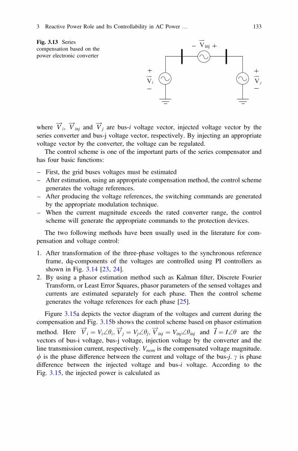
where V!

i, V!

inj and V!

j are bus-i voltage vector, injected voltage vector by the

series converter and bus-j voltage vector, respectively. By injecting an appropriate

voltage vector by the converter, the voltage can be regulated.

The control scheme is one of the important parts of the series compensator and

has four basic functions:

– First, the grid buses voltages must be estimated

– After estimation, using an appropriate compensation method, the control scheme

generates the voltage references.

– After producing the voltage references, the switching commands are generated

by the appropriate modulation technique.

– When the current magnitude exceeds the rated converter range, the control

scheme will generate the appropriate commands to the protection devices.

The two following methods have been usually used in the literature for com-

pensation and voltage control:

1. After transformation of the three-phase voltages to the synchronous reference

frame, dq-components of the voltages are controlled using PI controllers as

shown in Fig. 3.14 [23, 24].

2. By using a phasor estimation method such as Kalman filter, Discrete Fourier

Transform, or Least Error Squares, phasor parameters of the sensed voltages and

currents are estimated separately for each phase. Then the control scheme

generates the voltage references for each phase [25].

Figure 3.15a depicts the vector diagram of the voltages and current during the

compensation and Fig. 3.15b shows the control scheme based on phasor estimation

method. Here V!

i ¼ Vi\hi; V!

j ¼ Vj\hj; V!

inj ¼ Vinj\hinj and ~I ¼ I\h are the

vectors of bus-i voltage, bus-j voltage, injection voltage by the converter and the

line transmission current, respectively. Vnom is the compensated voltage magnitude.

/ is the phase difference between the current and voltage of the bus-j. c is phase

difference between the injected voltage and bus-i voltage. According to the

Fig. 3.15, the injected power is calculated as

Vi

injV

V j

Fig. 3.13 Series

compensation based on the

power electronic converter


Pinj ¼ Pout � Pin ¼ Vj I cosð/Þ � Vi I cosð/� hj þ hiÞ ð3:17Þ

where Pout is the output power and Pin is the input power. Since the compensation

should be done by exchanging only reactive between the series converter and the

network, so Pinj = 0 is assumed. In other words, the injected voltage should be

perpendicular to the current, so no active power is exchanged between the converter

(a)

(b)

Fig. 3.15 Voltage control based on phasor estimation by series compensator, a vector diagram of

the voltages and current during compensation, b block diagram of the control scheme

Notch Filter PI ++

++

++

Positive Controller

aV

bV

cV

pd

V

nomV

eθ

abc dq

Notch Filter

pq

VPI

*pqV 0

eθ

dq abc PWM

Notch Filter PI

+

+

Negative Controller

nd

V

*=

dV 0n

abc dq

Notch Filter

nq

VPI

eθ

dq abc

*=qV 0n

eθ

Fig. 3.14 Voltage control block diagram in dq reference frame


and the network. By doing a small amount of computations and trigonometric

relations, the injected voltage magnitude (Vinj) and c are obtained as follows:

c ¼ arc sinðVnom cosð/Þ

Vi

Þ ð3:18Þ

Vinj ¼ffiffiffiffiffiffiffiffiffiffiffiffiffiffiffiffiffiffiffiffiffiffiffiffiffiffiffiffiffiffiffiffiffiffiffiffiffiffiffiffiffiffiffiffiffiffiffiffiffiffiffiffiffiffiffiffiffiffiffiffiffiffiffi

V2nom þV2

i � 2Vnom Vi sinðcþ/Þq

ð3:19Þ

After producing the voltage references, the inverter output voltages are injected

in series by three single-phase transformers. To eliminate the switching frequency

harmonics, a low-pass filter for each phase is used, which consists of the leakage

inductance of the series transformer and the filter capacitor. Also, a parallel switch

for each phase is used to bypass the series converter in fault conditions.

3.5 Conclusion

An overview of the basic principles of the power transmission operation and the

reactive power role in the transmission system has been presented. The flow of

reactive power causes additional heating of the lines and voltage drops in the

network. High reactive power consumption by heavily loaded transmission line

lead to voltage dips in the system and limit the generation of the active power.

Voltage and reactive power control causes that a stable, efficient, and reliable

operation of the power system is achieved and utilization of the transmission system

is maximized.

References

1. V. Patel, J.G. Jamnani, Techniques to Increase Surge Impedance Loading Level of EHV AC

Transmission Lines for Improving Power Transfer Capability, IEEE International Conference

on Computation of Power, Energy Information and Communication, (ICCPEIC), 2015,

pp. 518–523.

2. A.K. Mohanty, A.K. Barik, Power System Stability Improvement Using FACTS Devices, Int.

J. Mod. Eng. Res., vol. 1, no. 2, pp. 666–672, 2009.

3. F.S. Moreira, T. Ohishi, J.I.D.S. Filho, Influence of the Thermal Limits of Transmission Lines

in the Economic Dispatch, IEEE Power Engineering Society General Meeting, 2006, pp. 1–6.

4. R. Mathur, R. Varma, Reactive Power Control in Electrical Power Transmission Systems,

2002, Wiley-IEEE Press.

5. P. Kundur, Power System Stability and Control, 1994, McGrawHill.

6. D. Biggar, M. Hesamzadeh, Introduction to Electric Power Systems, 2014, Wiley-IEEE Press.

7. X. Yu, S. Cao, H. Jia, P. Zhang, Impact of the Exciter Voltage Limit to Power System Small

Signal Stability Region, Proc. of IEEE Power Engineering Society General Meeting, 2007,

pp. 1–7.


8. K. Bhattacharya, J. Zhong, Reactive Power as an Ancillary Service, IEEE Trans. Power Syst.,

vol. 16, no. 2, pp. 294–300, 2001.

9. T. Zabaiou, L.A. Dessaint, I. Kamwa, Preventive Control Approach for Voltage Stability

Improvement Using Voltage Stability Constrained Optimal Power Flow based on Static Line

Voltage Stability Indices, IET Gener., Transm. Distrib., vol. 8, no. 5, pp. 924–934, 2014.

10. Z. Chen, F. Blaabjerg, Y. Hu, Stability Improvement of Wind Turbine Systems by

STATCOM, Proc. of IEEE Industrial Electronics, 2006, pp. 4213–4218.

11. F.A.L. Jowder, Influence of Mode of Operation of the SSSC on the Small Disturbance and

Transient Stability of a Radial Power System, IEEE Trans. Power Syst., vol. 20, no. 2,

pp. 935–942, 2005.

12. X. Jiang, J.H. Chow, A.A. Edris, B. Fardanesh, E. Uzunovic, Transfer Path Stability

Enhancement by Voltage-Sourced Converter-Based FACTS Controllers, IEEE Trans. Power

Deliv., vol. 25, no. 2, pp. 1019–1025, 2010.

13. M.H. Haque, Evaluation of First Swing Stability of a Large Power System with

Various FACTS Devices, IEEE Trans. Power Syst., vol. 23, no. 3, pp. 1144–1151, 2008.

14. S. Kannan, S. Jayaram, M. Salama, Real and Reactive Power Coordination for a Unified

Power Low Controller, IEEE Trans. Power Syst., vol. 19, no. 3, pp. 1454–1461, 2004.

15. V. Azbe, R. Mihalic, The Control Strategy for an IPFC Based on the Energy Function, IEEE

Trans. Power Syst., vol. 23, no. 4, pp. 1662–1669, 2008.

16. G.M. Vireshkumar, F.R. Basangouda, H.J. Suresh, Review on Comparison of FACTS

Controllers for Power System Stability Enhancement, International Journal of Scientific and

Research Publications, vol. 3, no. 3, pp. 57–58, 2013.

17. K.R. Padiyar, FACTS Controllers in Transmission and Distribution, 2007, New Age

Intenational.

18. E. Acha, V.G. Agelidis, O. Anaya-Lara, T.J.E. Miller, Power Electronic Control in Electrical

Systems, 2002, Newnes.

19. T.J.E. Miller, Reactive Power Control in Electric Systems, 1982,Wiley-Interscience.

20. P.L. Nguyen, Q.C. Zhong, F. Blaabjerg, J. M. Guerrero, Synchronverter-Based Operation of

STATCOM to Mimic Synchronous Condensers, Proc. of IEEE Conference on Industrial

Electronics and Applications, (ICIEA), 2012, no. 2, pp. 942–947.

21. L. Liu, H. Li, Y. Xue, W. Liu, Reactive Power Compensation and Optimization Strategy for

Grid-Interactive Cascaded Photovoltaic Systems, IEEE Trans. Power Electron., vol. 30, no. 1,

pp. 188–202, 2015.

22. X. Jiang, X. Fang, J.H. Chow, A.A. Edris, E. Uzunovic, M. Parisi, L. Hopkins, A Novel

Approach for Modeling Voltage-Sourced Converter-Based FACTS Controllers, IEEE Trans.

Power Deliv., vol. 23, no. 4, pp. 2591–2598, 2008.

23. J.G. Nielsen, M. Newman, H. Nielsen, F. Blaabjerg, Control and Testing of a Dynamic

Voltage Restorer (DVR) at Medium Voltage Level, IEEE Trans. Power Electron., vol. 19, no.

3, pp. 806–813, 2004.

24. Y. Shokri, E. Ebrahimzadeh, H. Lesani, S. Afsharnia, Performance Improvement of

DFIG-Based Wind Farm Using Multilevel Cascaded Hbridge Converter under Unbalanced

Grid Voltage Conditions, Proc. of 14th Int. Conf. on Environ. and Elec. Eng. (EEEIC), 2014,

pp. 158–163.

25. E. Ebrahimzadeh, S. Farhangi, H. Iman-eini, F.B. Ajaei, R. Iravani, Improved Phasor

Estimation Method for Dynamic Voltage Restorer Applications, IEEE Trans. Power Deliv.,

vol. 30, no. 3, pp. 1467–1477, 2015.


Chapter 4

Reactive Power Compensation in Energy

Transmission Systems with Sinusoidal

and Nonsinusoidal Currents

Milan Stork and Daniel Mayer

Abstract A standout amongst the most noteworthy current talks in electricaldesigning is the meaning of the responsive power under nonsinusoidal conditions innonlinear electric frameworks. New meanings of responsive power have beentalked about in the most recent years. Despite the fact that the component of electricenergy stream for nonsinusoidal conditions is all around depicted today, so toll isnot yet accessible a summed up power hypothesis, and hypothetical figuring for theconfiguration of such gadgets as dynamic channels or element compensators.Thusly the undertaking of planning compensators for advance energy transmissionwith nonlinear time-fluctuating loads in nonsinusoidal administrations is, a longway from clear. Voltage and current harmonics created by nonlinear loads incre-ment power losses in transmission frameworks and, in this manner, negativelyaffect effectivity of appropriation frameworks and parts. While a few harmonics arebrought on by framework nonlinearities, for example, transformer immersion, mostharmonic are delivered by power electronic loads, for example, flexible velocitydrives and diode span rectifiers. In this chapter the reactive power compensation forsinusoidal and nonsinusoidal circumstances, where nonlinear circuit voltages andstreams contain harmonic are explained and reenacted. The results can be used forcontrol algorithms of automatic compensators which are also described. The mainaim of this chapter is based on the dissipative systems theory and therefore theoryof cyclodissipativity which can be used for calculation of compensation elements(capacitors, inductors) for reactive power compensation. The compensation ele-ments are determined by minimizing line losses. It will show that approach base ondissipative systems theory provides an important mathematical framework for

M. Stork (&)Department of Applied Electronics and Telecommunications, University of West Bohemia,Plzen, Czech Republice-mail: [email protected]

D. MayerDepartment of Theory of Electrical Engineering, University of West Bohemia,Plzen, Czech Republice-mail: [email protected]

© Springer International Publishing AG 2017N. Mahdavi Tabatabaei et al. (eds.), Reactive Power Control in AC Power Systems,Power Systems, DOI 10.1007/978-3-319-51118-4_4

137

analyzing and designing of compensators for reactive power compensation even forgeneral nonlinear loads. The presented theory is supplemented by a series ofexamples and simulations.

4.1 Introduction

A standout amongst the hugest current examinations in electrical designing is themeaning of the reactive power (RP) under nonsinusoidal conditions in nonlinearelectric frameworks. New meanings of RP have been talked about in the mostrecent years. Despite the fact that the component of electric energy stream fornonsinusoidal conditions is all around portrayed today, so admission is not yetaccessible a summed up power hypothesis, and hypothetical computations for theconfiguration of such gadgets as dynamic channels or element compensators. In thismanner, the undertaking of planning compensators for improve energy transmissionwith nonlinear time-changing loads in nonsinusoidal administrations is, a long wayfrom clear. Voltage and current harmonics created by nonlinear loads incrementpower loss in transmission frameworks and, in this manner, negatively affecteffectivity of conveyance frameworks and parts. While a few harmonics are createdby framework nonlinearities, for example, transformer immersion, most harmonicare delivered by power electronic loads, for example, notice adjustable speed drivesand diode span rectifiers. In this chapter the reactive power compensation forsinusoidal and nonsinusoidal circumstances, where voltages and streams containharmonic are contemplated and mimicked. The outcomes can be utilized for controlcalculations of programmed compensators. The fundamental point of this sectiondepends on the dissipative frameworks hypothesis and along these lines hypothesisof cyclodissipativity which can be utilized for estimation of compensation com-ponents (capacitors, inductors) for RP pay. It will demonstrate that approach baseon dissipative frameworks hypothesis gives a numerical structure to breaking downand planning of compensators.

Reactive power investigation and compensation are significant for conveyed eraand deregulation, which are the two primary procedures reshaping electric energyframeworks today. Conveyed era requires a portrayal of complex loads with bidi-rectional power streams, both in enduring state and in incessant homeless people.Deregulation requires exact evaluation of power streams, as well as of payendeavors and different administrations that incorporates numerous members andchiefs.

Our inspiration is to think about inert power and probability of pay for energyframeworks. Today, the exchanging power converters can working at time interimsmuch shorter than the key (50 or 60 Hz) period. Numerous broadly utilized outlineinstruments (e.g., those taking into account the idea of “quick reactive power”) aredescribed solely in the time space. Their application once in a while results inpresentation of harmonic that were not present in the first waveforms. This, thusly,might energize unmodeled progress, and bring about unsatisfactory drifters. The

138 M. Stork and D. Mayer

specialized means for online pay of polyphase frameworks are simply getting to beaccessible. This is valid for power electronic converters (e.g., voltage-sourcedinverters with quick exchanging and short reaction times) furthermore for controlequipment (e.g., reasonable miniaturized scale controllers with sign preparingability).

Improving energy exchange from an air conditioner source to a load is anestablished issue in electrical designing. The outline of power frameworks is suchthat the exchange happens at the key frequency of the source. Practically speaking,the proficiency of this exchange is typically diminished because of the phase shift inthe middle of voltage and current at the major frequency. The phase shift emergesto a great extent because of energy streams portraying electric engines. The powervariable (PF), characterized as the proportion between the genuine or dynamicpower (normal of the immediate power) and the clear power (the result of rms rootmean square estimations of the voltage and current), then communicates the energytransmission proficiency for a given load. The standard way to deal with dimin-ishing the responsive power is to utilize a compensator between the source and theload. Theoretical configurations of the compensator regularly expect that theidentical source comprises of a perfect generator having zero output impedance anddelivering an altered, simply sinusoidal voltage. On the off chance that the load isstraight time invariant (LTI), the subsequent enduring state mutt rent is a stagemoved sinusoid, and the PF is the cosine of the phase shift point. Accessiblecompensation innovations incorporate e.g. the pivoting hardware as well asexchanged capacitors and inductors and power electronic converters, for example,dynamic channels and adaptable air conditioning transmission frameworks.

4.2 Reactive Power Review

Energy handling frameworks have experienced significant changes as of late. Thisprocedure is principally determined by a longing to build proficiency, withdiminishment in energy costs, energy losses (and cooling necessities), and partmeasure. For productivity changes have been created the new advancements, (forexample, power electronics), and use of quicker actuators and controllers.

It is imperative that there exist useful impediments applicable for displaying andcontrol of dormant power. For instance, because of limited exchanging frequencythere exists a scope of frequencies where a dynamic channel (regularly a voltagesourced inverter) can work viably. The execution criteria are themselves innovationsubordinate—numerous instruments accessible in the field can just gauge amountsin the scope of roughly 1.5 kHz, however the most astounding harmonic utilized formetering reasons for existing is frequently the 23rd. Another for all intents andpurposes essential class of requirements is powered by material science of voltagesourced inverters, for example, limited energy storage, with constrained permittedvoltage variety of the primary capacitor and conceivably lacking voltage extent forfollowing of higher current harmonics.

4 Reactive Power Compensation in Energy Transmission Systems … 139

(a) Harmonic Standards: Standards and suggestions that recommend executioncriteria for electrical hardware are advanced by various associations around theworld (more than 50 national guidelines are said in [1]). The most powerfulones originate from the International Electrotechnical Commission (IEC) andby the IEEE, [1–3]. While the IEEE-519 prescribed practice concentrates on theclient/framework interface (the purported purpose of regular coupling) and onhigher power levels, the IEC-1000 standard (additionally embraced as theEuropean standard) incorporates limits for individual bits of gear, andapproaches to gauge the harmonic. These archives commonly list the extent ofparticular (low) current harmonics (both in relative and in outright terms), andan aggregate amount known as the total harmonic distortion (THD), that con-fines a potentially weighted total of squares of consonant sizes. Watch that allsignificant global measures are indicated in the frequency area. While thesebenchmarks can be deciphered as outside imperatives powered on the specialistoutlining an energy handling framework, it is critical to recall the real frame-work indications of expanded harmonics. These incorporate hardware impacts,(for example, disappointments of wires, power component redress capacitors,transformer and engine overheating, breaker stumbling) and framework wideissues (squinting of glowing lights and glint of glaring lights, impedance oncorrespondence frameworks) [3]. A late study of North American utilities [4]recommended that while the quantity of loads that create current harmonicwhen supplied with a (near) sinusoidal voltage is expanding powerfully, thereexists an essential absence of comprehension of energy streams includingnonsinusoidal waveforms and of approaches to decipher benchmarks.

A word about classification while everybody concurs that dynamic (or genuine)power is the dc part of the prompt power (every one of these amounts will becharacterized right away), a few creators save the name responsive power for thesupplement of dynamic power (the dormant power) at major frequency, or for thecomponent that can be repaid with direct latent circuit component; we utilize theassignments reactive and idle reciprocally (for additional on a proposed broughttogether phrasing see [5]).

(b) Power Systems: A spearheading chip away at this subject was attempted inEurope in the seventies, and brought about the Fryze-Buchholz-Depenbrock(FBD) strategy, compressed by the originator in [6]. This reference brings upthe likelihood of figuring ideas in the frequency space. Late down to earth usesof this time-area approach are exhibited in [7, 8].

Different references by Czarnecki, e.g. [9–13] together with here and therewarmed running with trade [14], tended to the issue from a power structure per-spective, and portrayed diverse miracles of utilitarian energy for circuit-basedcompensation in unbalanced three-stage systems. A repeat space presentation ofCzarnecki breaking down of three-stage systems is presented in [9]; we later give acomplete explanation in the general case. Note that other orthogonal weakeningsare doable for the sections of the inactive present, for instance, the one showed in


[15] that disconnects the part compensable by direct shunt components. A relatedresponsibility by an IEEE Power-Engineering Society Working Group is shown in[16]. An instructive and sensible power system test is given in [17].

The unmistakable power is one of the key thoughts while describing diversesums in polyphase structures, and a material science based comprehension is givenin [18]; a former study on the subject is depicted in [19]. A novel power systemorganized presentation of the thought responsive power with respect to vectorspaces and repeat parts is given in [20]. From the theoretical perspective, ourinvestigation heading contrasts from the strategy depicted in [20] in our emphasison projections in vector spaces where a polyphase sign is identified with by asingular part (point) of a suitable Hilbert space. This new vector space licenses us todecide a united treatment of each and every genuine class of responsive powercompensators as projections to suitable sub-spaces, and structures a reason forfruitful numerical procedure.

(c) Power Electronics: The exploration on polyphase frameworks in nonsinusoidaloperation has been reinvigorated by [21] that drew closer the issue from a downto earth stance, and proposed a helpful definition for the “quick” reactivepower. (An undifferentiated from idea was presented before by Depenbrock aspointed out in [6], yet remained basically obscure outside Germany.) The ideawas introduced in the time space, and in the exceptional instance of three-stageframeworks, so that the thought of vector (external) results of vectors could beutilized. An augmentation to four-conductor frameworks that can represent thezero-sequence components was presented in [22, 23]. Note that the momentaryresponsive power relates to the part of the inert power that can be repaidwithout energy stockpiling. A compensator construct only with respect to thisidea won’t just neglect to totally dispose of the idle power, yet might likewisebring extra harmonic [24] into the present waveform, as we show later. This isrecognized by one of the originators of the quick responsive power idea in [25].Hypothetical ideas proposed by Depenbrock and Akagi-Nabae have beenbroadly tried tentatively, for the most part in dynamic channel applications.Some illustrative studies are [26–31]. On account of three-stagethree-conductor frameworks, it is some of the time gainful to express appli-cable amounts regarding space vectors. The change is clear, and a trial con-firmation is introduced in [32].

4.3 Theoretical Background—Properties of Homogenous

Operators

In this part the properties of homogenous operators are presented [33, 34]. They areimportant for next parts of this chapter.


For any given periodic signal x(t) of period T the homogenous integral operatoris defined as

x_ðtÞ ¼ x wðtÞ � w

� �

¼ 2p

TwðtÞ � w� �

ð4:1Þ

where integral of voltage x(t) is

wðtÞ ¼Z

t

0

xðsÞds ð4:2Þ

and the average value over period T is

w ¼Z

T

0

wðsÞds ð4:3Þ

Similarly, the homogenous differential operator is

x^ðtÞ ¼ 1

x

dxðtÞdt

ð4:4Þ

Note that x_and x

^are dimensionally homogenous to basic quantity x [33]. The

internal product of two periodic variables x(t) and y(t) is defined as

x; yh i ¼ 1

T

Z

T

0

xðtÞyðtÞdt ð4:5Þ

and norm of variable x(t) (X is rms—root mean square) is

xk k ¼ffiffiffiffiffiffiffiffiffiffi

x; xh ip

¼


1

T

Z

T

0

x2ðtÞdt

v

u

u

u

t ¼ X ð4:6Þ

The homogenous operators have following properties [from (4.7) to (4.17)]

x; x_

D E

¼ x; x^

D E

¼ 0 ð4:7Þ

x_; x^

D E

¼ � xk k2 ð4:8Þ


x ¼ y^ , x

_ ¼ y ð4:9Þ

x_; y

D E

¼ � x; y_

D E

ð4:10Þ

x^; y

D E

¼ � x; y^

D E

ð4:11Þ

x_; y^

D E

¼ x^; y_

D E

¼ � x; yh i ð4:12Þ

Moreover, if x and y are sinusoidal quantities with rms values respectively equalto X and Y and phase difference equal to u, the following properties hold:

xk k ¼ x_

�

�

�

� ¼ x^

�

�

�

� ¼ X ð4:13Þ

x_þ x

^ ¼ 0 ð4:14Þ

x2 þ x_2 ¼ x2 þ x

^2 ¼ x2 � x_x^ ¼ 2 xk k2¼ 2X2 ð4:15Þ

xy� x_y^ ¼ xy� x

^y_ ¼ 2XY cos u ð4:16Þ

x_y� xy

_ ¼ xy^ � x

^y ¼ 2XY sin u ð4:17Þ

Moreover, expressing variable x(t) by its Fourier series:

xðtÞ ¼X

1

k¼1

xkðtÞ ¼X

1

k¼1

ffiffiffi

2p

Xk sinðkxtþukÞ ð4:18Þ

For homogenous variables

x_ðtÞ ¼

X

1

k¼1

x_

kðtÞ ¼ �X

1

k¼1

ffiffiffi

2p Xk

kcosðkxtþukÞ ð4:19Þ

x^ðtÞ ¼

X

1

k¼1

x^

kðtÞ ¼X

1

k¼1

ffiffiffi

2p

kXk cosðkxtþukÞ ð4:20Þ


4.4 Cyclodissipativity Approach

It will be reflected the typical energy transmission from an AC generator to a load.The voltage and current of the supplier are functions of time and are stand for thecolumn vectors vS, iS 2 ℜq. The load is defined by a (conceivably nonlinear andtime-varying) q–port system R [35, 36].

There are will the two following assumptions:(A1) All the signs in the system are periodic with fundamental period T and fit

into the space

L2½0; TÞ : x : ½0; TÞ ! <q xk k2:¼ 1

T

Z

T

0

xðsÞj j2ds\1

�

�

�

�

�

�

8

<

:

9

=

;

ð4:21Þ

where ||.|| is named the RMS value of b and |.| is the Euclidean standard.

(A2) The supplier is ideal, in the sense that vS stays unaffected for all loads.

Assumption (A1) captures the essentially rational method that the organism func-tions in a periodic, though not unavoidably sinusoidal, steady-state system. This isthe case of the vast majority of applications of attention for the problem at hand[36].

Assumption (A2) is the similar to saying that the supplier has zero impedance and isdefensible by the fact that most AC device function at a specified voltage, with theactual drained current being stated by the load [36].

The active power supplied by the source is defined as

P :¼ vS; iSh i ¼ 1

T

Z

T

0

vTS ðtÞiSðtÞdt ð4:22Þ

and :h i means the internal creation in L2[0, T). From (4.22) and theCauchy-Schwarz inequality [36] is

P� vSk k � iSk k ¼ : S ð4:23Þ

where is defined the apparent power S. From the inequality above we achieve that,under Assumption (2), S is the uppermost average power supplied to the load for allloads that have the identical rms current ||iS||. The characteristics holds if and only ifvS and iS are collinear. If this is not the case P < S and compensation schemes arepresented to decrease this incongruity [36]. That is, to maximize the proportion P/S

- that is called the PF. A typical compensation formation (which can be easilyprolonged to n-phase system) is shown in Fig. 4.1 where, to preserve the rated


voltage at the load stations the compensator YC is located in parallel. Similarly, toevade power indulgence, YC is restricted to be lossless, that is

v; iCOh i ¼ 0 ð4:24Þ

where iCO is the compensator current and notification that vS = v (Fig. 4.1). Fromthe former can be result that the PF compensation problem is accurately equivalentto the problem of minimization of ||iS|| subject to the restriction (4.24). From

iSk k2¼ ik k2 þ iCk k2 þ 2 iC; ih i ð4:25Þ

it is clear that an obligatory situation to decrease the rms value of iS is

iC; ih i\0 ð4:26Þ

It turns out that the latter circumstance and the limitation of compensator loss-lessness can be recognized using the perception of cyclo-dissipativity and itsconnected abstract energy [36–41].

Definition 1 Assume a dynamical system, with input u 2 L2[0,T) and output y 2L2[0,T), acknowledges a state–space picture with state vector x 2 X [42]. Thesystem is cyclo-dissipative with respect to the supply rate w(u, y), where w: L2[0,T) � L2[0,T) ! ℜ, if and only if

Z

T

0

w uðtÞ; yðtÞð Þdt� 0 ð4:27Þ

For all u: [0, T)! L2[0,T) such that x(T) = x0 where x(0) = x0. It is said to becyclo-lossless if the inequality holds with identity. In other words, a system is

cyclo-dissipative when it cannot create (abstract) energy over closed paths in the

state-space. It might, though, produce energy alongside some preliminary share ofsuch a trajectory; if so, it would not be dissipative. On the other hand, every

dissipative system is cyclo-dissipative. For instance, (possibly nonlinear) RLCcircuits with input and output their terminal currents and voltages, respectively, arecyclo-dissipative with supply rate w(u, y) = uTy provided that all resistances arepassive (This can be easily proven using Tellegen’s Theorem [42–44]). Note that itis not presumed that inductors and capacitors are passive-that is, that their stored

CYSv v

COi

i

Load

Comp

SiFig. 4.1 Principle of typicalreactive power compensation


energy is non–negative-if so, the circuit is in addition passive. It has been shown in[42–44] that, correspondingly to dissipative systems, one can use storage functionsand dissipation differences to characterize cyclo-dissipativity.

Theorem 1 A system with state depiction is cyclo-dissipative if, for all x 2 X which

are both controllable and reachable, there exists a virtual storage function /:X!R [42]. That is, a function that satisfies

/ðx0ÞþZ

T

0

w uðtÞ; yðtÞð Þdt�/ðx1Þ ð4:28Þ

for u 2 L2[0,T) such that x(0) = x0 and x(T) = x1. In following part, the instances ofreactive power compensation based on cyclo-dissipativity method are presented.

4.5 Reactive Power Compensation

In this part on the first, the simple example concerning linear circuit and nonhar-monic power source is presented. The second example is devoted to nonlinearcircuit. Booth examples are simply extended to q-phase version.

Example 4.1 [36]: Suppose linear system, power source, compensator and serialconnection of RLC and nonharmonic power source (Fig. 4.2) [36]. Supply voltagevS is

vsðtÞ ¼ffiffiffi

2p

A1 sinðx0tÞþA3 sinð3x0tÞð þA5 sinð5x0tÞÞ ð4:29Þ

where A1 = 360, A3 = 144, A5 = 42, x0 = 100p [rad/s] and R = 15 [X], L = 0.08[H], C = 0.0212 [mF]. Load impedances Zn (for n = 1, 3, 5) are given

Zn ¼ Rþ jx0nLþ1

jx0nCn ¼ 1; 3; 5 ð4:30Þ

For calculated values Z1 = 15 – 125.14j; Z3 = 15 + 24.97j; and Z5 = 15 + 95j,the effective currents are

in ¼ An=Zn n ¼ 1; 3; 5 ð4:31Þ

C

R

L CY

Sv vCOi

i

LoadComp

SiFig. 4.2 Example of RPcompensation for linear RLCload and nonharmonic source


Numerical values of currents are i1 = 0.34 + 2.8361j; i3 = 2.54 – 4.24j;i5 = 0.0681 − 0.4313j.

Total effective current through the load is

i ¼ ink k ¼ffiffiffiffiffiffiffiffiffiffiffiffiffiffiffiffi

X

n

inj j2r

¼ffiffiffiffiffiffiffiffiffiffiffiffiffiffiffiffiffiffiffiffiffiffiffiffiffiffiffiffiffiffiffiffiffiffi

i1j j2 þ i3j j2 þ i5j j2q

; n ¼ 1; 3; 5 ð4:32Þ

therefore i = 5.7257 [A]. For uncompensated circuit (YC!0) iS = i and apparentpower is

S ¼ vSk k � iSk k ¼ffiffiffiffiffiffiffiffiffiffiffiffiffiffiffiffiffiffiffiffiffiffiffiffiffiffiffiffiffiffiffiffiffiffiffiffiffiffiffi

A1j j2 þ A3j j2 þ A5j j2q

� �

�ffiffiffiffiffiffiffiffiffiffiffiffiffiffiffiffiffiffiffiffiffiffiffiffiffiffiffiffiffiffiffiffiffiffi

i1j j2 þ i3j j2 þ i5j j2q

� �

ð4:33Þ

Result is S = 2233 [VA] and active power (average power) is

P ¼ vS; iSh i ¼ 1

T

Z

T

0

vTS ðtÞiSðtÞdt ¼ Ri2S ð4:34Þ

P = 491.8 [W]. PF for uncompensated circuit (YC!0) is

PF ¼ P

S¼ 491:76

2233¼ 0:22 ð4:35Þ

For circuit compensated by capacitor

iSk k2¼ iþ iCOk k2¼ ik k2 þ iCOk k2 þ 2 i; iCOh i ð4:36Þ

and current iC0 for compensation capacitor

iCOðtÞ ¼ CCO

dvSðtÞdt

ð4:37Þ

therefore

iCO ¼ CCO _vS ð4:38Þ

and substitution of Eq. (4.18) into (4.16)

iSk k2¼ iþ iCOk k2¼ ik k2 þ CCO _vSk k2 þ 2 i;CCO _vSh it ð4:39Þ


after some manipulations

iSk k2¼ iþ iCOk k2¼ ik k2 þC2CO _vSk k2 þ 2CCO i; _vSh i ð4:40Þ

For compensated circuit iSk k2\ iþ iCOk k2 Eq. is

iSk k2\ iþ iCOk k2¼ ik k2 þC2CO _vSk k2 þ 2CCO i; _vSh i ð4:41Þ

Using the property (4.42)

_x; yh i ¼ � x; _yh i ð4:42Þ

in Eq. (4.41) results

iSk k2\ iþ iCOk k2¼ ik k2 þ C2CO _vSk k2� 2CCO

_i; vS

D E

ð4:43Þ

Minimal value of iS (or minimum of apparent power S) can be found for

d

dCCO

ik k2 þC2CO _vSk k2 � 2CCO

_i; vS

D E

¼ 0 ð4:44Þ

therefore

2CCO _vSk k2 � 2 _i; vS

D E

¼ 0 ð4:45Þ

Optimal value of compensation capacitor is

CCO ¼_i; vS

D E

_vSk k2ð4:46Þ

where

_i; vS

D E

¼ Re jx0i1A1f gþRe j3x0i3A3f gþRe j5x0i5A5f g ¼ 282800 ð4:47Þ

and

_vSk k2¼ A1x0ð Þ2 þ A33x0ð Þ2 þ A55x0ð Þ2 ¼ 3:5563 � 1010 ð4:48Þ

The optimal capacitor for compensation of reactive power [according (4.46)] is

CCO ¼ 282800= 3:5563 � 1010� �

¼ 7:9521½lF�


This result was confirmed by simulation (searching for optimal value) asFig. 4.3. Currents through the compensation capacitor

iCOn ¼ jnx0CCOAn; n ¼ 1; 3; 5 ð4:49Þ

iCO1 = 0 + 0.899j; iCO3 = 0 + 1.079j; iCO5 = 0 + 0.525j and currents fromsource after compensation iS1 = 0.34 + 3.735j; iS3 = 2.545 – 3.158j; iS5 = 0.0681 +0.0933j, and total effective current from source for circuit with compensationcapacitor is iS = 5.5259 (without compensation was 5.72 A) and apparent power isS = 2155. PF for compensated circuit is PF ¼ P=S ¼ 491:8=2155 ¼ 0:228.

The circuit can be compensated also by inductor where compensation current isgiven as

iL ¼1

LC

Z

vSdt ð4:50Þ

For compensation by means of inductor, Eq. (4.43) is changed

iSk k2\ iþ iLk k2¼ ik k2 þ 1

LC

Z

vS

�

�

�

�

�

�

�

�

2

þ 21

LC

Z

vS; i

� �

ð4:51Þ

For compensated circuit

Fig. 4.3 Current iS versus value of compensation capacitor CCO (Example 4.1)


iSk k2\ iþ iLk k2 ¼ ik k2 þ 1

L2C

Z

vS

�

�

�

�

�

�

�

�

2

þ 2

LCi;

Z

vS

� �

ð4:52Þ

After some manipulation, optimal value of compensation inductor is

LC ¼ �R

vS�

�

�

�

2

i;R

vS � ð4:53Þ

where

Z

vS

�

�

�

�

�

�

�

�

2

¼ A1

x0

�

�

�

�

�

�

�

�

� �2

þ A3

3x0

�

�

�

�

�

�

�

�

� �2

þ A5

5x0

�

�

�

�

�

�

�

�

� �2

¼ 1:34 ð4:54Þ

and

i;

Z

vS

� �

¼ Re jA1

x0i1

� �

þRe jA3

3x0i3

� �

þRe jA5

5x0i5

� �

¼ �2:59 ð4:55Þ

Therefore optimal compensation inductor [according Eq. (4.53)] is

LC ¼ �1:337=� 2:5909 ¼ 0:516 ½H� ð4:56Þ

This result was confirmed by simulation (Fig. 4.4). Current through the com-pensation inductor

Fig. 4.4 Current iS versus value of compensation inductor LC (Example 4.1)


iLn ¼ An=jnx0LC; n ¼ 1; 3; 5. . . ð4:57Þ

Calculated values are iL1 = 0 – 2.22j; iL3 = 0 – 0.296j; iL5 = 0 – 0.052j. Currentsfrom source after compensation are iS1 = 0.34 + 0.616j; iS3 = 2.545 – 4.534j;iS5 = 0.068 – 0.483j and total effective current from source for circuit with com-pensation inductor is iS = 5.27, and apparent power is S = 2055, and PF forcompensated circuit is PF ¼ P=S ¼ 491:8=2055 ¼ 0:24.

This result was confirmed by simulation (searching for optimal value) asFig. 4.4.

Example 4.2 [36]: Suppose linear system, power source, compensator and serialconnection of RL and nonharmonic power source shown in Fig. 4.5 [36], instead ofnonlinear inductor the nonharmonic power source is used. Supply voltage vS is

vsðtÞ ¼ffiffiffi

2p

A1 sinðx0tÞþA3 sinð3x0tÞð Þ ð4:58Þ

where A1 = 220, A3 = 70, x0 = 100p [rad/s] and R = 10 [X], L = 0.2 [H].Similarly as in Example 4.1, the load impedances Zn (for n = 1, 3) are given

Zn ¼ Rþ jx0nL n ¼ 1; 3 ð4:59Þ

For calculated values Z1 = 10 + 62.8j, Z2 = 10 + 188.5j, the effective currentsare i1 = 0.54 – 3.4j; i3 = 0.02 – 0.37j;

For uncompensated circuit (YC ! 0), total effective current through the loadaccording Eq. (4.22) is iS = i = 3.48 [A] and apparent power (4.23) is S = 802.9[VA] and active power (4.24) is P = 121 [W]. For uncompensated circuit isPF = 0.15. By the same way as in previous Example 4.1, using (4.40), (4.45) and(4.46) calculated values are

_i; vS

D E

¼ 260450 ð4:60Þ

and

_vSk k2¼ 9:13 � 109 ð4:61Þ

R

L CY

Sv vCOi

i

LoadComp

SiFig. 4.5 Example of RPcompensation for linear RLload and nonharmonic source


Optimal value of compensation capacitor is

CCO ¼_i; vS

D E

_vSk k2¼ 260450

9:13 � 109 ¼ 28:5 � 10�6 ð4:62Þ

This result was confirmed by simulation (searching for optimal value) asFig. 4.6.

For circuit compensated by capacitor i = 2.16 [A] and apparent power isS = 498.6 [VA], active power is P = 121 [W] and. PF = 0.22. The compensationby means of inductor is not possible because result according Eq. (4.53) has neg-ative sign. Simulation results are shown in Fig. 4.7, where compensation capacitoris connected in time � 0.44 s.

Example 4.3 [36]: Suppose nonlinear circuit with triac (Fig. 4.8) andnon-sinusoidal power source vS(t) = 220sin(100pt) + 30sin(300pt), R = 10 X anda = p/2. By the same way as in previous Example 4.1, using (4.60), (4.61) and(4.62) calculated values are

_i; vS

D E

¼ � i; _vSh i ¼ �3:6 � 105 ð4:63Þ

and

_vSk k2¼ 5:58 � 109 ð4:64Þ

Fig. 4.6 Current iS versus value of compensation capacitor CCO (Example 4.2)


Optimal value of compensation capacitor can be calculated from

CCO ¼ � i; _vSh i_vSk k2

¼ �ð�3:6 � 105Þ5:58 � 109 ¼ 64:7 � 10�6 ð4:65Þ

Optimal value of compensation capacitor (CCO = 65 [lF]) was confirmed bysimulation as Fig. 4.9. For uncompensated circuit effective current is

iS ¼ 15:7 A½ �; P ¼ 2462 W½ �; S ¼ 3484 VA½ �; PF ¼ 0:71

After compensation effective current from source is

iS ¼ 14:92 A½ �; P ¼ 2462 W½ �; S ¼ 3315 VA½ �; PF ¼ 0:743

The time evolutions of signals in nonlinear circuit are shown in Fig. 4.10. It isimportant to note that inductor is not possible for compensation because resultaccording Eq. (4.53) has negative sign.

Fig. 4.7 Time evolution of voltage (top), current from source (middle) and effective current fromsource for uncompensated (time <0.44) and compensated circuit (time � 0.44)

R CY

Sv vCOi

i

LoadComp

Si

α

Fig. 4.8 Nonlinear circuitwith triac


Previous results can be used for automatic compensation of RP. The timeevolution of signals (for circuit in Fig. 4.8) is shown in Fig. 4.11. In time oft1 = 0.2 [s] start automatic compensation [repeated evaluation of Eq. (4.64)] andchanging value of compensation capacitor according condition in circuit (CCO = f

(iS(t),vS(t))).From the beginning, until t2 the power source voltage is vS tð Þ ¼

220 sin 100ptð Þþ 30 sin 300ptð Þ after t2 voltage is sinusoidalvS(t) = 220 sin (100pt).

The effective value of supply current ii is repeatedly calculated and smoothed bylow-pass filter. From the Fig. 4.11 can be seen decreasing supply current value afterstart of compensation and once more decreasing after changing supply voltage topure sinusoidal. In Fig. 4.12, the Value of compensation capacitor versus triac fireangle alpha is displayed.

4.6 Extension to Three-Phase Networks

The recently proposed networks were devoted to the analysis of single phasesystems. In this chapter it is extended to three-phase networks.

The extension of the above theory to poly-phase systems is straightforward for 4wire Y connection, but for 3 wire network with unbalanced terms, delta connectionand compensation of reactive power opens several questions [45–47]. In this partthe compensation of reactive power and unbalanced currents of three-phase networkwill described [48–52].

Fig. 4.9 Current iS versus value of compensation capacitor CCO for nonlinear circuit(Example 4.3)


Considerations in this part are devoted to three-phase, three-wire circuits, shownin Fig. 4.13 with linear, time-invariant loads supplied with a sinusoidal symmetricalvoltage [53–55]. For any such loads there exist equivalent resistive and balancedloads shown in Fig. 4.14 that at the same voltage has the same active power P, asthe original load. The Three-phase source with line resistance, transformer TR (D toY connection) and load ZR, ZS, ZT is shown in Figs. 4.15 (without compensation)and 4.16 (with compensation).

Suppose three-phase, sinusoidal line-to-ground voltages uR, uS and uT and linecurrents iR, iS and iT. The active and reactive powers is defined as

P ¼ 1

T

Z

T

0

uRiR þ uSiS þ uT iTð Þdt ¼X

f¼R;S;T

Uf If cosðuf Þ ð4:66Þ

Q ¼X

f¼R;S;T

Uf If sinðuf Þ ð4:67Þ

There are several definitions of apparent power S. The definition according(4.68) is used

Fig. 4.10 Voltage and currents in nonlinear circuit. From top to bottom: Power source voltage,current through the load, current through compensation capacitor and current from source aftercompensation (Example 4.3)


Fig. 4.11 Time diagram of voltage and currents in nonlinear circuit during the automaticcompensation. From top to bottom: Voltage of power source, supply current iS, effective value ofsupply current, current through the load. Compensation start in time t = 0.2. Source voltage ischanged in t = 0.4 to pure sinusoidal. The time slice is 0:20� 0:50h i (Example 4.3)

0 20 40 60 80 100 120 140 160 1800

20

40

60

80

100

120

Alpha [deg]

Co

mp

en

sati

on

cap

acit

or

[ /uF

]

Fig. 4.12 Value of compensation capacitor versus alpha (Example 4.3)


RZ

Ri

Load

RR

SR

TR

Si

Ti

RV

SV

TV

SZ

TZ

Ni

Fig. 4.13 Three-phase star(Y) network with lineresistances RR, RS, RT, loadsZR, ZS, ZT and neutral wire

eR

Ri LRR

LSR

LTR

Si

Ti

i

Fig. 4.14 Three-phaseresistive load RLR, RLS, RLT

and its equivalent Re

RZR

i

Load

RR

SR

TR

Si

Ti

RV

SV

TV

SZ

TZ

TR

∆

Fig. 4.15 Three-phasesource with line resistance,transformer TR (D to Y) andload ZR, ZS, ZT

RV

Ri

Load

Comp

TR

SV

TV

RR SR TR

Si

Ti

1Ri

1Si 1T

i

Fig. 4.16 Three-phasenetwork with transformer TR(D to Y connection), load andcompensation


S ¼ffiffiffiffiffiffiffiffiffiffiffiffiffiffiffiffiffiffiffiffiffiffiffiffiffiffiffiffi

U2R þU2

S þU2T

q

�ffiffiffiffiffiffiffiffiffiffiffiffiffiffiffiffiffiffiffiffiffiffiffi

I2R þ I2S þ I2T

q

¼ uk k � ik k ð4:68Þ

The active power in three-phase system in frequency domain is

P ¼ ðu; iÞ ¼ ReX

n2NUT

n In ð4:69Þ

where asterisk denotes a conjugate number. The RMS value of a three-phase vectoris defined as:

xk k ¼ffiffiffiffiffiffiffiffiffiffiffiffiffiffiffiffiffiffiffiffiffiffi

X

n2NXTn � X

n

r

¼

ffiffiffiffiffiffiffiffiffiffiffiffiffiffiffiffiffiffiffiffiffiffiffiffiffiffiffiffiffiffiffiffiffiffiffiffiffiffiffiffiffiffiffiffiffiffiffiffiffiffi

X

n2NXRn;XSn;XTn½ �

XRn

XSn

XTn

2

4

3

5

v

u

u

u

t ð4:70Þ

For serial connection of RZ and LZ between phase R-S admittance is

YRS ¼1

RZ þ jxLZ¼ 1

RZ þXZ

ð4:71Þ

The equivalent admittance Ye for three admittances is

Ye ¼ YRS þ YST þ YTR ð4:72Þ

The equivalent admittance Ge and susceptance Be are given by

Ge ¼ ReðYeÞ; Be ¼ ImðYeÞ ð4:73Þ

Unbalanced admittance A is

A ¼ �ðYST þ YTRej2p=3 þ YRSe

j4p=3Þ ð4:74Þ

Voltage v across phase is

v ¼ffiffiffi

3p

vf ð4:75Þ

Active current ia, reactive current ir unbalanced current iu and total current i are

ia ¼ Gev ¼ Ge

ffiffiffi

3p

vf ; ir ¼ Bej jv; iu ¼ A � vj j

ik k ¼ffiffiffiffiffiffiffiffiffiffiffiffiffiffiffiffiffiffiffiffiffiffiffiffiffiffiffiffiffiffiffiffiffiffiffiffiffiffiffiffiffi

iak k2 þ irk k2 þ iuk k2q ð4:76Þ


Active power P

P ¼ Gev2s ¼ Ge vk k2 ð4:77Þ

Reactive power Q

Q ¼ vk k � irk k ¼ �Im YRS uRSk k2 þ YST uRSk k2 þ YTR uRSk k2n o

¼ �Be vk k2

ð4:78Þ

Unbalanced power D

D ¼ vk k � iuk k ¼ Aj j vk k2 ð4:79Þ

Apparent power S is calculated by

S ¼ vk k � ik k ¼ffiffiffiffiffiffiffiffiffiffiffiffiffiffiffiffiffiffiffiffiffiffiffiffiffiffiffi

P2 þQ2 þD2p

ð4:80Þ

Power Eq. (4.80) shows that reactive power and unbalanced power (reactivecurrent and unbalanced current) increase apparent power and decrease power factor[Eq. (4.35)]. Thus reduction of booth currents leads to PF improvement. Thesecurrents can be reduced by shunt compensator. Compensator is composed fromreactive passive parts e.g. inductors and capacitors, or three-phase inverter withcontrol systems. The structure of reactive compensator is shown in Fig. 4.18(Comp), susceptances WRS, WST and WTR, connected in delta configuration (it issupposed that WRS, WST and WTR are ideal loss-less parts).

From unbalanced admittance A and equivalent susceptance Be is possible cal-culate the compensation susceptances WXY from following equations. The reactivecurrent is compensated if:

Be þWRS þWST þWTR ¼ 0 ð4:81Þ

The unbalanced current is compensated if

A� j WST þ ej2p=2WTR þ ej4p=2WRS

¼ 0þ j0

A� j WST þ � 1

2þ j

ffiffiffi

3p

2

� �

WTR þ � 1

2� j

ffiffiffi

3p

2

� �

WRS

� �

¼ 0þ j0ð4:82Þ

The Eq. (4.82) is split on real and imaginary parts. Real part:

Re A� j WST þ � 1

2þ j

ffiffiffi

3p

2

� �

WTR þ � 1

2� j

ffiffiffi

3p

2

� �

WRS

� ��

¼ 0 ð4:83Þ


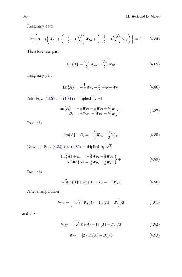
Imaginary part:

Im A� j WST þ � 1

2þ j

ffiffiffi

3p

2

� �

WTR þ � 1

2� j

ffiffiffi

3p

2

� �

WRS

� ��

¼ 0 ð4:84Þ

Therefore real part

Re Af g ¼ffiffiffi

3p

2WRS �

ffiffiffi

3p

2WTR ð4:85Þ

Imaginary part

Im Af g ¼ � 1

2WRS �

1

2WTR þWST ð4:86Þ

Add Eqs. (4.86) and (4.81) multiplied by −1

Im Af g ¼ � 12WRS � 1

2WTR þWST

Be ¼ �WRS �WTR �WST

�

þ ð4:87Þ

Result is

Im Af gþBe ¼ � 3

2WRS �

3

2WTR ð4:88Þ

Now add Eqs. (4.88) and (4.85) multiplied byffiffiffi

3p

Im Af gþBe ¼ � 32WRS � 3

2WTRffiffiffi

3p

Re Af g ¼ 32WRS � 3

2WTR

�

þ ð4:89Þ

Result is

ffiffiffi

3p

Re Af gþ Im Af gþBe ¼ �3WTR ð4:90Þ

After manipulation

WTR ¼ �ffiffiffi

3p

� ReðAÞ � ImðAÞ � Be

h i

=3 ð4:91Þ

and also

WRS ¼ffiffiffi

3p

ReðAÞ � ImðAÞ � Be

h i

=3 ð4:92Þ

WST ¼ 2 � ImðAÞ � Be½ �=3 ð4:93Þ


Values of compensation capacitors CXY or inductors LXY are calculated by

ifWXY[ 0 then CXY ¼ WXY

x

WXY\0 then LXY ¼ � 1xWXY

�

ð4:94Þ

The previous derivation and results will used in next two examples forthree-phase network compensation.

Example 4.4 [50, 51]: Suppose three-phase network with loss-less transformer TR(1:1) in D−Y connection and non-symmetrical resistive load ZL = RL = 3 X,VR = 277∠0°, VS = 277∠120°, VT = 277∠240° V, x = 2pf = 314,RR = RS = RT = 0.01 X (Figs. 4.17, 4.18, 4.19 and 4.20).

YRS ¼1

RZ þ jxLZ¼ 1

RZ þXZ

¼ 1

3þ j0ð4:95Þ

The equivalent admittance Ye is

Ye ¼ YRS þ YST þ YTR ¼ 1

3þ j0þ 0þ 0 ¼ 0:33 ð4:96Þ


Ge ¼ ReðYeÞ ¼ ReðYRSÞ ¼ 0:33; Be ¼ ImðYeÞ ¼ ImðYRSÞ ¼ 0 ð4:97Þ



j4p=3Þ ¼ �ð0:33ej4p=3Þ ¼ 0:167 þ 0:289j ð4:98Þ

RV

Ri

Li

Load

TR

SV

TV

RR

0i = 0i = 0i =

SR TR

Si

Ti

1Ri

1Si S

Z

LZ

Fig. 4.17 Three-phasenetwork with transformer TR(D to Y connection) withunbalanced load


RV

RSW

Ri

Li

Load

Comp

TR

SV

TV

RR

0i = 0i = 0i =

SR TR

STW

RTW

Si

Ti

1Ri

1Si 1T

i

LZ

Fig. 4.18 Three-phasenetwork with transformer TR(D to Y connection) withunbalanced load andcompensation circuit

RV

RSW

Ri

Li

Load

Comp

SV

TV

RR

0i = 0i = 0i =

SR TR

STW

RTW

Si

Ti

1Ri

1Si 1T

i

LZ

Fig. 4.19 Three-phaseequivalent network withunbalanced load andcompensation circuit. Avoidof transformer (Figs. 4.17 and4.18) was possible by meansof Y-load to D-loadtransformation

LZ

RI RR

SR

TR

SI

TI

RV

SV

TV

1C

4I1

I

2I

3I

2C

Comp

L

Fig. 4.20 Three-phasenetwork with load ZL andcompensation parts C1, C2

and L


Voltage across phase v is

v ¼ffiffiffi

3p

vf ¼ffiffiffi

3p

� 277 ¼ 480 ð4:99Þ


ia ¼ Gev ¼ Ge

ffiffiffi

3p

vf ¼ 160; ir ¼ Bej jv ¼ 0; iu ¼ A � vj j ¼ 160


iak k2 þ irk k2 þ iuk k2q

¼ffiffiffiffiffiffiffiffiffiffiffiffiffiffiffiffiffiffiffiffiffiffiffiffiffiffiffiffiffiffiffiffi

1602 þ 0þ 1602p

¼ 226ð4:100Þ

Active power

P ¼ Gev2s ¼ Ge vk k2¼ 76729 ð4:101Þ

Reactive power Q

Q ¼ �Im YRS uRSk k2 þ YST uRSk k2 þ YTR uRSk k2n o

¼ �Bev2s ¼ �Be vk k2¼ 0

ð4:102Þ

Unbalanced power D

D ¼ vk k � iuk k ¼ Aj j vk k2¼ 479:7 � 160 ¼ 76:7 � 103 ð4:103Þ

Phase currents for uncompensated circuit iR = iS = 160 A, iT = 0. Apparentpower S and power factor PF for uncompensated circuit

S ¼ vk k � ik k ¼ 479:7 � 226 ¼ 1:1 � 105; PF ¼ P

S¼ 76729

110000¼ 0:7 ð4:104Þ

From unbalanced admittance A and equivalent susceptance Be is possible cal-culate the compensation susceptances Wxy according following equations

WRS ¼ffiffiffi

3p


h i

=3 ¼ 0:289� 0:289

3¼ 0 ð4:105Þ

WST ¼ 2 � ImðAÞ � Be½ �=3 ¼ 2 � 0:289� 0

3¼ 0:192 ð4:106Þ

WTR ¼ �ffiffiffi

3p


h i

=3 ¼ �0:289� 0:289� 0

3¼ 0:192

ð4:107Þ


Values of compensation capacitors and inductors are calculated accordingEq. (4.84)

C1 ¼WRS

x¼ 0

314¼ 0

C2 ¼WST

x¼ 0:192

314¼ 6:13 � 10�4

L ¼ � 1

xWTR

¼ � 1

314 � ð�0:192Þ ¼ 0:016

ð4:108Þ

Phase currents for compensated circuit ||iR| = ||iS| = ||iT| = 92.4 A. Apparentpower S and power factor PF for compensated circuit is

S ¼ vk k � ik k ¼ 479:7 �ffiffiffiffiffiffiffiffiffiffiffiffiffiffiffiffiffi

3 � 92:42p

¼ 7:9 � 103; PF ¼ P

S¼ 76700

79000¼ 0:97

ð4:109Þ

The circuit diagram for network with compensation is shown in Fig. 4.20.Solving the Eqs. (4.85)–(4.89) gives the same results (phase currents) as previouscalculation.

RRI1 þ ZL I1 � I3ð ÞþRS I1 � I2ð Þ ¼ UR\0� US\� 120

RS I2 � I1ð Þ � j

xC2I2 � I4ð ÞþRT I2 ¼ US\� 120� UT\120

ZL I3 � I1ð Þ � j

xC1I3 � I4ð Þ ¼ 0

jxLI4 �j

xC2I4 � I2ð Þ � j

xC1I4 � I3ð Þ ¼ 0

ð4:110Þ

Matrix M derived from (4.110) is

M ¼

RR þRS þ ZL �RS �ZL 0�RS RS þRT þ �j

xC20 j

xC2

�ZL 0 ZL þ �j

xC1

j

xC1

0 j

xC2

j

xC1jxLþ �j

xC1þ �j

xC2

2

6

6

6

4

3

7

7

7

5

ð4:111Þ

Matrix equation is

M �I1I2I3I4

2

6

6

4

3

7

7

5

¼UR\0� US\� 120

US\� 120� UT\12000

2

6

6

4

3

7

7

5

ð4:112Þ


Currents I1 to I4 can are calculated from

I1I2I3I4

2

6

6

4

3

7

7

5

¼ M�1

UR\0� US\� 120US\� 120� UT\120

00

2

6

6

4

3

7

7

5

ð4:113Þ

Phase currents are

IR ¼ I1; IS ¼ I2 � I1; IT ¼ �I2 ð4:114Þ

The theoretical derivations were supported by simulation. The network wassimulated without compensation part and with compensation part, connected byswitch SW (Fig. 4.21). The time evolution of VR, IR, VS, IS and VT, IT beforecompensation is shown in Fig. 4.22. The same time evolution of phase’s voltagesand currents after compensation is shown in Fig. 4.23. The Fig. 4.24 presents timeevolution of effective values of phase currents before and after connection ofcompensation circuit (compensation circuit was connected in time = 0.44 s)

Example 4.5 [50, 51]: Suppose three-phase network with loss-less transformer TR(1:1) in D–Y connection and non-symmetrical RL load ZL = RL + jxLZ = 30 + j10,VR = 6000 ∠ 0°, VS = 6000 ∠ 120°, VT = 6000 ∠ 240° V, x = 2pf = 314[rad/sec], RR = RS = RT = 0.1 X (Fig. 4.17).

YRS ¼1

RZ þ jxLZ¼ 1

RZ þXZ

¼ 1

30þ j10¼ 0:03� 0:01j ð4:115Þ

The equivalent admittance Ye is

Ye ¼ YRS þ YST þ YTR ¼ 0:03� 0:01j ð4:116Þ


Ge ¼ ReðYeÞ ¼ ReðYRSÞ ¼ 0:03; Be ¼ ImðYeÞ ¼ ImðYRSÞ ¼ �0:01 ð4:117Þ



j4p=3Þ ¼ 0:0237 þ 0:021j ð4:118Þ

LZ

RI RR

SR

TR

SI

TI

RV

SV

TV

1C

2C

Comp

L

SWFig. 4.21 Three-phasenetwork with load ZL,compensation parts C1, C2

and L and switch SW which isused for connectioncompensation parts


Fig. 4.22 Time evolution of voltages and currents in circuit according Example 4.4, beforecompensation. From top to bottom: Voltage VR, current iR, voltage VS, current iS, voltage VT,current iT

Fig. 4.23 Time evolution of voltages and currents in circuit according Example 4.4, aftercompensation. From top to bottom: Voltage VR, current iR, voltage VS, current iS, voltage VT,current iT



ia ¼ Gev ¼ Ge

ffiffiffi

3p

vf ¼ 311:8; ir ¼ Bej jv ¼ 104; iu ¼ A � vj j ¼ 328:6


iak k2 þ irk k2 þ iuk k2q

¼ 464:7ð4:119Þ

Active power

P ¼ Gev2s ¼ Ge vk k2¼ 3:24 � 106 ð4:120Þ

Reactive power Q

Q ¼ �Bev2s ¼ �Be vk k2¼ 1:08 � 106 ð4:121Þ

Unbalanced power D

D ¼ vk k � iuk k ¼ Aj j vk k2¼ 10392 � 328:6 ¼ 3:4 � 106 ð4:122Þ

Phase currents for uncompensated circuit iR = iS = 328.6 A, iT = 0. Apparentpower S and power factor PF for uncompensated circuit

Fig. 4.24 Time evolution of RMS currents in circuit according Example 4.4, before and aftercompensation. Compensation parts are connected in time � 0.44. From top to bottom: RMScurrents iR, iS, iT


S ¼ vk k � ik k ¼ 10392 � 464:7 ¼ 4:83 � 106; PF ¼ P

S¼ 3:24 � 106

4:83 � 106 ¼ 0:67

ð4:123Þ

From unbalanced admittance A and equivalent susceptance Be is possible cal-culate the compensation susceptances Wxy according following equations:

WRS ¼ffiffiffi

3p


h i

=3 ¼ 0:01 ð4:124Þ

WST ¼ 2 � ImðAÞ � Be½ �=3 ¼ 0:0173 ð4:125Þ

WTR ¼ �ffiffiffi

3p


h i

=3 ¼ �0:0173 ð4:126Þ

Values of compensation capacitors and inductors are calculated accordingEq. (4.84)

C1 ¼WRS

x¼ 0:01

314¼ 3:18 � 10�5

C2 ¼WST

x¼ 0:0173

314¼ 5:52 � 10�5

L ¼ � 1

xWTR

¼ � 1

314 � ð�0:0173Þ ¼ 0:184

ð4:127Þ

Phase currents for compensated circuit iR = iS = iT = 180.4 A. Apparent powerS and power factor PF for compensated circuit is

S ¼ vk k � ik k ¼ 10392 �ffiffiffiffiffiffiffiffiffiffiffiffiffiffiffiffiffiffiffi

3 � 180:42p

¼ 3:25 � 106

PF ¼ P

S¼ 3:24 � 106

3:25 � 106 ¼ 0:99ð4:128Þ

The theoretical results were confirmed by simulation. The time evolution of VR,IR, VS, IS and VT, IT before compensation is shown in Fig. 4.25. The same timeevolution of phase’s voltages and currents after compensation is shown inFig. 4.26. The Fig. 4.27 presents time evolution of effective values of phase cur-rents before and after connection of compensation circuit (compensation circuit wasconnected in time = 0.44 s)

It past hypothesis and samples was demonstrated, that direct loads with lowpower component, (for example, prompting engines) and unbalance can beamended with a detached system of capacitors or inductors. Nonlinear loads, forexample, rectifiers, contort the current drawn from the framework. In such cases,dynamic or aloof power variable remedy might be utilized to check the twisting andraise the power element. The gadgets for redress of the power variable might be at afocal substation, spread out over a circulation framework, or incorporated with


power devouring gear. For nonlinear load the higher harmonic are produced. Theseharmonics can be e.g. stifled by serial reverberation circuits.

Rather than utilizing an arrangement of exchanged capacitors for pay, anemptied synchronous engine can supply reactive power. The reactive power drawnby the synchronous engine is an element of its field excitation. This is alluded to asa synchronous condenser. It is begun and joined with the electrical system. It worksat a main power variable and puts VARS (reactive energy) onto the system asrequired to bolster a framework’s voltage or to keep up the framework power factorat a predefined level. The condenser’s establishment and operation are indistin-guishable to substantial electric engines. Its essential leverage is the simplicity withwhich the measure of remedy can be balanced; it acts like an electrically variablecapacitor. Not at all like capacitors, the measure of reactive power supplied isrelative to voltage (not the square of voltage), this enhances voltage security onextensive systems. Synchronous condensers are regularly utilized as a part ofassociation with high-voltage direct-current transmission ventures or in expansivemechanical plants, for example, steel factories.

For power variable remedy of high-voltage power frameworks or huge, fluctu-ating modern loads, power electronic gadgets, for example, the Static VAR com-pensator [56, 57] or STATCOM [58, 59] are progressively utilized. Theseframeworks can remunerate sudden changes of power element a great deal more

Fig. 4.25 Time evolution of voltages and currents in circuit according Example 4.5, beforecompensation. From top to bottom: Voltage VR, current iR, voltage VS, current iS, voltage VT,current iT


Fig. 4.26 Time evolution of voltages and currents in circuit according Example 4.5, aftercompensation. From top to bottom: Voltage VR, current iR, voltage VS, current iS, voltage VT,current iT

Fig. 4.27 Time evolution of RMS currents in circuit according Example 4.4, before and aftercompensation. Compensation parts are connected in time � 0.44. From top to bottom: RMScurrents iR, iS, iT


quickly than contactor exchanged capacitor banks, and being strong state requireless upkeep than synchronous condensers.

4.7 Quantifying of Reactive Power in Energy Meters

The sum and unpredictability of family unit electrical gear has expanded immenselyin the course of the most recent couple of years. Electronic counterbalance lighting,PC screens and ventilation systems are welcome options to our homes howeveraccompanied extra weights. One of these is on the power matrix, as these machinesproduce more signal harmonic.

This adjustment at last buyer profile is a hindrance for energy wholesalers whichcharge energy construct just with respect to dynamic power. With the use ofnonlinear loads to electrical cables the dynamic energy no more speaks to theaggregate energy conveyed. As a reaction to enhance charging, the estimation ofreactive energy is increasing interest.

Electromechanical meters have set a point of reference in responsive energycharging. Despite the fact that they are data transfer capacity restricted and can’tconsider harmonic of the line frequency, they are upheld by the worldwide standardfor rotating current static VAR-hour meters for responsive energy (IEC-1268) [60].The standard characterizes reactive energy estimations at the crucial line frequency,which suggests that it is not compulsory to incorporate harmonics. It likewiseindicates extra testing conditions to check the vigor of the estimations against thethird consonant, the dc counterbalance in the present data, and the line frequencyvariety. The different responsive power estimation routines exhibited in this chapterare assessed against these basic tests of the IEC-1268 (Table 4.1) [61].

4.7.1 Reactive Power IEEE Definition

The reactive power is well-defined in the IEEE Standard Dictionary 100-1996under the energy “magner” as:

RP ¼X

1

n¼1

VnIn sinðunÞ ð4:129Þ

where Vn and In are respectively the voltage and current RMS values of the nthharmonics of the line frequency, and un is the phase difference between the voltageand the current nth harmonics. An agreement is also adopted stating that thereactive energy should be positive for inductive load.

In an electrical framework containing absolutely sinusoidal voltage and currentwaveforms at a settled frequency, the estimation of reactive power is simple and can


be expert utilizing a few systems without blunders. In any case, in the vicinity ofnonsinusoidal waveforms, the energy contained in the harmonic causes estimationblunders.

By Fourier hypothesis any occasional waveform can be composed as anaggregate of sin and cosine waves. As energy meters manage occasional signs at theline frequency both current and voltage inputs of a solitary stage meter can beportrayed by:

vðtÞ ¼X

1

n¼1

ffiffiffi

2p

Vn sinðnx0tÞ ð4:130Þ

iðtÞ ¼X

1

n¼1

ffiffiffi

2p

In sinðnx0tþunÞ ð4:131Þ

where Vn, In are and un are defined as in Eq. (4.129) and x0 is frequency in rad.s−1.

4.7.2 Reactive Power Calculation

Method 1—Power Triangle

The Power triangle method is based on the assumption that the three energies,apparent, active and reactive, form a right-angle triangle. The reactive power canthen be processed by estimating the active and apparent energies and applying:

Table 4.1 Error benchmark of different reactive energy calculation methods

Test Powertriangle

Timedelay

Low passfilter

IEC 1268-referencetest

Voltage and currentInput f: PF = 0

Negligible Negligible Negligible

IEC 1268-frequencyvariation test

Reference test f ± 2%and PF = 0.87

Negligible 5.4% Negligible

IEC 1268-harmonictest

Reference test +10% ofthe third harmonics on thecurrent signal

0.5% Negligible Negligible

IEC 1268-DCcomponent test

Reference test with halfway rectified sin wave onthe current input

Negligible Negligible Negligible

Reference test +10% of the third harmonics onvoltage input and 20% of the third harmonics oncurrent input (u1 = u2 = 30°)

1.9% 4% 1%


RP ¼ffiffiffiffiffiffiffiffiffiffiffiffiffiffiffiffiffiffiffiffiffiffiffiffiffiffiffiffiffiffiffiffiffiffiffiffiffiffiffiffiffiffiffiffiffiffiffiffiffiffiffiffiffiffiffiffiffiffiffiffiffiffiffiffiffiffiffiffiffi

Apparent power2 � Active power2p

ð4:132Þ

Despite the fact that this strategy gives amazing results with immaculate sinu-soidal waveforms, perceptible mistakes show up in vicinity of harmonic(Table 4.1).

Method 2—Time Delay

A period deferral is acquainted with movement one of the waveforms by 90° at thecrucial frequency and duplicate the two waveforms:

RP ¼ 1

T

Z

T

0

vðtÞ � i tþ T

4

� �

dt ð4:133Þ

where T is the period of the fundamental frequency. In an electronic DSP system,this technique can be applied by delaying the samples of one input by the quantityof samples representing a quarter-cycle of the fundamental line frequency fline(Fig. 4.28).This technique presents disadvantages if the line frequency changes and thequantity of tests no more speaks to a quarter-cycle of the crucial frequency. Hugemistakes are then acquainted with the outcomes (Table 4.1).

Method 3—Low-Pass Filter

A steady 90° phase shift over frequency with a lessening of 20 dB/decade ispresented. This arrangement, which has been executed by Analog Devices, can beacknowledged with a solitary pole low-pass channel on one channel information(Fig. 4.29). On the off chance that the cut-off frequency of the low-pass channel ismuch lower than the central frequency, this arrangement gives a 90° phase shift atany frequency higher than the principal frequency. It likewise constricts thesefrequencies by 20 dB/decade. The square chart of the framework utilizing firstrequest low-pass channel technique is appeared in Fig. 4.30.

Also to technique 2, this arrangement is defenseless to varieties of the line fre-quency. Be that as it may, a dynamic compensation of the addition constriction withthe line frequency can be accomplished by assessing the line time of the sign(Table 4.1). As clarified above, various techniques can be utilized to figure thereactive power. The hypothetical meaning of the responsive power is hard to actu-alize in an electronic framework at a sensible expense. It requires a committed DSPto prepare the Hilbert change important to get a consistent stage movement of 90° atevery frequency. A few arrangements have been created to beat this constraint.


4.7.3 Example of Integrated Circuits for Reactive Power

Measuring

The ADE7753 [62] is single-phase and ADE7854A/ADE7858A/ADE7868A/ADE7878A [63–67] are high accuracy, 3-phase electrical energymeasurement ICs with serial interfaces and three flexible pulse outputs. The devices

Delay line N samples

Equivalent 90°

Calculate

fs=4N·fline

⊗

Sampling

frequency

Sf

ADC

Measure fline

LPF

ADC( )u t

( )i t

Reactive

power

Q

Fig. 4.28 Block diagram of the system using frequency changing compensated T/4 delayalgorithm

Fig. 4.29 Magnitude and phase response of low-pass filter 1st order with cutoff frequency 2 Hz

LPF

2 Hz

⊗

Sampling

frequencySf

ADC

LPF

ADC( )u t

( )i t

Reactive

power

Q

Fig. 4.30 Block diagram ofthe system using first orderlow-pass filter method


incorporate second-order R–D analog-to-digital converters (ADCs), a digital inte-grator, reference circuitry, and all signal processing required to perform total (fun-damental and harmonic) active, reactive (ADE7858A, ADE7868A, andADE7878A), and apparent energy measurement and rms calculations. TheADE7878A can also perform fundamental-only active and reactive energy mea-surement and rms calculations.

A fixed function digital signal processor (DSP) executes the signal processing.The DSP program is stored in the internal ROM memory. TheADE7854A/ADE7858A/ADE7868A/ADE7878A can measure active, reactive, andapparent energy in various 3-phase configurations, such as wye or delta services,with both three and four wires. Aside from regular rms measurements, which areupdated every 8 kHz, these devices measure low ripple rms values, which areaveraged internally and updated every 1.024 s. The devices provide system cali-bration features for each phase, that is, rms offset correction, phase calibration, andgain calibration.

Harmonic Power Measurement with Electronic Energy Meters

Measuring Harmonic power is an important performance measure of new energymeters. Electro-mechanical meters typically measure only up to the 5th harmonic.IEC specification does not require measurement above 5th harmonic. Harmonicpower has been measured in the field at up to 9.3% of the total active power up tothe 50th harmonic. Accurate measurement of harmonics can be limited by thecharacteristics of the ADCs.Minimum requirements for electronic meters:Analog input bandwidth � 4 kHzADC Sampling frequency � 8kspsWith an analog input bandwidth of >4 kHz, Signals up to the 63rd harmonic will beprocessed correctly (in 50 and 60 Hz systems)

Tests Description and Test Results

Harmonic components in the voltage and current

Test Conditions

Channel 1 input: Sine wave at 50 Hz (140 mV) + Sine wave at 250 Hz (56 mV)Channel 2 input: Sine wave at 50 Hz (250 mV) + Sine wave at 250 Hz (25 mV)

Reference Conditions

Channel 1 input: Sine wave at 50 Hz (140 mV)Channel 2 input: Sine wave at 50 Hz (250 mV)

Measurement

Energy Accumulated over 4095 half line cycles (40.95 s)Result

0.09% Error in Active Energy Measurement (IEC Limit is 0.8%)0.46% Error in Reactive Energy Measurement


DC and even harmonics in the AC current

Half-Wave rectified waveform test (Fig. 4.31)Test Conditions

Channel 1 input: Half wave rectified waveform at 50 Hz (300 mV)Channel 2 input: Sine wave at 50 Hz (250 mV)Reference ConditionsChannel 1 input: Sine wave at 50 Hz (150 mV)Channel 2 input: Sine wave at 50 Hz (250 mV)Measurement


0.28% Error in Active Energy Measurement (IEC Limit is 3%)0.27% Error in Reactive Energy Measurement (IEC Limit is 3%)

Odd harmonics in the AC current

Phase-Fired waveform test (Fig. 4.32)Test ConditionsChannel 1 input: Phase fired rectified waveform at 50 Hz (80 mV)Channel 2 input: Sine wave at 50 Hz (250 mV)Reference Conditions

Channel 1 input: Sine wave at 50 Hz (40 mV)Channel 2 input: Sine wave at 50 Hz (250 mV)Measurement


0.34% Error in Active Energy Measurement (IEC Limit is 3%)0.62% Error in Reactive Energy Measurement

0 5 10 15 20 25 30

-0.6

-0.4

-0.2

0

0.2

0.4

0.6

0.8

1

1.2

Cu

rre

nt

am

pli

tud

e [

A]

Time [ms]

Fig. 4.31 Half-Wave rectified waveform test. Solid line—test waveform, dash line—referencewaveform


Sub-harmonics in the AC current circuit

Burst-Fired waveform test (Fig. 4.33)Test Conditions

Channel 1 input: Phase fired rectified waveform at 50 Hz (80 mV)Channel 2 input: Sine wave at 50 Hz (250 mV)Reference Conditions

Channel 1 input: Sine wave at 50 Hz (40 mV)Channel 2 input: Sine wave at 50 Hz (250 mV)Measurement


0.28% Error in Active Energy Measurement (IEC Limit is 3%)0.29% Error in Reactive Energy Measurement

4.7.4 Summary

With more nonlinear loads in family unit machines, measuring reactive energyprecisely turns into a key issue for energy wholesalers. Conventional estimationtechniques like the Power triangle and the Time delay com-employ with universalgauges yet indicate restrictions in the vicinity of harmonics or line frequencyvariety. With the most recent headways in incorporated circuit advancement, asproposed e.g. by Analog Devices, energy meter planners can now effectivelyactualize more exact responsive energy estimations and consequently, fulfilldeveloping necessities from energy suppliers. The ADCs of Electronic EnergyMeters should have wide enough bandwidth (>4 kHz) to measure harmonic power.

0 5 10 15 20 25 30 35 40

-1

-0.8

-0.6

-0.4

-0.2

0

0.2

0.4

0.6

0.8

1C

urr

en

t a

mp

litu

de

[A

]

Time [ms]

Fig. 4.32 Phase-Fired waveform test. Solid line—test waveform, dash line—reference waveform


The ADC sampling frequency should be high enough (>8 ksps) to preventdistortion of the sampled waveform. ADE products exceed the Watt-hour andVAR-hour IEC specifications for harmonic influence. The rms measurement of theADE7753 and ADE7854A/ADE7858A/ADE7868A/ADE7878A has been provenaccurate over a wide range of harmonics.

4.8 Active Power Factor Correction

An ideal Power Factor Corrector (PFC) takes from the supply Vi a current IL whichis proportional to the supply voltage as pure resistance load RL [67–69]

IL ¼Vi

RL

ð4:134Þ

Power factor definition—for sinusoidal input voltage

PF ¼ V1I1 cosðu1ÞV1IiRMS

¼ I1

IiRMS

cosðu1Þ ð4:135Þ

Where I1/IiRMS is distortion factor (DF) and cos(u1) is displacement factor andTHD is total harmonic distortion.

0 10 20 30 40 50 60

-1

-0.8

-0.6

-0.4

-0.2

0

0.2

0.4

0.6

0.8

1C

urr

en

t a

mp

litu

de

[A

]

Time [ms]

Fig. 4.33 Burst-Fired waveform test. Solid line—test waveform, dash line—reference waveform.Test waveform is on for 2 cycles and off for 2 cycles


THD ¼ffiffiffiffiffiffiffiffiffiffiffiffiffiffiffiffiffiffiffi

I2iRMS � I21

p

I1ð4:136Þ

The ideal PF = 1 implies:

(a) Zero phase shift between voltage and current fundamental component (u1 = 0)(b) Zero current harmonic content (Fig. 4.34).

Reasons for power factor correction

(a) Increased source efficiency

– lower losses on source impedance– lower voltage distortion (cross-coupling)– higher power available from a given source

(b) Reduced low-frequency harmonic pollution(c) Compliance with limiting standards (IEC 555-2, IEEE 519 etc.)

Power factor correction techniques

Passive methods: LC filters

– power factor not very high– bulky components– high reliability– suitable for very small or high power levels

The easiest approach to control the harmonic current is to utilize a channel thatpasses current just at line frequency (50 or 60 Hz), as Fig. 4.35 [70–72]. Thechannel comprises of capacitors or inductors, and makes a non-direct gadget lookmore like a straight load. A sample of aloof PFC is a valley-fill circuit.

A detriment of latent PFC is that it requires bigger inductors or capacitors thanan identical power dynamic PFC circuit [73–75]. Likewise, by and by, detachedPFC is frequently less viable at enhancing the power variable [76].

Dynamic techniques: High-frequency converters

– high power factor (drawing nearer solidarity)– probability to present a high-frequency insulating transformer– design subordinate high-frequency harmonics era (EMI issues)– suitable for little and medium power levels

Active PFC is the use of power electronics to adjust the waveform of currentdrawn by a load to progress the power factor [76]. Some kinds of the active PFC arebuck, boost, buck-boost and synchronous condenser. Active power factor adjust-ment can be single-stage or multi-stage. In the case of a switched-mode powersupply, a boost converter is placed in between the connection rectifier and the coreinput capacitors. The boost converter endeavors to preserve a constant DC busvoltage on its output while drawing a current that is continuously in phase with andat the same frequency as the line voltage. Another switched-mode converter inside


0 0.005 0.01 0.015

0

0.2

0.4

0.6

0.8

1

Time [s]

v

i

Fig. 4.34 Example of non-ideal PF. Zero displacement between voltage and current fundamentalcomponent (top), but higher harmonic in current (cos(u1) = 0, DF 6¼0). Zero current harmoniccontent (bottom), but nonzero phase shift (cos(u1)6¼0, DF = 0)

Fig. 4.35 Example of passive PFC [70, 71]


the power source produces the anticipated output voltage from the DC bus. Thismethod necessitates extra semiconductor switches and control electronics, butpermits inexpensive and minor passive components. It is regularly used in practice.Switched-mode power sources (SMPS) with passive PFC can accomplish powerfactor of approximately 0.7–0.75, SMPSs with active PFC, up to 0.99 power factor,while a SMPSs without any power factor rectification have a power factor of onlyabout 0.55–0.65 [77].

Due to their very extensive input voltage range, many power supplies with activePFC can spontaneously regulate to function on AC power from about 100 V(Japan) to 230 V (Europe). That feature is principally welcome in power suppliesfor laptops [78–83].

Active power factor correction (DPFC), occasionally mentioned to as “real-timepower factor correction,” is used for electrical steadying in cases of fast loadchanges (e.g. at large manufacturing sites). DPFC is suitable when normal powerfactor correction would affect over or under correction [83] DPFC uses semicon-ductor switches, normally thyristors, to rapidly connect and disconnect capacitors orinductors from the grid in order to progress power factor.

Active power factor corrector

Standard conformation—Two stage PFC, Cascade connection, shown inFig. 4.36 [68]. More detailed of block diagram of the classic PFC circuit is dis-played in Fig. 4.37.

There are two ways of PFC operation; intermittent and continuous mode.Intermittent way is when the boost converter’s MOSFET is turned on when theinductor current touches zero, and turned off when the inductor current encountersthe anticipated input reference voltage as shown in Fig. 4.38. In this mode, theinput current waveform tracks that of the input voltage, consequently reaching apower factor of near to 1 [84, 85].

Intermittent mode can be used for SMPS that have power levels of 300 W orless. Compared to continuous type equipment, discontinuous ones use greater coresand have upper RI2 and skin effect losses due to the greater inductor currentfluctuates. With the amplified swing a bigger input filter is also obligatory. On thepositive cross, since discontinuous type equipment change the boost MOSFET onwhen the inductor current is at zero, there is no opposite retrieval current (IRR)specification required on the boost diode. This means that fewer expensive diodescan be used.

DC-DC

converterpreregulator v

i

energystorage

1i

1v

Fig. 4.36 The block diagramof two stage PFC cascadeconnection


Continuous mode naturally suits SMPS power levels bigger than 300 W. This iswhere the boost converter’s MOSFET does not switch on when the boost inductoris at zero current, in its place the current in the energy transmission inductor at notime grasps zero during the switching sequence (Fig. 4.39).

Leading Edge Modulation/Trailing Edge Modulation (LEM/TEM) versus

Trailing Edge Modulation/Trailing Edge Modulation (TEM/TEM)

Leading edge/trailing edge modulation is a patented Fairchild technique tosynchronize the PFC controller to the pulse-width modulation (PWM) controller[85]. Naturally TEM/TEM is used in PFC/PWM controllers which outcomes in anextra stage as well as a larger PFC bulk capacitor (as shown below).

Fig. 4.37 Block diagram of the classic PFC circuit [68]

Fig. 4.38 Discontinuous mode of PFC operation


Figure 4.40 illustrates the PFC inductor being energized. Figure 4.41 shows theenergy from the inductor being transferred into the PFC bulk capacitor. When thePWM switch is shut, as shown in Fig. 4.42, the energy kept within the PFC bulkcapacitor is used to drive the load. Every time this cycle is recurred, the PFC bulkcapacitor has to be completely charged since it is fully discharged when the PWMswitch is shut.

Fairchild Patented Leading Edge Modulation/Trailing Edge Modulation

(LEM/TEM) Technique

In LET/TEM the PFC and PWM switches are tied together, but opening andclosing 180° out of phase, so when the PFC switch is open the PWM switch is shutand vice versa [85]. Originally while the PFC switch is shut, the PFC inductor isenergized, once the PWM switch is shut, both the output and the PFC bulkcapacitor are energized. Figures 4.43 and 4.44 show that upon frequency of this

Fig. 4.39 Inductor current incontinuous mode of PFCoperation

Fig. 4.40 Energizing the PFC Inductor [85]


cycle, the PFC bulk capacitor does not have to be that huge because it is not drivingthe output all by itself, the PFC inductor is serving out as well.

There are numerous standards in place to drive power consumption to a powerfactor of 1 and preserve total harmonic alteration to a minimum. Depending on theoutput power and the designer’s requirements, a SMPS can be designed with eithera discontinuous or continuous method standalone PFC controller, or a continuous

Fig. 4.41 Charging the PFC Bulk Capacitor [85]

Fig. 4.42 Powering the Output [85]

Fig. 4.43 Energizing the PFC Inductor [85]


PFC/PWM mode device can be used. PFC controllers are predicted to quickly growin near future, and standards are dropping the smallest power restrictions on sys-tems that necessitate PFC, more and more PFC controllers will be used.

4.9 Conclusion

In this chapter the theory and principle reactive power compensation for one-phaseand three-phase networks were described. On the beginning the cyclodissipativityused for reactive power compensation was presented. Results of this theory wereused in several examples. It was demonstrated that the results can be used forcontrol algorithms of automatic compensator. In the first parts of chapter thereactive power decreasing (or power factor increasing) was based on passivecompensation (capacitor, inductor). The one subchapter was also devoted to digitalpower and energy meter description. In the last subchapter the active power filterswere also described.

The main aim of this chapter was to show different principles of reactive powercompensation, theory and examples which can be used for effective calculation ofcompensation elements.

Acknowledgements Milan Stork’s participation was supported by Department of AppliedElectronics and Telecommunications, University of West Bohemia, Plzen, Czech Republic and bythe European Regional Development Fund and the Ministry of Education, Youth and Sports of theCzech Republic under the Regional Innovation Centre for Electrical Engineering (RICE), projectNo. No. LO1607, the Internal Grant Agency of University of West Bohemia in Pilsen, the projectSGS-2015-002 and GA15-22712S.

Fig. 4.44 Charging the PFC Bulk Capacitor and Powering the Output [85]


References

1. V.A. Katic, Network Harmonic Pollution - A Review and Discussion of International andNational Standards and Recommendations, Proc. Power Electronics Congress - CIEP, 1994,pp. 145–151.

2. T.S. Key, J.S. Lai, IEEE and International Harmonic Standard Impact on Power ElectronicEquipment Design, Int. Conf. Industrial Electronics, Control and Instrumentation IECON,1997, pp. 430–436.

3. A. Rash, Power Quality and Harmonics in the Supply Network: A Look at Common Practicesand Standards, Proc. Mediterranean Electrotechnical Conf. MELECON, 1998, pp. 1219–1223.

4. IEEE PES Working Group on Nonsinusoidal Situations, A Survey of North American ElectricUtility Concerns Regarding Nonsinusoidal Waveforms, IEEE Trans. Power Delivery, vol. 11,pp. 73–78, Jan. 1996.

5. A. Ferrero, Definitions of Electrical Quantities Commonly Used in Nonsinusoidal Conditions,Eur. Trans. Electric Power, vol. 8, pp. 235–240, 1998.

6. M. Depenbrock, The FBD Method, a Generally Applicable Tool for Analyzing PowerRelations, IEEE Trans. Power Systems, vol. 8, pp. 381–387, May 1993.

7. M. Depenbrock, V. Staudt, The FBD Method as a Tool for Compensating Total NonactiveCurrents, Proc. Int. Conf. Harmonics and Quality of Power, 1998, pp. 320–324.

8. M. Depenbrock, V. Staudt, Stability Problems if Three-Phase Systems with BidirectionalEnergy Flow Are Compensated Using the FBD Method, Proc. Int. Conf. Harmonics andQuality of Power, 1998, pp. 325–330.

9. L.S. Czarnecki, Minimization of Unbalanced and Reactive Currents in Three-PhaseAsymmetrical Circuits with Nonsinusoidal Voltage, Proc. Inst. Elect. Eng. B, vol. 139,pp. 347–354, 1992.

10. L.S. Czarnecki, Physical Reasons of Currents RMS Value Increase in Power Systems withNonsinusoidal Voltage, IEEE Trans. Power Delivery, vol. 8, pp. 437–447, Jan. 1993.

11. L.S. Czarnecki, Misinterpretations of Some Power Properties of Electric Circuits, IEEE Trans.Power Delivery, vol. 9, pp. 1760–1769, Oct. 1994.

12. L.S. Czarnecki, Power related Phenomena in Three-Phase Unbalanced Systems, IEEE Trans.Power Delivery, vol. 10, pp. 1168–1176, July 1995.

13. L.S. Czarnecki, Comments on Active Power Flow and Energy Accounts in Electrical Systemswith Nonsinusoidal Waveforms and Asymmetry, IEEE Trans. Power Delivery, vol. 11,pp. 1244–1250, July 1996.

14. L.S. Czarnecki, Comments, with a Reply on a New Control Philosophy for Power ElectronicConverters as Fictitious Power Compensators, IEEE Trans. Power Electron., vol. 5, pp. 503–504, Oct. 1990.

15. P. Mattavelli, P. Tenti, Design Aspects of Hybrid Compensation Systems, Eur. Trans. ElectricPower, vol. 8, pp. 375–382, 1998.

16. IEEE PES Working Group on Nonsinusoidal Situations, Practical Definitions for Powers inSystems with Nonsinusoidal Waveforms and Unbalanced Loads: A Discussion, IEEE Trans.Power Delivery, vol. 11, pp. 79–101, Jan. 1996.

17. E.B. Makram, S. Varadan, Definition of Power Components in the Presence of DistortedWaveforms Using Time-Domain Technique, Proc. Southeastern Symp. System Theory, 1991,pp. 536–539.

18. A. Emanuel, Apparent Power: Components and Physical Interpretation, Proc. Int. Conf.Harmonics and Quality of Power, 1998, pp. 1–13.

19. W. Shepherd, P. Zand, Energy Flow and Power Factor in Nonsinusoidal Circuits, Cambridge,U.K.: Cambridge Univ. Press, 1979.

20. N. LaWhite, M. Ilic, Vector Space Decomposition of Reactive Power for PeriodicNonsinusoidal Signals, IEEE Trans. Circuits Syst. I, vol. 44, pp. 338–346, Apr. 1997.


21. H. Akagi, Y. Kanazawa, A. Nabae, Instantaneous Reactive Power Compensators ComprisingSwitching Devices without Energy Storage Components, IEEE Trans. Ind. Application, vol.20, pp. 625–630, May/June 1984.

22. F.Z. Peng, J.S. Lai, Generalized Instantaneous Reactive Power Theory for Three-Phase PowerSystems, IEEE Trans. Instrum. Measur., vol. 45, pp. 293–296, Feb. 1996.

23. F.Z. Peng, G.W. Ott, D.J. Adams, Harmonic and Reactive Power Compensation Based on theGeneralized Instantaneous Reactive Power Theory for Three-Phase Four-Wire Systems, IEEETrans. Power Electron., vol. 13, pp. 1174–1181, Nov. 1998.

24. J.L. Willems, Critical Analysis of the Concepts of Instantaneous Power Current and ActiveCurrent, Eur. Trans. Electric Power, vol. 8, pp. 271–274, 1998.

25. A. Nabae, T. Tanaka, A Quasi Instantaneous Reactive Power Compensator for Unbalancedand Nonsinusoidal Three-Phase Systems, Proc. IEEE Power Electronics Specialists Conf.,1998, pp. 823–828.

26. J.H.R. Enslin, J.D. van Wyk, Measurement and Compensation of Fictitious Power underNonsinusoidal Voltage and Current Conditions, IEEE Trans. Instrum. Measurement, vol. 37,pp. 403–408, Sept. 1988.

27. F.P. Venter, J.D. van Wyk, L. Malesani, A Comparative Evaluation of Control Strategies forCurrent-Fed Converters as Filters for Nonactive Power in Networks, Proc. IEEE IAS AnnualMeeting, 1992, pp. 829–836.

28. P. Salmeron, J. C. Montano, Instantaneous Power Components in Polyphase Systems underNonsinusoidal Conditions, Proc. Inst. Elect. Eng. Sci. Meas. Technol., vol. 143, pp. 151–155,1996.

29. W. le Roux, J.D. van Wyk, Correspondence and Difference between the FBD and CzarneckiCurrent Decomposition Methods for Linear Loads, Eur. Trans. Electric Power, vol. 8,pp. 329–336, 1998.

30. W. le Roux, J.D. van Wyk, Evaluation of Residual Network Distortion during CompensationAccording to the Instantaneous Power Theory, Eur. Trans. Electric Power, vol. 8, 1998,pp. 337–344.

31. R. Gretsch, M. Neubauer, System Impedances and Background Noise in the Range 2 kHz to9 kHz, Eur. Trans. Electric Power, vol. 8, pp. 369–374, 1998.

32. G. Blajszczak, Space Vector Control of a Unified Compensator for Nonactive Power, Proc.Inst. Elect. Eng. C, vol. 141, pp. 207–211, 1994.

33. P. Tenti, P. Mattavelli, A Time-Domain Approach to Power Term Definitions underNon-Sinusoidal Conditions, Sixth International Workshop on Power Definitions andMeasurements under Non-Sinusoidal Conditions Milano, October 13–15, 2003

34. E. Tedeschi, P. Tenti, Cooperative Design and Control of Distributed Harmonic and ReactiveCompensators, International School on Nonsinusoidal Currents and Compensation Lagow,Poland, 2008.

35. D. Jeltsema, E. Garcia Canseco, R. Ortega, J.M.A. Scherpen, Towards a RegulationProcedure for Instantaneous Reactive Power, 16th IFAC World Congress, Prague, Czech,July 4–8 2005.

36. E.G. Canesco, R. Grino, R. Ortega, M. Salichs, A.M. Stankovic, Power-Factor Compensationof Electrical Circuits, IEEE Control Systems Magazine, April 2007, pp. 46–59.

37. D. Luenberger, Optimization by Vector Space Methods, New York: Wiley & Sons Inc., 1969.38. R. Ortega, E. Garcia Canseco, Inter-Connection and Damping Assignment Passivity Based

Control: A Survey, European Journal of Control: Special Issue on Lagrangian andHamiltonian Systems, vol. 10, pp. 432–450, December 2004.

39. A. Astolfi, R. Ortega, R. Sepulchre, Stabilization and Disturbance Attenuation of NonlinearSystems Using Dissipativity Theory, European Journal of Control, vol. 8, no. 5, pp. 408–433,2002.

40. D. Mayer, J. Hrusak, M. Stork, On State-Space Energy Based Generalization ofBrayton-Moser Topological Approach to Electrical Network Decomposition, Springer,Computing, 2013.


41. D.J. Hill, P.J. Moylan, Dissipative Dynamical Systems: Basic Input-Output and StateProperties, Journal of the Franklin Institute, vol. 309, no. 5, pp. 327–357, May 1980.

42. P. Penfield, R. Spence, S. Duinker, Tellegen’s Theorem and Electrical Networks, MIT Press,1970.

43. D. Jeltsema, Modeling and Control of Nonlinear Networks: A Power Based Perspective, Ph.D. dissertation, Delft University of Technology, The Netherlands, May 2005.

44. D. Jeltsema, R. Ortega, J.M.A. Scherpen, On Passivity and Power-Balance Inequalities ofNonlinear RLC Circuits, IEEE Trans. on Circuits and Systems-Fund. Theory and Appl., vol.50, no. 9, 2003, pp. 1174–1178.

45. L.S. Czarnecki, What is Wrong with the Budeanu Concept of Reactive and Distortion Powerand Why it Should Be Abandoned, IEEE Trans. on Instrumentation and Measurement, vol.IM-36, no. 3, September 1987, pp. 834–837.

46. L.S. Czarnecki, Powers in Nonsinusoidal Networks: Their Interpretation, Analysis, andMeasurement, IEEE Trans. on Instrumentation and Measurement, vol. 39, no. 2, April 1990,pp. 340–345.

47. L.S. Czarnecki, Power Related Phenomena in Three-Phase Unbalanced Systems, IEEE Trans.on Power Delivery, vol. 10, no. 3, pp. 1168–1176, 1995.

48. L.S. Czarnecki, Closure on Instantaneous Reactive Power p-q Theory and Power Properties ofThree-Phase Systems, IEEE Trans. on Power Delivery, vol. 23, no. 3, 2000.

49. L.S. Czarnecki, Powers and Compensation in Circuits with Periodic Voltages and Currents,Part 8: Balancing and Reactive Power Compensation of Three-Phase Linear Loads, Journal onElectrical Power Quality and Utilization, vol. 7, no. 1, 2001, pp. 9–15.

50. L.S. Czarnecki, Currents’ Physical Components (CPC) in Circuits with NonsinusoidalVoltages and Currents, Part 1: Single-Phase Linear Circuits, Electrical Power Quality andUtilization Journal, vol. XI, no. 2, 2005, pp. 27–48.

51. L.S. Czarnecki, Currents’ Physical Components (CPC) in Circuits with NonsinusoidalVoltages and Currents, Part 2: Three-Phase Three-Wire Linear Circuits, Electrical PowerQuality and Utilization Journal, vol. XII, no. 1, 2006, pp. 3–13.

52. P. Tenti, J.L. Willems, P. Mattavelli, E. Tedeschi, Generalized Symmetrical Components forPeriodic Non-Sinusoidal Three Phase Signals, Seventh International Workshop on PowerDefinition and Measurements under Nonsinusoidal Conditions, Cagliari, Italy, July 2006.

53. L.S. Czarnecki, Could Power Properties of Three-Phase Systems be Explained in Terms of thePoynting Vector?, IEEE Trans. on Power Delivery, vol. 21, no. 1, Jan. 2006, pp. 339–344.

54. E. Tedeschi, P. Tenti, P. Mattavelli, Cooperative Operation of Active Power Filters byInstantaneous Complex Power Control, Proc. of the 7th Int. Conf. on Power Electronics andDrive Systems (PEDS 07), Bangkok, Nov. 2007.

55. L.S. Czarnecki, Powers and Compensation in Circuits with Nonsinusoidal Voltages andCurrents, Part 2: Current Physical Components and Compensation in LTI Circuits, On-LineJournal on Control and Electrical Engineering, vol. 1, no. 2, 2010, pp. 71–79

56. D.J. Sullivan, Improvement in Voltage and Dynamic Performance of Power TransmissionSystem Using Static Var Compensators, BSEET, Pennsylvania State University, 1995.

57. N. Sabai, H.N. Maung, T. Win, Voltage Control and Dynamic Performance of PowerTransmission System Using Static Var Compensator, World Academy of Science,Engineering and Technology, 42, 2008

58. K.K. Sen, STATCOM-Static Synchronous Compensator Theory, Modelling andApplications, IEEE PES Winter Meeting 2, 1999, pp. 1177–1183.

59. G.A. Adepoju, O.A. Komolafe, Analysis and Modelling of Static Synchronous Compensator(STATCOM): A comparison of Power Injection and Current Injection Models in Power FlowStudy, International Journal of Advanced Science and Technology, vol. 36, November 2011.

60. J. Radatz, The IEEE Standard Dictionary of Electrical and Electronics Terms, Sixth EditionStandards Coordinating Committee 10, Terms and Definitions.

61. E. Moulin, Measuring Reactive Power in Energy Meters, Metering International, Issue 1,2002, http://libvolume3.xyz/electrical/btech/semester3/electricalandelectronic-measurements/measurementofpowerandenergy/measurementofpowerandenergytutorial1.pdf


http://libvolume3.xyz/electrical/btech/semester3/electricalandelectronic-measurements/measurementofpowerandenergy/measurementofpowerandenergytutorial1.pdf

http://libvolume3.xyz/electrical/btech/semester3/electricalandelectronic-measurements/measurementofpowerandenergy/measurementofpowerandenergytutorial1.pdf

62. ADE7753 - Single-PhaseMultifunctionMetering ICwith di/dt Sensor Interface,AnalogDevices,http://www.analog.com/media/en/technical-documentation/data-sheets/ADE7753.pdf

63. ADE7854A/ADE7858A/ADE7868A/ADE7878A - Polyphase Multifunction EnergyMetering IC, Analog Devices, http://www.analog.com/media/en/technicaldocumentation/data-sheets/ADE7854A_7858A_7868A_7878A.pdf

64. H. Mani, Differences Between the ADE7854A/ADE7858A/ADE7868A/ADE7878A andADE7854/ADE7858/ADE7868/ADE7878 Products, Analog Devices, AN-1272, http://www.analog.com/media/en/technical-documentation/application-notes/AN-1272.pdf

65. Evaluating the ADE7854A/ADE7858A/ADE7868A/ADE7878A Energy Metering ICs,Analog Devices, http://www.analog.com/media/en/technical-documentation/user-guides/EVAL-ADE7878AEBZ_UG-545.pdf

66. ADE7880 - Polyphase Multifunction Energy Metering IC with Harmonic Monitoring, AnalogDevices, http://www.analog.com/media/en/technical-documentation/data-sheets/ADE7880.pdf

67. ADE7816 - Six Current Channels, One Voltage Channel Energy Metering IC, Analog Devices,http://www.analog.com/media/en/technical-documentation/data-sheets/ADE7816.pdf

68. P. Tenti, G. Spiazzi, Harmonic Limiting Standards and Power Factor Correction Techniques,6th European Conference on Power Electronics and Applications - EPE’95, 1995

69. IEEE 519 Recommended Practices and Requirements for Harmonic Control in ElectricalPower Systems, IEEE Industry Applications Society/ Power Engineering Society. 1993.

70. N. Mohan, et al., Power Electronics: Converters, Applications, and Design, New York: NY,USA, John Wiley & Sons, Inc., 1995.

71. O. Garcia, J.A. Cobos, R. Prieto, P. Alou, J. Uceda, Single Phase Power Factor Correction: ASurvey, IEEE Trans. Power Electron., vol. 18, no. 3, pp. 749–755, May 2003.

72. Power Factor Correction Handbook, http://www.onsemi.com/pub_link/Collateral/HBD853-D.PDF, ON Semiconductor, 2007.

73. B. Schramm, Power Supply Design Principles: Techniques and Solutions, Part 3, http://www.nuvation.com/corporate/news/newsletter/fall2006/.

74. W.H. Wolfle, W.G. Hurley, Quasi-Active Power Factor Correction with a Variable InductiveFilter: Theory, Design and Practice, IEEE Transactions on Power Electronics, vol. 18, No. 1,January 2003.

75. W.H. Wolfle, W.G. Hurley, Quasi-Active Power Factor Correction: The Role of VariableInductance, Power Electronics, http://www.nuigalway.ie/power_electronics/projects/quasi_active.html.

76. I. Sugawara, Y. Suzuki, A. Takeuchi, T. Teshima, Experimental Studies on Active andPassive PFC Circuits, INTELEC 97, 19th International Telecommunications EnergyConference, pp. 57178, 19–23 Oct 1997, doi:10.1109/INTLEC.1997.

77. C. Chavez, J.A. Houdek, Dynamic Harmonic Mitigation and Power Factor Correction, http://dx.doi.org/10.1109/EPQU.2007.4424144, IEE Electrical Power Quality, 2007.

78. D. Adar, G. Rahav, S. Ben Yaakov, A Unified Behavioral Average Model of SEPICConverters with Coupled Inductors, IEEE PESC’97, vol. 1, pp. 441–446, 1997.

79. V. Vorperian, Simplified Analysis of PWM Converters Using Model of PWM Switch, Parts I(CCM) and II (DCM), IEEE Trans. on Aerospace Electronic Systems, vol. 26, 1990, pp. 497–505.

80. B. Keogh, Power Factor Correction Using the Buck Topology - Efficiency Benefits andPractical Design Considerations, Texas Instruments Power Supply Design SeminarSEM1900, Topic 4 TI Literature Number: SLUP264, 2010.

81. J.P.R. Balestero, F.L. Tofoli, R.C. Fernandes, G.V. Torrico, F.J.M. de Seixas, Power FactorCorrection Boost Converter Based on the Three-State Switching Cell, IEEE Trans. Ind.Electron., vol. 59, no. 3, pp. 1565–1577, Mar. 2012.

82. C. Qiao, K.M. Smedley, A Topology Survey on Single-Stage Power Factor Corrector with aBoost Type Input-Current-Shaper, IEEE Trans. Power Electron., vol. 16, no. 3, pp. 360–368,May 2011.


http://www.analog.com/media/en/technical-documentation/data-sheets/ADE7753.pdf

http://www.analog.com/media/en/technicaldocumentation/data-sheets/ADE7854A_7858A_7868A_7878A.pdf

http://www.analog.com/media/en/technicaldocumentation/data-sheets/ADE7854A_7858A_7868A_7878A.pdf

http://www.analog.com/media/en/technical-documentation/application-notes/AN-1272.pdf

http://www.analog.com/media/en/technical-documentation/application-notes/AN-1272.pdf

http://www.analog.com/media/en/technical-documentation/user-guides/EVAL-ADE7878AEBZ_UG-545.pdf

http://www.analog.com/media/en/technical-documentation/user-guides/EVAL-ADE7878AEBZ_UG-545.pdf



http://www.onsemi.com/pub_link/Collateral/

http://www.nuvation.com/corporate/news/newsletter/fall2006/

http://www.nuvation.com/corporate/news/newsletter/fall2006/

http://www.nuigalway.ie/power_electronics/projects/quasi_active.html

http://www.nuigalway.ie/power_electronics/projects/quasi_active.html

http://dx.doi.org/10.1109/INTLEC.1997

http://dx.doi.org/10.1109/EPQU.2007.4424144

http://dx.doi.org/10.1109/EPQU.2007.4424144

83. A. El Aroudi, R. Haroun, Cid-Pastor, L.M. Salamero, Suppression of Line FrequencyInstabilities in PFC AC-DC Power Supplies by Feedback Notch Filtering the Pre-RegulatorOutput Voltage, IEEE Trans. on Circuit and Systems-I: Regular Papers, vol. 60, no. 3, March2013.

84. Design of Power Factor Correction Using FAN7527, Application Note AN4107, FairchildSemiconductor, http://www.fairchildsemi.com/an/AN/AN-4107.pdf, 2004.

85. Power Factor Correction (PFC) Basics, Application Note 42047, Fairchild Semiconductor,http://www.fairchildsemi.com/an/AN/AN-42047.pdf, 2004.


http://www.fairchildsemi.com/an/AN/AN-4107.pdf

http://www.fairchildsemi.com/an/AN/AN-42047.pdf

Chapter 5

Reactive Power Control in Wind Power

Plants

Reza Effatnejad, Mahdi Akhlaghi, Hamed Aliyari, Hamed Modir

Zareh and Mohammad Effatnejad

Abstract Studies in this chapter have been performed on the interaction between

wind farm, reactive power compensation, and the power system network. The

fluctuation of the loads and the output of wind turbine units in power system have

made the reactive power compensation an effective procedure. Considering the

wind turbine power plant as a distributed generation unit, there would be some

positive effect on the network, i.e. distributed system and upper hand grid reliability

improvement, improving the environmental issues and development of power grid

planning. In order to achieve better condition of reactive power in the network the

existing conventional Asynchronous Induction motor (Constant Speed) should be

replaced by Wound Rotor Synchronous Induction motor (variable speed), namely,

Doubly Fed Induction Generator (DFIG). The control system of a DFIG wind

turbine is usually comprised of two parts: electrical and mechanical control. The

former includes the control of converter in the rotor side and control of converter in

the grid side and the latter includes the control of the angel of turbine blade. The

standard IEEE 30-bus System is Consider as the test system. Three methods are

applied. Newton-Raphson algorithm, using second generation of smart genetic

R. Effatnejad (&) � M. Akhlaghi � H. Modir Zareh

Department of Electrical Engineering, Karaj Branch, Islamic Azad University,

Karaj, Alborz, Iran


M. Akhlaghi


H. Modir Zareh


H. Aliyari

Department of Electrical Engineering, Faculty of Electrical Engineering,

Qazvin Branch, Islamic Azad University, Qazvin, Iran


M. Effatnejad

Department of Electrical Engineering, Civil Aviation Technology College,

Tehran, Iran





191

algorithm with non-dominated sorting without any power plant, and the last is using

second generation of smart genetic algorithm with the non-dominated sorting with

the assumption of the presence of wind power plants. Results show that the pres-

ence of wind power plant is effective in improving the reactive power in the grid.

5.1 Introduction

The daily increase of need to electrical energy has been converted into a serious

problem and taking into consideration the environmental problems of electricity

generation by the fossil fuel power plants, the development of renewable energy

resources seems to be the only logic way.

Today, concurrent with the development of the new technologies, electricity

world is facing noticeable changes from the viewpoint of issues such adjustment,

social and environmental regulations. The prevailing power plant is equipped in

particular with special instruments for the control of grid frequency, in order to

guarantee the system balance. A similar controlling structure has been developed in

the area of voltage control, though its use has been less prevailing.

With regard to the increase of the share of renewable energy systems from

energy generation, such as photovoltaic systems and wind farms, the grid man-

agement has been converted into one of the very important necessities in creation of

a balance between generation and consumption in an ideal and highly output form

[1].

In addition, the energy generation based on renewable energy systems causes to

make the process of forecasting and control of load distribution in the grid to be

much more difficult. In such a scenario, the load distribution management is

changed into a determining factor in the connection of generated energy by

non-centralized renewable resources to the grid.

At present, renewable energy resources exist in a broad but non-centralized form

at the sub-distribution and distribution systems. They are very frequent and their

accessibility is predictable but they are not fully reliable. However, these resources

have not been utilized fully yet to be able to detect their weak points and strengths.

In a separate form, these resources cause the reduction of ability to control the

voltage. These units are mostly managed by distribution system operators and have

a difficult coordination with the transmission system operators.

With the fast expansion of the technology of wind energy and considering the

national policies on renewable energy resources, wind energy has been noticed

vastly in energy generation. The wind units in a useful and noticeable rate of energy

are available. They have a zero fuel cost and the energy generation by these units is

very ideal from the environmental viewpoint.

The wind farms at a large scale will have a great impact on the reliability and

stable performance of the power system for two main reasons. First, the areas which

192 R. Effatnejad et al.

are under the blowing of rich resources of wind energy and can be used in order to

develop the generation of energy from wind power. In most of the cases, they are

located in a region that the power grid faces problems and weakness for connection.

Secondly, it is the nature of the wind energy which has been identified as an

unstable energy. So, the active power from the generator connected to the wind

turbine changes with the wind speed. The serious problem is the intensive reduction

of voltage quality of the local electricity grid in the place or near wind farm. The

power grid causes fluctuation of reactive power and in the continuation; it will have

impact on system voltage and even causes a global blackout.

The adjustment of the reactive power is one of the important issues in connection

with the large wind farms which should receive a specific notice. The rate of the

reactive power absorption or injected by the wind units in the farm and electricity

grid is changing constantly and its reason is the constant changes of power due to

change in wind speed. By the way, considering the fact that the size and number of

wind farms which contribute in the generation of electrical energy is increasing, it is

not possible to ignore the reactive power which is generated in wind farms in large

scales.

With the development of use of wind energy resources in larger scales, all effects

which this energy has on the power quality and tolerated by the electricity grid, is

not economic and even sometimes seems to be unbearable. So, proper compensa-

tion of reactive power besides the wind turbine units seems to be an essential issue.

The compensation of reactive power can cause the increase of adjustable ability of

the reactive power which may lead to the voltage stability in wind farms.

Optimization and control of reactive power in the power system through suitable

allocation of reactive power resources and rational compensation of the reactive

loads is the best effective method to reduce the losses of power in the grid and

control of voltage level at power grid.

The units of wind turbines in power station scales could be able to adjust the

voltage by the dynamic supply of reactive power. From the viewpoint of utilization

of power system, wind farms should have the control ability in agreement with

other resources of electricity generation. The ability of voltage adjustment of wind

turbines units is different depending on the technology used in the construction of

generation and also its manufacturer. The units of wind turbines of the type of 1 and

2 which are based on induction generator, do not have any control ability of voltage

in nature. Type 3 and 4 of wind turbine units include power electronic converters,

so they have the ability to adjust the reactive power and consequently they have the

ability of voltage control. For some reasons, in most of the cases, this ability is not

used in the type 3 units, but mostly they are used in the mode of unity power factor.

When the adjustment of reactive power is employed, coordination is made among

the reactive adjustment points of wind turbine units usually by a central controller

which determines an ideal program for all existing units in the wind farm [2].

5 Reactive Power Control in Wind Power Plants 193

5.2 Indices Affecting the Wind Turbine Units

from the Reactive Power Viewpoint

The increase of wind power share and larger wind turbines have made the evalu-

ation of voltage conditions of connection to the wind turbine grids with further

details and using the load flow analysis, an interesting issue. In load flow analysis,

voltage of each knot is determined by the given load. In a radius grid consisting of

wind units and consumers, the minimum voltage occurs mainly when there is zero

generation and maximum consumption and the maximum of voltage occurs in

minimum load and maximum generation. If the minimum and maximum of the

voltage, both are in an acceptable level, it can be said that the situation of the grid is

confirmed, otherwise, the grid should be reinforced.

Having precise and confirmed information on the maximum output power and

reactive power and other indices related to that are the calculation requirements

which have been mentioned before.

• Maximum of Output Power

The maximum of output power of wind turbine is the necessary feature in deter-

mining the strength necessary for the grid in the connection point of the place where

the wind turbine unit is installed. On this basis, the following data seems to be

necessary.

The reference power which based on definition is the highest point of curve for

the power according to IEC 1400-12/2 standard.

The maximum of continues power includes the maximum of continues power

which the system of turbine control permits and the output power irrespective of

atmospheric conditions (wind and air density) and the grid should not surpass that.

In practice, it means that the wind turbine should be equipped with a mechanism to

control its own performance, so that this continues output power will never exceed

a certain limit. The maximum of continues power can be obtained with the eval-

uation of the controlling system of turbine or calculations in accordance with the

IEC 1400-12/12 standard [3, 4].

The maximum instantaneous power is the maximum of instantaneous output

power from turbine in the normal operating condition and standard air density.

Measuring this power is also taken place according to IEC 1400-12/2 standard.

Wind turbines with fixed speed, with the controlling system of pitch and stall

have the ability to produce the peak power output, i.e. higher than nominal power

and at the same time, the wind turbines of flexible speed and Optislip, due to speed

or flexible slip, have certain limits in their own moment output power.

• Reactive Power

The reactive power of wind turbines (generation or consumption) has also impor-

tant and necessary features in determining the rate of strength of the grid in the joint

connection point of the place where the turbine is installed. The reactive power


(or power factor) can be determined through measuring special functions which are

related to the output of the wind turbines power.

The reactive power consuming in the wind turbine units which are connected to

frequency converter (variable speed wind turbines) is usually zero. Whereas the

consumption of reactive power in prevailing types of wind turbine with induction

generations varies according to a function of their generation active power. Wind

turbines with induction generator are usually used along with compensators. So the

coefficient of their power depends on the size and type of generator design is

variable from 1 in zero generations to 0.98 in nominal generation. In the event of

need, it is possible to achieve the coefficient of unity power factor through con-

nection of larger capacitor bank to the wind turbine [3].

• Flicker

Flicker is a description of the fast changes of voltage on incandescent lamps. Fast

changes of voltage are created due to change in the consumption of grid loads

which leads to the creation of fluctuation in the active and reactive power. Wind

turbines are also sources of power fluctuations which mainly are due to the impact

of disruption (turbulence) of wind and tower shade which leads to the periodical

fluctuation of power in a frequency in which the rotor blades passes through vertical

pivots of the tower. Flicker also depends on the ratio of X/R and level of short

circuit (fault level) in the Point of common coupling (PCC) [3, 5].

• Harmonic

Voltage deviation from the 50 Hz full sinusoidal shape curve leads to creation of

harmonic and noise in the network. Harmonic and noise causes the increase of

losses in the power system. In some cases, they can lead to the creation of overload

on batteries, transformers and other electrical equipment. The creation of disruption

in telecommunication systems and fault of controlling equipment are other out-

comes of these two phenomena. Since the frequency converters create a current

with an incomplete sinusoidal wave shape, the of the variable speed wind units

equipped with the frequency converter can lead to the harmonic generation in the

power network and the current harmonic leads to the creation of harmonic in the

voltage waveform. The amplitude of voltage harmonic is related to the current

harmonic amplitude and impedance of the grid in the current frequency [3, 5].

5.3 Types of Wind Turbine Connection to the Power Grid

Wind Turbine Structure

The main parts of wind turbine unit contain the main tower, blades, gearbox,

generator and axel of the turbine. In order to control the speed of rotating shaft of

the generator, the gearbox is used.


In order to gain the maximum energy from the wind, it is necessary that the

angle of blades changes with the change in the wind speed, and this function is done

by controlling the angle of the blade. Also after measuring the wind direction, a

small engine called Yaw, turns the whole upper part of the turbine tower to be

placed in proper line with the wind blowing direction.

Types of Wind Turbines

• Fixed Speed Wind Turbines

By the early 1990, the standard of installation and utilization was based on wind

turbines with fixed speed. In these types of turbines, irrespective of wind speed, the

speed of turbine rotor (shaft) is fixed. This speed depends on the frequency of the

generator construction grid and also the ratio of gears in the gearbox.

These types of turbines have Squirrel-cage induction generator or with the

wounded rotor which are directly connected to the power grid. These generators are

equipped with a soft starter and capacitor banks for the reactive power compen-

sation. These generators have been designed such that in a specific speed of wind

could have the greatest output. In order to increase the generation power of gen-

erator, these wind turbines have two types of adjustment on the stator windings.

One is used in low speeds of wind (mainly 8 poles) and the other is used in the

average or high speed (4 poles or 6 poles). These types of turbines have advantages

such as simplicity, reinforcement and high reliability and many scientific and

research works have been made on them. The price of electrical parts and their drive

is also low. The important disadvantages of these turbines also include the

uncontrollable consuming reactive power, mechanical stress and limited control of

power quality. Due to the performance of their fixed speed, all fluctuations in the

wind speed emerge in form of fluctuations in the mechanical moment and thereby in

form of fluctuations in the electrical power of the grid. As for the weak grids, the

power fluctuations can lead to large voltage fluctuations which cause the consid-

erable losses in the transmission lines [6].

• Variable Speed Wind Turbines

In recent years, wind turbines with variable speed have formed the dominant

majority (among the installed turbines). In this status, it is possible to adjust the

rotor rotating speed (with the increase or reduction of acceleration). The fixed speed

is kept and stabilized in a fixed and pre-determined rate to be able to achieve a high

power factor. In this status, the generator torque is kept relatively fixed and changes

in the wind blowing leads to changes in the generator speed.

The electrical system of wind turbines with variable speed is more complex than

turbines with fixed speed. These types of turbines mainly have induction generator

or Synchronous one and are connected to the grid through a power converter. The

advantages of these types of turbines include: the increase of energy obtained from

the wind, improvement of the power quality and reduction of mechanical stress.

Their disadvantages also include: losses in the electronic drives equipment, using

more devices and increase of cost resulting from the equipment of electronic


systems. In these types of turbines, the power fluctuations resulting from wind

fluctuations mainly appear in form of changes in the rotor speed of turbine and

generator [6].

• Power Control Concepts

The most simple, strong and cheap control method is the inactive control in which

the blades are screwed inside the ball with a fixed angle. The rotor design is such

that in the event that the wind speed exceeds a certain limit, rotor could loss the

wind power. So the aerodynamic powers of blades are limited. Such an adjustment

of aerodynamic power causes to have less power fluctuations proportional to the

adjustment of power in a fast steps. Some of the deficiencies of this method are the

low output in low speeds of wind, lack of auxiliary start and changes in the

maximum power of the stable status as a result of changes in air density and

network frequency.

Other type of control is the step control (active control) in which the blades can

be twisted in the times when the output power is very low or high towards the wind

direction or opposite to it accordingly.

In general, the advantages of this type of control are the good control of power,

auxiliary restart and emergency stoppage. From electrical viewpoint, the good

control means that in high speeds, the main rate of output power to be close to the

nominal rate of generator. Some of its disadvantages are the additional complexity

resulting from the step mechanism and more fluctuations of the power in high

speeds. During storm and limited speeds of the step mechanism, the instantaneous

power fluctuates around the nominal rate [6].

The third controlling strategy is active fatigue control. In the low speeds of wind,

in order to have access to the maximum output, the blades are turned like a step

controlled wind turbine. In the high speeds, blades are into a deep and slow fatigue

and in the direction opposite to the controlled turbine with pace. With this type of

control, a clearer limited power (without high fluctuations of controlled wind tur-

bines with pace) is obtained. This type of control has advantages such as ability to

compensate the air density changes. Combination with the step mechanism has

eased the stoppages of the emergency status and start of wind turbines [6].

5.4 Types of Modern Generators

Type A: Fixed Speed

As the SCIG constantly extracts the reactive power from the grid, this arrangement

uses a capacitor bank to compensate the reactive power. The soft, smooth and clear

connection to the grid is obtained through a soft starter. As it was mentioned, on the

case of weak grids, the wind fluctuations are converted into voltage fluctuations.

These types of turbines can absorb variable quantities of power from the grid and


this also increases the voltage fluctuation and line losses. So, some of the most

important deficiencies of this generator and related systems include:

– Lack of control over speed

– A need to having a strong grid

– A need to having a strong mechanical structure to be able to bear the high

mechanical stresses.

Type B: Limited Variable Speed

That category of wind turbines which are limited with the variable speed have

variable resistance in the rotor and are identified with the name of Opt slip. In this

type of arrangement, the wounded rotor induction generation is used. Generator is

directly connected to the grid, and in order to have a better connection, a soft starter

is used. The variable resistance of rotor of these types of generators can be adjusted

with the controlled converter by optic pulses which have been installed above the

rotor axel. This optic equipment is in need of expensive slip rings (which demands

brush and maintenance).

In this case, the rotor resistance can be changed and thus control the slip in this

way. By this means, the output power of the system is controlled. The range of

dynamic speed control depends on the size of the rotor variable resistance.

Typically, the speed limit is zero to 10% over the Synchronous speed. The energy

resulting from the conversion of additional energy is lost in form of heat. In 1998,

two engineers, namely Wallen and Oliner introduced the concept of replacement in

which, passive parts has been put forth instead of power electronic converters. This

concept has a 10% slip but unfortunately had no control on slip [6].

Type C: Variable Speed with Frequency Converter with Fractional Capacity

This type of generator is known as doubly fed induction generator (DFIG). The

converter capacity (frequency converter with fractional capacity) is about 30% of

the nominal power of the generator. This converter does the compensation of

reactive power and by the way, at the time of connection to the power grid, it gives

a clear and smoother state. This type of arrangement has a broader limit as com-

pared with Optislip in the dynamic control of voltage. The limit of their speed is

usually in a broader limit as compared with Synchronous speed. Smaller frequency

converter is more economic from the economic point of view. The main deficiency

of this method is the use of slip rings and their protection against the grid faults [6].

Type D: Variable Speed with Frequency Converter with Full Capacity

In this method, generator is connected to the grid through a converter (frequency

converter with full capacity). The frequency converter does the compensation of

reactive power and at the time of connection to the grid has a clear and smoother

feature. This type of generator can be motivated in electrical form like WRIG,

WRSG’s or to be incited through a permanent magnet (PMSG). Some of the wind

turbines of full variable speed do not have any kind of gearboxes. In these cases, the

multi-polar generators which receive commands directly (in a large diameter) are

used [6].


Asynchronous Generators (Induction)

Asynchronous generator is the most prevailing generator which is used in wind

turbines. The mechanical strength and simplicity and cheap price are some of its

advantages and need to magnetizing current is among its disadvantages. Its con-

suming reactive power is supplied either by capacitor bank or power electronic

devices. The created magnetic field in it is rotating with a speed which is deter-

mined by the windings poles and grid frequency and is called Synchronous speed.

If rotor turns with a speed more than Synchronous speed, in that magnetic field,

voltage is induced and the current is flowing in its windings.

In SCIG generators whose speed changes only about many percent due to

changes of wind speed, so that they are mostly used along with the turbines of type

“A” (fixed speed). SCIG generator has a sharp torque-speed characteristic, so that

the vibrations of wind power are directly transferred to the power grid. These

transient states especially at the time of connection of wind turbine to the grid are

critical because they give rise to the creation of inrush current of seven to eight

times of the nominal flow. In the weak grids, this rate of inrush current can cause

intensive disruption. So, connection of SCIG generators to the grid is done slowly

and by a soft starter to limit the inrush current.

In SCIG generators, there is a liner relation between the rate of necessary

capacitor bank, active power, terminal voltage and rotor speed. That means, in the

event of intensive winds, the turbine can produce a more active power if it could

absorb more reactive power from the grid. In these types of generators, if a fault

occurs, due to the unbalance of mechanical and electrical powers, the rotor speed

increases. So by removing the fault, SCIG extracts more reactive power from the

grid which causes the greater reduction of the voltage [6].

In the wounded rotor induction generator, the electrical specifications of the

rotor can be controlled from outside and affects its voltage. The rotor winding can

be connected through a brush and slip rings to the outside or through power

electronic devices which might need to slip rings and brushes or might not need,

generator can become magnetic through stator or rotor. There is a possibility for

retrieval of slip energy from rotor circuit and rotating to the stator outlet. In wind

turbines, most of the following arrangements which are related to WRIG are used.

1. Induction generator of (Optslip) which is used in type (OSIGB).

2. Doubly fed Induction Generation which is used in type C.

In Optislip generators, converter is controlled in optic form (The converter which

changes the rotor resistance), so that there is no need to slip rings. Stator is also

connected directly to the power grid. The range of operating speed in this case as

compared to SCIG generators is greater and more advanced from the viewpoint of

system. For a specific spectrum, this concept can reduce the mechanical loads and

power vibrations resulting from storms. The disadvantages of this method include:

1. Speed limit. Mainly it is about zero to 10% and this is independent from the rate

of variable resistance of rotor.

2. It has a weak control on active and reactive powers.

3. Slip power against flexible power is annihilated in form of loss.


The doubly fed induction generator (DFIG) is an interesting option or an

increasing market and with demand. DFIG is a WRIG in which its stator is directly

connected to the three phase grid with fixed frequency and rotor winding is fed

through a voltage source converter with back to back single direction IGBT

switches. The doubly fed phrase refers to this reality that stator gives voltage for the

loads fed to the power grid and rotor voltage is created by the power converter. The

performance speed of this system is in a vast scope but limited. Converter com-

pensates the difference of electrical and mechanical frequency by injecting the

current into the rotor with a flexible frequency. Both during the normal operating

condition and during faults, the generator behavior is adjusted by the power con-

verter and its controllers.

Power converter is comprised of two converters, the converter in the side of the

grid and converter in the side of rotor, which are controlled independently. The

main idea is that the converter of the side of rotor controls the powers of active and

reactive power by controlling the rotor flow. Whereas the converter of the line side,

controls the voltage of DC side to be assured of the performance of converter in the

coefficient of unity power factor (zero reactive power). Depending on the operating

conditions of drive, power is entering into the rotor or exited from it. In the

over-Synchronous condition the power can be flowed towards the grid and in

under-Synchronous conditions, power flows from grid towards rotor. In both cases,

power goes from stator towards grid side. The advantages of DFIG generators

include:

1. Having ability to control the reactive power

2. Having ability to make an independent control of active and reactive powers

with rotor flow control

3. Ability of magnetism by rotor side

4. Ability to produce the reactive power which is delivered to stator.

As it was mentioned, converter in the side of grid operates at the unity power

factor and does not involve itself in the exchange of reactive power. Of course on

the case of weak grids, in the event of voltage fluctuations, DFIG generators might

be commanded to exchange the reactive power with the grid, and the ability to

control voltage is not related to the overall generator power but related with speed

limit and slip power. Converter price is proportional to the range of speed around

the Synchronous speed. The inevitable deficiency of DFIG generators is the use of

slip rings [6].

Synchronous Generator

Synchronous generator in comparison with the induction generator with similar

specifications and similar size is more expensive and complex. Its most important

advantage is lack of need to a flow for magnetizing and thereby, through a converter

(power electronic), it is connected to the main grid. Converter has the following two

important objectives too:


1. For acting as a reinforce of power against the power vibrations (resulting from

flexible energy of wind and storm and transit states of the side of power system

2. For the control of magnetic field to maintain Synchronism and prevent from

Synchronization problems with the power grid.

The application of such a generator, gives permits to work with a variable speed

to wind turbines. These types of generators are either of the type of winded rotors

(WRSG) or of the type of permanent magnetic rotor (PMSG).

Due to known state of stable and transit performance of these types of generates,

no much discussion are made on them. Other generators in use for wind turbines

include [6]:

1. High voltage generators

2. Switched reluctance generators

3. Diagonal flux generators.

5.5 Wind Turbine Requirements During Connection

to the Grid Considering Reactive Power Aspects

Deciding about the system of reactive power compensation in the area of wind

turbine power plants design, many cases should be taken into consideration. Most

of the wind power stations for connection to the grid are bound to observe certain

principles which has been confirmed through a series of agreement under the

supervision of the management of all-nation electricity grid and necessary param-

eters for this connection is defined in accordance with the agreement. These

necessities can be taken from the world, local standards or cases necessary for the

local grid. Some of the necessities can be the result of the study of effects of the

system which had been conducted earlier. For example, in some standards, the

minimum coefficient of power and Voltage ride through (VRT) for the connection

of wind turbines to the grid is considered as the main requirements. The wind power

plants designers should be aware that a reactive power compensator cannot solely

be a guarantee for low voltage ride through in the wind turbine power plant [5].

After meeting the main conditions for the connection of wind turbine to the grid,

other cases such as the time of responding, voltage control requirements, necessities

for the control of power factor, stable susceptance requirements, low voltage ride

through, high voltage ride through, post emergency requirements and voltage

retrieval requirements are considered as another part of the requirements for the set

of wind power plant and reactive power compensation system.

• Power Factor

The agreement of the wind power plant power factor usually should be measured

with POI. Wind power is authorized to meet the condition of power factor through

the abilities of wind turbine generator (WTG), fixed or parallel reactors/capacitors


or a combination of both states. For example FERC institution makes wind power

plants bound to observe the power factor from 0.95 lead to 0.95 lag, of course,

provided that the system studies by the officials of the transmission system indicates

that such a condition is necessary to guarantee the security of utilization. Wind

power plant usually pursues the voltage planning (static voltage) imposed from the

transmission system which following it, the power factor of wind power plant is

determined in the operating state and desired time. It is possible that the wind power

plant be unable to secure the all conditions of the power factor limitation in all

possible operating scenarios [5].

• Voltage Dynamic Backup Requirements

Some institutions believe that the sufficiency of voltage dynamic supply, like sta-

bilizer of power system and automatic voltage regulations in the conventional

power plants units is one of the requirements of wind power plants. Such obliga-

tions can be imposed when the authorities of transmission system has come to this

conclusion through system studies that the dynamic capability of wind turbine

power plant is necessary for maintaining the security of system operating condition

[5].

• Low Voltage Ride through (LVRT) Requirements

Low voltage ride through ability in wind power plants is one of its requirements for

the connection to the power transmission grid. Wind turbine power plants are bound

to remain in the state of connection to the grid during the occurrence of 3 phase

faults with the time to remove the faults of 4 to 9 cycles. In the other words, the

wind turbine unit should not be outage for the state in which the voltage in the side

of high voltage of the wind unit transformer substation is up to the time of 0.15 s in

zero quantity. Also, wind power plants should remain in the circuit during the phase

to the ground faults with the removing delay time and retrieval the post fault voltage

to the pre fault amount. LVRT requirements are not applied for the faults among the

generator terminals of wind turbine and the side of high voltage of wind power

plant transformer [5, 7].

• High Voltage Ride Through (HVRT) Requirements

Wind power plants are exposed to high voltages and these voltages might occur due

to reasons such as removal and clearance of faults, losing large loads or other

system transient states in the grid. Some institutes intends to include certain obli-

gations about HVRT. In many European countries, wind power plants bound to

remain in the generation circuit in situations in which the high voltage is up to

110% of nominal voltage at the POI. Also these power plants should remain in

circuit for higher voltages if the fault time is less than the pre-determined time

[5, 7].


5.6 Wind Turbine Power Plant from Distributed

Generation Viewpoint

Considering the wind turbine units as the distributed generation at the distribution

and sub-distribution levels, it is possible to achieve good results in different areas

related to electricity energy and environmental effects. In the continuation of the

discussion, some of these effects are pointed out briefly.

• Effect of Wind Turbine Units in the Role of Distributed Generation

Resources on Reliability of Distribution System

One of the most important feature of distribution system is its level of reliability. As

we know, one way to improve the distribution system reliability is to reduce the

outage time or in the other words, the reduction of load retrieval time for a part of

consumers which have been detached from the electricity grid as an incident.

Distributed generation resources can improve the reliability in this way. When there

is a failure in the main grid, they can supply part of the load in island form which is

not in the failure area and has been in outage as a result of fault in the grid. Thus, the

time of load retrieval in these consumers, from the time of the repair of

out-of-service part of the grid, will reduce to the duration of switching and DG

re-running.

This state of DG performance, is also called backup state. In this state, it is

possible that DG acts prior to failure in parallel form with the main grid and after

the fault occurs in the grid, enters the island form. In this event, it should be noted

that after the fault occurs, first DG is detached from the grid and after detaching the

failure cause, it is connected to the grid for supplying a part of the load once again.

The reason for doing this process is to prevent from the lack of protective coor-

dination in the grid and also formation of unwanted islands which in addition to

technical problems will bring about the personnel security issues too. Another issue

which should be noticed is that the DG should have required capacity for supplying

the load inside the island [7–9].

• The Impact of Wind Turbine Units in the Role of Distributed Generation

on the Reliability of Upper Hand Grid

As the presence of a distributed generation unit can have impact on the reliability of

distribution grid, it could influence on the upper hand grid reliability, because with

the installation of a unit in distribution grid, the load curve seen in the side of the

distribution substation changes. As this curve contributes in the trend of reliability

calculation, so that with the installation of each DG in the distribution grid, as much

as the reduction of the substation load curve, the reliability index of upper hand grid

will change [8, 10].


• The Effect of Wind Turbine Units in Improving the Environmental Issues

Employing the wind turbine units in the role of resources for distributed generation

in the power grid can be effective in improving environmental issues in two ways:

1. Limiting the dissemination of greenhouse gases: Using the distributed genera-

tion resources in particular, the resources based on renewable energies such as

wind and co-generation of heat and power (CHP), limits the dissemination of

greenhouse gases which is itself one of the stimulants for the use of these

resources in the power system.

2. Preventing from the construction of transmission lines and new power plants:

One of the other important effects of the distributed generation resources from

the environmental viewpoints is to prevent from construction of transmission

lines and new power plants whose performance increases the public opposition

because the construction of these power plants reduces the environment beauty

and capture a large space too [8, 11].

• The Effect of Installation of Wind Turbine Units in DG Role in Planning for

the Development of Power Grid

The effect of distributed generation resources on the planning for the development

of power grid should be studied from some aspects. These cases include the

development of power grid for the grid load supply or in other words the study of

system sufficiency at two levels of distribution and generation.

One of the important effects of the presence of distributed generation resources

in the distribution grid is the concurrent replacement or delay of investment for the

development of distribution and sub-distribution of substations. As these resources

by themselves as the small power plants deal with the supplying the grid loads, so

the rate of electrical power received from the generation and transmission system is

reduced and investment for the promotion of substations capacity or construction of

new posts are postponed. The important point which should be taken into con-

sideration on this case is to determine the level of sections of distribution cables.

As the rate of load growth is determined with the measurement of grid load in

distribution substations, the presence of distributed generation resources might

cause the misleading of system designers and some of the distribution lines face

overload gradually. As the occurrence of this issue will cause the disconnection of

distribution lines and reduction of reliability, more accurate assessments should be

done on this issue. Another issue which is put forth at distribution level is to study

the sufficiency of power system at the level of distribution grid. The issue is put

forth in this way that the presence of wind turbine units in the role of distributed

generation resources can to which extent be an alternative for the power purchased

from the transmission grid. In order to respond to this question, certain studies have

been done to study the sufficiency of the distribution system in the presence of

distributed generation resources [8].


5.7 Doubly Fed Induction Machine

The presence of wind energy resources in the power grids is expanding and in many

wind farms, the doubly fed induction machines are used for the generation of

electrical energy. When the power grid faces a serious disruption, the wind turbine

generations in the wind farms are not able to adjust the reactive power dynamically

because they are under operation with the unity power factor. So, this status lead to

the intensive fall of voltage to the extent that the wind turbine generators makes

tripping and are outage and this issue has directly impact on the regular perfor-

mance of wind farm and threaten the grid security. So, the study of the quality of

contribution of wind farms in the voltage regulation of power grid and quality of

full utilization from the adjustment ability of the wind turbines reactive power is an

effective way to reduce the voltage fluctuations and control of voltage durability in

the common connection point of the grid and assurance of the secure performance

of the power grid system [12].

As the power generation in distributed and uncontrolled form increase the risk of

power system operation and may lead to reduction of power quality (placing the

electrical variables outside the limit of use, risk of de-functioning or exit of

equipment, etc.), so the power generation companies try to control the reactive

power of wind farms through doubly fed machines and on this basis, it is possible to

achieve the control of voltage level at distribution grids. It is worth mentioning that

in these types of generations, the control of active and reactive power is possible

and consequently, they can be used as a source for the continuous reactive power in

the electricity generation institutes [12, 13].

5.7.1 Doubly Fed Induction Generator (DFIG) Modeling

The main structure of a DFIG is shown in Fig. 5.1. Wind turbine is connected to

DFIG through a mechanical system and this mechanical system includes a low

speed shaft (axle) and a high speed shaft which have been detached from each other

by a gearbox. The induction generator and wounded rotor in this structure, fed from

both sides the rotor and stator of electrical grid. In this machine, stator has been

directly connected to power grid whereas the rotor has been connected to grid

through AC/DC/AC variable frequency power electronic converter. In order to

generate the power in the fixed voltage and frequency for a power grid in the speed

limit between upper Synchronous and lower-Synchronous speed, it is necessary to

control the transfer power between rotor and grid both from the viewpoint of

quantity and direction. The variable frequency converter is comprised of two pulse

modulation width converter (PMW) which includes Rotor Side Converter and Grid

Side Converter (GSC).


These converters have been connected back to back through a DC link capacitor.

The Crow-bar system which exists in most DFIG is used to short circuit the rotor

circuit at the time of fault in order to protect the rotor windings and RSC (Rotor

Side Converter) against over-currents of rotor windings.

For a more precise discussion on this case, the following cases can be taken into

consideration [14]. In DFIG system, the frequency of stator is fixed and equal to the

grid frequency. As it was said, with the control of applied frequency to rotor, with

regard to the change in the wind speed, it is possible to control the system.

In the event that rotor is fed with a variable frequency and voltage by the power

electronic converter, the generator will provide a variable frequency and voltage in

stator.

With regard to the explanations presented, it can be shown that in the remaining

state, the mechanical speed of axle xsh is obtained from the following relation:

xsh ¼ xs � xr ð5:1Þ

where xsh, xs and xr, accordingly include the angle speed of stator voltage, angle

speed of applied voltage on rotor and angle speed of rotor shaft.

Positive sign in the above relation is when the sequence of rotor and stator phase

are similar and xsh\xs. This state is called sub-synchronous performance. The

negative sign in this state is corresponding with the state in which the rotor phase

sequence is negative (opposite to the sequence of stator phase) and xsh[xs. This

state is called the over-synchronous mode.

With the assumption that DFIG function in the steady state, the existing relation

between mechanical power, electrical power of rotor and electrical power of stator

has been shown in Fig. 5.2. In this figure Pm indicates the mechanical power

delivered to generator, Pr indicates the rotor power, Pairgap is the power of generator

Fig. 5.1 DFIG structure


air distance and Ps is equal to the power delivered to the grid by stator. In this figure

and relations of Pg indicate the total generating and delivered power to the grid.

Pm ¼ Ps � Pr ð5:2Þ

Considering the DFIG equations, simply it can be shown that the following

relation is established between stator power, rotor power and the power applied on

generator shaft.

One system including DFIG can deliver the electrical power through both ways

of stator to the grid but through rotor circuit can absorb energy and power from the

grid too.

Delivery or absorption power by rotor depends on the speed of generator turn. If

generator is in the over-Synchronous mode, power through rotor and through

converters will be injected to the grid and if the generator is in sub-Synchronous

mode, in this case rotor will absorb the power through converters. These two

working modes are shown in Fig. 5.2 in which xs is equal to Synchronous speed

and xr is equal to rotor speed.

With regard to the Fig. 5.2, it can be learned that in the event that the stator

losses is ignored, the Eq. (5.3) and in the event of ignoring the rotor losses, the

Eq. (5.4) is obtained.

Pairgap ¼ Ps ð5:3Þ

Pairgap ¼ Pm � Pr ð5:4Þ

From the above two and equation, the stator power is stated by using the fol-

lowing relation:

Ps ¼ Pm � Pr ð5:5Þ

The above relation can be written in form of generator torque:

Txs ¼ Txr � Pr ð5:6Þ

Fig. 5.2 DFIG power flow

diagram


In which Ps ¼ Txs and Pm ¼ Txr. With the right arrangement of the above

relation, it is possible to achieve the following equation:

Pr ¼ Tðxs � xrÞ ð5:7Þ

Then the rotor power can be related to slip in the following form:

Pr ¼ �sTxs ¼ �sPs ð5:8Þ

In which slip means the same s, in terms of phrases of xs and xr are stated as

follows:

s ¼xs � xr

xs

ð5:9Þ

With the combination of the above relations, the mechanical power i.e. Pm is

stated as follows:

Pm ¼ Ps � Pr ¼ Ps � sPs ¼ ð1� sÞPr ð5:10Þ

Finally, the total delivered power to the grid, i.e. Pg is stated by using the

following relation:

Pg ¼ Ps þPr ð5:11Þ

With regard to the equation Pr ¼ �sPs, it is seen that the direction of flow in

rotor depends on the rotor performance speed. The direction of power includes to

two states of sub-Synchronous and super-Synchronous performance. So, the rotor

circuit in the generator state can both absorb the electrical power and inject the

electrical power to the grid. Table 5.1 shows different working modes for the

doubly fed induction generator [15].

The dynamic equation of a doubly fed induction generator with three phases in

the Synchronous rotating reference frame of d–q is written as follows [15]:

Vds ¼ VsIds � xkqs þdkds

dtð5:12Þ

Table 5.1 Possible states for

the doubly fed induction

generator

Under sync Upper sync

Motor Generator Motor Generator Functional

status

0> 0< 0> 0< Pm

>0 0> 0> 0< Pr

0> 0< 0> 0< Ps


Vqs ¼ VsIqs � xkds þdkqs

dtð5:13Þ

Vdr ¼ VsIdr � sxkqr þdkdr

dtð5:14Þ

where xs shows the Synchronous reference frame rotating speed and sxs ¼xs � xr shows the slip frequency and the linking flow of DFIG is specified with the

following relations.

kds ¼ Llsids þ Lmðids � idrÞ ¼ Lsids þ Lmidr ð5:15Þ

kqs ¼ Llsiqs þ Lmðiqs � iqrÞ ¼ Lsiqs þ Lmiqr ð5:16Þ

kdr ¼ Llridr þ Lmðids � idrÞ ¼ Lmids þ Lridr ð5:17Þ

kqr ¼ Llriqr þ Lmðiqs � iqrÞ ¼ Lmiqs þ Lriqr ð5:18Þ

where Llr, Lm, Lls, Lr ¼ Lm þ Llr, Ls ¼ Lm þ Lls of the rotor and stator linking

inductances and counterpart. DFIG electromagnetic torque is shown as follows:

Te ¼3

2

p

2Lmðiqsidr � idsiqrÞ ð5:19Þ

where p shows the number of poles of induction machines. Ignoring the losses of

the power related to the stator resistance, active and reactive powers of stator are

obtained in form of the following equations:

Ps ¼3

2ðVdsids � VqsiqsÞ ð5:20Þ

Qs ¼3

2ðVqsids � VdsiqsÞ ð5:21Þ

And the active and reactive power of rotor is specified with the following

equations:

Pr ¼3

2ðVdridr � VqriqrÞ ð5:22Þ

Qr ¼3

2ðVqridr � VdriqrÞ ð5:23Þ


5.7.2 DFIG Shaft System Model

DFIG wind turbine shaft system has been formed in form of an integrated shaft or

in form of two high speed and low speed axels which have been connected to each

other by a gearbox. In the first model, the fix of total inertia of the system is

specified as follows:

Hm ¼ Ht þHg ð5:24Þ

where Hg is generator inertia and Ht is turbine inertia. The electromechanical

equation of DFIG wind turbine generator is shown as follows:

2Hm

dxm

dt¼ Tm þ Te � Dmxm ð5:25Þ

which Tm shows the mechanical torque applied on turbine in pre-unit, Te is the

electromagnetic torque of machine and xm is the revolving speed in the per unit and

m shows the mortal coefficient of shaft system. Due to the fact that there is a

possibility of risk of rotating fluctuation of wind turbine and electrical quantities, in

shaft system, mostly two models of shafts are used which one has a low speed and

related to turbine and the other has a greater speed and related to generator and

these two parts have been connected to each other by a gearbox. This type of model

has been shown in Fig. 5.3.

Electromechanical equations of this system are obtained as follows:

2Ht

dxt

dt¼ Tm � Dtxt � Dtgðxt � xrÞ � Ttg ð5:26Þ

2Hg

dxr

dt¼ Ttg � Dgxr þDtgðxt � xrÞ � Te ð5:27Þ

dTtg

dt¼ Ktgðxt � xrÞ ð5:28Þ

Fig. 5.3 DFIG wind turbine

two part shaft system model


where xt and xr show the turbine and generator rotor speed in per unit and Ttg the

local torque, Dtg, Dt and Dg show the turbine mortality coefficient, generator and

gearbox and Ktg shows the strength of gearbox. Ignoring the mortality coefficient of

turbine and generator, the function of transfer from electrical torque of the generator

with the speed of xr rotor for DFIG wind turbine has been shown as follows. In

Fig. 5.3, N1/Ng specifies the ratio of gears of gearbox.

Wr

Te¼

1

2ðHt þHgÞs

2Hts2 þDtgsþKtg

2HtHg

Ht þHgs2 þDtgsþKtg

ð5:29Þ

5.7.3 DFIG Wind Turbine Generator Control

The control system of a DFIG wind turbine usually is comprised of two parts: The

part of electrical control and the part of mechanical control. The part of electrical

control includes the control of converter in the rotor side and control of converter in

the grid side.

The part of mechanical control includes the control of the angel of turbine blade.

Figure 5.4 shows the system of simulated wind power plant in MATLAB software

which is connected to a power grid.

Rotor Side Control Converter

The necessity of the rotor side control converter is to achieve the following

objectives: [16]

1. Adjustment of DFIG rotor speed for maximum power absorption

2. Maintaining the output frequency and voltage of DFIG stator in fixed quantity

3. Control of DFIG reactive power.

Fig. 5.4 Wind power plant system in MATLAB software


In DFIG, the mentioned objectives are usually obtained by adjusting the rotor

current in the revolving frame of reference stator flux. In the rotating reference

frame, the stator flux of d axel matches with the linking flux of stator Fig. 5.4 shows

the design of RSC vector control [16].

In the d–q reference frame, there prevails a mathematical relation among the

components of d and q axel which is shown as follows:

iqs ¼�Lmiqr

Lsð5:30Þ

ids ¼Lmðims � idrÞ

Lsð5:31Þ

Te ¼� 3

2

p

2L2mimsiqr

Lsð5:32Þ

Qs ¼3

2xsL

2mimsðims � idrÞLs ð5:33Þ

Such that

Vdr ¼ rridr þ rLrdidr

dt� sxsrLriqr ð5:34Þ

Vqr ¼ rriqr þ rLrdiqr

dt� sxsðrLridr þ

L2mims

LsÞ ð5:35Þ

ims ¼Vqs � rsiqs

xsLmð5:36Þ

r ¼ 1�L2mLsLr

ð5:37Þ

The above equations show that the DFIG (xr) rotor speed as a result of stator

active power can be controlled with the adjustment of the component of q (Iqr) axel

current and Eq. (5.23) shows that the Qs stator reactive power is controlled by

adjusting the component of d axel of Idr rotor current. So that, the reference

quantities of Iqr and Idr are obtained directly from the adjustment of stator reactive

power and rotor speed or DFIG stator power.

Considering Fig. 5.5 from the comparison of real measured flows and reference

currents obtained and their reinforcement by PI controllers, the reference compo-

nents of d and q of rotor voltage are obtained. In Fig. 5.5, Vqr and Vdr components

only depend on Idr and Iqr currents. So, they can be adjusted independently by Idrand Iqr. Then, these quantities are compared with the simplified quantities in

Eqs. (5.30) and (5.31). Then they are modulated by PWM for IGBT.


The reactive power control can be used to achieve the coefficient of ideal power

in the DFIG connection point. When WTG feeds a strong power system, the

reference reactive power can be adjusted for simplicity in zero. For the control of

active power, the curve of feature of power-speed is used which is known as the

curve of feature of absorption. [Calculations for the wind turbine power].

This feature has been shown in Fig. 5.6 by ABCD curve. In this curve, first the

turbine speed is measured. Then the mechanical power related to the same speed is

used as the reference power for the control circle of active power P�s . The point

between B and C is the geometrical place of the maximum of turbine power and

power in D point and higher than that is equal to one per unit.

Fig. 5.5 RSC controlling

circuit

Fig. 5.6 Curve of feature of

power absorption


The reactive power causes changes in the systemized stabilized voltage and also

indirectly causes the increase of costs of power system. Thus, the optimal distri-

bution of reactive power which is a sub-problem of optimal load flow (OPF) and

mainly is done through suitable control of reactive power resource is of great

significance.

5.8 Calculation of Power Resulting from Wind

The wind kinetic energy is proportional with the square of its speed or when it hits

the surface; its kinetic energy is converted into pressure (power) over that surface.

As we know, the multiplication of power in speed gives the power and as the

wind power is proportional with the square of its speed, the wind power will be

proportional with the cubic of its speed.

Ec ¼ 0:5MV2w ð5:38Þ

P ¼ 0:5pAV3w ð5:39Þ

As it is specified from the Eq. (5.38), the mechanical power of wind power has a

direct connection with the cube power of wind speed. The high speeds of wind are

not usually repeated and are non-economic to be able to put the accessible power

and also the controlling systems based on using these types of speed, as a result,

with the aerodynamic design of blades, the increase of the power in lieu of high

speed will be prevented. The curve of Fig. 5.7 shows the changes of output power

of wind turbine in lieu of changes of wind speed.

One of the most prevailing methods to stabilizing the output power of wind

turbine is to use the change of angle of blades paces. Usually for modeling, the

mutual effect of wind and turbine blades, a coefficient of power in Eq. (5.39) is

used. Thus, the following relation is obtained:

Pm ¼ 0:5pAV3wCðh; kÞ ð5:40Þ

Fig. 5.7 Curve of output

power in lieu of change of

wind speed


where Cðh; kÞ is the power coefficient of h angle of blades pace and k is the ratio of

speed of blade top to the wind speed. Figure 5.8 shows the method of change of

power coefficient in terms of k variable.

Theoretically, the maximum of wind power in a wind turbine which might be

changed into mechanical energy, 16.27 is almost 3.59% of wind kinetic energy and

this issue in 1972 was put by Betez. The aerodynamic deficiencies in practical

machines and mechanical and electrical loses cause the real power to be less than

the rate calculated through theory and in practice, the fixed coefficient of 593.0

cannot surpass 4.0.

5.9 Air Density Changes Proportional with the Height

and Temperature Degree

Air density changes with the height changes and also with the changes of tem-

perature degree.

Air density in regular conditions of 60 F is equal to 5.15 C near the sea

21.1 kg/m3.

Air density in the height over the earth lowers. The ratio of air density in

different heights to the air density in zero height of the sea surface is called the ratio

of density in height.

Air density in different degrees of temperature changes such that in the degrees

higher than 60 F, air density reduces. The ratio of air density in different temper-

ature to the air density in 60 °F is called the ratio of density in temperature.

Changes of Wind Speed Proportional with the Height

Wind speed in the heights of about some thousands meters is basically related to the

difference of atmosphere pressure. The closeness of wind to the earth makes the

Fig. 5.8 Change of power

coefficient in terms of k

variable


wind speed to be reduced noticeably. Though finding a precise relation between

wind speed and its distance from the earth due to the situation of the earth from the

viewpoint of ups and downs is difficult, but in this line, the experimental relations

have been presented. One relation by Helman to obtain the speed in the inaccessible

heights is as follows:

Vh2 ¼ Vh1

h2

h1

� �a

ð5:41Þ

where h1 is the measured height, h2 the concerned height, Vh1 is the wind average

speed in the measured height, Vh2 is the wind average speed in the ideal height and

a is the sign of Helman whose quantity depends on unsmooth statuses of heating

classes and its quantity is obtained experimentally. For example, the quantity of a in

the seashore areas is less than points far from the sea such that in the surrounding

areas it is almost 1429.0 and in the forest and hills areas it is usually between 2.0

and 3.0.

As we see, the wind speed increases with the increase of height from the land

surface. The 10 m height has been identified as a suitable height for the installation

of average wind turbines in the world.

5.10 Load Control, Frequency and Voltage-Reactive

Power in Diesel Generators

The main part of the system of frequency-load control is the system of adjustment

of diesel engine speed which receives the frequency deviation or frequency or

power and converts it into a suitable reaction to control the rate of input fuel into the

diesel engine.

For adjusting the diesel engine speed to control load-frequency, three types of

control can be employed which include:

• Speed manual changer

• By governor

• Through feedback.

For the control of voltage—power reactive, the simplest solution, is to control

the Synchronous generator inciting which is point out at the following lines:

The current to incite the Synchronous generators is usually supplied by a DC

generator which is the same shaft with turbine-generator.

The full control system is known as automatic voltage regulator (AVR). In the

simplest way, the output voltage of Synchronous generator is sampled and after, it

is compared with the reference voltage and the resulting error after reinforcement is

applied on the inciting field of an Amplidyne which the Amplidyne also will incite

and control the main field of generator.


In the large systems of wind power for the control of load-frequency and

voltage-power control of reactive, it is possible to use the microprocessor methods

to increase the easiness and accuracy of the job which is beyond the scope of the

present discussion.

Traditionally, OPF issue is used in form of economic load flow. In this case, the

object function is to minimize the fuel cost, but the functions of other objective can

also use in this issue. In some cases, it is possible that a number of functions

concurrently become optimal as the target functions which in this case, the issue

takes the form of target multi-function. The formulation of the issue is as the

following form:

min=max Fðx; uÞ ¼

f1ðx; uÞf2ðx; uÞ

:fnðx; uÞ

2

6

6

4

3

7

7

5

8

>

>

<

>

>

:

9

>

>

=

>

>

;

; n ¼ 1; 2; . . .;Nobj ð5:42Þ

s:t:hðs; uÞ� 0

gðs; uÞ ¼ 0

�

ð5:43Þ

where u is the vector of controlling or independent variables of grid including the

generative powers apart from reference bass, generators voltages, transformer tap

and injected reactive power by parallel elements and can be expressed in the

following form.

u ¼ ðPG;VG; T ;QshÞ ð5:44Þ

x ¼ ðPGref ;V ; d;QGÞ ð5:45Þ

Also, x is the vector of status or dependent variables of the grid including load

bass voltage, base voltage phase, generators reactive power, generative power in

reference bass and can be expressed as follows:

G(x, u) represents the equal constraints which indicates the equations of system

load distribution. With the adjustment of u as the controlling variable in each stage

and solving the non-linear equations of load flow, the corresponding x quantities are

calculated.

H(x, u) indicates the unequal constraints and includes the following cases:

Equal constraints:

PGi � PDi ¼X

NBuses

j¼1

ViVJYij Cosðhij � di þ djÞ� 8i; j 2 NBuses ð5:46Þ

QGi � QDi ¼X

NBuses

j¼1

ViVJYij sinðhij � di þ djÞ� 8i; j 2 NLoad Buses ð5:47Þ


X

Ng

i

PGi ¼ PD þPLoss ð5:48Þ

X

Ng

i

QGi ¼ QD þQLoss ð5:49Þ

Unequal constraints:

(A) Capacity limits of generation units which includes the high and low limit of

voltage rate, generation power of active and reactive. The output power of each

generator should not be more than its nominal rate and also it should not be less

than the quantity which is necessary for the durable use of steam boiler. So, the

generation is limited such that it could place between the two predetermined

limits of minimum and maximum:

VminGi

�VGi�Vmax

Gið5:50Þ

PminGi

�PGi�Pmax

Gið5:51Þ

QminGi

�QGi�Qmax

Gi

i ¼ 1; 2; ; . . .;Ng

ð5:52Þ

(B) Compensational power limits by parallel elements

Qminshi

�Qshi �Qmaxshi

ð5:53Þ

(C) Limit of tap transformer

tmini � tii � tmax

i ð5:54Þ

(D) Limit of equipment use which includes the acceptable scope for the voltage and

loading rate:

Vmini �Vii

�Vmaxi ð5:55Þ

PLi �PmaxLi

QLi �QmaxLi

�

; i ¼ 1; 2; 3; . . .;NBranches ð5:56Þ

In this discussion, the optimization of reactive power is concerned which the

objectives can be stated as follows [17–19].


5.10.1 Minimizing the Real Losses

One of important goals of optimal use of reactive power is to minimize the losses of

real power in the transfer grid which in this chapter has been considered as the

function of the goal of optimization problem. The rate of losses in the transfer grid

can be calculated as follows [18, 20, 21]:

PLoss ¼X

NL

k¼1

gk½V2i þV2

j � 2ViVj cos ðdi � djÞ� ð5:57Þ

where Vi and Vj are the primary and last bus bar voltage, hij is the angle difference

between bus bar i and j and gij is the conductive media between bus bar i and j.

5.10.2 Durability Indicator Calculation

There are many indicators for the analysis of the voltage improvement in power

systems including P–V curve analysis, Q–V curve analysis and L-index indicator. In

this research, the L-index indicator is used to analysis the durability and voltage

sensitivity. For this purpose, one system of n bus bar is divided into two groups of

generative and load bus bars. The bus bars 1 to g are the generative bus bars and bus

bars g + 1 are load bus bars.

IgIl

� �

¼Ygg YglYlg Yll

� �

Vg

Vl

� �

ð5:58Þ

With regard to the admittance matrix, the L indicator for load bus bars is

obtained from the following relation.

Lj ¼ 1�X

Ng

i¼1

Fij

Vi

Vj

�

�

�

�

�

�

�

�

�

�

; j ¼ Ng þ 1; . . .; n ð5:59Þ

Fij

�

can be calculated with regard to the admittance matrix in the following

form.

Fij

�

¼ � YLL½ ��1YLG½ � ð5:60Þ

L is an index between zero and one. To the extent that this index is closer to one,

to the same extent it indicates the instability and disruption of voltage and the more

this index is closer to zero, the more durability it has.


L ¼ maxðLjÞ; j 2 aj ð5:61Þ

5.10.3 Voltage Profile Indicator

As voltage is one of the most important standards from the viewpoint of power

quality in presenting services by the electricity companies, so that in the distribution

networks, great attention has been made to study the impact of units on voltage. The

optimization of voltage profile in power systems is of great significance.

In the power grids, there is an effort to minimize the voltage profile. In Vrefi

calculations, 1 per-unit is considered.

DVL ¼X

NPQ

i�1

Vi � Vrefi

�

�

�

�

�

� ð5:62Þ

5.11 IEEE Standard 30-Bus Test System

The single line 30-bus bar standard system is shown in Fig. 5.9. As it is obvious in

Fig. 5.9 it has 6 generator buses bar. The specifications of these generator units are

shown in Table 5.2. As it is clear, the limits of active power generation and cost

coefficients and coefficients of pollution rate of each of the units have been pointed

out.

Fig. 5.9 IEEE standard 30-bus test system


The first method is to use the algorithm of N.R. whose results can be observed in

Table 5.3.

The next step is to calculate the system calculations with the smart algorithm of

the second generation of genetics with non-dominated sorting.

In this scenario, it is assumed that no wind power plant is placed in the grid and

we have no limitation on this case and the problem is defined inform of a

three-target problem to reduce the losses, voltage profile and voltage durability. It is

clear that the reading of the problem in this state has three dimensions. With the

implementation of algorithm of the best reading in the tridimensional space, they

have formed a curve which totally none of the spots have a priority over the other

one and the selection of the best response is done merely based on the indicators of

losses, voltage profile and voltage durability and their preference is made with the

employment of algorithm system.

Here it is worth pointing that from the viewpoint of Pareto superiority, the

extreme points of Pareto front in fact is the optimal solution to the optimization

issue, when each of the objectives are studied exclusively.

So, considering this issue, it is possible to study the quality of responses resulting

from the suggested algorithm can be studied during the analysis of responses.

Figure 5.10 shows the set of optimal Pareto. After optimization, it is observed

that the best reading of the last repetition of Algorithm has N-member which none

of them has priority over the other one. The lack of existing continuity is due to the

disrupted nature of optimization process. The resulting optimal point based on

algorithm output is a suggestion. The best responses which optimize each of the

three objectives in this state exclusively are displayed in Table 5.4.

The next step is to calculate the system with the smart algorithm of the second

generation of genetics with the non-dominated sorting with the assumption of the

presence of wind power plants with 10 MW active powers with power coefficient of

0.9.

Table 5.2 Specifications of the system generator units [22]

No. k n c b a c b a PGmin PGmax

PG1 2.857 2e-4 0.0649 −0.05543 0.04091 100 200 10 5 150

PG2 3.333 5e-4 0.05638 −0.06047 0.02543 120 150 10 5 150

PG5 8 e-6 0.04586 −0.05094 0.04258 40 180 20 5 150

PG8 2 2e-3 0.0338 −0.0355 0.05326 60 100 10 5 150

PG11 8 e-6 0.04586 −0.05094 0.04258 40 180 20 5 150

PG13 6.667 e-5 0.0515 −0.05555 0.06131 100 150 10 5 150

Table 5.3 N.R. results Method N.R.

Loss 4.6174

Voltage deviation 0.6783

Voltage stability 0.1171


In this scenario, it is assumed that one power plant has been placed in the grid

and the capacity generation limit of 10 MW active powers with power coefficient of

0.9 and the goal is to improve the reactive power. The problem is defined in for of a

three-target problem to reduce the losses, voltage profile and voltage durability. It is

clear that the reading of the problem in this state is three dimensional.

With the implementation of the best algorithm of reading in tridimensional

space, they have formed a curve which totally none of the points is preferred to the

others and the selection of the most suitable response is merely done based on the

indicators of loss indictors, voltage profile and voltage durability and their pref-

erence is done by employing the algorithm system.

Figure 5.11 shows the optimal Pareto of this system. After optimization, it is

observed that the best reading of the last repetition of Algorithm has N member and

none of them has priority over the others. The resulting optimal point based on

algorithm output is a proposal. The best response which optimizes exclusively each

of the three objectives put forth in this state is displayed in Table 5.5.

Fig. 5.10 Curves of the first Pareto front without wind turbine

Table 5.4 Results without wind turbine

Method Best loss Best voltage deviation Best voltage stability

Loss 1.5198 4.1485 5.3467

Voltage deviation 0.5392 5.6788e–06 0.5073

Voltage stability 0.0486 0.0589 0.301


Comparing the results, it is clearly learned that the presence of wind power plant

is effective in improving the reactive power in the grid.

5.12 Conclusion

The role of wind power plant in today’s environmental and energy dependable

development is so crucial. Lots of studying and researches have been performed on

wind power technologies and numbers of wind farm have been utilized around the

world. The performance of overall wind power plant depends on the subsystem

such as reactive power compensation and energy storage to maintain stability.

However, with the increasing capacity of the wind power plant the cost and benefit

of these subsystems became unfeasible. By increasing the wind farm capacity the

cost for reactive power and energy storage increases. In future works, it could be

feasible to test wind power plant using combined capacitor and reactive power

compensation which could low the cost. The overall development of these sub-

systems in wind power plant depends on their cost.

Fig. 5.11 Curves of the first Pareto front with wind turbine

Table 5.5 Results with wind turbine

Method Best loss Best voltage deviation Best voltage stability

Loss 1.4503 1.7768 2.4338

Voltage deviation 0.5167 9.7316e–05 0.3332

Voltage stability 0.0709 0.0447 0.0305


It is also concluded that a DFIG is a wound-rotor doubly-fed electric machine

(similar to a Synchronous generator), and as its rotor circuit is controlled by a power

electronics converter, the induction generator is able to control import and export

reactive power. The control of the rotor voltages and currents enables the induction

machine to remain Synchronized with the grid while the wind turbine speed varies.

A variable speed wind turbine compared to a fixed speed wind turbine utilizes the

available wind resource more efficiently, especially during light wind conditions.

The converter cost is not as high as other variable speed solutions because only a

fraction of the Mechanical Power is fed to the grid through the converter, the rest

being fed to grid directly from the stator. The mechanical efficiency in a wind

turbine is dependent of the power co-efficient. The power co-efficient of a rotating

wind turbine is given by the pitch angle and the tip speed ratio. Adjustable speed

will improved the system efficiency since the turbine speed can be adjusted as a

function of wind speed to maximize output power.

Performing simulations and by looking through real experiments it can be

concluded that the wind turbine unit utilizing double fed induction generator is an

important and effective tool from the voltage regulation point of view. So it plays a

significant role in supplying the reactive power of the network.

References

1. A. Berizzi, C. Bovo, V. Ilea, M. Merlo, A. Miotti, F. Zanellini, Decentralized Reactive Power

Control of Wind Power Plants, 2nd IEEE Energycon Conference & Exhibition, Future Energy

Grids and Systems Symp, 2012.

2. D.F. Opila, A.M. Zeynu, I.A. Hiskens, Wind Farm Reactive Support and Voltage Control,

IREP Symposium - Bulk Power System Dynamics and Control - VIII (IREP), Buzios, RJ,

Brazil, August 1–6, 2010.

3. M.A. Nielsen, Power Quality and Grid Connection of Wind Turbines, Proc. of Solar ’97 -

Australian and New Zealand Solar Energy Society, Paper 154: Nielsen.

4. R. Jacobson, B. Gregory, Wind Power Quality Test for Comparison of Power Quality

Standards, National Wind Technology Center, June 1999.

5. E.H. Camm, et al., Reactive Power Compensation for Wind Power Plants, IEEE PES Wind

Plant Collector System Design Working Group, 2009.

6. A. Zare Bargabadi, Design of Power Oscillation Damping Controller Using Hybrid Fuzzy

Logic and Computational Intelligence Base on Power System Stabilizer (PSS) and

Supplementary Controller of Doubly Fed Induction Generator (DFIG) Wind Turbine,

M.Sc. Thesis, Karaj Branch, Islamic Azad University, Summer 2014.

7. J.M. Garcia, M. Babazadeh, Control of Large Scale Wind Power Plants, IEEE Power and

Energy Society General Meeting, 2012.

8. H. Modirzare, Analysis Impact of DG at Power System Planning Aspect of Reactive Power

for Improvement Power Quality, M.Sc. Thesis, Karaj Branch, Islamic Azad University,

Summer 2013.

9. H. Modirzare, P. Ramezanpour, R. Effatnejad, Optimal Allocation of DG Units and Var

Compensators Suspect to GA Based Reactive Power for Power Losses Decreasing and

Voltage Stability and Profile Improvements, International Journal on Technical and Physical

Problems of Engineering (IJTPE), issue 18, vol. 6, no. 1, pp. 125–130, March 2014.


10. M. Akhlaghi, Improving Reliability Indices in HL2 System Through Reactive Power

Management, M.Sc. Thesis, Karaj Branch, Islamic Azad University, February 2014.

11. M. Akhlaghi, P. Ramezanpour, R. Effatnejad, Weak Points Identification of HL2 Systems

Using Contingency Analysis, The International Conference in New Research of Electrical

Engineering and Computer Science, September 2015.

12. V. Karunakaran, R. Karthikeyan, Reactive Power Management for Wind Electric Generator,

International Journal of Scientific & Engineering Research, vol. 2, issue 5, May 2011.

13. X. Chen, Reactive Power Compensation and Energy Storage in Wind Power Plant, A Major

Qualifying Project Report Submitted to the Faculty of Worcester Polytechnic Institute in

Partial Fulfillment of Requirements for the Degree of Bachelor of Science, January 2012.

14. H. Akagi, H. Sato., Control and Performance of a Doubly-Fed Induction Machine Intended

for a Flywheel Energy Storage System, IEEE Trans. on Power Electronics, vol. 17, no. 1,

pp. 109–116, 2002.

15. V. Akhmatov, Induction Generators for Wind Power, Multi-Science Publishing, Brentwood,

2007, ISBN 10: 0906522404.

16. Y. Mishra, S. Mishra, M. Tripathy, N. Senroy, Z. Dong, Improving Stability of a DFIG-Based

Wind Power System with Tuned Damping Controller, IEEE Trans. on Energy Conversion,

vol. 24, no. 3, pp. 650–660, 2009.

17. Z.X. Liang, J.D. Glover, A Zoom Feature for a Programming Solution to Economic Dispatch

Including Transmission Losses, IEEE Trans. Power Syst., 7(2):544–50, 1992.

18. H. Aliyari, R. Effatnejad, A. Areyaei, Economic Load Dispatch with the Proposed GA

Algorithm for Large Scale System, Journal of Energy and Natural Resources, 3(1):1–5, 2014.

19. R. Effatnejad, H. Aliyari, H. Tadayyoni, A. Abdollahshirazi, Novel Optimization Based on

the Ant Colony for Economic Dispatch, International Journal on Technical and Physical

Problems of Engineering (IJTPE), issue 15, vol. 5, no. 2, pp. 75–80, June 2013.

20. H. Shayeghi, A. Ghasemi, Application of MOPSO for Economic Load Dispatch Solution with

Transmission Losses, International Journal on Technical and Physical Problems of

Engineering (IJTPE), issue 10, vol. 4, no. 1, pp. 27–34, March 2012.

21. A. Khorsandi, S.H. Hosseinian, A. Ghazanfari, Modified Artificial Bee Colony Algorithm

Based on Fuzzy Multi-Objective Technique for Optimal Power Flow Problem, Electric Power

Systems Research, 95: 206–213, 2013.

22. H. Aliyari, Application of Meta-heuristic Algorithms for Multi-Objective Optimization of

Reactive Power, Power Losses and Cost Function in Power System, M.Sc. Thesis, Science

and Research Alborz Branch, Islamic Azad University, August 2014.


Chapter 6

Reactive Power Control and Voltage

Stability in Power Systems

Mariana Iorgulescu and Doru Ursu

Abstract Reactive power control is sometimes the best way to enhance power

quality and voltage stability. In the first part of chapter we describe the reactive

power flow impact in the system starting from the definitions of power components

and presentation of the electrical equipment that produces or absorbs the reactive

power. Then we present the reactive power control and the relations between

voltage stability and reactive power. The third part of chapter contains reactive

power control methods for voltage stability. In the end of chapter we present the

management of voltage control based on case studies.

6.1 Introduction

It is known that the energy system is a great system, complex and continuous

change. The electro-energetically system is a system made up of an ensemble of

interconnected sub-systems. These sub-systems consist of generators, transformers,

electric lines and many types of consumers, those that actually constitute the load of

this system [1, 2]. Every moment of time the system operates in and out of its

elements causes changes in system parameters. The quality of electricity delivered

to consumers is a very important requirement in the power system operation. For

every moment in time, for a system with a stable functioning, there must be a very

good balance between the quantity of energy produced by hydro-generators,

turbo-generators, nuclear reactors and the energy consumed by the loads at a certain

moment. For an optimal functioning of the system and for reducing the energy

losses in the system, it is necessary to lower the reactive power circulation [2].

M. Iorgulescu (&)

Faculty of Electronics, Communications and Computers, University of Pitesti,

Pitesti, Romania


D. Ursu

CEZ Distribute, Craiova, Romania





227

Due to a permanent need for consuming electric energy, on the one hand, and the

rise in the prices of the classic fuels, on the other, new sources of renewable energy

have been developed [3, 4]. Their placement has led to the appearance of the

problems related to the instability of the system and of the voltage in its nodes. The

voltage stability is intimately related to the reactive power control, achieved by

means of series capacitors, synchronous condensers, and the modern static

compensator.

Another extremely important problem in the energetic system is the quality of

the delivered electric energy as it conditions the proper functioning of the

electro-energetic system and of its consumers.

Power quality parameters are:

• Voltage supply;

• Frequency;

• Total harmonic distortion of the voltage wave;

• Symmetry phase voltage system;

• Continuity of supply.

Voltage stability and frequency stability have lately become became the two

important electric power quality parameters in the functioning of the power system.

Equally important is the knowledge of how the power system elements that can

cause system instability function. The voltage is a parameter of the electric energy

which is different in the energy system nodes. This parameter depends on the values

of the impedance of the elements which are in the network or exit the system and,

implicitly, on the voltage drops on these impedances. Maintaining the imposed

voltage level in a network node constitutes a problem of the area corresponding to

that node and can be achieved by different means of adjusting the voltage. The ways

the voltage can be adjusted in the power system is the focus of the specialists in the

field of electric energy. The voltage stability within the nodes of the system is very

important in coordinating and operating the system. Problems related to the voltage

instability led to the fall of energy systems in countries like Japan in July 1987, on

August 14th 2003 in US and Canada, on September 23rd 2003 in eastern Denmark

and southern Sweden and days later in Italy and Central Europe following the

cascade outage [5].

Considering the possibility of such blackouts appearing in energy systems,

artificial intelligence based systems have been developed and tested, aimed at

helping the adjustment of voltage and, implicitly, the system’s stable functioning

[6]. Such an example of information system was called STABTEN and it was

developed and tested by using the CIGRES 32 scheme [7].

The method of using such a device for controlling voltage in an energy system

pilot, electronic device which is called ASVR—Automatic Secondary Voltage

Regulation—as it is presented in the final of the chapter, is a successfully used

method for adjusting voltage by means of optimal reactive power control.

228 M. Iorgulescu and D. Ursu

6.2 Impact of Reactive Power Flow in Power System

In order to study the reactive power impact in the system, it is important to start

with the term—power—in the electrical system it refers to the energy-related

quantities flowing in the transport and distribution network.

The instantaneous power is the product of voltage and current with the following

equation:

p tð Þ ¼ u tð Þi tð Þ ð6:1Þ

Voltage and current can be in phase or not. When these are not in phase there are

two components of power:

• active power P, that is measured in Watts

P ¼ UI cosu W½ � ð6:2Þ

• reactive power Q (it is known as imaginary of apparent power), that is measured

in VAr

Q ¼ UI sinu VAr½ � ð6:3Þ

In the above equations, I and U are rms values of current and voltage, and u is

the phase angle by which the current out phasing the voltage.

The combination of active power with reactive is apparent power S, measured in

VA.

S ¼ Pþ jQ VA½ � ð6:4Þ

Reactive power—Q represents a part of apparent power—S. Reactive power is in

opposition with active power—P. Reactive power is necessary to maintain voltage

and to distribute active power through transmission lines. In this way different loads

that use reactive power to convert the received power in mechanical, illumination

and others will be in use. In case the presence of reactive power is under the

acceptable level the voltage cracks down. The system can become unstable because

the loads do not receive necessary power through the transmission line.

It is important to study reactive power flow in system because some equipment

depends on these few factors can absorb or produce this type of power. Depending

on the phase angle between current and voltage, the electrical equipment will

consume an amount of reactive power.

In power system there are types of electrical equipment of the system that

producing or absorbing reactive power, such as [10]:

6 Reactive Power Control and Voltage Stability in Power Systems 229

• Synchronous machines are electrical machines with three operating conditions:

motor, generator and condenser. In generator mode the electrical machines

depending on the excitation level can generate or absorb reactive power together

with active power. When the machine is overexcited it supplies reactive power,

and when is under excited it absorbs reactive power.

• Loads are in a great number in the power system. The number of loads, their

characteristics or power are dependent on the time of day, season or weather. In

rated state every load absorbs active power and reactive power both leading to

voltage variations. Some loads operate with low power factor (can be indeed

0.6), with important losses of active power in transmission network. In this case

is mandatory for industrial consumers to improve the load power factor by

natural means first and specialized devices second.

• Transmission lines are parts of the transport and distribution system. Across the

lines the voltage and current parameters change in every moment, proving the

series and shunt parameters. Based on equivalent circuit it is settled that a

transmission line is characterized by the following circuit parameters:

– longitudinal or series parameters: resistance R and reactance X;

– and transversal or shunt parameters: conductance G and susceptance B.

Symbols of the parameters indicate their per-kilometer values.

Depending on the load current lines absorb or supply reactive power. In case of

loads below the natural load, the lines produce net reactive power, if the opposite

situation applies, at loads above natural load, the lines absorb reactive power.

The reactive power is given by [1]:

Q VAr½ � ¼ U2 V½ �B Siemens=km½ � ð6:5Þ

All parameters of the line are significantly different functions of the conductor

size, material, spacing, height above ground, and temperature.

• The distribution network is built sometimes in underground cables. These

cables are always loaded below their natural loads. The series parameters—

especially reactance is lower but shunt parameter—capacitance is higher, affects

by charging reactive power under all operating conditions. Based on these, it is

very important to design the line with the proper length in order to respect the

cable thermal capability.

Reactive power flow in electrical network has a negative impact on the power

system. In practice almost always the specialists work to reduce the level of

reactive power in order to improve the system efficiency.

Effects of the reactive power flow in network are:

• active power losses increase. In reactive power presence this losses will be:

DP ¼ DPa þDPr ð6:6Þ


• equipment oversize that increase the installation’s cost. It is known that the

equipment’s proportion is according to:

Sn ¼ Pn= cosun ð6:7Þ

Operating mode with:

cosu\ cosun ð6:8Þ

leads to

Sproportion[ Sn ð6:9Þ

• decrease of supporting capacity of electrical networks:

P ¼ S cosu\Pn ¼ Sn cosun ð6:10Þ

• increase of lost voltage:

DU ¼ U1 � U2 ¼ RI cos þXI sin ¼ DUa þDUr ð6:11Þ

6.3 Reactive Power Control in Electrical Networks

6.3.1 Reasons and Nature of Voltage Variations

in Electrical Networks

Reactive power control is fulfilled according to reactive power variations. In steady

state of electrical network the voltage is a parameter variable in time and space.

Voltage variation in space is given by the different voltage nodes induced by the

drops in voltage. These drops in voltage are brought by active and reactive power

flow in electrical networks and power transformers.

Considering a power transformer or an electrical network with the following

single phase equivalent diagram, Fig. 6.1—longitudinal impedance with equation

[8, 9]:

Z ¼ Rþ jX ð6:12Þ

Fig. 6.1 Single phase

equivalent circuit


It establishes the complex drop in voltage with two components:

– a longitudinal component DU, regularly named drop in voltage, with the

equation:

DU ¼ U1 � U2 ffiPRþQX

U2

ffiPRþQX

Un

ð6:13Þ

– a transversal component dU, determination of angle h value between voltage in

the extreme of network, with the equation:

dU ¼PX � QR

U2

ffiPX � QR

Un

ð6:14Þ

Practical longitudinal impedances of transmission lines are characterized by the

small value of resistance comparative with inductive reactance R � X.

Based on the phase diagram of drop in voltage, Fig. 6.2, and equations of drop

in voltage, approximate equations of DU are

DU ffiQX

Un

ð6:15Þ

h ¼ arcsindU

U1

ffi arcsinPX

U2n

ð6:16Þ

These equations point out an important characteristic of the system, the level of

voltage is determined by the reactive power flow and the h value by the active

power flow.

Time variations of voltage in network nodes are tie-in with the voltage drops

variations in time. These variations have the following causes:

– active and reactive power flow variability in time as a consequence of variation

of absorbed power by the consumers and produced power by the power plant,

also.

Fig. 6.2 Phasor diagram of

drop in voltage on

longitudinal impedance


– modification of the network topology, longitudinal impedance and transversal

admittance. This change is imposed by the necessity for optimizing the technical

indicators of loaded transmission lines.

As a result, in one node of the network the voltage is variable in time U(t).

Voltage variation in time in the node is named voltage deviation, measured as per

cent at one moment in time, with the equation:

DU tð Þ ¼U tð Þ � Un

Un

100½%� ð6:17Þ

These voltage variations can be hard growing or fast.

Hard growing variations appear as a consequence of a flawed control or over-

loaded electric network. This variation can be automatically controlled through

regulators. The regulators send an impulse to beakers in order to introduce the

compensation equipment into the circuit, such as synchronous compensators, bank

of capacitors or transversal coil.

Fast growing of reactive power can be controlled automatically trough regulators

with static commutation (GTO) in order to introduce quickly compensation

equipment in the circuit.

Synchronous machines, bank of capacitors, GTO and various types of other

equipment are used to maintain voltages throughout the transmission system.

Injecting reactive power in the system increases voltages, and absorbing reactive

power decreases voltages.

6.3.2 Reactive Power Control Methods for Voltage Stability

The voltage is one parameter that fluctuates in time due to the modification of the

total power absorbed by the receptor, together with operating specification of the

power system (revisions, failures, etc.). Also, the voltage fluctuates in dimension

because of lost voltage in network leads to different values of voltage in different

nodes.

Level of voltage is indissolubly linked to a stable operating of the power system.

Also the voltage adjustment is interrelated with the reactive power control possi-

bilities. Reactive power control methods for voltage stability are presented in the

next section.


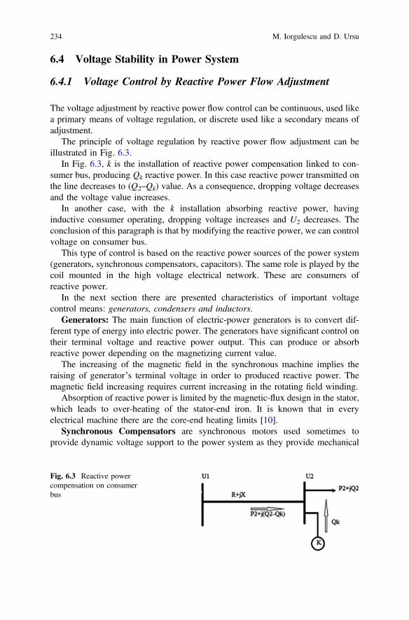
6.4 Voltage Stability in Power System

6.4.1 Voltage Control by Reactive Power Flow Adjustment

The voltage adjustment by reactive power flow control can be continuous, used like

a primary means of voltage regulation, or discrete used like a secondary means of

adjustment.

The principle of voltage regulation by reactive power flow adjustment can be

illustrated in Fig. 6.3.

In Fig. 6.3, k is the installation of reactive power compensation linked to con-

sumer bus, producing Qk reactive power. In this case reactive power transmitted on

the line decreases to (Q2–Qk) value. As a consequence, dropping voltage decreases

and the voltage value increases.

In another case, with the k installation absorbing reactive power, having

inductive consumer operating, dropping voltage increases and U2 decreases. The

conclusion of this paragraph is that by modifying the reactive power, we can control

voltage on consumer bus.

This type of control is based on the reactive power sources of the power system

(generators, synchronous compensators, capacitors). The same role is played by the

coil mounted in the high voltage electrical network. These are consumers of

reactive power.

In the next section there are presented characteristics of important voltage

control means: generators, condensers and inductors.

Generators: The main function of electric-power generators is to convert dif-

ferent type of energy into electric power. The generators have significant control on

their terminal voltage and reactive power output. This can produce or absorb

reactive power depending on the magnetizing current value.

The increasing of the magnetic field in the synchronous machine implies the

raising of generator’s terminal voltage in order to produced reactive power. The

magnetic field increasing requires current increasing in the rotating field winding.

Absorption of reactive power is limited by the magnetic-flux design in the stator,

which leads to over-heating of the stator-end iron. It is known that in every

electrical machine there are the core-end heating limits [10].

Synchronous Compensators are synchronous motors used sometimes to

provide dynamic voltage support to the power system as they provide mechanical

Fig. 6.3 Reactive power

compensation on consumer

bus


power to their load. In some power plants the hydro units are designed to permit the

generator to function without its mechanical power source simply to provide the

reactive power capability to the power system [10]. These hydro units work as a

compensators when the active power generation is not necessary, Fig. 6.4.

For a magnetizing current value Ie0,produced reactive power is zero. In case

Ie[ Ie0 the synchronous condenser operates overexcited, with power factor

capacitive conveying in electric network reactive power. When Ie\Ie0 the syn-

chronous condenser operates under excited, with power factor inductive absorbing

from electric network reactive power. Proportion of maximum reactive power

absorbed Qksb and produced power Qk

s it is a very important characteristic of the

condenser operation.

Advantages of using synchronous condenser are:

– operating possibilities as reactive power generator or consumer;

– continuous regulation of produced or absorbed reactive power by magnetization

current;

– contribution to the system stability, with auto-regulation effect, once the

decrease of voltage leads to an increase in reactive power supplied.

A disadvantage can be the limited applicability of synchronous condensers on a

large scale. The disadvantage is due to the consumption of active power around 3%

of machine’s reactive power rating, or operating expenses.

Capacitors are passive devices that generate reactive power, with some

advantages:

– significant real-power losses around 2–3% from the rated power;

– low operating expense;

– possibility to space out payment of investment by gradually developing the

capacitor bank with new elements.

Capacitor banks are composed of individual capacitor connected in series and/or

parallel in order to obtain the desired capacitor-bank voltage and capacity rating

Fig. 6.4 Reactive power

variation versus magnetizing

current


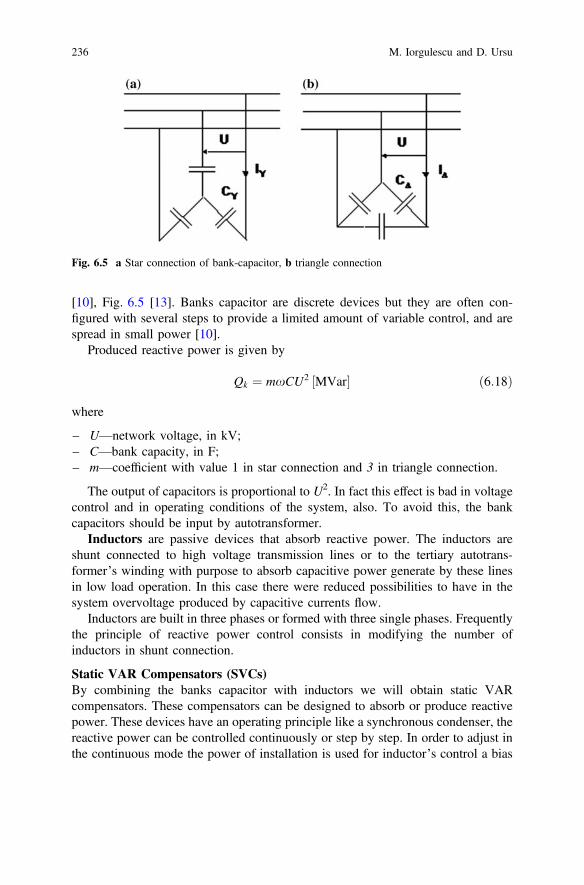
[10], Fig. 6.5 [13]. Banks capacitor are discrete devices but they are often con-

figured with several steps to provide a limited amount of variable control, and are

spread in small power [10].

Produced reactive power is given by

Qk ¼ mxCU2 ½MVar� ð6:18Þ

where

– U—network voltage, in kV;

– C—bank capacity, in F;

– m—coefficient with value 1 in star connection and 3 in triangle connection.

The output of capacitors is proportional to U2. In fact this effect is bad in voltage

control and in operating conditions of the system, also. To avoid this, the bank

capacitors should be input by autotransformer.

Inductors are passive devices that absorb reactive power. The inductors are

shunt connected to high voltage transmission lines or to the tertiary autotrans-

former’s winding with purpose to absorb capacitive power generate by these lines

in low load operation. In this case there were reduced possibilities to have in the

system overvoltage produced by capacitive currents flow.

Inductors are built in three phases or formed with three single phases. Frequently

the principle of reactive power control consists in modifying the number of

inductors in shunt connection.

Static VAR Compensators (SVCs)

By combining the banks capacitor with inductors we will obtain static VAR

compensators. These compensators can be designed to absorb or produce reactive

power. These devices have an operating principle like a synchronous condenser, the

reactive power can be controlled continuously or step by step. In order to adjust in

the continuous mode the power of installation is used for inductor’s control a bias

Fig. 6.5 a Star connection of bank-capacitor, b triangle connection


winding or thyristors control scheme. This control is very useful for the receivers,

whose operations produce power surges in the electrical network.

Static Synchronous Compensators (STATCOMs)

The STATCOM (STATic synchronous COMpensator) is a shunt-connected reac-

tive compensation equipment which generates and absorbs reactive power. Its

output can be varied so as to maintain control of the power system specific

parameters [14–16, 19].

The STATCOM belongs to the family of devices known as flexible AC trans-

mission system (FACTS). The schematic diagram is presented in Fig. 6.6.

STATCOMs give the power system the following advantages:

– using capacitors and inductors combined with fast switches, finally, STATCOM

uses power electronics to synthesize the reactive power output [10].

– output capability is commonly symmetrical, providing as much capability for

production as absorption [10].

– controls are designed to provide a fast and effective voltage control

– STATCOMs capacity is not affected by degraded voltage.

– STATCOMs are current limited so their MVAr capability responds linearly to

voltage, increasing STATCOMs’ usefulness in preventing voltage collapse [10].

The voltage control in the medium voltage network can be made using a system

called by its developers UPQC (Unified Power Quality Conditioner), Fig. 6.7 [17].

It has the role of compensating the voltage variations and of ensuring the user’s

clamps receive a set voltage, practically constant. This installation was tested within

the medium voltage network which a photo-voltaic plant was connected to.

The installation has the role of correcting the ir electric current loop absorbed by

the user as the parallel converter introduces a if current with such a synthesized form

Fig. 6.6 STATCOM

schematic diagram [16]


that the ir electric current to be sinusoidal. The Uf voltage introduced in series with

the network voltage by the serial converter maintains a constant value of the user

supply voltage.

6.4.2 Voltage Control by Power Network

Parameters Adjustment

This process of voltage adjustment involves changes in electrical network param-

eters, either by connecting or disconnecting circuits operating in parallel, or by

compensating the inductive reactance power lines.

Some parts of the electrical network are built in parallel connection—two or

three circuits, transmission lines or power transformers connected in parallel [8].

One of these can be activated or also stopped from operating, can modify longi-

tudinal parameters (impedance) of network, leading to change voltage in con-

sumption nodes.

In the analyzed Fig. 6.8 under the minimum load operating conditions or empty

load voltage U2 consumer bars may increase above the rated value. Disconnecting a

circuit power line or a transformer in the network increase the longitudinal impe-

dance of the circuit and voltage drop, respectively, so that the voltage level can

lower the U2 consumer bars.

Fig. 6.7 Electrical network conditioner UPQC [17]

Fig. 6.8 Electrical network

to a consumer through two

parallel circuits


In practice, disconnecting transformers operating in parallel, with voltage control

purpose in low load operating case is a measure recommended in terms of reducing

power losses and active energy in electricity network. Because the power trans-

former is a component of the electrical networks that presents a high level of safety

in operation, it is generally accepted to operate transformer stations with a single

transformer.

Regarding take off transmission lines, it is important to know that these are less

reliable in operation and in practice, it is not recommended to disconnect trans-

mission line circuits to control voltage in electrical networks.

Another procedure used for voltage control is used cascade circuit compensation

of an electrical network by inductive reactance. This is accomplished by the

capacitors mounted in cascade with reactance, Fig. 6.9, obtaining a reduction

longitudinal reactance of the line and thus a decrease of voltage drops.

In Fig. 6.10 there is represented a single phase equivalent circuit of a com-

pensated electrical network

XL ¼ xL ð6:19Þ

is transmissions line reactance, and

XC ¼1

xCð6:20Þ

is capacitive reactance series on line. Resulted reactance will be

Fig. 6.9 Capacitor mounted

in cascade on transmissions

line

Fig. 6.10 Single phase

equivalent circuit of

compensated electrical

network


X ¼ XL � XC ¼ xL�1

xCð6:21Þ

Based on the capacitive reactance’s value there are the following situations:

– under-compensated line, when XC\XL;

– total compensated line, when XC ¼ XL;

– over compensated line, when XC[XL.

Longitudinal compensation with banks capacitor series connected with long

lines of electricity transmission is done in order to increase the transport capacity of

these lines and limits of stable operation of the power system.

To control voltage from a practical standpoint, series compensation with banks

capacitor is important for the medium voltage lines in the following cases:

– overhead lines relatively long, slow voltage variations reduction to consumers;

– electrical lines feed to consumers that produce shock load in the network, in

order to reduce shock occurring in the voltage corresponding to power supply.

On the other hand, it must be known that the compensation process causes some

negative phenomenon: ferro-resonance, under-synchronous resonance or oscillation

of the synchronous machines. For limiting them a research to develop possibilities

and removing their appearance is required.

Measures that can be taken to avoid these are:

– restrict the compensation to between 1.5 and 2;

– using series or parallel resistors with banks capacitors.

Another drawback of the procedure- series bank capacitors for compensation of

the inductive reactance of the power lines is the increase of the short-circuit current,

symmetrical and non-symmetrical. The capacitors are protected by special circuits

in the short circuit case within power system. This method is used in heavy growing

and fast variation of reactive power in the system.

6.4.3 Node Voltage Set Up

The importance of voltage control in electrical network nodes is to change the level

of voltage in admissible in them. This process seems to be the most natural, but it

will not remove the cause of voltage fluctuations causing variations reactive loads

transiting through electric transmission elements and distribution network. This

voltage control method consists in injection of supplementary voltage in order to

compensate longitudinal component of lost voltage. The injection voltage is real-

ized by autotransformers or power transformer equipped with adjuster under lon-

gitudinal load or transversal. Often are used in power system voltage control by the

automat voltage regulator.


Base on introducing additional voltage in an electrical network, there are the

following types of control methods [18]:

• longitudinal adjustment, which is intended to compensate the longitudinal

component of drop in voltage. Additional being introduced in phase with the

line voltage at that point;

• transverse adjustment when additional voltage is in with quadrature voltage

network at that point, and serves mainly to modify the power flow in the mesh

network topology;

• adjustable long-transverse, when the longitudinal adjustment is used to adjust

the transverse correlated.

In terms of structural and functional features of the used means to introduce

additional voltage, there are to be distinguished two types of control:

– direct control, which is performed using power transformers and autotrans-

formers fitted with sockets for adjusting the working windings, as well as with

devices for switching them in the presence or absence of load;

– indirect control, which is performed by means of special transformers and

special autotransformer-overvoltage transformer. These constitute complexes

devices that can be associated to regulating power transformers non-adjustable

or can be used separately. These also include the regulators induction.

6.4.4 Management of Voltage Control

Base of voltage adjustment consists of generating units by using their capability

to absorb and debit reactive power (to modify the magnetization current and

implicit electromotive force linked by synchronous reactance), within diagram

P-Q available.

For basic voltage control use the following devices:

– Synchronous condenser;

– Synchronous generators operating in thermo and hydro plants;

– Wind power plants;

– Photovoltaic power plants.

All other means of voltage control, maintained by the consumers/network

operators have a secondary role regardless of their number and capability and they

come in support of the generating sets without replacing the first.

These are:

– Banks capacitors;

– Inductors;

– Control by power transformer sockets;

– Connect/disconnect of electrical lines transmission.


6.5 Case Studies

1. Q–V voltage regulation approach in the pilot node using an automatic

voltage control (ASVR—Automatic Secondary Voltage Regulation) devel-

oped in Romania

The goal is to maintain the required voltage in the pilot node within the desired

voltage domain. ASVR equipment consists of an independent regulator working on

the principle of regulatory with negative feedback response.

ASVR are placed in the power plant or electrical station, and the desired voltage

it is received by the voltage domain that must keep it in pilot node.

ASVR = Automatic Secondary Voltage Regulation in pilot node of 400 kV—

automation which controls the voltage in the 400 kV pilot node from a trans-

formation station.

Further on we will refer to such a system associated to a wind plant, but this

system can be used for any kind of plant, photo-voltaic, for example.

The wind plants management system—which is capable of controlling in real

time depending on the imposed voltage level, meaning the decrease of increase of

produced reactive power, by controlling the voltage in the medium voltage network

(MT) and in the 110 kV, through the modification of the plots at the transformers

(power transformer 110/MT from the power transformer transformation stations and

power transformer 400/110 kV from the system station), according to the set

voltage value from the 400 kV pilot node, but also to the park’s reactive power

availability at that moment, increasing or decreasing the transit of active energy

from the wind park, if the adjustment analysis takes into consideration the electric

scheme from Fig. 6.11.

The automatic installation for the secondary adjustment of the ASVR voltage is

destined to the voltage adjustment at the 400 kV level in the 400/110/MT station, as

the reference is given the voltage value on the station’s 400 kV bars.

Thus, in order to achieve this objective, there are used both the wind generator

capacity to produce/consume reactive power, but also switching the plots of the

MT/110 kV transformers and the 400/110/MT transformers.

The primary adjustment loop U–Q of the wind generator group has as reference

the value of the voltage on the 110 kV bars so that the reactive power variation of

the generators would follow the variation of this voltage, which, in turn—according

to the ASVR logic—is proportional to the voltage variation on the 400 kV bars.

Additionally, in order to extend the adjustment band, under the conditions of

maintaining the inferior voltage of 110 kV, MT and 0.5 kV within the admitted

limits, there are used the voltage regulators of the MT/110 kV transformers,

respectively the 400/110/MT which act on the plot switches at the ASVR

command.

From a practical standpoint, compared to the initial (primary) function of

adjusting the voltage to the 110 kV through the variation of the wind generators


reactive power, the ASVR installation is designed to perform the following sup-

plementary functions:

• The voltage adjustment by modifying the reactive energy produced by the wind

generators from the wind power plants by means of the command-control

system WFMS, having as reference the voltage at the level of 400 kV bars;

• automatic switching of 400/110/MT transformer plots from the 400 kV station;

• automatic switching of MT/110 kV transformer plots from all stations corre-

sponding to the plant;

• coordinating the three preious functions.

• observing the condition to maintain the voltage levels inferior to 400 kV

(meaning 110 kV, MT and 0.4 kV) within the admitted limits.

• ASVR is composed of three adjustment loops, as follows:

• adjustment loop voltage 400 kV;

• adjustment loop voltage 110 kV;

• adjustment loop voltage MT.

The three adjustment loops function simultaneously, as they coordinated by the

ASVR logic. Not including one of the loops in the ASVR scheme implies the

ASVR functioning without the adjustment system corresponding to that loop (for

example, not including the Mt adjustment loop determines the ASVR functioning

without the MT/110 kV plot switching).

Fig. 6.11 The transformer station through which a central debits


The coordinating function of the three adjustment loops leads to a hierarchy of

their actions, so that the adjustment process records the following hierarchy

(priority):

1. loading/unloading with reactive energy the wind generator ensemble from the

electric plant;

2. plot switching at the MT/110 kV transformers of the producer (from the plant

stations);

3. plot switching at the 400/110/MT transformers from the 400/110 kV where the

pilot node is considered.

The adjustment loop ensemble which ASVR consists of is schematically pre-

sented in Fig. 6.12.

Release period/start: The interval between two control interventions are usually

set on 18 � 20 s. Also every deviation must be eliminated by occurred adjusting

120 s of its release.

Fig. 6.12 ASVR integration in electrical network


• The ASVR will command the power transformers 400/110 kV on the basis of

criterion of minimal voltage difference between the sockets;

• In case of increase voltage 110 kV will be used by the transformer with the

socket on lower voltage;

• When voltage decreases 110 kV the transformer is used with socket to the

higher voltage;

• The criterion of reactive power transfer will be applied in voltage equality

between the sockets.

2. Q–V voltage control in wind power plant, with imposed Q

We have a wind power plant to which a ASVR is used in order to maintain voltage

in the 110 kV, the consign the plant receives being of reactive power Qabs or

debited Q, according to the ‘scale’ chart from Fig. 6.13 and the adjustment itself

consists in loading/unloading the wind generator group from the wind plant with

reactive energy.

In the diagram presented in Fig. 6.13, imposed Q, as follows ASVR, Q absorbed

or Q produced to be as close to the preset value. These values are indicated by

Q measured which falls or how much it increases depending on the preset value

Q. Also voltage of 110 kV aims at absorbing or dispensing Q, dropping respectively

U with an increase for which we have in view the achievement of a certain preset Q.

Acquisition and execution of preset reactive power provided by ASVR con-

trollers will be using the entire reactive power reserves that actions wind power

plant, including the existing compensation means to them. In case P = 0 for a wind

plant will provide for the adjustment Q = 0 or Q 6¼ 0, and the controller must know

the limits of maximum and minimum reactive power that wind plant led so it can

provide active power when it’s generated or not.

Fig. 6.13 Q–V diagram with imposed Q


3. Q–V voltage control in photovoltaic power plant, with imposed U

We have a wind power plant to which a ASVR is used in order to maintain voltage

in the 110 kV, the consign the plant receives being of voltage adjustment U,

according to the ‘scale’ chart from Fig. 6.13 and the adjustment itself consists in the

three loops’ coordinated functioning, thus leading to a hierarchy of their actions so

that the adjustment process can be performed.

In the diagram, in Fig. 6.14 can be seen as an imposed voltage, ASVR follows

that voltage 110 kV to be as close to the preset value. These values are indicated by

measured voltage that goes up and down depending on the value of voltage. Also

instruction for reactive power Q is produced or absorbed in order to increase,

decrease voltage respectively, as we have in mind to reaching any preset voltage.

According to the short-circuit on bar power at the voltage level for which the

voltage is aimed to be adjusted, there are the results ∆Q/∆U [MVAr/kV] for the

voltage level we want to maintain, meaning, for example, that, at a variation of

2 kV we approximate ±16 MVAr (Fig. 6.14), respectively at a de ±8 MVAr

variation, as the voltage varies with ±1 kV/8MVAr (the mentioned values are just

for exemplification, as they depend on the voltage level where the adjustment is

made). The dU/dT value shows the response speed, the decrease/increase of voltage

in a minute, indicating the system’s capability to reach the values for U consign,

according to the voltage rise.

Fig. 6.14 Q–V diagram photovoltaic power plant—U preset


6.6 Conclusion

The wide development of renewable energy sources connected to the high medium

voltage lines imposed the development of specific solutions for the voltage control

in the point where these sources connect or in their vicinity.

Today’s energy systems are facing the problem that, in some areas of the system

there are is an exceeding production, while in other areas the production is lower,

while energy is transited from the sources in order to balance the consumption. All

these occur as result of the way the plants are located, as they, for different reasons,

chosen for other criteria than the optimal location and, considering the degree to

which the network in loaded, the power is transited to a consumption node which

can be, in some situations, very far from the source, this leading to a decrease in the

area’s level of voltage. The phenomenon can also appear in reverse, meaning an

increase in voltage, in the situations when the plant connection is made in nodes

with reduced short-circuit power, thus appearing the limitation of the power debited

by the plant in accordance with the voltage maximally admitted at the final con-

sumers, especially in the cases of plants recorded at the MT lines.

For these reasons, it is important to control the voltage level, and this is why one

must always analyze solutions to maintain the voltage within the limits which are

adequate for the user’s system.

For the transport network, one of the solutions is the ASVR system which

maintains the voltage in pilot node chosen in the system, compensating the voltage

variations in the system, with the three presented adjustment loops, thus using two

of the adjustment methods, the reactive energy absorption and debit and the lon-

gitudinal and long-transversal voltage adjustment in the transformers by using the

plots. The ASVR can be also used in the distribution network, with less control

loops, two or even one.

Considering the voltage variation at the final user clamps, from each voltage

level from the system, depends in each moment on production, consumption,

network loading, using an automated voltage regulator for that voltage level allow

for the necessary conditions of ensuring the quality of the energy from the network

and, consequently, for all users.

References

1. C.W. Taylor, Power System Voltage Stability, McGraw Hill, 1994.

2. T.J.E. Miller, Reactive Power Control in Electric System, 1982, John Wiley & Sons, Inc.,

USA.

3. P.W. Sauer, Chapter 2, Reactive Power and Voltage Control Issues in Electric Power

Systems.

4. J. Hossain, H.R. Pota, Robust Control forGridVoltage Stability: High Penetration ofRenewable

Energy, Power Systems, DOI:10.1007/978-981-287-116-9_2, Springer Science-Business

Media, Singapore, 2014.


http://dx.doi.org/10.1007/978-981-287-116-9_2

5. IEEE Power Engineering Society Administrative Committee of the Power System Dynamic

Performance Committee, Causes of the 2003 Major Grid Blackouts in North America and

Europe, and Recommended Means to Improve System Dynamic Performance.

6. W. Nakawiro, Voltage Stability Assessment and Control of Power Systems Using

Computational, Intelligence, http://duepublico.uniduisburgessen.de/servlets/DerivateServlet/

Derivate-26570/Nakawiro_Worawat_Diss.pdf, 2011.

7. C. Bulac, M. Eremia, A.I. Bulac, I. Tristiu, Voltage stability in SEE Phenomenon Assessment

and Control through Artificial Intelligence Techniques, Power Journal 47-1999, no. 2.

8. A. Poeata, et al., Transport and Distribution of Electricity, Bucharest, pp. 267–310.

9. M. Eremia, P. Simon, D. Petricica, D. Gheorghiu, Some Aspects of Hierarchical Voltage -

Reactive Power Control, Power Engineering Society Summer Meeting, 2001, vol. 2,

DOI: 10.1109/PESS.2001.970170, Publication Year: 2001, pp. 872–880, vol. 2.

10. http://electrical-engineering-portal.com/how-reactive-power-is-helpful-to-maintain-a-system-

healthy.

11. F.A. Viawan, D. Karlsson, Coordinated Voltage and Reactive Power Control in the Presence

of Distributed Generation, Power and Energy Society General Meeting - Conversion and

Delivery of Electrical Energy in the 21st Century, 2008 IEEE, DOI:10.1109/PES.2008.

4596855, Publication Year: 2008, pp. 1–6.

12. E. Demirok, P. Casado Gonzalez, K.H.B. Frederiksen, D. Sera, P. Rodriguez, R. Teodorescu,

Local Reactive Power Control Methods for Overvoltage Prevention of Distributed Solar

Inverters in Low-Voltage Grids, IEEE Journal of Photovoltaics, vol. 1, no. 2, December 2011.

13. S. Bisanovic, M. Hajro, M Samardzic, One Approach for Reactive Power Control of

Capacitor Banks in Distribution and Industrial Networks, Electrical Power and Energy

Systems, 60, pp. 67–73, 2014.

14. C.A. Canizares, Modeling and Implementation of TCR and VSI Based FACTS Controllers,

Internal Report, ENEL and Politecnico di Milano, Milan.

15. H. Mori, Y. Goto, A Parallel Tabu Search Based Method for Determining Optimal Allocation

of FACTS in Power Systems, Proc. of the International Conference on Power System

Technology (PowerCon 2000), vol. 2, pp. 1077–1082, 2000.

16. S. Kamel, F. Jurado, D. Vera, A Simple Implementation of Power Mismatch STATCOM

Model into Current Injection Newton-Raphson Power-Flow Method, Electrical Engineering,

96:135–144

DOI 10.1007/s00202-013-0288-4, Springer, 2014.

17. A. Marinescu, M. Radulescu, N. Golovanov, Control in Blood Medium Voltage Networks

Are Connected Renewable Energy, VIIIth Edition of the ASTR Conference.

18. G. Georgescu, et al., Transport and Distribution of Electricity, Ghe. Asachi Publishing House,

Iasi 2001.

19. E. Nasr Azadani, Optimal Placement of Multiple STATCOM for Voltage Stability Margin

Enhancement Using Particles Warm Optimization, Electrical Engineering, September 2008.


http://duepublico.uniduisburgessen.de/servlets/DerivateServlet/Derivate-26570/Nakawiro_Worawat_Diss.pdf

http://duepublico.uniduisburgessen.de/servlets/DerivateServlet/Derivate-26570/Nakawiro_Worawat_Diss.pdf

http://dx.doi.org/10.1109/PESS.2001.970170

http://electrical-engineering-portal.com/how-reactive-power-is-helpful-to-maintain-a-system-healthy

http://electrical-engineering-portal.com/how-reactive-power-is-helpful-to-maintain-a-system-healthy

http://dx.doi.org/10.1109/PES.2008.4596855

http://dx.doi.org/10.1109/PES.2008.4596855

http://dx.doi.org/10.1007/s00202-013-0288-4

Part II

Compensation and Reactive PowerOptimization in AC Power Systems

Chapter 7

Optimal Reactive Power Control

to Improve Stability of Voltage in Power

Systems

Ali Ghasemi Marzbali, Milad Gheydi, Hossein Samadyar,

Ruhollah Hoseyni Fashami, Mohammad Eslami

and Mohammad Javad Golkar

Abstract The current power systems have works near to the marginal voltage

stability due to the market performance as well as their weightier operation loadings

along with consideration of environmental constraints of transmission as well as

generation capacity enlargement. In other words, at the present time wind power

has confirmed to be one of the most efficient and competitive renewable resources

and therefore, its use is indeed continually growing. Little wind power infiltration

planes are generally contained in the current grid networks in view of that it is

passively controlled and operated. On the other hand, this statement is no more

suitable for immediately after the wind power energy infiltration commences

A. Ghasemi Marzbali (&)Technical Engineering Department, University of Mohaghegh Ardabili, Ardabil, Irane-mail: [email protected]

M. Gheydi � H. SamadyarYoung Researchers and Elites club, Science and Research Branch, Islamic Azad University,Tehran, Irane-mail: [email protected]

H. Samadyare-mail: [email protected]

R.H. FashamiElectrical Engineering Department, Damavand Branch, Islamic Azad University,Tehran, Irane-mail: [email protected]

M. EslamiDepartment of Electrical and Computer Engineering, Nikshahr Branch,Islamic Azad University, Zahedan Branch, Nikshahr, Irane-mail: [email protected]

M.J. GolkarDepartment of Electrical and Computer Engineering, Zahedan Branch,Islamic Azad University, Zahedan, Irane-mail: [email protected]


251

growing, a broad scope of scientific issues can come out, namely: voltage rise,

bi-directional power flow, improved power quality issues as well as distorted

voltage stability. The additional improvement of electricity construction from

renewable resources in a trustworthy as well as consistent system performance is

driving transmission as well as distribution control utilizers to employ novel

working models that are not presently extant. A serious subject of the demanding

status described in the foregoing is the reactive power managing that involves the

planning as well as operation deeds that are asked for to be executed to get better

voltage profile as well as stability in the power networks. For this reason, voltage

stability is a major issue of current power systems. It signifies the capableness of a

power system to keep voltage when the required load is boosted. Researches about

this kind of instability fact proceed with its control as well as evaluation. The first

one designates if a power system runs in the safe operational area, while the second

one will carry out essential control actions if a power system gets close to unsafe

operational zone. Diverse approaches put forth in the chapter deal with offline and

online purposes. The center of attention of this chapter is the second part; it means

control of voltage stability. Three major methods have been utilized for voltage

stability which are reactive power management, load shedding and active power

re-dispatch. Reactive power management signifies the ways designating the place of

novel VAR sources and/or settings of the VAR sources that are installed currently

and the settings of facilities including on-load tap changers (OLTCs). Reactive

power sources ordinarily consist of synchronous generators/condensers,

reactor/capacitor banks, as well as flexible AC transmission systems (FACTS)

controllers. It can be classified into two subjects as reactive source programming as

well as reactive power dispatch. For reactive programming, the concerned temporal

duration is the coming few months or years, and besides considering the optimum

milieu of facilities that are installed currently, installation of novel reactive power

sources is contemplated. It is performed in offline and online ways. The main

purposes of offline reactive dispatch can be found in the duration of the coming few

days or weeks, while, another model is carried out in the coming few minutes or

hours. Opposing the reactive planning, both online and offline reactive power

dispatches only designate the optimum settings of extant facilities. Optimal reactive

power flow (ORPF) which is a specific instance of the optimal power flow (OPF)

issue is an utterly significant instrument with regard to assured and gainful uti-

lization of power systems. The OPF’s control parameters have a proximate con-

nection with the reactive power flow, including shunt capacitors/reactors, voltage

magnitudes of generator buses, output of static reactive power compensators,

transformer tap-settings. In the ORPF problem, the transmission power falloff is

brought to a minimum and the voltage profile is modified and the operating and

physical constraints are satisfied. Note that shunt capacitors/reactors and

tap-settings of transformers are discrete variables while and except other variables

are continuous. Hence, the reactive power dispatch issue is nonlinear, non-convex

has equality and inequality limitations and has discrete and continuous variables.

252 A. Ghasemi Marzbali et al.

7.1 Introduction

By the elevated exploitation as well as loading of the grid transmission system and

besides because of refined enhanced operating conditions the issue of voltage

stability and voltage collapse draws increasing consideration. A voltage drop could

be taken in the power systems or subsystems and could emerge very suddenly [1].

Constant controlling of the system status is hence necessary. The reason of the 1977

New York blackout has been substantiated to be the reactive power issue. The 1987

Tokyo blackout was accepted to be because of reactive power deficit as well as a

voltage drop at peak load in summer.

These facts have strongly shown that reactive power play an important role in

the security of power systems as view of voltage stability. An appropriate com-

pensation of system voltage profiles will improve the system securities in the

operation and will decrease system losses [2]. The essential purpose of voltage

regulation in the distribution system performance is to maintain the status voltage in

the power system steady in the suitable scope. The desirable voltages could be

acquired by either directly manipulating the voltage or reactive power flow which in

its own right will influence the voltage collapse. The reactive tools usually

employed for the voltage and reactive power control are on-load tap-changer

(OLTC) transformers, steps voltage regulator and switched shunt capacitors [3, 4].

Such reactive tools are generally utilized on the basis of a presumption that power

runs in just one direction and the voltage diminishes along the feeder, from the

substation to the remote end.

An OLTC transformer is a transformer with automatically changeable taps.

The OLTC is a section of most of HV/MV substation transformers [5]. A shunt

capacitor produces reactive power to make up for the reactive power demand and

hence increases the voltage. Shunt capacitors could be installed in the substation

(hereinafter referred to as substation capacitors) or along the feeder (hereinafter

referred to as feeder capacitors). A steps voltage regulator is an autotransformer

with automatically adjustable taps that is ordinarily installed when the feeder is too

long in such a manner which voltage regulation with OLTC and shunt capacitors is

not enough. Voltage and reactive power control entails suitable coordination

between the extant voltage and reactive power control equipment [6].

Many distribution network operators (DNOs) control these equipment locally via

use of customary controllers to keep the voltages in the distribution system about

approved range while bring to a minimum the voltage collapse and power falloffs.

Various techniques have been presented in order to get better voltage and reactive

power control in the distribution system for programming and operation stages.

Within this time, many scholars have presented the trouble of voltage and reactive

power control in distribution power systems through concentrating on automated

distribution power system, with off-line setting control or real time control. The

offline setting control intends to explore a dispatch program for OLTC movement

and capacitor switching on the basis of day-ahead load prediction, in the meantime

7 Optimal Reactive Power Control to Improve … 253

the real time control endeavors to control the capacitor and OLTC on the basis of

real time surveying and trainings [7]. The major difficulty in utilization of the

off-line setting control way is its affiliation to remote control and communication

links to all capacitors. Nonetheless, a lot of DNOs do not communicate with links

that are downstream to the feeder capacitor locations.

In the other hand, the nature of modern power systems has changed due to a

variety of factors: the increased demand for sustainability, rises in the price of oil

and the need for the reduction of greenhouse gases, all of which have driven a large

increase in the level of wind generation in the power system. The intergovernmental

panel on climate change has cited that wind energy will be the primary source of

renewable generation in the electricity sector [8]. Wind generation in both Europe

and the United States is the dominant renewable resource currently present in power

systems. In Europe, wind energy is set to triple in penetration by the year 2020,

with 15.7% of the continent’s total energy supplied by wind generation [9]. In the

United States, there is currently 42,432 MW of installed capacity providing 2.3% of

the U.S. electricity mix, with the number set to rise to 25% by the year 2025 [10].

With wind generation set to become a significant generation resource in power

systems around the world, it will become increasingly important to fully understand

its impacts and interaction with the conventional elements in power systems. In

fact, the real power unit output is generally restricted by radius (VtIa), as follows

P2G þQ2

G �ðVtIaÞ2 ð7:1Þ

Constrain of field is circular (VtEf/Xs) at (0, −Vt2/Xs). It can be defined as

P2G þ QG þ

V2t

Xs

� �2

�VtEf

Xs

� �2

ð7:2Þ

where, PG, QG, Vt, Ia, Ef and Xs are active power, reactive power, terminal voltage,

armature current, Excitation voltage and Synchronous reactance of the synchronous

generator, respectively.

Fundamentally, power systems have been designed and operated around the

concept of generation delivery from large synchronous machines. These machines

have high levels of reliability and complex control systems that allow the system to

maintain high levels of operational security. The correct operation and control of

these machines across the full spectrum of time-frames is critical for maintaining

reliable power system operation and stability [11–13].

Maintaining voltage stability requires that the various components and elements

of the system can interact without issue across all of the timeframes of the stability

spectrum. Wind generation will have significant impact across the power system

stability time-frame and as wind generation becomes a more common source of

generation in the system, new mitigation techniques will be necessary to continue


operating the power system in an assured and stable way [14]. While the effect of

reactive power reserves (RPRs) on system stability is widely acknowledged, few

studies have been conducted to investigate how RPR levels could be used to

indicate the amount of voltage stability margin (VSM) [15].

In contemporary years, certain papers with mathematical algorithms have been

presented to think out the reactive power dispatch (RPD) problem [16–19]. These

algorithms, including Non-linear Programming (NLP), Newton method, Gradient

method, Linear Programming (LP), Jacobian matrix, Quadratic Programming (QP),

interior point methods and so on, have been fruitfully used for thinking out the RPD

problem. However, certain drawbacks are still linked to them. The RPD problem is

non-linear, non-differential and non-convex problem with more than one local

optimum, while these methods work based linearizing which make them less effi-

cient in finding the global optimum. On the other hand, some of these methods

suffer from special shortages, such as mathematical complexity and insecure

convergence (NLP), piecewise quadratic cost approximation (QP), convergences to

local optima (Newton method), a simplified piecewise linear estimate (LP), etc.

Also, their optimization process mainly depends on the initial solution and can

easily fall into local optima.

To overcome these disadvantages, different heuristic-based techniques are

developed for solving the RPD problem. Population-based optimization techniques

inspired by nature may be classed in two significant categories that are swarm

intelligence and evolutionary algorithms. Many methods rooted in these techniques

including fuzzy Adaptive Particle Swarm Optimization (FAPSO) [20], Real Genetic

Algorithms (RGA) [21], Tabu Search (TS) [22], Particle Swarm Optimization

(PSO) [23], Improved PSO (IPSO) [24], stochastic method [25], Hybrid Stochastic

Search (HSS) [26], Differential Evolution (DE) [27], Artificial Bee Colony (ABC)

[28] as well as other methods have been broadly employed in the problem of RPD.

However, these methods appear to be proper approaches for the unravelment of the

RPD variable optimization problem.

Attention to use optimization methods in distributed generation is increasing

[29, 30]. In [31], an optimization method employed for wind power is offered, by a

primal-dual predictor corrector interior point method, employed to explore the

operating points of a single WT in a WF. The voltage stability based on reactive

power control has been reviewed in rest of this chapter. The real transmission power

loss minimization is consider as function, meantime the permitted transformer

capacity, voltage range and conductor current capacity are added as the loading

limitations. Moreover, OLTC operation and voltage fluctuation index are also

analyzed. The reactive power in term of voltage stability is shown with reactive

power control and local voltage in which timing of feeder capacitors are monitored

and is still broadly employed.


7.2 Voltage Stability Based RPD Model

The different purposes of power system are sum of voltage deviations on load

busses, system transmission falloffs, voltage stability, security, etc. Such purposes

are contradictory in their essence and couldn’t be dealt with by customary single

purpose optimization techniques. Generally, the RPD model could be explained as

follows in mathematical terms:

Problem Purposes

• Purpose 1: Bringing to a minimum the total real power losses

Transmission falloffs in the network can be stated as economic losses procuring no

advantages. Thus, transmission falloffs are understood as a falloff in proceeds via

the utility. The intensity of each falloff requires accurate estimation and applicable

moves made to bring them to a minimum. When the transmission falloffs are stated

with regard to bus voltages and associated angles, the falloffs could be stated based

on Newton–Raphson as follows

J1 ¼ Plossðx; uÞ ¼X

NL

k¼1

gk½V2i þV2

j � 2ViVj cosðhi � hjÞ ð7:3Þ

i and j end respectively if gk is the conductance of the line i-j, Vi and Vj are line

voltages and hi and hj are the line angles at the line. The kth network branch is k. It

connects bus i to bus j. If ND is the set of numbers of power demand bus and

j = 1,2, …, Nj where, Nj is the set of numbers of buses in adjacency with bus j,

i = 1,2, …, ND. PG is the active power in line i and j. x and u are the dependent

variables vectors and vector of control variables, respectively.

• Objective 2: Bringing voltage deviation to a minimum

Satisfying user’s demands with the smallest expense with a desirable continuity of

supply and sufficiently little deviation in voltage is the second function of one RPD

problem. The following is its expression

J2 ¼ VDðx; uÞ ¼X

Nd

i¼1

jVi � 1:0j ð7:4Þ

where, Nd is number of load buses.

• Objective 3: Minimization of L-index voltage stability

Voltage stability and voltage drop problem draws increasing attention by increasing

the power transmission system loading and exploitation, a voltage collapse could


happen in systems or subsystems. And it could emerge very suddenly [15, 34]. L-

index, Lj of the jth bus could be stated by means of below equation

Lj ¼ 1�P

NPV

i¼1

FjiVi

Vj

�

�

�

�

�

�

�

�

; j ¼ 1; 2; . . .;NPQ

Fji ¼ �½Y1��1½Y2�

8

<

:

ð7:5Þ

where, NPV and NPQ are numbers of PV and PQ buses, respectively. Y1 and Y2 are

the YBUS system sub-matrices acquired following the segregation of PQ and PV bus

parameters as shown in the below equation

Y1 Y2Y3 Y4

� �

VPQ

VPV

� �

¼IPQIPV

� �

ð7:6Þ

where L-index is calculated for the whole load buses. Lj shows there weren’t load

case and voltage drop circumstances of bus j in a feasible numerical range of [0, 1].

Thus, a representative L delineating the fixedness of the complete system is

formulated as follows

L ¼ maxðLjÞ; j ¼ 1; 2; . . .;NPQ ð7:7Þ

In the optimal RPD problem, incorrect tuning of continuous and discrete control

variable settings might boost the L-index value, which may reduce the system

voltage fixedness outskirt. Let the maximum value of L-index be denoted as Lmax.

Therefore, to improve the voltage fixedness and to keep the system remote from the

voltage drop margin, the formula for the succeeding purpose function will be as

follows

J3 ¼ VLðx; uÞ ¼ Lmax ð7:8Þ

Objective Constraints

• Limitations 1: Equality Limitations

Power balance is equality limitations. To rephrase, the total power generation (PG)

must cover the total demand (PD) as well as total real power losses in transmission

lines. Equality constraints of real and reactive power in each bus can be expressed

as below

PGi� PDi

¼ Vi

P

NB

j¼1

Vj½Gij cosðhi � hjÞþBij sinðhi � hjÞ�

QGi� QDi

¼ Vi

P

NB

j¼1

Vj½Gij sinðhi � hjÞ � Bij cosðhi � hjÞ�

8

>

>

>

<

>

>

>

:

ð7:9Þ


where; NB and QGi are the numbers of buses and the reactive power produced for ith

bus, respectively; PDi and QDi are real and reactive power at the ith load bus,

respectively; Gij and Bij are the transfer conductance and susceptance between bus

i and bus j, respectively; Vi and Vj are the voltage intensities at bus i and bus j,

respectively; and hi and hj are the voltage angles at bus i and bus j, respectively. The

equality limitations in (7.9) are nonlinear equations which could be thought out by

employing Newton-Raphson method to create an answer to the load flow problem.

Within the duration of answering, the real power output of one generator, titled

slack generator, remains to fill in the real power losses and satisfy the equality

limitation in Eq. (7.9). The load flow answer produces all bus voltage intensities

and angles. Therefore, the real power losses in transmission lines could be obtained

using Eq. (7.3).

• Limitation 2: Generation Capacity Limitations

For solid performance, the generator reactive power and bus voltage can be con-

strained through lower and upper limits as below

Qmini �Qi �Qmax

i ; vmini � vi � vmax

i ð7:10Þ

where, Qimin, Qi

max, vimin and vi

max are the minimal and maximal value for reactive

power and voltage magnitude of the ith transmission line, respectively. A clarified

input/ output curve of the thermal unit understood as heat rate curve is indicated in

Fig. 7.1.

• Limitation 3: Line flow Limitations

A significant limitation of RPD problem is the line limitation. Since any line has a

constrained capacity for current power, the constraint should be checked following

the power system load flow. For that reason, this section argued the answer for RPD

problem with line flow limitations. The following is the modeling of this constraint

Fig. 7.1 Operating expensescurve for one generator


SLf ;k�

�

�

�� SmaxLf ;k; k ¼ 1; 2; . . .; L ð7:11Þ

where SLf,k is the real line k power flow; SmaxLf ;k is the upper limit of power flow of

line k. L is the number of transmission lines [3].

• Constraints 4: Discrete control variables

The shunt susceptance (Bsh) and transformer tap settings (Ti) values are taken as

discrete values. These must be constrained by their lower and upper limits as below

Tmini � Ti � Tmax

i

Bminshi

�Bshi�Bmax

shi

�

ð7:12Þ

Problem formulation

Adding up the entire purpose performances and the equality and inequality limi-

tations, a nonlinear limited multi-purpose optimization problem in mathematical

terms could be the formula for the RPD problem, which can be represented by

JFinal ¼ minPG

½VLðx; uÞ;Plossðx; uÞ;VDðx; uÞ�

s:t: :

gðx; uÞ ¼ 0

hðx; uÞ� 0

xT ¼ ½½VL�T; ½SL�

T; ½QG�

T �

uT ¼ ½½VG�T; ½QC�

T; ½T �T �

JFinal ¼ minPG

½VLðx; uÞ;Plossðx; uÞ;VDðx; uÞ�

ð7:13Þ

where, g and h are the equality and inequality limitations, respectively. [VL], [QG]

and [SL] are the vectors of load bus voltages, generator reactive power outputs and

the transmission line loadings, respectively. [VG], [T] as well as [QC] are the vectors

of generator bus voltages, transformer taps and reactive compensation instruments,

respectively.

7.3 Reactive Power Capacity and Control Options

in Wind Farms

The requisite of the membership of WFs in grid control matters has increased the

inclusion of power electronics and the expansion of new WT generation concepts,

leading to variable speed wind turbines [30]. The most popular wind generation

technology employed among them today is the DFIG. In this study, the DFIG


technology is employed. The capacity of reactive power injection into the grid

generally is associated to the used control approach, the active power generation

and the converter size. The P-Q quality of the WTs employed in this study is given

in Fig. 7.2. Specifically, it shows the business wind generator Gamesa WT

G80-2.0 MW [26]; the useful data are given in Table 7.1. This WT acts with Power

Factor (PF) 0.98 capacitive and 0.96 inductive. Consequently, the reactive power

capability is bounded relying on the active power production. Its reactive power

capacity is shown with the WT’s trait and the influences of lines as well as cables.

Thus, the WFP-Q trait is analogous to the same for the WTs. However, it’s oriented

to the capacitive side, as displayed in Fig. 7.3.

The green line shows the PQ trait of WF for PF = 1. For a power production less

than 10 MW, the cable influence is larger than the transformer influence, since the

transformer influence is paramount for large output power from WF. Thus, novel

consumption and production of WF areas are modeled, for a range in which the WF

alters the reactive power requisites exists. If the WF gets a capacitive reactive power

in the small active power production range, the WTs set point will alter to be

inductive. Voltage control can be performed via reactive power injection as well as

transformer taps, like the way it is given in Table 7.2.

Fig. 7.2 Q property of anindividual WT appertaining toG80-2.0 MW

Table 7.1 Properties of wind power

Parameter Value Parameter Value

Diameter 80 m PN 2.1 MW

Rotational speed 1680 rpm Voltage 0.68 kV

Type DFIG Power factor 0.978 CAP–0.957 IND


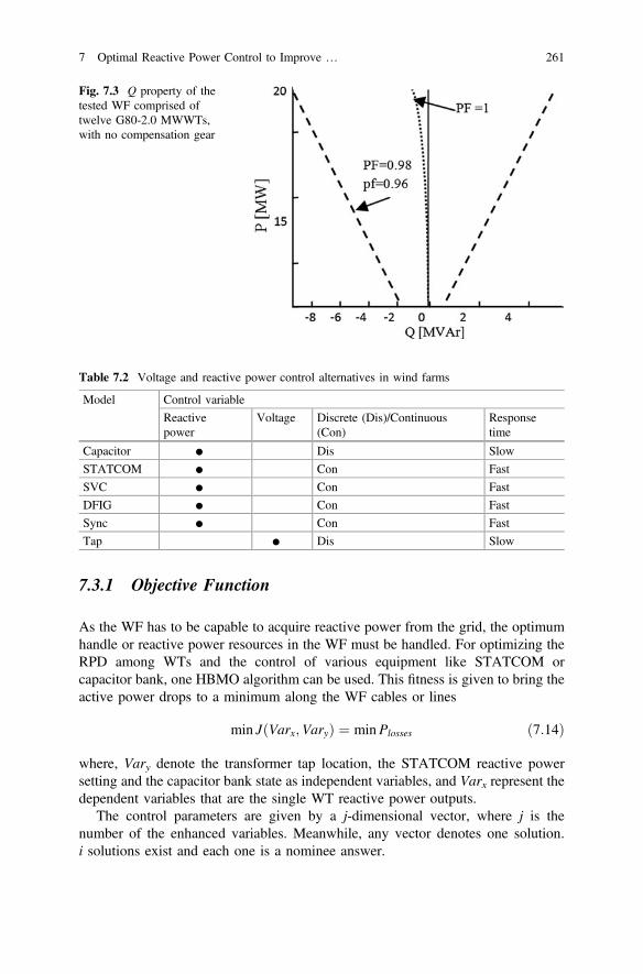
7.3.1 Objective Function

As the WF has to be capable to acquire reactive power from the grid, the optimum

handle or reactive power resources in the WF must be handled. For optimizing the

RPD among WTs and the control of various equipment like STATCOM or

capacitor bank, one HBMO algorithm can be used. This fitness is given to bring the

active power drops to a minimum along the WF cables or lines

min JðVarx;VaryÞ ¼ minPlosses ð7:14Þ

where, Vary denote the transformer tap location, the STATCOM reactive power

setting and the capacitor bank state as independent variables, and Varx represent the

dependent variables that are the single WT reactive power outputs.

The control parameters are given by a j-dimensional vector, where j is the

number of the enhanced variables. Meanwhile, any vector denotes one solution.

i solutions exist and each one is a nominee answer.

Fig. 7.3 Q property of thetested WF comprised oftwelve G80-2.0 MWWTs,with no compensation gear

Table 7.2 Voltage and reactive power control alternatives in wind farms

Model Control variable

Reactivepower

Voltage Discrete (Dis)/Continuous(Con)

Responsetime

Capacitor ● Dis Slow

STATCOM ● Con Fast

SVC ● Con Fast

DFIG ● Con Fast

Sync ● Con Fast

Tap ● Dis Slow


7.3.2 Objective Constraints

The reactive power of each WT, tab of transformers and the STATCOM reactive

power are constrained by

VarminWTi

�VarWTi �VarmaxWTi

; i ¼ 1; 2; . . .;NG ð7:15Þ

Tmini � Ti � Tmax

i ð7:16Þ

VarminStatcom �VarStatcom �Varmax

Statcom ð7:17Þ

Moreover, an additional equality limitation exists. The reactive power prereq-

uisite in Point of Common Coupling (PCC) for the voltage control task can be

modeled as an equality limitation by

Var�PCC ¼ VarmeasPCC ð7:18Þ

Within this study, the exploration of possible answers is employed to certificate

an answer which meets the limitations that can be defined as follows

SOkþ 1i ¼

SOki þ vkþ 1

i ; SOmini � SOk

i þ vkþ 1i � SOmax

i

SOmaxi ; SOk

i þ vkþ 1i [ SOmax

i

SOmini ; SOmin

i [ SOki þ vkþ 1

i

8

<

:

ð7:19Þ

With Eq. (7.9), the inequality restraints are met, the equality restraint (7.18) still

needs to be answered. Because in the WF the main elements influencing the

reactive power flow are the reactive power consumption of transformers, a scheme

for meeting the equality constraint is introduced. Yet, bearing in mind the goal to

Fig. 7.4 Flowchart for the possible answer exploration process


decrease the searching CPU time to explore a possible answer, the equality con-

strain is improved and an error value ɛ is modeled.

Var�PCC � VarmeasPCC

�

�

�

�

\e ð7:20Þ

This strategy is given in Fig. 7.4.

7.4 Voltage Stability Based RPP Model

Voltage deviation and stability limitedVAr programming orReactive Power Planning

(RPP) is a significant demanding effect in power systems [32]. Investigations on

voltage fixedness are fundamentally related to reactive power compensation sources.

Having adequate reactive power compensation sources, principally in the shunt

connection, the voltage stability boundary could be boosted a lot to make sure of

system security [33]. Thus, appropriate programming of reactive power is a serious

matter because of its specialized harness and the large expense of relocating a shunt

compensator in economic terms when that is assembled. As an important demanding

problem in power system research, RPP or VAr programming is a mixed integer

nonlinear optimization programming with a huge scale of optimal variables [34]. The

VAr programming is delineated in this part of applicable operational account limi-

tations at various load levels. Themathematic formulation of optimization-based RPP

model via accounting for voltage fixedness limitation could be stated as follows

min aP

k¼1;...;NL

PðkÞ

loss þ bP

i¼1;...;N

Qciyi þ cP

Nd

i¼1

Vi � V0i

�

�

�

�

; s:t::

P

N

i¼1

yi ¼ Nc

PðkÞGi

� PðkÞLi

� VðkÞi

P

jwi

VðkÞj � ðGij cos h

ðkÞij þBij sin h

ðkÞij Þ ¼ 0

QðkÞGi

þQðkÞCiðyiÞ � Q

ðkÞLi

� VðkÞi

P

jwi

VðkÞj � ðGij sin h

ðkÞij � Bij cos h

ðkÞij Þ ¼ 0

VðkÞimin �V

ðkÞi �V

ðkÞimax; � S

ðkÞijmax � S

ðkÞij � S

ðkÞijmax

PðkÞGimin �P

ðkÞGi

�PðkÞGimax; i 2 NG

QðkÞCimin �Q

ðkÞCi

�QðkÞCimax; i 2 NG

PðkÞtieline � TTCðQ

ðkÞC Þ

ð7:21Þ

and,

PðkÞloss ¼

X

gijððVðkÞi Þ2 þðV

ðkÞj Þ2 � 2V

ðkÞi V

ðkÞj cos h

ðkÞij Þ ð7:22Þ

where, NG, N, NL and Nc, are number of generators, number of buses, number of

operation load levels and number of VAr sources whichmust be installed, respectively.


Subscript k indicates different load levels which k = 1,…, NL. T(k), a, b and yi are

the time period of load level kth year, the energy expense per kWh, the calculated

mean yearly preservation and assignment expense and binary variable (yi = 1” if

the VAr tool is installed at bus i, or else, “0”), respectively. PGi, QGi, PLi, and QLiare the generator active outputs, reactive power outputs, the load active and reactive

power demands at bus i, respectively. Sijk is the line flow of line i-j where load level

is k; other than for the value of zero, Qci is housed in a certain VAr capacity interval

at bus i, Qcik is the VAr capacity needed at load level k, and Qci is the ultimate VAr

size at bus i; Ptieline is the total active power flow with the tie lines from the source

zone to sink zone; TTC(Qc(k)) is a piecewise linear interpolation function employed

as static voltage fixedness limitation to be delineated later in this research, and Qc is

the Qci set at all nominee buses.

The Eq. (7.3) brings the yearly expense of power system, voltage deviation and

real falloffs plus VAr tool to a minimum. Nonetheless, additional purposes could be

accounted for namely bringing generation expense and VAr installation expense,

etc. to a minimum However, such points do not alter the point of focus in this study,

and other purpose performances could be accounted for if it is needed in a certain

power system. The mentioned VAr programming plane is static voltage stability

(SVS) limited OPF model. The important cause for the computational demand of

the voltage fixedness limited OPF model is the requisite of two constraints and

variables sets associated to the regular performance and drop points [32]. The two

variables sets offer a demand to answer the optimization model, particularly for a

huge power system having several conditions. To depict this demand, TTC could be

employed to roughly offer the SVS limitation. At a stable VAr compensation model

by accounting for certain plausible conditions that are clarified in advance, the

security limited TTC optimization model is given by

mink

maxP

i 2 Source Area

j 2 Sink Area

ðPðkÞ

ij � Pij0Þ

8

>

>

>

>

<

>

>

>

>

:

9

>

>

>

>

=

>

>

>

>

;

; s:t::

P

N

i¼1

yi ¼ Nc

PðkÞGi

� PðkÞLi

� VðkÞi

P

jwi

VðkÞj � ðGij cos h

ðkÞij þBij sin h

ðkÞij Þ ¼ 0

QðkÞGi

þQðkÞCiðyiÞ � Q

ðkÞLi

� VðkÞi

P

jwi

VðkÞj � ðGij sin h

ðkÞij � Bij cos h

ðkÞij Þ ¼ 0

VðkÞimin �V

ðkÞi �V

ðkÞimax;�S

ðkÞijmax � S

ðkÞij � S

ðkÞijmax

PðkÞGimin �P

ðkÞGi

�PðkÞGimax; i 2 SourceArea

QðkÞCimin �Q

ðkÞCi

�QðkÞCimax; i 2 SourceArea

PðkÞ

Li

P0

Li

¼Q

ðkÞ

Li

Q0

Li

; i 2 SinkArea

ð7:23Þ


where, QLi0 and PLi

0 are the base case reactive and real power demands at load bus i,

respectively. Pij0 expresses the base case power flow between line i-j; and Pij(k)

indicates the line flow of line i-j, having Var compensation. Meanwhile, the

superscript k = 1,…, Ncntg, characterizes various performance statuses with the

regular performance, and k > 0 characterizing the post-condition statuses for the kth

condition phenomenon.

7.5 Simulation

A. Voltage stability in wind farm

Wind Energy is one of the greatly encouraging renewable energy sources in

Mongolia. WF within Inner Mongolia owns 200 wind turbines which are broken

down into 20 sets, and there are 10 turbines in any set. The total installed capacity is

as high as 300 MW. The wind turbine increases to 35 kV by box-type transformer

T2, afterwards by 20 35 kV coupled transmission lines to the substation, which is

comprised of two principal parts of the 220 kV transformer step-up substation.

There are 403 nodes in the wind farm model, because of its sophistication and

restricted area [35], only 42 nodes were selected as shown in Fig. 7.5. To account

for cable lines losses, Static VAr compensation (SVC) is installed in the nodes for

simulation. By computing the wind farm in the network, the optimum reactive

compensation could be answered. Reference power SB is 100 MW, reference

voltage is 220 kV, and the largest reactive investment is 500 million.

Encrypt the SVC and on-load tap modifier. 50 is the highest code, and 100 is the

highest number of disasters. Table 7.3 shows the compared of reactive power

optimization between Traditional Genetic Algorithm (TGA), Improved Genetic

Algorithm (IGA) and Honey Bee Mating Optimization (HBMO). The IGA reduces

the network losses and financing of compensation gear. And it’s more appropriate

than TGA.

B. Voltage stability founded on RPP

The IEEE 118-bus system [37, 38] is employed for case study, as indicated in

Fig. 7.6. This power system is altered by decreasing maximal generator reactive

power output and boosting reactive load, as indicated in Tables 7.4 and 7.5. This

adjustment is employed in order to build the system stressed enough in the manner

that the reactive power compensation is required. Therefore, the voltage intensity at

bus 30 in the altered system is less than 0.944 p.u. in the case with heavy loading.

The altered system information are employed as the “heavy-load” case. Afterwards,

loads are moved down by 0.78 to construct the “medium-load” case, and moved

down more by 0.76 to make the “light-load” case. In the total 8760 h yearly,

heavy-load and light-load cases are presumed to be 1200 h each condition, and

therefore, the medium-load case gets 6360 h. a, b and v are 40 $/MWh,

3600 $/year and 6400 kV for each VAr tool.


In this section, certain indices founded on voltage fixedness are indicated to

mention new nominee VAr tools. Furthermore, we must employ the indices that

could provide data at all load buses. Hence, three indices constituted voltage and

voltages fixedness associated information of any bus to appear in the index dataset

matrix for fuzzy grouping. They are L-index, H/H0 Index, and ultimately a voltage

fluctuation index.

(1) H/H0 Index: This index formulated in Eq. (7.24), is used to grant the test

system delicate bus associated data.

Fig. 7.5 The model of the wind farm having 42 nodes

Table 7.3 Contrasted conclusions of reactive power optimization in wind farms

Project Financing of reactive powercompensation (million Yuan)

The system falloff (kW)

V = 4 m/s V = 8 m/s V = 12 m/s

TGA [36] 338 1872 2480 3129

IGA [36] 336 1731 2292 2892

HBMO [1] 311 1721 2282 2671


Area

Fig. 7.6 IEEE 118-bus system

Table 7.4 Altered reactive load demand in the IEEE 118-bus system

PQ bus no Q MVar PQ bus no Q MVar PQ bus no Q MVar

2 24 30 5 57 17

3 43 33 26 58 17

5 6 35 36 60 83

7 24 37 5 63 5

9 5 38 4 64 5

11 75 39 36 67 33

13 39 41 45 68 5

14 19 43 21 71 5

16 30 44 21 75 51

17 17 45 58 78 72

20 23 47 32 79 41

21 19 48 24 81 5

22 15 50 21 82 55

23 13 51 21 83 25

28 21 52 23 84 16

29 28 53 28 86 26


H

H0

¼H1

H01

; . . .;

Hk

H0k

� �

ð7:24Þ

where, H and H0 are base case voltage intensity vectors at each bus and the voltage

intensity with all loads adjusted to 0 for the power system [39].

(2) L-Index: With the boosted loading and utilization of the power transmission

system and also because of enhanced optimized performance, the issue of

voltage fixedness and voltage drop draw increasing attention. A voltage drop

could happen in systems or subsystems and could emerge very suddenly.

L-index, Lj of the jth bus could be stated by using the equation below

Lj ¼ 1�P

NPV

i¼1

FjiVi

Vj

�

�

�

�

�

�

�

�

�

½Y1� � Fji ¼ �½Y2�; j ¼ 1; 2; . . .;NPQ

8

<

:

ð7:25Þ

where, NPV and NPQ are number of PV and PQ bus, respectively. Parameters Y1 and

Y2 are the system YBUS sub-matrices acquired following segregating the PQ and PV

bus bar parameters as shown in Eq. (7.26)

Y1 Y2Y3 Y4

� �

¼IPQIPV

� �

�VPQ

VPV

� ��1( )

ð7:26Þ

Table 7.5 Altered generatormaximal reactive poweroutput

Gen no QGmax Gen no QGmax Gen no QGmax

1 12 42 295 80 277

4 295 46 95 85 19

6 46 49 205 87 997

8 295 54 295 89 297

10 195 55 18 90 297

12 115 56 10 91 97

15 25 59 175 92 5

18 45 61 295 99 96

19 20 62 15 100 151

24 296 65 195 103 36

25 136 66 195 104 19

26 996 69 295 105 19

27 296 70 27 107 197

31 296 72 97 110 19

32 38 73 97 111 997

34 21 74 5 112 997

36 21 76 17 113 197

40 295 77 67 116 997


where L-index is computed for the entire load buses and Lj indicates no load case

and voltage drop circumstances of bus j in a possible numerical range of (0, 1).

(3) Bringing voltage deviation to a minimum: The three index of an RPP problem

is to satisfy consumer’s demands with the lease expense with a desirable

expectance of persistence of supply and adequately little voltage deviation. It

can be stated as

Table 7.6 Three indices employed for fuzzy grouping algorithm

PQ

bus noL-index H/H0 Voltage

fluctuation (%)PQ

bus noL-index H/H0 Voltage

fluctuation (%)

2 0.9554 1.0441 1.4252 57 0.9552 1.0222 1.6092

3 0.9577 1.0431 1.6084 58 0.9519 1.0356 1.0193

5 0.9543 1.0721 1.6271 60 0.9728 1.0523 1.3364

7 0.9540 1.0692 1.5476 63 0.9765 1.0223 1.1155

9 0.9762 1.0561 1.0672 64 0.9627 1.0522 1.6726

11 0.9672 1.0365 1.1797 67 0.9512 1.0623 1.4891

13 0.9663 1.0702 1.2301 68 0.9573 1.0111 1.3433

14 0.9540 1.0454 1.4635 71 0.9603 1.0112 1.3234

16 0.9751 1.0302 1.0932 75 0.9540 1.0228 1.0472

17 0.9684 1.0821 1.4954 78 0.9521 1.0091 1.0253

20 0.9605 1.0761 1.0731 79 0.9521 1.0022 1.7192

21 0.9654 1.0456 1.4490 81 0.9521 1.0435 1.0451

22 0.9620 1.0541 1.3393 82 0.9692 1.0074 1.3584

23 0.9522 1.0510 1.5352 83 0.9723 1.0234 1.0665

28 0.9571 1.0181 1.4912 84 0.9693 1.0692 1.5623

29 0.9535 1.0261 1.6224 86 0.9632 1.0024 1.5616

30 0.9555 1.0413 1.6123 88 0.9664 1.0806 1.4963

33 0.9572 1.0211 1.2296 93 0.9585 1.0646 1.1035

35 0.9625 1.0727 1.4875 94 0.9723 1.0425 1.4534

37 0.9513 1.0162 1.1354 95 0.9534 1.0527 1.3557

38 0.9771 1.0196 1.0218 96 0.9723 1.0225 1.6687

39 0.9782 1.0149 1.5113 97 0.9529 1.0392 1.4454

41 0.9647 1.0197 1.3435 98 0.9630 1.0833 1.5493

43 0.9641 1.0378 1.3297 101 0.9682 1.0473 1.3134

44 0.9601 1.0272 1.6215 102 0.9728 1.0452 1.2973

45 0.9772 1.0813 1.4145 106 0.9523 1.0229 1.5662

47 0.9611 1.0374 1.4273 108 0.9779 1.0422 1.0548

48 0.9533 1.0161 1.5944 109 0.9733 1.0541 1.0915

50 0.9730 1.0751 1.5528 114 0.9642 1.0590 1.1195

51 0.9610 1.0873 1.3926 115 0.9632 1.0342 1.2683

52 0.9570 1.0382 1.1283 117 0.9633 1.0321 1.5714

53 0.9620 1.0094 1.1636 118 0.9578 1.0864 1.5515


J2 ¼ VDðx; uÞ ¼X

Nd

i¼1

jVi � Vspi j ð7:27Þ

where, Nd is number of load buses. The fuzzy grouping technique is first performed

for the heavy load case by employing three various kinds of indices: L-index, H/H0

index, and the voltage fluctuation index. Particularly, the voltage fluctuation

manifests the relative deviation of the voltage intensity at the maximal TTC

between zones 2 and 4 from the voltage intensity at the base operation case.

Table 7.6 indicates the value of the indices at PQ buses, and Fig. 7.7 demonstrates

post-standardization indices.

Because ordinarily more than one nominee location is available for installation

of VAr (particularly in huge-scale power system), the least four values for any

index are analyzed. The six weakest buses are {79, 78, 81, 37, 67, 23} on the basis

of L-index, buses {79, 76, 82, 78, 53, 68} on the basis of H/H0 index, and buses

{79, 58, 38, 78, 81, 75} employing the voltage fluctuation index. Based on

graphical review, the indices do not create identical assessment for the whole buses,

which could similarly be observed from Fig. 7.7.

To explore an all-out exploitation of all the indices, it is mandatory to bring in

the fuzzy theory to cluster the weak load buses. The whole PQ buses in the test

system are contained in the fuzzy grouping procedure. The fuzzy clustering method

categorizes the whole load buses into three sets that are: {79}; {78, 76, 81}; {other

PQ buses}. From the perspective of voltage intensities, Bus 79 has both the least

base-case voltage intensity and the maximum voltage fluctuation, therefore it finally

0.3

0.4

0.5

0.6

0.7

0.8

0.9

1

2 5 9

13

16

20

22

28

30

35

38

41

44

47

50

52

57

60

64

68

75

79

82

84

88

94

96

98

102

108

114

117

PQ Bus

L-Index

U/U0

Voltage Fluctuation (%)

Fig. 7.7 Values of three indices after standardization


differentiates itself from the entire other buses. Furthermore, Buses 78, 76 and 81

are weak buses possessing resembling properties categorized in the second

group. From the conclusions of the fuzzy grouping algorithm, Buses 30, 78, 76, and

81 are selected as nominee buses for novel VAr tools.

7.6 Conclusion

In this chapter, different models of reactive power dispatch/control system has been

illustrated to minimize instability of bus voltage and generators using coordinate

and optimal design of the generator voltages, transformers, switchable reactors and

capacitors. Control of bus voltage has been shown to modify the reactive power

aims and overtake them via the communication power system to the simulator. The

RPD problem is implemented based on the active power aims place by active

dispatch software.

Examinations of voltage fixedness are basically associated to reactive power

compensation sources. Having sufficient reactive power compensation sources,

mainly in the shunt connection, the voltage fixedness confine could be much booted

to make sure of system security. This chapter solves the voltage stability as view of

reactive power control problem by accounting for conditions and various load

levels. In other words, this chapter offers voltage fixedness in customary distribu-

tion systems. Reactive power transmission, various voltage unstableness mecha-

nisms and the static and dynamic reactive power sources role in various voltage

unstableness mechanisms are examined. The chapter commences with a sketch of

understood conclusions to update the audience’s knowledge. Afterwards, the case

study will demonstrate certain significant characteristics of the voltage fixedness

concept in distribution systems. Moreover, reactive power dispatch in the wind

farm is debated. It shows voltage stability with wind farm is better if correctly

models its uncertainties.

References

1. A. Ghasemi, K. Valipour, A. Tohidi, Multiobjective Optimal Reactive Power Dispatch Usinga New Multiobjective Strategy, Electrical Power and Energy Systems, vol. 57, pp. 318–334,2014.

2. K. Ayana, U. Kilic, Artificial Bee Colony Algorithm Solution for Optimal Reactive PowerFlow, Applied Soft Computing, vol. 12, pp. 1477–1482, 2012.

3. T.A. Short, Electric Power Distribution Handbook, CRC Press LLC, 2004.4. T. Gonen, Electric Power Distribution System, McGraw-Hill Book Company, 1986.5. M. Paramasivam, A. Salloum, V. Ajjarapu, V. Vittal, N.B. Bhatt, S. Liu, Dynamic

Optimization Based Reactive Power Planning to Mitigate Slow Voltage Recovery and ShortTerm Voltage Instability, IEEE Trans. Power Syst., vol. 28, no. 4, pp. 3865–3873, Nov. 2013.

6. C.W. Taylor, Power System Voltage Stability, New York, NY, USA: McGraw-Hill, 1994.


7. B. Zhou, K.W. Chan, T. Yu, C.Y. Chung, Equilibrium-Inspired Multiple Group SearchOptimization with Synergistic Learning for Multiobjective Electric Power Dispatch, IEEETrans. Power Syst., vol. 28, no. 4, pp. 3534–3545, Nov. 2013.

8. M. Zare, T. Niknam, A New Multiobjective for Environmental and Economic Management ofVolt/Var Control Considering Renewable Energy Resources, Energy, vol. 55, pp. 236–252,2013.

9. D.S.B. Alencar, D.A.A. Marcio Formiga, Multiobjective Optimization and Fuzzy LogicApplied to Planning of the Volt/Var Problem in Distributions Systems, IEEE Trans. PowerSyst., vol. 25, no. 3, pp. 1274–1281, 2010.

10. T. Niknam, M. Zare, J. Aghaei, Scenario Based Multiobjective Volt/Var Control inDistribution Networks Including Renewable Energy Sources, IEEE Trans Power Deliv., vol.27, no. 4, pp. 2004–2019, 2012.

11. A. Ghasemi, H. Shayeghi, H. Alkhatib, Robust Design of Multimachine Power SystemStabilizers Using Fuzzy Gravitational Search Algorithm, Electrical Power and EnergySystems, vol. 51, pp. 190–200, 2013.

12. G. Rogers, Power System Oscillations, 1st Ed, Springer, 1999.13. H. Shayeghi, A. Ghasemi, A Multiobjective Vector Evaluated Improved Honey Bee Mating

Optimization for Optimal and Robust Design of Power System Stabilizers, Electrical Powerand Energy Systems, vol. 62, pp. 630–645, 2014.

14. M. Noshyar, H. Shayeghi, A. Talebi, A. Ghasemi, N.M. Tabatabaei, Robust Fuzzy-PIDController to Enhance Low Frequency Oscillation Using Improved Particle SwarmOptimization, International Journal on Technical and Physical Problems of Engineering(IJTPE), vol. 5, no. 1, pp. 17–23, 2013.

15. A. Ghasemi, M.J. Golkar, A. Golkar, M. Eslami, Reactive Power Planning Using a NewHybrid Technique, Soft Comput., vol. 20, pp. 589–605, 2016.

16. K.Y. Lee, Y.M. Park, J.L. Ortiz, A United Approach to Optimal Real and Reactive PowerDispatch, IEEE Trans. Power Appar. Syst. PAS, vol. 104, no. 5, pp. 1147–1153, 1985.

17. S. Granville, Optimal Reactive Power Dispatch through Interior Point Methods, IEEE Trans.Power Syst., vol. 9, no. 1, pp. 98–105, 1994.

18. N.I. Deeb, S.M. Shahidehpour, An Efficient Technique for Reactive Power Dispatch Using aRevised Linear Programming Approach, Int. J. Electr. Power Syst. Res., vol. 15, pp. 121–134,1988.

19. N. Grudinin, Reactive Power Optimization Using Successive Quadratic ProgrammingMethod, IEEE Trans. Power Syst., vol. 13, no. 4, pp. 1219–1225, 1998.

20. Z. Wen, L. Yutian, Multiobjective Reactive Power and Voltage Control Based on FuzzyOptimization Strategy and Fuzzy Adaptive Particle Swarm, Int. J. Electr. Power Energy Syst.,vol. 30, pp. 525–532, 2008.

21. Q.H. Wu, Y.J. Cao, J.Y. Wen, Optimal Reactive Power Dispatch Using an Adaptive GeneticAlgorithm, Int. J. Electr. Power Energy Syst., vol. 20, no. 8, pp. 563–569, 1998.

22. D. Nualhong, S. Chusanapiputt, S. Phomvuttisarn, S. Jantarang, Reactive Tabu Search forOptimal Power Flow under Constrained Emission Dispatch, Proc. Tencon., pp. 327–330,2004.

23. H. Yoshida, K. Kawata, Y. Fukuyama, S. Takayama, Y. Nakanishi, A Particle SwarmOptimization for Reactive Power and Voltage Control Considering Voltage SecurityAssessment, IEEE Trans. Power Syst., vol. 14, no. 4, pp. 1232–1239, 2000.

24. L.D. Arya, L.S. Titare, D.P. Kothari, Improved Particle Swarm Optimization Applied toReactive Power Reserve Maximization, Int. J. Electr. Power Energy Syst., vol. 32, pp. 368–374, 2010.

25. Z. Hua, X. Wang, G. Taylor, Stochastic Optimal Reactive Power Dispatch: Formulation andSolution Method, Int. J. Electr. Power Energy Syst., vol. 32, pp. 615–621, 2010.

26. D.B. Das, C. Patvardhan, Reactive Power Dispatch with a Hybrid Stochastic SearchTechnique, Int. J. Electr. Power Energy Syst., vol. 24, pp. 731–736, 2002.

27. D. Karaboga, S. Okdem, A Simple and Global Optimization Algorithm for EngineeringProblems: Differential Evolution Algorithm, Turk. J. Electr. Eng., vol. 12, no. 1, 2004.


28. K. Ayana, U. Kilic, Artificial Bee Colony Algorithm Solution for Optimal Reactive PowerFlow, Appli Soft Compu., vol. 12, pp. 1477–1482, 2012.

29. P. Vovos, A. Kiprakis, A. Wallace, G. Harrison, Centralized and Distributed Voltage Control:Impact on Distributed Generation Penetration, IEEE Trans Power Syst., vol. 22, no. 1,pp. 476–83, 2007.

30. J.K. Kaldellis, K.A Kavadias, A.E. Filios, A New Computational Algorithm for theCalculation of Maximum Wind Energy Penetration in Autonomous Electrical GenerationSystems, Appl. Energy, vol. 86, pp. 1011–23, 2009.

31. R. Almeida, E. Castronuovo, J. Lopes, Optimum Generation Control in Wind Parks WhenCarrying out System Operator Requests, IEEE Trans Power Syst., vol. 21, no. 2, pp. 718–25,2006.

32. A. Monica, A. Hortensia, A.O. Carlos, A Multiobjective Approach for Reactive PowerPlanning in Networks with Wind Power Generation, Renewable Energy, vol. 37, pp. 180–191, 2012.

33. H. Amaris, M. Alonso, Coordinated Reactive Power Management in Power Networks withWind Turbines and Facts Devices, Energy Conversion and Management, vol. 52, no. 7,pp. 2575–2586, 2011.

34. S. Ramesha, S. Kannan, S. Baskar, Application of Modified NSGA-II Algorithm toMultiobjective Reactive Power Planning, Applied Soft Computing, vol. 12, pp. 741–753,2012.

35. J. Wiik, J O. Gjerde, T. Gjengedal, Steady State Power System Issues When Planning LargeWind Farms,” IEEE Power Engin Soci Win Meeting, 2002, pp. 657–661.

36. Z. Xiang Jun, T. Jin, Z. Ping, P. Hui, W. Yuan Yuan, Reactive Power Optimization of WindFarm based on Improved Genetic Algorithm, Energy Procedia, vol. 14, pp. 1362–1367, 2012.

37. A. Rabiee, M. Vanouni, M. Parniani, Optimal Reactive Power Dispatch for ImprovingVoltage Stability Margin Using a Local Voltage Stability Index, Energy Conversion andManagement, vol. 59, pp. 66–73, 2012.

38. A. Ghasemi, H. Afaghzadeh, O. Abedinia, S.N. Mohammad, Artificial Bee Colony AlgorithmTechnique for Economic Load Dispatch Problem, Proceedings of EnCon2011 4thEngineering Conference Kuching, Sarawak, Malaysia, pp. 1–6, 2011.

39. Y. Wang, F. Li, Q. Wan, H. Chen, Reactive Power Planning Based on Fuzzy Clustering, GrayCode, and Simulated Annealing, IEEE Transactions on Power Systems, vol. 26, no. 4,pp. 2246–2255, 2011.


Chapter 8

Reactive Power Compensation

in AC Power Systems

Ersan Kabalci

Abstract This chapter introduces most widely used reactive power compensators

considering the recent advances seen in industrial applications. In order to provide

better and deeper knowledge for authors, the basic principles of reactive power

compensation and symmetrical systems are presented primarily. The theoretical

backgrounds are discussed by comparing each approach and application types in

detail. The remainder of the chapter is organized by considering the comprehensive

figure that is illustrated in the third section. Thereby, the first generation conven-

tional compensators and lately improved FACTS are introduced in the following

sections. Furthermore, the compensation devices are also listed according to their

integration to transmission line as shunt, series, and shunt-series devices. The cir-

cuit diagrams and control characteristics of each compensation device are presented

with its analytical expressions. The power flow control, voltage and current mod-

ifications, and stability issues are illustrated with phasor diagrams in order to create

further knowledge on operation principles for each device. The comparisons are

associated with similar devices and emerging technologies.

8.1 Introduction

This chapter deals with reactive power definition, analytical background, and

compensation methods applied for reactive power. The reactive power compensa-

tion is also known as VAR compensation in several textbooks. The VAR com-

pensation implies the volt-ampere-reactive that is unit of the reactive power. The

demands of lower power losses, faster response to parameter change of the system,

and higher system stability have stimulated the development of the flexible ac

transmission systems (FACTS) that stands for compensation systems connected to

the transmission line in series or shunt. Besides the series and shunt connections of

E. Kabalci (&)

Department of Electrical and Electronics Engineering, Faculty of Engineering

and Architecture, Nevsehir HBV University, Nevsehir, Turkey





275

controllers, the most comprehensive compensators are implemented with semi-

conductor converters based on multilevel topologies.

The static synchronous compensator (STATCOM) that is usually defined as

self-commutated or static VAR compensator is a voltage source converter (VSC)

based on controllable switches to control the reactive power Q continuously.

Furthermore, STATCOM is shunt connected to the utility grid or system at the

point of common coupling (PCC). The maximum value of Q is adjusted relatively

to the voltage, and the maximum available Q is slightly decreased when the voltage

is decreased. Thus, the instability of the voltage causes imbalances on Q. The load

current consists of three components as active power (P), reactive power (Q), and

harmonic contents where the demanded current should be purely sinusoidal and in

phase with the line voltage. The STATCOM also eliminates harmonic contents of

the generated voltage and current waveforms by using several control methods and

topological configurations.

The multipulse converters are developed using the most widely known six-pulse

configurations. The variations of multipulse converters are built by combining

six-pulse converters via phase-shifting isolation transformers. On the other hand,

multilevel converters were developed as an alternative to the multipulse configu-

rations owing to their multi MVA switching capability that is inherited from series

or parallel connection of modular cells. The most widely known topologies of

multilevel converters are diode clamped, flying capacitor, and cascaded H-bridge

configurations that are also introduced in this chapter. The multilevel converter

topologies provide several advantages such as harmonic elimination, lower elec-

tromagnetic interference, better output waveforms, and increased power factor

correction capabilities together. Furthermore, each switch can be controlled indi-

vidually to robustly tackle the unbalanced load operations even in higher switching

frequencies relatively to the multipulse configuration. The following sections

introduce the basic principles of reactive power compensation, the state-of-art in

compensator devices, conventional and FACTS compensators. The control and

operation characteristics of converters are also surveyed in terms of the main

topological issues.

8.2 Basic Principles of Photovoltaic Energy Conversion

8.2.1 Background

The increased energy demand of the power industry has caused several require-

ments since past a few decades. The distributed generation (DG) and microgrid

opportunities that are additionally promoted by renewable energy source (RES)

integration have accelerated the growth of conventional grid. Therefore, the number

of power plants types and substations, and the length of transmission and distri-

bution lines are increased rapidly than ever before. The most widely installed

276 E. Kabalci

devices to control the conventional grid are mechanic circuit breakers where the

response times are quite long to interact rapidly against the frequently changing

loads. The loads require electrical or magnetic field to generate the reactive power.

The reactive power consumers using inductive power are electrical motors, gen-

erators with lagging power factor, transformers, and transmission lines with heavy

current loads. The transmission lines without any load or with low-level loads,

rectifiers with capacitor filters, capacitors, generators operating at lagging power

factor generate reactive power to meet the electrical field requirement where these

kinds of loads presents capacitive power.

The electrical power is defined in three types as apparent power S, active power

P, and reactive power Q in ac where the apparent power consist of real part P and

imaginary part Q as seen in Fig. 8.1.

The equations seen in Fig. 8.1 are depended to impedances where apparent

resistance and reactance compose it as follows;

Z ¼ Rþ jX ð8:1Þ

where the reactance is depended on the particular frequency under consideration

and can be calculated for capacitances or inductances as given in Eq. (8.2),

respectively [1–3];

XC ¼ 1

xC; XL ¼ xL ð8:2Þ

The equations given above prove that the reactive power is depended on the

reactance where the voltage and frequency are effective parameters. The ac power

systems are expected to present constant voltage and frequency at any node under

ideal conditions. Furthermore, the total harmonic distortion (THD) ratio should be

zero and power factor (PF) should be unity in an ideal ac power system. The

constant frequency is provided by sustaining the balance between generated and

consumed power rates that is completely irrespective of voltage.

On the other hand, the voltage plays a vital role on system stability where it can

be easily affected by varying reactive power. Thus, it clearly depicts that the focus

of reactive power compensation is related to pursuing the system stability for all

players in a transmission system, for both of generators and loads. The reactive

power compensation is handled in two aspects as load compensation to improve the

power quality for individual or particular loads, and transmission compensation that

deals with long-distance and high voltage transmission lines [4].

Fig. 8.1 The power triangle

8 Reactive Power Compensation in AC Power Systems 277

The load compensation is expected to manage three main objectives that are

listed as power factor correction, load balancing, and voltage regulation. The

power factor correction minimizes the required reactive power that is met by central

power stations. A great part of industrial loads operates at lagging PF that causes

reactive power demand to consume. The power factor correction is used to provide

the required reactive power locally instead of consuming from utility grid.

Therefore, the PF of loads are increased up to unity value by decreasing the reactive

power demand from utility, and the efficiency and capacity of generating stations

are improved that support to sustain voltage stability on the transmission lines.

The load balancing is also performed in a similar way to power factor correction

in order to decrease the required load current that tends to be higher than required

active power rates. Since the higher load current increases joule losses in trans-

mission and distribution lines, the load balancing allows minimizing line losses by

this way. The voltage regulation is related to maintain utility supply at the allowed

limits against rapidly and heavily changing load situations, that cause to voltage

dips and flickers. It is based on installing a robust power system including high

sized and number of generating units, and interconnecting to construct an intensive

network. Since this approach seems high-cost and open to severe faults, the

appropriate sizing and reactive power compensation of transmission and distribu-

tion lines can carry out another solution. The effect of PF on the transmission line

losses can be expressed analytically as seen in Eq. (8.3) where the losses are

quadratically increased against decreasing PF.

PL ¼ lP2

kAV2ðcosuÞ2ð8:3Þ

The parameters given in the equation are;

l = length of the conductor,

P = carried active power,

k = electrical conductivity,

A = cross-section of the conductor,

V = line voltage,

cos u = fundamental frequency PF.

The transmission line losses can be decreased to kPL factor by improving the

cosu fundamental frequency PF to cos u1;

kPL ¼ 1� cosu

cosu1

� �2

ð8:4Þ

where the reactive power compensation in power systems provides to increase

system stability by managing the PF. The reactive power compensation helps to

increase available maximum load of any transmission line to the thermal limits

under stability ranges without complex sizing requirements. This is obtained by

278 E. Kabalci

using traditional reactive power compensations such as series or shunt capacitors,

and variable compensators. On the other hand, the most recent compensation

technologies under FACTS group enables to manage system stability relevant to

voltage control, power demand control, and transient controls [1, 4].

8.2.2 The Theory of Reactive Power Compensation

The basic relations across the source and load should be realized to comprehend

reactive power compensation theory. A pure resistive load as seen in Fig. 8.2a

generates a phase difference d between load voltage V and source voltage E while

consuming power. The PF angle u in a resistive loaded system is zero since that is

between V and I. The voltage difference between source and load is expressed with

jXSI that is orthogonal to terminal voltage as shown in Fig. 8.2b.

The pure inductive loaded system and phasor diagram are illustrated in Fig. 8.3

referring to aforementioned approach. The pure inductive loads, i.e. shunt reactors

used in tap-changing transformers and generation stations, do not draw power and d

between load voltage V and source voltage E is zero. Since the voltage drop jXSI is

in phase between V and E, the load voltage is easily affected by the inductive load

current. This situation is the main reason of the shunt reactors usage to reduce the

voltage.

The phasor diagram of the pure capacitive loaded system seen in Fig. 8.4a is

opposite to pure inductive load. It also do not draw power and d between load

voltage V and source voltage E is zero as similar to pure inductive loaded system.

The capacitive loads, i.e. shunt capacitors, are used to increase the line voltage in

the transmission and distribution lines, and this type of applications are used to

Fig. 8.2 Pure resistive loaded system, a circuit diagram, b phasor diagram

Fig. 8.3 Pure inductive loaded system, a circuit diagram, b phasor diagram


tolerate the tendency to reduce the line voltage under heavy loads [4–6]. The load

type defines that the current phasor to be in phase, lagging, or leading to the voltage

phasor in an AC system. If we assume a power system installed as seen in Fig. 8.5a

with terminal voltage E and transmission line impedance with jXS, the PF is defined

by load type.

In a resistive loaded application of this system, the current and terminal voltage

will remain in same phase as seen in Fig. 8.5b where the system operates at unity

PF. In an inductively loaded system, the current phasor is moved to clockwise as

shown in Fig. 8.5c. In this case, the phase angle between current and terminal

voltage u is negative, and the power system operates at lagging PF that requires

higher source voltage E for an exact load comparing to unity PF operation. In the

third option, the leading PF occurs depending on the capacitive impedance of load

where the phase angle between current and terminal voltage u is positive as seen in

Fig. 8.5d. At this operation, the source voltage E required for an exact load is lower

than unity PF operation.

Fig. 8.4 Pure capacitive loaded system, a circuit diagram, b phasor diagram

Fig. 8.5 PF analyses in an AC system, a circuit diagram, b resistive load phasor diagram,

c inductive load phasor diagram, d capacitive load phasor diagram

280 E. Kabalci

The symmetrical systems where both sides of transmission line are comprised of

generators or sources instead of source-load system are one of the most important

application area of reactive power compensation. The most basic structure of such a

system is illustrated in Fig. 8.6 similarly to pure resistive, inductive, and capacitive

loaded systems.

The symmetrical system includes two sources at each side of transmission line

where the basic definitions are done as source voltage ES and receptor voltage ER.

However, this simple model can be assumed as generation stations connected over a

line with jX impedance. Although the system may include several industrial loads,

they are not considered in this power system since the main concern is directed to

power exchange between generators. The bi-directional power flow is analyzed

regarding to source voltage ES, receptor voltage ER, impedance X, and phase angle

among voltage phasors d as follows;

P ¼ ESER

Xsin d ð8:5Þ

Besides the phase angle d, there are two PF angles for each terminal voltages

where uS denotes the phase angle between source voltage ES and I phasor while uR

depicts the phase angle between receptor voltage ER and I phasor [4, 6–8].

The basic idea of compensation is based on ideal shunt or ideal series com-

pensators that constitute a lossless power system among the generators and loads

connected over a transmission line as expressed in symmetrical system. The

operation of an ideal shunt compensator consisting of capacitors compensates the

power system by conditioning the PF angle where its operating principle is

explained referring to Fig. 8.7. A symmetrical system and a shunt compensator

integrated to the system at the middle of the transmission line is illustrated in the

figure where source and receptor impedances (ZS, ZR), line parameters (jXS/2),

voltages at PCC with phase angles (ES, ER, d1, d2) are indicated. The shunt com-

pensator connected in the middle of the transmission line is a voltage source that is

continuously controlled where ES and ER sources supply same magnitude and phase

angles are defined by the degrees of d1 and d2. Furthermore, voltage and phase

Fig. 8.6 Symmetrical system with source and receptor sections, a circuit diagram, b phasor

diagram


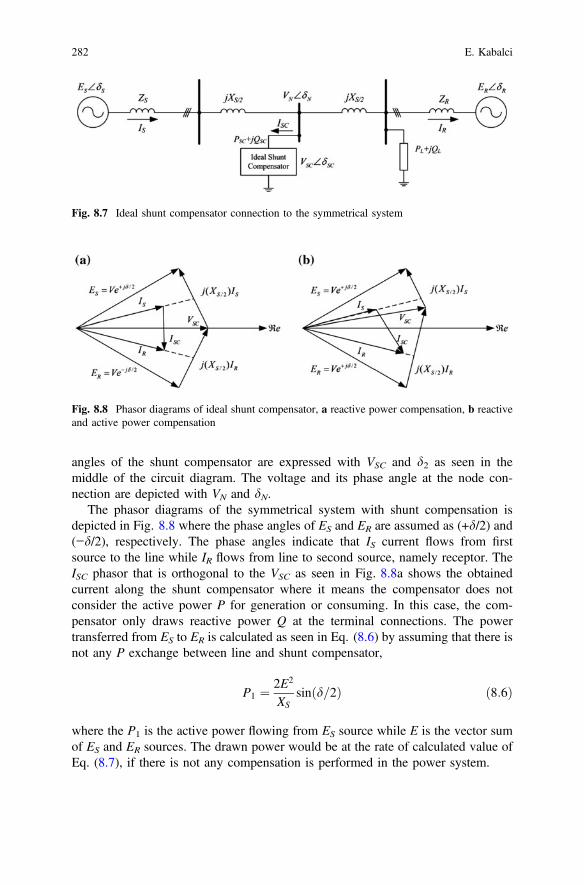
angles of the shunt compensator are expressed with VSC and d2 as seen in the

middle of the circuit diagram. The voltage and its phase angle at the node con-

nection are depicted with VN and dN.

The phasor diagrams of the symmetrical system with shunt compensation is

depicted in Fig. 8.8 where the phase angles of ES and ER are assumed as (+d/2) and

(−d/2), respectively. The phase angles indicate that IS current flows from first

source to the line while IR flows from line to second source, namely receptor. The

ISC phasor that is orthogonal to the VSC as seen in Fig. 8.8a shows the obtained

current along the shunt compensator where it means the compensator does not

consider the active power P for generation or consuming. In this case, the com-

pensator only draws reactive power Q at the terminal connections. The power

transferred from ES to ER is calculated as seen in Eq. (8.6) by assuming that there is

not any P exchange between line and shunt compensator,

P1 ¼2E2

XS

sinðd=2Þ ð8:6Þ

where the P1 is the active power flowing from ES source while E is the vector sum

of ES and ER sources. The drawn power would be at the rate of calculated value of

Eq. (8.7), if there is not any compensation is performed in the power system.

Fig. 8.7 Ideal shunt compensator connection to the symmetrical system

Fig. 8.8 Phasor diagrams of ideal shunt compensator, a reactive power compensation, b reactive

and active power compensation

282 E. Kabalci

P1 ¼V2

XL

sinðdÞ ð8:7Þ

Since [2 sin(d/2)] is ever greater than sind, that is in the range of [0, 2p], the

control capability of line is increased by the compensator. When the phase angles of

ES and ER differ from d/2, active and reactive power components are generated in

the power exchange through sources as shown in Fig. 8.8b. In this situation, the

shunt compensator should be operated to adjust any of P or Q owing to its power

electronics based structure. Furthermore, the device structure also varies according

to requirement of P or Q compensation since they have opposite phasor charac-

teristic caused by the stored energy type [6–9].

The ideal series compensator that is connected to the transmission line in series

is constituted by a voltage source VSC as shown in Fig. 8.9. The current value that is

delivered from source to receptor over transmission line is calculated as follows;

I ¼ ðESR � ESCÞjXS

; ESR ¼ ES � ER ð8:8Þ

The series compensator utilizes capacitor banks to minimize the overall reac-

tance of a transmission line at the line frequency where the reactance balance is

arranged by the reactive power of capacitors. The reactive voltage that is generated

by capacitors provides to improve phase angle and voltage stability in addition to

load sharing optimization.

The phasor diagrams of the symmetrical system with ideal series compensation

is depicted in Fig. 8.10 where the phase angles of ES and ER are assumed as (+d/2)

and (−d/2), respectively. The series compensator does not generate or consume any

active power when the compensator voltage VSC is generated orthogonal to the line

current I. The power type of the series compensator is just reactive power and the

reactance is balanced by using capacitive or inductive impedances. The equivalent

impedance Xeq is calculated by

Xeq ¼ XS 1þ kð Þ ð8:9Þ

Fig. 8.9 Ideal series compensator connection to the symmetrical system


k ¼ XC

XS

; 0� kj j � 1 ð8:10Þ

where XC is the series compensation reactance. The compensation factor k is

positive at the inductive reactance and negative at the capacitive reactance. The

compensation voltage VSC and the delivered power are calculated as follows

VSC ¼ IXeq ð8:11Þ

PS ¼V2

XSð1� kÞ sin d ð8:12Þ

where the equation depicts that the delivered power can be adjusted by selecting the

proper k factor. Similarly, the reactive power delivered by series compensator to

receptor is determined as seen in Eq. 8.13;

QS ¼2V2k

XSð1� kÞ2ð1� cos dÞ ð8:13Þ

Fig. 8.10 Phasor diagram of ideal series reactive compensator; a capacitive operation without

compensation, b capacitive operation with compensation, c reactive operation without compen-

sation, d reactive operation with compensation

284 E. Kabalci

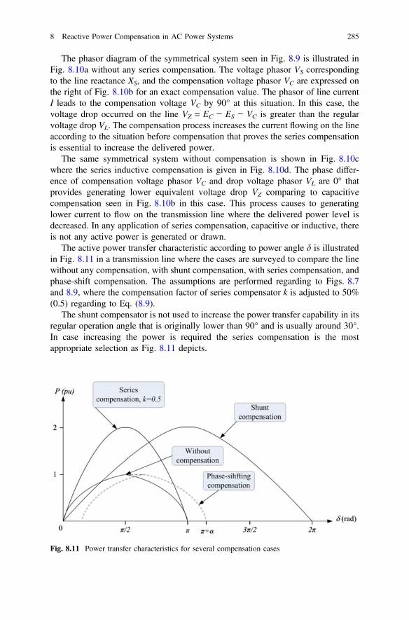
The phasor diagram of the symmetrical system seen in Fig. 8.9 is illustrated in

Fig. 8.10a without any series compensation. The voltage phasor VS corresponding

to the line reactance XS, and the compensation voltage phasor VC are expressed on

the right of Fig. 8.10b for an exact compensation value. The phasor of line current

I leads to the compensation voltage VC by 90° at this situation. In this case, the

voltage drop occurred on the line VZ = EC − ES − VC is greater than the regular

voltage drop VL. The compensation process increases the current flowing on the line

according to the situation before compensation that proves the series compensation

is essential to increase the delivered power.

The same symmetrical system without compensation is shown in Fig. 8.10c

where the series inductive compensation is given in Fig. 8.10d. The phase differ-

ence of compensation voltage phasor VC and drop voltage phasor VL are 0° that

provides generating lower equivalent voltage drop VZ comparing to capacitive

compensation seen in Fig. 8.10b in this case. This process causes to generating

lower current to flow on the transmission line where the delivered power level is

decreased. In any application of series compensation, capacitive or inductive, there

is not any active power is generated or drawn.

The active power transfer characteristic according to power angle d is illustrated

in Fig. 8.11 in a transmission line where the cases are surveyed to compare the line

without any compensation, with shunt compensation, with series compensation, and

phase-shift compensation. The assumptions are performed regarding to Figs. 8.7

and 8.9, where the compensation factor of series compensator k is adjusted to 50%

(0.5) regarding to Eq. (8.9).

The shunt compensator is not used to increase the power transfer capability in its

regular operation angle that is originally lower than 90° and is usually around 30°.

In case increasing the power is required the series compensation is the most

appropriate selection as Fig. 8.11 depicts.

Fig. 8.11 Power transfer characteristics for several compensation cases


The most important supplement of shunt compensator is to increase the power

stability of the system. The phase-shifting compensator has a great potential for

symmetrical systems under exceeding or unpredictable phase differences. It is

preferred to stabilize the phase fluctuations instead of increasing the power [6, 9–

11].

8.2.3 Devices Used in Reactive Power Compensation

The FACTS originated from several reactive power compensators propose exten-

sive use of power electronic devices and systems in ac power control. There are

several FACTS devices are proposed and being studied since 1990. The first

generation conventional compensators were constituted of inductive and capacitive

reactive elements to build shunt, series, and shunt-series compensators as illustrated

in Fig. 8.12. The improvements of power semiconductors promoted new device

types and synthesizes of circuit topologies depending the capabilities of semicon-

ductors. The aggregated terms of FACTS include several device types as seen on

the right hand side of Fig. 8.12 where the commutation style is one of the most

Fig. 8.12 A comprehensive list of FACTS devices

286 E. Kabalci

widely accepted indicator to classify device topologies. The connection type to the

transmission line is another significant indicator to detect the usage of FACTS.

The essential application areas of FACTS are power flow control, voltage

control, VAR compensation, stability improvement in terms of phase and voltage,

power conditioning, and interconnection of several sources in distributed genera-

tion. The connection type to the transmission line and semiconductors of com-

pensators involve several different operating characteristics. The conventional

compensators are constructed with static components such as diodes, inductances,

capacitances, and mechanic controllable devices such as tap-changing transformers.

The modern FACTS devices are installed by using more sophisticated compo-

nents as thyristors or bi-directional semiconductors such as gate turn-off thyristors

(GTOs), insulated gate bipolar transistors (IGBTs) or insulated gate commutated

thyristors (IGCTs). The thyristor-based topologies are known as line commutated

due to unidirectional switching property of the device is depended to the half-cycle

polarity of the line. However, the advanced technology of bi-directional switches

allow commutating the FACTS at the desired period of entire cycle [4, 6, 7, 12]. In

this case, voltage source converters (VSCs) generate completely controllable output

in terms of magnitude and phase angle owing to pulse width modulation (PWM)

methods used to control IGBTs or IGCTs. The PWM frequency is freely adjusted to

decrease THD ratio of the generated output voltage and compensate the power

quality of the transmission line. Therefore, particular designs can be carried out in

terms of device topology and commutation methods [6, 11–14].

The line commutated FACTS devices can be listed as thyristor-switched ca-

pacitor (TSC), thyristor-controlled reactor (TCR), static VAR compensator (SVC),

thyristor-controlled series compensator (TCSC) that all are based on aforemen-

tioned ideal shunt or series compensator methodology as shown in Fig. 8.12. The

right hand side of FACTS listed in Fig. 8.12 includes VSCs with advanced tech-

nologies of STATCOM, static synchronous series compensator (SSSC), unified

power flow controller (UPFC)), dynamic power flow controller (DPFC) and HVDC

VSCs. The FACTS improve the stability and power quality by adapting to rapidly

changing line situations and dynamically responding even at the voltage dip and

flicker cases.

The illustration given in the figure is also coloured in order to express appli-

cation aims of compensators regarding to particular requests. The reactive power

compensation and voltage control is primarily performed by selecting shunt devices

that are shown in the first line of the figure. The SVCs are capable to present more

accurate and smoother control comparing to mechanically switched shunt com-

pensators. In this case, the STATCOM is the most recent and the most robust shunt

compensator device comparing to others. The series devices shown in green box are

preferred to compensate the line stability and reactive power depending to its

adaptive impedance feature. These devices are implemented according to TSC,

TCR, and SVCs where the main difference is their series connection to the trans-

mission line. In the most cases, the series compensators are used a thyristor by-pass

in order to protect the compensator.


The TCSC provides a controllable capacitance to perform power flow control

and oscillation damping among the sources and loads. The TCSC is a quite effective

device against the damping problems occurred during the integration of large power

systems, and they can more accurately overcome similar problems than SSSC

device that is not contemporarily being used in the transmission lines since their

higher costs.

Furthermore, the TCSC prevents the of sub-synchronous resonance (SSR)

problem that is seen as an interaction between heat based generating systems and

series compensated systems. One of the most significant application areas of series

compensators is seen in distribution lines of industrial plants against voltage dips

and flickers. These special devices are known as dynamic voltage restorer (DVR)

or static voltage restorer (SVR) [6, 11, 13–18].

The most extensively researched and improving compensation devices designed

in shunt and series connection to perform power flow control. These are shown in

red box of Fig. 8.12 as a new line. The increased energy demand requires dynamic

and balanced power flow control between overloaded units and spare power sys-

tems of transmission line. The phase shifting or tap changing transformers

(PST) are the first generation devices of shunt-series compensators.

As it is easily realized, the lower response speed, lower control ability, and

periodic maintenance requirements of these devices are their drawbacks comparing

to semiconductors. The unified power flow controller (UPFC) is a more sophisti-

cated and convenient compensator owing to its fast and dynamic structure. It can be

assumed as a composition of a STATCOM and an SSSC using common dc link for

power flow control. The dc link is generated by a small capacitor connected

between STATCOM and SSSC where the STATCOM draws active power and

SSSC generates power at the same ratio to balance the transmission line.

The main drawback of this installation is its high cost caused by power semi-

conductors used in both devices. The dynamic power flow controller (DPFC) that is

a combination of one traditional PST and a SSSC/thyristor switched series reactor

(TSSR) is improved to tackle this situation by providing a simpler device to per-

form the same issue with low cost. The DPFC provides more dynamic performance

than a traditional PST where it controls the reactance by a set of thyristors inte-

grated to the transmission line serially. It is capable to control the active and

reactive power delivered through the transmission line. Depending on the reactive

power requirements of the system, the DPFC configuration is implemented by using

a mechanically switched shunt capacitor (MSC) [6, 7, 11, 14].

The high voltage direct current (HVDC) compensators are associated with

FACTS in industrial applications as shown in Fig. 8.12. HVDC and FACTS

experienced researches and improvements primarily based on thyristors and

recently based on bi-directionally controlled semiconductors. The power converters

defined as back-to-back (B2B) systems can be built up with thyristors or

bi-directional semiconductors such as IGBT, IGCT where they allow to the com-

plete control of power flow while the thyristor based topologies controls only the

active power. Although the drawbacks of thyristor devices, the VSCs based on

HVDC B2B systems are capable to decouple frequency at the both sides of

288 E. Kabalci

symmetrical systems. Furthermore, many PWM control methods decreasing THD

and electromagnetic interference (EMI) are implemented owing to advantages of

recent power semiconductors.

The HVDC and FACTS are fully or are partially integrated in many applications.

It is noted that there are more than a hundred HVDC power plants are installed in

worldwide, delivering more than 80 GW power. The current source converters

(CSCs) alternatively to VSCs find application areas in power systems especially at

1000 MW and over. However, they are assumed as a mature technology since

thyristor based configurations. The CSCs are naturally resistant against short cir-

cuits since the series inductor helps to limit inrush currents appearing at faulty

operations while VSCs are weaker at line faults. The dc circuit breakers and cable

are more attractive for VSC HVDCs in this case [7, 13–16].

8.3 Conventional Equipment for Reactive Power

Compensation

The VAR compensators based on generating are classified into two groups as

rotating and static generators. The antecedent applications of shunt capacitor and

shunt inductor as power flow controllers (PFCs) are dated to 1914. The power

semiconductors have attracted the improvement of static VAR compensators

starting from last half of previous century. Then, the thyristor switched capacitors

and reactors are improved to utilize rapid and dynamic response of power electronic

devices. Afterwards, they are associated with tap-changing and PSTs that is the

most reliable way to control the delivered power on the parallel transmission lines.

The PFCs such as PSTs and series compensators were widely used in steady-state

operation of transmission line that the technique is implemented by observing the

effect of compensator on the power flow. The technique lying behind PST com-

pensation is its unique and different design criteria comparing to regular power

transformers. It can be produced as two-core or single-core symmetrical/

asymmetrical constructions.

The power flow control based on PST can be performed by adjusting the

phase-shift angle dC between source and receptor sides of symmetrical system as

seen in power controller plane in Fig. 8.13. This method is used to determine

steady-state conditions of the transmission line where the delivered active power is

compensated by PFC [11, 19, 20–25].

The power controller plane is used to detect the power limits of the transmission

line and the compensator. The bounded area is called the “operating area” depicting

all operating points of the PFC to ensure operation is limited in the steady-state. The

first generation compensators based on capacitor or inductors were arranged

regarding to steady-state assumptions. However, the widely fluctuating loads

expose the power system to large reactive power variations. In this case, the fixed

capacitor banks lack to compensate the reactive power leading to


over-compensation or under-compensation. The switched capacitor and reactors are

proposed to tackle this drawback by providing variable compensation owing to

variable switching angle. The primary switching applications were being performed

using mechanical switches such as relays and circuit breakers that are replaced with

power semiconductors lately [6, 9, 11].

8.3.1 Thyristor Switched Capacitor (TSC)

The TSC is shown in Fig. 8.14a that is constructed with a line transformer,

bi-directional thyristor valve, and a capacitor where a small inductance can be

added in series to limit the current. Either the SVCs are defined with switched or

control as previously expresses TSC and TCR. The switching term is used to

emphasize that the thyristors are turned on at the exact angles only when

zero-voltage switching (ZVS) condition is achieved for TSC. The voltages at the

thyristor terminals are kept at zero in ideal conditions. However, the required

positive amplitude across anode to cathode for switching thyristors is provided in

practice, and thyristor valve provides connection and disconnection of capacitors to

the line. In the case of a small reactor is preferred to use, it should be located among

the transformer and thyristor valve to prevent inrush currents under critical

conditions.

Fig. 8.13 Operating area of a power flow controller (PFC) in the power controller plane

290 E. Kabalci

The thyristor valve is closed in case of steady-state conditions and TSC is

connected to the transmission line where it is imposed to handle sinusoidal ac line

voltage. The TSC current at this interval is

IS�S ¼ Vn2

n2 � 1xC cosxt ð8:14Þ

where V is the terminal voltage of TSC and n is given by

n ¼ 1ffiffiffiffiffiffiffiffiffiffiffiffi

x2LCp ¼

ffiffiffiffiffiffi

XC

XL

r

ð8:15Þ

The current flowing across the capacitor at a given interval t is determined by the

following where it is assumed that the equivalent resistance of the TSC is nearly

zero comparing to the transmission system;

iðtÞ ¼ Vm

XC � XL

cosðxtþ aÞ � Vm

XC � XL

cosðaÞ cosðxrtÞ

þ XCVm sinðaÞxrLðXC � XLÞ

� VCO

xrL

� �

sinðxrtÞð8:16Þ

xr ¼1ffiffiffiffiffiffi

LCp ð8:17Þ

Fig. 8.14 Thyristor switched capacitor, a circuit diagram, b control characteristic of SVC


where Vm is the instantaneous maximum voltage of the source, XC and XL are

capacitive and inductive reactance of the compensator, a is the phase-shift angle of

voltage when the capacitor is connected to the line, xr is the resonance frequency,

and VC0 is the capacitor voltage at t = 0−

Since the capacitor voltage VC0 is equal to source voltage, the current component

of the TSC will be zero when the capacitor is connected at the peak value of source

voltage Vm, (a = ±90°). When the TSC is disconnected from line, the capacitor will

be charged to the source voltage and remains at this value. In case the capacitor

voltage is protected at the maximum peak value, the TSC can be switched again

without any fluctuation. Furthermore, the reconnection of capacitor to the line may

be done between zero and peak VC0 [6, 11, 15].

The steady-state control characteristic of SVC seen in Fig. 8.14b represents the

control area on the line of ADB. The 0A line depicts the maximum limit of

capacitor while BC line shows the maximum inductor limit in terms of voltage and

current values. It should be noted that the SVC current is positive while the sus-

ceptance is inductive. Thus,

IS�S ¼ �BSVCVSVC ð8:18Þ

The slope of 0A line is determined by the susceptance of the capacitor BC, while

the slope of OBC line depends on susceptance of the reactor BL. A positive slope in

the range between 1–5% is presented to allow shunt operation of several SVCs

connected to the same transmission line, and to prevent the operating at the lower

and higher limits.

The steady-state degree of SVC line voltage is detected regarding to the system

parameters and control features. The system characteristic seen in Fig. 8.14b with a

negative slope is given by

VSVC ¼ VTh � XThIS�S ð8:19Þ

where VTh and XTh are the Thevenin voltage and reactance calculated from the SVC

side to line as follows;

VTh ¼V cosðd=2Þcosðd=2Þ ð8:20Þ

XTh ¼Zn

2tanðh=2Þ ð8:21Þ

where Zn is the surge impedance given by [26]

Zn ¼ffiffiffiffi

L

C

r

ð8:22Þ

292 E. Kabalci

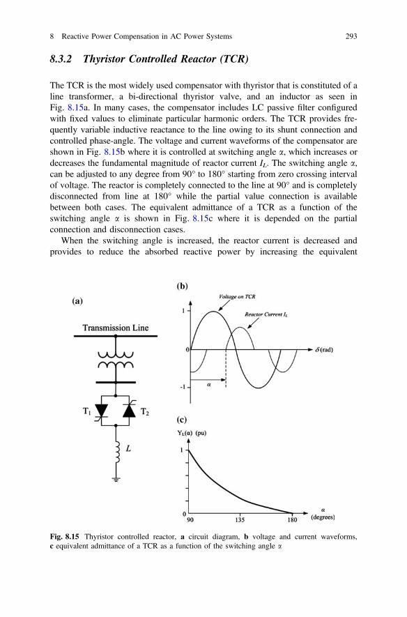
8.3.2 Thyristor Controlled Reactor (TCR)

The TCR is the most widely used compensator with thyristor that is constituted of a

line transformer, a bi-directional thyristor valve, and an inductor as seen in

Fig. 8.15a. In many cases, the compensator includes LC passive filter configured

with fixed values to eliminate particular harmonic orders. The TCR provides fre-

quently variable inductive reactance to the line owing to its shunt connection and

controlled phase-angle. The voltage and current waveforms of the compensator are

shown in Fig. 8.15b where it is controlled at switching angle a, which increases or

decreases the fundamental magnitude of reactor current IL. The switching angle a,

can be adjusted to any degree from 90° to 180° starting from zero crossing interval

of voltage. The reactor is completely connected to the line at 90° and is completely

disconnected from line at 180° while the partial value connection is available

between both cases. The equivalent admittance of a TCR as a function of the

switching angle a is shown in Fig. 8.15c where it is depended on the partial

connection and disconnection cases.

When the switching angle is increased, the reactor current is decreased and

provides to reduce the absorbed reactive power by increasing the equivalent

Fig. 8.15 Thyristor controlled reactor, a circuit diagram, b voltage and current waveforms,

c equivalent admittance of a TCR as a function of the switching angle a


inductance. The reactor current is calculated depending on inductor and switching

angle as given by

ITCR ¼ Vrms

pxLð2p� 2aþ sinð2aÞÞ ð8:23Þ

The TCR compensators provide continuous control, maximum delay limited to

one cycle at most, and very low transients during connection and disconnection.

However, the significant drawback of the compensator is higher losses in inductive

operation areas, and low ordered harmonics of current. The magnitude of current

harmonics are defined as shown in Eq. (8.24)

Ik ¼4Vrms

pXL

sinðkþ 1Þa2ðkþ 1Þ þ sinðk � 1Þa

2ðk � 1Þ � cosðaÞ sinðkaÞk

� �

ð8:24Þ

where k is harmonic orders; k = 3, 5, 7,… [6, 11, 15, 27, 28].

8.3.3 Thyristor Controlled Series Compensator (TCSC)

The thyristor-controlled series compensator (TCSC) is shown in Fig. 8.16. This

compensator is implemented regarding to series connection of a TCR to the

transmission line. In the series connection case, a capacitor should be shunt con-

nected to TCR in order to control the current. The most significant advantage of

TCSC is balance the damping occurred while integrating large power systems, and

to overcome SSR. The circuit diagram seen in figure is identical to regular SVC that

is shunt connected to the line.

The TCSC presents two particular principles that are variable capacitive reac-

tance and variable inductance. Both of these principles are managed by TCSC

switching methods that are used to control the thyristor valve. Consequently, this

configuration provides a continuously controlled series capacitor. The equivalent

Fig. 8.16 Thyristor controlled series compensator

294 E. Kabalci

resistance of TCSC is depicted in Fig. 8.17 as a function of the switching angle a

where it is operated in two different areas as inductive and capacitive. The transition

between operation ranges appears at around 145° in this case. The regular operation

of TCSC is performed in capacitive area up to 180° that the minimum impedance is

obtained around this angle. The maximum impedance Zmax is presented at 150°

switching angle where the resonance around this area is not considered safe for

operating.

The TCSC can also be operated in inductive region that is performed by limiting

the switching angle between 90° and 140°, where the a lower than 90° causes to

decrease the amount of the delivered power [6, 11].

8.4 Flexible AC Transmission System (FACTS)

The force-commutated or self-commutated compensators are implemented by using

VSC in order to provide more flexible and robust compensation comparing to

conventional line-commutated compensators. The FACTS are integrated to sym-

metrical systems in shunt, series, or shunt-series connections as conventional

compensators and SVCs. The most widely used FACTS are STATCOM and SSSCs

where the each compensator is based on VSC to generate compensating voltage and

increase the system stability. The most significant contribution of FACTS is har-

monic elimination capability that is provided by the sophisticated device configu-

rations and control algorithms.

The improvement of high-power VSCs is promoted by the development of

force-commutated semiconductors such as GTOs, IGBTs, and IGCTs. The primary

applications of VSCs are shown in Fig. 8.18 where two-level six-pulse VSC is

illustrated in Fig. 8.18a and three-level diode clamped topology is shown in

Fig. 8.18b. The VSCs are configured with GTOs and antiparallel diodes in order to

provide bi-directional current flow where the switches could be IGBT or IGCT. The

voltage blocking capability of the VSCs given in the figure is unidirectional. In case

of CSCs used, the voltage blocking capability is shifted to bi-directional while the

Fig. 8.17 Equivalent resistance of TCSC as a function of the switching angle a


current flow is performed in unidirectional mode. The regular operation of VSC is

performed with a voltage source connected to the dc side that allows only reactive

power compensation in a compensator application by replacing the dc source with a

capacitor [6, 9, 11, 14].

However, in case that active power management is also required, then the circuit

involves a small reactor on the ac side of compensator to limit the inrush currents

and current spikes during the transients. The first installation of high-power VSC

configured in six-pulse topology with 10 MW rated power is done in Japan, in 1991

[6, 11, 29]. The switching frequency was in the line frequency to ensure the stability

of the compensator, and eight sets of six VSCs were building a 48-pulse VSC

compensator with 80 MVA compensation capability. The ensuing applications of

force-commutated VSCs have presented effective compensations and the researches

on VSC accelerated their integration to industrial plants.

The emerging power systems and FACTS require more effective controllers such

as STATCOMs, (SSSC, UPFC), the inter-phase power controller (IPC), the

thyristor-controlled braking resistor (TCBR), the thyristor-controlled voltage limiter

(TCVL), the battery energy storage system (BESS), and the superconducting

magnetic energy storage (SMES) systems [30].

Fig. 8.18 VSC topologies

used in FACTS, a basic

six-pulse two-level VAR

compensator, b basic

three-level VAR compensator

296 E. Kabalci

8.4.1 Static Synchronous Compensator (STATCOM)

A STATCOM is a VSC based compensating device that is shunt connected to the

transmission line. A STATCOM integrated to the line and shunt to generators and

load operates by generating or absorbing reactive load to compensate the trans-

mission line. The operation principle of STATCOM makes it either a source or a

load for the transmission line by replacing widely known series or shunt FACTS.

The STATCOM increases the power quality by performing several compensations

such as dynamic voltage control, oscillation damping of power line, pursuing the

stability during transients, flicker and sag-swell controls, and active and reactive

power (PQ) control in transmission systems. Furthermore, STATCOMs substitute

SVC devices in the distribution systems [4, 6, 30].

Figure 8.19a shows the basic connection of STATCOM to transmission line

where the reactive power control is performed by controlling the terminal voltages.

Fig. 8.19 STATCOM,

a circuit diagram of line

integration, b control

characteristic of STATCOM


The transmission line is configured in symmetrical system that ES denotes the source

voltage, while the line impedance XS, line voltage VL, line current IL, and receptor

voltage ER are indicated. The reactive power is controlled depending on the com-

pensator voltage VI control by assuming that is in phase with the source voltage ES.

There are three options to determine the reactive power of STATCOM according to

correspondence among the source and STATCOM voltages. In case of equality,

there is not any active or reactive power generated or absorbed in STATCOM.When

the source voltage exceeds, than the reactive power of STATCOM is shifted to

inductive. In the case of the source voltage is lower than STATCOM voltage, this

causes to capacitive reactive power.

A typical V-I characteristic of STATCOM as shown in Fig. 8.19b, illustrates this

situation where the STATCOM can perform inductive or capacitive compensation

regarding to its line current. Besides, the V-I characteristics show that STATCOM

provides fully capacitive or inductive power starting from lower voltages even from

0.15 p.u.

Thus, the main case that should be handled in reactive power compensation by

using STATCOM is to control the magnitude of compensator voltage VI. This

operation is performed based on two basic principles where one is used in multi-

pulse converters and the other one for PWM controlled multilevel converters. The

capacitor voltage building the dc line can be fixed to a stable magnitude in PWM

control of multipulse converter based STATCOM where the compensator voltage is

controlled by the modulator. This is managed by adjusting the switching angle

owing to PWM modulator. The second STATCOM configuration based on mul-

tilevel converters should control the capacitor voltage only to sustain its constant

value. The control methods can be either scalar or vector based in this configura-

tion. Furthermore, the multilevel configuration allows switching with high fre-

quency PWM to decrease THD of reactive components [6, 9, 14]. The following

sections are dedicated VSC topologies used in STATCOMs where multipulse

configurations are indicated by 12-pulse and 24-pulse converters. Afterwards,

multilevel topologies and controller structures are analysed to compare to multi-

pulse STATCOMs at a glance.

8.4.1.1 Multi-pulse Converter Based STATCOM

The first VSC based STATCOM applications are developed with multi-pulse con-

verters owing to their lower losses and lower harmonic contents comparing to con-

ventional compensators. The multi-pulse converter topologies consist of several

six-pulse VSC circuits where a basic VSC STATCOM in the configuration of

six-pulse two-level was illustrated in Fig. 8.18a. The switching devices of the system

were GTOs that the converter could generate balanced three-phase ac output voltages

by using a dc capacitor as the voltage source. The frequency of the output voltage is

adjusted by the modulating frequency of GTO switches and the phase voltages are

coupled to ac grid over an interconnection reactor [9, 31, 32].

298 E. Kabalci

The 12-pulse converters are constituted of six-pulse converters connected in

parallel as shown in Fig. 8.20. The expressed configuration is improved regarding

to two-level topology shown in Fig. 8.18a while another configuration is in

three-level structure as illustrated in Fig. 8.18b. The two-level topology requires

non-identical winding types for each six pulse VSC that one is D-Y connected

while other is Y-Y connected to ac grid. The D connected secondary of the

transformer with three times higher turns according to Y connected secondary

provides 30° phase shift comparing to other. Therefore, the lower ordered har-

monics are easily eliminated.

The output phase voltage of STATCOM can be calculated by using Eq. (7.25)

where n1 and n2 are the voltage ratios of the corresponding VSC transformers while

va−Y and va−D are the output voltages of the Y-Y and D-Y connected converters,

respectively [9].

va ¼ n1va;Y þ n2va;Dffiffiffi

3p ð8:25Þ

The voltage magnitude of VSC output depends on modulation index mi of

control signal that allows obtaining the output voltage at miVdc where Vdc is the

voltage across the capacitor. The control signal that is based on some variation of

PWM generates switching angle a that generates the STATCOM bus voltage at

VS\dS form. The Eq. (8.26) expresses the admittance of transformer

Y ¼ 1

Rþ jXS

¼ Gþ jB ð8:26Þ

Fig. 8.20 Circuit diagram of two-level 12-pulse STATCOM


http://dx.doi.org/10.1007/978-3-319-51118-4_7

that manages the active or reactive power injection to the transmission line. The

reactive power generation or absorption ability of STATCOM depends on the

control voltage of PWM modulator. The injected reactive power to utility grid is

presented as follows

Q ¼ V2SB� miVdcVSB cosðdS � aÞþmiVdcVSG sinðdS � aÞ ð8:27Þ

In case of VS > miVdc, Q will be positive that causes STATCOM to absorb

reactive power or vice versa [9]. The active power generated by the source to charge

the capacitor is expressed as follows,

P ¼ VSj jmiVdc

XS

sinðdS � aÞ ð8:28Þ

The 24-pulse converter topology of STATCOM consists of six-pulse converters

where it eliminates the 6n ± 1 ordered harmonics. The 23rd, 25th, 47th, and 49th

harmonics in the ac output waveform are naturally eliminated since the n = 4 for

24-pulse converter. The 24-pulse STATCOM constituting two-level VSCs is

illustrated in Fig. 8.21 where this topology is also known as quasi 24-pulse [9, 33].

Each VSC and transformer connection configures a stage that each one is connected

to the transmission line by Y-Y and ∆-Y connections of transformers. The trans-

formers may connected in zigzag that generates 15° phase shift according to each

other with −7.5°, 7.5°, 22.5°, and 37.5° angles [9, 33, 34].

Another topology of quasi 24-pulse STATCOM is presented in Fig. 8.22 [35]

where the VSCs are constituted according to neutral point clamping

(NPC) topology that is previously shown in Fig. 8.18b.

The conduction angle a defines the negative and positive cycles of intervals

where a = 180 − 2b, where 2b stands for the dead-band angle. The on-off spectral

transitions are ensured by the dead-band angle where the output voltages of a

six-pulse three-level VSC is given by Eq. (8.29).

Fig. 8.21 Circuit diagram of a quasi two-level 24-pulse STATCOM

300 E. Kabalci

V1 ¼2

ffiffiffi

6p

p

vdc

2sin

180� 2b

2

� �

ð8:29Þ

On the other hand, output voltages of a 24-pulse three-level VSC is given as

follows while the active and reactive powers are calculated as given below by

considering XS as the reactance along with STATCOM and the transmission line by

using Eqs. (8.31) and (8.32) [9, 35]

Vc1 ¼ np2

ffiffiffi

6p

6p

vdc

2sin

180� 2b

2

� �

cosp

24ð8:30Þ

P ¼ VLVS sin dS

XS

ð8:31Þ

Q ¼ VS

VS � VL sin dS

XS

� �

ð8:32Þ

where the phase angle d between the ac bus voltage VS and STATCOM output

voltage VL sustains the dc line voltage Vdc at a constant value.

Fig. 8.22 Circuit diagram of a three-level 24-pulse STATCOM


8.4.1.2 Multilevel Converter Based STATCOM

In addition to their power conversion applications, the multilevel converters

(MLC) are widely used in active filters, and FACTS. Although the primary

applications are improved for medium power ranges, the recent applications have

been increased the power range from a few kWs to multi MWs owing to their

cascaded topologies. Almost all the three-level STATCOM topologies are imple-

mented with conventional diode clamped (DC) topology where the switching

devices were GTOs. This approach indicates that the control strategy of DC is the

simplest one among other three-level MLCs in medium and high power application.

The flying capacitor MLC (FC-MLI) that is one of the outstanding topology

allows constructing low cost systems, particularly in high power applications,

comparing to the DC. However, it involves pre-charge arrangement for the

capacitors that are connected through the upper and lower arms. The cascaded

H-bridge (CHB) topology is the most recent topology among others that extended

its operation area since it provides higher power conversion and lower cost for a

given output magnitude level. The CHB consists of several H-bridge cells con-

nected in series to generate multilevel output voltage. One of the most significant

features of this topology is higher switching frequency comparing the previous

topologies, and increased power rate handled by the total device and equally shared

to the each cell. Furthermore, the CHB based STATCOM is capable to eliminate

harmonics and to compensate reactive power in superior comparing others.

The main requirement of this configuration is its separated dc sources. However,

CHB can be easily integrated to various type of energy sources to obtain higher

output levels and energy storage applications [9, 36–39].

Figure 8.23 shows the circuit diagram of STACOM configured by using

three-phase five-level CHB including series connection of three-level H-bridge cells

at each phase leg. The output voltage synthesis of H-bridges generate a combined

phase voltage in staircase waveform oscillating in the ranges of +Vdc, 0, −Vdc.

Where Va1 and Va2 voltages of series connected H-bridge cells synthesize the

phase voltage Van in a stepped waveform as seen in Fig. 8.24. The positive levels of

output voltage are indicated with P1 and P2 while the negatives are P11 and P2

1.

Equation (8.33) expresses the Fourier series expansion of the general multilevel

stepped output voltage while the transform applied to the STATCOM in Fig. 8.23

is shown in Eq. (8.34), where n represents harmonic order of the output voltage.

VanðtÞ ¼4Vdc

p

X

1

n¼1;3;5;...

cosðna1Þþ cosðna2Þþ . . .þ cosðna5Þ½ � sinðnxtÞn

ð8:33Þ

The switching angles a1, a3,…, a5 in Eq. (7.33) are selected for the minimum

voltage harmonics [36, 40].

302 E. Kabalci

http://dx.doi.org/10.1007/978-3-319-51118-4_7

Van5ðtÞ ¼4Vdc

p

X

1

n¼1;3;5;...

cosðna1Þþ cosðna2Þ½ � sinðnxtÞn

ð8:34Þ

Researchers have proposed novel MLCs based on hybrid topologies that are

based on the existing devices [36, 40].

8.4.2 Static Synchronous Series Compensator (SSSC)

The series capacitor based compensation that brings some capabilities such as

increasing the transient stability, reactance control, and load sharing is a conven-

tional technique that was introduced in Sect. 8.3.3. Even though the series com-

pensation is assumed to be used to decrease the reactive impedance of the

transmission line, it is actually operated by increasing the line voltage, current, and

thereby the delivered power from source to load. Although the mentioned advan-

tages, series compensation has several drawbacks on SSR issues that large energy

exchange is done by several sources under synchronous system frequency.

Fig. 8.23 Circuit diagram of a five-level CHB STATCOM


There are several studies are performed to overcome SSR problem. The robust

control methods and configurations of FACTS stand out of other methods proposed

by researchers. The SSSC has been developed as an alternative to the TCSC devices

where the SSR immunity is inherited from TCSC. In addition to regular advantages

of series compensators, SSSC presents numerous capabilities to increase the reac-

tive power control and stability issues. Furthermore, there are several studies are

noted that SSSCs effectively damps the SSR comparing regular series compensators

[6, 11, 14, 41–46].

Figure 8.25 illustrates basic circuit diagram of a SSSC based on VSC similar to

STATCOM that is serially connected to the transmission line, and a capacitor on

the dc side. The SSSC controller considers the line current and line voltage to

compensate the transmission line by adjusting the reactance in steady-state opera-

tion. It should be noted that in case the current is flowing in the line, then SSSC

generates compensation voltage VC that is quadrature to the current and regulates

the reactive power demand. The compensation characteristic of the device is same

with the one shown in Fig. 8.11 for 0 < d < 180° during series compensation that

yields positive magnitude power delivered.

Fig. 8.24 Phase voltage generation of a five-level CHB STATCOM

304 E. Kabalci

The fundamental operating principles of SSSC is compared to conventional

series capacitive compensator as shown in Fig. 8.26 where the circuit diagrams for

only series compensation with only capacitive compensator (Fig. 8.26a) and with

SSSC (Fig. 8.26c), and respective phasor diagrams are analyzed. Despite it is

assumed to decrease the line impedance, a series capacitor increases the line

voltage, line current, and consequently the power through the line impedance. This

approach may be considered irrelevant. However, the voltage along the transmis-

sion line is the significant parameter while the capacitor is cared to increase the

voltage in order to provide the required current level. The steady-state power

transmission can be realized when a synchronous voltage source follows the series

compensation as shown in Fig. 8.26c that is analytically presented as follows

Vq ¼ VC ¼ �jXCI ð8:35Þ

It should be noted that there are particular differences between series capacitive

compensator and synchronous voltage source type compensator. The operational

characteristic of a series capacitor can be illustrated with an ideal voltage source.

However, SSSC is significantly different from the series capacitor in terms of

delivered power and angle characteristics, active power exchange, and immunity to

resonance and SSR, and control ranges.

Capacitor provides reactive impedance that causes proportional voltage to the

line current when it is series connected to the line. The compensation voltage is

changed regarding to the transmission angle d and line current. The delivered power

PS is a function of the series compensation degree s where it is given by

Pq ¼V2

XLð1� sÞ sin d ð8:36Þ

where V = V1 = V2 and d = d1 − d2. The delivered power PS regarding to trans-

mission angle d is shown in Fig. 8.27a as a function of s (s = 0, s = 1/3, and

Fig. 8.25 Static synchronous series compensator (SSSC)


s = 1/5). Additionally, SSSC is independent from line current while compensating

the voltage. The delivered power Pq is a parametric function of injected voltage

Vq ¼ Vq

�

�

�

� series to line where Vq ¼ Vq½I= I�

�

�

��e�j90� that is also given by

Pq ¼V2

XL

sin dþ V

XL

Vq cosd

2ð8:37Þ

The delivered power Pq is shown in Fig. 8.27b as a parametric function of

injected voltage Vq against transmission angle d. The normalized Vq voltage is

selected to provide same maximum power with series capacitor configuration. The

comparison of Fig. 8.27a, b expresses that the series capacitor increases the

delivered power by a fixed rate of the delivered by the uncompensated line at a

given transmission angle d. On the other hand, the SSSC increases the delivered

power by a fixed fraction of the maximum power available by uncompensated line

independent from d in the angle range of 0 � d � 90° [41, 45–47].

8.4.3 Unified Power Flow Controller (UPFC)

The UPFC is a VSC based shunt-series compensator that is constituted of

STATCOM and SSSC combination with a common dc link as shown in Fig. 8.28.

Fig. 8.26 Symmetrical system under series compensating, a circuit diagram of series compen-

sating capacitor, b phasor diagram of capacitor, c circuit diagram of SSSC, d phasor diagram of

SSSC

306 E. Kabalci

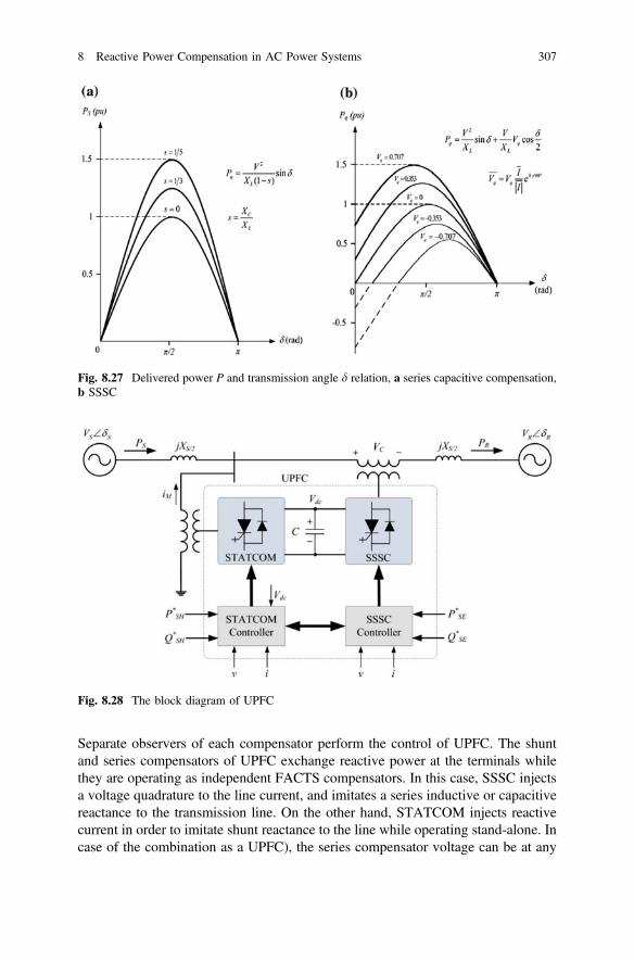
Separate observers of each compensator perform the control of UPFC. The shunt

and series compensators of UPFC exchange reactive power at the terminals while

they are operating as independent FACTS compensators. In this case, SSSC injects

a voltage quadrature to the line current, and imitates a series inductive or capacitive

reactance to the transmission line. On the other hand, STATCOM injects reactive

current in order to imitate shunt reactance to the line while operating stand-alone. In

case of the combination as a UPFC), the series compensator voltage can be at any

Fig. 8.27 Delivered power P and transmission angle d relation, a series capacitive compensation,

b SSSC

Fig. 8.28 The block diagram of UPFC


phase corresponding to the predominant line current. Thereby, the exchanged

power can be reactive as well as active power at the terminals of compensators. The

active power exchanged by any of the compensators is transmitted to the other

compensator across the common dc-link. However, exchanged reactive power is

independent from each other compensator.

The controller of STATCOM dynamically adjusts the phase angle between the

VSC output voltage and line voltage to get the STATCOM generated or absorbed

desired reactive power at the compensation connection. The SSSC can be operated

in several modes such as voltage injection, regulation of phase angle, emulation of

the line impedance, and automatic power flow control. In any of these applications,

SSSC injects a voltage over its series connection to the line. The SSSC can be

operated in the same way as examined in the previous section to control active and

reactive current. The active power control would fluctuate capacitor voltage that

should be observed by STATCOM [6, 11, 14, 26, 47].

The controller of STATCOM dynamically adjusts the phase angle between the

VSC output voltage and line voltage to get the STATCOM generated or absorbed

desired reactive power at the compensation connection. The maximum value of

series voltage VC is limited by SSSC that is the most significant advantage com-

paring to thyristor-based compensators. In the case reactive power exchange, the

UPFC increases the source voltage VS while generating reactive power, and

decreases while absorbing the reactive power. The power flow of UPFC through the

transmission line is analyzed as follows;

PS ¼ Psh þ<ðVSI�RÞ ð8:38Þ

QS ¼ Qsh þ=ðVRI�RÞ ð8:39Þ

PR ¼ �<ðVRI�RÞ ð8:40Þ

QR ¼ �=ðVRI�RÞ ð8:41Þ

where ssh ¼ffiffiffiffiffiffiffiffi

3=8p

� rsh. The powers Psh and Qsh absorbed by shunt compensator,

and common dc voltages are given by

Psh ¼ V2SGsh � sshVdcVSGsh cosðhS � aÞ � sshVdcVSBsh sinðhS � aÞ ð8:42Þ

Qsh ¼ V2SBsh � sshVdcVSBsh cosðhS � aÞ � sshVdcVSGsh sinðhS � aÞ ð8:43Þ

Vdc ¼Psh

CVdc

þ <ðVSI�RÞ

CVdc

� Vdc

RCC�RshðP2

shþQ2

shÞ

CVdcV2S

� RseI2R

CVdc

ð8:44Þ

where Gsh is the conductance, and Bsh is the susceptance of STATCOM while h is

phase angle of the transmission line and a is the phase angle of the compensator

[47].

308 E. Kabalci

8.5 State-of-the-Art Equipment for Reactive Power

Compensation

8.5.1 Dynamic Power Flow Controller (DPFC)

The DPFC is one of the emerging compensators configured with a standard PST for

tap-changing, and several series TSC and TCRs as shown in Fig. 8.29. All the

compensators connected in the DPFC are introduced in the previous sections of this

chapter. The resulting stepped reactance of DPFC is obtained owing to binary

arrangement of reactor and capacitor reactance. The PST controls the phase of

transmission line voltage in order to control the power flow across the line.

Although the system response of PST is slower since its mechanical configuration,

this issue is regulated by rapid structure of TSC and TCR. The series compensators

are operated at zero current in order to eliminate harmonic contents. The most

significant advantage of DPFC is its lower cost comparing other FACTS.

Furthermore, DPFC has several significant advantages according to PST that are

related to the speed of power flow control, and reactive power compensation. The

dynamic response of DPFC is quite effective on power oscillation damping

(POD) and transient stability in addition to steady-state stability. Furthermore,

DPFC is more appropriate in corrective compensation, thereby the system stability

and voltage stability is improved owing to its TSC and TCR configuration. This is

particularly efficient during overload situations by supporting the transmission line

with rapid voltage response. The reactive power consumption of PST is a serious

problem in weak grids. DPFC overcomes this issue by compensating the

tap-dependency of series inductance, and improves voltage stability [48–50].

The reactance, impedance, and admittance of the transmission line starting from

shunt connection of PST a to end of the TCR b are given by;

Xab ¼ kLXL þ k2XE þXB þXLine � kCXC ð8:45Þ

Zab ¼ Rab þ jXab ð8:46Þ

Fig. 8.29 The block diagram of DPFC


Ys ¼ Yab ¼1

Zab¼ GS þ jBS ð8:47Þ

where kLXL and kCXC represent the reactive and capacitive modules by ignoring

ohmic losses, and k is the PST voltage ratio which is between −1 and 1, XE, XB, XP

and Rv are PST internal parameters [51].

8.5.2 VSC-Based HVDC Transmission

The HVDC is an appropriate method used in dc transmission systems. The block

diagram of HVDC system is illustrated in Fig. 8.30 that is constituted with VSCs

connected B2B. The dc side of converters are coupled with capacitors to regulate

the dc line voltage. One of the most significant advantages of VSC based HVDC

system is its capability to control active and reactive power separately at each

terminal sides that make this system convenient for weak power systems.

Furthermore, VSC based HVDC is more effective than CSC on the improvement of

system stability and power flow control, and isolation under transients owing to its

rapid dynamic response.

The VSC based HVDC can also be used in the interline power flow controller

IPFC that is utilized to transfer active power among dc link buses. HVDC system

can be seen as an extension of UPFCas well as IPFC in some cases. The main

difference between both systems is segmentation of transmission line while HVDC

system does, UPFC does not divide.

The HVDC systems with thyristor-based converters control the dc-line current

while the most widely used VSC-based configuration controls the dc-line voltage.

This difference in the device topology allows using HVDC system in the integration

of asynchronous sources. The increased power demand and high rate integration of

large distributed sources are handled owing to modular multilevel converter

(MMC) based HVDC that is installed by series and parallel connection of VSC

cells as shown in Fig. 8.31 [6, 40, 52].

The HVDC systems with thyristor-based converters control the dc-line current

while the most widely used VSC-based configuration controls the dc-line voltage.

This difference in the device topology allows using HVDC system in the integration

Fig. 8.30 The block diagram of HVDC transmission system

310 E. Kabalci

of asynchronous sources. The increased power demand and high rate integration of

large distributed sources are handled owing to MMC based HVDC that is installed

by series and parallel connection of VSC cells. The most recent applications are

performed by MMC topology since its footprint requirements are lower, and cap-

able to control active and reactive power independently. Furthermore, it brings the

advantages of lower switching losses, lower dv/dt ratio, modular structure, recon-

figurable topology, and direct connection to the power systems without power

transformer requirement that decreases the substation area. Besides, MMC con-

figuration provides to use several types of energy storage systems [6, 40, 52].

8.6 Conclusion

The most widely used reactive power compensators in transmission line compen-

sation are introduced in this chapter. The theoretical backgrounds, applications, and

compensation methods are discussed in a comprehensive approach by listing the

compensator according to their improvements. The shunt devices among others are

Fig. 8.31 The block diagram of MMC based HVDC system


being widely used for reactive power compensation and thereby for voltage control.

The first improvement seen in compensators is SVCs that are replaced with

mechanically switched devices in order to provide more accurate and precise control.

The primary contribution of SVC was its rapid and dynamic response to the line

fluctuations. However, it was not efficient enough against fast changing power quality

problems such as voltage dips and flickers that required the implementation of more

robust compensators. The FACTS are improved to overcome this kind of stability

problems where the first one was STATCOM listed in the shunt compensator

group. In addition to shunt devices, the series compensation devices that are capable

to improve line impedance and stability are also considered in FACTS family.

Although the SSSC is a mature technology in series compensation, the TCSC is

based on a device that is efficient on damping the SSR and improvement of system

stability. However, series VSC based compensators are mostly used in distribution

lines instead of transmission lines. The most extensively researched compensators

are in shunt-series configurations that are more convenient in power flow control

comparing to previous configurations.

The PST are the most common compensators used in power flow control. The

drawbacks of this device such as higher footprint and maintenance requirement

have promoted the alternative compensators as UPFC), IPFC, and DPFC. Although

the UPFC was known for a long time, it is installed for testing and improvement

applications. The gap between PST and UPFC) has been fulfilled by DPFC that was

meeting the dynamic power flow control requirement with its simpler configuration

by overcoming drawbacks of both systems. The most recent compensator

responding the industry requirements is VSC-based HVDC compensator. The VSC

and MMC configurations brought numerous advantages such as fully independent

power control, modular structure, improved voltage and stability control and

dynamic power flow control comparing the previous devices.

Although the FACTS are generally recognized as a new technology, there are

lots of FACTS are being operated in the industry. The most widely used device is

SVC first installed in 1970s and it is known that the total installed SVC compen-

sator capacity is over than 100.000 MVA. It is also noted by literature that over

than 700 conventional series compensation plants are installed worldwide that are

capable to compensate around 350.000 MVA total power. The successor tech-

nologies as VSC-based and MMC HVDC B2B compensators, STATCOM, TSCS,

and DPFC present quick improvements in their application areas.

References

1. W. Hofmann, J. Schlabbach, W. Just, Reactive Power Compensation: A Practical Guide, First

Edition, John Wiley & Sons Ltd, 2012.

2. P.R. Sharma, A. Kumar, N. Kumar, Optimal Location for Shunt Connected FACTS Devices

in a Series Compensated Long Transmission Line, Turk J. Elec. Engineering, vol. 15, no. 3,

pp. 321–328, 2007.

312 E. Kabalci

3. M. Beza, Control of Energy Storage Equipped Shunt-Connected Converter for Electric Power

System Stability Enhancement, Thesis, Department of Energy and Environment Chalmers

University of Technology, Gothenburg, Sweden, 2012.

4. E. Acha, V. Agelidis, O. Anaya, T.J.E. Miller, Power Electronic Control in Electrical

Systems, Newnes Power Engineering Series, ISBN-13: 978-0750651264, 2002.

5. H. Amaris, M.A. Carlos, A. Ortega, Reactive Power Management of Power Networks with

Wind Generation, Lecture Notes in Energy, Springer-Verlag, London, 2013.

6. E.H.Watanabe, M. Aredes, P.G. Barbosa, F.K. de Araujo Lima, R.F. da Silva Dias, G. Santos Jr.,

32 - Power Electronic Control in Electrical Systems, Power Electronics Handbook, Third

Edition, Edited byMuhammad H. Rashid, Butterworth-Heinemann, Boston, pp. 851–877, 2011.

7. X.P. Zhang, C. Rehtanz, B. Pal, Flexible AC Transmission Systems: Modelling and Control,

Springer-Verlag, Berlin, Heidelberg, 2012.

8. T. Petersson, Reactive Power Compensation, ABB Technical Report, no. 500-028E, pp. 1–25,

Dec. 1993.

9. F. Shahnia, et al. (Eds.), Static Compensators (STATCOMs) in Power Systems, Springer

Science+Business Media, Singapore, 2015.

10. H.K. Tyll, F. Schettle, Historical Overview on Dynamic Reactive Power Compensation

Solutions from the Begin of AC Power Transmission Towards Present Applications, Power

Systems Conference and Exposition, pp. 1–7, 15–18 March 2009.

11. J. Dixon, L. Moran, J. Rodriguez, R. Domke, Reactive Power Compensation Technologies:

State-of-the-Art Review, Proceedings of the IEEE, vol. 93, no. 12, pp. 2144–2164, Dec. 2005.

12. A.A. Edris, et al., Proposed Terms and Definitions for Flexible AC Transmission Systems

(FACTS), IEEE Trans. Power Delivery, vol. 12, no. 4, pp. 1848–1853, October 1997.

13. N. Flourentzou, V.G. Agelidis, G.D. Demetriades, VSC-Based HVDC Power Transmission

Systems: An Overview, IEEE Transactions on Power Electronics, vol. 24, no. 3, pp. 592–602,

March 2009.

14. K. Kalyan, M.L. Sen, Introduction to FACTS Controllers, The Institute of Electrical and

Electronics Engineers, Inc., 2009.

15. L. Gyugyi, Power Electronics in Electric Utilities: Static VAR Compensators, Proceedings of

the IEEE, vol. 76, no. 4, pp. 483–494, Apr. 1988.

16. L. Liu, H. Li, Y. Xue, W. Liu, Reactive Power Compensation and Optimization Strategy for

Grid-Interactive Cascaded Photovoltaic Systems, IEEE Transactions on Power Electronics,

vol. 30, no. 1, pp. 188–202, Jan. 2015.

17. H. Akagi, E.H. Watanebe, M. Aredes, Instantaneous Power Theory and Applications to

Power Conditioning, IEEE Press, 2007.

18. F.L. Luo, H. Ye, M. Rashid, Digital Power Electronics and Applications, ISBN:

0-1208-8757-6, Elsevier, USA, 2005.

19. J. Brochu, F. Beauregard, J. Lemay, P. Pelletier, R.J. Marceau, Steady-State Analysis of

Power Flow Controllers Using the Power Controller Plane, IEEE Transactions on Power

Delivery, vol. 14, no. 3, pp. 1024–1031, Jul. 1999.

20. U.N. Khan, T.S. Sidhu, A Phase-Shifting Transformer Protection Technique Based on

Directional Comparison Approach, IEEE Transactions on Power Delivery, vol. 29, no. 5,

pp. 2315–2323, Oct. 2014.

21. R. Baker, G. Guth, W. Egli, P. Eglin, Control Algorithm for a Static Phase Shifting

Transformer to Enhance Transient and Dynamic Stability of Large Power Systems, IEEE

Transactions on Power Apparatus and System, vol. PAS-101, no. 9, pp. 3532–3542, Sept.

1982.

22. R. Mihalic, P. Zunko, Phase-Shifting Transformer with Fixed Phase between Terminal

Voltage and Voltage Boost: Tool for Transient Stability Margin Enhancement, IEE

Proceedings - Generation, Transmission and Distribution, vol. 142, no. 3, pp. 257–262,

May 1995.

23. J. Verboomen, D. Van Hertem, P.H. Schavemaker, W.L. Kling, R. Belmans, Analytical

Approach to Grid Operation with Phase Shifting Transformers, IEEE Transactions on Power

Systems, vol. 23, no. 1, pp. 41–46, Feb. 2008.


24. J. Mescua, A Decoupled Method for Systematic Adjustments of Phase-Shifting and

Tap-Changing Transformers, IEEE Transactions on Power Apparatus and Systems, vol.

PAS-104, no. 9, pp. 2315, 2321, Sept. 1985

25. Ch.N. Huang, Feature Analysis of Power Flows Based on the Allocations of Phase-Shifting

Transformers, IEEE Transactions on Power Systems, vol. 18, no. 1, pp. 266–272, Feb. 2003.

26. K.R. Padiyar, FACTS: Controllers in Power Transmission and Distribution, Anshan

Publishers, 1st Edition (August 15, 2009), 978-1848290105.

27. A.K. Chakravorti, A.E. Emanuel, A Current Regulated Switched Capacitor Static Volt

Ampere Reactive Compensator, IEEE Transactions on Industry Applications, vol. 30, no. 4,

pp. 986–997, Jul./Aug. 1994.

28. H. Jin, G. Goos, L. Lopes, An Efficient Switched-Reactor-Based Static VAr Compensator,

IEEE Transactions on Industry Applications, vol. 30, no. 4, pp. 998–1005, Jul./Aug. 1994.

29. S. Mori, K. Matsuno, M. Takeda, M. Seto, Development of a Large Static Var Generator

Using Self-Commutated Inverters for Improving Power System Stability, IEEE Transactions

Power Delivery, vol. 8, no. 1, pp. 371–377, February 1993.

30. R. Mohan Mathur, R.K. Varma, Thyristor Based FACTS Controllers for Electrical

Transmission Systems, ISBN: 978-0-471-20643-9, Wiley-IEEE Press, 2002.

31. B. Singh, K.V. Srinivas, Three-Level 12-Pulse STATCOM with Constant DC Link Voltage,

2009 Annual IEEE India Conference (INDICON), pp. 1–4, 18–20 Dec. 2009.

32. S.R. Barik, B. Nayak, S. Dash, A Comparative Analysis of Three Level VSC Based

Multi-Pulse STATCOM, International Journal of Engineering and Technology (IJET), vol. 6,

no. 3, pp. 1550–1563, Jun.–Jul. 2014.

33. N. Voraphonpiput, S. Chatratana, Analysis of Quasi 24-Pulse STATCOM Operation and

Control Using ATP-EMTP, IEEE Region 10 Conference TENCON 2004, vol. C, pp. 359–

362, 21–24 Nov. 2004.

34. B. Singh, R. Saha, A New 24-Pulse STATCOM for Voltage Regulation, Int. Conf. on Power

Electronics, Drives and Energy Systems, pp. 1–5, 12–15 Dec. 2006.

35. K.V. Srinivas, B. Singh, Three-Level 24-Pulse STATCOM with Pulse Width Control at

Fundamental Frequency Switching, IEEE Industry Applications Society Annual Meeting

(IAS), pp. 1–6, 3–7 Oct. 2010.

36. I. Colak, E. Kabalci, R. Bayindir, Review of Multilevel Voltage Source Inverter Topologies

and Control Schemes, Energy Conversion and Management, vol. 52, no. 2, pp. 1114–1128,

February 2011.

37. I. Colak, E. Kabalci, Practical Implementation of a Digital Signal Processor Controlled

Multilevel Inverter with Low Total Harmonic Distortion for Motor Drive Applications,

Journal of Power Sources, vol. 196, no. 18, pp. 7585–7593, 2011.

38. I. Colak, E. Kabalci, Developing a Novel Sinusoidal Pulse Width Modulation (SPWM)

Technique to Eliminate Side Band Harmonics, International Journal of Electrical Power and

Energy Systems, vol. 44, pp. 861–871, 2013.

39. I. Colak, E. Kabalci, Implementation of Energy Efficient Inverter for Renewable Energy

Sources, Electric Power Components and Systems, vol. 41, no. 1, pp. 31–46, 2013.

40. D. Soto, T.C. Green, A Comparison of High-Power Converter Topologies for the

Implementation of FACTS Controllers, IEEE Transactions on Industrial Electronics, vol.

49, no. 5, pp. 1072–1080, Oct. 2012.

41. L. Gyugyi, C.D. Schauder, K.K. Sen, Static Synchronous Series Compensator: A Solid-State

Approach to the Series Compensation of Transmission Lines, IEEE Transactions on Power

Delivery, vol. 12, no. 1, pp. 406–417, Jan. 1997.

42. A.C. Pradhan, P.W. Lehn, Frequency-Domain Analysis of the Static Synchronous

Series Compensator, IEEE Transactions on Power Delivery, vol. 21, no. 1, pp. 440–449,

Jan. 2006.

43. M. Farahani, “Damping of Subsynchronous Oscillations in Power System Using Static

Synchronous Series Compensator, IET Generation, Transmission & Distribution, vol. 6, no.

6, pp. 539–544, Jun. 2012.

314 E. Kabalci

44. M. Saradarzadeh, S. Farhangi, J.L. Schanen, P.O. Jeannin, D. Frey, Application of Cascaded

H-Bridge Distribution-Static Synchronous Series Compensator in Electrical Distribution

System Power Flow Control, IET Power Electronics, vol. 5, no. 9, pp. 1660–1675, Nov. 2012.

45. X.P. Zhang, Advanced Modeling of the Multi-Control Functional Static Synchronous Series

Compensator (SSSC) in Newton Power Flow, IEEE Transactions on Power Systems, vol. 18,

no. 4, pp. 1410–1416, Nov. 2003.

46. R. Benabid, M. Boudour, M.A. Abido, Development of a New Power Injection Model with

Embedded Multi-Control Functions for Static Synchronous Series Compensator, IET

Generation, Transmission & Distribution, vol. 6, no. 7, pp. 680–692, Jul. 2012.

47. R. Natesan, G. Radman, Effects of STATCOM, SSSC and UPFC on Voltage Stability,

Proceedings of the Thirty-Sixth Southeastern Symposium on System Theory, pp. 546–550,

2004.

48. C. Rehtanz, Dynamic Power Flow Controllers for Transmission Corridors, IREP Symposium

Bulk Power System Dynamics and Control - VII, Revitalizing Operational Reliability, pp. 1–9,

19–24 Aug. 2007.

49. N. Johansson, Aspects on Dynamic Power Flow Controllers and Related Devices for

Increased Flexibility in Electric Power Systems, Royal Institute of Technology School of

Electrical Engineering Division of Electrical Machines and Power Electronics, PhD.

Dissertation, Stockholm, 2011.

50. U. Hager, K. Gorner, C. Rehtanz, Hardware Model of a Dynamic Power Flow Controller,

IEEE Trondheim PowerTech, pp. 1–6, 19–23 Jun. 2011.

51. R. Ahmadi, A. Sheykholeslami, A.N. Niaki, H. Ghaffari, Power Flow Control and Solutions

with Dynamic Flow Controller, IEEE Canada Electric Power Conference, EPEC 2008, pp. 1–6,

6–7 Oct. 2008.

52. J. Dorn, H. Huang, D. Retzmann H., Multilevel Voltage-Sourced Converters for HVDC and

FACTS Applications, Cigre SC B4 Colloquium, Bergen and Ullensvang, pp. 1–8, Norway,

2009.


Chapter 9

Optimal Placement of Reactive Power

Compensators in AC Power Network

Hossein Shayeghi and Yashar Hashemi

Abstract A framework and versatile approach is presented in this chapter to

extend a multi-objective reactive power planning (RPP) method for concurrently

study of reactive power from flexible alternating current transmission system

(FACTS) devices and capacitor banks. The proposed plan will enable system

operators to define the optimal location of FACTS devices and capacitor banks that

should be connected in the network to improve voltage stability, active power

losses and the cost of VAR injection. A formulation and solution method are

presented for the RPP problem, including FACTS devices and capacitor banks.

Nomenclature

FDM Fuzzy decision making NTVE Nonlinear time-varyingevolution

RPP Reactive power planning Zshi, Zsein Shunt and series transformerimpedances

FACTS Flexible ac transmissionsystem

Vshi;Vsein Injected voltage of M-FACT

MO Multi-objective DPg;j The change in the plan of thejth generator

SLP Sequential linearprogramming

xiðkÞ Situation of ith particle atiteration k

MILP Mixed integer linearprogramming

xliðkÞ Local best of ith particle atiteration k

OPF Optimal power flow xg Global best of all particles

SVC Static VAR compensator viðkÞ Velocity of ith particle atiteration k

(continued)

H. Shayeghi (&) � Y. HashemiTechnical Engineering Department, University of Mohaghegh Ardabili, Ardabil, Irane-mail: [email protected]

Y. Hashemie-mail: [email protected]


317

(continued)

STATCOM Static synchronouscompensator

c1 Cognitive parameter(acceleration coefficient)

TCSC Thyristor controlledseries compensator

c2 Social parameter (accelerationcoefficient)

UPFC Unified power flowcontroller

/1;/2 Random numbers between 0and 1

PST Phase-shiftingtransformer

SiSC; SiHFC Size related to the ith HFCand slow VAR device

MSC Mechanically-switchedshunt capacitor

kS; kR Stator and rotor leakage factor

TSSC Thyristor switched seriescapacitor

QGSC Reactive power injected fromGSR

TSSR Thyristor switched seriesreactor

SGSC Apparent power of GSC

DM Decision makers kL; kC The amount of XC and XL inservice

HFC Hybrid flow controller CiHFC;CiSC Cost function of the ith HFCand slow VAR device

M-FACTS Multi-converter FACTS k PST voltage ratio

MOP Multi-objective problem rT Discount rate

MOPSO-NTVE Multi-objective particleswarm optimization

9.1 Introduction

Reactive power planning includes all management actions to improve the voltage

profile, voltage stability and other objectives. Recent researches have represented

optimization-based techniques to verify RPP issue. RPP problem is one of the most

challenging issues in power system studies. Current costs such as variable and fixed

VAR set up cost, power loss cost, and fuel cost may be used for target function of

RPP [1]. Other targets may be deviation from a given plan of a control parameter

(such as voltage) or voltage stability margin that is used as a multi-objective (MO)

model [2]. Several network blackouts related to deficiency of reactive power in

stiffly stressed situations have shown that voltage collapse issue is closely related to

reactive power handling [3]. Thus, the main purpose of the RPP problem is to

obtain minimum investment cost in new reactive plan which is necessary to pre-

serve acceptable voltage profiles [4].

Power grids are stressed due to various causes; high cost of extending trans-

mission lines, difficulty of getting right of way, and change in generating schemes

related to pecuniary and environmental concerns, and enlarged loading of trans-

mission grid. These issues have infused power utilities to discuss maintaining

318 H. Shayeghi and Y. Hashemi

against voltage instability as an essential option in reactive power planning. Hence,

the coordinated VAR management plan can be verified as specifying reactive power

expansion plan that convinces requirements for voltage deviation and voltage

permanency. This issue makes a great non-linear optimization subject.

Different methods are used to solve RPP problem. Sequential linear program-

ming (SLP) was reported for VAR management and pricing in [5]. Other proce-

dures have considered integer parameters to shape discrete scales and fixed costs,

mainly based on Benders decomposition [6]. This technique mixes use of mixed

integer linear programming (MILP) for finance sub-problem and classical optimal

power flow (OPF) for operational sub-problem.

Reactive power management has gained more importance due to the inclusion of

FACTS devices in transmission networks in the system [7]. Optimal allocation of

fast reactive power tools, as for example static VAR compensator (SVC) [8], static

synchronous compensator (STATCOM), static inter-phase power controller (SIPC)

[9], thyristor controlled series compensator (TCSC) and unified power flow con-

troller (UPFC), is a critical component in RPP problem solution or VAR man-

agement. Hybrid flow controller (HFC) is a novel FACTS device that is constructed

from a conventional phase-shifting transformer (PST), a mechanically-switched

shunt capacitor (MSC), a multi-module thyristor switched series capacitor (TSSC)

and a multi-module thyristor switched series reactor (TSSR) [10].

With regard to property of series and shunt compensation in HFC structure, its

function is similar to UPFC. Since HFC has some preference than the UPFC, it is

expected that application of this device would be expanded. Cost efficiency of HFC

is better than UPFC [11]. In [12], it was indicated that HFC may be used for the

most effective satisfaction of dispatcher demand supported technical and economic

characteristics. Simplicity of idea, management and operational ways, lower loss

and higher efficiency are the advantages of HFC. Furthermore, HFC produces low

harmonics and has no incompatible result on power quality index.

There are many structures by combining two or more converter blocks. Interline

power flow controller (IPFC), the generalized unified power flow controller

(GUPFC) and generalized interline power flow controller (GIPFC) are developed to

regulate power flows of sub-grid rather than regulate power flow of single line by a

UPFC or static synchronous series compensator (SSSC). The suitable control ability

of the multi-converter FACTS (M-FACTS) presents an excellent potential in

solving several problems in electric utilities [13]. The optimal power flow with the

M-FACTS devices would be an effective tool to control, plan and manage power

network [14].

9.1.1 Objectives

A framework for deriving FACTS steady state studies based on injection models is

presented. The presented framework has the following specifications:

9 Optimal Placement of Reactive Power Compensators in AC Power … 319

• Active and reactive power is applied as management parameters. It’s a suitable

technique which models nearly any kind of FATCS tools. In this model, FACTS

control parameters are the injected powers.

• In this model, the injected power is an independent index that does not change

with the amplitudes and phases of linked node voltage. In this case the Jacobian

matrix does not vary within power flow iterations.

• Since in the model built, power injections are treated as values, which do not

vary with the connected node voltage, thereby the need not to be modified

during the. Thus, it is easy and efficient to implement.

In this chapter the injection model of FACTS devices is used to investigate its

effect on power flow of the power system. At first, the injection pattern of FACTS

tools is extracted. Then, a steady state study is defined by FACTS devices injection

pattern. To find size and site of FACTS tools, a multi-objective optimization pro-

cedure is developed for decreasing the overall costs of RPP and improving voltage

behavior of the power network. Multiple objectives are considered at the same time

which addresses the multi-objective design technique. In a case that FACTS devices

are connected in a power grid, its cost should be considered that it is related to the

converter capacity. The purpose of RPP is to prepare adequate VAR sources for the

system to be acted economically. The aims of VAR design issues contain

decreasing investment cost and voltage deviation, and voltage stability criterion

maximization.

In multi-target issues the objectives are in contrast with each other. Thus, a set of

solutions is obtained instead of one. In this work, multi-objective optimization

algorithms are used to get the non-dominated set. This survey implements an

external archive to retain all non-dominated sets within the evolutionary procedure

and a fuzzy decision-making technique is used to group these solutions based on

their significance. Decision makers can choose the suitable solution among them by

utilizing the fuzzy decision-making manner. Applying a multi-target optimization

method is an appropriate method to plan and to placement reactive power tools by

considering simultaneously an extensive range of target functions such as: cor-

recting the voltage stability, power losses reduction or decreasing the cost of VAR

sources.

The presented procedure is applied on IEEE 57 bus power grid to illustrate the

optimal operation of power network and the achieved outcomes are compared. Two

new FACTS devices, HFC and M-FACTS, are discussed in this chapter.

The chapter is organized into 5 sections. The second section verifies FACTS

devices and their use in the intent of RPP and operational subjects with power flow

issues. The overall aims and objectives of the FACTS technology are achieved in

Sect. 9.2. This section reviews the steady condition behaviors of the transmission

lines. Also, it contains the analysis of FACTS controller on power flow and voltage

profile. Section 9.2 covers the modeling of the various FACTS devises, HFC and

GUPFC. The second section presents the modeling and steady state characteristics

of HFC and GUPFC. In each case of FACTS devices, the action of the FACTS

tools is clarified with the explanation of the power circuit, associated controllers and


operating modes. The idea of the application of multi-objective optimization

method in achieving the desired level of techno-economic share of FACTS devices

in power grid action and RPP issue is given in two Sects. 9.3 and 9.4. In these

sections to extract size and site of FACTS tools and capacitor banks,

multi-objective optimization algorithm based on multi-attribute decision making

method is developed by formulating the overall costs of power generation and

maximizing of profit. The method of investment analysis and the allocation process

of FACTS devices in power network are explained in Sect. 9.5. Section 9.5 pro-

vides the test network. Simulation outcomes of the presented technique and con-

clusion remarks are presented in Sect. 9.5.

9.2 Steady State Characteristics of the FACTS Devices

9.2.1 Hybrid Flow Controller

The power injection model of [12] is used to model HFC. This model of HFC is

suitable for conventional power flow analysis. The accuracy and the conformability

of this model on any power system leads to accurate steady state analysis. The

structure of the HFC has been given in Fig. 9.1. Vi and Vj are voltage phasors of

buses i, j, respectively. The PST induces voltage VP and V 0i is the voltage of the

HFC internal node. Magnitude of VXC and VXL depend on value of line flow Iij and

the number of TSSC and TSSR units. The series injected voltage of PST and the

limitation proposing power interchange between transformers of the PST, can be

explained as follows equations

VP ¼ jkVE ð9:1Þ

VE ¼ Vi � jXEIE ð9:2Þ

VPI�ij ¼ VEI

�E ð9:3Þ

where, k is the PST voltage proportion and XE is the leakage reactance related to

excitation transformer. Substituting (9.1) in (9.3), we obtain

Ii

MSC

IMSC

L1C1

iVVi Iij

VP

IE

LE

VE

IjVj

VXC VXL

TSSC1 TSSCn TSSR1 TSSRn

CnLn

LB

Fig. 9.1 Schematic diagram of HFC


IE ¼ �jkIij ð9:4Þ

The line current Iij is as follows

Iij ¼1þ jkð ÞVi � Vj

jðkLXL þ k2XE þXB � kCXCÞð9:5Þ

where, kL and kC are the amount of XC and XL in service and XB is the leakage

reactance of series transformer. The currents Ii and Ij based on Vi and Vj is

developed as follows:

Ii ¼1þ k2ð ÞVi � 1� jkð ÞVj

� �

jðkLXL þ k2XE þXB � kCXC þXSÞð9:6Þ

Ij ¼1þ jkð ÞVi � Vj

� �

jðkLXL þ k2XE þXB � kCXC þXSÞþ

Vj

jXMSC

ð9:7Þ

If the current IB be expressed as

IB ¼Vi � Vj

jXB

ð9:8Þ

The injected current into bus i is as follows

ISS ¼ IB � Ii ¼1þ k2ð ÞVi � 1� jkð ÞVj

� �

jðkLXL þ k2XE þXB � kCXC þXSÞþ

�Vi þVj

� �

jXB

ð9:9Þ

The active and reactive power PSS and QSS injected by ISS into bus i are written as

PSS ¼ �Vij j Vj

�

�

�

� k cos hi � hj� �

þ sin hi � hj� ��

ðkLXL þ k2XE þXB � kCXC þXSÞþ

Vij j Vj

�

�

�

�

XB

sin hi � hj� �

ð9:10Þ

QSS ¼ �Vij j Vij j 1þ k2ð Þþ k Vj

�

�

�

� sin hi � hj� �

� Vj

�

�

�

� cos hi � hj� ��

ðkLXL þ k2XE þXB � kCXC þXSÞ

þVij j

XB

Vij j � Vj

�

�

�

� cos hi � hj� ��

ð9:11Þ

The injected current into bus j can be determined as follows

ISR ¼ Ij � IB ¼1þ jkð ÞVi � Vj

� �

jðkLXL þ k2XE þXB � kCXC þXSÞ

þ�Vi þVj

� �

jXB

þVj

jXMSC

ð9:12Þ


According to Fig. 9.2 the active and reactive power injected by ISR into bus

j are as

PSR ¼ �PSS ð9:13Þ

QSR ¼ �Vij j Vij j cos hi � hj

� �

� k Vj

�

�

�

� sin hi � hj� �

� Vj

�

�

�

�

� �

ðkLXL þ k2XE þXB � kCXC þXSÞ

þVj

�

�

�

� Vj

�

�

�

�� Vij j cos hi � hj� ��

XB

þkm Vj

�

�

�

�

2

XMSC

ð9:14Þ

9.2.2 Multi-converter FACTS Devices

The principle aim of the M-FACTS is to adjust the voltage and power flow [15].

The circuit of the M-FACTS including of a shunt injected voltage source and two

series injected voltage sources is given in Figs. 9.3 and 9.4. Active power can be

interchanged among these converters based on the DC branch. In M-FACTS with

one shunt converter and two series converters, it can adjust five power grid

parameters such as node voltage and active and reactive power of two lines.

Ii

PSS+jQSS

IB IjjXB

PSR+jQSR

i iV j jVFig. 9.2 Injection model forHFC

Vj

Vk

ViVseij

Vseik

Vshi VSC VSC

VSC

VSC

Fig. 9.3 M-FACTS structurewith a shunt converter andseveral series converter


More series converters can present more degrees of control. The Zshi and Zsein in

Fig. 9.4 are shunt and series transformer impedances. The injected voltage sources

that are shown in Fig. 9.2 are explained as follows:

Vshi ¼ Vshi\hshi ð9:15Þ

Vsein ¼ Vsein\hsein ð9:16Þ

where Vshi;Vsein are injected voltage of M-FACTS and n ¼ j; k; . . ..

9.2.2.1 Power Flow Equations of M-FACTS

As shown in Fig. 9.4, the power flow relations of M-FACTS can be given as

Pi ¼ V2i gii � ViVshi gshi cos hi � hshið Þþ bshi sin hi � hshið Þð Þ

�X

n

ViVn gin cos hin þ bin sin hinð Þ

�X

n

ViVsein gin cos hi � hseinð Þþ bin sin hi � hseinð Þð Þ

ð9:17Þ

Qi ¼ �V2i bii � ViVshi gshi sin hi � hshið Þþ bshi sin hi � hshið Þð Þ

�X

n

ViVn gin sin hin � bin cos hinð Þ

�X

n

ViVsein gin sin hi � hseinð Þ � bin cos hi � hseinð Þð Þ

ð9:18Þ

Pni ¼ V2ngnn � ViVn gin cos hn � hið Þþ bin sin hn � hið Þð Þ

VnVsein gin cos hn � hseinð Þþ bin sin hn � hseinð Þð Þð9:19Þ

Pi+jQi

Vi Zseij

Zseik

Zshi

Vsein

Vj

Vk

Pji+jQji

Pki+jQki

Iji

Iki

Vseij

Vseik

Vshi

Fig. 9.4 M-FACTS diagramwith a shunt converter andseveral series converters


Qni ¼ �V2nbnn � ViVn gin sin hn � hið Þ � bij cos hn � hið Þ

� �

VnVsein gin cos hn � hseinð Þ � bin cos hn � hseinð Þð Þð9:20Þ

where gshi þ jbshi ¼ 1=Zshi, gin þ jbin ¼ 1=Zsein, gnn þ jbnn ¼ 1=Zn,gii ¼ gshi þ

P

n

gin, bii ¼ bshi þP

n

bin, and n ¼ j; k; . . .

9.2.2.2 Operating Limitations of M-FACTS

Active power change in DC branch based on operating limitations among con-

verters is as follows:

PE ¼ Re VshiI�shi �

X

n

VseinI�ni

!

¼ 0 ð9:21Þ

or

PE ¼ V2shigshi � ViVshi gshi cos hi � hshið Þ � bshi sin hi � hshið Þð Þ

þX

n

V2seingin � ViVsein gin cos hi � hseinð Þ � bin sin hi � hseinð Þð Þ

� �

þX

VnVsein gin cos hn � hseinð Þ � bin sin hn � hseinð Þð Þ ¼ 0

ð9:22Þ

where n ¼ j; k; . . .. The related injected voltage source bound limitations

Vminshi �Vshi �Vmax

shi

hminshi � hshi � hmax

shi

Vminsei �Vsei �Vmax

sei

hminsei � hsei � hmax

sei

where n ¼ j; k; . . .

9.2.2.3 Injection Pattern of GUPFC

In general, GUPFC consist three voltage source converters and using this basic

configuration, it can adjust simultaneously power flow in two transmission lines by

varying device control parameters. For the sake of explanation, the complete

voltage source-based mathematical modeling of GUPFC is presented in this section.

The principle configuration of GUPFC linked between nodes i, j and k is illustrated

in Fig. 9.5.


In this configuration, two voltage source converters are connected in two dif-

ferent transmission lines having a common bus. The third converter is connected at

this common bus and acts as a shunt connected voltage source converter. This shunt

converter supplies the power that is supplied by the series converters. All these

converters are linked through a common DC branch to exchange the power flow.

For the sake of simplification, it is assumed that, the voltage injected by the series

converters is sinusoidal and the reactance of the coupling transformer is neglected.

With these assumptions, the final voltage source plan of GUPFC is exhibited in

Fig. 9.6. The voltages at GUPFC connected buses can be expressed as

Vm ¼ jVmj\dm 8 m ¼ i; j; k ð9:23Þ

The applied voltage of the series converters can be represented as:

Vm ¼ Vmj j\dm 8 m ¼ i; j; k ð9:24Þ

In Fig. 9.2, the voltage behind the series voltage source can be expressed for

both converters as:

V0im ¼ V i þV se;im 8 m ¼ j; k ð9:25Þ

Bus-j

Bus-k

Receiving end II

Shunt

converter

Series

converter I

Series

converter II

Receiving

end ISeries

transformer I

Shunt

tran

sform

er

Sending

end

Bus-i

Series

transformer II

jjV δ∠

kkV δ∠

iiV δ∠

Fig. 9.5 Schematic diagramof GUPFC

+_

+ _

ijseV , ijV ′

′

ijsejX ,jV

Bus-j

+ _

ikseV , ikViksejX ,

kV

Bus-k

shjX

shV

Fig. 9.6 Voltage sourcemodel of GUPFC


To develop the injection pattern, the voltage source exhibition is converted into an

equivalent current source model using Norton’s theorem and is shown in Fig. 9.7.

Ise;im ¼ �jBse;imV se;im ð9:26Þ

where Bse;im ¼ 1=jXse;im is the admittance of the coupling transformer.

Using this, the power injected by these sources at the device connected buses can

be expressed as

Si;se ¼ V ið�Ise;ij � Ise;ikÞ� ð9:27Þ

Sm;se ¼ VmI�se;im ð9:28Þ

Using Eqs. (9.4), (9.5) and (9.6) can be simplified as:

�Si;se ¼X

m¼j;k

ð�jViVse;imBse;im\ðdi � hse;imÞÞ ð9:29Þ

Sm;se ¼ jVmVse;imBse;im\ðdm � hse;imÞ 8 m ¼ j; k ð9:30Þ

The final series voltage source with the related power injections is illustrated in

Fig. 9.8.

Similarly, the shunt VSC can be modeled as a power injection pattern at the

respective bus. In this modeling, it is assumed that, the reactive power applied by

jV

Bus-j

kV

ijsejB ,

ijseI ,

iksejB ,

ikseI , Bus-k

iV

Bus-i

Fig. 9.7 Equivalent currentsource model GUPFC

jV

Bus-i Bus-j

kV

ijsejX ,

iksejX ,

Bus-k

iV sejS ,

sekS ,seiS ,

Fig. 9.8 Voltage sourcemodel of GUPFC


the shunt VSC is zero, because the purpose of this reactive power is to preserve the

voltage value at the converter connected node. The equivalent shunt voltage source

pattern of GUPFC is illustrated in Fig. 9.9. The net active power applied at shunt

converter connected bus can be expressed as:

Psh ¼ �Pseries;ij � Pseries;ik ð9:31Þ

The magnitude of the apparent power of series converters can be calculated as:

Sseries;im ¼ V se;imI�ij ¼ jV se;imBse;imðV 0

ij � VmÞ� 8 m ¼ j; k ð9:32Þ

Using Eq. (9.32), after simplifying, the expressions for active and reactive

powers supplied by the series converters derived are

Pseries;im ¼ ViVse;imBse;im sinðhse;im � diÞ

� VmVse;imBse;im sinðhse;im � djÞ 8m ¼ j; k

Qseries;im ¼ �ViVse;imBse;im cosðhse;im � diÞ

þVmVse;imBse;im cosðhse;im � djÞ � V2se;ijBse;ij 8 m ¼ j; k

ð9:33Þ

The final power injection pattern is obtained by combining series voltage source

pattern and shunt voltage source model. The combined model is displayed in

Fig. 9.10. The respective power injections at GUPFC connected buses can be

obtained as

jV

Bus-i Bus-j

kV

ijsejX ,

iksejX ,

Bus-k

iV

shP

Fig. 9.9 Equivalent shuntvoltage source pattern

jV

Bus-iBus-j

kV

ijsejX ,

iksejX ,

Bus-k

iVGUPFCjS

GUPFCkS

GUPFCiS

Fig. 9.10 Equivalent powerinjection model of GUPFC


PGUPFCi ¼ 2ViVse;ijBse;ij sinðdi � hse;ijÞþ 2ViVse;ikBse;ik sinðdi � hse;ikÞ

� ViVse;ijBse;ij sinðdi � hse;ijÞ � ViVse;ikBse;ik sinðdi � hse;ikÞ

QGUPFCi ¼ �ViVse;ijBse;ij sinðdi � hse;ijÞ � ViVse;ikBse;ik sinðdi � hse;ikÞ

PGUPFCj ¼ �VjVse;ijBse;ij sinðdj � hse;ijÞ

QGUPFCj ¼ VjVse;ijBse;ij cosðdj � hse;ijÞ

PGUPFCk ¼ �VkVse;ikBse;ik sinðdk � hse;ikÞ

QGUPFCk ¼ VkVse;ikBse;ik cosðdk � hse;ikÞ

ð9:34Þ

9.3 RPP by VAR Resources

The VAR management problem is the determination of an action and provision of

new reactive tools that minimize RPP cost (INV), voltage deviation (VD) and

STC-criterion (STC).

RPP cost (INV): The first target function includes two sections. The first section

determines the overall cost of energy loss (ELC) as bellow:

ELC ¼ 24� 365� hPloss ð9:35Þ

where h is per-unit energy cost (0.06 $/KWh). The power loss in transmission

branches can be given as follows

Ploss ¼X

nl

k¼1

gk V2i þV2

j � 2ViVj cos di � dj� �

h i

ð9:36Þ

The cost of the new prepared VAR tools is systematized as the total investment

cost of VAR device, as OCvar

OCvar ¼rT rT þ 1ð ÞnT

1þ rTð ÞnT�1�X

i2X

CiFACTSSiFACTS þCiSCSiSCð Þ ð9:37Þ

where, CiFACTS and CiSC are the cost function of the ith FACTS and slow VAR

device. SiFACTS and SiSC refer to size related to them and X is the set of all candidate

locations. For long-term cost analysis, it is necessary to consider the lifetime and

discount rate as nT and rT, respectively. The cost function of the HFC, M-FACTS

and slow VAR device can be represented in a quadratic form [16, 17]

Ci;HFC ¼ 0:00012 S2i;HFC � 0:10764 Si;HFC þ 75:288 ð9:38Þ

Ci;SC ¼ 0:000000014 S3i;SC � 0:0000014 S2i;SC þ 0:0052 Si;SC þ 0:91 ð9:39Þ


CM�FACTS ¼ 0:00045 S2M�FACTS � 0:40365 SM�FACTS þ 282:33 ð9:40Þ

where SiSC , SiHFC are size related to the ith HFC. Thus, the overall cost can be

presented as the sum of two costs as OCvar and ELC. The annual cost is calculated

as follows

INV ¼ min OCvar þELCð Þ ð9:41Þ

Voltage deviation (VD): This target is to optimize the voltage magnitude varia-

tions at load nodes that can be presented by

VD ¼ minX

NL

k¼1

VK � 1j j

( )

ð9:42Þ

where, NL is the number of load nodes.

STC criterion (STC): This aim is to optimize the index for defining the voltage

stability of the system and is given by [18]

STC ¼ min maxj2NL

STCj

� �

� �

ð9:43Þ

Equation (9.43) requires finding the magnitude for STCj in total load buses.

After determining all magnitudes of STCj, the load node which has the maximum

STCj is found. The definition of STCj among total load buses has been presented by

Eq. (9.44). One method of determining STC is

STC ¼ min maxj2NL

Vj �P

i2NG

HjiVi

Vj

�

�

�

�

�

�

�

�

�

�

�

�

8

<

:

9

=

;

ð9:44Þ

The magnitudes of Hji are received from the HLG matrix as follows

HLG ¼ � YLL½ ��1YLG½ � ð9:45Þ

where, YLL and YLG are separated sections of grid Y-bus matrix. The elements of

HLG matrix are complex and its columns related to the generator node numbers and

rows related to the load node numbers. This matrix presents the data for each load

node about the value of power that should be given from each generator in the

normal and grid contingencies as far as the system efficiency is assumed based on

voltage profiles. To guarantee the stability situation, the state of STCj � 1 must not

be deviated for any of the jth node.


9.4 MOPSO-NTVE Algorithm Implementation to Solve

RPP Problem

Multi-objective optimization: To determine the collection of solutions related to the

multi-target problem, Pareto optimality idea is applied [19]. The total multi-target

optimization issue, without limitations, can be presented as bellow [20]

min f ðxÞ ¼ f1ðxÞ; f2ðxÞ; . . .; fmðxÞð Þ ð9:46Þ

where x 2 X is a possible solution set, X is the possible area of the problem, m is

the number of targets and fiðxÞ is the ith target function of the matter. The aim is to

optimize m target functions concurrently, to determine a suitable trade-off of

solutions that present the best agreement among the objectives. So, assuming

f ðxÞ ¼ f1ðxÞ; f2ðxÞ; . . .; fmðxÞð Þ and f ðyÞ ¼ f1ðyÞ; f2ðyÞ; . . .; fmðyÞð Þ, f ðxÞ dominates

f ðyÞ, denoted by f ðxÞ\f ðyÞ, if and only if (minimization) [21]:

8i 2 1; 2; . . .;mf g : fi xð Þ� fi yð Þ

9i 2 1; 2; . . .;mf g : fi xð Þ\fi yð Þð9:47Þ

If there is no f ðyÞ that dominates f ðxÞ, f ðxÞ is non-dominated. Moreover, if there

is no solution y that dominates x, x is defined Pareto optimal and f ðxÞ is a

non-dominated purpose vector. The Pareto optimal set is signified by P�, and the

collection of total non-dominated target vector is defined Pareto front, signified by

PF�.

Multi-objective particle swarm optimization method with nonlinear time-varying

evolution (MOPSO-NTVE): The position and the velocity of the ith individual in the

n-dimensional search region is verified as xi ¼ ½ xi;1 xi;2 . . . xi;n � and

vi ¼ ½ vi;1 vi;2 . . . vi;n �, respectively where viðkÞ is velocity of ith particle at

iteration k and xiðkÞ is situation of ith particle at iteration k. The local best of the ith

individual is defined as xli ¼ ½ xli;1 xli;2 � � � xli;n � and the global best determined

so far explained as xg ¼ ½ xg1 xg2 � � � xgn �. At each iteration, the new velocities of

the individuals are updated by employing the given equation:

vi kþ 1ð Þ ¼ Cð/ÞfxðkÞviðkÞþ c1ðkÞu1ðxliðkÞ � xiðkÞÞ

þ c2ðkÞu2ðxgðkÞ � xiðkÞÞg for i ¼ 1; 2; . . .;m

ð9:48Þ

The first section illustrates the current velocity of the individual, second section

represents the cognitive term of MOPSO-NTVE and the third section related to the

social term of MOPSO-NTVE. Each individual moves from the current condition to

the next one by the changed velocity as bellow


xiðkþ 1Þ ¼ xiðkÞþ vi kþ 1ð Þ for i ¼ 1; 2; . . .;m ð9:49Þ

where m and k are number of individuals and current iteration, xiðkÞ is the situation

of ith individual at iteration k, xliðkÞ and xg are local and global best, viðkÞ is velocity

of ith individual, c1 and c2 are cognitive and social index, and u1 and u2 are

random numbers between 0 and 1.

The cognitive index c1 starts with a high magnitude c1max and non-linearity

reduces to c1min. Moreover, the social index c2 starts with a low magnitude c2min

and non-linearity enhances to c2max according to the following functions [22]

x kð Þ ¼ xmin þitermax � k

itermax

� �a

xmax � xminð Þ ð9:50Þ

c1 kð Þ ¼ c1min þitermax � k

itermax

� �b

c1max � c1minð Þ ð9:51Þ

c2 kð Þ ¼ c2max þitermax � k

itermax

� �c

c2min � c2maxð Þ ð9:52Þ

C /ð Þ ¼2

2� /�ffiffiffiffiffiffiffiffiffiffiffiffiffiffiffiffiffi

/2 � 4/p

�

�

�

�

�

�

where 4:1�/� 4:2 ð9:53Þ

where itermax is the maximum iteration and a, b and c are constant rates.

To determine the optimal mixture of a, b and c, overall combinations must be

analyzed ad c1 is cognitive parameter (acceleration coefficient) and c2 is Social

parameter (acceleration coefficient). It is considered that:

a; b; c 2 f0; 0:5; 1; 1:5; 2g ð9:54Þ

There are 53 feasible combinations for the indexes of a, b and c. These three

indexes have many feasible magnitudes, but it may not be possible to implement the

experiments of all combinations. Thus, to sample a small subset of this large

number of tests, an orthogonal design method will be employed. Details of the

orthogonal way and its utilization have been explained in [23]. The following is an

L25ð56Þ orthogonal array that can deal with at most six variables in five feasible

magnitudes with 25 tests. Instead of 53 feasible combinations, one only requires to

implement 25 tests to find optimal combination of a, b and c.


L25ð56Þ ¼

1 1 1 1 1 1

1 2 2 2 2 2

1 3 3 3 3 3

1 4 4 4 4 4

1 5 5 5 5 5

2 1 2 3 4 5

2 2 3 4 5 1

2 3 4 5 1 2

2 4 5 1 2 3

2 5 1 2 3 4

3 1 3 5 2 4

3 2 4 1 3 5

3 3 5 2 4 1

3 4 1 3 5 2

3 5 2 4 1 3

4 1 4 2 5 3

4 2 5 3 1 4

4 3 1 4 2 5

4 4 2 5 3 1

4 5 3 1 4 2

5 1 5 4 3 2

5 2 1 5 4 3

5 3 2 1 5 4

5 4 3 2 1 5

5 5 4 3 2 1

2

6

6

6

6

6

6

6

6

6

6

6

6

6

6

6

6

6

6

6

6

6

6

6

6

6

6

6

6

6

6

6

6

6

6

6

6

6

6

6

6

6

6

6

6

4

3

7

7

7

7

7

7

7

7

7

7

7

7

7

7

7

7

7

7

7

7

7

7

7

7

7

7

7

7

7

7

7

7

7

7

7

7

7

7

7

7

7

7

7

7

5

ð9:55Þ

9.4.1 Fuzzy Decision Making

When solutions according to the extracted Pareto-optimal set are determined by

MOPSO-NTVE method, it needs to select one of them for applying [24]. A linear

membership equation is assumed for each of the target functions [12]. The mem-

bership equation is verified as bellow [25]

vi ¼

1; OFi �OFmini

OFmaxi

�OFi

OFmaxi

�OFmini

OFmini \OFi\OFmax

i

0 OFi �OFmaxi

8

>

<

>

:

ð9:56Þ

for minimized target functions and


vi ¼

0; OFi �OFmini

OFi�OFmaxi

OFmaxi

�OFmini

OFmini \OFi\OFmax

i

1 OFi �OFmaxi

8

>

<

>

:

ð9:57Þ

for maximized target functions. Where OFmini and OFmax

i are the minimum and the

maximum magnitude of ith target function among total non-dominated solutions,

respectively. The membership equation v is changed between 0, 1. Where v ¼ 0

demonstrates the incompatibility of the solution with the set, while v ¼ 1 presents

full compatibility. Figure 9.11 shows a typical structure of the membership

equation.

For each non-dominated solution k, the normalized membership equation vk is

extracted as:

vk ¼

PNob

i¼1 vki

PMk¼1

PNob

i¼1 vki

ð9:58Þ

where M and Nob are the number of non-dominated solutions and target functions.

The function vk can be stated as a membership function of non-dominated solutions

in a fuzzy set, where the solution having the maximum membership in the fuzzy

collection is assumed as the best compromise solution.

9.5 Implementation

MOPSO-NTVE algorithm is applied to determine optimal reactive plan. A decision

making method according to FDM algorithm is followed to determine the best

solution from the collection of Pareto-solutions created by MOPSO-NTVE tech-

nique. Details of the solution synthesis are given in Figs. 9.12, 9.13 and 9.14. For

this purpose, an initial population of MPSO-NTVE is randomly produced. For each

particle, AC-OPF is directed and STC and VD are calculated. Then, the investment

cost is gained. The calculation is repeated until the stopping condition is obtained.

As shown in Fig. 9.15, in the RPM problem codification, each chromosome is

maxiOF

min(1, )iOF

iχ

1

0 iOF

Fig. 9.11 Linearmembership equation


End

START

Input network data

Encoding

Verify objective functions

related to RPP:

a) Investment cost of RPP

problem

b) Voltage deviation

c) STC-criterion

A

Report output of RPP as:

1) HFC size, setting and site

2) GUPFC size, setting and

site

3) The rate of reactive power

injection from slow VAR

device

B

Sub-algorithm for

MOPSO -NTVE

Sub-algorithm for

fuzzy decision making

Fig. 9.12 Flowchart of the proposed RPP

xlset x

gset Current population Pareto set

Generate next

population

Extended

Pareto set

Non-dominated

sorting

Choose N random population from specified top part

of first front

Non-dominated

sorting

Temporary set

Updated

x lset

Next

populationUpdated

xgset

Updated

Pareto set

Gen

erat

ioni

Gen

erat

ion

i +1

A

A

Fig. 9.13 Sub-algorithm of A for design procedure delineated in Fig. 9.12


formed from four parts of number, location, size and settings of the candidate VAR

devices to be installed.

The proposed management method is implemented on a test system. The test

grid employed in this work is a part of the American electric power system, AEP,

applied in the Midwest in the early 1960s and is better identified as IEEE 57-node

test system. The system data are available in MATPOWER toolbox [22]. The basic

configuration of the test system is depicted in Fig. 9.16. The network as shown in

Fig. 9.16 includes of 57 buses, 7 generators, and 80 lines. The generators are placed

at nodes 1, 2, 3, 6, 8, 9, and 12. The voltage constraints are adjusted between 0.94

and 1.06 p.u.

Dominated solutions

Non-Dominated solutions

Pareto -front

f2

f1

B

B

Fuzzy mechanism

min(1, )

iOF

i

1

0iOF

f1(x)

f2(x)

Fig. 9.14 Sub-algorithm of B for design procedure delineated in Fig. 9.12

0.12 0.7 0.5 0.62 0.23

Need or lack of need for reactive power sources

Reactive power sources settings11.1 19.3 121 323 18.4

18 3 12 22 26

Reactive power sources locations

Reactive power sources sizes

0 1 1 0 1

Fig. 9.15 Simple codification for RPP problem


The constraints have been enforced based on Eq. (9.59):

Evaluation Function = Objective Functionþ a Constraints Violationsð Þ ð9:59Þ

where a is a large value and constraint violations are analyzed as the aggregate of

the absolute magnitudes of all deviations. The solution will end up with the least

cost selection without violating limitations. Also, discrete variables have been

encoded based on “ceil” operators.

To analyze the effect of different FACTS tools on the power system operation,

the following scenarios are studied:

• Framework 1: Slow VAR device allocation.

• Framework 2: Slow VAR device with HFC allocation.

• Framework 3: Slow VAR device with GUPFC allocation.

The performance of two frameworks is evaluated on the test system. For this

purpose, the steps of the RPP problem (as given in Fig. 9.12) are performed. The

Pareto-optimal archive obtained by MOPSO-NTVE algorithm in two-dimensional

and three-dimensional target functions is depicted in Figs. 9.17, 9.18 and 9.19. It is

observed that the gained solutions are distributed in the area, except some dis-

continuity, created by the discrete decision parameters. The trade-offs represented in

B1B2B3B4B5 B16

B6

B7

B8

B12

B10B9

B34

B55

B54

B53

B52

B29

B42 B43B32B31

B30 B33

B35

B26

B27

B28

B17

B13

B14

B15

B46

B47

B48

B44

B45

B18 B19

B20

B21

B22

B23

B24

B25

B36 B37

B38 B39

B40

B57

B56 B41 B11

B50

B51

B49

Fig. 9.16 IEEE 57-bus system


Figs. 9.17, 9.18 and 9.19 can help the decision maker to choose appropriate ref-

erence membership magnitudes.

A decision making approach by employing FDM theory is followed to deter-

mine the best solution as new lines from the collection of Pareto-solutions gained

by MOPSO-NTVE method. FDM is used to choose size and site of the reactive

power sources. Complete results related to two frameworks and four optimization

methods, MOPSO, MOPSO-TVIW, MOPSO-TVAC and MOPSO-NTVE are

tabled in Table 9.1.

3.5 3.6 3.7 3.8 3.93

4

5

6

INV ($*106/year) INV ($*106/year)

Vo

lta

ge

De

via

tio

n (

VD

)

3.5 3.6 3.7 3.8 3.90.34

0.36

0.38

0.4

ST

C-C

rite

rio

n (

ST

C)

3 3.5 4 4.5 5 5.5 60.34

0.36

0.38

0.4

Voltage Deviation (VD

)

ST

C-C

rite

rio

n (

ST

C)

3.43.6

3.84

24

6

0.35

0.4

INV ($*106 /year)

Voltage Deviation (VD )

ST

C-C

rite

rio

n (

ST

C)

Fig. 9.18 The Pareto archive in two-dimensional and three-dimensional objective area based onframework 2

4

5

6

7

Vo

lta

ge

De

via

tio

n (

VD

)

4.5 4.6 4.7 4.8 4.9 50.76

0.78

0.8

0.82

0.84

INV ($*106/year)

4.5 4.6 4.7 4.8 4.9 5

INV ($*106/year)

ST

C-C

rite

rion (

ST

C)

4 4.5 5 5.5 6 6.5 70.76

0.78

0.8

0.82

0.84


)

ST

C-C

rite

rion (

ST

C)

4.44.6

4.85

46

80.75

0.8

0.85

INV ($*106 /year)


ST

C-C

rite

rion (

ST

C)



1.9 2 2.1 2.2 2.3 2.4 2.51

2

3

4

5

INV ($*106/year)

Vo

lta

ge

De

via

tio

n (

VD

)

1.9 2 2.1 2.2 2.3 2.4 2.50.1

0.12

0.14

0.16

0.18

INV ($*106/year)

ST

C-C

rite

rio

n (

ST

C)

1.5 2 2.5 3 3.5 4 4.50.1

0.12

0.14

0.16

0.18


)

ST

C-C

rite

rio

n (

ST

C)

1.52

2.5

0

50.1

0.15

0.2

INV ($*106/year)


ST

C-C

rite

rion (

ST

C)


Table 9.1 Location, size and setting of reactive power sources added to network in frameworksunder different solution methods

Framework 1 Framework 2 Framework 3

Slow VARdevicesMVAr (bus)


HFCMVAr(location)


GUPFCMVAr(location)

MOPSO Q16 = 423.57Q4 = 355.56Q46 = 436.56Q21 = 365.56Q49 = 367.97Q39 = 314.56Q22 = 431.56Q11 = 478.03Q32 = 434.67

Q14 = 476.56Q19 = 523.56Q35 = 437.67Q55 = 456.73

33.34(13-9)

Q11 = 475.23Q53 = 478.25

13.26(24-25,24-23)

MOPSO-TVIW Q41 = 414.76Q57 = 432.45Q39 = 421.45Q43 = 431.56Q44 = 476.67Q14 = 365.76Q50 = 432.67Q12 = 391.67

Q48 = 394.67Q56 = 512.56Q43 = 476.56Q30 = 456.65

32.9788(22-21)

Q27 = 487.67Q10 = 421.78

12.6786(45-44,45-38)

MOPSO-TVAC Q18 = 409.65Q46 = 434.74Q50 = 446.76Q49 = 346.76Q39 = 476.65Q41 = 421.76Q56 = 365.74Q31 = 418.76

Q11 = 535.87Q35 = 465.76Q32 = 421.85Q7 = 365.87

32.6457(23-22)

Q57 = 353.64Q20 = 365.87

11.6543(29-28,29-52)

(continued)


To identify the advantage of the presented method, results of frameworks 1 and 2

in four solution methods are compared and tabled in Table 9.2. As shown in this

table, RPP cost (INV) for framework 1 is: 4.9560, 4.8598, 4.7767 and 4.7257 and, for

framework 2 it is: 4.0932, 3.9517, 3.8544 and 3.7713 and, for framework 3 it is:

2.9886, 2.8361, 2.3361 and 2.0085. RPP cost in framework 3 has 39.69, 41.64, 51.09

and 57.49% decrease compared to framework 1 and, 26.98, 28.23, 39.39 and 46.74%

decrease compared to framework 2. This economic perspective of the presented way

reveals priority of the obtained optimal configuration in framework 3 and the

advantages of GUPFC than HFC and capacitor banks. From the viewpoint of voltage

deviation (VD) and STC-criterion, these two indices in framework 2 are significantly

improved than the framework 1 in each four scenarios as displayed in Table 9.2.

Simulation test is applied for different discount rates to evaluate robustness of

the proposed RPP problem. As shown in Table 9.3 twelve cases, C1 to C12, are

studied. All the parameters for three discount rates (rT = 5, 10 and 20%) and three

Table 9.2 Frameworks results

Solutionmethods

RPM cost(INV) ($ � 106/year)

Voltagedeviation (VD)

STC-criterion(STC)

Framework1

MOPSO 4.9560 5.3219 0.7832

MOPSO-TVIW 4.8598 5.0032 0.7755

MOPSO-TVAC 4.7767 4.9821 0.7743

MOPSO-NTVE 4.7257 4.9532 0.76432

Framework2

MOPSO 4.0932 4.3217 0.3689

MOPSO-TVIW 3.9517 4.2345 0.3578

MOPSO-TVAC 3.8544 4.1234 0.3521

MOPSO-NTVE 3.7713 3.9865 0.3456

Framework3

MOPSO 2.9886 2.6422 0.1789

MOPSO-TVIW 2.8361 2.5432 0.1675

MOPSO-TVAC 2.3361 2.4321 0.1298

MOPSO-NTVE 2.0085 2.3456 0.1234





HFCMVAr(location)


GUPFCMVAr(location)

MOPSO-NTVE Q4 = 529.32Q20 = 440.84Q46 = 377.67Q50 = 457.34Q38 = 401.83Q24 = 277.65Q43 = 357.67Q53 = 401.86

Q21 = 163.75Q14 = 189.78Q11 = 163.75Q33 = 189.78

27(49-38)

Q = 229.32Q40 = 340.84

10(15-13,15-14)


Table 9.3 Considered cases Case Discount rate (%) Solution methods

C.1 rT = 5 MOPSO

C.2 rT = 5 MOPSO-TVIW

C.3 rT = 5 MOPSO-TVAC

C.4 rT = 5 MOPSO-NTVE

C.5 rT = 10 MOPSO




C.9 rT = 20 MOPSO




0

1

2

3

4

5

6

INV

($

*10^

6 /y

ear)


0

1

2

3

4

5

6

Volt

age

Dev

iati

on

(V

D)

0

0.1

0.2

0.3

0.4

0.5

0.6

0.7

0.8

0.9

1

C.1 C.2 C.3 C.4 C.5 C.6 C.7 C.8 C.9 C.10 C.11 C.12

C.1 C.2 C.3 C.4 C.5 C.6 C.7 C.8 C.9 C.10 C.11 C.12

C.1 C.2 C.3 C.4 C.5 C.6 C.7 C.8 C.9 C.10 C.11 C.12

ST

C-C

rite

rion

(S

TC

)

Fig. 9.20 Comparison of the performances


scenarios have been extracted, as depicted in Fig. 9.20. Results of both frameworks

will change by increasing or decreasing the discount rate, but framework 3 has the

best results and low changes than the nominal value of discount rate and achieves

good robust performance.

9.6 Conclusion

An attempt has been made in this chapter to study solving RPP problem while HFC

and GUPFC are involved in power system. A suitable model to compute reactive

power that has to be injected by HFC and GUPFC is imported in the solution

procedure. Multi-objective PSO-NTVE algorithm is employed and, from a decision

maker perspective; the FDM method is used to define solutions by considering all

attributes from the set of Pareto-solutions. The presented solution procedure

is implemented on the IEEE 57-bus system as the first attempt for RPP.

A comparative survey confirms that the presented management algorithm signifi-

cantly improves the cost related to RPP.

The results show that inclusion of the reactive power capability of HFC and

GUPFC can improve voltage stability and voltage profile. The obtained results for

various scenarios reveal that this planning method is a useful management tool for

solving RPP issue. The presented planning method permits the power system

designers to modify the structure of the system to obtain the best optimal program

for the expanded system. Simultaneous planning of reactive power expansion

with the presence of capacitor banks and FACTS devices instead of separate

planning can be led to more economic, applicable and optimal scheme in a power

network.

References

1. H. Shayeghi, M. Ghasemi, FACTS Devices Allocation Using a Novel DedicatedImproved PSO for Optimal Techno-Economic Operation of Power System, Journal ofOperation and Automation in Power Engineering, 1 (2), 2013.

2. A. Rabiee, M. Vanouni, M. Parniani, Optimal Reactive Power Dispatch for ImprovingVoltage Stability Margin Using a Local Voltage Stability Index, Energy Conversion andManagement, 59:66-73, 2012.

3. M. Mahfouz, M.A. El-Sayed, Static Synchronous Compensator Sizing for Enhancement ofFault Ride-through Capability and Voltage Stabilization of Fixed Speed Wind Farms, IETRenewable Power Generation, 8 (1):1-9, 2014.

4. R.A. Hooshmand, R. Hemmati, M. Parastegari, Combination of AC Transmission ExpansionPlanning and Reactive Power Planning in the Restructured Power System, Energy Conversionand Management, 55:26-35, 2012.

5. I.P. Abril, J.A.G. Quintero, VAR Compensation by Sequential Quadratic Programming. IEEETransactions on Power Systems, 18 (1):36-41, 2003.


6. T. Akbari, A. Rahimikian, A. Kazemi, A Multi-Stage Stochastic Transmission ExpansionPlanning Method, Energy Conversion and Management, 52 (8):2844-2853, 2011.

7. E. Ghahremani, I. Kamwa, Optimal Placement of Multiple-Type FACTS Devices toMaximize Power System Loadability Using a Generic Graphical User Interface, IEEETransactions on Power Systems, 28 (2):764-778, 2013.

8. H. Shayeghi, M. Ghasemi, FACTS Devices Allocation Using a Novel DedicatedImproved PSO for Optimal Techno-Economic Operation of Power System, Journal ofOperation and Automation in Power Engineering, 1 (2):124-135, 2013.

9. J. Pourhossein, G. Gharehpetian, S. Fathi, Static Inter-Phase Power Controller (SIPC)Modeling for Load Flow and Short Circuit Studies, Energy Conversion and Management,64:145-151, 2012.

10. S.A.N. Niaki, R. Iravani, M. Noroozian, Power Flow Model and Steady-State Analysis of theHybrid Flow Controller, IEEE Transactions on Power Delivery, 23 (4):2330-2338, 2008.

11. H. Shayeghi, Y. Hashemi, Technical-Economic Analysis of Including Wind Farms and HFCto Solve Hybrid TNEM-RPM Problem in the Deregulated Environment, Energy Conversionand Management, 80:477-490, 2014.

12. A. Lashkar Ara, A. Kazemi, S. Nabavi Niaki, Multiobjective Optimal Location of FACTSShunt-Series Controllers for Power System Operation Planning, IEEE Transactions on PowerDelivery, 27 (2):481-490, 2012.

13. Y. Hashemi, H. Shayeghi, B. Hashemi, Attuned Design of Demand Response Program andM-FACTS for Relieving Congestion in a Restructured Market Environment, Frontiers inEnergy, 9:1-15, 2015.

14. B.S. Rao, K. Vaisakh, Multi-Objective Adaptive Clonal Selection Algorithm for SolvingOptimal Power Flow Considering Multi-Type FACTS Devices and Load Uncertainty,Applied Soft Computing, 23:286-297, 2014.

15. Fardanesh B, Optimal utilization, sizing, and steady-state performance comparison ofmulticonverter VSC-based FACTS controllers. IEEE Transactions on Power Delivery, 19(3):1321-1327. doi:10.1109/TPWRD.2004.829154, 2004.

16. K. Habur, D. OLeary, FACTS-Flexible Alternating Current Transmission Systems-for CostEffective and Reliable Transmission of Electrical Energy, Siemens-World BankDocument-Final Draft Report, Erlangen, 2004.

17. M. Eghbal, N. Yorino, E. El-Araby, Y. Zoka, Multi-Load Level Reactive Power PlanningConsidering Slow and Fast VAR Devices by Means of Particle Swarm Optimization, IETGeneration, Transmission & Distribution, 2 (5):743-751, 2008.

18. G. Yesuratnam, D. Thukaram, Congestion Management in Open Access Based on RelativeElectrical Distances Using Voltage Stability Criteria, Electric Power Systems Research, 77(12):1608-1618, 2007.

19. C. Coello, G. Lamont, D. Veldhuizen, Evolutionary Algorithms For solving Multi-ObjectiveProblems, Springer, 2007.

20. F. Gunes, U. Ozkaya, Multiobjective FET Modeling Using Particle Swarm OptimizationBased on Scattering Parameters with Pareto Optimal Analysis, Turk J. Elec Eng. &Comp. Sci., 20 (3):353-365, 2012.

21. A. Kavousi Fard, T. Niknam, Multi-Objective Probabilistic Distribution FeederReconfiguration Considering Wind Power Plants, International Journal of Electrical Power& Energy Systems, 55:680-691, 2014.

22. C. Ko, Y. Chang, C. Wu, A PSO Method with Nonlinear Time Varying Evolution forOptimal Design of Harmonic Filters, IEEE Transactions on Power Systems, 24 (1):437-444,2009.

23. Y. Leung, Y. Wang, An Orthogonal Genetic Algorithm with Quantization for GlobalNumerical Optimization, IEEE Transactions on Evolutionary Computation, 5 (1):41-53, 2001.


http://dx.doi.org/10.1109/TPWRD.2004.829154

24. A. Mazza, G. Chicco, A. Russo, Optimal Multi-Objective Distribution SystemReconfiguration with Multi Criteria Decision Making-Based Solution Ranking andEnhanced Genetic Operators, International Journal of Electrical Power & Energy Systems,54:255-267, 2014.

25. S. Christa, P. Venkatesh, Multi-Objective Optimization Problem for the Thyristor ControlledSeries Compensators Placement with Multiple Decision-Making Approaches, EuropeanTransactions on Electrical Power, 23 (2):249–269, doi:10.1002/etep.658, 2011.


http://dx.doi.org/10.1002/etep.658

Chapter 10

Reactive Power Optimization in AC Power

Systems

Ali Jafari Aghbolaghi, Naser Mahdavi Tabatabaei,


10.1 Introduction

Reactive Power is one of the most important features in power networks so that itsappropriate production and distribution among consumers can affect performance,efficiency, and reliability of the power networks positively. Creating competitivemechanism via establishing a market to present different services and changing thecurrent rules necessitate that in the new condition programming and controlling ofreactive power as well as the voltage to be considered more accurately. The purposeof reactive power optimization in AC power systems is to recognize the best valuefor control variables in order to optimize the target function considering the possibleconstraints. With current developments of power grids, it has been growing inpopularity among researchers to probe into how to use existent reactive powercompensators in order to reduce active power losses and improve voltage profile.

The reactive power optimization is a complicated problem with a broad solutionspace, nonlinear and non-convex, in which there both continuous are and discretevariables. In general, reactive power optimization problem entails two separatebranches as optimal placement of reactive power compensators and optimal oper-

A. Jafari Aghbolaghi (&)Zanjan Electric Energy Distribution Company, Zanjan, Irane-mail: [email protected]

N. Mahdavi TabatabaeiElectrical Engineering Department, Seraj Higher Education Institute, Tabriz, Irane-mail: [email protected]

N.S. BoushehriDepartment of Management, Taba Elm International Institute, Tabriz, Irane-mail: [email protected]

F. Hojjati ParastAndishmand Shomal Gharb Engineering Consultancy, Zanjan, Irane-mail: [email protected]


345

ation of existent reactive power compensators. Optimal placement of reactive powercompensators problem tries to determine three parameters as the type of thecompensator, the rate of the output power and installation location. However,optimal operation of existing reactive power compensators is about determiningoptimal reactive power output for the compensators that have already beeninstalled.

Although producing reactive power involves no fee in the operation step, itinfluences the final cost via affecting the active power losses in power transmissionsystem significantly. Optimal distribution of reactive power is a sub-problem ofOptimal Power Flow (OPF) and the parameters that should be controlled areactually the control variables such as output reactive power or the terminal voltageof generators, output reactive power of all reactive power compensators, andtap-changing transformers’ tap settings. Since flowing reactive power throughpower transmission system results in active power losses, the main goal of reactivepower optimization is to reduce the active power losses via optimal controlling ofthe above mentioned parameters considering the security aspects, which must befulfilled in order to have a reliable and stable power network with which consumerscan be fed continuously.

In addition, some other goals are pursuit beside the main goal, like improvingvoltage profile which involves the security measures of power systems. Therefore,the target function of reactive power optimization problem is active power lossesequation, in which some constraints should be included as voltage rate boundaries,equipment’s power output limits, and transmission system margins for carryingpower etc. In the reactive power optimization problem, there are both continuousand discrete types of variables, of which should be determined by an optimizationalgorithm that leads the power system to contain least possible active power losses.In one hand, discrete variables are transformers’ tap settings and capacitors’ outputpowers. In the other hand, continuous variables are reactive power outputs ofgenerators as well as synchronous compensators’.

In the recent years, wide variety of optimization algorithms have been recom-mended to solve the reactive power optimization problem, containing traditionalalgorithms such as quadratic programing (QP) and sequential quadratic program-ming (SQP) etc., and heuristic ones which are inspired by nature such as particleswarm optimization (PSO), genetic algorithm (GA), evolutionary programming (EP)and their derivatives etc. Traditional algorithms have too many defects encounteringproblems that have nonlinear essences, the ones which consist of discrete variablesand have got many local optimum solutions. Eventually, traditional gradient basedalgorithms lose their capability to be efficiently solve such challenging optimizationproblems. Overall, the traditional optimization algorithms become nonfunctionalconfronting practical reactive power optimization in large power systems havinghuge dimensions. On the other hand, optimization algorithms inspired by naturehave proved their high performance optimizing problems with so many variablescovering discrete and continuous ones while having many local optimum points.

This chapter is focusing on the reactive power optimization using artificialoptimization algorithms and trying to give a comprehensive perspective of all

346 A. Jafari Aghbolaghi et al.

formulations and constraints that are needed in order to implement reactive poweroptimization problem and use its practical implications effectively. First, brieffundamentals of reactive power optimization containing some relevancies which areof crucial importance is presented. Second, to enlighten how reactive power opti-mization works the classic method of reactive power optimization is presented,thanks to [1]. Third, basic principles and problem formulation of reactive poweroptimization using artificial intelligent algorithms is elaborated. Fourth, particleswarm optimization algorithm and pattern search method and how to use them inreactive power optimization problem have been expounded defining PSO’sparameters way back into reactive power optimization involving ones. Finally, theoffered algorithms simulation result on two case studies have been presented.

10.2 Fundamentals of Reactive Power Optimization

There are two types of reactive power flow in power transmission systems; one forfulfilling transmission system needs and the other for feeding loads that naturallyconsume reactive power in order to work properly, that cause according toEq. (10.1) active power losses and following that, the fuel consumption of thepower plant raises [2]. Taking the Eq. (10.1) into consideration, it is obvious thatthe imaginary part of the current equation simply affects the absolute value of thatwhich influences total active power losses in the next place.

In addition, there is no any control possible on IR as it is corresponding current to theactive power which should be supplied to the loads via transmission systems. Theidealistic condition recommends compensating all the reactive power needs of the loadsat the same place, just beside the loads, in order not to impose reactive current intotransmission systems. The closer reactive power compensator to loads, the less reactivepower flowing in power transmission systems. It is not feasible however, because oftechnical and economical restrictions upon that, such as the relevancyof voltage stabilityto the reactive power in AC power systems, of which was broadly investigated in [3, 4].

Reactive power is absorbed by different equipment as synchronous condensersbeing operated with lagging power factor, shunt reactors, transmission lines andtransformers’ inductances, static reactive power compensators and loads etc., whilebeing injected to transmission systems by generators, synchronous condensersoperating with leading power factor, static capacitors, static compensators, andtransmission lines’ capacitances etc. [2]. There is another type of equipment thatavails power system operators to have a control on reactive power flow throughtransmission system and it is transformers with tap changing facility under the loadcondition. There is a straight connection between two neighboring buses’ voltagesand reactive power flow in the corresponding transmission system which connectsthem together. In simple words, reactive power flows from the bus having highervoltage magnitude to the bus which has lower voltage magnitude in order to nat-urally raise the second bus’s voltage close to the same level. Take a simple networkshown in Fig. 10.1 into consideration, reactive power will flow from the slack bus

10 Reactive Power Optimization in AC Power Systems 347

to the PV bus if slack bus’s voltage magnitude is higher than PV bus’s. On thewhole, there would not be any reactive power flow in transmission systems if thevoltage magnitudes of all buses are equal.

Ploss ¼ R Ij j2

I ¼ IR þ jIX

�

ð10:1Þ

Iij ¼Vi � Vj

Zijð10:2Þ

Pij þ jQij ¼ ViI�ij ð10:3Þ

(10.2) and (10.3)

) Pij þ jQij ¼ Vi

Vi � Vj

Zij

� ��

ð10:4Þ

V�i ¼ Vij j cos di � j sin dið Þ

V�j ¼ Vj

�� cos dj � j sin dj� �

Z�ij ¼ Zij

�� cos hij � j sin hij� �

:

8

>><

>>:

ð10:5Þ

where, |Vi| and |Vj| are voltage magnitudes of ith and jth busbars respectively. |Zij| isabsolute value of the impedance of transmission line between ith and jth busbars. diand di are the voltage angles of ith and jth busbars respectively, while hij is angle ofimpedance between ith and jth busbars.

G G

Generator BGenerator A

Line A

Line

C

Line B

PV BusSlack Bus

PQ Bus

Load A

Load B

Fig. 10.1 Three-bus power system


Expanding Eq. (10.4) using the assumptions of Eq. (10.5) will be as following

Pij þ jQij

¼ Vij j cos di þ j sin dið ÞVij j cos di � j sin dið Þ � Vj

�� cos dj � j sin dj� �

Zij�� cos hij � j sin hij� �

" #

ð10:6Þ

¼ Vij j cos di þ j sin dið ÞVij j cos di � j Vij j sin di � Vj

�� cos dj þ j Vj

�� sin dj


" #

¼

Vij j2cos2 di � j Vij j2sin di cos di � Vij j Vj

�� cos di cos dj þ j Vij j Vj

�� sin dj cos di

þ j Vij j2sin di cos di þ Vij j2sin2 di � j Vij j Vj

��sin di cos dj � Vij j Vj

�� sin dj sin di

0

@

1

A


¼

Vij j2cos2 di � Vij j Vj

�� cos di cos dj þ Vij j2sin2 di � Vij j Vj

�� sin dj sin di

�

þ j � Vij j2sin di cos di þ Vij j Vj

�� sin dj cos di þ Vij j2sin di cos di � Vij j Vj

��sin di cos dj

�

0

B@

1

CA


¼Vij j2� Vij j Vj

�� cos di cos dj þ sin dj sin di� ��

þ j Vij j Vj

�� sin dj cos di � sin di cos dj� ��


¼

Zij�� Vij j2cos hij � Zij

�� Vij j Vj

�� cosðdj � diÞ cos hij þ j Zij

�� Vij j Vj

�� sinðdj � diÞ cos hij

þ j Zij�� Vij j2sin hij � j Zij

�� Vij j Vj

�� cosðdj � diÞ sin hij � Zij

�� Vij j Vj

�� sinðdj � diÞ sin hij

0

@

1

A

Zij��2

Pij þ jQij

¼

Zij�� Vij j2cos hij � Zij

�� Vij j Vj

�� cosðdj � diÞ cos hij � Zij

�� Vij j Vj

�� sinðdj � diÞ sin hij

þ j Zij�� Vij j Vj

�� sinðdj � diÞ cos hij þ Zij

�� Vij j2sin hij � Zij

�� Vij j Vj

�� cosðdj � diÞ sin hij

�

0

@

1

A

Zij��2

ð10:7Þ

Qij ¼Vij j2sin hij þ Vij j Vj

��sinðdj � di � hijÞ

Zij��

ð10:8Þ

The term (dj − di) has a minute value and can be neglected in order to simplifyEq. (10.8), then


Qij ¼Vij j2sin hij � Vij j Vj

��sin hij

Zij��

ð10:9Þ

Qij ¼sin hij

Zij��

!

|fflfflfflfflfflffl{zfflfflfflfflfflffl}

Constant

Vij j Vij j � Vj

��

� �

|fflfflfflfflfflfflfflffl{zfflfflfflfflfflfflfflffl}

VoltageDifference

ð10:10Þ

Therefore, Eq. (10.10) shows that the value of the corresponding Qij flowing intransmission systems is directly dependent on the difference of voltage magnitudesbetween ith and jth busbars.

According to the electrical rules which synchronous machines work based on,the reactive power injected or absorbed by a synchronous generator can be con-trolled by its excitation system that affects the generator’s terminal voltagestraightforwardly [5]. Take Fig. 10.2 into consideration as a simplified electricalcircuit of synchronous generators and power systems, then reactive powerabsorbing or producing by the generator will be as the following:

V ¼ Vj j\0Ef ¼ Ef

��\d

X ¼ Xe þXs

8

<

:ð10:11Þ

I ¼Ef

��\d� Vj j\0

X\90ð10:12Þ

The apparent power transmitted from the generator to the infinite bus is:

S ¼ Pþ jQ ¼ Ef I� ð10:13Þ

Expanding Eq. (10.13) using Eqs. (10.11) and (10.12) will be as following

S ¼ Ef

��\d

Ef

��\� d� Vj j

X\� 90¼

Ef

��2\90� Ef

�� Vj j\90þ d

Xð10:14Þ

XeXs

|Ef |

Vt V=|V| 0Fig. 10.2 The simplifiedelectrical circuit ofsynchronous generator


Then by segregating Eq. (10.14), the reactive power absorbed or injected to theinfinite busbar by the synchronous generator will be as following

Q ¼Ef

��

XEf

�� Vj j cos d

� �ð10:15Þ

where Vt is the voltage of infinite busbar and d is the angle between infinite busbarand the generator’s terminal under no-load condition.

If the voltage magnitude of the infinite busbar to be considered as constant, it isobvious that consuming or feeding reactive power by the generator is entirelycorrelated with the generator’s voltage magnitude which is controlled by theexcitation system, while the active power being transmitted assumed to be constantover the handling period [5]. There is another issue as voltage regulation which isassociated with the reactive power control in AC power systems. The voltageregulation is defined as a proportional (per-unit) change in the voltage magnitude ofsupply terminal in relation to defined change to the load current (e.g., from no-loadto full-load).

Taking Fig. 10.3 as Thevenin equivalent of supply system into consideration,the voltage drop in the transmission system in the absence of compensator is shownin Fig. 10.4 as DV, which is as the following

DV ¼ E � V ¼ ZsIl ð10:16Þ

Zs ¼ Rs þ jXs

Il ¼Pl � jQl

V

8

<

:ð10:17Þ

E

V

Is

Zs = Rs + jXs

Yl = Gl + jBlPl + jQl

Il

Fig. 10.3 The single-phaseThevenin equivalent circuit


So that

DV ¼ Rs þ jXsð ÞPl � jQl

V

� �

ð10:18Þ

¼RsPl þXsQl

V

� �

þ jXsPl � RsQl

V

� �

ð10:19Þ

¼ DVR þ jDVX ð10:20Þ

The voltage drop has two components as DVR in the same phase with V and DVX

in quadrature with V which is illustrated in Fig. 10.4 elaborately. It is obvious thatthe magnitude and the phase of V are functions of the magnitude and the phase ofload current so that the amount of voltage regulation depends straightly on theamount of real power as well as reactive power consuming of the load [2].

According to Eq. (10.10) reactive power flowing in transmission systems is afunction of the difference of voltage magnitude between two neighboring busbars.Hence, the bigger the difference, the higher amount of reactive power flows towardbusbar having lower voltage magnitude in order to raise it, and it causes additionalactive power losses in transmission systems. Therefore, it would be such a greatasset if reactive power could be compensated at the same place as loads lie, whichwould help the power factor to reach near the unique value. However, a voltagedrop that is relevant to active current flow in transmission systems would yet beconsistent. Considering Eq. (10.18) while having loads’ reactive power consump-tion compensated on-site, the equation will be as the following

DV ¼ Rs þ jXsð ÞPl

V

� �

ð10:21Þ

¼RsPl

V

� �

þ jXsPl

V

� �

ð10:22Þ

¼ DVR þ jDVX ð10:23Þ

In order to have a voltage regulation by the value of zero, the reactive powerconsumption by the load and the voltage drop being caused by active currentflowing in the transmission system should be compensated. Referring to Fig. 10.5,

V

E

Il

RsIs

VR

VXVFig. 10.4 The correspondingphasor diagram to Fig. 10.3,without compensation


it is possible to have |E| = V via producing reactive power and injecting to the loadbusbar in presence of the load which will be greater than the load’s absorption [2].

For sum up, all the components of power systems work together continuously asa united structure so that any single change in any part will influence all the otherparameters directly, some of which are explained in the current section regardingthat they are associated with reactive power’s role in AC power systems. Therefore,all the relations should be evaluated carefully whenever a change happens in aspecific parameter, which necessitates having a comprehensive control system tofulfill all the needs of power systems in order to have a reliable, stable, and acost-effective energy produced and dispatched.

10.3 Reactive Power Optimization Using Classic Methods

The main aim of reactive power optimization is to minimize reactive power flowingin transmission systems including transmission lines, transformers etc., which leadsto less real power losses. This will be approachable via specifying the best reactivepower output value of the reactive power compensators and the other controllableparameters under a number of constraints which should be met in order to have areliable, stable and cost-effective power system [1].

At first glance, it might come into mind that if loads’ reactive power con-sumption need to be met just by the nearest reactive power source (in terms ofelectrical distance), the active power losses would be minimized, although it is notsuch a true interpretation. On one hand, while it is being talked about reactivepower optimization, it should be considered that reactive power in AC powersystems has plenty of associations with the other parameters of the system, most of

V

E

Il

RsIs

l

s

I

Is

V

Fig. 10.5 The correspondingphasor diagram to Fig. 10.3,with compensation


which are crucial in terms of power system security and reliability. On the otherhand, reactive power optimization is not a straight optimization, however, thepower flow plays a key role in the reactive power optimization problem. Forinstance, the voltage magnitude is one of the most important parameters whichinfluences and also is influenced by reactive power of the system.

According to Eq. (10.1), reactive power loss in AC power network can beconsidered as a function of load active and reactive power consumption as

PL ¼ PL P1;P2; . . .; Pn;Q1;Q2; . . .; Qnð Þ ð10:24Þ

Reactive power optimization is a constrained optimization problem that may beattacked formally using advanced calculus methods involving Lagrange function. Inclassic reactive power economic dispatch, the active power of all generators arealready known and fixed during optimization procedure, except slack bus’s, so thatany change in active power losses associated to reactive power optimization couldbe distinguished easily. One of the well-known techniques to implement opti-mization in power network, of which consists of some constraints to be fulfilled, isthe Lagrange method. In reactive power optimization, one of the main constraints isreactive power balance as Eq. (10.25), which is shown in the following [1]

XM

i¼1

QGi ¼ QD þQL ð10:25Þ

where QG includes all reactive power sources, QD is reactive power demands of theloads, and QL is reactive power losses in the transmission system.

In order to establish the necessary conditions for an extreme value of theobjective function, the constraint functions should be added to the objectivefunction after the constraint functions has been multiplied by an undeterminedmultiplier. This is known as Lagrange function and is shown in Eq. (10.26).

L ¼ FT þ k/ ð10:26Þ

where, FT is target function which is aimed to be optimized, k is an unspecifiedmultiplier, and / contains all the probable constraint functions that must be metduring the optimization procedure.

Therefore, the Lagrange function formed to decrease active power losses, sub-jected to equality constraint of producing and consuming reactive power, con-structed from Eqs. (10.24) and (10.25) will be as

L ¼ PL � kXM

i¼1

QGi � QD � QL

!

ð10:27Þ


Then, the necessary condition to have an extreme value for the Lagrangefunction is to set the first derivative of the function with respect to each independentvariables (QG and k) equal to zero [1].

@L

@QGi

¼@PL

@QGi

� k 1�@QL

@QGi

� �

¼ 0 i ¼ 1; 2; . . .; M ð10:28Þ

@L

@k¼ �

XM

i¼1

QGi � QD � QL

!

¼ 0 ð10:29Þ

From Eq. (10.28)

@PL

@QGi

�1

1� @QL

@QGi

� ¼ k i ¼ 1; 2; . . .; N ð10:30Þ

Equation (10.30) is the formula of reactive power economic dispatch, where,@PL

@QGiis incremental rate of active power losses with respect to ith reactive power

source, @QL

@QGiis incremental reactive power losses with respect to ith reactive power

source.

The terms @PL

@QGiand @QL

@QGican be calculated with impedance matrix method which

is depicted below.The real power losses in power transmission systems can be represented as [1]

PL þ jQL ¼ VT I� ¼ ðZIÞT I ¼ ITZT I� ð10:31Þ

I ¼ IP þ jIQ ð10:32Þ

Z ¼ Rþ jX ð10:33Þ

where, I is the current vector in transmission lines, I* is the conjugate current vectorin transmission lines, Z is the impedance matrix of transmission lines, and VT is thevoltage vector of all busbars.

Substituting Eqs. (10.32) and (10.33) into Eq. (10.31), PL and QL will beobtained as [1]

PL ¼Xn

j¼1

Xn

k¼1

Rjk IPjIPk þ IQjIQk� �

ð10:34Þ

QL ¼Xn

j¼1

Xn

k¼1

Xjk IPjIPk þ IQjIQk� �

ð10:35Þ


The relation between injected power and current to the system is

Pi þ jQi ¼ Vi cos hi þ jVi sin hið Þ IPi � jIQið Þ ð10:36Þ

Then IPi and IQi will be as the following

IPi ¼Pi cos hi þ jQi sin hi

Vi

ð10:37Þ

IQi ¼Pi sin hi þ jQi cos hi

Vi

ð10:38Þ

Substituting Eqs. (10.37) and (10.38) into Eqs. (10.34) and (10.35) PL and QL

will be as [1]

PL ¼Xn

j¼1

Xn

k¼1

ajk PjPk þQjQk

� �þ bjk QjPk � PjQk

� � �ð10:39Þ

QL ¼Xn

j¼1

Xn

k¼1

djk PjPk þQjQk

� �þ cjk QjPk � PjQk

� � �ð10:40Þ

where

ajk ¼Rjk

VjVk

cos hj � hk� �

ð10:41Þ

bjk ¼Rjk

VjVk

sin hj � hk� �

ð10:42Þ

djk ¼Xjk

VjVk

cos hj � hk� �

ð10:43Þ

ajk ¼Xjk

VjVk

sin hj � hk� �

ð10:44Þ

Then, taking the first derivative of Eq. (10.39) into consideration with respect toindependent variables, the consequence will be as following [1]

@PL

@Pi

¼Xn

j¼1

Xn

k¼1

@

@Pi

ajk PjPk þQjQk

� �þ bjk QjPk � PjQk

� � �

¼ 2Xn

k¼1

Pkaik � Qkbikð ÞþXn

i¼1

Xn

k¼1

PjPk þQjQk

� � @ajk

@Pi

þ bjk QjPk � PjQk

� � bjk

@Pi

� �

|fflfflfflfflfflfflfflfflfflfflfflfflfflfflfflfflfflfflfflfflfflfflfflfflfflfflfflfflfflfflfflfflfflfflfflfflfflfflfflfflfflfflfflfflfflfflfflfflffl{zfflfflfflfflfflfflfflfflfflfflfflfflfflfflfflfflfflfflfflfflfflfflfflfflfflfflfflfflfflfflfflfflfflfflfflfflfflfflfflfflfflfflfflfflfflfflfflfflffl}

�0

ð10:45Þ


The second term of the Eq. (10.45) is negligible, and then it will be simplified as[1]

@PL

@Pi

� 2Xn

k¼1

Pkaik � Qkbikð Þ ð10:46Þ

In a high-voltage power network, (hj − hk) is infinitesimal, then sin (hj − hk)0. Therefore, bjk can be ignored as well.

@PL

@Pi

� 2Xn

k¼1

Pkaik ð10:47Þ

Similarly

@PL

@Qi

� 2Xn

k¼1

Qkaik ð10:48Þ

@QL

@Pi

� 2Xn

k¼1

Pkdik ð10:49Þ

@QL

@Qi

� 2Xn

k¼1

Qkdik ð10:50Þ

Considering real and reactive power consumption of loads constant during theoptimization procedure, two assumptions as the following can be made [1]

dPi ¼ d PGi � PDið Þ ¼ dPGi ð10:51Þ

dQi ¼ d QGi � QDið Þ ¼ dQGi ð10:52Þ

Then, Eq. (10.47) to Eq. (10.50) can be written as

@PL

@PGi

� 2Xn

k¼1

Pkaik ð10:53Þ

@PL

@QGi

� 2Xn

k¼1

Qkaik ð10:54Þ

@QL

@PGi

� 2Xn

k¼1

Pkdik ð10:55Þ


@QL

@QGi

� 2Xn

k¼1

Qkdik ð10:56Þ

Therefore, if the power system which is being investigated has enough amountof reactive power sources, the steps of classic reactive power optimization usingLagrange function would be as following [1]:

I. Power flow calculations should be carried out in order to have all generators’active power output, then fix them all in the current value as active powerconsumption of loads has been considered constant, the only exception is theslack generator. The output power of slack generators would not remain con-stant during reactive power optimization.

II. The value of k should be computed for each reactive power source usingEqs. (10.54) and (10.56). For the sources having k < 0, it means the activepower losses of the system can be reduced by increasing the output amount ofreactive power of the source. For the sources having k > 0, it will be vice versa.Therefore, in order to decrease active power losses of the system, the amount ofreactive power output should be increased for the sources having k < 0 and alsodecreased for the sources having k > 0. Each time, the source with minimumvalue of k will be chosen to increase its output if k < 0, and the source withmaximum value of k to decrease its output if k > 0. Eventually, power flowcalculations should be computed to have the result of optimization.

III. Using power flow results, the active power losses can be computed. Since theactive power output of the reference unit was not fixed, whatever happening tothe active power losses of the system can be sensed in the active power outputof the slack generator. The reactive power process will be continued until activepower losses cannot be reduced anymore.

It should be noted that limitations of reactive power sources were not consideredin the procedure above. There is a limitation for each reactive power source as

QGimin �QGi �QGimax ð10:57Þ

If they are supposed to be considered, the constraint in Eq. (10.57) should bechecked in every iteration for each source. When it comes to choose an outputamount for the power of the sources according to their k value, if k suggests toincrease the output power of the ith source while it is exceeding either its above orits below margins, the amount of output reactive power of the corresponding sourceshould be set to its margins accordingly. Thus, the source which its output powerhas been adjusted to either its maximum or its minimum values will not be con-sidered any longer in the reactive power optimization procedure [1].

The above-mentioned structure of minimizing active power losses using reactivepower economic dispatch was a simplified method depicted in order to represent the


concept, and it is not much of a practical method to be used in a real system havinglarge dimensions and plenty of constraints, as voltage profile, transmission linesbounds etc. There are a lot of conventional optimization methods which can befound in [6]. In the next section, reactive power optimization using artificialintelligence algorithms and the used model will be described elaborately, which ismore applicable when it comes to a large system in which all the security con-straints should be considered.

The reason why heuristic methods are highly concerned in reactive poweroptimization is a few complexities in such problems’ nature, some of which knownas non-convexity, having continuous and discrete variables, and having plenty oflocal and global optimums. Conventional methods and algorithms which were usedto optimize such problems proved themselves rather unable to be applied on theproblem satisfactorily, because conventional methods mostly use the gradient of theobjective function, leading to a local minimum rather than a global one. Anotherproblem is that conventional methods need the derivatives of objective functionswhich are not accessible in the ones consisting of discrete variables. Thus, there is acompelling need to some sort of algorithms, of which are able to redeem alldefections of the conventional ones when applying to optimization problems inorder to have as much performance as possible. Although pure mathematicalmethods like Lagrange function are very precise, the performance of intelligentalgorithms has been proved in plenty of cases, and they happen to be more efficientthan conventional methods in many of aspects.

10.4 Reactive Power Optimization Using Artificial

Intelligent Algorithms

As it has been mentioned in the last part of previous section, the accuracy ofconventional methods is their most redeeming feature, although they cause prob-lems in terms of mathematical fulfilments. The conventional methods are notcapable of finding the global optimum of the target function and they will get intotrouble if the objective function consists of discrete variables. In addition, classicpure mathematical methods need the derivatives of target function, which willimpose so many difficulties to the optimization procedure, such as the complexitiesthat calculating derivatives of some functions possess. Heuristic algorithms use thetarget function itself during the optimization procedure instead of its derivatives andthey are readily able to find the global optimum point. Fortunately, heuristicalgorithms have solved many drawbacks that conventional algorithms had, and alsothey have proven their capabilities in the optimization respect. Therefore, it is worthto put some effort on using heuristic methods to optimize engineering problems likethe reactive power optimization.


10.4.1 Basic Principles

There are two types of variables concerning reactive power optimization as controland state variables. The terminal voltage of generators, tap setting of transformersand reactive power output of reactive power sources are control variables that arechangeable within their bounds. Control variables are the tools that heuristicalgorithms use in order to optimize the target function. The voltage magnitudes andvoltage angels of PQ buses are state variables, of which the active power losses canbe computed using Eq. (10.58) and the corresponding values. The general proce-dure of optimization by heuristic algorithms is shown in Fig. 10.6, whereas theflowchart of reactive power optimization using intelligent algorithms is shown inFig. 10.7.

Floss ¼XNL

k¼1

gk V21;k þV2

2;k � 2V1;kV2;k cos h1;k � h2;k� �h i

ð10:58Þ

where, gk is conductance value of the transmission line between starting and endingbuses, V1,k and V2,k are voltage magnitudes of starting and ending buses, and, h1,kand h2,k are voltage angles of starting and ending buses, respectively.

Start

Initiate values for control variables

Calculate the fitness function

Has the function

been optimized?

Apply operators of

heuristic algorithm to

control variables

Stop

Yes

No

Fig. 10.6 General procedureof optimization by heuristicalgorithms


As it can be inferred from Figs. 10.6 and 10.7, there is an important point inreactive power optimization problem to pay attention to, which is the calculation ofobjective function in order to examine whether it has improved or not. There is oneextra step in reactive power optimization as the power flow calculation, shown withdashed rectangle in Fig. 10.7. In order to evaluate the objective function repre-sented by Eq. (10.58) in which both state and control variables are involved, afterinitializing and/or determining control variables by heuristic algorithms, power flowshould be run to make calculation of fitness function available. In other words, wehave to run power flow calculations in order to achieve the values for the statevariables which are mentioned before.

Initialize control variables

using intelligent algorithms

or use standard values

Run power flow and obtain

values of state variables

Apply the values of

control variables to

power network

Optimization successful?

Calculate fitness of

objective function using

state variables

Apply the operators of

heuristic algorithm to

control variables in order

to reach better position

No

Yes

Start

Stop

Fig. 10.7 General reactivepower optimization trendusing intelligent algorithms


10.4.2 Problem Formulation of Reactive Power

Optimization

There are several methods of formulating and modeling reactive power optimizationproblem according to what exactly is expected as its practical implications, forinstance, what constraints should be considered and what objectives are aspired willdetermine the approach. In this section, one general model will be presented whichis useful when it turns to be used in heuristic algorithms to optimize reactive powerin AC power systems.

The objective function of the optimal reactive power flow (ORPF) includestechnical and financial goals. The economic goal has mainly considered minimizingactive power losses in transmission systems. The technical goals are to diminishvoltage deviation of PQ buses (VD) from the ideal voltage setting and to increasevoltage stability index (VSI). Therefore, objective functions for both the technicaland monetary goals are considered in this chapter as following [7]

f ðXÞ ¼ minðPLÞ

subject to:ðVDÞ

ðVSIÞ

(

10.4.2.1 Active Power Losses Objective Function

Reducing active power losses is the most crucial aim of reactive power optimizationproblem, which influences final cost of dispatched energy. The active power lossescan be computed by Eq. (10.59) as follows

Floss ¼XN

k¼1

gk V21;k þV2

2;k � 2V1;kV2;k cos h1;k � h2;k� �h i

ð10:59Þ

where, gk is conductance of the transmission line between starting and endingbuses, V1,k and V2,k are voltage magnitudes of starting and ending buses, and h1,kand h2,k are voltage angles of starting and ending buses, respectively, and N is thenumber of transmission lines.

10.4.2.2 Voltage Deviation Constraint

Another significant goal of reactive power optimization in AC power systems is toshrink voltage deviation. Electrical equipment is designed for optimal operation atits nominal voltage. Any deviance from the nominal voltage can result in reducingthe general effectiveness and decreasing longevity of electrical apparatus. Voltage


deviance constraint is to enhance the voltage profile of power systems by mini-mizing the summation of voltage deviations at load buses. The voltage devianceconstraint can be considered as the least possible amount of voltage deviationsummation at each load bus. This function is defined as follows:

VD ¼XM

j¼1

Vj � Vrefj

��

�� ð10:60Þ

where, Vj is the actual voltage of jth load bus, Vjref is the ideal voltage of jth load

bus, and M is number of load buses [8].

10.4.2.3 System Voltage Stability Index

A rather simple voltage stability index to define is V/V0 ratio, where V is the voltagemagnitude of all the PQ buses under load condition and V0 is the voltage magnitudeof all the PQ buses under no-load condition, both identified from load flow cal-culations or state estimation studies of the system. The ratio V/V0 at each nodeoffers a voltage stability diagram for the corresponding bus, providing powersystem operators with weak spots to be taken care of. There are wide range ofindices for this purpose, while the current being chosen for the sake of simplicity.

VSI ¼XT

i¼1

1�Vi

Vi0

��

��

ð10:61Þ

where, Vi is the voltage magnitude of ith PQ bus under load condition, Vi0 is thevoltage magnitude of ith PQ bus under no-load condition, and T is number of loadbuses, respectively.

10.4.2.4 Constraints of Control and State Variables

The control variable constraints embrace tap changer settings of all transformers T,the output capacity of reactive power compensators C, and terminal voltage of allthe generators V. The state variables consist of voltage magnitude of all PQ busesU, and reactive power output of all generators Q. Thus, the restriction expressionsof control and state variables can be written as

VGk;min\VGk\VGk;max ð10:62Þ

Ti;min\Ti\Ti;max ð10:63Þ


Cj;min\Cj\Cj;max ð10:64Þ

QGk;min\QGk\QGk;max ð10:65Þ

Vl;min\Ul\Vl;max ð10:66Þ

where, VGk,min (VGk,max), Ti,min (Ti,max), Cj,min (Cj,max), QGk,min (QGk,max) and Vl,min

(Vl,max) are lower (upper) boundary values of PV bus voltages, tap ratio of trans-formers, reactive power output of compensators, reactive power output of PV busesand voltage magnitude of load buses, respectively.

10.4.2.5 System Power Flow Constraint Equations

The reactive power optimization must fulfill the power flow balances, which arewritten as

PGi � PLi � Vi

Xn

j¼1

Vj Gij cos dij þBij sin dij� �

¼ 0 ð10:67Þ

QGi � QLi � Vi

Xn

j¼1

Vj Gij sin dij � Bij cos dij� �

¼ 0 ð10:68Þ

where, n is number of buses, PGi and QGi are generator active and reactive power ofthe ith bus. PLi and QLi are load active and reactive power of ith bus. Vi and Vj arevoltage magnitudes of ith and jth buses (two neighboring busbars). Gij, Bij, and dijare conductance parameters and voltage angle between ith and jth buses,respectively.

It should be noted that the optimization algorithm that determines the controlvariables in relation to the optimization procedure, satisfies the correspondingconstraints as well. The constraints related to state variables will be met by thestandard power flow procedure and the algorithm being used, such as Newton orGauss Sidle. In addition, violations happened in the state variables due to adjustingcontrol variables, can be controlled using a penalty function added to the finalobjective function of reactive power optimization.

10.4.2.6 General Form of Objective Functions Used in Intelligent

Algorithms

Most of the intelligent optimization algorithms tend to have an unconstrainedobjective function rather than a constrained one. However, different sorts of con-straints such as linear and non-linear are typically inseparable part of optimizationprocedure. Therefore, there is a compelling need to be able to convert a constrained


fitness function to an unconstrained one in order to use it in intelligent algorithms.The solution is the penalty function which exactly transforms both objectivefunction and its constraints to a unique unconstrained function.

Considering the optimization problem generally as Eq. (10.69) [6]

minimize f ðXÞ

subject to:gjðXÞ� 0 j ¼ 1; . . .; m

hiðXÞ ¼ 0 i ¼ 1; . . .; n

(

ð10:69Þ

It has been converted into an unconstrained optimization fitness function byconstructing a function of the form:

/ Xð Þ ¼ f Xð ÞþXm

i¼1

ri giðXÞh i2 þXp

j¼1

Rj hjðXÞ� �2

ð10:70Þ

where X is the vector of control variables, ri and Rj are penalty multipliers which areconstant for all the constraints during the optimization procedure, gi(X) andHj(X) are inequality and equality constraints, respectively. giðXÞh i is the bracketfunction which is defined as Eq. (10.71).

giðXÞh i ¼giðXÞ giðXÞ[ 00 giðXÞ� 0

�

ð10:71Þ

Equation (10.70) can be considered for maximization or minimization problemsappropriate to which optimization algorithm is being used. If a specific algorithm isnaturally good at minimizing functions and it is used to minimize a function, then itwill be better to use F(X) = /(X) as the fitness function, Otherwise it will be betterto use the form shown in Eq. (10.72) to define the maximization problem back tominimization one. For instance, Genetic Algorithm is naturally good at maximizingobjective functions, thus the fitness function shown in (10.72) will be used if theconsidered problem aims to minimize the objective function.

FðXÞ ¼1

/ðXÞð10:72Þ

As it can be seen in the Eq. (10.70), /(X) is a new fitness function consisting ofconstraints and the objective function itself. It is forced by an additional value,multiplying ri and Rj, which are allocated big values in case the optimizationprocedure violates the minimum and maximum bounds of constraints. Therefore,the new objective function will have a huge value when the limits are violated,having been influenced by the multipliers. It is the exact method optimizationalgorithms use to perceive whether the bounds are violated or not. The samemethod is highly appreciated when it comes to using intelligent algorithms inreactive power optimization problem.


Thus, the penalty function to use in intelligent algorithms for reactive poweroptimization will be as follows

f V ; hð Þ ¼XN

k¼1

gk V21;k þV2

2;k � 2V1;kV2;k cos h1;k � h2;k� �h i

|fflfflfflfflfflfflfflfflfflfflfflfflfflfflfflfflfflfflfflfflfflfflfflfflfflfflfflfflfflfflfflfflfflfflfflfflfflfflfflfflffl{zfflfflfflfflfflfflfflfflfflfflfflfflfflfflfflfflfflfflfflfflfflfflfflfflfflfflfflfflfflfflfflfflfflfflfflfflfflfflfflfflffl}

Ploss

þ kvXM

j¼1

Vj � Vrefj

��

��

|fflfflfflfflfflfflfflfflfflfflfflfflffl{zfflfflfflfflfflfflfflfflfflfflfflfflffl}

Voltage Deviation

þ ksXT

i¼1

1�Vi

Vi0

��

��

|fflfflfflfflfflfflfflfflfflfflffl{zfflfflfflfflfflfflfflfflfflfflffl}

Voltage Stability

ð10:73Þ

where, f is an unconstrained objective function, kv and ks are penalty multiplierswhich are used to obligate optimization procedure not to violate the correspondingbounds.

It should be noted that the constraints related to control variables are usuallymanaged by optimization algorithms, while the constraints pertinent to power flowcalculations represented by Eqs. (10.67) and (10.68) will be met by power flow.Moreover, the constraints containing state variables should be included in thepenalty function to be fulfilled. There is another way to consider constraints of statevariables and that is multi-objective optimization methods, in which each constraintis defined as an objective function separately and the procedure drives the mainobjective function as well as all the constraints simultaneously to be optimized andfulfilled. There is a major difference between using multi-objective optimizationmethods and single-objective ones, and that is, all the objectives including mainfitness function are driven to be minimized while the multi-objective approaches areused. Using penalty function method (single-objective), however, tries to keep theconstraints within their bounds.

10.5 Particle Swarm Optimization Algorithm

Particle swarm optimization (PSO) is one of the most successful optimizationapproaches, of which was inspired by nature. It has broadly been used in all sorts ofoptimization problems that possess large search spaces, without needing gradientsof objective functions. Particle swarm optimization algorithm is based on theperformance of a colony or swarm, a flock of birds, a school of fish and/or any kindof creatures that live in groups. The particle swarm optimization algorithm tries tosimulate the behavior of these collective organisms which have evolved alongcenturies in order to enhance their performance of finding food, encounteringdanger and keeping themselves more competitive in a world that adaptability is aprerequisite feature to survive. The word ‘particle’ notes to an individual in a swarmwhich acts in a distributed way using its own intellect and also the cooperativeintelligence of the crowd.


Taking Fig. 10.8 into consideration, since there is sight limitation under thewater, each individual can just see a near distance radially so that can put all ofthem into trouble all the time facing sharks or any offensive actions. Nevertheless,they have been capable of keeping their species alive in harsh nature of theunderwater. As it can be seen in the photo, individuals try to move close to eachother keeping precautionary distance so that whenever there is a danger the nearestindividual will sense it and act, and since all of them follow the same rules, thefarthest one in the group will sense the danger and act appropriately. That was justone of the advantages taken by swarms in the nature, using individualistic intelli-gence as well as the collective intelligence. Optimization methods founded onswarm intelligence are called behaviorally enthused processes which are calledevolution-based procedures. The PSO algorithm was originally proposed byKennedy and Eberhart in 1995 [1].

On the whole, each particle tries to observe three rules instinctively in swarmsand these rules are the bases of the optimization algorithm as well. Rules are asfollows [1]:

1. It tries not to come too near and not to go too far from other individualssimultaneously.

2. It directs toward the middling track of other individuals.3. It tries to fit the “average position” among other individuals with no extensive

gaps in the flock.

Three rules mentioned above lead to the behavior of the swarm which is basedon a mixture of three simple features as follows [1]:

1. Cohesion, which tries to keep the swarm altogether.2. Separation, which causes the individuals not to came too close to each other.3. Alignment, which causes the swarm to keep an eye on the general heading point

of the flock.

Fig. 10.8 A fish swarmusing their collectiveintelligence


In general, size of the swarm is assumed to be fixed, whereas each particlesituated primarily at accidental positions in the multidimensional space of theoptimization problem. Each individual has two sorts of data as position andvelocity, both of which are stored and compared to each other continuously duringthe optimization procedure in order to work out the best position discovered by theparticles. The velocity and position in the previous iteration are used to determinethe new values of them in the next iteration. This process runs consecutively until ithas found the best position possible or has reached one of the stopping criteria.Therefore, in simple words the procedure of particle swarm optimization algorithmis generally as follows [6]:

1. All the particles exchange their latest information with each other simultane-ously to figure out which particle has found the best location so far.

2. All the particles considering the location and velocity of each one incline to thebest point found in relation to their current parameters.

3. The past memory of each particle as well as its current position affects the nextposition where it will be.

Overall, the particle swarm optimization algorithm quests for the optimumposition via a group of individuals similar to other AI-based exploratory opti-mization methods. The presented model simulates a partly random search methodthat is armed with individualistic and collective artificial intelligence, leading theprocess to a global optimum point of the objective function.

10.5.1 Computational Implementation of PSO for Reactive

Power Optimization

Since the concept of particle swarm optimization algorithm has been elaborated inmany articles and book chapters like [6, 9], this section focuses on the computa-tional implementation of particle swarm algorithm in reactive power optimizationproblem instead of the algorithm itself. A reactive power optimization problemincluding the constraints using penalty function can be considered as:

f V 0; h0ð Þ ¼XN

k¼1

gk V 021;k þV 02

2;k � 2V 01;kV

02;k cos h01;k � h02;k

� h i

þ kvXM

j¼1

V 0j � V

0refj

��

��þ ks

XT

i¼1

1�V 0i

V 0i0

��

��

ð10:74Þ

As particle swarm optimization algorithm is naturally good at maximizingobjective functions, then the appropriate fitness function in order to minimize thetarget function in Eq. (10.74) will be as follows


maximizeFðV 0; h0Þ ¼1

f ðV 0; h0Þð10:75Þ

Subject to control variables, such as terminal voltages of generator buses, tapsettings of transformers, and reactive power output of compensators

X ¼ ½V T C � ð10:76Þ

V ¼ V1 V2 . . . Vn½ � ð10:77Þ

T ¼ T1 T2 . . . Tm½ � ð10:78Þ

C ¼ C1 C2 . . . Cd½ � ð10:79Þ

XðlÞ ¼ Vmin Tmin Cmin½ � ð10:80Þ

XðuÞ ¼ Vmax Tmax Cmax½ � ð10:81Þ

where, X is the vector of control variables, while X(l) and X(u) are lower and upperbounds of them, V is a vector containing terminal voltages of generator buses, T is avector consisting of tap settings of transformers, and C is the vector of reactivepower compensators. n, m and d are the number of generator buses, transformshaving tap changing facility, and compensators, respectively.

The PSO procedure can be implemented through the following steps [1]:

1. Consider N as the size of the swarm which is mostly between 20 and 30. It isobvious that taking big numbers will raise the time of evaluation of the objectivefunction and will influence the total calculation time. However, it should not betoo small either as it can affect the performance of the PSO algorithm. Ingeneral, the size of the population is obtained using trial and error method foreach optimization problem, although there as some approximate methods toapply in order to get appropriate numbers for them [6].

2. Produce the primary population of X in between X(l) and X(u) randomly as X1, X2,…, XN. Henceforth, for the sake of convenience, the position of jth individualand its speed in ith iteration are signified as Xj

(i) and Vj(i), respectively.

Accordingly, the particles created initially are indicated as X1(0), X2(0), …,XN(0). The vectors Xj(0) (j = 1, 2, …, N) are called particles or coordinatevectors of particles [6].

3. Apply the generated control variables to the power network and run power flowin order to obtain the values of state variables, because the objective function inEq. (10.75) needs the values of both state (voltage magnitudes of PQ buses) andcontrol variables (voltage values of PV buses). After doing power flow, the busvoltages and voltage angles will be considered as follows [6]:


YjðiÞ ¼ V 0 h0 �

ð10:82Þ

where, V′ is the vector of voltage magnitudes and h′ is the vector of voltageangles of all the buses.

4. Work out the values of the objective function for each particle as F[(Y1(0)), F(Y2(0)), …, F(YN(0)].

5. Determine the velocity values for all the particles. The velocity will help leadingthe particles through reaching the optimum point. Primarily, the speed value forall the particles are presumed zero. Then, set the iteration number to one (i = 1).

6. In the ith iteration, the two following significant parameters should be calculatedusing the data of jth particle:

(a) Work out the best value of the objective function for Xj among all theiterations and allocate it to Pbest,j (personal best) which is the best value ofthe F[Yj(i)] found by jth individual so far. Find the best value of theobjective function for all the particles (X) among all the iterations so far andassign it to Gbest (global best), which is the best value found for theobjective function F[Yj(i)] j = 1, 2, 3, …, N [1].

(b) Find the velocity of jth particle in ith iteration by means of the followingequation:

VjðiÞ ¼ hVjði� 1Þþ c1r1 Pbest; j � Xjði� 1Þ �

þ c2r2 Gbest � Xjði� 1Þ �

j ¼ 1; 2; . . .; N

ð10:83Þ

where, c1 and c2 are the perceptive (individual) and collective (group)learning coefficients, respectively. r1 and r2 are uniformly distributedrandom numbers in the range of 0 and 1. The factors c1 and c2 signify thecomparative rank of the memory (location) of the particles to the memory(location) of the swarm. c1 and c2 are commonly considered to have theamount of 2 in a lot of implementations. The inertia weight h is a constantwhich is used in order to decrease the velocities as time goes by (oriterations), facilitating the swarm to congregate more precisely andproficiently compared to the original PSO algorithm. Equation (10.83)represents a formulation for adjusting the velocity, which helps the accuracyincrease. Equation (10.83) demonstrates that a greater amount of h supportsglobal exploration, while a smaller value encourages a local explorationbetter. Hence, a great value of h marks the algorithm continually discovernew areas deprived of much local examination, failing to find the trueoptimum point. To strike a balance between global and local search in orderto speed up converging to the exact optimal location, an inertia coefficientwhose value declines linearly in relation to the iteration number has beenused as [6]


hðiÞ ¼ hmax �hmax � hmin

imax

� �

i ð10:84Þ

where, hmax and hmin are primary and final values of the inertia weight,respectively. imax is the maximum quantity of iterations used in PSO. Valuesof hmax = 0.9 and hmin = 0.4 are commonly used [6].

(c) Find the coordinate of the jth particle in ith iteration using [6]

XjðiÞ ¼ Xjði� 1ÞþVjðiÞ; j ¼ 1; 2; . . .; N ð10:85Þ

Evaluate the values of objective function for all the particles as F[Y1(i)], F[Y2(i)], …, F[YN(i)], in which the matrix Y is acquired from the power flowcalculations after applying new control variables to the power network [6].

7. Check if the algorithm has reached the optimal point or not, which is applicablevia creating and checking a few stopping criteria for the optimization problem. Ifthe points of all particles congregate to the similar set of values, the technique isconsidered to be converged. If the convergence criterion is not met, step 6 willbe reiterated by updating the iteration number to i = i + 1, and calculating thenew values for Pbest,j and Gbest. The reiterative procedure will continue untilalmost all of the particles congregate to the same optimal point. The flow chartof PSO algorithm founded on above declared process is shown in Fig. 10.9 [6].

There are plenty of stopping criteria to use, of which can be chosen in relation towhat the algorithm is expected to do or reach. The first one can be the iterationnumber so that the process will stop after a specified number of iterations whetherthe algorithm has reached the optimum point or not. The second one can be con-sidered as the time duration of the process running, which completely depends onhow heavy the process might be. The third one can be to use a pre-specified fitnessvalue and compare the last overcome of the optimization procedure to it, and then ifthe appropriateness of the solution is met, the process can be stopped. The fourthone can be taken as whether there is any substantial progression in the result or not,and stop the process if not. Usually a combination of several criteria is used inpractice appropriate to what the expectation is from the algorithm and the proce-dure. Mostly, the criteria that consider just the calculation cost such as the timeduration and the number of iterations can be used with some other criteria thatconsider the fitness of the result.


Create an initial swarm of

control variables


values for the state variables

Apply the values of control

variable to the power network

Check stopping criteria

Evaluate the fitness of each

particle

Check and update the

individual and global best

Dissatisfied

Satisfied

Start

Stop

Update the velocity value of

each individual

Update positions of the

individuals

i = i + 1

Fig. 10.9 The flowchart ofreactive power optimizationusing PSO

10.6 Pattern Search Optimization Algorithm

Pattern search (PS) algorithm is one of the arithmetical optimization approachesthat do not need the gradient of the objective function which is meant to be opti-mized. Therefore, PS can be used on discrete functions that are not differentiable aswell. Such optimization means are also recognized as direct-search, derivative-free,or black-box methods. They are founded on producing search patterns whichpositively sweep the search space in order to detect the minimum points. Theprocedure of optimizing starts from a random starting point, though being highlydependent on what location they start from (initial point) is their biggest defect.This drawback can cause the optimization procedure to get stuck in one of the localminimums which is not favorable. However, because of their flexibility, they can be


integrated with heuristic algorithms (global optimizers) for global search, which is amode pattern search technique receives some of the properties of the importedglobal optimization technique (global optimization), without risking the conver-gence and being trapped in one of the local optimum points [10–12].

10.6.1 Mathematical Description of Pattern Search

Optimization Algorithm

Pattern search algorithm can be counted as a direct search optimization algorithm inwhich the central notion is on the positive spanning sets. This section will presentthe PS algorithm in search/poll framework which is the best choice when it comesto cooperate with heuristic algorithms. One of the simplest positive spanning sets isformed by the vectors of the canonical foundation and also their negatives [10, 12]

D� ¼ e1; . . .; en;�e1; . . .; �enf g ð10:86Þ

The set D� is also a (highest) positive basis. The basic straight search techniquebased on this progressive spanning set is recognized as coordinate or compasssearch. Bearing in mind a progressive spanning set as D and the recent iteration y(t),two groups of points are defined as the net Mt and the election set Pt. The net Mt isknown as [10]

Mt ¼ yðtÞ þ aðtÞDz; z 2 ZDj jþ

n o

ð10:87Þ

where a(t) > 0 is the mesh dimension factor and also identified as the step-lengthcontroller, and Zþ is the set containing nonnegative integer numbers. The mesh hasto fulfil some integrality necessities for the technique to attain global convergenceto static points from random initial points. The matrix D has to be in the formula of

GZ, where G 2 Rn�n is a nonsingular producing matrix and G 2 Rn�n. The pro-gressive foundation D� meets the prerequisites when G is entitled the identitymatrix. The pursuit step conducts a limited exploration in the net Mt. The poll stepis performed only if the examination step fails to discover a position for which f islesser than f(y(t)). The poll step assesses the function at the positions in the poll setPt in order to discover a location where f is minor than f(y(t)) [10, 12]

Pt ¼ yðtÞ þ aðtÞd; d 2 Df g ð10:88Þ

It should be noted that Pt is a subdivision of Mt. If f is constantly differentiable aty(t), the poll step is assured to succeed if a(t) is appropriately small, since theprogressive spanning set D comprises at least one pattern of descent which sorts anacute angle with �rf yðtÞð Þ. Consequently, if the poll step flops to discover acoordination better than the former one, the net size factor must be made smaller.The poll step which is the key tool of pattern search approach to explore the optimalpoint guarantees the global convergence.


In order to extrapolate pattern search optimization procedure for bound con-strained problems, it is indispensable to use a practicable primary guess y(0)2X andto keep feasibility of the iterates safe by declining any trial position that is out of theacceptable region. Rejecting unviable test locations can be achieved by applying apattern search algorithm to the subsequent penalty function [10, 12].

f ðzÞ ¼f ðzÞ if z 2 X

þ1 otherwise

�

ð10:89Þ

There is no big dissimilarity between constrained and unconstrained patternsearch optimization algorithm excluding it is applied to the minimization of f

(z) subject to simple bounds and to the refusal of impractical test points. It is alsoessential to embrace in the exploration directions D those patterns that warranty theexistence of a practicable descent track at any nonstationary location of the boundconstrained problem [10].

In order to have an elaborate depiction of the basic pattern search algorithm, it isnecessary to state in what way to expand and contract the net size or step-lengthcontrol factor a(t). The growths and reductions use the parameter /(t) and h(t),respectively, which must observe the subsequent rules:

/ðtÞ ¼ �T lt ; for some lt 2 0; . . .; lmaxf g if t is successfulhðtÞ ¼ �Tmt ; for somemt 2 mmin; . . .; �1f g if t is unsuccessful

ð10:90Þ

where, �T[ 1 is a positive rational, lmax is a nonnegative integer, and mmin is anegative integer, selected at the commencement of the procedure and unaffectedwith t. For instance, it can be considered h(t) = 0.5 for unproductive iterations and/(t) = 1 or /(t) = 2 for up-and-coming iterations [10, 12].

The process of basic pattern search method has been offered in follows [10]:

1. Select a positive rational �T and the tolerance atol > 0 as the stopping criterion.Pick the positive spanning set D ¼ D�.

2. Set t = 0. Choose an primary practical guess y(0). Pick a(0) > 0.3. [Search Step], Assess f at a limited number of points in Mt. If a position z(t) 2Mt

is discovered for which f ðzðtÞÞ\f ðyðtÞÞ then set y(t + 1) = z(t), a(t + 1) = /(t)a(t) (optionally increasing the net size factor), and tag both the exploration stepand the present iteration as successful.

4. [Poll Step], Avoid the poll step if the examination step was successful.

• If there exists d(t) 2 D so that f ðyðtÞþ aðtÞdðtÞÞ\f ðyðtÞÞ, then:

Set y(t + 1) = y(t) + a(t)d(t) (poll step and iteration successful).Set a(t + 1) = /(t)a(t) (optionally increase the net size factor).

• Otherwise, f ðyðtÞþ aðtÞdðtÞÞ f ðyðtÞÞ for all d(t) 2 D, and:

Set y(t + 1) = y(t) (iteration and poll step unsuccessful).Set a(t + 1) = h(t)a(t) (contract the net size factor).

5. If a(t + 1) < atol then break, where atol is the least value which is defined as themesh dimension factor. Otherwise, increase t by one and go to Step 3.


10.6.2 Pattern Search Algorithm in Simple Words

The flowchart of pattern search algorithm is shown in Fig. 10.10 in the simplestway possible. At first an initial point as well as initial step size are producedrandomly as x0 2 Rn (for one dimensional problem) and D0[ 0, respectively.Then, the fitness function will be calculated in neighboring pointsx0; x0 þD; x0 � D. If f ðx0 þDÞ\f ðx0Þ then the point x0 þD will be considered asthe center point and D will be added to it, then new fitness values will be computed.This procedure will be continued until the fitness value does not get better, then thevalue of D will be decreased and added to center point, afterwards new fitnessvalues will be calculated again. This procedure will go on until the stopping criteriastop the algorithm. A simple graphical example has shown in the Fig. 10.11 inorder to illustrate how the algorithm works.

10.7 Particle Swarm Pattern Search Algorithm

The most considerable feature that distinguishes heuristic optimization techniquesfrom traditional ones is their capability to find the global optimum point, notneeding the gradient of the objective function as a great asset, so that the cost of thecalculation (considering time as a resource) will be decreased. Nevertheless, theirlocal minimization is not as efficient as their global optimization, or in anotherwords, is more time consuming in comparison with to the extent the function getsminimized. Moreover, pattern search algorithm is such a great direct local mini-mizer, although in some cases it has proved its power finding even global optimumpoint. The more problem space gets non-convex, however, the more pattern searchalgorithm seems to fail finding the global optimum point, because of the so manylocal optimum points which exist. Therefore, the pattern search algorithm will bemore practical finding local optimum points rather than global ones. In addition,pattern search algorithm is highly dependent on the starting point which is normallychosen randomly so that different starting points can lead the algorithm to differentsolutions not probably being a global optimum point.

The idea is to take the advantages of both types using heuristic algorithms as theglobal optimizers and direct search methods as local optimizers, in this case patternsearch algorithm. Since pattern search algorithm needs a starting point and the finalanswer is directly dependent on it, considering the global minimum point found byintelligent algorithms like PSO that is mostly near the exact solution as a startingpoint to pattern search algorithm will fasten the optimization procedure finding themore accurate point. Likewise, if there is a time limitation to calculation, using theparticle swarm pattern search algorithm will not be empty of favor [10].

There are some different strategies combining an intelligent optimization algo-rithm and a direct search method, each of them has its own advantages and dis-advantages. For instance, one can be considered as a series one where a heuristicalgorithm is chosen to implement a global optimization, after reaching near theglobal optimum point the direct search method is used in order to pinpoint the localone of the neighboring search space in which the best optimum point lies. The first


Specify expansion and

contraction multipliers

Check stopping criteriaDissatisfied

Satisfied

Start

Produce the initial point

randomly

Calculate fitness function

Has fitness value

got better?

Use contraction multiplier

Select the best candidate as

the central point

Stop

Use expansion multiplier

Produce points having

specified structure of

reticulation around the initial

point

Calculate fitness function for

the new points created

Yes

No

Fig. 10.10 Flowchart of pattern search optimization algorithm


Fig. 10.11 Graphical show of how pattern search optimization algorithm works [12]


strategy is the simplest and fastest one which can be taken into practice. Theflowchart of the first strategy has been shown in Fig. 10.12. The second strategycan be like using a direct search method for each point found by particles (PSO) orgenes (genetic algorithm) in order to find the exact optimum point using positionsof particles of each iteration as starting points for direct search methods. Thisapproach can be more time consuming than the first one, as the direct searchprocess should be applied to each particle. Although, It sounds to be more accurateand also more reliable than waiting to an intelligent algorithm to find a globaloptimum point, in each iteration an exact optimum point (probably not global one atthe beginning) will be found so that in online implications would be at work. Theflowchart of second strategy has been shown in Fig. 10.13 [10, 12].

In order to avoid implementation difficulties, the first strategy has been chosen tobe presented in this section. In addition, it can be turned to the other strategy readilyconsidering a few changes in the procedure. Therefore, the first strategy as particleswarm pattern search algorithm can be coincided as follows:

The particle swarm pattern search algorithm procedure can be implementedthrough the following steps [6]:

1. Consider N as the size of the swarm which is mostly between 20 and 30. It isobvious that taking big numbers will raise the time of evaluation of theobjective function and will influence the total calculation cost. However, itshould not be too small as it can affect the performance of the PSO algorithm.In general, the number of population is obtained using trial and error methodfor each optimization problem, although there are some approximate methodsto apply in order to get the appropriate numbers. Choose appropriate stoppingcriteria for PSO algorithm, considering the fact that optimization procedure willgo on after getting to the neighborhood of global optimum point with patternsearch algorithm which has its own stopping criteria [6].

Start

Use an intelligent algorithm to implement

global optimization, such as PSO

Use the final result of the global optimizer

as the starting point for the direct search

algorithm to pinpoint the optimum value

Stop

Fig. 10.12 Flowchart of thefirst strategy using heuristicalgorithms incorporated withdirect search method


2. Produce the primary population of X in the assortments X(l) and X(u) randomlyas X1, X2, …, XN. Henceforth, for the sake of convenience, the position of andvelocity of jth individual in ith iteration are signified as Xj

(i) and Vj(i), respec-

tively. Accordingly, the particles created at the beginning are indicated as X1(0),X2(0), …, XN(0). The vectors Xj(0) (j = 1, 2, …, N) are called particles orvectors of coordinates of particles [6].

3. Apply the generated control variables to the power network and run power flowin order to obtain state variables as they are needed in the objective functionrepresented by Eq. (10.75). Therefore, after doing power flow the bus voltagesand voltage angels will be considered as follows [6]

Create an initial swarm

(PSO)


Apply direct search method

to each particle (PS)



(PSO)

Dissatisfied

Satisfied

Start

Stop

Update the velocity value for

each individual (PSO)

Update the position of all

individuals

i = i + 1

Use coordinates of each

particle as a starting point to

the direct search algorithm

Consider new points found

by direct search method as

new positions of particles

Fig. 10.13 The flowchart ofthe second strategy usingheuristic algorithmsincorporated with directsearch methods


YjðiÞ ¼ V 0 h0 �

ð10:91Þ

where, V′ is the vector of voltage magnitudes of all buses and h′ is the busvoltage angles.

4. Calculate the objective function values for all the particles as F(Y1(0)), F

(Y2(0)), …, F(YN(0)].5. Find the velocities of particles, which will help particles reach the optimum

point. Primarily, the velocities of all particles are presumed zero. Set the iter-ation number to i = 1.

6. In the ith iteration, the two following significant parameters should be calcu-lated using the data of jth particle:

(a) Work out the best value of the objective function for Xj among all theiterations and allocate it to Pbest,j (personal best) which is the best value ofthe F[Yj(i)] found by jth individual so far. Find the best value of theobjective function for all the particles (X) among all the iterations so far andassign it to Gbest (global best), which is the best value found for theobjective function F[Yj(i)] j = 1, 2, 3, …, N [1].

(b) Find the velocity of jth particle in ith iteration by means of the followingequation

VjðiÞ ¼ hVjði� 1Þþ c1r1 Pbest; j � Xjði� 1Þ �

þ c2r2 Gbest � Xjði� 1Þ �

j ¼ 1; 2; . . .; N

ð10:92Þ

where, c1 and c2 are the perceptive (individual) and collective (group)learning coefficients, respectively. r1 and r2 are uniformly distributedrandom numbers in the range of 0 and 1. The factors c1 and c2 signify thecomparative rank of the memory (location) of the particles to the memory(location) of the swarm. c1 and c2 are commonly considered to have theamount of 2 in a lot of implementations. The inertia weight h is a constantwhich is used in order to decrease the velocities as time goes by (oriterations).

hðiÞ ¼ hmax �hmax � hmin

imax

� �

i ð10:93Þ

where, hmax and hmin are primary and final values of the inertia weight,respectively. imax is the maximum quantity of iterations used in PSO.Values of hmax = 0.9 and hmin = 0.4 are commonly used [1].


(c) Calculate the location or coordinate of the jth particle in ith iteration as [6]

XjðiÞ ¼ Xjði� 1ÞþVjðiÞ; j ¼ 1; 2; . . .; N ð10:94Þ

Evaluate the values of objective function for all the particles as F[Y1(i)], F[Y2(i)], …, F[YN(i)], in which the matrix Y is acquired from the power flowcalculations after applying new control variables to the power network [1].

7. Check if the algorithm has reached the optimal point or not, which is applicablevia creating and checking a few stopping criteria for the optimization problem.If the points of all particles congregate to the similar set of values, the techniqueis considered to be converged. If the convergence criterion is not met, step 6will be reiterated by updating the iteration number to i = i + 1, and calculatingthe new values for Pbest,j and Gbest. The reiterative procedure will continue untilalmost all of the particles congregate to the same optimal point. The flow chartof PSO algorithm founded on above declared process is shown in Fig. 10.9 [6].

8. Select a positive rational �T and the tolerance atol > 0 as the stopping criterion.Pick the positive spanning set D ¼ D�.

9. Set t = 0. Choose a primary practical guess y(0) and pick a(0) > 0. The bestposition found by PSO algorithm will be considered as the initial point in thisstep.

10. Apply control variables to the power network and implement power flow tocalculate the state values as

Y ¼ V 0 h0 �

ð10:95Þ

11. [Search Step], Assess f using Eq. (10.74) at a limited number of positions inMt.If a coordinate Z 0ðtÞ 2 Mt is discovered for which f ðYZ 0ðtÞÞ\f ðYZðtÞÞ, [where,

ðYZ 0ðtÞÞ is a matrix containing the values for the state variables after doing

power flow for Z 0ðtÞ], then consider ZðtÞ ¼ Z 0ðtÞ and a(t + 1) = /(t)a(t) (op-tionally increasing the net size factor), and state successful both the explorationstep and the present iteration.

Z ¼ ½V T C � ð10:96Þ

V ¼ V1 V2 . . . Vn½ � ð10:97Þ

T ¼ T1 T2 . . . Tm½ � ð10:98Þ

C ¼ C1 C2 . . . Cd½ � ð10:99Þ

a ¼ ½ a1 a2 . . . an � ð10:100Þ

12. [Poll Step], Avoid the poll step if the exploration step was successful.

• If there exists [Z(t) + a(t)d(t)] 2 D so that f ðYZðtÞþ aðtÞdðtÞÞ\f ðYZðtÞÞ, then


Consider Z(t + 1) = Z(t) + a(t)d(t) (poll stage and iteration successful).Adjust a(t + 1) = /(t)a(t) (optionally increase the net size factor).

• Otherwise, f ðYZðtÞþ aðtÞdðtÞÞ f ðYZðtÞÞ for all d(t) 2 D, and

Consider Z(t + 1) = Z(t) (iteration and poll stage unsuccessful).Adjust a(t + 1) = h(t)a(t) (contract the net size factor).

13. If a(t + 1) < atol then stop, where atol is the least value which is defined as themesh dimension factor. Otherwise, increase t by one and go to step 10.The flowchart of particle swarm pattern search algorithm which was mentionedabove is shown in Fig. 10.14. In the next section practical implementation ofreactive power optimization using the proposed particle swarm pattern searchalgorithm will be presented.

10.8 Simulation Results of Reactive Power Optimization

Two algorithms as particle swarm pattern search and genetic pattern search algo-rithms have been implemented on two standard systems as IEEE 6-bus and IEEE14-bus and the results have been compared. In addition, the simulation results forIEEE 39-bus New England power network using particle swarm pattern searchalgorithm has been presented in this section. Besides, how to implement suchoptimization procedures using MATLAB and DIgSILENT has been presented inChap. 11 step by step.

10.8.1 Case Study 1—IEEE 6-Bus Power Network

The corresponding data for IEEE 6-bus power grid has been presented in Appendix1. The results for reactive power optimization on the related network will be offeredin this section.

10.8.1.1 Reactive Power Optimization Using Particle Swarm Pattern

Search Algorithm

The initial conditions and power flow results for 6-bus power network are presentedin Table 10.19. In addition, the corresponding data after the optimization procedureon the same power grid are presented as below Figs. 10.15, 10.16 and 10.17.

Referring to Tables 10.1, 10.2 and 10.3, it is obvious that operational parametershave been improved considerably. Active power losses have decreased from


http://dx.doi.org/10.1007/978-3-319-51118-4_11

Create an initial swarm of

control variables


the values for state variables

Apply the values of control

variables to power network


Evaluate the fitness for each

particle



Dissatisfied

Satisfied

Start

Update the velocity of each

individual

Update individuals’ position

i = i + 1

Choose the best particle as the

starting point for pattern

search algorithm

Produce points having

specified structure of

reticulation around the initial

point

Apply the control variables’

values to the power network


the state variables

Calculate fitness function for

the new points created

Has fitness value

got better?

Use contraction multiplier

Use expansion multiplier

Select the best candidate as

the central value


Stop

Yes

No

Dissatisfied

Satisfied

Fig. 10.14 Flowchart ofparticle swarm pattern searchoptimization algorithm


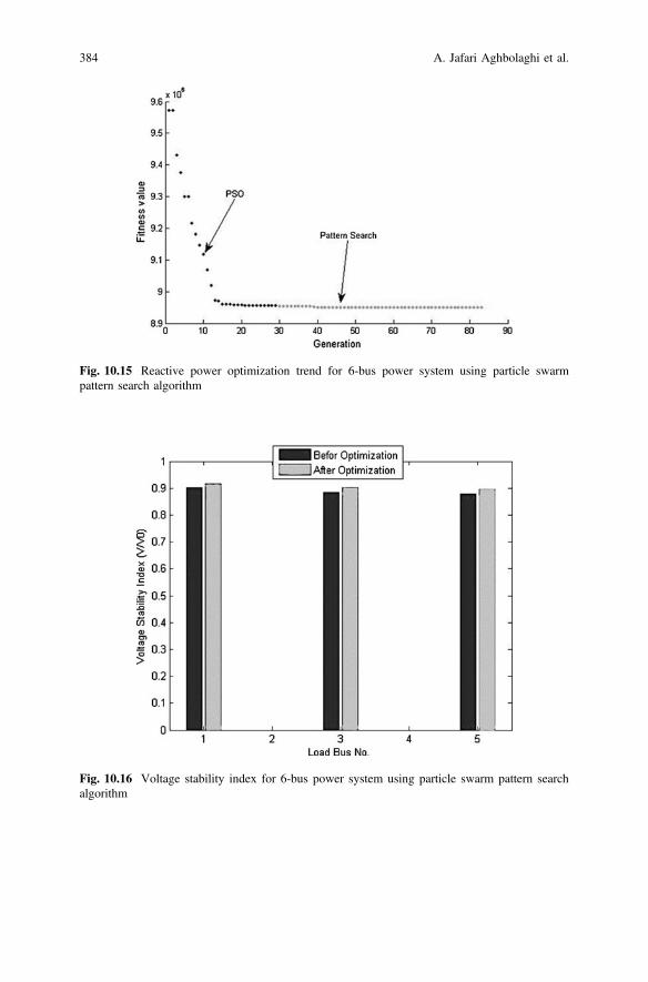
Fig. 10.15 Reactive power optimization trend for 6-bus power system using particle swarmpattern search algorithm

Fig. 10.16 Voltage stability index for 6-bus power system using particle swarm pattern searchalgorithm


10,778,370 to 8,950,232 (W). Likewise, the total value of voltage stability indexhas increased from 2.665148 to 2.715127, and the total value of voltage deviationof load buses has been reduced considerably from 15.65904 to 1.185288 kV.

Fig. 10.17 Voltage deviation for 6-bus power system using particle swarm pattern searchalgorithm

Table 10.1 Power flow results after optimization for 6-bus power system using particle swarmpattern search algorithm

Bus no. Voltage magnitudesand angles

Load consumption Injection power

V (kV) h (degree) Pl (MW) Ql (MVar) PG (MW) QG (MVar)

1 62.97 −11.69 55 13 0 0

2 72.45 −3.59 0 0 50 22.65

3 62.98 −10.97 50 5 0 5

4 63.86 −8.79 0 0 0 0

5 61.82 −11.23 0.3 18 0 5

6 69.30 0 0 0 93.96 33.13

Table 10.2 Active powerlosses for 6-bus power systemusing particle swarm patternsearch algorithm

Active power losses (initial condition) 10,778,370 (W)

Active power losses (after optimization) 8,950,232 (W)

Reduction percentage 16.96121%


10.8.1.2 Reactive Power Optimization Using Genetic Pattern Search

Algorithm

The initial conditions and power flow results for 6-bus power network are presentedin Table 10.18. In addition, the corresponding data after the optimization procedureon the same power grid are presented as below Figs. 10.18, 10.19 and 10.20.

Considering Tables 10.4, 10.5 and 10.6, a marked improvement is obvious inthe operational parameters. Active power losses have decreased from 10,778,370 to8,950,550 (W). Similarly, the total value of voltage stability index has increasedfrom 2.665148 to 2.712409, and the total value voltage deviation of load buses hasreduced from 15.65904 to 2.127879 kV.

Table 10.3 Voltage deviation and voltage stability data for 6-bus power system using particleswarm pattern search algorithm

Bus no. Voltage stability index value V/V0

ideal value = 1Voltage deviation of load buses

Initial status After optimization Initial status kV After optimization kV

1 0.9009016 0.9161407 4.881641 0.03538300

3 0.8845708 0.9021702 4.934923 0.02064700

5 0.8796755 0.8968166 5.842471 1.129258

Total 2.665148 2.715127 15.65904 1.185288

Fig. 10.18 Reactive power optimization trend for 6-bus power system using genetic patternsearch algorithm


Fig. 10.19 Voltage stability index for 6-bus power system using genetic pattern search algorithm

Fig. 10.20 Voltage deviation for 6-bus power system using genetic pattern search algorithm


10.8.2 Case Study 2—IEEE 14-Bus Power Network

The corresponding data to IEEE 14-bus power grid are accessible in Appendix 2.The results for reactive power optimization on the related network will be presentedin this section.


Search Algorithm

The initial circumstances and power flow results for 14-bus power network arepresented in Table 10.22. In addition, the corresponding data after the optimizationprocedure on the same power grid are presented as below Figs. 10.21, 10.22 and10.23.

Table 10.4 Power flow results after optimization for 6-bus power system using genetic patternsearch algorithm




1 62.96 −11.69 55 13 0 0

2 72.45 −3.59 0 0 50 22.65

3 62.98 −10.97 50 5 0 5

4 63.86 −8.79 0 0 0 0

5 61.87 −11.23 0.3 18 0 5

6 69.30 0 0 0 93.96 33.13

Table 10.5 Active powerlosses data for 6-bus powersystem using genetic patternsearch algorithm

Active power losses (initial condition) 10,778,370 (W)

Active power losses (after optimization) 8,950,550 (W)


Table 10.6 Voltage deviation and voltage stability data for 6-bus power system using geneticpattern search algorithm


Ideal value = 1Voltage deviation of load buses


1 0.9009016 0.9152744 4.881641 0.4280500

3 0.8845708 0.9011948 4.934923 0.3137400

5 0.8796755 0.8959399 5.842471 1.386089

Total 2.665148 2.712409 15.65904 2.127879


Regarding Tables 10.7, 10.8 and 10.9, active power losses have decreased from16,710,700 to 9,823,200 (W). Likewise, the total value of voltage stability indexhas increased from 8.953467 to 9.708002 and total value of voltage deviation ofload buses has reduced considerably from 219.7092 to 56.17259 kV.

Fig. 10.21 Reactive power optimization trend for 14-bus power system using particle swarmpattern search algorithm

Fig. 10.22 Voltage stability index for 14-bus power system using particle swarm pattern searchalgorithm


Table 10.7 Power flow results after optimization for 14-bus power system using particle swarmpattern search algorithm

Bus no. Voltage magnitudes andangles



1 125.376906 0 0 0 231.36 45.67

2 121.000004 −3.957964 21.7 12.7 40 16.73

3 114.908254 −10.725941 94.2 19 0 7.436791

4 116.456311 −8.576776 47.8 0 0 0

5 117.737189 −7.335156 7.6 1.6 0 0

6 116.381916 −13.008229 11.2 7.5 0 2.399997

7 114.224630 −11.632678 0 0 0 0

8 114.805564 −11.632674 0 0 0 3.129134

9 112.753677 −13.290581 29.5 16.6 0 0

10 112.559232 −13.530266 9 5.8 0 0

11 114.056146 −13.391523 3.5 1.8 0 0

12 114.573162 −13.866247 6.1 1.6 0 0

13 113.897577 −13.900069 13.5 5.8 0 0

14 111.226337 −14.602206 14.9 5 0 0

Fig. 10.23 Voltage deviation for 14-bus power system using particle swarm pattern searchalgorithm


10.8.2.2 Reactive Power Optimization Using Genetic Pattern Search

Algorithm

The initial circumstances and power flow results for 14-bus power network arepresented in Table 10.22. In addition, the corresponding data after the optimizationprocedure on the same power grid are presented as below Figs. 10.24, 10.25 and10.26.

Referring to Tables 10.10, 10.11 and 10.12, active power losses have decreasedremarkably from 16,710,700 to 9,862,619 (W). Similarly, the total value of voltagestability index increased from 8.953467 to 9.655891 and the total value of voltagedeviation of load buses has reduced considerably from 219.7092 to 57.82206 kV.

10.8.3 Case Study 3—IEEE 39-Bus New England Power

Network

The corresponding data to IEEE 39-bus New England power grid are accessible inAppendix 3. The results for reactive power optimization on the related network willbe presented in this section.

Table 10.8 Active powerlosses data for 14-bus powersystem using particle swarmpattern search algorithm

Active power losses (initial condition) 16710700 (W)

Active power losses (after optimization) 9823200 (W)


Table 10.9 Voltage deviation and voltage stability data for 14-bus power system using particleswarm pattern search algorithm




2 9.409176 0.9552817 6.499059 11

3 8.398882 0.8916201 16.96615 4.975350

4 8.563136 0.9047917 15.24372 6.534758

5 8.728775 0.9160301 13.45913 7.815445

6 7.977896 0.8778006 21.72454 6.421239

9 7.835140 0.8636542 23.25914 2.831756

10 7.761442 0.8598163 24.08241 2.630989

11 7.822556 0.8658360 23.42380 4.112191

12 7.780087 0.8651542 23.91052 4.615991

13 7.718829 0.8609605 24.58441 3.943326

14 7.538748 0.8470567 26.55627 1.291542

Total 8.953467 9.708002 219.7092 56.17259


Fig. 10.24 Reactive power optimization trend for 14-bus power system using genetic patternsearch algorithm

Fig. 10.25 Voltage stability index for 14-bus power system using genetic pattern searchalgorithm


Table 10.10 Power flow results after optimization for 14-bus power system using genetic patternsearch algorithm




1 125.803591 0 0 0 231.42 58.56

2 120.793094 −3.853065 21.7 12.7 40 −0.15

3 115.351591 −10.701274 94.2 19 0 12.74691

4 116.493973 −8.503816 47.8 0 0 0

5 117.785497 −7.265805 7.6 1.6 0 0

6 116.251125 −12.931138 11.2 7.5 0 23.72837

7 114.143428 −11.564184 0 0 0 0

8 114.561700 −11.564181 0 0 0 2.373186

9 112.686674 −13.225312 29.5 16.6 0 0

10 112.480325 −13.463648 9 5.8 0 0

11 113.951417 −13.320288 3.5 1.8 0 0

12 114.445424 −13.791402 6.1 1.6 0 0

13 113.773793 −13.826640 13.5 5.8 0 0

14 111.132858 −14.535142 14.9 5 0 0

Fig. 10.26 Voltage deviation for 14-bus power system using genetic pattern search algorithm



Search Algorithm

The initial circumstances and power flow results for 39-bus New England powernetwork are presented in Table 10.13. In addition, the corresponding data after theoptimization procedure on the same power grid are presented as below Fig. 10.27.

One of the best criteria that can be taken into consideration as the calculationcost is Number of Function Evaluation (NFE) when it comes to comparing theperformance of two or more intelligent algorithms, especially the ones which do notuse the gradient of objective functions but the function itself. As it can be inferredfrom the name, each time the algorithm refers to the objective function to work itsvalue out the amount of NFE increases by one. Eventually, the best optimum pointfound by every algorithm can be compared to one another in relation to their NFE.In addition, NFE itself can be considered as a stopping criterion as well based onthe requirements of the corresponding study.

As mentioned before, one of the benefits of using MATLAB and DIgSILENTtogether is to take the advantages of built-in toolboxes and functions in both. Afterthe optimization procedure small signal analysis (Eigenvalue or Modal Analysis)has been carried out for the grid in PowerFactory without experiencing

Table 10.11 Active powerlosses data for 14-bus powersystem using genetic patternsearch algorithm

Active power losses (Initial condition) 16710700 (W)

Active power losses (After optimization) 9862619 (W)


Table 10.12 Voltage deviation and voltage stability data for 14-bus power system using geneticpattern search algorithm




2 9.409176 0.9476370 6.499059 10.59916

3 8.398882 0.8850283 16.96615 4.580411

4 8.563136 0.8994890 15.24372 6.543957

5 8.728775 0.9111127 13.45913 7.844678

6 7.977896 0.8734883 21.72454 6.543719

9 7.835140 0.8599726 23.25914 3.448204

10 7.761442 0.8561004 24.08241 3.164167

11 7.822556 0.8618414 23.42380 4.445315

12 7.780087 0.8609751 23.91052 4.777684

13 7.718829 0.8568609 24.58441 4.141013

14 7.538748 0.8433849 26.55627 1.733747

Total 8.953467 9.655891 219.7092 57.82206


programming difficulties and the result has been shown in Fig. 10.28. The stepshow to calculate eigenvalues has been presented in Chap. 11.

According to Tables 10.14, 10.15 and 10.16, active power losses have decreasedfrom 28,194,720 to 26,266,740 (W) via adjusting the terminal voltages of

Fig. 10.27 Reactive power optimization trend for 39-bus New England power system usingparticle swarm pattern search algorithm

Fig. 10.28 Eigenvalues of 39-bus New England power system without power system stabilizersafter optimization


http://dx.doi.org/10.1007/978-3-319-51118-4_11

Table 10.13 Active power losses data of IEEE 39-bus New England power system using particleswarm pattern search algorithm

Bus name Voltage magnitudes p.u. Voltage angles deg. Generators

P (MW) Q (Mvar)

Bus01 1.0474 −8.44 – –

Bus02 1.0487 −5.75 – –

Bus03 1.0302 −8.60 – –

Bus04 1.0039 −9.61 – –

Bus05 1.0053 −8.61 – –

Bus06 1.0077 −7.95 – –

Bus07 0.9970 −10.12 – –

Bus08 0.9960 −10.62 – –

Bus09 1.0282 −10.32 – –

Bus10 1.0172 −5.43 – –

Bus11 1.0127 −6.28 – –

Bus12 1.0002 −6.24 – –

Bus13 1.0143 −6.10 – –

Bus14 1.0117 −7.66 – –

Bus15 1.0154 −7.74 – –

Bus16 1.0318 −6.19 – –

Bus17 1.0336 −7.30 – –

Bus18 1.0309 −8.22 – –

Bus19 1.0499 −1.02 – –

Bus20 0.9912 −2.01 – –

Bus21 1.0318 −3.78 – –

Bus22 1.0498 0.67 – –

Bus23 1.0448 0.47 – –

Bus24 1.0373 −6.07 – –

Bus25 1.0576 −4.36 – –

Bus26 1.0521 −5.53 – –

Bus27 1.0377 −7.50 – –

Bus28 1.0501 −2.01 – –

Bus29 1.0499 0.74 – –

Bus30 1.0475 −3.33 250.00 146.16

Bus31 0.9820 0.00 520.81 198.25

Bus32 0.9831 2.57 650.00 205.14

Bus33 0.9972 4.19 632.00 109.91

Bus34 1.0123 3.17 508.00 165.76

Bus35 1.0493 5.63 650.00 212.41

Bus36 1.0635 8.32 560.00 101.18

Bus37 1.0278 2.42 540.00 0.44

Bus38 1.0265 7.81 830.00 22.84

Bus39 1.0300 −10.05 1000.00 88.28


Table 10.15 The tap setting of transformers of IEEE 39-bus New England power system afteroptimization



V (kV) h (degree) Pl

(MW)Ql

(Mvar)PG (MW) QG (Mvar)

1 364.810659 −6.452421 – – – –

2 370.798179 −3.981883 – – – –

3 372.902266 −6.776672 322.0 2.4 – –

4 374.141517 −7.781993 500.0 184.0 – –

5 374.772457 −6.949538 – – – –

6 375.577162 −6.385371 – – – –

7 372.536129 −8.253005 233.8 84.0 – –

8 371.586660 −8.667435 522.0 176.0 – –

9 366.270135 −8.296282 – – – –

10 377.511546 −4.188488 – – – –

11 376.869300 −4.942417 – – – –

12 150.734523 −4.933962 7.5 88.0 – –

13 377.168446 −4.770793 – – – –

14 376.168387 −6.099718 – – – –

15 375.663420 −6.121481 320.0 153.0 – –

16 376.505858 −4.680447 329.0 32.3 – –

17 375.344286 −5.652905 – – – –

18 374.016041 −6.467971 158.0 30.0 – –

19 379.190499 0.018998 – – – –

20 237.505552 −0.769076 628.0 103.0 – –

21 375.538973 −2.509637 274.0 115.0 – –

22 378.827835 1.548230 – – – –

23 377.526406 1.366011 247.5 84.6 – –

24 377.641053 −4.568311 308.6 −92.2 – –

25 375.556902 −2.870753 224.0 47.2 – –

26 376.153057 −3.965808 139.0 17.0 – –

27 374.094746 −5.811787 281.0 75.5 – –

28 371.978374 −0.616475 206.0 27.6 – –

29 370.455789 2.031981 283.5 26.9 – –

30 17.130497 −1.599642 – – 250.0 −54.17687004

(continued)

Table 10.14 Power flow results after optimization for 39-bus New England power system usingparticle swarm pattern search algorithm

Active power losses (Initial condition) 28194720 (W)

Active power losses (After optimization) 26266740 (W)



generators and the tap settings of transformers considering the voltage limitationsfor all the busbars.

10.9 Summary

Investigating active power losses caused in transmission system is of crucialimportance in designing power systems as well as their operation and development,of which so many methods have been carried out practically on. Plenty ofapproaches have been recommended in order to decrease active power losses in




V (kV) h (degree) Pl

(MW)Ql

(Mvar)PG (MW) QG (Mvar)

31 17.926045 0.000000 9.2 4.6 517.55180622 179.62643204

32 17.584661 2.436932 – – 650.0 82.93753618

33 17.681268 4.575524 – – 632.0 328.35318619

34 16.557073 4.375941 – – 508.0 −164.8434324

35 17.899414 6.135797 – – 650.0 128.77506507

36 18.144109 8.626973 – – 560.0 46.86633642

37 17.536826 3.495544 – – 540.0 19.78359724

38 17.563459 8.560209 – – 830.0 −58.73820034

39 355.349990 −7.996433 1104.0 250.0 1000 −332.33380789

Table 10.16 The data for transmission lines and transformers of IEEE 6-bus standard powersystem

From bus To bus Transformers tap magnitude (p.u.) Transformers tap tap position

12 11 1.0000 0

12 13 1.0000 0

6 31 1.0350 1

10 32 1.0350 1

19 33 1.0700 2

20 34 1.0000 0

22 35 1.0250 1

23 36 1.0000 –

25 37 1.0250 1

2 30 1.0250 1

29 38 1.0000 0

19 20 1.0300 1


power grid in which reactive power optimization is one of the most influential ones.Reactive power optimization investigates the operational condition of reactivepower sources in AC power systems in order to have a minimum reactive powercurrent flowing in transmission systems to lessen active power losses associatedwith it. There are three main parameters on which power system operators havecontrol, as the voltage magnitude of PV busbars, reactive power output of com-pensators and tap setting of transformers which have under-load tap changerfacility. It seems quite obvious that the number of controlling parameters can be somany in a real power network so as there are eight dimensions in a 14-bus powergrid. In addition, since there is a tough association between plenty of parameters inelectric power systems, reactive power optimization is a very nonlinear and non-convex problem comprising discrete and continuous variables simultaneously,which has a lot of local optimum points so that traditional optimization algorithms,most of which are based on the gradient of objective function, lose theirperformance.

Heuristic optimization methods have proven their performance in such complexoptimization problems and it will be efficient to be able to use them in reactivepower optimization problem as well. Two heuristic algorithms in combination withdirect search optimization methods have been applied to three standard power gridsand the results have been presented. Genetic and particle swarm optimizationalgorithms are great methods in terms of global optimization, whereas patternsearch optimization method is remarkable in the respect of local optimization.Therefore, using a combination of a global optimizer and a local one will have somany benefits in its favor. There are plenty of articles, book chapters, books etc. inthis respect so that each ones’ advantages can be taken.

This chapter tries to focus on the fundamentals and implementation of reactivepower optimization problem using MATLAB and DIgSILENT and creating aneffectual link between them. It will avail engineers of using the professional tools ofPowerFactory DIgSILENT in the respect of electrical engineering as stabilityanalysis, power flow calculations etc. Besides, MATLAB also has got a lot oftoolboxes and flexibility while optimizing problems, using artificial intelligence.The method has been presented for a simple standard power grid step by step usingparticle swarm pattern search algorithm in Chap. 11, while both MATLAB andDIgSILENT files for both approaches have been presented in book attachment asparticle swarm pattern search and genetic pattern search for IEEE 6- and 14-buspower grids. In addition, reactive power optimization using built-in particle swarmand pattern search algorithm on IEEE 39-bus New England power system has beendepicted in Chap. 11.


http://dx.doi.org/10.1007/978-3-319-51118-4_11

http://dx.doi.org/10.1007/978-3-319-51118-4_11

Appendices

Appendix 1: IEEE 6-Bus Standard Power System

The single-line diagram of IEEE 6-bus power network has been presented inFig. 10.29 and the corresponding data are given in Tables 10.17, 10.18 and 10.19.

Appendix 2: IEEE 14-Bus Standard Power System

The single-line diagram of IEEE 14-bus power network has been presented inFig. 10.30 and the corresponding data are given in Tables 10.20, 10.21 and 10.22.

G 1.05 0

GP = 50 MW

V = 1.1

1:0.91

1:0.9725

P = 30 MW

Q = 18 MVAR

P = 50 MW

Q = 5 MVAR

P = 55 MW

Q = 13 MVAR

Q = 5 MVAR

Q = 5 MVAR

Bus 6

Bus 3 Bus 2

Bus 4

Bus 5

Bus 1

Fig. 10.29 Single-line diagram of IEEE 6-bus standard power system

Table 10.17 The corresponding limitations for control and state variables of IEEE 6-bus standardpower system

Lineno.

Startingbusbar

Endingbusbar

Line impedances Line admittances Transformer tapsettingsR (X) X (X) G (S) B (S)

1 6 3 4.88187 20.55942 0.0109 −0.0460 –

2 6 4 3.1752 14.6853 0.0141 −0.0651 –

3 4 3 3.84993 16.15383 0.0140 −0.0586 –

4 5 2 11.19258 25.4016 0.0145 −0.0330 –

5 2 1 28.69587 41.6745 0.0112 −0.0163 –

6 3 5 0 11.907 0 −0.0840 0.9725

7 4 1 0 5.27877 0 −0.1894 0.9100


Table 10.18 Initial statues and power flow results for IEEE 6-bus standard power system

Transformer tapsettings

Voltagemagnitudesof PVbusbars

Outputcapacityofreactivepowersources

Load bus voltagemagnitudes

Reactive power output ofPV busbars

T35, T41 V6 V2 Q3 Q4 V1, V3, V5 Q2, Q6

Min 0.910 63 69.3 0.0 0.0 56.7 −20

Max 1.110 69.3 72.45 5.0 5.0 69.3 100

Table 10.19 The data for transmission lines and transformers of IEEE 14-bus standard power system




1 58.12 −13.24 55 13 0 0

2 69.3 −4.78 0 0 50 27.63

3 58.07 −12.44 50 5 0 0

4 59.11 −9.85 0 0 0 0

5 57.16 −12.87 0.3 18 0 0

6 66.15 0 0 0 95.79 44.37

Fig. 10.30 Single-line diagram of IEEE 14-bus standard power system


Table

10.20

Thecorrespondinglimitationsto

controlvariablesofIEEE14-busstandardpower

system

Lineno.

Startingbusbar

Endingbusbar

Lineim

pedances

Lineadmittances

Linecapacitances

Transform

ertapsettings

R(X

)X(X

)G

(S)

B(S)

C(F)

11

22.34498

7.15957

0.041315

−0.12614

4.3636e–4

–

21

56.53763

26.98784

0.0085

−0.0350

4.066e–4

–

32

35.68579

23.95437

0.0094

−0.0395

3.61983e–4

–

42

47.03131

21.33472

0.0139

−0.0423

3.0909e–4

–

52

56.89095

21.03948

0.0141

−0.0429

2.80991e–4

–

63

48.10821

20.69463

0.0164

−0.0419

2.8595e–4

–

74

51.61535

5.09531

0.0565

−0.1783

1.05785e–4

–

84

70

25.30352

0−0.0395

00.978

94

90

67.29778

0−0.0149

00.969

10

56

030.49442

0−0.0328

00.932

11

611

11.49258

24.0669

0.0162

−0.0338

0–

12

612

14.87211

30.95301

0.0126

−0.0262

0–

13

613

8.00415

15.76267

0.0256

−0.0504

0–

14

78

021.31415

0−0.0469

0–

15

79

013.31121

0−0.0751

0–

16

910

3.84901

10.2245

0.0322

−0.0857

0–

17

914

15.38031

32.71598

0.0118

−0.0250

0–

18

10

11

9.92805

23.24047

0.0155

−0.0364

0–

19

12

13

26.73132

24.18548

0.0206

−0.0186

0–

20

13

14

20.68253

42.11042

0.0094

−0.0191

0–


Appendix 3: IEEE 39-Bus New England Power System

The Single-line diagram of IEEE 39-bus New England power system has beenshown in Fig. 10.31 and the corresponding data are given in Tables 10.23, 10.24,10.25, 10.26, 10.27 and 10.28. The nominal frequency of the New Englandtransmission system is 60 Hz and the main voltage level is 345 kV (nominalvoltage). For nodes at a different voltage level, following nominal voltages havebeen assumed for the PowerFactory model: Bus 12–138 kV, Bus 20–230 kV, Bus30 and Bus 38–16.5 kV [13].

Table 10.21 Initial statuesand power flow results forIEEE 14-bus standard powersystem

Transformertap settings

Voltagemagnitudesof PVbusbars

Output capacityof reactive powersources

T47, T49, T56 V1 V2 Q3 Q6 Q8

Min 0.910 110 110 0.0 −6 −6

Max 1.110 126.5 121 40 24 24

Table 10.22 Data of lines of IEEE 39-bus New England power system (100 MVA, 60 Hz) [13]

Bus no. Voltagemagnitudes andangles


V (kV) h (°) Pl (MW) Ql (MVar) PG (MW) QG (MVar)

1 110 0 0 0 242.05 102.32

2 102.39 −6.54 21.7 12.7 40 50

3 91.83 −16.11 94.2 19 0 0

4 93.67 −12.60 47.8 0 0 0

5 95.53 −10.60 7.6 1.6 0 0

6 87.10 −19.66 11.2 7.5 0 0

7 88.14 −17.72 0 0 0 0

8 88.14 −17.72 0 0 0 0

9 85.51 −20.66 29.5 16.6 0 0

10 84.68 −21.02 9 5.8 0 0

11 85.36 −20.58 3.5 1.8 0 0

12 84.88 −21.21 6.1 1.6 0 0

13 84.19 −21.35 13.5 5.8 0 0

14 82.17 −22.85 14.9 5 0 0


Fig. 10.31 Single-line diagram of IEEE 39-bus New England power system [13]

Table 10.23 Load demands of IEEE 39-bus New England power system [13]

Line From bus To bus R in p.u. X in p.u. B in p.u.

Line 01–02 Bus 01 Bus 02 0.0035 0.0411 0.6987

Line 01–39 Bus 01 Bus 39 0.0010 0.0250 0.7500

Line 02–03 Bus 02 Bus 03 0.0013 0.0151 0.2572

Line 02–25 Bus 02 Bus 25 0.0070 0.0086 0.1460

Line 03–04 Bus 03 Bus 04 0.0013 0.0213 0.2214

Line 03–18 Bus 03 Bus 18 0.0011 0.0133 0.2138

Line 04–05 Bus 04 Bus 05 0.0008 0.0128 0.1342

Line 04–14 Bus 04 Bus 14 0.0008 0.0129 0.1382

Line 05–06 Bus 05 Bus 06 0.0002 0.0026 0.0434

Line 05–08 Bus 05 Bus 08 0.0008 0.0112 0.1476

Line 06–07 Bus 06 Bus 07 0.0006 0.0092 0.1130

Line 06–11 Bus 06 Bus 11 0.0007 0.0082 0.1389

Line 07–08 Bus 07 Bus 08 0.0004 0.0046 0.0780

Line 08–09 Bus 08 Bus 09 0.0023 0.0363 0.3804

Line 09–39 Bus 09 Bus 39 0.0010 0.0250 1.2000

Line 10–11 Bus 10 Bus 11 0.0004 0.0043 0.0729

Line 10–13 Bus 10 Bus 13 0.0004 0.0043 0.0729

Line 13–14 Bus 13 Bus 14 0.0009 0.0101 0.1723

(continued)



Line From bus To bus R in p.u. X in p.u. B in p.u.

Line 14–15 Bus 14 Bus 15 0.0018 0.0217 0.3660

Line 15–16 Bus 15 Bus 16 0.0009 0.0094 0.1710

Line 16–17 Bus 16 Bus 17 0.0007 0.0089 0.1342

Line 16–19 Bus 16 Bus 19 0.0016 0.0195 0.3040

Line 16–21 Bus 16 Bus 21 0.0008 0.0135 0.2548

Line 16–24 Bus 16 Bus 24 0.0003 0.0059 0.0680

Line 17–18 Bus 17 Bus 18 0.0007 0.0082 0.1319

Line 17–27 Bus 17 Bus 27 0.0013 0.0173 0.3216

Line 21–22 Bus 21 Bus 22 0.0008 0.0140 0.2565

Line 22–23 Bus 22 Bus 23 0.0006 0.0096 0.1846

Line 23–24 Bus 23 Bus 24 0.0022 0.0350 0.3610

Line 25–26 Bus 25 Bus 26 0.0032 0.0323 0.5130

Line 26–27 Bus 26 Bus 27 0.0014 0.0147 0.2396

Line 26–28 Bus 26 Bus 28 0.0043 0.0474 0.7802

Line 26–29 Bus 26 Bus 29 0.0057 0.0625 1.0290

Line 28–29 Bus 28 Bus 29 0.0014 0.0151 0.2490

Table 10.24 Generatordispatch of IEEE 39-bus NewEngland power system [13]

No. Load Bus P (MW) Q (Mvar)

1 Load 03 Bus 03 322.0 2.4

2 Load 04 Bus 04 500.0 184.0

3 Load 07 Bus 07 233.8 84.0

4 Load 08 Bus 08 522.0 176.0

5 Load 12 Bus 12 7.5 88.0

6 Load 15 Bus 15 320.0 153.0

7 Load 16 Bus 16 329.0 32.3

8 Load 18 Bus 18 158.0 30.0

9 Load 20 Bus 20 628.0 103.0

10 Load 21 Bus 21 274.0 115.0

11 Load 23 Bus 23 247.5 84.6

12 Load 24 Bus 24 308.6 −92.2

13 Load 25 Bus 25 224.0 47.2

14 Load 26 Bus 26 139.0 17.0

15 Load 27 Bus 27 281.0 75.5

16 Load 28 Bus 28 206.0 27.6

17 Load 29 Bus 29 283.5 26.9

18 Load 31 Bus 31 9.2 4.6

19 Load 39 Bus 39 1104.0 250.0


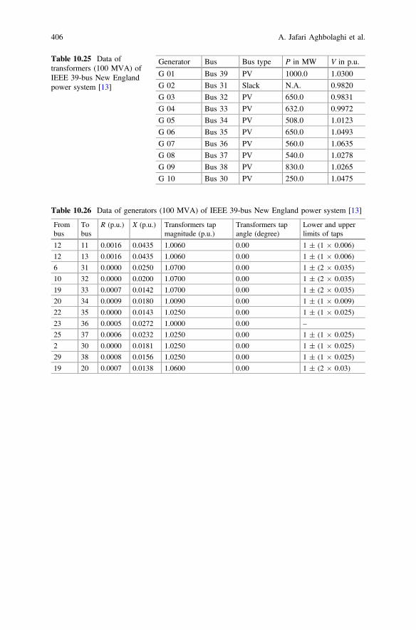
Table 10.25 Data oftransformers (100 MVA) ofIEEE 39-bus New Englandpower system [13]

Generator Bus Bus type P in MW V in p.u.

G 01 Bus 39 PV 1000.0 1.0300

G 02 Bus 31 Slack N.A. 0.9820

G 03 Bus 32 PV 650.0 0.9831

G 04 Bus 33 PV 632.0 0.9972

G 05 Bus 34 PV 508.0 1.0123

G 06 Bus 35 PV 650.0 1.0493

G 07 Bus 36 PV 560.0 1.0635

G 08 Bus 37 PV 540.0 1.0278

G 09 Bus 38 PV 830.0 1.0265

G 10 Bus 30 PV 250.0 1.0475

Table 10.26 Data of generators (100 MVA) of IEEE 39-bus New England power system [13]

Frombus

Tobus

R (p.u.) X (p.u.) Transformers tapmagnitude (p.u.)

Transformers tapangle (degree)

Lower and upperlimits of taps

12 11 0.0016 0.0435 1.0060 0.00 1 ± (1 � 0.006)

12 13 0.0016 0.0435 1.0060 0.00 1 ± (1 � 0.006)

6 31 0.0000 0.0250 1.0700 0.00 1 ± (2 � 0.035)

10 32 0.0000 0.0200 1.0700 0.00 1 ± (2 � 0.035)

19 33 0.0007 0.0142 1.0700 0.00 1 ± (2 � 0.035)

20 34 0.0009 0.0180 1.0090 0.00 1 ± (1 � 0.009)

22 35 0.0000 0.0143 1.0250 0.00 1 ± (1 � 0.025)

23 36 0.0005 0.0272 1.0000 0.00 –

25 37 0.0006 0.0232 1.0250 0.00 1 ± (1 � 0.025)

2 30 0.0000 0.0181 1.0250 0.00 1 ± (1 � 0.025)

29 38 0.0008 0.0156 1.0250 0.00 1 ± (1 � 0.025)

19 20 0.0007 0.0138 1.0600 0.00 1 ± (2 � 0.03)


Table

10.27

DataofAVRsofIEEE39-busNew

Englandpower

system

[13]

Unitno.

H(s)

Ra(p.u.)

x’d(p.u.)

x’q(p.u.)

x d(p.u.)

x q(p.u.)

Tʹ d0(s)

Tʹ q0(s)

x l(p.u.)

x″(p.u.)

T″d0(s)

T″q0(s)

1500.0

0.0000

0.0060

0.0080

0.0200

0.0190

7.000

0.700

0.0030

0.0040

0.050

0.035

230.3

0.0000

0.0697

0.1700

0.2950

0.2820

6.560

1.5000

0.0350

0.0500

0.050

0.035

335.8

0.0000

0.0531

0.0876

0.2495

0.2370

5.700

1.5000

0.0304

0.0450

0.050

0.035

428.6

0.0000

0.0436

0.1660

0.2620

0.2580

5.690

1.5000

0.0295

0.0350

0.050

0.035

526.0

0.0000

0.1320

0.1660

0.6700

0.6200

5.400

0.4400

0.0540

0.0890

0.050

0.035

634.8

0.0000

0.0500

0.0814

0.2540

0.2410

7.300

0.4000

0.0224

0.0400

0.050

0.035

726.4

0.0000

0.0490

0.1860

0.2950

0.2920

5.660

1.5000

0.0322

0.0440

0.050

0.035

824.3

0.0000

0.0570

0.0911

0.2900

0.2800

6.700

0.4100

0.0280

0.0450

0.050

0.035

934.5

0.0000

0.0570

0.0587

0.2106

0.2050

4.790

1.9600

0.0298

0.0450

0.050

0.035

10

42.0

0.0000

0.0310

0.0500

0.1000

0.0690

10.200

0.0000

0.0125

0.0250

0.050

0.035


Table

10.28

Initialstatues

andpowerflow

resultsforIEEE39-busNew

Englandpower

system

[13]

Unitno.

Ka=KA

Ta=TA

Vrm

in=VRmin

Vrm

ax=VRmax

Ke=KE

Te=TE

Kf=KF

Tf=TF

Se1=C1

Se2=C2

E1=EX1

E2=EX2

26.2

0.05

−1.0

1.0

−0.6330

0.405

0.0570

0.500

0.660

0.880

3.036437

4.048583

35.0

0.06

−1.0

1.0

−0.0198

0.500

0.0800

1.000

0.130

0.340

2.342286

3.123048

45.0

0.06

−1.0

1.0

−0.0525

0.500

0.0800

1.000

0.080

0.314

2.868069

3.824092

540.0

0.02

−10.0

10.0

1.0000

0.785

0.0300

1.000

0.070

0.910

3.926702

5.235602

65.0

0.02

−1.0

1.0

−0.0419

0.471

0.0754

1.246

0.064

0.251

3.586801

4.782401

740.0

0.02

−6.5

6.5

1.0000

0.730

0.0300

1.000

0.530

0.740

2.801724

3.735632

85.0

0.02

−1.0

1.0

−0.0470

0.528

0.0854

1.260

0.072

0.282

3.191489

4.255319

940.0

0.02

−10.5

10.5

1.0000

1.400

0.0300

1.000

0.620

0.850

4.256757

5.675676

10

5.0

0.06

−1.0

1.0

−0.0485

0.250

0.0400

1.000

0.080

0.260

3.546099

4.728132


References

1. S.R. Singiresu, Engineering Optimization - Theory and Practice, Hoboken, New Jersey: JohnWiley & Sons, Inc., 2009.

2. J. Zhu, Reactive Power Optimization, in Optimization of Power System Operation, NewJersey, John Wiley & Sons, pp. 409–454, 2009.

3. T.J. Miller, Reactive Power Coordination, in Reactive Power Control in Electric Systems,New York, John Wiley & Sons, pp. 353–363, 1982.

4. P. Kundur, Power System Stability and Control, New York: McGraw-Hill, 1994.5. J. Machowski, J.W. Bialek, J.R. Bumby, Power System Dynamics, John Wiley & Sons, 2008.6. H. Saadat, Power System Analysis, New York: McGraw-Hill, 1999.7. X. Hugang, C. Haozhong, L. Haiyu, Optimal Reactive Power Flow Incorporating Static

Voltage Stability Based on Multi-Objective Adaptive Immune Algorithm, Energy Conversionand Management, vol. 49, pp. 1175–1181, 2008.

8. T. Niknam, M.R. Narimani, R. Azizipanah Abarghooee, B. Bahmani Firouzi, Multi-ObjectiveOptimal Reactive Power Dispatch and Voltage Control: A New Opposition-BasedSelf-Adaptive Modified Gravitational Search Algorithm, IEEE Systems Journal, vol. 7,pp. 742–753, 2013.

9. S.A.H. Soliman, H.A.A. Mantawy, Modern Optimization Techniques with Applications inElectric Power Systems, New York Heidelberg Dordrecht London: Springer, 2012.

10. A.I.F. Vaz, L. Vicente, A Particle Swarm Pattern Search Method for Bound ConstrainedGlobal Optimization, Department of Production and Systems, School of Engineering,University of Minho, Campus of Gualtar, Braga, Portugal, 2006.

11. Wikipedia, the Free Encyclopedia, https://en.wikipedia.org/wiki/Pattern_search_(optimization).

12. M.A. Abramson, C. Audet, J. Dennis, Generalized Pattern Search Algorithms - Unconstrainedand Constrained Cases, IMA Workshop - Optimization in Simulation Based Models.

13. DIgSILENT PowerFactory Version 15 User Manual, Gomaringen, Germany: DIgSILENTGmbH, 2014.


https://en.wikipedia.org/wiki/Pattern_search_

Chapter 11

Reactive Power Optimization

Using MATLAB and DIgSILENT

Naser Mahdavi Tabatabaei, Ali Jafari Aghbolaghi,


Abstract There are plenty of methods to implement reactive power optimization,

such as coding in MATLAB on its own or DIgSILENT, both of which are powerful

pieces of software in the electrical engineering respect. However, on one hand

MATLAB has a lot of toolboxes, functions, flexibility etc. when it comes to be used

in implementation of artificial intelligence and heuristic algorithms. On the other

hand, DIgSILENT is such a powerful tool while studying power network stability,

power flow calculations, ready-to-use equipment blocks etc., which provides

operators with the simplicity of carrying out their studies. Therefore, it would be

very efficient to be available of using both pieces of software in parallel in order to

take each one’s advantages. In this method, calculations related to power network

are executed in DIgSILENT, the ones related to heuristic algorithms are carried out

in MATLAB. Although both of them are able to put the whole procedure into

practice solely, the point is to take the redeeming features of both to do the process

as fast, simple, accurate as possible.

N. Mahdavi Tabatabaei (&)

Electrical Engineering Department, Seraj Higher Education Institute, Tabriz, Iran


A. Jafari Aghbolaghi � F. Hojjati ParastAndishmand Shomal Gharb Engineering Consultancy, Zanjan, Iran


F. Hojjati Parast


N.S. Boushehri

Department of Management, Taba Elm International Institute, Tabriz, Iran



N. Mahdavi Tabatabaei et al. (eds.), Reactive Power Control in AC Power Systems,Power Systems, DOI 10.1007/978-3-319-51118-4_11

411

11.1 Introduction

There are plenty of methods to implement reactive power optimization, such as

coding in MATLAB on its own or DIgSILENT, both of which are powerful pieces

of software in the electrical engineering respect. However, on one hand MATLAB

has a lot of toolboxes, functions, flexibility etc. when it comes to be used in

implementation of artificial intelligence and heuristic algorithms. On the other hand,

DIgSILENT is such a powerful tool while studying power network stability, power

flow calculations, ready-to-use equipment blocks etc., which provides operators

with the simplicity of carrying out their studies. Therefore, it would be very efficient

to be available of using both pieces of software in parallel in order to take each

one’s advantages. In this method, calculations related to power network are exe-

cuted in DIgSILENT, the ones related to heuristic algorithms are carried out in

MATLAB. Although both of them are able to put the whole procedure into practice

solely, the point is to take the redeeming features of both to do the process as fast,

simple, accurate as possible.

The reason why it is beneficial to employ MATLAB and DIgSILENT both

together to optimize reactive power in AC power systems is to simplify some basic

approaches which should be done, although they are not the very case on which

need to be concentrated. Therefore, using some ready-to-use tools and techniques

will avail researchers of skipping the affairs that do not need to be spent much time

on. For instance, in the reactive power optimization problem power flow calcula-

tions, stability analysis, modelling equipment etc. are not inevitable to use, whereas

they are readily accessible without programming difficulties in DIgSILENT soft-

ware. Thus, avoiding some routine and basic affairs, researchers could focus their

energy on the further studies. This section will present an efficient approach using

both MATLAB and DIgSILENT software in order to put reactive power opti-

mization into practice so that both pieces of software will work in parallel until the

optimum point has been found.

11.2 How to Implement Reactive Power Optimization

Using MATLAB and DIgSILENT

The theoretical aspect of reactive power optimization has been presented elabo-

rately in Chap. 10. In this section, DIgSILENT will do power flow calculations and

other processes related to optimization procedure will be carried out by MATLAB.

One of the best ways to couple MATLAB and DIgSILENT is to use text files to

exporting data, importing data and also to issue orders to the both applications. It

should be noted that it is assumed the reader has an intermediate level of knowledge

of using DIgSILENT and MATLAB.

412 N. Mahdavi Tabatabaei et al.

http://dx.doi.org/10.1007/978-3-319-51118-4_10

Having traced the power network in DIgSILENT and coded the optimization

algorithm in MATLAB, the general procedure of reactive power optimization

coupling DIgSILENT and MATLAB will be as follows:

1. At the beginning, control variables are initiated by optimization algorithm

within feasible bounds and then are written in a text file named “ToDIg.txt”,

while DIgSILENT is already waiting to a command from MATLAB to do the

power flow calculations.

2. MATLAB sends a command to run the power flow to DIgSILENT via a text file

named “Couple.txt”, which contains either “0” or “1” as stop or start order

and/or “2” noting end of the procedure (completely stop DIgSILENT). Since the

commands will be commuted between DIgSILENT and MATLAB steadily in a

text file as “Couple.txt”, if “0” is stop command to DIgSILENT, it is start

command to MATLAB and/or vice versa. In this chapter, 1 is used to start

DIgSILENT and 0 to stop it.

3. After getting run command, DIgSILENT reads the new control variables created

and written by MATLAB into “ToDIg.txt” and applies them to the power

network and implements power flow calculations. After finishing power flow,

DIgSILENT writes new state values as voltage magnitudes and angles of all

busbars into another text file named “LoadFlow.txt”. Then it writes “0” in

“Couple.txt” to send an order as to start MATLAB to continue the procedure.

4. MATLAB starts to calculate and investigate the fitness function. If the stopping

criteria have been reached, the optimization procedure gets over and the best

coordinates found so far will be chosen as the best values for the control

variables, if not, the optimization algorithm produces new set of control vari-

ables and writes in “ToDIg.txt” to send to DIgSILENT. Then the procedure

continues from step 2 again.

The simple flowchart of above-presented approach has been shown in Fig. 11.1

to elaborate the trend. It will be presented step by step in the next section as

elaborate as possible considering the fact that reader has intermediate level of

knowledge using MATLAB and DIgSILENT.

Hence, optimizing reactive power in order to reduce active power losses in AC

power systems based on the approach presented in this chapter has two different

stages. One is preparing a power network in DIgSILENT software and the other is

coding the optimization algorithm in MATLAB software, both of which will be

explained step by step in the next phases of the chapter.

11.2.1 First Step—Tracing a 6-Bus IEEE Standard Power

Network in DIgSILENT

The first step toward putting reactive power optimization into practice using

MATLAB and DIgSILENT is to have a network ready in DIgSILENT to apply the

11 Reactive Power Optimization Using MATLAB and DIgSILENT 413

optimization algorithm on. The IEEE 6-bus standard system given in the appen-

dices section of Chap. 10 is used in order to elaborate the approach. The power grid

has already traced for you and the corresponding file has been presented in the book

attachments, although a brief explanation how to create a project is presented. The

base values are considered as follows:

Initialize control variables

using intelligent algorithms in

MATLAB

Send run signal to

DIgSILENT (“Couple.txt”)

Write information in a txt file

in a specified location to send

to DIgSILENT (“ToDIg.txt”)

Is stopping criterion

satisfied?

Run Power flow using

DIgSILENT and write state

values to (“LoadFlow.txt”)

Apply the operators of

optimization algorithm to the

control variablesSend run signal to MATLAB

(“Couple.txt”)

Calculate fitness function

using state values which are

obtained from power flow

calculations

Yes

No

Start

Stop

Fig. 11.1 The flowchart of

reactive power optimization

using DIgSILENT and

MATLAB


http://dx.doi.org/10.1007/978-3-319-51118-4_10

Vbase ¼ 63 kV ð11:1Þ

Sbase ¼ 100 MVA ð11:2Þ

11.2.1.1 Creating a New Project in DIgSILENT

To build a new project, the instruction below should be followed:

Open DIgSILENT software, go to File Menu ! New ! Project (Fig. 11.2),

then enter the project name in the matching field (Fig. 11.3), then leave all other

settings as default and click on OK. Start tracing the 6-bus power grid (Fig. 11.4)

with the given data in appendices section of Chap. 10 (use the software’s user

manual for more information).

Figure 11.5 shows the 6-bus power grid after being traced in DIgSILENT, its file

has been presented in the book attachments as well and it can be imported to the

software in order to avoid drawing it again. After tracing the basic network, there

are some extra steps which should be done.

11.2.1.2 How to Enter Operational Limitations of Generators

To enter operational limitations of generators, double click on bus-6 generator

(Fig. 11.6) ! go to “Load Flow” tab and tick “Use Limits Specified in Type” in

Reactive Power Operational Limits section (Fig. 11.7). Then go to “Basic Data”

tab ! “Right Arrow” in front of Type (Fig. 11.8), then enter the values of Nominal

Fig. 11.2 DIgSILENT PowerFactory—creating a new project [1]


http://dx.doi.org/10.1007/978-3-319-51118-4_10

Apparent Power, Nominal Voltage etc. ! then go to Power Flow tab on the same

page (Fig. 11.9) and enter Reactive Power Limits. The same procedure as gener-

ators should be done to the synchronous condensers for which the parameter is

“qgini” (Fig. 11.10).

It should be noted that every filed and variable in DIgSILENT has a separate

parameter which will be at work when it comes to be used in DIgSILENT

Fig. 11.3 DIgSILENT PowerFactory—assigning a name to the project [1]

Fig. 11.4 DIgSILENT PowerFactory—tracing sheet [1]


Programming Language (DPL) to assign and/or read the values of different

parameters. To work out what the parameter for a specific field is, just hold mouse

pointer on the field then the parameter will be shown, for example, the voltage

magnitude parameter for generators is “usetp” (Fig. 11.11).

Fig. 11.5 DIgSILENT PowerFactory—IEEE 6-bus power grid [1]

Fig. 11.6 DIgSILENT PowerFactory—the main page of synchronous generators [1]


11.2.1.3 How to Adjust Tap Settings for Transformers

In order to set initial tap settings for the transformers to be in an appropriate form

for controlling by DPL, double click on a transformer ! click on “Right Arrow” in

front of “Type” (Fig. 11.12) ! enter the values for “Rated Power”, “Rated

Voltage” etc. (Fig. 11.13) ! then go to VDE/IEC “Short-Circuit” tab (Fig. 11.14)

Fig. 11.7 DIgSILENT PowerFactory—the main page of synchronous generators, “Load Flow”

tab [1]

Fig. 11.8 DIgSILENT PowerFactory—adjusting nominal apparent power of synchronous

generators [1]


and enter the values for “Additional Voltage Per Tap” = 0.0001, “Neutral

Position” = 10,000, “Minimum Position” = 9100 and “Maximum

Position” = 11,100 according to 6-bus IEEE power grid then click OK ! go to

“Power Flow” tab (Fig. 11.15), you will see the tap changer data that you have

already assigned. The parameter for tap setting is “nntap” which is shown when

holding mouse pointer on “Tap Position” field.

Fig. 11.9 DIgSILENT PowerFactory—adjusting reactive power limitations of synchronous

generators [1]

Fig. 11.10 DIgSILENT PowerFactory—adjusting voltage magnitudes of synchronous generators

[1]


11.2.2 Second Step—How to Use DIgSILENT Scripting

Facility

There are some prerequisite steps while using DIgSILENT scripting facility, such

as creating a DPL command set, creating a general set and introducing external

variables to the DPL command set, each of which are representatives of parameters

that are needed in order to control or extract values of parameters from equipment

Fig. 11.11 DIgSILENT PowerFactory—the main page for transformers [1]

Fig. 11.12 DIgSILENT PowerFactory—the main page for transformers, “Basic Data” tab [1]


during the optimization procedure. All the steps have been represented in the

following sections.

11.2.2.1 How to Create a DPL Command Set

In order to have an efficient communication between MATLAB and DIgSILENT

scripting is inevitable. To write a script in DIgSILENT click on “Open Data

Fig. 11.13 DIgSILENT PowerFactory—adjusting tap settings of transformers [1]

Fig. 11.14 DIgSILENT PowerFactory—the main page for transformers, “Load Flow” tab [1]


Manager” on the main toolbar (Fig. 11.16) ! click on “New Object” on the “Data

Manager” window and choose “DPL Command and more” (Fig. 11.17), then click

on OK ! write the script in the “Scrip” tab of “DPL Command” window

(Fig. 11.18). The corresponding script to reactive power optimization for IEEE

6-bus power network has been given in the attachments.

Fig. 11.15 DIgSILENT PowerFactory—setting up operational limitations for synchronous

condensers [1]

Fig. 11.16 DIgSILENT PowerFactory—“data manager” [1]


11.2.2.2 How to Create a “General Set” and Introduce It to DPL

There are a few other steps toward being able to use DPL dynamically in order to

assign and export data, for instance, defining control and state variables to the

written script in DPL. First, select all the equipment and right click

on ! “Define” ! “General Set” (Fig. 11.19). To introduce the control variables

of the network to the corresponding DPL, click on “Open Data Manager” on the

main toolbar (Fig. 11.16) ! right click on the script you have already created and

Fig. 11.17 DIgSILENT PowerFactory—creating DPL command [1]

Fig. 11.18 DIgSILENT PowerFactory—“DPL command” window [1]


then click on “Edit” (Fig. 11.20) ! in the “Basic Options” tab, select the general

set to your script (Figs. 11.21 and 11.22). Please note that the settings related to the

“General Set” section may be necessary to be done again after exporting the net-

work in order to use it elsewhere, otherwise the DPL would not be able to access

the equipment.

Fig. 11.19 DIgSILENT PowerFactory—creating general set [1]

Fig. 11.20 DIgSILENT PowerFactory—introducing “General Set” to DPL command [1]




11.2.2.3 How to Introduce External Variables to DPL

In the “DPL Command” window and in the “External Objects” section the state

variables should be defined. To do this, click on “Name” filed and assign a variable

name like “G2” as the voltage magnitude variable of the generator of

bus-2 ! double click in the “Object” filed and select Generator-2 from the list

(Fig. 11.23). In order to be available of using power flow calculations in the script,

it should be defined just like control variables (Fig. 11.24). The final phase is to

write the script in the scripting window. The corresponding script has written and

explained step by step in the next stages.


11.2.2.4 How to Write Scripts for DIgSILENT and MATLAB Step

by Step

This section will present an expressive explanation of the written script for

DIgSILENT and MATLAB step by step. It would be better to describe the written

script for reactive power optimization using presented method dynamically

switching from one piece of software to the other, so the procedure of the written

Fig. 11.23 DIgSILENT PowerFactory—defining external variables to the DPL [1]

Fig. 11.24 DIgSILENT PowerFactory—introducing “Load Flow Calculation” function to DPL

[1]


program in both pieces of software will be easy to comprehend. The procedure has

been explained in following just as it will run and switch between two pieces of

software practically.

Initializing MATLAB Software

Since the suggested procedure of optimizing reactive power using DIgSILENT and

MATLAB has programmed the way to consider MATLAB as the main calculator

and DIgSILENT as the implicit one, the procedure turns out to be started by

MATLAB [2].

Initializing MATLAB

clear

clc

close all;

hold on;

CostFunction=@(x) OF_GA_PSO_PS(x); % Defining Cost Function for PSO Algorithm

tic

%% Global Parameters

nVar=6;

VarMin=[1.1 1 9100 9100 0 0]; % Lower Bounds of Control Variables

VarMax=[1.15 1.1 11100 11100 5 5]; % Upper Bounds of Control Variables

%Creating 'ToDIg.txt' file to export the control variables values to be imported in

DIgSILENT

t=fopen('ToDIg.txt','w');

fprintf(t,'%d %d %d %d %d %d',1.1,1.05,9725,9100,0,0);

fclose(t);

% Making a blank "Couple.txt" file to order the switching process between MATLAB and

DIgSILENT

t=fopen('Couple.txt','w');

fprintf(t,'%d',0);

fclose(t);

% Waiting for DIgSILENT to Carry Out Power Flow Calculation

a=0;

while a==0

pause(0.01);

a=load('Couple.txt');

end


In the codes above, ‘clear’ was used to clear all possible existent variables in

workplace, ‘clc’ to clear the workplace itself, ‘close all’ to close all possible open

figures, and ‘hold on’ to retain the current graph and to add another graph to it.

MATLAB adjusts the axes ranges to display full range of the added graphs.

‘CostFunction = @(x) OF_GA_PSO_PS(x);’ is used to define ‘OF_GA_PSO_PS

(x)’ as the ‘CostFunction’ which is used within the PSO codes that will be pre-

sented in the next steps. ‘tic’ in the beginning and ‘toc’ at the end of the entire code

are used to measure calculation time. In addition, ‘VarMin’ and ‘VarMax’ consist

of lower and upper bounds of the control variables which were presented in

appendices section of Chap. 10, and ‘nVar’ is the number of control variables,

respectively [2].

In order to enter the values for control variables into DIgSILENT a ‘.txt’ file as

‘ToDIg.txt’ is created using the codes presented above. In the same way, it is

needed to have a ‘.txt’ file as ‘Couple.txt’ to command both pieces of software one

to proceed and the other to stop. It is noted that, in ‘Couple.txt’, 0 is written to

mandate DIgSILENT to carry on and 1 to MATLAB, whenever one works the

other stops. Thus, in general when ‘Couple.txt’ in the scripting section emerges, it

means that process is being switched from one piece of software to the other.

Therefore, at the end of codes above ‘Couple.txt’ switches the rest of the process to

be continued in DIgSILENT.

Initializing DIgSILENT Software

Like any other programming language, there are some primary steps to take in DPL,

such as defining and initiating the variables that are used in the script [1].

Initializing DIgSILENT

int a;

object o;

double V,U,Phi,VL;

double VG2,VG6,TT35,TT41,QC3,QC4;

set s1,s2;

string str1;

a=0;


http://dx.doi.org/10.1007/978-3-319-51118-4_10

where, ‘double’ and ‘int’ are used to define real and integer variables respec-

tively, ‘object’ is a reference to apparatus in DIgSILENT, ‘set’ is also used to

address an array of components, and ‘string’ is used to define string class variables.

DPL uses the following internal parameter types [1]:

– double, a 15 digits real number

– int, an integer number

– string, a string

– object, a reference to a PowerFactory objects

– set, a container of objects

Vectors and Matrices are available as external objects. The syntax for defining

variables is as follows:

– [VARDEF] = [TYPE] varname, varname, …, varname;– [TYPE] = double | int | object | set

All the parameters should be defined in the first lines of the DPL script. The

semicolon is obligatory. Examples [1]:

– double Losses, Length, Pgen;– int NrOfBreakers, i, j;– string txt1, nm1, nm2;– object O1, O2, BestSwitchToOpen;– set AllSwitches, AllBars;

Running Power Flow in DIgSILENT Based on Initial Condition

Equations (10.59) and (10.61) will be used to calculate active power losses and

voltage stability index in 6-bus power network, of which contain state variables that

should be taken from power flow calculations. Thus, in this step DIgSILENT will

run power flow on the given power grid [1].


http://dx.doi.org/10.1007/978-3-319-51118-4_10

http://dx.doi.org/10.1007/978-3-319-51118-4_10

Running Power Flow in DIgSILENT Based on Initial Condition DIgSILENT

! IEEE Standard Circumstances

fopen('d:\Project\ToDIg.txt','r',0);

fscanf(0,'%d %d %d %d %d %d',VG2,VG6,TT35,TT41,QC3,QC4);

fclose(0);

G2:usetp=VG2;

G6:usetp=VG6;

T35:nntap=TT35;

T41:nntap=TT41;

Q3:qgini=QC3;

Q4:qgini=QC4;

! Load Flow Calculation

ClearOutput();

ResetCalculation();

Ldf.Execute();

! Exporting Load Flow Calculation’s Result

s1=SEL.AllBars();

s1.SortToName(0);

fopen('d:\Project\LoadFlow.txt','w',0);

o=s1.First();

while (o) {

V=o:m:Ul;

U=o:m:u1;

Phi=o:m:phiu;

str1=o:loc_name;

fprintf(0,'%f\t %f\t %f\t',V,U,Phi);

o=s1.Next();

}

fclose(0);

In the codes above, “! IEEE Standard Circumstances” section is used to import

and apply control variables written by MATLAB in “ToDIg.txt” to the power grid

in DIgSILENT. “! Load Flow Calculation” sector is used to carry load flow out on

the power grid. Finally, “! Exporting Load Flow Calculation’s Result” step is used

to write the corresponding state variables in a file as “LoadFlow.txt” to be imported

in MATLAB for further calculations.

In order to find a parameter name for each kind of equipment follow the

instruction below:

Do right click on the “Result Box” of the equipment ! “Edit Format for Nodes”

(Fig. 11.25) ! Right click on “Variable” column ! “Insert Row(s)”

(Fig. 11.26) ! Double click on the newly created row ! a new window entitled


“Variable Selections” will be opened (Fig. 11.27) ! Select “Load Flow” tab in the

left side of the window ! In the “Available Variables” subsection choose the set of

variables which is needed ! In the “Selected Variables” subsection see the

parameters which can be directly used in the DPL.

Fig. 11.25 DIgSILENT PowerFactory—“Edit Format for Nodes” [1]

Fig. 11.26 DIgSILENT PowerFactory—“Edit Format for Nodes” “Insert Row(s)” [1]


Voltage Stability Index Process Before Reactive Power Optimization

According to the method explained in Sect. 10.4.2.3, the voltage magnitudes for

PQ buses should be obtained after and before reactive power optimization under

no-load and loaded circumstances. Another text file as “LoadBusVoltagesFLBO.

txt” has been considered to embody voltage magnitudes of PQ buses under loaded

condition before optimization, and “LoadBusVoltagesNLBO.txt” for under no-load

condition before optimization which will be used in MATLAB for further processes

of voltage stability index [1].

Fig. 11.27 DIgSILENT PowerFactory—“Variable Selection” window [1]


http://dx.doi.org/10.1007/978-3-319-51118-4_10

The Needed Calculations for Voltage Stability Index DIgSILENT

!! Start of Voltage Stability Index Process Before Optimization

fopen('d:\Project\LoadBusVoltagesFLBO.txt','w',0);

o=s1.First();

while (o) {

VL=o:m:Ul;

str1=o:loc_name;

fprintf(0,'%f\t',VL);

o=s1.Next();

}

fclose(0);

! Making All Loads OutofService

s2=SEL.AllLoads();

o=s2.First();

while(o){

o:outserv=1;

o=s2.Next();

}

! Load Flow calculation without Load

ClearOutput();

ResetCalculation();

s1=SEL.AllBars();

s1.SortToName(0);

Ldf.Execute();

fopen('d:\Project\LoadBusVoltagesNLBO.txt','w',0);

o=s1.First();

while (o) {

VL=o:m:Ul;

str1=o:loc_name;


o=s1.Next();

}

fclose(0);

! Making All Loads Back to Service

s2=SEL.AllLoads();

o=s2.First();

while(o){

o:outserv=0;

o=s2.Next();

}

!! End of Voltage Stability Index Process Before Optimization


! Send Run Message to MATLAB

fopen('d:\Project\Couple.txt','w',1);

fprin (1,'%d',1);

fclose(1);

! Wai ng to Get Run Signal from MATLAB

a=1;

while(a=1){

fopen('d:\Project\Couple.txt','r',0);

fscanf(0,'%d',a);

fclose(0);

}

There is a parameter to make a component of the network out of or back to

service by the name “outserve”. As it has shown in the “! Making All Loads Out of

Service” section, at first all the loads should be selected as a set, then allocating

“outserv = 1” for them one by one to make them out of service. After having all the

data gained which is needed to calculate voltage stability index before optimization

for further comparisons with the data after optimization procedure, DIgSILENT

will send a run signal to MATLAB using “Couple.txt” to continue the procedure.

Active Power Losses Calculation Based on Initial Circumstances

In order to calculate active power losses based on initial conditions to figure out

how much active power losses has decreased in the reactive power optimization

procedure the following code will be proceeded in MATLAB [2].


Initial Active Power Losses Calculation MATLAB

% Waiting for DIgSILENT to Carry Out Power Flow Calculation

a=0;

while a==0

pause(0.01);


end

% Loading Power Flow Results From DIgSILENT

BUSData=load('LoadFlow.txt');

BUSData(:,1)=BUSData(:,1)*1000; %Transferring Voltage from KV to

V

G=[0.0109 0.0141 0.0140 0.0145 0.0112 0 0]; %The line's Conductance

PL1=abs(G(1)*(BUSData(6,1)^2+BUSData(3,1)^2-

2*BUSData(6,1)*BUSData(3,1)*cos(deg2rad(BUSData(6,3)-BUSData(3,3)))));









OF_IEEE=PL1+PL2+PL3+PL4+PL5;

GlobalBest.Cost=OF_IEEE;

Scripting Particle Swarm Optimization

Scripting PSO algorithm has done based on the PSO theory which was presented in

Sect. 10.5.1. Some further explanations have been given in the script to enlighten

what is going on. The “Particle Swarm Optimization Algorithm” is as follows [2].


http://dx.doi.org/10.1007/978-3-319-51118-4_10

Particle Swarm Optimization Algorithm MATLAB

%% Using PSO as Optimization Algorithm

VarSize=[1 nVar]; % Size of Decision Variables Matrix

%PSO Parameters

MaxIt=30; % Maximum Number of Iterations

nPop=20; % Population Size (Swarm Size)

% Constriction Coefficients

phi1=2.05;

phi2=2.05;

phi=phi1+phi2;

chi=2/(phi-2+sqrt(phi^2-4*phi));

w=chi; % Inertia Weight

wdamp=1; % Inertia Weight Damping Ratio

c1=chi*phi1; % Personal Learning Coefficient

c2=chi*phi2; % Global Learning Coefficient

% Velocity Limits

VelMax=0.1*(VarMax-VarMin);

VelMin=-VelMax;

% Initialization

empty_particle.Position=[];

empty_particle.Cost=[];

empty_particle.Velocity=[];

empty_particle.Best.Position=[];

empty_particle.Best.Cost=[];

particle=repmat(empty_particle,nPop,1);

for i=1:nPop

% Initialize Position

particle(i).Position=unifrnd(VarMin,VarMax,VarSize);

% Initialize Velocity

particle(i).Velocity=zeros(VarSize);

% Evaluation

[particle(i).Cost particle(i).Sol]=CostFunction(particle(i).Position);

% Update Personal Best

particle(i).Best.Position=particle(i).Position;

particle(i).Best.Cost=particle(i).Cost;


particle(i).Best.Sol=particle(i).Sol;

% Update Global Best

if particle(i).Best.Cost<GlobalBest.Cost

GlobalBest=particle(i).Best;

end

end

BestCost=zeros(MaxIt,1);

% PSO Main Loop

for it=1:MaxIt

for i=1:nPop

% Update Velocity

particle(i).Velocity = w*particle(i).Velocity ...

+c1*rand(VarSize).*(particle(i).Best.Position-particle(i).Position) ...

+c2*rand(VarSize).*(GlobalBest.Position-particle(i).Position);

% Apply Velocity Limits

particle(i).Velocity = max(particle(i).Velocity,VelMin);

particle(i).Velocity = min(particle(i).Velocity,VelMax);

% Update Position

particle(i).Position = particle(i).Position + particle(i).Velocity;

% Velocity Mirror Effect

IsOutside=(particle(i).Position<VarMin | particle(i).Position>VarMax);

particle(i).Velocity(IsOutside)=-particle(i).Velocity(IsOutside);

% Apply Position Limits

particle(i).Position = max(particle(i).Position,VarMin);

particle(i).Position = min(particle(i).Position,VarMax);

% Evaluation

[particle(i).Cost particle(i).Sol] = CostFunction(particle(i).Position);

% Update Personal Best

if particle(i).Cost<particle(i).Best.Cost

particle(i).Best.Position=particle(i).Position;

particle(i).Best.Cost=particle(i).Cost;

particle(i).Best.Sol=particle(i).Sol;


% Update Global Best

if particle(i).Best.Cost<GlobalBest.Cost

GlobalBest=particle(i).Best;

end

end

end

clc

BestCost(it)=GlobalBest.Cost;

per=round(it*100/MaxIt);

fprintf('Processing : %d\n %',per);

disp(['Best Cost = ' num2str(BestCost(it))]);

w=w*wdamp;

%plot(BestCost,'LineWidth',2);

% set(gca,'xlim',[0,MaxIt]);

%xlabel('Iteration');

%ylabel('Fitness value');

plot(it,GlobalBest.Cost,'.k');

%semilogy(BestCost,'LineWidth',2);

%ylabel('Best Cost');

end

OF_PSO=GlobalBest.Cost;

Var_PSO=GlobalBest.Position;

In the “% Evaluation” sections in the codes above, PSO algorithm uses

“CostFunction” to evaluate how much the fitness function has gotten optimized,

which was defined as “CostFunction = @(x) OF_GA_PSO_PS(x);” at the begin-

ning of the codes in another m.file as a function “OF_GA_PSO_PS(x)” [2].

Cost Function Evaluation of Reactive Power Optimization

In order to have the coherency aspect in the coding section, fitness function of the

optimization procedure has been programmed in a separate function m.file entitled

“OF_GA_PSO_PS.m” which will be called within the main code wherever it is

needed. Evaluation process applies on every particle in each iteration in order to get

their appropriateness amount. The function file is as follows [2].


Cost Function of Reactive Power Optimization - A MATLAB

function [F ContVar]=OF_GA_PSO_PS(x)

ContVar=x;

Vref=1;

%Kv=10;

G=[0.0109 0.0141 0.0140 0.0145 0.0112 0 0]; %The lines’ Conductance

%B=[-0.0460 -0.0586 -0.0330 -0.0163 -0.0840 -0.1894]; %The lines’ Susceptance

%% Calculation of Objective Function (Ploss)

t=fopen('ToDIg.txt','w');

fprintf(t,'%d %d %d %d %d

%d',ContVar(1),ContVar(2),ContVar(3),ContVar(4),ContVar(5),ContVar(6));

fclose(t);

% Send a Signal to Run Power Flow in DIgSILENT


fprintf(t,'%d',0);

fclose(t);

% Wait to DIgSILENT Runs Power Flow Calculation

a=0;

while a==0

pause(0.01);


end

It should be mentioned that in the cost function above, just the active power

losses have been considered as an objective function for the sake of simplicity. The

other constraints can be added easily to the main fitness function using penalty

function. In the “%% Calculation of Objective Function (Ploss)” section, at first the

gained positions (values for control variables) by particles are written in the

“ToDIg.txt” in order to be imported in DIgSILENT. Then, another command is

used to run power flow in DIgSILENT via “Couple.txt”. Whilst the codes above in

MATLAB is being proceeded, DIgSILENT is waiting to receive an order from

MATLAB to run power flow calculations for the new values of control variables as

the codes below [1, 2].


RUNNING POWER FLOW TO EVALUATE FITNESS VALUE OF EACH

PARTICLE

DIgSILENT

a=1;

while(a=1){


fscanf(0,'%d',a);

fclose(0);

}

! The Main Loop of Fitness Function Evaluation of Particles

while(a<>2)

{

fopen('d:\Project\ToDIg.txt','r',0);

fscanf(0,'%d %d %d %d %d %d',VG2,VG6,TT35,TT41,QC3,QC4);

fclose(0);

G2:usetp=VG2;

G6:usetp=VG6;

T35:nntap=TT35;

T41:nntap=TT41;

Q3:qgini=QC3;

Q4:qgini=QC4;

! Load Flow Calculation

ClearOutput();

ResetCalculation();

s1=SEL.AllBars();

s1.SortToName(0);

Ldf.Execute();

fopen('d:\Project\LoadFlow.txt','w',0);

o=s1.First();

while (o) {

V=o:m:Ul;

U=o:m:u1;

Phi=o:m:phiu;

str1=o:loc_name;

fprintf(0,'%f\t %f\t %f\t',V,U,Phi);

o=s1.Next();

}

fclose(0);

!Send Run Message to MATLAB



fprintf(1,'%d',1);

fclose(1);

! Wait for MATLAB Run

a=1;

while(a=1){


fscanf(0,'%d',a);

fclose(0);

}

} ! End of the Main Loop

In the codes above, DIgSILENT gets new values for control variables and

applies them to the network, then runs power flow and writes the state values in the

“LoadFlow.txt” to be exported to MATLAB. In the end, DIgSILENT sends a signal

to MATLAB to declare its work has finished and results are ready to use.

MATLAB gets the signal and starts processing upon the state variables. It should be

noted that, in this section the number of power flow calculations equals to the

number of particles which is determined at the beginning of MATLAB codes

multiplied by the number of iterations. Therefore, if there are 10 particle and 10

iteration, the number of power flow calculations will be 100.


Cost Function of Reactive Power Optimization - B MATLAB


a=0;

while a==0

pause(0.01);


end

BUSData=load('LoadFlow.txt'); % Bus Data Loading

BUSData(:,1)=BUSData(:,1)*1000; % Changing Voltage from KV to V











PL=PL1+PL2+PL3+PL4+PL5;

%VD1=Kv*((abs(BUSData(1,2)-Vref)>0.05)*(abs(BUSData(1,2)-Vref)));

%VD3=Kv*((abs(BUSData(3,2)-Vref)>0.05)*(abs(BUSData(3,2)-Vref)));

% VD5=Kv*((abs(BUSData(5,2)-Vref)>0.05)*(abs(BUSData(5,2)-Vref)));

%VD=VD1+VD3+VD5;

%F=PL+VD;

F=PL;

end

The PSO algorithm will be proceeded until the given stopping criteria have been

exceeded. After having the optimization procedure by PSO finished, it is time to use

Patter Search algorithm to pinpoint the exact optimum location [1, 2].

Using Pattern Search Algorithm as Supplementary Optimization Algorithm

As immediately as PSO algorithm finishes its procedure, the Pattern Search algo-

rithm starts its local optimizing. The best result discovered by PSO is considered as

the starting point for pattern search algorithm to pinpoint the optimum point. There

is a very complete toolbox for pattern search algorithm as a built-in function in

MATLAB, of which is going to be used in series with PSO algorithm. In order to

use pattern search combined with PSO algorithm as a collective one, it is needed to

have the codes of pattern search. Fortunately, MATLAB has given this availability


to its users to extract the codes form the toolbox. It is readily accessible clicking on

“File” menu then “Generate Code” after adjusting all the corresponding parameters

in the toolbox window (Fig. 11.28). Referring to help documentation of MATLAB

and following the written codes will reveal what has been done.

After generating the script of pattern search via the related toolbox, a general

structure of the algorithm will be given which has been formed to optimize reactive

power as follows [2].

Pattern Search Algorithm - Main Code MATLAB

%% Using Pattern Search Algorithm as Second Optimization Algorithm

x0=Var_PSO; % Using Best Control Variable Obtained from PSO to Start Point of

Pattern Search Algorithm

MaxIterPS=60; % Maximum Number of Iteration for Pattern Search Algorithm

[Var_PS,OF_PS,exitflag,output] = PatternSearchTool(x0,VarMin,VarMax,MaxIterPS);

LossReductionPercent=((OF_IEEE-OF_PS)/OF_IEEE)*100;

In order to adjust corresponding parameters for Pattern Search algorithm in the

scripts, another function as “psoptimset” is needed. The related function has been

implemented as follows for reactive power optimization. MATLAB software itself

has an elaborate guide on different adjustments of the Pattern Search algorithm

which is the best resource to pursue for more information [2].

Fig. 11.28 MATLAB—Pattern Search toolbox [2]


Pattern Search Algorithm - Adjusting psoptimset MATLAB

%% Pattern Search Optimization Tool

function [x,fval,exitflag,output] = PatternSearchTool(x0,VarMin,VarMax,MaxIterPS)

options = psoptimset;

% Modify Options Setting

options = psoptimset(options,'MaxIter', MaxIterPS);

options = psoptimset(options,'MeshAccelerator', 'on');

options = psoptimset(options,'CompletePoll', 'on');

options = psoptimset(options,'SearchMethod', @GPSPositiveBasis2N);

options = psoptimset(options,'CompleteSearch', 'on');

options = psoptimset(options,'Display', 'iter');

options = psoptimset(options,'OutputFcns', { @PatternSearchOutputFcn });

[x,fval,exitflag,output] =

patternsearch(@OF_GA_PSO_PS,x0,[],[],[],[],VarMin,VarMax,[],options);

Finishing the Optimization Procedure

After having the optimization procedure finished and the optimum point found by

pattern search algorithm, MATLAB sends a stop signal to the main power flow

calculation loop of DIgSILENT. In addition, “toc” is used to stop measuring of how

much time has been spent during optimization procedure. The codes are as follows [2].

Finishing the Optimization Process MATLAB

%% Finishing Process

% Send a Signal to Stop DIgSILENT


fprintf(t,'%d',2);

fclose(t);

hold off;

toc


a=2;

while a==0

pause(0.01);


end

Voltage Stability Index Process After Reactive Power Optimization

After having the optimization procedure finished, DIgSILENT runs a power flow

considering the best optimum point found under loaded and no-load circumstances,


then writes the results in “LoadBusVoltagesFLAO.txt” and

“LoadBusVoltagesNLAO.txt”, respectively. Afterwards, all the loads should be set

back to service in order to have the power network in normal condition.

DIgSILENT has finished its duty in this section and the procedure is switched to

MATLAB to further calculations [1].

The Needed Calculations for Voltage Stability Index DIgSILENT

!!! Start Voltage Stability Index Process After Optimization

ClearOutput();

ResetCalculation();

s1=SEL.AllBars();

s1.SortToName(0);

Ldf.Execute();

fopen('d:\Project\LoadBusVoltagesFLAO.txt','w',0);

o=s1.First();

while (o) {

VL=o:m:Ul;

str1=o:loc_name;


o=s1.Next();

}

fclose(0);

! Making All Loads Out of Service

s2=SEL.AllLoads();

o=s2.First();

while(o){

o:outserv=1;

o=s2.Next();

}

! Load Flow calculation without Load

ClearOutput();

ResetCalculation();

s1=SEL.AllBars();

s1.SortToName(0);

Ldf.Execute();

fopen('d:\Project\LoadBusVoltagesNLAO.txt','w',0);

o=s1.First();

while (o) {

VL=o:m:Ul;

str1=o:loc_name;


o=s1.Next();

}

fclose(0);

! Make All Loads Back to Service

s2=SEL.AllLoads();

o=s2.First();


while(o){

o:outserv=0;

o=s2.Next();

}

!! End Voltage Stability Index Process After Optimization

! Send Run Message to MATLAB


fprintf(1,'%d',1);

fclose(1);

Final Calculations of Voltage Stability Index

After having all the data obtained via power flow calculations in DIgSILENT that is

initially needed thorough processing the voltage stability index before and after

optimization procedure, MATLAB gets the data and carries further calculations on

them to have kind of tangible information of how much the index has been

improved. The related codes are as follows [2].

Voltage Stability Index Final Calculations MATLAB

%% Voltage Stability Index Calculation

VLNLBF=1000*load('LoadBusVoltagesNLBO.txt'); % Voltage-Load Bus-No load-Before-

Optimization

VLFLBF=1000*load('LoadBusVoltagesFLBO.txt'); % Voltage-Load Bus-Full load-Before-

Optimization

VLNLAF=1000*load('LoadBusVoltagesNLAO.txt'); % Voltage-Load Bus-No load-Before-

Optimization

VLFLAF=1000*load('LoadBusVoltagesFLAO.txt'); % Voltage-Load Bus-Full load-Before-

Optimization

VSI.BO(1)=VLFLBF(1)/VLNLBF(1);



VSI.AO(1)=VLFLAF(1)/VLNLAF(1);



hold on;

figure;

BarSort=[VSI.BO(1),VSI.AO(1);0,0;VSI.BO(2),VSI.AO(2);0,0;VSI.BO(3),VSI.AO(3)];

bar(BarSort);

xlabel('Load Bus No.');

ylabel('Voltage Stability Index (V/V0)');

legend('Befor Optimization','After Optimization');

hold off;


Voltage Deviation Calculations Before and After Optimization

Another index as voltage deviation before and after reactive power optimization has

been considered in order to work out the impact of the optimization on the voltage

deviation of PQ busbars. The related data have been put in the bar figures to have an

easy comparison between them. The codes are as following [2].

Voltage Deviation Calculations MATLAB

%% Deviation of LoadBus's Voltages Before and After Optimization

Vref=63000;

VD.BO(1)=abs(VLFLBF(1)-Vref);



VD.AO(1)=abs(VLFLAF(1)-Vref);



figure;

BarSort=[VD.BO(1),VD.AO(1);0,0;VD.BO(2),VD.AO(2);0,0;VD.BO(3),VD.AO(3)];

bar(BarSort);

xlabel('Load Bus No.');

ylabel('Voltage Deviation, Unit (V)');

legend('Befor Optimization','After Optimization');

hold off;

Reduction Figures of Active Power Losses

A bar type figure has been considered to indicated how much active power losses

have reduced due to reactive power optimization using particle swarm algorithm as

the main and global optimizer with the association of Pattern Search as the sup-

plementary one, which is rather a local optimizer [2].


Active Power Losses Reduction MATLAB

%% Plot Bars of Loss Reduction

figure;

BarSort=[OF_IEEE,OF_PS];

bar(BarSort,0.1);

xlabel('1-IEEE-Standard 2-PSO+PS Algorithm');

ylabel('Ploss, Unit (W)');

hold off;

Representing All Data in MATLAB Command Window

In addition to the figures which are planned to indicate the data that provide us with

having an easy comparison of the power network state before and after optimiza-

tion, the additional and accurate data will be presented in the command window of

MATLAB which are produced using the codes below [2].


Specifying All the Data Related to Reactive Power Optimization MATLAB

%% Indicating Results

disp('=======================================================');

str = sprintf('Total Real Power Losses (W) on IEEE-Standard Circumstance = %d

.',OF_IEEE);

disp(str);

disp('=======================================================');

str = sprintf('Total Real Power Losses (W) After Optimization Using PSO+PS = %d

.',OF_PS);

disp(str);

disp('=======================================================');

str = sprintf('The Percentage of Power Loss Reduction = %d .',LossReductionPercent);

disp(str);

disp('=======================================================');

disp('The Voltage Stability Index for Load Buses Before Optimization:');

disp('----------');

str = sprintf('VSI_Bus_1 = %d .', VSI.BO(1));

disp(str);


disp(str);


disp(str);

disp('----------');

disp('The Voltage Stability Index for Load Buses After Optimization:');

disp('----------');

str = sprintf('VSI_Bus_1 = %d .', VSI.AO(1));

disp(str);


disp(str);


disp(str);

disp('----------');

disp('=======================================================');

disp('The Sum of Voltage Stability Index for all Load Buses Before and After Optimization

are as follow:');


disp('Considering the Ideal Value is 3');

disp('----------');

VSI_Total_BO=VSI.BO(1)+VSI.BO(2)+VSI.BO(3);

VSI_Total_AO=VSI.AO(1)+VSI.AO(2)+VSI.AO(3);

str = sprintf('Befor Optimization = %d .', VSI_Total_BO);

disp(str);

str = sprintf('After Optimization = %d .', VSI_Total_AO);

disp(str);

disp('=======================================================');

disp('The Voltage Deviation for Load Buses Before Optimization:');

disp('----------');

str = sprintf('VD_Bus_1 = %d .', VD.BO(1));

disp(str);


disp(str);


disp(str);

disp('----------');

disp('The Voltage Deviation for Load Buses After Optimization:');

disp('----------');

str = sprintf('VD_Bus_1 = %d .', VD.AO(1));

disp(str);


disp(str);


disp(str);

disp('----------');

disp('=======================================================');

disp('The Sum of Voltage Deviations for all Load Buses Before and After Optimization are

as follow:');

disp('----------');

VD_Total_BO=VD.BO(1)+VD.BO(2)+VD.BO(3);

VD_Total_AO=VD.AO(1)+VD.AO(2)+VD.AO(3);

str = sprintf('Before Optimization = %d .', VD_Total_BO);

disp(str);

str = sprintf('After Optimization = %d .', VD_Total_AO);

disp(str);


disp('=======================================================');

disp('The Control Variables After Optimization are as follow:');

disp('----------');

VG_Bus2 = Var_PS(1,1);

VG_Bus6 = Var_PS(1,2);

TT_Bus35=Var_PS(1,3);

TT_Bus14=Var_PS(1,4);

QC_Bus3=Var_PS(1,5);

QC_Bus4=Var_PS(1,6);

str = sprintf('Generator Voltage in Bus_2 Before and After Optimization are %d and %d,

respectively.',1.1,VG_Bus2);

disp(str);

str = sprintf('Generator Voltage in Bus_6 Before and After Optimization are %d and %d,

respectively.',1.05,VG_Bus6);

disp(str);

str = sprintf('Tap Position of transformer 3 to 5 Before and After Optimization are %d

and %d, respectively.',9725,TT_Bus35);

disp(str);

str = sprintf('Tap Position of Transformer 1 to 4 Before and After Optimization are %d

and %d, respectively.',9100,TT_Bus14);

disp(str);

str = sprintf('Reactive Power Output of Synchronize Condenser on Bus_3 Before and

After Optimization are %d and %d, respectively.',0,QC_Bus3);

disp(str);

str = sprintf('Reactive Power Output of Synchronize Condenser on Bus_4 Before and

After Optimization are %d and %d, respectively.',0,QC_Bus4);

disp(str);

disp('=======================================================');

11.2.3 Third Step—How to Run MATLAB and DIgSILENT

to Start Optimizing Reactive Power

After having the mfiles of MATLAB and scripts of DIgSILENT ready, it is the final

step to run the optimization process. It should be noted that, according to the

structure used in the script files enclosed with this chapter, the mfile of MATLAB is

the first one which should be run and then DIgSILENT. To run the optimization

procedure via MATLAB by “RPObyPSOplusPS.m” simply click on “Run” icon in


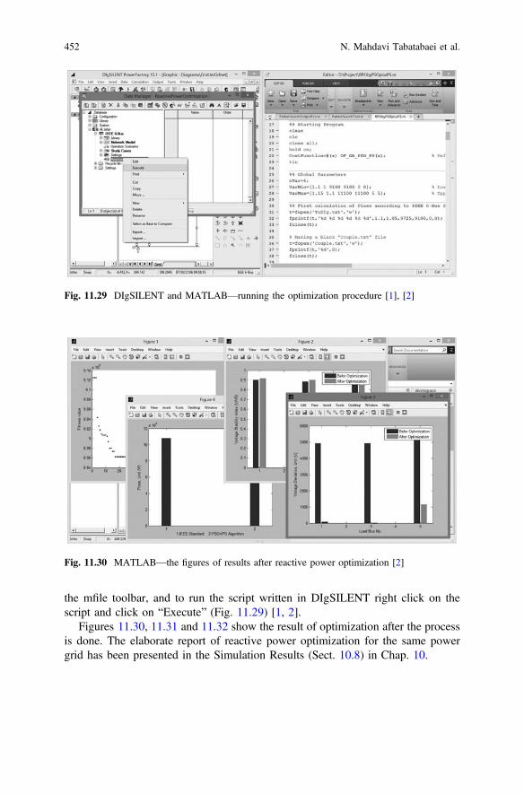
the mfile toolbar, and to run the script written in DIgSILENT right click on the

script and click on “Execute” (Fig. 11.29) [1, 2].

Figures 11.30, 11.31 and 11.32 show the result of optimization after the process

is done. The elaborate report of reactive power optimization for the same power

grid has been presented in the Simulation Results (Sect. 10.8) in Chap. 10.

Fig. 11.29 DIgSILENT and MATLAB—running the optimization procedure [1], [2]

Fig. 11.30 MATLAB—the figures of results after reactive power optimization [2]


http://dx.doi.org/10.1007/978-3-319-51118-4_10

http://dx.doi.org/10.1007/978-3-319-51118-4_10

11.3 How to Use Built-in Optimization Functions

to Implement Reactive Power Optimization

This section will present the simplest and more efficient way of carrying out

reactive power optimization on 39-bus New England power network using built-in

functions of MATLAB software and the corresponding ready-to-use network of

DIgSILENT. The optimization algorithm will be particle swarm pattern search

algorithm as its efficiency has been investigated before. Fortunately, both the

Fig. 11.31 MATLAB—the results which are represented in command window [2]

Fig. 11.32 DIgSILENT PowerFactory—the power network after reactive power optimization [1]


optimization algorithms are available in MATLAB without suffering programming

difficulties so much. In addition, the power network of IEEE 39-bus New England

is available in DIgSILENT 15.1 which can be used as a reliable case study in terms

of the correctness of the data.

11.3.1 How to Prepare the Network in DIgSILENT

To do this there will be different approaches. IEEE 9-, 14- and 39-bus networks are

readily available as examples of DIgSILENT 15.1 software. If they will satisfy the

studies that are being done, they can be simply imported from the software’s data

without bothering tracing and implementing them from scratch, otherwise the steps

related to creating a new project presented in Sect. 11.2.1 will be at work. In

addition, the related file has been enclosed with the chapter and can be imported

easily in DIgSILENT.

11.3.1.1 How to Import IEEE 39-Bus New England Power Network

from the Examples or a File

In order to import the power network from the examples open DIgSILENT

PowerFactory ! go to the File Menu and press Examples (Fig. 11.33) ! in

“Additional Examples” tab choose “39 Bus System” and press Folder Icon (Import

and activate Example Project) (Fig. 11.34). Then the corresponding power network

will be opened and activated and is ready to put a few changes on it (Fig. 11.35).

Fig. 11.33 DIgSILENT PowerFactory—File Menu ! Examples


11.3.1.2 Putting Finishing Touches on the Power Network

in DIgSILENT

The next stage will be preparing the prerequisite conditions toward using

DIgSILENT scripting facility. The first step will be “Creating a DPL Command

Set”, refer to the Sect. 11.2.2.1 to find out how to do so. The next step will be

creating a general set and introducing it to the DPL which can be easily found in

Sect. 11.2.2.2. The third step is introducing external variables to DPL which is

Fig. 11.34 DIgSILENT PowerFactory—Examples ! 39 Bus System

Fig. 11.35 DIgSILENT PowerFactory—39 Bus System ready to use


already represented in Sect. 11.2.2.3. According to IEEE 39-bus New England

Power network given in Chap. 10, there are 20 control variables as the voltage

magnitude of 9 generators and the tap setting for 11 transformers, all of which

should be defined in the “External Objects” section (Fig. 11.36). The final result has

been shown in Fig. 11.36 and the file is enclosed with the chapter ready to be

imported, containing all the necessary changes. Eventually, the script related to

Reactive Power Optimization will be written in the “Script” tab in the “DPL

Command” window.

11.3.2 How to Write Scripts for DIgSILENT and MATLAB

Step by Step

This section will represent the procedure of the reactive power optimization using

built-in functions of MATLAB step by step. All the functions will be introduced

where necessary in order to make it easy to comprehend. The optimization algo-

rithm has considered to be particle swarm optimization algorithm, both of which

have got their own efficient functions in MATLAB.

11.3.2.1 Initializing and Defining the Problem in MATLAB

As presented in the codes below, global variables have been considered to be used.

Global variables are at work when a variable comes to be used in several functions

and each function makes its own changes on the variable, all of which are vital in

the procedure. Their values should be set to zero right at the beginning in order to

Fig. 11.36 DIgSILENT PowerFactory—DPL command set


http://dx.doi.org/10.1007/978-3-319-51118-4_10

avoid any unexpected interference during several implementations of the process.

Cost function has been written as a function itself and defined to the procedure

using “Cost function” section in the scripts below. The rest of the codes represents

the definition of the upper and lower boundaries of the control variables.

Initializing and Defining the ProblemMATLAB

RPONewEngland.m

clc;

clear;

close all;

%% Problem Definition

global nfe NFE BVMin BVMax BestFunValuePSO IterationPSO BestFunValuePS

IterationPS;

NFE = 0;

nfe = 0;

BestFunValuePSO = 0;

IterationPSO = 0;

BestFunValuePS = 0;

IterationPS = 0;

CostFunction = @(OCV) RPO_Function(OCV); % Cost Function

% Decision Variables %

% VG02,VG03,VG04,VG05,VG06,VG07,VG08,VG09,VG10

% TT1211,TT1213,TT0631,TT1032,TT1933,TT2034,TT2235,TT2537,TT0230

% TT2938,TT1920

% Busbars Voltage Limits P.U. %

% Acceptable Voltage Limitations, +-10% for 16.5, 138, and 230 kV Busbars,

% +-5% for 345 kV Busbars

% BVMin = [0.95 0.95 0.95 0.95 0.95 0.95 0.95 0.95 0.95 0.95 0.95 0.90...

% 0.95 0.95 0.95 0.95 0.95 0.95 0.95 0.90 0.95 0.95 0.95 0.95 0.95...

% 0.95 0.95 0.95 0.95 0.9 0.9 0.9 0.9 0.9 0.9 0.9 0.9 0.9 0.9];

% BVMax = [1.05 1.05 1.05 1.05 1.05 1.05 1.05 1.05 1.05 1.05 1.05 1.10...

% 1.05 1.05 1.05 1.05 1.05 1.05 1.05 1.10 1.05 1.05 1.05 1.05 1.05...

% 1.05 1.05 1.05 1.05 1.10 1.10 1.10 1.10 1.10 1.10 1.10 1.10 1.10 1.10];

% Busbars Voltage Limits P.U. %

% Acceptable Voltage Limitations, +-10% for 16.5, 138, 230 and 345 kV Busbars

BVMin = 0.9*ones(1,39);

BVMax = 1.1*ones(1,39);

% Generators Voltage Limits P.U. %

GVMin = [0.9 0.9 0.9 0.9 0.9 0.9 0.9 0.9 0.9];

GVMax = [1.1 1.1 1.1 1.1 1.1 1.1 1.1 1.1 1.1];

% Transformators Tap Limits %


TTMin = [-1 -1 -2 -2 -2 -1 -1 -1 -1 -1 -2];

TTMax = [1 1 2 2 2 1 1 1 1 1 2];

VarMin = [GVMin TTMin]; % Lower Bound of Variables

VarMax = [GVMax TTMax]; % Upper Bound of Variables

11.3.2.2 Initial Power Losses According to New England 39-Bus

Network

In order to calculate initial value of active power losses according to IEEE 39-bus

New England it is needed to apply initial condition to the network and after running

power flow calculation of losses will be feasible. The matrix “SVCV” represents

Standard Values for Control Variables which are taken from the data given in the

appendix section of Chap. 10. Then they will be exported in a “.txt” file as “OCV.

txt” to be imported in DIgSILENT. Finally, MATLAB will make a “Couple.txt” file

as a means of exchanging commands between two pieces of software, waiting for

DIgSILENT to implement its duty.

Initial Power LossesMATLAB

RPONewEngland.m

%% Initial Power Losses According to New England 39-Bus Network

% Standard Values for Control Variables %

SVCV = [0.982 0.9831 0.9972 1.0123 1.0493 1.0635 1.0278 1.0265 1.0475...

1 1 2 2 2 1 1 1 1 1 2];

t = fopen('OCV.txt','w'); % Optimal Control Variables

fprintf(t,'%d %d %d %d %d %d %d %d %d %d %d %d %d %d %d %d %d %d %d %d',SVCV);

fclose(t);

% Making a Blank "Couple.txt" File, 0 => DIgSILENT, 1 => MATLAB %

t = fopen('Couple.txt','w');

fprintf(t,'%d',0);

fclose(t);

% Waiting for DIgSILENT to Complete the PowerFlow Process %

a = 0;

while a == 0

pause(0.02);

a = load('Couple.txt');

end


http://dx.doi.org/10.1007/978-3-319-51118-4_10

11.3.2.3 Initializing DIgSILENT Software

Initializing DIgSILENT consists in defining variables, which will be used

throughout the procedure of optimization. Integer variables for storing and using

integer values, object variables for storing equipment used in the power network,

double variables for storing values for control variables, set variables for storing a

group of objects, and string variables for storing string values.

Initializing DIgSILENT Software DIgSILENT

int a;

object o;

double V,U,Phi,Ploss,Qloss;

double VG02,VG03,VG04,VG05,VG06,VG07,VG08,VG09,VG10,TT1211,TT1213,

TT0631,TT1032, TT1933,TT2034,TT2235,TT2537,TT0230,TT2938,TT1920;

set s1;

string BusName,LineName;

a=1;

11.3.2.4 How to Apply Control Variables to the Network

The main loop of reactive power optimization in DIgSILENT consist in running

power flow and exporting the results. Each time MATLAB wants DIgSILENT run,

the procedure in DIgSILENT starts from this session, and if MATLAB sends

command signal as “2”, the procedure in DIgSILENT will be over. Referring to the

codes below, DIgSILENT first reads the “OCV.txt” file written by MATLAB and

then allocated the values to the control variables “VG02” to “TT1920”. Then

applying the values using the external objects defined in Sect. 11.3.1.2 will be

feasible as done below. It means that now the values considered to be control

variables are set to the values created by MATLAB. The next step will be running

the power flow according to new values.


Applying Control Variables to the Network DIgSILENT

!! The Main Loop of Reactive Power Optimization

while(a<>2) ! Checking to Finish the Process

{

fopen('C:\Users\ALI JAFARI\Documents\MATLAB\

IEEE 39-Bus New England Power System\Reactive Power Optimization\OCV.txt','r',0);

fscanf(0,'%d %d %d %d %d %d %d %d %d %d %d %d %d %d %d %d %d %d %d

%d',VG02,VG03,VG04,VG05,VG06,VG07,VG08,VG09,VG10,TT1211,TT1213,

TT0631,TT1032,TT1933,TT2034,TT2235,TT2537,TT0230,TT2938,TT1920);

fclose(0);

G02:usetp = VG02;

G03:usetp = VG03;

G04:usetp = VG04;

G05:usetp = VG05;

G06:usetp = VG06;

G07:usetp = VG07;

G08:usetp = VG08;

G09:usetp = VG09;

G10:usetp = VG10;

T1211:nntap = TT1211;

T1213:nntap = TT1213;

T0631:nntap = TT0631;

T1032:nntap = TT1032;

T1933:nntap = TT1933;

T2034:nntap = TT2034;

T2235:nntap = TT2235;

T2537:nntap = TT2537;

T0230:nntap = TT0230;

T2938:nntap = TT2938;

T1920:nntap = TT1920;

11.3.2.5 Running Load Flow in the Script Section in DIgSILENT

After applying values for control variables, it is time to carry the load flow cal-

culations out. To do so, load flow should be introduced to the DPL command set as

an external object, which is illustrated in Sect. 11.2.2.3. The procedure is as the

following.


Running Load Flow DIgSILENT

! Running Load Flow Calculation

ClearOutput();

ResetCalculation();

Ldf.Execute();

11.3.2.6 Exporting Load Flow Results from DIgSILENT

The results of power flow will be exported using “fprintf” function via “LoadFlow.

txt” as a comma separated value (CSV) file. The data being exported completely

depends on what type of information is exactly needed within the calculations in

MATLAB pertaining to the study being done. In this section voltage magnitudes,

p.u. values for the voltages and voltages degrees have been exported.

Exporting Load Flow Results DIgSILENT

! Exporting Load Flow Results

fopen('C:\Users\ALI JAFARI\Documents\MATLAB\IEEE 39-Bus New England Power

System\Reactive Power Optimization\LoadFlow.txt','w',0);

fprintf(0,'%s,%s,%s,%s','BusName','Voltage_V','Voltage_PU','VoltageAngle_Deg');

s1 = SEL.AllBars();

s1.SortToName(0);

o = s1.First();

while (o){

V = o:m:Ul;

U = o:m:u1;

Phi = o:m:phiu;

BusName = o:loc_name;

fprintf(0,'%s,%f,%f,%f',BusName,V,U,Phi);

o = s1.Next();

}

fclose(0);

11.3.2.7 Exporting Transmission Lines Power Losses

from DIgSILENT

The transmission lines power losses can also be exported from DIgSILENT instead of

calculating them in MATLAB using the active power losses of transmission lines

equation expressed in Chap. 10. The only thing which should be done is to find the

appropriate parameter name for active power losses to be able to export the corre-

spondingvalue for all the transmission lines.DIgSILENT is able to calculatewide range

of parameters related to power flowwithout suffering programming difficulties. How to

find the parameter namewhich is used in the scripting session to export the related value


http://dx.doi.org/10.1007/978-3-319-51118-4_10

has been presented in Section “Running Power Flow in DIgSILENT Based on Initial

Condition”. Following the same instruction, “Ploss_bus1” is representative of active

power losses in transmission lines and can be used in the scripting segment to export the

results. The following code exports power losses for transmission lines in

“TLPowerLosses.txt” as a CSV file. Eventually, DIgSILENT sends a signal to

MATLAB via “Couple.txt” to let it know that power flow is done, results are exported

and ready to use, then it waits to get another set of values for control variables and

another command from MATLAB to run power flow based on new condition again.

Exporting Transmission Lines Power Losses DIgSILENT

! Exporting Transmission Lines Power Losses


System\Reactive Power Optimization\TLPowerLosses.txt','w',0);

fprintf(0,'%s,%s,%s','LineName','ActivePowerLoss_W','ReactivePowerLoss_VAR');

s1 = SEL.AllLines();

s1.SortToName(0);

o = s1.First();

while (o){

Ploss = o:m:Ploss:bus1;

Qloss = o:m:Qloss:bus1;

LineName = o:loc_name;

fprintf(0,'%s,%f,%f',LineName,Ploss,Qloss);

o = s1.Next();

}

fclose(0);

! Sending Run Signal to MATLAB


System\Reactive Power Optimization\Couple.txt','w',1);

fprintf(1,'%d',1);

fclose(1);

! Waitign for MATLAB to Finish the Corresponding Calculations

a = 1;

while(a = 1){


System\Reactive Power Optimization\Couple.txt','r',0);

fscanf(0,'%d',a);

fclose(0);

}

}

11.3.2.8 Importing Active Power Losses from Text File in MATLAB

In order to import power losses results into MATLAB from the “TLPowerLosses.

txt” file, a built-in function called “readtable(‘TLPowerLosses’)” can be used,


which creates a table by reading column oriented data from a file. “readtable”

creates one variable in “TLPL” for each column in the file and reads variable names

from the first row of the file. In the following code MATLAB imports the data

written by DIgSILENT in the “TLPowerLosses.txt” file and then sums up the

values in the “ActivePowerLoss_W” column to work out the total value of active

power losses in transmission lines and stores it in “PowerLosses.Initial.APL”. In

addition, it saves the values for control variables in “PowerLosses.Initial.Position”.

Importing Active Power Losses from “TLPowerLosses.txt”MATLAB

RPONewEngland.m

% Loading Active Power Losses from DIgSILENT Calculation %

TLPL = readtable('TLPowerLosses'); % Transmission Lines Power Losses Data

PowerLosses.Initial.APL = sum(TLPL.ActivePowerLoss_W);

PowerLosses.Initial.Position = SVCV;

11.3.2.9 Reactive Power Optimization Using Built-in Particle Swarm

Function

MATLAB provides a built-in function for particle swarm optimization algorithm in

its recent versions. It can be effortlessly used in optimization algorithms adjusting

some parameters without programming the algorithm itself. A user defined function

has been created as “ParticleSwarmTool” in order to gather all the corresponding

parameters and the Particle Swarm built-in function in a unique mfile. The inputs to

this function is just lower and upper bounds for control variables and the initial

position which is optional.

Reactive Power Optimization Using PSO AlgorithmMATLAB

RPONewEngland.m

%% Reactive Power Optimization Using PSO Algorithm

[PowerLosses.PSO.Position,PowerLosses.PSO.APL,exitflagPSO] = ...

ParticleSwarmTool(VarMin,VarMax);

LNFE = length(nfe);

The main function which carries out the optimization procedure is “particleswarm”,

while there are a fewprerequisite adjustments to bemade before using the function itself.

In order to access the details of the particle swarm optimization function MATLAB

provides another function as “optimoptions”. The detailed information about how to use

it is available either online or MATLAB software local help. In this section just the

needed adjustments have been presented. “options = optimoptions

(options,‘InitialSwarm’, [0.982 0.9831 0.9972, 1.0123 1.0493 1.0635 1.0278 1.0265

1.0475 1 1 2 2 2 1 1 1 1 1 2]);” has been used to define initial point to PSO algorithm


which is optional. Self-adjustment and social-adjustment rates have been specified to the

function using “options = optimoptions(options,‘SelfAdjustment’,1.49);” and “op-

tions = optimoptions(options,‘SocialAdjustment’,1.49);”. In addition, the member of

members in the swarm has been defined using “options = optimoptions

(options,‘SwarmSize’,20);” and so forth, to see more information please refer to

MATLAB software help.

Reactive Power Optimization Using PSO AlgorithmMATLAB

ParticleSwarmTool.m

function [x,fval,exitflagPSO] = ParticleSwarmTool(VarMin,VarMax)

nVar = 20; % Number of Decision Variables

options = optimoptions('particleswarm');

options = optimoptions(options,'CreationFcn',@pswcreationuniform);

options = optimoptions(options,'Display','Iter');

options = optimoptions(options,'DisplayInterval',1);

options = optimoptions(options,'FunValCheck','off');

options = optimoptions(options,'HybridFcn',[]);

options = optimoptions(options,'InertiaRange',[0.1 1.1]);

options = optimoptions(options,'InitialSwarm',[0.982 0.9831 0.9972...

1.0123 1.0493 1.0635 1.0278 1.0265 1.0475 1 1 2 2 2 1 1 1 1 1 2]);

options = optimoptions(options,'InitialSwarmSpan',2000);

options = optimoptions(options,'MaxIter',Inf);

options = optimoptions(options,'MaxTime',Inf);

options = optimoptions(options,'MinFractionNeighbors',0.25);

options = optimoptions(options,'ObjectiveLimit',-Inf);

options = optimoptions(options,'OutputFcns',@ParticleSwarmOutputFcn);

options = optimoptions(options,'PlotFcns',[]);

options = optimoptions(options,'SelfAdjustment',1.49);

options = optimoptions(options,'SocialAdjustment',1.49);

options = optimoptions(options,'StallIterLimit',20);

options = optimoptions(options,'StallTimeLimit',Inf);

options = optimoptions(options,'SwarmSize',20);

options = optimoptions(options,'TolFun',1e-2);

options = optimoptions(options,'UseParallel',0);

options = optimoptions(options,'Vectorized','off');

% The Main Function of Particle Swarm Optimization Algorithm %

[x,fval,exitflagPSO] = ...

particleswarm(@RPO_Function,nVar,VarMin,VarMax,options);

The general form to use the built-in function of particle swarm is like “[x,fval,exitflag,

output] = particleswarm(fun,nvars,lb,ub,options)” in which “x” returns the position of

control variables, “fval” represents the best cost, “exitflag” describes the exit condition,

“output” containing information about the optimization process, “fun” is a function con-

taining objective function, “nvars” refers to number of control variables, “lb” and “lu”

embodies lower and upper bounds for control variables and “options” is a variables


consisting of all the setting parameters of PSO function. The objective function will be

defined as the following codes.

Reactive Power Optimization Objective FunctionMATLAB

RPO_Function.m

function [OF] = RPO_Function(OCV)

global NFE BVMin BVMax;

NFE = NFE+1;

k = 1e15; % Penalty Factor

% Calculation of Objective Function (Ploss) %

t = fopen('OCV.txt','w'); % Consisting of Optimal Control Variables

fprintf(t,'%d %d %d %d %d %d %d %d %d %d %d %d %d %d %d %d %d %d %d

%d',OCV);

fclose(t);

% Sending Run Signal to DIgSILENT; 0 => DIgSILENT, 1 => MATLAB %


fprintf(t,'%d',0);

fclose(t);

% Waiting for DIgSILENT to Complete the PowerFlow Process %

a = 0;

while a == 0

pause(0.03);

a = load('Couple.txt');

end

% Loading Power Losses from DIgSILENT Calculation %

TLPL = readtable('TLPowerLosses'); % Transmission Lines Power Losses Data

FAPL = sum(TLPL.ActivePowerLoss_W); % Transmission Systems Active

Power Losses

% FRPL = sum(TLPL.ReactivePowerLoss_VAR); % Transmission Systems Reactive

Power Losses

% Applying Penalty to the Cost Function for Keeping Voltages of PQ Busbars Within

the Limitations %

PF = readtable('LoadFlow'); % Load Flow Results

PQBV = (PF{1:29,3})'; % Extracting PQ Busbars Voltatges

PV = k*sum(BVMax(1:29)-PQBV<0|BVMin(1:29)-PQBV>0); % To Apply a Penalty to

the Cost Function

% if There is a Voltage Violation

OF = FAPL + PV;

end


In the reactive power optimization function above “NFE” has been considered to

work the number of function evaluation out. “% Calculation of Objective Function

(Ploss) %” section tries to apply the new set of control variables to the power

network in DIgSILENT and carries out power flow and the calculates active power

losses accordingly. Section “% Applying Penalty to the Cost Function for Keeping

Voltages of PQ Busbars Within the Limitations %” has been considered to apply a

penalty to the cost value if there is a violation in the voltages of PQ busbars. The

particle swarm built-in function refers to the objective function several times to

figure out if the objective function has been optimized or not.

In order to have access to the detailed data throughout the procedure a user

defined function “ParticleSwarmOutputFcn” has been used, which is a facility that

built-in PSO function provides. It also can be used in order to stop the function

using a specific criterion, to see more information refer to MATLAB software help

documentation. The code is as following.

Particle Swarm Output FunctionMATLAB

ParticleSwarmOutputFcn.m

function stop = ParticleSwarmOutputFcn(optimValues,state)

global nfe NFE BestFunValuePSO IterationPSO;

stop = false; % This function does not stop the solver

switch state

case 'init'

case 'iter'

BestFunValuePSO(optimValues.iteration) = optimValues.bestfval;

nfe(optimValues.iteration) = NFE;

case 'done'

IterationPSO = optimValues.iteration;

end

After finishing the optimization procedure of the PSO function, the optimum

positions for control variables are stored in “PowerLosses.PSO.Position” and the

cost value for the values of control variables in “PowerLosses.PSO.APL”. The next

step will be using Pattern Search as the supplementary optimization algorithm to

pinpoint the exact optimum control variables.


11.3.2.10 Reactive Power Optimization Using Built-in Pattern Search

Function

Pattern search optimization algorithm has been used as a supplementary opti-

mization algorithm in case PSO is not able to pinpoint the optimum control vari-

ables. User defined “PatternSearchTool” has been considered to gather all the

parameters and settings which are needed to adjust and run pattern search algorithm

all together. The codes below call the function.

Reactive Power Optimization Using Pattern SearchMATLAB

RPONewEngland.m

%% Reactive Power Optimization Using PatternSearch Algorithm

[PowerLosses.PS.Position,PowerLosses.PS.APL,exitflagPS] = ...

PatternSearchTool(PowerLosses.PSO.Position,VarMin,VarMax);

The main function which carries out the optimization procedure is “pat-

ternsearch”, while there are a few requirements needed to be met before using the

function itself. In order to access the details of the pattern search function,

MATLAB provides another function as “psoptimset”. The detailed information

about how to use it is available either online or MATLAB software local help. In

this section just the needed adjustments have been presented. “options = psoptimset

(options,‘TolFun’,1e-4);” is the tolerance on the objective function which stops the

optimization procedure if both the change in function value and the mesh size are

less than “TolFun”.

The general form to use the built-in function of pattern search is like “[x,fval,

exitflag,output] = patternsearch(fun,x0,A,b,Aeq,beq,LB,UB)” in which “x” returns

the position of control variables, “fval” represents the best cost, “exitflag” describes

the exit condition, “output” containing information about the optimization process,

“fun” is a function containing objective function, “x0” is the starting point to the

pattern search algorithm, “A”, “b”, “Aeq” and “beq” are parameters of inequality

and equality constraints, “LB” and “UB” lower bounds and upper bounds of the

control variables, and “options” is a variables consisting of all the setting param-

eters of pattern search function.


Reactive Power Optimization Using Pattern SearchMATLAB

PatternSearchTool.m

function [x,fval,exitflagPS] = PatternSearchTool(x0,VarMin,VarMax)

options = psoptimset;

options = psoptimset(options,'TolMesh',[]);

options = psoptimset(options,'TolCon',[]);

options = psoptimset(options,'TolX',[]);

options = psoptimset(options,'TolFun',1e-4);

options = psoptimset(options,'TolBind',[]);

options = psoptimset(options,'MaxIter',Inf);

options = psoptimset(options,'MaxFunEvals',[]);

options = psoptimset(options,'TimeLimit',[]);

options = psoptimset(options,'MeshContraction',[]);

options = psoptimset(options,'MeshExpansion',[]);

options = psoptimset(options,'MeshAccelerator','on');

options = psoptimset(options,'MeshRotate',[]);

options = psoptimset(options,'InitialMeshSize',[]);

options = psoptimset(options,'ScaleMesh',[]);

options = psoptimset(options,'MaxMeshSize',[]);

options = psoptimset(options,'InitialPenalty',[]);

options = psoptimset(options,'PenaltyFactor',[]);

options = psoptimset(options,'PollMethod',[]);

options = psoptimset(options,'CompletePoll',[]);

options = psoptimset(options,'PollingOrder','Success');

options = psoptimset(options,'SearchMethod',@GPSPositiveBasis2N);

options = psoptimset(options,'CompleteSearch',[]);

options = psoptimset(options,'Display','iter');

options = psoptimset(options,'OutputFcns',@PatternSearchOutputFcn);

options = psoptimset(options,'PlotFcns',[]);

options = psoptimset(options,'PlotInterval',[]);

options = psoptimset(options,'Cache',[]);

options = psoptimset(options,'CacheSize',[]);

options = psoptimset(options,'CacheTol',[]);

options = psoptimset(options,'Vectorized',[]);

options = psoptimset(options,'UseParallel',[]);

% The Main Function of Pattern Search Optimization Algorithm %

[x,fval,exitflagPS] = ...

patternsearch(@RPO_Function,x0,[],[],[],[],VarMin,VarMax,[],options);

“options = psoptimset(options,‘OutputFcns’,@PatternSearchOutputFcn);” is

used to access the detailed information during the optimization procedure in every

iteration as presented for PSO function in Sect. 11.3.2.9. See the help documen-

tation of MATLAB for more information how to use it.


Pattern Search Output FunctionMATLAB

PatternSearchOutputFcn.m

function [stop,options,optchanged] =

PatternSearchOutputFcn(optimValues,options,state)

global nfe NFE BestFunValuePS IterationPS IterationPSO;

stop = false; % This function does not stop the solver

optchanged = false;

switch state

case 'init'

case 'iter'

BestFunValuePS(optimValues.iteration) = optimValues.fval;

nfe(optimValues.iteration + IterationPSO) = NFE;

case 'done'

IterationPS = optimValues.iteration;

end

After finishing the optimization procedure by Pattern Search function, the

optimum positions for control variables are stored in “PowerLosses.PS.Position”

which will be best point found, and the best cost value will be saved in

“PowerLosses.PS.APL” which is the best minimum cost.

11.3.2.11 Finishing the Optimization Procedure and Exporting

Results

After finishing optimization procedure, the final step will be sending a stop signal to

DIgSILENT and printing the data in relation to what information was meant to be

exported. The following codes are an example of such processes.


Finishing the Optimization ProcedureMATLAB

RPONewEngland.m

%% Sending Stop Signal to DIgSILENT


fprintf(t,'%d',2);

fclose(t);

%% Results

clc

hold on

plot(nfe(1:LNFE),BestFunValuePSO,'-o','LineWidth',1);

plot(nfe(LNFE+1:end),BestFunValuePS,'-.*','LineWidth',1);

xlabel('Number of Function Evaluation (NFE)');

ylabel('Active Power Losses (W)');

LR = PowerLosses.Initial.APL - PowerLosses.PS.APL; % Losses Reduction

LRP = 100*((PowerLosses.Initial.APL-PowerLosses.PS.APL)...

/PowerLosses.Initial.APL); % Losses Reduction Percentage, Total

disp('------------------------------------------------------------------');

str = sprintf('Initial Active Power Losses (W) = %d',...

PowerLosses.Initial.APL);

disp(str);

disp('------------------------------------------------------------------');

str = sprintf('Active Power Losses After Optimization (W) = %d',...

PowerLosses.PS.APL);

disp(str);

disp('------------------------------------------------------------------');

str = sprintf('Losses Reduction (W), Total = %d',LR);

disp(str);

disp('------------------------------------------------------------------');

str = sprintf('Losses Reduction Percentage , Total = %d',LRP);

disp(str);


11.3.3 How to Run the Optimization Procedure

After having the mfiles of MATLAB and scripts of DIgSILENT ready, it is the final

step to run the optimization process. It should be noted that, according to the

structure used in the script files enclosed with this chapter, the mfile of MATLAB is

the first one which should be run and then DIgSILENT. To run the optimization

procedure via MATLAB by “RPO_NewEngland.m” simply click on “Run” icon in

the mfile toolbar, and to run the script written in DIgSILENT right click on the

script and click on “Execute” (Fig. 11.37).

Figure 11.38 shows the result of optimization after the process is done for one

run. The elaborate report of reactive power optimization for the same power grid

has been presented in the Simulation Results in Chap. 10.

11.3.4 How to Run Small Signal Analysis in DIgSILENT

There are a few steps through running small signal analysis in DIgSILENT.

The IEEE 39-bus New England power system is already prepared for carrying out

such analysis. To run the process, activate Small Signal Analysis in the Study Case

section (Fig. 11.39), then choose Modal Analysis toolbar (Fig. 11.40). The equa-

tion system has to be initialized (Calculate Initial Conditions) (Fig. 11.41), then

Fig. 11.37 DIgSILENT and MATLAB—how to run the optimization procedure


http://dx.doi.org/10.1007/978-3-319-51118-4_10

calculation of the eigenvalues can be executed by pressing the button Modal

Analysis (Fig. 11.41). The study case “Small Signal Analysis (Eigenvalues)”

contains an eigenvalue plot which displays the results (Fig. 11.41) [1].

Fig. 11.39 DIgSILENT PowerFactory—activating Small Signal Analysis study case

Fig. 11.38 MATLAB—the result after the optimization


11.4 Summary

The main objective of reactive power optimization is to reduce active power losses

in the power network and improve voltage profile. Reactive power optimization

problem is a multidimensional problem which has plenty of local optimum points

that causes the traditional optimization methods, which mostly are based on gra-

dient method, to have difficulty finding the global point. Heuristic algorithms have

Fig. 11.41 DIgSILENT PowerFactory—Eigenvalue Plot

Fig. 11.40 DIgSILENT PowerFactory—Modal Analysis tool


proved their high performance in optimizing these kind of complex problems, one

of which is the particle swarm optimization algorithm that is highly appreciated in

terms of global optimization. In addition, there are some direct search methods

which do not use target function’s gradient but itself, of which are very performable

when it comes to local optimization. It seems, then, applicable to use a local

optimization algorithm in association with a global optimizer to pinpoint the

optimum point.

In this chapter, PSO algorithm has been considered as the main and global

optimizer and pattern search algorithm as supplementary and the local one through

optimizing reactive power in the power grid. This chapter represents a particle

swarm pattern search algorithm to optimize reactive power to decrease active power

losses in an IEEE 6-bus power network. The optimization procedure has done by an

approach consisting of two software MATLAB and DIgSILENT which is explained

step by step. In addition, another method to optimize reactive power using ready to

use IEEE 39-bus New England in DIgSILENT and built-in optimization functions

in MATLAB has been presented while considering the fact that the reader has

intermediate knowledge how to use both pieces of software. The corresponding

files have been attached with the book to use. Additional approaches containing

reactive power optimization using genetic pattern search algorithm for IEEE 6-bus

power grid, particle swarm pattern search algorithm for IEEE 14-bus and genetic

pattern search algorithm for IEEE 14-bus have been enclosed with the book. The

simulations results have been presented in Chap. 10 (10.8—Reactive Power

Optimization Simulation Results) and further comparisons have been put there.

Overall, the aim of this chapter was to present an introductory method through

using MATLAB and DIgSILENT working together in order to avoid a few

unimportant steps towards further studies in the AC power network.

References

1. DIgSILENT PowerFactory Version 15 User Manual, Gomaringen, Germany: DIgSILENT

GmbH, 2014.

2. MATLAB Help, The MathWorks, Inc., 2014.


http://dx.doi.org/10.1007/978-3-319-51118-4_10

Chapter 12

Multi-objective Optimal Reactive Power

Dispatch Considering Uncertainties

in the Wind Integrated Power Systems

Seyed Masoud Mohseni-Bonab, Abbas Rabiee

and Behnam Mohammadi-Ivatloo

Abstract One of the most principle optimization problems which gained the

attention of power system operators around the world is optimal power flow (OPF).

The OPF basically performs an intelligent power flow and optimizes the system

operation condition by optimally determination of control variables. It also con-

siders a specific set of operational constraints and technical limits for this aim,

which guaranties both feasibility and optimality of the scheduled operation con-

dition. Generally, this problem can be categorized into two main sub-problems, i.e.

optimal reactive power dispatch (ORPD) and optimal real power dispatch, which

are differ in their aims and control variables. This chapter deals with the first one,

ORPD, which has significant impact on power system security. ORPD is modeled

as an optimization problem with nonlinear functions and mixed continuous/discrete

variables. Thus, it is a complicated optimization problem. The multi-objective

ORPD (MO-ORPD) problem is studied, taking into account different operational

constraints such as bus voltage limits, power flow limits of branches, limits of

generators voltages, transformers tap ratios and the amount of available reactive

power compensation at the weak buses. Three different objective functions are

considered in the proposed MO-ORPD framework, which are minimizing total

active power losses, minimizing voltage variations and minimizing voltage stability

index (L-index). These conflicting objectives are optimized via e-constraint method.

In order to model the stochastic behavior of demand and wind power generation, it

is necessary to modify the MO-ORPD problem, and develop a probabilistic

approach to handle the uncertainties in MO-ORPD problem. Hence, a two-stage

stochastic MO-ORPD (SMO-ORPD) is suggested to handle the load and wind

power uncertainties in the MO-ORPD problem. In the proposed two-stage

S.M. Mohseni-Bonab � A. Rabiee (&)

Department of Electrical Engineering, University of Zanjan, Zanjan, Iran


S.M. Mohseni-Bonab

e-mail: [email protected]; [email protected]

B. Mohammadi-Ivatloo

Faculty of Electrical and Computer Engineering, University of Tabriz, Tabriz, Iran





475

stochastic optimization model, the decision variables are classified into two cate-

gories, namely, “here and now” and “wait and see” variables. The optimal values of

“here and now” variables should be known before realization of scenarios, and

therefore, their values are the same for all scenarios while the optimal values of

“wait and see” variables are based on the realized scenario, and hence their values

are scenario dependent. Moreover, in order to examine performance of the proposed

SMO-ORPD and the impact of wind power generation on the results of

SMO-ORPD, deterministic ORPD (DMO-ORPD) has also been solved in two

modes: DMO-ORPD without wind farms (WFs) and any uncertainty, for the sake

of comparison with the available methods in recent literature, and DMO-ORPD

with WFs. In this chapter the reactive power compensation devices are modeled as

discrete/continuous control variables. DMO-ORPD and SMO-ORPD are formu-

lated as mixed integer non-linear program (MINLP) problems, and solved by

General Algebraic Modeling System (GAMS). Also, the IEEE 30-bus standard

system is utilized for evaluation of the proposed MO-ORPD models.

12.1 Introduction and Problem Statement

Optimal reactive power dispatch (ORPD) is an important problem for power util-

ities from the viewpoints of system security and energy losses. ORPD is a specific

form of optimal power flow (OPF) problem, in which various objective functions

such as transmission losses or voltage stability enhancement indices are optimized

by adjusting the generator voltages set-points, reactive power compensation in

weak buses and optimal setting of transformers tap ratios.

12.1.1 Background and Review of the Recent Literature

Active power losses are the most important objective function used in the classical

OPRD problem. Many heuristic algorithms such as multi-agent-based particle

swarm optimization approach (MA-PSO) [1], seeker optimization algorithm

(SOA) [2], shuffled frog leaping algorithm (SFLA) and Nelder–Mead SFLA

(NM-SFLA) [3], combination of hybrid modified imperialist competitive algorithm

(MICA) and invasive weed optimization (IWO) named as (MICA-IWO) [4],

combination of modified teaching learning algorithm (MTLA) and double differ-

ential evolution (DDE) algorithm [5] have been developed to obtain optimal

solutions of ORPD while satisfying technical constraints. In [6], active power losses

are minimized in wind farms (WFs) by PSO algorithm taking into consideration the

reactive power requirement at the point of common coupling (PCC).

In some papers, active power losses are considered with two other common

objective functions of ORPD. At the first category active power losses are con-

sidered with voltage deviation, while in the second category active power losses are

476 S.M. Mohseni-Bonab et al.

optimized along with a voltage stability enhancement index. In the third category

active power losses are considered with both of the other objectives. In order to

handle these categories, various intelligent algorithms are employed in the existing

literature, such as feasible solutions differential evolution (SF-DE), self-adaptive

penalty DE (SP-DE), e-constraint DE (EC-DE) and stochastic ranking DE (SR-DE)

in [7], evolutionary programming (EP), PSO, DE and the hybrid differential evo-

lution (HDE) in [8], combination of NM and Firefly Algorithm (FA) in [9], PSO

with an aging leader and challengers (ALC-PSO) in [10] and gray wolf optimizer

(GWO) in [11], linear programming (LP) based method using FACTS devices in

[12], nonlinear programming (NLP) based method for optimizing local voltage

stability index in [13], SOA in [14], DE in [15], PSO, simple genetic algorithm

(SGA) and harmony search algorithm (HSA) in [16], gravitational search algorithm

(GSA) in [17].

A different research carried out on the single objective ORPD problem, in which

steady state voltage stability analysis has been carried out in [18] considering initial

conditions for transient stability (TS), small disturbance (SD), and continuation

power flow (CPF) for minimizing real power losses. Also, penalty function based

method has been presented in [19] to convert discrete ORPD model to a continuous

and differentiable model.

The multi-objective ORPD (MO-ORPD) has attracted the attention researchers in

recent years. Similar to single objective OPRD, many algorithms utilized to deal

with MO-ORPD by considering two or three objective conflicting functions,

simultaneously. Most popular objective function of MO-ORPD problem is real

power losses which is considered with voltage deviation (as the conflicting objective

function) in [20], and solved by strength Pareto evolutionary algorithm (SPEA).

Also, it is solved in [21] by non-dominated sorting genetic algorithm-II (NSGA-II).

MO-ORPD problem is modeled as a mixed integer nonlinear program (MINLP)

and solved in some literature with considering real power losses and Lmax index. It

is worth to note that, Lmax is a voltage stability index, where it varies from 0 at

no-load condition to 1 at voltage collapse point. In [22], NSGA-II and modified

NSGA-II (MNSGA-II), In [23] hybrid fuzzy multi-objective evolutionary algorithm

(HFMOEA) and in [24], chaotic improved PSO based multi-objective optimization

(MOCIPSO) and improved PSO-based multi-objective optimization (MOIPSO) are

used for this aim. In more advanced MO-ORPD problem, three objective functions

are considered simultaneously. For instance, teaching learning based optimization

(TLBO) and quasi-oppositional TLBO (QOTLBO) in [25], chaotic parallel vector

evaluated interactive honey bee mating optimization (CPVEIHBMO) in [26], and

strength Pareto multi-group search optimizer (SPMGSO) [27] are used to solve

MO-ORPD problem.

Moreover, in recent literature ORPD or MO-ORPD problems are solved con-

sidering the effects of technical uncertainties raised from the power system

restructuring, probable disturbances, or the integration of renewable energies. In

[28], chance constrained programming technique is proposed to solve ORPD

problem with the aim of minimizing active power losses. Nodal power injections

and random branch outages are considered as uncertainty sources. In [29, 30]

12 Multi-objective Optimal Reactive Power Dispatch … 477

the load uncertainty is included in MO-ORPD problem, considering different

objective functions. Monte Carlo simulations (MCS) are used for handling the load

uncertainties in the nonlinear constrained multi objective ORPD problem.

12.1.2 Chapter Contributions

The main focus of this chapter is to solve the MO-ORPD problem in a wind

integrated power system considering the uncertainties of load demand and wind

power generation. Even these two sources of uncertainty are considered here, but

the proposed method is generic and other uncertainty sources could be included via

the proposed scenario based approach. The normal probability distribution function

(PDF) and Rayleigh (PDF) are used for modeling the load and wind speed

uncertainties, respectively.

Three different objective functions, namely active power losses, voltage stability

index (Lmax), and voltage deviations at load buses are considered. The

multi-objective problem is handled using e-constraint technique and optimal Pareto

sets are obtained for each pair of the above objective functions. In this chapter, for

the sake of comparison with existing methods, the reactive power compensation by

shunt VAR compensators is modeled as continuous variable in deterministic

MO-ORPD (DMO-ORPD), while in real world problems discrete model is

employed for these devices in the proposed stochastic MO-ORPD (SMO-ORPD).

Thus, the DMO-ORPD is a NLP problem, while the SMO-ORPD is a MINLP

problem. The proposed optimization problems are implemented in GAMS [31], and

solved by SNOPT [32] and SBB [33] solvers, for NLP and MINLP problems,

respectively.

Hence, the main contributions of this chapter are outlined as follows:

• Modeling and including stochastic nature of loads and wind power generations

in the MO-ORPD problem (i.e. development of SMO-ORPD problem).

• Investigation of the impact of renewable power generation on the results

obtained by ORPD problem.

• Utilizing discrete model for shunt VAR compensation devices in the proposed

SMO-ORPD problem, since most of the pervious literature used continuous

modeling for capacitor banks.

• Implementation of e-constraint technique and fuzzy satisfying criteria to solve

the MO-ORPD problem, and for selection of the best compromise solution,

respectively.

• Providing comprehensive illustrative studies for different types of ORPD

problem, such as DMO-ORPD with and without wind integration and

SMO-ORPD.

• Comparison of the obtained results for DMO-ORPD case with previously

published methods in literature, which confirms the efficiency of the proposed

method.


12.2 Uncertainty Modeling

Uncertain parameters in power systems are classified to technical and economical

parameters. Technical parameters consist of operational (like demand and genera-

tion) and topological parameters, whereas economical parameters include

macroeconomic and microeconomic parameters [34]. There are different methods

for modeling these uncertain parameters which are summarized in Fig. 12.1. In this

chapter, scenario based probabilistic method is utilized to handle to uncertainties.

At the following, the detailed description of considered scenarios is given.

12.2.1 Demand Uncertainty Characterization via Scenario

Based Modeling

On account of stochastic nature of the load demand in electric power systems, it is

required to model the load uncertainty in operation and planning of power systems.

In the general manner load uncertainty can be modeled using the normal or

Gaussian PDF [35]. In this chapter, it is presumed that the mean and standard

deviation of the load PDF, µD and rD are known. Probability of d-th load scenario

is represented by pd (probability of demand scenario d) and calculated using (12.1).

Figure 12.2 shows the load levels. It is worth to note that PminDd

and PmaxDd

(minimum/maximum value of real power demand at d-th load scenario) are the

boundaries of d-th interval (or d-th load scenario), as shown in Fig. 12.2.

pd ¼Z

PmaxDd

PminDd

1ffiffiffiffiffiffiffiffiffiffi

2pr2p exp � PD � lDð Þ

2r2

2" #

dPD ð12:1Þ

Uncertainty modeling

approaches

IGDT

Probabilistic

Interval based analysis

Robust optimization

Hybrid probabilistic-possibilistic

Possibilistic

Monte Carlo simulation (MCS)

Point estimate method (PEM)

Scenario-based modeling

Fuzzy-Scenario

Fuzzy-Monte Carlo

Fig. 12.1 Uncertainty modeling approaches [34]


PDd¼ 1

pd

Z

PmaxD;d

PminD;d

PD � 1ffiffiffiffiffiffiffiffiffiffi

2pr2p exp � PD � lDð Þ

2r2

2" # !

dPD ð12:2Þ

12.2.2 Wind Power Generation Uncertainty Modeling

Principally the wind speed uncertainty is modeled using the Rayleigh or

Weibul PDF [36, 37]. It should be noticed that the Weibull distribution is a gen-

eralized form of the Rayleigh PDF. The Rayleigh PDF of the wind speed which is

depicted in Fig. 12.3, can be exhibited as follows

PDFðvÞ ¼ v

c2

� �

exp � vffiffiffi

2p

c

� �2" #

ð12:3Þ

where v is wind speed in m/s.

(a) (b)

Fig. 12.2 The load PDF and load scenarios, a Normal PDF, b considered scenarios

PDF

Wind Speed (m/sec)

Fig. 12.3 Rayleigh PDF for

wind speed characterization


The wind speed variation range is classified into intervals, which is named wind

scenarios. The probability of each scenario can be calculated from the following

equation. The probability of scenario s and the corresponding wind speed vs is

calculated using the following equations.

pw ¼Z

vf ;w

vi;w

v

c2

� �

exp � vffiffiffi

2p

c

� �2" #

dv ð12:4Þ

vw ¼ 1

pw

Z

vf ;w

vi;w

v� v

c2

� �

exp � vffiffiffi

2p

c

� �2" # !

dv ð12:5Þ

where, vw is the wind speed at w-th wind scenario, and vi;w; vf ;w are the starting and

the last points of wind speed’s interval at w-th scenario, respectively. Also, c is

scaling parameter which is acquired by historical wind data.

The characteristics curve of a wind turbine determines the correspondence

between the available wind speed and generated wind power. A linearized char-

acteristics curve is presented in Fig. 12.4 [38]. Using this curve, the predicted

production power of the wind turbine for various wind speeds can be obtained using

the following equation.

Pavlw ¼

0 vw � vcin or vw � vcoutvw�vc

in

vrated�vcin

Pwr vcin � vw � vrated

Pwr vrated � vw � vcout

8

<

:

ð12:6Þ

where, Pavlw is available wind power generation, vcin; v

cout are cut-in/out speed of wind

turbine in m/s, and vrated is rated speed of wind turbine in m/s.

Win

d P

ow

er G

ener

atio

n (

W)

Wind Speed

(m/sec)

Maximum power limit

c

inv c

outvrated

v

r

WP

Fig. 12.4 The power curve of a wind turbine


By producing the appropriate number of scenarios for wind power and load

demand, the whole number of compound wind-load scenarios is attained by mul-

tiplying the number of wind and load individual scenarios. The probability of

scenario s, which is acquired considering w-th scenario of wind and d-th scenario of

load demand, can be attained using the following equation.

ps ¼ pw � pd ð12:7Þ

where, ps is probability of scenario s, and pw is probability of wind power gen-

eration scenario w.

Figure 12.5 illustrates the procedure used to generate the total number of 15

wind-load scenarios with related probabilities. As presented in Fig. 12.5, the nor-

mal probability distribution function (PDF) and Rayleigh (PDF) are used for

modeling the load and wind speed uncertainties. The mean value of this PDF is the

rated power of loads given in [39]. The standard deviation is supposed to be 2% of

the mean load. Also, the entire PDF of loads is divided into three discrete areas and

hence three scenarios are considered for loads. The parameters of wind speed PDF

and the correlating wind power generation scenarios for this wind farm are adjusted

from [40]. There are five wind power generation scenarios, which their features are

summarized in Fig. 12.5.

PD

F

Load

d2d1 d3

Win

d P

ow

er

Gen

erat

ion (

W)

Wind Speed

(m/sec)

Maximum power limit

c

inv c

outvrated

v

r

WP

Wind power generation

scenarios

Wind (%)w

w1 0 0.0689

w2 12.87 0.2044

w3 49.37 0.4048

w4 86.83 0.1992

w5 100 0.1227

Scenario

Number

Load

(%)

Wind

(%)s

s1 97 0 0.010335

s2 97 12.87 0.03066

s3 97 49.37 0.06072

s4 97 86.83 0.02988

s5 97 100 0.018405

s6 100 0 0.04823

s7 100 12.87 0.14308

s8 100 49.37 0.28336

s9 100 86.83 0.13944

s10 100 100 0.08589

s11 103 0 0.010335

s12 103 12.87 0.03066

s13 103 49.37 0.06072

s14 103 86.83 0.02988

s15 103 100 0.018405

PDF

Wind Speed (m/sec)

load scenarios

Load (%)d

d1 97 0.15

d2 100 0.7

d3 103 0.15

π

π

π

Dµ

D Dµ σ−

D Dµ σ+ 2

D Dµ σ+2

D Dµ σ−

Fig. 12.5 Illustration of scenario generation procedure


12.3 The Problem Formulation

In this section, the studied objective functions, description of e-constraint method

for dealing with the MO-ORPD, fuzzy satisfaction method for selection of the best

compromise solution, and the operational constraints such as load flow equations

along with various technical limits, are represented.

12.3.1 Objective Functions

Voltage stability of the power system is greatly related to reactive power man-

agement. Hence, voltage stability improvement is also considered as another

objective function along with the total active power losses and voltage deviations.

These objective functions may be conflicted [2, 24]. The subsets of ORPD problem

variables can be stated as follows.

�H ¼

Vi; 8i 2 XG

tm; 8m 2 XT

QCi;s; 8i 2 XC; 8s 2 XS

PWi;s; 8i 2 XW ; 8s 2 XS

QWi;s; 8i 2 XW ; 8s 2 XS

2

6

6

6

6

6

6

4

3

7

7

7

7

7

7

5

�X ¼

Vi;s; 8i 2 XPQ; 8s 2 XS

hi;s; 8i 2 XB; 8s 2 XS

S‘;s; 8‘ 2 XL; 8s 2 XS

QGi;s; 8i 2 XG; 8s 2 XS

PGi;s; 8i ¼ sb; 8s 2 XS

2

6

6

6

6

6

6

4

3

7

7

7

7

7

7

5

ð12:8Þ

where,H is vector of control variables, X is vector of state (or dependent) variables,

XB is set of all buses, XL is set of all branches, XG is set of all generating units, XW

is set of wind farms, XS is set of all possible scenarios, XT is set of all tap changing

transformers, XC is set of all VAR compensators, XPQ is set of system PQ buses,

and XBiis set of buses connected to bus i.

12.3.1.1 Minimization of Total Active Power Losses

Minimizing the total power losses in transmission system is critical objective in

power systems for improvement of the total energy efficiency and economic

reasons. The active power losses in scenario s is mathematically expressed as

follows.


PLs Hs;Xs

� �

¼X

i2XG

PGi;s þX

i2XW

PWi;s �X

i2XB

PDi;s ð12:9Þ

where, PLs is active power losses in scenario s, PGi;s is active power production of

generator at bus i in scenario s, PWi;s active power generation of wind farm at

scenario s, and PDi;s real power demand of i-th bus in scenario s.

Expected value of power losses (EPL), NPL, over the whole scenarios is con-

sidered as the first objective function, F1. It is computed using the following

equation.

F1 ¼ NPL ¼X

s2XS

ps � PLsð Þ ð12:10Þ

where, NminPL =N

maxPL are minimum/maximum value for expected real power loss.

12.3.1.2 Minimization of Voltage Deviations

The second objective of ORPD problem is to sustain a proper voltage level at load

buses. Electrical equipment is constructed for optimal operation of nominal voltage.

Any violation from this rated voltage can result in reduced efficiency and life

reduction of electric devices. Thus, the voltage profile of the system could be

optimized by minimization of the total voltage deviations (VD) from the corre-

sponding rated values at load buses. This objective function is represented as

follows.

VDs Hs;Xs

� �

¼X

i2XPV

Vi;s � Vspci;s

ð12:11Þ

where, VDs is voltage deviations value in scenario s, Vi;s is voltage magnitude of

bus i in scenario s, and XPV is set of system PV buses.

Similar to the F1, here, the expected value of voltage deviations (EVD), NVD, is

the second conflicting objective function (F2). EVD is calculated as follows.

F2 ¼ NVD ¼X

s2XS

ps � VDsð Þ ð12:12Þ

where, NminVD =N

maxVD are minimum/maximum value of expected voltage deviation.

12.3.1.3 Minimization of Voltage Stability Index (L-Index)

Some methods can be used for associating static voltage stability enhancement in

ORPD problem. For example, power-voltage curves is utilized as an index in [41]


for static voltage stability modeling. Static voltage stability index based on the

modal analysis was used in [42] for determination of voltage stability margin.

Minimum singular value of the load flow Jacobin matrix [43] and minimum L-

index [44] are other indexes used for determining the voltage stability margin of the

system. In this chapter L-index is selected for quantifying voltage stability. This

index illustrates the distance of the current state of power system from the voltage

stability limit point, which is evaluated using power flow solution. It should be

mentioned that the value of L-index varies between 0 and 1. L-index value less than

1 (voltage collapse point) and close to 0 (no load point) corresponds with more

voltage stability margin. The voltage magnitude and phase angle of network buses

are functions of system load and generation. By enlarging the transmitted power

and for near maximum power transfer position, the voltage stability index values for

load buses becomes closer to 1, which shows that the system is closer to voltage

collapse. For any load node j, L-index can be expressed as [25]

Lj ¼ 1�X

i2XG

kjiV i

V j

; 8j 2 XPQ ð12:13Þ

where, V i ¼ Vi\di and V j ¼ Vj\dj. In order to calculate kji, the system YBUS matrix

is reorganized as follows

ILIG

�

¼ YGG YGLYLG YLL

�

VL

VG

�

ð12:14Þ

where VL and IL are the vectors of PQ buses voltage and injected currents phasors,

whereas VG and IG are the ones for generator buses (including slack and PV buses).

Since, IL ¼ 0; the following expression can be inferred from (12.14).

C ¼ � YLL½ ��1YLG½ � ð12:15Þ

Since C is a complex matrix, then kji in (12.13) can be obtained as follows.

C ¼ kji�

; ð8j 2 XPQ; 8i 2 XGÞ ð12:16Þ

where, i, j are indexes of bus numbers.

Therefore, for each scenario s, the maximum value of L-index among all load

buses is considered as the voltage stability index as follows

LMs Hs;Xs

� �

¼ maxðLjÞ; 8j 2 XPQ ð12:17Þ

where, LMs is Lmax value in scenario s.


The third objective ðF3Þ is the expected value of Lmax, NLM , for all scenarios,

which is obtained as follows

F3 ¼ NLM ¼X

s2XS

ps � LMsð Þ ð12:18Þ

where, NminLM =Nmax

LM are minimum/maximum value of ELmax.

12.3.2 e-Constraint Method

e-constraint method is an approach in which the multi-objective optimization

problem is converted to a conventional single-objective problem [35]. In this

method, all objective functions except one, considered as inequality constraints by

assigning a proper value of control parameter named as e parameter. In the pro-

posed SMO-ORPD problem, two different multi-objective cases are studied.

In the first case (Case-I), F1 and F2 are minimized. In order to solve this

multi-objective optimization problem by e-constraint method, one of the objective

functions (here we assumed F2) is moved to the constraints, i.e. it is considered as a

constraint and the other objective (here, F1) is minimized subject to this new

constraint and the constraints of the original multi-objective problem, as follows.

min F1ð Þs:t:: F2 � eF2

ð12:19Þ

It can be observed from (12.19) that NVD is constrained by the parameter e. This

parameter varies from the minimum value to the maximum value of F2 (from Fmin2

to Fmax2 ) and F3 (from Fmin

3 to Fmax3 ) gradually, and for any value of eF2

the

modified single objective optimization problem (12.19) is solved. The set of

obtained solutions for the entire variations of eF2are called Pareto optimal front of

the multi-objective optimization problem.

Similarly, in the second case (Case-II), F1 and F3 are minimized. In the e-

constraint method, one of the objectives (here F3) is moved to the constraints, i.e. it

is considered as a constraint and the other objective (F1) is minimized subject to this

new constraint and the constraints of the original multi-objective problem, as

follows.

min F1ð Þs:t: : F3 � eF3

ð12:20Þ

Similarly, in this case NLM is constrained by the parameter eF3. This parameter

varies from the minimum value to the maximum value of F3 (from Fmin3 to Fmax

3 )


gradually, and for any value of eF3the modified single objective optimization

problem (12.20) is solved and the Pareto optimal front of the problem is obtained.

12.3.3 Fuzzy Decision Maker

By solving the MO-ORPD problem a Pareto front is derived. The solutions corre-

sponding to Pareto front are non-dominated solution and another method is required

to select the best compromising solution among the obtained non-dominated solu-

tions. Fuzzy decision maker is utilized in this chapter for this purpose. In this method

a fuzzy membership function is assigned to each solution in the Pareto front. The

fuzzy membership is in the interval [0, 1]. The linear fuzzy membership functions

can be expressed for k-th objective function using the following equation [35].

lk ¼1 Fk �Fmin

kFk�Fmax

k

Fmink

�Fmaxk

Fmink �Fk �Fmax

k

0 Fk �Fmaxk

8

>

<

>

:

ð12:21Þ

where, k is index of objective functions, Fk is individual value of k-th conflicting

objective function and Fk is normalized value of k-th objective function.

For the obtained Pareto optimal set, the best compromise solution can be

selected using the min-max method described in [45]. In this method, for r-th Pareto

optimal solution the minimum membership number ðlrÞ is obtained as follows:

lr ¼ minðlkÞ;8k 2 XOF ð12:22Þ

where, XOF is set of conflicting objective functions.

Now, the best compromise solution is that which has the maximum value of

minimum membership number, as follows:

l_ ¼ maxðlrÞ; 8r 2 XPOS ð12:23Þ

where, XPOS is set of all optimal Pareto solutions of a multi-objective optimization

problem.

12.3.4 Constraints

12.3.4.1 Equality Constraints (AC Power Balance Equations)

The feasible solution should assure the power flow equations in each scenario,

which are represented mathematically in the following.


PGi;sþPWi;s�PDi;s ¼P

j2XBi

Vi;sVj;s Gij cos hi;s� hj;s� �

þBij sin hi;s� hj;s� ��

QGi;sþQWi;sþQCi;s�QDi;s ¼P

j2XBi

Vi;sVj;s Gij sin hi;s� hj;s� �

�Bij cos hi;s� hj;s� ��

8

>

<

>

:

ð12:24Þ

where, PGi;s;QGi;s are active and reactive powers production of generator at bus i in

scenario s, PWi;s;QWi;s active and reactive power generations of wind farm at sce-

nario s, PDi;s;QDi;s real and reactive power demand of i-th bus in scenario s, and

Gij;Bij are real and imaginary parts of ij-th element of YBUS matrix (pu/radian).

12.3.4.2 Inequality Constraints

The active and reactive power output of generators and voltage magnitudes of all

buses should be kept in the predefined ranges as follows.

PminGi

�PGsl;s �PmaxGi

; 8i ¼ sb; 8s 2 XS ð12:25Þ

QminGi

�QGi;s �QmaxGi

; 8i 2 XG; 8s 2 XS ð12:26Þ

Vmini �Vi;s �Vmax

i ; 8i 2 XB; 8s 2 XS ð12:27Þ

where, PminGi

;PmaxGi

are minimum and maximum value for active power, QminGi

;QmaxGi

are minimum and maximum value for reactive power of generator at bus i, and

Vmini =Vmax

i are minimum and maximum value for voltage magnitude of i-th bus.

The power flowing from the branches is constrained to its maximum value as

follows.

S‘;s

� Smax‘ ; 8‘ 2 XL; 8s 2 XS ð12:28Þ

where, ‘ is index of transmission lines, S‘;s is power flow of ‘ - th branch in

scenario s, and Smax‘ is maximum transfer capacity of line ‘.

The tap amounts of tap changers are also restricted as follows.

tminm � tm � tmax

m ; 8m 2 XT ð12:29Þ

where, m is index of tap changing transformers, and tminm ; tmax

m are

minimum/maximum value for m-th tap changer.

It is noteworthy that the reactive power output of VAR compensation devices are

modeled as a multi-step compensation, i.e. a discrete variable is utilized for each

VAR compensation node as follows, which determines the required steps for VAR

injections.


QCi;s ¼ QbCi� uCi;s; 8i 2 XC; 8s 2 XS ð12:30Þ

where, QCi;s is reactive power compensation at bus i in scenario s, QbCi

is VAR

compensation capacity in each step at bus i, and uCi;s is reactive power compen-

sation step at bus i in scenario s.

The reactive power compensation stages are restricted as follows

uminCi

� uCi;s � umaxCi

8i 2 XC; 8s 2 XS ð12:31Þ

where, uminCi

; umaxCi

are minimum and maximum value for reactive power compen-

sation at bus i.

Also, for the available active and reactive power outputs of wind farms, the

following constraints should be satisfied

0�PWi;s � fWi;s� Pr

Wi; 8i 2 XW ; 8s 2 XS ð12:32Þ

QminWi

�QWi;s �QmaxWi

; 8i 2 XW ; 8s 2 XS ð12:33Þ

where, PrWi

is wind farm rated capacity installed in bus i, fWi;sis percentage of wind

power rated capacity realized at scenario s in bus i, and QminWi

;QmaxWi

are

minimum/maximum value of reactive power produced by wind farm.

In this chapter in line with references [35–37], the reactive power output of wind

farms are related to the active power output as follows.

QmaxWi

¼ tan cos�1ðPFlg;iÞ� �

� PWi;s

QminWi

¼ � tan cos�1ðPFld;iÞ� �

� PWi;s

(

ð12:34Þ

where, PFlg;i;PFld;i are lag/lead power factor limits of the wind farms located at

node i.

12.4 Scenario Generation and Two-Stage Stochastic

Programming

In this chapter two-stage stochastic programming method is utilized for decision

making in an uncertain environment. In this method, the decision variables are

classified as “here and now” and “wait and see” variables [46]. The optimal values

of “here and now” or “first stage” variables should be recognized before realization

of scenarios. In other words, their values are scenario independent and are similar

for all scenarios. In other words, the optimal values of “wait and see” or “second

stage” variables should be considered after realization of the scenarios. In other

words, their values are scenario dependent and may be different for different


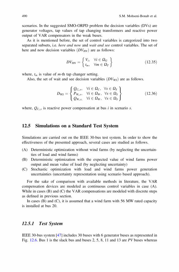
scenarios. In the suggested SMO-ORPD problem the decision variables (DVs) are

generator voltages, tap values of tap changing transformers and reactive power

output of VAR compensators in the weak buses.

As it is mentioned before, the set of control variables is categorized into two

separated subsets, i.e. here and now and wait and see control variables. The set of

here and now decision variables ðDVHNÞ are as follows:

DVHN ¼ Vi; 8i 2 XG

tm; 8m 2 XT

� �

ð12:35Þ

where, tm is value of m-th tap changer setting.

Also, the set of wait and see decision variables ðDVWSÞ are as follows.

DWS ¼QCi;s; 8i 2 XC; 8s 2 XS

PWi;s; 8i 2 XW ; 8s 2 XS

QWi;s; 8i 2 XW ; 8s 2 XS

8

<

:

9

=

;

ð12:36Þ

where, QCi;s is reactive power compensation at bus i in scenario s.

12.5 Simulations on a Standard Test System

Simulations are carried out on the IEEE 30-bus test system. In order to show the

effectiveness of the presented approach, several cases are studied as follows.

(A) Deterministic optimization without wind farms (by neglecting the uncertain-

ties of load and wind farms)

(B) Deterministic optimization with the expected value of wind farms power

output and mean value of load (by neglecting uncertainty)

(C) Stochastic optimization with load and wind farms power generation

uncertainties (uncertainty representation using scenario based approach).

For the sake of comparison with available methods in literature, the VAR

compensation devices are modeled as continuous control variables in case (A).

While in cases (B) and (C) the VAR compensations are modeled with discrete steps

as defined in previous section.

In cases (B) and (C), it is assumed that a wind farm with 56 MW rated capacity

is installed at bus 20.

12.5.1 Test System

IEEE 30-bus system [47] includes 30 buses with 6 generator buses as represented in

Fig. 12.6. Bus 1 is the slack bus and buses 2, 5, 8, 11 and 13 are PV buses whereas


the remaining 24 buses are PQ buses. The network consists of 41 branches, 4

transformers and 9 capacitor banks. Four branches, 6–9, 6–10, 4–12 and 28–27 are

under load tap changing transformers. The tap ratios are within the interval [0.9,

1.1]. Additionally, buses 10, 12, 15, 17, 20, 21, 23, 24 and 29 are selected as shunt

VAR compensation buses.

In each study we have considered two cases regarding the objective functions.

As mentioned in Sect. 12.2, in MO-ORPD problem F1 with F2 and F1 with F3 are

conflicting. Minimization is classified in two part PL/NPL and VD/NVD (Case I) and

PL/ and LM/NLM (Case II). Figure 12.7 shows the case studies conducted in this

chapter. For each case, at first the DMO-ORPD is solved for the sake of comparison

with the existing methods, and then SMO-ORPD is solved to investigate the impact

of uncertainties on the obtained results.

29

System description

30 Buses

41 Branches

21 Load sides

6 Thermal units

9 VAR compensator

4 Tab changer

1 Wind farms

G

C

30

2728

26

25

23 24

15 18

19

14

G

G

G

1720

16

21

22

12

10

1 3 4

2

G

G

C

5 7

6

9

8

11

G

13

C

C

C

C

C

C

C C

Fig. 12.6 One-line diagram of IEEE 30-bus test system


12.5.2 Case-I: Active Power Loss Versus Voltage Deviations

(PL-VD)

12.5.2.1 Solving DMO-ORPD Without WFs

In this case, the Pareto front is attained for IEEE 30-bus test system without

considering any uncertainty and without wind power integration. The VAR com-

pensation devices are modeled by continuous variables for the sake of comparison

with the previously published works in literature. The data of compensation limits

are available in Appendix (Table 12.15). Table 12.1 summarizes the acquired

Pareto solutions for this case. By using min-max fuzzy satisfying criterion, it is

observed from Table 12.1 that the best compromise solution is Solution#16, with

the maximum weakest membership function of 0.7734. The corresponding PL and

VD are equal to 4.4438 MW and 0.0092, respectively. It is also noticeable that

Solution#1 corresponds to the loss minimization case in Solution#1, only PL is

minimized, and the minimum value of PL is obtained 4.2875 MW. The Pareto

optimal front of the two objective functions is depicted in Fig. 12.8. For this

solution, the optimal values of control variables are given in Table 12.2.

12.5.2.2 Solving DMO-ORPD with Expected WFs

According to Fig. 12.6, IEEE-30 bus is modified and it is presupposed that wind

turbine is located in bus 20. In this part, by using Fig. 12.5, the expected value of

wind turbine generation is taken account in simulation. Wind power capacity

MO-ORPD

Case-I

Objective functions:

PL - VD

Case-II

Objective functions:

PL - LM

DM

O-O

RP

D w

ithout

WF

s

DM

O-O

RP

D w

ith e

xpec

ted W

Fs

SM

O-O

RP

D w

ith W

Fs

DM

O-O

RP

D w

ithout

WF

s

DM

O-O

RP

D w

ith e

xpec

ted W

Fs

SM

O-O

RP

D w

ith W

Fs

Fig. 12.7 Illustration of the

studied cases


amounted to twenty percent of the total load on the network is considered. Expected

value of wind farm generation is calculated as:

Pw;exp ¼X

s2XS

ps � fWi;s� Pr

Wi

� �

ð12:37Þ

Table 12.1 Pareto optimal

solutions for DMO-ORPD

without WFs (Case-I)

# PL (MW) VD l1 l2 lr

1 4.2875 0.0387 1 0 0

2 4.2882 0.0367 0.999 0.0521 0.0521

3 4.2904 0.0348 0.9958 0.1047 0.1047

4 4.2944 0.0328 0.990 0.1574 0.1574

5 4.3005 0.0308 0.9811 0.2101 0.2101

6 4.3092 0.0288 0.9686 0.2627 0.2627

7 4.3190 0.0269 0.9543 0.3154 0.3154

8 4.3293 0.0249 0.9395 0.3681 0.3681

9 4.3401 0.0229 0.9238 0.4207 0.4207

10 4.3515 0.0210 0.9072 0.4734 0.4734

11 4.3637 0.0190 0.8896 0.5260 0.5260

12 4.3767 0.0170 0.8706 0.5787 0.5787

13 4.3909 0.0151 0.8501 0.6314 0.6314

14 4.4064 0.0131 0.8276 0.6840 0.6840

15 4.4238 0.0111 0.8024 0.7367 0.7367

16 4.4438 0.0092 0.7734 0.7894 0.7734

17 4.4680 0.0072 0.7384 0.8420 0.7384

18 4.4999 0.0052 0.6921 0.8947 0.6921

19 4.5544 0.0033 0.6132 0.9473 0.6132

20 4.9774 0.0013 0 1 0

0 0.005 0.01 0.015 0.02 0.025 0.03 0.035 0.044.2

4.3

4.4

4.5

4.6

4.7

4.8

4.9

5

X: 0.00916

Y: 4.444

VD

PL

(M

W)

Fig. 12.8 Pareto optimal

front for DMO-ORPD

without WFs (Case-I)


It is explained that, discrete steps for compensation devices is used during this

section based on the data provided in appendix (Table 12.15). Various Pareto

solutions for this part are provided in Table 12.3. In order to solve the

multi-objective ORPD problem by e-constraint method, maximum and minimum

values of the real power loss ðF1Þ and voltage deviation ðF2Þ are considered, whichare equal to 3.8771 MW, 3.1651 MW, 0.0428 pu and 0.0012 pu, respectively.

These extreme values are reached by maximizing and minimizing the objective

functions of MO-ORPD individually. It means that in Solution#1 and #20 the

objectives are minimizing the PL and VD, respectively. Among these optimal

solutions, Solution#16 is minimizing both objectives, with the equal to 3.2983 MW

PL and the VD of 0.0099. Pareto front of answers and control variables for BCS of

this case are reported in Fig. 12.9 and Table 12.4, respectively.

12.5.2.3 Solving SMO-ORPD with WFs

In this case the load and wind power uncertainties are considered in the MO-ORPD

using the previously described two stage stochastic programming approach.

Table 12.2 Optimal control variables for the best compromise solution (Solution#16) in (Case-I)

Control parameters Parameter DMO-ORPD (without WF)

Generator parameters Vg1 (pu) 1.0295

Vg2 (pu) 1.0204

Vg5 (pu) 1.0093

Vg8 (pu) 1.0030

Vg11 (pu) 1.0148

Vg13 (pu) 1.0258

Pg1 (MW) 62.8438

Compensation Qc10 (MVar) 0

Qc12 (MVar) 0

Qc15 (MVar) 3.8495

Qc17 (MVar) 3.6873

Qc20 (MVar) 2.6983

Qc21 (MVar) 6.6481

Qc23 (MVar) 1.7635

Qc24 (MVar) 3.0855

Qc29 (MVar) 2.2464

Transformer tap changer t6-9 0.9706

t6-10 1.1000

t4-12 0.9812

t28-27 0.9970


The attained Pareto optimal solutions in this case are presented in Table 12.5. It is

observed from this table that NPL varies from 3.4003 to 4.1891 MW, while NVD

varies from 0.0431 to 0.0013, respectively. The Solution#1 corresponds to the NPL

minimization case, where the minimum value of 3.4003 MW is obtained for NPL,



with expected WFs (Case-I)

# PL (MW) VD l1 l2 lr

1 3.1651 0.0428 1 0 0

2 3.166 0.0406 0.9987 0.0526 0.0526

3 3.1696 0.0384 0.9937 0.1052 0.1052

4 3.1759 0.0362 0.9849 0.1579 0.1579

5 3.183 0.0340 0.9749 0.2105 0.2105

6 3.1904 0.0318 0.9645 0.2631 0.2631

7 3.1982 0.0296 0.9535 0.3158 0.3158

8 3.2064 0.0275 0.9421 0.3684 0.3684

9 3.215 0.0253 0.9300 0.4210 0.4210

10 3.2241 0.0231 0.9172 0.4737 0.4737

11 3.234 0.0209 0.9032 0.5263 0.5263

12 3.2445 0.0187 0.8886 0.5789 0.5789

13 3.2556 0.0165 0.8729 0.6316 0.6316

14 3.2681 0.0143 0.8553 0.6842 0.6842

15 3.2823 0.0121 0.8355 0.7368 0.7368

16 3.2983 0.0099 0.8129 0.7895 0.7895

17 3.3182 0.0077 0.7850 0.8421 0.7850

18 3.3453 0.0055 0.7470 0.8947 0.7470

19 3.3928 0.0033 0.6801 0.9474 0.6801

20 3.8771 0.0012 0 1 0

0 0.01 0.02 0.03 0.04 0.053.1

3.2

3.3

3.4

3.5

3.6

3.7

3.8

3.9

4

X: 0.00992

Y: 3.298

VD

PL

(M

W)

Fig. 12.9 Pareto front of

DMO-ORPD with WFs

(Case-I)


whereas Solution#20 deals with the case of NVD minimization, in which the min-

imum value of NVD is 0.0431. It is observed from Table 12.5 that Solution#16 is the

best compromise solution, with NPL equals to 3.5475 MW and NVD equals to

0.0101. Also, Fig. 12.10 depicts the obtained optimal Pareto front in this case.

Table 12.6 summarizes the obtained optimal here and now control variables for

the best compromise solution. Also, the optimal values of wait and see control

variables are depicted in Figs. 12.11, 12.12 and 12.13, in all possible scenarios.

Figure 12.11 shows the active power generation at the slack bus (bus 1) in all 15

scenarios. Figure 12.12 represents the active/reactive power output of the wind

farm in all scenarios. The optimal amount of reactive power compensation steps are

also given in Fig. 12.13.

Table 12.4 Optimal control variables for the best compromise solution (Solution#16) in

DMO-ORPD with expected wind-(Case-I)

Control parameters Parameter DMO-ORPD (with WF)


Vg2 (pu) 1.0161

Vg5 (pu) 1.0062

Vg8 (pu) 1.0015

Vg11 (pu) 1.0156

Vg13 (pu) 1.0248

Pg1 (MW) 48.2003

Compensation (switching steps) uc10 0

uc12 0

uc15 1

uc17 2

uc20 1

uc21 3

uc23 1

uc24 3

uc29 1

Wind farms parameters Pw19 (MW) 29.222

Qw19 (MVar) 2.2632


t6-10 1.1000

t4-12 0.9840

t28-27 0.9936



solutions for SMO-ORPD

(Case-I)

# NPL (MW) NLM l1 l2 lr

1 3.4003 0.0431 1 0 0

2 3.4188 0.0409 0.9765 0.0526 0.0526

3 3.4194 0.0387 0.9758 0.1053 0.1053

4 3.4213 0.0365 0.9734 0.1579 0.1579

5 3.4253 0.0343 0.9683 0.2105 0.2105

6 3.4322 0.0321 0.9595 0.2632 0.2632

7 3.4405 0.0299 0.9490 0.3158 0.3158

8 3.4492 0.0277 0.9380 0.3684 0.3684

9 3.4584 0.0255 0.9264 0.4211 0.4211

10 3.4681 0.0233 0.914 0.4737 0.4737

11 3.4785 0.0211 0.9008 0.5263 0.5263

12 3.4897 0.0189 0.8867 0.5790 0.5790

13 3.5018 0.0167 0.8713 0.6316 0.6316

14 3.5152 0.0145 0.8543 0.6842 0.6842

15 3.5302 0.0123 0.8353 0.7368 0.7368

16 3.5475 0.0101 0.8133 0.7895 0.7895

17 3.5687 0.0079 0.7865 0.8421 0.7865

18 3.5949 0.0057 0.7533 0.8947 0.7533

19 3.6396 0.0035 0.6967 0.9474 0.6967

20 4.1891 0.0013 0 1 0

0 0.01 0.02 0.03 0.04 0.053.4

3.5

3.6

3.7

3.8

3.9

4

4.1

4.2

X: 0.01007

Y: 3.548

EVD

EP

L (

MW

)


SMO-ORPD (Case-I)


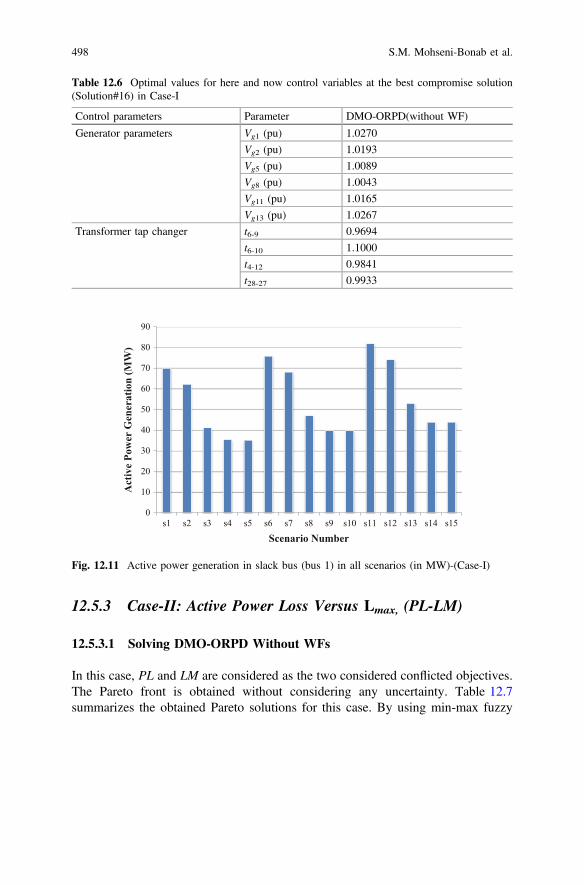
12.5.3 Case-II: Active Power Loss Versus Lmax, (PL-LM)

12.5.3.1 Solving DMO-ORPD Without WFs

In this case, PL and LM are considered as the two considered conflicted objectives.

The Pareto front is obtained without considering any uncertainty. Table 12.7

summarizes the obtained Pareto solutions for this case. By using min-max fuzzy

Table 12.6 Optimal values for here and now control variables at the best compromise solution

(Solution#16) in Case-I

Control parameters Parameter DMO-ORPD(without WF)


Vg2 (pu) 1.0193

Vg5 (pu) 1.0089

Vg8 (pu) 1.0043

Vg11 (pu) 1.0165

Vg13 (pu) 1.0267


t6-10 1.1000

t4-12 0.9841

t28-27 0.9933

0

10

20

30

40

50

60

70

80

90

s1 s2 s3 s4 s5 s6 s7 s8 s9 s10 s11 s12 s13 s14 s15

Acti

ve P

ow

er G

en

erati

on

(M

W)

Scenario Number

Fig. 12.11 Active power generation in slack bus (bus 1) in all scenarios (in MW)-(Case-I)


satisfying method, it is evident from Table 12.7 that the best compromise solution

is Solution#17, with the maximum weakest membership function of 0.7988. The

corresponding PL and LM are equal to 4.6106 MW and 0.1199 pu, respectively.

Pareto front of this case is available in Fig. 12.14. Table 12.8 summarizes the

obtained control variables for the best compromise solution, Solution#17, of this

case.

-5

0

5

10

15

20

25

30

35

40

s1 s2 s2 s3 s4 s5 s6 s7 s8 s9 s10 s11 s12 s13 s14 s15

Win

d F

arm

Act

ive/

Rea

ctiv

e p

ow

er o

utp

ut

Scenario Number

Pw

Qw

Fig. 12.12 Active/reactive power output of wind farm (located at bus 20) in all scenarios (in MW

and MVAR) - (Case-I)

0

1

2

3

4

5


Sw

itch

ing S

tep

Scenario Number

Bus 10

Bus 12

Bus 15

Bus 17

Bus 20

Bus 21

Bus 23

Bus 24

Bus 29

Fig. 12.13 Switching steps in VAR compensation buses at different scenarios (Case-I)


12.5.3.2 Solving DMO-ORPD with Expected WFs

Similar to Case-I, in this case, expected value of wind power as an input power is

calculated by Eq. 12.37. Table 12.9 shows the obtained 20 selected Pareto solu-

tions for this case. Among this answers, Solution#17 has minimized both objective

simultaneously with PL = 3.2751 and LM = 0.1146. Figure 12.15 depicts the



without WFs (Case-II)

# PL (MW) LM l1 l2 lr

1 4.2875 0.1323 1 0 0

2 4.2879 0.1315 0.9997 0.0526 0.0526

3 4.2893 0.1308 0.9989 0.1053 0.1053

4 4.2918 0.1300 0.9973 0.1579 0.1579

5 4.2956 0.1292 0.9949 0.2105 0.2105

6 4.3012 0.1284 0.9915 0.2632 0.2632

7 4.3087 0.1277 0.9868 0.3158 0.3158

8 4.3187 0.1269 0.9806 0.3684 0.3684

9 4.3318 0.1261 0.9724 0.4210 0.4210

10 4.3475 0.1253 0.9626 0.4737 0.4737

11 4.3659 0.1246 0.9512 0.5263 0.5263

12 4.3869 0.1238 0.9381 0.5789 0.5789

13 4.4105 0.1230 0.9234 0.6316 0.6316

14 4.4403 0.1222 0.9048 0.6842 0.6842

15 4.4835 0.1215 0.8779 0.7368 0.7368

16 4.5413 0.1207 0.8420 0.7895 0.7895

17 4.6106 0.1199 0.7988 0.8421 0.7988

18 4.7219 0.1191 0.7295 0.8947 0.7295

19 5.0212 0.1184 0.5431 0.9474 0.5431

20 5.8934 0.1176 0 1 0

0.118 0.12 0.122 0.124 0.126 0.128 0.13 0.1324.2

4.4

4.6

4.8

5

5.2

5.4

5.6

5.8

6

X: 0.1199

Y: 4.611

Lmax

PL

(M

W)


DMO-ORPD without WFs

(Case-II)


Pareto front of this case. According to Fig. 12.15, it is clear that when wind power

injected into the network, it substantially reduces network losses and increases

network stability. Table 12.10 presents the obtained control variables for best

solution of this case (Solution#17).

12.5.3.3 Solving SMO-ORPD with WFs

The uncertainty is modeled using scenario based approach for Case-II and results of

Pareto solutions are presented in Table 12.11. Figure 12.16 shows the Pareto front

for Case-II with considering load and wind uncertainties using scenario based

approach.

Similar to Case-I, here and now control variables are shown in Table 12.12 and

wait and see control variables are shown in Figs. 12.17, 12.18 and 12.19. It should

be noticed that, these variables are presented for BCS (Solution#16).

Table 12.8 Optimal control variables for the best compromise solution (Solution#17) in

DMO-ORPD without wind-Case-II



Vg2 (pu) 1.0286

Vg5 (pu) 1.0182

Vg8 (pu) 1.0134

Vg11 (pu) 1.0110

Vg13 (pu) 1.0434

Pg1 (MW) 63.0106

Compensation Qc10 (MVar) 8.2754

Qc12 (MVar) 0

Qc15 (MVar) 0

Qc17 (MVar) 7.0185

Qc20 (MVar) 4.0128

Qc21 (MVar) 14.2677

Qc23 (MVar) 2.9065

Qc24 (MVar) 7.7563

Qc29 (MVar) 0


t6-10 0.9000

t4-12 0.9956

t28-27 0.9719




with expected WFs (Case-II)

# PL (MW) LM l1 l2 lr

1 3.1651 0.1247 1 0 0

2 3.1654 0.1241 0.9994 0.0526 0.0526

3 3.1662 0.1234 0.9979 0.1053 0.1053

4 3.1682 0.1228 0.9943 0.1579 0.1579

5 3.1707 0.1222 0.9895 0.2105 0.2105

6 3.1742 0.1215 0.9832 0.2632 0.2632

7 3.1786 0.1209 0.9749 0.3158 0.3158

8 3.1841 0.1203 0.9647 0.3684 0.3684

9 3.1905 0.1196 0.9528 0.4210 0.4210

10 3.1977 0.1190 0.9395 0.4737 0.4737

11 3.2056 0.1184 0.9247 0.5263 0.5263

12 3.2144 0.1178 0.9084 0.5789 0.5789

13 3.2242 0.1171 0.8901 0.6316 0.6316

14 3.235 0.1165 0.8700 0.6842 0.6842

15 3.2468 0.1159 0.8481 0.7368 0.7368

16 3.2597 0.1152 0.8241 0.7895 0.7895

17 3.2751 0.1146 0.7955 0.8421 0.7955

18 3.2944 0.1140 0.7594 0.8947 0.7594

19 3.3189 0.1133 0.7139 0.9473 0.7139

20 3.7027 0.1127 0 1 0

0.112 0.114 0.116 0.118 0.12 0.122 0.124

3.1

3.2

3.3

3.4

3.5

3.6

3.7

X: 0.1146

Y: 3.275

Lmax

PL

(M

W)


DMO-ORPD with WFs

(Case-II)


12.6 Discussions on the Results

12.6.1 Comparison of DMO-ORPD Performance

with Pervious Literature

In Tables 12.13 and 12.14 the obtained PL, VD and LM are compared with the

results reported by some recently published algorithms. Table 12.13 shows the

obtained PL and VD for Solution#1 (PL minimization), Solution#20 (VD mini-

mization), and Solution#16 (compromise solution), whereas Table 12.14 give a

comparison for PL and LM. Solution#1 (PL minimization), Solution#20 (LM

minimization), and Solution#17 (compromise solution) are compared with recently

published works. According to these tables, it can be observed that the obtained

Table 12.10 Optimal control variables for the best compromise solution (Solution#17) in Case-II

Control parameters Parameter DMO-ORPD (with WF)


Vg2 (pu) 1.0301

Vg5 (pu) 1.0204

Vg8 (pu) 1.0161

Vg11 (pu) 1.0136

Vg13 (pu) 1.0461

Pg1 (MW) 49.3914

Compensation

(switching steps)

uc10 0

uc12 0

uc15 1

uc17 2

uc20 1

uc21 4

uc23 1

uc24 3

uc29 1

Wind Farms parameters Pw20 (MW) 29.2220

Qw20 (MVar) 2.4846


t6-10 0.9000

t4-12 0.9930

t28-27 0.9761



solutions for SMO-ORPD)

(Case-II)

# NPL (MW) NLM l1 l2 lr

1 3.4815 0.1258 1 0 0

2 3.4865 0.1251 0.9915 0.0635 0.0635

3 3.4881 0.1245 0.9887 0.1264 0.1264

4 3.4914 0.1239 0.9831 0.1890 0.1890

5 3.4918 0.1233 0.9824 0.2513 0.2513

6 3.4942 0.1227 0.9783 0.3131 0.3131

7 3.4989 0.1221 0.9702 0.3745 0.3745

8 3.5048 0.1215 0.9601 0.4352 0.4352

9 3.5118 0.1209 0.9481 0.4952 0.4952

10 3.5196 0.1204 0.9347 0.5541 0.5541

11 3.5279 0.1198 0.9204 0.6117 0.6117

12 3.5375 0.1193 0.9040 0.6675 0.6675

13 3.5485 0.1188 0.8851 0.7208 0.7208

14 3.5602 0.1183 0.8650 0.7703 0.7703

15 3.573 0.1179 0.8431 0.8143 0.8143

16 3.5873 0.1175 0.8187 0.8488 0.8187

17 3.6039 0.1174 0.7901 0.8658 0.7901

18 3.6214 0.1172 0.7600 0.8863 0.7600

19 3.6399 0.1171 0.7283 0.8942 0.7283

20 4.0646 0.1161 0 1 0

0.116 0.118 0.12 0.122 0.124 0.1263.4

3.5

3.6

3.7

3.8

3.9

4

4.1

4.2

X: 0.1175

Y: 3.587

ELmax

EP

L (

MW

)


SMO-ORPD (Case-II)


solutions are superior to the previously reported ones like as gravitational search

algorithm (GSA) [17], differential evolutionary algorithm [15], quasi-oppositional

teaching learning based optimization (TLBO) algorithm [25] and chaotic parallel

vector evaluated interactive honey bee mating optimization (CPVEIHBMO) [26].

Table 12.12 Optimal values for here and now control variables at the best compromise solution

(Solution#16) in Case-II



Vg2 (pu) 0.9976

Vg5 (pu) 1.0083

Vg8 (pu) 1.0092

Vg11 (pu) 1.0246

Vg13 (pu) 1.0398


t6-10 0.9000

t4-12 0.9821

t28-27 0.9698

0

20

40

60

80

100

120

140

160

180

200


Act

ive

Po

wer

Gen

era

tio

n (

MW

)

Scenario Number

Fig. 12.17 Active power generation in slack bus (bus 1) in all scenarios (in MW)-(Case-II)


-20

-10

0

10

20

30

40

50

60


Win

d F

arm

Act

ive/

Rea

ctiv

e p

ow

er o

utp

ut

Scenario Number

Pw

Qw

Fig. 12.18 Active and reactive power output of wind farm (located at bus 20) in all scenarios (in

MW and MVAR)—(Case-II)

0

1

2

3

4

5


Sw

itch

ing S

tep

Scenario Number

Bus 10

Bus 12

Bus 15

Bus 17

Bus 20

Bus 21

Bus 23

Bus 24

Bus 29

Fig. 12.19 Switching steps in VAR compensation buses at different scenarios (Case-II)


12.6.2 Impact of Wind Energy on MO-ORPD Problem

Figures 12.20 and 12.21 summarize the obtained results of DMO-ORPD with and

without WFs and SMO-ORPD for both Case-I and Case-II. According to

Fig. 12.20a, it is clear that by installing wind farms on the system, real power losses

(PL in deterministic and EPL in stochastic model) are reduced considerably. It is

also observed from this figure that in the case of SMO-ORPD, the EPL is higher

than the case of DMO-ORPD with expected wind. Besides, Fig. 12.20b depicts the

obtained values for VD and EVD in both Case-I and II. It is evidently observed from

this figure that, installation of wind farm leads to deterioration of voltage deviations,

especially in the case of SMO-OPRD. This is mainly because of fluctuations of

wind farm output power, in different scenarios.

Also, Fig. 12.21 shows the obtained values of PL (and EPL) along with Lmax

(and ELM) in Case-II. According to Fig. 12.21a active power losses are decreased

when the wind farm is considered, both in DMO-ORPD (with wind farm) and

SMO-ORPD. Besides, according to Fig. 12.21b the voltage stability of system

increases in the presence of wind farm, since the Lmax and ELM reduced in both

DMO-ORPD (with wind farm) and SMO-ORPD cases.

Table 12.13 Comparison of the obtained PL and VD in DMO-ORPD (without WFs), with the

published methods

PL

Minimization

VD

Minimization

PL (MW)

Compromise solution

Proposed 4.2875 4.9774 4.4438

CPVEIHBMO [26] 4.37831 4.994831 5.3243

HBMO [26] 4.40867 5.2092 5.535

QOTLBO [25] 4.5594 6.4962 5.2594

NSGA-II [27] 5.137 5.686 –

DE [15] 4.555 6.4755 –

SPMGSO [27] 5.123 5.96 –

GSA [17] 4.5143 4.9752 –

PL

minimization

VD

minimization

VD (pu)

Compromise solution

Proposed 0.0387 0.0013 0.0092

CPVEIHBMO [26] 0.67352 0.198756 0.7397

HBMO [26] 0.87364 0.2106 0.87664

QOTLBO [25] 1.9057 0.0856 0.121

NSGA-II [27] 0.6443 0.1789 –

DE [15] 1.9989 0.0911 –

SPMGSO [27] 0.73986 0.1438 –

GSA [17] 0.8752 0.2157 –


The obtained results imply the positive impact of wind power generation on the

voltage stability enhancement and decreasing system real power losses. Also, it can

be observed that the installed wind farm has little effects on the voltage deviations.

Table 12.14 Comparison of the obtained PL and LM in DMO-ORPD (without WFs), with the

published methods

PL

minimization

LM

minimization

PL (MW)

Compromise solution

Proposed 4.2875 5.8934 4.6106

CPVEIHBMO [26] 4.7831 6.6501 5.3243

HBMO [26] 4.40867 6.66 5.5352

QOTLBO [25] 4.5594 5.2554 5.2594

MOCIPSO [24] 5.174 5.419 5.232

MOPSO [24] 5.233 5.528 5.308

DE [15] 4.555 7.0733 –

RGA [22] 4.951 5.0912 –

CMAES [22] 4.945 5.129 –

GSA [17] 4.5143 6.6602 –

PL

minimization

LM

minimization

LM (pu)

Compromise solution

Proposed 0.1323 0.1176 0.1199

CPVEIHBMO [26] 0.141 0.116 -

HBMO [26] 0.12101 0.111 0.1163

QOTLBO [25] 0.1263 0.1147 0.1203

MOCIPSO [24] 0.1273 0.1242 0.1254

MOPSO [24] 0.12664 0.1141 11.821

DE [15] 0.1317 0.1192 0.12191

RGA [22] 0.5513 0.1246 –

CMAES [22] 0.13965 0.1386 –

GSA [17] 0.13944 0.1382 –


0

1

2

3

4

5

6

PL minimization VD minimization Compromise solution

DMO-ORPD (without WFs)

DMO-ORPD (with WFs)

SMO-ORPD (with WFs)

0

0.005

0.01

0.015

0.02

0.025

0.03

0.035

0.04

0.045

0.05

PL minimization VD minimization Compromise solution


DMO-ORPD (with WFs)

SMO-ORPD (with WFs)

(a)

(b)

Fig. 12.20 Comparison of

the obtained results of Case-I

in different conditions, a PL

and EPL (MW), b VD and

EVD (pu)

0

1

2

3

4

5

6

7

PL minimization LMax minimization Compromise solution


DMO-ORPD (with WFs)

SMO-ORPD (with WFs)

0.1

0.105

0.11

0.115

0.12

0.125

0.13

0.135

PL minimization LMax minimization Compromise solution


DMO-ORPD (with WFs)

SMO-ORPD (with WFs)

(a)

(b)

Fig. 12.21 Comparison of

the obtained results of Case-II

in different conditions, a PL

and EPL (MW), b LM and

ELmax


12.7 Conclusions

In this chapter the stochastic multi-objective optimal reactive power dispatch

(SMO-ORPD) problem in a wind integrated power system is studied by considering

the uncertainties of system load and wind power generations. For decision making

under the above uncertainties two-stage stochastic optimization model is utilized. In

the multi-objective optimization framework real power losses, voltage deviation

and voltage stability improvement index (L-index) are optimized simultaneously.

The e-constraint method is utilized to solve multi-objective optimization problem.

The obtained results in the deterministic case are compared with the recently

applied intelligent search-based algorithms and it is found that the suggested

method can find better solutions for both objective functions in this case.

In the stochastic case, a comprehensive set of decision variables including here

and now and wait and see control variables are obtained. The offered SMO-ORPD

model is verified using the IEEE 30-bus test system. The numerical results sub-

stantiate that in the presence of wind power generation, the expected value of active

power losses and L-index are reduced in comparison with the deterministic case.

This confirms the positive influence of wind power generation on the reduction of

system losses.

Appendix

See Table 12.15.

Table 12.15 The data of VAR Compensation devices

Bus No. DMO-ORPD without WFs [26, 47] DMO-ORPDwith WFs

SMO-ORPD with WFs

QminCi

(MVAR) QmaxCi

(MVAR) IminCi

ImaxCi

QCi(MVAR)

10 0 36 0 1 1

12 0 36 0 3 1.5

15 0 36 0 1 1.5

17 0 36 0 2 2

20 0 36 0 1 0.5

21 0 36 0 4 2

23 0 36 0 1 1

24 0 36 0 3 1.5

29 0 36 0 1 0.5


References

1. B. Zhao, C. Guo, Y. Cao, A Multiagent-Based Particle Swarm Optimization Approach

for Optimal Reactive Power Dispatch, IEEE Transactions on Power Systems, vol. 20,

pp. 1070–1078, 2005.

2. C. Dai, W. Chen, Y. Zhu, X. Zhang, Seeker Optimization Algorithm for Optimal Reactive

Power Dispatch, IEEE Transactions on Power Systems, vol. 24, pp. 1218–1231, 2009.

3. A. Khorsandi, A. Alimardani, B. Vahidi, S. Hosseinian, Hybrid Shuffled Frog Leaping

Algorithm and Nelder-Mead Simplex Search for Optimal Reactive Power Dispatch, IET

Generation, Transmission & Distribution, vol. 5, pp. 249–256, 2011.

4. M. Ghasemi, S. Ghavidel, M.M. Ghanbarian, A. Habibi, A New Hybrid Algorithm for

Optimal Reactive Power Dispatch Problem with Discrete and Continuous Control Variables,

Applied Soft Computing vol. 22, pp. 126–40, 2014.

5. M. Ghasemi, M.M. Ghanbarian, S. Ghavidel, S. Rahmani, E. Mahboubi Moghaddam,

Modified Teaching Learning Algorithm and Double Differential Evolution Algorithm for

Optimal Reactive Power Dispatch Problem: A Comparative Study, Information Sciences, vol.

278, pp. 231–249, 2014.

6. M. Martinez Rojas, A. Sumper, O. Gomis Bellmunt, A. Sudria Andreu, Reactive Power

Dispatch in Wind Farms Using Particle Swarm Optimization Technique and Feasible

Solutions Search, Applied Energy, vol. 88, pp. 4678–4686, 2011.

7. R. Mallipeddi, S. Jeyadevi, P.N. Suganthan, S. Baskar, Efficient Constraint Handling for

Optimal Reactive Power Dispatch Problems, Swarm and Evolutionary Computation, vol. 5,

pp. 28–36, 2012.

8. C.M. Huang, S.J. Chen, Y.C. Huang, H.T. Yang, Comparative Study of Evolutionary

Computation Methods for Active-Reactive Power Dispatch, IET Generation, Transmission &

Distribution, vol. 6, pp. 636–645, 2012.

9. A. Rajan, T. Malakar, Optimal Reactive Power Dispatch Using Hybrid Nelder-Mead Simplex

Based Firefly Algorithm, International Journal of Electrical Power & Energy Systems, vol. 66,

pp. 9–24, 2015.

10. R.P. Singh, V. Mukherjee, S. Ghoshal, Optimal Reactive Power Dispatch by Particle Swarm

Optimization with an Aging Leader and Challengers, Applied Soft Computing, vol. 29,

pp. 298–309, 2015.

11. M.H. Sulaiman, Z. Mustaffa, M.R. Mohamed, O. Aliman, Using the Gray Wolf Optimizer for

Solving Optimal Reactive Power Dispatch Problem, Applied Soft Computing, vol. 32,

pp. 286–292, 2015.

12. D. Thukaram, G. Yesuratnam, Optimal Reactive Power Dispatch in a Large Power System

with AC-DC and FACTS Controllers, Generation, Transmission & Distribution, IET, vol. 2,

pp. 71–81, 2008.

13. A. Rabiee, M. Vanouni, M. Parniani, Optimal Reactive Power Dispatch for Improving

Voltage Stability Margin Using a Local Voltage Stability Index, Energy Conversion and

Management, vol. 59, pp. 66–73, 2012.

14. C. Dai, W. Chen, Y. Zhu, and X. Zhang, Reactive Power Dispatch Considering Voltage

Stability with Seeker Optimization Algorithm, Electric Power Systems Research, vol. 79,

pp. 1462–1471, 2009.

15. A. Ela, M. Abido, S. Spea, Differential Evolution Algorithm for Optimal Reactive Power

Dispatch, Electric Power Systems Research, vol. 81, pp. 458–464, 2011.

16. A. Khazali, M. Kalantar, Optimal Reactive Power Dispatch Based on Harmony Search

Algorithm, International Journal of Electrical Power & Energy Systems, vol. 33, pp. 684–692,

2011.

17. S. Duman, Y. Sonmez, U. Guvenc, N. Yorukeren, Optimal Reactive Power Dispatch Using a

Gravitational Search Algorithm, IET Generation, Transmission & Distribution, vol. 6,

pp. 563–576, 2012.


18. J.M. Ramirez, J.M. Gonzalez, T.O. Ruben, An Investigation about the Impact of the Optimal

Reactive Power Dispatch Solved by DE, International Journal of Electrical Power & Energy

Systems, vol. 33, pp. 236–244, 2011.

19. E.M. Soler, E.N. Asada, G.R. Da Costa, Penalty-Based Nonlinear Solver for Optimal

Reactive Power Dispatch with Discrete Controls, IEEE Transactions on Power Systems, vol.

28, pp. 2174–2182, 2013.

20. M. Abido, J. Bakhashwain, Optimal VAR Dispatch Using a Multi-Objective Evolutionary

Algorithm, International Journal of Electrical Power & Energy Systems, vol. 27, pp. 13–20,

2005.

21. L. Zhihuan, L. Yinhong, D. Xianzhong, Non-Dominated Sorting Genetic Algorithm-II for

Robust Multi-Objective Optimal Reactive Power Dispatch, Generation, Transmission &

Distribution, IET, vol. 4, pp. 1000–1008, 2010.

22. S. Jeyadevi, S. Baskar, C. Babulal, M. Willjuice Iruthayarajan, Solving Multi-Objective

Optimal Reactive Power Dispatch Using Modified NSGA-II, International Journal of

Electrical Power & Energy Systems, vol. 33, pp. 219–228, 2011.

23. A. Saraswat, A. Saini, Multi-Objective Optimal Reactive Power Dispatch Considering

Voltage Stability in Power Systems Using HFMOEA, Engineering Applications of Artificial

Intelligence, vol. 26, pp. 390–404, 2013.

24. G. Chen, L. Liu, P. Song, Y. Du, Chaotic Improved PSO-Based Multi-Objective Optimization

for Minimization of Power Losses and L Index in Power Systems, Energy Conversion and


25. B. Mandal, P.K. Roy, Optimal Reactive Power Dispatch Using Quasi-Oppositional Teaching

Learning Based Optimization, International Journal of Electrical Power & Energy Systems,

vol. 53, pp. 123–134, 2013.

26. A. Ghasemi, K. Valipour, A. Tohidi, Multi-Objective Optimal Reactive Power Dispatch

Using a New Multi-Objective Strategy, International Journal of Electrical Power & Energy

Systems, vol. 57, pp. 318–334, 2014.

27. B. Zhou, K. Chan, T. Yu, H. Wei, J. Tang, Strength Pareto Multi-Group Search Optimizer for

Multi-Objective Optimal VAR Dispatch, IEEE Transactions on Industrial Informatics, vol.

10, pp. 1012–1022, 2014.

28. Z. Hu, X. Wang, G. Taylor, Stochastic Optimal Reactive Power Dispatch: Formulation and

Solution Method, International Journal of Electrical Power & Energy Systems, vol. 32,

pp. 615–621, 2010.

29. S. M. Mohseni Bonab, A. Rabiee, S. Jalilzadeh, B. Mohammadi Ivatloo, and S. Nojavan,

“Probabilistic Multi Objective Optimal Reactive Power Dispatch Considering Load

Uncertainties Using Monte Carlo Simulations, Journal of Operation and Automation in

Power Engineering, vol. 3(1), pp. 83–93, 2015.

30. S. M. Mohseni Bonab, A. Rabiee, B. Mohammadi Ivatloo, Load Uncertainty Analysis in

Multi Objective Optimal Reactive Power Dispatch Considering Voltage Stability, Majlesi

Journal of Energy Management, vol. 4(2), pp. 23–30, 2015.

31. A. Brooke, D. Kendrick, A. Meeraus, GAMS Release 2.25: A User’s Guide: GAMS

Development Corporation Washington, DC, 1996.

32. P.E. Gill, W. Murray, M.A. Saunders, SNOPT: An SQP Algorithm for Large-Scale

Constrained Optimization, SIAM Journal on Optimization, vol. 12, pp. 979–1006, 2002.

33. The GAMS Software Website, http://www.gams.com/dd/docs/solvers/sbb.pdf, 2013.

34. A. Soroudi, T. Amraee, Decision Making under Uncertainty in Energy Systems: State of the

Art, Renewable and Sustainable Energy Reviews, vol. 28, pp. 376–384, 2013.

35. A. Rabiee, A. Soroudi, B. Mohammadi Ivatloo, M. Parniani, Corrective Voltage Control

Scheme Considering Demand Response and Stochastic Wind Power, IEEE Transactions on

Power Systems, vol. 29, pp. 2965–2973, 2014.

36. A. Soroudi, B. Mohammadi Ivatloo, A. Rabiee, Energy Hub Management with Intermittent

Wind Power, in Large Scale Renewable Power Generation, Springer, pp. 413–438, 2014.


http://www.gams.com/dd/docs/solvers/sbb.pdf

37. A. Rabiee, A. Soroudi, Stochastic Multiperiod OPF Model of Power Systems with

HVDC-Connected Intermittent Wind Power Generation, IEEE Transactions on Power

Delivery, vol. 29, pp. 336–344, 2014.

38. A. Soroudi, A. Rabiee, A. Keane, Stochastic Real-Time Scheduling of Wind-Thermal

Generation Units in an Electric Utility, IEEE System Journal, 2014.

39. R.D. Zimmerman, C.E. Murillo Sanchez, D. Gan, A MATLAB Power System Simulation

Package, 2005.

40. S. Wen, H. Lan, Q. Fu, D. Yu, L. Zhang, Economic Allocation for Energy Storage System

Considering Wind Power Distribution, IEEE Transactions on power Systems, vol. 30(2),

pp. 644–52, 2015.

41. C.A. Canizares, Voltage Stability Assessment: Concepts, Practices and Tools, Power System

Stability Subcommittee Special Publication IEEE/PES, thunderbox.uwaterloo.

ca/*claudio/claudio.html#VSWG, 2002.

42. F. Jabbari, B. Mohammadi Ivatloo, Static Voltage Stability Assessment Using Probabilistic

Power Flow to Determine the Critical PQ Buses, Majlesi Journal of Electrical Engineering,

vol. 8, pp. 17–25, 2014.

43. H. Xiong, H. Cheng, H. Li, Optimal Reactive Power Flow Incorporating Static Voltage

Stability Based on Multi-Objective Adaptive Immune Algorithm, Energy Conversion and


44. R. Raghunatha, R. Ramanujam, K. Parthasarathy, D. Thukaram, Optimal Static Voltage

Stability Improvement Using a Numerically Stable SLP Algorithm, for Real Time

Applications, International Journal of Electrical Power & Energy Systems, vol. 21,

pp. 289–297, 1999.

45. X. Wang, Y. Gong, C. Jiang, Regional Carbon Emission Management Based on Probabilistic

Power Flow with Correlated Stochastic Variables, IEEE Transactions on Power Systems, vol.

30, pp. 1094–1103, 2014.

46. M. Alipour, B. Mohammadi Ivatloo, K. Zare, Stochastic Risk-Constrained Short-Term

Scheduling of Industrial Cogeneration Systems in the Presence of Demand Response

Programs, Applied Energy, vol. 136, pp. 393–404, 2014.

47. R.D. Zimmerman, C.E. Murillo Sanchez, R.J. Thomas, MATPOWER: Steady-State

Operations, Planning, and Analysis Tools for Power Systems Research and Education,

IEEE Transactions on Power Systems, vol. 26, pp. 12–19, 2011.


Part III

Challenges, Solutions and Applications inAC Power Systems

Chapter 13

Self-excited Induction Generator

in Remote Site

Ezzeddine Touti, Remus Pusca, J. Francois Brudny

and Abdelkader Chaari

Abstract This chapter is devoted to the analysis of a self-excited asynchronous

generator working in autonomous generation mode. It proposes a method of

detection of the generator operating points and the control procedures which makes

it possible to maintain quasi constant the frequency values. These strategies prevent

the disengagement of the generator and use a Thyristor Controlled Reactor to

regulate the reactive power. The control strategies present the study of the fre-

quency in the steady case by the use of an appropriate single phase equivalent

circuit. The space vector formalism is also used to study the transitory and steady

output signals. At the end of the chapter, one will discuss the experimental vali-

dation of theoretical and numerical results.

13.1 Introduction

During the last decades, due to technological and industrial developments which

impose the continuous demand of energy and when the cost of different types of

energy increase, the efforts were continued to look for other solutions to diversify

alternative energy sources. In this context, the wind energy seems to be a promising

alternative source which can accompany the classical energy sources [1, 2]. The use

E. Touti (&)

University of Northern Border, Arar, Saudi Arabia


R. Pusca � J.F. BrudnyLSEE, University of Artois, Bethune, France


J.F. Brudny


A. Chaari

Taha Hussein, University of Tunis, Tunis, Tunisia





517

of wind turbines is an attractive solution because they can provide energy at a

competitive price and mainly it does not cause environmental contamination [3].

The work presented in this chapter treats the study of a three-phase Self-excited

Induction Generator (SEIG) generating power in remote site. The strategy presented

allows the regulation of the reactive power. Consequently it enables the maintaining

of the frequency at quasi constant values.

Including Induction Machine (IM) in the wind generator, in the cases of limited

electric power demand, becomes more and more expanded which explain their

increased use in the electrical energy generation [3–6]. The IM is widely used

because of its robustness, reliability, low cost and little maintenance [7–9].

Nevertheless, these types of generators require an external supply on reactive power

needed for the machine magnetization and to establish the remnant rotating mag-

netic flux wave [10, 11]. In the case of Induction Generator (IG) connected at the

grid, the IM use current drawn from the grid to creates the magnetic field.

In remote site, the IG can operate in autonomous mode only when capacitors are

connected at its stator terminals to produce the necessary reactive power for

machine but also for its load.

The Self-excited Induction Generator (SEIG) has been discovered for a few

decades and was experienced at several remote sites, but the wave quality is not

optimized. Also, one encounters difficulties such as frequency and voltage control

[12, 13]. These difficulties are due to the inverse nature of the problem when no

theory is available to describe the system. Indeed in this working mode the voltage,

the frequency and the rotor sleep are unknown.

In order to overcome these difficulties and to increase robustness of regulation

system this chapter presents a control law established for a resistive-inductive load

supplied by a SEIG and which can be considered as a preliminary study for an

electrical motors load. When a ‘real’ load is presented the difficulty consist in

adapting the control low, because during the regulation an important transient state

appears. In this regard, it is assumed that L will be maintained constant and that the

voltage regulation will be realized acting only on R load.

This chapter presents the theoretical background of output voltage and frequency

regulation for autonomous induction generators. It covers the analysis, modeling

and simulation of an isolated self-excited induction generator working in remote

site. Indeed, we are interested in the studying of a system able to vary the

C capacitor when the SEIG supplies a resistive-inductive load (R–L). It suffices to

parallel connect a fixed capacitor CM and a regulating inductive load (LR) connected

to the isolated network via a dimmer. This system will control the reactive power

consumption variation. The total reactive power is delivered by fixed capacitor CM

and can be variable and so adjustable continuously by means of the TCR and the

regulating inductive load.

One treats, in the first section, the steady state analysis of IM. This study is based

on a single phase equivalent circuit definition while considering the concept of

voltage source. One will discuss subsequently the developed frequency control law.

The operating points of the SEIG are fixed such that they give rated output at the

rated conditions of voltage, current and speed. The objective of the various

518 E. Touti et al.

developments presented is to determine the exact operating points, and for that it is

proposed to use as mathematical solution an iterative (Newton-Raphson) method or

a graphical approach. The self-excited induction generator modeling based on space

phasor formalism is treated in the second section. Subsequently, one presents the

analysis of the control law effectiveness in the steady and transient state cases. In a

standalone SEIG, the capacitors connected across the SEIG terminals can supply

the reactive power requested by the SEIG as well as the load.

In the next part of this chapter, is presented the reactive power control strategy

and the operating intervals imposed on the dimmer to stabilize the frequency. The

dimmer allows the capacitors value variation across the machine terminals.

13.2 Proposed Autonomous Configuration

Figure 13.1 presents the global SEIG system configuration proposed for operating

in remote site. Considering the wind as a prime mover, this asynchronous generator,

which works in autonomous mode, will provide electrical power to supply a

R–L load.

In this configuration the capacitor bank allows to provide the reactive power

needed for generator magnetization [14–17] as well as the load. This section starts

by studying the induction machine and its modeling. To establish the model of the

asynchronous machine, we adopt the following simplifying hypotheses:

– The air gap has a uniform thickness by neglecting the slotting effects and

saturation effects

– The winding resistances does not vary with temperature,

Fig. 13.1 Global diagram configuration of an isolated SEIG

13 Self-excited Induction Generator in Remote Site 519

– The iron losses are neglected.

– It is admitted that the magnetomotive force, which is created by each phase of

the stator and rotor, has a sinusoidal spatial distribution along the air gap.

These assumptions lead to consider a constant inductance. However, the mutual

inductances between the stator and rotor windings are variable according to a

sinusoidal law and depend on the electrical angle of their magnetic axes.

Figure 13.2 represents the asynchronous machine in the electrical space (real

variables reference). This figure shows a three phase nafictitious winding. They are

distributed as the rotor windings of the reel coil in the objective of taking account of

the self-excitation phenomenon.

13.2.1 Space Vector Concept

Space vector is used in order to overcome the difficulties of the working with three

variables by simplifying the mathematical formulation through only two variables

[18]. Hence, a view of the rotational dynamics is improved using the space vector

formalism. Consequently, one joins at three variables x1, x2 and x3 which belong to

the assembly of real numbers, a complex number called vector of direct and inverse

components. In a fixed reference, one can express this vector, denoted �x, using the

given relationship

Fig. 13.2 Representation of the machine statoric and rotoric windings

520 E. Touti et al.

�x ¼ xd þ jxq ¼ 2=3ð Þ 1þ aþ a2� �

x1 x2 x3½ �t ð13:1Þ

where a ¼ ej2p=3 is a rotational operator.

One will consider a moving reference with rotational angle h. This vector

denoted �X presented in Fig. 13.3 is given using the following equation

�X ¼ XD þ jXQ ¼ �x e�jh ð13:2Þ

In the case of the study of a time derivative, following equation must be used

e�jh d�x

dt¼ jx0ð Þ�Xþ d�X

dtð13:3Þ

13.2.2 Induction Generator Model

The real machines, with their different kinds of windings and geometries, are too

complex to lend itself to an analysis taking into account their exact configurations,

hence the need to develop a model whose behavior is as close as possible to that of

the original [19, 20]. In this context, it is essential to use a simple model to facilitate

digital implementation and minimize the simulator computation time.

Through a numerical implementation of the SEIG model based on the space

vector, one can study its steady and transient state. This study concerns a

three-phase induction machine with p pole pair cage rotor. One will confuse the

rotor and stator spatial reference (d r and d s) with the rotor and stator phase 1 axes.

The asynchronous generator must have a rotor residual magnetic field [21, 22], to

produce the stator voltage. Let us consider a fictitious na winding to create this

Fig. 13.3 Changing of reference frame


magnetic field during the SEIG start-up step. These coils of na turns are considered

supplied by iaq DC currents (q = 1, 2 or 3). These all currents are null after the

start-up step. The stator space vector variables referred to d s are denoted �xs. Also,

one will denote �xr the rotor space vector variables defined relatively to d r. The

stator space vector variables defined relatively to d r are labelled �x0s. One can deduce�x0s from �xs using variable change: �x0 s ¼ �xs expð�jhÞ where: h ¼ h0 þx0t representsthe spatial angular gap between d r and d s, also x0 ¼ pX0 where X0 is the machine

rotor angular speed. The asynchronous generator is characterized by the voltage

equations written in the rotor reference frame which are expressed by the following

system

�v0s ¼ rs�i0s þ ddt�u0s þ jx0�u0s

�vr ¼ rr�i r þ ddt�ur

�va ¼ ra�i a þ ddt�ua

8

<

:

ð13:4Þ

The per phase winding resistances, in system (13.4), are represented by

r. Whereas the fluxes linked by the rotor, the stator and the fictitious windings are

labeled �u0s, �ur and �ua. They are given by

�ur ¼ Lrð1þ krÞ�ir þMrs�i0s þMra�ia

�ua ¼ Lað1þ kaÞ�ia þMas�i0s þMar�ir

�u0s ¼ Lsð1þ ksÞ�i0s þMsr�ir þMsa�ia

8

<

:

ð13:5Þ

To take into account the remnant flux, one use ka ¼ la=La to characterize the

fictitious windings leakage inductance. Msr, Msa and Mra are the mutual induc-

tances between the stator, the rotor and the fictitious windings (it is considered that

Msr ¼ Mrs, Msa ¼ Mas and Mra ¼ Mar). The L quantities given in (13.5) represent

the main winding cyclic inductances, whereas the cyclic mutual inductances

between various windings are denoted M:kr and ks are expressed by: kr ¼ lr=Lr

and ks ¼ ls=Ls where lr and ls represent respectively the rotoric and the statoric

leakage inductances. Assuming that ns=nr ¼ffiffiffi

2p

, the M inductance can be given by

Mra ¼ffiffiffiffiffiffiffiffiffi

LrLap

. Regarding the studied model, one considers that the saturation effect

is neglected, which make constant all the main and mutual inductance coefficients.

Through Eqs. (13.4) and (13.5), the statoric voltage defined in d r reference will be

expressed as

�v0s ¼ ½rs þ jx0L0s��i0s þ L0sdi

0s

dtþ jx0Msr�ir þMsr d

�ir

dtþ jx0Msa�ia ð13:6Þ

where L0s ¼ Lsð1þ ksÞ and L0r ¼ Lrð1þ krÞ.

522 E. Touti et al.

From rotoric voltage equation we can deduce

rr�ir þ L0rd�ir

dt¼ �Msr d

�i0s

dtð13:7Þ

For the R–L load, one can write the SEIG output current as

�is ¼ �ð�iR þ�iC þ�iLÞ ð13:8Þ

where

�iR ¼ �v0s

R;�iC ¼ C

d�v0s

dt;�iL ¼

1

L

Z

�v0sdt ð13:9Þ

x can be calculated considering the slip s given in: X0 ¼ ð1� sÞX while taking

into account the synchronous angular speed X0 ¼ x0=p. Furthermore, to complete

the SEIG modelling during transients and steady states, one has to consider the

mechanical relationship given by

Tw ¼ Te þ Tf þ JdX0

dtð13:10Þ

where J represents the overall system inertia and Tf include the machine friction

and windage torque. The Te electromagnetic torque and the wind power Pw acting

on the blades are related by

Pw ¼ ðTe þ Tf ÞX0 ð13:11Þ

The Te machine electromagnetic torque is defined by the cross product

Te ¼ 3pð�w0s ��i0sÞ=2 ð13:12Þ

As one has already said that all coefficients of the main and mutual inductances

are considered constant. Also, the�ia time derivative is null as it is a DC current. For

numerical implementation of the SEIG during the step of the self-exciting the �ia

current in each phase is not null ( �iaq

�

�

�

�

�

� ¼ 0:2 A).

13.2.3 Startup of the SEIG

The variation of the voltage space phasor modulus is obtained using the record of

each line to neutral voltage values v1; v2; v3 and then one applies the transfor-

mation given by


�vsj j ¼ 2

3ðv1 þ av2 þ a2v3Þ

�

�

�

�

�

�

�

�

ð13:13Þ

Figure 13.4 presents the simulation results of �v0sj j ¼ �vsj j (solid line) and x0

(dashed line). The curves of these variables are represented versus time expressed in

seconds (s).

Considering a constant power Pw ¼ 1884W which is applied to SEIG shaft, the

variations of the last variables throughout startup are presented in Fig. 13.4 for an

initial given load R ¼ R0 ¼ 111X, C ¼ C0 ¼ 87:5 lF, L0 ¼ 170 mH.

From a zero speed, the steady state is reached at t ¼ 6 s; when�i0s,�ir and �v0s haveconstant moduli while turning at the same sx speed.

It is obtained: �i0sj j ¼ 3:92A, �irj j ¼ 4:54A, �vsj j ¼ �vsj j ¼ 317:7 V,

sx ¼ 18:9 rad:s�1, x0 ¼ 332:1 rad:s�1 and x ¼ 313:2 rad:s�1 because

x0 ¼ x� sx. One can deduce the slip value s ¼ �6:03%. The line to line RMS

voltage obtained can be deduced from Usj j ¼ �vsj j �ffiffiffiffiffiffiffiffi

3=2p

¼ 389:1 V. By against,

the line to line voltage evolution versus time obtained by simulation is shown in

Fig. 13.5a, b. In steady state, the line to line RMS voltage obtained is

550:1=ffiffiffi

2p

¼ 389V. The simulation model shows that there is an important voltage

peak which appears at startup if cares are not taken.

In order to avoid such voltage important variations in practical testing, it is

recommended to perform the machine startup at no load and low power. It is also

Fig. 13.4 Variations of x0 and �vsj j at SEIG startup

524 E. Touti et al.

necessary to gradually increase the SEIG shaft power (if possible). Also the starting

procedure must follow specific steps for coupling C and R–L at the SEIG terminals.

Such proceedings may be implemented in a control circuit or performed manually.

This startup (at no load and low wind power) is presented in Fig. 13.5b. In practice,

the duration of the transient state at startup depends on the procedure chosen

according to the load and the wind turbine characteristics. Starting from t = 0 with

null speed and voltage, the SEIG evolves to attain stable regime for R = R0 = 111

Fig. 13.5 Stator voltage at startup, a simulation result, b experimental result


X and C = C0 = 87.5 lF. In steady state, the line to line RMS voltage obtained

(550.1/√2 = 389 V) corresponds to a SEIG shaft power Pw which is constant.

13.3 Steady State Analysis

13.3.1 Single Phase Equivalent Circuit Model

Using the concept of induced voltage source, Fig. 13.6 presents the single phase

equivalent circuit of an induction machine with p pole pair. A parallel (R–L) load is

connected across the stator terminals.

The capacitor bank C delivers the reactive power required by the load as well as

the generator [23]. Hence, the self-excited induction generator operating is char-

acterized by given system

V s ¼ rsIs þ jxsIs þEsR

EsR ¼ Es

ðsÞ þEsðrÞ

�

ð13:14Þ

where

EsðsÞ ¼ jXsIs

EsðrÞ ¼ jXsI 0r

EsR ¼ jXsIsR

8

<

:

ð13:15Þ

where IsR represents the fictitious current in the stator having to same magnetic

effects of that those created by Is and I 0r

IsR ¼ Is þ I 0r ð13:16Þ

As the iron losses have been neglected, this SEIG model will be characterized by

the given parameters of Xs ¼ Lsx, with Ls the cyclic magnetizing inductance and x

Fig. 13.6 Single phase equivalent circuit with parallel R–L load

526 E. Touti et al.

stator angular frequency, xs ¼ lsx, with ls the statoric leakage inductance, and

x0r ¼ l0rx, with l0r the rotoric leakage inductance related to the stator.

The K variable shown in Fig. 13.6 is expressed by

K ¼ I 0r=Is

K ¼ �jLssx= r0r þ jðLs þ l0rÞsx½ �

�

ð13:17Þ

Considering the equations from (13.14) to (13.16), one can deduce the time

vector diagram. Taking into account the real and imaginary parts of the complex

variables, one finds the following system

s2x4RLCA0 þ s2x2½LE00 � RA0� þ sx2LLs2r0r � x2RLCD0

þRD0 þðRþ rsÞLr0r2 ¼ 0

s2x4LA00 � sx4LB þ s2x2rsE0 þ sx2Ls2Rr0r

�x2LD00 þRrsr0r2 ¼ 0

8

>

>

>

>

<

>

>

>

>

:

ð13:18Þ

The constants A00, B, D00, E00 are expressed by

A00 ¼ Ls2ð1þ krÞ Ls 1� ð1þ ksÞð1þ krÞ½ � � rsRCð1þ krÞf gB ¼ Ls2RCr0r

D00 ¼ r0r2 Lsð1þ ksÞþ rsRCf gE00 ¼ Ls2ð1þ krÞ2 Rþ rs½ �

8

>

>

<

>

>

:

ð13:19Þ

To obtain the values of the quantities A′, D′ and E′, one will considers that rs ¼ 0

in the expression of A00, B and E00. The electromagnetic torque Te of IM can be

expressed from the cross product

Te ¼ k E!s

ðsÞ � E!s

ðrÞ ð13:20Þ

where k ¼ 3p=xXs. The RMS voltage at the output of the generator is given by

V s ¼ RLxffiffiffiffiffiffiffiffiffiffiffiffiffiffiffiffiffiffiffiffiffiffiffiffiffiffiffiffiffiffiffiffiffiffiffiffiffiffiffiffiffiffiffiffiffiffiffiffi

ðLxÞ2 þR2ðLCx2 � 1Þ2q Is ð13:21Þ

Hence the expression of the electromagnetic torque

Ce ¼3P

xXs

SXs3r0r½ðLxÞ2 þR2ðLCx2 � 1Þ2V s2�ðr0r2 þ S2Ls2ð1þ krÞ2x2ÞRLx2

ð13:22Þ

which allows to express V s versus Te


V s ¼ RL

Ls

ffiffiffiffiffiffiffiffiffiffiffiffiffiffiffiffiffiffiffiffiffiffiffiffiffiffiffiffiffiffiffiffiffiffiffiffiffiffiffiffiffiffiffiffiffiffiffiffiffiffiffiffiffiffiffiffiffiffiffiffiffiffiffi

Tex

3p

r0r2 þ s2Ls2ð1þ krÞ2x2

s½L2x2 þR2ðLCx2 � 1Þ2�r0r

s

ð13:23Þ

13.3.2 Identification of IM Operating Points

The analysis of the system (13.18) can conclude that x and s depend only on the

load (R, L), the capacitor C and the machine parameters. Therefore, if one imposes

these parameters, the self-excited induction generator will be locked on fixed x and

s independently of Pw values. In the objective of developments illustration, the

studied generator is characterized by rated values given in appendix. When nec-

essary, one uses the lower index “rat”. For practical tests, one connects the stator

windings in star, to prevent the machine from high destructive transients which

occurs during Pw and load variations, but also to evade magnetic saturation. The R,

C and L shall be chosen such a way that the electrical reference of the Operating

Point (OP), indicated with the lower index “ref”, may decreases from the rated

values by affiffiffi

3p

ratio. To determine the xex and sex exact values, one must take into

account the parasitic elements. In order to solve system (13.18), two methods are

used: an iterative (Newton-Raphson) and graphical methods.

13.3.2.1 Graphical Operating Point Determination

Starting with the first relationship of system (13.18), one can obtain

M1x4 þN1x

2 þP1 ¼ 0 ð13:24Þ

where M1, N1 and P1 are expressed by

M1 ¼ LRCA0s2

N1 ¼ ðLE00 � RA0Þs2 þ LLs2r0rs� RLCD0

P1 ¼ RD0 þ LðRþ rsÞr0r2

8

<

:

ð13:25Þ

Since M1 is negative, one will consider only the positive x value because the

quantity under the radical is greater than unity. The root of (13.24) can be given by

x1 ¼ �N1 1þffiffiffiffiffiffiffiffiffiffiffiffiffiffiffiffiffiffiffiffiffiffiffiffiffiffiffiffiffiffi

1� 4M1P1=N21

q

� �

=2M1

� 1=2

ð13:26Þ

528 E. Touti et al.

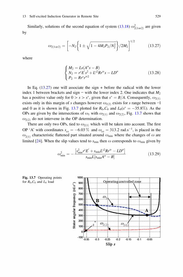
Similarly, solutions of the second equation of system (13.18) x22ð1or2Þ are given

by

x2ð1or2Þ ¼ �N2 1�ffiffiffiffiffiffiffiffiffiffiffiffiffiffiffiffiffiffiffiffiffiffiffiffiffiffiffiffiffiffi

1� 4M2P2=N22

q

� �

=2M2

� 1=2

ð13:27Þ

where

M2 ¼ LsðA00s� BÞN2 ¼ rsE

0s2 þ Ls2Rr0rs� LD00

P2 ¼ Rrsr0r2

8

<

:

ð13:28Þ

In Eq. (13.27) one will associate the sign + before the radical with the lower

index 1 between brackets and sign − with the lower index 2. One indicates that M2

has a positive value only for 0[ s[ s�, given that s� ¼ B=A. Consequently, x2ð1Þexists only in this margin of s changes however x2ð2Þ exists for s range between −l

and 0 as it is shown in Fig. 13.7 plotted for R0,C0 and L0(s� ¼ �35:8%). As the

OPs are given by the intersections of x1 with x2ð1Þ and x2ð2Þ, Fig. 13.7 shows that

x2ð2Þ do not intervene in the OP determination.

There are only two OPs, tied to x2ð1Þ which will be taken into account. The first

OP ‘A’ with coordinates sex ¼ �6:03% and xex ¼ 313:2 rad:s�1, is placed in the

x2ð1Þ characteristic flattened part situated around xmin where the changes of x are

limited [24]. When the slip values tend to smin then x corresponds to xmin given by

x2min ¼ � s2minr

sE0 þ sminL

s2Rr0r � LD00� �

sminL sminA00 � B½ � ð13:29Þ

Fig. 13.7 Operating points

for R0,C0 and L0 load


Now we will consider the second equation with unknown s to find smin, we will

have

s1;2 ¼x4LB� RLs2r0rx2 �

ffiffiffiffiffiffiffiffiffiffiffiffiffiffiffiffiffiffiffiffiffiffiffiffiffiffiffiffiffiffiffiffiffiffiffiffiffiffiffiffiffiffiffiffiffiffiffiffiffiffiffiffiffiffiffiffiffiffiffiffiffiffiffiffiffiffiffiffiffiffiffiffiffiffiffiffiffiffiffiffiffiffiffiffi

ðRLs2r0rx2 � x4LBÞ2 � 4 LA00x4 þ rsE0x2½ �q

: �x2LD00 þ rsr0r2R½ �2LA00x4 þ 2x2E0rs

ð13:30Þ

For the s existence, it is necessary that the quantity under the radical is positive

or zero. So we obtain

smin ¼LBx2

min � RLs2r0r

2LA00x2min þ 2rsE0 ð13:31Þ

which gives

s2min Ls2Rr0rLA00 þ rsE0LB� �

þ smin �2A00D00L2� �

þD00BL2 ¼ 0 ð13:32Þ

where xmin is considered the minimum angular frequency. The roots of this

equation are given by

smin ¼A00D00L

Ls2Rr0rA00 þBE0rs1�

ffiffiffiffiffiffiffiffiffiffiffiffiffiffiffiffiffiffiffiffiffiffiffiffiffiffiffiffiffiffiffiffiffiffiffiffiffiffiffiffiffiffiffiffiffiffiffiffi

1� B Ls2Rr0rA00 þ rsE0B½ �A002D00L

r" #

ð13:33Þ

The area, considered as stable operating zone, is limited on the left taking into

account the machine energetic performances. Whereas the OP ‘B’ is placed far from

the stable zone and possesses high x and s values which can destroy the SEIG

energetic performance.

13.3.2.2 Evolution of Operating Point for Variation of the L Load

To distinguish the L effect on the OPs, one has presented in Fig. 13.8 various cases

for L values such as 0.17 H (L0), 1, 10 and 100 H. The case of L ¼ 100 H may be

considered practically as a resistive load. From system (13.18), one deduces that

R ¼ R0, however C should have respectively the values C0, 32:52 lF, 22:4 lF and

21:37 lF.As already indicated that, irrespective of L value, x2ð2Þ never intervenes in the

OP determination. Therefore, one does not take into account x2ð2Þ in the next few

analyses. Furthermore, it is noted that xex increases with L however sex possesses

quasi constant values. Also, one can note that the margin for x nearly constant

increases as L increases. This behavior can be benefit if there are no constraints on

the energetic performance of the machine.

530 E. Touti et al.

13.3.2.3 Newton-Raphson Numerical Solution

The numerical analysis is performed using the equations system (13.18) denoted by

g1 and g2 respectively for the first and the second equation where the unknown are

x and s.

g1 ¼ s2x4RLCA0 þ s2x2½LE00 � RA0� þ sx2LLs2r0r

�x2RLCD0 þRD0 þðRþ rsÞLr0r2g2 ¼ s2x4LA00 � sx4LB þ s2x2rsE0

þ sx2Ls2Rr0r � x2LD00 þRrsr0r2

8

>

>

>

>

<

>

>

>

>

:

ð13:34Þ

Using the iterative Newton-Raphson method based on the successive use of the

Jacobian for the regulation of the variables adjustment pitch, it is possible to find a

numerical solution of the nonlinear static system (13.34) [25–27].

The approximation of the gi (i = 1, 2) functions by a Taylor development

stopped at the first order around the initial condition x0ðx0 ¼ 314; s0 ¼ �1Þ to a

zero target for these functions, allows to deduce the necessary variation of the

variables x and s.

Fig. 13.8 Impact of L on the operating points positions, a L = 0.17 H, b L = 0.55 H, c L = 1 H,

d L = 100 H


The calculation is redone as g1 and g2 continue to exceed calculation accuracy

fixed in advance. The algorithm of the Newton-Raphson method is summarized by

the flowchart presented by Fig. 13.9. To stop the algorithm, a convergence test

which usually comprises a double control is established:

The first concerns a limited number of iterations and the second concerns the

accuracy. This second test could be expressed as

Fig. 13.9 Flowchart of the iterative method of Newton-Raphson

532 E. Touti et al.

maxð gij jÞ � er ð13:35Þ

where er is a tolerance computation fixed by the operator (er = 0.001).This

approach allowed to find xex ¼ 315:6 rad/s and sex ¼ �6%.

13.4 Impact of the C Variation on the Frequency

Figure 13.7 revealed the possibility of stabilizing the SEIG output frequency for an

operating point defined at the bottom of the curve. Therefore, it is necessary to

choose the load R–L and the capacitor C required for the wind turbine operating at

this point. Given that the curve is flattened around this point, limited variations of

the R load around 19% will keep quasi constant the frequency by changing the

capacitor C. Table 13.1 gives calculation and measurement example.

There are five cases presented in Table 13.1. The first was carried out for

R0 = 111 X and C0 = 87.5 lF. This is the central SEIG operating point (Fig. 13.7).

In the following, some variations in the R load will be tested around this central

operating point « A » which is characterized by s = –5.7% and x = 312.7 rad/s

(f = 49.8 Hz).

These changes move the operating point to right and left of the central operating

point. Regarding the second case, we choose R = 132 X (variation of 19%) that

corresponds to the machine discharge characterized by the operating point whose

cordinates are s = –4.8% and x = 315.8 rad/s (a displacement to the right,

f = 50.3 Hz, Df = 0.5 Hz). The capacitor value should be 83.12 lF, but considering

our capacitor bank we used C = 83 lF. For comparison, we have also tested (test 3)

a variation of R value (R = 132 X) without changing C (C = C0 = 87.5 lF). We

notice a slightly greater change in the stator angular frequency (x = 307 rad/s,

f = 48.8 Hz, Df = 1 Hz).

A fourth pair (R, C) was considered (a displacement to the left) such as R = 86 X

(variation of 22.5%) and C = 95.5 lF which corresponds to an increase in the load.

The change in C provides a smaller variation of x (x = 311.5 rad/s, f = 49.6 Hz,

Df = 0.2 Hz). This case will be compared to another fifth case where C is kept

constant when R varies (R2 = 86 X and C2 = C0 = 87.5 lF). It is also noted a

Table 13.1 Changes in angular frequency, slip and voltage versus load at constant power

L = 170 mH

Pw = 1884 W

Experimental values Theoretical values

R

X

C

lF

x

rad/s

f

Hz

s % V

volts

x

rad/s

f

Hz

s %

C variable 111 87.5 312.7 49.8 −5.7 224.5 313.2 49.8 −6.03

132 83 315.8 50.3 −4.8 245.4 317.4 50.5 −5.08

86 95.5 311.5 49.6 −7.7 192.3 308.3 49.09 −7.8

C = 87.5 lF = constant 132 87.5 307 48.8 −4.9 244.2 308.7 49.1 −5.08

86 87.5 322.3 51.3 −7.6 192.8 324.2 51.6 −7.8


greater variation of the stator angular frequency x (x = 322.3 rad/s, f = 51.3 Hz,

Df = 1.5 Hz).

According to the results predicted by the developed model, Table 13.1 confirms

that when considering a R–L load we can improve the stator frequency stability at

the wind generator output by changing C. In fact, we obtain a frequency change

near zero (1%) for R variation about 19%. This change is more important (3%) if

C has not changed.

When the load is purely resistive, this variation may become much more

important (11%). Other tests have been carried out for other operating points. They

confirmed identically the test already presented. The theoretical values shown in

Table 13.1 are obtained from graphical method (paragraph II) or numerically

computed based on the analytical study already developed. It is noted that these

values are close to those experimentally obtained. By maintaining constant tan q,

one can obtain an operating while keeping the frequency at quasi constant values

without need of any control loop of this variable. Here q is the argument of the

whole load and capacitor which are placed in parallel and connected to the SEIG

stator.

13.4.1 Load Variation at Constant C

The angular frequencies variations for a load R change about 22% are shown in

Fig. 13.10a, b.

The reduction of R values from reference point R0 ¼ 111 X can displace the OPs

to the curved area in the direction of increasing speed. This can cause a significant

increase in the stator voltage frequency. This is due to the fact that C value is kept

constant while varying R. In a second test we will increase the R value while

keeping C constant. We can note a significant frequency change. By against, the

Fig. 13.10 a Decrease in R value at constant C = 87.5 lF, b Increase in R value at constant

C = 87.5 lF

534 E. Touti et al.

increases in R values are unlimited unless the machine energetic performance and

voltage stability are lost.

13.4.2 R Load Variation at Variable C

In this case we will accompany to any R variation a change in the value of

C. Figure 13.11 shows the considered study with two tests of load tilting around the

initial operating point (R0 and C0). The strategy proposed for controlling the fre-

quency needs the definition of pairs (R, C) allowing to reach the OP in the con-

trolled zone. With the considered machine parameters, we lead to the point A

(Fig. 13.7) corresponding to R0 = 111 X and C0 = 87.5 lF. The next stage is to act

on R and therefore C while respecting the following law which is deduced from

tan q ¼ constant.

C ¼ ðRþR0ðLC0x2rat � 1ÞÞ

LRx2rat

ð13:36Þ

In Fig. 13.11 is noted that the change of the pair (R, C) while respecting the

Eq. (13.36), the frequency is kept quasi constant during the wind generator oper-

ating. We also note a small change in frequency (Df 1.5%) if R varies about 20%

from R0. Through against, if C is kept constant while changing R close to 20%, the

frequency variation can exceed 3.5%. Figure 13.10a, b show the changes of the OP

Fig. 13.11 Tilting from R0 = 111 X and C0 = 87.5 lF to (R2 = 86 X, C2 = 95.5 lF) and

(R1 = 132 X, C1 = 83 lF)


positions for only R load variations (L and C kept constant). Figure 13.11 presents

the results of the R variations with variable C. It is noted that the three character-

istics are confused in the stable region shown in Fig. 13.7 when applying the

f frequency control law.

13.5 Reactive Power Control

We consider the SEIG operation in remote site. By mean of the analytical method

developed in Sect. 13.3, it is possible to find a couple R, C adapted for a given

inductive load L. This study leads to some operating points around the point A

within the stable zone (Fig. 13.7). When the power Pw varies, the voltage regulation

may be ensured by changing a resistive R load. This change concerns only the

consumers who are not priority and they can be disconnected or introduced in

accord with the wind power changes. The R load changes must be accompanied by

a modification of the reactive power provided by the capacitor CM in order to

stabilize the frequency. One can assure the reactive power changes using thyristor

controlled reactor. This dimmer mounting is controlled by the firing angle w as in

Fig. 13.12 [28].

Let us consider that regulating inductive load LR have also an internal resistance

RLR . We talk about a load ZR. By means of this system, a reactive power consumer

can be disconnected or introduced in the isolated grid. According to Eq. (13.36),

the R load variation is accompanied by a capacitor change C ¼ CeqðwÞ through

changing the firing angle w. In this case, the equivalent reactive power available on

the isolated grid is defined by

Qeq ¼ �U2xCeqðwÞ ð13:37Þ

In practice, the evolution of w depends on the previously calculated values in

order to ensure a relative voltage stability obtained by coupling or decoupling the

non-priority loads with maximal variation about DR ±20%. This change keeps

quasi constant the voltage and the frequency without the need of electronic power

converters.

Fig. 13.12 Regulating load

in parallel with the capacitor

CM

536 E. Touti et al.

13.5.1 Variation of the Capacity

To regulate the reactive power, a three-phase system using a balanced load ZR is

considered. The CM capacitor modification is realized using balanced regulating

impedance ZR which is constituted by a resistance RLR in series with an inductance

LR. This load is supplied through a three-phase dimmer as it is shown in

Fig. 13.13a. The dimmer choice is due to its low cost and its ability to compensate

reactive power. Let us denote / the regulating impedance argument.

To simplify the analytical study, it has been presented the v01ðhÞ voltage curve

and that of i01ðhÞ corresponding current in Fig. 13.13b. It is assumed that the i03ðhÞthird phase current will be null for an angle h ¼ h1. The thyristor firing angle will

be noted w.

We will start the analytical study of the system, cited above, by considering a

single phase dimmer model (Fig. 13.14a) which feed an inductive load ZR.

In order to characterize the voltage V 0qðhÞ (q = 1, 2, 3) applied to the regulating

load, a Fourier analysis is carried out. This development provides the RMS fun-

damental voltage value V 0q1 given by [29]

Fig. 13.13 a Dimmer connected to regulating load, b Voltage and current characteristics: 1st

mode

Fig. 13.14 a Single-phase dimmer, b current and voltage waveforms


V 0q1 ¼

Vq

p

1

2� 1

2cos 2 b� wð Þþ b� wð Þ2 þ

þ b� wð Þ sin 2w� sin 2bð Þ

2

4

3

5

12

ð13:38Þ

where Vq is the RMS value of phase to neutral voltage applied to the dimmer input

and b is the angle for which the current becomes zero in phase q. For xLR RLR

the reactive power absorbed by LR is determined by

QLR ¼ V0

q1I0

q1 sin/1 ð13:39Þ

with

I 0q1 ¼ V 0q1= ZRj j ¼ V 0

q1= R2LRþ LRxð Þ2

h i12 ð13:40Þ

where I 0q1 is the RMS value of the fundamental current and /n ¼ a tanðn:LRx=RLRÞwith n = 1. Let us assume that LR consumes a part of reactive power which is

produced by the total capacitor CM , the capacitance of capacitor removed CðwÞ willbe expressed as

C wð Þ ¼ 1

xp2ffiffiffiffiffiffiffiffiffiffiffiffiffiffiffiffiffiffiffiffiffiffiffiffiffiffi

R2LRþ LRxð Þ2

q

1

2� 1

2cos 2 b� wð Þþ b� wð Þ2 þ

þ b� wð Þ sin 2w� sin 2bð Þ

2

4

3

5 sin/1

ð13:41Þ

Taking into account the Eq. (13.41), the total capacitor CM is modified by means

of the dimmer. The capacitance of the equivalent capacitor Ceq at the SEIG ter-

minals is expressed as

CeqðwÞ ¼ CM � CðwÞ ð13:42Þ

In the three phase operating case, the reactive power absorbed can be monitored

by the dimmer control while / < w < 5p/6. Depending on the load parameters

ðLR;RLRÞ, two operating modes of the dimmer are possible [30].

– Mode 1: 2 or 3 thyristors conduct simultaneously (u < w < wlim)

– Mode 3: 2 or 0 thyristors conduct simultaneously (wlim < w < 5p/6)

The transition from mode 1 to mode 3 occurs for a w > wlim. The wlim value can

be obtained from the following relationship

sinðwlim � /� 4p

3Þ ¼ � sinðwlim � /Þ 1� 2e�p=3q

2� e�p=3qð13:43Þ

538 E. Touti et al.

where q ¼ LRx=RLR . Therefore, it is possible that the dimmer can operates in one

of two modes. Nevertheless, the mode 3 corresponds to a small variation in the

current RMS value which causes a discontinuity for the current weak value. For a

given reactive power variation at the SEIG output, it is preferred that the dimmer

operates in the mode 1 because there is a possible larger variation range of CðwÞand more stability was noticed. The Eq. (13.41) enables to compute this capaci-

tance if b is well known. Considering q = 1 (Fig. 13.14b) and taking into account

the system symmetry for the mode 1, the current cancellation angle b can be

expressed as

b ¼ pþw� a ¼ 2p

3þ h1 ð13:44Þ

where a ¼ wþ p=3� h1 (Fig. 13.14b) and h1 represents the current cancellation

angle in the third phase i03 hð Þ obtained from

sinðh1 � /� 4p

3Þeðh1�wÞ=q ¼ � sinðw� /Þ 1� 2e�p=3q

2� e�p=3qð13:45Þ

However it is noted that for h 2 w� b½ � the Eq. (13.41) considers only V 0q1

applied to the load. Nevertheless, during this interval, the signals are not sinusoidal

at the dimmer output. In the case of three-phase system, the RMS fundamental

voltage value V 01 is given by the following relationship

V 01 ¼

3V

2pððh1 � wþ p

3� 1

2sin 2ðh1 þ

2p

3Þþ 1

2sin 2wÞ2

þ 1

4ðcos 2w� cos 2ðh1 þ

2p

3ÞÞ2Þ1=2

ð13:46Þ

where V is the phase to neutral voltage RMS value applied to the dimmer input.

The h1 angle is determined by the numerical resolution of the Eq. (13.45). The

reactive power consumed by the regulating inductive load is defined by

QLR ¼ 3VI 01 sin/1 ð13:47Þ

where /1 is given by

/1 ¼ a tanðLRx=RLRÞ ð13:48Þ

and the I 01 current RMS value is deduced from (13.46) according to the relationship

I 01 ¼ V 01=

ffiffiffiffiffiffiffiffiffiffiffiffiffiffiffiffiffiffiffiffiffiffiffiffiffiffiffiffiffiffiffiffi

R2LRþðLRxÞ2

�

r

ð13:49Þ


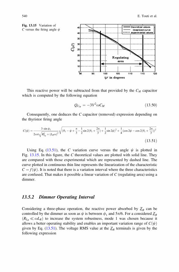
This reactive power will be subtracted from that provided by the CM capacitor

which is computed by the following equation

QCM¼ �3V2xCM ð13:50Þ

Consequently, one deduces the C capacitor (removed) expression depending on

the thyristor firing angle

CðwÞ ¼ 3 sin/1

2xp

ffiffiffiffiffiffiffiffiffiffiffiffiffiffiffiffiffiffiffiffiffiffiffiffiffiffi

R2LRþðLRxÞ2

q

ffiffiffiffiffiffiffiffiffiffiffiffiffiffiffiffiffiffiffiffiffiffiffiffiffiffiffiffiffiffiffiffiffiffiffiffiffiffiffiffiffiffiffiffiffiffiffiffiffiffiffiffiffiffiffiffiffiffiffiffiffiffiffiffiffiffiffiffiffiffiffiffiffiffiffiffiffiffiffiffiffiffiffiffiffiffiffiffiffiffiffiffiffiffiffiffiffiffiffiffiffiffiffiffiffiffiffiffiffiffiffiffiffiffiffiffiffiffiffiffiffiffiffiffiffiffiffiffiffiffiffiffiffiffiffiffiffiffiffiffiffiffiffiffiffiffiffiffiffi

ðh1 � wþ p

3� 1

2sin 2ðh1 þ

2p

3Þþ 1

2sin 2wÞ2þ 1

4ðcos 2w� cos 2ðh1þ

2p

3ÞÞ2

r

ð13:51Þ

Using Eq. (13.51), the C variation curve versus the angle w is plotted in

Fig. 13.15. In this figure, the C theoretical values are plotted with solid line. They

are compared with those experimental which are represented by dashed line. The

curve plotted in continuous thin line represents the linearization of the characteristic

C ¼ f ðwÞ. It is noted that there is a variation interval where the three characteristics

are confused. That makes it possible a linear variation of C (regulating area) using a

dimmer.

13.5.2 Dimmer Operating Interval

Considering a three-phase operation, the reactive power absorbed by ZR can be

controlled by the dimmer as soon as w is between /1 and 5p/6. For a considered ZR

ðRLR �xLRÞ to increase the system robustness, mode 1 was chosen because it

allows a better operating stability and enables an important variation range of CðwÞgiven by Eq. (13.51). The voltage RMS value at the ZR terminals is given by the

following expression

Fig. 13.15 Variation of

C versus the firing angle w

540 E. Touti et al.

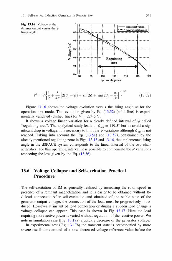
V 0 ¼ V1

2þ 3

4p2ðh1 � wÞþ sin 2wþ sinð2h1 þ

p

3Þ

h i

�� 1=2

ð13:52Þ

Figure 13.16 shows the voltage evolution versus the firing angle w for the

operation first mode. This evolution given by Eq. (13.52) (solid line) is experi-

mentally validated (dashed line) for V ¼ 224:5 V.

It shows a voltage linear variation for a clearly defined interval of w called

“regulating area”. The analytical study leads to wlim ¼ 119:5 but to avoid a sig-

nificant drop in voltage, it is necessary to limit the w variations although wlim is not

reached. Taking into account the Eqs. (13.51) and (13.52), constrained by the

already mentioned regulating zone in Figs. 13.15 and 13.16, the implemented firing

angle in the dSPACE system corresponds to the linear interval of the two char-

acteristics. For this operating interval, it is possible to compensate the R variations

respecting the low given by the Eq. (13.36).

13.6 Voltage Collapse and Self-excitation Practical

Procedure

The self-excitation of IM is generally realized by increasing the rotor speed in

presence of a remnant magnetization and it is easier to be obtained without R–

L load connected. After self-excitation and obtained of the stable state of the

generator output voltage, the connection of the load must be progressively intro-

duced. However at instant of load connection or during a sudden load change a

voltage collapse can appear. This case is shown in Fig. 13.17. Here the load

requiring more active power is varied without regulation of the reactive power. We

note in simulation case (Fig. 13.17a) a quickly decrease of the generator voltage.

In experimental test (Fig. 13.17b) the transient state is accompanied by more

severe oscillations around of a new decreased voltage reference value before the

Fig. 13.16 Voltage at the

dimmer output versus the w

firing angle


voltage collapse and the machine dropping out. These voltage oscillations are

dangerousness for IM or for the load and their amplitude must be controlled.

However, this relatively long transitory interval which is visible in experimental

tests show that the system has a good stability and the SEIG voltage collapse appear

more letter. So it can be easier to readjust the load in order to avoid the machine

dropping out. Therefore in order to decrease the voltage oscillation amplitude, the

load variation must be accompanied by capacitors with appropriate values.

Generally voltage collapse is accompanied by a dropping out of the machine and

the self-excitation of IM can be assured only in the presence of a residual magnetic

field. If IG work in remote site, a specific procedure is necessary for return it at the

self-excitation step. A specific procedure is proposed in [31] where the reactive

energy is given by a capacitor banc charged by a DC source. To make a success of

the self-excited procedure the IG rotational speed must be increased at estimated

calculated value taking in consideration the load.

Another procedure which we propose is shown in Fig. 13.18. Here the load is

disconnected by breaker 1 and a DC supply is applied at the stator windings in two

steps: the first by closing breakers 1–2, 3–4 and the second by changing 3–4 with

Fig. 13.17 Voltage collapse during sudden load variation, a simulation result, b experimental

result

Fig. 13.18 Practical startup procedure

542 E. Touti et al.

4–5. The current must be limited at the generator nominal value In. It is also

possible after its disengagement to supply the machine with AC power system in

order to operate as an asynchronous motor mode.

13.7 Conclusion

The work presented in this chapter treated a numerical model of a three phase Self

Excited Induction Generator which operates in remote site. This wind generator

supplies an inductive-resistive load connected in parallel with capacitor banks. This

latter provides the reactive power required by the SEIG as well as the load.

A control strategy, based on the reactive power change was studied. This study was

conducted while respecting the low tan q ¼ constant from which, any change of

C is realized by adjusting the thyristors firing angle of the dimmer which feed a

regulating load. The first part treats the use of space vector formalism in order to

develop the SEIG model. The second part deals with the steady state studies by

means of a single phase equivalent circuit. Another section of this chapter discusses

the frequency control law. The operating points of the SEIG are fixed such that they

give rated output at the rated conditions of voltage, current and speed. In the last

part of this chapter, is presented the reactive power control strategy and the oper-

ating intervals imposed on the dimmer for stabilizing the frequency. The dimmer

allows obtaining a variable capacitor across the machine terminals.

Appendix

The parameters of Induction Machine used in this study are: 380V=660V,

7:3A=4:2A, cosu ¼ 0:8, p ¼ 2, f=50 Hz, 1420 rpm, 3 kW, ns=nr ¼ffiffiffi

2p

, rr ¼ 3X,

Lr ¼ 267mH, Msr ¼ 377mH, ra ¼ 10X, Msa ¼ 100mH; la ¼ 5mH,

La ¼ 18:7mH, ka ¼ 0:26, Mra ¼ffiffiffiffiffiffiffiffiffi

LaLrp

¼ 70:6mH, Ls ¼ 534mH, rs ¼ 8:66X,r0r ¼ 6X, ls ¼ 24:24mH, l0r ¼ 36:36mH, ks ¼ 0:0454, kr ¼ 0:068, Tf ¼ 1:3 Nm,

LR ¼ 215mH, CM ¼ 113 lF, 380V=660V, 7:3A=4:2A, V sref ¼ 223V,

sref ¼ 5:4%, Isref ¼ 2:42A, xref ¼ 314:2 rad s�1.

References

1. G.M. Joselin Herbert, S. Iniyan, E. Sreevalsan, S. Rajapandian, A Review of Wind Energy

Technologies, Renewable and Sustainable Energy Reviews, 11, pp. 1117–1145, 2007.

2. A.H.M.A. Rahim, M. Ahsanul Alam, M.F. Kandlawala, Dynamic Performance Improvement

of an Isolated Wind Turbine Induction Generator, Computers and Electrical Engineering, 35,

pp. 594–607, 2009.


3. G.K. Kasal, B. Singh, Voltage and Frequency Controllers for an Asynchronous

Generator-Based Isolated Wind Energy Conversion System, IEEE Trans. Energy Convers.,

vol. 26, no. 2, pp. 402–416, 2011.

4. Y.Y. Deng, K. Blok, K. van der Leun, Transition to a Fully Sustainable Global Energy

System, Energy Strategy Reviews, 1, pp. 109–121, 2012.

5. M. Godoy Simoes, F.A. Farret, Renewable Energy Systems: Design and Analysis with

Induction Generators, CRC PRESS, USA, 2004.

6. P. Gipe, Evaluating the Technology - What Works and What Doesn’t, Chelsea Green

Publishing Company, Wind Power for Home & Business, 1993.

7. S. Kumar, R. Narayan, Effect of Capacitive VAR on Performance of Three-Phase

Self-Excited Induction Generator, International Journal of Emerging Technology and

Advanced Engineering, vol. 2, issue 12, pp. 253–258, December 2012.

8. Sh. Vadhera, K.S. Sandhu, Constant Voltage Operation of Self-Excited Induction Generator

Using Optimization Tools, International Journal of Energy and Environment, issue 4, vol. 2,

pp. 191–198, 2008.

9. H. Kumar, N. Kamal, Steady State Analysis of Self-Excited Induction Generator,

International Journal of Soft Computing and Engineering, vol. 1, issue 5, pp. 248–253,

November 2011.

10. Sh. Boora, Analysis of Self-Excited Induction Generator under Balanced or Unbalanced

Conditions, Int. J. on Electrical and Power Engineering, vol. 1, no. 3, pp. 59–63, 2010.

11. A.L. Alolah, M.A. Alkanthal, Optimization Based Steady State Analysis of Three

Phase SEIG, IEEE Trans. Energy Convers., vol. 15, no. 1, pp. 61–65, 2000.

12. T. Ahmed, O.H. Noro, E.M. Nakaoka, Terminal Voltage Regulation Characteristics by Static

Var Compensator for a Three Phase Self-Excited Induction Generator, IEEE Trans. Ind.

Appl., vol. 40, no. 4, pp. 978–988, 2004.

13. A.L. Alolah, M.A. Alkanthal, Optimization Based Steady State Analysis of Three

Phase SEIG, IEEE Trans. Energy Convers., vol. 15, no. 1, pp. 61–65, 2000.

14. A.E. Kalas, M.H. Elfar, S.M. Sharaf, Particle Swarm Algorithm-Based Self-Excited Induction

Generator Steady State Analysis, The Online Journal on Electronics and Electrical

Engineering (OJEEE), vol. 3, no. 1, pp. 369–373, 2013.

15. A. Nesba, R. Ibtiouen, O. Touhami, Dynamic Performances of Self-Excited Induction

Generator Feeding Different Static Loads, Serbian Journal of Electrical Engineering, vol. 3,

no. 1, pp. 63–76, June 2006.

16. S. Devabhaktuni, S.V. Jayaram Kumar, Performance Analysis of Wind Turbine Driven

Self-Excited Induction Generator with External Rotor Capacitance, International Journal of

Advanced Engineering Sciences and Technologies, vol. 10, no. 1, pp. 1–6, 2011.

17. L. Louze, A.L. Nemmour, A. Khezzar, M.E. Hacil, M. Boucherma, Cascade Sliding Mode

Controller for Self-Excited Induction Generator, Renewable Energies Revue, vol. 12, no. 4,

pp. 617–626, 2009.

18. R. Romary, J.F. Brudny, Chapter on: Harmonic Torques of Electrical AC Electrical Drives,

Second Edition of the Industrial Electronics Handbook, CRC Press & IEEE Press, Part II,

Chapter 11, Editors: B.M. Wimamowski, J.D. Irwin, ISBN: 9781439802854, ISBN 10:

1439802858, pp. 10.1–10.27, February 2011.

19. M. Radic, Z. Stajic, N. Floranovic, Performance Characteristics of a Three-Phase Self-Excited

Induction Generator Driven by Regulated Constant Speed Turbine, Automatic Control and

Robotics, vol. 11, no. 1, pp. 57–67, 2012.

20. R.J. Harrington, F.M.M. Bassiouny, New Approach to Determine the Critical Capacitance for

Self-Excited Induction Generators, IEEE Transactions on Energy Conversion, vol. 13, no. 3,

pp. 244–249, 1998.

21. I. Boldea, Variable Speed Generator, The Electric Generator Handbook, Edition Tailor &

Francis Group, USA, pp. 1–30, 2006.

22. A. Kheldoun, L. Refoufi, Dj. Eddine Khodja, Analysis of the Self-Excited Induction

Generator Steady State Performance Using a new Efficient Algorithm, Electric Power Syst.

Res., 86, pp. 61–67, 2012.

544 E. Touti et al.

23. J.F. Brudny, R. Pusca, H. Roisse, Wind Turbines Using Self-Excited Three-Phase Induction

Generators: An Innovative Solution for Voltage-Frequency Control, Eur. Phys. J. Appl. Phys.,

vol. 43, pp. 173–187, 2008.

24. E. Touti, R. Pusca, J.P. Manata, J.F. Brudny, A. Chaari, Enhancement of the Voltage and

Frequency at the Self-Excited Induction Generator Outputs by Adjusting Terminal Capacitor,

9th International Conference on Industrial Power Engineering, Bacau, Romania, pp. 199–208,

22–24 May 2014.

25. S.P. Singh, B. Singh, M.P. Jain, Comparative Study on the Performance of a Commercially

Designed Induction Generator with Induction Motors Operating as Self-Excited Induction

Generators, IEE Proceedings - C, vol. 140, no. 5, pp. 374–380, September 1993.

26. S.S. Murthy, O.P. Malik, A.K. Tandon, Analysis of Self-Excited Induction Generator, Proc.

Inst. Elect. Eng. C, vol. 129, no. 6, pp. 260–265, November 1982.

27. J.J. Grainger, W.D. Stevenson, Power System Analysis, ISBN 0-07-061293-5, McGraw-Hill,

Inc., USA, pp. 342–356, 1994.

28. E. Touti, R. Pusca, A. Chaari, Dimmer Control for Voltage Transient Performance

Improvement in Isolated Wind Turbine, Wulfenia Journal, vol. 20, no. 4, Klagenfurt, Austria,

pp. 108–117, April 2013.

29. E. Touti, R. Pusca, J.P. Manata, J.F. Brudny, A. Chaari, Active and Reactive Power

Regulation in Remote Site Equipped with Self-Excited Induction Generator, 12th

International Conference on Science and Techniques of Automatic Control and Computer

Engineering, STA’2011, Tunisia, pp. 593–607, 2011.

30. Ch. Rombaut, G. Seguier, R. Bausiere, Power Converters - Alternative Conversion, vol. 2,

TEC& DOC, ISBN 2-85206-316-6, 1986.

31. J.F. Brudny, H. Roisse, G. Peset, Practical Approaches for the Study of Wind Machine

Self-Excited Induction Generators, International Conference Wind Energy and Remote

Regions, Magdalen Islands, pp. 1–10, 19–21 October 2005.


Chapter 14

Communications for Electric Power

System

Maaruf Ali and Nicu Bizon

Abstract This chapter is an overview on Communications applied for the Electric

Power Systems. Thus, in the first section of this chapter, the Standards for Electric

Power Systems Communications are briefly shown in order to understand the

communication infrastructure requirements for the Smart Grids. The layers of the

Smart Grid Network are (1) Power Grid, (2) Smart Grid and (3) Application. This

chapter is focused on the Smart Grid layer, which has three primary functions to

accomplish in real-time the requests of both consumers and suppliers based on

Communications Technologies for Smart Grid Metering. So, Smart Grid Metering

is an important interface to be implemented and integrated with Smart Grids based

on technologies such as Fibre Optic Communication, x Digital Subscriber

Line/Loop, Power Line Communications, and Wireless Technologies. The Wireless

Technologies for the Smart Grid Architecture of Communication System used for

Power System Control is approached here as well. Some examples of

Communication Systems for the Electric Power System based on IEEE standard

(such as IEEE 802.11 Mesh Networking, IEEE 802.15.4 Wireless Sensor Networks

and so on) are presented at the end of this chapter. Last section concludes the

chapter.

M. Ali

Department of Science and Technology,

University of Suffolk Neptune Quay, Ipswich, UK


N. Bizon (&)

Faculty of Electronics, Communication and Computers,

University of Piteşti, Piteşti, Romania





547

14.1 Introduction

With the need to increase autonomous and automated monitoring of the electrical

power system, various communication technologies are being considered for

exploitation. This is an evolving process and the global market still has not reached

a mature stable point in its adoption of any one particular technology. One major

consideration is the maintenance of the power grid in a stable state, with minimal

power outages.

The implementation of a smart grid requires the essential components of an

effective communication technology coupled with an intelligent low maintenance

and low energy drain device. The system must require the absolute minimal con-

sumer interaction, preferably a set and forget device. Studies have focused on using

both wireless and wired technologies. These are outlined in this chapter. However,

they all have their limitations, especially for wireless coverage using frequencies

higher than 2 GHz. This is due to propagation characteristics and signal attenuation

through building materials.

A definition of a smart grid is provided by the European Commission: “Smart

grids are energy networks that can automatically monitor energy flows and adjust to

changes in energy supply and demand accordingly. When coupled with smart

metering systems, smart grids reach consumers and suppliers by providing infor-

mation on real-time consumption.” [1].

It has to be stressed that smart grid communication is bidirectional, not neces-

sarily at the same time, between the customer and the utility company. The smart

grid is normally considered to consist of the parts of: generation, distribution and

consumption of the energy [2]. The transmission network itself is not usually

considered, as it can use any existing networking technology. This concept can be

summarized in Fig. 14.1.

The use of a well-integrated smart grid is of immense benefit to both the con-

sumer and the energy producer, these include [2]:

Fig. 14.1 The layer view of

the smart grid network

548 M. Ali and N. Bizon

• A better power distribution management policy to handle peak demands, min-

imizing load shedding;

• Efficient integration of renewable power sources into the grid;

• Consumers being able to utilize cheap power;

• Consumers being able to sell excess power during peak demand by the grid—

for those generating their own, for example using a CHP [Combined Heat and

Power] unit and

• Maintaining a stable power grid.

The smart grid layer has three primary functions to fulfill, these being of pro-

viding [3, 4]:

• Smart Network Management—such as data acquisition, transmission,

switching and monitoring of the energy flow between the customer and the

supplier, ensuring an acceptable quality of service;

• Smart Integrated Generation—encompassing energy distribution, storage,

fusion from diverse sources integration with provision of future grid scalability.

The need to provide charging points to EV (electric vehicle) should also be

provisioned as they become more commonly accepted by the general populace;

• Smart Market—two-way communication functionality must be implemented

between the meter and the utility company in order to support advanced features

such as dynamic pricing and load control. The meter in itself must offer

advanced functionalities beyond just registering energy usage. Thus the smart

meter must be coupled with inbuilt networking technologies linked to network

gateways, much like how modern multimedia services are internetworked.

An EU Commission report also estimates that by 2020, about 245 million smart

meters will be deployed just in the EU alone.

Whatever technology is employed, data protection, privacy and security are of

the utmost importance to protect everyone in the revenue stream. Thus some form

of encryption, preferably end-to-end from the consumer premises to the utility

company should be implemented over the data channel.

14.2 Standards for Electric Power Systems

Communications

For any implementation of a smart grid system, it must adhere to these commu-

nication infrastructure requirements [5]:

(a) Scalability

The number of consumers requiring connections to the energy grid is predicted to

grow exponentially. Fortunately the reliance upon the network communication

technology requirements in terms of protocols and signaling are expected to be the

same. Thus scalability is an important factor to be dimensioned into a smart grid

network for future growth. This will entail the use of a myriad of M2M

14 Communications for Electric Power System 549

(machine-to-machine) devices being linked to the low voltage electricity grid

(11 kV level). The addressing task of each network device or devices will be helped

by the utilization of IPv6 (Internetwork Protocol version 6) with its 128 bit

addressing space.

(b) Network Performance

Under this term are specific network performance parameters such as the data rate,

the quality of service, the network delay. Fortunately these parameters are not so

stringent as those required for conveying multimedia real-time network traffic

though the Internet. Smart grids require only data transfer rates of 10 Kb or less

with latencies less than 100 ms, for network originating control and signaling

information. Customer premises meter-originating data are even less demanding,

being able to function with higher latencies of up to 72 h!

(c) Availability

Any power utility company must ensure they can deliver power ideally with 100%

uptime or at best with the absolute minimum downtime or power outage of say at

most a few hours. Even if an outage is unavoidable, then power must be maintained

by rerouting to such critical facilities like hospitals. Load shedding must be avoided

wherever possible. For smart grids, availability also means being in active com-

munication link, this is less of a problem for power being provided by fixed net-

work connections. However, radio links must be maintained for smart metering

being provided by wireless radio transmission links. Radio interference must be

combatted and error correction must be built into the transmission protocol to

survive in a noisy radio transmission environment. To maintain network efficiency,

FEC (Forward Error Correction) coding should be employed, avoiding the need for

any ARQ (Automatic Repeat reQuest) of the data packets.

Some smart grid services, especially at the industrial level require an SLA

(Service Level Agreement) of between 99.5 and 99.9%. This can be made possible

by service reservation and prioritization of queues. Again, at the consumer premises

level, the requirements are less stringent and can be relaxed by having the metering

data being stored locally before being uploaded when the smart grid network

becomes online or less congested again. Hence, an SLA of less than 90% may be

tolerable.

(d) Costs

When a smart meter is to be installed, two cost factors need to be taken into

account, these being the price of the smart meter itself and the actual installation

cost of the meter into the consumer premise or the home. The smart meter needs to

offer several functionalities and also need to be made appealing to the user whilst

keeping the cost to a minimum for the power utility company. Most consumers

expect their smart meters to be installed at zero cost to them, with the entire cost

being borne by the power utility company themselves. The installation of the smart

meter should be as simple as possible with automatic self-configuration and


diagnostics. This will minimize retraining of the installers. A third factor that also

needs to be considered is the actual transmission cost of each reading, in either

direction. These exchanges of data need to be reliable and cost effective, without

overwhelming the network capacity. This is of particular concern when expecting

readings from a large city from millions of potential customers. Thus some form of

data scheduling may be necessary.

(e) Security

Protection of the smart grid network is extremely important, not only to protect the

personal billing information of the consumer, but also to protect the network from

spoofing and infiltration by hackers attempting to defraud and bring down the entire

network. Thus, the user data must be protected from: misuse, the network from

hackers and the messages must be conveyed securely to arrive uncorrupted. The

technology for secure transmission of sensitive data already exist in conveying data

through the internet and this can be applied in the case for the future advanced fully

integrated smart grid network.

(f) Smart meter grid/system life-cycle

The smart grid community would like to see a life-cycle of at least 15 years with

standardization and interoperability as key features. This is to ensure longevity of

the network and ease of maintenance with minimal cost. Implementing a new smart

gird network is quite an expensive endeavor and these considerations of using

standardized, COTS (Customised-of-The-Shelf) smart meter components should

allow a cost effective implementation, deployment, maintenance and safe realiza-

tion of the national and international smart grid network. The utility companies’

goal is to minimize their maintenance of their smart meters, thus achieving con-

siderable cost savings. They also do not like to be locked into purchasing from one

specific vendor for the entire lifetime of their smart grid network.

(g) Control

To enable a smart grid to be under the effective control of the power generating

utility, it may become necessary for the utility to use their own network - totally

under their control. This is especially relevant when the network demands may

exceed previously agreed SLAs with their third party data network capacity pro-

viders. The network must be always made available to the utility, this can only be

guaranteed if the data network is under the total control of the utility. This will thus

avoid complications of legal interpretations of contract laws and what to do when

the network services beyond the initially agreed service levels are required.

A solution may be is to use power line data transmission technology or to set-up a

dedicated wireless network, for example like the GSM-R (Global System for

Mobile Communications—Railway) network. This is the GSM mobile communi-

cations network, specifically employed by the railway operators, using their own

frequencies.


14.3 Communications Technologies for Smart Grid

Metering

Whatever technology is chosen, they must adhere to the above requirements. It may

also be noted that some situations may require the use of more than one type of

technology. The types of technologies that are currently being utilized in the smart

grid can be categorized into two, these being wired or wireless [6–8]. For most

practical implementation both are required together.

14.3.1 Wired Technologies for Smart Grid [3]

a. Fibre Optic Communication

Without doubt, the use of fibre optic cabling to network the smart grid offers the

advantage of the availability of a high bandwidth, compared to using copper cables

or twisted pair wires. However, the penetration of optical fibre to the home is still at

a low level. The main reason for this is the high cost of deployment. This situation

is slowly changing as the uptake of ‘Fibre to the Home’ (FTTH) continues to

accelerate. New regional developments and new build towns, villages and cities are

far easier to network cost effectively using fibre cabling technology to the local

electricity generating substation, however.

b. xDSL (x Digital Subscriber Line/Loop)

For most of the industrialized nations, broadband services are provided by a form of

DSL technology, hence the ‘x’ in the acronym. The cities are well served in this

regard. It would appear that this form of technology is ideally suited to implement

the smart grid. However, there are many challenges, these being the regulatory

issues and the cost of the equipment, to actually interface into the DSL line itself,

along with being dependent on the customer. It must also be noted that the smart

grid is at the mercy of the customer paying for the DSL line and not terminating the

contract. Despite these potential problems, smart meters are already deployed that

use WiFi connections and the DSL line to carry the data back to the power gen-

erating companies.

c. Power Line Communications [7, 8]

Using the actual power line infrastructure itself to both carry electricity and data

makes much commercial sense as the network is already there and the company has

full control over their grid. Such technologies are already being utilized. However,

the actual transmission is functional and possible between the transformers only and

not through the transformers. The data is transmitted by carrier modulation. The use

of multiple carriers, much like DSL technology, now enables broadband commu-

nication to also take place. For power line communications to be effective, the


signal must operate in a very electrically noisy environment. The technology cur-

rently offers two modes of operation, this being narrow band and broadband.

Wideband communication suffers from greater attenuation and restricted range.

Depending on the scenario, a mixture of both narrow band and broadband power

line communication is generally utilized. In the event of a break in the power line

due to say a storm or from solar radiation, then complete breakdown in smart

metering will occur. Thus some form of a redundant backup network must be in

place. This will add a further cost to the power line smart grid network.

The implementation of power line communication is still in its infancy and no

internationally agreed standard currently exists. Pilot schemes are in operation and

performance data continues to be gathered.

14.3.2 Wireless Technologies for Smart Grid [3, 6]

There are two ways of implementing a smart grid using wireless technology. One is

to use the currently available wireless technologies and mobile cellular networks.

The other is to set up a private wireless localized network. Clearly the first one has

the advantage of a lower cost as the infrastructure is already in place. The major

disadvantage is the lack of control by the utility itself. This is not a problem,

however, when a private wireless network is used. The major disadvantage here

would be the high initial cost in setting up the private wireless network. Using any

shared or unlicensed part of the electromagnetic spectrum would not be an

advantage, as the utility company would have to compete with other users and the

consequent radio noise, both affecting the effective data throughput. For in-building

use, frequencies up to 1 GHz may be employed before attenuation becomes a

severe problem. This would mean that the lower GSM and GPRS (General Packet

Radio Service) frequencies of 450, 800 and 900 MHz should only be utilized.

a. GSM and GPRS services at 900 MHz

The bandwidth is adequate and the technology is mature to implement a smart grid

solution using GSM/GPRS at 900 MHz currently. Indoor coverage also exists with

the use of microcells and femtocells. However, in dense urban areas, network

congestion and availability is a serious problem and alternative, more secure

solution is needed. However, latency is a problem and the network is being

upgraded to other services. Thus the long stability of the technology is of major

concern to the utilities.

b. 800 MHz and LTE (Long Term Evolution)

The use of this fourth generation mobile technology with its broadband data

capacity offers clearly a superior alternative for implementing the smart grid. The

technology is also available over different frequency bands. The lower band of

800 MHz is of particular interest for implementing the smart grid. As LTE


continues to be rolled out and deployed, it will make implementing a smart grid

using this solution an economic viability. Though this is not currently the state and

not all regions offer LTE services at 800 MHz. Primarily it is designed for voice

and internet traffic and not for M2M (Machine-to-Machine) data traffic. The utility

also has to rely on the commercial third party provider, thus losing control of the

network.

c. 450 MHz and CDMA (Code Division Multiple Access)

With its wider cellular coverage requiring fewer base stations and greater

in-building penetration depth and hence lower cost, this under-utilized technology

can be effectively employed to form regional smart grids. The smart grids will be

regional due to the regional availability of these cellular technologies, as they are

not deployed globally. Growth in areas like Brazil is possible. Compared with the

other cellular technologies, the use of CDMA over 450 MHz is technically the most

viable solution, where it exists geographically.

14.4 Architecture of Communication System Used

for Power System Control

The complexity of the information flow in a smart grid framework is shown in

Fig. 14.2. The quantity of monitored data will vastly exceed that of command and

control data, this is so, because of the myriad of devices that have to be monitored

[9]. Clearly the control, command and billing channels need to be highly secure and

the information conveyed in a timely manner to be acted upon when demand for

Fig. 14.2 NIST Smart Grid Framework 3.0 [9]


action requires it. In some parts of the world, effective monitoring of “stolen

energy” is of paramount importance. Figure 14.2, also identifies five areas of a

power generation system: the residence, the distribution system, the substation, the

transmission system and the generating station.

14.5 Examples of Communication Systems for Electric

Power System

A summary of the main technologies is given in Table 14.1 [3]. These technologies

should not be seen as competitive, but rather as complementary depending on the

scale, cost and geographical region of the intended smart grid implementation.

Table 14.1 Properties of the Communication Systems for the Smart Grid [3]

Parameters GSM

900 MHz

LTE

800 MHz

CDMA

450 MHz

Fibre

optic

DSL Power line

Scalability—

competition on

resources

Yes Yes No No No No

Low latency No Yes Yes Yes Yes Narrow

band—no

Data rate

sufficiency

Problematic Yes Yes Yes Yes Narrow

band—no

Enhanced

resiliency

Not

available

Not

available

Available Available Only

limited

SLAs

Not

available

Indoor penetration Fair Fair Good Good Good Good

System

availability

Constrained Constrained Yes Yes Yes Constrained

M2M optimized No No Yes No No No

Interference

expectability

No No No No No Expected

Economic

nationwide

coverage

Yes Yes Yes Very

limited

Partially

limited

Limited

Installation/rollout Simple Simple Simple Difficult Difficult Simple

Security Public grid Public grid Closed

network

Public

grid

Public

grid

Closed

network

Long-term

availability

No Yes Yes Yes Yes Yes

Customer

behaviour

dependent

No No No Yes Yes No

Exposure to

broadband market

developments

No Yes No No Yes No


Seven important parameters need to be carefully evaluated for the communi-

cation network, these being: latency, bandwidth, resilience, security, scalability,

coverage and the life expectancy [10].

The latency is the round trip delay between the transmitter and the receiver,

which includes the media access time, the propagation delay and queuing but not

the processing time at the destination.

When considering the bandwidth of the communication link, the effect of

channel coding and error coding in reducing the effective goodput of the infor-

mation transfer capacity must be calculated. The ability of the communication link

to recover from noise and natural disasters such as earthquakes is in the domain of

the resilience of the link. Security is of ever increasing importance when deciding to

adopt the appropriate wireless technology in our uncertain world. Unauthorized

access must be prevented and confidentiality of data must be protected. Attacks

from ‘vampire’ nodes can be prevented by using techniques such as mutual

authentication. Clearly low powered wireless technologies are only suitable for

small-scale applications, thus the coverage of the wireless technology has to be

appropriate to the application. With a rapidly expanding market, scalability of the

technology must be seamless and implementable with ease. For example it must be

relatively easy to poll a rapidly increasing number of measuring devices at the

correct rate. The life expectancy of the communication network must match that of

the distribution generation system, otherwise it does not make any economic sense

Fig. 14.3 The Integration of WiMAX for Smart Grid Applications [11]


to select the communication network in the first place. This is not an easy decision

to make with technologies having a short life lifetime often considerably less than

the electrical distributed generation system. When updating the communication

network, fault tolerance will become more of a critical factor to prevent power

outages in times of excessive or peak demands, especially when handling the

signaling to implement an efficient load shedding algorithm.

A practical implementation of a smart grid network, as shown in Fig. 14.3, is to

combine several technologies together, both wired and wireless including public

and private networks.

14.6 Overview of IEEE 802.11 Mesh Networking

Whatever incarnation a smart grid takes, it will likely consist of a mesh network as

show in Fig. 14.4, applied to a smart grid. The main difference with this type of

network is that not all the nodes have access to the wired network, instead access is

gained via anchor access points. Having key access points means that congestion

management is a priority to free up bottlenecks. Latency and jitter throughout the

mesh must also be taken into account. To enhance radio resource planning and

security monitoring, a smart grid should employ a controller-based WLAN

architecture.

Fig. 14.4 Mesh Networking in Smart Grid Application [12]


14.7 IEEE 802.15.4 Wireless Sensor Networks

At the heart of the smart grid will be the sensors that are used to monitor the smart

grid and to implement it. Clearly a wireless sensor network will afford the greatest

flexibility in its placement. The use of an already existing standard, such as the

IEEE 802.15.4 is judicious. This IEEE standard is mainly concerned with speci-

fying the requirements for power efficient low data rate wireless networks. The

ZigBee protocol is the main driver behind this protocol. Other competing standards

such as the WirelessHART and ISA100.11a use the physical layer of this standard

but have their own respective different layer two MAC (Media Access Control)

definitions. Clearly using the lower frequency bands operation below 1 GHz, suf-

fering less attenuation will give longer radio propagation paths than using the

2.4 GHz microwave band.

14.8 Conclusion

Those technologies that are resilient to network limitations should be considered for

implementing the future smart grid. An overview of the various technologies, both

wired and wireless, have shown that they have their respective advantages and

disadvantages. The conclusion of this chapter author is that of a hybrid solution

utilizing both wired and wireless technologies. The initial fast deployment should

be to utilize the underlying cellular technologies to gain a market share. Then the

future would be to gradually wean away from commercial networks over to the use

of a private network set up by the utilities themselves. The use of the 450 MHz

frequency is ideally suited for smart grid use and the cellular technology of CDMA

in particular.

The deployment any particular technology is also dependent on the level of

urbanization of the environment. Rural areas will tend to favour a wireless smart

grid solution, whereas heavily urbanized regions will favour a more commercial

cellular solution, using WiFi or WiMax for example.

For the interim phase, redundancy must be seriously considered in order not to

be over dependent on any third party commercial network [13].

Finally the future smart grid should ideally be a “self-healing grid”. A self

healing grid would be able to identify any problems and fix itself without any

human intervention. “Not only can a self-healing grid avoid or minimize blackouts

and associated costs, it can minimize the impacts of deliberate attempts by terrorists

or others to sabotage the power grid” [14].


References

1. https://ec.europa.eu/energy/en/topics/markets-and-consumers/smart-grids-and-meters.

2. Nicu Bizon, N.M. Tabatabaei, H. Shayeghi (Ed.), Analysis, Control and Optimal Operations

in Hybrid Power Systems - Advanced Techniques and Applications for Linear and Nonlinear

Systems, Springer Verlag London Limited, London, UK, 2013.

3. B. Sorries, https://www.cdg.org/resources/files/white_papers/CDG450SIG_Communication%

20_Technologies_Networks_Smart_Grid_Smart_Metering_SEPT2013.Pdf.

4. M. Shahidehpour, Y. Wang, Communication and Control in Electric Power Systems:

Applications of Parallel and Distributed Processing, Wiley-IEEE Press, London, UK, 2003.

5. M. Uslar, M. Specht, C. Danekas, J. Trefke, S. Rohjans, J.M. Gonzalez, C. Rosinger, R.

Bleiker, Standardization in Smart Grids: Introduction to IT-Related Methodologies,

Architectures and Standards, Verlag London Limited, London, UK, 2013.

6. S. Borlase, Smart Grids: Infrastructure, Technology, and Solutions, Wiley-IEEE Press,

London, UK, 2014.

7. S.F. Bush, Smart Grid: Communication-Enabled Intelligence for the Electric Power Grid,

Wiley-IEEE Press, London, UK, 2014.

8. N. Bizon, N.M. Tabatabaei (Ed.), Advances in Energy Research: Energy and Power

Engineering, Nova Science Publishers Inc., USA, 2013.

9. http://www.nist.gov/smartgrid/images/FrameworkGraphic_1_1.jpg.

10. M.S. Thomas, John Douglas McDonald, Power System SCADA and Smart Grids, 2015, CRC

Press.

11. M. Paolini, Empowering the smart grid with WiMAX, http://www.senzafiliconsulting.com/

Blog/tabid/64/articleType/ArticleView/articleId/32/Empowering-the-smart-grid-with-

WiMAX.aspx.

12. http://www.trilliantinc.com/solutions/multi-tier-architecture/.

13. M. Shahidehpour, H. Yamin, Z. Li, Market Operations in Electric Power Systems:

Forecasting, Scheduling, and Risk Management, Wiley-IEEE Press, 2002.

14. M. Amin, The Self Healing Grid: A Concept Two Decades in the Making, IEEE Smart Grid

Newsletter Compendium, 2015, http://www.qmags.com/qmct.asp?q=382&qt=3872236&u=/

OLHit.asp?pub=SGNC&upid=19496&s=ML&url=/SGNC2015.


https://ec.europa.eu/energy/en/topics/markets-and-consumers/smart-grids-and-meters

https://www.cdg.org/resources/files/white_papers/CDG450SIG_Communication%20_Technologies_Networks_Smart_Grid_Smart_Metering_SEPT2013.Pdf

https://www.cdg.org/resources/files/white_papers/CDG450SIG_Communication%20_Technologies_Networks_Smart_Grid_Smart_Metering_SEPT2013.Pdf

http://www.nist.gov/smartgrid/images/FrameworkGraphic_1_1.jpg

http://www.senzafiliconsulting.com/Blog/tabid/64/articleType/ArticleView/articleId/32/Empowering-the-smart-grid-with-WiMAX.aspx



http://www.trilliantinc.com/solutions/multi-tier-architecture/

http://www.qmags.com/qmct.asp?q=382&qt=3872236&u=/OLHit.asp?pub=SGNC&upid=19496&s=ML&url=/SGNC2015

http://www.qmags.com/qmct.asp?q=382&qt=3872236&u=/OLHit.asp?pub=SGNC&upid=19496&s=ML&url=/SGNC2015

Chapter 15

SCADA Applications for Electric Power

System

Florentina Magda Enescu and Nicu Bizon

Abstract Main objective of this chapter is to present the Supervisory Control and

Data Acquisition (SCADA) technology applied in the energy sector which requires

distributed control and monitoring at different levels. If the process is distributed,

then the advantages of SCADA system will be seen through low costs related to

movements of the equipment to improve the performance tracking. Processes that

need to be monitored on a large area, and request frequent and immediate inter-

ventions, can be solved more efficiently through a SCADA system. For this, the

connection between the master station and remote units must be done via a com-

munication system which can use different communication technologies such as

cable, radio, mobile phones, and even satellites. The optimum data transfer may be

obtained by using a specific communication protocol. It is worth to mention that

such SCADA-based communications are developed using the optical fiber com-

munications technology via the Internet. The information flow between remote and

central SCADA units could be designed to be bidirectional for high performance and

reliability of the distributed control system, but note that both digital and analog

signals are involved in such systems. Besides, an important issue is the information

security related to such systems. It is known that the automation and real-time

control are used via the Internet and wireless technology, but these technologies have

also brought some security problems, having a strong impact both in the business

and to the users. The SCADA applications analyzed in this chapter is focused on

Electrical Power Systems (EPS). The stepwise step design is shown using the pro-

gramming environment named VIJEO CITECT SURVEILLANCE SOFTWARES

—version 7.40®. The main objective is to show how can be optimized the real-time

control to obtain affordable solutions for the EPS based on Renewable Energy

F.M. Enescu (&)

Department of Electronics, Computers and Electrical Engineering, Faculty of Electronics,

Communications and Computers, University of Piteşti, Piteşti, Romania


N. Bizon

Faculty of Electronics, Communications and Computers,

University of Piteşti, Piteşti, Romania





561

Sources (RESs). The both current and optimized solutions are presented, and the role

of the reactive power is highlighted in the comparative solutions shown, which are

implemented in practice as well. This was achieved by optimizing the SCADA

solution of the operation, transmission and overseeing the execution of programs for

the operation of power plant trough: (1) the description of the existing solution;

(2) the description of the proposed solution with redundant SCADA servers; (3) the

disadvantages of the proposed solution with Remote Terminal Unit 32 (RTU32).

The optimization of the applications has been carried out because the graphical

interface is poor, as long as the only information displayed is from the distribution

stations, the states of the switches in medium-voltage lines and of the equipment in

the stations. Therefore the dispatcher has not displayed the graphical information

about the status of the line equipment, and does not have a quick overview to state of

the medium-voltage line as well. Thus, the dispatcher must consult the printed

diagrams, which means time consumed and such complicated maneuvers will

occupy the most time their activity during a day. Thus, here it will be shown the steps

to optimize the graphical interface in order to quickly see the status of the EPS.

Furthermore, by improving the graphic interface, the efficiency in carrying out the

appropriate maneuvers will increase, as well as the degree of safety. The applications

have been designed with high flexibility and can be used either for small applica-

tions, either for large size systems. Also, the graphic interface was designed to

display online the page’s status and the trends in state variables.

15.1 Introduction

In last decades the automation devices have evolved from simple electronics cir-

cuits used to monitor and control the parameters of the industrial processes [1], to

smart devices that communicate with each other in automation networks [2]. The

evolution of the automation devices has led to the development of technique for

visualization of control parameters and state variables from the automation process

[3]. The companies producing automation equipment are those that have achieved

the first visualization systems. In time, they have developed the generic software

named Viewer, which is adaptable to various situations possible in distributed

processes [4, 5].

The SupervisoryControl andDataAcquisition (SCADA) system collects data from

the distributed processes through sensors. The central computer will store this big data

after a preliminary processing. The system can receive commands automatically or

manual commands based on the processed data by the human operator [6].

The first SCADA systems, which allowed acquisition and real-time data anal-

ysis, have appeared in the 1960s, but then were rarely used in installations. The

term SCADA was referred to a comprehensive system of measurement and control.

The Programmable Logic Controllers (PLCs), which were designed and built by

Gould Modicon in 1971, have changed the philosophy to use the SCADA. The

PLCs in EPS have been introduced in 1977 by Allen-Bradley, and this was easily

562 F.M. Enescu and N. Bizon

accepted by electricians. The term of SCADA has been used for the first time in the

late 1980s. This term was not widely used until the 1990s when the technology

evolved. In 1998, most of the PLC manufacturers integrate the Human Machine

Interface (HMI) in/SCADA systems using communication systems and open pro-

tocols, nonproprietary. The HMI/SCADA systems offer total compatibility with

PLC-s by including the following components [7]: the HMI, the controllers, the

input-output devices, the networks, the appropriate software etc.

A generic SCADA system must to implement a distributed database that con-

tains elements called endpoints, which can be either hardware or software. Thus, the

distributed database is composed by hardware and software items. The system

SCADA controls and monitors the input or output endpoints. The record of each

endpoint, including its dynamic, is stored in the database to have the history of all

endpoints. This will help in predictive maintenance and the security of the EPS as

well [8, 9].

So, the SCADA system has a multi-layered structure composed from basic

functions and graphical user interfaces which are hardware and software supervised

in real-time [10, 11]. From the point of view of the design environment, a SCADA

system contains some specific instruments such as: text editing applications,

graphics editors, tools to import/export from/to SCADA libraries to achieve con-

figuration parameters, drivers & tools with advanced features for HMI interfaces,

etc. [12].

The carrying-out of a project in the SCADA system, the following aspects must

be taken into consideration [10, 11]:

– the needed components to be easily accessible from the point of view of visi-

bility and how these are collaborating;

– timing sequence;

– scalability;

– flexibility to extend the system by the addition of new subsystems;

– redundancy;

– the initial statuses that should be determined;

– the operation diagram of the system.

The functions of the SCADA system are the following [1, 2, 8]:

• acquires data collected from the process;

• manages alarms;

• allows the needed actions for automation:

– a technological preset action;

– an initiating action of the events;

– a monitoring of the pre-defined sequences.

• stores and archived data;

15 SCADA Applications for Electric Power System 563

• generates and pursues reports:

– a default graphics;

– a multiple graphics scaling;

– a history of graphs.

• allows the dispatcher to control the process via the HMI;

• allows the communication with user interface via the HMI using:

– a libraries with symbols;

– a connection between process and graphic elements;

– a link between screens;

– a collection of command’s operators:

– an animation based on multimedia features;

– a possibility of connection with other platforms [5].

SCADA systems may be extended to Large Scale System by architecture,

maintenance, post-processing, decision support systems, and economic planning [4,

7].

The architecture of hydro energy system is proposed in [12] and extended here to

the architecture shown in Fig. 15.1.

Fig. 15.1 Extended SCADA architecture with application in hydro-energetics


A number of recent studies in the scientific literature have highlighted the

importance of the SCADA systems for RES hybrid EPS [1, 13–15], and in par-

ticular, their use for hydropower plants as below:

– the SCADA system applied for hydropower plants connected to national EPS;

– the use of metering systems for the electric power and water from hydropower

plants;

– monitoring and control of the hydro power plants;

– monitoring and control of the hydropower plants and RESs used for hybrid EPS.

The SCADA architecture for a hydropower plant is presented in this chapter at

level of hardware and software. Five levels of SCADA hierarchy are essentially in

complex system [1, 9–11]:

• the devices level for instrumentation and control operations;

• the Remote Terminal Unit (RTU) terminals level;

• the communications system level;

• the master station level;

• the data processing level.

The evolution of SCADA systems is also shown as system generations for cyber

security. The cyber security risk assessment for SCADA includes:

– Causes which can lead to catastrophic situations from common technical

incidents;

– Cyber Security concepts;

– How incidents are treated;

– The tolerance which is acceptable;

A survey is conducted for a specific hydropower plant from Romania based on

SCADA system. Also, an overview of the programming in VIJEO

CITECT SURVEILLANCE SOFTWARES 7.40® is shown, and the projects to

monitor the medium power subsystem of the EPS based on RESs is described

step-by-step [10, 16–19].

SCADA system allows the command, control and operation of installations both

from the control room of the station and from the center point. The main operative

functions of the management system are as follows:

– acquisition, processing and exchange of data;

– instant recording of data;

– transmission by the higher command center (subsequently implemented);

– remote control (control room) and the local branch of the circuit breakers, traps,

etc.;

– indication of the position of switching equipment;

– measurement of analog quantities;

– metering;

– sequential recording of data;

– the processing and management of alarms;


– voltage control circuits and plots;

– remote control and adjustment in plants;

– marking;

– long-term information archiving;

– registration of damage;

– interlock of primary equipment;

– switching sequences with checking of signals’ timing;

– surveillance system.

All these features are available in new SCADA user interface with VIJEO

CITECT SURVEILLANCE SOFTWARES.

Today, a SCADA system operates on large distances, up to the level of a country

or continent, if we consider that the national EPSs will be integrated based on smart

grids and these technologies. Examples of such processes are given below [20–24]:

– the groups of small hydro stations that are switched on and off in response to

energy demand of customers and which are located, in general, in remote places.

These systems can be controlled by opening or closing the turbine valves, but

must be pursued continuously in order to quickly respond to the dispatcher’s

energy demands;

– the electrical transmission systems, which cover thousands of km2, can be

controlled by closing or opening the grid breakers, but these must respond

almost instantly to the load demand on the line;

– the areas of oil and gas extraction, including sensors, collection systems,

measurement equipment and pumps. These systems are generally distributed

over wide areas, require relatively simple controls, such as starting or stopping

motors, and metrological information on a regular basis, but must quickly

respond to the exploitation conditions;

– the distribution network of gas, petroleum, chemicals, water, which have ele-

ments that are located at different distances from a central point of control.

These can be controlled by closing or opening valves or starting and stopping

the pumps, but must rapidly respond to market conditions and alarms due to the

losses from toxic or dangerous materials;

– irrigation systems covering hundreds of km2 can be controlled by closing or

opening of simple valves, but also require a relative complex measurement of

water supplied to consumers based on centralized system.

In conclusion, the SCADA system is useful because it helps to [7, 10]:

– optimize the process;

– take a decision objectively;

– increase the efficiency of use for the exploitation equipment;

– decrease energy costs;

– reduce the capital in the future;

– improve the services for the future;

– obtain competitive advantages on the market;


– decrease the number of staff;

– solve the problems of the environment;

– use of a new system instead of the old ones which are exceeded.

15.2 Research Extracts from Literature

The study shown in this section is linked to:

– The Electric Power Systems (EPS) as a critical infrastructure;

– Advanced SCADA architectures;

– SCADA system for optimal energy management;

– Cyber security risk assessment for SCADA;

– New SCADA applications.

A. SCADA system for driving the stock records from the hydropower plants

developed in Valcea region

The SCADA system presented in this section is used in Valcea region, Romania,

for driving the hydropower plants from the dispatcher station. The driving system

from the Hydro-energetic Dispatcher (HD) contains (Fig. 15.2):

Fig. 15.2 Research extracts from literature


– SCADA systems in central dispatcher;

– SCADA systems in local dispatcher.

The HD is connected with the Dispatcher in Local Center (DLC) by modems on

wire or using the Global System for Mobile communications (GSM), in last case a

large communication network dedicated to this process is obtained [12, 25, 26].

This system allows the control of the operative functions, the automatic acquisition

of data, and generation of the databases needed. All these actions and data records

are necessary for rational utilization of RESs. Note that this SCADA architecture is

of open system type, which ensures integration of the regional power plants into

national system and flexibility to further develop this system.

The SCADA system from HD station provides information for water flow

planning in relation with energy demand from dispatcher, which is of following

type [12]:

– for monitoring and ensuring the service continuity for power stations and power

substations subordinated to them.

– for implementation of the governmental program to monitor the operation of the

main power stations;

– for energy management and operative management in each power stations;

– for operative exploitation of water accumulations and optimal distribution of the

water flow to power stations;

– for operation in normal and hazard situations based on the remote control units,

switching equipment and primary outlet installations (Fig. 15.2).

The SCADA system from DLC provides information for:

– primary processing of data;

– storage of data during a limited period;

– increasing the reliability and the maintenance capacity of system.

Because this architecture is of distributed type, the functions of the system must

to show in real time:

– the retrieval numeric signals for the status of switches and splitters, the opera-

tional equipment, the power cells, the protection loops, and timing cells;

– the acquired and processed signals (of analogue and digital type) form the

hydroelectric power stations monitored;

– the commands to hydroelectric power plants, both in the local and central

interfaces of the dispatcher from each hydropower plants;

– the alarm signals from the dispatchers in the event of the appearance of some

defects;

– the record of the number of operations for each equipment, which is used in the

management of revisions;

– the schematic diagrams of the hydropower plants monitored, the status of state

variables from these diagrams, the wiring diagrams and the synoptic chart of the

installations used [13];


– the stored records using the graphical or tabular configurations, features which

are selectable by the operator [17].

B. Metering systems of electricity and water for a residential house

The metering of electricity and water flow requested by a residential house is also a

usual application of SCADA system. The SCADA system are responsible for

automatic reading of the meters installed and storing the data in SQL database as a

record which contains the index of consumption, the location, the time, the state of

protection circuits etc. These data generate some alarms and reports related to

monthly consumptions, which are used for the allocation of costs facilities for each

location and meter. Data are provided directly in Comma Separated Values

(CSV) format to be imported directly into the billing software.

The network architecture is standard [10, 27, 28], and contains the following

levels:

– monitoring software: it is composed from separate applications, which are

running on different servers; it can be accessed directly on the web through

monitoring portal, which displays graphical reports in real-time based on the

data received;

– data concentrators, which are used to link the software that is run on the server

and the meters installed in each home;

– metering level, which provides support for remote transmission of the index of

consuming or other monitored parameters.

– Such mattering systems allow the following automatic operations [29–33]:

– reading the consumption and other parameters in the days and at the times

programmed by the user; note that data supplied by the meters installed can also

be read out manually, at the request of a user, in order to determine current

consumption or to verify the proper operation of equipment;

– disconnection of the consumers can be remote controlled using the SCADA

software and flow’s distributors installed in the network;

– graphical analysis of the daily profile for the load demand or the carbon foot-

print reported to a day, week, or month, or other parameters available directly in

web portal;

– detection and location of the faults arising in operation of the equipment

(meters, concentrators, etc.) or the software modules, and generation of alarms

via email to the authorized users;

– computing of daily consumption and monthly consumption (which is used for

the forecast of the energy sources) by using the software management based on

the difference between the automatic readings;

– exporting of the various query reports generated from the database to Excel or

other formats.

C. Monitoring and control of the renewable energy sources

The RESs (solar energy and wind power especially) are used in hybrid power

systems based on distributed generation because:


– the actual consumption increased and the trend for the energy; price is to rise

even higher in years to come;

– the classical resources begin to run out;

– the importance of RESs in climate change [13–15].

The evolution of energy systems can be monitored in the Table 15.1.

Two examples of RES hybrid power systems are given below:

1. Diesel-wind turbine hybrid EPS to supply the industrial consumers (Fig. 15.3).

The application is submitted in under (Fig. 15.3) Sect. 15.7.2

2. Home applications based on solar power (Fig. 15.4)

Supervision and monitoring of the small photovoltaic parks

The dispatchers of small photovoltaic parks make the surveillance with dedicated

appliances that enable measurements to be processed via Bluetooth from inverters.

Supervision and monitoring in parks large photovoltaic

Supervision and monitoring of the large photovoltaic parks

The dispatchers of large photovoltaic parks use SCADA systems to monitoring the

energy generated based on compact reconfigurable items which may avoid the fall

Table 15.1 The evolution of energy systems

Year Energy based on

The future Hydrogen—combustion chef

2010 Solar

2003 Wind

1969 Electric

Power

Plant

1948 Petroleum

1900 Steam


of some subsystems. These items can be easily changed, reconfigured and main-

tained [10].

The optimal energy management strategies may be the following [20]:

– to control the balance between supply and demand with a lesser impact on

carbon emissions and high profitability in maintaining the business;

– to distribute the energy generated for different energy sources (in particular from

RESs);

– to offer clean energy at reasonable costs and under a control of the impact to the

ambient.

Fig. 15.4 Exploiting the RESs for usual home applications

Fig. 15.3 SCADA system for hybrid EPS based on RESs


15.3 Hardware and Software for SCADA Systems

As it is known, the SCADA systems are able to measure and monitor different

parameters and variables, such as: the level of liquids, the volume of the gases, the

volumetric flow rate, the mass of liquids and gases, the pressure, the temperature,

the humidity, the viscosity, the position and the moving, etc. For this, some signals

must be acquired based on the appropriate sensors and transducers from different

electrical and electronic devices, before to be processed and analyzed by SCADA

system. These data can be used for supervision of remote processes. For this, the

data are processed and analyzed to generate reports which will be transmitted to

control the processes parameters within certain limits. The SCADA applications

have two basic levels:

– the customer level, which will be performed the human-machine interaction;

– the data server level which will control the entire process.

Thus, the data server sends these data to the customer level via remote equip-

ment such as PLCs (connected to the database server either directly or via a

communications network, using various communication protocols). The developed

protocols can be property of a company (e.g. Siemens H1) or of open type

(Modbus, Profibus etc.). Database servers can be fully connected to each other and

also to the customer stations through Local Area Network (LAN) networks based

on Ethernet technology [21–23]. The SCADA systems may be relatively simple or

very complex, depending of the dimension and complexity of the process moni-

tored. These systems operate in real-time using a database system named Real Time

Data Base (RTDB), which can be found on one of servers [3].

15.3.1 Hardware Architectures

The servers are responsible for the acquisition and management of data for a set of

parameters. Is it possible to have dedicated servers for certain tasks (for example, if

the objective is to develop the process servers), servers dealing with the handling of

alarms, or file servers [23].

A SCADA server will be connected directly to the PLC via an Open Platform

Communications (OPC) or a RTU, which both collects and consolidates data from

and from PLC-uri (Fig. 15.5). The SCADA takes on request the data from indicator

reading appliances and equipment condition.

The OPC and RTU work as a data concentrator. The data is structured using a

man-machine interface (HMI) in a convenient format for the operator in order to be

able to take any decisions that would optimize the communication between the

equipment.


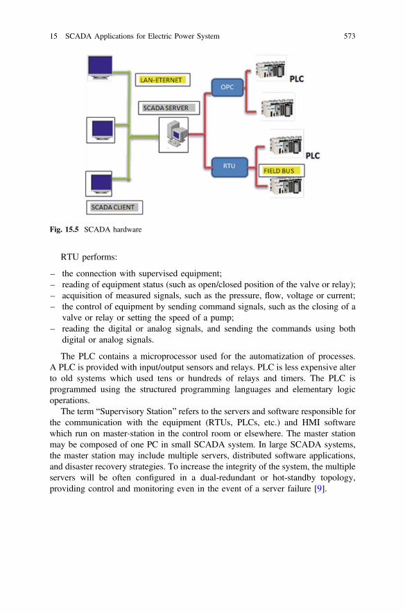
RTU performs:

– the connection with supervised equipment;

– reading of equipment status (such as open/closed position of the valve or relay);

– acquisition of measured signals, such as the pressure, flow, voltage or current;

– the control of equipment by sending command signals, such as the closing of a

valve or relay or setting the speed of a pump;

– reading the digital or analog signals, and sending the commands using both

digital or analog signals.

The PLC contains a microprocessor used for the automatization of processes.

A PLC is provided with input/output sensors and relays. PLC is less expensive alter

to old systems which used tens or hundreds of relays and timers. The PLC is

programmed using the structured programming languages and elementary logic

operations.

The term “Supervisory Station” refers to the servers and software responsible for

the communication with the equipment (RTUs, PLCs, etc.) and HMI software

which run on master-station in the control room or elsewhere. The master station

may be composed of one PC in small SCADA system. In large SCADA systems,

the master station may include multiple servers, distributed software applications,

and disaster recovery strategies. To increase the integrity of the system, the multiple

servers will be often configured in a dual-redundant or hot-standby topology,

providing control and monitoring even in the event of a server failure [9].

Fig. 15.5 SCADA hardware


15.3.2 Generations of SCADA Systems

In this section will be presented briefly the well-known generations of SCADA

systems.

• First generation is of “monolithic” type based on mainframe computers. The

SCADA system was developed under conditions in which there were no

computer networks. So, the SCADA systems were dependent designed to

number of remote terminal units because the RTU was developed later

(Fig. 15.6). An additional mainframe computer is added in the event of failure of

the master system.

• Second generation is of “distributed” type because the information is shared in

real time in the LAN. The data processing is done on several stations connected

to the LAN (Fig. 15.7). Responsibilities are divided to each station, which

enables high speed data processing at reduced cost in comparison with first

generation.

• Third generation is of “network” type because the SCADA system uses the open

system architecture, where can be easily connected peripherals such as printers,

hard drives etc. The communication between the SCADA master and networked

remote terminal unit is based on Wide Area Network (WAN) protocols such

Internet Protocol (IP) address (Fig. 15.8). But the use of IP address standard via

Internet makes the SCADA systems vulnerable to cyber-attacks. Consequently,

new network protocols are developed by companies, but still remain important

security issues to be solved.

Fig. 15.6 First generation of SCADA systems


Fig. 15.7 Second generation of SCADA systems

Fig. 15.8 Third Generation of SCADA systems


15.3.3 Software Architectures

The SCADA applications are implemented based on the software architecture

(Fig. 15.9).

SCADA software architecture has at least two components:

• the SCADA server application;

• the SCADA client application;

The SCADA server application; is multi-tasking being responsible for storing

the SCADA client applications in a database. The SCADA client application

receives data via serial port using RS232 and MODBUS RTU protocols.

In many cases the SCADA applications shall be addressed to and remove the

users who have not an Internet connection. In this case it is necessary a new

software component on a Web server. A Web server is used for generating dynamic

Web pages, which are supplied to customers decrease. The Web SCADA clients

can benefit to real-time access (in a manner similar to regular SCADA clients) to the

lists of parameters, the lists of events and the list of alarms via a simple browser.

But, the Web SCADA clients do not receive the same level of graphical user

interfaces and have the same HMI features as the regular SCADA clients. The

regular SCADA clients are accustomed to running specific applications as opposed

to The Web SCADA clients who view the Web pages provided by Web SCADA

server. In order to reduce as much difference between the regular SCADA clients

Fig. 15.9 SCADA software architecture


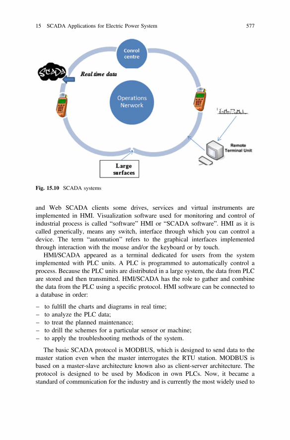
and Web SCADA clients some drives, services and virtual instruments are

implemented in HMI. Visualization software used for monitoring and control of

industrial process is called “software” HMI or “SCADA software”. HMI as it is

called generically, means any switch, interface through which you can control a

device. The term “automation” refers to the graphical interfaces implemented

through interaction with the mouse and/or the keyboard or by touch.

HMI/SCADA appeared as a terminal dedicated for users from the system

implemented with PLC units. A PLC is programmed to automatically control a

process. Because the PLC units are distributed in a large system, the data from PLC

are stored and then transmitted. HMI/SCADA has the role to gather and combine

the data from the PLC using a specific protocol. HMI software can be connected to

a database in order:

– to fulfill the charts and diagrams in real time;

– to analyze the PLC data;

– to treat the planned maintenance;

– to drill the schemes for a particular sensor or machine;

– to apply the troubleshooting methods of the system.

The basic SCADA protocol is MODBUS, which is designed to send data to the

master station even when the master interrogates the RTU station. MODBUS is

based on a master-slave architecture known also as client-server architecture. The

protocol is designed to be used by Modicon in own PLCs. Now, it became a

standard of communication for the industry and is currently the most widely used to

Fig. 15.10 SCADA systems


connect all the industrial devices. The protocols contain extensions to operate over

Transmission Control Protocol (TCP/IP). In practice, it is suggested to avoid the

security of Internet connection in order to reduce risks of cyber-attacks.

This protocol has the following features:

1. it is an open protocol with available documentation;

2. it can be quickly implemented (in few days, not months);

3. it works with bits and bytes, so no particular requirements on implementation.

MODBUS allows the management of the network devices, which gives new

features to the SCADA system related to flexibility, reliability and safety in oper-

ation at high performance.

Fig. 15.11 SCADA energy management system


15.4 Assessment of Cyber Security Risk for SCADA

The developments in Information Technology (IT) systems regarding the safety of

SCADA systems are shown in Table 15.2 [9–11].

Catastrophic situations which may occur due to incidental technical at level of

the automation systems, Energy Management System (EMS), SCADA system,

communications system, and support infrastructure. Besides these, other causes

may be the incidents of cyber security and problems in the management of emer-

gency situations.

New risks which occurred

“The Stuxnet incident has underlined what many ICS security experts had assumed

for a long time: A sophisticated cyber-induced attack against an industrial facility

would try to attack control systems rather than IT systems”—CIGRE WG

B5-D2.46

– June 2010, Stuxnet was discovered;

– September 1, 2011, Duqu was discovered;

– May 2012, Flame Retardants was discovered;

– June 2012, Gauss was discovered;

– etc.

What is the concept of Cyber Security?

Security of those systems cannot be treated as a whole, and nobody can guarantee

perfect security, because there is any system of defense perfect. Measures to protect

and prevention are not enough, because emergencies and viruses could act in time

using hidden forms or different rules. It is important as process to be defined from

the point of view of management and responses to the incidents [8]. Incidents may

be treated as shown in Fig. 15.12.

Safety in the field of energy must be monitored on the basis of production,

transport and distribution, until to the end-consumer. In general, the current

Table 15.2 Systems developments in IT and SCADA security

Past Present and future

SCADA (Fig. 15.10) SCADA + Energy management system (EMS) + protection

to electromagnetic pulse (EMP) (Fig. 15.11)

Closed systems Partially open systems

Push-to-talk communications

and cyber safe

Bi-directional communication and high cyber security

(CIGRE—WG D2.34)

Few information More information

Dedicated operating system

(OS)

Standard OS + commercial OS

Few security requirements Consistent data requirements


problems are treated without taking into account new risks which can appear and

could make huge damage, if will not be considered.

Risk assessment management involves the following stages:

– the analysis by which risks are identified in order to be assessed;

– the risks assessment from the point of view of the impact and likelihood of

occurrence within tolerance imposed;

– the future decision by identifying and understanding risk [24].

Risk assessment can be done using several tools, one of the most popular being

the probability-impact matrix which encompasses:

– the assessment of the probability that a risk to materialize and measured the

degree of certainty:

– the assessment of the impact as the consequence or effect, where the risk would

materialize. In the impact assessment, account shall be taken of the fact that the

risks that have a strong impact on acute misconduct, while those which mani-

fests itself frequently and have a low impact signals a chronic problem;

– the evaluation of risk exposure as a combination of probability and impact can

be felt where the risk would be materialize. In case of the materialization, the

risk exposure is, in fact, an impact [24].

As a result of completing the stages of identifying and assessing of possible risk,

finally, a synthetic and clear representation of the risks must be drawn, mentioning

their ranking in accordance with the level of exposure. The prioritization of risks is

a very important tool in risk management. Tolerance is estimated by determining

the level of risk accepted. The level of risk accepted is established after the adoption

of the response. The following should be taken into account:

– inherent risks;

– residual risks.

Fig. 15.12 Procedure for

treating the incidents


Risk tolerance involves some subjectivity because it depends to a large extent by

the way in which this is perceived as risk. Risks which have a high level of the

exposure is located on top of the tolerance and should be dealt with by means of

measures by which exposure to residual risks must be made under this tolerance

[24] (Fig. 15.13).

15.5 SCADA Applications

The HMI/SCADA software can be installed on personal computers or embedded

computers with touch-screen, distributed through the house or into the industrial

process. It runs a real time operating systems because it must respond in the shortest

time to changes in the parameters of the process monitored. Consequently, the

HMI/SCADA software must meet the following requirements:

– to be easy to use;

– to have an intuitive interface;

– to provide increased security;

– to enable the remote access (if it is the case);

– to be easily to access and use the information;

– to be flexible in use;

– to have the possibility of communication through the various services (sms,

e-mail, fax).

The HMI/SCADA software must be capable of performing certain functions,

such as:

– control and supervision of process;

– alarming the user;

– acquisition of the data needed;

– storing of the events;

– keeping the databases updated;

– developing of graphical evolution of the process;

– coupling with Enterprise Resource Planning (ERP) software.

Fig. 15.13 Assessment of exposure to risks


The most important element of an integrated HMI/SCADA is the interface that

connects the command and the system that is monitored. This interface is used by

the human operator to access:

– the graphic elements that symbolize the automated technological process in a

systemic, appropriate and intuitive manner;

– the most important functions in order to enable all functionalities;

– the state of alarm variables and the alarms history;

– and many other information displayed in a form easy to be followed by the

human operator to see the evolution over time of the process monitored.

Optimization through SCADA solutions

Currently, in the world and in our country, the energy industry is characterized by

profound structural transformations. Besides these requests for structural changes,

the function in a competitive market leads to the amplification of the current efforts

made by the power companies to increase efficiency and quality of their service.

One of the ways of achieving this aim is the orientation towards the smart grids

based on a new strategy for energy management. Thus, information of the EP

system is one of the basic prerequisites for increasing the effectiveness and safety of

the operation of the national energy system. An example of optimization of the

electric power stations along a river is shown in next section.

15.5.1 SCADA System Existing in a Hydropower Plant

The existing SCADA system (Fig. 15.14) consists of:

– the SCADA systems associated with each Hydro Electric central Computer

(HEC) (HEC1, HEC2, HECi);

– the SCADA System for the Hydro Energy Dispatching (HED) from based

Hydroelectric Station (HS).

– At the level of the HECs arrangement, the SCADA system is composed of:

– Distributed Antenna System (DAS) which represents the equipment for the data

transmitted between the SCADA processes in HEDs from the Hydroelectric

Station (HS).

The DAS has available four RS232 l ports and an Ethernet port. The commu-

nication protocols supported are: (1) the DAS Serial, (2) the Modbus RTU, (3) the

International Electrotechnical Commission (IEC) 1107 Mode C for serial ports,

(4) the DAS TCP/IP, and (5) the Modbus TCP for the Ethernet port. Note that the

communication with HEDs is made through the DAS serial ports on two redundant

paths: (1) using the telephone line and the communication protocol; (2) using the

radio communication protocol.

– Functional Assemblies (FAs 1–4) may represent Hydro-aggregate automation

systems, automation systems, General Services (GS), and HEC barrage.


Fig.15.14

Architecture

oftheexistingSCADA

System


The communication protocols implemented in the FA are the OPC industrial

communication protocol (available in Wincc, Cimplicity). Communication with

DAS is via Ethernet using the Modbus TCP protocol, which has the role of protocol

gateway between OPC industrial communication protocol (available in Wincc,

Cimplicity) and Modbus TCP protocol (available in DAS-900).

– The operating Console of the SCADA HEC is based on the OPC industrial

communication protocol available in SCADA iFix (Intellution).

Programmable thermometry in Hydro-agregate Automation (HA1, HA2) sys-

tems is made based on (1) Modbus RTU communication protocols, which assure

the communication with DAS via RS485 (or RS232) with the energy meters.

CewePrometer is a family of high-precision four-quadrant energy meters which

has the following communication protocols available: (1) Digital Library

Management System (DLMS) (used by the energy metering application) and

(2) IEC 1107 serial C Mode. Communication with DAS is via RS-422 (or RS232)

using the communication protocol IEC 1107.

The HED of the SCADA system is composed of:

– The Serial Router (8 + 8 ports) is composed by two industrial computers with

QNX operating system. Communication protocols supported by the application

are the DAS Serial and DAS TCP/IP Ethernet. Communication with DAS HECs

is done in two paths as well.

– The radio Router System assures the communications with 16 hydroelectric

power plants through radio-relay, using the same communication protocols as

the Serial Router.

– The SCADA application is installed on the SCADA iFix (Intellution) server and

the OPC/DAS TCP/IP gateway. The second SCADA server will operates as the

main SCADA server if will be the case.

– The Data Base (DB) SCADA server use the iFix application based on the

Microsoft SQL Server (MS SQL). MS SQL server is the data source for the

“Technical Management” application.

– Technical Management server is a computer on which is installed and runs the

“Technical Management” application based on the installed MS SQL server and

WEB server.

Information flow diagram

From the point of view of information flow, the existing SCADA is presented in

Figs. 15.15 and 15.16. Thus, at the level of DAS-900, the HEC data concentrator

acquires specific data for HECs SCADA from the FAs. FA1 and FA2 read the data

from the automation systems HA1 and HA2. The General Services (GS) and the

Barrage application use the OPC protocol (existing graphic stations as base driver)

via the Modbus-TCP from the DAS-900. This conversion from OPC to

Modbus-TCP has the following disadvantages:


Fig.15.15

SCADA

system

inform

ationfeeds


– the software application is not documented and it is very hard to be interfaced

based on standard protocols with existing SCADA architectures. It appeared as a

necessity to interface DAS-900, which doesn’t support for the OPC protocol,

with the process charts from the HEC stations, which have locally implemented

the OPC protocol;

– it requires automatic start and stop upon launching the application of monitoring

and control on each processor of the workstation graphics or restarting the

operating system. So, it must be individually monitored for any restart in the

event of a communication blockage;

Fig. 15.16 Streams and SCADA system architecture for the river hydro-arrangement


– as was seen in operation, there were frequent blockages of this application,

which means that data and commands are not passed to and from the hierar-

chical level;

– the application for operation relies on two text files with strict rules of editing

(spaces, TABs, bookmarks, etc.), which must be configured identically for each

workstation graphics (HA1, HA2, General Services, and Barrage) and

DAS-900. Note that the existing SCADA system has the possibility of trans-

mission the commands, but at the present time these are not used.

Thermometry system for the HA1 and HA2 will read the temperatures monitored

and the CewePrometer meters will give the main electric values: active power,

reactive power, voltage, current etc. The data concentrated in DAS900 are trans-

mitted by the SCADA system to the HED through the two redundant paths men-

tioned above. DAS900 system has the option of receiving SCADA commands and

records from HED, but at the present time these are not used.

The SCADA data acquired and processed by the HED are stored in the MS SQL

database in order to be used by the “Technical Management” application.

15.5.2 SCADA System Proposed at the River

Hydro-Arrangement

The proposed architecture (Figs. 15.17 and 15.18) was chosen to obtain an

increased security by physical separation of the LANs HEC, SCADA LAN,

LAN DSZ, and LAN CORPORATE using Router/Firewall equipment.

The implementation of a fiber optic network (of redundant ring type) will

facilitate the communication between the HEDs related to East River and HEC.

The IEC 60870-5-104 communication protocol is proposed, which is an industrial

protocol suitable for communication between servers and optimized SCADA net-

work of HED and HEC WAN.

Note that the existing radio network will remain functional as a backup plan for

fiber-optic (FO) network. Thus, the IEC 60870-5-101 radio protocol will be used as

a hot backup (with automatic switching) for the IEC 60870-5-104 main protocol

based on FO network. Consequently, the HED communication with other HECs

will not be affected.

The managers of the Hydro-electrica (HE) Company aim to implement a central

SCADA system data of “real time” type on all hydro-stations. For reasons of

security and reliability, it is not recommended to send the data directly from

HE SCADA LAN (which is a closed and secure network), but it is possible to

transmit data from the isolated nodes. The Technical Management server has all the

necessary facilities for data transmission to HE Company.

The proposal to modernize the HEC architecture by replacing the existing

equipment with new DAS-900 equipment and two SCADA redundant servers (with


Fig.15.17

Architecture

oftheproposedSCADA

system


hot redundancy) to eliminate the existing malfunctions and in addition to implement

new communication functions needed for operation in HED such as

• Bidirectional communication between the automation systems (HA1, HA2,

Barrage, GS) using the OPC industrial protocol, without the need of other

applications for data conversion;

• Communication (in terms of realtime monitoring of the main electrical vari-

ables) with existing CewePrometer meters using the IEC1107 and Ethernet

TCP-IP communication protocols;

Fig. 15.18 Streams and SCADA system architecture proposed for river hydro-arrangement


• Bidirectional communication (in terms of data monitoring and transmission of

commands) of HED SCADA system using two paths communication: IEC

60870-5-104 communication protocol (primary path) and IEC 60870-5-101

(backup path).

The SCADA applications dedicated servers hold a large number of standardized

protocols for direct communication with automation devices used in monitoring and

management of industrial processes. The advantages for data acquisition and

remote management of the hydropower plants retrofitted with redundant SCADA

servers are:

– Simplification of the structure by removing the SCADA DAS-900 equipment

(or other similar equipment) and use of the redundant servers for sending

commands and data from the central dispatcher and vice versa; this allows easy

capacity expansion and further development of software, no constraints;

– The use of a SCADA software installed on the server, ensuring direct con-

nection via OPC industrial communication protocol to the existing equipment

for the management and supervision of the processes, without intermediate

software; servers will provide the following functions: acquisition, operation of

data, storage and archiving, printing and reporting to the higher and lower levels

of communication, supervision of automated processes.

This will also assure: (1) communication with existing equipment installed

(meters, protection relays etc.), (2) high speed communication through the FO

network of the each HEC and HED, (3) improved security provided by the two

levels SCADA servers (two network cards and firewalls on the routers), (4) local

drivers and OPC connectivity with inferior equipment levels, (5) storage and

upgrade of existing licenses for iFix and SQL Server, (6) uninterrupted operation

through hot-plug functions of the redundant servers, both in terms of data (change

of the HDD without stopping the server) and to server maintenance (change of the

power supply without stopping the server), and (7) easy interfacing with HED

Technical Management server.

15.5.3 Issues Related to Data Acquisition and Remote

Management

Issues related to data acquisition and remote management applications of the power

plants, which running on hydropower facilities with RTU, are the following:

– RTU32 in the proposed SCADA architecture is not hot redundant at equipment

level;

– Unable to communicate with graphic stations of the RTU process and SCADA

servers via the OPC industry standard protocol;


– The need to create a new application (named “Date Gateway”) at the level of

SCADA servers, as well as the “Technical Management” server, for bidirec-

tional communication between the servers;

– Managing under Windows XP of the Setup software in RTU with Straton;

– Bringing of electrical signals directly through wires to the level 1 (RTU 32

level) is not indicated, but the solution to bring them to level 0 (PLC and RTU)

it is recommended.

15.6 Overview of the Programming Environment VIJEO

CITECT 7.40

CitectSCADA system is considered one of the most complex and complete

products for the SCADA systems [34, 35], being part of the VIJEO CITECT

SURVEILLANCE SOFTWARES 7.40® of to the Schneider company. This software

product includes over 150 drivers for communication with the input-output devices

and over 350models for PLCs, RTUs, controllers and regulators, barcode readers etc.

For any type of SCADA application, this system offers the needed flexibility in

implementation and execution of the project, in terms of speed, efficiency and

accessibility. More detailed, the CitectSCADA system offers the following

opportunities to user:

– Use of the HMI graphic pages for central or local control stations;

– Realization of operation stages by creating the graphical control buttons;

– Display the status of the actuators via graphical charts;

– Display the alarm messages and their evolution;

– Language selectable to display the messages;

– Achieving of universal commands through the keystrokes;

– Controlling, storing, monitoring and displaying of the alarms;

– View the graphs in real time or in “history record”;

– Efficient and effective monitoring of the system;

– Creating of reports;

– Supervision of product quality by Statistical Process Control (SPC);

– Acceptance of transferring data with other applications;

– Security system can be configured on the priority levels.

VIJEO CITECT SURVEILLANCE SOFTWARES has the following modules:

– Citect Explorer;

– Project Editor;

– Graphics Builder;

– Cicode Editor.


Citect Explorer

The Citect Explorer module is used to create and manage a CitectSCADA project.

This controls the configuration permitting enforcement of project in the rest of

modules. Citect Explorer screen is shown in Fig. 15.19a:

The launch of the Citect Explorer module will automatically run the Project

Editor and Graphics Builder modules, but these are minimized in Fig. 15.19a. The

close of Citect Explorer module will close all CitectSCADA applications.

Project Editor

TheProject Editormodule is used to create andmanage the configuration information of

CitectSCADA project. The Project Editor window can be viewed by all projects.

Special commands are accessible from the buttons or submenus (Fig. 15.19b).

Citect Graphics Builder

The Graphics Builder module is used to achieve pages and editing graphical objects

used on other new graphics (Fig. 15.19c). Graphics Builder editor is activated by a

double click on a graphic object in Citect Explorer.

Cicode Editor

The programs are edited in the window of Cicode Editor. The Cicode Editor menu

contains a list of functions. The support information for functions is obtained by a

right click on the name of the function (Fig. 15.19d).

Configuring CitectSCADA Projects

The schematic of a CitectSCADA project looks like in Fig. 15.19e.

As can be seen in Fig. 15.19e, the CitectSCADA project includes the following

items:

– Graphics;

– Databases;

– Cicode programs.

Graphics mean a graphic page which allows the monitor to display the graphical

interface with control buttons.

Databases allow the storage of process information collected for monitoring and

controlling the system. These may be linked to the graphics page if desired.

Cicode programs allow functionality and contain a number of useful functions

stored.

In all projects carried out, the user can:

– Create;

– Select;

– Open;

– Shut down;

– Delete;

– Etc.


Fig. 15.19 a Screen of citect explorer. b Screen of project editor. c Screen of graphics builder

d Screen of cicode editor. e Scheme of the CitectSCADA project


Fig. 15.19 (continued)


15.7 Developing Step by Step a SCADA Application

for Electric Power System

Application 1

15.7.1 Implementing a Medium Voltage EPS Based

on RESs

The CitectSCADA environment is used here to develop step by step a SCADA

application for the Electric Power System based on RESs. The both interfaces will

be shown in this section in order to shown the advantages of the new SCADA

interface, which is a friendly and intuitive interface, with a high degree of inte-

gration schemes, facilitating for more dispatchers to work simultaneously.

The old interface

As can be seen in Fig. 15.20, the old interface used is poor. In case of maneuvers in

power installations, the dispatcher has a limited overview on the system.

The new interface

A SCADA application is developed step-by-step starting with the identification of

needed elements and objects, which then will be set for data acquisition, command

and control equipment etc. The software structure will be identified correspondingly

in the hardware structure.

A new project must be opened and created, and finally must be saved. The

project will define the appropriate hardware to achieve a simulation structure using

the graphical page. For the simulation process, the structure must be monitored to

be identified and set properly in the graphic pages as associations of hardware items

Fig. 15.20 Medium-voltage EPS based on RESs represented in the existing SCADA system


and their appropriate functions. An important step will be dedicated to security,

namely:

– setting application users;

– setting their rights.

After implementation of the simulation structure, each item must be check using

the software to test all functional features (Fig. 15.21a).

The steps for creating a new project are:

– From the Citect Explorer ! File ! New Project, a new project called

“Micro_energy” is open (see Fig. 15.21b);

– From the Citect Explorer ! gen ! Communications ! Clusters, define a

cluster of communication called “sch_el_cluster” (Fig. 15.21c);

– From the Citect Project Editor ! Servers ! Network Address, define the

TCP/IP address 127.0.0.1 called “sch_el_adr”;

Address “sch_el_adr” is the TCP/IT data acquisition system which are allocated

to the system (Fig. 15.21d).

– Then, the further facilities will be configured as below:

1. “Alarm”: From the Citect Project Editor ! Servers ! Alarm Server

(Fig. 15.21e).

2. “Trending”: From the Citect Project Editor ! Servers ! Server Report

(Fig. 15.21f).

3. “Report”: From the Citect Project Editor ! Servers ! Server Trend

(Fig. 15.21g).

4. “I/O Server”: From the Citect Project Editor ! Servers ! I/O Server

(Fig. 15.21h).

5. “Express Communications Wizard”: From the Citect Explorer ! gen !

Communications ! Express I/O Device Setup ! Next ! Use an existing

I/O ! Disk I/O Device ! Citect generic Protocol ! Automatic refresh of

tags ! Finish (Fig. 15.21i).

15.7.1.1 Making the Graphic Page

To this end, in this section the libraries of the associated elements, which are

required or which must be designed or imported if there are no such elements, are

shown below (Fig. 15.21j).

The following symbols and window is used for the transformer and to set the

voltage ratio, and to obtain the animation symbol in order to switch the power on or

off the power for transformer (Fig. 15.21k).

Each of the symbols used in application are briefly shown for further identifi-

cation. Also a suggestive name, a label and a serial number will be associated to


Fig. 15.21 a Concept

diagram of the SCADA

application. b Window “New

Project”. cWindow “Cluster”.

d Window “Network

Address”. e Window “Alarm

Server”. f Window “Report

Server”. g Window “Trend

Server” h Window “I/O

Server”. i Window “Express

communications wizard”.

j Imported images.

k “Transformer” symbol and

window “Symbol Set

Properties”. l “Electrical

splitter” symbol and window

“Symbol Set Properties”

m “Switch” symbol and

window “Symbol Set

Properties”. n Animated

symbols. oWindow “Variable

Tags”. p Window “Symbol

Set Properties”. qWindow for

proposed process. r Graphic

window of the active process.

s The sequence of code in the

graphical user interface (GUI)


each symbol (Fig. 15.21l). See below the symbols for the electrical splitter

(Fig. 15.21l) and the switch (Fig. 15.21m).

In the same manner are designed the next symbols used in application

(Fig. 15.21n).

Industrial consumers Photovoltaic boiler

Households Wind

Transformer

Electrical splitter

(j)

(k)

(i)



15.7.1.2 Configuring the Variables

All SCADA application are based on the setting and using of the tag-type variables.

Tags are the interface between the user and the monitor. There are several types of

tag-type variables:

Switch

Biomass power plant Hydropower

Power station Power level

(m)

(n)

(o)



• Tag Variables are variables that are directly related to the process, being

modified directly by the acquisition and control system, and similarly, they also

have direct access to the SCADA application;

• Local Variables—required in the SCADA application development;

• Trends Variables—required for plotting the variables acquired from the process

monitored.

To add a tag variable for a switch or a splitter remote controlled, proceed as

follows, using Citect Project Editor ! Tags ! Variable Tags (Fig. 15.21o).



As shown, the variable called “s1” will be associated with the separator s1.

Similarly, the rest of the variables were introduced and associated with each

switching element or existing splitter shown in the diagram from Fig. 15.20

To associate an element to a symbol variable, the Properties window must be

open for that element, as shown in the following figure for “Up command”. Here,

access the list of variables using the right button. From the list that appears, select

the setting required for an ease of identification which containing a serial number

associated with its name (Fig. 15.21p).

15.7.1.3 Method of Implementation

A new graphic page with the name “L 20 kV SCADA” will be created from the

Citect Explorer ! gen ! Graphics ! Pages ! Next ! Create new page !

(Fig. 15.21q). Place the elements in the graphic page using the library and then

configure the related functions as indicated above. One can start the graphical page

in accordance with the operating mode of each one, and then the variables will be

set; or vice versa, the design program being very flexible.

The simulation diagram is tested if running proper. Operation for each item is

tested with the left button of the mouse, in different combinations of the tabs. Also,



the operation of the power level indicators is checked. Adjustment is possible

through the existing cursor for both consumers and energy producers. If it appears

that there are inconsistencies, errors and changes are required. Finally, the appli-

cation will be saved.

The whole process of the distribution system is monitored and controlled per-

manently by SCADA. The interface used is improved, showing the new features

implemented at level of the dispatcher, which has an overview of the EPS and can

perform maneuvers in the system in order to control the process. Besides the

information about the state of switches at distribution stations, distribution lines

appear illustrated to both household and industrial consumers. Depending on

environmental conditions and the load demands are enabled the available energy

sources: power plants, small hydro, wind turbines, biomass power plants and

photovoltaic plants. These sources have the level indicators for the active power and

the reactive power that can be modified and tracked at the consumer and the

producer (Fig. 15.21s). The most important resource to increase the energy effi-

ciency is to reduce own energy consumption.

An effective tool for studies and planning of the development of electricity

distribution networks, and to reduce the domestic electricity consumption, is the

analysis of the load profiles.

This verification process is repeated as many times as necessary, until the

application will work correctly and as it is specified (Fig. 15.21r).

The application contains circuit breakers and disconnectors that will act as in the

“General Regulation” of the maneuvers in the electrical installations and EPS

(Fig. 15.21s).

Application 2

15.7.2 Diesel—Wind Turbine Hybrid EPS to Supply

the Industrial Consumers

15.7.2.1 Concept Diagram of the Application

The concept diagram of this application is shown in Fig. 15.22.

15.7.2.2 Description of the Operation Diagram

The scheme shown in Fig. 15.23 considers the case of an industrial consumer

powered from three different energy sources: wind, diesel, national EPS. Energy

management strategy implemented is simple: the industrial consumer will be feed

from the RES available, but not from two or more sources.


Fig. 15.22 Concept diagram of the application

Fig. 15.23 EPS based on RESs


In this conception, the wind system is a priority, following on same level diesel

generator and EPS. If the wind starts and can rotate the wind turbine, then the

electric consumers will switch to energy produced by the wind turbine. If the wind

stops, then the consumer will be automatically feed from the other two sources,

whichever is convenient based on the specification: if the chosen second source will

be interrupted, then it will automatically switch to the third variant. The energy

management strategy will switch the consumer to energy line of the wind turbine if

the wind will appear again.

In the scheme shown in Fig. 15.3 were also introduced three buttons as follows:

– “WIND ON” AND “WIND OFF” to start/stop voluntary the wind farm;

– “APN ON” and “APN OFF” to start/stop the industrial consumers;

– “GENERAL_ON” “GENERAL_OFF” to start/stop automatically the power

flow between the national grid and diesel generator.

If wind turbine works, then the network between “SWITCH GEN/NETWORK”

and “APN” switch is not active for reasons related to consumer protection.

The panel with cursor simulates wind speed which is established in a certain

margin and which can turn on/off the wind turbine.

15.8 Conclusion

The focus on new IT strategies represents one of the basic premises of increasing

the efficiency and safety of the national energy system.

Advantages and disadvantages of using a SCADA system were illustrated by

applications shown in this chapter.

The first application proposed for River Hydro arrangement presents a complex

SCADA architecture. For the existing architecture, it was proposed some

improvements in order to increase its performance:

– Implementing a network ring-type redundant with fiber-optic which will facil-

itate communication between HED and HEC network, instead of the radio

communication (which will remain operational as standby solution);

– Replacing of the existing equipment (DAS900 in Figs. 15.14, 15.15, and 15.16)

with a new equipment (2 redundant servers), which will eliminate the existing

DAS dysfunctions and in addition will implement new functions that are nec-

essary in exploitation of the hydro facilities: (1) a bi-directional communication

(for the purpose of monitoring and transmission of commands) with the

automation systems (as HA1, HA2, SG, and Barrage) using the Open Platform

Communications (OPC) industrial protocol; (2) a dedicated server for SCADA

applications which has a very large number of standardized protocols for direct

communication with devices of automation used in monitoring and driving of

the industrial processes.


– Simplification of the SCADA architecture (Fig. 15.17) by (1) using the DROP

software on the servers, (2) ensuring the direct connection between equipment

without intermediate software, (3) ensuring a high speed communication with

existing equipment based on the standard protocols, and implementing of high

security levels for servers;

– Assuring of local drivers and OPC connectivity (Fig. 15.18) will permit (1) the

functioning without interruption using the hot-plug redundant servers, (2) a

future expansion and easy software development, without constraints, and (3) a

simple interfacing of the equipment starting from the top-level to the

bottom-level.

The second application proposed in this chapter has shown the stepwise

implementation of a medium-voltage EPS based on RESs. The application is

implemented using the HMI interfaces of the programming environment VIJEO

CITECT®. This application provides an improved and friendly interface, with a

high degree of integration of the schemes that facilitates easy operation of the

system. Compared to the initial application, this new application enables:

– Monitoring and handling of the active and reactive power level indicators; the

power factor is possible to be evaluated and improved in real-time;

– Monitoring is done both for consumers and producers using visualization in

both value and graphic representations.

– The application will allow a quick view of the irregularities occurring in the

system, so it will be possible to eliminate them (Fig. 15.21q, r, s).

Another application shows a diesel—wind turbine hybrid EPS used to supply the

industrial consumers. This system has the advantage that the wind speed is per-

manently monitored and adjusted if is the case. The advantages of this supply

system are the low costs and the flexibility in choosing of best variants to use the

RESs in relation with the environment conditions.

Even if the initial costs related to SCADA implementation are relatively high,

these will be recovered in short time due to the advantages offered by the SCADA:

– improved operation of the installation and of the process, whence a number of

savings will appear as a result of the optimization operation;

– increased productivity;

– full operational control of the process being monitored;

– safety, robustness, minimum expenditure in exploitation;

– improved system safety due to a better information of the dispatchers and

improved supervision;

– energy savings due to optimization of the manufacturing processes;

– improving the access to information, and their quality and visualization in

real-time;

– extremely easy to extend the system;

– the possibility to be connected with different systems.


15.9 Trends in the Evolution of SCADA Systems

The trends in the evolution of SCADA systems refer to communications, RTU and

MTU as follow:

– The development of new communication technology to optimize the equipment

used as size and energy consumption, making it possible to integrate them even

in the RTU;

– The upgrade of the radio equipment with numerical subsystems to perform the

auto-calibration, which reduce the starting time of the transmitters up to

seconds;

– The use of the geostationary satellites for SCADA systems using portable

broadcasting stations which have the price comparable with that of mobile

phones;

– The use of communications on fiber-optic, which offers the advantages of high

speed transmission, increased safety and confidentiality; this technology is well

adapted to the needs of communications in field of energy as well;

– The development in the RTU units based on embedded computers allowed more

flexibility related to its functionality as controllers, meters, energy management

units etc.

The later developments of the MTU units are focused along three levels:

(1) improved operator interface (graphical user interfaces, windows, objects,

graphics-oriented etc.), (2) increased autonomy of the intelligent self-trained sys-

tems, and (3) improved car-to-car communication based on LAN networks.

References

1. J. Figueiredo, J. Sa da Costa, A SCADA System for Energy Management in Intelligent

Buildings, Energy and Buildings, vol. 49, pp. 85–98, 2012.

2. J. Tomic, et al., Smart SCADA System for Urban Air Pollution Monitoring, Measurement,

vol. 58, pp. 138–146, 2014.

3. O. Barana, et al., Comparison between Commercial and Open Source SCADA Packages - A

Case Study, Fusion Engineering and Design, vol. 85, pp. 491–495, 2010.

4. A. Gligor, T. Turc, Development of a Service Oriented SCADA System, Procedia Economics

and Finance, vol. 3, pp. 256–261, 2012.

5. Z. Vale, et al., Distribution System Operation Supported by Contextual Energy Resource

Management Based on Intelligent SCADA, Renewable Energy, vol. 52, pp. 143–153, 2013.

6. P. Novak, et al., Integration Framework for Simulations and SCADA Systems, Simulation

Modelling Practice and Theory, vol. 47, pp. 121–140, 2014.

7. A. Daneels, What is SCADA, International Conference on Accelerator and Large

Experimental Physics Control Systems, Trieste, Italy, pp. 339–343, 1999.

8. A. Rezai, et al., Secure SCADA Communication by Using a Modified Key Management

Scheme, ISA Transactions, vol. 52, pp. 517–524, 2013.

9. B. Genge, C. Siaterlis, Physical Process Resilience-Aware Network Design for SCADA

Systems, Computers and Electrical Engineering, vol. 40, pp. 142–157, 2014.


10. F.M. Enescu, Start to Design the HMI/SCADA - Applications (in Romanian), ISBN

978-606-560-425-4, Ed. Univ. Pitesti, 2015.

11. A. Fahad, et al., PPFSCADA: Privacy Preserving Framework for SCADA Data Publishing,

Future Generation Computer Systems, vol. 37, pp. 496–511, 2014.

12. E. Ozdemir, M. Karacor, Mobile Phone Based SCADA for Industrial Automation, ISA

Transactions, vol. 45, pp. 67–75, 2006.

13. M. Schlechtingen, et al., Wind Turbine Condition Monitoring Based on SCADA Data Using

Normal Behavior Models, Part 1: System Description, Applied Soft Computing, vol. 13,

pp. 259–270, 2013.

14. M. Schlechtingen, I.F. Santos, Wind Turbine Condition Monitoring Based on SCADA Data

Using Normal Behavior Models, Part 2: Application Examples, Applied Soft Computing, vol.

14, pp. 447–460, 2014.

15. C.D. Dumitru, A. Gligor, A Management Application for the Small Distributed Generation

Systems of Electric Power Based on Renewable Energy, Procedia Economics and Finance,

vol. 15, pp. 1428–1437, 2014.

16. R.H. McClanahan, The Benefits of Networked SCADA Systems Utilizing IP Enabled

Networks, Rural Electric Power Conference, 2002 IEEE, pp. C5- C5_7, 5–7 May 2002.

17. http://www.7t.dk/igss/default.asp - IGSS SCADA System - 2009.

18. http://www.7t.dk/igss/default.asp?showid=374 - IGSS Online SCADA Training - 2009.

19. http://www.7t.dk/free-scada-software/index.html - IGSS Free SCADA Software - 2009.

20. C.P. Nicolaou, et al., Measurements and Predictions of Electric and Magnetic Fields from

Power Lines, Electric Power Systems Research, vol. 81, pp. 1107–1116, 2011.

21. I. Morsi, L.M. El-Din, SCADA System for Oil Refinery Control, Measurement, vol. 47,

pp. 5–13, 2014.

22. A. Salihbegovic, et al., Web Based Multilayered Distributed SCADA/HMI System in

Refinery Application, Computer Standards & Interfaces, vol. 31, pp. 599–612, 2009.

23. R. Ahiska, H. Mamur, A Test System and Supervisory Control and Data Acquisition

Application with Programmable Logic Controller for Thermoelectric Generators, Energy

Conversion and Management, vol. 64, pp. 15–22, 2012.

24. C. Damian, et al., Analysis of an Event in an Electric Transformer Station by Means of the

SCADA System, Procedia Technology, vol. 12, pp. 740–746, 2014.

25. http://www.automation.ro/pdf/fisa_prez_SCADA_somes.pdf.

26. G. Clarke, D. Reynders, Practical Modern SCADA Protocols: DNP3, 60870.5 and Related

Systems, Elsevier Ltd, 2003.

27. http://www.scada.ro/index.php%3Foption%3Dcom_content%26id%3D116%26lang%3Dro.

28. D. Bordea, Smart Grid or Secure Grid - New Opportunities and New Risks (in Romanian),

http://cnrcme.ro/foren2014/presentations/RTF%202/pdf/02%20Dan%20Bordea%20foren%

202014.pdf.

29. K. Jamuna, K.S. Swarup, Optimal Placement of PMU and SCADA Measurements for

Security Constrained State Estimation, Electrical Power and Energy Systems, vol. 33,

pp. 1658–1665, 2011.

30. G.N. Korres, N.M. Manousakis, State Estimation and Bad Data Processing for Systems

Including PMU and SCADA Measurements, Electric Power Systems Research, vol. 81,

pp. 1514–1524, 2011.

31. W. Yang, et al., Wind Turbine Condition Monitoring by the Approach of SCADA Data

Analysis, Renewable Energy, vol. 53, pp. 365–376, 2013.

32. P. Cross, X. Ma, Nonlinear System Identification for Model-Based Condition Monitoring of

Wind Turbines, Renewable Energy, vol. 71, pp. 166–175, 2014.

33. E Luiijf, et al., Assessing and Improving SCADA Security in the Dutch DrinkingWater Sector,

International Journal of Critical Infrastructure Protection, vol. 4, no. 3–4, pp. 124–134, 2011.

34. http://www.citect.com/ - CITECTSCADA -2009.

35. http://www.free-scada.org/ - Free SCADA - 2009.


http://www.7t.dk/igss/default.asp

http://www.7t.dk/igss/default.asp?showid%3D374

http://www.7t.dk/free-scada-software/index.html

http://www.automation.ro/pdf/fisa_prez_SCADA_somes.pdf

http://www.scada.ro/index.php%253Foption%253Dcom_content%2526id%253D116%2526lang%253Dro

http://cnrcme.ro/foren2014/presentations/RTF%202/pdf/02%20Dan%20Bordea%20foren%202014.pdf

http://cnrcme.ro/foren2014/presentations/RTF%202/pdf/02%20Dan%20Bordea%20foren%202014.pdf

http://www.citect.com/

http://www.free-scada.org/

Chapter 16

Effect of Geomagnetic Storms on Electric

Networks

Daniel Mayer and Milan Stork

Abstract The beginning of this chapter summarizes the findings of the physicalnature of Earth’s magnetic field and its measurements in geomagnetic observatories.Experience shows that the variation of the geomagnetic field may affect the oper-ation of various distracting electronic devices, such as systems for the transmissionof electrical energy. It is derived an algorithm for calculating the currents that canbe induced in the power lines and can lead to the violation of stability of the system.The algorithm is demonstrated in the illustrative example.

16.1 Introduction

Solar activity causes changes (variation) of the magnetic field on the surface of theEarth. If these changes are insignificant, affect life on Earth, or the technicalequipment. Exceptionally, however, a large and rapid variations of the geomagneticfield, the so-called magnetic storms, which have the character of shock waves, mayadversely affect living organisms (including humans), and the technical systemsthat people use. There are also pessimistic forecast of extremely strong magneticstorms, according to which may be threatened the modern civilization. Thesophisticated technology you use, the more this technique is vulnerable and thus thethreat of strong magnetic storms becomes actual. Geomagnetic variations, one

D. Mayer (&)Department of Theory of Electrical Engineering, University of West Bohemia,Plzen, Czech Republice-mail: [email protected]

M. StorkDepartment of Applied Electronics and Telecommunications,University of West Bohemia, Plzen, Czech Republice-mail: [email protected]


611

cannot avoid, but they can be a threat to some approximation of the short-termpredictor. Magnetic storms can cause serious disorders in technical systems. Reducethe quality of the radio connections, may damage the cable telecommunicationnetworks and satellite communications systems and thus block the data transmis-sion, can interfere with navigational systems and thus jeopardizing the safety of airtransport.

Induced currents accelerate corrosion of pipelines transporting oil and gas, onrailways may disrupting signaling devices and, in particular, threatens the stabilityof large electrification systems which can cause widespread blackouts and in limitcase can cause a total collapse of the system and global chaos, with disastrousconsequences [1–8].

Geomagnetic activity is monitored by the global network of regional centers [9],one of which is in Prague, Czech, with geomagnetic observatories in the Budkovnear Prachatic. Geomagnetic measurements carried out here continuously, atintervals of one minute, or every second, with an accuracy of 0, 1 [nT] and theresults are forwarded to the World Data Center in Boulder (USA) and to theInternational Centre in Edinburgh (Scotland). Geophysical Institute issues from1994 forecasts of geomagnetic activity for Central Europe, Fig. 16.1, [10]. Theissue of the geomagnetic field is also successfully engaged in work teams Instituteof Atmospheric Physics of AS CR and the Astronomical Institute of Academy ofScience, Czech [11].

This chapter presents a conceptual design that allows prediction of electricalpower system emergency conditions by magnetic storms.

Fig. 16.1 The course of the vertical component of the geomagnetic field on 22 March 2013, asmeasured by certified geomagnetic observatory at Budkov, Czech [10]

612 D. Mayer and M. Stork

16.2 The Emergence of Geomagnetism and Geomagnetic

Storms

16.2.1 Earth Magnetic Field

Internal geomagnetic field: W. Gilbert is more than 400 years ago believed that atthe center of the Earth is a permanent magnet—a magnetic dipole which generates amagnetic field on the surface of the Earth. In the northern hemisphere is the southmagnetic pole and the axis of magnetic dipole is inclined by 11.8° of the Earth’saxis (Fig. 16.2). For dipole configuration performed in 1828, C.F. Gauss mathe-matical solution of the geomagnetic field using the spherical harmonic analysis. C.F. Gauss also developed a method of measuring absolute geomagnetic field andtogether with A. Humboldt and E. Weber established a worldwide network ofobservatories for continuous measurement of the geomagnetic field. The firstgeomagnetic observatory in Central and Eastern Europe was founded in 1839, K.Kreil in Prague. Measurement of the geomagnetic field and plotting global magneticmaps in different epochs showed that the geomagnetic field is not stationary, butwith time changes—we are talking about secular variations. These are changes thatare caused by physical processes in the Earth’s core. These changes are very slow,are detected on the scale of decades, and our problem geomagnetic field effect onthe electricity system are completely irrelevant [12, 13].

Fig. 16.2 Geomagnetic fieldundisturbed with the solarwind

16 Effect of Geomagnetic Storms on Electric Networks 613

The idea of geomagnetism with the permanent dipole magnet was abandonedafter finding that the Earth’s core there is a temperature above the Curie tempera-ture; the ferromagnetic magnetic domains are randomly oriented. For example, at adepth of 100 km below the surface temperature is of the order of 1000 °C, which issignificantly higher than the Curie temperature of the ferromagnetic material. In thefirst period at least century model was designed to explain geomagnetism—calledgeodynamo [12]. Its physical nature is the rotational flow liquid outer core of theEarth, which is composed mainly of iron and nickel. Since it is an electricallyconductive environment that in a magnetic field (maybe a weak magnetic field suchas the Sun), induce in it a very high electric current (about 109 A), which generatesthe geomagnetic field.

Model of geodynamo and his subsequent mathematical description underwent acomplex evolution, in which participated many leading astrophysicists. Soon he hadshown that simply cannot be represented geodynamo, with an axially symmetrical,stationary flow, as initially anticipated. The most accurate model, developed byGlatzmaier and Roberts [14], has a much more complex configuration: there are thethree-dimensional, turbulent, unsteady magneto-hydrodynamic process, in whichthe applied laws of electromagnetic induction, the laws of fluid flow, electromag-netic and gravitational forces, Coriolis force, temperature convection and electriccurrents in the ionosphere. Although contemporary computers allow only anapproximate solution of this complex dynamic process, computer simulation can beexplained by secular variation and even inversion (i.e. change of polarity) geo-magnetic field in the distant geological past of the Earth. The development of thetheory of geodynamo deals e.g. the work of Chicago astrophysicist professor Parker[15, 16].

In order to understand the mechanism of the Earth’s geomagnetic field gener-ation including its chaotic reversals several attempts to create an adequate enough,but sufficiently simple theory of mathematical models have been undertaken [14].Some models in form of physically motivated sets of nonlinear ordinary differentialequations were derived. Also a variety of different dynamo models based on aphysical analogy, manifesting strongly nonlinear phenomena, has often been usedfor explanation of the origin and chaotic-like behavior related to stellar and planetmagnetic fields [17].

The irregular changes in the Earth’s magnetic field polarity occurring in irregularintervals of order hundred thousands to millions of years have been widelyinvestigated by means a concept of geodynamo in the second half of the lastcentury.

Results obtained by computer simulation are compared with measured valuesobtained by geomagnetic observatories, and also using satellites. About secularvariations of the geomagnetic field in the past centuries, resp. millennia informarchaeomagnetic studies based on the determination of remanent magnetism burnedarchaeological objects of known age. For example, the samples derived fromprehistoric kilns or hearths to determine direction and magnitude of the magneticintensity of the geomagnetic field, in which there was examined object at the timeof burning. Information about the geomagnetic field of the Earth before tens of


thousands to millions of years of research provide paleomagnetic remanent mag-netization Quaternary of volcanic and sedimentary rocks, geological and radio-carbon dating methods, based on the decay of atmospheric carbon 14C. This willalso find information on the geomagnetic poles wandering around the geographicpoles in various geological epochs and then on multiple geomagnetic polarityinversion [18–24].

Intuitively, any real-world system which is able to convert mechanical powerinto its electric or electromagnetic form can be considered as a dynamo. Whenstable equilibrium between the mechanical input and the generated output electricalcurrent is reached we get a self-sustaining magnetic dynamo. In theory of theEarth’s geomagnetic field generation the physical concept of geodynamo has beenintroduced. The simplified view of the Earth’s interior, which structure is known toplay a crucial role in this context, is displayed in the Fig. 16.3.

The key idea of [25], the most popular Larmor’s explanation for planetarymagnetism is very simple. Any real-world dynamo generates a current. Everycurrent produces magnetic field accumulating an energy. Therefore input power,both mechanical and magnetic, must be put into the system in order to maintain itsmotion. This is the reason why an input torque has to be applied, because otherwisethe dynamo would run down due to Ohmic heating.

Now comes a new idea concerning internal power-informational interactions andwell known destabilizing effects of the positive feedback. Let’s assume existence ofa current-carrying wire around the rotation axle of a rotating electromechanicalsystem. It is easy to imagine that under certain conditions the resulting magneticfield reinforces the external field already present. The stronger field increases theLorenz force and thus increase of the current follows. The growing current in turncreates an even stronger field, which increases the current again, and so forth. It canbe demonstrated that under proper conditions the induced magnetic field willcompletely supplant the external field and as a result only mechanical energy needsbe supplied. At about the same time as the Larmor’s theory of planetary magnetismwas published, evidence for chaotic-like reversals in the Earth’s magnetic fieldappeared and began to accrue. This evidence came from paleomagnetic record,particularly from lava flows. This record indicates the presence of magnetic fieldover some billions of years [26], necessitating a self-regenerative energy source like

Fig. 16.3 Simplified view ofthe Earth’s interior


a dynamo. The paleomagnetic record also indicates numerous reversals over geo-logical history.

The geophysics community has long conjected that a geodynamo in the outercore (Fig. 16.1) is the source of the Earth’s geomagnetic field. Now, it became clearthat the cause of Earth’s main magnetic field is the turbulent flow of conductingmaterial deep in the interior, which can only mean the outer core. It means thatLarmor’s hypothesis was correct. About the question of the energy source thatstimulates this turbulent flow, or equivalently about the physical nature of energy todrive the geodynamo with chaotic behavior, still remains considerable uncertainty.The problem is subject of further structurally oriented experimental as well astheoretical physical research.

In order to understand the mechanism of the magnetic field generation in theEarth’s outer core the so called “dynamo effect” plays a crucial role and requiresfurther research efforts. An alternative fundamentally different research direction,totally ignoring any information about the actual physical system structure seem tobe possible [25, 27–31]. One such an approach is based on a very simple structureof the electromechanical system illustrated by the Fig. 16.4.

The physical analogy of the geodynamo with different modifications of theone-disc, as well as the two-disc unipolar dynamos including the Rikitake systemdepicted in the Fig. 16.4 is obvious [29]. The structure of the double-disc dynamo,in which the field of one dynamo is applied to a second dynamo and vice versa insuch a way that a destabilizing nonlinear positive feedback arises can exhibitsudden reversals and chaotic-like field changes. However, it is fair to notice that inthe Earth’s interior context such a model is structurally highly unrealistic. It follows

Fig. 16.4 Physical structure of the Rikitake dynamo


that the paleomagnetic record, particularly from lava flow, as well as observed dataproduced by complicated magneto-hydro-dynamical effects including geomagneticinversion, cannot be expected to be completely explained by such simple models.

For instance, Hide showed in [28] that neglecting effects of mechanical frictionis unwarranted for the two-disc dynamo. Moreover, in case of a symmetricmechanical friction the conventional model of the two-disc dynamo was due effectsof a positive feedback proven to be structurally unstable and hence incapable toproduce any chaotic oscillations.

In [30] a further natural question was discussed, whether the last statementsconcerning instability and chaotic oscillations remain valid when the azimuthalcurrent distribution will be considered. In such a way interesting positive answersfor modified two-disc Rikitake as well as one-disc dynamo have been gained.

Geomagnetic field generates the Earth’s magnetosphere. Magnetic inductionvector B has components Bx and By lying on the surface of the Earth (the resultantof the horizontal component Bh) and the vertical component Bn, which has adirection normal to the surface of the earth (Fig. 16.5). In geophysics usuallydetermines the vector B from angles a (magnetic declination) and b (magneticinclination) and from the normal component Bn. The vector magnetic field on thesurface of the Earth is at the poles B * 60 lT, the magnetic equator B * 30 lTand in Czech is B * 44 lT [10].

16.2.2 Solar Activity

External geomagnetic field: The magnetic field effects contribute their electriccurrents in the ionosphere and magnetic field of the Sun and other planets. Over ahundred years ago it was found that there is a fairly rapid geomagnetic field vari-ations that correlate with solar activity and show some periodicity—we are talkingabout variations of daily, annual, eleven year and lunar. For our problem are crucial

Fig. 16.5 Vector of thegeomagnetic field and itscomponents:B = iBx + jBy + kBn


variations, which have their origin in solar flares, when there is a surge of coronalmass containing electrons and high-energy protons and heavier ions, which thenspread with great speed in interplanetary space. This product solar activity is knownas a CME (Coronal Mass Ejection) and its flow is called the solar wind. The delaybetween the occurrence of solar flares and geomagnetic field variations usually lastsone to two days. The process flow of the solar wind in the interplanetary spaceundertook the marking space weather. Input electrically charged particles of thesolar wind around the Earth to prevent the geomagnetic field [12, 31–34].

Solar wind interaction with the magnetosphere is reflected by the fact that theaction of the Lorentz force is electrically charged particles moving in the directionof the magnetic field lines and flow around the magnetosphere. Thus the solar winddistorts the shape of the magnetosphere (Fig. 16.6): the front (daily, windward) sideof the magnetosphere is compressed to about ten Earth radii (about 60,000 km) anddark (night, leeward) side is extended into a long tail of magnetosphere whichextends far beyond the orbit of the moon [12]. Geomagnetism thus shields Earthfrom solar wind and thus protects the Earth’s biosphere. Without geomagnetismwould not exist on our planet, the existing forms of life. Just around the geo-magnetic poles, where the magnetic induction vector approximately perpendicularto the surface of the Earth, created channels through which the solar wind inparticles can partially penetrate into the deeper layers of the magnetosphere andendanger passengers and crew transoceanic years.

If CME has a sufficiently high energy of solar wind hits the Earth’s magneto-sphere, the geomagnetic activity reflected not only in the polar regions, but some ofthis energy is transferred to the magnetosphere, resulting in rapid variations of thegeomagnetic field. Their intensity is different: from minor defects, which occurseveral times a day, to strong variations, caused by the solar wind in shock wave—called magnetic storms [19, 35, 36]. There are accompanied by polar lights.

Aurora is luminous phenomena in Earth’s atmosphere. They are caused by theexcitation of atoms of the atmosphere in heights between 70 and 1000 km with

Fig. 16.6 Magnetosphere deformed with onslaught of the solar wind


particles of the solar wind. They can watch them as green glowing walls andcolumns that changes in seconds to minutes. During increased solar activity con-stitutes the entire auroral ring around the northern and southern magnetic field.

Minor variations in the time of day quiet geomagnetic field are 20–30 nT andduring the day, resp. year show some periodicity. On the other hand, for bigmagnetic storms geomagnetic field reaching up to hundreds nT.

In contrast, the changes of the internal magnetic field is changing in units nT peryear. In order to perform these precise measurements are supplemented by con-tinuous variation measurements with accurate absolute measurements. Note that thelink between solar and geomagnetic activity is not as a close as previously assumed.The dynamics of the magnetosphere CME activity is complicated and can bedescribed mathematically by a system of partial differential equations ofNavier-Stokes, Maxwell’s equations and the equations for heat conduction. This iscalled a coupled nonlinear problem that has so far been found only an approximatesolution.

Any contact with the Earth’s magnetosphere significant object CME with con-sequent development of geomagnetic storms beyond our control, but we try toconstruct mathematical models whose simulations of this natural phenomenon canpredict the time for us to perform technical measures to prevent greater damage.

16.3 Definition of the Problem

In this work we calculate parasitic currents during geomagnetic storms can induceelectricity wires in the network. The question of the influence of variations of thegeomagnetic field on the electricity supply system, caused by solar activity, becamecurrent at the end of the last century, in connection with several big accidents.Examples include massive power supply outage on the east coast of North Americain October 1989. The largest solar flare observed followed by a strong magneticstorm (B * 3000 lT) registered British astronomer R. Carrington in August 1859.Since the introduction of electricity into practice at that time was at the verybeginning, although magnetic storm knocked out telegraph network in the entirenorthern hemisphere, but did not cause more damage. At a time when the entirehuman civilization dependent electrical and electronics might causes incalculablesimilar storm damage.

In recent times there has been a strong magnetic storm, coupled with the rapidchanges in the magnetic field 13 March 1989, in the Canadian province of Quebec.Total mains power failures hit Ontario, British Columbia and parts of NorthAmerica. After a period of nine hours or more were 6 million people withoutelectricity. After 24 h have been taken out of operation US navigation satellites.That event began systematically monitor space weather. List of magnetic storms,which damaged electrical equipment in different parts of the country, is given in [1].

Research into this phenomenon is discussed by many authors, among whom asignificant proportion by Finnish authors [1, 2, 37–41]. In addition to electrical


systems were also considered telecommunications networks, network for transportoil and gas [16] and the rail track. Despite great efforts has been devoted toresolving this issue, no matter reliable prediction of the effects of magnetic stormsclosed.

Physical causes harm of electricity networks are parasitic currents induced bygeomagnetic variations in the branches of the transmission network—the abbre-viation indicate the GIC (Geomagnetically Induced Currents) [42]. Geomagneticvariations have the character of shock waves, which are changes in seconds. GICare superimposed together with the operating currents in the lines electricity systemthat transmits active and reactive power. In terms of electrical networks, thesechanges are very slow and therefore GIC denoted as quasi-DC currents. It followsthat it is sufficient to count only with the resistance of the transmission lines, whilethe effect of inductance, capacity coupling and skin effect are negligible. GICcausing more load of conductor by current, increase the transmission losses,increase the voltage drop in the lines and cause oversaturation magnetic circuits oftransformers and thus may cause a violation of stability and eventually black-out ofsystem.

16.4 Geomagnetic Field on the Surface of the Earth

and Its Rapid Variations

For electromagnetic induction GIC in the branches of the network is important therate of time of normal (vertical) components of Bn(t) of vector magnetic inductionB. The magnetic storm on Earth is delayed eruption on the Sun for about 25–60 h.Drawing on many years of observations of solar and geomagnetic variations sub-sequent measurements can thus be predicted with a certain probability what will beBn(t). Estimated process Bn(t) will be for us starting point for a further specified sizecalculation algorithm GIC.

16.5 Calculation of Geomagnetically Induced Currents

Investigated power system will be replaced by network N distributed in the plane (x,y), which consists from n irregular polygons having m branches and p nodes etc.(Fig. 16.7). We know: The topological structure of the network N, i.e. the graph G,the metric structure of network N, i.e. the geometric dimensions of the networkN which are given by the coordinates of the vertices of each polygon and itsphysical structure, which are given by the resistance Ri (i = 1,…, m) of each branchof network. On the network N operates time-varying geomagnetic field; we knowits axial (vertical) component Bn(t) and we assume that in the field (x, y) of networks


N, the value of Bn(t) does not change. Using knowledge of matrix analysis ofelectrical circuits [43, 44], let the ith polygon containing a loop ci is irregular andhis vertices have coordinates (x1, y1), ….., (xp, yp). Polygons graph G is a set ofn independent loops {c1, …, cn}. According to the second Maxwell’s equationsapply to the ith loop ci.

I

ci

Edl ¼ � dUi

dt; i ¼ 1; . . .; n ð16:1Þ

where E is the intensity of electric field and

Ui ¼Z

Si

BndS ¼ SiBn ð16:2Þ

is the magnetic flux coupled with loop ci. Equation (16.1) can be written as

X

k

�uk ¼ SidBn i

dtð16:3Þ

where uk is the voltage of the kth branch, which is incident with ith loop ci and Si isthe content of the ith polygon. It is calculated from the formula

Si ¼1

2x1ðy2 � ypÞþ x2ðy3 � y1Þþ . . .þ x1ðy1 � yp�1Þ

��

�

�

�

¼ 1

2y1ðx2 � xp�1Þþ y2ðx3 � x1Þþ . . .þ ynðx1 � xp�1Þ

��

�

�

�

ð16:4Þ

Fig. 16.7 Polygonal networkN—general model of thetransmission system


The Eq. (16.3) can be written in matrix form

Cu ¼ FðtÞ ð16:5Þ

where C(n, m) is the second incidence matrix, which is determined by the topologyof network N. It is a rectangular matrix whose rows (columns) correspond to loops(branches) of G. Her elements are: +1 (or –1) if kth branch is incident with ith loopconsistently (or vice versa), or 0 if the kth branch is not incident with ith loop (i = 1,…, n, k = 1, …, m), u is the vector of voltage branch and F(t) is the vector ofinduced voltages in the loops.

u¼u1

. . .::um

2

4

3

5; F(t)¼S1

. . .::Sn

2

4

3

5

dBn

dtð16:6Þ

We introduce the vector of currents in the branches i and the vector of current inthe loop iʹ

iðtÞ¼i1

. . .::im

2

4

3

5; i0ðtÞ¼i01

. . .::i0n

2

4

3

5 ð16:7Þ

Both matrices i and iʹ are linked together with a second incidence matrix

i ¼ CT i0 ð16:8Þ

where the upper index “T” denotes the matrix transpose.Between vector of branches voltage u and a vector of branch currents i is true the

Ohm’s Law, which written by matrix is

u ¼ Ri ð16:9Þ

where R is a diagonal matrix of branch resistances: R = diag [R1, ….. Rm].We multiplying Eq. (16.9) by the left matrix C and substituting the vector i from

Eq. (16.8)

Cu ¼ CRi ¼ CRCT i0 ð16:10Þ

with help of Eq. (16.5), we determine

FðtÞ ¼ CRCT i0 ð16:11Þ

Thence calculate the vector of loop currents iʹ and using Eqs. (16.8), (16.11) and(16.5) we find vector of instantaneous values of GIC in the branches of thenetwork N


iðtÞ ¼ CT CRCT� �

SdBn

dtð16:12Þ

Using the vector i(t) can be easily determined the vector of rms current in thebranches Ief.

iðtÞ ¼ CT CRCT� �

SdBn

dt¼ Af ðtÞ ð16:13Þ

16.6 Illustrative Example

The network N in the plane (x, y) has the topological structure characterized bygraph G in Fig. 16.8, his metric structure is determined by the coordinates of nodesof the graph G: (0, 0), (220, 40), (180, 180), (30, 140) and (80, 70) km, and thephysical structure of the network N is determined by the resistance of branches:R1 = 32.1 X, R2 = 50.2 X, R3 = 32.1 X, R4 = 34.6 X, R5 = 19 X, R6 = 24.1 X,R7 = 31.7 X, R8 = 33 X. Measurements were found the normal component of themagnetic induction of the geomagnetic field with a time step of 1 s; graph of Bn(t) isthe upper Fig. 16.7, determine the immediate and effective values GIC in branchesof network N.

Fig. 16.8 Network N, which is solved


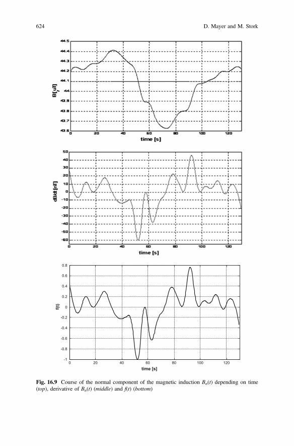
0 20 40 60 80 100 120-1

-0.8

-0.6

-0.4

-0.2

0

0.2

0.4

0.6

0.8

time [s]

f(t)

Fig. 16.9 Course of the normal component of the magnetic induction Bn(t) depending on time(top), derivative of Bn(t) (middle) and f(t) (bottom)


Using the spline interpolation and subsequent numerical derivative of thefunction Bn(t) can be found dBn/dt. This function was normalized by its maximumsize, max[|dBn/dt|] = 60 [nT].

Graph of standardized function f ðtÞ ¼ 1max dBn=dtj j :

dBn

dt¼ 1

60 :dBn

dtis in the bottom

part of Fig. 16.9.Oriented graph G (arbitrarily). The second incidence matrix, matrix of resis-

tances of branches and vector of loops of polygon surfaces of network are

C ¼

1 0 0 0 1 �1 0 0

0 1 0 0 0 1 �1 0

0 0 1 0 0 0 1 �1

0 0 0 1 �1 0 0 1

2

6

6

6

4

3

7

7

7

5

R ¼ diag 32:150:232:134:61924:131:733½ � X½ �

S ¼

4:5

6:1

9:2

6:25

2

6

6

6

4

3

7

7

7

5

� 109 m2� �

ð16:14Þ

Substituting of matrix (16.14) into Eq. (16.13) get the vector of instantaneousvalues of currents in the branches of the network i(t). Can easily calculate the rmscurrents in the branches of network Ief, in the time interval t 2 ⟨0, 130⟩ [s].

iðtÞ ¼ Af ðtÞ ¼

9:59:412:611:2�1:7�0:093:2�1:4

2

6

6

6

6

6

6

6

6

6

6

4

3

7

7

7

7

7

7

7

7

7

7

5

f ðtÞ ; Ief ¼

2:92:83:83:40:530:030:980:42

2

6

6

6

6

6

6

6

6

6

6

4

3

7

7

7

7

7

7

7

7

7

7

5

½A� ð16:15Þ

The time evolution of currents i(t) [from i1(t) to i8(t)] are shown in Fig. 16.10.

16.7 Effect of Changes in the Earth’s Magnetic Field

on the Reliability of the Distribution Power Network

In the previous section we explain the physical causes of time-variable Earth’smagnetic field and subsequent we found the solution of relatively slow variablephenomenon in the electricity network. We formulate the algorithm of calculationof the values of the quasi-direct current that induce in the branches of the electricity


network. These currents generate electric power which is completely converted toelectric heat in conductors of transmission lines and in the winding of the trans-formers in the electricity system. These currents are purely parasitic and do notparticipate on the transmission of power from generators to appliances, as well asreactive power during normal operation of network. During magnetic storms (i.e. inthe relatively quick changes in the Earth’s magnetic field), this can cause thedissipation of heat damage to wires of transmission lines and windings of thetransformers. This will avoid using the protection network, but at the cost of theinterruption of power supply, which leads to a collapse of the electricity system.

Let in the ith transmission line is the current

iikðtÞ ¼ Ioi þffiffiffi

2p

Ii k sinðkxtþui kf g; k ¼ 1; 2; . . .;1 ð16:16Þ

where I0i is the value of quasi-direct current components induced by changing themagnetic field of the Earth, and the Iik and uik are the effective value of the kthharmonic currents and their phase shift, both in the ith wire of transmission line.Then the dissipated power in the ith wire, according to the Parseval identity, may beexpressed as a Joule’s power

Pi ¼ Ri

X

1

k¼0

I2ik ð16:17Þ

Fig. 16.10 Currents i1 (top) to i8 (bottom) for network according Fig. 16.8


A more complicated case occurs in the transformer winding. A quasi-directcurrent cause not only increases Joule losses in the windings, but also causesreduction of magnetization of magnetic circuit of the transformer.

Decreases permeability of the magnetic circuit and also reduction of theinductance of the windings can leads to a decrease the stability of the electricitysystem and cause also reactive power increasing.

16.8 Conclusion

The input value when calculating the GIC is the time course of the vertical com-ponent of the magnetic induction Bn(t), which can only be estimated based on alarger number of long-term measurements. It is therefore a typical task withuncertain input data. These tasks are resolved in principle, two different approaches:stochastic (probabilistic), or the method of reliable solutions (i.e. using worst-casescenario), we assume the “worst” possible over Bn(t), even if the probability of itsoccurrence is small. The second of the two approaches is therefore pessimistic, butit is “safer”.

The size of the GIC is not crucial size of the normal component of the magneticintensity Bn, but the size of its derivative, i.e. dBn/dt. Based on the observation ofthe geomagnetic field it can be assumed that strong geomagnetic shock waves,which entitle to predict the state of emergency power system, events are very rare.

On presented example it was shown, that for electrical networks are strongmagnetic storms dangerous, because of induction of quasi-direct current. This leadsto current overload of lines. Most dangerous is it this quasi-dc part for transformersespecially for magnetic saturation [45, 46]. These phenomena can be avoided bymeans of protections which excludes some parts of networks from work.

Should such a quite exceptional magnetic storms occurred, can the systemoperator to prevent destructive situations only intervention in the topologicalstructure of the transmission system. Example, it can transform the transmissionsystem into smaller units, or may interrupt galvanic connection some exposed lineof system included with isolating transformers.

Acknowledgements Milan Stork’s participation was supported by Department of AppliedElectronics and Telecommunications, University of West Bohemia, Plzen, Czech Republic and bythe European Regional Development Fund and the Ministry of Education, Youth and Sports of theCzech Republic under the Regional Innovation Centre for Electrical Engineering (RICE), projectNo. No. LO1607, the Internal Grant Agency of University of West Bohemia in Pilsen, the projectSGS-2015-002 and GA15-22712S.


References

1. D.H. Boteler, et al., The Effects of Geomagnetic Disturbances on Electrical Systems at theEarth’s Surface, Adv. Space Res., vol. 22, no. 1, pp. 17–27, 1998.

2. T. Makinen, Geomagnetically Induced Currents in the Finish Power Transmission System,Finnish Meteorological Institute Geophysical Publications, no. 32, pp. 101, 1993.

3. V.D. Albertson, J.N. Thorson, S.A. Miske, The Effects of Geomagnetic Storms on ElectricalPower Systems, IEEE Trans., PAS-94, pp. 1931, 1974.

4. R.A. Gummow, P. Eng, GIC Effects on Pipeline Corrosion and Corrosion Control Systems,Journal of Atmospheric and Solar-Terrestrial Physics, vol. 64, pp. 1755–1764, 2002.

5. D.H. Boteler, R.J. Pirjola, H. Nevanlinna, The Effects of Geomagnetic Disturbances onElectrical Systems at the Earth Surface, Adv. Space Res., vol. 22, no. 1, pp. 17–27, 1998.

6. E.A. Eroshenko, et al., Effects of Strong Geomagnetic Storms on Northern Railways inRussia, Adv. Space Res., vol. 46, issue 9, pp. 1102–1110, 2010.

7. R.A. Gummow, GIC Effects on Pipeline Corrosion and Corrosion Control Systems, Journal ofAtmospheric and Solar-Terrestrial Physics, vol. 64, pp. 1755–1764, 2002.

8. Y. Gallet, et al., Possible Impact of the Earth’s Magnetic Field on the History of AncientCivilizations, Earth Planet, Scientific Letters, vol. 246, no. 1–2, pp. 17–26, 2006.

9. V. Haak, S. Maus, M. Koret, H. Luhr, The Earth’s Magnetic Field Screening and Monitoring,Physics in our Time, vol. 35, no. 5, pp. 218–224, 2003.

10. http://bdv.ig.cas.cz/index.html, http://rwcprague.ufa.cas.cz.11. Z. Nemecek, et al., Dynamics of Magnetosphere and Ionization Processes and its Correlation

with Solar Activity, Bull. GACR, vol. 14/4, no. 5–10, 2006 (in Czech).12. J. Klezcek, Great Encyclopedia of the Universe, Academia, Prague, ISBN 80-200-0906-X,

2002 (in Czech).13. R. Lanza, A. Meloni, The Earth’s Magnetism, Springer, Berlin, ISBN 3-540-27979-2, 2006.14. G.A. Glatsmaier, P.H. Roberts, Phys. Earth Planet, Inter., vol. 91, pp. 63, 1995.15. E.N. Parker, Cosmically Magnetic Fields, Clarendon Press, Oxford, 1979.16. E.N. Parker, Interplanetary Dynamical Processes, Wiley-Interscience, New York, 1963.17. D. Stevenson, Planetary Magnetic Fields, Earth and Planetary Science Letter, 6523, pp. 1–11,

2002.18. P. Ertepinar, et al., Archaeomagnetic Study of Five Mounds from Upper Mesopotamia

between 2500 and 700 BCE, Earth and Plane. Sci. Letters, vol. 357–358, pp. 84–98,December 2012.

19. J.P. Legrand, P.A. Simon, Geomagnetic Storms and their Associated Forecasts,Solar-Terrestrial Predictions - IV, Ed. by J. Hruska, et al., NOAA, Boulder, vol. 3,pp. 191, 1993.

20. G. Verbanac, et al., Four Decades of Geomagnetic and Solar Activity: 1960–2001, Journal ofAtmospheric and Solar-Terrestrial Physics, vol. 72, issue 7–8, pp. 607–616, 2010.

21. P.N. Mayaut, Analysis of Storm Sudden Comment Cements for the Years 1868–1967, Journalof Geophysics, Res. 111, 1975.

22. P. Ertepinas, et al., Archaeomatic Study of Five Mounds from Upper Meoptamia between2500 and 700 BCE: Further Evidence for an Extremely Strong Geomagnetic field from 3000Years Ago, Earth and Planetary Science Letters, vol. 357–358, pp. 89–98, December 2012.

23. Y. Gallet, et al., On the Use of Archeology in Geomagnetism and vice-versa: RecentDevelopments in Archaeomagnetism, C.R. Physic, vol. 10, no. 7, pp. 530–648, 2009.

24. T. Nagata, et al., Secular Variation of Geomagnetic Total Force during the Last 5000 Years,Journal of Geophysics Research, vol. 68, pp. 5277–5281, 1963.

25. J. Larmor, Possible Rotational Origin of Magnetic Fields of Sun and Earth, Elect. Rev. 85,1919.

26. D. Sisan, W. Shew, D. Lathrop, Lorenz Force Effects in Magneto-Turbulence, Physics ofEarth and Planetary Interiors, vol. 135, pp. 137–159, 2003.


http://bdv.ig.cas.cz/index.html

http://rwcprague.ufa.cas.cz

27. B. Skala, J. Hrusak, D. Mayer, M. Stork, On Strongly Nonlinear Phenomena in ElectricalMachines, New Aspects of Systems, Proceedings of 12th WSEAS International Conferenceon Systems, Heraklion, Greece, pp. 120–125, July 22–24, 2008.

28. R. Hide, Structural Instability of Rikitake Disc Dynamo, Geoph. Res. Letter, vol. 22,pp. 1057–1059, 1995.

29. T. Rikitake, Electromagnetism and the Earth’s Interior, Elsevier, Amsterdam, 1966.30. F. Plunian, P. Marty, A. Alemany, Chaotic Behavior of the Rikitake Dynamo with Symmetric

Mechanical Friction and Azimuthal Currents, Proc. Roy. Soc. Lond., vol. 454, pp. 1835–1842, 1998.

31. D.F. Webb, Solar and Geomagnetic Disturbances during the Declining Phase of Recent SolarCycles, Adv. Space Res., vol. 16, no. 9, pp. 57–69, 1995.

32. E. Correia, R.V. de Souza, Identification of Solar Sources of Major Geomagnatic Storms,Journal of Atmospheric and Solar-Terrestrial Physics, vol. 67, issue 17–18, pp. 1702–1705,2005.

33. J.R. Wait, Theory of Magneto-Telluric Fields, Journal Res. National Bureau of Standards, vol.66D, no. 5, pp. 509–541, Sept./Oct. 1962.

34. S.P. Plun Keit, et al., Solar Source Regions of Coronal Man Ejections and their GeomagneticEfforts, Journal of Atmospheric and Solar-Terrestrial Physics, vol. 63, issue 5, pp. 398–407,March 2001.

35. P.N. Mayaud, Analysis of Storm Sudden Commencements for the Years 1868–1967, JournalGeophysics Res., vol. 80, pp. 111, 1975.

36. R. Wang, Large Geomagnetic Storms of Extreme Solar Event Periods in Solar Cycle, Adv.Space Res., vol. 40, issue 12, pp. 1835–1841, 2007.

37. J.P. Elovaara, et al., Geometrically Induced Currents in the Nordic Power Systems,Proceedings of the CIGRE, Paper 36–301, Paris, pp. 10, 30 August - 5 September 1992.

38. A.A. Viljanen, R. Pirjola, Geomagnetically Induced Currents in the Finnish High VoltagePower System - A Geophysical Review, Surv. Geophys, vol. 15, pp. 383–408, 1994.

39. R. Pirjola, M. Lehtinen, Currents Produced in the Finnish 400 kV Power Transmission Gridand in the Finnish Natural Gas Pipeline by Geomagnetically-Induced Electric Fields, Ann.Geophys., vol. 3, pp. 485–491, 1985.

40. R. Pirjola, et al., Prediction of Geomagnetically Induced Currents in Power TransmissionSystems, Adv. Space Res., vol. 26, no. 1, pp. 1–14, 2000.

41. I.A. Erinmez, et al., Management of the Geomagnetically Induced Current Risks on thisNational Grid Company’s Electric Power Transmission Systems, Journal of Atm. and Solar-Terrestrial Physics, vol. 64, pp. 743–756, March-April 2002.

42. T.S. Molinski, Why Utilities Respect Geomagnetically Induced Currents, Journal ofAtmospheric and Solar-Terrestrial Physics, vol. 64, issue 16, pp. 1765–1778, 2002.

43. D. Mayer, Analysis of Electrical Circuit with Matrix Calculus, Academia, Prague, 1966 (inCzech).

44. D. Mayer, Introduction to the Theory of Electric Circuits, 2nd Ed., SNTL/ALFA, Prague,1981 (in Czech).

45. L. Bolduc, J. Aubin, Effects of Direct Currents in Power Transformers, Part I: A GeneralTheoretical Approach, Electric Power Systems Research, vol. 1, issue 4, pp. 291–298, 1978.

46. W.B. Gish, W.E. Feero, G.D. Rockefeller, Rotor Heating Effects from Geomagnatic InducedCurrents, IEEE Trans. Power Delivery, vol. 9, no. 2, pp. 712–719, April 1994.


Index

A

Active power, 144, 147, 151, 152, 155, 158,

159, 175, 178, 179, 185

Alternating Current Transmission System

(FACTS), 317, 319, 320, 323, 324, 329,

337, 342

Apparent power, 144, 147–149, 151, 152, 155,

159, 163, 164, 167, 168

Artificial Bee Colony (ABC), 255

Aurora, 618

Automatic compensation, 154, 156

Automatic Repeat reQuest (ARQ), 550

Automatic Secondary Voltage Regulation, 228,

242

B

Back-to-Back (B2B), 288, 310, 312

Balanced loads, 155

Bandwidth, 552, 553, 556

Banks capacitors, 240, 241

Battery Energy Storage System (BESS), 296

Best compromise solution, 478, 483, 487, 492,

494, 496, 498, 499, 501, 503, 505

C

Cascaded H-Bridge (CHB), 302–304

Cicode programs, 592

CitectSCADA, 591–593

Code Division Multiple Access (CDMA), 554,

555, 558

Combined Heat and Power (CHP), 549

Comma separated value (CSV), 461

Communications, 547, 549, 551, 552

Compensator, 137–139, 141, 145, 146, 151,

159, 169, 185

Constraints, 337

Control, 227, 233

Cost function, 329

Coverage, 548, 553, 555

Current Source Converter (CSC), 289

Customised-Of-The-Shelf (COTS), 551

Cyber, 565, 567, 579

Cyber attacks, 574, 578

Cyber security, 565, 579

Cyclodissipativity, 137, 138, 144, 185

D

Decision variable, 476, 489, 490, 510

Delta configuration, 159

Deterministic ORPD (DMO-ORPD), 476, 478,

491–496, 498, 500–503, 505, 507, 508, 510

Differential Evolution (DE), 255

Digital signal processor, 175

DIgSILENT Programming Language (DPL),

417

Diode clamped, 295, 302

Dissipative systems, 137, 146

Distributed generation (DG), 191, 203, 204,

276, 287

Distribution Network Operator (DNO), 253

Double fed induction generator (DFIG), 224

Dynamical system, 145

Dynamic Power Flow Controller (DPFC), 287,

288, 309, 312

Dynamic Voltage Restorer (DVR), 288

E

Earth’s magnetosphere, 618

Electric Power Systems, 547, 549

Electric Vehicle (EV), 549

Electromagnetic Interference (EMI), 276, 289

Energy loss, 329

Energy storage system, 296, 311

Energy transmission, 137–139, 144, 182

Evolutionary programming (EP), 346

Expected value of power loss, 484



Power Systems, DOI 10.1007/978-3-319-51118-4

631

Expected value of voltage deviation, 484

F

Fibre Optic Communication, 547, 552

Fibre to the Home (FTTH), 552

Fixed capacitor, 518

Fixed Capacitor Thyristor-Controlled Reactor

(FCTCR), 124, 125

Flexible AC Transmission Systems (FACTS),

252, 275, 312

Flying capacitor MLC (FC-MLI), 302

Forward Error Correction (FEC), 550

Fuzzy Adaptive Particle Swarm Optimization

(FAPSO), 255

Fuzzy decision making, 320, 333

G

Gate Turn-Off Thyristor (GTO), 287, 295, 298,

302

Generalized Unified Power Flow Controller

(GUPFC), 319, 320, 325–328, 337, 339,

340, 342

General Packet Radio Service

(GPRS), 553

Genetic algorithm (GA), 192, 346, 365, 378

Geodynamo, 614–616

Geomagnetic activity, 612, 618

Geomagnetic storm, 611, 613, 619

Geomagnetism, 613, 614, 618

Global System for Mobile Communications

(GSM), 551, 553, 555

Global System for Mobile Communications -

Railway (GSM-R), 551

Goodput, 556

H

High Voltage Direct Current (HVDC),

287–289, 310–312

HMI, 563, 564, 572, 573, 576, 577, 581, 582,

591, 607

Homogenous operators, 141, 142

Honey Bee Mating Optimization (HBMO), 265

Hybrid Flow Controller (HFC), 319–321, 323,

329, 330, 337, 339, 340, 342

Hybrid Stochastic Search (HSS), 255

I

IEEE 802.11 Mesh Networking, 547, 557

IEEE 802.15.4 Wireless Sensor Network, 547,

558

IEEE Standard, 547, 558

Improved Genetic Algorithm (IGA), 265

Improved PSO (IPSO), 255

Incidence matrix, 622, 625

Induction machine (IM), 518, 519, 521, 526,

542

Insulated Gate Bipolar Transistor (IGBT), 287,

288, 295

Insulated Gate Commutated Thyristor (IGCT),

287, 288, 295

Interline Power Flow Controller (IPFC), 127,

128, 310, 312, 319

Internal product, 142

Internetwork Protocol version 6 (IPv6), 550

Inter-phase power controller (IPC), 296, 319

ISA100.11a, 558

K

Kirchhoff current law (KCL), 50, 57, 58, 66,

72, 97, 98, 100, 103, 105, 106, 108, 109,

111

Kirchhoff voltage law (KVL), 57, 58, 66, 67,

97, 100, 103, 111

L

LAN, 572, 574, 587, 608

Latency, 553, 556, 557

Life expectancy, 556

Linear Programming (LP), 255

Long Term Evolution (LTE), 553, 555

Loss, 193, 195, 196, 198, 199, 207, 209, 219,

221–223

Low-pass filter, 154, 173, 174

M

Machine-To-Machine (M2M), 550, 554, 555

Magnetic storm, 611, 612, 618–620, 626, 627

Media Access Control (MAC), 558

Metering, 547, 548, 550–552

Minimal value, 148

Mixed integer non-linear program (MINLP),

476

Modular Multilevel Converter (MMC),

310–312

Monte Carlo simulation (MCS), 478

MOPSO-NTVE, 331, 333, 334, 337, 338, 340,

341

MOPSO-TVAC, 338, 339, 341

MOPSO-TVIW, 338, 339, 341

MS SQL database, 587

MTU, 608

Multi-converter FACTS (M-FACTS), 319,

320, 323, 324, 329

Multilevel Converter, 276, 298, 302

Multi-objective, 318, 320, 321, 331, 342

Multi-Objective Optimal Reactive Power

Dispatch (MO-ORPD), 475, 477, 478, 491,

494, 507

632 Index

Multi-objective optimization, 320, 321, 331

N

Network, 612, 613, 619–623, 625–627

Neutral Point Clamped (NPC), 131

Nodal Method, 50, 97

Nonlinear, 137, 138, 144–146, 151–156, 168,

171, 177

Non-Linear Programming (NLP), 255

Nonsinusoidal, 137, 138, 140, 141, 172

Number of Function Evaluation (NFE), 394,

457, 463, 465, 466, 469, 470

O

On-Load Tap Changer (OLTC), 252, 253, 255

Operating point, 517, 518, 528–531, 533–535,

543

Optimal power flow (OPF), 214, 217, 252, 264,

346, 475, 476

Optimal reactive power dispatch, 475, 476, 510

Optimal reactive power flow (ORPF), 252, 362

P

Pareto front, 221, 222

Particle Swarm Optimization (PSO), 255, 346,

366–371, 375, 378, 399, 427, 428, 435,

437, 438, 439, 442, 443, 449, 463,

465–468, 474

Pattern search, 347, 372–378, 382–385, 387,

389, 391, 397

Phase-shifting transformer (PST), 310, 319,

321

Planetary magnetism, 615

Point of Common Coupling (PCC), 262, 276,

281

Polyphase, 139, 141

Power factor, 17, 31, 35–38, 43, 44, 276–278

Power Flow Controller, 287–290, 308–310,

312

Power Line Communications (PLC), 547, 552

Power loss, 475–477, 483, 484, 492, 494, 498,

507, 510

Power quality, 227, 228, 237

Power system, 3–6, 21, 26, 31, 45, 227–229,

233, 234, 237, 240, 246, 247

Power transfer theorem, 50, 97

Power transformer sockets, 241

Power triangle, 172, 177

Probability distribution function (PDF),

478–480, 482

Pulse Width Modulation (PWM), 287

Q

Quadratic Programming (QP), 255, 346

R

Reactive power, 4, 12, 17, 34–38, 42–44,

137–139, 141, 145, 146, 148, 154, 155,

159, 163, 167, 169, 171–174, 185, 191,

193–200, 205, 209, 211–214, 216–218,

222–224, 227–237, 240–243, 245, 246

Reactive power compensation, 36, 38, 44

Reactive power consumption, 34, 35, 38, 44

Reactive Power Dispatch (RPD), 255–258,

261, 271

Reactive Power Planning (RPP), 263, 265, 269,

318

Real Genetic Algorithms (RGA), 255

Reliability, 191, 192, 196, 203, 204

Renewable energy source, 276

Resilience, 556

Resistive-inductive load, 518

Rikitake system, 616

Root mean square, 51

S

SCADA, 561–579, 581–591, 595, 597,

601–604, 606–608

Scalability, 549, 556

Security, 549, 551, 555, 556

Self-excited induction generator, 518, 526, 528

Sequential Quadratic Programming

(SQP), 346

Service Level Agreement (SLA), 550, 551, 555

Sinusoidal signal, 50–53, 97, 111

Smart grid, 554–557

Smart Integrated Generation, 549

Smart Market, 549

Smart Network Management, 549

Solar activity, 611, 617, 619

Solar wind, 613, 618, 619

Standards for power systems, 3, 26

Static Synchronous Compensator

(STATCOM), 276, 296–298, 319

Static Synchronous Series Compensator

(SSSC), 127, 128

Static VAr Compensation (SVC), 261, 265

Static VAR Compensator, 276, 287, 289

Static Voltage Restorer (SVR), 288

Static Voltage Stability (SVS), 264

STC, 329, 330, 334, 340

Stochastic MO-ORPD (SMO-ORPD), 475,

476, 478, 486, 490, 491, 497, 501, 504, 507

Index 633

Sub-Synchronous Resonance (SSR), 123, 288,

294, 303–305, 312

Superconducting Magnetic Energy Storage

(SMES), 296

Surge Impedance Loading (SIL), 118, 132

Switched, 179

Synchronous condenser, 228, 235, 236, 241

T

Tabu Search (TS), 255

Tellegen’s theorem, 145

Three-phase networks, 154, 185

Throughput, 553

Thyristor-Controlled Braking Resistor

(TCBR), 296

Thyristor-Controlled Reactor (TCR), 124, 125,

287, 290, 293, 294, 309, 517, 536

Thyristor-Controlled Series Capacitor (TCSC),

126

Thyristor-Controlled Series Compensator

(TCSC), 287, 294, 295

Thyristor-Controlled Series Reactor (TCSR),

126

Thyristor-Controlled Voltage Limiter (TCVL),

296

Thyristor-Switched Capacitor (TSC), 124, 125,

287, 290–292, 309

Thyristor-Switched

Capacitor-Thyristor-Controlled Reactor

(TSC-TCR), 124, 125

Thyristor-Switched Reactor (TSR), 124, 125

Thyristor-Switched Series Capacitor (TSSC),

125, 319

Thyristor Switched Series Reactor (TSSR), 319

Time delay, 172, 173, 177

Total harmonic distortion, 28, 41, 80, 277

Traditional Genetic Algorithm (TGA), 265

U

Unbalanced, 140, 154, 158, 161–163, 165, 168

Unified Power Flow Controller (UPFC), 127,

128, 287, 288, 296, 306–308, 310, 312,

319, 320

V

Vijeo Citect Surveillance Softwares, 561, 565,

566, 591

Volt Ampere Reactive (VAR), 275, 276, 287,

289, 296

Voltage collapse, 318

Voltage Deviation (VD), 195, 221–223, 329,

362, 385, 386, 388, 390, 476, 478, 483,

484, 492, 494, 507, 510

Voltage profile, 318

Voltage Source Converter (VSC), 276,

287–289, 295–301, 304, 306, 308, 310–312

Voltage stability, 193, 221–223, 227, 228, 233,

246, 247, 318, 475–478, 483–485, 507, 510

Voltage Stability Index (VSI), 362, 384, 386,

387, 389

Voltage Stability Margin (VSM), 255

W

WiFi, 552, 558

WiMAX, 556, 558

Wind farm, 259, 261, 265, 266, 271, 476, 482,

483, 488, 489, 493, 496, 503, 506, 508

Wind power plant, 192, 201, 202, 211, 221,

223, 241, 243

Wind turbine, 191, 193–199, 201, 202, 204,

205, 210, 211, 213–215, 222–224, 259, 265

WirelessHART, 558

Wireless network, 553, 558

Wireless technologies, 547, 553, 556

X

X Digital Subscriber Line/Loop (xDSL), 547,

552

Z

Zero-Voltage Switching (ZVS), 290

ZigBee, 558

634 Index

Reactive Power Control in AC Power Systems

Documents

Transcript of Reactive Power Control in AC Power Systems