IFPRI Discussion Paper 00811

October 2008

Reaching Middle-Income Status In Ghana By 2015

Public Expenditures and Agricultural Growth

Samuel Benin Tewodaj Mogues Godsway Cudjoe

Josee Randriamamonjy

Development Strategy and Governance Division

INTERNATIONAL FOOD POLICY RESEARCH INSTITUTE

The International Food Policy Research Institute (IFPRI) was established in 1975. IFPRI is one of 15 agricultural research centers that receive principal funding from governments, private foundations, and international and regional organizations, most of which are members of the Consultative Group on International Agricultural Research (CGIAR).

FINANCIAL CONTRIBUTORS AND PARTNERS IFPRI’s research, capacity strengthening, and communications work is made possible by its financial contributors and partners. IFPRI gratefully acknowledges generous unrestricted funding from Australia, Canada, China, Denmark, Finland, France, Germany, India, Ireland, Italy, Japan, the Netherlands, Norway, the Philippines, Sweden, Switzerland, the United Kingdom, the United States, and the World Bank.

AUTHORS Samuel Benin, International Food Policy Research Institute Research Fellow, Development Strategy and Governance Division Tewodaj Mogues, International Food Policy Research Institute Research Fellow, Development Strategy and Governance Division Godsway Cudjoe, International Food Policy Research Institute - Ghana Research Officer, Development Strategy and Governance Division Josee Randriamamonjy, International Food Policy Research Institute Research Analyst, Development Strategy and Governance Division

Notices 1 Effective January 2007, the Discussion Paper series within each division and the Director General’s Office of IFPRI were merged into one IFPRI–wide Discussion Paper series. The new series begins with number 00689, reflecting the prior publication of 688 discussion papers within the dispersed series. The earlier series are available on IFPRI’s website at www.ifpri.org/pubs/otherpubs.htm#dp. 2 IFPRI Discussion Papers contain preliminary material and research results. They have not been subject to formal external reviews managed by IFPRI’s Publications Review Committee but have been reviewed by at least one internal and/or external reviewer. They are circulated in order to stimulate discussion and critical comment.

Copyright 2008 International Food Policy Research Institute. All rights reserved. Sections of this material may be reproduced for personal and not-for-profit use without the express written permission of but with acknowledgment to IFPRI. To reproduce the material contained herein for profit or commercial use requires express written permission. To obtain permission, contact the Communications Division at ifpri-copyright@cgiar.org.

iii

Contents

Acknowledgments v 

Abstract vi 

1. Introduction 1 

2. Public Spending, Growth and Poverty in Ghana 3 

3. Conceptual Framework 12 

4. Data and Estimation 16 

5. Results and Discussion 20 

6. Conclusions 34 

Appendix: Supplementary Tables 36 

References 40 

iv

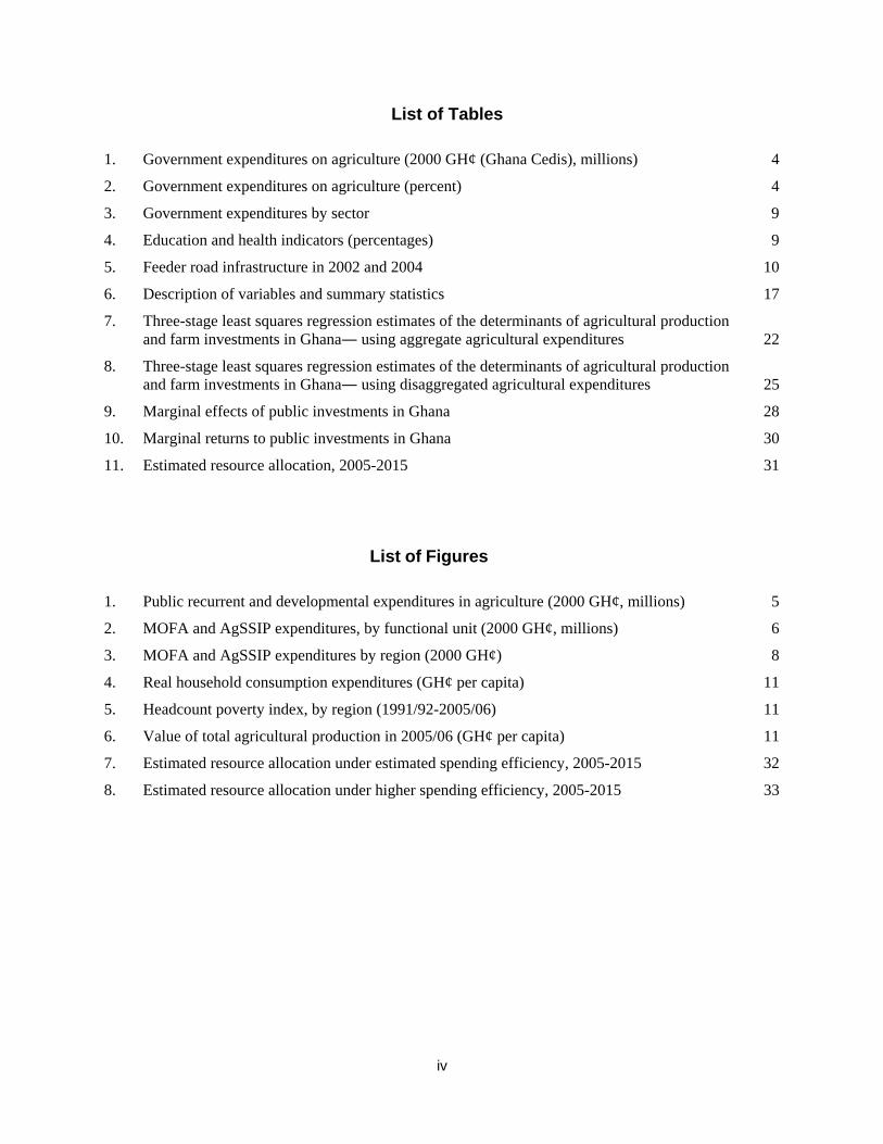
List of Tables

1. Government expenditures on agriculture (2000 GH¢ (Ghana Cedis), millions) 4 

2. Government expenditures on agriculture (percent) 4 

3. Government expenditures by sector 9 

4. Education and health indicators (percentages) 9 

5. Feeder road infrastructure in 2002 and 2004 10 

6. Description of variables and summary statistics 17 

7. Three-stage least squares regression estimates of the determinants of agricultural production and farm investments in Ghana― using aggregate agricultural expenditures 22 

8. Three-stage least squares regression estimates of the determinants of agricultural production and farm investments in Ghana― using disaggregated agricultural expenditures 25 

9. Marginal effects of public investments in Ghana 28 

10. Marginal returns to public investments in Ghana 30 

11. Estimated resource allocation, 2005-2015 31 

List of Figures

1. Public recurrent and developmental expenditures in agriculture (2000 GH¢, millions) 5 

2. MOFA and AgSSIP expenditures, by functional unit (2000 GH¢, millions) 6 

3. MOFA and AgSSIP expenditures by region (2000 GH¢) 8 

4. Real household consumption expenditures (GH¢ per capita) 11 

5. Headcount poverty index, by region (1991/92-2005/06) 11 

6. Value of total agricultural production in 2005/06 (GH¢ per capita) 11 

7. Estimated resource allocation under estimated spending efficiency, 2005-2015 32 

8. Estimated resource allocation under higher spending efficiency, 2005-2015 33 

v

ACKNOWLEDGMENTS

We would like to thank the Ghana Statistical Services for allowing us advance access to the 2005/06 Ghana Living Standards Survey, and the Accountant General’s Office, Ministry of Food and Agriculture, Ministry of Roads Transport, Ghana Education Service and Ministry of Health for providing data on public expenditures. The study was funded by the United States Agency for International Development (USAID) Ghana Mission through their support of the Ghana Strategy Support Program (GSSP). For further information on GSSP, please see www.ifpri.org/themes/gssp.htm

vi

ABSTRACT

Using district-level data on public expenditures from 2000 to 2006, and household-level production data from the 2005/06 Ghana Living Standards Survey, this paper estimates the returns to different types of public investments across four agro-ecological zones of Ghana. We then assess the amount of public agricultural expenditures required to raise agricultural growth to 6.9 percent per year until 2015, as this is the target growth needed for Ghana to achieve its goal of middle-income status. The results reveal that provision of various public goods and services has substantial impact on agricultural productivity. A one percent increase in public spending on agriculture is associated with a 0.15 percent increase in agricultural labor productivity, with a benefit-cost ratio of 16.8. Spending on feeder roads ranks second (with a benefit-cost ratio of 8.8), followed by health (1.3). Formal education was negatively associated with agricultural productivity. The estimated marginal effects and returns differ across the four agro-ecological zones. For Ghana to achieve middle income status by 2015, agricultural public spending should grow at an estimated rate of 19.6 percent per year, or by a total amount of GH¢264 million (or US$478 million) per year in 2000 prices over the 2005–2015 period. These requirements are lower if the government is able to achieve a higher efficiency in its public spending than the estimated elasticity of 0.15; this could potentially be achieved by reforming public institutions to improve the provision of agriculture-related public goods and services.

Keywords: agricultural development, Ghana, public spending and investments

1

1. INTRODUCTION

The government of Ghana, in its Growth and Poverty Reduction Strategy (GPRS II), declared its new developmental goal of reaching middle-income status, defined as raising the per capita income of Ghanaians to at least US$1000, by 2015 (NDPC 2005). The country’s developmental strategy seeks to propel economic growth through structural transformation arising from growth in the agricultural sector. Agriculture has the potential to be an engine of growth; as in many other African and developing countries, agriculture is the single highest contributor to GDP and provides employment for a majority of the population in Ghana. With the bulk of the poor, especially women, engaged in this sector, agriculture-driven economic growth also has attractive distributional properties. Especially in regions where the sector constitutes a large share of the economy, accelerated agricultural growth is nearly a precondition for rapid economy-wide growth, as found in the case of Ghana (Breisinger et al. 2008) and elsewhere (Diao et al. 2007; Thurlow et al. 2007).

Similar to many governments in Africa and developing countries in other regions, the government of Ghana is faced with limited policy instruments for promoting growth and equitable distribution,1 and therefore must play a key role in directing public sector resources not only to improve technology, human capital and infrastructure for development, but also with the aim of providing incentives and promoting private sector investments. In light of the central role that agriculture plays in Ghana’s developmental strategy, this raises a number of key questions. For example, how much public expenditures in agriculture will be required to achieve the country’s growth targets? Would allocating 10 percent of national budgetary resources to the agricultural sector, as suggested by the Comprehensive Africa Agriculture Development Programme (CAADP) (AU/NEPAD 2003), be sufficient for achieving the targets? How should agricultural and other public expenditure resources be allocated among different types of public goods and services (e.g. agricultural research, extension, irrigation, roads, education, and health) and across geographic areas to improve the distributional outcomes and impacts?

This paper addresses these questions by first estimating the returns to public spending in agriculture and other sectors of the economy across different geographic areas of Ghana. We then use the results to assess the amount of public agricultural expenditures required to achieve CAADP’s 6 percent agricultural growth target, as well as the growth rate identified in Breisinger et al. (2008) as being needed for Ghana to reach middle-income country status by 2015.

The empirical studies on returns to public investments in terms of agricultural growth and poverty reduction is dominated by analyses of individual public investment programs, such as agricultural research or extension (e.g. Evenson 2001; Alston et al. 2000; Evenson et al. 1999; Rosegrant and Evenson 1995), health (e.g. Collier et al. 2002), other social sectors (e.g. Gomanee et al. 2003), or infrastructure (see Guild 2000 for a review). These studies, however, have limited application when considering prioritization of resources across alternative and often competing public programs. The literature on the prioritization of public investment programs is mostly limited to developed countries, with relatively few studies in the developing country context (on the latter, see Fan et al. 2000 for work on India; Fan and Zhang 2004 on China; Fan and Rao 2003 for cross-country analysis; Fan et al. 2004 and 2005 on Uganda and Tanzania respectively; and Mogues et al. 2007 on Ethiopia). The relative lack of evidence from developing countries is primarily due to a lack of adequate spatially-disaggregated time-series data on public expenditures,2 especially in African and Latin American countries. Adequate time-series data are necessary for this type of analysis, since the effects of public investments commonly materialize with a

1 Due to the existence of a large informal sector that is effectively immune from taxation in developing countries, the governments of these countries tend to have fewer tax instruments than rich countries. Also, imposing taxes on some branches of the economy and not on others can create high economic distortions (Auriol and Warlters 2002).

2 Public expenditure is typically made up of two components: recurrent and capital or developmental expenditure. Recurrent expenditure typically includes salaries for employees, overheads, administration and operational costs for delivery of public goods and services. The capital or developmental component is the part of public expenditure that adds to the public capital stock (e.g. agricultural research facilities, technologies, irrigation dams and canals, roads, electricity grids, schools, knowledge, hospitals, etc.) and is also referred to as public investments.

2

lag, the length of which varies substantially by the type of investments and the outcome of interest. Spatially-disaggregated data are important both as the main basis of cross-sectional variation in estimation, and for assessing the returns to expenditures in different geographic areas (e.g. in areas of high versus low agricultural potential). Although the theory is clear on the expected impacts of different types of public investment programs on growth and poverty reduction, there is a relatively large variation in the empirical findings on the magnitude and (to some extent) direction of these impacts, due to variation in the employed methodologies and data. Differences arise from a number of considerations, such as the use of aggregate versus partial productivity measures in determining the agricultural productivity outcomes of public expenditures, treatment of the potential endogeneity of public expenditures, lags between spending and outcome variables, and the level of analysis, particularly in terms of the geographic units and sectoral categorization of spending. See Guild (2000), Zhang and Fan (2004) and Mogues et al. (2007) for discussions of the various approaches in the empirical literature.

The rest of the paper is organized as follows. First, we examine trends in and composition of public expenditures on agriculture in Ghana. We then present the conceptual framework that we use to quantify and analyze the impacts of government spending on agriculture and provision of other public goods and services on agricultural productivity. The data, estimation procedures, and results are then presented, followed by conclusions and implications.

3

2. PUBLIC SPENDING, GROWTH AND POVERTY IN GHANA

Public Expenditures in Agriculture In 2003, African leaders decided, through the CAADP initiative of NEPAD (the New Partnership for Africa’s Development), to allocate at least 10 percent of their public expenditures to agriculture. This is an ambitious goal relative to the actual paltry shares of agricultural spending, and it has (among other things) created an incentive for governments to consider a broad definition of agricultural spending, namely one that includes spending on rural roads and multi-sectoral projects (e.g. dams, which serve in both energy generation and irrigation). Thus, NEPAD’s CAADP initiative has generated increasing debate on how to appropriately define agricultural public expenditure. The African Union’s NEPAD developed a standard definition that is more or less consistent with the International Monetary Fund (IMF) classification of functional areas of government (COFOG) (AU/NEPAD 2005; IMF 2001), though some important differences remain between the two key sources. For example, while agricultural research and development (R&D) is included in the core areas of agriculture under the AU/NEPAD definition, the IMF classification gives it a separate non-agricultural category under R&D for Economic Affairs. Under the AU/NEPAD definition, the multi-sectoral projects mentioned above, which many governments include in ‘agricultural public spending,’ are legitimately part of agricultural public spending if at least 70 percent of the costs are directly related to agricultural activities. While establishing this can be a tedious exercise, it is necessary for full accounting. In the IMF’s COFOG, however, expenditure on such projects is excluded from agriculture. Although the definition of what should and should not fall under agricultural public spending seems somewhat ambiguous, it is generally agreed that the definition includes at least public spending related to the sub-sectors of crops, livestock, fisheries, forestry, and natural resources. Another way of defining it, perhaps from a broader perspective, is in terms of function; this would lead to the inclusion of public spending on agricultural research, agricultural extension and training, agricultural marketing, agricultural inputs (e.g. seeds, fertilizers, chemicals, etc.), irrigation, rural agricultural infrastructure (feeder roads, marketing information system, post-harvest handling, etc.), food security or food imports, etc. Although not classified as agricultural spending, expenditures in various other sectors (e.g. spending on transport, power, education, and health) can also contribute to agricultural growth.

The implication of even the narrower definition in the case of Ghana, as in many agriculture-dependent economies, is that agricultural spending takes place not only through the conventional Ministry of Agriculture, but also through various other government ministries and agencies. In Ghana for example, fisheries and forestry fall under two separate ministries. Cocoa, which attracts the bulk of government’s agricultural expenditures, falls under the Ghana Cocoa Board, which in turn is under the Ministry of Finance and Economic Planning. Agricultural R&D is managed by the Council for Scientific and Industrial Research (CSIR), which reports to the Ministry of Education, Sports and Science (MESS).3 The AU/NEPAD definition of agricultural expenditure also includes spending on agricultural education in universities; in Ghana, this falls under the National Council for Tertiary Education, which is in turn under MESS. Other government expenditures on agriculture in Ghana is undertaken through the Ministry of Trade and Industry (regarding agricultural marketing and trade and food imports), the Ministry of Roads and Transport (regarding feeder roads development), the Ministries of Local Government and Rural Development, Women and Children Affairs, and Manpower Development and Employment (all regarding agricultural community-based development projects), and Presidential Special Initiatives on agriculture. Thus, even with a clearly defined agricultural sector, it is usually difficult to obtain actual expenditures data on the sector when the audited public accounts do not have clearly defined line items.

The primary source of data on the government’s agricultural expenditures we use in this study is the Controller and Accountant General’s Department (CAGD), supplemented with data from several other sources, including the Ministry of Food and Agriculture (MOFA), the Ghana Cocoa Board (COCOBOD), and the Council for Scientific and Industrial Research (CSIR). As shown in Table 1, the

3 Until 2007, CSIR was under the Ministry of Environment, Science and Technology.

4

Government of Ghana’s resource allocation to the agricultural sector nearly doubled between 2000 and 2005. Interestingly, MOFA, the conventional ministry responsible for the agricultural sector, accounts for only 25 percent of total public spending on the sector. The percentage drops to 20 percent when spending on feeder roads is counted as part of agricultural spending. Agencies other than the core ministry seem to have gained over time in their relative importance for developing the sector; an agricultural sector expenditure review carried out across similar expenditure categories and ministries, departments, and agencies (MDAs) over 1995-97 showed MOFA as the highest spender of public funds allocated to the sector, accounting for between 48 and 57 percent of the total expenditures in the sector (MOFA 1999).

Table 1. Government expenditures on agriculture (2000 GH¢ (Ghana Cedis), millions1)

MOFA and MOF2 DOF3 CSIR4 COCOBOD5 2000 5.16 0.94 3.80 20.51 2001 4.74 0.73 3.63 22.71 2002 5.30 0.68 4.50 18.06 2003 11.13 0.72 3.88 25.10 2004 19.96 3.93 6.36 36.84 2005 14.56 2.08 5.08 36.43 Sources: Office of the Controller and Accountant General; Statistics, Research and Information Department (SRID) of MOFA. Notes: 1 Government expenditures are financed from internally generated funds, and from overseas developmental assistance in the form of loans and grants. In 2000, US$1 ≈ GH¢0.55. 2 Until 2005, MOF (Ministry of Fisheries) was part of MOFA (Ministry of Food and Agriculture). In 2005, the allocation to MOF was GH¢0.4 million. 3 DOF is the Department of Forestry under the Ministry of Lands and Forestry. 4 CSIR is the Council for Scientific and Industrial Research. 5 COCOBOD is the Ghana Cocoa Board.

A critical issue in the debate on using agriculture to drive overall economic development is the disproportionately low government commitment to the sector relative to the total public budget, especially in light of the agricultural sector’s role in African economies (World Bank 2008). As shown in Table 2, counting only MOFA’s (and MOF’s) expenditures as the government’s expenditures on the sector in Ghana indicates a low expenditure of 1.2 percent of total government spending or 0.8 percent of agricultural GDP. When we account for agricultural spending in the other three MDAs, the share rises to 5.2 percent of total government spending, or 3.6 percent of agricultural GDP. Including feeder roads investments in agricultural expenditures raise these percentages to 6.5 and 4.4, respectively.

Table 2. Government expenditures on agriculture (percent)

Percent of total expenditures Percent of agricultural GDP MOFA and MOF MOFA, MOF, DOF,

CSIR, COCOBOD MOFA and MOF MOFA, MOF, DOF,

CSIR, COCOBOD 2000 0.8 3.2 0.5 3.2 2001 0.7 4.7 0.5 3.2 2002 0.7 3.9 0.5 2.5 2003 1.4 5.0 0.9 3.3 2004 2.0 6.7 1.4 4.8 2005 1.5 5.8 1.0 4.0 Average 1.2 5.2 0.8 3.6 Sources: Authors’ calculation based on data from the Office of the Controller and Accountant General and the Statistics, Research and Information Department (SRID) of MOFA (see Table 1). Notes: See footnotes to Table 1 for abbreviations.

5

Note that since we do not account for additional public agricultural expenditures through other MDAs,4 the actual shares may be higher than those shown in Table 2. As reported here, however, the share spent on agriculture is lower than the annual average share spent on the health (8.3 percent) or education (28.3 percent) sectors within the same period, but higher than the share spent on roads and transport (1.7 percent). Note that the expenditures reported above also do not include direct donor spending on the sector that falls outside the government treasury or falls under projects managed by non-government agencies. Since such sources are considered public funds, agricultural public expenditures as a share of agricultural GDP is likely to be much higher than previously thought (World Bank 2008).

Developmental and Recurrent Agricultural Expenditures

Figure 1 shows that the bulk of the government’s expenditures on the sector was allocated to recurrent activities, particularly salaries. Real investments funding rose substantially in 2003 and was maintained through 2005. The relatively low level of government (domestic) capital investments reflect the high level of direct donor funding or projects for developmental activities in the sector, but also raises questions about the sustainability of donor support to the sector and concern regarding the government’s ability to maintain this level of funding in the event of a substantial reduction in donor funds. Mainstreaming project activities into the government budget may be a useful way to allow donor projects to wind down. In general, donors provide the bulk of developmental spending in Ghana. In 2003, for example, about 35 percent of the government’s total budget was comprised of various multilateral and bilateral grants and loans from donors (Quartey 2005). However, some aid agencies implement developmental activities directly in partnership with the private sector and non-governmental organizations. The amount of donor spending through these arrangements or outside the government financial system, while believed to be substantial, is not available for the present study. The United States Agency for International Development (USAID), for example, which is one of the aid agencies that does not provide budgetary support, is the third largest bilateral donor (UNDP cited in USAID 2008). Between 2004 and 2006, USAID spent about USD7.3 million per year on its ‘Increase Competitiveness of Private Sector’ program, under its ‘Economic Growth, Agriculture and Trade’ Strategic Objective (USAID 2008).

Figure 1. Public recurrent and developmental expenditures in agriculture (2000 GH¢, millions)

Source: Authors’ calculation based on data from the office of the Controller and Accountant General. Notes: Public expenditures in agriculture include spending by MOFA, MOF, CSIR, and DOF (see notes to Table 1).

4 Other government expenditures on agriculture not accounted for include those undertaken through the Ministry of Trade

and Industry (regarding agricultural marketing and trade and food imports), the Ministries of Local Government and Rural Development, Women and Children Affairs, and Manpower Development and Employment (all regarding agriculture community-based development projects), and Presidential Special Initiatives on agriculture.

0

3

6

9

12

15

18

0

20

40

60

2000 2001 2002 2003 2004 2005

perc

ent

2000

GH

¢, m

illio

ns

Developmental (2000 GH¢, mil.)Recurrent (2000 GH¢, mil.)Developmental (percent of total)

6

Functional Composition and Spatial Disaggregation of Agricultural Expenditures

The first two graphs of Figure 2 show that about 50-75 percent of MOFA’s expenditures was at the sub-national level, reflecting a relatively high degree of deconcentrated (albeit not decentralized) spending. However, the share spent at the sub-national level fell over time from 65 to 62 and then 58 percent in 2000, 2002 and 2005, respectively. Spending at the level of the technical directorate was much lower than the amount spent at the headquarters (excluding the directorates). Although spending at the directorate level is still part of central spending, it can be disaggregated by subsector, as the directorates are primarily responsible for the promotion of technologies that are developed by the agricultural research institutions. The second and third graphs present the spending trends of the Agricultural Services Sector Investment Programme (AgSSIP), which is a large, countrywide donor-supported program that provides investments across a range of agricultural sub-sectors (World Bank 2000).5 AgSSIP, as the name implies, covers the entire sector, and the agricultural expenditures data extend to other MDAs outside MOFA, including the Ministry of Lands and Forestry (MOLF), CSIR, COCOBOD, the Ministry of Manpower, Youth and Employment, and the Ministry of Women and Children Affairs. As seen in Figure 2, AgSSIP spending on research is relatively low. Infrastructure (including irrigation and engineering services) and extension attracted the bulk of non-administrative funds, followed by crops and livestock development. The amount spent on natural resource management was relatively insignificant, raising concerns about the sustainability of potential productivity increases.

Figure 2. MOFA and AgSSIP1 expenditures, by functional unit (2000 GH¢, millions)

5 We examine the functional and spatial disaggregation of MoFA and AgSSIP expenditures only, due to lack of similar data

for the MDAs.

MOFA

0

3

6

9

12

2000 2001 2002 2003 2004 2005

Technical Directorates Headquarters RADUs

7

Figure 2. Continued

Source: Authors’ calculation based on data from MOFA. Notes: 1 Agricultural Services Sector Investment Programme. Notes: RADU = Regional Agricultural Development Unit. NRM = Natural Resource Management.

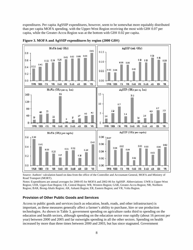
There is substantial variation in MOFA and AgSSIP regional-level expenditures across the 10 Regional Agricultural Development Units of Ghana (Figure 3). The Volta Region attracted the largest share of MOFA spending, followed by the Eastern, Ashanti and Brong-Ahafo Regions, while the Upper-West and Upper-East Regions attracted the least. When the area or population is taken into account, the picture is totally different. The average annual amount spent by MOFA per unit area in the Greater-Accra Region (GH¢ 152 per sq km) overwhelmed expenditures in all other regions. The next-largest recipients of expenditures per area unit were the Central and Upper-East, with the Upper-West, Brong-Ahafo and Northern Regions attracting the least expenditures. In terms of expenditures per capita, however, the Upper-West, Volta and Upper-East Regions were at the top, while the population-dense Ashanti and Greater-Accra Regions were at the bottom.

AgSSIP expenditures exhibit similar patterns. The average annual amount spent per unit area was highest in the Greater-Accra Region (GH¢ 13.2 per sq km), followed by the Central, Eastern and Upper-East Regions, while the Northern, Upper-West and Brong-Ahafo Regions accounted for the least

AgSSIP

0.0

0.5

1.0

1.5

2002 2003 2004 2005 2006

Colleges andResearch

Headquarters

TechnicalDirectorates

RADUs

AgSSIP

0.0

0.1

0.1

0.2

0.2

0.3

0.3

2002 2003 2004 2005 2006

NRM

Fishery

Infrastructure

Extension

Admin/Plan

Crops

Livestock

Other

8

expenditures. Per capita AgSSIP expenditures, however, seem to be somewhat more equitably distributed than per capita MOFA spending, with the Upper-West Region receiving the most with GH¢ 0.07 per capita, while the Greater-Accra Region was at the bottom with GH¢ 0.02 per capita.

Figure 3. MOFA and AgSSIP expenditures by region (2000 GH¢)

Source: Authors’ calculation based on data from the office of the Controller and Accountant General, MOFA and Ministry of Road Transport (MORT). Notes: Expenditures are annual averages for 2000-05 for MOFA and 2002-06 for AgSSIP. Abbreviations: UWR is Upper-West Region; UER, Upper-East Region; CR, Central Region; WR, Western Region; GAR, Greater-Accra Region; NR, Northern Region; BAR, Brong-Ahafo Region; AR, Ashanti Region; ER, Eastern Region; and VR, Volta Region.

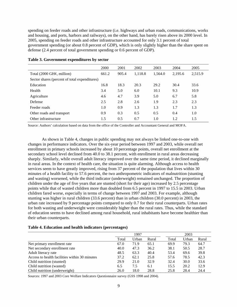
Provision of Other Public Goods and Services Access to public goods and services (such as education, heath, roads, and other infrastructure) is important, as these measures generally affect a farmer’s ability to purchase, hire or use production technologies. As shown in Table 3, government spending on agriculture ranks third to spending on the education and health sectors, although spending on the education sector rose rapidly (about 16 percent per year) between 2000 and 2005 and far outweighs spending in all the other sectors. Spending on health increased by more than three times between 2000 and 2003, but has since stagnated. Government

9

spending on feeder roads and other infrastructure (i.e. highways and urban roads, communications, works and housing, and ports, harbors and railways), on the other hand, has barely risen above its 2000 level. In 2005, spending on feeder roads and other infrastructure accounted for only 3.1 percent of total government spending (or about 0.8 percent of GDP), which is only slightly higher than the share spent on defense (2.4 percent of total government spending or 0.6 percent of GDP).

Table 3. Government expenditures by sector

2000 2001 2002 2003 2004 2005 Total (2000 GH¢, million) 661.2 905.4 1,118.8 1,564.0 2,195.6 2,515.9 Sector shares (percent of total expenditures) Education 16.8 18.3 20.3 29.2 30.4 33.6 Health 3.4 5.0 6.0 10.1 9.3 10.9 Agriculture 4.6 4.7 3.9 5.0 6.7 5.8 Defense 2.5 2.8 2.6 1.9 2.3 2.3 Feeder roads 1.0 0.9 1.3 1.3 1.7 1.3 Other roads and transport 0.9 0.3 0.5 0.5 0.4 1.0 Other infrastructure 1.5 0.5 0.7 1.0 1.2 1.5

Source: Authors’ calculation based on data from the office of the Controller and Accountant General and MOFA.

As shown in Table 4, changes in public spending may not always be linked one-to-one with changes in performance indicators. Over the six-year period between 1997 and 2003, while overall net enrollment in primary schools increased by about 10 percentage points, overall net enrollment at the secondary school level declined from 40.0 to 38.1 percent, with enrollment in rural areas decreasing sharply. Similarly, while overall adult literacy improved over the same time period, it declined marginally in rural areas. In the context of health care, the situation is quite alarming. Although access to health services seem to have greatly improved, rising from 37 percent of the population that lives within 30 minutes of a health facility to 57.6 percent, the two anthropometric indicators of malnutrition (stunting and wasting) worsened, while the third indicator (underweight) remained unchanged. The proportion of children under the age of five years that are stunted (short for their age) increased by 2.5 percentage points while that of wasted children more than doubled from 6.5 percent in 1997 to 15.5 in 2003. Urban children fared worse, especially in terms of change between 1997 and 2003. For example, although stunting was higher in rural children (33.6 percent) than in urban children (30.0 percent) in 2003, the urban rate increased by 9 percentage points compared to only 0.7 for their rural counterparts. Urban rates for both wasting and underweight were considerably higher than the rural rates. Thus, while the standard of education seems to have declined among rural household, rural inhabitants have become healthier than their urban counterparts.

Table 4. Education and health indicators (percentages)

1997 2003 Total Urban Rural Total Urban Rural Net primary enrollment rate 67.0 71.9 65.1 69.9 79.3 64.7 Net secondary enrollment rate 40.0 47.3 36.2 38.1 50.5 28.7 Adult literacy rate 48.5 63.3 40.4 53.4 69.6 39.8 Access to health facilities within 30 minutes 37.2 62.1 25.8 57.6 78.5 42.3 Child nutrition (stunted) 29.9 21.0 32.9 32.4 30.0 33.6 Child nutrition (wasted) 6.5 7.5 6.1 15.5 20.2 12.9 Child nutrition (underweight) 26.0 18.0 28.8 25.8 28.4 24.4 Sources: 1997 and 2003 Core Welfare Indicators Questionnaire survey (GSS 1998 and 2004).

10

The total feeder road network increased by about 6,000 km (or 18.3 percent) between 2002 and 2004, with the Upper-West and Northern Regions experiencing the most growth (46.5 and 41.9 percent, respectively), followed by the Brong-Ahafo and Western Regions, which showed 36 and 33 percent growth, respectively (Table 5). Similarly, the quality of roads also improved significantly. The share of roads classified as poor declined by 12 percentage points, while those classified as good and fair increased by 2.5 and 9.5 percentage points, respectively. The improvement in the quality of feeder roads was greatest in the Eastern, Greater-Accra and Upper-East Regions.

Table 5. Feeder road infrastructure in 2002 and 2004

2002 2004 Length

(km) Density (km per sq. km)

Quality (percent of total length)

Length (km)

Density (km per sq. km)

Quality (percent of total length)

Good Fair Poor Good Fair Poor Region Ashanti 5,290.8 0.22 27.9 26.9 45.2 5,043.7 0.21 32.17 37.55 30.28 Brong-Ahafo 4,860.0 0.13 30.0 21.4 48.6 6,606.0 0.18 42.64 16.68 40.68 Central 3,197.4 0.33 22.4 38.4 39.3 3,318.2 0.34 29.60 47.40 23.00 Eastern 3,366.0 0.21 44.9 14.1 40.9 3,098.4 0.19 64.40 29.73 5.87 Greater Accra 1,013.9 0.28 46.6 13.7 39.8 1,111.6 0.30 48.35 23.23 28.42 Northern 4,293.7 0.06 21.7 11.4 66.9 6,093.9 0.09 22.97 32.59 44.44 Upper East 1,186.6 0.14 51.5 9.3 39.1 1,346.9 0.16 28.86 27.08 44.06 Upper West 1,951.6 0.10 40.2 8.3 51.5 2,858.8 0.15 36.16 23.84 40.00 Volta 3,048.5 0.17 35.9 23.8 40.3 3,257.4 0.18 32.94 35.93 31.13 Western 4,388.4 0.18 36.5 10.2 53.3 5,825.8 0.24 29.52 18.31 52.17 Ghana 32,596.8 0.14 32.7 19.1 48.2 38,560.8 0.17 35.19 28.57 36.24 Source: Ministry of Road Transport (see Table A1 in the Appendix for details by district).

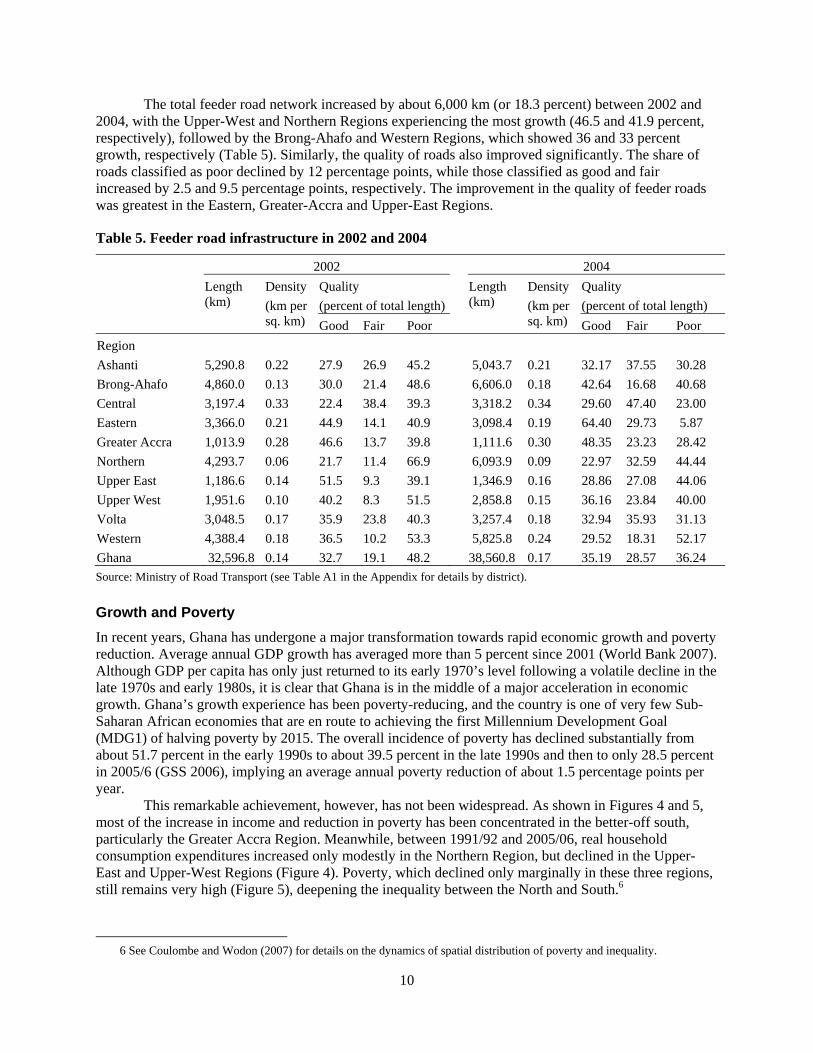
Growth and Poverty In recent years, Ghana has undergone a major transformation towards rapid economic growth and poverty reduction. Average annual GDP growth has averaged more than 5 percent since 2001 (World Bank 2007). Although GDP per capita has only just returned to its early 1970’s level following a volatile decline in the late 1970s and early 1980s, it is clear that Ghana is in the middle of a major acceleration in economic growth. Ghana’s growth experience has been poverty-reducing, and the country is one of very few Sub-Saharan African economies that are en route to achieving the first Millennium Development Goal (MDG1) of halving poverty by 2015. The overall incidence of poverty has declined substantially from about 51.7 percent in the early 1990s to about 39.5 percent in the late 1990s and then to only 28.5 percent in 2005/6 (GSS 2006), implying an average annual poverty reduction of about 1.5 percentage points per year.

This remarkable achievement, however, has not been widespread. As shown in Figures 4 and 5, most of the increase in income and reduction in poverty has been concentrated in the better-off south, particularly the Greater Accra Region. Meanwhile, between 1991/92 and 2005/06, real household consumption expenditures increased only modestly in the Northern Region, but declined in the Upper-East and Upper-West Regions (Figure 4). Poverty, which declined only marginally in these three regions, still remains very high (Figure 5), deepening the inequality between the North and South.6

6 See Coulombe and Wodon (2007) for details on the dynamics of spatial distribution of poverty and inequality.

11

Figure 4. Real household consumption expenditures (GH¢ per capita)

Source: 2005/06 Ghana Living Standards Survey (GSS 2006).

Figure 5. Headcount poverty index, by region (1991/92-2005/06)

Source: Author’s calculation based on 2005/06 Ghana Living Standards Survey data (GSS 2006) and CPI data from the World Development Indicators (World Bank 2007). Notes: In constant 2000 values.

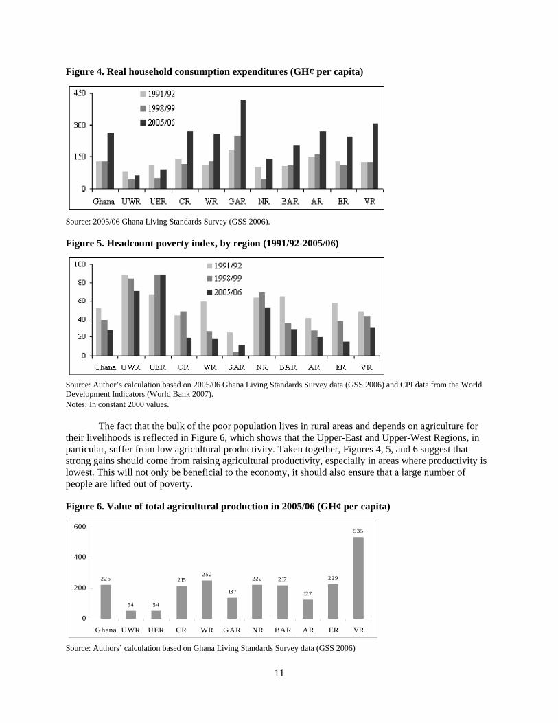
The fact that the bulk of the poor population lives in rural areas and depends on agriculture for their livelihoods is reflected in Figure 6, which shows that the Upper-East and Upper-West Regions, in particular, suffer from low agricultural productivity. Taken together, Figures 4, 5, and 6 suggest that strong gains should come from raising agricultural productivity, especially in areas where productivity is lowest. This will not only be beneficial to the economy, it should also ensure that a large number of people are lifted out of poverty.

Figure 6. Value of total agricultural production in 2005/06 (GH¢ per capita)

Source: Authors’ calculation based on Ghana Living Standards Survey data (GSS 2006)

225

54 54

215252

137

222 217

127

229

535

0

200

400

600

Ghana UWR UER CR WR GAR NR BAR AR ER VR

12

3. CONCEPTUAL FRAMEWORK

In this section, we present the conceptual framework we use to quantify and analyze the impacts of public spending on agriculture and other services (including education, health, and roads) on agricultural productivity growth. There is a well-established body of literature on how different types of public investments in agriculture and provision of other public goods and services can affect agricultural productivity growth. The general notion is that public and private capital complement one another, so an increase in the public capital stock raises the productivity of all factors in production (Anderson et al. 2006). By raising the productivity of all factors in production, public capital investments crowd-in private capital investments (David et al. 2000; Malla and Gray 2005), which further contributes to raising productivity. Of course, crowding-out of private capital investments, with contrasting effects on productivity growth, may also occur. It is also possible that public spending may not create any productive capital (Devarajan et al. 1996), meaning that the link between public spending and productivity is weak. To conceptualize these relationships further, we draw from the literature on agricultural household models (Singh et al. 1986; de Janvry et al. 1991), adoption of agricultural technologies (Feder et al. 1985; Feder and Umali 1993), and determinants of farm investments (Ervin and Ervin 1982).

The impact of public spending on agricultural technology adoption and productivity is typically captured by measuring household access to public goods and services such as extension, subsidies, markets, credit, education, heath, roads, etc. These factors generally affect a household’s ability to purchase, hire or use the technologies, which in turn raises agricultural productivity. Agricultural extension, for example, creates technological awareness and helps develop or strengthen the farmers’ knowledge regarding the technologies and their use. By creating awareness, extension also raises the ability of farmers to demand technologies and advisory services that meet their specific needs. Similarly, public spending on other support services, such as pest control and produce inspection/grading, can help reduce farmers’ post-harvest losses, improve product quality, and raise the value of production.

New technologies, however, tend to be highly complex, knowledge-intensive, and location-specific, meaning that knowledge and skills are required for successful adoption. Therefore, human capital development is critical; its link to economic growth has long been established (Schultz 1982) and there is a large body of evidence on its positive impacts, especially relating to the education and health sectors (see e.g. World Bank 2001; Fan 2008; Tompa 2002). For example, public spending on the education sector, which directly leads to improvements in enrollment and teacher quality, also increases the stock of human capital and raises productivity, whether it be on the farm, within the rural labor force, or in the household. At the individual household level, however, it is important to note that education can have a negative impact on agricultural production when it promotes off-farm employment opportunities and exit options out of agriculture. The argument also holds for road development and other public investment programs that promote exit options out of agriculture. Investments in education also complement investments in agricultural research and extension, for example, because more highly educated farmers are better positioned to adopt improved technologies and influence adoption among their colleagues. The productivity impacts of human health are similar to those of education, as public spending on the health sector directly improves the delivery and use of health services, thereby contributing to human capital development. Health problems such as HIV/AIDS and tuberculosis, as well as other debilitating illnesses (e.g. malaria), have major negative economic effects, such as lost work days and wages, decreased productivity, and increased medical costs and burden of family care (Tompa 2002).

By reducing transportation and transactions costs, lowering agricultural input prices and raising farm gate prices, public spending-derived improvements in rural infrastructure in general and rural roads in particular can help give farmers greater access to technology, better ability to purchase or hire inputs, and a higher value of production. It has also been demonstrated that the impacts of public spending on rural roads can also be manifested through several indirect pathways, such as improved access to education, health, and other support services (see Guild 2000; Fan et al. 2000 and 2004).

13

Various studies on agricultural household models, adoption of agricultural technologies, and determinants of farm investments have identified several other determinants of household farm investments. The factors that determine the profitability of agricultural production are especially important. These include: land tenure status (which affects the future returns from current practices); households’ endowments of human, physical, financial and social capital (which are important for use of labor, draft power, manure, credit, etc., especially where markets for such inputs are lacking); and biophysical factors such as and rainfall, population density and other village-level factors (which affect local comparative advantages) (e.g.: Ervin and Ervin 1982; Feder et al. 1985; Singh et al. 1986; de Janvry et al. 1991; Feder and Umali 1993; Pender et al. 1999).

Regression Model Consistent with the conceptual framework above, public spending can have both direct and indirect impacts on productivity. Fan and Pardey (1992) point out that omitting public investments such as agricultural R&D investments from regression models for public investments analyses can bias the estimates of the marginal effects of the variables included in the models. It is now common to include public investments, in addition to private farm investments, input use, and biophysical, institutional and policy factors, as determinants of agricultural productivity, typically using either the production function approach or the total factor productivity (TFP) approach (e.g. Rosegrant and Evenson 1995; Fan et al. 2000; Fan and Zhang 2004; Fan and Rao 2003; Zhang and Fan 2004; Huffman and Evenson 2006).

Here, we use the production function approach, which is modeled as a function of public investments in agriculture and human capital, private farm investments, input use, farm characteristics, household characteristics and endowments, and village-level biophysical and institutional characteristics. Some of the determinants in the production function (e.g. farm investments and input use) are potentially endogenous, since they may depend on the profitability of production. Similarly, the amount of public investments made in a particular sector or activity may depend on the sector performance or the returns to investments in the activity, implying endogeneity of public investments; when ignored, this may lead to biased estimates (Greene 1993). The notion that growth in public capital is an endogenous process (or an outcome, rather than a cause, of growth in income) is a debatable and empirical issue (see Ansari et al. 1997; Zhang and Fan 2004). Thus, similar to Fan et al. (2000 and 2004), we use a simultaneous-equations approach to quantify and analyze the impacts of public investments in agriculture, education, health, and rural roads on agricultural productivity. The systems approach, assuming the equations are correctly specified, is superior to the reduced-form single-equation approach that has been used in many past studies. The reduced-form specification eliminates the potential for endogeneity bias and allows us to estimate the total impacts of the exogenous explanatory variables on the dependent variable. However, the policy implications of the estimated parameters can be misleading, because changes in public investments are not linked one-to-one with changes in outcomes. Therefore, reduced-form estimates may not be appropriate when making recommendations about whether and how to increase or decrease public investments (Herrera 2007). The development hypotheses show that public investments affect productivity through multiple channels; it is also an objective of this paper to estimate the different intermediate effects.

The system of equations and conceptual variables used in this study are shown in equations 1, 2 and 3.

AGOUT_PCh = f (PAGINVd, OTHPINVd, FARMINVh, FARM_XICSh, HHD_XICSh, OTHER_Ad) (1)

FARMINVh = f (PAGINVd, OTHPINVd, FARM_XICSh, HHD_XICSh, OTHER_Fd) (2)

PAGINVd = f (AGPERFd, OTHPINVd, OTHER_Pd) (3)

14

Equation (1) is a household agricultural production function, where the dependent variable AGOUT_PCh, measured as the value total agricultural output per capita of a household, is a function of public investments in agriculture (PAGINVd) and the other sectors of education, health and rural roads (OTHPINVd). This captures the direct effects of public investments.7 Other determinants include the following measures: private farm investments and inputs in agricultural production (FARMINVh); farm characteristics (FARM_XICSh) such as endowments of land, livestock and equipment; household characteristics (HHD_XICSh) such as size, gender, age, and income strategies; and village-level biophysical factors and other factors affecting agricultural production (OTHER_Ad).

In equation (2), private farm investments are derived as a function of public investments in agriculture and the other sectors, in order to capture the indirect effects of public investments. The other determinants are farm and household characteristics, as well as other factors affecting farm investments (OTHER_Fd), as discussed above. Equation (3) captures the possible endogeneity of public investments in agriculture, and is modeled as a function of agricultural performance at the district level (AGPERFd), along with other factors affecting public investments decision in agriculture, such as public investments in other sectors (OTHPINVd), and various socio-cultural, political and institutional factors (OTHER_Pd). Equation (3) is modeled after the notion of placement effects of public investment programs, where prior agricultural performance and district characteristics may have an impact on attracting resources into the district, both from the central government and from donors. We recognize possible spending interactions across districts in the sense that the spending decisions in one district can have positive or negative effects on the spending decisions in neighboring districts, due to mobility and information asymmetries among local government officials and politicians (Case et al. 1993; Figlio et al. 1999). However, we do not have the spatial information necessary to model and assess such spillover effects of public spending.

Marginal Effect of Public Investment on Agricultural Productivity The marginal effect of public investments on agricultural productivity can be calculated by totally differentiating the system of equations with respect to the particular public investments variable. In terms of elasticity, for example, the elasticity of agricultural productivity with respect to public investments in agriculture (∈PAGINV) can be obtained by:

PAGINVFARMINV

FARMINVPCAGOUT

PAGINVPCAGOUT

PAGINVdPCdAGOUT

PAGINV ∂∂

∗∂

∂+

∂∂

=≡∈___

. (4)

The subscripts have been dropped for notational simplicity. The first term on the right-hand side captures the direct effects, while the second and third terms together capture the indirect effects. The second term is the typical production function estimates of farm investments, technology adoption, input use, etc. The third term captures the crowding-in (or crowding-out) effects of public investments in agriculture on private farm investments, etc. Similarly, the elasticity of agricultural productivity with respect to public investments in the other sectors (∈OTHPINVi) can be obtained by:

iiiOTHPINV OTHPINV

FARMINVFARMINV

PCAGOUTOTHPINV

PCAGOUTdOTHPINV

PCdAGOUTi ∂

∂∗

∂∂

+∂

∂=≡∈

___

. (4')

The subscript i associated with OTHPINVi is used to capture the separate effects of public investments in education, health, and rural roads.

7 Subscripts h and d denote household and district, respectively.

15

Marginal Return to Public Spending The marginal returns to public investments (i.e. the benefit-cost ratio or BCR) can be calculated by multiplying equations (4) and (4') by the respective ratio of agricultural output per capita to public investments according to:

BCRPAGINV PAGINV

PCAGOUTPAGINV

_⋅=∈

(5)

BCROTHPINVi iOTHPINV OTHPINV

PCAGOUTi

_⋅=∈

. (5')

The marginal returns are measured as a ratio and provide information for comparing the relative benefits of an additional unit of expenditures for different outcomes. The marginal returns can then be compared across different geographic areas, and this information can be used for setting future priorities for public expenditures with the goal of further increasing agricultural productivity or improving the efficiency of public spending.

Spending Required to Meet Specified Growth Targets We next examine the level of public spending required to achieve a particular growth target or the growth rate needed to reach middle-income country status in Ghana. The annual growth rate in public spending in agriculture (Ėaginv) needed to achieve a particular agricultural growth rate (θag) is given by:8

agagnagOTHPINVPAGINV

nagnaginvOTHPINVagaginv s

sEPAGINV

dPAGINVE⋅⋅∈+∈

⋅⋅∈−=≡

)],([)(

φ

θ &&

, (6)

where Ėnaginv is the annual growth rate in non-agricultural investments; φnag,ag is the multiplier effect or linkage (i.e. trade-offs and complementarities) between agricultural and non-agricultural investments; and sag and snag are shares of agriculture and non-agriculture in GDP, respectively. Using the simplifying assumption that there are no trade-offs or complementarities between agricultural and non-agricultural investments, i.e. φnag,ag=0, equation 6 simplifies to:

agPAGINV

nagnaginvOTHPINVagaginv s

sEE

⋅∈

⋅⋅∈−=

)( &&

θ

. (7)

8 This is derived by decomposing agricultural growth into effects associated with agricultural and non-agricultural

investment growth, and taking their interactions (i.e. trade-offs and complementarities) into account: ).,()()( nagnaginvagnagOTHPINVnagnaginvnaginvagaginvPAGINVag sEsEsE ⋅⋅⋅∈+⋅⋅∈+⋅⋅∈≡ &&& φθ

See Fan et al. (2008) for details.

16

4. DATA AND ESTIMATION

Data The data used in this study come from various sources. Public agricultural expenditures are made up of two components: district- and regional-level disaggregated data from the Agriculture Services Sector Investment Programme (AgSSIP) from 2001 to 2006, and regional-level disaggregated data from the Ministry of Food and Agriculture (MOFA) for the same period. The agricultural production and private farm investments data are from the most recent (2005/06) Ghana Living Standards Survey (GLSS5), while the data on public goods and services are from the 2003 Core Welfare Indicators Questionnaire survey (CWIQ) and various government ministries, departments and agencies (MDAs). We limit the sample to only rural areas. Below, we discuss some of the key variables used in the regressions, and how they were measured. These variables capture the conceptual factors discussed above; detailed descriptions and summary statistics are presented in Table 6.

Value of total agricultural output per capita (AGOUT_PCh). The GLSS5 data show that households engage in the production of multiple crops on their farmlands, and in other agricultural activities (livestock, fishery and hunting). Therefore, we use monetary value to aggregate all agricultural production activities of the household, based on the households’ reported value, to obtain the total annual value of agricultural production. In the survey, the output and values of crops harvested in piecemeal fashion, incremental amounts, or only when needed for consumption and sale (e.g. roots, tubers and other starchy crops, fruits, vegetables, etc.), are only available from households that harvested any output within the two weeks prior to the time of the interview. Thus, the sample underestimates the value of total agricultural production of households that cultivated these crops but did not harvest them within the two weeks prior to the survey. We accordingly use a regression approach to estimate the total value of output of these crops for the relevant households.

The utilized explanatory variables include area cultivated and other typical farm and household characteristics. The resulting total value of agricultural production is divided by household size and then converted to 2000 value terms using regional consumer price indices. All monetary values are converted to 2000 constant prices, in order to exclude the influence of inflation and other temporal monetary and fiscal trends.

Private farm investments and assets. Households’ agricultural investments are separated into initial stocks (i.e. holdings before the survey period) and flows (i.e. investments made during the survey period). Initial stocks are grouped into three categories: livestock assets, measured in tropical livestock units (TLUs);9 crop-production equipment; and other agricultural equipment. Flows during the survey period (FARMINVh) are aggregated across all categories (e.g. tractors, ploughs, spraying machines, livestock, outboard motors, fishing nets, improved seed, fertilizer, pesticide, feed, fuel, hired labor, etc.) into a single metric. It would be ideal to assess the effects of the individual investments and inputs. However, not all households made investments in every category (e.g. tractors, ploughs, spraying machines, livestock, outboard motors, fishing nets, etc.) or used every input (e.g. improved seed, fertilizer, pesticide, feed, fuel, hired labor, etc.). Given the existence of a non-negligible number of households with zero values (or truncated observations) for each type of investments or inputs, and the fact that the standard simultaneous-equations estimation technique is not appropriate for truncated dependent variables, we aggregate agricultural investments into a single metric.

9 Livestock is aggregated using the following weights: cattle (1), donkeys and pigs (0.36), sheep and goats (0.09) and

rabbits and poultry (0.01).

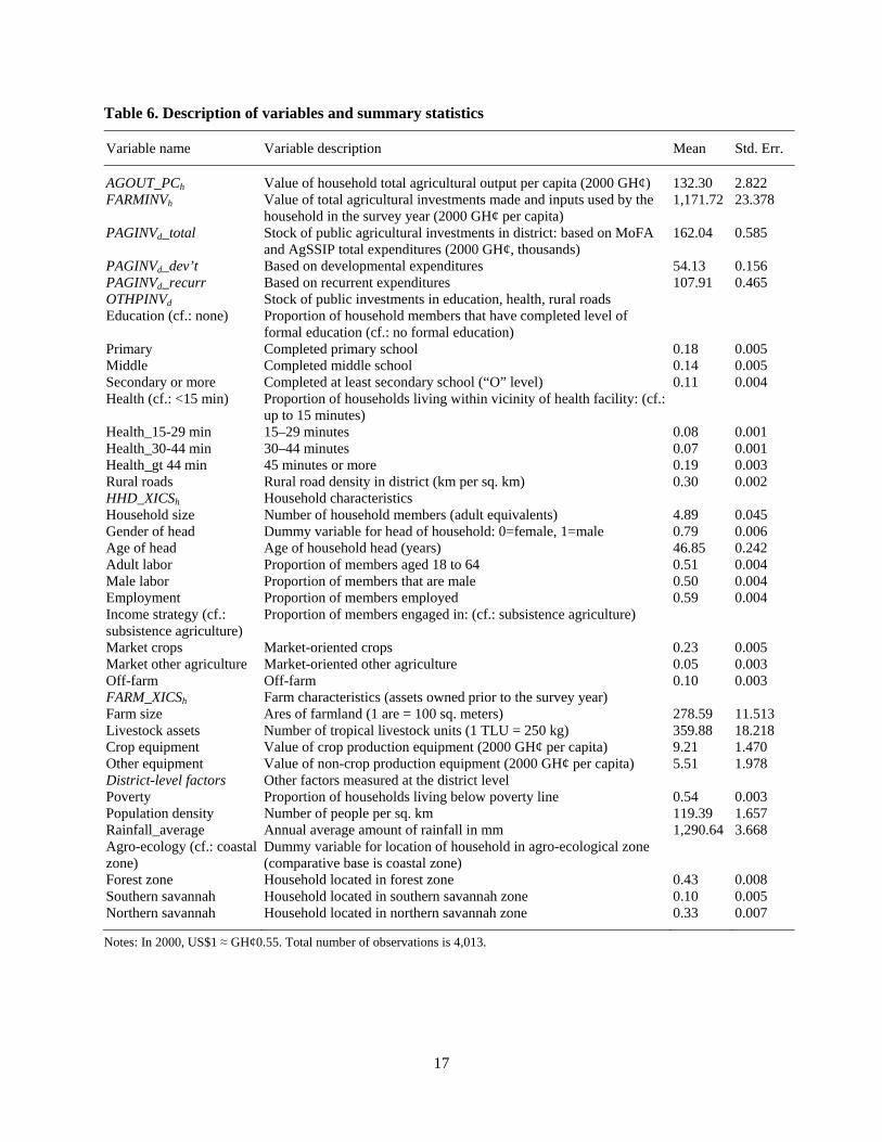
17

Table 6. Description of variables and summary statistics

Variable name Variable description Mean Std. Err.

AGOUT_PCh Value of household total agricultural output per capita (2000 GH¢) 132.30 2.822 FARMINVh Value of total agricultural investments made and inputs used by the

household in the survey year (2000 GH¢ per capita) 1,171.72 23.378

PAGINVd_total Stock of public agricultural investments in district: based on MoFA and AgSSIP total expenditures (2000 GH¢, thousands)

162.04 0.585

PAGINVd_dev’t Based on developmental expenditures 54.13 0.156 PAGINVd_recurr Based on recurrent expenditures 107.91 0.465 OTHPINVd Stock of public investments in education, health, rural roads Education (cf.: none) Proportion of household members that have completed level of

formal education (cf.: no formal education)

Primary Completed primary school 0.18 0.005 Middle Completed middle school 0.14 0.005 Secondary or more Completed at least secondary school (“O” level) 0.11 0.004 Health (cf.: <15 min) Proportion of households living within vicinity of health facility: (cf.:

up to 15 minutes)

Health_15-29 min 15–29 minutes 0.08 0.001 Health_30-44 min 30–44 minutes 0.07 0.001 Health_gt 44 min 45 minutes or more 0.19 0.003 Rural roads Rural road density in district (km per sq. km) 0.30 0.002 HHD_XICSh Household characteristics Household size Number of household members (adult equivalents) 4.89 0.045 Gender of head Dummy variable for head of household: 0=female, 1=male 0.79 0.006 Age of head Age of household head (years) 46.85 0.242 Adult labor Proportion of members aged 18 to 64 0.51 0.004 Male labor Proportion of members that are male 0.50 0.004 Employment Proportion of members employed 0.59 0.004 Income strategy (cf.: subsistence agriculture)

Proportion of members engaged in: (cf.: subsistence agriculture)

Market crops Market-oriented crops 0.23 0.005 Market other agriculture Market-oriented other agriculture 0.05 0.003 Off-farm Off-farm 0.10 0.003 FARM_XICSh Farm characteristics (assets owned prior to the survey year) Farm size Ares of farmland (1 are = 100 sq. meters) 278.59 11.513 Livestock assets Number of tropical livestock units (1 TLU = 250 kg) 359.88 18.218 Crop equipment Value of crop production equipment (2000 GH¢ per capita) 9.21 1.470 Other equipment Value of non-crop production equipment (2000 GH¢ per capita) 5.51 1.978 District-level factors Other factors measured at the district level Poverty Proportion of households living below poverty line 0.54 0.003 Population density Number of people per sq. km 119.39 1.657 Rainfall_average Annual average amount of rainfall in mm 1,290.64 3.668 Agro-ecology (cf.: coastal zone)

Dummy variable for location of household in agro-ecological zone (comparative base is coastal zone)

Forest zone Household located in forest zone 0.43 0.008 Southern savannah Household located in southern savannah zone 0.10 0.005 Northern savannah Household located in northern savannah zone 0.33 0.007

Notes: In 2000, US$1 ≈ GH¢0.55. Total number of observations is 4,013.

18

Public investments in agriculture (PAGINVd). We use district- and region-level disaggregated expenditures data from AgSSIP and region-level disaggregated expenditures data from the Ministry of Food and Agriculture, both from 2002 to 2006.10 We first distribute the regional expenditures equally across the relevant districts, and then construct an agricultural public capital stock variable by applying a 10 percent depreciation rate (based on the average inflation rate) and 16 percent discount rate (based on common government practice) (BOG 2007). Since households were interviewed at different times over a two-year period and agricultural production data were obtained for the 12 months prior to the interview, we vary the stock variable according to when the household was interviewed, in order to maintain consistency with the period of the production data. For example, if a household was interviewed in December 2005, then we use agricultural production data for January 2005 to December 2005, and do not consider the public agricultural expenditures in 2006. Rather, the public investments stock variable, which may be hypothesized as impacting agricultural production during the January-December 2006 time period, is created using data from 2002 through 2005. The values are divided by the total land area to make them comparable across districts. In general, we expect the impacts to differ by type of spending; we therefore separate the variable into recurrent (PAGINVd_recurr) and developmental (PAGINVd_dev’t) spending. To do this, we consider all AgSSIP expenditures as developmental spending. For the MOFA’s agricultural expenditures, however, we use 1, 17, 15, 17 and 20 percent of the total expenditures as developmental spending for 2002, 2003, 2004, 2005 and 2006, respectively (see Figure 1).

Public investments in education, health and rural roads (OTHPINVd). Unlike public spending information on the agricultural sector, we were unable to obtain detailed district-level disaggregated expenditures data on these sectors. Therefore, we use different measures of the stock of public investments based on data availability. For education, we use the proportion of household members that completed at least primary education (as opposed to those who have not). The stock of public investments in health is measured in a similar fashion, by the proportion households in the district that are located within 15-29 minutes, 30-44 minutes, and more than 44 minutes from a health center (as opposed to those that are located within 15 minutes). For rural roads, we use the rural road density in the district, measured as the number of kilometers of roads per square kilometer of total land area.

Other factors included are household characteristics that measure labor availability (number, gender and age composition), employment, and livelihood strategy in terms of pursuing subsistence or marketed-oriented agriculture or off-farm activities. We also include district-level factors on rainfall, population density, headcount poverty ratio (a measure of the performance of a district’s productivity), and location in one of four agro-ecological zones in Ghana: coastal, forest, northern savannah, and southern savannah (described in detail in Table A2 of the Appendix). We also estimate the equations separately for the four zones. These zones primarily determine the costs and risks of producing different agricultural commodities, as well as the opportunities and returns to alternative income-generating activities, both on- and off-farm (Pender et al. 1999). The northern savannah zone typically has one rainy season; millet and guinea corn are the major staples, although maize, groundnuts and vegetables are also cultivated. The other zones are characterized by a bi-modal rainfall distribution. The forest zone has the highest rainfall, followed by the coastal zone. Due to low rainfall, the northern savannah zone tends to receive most Ghanaian irrigation projects. The northern savannah zone stands out from the other three zones when we compare the mean values of most of the variables. The region is characterized by larger households, lower educational attainment levels, and a low prevalence of non-agricultural occupation activities. The latter implies limited livelihood options and little use of hired labor (suggesting labor abundance); this is consistent with the chronic high poverty rates that are observed in the northern parts of Ghana.

10 Note that these two sources of expenditure do not include expenditures at the center or headquarters. They also do not capture total public expenditure in the agricultural sector as defined under the CAADP initiative, which includes fishery and forestry (AU/NEPAD 2005). In Ghana, fisheries, forestry and agricultural research fall under other ministries. AgSSIP covers the entire sector. We are, however, missing agricultural expenditures by ministries and government agencies other than the Ministry of Food and Agriculture (MOFA)―see footnote 2.

19

Estimation Approaches and Issues We use a three-stage least squares (3SLS) econometric approach to simultaneously estimate equations (1) through (3). There are a couple of data and estimation issues to keep in mind when using this approach. One of the issues has to do with the estimation of equation (3) within the system, where the unit of observation of the dependent variable is the district. This is different from the other two equations, wherein the unit of observation of the dependent variables is the household. This poses a problem for implementing 3SLS, which requires the same number of observations for each of the dependent variables. One way to handle this in general is to aggregate the household data upwards to the district level. However, this could not be done for a reliable estimation because the GLSS5 survey data, as in many such national surveys in other countries, are not representative at the district level. Thus, we do not estimate equation (3) explicitly, but rather use the potential explanatory variables of equation (3) as instruments for public agricultural investments in the simultaneous estimation of equations (1) and (2). The drawback of doing this is that we are unable to obtain and discuss the coefficients on the determinants of public investments in agriculture. Nevertheless, this does not affect our ability to achieve the main objectives of estimating the returns to public spending in agriculture, and determining the amount of agricultural public expenditures required to achieve the CAADP and middle-income-country status agricultural growth rates, as specified in equations (5) and (6), respectively.

Another issue to deal with is the identification of equations (1) and (2) in the sense of excluding some of the explanatory variables used in estimating equation (3) from equations (1) and (2), as well as excluding some of the explanatory variables (or instruments) used in estimating equation (2) from equation (1). The utilized instruments include household-level adult and male labor, employment and income strategy, and district-level poverty. Since the use of weak instruments could yield more biased estimates than those obtained if the parameters are estimated by an ordinary least squares (OLS) method (Greene 1993), the desired instruments are selected based on Hansen’s (1982) chi-squared test of identification.

Using a large number of explanatory variables can introduce multicollinearity problems, which can bias estimates of the parameters (Greene 1993). This is not a problem here since the value of the largest variance inflation factor (VIF) associated with the explanatory variables in the various equations is 10, which is less than the cut-off point of 20 suggested by Kennedy (1985). The only exception is seen in the estimation for the coastal agro-ecological zone, where recurrent and developmental agricultural spending (i.e. PAGINVd_recurr and PAGINVd_dev’t) have VIF values of 28 and 31, respectively, likely due to the small sample size from this zone compared with the other agro-ecological zones. The regression results, however, do not show any anomalies compared with those estimated from the total sample or the other agro-ecological zones.

20

5. RESULTS AND DISCUSSION

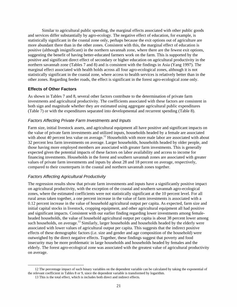
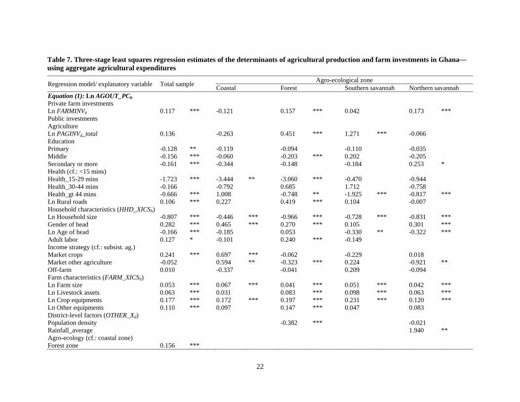
Details of the regression results from the total sample and the four agro-ecological zones (coastal, forest, northern savannah and southern savannah) are presented in Tables 7 and 8. Table 7 shows the results using aggregate agricultural spending, while Table 8 shows the results when we separate agricultural spending into developmental and recurrent expenditures. The marginal effects associated with the various public goods and services, based on equations (4) and (4'), are shown in Table 9.

Effects of Public Agricultural Spending As shown by the regression results, agricultural public expenditures in recent years had a significant positive impact on agricultural productivity associated with private farm investments and inputs, especially in the two savannah agro-ecological zones. For all rural areas taken together, the marginal effect is estimated at 0.15, and is derived from both direct and indirect sources (Tables 7 and 8). This means that a one percent increase in agricultural public expenditures is associated with a 0.15 percent increase in the value of agricultural production per capita (Table 9). This overall elasticity compares favorably with estimated elasticities for the sector in other countries, including, for example, the elasticity with respect to agricultural capital expenditures in Rwanda (0.17; Diao et al., 2007) and spending on agricultural research and extension in the U.S. (0.11-0.19; Huffman and Evenson, 2006). As expected, the effect associated with developmental spending is much larger, with an elasticity of 0.54; this counteracts the negative effect associated with the recurrent spending component. This result reflects the low government capital-recurrent expenditures ratio in the agricultural sector, which emphasizes the fact that simply paying staff salaries, administrative costs and other overhead is unlikely to yield any substantive improvement. The estimated elasticity associated with developmental expenditures is higher than some of those estimated in other studies, such as the elasticity with respect to agricultural research in India (0.25; Fan et al., 2000) and agricultural capital expenditures in Africa (0.3; Fan and Rao 2003).

The effect of agricultural public spending differs substantially when estimated for the specific agro-ecological zones. As shown in Table 9, the marginal effect of aggregate spending is positive and statistically significant only in the forest and southern savannah zones, where we see elasticities of 0.45 and 1.30, respectively. The insignificance of aggregate spending in the coastal and northern savannah zones is due to the counteracting negative effects associated with recurrent spending. This is in sharp contrast to the situation in the southern savannah zone, where recurrent expenditures are the sole driver of agricultural productivity.

Effects of Other Public Goods and Services As also shown in Table 9, greater access to health services and greater density of rural roads are associated with greater value of agricultural production per capita. For all rural areas taken together, households located more than 15 minutes away from a health center have an approximately 54 percent lower value of agricultural production per capita compared to those located within 15 minutes of a health center. The elasticity with respect to feeder road density is 0.1, meaning that a 10 percent increase in rural road density is associated with a one percent increase in the value of agricultural production per capita. Formal education, on the other hand, has a negative impact, with 8.7 percent difference between those without formal education and those completing at least primary education. As shown in Tables 7 and 8, while the effects of health and feeder roads are direct only, the effects of education are both direct and indirect. Households with more educated members have greater private farm investments, although this difference is not sufficient to override the direct negative effects, which are most likely due to allocation of skilled labor away from the farm (Jolliffe 2004). The effects of education found here are consistent with those observed in many previous studies on Latin America or other African countries, but contradict findings in Asia (Jolliffe 2004).11

11 See Jamison and Lau (1982) for a review of the evidence.

21

Similar to agricultural public spending, the marginal effects associated with other public goods and services differ substantially by agro-ecology. The negative effect of education, for example, is statistically significant in the coastal zone only, perhaps because the exit options out of agriculture are more abundant there than in the other zones. Consistent with this, the marginal effect of education is positive (although insignificant) in the northern savannah zone, where there are the fewest exit options, suggesting the benefit of having better-educated farmers work on the farm. This is supported by the positive and significant direct effect of secondary or higher education on agricultural productivity in the northern savannah zone (Tables 7 and 8) and is consistent with the findings in Asia (Yang 1997). The marginal effect associated with health holds across all four agro-ecological zones, although it is not statistically significant in the coastal zone, where access to health services is relatively better than in the other zones. Regarding feeder roads, the effect is significant in the forest agro-ecological zone only.

Effects of Other Factors As shown in Tables 7 and 8, several other factors contribute to the determination of private farm investments and agricultural productivity. The coefficients associated with these factors are consistent in both sign and magnitude whether they are estimated using aggregate agricultural public expenditures (Table 7) or with the expenditures separated into developmental and recurrent spending (Table 8).

Factors Affecting Private Farm Investments and Inputs

Farm size, initial livestock assets, and agricultural equipment all have positive and significant impacts on the value of private farm investments and utilized inputs, households headed by a female are associated with about 40 percent less value on average.12 Households with more male labor are associated with about 32 percent less farm investments on average. Larger households, households headed by older people, and those having more employed members are associated with greater farm investments. This is generally expected given the potential impacts of these factors on labor availability and access to income for financing investments. Households in the forest and southern savannah zones are associated with greater values of private farm investments and inputs by about 28 and 18 percent on average, respectively, compared to their counterparts in the coastal and northern savannah zones together.

Factors Affecting Agricultural Productivity

The regression results show that private farm investments and inputs have a significantly positive impact on agricultural productivity, with the exception of the coastal and southern savannah agro-ecological zones, where the estimated coefficients were not statistically significant at the 10 percent level. For all rural areas taken together, a one percent increase in the value of farm investments is associated with a 0.12 percent increase in the value of household agricultural output per capita. As expected, farm size and initial capital stocks in livestock, cropping equipment, and other agricultural equipment all had positive and significant impacts. Consistent with our earlier finding regarding lower investments among female-headed households, the value of household agricultural output per capita is about 38 percent lower among such households, on average.13 Similarly, larger households and households headed by the elderly were associated with lower values of agricultural output per capita. This suggests that the indirect positive effects of these demographic factors (i.e. size and gender and age composition of the household) were outweighed by the direct negative effects. Together, these findings suggest that poverty and food insecurity may be more problematic in large households and households headed by females and the elderly. The forest agro-ecological zone was associated with the greatest value of agricultural productivity on average.

12 The percentage impact of such binary variables on the dependent variable can be calculated by taking the exponential of

the relevant coefficient in Tables 8 or 9, since the dependent variable is transformed by logarithm. 13 This is the total effect, which is includes both direct and indirect effects.

22

Table 7. Three-stage least squares regression estimates of the determinants of agricultural production and farm investments in Ghana― using aggregate agricultural expenditures

Regression model/ explanatory variable Total sample Agro-ecological zone Coastal Forest Southern savannah Northern savannah

Equation (1): Ln AGOUT_PCh Private farm investments Ln FARMINVh 0.117 *** -0.121 0.157 *** 0.042 0.173 *** Public investments Agriculture Ln PAGINVd_total 0.136 -0.263 0.451 *** 1.271 *** -0.066 Education Primary -0.128 ** -0.119 -0.094 -0.110 -0.035 Middle -0.156 *** -0.060 -0.203 *** 0.202 -0.205 Secondary or more -0.161 *** -0.344 -0.148 -0.184 0.253 * Health (cf.: <15 mins) Health_15-29 mins -1.723 *** -3.444 ** -3.060 *** -0.470 -0.944 Health_30-44 mins -0.166 -0.792 0.685 1.712 -0.758 Health_gt 44 mins -0.666 *** 1.008 -0.748 ** -1.925 *** -0.817 *** Ln Rural roads 0.106 *** 0.227 0.419 *** 0.104 -0.007 Household characteristics (HHD_XICSh) Ln Household size -0.807 *** -0.446 *** -0.966 *** -0.728 *** -0.831 *** Gender of head 0.282 *** 0.465 *** 0.270 *** 0.105 0.301 *** Ln Age of head -0.166 *** -0.185 0.053 -0.330 ** -0.322 *** Adult labor 0.127 * -0.101 0.240 *** -0.149 Income strategy (cf.: subsist. ag.) Market crops 0.241 *** 0.697 *** -0.062 -0.229 0.018 Market other agriculture -0.052 0.594 ** -0.323 *** 0.224 -0.921 ** Off-farm 0.010 -0.337 -0.041 0.209 -0.094 Farm characteristics (FARM_XICSh) Ln Farm size 0.053 *** 0.067 *** 0.041 *** 0.051 *** 0.042 *** Ln Livestock assets 0.063 *** 0.031 0.083 *** 0.098 *** 0.063 *** Ln Crop equipments 0.177 *** 0.172 *** 0.197 *** 0.231 *** 0.120 *** Ln Other equipments 0.110 *** 0.097 0.147 *** 0.047 0.083 District-level factors (OTHER_Xd) Population density -0.382 *** -0.021 Rainfall_average 1.940 ** Agro-ecology (cf.: coastal zone) Forest zone 0.156 ***

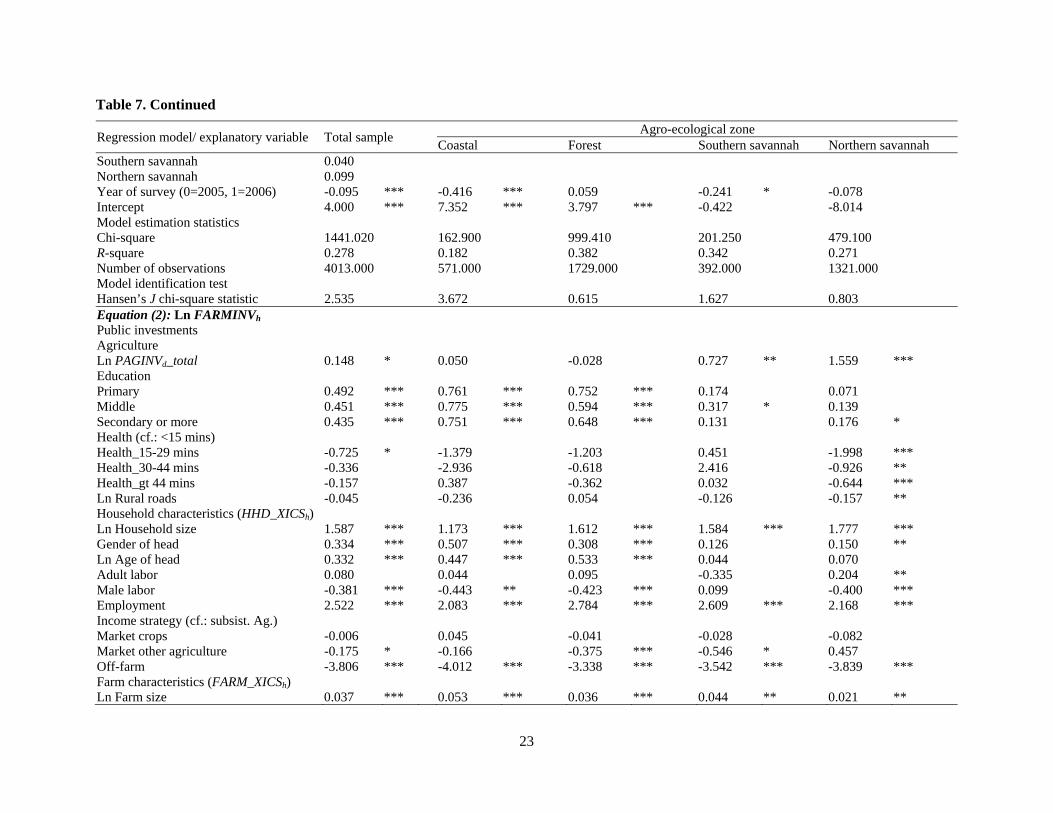
23

Table 7. Continued

Regression model/ explanatory variable Total sample Agro-ecological zone Coastal Forest Southern savannah Northern savannah

Southern savannah 0.040 Northern savannah 0.099 Year of survey (0=2005, 1=2006) -0.095 *** -0.416 *** 0.059 -0.241 * -0.078 Intercept 4.000 *** 7.352 *** 3.797 *** -0.422 -8.014 Model estimation statistics Chi-square 1441.020 162.900 999.410 201.250 479.100 R-square 0.278 0.182 0.382 0.342 0.271 Number of observations 4013.000 571.000 1729.000 392.000 1321.000 Model identification test Hansen’s J chi-square statistic 2.535 3.672 0.615 1.627 0.803 Equation (2): Ln FARMINVh Public investments Agriculture Ln PAGINVd_total 0.148 * 0.050 -0.028 0.727 ** 1.559 *** Education Primary 0.492 *** 0.761 *** 0.752 *** 0.174 0.071 Middle 0.451 *** 0.775 *** 0.594 *** 0.317 * 0.139 Secondary or more 0.435 *** 0.751 *** 0.648 *** 0.131 0.176 * Health (cf.: <15 mins) Health_15-29 mins -0.725 * -1.379 -1.203 0.451 -1.998 *** Health_30-44 mins -0.336 -2.936 -0.618 2.416 -0.926 ** Health_gt 44 mins -0.157 0.387 -0.362 0.032 -0.644 *** Ln Rural roads -0.045 -0.236 0.054 -0.126 -0.157 ** Household characteristics (HHD_XICSh) Ln Household size 1.587 *** 1.173 *** 1.612 *** 1.584 *** 1.777 *** Gender of head 0.334 *** 0.507 *** 0.308 *** 0.126 0.150 ** Ln Age of head 0.332 *** 0.447 *** 0.533 *** 0.044 0.070 Adult labor 0.080 0.044 0.095 -0.335 0.204 ** Male labor -0.381 *** -0.443 ** -0.423 *** 0.099 -0.400 *** Employment 2.522 *** 2.083 *** 2.784 *** 2.609 *** 2.168 *** Income strategy (cf.: subsist. Ag.) Market crops -0.006 0.045 -0.041 -0.028 -0.082 Market other agriculture -0.175 * -0.166 -0.375 *** -0.546 * 0.457 Off-farm -3.806 *** -4.012 *** -3.338 *** -3.542 *** -3.839 *** Farm characteristics (FARM_XICSh) Ln Farm size 0.037 *** 0.053 *** 0.036 *** 0.044 ** 0.021 **

24

Table 7. Continued

Regression model/ explanatory variable Total sample Agro-ecological zone Coastal Forest Southern savannah Northern savannah

Ln Livestock assets 0.012 * 0.009 0.011 0.026 0.016 * Ln Crop equipments 0.044 *** 0.106 * 0.050 ** 0.113 ** 0.011 Ln Other equipments 0.045 ** 0.071 0.079 * 0.014 0.099 *** District-level factors (OTHER_Xd) Poverty 0.625 *** 1.713 *** 0.231 1.833 Population density -0.196 *** 0.123 *** Rainfall_average 1.994 *** Agro-ecology (cf.: coastal zone) Forest zone 0.230 *** Southern savannah 0.170 ** Northern savannah -0.100 Year of survey (0=2005, 1=2006) -0.013 -0.386 *** 0.054 0.339 *** 0.017 Intercept 0.524 0.577 1.785 * -2.280 -19.345 *** Model estimation statistics Chi-square 8798.370 1023.740 3197.960 837.120 5131.370 R-square 0.687 0.642 0.649 0.681 0.795 Number of observations 4013.000 571.000 1729.000 392.000 1321.000 Notes: See Table 4 for a detailed description of the variables. All continuous variables are transformed by natural logarithm, which is indicated by Ln. *, ** and *** means that the coefficient is statistically significant at the 10 percent, 5 percent or 1 percent level, respectively.

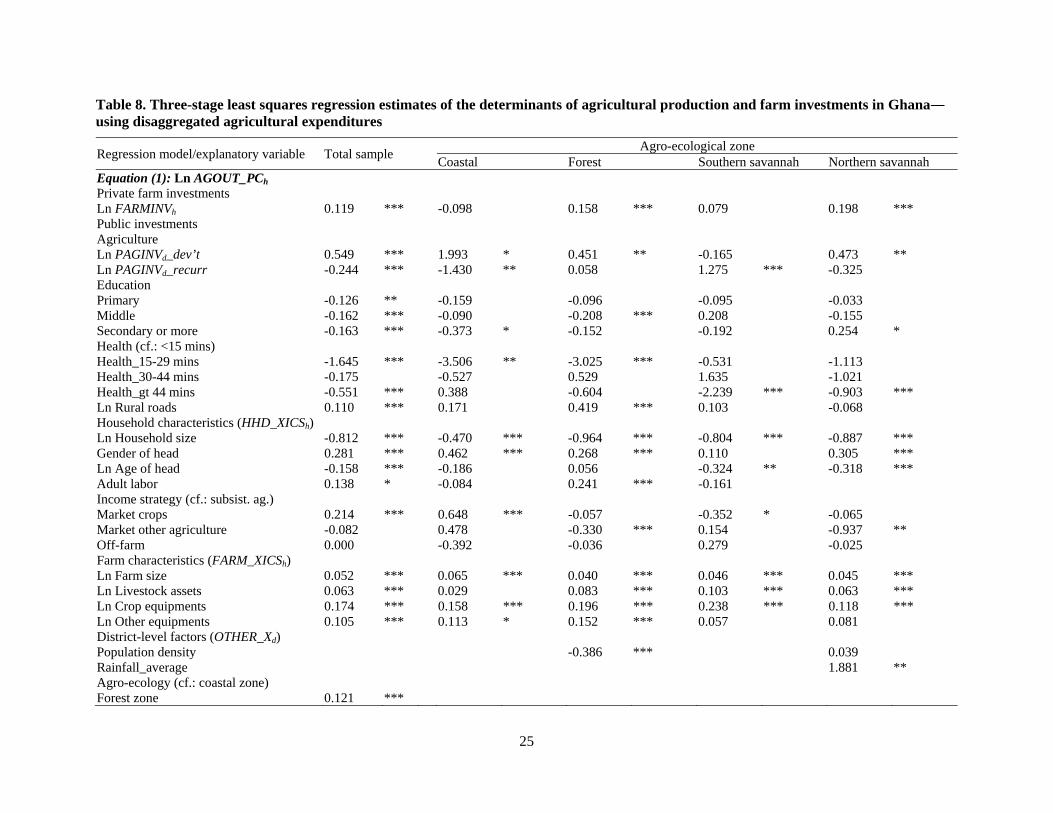
25

Table 8. Three-stage least squares regression estimates of the determinants of agricultural production and farm investments in Ghana― using disaggregated agricultural expenditures

Regression model/explanatory variable Total sample Agro-ecological zone Coastal Forest Southern savannah Northern savannah

Equation (1): Ln AGOUT_PCh Private farm investments Ln FARMINVh 0.119 *** -0.098 0.158 *** 0.079 0.198 *** Public investments Agriculture Ln PAGINVd_dev’t 0.549 *** 1.993 * 0.451 ** -0.165 0.473 ** Ln PAGINVd_recurr -0.244 *** -1.430 ** 0.058 1.275 *** -0.325 Education Primary -0.126 ** -0.159 -0.096 -0.095 -0.033 Middle -0.162 *** -0.090 -0.208 *** 0.208 -0.155 Secondary or more -0.163 *** -0.373 * -0.152 -0.192 0.254 * Health (cf.: <15 mins) Health_15-29 mins -1.645 *** -3.506 ** -3.025 *** -0.531 -1.113 Health_30-44 mins -0.175 -0.527 0.529 1.635 -1.021 Health_gt 44 mins -0.551 *** 0.388 -0.604 -2.239 *** -0.903 *** Ln Rural roads 0.110 *** 0.171 0.419 *** 0.103 -0.068 Household characteristics (HHD_XICSh) Ln Household size -0.812 *** -0.470 *** -0.964 *** -0.804 *** -0.887 *** Gender of head 0.281 *** 0.462 *** 0.268 *** 0.110 0.305 *** Ln Age of head -0.158 *** -0.186 0.056 -0.324 ** -0.318 *** Adult labor 0.138 * -0.084 0.241 *** -0.161 Income strategy (cf.: subsist. ag.) Market crops 0.214 *** 0.648 *** -0.057 -0.352 * -0.065 Market other agriculture -0.082 0.478 -0.330 *** 0.154 -0.937 ** Off-farm 0.000 -0.392 -0.036 0.279 -0.025 Farm characteristics (FARM_XICSh) Ln Farm size 0.052 *** 0.065 *** 0.040 *** 0.046 *** 0.045 *** Ln Livestock assets 0.063 *** 0.029 0.083 *** 0.103 *** 0.063 *** Ln Crop equipments 0.174 *** 0.158 *** 0.196 *** 0.238 *** 0.118 *** Ln Other equipments 0.105 *** 0.113 * 0.152 *** 0.057 0.081 District-level factors (OTHER_Xd) Population density -0.386 *** 0.039 Rainfall_average 1.881 ** Agro-ecology (cf.: coastal zone) Forest zone 0.121 ***

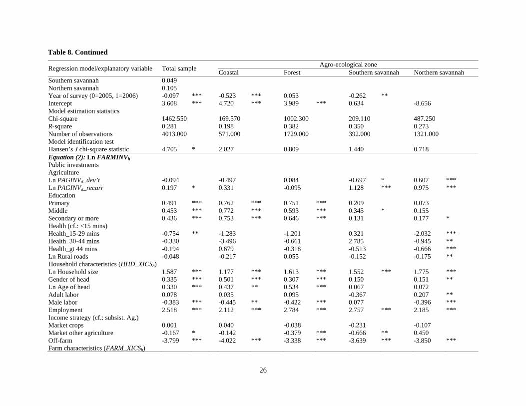
26

Table 8. Continued

Regression model/explanatory variable Total sample Agro-ecological zone Coastal Forest Southern savannah Northern savannah

Southern savannah 0.049 Northern savannah 0.105 Year of survey (0=2005, 1=2006) -0.097 *** -0.523 *** 0.053 -0.262 ** Intercept 3.608 *** 4.720 *** 3.989 *** 0.634 -8.656 Model estimation statistics Chi-square 1462.550 169.570 1002.300 209.110 487.250 R-square 0.281 0.198 0.382 0.350 0.273 Number of observations 4013.000 571.000 1729.000 392.000 1321.000 Model identification test Hansen’s J chi-square statistic 4.705 * 2.027 0.809 1.440 0.718 Equation (2): Ln FARMINVh Public investments Agriculture Ln PAGINVd_dev’t -0.094 -0.497 0.084 -0.697 * 0.607 *** Ln PAGINVd_recurr 0.197 * 0.331 -0.095 1.128 *** 0.975 *** Education Primary 0.491 *** 0.762 *** 0.751 *** 0.209 0.073 Middle 0.453 *** 0.772 *** 0.593 *** 0.345 * 0.155 Secondary or more 0.436 *** 0.753 *** 0.646 *** 0.131 0.177 * Health (cf.: <15 mins) Health_15-29 mins -0.754 ** -1.283 -1.201 0.321 -2.032 *** Health_30-44 mins -0.330 -3.496 -0.661 2.785 -0.945 ** Health_gt 44 mins -0.194 0.679 -0.318 -0.513 -0.666 *** Ln Rural roads -0.048 -0.217 0.055 -0.152 -0.175 ** Household characteristics (HHD_XICSh) Ln Household size 1.587 *** 1.177 *** 1.613 *** 1.552 *** 1.775 *** Gender of head 0.335 *** 0.501 *** 0.307 *** 0.150 0.151 ** Ln Age of head 0.330 *** 0.437 ** 0.534 *** 0.067 0.072 Adult labor 0.078 0.035 0.095 -0.367 0.207 ** Male labor -0.383 *** -0.445 ** -0.422 *** 0.077 -0.396 *** Employment 2.518 *** 2.112 *** 2.784 *** 2.757 *** 2.185 *** Income strategy (cf.: subsist. Ag.) Market crops 0.001 0.040 -0.038 -0.231 -0.107 Market other agriculture -0.167 * -0.142 -0.379 *** -0.666 ** 0.450 Off-farm -3.799 *** -4.022 *** -3.338 *** -3.639 *** -3.850 *** Farm characteristics (FARM_XICSh)

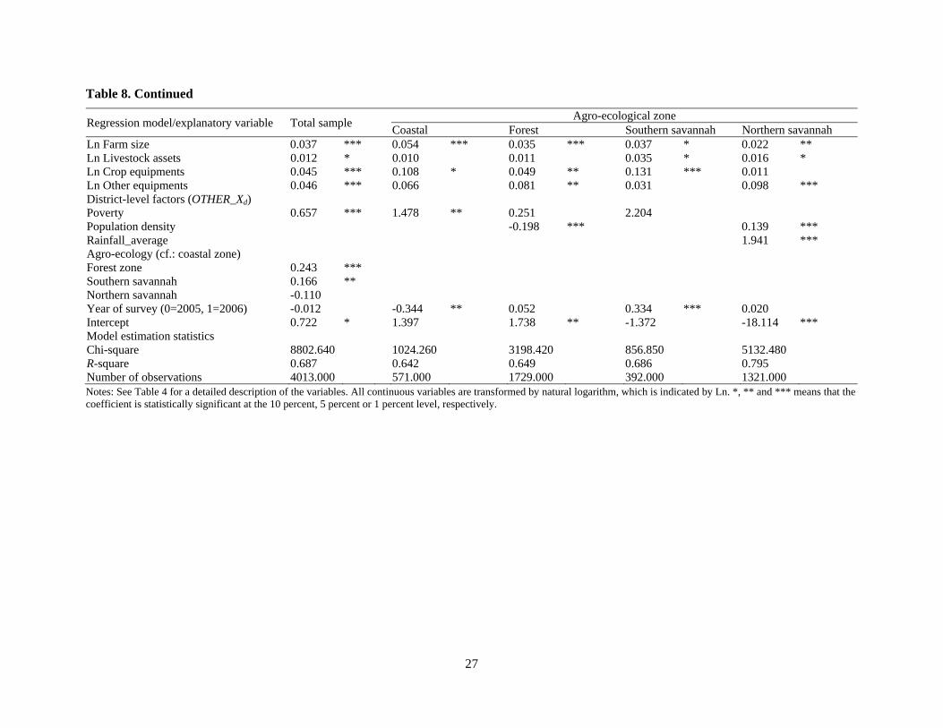
27

Table 8. Continued

Regression model/explanatory variable Total sample Agro-ecological zone Coastal Forest Southern savannah Northern savannah

Ln Farm size 0.037 *** 0.054 *** 0.035 *** 0.037 * 0.022 ** Ln Livestock assets 0.012 * 0.010 0.011 0.035 * 0.016 * Ln Crop equipments 0.045 *** 0.108 * 0.049 ** 0.131 *** 0.011 Ln Other equipments 0.046 *** 0.066 0.081 ** 0.031 0.098 *** District-level factors (OTHER_Xd) Poverty 0.657 *** 1.478 ** 0.251 2.204 Population density -0.198 *** 0.139 *** Rainfall_average 1.941 *** Agro-ecology (cf.: coastal zone) Forest zone 0.243 *** Southern savannah 0.166 ** Northern savannah -0.110 Year of survey (0=2005, 1=2006) -0.012 -0.344 ** 0.052 0.334 *** 0.020 Intercept 0.722 * 1.397 1.738 ** -1.372 -18.114 *** Model estimation statistics Chi-square 8802.640 1024.260 3198.420 856.850 5132.480 R-square 0.687 0.642 0.649 0.686 0.795 Number of observations 4013.000 571.000 1729.000 392.000 1321.000 Notes: See Table 4 for a detailed description of the variables. All continuous variables are transformed by natural logarithm, which is indicated by Ln. *, ** and *** means that the coefficient is statistically significant at the 10 percent, 5 percent or 1 percent level, respectively.

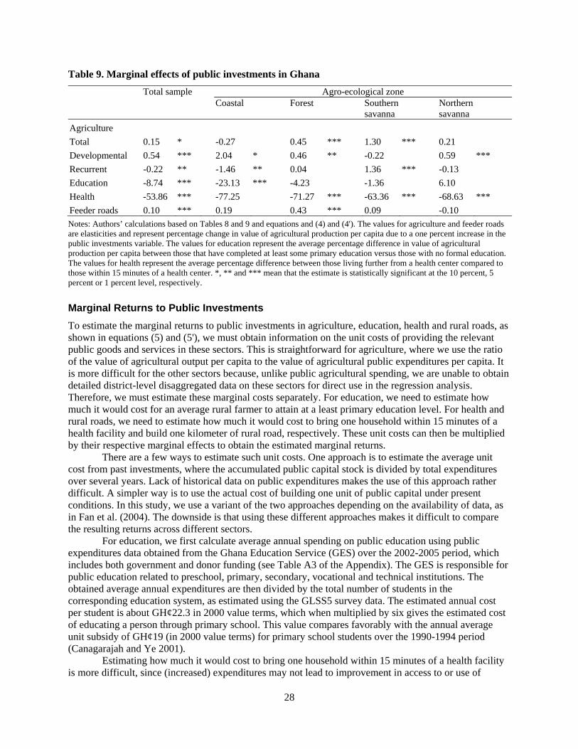
28

Table 9. Marginal effects of public investments in Ghana

Total sample Agro-ecological zone Coastal Forest Southern

savanna Northern savanna

Agriculture Total 0.15 * -0.27 0.45 *** 1.30 *** 0.21 Developmental 0.54 *** 2.04 * 0.46 ** -0.22 0.59 *** Recurrent -0.22 ** -1.46 ** 0.04 1.36 *** -0.13 Education -8.74 *** -23.13 *** -4.23 -1.36 6.10 Health -53.86 *** -77.25 -71.27 *** -63.36 *** -68.63 *** Feeder roads 0.10 *** 0.19 0.43 *** 0.09 -0.10 Notes: Authors’ calculations based on Tables 8 and 9 and equations and (4) and (4'). The values for agriculture and feeder roads are elasticities and represent percentage change in value of agricultural production per capita due to a one percent increase in the public investments variable. The values for education represent the average percentage difference in value of agricultural production per capita between those that have completed at least some primary education versus those with no formal education. The values for health represent the average percentage difference between those living further from a health center compared to those within 15 minutes of a health center. *, ** and *** mean that the estimate is statistically significant at the 10 percent, 5 percent or 1 percent level, respectively.

Marginal Returns to Public Investments To estimate the marginal returns to public investments in agriculture, education, health and rural roads, as shown in equations (5) and (5'), we must obtain information on the unit costs of providing the relevant public goods and services in these sectors. This is straightforward for agriculture, where we use the ratio of the value of agricultural output per capita to the value of agricultural public expenditures per capita. It is more difficult for the other sectors because, unlike public agricultural spending, we are unable to obtain detailed district-level disaggregated data on these sectors for direct use in the regression analysis. Therefore, we must estimate these marginal costs separately. For education, we need to estimate how much it would cost for an average rural farmer to attain at a least primary education level. For health and rural roads, we need to estimate how much it would cost to bring one household within 15 minutes of a health facility and build one kilometer of rural road, respectively. These unit costs can then be multiplied by their respective marginal effects to obtain the estimated marginal returns.

There are a few ways to estimate such unit costs. One approach is to estimate the average unit cost from past investments, where the accumulated public capital stock is divided by total expenditures over several years. Lack of historical data on public expenditures makes the use of this approach rather difficult. A simpler way is to use the actual cost of building one unit of public capital under present conditions. In this study, we use a variant of the two approaches depending on the availability of data, as in Fan et al. (2004). The downside is that using these different approaches makes it difficult to compare the resulting returns across different sectors.

For education, we first calculate average annual spending on public education using public expenditures data obtained from the Ghana Education Service (GES) over the 2002-2005 period, which includes both government and donor funding (see Table A3 of the Appendix). The GES is responsible for public education related to preschool, primary, secondary, vocational and technical institutions. The obtained average annual expenditures are then divided by the total number of students in the corresponding education system, as estimated using the GLSS5 survey data. The estimated annual cost per student is about GH¢22.3 in 2000 value terms, which when multiplied by six gives the estimated cost of educating a person through primary school. This value compares favorably with the annual average unit subsidy of GH¢19 (in 2000 value terms) for primary school students over the 1990-1994 period (Canagarajah and Ye 2001).

Estimating how much it would cost to bring one household within 15 minutes of a health facility is more difficult, since (increased) expenditures may not lead to improvement in access to or use of

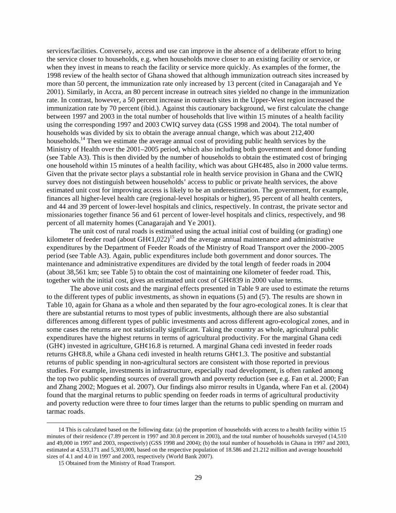
29

services/facilities. Conversely, access and use can improve in the absence of a deliberate effort to bring the service closer to households, e.g. when households move closer to an existing facility or service, or when they invest in means to reach the facility or service more quickly. As examples of the former, the 1998 review of the health sector of Ghana showed that although immunization outreach sites increased by more than 50 percent, the immunization rate only increased by 13 percent (cited in Canagarajah and Ye 2001). Similarly, in Accra, an 80 percent increase in outreach sites yielded no change in the immunization rate. In contrast, however, a 50 percent increase in outreach sites in the Upper-West region increased the immunization rate by 70 percent (ibid.). Against this cautionary background, we first calculate the change between 1997 and 2003 in the total number of households that live within 15 minutes of a health facility using the corresponding 1997 and 2003 CWIQ survey data (GSS 1998 and 2004). The total number of households was divided by six to obtain the average annual change, which was about 212,400 households.14 Then we estimate the average annual cost of providing public health services by the Ministry of Health over the 2001–2005 period, which also including both government and donor funding (see Table A3). This is then divided by the number of households to obtain the estimated cost of bringing one household within 15 minutes of a health facility, which was about GH¢485, also in 2000 value terms. Given that the private sector plays a substantial role in health service provision in Ghana and the CWIQ survey does not distinguish between households’ access to public or private health services, the above estimated unit cost for improving access is likely to be an underestimation. The government, for example, finances all higher-level health care (regional-level hospitals or higher), 95 percent of all health centers, and 44 and 39 percent of lower-level hospitals and clinics, respectively. In contrast, the private sector and missionaries together finance 56 and 61 percent of lower-level hospitals and clinics, respectively, and 98 percent of all maternity homes (Canagarajah and Ye 2001).

The unit cost of rural roads is estimated using the actual initial cost of building (or grading) one kilometer of feeder road (about GH¢1,022)15 and the average annual maintenance and administrative expenditures by the Department of Feeder Roads of the Ministry of Road Transport over the 2000–2005 period (see Table A3). Again, public expenditures include both government and donor sources. The maintenance and administrative expenditures are divided by the total length of feeder roads in 2004 (about 38,561 km; see Table 5) to obtain the cost of maintaining one kilometer of feeder road. This, together with the initial cost, gives an estimated unit cost of GH¢839 in 2000 value terms.

The above unit costs and the marginal effects presented in Table 9 are used to estimate the returns to the different types of public investments, as shown in equations (5) and (5'). The results are shown in Table 10, again for Ghana as a whole and then separated by the four agro-ecological zones. It is clear that there are substantial returns to most types of public investments, although there are also substantial differences among different types of public investments and across different agro-ecological zones, and in some cases the returns are not statistically significant. Taking the country as whole, agricultural public expenditures have the highest returns in terms of agricultural productivity. For the marginal Ghana cedi (GH¢) invested in agriculture, GH¢16.8 is returned. A marginal Ghana cedi invested in feeder roads returns GH¢8.8, while a Ghana cedi invested in health returns GH¢1.3. The positive and substantial returns of public spending in non-agricultural sectors are consistent with those reported in previous studies. For example, investments in infrastructure, especially road development, is often ranked among the top two public spending sources of overall growth and poverty reduction (see e.g. Fan et al. 2000; Fan and Zhang 2002; Mogues et al. 2007). Our findings also mirror results in Uganda, where Fan et al. (2004) found that the marginal returns to public spending on feeder roads in terms of agricultural productivity and poverty reduction were three to four times larger than the returns to public spending on murram and tarmac roads.

14 This is calculated based on the following data: (a) the proportion of households with access to a health facility within 15 minutes of their residence (7.89 percent in 1997 and 30.8 percent in 2003), and the total number of households surveyed (14,510 and 49,000 in 1997 and 2003, respectively) (GSS 1998 and 2004); (b) the total number of households in Ghana in 1997 and 2003, estimated at 4,533,171 and 5,303,000, based on the respective population of 18.586 and 21.212 million and average household sizes of 4.1 and 4.0 in 1997 and 2003, respectively (World Bank 2007).

15 Obtained from the Ministry of Road Transport.

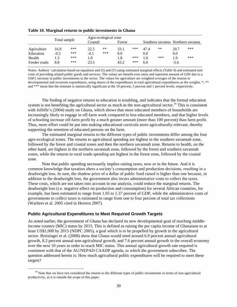
30

Table 10. Marginal returns to public investments in Ghana

Total sample Agro-ecological zone Coastal Forest Southern savanna Northern savanna

Agriculture 16.8 *** 22.5 ** 33.1 *** 47.4 ** 20.7 *** Education -0.2 *** -0.1 *** 0.0 0.0 0.0 Health 1.3 *** 1.0 1.8 *** 1.6 *** 1.9 *** Feeder roads 8.8 *** 23.5 43.2 *** 6.0 -5.6

Notes: Authors’ calculation based on equations and (5) and (5') using estimated marginal effects (Table 9) and estimated unit costs of providing related public goods and services. The values are benefit-cost ratios and represent amount of GH¢ due to a GH¢1 increase in public investments in the sector. The values for agriculture are weighted averages of the returns to developmental and recurrent expenditures, using shares of the expenditures in total agricultural expenditures as the weights. *, ** and *** mean that the estimate is statistically significant at the 10 percent, 5 percent and 1 percent levels, respectively.

The finding of negative returns to education is troubling, and indicates that the formal education system is not benefiting the agricultural sector as much as the non-agricultural sector.16 This is consistent with Jolliffe’s (2004) study on Ghana, which shows that more educated members of households are increasingly likely to engage in off-farm work compared to less educated members, and that higher levels of schooling increase off-farm profit by a much greater amount (more than 100 percent) than farm profit. Thus, more effort could be put into making educational curricula more agriculturally-relevant, thereby supporting the retention of educated persons on the farm.

The estimated marginal returns to the different types of public investments differ among the four agro-ecological zones. The returns to agricultural spending are highest in the southern savannah zone, followed by the forest and coastal zones and then the northern savannah zone. Returns to health, on the other hand, are highest in the northern savannah zone, followed by the forest and southern savannah zones, while the returns to rural roads spending are highest in the forest zone, followed by the coastal zone.

Note that public spending necessarily implies raising taxes, now or in the future. And it is common knowledge that taxation alters a society’s consumption and production decisions, resulting in a deadweight loss. In sum, the shadow price of a dollar of public fund raised is higher than one because, in addition to the deadweight loss, the government also incurs administrative costs to collect the taxes. These costs, which are not taken into account in our analysis, could reduce the marginal returns. The deadweight loss (i.e. negative effect on production and consumption) for several African countries, for example, has been estimated to range from 1.05 to 1.37 percent of GDP, while the administrative costs of governments to collect taxes is estimated to range from one to four percent of total tax collections (Warlters et al. 2005 cited in Herrera 2007).

Public Agricultural Expenditures to Meet Required Growth Targets As noted earlier, the government of Ghana has declared its new developmental goal of reaching middle-income country (MIC) status by 2015. This is defined as raising the per capita income of Ghanaians to at least US$1,000 by 2015 (NDPC 2005), a goal which is to be propelled by growth in the agricultural sector. Breisinger et al. (2008) show that Ghana would need around 6.9 percent annual agricultural growth, 8.2 percent annual non-agricultural growth, and 7.6 percent annual growth in the overall economy over the next 10 years in order to reach MIC status. This annual agricultural growth rate required is consistent with that of the AU/NEPAD CAADP agenda, to which the government subscribes. The question addressed herein is: How much agricultural public expenditures will be required to meet these targets?

16 Note that we have not considered the returns to the different types of public investments in terms of non-agricultural

productivity, as it is outside the scope of this paper.

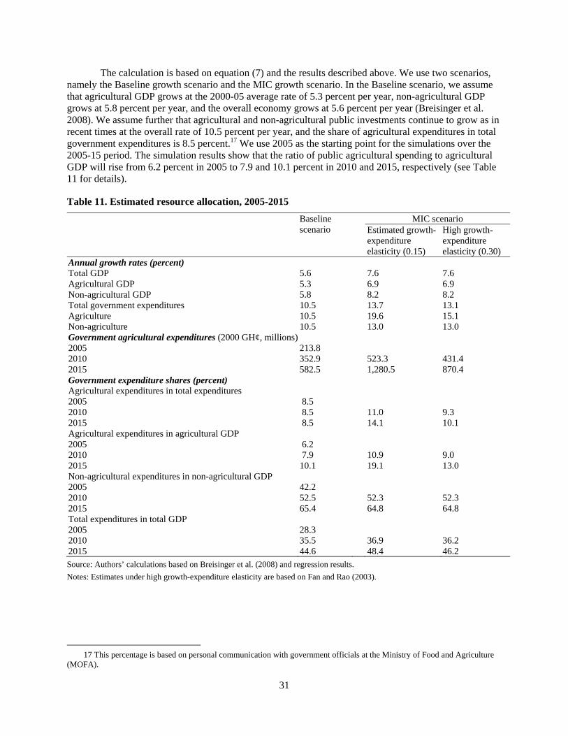
31

The calculation is based on equation (7) and the results described above. We use two scenarios, namely the Baseline growth scenario and the MIC growth scenario. In the Baseline scenario, we assume that agricultural GDP grows at the 2000-05 average rate of 5.3 percent per year, non-agricultural GDP grows at 5.8 percent per year, and the overall economy grows at 5.6 percent per year (Breisinger et al. 2008). We assume further that agricultural and non-agricultural public investments continue to grow as in recent times at the overall rate of 10.5 percent per year, and the share of agricultural expenditures in total government expenditures is 8.5 percent.17 We use 2005 as the starting point for the simulations over the 2005-15 period. The simulation results show that the ratio of public agricultural spending to agricultural GDP will rise from 6.2 percent in 2005 to 7.9 and 10.1 percent in 2010 and 2015, respectively (see Table 11 for details).

Table 11. Estimated resource allocation, 2005-2015

Baseline scenario

MIC scenario Estimated growth-expenditure elasticity (0.15)

High growth-expenditure elasticity (0.30)

Annual growth rates (percent) Total GDP 5.6 7.6 7.6 Agricultural GDP 5.3 6.9 6.9 Non-agricultural GDP 5.8 8.2 8.2 Total government expenditures 10.5 13.7 13.1 Agriculture 10.5 19.6 15.1 Non-agriculture 10.5 13.0 13.0 Government agricultural expenditures (2000 GH¢, millions) 2005 213.8 2010 352.9 523.3 431.4 2015 582.5 1,280.5 870.4 Government expenditure shares (percent) Agricultural expenditures in total expenditures 2005 8.5 2010 8.5 11.0 9.3 2015 8.5 14.1 10.1 Agricultural expenditures in agricultural GDP 2005 6.2 2010 7.9 10.9 9.0 2015 10.1 19.1 13.0 Non-agricultural expenditures in non-agricultural GDP 2005 42.2 2010 52.5 52.3 52.3 2015 65.4 64.8 64.8 Total expenditures in total GDP 2005 28.3 2010 35.5 36.9 36.2 2015 44.6 48.4 46.2 Source: Authors’ calculations based on Breisinger et al. (2008) and regression results. Notes: Estimates under high growth-expenditure elasticity are based on Fan and Rao (2003).

17 This percentage is based on personal communication with government officials at the Ministry of Food and Agriculture

(MOFA).

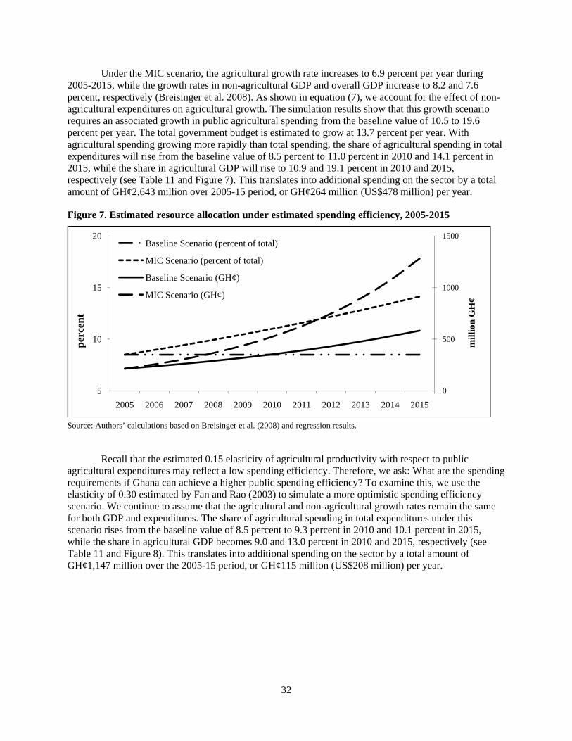
32

Under the MIC scenario, the agricultural growth rate increases to 6.9 percent per year during 2005-2015, while the growth rates in non-agricultural GDP and overall GDP increase to 8.2 and 7.6 percent, respectively (Breisinger et al. 2008). As shown in equation (7), we account for the effect of non-agricultural expenditures on agricultural growth. The simulation results show that this growth scenario requires an associated growth in public agricultural spending from the baseline value of 10.5 to 19.6 percent per year. The total government budget is estimated to grow at 13.7 percent per year. With agricultural spending growing more rapidly than total spending, the share of agricultural spending in total expenditures will rise from the baseline value of 8.5 percent to 11.0 percent in 2010 and 14.1 percent in 2015, while the share in agricultural GDP will rise to 10.9 and 19.1 percent in 2010 and 2015, respectively (see Table 11 and Figure 7). This translates into additional spending on the sector by a total amount of GH¢2,643 million over 2005-15 period, or GH¢264 million (US$478 million) per year.

Figure 7. Estimated resource allocation under estimated spending efficiency, 2005-2015

Source: Authors’ calculations based on Breisinger et al. (2008) and regression results.

Recall that the estimated 0.15 elasticity of agricultural productivity with respect to public agricultural expenditures may reflect a low spending efficiency. Therefore, we ask: What are the spending requirements if Ghana can achieve a higher public spending efficiency? To examine this, we use the elasticity of 0.30 estimated by Fan and Rao (2003) to simulate a more optimistic spending efficiency scenario. We continue to assume that the agricultural and non-agricultural growth rates remain the same for both GDP and expenditures. The share of agricultural spending in total expenditures under this scenario rises from the baseline value of 8.5 percent to 9.3 percent in 2010 and 10.1 percent in 2015, while the share in agricultural GDP becomes 9.0 and 13.0 percent in 2010 and 2015, respectively (see Table 11 and Figure 8). This translates into additional spending on the sector by a total amount of GH¢1,147 million over the 2005-15 period, or GH¢115 million (US$208 million) per year.

0

500

1000

1500

5

10

15

20

2005 2006 2007 2008 2009 2010 2011 2012 2013 2014 2015

mill

ion

GH

¢

perc

ent

Baseline Scenario (percent of total)

MIC Scenario (percent of total)

Baseline Scenario (GH¢)

MIC Scenario (GH¢)

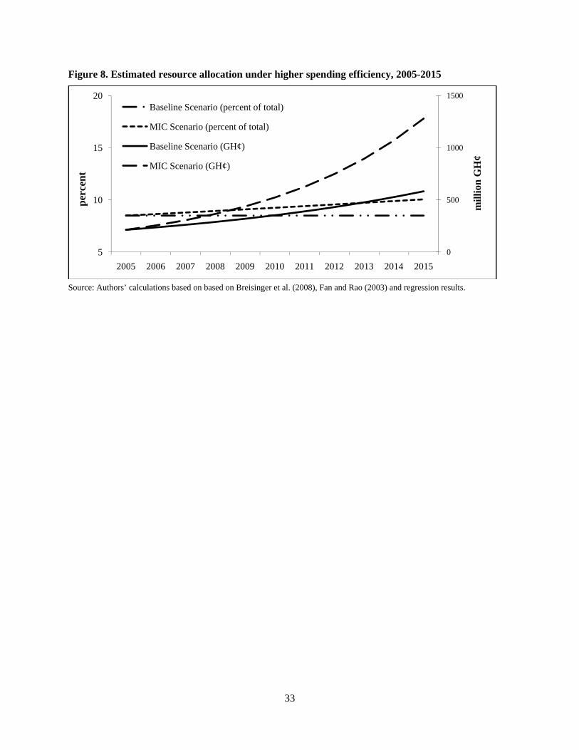
33

Figure 8. Estimated resource allocation under higher spending efficiency, 2005-2015

Source: Authors’ calculations based on based on Breisinger et al. (2008), Fan and Rao (2003) and regression results.

0

500

1000

1500

5

10

15

20

2005 2006 2007 2008 2009 2010 2011 2012 2013 2014 2015

mill

ion

GH

¢

perc

ent

Baseline Scenario (percent of total)

MIC Scenario (percent of total)

Baseline Scenario (GH¢)

MIC Scenario (GH¢)

34

6. CONCLUSIONS

In recent years, Ghana has undergone a major transformation towards rapid economic growth and poverty reduction. However, the benefits have not been widespread, as most of the income increases and poverty reduction effects have been concentrated in the south, deepening the inequality between the north and south. The government of Ghana has declared its new developmental goal of reaching middle-income status by 2015, to be achieved by generating at least 6 percent annual growth in the agricultural sector. With public spending being one of the government’s main policy instrument for promoting growth, the amount of public expenditures required to achieve the government’s growth target and related poverty-reduction goal has become key in policy making. Using district-level disaggregated public expenditures data from 2000 to 2006 and household-level production data from the 2005/06 Ghana Living Standards Survey, we herein address this knowledge gap by assessing the returns to different types of public investments across four agro-ecological zones of Ghana. These results are then used to estimate the amount of agricultural public expenditures required to achieve Ghana’s developmental targets.

Descriptive analysis of public expenditures data shows that the Ministry of Food and Agriculture (MOFA) accounts for only about 25 percent of the total government expenditures on the sector, which represents about 1.2 percent of total government spending or 0.9 percent of agricultural GDP. When we account for agricultural spending through other ministries, departments and agencies (MDAs), particularly the Department of Forestry, Council for Scientific and Industrial Research, and the Ghana Cocoa Board, the share rises to 5.2 percent of total government spending or 3.6 percent of agricultural GDP. Government officials have estimated the share to be even higher, at about 8.5 percent of total government expenditures.

The bulk of the government’s expenditures on the agricultural sector is spent on recurrent activities. While this reflects the high level of direct donor involvement in developmental activities in the sector (i.e. donor spending outside budgetary support), it also raises questions on the sustainability of donor support to the sector, and how donor-funded capital investments will be maintained or replaced in the future.

Looking at the functional disaggregation of expenditures, we find that about 50-75 percent is undertaken at the regional and district levels. The amount spent on agricultural research is relatively low, and there is a large and significant variation in expenditures across the ten administrative regions, both in terms of the total amount spent and the amount spent per unit area or per capita. However, the pattern of variation across the regions differs among the different indicators, suggesting that provision of different agricultural public goods and services may not be always skewed in the same direction or biased against the same region(s).

The results of our econometric analysis show that an increase in public spending in the agricultural sector by one percent is associated with a 0.15 percent increase in the value of agricultural production per capita. The effect associated with developmental spending was much larger (elasticity of 0.54), counteracting the negative effect associated with the recurrent spending component. This result reflects the low government capital-recurrent expenditures ratio in the sector, emphasizing that simply paying staff salaries, administrative costs and other overheads is unlikely to yield any substantive results. Provision of other public goods and services (e.g. rural roads and health sector improvements) also have statistically significant impacts on agricultural productivity. A one percent increase in rural road density is associated with a 0.10 percent increase in the value of agricultural production per capita. Households located more than 15 minutes away from a health center have an approximately 54 percent lower value of agricultural production per capita on average compared to households located within 15 minutes of a health center. These effects translate into very high economic returns. For a marginal Ghana cedi (GH¢) invested directly in agriculture, GH¢16.8 is returned in terms of the value of agricultural productivity. One marginal Ghana cedi invested in feeder roads returns GH¢8.8 from greater agricultural productivity, while investments in health returns GH¢1.3 from greater agricultural productivity. Furthermore, the returns differ among the various agro-ecological zones. Formal education, on the other hand, was found to

35

be negatively associated with agricultural productivity, with about 8.7 percent difference between those without formal education and those completing at least primary education. Together, these results suggest that high benefits can be obtained from additional public spending on the agricultural sector, particularly developmental spending and capital investments. The results further suggest that it could be helpful to target different investments to different regions, while it might be useful to include more agriculturally-relevant information within the educational system.

For Ghana to achieve middle-income status by 2015, public spending in agriculture would have to grow at 19.6 percent per year, and the share of agricultural spending in total expenditures will have to rise from the current government estimated value of 8.5 percent to 11.0 percent in 2010 and 14.1 percent in 2015. These increases would translate into additional agricultural expenditures by a total amount of GH¢2,643 million over the 2005-15 period, or GH¢264 million per year. If the government is able to achieve greater efficiency in its spending, i.e. raise the elasticity of agricultural productivity with respect to public agricultural expenditures from the estimated value of 0.15 to say 0.3, then the additional agricultural spending required will be only GH¢1,147 million over the 2005-15 period, or GH¢115 million per year. Although Ghana is quite close to achieving the underlying agricultural growth rate required to reach its middle-income goal by 2015 (i.e. 6.9 percent compared to the current rate of 5.3 percent), it will be necessary to raise agricultural expenditures. However, it will be important to improve the political and institutional context of public spending programs by, for example, reforming public institutions, particularly those with agriculture-related functions, to improve the efficiency of spending and provision of public goods and services.

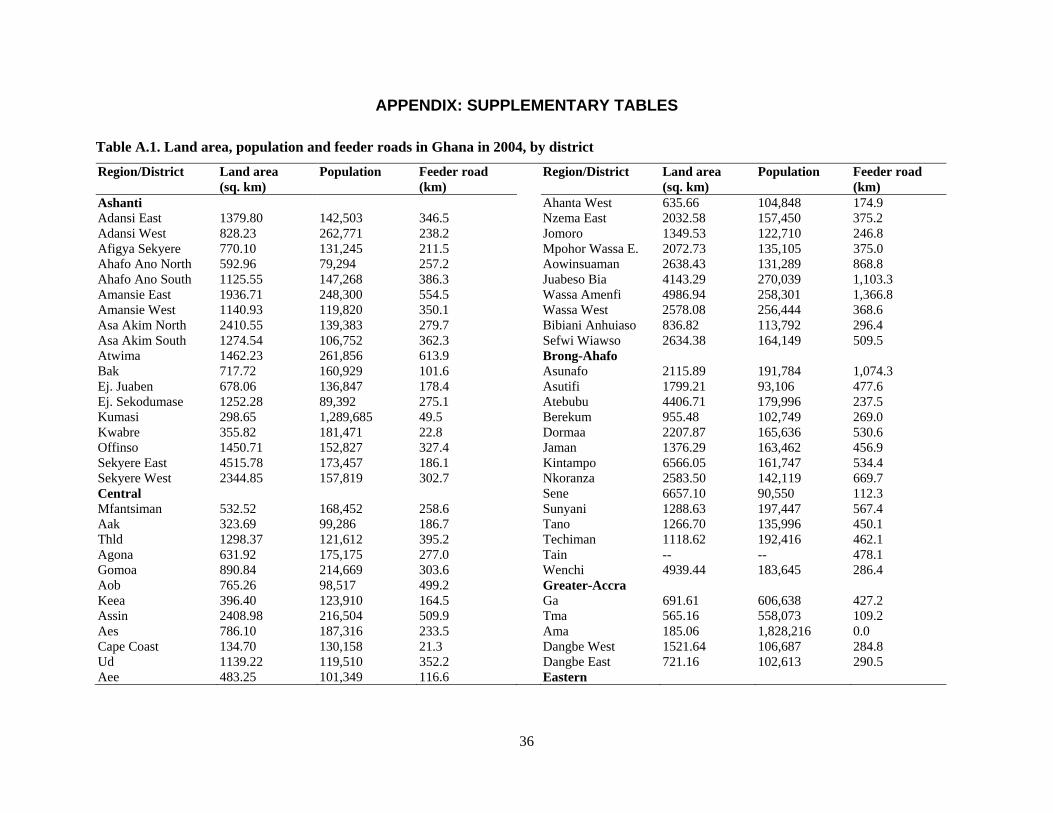
36

APPENDIX: SUPPLEMENTARY TABLES

Table A.1. Land area, population and feeder roads in Ghana in 2004, by district

Region/District Land area (sq. km)

Population Feeder road (km)

Region/District Land area (sq. km)

Population Feeder road (km)

Ashanti Ahanta West 635.66 104,848 174.9 Adansi East 1379.80 142,503 346.5 Nzema East 2032.58 157,450 375.2 Adansi West 828.23 262,771 238.2 Jomoro 1349.53 122,710 246.8 Afigya Sekyere 770.10 131,245 211.5 Mpohor Wassa E. 2072.73 135,105 375.0 Ahafo Ano North 592.96 79,294 257.2 Aowinsuaman 2638.43 131,289 868.8 Ahafo Ano South 1125.55 147,268 386.3 Juabeso Bia 4143.29 270,039 1,103.3 Amansie East 1936.71 248,300 554.5 Wassa Amenfi 4986.94 258,301 1,366.8 Amansie West 1140.93 119,820 350.1 Wassa West 2578.08 256,444 368.6 Asa Akim North 2410.55 139,383 279.7 Bibiani Anhuiaso 836.82 113,792 296.4 Asa Akim South 1274.54 106,752 362.3 Sefwi Wiawso 2634.38 164,149 509.5 Atwima 1462.23 261,856 613.9 Brong-Ahafo Bak 717.72 160,929 101.6 Asunafo 2115.89 191,784 1,074.3 Ej. Juaben 678.06 136,847 178.4 Asutifi 1799.21 93,106 477.6 Ej. Sekodumase 1252.28 89,392 275.1 Atebubu 4406.71 179,996 237.5 Kumasi 298.65 1,289,685 49.5 Berekum 955.48 102,749 269.0 Kwabre 355.82 181,471 22.8 Dormaa 2207.87 165,636 530.6 Offinso 1450.71 152,827 327.4 Jaman 1376.29 163,462 456.9 Sekyere East 4515.78 173,457 186.1 Kintampo 6566.05 161,747 534.4 Sekyere West 2344.85 157,819 302.7 Nkoranza 2583.50 142,119 669.7 Central Sene 6657.10 90,550 112.3 Mfantsiman 532.52 168,452 258.6 Sunyani 1288.63 197,447 567.4 Aak 323.69 99,286 186.7 Tano 1266.70 135,996 450.1 Thld 1298.37 121,612 395.2 Techiman 1118.62 192,416 462.1 Agona 631.92 175,175 277.0 Tain -- -- 478.1 Gomoa 890.84 214,669 303.6 Wenchi 4939.44 183,645 286.4 Aob 765.26 98,517 499.2 Greater-Accra Keea 396.40 123,910 164.5 Ga 691.61 606,638 427.2 Assin 2408.98 216,504 509.9 Tma 565.16 558,073 109.2 Aes 786.10 187,316 233.5 Ama 185.06 1,828,216 0.0 Cape Coast 134.70 130,158 21.3 Dangbe West 1521.64 106,687 284.8 Ud 1139.22 119,510 352.2 Dangbe East 721.16 102,613 290.5 Aee 483.25 101,349 116.6 Eastern

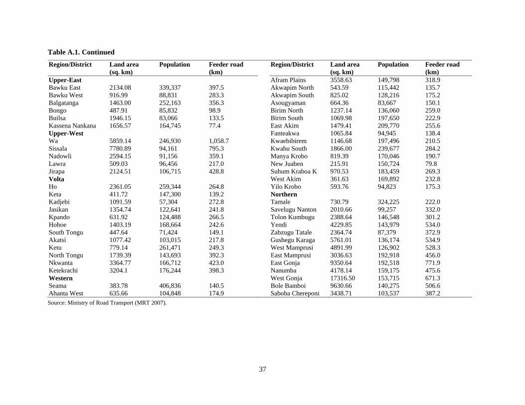
37

Table A.1. Continued

Region/District Land area (sq. km)

Population Feeder road (km)

Region/District Land area (sq. km)

Population Feeder road (km)

Upper-East Afram Plains 3558.63 149,798 318.9 Bawku East 2134.08 339,337 397.5 Akwapim North 543.59 115,442 135.7 Bawku West 916.99 88,831 283.3 Akwapim South 825.02 128,216 175.2 Balgatanga 1463.00 252,163 356.3 Asougyaman 664.36 83,667 150.1 Bongo 487.91 85,832 98.9 Birim North 1237.14 136,060 259.0 Builsa 1946.15 83,066 133.5 Birim South 1069.98 197,650 222.9 Kassena Nankana 1656.57 164,745 77.4 East Akim 1479.41 209,770 255.6 Upper-West Fanteakwa 1065.84 94,945 138.4 Wa 5859.14 246,930 1,058.7 Kwaebibirem 1146.68 197,496 210.5 Sissala 7780.89 94,161 795.3 Kwahu South 1866.00 239,677 284.2 Nadowli 2594.15 91,156 359.1 Manya Krobo 819.39 170,046 190.7 Lawra 509.03 96,456 217.0 New Juaben 215.91 150,724 79.8 Jirapa 2124.51 106,715 428.8 Suhum Kraboa K 970.53 183,459 269.3 Volta West Akim 361.63 169,892 232.8 Ho 2361.05 259,344 264.8 Yilo Krobo 593.76 94,823 175.3 Keta 411.72 147,300 139.2 Northern Kadjebi 1091.59 57,304 272.8 Tamale 730.79 324,225 222.0 Jasikan 1354.74 122,641 241.8 Savelugu Nanton 2010.66 99,257 332.0 Kpando 631.92 124,488 266.5 Tolon Kumbugu 2388.64 146,548 301.2 Hohoe 1403.19 168,664 242.6 Yendi 4229.85 143,979 534.0 South Tongu 447.64 71,424 149.1 Zabzugu Tatale 2364.74 87,379 372.9 Akatsi 1077.42 103,015 217.8 Gushegu Karaga 5761.01 136,174 534.9 Ketu 779.14 261,471 249.3 West Mamprusi 4891.99 126,902 528.3 North Tongu 1739.39 143,693 392.3 East Mamprusi 3036.63 192,918 456.0 Nkwanta 3364.77 166,712 423.0 East Gonja 9350.64 192,518 771.9 Ketekrachi 3204.1 176,244 398.3 Nanumba 4178.14 159,175 475.6 Western West Gonja 17316.50 153,715 671.3 Seama 383.78 406,836 140.5 Bole Bamboi 9630.66 140,275 506.6 Ahanta West 635.66 104,848 174.9 Saboba Chereponi 3438.71 103,537 387.2 Source: Ministry of Road Transport (MRT 2007).

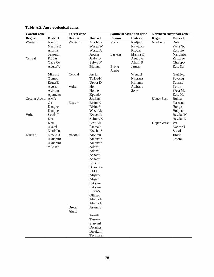
38

Table A.2. Agro-ecological zones

Coastal zone Forest zone Southern savannah zone Northern savannah zone Region District Region District Region District Region District Western Jomoro Western Mpohor- Volta Kadjebi Northern Bole Nzema E Wassa W Nkwanta West Go Ahanta Wassa A Krachi East Go Sekondi Aowin Eastern Manya K Nanumba Central KEEA Juabeso Asuogya Zabzugu Cape Co Sefwi W Afram P Cherepo Abura/A Bibiani Brong

Ahafo Jaman East Da

Mfantsi Central Assin Wenchi Gushieg Gomoa Twifo/H Nkoranz Savelug Efutu/E Upper D Kintamp Tamale Agona Volta Ho Atebubu Tolon Asikuma Hohoe Sene West Ma Ajumako Kpando East Ma Greater Accra AMA Jasikan Upper East Builsa Ga Eastern Birim N Kassena Dangbe Birim S Bongo Dangbe West Ak Bolgata Volta South T Kwaebib Bawku W Keta Suhum/K Bawku E Ketu East Ak Upper West Wa Akatsi Fanteak Nadowli NorthTo Kwahu S Sissala Eastern New Jua Ashanti Atwima Jirapa- Akuapim Amansie Lawra Akuapim Amansie Yilo Kr Adansi Adansi Ashanti Ashanti Ejusu/J Bosomtw KMA Afigya/ Afigya Sekyere Sekyere Ejura/S Offinso Ahafo-A Ahafo-A Brong

Ahafo Asunafo

Asutifi Tanoso Sunyani Dormaa Berekum Techiman

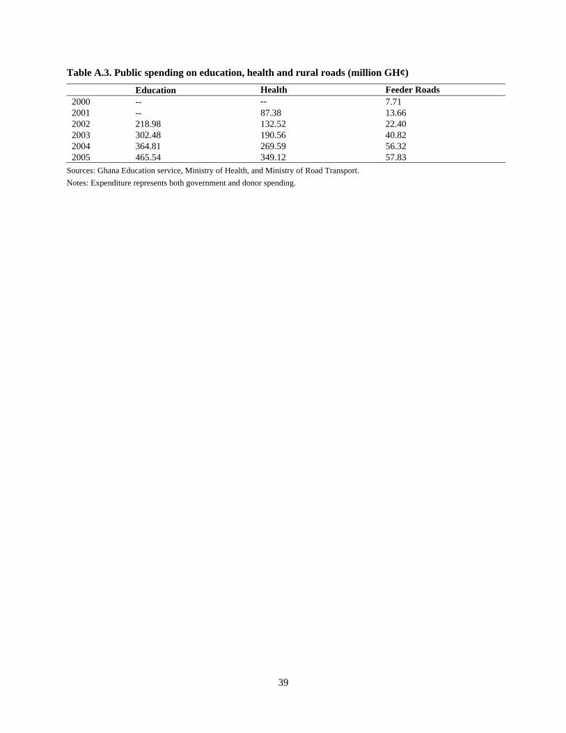
39

Table A.3. Public spending on education, health and rural roads (million GH¢)

Education Health Feeder Roads 2000 -- -- 7.71 2001 -- 87.38 13.66 2002 218.98 132.52 22.40 2003 302.48 190.56 40.82 2004 364.81 269.59 56.32 2005 465.54 349.12 57.83

Sources: Ghana Education service, Ministry of Health, and Ministry of Road Transport. Notes: Expenditure represents both government and donor spending.

40

REFERENCES

Alston, J.M., Chan-Kang, C., Marra, M.C., Pardey, P.G. and Wyatt, T.J. 2000. A meta analysis of rates of return to agricultural R&D: ex pede herculem? Research Report 113, International Food Policy Research Institute, Washington DC, USA.

Anderson, E., de Renzio, P. and Levy, S. 2006. The role of public investment in poverty reduction: theories, evidence and methods. Working Paper 23, Overseas Development Institute, London, UK.

Ansari, M.I., Gordon, D.V. and Akuamoah, C. 1997. Keynes versus Wagner: public expenditure and national income for three African countries. Applied Economics 29:543-550.

Auriol, E. and Warlters, M. 2002.Taxation base in developing countries. The Economics Web Institute (http://www.economicswebinstitute.org/main.htm).

AU/NEPAD (Africa Union/New Partnership for Africa’s Development). 2005. Guidance note for agricultural expenditure tracking system in African countries. NEPAD, Midrand, South Africa.

AU/NEPAD (Africa Union/New Partnership for Africa’s Development). 2003. Comprehensive Africa Agriculture Development Programme. NEPAD, Midrand, South Africa.

BOG (Bank of Ghana). 2007. Statistical Bulletin. BOG, Accra, Ghana.

Breisinger, C., Diao, X., Thurlow, J., Yu, B. and Kolavalli, S. 2008. Accelerated growth and structural transformation: assessing Ghana’s options to reach middle-income status. IFPRI Discussion Paper 750, International Food Policy Research Institute, Washington DC, USA.

Canagarajah, S. and Ye, X. 2001. Public Health and Education Spending in Ghana in 1992-98: Issues of Equity and Efficiency. Policy Research Working Paper 2579. World Bank, Washington DC, USA.

Case, A.C., Rosen, H.S. and Hines, J.R. 1993. Budget spillovers and fiscal policy Interdependence: evidence from the States. Journal of Public Economics 52:285-307.

Collier, P., Dercon, S. and Mackinnon, J. (2002). Density versus Quality in Health Care Provision: Using Household Data to make Budgetary Choices in Ethiopia. World Bank Economic Review 16(3): 425-448.

Coulombe, H. and Wodon, Q. 2007. Poverty, livelihoods, and access to basic services in Ghana: an overview. Paper prepared for the Ghana CEM technical review growth workshop in Accra, May 2-3, 2007. World Bank, Accra, Ghana.

David, P.A., Hall, B.H. and Toole, A.A. 2000. Is public R&D a complement or substitute for private R&D? A review of the econometric evidence Research Policy 29(4-5):497-529.

Devarajan, S., V. Swaroop and H.F. Zou (1996). The Composition of Public Expenditure and Economic Growth. Journal of Monetary Economics 37(2-3): 313-344.

Diao, X., Hazell, P., Resnick, D. and Thurlow, J. 2007. The role of agriculture in development: implications for sub-Saharan Africa. Research Report 153, International Food Policy Research Institute, Washington DC, USA.

Ervin, E.A and Ervin, D.E. 1982. Factors affecting the use of soil conservation practices: hypotheses, evidence, and policy implications. Land Economics 58(3):277-292.

Evenson, R.E. 2001. Economic impacts of agricultural research and extension. In B.L. Gardner and G. Rausser (eds.). Handbook of Agricultural Economics, Vol. 1A. New York: North-Holland.

Evenson, R.E., Pray, C.E. and Rosegrant, M.W. 1999. Agricultural research and productivity growth in India. Research Report 109, International Food Policy Research Institute, Washington, DC., USA.

Fan, S (Ed.). 2008. Public expenditures, growth, and poverty: lessons from developing countries. Johns Hopkins University Press, Baltimore, MD, USA.

Fan, S., Johnson, M., Saurkar, A. and Makombe, T. 2008. Investing in African Agriculture to Halve Poverty by 2015. IFPRI Discussion Paper 751, International Food Policy Research Institute, Washington DC, USA.

41

Fan, S., Hazell, P. and Thorat, S. 2000. Government spending, agricultural growth and poverty in rural India. American Journal of Agricultural Economics 82(4):1038-51.

Fan, S., Nyange, D. and Rao, N. 2005. Public investment and poverty reduction in Tanzania: evidence from household survey data. Development Strategy and Governance Division Discussion Paper 18, International Food Policy Research Institute, Washington DC, USA.

Fan, S. and Rao, N. 2003. Public spending in developing countries: trend, determination and impact. Environment and Production Technology Division Discussion Paper 99, International Food Policy Research Institute, Washington DC, USA.

Fan, S. and Pardey, P.G. 1992. Agricultural research in China: its institutional development and impact. International Service for National Agricultural Research, the Hague, Netherlands.

Fan, S. and Zhang, X. 2004. Investment, Reforms and Poverty in Rural China. Economic Development and Cultural Change 52(2):395-422.

Fan, S., Zhang, X. and Rao, N. 2004. Public expenditure, growth and poverty reduction in rural Uganda. Development Strategy and Governance Division Discussion Paper 4, International Food Policy Research Institute, Washington DC, USA.

Feder, G., Just, R., Zilberman, D., 1985. Adoption of agricultural innovations in developing countries: a survey. Economic Development and Cultural Change 30, 59-76.

Feder, G., Umali, D., 1993. The adoption of agricultural innovations: a review. Technological Forecasting and Social Change 43, 215-239.

Figlio, D.N., Kolpin, V.W. and Reid W.E. 1999. Do States play welfare games? Journal of Urban Economics 46: 437-454.

Gomanee, K., Girma, S. and Morrissey, O. 2003. Aid, Public Spending and Human Welfare: Evidence from Quantile Regressions. Paper presented at the DSA Annual Conference, Glasgow, 10-12 September 2003.

Greene, W.H. 1993. Econometric analysis. New York, USA: Macmillan Publishing Company.

GSS (Ghana Statistical Service). 2006. 2005/06 Ghana Living Standards Survey data. GSS, Accra, Ghana.

GSS (Ghana Statistical Service). 2004. 2003 Core Welfare Indicators Survey, Ghana: main report. GSS, Accra, Ghana.

GSS (Ghana Statistical Service). 1998. 1997 Core Welfare Indicators Survey, Ghana: main report. GSS, Accra, Ghana.

Guild, R.L. 2000. Infrastructure investment and interregional development: Theory, Evidence, and Implications for Planning. Public Works Management and Policy 4(4):274-285.

Hansen, L.P. 1982. Large sample properties of generalized method of moments estimators. Econometrica 50:1029-1054.

Herrera, S. 2007. Public expenditure and growth. Policy Research Working Paper 4372. World Bank, Washington, DC.

Huffman, W.E. and Evenson, R.E. 2006. Do formula or competitive grant funds have greater impact on state agricultural productivity? American Journal of Agricultural Economics 88(4):783-798.

IMF (International Monetary Fund). 2001. Government finance statistics manual 2001. IMF, Washington, D.C., USA. http://www.imf.org/external/pubs/ft/gfs/manual/index.htm.

de Janvry, A., Fafchamps, M., Sadoulet, E., 1991. Peasant household behaviour with missing markets: some paradoxes explained. Economic Journal 101:1400-1417.

Jamison, D. and Lau, L. 1982. Farmer education and farm efficiency. The World Bank Press, Washington, DC.

Jolliffe, D. 2004. The impact of education in rural Ghana: examining household labor allocation and returns on and off the farm. Journal of Development Economics 73:287-314.

42

Kennedy, P. 1985. A guide to econometrics. MIT Press, Cambridge, MA, USA.

Malla, S. and Gray, R. 2005. The crowding effects of basic and applied research: a theoretical and empirical analysis of an agricultural biotech industry. American Journal of Agricultural Economics 87(2):423-438.

MOFA (Ministry of Food and Agriculture). 1999. Agricultural sector expenditure review, 1995-1997. MOFA, Accra, Ghana.

Mogues, T., Ayele, G., and Paulos, Z. 2007. The Bang for the Birr: Public Expenditures and Rural Welfare in Ethiopia. IFPRI Discussion Paper 702. International Food Policy Research Institute. Washington DC, USA.

MRT (Ministry of Road Transport). 2007 Road Infrastructure Indicators. MRT, Ghana.

NDPC (National Development Planning Commission). 2005. Growth and poverty reduction strategy (GPRS II), 2006-2009. NDPC, Accra, Ghana.

Pender, J., Place, F., and Ehui, S. 1999. Strategies for sustainable agricultural development in the east African highlands. Environment and Production Technology Department Working Paper 41. International Food Policy Research Institute, Washington DC, USA.

Quartey, P. 2005. Innovative ways of making aid effective in Ghana: tied aid versus direct budgetary support. Journal of International Development 17:1077–1092.

Rosegrant, M.W. and Evenson, R.E. 1995. Total factor productivity and sources of long-term growth in Indian agriculture. Environment and Production Technology Discussion Paper 7, International Food Policy Research Institute, Washington, DC, USA

Schultz, T. 1982. Investing in people: the economics of population quality. University of California Press, Berkeley, USA.

Singh, I., Squire, L., Strauss, J., 1986. Agricultural household models: extensions, policy and applications. John Hopkins University: Baltimore, MD, USA.

Thurlow, J., Kiringai, J. and Gautam, M. 2007. Rural investments to accelerate growth and poverty reduction in Kenya. IFPRI Discussion Paper 723, International Food Policy Research Institute, Washington DC, USA.

Tompa, E. 2002. The impact of health on productivity: empirical evidence and policy implications, the review of economic performance and social progress 2002:181-202 (http://www.csls.ca/repsp/2/emiletompa.pdf).

USAID (the United States Agency for International Development). 2008. Budget, plans and performance: Ghana. USAID, USA. (http://www.usaid.gov/policy/budget/cbj2006/afr/gh.html).

World Bank. 2000. Project Appraisal Document – Agricultural Services Subsector Investment Project, Ghana. World Bank, Washington DC, USA.

World Bank. 2008. World development report 2008: agriculture for development. World Bank. Washington DC, USA.

World Bank. 2007. World Development Indicators. World Bank. Washington DC, USA.

World Bank. 2001. World development report 2000/2001: attacking poverty. Oxford University Press, Oxford, UK.

Yang, D. 1997. Education and off-farm work. Economic Development and Cultural Change 45:613–632.

Zhang, X. and Fan, S. 2004. How productive is infrastructure? A new approach and evidence from rural India. American Journal of Agricultural Economics 86(2):492-501.

RECENT IFPRI DISCUSSION PAPERS

For earlier discussion papers, please go to www.ifpri.org/pubs/pubs.htm#dp. All discussion papers can be downloaded free of charge.

810. Integrating survey and ethnographic methods to evaluate conditional cash transfer programs. Michelle Adato, 2008.

809. European Union: Shadow WTO agricultural domestic support notifications. Tim Josling and Alan Swinbank, 2008.

808. Bt Cotton and farmer suicides in India: Reviewing the evidence. Guillaume P. Gruère, Purvi Mehta-Bhatt, and Debdatta Sengupta, 2008.

807. Gender, caste, and public goods provision in Indian village governments. Kiran Gajwani and Xiaobo Zhang, 2008.

806. Measuring Ethiopian farmers’ vulnerability to climate change across regional states. Temesgen Deressa, Rashid M. Hassan, and Claudia Ringler, 2008.

805. Determinants of agricultural protection from an international perspective: The role of political institutions. Christian H.C.A. Henning, 2008

804. Vulnerability and the impact of climate change in South Africa’s Limpopo River Basin. Sharon Shewmake, 2008.

803. Biofuels, poverty, and growth: A computable general equilibrium analysis of Mozambique. Channing Arndt, Rui Benfica, Finn Tarp, James Thurlow, and Rafael Uaiene

802. Agricultural exit problems: Causes and consequences. Derek Headey, Dirk Bezemer, and Peter B. Hazell, 2008.

801. Cotton-textile-apparel sectors of India: Situations and challenges faced. Jatinder S. Bedi and Caesar B. Cororaton, 2008.

800. Cotton-textile-apparel sectors of Pakistan: Situations and challenges faced. Caesar B. Cororaton, Abdul Salam, Zafar Altaf, and David Orden, with Reno Dewina, Nicholas Minot, and Hina Nazli, 2008.

799. Race to the top and race to the bottom: Tax competition in rural China. Yi Yao and Ziaobo Zhang, 2008.

798. Analyzing the determinants of farmers’ choice of adaptation methods and perceptions of climate change in the Nile Basin of Ethiopia. Temesgen Deressa, R.M. Hassan, Tekie Alemu, Mahmud Yesuf, Claudia Ringler, 2008

797. Economic transformation in theory and practice: What are the messages for Africa? Clemens Breisinger and Xinshen Diao, 2008.

796. Biosafety at the crossroads: An analysis of South Africa’s marketing and trade policies for genetically modified products. Guillaume P. Gruère and Debdatta Sengupta, 2008.

795. Publish or patent? Knowledge dissemination in agricultural biotechnology. An Michiels and Bonwoo Koo, 2008.

794. Agricultural growth and investment options for poverty reduction in Malawi. Samuel Benin, James Thurlow, Xinshen Diao, Christen McCool, Franklin Simtowe, 2008.

793. China: Shadow WTO agricultural domestic support notifications. Fuzhi Cheng, 2008.

792. India: Shadow WTO agricultural domestic support notifications. Munisamy Gopinath, 2008.

791. Agricultural growth and investment options for poverty reduction in Zambia. James Thurlow, Samuel Benin, Xinshen Diao, Henrietta Kalinda, and Thomson Kalinda, 2008.

790. Agricultural growth and investment options for poverty reduction in Uganda. Samuel Benin, James Thurlow, Xinshen Diao, Allen Kebba, Nelson Ofwono, 2008.

789. Agricultural public spending in Nigeria. Tewodaj Mogues, Michael Morris, Lev Freinkman, Abimbola Adubi, and Simeon Ehui; with Chinedum Nwoko, Olufemi Taiwo, Caroline Nege, Patrick Okonji, and Louis Chete, 2008.

788. Choosing sensitive agricultural products in trade negotiations. Sébastien Jean, David Laborde, and Will Martin, 2008.

787. An updated look at the recovery of agricultural productivity in Sub-Saharan Africa. Alejandro Nin Pratt and Bingxin Yu. 2008

786. Migration, poverty, and inequality: Evidence from Burkina Faso. F.S. Wouterse. 2008

785. Insecticide use on vegetables in Ghana: Would GM seed benefit farmers? Daniela Horna, Melinda Smale, Ramatu Al-Hassan, José Falck-Zepeda, and Samuel E. Timpo, 2008.

INTERNATIONAL FOOD POLICY RESEARCH INSTITUTE

www.ifpri.org

IFPRI HEADQUARTERS

2033 K Street, NW Washington, DC 20006-1002 USA Tel.: +1-202-862-5600 Fax: +1-202-467-4439 Email: ifpri@cgiar.org

IFPRI ADDIS ABABA

P. O. Box 5689 Addis Ababa, Ethiopia Tel.: +251 11 6463215 Fax: +251 11 6462927 Email: ifpri-addisababa@cgiar.org

IFPRI NEW DELHI

CG Block, NASC Complex, PUSA New Delhi 110-012 India Tel.: 91 11 2584-6565 Fax: 91 11 2584-8008 / 2584-6572 Email: ifpri-newdelhi@cgiar.org