Rapid Nonlinear Topology Optimization using Precomputed Reduced-Order Models

IntroductionTopology Optimization

Model Order ReductionApplicationsConclusion

Rapid Nonlinear Topology Optimization usingPrecomputed Reduced-Order Models

Matthew J. Zahr and Charbel Farhat

Farhat Research GroupStanford University

17th U.S. National Congress on Theoretical and AppliedMechanics

Michigan State UniversityJune 15 - 20, 2014

M. J. Zahr and C. Farhat



Motivation

For industry-scale design problems,topology optimization is a beneficial toolthat is time and resource intensive

Large number of calls to structural solverusually requiredEach structural call is expensive,especially for nonlinear 3DHigh-Dimensional Models (HDM)

Use a Reduced-Order Model (ROM) as asurrogate for the structural model in amaterial topology optimization loop

Large speedups over HDM realized

524 MARTINS, ALONSO, AND REUTHER

Fig. 1 Elliptic vs aerostructural optimum lift distribution.

Fig. 2 Natural laminar-flow supersonic business-jet configuration.

but an objective function that reflects the overall mission of the par-ticular aircraft. Consider, for example, the Breguet range formulafor jet-powered aircraft:

Range = Vc

CL

CDln Wi

W f(1)

where V is the cruise velocity and c is the thrust-specific fuel con-sumption of the powerplant. CL/CD is the ratio of lift to drag, andWi/W f is the ratio of initial and final cruise weights of the aircraft.

The Breguet range equation expresses a tradeoff between the dragand the empty weight of the aircraft and constitutes a reasonable ob-jective function to use in aircraft design. If we were to parameterizea design with both aerodynamic and structural design variables andthen maximize the range for a fixed initial cruise weight, subject tostress constraints, we would obtain a lift distribution similar to theone shown in Fig. 1.

This optimum lift distribution trades off the drag penalty associ-ated with unloading the tip of the wing, where the loading contributesmost to the maximum stress at the root of the wing structure in orderto reduce the weight. The end result is an increase in range whencompared to the elliptically loaded wing because of a higher weightfraction Wi/W f . The result shown in Fig. 1 illustrates the need fortaking into account the coupling of aerodynamics and structureswhen performing aircraft design.

The aircraft configuration used in this work is the supersonicbusiness jet shown in Fig. 2. This configuration is being developedby the ASSET Research Corporation and is designed to achieve alarge percentage of laminar flow on the low-sweep wing, resultingin decreased friction drag.11 The aircraft is to fly at Mach 1.5 andhave a range of 5300 miles.

Detailed mission analysis for this aircraft has determined thatone count of drag (!CD = 0.0001) is worth 310 lb of empty weight.This means that to optimize the range of the configuration we can

minimize the objective function

I = "CD + #W (2)

where CD is the drag coefficient, W is the structural weight inpounds, and "/# = 3.1 ! 106.

We parameterize the design using an arbitrary number of shapedesign variables that modify the outer-mold line (OML) of the air-craft and structural design variables that dictate the thicknesses ofthe structural elements. In this work the topology of the structureremains unchanged, that is, the number of spars and ribs and theirplanform-view location is fixed. However, the depth and thicknessof the structural members are still allowed to change with variationsof the OML.

Among the constraints to be imposed, the most obvious one isthat during cruise the lift must equal the weight of the aircraft. In ouroptimization problem we constrain the CL by periodically adjustingthe angle of attack within the aerostructural solver.

We also must constrain the stresses so that the yield stress of thematerial is not exceeded at a number of load conditions. There aretypically thousands of finite elements describing the structure ofthe aircraft, and it can become computationally very costly to treatthese constraints separately. The reason for this high cost is thatalthough there are efficient ways of computing sensitivities of a fewfunctions with respect to many design variables and for computingsensitivities of many functions with respect to a few design variables,there is no known efficient method for computing sensitivities ofmany functions with respect to many design variables.

For this reason we lump the individual element stresses usingKreisselmeier–Steinhauser (KS) functions. In the limit all elementstress constraints can be lumped into a single KS function, thusminimizing the cost of a large-scale aerostructural design cycle.Suppose that we have the following constraint for each structuralfinite element:

gm = 1 " $m/$y # 0 (3)

where $m is the von Mises stress in element m and $y is the yieldstress of the material. The corresponding KS function is defined as

KS = " 1%

ln!"

m

e"%gm

#(4)

This function represents a lower bound envelope of all of the con-straint inequalities, where % is a positive parameter that expresseshow close this bound is to the actual minimum of the constraints.This constraint lumping method is conservative and might notachieve the same result as treating the constraints separately. How-ever, the use of KS functions has been demonstrated, and it consti-tutes a viable alternative, being effective in optimization problemswith thousands of constraints.12

Having defined our objective function, design variables, and con-straints, we can now summarize the aircraft design optimizationproblem as follows:

Minimize:

I = "CD + #W, x $ Rn

Subject to:

CL = CLT , KS # 0, x # xmin

The stress constraints in the form of KS functions must be enforcedby the optimizer for aerodynamic loads corresponding to a numberof flight and dynamic load conditions. Finally, a minimum gauge isspecified for each structural element thickness.

Analytic Sensitivity AnalysisOur main objective is to calculate the sensitivity of a multidisci-

plinary function with respect to a number of design variables. Thefunction of interest can be either the objective function or any of theconstraints specified in the optimization problem. In general, suchfunctions depend not only on the design variables, but also on the

Dow

nloa

ded

by S

TAN

FORD

UN

IVER

SITY

on

July

16,

201

3 | h

ttp://

arc.

aiaa

.org

| D

OI:

10.2

514/

1.11

478




0-1 Material Topology Optimization

minimizeχ∈Rnel

L(u(χ),χ)

subject to c(u(χ),χ) ≤ 0

u (structural displacements) is implicitly defined as afunction of χ through the HDM equation

f int(u) = f ext

Ce = Ce0χe ρe = ρe0χe χe =

0, e /∈ Ω∗

1, e ∈ Ω∗

General nonlinear setting considered (geometric andmaterial nonlinearities)




Projection-Based ROMNonlinear ROM BottleneckROM PrecomputationsReduced Topology Optimization

Reduced-Order Model

Model Order Reduction (MOR) assumptionState vector lies in low-dimensional subspace defined by aReduced-Order Basis (ROB) Φ ∈ RN×ku

u ≈ Φy

ku N

N equations, ku unknowns

f int(Φy) = f ext

Galerkin projection

ΦT f int(Φy) = ΦT f ext





NL ROM Bottleneck - Internal Force

ΦT f int(Φy)= ΦT f ext





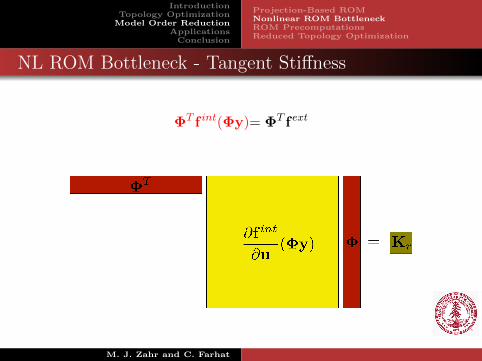
NL ROM Bottleneck - Tangent Stiffness

ΦT f int(Φy)= ΦT f ext





Approximation of reduced internal force, ΦT f int(Φy)

For general nonlinear problems, high-dimensional quantitiescannot be precomputed since they change at every iteration

For polynomial nonlinearities, there is an opportunity forprecomputation

ApproachApproximate fr = ΦT f int(Φy) by polynomial via Taylorseries

We choose a third-order seriesExact representation of reduced internal force for St.Venant-Kirchhoff materials

Precompute coefficient tensorsOnline operations will only involve small quantities

Remove online bottleneckPay price in offline phase





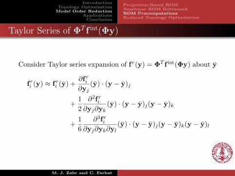
Taylor Series of ΦT f int(Φy)

Consider Taylor series expansion of f r(y) = ΦT f int(Φy) about y

f ri (y) ≈ f ri (y) +∂f ri∂yj

(y) · (y − y)j

+1

2

∂2f ri∂yj∂yk

(y) · (y − y)j(y − y)k

+1

6

∂3f ri∂yj∂yk∂yl

(y) · (y − y)j(y − y)k(y − y)l





Reduced Derivatives

Reduced derivatives computable by:

Projection of full order derivativesDirectly via finite differences

αi = f ri (y) = Φpifintp (Φy)

βij =∂f ri∂yj

(y) = ΦpiΦqj

∂f intp

∂uq(Φy)

γijk =∂2f ri

∂yj∂yk(y) = ΦpiΦqjΦrk

∂f intp

∂uq∂ur(Φy)

ωijkl =∂3f ri

∂yj∂yk∂yl(y) = ΦpiΦqjΦrkΦsl

∂f intp

∂uq∂ur∂us(Φy)





Reduced internal force

Reduced internal force becomes

f ri (y) = αi + βij(y − y)j

+1

2γijk(y − y)j(y − y)k

+1

6ωijkl(y − y)j(y − y)k(y − y)l,

which only depends on quantities scaling with the reduceddimension.





Reduced internal force - material dependence

As written, the material properties for a given material arebaked into the polynomial coefficients

For notational simplicity, we consider two materialparameters: ρ (density) and η

α = α(ρ, η)

β = β(ρ, η)

γ = γ(ρ, η)

ω = ω(ρ, η)

In the context of 0-1 topology optimization, α,β,γ,ω needto be recomputed at each new distribution of ρ, η

Extremely expensive – destroy all speedup potential





Material Representation

Recall the material parameters are spatial distributions, i.e.ρ = ρ(X) and η = η(X)

Define admissible distributions: φρi ni=1, φηi ni=1

Require

ρ(X) = φρi (X)ξi

η(X) = φηi (X)ξi

Many possible choices admissible distributions

Here, collected via configuration snapshots





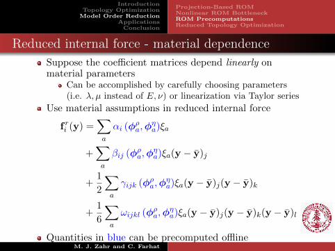
Reduced internal force - material dependence

Suppose the coefficient matrices depend linearly onmaterial parameters

Can be accomplished by carefully choosing parameters(i.e. λ, µ instead of E, ν) or linearization via Taylor series

Use material assumptions in reduced internal force

f ri (y) =∑a

αi (φρa,φηa)ξa

+∑a

βij (φρa,φηa)ξa(y − y)j

+1

2

∑a

γijk (φρa,φηa)ξa(y − y)j(y − y)k

+1

6

∑a

ωijkl (φρa,φ

ηa)ξa(y − y)j(y − y)k(y − y)l

Quantities in blue can be precomputed offlineM. J. Zahr and C. Farhat




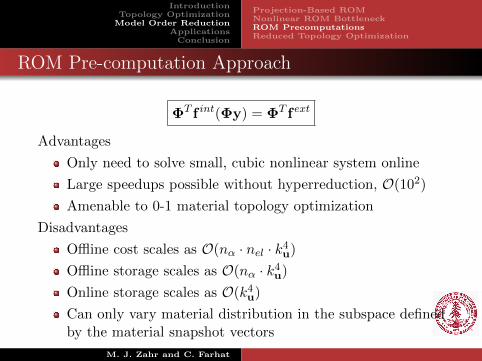
ROM Pre-computation Approach


Advantages

Only need to solve small, cubic nonlinear system online

Large speedups possible without hyperreduction, O(102)

Amenable to 0-1 material topology optimization

Disadvantages

Offline cost scales as O(nα · nel · k4u)

Offline storage scales as O(nα · k4u)

Online storage scales as O(k4u)

Can only vary material distribution in the subspace definedby the material snapshot vectors





Reduced Topology Optimization

minimizeξ∈Rn

L(y(ξ), ξ)

subject to c(y(ξ), ξ) ≤ 0

y is implicitly defined as a function of ξ through the ROMequation


which can be computed efficiently




Wing Box Design

Problem Setup

Neo-Hookean material

90,799 tetrahedralelements

29,252 nodes, 86,493 dof

Static simulation with loadapplied in 10 increments

Loads: Bending (X- andY- axis), Twisting,Self-Weight

ROM size: ku = 5

NACA0012




Wing Box Design

Problem Setup



29,252 nodes, 86,493 dof



ROM size: ku = 5

40 Ribs




Wing Box Design

Problem Setup



29,252 nodes, 86,493 dof



ROM size: ku = 5




Wing Box Design

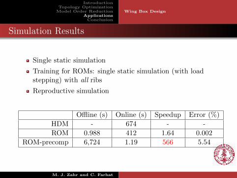
Simulation Results

Single static simulation

Training for ROMs: single static simulation (with loadstepping) with all ribs

Reproductive simulation

Offline (s) Online (s) Speedup Error (%)

HDM - 674 - -

ROM 0.988 412 1.64 0.002

ROM-precomp 6,724 1.19 566 5.54




Wing Box Design

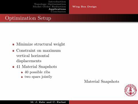
Optimization Setup

Minimize structural weight

Constraint on maximumvertical horizontaldisplacements

41 Material Snapshots

40 possible ribstwo spars jointly

Material Snapshots




Wing Box Design

Optimization Results

0 1 2 3 4 5 6 7 8 92500

3000

3500

4000

4500

5000

Iteration

ObjectiveFunction

All ribsNo ribsConstraint ViolatedConstraints Satisfied

Optimization Iterates




Wing Box Design

Optimization Results

Deformed Configuration (Optimal Solution)

Initial Guess Optimal Solution

Structural Weight 4.67× 103 3.02× 103

Constraint Violation 0 7.10× 10−23




Conclusion and Future Work

New method for materialtopology optimization usingreduced-order models

Applicable in nonlinearsettingO(102) speedup over HDM

Strongly enforcemanufacturability constraints

selection of materialsnapshots

Address large problems

Investigate extending methodto more sophisticated topologyoptimization techniques


Rapid Nonlinear Topology Optimization using Precomputed Reduced-Order Models

Documents

Transcript of Rapid Nonlinear Topology Optimization using Precomputed Reduced-Order Models