1

Random Matrix Based Extended Target Trackingwith Orientation: A New Model and Inference

Barkın Tuncer, Student Member, IEEE, Emre Ozkan, Member, IEEE,

Abstract—In this study, we propose a novel extended targettracking algorithm which is capable of representing the extentof dynamic objects as an ellipsoid with a time-varying orientationangle. A diagonal positive semi-definite matrix is defined to modelobjects’ extent within the random matrix framework where thediagonal elements have inverse-Gamma priors. The resultingmeasurement equation is non-linear in the state variables, and itis not possible to find a closed-form analytical expression for thetrue posterior because of the absence of conjugacy. We use thevariational Bayes technique to perform approximate inference,where the Kullback-Leibler divergence between the true and theapproximate posterior is minimized by performing fixed-pointiterations. The update equations are easy to implement, andthe algorithm can be used in real-time tracking applications.We illustrate the performance of the method in simulations andexperiments with real data. The proposed method outperformsthe state-of-the-art methods when compared with respect toaccuracy and robustness.

Index Terms—Target tracking, extended target tracking, ran-dom matrix model, orientation, variational Bayes

I. INTRODUCTION

EXTENDED target tracking (ETT) problem involves pro-cessing multiple measurements that belong to a single

target at each scan. In contrast to conventional tracking algo-rithms, which rely on point target assumption, ETT algorithmsaim at estimating the target extent, which can be defined as thetarget-specific region that generates multiple measurements.Previous studies in the ETT literature can be broadly catego-rized into four groups:• Simple shape models• Random matrix (RM) based models• Random hyper-surface (RHS) based models• Mixture models

A simple approach to ETT involves assuming a predefinedshape for the extent/contour of the object such as a circle, arectangle, or a line [1]–[3]. The most common approaches inthe literature utilize RM models, where the target extent isrepresented by an ellipse [4]–[7]. Alternatively, RHS modelsare suggested in [8], [9]. More recently, Gaussian Process (GP)based models are proposed for extended target tracking [10]–[12]. Another fold of studies focuses on modeling the targetextent with multiple ellipses [13]–[16].

RM models represent the elliptical extent of a target byan unknown positive semi-definite matrix (PSDM). In theBayesian framework, inverse-Wishart (IW) distribution definesa conjugate prior for PSDMs. In RM based ETT models, theoverall target state is composed of a Gaussian kinematic statevector and an IW distributed extent matrix. Several algorithmsare proposed to approximate or compute the posterior ofthis augmented state. In [4], exact inference is performed byneglecting the measurement noise and exploiting the resulting

Authors are with the Department of Electrical and Electronics En-gineering, Middle East Technical University, Ankara, Turkey e-mail:barkint@metu.edu.tr, emreo@metu.edu.tr.

conjugacy. This model is restrictive in the sense that thekinematic state vector has to be composed of the target’sposition and higher-order spatial components such as velocityand acceleration. Koch’s RM model is later improved in[5] to account for the measurement noise in the updates atthe expense of exact inference. The update equations in [5]are intuitive, but the approximations are difficult to quantifytheoretically. This problem is later addressed by [6], wherethe variational Bayes technique is used to obtain approximateposteriors.

None of the aforementioned RM models is capable oftracking the heading angle of an extended target. They insteadrely on a forgetting factor to forget the sufficient statisticsof the unknown extent matrix in time to account for thechanges in the orientation of the target. Such an approachis problematic as it aims to discard the information collectedin the past and try to explain the change in the orientation asthe change in the target shape. There are earlier studies thataim at estimating the orientation angle of elliptical objects[17]–[20]. In [20], the orientation of the target is estimated byusing the information that is obtained from the trajectory of thetarget. The methods that are proposed in [17]–[19] express theunknown extent parametrically and perform inference usingextended Kalman filters together with pseudo-measurements.In these approaches, an explicit nonlinear measurement equa-tion is derived where the kinematic and shape parameters arerelated to measurements by multiplicative random variables.The inference in [19] involves second-order Taylor seriesapproximation to approximate the pseudo-measurement co-variance matrix. In [18], the authors improved the algorithmin [19] further and eliminated the need for computing Hessianmatrices. Instead, they showed that the expectation and the co-variance of the pseudo-measurements could be approximatedfrom the original measurement covariance matrix. In [17],the predicted measurement covariance matrix approximationis calculated more precisely.

There are several drawbacks of the methods in [17]–[19].The models used in these methods involve a multiplicativenoise term, which introduces additional non-linearity in theproblem, and it makes performing inference more difficult.The methods require a pseudo-measurement, which mustbe constructed from the original measurements to updatekinematic and extent states separately. The measurementscollected at one time instant must be processed sequentially.Changing the order of the measurements causes minor changesin the performance [17]. The state variables corresponding tothe semi-axes lengths, which are positive by definition, aredistributed with Gaussian distributions whose support coversboth positive and negative real line. In some cases, it canbe challenging to reflect available information into the priorsdefined in [17], which may cause a collapse in the extentestimates in the subsequent measurement updates.

In this work, we propose a novel RM model that defines aGaussian prior for the heading angle and an inverse Gamma

arX

iv:2

010.

0882

0v2

[st

at.M

L]

8 M

ar 2

021

2

prior for the extent parameters, which guarantee positive semi-definiteness. It is not possible to find a closed-form expressionfor the resulting posterior hence we utilize the variationalBayes technique to perform approximate inference. The vari-ational Bayes technique is successfully applied to complexfiltering problems in the literature to obtain approximateposteriors [6], [21]–[25].

The contributions of this manuscript can be listed as follows.

• We provide a novel solution that can track the orientationof a target and estimate its extent jointly.

• The proposed solution utilizes appropriate priors, whichare defined over non-negative real numbers, for the un-known extent parameters.

• The problem formulation does not rely on multiplicativenoise terms or pseudo-measurements.

• The measurement update can be performed by processingmultiple measurements as a batch. The update does notdepend on the order of the measurements.

• The uncertainty in the orientation and shape parameterscan be expressed separately.

• The inference is performed via the well-known variationalBayes technique.

The paper is organized as follows. In Section II, we for-mulate the problem of joint shape estimation and trackingof elliptical objects with time-varying orientation. In thesubsequent sections, we present the inference method. Themeasurement update is derived in Section III. Time update isgiven in Section IV. A closer look at a single measurementupdate and its comparison with the state-of-the-art extendedKalman filter (EKF) algorithm is given in Section V. Lastly,the results are presented and discussed in Section VI.

TABLE I: NOTATIONS

• Set of real matrices of size m× n is represented with Rm×n.• Set of symmetric positive definite and semi-definite matrices of size n×n

is represented with Sn++ and Sn+, respectively.• N (x;µ,Σ) represents the multivariate Gaussian distributions with mean

vector µ ∈ Rnx and covariance matrix Σ ∈ Snx++,• IG(σ;α, β) represents the inverse Gamma distribution over the scalar σ ∈

R+ with shape and scale parameters α ∈ R+ and β ∈ R+ respectively,

IG(σ;α, β) =βα

Γ(α)σ−α−1 exp

(−β

σ

),

• The number of measurements at time k is represented by mk ∈ Z+.• For given measurement number of mk , Yk represents the measurement set{y1k, . . . ,y

mkk } at time k.

• For any number a ∈ Z+, Zk represents the variable set {z1k, . . . , zak} at

time k.• rk represent the vector [r1k, . . . , r

ak ]T with size a ∈ Z+.

• KL denotes the Kullback-Leibler divergence between two distributions q(x)and p(x),

KL(q(x)||p(x)

),∫q(x) log

(q(x)

p(x)

)dx.

• det(A) denotes the determinant of matrix A.• Tr

[A]

=∑ni=1 aii where aii is the ith diagonal element of A ∈ Rn×n.

• Ep denotes the expectation operator, and p emphasizes the underlyingprobability distribution(s).

• diag(a1, a2, . . . , an) returns the diagonal matrix whose diagonal elementsare a1, a2, . . . , an.

• blkdiag(A1, A2, . . . , AN ) returns the block diagonal square matrixwhose main-diagonal blocks are the input matrices A1, A2, . . . , AN .

• h.o.t. stands for higher-order terms.

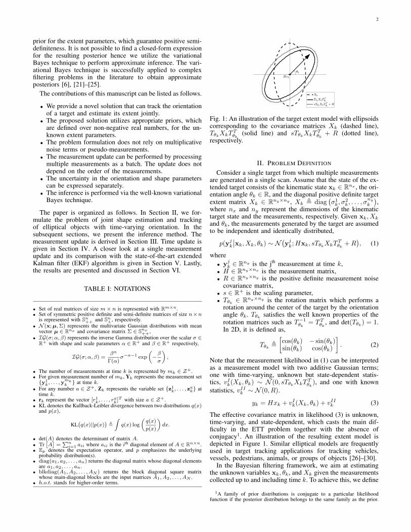
Fig. 1: An illustration of the target extent model with ellipsoidscorresponding to the covariance matrices Xk (dashed line),TθkXkT

Tθk

(solid line) and sTθkXkTTθk

+ R (dotted line),respectively.

II. PROBLEM DEFINITION

Consider a single target from which multiple measurementsare generated in a single scan. Assume that the state of the ex-tended target consists of the kinematic state xk ∈ Rnx , the ori-entation angle θk ∈ R, and the diagonal positive definite targetextent matrix Xk ∈ Rny×ny , Xk , diag

(σ1k, σ

2k, . . . , σ

nyk

),

where nx and ny represent the dimensions of the kinematictarget state and the measurements, respectively. Given xk, Xk

and θk, the measurements generated by the target are assumedto be independent and identically distributed,

p(yjk∣∣xk, Xk, θk) ∼ N

(yjk;Hxk, sTθkXkT

Tθk

+R), (1)

where• yjk ∈ Rny is the jth measurement at time k,• H ∈ Rny×nx is the measurement matrix,• R ∈ Rny×ny is the positive definite measurement noise

covariance matrix,• s ∈ R+ is the scaling parameter,• Tθk ∈ Rny×ny is the rotation matrix which performs a

rotation around the center of the target by the orientationangle θk. Tθk satisfies the well known properties of therotation matrices such as T−1θk

= TTθk , and det(Tθk) = 1.In 2D, it is defined as,

Tθk ,

[cos(θk) − sin(θk)sin(θk) cos(θk)

]. (2)

Note that the measurement likelihood in (1) can be interpretedas a measurement model with two additive Gaussian terms;one with time-varying, unknown but state-dependent statis-tics, vIk(Xk, θk) ∼ N (0, sTθkXkT

Tθk

), and one with knownstatistics, vIIk ∼ N (0, R).

yk = Hxk + vIk(Xk, θk) + vIIk (3)

The effective covariance matrix in likelihood (3) is unknown,time-varying, and state-dependent, which casts the main dif-ficulty in the ETT problem together with the absence ofconjugacy1. An illustration of the resulting extent model isdepicted in Figure 1. Similar elliptical models are frequentlyused in target tracking applications for tracking vehicles,vessels, pedestrians, animals, or groups of objects [26]–[30].

In the Bayesian filtering framework, we aim at estimatingthe unknown variables xk, θk, and Xk given the measurementscollected up to and including time k. To achieve this, we define

1A family of prior distributions is conjugate to a particular likelihoodfunction if the posterior distribution belongs to the same family as the prior.

3

appropriate priors for the unknowns and try to compute theirposteriors in a recursive manner. This is generally performedby repeating two recursive steps:• Time Update (Prediction): At any time step k, the

predictive distribution p(xk, Xk, θk|Y1:k−1) is computedaccording to Chapman-Kolmogorov equation by usingthe posterior from the previous time step k − 1, and thetransition density induced by the system dynamics.

• Measurement Update (Correction): When the newmeasurements Yk are available, the posterior distri-bution p(xk, Xk, θk|Y1:k) is computed by using theBayes’ rule. In this step, the predictive distributionp(xk, Xk, θk|Y1:k−1) is used as the prior.

Unfortunately, it is not possible to obtain a closed formexpression for the posterior in our problem. Therefore, we willlook for an approximate analytical solution using a variationalapproximation.

Before introducing the details of this approximation, we willfirst define the prior distributions of the unknown variables.The joint prior distribution of the kinematic state, the extent,and the orientation is specified as

p(x0, X0, θ0) = N (x0; x0, P0)×ny∏i=1

IG(σi0;αi0, β

i0

)×N

(θ0; θ0,Θ0

), (4)

where X0 , diag(σ10 , σ

20 , . . . , σ

ny0

), and IG

(σi0;αi0, β

i0

)denotes the inverse Gamma distribution. Here, x0 and P0

are the prior mean and covariance matrix of the Gaussiankinematic state vector x0, respectively. The prior mean andcovariance matrix of the orientation angle θ0 are denoted byθ0 and Θ0, respectively. Please see Table I for the completelist of the notations.In the following sections, we will describe the MeasurementUpdate and Time Update steps of the proposed method indetail.

III. MEASUREMENT UPDATE

Suppose at time k, we have the following conditionalpredicted density for the kinematic, orientation, and extentstates:

p(xk, Xk, θk|Y1:k−1) = N (xk; xk|k−1, Pk|k−1)

×ny∏i=1

IG(σik|k−1;αik|k−1, βik|k−1)

×N(θk; θk|k−1,Θk|k−1

). (5)

The left-hand side of the above expression is conditioned onthe measurements up to and including time instant k− 1. Thepredicted mean and covariance of the Gaussian state vector isrepresented by xk|k−1 and Pk|k−1, respectively. The shape andthe scale variables for the ith diagonal element of the inverseGamma distributed extent state Xk are αik|k−1 and βik|k−1.When the measurements Yk are available at time k, theposterior distribution can be computed using Bayes’ rule

p(xk, Xk, θk|Y1:k)

=p(Yk|xk, Xk, θk)p(xk, Xk, θk|Y1:k−1)

p(Yk|Y1:k−1). (6)

By assuming conditional independence of the measurementsat time k, the measurement likelihood can be factorized as

p(Yk|xk, Xk, θk) =

mk∏j=1

p(yjk|xk, Xk, θk)

=

mk∏j=1

N (yjk;Hxk, sTθkXkTTθk

+R). (7)

In the following, we will describe a variational inferencebased approximation method to estimate the posterior distri-bution using the likelihood function in (7).

A. Variational InferenceAn approximate analytical solution for the posterior density

in (6) can be obtained as a product of factorized probabilitydensity functions (PDFs) using a variational approximation.Before we present the details, we need to define additionalinstrumental variables to address the absence of conjugacycaused by the additive measurement noise covariance termR in the likelihood. We will call these variables noise-freemeasurements [6], and denote them with Zk = {zjk}

mkj=1. By

using Zk, the measurement likelihood in (7) can be expressedas

N (yjk;Hxk, sTθkXkTTθk

+R) =∫N (yjk;zjk, R)N (zjk;Hxk, sTθkXkT

Tθk

)dzjk (8)

for a single measurement. Note that the measurement likeli-hood is the marginal of the following joint density

p(yjk, zjk|xk, Xk) = N (yjk; zjk, R)

×N (zjk;Hxk, sTθkXkTTθk

). (9)

Let us include the instrumental variable Zk in the posterior.Later, it will be marginalized out to obtain the posterior of thestates

p(xk, Xk, θk,Zk|Y1:k) ≈ qx(xk)qX(Xk)qθ(θk)qZ(Zk).(10)

Here, qZ(Zk) denotes the approximate density of the instru-mental variable Zk. The idea of variational approximationis to seek factorized densities whose product minimizes thefollowing cost function.

qx, qX , qθ, qZ = arg minqx,qX ,qθ,qZ

KL(qx(xk)qX(Xk)qθ(θk)qZ(Zk)

||p(xk, Xk, θk,Zk|Y1:k)). (11)

The solution of the optimization problem (11) satisfies thefollowing equation [31, Ch. 10]:

log qφ(φk) =E\φ[log p(xk, Xk, θk,Zk,Yk|Y1:k−1)

]+ c\φ

(12)

where φ ∈ {xk, Xk, θk,Zk}, and \φ is the set of all elementsexcept φ, e.g., E\xk will denote expectation with respectto variables Xk, θk, Zk. The constant term with respectto variable φ will be denoted by c\φ. The joint densityp(xk, Xk, θk,Zk,Yk|Y1:k−1) in (12) can be written explicitlyas

p(xk, Xk, θk,Zk,Yk|,Y1:k−1)

=p(Yk|Zk)p(Zk|xk, Xk, θk)p(xk, Xk, θk|Y1:k−1)

4

=

mk∏j=1

N (yjk; zjk, R)

mk∏j=1

N (zjk;Hxk, sTθkXkTTθk

)

×N (xk; xk|k−1, Pk|k−1)

ny∏i=1

IG(σik|k−1;αik|k−1, βik|k−1)

×N (θk; θk|k−1,Θk|k−1). (13)

The optimization problem (11) can be solved by fixed-pointiterations [31, Ch. 10]. Each iteration is performed by updatingonly one factorized density in (10) while keeping all other den-sities fixed to their last estimated values. The update equationsof the approximate densities in the (` + 1)th iteration will begiven in the following subsections. To simplify the notations,p(xk, Xk, θk,Zk,Yk|Y1:k−1) is denoted as P kx,X,θ,Z,Y in the

sequel.1) Computation of q(`+1)

x (·): Substituting the previous es-timates of the factorized densities into equation (12) yields

log q(`+1)x

(xk)

= E\xk[logP kx,X,θ,Z,Y

]+ c\xk . (14)

The expectation above can be simplified as

E\xk[logP kx,X,θ,Z,Y

]= E\xk

[logP

(Zk|xk, Xk, θk

)]+ logN (xk; xk|k−1, Pk|k−1) + c\xk (15a)

=

mk∑j=1

−0.5 Tr

[(zjk −Hxk

)(zjk −Hxk

)T× E

q(`)X ,q

(`)θ

[(sTθkXkT

Tθk

)−1] ]

+ logN (xk; xk|k−1, Pk|k−1) + c\xk (15b)

= −0.5 Tr

[mk

(zk −Hxk

)(zk −Hxk

)T× E

q(`)X ,q

(`)θ

[(sTθkXkT

Tθk

)−1] ]

+ logN (xk; xk|k−1, Pk|k−1) + c\xk (15c)

= logN (zk;Hxk,Eq(`)X ,q

(`)θ

[(sTθkXkT

Tθk

)−1]−1

mk)

+ logN (xk; xk|k−1, Pk|k−1) + c\xk , (15d)

where zjk , Eq(`)Z

[zjk], and zk , 1mk

∑mkj=1 z

jk. It can be seen

from (15d) that q(`+1)x (xk) is a Gaussian PDF with mean

vector x(`+1)k|k and covariance P (`+1)

k|k

q(`+1)x (xk) = N (xk; x

(`+1)k|k , P

(`+1)k|k ), (16)

where

x(`+1)

k|k = P(`+1)

k|k (P−1k|k−1xk|k−1

+mkHTE

q(`)X,q

(`)θ

[(sTθkXkT

Tθk )−1

]zk), (17a)

P(`+1)

k|k = (P−1k|k−1 +mkH

TEq(`)X,q

(`)θ

[(sTθkXkT

Tθk )−1

]H)−1.

(17b)

2) Computation of q(`+1)X (·): Substituting the factorized

densities from the previous variational iteration into equation(12) yields

log q(`+1)X

(Xk

)= E\Xk

[logP kx,X,θ,Z,Y

]+ c\Xk (18)

Substituting (13) into (18) and grouping the constant termswith respect to Xk results in

E\Xk[logP kx,X,θ,Z,Y

]= E\Xk

[logP

(Zk|xk, Xk, θk

)]+

ny∑i=1

log IG(σik|k−1;αik|k−1, βik|k−1) + c\Xk (19a)

=−mk

2log |sXk|

− 1

2Tr

[ mk∑j=1

E\Xk[(zjk −Hxk)(zjk −Hxk)T

× (sTθkXkTTθk

)−1]]

+

ny∑i=1

log IG(σik|k−1;αik|k−1, βik|k−1) + c\Xk . (19b)

Consequently, the approximate posterior density qX followsan inverse-Gamma distribution

q(`+1)X (Xk) =

ny∏i=1

IG(σi,(`+1)k|k ;α

i,(`+1)k|k , β

i,(`+1)k|k ), (20)

where

αi,(`+1)k|k = αik|k−1 + 0.5mk, (21a)

βi,(`+1)k|k = βik|k−1 +

1

2s

mk∑j=1

Eq(`)x ,q

(`)θ ,q

(`)Z

[zjk(zjk)T ]ii, (21b)

and zjk , TTθk(zjk −Hxk).3) Computation of q(`+1)

Z (·): Substituting the factorizeddensities from the previous variational iteration into equation(12) yields

log q(`+1)Z

(Zk)

= E\Zk[logP kx,X,θ,Z,Y

]+ c\Zk . (22)

The expectation above can be expressed as

E\Zk[logP kx,X,θ,Z,Y

]= E\Zk

[logP

(Zk|xk, Xk, θk

)]+

mk∑j=1

logN (yjk; zjk, R) + c\Zk (23a)

=

mk∑j=1

−1

2Tr

[(zjk −Hxk)(zjk −Hxk)T

× Eq(`)X ,q

(`)θ

[(sTθkXkT

Tθk

)−1] ]

+

mk∑j=1

logN (yjk; zjk, R) + c\Zk , (23b)

where xk = Eq(`)x

[xk]. Update equations for the approximateposterior density qZ in the (`+ 1)th iteration are given by

q(`+1)Z (Zk) =

mk∏j=1

N (zjk; zj,(`+1)k ,Σ

z,(`+1)k ), (24)

where

zj,(`+1)k = Σ

z,(`+1)k

(Eq(`)X ,q

(`)θ

[(sTθkXkT

Tθk

)−1]HE

q(`)x

[xk]

5

+R−1yjk

), (25a)

Σz,(`+1)k =

(Eq(`)X ,q

(`)θ

[(sTθkXkT

Tθk

)−1]

+R−1)−1

. (25b)

4) Computation of q(`+1)θ (·): The update equations for

q(`+1)θ (·) is obtained by substituting the factorized densities

from the previous variational iteration into equation (12)

log q(`+1)θ

(θk)

= E\θk[logP kx,X,θ,Z,Y

]+ c\θk . (26)

Substituting (13) into (26) and grouping the constant termswith respect to θk results in

E\θk[logP kx,X,θ,Z,Y

]= E\θk

[logP

(Zk|xk, Xk, θk

)]+ logN (θk; θk|k−1,Θk|k−1) + c\θk (27a)

=−1

2

mk∑j=1

E\θk

[Tr[(zjk −Hxk)(zjk −Hxk)T

× (sTθkXkTTθk

)−1]]

+ logN (θk; θk|k−1,Θk|k−1) + c\θk (27b)

Unfortunately, it is not possible to obtain an exact com-pact form PDF for q(`+1)

θ

(θk)

because of the non-linearitiesinvolved in (27b). To address this issue, we will make afirst order approximation of the non-linear function f(θk) ,TTθk(zjk−Hxk) using its Taylor series expansion around θ(`)k|k,

f(θk) = f(θ(`)k|k) +∇f(θ

(`)k|k)(θk − θ(`)k|k) + h.o.t., (28)

where ∇f(θ(`)k|k) ,

∂f

∂θk

∣∣∣∣θk=θ

(`)

k|k

.

By plugging in the first order approximation of f(θk) into(27b), the expectation term can be written as

E\θk[(a− bθk)T (sX)−1(a− bθk)

],

where

a ,[f(θ

(`)k|k)−∇f(θ

(`)k|k)θ

(`)k|k], (29)

b , −∇f(θ(`)k|k). (30)

Through algebraic manipulations, q(`+1)θ (θk) can be ex-

pressed as a Gaussian PDF with mean vector θ(`+1)k|k and

covariance Θ(`+1)k|k ,

q(`+1)θ (θk) = N (θk; θ

(`+1)k|k ,Θ

(`+1)k|k ), (31)

where

θ(`+1)k|k = Θ

(`+1)k|k

(Θ−1k|k−1θk|k−1 + δ

), (32a)

Θ(`+1)k|k =

(Θ−1k|k−1 + ∆

)−1, (32b)

δ =

mk∑j=1

Tr

[sX−1k (T ′

θ(`)

k|k)T(zjk −Hxk

)(·)T

(T ′θ(`)

k|k)θ

(`)k|k

]− Tr

[sX−1k TT

θ(`)

k|k

(zjk −Hxk

)(·)T

(T ′θ(`)

k|k)

], (32c)

∆ =

mk∑j=1

Tr

[sX−1k (T ′

θ(`)

k|k)T(zjk −Hxk

)(·)T

(T ′θ(`)

k|k)

],

(32d)

where sX−1k = Eq(`)X

[(sXk)−1],(zjk −Hxk

)(·)T

=

Eq(`)Z ,q

(`)x

[(zjk −Hxk

)(·)T

], and T ′θ(`)

k|k,

∂Tθk∂θk

∣∣∣∣θk=θ

(`)

k|k

.

The derivations of δ and ∆ are given in Appendix A.By using the expressions derived so far, we can set up

variational iterations to find the approximate posteriors qx,qX , qθ, and qZ. The noise-free measurement set Zk can bemarginalized out from the joint density, and an approximationfor p(xk, Xk, θk|,Y1:k) is obtained.

5) Expectation Calculations: The relevant expectations inthe variational iterations can be computed by using the fol-lowing set of equations:

Eq(`)x

[xk] = x(`)k|k, (33a)

Eq(`)Z

[zjk] = zj,(`)k , (33b)

Eq(`)X

[(sXk)−1] = diag

(α1,`

sβ1,`,α2,`

sβ2,`, . . . ,

αny,`

sβny,`

), (33c)

Eq(`)Z ,q

(`)x

[(zjk −Hxk

)(·)T

] = HP(`)k|kH

T + Σz,(`)k

+(zj,(`)k −Hx

(`)k|k

)(zj,(`)k −Hx

(`)k|k

)T, (33d)

Eq(`)x ,q

(`)θ ,q

(`)Z

[zjk(zjk)T ]

= Eq(`)θ

[TTθk

((zj,(`)k −Hx

(`)k|k

)(zj,(`)k −Hx

(`)k|k

)T+HP

(`)k|kH

T + Σz,(`)k

)Tθk

], (33e)

where the expectation in (33e) can be calculated by using theidentity TTθk = T−θk and Lemma 1.

Eq(`)X

[(sXk)] =

diag

(sβ1,`

(α1,` − 1),

sβ2,`

(α2,` − 1), . . . ,

sβny,`

(αny,` − 1)

)(34)

The initial conditions for the quantities can be chosen aszj,(0)k = yjk, Σ

z,(0)k = E

q(0)X

[(sXk)], x(0)k|k = xk|k−1, P (0)

k|k =

Pk|k−1, α(0)k|k = αk|k−1 and β(0)

k|k = βk|k−1.6) Calculation of E

q(`)X ,q

(`)θ

[(TθkXkT

Tθk

)−1]: This expec-

tation can be calculated exactly, thanks to the factorizeddistributions.

Lemma 1: Given

M−1 =

[m11 m12

m21 m22

],

and q(`)θ (θk) = N (θk, θ

(`)k|k,Θ

(`)k|k), the entries of the matrix

Eq(`)θ

[(TθkMTTθk)−1

]can be computed as:

Eq(`)θ

[(TθkMTTθk)−1

]11

= [m11 m22 −(m12 +m21)]K(θ(`)k|k,Θ

(`)k|k

),

(35a)

Eq(`)θ

[(TθkMTTθk)−1

]12

= [m12 −m21 m11 −m22]K(θ(`)k|k,Θ

(`)k|k

), (35b)

6

Eq(`)θ

[(TθkMTTθk)−1

]21

= [m21 −m12 m11 −m22]K(θ(`)k|k,Θ

(`)k|k

), (35c)

Eq(`)θ

[(TθkMTTθk)−1

]22

= [m22 m11 m12 +m21]K(θ(`)k|k,Θ

(`)k|k

), (35d)

where

K(θ(`)k|k,Θ

(`)k|k

),

1 + cos(2θ

(`)k|k) exp(−2Θ

(`)k|k)

1− cos(2θ(`)k|k) exp(−2Θ

(`)k|k)

sin(2θ(`)k|k) exp(−2Θ

(`)k|k)

. (35e)

The proof is given in Appendix B.Corollary 1:

Eq(`)X ,q

(`)θ

[(sTθkXkT

Tθk

)−1]

= (1− exp(−2Θ(`)k|k))

Tr(Eq(`)X

[(sXk)−1])

2I2

+ exp(−2Θ(`)k|k)

(Tθ(`)

k|kEq(`)X

[(sXk)−1]TTθ(`)

k|k

), (36)

where I2 is 2x2 identity matrix. This expression is obtainedfrom Lemma 1 by exploiting the fact that the matrix Xk isdiagonal by definition.

A summary of the resulting iterative measurement updateprocedure is given in Algorithm 1.

Algorithm 1 Variational measurement update

Given xk|k−1, Pk|k−1, {αik|k−1, βik|k−1}

nyi=1, θk|k−1, Θk|k−1 and

Yk; calculate xk|k, Pk|k, {αik|k, βik|k}nyi=1, θk|k, Θk|k as follows.

Initializationx(0)

k|k ← xk|k−1, P(0)

k|k ← Pk|k−1,θ(0)

k|k ← θk|k−1, Θ(0)

k|k ← Θk|k−1,αi,(0)

k|k ← αik|k−1, βi,(0)

k|k ← βik|k−1 for i = 1, . . . , ny ,zj,(0)

k|k ← yjk for j = 1, . . . ,mk,Σz,(0)k ← E

q(0)X

[(sXk)] using (34)Iterations:for ` = 0, . . . , `max − 1 do

Calculate the expectations in (33), and (36)Update x

(`+1)

k|k , and P (`+1)

k|k using (17)Update θ(`+1)

k|k , and Θ(`+1)

k|k using (32)Update αi,(`+1)

k|k , and βi,(`+1)

k|k using (21) for i = 1, . . . , ny

Update zj,(`+1)k , and Σ

z,(`+1)k using (25) for j = 1, . . . ,mk

end forSet final estimates:xk|k = x

(`max)

k|k , Pk|k = P(`max)

k|k ,θk|k = θ

(`max)

k|k , Θk|k = Θ(`max)

k|k ,αik|k = α

i,(`max)

k|k , βik|k = βi,(`max)

k|k for i = 1, . . . , ny

IV. TIME UPDATE

Once the measurement update is performed, the sufficientstatistics of the posterior density must be propagated in timein accordance with the target dynamics. An optimal timeupdate step requires the solution to the following Chapman-Kolmogorov equation

p(xak, Xk|Y1:k−1) =

∫p(xak, Xk|xak−1, Xk−1)

p(xak−1, Xk−1|Y1:k−1)dxak−1dXk−1,(37)

where xak ,[xTk θk

]T. Unfortunately, it is not possible to

obtain an exact compact form analytical expression for mostextended target tracking models. Therefore various indepen-dence conditions are implied to perform time updates in theliterature [4], [5], [7], [20]. For a detailed analysis of possibletime update approaches, interested readers can refer to [20]and the references therein.

In the random matrix framework, it is possible to assumethat the dynamical models of the kinematic state and the extentstate are independent [5],

p(xk, Xk|xk−1, Xk−1) = p(xk|xk−1)p(Xk|Xk−1). (38)

Consequently, the time update of the kinematic state and theextent state can be decoupled for factorised posteriors. Thetime update of the kinematic state follows the Kalman filterprediction equations if the underlying dynamics are linear.Consider the following state space model which describes thedynamics of the augmented state vector xak,

xak = Fxak−1 + uk, uk ∼ N (0, Q). (39)

The prediction density N (xak|k−1; xak|k−1, Pak|k−1) is obtained

by updating the sufficient statistics (mean and covariance)of the Gaussian components in accordance with the systemdynamics

xak|k−1 = F xak−1|k−1, (40a)

P ak|k−1 = FP ak−1|k−1FT +Q. (40b)

where P ak , blkdiag(Pk, Θk).In most tracking applications, the exact dynamics of the

extent state is unknown. Even in the case where the dynamicequations of the extent states are available, the transitiondensity induced by the known dynamics may not lead to aprediction update that results in the same family of probabilitydistributions using (37). If the dynamics of the extent stateis slowly varying but unknown, it is possible to obtain themaximum entropy prediction density of the extent states byutilizing a forgetting factor [32, Theorem 1]. In that case,the sufficient statistics of the inverse Gamma distribution isupdated as

αik|k−1 = γkαik−1|k−1, (41a)

βik|k−1 = γkβik−1|k−1, for i = 1, . . . , ny (41b)

where γ is the forgetting factor. We prefer to use the maximumentropy prediction density in the time update. However, itis possible to perform alternative time updates within theproposed framework.

V. A CLOSER LOOK TO A SINGLE MEASUREMENT UPDATE

In this section, we investigate the proposed measurementupdate, here and after denoted as VB, in more detail andillustrate its capabilities in comparison with a state-of-the-artextended Kalman filter (EKF) algorithm [17]. For this purpose,we initiate the prior mean and covariance of both approachesthe same; and we compare the posterior distribution of theextent states. Consider the example given in Figure 2, wherethe prior mean of the target’s location is [−20 − 20]T . Themeasurements are shown with blue stars, and the posteriormeans of the VB and EKF updates are shown with the solidgreen and red lines, respectively. The median of the trueposterior, which is computed by using 1 million Monte Carlosamples, is shown with the solid black line. The mean of the

7

-25 -20 -15 -10 -5 0 5 10

-25

-20

-15

-10

-5

0

5Posterior

VB #2

VB #3

Fig. 2: A single measurement update for VB and the EKFapproach. The prior and posterior mean shape estimates arerepresented by green dotted and solid lines for VB, respec-tively. The red dashed line indicates the prior mean shapeestimate while the red solid line depicts the posterior meanestimate for EKF approach. The VB #i denotes the ith

variational iteration shape estimate mean of the VB algorithm.

extent and kinematic state distributions at the end of each VBiteration is denoted by VB #i where #i stands for the ith

variational iteration. A total of 10 iterations are performedwithin the variational update. As shown in Figure 2, theposterior found by the VB algorithm is closer to the trueposterior than the posterior computed by the EKF, thanksto the iterative nature of the VB updates. Unlike EKF, theVB algorithm performs multiple iterations in a single updateand performs multiple linearizations during the iterations bytaking all available measurements into account. The ability tocompute the posterior iteratively is the key concept to explainthe superior performance of VB in the experiments given inSection VI.

Lastly, we compare the average computation time of thealgorithms. The simulations for the illustrative example are runin Matlab(R) R2019b on a standard laptop with an Intel(R)Core(TM) i7-6700HQ 2.60 GHz platform with 16 GB ofRAM. We compare naive implementations of the algorithmswithout exploiting any code optimization methods. A singlemeasurement update (with 10 iterations) and a single varia-tional iteration for VB takes 2.3 × 10−3 sec and 2.1 × 10−4

sec, respectively. On the other hand, it takes 8.6 × 10−4

sec to perform a measurement update for the EKF. Therelevant parameters of the illustrative example are given inthe Appendix-C.

VI. EXPERIMENTAL RESULTS

In this section, we evaluate the performance of the proposedmethod and compare it with relevant elliptical object trackingalgorithms in the literature. The comparison is performedthrough both simulations and real data experiments. Thealternative models are selected as the state-of-the-art EKFapproach that is capable of tracking the orientation of ellipticalobjects [17] and the widely used RM based ETT model [5].In the sequel, we denote these algorithms as Algorithm-1 andAlgorithm-2, respectively. The simulation results are presentedin Section VI-A, and the results of the real-data experimentare given in Section VI-B.

A. SimulationsIn the simulations, we use the Gaussian Wasserstein (GW)

distance [33], [34] and root-mean-square-error (RMSE) forperformance evaluation and comparison,

GW(ma, Xa,mb, Xb)2

, ‖ma −mb‖22︸ ︷︷ ︸1st Term

+ Tr[Xa +Xb − 2(X12a XbX

12a )

12 ].︸ ︷︷ ︸

2nd Term(42)

Here, ma, mb and Xa, Xb stand for two different centerlocations and elliptic extent matrices, respectively. The firstterm in (42) corresponds to the error in the estimation of theobject’s center, and the second term corresponds to the error inextent estimation. We report both terms in (42) in addition tothe overall GW distance to provide insight into the estimationperformance of the algorithms in detail. Furthermore, wecompare the RMSE of the orientation estimations which isdefined by

RMSE(θtrue, θ) =

√√√√ 1

N

N∑k=1

(θk,true − θk)2, (43)

where N denotes the number of time steps in a single run.1) Constant Velocity Model: In the first experiment, a

dynamic object is simulated, which moves according to thenearly constant velocity model defined by the following pa-rameters.

F =

[1 T0 1

]⊗ I2, F = blkdiag(F , 1), (44a)

P0 = I5, x0 = [0 0 50 0 0]T, (44b)

Xtrue =

[50 00 600

], Q = σ2

[T 3

3T 2

2T 2

2 T

]⊗ I2, (44c)

Q = blkdiag(Q, σθ), R = 5× I2, (44d)

where T = 0.1, σ = 1, and σθ = 0.01. In this simulation,the parameters of the motion model are fully provided to thetracking algorithms so that the error due to model-mismatchdoes not affect the estimation performance. Throughout thetrajectory, the object generates an average of 10 measurementsper scan. We investigate two different cases separately; in thefirst case, the measurements follow a Gaussian distribution,and in the second case, they follow a uniform distribution.All simulation experiments were performed 100 times withdifferent realizations of the process noise, measurement noise,and measurement origin at each simulation. The presentednumbers are the average of these 100 Monte Carlo (MC) runs.The algorithm specific initial shape variables for VB are setto α1,2

0 = [2 2]T and β1,20 = [100 100]T . The number of

variational iterations is 10.The shape variables are initialized for Algorithm-2 as

v0 = 4 and V0 = diag([100, 100]). The forgetting factoris set to γ = 0.99 for both VB and Algorithm-2. To beconsistent with [17], we use the same notations for theparameters of Algorithm-1. The prior mean and covariancematrix of the shape variables of Algorithm-1 are selected tobe p0 = [0 10 10]T and Cp0 = diag([1, 20, 20]). The vectorp0 consists of [θ, l1, l2] where, θ, l1, and l2 are the orientationand the semi-axis lengths, respectively. The process noisecovariance matrix for the shape variables for Algorithm-1 isCwp = diag([10−2, 0.1, 0.1]). The kinematic state transition

8

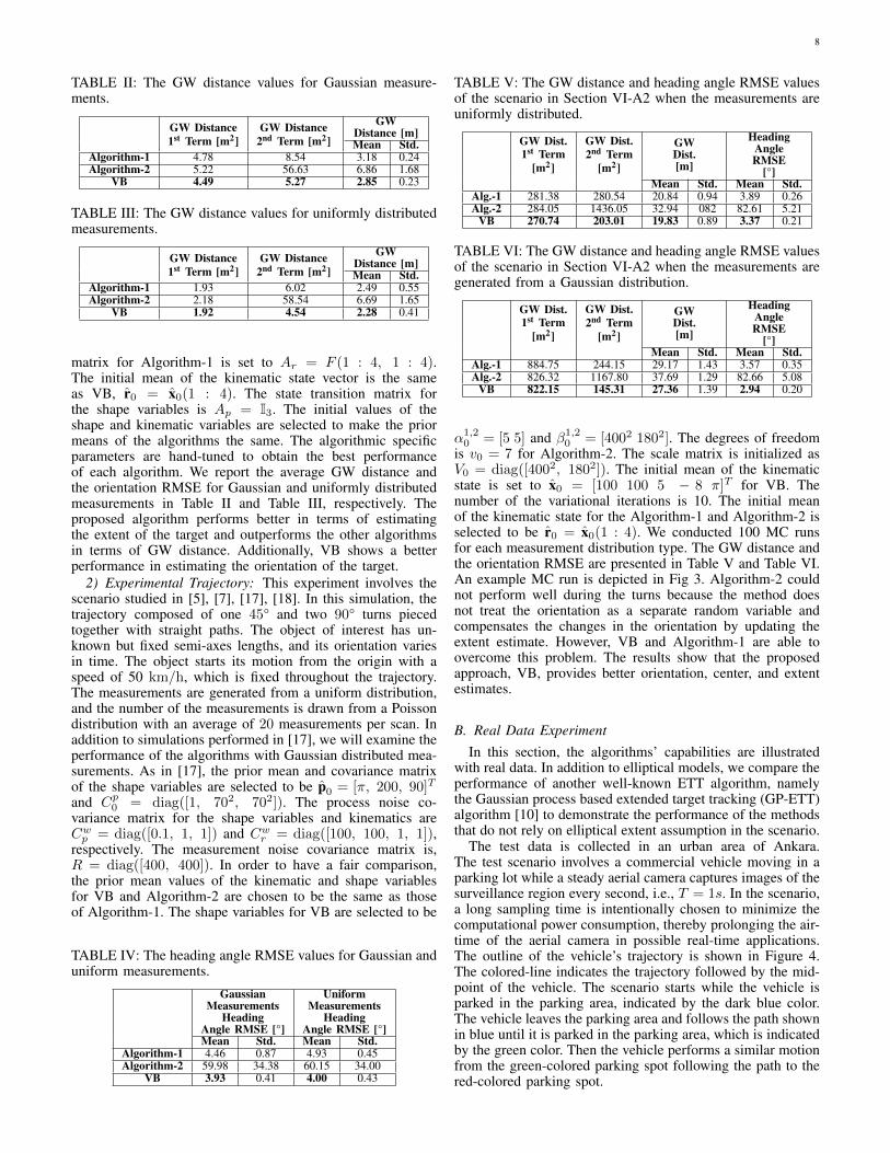
TABLE II: The GW distance values for Gaussian measure-ments.

GW Distance1st Term [m2]

GW Distance2nd Term [m2]

GWDistance [m]Mean Std.

Algorithm-1 4.78 8.54 3.18 0.24Algorithm-2 5.22 56.63 6.86 1.68

VB 4.49 5.27 2.85 0.23

TABLE III: The GW distance values for uniformly distributedmeasurements.

GW Distance1st Term [m2]

GW Distance2nd Term [m2]

GWDistance [m]Mean Std.

Algorithm-1 1.93 6.02 2.49 0.55Algorithm-2 2.18 58.54 6.69 1.65

VB 1.92 4.54 2.28 0.41

matrix for Algorithm-1 is set to Ar = F (1 : 4, 1 : 4).The initial mean of the kinematic state vector is the sameas VB, r0 = x0(1 : 4). The state transition matrix forthe shape variables is Ap = I3. The initial values of theshape and kinematic variables are selected to make the priormeans of the algorithms the same. The algorithmic specificparameters are hand-tuned to obtain the best performanceof each algorithm. We report the average GW distance andthe orientation RMSE for Gaussian and uniformly distributedmeasurements in Table II and Table III, respectively. Theproposed algorithm performs better in terms of estimatingthe extent of the target and outperforms the other algorithmsin terms of GW distance. Additionally, VB shows a betterperformance in estimating the orientation of the target.

2) Experimental Trajectory: This experiment involves thescenario studied in [5], [7], [17], [18]. In this simulation, thetrajectory composed of one 45° and two 90° turns piecedtogether with straight paths. The object of interest has un-known but fixed semi-axes lengths, and its orientation variesin time. The object starts its motion from the origin with aspeed of 50 km/h, which is fixed throughout the trajectory.The measurements are generated from a uniform distribution,and the number of the measurements is drawn from a Poissondistribution with an average of 20 measurements per scan. Inaddition to simulations performed in [17], we will examine theperformance of the algorithms with Gaussian distributed mea-surements. As in [17], the prior mean and covariance matrixof the shape variables are selected to be p0 = [π, 200, 90]T

and Cp0 = diag([1, 702, 702]). The process noise co-variance matrix for the shape variables and kinematics areCwp = diag([0.1, 1, 1]) and Cwr = diag([100, 100, 1, 1]),respectively. The measurement noise covariance matrix is,R = diag([400, 400]). In order to have a fair comparison,the prior mean values of the kinematic and shape variablesfor VB and Algorithm-2 are chosen to be the same as thoseof Algorithm-1. The shape variables for VB are selected to be

TABLE IV: The heading angle RMSE values for Gaussian anduniform measurements.

GaussianMeasurements

HeadingAngle RMSE [°]

UniformMeasurements

HeadingAngle RMSE [°]

Mean Std. Mean Std.Algorithm-1 4.46 0.87 4.93 0.45Algorithm-2 59.98 34.38 60.15 34.00

VB 3.93 0.41 4.00 0.43

TABLE V: The GW distance and heading angle RMSE valuesof the scenario in Section VI-A2 when the measurements areuniformly distributed.

GW Dist.1st Term

[m2]

GW Dist.2nd Term

[m2]

GWDist.[m]

HeadingAngleRMSE

[°]Mean Std. Mean Std.

Alg.-1 281.38 280.54 20.84 0.94 3.89 0.26Alg.-2 284.05 1436.05 32.94 082 82.61 5.21

VB 270.74 203.01 19.83 0.89 3.37 0.21

TABLE VI: The GW distance and heading angle RMSE valuesof the scenario in Section VI-A2 when the measurements aregenerated from a Gaussian distribution.

GW Dist.1st Term

[m2]

GW Dist.2nd Term

[m2]

GWDist.[m]

HeadingAngleRMSE

[°]Mean Std. Mean Std.

Alg.-1 884.75 244.15 29.17 1.43 3.57 0.35Alg.-2 826.32 1167.80 37.69 1.29 82.66 5.08

VB 822.15 145.31 27.36 1.39 2.94 0.20

α1,20 = [5 5] and β1,2

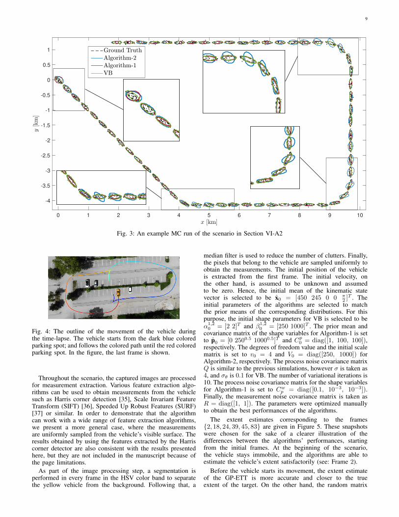
0 = [4002 1802]. The degrees of freedomis v0 = 7 for Algorithm-2. The scale matrix is initialized asV0 = diag([4002, 1802]). The initial mean of the kinematicstate is set to x0 = [100 100 5 − 8 π]T for VB. Thenumber of the variational iterations is 10. The initial meanof the kinematic state for the Algorithm-1 and Algorithm-2 isselected to be r0 = x0(1 : 4). We conducted 100 MC runsfor each measurement distribution type. The GW distance andthe orientation RMSE are presented in Table V and Table VI.An example MC run is depicted in Fig 3. Algorithm-2 couldnot perform well during the turns because the method doesnot treat the orientation as a separate random variable andcompensates the changes in the orientation by updating theextent estimate. However, VB and Algorithm-1 are able toovercome this problem. The results show that the proposedapproach, VB, provides better orientation, center, and extentestimates.

B. Real Data ExperimentIn this section, the algorithms’ capabilities are illustrated

with real data. In addition to elliptical models, we compare theperformance of another well-known ETT algorithm, namelythe Gaussian process based extended target tracking (GP-ETT)algorithm [10] to demonstrate the performance of the methodsthat do not rely on elliptical extent assumption in the scenario.

The test data is collected in an urban area of Ankara.The test scenario involves a commercial vehicle moving in aparking lot while a steady aerial camera captures images of thesurveillance region every second, i.e., T = 1s. In the scenario,a long sampling time is intentionally chosen to minimize thecomputational power consumption, thereby prolonging the air-time of the aerial camera in possible real-time applications.The outline of the vehicle’s trajectory is shown in Figure 4.The colored-line indicates the trajectory followed by the mid-point of the vehicle. The scenario starts while the vehicle isparked in the parking area, indicated by the dark blue color.The vehicle leaves the parking area and follows the path shownin blue until it is parked in the parking area, which is indicatedby the green color. Then the vehicle performs a similar motionfrom the green-colored parking spot following the path to thered-colored parking spot.

9

0 1 2 3 4 5 6 7 8 9 10

-4

-3.5

-3

-2.5

-2

-1.5

-1

-0.5

0

0.5

1

Fig. 3: An example MC run of the scenario in Section VI-A2

Fig. 4: The outline of the movement of the vehicle duringthe time-lapse. The vehicle starts from the dark blue coloredparking spot; and follows the colored path until the red coloredparking spot. In the figure, the last frame is shown.

Throughout the scenario, the captured images are processedfor measurement extraction. Various feature extraction algo-rithms can be used to obtain measurements from the vehiclesuch as Harris corner detection [35], Scale Invariant FeatureTransform (SIFT) [36], Speeded Up Robust Features (SURF)[37] or similar. In order to demonstrate that the algorithmcan work with a wide range of feature extraction algorithms,we present a more general case, where the measurementsare uniformly sampled from the vehicle’s visible surface. Theresults obtained by using the features extracted by the Harriscorner detector are also consistent with the results presentedhere, but they are not included in the manuscript because ofthe page limitations.

As part of the image processing step, a segmentation isperformed in every frame in the HSV color band to separatethe yellow vehicle from the background. Following that, a

median filter is used to reduce the number of clutters. Finally,the pixels that belong to the vehicle are sampled uniformly toobtain the measurements. The initial position of the vehicleis extracted from the first frame. The initial velocity, onthe other hand, is assumed to be unknown and assumedto be zero. Hence, the initial mean of the kinematic statevector is selected to be x0 = [450 245 0 0 π

2 ]T . Theinitial parameters of the algorithms are selected to matchthe prior means of the corresponding distributions. For thispurpose, the initial shape parameters for VB is selected to beα1,20 = [2 2]T and β1,2

0 = [250 1000]T . The prior mean andcovariance matrix of the shape variables for Algorithm-1 is setto p0 = [0 2500.5 10000.5]T and Cp0 = diag([1, 100, 100]),respectively. The degrees of freedom value and the initial scalematrix is set to v0 = 4 and V0 = diag([250, 1000]) forAlgorithm-2, respectively. The process noise covariance matrixQ is similar to the previous simulations, however σ is taken as4, and σθ is 0.1 for VB. The number of variational iterations is10. The process noise covariance matrix for the shape variablesfor Algorithm-1 is set to Cwp = diag([0.1, 10−3, 10−3]).Finally, the measurement noise covariance matrix is taken asR = diag([1, 1]). The parameters were optimized manuallyto obtain the best performances of the algorithms.

The extent estimates corresponding to the frames{2, 18, 24, 39, 45, 83} are given in Figure 5. These snapshotswere chosen for the sake of a clearer illustration of thedifferences between the algorithms’ performances, startingfrom the initial frames. At the beginning of the scenario,the vehicle stays immobile, and the algorithms are able toestimate the vehicle’s extent satisfactorily (see: Frame 2).

Before the vehicle starts its movement, the extent estimateof the GP-ETT is more accurate and closer to the trueextent of the target. On the other hand, the random matrix

10

Fig. 5: A representative MC run of the real data experiment. The extent estimates of VB, Algorithm-1, Algorithm-2, andGP-ETT are shown in black, red, blue, and green lines, respectively. The measurements are represented with green dots.

approaches are significantly advantageous throughout this sce-nario because they can fully exploit the prior informationthat the target’s extent is close to an elliptical shape. GP-ETT algorithm aims at estimating the contours of objectshaving arbitrary shapes and its performance degrades when themeasurements are originating from the surface of objects andthe number of the surface measurements is low. The algorithmis essentially trying to solve a harder problem because it hasmore degrees of freedom to represent the unknown extent anda greater uncertainty to resolve compared to the ellipsoidaltarget tracking methods.

When the vehicle is moving in a straight path, such asin Frame 18 and Frame 39, the performance of all randommatrix based algorithms are satisfactory. However, when thevehicle performs a maneuver, as in Frame 24, Frame 45 andFrame 83, VB shows superior performance in estimating theorientation of the vehicle. During the maneuvers, Algorithm-2 cannot estimate the extent accurately because it does nottreat the heading angle as a separate random variable, and ittries to adapt to the changes in the orientation by updating theextent states. Algorithm-1 also struggles to find the correctorientation of the vehicle. However, VB can provide accurateestimates of the extent thanks to its iterative updates. Note thatVB and Algorithm-1 use the same process noise variance forthe orientation. Since the vehicle is stable in the first couple offrames and the algorithms are able to estimate the extent accu-rately, increasing the variance values of the shape variables forAlgorithm-1 does not improve the performance of estimatingthe extent further. Additionally, if the variance values areincreased too much, the extent estimates of Algorithm-1 tendto collapse to zero. We encountered a similar problem whiletuning Algorithm-1 in the simulation scenarios. We report oneexample of such behavior in a single measurement update inAppendix D for interested readers.

VII. CONCLUSION AND DISCUSSION

ETT involves tracking objects that generate multiple mea-surements per scan. In most ETT applications, the orientationof the extended targets changes in time. In standard RMbased ETT methods, this phenomenon is addressed by aforgetting factor, which aims at forgetting the accumulated

information. In this work, we proposed a novel approachfor extended target tracking that is capable of simultaneouslyestimating the kinematic, extent, and orientation states of anextended target. We use the variational Bayes technique forinference and define appropriate priors for the unknown statevariables that can accurately model the changes in the extendedtargets’ orientation. The performance and capabilities of thealgorithm are demonstrated through simulations and real dataexperiments. Experimental results on simulations and real datademonstrate that the proposed method significantly improvesthe tracking performance, as well as the accuracy in estimatingthe orientation and the shape of the object compared to thestate-of-the-art methods.

It is also worth mentioning that variational Bayes ap-proaches resort to factorized distributions, which lose thecorrelation structure in the posterior density. An algorithmthat does not neglect correlation terms may provide betterestimation performance than such variational methods. In ourexperience (as illustrated in benchmark scenarios and realdata experiments in Sections V-VI), the iterative optimizationstructure provided by the variational inference framework out-performs the alternative solutions by overcoming the disadvan-tages associated with the factorized approximation. However,improved performance can be achieved by further exploitingthe correlation structure in the true posterior.

The model and the technique we use might also be applica-ble to estimation problems other than extended target trackingapplications, which involve dynamic elliptical representationsor unknown covariance matrices with similarly structureduncertainty. These problems may include, but are not limitedto, obtaining elliptical bounds in power systems [38], [39],estimating ellipsoid sets containing target states over sensornetworks [40] or spectrum representation in speech processing[41], [42].

REFERENCES

[1] M. Baum, V. Klumpp, and U. D. Hanebeck, “A novel Bayesian methodfor fitting a circle to noisy points,” in 13th International Conference onInformation Fusion (FUSION). IEEE, 2010, pp. 1–6.

[2] K. Granstrom, C. Lundquist, and U. Orguner, “Tracking rectangularand elliptical extended targets using laser measurements,” in 14thInternational Conference on Information Fusion (FUSION), July 2011,pp. 1–8.

11

[3] K. Granstrom and C. Lundquist, “On the use of multiple measurementmodels for extended target tracking,” in 16th International Conferenceon Information Fusion (FUSION), July 2013, pp. 1534–1541.

[4] J. W. Koch, “Bayesian approach to extended object and cluster trackingusing random matrices,” IEEE Transactions on Aerospace and ElectronicSystems, vol. 44, no. 3, pp. 1042–1059, July 2008.

[5] M. Feldmann, D. Franken, and W. Koch, “Tracking of extended objectsand group targets using random matrices,” IEEE Transactions on SignalProcessing, vol. 59, no. 4, pp. 1409–1420, April 2011.

[6] U. Orguner, “A variational measurement update for extended targettracking with random matrices,” IEEE Transactions on Signal Process-ing, vol. 60, no. 7, pp. 3827–3834, July 2012.

[7] J. Lan and X. R. Li, “Tracking of extended object or target group usingrandom matrix – Part I: New model and approach,” in 15th InternationalConference on Information Fusion (FUSION), Singapore, Jul. 2012, pp.2177–2184.

[8] M. Baum and U. D. Hanebeck, “Random hypersurface models forextended object tracking,” in IEEE International Symposium on SignalProcessing and Information Technology (ISSPIT), Dec 2009, pp. 178–183.

[9] M.Baum and U. D. Hanebeck, “Shape tracking of extended objects andgroup targets with star-convex RHMs,” in 14th International Conferenceon Information Fusion (FUSION), July 2011, pp. 1–8.

[10] N. Wahlstrom and E. Ozkan, “Extended target tracking using Gaussianprocesses,” IEEE Transactions on Signal Processing, vol. 63, no. 16,pp. 4165–4178, Aug 2015.

[11] E. Ozkan, N. Wahlstrom, and S. J. Godsill, “Rao-Blackwellised particlefilter for star-convex extended target tracking models,” in 19th Inter-national Conference on Information Fusion (FUSION), July 2016, pp.1193–1199.

[12] M. Kumru and E. Ozkan, “3D extended object tracking using recursiveGaussian processes,” in 2018 21st International Conference on Infor-mation Fusion (FUSION). IEEE, 2018, pp. 1–8.

[13] J. Lan and X. R. Li, “Tracking of maneuvering non-ellipsoidal extendedobject or target group using random matrix,” IEEE Transactions onSignal Processing, vol. 62, no. 9, pp. 2450–2463, May 2014.

[14] K. Granstrom, “An extended target tracking model with multiplerandom matrices and unified kinematics,” CoRR, vol. abs/1406.2135,2014. [Online]. Available: http://arxiv.org/abs/1406.2135

[15] Q. Hu, H. Ji, and Y. Zhang, “Tracking of maneu-vering non-ellipsoidal extended target with varying numberof sub-objects,” Mechanical Systems and Signal Processing,vol. 99, pp. 262 – 284, 2018. [Online]. Available:http://www.sciencedirect.com/science/article/pii/S0888327017303254

[16] S. F. Kara and E. Ozkan, “Multi-ellipsoidal extended target trackingusing sequential Monte Carlo,” in 2018 21st International Conferenceon Information Fusion (FUSION). IEEE, 2018, pp. 1–8.

[17] S. Yang and M. Baum, “Tracking the orientation and axes lengths ofan elliptical extended object,” IEEE Transactions on Signal Processing,vol. 67, no. 18, pp. 4720–4729, Jul 2019.

[18] ——, “Extended Kalman filter for extended object tracking,” in 2017IEEE International Conference on Acoustics, Speech and Signal Pro-cessing (ICASSP). IEEE, 2017, pp. 4386–4390.

[19] ——, “Second-order extended Kalman filter for extended object andgroup tracking,” in 2016 19th International Conference on InformationFusion (FUSION). IEEE, 2016, pp. 1178–1184.

[20] K. Granstrom and U. Orguner, “New prediction for extended targetswith random matrices,” IEEE Transactions on Aerospace and ElectronicSystems, vol. 50, no. 2, pp. 1577–1589, Apr. 2014.

[21] V. Smidl and A. Quinn, “Variational Bayesian filtering,” IEEE Transac-tions on Signal Processing, vol. 56, no. 10, pp. 5020–5030, 2008.

[22] S. Sarkka and A. Nummenmaa, “Recursive noise adaptive Kalmanfiltering by variational Bayesian approximations,” IEEE Transactionson Automatic control, vol. 54, no. 3, pp. 596–600, 2009.

[23] H. Nurminen, T. Ardeshiri, R. Piche, and F. Gustafsson, “Skew-t filterand smoother with improved covariance matrix approximation,” IEEETransactions on Signal Processing, vol. 66, no. 21, pp. 5618–5633, 2018.

[24] H. Nurminen, T. Ardeshiri, R. Piche, and F. Gustafsson, “Robustinference for state-space models with skewed measurement noise,” IEEESignal Processing Letters, vol. 22, no. 11, pp. 1898–1902, 2015.

[25] Y. Huang, Y. Zhang, Z. Wu, N. Li, and J. Chambers, “A novel adaptiveKalman filter with inaccurate process and measurement noise covariancematrices,” IEEE Transactions on Automatic Control, vol. 63, no. 2, pp.594–601, 2017.

[26] K. Granstrom, S. Renter, M. Fatemi, and L. Svensson, “Pedestriantracking using velodyne data—Stochastic optimization for extendedobject tracking,” in 2017 IEEE Intelligent Vehicles Symposium (IV).IEEE, 2017, pp. 39–46.

[27] L. Guerlin, B. Pannetier, M. Rombaut, and M. Derome, “Study on grouptarget tracking to counter swarms of drones,” in Signal Processing,Sensor/Information Fusion, and Target Recognition XXIX, vol. 11423.International Society for Optics and Photonics, 2020, p. 1142304.

[28] S. Scheidegger, J. Benjaminsson, E. Rosenberg, A. Krishnan, andK. Granstrom, “Mono-camera 3D multi-object tracking using deep learn-

ing detections and pmbm filtering,” in 2018 IEEE Intelligent VehiclesSymposium (IV). IEEE, 2018, pp. 433–440.

[29] C. Veiback, “Tracking of animals using airborne cameras,” Ph.D. dis-sertation, Linkoping University Electronic Press, 2016.

[30] G. Vivone, P. Braca, A. Natale, J. Chanussot, and K. Granstrom,“Converted measurements Bayesian extended target tracking applied toX-band marine radar data,” Journal of Advances in Information Fusion,vol. 12, 01 2016.

[31] C. M. Bishop, Pattern Recognition and Machine Learning (InformationScience and Statistics). Secaucus, NJ, USA: Springer-Verlag New York,Inc., 2006.

[32] E. Ozkan, V. Smıdl, S. Saha, C. Lundquist, and F. Gustafsson,“Marginalized adaptive particle filtering for nonlinear modelswith unknown time-varying noise parameters,” Automatica,vol. 49, no. 6, pp. 1566 – 1575, 2013. [Online]. Available:http://www.sciencedirect.com/science/article/pii/S0005109813001350

[33] C. R. Givens, R. M. Shortt et al., “A class of Wasserstein metrics forprobability distributions.” The Michigan Mathematical Journal, vol. 31,no. 2, pp. 231–240, 1984.

[34] S. Yang, M. Baum, and K. Granstrom, “Metrics for performanceevaluation of elliptic extended object tracking methods,” in 2016 IEEEInternational Conference on Multisensor Fusion and Integration forIntelligent Systems (MFI). IEEE, 2016, pp. 523–528.

[35] C. G. Harris, M. Stephens et al., “A combined corner and edge detector.”in Alvey vision conference, vol. 15, no. 50. Citeseer, 1988, pp. 10–5244.

[36] D. G. Lowe, “Distinctive image features from scale-invariant keypoints,”International journal of computer vision, vol. 60, no. 2, pp. 91–110,2004.

[37] H. Bay, T. Tuytelaars, and L. Van Gool, “Surf: Speeded up robustfeatures,” in European conference on computer vision. Springer, 2006,pp. 404–417.

[38] X. Qing, F. Yang, and X. Wang, “Extended set-membership filterfor power system dynamic state estimation,” Electric power systemsresearch, vol. 99, pp. 56–63, 2013.

[39] W. Chen, D. Ding, H. Dong, and G. Wei, “Distributed resilient filteringfor power systems subject to denial-of-service attacks,” IEEE Transac-tions on Systems, Man, and Cybernetics: Systems, vol. 49, no. 8, pp.1688–1697, 2019.

[40] D. Ding, Z. Wang, and Q.-L. Han, “A set-membership approach to event-triggered filtering for general nonlinear systems over sensor networks,”IEEE Transactions on Automatic Control, vol. 65, no. 4, pp. 1792–1799,2019.

[41] E. Ozkan, I. Ozbek, and M. Demirekler, “Dynamic speech spectrumrepresentation and tracking variable number of vocal tract resonancefrequencies with time-varying Dirichlet process mixture models,” IEEETransactions on Audio, Speech, and Language Processing, vol. 17, no. 8,pp. 1518–1532, Nov 2009.

[42] D. Carevic and S. Davey, “Two algorithms for modeling and trackingof dynamic time-frequency spectra,” IEEE Transactions on Signal Pro-cessing, vol. 64, no. 22, pp. 6030–6045, 2016.

APPENDIX ACALCULATION OF δ AND ∆

In Section III-A4, we introduced the update formulas forthe orientation distribution as below.

θ(`+1)k|k = Θ

(`+1)k|k

(Θ−1k|k−1θk|k−1 + δ

), (45)

Θ(`+1)k|k =

(Θ−1k|k−1 + ∆

)−1, (46)

Here, the variables δ and ∆ are derived from the expectationin (47).

−1

2

mk∑j=1

E\θk[(a− bθk)T (sX)−1(a− bθk)

], (47)

where δ and ∆ are denoted as

δ ,mk∑j=1

Tr[Eq(`)X

[(sXk)−1

]Eq(`)x ,q

(`)Z

[abT

]], (48)

∆ ,mk∑j=1

Tr[Eq(`)X

[(sXk)−1

]Eq(`)x ,q

(`)Z

[bbT]], (49)

and

a = (Tθ(`)

k|k)T (zjk −Hxk)− (T ′

θ(`)

k|k)T (zjk −Hxk)θ

(`)k|k,

(50)

12

b = −(T ′θ(`)

k|k)T (zjk −Hxk). (51)

When the a and b variables are substituted into (48) and (49),we obtain the δ and ∆ variables as

δ =

mk∑j=1

Tr

[sX−1k (T ′

θ(`)

k|k)T(zjk −Hxk

)(·)T

(T ′θ(`)

k|k)θ

(`)k|k

]− Tr

[sX−1k TT

θ(`)

k|k

(zjk −Hxk

)(·)T

(T ′θ(`)

k|k)

], (52)

∆ =

mk∑j=1

Tr

[sX−1k (T ′

θ(`)

k|k)T(zjk −Hxk

)(·)T

(T ′θ(`)

k|k)

], (53)

where(zjk −Hxk

)(·)T

= Eq(`)x ,q

(`)Z

[(zjk −Hxk

)(·)T ]

,

and sX−1k = Eq(`)X

[(sXk)−1

].

APPENDIX BPROOF OF LEMMA 1

In this section we will give the proof of Lemma 1 tocalculate E

q(`)θ

[(sTθkMTTθk)−1

]. In the formulation, we first

multiply the matrices inside the expectation. Then, the expec-tation of each entry of the resultant matrix is taken. First,notice that, (

TθkMTTθk)−1

= TθkM−1TTθk . (54)

Given

M−1 =

[m11 m12

m21 m22

],

the expression whose expectation has to be taken becomes

Λ = TθkM−1TTθk

=

[cos(θk) − sin(θk)sin(θk) cos(θk)

] [m11 m12

m21 m22

]×[

cos(θk) sin(θk)− sin(θk) cos(θk)

], (55a)

Λ(1, 1) = m11 cos2(θk) +m22 sin2(θk)

− (m12 +m21) cos(θk) sin(θk), (55b)Λ(1, 2) = m12 cos2(θk)−m21 sin2(θk)

+ (m11 −m22) cos(θk) sin(θk), (55c)Λ(2, 1) = m21 cos2(θk)−m12 sin2(θk)

+ (m11 −m22) cos(θk) sin(θk), (55d)Λ(2, 2) = m22 cos2(θk) +m11 sin2(θk)

+ (m12 +m21) cos(θk) sin(θk). (55e)

Now the following trigonometric transformations are utilizedand the expectations are taken with respect to the resultingexpressions.

cos2(θk) =1 + cos(2θk)

2, sin2(θk) =

1− cos(2θk)

2,

(56a)

cos(θk) sin(θk) =sin(2θk)

2, (56b)

Eq(`)θ

[cos(2θk)] = cos(2θ(`)k|k) exp(−2Θ

(`)k|k)), (56c)

Eq(`)θ

[sin(2θk)] = sin(2θ(`)k|k) exp(−2Θ

(`)k|k)). (56d)

By substituting the expressions in (55) with the correspondingequalities given in (56) Lemma 1 is obtained.

APPENDIX CTHE PARAMETERS OF THE EXPERIMENT IN SECTION VIn this section, the parameters of the experiment given in

Section V are summarized. The prior shape estimate is apartfrom the true center location of the target by (20, 20) units inthe 2D coordinate frame. The extent of the ground truth objectis parametrized as diag([6, 0.5]) with 0° orientation. The meanof the prior extent ellipse parameters for both methods areequal to the parameters of the ground truth extent. The priorshape parameters of the proposed algorithm are selected to beα1,20 = [101 101]T and β1,2

0 = [600 50]T . The prior meanof the orientation variable is taken as θ0 = π

2 . To have areasonable comparison, the mean vector and the variance ofthe shape parameters for the EKF approach are selected tomatch with those of the VB algorithm. The prior kinematicstate covariance matrix is P0 = diag([300, 300, 1, 1, π

2 ]).The measurement noise covariance matrix is R = diag([1, 1]).In this experiment, the number of measurements is 10, andthe measurements are generated according to a Gaussiandistribution. However, the trials with the uniformly distributedmeasurements yield similar results.

APPENDIX DAN EXAMPLE FOR THE COLLAPSING EXTENT ESTIMATES

Here we repeated the simulation in Section V with thefollowing set of parameters:For VB, the prior mean of the target’s kinematic state isx0 = [−30 − 30 1 1 π

2 ]T . The prior kinematic statecovariance matrix is P0 = diag([300, 300, 1, 1, π

2 ]).The shape parameters for VB is α1,2 = [11 11]T andβ1,2 = [600 50]T . For Algorithm-1, the prior mean vectorand covariance matrix of the kinematic state is r0 = x0(1 : 4)and Cr0 = diag([300, 300, 1, 1]), respectively. The priormean and variance of the extent parameters are the same forboth algorithms. The number of measurements generated fromthe target is 10. The measurement noise covariance matrix isR = diag([1, 1]). A single measurement update of VB andAlgorithm-1 is visualized in Figure 6.

-40 -30 -20 -10 0 10 20

-45

-40

-35

-30

-25

-20

-15

-10

-5

0

5

Fig. 6: The visualization of the collapsing behavior ofAlgorithm-1. Blue stars represent the measurements, the solidgreen and red lines stand for the posterior means of the VBand EKF updates, respectively. The solid black line indicatesthe median of the true posterior, which is computed by using1 million Monte Carlo samples.

13

Barkın Tuncer (S’20) Barkın Tuncer received hisB.Sc. degree in Electrical and Electronics Engineer-ing from Middle East Technical University (METU),Ankara, Turkey, 2019. Since 2019, he has beenworking toward the M.Sc. degree in the Roboticsspecialization area at METU while working as ateaching assistant. His research interest includesextended target tracking, statistical signal process-ing, Bayesian inference, machine learning, and deeplearning.

Emre Ozkan (S’04 - M’10) received his B.Sc. andPhD degrees in Electrical and Electronics Engineer-ing from Middle East Technical University (METU),Ankara, Turkey, in 2009. Between 2009 and 2011,he worked as a postdoctoral associate in the Divisionof Automatic Control, Department of Electrical En-gineering, Linkoping University, Sweden. Between2011 and 2015 he worked as an Assistant Professorin the same group. In 2015, he worked as a visitingresearcher at Signal Processing and CommunicationsLaboratory at the University of Cambridge. Cur-rently, he is an Assistant Professor at METU. His

research focuses on target tracking, statistical signal processing, estimationtheory, sensor fusion, Monte Carlo methods and Bayesian inference.