Random field theory-based p-values: A review of the SPM implementation

Dirk Ostwald∗, Sebastian Schneider, Rasmus Bruckner, Lilla Horvath

Institute of Psychology and Center for Behavioral Brain Sciences,Otto-von-Guericke Universität Magdeburg, Germany

Abstract

P-values and null-hypothesis significance testing are popular data-analytical tools in functionalneuroimaging. Sparked by the analysis of resting-state fMRI data, there has been a resurgence ofinterest in the validity of some of the p-values evaluated with the widely used software SPM in recentyears. The default parametric p-values reported in SPM are based on the application of results fromrandom field theory to statistical parametric maps, a framework commonly referred to as RFT.While RFT was established two decades ago and has since been applied in a plethora of fMRI studies,there does not exist a unified documentation of the mathematical and computational underpinningsof RFT as implemented in current versions of SPM. Here, we provide such a documentation withthe aim of contributing to contemporary efforts towards higher levels of computational transparencyin functional neuroimaging.

Keywords: fMRI, GLM, SPM, p-values, random field theory

1. Introduction

Despite their debatable value in a scientific context, p-values and statistical hypothesis testingremain popular data-analytical techniques (Fisher, 1925; Neyman and Pearson, 1933; Benjaminet al., 2018). Given recent discussions about the reproducibility of quantitative empirical findings(e.g. Ioannidis, 2005; Button et al., 2013), there has been a resurgence of interest in the validityof p-values and statistical hypothesis tests involved in the analysis of fMRI data with the popularsoftware packages SPM and FSL (Eklund et al., 2016; Mumford et al., 2016; Brown and Behrmann,2017; Eklund et al., 2017; Cox et al., 2017; Kessler et al., 2017; Flandin and Friston, 2017; Bowringet al., 2018; Geuter et al., 2018; Turner et al., 2018; Slotnick, 2017b,a; Mueller et al., 2017; Eklundet al., 2018; Gopinath et al., 2018b,a; Bansal and Peterson, 2018; Gong et al., 2018; Geerligs andMaris, 2021; Davenport and Nichols, 2021). The default parametric p-values reported in SPMand FSL are based on the application of results from random field theory to statistical parametricmaps and derive from the fundamental aim to control the multiple testing problem entailed bythe mass-univariate analysis of fMRI data (Friston et al., 1994a; Poline and Brett, 2012; Monti,2011; Ashburner, 2012; Jenkinson et al., 2012; Nichols, 2012). In brief, the p-values reported bySPM and FSL are exceedance probabilities of topological features of a data-adapted null hypothesisrandom field model. Historically, this framework was established in a series of landmark papers inthe 1990’s, with some additional contributions in the early 2000’s (Friston et al., 1991; Worsley

∗Corresponding authorEmail address: dirk.ostwald@ovgu.de (Dirk Ostwald)

arX

iv:1

808.

0407

5v3

[q-

bio.

QM

] 9

Aug

202

1

et al., 1992; Friston et al., 1994b; Worsley et al., 1996; Friston et al., 1996; Kiebel et al., 1999;Jenkinson, 2000; Hayasaka and Nichols, 2003; Hayasaka et al., 2004). In the following, we willcollectively refer to this framework as “random field theory-based p-value evaluation”, which iscommonly abbreviated RFT in the neuroimaging literature (cf. Nichols, 2012).

While RFT was established almost two decades ago and has since been applied in a plethoraof functional neuroimaging studies, there does not exist a unified documentation of the mathe-matical and computational underpinnings of RFT. More specifically, the early landmark papers onthe approach are characterized by an evolution of ideas which were often superseded by later de-velopments. In these later developments, however, the RFT framework was not constructed fromfirst principles again, such that many important implementational details were rendered opaque.As concrete examples, the conceptual papers by Friston et al. (1994b) and Friston et al. (1996)mention the expected Euler characteristic, which is central to the current SPM implementation ofRFT, only in passing. They are also concerned with Gaussian random fields only, rather than theT and F random fields that are routinely assessed using RFT. Similarly, the technical papers byKiebel et al. (1999), Hayasaka and Nichols (2003), and Hayasaka et al. (2004) present variationson the estimation of RFT’s null model parameters without a definite commitment to the approachthat is currently implemented in SPM. Finally, reviews of the approach, such as provided by Nicholsand Hayasaka (2003), Friston (2007b), Worsley (2007), and Flandin and Friston (2015) only covercertain aspects of RFT and usually omit many computational details that would be required forits de-novo implementation. Given this unsatisfying state of the RFT literature and the recentcommotion with regards to the approach, we reasoned that a comprehensive documentation of themathematical and computational underpinnings of RFT may help to alleviate uncertainties aboutthe conceptual and implementational details of the approach for neuroimaging analysis novices,practitioners and theoreticians alike. Here, we thus aim to provide such a documentation.

We constrain our treatment by what probably constitutes the most important practical aspectof the RFT approach: the SPM results table (Figure 1). We focus on the RFT implementationin SPM rather than FSL, because SPM remains the most commonly used software tool in theneuroimaging community and because the origins of RFT are closely linked to the development ofSPM (Carp, 2012; Borghi and Van Gulick, 2018; Ashburner, 2012). More specifically, we focus onthe mathematical theory and statistical evaluation of the p-values reported in the set-level, cluster-level, and peak-level columns, as well as the footnote of the results table of SPM12 Version 7771.Note that in the following, all references to SPM imply a reference to SPM12 Version 7771 rununder Matlab R2021a (Version 9.10.0.1710957, Update 4). We particularly address the applicationof RFT in the context of GLM-based fMRI data analysis, and do not discuss other applications,such as in the analysis of M/EEG data (e.g., Kilner and Friston, 2010). Our guiding example isa second-level one-sample T -test design as shown in Figure 1. With respect to multiple testingcontrol, we focus on the family-wise error rate (FWER)-corrected p-values and do not cover thelater addition of false discovery rate-corrected q-values (Chumbley and Friston, 2009; Chumbleyet al., 2010). With respect to FWER control, we focus on the evaluation of p-values rather thanstatistical hypothesis tests. This is warranted by the fact that SPM de-facto only evaluates p-values,while statistical hypothesis tests are performed by the SPM user, who typically decides to reportonly activations at a given level of significance. Finally, from an implementational perspective, weprimarily focus on the functionality of the spm_list.m, spm_P_RF.m, spm_est_smoothness.m,and spm_resel_vol.c functions and cover computational aspects of more low-level SPM routinesonly in passing. With these constraints in place, we next review the outline of our treatment andpreview the central points of each section.

2

Figure 1. The SPM results table for a second-level one-sample T -test design relating to the positive main effect ofvisual stimulus coherence in a perceptual decision making fMRI study (Georgie et al., 2018). The central aim of thiswork is to document the mathematical and computational underpinnings of the p-values listed in the SPM resultstable. As indicated by the whitened parts of the table, we only consider corrected p-values related to FWER control.For implementational details of the evaluation of the SPM results table using the SPM12 Version 7771 distribution,please see rft_1.m.

3

Overview

Overall, we proceed in three main parts, Section 2: Background, Section 3: Theory, and Section 4:Application. In Section 2: Background, we establish a few key definitions from the two main pillarsof RFT: random field theory and geometry (Adler, 1981; Adler and Taylor, 2007). Specifically, inSection 2.1: Real-valued random fields, we define the concept of a real-valued random field anddiscuss some subtle but important aspects of this definition. Our definition rests on mathemati-cal probability theory, in which random variables are understood as mappings between probabilityspaces. Readers unfamiliar with these measure-theoretic underpinnings of probability theory arerecommended to consult appropriate references from the general literature, such as Billingsley(1978); Rosenthal (2006); Fristedt and Gray (2013); Kallenberg (2021). After discussing a fewanalytical features of random fields (expectation and covariance functions, stationarity), we intro-duce the central classes of random fields for RFT in Section 2.2: Gaussian and Gaussian-relatedrandom fields. As a toy example that we will return to repeatedly, we introduce two-dimensionalGaussian random fields with Gaussian covariance functions. Such Gaussian random fields have thefeature that their smoothness in the RFT-sense can be captured by a single parameter of theircovariance function. We also introduce the central notions of Z-, T - and F - fields, which we willoften refer to as Gaussian-related random fields (cf. Adler, 2017) and consider as the theoreticalanalogues to statistical parametric maps that derive from the practical analysis of fMRI data. InSection 2.3: Volumetrics we then introduce two geometric foundations of RFT, Lebesgue measureand intrinsic volumes. These geometric concepts are of central importance in RFT, because theprobability distributions of topological features of Gaussian-related random fields (for example, theprobability of the global maximum to exceed a given value) depend not only on the characteristicsof the Gaussian-related random field, but also on the volume of the space it extends over. InRFT, this dual dependency is condensed in the notion of resel volumes. In brief, resel volumes aresmoothness-adjusted intrinsic volumes, which in turn are coefficients in a formula for the Lebesguemeasure of tubes. The treatment in Section 2.3 is necessarily shallow and emphasizes intuitionover formal rigour.

Section 3: Theory is devoted to the theoretical development of RFT. The central part ofthis section is the delineation of the parametric probability distributions used by RFT to capturethe stochastic behaviour of topological features of a Gaussian-related random field’s excursionset under the null hypothesis. The exceedance probabilities of these parametric distributions forobserved data are the p-values reported in the SPM results table. We discuss the theory of RFTagainst the background of a continuous space, discrete data point model. This model is conceivedas the theoretical analogue to the familiar mass-univariate GLM and is formally introduced at theoutset of Section 3. Section 3.1: Excursion sets, smoothness, and resel volumes then introducesthree foundational concepts of RFT: excursion sets of Gaussian-related random fields are subsetsof the field’s domain on which the field exceeds a pre-specified value u. In the applied neuroimagingliterature, this value u (or, more specifically, its equivalent p-value) is known as the cluster-formingthreshold (Nichols et al., 2016) and has been at the center stage of the recent debate on the validityof parametric p-values in fMRI data analysis (e.g., Flandin and Friston, 2017). The topologicalconstitution of excursion sets, and hence the probability distributions of their features, depends ina predictable manner on the value of u and on the smoothness of the underlying Gaussian-relatedrandom field. In the applied neuroimaging literature, the smoothness measure employed by RFT isknown as “FWHM” (e.g., Eklund et al., 2016). In fact, the parameterization of a Gaussian-relatedrandom field’s smoothness in terms of the full widths at half maximum (FWHMs) of isotropicGaussian convolution kernels applied to hypothetical white-noise Gaussian random fields conforms

4

to a reparameterization of a more fundamental smoothness measure and was introduced early on inthe RFT literature (Friston et al., 1991; Worsley et al., 1992). We introduce this more fundamentalsmoothness measure in the Smoothness subsection of Section 3.1. To obtain an intuition aboutthis measure, we show analytically in Supplement S1 that for Gaussian random fields with Gaussiancovariance functions it evaluates to a scalar multiple of the covariance function’s length parameter.We close Section 3.1 by introducing the FWHM reparameterization of smoothness and finallyconjoining the probabilistic and geometric threads of our exposition in the notion of resel volumes.Equipped with these foundations, we then proceed to the core of RFT theory in Section 3.2:Probabilistic properties of excursion set features. More specifically, upon establishing a set ofexpected values, we review the probability distributions of the following excursion set features asevaluated by the SPM implementation of RFT: (1) the global maximum, (2) the number of clusters,(3) the cluster volume, (4) the number of clusters of a given volume, and (5) the maximal clustervolume. We supplement this discussion with number of proofs in Supplement S1. The distributionsof the global maximum and the maximal cluster volume are the distributions that endow the SPMimplementation of RFT with FWER control at the peak- and cluster-level, respectively. To thisend, we review the principal idea of controlling the FWER by means of maximum statistics inSupplement S2. With all theoretical aspects in place, we are then in the position to consider theapplication of RFT theory in a GLM-based fMRI data-analytical setting.

We thus begin Section 4: Application by reconsidering the continuous space GLM introducedin Section 3 from the discrete spatial sampling perspective of fMRI. In Section 4.1: Parameterestimation we then discuss how RFT furnishes a data-adaptive null hypothesis model by estimatingthe smoothness and approximating the intrinsic volumes of the Gaussian-related random field thatunderlies the observed data. The estimated FWHM smoothness parameters and intrinsic volumesare combined in estimated resel volumes, which form the pivot point between the data-driven andtheory-based aspects of RFT. We then close our treatment by considering the p-values reported inthe SPM results table. As will become evident, the p-values reported for set-, cluster-, and peak-level inferences can actually be evaluated using a single (Poisson) cumulative distribution functionthat is adapted for different topological statistics and data-based null model characteristics (Fristonet al., 1996). Finally, in Section 5: Discussion, we briefly explore potential future avenues for thefurther refinement of RFT.

In summary, we make the following novel contributions to the literature. From a scientificperspective, we provide a unified review of RFT, which is both mathematically comprehensive andcomputationally explicit. As such, our treatment allows for the detailed statistical interpretation ofthe experimental effects reported using RFT in the last decades. Further, given the recent discus-sions on the validity of SPM’s cluster-level p-values, our treatment has the potential to serve asa readily accessible starting point for the further refinements of RFT. Finally, from an educationalperspective, we provide a novel resource to introduce newcomers to the field of computationalcognitive neuroscience to one of functional neuroimaging’s equally most basic (univariate cogni-tive process mapping using the GLM) and sophisticated (random field-based modelling) analysistools. All custom written Matlab code (The MathWorks, NA) implementing simulations and visu-alizations reported on herein is available from https://osf.io/3dx9w/. The code repository alsocontains the group-level fMRI data evaluated in Figure 1, and documented and revised versions ofSPM’s parameter estimation and p-value evaluation routines (rft_spm_est_smoothness.m andrft_spm_table.m, respectively). For details, please refer to the OSF project documentation.

5

Symbol Meaning

N0, Nm, N0m The sets N ∪ 0, 1, 2, ..., m, and 0, 1, ..., m, respectively

|S| Cardinality of a set S

ei ith standard basis vector for Rd

||x ||2 Euclidean norm of x ∈ Rd

|A| Determinant of a matrix A ∈ Rd×d

p.d. Positive-definite

inf, sup Infimum, supremum

∇f (x) Gradient of a function f : Rd → R at x∂∂xif (x) ith partial derivative of a function f : Rd → R at x , i = 1, ..., d

Γ(x) Gamma function evaluated at x ∈ RP,E,C Probability, expectation, covariance

N(µ,Σ) Gaussian distribution

• End of definition

2 End of proof

Table 1. List of mathematical symbols. Note that the meaning of the symbol | · | is usually clear from the context.

Prerequisites and notation

We assume throughout that the reader is familiar with the theoretical and practical aspects ofGLM-based fMRI analysis as presented for example in Kiebel and Holmes (2007); Monti (2011);Poline and Brett (2012) and Poldrack et al. (2011). We presume that a familiarity with basicconcepts of the multiple testing problem entailed by the mass-univariate GLM-based analysis offMRI data, as covered for example in Brett et al. (2007); Nichols (2012) and Ashby (2011) isbeneficial. As mentioned above, we provide a synopsis of essential aspects from the theory ofmultiple testing in Supplement S2. In Table 1, we list mathematical symbols that will be usedthroughout.

2. Background

2.1. Real-valued random fields

We commence by discussing some basic aspects of real-valued random fields. For comprehensiveintroductions to the theory of random fields, see for example Christakos (1992), Abrahamsen(1997), Adler (1981) and Adler and Taylor (2007). We use the following definition:

Definition 1 (Real-valued random field). A real-valued random field X(x)|x ∈ S on a domainS ⊂ RD is a set of random variables X(x) on a probability space (Ω,A,P), i.e., for each x ∈S,X(x) : Ω→ R is a random variable.

•

A variety of notations for real-valued random fields exist. In the RFT literature, random fields aremost commonly denoted by “X(x), x ∈ S” (e.g., Worsley, 1994; Taylor and Worsley, 2007; Flandinand Friston, 2015), a convention which we shall follow herein. With regards to this notation, it is

6

important to realize that the symbol X(x) denotes a random variable, while it may look suspiciouslylike the value of a function X evaluated for an input argument x . This is of course intentional:because each X(x) of a real-valued random field is a real-valued random variable, it can be writtenas

X(x) : Ω→ R, ω 7→ X(x)(ω). (1)

In expression (1), X(x)(ω) denotes the value in R that X(x) takes on for the input argumentω ∈ Ω. Because the double bracket notation X(x)(ω) is rather unconventional, an alternativenotation mainly used in the mathematical literature is to write a real-valued random field as

X : S ×Ω→ R, (x, ω) 7→ X(x, ω), (2)

or to denote the constituent random variables of a real-valued random field by

Xx : Ω→ R, ω 7→ Xx(ω). (3)

The three different notations of expressions (1), (2) and (3) make the same point: for a fixedω, X(x), X, or Xx is a deterministic, real-valued function with domain S. The notation X(x)

suppresses the dependency of this function on the random elementary outcome ω, while the othertwo notations do not. The clearest notation in this regard is perhaps offered by expression (2),but the notation X(x), x ∈ S seems to be generally preferred. Crucially, and these notationalsubtleties aside, the domain S of a random field is usually an uncountable infinite set (such as aD-dimensional interval), which implies that a random field usually comprises an uncountable infinitenumber of random variables.

Two further aspects of Definition 1 are worth discussing. First, we chose the same letter forboth the random field (capital X) and the domain values (lowercase x), because on the one hand,we will need to define specific random fields later on, and X is for the current purposes perhapsthe most generic choice, while on the other hand, x invokes a clearer notion of a spatial domainthan, say, t. In fact, t is a popular letter for the elements of the domain of a random field (e.g.,Worsley (1994)). However, because random fields will be used in the context of RFT for GLM-based fMRI data analysis as spatial models, we prefer x . Second, we defined the domain S to be asubset of RD. We use the letter S, because in the context of RFT, the domains of random fieldsof interest are typically referred to as search spaces. Intuitively, the search spaces of interest inGLM-based fMRI data analysis correspond to the brain (in whole-brain analyses) or brain regions ofinterest (in small volume correction analyses). The D we have primarily in mind is D = 3, i.e., thecase of random fields over three-dimensional space, such as a volume of observed test statistics.For visualization purposes we will also consider the case D = 2. In the case of D = 1, randomfields are commonly referred to as random processes, or perhaps even more often as stochasticprocesses. Finally, a linguistic remark: because, as the pinnacle of mass-univariate GLM-basedfMRI data analysis, RFT concerns only univariate statistical values, we are in fact only concernedwith real-valued (as opposed to, say, vector-valued) random fields. We will therefore use the terms“real-valued random field” and “random field” interchangeably henceforth.

Expectation, covariance, and variance functions

Like random variables, random fields have certain analytical features that express their expected(or “average”) behaviour over many realizations. These features, which generalize the concepts ofa random variable’s expectation and variance, are known as expectation, covariance, and variance

7

functions. We use the following definitions (cf. Abrahamsen, 1997):

Definition 2 (Expectation, covariance, and variance functions). For a real-valued random fieldX(x), x ∈ S, the expectation function is defined as

m : S → R, x 7→ m(x) := E(X(x)), (4)

the covariance function is defined as

c : S × S → R, (x, y) 7→ c(x, y) := C(X(x), X(y)) (5)

and the variance function is defined as

s2 : S → R≥0, x 7→ s2(x) := c(x, x). (6)

•

Note that the expectation and covariance expressions (4) and (5) are evaluated for the randomvariables X(x) and X(x), X(y), respectively, with regards to the probability measure of the under-lying probability space. Further note that the variance function is defined directly in terms of thecovariance function.

Stationarity

An important property of real-valued random fields, and a fundamental assumption for the randomfields considered in RFT, is stationarity. We define stationarity in the wide sense as follows (cf.Abrahamsen, 1997):

Definition 3 (Wide-sense stationarity). A real-valued random field X(x), x ∈ S is called stationaryin the wide sense, if the expectation function of X(x) is a constant function,

m : S → R, x 7→ m(x) := m for m ∈ R (7)

and the covariance function of X(x) is a function of the separation of its arguments only, i.e., forall x, y ∈ S and d := x − y , the covariance function (5) can be written as

c : S → R, d 7→ c(d). (8)

•

In addition to stationarity in the wide sense, there exists the notion of stationarity in the strict sense(Abrahamsen, 1997). Stationarity in the strict sense means that all finite-dimensional distributionsof a real-valued random field are invariant under arbitrary translations of their support argumentsin the domain of the real-valued field. Because stationarity in the wide and the strict sense areequivalent for Gaussian and Gaussian-related random fields, which are our primary concern herein,and because the concept of wide-sense stationarity is more readily applicable in the computationalsimulation of random fields, we only formalize stationarity in the wide sense. Note, however, thatin general, stationarity in the strict sense implies stationarity in the wide sense, but not vice versa.Henceforth, we shall only use the term “stationarity” to mean stationarity in the wide sense. Finally,note that stationary random fields are also sometimes referred to as “homogeneous” random fields(e.g., Adler (1981), Worsley (1995)).

8

The role of stationarity for RFT is fundamental, because, intuitively, it corresponds to theassumption that the null hypothesis holds true at every location of the search space S, and thenull hypotheses over the entire search space are identical. More explicitly, defining m := 0 for astationary real-valued random field corresponds to the assumption that the expected value of therandom variable at each location is 0, which, from the perspective of statistical testing is identicalwith the expectation of no effect, i.e., a simple null hypothesis.

2.2. Gaussian and Gaussian-related random fields

Gaussian random fields

We next introduce a central class of random fields for RFT, Gaussian random fields, and use theseto make the definitions of random fields, their associated expectation, covariance, and variancefunctions, as well as the concept of stationarity more concrete.

Definition 4 (Gaussian random field). A Gaussian random field (GRF) on a domain S ⊂ RD is arandom field G(x), x ∈ S, such that every finite-dimensional vector of random variables

g := (G(x1), G(x2), ..., G(xn))T (9)

is distributed according to a multivariate Gaussian distribution.

•

This definition implies that the random vector g is distributed according to a multivariate Gaussiandistribution for every choice of the xi , i = 1, ..., n and n ∈ N, such that we can write

g ∼ N(µ,Σ) for µ ∈ Rn,Σ ∈ Rn×n p.d. . (10)

Moreover, if we denote the expectation function and the covariance function of a GRF by m and c ,respectively, the expectation parameter µ ∈ Rn and covariance matrix parameter Σ = (Σi j) ∈ Rn×n,p.d. in expression (10) have the entries

µi = m(xi) and Σi j = c(xi , xj) for i , j = 1, ..., n. (11)

Notably, expressions (10) and (11) achieve two things: first, they allow for reducing the fairlyabstract concept of a random field to the multivariate Gaussian distribution as an arguably morefamiliar entity. Second, they immediately imply a computational approach to obtain realizationsfrom a GRF: if one defines a set of discrete support points x1, ..., xn in the domain of a GRF ofinterest and evaluates the expectation and covariance functions of the GRF at these points, oneobtains an expectation parameter and a covariance matrix that can be used as parameters fora multivariate Gaussian distribution random vector generator. Of course, this requires that theexpectation and covariance functions of the GRF are defined as well.

Defining appropriate covariance functions and deciding whether a given function is actually asuitable covariance function, such that the corresponding covariance matrix is positive-definite,is a mathematical problem on its own (see e.g., Rasmussen and Williams (2006, Chapter 4),Abrahamsen (1997)), and we will not delve into this issue here. We do, however, provide animportant example of a valid covariance function, the so-called Gaussian covariance function (GCF)

9

given by (e.g., Christakos (1992, p. 71) and Powell et al. (2014, p. 5))

γ : S × S → R>0, (x, y) 7→ γ(x, y) := v exp

(−||x − y ||22

`2

)with v , ` > 0. (12)

Note that the variance function of a GRF with a GCF evaluates to

s2(x) = γ(x, x) = v , (13)

and that the GCF is de-facto a function of the scalar Euclidean distance

δ := ||x − y ||2 ∈ R≥0 (14)

between x and y only. It may thus equivalently be expressed as

γ : R≥0 → R>0, δ 7→ γ(δ) := v exp

(−δ2

`2

)with v , ` > 0, (15)

for which v = γ(0). The parameter ` in eqs. (12) and (15) is a length constant and determinesthe strength of the covariation of the random variable X(x) and X(y) at a distance δ = ||x − y ||2(Figure 2A and B). Intuitively, the larger the value of `, the stronger the covariation at a givendistance, and hence the less variable the profile of GRF realizations over space. In Figure 2C,we visualize the dependency of realizations of GRFs with GCF on the parameter `, for GRFs withdomain S = [0, 1] × [0, 1] ⊂ R2 and constant zero mean function. Note that the GCF is called“Gaussian” because of its functional form, and not because we consider it in the context of Gaussianrandom fields. Further note that for a constant mean function, GRFs with GCF are stationary.Finally, note that GRFs with D = 1 are known as Gaussian processes and enjoy some popularity inthe machine learning community (Rasmussen, 2004; Rasmussen and Williams, 2006).

Gaussian-related random fields

Three additional random fields that derive from Gaussian random fields are of central importance inRFT. These fields, often referred herein under the umbrella term Gaussian-related random fields,can be considered the random field analogues of the Z-, T -, and F -distributions (Shao, 2003).Following Worsley (1994) and Adler (2017), we define these fields as follows:

Definition 5 (Gaussian-related random fields: Z-,T -, and F -fields). A Z-field on a domain S ⊂ RDis a stationary Gaussian random field with constant expectation function m(x) := 0 and variancefunction s2(x) = 1. Let

Z1(x), ..., Zn(x), x ∈ S (16)

be n independent Z-fields, i.e.,

C(Zi(x), Zj(x)) = 0 for all 1 ≤ i , j ≤ n, i 6= j, x ∈ S (17)

and letC(∇Zi(x)) = C(∇Zj(x)) for all 1 ≤ i , j ≤ n, i 6= j, x ∈ S. (18)

Then

T (x) :=Z1(x)

√n − 1√∑n

i=2 Z2i (x)

, x ∈ S (19)

10

.(x; 0)

0 0.5 1x1

0

0.5

1

x2

A

0.5 1

0 0.1 0.2 0.3 0.4 0.5 0.6 0.7/

0

0.5

1~.(/)

B

` = 0.1` = 0.12` = 0.15` = 0.17` = 0.2` = 0.22` = 0.25` = 0.28` = 0.3

` = 0.1

0 0.5 1x1

0

0.5

1

x2

C

-4 -2 0 2 4

` = 0.12

0 0.5 1x1

0

0.5

1

x2

-4 -2 0 2 4

` = 0.15

0 0.5 1x1

0

0.5

1

x2

-4 -2 0 2 4

` = 0.17

0 0.5 1x1

0

0.5

1

x2

-4 -2 0 2 4

` = 0.2

0 0.5 1x1

0

0.5

1

x2

-4 -2 0 2 4

` = 0.22

0 0.5 1x1

0

0.5

1

x2

-4 -2 0 2 4

` = 0.25

0 0.5 1x1

0

0.5

1

x2

-4 -2 0 2 4

` = 0.28

0 0.5 1x1

0

0.5

1

x2

-4 -2 0 2 4

` = 0.3

0 0.5 1x1

0

0.5

1

x2

-4 -2 0 2 4

Figure 2. Realizations of Gaussian random fields with Gaussian covariance functions (GCFs). (A) Panel A visualizesa GCF for a random field with two-dimensional domain D = 2 of the form of expression (12) with y = (0, 0)T withparameters v = 1 and ` = 1. (B) Panel B visualizes GCFs for a random field with two-dimensional domain D = 2

of the form of expression (15) with parameter v = 1 and varying length constants `. Note that the height of γ at adistance δ indicates the amount of covariation between two random variables at distance δ in the random field. (C)Panel C depicts nine realizations of a Gaussian random field with domain S = [0, 1]× [0, 1] with 26 support points ineach dimension, corresponding to spatially arranged samples from a 26 dimensional multivariate Gaussian distributionof the form given by expressions (10) and (11). Each realization is based on a Gaussian random field with Gaussiancovariance function of varying length parameter `, as indicated in the subpanel titles. Note that for larger values of`, and hence larger covariation of two arbitrary random variables of the field at distance δ, the realizations show lessvariability over space, and appear “smoother” than for smaller values of `. For the full implementational details ofthese simulations, please see rft_2.m.

11

is called a T -field with n − 1 degrees of freedom. Finally, let

Z1(x), ..., Zn(x), Zn+1(x), ..., Zn+m(x), x ∈ S (20)

be n +m independent Z-fields, i.e.,

C(Zi(x), Zj(x)) = 0 for all 1 ≤ i , j ≤ n +m, i 6= j, x ∈ S (21)

and letC(∇Zi(x)) = C(∇Zj(x)) for all 1 ≤ i , j ≤ n +m, i 6= j, x ∈ S. (22)

Then

F (x) :=m∑ni=1 Z

2i (x)

n∑n+mi=n+1 Z

2i (x)

, x ∈ S (23)

is called an F -field with n,m degrees of freedom.

•

In the context of RFT, we conceive of Z-, T - and F -fields as the theoretical, continuous-spaceanalogues of statistical parametric maps, i.e., discrete-space spatial maps of realized Z-, T - andF -statistics (cf. Friston, 2007a).

2.3. Volumetrics

A fundamental aspect of RFT is the fact that the probability distributions of topological featuresof random fields, such as the maximum of a random field to exceed a given threshold value, dependon (1) the stochastic characteristics of the random field and (2) the size of the search spaceover which the random field extends. Intuitively, the larger the space over which the random fieldextends and the more variable the random field per unit space, the higher the probability that,for example, the maximum of the field exceeds a given threshold value. Because random fieldsare mathematically developed over continuous space, the question of the size of a subset of arandom field’s domain is not trivial and rests on a large body of mathematical work that fallsinto the realms of differential and integral geometry (Adler and Taylor, 2007, Part II). We hereprovide a bare minimum of terminology for describing volumes in continuous space by focussingon the notions of Lebesgue measure and intrinsic volumes. Lebesgue measure is a fundamentalvolume measure in mathematical measure theory and forms the basis for the concept of intrinsicvolumes. Intrinsic volumes in turn are the foundation for the concept of resel volumes as discussedin Section 3.1: Excursion sets, smoothness, and resel volumes.

Lebesgue measure

Lebesgue measure is a fundamental building block of mathematical measure theory. Intuitively,Lebesgue measure can be understood as deriving from the desire to allocate a meaningful notionof volume to geometric objects that are modelled as subsets of RD. Specifically, the measureshould (a) be compatible with the usual notion of length, area, and volume for lines, rectangles,and cuboids, respectively, (b) be smaller for an object A than for an object B, if A can be fit intoobject B, (c) be invariant under translations of the object, and (d) be additive in the sense thatif two objects do not overlap, their joint volume is the sum of their individual volumes (Meisters,1997). Lebesgue measure is a measure that fulfills these properties for a large class of subsets of

12

RD. A full development of Lebesgue measure from first principles is beyond our scope and can befound in many books (e.g., Billingsley, 1978; Cohn, 1980; Stein and Shakarchi, 2009). Instead, wehere provide a general definition of Lebesgue measure based on Hunter (2011), discuss some ofthe intuition associated with this definition, and finally list some values for the Lebesgue measureof some familiar geometric objects.

Definition 6 (Lebesgue outer measure, Lebesgue measure). Let

R = [a1, b1]× · · · × [aD, bD] ⊂ RD, with −∞ < ad ≤ bd <∞, d = 1, ..., D (24)

denote a D-dimensional closed rectangle with sides oriented parallel to the coordinate axes, letR(RD)denote the set of all such rectangles in RD, and let

ϕ : R(RD)→ [0,∞[, R 7→ ϕ(R) :=

D∏d=1

(bd − ad) (25)

denote the volume of a rectangle in RD. Then the Lebesgue outer measure is defined as

λ∗ : P(RD)→ [0,∞], S 7→ λ∗(S) := inf

∞∑i=1

ϕ(Ri)|S ⊂ ∪∞i=1Ri , Ri ∈ R(RD)

, (26)

where the infimum is taken over all countable collections of rectangles whose union contains S, aset S ⊂ RD is called Lebesgue measurable, if for every A ⊂ RD

λ∗(A) = λ∗(A ∩ S) + λ∗(A\S), (27)

and the Lebesgue measure is defined as the function

λ : P(RD)→ [0,∞], S 7→ λ(S) := λ∗(S). (28)

•

The definition of Lebesgue measure thus rests on a familiar concept: the measure of a D-dimensional rectangle corresponds to the product of its side lengths. For D = 1, this correspondsto the length of a line, for D = 2 to the area of a rectangle (Figure 3A), and for D = 3 to thevolume of a cuboid. This familiar measure of the content of D-dimensional rectangles is used inDefinition 6 to define an approximation of the measure of arbitrary geometric objects modelledby a subset S ⊂ RD in expression (26). Specifically, the Lebesgue outer measure of S is givenby finding the smallest possible value of the countable sum of rectangle volumes, the rectanglesof which cover the set S of interest (Figure 3B). Lebesgue measure itself is then defined as theLebesgue outer measure restricted to a subset of subsets of RD which fulfil the condition of eq.(27).

The definition of Lebesgue measure by Definition 6 is fairly abstract. For concrete subsets ofRD of geometrical interest, for example a circle in R2 or a cuboid in R3, it is not immediately clearhow to compute their Lebesgue measure based on this definition. Lebesgue measure has, however,many mathematically desirable properties. For example, it can be shown that Lebesgue measureindeed fulfils the desiderata (a) - (d) discussed above, and, for D-dimensional rectangles, simplifiesto the volume of rectangles (25). Some other noteworthy values of Lebesgue measure are the

13

Lebesgue measures of intervals in R,

λ(]a, b[) = λ([a, b[) = λ(]a, b]) = λ([a, b]) = b − a, (29)

and the Lebesgue measure of a closed ball B with radius r > 0 in RD,

λ(B) = λ(x ∈ RD| ||x ||2 ≤ r

)=

πD/2

Γ(D/2 + 1)rD. (30)

Finally, Lebesgue measure forms the foundation for the notion of the intrinsic volumes of a subsetof RD as discussed next.

Intrinsic volumes

In general, intrinsic volumes can be thought of as measures of the 0- to D-dimensional size of a setS ⊂ RD. Historically, Worsley et al. (1992) introduced the RFT framework for three-dimensionalexcursion sets only, for which it was assumed that the probability of them to touch the search spaceboundary was negligible. For these excursion sets, Lebesgue measure as a measure of volume wassufficient. Worsley et al. (1996) then introduced corrections for these “boundary effects” whichrequire more refined measures of volume. These more refined measures of volume are furnishedby intrinsic volumes, which appear in the mathematical literature under a variety of names, suchas Quermassintegrale, Minkowski functionals, Dehn-Steiner functionals, integral curvatures, andEuclidean Lipschitz-Killing curvatures (Adler and Taylor, 2007; Adler et al., 2015; Adler, 2017). Asfor the Lebesgue measure, a development of the concept of intrinsic volumes from first principlesis beyond our scope. We thus content with a general definition of intrinsic volumes, for whichwe attempt to provide some intuition, and with listing some values for the intrinsic volumes offamiliar geometric entities. As a general definition of the intrinsic volumes of a D-dimensionalsearch volume S ∈ RD, we use the following implicit definition provided by Taylor and Worsley(2007, Appendix A.1.1) and Adler et al. (2015, pp. 99 - 101)):

Definition 7 (Tube, intrinsic volumes). Let S ⊂ RD and let a tube TS,r of radius r around S bedefined as

TS,r := x ⊂ RD|δ(x, S) ≤ r with δ(x, S) := infy∈S||x − y ||2. (31)

Then, for a convex set S ∈ R the Lebesgue measure of TS,r is given by

λ(TS,r ) =

D∑i=0

bD−i rD−iµd(S) with bj :=

πj/2

Γ(j/2 + 1)for j = D − i and i = 0, ..., D. (32)

and µ0(S), µ1(S), ..., µD(S) are the intrinsic volumes of S.

•

Note that the definition of the intrinsic volume µ0(S), ..., µD(S) of a set S ⊂ RD is implicit herein the sense that the quantities µ0(S), ..., µD(S) appear as coefficients in the sum formula for theLebesgue measure of a tube, and no direct way of how to evaluate these coefficients is provided.Also note that the bj correspond to the Lebesgue measures of unit balls in R (cf. (30) withr := 1). To gain some insight into the meaning of this implicit definition of intrinsic volumes,we follow (Adler et al., 2015, pp. 100-101) and discuss its application to a two-dimensional tubearound a triangle (Figure 3C). Here, the triangle corresponds to the set S ⊂ R2 in eq. (31). A

14

two-dimensional tube TS,r of radius r around S is then formed by considering all points x ∈ R2

for which the distance δ(x, S) between the point x and the subset S is smaller than r ≥ 0. Thecharacteristic shape of a tube is afforded by the measure of distance δ(x, S): for its evaluation, allpoints y ∈ S are considered, their Euclidean distance to x evaluated, and the distance between xand S then corresponds to the smallest distance between any y ∈ S and x . This can be made moreconcrete by considering the tube around the triangle in Figure 3C. First, consider the three sidesof the triangle. Here, the smallest distance between a point x ∈ R2 and a point y ∈ S is givenby moving away from the triangle in a perpendicular manner. However, at the three corners of thetriangle, the smallest distance from the cornerpoint is given by the corresponding arc of the circleof radius r centred on the triangle’s corner. By inspection of Figure 3C it can be inferred that theLebesgue measure of the tube TS,r , which in this two-dimensional scenario corresponds to the areaof the tube, comprises three principal contributions: the area of the original triangle, the areas ofthe three rectangles at the sides of the triangle, and the contributions of the disc sections at thethree corners of the triangle. With a little geometric intuition, it can also be inferred that thesethree disc sections in fact together form a full circle of radius r . Steiner’s formula of expression(32) in the current context then states

λ(TS,r ) = πr2µ0(S) + 2rµ1(S) + µ2(S). (33)

The first term in eq. (33) corresponds to the area of a circle with radius r , if µ0(S) = 1. Thus,the 0th-order intrinsic volume of a triangle appears to be 1. More generally, the 0th-order intrinsicvolume corresponds to the Euler characteristic of a subset S ⊂ RD, which will be discussed inSection 3.2: Probabilistic properties of excursion set features. The second term in eq. (33)corresponds to the area of the three rectangles of the tube, if µ1(S) measures the perimeter of thetriangle (i.e., the sum of its side lengths) and is multiplied by 1/2. Finally, it follows that µ2(S)

must measure the area of the triangle. Note that it is also possible to form a three- or higherdimensional tube around a triangle. More generally, it can be shown that the intrinsic volumes oftwo-dimensional subsets S ⊂ R2 are given by

µ0(S) : Euler characteristic of S

µ1(S) : 0.5 · Circumference of S

µ2(S) : Area of S,

(34)

and for three-dimensional subsets S ⊂ R3 by

µ0(S) : Euler characteristic of S

µ1(S) : 2 · Caliper diameter of S

µ2(S) : 0.5 · Surface area of S

µ3(S) : Volume of S.

(35)

Here, the caliper diameter of a convex object is evaluated by placing the solid between two parallelplanes (or calipers), measuring the distance between the planes, and averaging over all rotations ofobject. This kind of measurement can be formed using a caliper, a tool that is shown in Figure 3D.As mentioned above, the concept of the Euler characteristic will be elaborated on below. As forLebesgue measure, it should be evident by now that evaluating the intrinsic volumes for a givengeometric object that is modelled as a subset of RD is not trivial. In Figure 3E, we collect theintrinsic volumes of a number of elementary geometrical objects.

Finally, we note that in the context of RFT, the intrinsic volumes of the search space of interest

15

are evaluated numerically based on an algorithm proposed by (Worsley et al., 1996). This algorithmimplies that the first and second order intrinsic volumes in the case S ⊂ R3 can be decomposedinto contributions from one- and two-dimensional subspaces along the cardinal axes, i.e., that

µ1(S) = µx11 (S) + µx2

1 (S) + µx31 (S) (36)

µ2(S) = µx1x22 (S) + µx1x3

2 (S) + µx2x32 (S), (37)

where µxd1 (S) ∈ R, d = 1, 2, 3 denotes a contribution from the respective one-dimensional subspaceof R3, and µxixj2 (S), 1 ≤ i , j ≤ 3, i 6= j denotes a contribution from the respective two-dimensionalsubspace of R3. Inspection of the analytical intrinsic volumes in Figure 3E indicates that thisdecomposition clearly holds for box-shaped geometric objects.

3. Theory

We develop the theory of RFT against the background of the continuous space, discrete data pointmodel

Yi(x) = miβ(x) + σZi(x) for i = 1, ..., n and x ∈ S ⊆ R3. (38)

Here, Yi(x) denotes a random variable that models the ith of n data observations at spatial locationx ∈ R3, mi ∈ Rp is a known space-independent vector of p model constraints (commonly the ithrow of a design matrix), β(x) is an unknown data point-independent value of a space-dependenteffect size parameter function β : R3 → Rp, σ > 0 is an unknown standard deviation parameter,and Zi(x) is a Z-field modelling observation error. In line with Definition 5 we assume that theZi(x), i = 1, ..., n are independent and of identical gradient covariances. The model equation (38)should thus be read as the generalization of the familiar mass-univariate GLM-based fMRI dataanalysis equation (e.g., Kiebel and Holmes, 2007, eq. 8.6) to continuous space, which entailsthat the data observations Yi(x) are (usually non-stationary) random fields. In the context ofGLM-based fMRI data analysis, eq. (38) may represent a first-level model, in which case themi are typically derived from the convolution of condition-specific trial onset functions with ahaemodynamic response function and it is assumed that temporal error correlations have beenaccounted for by pre-whitening (e.g., Glaser and Friston, 2007). Equivalently, eq. (38) mayrepresent a second-level model in the summary statistics approach (e.g. Mumford and Nichols,2006), in which case the mi typically represent categorical statistical designs and comprise primarilyones and zeros, and the assumption of independent error contributions is natural.

The fundamental aim of RFT is to evaluate the probabilities of topological features of statisticalparametric maps under the null hypothesis of no activation. With regards to the model of eq. (38),such a null hypothesis corresponds to β(x) = 0 for all x ∈ R3. The null hypothesis thus entails thatthe standardized data observations σ−1Yi(x), i = 1, ..., n are Z-fields. Consequently, the evaluationof location-specific T - or F -ratios (cf. the right-hand sides of eqs. (19) and (23), respectively)results in T - or F -fields. In the current section, we are concerned with the probabilistic theory oftopological features of these Gaussian-related random fields, which we will denote generically byX(x), x ∈ S. As outlined in the Introduction, we first consider the fundamental RFT conceptsof excursion sets, smoothness, and resel volumes of Gaussian-related random fields. Building onthese concepts, we then consider the theory of the probabilistic properties of excursion set features.It should be noted that throughout this section we assume a continuous model of space and thevalidity of the null hypothesis.

16

𝜇𝜇0(𝑆𝑆) 𝜇𝜇1(𝑆𝑆) 𝜇𝜇2(𝑆𝑆) 𝜇𝜇3(𝑆𝑆)

Sphere with radius 𝑟𝑟 1 4𝑟𝑟 2𝜋𝜋𝑟𝑟2 (4/3)𝜋𝜋𝑟𝑟3

Hemisphere with radius 𝑟𝑟 1 2 + 𝜋𝜋/2 𝑟𝑟 (3/2)𝜋𝜋𝑟𝑟2 (2/3)𝜋𝜋𝑟𝑟3

Disk with radius 𝑟𝑟 1 𝜋𝜋𝑟𝑟 𝜋𝜋𝑟𝑟2 0

Cuboid with side lengths 𝑎𝑎, 𝑏𝑏, 𝑐𝑐 1 𝑎𝑎 + 𝑏𝑏 + 𝑐𝑐 𝑎𝑎𝑏𝑏 + 𝑎𝑎𝑐𝑐 + 𝑏𝑏𝑐𝑐 𝑎𝑎𝑏𝑏𝑐𝑐

Rectangle with side lengths 𝑎𝑎, 𝑏𝑏 1 𝑎𝑎 + 𝑏𝑏 𝑎𝑎𝑏𝑏 0

Line with length 𝑎𝑎 1 𝑎𝑎 0 0

A B C D

E

Search space 𝑆𝑆 ⊂ ℝ3

Figure 3. Lebesgue measure and intrinsic volumes. (A) A rectangle R with sides oriented parallel to the coordinateaxes in R2. (B) A visualization of Lebesgue outer measure. Consider the central object with the strong outlineas a subset S ⊂ R2. Then S can be covered by a (possibly infinite) union of rectangles, such that S ⊂ ∪∞i=1Ri .The panel shows a coverage of S afforded by a finite number of rectangles. Clearly, in general the volume of thecoverage overestimates the volume of the object of interest. (C) A two-dimensional tube around a triangle. Thecentral grey area shows the triangle. The union of the triangle, the white rectangles, and the dark grey disc sectionsforms the two-dimensional tube around the triangle. (D) A caliper. (E) Intrinsic volumes for a selected set of basicgeometric shapes as listed in Worsley et al. (1996, Table I)). Note that the intrinsic volumes of orders higher thanthe dimensionality of the geometric object are zero.

17

3.1. Excursion sets, smoothness, and resel volumes

Excursion sets

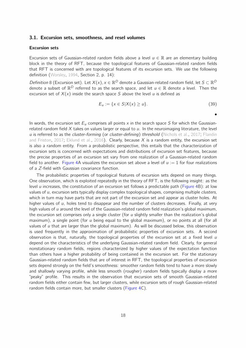
Excursion sets of Gaussian-related random fields above a level u ∈ R are an elementary buildingblock in the theory of RFT, because the topological features of Gaussian-related random fieldsthat RFT is concerned with are topological features of its excursion sets. We use the followingdefinition (Worsley, 1994, Section 2, p. 14):

Definition 8 (Excursion set). Let X(x), x ∈ RD denote a Gaussian-related random field, let S ⊂ RDdenote a subset of RD referred to as the search space, and let u ∈ R denote a level. Then theexcursion set of X(x) inside the search space S above the level u is defined as

Eu := x ∈ S|X(x) ≥ u. (39)

•

In words, the excursion set Eu comprises all points x in the search space S for which the Gaussian-related random field X takes on values larger or equal to u. In the neuroimaging literature, the levelu is referred to as the cluster-forming (or cluster-defining) threshold (Nichols et al., 2017; Flandinand Friston, 2017; Eklund et al., 2016). Clearly, because X is a random entity, the excursion setis also a random entity. From a probabilistic perspective, this entails that the characterization ofexcursion sets is concerned with expectations and distributions of excursion set features, becausethe precise properties of an excursion set vary from one realization of a Gaussian-related randomfield to another. Figure 4A visualizes the excursion set above a level of u := 1 for four realizationsof a Z-field with Gaussian covariance function.

The probabilistic properties of topological features of excursion sets depend on many things.One observation, which is exploited repeatedly in the theory of RFT, is the following insight: as thelevel u increases, the constitution of an excursion set follows a predictable path (Figure 4B): at lowvalues of u, excursion sets typically display complex topological shapes, comprising multiple clusters,which in turn may have parts that are not part of the excursion set and appear as cluster holes. Athigher values of u, holes tend to disappear and the number of clusters decreases. Finally, at veryhigh values of u around the level of the Gaussian-related random field realization’s global maximum,the excursion set comprises only a single cluster (for u slightly smaller than the realization’s globalmaximum), a single point (for u being equal to the global maximum), or no points at all (for allvalues of u that are larger than the global maximum). As will be discussed below, this observationis used frequently in the approximation of probabilistic properties of excursion sets. A secondobservation is that, naturally, the topological properties of the excursion set at a fixed level udepend on the characteristics of the underlying Gaussian-related random field. Clearly, for generalnonstationary random fields, regions characterized by higher values of the expectation functionthan others have a higher probability of being contained in the excursion set. For the stationaryGaussian-related random fields that are of interest in RFT, the topological properties of excursionsets depend strongly on the field’s smoothness: smoother random fields tend to have a more slowlyand shallowly varying profile, while less smooth (rougher) random fields typically display a more“peaky” profile. This results in the observation that excursion sets of smooth Gaussian-relatedrandom fields either contain few, but larger clusters, while excursion sets of rough Gaussian-relatedrandom fields contain more, but smaller clusters (Figure 4C).

18

Figure 4. Excursion sets. (A) This panel visualizes the random nature of excursion sets. The upper row of fourpanels depicts four realizations of a Z-field with a Gaussian covariance function with parameters v = 1, ` = 0.15.The lower four panels depict the realization-specific excursion set for a fixed level of u = 1. Points included in theexcursion sets are marked white, points not included in the excursion sets are black. (B) This panel visualizes thetopological properties of the excursion set of a single Z-field realization (leftmost subpanel) as a function of the levelvalue u. As u increases from −0.5 to 2, the topological constitution of the excursion set becomes less complex,and, in the limit of high levels u comprises a single cluster comprising the global maximum of the Gaussian-relatedrandom field’s realization or no points at all. (C) This panel visualizes the dependency of the topological propertiesof the excursion set on the smoothness of the Gaussian-related random field. The left two subpanels show a Z-fieldrealization and its corresponding excursion set for u = 1 for a rough (non-smooth) field. The excursion set comprisesmany small clusters. The right two subpanels show the same entities for a smoother field. Here, the excursion setcomprises a smaller number of clusters, which are larger than in the case of the rough Z- field. For implementationaldetails of these simulations, please see rft_4.m.

19

Smoothness

As visualized in Figure 2 and Figure 4, realizations of random fields can be smooth, i.e., varyinglittle over a given spatial distance, or rough, i.e., varying strongly over a given spatial distance.This intuitive notion of smoothness is an important determinant of the probabilistic behaviour oftopological features of random fields and of central importance in RFT (Friston et al., 1991).Thus, in order to establish quantitative relationships between a Gaussian-related random field’ssmoothness and the probabilistic behaviour of its topological features, a quantitative measure ofsmoothness is required. The principle measure used to quantify smoothness in RFT is the reciprocalunit-square Lipschitz-Killing curvature (Taylor and Worsley, 2007, eq. 3), defined as

ς :=1∫

[0,1]D |V (∇X(x)) |12 dx

, (40)

whereV(∇X(x)) :=

(C(∂

∂xiX(x),

∂

∂xjX(x)

))1≤i ,j≤D

(41)

denotes the D × D variance matrix of the gradient components (i.e., partial derivatives) of therandom field at x ∈ [0, 1]D. Note that we refer to V(∇X(x)) as a variance matrix (as opposed toa covariance matrix) despite the fact that entries of V(∇X(x)) are given by covariances. This ismotivated by the fact that these covariances refer to the partial derivatives of the identical randomvariable X(x) and not to partial derivatives of covariances of two different random variables (Fristonet al., 1991; Worsley et al., 1992; Taylor and Worsley, 2007). In the following, we first attemptto elucidate in which sense eqs. (40) and (41) capture the intuitive notion of a random field’ssmoothness. We then discuss, how eq. (40) is reformulated in RFT to give rise to the “full widthat half maximum” parameterization of smoothness. Throughout, we make the assumption that therandom field’s gradient exists at all locations of the random field’s domain, i.e., that the randomfield is differentiable with respect to space.

To obtain a first intuition in which sense eqs. (40) and (41) provide a measure of smoothness,we consider the case of a stationary GRF on a one-dimensional domain (D = 1) with a GCF γ andparameters v := 1 and ` > 0. In this case, the gradient of X at the location x ∈ [0, 1] simplifies tothe derivative of X with respect to x , which, in line with the conventions of spatial statistics, wedenote by X(x). Further, the variance matrix of the gradient components simplifies to the varianceof this spatial derivative, and the determinant to the absolute value, which in turn is redundant fora non-negative variance. We are thus led to consider

ς =1∫

[0,1]V(X(x))12 dx

. (42)

We may first note that, regardless of the type of random field, the reciprocal of the square ofthe variance of the spatial derivative of the random field at a location x is a sensible measure ofthe field’s smoothness, if we assume that this value is constant over space: naturally, the spatialderivative quantifies the rate of change of the values of the random field, and if this is high, therandom field changes a lot, if it is low, the random field does not change much. In addition, thevariance describes how variable this spatial variability is over realizations of the random field, and,if it is small, most realizations of the random field with small spatial derivatives will appear smooth.Furthermore, for the current example of a one-dimensional GRF with a GCF, one may analytically

20

evaluate eq. (42) and, as shown in Supplement S1.1, obtains

ς =`√2. (43)

Thus, for the current scenario, the smoothness measure defined by eqs. (40) and (41) is directlyrelated to the spatial covariation parameter of the covariance function of the GRF. This is, ofcourse, a special case. An important aspect of eq. (40) is that it is defined as long as the partialderivatives of the random field of interest are defined, but for many random fields it may notdirectly map onto a single parameter of the field’s covariance function. This is analogous to thedifference between a variance of a random variable and the variance parameter of a univariateGaussian distribution: while the former concept applies to any random variable, the case that itdirectly maps onto a parameter of the probability density function of a random variable, like thevariance parameter of the univariate Gaussian, is rather an exception.

More generally, the smoothness measure defined by eqs. (40) and (41) involves the deter-minants of the spatial gradients at locations x ∈ [0, 1]D. Assuming again that the gradients areconstant over space, we next consider the two-dimensional scenario (D = 2). In this case, thedeterminant is given by

|V(∇X(x))| = V(∂

∂x1X(x)

)V(∂

∂x2X(x)

)− C

(∂

∂x1X(x),

∂

∂x2X(x)

)2

. (44)

As is evident from eq. (44), the variances and covariances of the field’s partial derivatives makeopposing contributions to the field’s smoothness: the variances of the partial derivatives contributeto roughness, while the covariances of the partial derivatives contribute to the field’s smoothness.The former was already observed for the one-dimensional scenario. The latter can be interpretedas follows: a systematic simultaneous change of values in the direction of both the x1 and x2

ordinates indicates smoothness. Finally, an intuition about the three-dimensional case is affordedby the intuitive view of the determinant of a 3 × 3 matrix as the magnification factor of thevolume of a unit cuboid under the linear transform furnished by the matrix (Hannah, 1996). Inthis case, large values for the off-diagonal elements with respect to the diagonal elements imply asmaller magnification and vice versa, thus implicating large variances of the partial derivatives inlow smoothness and large correlations of the partial derivatives in high smoothness. In summary,if a random field is differentiable with respect to space, then eqs. (40) and (41) provide a sensiblescalar measure of the intuitive notion of a random field’s smoothness.

Smoothness reparameterization

While ς thus constitutes a perfectly fine scalar measure of a Gaussian-related random field’s smooth-ness, Friston et al. (1991) and Worsley et al. (1992) proposed to reparameterize ς in the three-dimensional case (D = 3) as

ς = (4 ln 2)−32 fx1fx2fx3 with fx1 , fx2 , fx3 > 0. (45)

In the context of RFT, the values fx1 , fx2 , fx3 are referred to as the full widths at half maximum(FWHMs) in direction x1, x2 and x3, respectively. The reparameterization of smoothness in termsof FWHMs oriented along the cardinal axes of three-dimensional space was motivated by assumingthat the realization of a Gaussian-related random field of interest had been created by convolving

21

a GRF with a white-noise covariance function with a Gaussian convolution kernel (see SupplementS1.2 for formal definitions of these entities). In this case, the smoothness of the resulting Gaussian-related random field depends on the spatial width of the Gaussian convolution kernel. The spatialwidth of a Gaussian convolution kernel, in turn, can be described in terms of the covariance matrixof the kernel. If it is assumed that the covariance matrix of the Gaussian convolution kernel isdiagonal, then the width of the convolution kernel is determined by the three diagonal parametersσ2x1, σ2x2

and σ2x3, which govern the widths of the respective one-dimensional marginal Gaussian

functions of the convolution kernel. An alternative representation of the width of a Gaussianfunction in turn is afforded by its FWHM: in general, the FWHM of a function f is the value xfor which f (−x/2) = f (x/2) = f (0)/2. As shown in Supplement S1.2, for a univariate Gaussianfunction extending over the x1 domain with variance parameter σ2

x , this value is given by

fx =√

8 ln 2σx . (46)

In other words, the FWHM of a univariate Gaussian function is a scalar multiple of the square rootof its variance parameter. Eq. (45) was then motivated by approximating the variance matrix ofpartial derivatives V(∇X(x)) of a given Gaussian-related random field X(x), x ∈ S by the variancematrix of partial derivatives of a hypothetical random field Y (x), x ∈ S that was imagined to havebeen created by the convolution of a white-noise GRF with an isotropic Gaussian convolution kernelparameterized in terms of its FWHMs fx1 , fx2 , and fx3 . For such a field, the variance matrix of partialderivatives was proposed to be independent of space and of the form (Worsley et al., 1992, eq. 2)

V(∇Y (x)) = 4 ln 2

f −2x1

0 0

0 f −2x2

0

0 0 f −2x3

=: Λ. (47)

For this hypothetical field, it then follows directly that

ς =

(∫[0,1]D

|Λ|12 dx

)−1

=(

(4 ln 2)3(fx1fx2fx3 )−2)− 1

2 = (4 ln 2)−32 fx1fx2fx3 . (48)

In Supplement S1.2 we show that the diagonal elements of the variance matrix of gradient com-ponents of a three-dimensional white-noise GRF convolved with an isotropic Gaussian convolutionkernel with FWHMs fx1 , fx2 , and fx3 are indeed of the form implied by the right-hand side of eq.(47) (see Holmes (1994) and Jenkinson (2000) for similar work). Note, however, that this only(at least partially) validates the construction of the approximation, but not the approximation

V(∇X(x)) ≈ V(∇Y (x)), (49)

which is implicit in the reparameterization of the smoothness parameter of a given Gaussian-relatedrandom field X(x), x ∈ S in terms of FWHMs, perse.

Resel volumes

Building on the parameterization of smoothness in terms of FWHMs, the concept of resel volumeswas introduced by Worsley et al. (1992). Intuitively, resel volumes are the smoothness-adjustedintrinsic volumes of subsets of domains of random fields. Stated differently, the smoother a randomfield, the larger the resel volumes of subsets of its domain at constant intrinsic volumes. Based onthe general definition of intrinsic volumes for the three-dimensional case (35), the decomposition

22

of the first- and second-order intrinsic volumes (36), and the FWHM parameterization of a randomfield’s smoothness (48), the resel volumes of a set S ⊂ RD in the domain of a random field arethen defined as follows (Worsley et al., 1996, pp. 63, eq. (3.2)):

Definition 9 (Resel volumes). Let X(x), x ∈ R3 denote a Gaussian-related random field withsmoothness

ς = (4 ln 2)−32 fx1fx2fx3 (50)

and let S ⊂ R3 denote a subset of the domain of the Gaussian-related random field. Then the0th- to 3rd-order resel volumes of S are defined in terms of the intrinsic volumes of S and thesmoothness parameters fx1 , fx2 and fx3 by

R0(S) := µ0(S) (51)

R1(S) :=1

fx1

µx11 (S) +

1

fx2

µx21 (S) +

1

fx3

µx31 (S) (52)

R2(S) :=1

fx1fx2

µx1x22 (S) +

1

fx1fx3

µx1x32 (S) +

1

fx2fx3

µx2x32 (S) (53)

R3(S) :=1

fx1fx2fx3

µ3(S) (54)

•

The resel volumes of a given set S ⊂ R3 can thus be readily evaluated if the intrinsic volumes of Sand their subspace contributions, as well as the FWHM smoothness parameters fx1 ,fx2 , fx3 of theGaussian-related random field extending over S, are known.

3.2. Probabilistic properties of excursion set features

The probabilistic properties of the following five topological features of excursion sets of Gaussian-related random fields form the core of RFT theory: (P1) the global maximum of the Gaussian-related random field, (P2) the number of clusters within an excursion set, (P3) the volume ofclusters within an excursion set, (P4) the number of clusters of a given volume within an excursionset, and (P5) the maximal volume of a cluster within an excursion set. In the theory of RFT,these topological features are described by random variables, the probability distributions of whichare governed by the stochastic and geometric characteristics of the underlying Gaussian-relatedrandom field and the level u of the respective excursion sets. The dependencies of the respectivedistributions on the properties of the underlying Gaussian-related random field and the excursionset level are mitigated by four expected values: (E1) the expected volume of an excursion set,(E2) the expected number of local maxima within an excursion set, (E3) the expected number ofclusters within an excursion set, and (E4) the expected volume of a cluster within an excursion set.In the following, we first discuss the parametric dependencies of these expectations on the type ofGaussian-related random field and its resel volumes, i.e., its smoothness and intrinsic volumes. Wethen discuss the probability distributions of the five topological features that form the core of RFTtheory. As will become evident throughout this section, a defining characteristic of RFT theory isthat the parametric distributional forms of virtually all topological features of interest derive fromapproximations, rather than analytical transforms of the probability density functions describing theGaussian-related random fields under functions that instantiate the topological features. For thepresentation of RFT theory herein, this entails that we will most often only report the parametricdistributional form of a given topological feature under RFT and discuss some background about its

23

motivation, rather than analytically deriving the respective parametric distributional form from firstprinciples. The approximative-parametric nature is inherent to RFT and is rooted in the seminalworks by Adler and Hasofer (1976) and Adler (1976) and has more recently seen major advancesby Taylor et al. (2005, 2006) and Adler and Taylor (2007) (see also Adler (2000) for a historicalperspective).

Expected values

(E1) The expected volume of an excursion set

Recall that an excursion set Eu is a subset of the search space S for which a Gaussian-relatedrandom field takes on values larger or equal to u ∈ R. As discussed above, the standard analyticalmeasure that assigns a notion of volume to subsets of RD is the Lebesgue measure λ, which returnsthe Lebesgue volume λ(Eu) of the excursion set. As discussed by Adler (1981, Section 1.7, pp.18 - 19), the expected value of the Lebesgue volume of an excursion set is given by

E (λ(Eu)) = λ(S)(1− FX(u)), (55)

where λ(S) denotes the Lebesgue volume of the search space and FX denotes the distributionfunction of the Gaussian-related random field at the origin (see also Hayasaka and Nichols (2003,eq. 4) and, for Z-fields, Friston et al. (1994b, eq. 3)). Because for stationary random fields, thisdistribution function equals the distribution functions at all other locations of the random field, wedenote it by FX without reference to its spatial position. A brief derivation of eq. (55) is providedin Supplement S1.3. As it stands, eq. (55) has strong intuitive appeal: the expected value of theexcursion set Eu is a proportion of the search space S, and the proportion factor is given by theprobability of the Gaussian-related random field to take on values larger than u at each point inspace. For example, for small values of u, the probability that the Gaussian-related random fieldtakes on values larger than u is always higher than for larger values of u. Accordingly, the expectedvalue of the volume of the excursion set is larger in the former than in the latter case. From eq.(55), it follows directly that if the three-dimensional volume of the search space is expressed interms of the third-order resel volume R3(S), then the expected third-order resel volume of theexcursion set is given by

E(R3(Eu)) = R3(S)(1− FX(u)). (56)

In the following, we will denote the random variable modelling the expected volume of an excursionset independent of its unit of measurement by Vu, where Vu := λ(Eu) or Vu := R3(Eu) dependingon the specified context. We visualize the expected volume of the excursion set as a function of uand R3(S) in Figure 5B. As is evident from this visualization, the expected volume of an excursionset E(Vu) decreases with higher cluster-forming thresholds u and higher Gaussian-related randomfield smoothness, i.e., decreasing third-order resel volume R3(S).

(E2) The expected number of local maxima within an excursion set

Let Mu denote the number of local maxima of a Gaussian-related random field X(x), x ∈ RDabove u inside a set S ⊂ RD. Then Mu is also the number of local maxima of the excursion set Eu.In RFT, the expected number of local maxima of a Gaussian-related random field is approximatedby the expected Euler characteristic χ(·) of the excursion set (Worsley, 1994, Section 2, p. 15),i.e.

E(Mu) ≈ E(χ(Eu)). (57)

24

To unpack expression (57), we first discuss the notion of the Euler characteristic as a topologicalmeasure. We then consider the motivation for the approximation of expression (57), and finallydiscuss the parametric closed form for the expected Euler characteristic used in RFT.

The Euler characteristic is a function and is referred to as a topological invariant. Topologicalinvariants measure the geometrical characteristics of geometrical objects irrespective of the waythey are bent. A formal description of the Euler characteristic is beyond our current scope, because,as Adler (2000, p.16) puts it, the Euler characteristic “(...) is one of those unfortunate cases inwhich what is easy for the human visual system to do quickly and effectively requires a lot morecare when mathematicised”. This care is not warranted here, because, as will be seen below, theexpected Euler characteristic of the excursion set Eu will itself be approximated by a function ofu without recourse to an actual evaluation of χ(Eu). We thus only provide a brief intuition forthe Euler characteristic itself: for a three-dimensional volume of interest, the Euler characteristiccounts, in an alternating sum, the number of three types of topological features: (1) connectedcomponents, (2) visible open holes, often referred to as handles, and (3) invisible voids. Semi-formally, the Euler characteristic of an excursion set Eu is hence given by

χ(Eu) = Number of connected components of Eu−Number of handles of Eu+Number of voids in Eu.

(58)

The following examples for familiar geometric objects provided by Worsley (1996a) are instructive:

χ(Eu) = 1 for a single solid excursion set (1 connected component - 0 handles + 0 voids),

χ(Eu) = 0 for a doughnut-shaped excursion set (1 connected component - 1 handles + 0 voids),

χ(Eu) = −2 for a pretzel-shaped excursion set (1 connected component - 3 handles + 0 voids),

χ(Eu) = 2 for a tennisball-shaped excursion set (1 connected component - 0 handles + 1 voids).

More qualitatively, if an excursion set comprises many disconnected components, each with veryfew holes (in astrophysics referred to as a “meatball” topology), the Euler characteristic is positive;if the clusters of an excursion set are connected by many bridges, thus creating many holes (inastrophysics referred to as a “sponge” topology), the Euler characteristic is negative, and if theexcursion set comprises many surfaces that enclose hollows (in astrophysics referred to as a “bubble”topology), the Euler characteristic is again positive.

In the theory of RFT, it is, however, not the value of the Euler characteristic for a specificrealization of an excursion set that is of primary interest, but rather its expected value - as evidentfrom the right-hand side of expression (57). This approximation (or “heuristic”) is based on thefollowing intuition: as the threshold value u that defines the excursion set Eu increases, voids andhandles of the excursion set tend to disappear, and what remains are isolated connected componentsof the excursion set (in the neuroimaging literature referred to as clusters). In this scenario,χ(Eu) thus counts the number of connected components (cf. eq. (58)). Each of the clusters inthe excursion set naturally contains a local maximum of the excursion set, which thus motivatesto approximate the expected number of local maxima by the expected Euler characteristic overrealizations of the Gaussian-related random field X(x). As for the accuracy of this approximation,it has been demonstrated that it becomes exact in the limit of very high values of u, in which χ(Eu)

evaluates to either 1 (one remaining cluster) or 0 (no remaining clusters) (Taylor et al., 2005).For lower values of u, an analytical validation does not seem to exist so far. Crucially though, theapproximation in expression (57) is helpful from a mathematical perspective, because there exists

25

a parametric closed form for the expected Euler characteristic. This parametric closed form wasintroduced by (Worsley et al., 1996, eq. 3.1) and is given by

E(χ(Eu)) =

D∑d=0

Rd(S)ρd(u), (59)

where the Rd(S), d = 0, ..., D are the d-dimensional resel volumes of the search space and theρd(u) are referred to as Euler characteristic (EC) densities. The formula on the right-hand sideof eq. (59) is powerful because it decomposes the expected value of the Euler characteristic into(1) smoothness-adjusted volumetric contributions from each of the d = 0 to d = D dimensions ofthe search space, and (2) unit volume-smoothness densities ρd that only depend on the value of uand the type of Gaussian-related random field on the other hand. We have already discussed themeaning of the Rd in Section 3.1 and hence focus on the EC densities in the following. Intuitively,the functions

ρd : R→ R, u 7→ ρd(u) for d = 0, ..., D (60)

describe the contribution of unit smoothness resel volumes to the expected value of the Eulercharacteristic. The values taken by these functions depend on u, and in general, as the value ofu increases (i.e., the excursion set is formed based on a higher threshold), these values decrease.For constant resel volumes, this implies that the value of the expected Euler characteristic, andthus the approximated expected number of local maxima, decreases. The exact parametric formsof the function ρd depend on the type of Gaussian-related random field and have been analyticallyevaluated by Worsley (1994). We list their functional forms in Table 2 and visualize their formbased on their SPM implementation in Figure 5A. Note that the 0th order EC density of each fieldcorresponds to 1− FX(u), where FX denotes the distribution function of the respective field. Thisallows for evaluating the expected volume of the excursion set as expressed in eq. (56) in termsof the third order resel volume and the 0th order EC density. In summary, the expected number oflocal maxima of an excursion set can thus be approximated for a given Gaussian-related randomfield in a straight-forward manner, if the field’s resel volumes are known (or have been estimated).

(E3) The expected number of clusters within an excursion set

In the SPM implementation of RFT, the expected number of clusters is approximated by theexpected Euler characteristic (Friston et al., 2007, Chpt. 18, pp. 233-234, Chpt. 19, pp. 240-241).This means that the approximations of the expected number of local maxima and the approximationof the expected number of clusters are identical. This identity entails the assumption that eachcluster contains only a single local maximum of the excursion set. Cast more formally, let Mu

denote the number of local maxima of an excursion set Eu, and let

M := m1, ..., mMu ⊂ Eu (61)

denote the set of local maxima of Eu. Clusters are unconnected components of the excursion setand thus form a partition Pu of Eu, i.e.,

Pu = C1, ..., CCu with Ci ∪ Cj = ∅ for i 6= j and ∪Cui=1 Ci = Eu, (62)

whereCu := |Pu| (63)

denotes the number of clusters. While each cluster contains at least one local maximum, in general

26

Z-field Euler characteristic densities

ρ0(u) =∫∞u

1

(2π)1/2 exp(−t2/2

)dt

ρ1(u) = (4 ln 2)1/2

2πexp

(−u2/2

)ρ2(u) = 4 ln 2

(2π)3/2 exp(−u2/2

)u

ρ3(u) = (4 ln 2)3/2

(2π)2 exp(−u2/2

)(u2 − 1)

T -field Euler characteristic densities

ρ0(u; ν) =∫∞u

Γ( ν+12 )

√νπΓ( ν2 )

(1+ t2

ν

)−1/2(ν+1) dt

ρ1(u; ν) = (4 ln 2)1/2

2π

(1 + u2

ν

)−1/2(ν−1)

ρ2(u; ν) =(4 ln 2)Γ( ν+1

2 )(2π)3/2( ν2 )

1/2Γ( ν2 )

(1 + u2

ν

)−1/2(ν−1)

u

ρ3(u; ν) = (4 ln 2)3/2

(2π)2

(1 + u2

ν

)−1/2(ν−1) (ν−1νu2 − 1

)F -field Euler characteristic densities

ρ0(u; ν1, ν2) =∫∞u

Γ((ν1+ν2)/2)Γ(ν1/2)Γ(ν2/2)

ν1ν2

(ν1ν2t)1/2(ν1−2) (

1 + ν1tν2

)−1/2(ν1+ν2)

dt

ρ1(u; ν1, ν2) = (4 ln 2)1/2

(2π)1/2

Γ((ν1+ν2−1)/2)21/2

Γ(ν1/2)Γ(ν2/2)

(ν1uν2

)1/2(ν1−1) (1 + ν1u

ν2

)−1/2(ν1+ν2−2)

ρ2(u; ν1, ν2) = 4 ln 22π

Γ((ν1+ν2−2)/2)Γ(ν1/2)Γ(ν2/2)

(ν1uν2

)1/2(ν1−2) (1 + ν1u

ν2

)−1/2(ν1+ν2−2) ((ν2 − 1) ν1u

ν2− (ν1 − 1)

)ρ3(u; ν1, ν2) = (4 ln 2)3/2

(2π)3/2

Γ((ν1+ν2−3)/2)2−1/2

Γ(ν1/2)Γ(ν2/2)

(ν1uν2

)1/2(ν1−3) (1 + ν1u

ν2

)−1/2(ν1+ν2−2)

×(

(ν2 − 1)(ν2 − 2)(ν1uν2

)2

− (2ν1ν2 − ν1 − ν2 − 1) ν1uν2

+ (ν1 − 1)(ν1 − 2)

)Table 2. Euler characteristic densities for Z-fields and for T - and F -fields with ν and ν1, ν2 degrees of freedom,respectively. Note that the 0th-order Euler characteristic densities correspond to complementary distribution functionsof Z, T and F random variables. Reproduced from Table II in Worsley et al. (1996).

it is very well possible that a given cluster comprises multiple local maxima. This is also a commonfinding in the actual analysis of fMRI data using SPM, in which case the local maxima for largeclusters are indeed listed in the SPM results table based on a distance selection criterion of typicallylarger than 8 mm apart. The validity of the approximation chain

E(Cu) ≈ E(Mu) ≈ E(χ(Eu)) =

D∑d=0

Rd(S)ρd(u), (64)

thus strongly rests on the assumption of high values for the excursion set-defining threshold u: inthe case that only the global maximum of the random field is contained in the single connected

27

component of the field’s excursion set, the number of local maxima of the excursion set and thenumber of clusters are identical with probability one. In Figure 5B, we visualize the expected numberof clusters E(Cu) within an excursion set over a range of values for u and interpolations of theresel volumes R0(S), ..., R3(S) of the exemplary data set underlying Figure 1. As is evident fromthis visualization, the expected number of clusters within an excursion set decreases with increasingvalues for the cluster-forming threshold and increasing smoothness of the Gaussian-related randomfield, corresponding to decreasing resel volumes.

(E4) The expected volume of clusters within an excursion set

The expected volume of a single cluster is evaluated in RFT based on the expressions for (1)the expected volume of the excursion set, and (2) the expected number of clusters in such anexcursion set. For a value u ∈ R, let the cluster volume be defined by the random variable

Ku :=VuCu. (65)

Then, if Vu and Cu are independent random variables with finite expected values, the expectedcluster volume is given by

E(Ku) =E(Vu)

E(Cu)(66)

(e.g., Friston et al. (1996, eq. 2), Hayasaka and Nichols (2003, eq. 3)). Naturally, if the expectedvolume of the excursion set is expressed in terms of Lebesgue measure, i.e., Vu = λ(Eu), eq. (66)denotes the expected cluster Lebesgue volume, and if the expected volume of the excursion set isexpressed in terms of third-order resel volume, i.e., Vu = R3(Eu), eq. (66) denotes the expectedcluster resel volume. We visualize the expected cluster resel volume as a function of the cluster-forming threshold and the smoothness of the Gaussian-related random field in Figure 5B. As isevident from this visualization, the expected cluster resel volume decreases with increasing valuesof the cluster-forming threshold and increasing Gaussian-related random field smoothness.

Probability distribution of excursion set features

(P1) The distribution of the global maximum of a Gaussian-related random field

Historically, the distribution of the global maximum of a Gaussian-related random field has beenone of the seeds of the RFT framework (Worsley et al., 1992). This is because maximum statisticsafford FWER control in multiple testing scenarios, as we show in Supplement S2. To introducethe distribution of the global maximum used in RFT, let

Xm := maxx∈S

X(x) (67)

denote the global maximum of the Gaussian-related random field X(x) on a set S. In RFT, theprobability distribution of the global maximum is specified in terms of its distribution function,which is assumed to be of the following form (e.g., Worsley et al. (1992, eqs. 1,6), Worsley et al.(1996, eq. 3.1))

FXm : R→ [0, 1], u 7→ FXm(u) := 1− E(χ(Eu)). (68)

The reasoning behind this form is similar to that justifying the approximation of the expectednumber of local maxima by the expected Euler characteristic: first, if the excursion set defining

28

5 10u

0

0.2

0.4

Z--eldA

;0

;1

;2

;3

5 10u

0

0.2

0.4

T (15)--eld

;0

;1

;2

;3

5 10u

0

0.5

1F (1; 20)--eld

;0

;1

;2

;3

E(Vu)

2004006008001000R3(S)

8

9

10

11

12

u

B

1 2 3 4#10-4

E(Cu)

12345w

8

9

10

11

12

u

0.05 0.1 0.15 0.2

E(Ku)

12345w

8

9

10

11

12

u

0.5 1 1.5#10-3

P(Xm 6 u)

12345w

8

9

10

11

12

u

C

0.05 0.1 0.15 0.2

P(Cu = c); u = 6.5

12345w

0

2

4

c

0 0.2 0.4 0.6 0.8 1

ln fKu(k); u =6.5

12345w

0

10

20

30

k

-600 -400 -200

P(C6k;u = c); u = 6.5, k = 0.001

12345w

0

2

4

c

0 0.2 0.4 0.6 0.8 1

P(C6k;u = c); u = 7.5, k = 0.001

12345w

0

2

4

c

0 0.2 0.4 0.6 0.8 1

P(C6k;u = c); u = 6.5, k = 0.01

12345w

0

2

4

c

0 0.2 0.4 0.6 0.8 1

Figure 5. Probabilistic properties of excursion set features. (A) Euler characteristic densities. The panels depict,from left to right, the Z-field Euler characteristic (EC) densities, the T -field EC densities for a T -field with 15degrees of freedom and the F -field EC densities for an F -field with (1,20) degrees of freedom. (B) Excursion setfeature expectations for a T -field with 15 degrees of freedom. From left to right, the panels show the expectedexcursion set volume E(Vu) in units of resels, the expected number of clusters E(Cu), and the expected clustervolume E(Ku) in resels as a function of the excursion set level u and a parameterization of smoothness. For theexpected excursion set volume, this smoothness parameter is given by the third-order resel volume. For the remainingpanels, including the panels in (C), we selected the resel volumes of the exemplary data set (cf. Figure 1) givenby R0(S) = 6.0, R1(S) = 32.8, R2(S) = 353.6, and R3(S) = 704.6 and evaluated (59) over a range of scalarmultiples wRd , d = 0, 1, 2, 3. The value of w ∈ [0, 5] is displayed on the x-axis. Note that smoothness increaseswith decreasing resel volumes. (C) Excursion set feature probability distributions for a T -field with 15 degrees offreedom as functions of smoothness. From the left to right, the panels show the probability for the maximum ofthe Gaussian-related random field to exceed a value u, P(Xm ≥ u), the probability for the number of clusters withinan excursion set to assume a value c, P(Cu = c), the log probability density for a cluster to assume a volume k,fKu (k). (D) The distribution of the number of clusters of a given volume within an excursion set. The panels depictP(C≥k,u = c) as a function of u and k.

29

value u is high enough, Eu will not comprise any handles and voids any more. Second, in the limitof even higher values u, there will remain only one connected component comprising the globalmaximum or no connected component at all. In this case, the Euler characteristic of the excursionset can assume only the values 1 or 0: if the global maximum is equal to or larger than the excursionset defining value, i.e., if Xm ≥ u, the Euler characteristic will assume the value 1, i.e., χ(Eu) = 1.If the global maximum is smaller than the excursion set defining value, i.e., if Xm < u, the Eulercharacteristic will assume the value 0, i.e., χ(Eu) = 0. That is, in the limit of high values for u, theEuler characteristic χ(Eu) of the excursion set can be conceived as a random variable taking onvalues in the set 0, 1 with a probability mass function defined in terms of the mutually exclusiveevent probabilities

P(χ(Eu) = 0) := P(Xm < u) and P(χ(Eu) = 1) := P(Xm ≥ u). (69)

Evaluating the expected value E(χ(Eu)) in this scenario then yields

E(χ(Eu)) = P(χ(Eu) = 0) · 0 + P(χ(Eu) = 1) · 1 = P(Xm ≥ u). (70)

With the definition of the cumulative distribution function of a continuous random variable, ex-pression (68) then follows directly.

It is instructive to consider the dependency of the probability for the global maximum to exceeda value u as a function of the Gaussian-related random field’s smoothness: an increase in thedegree of smoothness at constant intrinsic volumes results in a decrease of the Gaussian-relatedrandom field’s resel volumes (cf. Definition 9). A decrease in resel volumes at constant value u inturn leads to a decrease in the value of the expected Euler characteristic (cf. eq. (59)). A decreasein the expected Euler characteristic in turn results in an increase of the probability P(Xm < u) (cf.eq. (68)), which in turn is equivalent to a decrease of the probability P(Xm ≥ u). In summary,an increase in a Gaussian-related random field’s smoothness thus yields a lower probability for thefield’s global maximum to exceed a given value u. We visualize this dependency in Figure 5C. Notethat E(Cu) and P(Xm ≥ u) are identically equal to E(χ(Eu)).

(P2) The distribution of the number of clusters within an excursion set

The RFT approximation for the distribution of the number of clusters within an excursion setwas introduced by Friston et al. (1994b, eq. 8) and is of the form

Cu ∼ Poiss(λCu), (71)

whereλCu := E(Cu). (72)

That is, the number of clusters is assumed to be distributed according to a Poisson distributionwith parameter E(Cu), which in turn is available from eq. (64). Friston et al. (1994b) base theapproximation for the distribution of the number of clusters in an excursion set on Adler (1981,Theorem 6.9.3, p. 161) and the fact that a Poisson distribution is fully specified in terms of itsexpectation parameter. Theorem 6.9.3 in Adler (1981) is concerned with the limit probability ofan Euler characteristic number for high values of u and remarks that “Since this number is (...)essentially the same as the number of components of the excursion set (...) and the number oflocal maxima above u, these should have the same limiting distribution (...). This, however, hasnever been rigorously proven”. Intuitively, eq. (71) can be understood as reflecting the fact that theoccurrence of clusters in an excursion set under the null hypothesis should not depend on spatial

30

location, but only depend on an “average spatial occurrence rate” given by E(Cu). By means of theapproximation (64), an increase in the smoothness of a Gaussian-related random field results in adecrease of the expected number of clusters in an excursion set at a fixed level u. In Figure 5D,we visualize the dependency of P(Cu = c) as a function of the Gaussian-related random field’ssmoothness for a fixed level u = 6.5. As evident from the visualization, increases in smoothnessresult in a shift of probability mass towards smaller values of c .

(P3) The distribution of the volume of clusters within an excursion set

As in definition (65), let Ku denote a real-valued random variable that models the volume ofclusters within an excursion set measured either in terms of Lebesgue measure or third-order reselvolume. In the SPM implementation of RFT, the probability distribution of this random variable isassumed to be specified in terms of the probability density function (cf. Friston et al. (1994b, p.213, eq. (12)))

fKu : R≥0 → R≥0, k 7→ fKu(k) :=2κ

Dk

2D−1 exp

(−κk

2D

), (73)

where

κ :=

(Γ

(D

2+ 1

)1

E(Ku)

) 2D

. (74)

These expressions are motivated as follows. First, eq. (73) has been derived by Friston et al.(1994b) based on a result by Nosko (1969b,a, 1970). Nosko’s result, which is reported in Adler(1981, p. 158), states that the size of the distribution of connected components of a GRF’sexcursion set to the power of 2/D has an exponentional distribution with expectation parameterκ. As shown in Supplement S1.3, eq. (73) then follows directly from Nosko’s result by the changeof variables theorem (e.g., Fristedt and Gray (2013, p. 136)). Note that Adler (1981, p. 158)remarks that “no detailed proofs are given” for Nosko’s result. Second, eq. (74) follows from theexpression for the expected cluster volume eq. (66) and the fact that an exponential distributionis fully specified in terms of the reciprocal value of its expectation. It should be noted that theprobability density function eq. (73) applies to GRFs and, in the limit of high degrees of freedom, toT -fields (cf. comments in spm_P_RF.m). Refined results for the distribution of cluster volumesin excursion sets of T - and F -fields were derived by Cao (1999), but are not implemented in SPM.

For later reference, we note two formal consequences of the parametric form eq. (73) for theprobability distribution of the cluster volume Ku. First, as shown in Supplement S1.3, eq. (73)implies that the cumulative density function of the cluster volume is given by

FKu : R→ [0, 1], k 7→ FKu(k) = 1− exp(−κk

2D

). (75)

Second, from eq. (75) it follows directly, that the probability of the cluster volume to exceed aconstant k under the RFT framework evaluates to (cf. Friston et al. (1994b, eq. 11))

P(Ku ≥ k) = exp(−κk

2D

). (76)

In Figure 5C, we visualize the log probability density function fKu for a fixed value u = 6.5 as afunction of the Gaussian-related random field’s smoothness. The allocation of probability densitymirrors the effect of smoothness on the expected volume of clusters within the excursion set E(Ku)

in Figure 5B.

31

(P4) The distribution of the number of clusters of a given volume within an excursion set

Let C≥k,u denote a random variable that models the number of clusters within an excursion setof level u that have a volume equal to or larger than some constant k . Under the RFT framework,it is assumed that (cf. Friston et al. (1996, eq. 4))

C≥k,u ∼ Poiss(λC≥k,u), (77)

whereλC≥k,u := E(Cu)P(Ku ≥ k). (78)

That is, the random variable C≥k,u is assumed to be distributed according to a Poisson distribution,the expectation parameter of which is given by the product of the expected number of clusters andthe probability of a cluster volume to assume a value equal to or larger than the constant k . Noteagain that parametric forms for E(Cu) and P(Ku ≥ k) are available from eqs. (64) and (76),respectively. Further note that eq. (77) specifies probabilities of the form P(C≥k,u = i), whichshould be read as representing the probability that the number of clusters within an excursion setdefined by the level value u with a volume larger than or equal to k is i . For later reference, wenote that the sum

∑c−1i=0 P(C≥k,u = i) thus represents the probability that the number of clusters

within an excursion set defined by level u with volume larger than or equal to k is either smallerthan or equal to a constant c ∈ N minus 1, and hence the expression 1 −

∑c−1i=0 P(C≥k,u = i)

represents the probability that the number of clusters within an excursion set defined by level uhaving volume equal to or larger than k is equal to or larger than c .

Expressions (77) and (78) can be motivated as follows. Assume the existence of a randomvariable Cu that models the number of clusters within an excursion set at level u and the existenceof a parametric expression for its distribution (provided by eq. (71) and eq. (72) in the theory ofRFT). Assume further that one would like to specify the distribution P(C≥k,u) of a second randomvariable C≥k,u that models the number of clusters in an excursion set Eu at level u that havea volume equal to or larger than some constant k . By definition, this distribution is a marginaldistribution of the joint distribution

P(Cu, C≥k,u) = P(Cu)P(C≥k,u|Cu). (79)

Define the conditional distribution of C≥k,u given Cu by the binomial distribution

C≥k,u|Cu ∼ BNj(µ), with µ := P(Ku ≥ k) (80)

such that by definition

P(C≥k,u = i |Cu = j) =

(j

i

)µi(1− µ)j−i , for i ∈ N0

j and j ∈ N. (81)

Intuitively, the event that i of j realized clusters (i.e., i = 0, 1, ..., j) have a volume equal or largerto k is thus conceived as one realization of j independent Bernoulli events with “success probability”P(Ku ≥ k). Based on eq. (81), it can then be shown that (cf. Friston et al. (1996, Appendix))

P(C≥k,u = i) =

∞∑j=1

P(Cu = i , C≥k,u = j) =λiC≥k,u exp

(−λC≥k,u

)i !

, (82)

i.e., that such a random variable C≥k,u has a Poisson distribution with expectation parameter

32

λC≥k,u . We document the derivation of eq. (82) in Supplement S1.3. The importance of therandom variable C≥k,u in the SPM implementation of RFT will be elaborated on in Section 4.2.Finally, in Figure 5D, we visualize the distribution of C≥k,u as a function of smoothness and thevalues of u and k . At constant smoothness, increasing u and k leads to a shift of probability massto lower values of c .

(5) The distribution of the maximal cluster volume within an excursion set

Finally, to afford FWER control in multiple testing scenarios relating to the volume of clusterswithin excursion sets, a parametric form of the respective maximum statistic is required (cf. Sup-plement S2). To this end, let, for a set of c ∈ N of clusters within an excursion set Eu at level u,ki , i = 1, ..., c denote the volumes of clusters i = 1, ..., c . Further, let

Kmu := maxk1, ..., kc (83)

denote the maximal cluster volume within the excursion set. Then, with the definition of therandom variable C≥k,u, we have for k ∈ R

P(Kmu < k) = P(C≥k,u = 0) and P(Kmu ≥ k) = P(C≥k,u ≥ 1). (84)

In words, first, the probability that the maximal cluster volume within an excursion set Eu at levelu is smaller than a constant k is the same as the probability that the number of clusters in theexcursion set Eu which have a volume equal to or larger than k is zero. Second, the probabilitythat the maximal cluster volume in an excursion set Eu is equal to or larger than a constant kis the same as the probability that the number of clusters in the excursion set Eu which have avolume equal to or larger than k is equal to or larger than 1. The distribution of the maximalcluster volume Kmu is thus fully determined by the distribution of C≥k,u. For later reference, wenote that with eqs. (77), (78), and (82) (cf. (Friston et al., 1994b, eq. 14))

P(Kmu ≥ k) = P(C≥k,u ≥ 1)

= 1−0∑i=0

P(C≥k,u = i)

= 1− exp (−E(Cu)P(Ku ≥ k)) .

(85)

4. Application

The general theory of random fields - and the theory of RFT in particular - model three-dimensionalspace by R3. In reality, however, fMRI data points are only acquired at a finite number of discretespatial locations, commonly known as voxels. This discretization of space has to be accounted forwhen considering the application of RFT theory to GLM-based fMRI data analysis. In the currentsection, we thus consider the discrete space, discrete data-point linear model

Yiv = miβv + σZiv for i = 1, ..., n and v ∈ V, (86)

whereV := v |v = (v1, v2, v3) with v1 ∈ Nm1 , v2 ∈ Nm2 , v3 ∈ Nm3 (87)

denotes a voxel index set. Eq. (86) should be read as the discrete-space analogue of eq. (38) forwhich the continuous space coordinates x ∈ R3 have been replaced by voxel indices v ∈ V. We

33

assume that these voxel indices correspond to the weighting parameters of three orthogonal, butnot necessarily orthonormal, basis vectors bd ∈ R3, d = 1, 2, 3 of R3, such that the set

L :=

3∑d=1

vdbd |v1 ∈ Nm1 , v2 ∈ Nm2 , v3 ∈ Nm3

(88)

is a finite lattice covering the subset of R3 of interest. Assuming an MNI space bounding box of-78 to 78 mm in the coronal, -112 mm to 76 mm in the sagittal, and -70 mm to 95 mm in the axialdirection and a 2 × 2 × 2 mm voxel size, typical values for the number of indices are m1 = 79,m2 = 95, and m3 = 69. With these definitions, we thus have the correspondences

Yiv = Yi(x), βv = βi(x), and Ziv = Zi(x) for x :=

3∑d=1

vdbd and v ∈ V (89)

between the discrete space and the continuous space linear model representations of eqs. (86) and(38), respectively.

Building on these correspondences between the theoretical scenario of a continuous space andthe applied scenario of discrete spatial sampling, we are now in a position to discuss the applicationof the theoretical framework of the previous section to GLM-based fMRI data analysis. As outlinedin the Introduction, we first consider the parameter estimation of the RFT null model, whichcomprises the estimation of the Gaussian-related random field’s smoothness and the approximationof the search space’s intrinsic and resel volumes. We then consider the evaluation of the parametricp-values reported in the SPM results table.

4.1. Parameter estimation

As discussed in Section 3.2, the probability distributions of all excursion set features of a Gaussian-related random field depend on the resel volumes of the search space via the expected Eulercharacteristic (cf. eq. (59)). The resel volumes in turn depend on the FWHM parameterizationof the Gaussian-related random field’s smoothness and the search space’s intrinsic volumes (cf.Definition (9)). Application of the parametric forms for the probability distributions of excursionset features discussed in Section 3.2 in a data-analytical context thus necessitates the estimationof the Gaussian-related random field’s smoothness, the approximation of its search space’s intrinsicvolumes, and the subsequent evaluation of its resel volumes. In effect, the estimated resel volumesare intended to furnish a data-adaptive null hypothesis model against which the actually observeddata can be evaluated. Because the data typically do not fully conform to the null hypothesisβv = 0 for all v ∈ V, the SPM implementation of RFT bases its parameter estimation scheme onthe so-called standardized residuals

riv :=Yiv −mi βv√

1n−p

∑ni=1

(Yiv −mi βv

)2, i = 1, ..., n, v ∈ V, (90)

where βv denotes the Gauss-Markov estimator for the effect size parameter at voxel v . Practically,these values are stored in ResI_000*.nii files, which are created and deleted by SPM’s spm_spm.mfunction during SPM’s GLM estimation. Note that the denominator of the standardized residualsin eq. (90) corresponds to the estimate σ of the standard deviation parameter σ. Under theassumption that mi βv veridically reflects the expectation of Yiv , the standardized residuals can

34

thus be conceived as realizations of the Z-fields Zi(x) at discrete spatial locations (cf. eq. (38)and the introduction of Section 3). Stated differently, the RFT framework assumes that thestandardized residuals can be considered observations of the null hypothesis model used to evaluatethe probabilities of observed excursion set features. RFT parameter estimation as implemented inSPM’s spm_est_smoothness.m function then comprises three steps: first, the estimation of theFWHM smoothness parameters based on the standardized residuals, second, the approximation ofthe intrinsic volumes of the search space, and finally, the evaluation of the resel volumes.

FWHM smoothness parameter estimation

SPM’s estimation scheme for the FWHM smoothness parameters can be conceived as a two-stepprocedure. In the first step, an estimate of the smoothness parameter ς (cf. eq. (40)) of theZ-fields Zi(x) is constructed based on the standardized residuals. In a second step, this estimate isused together with an estimate of the approximating matrix Λ to afford the estimation of FWHMsmoothness parameters that conform to the equality of eq. (48) and, in their relative magnitude,reflect the diagonal entries of the variance matrix of partial derivatives (cf. eq. (41)). Morespecifically, the smoothness parameter estimate of the first step is evaluated as

ς :=1

1m

∑mv=1 |

nn(n−p)Vv |1/2

, (91)

where Vv ∈ R3×3 denotes a scaled voxel-wise estimate of the variance matrix of gradient compo-nents with elements

(Vv )jk :=

n∑i=1

(ri(v+ej ) − riv )(ri(v+ek) − riv ) for j, k = 1, 2, 3 and v ∈ V, (92)

m = m1 + m2 + m3 denotes the cardinality of the voxel index set, and n ≤ n denotes the sizeof a data point subset potentially used by SPM for computational efficiency. The forms of eqs.(91) and (92) are motivated as follows (Hayasaka and Nichols, 2003; Hayasaka et al., 2004):the (Vv )jk are products of the first-order finite differences between the standardized residuals ofadjacent voxel indices. These first-order finite differences may be interpreted as scaled versionsof numerical first-order derivatives. Notably, SPM thus foregoes the direct approximation of thegradient components of the Gaussian-related random field. The first order differences in the factorsin eq. (92) are evaluated by spm_sample_vol.c. The formation of the sum of products of thesefirst-order finite differences of standardized residuals in eq. (92) and its subsequent division by n canbe interpreted as an estimation of the (co)variances of the gradient components, if it is assumedthat the sample average over available data points n is zero. The subsequent multiplication by nand division by the degrees of freedom n − p is meant to rescale the respective estimates to theentire set of data points and render the estimate unbiased by effectively converting standardized tonormalized residuals (cf. spm_est_smoothness.m, comments ll. 144 - 169 and Worsley (1996b)).In effect, the sum terms in the denominator of eq. (91) can be interpreted as scaled voxel-specificnumerical estimates of the square root of the determinants of V(∇X(x)), x ∈ S. Finally, thesummation of these terms and division by the number of voxel indices m can be interpreted as thenumerical integration over the unit cuboid for first-order finite differences, rather than numericalderivative approximations to the Gaussian-related random fields’ gradient components. In Figure 6we demonstrate that a numerically simplified version of SPM’s smoothness parameter estimationapproach indeed results in a valid recovery of the smoothness parameter of a two-dimensional

35

Figure 6. Smoothness parameter estimation. To exemplify the smoothness estimation scheme of SPM’s RFTimplementation, we capitalize on the fact that for one-dimensional GRFs with Gaussian covariance function, thereciprocal unit-square Lipschitz-Kiling curvature ς is identical to the Gaussian covariance function’s length parameter` up to a factor of 2−1/2 (cf. eq. (43)). A straightforward estimator for ` is thus l :=

√2ς. For the simulations

depicted in the figure, we evaluated ς using numerical differentiation and sample variances to estimate ` for one-dimensional GRFs on the interval [0, 1]. We varied ` in the interval [0.04, 0.2] and examined sample sizes in the rangefrom n = 100 to n = 2000. (A) Panel A visualizes a sample of n = 100 rough GRF realizations with ` = 0.04 . (B)Panel B visualizes a sample of n = 100 smooth GRF realizations with ` = 0.2. (C) Panel C visualizes the absolutepercent relative estimation error |100 · (ˆ− `)/`| for the ensuing estimates. In general, this error is small (. 3 % onaverage) and decreases for larger sample sizes uniformly over the space of `. For the full implementational details ofthese simulations, please see rft_6.m.

Gaussian random field with Gaussian covariance function.

The reparameterization of smoothness in terms of FWHM smoothness parameters in the secondstep then is achieved by setting

fxj :=1

4 ln 2

(1

m

m∑v=1

n

n(n − p)(Vv )j j

)− 12

(93)

and

fxj =ς

13

(4 ln 2)−12

fxj(∏3k=1 fxj

) 13

(94)

for j = 1, 2, 3. Eqs. (93) and (94) implement SPM’s assumption that the variance matrix ofgradient components is of diagonal form and thus that the smoothness parameter ς can be repa-rameterized in terms of the FWHM smoothness parameters fxj (cf. eq. (47)). More specifically,these equations are motivated as follows (cf. spm_est_smoothness.m, comments ll. 246 - 248):the fxj can be interpreted as estimates of the diagonal elements of Λ based on the V(∇X(x))

matrix estimate discussed above. By normalizing these values using their geometric average in thesecond factor of eq. (94) and scaling the resulting normalized fxj ’s by the first factor, it is thenensured that the fxj ’s reproduce the smoothness parameter estimate ς if they are substituted asestimates of the fxj ’s in the matrix Λ (cf. eq. (48)). The thus evaluated estimates are then usedfor the evaluation of the resel volumes and are reported in the footnote of the SPM results tableas FWHM (voxels).

36

Intrinsic volume approximation

To approximate the intrinsic volumes of the search space, SPM uses an algorithm proposed byWorsley et al. (1996, pp. 62 -63) and implemented in spm_resels_vol.c. This algorithm cor-responds to a summation of the contributions of zero- to three-dimensional subspaces along thecardinal axes to the respective intrinsic volumes of the search space. More specifically, the algorithmevaluates

• the total number of voxelsm := mx1mx2mx3 , (95)

• the number of edges in the x1, x2 and x3 directions, i.e.,

me1 := |(v , v + e1)|v , v + e1 ∈ V|,me2 := |(v , v + e2)|v , v + e2 ∈ V|,me3 := |(v , v + e3)|v , v + e3 ∈ V|,

(96)

respectively,

• the number of faces in the x1-x2-, x1-x3-, and x2-x3- directions, i.e.,

mf12 := |(v , v + e1, v + e2, v + e1 + e2)|v , v + e1, v + e2, v + e1 + e2 ∈ V|,mf13 := |(v , v + e1, v + e3, v + e1 + e3)|v , v + e1, v + e3, v + e1 + e3 ∈ V|,mf23 := |(v , v + e2, v + e3, v + e2 + e3)|v , v + e2, v + e3, v + e2 + e3 ∈ V|,

(97)

respectively, and

• the number of cubes, i.e.,

mc := |(v, v + e1, v + e2, v + e3, v + e1 + e2, v + e2 + e3, v + e1 + e3, v + e1 + e2 + e3)

|v, v + e1, v + e2, v + e3, v + e1 + e2, v + e2 + e3, v + e1 + e3, v + e1 + e2 + e3 ∈ V|.(98)

Based on these counts and the physical voxel sizes δ1, δ2 and δ3 in the x1-, x2-, and x3-directions,respectively, the intrinsic volumes of the search space are then approximated by

µ0(S) = m − (me1 +me

2 +me3) + (mf

12 +mf13 +mf

23)−mc ,

µ1(S) = δ1(me1 −mf

12 −mf13 +mc) + δ2(me

2 −mf12 −mf

23 +mc) + δ3(me3 −mf

13 −mf23 +mc),

µ2(S) = δ1δ2(mf12 −mc) + δ1δ3(mf

13 −mc) + δ2δ3(mf23 −mc),

µ3(S) = δ1δ2δ3mc .

(99)

Note, for example, that µ3(S) corresponds to a summation of the volume δ1δ2δ3 of each of themc voxels constituting the search space. For a whole-brain GLM-based fMRI data analysis, thisquantity thus typically corresponds to an approximation of the physical brain volume by many smallcuboids.

Resel volume estimation

De-facto, SPM does not evaluate an approximation of the search space’s intrinsic volumes perse.Instead, it capitalizes on the subspace decomposition assumption of eq. (36) and directly estimates

37

the resel volumes in spm_resel_vol.m by

R0(S) = µ0(S),

R1(S) =(δ1

fx1

δ2

fx2

δ3

fx3

)me1 −mf12 −mf13 +mc

me2 −mf12 −mf23 +mc

me3 −mf13 −mf23 +mc

,

R2(S) =(δ1δ2

fx1 fx2

δ1δ3

fx1 fx3

δ2δ3

fx2 fx3

)mf12 −mcmf13 −mcmf23 −mc

, andR3(S) =

1

fx1 fx2 fx3

µ3(S).

(100)

The estimated resel volumes Rd(S), d = 0, 1, 2, 3 are the pivot points between the practicalperspective of the current section and the theoretical perspective of Section 3: Theory. As pre-viously noted, virtually all probability distributions of the topological features of interest in RFTdepend on the resel volumes via the expected Euler characteristic (cf. eq. (59)). Substitution ofRd(S), d = 0, 1, 2, 3 for the resel volumes in the expected Euler characteristic formula thus resultsin a set of probability distributions that reflect a data-adapted Gaussian-related random field nullmodel. The exceedance probabilities of the observed topological features of interest under thisdata-adapted null model are then reported in the SPM results table.

This concludes our discussion of the RFT parameter estimation scheme implemented in SPM.We provide a reproduction of this estimation scheme in a simplified and annotated version ofspm_est_ smoothness.m as rft_spm_est_smoothness.m in the accompanying OSF project.

4.2. The SPM results table

The majority of p-values in the SPM results table relate to the random variable C≥k,u introducedin Section 3.2 (Friston et al., 1996). Recall that C≥k,u models the number of clusters within alevel u-dependent excursion set Eu that have a volume equal to or larger than a constant k ∈ R.As discussed in Section 3.2, the random variable C≥k,u takes on values in N0 and is distributedaccording to a Poisson distribution with parameter λC≥k,u := E(Cu)P(Ku ≥ k), where E(Cu)

represents the expected number of clusters within an excursion set Eu and is given by eq. (64),while P(Ku ≥ k) denotes the probability for a cluster within an excursion set Eu to assume avolume equal to or larger than the constant k and is given by eq. (76). Formally, we have

C≥k,u ∼ Poiss(λC≥k,u), (101)

and thus

P(C≥k,u = c) = exp (−E(Cu)P(Ku ≥ k))(E(Cu)P(Ku ≥ k))c

c!for c = 0, 1, .... (102)

For ease of notation, we denote the distribution function of C≥k,u in the current section by

FλC≥k,u : N0 → [0, 1], c 7→ FλC≥k,u (c) :=

c∑j=0

P(C≥k,u = j). (103)

38

The majority of p-values in the SPM results table are then special cases of probabilities related toC≥k,u for the values c ∈ N0, k ∈ R, and u ∈ R and are evaluated using the implementation of thePoisson distribution function (103) in spm_Pcdf.m. To distinguish these special cases, we makethe following assumptions and use the following notation. We assume that

(1) a statistical parametric map, for example a three-dimensional voxel map comprising T valuerealizations, has been obtained,

(2) for this map, a cluster-forming threshold value u and a cluster-extent threshold value k in reselvolume have been defined,

(3) the number of clusters c in the resulting excursion set Eu has been evaluated,

(4) the volumes of these clusters ki , i = 1, ..., c have been assessed, and

(5) for each cluster, the maximum test statistic within this cluster has been evaluated and isdenoted by ti , i = 1, ..., c .

A few remarks from a practical perspective on these assumptions are in order. In SPM, statisticalparametric maps for T tests are evaluated based on GLM beta and variance parameter estimates foruser-defined contrast weight vectors and are saved under the filename spmT_000*.nii or the like.When interacting with SPM’s Results graphical user interface, or specifying options in SPM’s batcheditor for the Results Report module, the user is prompted to specify the cluster-forming thresholdvalue u by selecting a Threshold Type with options “None” and “FWE” for p-value adjustment, anda Threshold Value in the form of a p-value. The combination of these two options is evaluatedby SPM to define the value u as follows. In the case of “p-value adjustment: none” and thesubsequent specification of a p-value (e.g. 0.001), SPM uses the function spm_u.m to evaluatethe inverse cumulative density function for the probabilistic complement of the specified valueand the respective statistic. For example, in the case of a statistical parametric map comprisingT -values, u thus corresponds to the “critical T -value”, i.e., the value tc for which values of theT -statistic equal to or larger than tc have a probability of equal to or smaller than the specifiedp-value under the standard T - distribution with the appropriate degrees of freedom (e.g. for a Tdistribution with 30 degrees of freedom and p-values of 0.05, 0.025, and 0.001, the respective uvalues evaluate to 1.697,2.042, and 3.385, respectively). In the case of “p-value adjustment: FWE”and the subsequent specification of a p-value (e.g. 0.05), SPM uses the function spm_uc.m toevaluate a critical threshold using the RFT framework. This option leads, in general, to higher valuesfor u. The cluster-extent threshold k is specified by the user in units of voxels and is transformedinto units of resels by SPM by multiplying the user-specified value by 1/

∏3d=1 fxd . Finally, the

excursion set Eu, the number of clusters c , and the cluster-specific volume and maxima statisticski and ti , i = 1, ..., c are evaluated using low-level SPM functionality, such as spm_bwlabel.c,spm_clusters.m, and spm_max.m. For the computational details of these routines, the reader isreferred directly to the documentation in the functions’ headers. Based on an interaction betweenthe spm_list.m and spm_P_RF.m functions, SPM then documents p-values in the SPM resultstable for set-level, cluster-level and peak-level inferences (Friston et al., 1996). In the following,we specify for each level of inference which probabilities these p-values correspond to.

39

Set-level inference

Assume we are interested in the probability

P(C≥k ,u ≥ c), (104)

i.e., the probability that for the specified cluster-forming threshold u, the number of clusters withinthe excursion set Eu that have a volume equal to or larger than the specified cluster-extent thresholdvalue k is equal to or larger than the observed number of clusters c . Clearly, we have

P(C≥k ,u ≥ c) = 1− P(C≥k ,u < c)

= 1− FλC≥k ,u (c)(105)

and eq. (104) can thus be evaluated using the Poisson distribution function (103). In the SPMresults table, the probability P(C≥k ,u ≥ c) is reported as the “set-level p value” and the value c isdocumented as the number of clusters c (Figure 1 and Table 3). The idea behind using (104) is toenable inferences about “network-activations” (Friston et al., 1996, pp. 229-230): if the numberof actually observed clusters c exceeds the number E(Cu) of clusters expected under the RFTnull hypothesis model by a large margin, eq. (104) evaluates to a small value. In this case, itmay thus be concluded that the observed pattern of distributed clusters reflects the engagementof a distributed network of brain regions in the GLM contrast of interest. Note that the set-levelinference probability (104) is the only p-value of the SPM results table that directly depends onthe user specified cluster-extent threshold k .

Cluster-level inference

Assume that for a cluster of the excursion set Eu indexed by i , where i = 1, ..., c , we are interestedin the probability

P(C≥ki ,u ≥ 1), (106)

i.e., the probability that for the specified cluster-forming threshold u the number of clusters withinthe excursion set that have a volume equal to or larger than the observed cluster volume ki is equalto or larger than 1. For this probability, we have

P(C≥ki ,u ≥ 1) = 1− P(C≥ki ,u < 1)

= 1− FλC≥ki ,u(0)

= 1− P(C≥ki ,u = 0)

= 1− exp(−E(Cu)P(Ku ≥ ki)

)= P

(Kmu ≥ ki

).

(107)

From the second equality of eq. (107), we thus see that (106) can be evaluated using the Poissondistribution function (103). Moreover, from the last equality, we see that P(C≥ki ,u ≥ 1) correspondsto the probability for the maximal cluster volume within an excursion set Eu to exceed the valueki (cf. eq. (85)). Because the probability (106) hence relates to the maximum statistic forcluster extent, declaring a cluster activation significant, if P(C≥ki ,u ≥ 1) < α furnishes a statisticalhypothesis test for spatial cluster extent that controls the FWER at level α ∈ [0, 1] (cf. SupplementS2). Note that the family of statistical tests for which the Type I error rate is controlled here refers

40

to the volumes of clusters Ku within an excursion set. In the SPM results table, the probabilityP(C≥ki ,u ≥ 1) is reported as the “FWE-corrected p-value at the cluster level” for each cluster

i = 1, ..., c in the column labelled pFWE-corr and the voxel number equivalent ki∏3d=1 fxd of the

resel volume of each cluster i = 1, ..., c is reported in the column labelled kE (Figure 1 and Table 3).

As “uncorrected p-value at the cluster level” for cluster i = 1, ..., c SPM reports the probability

P(Ku ≥ ki), (108)

which corresponds to the probability that the cluster volume in an excursion set Eu exceeds theobserved volume of the ith cluster. Note that rejecting the null hypothesis based on P(Ku ≥ ki) < α

for a significance level α ∈ [0, 1] over a family of c clusters entails a probability of 1− (1−α)c forat least one Type I error and hence offers no FWER control. The “p-value correction” procedureimplied by the SPM results table header labelling can thus be interpreted as the transformation of(108) by means of the right-hand side of the penultimate equation in eq. (107).

Peak-level inference

Assume we are interested in the probability

P(C≥0,ti≥ 1), (109)

i.e., the probability that for a hypothetical cluster-forming threshold corresponding to the maximumstatistic ti of cluster i , there are one or more clusters within the excursion set that have a volumeequal to or larger than 0. We have

P(C≥0,ti≥ 1) = 1− P(C≥0,ti

< 1)

= 1− FλC≥0,ti

(0)

= 1− P(C≥0,ti= 0)

= 1− exp(−E(Cti )P(Kti ≥ 0)

)= 1− exp

(−E(Cti )

)≈ P(Xm ≥ ti).

(110)

In eq. (110), the penultimate equality follows with expression (76) for k = 0. As shown inSupplement S1, the ultimate approximation in eq. (110) follows using an approximation of theexponential function by the first two terms in its series definition (Friston et al., 1996, eq. 5).Thus, P(C≥0,ti

≥ 1) approximates the probability that the global maximum of the statistical fieldof interest is equal or larger to the observed cluster maximum statistic value ti . In the SPM table,P(C≥0,ti

≥ 1) is reported as the “FWE-corrected p-value at the peak level” for cluster i = 1, ..., c

(Figure 1 and Table 3). Because this probability hence relates to the maximum statistic for thetest statistics comprising the statistical parametric map, declaring a voxel test statistic significant,if P(Xm ≥ ti) < α furnishes a statistical hypothesis test for voxel test statistics that controls theFWER at level α ∈ [0, 1] (cf. Supplement S2). Note that the family of statistical tests for whichthe Type I error rate is controlled here refers to the values of voxel-wise test statistics.

Finally, the SPM results table also reports an “uncorrected p-value at the peak level”. Thisp-value is the probability P(C≥0,ti

≥ 1) under the assumption that the resel volumes of the searchspace are given by R0 = 1 and Rd = 0 for d = 1, 2, 3. Hence, in light of eqs. (68) (64), and

41

(110), this p-value is evaluated as

E(χ(Eti )) = ρ0(ti). (111)

Intuitively, this corresponds to the scenario of a Gaussian-related random field comprising onlypoint volumes at the locations of voxels with no spatial dependencies. Because the zero-orderEuler characteristic densities are equivalent to the cumulative density functions of the Z-,T -, andF -distributions, the uncorrected p-value at the peak level corresponds to the familiar p-value ofsingle statistical testing scenarios. From this perspective, the “p-value correction” at the peak-levelimplied by the SPM results table header hence corresponds to an adjustment of eq. (111) in termsof the search space’s intrinsic volumes (i.e., the multiple testing multiplicity) and the underlyingGaussian-related random field’s smoothness (i.e., the correlative nature of the multiple tests).

The SPM results table footnote

The footnote of the SPM results table documents a number of statistics that contextualize thereported p-values: the ‘Height threshold’ and ‘Extent threshold’ entries indicate the user-definedcluster-forming threshold u and the voxel number equivalent of the cluster-extent threshold, i.e.,k∏3d=1 fxd , respectively. In addition to these values, the height threshold entry lists the uncor-

rected and corrected peak-level p-value equivalents of u, and the extent threshold entry lists theuncorrected and corrected cluster-level p-values of k . The ‘Expected voxels per cluster <c>’ and‘Expected number of clusters <c>’ entries report the voxel equivalent of the expected cluster vol-ume, and the expected number of clusters with volume equal to or larger than the user-specifiedcluster-extent threshold k , respectively. The ‘FWEp’ and ’FWEc’ entries correspond to the criticalu value for a corrected peak-level p-value equal to or less than 0.05 and the smallest observedcluster size with a cluster-level corrected p-value less than 0.05, respectively. The ‘Degrees offreedom’ entry reports the degrees of freedom of the underlying GLM design in an F -test format,such that for a one-sample T -test, the first number is set to 1, and the second number correspondsto the degrees of freedom of the T -test, n− p. The ‘FWHM’ entry reports the estimated FWHMparameters in units of mm, i.e., δd fxd , d = 1, 2, 3 and in units of resels, i.e., fxd , d = 1, 2, 3. The‘Volume’ entry indicates the search space volume in terms of Lebesgue measure λ(S) = mδ inunits of mm3, where δ := δ1δ2δ3 is the Lebesgue volume of a single voxel in mm3, in terms ofthe number of voxels m, and in terms of the third-order resel volume R3(S). Finally, the ‘Voxelsize‘ entry reports the voxels sizes δ1, δ2, δ3 in units of mm and the volume of a “cuboid resel”f :=

∏3d=1 fxd in voxels.

This concludes our documentation of the SPM results table. For an overview, please seeTable 3. We provide a reproduction of SPM’s p-value tabulation functionality in simplified andannotated versions of spm_list.m and spm_P_RF.m as rft_spm_results_table.m in the accom-panying OSF project.

5. Discussion

RFT is a highly sophisticated and computationally efficient mathematical framework and has re-peatedly been validated empirically (e.g., Hayasaka and Nichols, 2003; Flandin and Friston, 2017;Davenport and Nichols, 2021). In the field of statistics, RFT probably constitutes the most orig-inal and most advanced contribution of the neuroimaging community (Adler et al., 2015), whilein the neuroimaging field itself, RFT likely constitutes the most routinely used statistical inference

42

set-level cluster-level peak-level

p c pFWE-corr kE puncorr pFWE-corr T puncorr

P(C≥k ,u ≥ c) c P(C≥ki ,u ≥ 1) ki f P(Ku ≥ ki) P(C≥0,ti≥ 1) ti ρ0(ti)

Height threshold u,∑D

d=0 ρd(u),P(C≥0,u ≥ 1) Degrees of freedom 1, n − p

Extent threshold k f ,P(Ku ≥ k),P(C≥k ,u ≥ 1) FWHM δd fxd , fxd d = 1, 2, 3

<k> E (Ku) f Volume λ(S), m,R3(S)

<c> E (Cu)P(Ku ≥ k) Voxel size δ1, δ2, δ3, f

FWEp uc |P(C≥0,uc ≥ 1) = 0.05

FWEc minki |P(C≥ki ,u ≥ 1) < 0.05

Table 3. p-values and other statistics reported in the SPM results table (cf. Figure 1). Clusters are indexed byi = 1, ..., c. We use the definitions f :=

∏3d=1 fxd and δ := δ1δ2δ3.

strategy (Nichols et al., 2016). Nonetheless, in the following, we will point to a few mathematicaland statistical issues that may be elaborated on in the further refinement of RFT.

First, from a mathematical perspective, it may be desirable to establish formal justificationsfor the distribution of the number of clusters within an excursion set and the distribution of thevolume of clusters within an excursion set. As noted by Adler (1981) and discussed in Section 3.2,the currently used parametric forms appear to lack formal proofs. Similarly, it may be a worthwhileendeavour to mathematically model the conditional probabilistic structure of the number of clustersand their associated volumes more explicitly. At present, it is assumed that the expected number ofclusters and the expected volume of a cluster are independent (cf. eq. (66)). This appears to bea rather strong assumption, given the finite size of the search space. Finally, following Taylor andWorsley (2007), it would be desirable to formally delineate some additional qualitative propertiesof the FWHM estimators implemented in SPM. The currently available reference in this regard,Worsley (1996b), appears to be somewhat outdated and superseded by the de-facto estimation ofthe FWHMs based on standardized, rather than normalized, residuals. Please note that given theapproximative nature of the entire RFT framework and its repeated empirical validation, we do notmean to imply by these suggestions that RFT as it stands is fundamentally flawed, but that thesefoundations could be elaborated on to further ground the approach mathematically.

Second, from a statistical perspective, a promising avenue for future research on RFT couldbe an update from the estimation of resel volumes to Lipschitz-Killing regression (Adler, 2017).In brief, Lipschitz-Killing regression foregoes an explicit approximation of the data’s smoothnessand intrinsic volumes and instead fits observed empirical Euler characteristics to the Gaussiankinematic formula (Taylor et al., 2006) via generalized least squares. As such it potentially offersbetter analytical tractability, facilitated diagnostic, and higher computational efficiency in higherdimensions, for example in the full spatiotemporal modelling of combined M/EEG and fMRI data.

Notwithstanding these potential future refinements, we hope that with our current documen-tation of RFT, we can contribute to the continuing efforts towards ever higher degrees of compu-tational reproducibility and transparency in computational cognitive neuroscience (Nichols et al.,2017; Poldrack et al., 2017; Millman et al., 2018; Toelch and Ostwald, 2018). Moreover, wehope that we can contribute to a factually grounded and technically precise discussion about themathematical and computational aspects of fMRI data analysis.

43

Data availability statement The data and code that support the findings of this study are openlyavailable from the Open Science Framework at http://doi.org/10.17605/OSF.IO/3DX9W.

References

Abrahamsen, P. (1997). A review of Gaussian random fields and correlation functions. TechnicalReport.

Adler, R. J. (1976). Excursions above a fixed level by n-dimensional random fields. Journal ofApplied Probability, pages 276–289.

Adler, R. J. (1981). The Geometry of Random Fields. John Wiley&Sons.

Adler, R. J. (2000). On excursion sets, tube formulas and maxima of random fields. Annals ofApplied Probability, pages 1–74.

Adler, R. J. (2017). Estimating thresholding levels for random fields via Euler characteristics.arXiv:1704.08562.

Adler, R. J. and Hasofer, A. (1976). Level crossings for random fields. The annals of Probability,pages 1–12.

Adler, R. J. and Taylor, J. E. (2007). Random Fields and Geometry. Springer Science & BusinessMedia.

Adler, R. J., Taylor, J. E., and Worsley, K. J. (2015). Applications of Random Fields and Geometry.Springer Science & Business Media.

Ashburner, J. (2012). SPM: A history. Neuroimage, 62(2):791–800.

Ashby, F. G. (2011). Statistical Analysis of fMRI Data. MIT press.

Bansal, R. and Peterson, B. S. (2018). Cluster-level statistical inference in fMRI datasets: Theunexpected behavior of random fields in high dimensions. Magnetic Resonance Imaging, 49:101–115.

Benjamin, D. J., Berger, J. O., Johannesson, M., Nosek, B. A., Wagenmakers, E.-J., Berk, R.,Bollen, K. A., Brembs, B., Brown, L., Camerer, C., et al. (2018). Redefine statistical significance.Nature Human Behaviour, 2(1):6.

Billingsley, P. (1978). Probability and Measure. John Wiley & Sons, Collier-Macmillan Publishers.

Borghi, J. A. and Van Gulick, A. E. (2018). Data management and sharing in neuroimaging:Practices and perceptions of MRI researchers. bioRxiv, page 266627.

Bowring, A., Maumet, C., and Nichols, T. (2018). Exploring the impact of analysis software ontask fMRI results. bioRxiv.

Brett, M., Penny, W., and Kiebel, S. (2007). Statistical Parametric Mapping: The analysis offunctional brain images. chapter Classical inference: Parametric Procedures, pages 223–231.Ac.

44

Brown, E. N. and Behrmann, M. (2017). Controversy in statistical analysis of functional magneticresonance imaging data. Proceedings of the National Academy of Sciences, 114(17):E3368–E3369.

Button, K. S., Ioannidis, J. P. A., Mokrysz, C., Nosek, B. A., Flint, J., Robinson, E. S. J., andMunafÃ2, M. R. (2013). Power failure: Why small sample size undermines the reliability ofneuroscience. Nature Reviews Neuroscience, 14(5):365–376.

Cao, J. (1999). The size of the connected components of excursion sets of χ 2, t and F fields.Advances in Applied Probability, 31(3):579–595.

Carp, J. (2012). The secret lives of experiments: Methods reporting in the fMRI literature.Neuroimage, 63(1):289–300.

Christakos, G. (1992). Random Field Models in Earth Sciences. Courier Corporation.

Chumbley, J., Worsley, K., Flandin, G., and Friston, K. (2010). Topological FDR for neuroimaging.Neuroimage, 49(4):3057–3064.

Chumbley, J. R. and Friston, K. J. (2009). False discovery rate revisited: FDR and topologicalinference using Gaussian random fields. Neuroimage, 44(1):62–70.

Cohn, D. L. (1980). Measure Theory, volume 165. Springer.

Cox, R. W., Chen, G., Glen, D. R., Reynolds, R. C., and Taylor, P. A. (2017). fMRI clustering andfalse-positive rates. Proceedings of the National Academy of Sciences, 114(17):E3370–E3371.

Davenport, S. and Nichols, T. E. (2021). The expected behaviour of random fields in high dimen-sions: Contradictions in the results of Bansal and Peterson (2018). Preprint, Neuroscience.

Eklund, A., Knutsson, H., and Nichols, T. E. (2018). Cluster failure revisited: Impact of first leveldesign and data quality on cluster false positive rates. arXiv preprint arXiv:1804.03185.

Eklund, A., Nichols, T. E., and Knutsson, H. (2016). Cluster failure: Why fMRI inferencesfor spatial extent have inflated false-positive rates. Proceedings of The National Academy OfSciences Of The United States Of America, 113(28):7900–7905.

Eklund, A., Nichols, T. E., and Knutsson, H. (2017). Reply to Brown and Behrmann, Cox, etal., and Kessler et al.: Data and code sharing is the way forward for fMRI. Proceedings of theNational Academy of Sciences, 114(17):E3374–E3375.

Fisher, R. A. (1925). Statistical Methods for Research Workers. Genesis Publishing Pvt Ltd.

Flandin, G. and Friston, K. (2015). Topological inference.

Flandin, G. and Friston, K. J. (2017). Analysis of family-wise error rates in statistical parametricmapping using random field theory. Human brain mapping.

Fristedt, B. E. and Gray, L. F. (2013). A Modern Approach to Probability Theory. Springer Science& Business Media.

Friston, K. (2007a). Statistical parametric mapping. chapter Statistical parametric mapping, pages10–31. Academic Press.

45

Friston, K. (2007b). Statistical Parametric Mapping: The analysis of functional brain images.chapter Topological inference, pages 237–245. Academic Press.

Friston, K., Penny, W., Ashburner, J., Kiebel, S., and Nichols, T. (2007). Statistical ParametricMapping: The Analysis of Functional Brain Images. Elsevier Science.

Friston, K. J., Frith, C., Liddle, P., and Frackowiak, R. (1991). Comparing functional (PET)images: The assessment of significant change. Journal of Cerebral Blood Flow & Metabolism,11(4):690–699.

Friston, K. J., Holmes, A., Poline, J.-B., Price, C. J., and Frith, C. D. (1996). Detecting activationsin PET and fMRI: Levels of inference and power. Neuroimage, 4(3):223–235.

Friston, K. J., Holmes, A. P., Worsley, K. J., Poline, J.-P., Frith, C. D., and Frackowiak, R. S.(1994a). Statistical parametric maps in functional imaging: A general linear approach. Humanbrain mapping, 2(4):189–210.

Friston, K. J., Worsley, K. J., Frackowiak, R., Mazziotta, J. C., and Evans, A. C. (1994b).Assessing the significance of focal activations using their spatial extent. Human brain mapping,1(3):210–220.

Geerligs, L. and Maris, E. (2021). Improving the sensitivity of cluster-based statistics for functionalmagnetic resonance imaging data. Human Brain Mapping, 42(9):2746–2765.

Georgie, Y. K., Porcaro, C., Mayhew, S., Bagshaw, A. P., and Ostwald, D. (2018). A perceptualdecision making EEG/fMRI data set. bioRxiv, page 253047.

Geuter, S., Qi, G., Welsh, R. C., Wager, T. D., and Lindquist, M. A. (2018). Effect size andpower in fMRI group analysis. bioRxiv.

Glaser, D. and Friston, K. (2007). Statistical parametric mapping. chapter Covariance components,pages 140–147. Academic Press.

Gong, W., Wan, L., Lu, W., Ma, L., Cheng, F., Cheng, W., Grünewald, S., and Feng, J. (2018).Statistical testing and power analysis for brain-wide association study. Medical Image Analysis,47:15–30.

Gopinath, K., Krishnamurthy, V., Lacey, S., and Sathian, K. (2018a). Accounting for non-gaussiansources of spatial correlation in parametric functional magnetic resonance imaging paradigms II:A method to obtain first-level analysis residuals with uniform and gaussian spatial autocorrelationfunction and independent and identically distributed time-series. Brain connectivity, 8(1):10–21.

Gopinath, K., Krishnamurthy, V., and Sathian, K. (2018b). Accounting for non-gaussian sources ofspatial correlation in parametric functional magnetic resonance imaging paradigms I: Revisitingcluster-based inferences. Brain connectivity, 8(1):1–9.

Hannah, J. (1996). A geometric approach to determinants. The American mathematical monthly,103(5):401–409.

Hayasaka, S. and Nichols, T. E. (2003). Validating cluster size inference: Random field andpermutation methods. Neuroimage, 20(4):2343–2356.

Hayasaka, S., Phan, K. L., Liberzon, I., Worsley, K. J., and Nichols, T. E. (2004). Nonstationarycluster-size inference with random field and permutation methods. Neuroimage, 22(2):676–687.

46

Holmes, A. (1994). Statistical Issues in Functional Brain Mapping. PhD thesis, University CollegeLondon.

Hunter, J. K. (2011). Measure Theory. University of California at Davis.

Ioannidis, J. P. (2005). Why most published research findings are false. PLoS medicine, 2(8):e124.

Jenkinson, M. (2000). Estimation of smoothness from the residual field. In Internal TechnicalReport TR00MJ3. University of Oxford.

Jenkinson, M., Beckmann, C. F., Behrens, T. E., Woolrich, M. W., and Smith, S. M. (2012). Fsl.Neuroimage, 62(2):782–790.

Kallenberg, O. (2021). Foundations of Modern Probability, volume 99 of Probability Theory andStochastic Modelling. Springer International Publishing, Cham.

Kessler, D., Angstadt, M., and Sripada, C. S. (2017). Reevaluating “cluster failure” in fMRI usingnonparametric control of the false discovery rate. Proceedings of the National Academy ofSciences, 114(17):E3372–E3373.

Kiebel, S. and Holmes, A. (2007). Statistical parametric mapping. chapter The general linearmodel, pages 101–125. Academic Press.

Kiebel, S. J., Poline, J.-B., Friston, K. J., Holmes, A. P., and Worsley, K. J. (1999). Robustsmoothness estimation in statistical parametric maps using standardized residuals from the gen-eral linear model. Neuroimage, 10(6):756–766.

Kilner, J. M. and Friston, K. J. (2010). Topological inference for EEG and MEG. The Annals ofApplied Statistics, pages 1272–1290.

Meisters, G. (1997). Lebesgue Measure on the real line. University of Nebraska, Lincoln.

Millman, K. J., Brett, M., Barnowski, R., and Poline, J.-B. (2018). Teaching computationalreproducibility for neuroimaging. arXiv preprint arXiv:1806.06145.

Monti, M. M. (2011). Statistical analysis of fMRI time-series: A critical review of the GLMapproach. Frontiers in human neuroscience, 5:28.

Mueller, K., Lepsien, J., Möller, H. E., and Lohmann, G. (2017). Commentary: Cluster failure:Why fMRI inferences for spatial extent have inflated false-positive rates. Frontiers in humanneuroscience, 11:345.

Mumford, J., Pernet, C., Yeo, B., Nickerson, D., Muhlert, N., Stikov, N., et al. (2016). Keep calmand scan on. Organization for Human Brain Mapping (OHBM).

Mumford, J. A. and Nichols, T. (2006). Modeling and inference of multisubject fMRI data. IEEEEngineering in Medicine and Biology Magazine, 25(2):42–51.

Neyman, J. and Pearson, E. (1933). On the problem of the most efficient tests of statisticalhypotheses. Philosophical Transactions of the Royal Society of London A: Mathematical, Physicaland Engineering Sciences, 231(694-706):289–337.

Nichols, T. and Hayasaka, S. (2003). Controlling the familywise error rate in functional neuroimag-ing: A comparative review. Statistical methods in medical research, 12(5):419–446.

47

Nichols, T. E. (2012). Multiple testing corrections, nonparametric methods, and random fieldtheory. Neuroimage, 62(2):811–815.

Nichols, T. E., Das, S., Eickhoff, S. B., Evans, A. C., Glatard, T., Hanke, M., Kriegeskorte, N.,Milham, M. P., Poldrack, R. A., Poline, J.-B., et al. (2017). Best practices in data analysis andsharing in neuroimaging using MRI. Nature neuroscience, 20(3):299.

Nichols, T. E., Das, S., Eickhoff, S. B., Evans, A. C., Glatard, T., Hanke, M., Kriegeskorte, N.,Milham, M. P., Poldrack, R. A., Poline, J.-B., and T., o. (2016). Best practices in data analysisand sharing in neuroimaging using MRI. Technical report, COBIDAS.

Nosko, V. (1969a). The characteristics of excursions of Gaussian homogeneous fields above a highlevel. In Proc. USSR-Japan Symp. on Probability Novosibirsk.

Nosko, V. (1969b). LOCAL STRUCTURE OF GAUSSIAN RANDOM FIELDS IN VICINITY OFHIGH-LEVEL SHINES. DOKLADY AKADEMII NAUK SSSR, 189(4):714.

Nosko, V. (1970). On shines of Gaussian random fields. Vestnik Moskov. Univ. Ser. I Mat. Meh,25(4):18–22.

Poldrack, R., Mumford, J., and Nichols, T. (2011). Handbook of Functional MRI Data Analysis.Cambridge University Press.

Poldrack, R. A., Baker, C. I., Durnez, J., Gorgolewski, K. J., Matthews, P. M., Munafò, M. R.,Nichols, T. E., Poline, J.-B., Vul, E., and Yarkoni, T. (2017). Scanning the horizon: Towardstransparent and reproducible neuroimaging research. Nature Reviews Neuroscience, 18(2):115.

Poline, J.-B. and Brett, M. (2012). The general linear model and fMRI: Does love last forever?Neuroimage, 62(2):871–880.

Powell, C. E. et al. (2014). Generating realisations of stationary gaussian random fields by circulantembedding. matrix, 2(2):1.

Rasmussen, C. and Williams, C. (2006). Gaussian Processes for Machine Learningg. The MITPress, Cambridge.

Rasmussen, C. E. (2004). Gaussian processes in machine learning. In Advanced Lectures onMachine Learning, pages 63–71. Springer.

Rosenthal, J. S. (2006). A First Look at Rigorous Probability Theory. World Scientific PublishingCompany.

Shao, J. (2003). Mathematical Statistics, Second Edition. Springer.

Slotnick, S. D. (2017a). Cluster success: fMRI inferences for spatial extent have acceptablefalse-positive rates. Cognitive neuroscience, 8(3):150–155.

Slotnick, S. D. (2017b). Resting-state fMRI data reflects default network activity rather than nulldata: A defense of commonly employed methods to correct for multiple comparisons. Cognitiveneuroscience, 8(3):141–143.

Stein, E. M. and Shakarchi, R. (2009). Real Analysis: Measure Theory, Integration, and HilbertSpaces. Princeton University Press.

48

Taylor, J., Takemura, A., Adler, R. J., et al. (2005). Validity of the expected Euler characteristicheuristic. The Annals of Probability, 33(4):1362–1396.

Taylor, J. E. et al. (2006). A gaussian kinematic formula. The Annals of Probability, 34(1):122–158.

Taylor, J. E. and Worsley, K. J. (2007). Detecting sparse signals in random fields, with an appli-cation to brain mapping. Journal of the American Statistical Association, 102(479):913–928.

Toelch, U. and Ostwald, D. (2018). Digital open science—Teaching digital tools for reproducibleand transparent research. PLoS biology, 16(7):e2006022.

Turner, B. O., Paul, E. J., Miller, M. B., and Barbey, A. K. (2018). Small sample sizes reduce thereplicability of task-based fMRI studies. Communications Biology, 1(1):62.

Worsley, K. (2007). Statistical Parametric Mapping: The analysis of functional brain images.chapter Random field theory, pages 232–236. Academic Press.

Worsley, K. J. (1994). Local maxima and the expected Euler characteristic of excursion sets of χ2, F and t fields. Advances in Applied Probability, pages 13–42.

Worsley, K. J. (1995). Estimating the number of peaks in a random field using the Hadwigercharacteristic of excursion sets, with applications to medical images. The Annals of Statistics,pages 640–669.

Worsley, K. J. (1996a). The geometry of random images. Chance, 9(1):27–40.

Worsley, K. J. (1996b). An Unbiased Estimator for the Roughness of a Multivariate GaussianRandom Field. Department of Mathematics and Statistics, McGill University Montréal, Canada.

Worsley, K. J., Evans, A. C., Marrett, S., and Neelin, P. (1992). A three-dimensional statisticalanalysis for CBF activation studies in human brain. Journal of Cerebral Blood Flow &Metabolism,12(6):900–918.

Worsley, K. J., Marrett, S., Neelin, P., Vandal, A. C., Friston, K. J., Evans, A. C., et al. (1996).A unified statistical approach for determining significant signals in images of cerebral activation.Human brain mapping, 4(1):58–73.

49

Supplement S1. Proofs

Supplement S1.1. Gaussian covariance functions and smoothness

We first collect a number of results on the relationships between a random field’s expectation andcovariance functions and the expectation and covariance functions of its gradient. We retrieve theseresults from Abrahamsen (1997, pp. 22 - 26), proofs of these results are available in Christakos(1992).

Derivatives of Gaussian random fields

Let X(x), x ∈ Rn denote a GRF on a probability space (Ω,A,P). Assume that X(x), x ∈ Rn hasdifferentiable sample paths. Then, for fixed ω ∈ Ω, the gradient field of X(x) is defined as

∇X(x) :=(∂∂xiX(x)

)1≤i≤n

:=(

limh→0X(x+hei )−X(x)

h

)1≤i≤n

∈ Rn, (S1.1)

where ei denotes the ith unit basis vector of Rn. Note that like the GRF X(x), x ∈ Rn, the gradientfield is a function of both the spatial coordinates x ∈ Rn and the (random) elementary outcomesω ∈ Ω. Let m and c denote the expectation and covariance functions of the GRF X(x), x ∈ Rn,respectively. Then the expectation function of the ith component of the gradient field is given by

mi : Rn → R, x 7→ mi(x) := E(∂

∂xiX(x)

)=

∂

∂xim(x) for i = 1, ..., n (S1.2)

and the covariance function of the ith and jth components of the gradient field is given by

ci j : Rn × Rn → R, (x, y) 7→ ci j(x, y) := C(∂

∂xiX(x),

∂

∂yjX(y)

)=

∂2

∂xi∂yjc(x, y) (S1.3)

for i , j = 1, ..., n. In words, the value of the expectation function of the ith component of a GRF’sgradient field is given by the value of the ith partial derivative of the GRF’s expectation function,and the value of the covariance function of the ith and jth components of a GRF’s gradient field atlocations x and y is given by the second-order partial derivative of the GRF’s covariance functionfor x and y with respect to the ith component of x and the jth component of y . Eq. (S1.3)provides an explicit expression for the variance matrix of a GRF’s gradient components in terms ofthe covariance function of the GRF. To see this, let X(x), x ∈ Rn with covariance function c . Letthe variance matrix of the partial derivatives of X at location x ∈ Rn be given by

V(∇X(x)) :=(C(∂∂xiX(x), ∂

∂xjX(x)

))1≤i ,j≤n

. (S1.4)

Then, from (S1.3), we have

C(∂

∂xiX(x),

∂

∂xjX(x)

)=

∂2

∂xi∂xjc(x, x) for 1 ≤ i , j ≤ n. (S1.5)

Proof of eq. (43)

To now show eq. (43), we proceed in five steps. We first show that for a (mean-square dif-ferentiable) random process X(x), x ∈ R the covariance of its derivative at locations x, y ∈ R

50

corresponds to the second derivative of its covariance function with arguments and x and y (Chris-takos, 1992, pp. 43 - 47), i.e.,

C(X(x), X(y)

)=

∂2

∂x∂yc(x, y). (S1.6)

We then consider the special case of a covariance function c(x, y) that can be written as a functionc(δ) of the difference δ = x−y between its input arguments and show that in this case (Christakos,1992, p. 71),

∂2

∂x∂yc(x, y) = −

d2

dδ2c(δ). (S1.7)

Next, we show that in this case

V(X(x)) = −d2

dδ2γ(δ). (S1.8)

We then consider the second-order derivative of the GCF γ and show that

−d2

dδ2γ(δ) = −

4δ2 − 2`2

`4γ(δ). (S1.9)

Finally, we show that it then follows that

ς =`√2. (S1.10)

(I) (S1.6) can be seen for a mean-square differentiable random process with constant zero meanfunction m(x) = 0 in general as follows. Recall that the ith partial derivative of a multivariatereal-valued function

f : Rn → R, x 7→ f (x) (S1.11)

at a point a ∈ Rn is defined as

∂

∂xif (a) := lim

h→0

f (a1..., ai + h, ..., an)− f (a1, ..., ai , ..., an)

h. (S1.12)

Then, the left-hand side of (S1.6) can be rewritten as

51

C(X(x), X(y)

)= E

(X(x)X(y)

)= E

(limh,r→0

1

hr((X(x + h)−X(x))(X(y + r)−X(y))

)= E

(limh,r→0

1

hr(X(x + h)X(y + r)−X(x + h)X(y)−X(x)X(y + r) + X(x)X(y)))

)= lim

h,r→0

1

hrE (X(x + h)X(y + r)− X(x + h)X(y)− X(x)X(y + r) + X(x)X(y))

= limh,r→0

1

hr(E(X(x + h)X(y + r))− E(X(x + h)X(y))− E(X(x)X(y + r)) + E(X(x)X(y)))

= limh,r→0

1

hr(c(x + h, y + r)− c(x + h, y)− c(x, y + r) + c(x, y))

= limh→0

1

hlimr→0

1

r(c(x + h, y + r)− c(x + h, y)− (c(x, y + r)− c(x, y)))

= limh→0

1

h

(∂

∂yc(x + h, y)− ∂

∂yc(x, y)

)=

∂2

∂x∂yc(x, y),

(S1.13)

where we repeatedly assumed the appropriateness of exchanging limits and integrals, capitalized onthe definition of the covariance function, and exploited the fact that m(x) = 0, x ∈ R.

(II) (S1.7) can be seen by considering a covariance function

c : R2 → R, (x, y) 7→ c(x, y) (S1.14)

which can be expressed as a function of the distance δ = x − y between x and y , i.e., that with afunction

c : R→ R, δ 7→ c(δ), (S1.15)

and the functionf : R2 → R, (x, y) 7→ f (x, y) := x − y (S1.16)

we can writec(x, y) = c(f (x, y)). (S1.17)

Then we have

∂2

∂x∂yc(x, y) =

∂2

∂x∂yc(f (x, y))

=∂

∂x

(∂

∂y(c(f (x, y)))

)=∂

∂x

(∂

∂yc(f (x, y))

∂

∂yf (x, y)

)=∂

∂x

(−∂

∂yc(f (x, y))

)=−

∂2

∂x∂yc(f (x, y))

=−d2

dδ2c(δ),

(S1.18)

52

where the last step follows with the definition of the total differential.

(III) With (S1.6) and (S1.7) we have for x = y :

V(X(x)

)= C

(X(x), X(x)

)=

∂2

∂x∂xγ(x, x) = −

d2

dδ2γ(0). (S1.19)

(IV) We have

−d2

dδ2γ(δ) = −

d

dδ

(d

dδγ(δ)

)= −

d

dδ

(d

dδ

(v exp

(−δ2

`2

)))= −

d

dδ

(γ(δ)

(−

2δ

`2

))= −

d

dδγ(δ)

(−

2δ

`2

)+ γ(δ)

d

dδ

(−

2δ

`2

)= −γ(δ)

(−

2δ

`2

)(−

2δ

`2

)+ γ(δ)

d

dδ

(−

2δ

`2

)= −

4δ2

`4γ(δ)−

2

`2γ(δ)

= −4δ2 − 2`2

`4γ(δ).

(S1.20)

(V) With δ = 0, we obtain from (S1.9)

V(X(x)

)=

2

`2. (S1.21)

Finally, substitution of (S1.21) in eq. (42) then yields

ς =

∫[0,1]

(2

`2

)− 12

dx =

∫[0,1]

`√2dx =

`√2. (S1.22)

2

Supplement S1.2. Elements of smoothness reparameterization

Proof of eq. (46)

The full width at half maximum fx of a univariate real-valued function h with a maximum at xm isdefined as the distance

fx := |x1 − x2| (S1.23)

of two points x1 ≤ xm ≤ x2, such that

h(x1) = g(x2) =1

2h(xm). (S1.24)

53

Let

g : R→ R, x 7→ g(x) :=1√

2πσ2exp

(−

1

2σ2(x − µ)2

)(S1.25)

denote the Gaussian function with parameters µ ∈ R and σ2 > 0. Then we have

g(x) =1

2g(xm)

⇔ 1√2πσ2

exp

(− 1

2σ2(x − µ)2

)=

1

2

1√2πσ2

exp

(− 1

2σ2(xm − µ)2

)⇔ exp

(− 1

2σ2(x − µ)2

)=

1

2exp

(− 1

2σ2(xm − µ)2

)⇔ exp

(− 1

2σ2(x − µ)2

)=

1

2exp

(− 1

2σ2(µ− µ)2

)⇔ exp

(− 1

2σ2(x − µ)2

)=

1

2

⇔ − 1

2σ2(x − µ)2 = − ln 2

⇔ (x − µ)2 = 2 ln 2σ2

(S1.26)

Assuming that g is centered on zero, i.e., µ = 0, then yields

x2 = 2 ln 2σ2 ⇒ x1,2 = ±√

2 ln 2σ (S1.27)

such thatfx = |x2 − x1| = 2

√2 ln 2σ =

√8 ln 2σ. (S1.28)

2

Diagonal elements of Λ

Here we show that the diagonal elements of the variance matrix of gradient components of arandom field that results from the convolution of a white-noise GRF with an isotropic Gaussianconvolution kernel parameterized by FWHMs are of the form specified in eq. (47). To this end, wefirst collect a number of results on the relationship between a Gaussian random field’s expectationand covariance functions and the expectation and covariance functions of a weighted integral ofthe Gaussian random field. Again, we retrieve these results from Abrahamsen (1997, pp. 22 - 26),with proofs delegated to Christakos (1992).

Integrals of random fields

Let X(x), x ∈ Rn denote a GRF with an everywhere continuous correlation function, and let

w : Rn × Rn, (x, y) 7→ w(x, y) (S1.29)

denote a piecewise continuous, bounded, and everywhere differentiable function. Then the Riemannintegrals

Y (x) :=

∫S

X(s)w(x, s) ds for x ∈ Rn (S1.30)

54

define a GRF on S ⊂ Rn . Let mX and cX denote the expectation and covariance functions ofX(x), x ∈ Rn, respectively. Then the expectation and covariance functions of Y (x), x ∈ S aregiven in terms of the expectation and covariance functions of X(x), x ∈ Rn and w by

mY : S → R, x 7→ mY (x) := E(Y (x)) =

∫S

mX(s)w(x, s) ds (S1.31)

and

cY : S × S → R, (x, y) 7→ cY (x, y) := C(Y (x), Y (y)) =

∫S

∫S

cX(s, t)w(x, t)w(y , s) ds dt.

(S1.32)In words, the expectation and covariance functions of the GRF resulting from the weighted integra-tion of a GRF X(x), x ∈ Rn are given by the weighted integrals of the expectation and covariancefunctions of the GRF X(x), x ∈ R, respectively. Furthermore, the gradient field of Y is given by

∇Y (x) :=(∂∂xiY (x)

)1≤i≤n

=(∫S X(s) ∂

∂xiw(x, s) ds

)1≤i≤n

, (S1.33)

the expectation function of the ith component of the gradient field of Y (x), x ∈ S is given by

mYi : Rn → R, x 7→ mYi (x) := E(∂

∂xiY (x)

)=

∫S

mX(s)∂

∂xiw(x, s) ds (S1.34)

for i = 1, ..., n, and the covariance function of the ith and jth components of the gradient field ofY (x), x ∈ Rn is given by

cYi j : Rn × Rn → R, (x, y) 7→ cYi j (x, y) := C(∂

∂xiY (x),

∂

∂yjY (y)

)=

∫S

∫S

cX(s, t)∂

∂xiw(x, t)

∂

∂yjw(y , s) ds dt (S1.35)

for i , j = 1, ..., n. In words, the expectation and covariance functions of the GRF Y (x), x ∈ S canbe evaluated based on the expectation and covariance functions of the GRF X(x), x ∈ S and thepartial derivatives of the weighting function w . As above, (S1.35) provides an explicit expressionfor the variance matrix of the GRF Y (x), x ∈ S’s gradient components for the case that the GRF isconstructed by means of a weighted integral of a GRF X(x), x ∈ Rn. Specifically, let the variancematrix of the partial derivatives of Y at location x ∈ S be given by

C(∇Y (x)) :=(C(∂∂xiY (x), ∂

∂xjY (x)

))1≤i ,j≤n

. (S1.36)

Then, from (S1.35), we have

C(∂

∂xiY (x),

∂

∂xjY (x)

)=

∫S

∫S

cX(s, t)∂

∂xiw(x, t)

∂

∂xjw(x, s) ds dt. (S1.37)

.

55

Proof for the diagonal elements in eq. (47)

Let wg denote an isotropic Gaussian convolution kernel, i.e.,

wg : R3 × R3 → R>0, (x, y) 7→ wg(x, y) :=

3∏k=1

gσk (xk , yk) (S1.38)

where

gσk : R× R→ R>0, (xk , yk) 7→ gσk (xk , yk) := (2π)−12 (σk)−1 exp

(−

1

2σ2k

(xk − yk)2

). (S1.39)

Further, letW (x), x ∈ R3 denote a stationary white-noise GRF, i.e., GRF with expectation function

mW (x) := 0 (S1.40)

and

cW (x, y) :=

σ2W := 1

2 (4π)32σ1σ2σ3 for x = y

0 for x 6= y .(S1.41)

Finally, let

Y (x) =

∫R3

W (s)wg(x, s) ds (S1.42)

denote the GRF that results from the convolution of W (x), x ∈ R3 with the Gaussian convolutionkernel wg. With (S1.37), the entries of the variance matrix of the gradient field of Y (x), x ∈ R3

are then given by

C(∂

∂xiY (x),

∂

∂xjY (x)

)=

∫R3

∫R3

cW (s, t)∂

∂xiwg(x, t)

∂

∂xjwg(x, s) ds dt. (S1.43)

To show that the diagonal entries of V(∇Y (x)) are of the form specified in eq. (47) we are thusled in step (I) to evaluate the partial derivatives of the convolution kernel wg(x, y) with respect toits first argument and in step (II) to evaluate the integral eq. (S1.43). We show below that thisresults in

V(∂

∂xdY (x)

)=

1

2σ2d

for d = 1, 2, 3. (S1.44)

In step (III), we then substitute the variance parameter of wg by its FWHMs parameterization andsee that indeed,

V(∂

∂xdY (x)

)= 4 ln 2f −2

xd. (S1.45)

(I) We have

56

∂

∂xiwg(x, y) = (2π)−

32 (σ1σ2σ3)−1 ∂

∂xi

3∏k=1

exp

(− 1

2σ2k

(xk − yk)2

)

= (2π)−32 (σ1σ2σ3)−1 ∂

∂xiexp

(− 1

2σ2k

3∑k=1

(xk − yk)2

)

= (2π)−32 (σ1σ2σ3)−1 exp

(− 1

2σ2k

3∑k=1

(xk − yk)2

)∂

∂xi

(− 1

2σ2i

(xi − yi)2

)= −wg(x, y)

(xi − yiσ2i

).

(S1.46)

(II) Substitution of (S1.46) in eq. (S1.43) then yields

C(∂

∂xiY (x),

∂

∂xjY (x)

)=

∫R3

∫R3

cW (s, t)

(xi − tiσ2i

)wg(x, t)

(xj − sjσ2j

)wg(x, s) ds dt

=

∫R3

cW (t, t)

(xi − tiσ2i

)wg(x, t)

(xj − tjσ2j

)wg(x, t) dt

= σ2W

∫R3

(xi − tiσ2i

)wg(x, t)

(xj − tjσ2j

)wg(x, t) dt.

(S1.47)

We next consider the case i = j = 1, i.e., the first diagonal elements of the variance matrix of thepartial derivatives of Y (x), x ∈ R3. We have

V(∂

∂x1Y (x)

)= σ2

W

∫R3

(x1 − t1

σ21

)2

w 2g (x, t) dt

= σ2W

∫R3

(x1 − t1

σ21

)2

w 2g (x, t) dt

= σ2W

∫R3

(x1 − t1

σ21

)2 3∏i=k

g2σk

(xk , tk) dt

= σ2W

∫R

(x1 − t1

σ21

)2

g2σ1

(x1, t1) dt1

∫Rg2σ2

(x2, t2) dt2

∫Rg2σ3

(x3, t3) dt3.

(S1.48)

We consider the remaining integrals in reverse order. For the latter two integrals, we have withi = 2, 3 (cf. Jenkinson (2000, eqs. 9- 13))

∫Rg2σi

(xi , ti) dti =

∫R

(1√

2πσ2i

exp

(− 1

2σ2i

(xi − ti)2

))2

dti

=1

2πσ2i

∫R

exp

(− 1

σ2i

(xi − ti)2

)dti

=1

2(πσ2

i )−1

∫R

exp

(− 1

σ2i

(ti − xi)2

)dti

=1

2(πσ2

i )−1(πσ2i )

12

=1√

4πσ2i

.

(S1.49)

57

For the first integral, we have

∫R

(x1 − t1

σ21

)2

g2σ1

(x1, t1) dt1 =1

σ41

∫R

(t1 − x1)2g2σ1

(x1, t1) dt1

=1

σ41

(∫Rt2

1g2σ1

(x1, t1) dt1 − 2x1

∫Rt1g

2σ1

(x1, t1) dt1 + x21

∫Rg2σ1

(x1, t1) dt1

)=

1

σ41

(∫Rt2

1g2σ1

(x1, t1) dt1 − 2x1

∫Rt1g

2σ1

(x1, t1) dt1 +x2

1√4πσ2

1

).

(S1.50)

For the remaining terms, we have

2x1

∫Rt1g

2σ1

(x1, t1) dt1 = 2x1

∫Rt1

(1√

2πσ21

exp

(− 1

2σ21

(x1 − t1)2

))2

dt1

= 2x11

2πσ21

∫Rt1 exp

(− 1

σ21

(t1 − x1)2

)dt1

= 2x11

2πσ21

√πσ2

1√πσ2

1

∫Rt1 exp

(− 1

σ21

(t1 − x1)2

)dt1

= 2x1

√πσ2

1

2πσ21

∫Rt1

1√πσ2

1

exp

(− 1

σ21

(t1 − x1)2

)dt1

=1√

4πσ21

2x21

(S1.51)

and

∫Rt2

1g2σ1

(x1, t1) dt1 =

∫Rt2

1

(1√

2πσ21

exp

(− 1

2σ21

(x1 − t1)2

))2

dt1

=1

2πσ21

∫Rt2

1 exp

(− 1

σ21

(x1 − t1)2

)dt1

=1

2πσ21

√πσ2

1√πσ2

1

∫Rt2

1 exp

(− 1

σ21

(x1 − t1)2

)dt1

=

√πσ2

1

2πσ21

∫Rt2

1

1√πσ2

1

exp

(− 1

σ21

(x1 − t1)2

)dt1

=1√

4πσ21

(σ21 + x2

1 ).

(S1.52)

Substitution then yields

∫R

(x1 − t1

σ21

)2

g2σ1

(x1, t1) dt1 =1

σ41

(1√

4πσ21

(σ21 + x2

1 )− 1√4πσ2

1

(2x21 ) + √

4πσ21

x21

)

=1

σ41

(1√

4πσ21

(σ21 + x2

1 − 2x21 + x2

1 )

)

=1

σ41

(σ2

1√4πσ2

1

)

=1

σ21

1√4πσ2

1

.

(S1.53)

58

We thus obtain

V(∂

∂x1Y (x)

)= σ2

W

1

σ21

1√4πσ2

1

1√4πσ2

2

1√4πσ2

3

= σ2W

1

σ21

1

(4π)32 σ1σ2σ3

=1

2σ21

(4π)32 σ1σ2σ3

(4π)32 σ1σ2σ3

=1

2σ21

.

(S1.54)

The equivalent line of reasoning yields

V(∂

∂x2Y (x)

)=

1

2σ22

(S1.55)

and

V(∂

∂x3Y (x)

)=

1

2σ23

. (S1.56)

(III) With the above and the form of the FWHM of a univariate Gaussian eq. (46), we have

V(∂

∂xdY (x)

)=

1

2σ2d

=1

2(

(8 ln 2)−12 fxd

)2

=1

2(8 ln 2)−1f 2xd

=1

28 ln 2f −2

xd

= 4 ln 2f −2xd

(S1.57)

for d = 1, 2, 3.

2

Supplement S1.3. Miscellaneous proofs

Proof of eq. (55)

Following Adler (1981, Section 1.7, pp. 18 - 19), eq. (55) can be seen as follows: appreciatingthat the Lebesgue volume of the excursion set can be written using the indicator function as

λ(Eu) =

∫S

1[u,∞[ (X(x)) dλ(x), (S1.58)

59

with respect to the Lebesgue measure, its expected value evaluates to

E(λ(Eu)) =

∫S

(∫S

1[u,∞[(X(x)) dλ(x)

)dP(X(x))

=

∫S

1 dP(X(x) ≥ u)

=

∫S

P(X(x) ≥ u) dλ(x).

(S1.59)

In words, integrating the indicator function for the set of values x for which X(x) ≥ u is equivalentto integrating the indicator function of the set S, i.e., the constant function 1 on S. This is inturn identical to integrating P(X(x) ≥ u) with respect to Lebesgue measure. Now, because X isstationary, we have

E(λ(Eu)) =

∫S

P(X(0) ≥ u) dλ(x)

=

∫S

1S(x)P(X(0) ≥ u) dλ(x)

(S1.60)

and with the linearity of the integral, it follows that

E(λ(Eu)) =

∫S

1S(x) dλ(x) · P(X(0) ≥ u)

= λ(S) · P(X(0) ≥ u)

= λ(S)(1− FX(u)).

(S1.61)

2

Proof of eq. (73)

Recall that for a real-valued random variable X with probability density function fX and an invertibleand differentiable function g : R→ R the probability density function fY of the (real-valued) randomvariable Y := g(X) can be evaluated as

fY (y) =fX(g−1(y))

|g′(g−1(y))| , (S1.62)

where g′ and g−1 denote the derivative and inverse of g, respectively. In the current scenario,the result by Nosko (1969b,a, 1970) and reiterated in Friston et al. (cf. 1994b, p. 212) and Cao

(cf. 1999, p.587) states that the size of a connected component of the excursion set K2Du has an

exponential distribution with expectation parameter κ. In light of (S1.62), we thus have

fK

2Du

(k

2D

):= κ exp

(−κk

2D

). (S1.63)

We defineg : R→ R, x 7→ g(x) := x

D2 (S1.64)

60

such that the inverse of g is given by

g−1 : R→ R, y 7→ g−1(y) = y2D , (S1.65)

because then

g−1(g(x)) = g−1(xD2

)=(xD2

) 2D

= x. (S1.66)

Note that

g′ : R→ R, x 7→ g′(x) =D

2xD2−1. (S1.67)

Substitution in eq. (S1.62) then yields for the probability density function fKu(k) of Ku:

fKu (k) =

fK

2Du

(g−1(k)

)|g′(g−1(k))|

=κ exp

(−κg−1(k)

)D2 (g−1(k))

D2−1

=κ exp

(−κk 2

D

)D2

(k

2D

)D2−1

=2κ

Dexp

(−κk

2D

)k−( 2

D (D2−1))

=2κ

Dexp

(−κk

2D

)k−(1− 2

D )

=2κ

Dk

2D−1 exp

(−κk

2D

).

(S1.68)

2

Proof of eq. (75)

By assuming that the distribution of Ku is absolutely continuous, we can prove eq. (75) byshowing that the functional form of the cumulative density function FKu is the anti-derivative ofthe probability density function fKu defined in eq. (73). We have

F ′Ku (k) =d

dk

(1− exp

(−κk

2D

))= −

d

dkexp

(−κk

2D

)= − exp

(−κk

2D

) d

dk

(−κk

2D

)= − exp

(−κk

2D

)(−κ

2

Dk

2D−1

)=

2κ

Dk

2D−1 exp

(−κk

2D

)= fKu (k)

(S1.69)

and see that indeed, eq. (75) specifies the anti-derivative of eq. (73).

61

2

Proof of eq. (82)

By the definition of marginal and conditional probabilities, we have

P(C≥k,u = i) =

∞∑j=1

P(Cu = j, C≥k,u = i)

=

∞∑j=1

P(Cu = j)P(C≥k,u = i |Cu = j).

(S1.70)

Substitution of the Poisson and Binomial forms for P(Cu = j) and P(C≥k,u = i |Cu = j) and, forease of notation, defining a := E(Cu) and b := P(Ku ≥ k), then yields

P(C≥k,u = i) =

∞∑j=1

aj exp(−a)

j!

j!

i !(j − i)!bi(1− b)j−i . (S1.71)

Definition of v := j − i (and hence j = v + i) then results in

P(C≥k,u = i) =

∞∑v+i=1

av+i exp(−a)

(v + i)!

(v + i)!

i !v !bi(1− b)v

=

∞∑v=0

avai exp(−a)

i !v !bi(1− b)v

=1

i !aibi exp(−a)

∞∑v=0

av

v !(1− b)v

=1

i !(ab)i exp(−a)

∞∑v=0

(a(1− b))v

v !

=1

i !(ab)i exp(−a) exp(a(1− b))

=1

i !(ab)i exp(−a + a − ab)

=1

i !(ab)i exp(−ab),

(S1.72)

where the fifth equation follows with the series definition of the exponential function

exp(x) :=

∞∑n=0

xn

n!. (S1.73)

We thus obtain

P(C≥k,u = i) =E(Cu)P(Ku ≥ k)i exp(−E(Cu)P(Ku ≥ k))

i !

=λiC≥k,u exp

(−λC≥k,u

)i !

.

(S1.74)

62

2

The approximation of P(Xm ≥ ti) by P(C≥0,ti≥ 1) derives from the approximation

P(C≥0,ti≥ 1) = 1− exp

(−E(Cti )

),≈ E(Cti ) (S1.75)

because with eqs. (64) and (68) it then follows that

E(Cti ) ≈ E(χ(Eti )) ≈ P(Xm ≥ ti). (S1.76)

We are thus interested in showing that

1− e−x ≈ x. (S1.77)

To this end, recall that

ex :=

∞∑i=0

x i

i !=x0

0!+x1

1!+

∞∑i=2

x i

i !. (S1.78)

Neglecting the series term on the right-hand side of eq. (S1.78) thus yields the approximation

ex ≈ 1 + x (S1.79)

and henceex ≈ 1 + x ⇔ −x ≈ 1− ex ⇔ −(−x) ≈ 1− e−x ⇔ x ≈ 1− e−x . (S1.80)

2

63

Supplement S2. Hypothesis testing and FWER control

In this Section we review the formal foundations of multiple testing theory with a focus of controllingthe FWER using maximum statistics. To establish intuition and notation, we first consider the singletest scenario.

The single test scenario

Probabilistic model. To introduce the notion of a single test, we consider a parametric proba-bilistic model Pθ(Y ) that describes the probability distribution of a random entity (i.e., a randomvariable or a random vector) Y and that is governed by a parameter θ ∈ Θ. The random entity Ymodels data and is assumed to take on values y ∈ Rn, n ≥ 1. Note that we do not consider theparameter θ to be a random entity and thus develop the following theory against the backgroundof the classical frequentist scenario.

Test hypotheses. In test scenarios, the parameter space Θ is partitioned into two disjoint subsets,denoted by Θ0 and Θ1, such that Θ = Θ0∪Θ1 and Θ0∩Θ1 = ∅. A test hypothesis is a statementabout the parameter governing Pθ(Y ) in relation to these parameter space subsets. Specifically,the statement

θ ∈ Θ0 ⇔ H = 0 (S2.1)

is referred to as the null hypothesis and the statement

θ ∈ Θ1 ⇔ H = 1 (S2.2)

is referred to as the alternative hypothesis. Note that we are concerned with the Neyman-Pearsonhypothesis testing framework and thus assume that null and alternative hypotheses always exist inan explicitly defined manner. A number of things are noteworthy. First, a statistical hypothesisis a statement about the parameter of a probabilistic model. In the following, we will use thesubscript notations PΘ0

and PΘ1to indicate that the parameter θ of the probabilistic model Pθ

is an element of Θ0 or Θ1, respectively. Second, the term null hypothesis is not necessarily thestatement that some parameter assumes the value zero, even if this is often the case in practice.Rather, the null hypothesis in a statistical testing problem is the statement about the parameterone is willing to nullify, i.e., reject. Finally, the expressions H = 0 and H = 1 are not conceivedas realizations of a random variable and hence hypothesis-conditional probability statements arenot meaningful. The statements H = 0 and H = 1 are merely equivalent expressions for θ ∈ Θ0

and θ ∈ Θ1, respectively: H = 0 refers to the true, but unknown, state of the world that the nullhypothesis is true and the alternative hypothesis is false (θ ∈ Θ0), and H = 1 refers to the true, butunknown, state of the world that the alternative hypothesis is true and the null hypothesis is false(θ ∈ Θ1). In general, hypotheses can be classified as simple or composite. A simple hypothesisrefers to a subset of parameter space which contains a single element, for example Θ0 := θ0. Acomposite hypothesis refers to a subset of parameter space which contains more than one element,for example Θ0 := R≤0. The commonly encountered null hypothesis Θ0 = 0, also referred to asnil hypothesis, is an example for a simple hypothesis.

64

Tests. Given the test hypotheses scenario introduced above, a test is defined as a mapping fromthe data outcome space to the set 0, 1, formally

φ(Y = ·) : Rn → 0, 1, y 7→ φ(Y = y). (S2.3)

Here, the test value φ(Y = y) = 0 represents the act of not rejecting null hypothesis, while thetest value φ(Y = y) = 1 represents the act of rejecting the null hypothesis. Rejecting the nullhypothesis is equivalent to accepting the alternative hypothesis, and accepting the null hypothesis isequivalent to rejecting the alternative hypothesis. In the following and in the main text, we suppressthe notational dependence of φ(Y = ·) on y and write φ(Y ) instead. Because Y is a random entity,the expression φ(Y ) is also a random entity. All tests φ(Y ) considered in the current study involvethe composition of a test statistic

γ(Y ) : Rn → R, (S2.4)

where R models the test statistic’s outcome space, and a subsequent decision rule

δ(γ(Y )) : R→ 0, 1, (S2.5)

such that the test can be written as

φ(Y ) = δ(γ(Y )) : Rn → 0, 1. (S2.6)

Note that, as for the test, we suppress the dependencies of γ(Y ) and δ(γ(Y )) on y ∈ Rn, suchthat both γ(Y ) and δ(γ(Y )) should be read as random entities. The subset of the test statistic’soutcome space for which the test assumes the value 1 is referred to as the rejection region of thetest. Formally, the rejection region is defined as

R := γ(Y ) ∈ R|φ(Y ) = 1 ⊂ R. (S2.7)

The random events φ(Y ) = 1 and γ(Y ) ∈ R are thus equivalent and associated with the sameprobability under Pθ(Y ). In a concrete test scenario, it is hence usually the probability distributionof the test statistic that is of principal concern for assessing the test’s outcome behaviour. Finally,all test decision rules considered in the context of the current study are based on the test statisticexceeding a critical value u ∈ R. By means of the indicator function, the tests considered here canthus be written

φ(Y = ·) : Rn → 0, 1, y 7→ φ(Y = y) := 1γ(Y =y)≥u :=

1, γ(Y = y) ≥ u0, γ(Y = y) < u.

(S2.8)

Note that (S2.8) describes the situation of one-sided tests. The one-sided one-sample T -test isa familiar example of the general test structure described by expression (S2.8): using the samplemean and sample standard deviation, a realization of the random entity Y is first transformed intothe value of the t-statistic, whose size is then compared to a critical value in order to decide forrejecting the null hypothesis or not.

Tests error probabilities. When conducting a hypothesis test as just described, two kinds oferrors can occur. First, the null hypothesis can be rejected (φ(Y ) = 1), when it is in fact true(θ ∈ Θ0). This error is referred to as the Type I error. Second, the null hypothesis may not berejected (φ(Y ) = 0), when it is in fact false (θ ∈ Θ1). The latter error is known as the Type II

65

error. The probabilities of Type I and Type II errors under a given probabilistic model are central tothe quality of a test: the probability of a Type I error is called the size of the test and is commonlydenoted by α ∈ [0, 1]. It is defined as

α := PΘ0(φ(Y ) = 1), (S2.9)

and also routinely referred to as the Type I error rate of the test. Its complementary probability,

PΘ0(φ(Y ) = 0) = 1− α, (S2.10)

is known as the specificity of a test. The probability of a Type II error

PΘ1(φ(Y ) = 0) (S2.11)

lacks a common denomination. Its complementary probability

β := PΘ1(φ(Y ) = 1) (S2.12)

is referred to as the power of a test. In words, the power of a test is the probability of accepting thealternative hypothesis (rejecting the null hypothesis), if θ ∈ Θ1, i.e., if the alternative hypothesisis true. Note that basic introductions to test error probabilities often denote the probability of aType II error by β ∈ [0, 1] and thus define power by 1− β. For our current purposes, we prefer thedefinition of eq. (S2.12), because it keeps the notation concise and is more coherent with commonnotations of test quality functions.

Significance level. It is important to distinguish between the size and the significance level of atest: a test is said to be of significance level α′ ∈ [0, 1], if its size α is smaller than or equal to α′,i.e., if

α ≤ α′. (S2.13)

If for a test of significance level α′ it holds that α < α′, the test is referred to as a conservativetest. If for a test of significance level α′ it holds that α = α′, the test is referred to as an exacttest. Tests with an associated significance level α′ for which α > α′ are sometimes referred to asliberal tests. Note, however, that such tests are, strictly speaking, not of significance level α′.

The test quality function. The size and the power of a test are summarized in the test’s qualityfunction. For a test φ(Y ), the test quality function is defined as

q : Θ→ [0, 1], θ 7→ q(θ) := EPθ(Y )(φ(Y )). (S2.14)

In words, the test quality function is a function of the probabilistic model parameter θ and assignsto each value of this parameter a value in the interval [0, 1]. This value is given by the expectationof the test φ under the probabilistic model Pθ(Y ). The definition of the test quality function ismotivated by the value it assumes for θ ∈ Θ0 and θ ∈ Θ1: because the random variable φ(Y )

only takes on values in 0, 1, the expected value EPθ(Y )(φ(Y )) is identical to the probability ofthe event φ(Y ) = 1 under Pθ(Y ). Thus, for θ ∈ Θ0, the test quality function returns the size ofthe test (eq. (S2.9)) and for θ ∈ Θ1, the test quality function returns the power of the test (eq.(S2.12)).

66

The test power function. For θ ∈ Θ1, the test quality function is also is referred to as the test’spower function and is denoted by

β : Θ1 → [0, 1], θ 7→ β(θ) := PΘ1(φ(Y ) = 1). (S2.15)

Test construction. In both applications and the theoretical development of statistical tests, theprobability for a Type I error, i.e., the test size, is usually considered to be more important than theType II error rate, i.e., the complement of the test’s power. In effect, when designing a test, thetest’s size is usually fixed first, for example by deciding for a significance level such as α′ = 0.05 andits associated critical value uα′ of the test statistic (cf. eq. (S2.8)). In a second step, different testsor different probabilistic models are then compared in their ability to minimize the probability of thetest’s Type II error, i.e., maximize the test’s power. For example, the celebrated Neyman-Pearsonlemma states that for tests of simple hypotheses, the likelihood ratio test achieves the highestpower for a given significance level over all conceivable statistical tests (Neyman and Pearson,1933). Inspired by current discussions about the power of tests in functional neuroimaging, inthe current study we primarily target the sample size as a parameter of the probabilistic model tooptimize different tests with respect to their Type II error rates given prefixed Type I error rates.

The multiple testing scenario

Probabilistic model. The notion of a multiple hypothesis test can be developed in analogy to thesingle test scenario. Like the single test scenario, the multiple testing scenario unfolds against thebackground of a parametric probabilistic model Pθ(Y ) that describes the probability distribution ofa random entity Y which models observed data taking on values in Rn. The parameter θ of themodel is assumed to take values in a parameter space Θ.

Multiple test hypotheses. In multiple testing scenarios comprising m ∈ N tests, the parameterspace is partitioned m times into disjoint subsets Θ

(i)0 and Θ

(i)1 , such that Θ = Θ

(i)0 ∪ Θ

(i)1 and

Θ(i)0 ∩ Θ

(i)1 = ∅ for i ∈ I := 1, ..., m and |I| = m. In analogy to the single test case, the

statementsθ ∈ Θ

(i)0 ⇔ H(i) = 0 and θ ∈ Θ

(i)1 ⇔ H(i) = 1 (S2.16)

about the true, but unknown, value of the parameter θ are referred to as the ith null and alter-native hypothesis, respectively. Collectively, the m null hypotheses and their associated alternativehypotheses are referred to as a hypotheses family and the set I is referred to as the hypothesesindex set. In the following, we will be concerned with the following situations

• all null hypotheses of the hypotheses family are true and all alternative hypotheses are false,

• some null hypotheses of the hypotheses family are true and the remaining alternative hypothesesare true,

• all null hypotheses of the hypotheses family are false and all alternative hypotheses are true.

For convenience, we will refer to these scenarios as the complete null hypothesis, the partial al-ternative hypothesis, and the complete alternative hypothesis, respectively. The following notationis helpful to formally express the complete null hypothesis and complete alternative hypothesis

67

scenarios, respectively:

θ ∈ Θ0 := ∩i∈IΘ(i)0 ⇔ H(i) = 0 for all i ∈ I (S2.17)

andθ ∈ Θ1 := ∩i∈IΘ(i)

1 ⇔ H(i) = 1 for all i ∈ I. (S2.18)

Note that despite the identical notation, the difference between the single test scenario null andalternative hypotheses (S2.1) and (S2.2), and the multiple testing scenario complete null andcomplete alternative hypotheses (S2.17) and (S2.18) should in general be clear from the context.As above, we will use the subscript notations PΘ0

and PΘ1to indicate that the parameter θ of

the probabilistic model Pθ is an element of the complete null or alternative hypotheses Θ0 orΘ1, respectively. In light of expressions (S2.17) and (S2.18), we denote the partial alternativehypothesis by

θ ∈ ∩i∈I1 Θ(i)1 for I1 ⊂ I with m1 := |I1|, (S2.19)

and refer to I1 as the alternative hypotheses index set. Given the binary nature of the ith null andalternative hypothesis, it follows immediately that in the case of (S2.19) it holds that

θ ∈ ∩i∈I0 Θ(i)0 for I0 := I \ I1 with |I0| = m −m1 =: m0. (S2.20)

We refer to I0 as the null hypotheses index set. The ratio of the cardinality of the alternativehypotheses index set and the cardinality of the hypotheses index set will be denoted by

λ =m1

m, (S2.21)

and will be referred to as the alternative hypotheses ratio. Note that λ = 0 corresponds tothe complete null hypothesis, whereas λ = 1 corresponds to the complete alternative hypothesis.Finally, for λ ∈]0, 1[, we use the subscript notation PλΘ1

to indicate that the parameter θ of theprobabilistic model Pθ is an element of a partial alternative hypothesis with alternative hypothesesratio λ.

Multiple test. For the multiple testing scenario, let

φi(Y = ·) : Rn → 0, 1, y 7→ φi(Y = y) for all i ∈ I (S2.22)

denote a test, such that φi(Y = y) = 0 represents the act of accepting the ith null hypothesis andrejecting the ith alternative hypothesis, while φi(Y = y) = 1 represents the act of rejecting the ithnull hypotheses and accepting the ith alternative hypothesis. Then a multiple test is a mapping

Φ(Y = ·) : Rn → 0, 1m, y 7→ Φ(Y = y) := (φi(Y = y))i∈I . (S2.23)

A multiple test can thus be conceived as an m-dimensional vector of single tests φi(Y = ·), theprobability distribution of which is governed by the parametric probabilistic model Pθ(Y ). As in thesingle test scenario, we will suppress the notational dependence of Φ(Y = ·) on y and write Φ(Y )

instead. Again, because the data Y is modelled as a random entity, the expression Φ(Y ) shouldbe read as a random vector. Similarly, as in the single test scenario we are only concerned withscenarios for which each constituent test φi(Y ) of Φ(Y ) is of the form

φi(Y = ·) : Rn → 0, 1, y 7→ φi(Y = y) := 1γi (Y =y)≥ui, (S2.24)

68

φi(Y ) = 0 φi(Y ) = 1

θ ∈ Θ(i)0 M00 M01 m0

θ ∈ Θ(i)1 M10 M11 m1

M00 +M10 M01 +M11 m

Table 4. The multiple testing scenario. The numbers m0 and m1 of true null and alternative hypotheses θ ∈ Θ(i)0

and θ ∈ Θ(i)1 , are assumed to be fixed and unknown. The outcome of the ith test φi(Y ), and hence also the

aggregate numbers of tests to assume either the value 0 or 1, Mi j , i = 0, 1, j = 0, 1, as well as their sums, M00 +M10

and M01 + M11 are random entities, all of which are governed by the parametric probabilistic model Pθ(Y ) and thefunctional forms of the test statistics γi , i = 1, ..., m.

whereγi(Y ) : Rn → R (S2.25)

denotes the ith test statistic with ith rejection region

Ri := γi(Y ) ∈ R|φi(Y ) = 1 ⊂ R, (S2.26)

and ui ∈ R denotes the ith critical value. The multiple one-sided one-sample T -tests commonlyperformed for group-level fMRI analyses are a familiar example of the general multiple test structuredescribed by eqs. (S2.23) - (S2.26): using voxel-specific sample means and sample standarddeviations, the data Y , usually comprising voxel-wise participant-specific beta parameter estimatecontrasts derived from first-level GLM analyses, is projected onto a set of m T -statistics. Thevalues of these m T -statistics individually evaluated with respect to appropriately defined criticalvalues, and for each of the m voxels, the null hypothesis of zero activation is either rejected or not.

Multiple test error probabilities. The multiple testing scenario induces a variety of test errorscenarios. While for the single test scenario there exist four possible constellations of true hy-potheses and test outcomes (θ ∈ Θj and φ(Y ) = k for j = 0, 1 and k = 0, 1) there exist 4m suchconstellations in the multiple testing scenario (θ ∈ Θ

(i)j and φi(Y ) = k for i = 1, ..., m, j = 0, 1 and

k = 0, 1). In other words, while a single test φ(Y ) may either result in either a Type I or a TypeII error (or a correct result), a multiple test Φ(Y ) may result in the simultaneous occurrence ofType I errors in some of its constituent single tests and Type II error in others of its constituentssingle tests (and correct results in the remaining single tests). This induces probabilities for theoccurrence of a variety of test error scenarios and hence a variety of Type I and Type II error rates.As Type II error rates are complementary probabilities of correct rejections of null hypotheses,different Type II error rates correspond to different notions of power. In the following, we firstreview the most commonly considered Type I and Type II error rates in multiple testing scenarios.We then consider the family-wise error rate and its control by means of maximum statistics.

The test error rates of multiple testing scenarios can be developed quantitatively as follows: asabove, let I0 and I1 denote the null and alternative hypotheses index sets, respectively (cf. eqs.(S2.20) and (S2.19)). Note again that the binary single test scenario implies that I = I0 ∪ I1 andI0 ∩ I1 = ∅ and that it is assumed that the sets I0 and I1 and their respective cardinalities m0

and m1 are true, but unknown, entities. Based on the probabilistic binary outcome of each testconstituent φi(Y ), the following quantities are induced at an aggregate level:

69

• the number M00 of tests for which θ ∈ Θ(i)0 and φi(Y ) = 0,

• the number M01 of tests for which θ ∈ Θ(i)0 and φi(Y ) = 1,

• the number M10 of tests for which θ ∈ Θ(i)1 and φi(Y ) = 0, and

• the number M11 of tests for which θ ∈ Θ(i)1 and φi(Y ) = 1.

The situation is summarized in Table 4. Note that the values m,m0 and m1 correspond to true,but unknown, quantities, the four quantities Mjk , j = 0, 1, k = 0, 1 correspond to unobservablerandom variables, and the quantities M00 +M10 and M01 +M11, i.e., the total number of acceptedand rejected null hypotheses, correspond to observable random variables. Commonly consideredType I error rates in this scenario are

• the family-wise error rate, defined as the probability for the event M01 ≥ 0, i.e., of one or moreType I errors,

• the per-family error rate, defined as the expectation of the unobservable random variable M01,i.e., the expected number of Type I errors,

• the per-comparison error rate, defined as the per-family error rate divided by the number ofhypotheses m, and

• the false-discovery rate, defined as the expectation of the random variable M01/(M01 +M11) ifM01 + M11 6= 0 and 0 if M01 + M11 = 0, i.e., the expected proportion of Type I errors amongthe rejected null hypotheses, or 0, if no hypotheses are rejected.

Notably, in contrast to the Type I error rate in the single test scenario (i.e., the size of a test),the Type I error rates in the multiple testing scenario refer to either probabilities (such as thefamily-wise error rate) or expectations of the counting random variables Mi j , i = 0, 1, j = 0, 1. Ina concrete multiple testing scenario, these probabilities and expectations have to be derived basedon the nature of the probabilistic model and the definition of the multiple test.

Multiple test construction. As in the single test scenario, multiple tests are usually constructedto first and foremost control a chosen Type I error rate at a desired significance level α′. In asecond step, additional test construction measures may then be taken to achieve a desired level ofa chosen power type. The random field theory-based fMRI inference framework has traditionallyfocussed on the family-wise error rate (FWER) as the target for Type I error rate control. In thefollowing, we shall thus further elaborate on the definition of the FWER and establish how thedistribution of the maximum statistic can be utilized for its control.

Maximum statistic-based FWER control. As introduced above, the FWER of a multiple testis defined as the probability of one or more Type I errors. More formally, let Φ(Y ) = (φi(Y ))i∈Idenote a multiple test with with hypotheses index set I and null hypotheses index set I0 ⊆ I, I0 6= ∅.Then the FWER is defined as the probability

αFWE := P∩i∈I0 Θ(i)0

(∪i∈I0φi(Y ) = 1) . (S2.27)

This expression is to be understood as follows: clearly, the FWER refers to the probability of eventsφi(Y ) = 1 under the probabilistic model for the case that at least one null hypothesis holds true,

70

i.e., I0 6= ∅. More specifically, the intersection subscript ∩i∈I0 Θ(i)0 qualifies that the parameter of

the probabilistic model is such, that all null hypotheses with indices in the set I0 ⊆ I, I0 6= ∅ hold.Complementary, the union statement ∪i∈I0φi(Y ) = 1 implies that the event φi1 (Y ) = 1 and/or theevent φi2 (Y ) = 1, ..., and/or the event φim0

(Y ) = 1 with ij ∈ I0 for j = 1, 2, ..., m0 occurs, i.e.,that at least one, but possible more, events φi(Y ) = 1 with i ∈ I0 occurs. This is equivalent to theprobability of the event M01 ≥ 0 as considered above. In analogy to the significance level in thesingle test scenario, a multiple test Φ(Y ) is then said to be of family-wise significance level α′FWE,if its FWER is equal to or smaller than α′FWE, i.e., if

αFWE ≤ α′FWE. (S2.28)

Equivalently, such a test is said to control the FWER at level α′FWE. If for a test Φ(Y ) it holds thatαFWE = α′FWE, we say that Φ(Y ) offers exact control of the FWER at level α′FWE. A general methodto establish FWER control for a multiple test of the form (S2.23) - (S2.26) at a level α′FWE isafforded by consideration of the distribution of the maximum test statistic

γ0max(Y ) := max

i∈I0γi(Y ). (S2.29)

The method rests on identifying a common critical value uFWEα′ ∈ R for all constituent tests φi(Y )

of the form (S2.24) that satisfies

P∩i∈I0 Θ(i)0

(γ0max(Y ) ≥ uFWE

α′ ) ≤ α′FWE. (S2.30)

Intuitively, requirement (S2.30) states that the probability of the maximum of the multiple test’stest statistics to assume a value larger than or equal to the critical value uFWE

α′ over the set of truenull hypotheses is smaller or equal to the the desired FWER control level α′FWE. As shown below,from requirement (S2.30) it readily follows that

P∩i∈I0 Θ(i)0

(∪i∈I0φi(Y ) = 1) ≤ α′FWE, (S2.31)

i.e., that the multiple test controls the FWER at level α′FWE. From an applied perspective, themaximum statistic-based FWER control approach entails that the distribution of the maximumstatistic over the set of true null hypotheses needs to be evaluated based on the form of theprobabilistic model and the resulting distributions of the component test statistics γi(Y ).

Proof of eq. (S2.31)

Let Φ(Y ) denote a multiple test of the form eqs. (S2.23) - (S2.26), and define ui := uFWEα′ for all i ∈ I0. Further,

let the critical value uFWEα′ be such that with the definition of the maximum statistic γ0

max(Y ) in eq. (S2.29) it holdsthat

P∩i∈I0 Θ(i)0

(γ0max(Y ) ≥ uFWE

α′

)≤ α′FWE. (S2.32)

Then, with the definition of the FWER in eq. (S2.27), it follows that

P∩i∈I0 Θ(i)0

(∪i∈I0 φi(Y ) = 1) = 1− P∩i∈I0 Θ(i)0

(∩i∈I0 φi(Y ) = 0)

= 1− P∩i∈I0 Θ(i)0

(γi1 (Y ) < uFWE

α′ , γi2 (Y ) < uFWEα′ , ..., γim0

(Y ) < uFWEα′

)= 1− P∩i∈I0 Θ

(i)0

(γ0max(Y ) < uFWE

α′

)= P∩i∈I0 Θ

(i)0

(γ0max(Y ) ≥ uFWE

α′

)≤ α′FWE,

(S2.33)

71

where on the right-hand side of the second equation ij ∈ I0 for j = 1, 2, ..., m0. In verbose form: the probability of theevent that one or more of the component tests φi(Y ), i ∈ I0 of the multiple test Φ(Y ) evaluate to 1 over the set oftrue null hypotheses I0 is equal to the complementary probability of the event that all component tests evaluate to 0

over the set of true null hypotheses I0. Given the form of the multiple test Φ(Y ), this probability in turn correspondsto the probability that all relevant component test statistics assume values smaller than the critical value uFWE

α′ . Thelatter event is identical to the event that the maximum statistic γ0

max(Y ) over the set of true null hypotheses issmaller than uFWE

α′ . The complementary probability of this event then implies the validity of eq. (S2.31).

2

A note on the usage of the terms “uncorrected single test” and “corrected multiple testing” inferencein the main text may be appropriate here: de-facto, FWER control in multiple testing is not basedon some form of correction procedure that turns an “uncorrected p-value” into a “corrected p-value”,but the two p-values of uncorrected and corrected inference instead refer to different statistics.Because the notion of “correcting for the multiple testing problem” using “corrected p-values” isdeeply engrained in the fMRI literature, however, we refrain from abandoning this terminology.

72